budgeting part 1 of 3 turning budgets into...
TRANSCRIPT
BUDGETING
Turning Budgets into BusinessHow to use an Excel-based budget to analyze company performance
By Jason Porter and Teresa Stephenson, CMA
P a r t 1 o f 3
34 S T R AT E G IC F I N A N C E I J u l y 2 0 1 1
J u l y 2 0 1 1 I S T R AT E G IC F I N A N C E 35
ILLU
STR
AT
ION
: R
OB
ER
T P
IZZ
O/W
WW
.RO
BE
RT
PIZ
ZO
.CO
M
s into Business
Budgeting. We can spend hours carefully
crafting an adaptable Excel-based budget,
but if we can’t use that budget to answer
actual questions about our products and
our business, the whole thing is worth-
less. A budget is only as useful as the information we
get out of it, so if we don’t have the tools to convert
budget data into useful information about our policies
and operating choices, we might want to spend our
time on something that matters more (like improving
our golf game). And it isn’t enough for just accoun-
tants to get something out of a budget. We have to cre-
ate a budget that provides useful information for all of
the decision makers in our company if we really want
to make a difference.
In a previous series of articles, we walked step-by-
step through the creation of an Excel-based Master
Budget (see Strategic Finance, February–July 2010). At
the end of the process, we talked about two basic ways
to use that budget to provide value to a company:
creating pro forma financial statements and perform-
ing cost-volume-profit (CVP) analysis. In this series of
three articles, we expand our discussion of how to use
an Excel-based budget for making managerial deci-
sions and investigating variances.
In this first article, we’ll walk you through how to
add a Contribution Margin Income Statement to your
existing Master Budget. Using the fixed- and variable-
cost information provided by this Income Statement,
we’ll calculate the breakeven point and margin of safe-
ty and discuss how these two important numbers can
be used in decision making. In the second and third
articles, we’ll discuss key steps in a comprehensive
variance analysis, comparing our budgeted revenues
and expenses to actual results.
Let’s get started.
Creating a Contribution MarginIncome StatementA Contribution Margin Income Statement is very dif-
ferent from a U.S. Generally Accepted Accounting
Principles (GAAP)-style Income Statement. First, the
expenses are broken down into variable and fixed costs
because those classifications typically are more useful
for internal decision-making techniques than the clas-
sifications used in a normal Income Statement. Sec-
ond, instead of calculating a gross margin, we subtract
variable costs from revenues to calculate a contribu-
tion margin. We can use the contribution margin to
36 S T R AT E G IC F I N A N C E I J u l y 2 0 1 1
BUDGETING
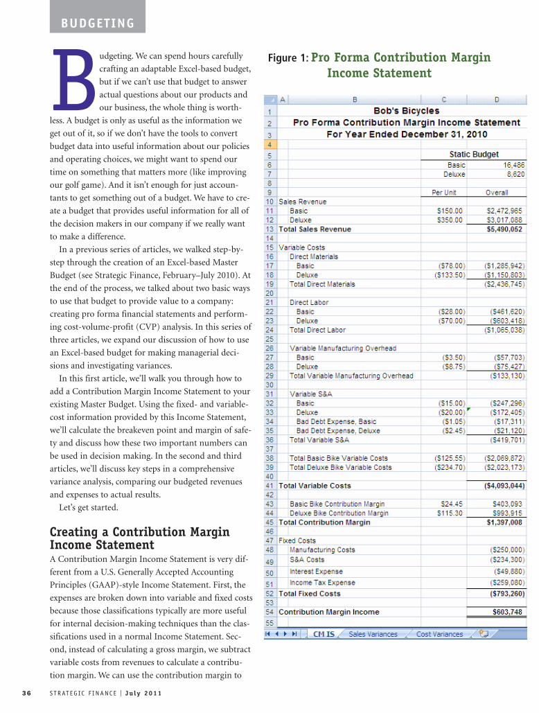
Figure 1: Pro Forma Contribution MarginIncome Statement
make managerial decisions quickly since it shows
how much additional money each sale contributes
toward increasing profit. Third, we add more
details that may be useful for making business
decisions. For example, we may choose to provide
specifics on quantity and type of production inputs
and per-unit costs, as well as total expenses. For
Bob’s Bicycles, our example company, we’ve chosen
to create a detailed Contribution Margin Income
Statement that will provide the information neces-
sary to perform both an overall breakeven analysis
and a detailed variance analysis (see Figure 1). This
detailed statement is sometimes referred to as a
“flex budget,” a useful summary budget that you
can easily adjust to show the estimated costs for
any particular level of sales.
To begin adding a Contribution Margin Income
Statement to our Master Budget, we need to create
a new tab in Excel. Since the purpose of this Income
Statement is different from the budgets already cre-
ated, we want to keep it separate from our earlier work (if
you don’t have a copy of the Bob’s Bicycles Master Budget
spreadsheet yet, you can receive one by e-mailing either
author). As we get started, keep in mind that a Contribu-
tion Margin Income Statement doesn’t follow U.S. GAAP,
so the result won’t match up with the Pro Forma Income
Statement we’ve already created (see Figure 2 and the June
2010 article). But when we’ve finished the Contribution
Margin Income Statement, we can reconcile the two net
incomes to ensure the accuracy of our work.
After we’ve created the new tab, we first need to calcu-
late net sales, so we start the statement with each type of
unit we sell (in our Bob’s Bicycles example, those are the
basic and deluxe bicycles) and how many of each unit we
plan to sell during the year. These quantities are the ones
we’ll “flex” to see how variable costs and contribution
margin change for various sales levels or assumptions we
make. Next, we list the budgeted sales price per unit and
calculate the overall sales revenue as the number sold
times the price per unit. The total number of units Bob’s
budgeted to sell and the price per unit can be found in
the Data Input Sheet (Figure 1, February 2010). In our
example, we don’t have any sales returns or discounts, so
net sales is simply total sales revenue. At this point, the
total revenue shown in column D of Bob’s Contribution
Margin Income Statement (Figure 1 in this article)
should match total revenue in the Sales Budget (Figure 4,
February 2010).
The next step in creating a Contribution Margin Income
Statement is subtracting the variable costs. In a manufac-
turing firm such as Bob’s Bicycles, variable costs include
direct materials, direct labor, variable manufacturing over-
head, and the variable portion of selling and administrative
expenses. Since we’re creating a detailed Contribution
Margin Income Statement, we list the per-unit costs sepa-
rately for each type of bicycle Bob’s manufactures. As with
sales, the second column is calculated as the per-unit cost
times the budgeted number of units sold.
The per-unit direct materials and direct labor costs are
already available in the Ending Inventory Budget (Figure
3, April 2010). Per-unit manufacturing overhead requires
a little more work. The per-unit overhead on the Ending
Inventory Budget uses Bob’s predetermined overhead rate
(POHR), which includes both variable and fixed over-
head costs. While the POHR is appropriate for setting
sales price and calculating U.S. GAAP net income, we
only want to include the variable portion of manufactur-
ing overhead in this part of the Contribution Margin
Income Statement. To get only the variable overhead allo-
cated to each type of bike, we take the variable overhead
rate, available in the Overhead Budget (Figure 1, April
2010), times the variable cost driver required for each
type of bike—direct labor hours for our example. The
drivers per unit are available in the Ending Inventory
Budget.
Variable selling and administrative costs, the next set of
variable costs, are found in the variable section of the
Selling and Administrative (S&A) Budget (Figure 4, April
J u l y 2 0 1 1 I S T R AT E G IC F I N A N C E 37
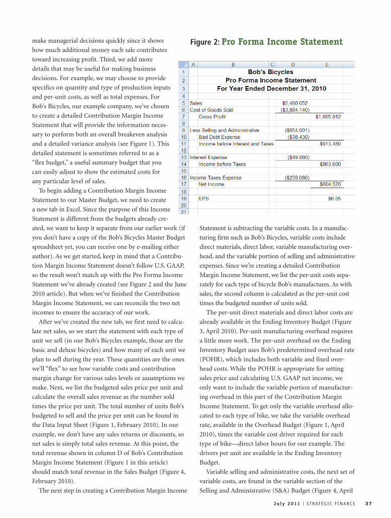
Figure 2: Pro Forma Income Statement
2010). But the allowance for bad debt requires a bit more
thought. Basically, we need to multiply net sales on
account by the estimate for uncollectible accounts. Both
of these estimates can be found on the Data Input Sheet.
In our Bob’s Bicycles example, we assumed that 70% of
net sales would be on account and that 1% of those credit
sales would be uncollectible. The product of these three
estimates is the Allowance for Bad Debt for each model of
bicycle. For example, for every basic bike Bob’s sells,
approximately $1.05 will be uncollectible ($150 sales
price times 70% credit sales times 1% uncollectible).
Obviously, this isn’t a “per bike” amount; most bikes will
be paid in full. But bad debt essentially can be amortized
over the budgeted unit bike sales in this manner. Alterna-
tively, you could use the total estimated bad-debt expense
reported in the Schedule of Cash Collections (Figure 4,
February 2010) as a fixed expense. You also could put
income taxes in either variable or fixed costs, depending
on how you choose to make your estimates. For the sake
of our demonstration, we chose to leave taxes in fixed
costs and treat bad-debt expense as a variable cost.
Once we’ve gathered the per-unit variable costs and
calculated the overall variable costs for each type of bike,
we can add up the overall values to get the total spent on
direct materials, the total spent on direct labor, and so on.
Finally, we add up each type of per-unit cost to get the
total variable cost for each unit we make. For example,
the total variable cost for basic bicycles is $125.55: $78 in
direct materials (DM), $28 in direct labor (DL), $3.50 in
manufacturing overhead (OH), $15 in variable S&A, and
$1.05 of allocated bad-debt expense. We calculate the
overall total variable costs in the same way to determine
how much Bob’s is spending to sell 16,486 basic bicycles
(approximately $2,069,872).
Now that we’ve budgeted revenues and variable costs,
we can calculate the contribution margin—or how much
each unit contributes toward increasing net income. To
calculate the per-unit contribution margin, we simply
subtract the variable costs per unit from sales price per
unit. The overall contribution margin is total sales minus
total variable costs. Even without any additional calcula-
tions, we now have some important information about
how our company actually makes its money each period.
In the Bob’s Bicycles example, we can see that, although
the company sells many more basic bicycles, it’s now very
obvious that the company makes much more profit by
selling deluxe bikes.
The final step in creating Bob’s Contribution Margin
Income Statement is to add in the fixed costs. These costs
are the same if Bob’s produces 10 units or 10,000.
Because they don’t change based on production, we don’t
have to list a per-unit cost. Instead, we simply put the
overall cost in our totals column. These costs include
fixed salaries, property taxes, depreciation, and other
items that don’t change based on production, even if they
do change each period. Bob’s has fixed manufacturing
costs of $250,000, fixed S&A costs of $234,300, interest
expense of $49,880, and income tax expense of $259,080.
The fixed production and S&A costs are in the Master
Budget and can be found in the Overhead Budget and
Selling and Administrative Budget, respectively. Interest
expense and income tax expense are also in the Master
Budget, and both can be found on the Pro Forma Income
Statement. Now we can calculate the total contribution
margin income (loss) by subtracting the total fixed costs
from the total contribution margin.
The Contribution Margin Income Statement that
we’ve created goes into a great deal of detail, but you
don’t have to make this statement so comprehensive.
Some companies choose to use only summary numbers
(such as total sales from the Pro Forma Income State-
ment). The type of Contribution Margin Income State-
ment you choose to create will depend on the questions
you want to answer. The detailed version we’re creating
is most appropriate for companies that want to do a full
variance analysis. If all you want to calculate is the
breakeven point and margin of safety, then you could
use a more condensed version.
38 S T R AT E G IC F I N A N C E I J u l y 2 0 1 1
BUDGETING
Comparing a Contribution MarginIncome Statement to a GAAP-basedPro Forma Income StatementRegardless of the format you use for your Contribution
Margin Income Statement, you’ll quickly notice that the
contribution margin net income doesn’t match the GAAP
net income reported on the Pro Forma Income Statement
that’s part of the traditional Master Budget. Bob’s budget-
ed contribution margin net income is $603,748, but the
budgeted Pro Forma Income Statement shows net income
of $604,520. This difference, about $772, comes from how
fixed costs are treated in the two income statements.
You probably remember that income can be calculated
using either “variable” or “absorption” costing. Variable
costing is what we do in a Contribution Margin Income
Statement when we show all fixed production costs as an
expense as they are incurred. Absorption costing, on the
other hand, records all production costs as inventory
first, then moves them to Cost of Goods Sold (COGS)
when units are sold. Absorption costing is the method
required by U.S. GAAP. If we produce more units than
we sell, some of the fixed costs will still be in inventory
at the end of the period under the absorption costing
method, but they will all appear in fixed costs in the
variable costing method. On the other hand, when we
produce less than we sell, COGS will include fixed costs
from production in previous periods under absorption
costing, and only the current period’s costs will be
included under variable costing. The only time the vari-
able and absorption net incomes match is when sales are
equal to production.
Let’s look at a simple example. Suppose that fixed
overhead cost per unit, the fixed portion of the POHR, is
$3 per unit and that we made 1,000 units and sold 800 of
them. In this case, absorption net income would exceed
variable or contribution margin income because produc-
tion exceeded sales. The amount of the difference would
be 200 units (the difference between production and
sales) times $3 per unit, or $600. In the second year, if we
produced 800 units but sold 1,000 units, the difference
would still be $600, but this time the absorption net
income would be smaller because production was less
than sales. Of course, total net income would be the
same over the two years since we produced a total of
1,800 units and sold all of them during that same period
of time.
This process is demonstrated for Bob’s Bicycles in Fig-
ure 3. We reconciled the difference between the two net
J u l y 2 0 1 1 I S T R AT E G IC F I N A N C E 39
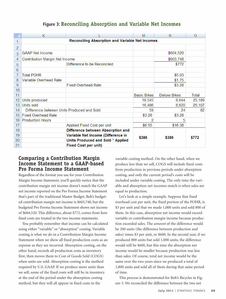
Figure 3: Reconciling Absorption and Variable Net Incomes

incomes by first taking the difference between production
and sales. The number of units produced is available in
the Production Budget (Figure 2, February 2010), and the
number of units sold is available in the Sales Budget. We
then calculated the total fixed cost allocated to each mod-
el as the fixed overhead rate (total POHR less the variable
overhead rate; both are available in the Overhead Budget)
times the direct labor hours required for each type of
bicycle, as reported in the Ending Inventory Budget.
Finally, we multiplied the difference in units produced
and units sold by the total fixed cost allocated to each
unit to get the total difference between variable and
absorption costs for the two types of bicycles. The sum of
the subtotals per bike is the total $772 difference men-
tioned earlier. If this calculation doesn’t work when you
do this for your company, then there’s a good chance that
something was missed or double counted in the Contri-
bution Margin Income Statement.
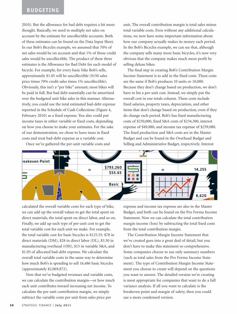
Calculating Breakeven Point andMargin of SafetyNow that we have a Pro Forma Contribution Margin
Income Statement, we can use the numbers to calculate
some useful information about our business. Two of the
most useful calculations are the breakeven point and
margin of safety. Breakeven and margin of safety are both
part of a cost-volume-profit analysis, which means that
we have to make some basic assumptions in order to
perform and interpret our calculations. The primary
assumption we must make is that the sales mix ratio is
constant over time. We must also assume that all costs
can be portrayed accurately as fixed or variable (mixed
costs are split into fixed and variable portions). Finally,
we must assume that we’re staying within the “relevant
range” (the range of production where total fixed costs
and variable costs per unit remain constant) and that the
time value of money isn’t material.
40 S T R AT E G IC F I N A N C E I J u l y 2 0 1 1
Figure 4: Calculating Breakeven Point and Margin of Safety
BUDGETING
To calculate the breakeven point, we first need to cal-
culate the weighted average contribution margin, which is
the contribution margin for each type of unit we sell
times that unit’s percentage of total unit sales. In our
example, Bob’s Bicycles plans to sell a total of 16,486
basic bicycles and 8,620 deluxe bicycles, or about 25,107
units. Based on these numbers, basic bicycles make up
about 66% of Bob’s sales, and deluxe bikes make up the
other 34%. To get the weighted average contribution
margin, we multiply the 66% times the basic bike’s $24.45
contribution margin and the 34% times the deluxe bike’s
$115.30. The sum of these two products (without round-
ing) gives Bob’s a weighted average contribution margin
of $55.65.
Once you have the weighted average contribution
margin, the breakeven point is an easy calculation: sim-
ply divide total fixed costs ($793,260 for Bob’s) by the
weighted average contribution margin. In our example,
Bob’s has a total breakeven point of 14,255 (see Figure
4). The actual result is 14,254.45, but since we can’t sell
0.45 units of a bike, we have to round the breakeven
point up to the nearest unit to ensure that Bob’s will
break even. If we set Excel to round to the nearest whole
unit, it would round down in this case, and Bob’s would
be slightly below breakeven. Since we want to round
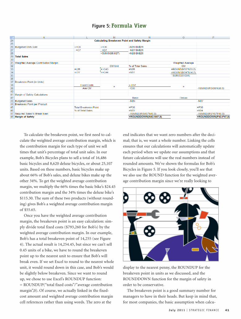
up, we chose to use Excel’s ROUNDUP function:
= ROUNDUP(“total fixed costs”/”average contribution
margin”,0). Of course, we actually linked in the fixed-
cost amount and weighted average contribution margin
cell references rather than using words. The zero at the
end indicates that we want zero numbers after the deci-
mal; that is, we want a whole number. Linking the cells
ensures that our calculations will automatically update
each period when we update our assumptions and that
future calculations will use the real numbers instead of
rounded amounts. We’ve shown the formulas for Bob’s
Bicycles in Figure 5. If you look closely, you’ll see that
we also use the ROUND function for the weighted aver-
age contribution margin since we’re really looking to
display to the nearest penny, the ROUNDUP for the
breakeven point in units as we discussed, and the
ROUNDDOWN function for the margin of safety in
order to be conservative.
The breakeven point is a good summary number for
managers to have in their heads. But keep in mind that,
for most companies, the basic assumption when calcu-
J u l y 2 0 1 1 I S T R AT E G IC F I N A N C E 41
Figure 5: Formula View
lating the breakeven point is that the current sales mix
won’t change. If it does, you need to calculate a new
breakeven point. Of course, that’s one of the benefits of
having the calculation in a spreadsheet. Just type in
the new sales assumptions, and the new value is auto-
matically calculated for you, even in the middle of a
meeting!
With the breakeven point calculated, the final calcula-
tion is the margin of safety. To get the margin of safety,
we first take the total breakeven point of 14,255 units
times the weighted average percentage for each unit.
Based on this calculation, Bob’s needs to sell 9,361 basic
bicycles and 4,895 deluxe bicycles each period in order to
break even. The margin of safety is the difference
between budgeted sales and the breakeven point. Bob’s
Bicycles has 7,125 basic bicycles and 3,725 deluxe bicy-
cles as its margin of safety. Figures 4 and 5 show these
results and the Excel formulas we used to calculate them.
Remember that the margin of safety includes both types
of bicycles with a constant sales mix. Another way to
look at it would be that the margin of safety is 10,850
bikes at Bob’s budgeted sales mix. If that sales mix varies
significantly from the budget, then you have to reevalu-
ate your breakeven point. For example, if Bob’s sold no
basic bicycles, then instead of needing to sell 4,895
deluxe bikes to break even, they would need to sell 6,880
instead.
Both of these calculations provide numbers that man-
agement can use to track company progress, especially
over time. Though the breakeven point provides infor-
mation about the bare minimum we need to cover fixed
costs, the margin of safety, as mentioned previously,
gives us a feel for not only how well we’re doing but also
how many units we’re selling each period that provide
actual profit. We would like to see a steady drop in the
breakeven point as we control costs, but that isn’t always
possible, especially in a period of inflation. Yet we
should see a definite increase in the margin of safety
over time as we improve sales and grow the business.
Dips in the margin of safety provide important signals
that we need to dig into the sales prices, competition,
and sales force incentives to see what isn’t working
properly. The margin of safety can also provide infor-
mation about the effectiveness of the current sales mix.
For example, the deluxe bikes provide a higher contri-
bution margin, yet with Bob’s current sales mix they are
only about a third of the company’s margin of safety on
a per-unit basis. It might be wise to increase advertising
or promotions to increase the sales of those bicycles.
Dropping the price a little to better compete in the mar-
ketplace might also be a wise move since the deluxe bike
has such a large contribution margin compared to the
basic model.
Benchmarking AnalysisNow that we have the basic foundation through our cre-
ation of a Contribution Margin Income Statement, we’re
ready to really dig into our performance. Future install-
ments of this series will include a discussion of creating a
Flexible Budget in the Contribution Margin format, gath-
ering actual performance numbers, calculating profit and
contribution margin variances, and calculating cost vari-
ances. We’ll automate the results as we go so when we
type in the budgeted values and actual results for each
year, Excel will automatically perform the calculations for
us. If we set this up carefully enough, the resulting tables
will provide sufficient detail and clarity that we can easily
hand them to other managers for use in company deci-
sion making.
Developing and using an Excel-based budget can be a
challenge, but once you’ve created the basic format, you
can use it for many years with only minor modifications.
Once you have the basics of your budget working well,
you can extend that budget to automatically make addi-
tional calculations about your performance. By using
your budget to provide real-time feedback, you can help
other managers see the value of your work and help them
improve their processes and generate more profit for the
company. This is where budgeting stops being an exercise
and starts being an integrated part of business! In our
next installment, we’ll discuss the first, and perhaps most
important, set of variances: the sales variances. Until
then, happy budgeting! SF
Jason Porter, Ph.D., is assistant professor of accounting at
the University of Idaho and is a member of IMA’s Washing-
ton Tri-Cities Chapter. You can reach him at (208) 885-
7153 or [email protected].
Teresa Stephenson, CMA, Ph.D., is associate professor of
accounting at the University of Wyoming and is a member
of IMA’s Denver-Centennial Chapter. You can reach her at
(307) 766-3836 or [email protected].
Note: A copy of the example spreadsheet, including all the
formulas, is available from either author. IMA members can
access all previous articles in the first series via the IMA
website at www.imanet.org after logging in.
42 S T R AT E G IC F I N A N C E I J u l y 2 0 1 1
BUDGETING