building a better non-uniform fast fourier transform · leslie greengard, ludvig af klinteberg,...
TRANSCRIPT

Building a better non-uniform fast Fourier transform
ICERM 3/12/18
Alex Barnett (Center for Computational Biology, Flatiron Institute)
This work is collaboration with Jeremy Magland.
We benefited from much discussions and/or codes, including:
Leslie Greengard, Ludvig af Klinteberg, Zydrunas Gimbutas, Marina Spivak,
Joakim Anden, and David Stein

Overview
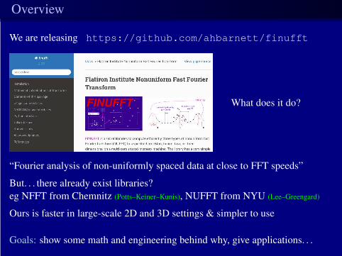
We are releasing https://github.com/ahbarnett/finufft

Overview
We are releasing https://github.com/ahbarnett/finufft
What does it do?

Overview
We are releasing https://github.com/ahbarnett/finufft
What does it do?
“Fourier analysis of non-uniformly spaced data at close to FFT speeds”
But. . . there already exist libraries?
eg NFFT from Chemnitz (Potts–Keiner–Kunis), NUFFT from NYU (Lee–Greengard)
Ours is faster in large-scale 2D and 3D settings & simpler to use
Goals: show some math and engineering behind why, give applications. . .

. . . and explain how “Tex” Logan—one of the best bluegrass fiddle players in
the country—is key to the story:

Recap the discrete Fourier transform (DFT)
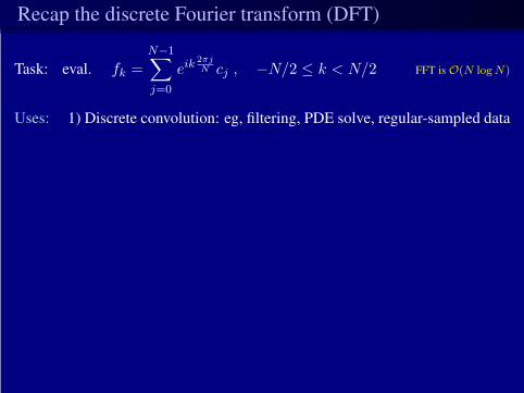
Task: eval. fk =N−1∑
j=0
eik2πj
N cj , −N/2 ≤ k < N/2 FFT is O(N logN)
Recap the discrete Fourier transform (DFT)
Task: eval. fk =N−1∑
j=0
eik2πj
N cj , −N/2 ≤ k < N/2 FFT is O(N logN)
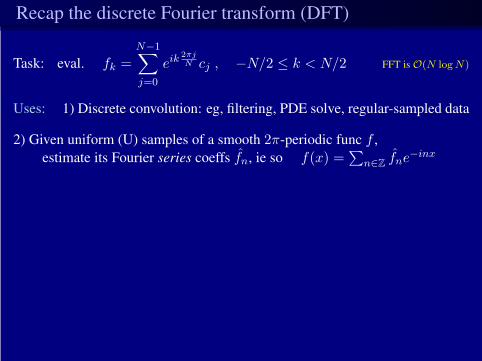
Uses: 1) Discrete convolution: eg, filtering, PDE solve, regular-sampled data
Recap the discrete Fourier transform (DFT)
Task: eval. fk =N−1∑
j=0
eik2πj
N cj , −N/2 ≤ k < N/2 FFT is O(N logN)
Uses: 1) Discrete convolution: eg, filtering, PDE solve, regular-sampled data
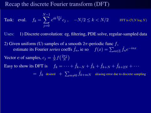
2) Given uniform (U) samples of a smooth 2π-periodic func f ,
estimate its Fourier series coeffs fn, ie so f(x) =∑
n∈Z fne−inx
Recap the discrete Fourier transform (DFT)
Task: eval. fk =N−1∑
j=0
eik2πj
N cj , −N/2 ≤ k < N/2 FFT is O(N logN)
Uses: 1) Discrete convolution: eg, filtering, PDE solve, regular-sampled data
2) Given uniform (U) samples of a smooth 2π-periodic func f ,
estimate its Fourier series coeffs fn, ie so f(x) =∑
n∈Z fne−inx
Vector c of samples, cj =1N f
(2πjN
)
Easy to show its DFT is fk = · · ·+ fk−N + fk + fk+N + fk+2N + · · ·= fk desired +
∑
m 6=0 fk+mN aliasing error due to discrete sampling
Key: f smooth ⇔ fn decays for |n| large ⇔ aliasing error small
eg (d/dx)pf bounded ⇒ fn = O(1/|n|p) p-th order convergence of error vs N
3) Estimate power spectrum of non-periodic signal on U grid
must first multiply by a “good” window function

Contrast: what does NUFFT compute?
Inputs: {xj}Mj=1 NU (non-uniform) points in [0, 2π)
{cj}Mj=1 complex strengths, N number of modes
Three flavors of task:
Type-1: NU to U, evaluates fk =M∑
j=1
eikxjcj , −N/2 ≤ k < N/2
F series coeffs of sum of point masses. Generalizes the DFT (was case xj = 2πj/N )
Type-2: U to NU, evaluates cj =∑
−N/2≤k<N/2eikxjfk , j = 1, . . . ,M
Evaluate usual F series at arbitrary targets. Is adjoint (but not inverse!) of type-1
Type-3: NU to NU, also needs NU output freqs {sk}Nk=1
evaluates fk =M∑
j=1
eiskxjcj , k = 1, . . . , N general exponential sum
• For dimension d = 2, 3 (etc), replace kxj by k · xj = k1xj + k2yj , etc

These tasks crop up a lot
• Magnetic resonance imaging (MRI).
f is unknown 2D image; seek its vector of values f on a U grid
Given data yj = f(kj) at NU set of Fourier pts kj :
spiral imaging PROPELLER
Evaluating the forward model, ie eval. y = Af , is a 2D type-2 NUFFT.
Reconstruct f by iteratively solving this (rect, ill-cond) linear system (eg Fessler)
Even computing a good preconditioner for this lin. sys. needs the NUFFT (Greengard–Inati ’06)

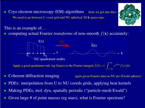
• Cryo electron microscopy (EM) algorithms (how we got into this)
We need to go between U voxel grid and NU spherical 3D k-space reps.

• Cryo electron microscopy (EM) algorithms (how we got into this)
We need to go between U voxel grid and NU spherical 3D k-space reps.
This is an example of. . .
• computing actual Fourier transforms of non-smooth f(x) accurately:
x kx1 xN
f(x) FTf(k)
NU quadrature nodes
Apply a good quadrature rule (eg Gauss) to the Fourier integral f(k) :=
∫∞
−∞
eikxf(x)dx
• Coherent diffraction imaging again given Fourier data on NU pts (Ewald spheres)
• PDEs: interpolation from U to NU coords grids, applying heat kernels
• Making PDEs, mol. dyn, spatially periodic (“particle-mesh Ewald”)
• Given large # of point masses (eg stars), what is Fourier spectrum?

A super-crude 1D type-1 NUFFT: “snap to fine grid”
Three steps: Set up fine grid on [0, 2π), spacing h = 2π/Nf , Nf > N

A super-crude 1D type-1 NUFFT: “snap to fine grid”
Three steps: Set up fine grid on [0, 2π), spacing h = 2π/Nf , Nf > N
a) Add each strength cj onto fine-grid cell w/ location xj nearest xj .

A super-crude 1D type-1 NUFFT: “snap to fine grid”
Three steps: Set up fine grid on [0, 2π), spacing h = 2π/Nf , Nf > N
a) Add each strength cj onto fine-grid cell w/ location xj nearest xj .
b) Call this vector {bl}Nf−1l=0 : take its size-Nf FFT to get {bk}Nf/2−1
k=−Nf/2.

A super-crude 1D type-1 NUFFT: “snap to fine grid”
Three steps: Set up fine grid on [0, 2π), spacing h = 2π/Nf , Nf > N
a) Add each strength cj onto fine-grid cell w/ location xj nearest xj .
b) Call this vector {bl}Nf−1l=0 : take its size-Nf FFT to get {bk}Nf/2−1
k=−Nf/2.
c) Keep just low-freq outputs: fk = bk, for −N/2 ≤ k < N/2
What is error? High freqs |k| = N/2 are the worst: relative error thus
eiN2xj − eiN2 xj = O(Nh) = O(N/Nf )
• 1st-order convergent: eg error 10−1 needs Nf ≈ 10N .
• in 3D needs Nf3 ≈ 103N3 1000× slower than plain FFT, for 1-digit accuracy! Terrible!
And yet the idea of dumping onto fine grid is actually good. . .
But need much more rapid convergence!

1D type-1 NUFFT algorithm
Three steps: Set up “not-as-fine” grid on [0, 2π), Nf = σN , upsampling σ ≈ 2
Pick a spreading kernel ψ(x) support must be only a few h wide
a) Spread each spike cj onto fine grid bl =∑M
j=1 cjψ(lh− xj) detail: periodize

1D type-1 NUFFT algorithm
Three steps: Set up “not-as-fine” grid on [0, 2π), Nf = σN , upsampling σ ≈ 2
Pick a spreading kernel ψ(x) support must be only a few h wide
a) Spread each spike cj onto fine grid bl =∑M
j=1 cjψ(lh− xj) detail: periodize
b) Do size-Nf FFT to get bk

1D type-1 NUFFT algorithm
Three steps: Set up “not-as-fine” grid on [0, 2π), Nf = σN , upsampling σ ≈ 2
Pick a spreading kernel ψ(x) support must be only a few h wide
a) Spread each spike cj onto fine grid bl =∑M
j=1 cjψ(lh− xj) detail: periodize
b) Do size-Nf FFT to get bkc) Correct for spreading: fk =
1ψ(k)
bk, for −N/2 ≤ k < N/2
Why? since you convolved sum of point masses∑M
j=1cjδ(x− xj) with ψ(x),
undo by deconvolving: dividing by kernel in Fourier domain
Type-2 similar; type-3 needs more upsampling (by σ2 not σ)

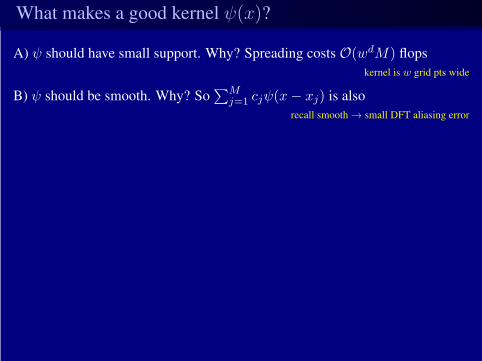
What makes a good kernel ψ(x)?
A) ψ should have small support. Why? Spreading costs O(wdM) flops
kernel is w grid pts wide
What makes a good kernel ψ(x)?
A) ψ should have small support. Why? Spreading costs O(wdM) flops
kernel is w grid pts wide
B) ψ should be smooth. Why? So∑M
j=1 cjψ(x− xj) is also
recall smooth → small DFT aliasing error

What makes a good kernel ψ(x)?
A) ψ should have small support. Why? Spreading costs O(wdM) flops
kernel is w grid pts wide
B) ψ should be smooth. Why? So∑M
j=1 cjψ(x− xj) is also
recall smooth → small DFT aliasing error
A) and B) are conflicting requirements :(
Rigorous error analysis: |fk − fk| ≤ ǫ‖c‖1
where ǫ = max|k|≤N/2,x∈R
1
|ψ(k)|∣
∣
∑
m 6=0
ψ(k +mNf )ei(k+mNf )x
∣
∣
k
(k)Ψ
−N/2 N/2 N−2N −N
usable band
ff f
want ψ large in |k| < N/2, small for |k| > Nf −N/2

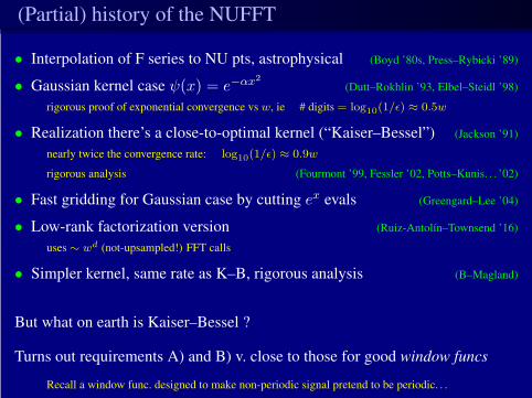
(Partial) history of the NUFFT
• Interpolation of F series to NU pts, astrophysical (Boyd ’80s, Press–Rybicki ’89)
• Gaussian kernel case ψ(x) = e−αx2
(Dutt–Rokhlin ’93, Elbel–Steidl ’98)
rigorous proof of exponential convergence vs w, ie # digits = log10(1/ǫ) ≈ 0.5w
• Realization there’s a close-to-optimal kernel (“Kaiser–Bessel”) (Jackson ’91)
nearly twice the convergence rate: log10(1/ǫ) ≈ 0.9w
rigorous analysis (Fourmont ’99, Fessler ’02, Potts–Kunis. . . ’02)
• Fast gridding for Gaussian case by cutting ex evals (Greengard–Lee ’04)
• Low-rank factorization version (Ruiz-Antolın–Townsend ’16)
uses ∼ wd (not-upsampled!) FFT calls
• Simpler kernel, same rate as K–B, rigorous analysis (B–Magland)
But what on earth is Kaiser–Bessel ?
Turns out requirements A) and B) v. close to those for good window funcs
Recall a window func. designed to make non-periodic signal pretend to be periodic. . .
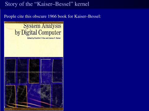
Story of the “Kaiser–Bessel” kernel
People cite this obscure 1966 book for Kaiser–Bessel:

Story of the “Kaiser–Bessel” kernel
People cite this obscure 1966 book for Kaiser–Bessel:
(had to buy 2nd-hand) Let’s open. . .

First appearance of Kaiser–Bessel in print
What does: “discovered” by Kaiser following a discussion with B. F. Logan mean?

Kaiser–Bessel Fourier transform pair
The truncated kernel
φKB(z) :=
{
I0(β√1− z2), |z| ≤ 1 we scale z := 2x/wh
0, otherwise
is the FT of
φKB(ξ) = 2sinh
√
β2 − ξ2√
β2 − ξ2
-1 -0.5 0 0.5 10
5
10
15
20
25
-15 -10 -5 0 5 10 15
0
10
20
30
Still unknown to Gradshteyn–Ryzhik, Bateman, Prudnikov, Wolfram r, Maple r . . .

Over to James Kaiser, Bell Labs (interviewed in ’97)
About 1960-’61, Henry Pollak, who was department head in the math research
area at Bell Labs, and two of his staff, Henry Landau, and Dave Slepian,
solved the problem of finding that set of functions that had maximum energy in
the main lobe consistent with certain roll-offs in the side lobes.
They showed that the functions that came out of that were the prolate
spheroidal wave functions . . . The program was about 600 lines of FORTRAN.
One of the nice features of Bell Laboratories is there were a lot very bright
people around, and one of the fellows that I always enjoyed talking to was Ben
Logan, a tall Texan from Big Spring, Texas.
https://www.youtube.com/watch?v=NU4l7xFhQdA&t=72s

Back to Kaiser. . .
So one day I went in Ben’s office and his chalkboard was just filled with
equations. Way down in the left-hand corner of Ben’s chalkboard was this
transform pair, the I0–sinh transform pair. I didn’t know what I0 was, I said,
“Ben, what’s I0?” He came back with “Oh, that’s the modified Bessel function
of the first kind and order zero.” I said, “Thanks a lot, Ben, but what is that?”
He said, “You know, it’s just a basic Bessel function but with purely imaginary
argument.” So I copied down the transform pair and went back to my office.
I wrote a program . . . got the data back and when I compared the I0 function to
the prolate, I said, “What’s going on here? They look almost identical!” The
answers were within about a tenth of a percent of one another. One program
[PSWF] required 600 lines of code and the other ten or twelve lines of code!
P.S. we now have a kernel needing < 1 line of code . . .

Compare the kernels
Plot the kernels for support of w = 13 fine grid points:
-5 0 50
0.2
0.4
0.6
0.8
1Gauss
K-B
ES
0 2 4 6
10 -10
10 -5
10 0
0 2 4 6
10 -10
10 -5
10 0
• very hard to distinguish on linear plot! Decays differ on log plot
• Kaiser–Bessel: tail of FT is at 10−12
• best truncated Gaussian has tail only at 10−7
• “ES” is our new kernel; v. close to KB
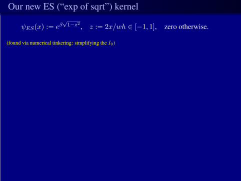
Our new ES (“exp of sqrt”) kernel
ψES(x) := eβ√1−z2 , z := 2x/wh ∈ [−1, 1], zero otherwise.
(found via numerical tinkering: simplifying the I0)

Our new ES (“exp of sqrt”) kernel
ψES(x) := eβ√1−z2 , z := 2x/wh ∈ [−1, 1], zero otherwise.
(found via numerical tinkering: simplifying the I0)
• its Fourier transform ψES has no known formula
1) Numerical consequence: use quadrature on FT to eval. 1ψES
for step c)

Our new ES (“exp of sqrt”) kernel
ψES(x) := eβ√1−z2 , z := 2x/wh ∈ [−1, 1], zero otherwise.
(found via numerical tinkering: simplifying the I0)
• its Fourier transform ψES has no known formula
1) Numerical consequence: use quadrature on FT to eval. 1ψES
for step c)
2) Analytic consequence: one has to work with the FT integral directly. . .
We prove essentially ǫ = O(√we−πw
√1−1/σ
)
as kernel width w →∞
• same exponential convergence rate as Kaiser–Bessel, and as PSWF (Fuchs ’64)
• consequence: w ≈ 7 gives accuracy ǫ = 10−6, w ≈ 13 gets ǫ = 10−12.
• However, evaluation now requires only one sqrt, one ex, couple of mults.
• proof is 8 pages: contour integrals split into parts, sums into various parts,
bounding the conditionally-convergent tail sum. . .

One proof ingredient
Asymptotics (in β) of the Fourier transform ψ(ρβ) =
∫ 1
−1eβ(
√1−z2−iρz)dz
via deforming to complex plane, steepest descent (saddle pts) (Olver)
Case (a): =0.8
-2 -1 0 1 2
Re z
-1
-0.5
0
0.5
1
1.5
2
2.5
3
Im z
-1 -0.5 0 0.5 1
108
0 u0
u
0
/2
v
bad
Case (b): =1.2
-2 -1 0 1 2
Re z
-1
-0.5
0
0.5
1
1.5
2
2.5
3
Im z
-1 -0.5 0 0.5 1
Summary: new approx. FT pair K–B & PSWF also may be interpreted this way
“ exp(semicircle)FT←→ exp(semicircle) + exponentially small tail ”

Implementation aspects
• Type 1,2,3 for dimensions d = 1, 2, 3: nine routines
• C++/OpenMP/SIMD, shared mem, calls FFTW. Apache license
• Wrappers to C, Fortran, MATLAB, octave, python, julia

Implementation aspects
• Type 1,2,3 for dimensions d = 1, 2, 3: nine routines
• C++/OpenMP/SIMD, shared mem, calls FFTW. Apache license
• Wrappers to C, Fortran, MATLAB, octave, python, julia
• Cache-aware multithreaded spreading:
Type-2 easy: parallelize over bin-sorted NU pts no collisons reading from U blocks
Type-1 not so: writes collide load-balancing, slow index-wrapping, ≤ 104 NU pts per subprob:
NU pts x j
copy over
w
N f
subproblems: each own thread
2D case, type−1, spread to fine grid:
1D kernel evals
outer prod
spread
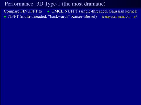
Performance: 3D Type-1 (the most dramatic)
Compare FINUFFT to • CMCL NUFFT (single-threaded, Gaussian kernel)
• NFFT (multi-threaded, “backwards” Kaiser–Bessel) ie they eval. sinch√1− x2

Performance: 3D Type-1 (the most dramatic)
Compare FINUFFT to • CMCL NUFFT (single-threaded, Gaussian kernel)
• NFFT (multi-threaded, “backwards” Kaiser–Bessel) ie they eval. sinch√1− x2
10 -10 10 -5
10 1
10 2
wa
ll-clo
ck t
ime
(s)
FINUFFT
NFFT no pre
NFFT pre
CMCL
BART
Fessler pre
2−3x
30x
10 -10 10 -5
10 1
10 2
wa
ll-clo
ck t
ime
(s)
FINUFFT
NFFT no pre
NFFT pre
BART
8x
10x
• all scale as O(M | log ǫ|d +N logN); it’s about prefactors and RAM usage
• at M = 108: we need only 2 GB, vs NFFT pre needs 60 GB at high acc.

3D Type-1: RAM & CPU usage for non-uniform density
We use all threads efficiently, vs NFFT assigns threads to fixed x-slices:
0 100 200 300 400 500 600 700 800 900
t (s)
-40
-20
0
20
40
60
RA
M (
byte
s/N
Up
t)
making data
start FINUFFT
start NFFT plan setx
start NFFT no-pre
0 100 200 300 400 500 600 700 800 900
t (s)
0
5
10
15
20
CP
U u
sa
ge
(th
rea
ds)
done from MATLAB via https://github.com/ahbarnett/memorygraph

Conclusions
NUFFT is a key tool with many scientific computing applications
We speed up and simplify the NUFFT using. . .
• mathematics: creation and rigorous analysis of new kernel func ψ• no analytic ψ need be known: instead use numerical quadrature
• cache-aware and thread-balanced implementation
Result: FINUFFT (Flatiron Institute Non-Uniform Fast Fourier Transform)
https://github.com/ahbarnett/finufft
fast, simple to install and use. Send me bug reports & feature req’s
Future:
• GPU spreader (build upon promising work of: Kunis–Kunis ’12, Ou ’17)
• math: “why” are PSWF and K–B so close to eβ√1−z2 ? no, it’s not WKB. . .

EXTRA SLIDES

Ongoing: Intel vector optimizations
Vector intrinsics accelerate by up to 2×: (Ludvig af Klinteberg)
• exploit SSE, SSE2, AVX, etc, common to 99% of CPUs.