building an optimal premium model for an insurance company€¦ · building an optimal premium...

Master in Mathematical Engineering

Modelling Week 2014

Alberto Martínez, Carlos Bernal, Carlos de Diego, Gabriel Valverde, Andreas Hadjittofis

Building an Optimal Premium Model for an Insurance Company


VIII UCM Modelling Week – 9/13 June 2014 – Building an optimal premium model for an insurance company

2

Table of Content

Introduction 3

Overview 5

Data Analysis

Descriptive Analysis 6

Sampling Phase 9

Data Processing 9

Modelling

Model I

Binary Logistic Regression 11

Model II

Multinomial Logistic Regression 14

Decision Tree 20

Neural Network 25

Optimization

Optimal model as combination of models 29

Validation of Models 32

Conclusions, Remarks and Next Steps 34



3

INTRODUCTION

We are interested in solving a CRM problem for an insurance company. The tasks to be

achieved are:

Finding the ideal target, in this case, people who are more likely to contract their

insurance products.

Identifying the premium we should offer to each client, that is to say, the optimal

price that should be offered to each client.

Calculating the difference between offering the premium randomly and optimally,

using the information obtained in the model.

Two databases with clients’ information are available:

In the first one we have the information of 20.000 clients which have already been

contacted; 9% of them have contracted the product.

Important data are included such as the premium offered, the number of products

that they have already bought, the number of years that they have been clients of the

company and the socioeconomic status (an economic and sociological measure

combined with the person’s work experience and his or his family’s economic and

social position in relation to others, based on income, education, and work

occupation).

In the second database of non‐previously contacted clients, we have the same

information about 10.000 clients but only 5.000 are going to be contacted due to

practical restrictions.

Is it worthwhile offering the same premium to all clients? Is it better to focus on people with

certain characteristics rather than choosing clients randomly?

The objective is, using the first database, find an optimal strategy to be able to contact to

those clients who are more likely to buy the product we are offering. This strategy should be

applied to the second database to get the ideal target.



4

INTRODUCTION

The premium is an important variable when deciding whether to contract insurance or

not. A high one is going to be rejected more frequently by potential clients, and a very low

one is not going to maximize the earnings of the company.

Therefore, once the ideal target is defined, an optimization problem should be

formulated to find the optimal premium which maximizes the number of sales,

and thus maximizes the amount of money that the company is going to earn.

When the optimal premium is calculated, a comparison between the optimal earning and the

one that we would get choosing the clients randomly can be calculated to prove the

usefulness of the analysis.

SAS, SPSS, Matlab and Excel have been used as software tools: Matlab has been used for

the optimization model and also for ROC curves.

OVERVIEW

This section provides a brief introduction regarding the roadmap followed and provides a

breakdown of the activities considered in the problem resolution.

The study covered is split in three main blocks: data analysis, modelling and

optimization. The areas/steps covered in each block are summarized in the following

figure:



5

OVERVIEW

Due to the amount of input variables and potential relationships between explanatory

variables, several models could be considered. However, the analysis is driven putting the

focus in the following initial hypothesis:

Conceptual Framework:

Two different models have been considered to approach the problem according to the

class variable defined:



6

DATA ANALYSIS DESCRIPTIVE ANALYSIS

The variables considered in the datasets are:

Variable Name Meaning

Obs Number of Observations

Sales It indicates whether the client bought a product: 1 (yes), 0 (otherwise)

Price Sensitivity It indicates the client's sensitivity to the price: 1 (less sensitive) - 6 (more sensitive)

PhoneType Client's phone type: Fixed or Mobile

Email It indicates whether the client's email is available: 1 (yes), 0 (otherwise)

Tenure Client's tenure (year when the person became a client of the company)

NumberofCampaigns Number of times the client has been called

ProdActive Number of active products

ProdBought Number of different products previously bought

Premium Offered Premium offered to the client

Phone Call Day Day the phone call is received

CodeCategory Category of the phone call answer

Birthdate Client's birthdate

Product Type It indicates the type of product that the client buys

Number of Semesters Paid Number of semesters paid

Socieconomic Status It indicates the client's socieconomic status

Province Province where the client lives

Right Address It indicates whether the client's address is correct: 1 (yes), 0 (otherwise)

Living Area (m^2) Estimated surface area of house

House Price Estimated price of the house

Income Estimated income

yearBuilt It indicates when the client's house was built

House Insurance Price of the house insurance

Pension Plan Estimated amount of money the client would have in a pension plan

Estimated number of cars Estimation of the number of cars owned by the client

Probability of Second

Residence Probability of having a second residence

Credit Estimation of the amount of credit that could be offered to the client

Savings Estimation of the amount of money saved by the client

Number of Mobile Phones Number of mobile phones

Number of Fixed Lines Number of Land Lines

ADSL It indicates whether the client has ADSL:1 (yes), 0 (otherwise)

3G Devices It indicates whether the client has 3G Devices:1 (yes), 0 (otherwise)

Type of House Type of house: Urban or Rural



7


With all the data available in the first database, it is really important to make a complete

descriptive analysis of the variables to understand the type of information we are dealing

with, which can give us an idea of which variables are relevant to help us solve our problem.

Our dataset is composed by 34 variables, and we must know which ones are significant and

relevant to explain the behaviour of our target variable.

In order to don´t extend the length of this document we have decided to focus on the

modelling step and from a descriptive analysis point of view we have just provided as

examples in the document, the barcharts crossing the target variable considered with the

most relevant explanatory variables we found.

We haven´t included contigency tables for cualitative variables, neither box-plots nor

distribution test for quantitative ones relating different variables and in case, running

different contrast to study more deeply the input variables.

By confronting each of the explicative variable against the target we might get an overall

idea of the correlation among them. For this reason we will show some charts:



8


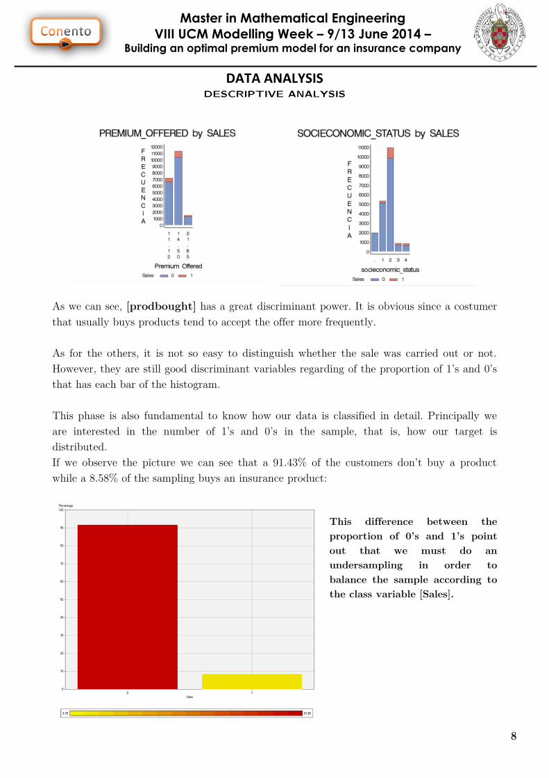
As we can see, [prodbought] has a great discriminant power. It is obvious since a costumer

that usually buys products tend to accept the offer more frequently.

As for the others, it is not so easy to distinguish whether the sale was carried out or not.

However, they are still good discriminant variables regarding of the proportion of 1’s and 0’s

that has each bar of the histogram.

This phase is also fundamental to know how our data is classified in detail. Principally we

are interested in the number of 1’s and 0’s in the sample, that is, how our target is

distributed.

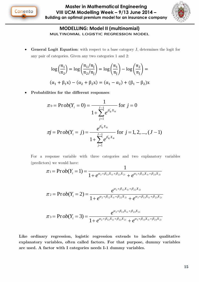
If we observe the picture we can see that a 91.43% of the customers don’t buy a product

while a 8.58% of the sampling buys an insurance product:

This difference between the

proportion of 0’s and 1’s point

out that we must do an

undersampling in order to

balance the sample according to

the class variable [Sales].



9

DATA ANALYSIS SAMPLING and DATA PROCESSING

Sampling Phase

As we said, the representation of the number of sales is lacking in size. This means an

inconvenient for our model since it can happen that our model wasn’t able to extract

patterns or rules that define this event.

To solve this problem, we should equalize the sample so that the percentage of 1’s will be

same as the number of 0’s. This method is known by under-sampling, that is, keep events of

interest and reduce the complementary event.

The technique of sampling used is the stratified sampling, so that we must select

representative elements from the different populations not homogeneous among themselves.

The size of the sample will be of 3600 registers more or less, consisting of 50% of 1’s and 50%

of 0’s.

Data Processing

In this point we will apply certain transformations to our data in order that our model could

estimate the parameters correctly. It is possible to identify two types of data treatment: one

based on the business and other based on statistics.

First, we need to deal missing values. It is necessary to recall that in our data sets we

encountered lots of missing values. In our case, we used three ways to achieve the purpose.

On the one hand, we implemented a regression method to predict some of the variables. In

concrete, “price sensitivity”. This variable has some missing values and we predicted them in

order to fill in the empty spaces. We selected correlative variables to predict the “price

sensitivity”.

On the other hand, for socio economic status variables like “socioeconomic status”, “living

area”, “house price”,… we took a by group average having into account the socio economic

status. Finally, for variables with lots of missing values (“ADSL”, “3G devices”, “number of

fixed lines” and “number of mobile phones”) we decided that the best way to deal with

them was by removing the variable itself.

Transformation of categorical variables splitting them into the corresponding binary dummy

variables for regression purposes and some numerical transformations for specific attributes

(i.e., birthday) has been done. Examples of that are SOCIECONOMIC_STATUS,

PRODUCT_TYPE,TYPE_OF_HOUSE,PHONE_TYPE,BIRTHDATE,PRICE_SENSITIVITY.



10

DATA ANALYSIS SAMPLING and DATA PROCESSING

Regarding initial variables selection, logistic regression with stepwise and forward methods

has been use as mechanism. Due to the different potential relationships between explanatory

variables, several runs/models have been done, forcing in some cases some variables of

interest to be present and therefore different results were obtained. Finally, a large enough

set of variables has been selected as initial selection (keep in mind that considering most of

input variables a regression ends with two or three relevant ones, for example, number of

campaigns and product bought).

CREDIT,EMAIL,NUMBEROFCAMPAIGNS,PRODACTIVE,PRODUCTBOUGHT,PROVINCE,RIGHT_AD

DRESS,SOCIOECONOMIC_STATUS,SAVINGS have been considered as input variables for model

II variants.



11

MODELLING: Model I (binary) BINOMIAL LOGISTIC REGRESSION MODEL

Model Definition

Let Y denote a binary response variable, X a set of explanatory variables and and π(x) =

Prob(Y=1|x). For a binary response, the regression model is the lineal

probability model. The linear probability model has a major problem: probabilities fall

between 0 and 1, but linear functions take values over the entire real line.

Usually, binary data result from a nonlinear relationship between π(x) and x. A fixed

change in x often has less impact when π(x) is near 0 or 1 than when π(x) is near 0.5.

In practice, nonlinear relationships between π(x) and x are often monotonic, with π(x)

increasing continuously or π(x) decreasing continuously as x increases. These relationships

provide S-shaped curves. The most important one corresponds with the logistic regression

model defined by:

As when and when .



12


If we consider as new response variable π(x) and the new variable

(log for the odds of π(x)) any real value between can be taken and therefore the linear

regression makes sense: , i.e., the log odds has the linear relationship.

General expression for the model:

General Logit Equation:

Probabilities for response variable:

for a case with two explanatory variables:

Use of Binomial Logistic Regression Model in the problem

Focusing in our problem, the aim is to predict the value of the binary variable “sales”

regarding to the sale or not of the product. Also, we must take into account the three

possible type of premium.

In order to achieve this, we are building a logistic regression. It will calculate the influence of

the different variables over the probability that the sale is done or not.

In our model we force one of the variables to be “premium”. This is because we would like to

obtain the probability of a customer to be a 1 conditioned to the premium offer, that is, the

probability for each premium. Apart from that variable, other variables will be determined

by the model to be included.

kiki

ikki

ikki XX

XX

XXie

e

eYobx

...

...

)...( 11

11

11 11

1)1(Pr)(

ii

ii

ii XX

XX

XXie

e

eYobx

2211

2211

2211 11

1)1(Pr)(



13


To sum up, the relevant variables are: Premium, Socioeconomic status, Right_address and

eMail.

The link function used for this model of regression model is the function logit, so that the

expression will have the next form:



14

MODELLING: Model II (multinomial) MULTINOMIAL LOGISTIC REGRESSION MODEL

Model Definition

Let J describe the number of categories (levels) for response variable Y and {π1,…, πj} the

probabilities for the different responses satisfying .

The probability distribution for the number of observations falling in the different J

categories follow a multinomial distribution. This distribution models the probability of the

different ways by which n independent observations can be spread out between the J

categories.

Given a nominal measure scale, the order betweeen categories is not relevant. A category is

taken as base response and a logit model is defined with respect to it.

where j = 1,...,J-1. The model has J-1 equations with their own parameters and the effects

vary with respect to the base category. When J=2, the model contains just one equation

and corresponds with the standard logistic regression model: log(π1/ π2)=log(π1).

General expression for the model:

Main characteristics:

As many equations as categories Y has.

For each variable, as many parameters as Y categories minus one are estimated.

It is required to use a category as a reference.



15


General Logit Equation: with respect to a base category J, determines the logit for

any pair of categories. Given any two categories 1 and 2:

Probabilities for the different responses:

For a response variable with three categories and two explanatory variables

(predictors) we would have:

Like ordinary regression, logistic regression extends to include qualitative

explanatory variables, often called factors. For that purpose, dummy variables

are used. A factor with I categories needs I-1 dummy variables.

0for

1

1)0(Pr

1

1

0'

j

e

YobJ

j

Xi

kikj

)1( ..., ,2 ,1for

1

)(Pr1

1

'

'

Jj

e

ejYobj

J

j

X

X

i

kikj

kikj

iiii XXXXiee

Yob223113322211221

1)1(Pr1

iiii

ii

XXXX

XX

iee

eYob

22311332221122

2221122

1)2(Pr2

iiii

ii

XXXX

XX

iee

eYob

22311332221122

2231133

1)3(Pr3



16


Use of Multinomial Logistic Regression Model in the problem

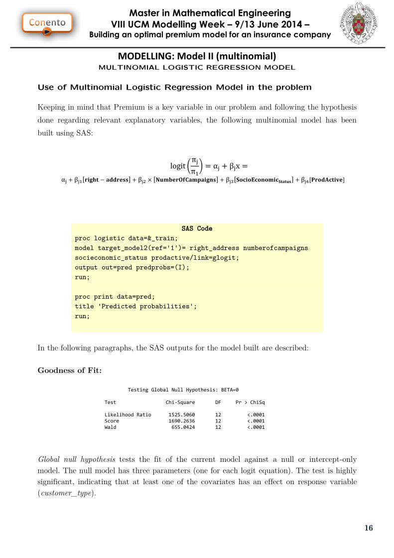
Keeping in mind that Premium is a key variable in our problem and following the hypothesis

done regarding relevant explanatory variables, the following multinomial model has been

built using SAS:

SAS Code

proc logistic data=&_train;

model target_model2(ref='1')= right_address numberofcampaigns

socieconomic_status prodactive/link=glogit;

output out=pred predprobs=(I);

run;

proc print data=pred;

title 'Predicted probabilities';

run;

In the following paragraphs, the SAS outputs for the model built are described:

Goodness of Fit:

Testing Global Null Hypothesis: BETA=0 Test Chi-Square DF Pr > ChiSq Likelihood Ratio 1525.5060 12 <.0001 Score 1690.2636 12 <.0001 Wald 655.0424 12 <.0001

Global null hypothesis tests the fit of the current model against a null or intercept-only

model. The null model has three parameters (one for each logit equation). The test is highly

significant, indicating that at least one of the covariates has an effect on response variable

(customer_type).



17


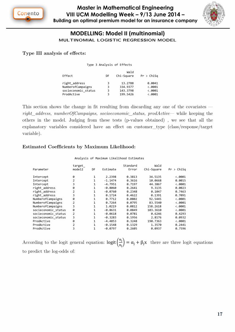
Type III analysis of effects:

Type 3 Analysis of Effects Wald Effect DF Chi-Square Pr > ChiSq right_address 3 13.2788 0.0041 NumberofCampaigns 3 334.9377 <.0001 socieconomic_status 3 143.3798 <.0001 ProdActive 3 199.5426 <.0001

This section shows the change in fit resulting from discarding any one of the covariates —

right_address, numberOfCampaigns, socioeconomic_status, prodActive— while keeping the

others in the model. Judging from these tests (p-values obtained) , we see that all the

explanatory variables considered have an effect on customer_type (class/response/target

variable).

Estimated Coefficients by Maximum Likelihood:

Analysis of Maximum Likelihood Estimates target_ Standard Wald Parameter model2 DF Estimate Error Chi-Square Pr > ChiSq Intercept 0 1 2.2398 0.3813 34.5135 <.0001 Intercept 2 1 -1.1474 0.3616 10.0668 0.0015 Intercept 3 1 -4.7951 0.7197 44.3867 <.0001 right_address 0 1 -0.8060 0.2641 9.3135 0.0023 right_address 2 1 -0.0760 0.2348 0.1047 0.7463 right_address 3 1 0.1724 0.4622 0.1391 0.7091 NumberofCampaigns 0 1 0.7712 0.0802 92.5445 <.0001 NumberofCampaigns 2 1 0.7264 0.0795 83.5540 <.0001 NumberofCampaigns 3 1 1.0219 0.0812 158.2618 <.0001 socieconomic_status 0 1 -0.8631 0.0849 103.3610 <.0001 socieconomic_status 2 1 -0.0618 0.0781 0.6246 0.4293 socieconomic_status 3 1 -0.3283 0.1956 2.8176 0.0932 ProdActive 0 1 -4.4853 0.3248 190.7363 <.0001 ProdActive 2 1 -0.1548 0.1329 1.3570 0.2441 ProdActive 3 1 -0.0797 0.2605 0.0937 0.7596

According to the logit general equation:

there are three logit equations

to predict the log-odds of:



18


Customer does not buy versus customer buys low-premium.

Customer buys medium-premium versus customer buys low-premium.

Customer buys high-premium versus customer buys low-premium.

Note: (customer_type = 1, i.e., customer buys low-premium is taken as reference category).



19


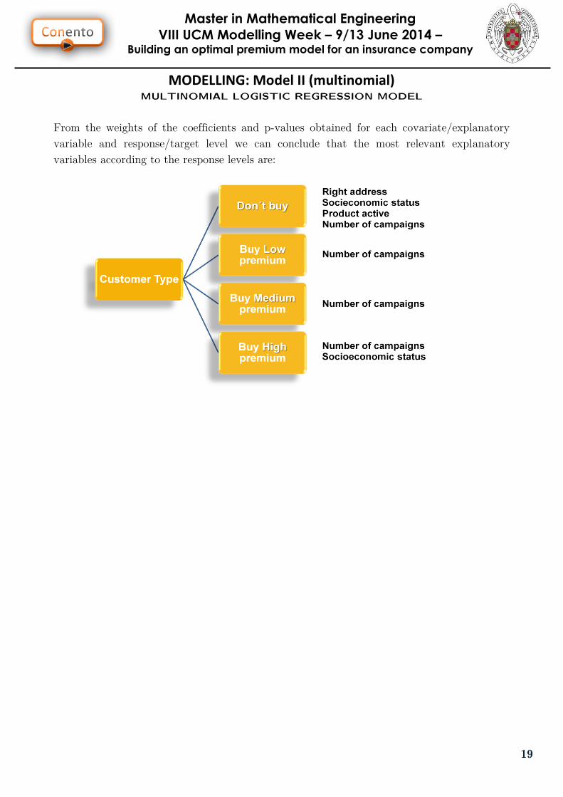
From the weights of the coefficients and p-values obtained for each covariate/explanatory

variable and response/target level we can conclude that the most relevant explanatory

variables according to the response levels are:



20

MODELLING: Model II (multinomial) DECISION TREE MODEL

A classification tree for the categorical target variable customer_type (model 2) has been

built according to the following characteristics:

Main Tree Parameters/Characteristics

Parameter/Criteria Value

Splitting criterion

(select useful inputs)

Uncertainty measure: Shannon Enthropy

Min number of observations in a leaf

(reduce partitions for each input)

6

Min observations required for a split search

(reduce partitions for each input)

24

Assessment

Model Assessment criterion

Subtree

(decision/ranking assessment &

pruning/ opt.complexity)

Average profit according to the profit/losses matrix.

Best assessment value.

In many cases, the value of making a true (or false)

positive decision differs from the value of making true

(or false) negative decision. In such a situation, the

concept of accuracy is generalized to profit and the

concept of misclassification is generalized to loss.

Profit Matrix associated with Assessment criterion

The following profit matrix has been defined:

predicted

3 2 1 0

r

e

a

l

3 3 -1 -1 -3

2 -1 3 1 -2.8

1 -1 1 3 -2.5

0 2 2 2 3

The idea with this matrix is to penalize the

cases where the predicted customer type is

lower than the observed one (the company

would lose incomes in case either a premium is

not offered to a potential customer or the

premium expected to be offered is lower than

the real one).

Highlight that whenever the predicted category is 2 and the observed 3 the penalty is higher than the

case where moves from 1 to 2 for predicted and observed respectively. That has to do with the fact

that the difference between premiums is greater in the first case than in the second one.



21


Customer Type Tree

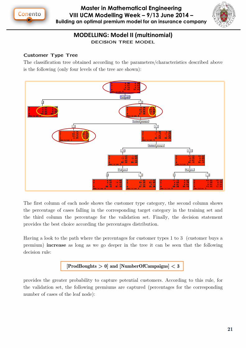
The classification tree obtained according to the parameters/characteristics described above

is the following (only four levels of the tree are shown):

The first column of each node shows the customer type category, the second column shows

the percentage of cases falling in the corresponding target category in the training set and

the third column the percentage for the validation set. Finally, the decision statement

provides the best choice according the percentages distribution.

Having a look to the path where the percentages for customer types 1 to 3 (customer buys a

premium) increase as long as we go deeper in the tree it can be seen that the following

decision rule:

[ProdBoughts > 0] and [NumberOfCampaigns] < 3

provides the greater probability to capture potential customers. According to this rule, for

the validation set, the following premiums are captured (percentages for the corresponding

number of cases of the leaf node):



22


Validation Set

Product bought > 0

Number of Campaigns < 3

1032 cases

230 cases

58 cases

Premium % captured Number of cases

1 51.8% 30

2 48.2% 28

3 0% 0

Training Set

Product bought > 0

Number of Campaigns < 3

2388 cases

529 cases

136 cases

Premium % captured Number of cases

1 50.7% 69

2 49.1% 67

3 0.1% 0

Customer Type Characterization: number of tree leaves vs events captured.

According to the

assessment criterion used,

with 10 leaves in the tree,

the percentage of events

captured is 2.85% (event

means the cases where

customer_type is greater

than 0, i.e., the customer

buys a premium).



23


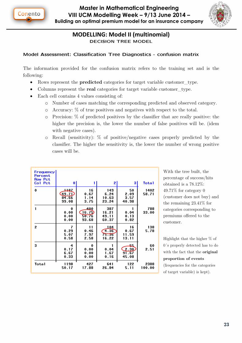
Model Assessment: Classification Tree Diagnostics - confusion matrix

The information provided for the confusion matrix refers to the training set and is the

following:

Rows represent the predicted categories for target variable customer_type.

Columns represent the real categories for target variable customer_type.

Each cell contains 4 values consisting of:

o Number of cases matching the corresponding predicted and observed category.

o Accuracy: % of true positives and negatives with respect to the total.

o Precision: % of predicted positives by the classifier that are really positive: the

higher the precision is, the lower the number of false positives will be. (idem

with negative cases).

o Recall (sensitivity): % of positive/negative cases properly predicted by the

classifier. The higher the sensitivity is, the lower the number of wrong positive

cases will be.

With the tree built, the

percentage of success/hits

obtained is a 78.12%:

49.71% for category 0

(customer does not buy) and

the remaining 23.41% for

categories corresponding to

premiums offered to the

customer.

Highlight that the higher % of

0´s properly detected has to do

with the fact that the original

proportion of events

(frequencies for the categories

of target variable) is kept).



24


Model Assessment: Profit Chart (Sensitivity)

For a 70% of the highest scores obtained

we get an expected profit of 3. From this

70% till complete the 100% of cases, the

average profit decrease sharply till a value

of 2.86. This result is in accordance with

the values obtained in the confusion

matrix.

Blue function represents a random model

and red function represents the tree model.



25

MODELLING: Model II (multinomial) NEURAL NETWORK

Introduction

A Neural Network has been used as third variant for the multinomial model (model II). The

following table provides a summary of some of the main advantages and disadvantages of

neural networks as classifiers:

Advantages Disadvantages

High Accuracy:

Neural networks are able to approximate

complex non-linear mappings.

Transparency:

Neural networks operate as “black boxes”,

therefore, lack of transparency

Noise Tolerance:

Neural networks are very flexible with

respect to incomplete, missing and noisy

data

May converge to local minima in the error

surface.

Independence from prior assumptions:

Neural networks do not make a priori

assumptions about the distribution of the

data, or the form of interactions between

factors.

Totally dependent on the quality and

amount of data available.

Flexible: Non-linear model making, flexible for

real applications.

Rule extraction is difficult.

The application of Neural Networks in Insurance industry has to do with:

Profit and growth

Understanding customer retention patterns (renewal/termination)

Direct marketing campaigns

Price setting.



26


Modelling

The main characteristics of the neural network defined are:

Multilayer perceptron model

2 hidden-layers feed forward neural network with 17 neurons each one:

o with two hidden layers we make possible to capture non-linear relationships.

o input layer contains as many neurons as explanatory variables considered (8)

o according to Lipman rule, the number of neurons for hidden layer are 17.

Hyperbolic Tangent as activation function

o due to the fact we have dichotomous variables, we need this activation

function.

Generic Linear combination function

Selection criterion: profit/loss matrix for back propagation with descend gradient (the

one already used for de classification tree).

Explanatory variables (neurons on input layer) have been standardized by average and

standard deviation: in this way, hyperbolic tangent function transforms inputs in (-1,1).



27


Results

Confusion matrix

Rows in the table represent predicted categories and columns the real/observed categories.

Having a look to the diagonal it is observed that a 72.3% of hits (let say “true positives”,

i.e., % of properly classified cases) are achieved by the model: 44.39% of 0´s contribution,

3.56% of 1´s contribution, 21.52% of 2´s contribution and 2.89% of 3´s contribution.

On the other hand, it is observed that:

Categories 0 and 2 are well predicted: 88.5% (1060/1198) for 0´s and 80.2% (514/641)

for 2´s.

It seems the model confuse 2´s with 1´s. However that´s not really important because

both levels of premiums differs only slightly in the price.

Categories 1 and 3 are worse classified than categories 0 and 2: 19.9% (85/427) for

1´s and 56.55% (69/122) for 3´s: 1´s have the worst prediction power.



28


With approximately 85 iterations the average profit stops to increase in parallel for training

and validation sets and this point is fixed for the optimal generalization. An average profit of

2.9 and 2.8 are obtained for training and validation sets respectively. Considering the profit

matrix defined, the values achieved by the model are high and that brings the classification

done is good enough.

Average profit by Neural Network iterations number for training and validation

datasets



29

OPTIMIZATION OPTIMAL MODEL AS COMBINATION OF MODELS

For model II, three variants have been built:

Multinomial model (model II) variants

MTREE

(m1) Tree model variant

MMLR

(m2) Multinomial logistic regression model variant

MNN

(m3) Neural Network model variant

In order to optimize our multinomial model a convex linear combination of previous models

has been used. It can be seen as:

where Mxxx refers to the model variant. The following figure summarize the idea of models

combination and provide as well the resulting coefficients:

Next paragraphs explain how the optimal model has been built.



30


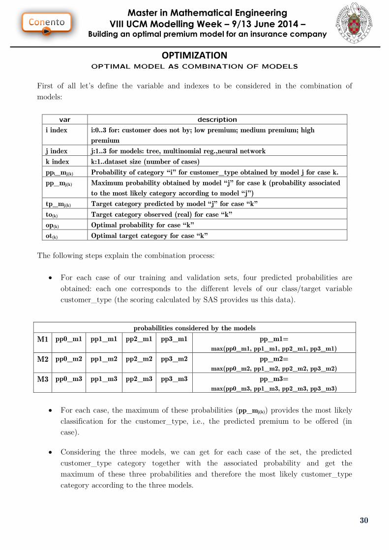
First of all let’s define the variable and indexes to be considered in the combination of

models:

var description

i index i:0..3 for: customer does not by; low premium; medium premium; high

premium

j index j:1..3 for models: tree, multinomial reg.,neural network

k index k:1..dataset size (number of cases)

ppi_mj(k) Probability of category “i” for customer_type obtained by model j for case k.

pp_mj(k) Maximum probability obtained by model “j” for case k (probability associated

to the most likely category according to model “j”)

tp_mj(k) Target category predicted by model “j” for case “k”

to(k) Target category observed (real) for case “k”

op(k) Optimal probability for case “k”

ot(k) Optimal target category for case “k”

The following steps explain the combination process:

For each case of our training and validation sets, four predicted probabilities are

obtained: each one corresponds to the different levels of our class/target variable

customer_type (the scoring calculated by SAS provides us this data).

probabilities considered by the models

M1 pp0_m1 pp1_m1 pp2_m1 pp3_m1 pp_m1=

max(pp0_m1, pp1_m1, pp2_m1, pp3_m1) M2 pp0_m2 pp1_m2 pp2_m2 pp3_m2 pp_m2=

max(pp0_m2, pp1_m2, pp2_m2, pp3_m2) M3 pp0_m3 pp1_m3 pp2_m3 pp3_m3 pp_m3=

max(pp0_m3, pp1_m3, pp2_m3, pp3_m3)

For each case, the maximum of these probabilities (pp_mj(k)) provides the most likely

classification for the customer_type, i.e., the predicted premium to be offered (in

case).

Considering the three models, we can get for each case of the set, the predicted

customer_type category together with the associated probability and get the

maximum of these three probabilities and therefore the most likely customer_type

category according to the three models.



31


Higher probability for each case according to models max.probs.

(and therefore most likely target category)

Case 1 pp_m1(1) pp_m2(1) pp_m3(1) pp(1)=max(pp_m1, pp_m2, pp_m3) … - - - -…

Case k pp1_m3(k) pp2_m3(k) pp3_m3(k) pp(k)=max(pp_m1, pp_m2, pp_m3) … - - - -

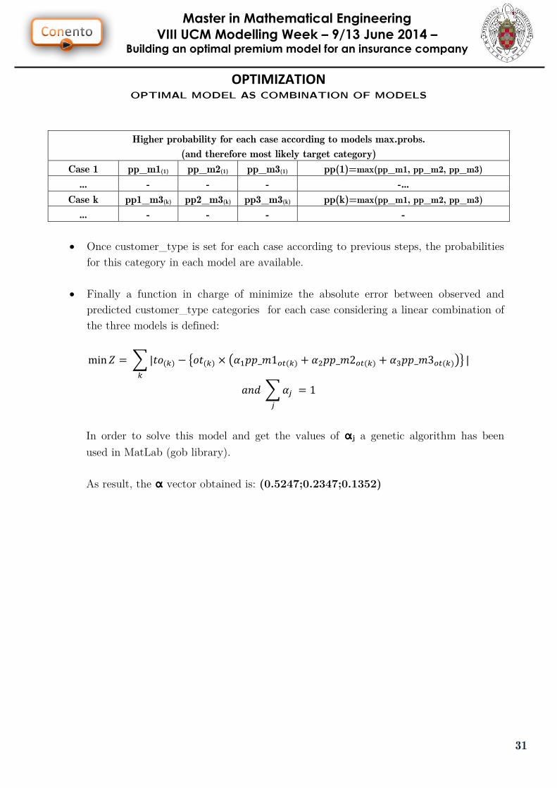
Once customer_type is set for each case according to previous steps, the probabilities

for this category in each model are available.

Finally a function in charge of minimize the absolute error between observed and

predicted customer_type categories for each case considering a linear combination of

the three models is defined:

In order to solve this model and get the values of αj a genetic algorithm has been

used in MatLab (gob library).

As result, the α vector obtained is: (0.5247;0.2347;0.1352)



32

VALIDATION OF MODELS

ROC curves for model-I & model-II variants and optimal

According to the shape of the ROC curves (area under curve) obtained for multinomial

model (model II) we can see that optimal, Decision Tree and Neural Network models provide

better prediction power than multinomial logistic regression model.

Keep in mind that no decision matrix (profit/loss) is used by this model. Optimal and

Decision Tree models overlap due to the fact that the tree is the most accurate and the

weight of the tree in the optimal model is the highest.

For model I similar results are obtained althought the area under ROC curve seems to be

lower than optimal or decision tree in model II. Therfore model II is prefered than model I to

predict buyer/not buyer.

Model-1



33

VALIDATION OF MODELS

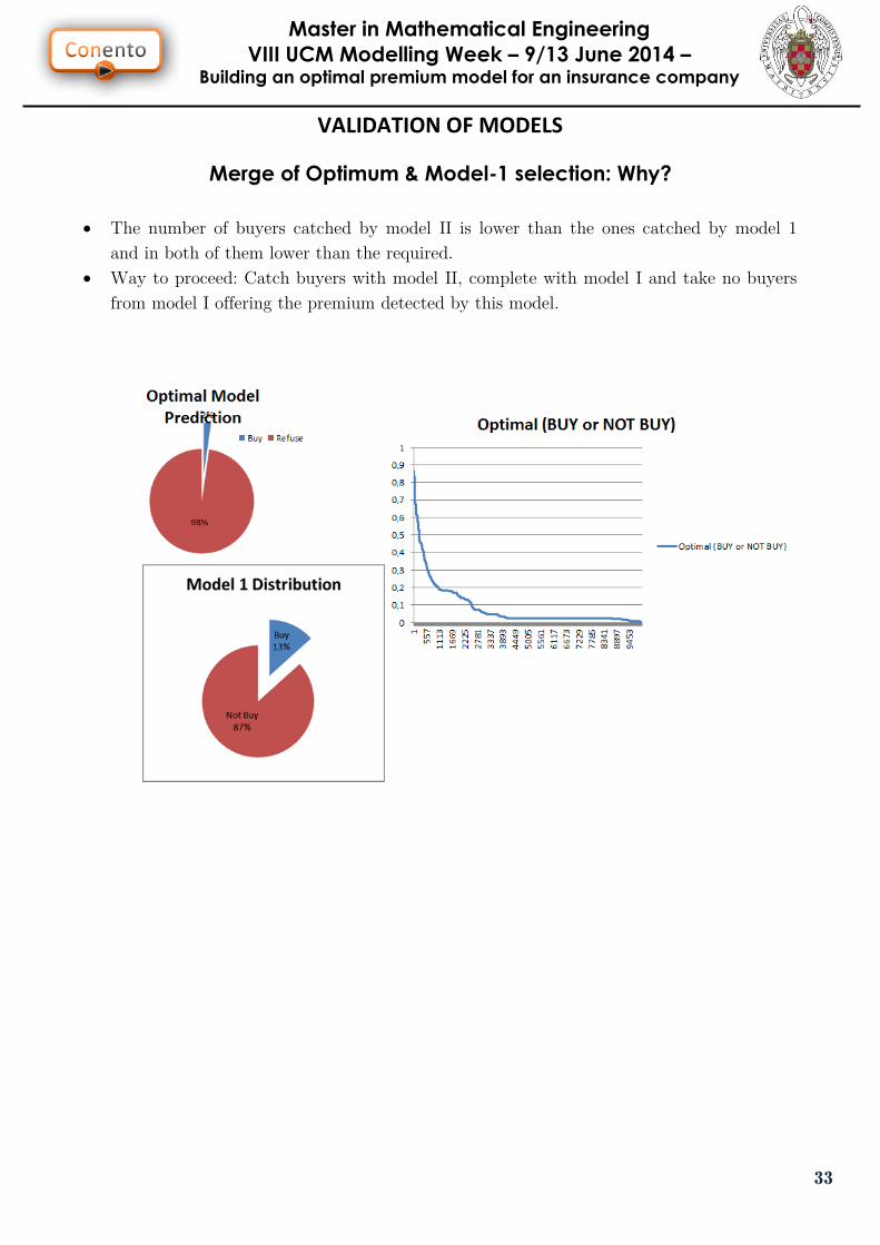
Merge of Optimum & Model-1 selection: Why?

The number of buyers catched by model II is lower than the ones catched by model 1

and in both of them lower than the required.

Way to proceed: Catch buyers with model II, complete with model I and take no buyers

from model I offering the premium detected by this model.



34

CONCLUSIONS, REMARKS and NEXT STEPS

Having a look to the profit analysis, we can conclude that:

First insight: we have found the optimal number of customers to call should be less

than 5000.

Second insight: the benefits with optimal model are much higher than the obtained

with the random model: around 20000 euros if we call the optimal number of

potential customers in the first case versus around 4500 euros calling to 5000 in the

second case (random model).

Remarks

• Followed two research lines. They converged in some aspects. They shed light about

the drivers and the forecasting ability

• Saved some difficulties:

• Missing values

• Ideate the models

• Decide the most relevant aspects

Next Steps • More time to know the insurance company interests about the model

• Analyze the relationship among the explanatory variables in depth, non linearities

and so on…

• Analyze robustness of all the models more carefully.

• With more information about costs, to build a better benefit function.

building an optimal premium model for an insurance company€¦ · building an optimal premium...

Documents