building better models

Copyright © 2010 SAS Institute Inc. All rights reserved.

Building Better ModelsMalcolm Moore

2

Copyright © 2010, SAS Institute Inc. All rights reserved.

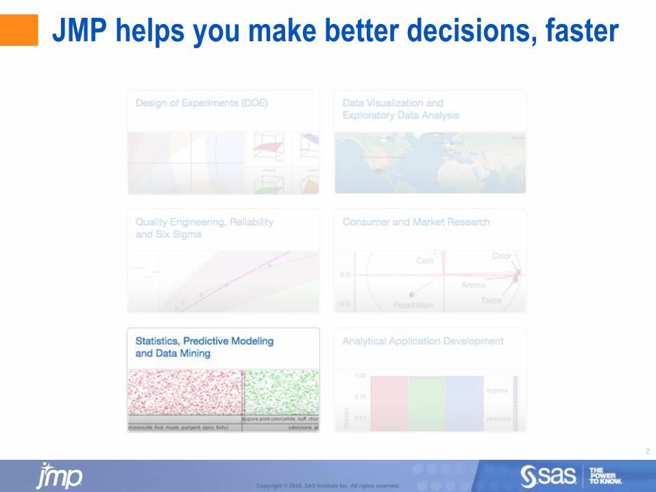
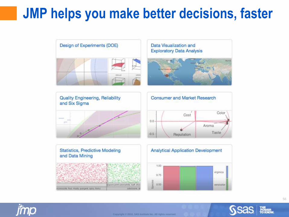
JMP helps you make better decisions, faster

3


We will show how you can use JMP to

Build better models

Manage “messy data” easily

Compare alternative models and approaches to quickly

Learn more from your data

Select the best variables

Make better predictions

Communicate the consequences to execs and other stakeholders

Make better decisions, faster

4


Ways of building better models

Help us to help you . . .

5


How many rows are in your data sets?

(Select one)

1. <1,000

2. 1001 to 10,000

3. 10,001 to 100,000

4. 100,001 to 1M

5. >1M

6


How many columns are in your data sets?

(Select one)

1. <20

2. 21 to 50

3. 51 to 100

4. 101 to 1,000

5. >1,000

7


Are your Xs correlated?

(Select one)

1. No

2. Moderately correlated

3. Strongly correlated

8


Does your original data contain missing cells, outliers or wrong values?(Select one)

1. Rarely

2. Sometimes

3. Always

9


How do you analyse / make sense of data?

(Select all that apply)

1. Tabular summaries

2. Graphs

3. Statistical methods

4. Data mining or predictive modelling

5. Quality or reliability methods

10


What’s your knowledge of statistics?

(Select one)

1. Low

2. Moderate

3. High

11


What function best describes your work?

(Select one)

1. Academia

2. Research

3. Development

4. Production

5. Marketing or Sales

6. Support Services

12


Topics Covered

Ways of building better statistical models.

Common statistical modeling methods:

Decision Trees, Uplift Modelling

Regression, PLS

Neural Networks

Shrinkage methods

Useful statistical modeling approaches:

Stepwise.

Boosting.

Model averaging, e.g. random forests.

Strategies for missing data

Case study approach to show the use of these methods and ideas.

13


What is a statistical model?

An empirical model that relates a set of inputs (predictors, Xs) to one or more outcomes (responses, Ys).

Separates the response variation into signal and noise:

Y = f(X) + E

Y is one or more continuous or categorical response outcomes.

X is one or more continuous or categorical predictors.

f(X) describes predictable variation in Y (signal).

E describes non-predictable variation in Y (noise).

“All models are wrong, but some are useful”

– George Box

14


What is a predictive model?

A type of statistical model where the focus is on predicting Y independent of the form used for f(X).

There is less concern about the form of the model –parameter estimation isn’t important. The focus is on how well it predicts.

http://en.wikipedia.org/wiki/Predictive_modelling

http://en.wikipedia.org/wiki/Predictive_modelling

15


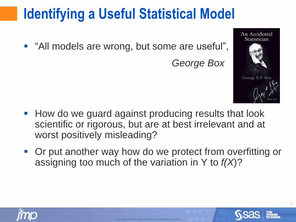
Identifying a Useful Statistical Model

“All models are wrong, but some are useful”,

George Box

How do we guard against producing results that look scientific or rigorous, but are at best irrelevant and at worst positively misleading?

Or put another way how do we protect from overfitting or assigning too much of the variation in Y to f(X)?

16


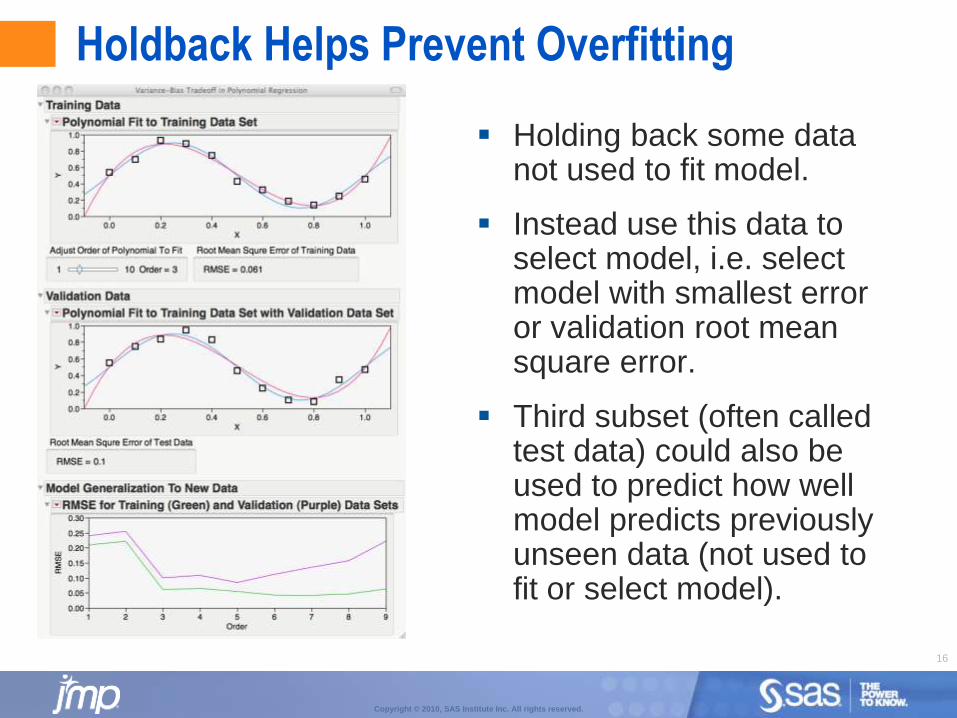
Holdback Helps Prevent Overfitting

Holding back some data not used to fit model.

Instead use this data to select model, i.e. select model with smallest error or validation root mean square error.

Third subset (often called test data) could also be used to predict how well model predicts previously unseen data (not used to fit or select model).

17


Model Validation Options

Large datasets use holdback which randomly split data into two or three subgroups:

Training: Used to build (fit or estimate) the model.

Validation: Used to select “best” model, i.e. model representing f(X) without overfitting.

Test: Used solely to evaluate the final model fit. Gives honest assessment of how well model predicts previously unseen data.

Small datasets use k-fold:

Randomly divides into k separate groups.

Hold out one of the “folds” from model building and fit a model to the rest of the data.

Held out portion is “scored” (predicted) by the model, and measures of model error recorded. Repeat for each fold.

Average error estimates across data folds and select model with smallest k-fold average error.

18


What About Missing Cells?

Some data sets are full of missing values or cells.

Standard methods drop a whole observation if any of the X’s are missing.

With lots of X’s may end up with little or no data for modelling.

Even when you do end up with enough data for modelling, if the mechanism that causes missing values is related to the response the data left will be a biased sample.

19


Missing Values

Sometimes emptiness is meaningful:

Loan applicant leaves ‘debt’ and ‘salary’ fields empty.

Job applicant leaves ‘previous job’ field empty.

Political candidate fills out a form and leaves ‘last conviction’ field empty.

Missing values are values too - They are just harder to accommodate in statistical methods.

Even if they are not informative we don’t want to throw away data, making our models less informative (lose power).

‘Informative Missing’ puts all data to use.

20


Informative Missing

Options for dealing with missing data depend on modelling method.

Regression methods:

Categorical Predictor:

» Creates separate level for missing data and treats it as such.

Continuous Predictor:

» The column mean is substituted for the missing value.

» Additionally an indicator column is added to the predictors where rows take value of 1 where data is missing, 0 otherwise.

This can significantly improve the fit when data is missing not at random and avoids data and power reduction due to missing cells in other situations:

http://blogs.sas.com/content/jmp/2013/10/29/its-not-just-what-you-say-but-what-you-dont-say-informative-missing/

http://blogs.sas.com/content/jmp/2013/10/29/its-not-just-what-you-say-but-what-you-dont-say-informative-missing/

21


Statistical Modeling

We will take a case study approach to introducing some of the common statistical modeling methods deployed with model validation approaches:

Types -

» Decision Trees

» Regression, PLS

» Neural Networks

» Shrinkage Methods

Approaches -

» Stepwise

» Boosting

» Model averaging, e.g. random forests


Case Study 1: RegressionBanding in a Printing Process

23


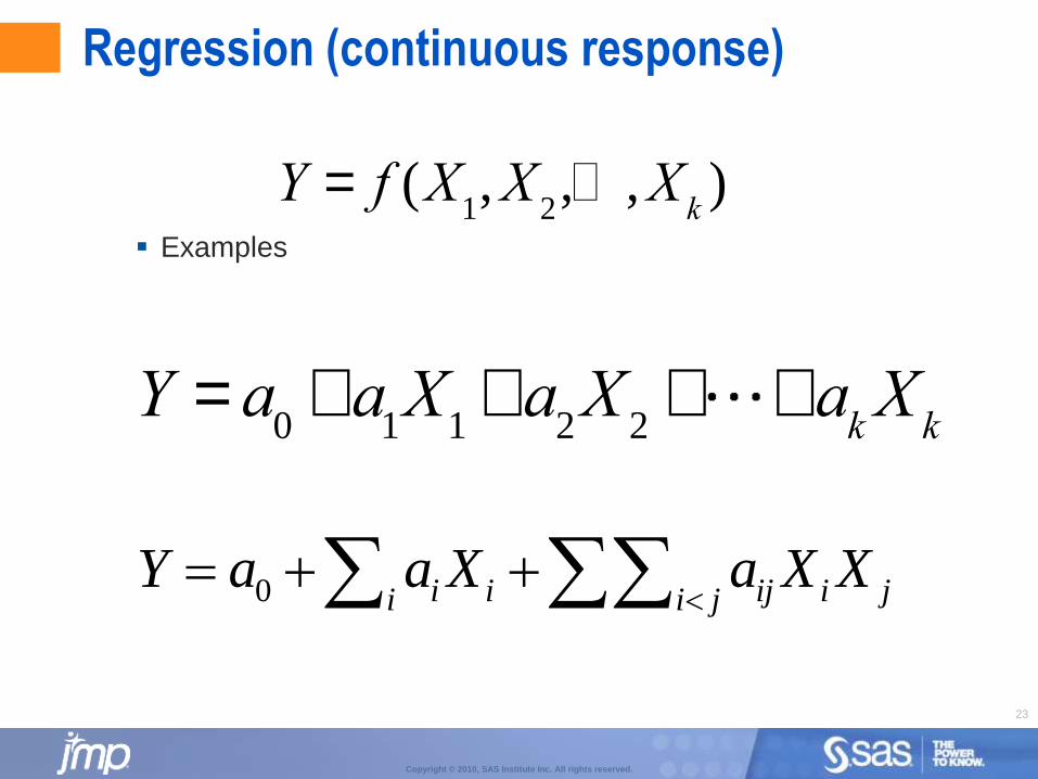
Regression (continuous response)

Examples

Y = f (X1,X

2,… ,X

k)

Y = a0+a

1X

1+a

2X

2+ +a

kXk

0 i i ij i ji i jY a a X a X X

24


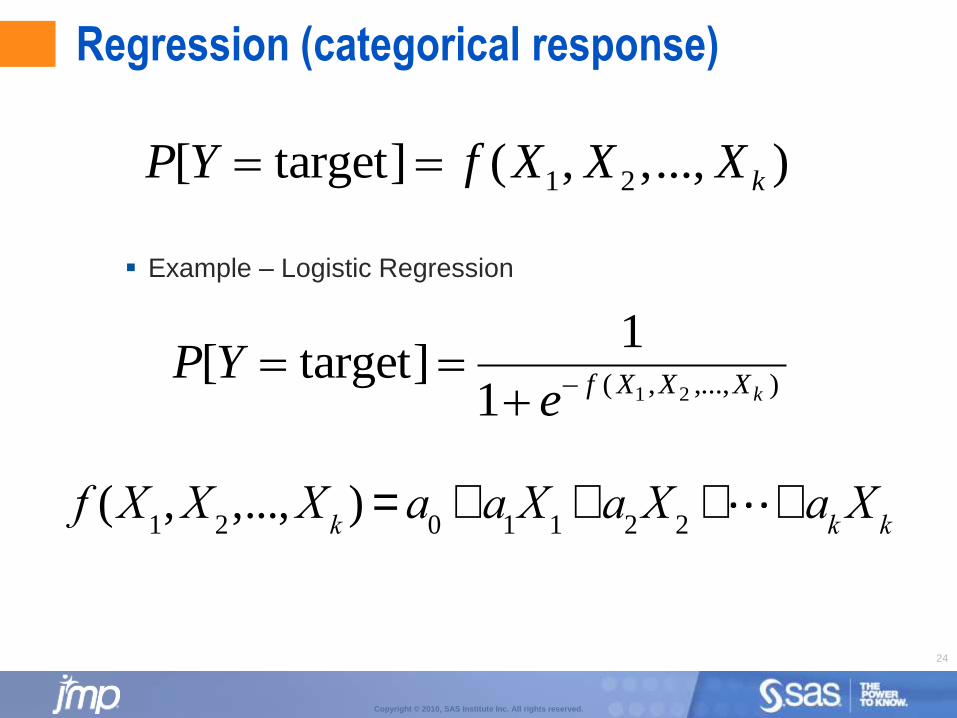
Example – Logistic Regression

Regression (categorical response)

1 2[ target] ( , ,..., )kP Y f X X X

1 2( , ,..., )

1[ target]

1 kf X X XP Y

e

f (X1,X

2,...,X

k) = a

0+a

1X

1+a

2X

2+ +a

kXk

25


Model Selection Stepwise Regression

Start with a base model: intercept only or all terms.

If intercept only, find term not included that explains the most variation and enter it into the model.

If all terms, remove the term that explains the least.

Continue until a stopping criterion is met (validation R-Square).

A variation of stepwise regression is all possible subsets (best subset) regression.

Examine all 2, 3, 4, …, etc. term models and pick the best out of each. Sometimes statistical heredity is imposed to make the problem more tractable.

See Gardner, S. “Model Selection: Part 2 - Model Selection Procedures“, ASQ Statistics Division Newsletter, Volume 29, No. 3, Spring, 2011, http://asqstatdiv.org/newsletterarch.php, for a discussion of stepwise regression for continuous response models.

http://asqstatdiv.org/newsletterarch.php

26


Model Selection

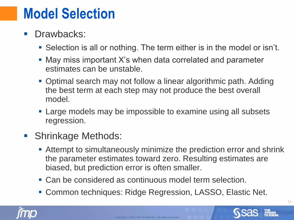
Drawbacks:

Selection is all or nothing. The term either is in the model or isn’t.

May miss important X’s when data correlated and parameter estimates can be unstable.

Optimal search may not follow a linear algorithmic path. Adding the best term at each step may not produce the best overall model.

Large models may be impossible to examine using all subsets regression.

Shrinkage Methods:

Attempt to simultaneously minimize the prediction error and shrink the parameter estimates toward zero. Resulting estimates are biased, but prediction error is often smaller.

Can be considered as continuous model term selection.

Common techniques: Ridge Regression, LASSO, Elastic Net.

27


Banding in a Printing ProcessExample 1


Case Study 2: Decision TreesWhich customer segments to target with campaigns

29


Decision Trees

Also known as Recursive Partitioning, CHAID, CART

Models are a series of nested IF() statements, where each condition in the IF() statement can be viewed as a separate branch in a tree.

Branches are chosen so that the difference in the average response between paired branches is maximised.

Doing so assigns more of the variation in Y to f(X).

Algorithm gets more complicated and computations more intensive with holdback.

30


Decision Tree

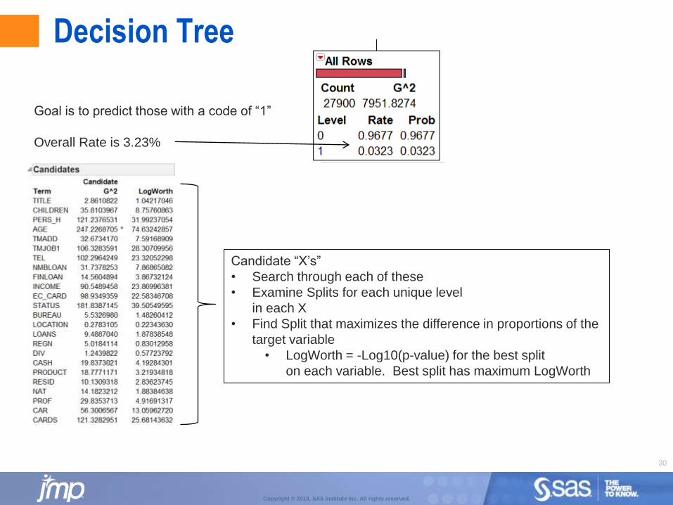
Goal is to predict those with a code of “1”

Overall Rate is 3.23%

Candidate “X’s”

• Search through each of these

• Examine Splits for each unique level

in each X

• Find Split that maximizes the difference in proportions of the

target variable

• LogWorth = -Log10(p-value) for the best split

on each variable. Best split has maximum LogWorth

31


Decision Tree

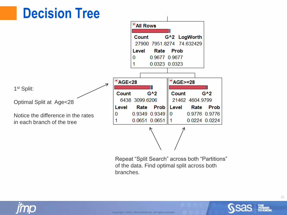
1st Split:

Optimal Split at Age<28

Notice the difference in the rates

in each branch of the tree

Repeat “Split Search” across both “Partitions”

of the data. Find optimal split across both

branches.

32


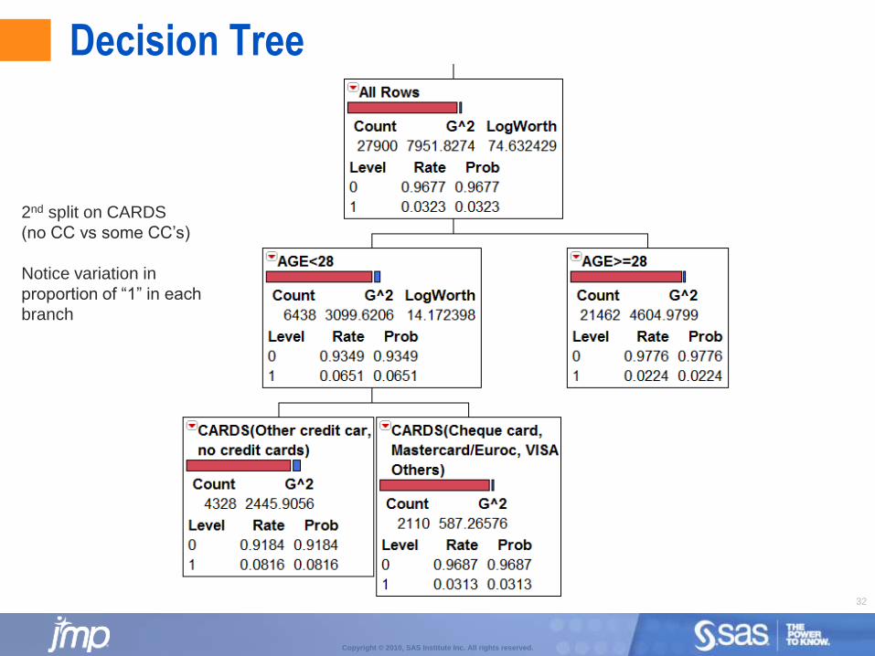
Decision Tree

2nd split on CARDS

(no CC vs some CC’s)

Notice variation in

proportion of “1” in each

branch

33


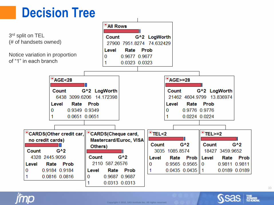
Decision Tree

3rd split on TEL

(# of handsets owned)

Notice variation in proportion

of “1” in each branch

34


Model Evaluation

Continuous response models evaluated using SSE (sum of squared error) measures such as R^2, adjusted R^2:

Other alternatives are information based measures such as AIC and BIC.

Categorical response models evaluated on ability to:

Sort portions of the data into different levels of response using ROC curves and Lift curves.

Categorize a new observation measured by confusion matrices and rates, as well as overall misclassification rate.

35


ROC Curve Example

36


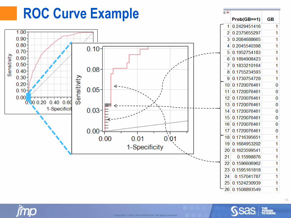
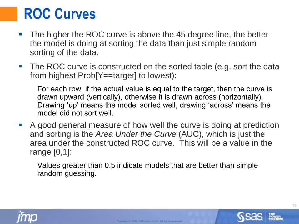
ROC Curves

The higher the ROC curve is above the 45 degree line, the better the model is doing at sorting the data than just simple random sorting of the data.

The ROC curve is constructed on the sorted table (e.g. sort the data from highest Prob[Y==target] to lowest):

For each row, if the actual value is equal to the target, then the curve is drawn upward (vertically), otherwise it is drawn across (horizontally). Drawing ‘up’ means the model sorted well, drawing ‘across’ means the model did not sort well.

A good general measure of how well the curve is doing at prediction and sorting is the Area Under the Curve (AUC), which is just the area under the constructed ROC curve. This will be a value in the range [0,1]:

Values greater than 0.5 indicate models that are better than simple random guessing.

37


Decision Trees: Which customer segments are most likely to churn

Example 2


Case Study 3: Uplift ModelingWhich customer segments to target with campaigns

39


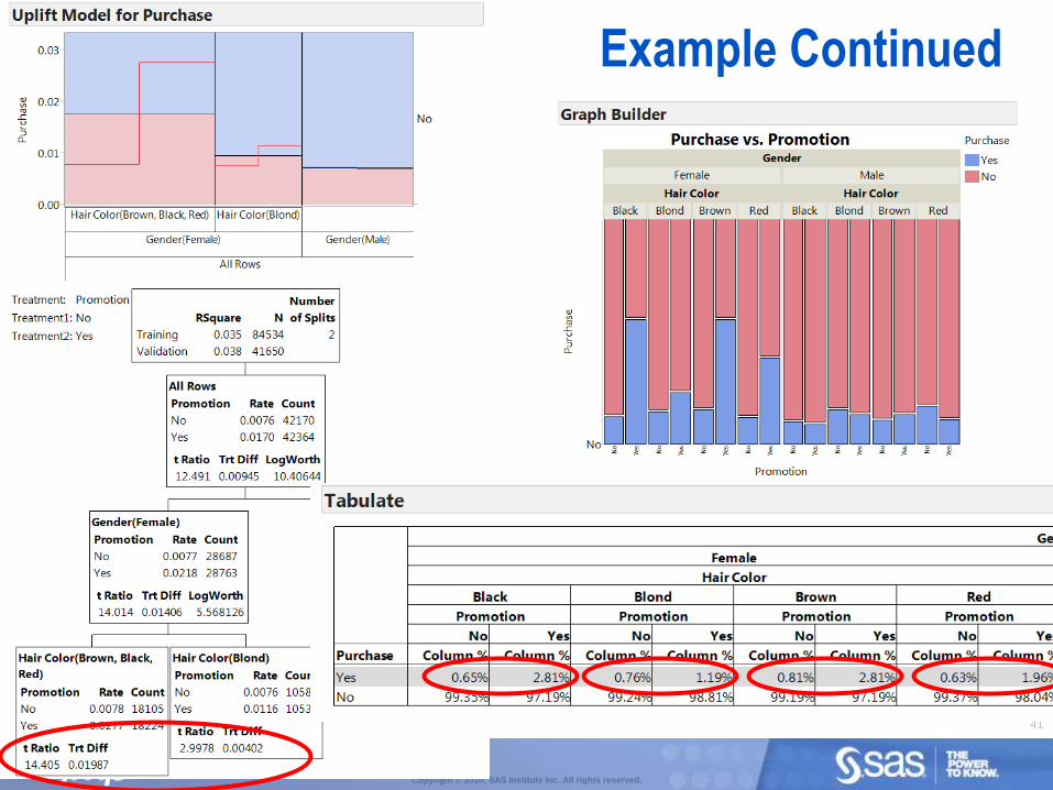
Uplift Modelling

Also known as incremental modelling, true lift modelling or net modelling.

Identifies individuals or sub-groups who are most likely to respond favourably to some action:

Customers likely to respond to marketing campaigns to help optimize marketing decisions

Patients likely to respond to medical intervention to help define personalized medicine protocols

Unlike traditional partition models that find splits to optimize a prediction, uplift models find splits to maximize a treatment difference.

Best split is the split that maximises the interaction of the split and treatment.

40


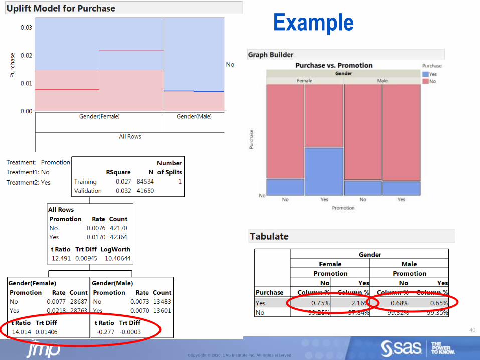
Example

41


Example Continued


Case Study 4: Bootstrap Forest and Boosted TreesQuantitative Structure-Activity Modeling

46


Improvements to Decision Trees

Two modifications to basic decision trees that (depending on circumstances and the specific data) may develop better models are:

1. Fit many models and average them -

Bootstrap Forest or Random Forest.

2. Fit a simple model and boost it by fitting a simple model to model errors and repeat several times -

Model Boosting or Boosted Tree.

47


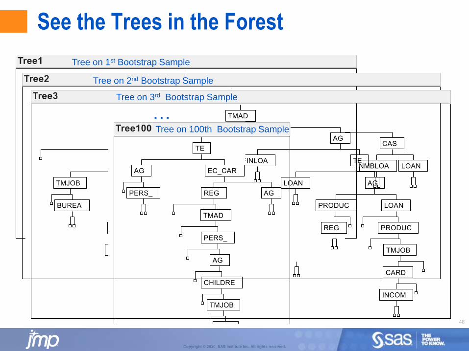
Bootstrap Forest

Bootstrap Forest:

For each tree, take a random sample (with replacement) of rows.

For each split, take a random sample (30% sample) of X’s.

Build decision tree.

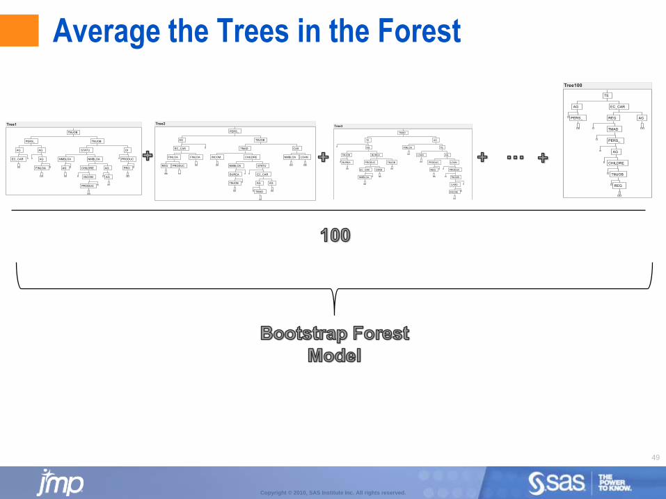
Repeat above process making many trees and average predictions across all trees (bagging).

Also known as a random forest.

Works very well on wide tables (with correlated X’s).

Can be used for both predictive modeling and variable selection.

48


See the Trees in the Forest

Tree on 1st Bootstrap Sample

Tree on 2nd Bootstrap Sample

Tree on 3rd Bootstrap Sample

…Tree on 100th Bootstrap Sample

49


Average the Trees in the Forest

50


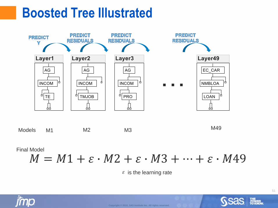
Boosted Tree

Beginning with the first tree (layer) build a small simple tree.

From the residuals of the first tree, build another small simple tree.

The next layer in the model is fit to the residuals from the previous layer, and residuals are saved from that new model fit.

This continues until a specified number of layers has been fit, or a determination has been made that adding successive layers doesn’t improve the fit of the model.

The final model is the weighted accumulation of all of the model layers.

51


Boosted Tree Illustrated

…

M1 M2 M3 M49

𝑀 = 𝑀1 + 𝜀 ∙ 𝑀2 + 𝜀 ∙ 𝑀3 +⋯+ 𝜀 ∙ 𝑀49

Models

Final Model

𝜀 is the learning rate

52


Boosted Tree

Boosted Trees:

Primarily used for building prediction models.

Not as good as Bootstrap Forest at exploring all the relationships between Y and the X’s, but still can be used for that purpose.

Results in ‘smaller’ models (fewer arithmetic operations), faster scoring.

53


Other Pro Modelling Methods

PLS

Neural Networks

Shrinkage Methods:

Ridge Regression, LASSO, Elastic Net

PCA Clustering

54


We have shown how you can use JMP to

Build better models

Manage “messy data” easily

Compare alternative models and approaches to quickly

Learn more from your data

Select the best variables

Make better predictions

Communicate the consequences to execs and other stakeholders

Make better decisions, faster

55


How mining your data helps your company

Increase growth and return

Reduce costs

Deliver a competitive edge

Improve loyalty

Accelerate innovation

Speed time to market

56


JMP helps you make better decisions, faster

57


What are you going to do next?

Visit jmp.com for more information about JMP

Sign up for our webinars and seminars

building better models

Software