Building HMSC step by step: single-species distribution modelling

Full HMSC Single-species HMSC

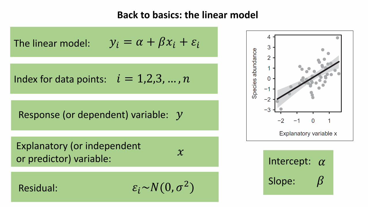
Back to basics: the linear model

𝑦𝑖 = 𝛼 + 𝛽𝑥𝑖 + 𝜀𝑖

𝑖 = 1,2,3, … , 𝑛

𝑦

𝑥

𝜀𝑖~𝑁(0, 𝜎2)

The linear model:

Index for data points:

Response (or dependent) variable:

Explanatory (or independent or predictor) variable:

Residual:𝛽

Intercept:

Slope:

𝛼

Several explanatory variables and the linear predictor

𝑦𝑖 = 𝛼 + 𝛽1𝑥𝑖1 + 𝛽1𝑥𝑖2 + 𝜀𝑖The linear model with two variables:

𝑦𝑖 = 𝛽1𝑥𝑖1 + 𝛽2𝑥𝑖2 + 𝛽3𝑥𝑖3 + 𝜀𝑖Can also be parameterized as:

𝑥𝑖1 = 1where for all sampling units 𝑖

𝑛𝑐

Can be written more compactly as where

𝐿𝑖 =𝑘=1

𝑛𝑐𝛽𝑘𝑥𝑖𝑘

is the linear predictor and is the number of covariates (including the intercept)

𝑦𝑖 = 𝐿𝑖 + 𝜀𝑖

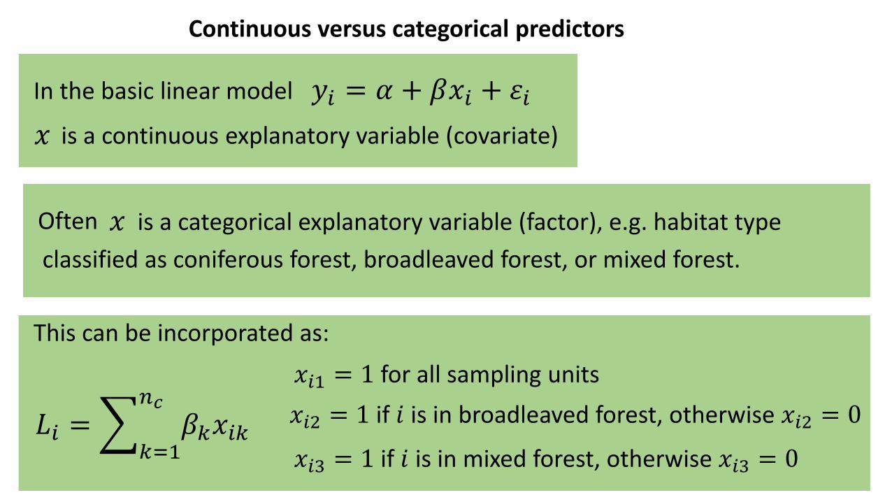
Continuous versus categorical predictors

In the basic linear model

𝐿𝑖 =𝑘=1

𝑛𝑐𝛽𝑘𝑥𝑖𝑘

𝑦𝑖 = 𝛼 + 𝛽𝑥𝑖 + 𝜀𝑖

𝑥 is a continuous explanatory variable (covariate)

Often 𝑥 is a categorical explanatory variable (factor), e.g. habitat type

classified as coniferous forest, broadleaved forest, or mixed forest.

𝑥𝑖1 = 1 for all sampling units

𝑥𝑖2 = 1 if 𝑖 is in broadleaved forest, otherwise 𝑥𝑖2 = 0

This can be incorporated as:

𝑥𝑖3 = 1 if 𝑖 is in mixed forest, otherwise 𝑥𝑖3 = 0

Generalized linear models

Presence-absence data: 𝑦𝑖~Bernoulli(𝜇𝑖)

Logistic regression: 𝜇𝑖 = logit−1(𝐿𝑖)

Probit regression: 𝜇𝑖 = Φ(𝐿𝑖)

𝐿Linear predictor

𝜇O

ccu

rren

ce

pro

bab

ility

Generalized linear models

Count data: 𝑦𝑖~Poisson(𝜇𝑖)

Poisson model𝜇𝑖 = exp(𝐿𝑖)

Lognormal Poisson model

𝐿Linear predictor

𝜇Ex

pec

ted

co

un

t

𝜇𝑖 = exp(𝐿𝑖 + 𝜀𝑖)

𝑦 = 3,0,0,2,1

𝑦 = 3,0,0,2,30,…

Hurdle models for zero inflated data

Assume that the data looks like 𝑦 = 0, 42, 39, 0, 43

We can model separately presence-absence

and abundance conditional on presence

𝑦 = 0, 1, 1, 0, 1

𝑦 = NA, 42, 39, NA, 43

These two parts of the hurdle-model can be fitted independently of each other, but they can be thought to jointly form one model.

The presence-absence part predicts if the species is present or not. If it is present, then the abundance (conditional on presence) part predicts how abundant the species is.

Mixed models: fixed effects and random effects

Linear model with fixed effects only:

𝐿𝑖 =𝑘=1

𝑛𝑐𝛽𝑘𝑥𝑖𝑘

𝑦𝑖 = 𝐿𝑖 + 𝜀𝑖

𝜀𝑖~𝑁(0, 𝜎2)

iid

Hierarchical study design: Plot

Sampling unit

Mixed models: fixed effects and random effects

Linear model with fixed and random effects:

𝐿𝑖 =𝑘=1

𝑛𝑐𝛽𝑘𝑥𝑖𝑘

𝑦𝑖 = 𝐿𝑖 + 𝑎𝑝(𝑖) + 𝜀𝑖

𝜀𝑖~𝑁(0, 𝜎2)

iid

Hierarchical study design: Plot

Sampling unit

𝑎𝑝~𝑁(0, 𝜎𝑃2)

iid

Mixed models: fixed effects and random effects

Spatial study design:

Mixed models: fixed effects and random effects

Spatial study design:

Linear model without spatial structure:

𝐿𝑖 =𝑘=1

𝑛𝑐𝛽𝑘𝑥𝑖𝑘

𝑦𝑖 = 𝐿𝑖 + 𝜀𝑖

𝜀𝑖~𝑁(0, 𝜎2)

iid

Mixed models: fixed effects and random effects

Spatial study design:

Linear model with spatial structure:

𝐿𝑖 =𝑘=1

𝑛𝑐𝛽𝑘𝑥𝑖𝑘

𝑦𝑖 = 𝐿𝑖 + 𝑎𝑖 + 𝜀𝑖

Cov 𝑎𝑖 , 𝑎𝑗 = 𝜎𝑆2 exp −𝑑𝑖𝑗/𝛼

𝜀𝑖~𝑁(0, 𝜎2)

iid𝑎𝑖~𝑁(0, 𝜎𝑆2)

Fitting a spatial model enables using spatial information when generating predictions