Building Query Compilers

(Under Construction)

[expected time to completion: 5 years]

Guido Moerkotte

December 8, 2014

Contents

I Basics 3

1 Introduction 5

1.1 General Remarks . . . . . . . . . . . . . . . . . . . . . . . . . . . 5

1.2 DBMS Architecture . . . . . . . . . . . . . . . . . . . . . . . . . 5

1.3 Interpretation versus Compilation . . . . . . . . . . . . . . . . . . 6

1.4 Requirements for a Query Compiler . . . . . . . . . . . . . . . . 9

1.5 Search Space . . . . . . . . . . . . . . . . . . . . . . . . . . . . . 11

1.6 Generation versus Transformation . . . . . . . . . . . . . . . . . 12

1.7 Focus . . . . . . . . . . . . . . . . . . . . . . . . . . . . . . . . . 12

1.8 Organization of the Book . . . . . . . . . . . . . . . . . . . . . . 13

2 Textbook Query Optimization 15

2.1 Example Query and Outline . . . . . . . . . . . . . . . . . . . . . 15

2.2 Algebra . . . . . . . . . . . . . . . . . . . . . . . . . . . . . . . . 16

2.3 Canonical Translation . . . . . . . . . . . . . . . . . . . . . . . . 17

2.4 Logical Query Optimization . . . . . . . . . . . . . . . . . . . . . 20

2.5 Physical Query Optimization . . . . . . . . . . . . . . . . . . . . 24

2.6 Discussion . . . . . . . . . . . . . . . . . . . . . . . . . . . . . . . 25

3 Join Ordering 31

3.1 Queries Considered . . . . . . . . . . . . . . . . . . . . . . . . . . 31

3.1.1 Query Graph . . . . . . . . . . . . . . . . . . . . . . . . . 32

3.1.2 Join Tree . . . . . . . . . . . . . . . . . . . . . . . . . . . 33

3.1.3 Simple Cost Functions . . . . . . . . . . . . . . . . . . . . 34

3.1.4 Classification of Join Ordering Problems . . . . . . . . . . 40

3.1.5 Search Space Sizes . . . . . . . . . . . . . . . . . . . . . . 41

3.1.6 Problem Complexity . . . . . . . . . . . . . . . . . . . . . 45

3.2 Deterministic Algorithms . . . . . . . . . . . . . . . . . . . . . . 47

3.2.1 Heuristics . . . . . . . . . . . . . . . . . . . . . . . . . . . 47

3.2.2 Determining the Optimal Join Order in Polynomial Time 49

3.2.3 The Maximum-Value-Precedence Algorithm . . . . . . . . 56

3.2.4 Dynamic Programming . . . . . . . . . . . . . . . . . . . 61

3.2.5 Memoization . . . . . . . . . . . . . . . . . . . . . . . . . 78

3.2.6 Join Ordering by Generating Permutations . . . . . . . . 79

3.2.7 A Dynamic Programming based Heuristics for Chain Queries 81

3.2.8 Transformation-Based Approaches . . . . . . . . . . . . . 94

i

ii CONTENTS

3.3 Probabilistic Algorithms . . . . . . . . . . . . . . . . . . . . . . . 1013.3.1 Generating Random Left-Deep Join Trees with Cross Prod-

ucts . . . . . . . . . . . . . . . . . . . . . . . . . . . . . . 1013.3.2 Generating Random Join Trees with Cross Products . . . 1033.3.3 Generating Random Join Trees without Cross Products . 1073.3.4 Quick Pick . . . . . . . . . . . . . . . . . . . . . . . . . . 1163.3.5 Iterative Improvement . . . . . . . . . . . . . . . . . . . . 1163.3.6 Simulated Annealing . . . . . . . . . . . . . . . . . . . . . 1173.3.7 Tabu Search . . . . . . . . . . . . . . . . . . . . . . . . . 1183.3.8 Genetic Algorithms . . . . . . . . . . . . . . . . . . . . . . 119

3.4 Hybrid Algorithms . . . . . . . . . . . . . . . . . . . . . . . . . . 1223.4.1 Two Phase Optimization . . . . . . . . . . . . . . . . . . 1223.4.2 AB-Algorithm . . . . . . . . . . . . . . . . . . . . . . . . 1223.4.3 Toured Simulated Annealing . . . . . . . . . . . . . . . . 1223.4.4 GOO-II . . . . . . . . . . . . . . . . . . . . . . . . . . . . 1233.4.5 Iterative Dynamic Programming . . . . . . . . . . . . . . 123

3.5 Ordering Order-Preserving Joins . . . . . . . . . . . . . . . . . . 1233.6 Characterizing Search Spaces . . . . . . . . . . . . . . . . . . . . 131

3.6.1 Complexity Thresholds . . . . . . . . . . . . . . . . . . . 1313.7 Discussion . . . . . . . . . . . . . . . . . . . . . . . . . . . . . . . 1353.8 Bibliography . . . . . . . . . . . . . . . . . . . . . . . . . . . . . 136

4 Database Items, Building Blocks, and Access Paths 1374.1 Disk Drive . . . . . . . . . . . . . . . . . . . . . . . . . . . . . . . 1374.2 Database Buffer . . . . . . . . . . . . . . . . . . . . . . . . . . . . 1464.3 Physical Database Organization . . . . . . . . . . . . . . . . . . . 1474.4 Slotted Page and Tuple Identifier (TID) . . . . . . . . . . . . . . 1504.5 Physical Record Layouts . . . . . . . . . . . . . . . . . . . . . . . 1514.6 Physical Algebra (Iterator Concept) . . . . . . . . . . . . . . . . 1524.7 Simple Scan . . . . . . . . . . . . . . . . . . . . . . . . . . . . . . 1524.8 Scan and Attribute Access . . . . . . . . . . . . . . . . . . . . . . 1534.9 Temporal Relations . . . . . . . . . . . . . . . . . . . . . . . . . . 1554.10 Table Functions . . . . . . . . . . . . . . . . . . . . . . . . . . . . 1554.11 Indexes . . . . . . . . . . . . . . . . . . . . . . . . . . . . . . . . 1564.12 Single Index Access Path . . . . . . . . . . . . . . . . . . . . . . 158

4.12.1 Simple Key, No Data Attributes . . . . . . . . . . . . . . 1584.12.2 Complex Keys and Data Attributes . . . . . . . . . . . . 163

4.13 Multi Index Access Path . . . . . . . . . . . . . . . . . . . . . . . 1654.14 Indexes and Joins . . . . . . . . . . . . . . . . . . . . . . . . . . . 1674.15 Remarks on Access Path Generation . . . . . . . . . . . . . . . . 1724.16 Counting the Number of Accesses . . . . . . . . . . . . . . . . . . 173

4.16.1 Counting the Number of Direct Accesses . . . . . . . . . . 1734.16.2 Counting the Number of Sequential Accesses . . . . . . . 1824.16.3 Pointers into the Literature . . . . . . . . . . . . . . . . . 187

4.17 Disk Drive Costs for N Uniform Accesses . . . . . . . . . . . . . 1884.17.1 Number of Qualifying Cylinders, Tracks, and Sectors . . . 1884.17.2 Command Costs . . . . . . . . . . . . . . . . . . . . . . . 189

CONTENTS iii

4.17.3 Seek Costs . . . . . . . . . . . . . . . . . . . . . . . . . . 189

4.17.4 Settle Costs . . . . . . . . . . . . . . . . . . . . . . . . . . 191

4.17.5 Rotational Delay Costs . . . . . . . . . . . . . . . . . . . 191

4.17.6 Head Switch Costs . . . . . . . . . . . . . . . . . . . . . . 193

4.17.7 Discussion . . . . . . . . . . . . . . . . . . . . . . . . . . . 193

4.18 Concluding Remarks . . . . . . . . . . . . . . . . . . . . . . . . . 194

4.19 Bibliography . . . . . . . . . . . . . . . . . . . . . . . . . . . . . 194

II Foundations 197

5 Logic, Null, and Boolean Expressions 199

5.1 Two-valued logic . . . . . . . . . . . . . . . . . . . . . . . . . . . 199

5.2 NULL values and three valued logic . . . . . . . . . . . . . . . . 199

5.3 Simplifying Boolean Expressions . . . . . . . . . . . . . . . . . . 200

5.4 Optimizing Boolean Expressions . . . . . . . . . . . . . . . . . . 200

5.5 Bibliography . . . . . . . . . . . . . . . . . . . . . . . . . . . . . 200

6 Functional Dependencies 203

6.1 Functional Dependencies . . . . . . . . . . . . . . . . . . . . . . . 203

6.2 Functional Dependencies in the presence of NULL values . . . . . 204

6.3 Deriving Functional Dependencies over algebraic operators . . . . 204

6.4 Bibliography . . . . . . . . . . . . . . . . . . . . . . . . . . . . . 204

7 An Algebra for Sets, Bags, and Sequences 205

7.1 Sets, Bags, and Sequences . . . . . . . . . . . . . . . . . . . . . . 205

7.1.1 Sets . . . . . . . . . . . . . . . . . . . . . . . . . . . . . . 205

7.1.2 Duplicate Data: Bags . . . . . . . . . . . . . . . . . . . . 207

7.1.3 Explicit Duplicate Control . . . . . . . . . . . . . . . . . . 210

7.1.4 Ordered Data: Sequences . . . . . . . . . . . . . . . . . . 211

7.2 Aggregation Functions . . . . . . . . . . . . . . . . . . . . . . . . 212

7.3 Operators . . . . . . . . . . . . . . . . . . . . . . . . . . . . . . . 216

7.3.1 Preliminaries . . . . . . . . . . . . . . . . . . . . . . . . . 217

7.3.2 Signatures . . . . . . . . . . . . . . . . . . . . . . . . . . . 219

7.3.3 Projection . . . . . . . . . . . . . . . . . . . . . . . . . . . 221

7.3.4 Selection . . . . . . . . . . . . . . . . . . . . . . . . . . . 222

7.3.5 Map . . . . . . . . . . . . . . . . . . . . . . . . . . . . . . 222

7.3.6 Unary Grouping . . . . . . . . . . . . . . . . . . . . . . . 223

7.3.7 Unnest Operators . . . . . . . . . . . . . . . . . . . . . . 224

7.3.8 Flatten Operator . . . . . . . . . . . . . . . . . . . . . . . 225

7.3.9 Join Operators . . . . . . . . . . . . . . . . . . . . . . . . 225

7.3.10 Groupjoin . . . . . . . . . . . . . . . . . . . . . . . . . . . 226

7.3.11 Min/Max Operators . . . . . . . . . . . . . . . . . . . . . 227

7.3.12 Other Dependent Operators . . . . . . . . . . . . . . . . . 228

7.4 Linearity of Algebraic Operators . . . . . . . . . . . . . . . . . . 229

7.4.1 Linearity of Algebraic Operators . . . . . . . . . . . . . . 229

7.4.2 Exploiting Linearity . . . . . . . . . . . . . . . . . . . . . 234

iv CONTENTS

7.5 Representations . . . . . . . . . . . . . . . . . . . . . . . . . . . . 2357.5.1 Three Different Representations . . . . . . . . . . . . . . . 2357.5.2 Conversion between Representations . . . . . . . . . . . . 2377.5.3 Conversion between Bulk Types . . . . . . . . . . . . . . 2377.5.4 Adjusting the Algebra . . . . . . . . . . . . . . . . . . . . 2387.5.5 Partial Preaggregation . . . . . . . . . . . . . . . . . . . . 239

7.6 A Note on Equivalences . . . . . . . . . . . . . . . . . . . . . . . 2397.7 Simple Reorderability . . . . . . . . . . . . . . . . . . . . . . . . 240

7.7.1 Unary Operators . . . . . . . . . . . . . . . . . . . . . . . 2407.7.2 Push-Down/Pull-Up of Unary into/from Binary Operators2427.7.3 Binary Operators . . . . . . . . . . . . . . . . . . . . . . . 244

7.8 Predicate Detachment and Attachment . . . . . . . . . . . . . . . 2497.9 Basic Equivalences for D-Join . . . . . . . . . . . . . . . . . . . . 2517.10 Equivalences for Outerjoins . . . . . . . . . . . . . . . . . . . . . 253

7.10.1 Outerjoin Simplification . . . . . . . . . . . . . . . . . . . 2597.10.2 Generalized Outerjoin . . . . . . . . . . . . . . . . . . . . 260

7.11 Equivalences for Unary Grouping . . . . . . . . . . . . . . . . . . 2627.11.1 An Elementary Fact about Grouping . . . . . . . . . . . . 2627.11.2 Join . . . . . . . . . . . . . . . . . . . . . . . . . . . . . . 2627.11.3 Left Outerjoin . . . . . . . . . . . . . . . . . . . . . . . . 2737.11.4 Left Outerjoin with Default . . . . . . . . . . . . . . . . . 2767.11.5 Full Outerjoin . . . . . . . . . . . . . . . . . . . . . . . . . 2777.11.6 D-Join . . . . . . . . . . . . . . . . . . . . . . . . . . . . . 2807.11.7 Groupjoin . . . . . . . . . . . . . . . . . . . . . . . . . . . 2827.11.8 Intersection and Difference . . . . . . . . . . . . . . . . . 287

7.12 Eliminating Redundant Joins . . . . . . . . . . . . . . . . . . . . 2877.13 Semijoin and Antijoin Reducer . . . . . . . . . . . . . . . . . . . 2887.14 Outerjoin Simplification . . . . . . . . . . . . . . . . . . . . . . . 2897.15 Correct and Complete Exploration of the Core Search Space . . . 289

7.15.1 The Core Search Space . . . . . . . . . . . . . . . . . . . 2897.15.2 Exploration . . . . . . . . . . . . . . . . . . . . . . . . . . 2917.15.3 More Issues . . . . . . . . . . . . . . . . . . . . . . . . . . 299

7.16 Logical Algebra for Sequences . . . . . . . . . . . . . . . . . . . . 3037.16.1 Introduction . . . . . . . . . . . . . . . . . . . . . . . . . 3037.16.2 Algebraic Operators . . . . . . . . . . . . . . . . . . . . . 3047.16.3 Equivalences . . . . . . . . . . . . . . . . . . . . . . . . . 3077.16.4 Bibliography . . . . . . . . . . . . . . . . . . . . . . . . . 307

7.17 Literature . . . . . . . . . . . . . . . . . . . . . . . . . . . . . . . 3077.18 ToDo . . . . . . . . . . . . . . . . . . . . . . . . . . . . . . . . . . 308

8 Declarative Query Representation 3098.1 Calculus Representations . . . . . . . . . . . . . . . . . . . . . . 3098.2 Datalog . . . . . . . . . . . . . . . . . . . . . . . . . . . . . . . . 3098.3 Tableaux Representation . . . . . . . . . . . . . . . . . . . . . . . 3098.4 Monoid Comprehension . . . . . . . . . . . . . . . . . . . . . . . 3098.5 Expressiveness . . . . . . . . . . . . . . . . . . . . . . . . . . . . 3098.6 Bibliography . . . . . . . . . . . . . . . . . . . . . . . . . . . . . 309

CONTENTS v

9 Translation and Lifting 311

9.1 Query Language to Calculus . . . . . . . . . . . . . . . . . . . . . 311

9.2 Query Language to Algebra . . . . . . . . . . . . . . . . . . . . . 311

9.3 Calculus to Algebra . . . . . . . . . . . . . . . . . . . . . . . . . 311

9.4 Algebra to Calculus . . . . . . . . . . . . . . . . . . . . . . . . . 311

9.5 Bibliography . . . . . . . . . . . . . . . . . . . . . . . . . . . . . 311

10 Query Equivalence, Containment, Minimization, and Factor-ization 313

10.1 Set Semantics . . . . . . . . . . . . . . . . . . . . . . . . . . . . . 314

10.1.1 Conjunctive Queries . . . . . . . . . . . . . . . . . . . . . 314

10.1.2 . . . with Inequalities . . . . . . . . . . . . . . . . . . . . . 316

10.1.3 . . . with Negation . . . . . . . . . . . . . . . . . . . . . . . 317

10.1.4 . . . under Constraints . . . . . . . . . . . . . . . . . . . . 317

10.1.5 . . . with Aggregation . . . . . . . . . . . . . . . . . . . . . 317

10.2 Bag Semantics . . . . . . . . . . . . . . . . . . . . . . . . . . . . 317

10.2.1 Conjunctive Queries . . . . . . . . . . . . . . . . . . . . . 317

10.3 Sequences . . . . . . . . . . . . . . . . . . . . . . . . . . . . . . . 318

10.3.1 Path Expressions . . . . . . . . . . . . . . . . . . . . . . . 318

10.4 Minimization . . . . . . . . . . . . . . . . . . . . . . . . . . . . . 319

10.5 Detecting common subexpressions . . . . . . . . . . . . . . . . . 319

10.5.1 Simple Expressions . . . . . . . . . . . . . . . . . . . . . . 319

10.5.2 Algebraic Expressions . . . . . . . . . . . . . . . . . . . . 319

10.6 Bibliography . . . . . . . . . . . . . . . . . . . . . . . . . . . . . 319

III Rewrite Techniques 321

11 Simple Rewrites 323

11.1 Simple Adjustments . . . . . . . . . . . . . . . . . . . . . . . . . 323

11.1.1 Rewriting Simple Expressions . . . . . . . . . . . . . . . . 323

11.1.2 Normal forms for queries with disjunction . . . . . . . . . 325

11.2 Deriving new predicates . . . . . . . . . . . . . . . . . . . . . . . 325

11.2.1 Collecting conjunctive predicates . . . . . . . . . . . . . . 325

11.2.2 Equality . . . . . . . . . . . . . . . . . . . . . . . . . . . . 325

11.2.3 Inequality . . . . . . . . . . . . . . . . . . . . . . . . . . . 326

11.2.4 Aggregation . . . . . . . . . . . . . . . . . . . . . . . . . . 327

11.2.5 ToDo . . . . . . . . . . . . . . . . . . . . . . . . . . . . . 329

11.3 Predicate Push-Down and Pull-Up . . . . . . . . . . . . . . . . . 329

11.4 Eliminating Redundant Joins . . . . . . . . . . . . . . . . . . . . 329

11.5 Distinct Pull-Up and Push-Down . . . . . . . . . . . . . . . . . . 329

11.6 Set-Valued Attributes . . . . . . . . . . . . . . . . . . . . . . . . 329

11.6.1 Introduction . . . . . . . . . . . . . . . . . . . . . . . . . 329

11.6.2 Preliminaries . . . . . . . . . . . . . . . . . . . . . . . . . 330

11.6.3 Query Rewrite . . . . . . . . . . . . . . . . . . . . . . . . 331

11.7 Bibliography . . . . . . . . . . . . . . . . . . . . . . . . . . . . . 332

vi CONTENTS

12 View Merging 335

12.1 View Resolution . . . . . . . . . . . . . . . . . . . . . . . . . . . 335

12.2 Simple View Merging . . . . . . . . . . . . . . . . . . . . . . . . . 335

12.3 Predicate Move Around (Predicate pull-up and push-down) . . . 336

12.4 Complex View Merging . . . . . . . . . . . . . . . . . . . . . . . 337

12.4.1 Views with Distinct . . . . . . . . . . . . . . . . . . . . . 337

12.4.2 Views with Group-By and Aggregation . . . . . . . . . . 338

12.4.3 Views in IN predicates . . . . . . . . . . . . . . . . . . . . 339

12.4.4 Final Remarks . . . . . . . . . . . . . . . . . . . . . . . . 339

12.5 Bibliography . . . . . . . . . . . . . . . . . . . . . . . . . . . . . 340

13 Quantifier treatment 341

13.1 Pseudo-Quantifiers . . . . . . . . . . . . . . . . . . . . . . . . . . 341

13.2 Existential quantifier . . . . . . . . . . . . . . . . . . . . . . . . . 342

13.3 Universal quantifier . . . . . . . . . . . . . . . . . . . . . . . . . . 342

13.4 Bibliography . . . . . . . . . . . . . . . . . . . . . . . . . . . . . 346

14 Unnesting Nested Queries 347

15 Optimizing Queries with Materialized Views 349

15.1 Conjunctive Views . . . . . . . . . . . . . . . . . . . . . . . . . . 349

15.2 Views with Grouping and Aggregation . . . . . . . . . . . . . . . 349

15.3 Views with Disjunction . . . . . . . . . . . . . . . . . . . . . . . 349

15.4 Bibliography . . . . . . . . . . . . . . . . . . . . . . . . . . . . . 349

16 Semantic Query Rewrite 351

16.1 Constraints and their impact on query optimization . . . . . . . 351

16.2 Semantic Query Rewrite . . . . . . . . . . . . . . . . . . . . . . . 351

16.3 Exploiting Uniqueness in Query Optimization . . . . . . . . . . . 352

16.4 Bibliography . . . . . . . . . . . . . . . . . . . . . . . . . . . . . 352

IV Plan Generation 353

17 Current Search Space and Its Limits 355

17.1 Plans with Outer Joins, Semijoins and Antijoins . . . . . . . . . 355

17.2 Expensive Predicates and Functions . . . . . . . . . . . . . . . . 355

17.3 Techniques to Reduce the Search Space . . . . . . . . . . . . . . 355

17.4 Bibliography . . . . . . . . . . . . . . . . . . . . . . . . . . . . . 355

18 Dynamic Programming-Based Plan Generation 357

18.1 Introduction . . . . . . . . . . . . . . . . . . . . . . . . . . . . . . 357

18.2 Hypergraphs . . . . . . . . . . . . . . . . . . . . . . . . . . . . . 358

18.3 CCPs: Csg-Cmp-Pairs for Hypergraphs . . . . . . . . . . . . . . 359

18.4 Neighborhood . . . . . . . . . . . . . . . . . . . . . . . . . . . . . 360

18.5 The CCP Enumerator BuEnumCppHyp . . . . . . . . . . . . . . . . 361

18.5.1 BuEnumCcpHyp . . . . . . . . . . . . . . . . . . . . . . . 362

18.5.2 EnumerateCsgRec . . . . . . . . . . . . . . . . . . . . . . 363

CONTENTS vii

18.5.3 EmitCsg . . . . . . . . . . . . . . . . . . . . . . . . . . . . 364

18.5.4 EnumerateCmpRec . . . . . . . . . . . . . . . . . . . . . . 365

18.5.5 EmitCsgCmp . . . . . . . . . . . . . . . . . . . . . . . . . 365

18.5.6 Neighborhood Calculation . . . . . . . . . . . . . . . . . . 365

18.6 DPhyp . . . . . . . . . . . . . . . . . . . . . . . . . . . . . . . . . 366

18.7 Adding Selections . . . . . . . . . . . . . . . . . . . . . . . . . . . 366

18.8 Adding Maps . . . . . . . . . . . . . . . . . . . . . . . . . . . . . 366

18.9 Adding Grouping . . . . . . . . . . . . . . . . . . . . . . . . . . . 366

19 Optimizing Queries with Disjunctions 367

19.1 Introduction . . . . . . . . . . . . . . . . . . . . . . . . . . . . . . 367

19.2 Using Disjunctive or Conjunctive Normal Forms . . . . . . . . . 368

19.3 Bypass Plans . . . . . . . . . . . . . . . . . . . . . . . . . . . . . 368

19.4 Implementation remarks . . . . . . . . . . . . . . . . . . . . . . . 370

19.5 Other plan generators/query optimizer . . . . . . . . . . . . . . . 370

19.6 Bibliography . . . . . . . . . . . . . . . . . . . . . . . . . . . . . 371

20 Generating Plans for the Full Algebra 373

21 Generating DAG-structured Plans 375

22 Simplifying the Query Graph 377

22.1 Introduction . . . . . . . . . . . . . . . . . . . . . . . . . . . . . . 377

22.2 On Optimizing Join Queries . . . . . . . . . . . . . . . . . . . . . 378

22.3 Graph Simplification Algorithm . . . . . . . . . . . . . . . . . . . 379

22.3.1 Simplifying the Query Graph . . . . . . . . . . . . . . . . 380

22.3.2 The Full Algorithm . . . . . . . . . . . . . . . . . . . . . . 382

22.3.3 Join Ordering Criterion . . . . . . . . . . . . . . . . . . . 383

22.3.4 Theoretical Foundation . . . . . . . . . . . . . . . . . . . 384

22.4 The Time/Quality Trade-Off . . . . . . . . . . . . . . . . . . . . 387

23 Deriving and Dealing with Interesting Orderings and Group-ings 389

23.1 Introduction . . . . . . . . . . . . . . . . . . . . . . . . . . . . . . 389

23.2 Problem Definition . . . . . . . . . . . . . . . . . . . . . . . . . . 390

23.2.1 Ordering . . . . . . . . . . . . . . . . . . . . . . . . . . . 390

23.2.2 Grouping . . . . . . . . . . . . . . . . . . . . . . . . . . . 392

23.2.3 Functional Dependencies . . . . . . . . . . . . . . . . . . . 393

23.2.4 Algebraic Operators . . . . . . . . . . . . . . . . . . . . . 393

23.2.5 Plan Generation . . . . . . . . . . . . . . . . . . . . . . . 394

23.3 Overview . . . . . . . . . . . . . . . . . . . . . . . . . . . . . . . 395

23.4 Detailed Algorithm . . . . . . . . . . . . . . . . . . . . . . . . . . 398

23.4.1 Overview . . . . . . . . . . . . . . . . . . . . . . . . . . . 398

23.4.2 Determining the Input . . . . . . . . . . . . . . . . . . . . 399

23.4.3 Constructing the NFSM . . . . . . . . . . . . . . . . . . . 400

23.4.4 Constructing the DFSM . . . . . . . . . . . . . . . . . . . 403

23.4.5 Precomputing Values . . . . . . . . . . . . . . . . . . . . . 404

viii CONTENTS

23.4.6 During Plan Generation . . . . . . . . . . . . . . . . . . . 40423.4.7 Reducing the Size of the NFSM . . . . . . . . . . . . . . . 40423.4.8 Complex Ordering Requirements . . . . . . . . . . . . . . 408

23.5 Experimental Results . . . . . . . . . . . . . . . . . . . . . . . . . 40923.6 Total Impact . . . . . . . . . . . . . . . . . . . . . . . . . . . . . 40923.7 Influence of Groupings . . . . . . . . . . . . . . . . . . . . . . . . 41123.8 Annotated Bibliography . . . . . . . . . . . . . . . . . . . . . . . 415

24 Cardinality and Cost Estimation 41924.1 Introduction . . . . . . . . . . . . . . . . . . . . . . . . . . . . . . 41924.2 A First Approach . . . . . . . . . . . . . . . . . . . . . . . . . . . 422

24.2.1 Top-Most Cost Formula (Overall Costs) . . . . . . . . . . 42224.2.2 Summation of Operator Costs . . . . . . . . . . . . . . . . 42224.2.3 CPU Cost . . . . . . . . . . . . . . . . . . . . . . . . . . . 42324.2.4 Abbreviations . . . . . . . . . . . . . . . . . . . . . . . . . 42324.2.5 I/O Costs . . . . . . . . . . . . . . . . . . . . . . . . . . . 42324.2.6 Cardinality Estimates . . . . . . . . . . . . . . . . . . . . 425

24.3 A First Logical Profile and its Propagation . . . . . . . . . . . . 42724.3.1 The Logical Profile . . . . . . . . . . . . . . . . . . . . . . 42724.3.2 Assumptions . . . . . . . . . . . . . . . . . . . . . . . . . 42824.3.3 Profile Propagation for Selection . . . . . . . . . . . . . . 43024.3.4 Profile Propagation for Join . . . . . . . . . . . . . . . . . 43624.3.5 Profile Propagation for Projection . . . . . . . . . . . . . 43724.3.6 Profile Propagation for Division . . . . . . . . . . . . . . . 44124.3.7 Remarks . . . . . . . . . . . . . . . . . . . . . . . . . . . . 442

24.4 Approximation of a Set of Values . . . . . . . . . . . . . . . . . . 44324.4.1 Approximations and Error Metrics . . . . . . . . . . . . . 44324.4.2 Example Applications . . . . . . . . . . . . . . . . . . . . 444

24.5 Approximation with Linear Models . . . . . . . . . . . . . . . . . 44524.5.1 Linear Models . . . . . . . . . . . . . . . . . . . . . . . . 44524.5.2 Example Applications . . . . . . . . . . . . . . . . . . . . 44924.5.3 Linear Models Under l2 . . . . . . . . . . . . . . . . . . . 45624.5.4 Linear Models Under l∞ . . . . . . . . . . . . . . . . . . . 46124.5.5 Linear Models Under lq . . . . . . . . . . . . . . . . . . . 46424.5.6 Non-Linear Models under lq . . . . . . . . . . . . . . . . . 47124.5.7 Multidimensional Models under lq . . . . . . . . . . . . . 472

24.6 Traditional Histograms . . . . . . . . . . . . . . . . . . . . . . . . 47324.6.1 Bucketization . . . . . . . . . . . . . . . . . . . . . . . . . 47424.6.2 Heuristics to Determine Bucket Boundaries . . . . . . . . 475

24.7 More on Q . . . . . . . . . . . . . . . . . . . . . . . . . . . . . . . 47624.7.1 Properties of the Q-Error . . . . . . . . . . . . . . . . . . 47624.7.2 Properties of Estimation Functions . . . . . . . . . . . . . 48424.7.3 θ,q-Acceptability . . . . . . . . . . . . . . . . . . . . . . . 48524.7.4 Testing θ,q-Acceptability for Buckets . . . . . . . . . . . . 48624.7.5 From Buckets To Histograms . . . . . . . . . . . . . . . . 48924.7.6 Q-Compression . . . . . . . . . . . . . . . . . . . . . . . . 498

24.8 One Dimensional Synopses . . . . . . . . . . . . . . . . . . . . . . 501

CONTENTS ix

24.8.1 Four Level Tree and Variants . . . . . . . . . . . . . . . . 501

24.8.2 Q-Histograms (Type I) . . . . . . . . . . . . . . . . . . . . 504

24.8.3 Q-Histogram (Type II) . . . . . . . . . . . . . . . . . . . . 504

24.9 Sketches For Counting The Number of Distinct Values . . . . . . 504

24.9.1 Linear Counting . . . . . . . . . . . . . . . . . . . . . . . 506

24.9.2 DvByKMinVal . . . . . . . . . . . . . . . . . . . . . . . . 506

24.9.3 Logarithmic Counting . . . . . . . . . . . . . . . . . . . . 507

24.9.4 SuperLogLog Counting . . . . . . . . . . . . . . . . . . . 508

24.9.5 HyperLogLog Counting . . . . . . . . . . . . . . . . . . . 511

24.9.6 DvByMinAvg . . . . . . . . . . . . . . . . . . . . . . . . . 511

24.9.7 DvByKMinAvg . . . . . . . . . . . . . . . . . . . . . . . . 512

24.9.8 Pointers to the Literature . . . . . . . . . . . . . . . . . . 512

24.10Multidimensional Synopsis . . . . . . . . . . . . . . . . . . . . . . 513

24.10.1 Introductory Example . . . . . . . . . . . . . . . . . . . . 513

24.10.2 Solving the Introductory Problem without 2-DimensionalSynopsis . . . . . . . . . . . . . . . . . . . . . . . . . . . . 515

24.10.3 Statistical Views . . . . . . . . . . . . . . . . . . . . . . . 516

24.10.4 Regular Partitioning: equi-width . . . . . . . . . . . . . . 517

24.10.5 Equi-Depth Histogram . . . . . . . . . . . . . . . . . . . . 517

24.10.6 2-Dimensional Synopsis based on SVD . . . . . . . . . . . 517

24.10.7 PHASED . . . . . . . . . . . . . . . . . . . . . . . . . . . 517

24.10.8 MHIST . . . . . . . . . . . . . . . . . . . . . . . . . . . . 517

24.10.9 GENHIST . . . . . . . . . . . . . . . . . . . . . . . . . . . 517

24.10.10HiRed . . . . . . . . . . . . . . . . . . . . . . . . . . . . . 517

24.10.11VI Histograms . . . . . . . . . . . . . . . . . . . . . . . . 517

24.10.12Grid Trees . . . . . . . . . . . . . . . . . . . . . . . . . . . 517

24.10.13More . . . . . . . . . . . . . . . . . . . . . . . . . . . . . . 517

24.11Iterative Selectivity Combination . . . . . . . . . . . . . . . . . . 517

24.12Maximum Entropy . . . . . . . . . . . . . . . . . . . . . . . . . . 518

24.13Selected Issues . . . . . . . . . . . . . . . . . . . . . . . . . . . . 518

24.13.1 Exploiting and Augmenting Existing DBMS Data Struc-tures . . . . . . . . . . . . . . . . . . . . . . . . . . . . . . 518

24.13.2 Sampling . . . . . . . . . . . . . . . . . . . . . . . . . . . 521

24.13.3 Query Feedback . . . . . . . . . . . . . . . . . . . . . . . 522

24.13.4 Combining Data Summaries with Sampling . . . . . . . . 522

24.13.5 Wavelets . . . . . . . . . . . . . . . . . . . . . . . . . . . . 522

24.13.6 Selectivity of String-Valued Attributes . . . . . . . . . . . 522

24.14Cost Functions . . . . . . . . . . . . . . . . . . . . . . . . . . . . 522

24.14.1 Disk-based Joins . . . . . . . . . . . . . . . . . . . . . . . 522

24.14.2 Main Memory Joins . . . . . . . . . . . . . . . . . . . . . 522

24.14.3 Additional Pointers to the Literature . . . . . . . . . . . . 522

V Implementation 525

25 Architecture of a Query Compiler 527

25.1 Compilation process . . . . . . . . . . . . . . . . . . . . . . . . . 527

x CONTENTS

25.2 Architecture . . . . . . . . . . . . . . . . . . . . . . . . . . . . . . 527

25.3 Control Blocks . . . . . . . . . . . . . . . . . . . . . . . . . . . . 527

25.4 Memory Management . . . . . . . . . . . . . . . . . . . . . . . . 529

25.5 Tracing and Plan Visualization . . . . . . . . . . . . . . . . . . . 529

25.6 Driver . . . . . . . . . . . . . . . . . . . . . . . . . . . . . . . . . 529

25.7 Bibliography . . . . . . . . . . . . . . . . . . . . . . . . . . . . . 529

26 Internal Representations 533

26.1 Requirements . . . . . . . . . . . . . . . . . . . . . . . . . . . . . 533

26.2 Algebraic Representations . . . . . . . . . . . . . . . . . . . . . . 533

26.2.1 Graph Representations . . . . . . . . . . . . . . . . . . . . 534

26.2.2 Query Graph . . . . . . . . . . . . . . . . . . . . . . . . . 534

26.2.3 Operator Graph . . . . . . . . . . . . . . . . . . . . . . . 534

26.3 Query Graph Model (QGM) . . . . . . . . . . . . . . . . . . . . . 534

26.4 Classification of Predicates . . . . . . . . . . . . . . . . . . . . . 534

26.5 Treatment of Distinct . . . . . . . . . . . . . . . . . . . . . . . . 534

26.6 Query Analysis and Materialization of Analysis Results . . . . . 534

26.7 Query and Plan Properties . . . . . . . . . . . . . . . . . . . . . 535

26.8 Conversion to the Internal Representation . . . . . . . . . . . . . 537

26.8.1 Preprocessing . . . . . . . . . . . . . . . . . . . . . . . . . 537

26.8.2 Translation into the Internal Representation . . . . . . . . 537

26.9 Bibliography . . . . . . . . . . . . . . . . . . . . . . . . . . . . . 537

27 Details on the Phases of Query Compilation 539

27.1 Parsing . . . . . . . . . . . . . . . . . . . . . . . . . . . . . . . . 539

27.2 Semantic Analysis, Normalization, Factorization, Constant Fold-ing, and Translation . . . . . . . . . . . . . . . . . . . . . . . . . 539

27.3 Normalization . . . . . . . . . . . . . . . . . . . . . . . . . . . . . 541

27.4 Factorization . . . . . . . . . . . . . . . . . . . . . . . . . . . . . 541

27.5 Constant Folding . . . . . . . . . . . . . . . . . . . . . . . . . . . 542

27.6 Semantic analysis . . . . . . . . . . . . . . . . . . . . . . . . . . . 542

27.7 Translation . . . . . . . . . . . . . . . . . . . . . . . . . . . . . . 544

27.8 Rewrite I . . . . . . . . . . . . . . . . . . . . . . . . . . . . . . . 549

27.9 Plan Generation . . . . . . . . . . . . . . . . . . . . . . . . . . . 549

27.10Rewrite II . . . . . . . . . . . . . . . . . . . . . . . . . . . . . . . 549

27.11Code generation . . . . . . . . . . . . . . . . . . . . . . . . . . . 549

27.12Bibliography . . . . . . . . . . . . . . . . . . . . . . . . . . . . . 550

28 Hard-Wired Algorithms 551

28.1 Hard-wired Dynamic Programming . . . . . . . . . . . . . . . . . 551

28.1.1 Introduction . . . . . . . . . . . . . . . . . . . . . . . . . 551

28.1.2 A plan generator for bushy trees . . . . . . . . . . . . . . 555

28.1.3 A plan generator for bushy trees and expensive selections 556

28.1.4 A plan generator for bushy trees, expensive selections andfunctions . . . . . . . . . . . . . . . . . . . . . . . . . . . 556

28.2 Bibliography . . . . . . . . . . . . . . . . . . . . . . . . . . . . . 556

CONTENTS xi

29 Rule-Based Algorithms 559

29.1 Rule-based Dynamic Programming . . . . . . . . . . . . . . . . . 559

29.2 Rule-based Memoization . . . . . . . . . . . . . . . . . . . . . . . 559

29.3 Bibliography . . . . . . . . . . . . . . . . . . . . . . . . . . . . . 559

30 Example Query Compiler 561

30.1 Research Prototypes . . . . . . . . . . . . . . . . . . . . . . . . . 561

30.1.1 AQUA and COLA . . . . . . . . . . . . . . . . . . . . . . 561

30.1.2 Black Dahlia II . . . . . . . . . . . . . . . . . . . . . . . . 561

30.1.3 Epoq . . . . . . . . . . . . . . . . . . . . . . . . . . . . . . 561

30.1.4 Ereq . . . . . . . . . . . . . . . . . . . . . . . . . . . . . . 563

30.1.5 Exodus/Volcano/Cascade . . . . . . . . . . . . . . . . . . 564

30.1.6 Freytags regelbasierte System R-Emulation . . . . . . . . 566

30.1.7 Genesis . . . . . . . . . . . . . . . . . . . . . . . . . . . . 567

30.1.8 GOMbgo . . . . . . . . . . . . . . . . . . . . . . . . . . . 569

30.1.9 Gral . . . . . . . . . . . . . . . . . . . . . . . . . . . . . . 572

30.1.10 Lambda-DB . . . . . . . . . . . . . . . . . . . . . . . . . . 575

30.1.11 Lanzelotte in short . . . . . . . . . . . . . . . . . . . . . . 575

30.1.12 Opt++ . . . . . . . . . . . . . . . . . . . . . . . . . . . . 576

30.1.13 Postgres . . . . . . . . . . . . . . . . . . . . . . . . . . . . 576

30.1.14 Sciore & Sieg . . . . . . . . . . . . . . . . . . . . . . . . . 578

30.1.15 Secondo . . . . . . . . . . . . . . . . . . . . . . . . . . . . 578

30.1.16 Squiral . . . . . . . . . . . . . . . . . . . . . . . . . . . . . 578

30.1.17 System R and System R∗ . . . . . . . . . . . . . . . . . . 580

30.1.18 Starburst and DB2 . . . . . . . . . . . . . . . . . . . . . . 580

30.1.19 Der Optimierer von Straube . . . . . . . . . . . . . . . . . 583

30.1.20 Other Query Optimizer . . . . . . . . . . . . . . . . . . . 584

30.2 Commercial Query Compiler . . . . . . . . . . . . . . . . . . . . 586

30.2.1 The DB 2 Query Compiler . . . . . . . . . . . . . . . . . 586

30.2.2 The Oracle Query Compiler . . . . . . . . . . . . . . . . . 586

30.2.3 The SQL Server Query Compiler . . . . . . . . . . . . . . 590

VI Selected Topics 591

31 Generating Plans for Top-N-Queries? 593

31.1 Motivation and Introduction . . . . . . . . . . . . . . . . . . . . . 593

31.2 Optimizing for the First Tuple . . . . . . . . . . . . . . . . . . . 593

31.3 Optimizing for the First N Tuples . . . . . . . . . . . . . . . . . . 593

32 Recursive Queries 595

33 Issues Introduced by OQL 597

33.1 Type-Based Rewriting and Pointer Chasing Elimination . . . . . 597

33.2 Class Hierarchies . . . . . . . . . . . . . . . . . . . . . . . . . . . 599

33.3 Cardinalities and Cost Functions . . . . . . . . . . . . . . . . . . 601

xii CONTENTS

34 Issues Introduced by XPath 60334.1 A Naive XPath-Interpreter and its Problems . . . . . . . . . . . 60334.2 Dynamic Programming and Memoization . . . . . . . . . . . . . 60334.3 Naive Translation of XPath to Algebra . . . . . . . . . . . . . . . 60334.4 Pushing Duplicate Elimination . . . . . . . . . . . . . . . . . . . 60334.5 Avoiding Duplicate Work . . . . . . . . . . . . . . . . . . . . . . 60334.6 Avoiding Duplicate Generation . . . . . . . . . . . . . . . . . . . 60334.7 Index Usage and Materialized Views . . . . . . . . . . . . . . . . 60334.8 Cardinalities and Costs . . . . . . . . . . . . . . . . . . . . . . . 60334.9 Bibliography . . . . . . . . . . . . . . . . . . . . . . . . . . . . . 603

35 Issues Introduced by XQuery 60535.1 Reordering in Ordered Context . . . . . . . . . . . . . . . . . . . 60535.2 Result Construction . . . . . . . . . . . . . . . . . . . . . . . . . 60535.3 Unnesting Nested XQueries . . . . . . . . . . . . . . . . . . . . . 60535.4 Cardinalities and Cost Functions . . . . . . . . . . . . . . . . . . 60535.5 Bibliography . . . . . . . . . . . . . . . . . . . . . . . . . . . . . 605

36 Outlook 607

A Query Languages? 609A.1 Designing a query language . . . . . . . . . . . . . . . . . . . . . 609A.2 SQL . . . . . . . . . . . . . . . . . . . . . . . . . . . . . . . . . . 609A.3 OQL . . . . . . . . . . . . . . . . . . . . . . . . . . . . . . . . . . 609A.4 XPath . . . . . . . . . . . . . . . . . . . . . . . . . . . . . . . . . 609A.5 XQuery . . . . . . . . . . . . . . . . . . . . . . . . . . . . . . . . 609A.6 Datalog . . . . . . . . . . . . . . . . . . . . . . . . . . . . . . . . 609

B Query Execution Engine (?) 611

C Glossary of Rewrite and Optimization Techniques 613

D Useful Formulas 619

Bibliography 620

Index 755

E ToDo 757

List of Figures

1.1 DBMS architecture . . . . . . . . . . . . . . . . . . . . . . . . . . 6

1.2 Query interpreter . . . . . . . . . . . . . . . . . . . . . . . . . . . 6

1.3 Simple query interpreter . . . . . . . . . . . . . . . . . . . . . . . 7

1.4 Query compiler . . . . . . . . . . . . . . . . . . . . . . . . . . . . 7

1.5 Query compiler architecture . . . . . . . . . . . . . . . . . . . . . 8

1.6 Execution plan . . . . . . . . . . . . . . . . . . . . . . . . . . . . 10

1.7 Potential and actual search space . . . . . . . . . . . . . . . . . . 12

1.8 Generation vs. transformation . . . . . . . . . . . . . . . . . . . . 13

2.1 Relational algebra . . . . . . . . . . . . . . . . . . . . . . . . . . 17

2.2 Equivalences for the relational algebra . . . . . . . . . . . . . . . 18

2.3 (Simplified) Canonical translation of SQL to algebra . . . . . . . 19

2.4 Text book query optimization . . . . . . . . . . . . . . . . . . . . 20

2.5 Logical query optimization . . . . . . . . . . . . . . . . . . . . . . 21

2.6 Different join trees . . . . . . . . . . . . . . . . . . . . . . . . . . 27

2.7 Plans for example query (Part I) . . . . . . . . . . . . . . . . . . 28

2.8 Plans for example query (Part II) . . . . . . . . . . . . . . . . . . 29

2.9 Physical query optimization . . . . . . . . . . . . . . . . . . . . . 30

2.10 Plan for example query after physical query optimization . . . . 30

3.1 Query graph for example query of Section 2.1 . . . . . . . . . . . 32

3.2 Query graph shapes . . . . . . . . . . . . . . . . . . . . . . . . . 33

3.3 Illustrations for the IKKBZ Algorithm . . . . . . . . . . . . . . . 55

3.4 A query graph, its directed join graph, some spanning trees andjoin trees . . . . . . . . . . . . . . . . . . . . . . . . . . . . . . . 56

3.5 A query graph, its directed join tree, a spanning tree and itsproblem . . . . . . . . . . . . . . . . . . . . . . . . . . . . . . . . 58

3.6 Search space with sharing under optimality principle . . . . . . . 63

3.7 Algorithm DPsize . . . . . . . . . . . . . . . . . . . . . . . . . . 70

3.8 Algorithm DPsub . . . . . . . . . . . . . . . . . . . . . . . . . . . 72

3.9 Size of the search space for different graph structures . . . . . . . 74

3.10 Algorithm DPccp . . . . . . . . . . . . . . . . . . . . . . . . . . . 75

3.11 Enumeration Example for DPccp . . . . . . . . . . . . . . . . . . 75

3.12 Sample graph to illustrate EnumerateCsgRec . . . . . . . . . . . 77

3.13 Call sequence for Figure 3.12 . . . . . . . . . . . . . . . . . . . . 77

3.14 Example of rule transformations (RS-1) . . . . . . . . . . . . . . 99

xiii

xiv LIST OF FIGURES

3.15 Encoding Trees . . . . . . . . . . . . . . . . . . . . . . . . . . . . 104

3.16 Paths . . . . . . . . . . . . . . . . . . . . . . . . . . . . . . . . . 105

3.17 Tree-merge . . . . . . . . . . . . . . . . . . . . . . . . . . . . . . 108

3.18 Algorithm UnrankDecomposition . . . . . . . . . . . . . . . . . . 110

3.19 Leaf-insertion . . . . . . . . . . . . . . . . . . . . . . . . . . . . . 110

3.20 A query graph, its tree, and its standard decomposition graph . . 111

3.21 Algorithm Adorn . . . . . . . . . . . . . . . . . . . . . . . . . . . 114

3.22 A query graph, a join tree, and its encoding . . . . . . . . . . . . 121

3.23 Pseudo code for IDP-1 . . . . . . . . . . . . . . . . . . . . . . . . 124

3.24 Pseudocode for IDP-2 . . . . . . . . . . . . . . . . . . . . . . . . 125

3.25 Subroutine applicable-predicates . . . . . . . . . . . . . . . . 127

3.26 Subroutine construct-bushy-tree . . . . . . . . . . . . . . . . . 128

3.27 Subroutine extract-plan and its subroutine . . . . . . . . . . . 128

3.28 Impact of selectivity on the search space . . . . . . . . . . . . . . 134

3.29 Impact of relation sizes on the search space . . . . . . . . . . . . 134

3.30 Impact of parameters on the performance of heuristics . . . . . . 134

3.31 Impact of selectivities on probabilistic procedures . . . . . . . . . 135

4.1 Disk drive assembly . . . . . . . . . . . . . . . . . . . . . . . . . 138

4.2 Disk drive read request processing . . . . . . . . . . . . . . . . . 139

4.3 Time to read 100 MB from disk (depending on the number of8 KB blocks read at once) . . . . . . . . . . . . . . . . . . . . . . 142

4.4 Time needed to read n random pages . . . . . . . . . . . . . . . . 144

4.5 Break-even point in fraction of total pages depending on page size145

4.6 Physical organization of a relational database . . . . . . . . . . . 148

4.7 Slotted pages and TIDs . . . . . . . . . . . . . . . . . . . . . . . 150

4.8 Various physical record layouts . . . . . . . . . . . . . . . . . . . 151

4.9 Clustered vs. non-clustered index . . . . . . . . . . . . . . . . . . 157

4.10 Illustration of seek cost estimate . . . . . . . . . . . . . . . . . . 190

5.1 Truth tables for two-valued logic . . . . . . . . . . . . . . . . . . 199

5.2 Simplification Rules . . . . . . . . . . . . . . . . . . . . . . . . . 200

5.3 Laws for two-valued logic . . . . . . . . . . . . . . . . . . . . . . 201

5.4 Comparison functions in the presence of NULL values . . . . . . 201

5.5 Truth tables for three-valued logic . . . . . . . . . . . . . . . . . 202

5.6 Interpretation of ⊥ values . . . . . . . . . . . . . . . . . . . . . . 202

7.1 Laws for Set Operations . . . . . . . . . . . . . . . . . . . . . . . 206

7.2 Laws for Bag Operations . . . . . . . . . . . . . . . . . . . . . . . 208

7.3 Decomposition of aggregate functions . . . . . . . . . . . . . . . . 215

7.4 Example for map and group operators . . . . . . . . . . . . . . . 222

7.5 Three possible representations of a bag . . . . . . . . . . . . . . . 236

7.6 Example for outerjoin reorderability (for strict q) . . . . . . . . . 253

7.7 Example for outerjoin reorderability (for non-strict q′) . . . . . . 254

7.8 Example for outerjoin reorderability (for partially non-strict q′) . 254

7.9 Example for outerjoin associativity for strict q . . . . . . . . . . . 255

7.10 Example for outerjoin associativity for non-strict q′ . . . . . . . . 256

LIST OF FIGURES xv

7.11 Example for outerjoin l-asscom for strict q . . . . . . . . . . . . . 256

7.12 Example for grouping and join . . . . . . . . . . . . . . . . . . . 264

7.13 Extended example for grouping and join . . . . . . . . . . . . . . 265

7.14 Example for Eqv. 7.113 . . . . . . . . . . . . . . . . . . . . . . . 270

7.15 Example relations . . . . . . . . . . . . . . . . . . . . . . . . . . 285

7.16 Join results . . . . . . . . . . . . . . . . . . . . . . . . . . . . . . 285

7.17 Left- and right-hand sides . . . . . . . . . . . . . . . . . . . . . . 286

7.18 Transformation rules for assoc, l-asscom, and r-asscom . . . . . . 289

7.19 Core search space example . . . . . . . . . . . . . . . . . . . . . . 290

7.20 The complete search space . . . . . . . . . . . . . . . . . . . . . . 291

7.21 Algorithm DPsube . . . . . . . . . . . . . . . . . . . . . . . . . . 293

7.22 Calculating TES for simple operator trees . . . . . . . . . . . . . 295

7.23 Example showing the incompleteness of CD-A . . . . . . . . . . . 296

7.24 Calculating conflict rules for simple operator trees . . . . . . . . 297

7.25 Example showing the incompleteness of CD-B . . . . . . . . . . . 298

7.26 Conflict detection for unary and binary operators . . . . . . . . . 300

7.27 Example for Map Operator . . . . . . . . . . . . . . . . . . . . . 304

7.28 Examples for unary grouping and the groupjoin . . . . . . . . . . 306

11.1 Simplification rules for boolean expressions . . . . . . . . . . . . 326

11.2 Axioms for equality . . . . . . . . . . . . . . . . . . . . . . . . . . 326

11.3 . . . . . . . . . . . . . . . . . . . . . . . . . . . . . . . . . . . . . 333

11.4 Axioms for inequality . . . . . . . . . . . . . . . . . . . . . . . . 334

18.1 Sample hypergraph . . . . . . . . . . . . . . . . . . . . . . . . . . 358

18.2 Trace of algorithm for Figure ?? . . . . . . . . . . . . . . . . . . 363

18.3 Pseudocode for calcNeighborhood . . . . . . . . . . . . . . . . . 366

19.1 DNF plans . . . . . . . . . . . . . . . . . . . . . . . . . . . . . . 368

19.2 CNF plans . . . . . . . . . . . . . . . . . . . . . . . . . . . . . . . 369

19.3 Bypass plans . . . . . . . . . . . . . . . . . . . . . . . . . . . . . 369

22.1 Runtimes for Different Query Graphs . . . . . . . . . . . . . . . . 379

22.2 Exemplary Simplification Steps for a Star Query . . . . . . . . . 380

22.3 Pseudo-Code for a Single Simplification Step . . . . . . . . . . . 381

22.4 The Full Optimization Algorithm . . . . . . . . . . . . . . . . . . 383

22.5 The Effect of Simplification Steps for a Star Query with 20 Re-lations . . . . . . . . . . . . . . . . . . . . . . . . . . . . . . . . . 387

22.6 The Effect of Simplification Steps for a Grid Query with 20 Re-lations . . . . . . . . . . . . . . . . . . . . . . . . . . . . . . . . . 388

23.1 Propagation of orderings and groupings . . . . . . . . . . . . . . 394

23.2 Possible FSM for orderings . . . . . . . . . . . . . . . . . . . . . 396

23.3 Possible FSM for groupings . . . . . . . . . . . . . . . . . . . . . 397

23.4 Combined FSM for orderings and groupings . . . . . . . . . . . . 397

23.5 Possible DFSM for Figure 23.4 . . . . . . . . . . . . . . . . . . . 397

23.6 Preparation steps of the algorithm . . . . . . . . . . . . . . . . . 399

23.7 Initial NFSM for sample query . . . . . . . . . . . . . . . . . . . 401

xvi LIST OF FIGURES

23.8 NFSM after adding DFD edges . . . . . . . . . . . . . . . . . . . 402

23.9 NFSM after pruning artificial states . . . . . . . . . . . . . . . . 402

23.10Final NFSM . . . . . . . . . . . . . . . . . . . . . . . . . . . . . . 402

23.11Resulting DFSM . . . . . . . . . . . . . . . . . . . . . . . . . . . 403

23.12contains Matrix . . . . . . . . . . . . . . . . . . . . . . . . . . . . 403

23.13transition Matrix . . . . . . . . . . . . . . . . . . . . . . . . . . . 403

23.14Plan generation for different join graphs, Simmen’s algorithm(left) vs. our algorithm (middle) . . . . . . . . . . . . . . . . . . 409

23.15Memory consumption in KB for Figure 23.14 . . . . . . . . . . . 411

23.16Time requirements for the preparation step . . . . . . . . . . . . 414

23.17Space requirements for the preparation step . . . . . . . . . . . . 415

24.1 Overview of operations for cardinality and cost estimations . . . 420

24.2 Sample for range query result estimation under CVA and ESA. . 431

24.3 Calculating the lower bound D⊥G . . . . . . . . . . . . . . . . . . 440

24.4 Calculating the estimate for DG . . . . . . . . . . . . . . . . . . . 441

24.5 Example frequency density and cumulated frequency . . . . . . . 451

24.6 Cumulated frequency and its approximation . . . . . . . . . . . . 452

24.7 Q-error and plan optimality . . . . . . . . . . . . . . . . . . . . . 456

24.8 Algorithm for best linear approximation under l∞ . . . . . . . . 465

24.9 Algorithm finding best linear approximation under lq. . . . . . . 470

24.10Sample data sets . . . . . . . . . . . . . . . . . . . . . . . . . . . 473

24.11Q-compression, logb-based . . . . . . . . . . . . . . . . . . . . . . 498

24.12Binary Q-compression . . . . . . . . . . . . . . . . . . . . . . . . 500

24.13FLT example 1 . . . . . . . . . . . . . . . . . . . . . . . . . . . . 501

24.14FLT example 2 . . . . . . . . . . . . . . . . . . . . . . . . . . . . 503

24.15Car database example . . . . . . . . . . . . . . . . . . . . . . . . 506

24.16Linear Counting . . . . . . . . . . . . . . . . . . . . . . . . . . . 507

24.17Algorithm DvByKMinVal . . . . . . . . . . . . . . . . . . . . . . 507

24.18Algorithm LogarithmicCounting . . . . . . . . . . . . . . . . . . . 508

24.19Algorithm PCSA . . . . . . . . . . . . . . . . . . . . . . . . . . . . 509

24.20Filling M for LogLogCounting, SuperLogLogCounting, and Hy-perLogLogCounting . . . . . . . . . . . . . . . . . . . . . . . . . 510

24.21SuperLogLog Counting . . . . . . . . . . . . . . . . . . . . . . . . 510

24.22Calculation of α . . . . . . . . . . . . . . . . . . . . . . . . . . . 511

24.23HyperLogLog Counting . . . . . . . . . . . . . . . . . . . . . . . 512

24.24DvByMinAvg . . . . . . . . . . . . . . . . . . . . . . . . . . . . . 513

24.25DvByKMinAvg . . . . . . . . . . . . . . . . . . . . . . . . . . . . 514

24.26Example for Equi-Depth Tree . . . . . . . . . . . . . . . . . . . . 517

24.27Sample B+-Tree . . . . . . . . . . . . . . . . . . . . . . . . . . . 519

25.1 The compilation process . . . . . . . . . . . . . . . . . . . . . . . 528

25.2 Class Architecture of the Query Compiler . . . . . . . . . . . . . 530

25.3 Control Block Structure . . . . . . . . . . . . . . . . . . . . . . . 531

27.1 Expression . . . . . . . . . . . . . . . . . . . . . . . . . . . . . . . 540

27.2 Expression hierarchy . . . . . . . . . . . . . . . . . . . . . . . . . 541

LIST OF FIGURES xvii

27.3 Expression . . . . . . . . . . . . . . . . . . . . . . . . . . . . . . . 54227.4 Query 1 . . . . . . . . . . . . . . . . . . . . . . . . . . . . . . . . 54327.5 Internal representation . . . . . . . . . . . . . . . . . . . . . . . . 54527.6 An algebraic operator tree with a d-join . . . . . . . . . . . . . . 54827.7 Algebra . . . . . . . . . . . . . . . . . . . . . . . . . . . . . . . . 549

28.1 A sample execution plan . . . . . . . . . . . . . . . . . . . . . . . 55228.2 Different join operator trees . . . . . . . . . . . . . . . . . . . . . 55328.3 Bottom up plan generation . . . . . . . . . . . . . . . . . . . . . 55528.4 A Dynamic Programming Optimization Algorithm . . . . . . . . 557

30.1 Beispiel einer Epoq-Architektur . . . . . . . . . . . . . . . . . . . 56230.2 Exodus Optimierer Generator . . . . . . . . . . . . . . . . . . . . 56430.3 Organisation der Optimierung . . . . . . . . . . . . . . . . . . . . 56730.4 Ablauf der Optimierung . . . . . . . . . . . . . . . . . . . . . . . 57030.5 Architektur von GOMrbo . . . . . . . . . . . . . . . . . . . . . . 57130.6 a) Architektur des Gral-Optimierers; b) Operatorhierarchie nach

Kosten . . . . . . . . . . . . . . . . . . . . . . . . . . . . . . . . . 57230.7 Die Squiralarchitektur . . . . . . . . . . . . . . . . . . . . . . . . 57930.8 Starburst Optimierer . . . . . . . . . . . . . . . . . . . . . . . . . 58130.9 Der Optimierer von Straube . . . . . . . . . . . . . . . . . . . . . 583

33.1 Algebraic representation of a query . . . . . . . . . . . . . . . . . 59733.2 A join replacing pointer chasing . . . . . . . . . . . . . . . . . . . 59933.3 A Sample Class Hierarchy . . . . . . . . . . . . . . . . . . . . . . 60033.4 Implementation of Extents . . . . . . . . . . . . . . . . . . . . . . 601

xviii LIST OF FIGURES

Preface

Goals

Primary Goals:

• book covers many query languages (at least SQL, OQL, XQuery (XPath))

• techniques should be represented as query language independent as pos-sible

• book covers all stages of the query compilation process

• book completely covers fundamental issues

• book gives implementation details and tricks

Secondary Goals:

• book is thin

• book is not totally unreadable

• book separates concepts from implementation techniques

Organizing the material is not easy: The same topic pops up

• at different stages of the query compilation process and

• at different query languages

Acknowledgements

Introducer to query optimization: Gunther von Bultzingsloewen

Peter Lockemann

First paper coauthor: Stefan Karl,

Coworkers: Alfons Kemper, Klaus Peithner, Michael Steinbrunn, DonaldKossmann, Carsten Gerlhof, Jens Claussen,

Sophie Cluet, Vassilis Christophides, Georg Gottlob, V.S. Subramanian,

Sven Helmer, Birgitta Konig-Ries, Wolfgang Scheufele, Carl-Christian Kanne,Thomas Neumann, Norman May, Matthias Brantner

Robin Aly

xix

LIST OF FIGURES 1

Discussions: Umesh Dayal, Dave Maier, Gail Mitchell, Stan Zdonik, TamerOzsu, Arne Rosenthal,

Don Chamberlin, Bruce Lindsay, Guy Lohman, Mike Carey, Bennet Vance,Laura Haas, Mohan, CM Park,

Yannis Ioannidis, Gotz Graefe, Serge Abiteboul, Claude Delobel PatrickValduriez, Dana Florescu, Jerome Simeon, Mary Fernandez, Christoph Koch,Adam Bosworth, Joe Hellerstein, Paul Larson, Hennie Steenhagen, HaraldSchoning, Bernhard Seeger,

Encouragement: Anand DeshpandeManuscript: Simone Seeger,and many others to be inserted.

2 LIST OF FIGURES

Part I

Basics

3

Chapter 1

Introduction

1.1 General Remarks

Query languages like SQL or OQL are declarative. That is, they specify whatthe user wants to retrieve and not how to retrieve it. It is the task of thequery compiler to generate a query evaluation plan (evaluation plan for short,or execution plan or simply plan) for a given query. The query evaluation plan(QEP) essentially is an operator tree with physical algebraic operators as nodes.It is evaluated by the runtime system. Figure 1.6 shows a detailed executionplan ready to be interpreted by the runtime system. Figure 28.1 shows anabstraction of a query plan often used to explain algorithms or optimizationtechniques.

The book tries to demystify query optimization and query optimizers. Bymeans of the multi-lingual query optimizer BD II, the most important aspectsof query optimizers and their implementation are discussed. We concentratenot only on the query optimizer core (Rewrite I, Plan Generator, Rewrite II)of the query compilation process but touch on all issues from parsing to codegeneration and quality assurance.

We start by giving a two-module overview of a database management sys-tem. One of these modules covers the functionality of the query compiler.The query compiler itself involves several submodules. For each submodule wediscuss the features relevant for query compilation.

1.2 DBMS Architecture

Any database management system (DBMS) can be divided into two majorparts: the compile time system (CTS) and the runtime system (RTS). Usercommands enter the compile time system which translates them into executa-bles which are then interpreted by the runtime system (Fig. 1.1).

The input to the CTS are statements of several kinds, for example connectto a database (starts a session), disconnect from a database, create a database,drop a database, add/drop a schema, perform schema changes (add relations,object types, constraints, . . . ), add/drop indexes, run statistics commands,manually modify the DBMS statistics, begin of a transaction, end of a transac-

5

6 CHAPTER 1. INTRODUCTION

CTS

RTS

user command (e.g. query)

execution plan

result

Figure 1.1: DBMS architecture

calculusinterpretation

Rewrite

queryresult

Figure 1.2: Query interpreter

tion, add/drop a view, update database items (e.g. tuples, relations, objects),change authorizations, and state a query. Within the book, we will only beconcerned with the tiny last item.

1.3 Interpretation versus Compilation

There are two essential approaches to process a query: interpretation and com-pilation.

The path of a query through a query interpreter is illustrated in Figure 1.2.Query interpretation translates the query string into some internal representa-tion that is mostly calculus-based. Optionally, some rewrite on this representa-tion takes place. Typical steps during this rewrite phase are unnesting nestedqueries, pushing selections down, and introducing index structures. After that,the query is interpreted. A simple query interpreter is sketched in Figure 1.3.The first function, interprete, takes a simple SQL block and extracts the dif-ferent clauses, initializes the result R and calls eval. Then, eval recursivelyevaluates the query by first producing the cross product of the entries in thefrom clause. After all of them have been processed, the predicate is applied andfor those tuples where the where predicate evaluates to true, a result tuple isconstructed and added to the result set R. Obviously, the sketeched interpreteris far from being efficient. A much better approach has been described by Wongand Youssefi [898, 928].

Let us now discuss the compilation approach. The different steps are sum-

1.3. INTERPRETATION VERSUS COMPILATION 7

interprete(SQLBlock x)

/* possible rewrites go here */s := x.select();f := x.from();w := x.where();R := ∅; /* result */t := []; /* empty tuple */eval(s, f , w, t, R);return R;

eval(s, f , w, t, R)

if(f .empty())if(w(t))R += s(t);

elseforeach(t′ ∈ first(f))

eval(s, tail(f), w, t t′, R);

Figure 1.3: Simple query interpreter

calculus algebracode

generation

plan generation /

translation

execution

plan

Rewrite / TransformationRewrite

query

Figure 1.4: Query compiler

marized in Figure 1.4. First, the query is rewritten. Again, unnesting nestedqueries is a main technique for performance gains. Other rewrites will be dis-cussed in Part ??. After the rewrite, the plan generation takes place. Here,an optimal plan is constructed. Whereas typically rewrite takes place on acalculus-based representation of the query, plan generation constructs an alge-braic expression containing well-known operators like selection and join. Some-times, after plan generation, the generated plan is refined: some polishing takesplace. Then, code is generated, that can be interpreted by the runtime system.More specifically, the query execution engine—a part of the runtime system—interpretes the query execution plan. Let us illustrate this. The following query

8 CHAPTER 1. INTRODUCTION

parsing

nfst

rewrite I

plan generation

rewrite II

code generation

abstract syntax tree

internal representation

internal representation

internal representation

internal representation

execution plan

query

query

optimizer

CTS

Figure 1.5: Query compiler architecture

is Query 1 of the now obsolete TPC-D benchmark [845].

SELECT RETURNFLAG, LINESTATUS,SUM(QUANTITY) as SUM QTY,SUM(EXTENDEDPRICE) as SUM EXTPR,SUM(EXTENDEDPRICE * (1 - DISCOUNT)),SUM(EXTENDEDPRICE * (1 - DISCOUNT)*

(1 + TAX)),AVG(QUANTITY),AVG(EXTENDEDPRICE),AVG(DISCOUNT),COUNT(*)

FROM LINEITEMWHERE SHIPDDATE <= DATE ’1998-12-01’GROUP BYRETURNFLAG, LINESTATUSORDER BY RETURNFLAG, LINESTATUS

1.4. REQUIREMENTS FOR A QUERY COMPILER 9

The CTS translates this query into a query execution plan. Part of the planis shown in Fig. 1.6. One rarely sees a query execution plan. This is the reasonwhy I included one. But note that the form of query execution plans differsfrom DBMS to DBMS since it is (unfortunately) not standardized the way SQLis. Most DBMSs can give the user abstract representations of query plans. Itis worth the time to look at the plans generated by some commercial DBMSs.

I do not expect the reader to understand the plan in all details. Some ofthese details will become clear later. Anyway, this plan is given to the RTSwhich then interprets it. Part of the result of the interpretation might look likethis:

RETURNFLAG LINESTATUS SUM QTY SUM EXTPR . . .A F 3773034 5319329289.68 . . .N F 100245 141459686.10 . . .N O 7464940 10518546073.98 . . .R F 3779140 5328886172.99 . . .

This should look familar to you.The above query plan is very simple. It contains only a few algebraic op-

erators. Usually, more algebraic operators are present and the plan is given ina more abstract form that cannot be directly executed by the runtime system.Fig. 2.10 gives an example of an abstracted more complex operator tree. Wewill work with representations closer to this one.

A typical query compiler architecture is shown in Figure 1.5. The first com-ponent is the parser. It produces an abstract syntax tree. This is not always thecase but this intermediate representation very much simplifies the task of fol-lowing component. The NFST component performs several tasks. The first stepis normalization. This mainly deals with introducing new variables for subex-pressions. Factorization and semantic analysis are performed during NFST.Last, the abstract syntax tree is translated into the internal representation. Allthese steps can typically be performed during a single path through the queryrepresentation. Semantic analysis requires looking up schema definitions. Thiscan be expensive and, hence, the number of lookups should be minimized. Af-ter NFST the core optimization steps rewrite I and plan generation take place.Rewrite II does some polishing before code generation. These modules directlycorrespond to the phases in Figure 1.4. They are typically further devided intosubmodules handling subphases. The most prominent example is the prepara-tion phase that takes place just before the actual plan generation takes place.In our figures, we think of preparation as being part of the plan generation.

1.4 Requirements for a Query Compiler

Here are the main requirements for a query compiler:

1. Correctness

2. Completeness

3. Generate optimal plan (viz avoid the worst case)

10 CHAPTER 1. INTRODUCTION

(group

(tbscan

segment ’lineitem.C4Kseg’ 0 4096

nalslottedpage 4096

ctuple ’lineitem.cschema’

[ 20

LOAD_PTR 1

LOAD_SC1_C 8 1 2 // L_RETURNFLAG

LOAD_SC1_C 9 1 3 // L_LINESTATUS

LOAD_DAT_C 10 1 4 // L_SHIPDATE

LEQ_DAT_ZC_C 4 ’1998-02-09’ 1

] 2 1 // number of help-registers and selection-register

) 10 22 // hash table size, number of registers

[ // init

MV_UI4_C_C 1 0 // COUNT(*) = 0

LOAD_SF8_C 4 1 6 // L_QUANTITY

LOAD_SF8_C 5 1 7 // L_EXTENDEDPRICE

LOAD_SF8_C 6 1 8 // L_DISCOUNT

LOAD_SF8_C 7 1 9 // L_TAX

MV_SF8_Z_C 6 10 // SUM/AVG(L_QUANTITY)

MV_SF8_Z_C 7 11 // SUM/AVG(L_EXTENDEDPRICE)

MV_SF8_Z_C 8 12 // AVG(L_DISCOUNT)

SUB_SF8_CZ_C 1.0 8 13 // 1 - L_DISCOUNT

ADD_SF8_CZ_C 1.0 9 14 // 1 + L_TAX

MUL_SF8_ZZ_C 7 13 15 // SUM(L_EXTDPRICE * (1 - L_DISC))

MUL_SF8_ZZ_C 15 14 16 // SUM((...) * (1 + L_TAX))

] [ // advance

INC_UI4 0 // inc COUNT(*)

MV_PTR_Y 1 1

LOAD_SF8_C 4 1 6 // L_QUANTITY

LOAD_SF8_C 5 1 7 // L_EXTENDEDPRICE

LOAD_SF8_C 6 1 8 // L_DISCOUNT

LOAD_SF8_C 7 1 9 // L_TAX

MV_SF8_Z_A 6 10 // SUM/AVG(L_QUANTITY)

MV_SF8_Z_A 7 11 // SUM/AVG(L_EXTENDEDPRICE)

MV_SF8_Z_A 8 12 // AVG(L_DISCOUNT)

SUB_SF8_CZ_C 1.0 8 13 // 1 - L_DISCOUNT

ADD_SF8_CZ_C 1.0 9 14 // 1 + L_TAX

MUL_SF8_ZZ_B 7 13 17 15 // SUM(L_EXTDPRICE * (1 - L_DISC))

MUL_SF8_ZZ_A 17 14 16 // SUM((...) * (1 + L_TAX))

] [ // finalize

UIFC_C 0 18

DIV_SF8_ZZ_C 10 18 19 // AVG(L_QUANTITY)

DIV_SF8_ZZ_C 11 18 20 // AVG(L_EXTENDEDPRICE)

DIV_SF8_ZZ_C 12 18 21 // AVG(L_DISCOUNT)

] [ // hash program

HASH_SC1 2 HASH_SC1 3

] [ // compare program

CMPA_SC1_ZY_C 2 2 0

EXIT_NEQ 0

CMPA_SC1_ZY_C 3 3 0

])Figure 1.6: Execution plan

4. Efficiency, generate the plan fast, do not waste memory

5. Graceful degradation

1.5. SEARCH SPACE 11

6. Robustness

First of all, the query compiler must produce correct query evaluation plans.That is, the result of the query evaluation plan must be the result of the queryas given by the specification of the query language. It must also cover thecomplete query language. The next issue is that an optimal query plan must(should) be generated. However, this is not always that easy. That is why somedatabase researchers say that one must avoid the worst plan. Talking aboutthe quality of a plan requires us to fix the optimization goal. Several goals arereasonable: We can optimize throughput, minimize response time, minimizeresource consumption (both, memory and CPU), and so on. A good querycompiler supports two optimization goals: minimize resource consumption andminimize the time to produce the first tuple. Obviously, both goals cannot beachieved at the same time. Hence, the query compiler must be instructed aboutthe optimization goal.

Irrespective of the optimization goal, the query compiler should produce thequery evaluation plan fast. It does not make sense to take 10 seconds to optimizea query whose execution time is below a second. This sounds reasonable butis not trivial to achieve. As we will see, the number of query execution plansthat are equivalent to a given query, i.e. produce the same result as the query,can be very large. Sometimes, very large even means that not all plans canbe considered. Taking the wrong approach to plan generation will result in noplan at all. This is the contrary of graceful degradation. Expressed positively,graceful degradation means that in case of limited resources, a plan is generatedthat may not be the optimal plan, but also not that far away from the optimalplan.

Last, typical software quality criteria should be met. We only mentionedrobustness in our list, but others like maintainability must be met also.

1.5 Search Space

For a given query, there typically exists a high number of plans that are equiva-lent to the plan. Not all of these plans are accessible. Only those plans that canbe generated by known optimization techniques (mainly algebraic equivalences)can potentially be generated. Since this number may still be too large, manyquery compilers restrict their search space further. We call the search spaceexplored by a query optimizer the actual search space. The potential searchspace is the set of all plans that are known to be equivalent to the given queryby applying the state of the art of query optimization techniques. The wholeset of plans equivalent to a given query is typically unknown: we are not surewhether all optimization techniques have been discovered so far. Figure 1.7illustrates the situation. Note that we run into problems if the actual searchspace is not a subset of the equivalent plans. Then the query compiler produceswrong results. As we will see in several chapters of this book, some optimizationtechniques have been proposed that produce plans that are not equivalent tothe original query.

12 CHAPTER 1. INTRODUCTION

search space

equivalent

actual

potentialsearch space

plans

Figure 1.7: Potential and actual search space

1.6 Generation versus Transformation

Two different approaches to plan generation can be distinguished:

• The transformation-based approach transforms one query execution planinto another equivalent one. This can, for example, happen by applyingan algebraic equivalence to a query execution plan in order to yield abetter plan.

• The generic or synthetic approach produces a query execution plan byassembling building blocks and adding one algebraic operator after theother, until a complete query execution plan has been produced. Notethat in this approach only when all building blocks and algebraic opertorshave been introduced the internal representation can be executed. Beforethat, no (complete) plan exists.

For an illustration see Figure 1.8.

A very important issue is how to explore the search space. Several well-known approaches exist: A∗, Branch-and-bound, greedy algorithms, hill-climbing,dynamic programming, memoization, [201, 509, 510, 654]. These form the basisfor most of the plan generation algorithms.

1.7 Focus

In this book, we consider only the compilation of queries. We leave out manyspecial aspects like query optimization for multi-media database systems or

1.8. ORGANIZATION OF THE BOOK 13

a) Generative Approach b) Transformational Approach

Figure 1.8: Generation vs. transformation

multidatabase systems. These are just two omissions. We further do not con-sider the translation of update statements which — especially in the presenceof triggers — can become quite complex. Furthermore, we assume the reader tobe familiar with the fundamentals of database systems [254, 464, 623, 681, 787]and their implementation [389, 305]. Especially, knowledge on query executionengines is required [333].

Last, the book presents a very personal view on query optimization. Tosee other views on the same topic, I strongly recommend to read the literaturecited in this book and the references found therein. A good start are overviewarticles, PhD theses, and books, e.g. [869, 311, 428, 429, 449, 522] [587, 590,635, 801, 821, 853, 854].

1.8 Organization of the Book

The first part of the book is an introduction to the topic. It should give anidea about the breadth and depth of query optimization. We first recapitulatequery optimization the way it is described in numerous text books on databasesystems. There should be nothing really new here except for some pitfalls wewill point out. The Chapter 3 is devoted to the join ordering problem. Thishas several reasons. First of all, at least one of the algorithms presented in

14 CHAPTER 1. INTRODUCTION

this chapter forms the core of every plan generator. The second reason is thatthis problem allows to discuss some issues like search space sizes and problemcomplexities. The third reason is that we do not have to delve into details.We can stick to very simple (you might call them unrealistic) cost functions,do not have to concern ourselves with details of the runtime system and thelike. Expressed positively, we can concentrate on some algorithmic aspectsof the problem. In Chapter 4 we do the opposite. The reader will not findany advanced algorithms in this chapter but plenty of details on disks and costfunctions. The goal of the rest of the book is then to bring these issues together,broaden the scope of the chapters, and treat problems not even touched bythem. The main issue not touched is query rewrite.

Chapter 2

Textbook Query Optimization

Almost every introductory textbook on database systems contains a section onquery optimization (or at least query processing) [254, 464, 623, 681, 787]. Also,the two existing books on implementing database systems contain a section onquery optimization [389, 305]. In this chapter we give an excerpt1 of thesesections and subsequently discuss the problems with the described approach.The bottom line will be that these descriptions of query optimization capturethe essence of it but contain pitfalls that need to be pointed out and gaps tobe filled.

2.1 Example Query and Outline

We use the following relations for our example query:

Student(SNo, SName, SAge, SYear)Attend(ASNo, ALNo, AGrade)

Lecture(LNo, LTitle, LPNo)Professor(PNo, PName)

Those attributes belonging to the key of the relations have been underlined.

With the following query we ask for all students attending a lecture by aProfessor called “Larson”.

select distinct s.SNamefrom Student s, Attend a, Lecture l, Professor pwhere s.SNo = a.ASNo and a.ALNo = l.LNo

and l.LPNo = p.PNo and p.PName = ‘Larson’

The outline of the rest of the chapter is as follows. A query is typicallytranslated into an algebraic expression. Hence, we first review the relationalalgebra and then discuss the translation process. Thereafter, we present the twophases of textbook query optimization: logical and physical query optimization.A brief discussion follows.

1We do not claim to be fair to the above mentioned sections.

15

16 CHAPTER 2. TEXTBOOK QUERY OPTIMIZATION

2.2 Algebra

Let us briefly recall the standard definition of the most important algebra-ic operators. Their inputs are relations, that is sets of tuples. Sets do notcontain duplicates. The attributes of the tuples are assumed to be simple (non-decomposable) values. The most common algebraic operators are defined inFig. 2.1. Although the common set operations union (∪), intersection (∩), andsetdifference (\) belong to the relational algebra, we did not list them. Re-member that ∪ and ∩ are both commutative and associative. \ is neither ofthem. Further, for ∪ and ∩, two distributivity laws hold. However, since theseoperations are not used in this section, we refer to Figure 7.1 in Section 7.1.1.

Before we can understand Figure 2.1, we must clarify some terms and no-tations. For us, a tuple is a mapping from a set of attribute names (or at-tributes for short) to their corresponding values. These values are taken fromcertain domains. An actual tuple is denoted embraced by brackets. Theyinclude a comma-separated list of the form attribute name, column and at-tribute value as in [name: ‘‘Anton’’, age: 2]. If we have two tupleswith different attribute names, they can be concatenated, i.e. we can take theunion of their attributes. Tuple concatentation is denoted by ‘’. For exam-ple [name: ‘‘Anton’’, age: 2] [toy: ‘‘digger’’] results in [name:

‘‘Anton’’, age: 2, toy: ‘‘digger’’]. Let A and A′ be two sets of at-tributes where A′ ⊆ A holds. Further let t a tuple with schema A. Then, we canproject t on the attributes in A (written as t.A). The resulting tuple contains on-ly the attributes in A′; others are discarded. For example, if t is the tuple [name:‘‘Anton’’, age: 2, toy: ‘‘digger’’] and A = name, age, then t.A isthe tuple [name: ‘‘Anton’’, age: 2].

A relation is a set of tuples with the same attributes. The schema of arelation is the set of attributes. For a relation R this is sometimes denoted bysch(R), the schema of R. We denote it by A(R) and extend it to any algebraicexpression producing a set of tuples. That is, A(e) for any algebraic expressionis the set of attributes the resulting relation defines. Consider the predicateage = 2 where age is an attribute name. Then, age behaves like a free variablethat must be bound to some value before the predicate can be evaluated. Thismotivates us to often use the terms attribute and variable synonymously. In theabove predicate, we would call age a free variable. The set of free variables ofan expression e is denoted by F(e).

Sometimes it is useful to work with sequences of attributes in compari-son predicates. Let A = 〈a1, . . . , ak〉 and B = 〈b1, . . . , bk〉 be two attributesequences. Then for any comparison operator θ ∈ =,≤, <,≥, >, 6=, the ex-pression AθB abbreviates a1θb1 ∧ a2θb2 ∧ . . . ∧ akθbk.

Often, a natural join is defined. Consider two relations R1 and R2. DefineAi := A(Ri) for i ∈ 1, 2, and A := A1 ∩ A2. Assume that A is non-emptyand A = 〈a1, . . . , an〉. If A is non-empty, the natural join is defined as

R1 BR2 := ΠA1∪A2(R1 Bp ρA:A′(R2))

where ρA:A′ renames the attributes ai in A to a′i in A′ and the predicate p hasthe form A = A′, i.e. a1 = a′1 ∧ . . . ∧ an = a′n.

2.3. CANONICAL TRANSLATION 17

σp(R) := r|r ∈ R, p(r)ΠA(R) := r.A|r ∈ R

R1 AR2 := r1 r2|r1 ∈ R1, r2 ∈ R2R1 Bp R2 := σp(R1 AR2)

Figure 2.1: Relational algebra

For our algebraic operators, several equivalences hold. They are given inFigure 2.2. For them to hold, we typically require that the relations involvedhave disjoint attribute sets. That is, we assume—even for the rest of the book—that attribute names are unique. This is often achieved by using the notationR.a for a relation R or v.a for a variable ranging over tuples with an attributea. Another possibility is to use the renaming operator ρ.

Some equivalences are not always valid. Their validity depends on whethersome condition(s) are satisfied or not. For example, Eqv. 2.4 requires F(p) ⊆ A.That is, all attribute names occurring in p must be contained in the attribute setA the projection retains: otherwise, we could not evaluate p after the projectionhas been applied. Although all conditions in Fig. 2.2 are of this flavor, we willsee throughout the course of the book that more complex conditions exist.

2.3 Canonical Translation

The next question is how to translate a given SQL query into the algebra.Since the relational algebra works on sets and not bags (multisets), we can onlytranslate SQL queries that contain a distinct. Further, we restrict ourselves EXto flat queries not containing any subquery. Since negation, disjunction, aggre-gation, and quantifiers pose further problems, we neglect them. Further, wedo not allow group by, order by, union, intersection, and except in ourquery. Last, we allow only attributes in the select clause and not more complexexpressions.

Thus, the generic SQL query pattern we can translate into the algebra looksas follows:

select distinct a1, a2, . . . , amfrom R1c1, R2c2, . . . , Rncnwhere p

Here, the Ri are relation names and the ci are correlation names. The ai inthe select clause are attribute names (or expressions of the form ci.ai) takenfrom the relations in the from clause. The predicate p is assumed to be aconjunction of comparisions between attributes or attributes and constants.

The translation process then follows the procedure described in Figure 2.3.First, we construct an expression that produces the cross product of the entries

18 CHAPTER 2. TEXTBOOK QUERY OPTIMIZATION

σp1∧...∧pk(R) ≡ σp1(. . . (σpk(R)) . . .) (2.1)

σp1(σp2(R)) ≡ σp2(σp1(R)) (2.2)

ΠA1(ΠA2(. . . (ΠAk(R)) . . .)) ≡ ΠA1(R)

if Ai ⊆ Aj for i < j (2.3)

ΠA(σp(R)) ≡ σp(ΠA(R))

if F(p) ⊆ A (2.4)

(R1 AR2) AR3 ≡ R1 A (R2 AR3) (2.5)

(R1 Bp1,2 R2) Bp2,3 R3 ≡ R1 Bp1,2 (R2 Bp2,3 R3)

if F(p1,2) ⊆ A(R1) ∪ A(R2)

and F(p2,3) ⊆ A(R2) ∪ A(R3) (2.6)

R1 AR2 ≡ R2 AR1 (2.7)

R1 Bp R2 ≡ R2 Bp R1 (2.8)

σp(R1 AR2) ≡ σp(R1) AR2

if F(p) ⊆ A(R1) (2.9)

σp(R1 Bq R2) ≡ σp(R1) Bq R2

if F(p) ⊆ A(R1) (2.10)

ΠA(R1 AR2) ≡ ΠA1(R1) A ΠA2(R2)

if A = A1 ∪A2, Ai ⊆ A(Ri) (2.11)

ΠA(R1 Bp R2) ≡ ΠA1(R1) Bp ΠA2(R2)

if F(p) ⊆ A, A = A1 ∪A2,

and Ai ⊆ A(Ri) (2.12)

σp(R1θR2) ≡ σp(R1)θσp(R2)

where θ is any of ∪, ∩, \ (2.13)

ΠA(R1 ∪R2) ≡ ΠA(R1) ∪ΠA(R2) (2.14)

σp(R1 AR2) ≡ R1 Bp R2 (2.15)

Figure 2.2: Equivalences for the relational algebra

found in the from clause. The result is

((. . . ((R1 AR2) AR3) . . .) ARn).

Next, we add a selection with the where predicate:

σp((. . . ((R1 AR2) AR3) . . .) ARn).

Last, we project on the attributes found in the select clause.

Πa1,...,an(σp((. . . ((R1 AR2) AR3) . . .) ARn)).

For our example query

2.3. CANONICAL TRANSLATION 19

1. Let R1 . . . Rk be the entries in the from clause of the query. Constructthe expression

F :=

R1 if k = 1((. . . (R1 AR2) A . . .) ARk) else

2. The where clause is optional in SQL. Therefore, we distinguish thecases that there is no where clause and that the where clause existsand contains a predicate p. Construct the expression

W :=

F if there is no where clauseσp(F ) if the where clause contains p

3. Let s be the content of the select distinct clause. For the canonicaltranslation it must be of either ’*’ or a list a1, . . . , an of attribute names.Construct the expression

S :=

W if s = ’*’Πa1,...,an(W ) if s = a1, . . . , an

4. Return S.

Figure 2.3: (Simplified) Canonical translation of SQL to algebra

select distinct s.SNamefrom Student s, Attend a, Lecture l, Professor pwhere s.SNo = a.ASNo and a.ALNo = l.LNo

and l.LPNo = p.PNo and p.PName = ‘Larson’

the result of the translation is

Πs.SName(σp(((Student[s] A Attend[a]) A Lecture[l]) A Professor[p]))

where p equals

s.SNo = a.ASNo and a.ALNo = l.LNo and l.LPNo = p.PNo and p.PName =‘Larson’.

Note that we used the notation R[r] to say that a relation named R has thecorrelation name r. During the course of the book we will be more preciseabout the semantics of this notation and it will deviate from the one suggestedhere. We will take r as a variable successively bound to the elements (tuples)in R. However, for the purpose of this chapter it is sufficient to think of itas associating a correlation name with a relation. The query is representedgraphically in Figure 2.7 (top).

20 CHAPTER 2. TEXTBOOK QUERY OPTIMIZATION

1. translate query into its canonical algebraic expression

2. perform logical query optimization

3. perform physical query optimization

Figure 2.4: Text book query optimization

2.4 Logical Query Optimization

Textbook query optimization takes place in two separate phases. The first phaseis called logical query optimization and the second physical query optimization.Figure 2.4 lists all these steps together with the translation step. In this sectionwe discuss logical query optimization. The foundation for this step is formedby the set of algebraic equivalences (see Figure 2.2). The set of algebraic equiv-alences spans the potential search space for this step. Given an initial algebraicexpression—resulting from the translation of the given query—the algebraicequivalences can be used to derive all algebraic expressions that are equivalentto the initial algebraic expression. This set of all equivalent algebraic expres-sions can be derived by applying the equivalences first to the initial expressionand then to all derived expressions until no new expression is derivable. There-by, the algebraic equivalences can be applied in both directions: from left toright and from right to left. Care has to be taken that the conditions attachedto the equivalences are obeyed.

Of course, whenever we find a new algebraic equivalence that could notbe derived from those already known, adding this equivalence increases ourpotential search space. On the one hand, this has the advantage that in a larg-er search space we may find better plans. On the other hand, it increases thealready large search space which might cause problems for its exploration. Nev-ertheless, finding new equivalences is a well-established sport among databaseresearchers.

One remark on better plans. Plans can only be compared if costs can be at-tached to them via some cost function. This is what happens in most industrialstrength query optimizers. However, at the level of logical algebraic expres-sions adding precise costs is not possible: too many implementation details aremissing. These are added to the plan during the next phase called physicalquery optimization. As a consequence, we are left with plans without costs.The only thing we can do is to heuristically judge the effectiveness of applyingan equivalence from left to right or in the opposite direction. As always withheuristics, the hope is that they work for most queries. However, it is typicallyvery easy to find counter examples where the heuristics do not result in thebest plan possible. (Again, best with respect to some metrics.) This finding canbe generalized: any query optimization that takes place in more than a singlephase risks missing the best plan. This is an important observation and we willcome back to this issue more than once.

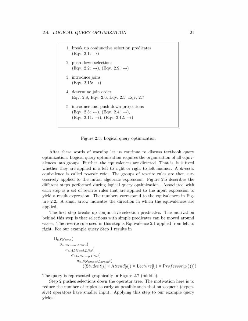
2.4. LOGICAL QUERY OPTIMIZATION 21

1. break up conjunctive selection predicates(Eqv. 2.1: →)

2. push down selections(Eqv. 2.2: →), (Eqv. 2.9: →)

3. introduce joins(Eqv. 2.15: →)

4. determine join orderEqv. 2.8, Eqv. 2.6, Eqv. 2.5, Eqv. 2.7

5. introduce and push down projections(Eqv. 2.3: ←), (Eqv. 2.4: →),(Eqv. 2.11: →), (Eqv. 2.12: →)

Figure 2.5: Logical query optimization

After these words of warning let us continue to discuss textbook queryoptimization. Logical query optimization requires the organization of all equiv-alences into groups. Further, the equivalences are directed. That is, it is fixedwhether they are applied in a left to right or right to left manner. A directedequivalence is called rewrite rule. The groups of rewrite rules are then suc-cessively applied to the initial algebraic expression. Figure 2.5 describes thedifferent steps performed during logical query optimization. Associated witheach step is a set of rewrite rules that are applied to the input expression toyield a result expression. The numbers correspond to the equivalences in Fig-ure 2.2. A small arrow indicates the direction in which the equivalences areapplied.

The first step breaks up conjunctive selection predicates. The motivationbehind this step is that selections with simple predicates can be moved aroundeasier. The rewrite rule used in this step is Equivalence 2.1 applied from left toright. For our example query Step 1 results in

Πs.SName(σs.SNo=a.ASNo(σa.ALNo=l.LNo(σl.LPNo=p.PNo(σp.PName=‘Larson′(

((Student[s] A Attend[a]) A Lecture[l]) A Professor[p])))))

The query is represented graphically in Figure 2.7 (middle).

Step 2 pushes selections down the operator tree. The motivation here is toreduce the number of tuples as early as possible such that subsequent (expen-sive) operators have smaller input. Applying this step to our example queryyields:

22 CHAPTER 2. TEXTBOOK QUERY OPTIMIZATION

Πs.SName(σl.LPNo=p.PNo(σa.ALNo=l.LNo(σs.SNo=a.ASNo(Student[s] A Attend[a])ALecture[l])

A(σp.PName=‘Larson′(Professor[p]))))

The query is represented graphically in Figure 2.7 (bottom).

Excursion In general, we might encounter problems when pushing down se-lections. It may be the case that the order of the cross products is not well-suitedfor pushing selections down. If this is the case, we must consider reordering crossproducts during this step (Eqv. 2.7 and 2.5). To illustrate this point considerthe following example query.

select distinct s.SNamefrom Student s, Lecture l, Attend awhere s.SNo = a.ASNo and a.ALNo = l.LNo

and l.LTitle = ‘Databases I’

After translation and Steps 1 and 2 the algebraic expression looks like

Πs.SName(σs.SNo=a.ASNo(σa.ALNo=l.LNo(

(Student[s] A σl.LT itle=‘Databases I′(Lecture[l])) A Attend[a]))).

Neither of σs.SNo=a.ASNo and σa.ALNo=l.LNo can be pushed down further. Onlyafter reordering the cross products such as in

Πs.SName(σs.SNo=a.ASNo(σa.ALNo=l.LNo(

(Student[s] A Attend[a]) A σl.LT itle=‘Databases I′(Lecture[l]))))

can σs.SNo=a.ASNo be pushed down:

Πs.SName(σa.ALNo=l.LNo(σs.SNo=a.ASNo(Student[s] A Attend[a])

Aσl.LT itle=‘Databases I′(Lecture[l])))

This is the reason why in some textbooks reorder cross products before selec-tions are pushed down [254]. In this appoach, reordering of cross products takesinto account the selection predicates that can possibly be pushed down to theleaves and down to just prior a cross product. In any case, the Steps 2 and 4are highly interdependent and there is no simple solution. 2

After this small excursion let us resume rewriting our main example query.The next step to be applied is converting cross products to join operations (Step3). The motivation behind this step is that the evaluation of cross products

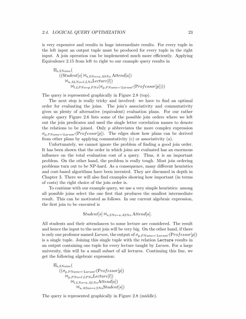
2.4. LOGICAL QUERY OPTIMIZATION 23

is very expensive and results in huge intermediate results. For every tuple inthe left input an output tuple must be produced for every tuple in the rightinput. A join operation can be implemented much more efficiently. ApplyingEquivalence 2.15 from left to right to our example query results in

Πs.SName(((Student[s] Bs.SNo=a.ASNo Attend[a])

Ba.ALNo=l.LNoLecture[l])Bl.LPNo=p.PNo(σp.PName=‘Larson′(Professor[p])))

The query is represented graphically in Figure 2.8 (top).The next step is really tricky and involved: we have to find an optimal

order for evaluating the joins. The join’s associativity and commutativitygives us plenty of alternative (equivalent) evaluation plans. For our rathersimple query Figure 2.6 lists some of the possible join orders where we leftout the join predicates and used the single letter correlation names to denotethe relations to be joined. Only p abbreviates the more complex expressionσp.PName=‘Larson′(Professor[p]). The edges show how plans can be derivedfrom other plans by applying commutativity (c) or associativity (a).

Unfortunately, we cannot ignore the problem of finding a good join order.It has been shown that the order in which joins are evaluated has an enormousinfluence on the total evaluation cost of a query. Thus, it is an importantproblem. On the other hand, the problem is really tough. Most join orderingproblems turn out to be NP-hard. As a consequence, many different heuristicsand cost-based algorithms have been invented. They are discussed in depth inChapter 3. There we will also find examples showing how important (in termsof costs) the right choice of the join order is.

To continue with our example query, we use a very simple heuristics: amongall possible joins select the one first that produces the smallest intermediateresult. This can be motivated as follows. In our current algebraic expression,the first join to be executed is

Student[s] Bs.SNo=a.ASNo Attend[a].

All students and their attendances to some lecture are considered. The resultand hence the input to the next join will be very big. On the other hand, if thereis only one professor named Larson, the output of σp.PName=‘Larson′(Professor[p])is a single tuple. Joining this single tuple with the relation Lecture results inan output containing one tuple for every lecture taught by Larson. For a largeuniversity, this will be a small subset of all lectures. Continuing this line, weget the following algebraic expression:

Πs.SName(((σp.PName=‘Larson′(Professor[p])

Bp.PNo=l.LPNoLecture[l])Bl.LNo=a.ALNoAttend[a])

Ba.ASno=s.SNoStudent[s])

The query is represented graphically in Figure 2.8 (middle).

24 CHAPTER 2. TEXTBOOK QUERY OPTIMIZATION

The last step minimizes intermediate results by projecting out irrelevantattributes. An attribute is irrelevant, if it is not used further up the operatortree. When pushing down projections, we only apply them just before a pipelineEXbreaker [333]. The reason is that for pipelined operators like selection, elimi-nating superfluous attributes does not gain much. The only pipeline breakeroccurring in our plan is the join operator. Hence, before a join is applied, weproject on the attributes that are further needed. The result is

Πs.SName(Πa.ASNo(

Πl.LNO(Πp.PNo(σp.PName=‘Larson′(Professor[p]))Bp.PNo=l.LPNo

Πl.LPno,l.LNo(Lecture[l]))Bl.LNo=a.ALNo

Πa.ALNo,a.ASNo(Attend[a]))Ba.ASno=s.SNo

Πs.SNo,s.SName(Student[s]))

This expression is represented graphically in Figure 2.8 (bottom).

2.5 Physical Query Optimization

Physical query optimization adds more information to the logical query eval-uation plan. First, there exist many different ways to access the data storedin a database. One possibility is to scan a relation to find the relevant tuples.Another alternative is to use an index to access only the relevant parts. If anunclustered index is used, it might be beneficial to sort the tuple identifiers(TIDs2) to turn otherwise random disk accesses into sequential accesses. Sincethere is a multitutude of possibilities to access data, this topic is discussed indepth in Chapter 4. Second, the algebraic operators used in the logical planmay have different alternative implementations. The most prominent exam-ple is the join operator that has many different implementations: simple nestedloop join, blockwise nested loop join, blockwise nested loop join with in-memoryhash table, index nested loop join, hybrid hash join, sort merge join, bandwidthjoin, special spatial joins, set joins, and structural joins. Most of these join im-plementations can be applied only in certain situations. Most algorithms onlyimplement equi-joins where the join predicate is a conjunction of simple equal-ities. Further, all the implementations differ in cost and robustness. But alsoother operators like grouping may have alternative implementations. Typically,for these operators exist sort-based and hash-based alternatives. Third, someoperators require certain properties for their input streams. For example, a sortmerge join requires its input to be sorted on the join attributes occurring inthe equalities of the join predicate. These attributes are called join attributes.The sortedness property can be enforced by a sort operator. The sort operator

2Sometimes TIDs are called RIDs (Row Identifiers).

2.6. DISCUSSION 25

is thus an enforcer since it makes sure that the required property holds. As wewill see, properties and enforcers play a crucial role during plan generation.

If common subexpressions are detected at the algebraic level, it might bebeneficial to compute them only once and store the result. To do so, a tmpoperator must be introduced. Later on, we will see more of these operatorsthat materialize (partial) intermediate results in order to avoid the same com-putation to be performed more than once. An alternative is to allow QEPswhich are DAGs and not merely trees (see Section ??).

Physical query optimization is concerned with all the issues mentionedabove. The outline of it is given in Figure 2.9. Let us demonstrate this forour small example query. Let us assume that there exists an index on the nameof the professors. Then, instead of scanning the whole professor relation, itis beneficial to use the index to retrieve only those professors named Larson.Further, since a sort merge join is very robust and not the slowest alternative,we choose it as an implementation for all our join operations. This requires thatwe sort the inputs to the join operator on the join attributes. Since sorting isa pipeline breaker, we introduce it between the projections and the joins. Theresulting plan is

Πs.SName(Sorta.ASNo(Πa.ASNo(

Sortl.LNo(Πl.LNO(Sortp.PNo(Πp.PNo(IdxScanp.PName=‘Larson′(Professor[p])))

Bsmjp.PNo=l.LPNo

Sortl.LPNo(Πl.LPno,l.LNo(Lecture[l])))

Bsmjl.LNo=a.ALNo

Sorta.ALNo(Πa.ALNo,a.ASNo(Attend[a]))))

Bsmja.ASno=s.SNo

Sorts.SNo(Πs.SNo,s.SName(Student[s])))

where we annotated the joins with smj to indicate that they are sort mergejoins. The sort operator has the attributes on which to sort as a subscript. Wecheated a little bit with the notation of the index scan. The index is a physicalentity stored in the database. An index scan typically allows to retrieve theTIDs of the tuples qualifying the predicate. If this is the case, another accessto the relation itself is necessary to fetch the relevant attributes (p.PNo inour case) from the qualifying tuples of the relation. This issue is rectified inChapter 4. The plan is shown as an operator graph in Figure 2.10.

2.6 Discussion

This chapter left open many interesting issues. We took it for granted that thepresentation of a query is an algebraic expression or operator tree. Is this reallytrue? We have been very vague about ordering joins and cross products. Weonly considered queries of the form select distinct. How can we assure correctduplicate treatment for select all? We separated query optimization into twodistinct phases: logical and physical query optimization. Any separation into

26 CHAPTER 2. TEXTBOOK QUERY OPTIMIZATION

different phases results in the danger of not producing an optimal plan. Logicalquery optimization turned out to be a little difficult: pushing selections downand reordering joins are mutually interdependent. How can we integrate thesesteps into a single one and thereby avoid the problem mentioned? Further, ourlogical query optimization was not cost based and cannot be: too much infor-mation is still missing from the plan to associate precise costs with a logicalalgebraic expression. How can we integrate the phases? How can we determinethe costs of a plan? We covered only a small fraction of SQL. We did not discussdisjunction, negation, union, intersection, except, aggregate functions, group-by, order-by, quantifiers, outer joins, and nested queries. Furthermore, howabout other query languages like OQL, XPath, XQuery? Further, enhance-ments like materialized views exist nowadays in many commercial systems.How can we exploit them beneficially? Can we exploit semantic information?Is our exploitation of index structures complete? What happens if we encounterNULL-values? Many questions and open issues remain. The rest of the bookis about filling these gaps.

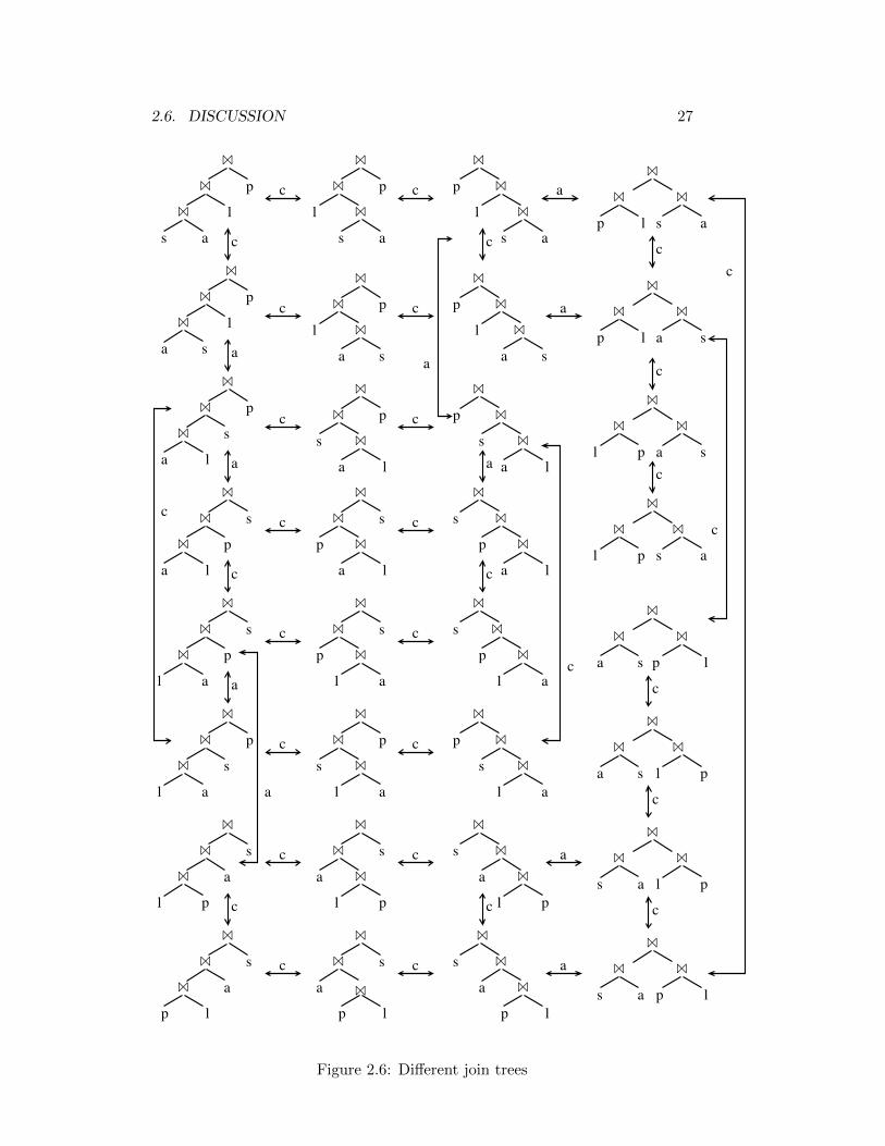
2.6. DISCUSSION 27

a

a

c

a

c

c

c

c

a

c

c

c

c

l

p

c

c

c

c

c

c

c

c

a

a

c

c

c

c

c

c

c

c

c

a

a

l

a

c

p

a

a

a

a

a

p

a

a

a

a

c

p

p

p

p

p

a

a

a

a

p

p

p

p p

p

p

pp

ll

ll

l

ll l

l

l ll

l

l l l

l

l l l

l

l l l

l

l l l

l

p

as

p

as

l

p

ass a

s

c

sa

asa

p

sasa

p

s

p

s s

as

s

p

s

p

s

p

s

p

s

p

c

s

psa

sa

p

s

p

s

p

s

s

a

s

a

s

a

s

a

c s

a

a

s

as

as

c

B

B

B

B

B

B

B

B

B

B

B B

B

BB

B

B

B

B

B

B

B

B

B

B

B

B

B

B

B

B

B

B

B

B B

B

BB

B

B

B

B

B

B

B

B

B

B

B

B

B

B

B

B

B

B

B

B B

B

BB

B

B

B

B

B

B

B

B

B

B

B

B

B

B

B

B

B

B

B

B B

B

B

B

B

B

B

B

B

B

B

B

B

Figure 2.6: Different join trees

28 CHAPTER 2. TEXTBOOK QUERY OPTIMIZATION

Professor[p]Attend[a] Lecture[l]Student[s]

Πs.SName

l.LPNo= p.PNo∧ p.PName= ′Larson′

σs.SNo= a.ASNo∧ a.ALNo= l.LNo∧

A

A

A

Professor[p]Lecture[l]Student[s] Attend[a]

Πs.SName

σl.LPNo= p.PNo

σs.SNo= a.ASNo

σa.ALNo= l.LNo

A

A

A

σp.PName= ′Larson′

Lecture[l]

Student[s] Attend[a]

Professor[p]

σp.PName= ′Larson′σa.ALNo= l.LNo

σs.SNo= a.ASNo

Πs.SName

σl.PNo= p.PNo

A

A

A

Figure 2.7: Plans for example query (Part I)

2.6. DISCUSSION 29

Professor[p]

Student[s] Attend[a]

Lecture[l]

Πs.SName

σp.PName= ′Larson′

Bs.SNo=a.ASNo

Ba.ALNo= l.LNo

Bl.PNo= p.PNo

Student[s]

Lecture[l]

Professor[p]

Attend[a]

Πs.SName

σp.PName= ′Larson′

Bp.PNo= l.LPNo

Bl.LNo= a.ALNo

Ba.ASNo= s.SNo

Student[s]

Professor[p]

Attend[a]

Lecture[l]

Πs.SNo,s.SName

Πp.PNo

σp.PName= ′Larson′

Πs.SName

Πa.ASNo

Πl.LNo Πa.ALNo,a.ASNo

Πl.LPNo,l.LNo

Ba.ASNo= s.SNo

Bl.LNo

Bp.PNo= l.LPNo

Figure 2.8: Plans for example query (Part II)

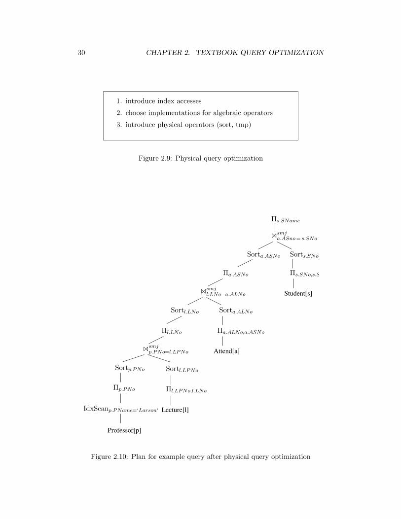
30 CHAPTER 2. TEXTBOOK QUERY OPTIMIZATION

1. introduce index accesses

2. choose implementations for algebraic operators

3. introduce physical operators (sort, tmp)

Figure 2.9: Physical query optimization

Attend[a]

Student[s]

Lecture[l]

Professor[p]

Πs.SNo,s.SName

Sorta.ALNo

Πa.ALNo,a.ASNo

Πl.LPNo,l.LNo

Πs.SName

Sorts.SNoSorta.ASNo

Πa.ASNo

Sortl.LNo

Πl.LNo

Sortl.LPNoSortp.PNo

Πp.PNo

IdxScanp.PName=′Larson′

Bsmjp.PNo=l.LPNo

Bsmjl.LNo=a.ALNo

Bsmja.ASno= s.SNo

Figure 2.10: Plan for example query after physical query optimization

Chapter 3

Join Ordering

The problem of join ordering is a very restricted and — at the same time —a very complex one. We have touched this issue while discussing logical queryoptimization in Chapter 2. Join ordering is performed in Step 4 of Figure 2.5.In this chapter, we simplify the problem of join ordering by not considering du-plicates, disjunctions, quantifiers, grouping, aggregation, or nested queries. Ex-pressed positively, we concentrate on conjunctive queries with simple and cheapjoin predicates. What this exactly means will become clear in the next section.Subsequent sections discuss different algorithms for solving the join orderingproblem. Finally, we take a look at the structure of the search space. This isimportant if different join ordering algorithms are compared via benchmarks.If the wrong parameters are chosen, benchmark results can be misleading.

The algorithms of this chapter form the core of every plan generator.

3.1 Queries Considered

A conjunctive query is one whose where clause contains a (complex) predicatewhich in turn is a conjunction of (simple) predicates. Hence, a conjunctivequery involves only and and no or or not operations. A simple predicate is ofthe form e1θe2 where θ ∈ =, 6=, <,>,≤,≥ is a comparison operator and the eiare simple expressions in attribute names possibly containing some simple andcheap arithmetic operators. By cheap we mean that it is not worth applyingextra optimization techniques. In this chapter, we restrict simple predicateseven further to the form A = B for attributes A and B. A and B must alsobelong to different relations such that every simple predicate in this chapteris a join predicate. There are two reasons for this restriction. First, the mostefficient join algorithms rely on the fact that the join predicate is of the formA = B. Such joins are called equi-joins. Any other join is called a non-equi-join. Second, in relational systems joins on foreign key attributes of one relationand key attributes of the other relation are very common. Other joins are rare.

A base relation is a relation that is stored (explicitly) in the database. Forthe rest of the chapter, let Ri (1 ≤ i ≤ n) be n relations. These relationscan be base relations but do not necessarily have to be. They could also bebase relations to which predicates have already been supplied, e.g. as a result

31

32 CHAPTER 3. JOIN ORDERING

Student Attend

LectureProfessor

a.ALNo = l.LNo

l.LPNo = p.PNo

p.PName = ’Larson’

s.SNo = a.ASNo

Figure 3.1: Query graph for example query of Section 2.1

of applying the first three steps of logical query optimization.Summarizing, the queries we consider can be expressed in SQL as

select distinct *from R1,. . . ,Rnwhere p

where p is a conjunction of simple join predicates with attributes from exactlytwo relations. The latter restriction is not really necessary for the algorithmspresented in this chapter but simplifies the exposition.

3.1.1 Query Graph

A query graph is a convenient representation of a query. It is an undirectedgraph with nodes R1, . . . , Rn. For every simple predicate in the conjunction Pwhose attributes belong to the relations Ri and Rj , we add an edge betweenRi and Rj . This edge is labeled by the simple predicate. From now on, wedenote the join predicate connecting Ri and Rj by pi,j . In general, pi,j can bea conjunction of simple join predicates connecting Ri and Rj .

If query graphs are used for more than join ordering, selections need to berepresented. This is done by self-edges from the relation to which the selectionapplies to itself. For the example query of Chapter 2.6, Figure 3.1 contains theaccording query graph.

Query graphs can have many different shapes. The shapes that play acertain role in query optimization and the evaluation of join ordering algorithmsare shown in Fig. 3.2. The query graph classes relevant for this chapter are chainqueries, star queries, tree queries, cyclic queries and clique queries. Note thatthese classes are not disjoint and that some classes are subsets of other classes.

EXIn this chaper, we only treat connected query graphs. These can be evalu-

ated without cross products.

Excursion In general, the query graph is a hypergraph [855] as the followingexample shows.

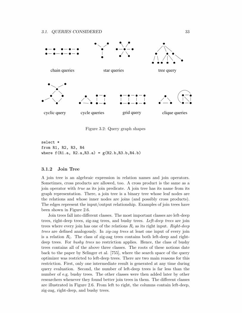
3.1. QUERIES CONSIDERED 33

chain queries star queries tree query

cyclic query cycle queries grid query clique queries

Figure 3.2: Query graph shapes

select *

from R1, R2, R3, R4

where f(R1.a, R2.a,R3.a) = g(R2.b,R3.b,R4.b)

3.1.2 Join Tree

A join tree is an algebraic expression in relation names and join operators.Sometimes, cross products are allowed, too. A cross product is the same as ajoin operator with true as its join predicate. A join tree has its name from itsgraph representation. There, a join tree is a binary tree whose leaf nodes arethe relations and whose inner nodes are joins (and possibly cross products).The edges represent the input/output relationship. Examples of join trees havebeen shown in Figure 2.6.

Join trees fall into different classes. The most important classes are left-deeptrees, right-deep trees, zig-zag trees, and bushy trees. Left-deep trees are jointrees where every join has one of the relations Ri as its right input. Right-deeptrees are defined analogously. In zig-zag trees at least one input of every joinis a relation Ri. The class of zig-zag trees contains both left-deep and right-deep trees. For bushy trees no restriction applies. Hence, the class of bushytrees contains all of the above three classes. The roots of these notions dateback to the paper by Selinger et al. [755], where the search space of the queryoptimizer was restricted to left-deep trees. There are two main reasons for thisrestriction. First, only one intermediate result is generated at any time duringquery evaluation. Second, the number of left-deep trees is far less than thenumber of e.g. bushy trees. The other classes were then added later by otherresearchers whenever they found better join trees in them. The different classesare illustrated in Figure 2.6. From left to right, the columns contain left-deep,zig-zag, right-deep, and bushy trees.

34 CHAPTER 3. JOIN ORDERING

Left-deep trees directly correspond to an ordering (i.e. a permutation) ofthe relations. For example, the left-deep tree

((((R2 BR3) BR1) BR4) BR5)

directly corresponds to the permutation R2, R3, R1, R4, R5. It should be clearthat there is a one-to-one correspondence between permutations and left-deepjoin trees. We will also use the term sequence of relations synonymously. Thenotion of join ordering goes back to the times where only left-deep trees wereconsidered and, hence, producing an optimal join tree was equivalent to opti-mally ordering the joins, i.e. determining a permutation with lowest cost.

Left-deep, right-deep, and zig-zag trees can be classed under the generalterm linear trees. Sometimes, the term linear trees is used synonymously forleft-deep trees. We will not do so. Join trees are sometimes called operator treesor query evaluation plans. Although this is not totally wrong, these terms havea slightly different connotation. Operator trees typically contain more thanonly join operators. Query evaluation plans (QEPs or plans for short) typicallyhave more information from physical query optimization associated with them.

3.1.3 Simple Cost Functions

In order to judge the quality of join trees, we need a cost function that associatesa certain positive cost with each join tree. Then, the task of join ordering is tofind among all equivalent join trees the join tree with lowest associated costs.

One part of any cost function are cardinality estimates. They are based onthe cardinalities of the relations, i.e. the number of tuples contained in them.For a given relation Ri, we denote its cardinality by |Ri|.

Then, the cardinality of intermediate results must be estimated. This isdone by introducing the notion of join selectivity. Let pi,j be a join predicatebetween relations Ri and Rj . The selectivity fi,j of pi,j is then defined as

fi,j =|Ri Bpi,j Rj ||Ri| ∗ |Rj |

This is the number of tuples in the join’s result divided by the number of tuplesin the Cartesian Product between Ri and Rj . If fi,j is 0.1, then only 10% ofall tuples in the Cartesian Product survive the predicate pi,j . Note that theselectivity is always a number between 0 and 1 and that fi,j = fj,i. We use anf and not an s, since the selectivity of a predicate is often called filter factor .

Besides the relation’s cardinalities, the selectivities of the join predicatespi,j are assumed to be given as input to the join ordering algorithm. Therefore,we can compute the output cardinality of a join Ri Bpi,j Rj , as

|Ri Bpi,j Rj | = fi,j |Ri||Rj |

From this it becomes clear that if there is no join predicate for two relationsRi and Rj , we can assume a join predicate true and associate a selectivity of1 with it. The output cardinality is then the cardinality of the cross product

3.1. QUERIES CONSIDERED 35

between Ri and Rj . We also define fi,i = 1 for all 1 ≤ i ≤ n. This allows us tokeep subsequent formulas simple.

We now need to extend our cardinality estimation to join trees. This can bedone by recursively applying the above formula. Consider a join tree T joiningtwo join trees T1 and T2, i.e. T = T1 B T2. Then, the result cardinality |T | canbe calculated as follows. If T is a leaf Ri, then |T | := |Ri|. Otherwise,

|T | = (∏

Ri∈T1,Rj∈T2fi,j) |T1| |T2|.

Note that this formula assumes that the selectivities are independent of eachother. Assuming independence is common but may be very misleading. Moreon this issue can be found in Chapter ??. Nevertheless, we assume independenceand stick to the above formula.

For sequences of joins we can give a simple cardinality definition. Let s =R1, . . . , Rn be a sequence of relations. Then

|s| =n∏

k=1

(k∏

i=1

fi,k|Rk|).

Given the above, a query graph alone is not really sufficient for the speci-fication of a join ordering problem: cardinalities and selectivities are missing.On the other hand, from a complete list of cardinalities and selectivities we canderive the query graph. Obviously, the following defines a chain query withquery graph R1 −−−R2 −−−R3:

|R1| = 10

|R2| = 100

|R3| = 1000

f1,2 = 0.1

f2,3 = 0.2

In all examples, we assume for all i and j for which fi,j is not given that thereis no join predicate and hence fi,j = 1.

We now come to cost functions. The first cost function we consider is calledCout. For a join tree T , Cout(T ) is the sum of all output cardinalities of all joinsin T . Recursively, we can define Cout as

Cout(T ) =

0 if T is a single relation|T |+ Cout(T1) + Cout(T2) if T = T1 B T2

From a theoretial point of view, Cout has many interesting properties: it issymmetric, it has the ASI property, and it can be applied to an expression ofthe logical algebra. From a practical point of view, however, it is rarely applied(yet).

In real cost functions, the cardinalities only serve as input to more complexformulas capturing the costs of a join implementation. Since real cost functions

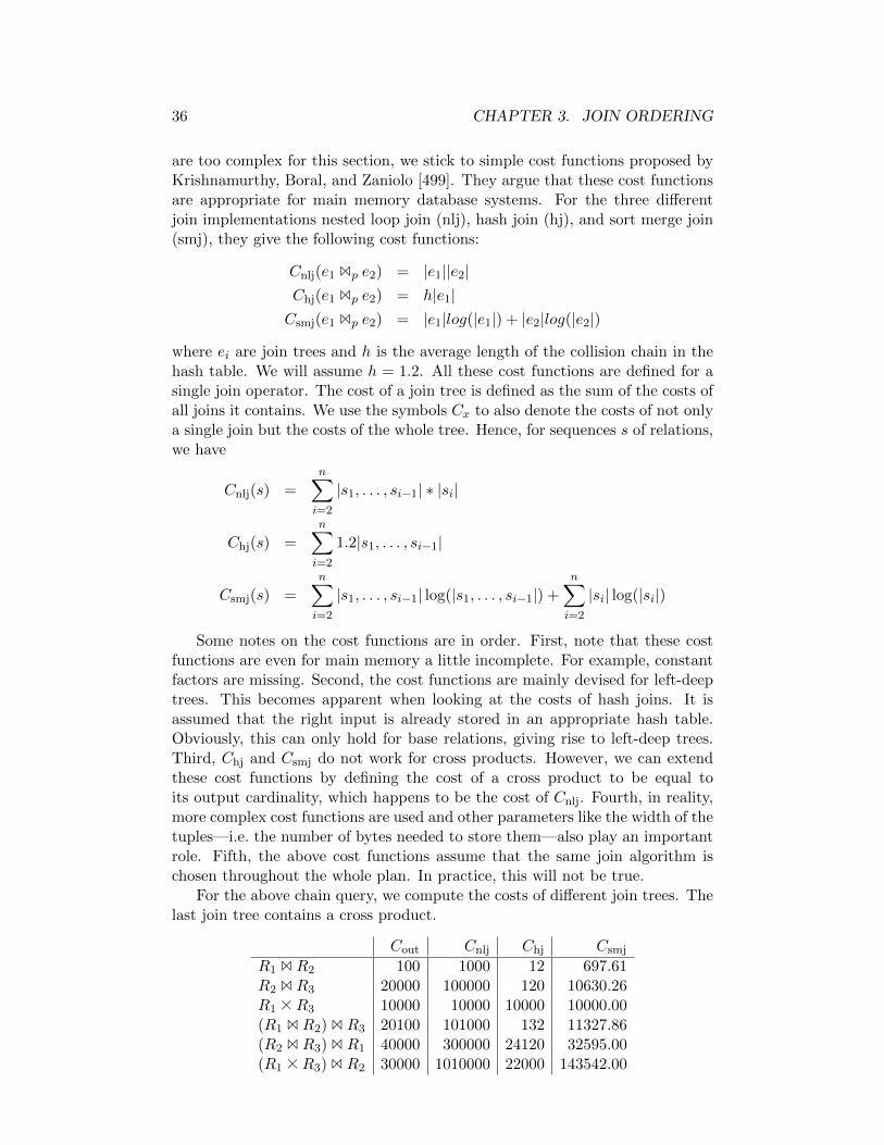
36 CHAPTER 3. JOIN ORDERING

are too complex for this section, we stick to simple cost functions proposed byKrishnamurthy, Boral, and Zaniolo [499]. They argue that these cost functionsare appropriate for main memory database systems. For the three differentjoin implementations nested loop join (nlj), hash join (hj), and sort merge join(smj), they give the following cost functions:

Cnlj(e1 Bp e2) = |e1||e2|Chj(e1 Bp e2) = h|e1|Csmj(e1 Bp e2) = |e1|log(|e1|) + |e2|log(|e2|)

where ei are join trees and h is the average length of the collision chain in thehash table. We will assume h = 1.2. All these cost functions are defined for asingle join operator. The cost of a join tree is defined as the sum of the costs ofall joins it contains. We use the symbols Cx to also denote the costs of not onlya single join but the costs of the whole tree. Hence, for sequences s of relations,we have

Cnlj(s) =n∑

i=2

|s1, . . . , si−1| ∗ |si|

Chj(s) =n∑

i=2

1.2|s1, . . . , si−1|

Csmj(s) =n∑

i=2

|s1, . . . , si−1| log(|s1, . . . , si−1|) +n∑

i=2

|si| log(|si|)

Some notes on the cost functions are in order. First, note that these costfunctions are even for main memory a little incomplete. For example, constantfactors are missing. Second, the cost functions are mainly devised for left-deeptrees. This becomes apparent when looking at the costs of hash joins. It isassumed that the right input is already stored in an appropriate hash table.Obviously, this can only hold for base relations, giving rise to left-deep trees.Third, Chj and Csmj do not work for cross products. However, we can extendthese cost functions by defining the cost of a cross product to be equal toits output cardinality, which happens to be the cost of Cnlj. Fourth, in reality,more complex cost functions are used and other parameters like the width of thetuples—i.e. the number of bytes needed to store them—also play an importantrole. Fifth, the above cost functions assume that the same join algorithm ischosen throughout the whole plan. In practice, this will not be true.

For the above chain query, we compute the costs of different join trees. Thelast join tree contains a cross product.

Cout Cnlj Chj Csmj

R1 BR2 100 1000 12 697.61R2 BR3 20000 100000 120 10630.26R1 AR3 10000 10000 10000 10000.00(R1 BR2) BR3 20100 101000 132 11327.86(R2 BR3) BR1 40000 300000 24120 32595.00(R1 AR3) BR2 30000 1010000 22000 143542.00

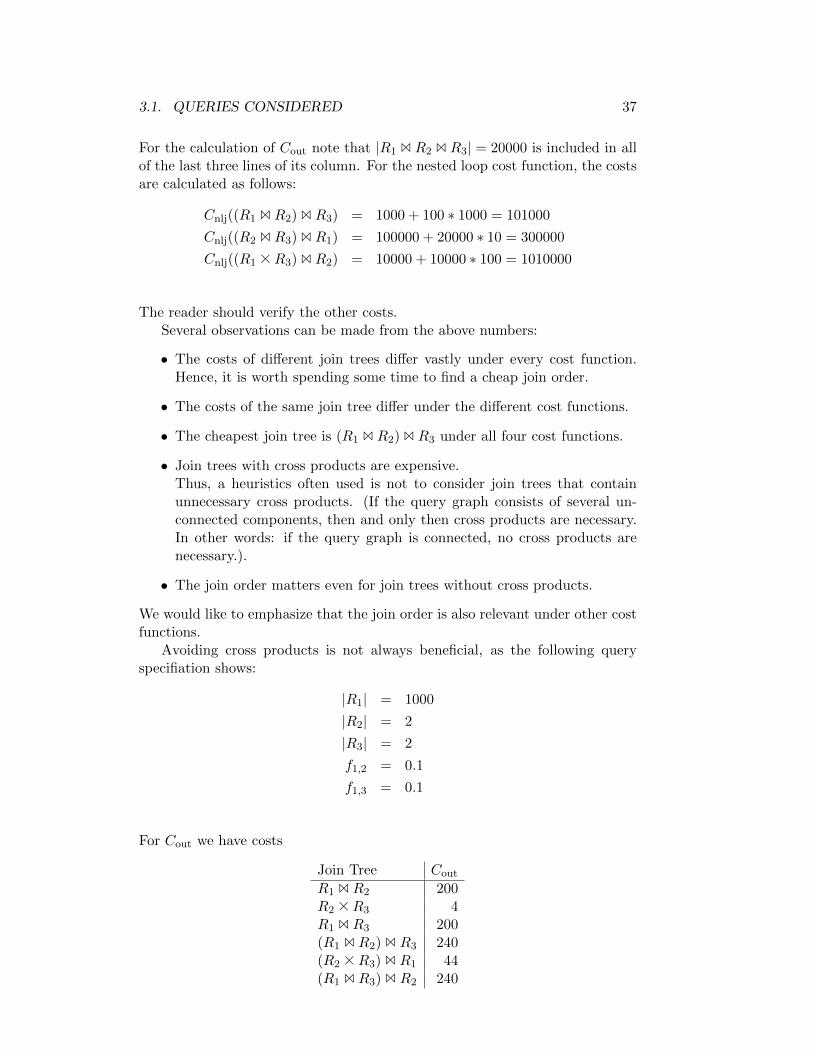
3.1. QUERIES CONSIDERED 37

For the calculation of Cout note that |R1 BR2 BR3| = 20000 is included in allof the last three lines of its column. For the nested loop cost function, the costsare calculated as follows:

Cnlj((R1 BR2) BR3) = 1000 + 100 ∗ 1000 = 101000

Cnlj((R2 BR3) BR1) = 100000 + 20000 ∗ 10 = 300000

Cnlj((R1 AR3) BR2) = 10000 + 10000 ∗ 100 = 1010000

The reader should verify the other costs.Several observations can be made from the above numbers:

• The costs of different join trees differ vastly under every cost function.Hence, it is worth spending some time to find a cheap join order.

• The costs of the same join tree differ under the different cost functions.

• The cheapest join tree is (R1 BR2) BR3 under all four cost functions.

• Join trees with cross products are expensive.Thus, a heuristics often used is not to consider join trees that containunnecessary cross products. (If the query graph consists of several un-connected components, then and only then cross products are necessary.In other words: if the query graph is connected, no cross products arenecessary.).

• The join order matters even for join trees without cross products.

We would like to emphasize that the join order is also relevant under other costfunctions.

Avoiding cross products is not always beneficial, as the following queryspecifiation shows:

|R1| = 1000

|R2| = 2

|R3| = 2

f1,2 = 0.1

f1,3 = 0.1

For Cout we have costs

Join Tree Cout

R1 BR2 200R2 AR3 4R1 BR3 200(R1 BR2) 1 R3 240(R2 AR3) 1 R1 44(R1 BR3) 1 R2 240

38 CHAPTER 3. JOIN ORDERING

Note that although the absolute numbers are quite small, the ratio of the bestand the second best join tree is quite large. The reader is advised to find moreexamples and to apply other cost functions.

The following example illustrates that a bushy tree can be superior to anylinear tree. Let us use the following query specification:

|R1| = 10

|R2| = 20

|R3| = 20

|R4| = 10

f1,2 = 0.01

f2,3 = 0.5

f3,4 = 0.01

If we do not consider cross products, we have for the symmetric (see below)cost function Cout the following join trees and costs:

Join Tree Cout

R1 BR2 2R2 BR3 200R3 BR4 2((R1 BR2) BR3) BR4 24((R2 BR3) BR1) BR4 222(R1 BR2) B (R3 BR4) 6

Note that all other linear join trees fall into one of these classes, due to thesymmetry of the cost function and the join ordering problem. Again, the readeris advised to find more examples and to apply other cost functions.

If we want to annotate a join operator by its implementation—which isnecessary for the correct computation of costs—we write Bimpl for an imple-mentation impl. For example, Bsmj is a sort-merge join, and the according costfunction Csmj is used to compute its costs.

Two properties of cost functions have some impact on the join orderingproblem. The first is symmetry. A cost function Cimpl is called symmetricif Cimpl(R1 Bimpl R2) = Cimpl(R2 Bimpl R1) for all relations R1 and R2. Forsymmetric cost functions, it does not make sense to consider commutativity.Hence, it suffices to consider left-deep trees only if we want to restrict ourselvesto linear join trees. Note that Cout, Cnlj, Csmj are symmetric while Chj is not.

The other property is the adjacent sequence interchange (ASI) property.Informally, the ASI property states that there exists a rank function such thatthe order of two subsequences is optimal if they are ordered according to therank function. The ASI property is formally defined in Section 3.2.2. Only fortree queries and cost functions with the ASI property, a polynomial algorithmto find an optimal join order is known. Our cost functions Cout and Chj have theASI property, Csmj does not. Summarizing the properties of our cost functions,we see that the classification is orthogonal:

3.1. QUERIES CONSIDERED 39

ASI ¬ ASI

symmetric Cout, Cnlj Csmj

¬ symmetric Chj (see text)

For the missing case of a non-symmetric cost function not having the ASIproperty, we can use the cost function of the hybrid hash join [229, 650].

We turn to another not really well-researched topic. The goal is to cutdown the number of cost functions which have to be considered for optimizationand to possibly allow for simpler cost functions, which saves time during plangeneration. Unfortunately, we have to restrict ourselves to left-deep join trees.Let s denote a sequence or permutation of a given set of joins. We define anequivalence relation on cost functions.

Definition 3.1.1 Let C and C ′ be two cost functions. Then

C ≡ C ′ :≺ (∀s C(s) minimal ≺ C ′(s) minimal)

Here, s is a join sequence.

Obviously, ≡ is an equivalence relation.

Now we can define the ΣIR property.

Definition 3.1.2 A cost function C is ΣIR :≺ C ≡ Cout.

That is, ΣIR is the set of all cost functions that are equivalent to Cout.

Let us consider a very simple example. The last element of the sum in Cout

is the size of the final join (all relations are joined). This is not the case for thefollowing cost function:

C ′out(s) :=n−1∑

i=2

|s1, . . . , si|

Obviously, we have C ′out is ΣIR. The next observation shows that we canconstruct quite complex ΣIR cost functions:

Observation 3.1.3 Let C1 and C2 be two ΣIR cost functions. For non-decreasing functions f1 : R → R and f2 : R × R → R and constants c ∈ Rand d ∈ R+, we have that EX

C1 + cC1 ∗ df1 C1

f2 (C1, C2)

are ΣIR. Here, denotes function composition and (·, ·) function pairing.

There are of course many more possibilites of constructing ΣIR functions. Forthe cost functions Chj, Csmj, and Cnlj, we now investigate which of them havethe ΣIR property.

40 CHAPTER 3. JOIN ORDERING

Let us consider Chj first. From

Chj(s) =n∑

i=2

1.2|s1, . . . , si−1|

= 1.2|s1|+ 1.2

n−1∑

i=2

|s1, . . . , si|

= 1.2|s1|+ 1.2C ′out(s)

and observation 3.1.3, we conclude that Chj is ΣIR for a fixed relation to bejoined first. If we can optimize Cout in polynomial time, then we can optimizeCout for a fixed starting relation. Indeed, by trying each relation as a startingrelation, we can find the optimal join tree in polynomial time. An algorithmEXthat computes the optimal solution for an arbitrary relation to be joined firstcan be found in Section 3.2.2.

Now, consider Csmj. Since

n∑

i=2

|s1, . . . , si−1|log(|s1, . . . , si−1|)

is minimal if and only ifn∑

i=2

|s1, . . . , si−1|

is minimal and∑n

i=2 |si| log(|si|) is independent of the order of the relationswithin s — that is constant — we conclude that Csmj is ΣIR.

Last, we have that Cnlj is not ΣIR. To see this, consider the followingcounter example with three relations R1, R2, and R3 of sizes 10, 10, and 100,resp. The selectivities are f1,2 = 9

10 , f2,3 = 110 , and f1,3 = 1

10 . Now,

|R1R2| = 90

|R1R3| = 100

|R2R3| = 100

and

Cnl(R1R2R3) = 10 ∗ 10 + 90 ∗ 100 = 9100

Cnl(R1R3R2) = 10 ∗ 100 + 100 ∗ 10 = 2000

Cnl(R2R3R1) = 10 ∗ 100 + 100 ∗ 10 = 2000

We see that R1R2R3 has the smallest sum of intermediate result sizes butproduces the highest cost. Hence, Cnlj is not ΣIR.

3.1.4 Classification of Join Ordering Problems

After having discussed the different classes of query graphs, join trees andcost functions, we can classify join ordering problems. To define a certain joinordering problem, we have to pick one entry from every class:

3.1. QUERIES CONSIDERED 41

Query Graph Classes × Possible Join Tree Classes × Cost FunctionClasses

The query graph classes considered are chain, star , tree, and cyclic. For the jointree classes we distinguish between the different join tree shapes, i.e. whetherthey are left-deep, zig-zag, or bushy trees. We left out the right-deep trees, sincethey do not differ in their behavior from left-deep trees. We also have to takeinto account whether cross products are considered or not. For cost functions,we use a simple classification: we only distinguish between those that have theASI property and those that do not. This leaves us with 4∗3∗2∗2 = 48 differentjoin ordering problems. For these, we will first review search space sizes andcomplexity. Then, we discuss several algorithms for join ordering. Last, we givesome insight into cost distributions over the search space and how this mightinfluence the benchmarking of different join ordering algorithms.

3.1.5 Search Space Sizes

Since search space sizes are easier to count if cross products are allowed, weconsider them first. Then we turn to search spaces where cross products arenot considered.

Join Trees with Cross Products We consider the number of join trees fora query graph with n relations. When cross products are allowed, the numberof left-deep and right-deep join trees is n!. By allowing cross products, thequery graph does not restrict the search space in any way. Hence, any of the n!permutations of the n relations corresponds to a valid left-deep join tree. Thisis true independent of the query graph.

Similarly, the number of zig-zag trees can be estimated independently ofthe query graph. First note that for joining n relations, we need n − 1 joinoperators. From any left-deep tree, we derive zig-zag trees by using the join’scommutativity and exchange the left and right inputs. Hence, from any left-deep tree for n relations, we can derive 2n−2 zig-zag trees. We have to subtractanother one, since the bottommost joins’ arguments are exchanged in differentleft-deep trees. Thus, there exists a total of 2n−2n! zig-zag trees. Again, thisnumber is independent of the query graph.

The number of bushy trees can be estimated as follows. First, we need thenumber of binary trees. For n leaf nodes, the number of binary trees is givenby C(n− 1), where C(n) is defined by the recurrence

C(n) =

n−1∑

k=0

C(k)C(n− k − 1)

with C(0) = 1. The numbers C(n) are called the Catalan Numbers (see [201]).They can also be computed by the following formula:

C(n) =1

n+ 1

(2n

n

).

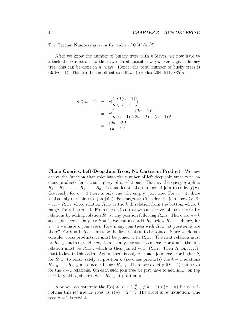
42 CHAPTER 3. JOIN ORDERING

The Catalan Numbers grow in the order of Θ(4n/n3/2).

After we know the number of binary trees with n leaves, we now have toattach the n relations to the leaves in all possible ways. For a given binarytree, this can be done in n! ways. Hence, the total number of bushy trees isn!C(n− 1). This can be simplified as follows (see also [296, 511, 835]):

n!C(n− 1) = n!1

n

(2(n− 1)

n− 1

)

= n!1

n

(2n− 2)!

(n− 1)!((2n− 2)− (n− 1))!

=(2n− 2)!

(n− 1)!

Chain Queries, Left-Deep Join Trees, No Cartesian Product We nowderive the function that calculates the number of left-deep join trees with nocross products for a chain query of n relations. That is, the query graph isR1 – R2 – . . . – Rn−1 – Rn. Let us denote the number of join trees by f(n).Obviously, for n = 0 there is only one (the empty) join tree. For n = 1, thereis also only one join tree (no join). For larger n: Consider the join trees for R1

– . . . – Rn−1 where relation Rn−1 is the k-th relation from the bottom where kranges from 1 to n− 1. From such a join tree we can derive join trees for all nrelations by adding relation Rn at any position following Rn−1. There are n−ksuch join trees. Only for k = 1, we can also add Rn below Rn−1. Hence, fork = 1 we have n join trees. How many join trees with Rn−1 at position k arethere? For k = 1, Rn−1 must be the first relation to be joined. Since we do notconsider cross products, it must be joined with Rn−2. The next relation mustbe Rn−3, and so on. Hence, there is only one such join tree. For k = 2, the firstrelation must be Rn−2, which is then joined with Rn−1. Then Rn−3, . . . , R1

must follow in this order. Again, there is only one such join tree. For higher k,for Rn−1 to occur safely at position k (no cross products) the k − 1 relationsRn−2, . . . , Rn−k must occur before Rn−1. There are exactly f(k − 1) join treesfor the k− 1 relations. On each such join tree we just have to add Rn−1 on topof it to yield a join tree with Rn−1 at position k.

Now we can compute the f(n) as n +∑n−1

k=2 f(k − 1) ∗ (n − k) for n > 1.Solving this recurrence gives us f(n) = 2n−1. The proof is by induction. Thecase n = 1 is trivial.

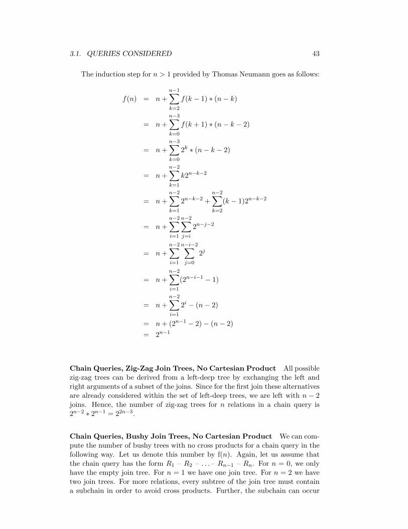
3.1. QUERIES CONSIDERED 43

The induction step for n > 1 provided by Thomas Neumann goes as follows:

f(n) = n+n−1∑

k=2

f(k − 1) ∗ (n− k)

= n+

n−3∑

k=0

f(k + 1) ∗ (n− k − 2)

= n+n−3∑

k=0

2k ∗ (n− k − 2)

= n+n−2∑

k=1

k2n−k−2

= n+

n−2∑

k=1

2n−k−2 +

n−2∑

k=2

(k − 1)2n−k−2

= n+n−2∑

i=1

n−2∑

j=i

2n−j−2

= n+n−2∑

i=1

n−i−2∑

j=0

2j

= n+n−2∑

i=1

(2n−i−1 − 1)

= n+

n−2∑

i=1

2i − (n− 2)

= n+ (2n−1 − 2)− (n− 2)

= 2n−1

Chain Queries, Zig-Zag Join Trees, No Cartesian Product All possiblezig-zag trees can be derived from a left-deep tree by exchanging the left andright arguments of a subset of the joins. Since for the first join these alternativesare already considered within the set of left-deep trees, we are left with n − 2joins. Hence, the number of zig-zag trees for n relations in a chain query is2n−2 ∗ 2n−1 = 22n−3.

Chain Queries, Bushy Join Trees, No Cartesian Product We can com-pute the number of bushy trees with no cross products for a chain query in thefollowing way. Let us denote this number by f(n). Again, let us assume thatthe chain query has the form R1 – R2 – . . . – Rn−1 – Rn. For n = 0, we onlyhave the empty join tree. For n = 1 we have one join tree. For n = 2 we havetwo join trees. For more relations, every subtree of the join tree must containa subchain in order to avoid cross products. Further, the subchain can occur

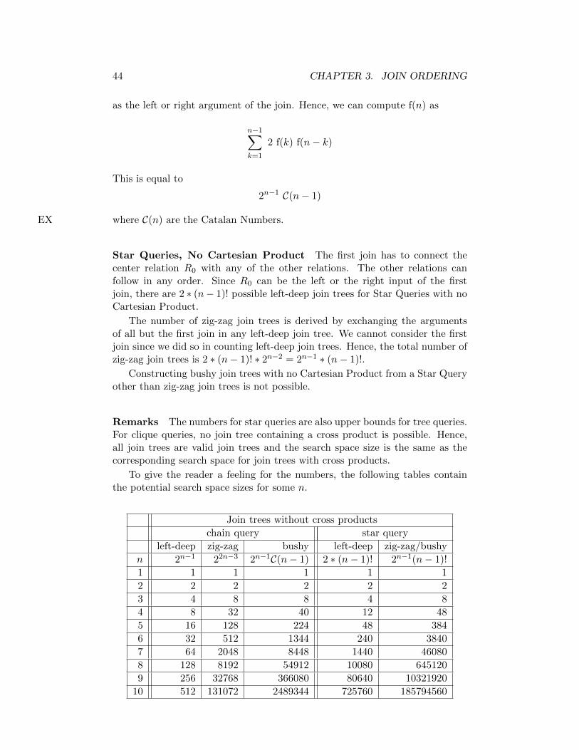
44 CHAPTER 3. JOIN ORDERING

as the left or right argument of the join. Hence, we can compute f(n) as

n−1∑

k=1

2 f(k) f(n− k)

This is equal to

2n−1 C(n− 1)

where C(n) are the Catalan Numbers.EX

Star Queries, No Cartesian Product The first join has to connect thecenter relation R0 with any of the other relations. The other relations canfollow in any order. Since R0 can be the left or the right input of the firstjoin, there are 2 ∗ (n− 1)! possible left-deep join trees for Star Queries with noCartesian Product.

The number of zig-zag join trees is derived by exchanging the argumentsof all but the first join in any left-deep join tree. We cannot consider the firstjoin since we did so in counting left-deep join trees. Hence, the total number ofzig-zag join trees is 2 ∗ (n− 1)! ∗ 2n−2 = 2n−1 ∗ (n− 1)!.

Constructing bushy join trees with no Cartesian Product from a Star Queryother than zig-zag join trees is not possible.

Remarks The numbers for star queries are also upper bounds for tree queries.For clique queries, no join tree containing a cross product is possible. Hence,all join trees are valid join trees and the search space size is the same as thecorresponding search space for join trees with cross products.

To give the reader a feeling for the numbers, the following tables containthe potential search space sizes for some n.

Join trees without cross products

chain query star query

left-deep zig-zag bushy left-deep zig-zag/bushy

n 2n−1 22n−3 2n−1C(n− 1) 2 ∗ (n− 1)! 2n−1(n− 1)!

1 1 1 1 1 1

2 2 2 2 2 2

3 4 8 8 4 8

4 8 32 40 12 48

5 16 128 224 48 384

6 32 512 1344 240 3840

7 64 2048 8448 1440 46080

8 128 8192 54912 10080 645120

9 256 32768 366080 80640 10321920

10 512 131072 2489344 725760 185794560

3.1. QUERIES CONSIDERED 45

With cross products/clique

left-deep zig-zag bushy

n n! 2n−2 ∗ n! n!C(n− 1)

1 1 1 1

2 2 2 2

3 6 12 12

4 24 96 120

5 120 960 1680

6 720 11520 30240

7 5040 161280 665280

8 40320 2580480 17297280

9 362880 46448640 518918400

10 3628800 928972800 17643225600

Note that in Figure 2.6 only 32 join trees are listed, whereas the number ofbushy trees for chain queries with four relations is 40. The missing eight casesare those zig-zag trees which are symmetric (i.e. derived by applying commu-tativity to all occurring joins) to the ones contained in the second column.

From these numbers, it becomes immediately clear why historically thesearch space of query optimizers was restricted to left-deep trees and crossproducts for connected query graphs were not considered.

3.1.6 Problem Complexity

The complexity of the join ordering problem depends on several parameters.These are the shape of the query graph, the class of join trees to be considered,whether cross products are considered or not, and whether the cost functionhas the ASI property or not. Not for all the combinations complexity resultsare known. What is known is summarized in the following table.

Query graph Join tree Cross products Cost function Complexity

general left-deep no ASI NP-hardtree/star/chain left-deep no one join method (ASI) Pstar left-deep no two join methods (NLJ+SMJ) NP-hard

general/tree/star left-deep yes ASI NP-hardchain left-deep yes — open

general bushy no ASI NP-hardtree bushy no — openstar bushy no ASI P

chain bushy no any P

general bushy yes ASI NP-hardtree/star/chain bushy yes ASI NP-hard

Ibaraki and Kameda were the first who showed that the problem of derivingoptimal left-deep trees for cyclic queries is NP-hard for a cost function for ann-way nested loop join implementation [421]. The proof was repeated for thecost function Cout which has the ASI property [186, 844]. In both proofs, the

46 CHAPTER 3. JOIN ORDERING

clique problem was used for the reduction [309]. Cout was also used in the otherproofs of NP-hardness results. The next line goes back to the same paper.Ibaraki and Kameda also described an algorithm to solve the join orderingproblem for tree queries producing optimal left-deep trees for a special costfunction for a nested-loop n-way join algorithm. Their algorithm was based onthe observation that their cost function has the ASI property. For this case,they could derive an algorithm from an algorithm for a sequencing problem forjob scheduling designed by Monma and Sidney [604]. They, in turn, used anearlier result by Lawler [516]. The algorithm of Ibaraki and Kameda was slightlygeneralized by Krishnamurthy, Boral, and Zaniolo, who were also able to sketcha more efficient algorithm. It improves the time bounds from O(n2 log n) toO(n2). The disadvantage of both approaches is that with every relation, a fixed(i.e. join-tree independent) join implementation must be associated before theoptimization starts. Hence, it only produces optimal trees if there is only onejoin implementation available or one is able to guess the optimal join methodbefore hand. This might not be the case. The polynomial algorithm which weterm IKKBZ is described in Section 3.2.2.

For star queries, Ganguly investigated the problem of generating optimalleft-deep trees if no cross products but two different cost functions (one fornested loop join, the other for sort merge join) are allowed. It turned out thatthis problem is NP-hard [301].

The next line is due to Cluet and Moerkotte [186]. They showed by reduc-tion from 3DM that taking into account cross products results in an NP-hardproblem even for star queries. Remember that star queries are tree queries andgeneral graphs.

The problem for general bushy trees follows from a result by Scheufele andMoerkotte [739]. They showed that building optimal bushy trees for crossproducts only (i.e. all selectivities equal one) is already NP-hard. This resultalso explains the last two lines.

By noting that for star queries, all bushy trees that do not contain a crossproduct are left-deep trees, the problem can be solved by the IKKBZ algorithmfor left-deep trees. Ono and Lohman showed that for chain queries dynamicprogramming considers only a polynomial number of bushy trees if no crossproducts are considered [626]. This is discussed in Section 3.2.4.

The table is rather incomplete. Many open problems exist. For example,if we have chain queries and consider cross products: is the problem NP-hardor in P? Some results for this problem have been presented [739], but it isstill an open problem (see Section 3.2.7). Open is also the case where weproduce optimal bushy trees with no cross products for tree queries. Yet anotherexample of an open problem is whether we could drop the ASI property and arestill able to derive a polynomial algorithm for a tree query. This is especiallyimportant, since the cost function for a sort-merge algorithm does not have theASI property.

Good summaries of complexity results for different join ordering problemscan be found in the theses of Scheufele [737] and Hamalainen [380].

Given that join ordering is an inherently complex problem with no polyno-mial algorithm in sight, one might wonder whether there exists good polynomial

3.2. DETERMINISTIC ALGORITHMS 47

approximation algorithms. Chances are that even this is not the case. Chatter-ji, Evani, Ganguly, and Yemmanuru showed that three different optimizationproblems — all asking for linear join trees — are not approximable [139].

3.2 Deterministic Algorithms

3.2.1 Heuristics

We now present some simple heuristic solutions to the problem of join ordering.These heuristics only produce left-deep trees. Since left-deep trees are equiv-alent with permutations, these heuristics order the joins according to somecriterion.

The core algorithm for the heuristics discussed here is the greedy algorithm(for an introduction see [201]). In greedy algorithms, a weight is associated witheach entity. In our case, weights are associated with each relation. A typicalweight function is the cardinality of the relation (|R|). Given a weight functionweight, a greedy join ordering algorithm works as follows:

GreedyJoinOrdering-1(R1, . . . , Rn, (*weight)(Relation))

Input: a set of relations to be joined and a weight function

Output: a join order

S = ε; // initialize S to the empty sequence

R = R1, . . . , Rn; // let R be the set of all relations

while(!empty(R)) Let k be such that: weight(Rk) = minRi∈R(weight(Ri));R\ = Rk; // eliminate Rk from RS = Rk; // append Rk to S

return S

This algorithm takes cross products into account. If we are only interestedin left-deep join trees with no cross products, we have to require that Rk isconnected to some of the relations contained in S in case S 6= ε. Note that amore efficient implementation would sort the relations according to their weight.

Not all heuristics can be implemented with a greedy algorithm as simple asabove. An often-used heuristics is to take the relation next that produces thesmallest (next) intermediate result. This cannot be determined by the relationalone. One must take into account the sequence S already processed, since on-ly then the selectivities of all predicates connecting relations in S and the newrelation are deducible. And we must take the product of these selectivities andthe cardinality of the new relation in order to get an estimate of the intermedi-ate result’s cardinality. As a consequence, the weights become relative to S. Inother words, the weight function now has two parameters: a sequence of rela-tions already joined and the relation whose relative weight is to be computed.Here is the next algorithm:

48 CHAPTER 3. JOIN ORDERING

GreedyJoinOrdering-2(R1, . . . , Rn,(*weight)(Sequence of Relations, Relation))

Input: a set of relations to be joined and a weight function

Output: a join order

S = ε; // initialize S to the empty sequence

R = R1, . . . , Rn; // let R be the set of all relations

while(!empty(R)) Let k be such that: weight(S,Rk) = minRi∈R(weight(S, Ri));R\ = Rk; // eliminate Rk from RS = Rk; // append Rk to S

return S

Note that for this algorithm, sorting is not possible. GreedyJoinOrdering-2

can be improved by taking every relation as the starting one.

GreedyJoinOrdering-3(R1, . . . , Rn, (*weight)(Sequence of Relations, Relation))

Input: a set of relations to be joined and a weight function

Output: a join order

Solutions = ∅;for (i = 1; i ≤ n; + + i) S = Ri; // initialize S to a singleton sequence

R = R1, . . . , Rn \ Ri; // let R be the set of all relations

while(!empty(R)) Let k be such that: weight(S,Rk) = minRi∈R(weight(S, Ri));R\ = Rk; // eliminate Rk from RS = Rk; // append Rk to S

Solutions += S;

return cheapest in Solutions

In addition to the relative weight function mentioned before, another of-ten used relative weight function is the product of the selectivities connectingrelations in S with the new relation. This heuristics is sometimes called MinSel .

The above two algorithms generate linear join trees. Fegaras proposed aheuristic (named Greedy Operator Ordering (GOO)) to generate bushy jointrees [266, 267]. The idea is as follows. A set of join trees Trees is initializedsuch that it contains all the relations to be joined. It then investigates all pairsof trees contained in Trees. Among all of these, the algorithm joins the twotrees that result in the smallest intermediate result when joined. The two treesare then eliminated from Trees and the new join tree joining them is added toit. The algorithm then looks as follows:

3.2. DETERMINISTIC ALGORITHMS 49

GOO(R1, . . . , Rn)Input: a set of relations to be joined

Output: join tree

Trees := R1, . . . , Rnwhile (|Trees| != 1)

find Ti, Tj ∈ Trees such that i 6= j, |Ti B Tj | is minimal

among all pairs of trees in Trees

Trees − = Ti;Trees − = Tj;Trees + = Ti B Tj;

return the tree contained in Trees;

Our GOO variant differs slightly from the one proposed by Fegaras. He usesarrays, explicitly handles the forming of the join predicates, and materializesintermediate result sizes. Hence, his algorithm is a little more elaborated, butwe assume that the reader is able to fill in the gaps.

None of our algorithms so far considers different join implementations. Anexplicit consideration of commutativity for non-symmetric cost functions couldalso help to produce better join trees. The reader is asked to work out the detailsof these extensions. In general, the heuristics do not produce the optimal plan. EXThe reader is advised to find examples where the heuristics are far off the bestpossible plan. EX

3.2.2 Determining the Optimal Join Order in Polynomial Time

Since the general problem of join ordering is NP-hard, we cannot expect tofind a polynomial solution for it. However, for special cases, we can expect tofind solutions that work in polynomial time. These solutions can also be usedas heuristics for the general case, either to find a not-that-bad join tree or todetermine an upper bound for the costs that is then fed into a search procedureto prune the search space.

The most general case for which a polynomial solution is known is charac-tized by the following features:

• the query graph must be acyclic

• no cross products are considered

• the search space is restricted to left-deep trees

• the cost function must have the ASI property

The algorithm was presented by Ibaraki and Kameda [421]. Later Krishna-murthy, Boral, and Zaniolo presented it again for some other cost functions(still having the ASI property) [499]. They also observed that the upper boundO(n2 log n) of the original algorithm could be improved to O(n2). In any case,the algorithm is based on an algorithm discovered by Monma and Sidney forjob scheduling [516, 604] . Let us call the (unimproved) algorithm IKKBZ-Algorithm.

50 CHAPTER 3. JOIN ORDERING

The IKKBZ-Algorithm considers only join operations that have a cost func-tion of the form:

cost(Ri 1 Rj) = |Ri| ∗ hj(|Rj |)where each Rj can have its own cost function hj . We denote the set of hj byH and parameterize cost functions with it. Example instanciations are

• hj ≡ 1.2 for main memory hash-based joins

• hj ≡ id for nested-loop joins

where id is the identity function. Let us denote by ni the cardinality of therelation Ri (ni := |Ri|). Then, the hi(ni) represent the costs per input tuple tobe joined with Ri.

The algorithm works as follows. For every relation Rk it computes theoptimal join order under the assumption that Rk is the first relation in the joinsequence. The resulting subproblems then resemble a job-scheduling problemthat can be solved by the Monma-Sidney-Algorithm [604].

In order to present this algorithm, we need the notion of a precedence graph.A precedence graph is formed by taking a node in the (undirected) query graphand making this node a root node of a (directed) tree where the edges pointaway from the selected root node. Hence, for acyclic, connected query graphs—those we consider in this section—a precedence graph is a tree. We constructthe precedence graph of a query graph G = (V,E) as follows:

• Make some relation Rk ∈ V the root node of the precedence graph.

• As long as not all relations are included in the precedence graph: Choosea relation Ri ∈ V , such that (Rj , Ri) ∈ E is an edge in the query graphand Rj is already contained in the (partial) precedence graph constructedso far and Ri is not. Add Rj and the edge Rj → Ri to the precedencegraph.

A sequence S = v1, . . . , vk of nodes conforms to a precedence graph G = (V,E)if the following conditions are satisfied:

1. for all i (2 ≤ i ≤ k) there exists a j (1 ≤ j < i) with (vj , vi) ∈ E and

2. there is no edge (vi, vj) ∈ E for i > j.

For non-empty sequences U and V in a precedence graph, we write U → V if,according to the precedence graph, U must occur before V . This requires Uand V to be disjoint. More precisely, there can only be paths from nodes in Uto nodes in V and at least one such path exists.

Consider the following query graph:

R5

R6

R4R3

R1

R2

3.2. DETERMINISTIC ALGORITHMS 51

For this query graph, we can derive the following precedence graphs:

R2R1

R3R5

R4

R6

R2R1

R3R6

R4

R5

R5R3

R6R5R3

R4

R5 R6

R4R2R1

R3

R6R5

R4R1

R3

R2

R6R5

R4R2

R3

R1

The IKKBZ-Algorithm takes a single precedence graph and produces a newone that is totally ordered. From this total order it is very easy to construct acorresponding join graph: the following figure contains a totally ordered prece-dence graph (left-hand side) as generated by the IKKBZ-Algorithm and thecorresponding join graph on the right-hand side.

R1 R2

R3

R4

R5

R6

B

B

B

B

B

R6

R5

R4

R3

R2

R1

Define

R1,2,...,k := R1 1 R2 1 · · · 1 Rk

n1,2,...,k := |R1,2,...,k|

For a given precedence graph, let Ri be a relation and Ri be the set of relationsfrom which there exists a path to Ri. Then, in any join tree adhering to the

52 CHAPTER 3. JOIN ORDERING

precedence graph, all relations in Ri and only those will be joined before Ri.Hence, we can define si =

∏Rj∈Ri fi,j for i > 1. Note that for any i only one j

with fi,j 6= 1 exists in the product. If the precedence graph is a chain, then thefollowing holds:

n1,2,...,k+1 = n1,2...,k ∗ sk+1 ∗ nk+1

We define s1 = 1. Then we have

n1,2 = s2 ∗ (n1 ∗ n2) = (s1 ∗ s2) ∗ (n1 ∗ n2)

and, in general,

n1,2,...,k =k∏

i=1

(si ∗ ni).

We call the si selectivities, although they depend on the precedence graph.The costs for a totally ordered precedence graph G can thus be computed

as follows:

CostH(G) =n∑

i=2

[n1,2,...,i−1 ∗ hi(ni)]

=n∑

i=2

[(i−1∏

j=1

sj ∗ nj) ∗ hi(ni)]

If we define hi(ni) = sini, then CostH ≡ Cout. The factor sini determines byhow much the input relation to be joined with Ri changes its cardinality afterthe join has been performed. If sini is less than one, we call the join decreasing,if it is larger than one, we call the join increasing . This distinction plays animportant role in the heuristic discussed in Section 3.2.3.

The cost function can also be defined recursively.

Definition 3.2.1 Define the cost function CH as follows:

CH(ε) = 0

CH(Rj) = 0 if Rj is the root

CH(Rj) = hj(nj) else

CH(S1S2) = CH(S1) + T (S1) ∗ CH(S2)

where

T (ε) = 1

T (S) =∏

Ri∈S(si ∗ ni)

It is easy to prove by induction that CH is well-defined and that CH(G) =CostH(G).EX

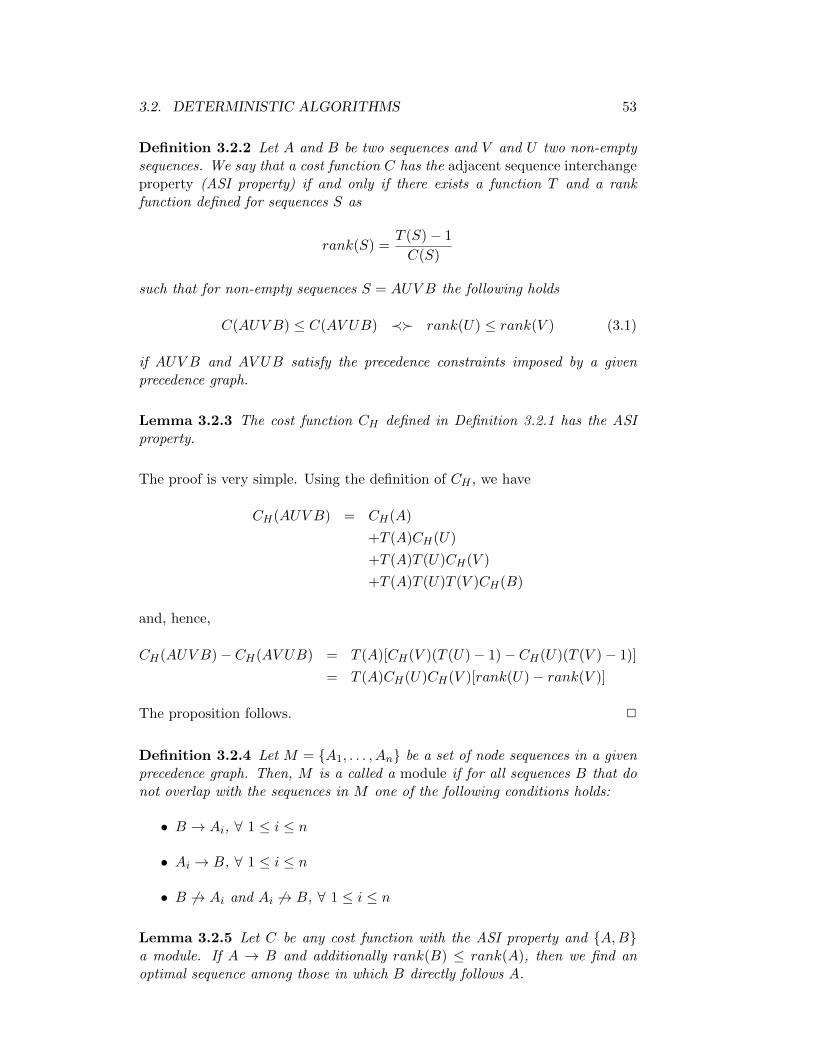
3.2. DETERMINISTIC ALGORITHMS 53

Definition 3.2.2 Let A and B be two sequences and V and U two non-emptysequences. We say that a cost function C has the adjacent sequence interchangeproperty (ASI property) if and only if there exists a function T and a rankfunction defined for sequences S as

rank(S) =T (S)− 1

C(S)

such that for non-empty sequences S = AUV B the following holds

C(AUV B) ≤ C(AV UB) ≺ rank(U) ≤ rank(V ) (3.1)

if AUV B and AV UB satisfy the precedence constraints imposed by a givenprecedence graph.

Lemma 3.2.3 The cost function CH defined in Definition 3.2.1 has the ASIproperty.

The proof is very simple. Using the definition of CH , we have

CH(AUV B) = CH(A)

+T (A)CH(U)

+T (A)T (U)CH(V )

+T (A)T (U)T (V )CH(B)

and, hence,

CH(AUV B)− CH(AV UB) = T (A)[CH(V )(T (U)− 1)− CH(U)(T (V )− 1)]

= T (A)CH(U)CH(V )[rank(U)− rank(V )]

The proposition follows. 2

Definition 3.2.4 Let M = A1, . . . , An be a set of node sequences in a givenprecedence graph. Then, M is a called a module if for all sequences B that donot overlap with the sequences in M one of the following conditions holds:

• B → Ai, ∀ 1 ≤ i ≤ n

• Ai → B, ∀ 1 ≤ i ≤ n

• B 6→ Ai and Ai 6→ B, ∀ 1 ≤ i ≤ n

Lemma 3.2.5 Let C be any cost function with the ASI property and A,Ba module. If A → B and additionally rank(B) ≤ rank(A), then we find anoptimal sequence among those in which B directly follows A.

54 CHAPTER 3. JOIN ORDERING

Proof Every optimal permutation must have the form (U,A, V,B,W ), sinceA → B. Assumption: V 6= ε. If rank(V ) ≤ rank(A), then we can ex-change V and A without increasing the costs. If rank(A) ≤ rank(V ), wehave rank(B) ≤ rank(V ) due to the transitivity of ≤. Hence, we can exchangeB and V without increasing the costs. Both exchanges produce legal sequencesobeying the precedence graph, since A,B is a module. 2

If the precedence graph demands A→ B but rank(B) ≤ rank(A), we speakof contradictory sequences A and B. Since the lemma shows that no non-emptysubsequence can occur between A and B, we will combine A and B into a newsingle node replacing A and B. This node represents a compound relationcomprising all relations in A and B. Its cardinality is computed by multiplyingthe cardinalities of all relations occurring in A and B, and its selectivity s isthe product of all the selectivities si of the relations Ri contained in A and B.The continued process of this step until no more contradictory sequence existsis called normalization. The opposite step, replacing a compound node by thesequence of relations it was derived from, is called denormalization.

We can now present the algorithm IKKBZ.

IKKBZ(G)Input: an acyclic query graph G for relations R1, . . . , RnOutput: the best left-deep tree

R = ∅;for (i = 1; i ≤ n; + + i) Let Gi be the precedence graph derived from G and rooted at Ri;T = IKKBZ-Sub(Gi);R+ = T;

return best of R;

IKKBZ-Sub(Gi)Input: a precedence graph Gi for relations R1, . . . , Rn rooted at some RiOutput: the optimal left-deep tree under Giwhile (Gi is not a chain) let r be the root of a subtree in Gi whose subtrees are chains;

IKKBZ-Normalize(r);merge the chains under r according to the rank function

in ascending order;

IKKBZ-Denormalize(Gi);return Gi;

IKKBZ-Normalize(r)Input: the root r of a subtree T of a precedence graph G = (V,E)Output: a normalized subchain

while (∃ r′, c ∈ V , r →∗ r′, (r′, c) ∈ E: rank(r′) > rank(c)) replace r′ by a compound relation r′′ that represents r′c;

3.2. DETERMINISTIC ALGORITHMS 55

;

We do not give the details of IKKBZ-Denormalize, as it is trivial.

R1

R2 R3 R4

R5 R6

4950

2425

R7

56

1920

45

12

R1

R2 R3 R4

R5 R6,7

4950

2425

56

1920

35

R6,735

R1

R2 R3 R44950

2425

1920

R556

R556

R1

R2 R3 R4,6,74950

2425

199320

R1

10

R5

18

R2

100

R3

100

R6

10

R7

20A)

B)E)

D)

C)F)

R4

100

15

110

13

12

14

12

Figure 3.3: Illustrations for the IKKBZ Algorithm

Let us illustrate the algorithm IKKBZ-Sub by a simple example. We usethe cost function Cout. Figure 3.3 A) shows a query graph. The relations areannotated with their sizes and the edges with the join selectivities. Chosing R1

as the root of the precedence graph results in B). There, the nodes are annotatedby the ranks of the relations. R4 is the root of a subtree all of whose subtreesare chains. Hence, we normalize it. For R5, there is nothing to do. The ranksof R6 and R7 are contradictory. We form a compound relation R6,7, calculateits cardinality, selectivity, and rank. The latter is shown in C). Merging thetwo subchains under R4 results in D). Now R1 is the root of a subtree withonly chains underneath. Normalization detects that the ranks for R4 and R5

are contradictory. E) shows the tree after introducing the compound relationR4,5. Now R4,5 and R6,7 have contradictory ranks, and we replace them by thecompound relation R4,5,6,7 as shown in F). Merging the chains under R1 givesG). Since this is a chain, we leave the loop and denormalize. The final result isshown in H).

56 CHAPTER 3. JOIN ORDERING

III a)

III

IV a)

V a)

III b)

IV b)

V b)

p2,3

p1,2

p3,4

p3,4

p2,3

p1,2

R2 R3R1 R4

p3,4

p2,3

p1,2

p1,2 p3,4

p2,3

R2R1

R3

R2R1 R4R3

R4R3R2R1

R4

B

B

B

B

B B

B

B B

Figure 3.4: A query graph, its directed join graph, some spanning trees andjoin trees

We can use the IKKBZ-Algorithm to derive a heuristics also for cyclicqueries, i.e. for general query graphs. In a first step, we determine a mini-mal spanning tree of the query graph. It is then used as the input query graphfor the IKKBZ-Algorithm. Let us call this the IKKBZ-based Heuristics.

3.2.3 The Maximum-Value-Precedence Algorithm

Lee, Shih, and Chen proposed a very interesting heuristics for the join orderingproblem [517]. They use a weighted directed join graph (WDJG) to representqueries. Within this graph, every join tree corresponds to a spanning tree.

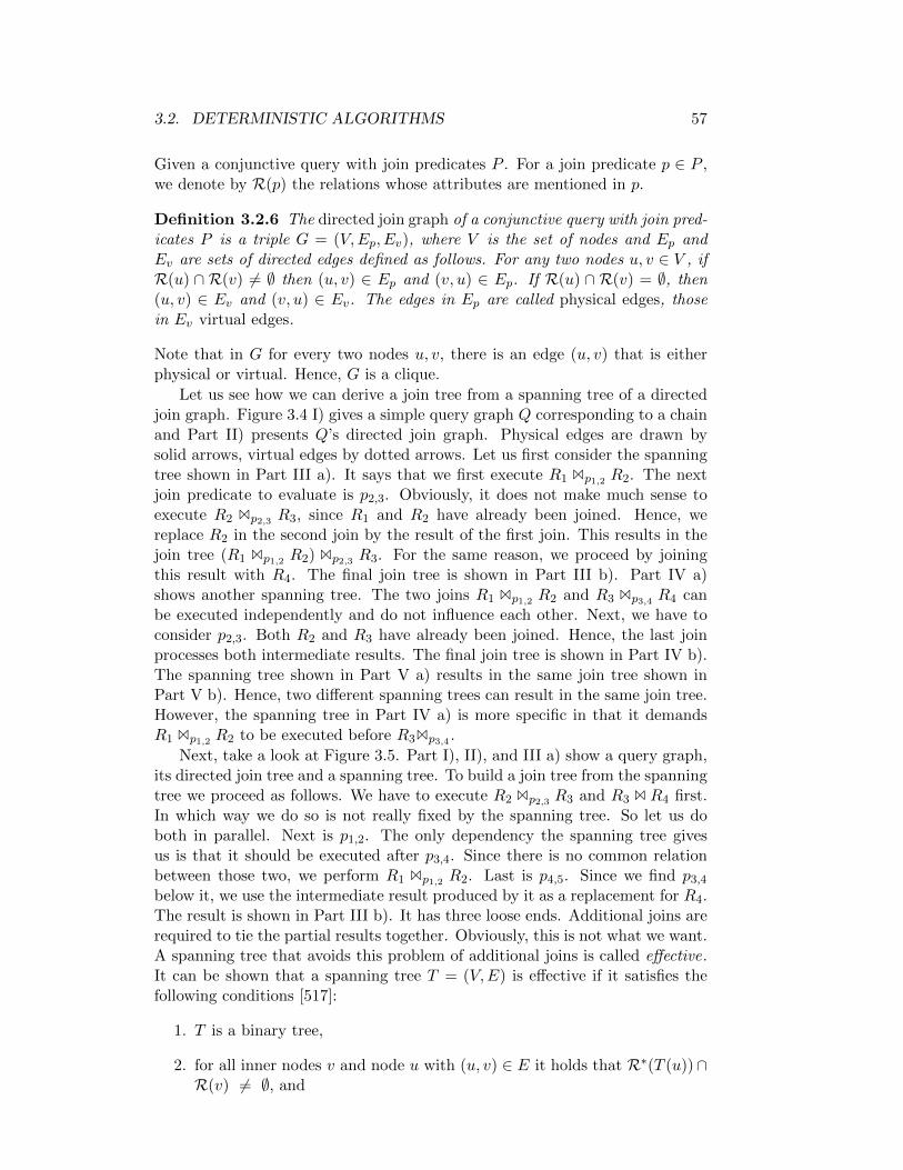
3.2. DETERMINISTIC ALGORITHMS 57

Given a conjunctive query with join predicates P . For a join predicate p ∈ P ,we denote by R(p) the relations whose attributes are mentioned in p.

Definition 3.2.6 The directed join graph of a conjunctive query with join pred-icates P is a triple G = (V,Ep, Ev), where V is the set of nodes and Ep andEv are sets of directed edges defined as follows. For any two nodes u, v ∈ V , ifR(u) ∩ R(v) 6= ∅ then (u, v) ∈ Ep and (v, u) ∈ Ep. If R(u) ∩ R(v) = ∅, then(u, v) ∈ Ev and (v, u) ∈ Ev. The edges in Ep are called physical edges, thosein Ev virtual edges.

Note that in G for every two nodes u, v, there is an edge (u, v) that is eitherphysical or virtual. Hence, G is a clique.

Let us see how we can derive a join tree from a spanning tree of a directedjoin graph. Figure 3.4 I) gives a simple query graph Q corresponding to a chainand Part II) presents Q’s directed join graph. Physical edges are drawn bysolid arrows, virtual edges by dotted arrows. Let us first consider the spanningtree shown in Part III a). It says that we first execute R1 Bp1,2 R2. The nextjoin predicate to evaluate is p2,3. Obviously, it does not make much sense toexecute R2 Bp2,3 R3, since R1 and R2 have already been joined. Hence, wereplace R2 in the second join by the result of the first join. This results in thejoin tree (R1 Bp1,2 R2) Bp2,3 R3. For the same reason, we proceed by joiningthis result with R4. The final join tree is shown in Part III b). Part IV a)shows another spanning tree. The two joins R1 Bp1,2 R2 and R3 Bp3,4 R4 canbe executed independently and do not influence each other. Next, we have toconsider p2,3. Both R2 and R3 have already been joined. Hence, the last joinprocesses both intermediate results. The final join tree is shown in Part IV b).The spanning tree shown in Part V a) results in the same join tree shown inPart V b). Hence, two different spanning trees can result in the same join tree.However, the spanning tree in Part IV a) is more specific in that it demandsR1 Bp1,2 R2 to be executed before R3Bp3,4 .

Next, take a look at Figure 3.5. Part I), II), and III a) show a query graph,its directed join tree and a spanning tree. To build a join tree from the spanningtree we proceed as follows. We have to execute R2 Bp2,3 R3 and R3 B R4 first.In which way we do so is not really fixed by the spanning tree. So let us doboth in parallel. Next is p1,2. The only dependency the spanning tree givesus is that it should be executed after p3,4. Since there is no common relationbetween those two, we perform R1 Bp1,2 R2. Last is p4,5. Since we find p3,4

below it, we use the intermediate result produced by it as a replacement for R4.The result is shown in Part III b). It has three loose ends. Additional joins arerequired to tie the partial results together. Obviously, this is not what we want.A spanning tree that avoids this problem of additional joins is called effective.It can be shown that a spanning tree T = (V,E) is effective if it satisfies thefollowing conditions [517]:

1. T is a binary tree,

2. for all inner nodes v and node u with (u, v) ∈ E it holds that R∗(T (u))∩R(v) 6= ∅, and

58 CHAPTER 3. JOIN ORDERING

I

III b)III a)

p1,2 p2,3 p3,4

R4 R5

p3,4

R2 R3R1

II p4,5

R3

?

p1,2

p4,5

p2,3R2

R5

R4R3 R2R1

B B

B

B

Figure 3.5: A query graph, its directed join tree, a spanning tree and its problem

3. for all nodes v, u1, u2 with u1 6= u2, (u1, v) ∈ E, and (u2, v) ∈ E one ofthe following two conditions holds:

(a) ((R∗(T (u1)) ∩R(v)) ∩ (R∗(T (u2)) ∩R(v))) = ∅ or

(b) (R∗(T (u1)) ∩R(v) = R(v)) ∨ (R∗(T (u2)) ∩R(v) = R(v)).

Thereby, we denote by T (v) the partial tree rooted at v and by R∗(T ′) =∪v∈T ′R(v) the set of all relations in subtree T ′.

We see that the spanning tree in Figure 3.5 III a) is ineffective since, forexample, R(p2,3) ∩ R(p4,5) = ∅. The spanning tree in Figure 3.4 IV a) is alsoineffective. During the algorithm we will take care—by checking the aboveconditions—that only effective spanning trees are generated.

We now assign weights to the edges of the directed join graph. For twonodes v, u ∈ V define u u v := R(u) ∩ R(v). For simplicity, we assume thatevery predicate involves exactly two relations. Then for all u, v ∈ V , u u vcontains a single relation. Let v ∈ V be a node with R(v) = Ri, Rj. Weabbreviate Ri Bv Rj by Bv. Using these notations, we can attach weights tothe edges to define the weighted directed join graph.

Definition 3.2.7 Let G = (V,Ep, Ev) be a directed join graph for a conjunctivequery with join predicates P . The weighted directed join graph is derived fromG by attaching a weight to each edge as follows:

• Let (u, v) ∈ Ep be a physical edge. The weight wu,v of (u, v) is defined as

wu,v =|Bu ||u u v| .

• For virtual edges (u, v) ∈ Ev, we define wu,v = 1.

3.2. DETERMINISTIC ALGORITHMS 59

(Lee, Shih, and Chen actually attach two weights to each edge: one additionalweight for the size of the tuples (in bytes) [517].)

The weights of physical edges are equal to the si of the dependency graphused in the IKKBZ-Algorithm (Section 3.2.2). To see this, assume R(u) =R1, R2, R(v) = R2, R3. Then

wu,v =|Bu ||u u v|

=|R1 Bu R2||R2|

=f1,2 |R1| |R2||R2|

= f1,2 |R1|

Hence, if the join R1 BuR2 is executed before the join R2 Bv R3, the input sizeto the latter join changes by a factor wu,v. This way, the influence of a joinon another join is captured by the weights. Since those nodes connected by avirtual edge do not influence each other, a weight of 1 is appropriate.

Additionally, we assign weights to the nodes of the directed join graph.The weight of a node reflects the change in cardinality to be expected whencertain other joins have been executed before. They are specified by a (partial)spanning tree S. Given S, we denote by BS

pi,j the result of the join Bpi,j if alljoins preceding pi,j in S have been executed. Then the weight attached to nodepi,j is defined as

w(pi,j , S) =|BS

pi,j ||Ri Bpi,j Rj |

.

For empty sequences ε, we define w(pi,j , ε) = |Ri Bpi,j Rj |. Similarly, we definethe cost of a node pi,j depending on other joins preceding it in some givenspanning tree S. We denote this by cost(pi,j , S). The actual cost function canbe one we have introduced so far or any other one. In fact, if we have a choiceof several join implementations, we can take the minimum over all their costfunctions. This then choses the most effective join implementation.

The maximum value precedence algorithm works in two phases. In the firstphase, it searches for edges with a weight smaller than one. Among these, theone with the biggest impact is chosen. This one is then added to the spanningtree. In other words, in this phase, the costs of expensive joins are minimized bymaking sure that (size) decreasing joins are executed first. The second phaseadds edges such that the intermediate result sizes increase as little as possible.

MVP(G)Input: a weighted directed join graph G = (V,Ep, Ev)Output: an effective spanning tree

Q1.insert(V ); /* priority queue with largest node weights w(·) first */

Q2 = ∅; /* priority queue with smallest node weights w(·) first */

G′ = (V ′, E′) with V ′ = V and E′ = Ep; /* working graph */

60 CHAPTER 3. JOIN ORDERING

S = (VS , ES) with VS = V and ES = ∅; /* resulting effective spanning tree */

while (!Q1.empty() && |ES | < |V | − 1) /* Phase I */

v = Q1.head();

among all (u, v) ∈ E′, wu,v < 1 such that

S′ = (V,E′S) with E′S = ES ∪ (u, v) is acyclic and effective

select one that maximizes cost(Bv, S) - cost(Bv, S′);

if (no such edge exists) Q1.remove(v);Q2.insert(v);continue;

MvpUpdate((u, v));recompute w(·) for v and its ancestors; /* rearranges Q1 */

while (!Q2.empty() && |ES | < |V | − 1) /* Phase II */

v = Q2.head();

among all (u, v), (v, u) ∈ E′ denoted by (x, y) henceforth

such that

S′ = (V,E′S) with E′S = ES ∪ (x, y) is acyclic and effective

select the one that minimizes cost(Bv, S′) - cost(Bv, S);

MvpUpdate((x, y));recompute w(·) for y and its ancestors; /* rearranges Q2 */

return S;

MvpUpdate((u, v))Input: an edge to be added to SOutput: side-effects on S, G′,ES ∪ = (u, v);E′ \ = (u, v), (v, u);E′ \ = (u,w)|(u,w) ∈ E′; /* (1) */

E′ ∪ = (v, w)|(u,w) ∈ Ep, (v, w) ∈ Ev; /* (3) */

if (v has two inflowing edges in S) /* (2) */

E′ \ = (w, v)|(w, v) ∈ E′;if (v has one outflowing edge in S) /* (1) in paper but not needed */

E′ \ = (v, w)|(v, w) ∈ E′;

Note that in order to test for the effectiveness of a spanning tree in thealgorithm, we just have to check the conditions for the node the selected edgeleads to.

MvpUpdate first adds the selected edge to the spanning tree. It then elim-inates edges that need not to be considered for building an effective spanningtree. Since (u, v) has been added, both (u, v) and (v, u) do not have to beconsidered any longer. Also, since effective spanning trees are binary trees, (1)

3.2. DETERMINISTIC ALGORITHMS 61

every node must have only one parent node and (2) at most two child nodes.The edges leading to a violation are eliminated by MvpUpdate in the lines com-mented with the corresponding numbers. For the line commented (3) we havethe situation that u→ v 99K w and u→ w in G. This means that u and w havecommon relations, but v and w do not. Hence, the result of performing v onthe result of u will have a common relation with w. Thus, we add a (physical)edge v → w.

3.2.4 Dynamic Programming

Algorithms

Consider the two join trees

(((R1 BR2) BR3) BR4) BR5

and(((R3 BR1) BR2) BR4) BR5.

If we know that ((R1BR2)BR3) is cheaper than ((R3BR1)BR2), we know thatthe first join tree is cheaper than the second. Hence, we could avoid generatingthe second alternative and still won’t miss the optimal join tree. The generalprinciple behind this is the optimality principle (see [200]). For the join orderingproblem, it can be stated as follows.1

Let T be an optimal join tree for relations R1, . . . , Rn. Then, everysubtree S of T must be an optimal join tree for the relations itcontains.

To see why this holds, assume that the optimal join tree T for relationsR1, . . . , Rncontains a subtree S which is not optimal. That is, there exists another jointree S′ for the relations contained in S with strictly lower costs. Denote byT ′ the join tree derived by replacing S in T by S′. Since S′ contains the samerelations as S, T ′ is a join tree for the relations R1, . . . , Rn. The costs of the joinoperators in T and T ′ that are not contained in S and S′ are the same. Then,since the total cost of a join tree is the sum of the costs of the join operatorsand S′ has lower costs than S, T ′ has lower costs than T . This contradicts theoptimality of T .

The idea of dynamic programming applied to the generation of optimal jointrees now is to generate optimal join trees for subsets of R1, . . . , Rn in a bottom-up fashion. First, optimal join trees for subsets of size one, i.e. single relations,are generated. From these, optimal join trees of size two, three and so on untiln are generated.

Let us first consider generating optimal left-deep trees. There, join trees forsubsets of size k are generated from subsets of size k − 1 by adding a new joinoperator whose left argument is a join tree for k − 1 relations and whose rightargument is a single relation. Exchanging left and right gives us the procedurefor generating right-deep trees. If we want to generate zig-zag trees since our

1The optimality principle does not hold in the presence of properties.

62 CHAPTER 3. JOIN ORDERING

cost function is asymmetric, we have to consider both alternatives and takethe cheapest one. We capture this in a procedure CreateJoinTree that takestwo join trees as arguments and generates the above-mentioned alternatives.In case we want to consider different implementations for the join, we have toperform the above steps for all of them and return the cheapest alternative.Summarizing, the pseudo-code for CreateJoinTree looks as follows:

CreateJoinTree(T1, T2)

Input: two (optimal) join trees T1 and T2.

for linear trees, we assume that T2 is a single relation

Output: an (optimal) join tree for joining T1 and T2.

BestTree = NULL;

for all implementations impl do if(!RightDeepOnly) Tree = T1 B

impl T2

if (BestTree == NULL || cost(BestTree) > cost(Tree)) BestTree = Tree;

if(!LeftDeepOnly) Tree = T2 B

impl T1

if (BestTree == NULL || cost(BestTree) > cost(Tree)) BestTree = Tree;

return BestTree;

The boolean variables RightDeepOnly and LeftDeepOnly are used to restrictthe search space to right-deep trees and left-deep trees. If both are false, zig-zagtrees are generated. However, CreateJoinTree also generates bushy trees, ifnone of the input trees is a single relation.

In case of linear trees, T2 will be the single relation in all of our algorithms.CreateJoinTree should not copy T1 or T2. Instead, the newly generated jointrees should share T1 and T2 by using pointers. Further, the join trees generateddo not really need to be generated except for the final (best) join tree: the costfunctions should be implemented such that they can be evaluated if they aregiven the left and right argument of the join.

Using CreateJoinTree, we are now ready to present our first dynamic pro-gramming algorithm in pseudo-code.

DP-Linear-1(R1, . . . , Rn)Input: a set of relations to be joined

Output: an optimal left-deep (right-deep, zig-zag) join tree

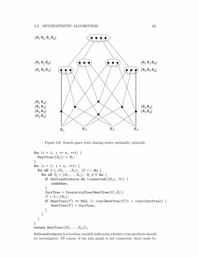
3.2. DETERMINISTIC ALGORITHMS 63

R1R4R3R2

R3R1 R2 R4

R1 R2 R4

R1 R2 R3

R1 R3

R1 R4

R1

R2 R3

R1 R3 R4

R2 R3 R4

R2

R4

R4

R2

R3

Figure 3.6: Search space with sharing under optimality principle

for (i = 1; i <= n; ++i) BestTree(Ri) = Ri;

for (i = 1; i < n; ++i)

for all S ⊆ R1, . . . , Rn, |S| = i do for all Rj ∈ R1, . . . , Rn, Rj 6∈ S do

if (NoCrossProducts && !connected(Rj, S)) continue;

CurrTree = CreateJoinTree(BestTree(S),Rj);S′ = S ∪ Rj;if (BestTree(S′) == NULL || cost(BestTree(S′)) > cost(CurrTree))

BestTree(S′) = CurrTree;

return BestTree(R1, . . . , Rn);NoCrossProducts is a boolean variable indicating whether cross products shouldbe investigated. Of course, if the join graph is not connected, there must be

64 CHAPTER 3. JOIN ORDERING

a cross product, but for DP-Linear-1 and subsequent algorithms we assumethat it is connected. The boolean function connected returns true, if there isa join predicate between one of the relations in its first argument and one ofthe relations in its second. The variable BestTree keeps track of the best jointrees generated for every subset of the relations R1, . . . , Rn. How this is donemay depend on several parameters. The approaches are to use a hash table oran array of size 2n(−1). Another issue is how to represent the sets of relations.XC search

space sizedifferenceproblem

Typically, bitvector representations are used. Then, testing for membership,computing a set’s complement, adding elements and unioning is cheap. Yetanother issue is the order in which join trees are generated. The procedureDP-Linear-1 takes the approach to generate the join trees for subsets of size1, 2, . . . , n. To do so, it must be able to access the subsets of R1, . . . , Rn ortheir respective join trees by their size. One possibility is to chain all the jointrees for subsets of a given size k (1 ≤ k ≤ n) and to use an array of size n tokeep pointers to the start of the lists. In this case, to every join tree the set ofrelations it contains is attached, in order to be able to perform the test Ri 6∈ S.One way to do this is to embed a bitvector into each join tree node.

Figure 3.6 illustrates how the procedure DP-Linear-1 works. In its firstloop, it initializes the bottom row of join trees of size one. Then it computesthe join trees joining exactly two relations. This is indicated by the next groupof join trees. Since the figure leaves out commutativity, only one alternativejoin tree for every subset of size two is generated. This changes for subsets ofsize three. There, three alternative join trees are generated. Only the best jointree is retained. This is indicated by the ovals that encircle three join trees.Only this best join tree of size three is used to generate the final best join tree.

The short clarification after the algorithm already adumbrated that theorder in which join trees are generated is not compulsory. The only necessarycondition is the following.

Let S be a subset of R1, . . . , Rn. Then, before a join tree for Scan be generated, the join trees for all relevant subsets of S mustalready be available.

Note that this formulation is general enough to also capture the generation ofbushy trees. It is, however, a little vague due to its reference to “relevance”.For the different join tree classes, this term can be given a precise semantics.EX

Let us take a look at an alternative order to join tree generation. Assumethat sets of relations are represented as bitvectors. A bitvector is nothing morethan a base two integer. Successive increments of an integer/bitvector lead todifferent subsets. Further, the above condition is satisfied. We illustrate this bya small example. Assume that we have three relations R1, R2, R3. The i-th bitfrom the right in a three-bit integer indicates the presence of Ri for 1 ≤ i ≤ 3.

3.2. DETERMINISTIC ALGORITHMS 65

000 001 R1010 R2011 R1, R2100 R3101 R1, R3110 R2, R3111 R1, R2, R3

This observation leads to another formulation of our dynamic programmingalgorithm. For this algorithm, it is very convenient to use an array of size 2n

to represent BestTree(S) for subsets S of R1, . . . , Rn.

DP-Linear-2(R1, . . . , Rn)Input: a set of relations to be joined

Output: an optimal left-deep (right-deep, zig-zag) join tree

for (i = 1; i <= n; ++i) BestTree(1 << i) = Ri;

for (S = 1; S < 2n; ++S)

if (BestTree(S) != NULL) continue;for all i ∈ S do S′ = S \ i;CurrTree = CreateJoinTree(BestTree(S′),Ri);if (BestTree(S) == NULL || cost(BestTree(S)) > cost(CurrTree)) BestTree(S) = CurrTree;

return BestTree(2n − 1);

DP-Linear-2 differs from DP-Linear-1 not only in the order in which join treesare generated. Another difference is that it takes cross products into account.

From DP-Linear-2, it is easy to derive an algorithm that explores the spaceof bushy trees.

DP-Bushy(R1, . . . , Rn)Input: a set of relations to be joined

Output: an optimal bushy join tree

for (i = 1; i <= n; ++i) BestTree(1 << i) = Ri;

for (S = 1; S < 2n; ++S)

if (BestTree(S) != NULL) continue;for all S1 ⊂ S do

66 CHAPTER 3. JOIN ORDERING

S2 = S \ S1;

CurrTree = CreateJoinTree(BestTree(S1), BestTree(S2));

if (BestTree(S) == NULL || cost(BestTree(S)) > cost(CurrTree)) BestTree(S) = CurrTree;

return BestTree(2n − 1);

This algorithm also takes cross products into account. The critical part is thegeneration of all subsets of S. Fortunately, Vance and Maier [865] provide acode fragment with which subset bitvector representations can be generatedvery efficiently. In C, this fragment looks as follows:

S1 = S & - S;

do /* do something with subset S1 */

S1 = S & (S1 - S);

while (S1 != S);

S represents the input set. S1 iterates through all subsets of S where S itself andthe empty set are not considered. Analogously, all supersets an be generatedas follows:

S1 = ~S & - ~S;

/* do something with first superset S1 */

while (S1) S1 = ~S & (S1 - ~S)

/* do something with superset S1

S represents the input set. S1 iterates through all supersets of S including Sitself.

Excursion Problem: exploiting orderings devastates the optimality principle.Example: . . .XC ToDo

Excursion Pruning . . .XC ToDo

Number of Entries to be stored in the dynamic programming table

If dynamic programming uses a static hash table, determining its size in advanceis necessary as the search space sizes differ vastly for different query graphs.In general, for every connected subgraph of the query graph one entry must

3.2. DETERMINISTIC ALGORITHMS 67

exist. Chains require far fewer entries than cliques. It would be helpful tohave a small routine solving the following problem: given a query graph, howmany connected subgraph are there? Unfortunatly, this problem is #-P hardas Sutner, Satyanarayana, and Suffel showed [825]. They build on results byValiant [863] and Lichtenstein [534]. (For a definition of #P-hard see the bookby Lewis and Papadimitriou [532] or the original paper by Valiant [862].)

However, for specific cases, these numbers can be given. If cross productsare consideres, the number of join trees stored in the dynamic programmingtable is

2n − 1

which is one for each non-empty subset of relations.

If we do not consider cross products, the number of entries in the dynamicprogramming table corresponds to the number of connected subgraphs of thequery graph. For connected query graphs, we denote this by #csg. For chains,cycles, stars, and cliques with n nodes, we have

#csgchain(n) =n(n+ 1)

2(3.2)

#csgcycle(n) = n2 − n+ 1 (3.3)

#csgstar(n) = 2n−1 + n− 1 (3.4)

#csgclique(n) = 2n − 1 (3.5)

These equations can be derived from the following by summing over k > 1where k gives the size of the connected subset:

#csgchain(n, k) = (n− k + 1)

#csgcycle(n, k) =

1 n = kn else

#csgstar(n, k) =

n k = 1(n−1k−1

)k > 1

#csgclique(n, k) =

(n

k

)

Number of Join Trees Investigated

The number of join trees investigated by dynamic programming was extensivelystudied by Ono and Lohman [625, 626]. In order to estimate these numbers, weassume that CreateJoinTree produces a single join tree and hence counts asone although it may evaluate the costs for several join alternatives. We furtherdo not count the initial join trees containing only a single relation.

Join Trees With Cartesian Product For the analysis of dynamic pro-gramming variants that do consider cross products, the notion of join-pair ishelpful. Let S1 and S2 be subsets of the nodes (relations) of the query graph.We say (S1, S2) is a join-pair, if and only if

68 CHAPTER 3. JOIN ORDERING

1. S1 and S2 are disjoint

If (S1, S2) is a join-pair, then (S2, S1) is a join pair. Further, if T1 is a join treefor the relations in S1 and T2 is one for those in S2, then we can construct twovalid join trees T1 1 T2 and T2 1 T1 where the joins may be cross products.Hence, the number of join-pairs coincides with the search space a dynamic pro-gramming algorithm explores. In fact, the number of join-pairs is the minimumnumber of join trees any dynamic programming algorithm that considers crossproducts has to investigate.

If CreateJoinTree considers commutativity of joins, the number of callsto it is precisely expressed by the count of non-symmetric join-pairs. In otherimplementations CreateJoinTree might be called for all join-pairs and, thus,may not consider commutativity. The two formulas below only count non-symmetric join pairs.

The numbers of linear and bushy join trees with cartesian product is easiestto determine. They are independent of the query graph. For linear join trees,the number of join trees investigated by dynamic programming is equal to thenumber of non-symmetric join-pairs which is

n2n−1 − n(n+ 1)

2

Dynamic programming investigates the following number of bushy trees ifcross products are considered.

(3n − 2n+1 + 1)

2

This is equal to the number of non-symmetric join-pairs.

Join Trees without Cross Products In this paragraph, we assume that thequery graph is connected. For the analysis of dynamic programming variantsthat do not consider cross products, it is helpful to have the notion of a csg-cmp-pair. Let S1 and S2 be subsets of the nodes (relations) of the query graph.We say (S1, S2) is a csg-cmp-pair , if and only if

1. S1 induces a connected subgraph of the query graph,

2. S2 induces a connected subgraph of the query graph,

3. S1 and S2 are disjoint, and

4. there exists at least one edge connected a node in S1 to a node in S2.

If (S1, S2) is a csg-cmp-pair, then (S2, S1) is a valid csg-cmp-pair. Further, if T1

is a join tree for the relations in S1 and T2 is one for those in S2, then we canconstruct two valid join trees T1 1 T2 and T2 1 T1. Hence, the number of csg-cmp-pairs coincides with the search space a dynamic programming algorithmexplores. In fact, the number of csg-cmp-pairs is the minimum number ofjoin trees any dynamic programming algorithm that does not consider crossproducts has to investigate.

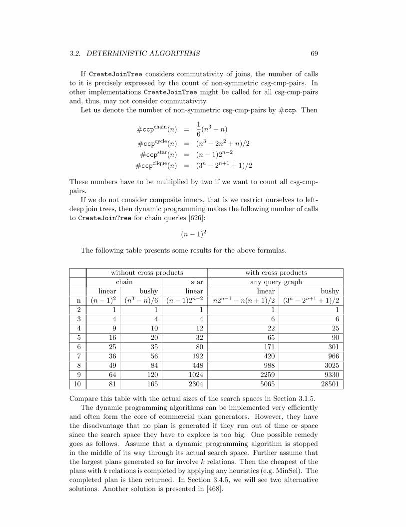
3.2. DETERMINISTIC ALGORITHMS 69

If CreateJoinTree considers commutativity of joins, the number of callsto it is precisely expressed by the count of non-symmetric csg-cmp-pairs. Inother implementations CreateJoinTree might be called for all csg-cmp-pairsand, thus, may not consider commutativity.

Let us denote the number of non-symmetric csg-cmp-pairs by #ccp. Then

#ccpchain(n) =1

6(n3 − n)

#ccpcycle(n) = (n3 − 2n2 + n)/2

#ccpstar(n) = (n− 1)2n−2

#ccpclique(n) = (3n − 2n+1 + 1)/2

These numbers have to be multiplied by two if we want to count all csg-cmp-pairs.

If we do not consider composite inners, that is we restrict ourselves to left-deep join trees, then dynamic programming makes the following number of callsto CreateJoinTree for chain queries [626]:

(n− 1)2

The following table presents some results for the above formulas.

without cross products with cross products

chain star any query graph

linear bushy linear linear bushy

n (n− 1)2 (n3 − n)/6 (n− 1)2n−2 n2n−1 − n(n+ 1)/2 (3n − 2n+1 + 1)/2

2 1 1 1 1 1

3 4 4 4 6 6

4 9 10 12 22 25

5 16 20 32 65 90

6 25 35 80 171 301

7 36 56 192 420 966

8 49 84 448 988 3025

9 64 120 1024 2259 9330

10 81 165 2304 5065 28501

Compare this table with the actual sizes of the search spaces in Section 3.1.5.The dynamic programming algorithms can be implemented very efficiently

and often form the core of commercial plan generators. However, they havethe disadvantage that no plan is generated if they run out of time or spacesince the search space they have to explore is too big. One possible remedygoes as follows. Assume that a dynamic programming algorithm is stoppedin the middle of its way through its actual search space. Further assume thatthe largest plans generated so far involve k relations. Then the cheapest of theplans with k relations is completed by applying any heuristics (e.g. MinSel). Thecompleted plan is then returned. In Section 3.4.5, we will see two alternativesolutions. Another solution is presented in [468].

70 CHAPTER 3. JOIN ORDERING

DPsize

Input: a connected query graph with relations R = R0, . . . , Rn−1Output: an optimal bushy join tree without cross productsfor all Ri ∈ R

BestPlan(Ri) = Ri;for all 1 < s ≤ n ascending // size of planfor all 1 ≤ s1 < s // size of left subplan

s2 = s− s1; // size of right subplanfor all S1 ⊂ R : |S1| = s1

S2 ⊂ R : |S2| = s2 ++InnerCounter;if (∅ 6= S1 ∩ S2) continue;if not (S1 connected to S2) continue;++CsgCmpPairCounter;p1=BestPlan(S1);p2=BestPlan(S2);CurrPlan = CreateJoinTree(p1, p2);if (cost(BestPlan(S1 ∪ S2)) > cost(CurrPlan))

BestPlan(S1 ∪ S2) = CurrPlan;

OnoLohmanCounter = CsgCmpPairCounter / 2;return BestPlan(R0, . . . , Rn−1);

Figure 3.7: Algorithm DPsize

Generating Bushy Trees without Cross Products

We now discuss dynamic programming algorithms to generate bushy trees with-out cross products. For this section, we assume that the query graph is con-nected. We will present three algorithms. The first algorithm (DPsize) gener-ates its plans in increasing size of subplans and, hence, is a generalization ofDP-Linear-1. The second algorithm (DPsub) geneerates its plans by consider-ing plans subsets as does DP-Linear-2. An analysis of these two algorithmsreveals that both are far away from the lower bound presented in the previoussections. Thus, a third algorithm (DPccp) which reaches this lower bound ispresented. The results of this section are taken from [595, 593].

Size-based enumeration: DPsize In general, dynamic programming gen-erates solutions for a larger problem in a bottom-up fashion by combining so-lutions for smaller problems. Taking this description literally, we can constructoptimal plans of size n by joining plans P1 and P2 of size k and n− k. We justhave to take care that (1) the sets of relations contained in P1 and P2 do notoverlap, and (2) there is a join predicate connecting a relation P1 with a relationin P2. After this remark, we are prepared to understand the pseudocode for

3.2. DETERMINISTIC ALGORITHMS 71

algorithm DPsize (see Fig. 3.7). A table BestPlan associates with each set ofrelations the best plan found so far. The algorithm starts by initializing thistable with plans of size one, i.e. single relations. After that, it constructs plansof increasing size (loop over s). Thereby, the first size considered is two, sinceplans of size one have already been constructed. Every plan joining n relationscan be constructed by joining a plan containing s1 relations with a plan con-taining s2 relations. Thereby, si > 0 and s1 + s2 = n must hold. Thus, thepseudocode loops over s1 and sets s2 accordingly. Since for every possible sizethere exist many plans, two more loops are necessary in order to loop over theplans of sizes s1 and s2. Then, conditions (1) and (2) from above are tested.Only if their outcome is positive, we consider joining the plans p1 and p2. Theresult is a plan CurrPlan. Let S be the relations contained in CurrPlan. IfBestPlan does not contain a plan for the relations in S or the one it containsis more expensive than CurrPlan, we register CurrPlan with BestPlan.

The algorithm DPsize can be made more efficient in case of s1 = s2. Thealgorithm as stated cycles through all plans p1 joining s1 relations. For eachsuch plan, all plans p2 of size s2 are tested. Assume that plans of equal size arerepresented as a linked list. If s1 = s2, then it is possible to iterate through thelist for retrieving all plans p1. For p2 we consider the plans succeeding p1 in thelist. Thus, the complexity can be decreased from s1∗s2 to s1∗s2/2 The followingformulas are valid only for the variant of DPsize where this optimization hasbeen incorporated (see [593] for details).

If the counter InnerCounter is initialized with zero at the beginning of thealgorithm DPsize, then we are able to derive analytically its value after DPsizeterminates. Since this value of the inner counter depends on the query graph,we have to distinguish several cases. For chain, cycle, star, and clique queries,we denote by Ichain

DPsize, IcycleDPsize, I

starDPsize, and Iclique

DPsize the value of InnerCounter

after termination of algorithm DPsize.For chain queries, we then have: Ichain

DPsize(n) =

1/48(5n4 + 6n3 − 14n2 − 12n) n even1/48(5n4 + 6n3 − 14n2 − 6n+ 11) n odd

For cycle queries, we have: IcycleDPsize(n) =

14(n4 − n3 − n2) n even14(n4 − n3 − n2 + n) n odd

For star queries, we have: IstarDPsize(n) =

22n−4 − 1/4

(2(n−1)n−1

)+ q(n) n even

22n−4 − 1/4(

2(n−1)n−1

)+ 1/4

(n−1

(n−1)/2

)+ q(n) n odd

with q(n) = n2n−1 − 5 ∗ 2n−3 + 1/2(n2 − 5n+ 4). For clique queries, we have:

IcliqueDPsize(n) =

22n−2 − 5 ∗ 2n−2 + 1/4

(2nn

)− 1/4

(nn/2

)+ 1 n even

22n−2 − 5 ∗ 2n−2 + 1/4(

2nn

)+ 1 n odd

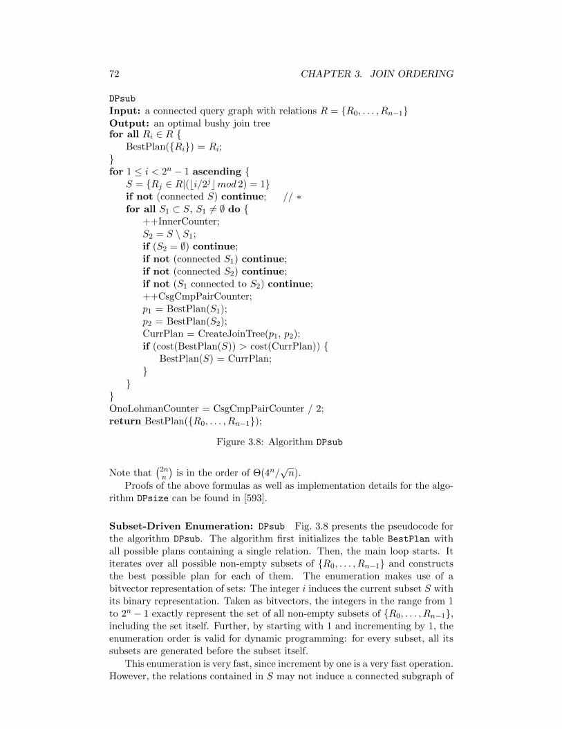
72 CHAPTER 3. JOIN ORDERING

DPsub

Input: a connected query graph with relations R = R0, . . . , Rn−1Output: an optimal bushy join treefor all Ri ∈ R

BestPlan(Ri) = Ri;for 1 ≤ i < 2n − 1 ascending

S = Rj ∈ R|(bi/2jcmod 2) = 1if not (connected S) continue; // ∗for all S1 ⊂ S, S1 6= ∅ do

++InnerCounter;S2 = S \ S1;if (S2 = ∅) continue;if not (connected S1) continue;if not (connected S2) continue;if not (S1 connected to S2) continue;++CsgCmpPairCounter;p1 = BestPlan(S1);p2 = BestPlan(S2);CurrPlan = CreateJoinTree(p1, p2);if (cost(BestPlan(S)) > cost(CurrPlan))

BestPlan(S) = CurrPlan;

OnoLohmanCounter = CsgCmpPairCounter / 2;return BestPlan(R0, . . . , Rn−1);

Figure 3.8: Algorithm DPsub

Note that(

2nn

)is in the order of Θ(4n/

√n).

Proofs of the above formulas as well as implementation details for the algo-rithm DPsize can be found in [593].

Subset-Driven Enumeration: DPsub Fig. 3.8 presents the pseudocode forthe algorithm DPsub. The algorithm first initializes the table BestPlan withall possible plans containing a single relation. Then, the main loop starts. Ititerates over all possible non-empty subsets of R0, . . . , Rn−1 and constructsthe best possible plan for each of them. The enumeration makes use of abitvector representation of sets: The integer i induces the current subset S withits binary representation. Taken as bitvectors, the integers in the range from 1to 2n − 1 exactly represent the set of all non-empty subsets of R0, . . . , Rn−1,including the set itself. Further, by starting with 1 and incrementing by 1, theenumeration order is valid for dynamic programming: for every subset, all itssubsets are generated before the subset itself.

This enumeration is very fast, since increment by one is a very fast operation.However, the relations contained in S may not induce a connected subgraph of

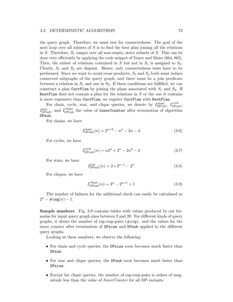
3.2. DETERMINISTIC ALGORITHMS 73

the query graph. Therefore, we must test for connectedness. The goal of thenext loop over all subsets of S is to find the best plan joining all the relationsin S. Therefore, S1 ranges over all non-empty, strict subsets of S. This can bedone very efficiently by applying the code snippet of Vance and Maier [864, 865].Then, the subset of relations contained in S but not in S1 is assigned to S2.Clearly, S1 and S2 are disjoint. Hence, only connectedness tests have to beperformed. Since we want to avoid cross products, S1 and S2 both must induceconnected subgraphs of the query graph, and there must be a join predicatebetween a relation in S1 and one in S2. If these conditions are fulfilled, we canconstruct a plan CurrPlan by joining the plans associated with S1 and S2. IfBestPlan does not contain a plan for the relations in S or the one it containsis more expensive than CurrPlan, we register CurrPlan with BestPlan.

For chain, cycle, star, and clique queries, we denote by IchainDPsub, Icycle

DPsub,

IstarDPsub, and Iclique

DPsub the value of InnerCounter after termination of algorithmDPsub.

For chains, we have

IchainDPsub(n) = 2n+2 − nn − 3n− 4 (3.6)

For cycles, we have

IcycleDPsub(n) = n2n + 2n − 2n2 − 2 (3.7)

For stars, we have

IstarDPsub(n) = 2 ∗ 3n−1 − 2n (3.8)

For cliques, we have

IcliqueDPsub(n) = 3n − 2n+1 + 1 (3.9)

The number of failures for the additional check can easily be calculated as2n −#csg(n)− 1.

Sample numbers Fig. 3.9 contains tables with values produced by our for-mulas for input query graph sizes between 2 and 20. For different kinds of querygraphs, it shows the number of csg-cmp-pairs (#ccp). and the values for theinner counter after termination of DPsize and DPsub applied to the differentquery graphs.

Looking at these numbers, we observe the following:

• For chain and cycle queries, the DPsize soon becomes much faster thanDPsub.

• For star and clique queries, the DPsub soon becomes much faster thanDPsize.

• Except for clique queries, the number of csg-cmp-pairs is orders of mag-nitude less than the value of InnerCounter for all DP-variants.

74 CHAPTER 3. JOIN ORDERING

Chain Cycle

n #ccp DPsub DPsize #ccp DPsub DPsize

2 1 2 1 1 2 15 20 84 73 40 140 120

10 165 3962 1135 405 11062 222515 560 130798 5628 1470 523836 1176020 1330 4193840 17545 3610 22019294 37900

Star Clique

n #ccp DPsub DPsize #ccp DPsub DPsize

2 1 2 1 1 2 15 32 130 110 90 180 280

10 2304 38342 57888 28501 57002 30699115 114688 9533170 57305929 7141686 14283372 30717387720 4980736 2323474358 59892991338 1742343625 3484687250 309338182241

Figure 3.9: Size of the search space for different graph structures

From the latter observation we can conclude that in almost all cases the testsperformed by both algorithms in their innermost loop fail. Both algorithmsare far away from the theoretical lower bound given by #ccp. This conclusionmotivates us to derive a new algorithm whose InnerCounter value is equal tothe number of csg-cmp-pairs.

Csg-cmp-pair enumeration-based algorithm: DPccp The algorithm DPsub

solves the join ordering problem for a given subset S of relations by consideringall pairs of disjoint subproblems which were already solved. Since the enumer-ation of subsets is very fast, this is a very efficient strategy if the search spaceis dense, e.g. for clique queries. However, if the search space is sparse, e.g. forchain queries, the DPsub algorithm considers many subproblems which are notconnected and, therefore, are not relevant for the solution, i.e. the tests in theinnermost loop fail for the majority of cases. The main idea of our algorithmDPccp is that it only considers pairs of connected subproblems. More precisely,the algorithm considers exactly the csg-cmp-pairs of a graph.

Thus, our goal is to efficiently enumerate all csg-cmp-pairs (S1, S2). Clearly,we want to enumerate every pair once and only once. Further, the enumera-tion must be performed in an order valid for dynamic programming. That is,whenever a pair (S1, S2) is generated, all non-empty subsets of S1 and S2 musthave been generated before as a component of a pair. The last requirement isthat the overhead for generating a single csg-cmp-pair must be constant or atmost linear. This condition is necessary in order to beat DPsize and DPsub.

If we meet all these requirements, the algorithm DPccp is easily specified:iterate over all csg-cmp-pairs (S1, S2) and consider joining the best plans as-sociated with them. Figure 3.10 shows the pseudocode. The first steps of anexample enumeration are shown in Figure 3.11. Thick lines mark the connect-ed subsets while thin lines mark possible join edges. Note that the algorithm

3.2. DETERMINISTIC ALGORITHMS 75

DPccp

Input: a connected query graph with relations R = R0, . . . , Rn−1Output: an optimal bushy join treefor all Ri ∈ R)

BestPlan(Ri) = Ri;for all csg-cmp-pairs (S1, S2), S = S1 ∪ S2

++InnerCounter;++OnoLohmanCounter;p1 = BestPlan(S1);p2 = BestPlan(S2);CurrPlan = CreateJoinTree(p1, p2);if (cost(BestPlan(S)) > cost(CurrPlan))

BestPlan(S) = CurrPlan;CurrPlan = CreateJoinTree(p2, p1);if (cost(BestPlan(S)) > cost(CurrPlan))

BestPlan(S) = CurrPlan;

CsgCmpPairCounter = 2 * OnoLohmanCounter;return BestPlan(R0, . . . , Rn−1);

Figure 3.10: Algorithm DPccp

22

10

1.Graph

32 32

...

...

7.6.5.4.3.2.

000111 1

3 32 32 3

Figure 3.11: Enumeration Example for DPccp

explicitly exploits join commutativity. This is due to our enumeration algo-rithm developed below. If (S1, S2) is a csg-cmp-pair, then either (S1, S2) or(S2, S1) will be generated, but never both of them. An alternative is to modifyCreateJoinTree to take care of commutativity.

We proceed as follows. Next we discuss an algorithm enumerating non-empty connected subsets S1 of R0, . . . , Rn−1. Then, we show how to enumer-ate the complements S2 such that (S1, S2) is a csg-cmp-pair.

Let us start the exposition by fixing some notations. Let G = (V,E) bean undirected graph. For a node v ∈ V define the neighborhood IN(v) of v asIN(v) := v′|(v, v′) ∈ E. For a subset S ⊆ V of V we define the neighborhood ofS as IN(S) := ∪v∈SIN(v) \ S. The neighborhood of a set of nodes thus consistsof all nodes reachable by a single edge. Note that for all S, S′ ⊂ V we have

76 CHAPTER 3. JOIN ORDERING

IN(S ∪ S′) = (IN(S) ∪ IN(S′)) \ (S ∪ S′). This allows for an efficient bottom-upcalculation of neighborhoods.

The following statement gives a hint on how to construct an enumerationprocedure for connected subsets. Let S be a connected subset of an undirectedgraph G and S′ be any subset of IN(S). Then S ∪ S′ is connected. As aconsequence, a connected subset can be enlarged by adding any subset of itsneighborhood.

We could generate all connected subsets as follows. For every node vi ∈ Vwe perform the following enumeration steps: First, we emit vi as a connectedsubset. Then, we expand vi by calling a routine that extends a given connect-ed set to bigger connected sets. Let the routine be called with some connectedset S. It then calculates the neighborhood IN(S). For every non-empty subsetN ⊆ IN(S), it emits S′ = S ∪N as a further connected subset and recursivelycalls itself with S′. The problem with this routine is that it produces duplicates.

This is the point where the breadth-first numbering comes into play. LetV = v0, . . . , vn−1, where the indices are consistent with a breadth-first num-bering produced by a breadth-first search starting at node v0 [201]. The ideais to use the numbering to define an enumeration order: In order to avoid du-plicates, the algorithm enumerates connected subgraphs for every node vi, butrestricts them to contain no vj with j < i. Using the definition Bi = vj |j ≤ i,the pseudocode looks as follows:

EnumerateCsg

Input: a connected query graph G = (V,E)Precondition: nodes in V are numbered according to a breadth-first searchOutput: emits all subsets of V inducing a connected subgraph of Gfor all i ∈ [n− 1, . . . , 0] descending

emit vi;EnumerateCsgRec(G, vi, Bi);

EnumerateCsgRec(G, S, X)N = IN(S) \X;for all S′ ⊆ N , S′ 6= ∅, enumerate subsets first

emit (S ∪ S′);for all S′ ⊆ N , S′ 6= ∅, enumerate subsets first

EnumerateCsgRec(G, (S ∪ S′), (X ∪N));

Let us consider an example. Figure 3.12 contains a query graph whosenodes are numbered in a breadth-first fashion. The calls to EnumerateCsgRec

are contained in the table in Figure 3.13. In this table, S and X are thearguments of EnumerateCsgRec. N is the local variable after its initialization.The column emit/S contains the connected subset emitted, which then becomesthe argument of the recursive call to EnumerateCsgRec (labelled by →). Sincelisting all calls is too lengthy, only a subset of the calls is listed.

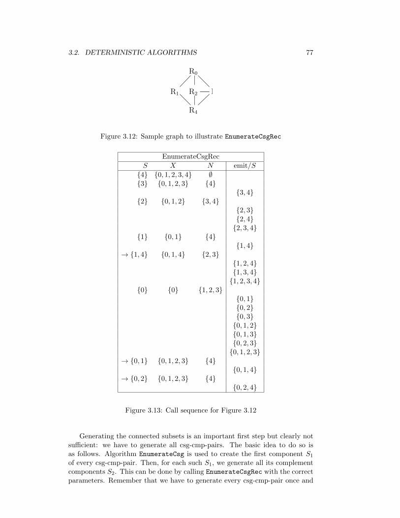
3.2. DETERMINISTIC ALGORITHMS 77

R0

R1 R2 R3

R4

Figure 3.12: Sample graph to illustrate EnumerateCsgRec

EnumerateCsgRec

S X N emit/S

4 0, 1, 2, 3, 4 ∅3 0, 1, 2, 3 4

3, 42 0, 1, 2 3, 4

2, 32, 42, 3, 4

1 0, 1 41, 4

→ 1, 4 0, 1, 4 2, 31, 2, 41, 3, 41, 2, 3, 4

0 0 1, 2, 30, 10, 20, 30, 1, 20, 1, 30, 2, 30, 1, 2, 3

→ 0, 1 0, 1, 2, 3 40, 1, 4

→ 0, 2 0, 1, 2, 3 40, 2, 4

Figure 3.13: Call sequence for Figure 3.12

Generating the connected subsets is an important first step but clearly notsufficient: we have to generate all csg-cmp-pairs. The basic idea to do so isas follows. Algorithm EnumerateCsg is used to create the first component S1

of every csg-cmp-pair. Then, for each such S1, we generate all its complementcomponents S2. This can be done by calling EnumerateCsgRec with the correctparameters. Remember that we have to generate every csg-cmp-pair once and

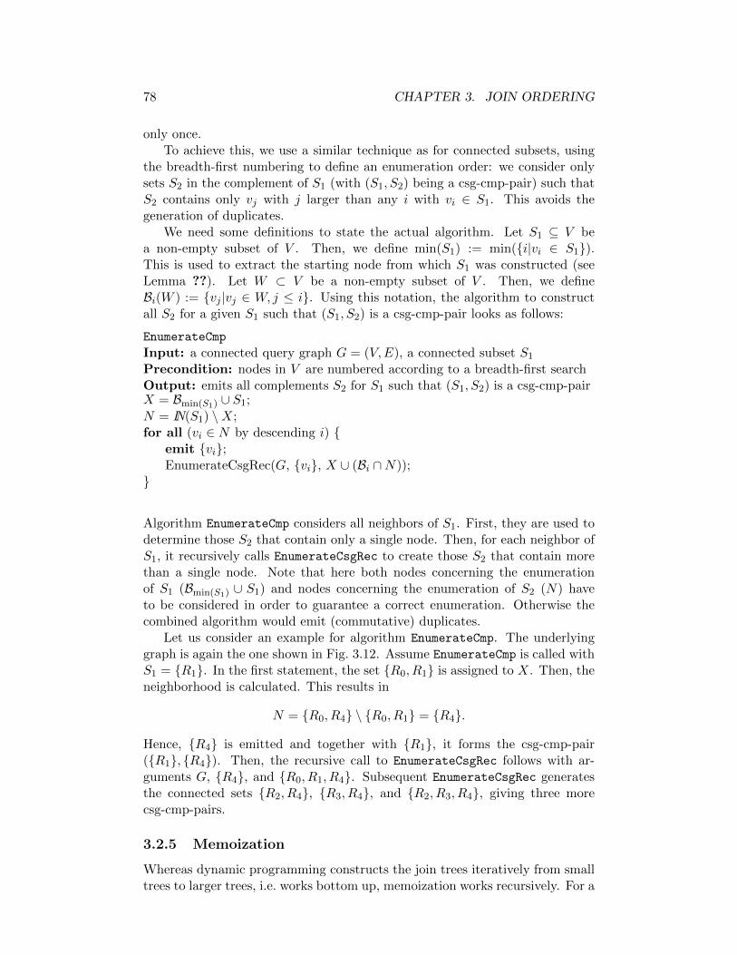
78 CHAPTER 3. JOIN ORDERING

only once.To achieve this, we use a similar technique as for connected subsets, using

the breadth-first numbering to define an enumeration order: we consider onlysets S2 in the complement of S1 (with (S1, S2) being a csg-cmp-pair) such thatS2 contains only vj with j larger than any i with vi ∈ S1. This avoids thegeneration of duplicates.

We need some definitions to state the actual algorithm. Let S1 ⊆ V bea non-empty subset of V . Then, we define min(S1) := min(i|vi ∈ S1).This is used to extract the starting node from which S1 was constructed (seeLemma ??). Let W ⊂ V be a non-empty subset of V . Then, we defineBi(W ) := vj |vj ∈ W, j ≤ i. Using this notation, the algorithm to constructall S2 for a given S1 such that (S1, S2) is a csg-cmp-pair looks as follows:

EnumerateCmp

Input: a connected query graph G = (V,E), a connected subset S1

Precondition: nodes in V are numbered according to a breadth-first searchOutput: emits all complements S2 for S1 such that (S1, S2) is a csg-cmp-pairX = Bmin(S1) ∪ S1;

N = IN(S1) \X;for all (vi ∈ N by descending i)

emit vi;EnumerateCsgRec(G, vi, X ∪ (Bi ∩N));

Algorithm EnumerateCmp considers all neighbors of S1. First, they are used todetermine those S2 that contain only a single node. Then, for each neighbor ofS1, it recursively calls EnumerateCsgRec to create those S2 that contain morethan a single node. Note that here both nodes concerning the enumerationof S1 (Bmin(S1) ∪ S1) and nodes concerning the enumeration of S2 (N) haveto be considered in order to guarantee a correct enumeration. Otherwise thecombined algorithm would emit (commutative) duplicates.

Let us consider an example for algorithm EnumerateCmp. The underlyinggraph is again the one shown in Fig. 3.12. Assume EnumerateCmp is called withS1 = R1. In the first statement, the set R0, R1 is assigned to X. Then, theneighborhood is calculated. This results in

N = R0, R4 \ R0, R1 = R4.

Hence, R4 is emitted and together with R1, it forms the csg-cmp-pair(R1, R4). Then, the recursive call to EnumerateCsgRec follows with ar-guments G, R4, and R0, R1, R4. Subsequent EnumerateCsgRec generatesthe connected sets R2, R4, R3, R4, and R2, R3, R4, giving three morecsg-cmp-pairs.

3.2.5 Memoization

Whereas dynamic programming constructs the join trees iteratively from smalltrees to larger trees, i.e. works bottom up, memoization works recursively. For a

3.2. DETERMINISTIC ALGORITHMS 79

given set of relations S, it produces the best join tree for S by recursively callingitself for every subset S1 of S and considering all join trees between S1 and itscomplement S2. The best alternative is memoized (hence the name). The rea-son is that two (even different) (sub-) sets of all relations may very well have thecommon subsets. For example, R1, R2, R3, R4, R5 and R2, R3, R4, R5, R6have the common subset R2, R3, R4, R5. In order to avoid duplicate work,memoization is essential.

In the following variant of memoization, we explore the search space of allbushy trees and consider cross products. We split the functionality across two EXfunctions. The first one initializes the BestTree data structure with singlerelation join trees for Ri and then calls the second one. The second one is thecore memoization procedure which calls itself recursively.

MemoizationJoinOrdering(R)Input: a set of relations ROutput: an optimal join tree for Rfor (i = 1; i <= n; ++i) BestTree(Ri) = Ri;

return MemoizationJoinOrderingSub(R);

MemoizationJoinOrderingSub(S)Input: a (sub-) set of relations SOutput: an optimal join tree for Sif(NULL == BestTree(S))

for all S1 ⊂ S do S2 = S \ S1;

CurrTree = CreateJoinTree(MemoizationJoinOrderingSub(S1), MemoizationJoinOrderingSub(S2));

if (BestTree(S) == NULL || cost(BestTree(S)) > cost(CurrTree)) BestTree(S) = CurrTree;

return BestTree(S);

Again, pruning techniques can help to speed up plan generation [770]. ToDo?

3.2.6 Join Ordering by Generating Permutations

For any set of cost functions, we can directly generate permutations. Gen-erating all permutations is clearly too expensive for more than a couple ofrelations. However, we can safely neglect some of them. Consider the joinsequence R1R2R3R4. If we know that R1R3R2 is cheaper than R1R2R3, wedo not have to consider R1R2R3R4. The idea of the following algorithm is toconstruct permutations by successively adding relations. Thereby, an extendedsequence is only explored if exchanging the last two relations does not result ina cheaper sequence.

80 CHAPTER 3. JOIN ORDERING

ConstructPermutations(Query Specification)

Input: query specification for relations R1, . . . , RnOutput: optimal left-deep tree

BestPermutation = NULL;

Prefix = ε;Rest = R1, . . . , Rn;ConstructPermutationsSub(Prefix, Rest);

return BestPermutation

ConstructPermutationsSub(Prefix, Rest)

Input: a prefix of a permutation and the relations to be added (Rest)

Ouput: none, side-effect on BestPermutation

if (Rest == ∅) if (BestPermutation == NULL || cost(Prefix) < cost(BestPermutation)) BestPermutation = Prefix;

return

foreach (Ri, Rj ∈ Rest)

if (cost(Prefix 〈Ri, Rj〉) ≤ cost(Prefix 〈Rj , Ri〉)) ConstructPermutationsSub(Prefix 〈Ri〉, Rest \ Ri);

if (cost(Prefix 〈Rj , Ri〉) ≤ cost(Prefix 〈Ri, Rj〉)) ConstructPermutationsSub(Prefix 〈Rj〉, Rest \ Rj);

return

The algorithm can be made more efficient, if the foreach loop considers onlya single relation and performs the swap test with this relation and the lastrelation occurring in Prefix.

The algorithm has two main advantages over dynamic programming andmemoization. The first advantage is that it needs only linear space opposedto exponential space for the two mentioned alternatives. The other mainadvantage over dynamic programming is that it generates join trees early,whereas with dynamic programming we only generate a plan after the wholesearch space has been explored. Thus, if the query contains too many joins—that is, the search space cannot be fully explored in reasonable time andspace—dynamic programming will not generate any plan at all. If stopped,ConstructPermutations will not necessarily compute the best plan, but stillsome plans have been investigated. This allows us to stop it after some timelimit has exceeded. The time limit itself can be fixed, like 100 ms, or variable,like 5% of the execution time of the best plan found so far.

The predicates in the if statement can be made more efficient if a (local)ranking function is available. Further speed-up of the algorithm can be achieved

3.2. DETERMINISTIC ALGORITHMS 81

if additionally the idea of memoization is applied (of course, this jeopardizesthe small memory footprint).

The following variant might be interesting if one is willing to go from linearspace consumption to quadratic space consumption. The original algorithmis then started n times, once for each relation as a starting relation. The ndifferent instantiations then have to run interleaved. This variant reduces thedependency on the starting relation.

Worst Case Analysis ToDo/EX

Pruning/memoization/propagation ToDo/EX

3.2.7 A Dynamic Programming based Heuristics for Chain Queries

In Section 3.1.6, we saw that the complexity of producing optimal left-deeptrees possibly containing cross products for chain queries is an open problem.However, the case does not seem to be hopeless. In fact, Scheufele and Mo-erkotte present two algorithms [737, 739] for this problem. For one algorithm,it can be proven that it has polynomial runtime, for the other, it can be proventhat it produces the optimal join tree. However, for none of them both couldbe proven so far.

Basic Definitions and Lemmata

An instance of the join-ordering problem for chain queries (or a chain queryfor short) is fully described by the following parameters. First, n relationsR1, . . . , Rn are given. The size of relation Ri (1 ≤ i ≤ n) is denoted by |Ri| ornRi . Second, the query graph G on the set of relations R1, . . . , Rn must be achain. That is, its edges are (Ri, Ri+1) | 1 ≤ i < n:

R1 — R2 — . . . — Rn

For every edge (Ri, Ri+1), there is an associated selectivity fi,i+1 = |Ri BRi+1|/|Ri × Ri+1|. We define all other selectivities fi,j = 1 for |i − j| 6= 1.They correspond to cross products.

In this section we consider only left-deep processing trees. However, weallow them to contain cross products. Hence, any permutation is a valid jointree. There is a unique correspondence not only between left-deep join treesbut also between consecutive parts of a permutation and segments of a left-deep tree. Furthermore, if a segment of a left-deep tree does not contain crossproducts, it uniquely corresponds to a consecutive part of the chain in the querygraph. In this case, we also speak of (sub)chains or connected (sub)sequences.We say that two relations Ri and Rj are connected if they are adjacent in G;more generally, two sequences s and t are connected if there exist relations Riin s and Rj in t such that Ri and Rj are connected. A sequence of relations sis connected if for all subsequences s1 and s2 satisfying s = s1s2 it holds thats1 is connected to s2.

Given a chain query, we ask for a permutation s = r1 . . . rn of the n relations(i.e. there is a permutation π such that ri = Rπ(i) for 1 ≤ i ≤ n) that producesminimal costs under the cost function Cout.

82 CHAPTER 3. JOIN ORDERING

Remember that the dynamic programming approach considers n2n−1−n(n+1)/2 alternatives for left-deep processing trees with cross products—independentlyof the query graph and the cost function. The question arises whether it is pos-sible to lower the complexity in case of simple chain queries.

The IKKBZ algorithm solves the join ordering problem for tree queries bydecomposing the problem into polynomially many subproblems which are sub-ject to tree-like precedence constraints. The precedence constraints ensure thatthe cost functions of the subproblems now have the ASI property. The remain-ing problem is to optimize the constrained subproblems under the simpler costfunction. Unfortunately, this approach does not work in our case, since no suchdecomposition seems to exist.

Let us introduce some notions used for the algorithms. We have to gener-alize the rank used in the IKKBZ algorithm to relativized ranks. We start byrelativizing the cost function. The costs of a sequence s relative to a sequenceu are defined as

Cu(ε) := 0

Cu(Ri) := 0 if u = ε

Cu(Ri) := (∏

Rj<uRiRi

fj,i)ni if u 6= ε

Cu(s1s2) := Cu(s1) + Tu(s1) ∗ Cus1(s2)

with

Tu(ε) := 1

Tu(s) :=∏

Ri∈s(∏

Rj<usRi

fj,i) ∗ ni

Here, Ri <s Rj is true if and only if Ri appears before Rj in s. As usual, emptyproducts evaluate to 1. Several things should be noted. First, Cus(t) = Cu(t)holds if there is no connection between relations in s and t. Second, Tε(Ri) =|Ri| and Tε(s) = |s|. That is, Tu generalizes the size of a single relation or of asequence of relations. Third, note that Cu(ε) = 0 for all u but Cε(s) = 0 onlyif s does not contain more than one relation. The special case that Cε(R) = 0for a single relation R causes some problems in the homogeneity of definitionsand proofs. Hence, we abandon this case from all definitions and lemmata ofthis section. This will not be repeated in every definition and lemma, but willimplicitly be assumed. Further, the two algorithms will be presented in twoversions. The first version is simpler and relies on a modified cost function C ′,and only the second version will apply to the original cost function C. As wewill see, C ′ differs from C in exactly the problematic case in which it is definedas C ′u(Ri) := |Ri|. Now, C ′ε(s) = 0 holds if and only if s = ε holds. Withinsubsequent definitions and lemmata, C can also be replaced by C ′ withoutchanging their validity. Last, we abbreviate Cε by C for convenience.

3.2. DETERMINISTIC ALGORITHMS 83

Example 1: Consider a chain query involving the relations R1, R2, R3. Theparameters are |R1| = 1, |R2| = 100, |R3| = 10 and f1,2 = f2,3 = 0.9. Theexpected size of the query result is independent of the ordering of the relations.Hence, we have

T (R1R2R3) = · · · = T (R3R2R1) = 100 ∗ 10 ∗ 1 ∗ .9 ∗ .9 = 810.

There are 6 possible orderings of the relations with the following costs:

C(R1R2R3) = 1 ∗ 100 ∗ 0.9 + 1 ∗ 100 ∗ 10 ∗ 0.9 ∗ 0.9 = 900C(R1R3R2) = 1 ∗ 10 + 1 ∗ 10 ∗ 100 ∗ 0.9 ∗ 0.9 = 820C(R2R3R1) = 100 ∗ 10 ∗ 0.9 + 100 ∗ 10 ∗ 1 ∗ 0.9 ∗ 0.9 = 1710C(R2R1R3) = C(R1R2R3)C(R3R1R2) = C(R1R3R2)C(R3R2R1) = C(R2R3R1)

Note that the cost function is invariant with respect to the order of the first tworelations. The minimum over all costs is 820, and the corresponding optimaljoin ordering is R1R3R2.

2

Using the relativized cost function, we can define the relativized rank.

Definition 3.2.8 (rank) The rank of a sequence s relative to a non-emptysequence u is given by

ranku(s) :=Tu(s)− 1

Cu(s)

In the special case that s consists of a single relation Ri, the intuition behindthe rank function becomes transparent. Let fi be the product of the selectivitiesbetween relations in u and Ri. Then ranku(Ri) = fi|Ri|−1

fi|Ri| . Hence, the rank

becomes a function of the form f(x) = x−1x . This function is monotonously

increasing in x for x > 0. The argument to the function f(x) is (for thecomputation of the size of a single relation Ri) fi|Ri|. But this is the factor bywhich the next intermediate result will increase (or decrease). Since we sum upintermediate results, this is an essential number. Furthermore, it follows fromthe monotonicity of f(x) that ranku(Ri) ≤ ranku(Rj) if and only if fi|Ri| ≤fj |Rj | where fj is the product of all selectivities between Rj and relations in u.

Example 1 (cont’d): Supposing the query given in Example 1, the optimalsequence R1R3R2 gives rise to the following ranks.

rankR1(R2) =TR1

(R2)−1

CR1(R2) = 100∗0.9−1

100∗0.9 ≈ 0.9888

rankR1(R3) =TR1

(R3)−1

CR1(R3) = 10∗1.0−1

10∗1.0 = 0.9

rankR1R3(R2) =TR1R3

(R2)−1

CR1R3(R2) = 100∗0.9∗0.9−1

100∗0.9∗0.9 ≈ 0.9877

Hence, within the optimal sequence, the relation with the smallest rank (hereR3, since rankR1(R3) < rankR1(R2)) is preferred. As the next lemma willshow, this is no accident.

84 CHAPTER 3. JOIN ORDERING

2

Using the rank function, the following lemma can be proved.

Lemma 3.2.9 For sequences

S = r1 · · · rk−1rkrk+1rk+2 · · · rnS′ = r1 · · · rk−1rk+1rkrk+2 · · · rn

the following holds:

C(S) ≤ C(S′)⇔ ranku(rk) ≤ ranku(rk+1)

where u = r1 · · · rk−1. Equality only holds if it holds on both sides.

Example 1 (cont’d): Since the ranks of the relations in Example 1 areordered with ascending ranks, Lemma 3.2.9 states that, whenever we exchangetwo adjacent relations, the costs cannot decrease. In fact, we observe thatC(R1R3R2) ≤ C(R1R2R3). 2

An analogous lemma still holds for two unconnected subchains:

Lemma 3.2.10 Let u, x and y be three subchains where x and y are not inter-connected. Then we have:

C(uxy) ≤ C(uyx)⇔ ranku(x) ≤ ranku(y)

Equality only holds if it holds on both sides.

Next, we define the notion of a contradictory chain, which will be essentialto the algorithms. The subsequent lemmata will allow us to cut down the searchspace to be explored by any optimization algorithm.

Definition 3.2.11 (contradictory pair of subchains) Let u, x, y be nonemp-ty sequences. We call (x, y) a contradictory pair of subchains if and only if

Cu(xy) ≤ Cu(yx) ∧ ranku(x) > rankux(y)

A special case occurs when x and y are single relations. Then the above condi-tion simplifies to

rankux(y) < ranku(x) ≤ ranku(y)

To explain the intuition behind the definition of contradictory subchains, weneed another example.

Example 2: Suppose a chain query involving R1, R2, R3 is given. The relationsizes are |R1| = 1, |R2| = |R3| = 10 and the selectivities are f1,2 = 0.5, f2,3 =0.2. Consider the sequences R1R2R3 and R1R3R2, which differ in the order ofthe last two relations. We have

rankR1(R2) = 0.8

rankR1R2(R3) = 0.0

rankR1(R3) = 0.9

rankR1R3(R2) = 0.5

3.2. DETERMINISTIC ALGORITHMS 85

and

C(R1R2R3) = 15

C(R1R3R2) = 20

Hence,

rankR1(R2) > rankR1R2(R3)

rankR1(R3) > rankR1R3(R2)

C(R1R2R3) < C(R1R3R2)

and (R2, R3) is a contradictory pair within R1R2R3. Now the use of the termcontradictory becomes clear: the costs do not behave as could be expected fromthe ranks. 2

The next (obvious) lemma states that contradictory chains are necessarilyconnected.

Lemma 3.2.12 If there is no connection between two subchains x and y, thenthey cannot build a contradictory pair (x, y).

Now we present the fact that between a contradictory pair of relations, therecannot be any other relation not connected to them without increasing cost.

Lemma 3.2.13 Let S = usvtw be a sequence. If there is no connection betweenrelations in s and v and relations in v and t, and ranku(s) ≥ rankus(t), thenthere exists a sequence S′ not having higher costs, where s immediately precedest.

Example 3: Consider five relations R1, . . . , R5. The relation sizes are |R1| =1, |R2| = |R3| = |R4| = 8, and |R5| = 2. The selectivities are f1,2 = 1

2 ,f2,3 = 1

4 , f3,4 = 18 , and f4,5 = 1

2 . Relation R5 is not connected to relations R2

and R3. Further, within the sequence R1R2R5R3R4 relations R2 and R3 havecontradictory ranks: rankR1(R2) = 4−1

4 = 34 and rankR1R2R5(R3) = 2−1

2 = 12 .

Hence, at least one of R1R5R2R3R4 and R1R2R3R5R4 must be of no greatercost than R1R2R5R3R4. This is indeed the case:

C(R1R2R3R5R4) = 4 + 8 + 16 + 8 = 36C(R1R2R5R3R4) = 4 + 8 + 16 + 8 = 36C(R1R5R2R3R4) = 2 + 8 + 16 + 8 = 34

2

The next lemma shows that, if there exist two sequences of single rank-sorted relations, then their costs as well as their ranks are necessarily equal.

Lemma 3.2.14 Let S = x1 · · ·xn and S′ = y1 · · · yn be two different rank-sorted chains containing exactly the relations R1, . . . , Rn, i.e.

rankx1···xi−1(xi) ≤ rankx1···xi(xi+1) for all 1 ≤ i ≤ n,ranky1···yi−1(yi) ≤ ranky1···yi(yi+1) for all 1 ≤ i ≤ n,

86 CHAPTER 3. JOIN ORDERING

then S and S′ have equal costs and, furthermore,

rankx1···xi−1(xi) = ranky1···yi−1(yi) for all 1 < i ≤ n

One could conjecture that the following generalization of Lemma 3.2.14 istrue, although no one has proved it so far.

Conjecture 3.2.1 Let S = x1 · · ·xn and S′ = y1 · · · ym be two different rank-sorted chains for the relations R1 . . . , Rn where the x′is and y′is are subsequencessuch that

rankx1···xi−1(xi) ≤ rankx1···xi(xi+1) for all 1 ≤ i < n,

ranky1···yi−1(yi) ≤ ranky1···yi(yi+1) for all 1 ≤ i < m,

and the subsequences xi and yj are all optimal (with respect to the fixed prefixesx1 . . . xi−1 and y1 . . . yj−1), then S and S′ have equal costs.

Consider the problem of merging two optimal unconnected chains. If weknew that the ranks of relations in an optimal chain are always sorted in as-cending order, we could use the classical merge procedure to combine the twochains. The resulting chain would also be rank-sorted in ascending order and,according to Lemma 3.2.14, it would be optimal. Unfortunately, this does notwork, since there are optimal chains whose ranks are not sorted in ascendingorder: those containing sequences with contradictory ranks.

Now, as shown in Lemma 3.2.13, between contradictory pairs of relationsthere cannot be any other relation not connected to them. Hence, in the mergingprocess, we have to take care that we do not merge a contradictory pair ofrelations with a relation not connected to the pair. In order to achieve this,we apply the same trick as in the IKKBZ algorithm: we tie the relations of acontradictory subchain together by building a compound relation. Assume thatwe tie together the relations r1, . . . , rn to a new relation r1,...,n. Then we definethe size of r1,...,n as |r1,...,n| = |r1 B . . . B rn| Further, if some ri (1 ≤ i ≤ n)does have a connection to some rk 6∈ r1, . . . , rn then we define the selectivityfactor fr1,...,n,rk between rk and r1,...,n as fr1,...,n,rk = fi,k.

If we tie together contradictory pairs, the resulting chain of compound re-lations still does not have to be rank-sorted with respect to the compoundrelations. To overcome this, we iterate the process of tying contradictory pairsof compound relations together until the sequence of compound relations isrank-sorted, which will eventually be the case. That is, we apply the normal-ization as used in the IKKBZ algorithm. However, we have to reformulate itfor relativized costs and ranks:

Normalize(p,s)while (there exist subsequences u, v (u 6= ε) and

compound relations x, y such that s = uxyvand Cpu(xy) ≤ Cpu(yx)and rankpu(x) > rankpux(y))

3.2. DETERMINISTIC ALGORITHMS 87

replace xy by a compound relation (x, y);return (p, s);

The compound relations in the result of the procedure Normalize are calledcontradictory chains. A maximal contradictory subchain is a contradictory sub-chain that cannot be made longer by further tying steps. Resolving the tyingsintroduced in the procedure normalize is called de-normalization. It works thesame way as in the IKKBZ algorithm. The cost, size and rank functions cannow be extended to sequences containing compound relations in a straightfor-ward way. We define the cost of a sequence containing compound relations tobe identical with the cost of the corresponding de-normalized sequence. Thesize and rank functions are defined analogously.

The following simple observation is central to the algorithms: every chaincan be decomposed into a sequence of adjacent maximal contradictory sub-chains. For convenience, we often speak of chains instead of subchains and ofcontradictory chains instead of maximal contradictory subchains. The mean-ing should be clear from the context. Further, we note that the decomposi-tion into adjacent maximal contradictory subchains is not unique. For exam-ple, consider an optimal subchain r1r2r3 and a sequence u of preceding rela-tions. If ranku(r1) > rankur1(r2) > rankur1r2(r3) one can easily show thatboth (r1, (r2, r3)) and ((r1, r2), r3) are contradictory subchains. Nevertheless,this ambiguity is not important since in the following we are only interest-ed in contradictory subchains which are optimal . In this case, the conditionCu(xy) ≤ Cu(yx) is certainly true and can therefore be neglected. One canshow that for the case of optimal subchains the indeterministically defined nor-malization process is well-defined, that is, if S is optimal, normalize(P,S) willalways terminate with a unique “flat” decomposition of S into maximal contra-dictory subchains (flat means that we remove all but the outermost parenthesis,e.g. (R1R2)(((R5R4)R3)R6) becomes (R1R2)(R5R4R3R6)).

The next two lemmata and the conjecture show a possible way to overcomethe problem that if we consider cross products, we have an unconstrained or-dering problem and the idea of Monma and Sidney as exploited in the IKKBZalgorithm is no longer applicable. The next lemma is a direct consequence ofthe normalization procedure.

Lemma 3.2.15 Let S = s1 . . . sm be an optimal chain consisting of the maxi-mal contradictory subchains s1, . . . , sm (as determined by the function normalize).Then

rank(s1) ≤ ranks1(s2) ≤ ranks1s2(s3)

≤ · · · ≤ ranks1...sm−1(sm),

in other words, the (maximal) contradictory subchains in an optimal chain arealways sorted by ascending ranks.

The next result shows how to build an optimal sequence from two optimalnon-interconnected sequences.

88 CHAPTER 3. JOIN ORDERING

Lemma 3.2.16 Let x and y be two optimal sequences of relations where x andy are not interconnected. Then the sequence obtained by merging the maximalcontradictory subchains in x and y (as obtained by normalize) according totheir ascending rank is optimal.

Merging two sequences in the way described in Lemma 3.2.16 is a funda-mental process. We henceforth refer to it by simply saying that we merge bythe ranks.

We strongly conjecture that the following generalization of Lemma 3.2.14is true, although it is yet unproven. It uses the notion of optimal recursivedecomposable subchains defined in the next subsection.

Conjecture 3.2.2 Consider two sequences S and T containing exactly the re-lations R1,. . . ,Rn. Let S = s1 . . . sk and T = t1 . . . tl be such that each of themaximal contradictory subchains si, i = 1, . . . , k and tj , j = 1, . . . , l are optimalrecursively decomposable. Then S and T have equal costs.

The first algorithm

We first use a slightly modified cost function C ′, which additionally respectsthe size of the first relation in the sequence, i.e. C and C ′ relate via

C ′u(s) =

C(s) + |nR|, if u = ε and s = Rs′

Cu(s), otherwise

This cost function can be treated in a more elegant way than C. The new rankfunction is now defined as ranku(s) := (Tu(s) − 1)/C ′u(s). Note that the rankfunction is now defined even if u = ε and s is a single relation. The size functionremains unchanged. At the end of this subsection, we describe how our resultscan be adapted to the original cost function C.

The rank of a contradictory chain depends on the relative position of therelations that are directly connected to it. For example, the rank of the con-tradictory subchain (R5R3R4R2) depends on the position of the neighbouringrelations R1 and R6 relative to (R5R3R4R2). That is, whether they appear be-fore or after the sequence (R5R3R4R2). Therefore, we introduce the followingfundamental definitions:

Definition 3.2.17 (neighbourhood) We call the set of relations that are di-rectly connected to a subchain (with respect to the query graph G) the completeneighbourhood of that subchain. A neighbourhood is a subset of the completeneighbourhood. The complement of a neighbourhood u of a subchain s is definedas v \ u, where v denotes the complete neighbourhood of s.

Note that the neighbourhood of a subchain s within a larger chain us is unique-ly determined by the subsequence u of relations preceding it. For convenience,we will often use sequences of preceding relations to specify neighbourhoods.We henceforth denote a pair consisting of a connected sequence s and a neigh-bourhood u by [s]u.

3.2. DETERMINISTIC ALGORITHMS 89

Definition 3.2.18 (contradictory subchain, extent) A contradictory sub-chain [s]u is inductively defined as follows.

1. For a single relation s, [s]u is a contradictory subchain.

2. There is a decomposition s = vw such that (v, w) is a contradictory pairwith respect to the preceding subsequence u and both [v]u and [w]uv arecontradictory subchains themselves.

The extent of a contradictory chain [s]u is defined as the pair consisting ofthe neighbourhood u and the set of relations occurring in s. Since contradicto-ry subchains are connected, the set of occurring relations has always the formRi, Ri+1, . . . , Ri+l for some 1 ≤ i ≤ n, 0 ≤ l ≤ n − i. An optimal contra-dictory subchain to a given extent is a contradictory subchain with lowest costamong all contradictory subchains of the same extent.

The number of different extents of contradictory subchains for a chain queryof n relations is 2n2 − 2n + 1. Each contradictory chain can be completelyrecursively decomposed into adjacent pairs of connected subchains. Subchainswith this property are defined next (similar types of decompositions occur in[418, 771]).

Definition 3.2.19 ((optimal) recursively decomposable subchain) A re-cursively decomposable subchain [s]u is inductively defined as follows.

1. If s is a single relation, then [s]u is recursively decomposable.

2. There is a decomposition s = vw such that v is connected to w and both[v]u and [w]uv are recursively decomposable subchains.

The extent of a recursively decomposable chain is defined in the same way asfor contradictory chains. Note that every contradictory subchain is recursivelydecomposable. Consequently, the set of all contradictory subchains for a certainextent is a subset of all recursively decomposable subchains of the same extent.

Example 4: Consider the sequence of relations

s = R2R4R3R6R5R1.

Using parentheses to indicate the recursive decompositions, we have the follow-ing two possibilities

(((R2(R4R3))(R6R5))R1)

((R2((R4R3)(R6R5)))R1)

The extent of the recursively decomposable subchainR4R3R6R5 of s is (R2, R3, R4, R5, R6). 2

The number of different recursively decomposable chains involving the rela-tions R1, . . . , Rn is rn, where rn denotes the n-th Schroder number [771]. Hence,

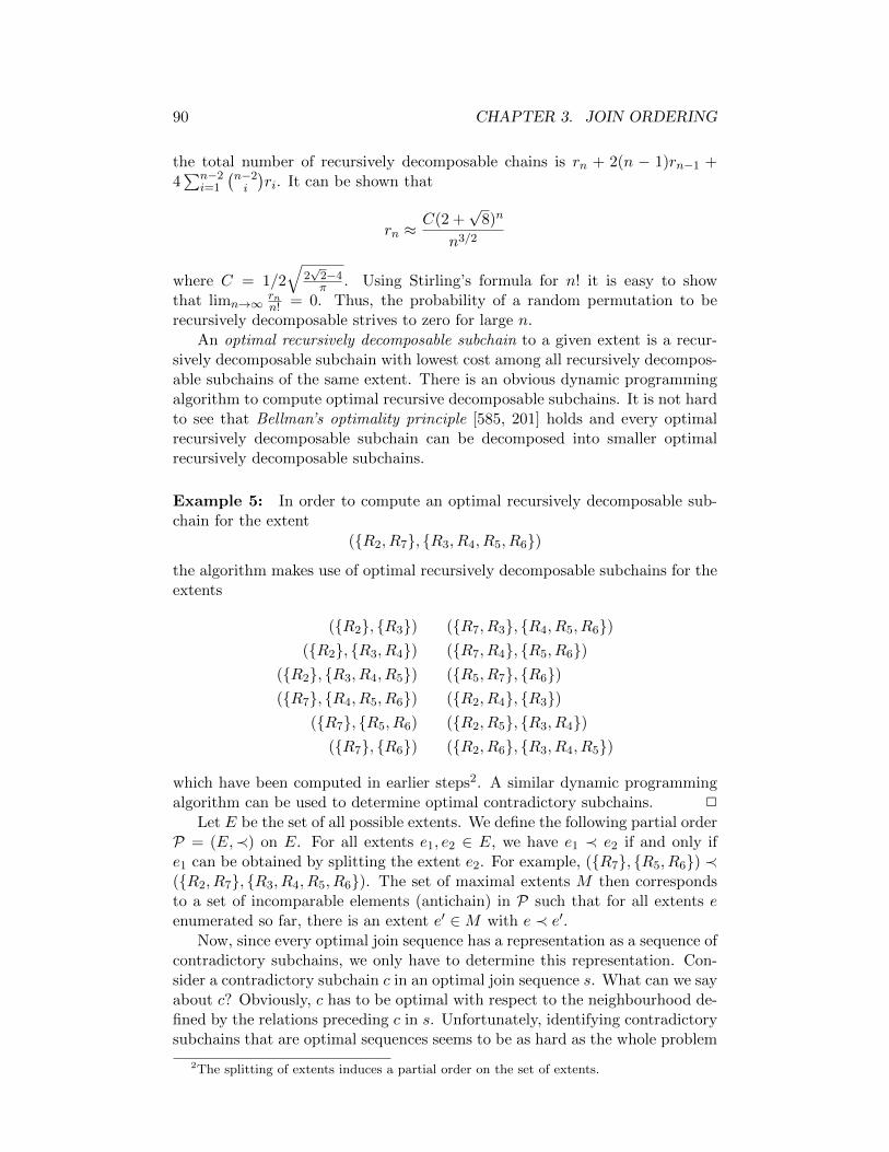
90 CHAPTER 3. JOIN ORDERING

the total number of recursively decomposable chains is rn + 2(n − 1)rn−1 +4∑n−2

i=1

(n−2i

)ri. It can be shown that

rn ≈C(2 +

√8)n

n3/2

where C = 1/2

√2√

2−4π . Using Stirling’s formula for n! it is easy to show

that limn→∞ rnn! = 0. Thus, the probability of a random permutation to be

recursively decomposable strives to zero for large n.

An optimal recursively decomposable subchain to a given extent is a recur-sively decomposable subchain with lowest cost among all recursively decompos-able subchains of the same extent. There is an obvious dynamic programmingalgorithm to compute optimal recursive decomposable subchains. It is not hardto see that Bellman’s optimality principle [585, 201] holds and every optimalrecursively decomposable subchain can be decomposed into smaller optimalrecursively decomposable subchains.

Example 5: In order to compute an optimal recursively decomposable sub-chain for the extent

(R2, R7, R3, R4, R5, R6)the algorithm makes use of optimal recursively decomposable subchains for theextents

(R2, R3) (R7, R3, R4, R5, R6)(R2, R3, R4) (R7, R4, R5, R6)

(R2, R3, R4, R5) (R5, R7, R6)(R7, R4, R5, R6) (R2, R4, R3)

(R7, R5, R6) (R2, R5, R3, R4)(R7, R6) (R2, R6, R3, R4, R5)

which have been computed in earlier steps2. A similar dynamic programmingalgorithm can be used to determine optimal contradictory subchains. 2

Let E be the set of all possible extents. We define the following partial orderP = (E,≺) on E. For all extents e1, e2 ∈ E, we have e1 ≺ e2 if and only ife1 can be obtained by splitting the extent e2. For example, (R7, R5, R6) ≺(R2, R7, R3, R4, R5, R6). The set of maximal extents M then correspondsto a set of incomparable elements (antichain) in P such that for all extents eenumerated so far, there is an extent e′ ∈M with e ≺ e′.

Now, since every optimal join sequence has a representation as a sequence ofcontradictory subchains, we only have to determine this representation. Con-sider a contradictory subchain c in an optimal join sequence s. What can we sayabout c? Obviously, c has to be optimal with respect to the neighbourhood de-fined by the relations preceding c in s. Unfortunately, identifying contradictorysubchains that are optimal sequences seems to be as hard as the whole problem

2The splitting of extents induces a partial order on the set of extents.

3.2. DETERMINISTIC ALGORITHMS 91

of optimizing chain queries. Therefore, we content ourselves with the followingweaker condition which may lead to multiple representations. Nevertheless, itseems to be the strongest condition for which all subchains satisfying the con-dition can be computed in polynomial time. The condition says that s shouldbe optimal both with respect to all contradictory chains of the same extent as sand with respect to all recursively decomposable subchains of the same extent.So far it is not clear whether these conditions lead to multiple representations.Therefore, we have no choice but to enumerate all possible representations andselect the one with minimal costs. Next we describe the first algorithm.

Algorithm Chain-I’:

1. Use dynamic programming to determine all optimal contradictory sub-chains.This step can be made faster by keeping track of the set M of all maximalextents (with respect to the partial order induced by splitting extents).

2. Determine all optimal recursively decomposable subchains for all extentsincluded in some maximal extent in M .

3. Compare the results from steps 1 and 2 and retain only matching sub-chains.

4. Sort the contradictory subchains according to their ranks.5. Eliminate contradictory subchains that cannot be part of a solution.6. Use backtracking to enumerate all sequences of rank-ordered optimal con-

tradictory subchains and keep track of the sequence with lowest cost.

In step 5 of the algorithm, we eliminate contradictory subchains that do notcontribute to a solution. Note that the contradictory subchains in an optimalsequence are characterized by the following two conditions.

1. The extents of all contradictory subchains in the representation build apartition of the set of all relations.

2. The neighbourhoods of all contradictory subchains are consistent with therelations occurring at earlier and later positions in the sequence.

Note that any contradictory subchain occurring in the optimal sequence (exceptat the first and last positions) necessarily has matching contradictory subchainspreceding and succeeding it in the list. In fact, every contradictory subchain Xoccurring in the optimal join sequence must satisfy the following two conditions.

1. For every relation R in the neighbourhood of X, there exists a contra-dictory subchain Y at an earlier position in the list which itself meetscondition 1, such that R occurs in Y , and Y can be followed by X.

2. For every relation R in the complementary neighbourhood of X, thereexists a contradictory subchain Y at a later position in the list whichitself meets condition 2, such that R occurs in the neighbourhood of Y ,and X can be followed by Y .

Using these two conditions, we can eliminate “useless” contradictory chainsfrom the rank-ordered list by performing a reachability algorithm for each of

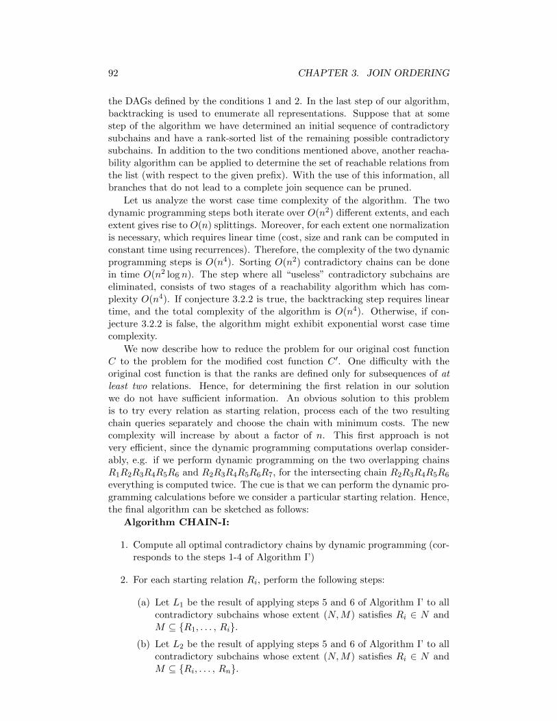
92 CHAPTER 3. JOIN ORDERING

the DAGs defined by the conditions 1 and 2. In the last step of our algorithm,backtracking is used to enumerate all representations. Suppose that at somestep of the algorithm we have determined an initial sequence of contradictorysubchains and have a rank-sorted list of the remaining possible contradictorysubchains. In addition to the two conditions mentioned above, another reacha-bility algorithm can be applied to determine the set of reachable relations fromthe list (with respect to the given prefix). With the use of this information, allbranches that do not lead to a complete join sequence can be pruned.

Let us analyze the worst case time complexity of the algorithm. The twodynamic programming steps both iterate over O(n2) different extents, and eachextent gives rise to O(n) splittings. Moreover, for each extent one normalizationis necessary, which requires linear time (cost, size and rank can be computed inconstant time using recurrences). Therefore, the complexity of the two dynamicprogramming steps is O(n4). Sorting O(n2) contradictory chains can be donein time O(n2 log n). The step where all “useless” contradictory subchains areeliminated, consists of two stages of a reachability algorithm which has com-plexity O(n4). If conjecture 3.2.2 is true, the backtracking step requires lineartime, and the total complexity of the algorithm is O(n4). Otherwise, if con-jecture 3.2.2 is false, the algorithm might exhibit exponential worst case timecomplexity.

We now describe how to reduce the problem for our original cost functionC to the problem for the modified cost function C ′. One difficulty with theoriginal cost function is that the ranks are defined only for subsequences of atleast two relations. Hence, for determining the first relation in our solutionwe do not have sufficient information. An obvious solution to this problemis to try every relation as starting relation, process each of the two resultingchain queries separately and choose the chain with minimum costs. The newcomplexity will increase by about a factor of n. This first approach is notvery efficient, since the dynamic programming computations overlap consider-ably, e.g. if we perform dynamic programming on the two overlapping chainsR1R2R3R4R5R6 and R2R3R4R5R6R7, for the intersecting chain R2R3R4R5R6

everything is computed twice. The cue is that we can perform the dynamic pro-gramming calculations before we consider a particular starting relation. Hence,the final algorithm can be sketched as follows:

Algorithm CHAIN-I:

1. Compute all optimal contradictory chains by dynamic programming (cor-responds to the steps 1-4 of Algorithm I’)

2. For each starting relation Ri, perform the following steps:

(a) Let L1 be the result of applying steps 5 and 6 of Algorithm I’ to allcontradictory subchains whose extent (N,M) satisfies Ri ∈ N andM ⊆ R1, . . . , Ri.

(b) Let L2 be the result of applying steps 5 and 6 of Algorithm I’ to allcontradictory subchains whose extent (N,M) satisfies Ri ∈ N andM ⊆ Ri, . . . , Rn.

3.2. DETERMINISTIC ALGORITHMS 93

(c) For all (l1, l2) ∈ L1 × L2, perform the following steps:

i. Let L be the result of merging l1 and l2 according to their ranks.

ii. Use RiL to update the current-best join ordering.

Suppose that conjecture 3.2.2 is true, and we can replace the backtracking partby a search for the first solution. Then the complexity of the step 1 is O(n4),whereas the complexity of step 2 amounts to

∑ni=1(O(i2)+O(n− i)2 +O(n)) =

O(n3). Hence, the total complexity would be O(n4) in the worst case. Ofcourse, if our conjecture is false, the necessary backtracking step might lead toan exponential worst case complexity.

The second algorithm

The second algorithm is much simpler than the first one but proves to be lessefficient in practice. Since the new algorithm is very similar to some parts ofthe old one, we just point out the differences between both algorithms. Thenew version of the algorithm works as follows.

Algorithm CHAIN-II’:

1. Use dynamic programming to compute an optimal recursive decomposablechain for the whole set of relations R1, . . . , Rn.

2. Normalize the resulting chain.

3. Reorder the contradictory subchains according to their ranks.

4. De-normalize the sequence.

Step 1 is identical to step 2 of our first algorithm. Note that Lemma 3.2.15cannot be applied to the sequence in Step 2, since an optimal recursive de-composable chain is not necessarily an optimal chain. Therefore, the questionarises whether Step 3 really makes sense. One can show that the partial orderdefined by the precedence relation among the contradictory subchains has theproperty that all elements along paths in the partial order are sorted by rank.By computing a greedy topological ordering (greedy with respect to the ranks),we obtain a sequence as requested in step 3.

Let us briefly analyze the worst case time complexity of the second algo-rithm. The first step requires time O(n4), whereas the second step requires timeO(n2). The third step has complexity O(n log n). Hence, the total complexityis O(n4).

Algorithm II’ is based on the cost function C ′. We can now modify thealgorithm for the original cost function C as follows.

Algorithm CHAIN-II:

1. Compute all optimal recursive decomposable chains by dynamic program-ming (corresponds to step 1 of Algorithm II’)

2. For each starting relation Ri, perform the following steps:

94 CHAPTER 3. JOIN ORDERING

(a) Let L1 be the result of applying the steps 2 and 3 of Algorithm II’ toall optimal recursive decomposable subchains whose extent (N,M)satisfies Ri ∈ N and M ⊆ R1, . . . , Ri.

(b) Let L2 be the result of applying the steps 2 and 3 of Algorithm II’ toall optimal recursive decomposable subchains whose extent (N,M)satisfies Ri N and M ⊆ Ri, . . . , Rn.

(c) Let L be the result of merging L1 and L2 according to their ranks.

(d) De-normalize L.

(e) Use RiL to update the current-best join ordering.

The complexity of Step 1 isO(n4), whereas the complexity of Step 2 amountsto∑n

i=1(O(i2) + O(n − i)2 + O(n)) = O(n3). Hence, the time complexity ofAlgorithm II is O(n4).

Summarizing, we are now left with one algorithm that produces the optimalresult but whose worst-case runtime behavior is unknown and one algorithmwith polynomial runtime but producing a result which has not been proven tobe optimal. Due to this lack of hard facts, Moerkotte and Scheufele ran about700,000 experiments with random queries of sizes up to 30 relations and fewerexperiments for random queries with up to 300 relations to compare the resultsof our algorithms. For n ≤ 15, they additionally compared the results with astandard dynamic programming algorithm. Their findings can be summarizedas follows.

• All algorithms yielded identical results.

• Backtracking always led to exactly one sequence of contradictory chains.

• In the overwhelming majority of cases the first algorithm proved to befaster than the second.

Whereas the run time of the second algorithm is mainly determined by thenumber of relations in the query, the run time of the first also heavily dependson the number of existing optimal contradictory subchains. In the worst case,the first algorithm is slightly inferior to the second. Additionally, Hamalainenreports on an independent implementation of the second algorithm [380]. Hecould not find an example where the second algorithm did not produce theoptimal result either. We encourage the reader to prove that it produces theoptimal result.EX

3.2.8 Transformation-Based Approaches

The idea of transformation-based algorithms can be described as follows. Start-ing from an arbitrary join tree, equivalences (such as commutativity and asso-ciativity) are applied to it to derive a set of new join trees. For each of thejoin trees, the equivalences are again applied to derive even more join trees.This procedure is repeated until no new join tree can be derived. This proce-dure exhaustively enumerates the set of all bushy trees. Furthermore, before an

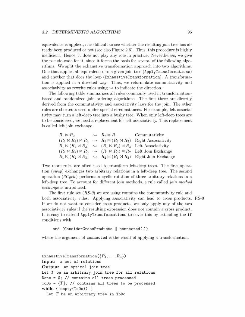
3.2. DETERMINISTIC ALGORITHMS 95

equivalence is applied, it is difficult to see whether the resulting join tree has al-ready been produced or not (see also Figure 2.6). Thus, this procedure is highlyinefficient. Hence, it does not play any role in practice. Nevertheless, we givethe pseudo-code for it, since it forms the basis for several of the following algo-rithms. We split the exhaustive transformation approach into two algorithms.One that applies all equivalences to a given join tree (ApplyTransformations)and another that does the loop (ExhaustiveTransformation). A transforma-tion is applied in a directed way. Thus, we reformulate commutativity andassociativity as rewrite rules using ; to indicate the direction.

The following table summarizes all rules commonly used in transformation-based and randomized join ordering algorithms. The first three are directlyderived from the commutativity and associativity laws for the join. The otherrules are shortcuts used under special circumstances. For example, left associa-tivity may turn a left-deep tree into a bushy tree. When only left-deep trees areto be considered, we need a replacement for left associativity. This replacementis called left join exchange.

R1 BR2 ; R2 BR1 Commutativity(R1 BR2) BR3 ; R1 B (R2 BR3) Right AssociativityR1 B (R2 BR3) ; (R1 BR2) BR3 Left Associativity(R1 BR2) BR3 ; (R1 BR3) BR2 Left Join ExchangeR1 B (R2 BR3) ; R2 B (R1 BR3) Right Join Exchange

Two more rules are often used to transform left-deep trees. The first opera-tion (swap) exchanges two arbitrary relations in a left-deep tree. The secondoperation (3Cycle) performs a cyclic rotation of three arbitrary relations in aleft-deep tree. To account for different join methods, a rule called join methodexchange is introduced.

The first rule set (RS-0) we are using contains the commutativity rule andboth associativity rules. Applying associativity can lead to cross products. RS-0If we do not want to consider cross products, we only apply any of the twoassociativity rules if the resulting expression does not contain a cross product.It is easy to extend ApplyTransformations to cover this by extending the if

conditions with

and (ConsiderCrossProducts || connected(·))

where the argument of connected is the result of applying a transformation.

ExhaustiveTransformation(R1, . . . , Rn)Input: a set of relations

Output: an optimal join tree

Let T be an arbitrary join tree for all relations

Done = ∅; // contains all trees processed

ToDo = T; // contains all trees to be processed

while (!empty(ToDo)) Let T be an arbitrary tree in ToDo

96 CHAPTER 3. JOIN ORDERING

ToDo \ = T;Done ∪ = T;Trees = ApplyTransformations(T);for all T ∈ Trees do

if (T 6∈ ToDo ∪ Done) ToDo + = T;

return cheapest tree found in Done;

ApplyTransformations(T)Input: join tree

Output: all trees derivable by associativity and commutativity

Trees = ∅;Subtrees = all subtrees of T rooted at inner nodes

for all S ∈ Subtrees do if (S is of the form S1 B S2) Trees + = S2 B S1;

if (S is of the form (S1 B S2) B S3) Trees + = S1 B (S2 B S3);

if (S is of the form S1 B (S2 B S3)) Trees + = (S1 B S2) B S3;

return Trees;

Besides the problems mentioned above, this algorithm also has the problemthat the sharing of subtrees is a non-trivial task. In fact, we assume thatApplyTransformations produces modified copies of T . To see how ExhaustiveTransformation

works, consider again Figure 2.6. Assume that the top-left join tree is the initialjoin tree. Then, from this join tree ApplyTransformations produces all treesreachable by some edge. All of these are then added to ToDo. The next callto ApplyTransformations with any to the produced join trees will have theinitial join tree contained in Trees. The complete set of visited join trees afterthis step is determined from the initial join tree by following at most two edges.

Let us reformulate the algorithm such that it uses a data structure similarto dynamic programming or memoization in order to avoid duplicate work. Forany subset of relations, dynamic programming remembers the best join tree.This does not quite suffice for the transformation-based approach. Instead, wehave to keep all join trees generated so far including those differing in the orderof the arguments or a join operator. However, subtrees can be shared. Thisis done by keeping pointers into the data structure (see below). So, the dif-ference between dynamic programming and the transformation-based approachbecomes smaller. The main remaining difference is that dynamic programming

3.2. DETERMINISTIC ALGORITHMS 97

only considers these join trees while with the transformation-based approachwe have to keep the considered join trees since other join trees (more beneficial)might be generatable from them.

The data structure used for remembering trees is often called the MEMOstructure. For every subset of relations to be joined (except the empty set), aclass exists in the MEMO structure. Each class contains all the join trees thatjoin exactly the relations describing the class. Here is an example for join treescontaining three relations.

R1, R2, R3 R1, R2BR3, R3 B R1, R2,R1, R3BR2, R2 B R1, R3,R2, R3BR1, R1 B R2, R3

R2, R3 R2B R3, R3B R2R1, R3 R1B R3, R3B R1R1, R2 R1B R2, R2B R1R3 R3

R2 R2

R1 R1

Here, we used the set notation . . . as an argument to a join to denote areference to the class of join trees joining the relations contained in it.

We reformulate our transformation-based algorithm such that it fills in anduses the MEMO structure [655]. In a first step, the MEMO structure is ini-tialized by creating an arbitrary join tree for the class R1, . . . , Rn and thengoing down this join tree and creating an entry for every join encountered.Then, we call ExploreClass on the root class comprising all relations to bejoined. ExploreClass then applies ApplyTransformations2 to every memberof the class it is called upon. ApplyTransformations2 then applies all rules togenerate alternatives.

ExhaustiveTransformation2(Query Graph G)Input: a query specification for relations R1, . . . , Rn.Output: an optimal join tree

initialize MEMO structure

ExploreClass(R1, . . . , Rn)return best of class R1, . . . , Rn

ExploreClass(C)

Input: a class C ⊆ R1, . . . , RnOutput: none, but has side-effect on MEMO-structure

while (not all join trees in C have been explored) choose an unexplored join tree T in CApplyTransformation2(T)mark T as explored

98 CHAPTER 3. JOIN ORDERING

return

ApplyTransformations2(T)Input: a join tree of a class COutput: none, but has side-effect on MEMO-structure

ExploreClass(left-child(T));ExploreClass(right-child(T));foreach transformation T and class member of child classes

foreach T ′ resulting from applying T to T if T ′ not in MEMO structure add T ′ to class C of MEMO structure

return

ApplyTransformations2 uses a set of transformations to be applied. We dis-cuss now the effect of different transformation sets on the complexity of thealgorithm. Applying ExhaustiveTransformation2 with a rule set consistingof Commutativity and Left and Right Associativity generates 4n−3n+1+2n+2−n − 2 duplicates for n relations. Contrast this with the number of join treescontained in a completely filled MEMO structure3: 3n − 2n+1 + n + 1. Thisclearly shows the problem.

The problem of generating the same join tree several times was consideredby Pellenkoft, Galindo-Legaria, and Kersten [655, 656, 657]. The solution lies inparameterizing ExhaustiveTransformation2 by an appropriate set of transfor-mations. The basic idea is to remember for every join operator which rules areapplicable to it. For example, after applying commutativity to a join operator,we disable commutativity for it.

For acyclic queries, the following rule set guarantees that all bushy jointrees are generated, but no duplicates [657]. Thereby, cross products are notconsidered. That is, a rule is only applicable if it does not result in a crossproduct. This restricts the applicability of the above algorithm to connectedqueries. We use Ci to denote some class of the MEMO structure. We call thefollowing rule set RS-1:RS-1

T1: Commutativity C1 B0 C2 ; C2 B1 C1

Disable all transformations T1, T2, and T3 for B1.

T2: Right Associativity (C1 B0 C2) B1 C3 ; C1 B2 (C2 B3 C3)Disable transformations T2 and T3 for B2 and enable all rules for B3.

T3: Left associativity C1 B0 (C2 B1 C3) ; (C1 B2 C2) B3 C3

Disable transformations T2 and T3 for B3 and enable all rules for B2.

3The difference to the according number for dynamic programming is due to the fact thatwe have to keep alternatives generated by commutativity and that join trees for single relationsare counted.

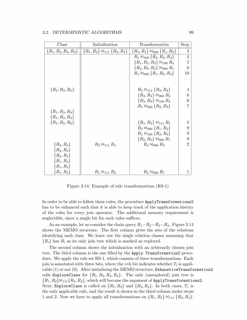
3.2. DETERMINISTIC ALGORITHMS 99

Class Initialization Transformation Step

R1, R2, R3, R4 R1, R2B111 R3, R4 R3, R4B000 R1, R2 3

R1 B100 R2, R3, R4 4R1, R2, R3B100 R4 5R2, R3, R4B000 R1 8R4 B000 R1, R2, R3 10

R2, R3, R4 R2 B111 R3, R4 4R3, R4B000 R2 6R2, R3B100 R4 6R4 B000 R2, R3 7

R1, R3, R4R1, R2, R4R1, R2, R3 R1, R2B111 R3 5

R3 B000 R1, R2 9R1 B100 R2, R3 9R2, R3B000 R1 9

R3, R4 R3 B111 R4 R4 B000 R3 2R2, R4R2, R3R1, R4R1, R3R1, R2 R1 B111 R2 R2 B000 R1 1

Figure 3.14: Example of rule transformations (RS-1)

In order to be able to follow these rules, the procedure ApplyTransformations2has to be enhanced such that it is able to keep track of the application historyof the rules for every join operator. The additional memory requirement isneglectible, since a single bit for each rules suffices.

As an example, let us consider the chain query R1−R2−R3−R4. Figure 3.14shows the MEMO structure. The first column gives the sets of the relationsidentifying each class. We leave out the single relation classes assuming thatRi has Ri as its only join tree which is marked as explored.

The second column shows the initialization with an arbitrarily chosen jointree. The third column is the one filled by the Apply Transformation2 proce-dure. We apply the rule set RS-1, which consists of three transformations. Eachjoin is annotated with three bits, where the i-th bit indicates whether Ti is appli-cable (1) or not (0). After initializing the MEMO structure, ExhaustiveTransformation2calls ExploreClass for R1, R2, R3, R4. The only (unexplored) join tree isR1, R2B111R3, R4, which will become the argument of ApplyTransformations2.Next, ExploreClass is called on R1, R2 and R3, R4. In both cases, T1 isthe only applicable rule, and the result is shown in the third column under steps1 and 2. Now we have to apply all transformations on R1, R2B111 R3, R4.

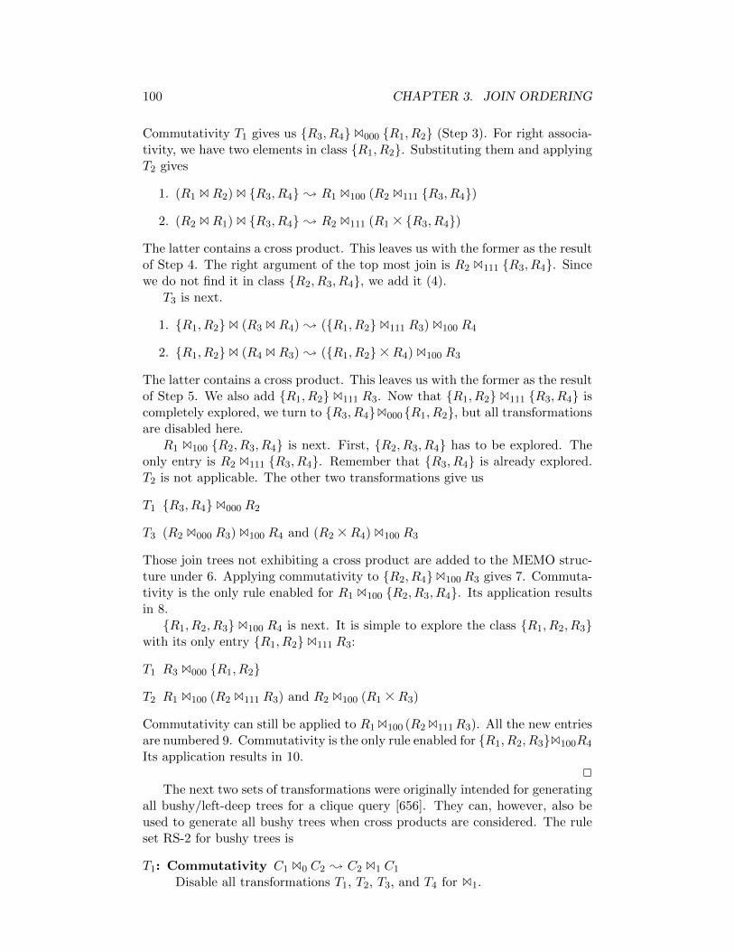
100 CHAPTER 3. JOIN ORDERING

Commutativity T1 gives us R3, R4B000 R1, R2 (Step 3). For right associa-tivity, we have two elements in class R1, R2. Substituting them and applyingT2 gives

1. (R1 BR2) B R3, R4 ; R1 B100 (R2 B111 R3, R4)

2. (R2 BR1) B R3, R4 ; R2 B111 (R1 A R3, R4)

The latter contains a cross product. This leaves us with the former as the resultof Step 4. The right argument of the top most join is R2 B111 R3, R4. Sincewe do not find it in class R2, R3, R4, we add it (4).

T3 is next.

1. R1, R2B (R3 BR4) ; (R1, R2B111 R3) B100 R4

2. R1, R2B (R4 BR3) ; (R1, R2AR4) B100 R3

The latter contains a cross product. This leaves us with the former as the resultof Step 5. We also add R1, R2B111 R3. Now that R1, R2B111 R3, R4 iscompletely explored, we turn to R3, R4B000R1, R2, but all transformationsare disabled here.

R1 B100 R2, R3, R4 is next. First, R2, R3, R4 has to be explored. Theonly entry is R2 B111 R3, R4. Remember that R3, R4 is already explored.T2 is not applicable. The other two transformations give us

T1 R3, R4B000 R2

T3 (R2 B000 R3) B100 R4 and (R2 AR4) B100 R3

Those join trees not exhibiting a cross product are added to the MEMO struc-ture under 6. Applying commutativity to R2, R4B100 R3 gives 7. Commuta-tivity is the only rule enabled for R1 B100 R2, R3, R4. Its application resultsin 8.

R1, R2, R3B100 R4 is next. It is simple to explore the class R1, R2, R3with its only entry R1, R2B111 R3:

T1 R3 B000 R1, R2

T2 R1 B100 (R2 B111 R3) and R2 B100 (R1 AR3)

Commutativity can still be applied to R1B100 (R2B111R3). All the new entriesare numbered 9. Commutativity is the only rule enabled for R1, R2, R3B100R4

Its application results in 10.

2

The next two sets of transformations were originally intended for generatingall bushy/left-deep trees for a clique query [656]. They can, however, also beused to generate all bushy trees when cross products are considered. The ruleset RS-2 for bushy trees is

T1: Commutativity C1 B0 C2 ; C2 B1 C1

Disable all transformations T1, T2, T3, and T4 for B1.

3.3. PROBABILISTIC ALGORITHMS 101

T2: Right Associativity (C1 B0 C2) B1 C3 ; C1 B2 (C2 B3 C3)Disable transformations T2, T3, and T4 for B2.

T3: Left Associativity C1 B0 (C2 B1 C3) ; (C1 B2 C2) B3 C3

Disable transformations T2, T3 and T4 for B3.

T4: Exchange (C1 B0 C2) B1 (C3 B2 C4) ; (C1 B3 C3) B4 (C2 B5 C4)Disable all transformations T1, T2, T3, and T4 for B4.

If we initialize the MEMO structure with left-deep trees, we can strip downthe above rule set to Commutativity and Left Associativity. The reason is anobservation made by Shapiro et al.: from a left-deep join tree we can generateall bushy trees with only these two rules [770].

If we want to consider only left-deep trees, the following rule set RS-3 isappropriate:

T1 Commutativity R1 B0 R2 ; R2 B1 R1

Here, the Ri are restricted to classes with exactly one relation. T1 isdisabled for B1.

T2 Right Join Exchange (C1 B0 C2) B1 C3 ; (C1 B2 C3) B3 C2

Disable T2 for B3.

3.3 Probabilistic Algorithms

3.3.1 Generating Random Left-Deep Join Trees with Cross Prod-ucts

The basic idea of the algorithms in this section and the following sections is togenerate a set of randomly chosen join trees, evaluate their costs, and returnthe best one. The problem with this approach lies in the random generation ofjoin trees: every join tree has to be generated with equal probability. Althoughthere are some advocates of the pure random approach [292, 293, 295, 291],typically a random join tree or a set of random join trees is used in subsequentalgorithms like iterative improvement and simulated annealing.

Obviously, if we do not consider cross products the problem is really hard,since the query graph plays an important role. So let us start with the simplestcase where random join trees are generated that might contain cross productseven for connected query graphs. Then, any join tree is a valid join tree.

The general idea behind all algorithms is the following. Assume that thenumber of join trees in the considered search space is known to be N . Then,instead of generating a random join tree directly, a bijective mapping fromthe interval of non-negative integers [0, N [ to a join tree in the search space isestablished. Then, a random join tree can be generated by (1) generating arandom number in [0, N [ and (2) mapping the number to the join tree. Theproblem of bijectively mapping an interval of non-negative integers to elementsof a set is usually called unranking . The opposite mapping is called ranking .Obviously, the crux in our case is the efficiency of the unranking problem.

102 CHAPTER 3. JOIN ORDERING

We start with generating random left-deep join trees for n relations. Thisproblem is identical to generating random permutations. That is, we look fora fast unranking algorithm that maps the non-negative integers in [0, n![ topermutations. Let us consider permutations of the numbers 0, . . . , n − 1.A mapping between these numbers and relations is established easily, e.g. viaan array. The traditional approach to ranking/unranking of permutations isto first define an ordering on the permutations and then find a ranking andunranking algorithm relative to that ordering. For the lexicographic order, al-gorithms require O(n2) time [535, 695]. More sophisticated algorithms separatethe ranking/unranking algorithms into two phases. For ranking, first the in-version vector of the permutation is established. Then, ranking takes place forthe inversion vector. Unranking works in the opposite direction. The inver-sion vector of a permutation π = π0, . . . , πn−1 is defined to be the sequencev = v0, . . . , vn−1, where vi is equal to the number of entries πj with πj > πiand j < i. Inversion vectors uniquely determine a permutation [843]. However,naive algorithms of this approach again require O(n2) time. Better algorithmsrequire O(n log n). Using an elaborated data structure, Dietz’ algorithm re-quires O((n log n)/(log log n)) [233]. Other orders like the Steinhaus-Johnson-Trotter order have been exploited for ranking/unranking but do not yield anyrun-time advantage over the above mentioned algorithms (see [498, 695]).

Since it is not important for our problem that any order constraints are sat-isfied for the ranking/unranking functions, we use the fastest possible algorithmestablished by Myrvold and Ruskey [613]. It runs in O(n) which is also easilyseen to be a lower bound.

The algorithm is based on the standard algorithm to generate random per-mutations [215, 242, 607]. An array π is initialized such that π[i] = i for0 ≤ i ≤ n− 1. Then, the loop

for (k = n− 1; k >= 0; −− k) swap(π[k], π[random(k)]);

is executed where swap exchanges two elements and random(k) generates arandom number in [0, k]. This algorithm randomly picks any of the possiblepermutations. Assume the random elements produced by the algorithm arern−1, . . . , r0 where 0 ≤ ri ≤ i. Obviously, there are exactly n(n − 1)(n −2) . . . 1 = n! such sequences and there is a one-to-one correspondence betweenthese sequences and the set of all permutations. We can thus unrank r ∈ [0, n![by turning it into a unique sequence of values rn−1, . . . , r0. Note that afterexecuting the swap with rn−1, every value in [0, n[ is possible at position π[n−1].Further, π[n−1] is never touched again. Hence, we can unrank r as follows. Wefirst set rn−1 = r mod n and perform the swap. Then, we define r′ = br/ncand iteratively unrank r′ to construct a permutation of n − 1 elements. Thefollowing algorithm realizes this idea.

Unrank(n, r) Input: the number n of elements to be permuted

and the rank r of the permutation to be constructed

3.3. PROBABILISTIC ALGORITHMS 103

Output: a permutation πfor (i = 0; i < n; + + i) π[i] = i;Unrank-Sub(n, r, π);return π;

Unrank-Sub(n, r, π) for (i = n; i > 0; −− i)

swap(π[i− 1], π[r mod i]);r = br/ic;

3.3.2 Generating Random Join Trees with Cross Products

Next, we want to randomly construct bushy plans possibly containing crossproducts. This is done in several steps:

1. Generate a random number b in [0, C(n− 1)[.

2. Unrank b to obtain a bushy tree with n− 1 inner nodes.

3. Generate a random number p in [0, n![.

4. Unrank p to obtain a permutation.

5. Attach the relations in order p from left to right as leaf nodes to the binarytree obtained in Step 2.

The only step that we still have to discuss is Step 2. It is a little involved and wecan only try to bring across the general idea. For details, the reader is referredto the literature [535, 536, 537].

Consider Figure 3.15. It contains all 14 possible trees with four inner nodes.The trees are ordered according to the rank we will consider. The bottom-mostnumber below any tree is its rank in [0, 14[. While unranking, we do not generatethe trees directly, but an encoding of the tree instead. This encoding works asfollows. Any binary tree corresponds to a word in a Dyck language with onepair of parenthesis. The alphabet hence consists of Σ = ′(′, ′)′. For join treeswith n inner nodes, we use Dyck words of length 2n whose parenthesization iscorrect. That is, for every ′(′, we have a subsequent ′)′. From a given join tree,we obtain the Dyck word by a preorder traversal. Whenever we encounter aninner node, we encode this with a ′(′. All but the last leaf nodes are encodedby a ′)′. Appending all these 2n encodings gives us a Dyck word of length 2n.Figure 3.15 shows directly below each tree its corresponding Dyck word. In theline below, we simply changed the representation by substituting every ′(′ by a′1′ and every ′)′ by a ′0′. The encoding that will be generated by the unrankingalgorithm is shown in the third line below each tree: we remember the places(index in the bit-string) where we find a ′1′.

104 CHAPTER 3. JOIN ORDERING

( ( ) ( ( ) ) )

11011000

1, 2, 4, 5

43

( ( ( ) ) ) ( )

11100010

1, 2, 3, 7

2

( ( ( ) ) ( ) )

11100100

1, 2, 3, 6

6

( ( ) ( ) ) ( )

11010010

1, 2, 4, 7

7

( ( ) ) ( ( ) )

11001100

1, 2, 5, 6

8

( ( ) ) ( ) ( )

11001010

1, 2, 5, 7

( ) ( ( ( ) ) )

10111000

1, 3, 4, 5

9

( ) ( ( ) ( ) )

10110100

1, 3, 4, 6

10 11

( ) ( ( ) ) ( )

10110010

1, 3, 4, 7

( ) ( ) ( ( ) )

10101100

1, 3, 5, 6

12

( ) ( ) ( ) ( )

10101010

1, 3, 5, 7

13

1

11101000

1, 2, 3, 5

( ( ( )( ) ) )

11110000

1, 2, 3, 4

0

( ( ( ( ) ) ) )

1, 2, 4, 6

5

11010100

( ( ) ( ) ( ) )

B

B

B

B

B

B

B

B

B B

B

B

B

B B

B

B

B

B

B

B

B

B

B

B

B B

B

B

B B

B

B

BB

B

B

B

B

B

B

B

B

B

B

B

B B

B

B

B

B

B

B

B

B

Figure 3.15: Encoding Trees

In order to do the unranking, we need to do some counting. Therefor, wemap Dyck words to paths in a triangular grid. For n = 4 this grid is shown inFigure 3.16. We always start at (0, 0) which means that we have not opened aparenthesis. When we are at (i, j), opening a parenthesis corresponds to goingto (i + 1, j + 1) and closing a parenthesis to going to (i + 1, j − 1). We havethus established a bijective mapping between Dyck words and paths in the grid.Thus counting Dyck words corresponds to counting paths.

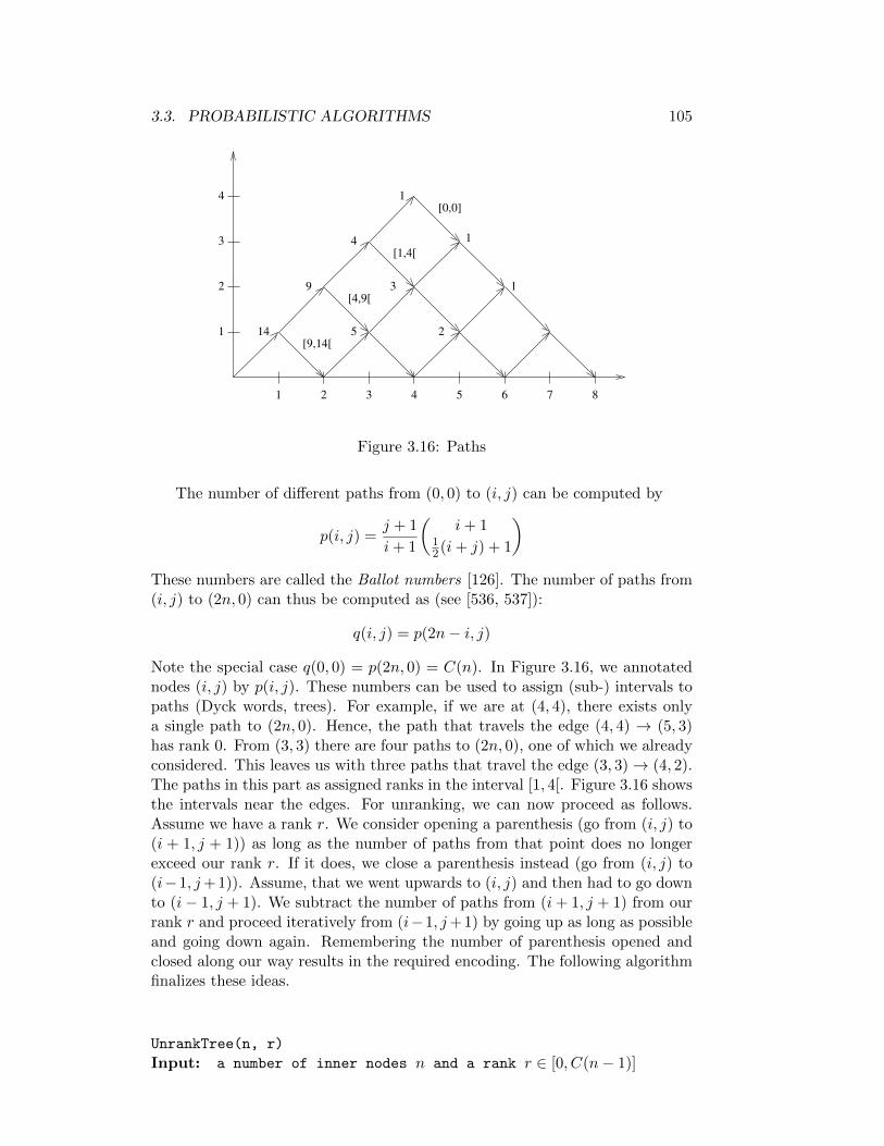
3.3. PROBABILISTIC ALGORITHMS 105

1

2

3

4

87654321

1

14

9

4

1

13

5 2

[0,0]

[1,4[

[9,14[

[4,9[

Figure 3.16: Paths

The number of different paths from (0, 0) to (i, j) can be computed by

p(i, j) =j + 1

i+ 1

(i+ 1

12(i+ j) + 1

)

These numbers are called the Ballot numbers [126]. The number of paths from(i, j) to (2n, 0) can thus be computed as (see [536, 537]):

q(i, j) = p(2n− i, j)

Note the special case q(0, 0) = p(2n, 0) = C(n). In Figure 3.16, we annotatednodes (i, j) by p(i, j). These numbers can be used to assign (sub-) intervals topaths (Dyck words, trees). For example, if we are at (4, 4), there exists onlya single path to (2n, 0). Hence, the path that travels the edge (4, 4) → (5, 3)has rank 0. From (3, 3) there are four paths to (2n, 0), one of which we alreadyconsidered. This leaves us with three paths that travel the edge (3, 3)→ (4, 2).The paths in this part as assigned ranks in the interval [1, 4[. Figure 3.16 showsthe intervals near the edges. For unranking, we can now proceed as follows.Assume we have a rank r. We consider opening a parenthesis (go from (i, j) to(i + 1, j + 1)) as long as the number of paths from that point does no longerexceed our rank r. If it does, we close a parenthesis instead (go from (i, j) to(i−1, j+1)). Assume, that we went upwards to (i, j) and then had to go downto (i− 1, j + 1). We subtract the number of paths from (i+ 1, j + 1) from ourrank r and proceed iteratively from (i−1, j+1) by going up as long as possibleand going down again. Remembering the number of parenthesis opened andclosed along our way results in the required encoding. The following algorithmfinalizes these ideas.

UnrankTree(n, r)

Input: a number of inner nodes n and a rank r ∈ [0, C(n− 1)]

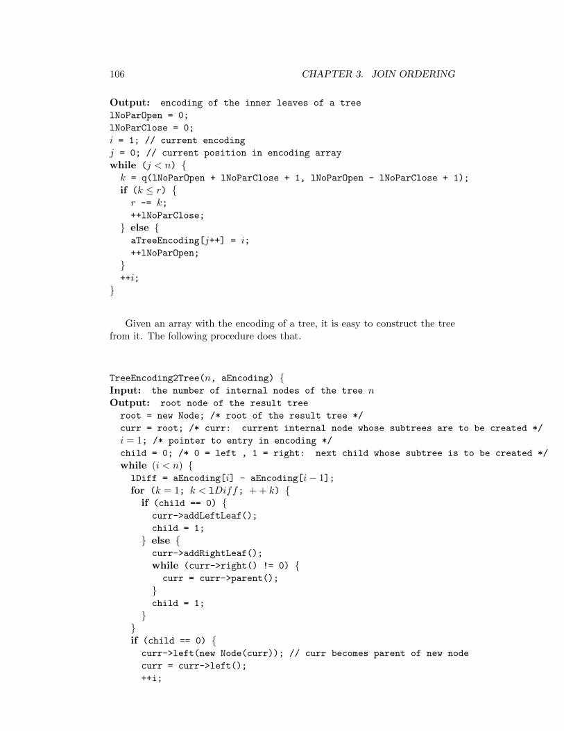
106 CHAPTER 3. JOIN ORDERING

Output: encoding of the inner leaves of a tree

lNoParOpen = 0;

lNoParClose = 0;

i = 1; // current encoding

j = 0; // current position in encoding array

while (j < n) k = q(lNoParOpen + lNoParClose + 1, lNoParOpen - lNoParClose + 1);

if (k ≤ r) r -= k;++lNoParClose;

else aTreeEncoding[j++] = i;++lNoParOpen;

++i;

Given an array with the encoding of a tree, it is easy to construct the treefrom it. The following procedure does that.

TreeEncoding2Tree(n, aEncoding) Input: the number of internal nodes of the tree nOutput: root node of the result tree

root = new Node; /* root of the result tree */

curr = root; /* curr: current internal node whose subtrees are to be created */

i = 1; /* pointer to entry in encoding */

child = 0; /* 0 = left , 1 = right: next child whose subtree is to be created */

while (i < n) lDiff = aEncoding[i] - aEncoding[i− 1];for (k = 1; k < lDiff; + + k)

if (child == 0) curr->addLeftLeaf();

child = 1;

else curr->addRightLeaf();

while (curr->right() != 0) curr = curr->parent();

child = 1;

if (child == 0)

curr->left(new Node(curr)); // curr becomes parent of new node

curr = curr->left();

++i;

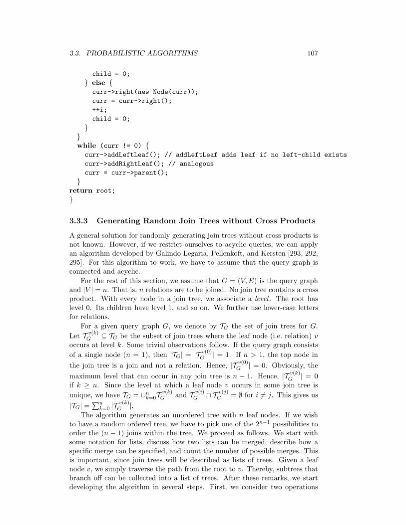
3.3. PROBABILISTIC ALGORITHMS 107

child = 0;

else curr->right(new Node(curr));

curr = curr->right();

++i;

child = 0;

while (curr != 0)

curr->addLeftLeaf(); // addLeftLeaf adds leaf if no left-child exists

curr->addRightLeaf(); // analogous

curr = curr->parent();

return root;

3.3.3 Generating Random Join Trees without Cross Products

A general solution for randomly generating join trees without cross products isnot known. However, if we restrict ourselves to acyclic queries, we can applyan algorithm developed by Galindo-Legaria, Pellenkoft, and Kersten [293, 292,295]. For this algorithm to work, we have to assume that the query graph isconnected and acyclic.

For the rest of this section, we assume that G = (V,E) is the query graphand |V | = n. That is, n relations are to be joined. No join tree contains a crossproduct. With every node in a join tree, we associate a level . The root haslevel 0. Its children have level 1, and so on. We further use lower-case lettersfor relations.

For a given query graph G, we denote by TG the set of join trees for G.

Let T v(k)G ⊆ TG be the subset of join trees where the leaf node (i.e. relation) v

occurs at level k. Some trivial observations follow. If the query graph consists

of a single node (n = 1), then |TG| = |T v(0)G | = 1. If n > 1, the top node in

the join tree is a join and not a relation. Hence, |T v(0)G | = 0. Obviously, the

maximum level that can occur in any join tree is n − 1. Hence, |T v(k)G | = 0

if k ≥ n. Since the level at which a leaf node v occurs in some join tree is

unique, we have TG = ∪nk=0Tv(k)G and T v(i)

G ∩ T v(j)G = ∅ for i 6= j. This gives us

|TG| =∑n

k=0 |Tv(k)G |.

The algorithm generates an unordered tree with n leaf nodes. If we wishto have a random ordered tree, we have to pick one of the 2n−1 possibilities toorder the (n − 1) joins within the tree. We proceed as follows. We start withsome notation for lists, discuss how two lists can be merged, describe how aspecific merge can be specified, and count the number of possible merges. Thisis important, since join trees will be described as lists of trees. Given a leafnode v, we simply traverse the path from the root to v. Thereby, subtrees thatbranch off can be collected into a list of trees. After these remarks, we startdeveloping the algorithm in several steps. First, we consider two operations

108 CHAPTER 3. JOIN ORDERING

(R, S, [1, 1, 0])

R2

R1

v

S1

S2

(R, S, [2, 0, 0])

v

S2

R2

S1

R1

S2

S1

(R, S, [0, 2, 0])

R2

R1

v

R S

v

S1

v

R1

R2 S2

Figure 3.17: Tree-merge

with which we can construct new join trees: leaf-insertion introduces a newleaf node into a given tree and tree-merging merges two join trees. Since wedo not want to generate cross products in this section, we have to apply theseoperations carefully. Therefor, we need a description of how to generate allvalid join trees for a given query graph. The central data structure for thispurpose is the standard decomposition graph (SDG). Hence, in the second step,we define SDGs and introduce an algorithm that derives an SDG from a givenquery graph. In the third step, we start counting. The fourth and final stepconsists of the unranking algorithm. We do not discuss the ranking algorithm.It can be found in [295].

We use the Prolog notation | to separate the first element of a list from itstail. For example, the list 〈a|t〉 has a as its first element and a tail t. Assumethat P is a property of elements. A list l′ is the projection of a list L on P , ifL′ contains all elements of L satisfying the property P . Thereby, the order isretained. A list L is a merge of two disjoint lists L1 and L2 if L contains allelements from L1 and L2 and both are projections of L.

A merge of a list L1 with a list L2 whose respective lengths are l1 and l2can be described by an array α = [α0, . . . , αl2 ] of non-negative integers whosesum is equal to l1. The non-negative integer αi−1 gives the number of elementsof L1 which precede the i-th element of L2 in the merged list. We obtain themerged list L by first taking α0 elements from L1. Then, an element from L2

follows. Then α1 elements from L1 and the next element of L2 follow and soon. Finally follow the last αl2 elements of L1. Figure 3.17 illustrates possiblemerges.

Compare list merges to the problem of non-negative (weak) integer com-position [?]. There, we ask for the number of compositions of a non-negativeinteger n into k non-negative integers αi with

∑ki=1 αk = n. The answer is(

n+k−1k−1

)[800]. Since we have to decompose l1 into l2 + 1 non-negative inte-

gers, the number of possible merges is M(l1, l2) =(l1+l2l2

). The observation

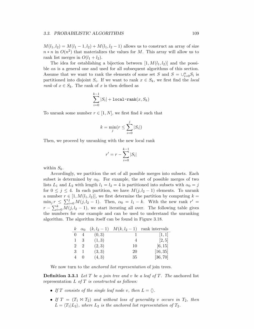
3.3. PROBABILISTIC ALGORITHMS 109

M(l1, l2) = M(l1 − 1, l2) +M(l1, l2 − 1) allows us to construct an array of sizen ∗ n in O(n2) that materializes the values for M . This array will allow us torank list merges in O(l1 + l2).

The idea for establishing a bijection between [1,M(l1, l2)] and the possi-ble αs is a general one and used for all subsequent algorithms of this section.Assume that we want to rank the elements of some set S and S = ∪ni=0Si ispartitioned into disjoint Si. If we want to rank x ∈ Sk, we first find the localrank of x ∈ Sk. The rank of x is then defined as

k−1∑

i=0

|Si|+ local-rank(x, Sk)

To unrank some number r ∈ [1, N ], we first find k such that

k = minj

(r ≤j∑

i=0

|Si|)

Then, we proceed by unranking with the new local rank

r′ = r −k−1∑

i=0

|Si|

within Sk.Accordingly, we partition the set of all possible merges into subsets. Each

subset is determined by α0. For example, the set of possible merges of twolists L1 and L2 with length l1 = l2 = 4 is partitioned into subsets with α0 = jfor 0 ≤ j ≤ 4. In each partition, we have M(j, l2 − 1) elements. To unranka number r ∈ [1,M(l1, l2)], we first determine the partition by computing k =minj r ≤

∑ji=0M(j, l2 − 1). Then, α0 = l1 − k. With the new rank r′ =

r −∑ki=0M(j, l2 − 1), we start iterating all over. The following table gives

the numbers for our example and can be used to understand the unrankingalgorithm. The algorithm itself can be found in Figure 3.18.

k α0 (k, l2 − 1) M(k, l2 − 1) rank intervals

0 4 (0, 3) 1 [1, 1]1 3 (1, 3) 4 [2, 5]2 2 (2, 3) 10 [6, 15]3 1 (3, 3) 20 [16, 35]4 0 (4, 3) 35 [36, 70]

We now turn to the anchored list representation of join trees.

Definition 3.3.1 Let T be a join tree and v be a leaf of T . The anchored listrepresentation L of T is constructed as follows:

• If T consists of the single leaf node v, then L = 〈〉.

• If T = (T1 B T2) and without loss of generality v occurs in T2, thenL = 〈T1|L2〉, where L2 is the anchored list representation of T2.

110 CHAPTER 3. JOIN ORDERING

UnrankDecomposition(r, l1, l2)Input: a rank r, two list sizes l1 and l2Output: a merge specification α.for (i = 0; i ≤ l2; + + i) alpha[i] = 0;

i = k = 0;while (l1 > 0 && l2 > 0) m = M(k, l2 − 1);if (r ≤ m) alpha[i+ +] = l1 − k;l1 = k;k = 0;−− l2;

else r− = m;

+ + k;

alpha[i] = l1;return alpha;

Figure 3.18: Algorithm UnrankDecomposition

w w

(T, 2)

T1

T2

v

T1

T2

v

(T, 1)

T1

T2

w

T

w

v

T1

T2

(T, 3)

Figure 3.19: Leaf-insertion

We then write T = (L, v).

Observe that if T = (L, v) ∈ TG, then T ∈ T v(k)G ≺ |L| = k.

The operation leaf-insertion is illustrated in Figure 3.19. A new leaf v isinserted into the tree at level k. Formally, it is defined as follows.

3.3. PROBABILISTIC ALGORITHMS 111

a b c d

e

e

c

b d

a

a

d

[0, 1]

[1]

[0, 1, 1]

[0, 1]

[1]

[0, 5, 5, 5, 3]

[0, 0, 2, 3]

+b

+c

+e

∗c

+c

Figure 3.20: A query graph, its tree, and its standard decomposition graph

Definition 3.3.2 Let G = (V,E) be a query graph, T a join tree of G. v ∈ Vbe such that G′ = G|V \v is connected, (v, w) ∈ E, 1 ≤ k < n, and

T = (〈T1, . . . , Tk−1, v, Tk+1, . . . , Tn〉, w) (3.10)

T ′ = (〈T1, . . . , Tk−1, Tk+1, . . . , Tn〉, w). (3.11)

Then we call (T ′, k) an insertion pair on v and say that T is decomposed into(or constructed from) the pair (T ′, k) on v.

Observe that leaf-insertion defines a bijective mapping between T v(k)G and inser-

tion pairs (T ′, k) on v, where T ′ is an element of the disjoint union ∪n−2i=k−1T

w(i)G′ .

The operation tree-merging is illustrated in Figure 3.17. Two trees R =(LR, w) and S = (LS , w) on a common leaf w are merged by merging theiranchored list representations.

Definition 3.3.3 Let G = (V,E) be a query graph, w ∈ V , T = (L,w) ajoin tree of G, V1, V2 ⊆ V such that G1 = G|V1 and G2 = G|V2 are connected,V1 ∪ V2 = V , and V1 ∩ V2 = w. For i = 1, 2:

• Define the property Pi to be “every leaf of the subtree is in Vi”,

• Let Li be the projection of L on Pi.

• Ti = (Li, w).

Let α be the integer composition such that L is the result of merging L1 and L2

on α. Then we call (T1, T2, α) a merge triplet. We say that T is decomposedinto (constructed from) (T1, T2, α) on V1 and V2.

Observe that the tree-merging operation defines a bijective mapping between

T w(k)G and merge triplets (T1, T2, α), where T1 ∈ T w(i)

G1, T2 ∈ T w(k−i)

G2, and α

specifies a merge of two lists of sizes i and k − i. Further, the number of thesemerges (i.e. the number of possibilities for α) is

(i+(k−i)k−i

)=(ki

).

A standard decomposition graph of a query graph describes the possibleconstructions of join trees. It is not unique (for n > 1) but anyone can be used

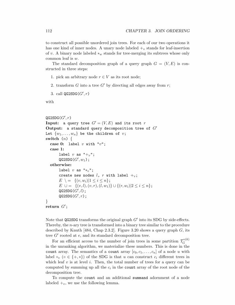
112 CHAPTER 3. JOIN ORDERING

to construct all possible unordered join trees. For each of our two operations ithas one kind of inner nodes. A unary node labeled +v stands for leaf-insertionof v. A binary node labeled ∗w stands for tree-merging its subtrees whose onlycommon leaf is w.

The standard decomposition graph of a query graph G = (V,E) is con-structed in three steps:

1. pick an arbitrary node r ∈ V as its root node;

2. transform G into a tree G′ by directing all edges away from r;

3. call QG2SDG(G′, r)

with

QG2SDG(G′, r)Input: a query tree G′ = (V,E) and its root rOutput: a standard query decomposition tree of G′

Let w1, . . . , wn be the children of v;switch (n)

case 0: label v with "v";case 1:

label v as "+v";

QG2SDG(G′, w1);

otherwise:label v as "∗v";create new nodes l, r with label +v;

E \ = (v, wi)|1 ≤ i ≤ n;E ∪ = (v, l), (v, r), (l, w1) ∪ (r, wi)|2 ≤ i ≤ n;QG2SDG(G′, l);QG2SDG(G′, r);

return G′;

Note that QG2SDG transforms the original graph G′ into its SDG by side-effects.Thereby, the n-ary tree is transformed into a binary tree similar to the proceduredescribed by Knuth [484, Chap 2.3.2]. Figure 3.20 shows a query graph G, itstree G′ rooted at e, and its standard decomposition tree.

For an efficient access to the number of join trees in some partition T v(k)G

in the unranking algorithm, we materialize these numbers. This is done in thecount array. The semantics of a count array [c0, c1, . . . , cn] of a node u withlabel v ( ∈ +, ∗) of the SDG is that u can construct ci different trees inwhich leaf v is at level i. Then, the total number of trees for a query can becomputed by summing up all the ci in the count array of the root node of thedecomposition tree.

To compute the count and an additional summand adornment of a nodelabeled +v, we use the following lemma.

3.3. PROBABILISTIC ALGORITHMS 113

Lemma 3.3.4 Let G = (V,E) be a query graph with n nodes, v ∈ V such thatG′ = G|V \v is connected, (v, w) ∈ E, and 1 ≤ k < n. Then

|T v(k)G | =

∑

i≥k−1

|T w(i)G′ |

This lemma follows from the observation made after the definition of the leaf-insertion operation.

The sets T w(i)G′ used in the summands of Lemma 3.3.4 directly correspond

to subsets T v(k),iG (k − 1 ≤ i ≤ n− 2) defined such that T ∈ T v(k),i

G if

1. T ∈ T v(k)G ,

2. the insertion pair on v of T is (T ′, k), and

3. T ′ ∈ T w(i)G′ .

Further, |T v(k),iG | = |T w(i)

G′ |. For efficiency, we materialize the summands in anarray of arrays summands.

To compute the count and summand adornment of a node labeled ∗v, we usethe following lemma.

Lemma 3.3.5 Let G = (V,E) be a query graph, w ∈ V , T = (L,w) a jointree of G, V1, V2 ⊆ V such that G1 = G|V1 and G2 = G|V2 are connected,V1 ∪ V2 = V , and V1 ∩ V2 = v. Then

|T v(k)G | =

∑

i

(k

i

)|T v(i)G1| |T v(k−i)

G2|

This lemma follows from the observation made after the definition of the tree-merge operation.

The sets T w(i)G′ used in the summands of Lemma 3.3.5 directly correspond

to subsets T v(k),iG (0 ≤ i ≤ k) defined such that T ∈ T v(k),i

G if

1. T ∈ T v(k)G ,

2. the merge triplet on V1 and V2 of T is (T1, T2, α), and

3. T1 ∈ T v(i)G1

.

Further, |T v(k),iG | =

(ki

)|T v(i)G1| |T v(k−i)

G2|.

Before we come to the algorithm for computing the adornments count andsummands, let us make one observation that follows directly from the abovetwo lemmata. Assume a node v whose count array is [c1, . . . , cm] and whosesummands is s = [s0, . . . , sn] with si = [si0, . . . , s

im], then ci =

∑mj=0 s

ij holds.

Figure 3.21 contains the algorithm to adorn SDG’s nodes with count andsummands. It has worst-case complexity O(n3). Figure 3.20 shows the count

adornment for the SDG. Looking at the count array of the root node, we seethat the total number of join trees for our example query graph is 18.

The algorithm UnrankLocalTreeNoCross called by UnrankTreeNoCross adornsthe standard decomposition graph with insert-at and merge-using annota-tions. These can then be used to extract the join tree.

114 CHAPTER 3. JOIN ORDERING

Adorn(v)Input: a node v of the SDG

Output: v and nodes below are adorned by count and summands

Let w1, . . . , wn be the children of v;switch (n)

case 0: count(v) := [1]; // no summands for vcase 1:

Adorn(w1);

assume count(w1) = [c10, . . . , c

1m1

];count(v) = [0, c1, . . . , cm1+1] where ck =

∑m1i=k−1 c

1i ;

summands(v) = [s0, . . . , sm1+1] where sk = [sk0, . . . , skm1+1] and

ski =

c1i if 0 < k and k − 1 ≤ i

0 else

case 2:Adorn(w1);

Adorn(w2);

assume count(w1) = [c10, . . . , c

1m1

];assume count(w2) = [c2

0, . . . , c2m2

];count(v) = [c0, . . . , cm1+m2 ] where

ck =∑m1

i=0

(ki

)c1i c

2k−i; // c2

i = 0 for i 6∈ 0, . . . ,m2summands(v) = [s0, . . . , sm1+m2 ] where sk = [sk0, . . . , s

km1

] and

ski =

(ki

)c1i c

2k−i if 0 ≤ k − i ≤ m2

0 else

Figure 3.21: Algorithm Adorn

UnrankTreeNoCross(r,v)

Input: a rank r and the root v of the SDG

Output: adorned SDG

let count(v) = [x0, . . . , xm];

k := minj r ≤∑j

i=0 xi; // efficiency: binary search on materialized sums.

r′ := r −∑k−1i=0 xi;

UnrankLocalTreeNoCross(v, r′, k);

The following table shows the intervals associated with the partitions T e(k)G for

the standard decomposition graph in Figure 3.20:

Partition Interval

T e(1)G [1, 5]

T e(2)G [6, 10]

T e(3)G [11, 15]

T e(4)G [16, 18]

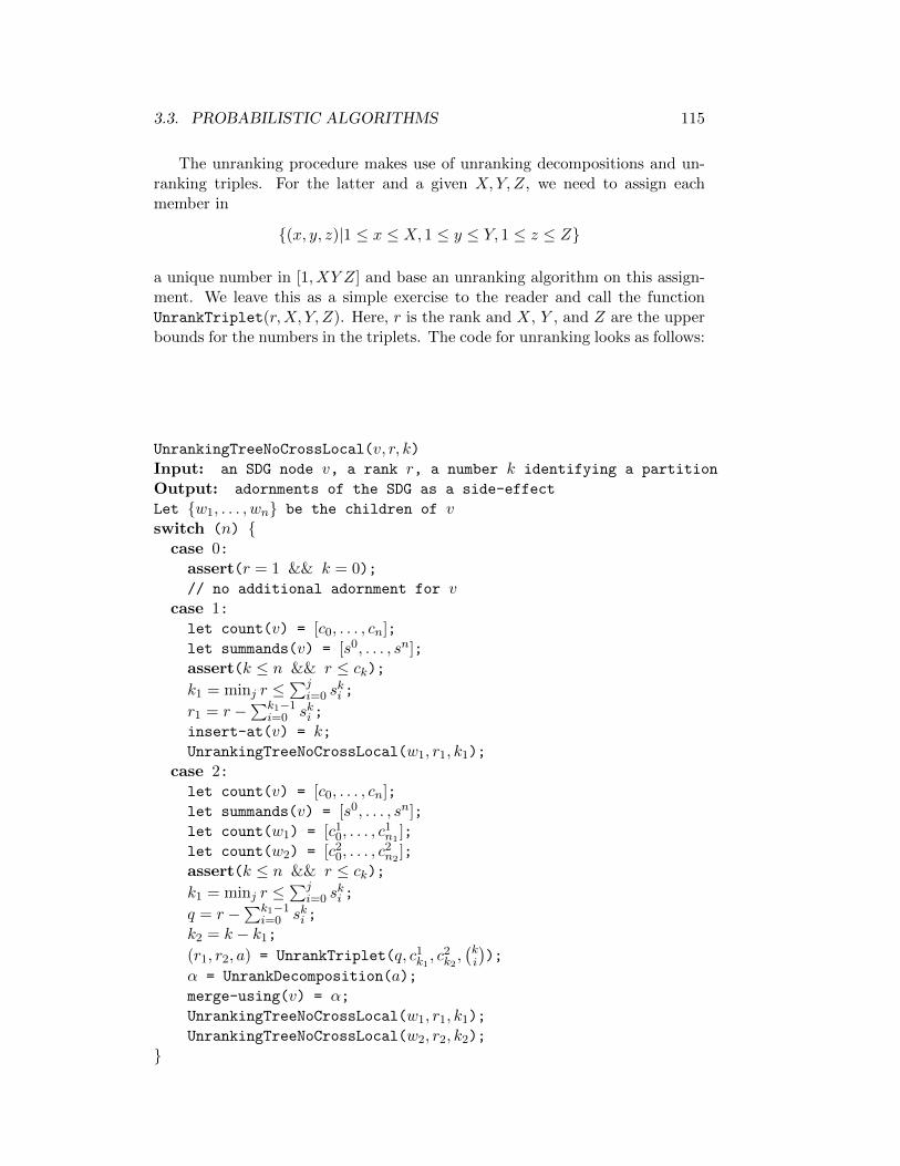
3.3. PROBABILISTIC ALGORITHMS 115

The unranking procedure makes use of unranking decompositions and un-ranking triples. For the latter and a given X,Y, Z, we need to assign eachmember in

(x, y, z)|1 ≤ x ≤ X, 1 ≤ y ≤ Y, 1 ≤ z ≤ Z

a unique number in [1, XY Z] and base an unranking algorithm on this assign-ment. We leave this as a simple exercise to the reader and call the functionUnrankTriplet(r,X, Y, Z). Here, r is the rank and X, Y , and Z are the upperbounds for the numbers in the triplets. The code for unranking looks as follows:

UnrankingTreeNoCrossLocal(v, r, k)Input: an SDG node v, a rank r, a number k identifying a partition

Output: adornments of the SDG as a side-effect

Let w1, . . . , wn be the children of vswitch (n)

case 0:assert(r = 1 && k = 0);// no additional adornment for v

case 1:let count(v) = [c0, . . . , cn];let summands(v) = [s0, . . . , sn];assert(k ≤ n && r ≤ ck);k1 = minj r ≤

∑ji=0 s

ki ;

r1 = r −∑k1−1i=0 ski ;

insert-at(v) = k;UnrankingTreeNoCrossLocal(w1, r1, k1);

case 2:let count(v) = [c0, . . . , cn];let summands(v) = [s0, . . . , sn];let count(w1) = [c1

0, . . . , c1n1

];let count(w2) = [c2

0, . . . , c2n2

];assert(k ≤ n && r ≤ ck);k1 = minj r ≤

∑ji=0 s

ki ;

q = r −∑k1−1i=0 ski ;

k2 = k − k1;

(r1, r2, a) = UnrankTriplet(q, c1k1 , c2k2,(ki

));

α = UnrankDecomposition(a);merge-using(v) = α;UnrankingTreeNoCrossLocal(w1, r1, k1);

UnrankingTreeNoCrossLocal(w2, r2, k2);

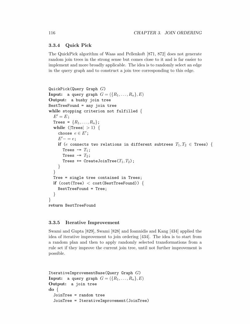
116 CHAPTER 3. JOIN ORDERING

3.3.4 Quick Pick

The QuickPick algorithm of Waas and Pellenkoft [871, 872] does not generaterandom join trees in the strong sense but comes close to it and is far easier toimplement and more broadly applicable. The idea is to randomly select an edgein the query graph and to construct a join tree corresponding to this edge.

QuickPick(Query Graph G)Input: a query graph G = (R1, . . . , Rn, E)Output: a bushy join tree

BestTreeFound = any join tree

while stopping criterion not fulfilled E′ = E;Trees = R1, . . . , Rn;while (|Trees| > 1) choose e ∈ E′;E′− = e;if (e connects two relations in different subtrees T1, T2 ∈ Trees) Trees -= T1;

Trees -= T2;

Trees += CreateJoinTree(T1, T2);

Tree = single tree contained in Trees;

if (cost(Tree) < cost(BestTreeFound)) BestTreeFound = Tree;

return BestTreeFound

3.3.5 Iterative Improvement

Swami and Gupta [829], Swami [828] and Ioannidis and Kang [434] applied theidea of iterative improvement to join ordering [434]. The idea is to start froma random plan and then to apply randomly selected transformations from arule set if they improve the current join tree, until not further improvement ispossible.

IterativeImprovementBase(Query Graph G)Input: a query graph G = (R1, . . . , Rn, E)Output: a join tree

do JoinTree = random tree

JoinTree = IterativeImprovement(JoinTree)

3.3. PROBABILISTIC ALGORITHMS 117

if (cost(JoinTree) < cost(BestTree)) BestTree = JoinTree;

while (time limit not exceeded)

return BestTree

IterativeImprovement(JoinTree)

Input: a join tree

Output: improved join tree

do JoinTree’ = randomly apply a transformation to JoinTree;

if (cost(JoinTree’) < cost(JoinTree)) JoinTree = JoinTree’;

while (local minimum not reached)

return JoinTree

The number of variants of iterative improvements is large. The first parame-ter is the used rule set. To restrict search to left-deep trees, a rule set consistingof swap and 3cycle is appropriate [829]. If we consider bushy trees, a completeset consisting of commutativity, associativity, left join exchange and right joinexchange makes sense. This rule set (proposed by Ioannidis and Kang) is ap-propriate to explore the whole space of bushy join trees. A second parameteris how to determine whether the local minimum has been reached. Consideringall possible neighbor states of a join tree is expensive. Therefor, a subset of sizek is sometimes considered. Then, for example, k can be limited to the numberof edges in the query graph [829].

3.3.6 Simulated Annealing

Iterative Improvement suffers from the drawback that it only applies a moveif it improves the current plan. This leads to the problem that one is oftenstuck in a local minimum. Simulated annealing tries to avoid this problem byallowing moves that result in more expensive plans [439, 434, 829]. However,instead of considering every plan, only those whose cost increase does not exceeda certain limit are considered. During time, this limit decreases. This generalidea is cast into the notion temperatures and probabilities of performing aselected transformation. A generic formulation of simulated annealing couldlook as follows:

SimulatedAnnealing(Query Graph G)Input: a query graph G = (R1, . . . , Rn, E)Output: a join tree

BestTreeSoFar = random tree;

Tree = BestTreeSoFar;

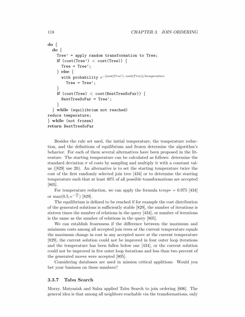
118 CHAPTER 3. JOIN ORDERING

do do Tree’ = apply random transformation to Tree;

if (cost(Tree’) < cost(Tree)) Tree = Tree’;

else with probability e−(cost(Tree′)−cost(Tree))/temperature

Tree = Tree’;

if (cost(Tree) < cost(BestTreeSoFar))

BestTreeSoFar = Tree’;

while (equilibrium not reached)

reduce temperature;

while (not frozen)

return BestTreeSoFar

Besides the rule set used, the initial temperature, the temperature reduc-tion, and the definitions of equilibrium and frozen determine the algorithm’sbehavior. For each of them several alternatives have been proposed in the lit-erature. The starting temperature can be calculated as follows: determine thestandard deviation σ of costs by sampling and multiply it with a constant val-ue ([829] use 20). An alternative is to set the starting temperature twice thecost of the first randomly selected join tree [434] or to determine the startingtemperature such that at least 40% of all possible transformations are accepted[805].

For temperature reduction, we can apply the formula temp∗ = 0.975 [434]

or max(0.5, e−λtσ ) [829].

The equilibrium is defined to be reached if for example the cost distributionof the generated solutions is sufficiently stable [829], the number of iterations issixteen times the number of relations in the query [434], or number of iterationsis the same as the number of relations in the query [805].

We can establish frozenness if the difference between the maximum andminimum costs among all accepted join trees at the current temperature equalsthe maximum change in cost in any accepted move at the current temperature[829], the current solution could not be improved in four outer loop iterationsand the temperature has been fallen below one [434], or the current solutioncould not be improved in five outer loop iterations and less than two percent ofthe generated moves were accepted [805].

Considering databases are used in mission critical applitions. Would youbet your business on these numbers?

3.3.7 Tabu Search

Morzy, Matyasiak and Salza applied Tabu Search to join ordering [606]. Thegeneral idea is that among all neighbors reachable via the transformations, only

3.3. PROBABILISTIC ALGORITHMS 119

the cheapest is considered even if its cost are higher than the costs of the currentjoin tree. In order to avoid running into cycles, a tabu set is maintained. Itcontains the last join trees generated, and the algorithm is not allowed to visitthem again. This way, it can escape local minima, since eventually all nodes inthe valley of a local minimum will be in the tabu set. The stopping conditionscould be that there ws no improvement over the current best solution foundduring the last given number of iterations or if the set neighbors minus the tabuset is empty (in line (*)).

Tabu Search looks as follows:

TabuSearch(Query Graph)

Input: a query graph G = (R1, . . . , Rn, E)Output: a join tree

Tree = random join tree;

BestTreeSoFar = Tree;

TabuSet = ∅;do Neighbors = all trees generated by applying a transformation to Tree;

Tree = cheapest in Neighbors \ TabuSet; (*)

if (cost(Tree) < cost(BestTreeSoFar)) BestTreeSoFar = Tree;

if(|TabuSet| > limit) remove oldest tree from TabuSet;

TabuSet += Tree;

while (not stopping condition satisfied);

return BestTreeSoFar;

3.3.8 Genetic Algorithms

Genetic algorithms are inspired by evolution: only the fittest survives [319].They work with a population that evolves from generation to generation. Suc-cessors are generated by crossover and mutation. Further, a subset of the cur-rent population (the fittest) are propagated to the next generation (selection).The first generation is generated by a random generation process.

The problem is how to represent each individual in a population. Thefollowing analogies are used:

• Chromosome ←→ string

• Gene ←→ character

In order to solve an optimization problem with genetic algorithms, an encodingis needed as well as a specification for selection, crossover, and mutation.

Genetic algorithms for join ordering have been considered in [72, 805]. Wefirst introduce alternative encodings, then come to the selection process, andfinally discuss crossover and mutation.

120 CHAPTER 3. JOIN ORDERING

Encodings We distinguish ordered list and ordinal number encodings. Bothencodings are used for left-deep and bushy trees. In all cases we assume thatthe relations R1, . . . , Rn are to be joined and use the index i to denote Ri.

1. Ordered List Encoding

(a) left-deep treesA left-deep join tree is encoded by a permutation of 1, . . . , n. Forinstance, (((R1 BR4) BR2) BR3) is encoded as “1423”.

(b) bushy treesBennet, Ferris, and Ioannidis proposed the following encoding scheme[72, 73]. A bushy join-tree without cartesian products is encoded asan ordered list of the edges in the join graph. Therefore, we num-ber the edges in the join graph. Then the join tree is encoded in abottom-up, left-to-right manner. See Figure 3.22 for an example.

2. Ordinal Number Encoding

(a) left-deep treesA join tree is encoded by using a list of relations that is short-ened whenever a join has been encoded. We start with the listL = 〈R1, . . . , Rn〉. Then within L we find the index of first rela-tion to be joined. Let this relation be Ri. Ri is the i-th relationin L. Hence, the first character in the chromosome string is i. Weeliminate Ri from L. For every subsequent relation joined, we againdetermine its index in L, remove it from L and append the index tothe chromosome string. For instance, starting with 〈R1, R2, R3, R4〉,the left-deep join tree (((R1 BR4)BR2)BR3) is encoded as “1311”.

(b) bushy treesAgain, we start with the list L = 〈R1, . . . , Rn〉 and encode a bushyjoin tree in a bottom-up, left-to-right manner. Let Ri B Rj be thefirst join in the join tree under this ordering. Then we look up theirpositions in L and add them to the encoding. Next we eliminate Riand Rj from L and push Ri,j to the front of it. We then proceedfor the other joins by again selecting the next join which now canbe between relations and/or subtrees. We determine their positionwithin L, add these positions to the encoding, remove them from L,and insert a composite relation into L such that the new compositerelation directly follows those already present. For instance, startingwith the list 〈R1, R2, R3, R4〉, the bushy join tree ((R1 BR2)B (R3 B

R4)) is encoded as “12 23 12”.

The encoding is completed by adding join methods.

Crossover A crossover generates a new solution from two individuals. There-fore, two partial solutions are combined. Obviously, its definition depends onthe encoding. Two kinds of crossovers are distinguished: the subsequence andthe subset exchange.

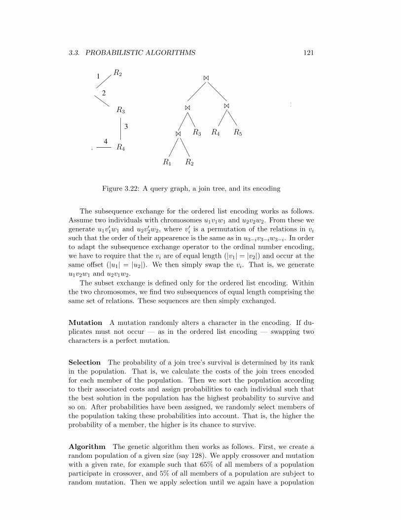
3.3. PROBABILISTIC ALGORITHMS 121

1

2

4

3

R2

1243B

R2R1

R4

R3 R5R4

R5

R1

R3

B

B

B

Figure 3.22: A query graph, a join tree, and its encoding

The subsequence exchange for the ordered list encoding works as follows.Assume two individuals with chromosomes u1v1w1 and u2v2w2. From these wegenerate u1v

′1w1 and u2v

′2w2, where v′i is a permutation of the relations in vi

such that the order of their appearence is the same as in u3−iv3−iw3−i. In orderto adapt the subsequence exchange operator to the ordinal number encoding,we have to require that the vi are of equal length (|v1| = |v2|) and occur at thesame offset (|u1| = |u2|). We then simply swap the vi. That is, we generateu1v2w1 and u2v1w2.

The subset exchange is defined only for the ordered list encoding. Withinthe two chromosomes, we find two subsequences of equal length comprising thesame set of relations. These sequences are then simply exchanged.

Mutation A mutation randomly alters a character in the encoding. If du-plicates must not occur — as in the ordered list encoding — swapping twocharacters is a perfect mutation.

Selection The probability of a join tree’s survival is determined by its rankin the population. That is, we calculate the costs of the join trees encodedfor each member of the population. Then we sort the population accordingto their associated costs and assign probabilities to each individual such thatthe best solution in the population has the highest probability to survive andso on. After probabilities have been assigned, we randomly select members ofthe population taking these probabilities into account. That is, the higher theprobability of a member, the higher is its chance to survive.

Algorithm The genetic algorithm then works as follows. First, we create arandom population of a given size (say 128). We apply crossover and mutationwith a given rate, for example such that 65% of all members of a populationparticipate in crossover, and 5% of all members of a population are subject torandom mutation. Then we apply selection until we again have a population

122 CHAPTER 3. JOIN ORDERING

of a given size. We stop after we have not seen an improvement within thepopulation for a fixed number of iterations (say 30).

3.4 Hybrid Algorithms

All the algorithms we have seen so far can be combined to result in new ap-proaches to join ordering. Some of the numerous possibilities have been de-scribed in the literature. We present them.

3.4.1 Two Phase Optimization

Two phase optimization combines Iterative Improvement with Simulated An-nealing [434]. For a number of randomly generated initial trees, Iterative Im-provement is used to find a local minimum. Then Simulated Annealing is start-ed to find a better plan in the neighborhood of the local minima. The initialtemperature of Simulated Annealing can be lower as is its original variants.

3.4.2 AB-Algorithm

The AB-Algorithm was developed by Swami and Iyer [830, 831]. It builds onthe IKKBZ-Algorithm by resolving its limitations. First, if the query graphis cyclic, a spanning tree is selected. Second, two different cost functions forjoins (join methods) are supported by the AB-Algorithm: nested loop join andsort merge join. In order to make the sort merge join’s cost model fit the ASIproperty, it is simplified. Third, join methods are assigned randomly beforeIKKBZ is called. Afterwards, an iterative improvement phase follows. Thealgorithm can be formulated as follows:

AB(Query Graph G)Input: a query graph G = (R1, . . . , Rn, E)Output: a left-deep join tree

while (number of iterations ≤ n2) if G is cyclic take spanning tree of Grandomly attach a join method to each relation

JoinTree = result of IKKBZ

while (number of iterations ≤ n2) apply Iterative Improvement to JoinTree

return best tree found

3.4.3 Toured Simulated Annealing

Lanzelotte, Valduriez, and Zait introduced toured simulated annealing as asearch strategy useful in distributed databases where the search space is even

3.5. ORDERING ORDER-PRESERVING JOINS 123

larger than in centralized systems [511]. The basic idea is that simulated an-nealing is called n times with different initial join trees, if n is the number ofrelations to be joined. Each join sequence in the set Solutions produced byGreedyJoinOrdering-3 is used to start an independent run of simulated an-nealing. As a result, the starting temperature can be decreased to 0.1 timesthe cost of the initial plan.

3.4.4 GOO-II

GOO-II appends an Iterative Improvement step to the GOO-Algorithm.

3.4.5 Iterative Dynamic Programming

Iterative Dynamic Programming combines heuristics with dynamic program-ming in order to overcome the deficiencies of both. It comes in two variants[495, 777]. The first variant, IDP-1 (see Figure 3.23), first creates all join treeswhich contain up to k relations where k is a parameter of the algorithm. Afterthis step, it selects the cheapest join tree comprising k relations, replaces it bya new compound relation and starts all over again. The iteration stops, whenonly one compound relation representing a join tree for all relations remains inthe ToDo list.

The second variant, IDP-2 (see Figure 3.24), works the other way round.It first applies a greedy heuristics to build join trees of size up to k. To thelarger subtree it applies dynamic programming to improve it. The result ofthe optimized outcome of the greedy algorithm is then encapsulated in a newcompound relation which replaces its constituent relations in the ToDo list. Thealgorithm then iterates until only one entry remains in the ToDo list.

Obviously, from these two basic variants several others can be derived. Asystematic investigation of the basic algorithms and their variants is given byKossmann and Stocker [495]. It turns out that the most promising variantsexist for IDP-1.

3.5 Ordering Order-Preserving Joins

This section covers an algorithm for ordering order-preserving joins [592]. Thisis important for XQuery and other languages that require order-preservation.XQuery specifies that the result of a query is a sequence. If no unordered ororder by instruction is given, the order of the output sequence is determinedby the order of the input sequences given in the for clauses of the query. Ifthere are several entries in a for clause or several for clauses, order-preservingjoin operators [175] can be a natural component for the evaluation of such aquery.

The order-preserving join operator is used in several algebras in the contextof

• semi-structured data and XML (e.g. SAL [69], XAL [283]),

• OLAP [791], and

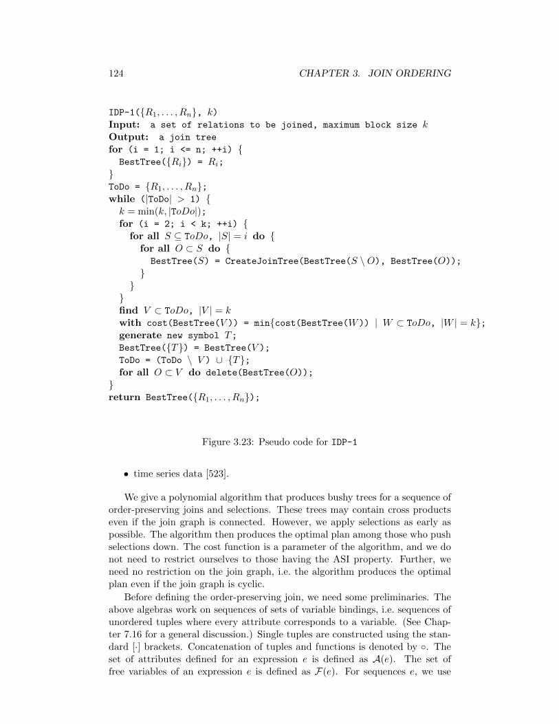
124 CHAPTER 3. JOIN ORDERING

IDP-1(R1, . . . , Rn, k)Input: a set of relations to be joined, maximum block size kOutput: a join tree

for (i = 1; i <= n; ++i) BestTree(Ri) = Ri;

ToDo = R1, . . . , Rn;while (|ToDo| > 1) k = min(k, |ToDo|);for (i = 2; i < k; ++i)

for all S ⊆ ToDo, |S| = i do for all O ⊂ S do BestTree(S) = CreateJoinTree(BestTree(S \O), BestTree(O));

find V ⊂ ToDo, |V | = kwith cost(BestTree(V )) = mincost(BestTree(W)) | W ⊂ ToDo, |W | = k;generate new symbol T;BestTree(T) = BestTree(V );ToDo = (ToDo \ V ) ∪ T;for all O ⊂ V do delete(BestTree(O));

return BestTree(R1, . . . , Rn);

Figure 3.23: Pseudo code for IDP-1

• time series data [523].

We give a polynomial algorithm that produces bushy trees for a sequence oforder-preserving joins and selections. These trees may contain cross productseven if the join graph is connected. However, we apply selections as early aspossible. The algorithm then produces the optimal plan among those who pushselections down. The cost function is a parameter of the algorithm, and we donot need to restrict ourselves to those having the ASI property. Further, weneed no restriction on the join graph, i.e. the algorithm produces the optimalplan even if the join graph is cyclic.

Before defining the order-preserving join, we need some preliminaries. Theabove algebras work on sequences of sets of variable bindings, i.e. sequences ofunordered tuples where every attribute corresponds to a variable. (See Chap-ter 7.16 for a general discussion.) Single tuples are constructed using the stan-dard [·] brackets. Concatenation of tuples and functions is denoted by . Theset of attributes defined for an expression e is defined as A(e). The set offree variables of an expression e is defined as F(e). For sequences e, we use

3.5. ORDERING ORDER-PRESERVING JOINS 125

IDP-2(R1, . . . , Rn, k)Input: a set of relations to be joined, maximum block size kOutput: a join tree

for (i = 1; i <= n; ++i) BestTree(Ri) = Ri;

ToDo = R1, . . . , Rn;while (|ToDo| > 1) // apply greedy algorithm to select a good building block

B = ∅;for all v ∈ ToDo, do B += BestTree(v);

do

find L,R ∈ Bwith cost(CreateJoinTree(L,R))

= mincost(CreateJoinTree(L′,R′)) | L′, R′ ∈ B;P = CreateJoinTree(L,R));B = (B \ L,R) ∪ P;

while (P involves no more than k relations and |B| > 1);// reoptimize the bigger of L and R,// selected in the last iteration of the greedy loop

if (L involves more tables than R) ReOpRels = relations involved in L;

else ReOpRels = relations involved in R;

P = DP-Bushy(ReOpRels);

generate new symbol T;BestTree(T) = P;ToDo = (ToDo \ ReOpRels) ∪ T;for all O ⊂ V do delete(BestTree(O));

return BestTree(R1, . . . , Rn);

Figure 3.24: Pseudocode for IDP-2

α(e) to denote the first element of a sequence. We identify single element se-quences with elements. The function τ retrieves the tail of a sequence, and ⊕concatenates two sequences. We denote the empty sequence by ε.

We define the algebraic operators recursively on their input sequences. Theorder-preserving join operator is defined as the concatenation of an order-preserving selection and an order-preserving cross product. For unary oper-ators, if the input sequence is empty, the output sequence is also empty. For

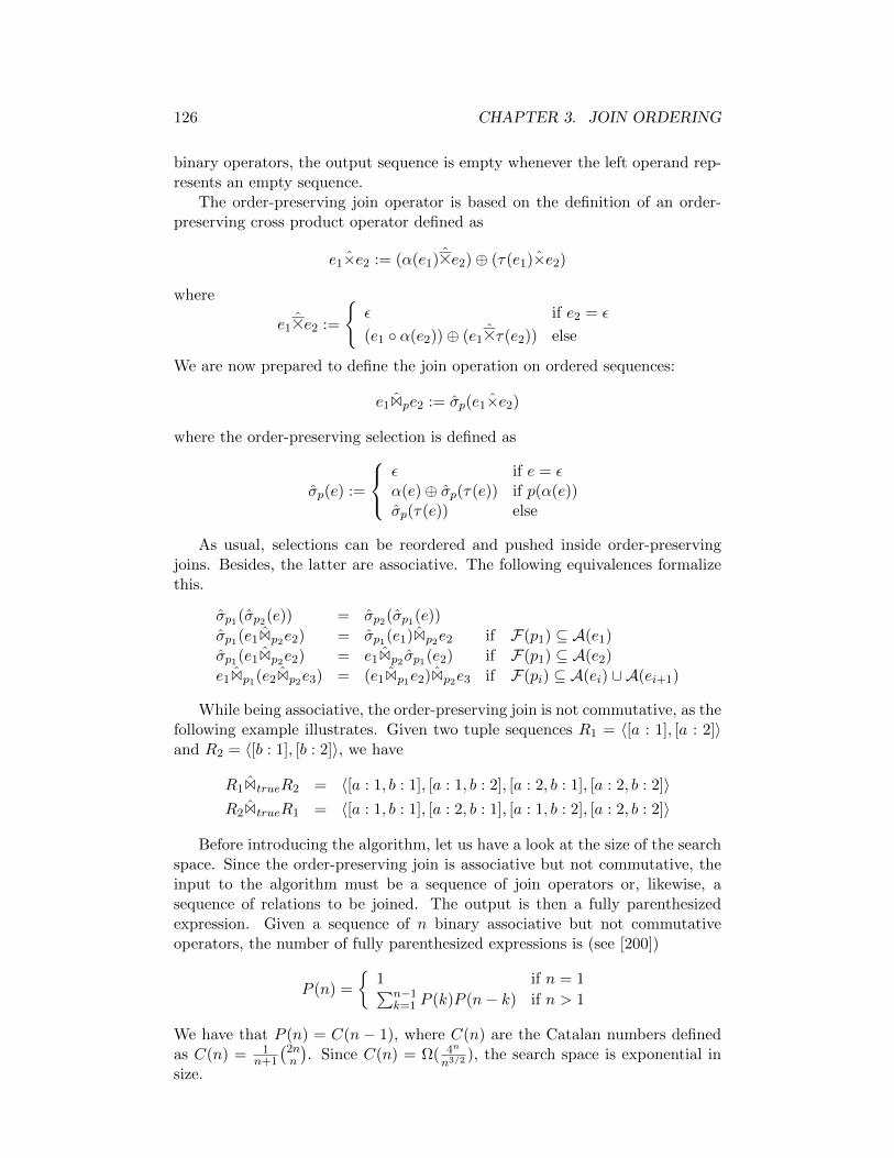
126 CHAPTER 3. JOIN ORDERING

binary operators, the output sequence is empty whenever the left operand rep-resents an empty sequence.

The order-preserving join operator is based on the definition of an order-preserving cross product operator defined as

e1×e2 := (α(e1)Ae2)⊕ (τ(e1)×e2)

where

e1Ae2 :=

ε if e2 = ε

(e1 α(e2))⊕ (e1Aτ(e2)) else

We are now prepared to define the join operation on ordered sequences:

e1Bpe2 := σp(e1×e2)

where the order-preserving selection is defined as

σp(e) :=

ε if e = εα(e)⊕ σp(τ(e)) if p(α(e))σp(τ(e)) else

As usual, selections can be reordered and pushed inside order-preservingjoins. Besides, the latter are associative. The following equivalences formalizethis.

σp1(σp2(e)) = σp2(σp1(e))

σp1(e1Bp2e2) = σp1(e1)Bp2e2 if F(p1) ⊆ A(e1)

σp1(e1Bp2e2) = e1Bp2 σp1(e2) if F(p1) ⊆ A(e2)

e1Bp1(e2Bp2e3) = (e1Bp1e2)Bp2e3 if F(pi) ⊆ A(ei) ∪ A(ei+1)

While being associative, the order-preserving join is not commutative, as thefollowing example illustrates. Given two tuple sequences R1 = 〈[a : 1], [a : 2]〉and R2 = 〈[b : 1], [b : 2]〉, we have

R1BtrueR2 = 〈[a : 1, b : 1], [a : 1, b : 2], [a : 2, b : 1], [a : 2, b : 2]〉R2BtrueR1 = 〈[a : 1, b : 1], [a : 2, b : 1], [a : 1, b : 2], [a : 2, b : 2]〉

Before introducing the algorithm, let us have a look at the size of the searchspace. Since the order-preserving join is associative but not commutative, theinput to the algorithm must be a sequence of join operators or, likewise, asequence of relations to be joined. The output is then a fully parenthesizedexpression. Given a sequence of n binary associative but not commutativeoperators, the number of fully parenthesized expressions is (see [200])

P (n) =

1 if n = 1∑n−1

k=1 P (k)P (n− k) if n > 1

We have that P (n) = C(n − 1), where C(n) are the Catalan numbers definedas C(n) = 1

n+1

(2nn

). Since C(n) = Ω( 4n

n3/2 ), the search space is exponential insize.

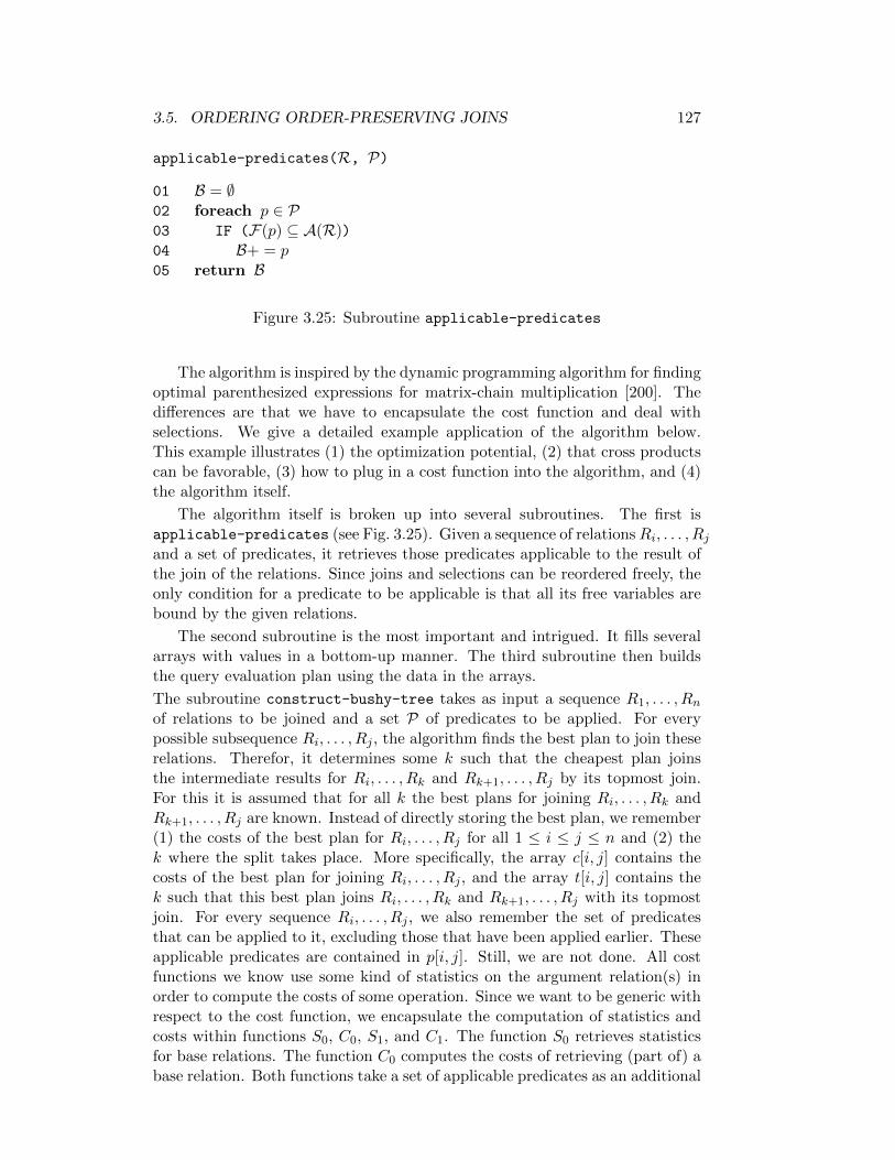
3.5. ORDERING ORDER-PRESERVING JOINS 127

applicable-predicates(R, P)

01 B = ∅02 foreach p ∈ P03 IF (F(p) ⊆ A(R))04 B+ = p05 return B

Figure 3.25: Subroutine applicable-predicates

The algorithm is inspired by the dynamic programming algorithm for findingoptimal parenthesized expressions for matrix-chain multiplication [200]. Thedifferences are that we have to encapsulate the cost function and deal withselections. We give a detailed example application of the algorithm below.This example illustrates (1) the optimization potential, (2) that cross productscan be favorable, (3) how to plug in a cost function into the algorithm, and (4)the algorithm itself.

The algorithm itself is broken up into several subroutines. The first isapplicable-predicates (see Fig. 3.25). Given a sequence of relationsRi, . . . , Rjand a set of predicates, it retrieves those predicates applicable to the result ofthe join of the relations. Since joins and selections can be reordered freely, theonly condition for a predicate to be applicable is that all its free variables arebound by the given relations.

The second subroutine is the most important and intrigued. It fills severalarrays with values in a bottom-up manner. The third subroutine then buildsthe query evaluation plan using the data in the arrays.

The subroutine construct-bushy-tree takes as input a sequence R1, . . . , Rnof relations to be joined and a set P of predicates to be applied. For everypossible subsequence Ri, . . . , Rj , the algorithm finds the best plan to join theserelations. Therefor, it determines some k such that the cheapest plan joinsthe intermediate results for Ri, . . . , Rk and Rk+1, . . . , Rj by its topmost join.For this it is assumed that for all k the best plans for joining Ri, . . . , Rk andRk+1, . . . , Rj are known. Instead of directly storing the best plan, we remember(1) the costs of the best plan for Ri, . . . , Rj for all 1 ≤ i ≤ j ≤ n and (2) thek where the split takes place. More specifically, the array c[i, j] contains thecosts of the best plan for joining Ri, . . . , Rj , and the array t[i, j] contains thek such that this best plan joins Ri, . . . , Rk and Rk+1, . . . , Rj with its topmostjoin. For every sequence Ri, . . . , Rj , we also remember the set of predicatesthat can be applied to it, excluding those that have been applied earlier. Theseapplicable predicates are contained in p[i, j]. Still, we are not done. All costfunctions we know use some kind of statistics on the argument relation(s) inorder to compute the costs of some operation. Since we want to be generic withrespect to the cost function, we encapsulate the computation of statistics andcosts within functions S0, C0, S1, and C1. The function S0 retrieves statisticsfor base relations. The function C0 computes the costs of retrieving (part of) abase relation. Both functions take a set of applicable predicates as an additional

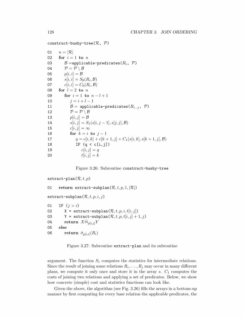
128 CHAPTER 3. JOIN ORDERING

construct-bushy-tree(R, P)

01 n = |R|02 for i = 1 to n03 B =applicable-predicates(Ri, P)04 P = P \ B05 p[i, i] = B06 s[i, i] = S0(Ri,B)07 c[i, i] = C0(Ri,B)08 for l = 2 to n09 for i = 1 to n− l + 110 j = i+ l − 111 B = applicable-predicates(Ri...j, P)12 P = P \ B13 p[i, j] = B14 s[i, j] = S1(s[i, j − 1], s[j, j],B)15 c[i, j] =∞16 for k = i to j − 117 q = c[i, k] + c[k + 1, j] + C1(s[i, k], s[k + 1, j],B)18 IF (q < c[i,j])

19 c[i, j] = q20 t[i, j] = k

Figure 3.26: Subroutine construct-bushy-tree

extract-plan(R, t, p)

01 return extract-subplan(R, t, p, 1, |R|)

extract-subplan(R, t, p, i, j)

01 IF (j > i)02 X = extract-subplan(R, t, p, i, t[i, j])03 Y = extract-subplan(R, t, p, t[i, j] + 1, j)

04 return XBp[i,j]Y

05 else06 return σp[i,i](Ri)

Figure 3.27: Subroutine extract-plan and its subroutine

argument. The function S1 computes the statistics for intermediate relations.Since the result of joining some relations Ri, . . . , Rj may occur in many differentplans, we compute it only once and store it in the array s. C1 computes thecosts of joining two relations and applying a set of predicates. Below, we showhow concrete (simple) cost and statistics functions can look like.

Given the above, the algorithm (see Fig. 3.26) fills the arrays in a bottom-upmanner by first computing for every base relation the applicable predicates, the

3.5. ORDERING ORDER-PRESERVING JOINS 129

statistics of the result of applying the predicates to the base relation and thecosts for computing these intermediate results, i.e. for retrieving the relevantpart of the base relation and applying the predicates (lines 02-07). Note thatthis is not really trivial if there are several index structures that can be applied.Then computing C0 involves considering different access paths. Since this is anissue orthogonal to join ordering, we do not detail on it.

After we have the costs and statistics for sequences of length one, we com-pute the same information for sequences of length two, three, and so on untiln (loop starting at line 08). For every length, we iterate over all subsequencesof that length (loop starting at line 09). We compute the applicable predicatesand the statistics. In order to determine the minimal costs, we have to considerevery possible split point. This is done by iterating the split point k from i toj − 1 (line 16). For every k, we compute the cost and remember the k thatresulted in the lowest costs (lines 17-20).

The last subroutine takes the relations, the split points (t), and the applica-ble predicates (p) as its input and extracts the plan. The whole plan is extractedby calling extract-plan. This is done by instructing extract-subplan to re-trieve the plan for all relations. This subroutine first determines whether theplan for a base relation or that of an intermediate result is to be constructed.In both cases, we did a little cheating here to keep things simple. The plan weconstruct for base relations does not take the above-mentioned index structuresinto account but simply applies a selection to a base relation instead. Obvi-ously, this can easily be corrected. We also give the join operator the wholeset of predicates that can be applied. That is, we do not distinguish betweenjoin predicates and other predicates that are better suited for a selection sub-sequently applied to a join. Again, this can easily be corrected.

Let us have a quick look at the complexity of the algorithm. Given n rela-tions withm attributes in total and p predicates, we can implement applicable-predicatesin O(pm) by using a bit vector representation for attributes and free variablesand computing the attributes for each sequence Ri, . . . , Rj once upfront. Thelatter takes O(n2m).

The complexity of the routine construct-bushy-tree is determined by thethree nested loops. We assume that S1 and C1 can be computed in O(p), whichis quite reasonable. Then, we have O(n3p) for the innermost loop, O(n2) calls toapplicable-predicates, which amounts to O(n2pm), and O(n2p) for calls ofS1. Extracting the plan is linear in n. Hence, the total runtime of the algorithmis O(n2(n+m)p)

In order to illustrate the algorithm, we need to fix the functions S0, S1, C0

and C1. We use the simple cost function Cout. As a consequence, the array ssimply stores cardinalities, and S0 has to extract the cardinality of a given baserelation and multiply it by the selectivities of the applicable predicates. S1 mul-tiplies the input cardinalities with the selectivities of the applicable predicates.We set C0 to zero and C1 to S1. The former is justified by the fact that everyrelation must be accessed exactly once and hence, the access costs are equal in

130 CHAPTER 3. JOIN ORDERING

all plans. Summarizing, we define

S0(R,B) := |R|∏

p∈Bf(p)

S1(x, y,B) := xy∏

p∈Bf(p)

C0(R,B) := 0

C1(x, y,B) := S1(x, y,B)

where B is a set of applicable predicates and for a single predicate p, f(p)returns its selectivity.

We illustrate the algorithm by an example consisting of four relationsR1, . . . , R4

with cardinalities |R1| = 200, |R2| = 1, |R3| = 1, |R4| = 20. Besides, we havethree predicates pi,j with F(pi,j) ⊆ A(Ri)∪A(Rj). They are p1,2, p3,4, and p1,4

with selectivities 1/2, 1/10, 1/5.

Let us first consider an example plan and its costs. The plan

((R1Bp1,2R2)BtrueR3)Bp1,4∧p3,4R4

has the costs 240 = 100 + 100 + 40.

For our simple cost function, the algorithm construct-bushy-tree will fillthe array s with the initial values:

s

200

1

1

20

After initilization, the array c has 0 everywhere in its diagonal and the array pempty sets.

For l = 2, the algorithm produces the following values:

l i j k s[i,j] q current c[i,j] current t[i,j]

2 1 2 1 100 100 100 1

2 2 3 2 1 1 1 2

2 3 4 3 2 2 2 3

For l = 3, the algorithm produces the following values:

l i j k s[i,j] q current c[i,j] current t[i,j]

3 1 3 1 200 101 101 1

3 1 3 2 200 200 101 1

3 2 4 2 2 4 4 2

3 2 4 3 2 3 3 3

For l = 4, the algorithm produces the following values:

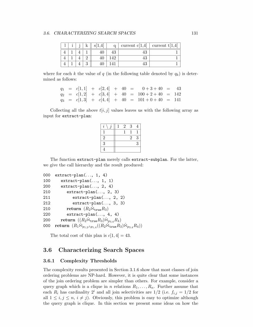
3.6. CHARACTERIZING SEARCH SPACES 131

l i j k s[1,4] q current c[1,4] current t[1,4]

4 1 4 1 40 43 43 1

4 1 4 2 40 142 43 1

4 1 4 3 40 141 43 1

where for each k the value of q (in the following table denoted by qk) is deter-mined as follows:

q1 = c[1, 1] + c[2, 4] + 40 = 0 + 3 + 40 = 43q2 = c[1, 2] + c[3, 4] + 40 = 100 + 2 + 40 = 142q3 = c[1, 3] + c[4, 4] + 40 = 101 + 0 + 40 = 141

Collecting all the above t[i, j] values leaves us with the following array asinput for extract-plan:

i \ j 1 2 3 4

1 1 1 1

2 2 3

3 3

4

The function extract-plan merely calls extract-subplan. For the latter,we give the call hierarchy and the result produced:

000 extract-plan(. . ., 1, 4)

100 extract-plan(. . ., 1, 1)

200 extract-plan(. . ., 2, 4)

210 extract-plan(. . ., 2, 3)

211 extract-plan(. . ., 2, 2)

212 extract-plan(. . ., 3, 3)

210 return (R2BtrueR3)220 extract-plan(. . ., 4, 4)

200 return ((R2BtrueR3)Bp3,4R4)

000 return (R1Bp1,2∧p1,4((R2BtrueR3)Bp3,4R4))

The total cost of this plan is c[1, 4] = 43.

3.6 Characterizing Search Spaces

3.6.1 Complexity Thresholds

The complexity results presented in Section 3.1.6 show that most classes of joinordering problems are NP-hard. However, it is quite clear that some instancesof the join ordering problem are simpler than others. For example, consider aquery graph which is a clique in n relations R1, . . . , Rn. Further assume thateach Ri has cardinality 2i and all join selectivities are 1/2 (i.e. fi,j = 1/2 forall 1 ≤ i, j ≤ n, i 6= j). Obviously, this problem is easy to optimize althoughthe query graph is clique. In this section we present some ideas on how the

132 CHAPTER 3. JOIN ORDERING

complexity of instances of the join ordering problem is influenced by certainparameters.

How can we judge the complexity of a single instance of a join ordering prob-lem? Using standard complexity theory, for single problem instances we easilyderive an algorithm that works in Θ(1). Hence, we must define other complexitymeasures. Consider our introductory join ordering problem. A simple greedyalgorithm that orders relations according to their cardinality produces an op-timal solution for it. Hence, one possibility to define the problem complexitywould be how far a solution produced by typical heuristics for join orderingdiffer from the optimal solution. Another possibility is to use randomized al-gorithms like iterative improvement of simulated annealing and see how far theplans generated by them deviate from the optimal plan. These approaches havethe problem that the results may depend on the chosen algorithm. This canbe avoided by using the following approach. For each join ordering probleminstance, we compute the fraction of good plans compared to all plans. There-for, we need a measure of “good”. Typical examples thereof would be to say aplan is “good” if it does not deviate more than 10% or a factor of two from theoptimal plan.

If these investigations were readily available, there are certain obvious ben-efits [491]:

1. The designer of an optimizer can classify queries such that heuristics areapplied where they guarantee success; cases where they are bound to failcan be avoided. Furthermore, taking into account the vastly different runtime of the different join ordering heuristics and probabilistic optimizationprocedures, the designer of an optimizer can choose the method thatachieves a satisfactory result with the least effort.

2. The developer of search procedures and heuristics can use this knowl-edge to design methods solving hard problems (as exemplified for graphcoloring problems [413]).

3. The investigator of different join ordering techniques is able to (1) con-sciously design challenging benchmarks and (2) evaluate existing bench-marks according to their degree of challenge.

The kind of investigation presented in this section first started in the contextof artificial intelligence where a paper by Cheeseman, Kanefsky, and Taylor[156] spurred a whole new branch of research where the measures to judgethe complexity of problem instances was investigated for many different NP-complete problems like satisfiability [156, 204, 315, 586], graph coloring [156],Hamiltonian circuits [156], traveling salesman [156], and constraint satisfaction[895].

We only present a small fraction of all possible investigations. The restric-tions are that we do not consider all parameters that possibly influence theproblem complexity, we only consider left-deep trees, and we restrict ourselvesto the cost function Chj. The join graphs are randomly generated. Startingwith a circle, we randomly added edges until a clique is reached. The read-er is advised to carry out his or her own experiments. Therefor, the following

3.6. CHARACTERIZING SEARCH SPACES 133

pointer into the literature might be useful. Lanzelotte and Valduriez provide anobject-oriented design for search strategies [509]. This allows easy modificationand even the exchange of the plan generator’s search strategy.

Search Space Analysis

The goal of this section is to determine the influence of the parameters on thesearch space of left-deep join trees. More specifically, we are interested in how avariation of the parameters changes the percentage of good solutions among allsolutions. The quality of a solution is measured by the factor its cost deviatesfrom the optimal permutation. For this, all permutations have to be gener-ated and evaluated. The results of this experiment are shown in Figures 3.28and 3.29. Each single curve accumulates the percentage of all permutationsdeviating less than a certain factor (given as the label) from the optimum. Theaccumulated percentages are given at the y-axes, the connectivity at the x-axes.The connectivity is given by the number of edges in the join graph. The curveswithin the figures are organized as follows. Figure 3.28 (3.29) shows varyingmean selectivity values (relation sizes) and variances where the mean selectivityvalues (relation sizes) increase from top to bottom and the variances increasefrom left to right.

Note that the more curves are visible and the lower their y-values, the harderis the problem. We observe the following:

• all curves exhibit a minimum value at a certain connectivity

• which moves with increasing mean values to the right;

• increasing variances does not have an impact on the minimum connectiv-ity ,

• problems become less difficult with increasing mean values.

These findings can be explained as follows. With increasing connectivity,the join ordering problem becomes more complex up to a certain point andthen less complex again. To see this, consider the following special thoughillustrative case. Assume an almost equal distribution of the costs of all al-ternatives between the worst case and optimal costs, equal relation sizes, andequal selectivities. Then the optimization potential worst case/optimum is 1for connectivity 0 and cliques. In between, there exists a connectivity exhibit-ing the maximum optimization potential. This connectivity corresponds to theminimum connectivity of Figures 3.28 and 3.29.

There is another factor which influences the complexity of a single probleminstance. Consider joining n relations. The problem becomes less complexif after joining i < n relations the intermediate result becomes so small thatthe accumulated costs of the subsequent n− i joins are small compared to thecosts of joining the first i relations. Hence, the ordering of the remaining n− irelations does not have a big influence on the total costs. This is the casefor very small relations, small selectivities, or high connectivities. The greaterselectivities and relation sizes are, the more relations have to be joined to reachthis critical size of the intermediate result. If the connectivity is enlarged, this

134 CHAPTER 3. JOIN ORDERING

critical size is reached earlier. Since the number of selectivities involved in thefirst few joins is small regardless of the connectivity, there is a lower limit to thenumber of joined relations required to arrive at the critical intermediate resultsize. If the connectivity is larger, this point is reached earlier, but there existsa lower limit on the connectivity where this point is reached. The reason forthis lower limit is that the number of selectivities involved in the joins remainssmall for the first couple of relations, independent of their connectivity. Theselines of argument explain subsequent findings, too.

The reader should be aware of the fact that the number of relations joined isquite small (10) in our experiments. Further, as observed by several researchers,if the number of joins increases, the number of “good” plans decreases [291, 827].That is, increasing the number of relations makes the join ordering problemmore difficult.

Figure 3.28: Impact of selectivity on the search space

Figure 3.29: Impact of relation sizes on the search space

Heuristics

For analyzing the influence of the parameters on the performance of heuristics,we give the figures for four different heuristics. The first two are very simple.The minSel heuristic selects those relations first of which incident join edgesexhibit the minimal selectivity. The recMinRel heuristic chooses those relationsfirst which result in the smallest intermediate relation.

We also analyzed the two advanced heuristics IKKBZ and RDC . The IKKBZheuristic [499] is based on an optimal join ordering procedure [421, 499] whichis applied to the minimal spanning tree of the join graph where the edges arelabeled by the selectivities. The family of RDC heuristics is based on the rela-tional difference calculus as developed in [402]. Since our goal is not to bench-mark different heuristics in order to determine the best one, we have chosenthe simplest variant of the family of RDC based heuristics. Here, the relationsare ordered according to a certain weight whose actual computation is—forthe purpose of this section—of no interest. The results of the experiments arepresented in Figure 3.30.

On a first glance, these figures look less regular than those presented so far.This might be due to the non-stable behavior of the heuristics. Nevertheless,we can extract the following observations. Many curves exhibit a peak at acertain connectivity. Here, the heuristics perform worst. The peak connectivityis dependent on the selectivity size but not as regular as in the previous curves.Further, higher selectivities flatten the curves, that is, heuristics perform betterat higher selectivities.

Figure 3.30: Impact of parameters on the performance of heuristics

3.7. DISCUSSION 135

Probabilistic Optimization Procedures

Figure 3.31 shows four pictures corresponding to simulated annealing (SA),iterative improvement (II), iterative improvement applied to the outcome ofthe IKKBZ heuristic (IKKBZ/II) and the RDC heuristic (RDC/II) [402]. Thepatterns shown in Figure 3.31 are very regular. All curves exhibit a peakat a certain connectivity. The peak connectivities typically coincide with theminimum connectivity of the search space analysis. Higher selectivities resultin flatter curves; the probabilistic procedures perform better. These findingsare absolutely coherent with the search space analysis. This is not surprising,since the probabilistic procedures investigate systematically —although withsome random influence— a certain part of the search space.

Given a join ordering problem, we can describe its potential search space asa graph. The set of nodes consists of the set of join trees. For every two jointrees a and b, we add an edge (a, b) if b can be reached from a by one of thetransformation rules used in the probabilistic procedure. Further, with everynode we can associate the cost its corresponding join tree.

Having in mind that the probabilistic algorithms are always in danger ofbeing stuck in a local minima, the following two properties of the search spaceare of interest:

1. the cost distribution of local minima, and

2. the connection cost of low local minima.

Of course, if all local minima are of about the same cost, we do not have toworry, otherwise we do. It would be very interesting to know the percentage oflocal minima that are close to the global minima.

Concerning the second property, we first have to define the connection cost.Let a and b be two nodes and P be the set of all paths from a to b. Theconnection cost of a and b is then defined as minp∈P maxs∈pcost(s)|s 6= a, s 6=b. Now, if the connection costs are high, we know that if we have to travelfrom one local minima to another, there is at least one node we have to passwhich has high costs. Obviously, this is bad for our probabilistic procedures.Ioannidis and Kang [435] call a search graph that is favorable with respect tothe two properties a well . Unfortunately, investigating these two propertiesof real search spaces is rather difficult. However, Ioannidis and Kang, latersupported by Zhang, succeeded in characterizing cost wells in random graphs[435, 436]. They also conclude that the search space comprising bushy trees isbetter w.r.t. our two properties than the one for left-deep trees.

Figure 3.31: Impact of selectivities on probabilistic procedures

3.7 Discussion

Choose one of dynamic programming, memoization, permutations as the coreof your plan generation algorithm and extend it with the rest of book. ToDo

136 CHAPTER 3. JOIN ORDERING

3.8 Bibliography

ToDo: Oezsu, Meechan [636, 637]

Chapter 4

Database Items, BuildingBlocks, and Access Paths

In this chapter we go down to the storage layer and discuss leaf nodes of queryexecution plans and plan fragments. We briefly recap some notions, but readinga book on database implementation might be helpful [389, 305]. Althoughalternative storage technologies exist and are being developed [735], databasesare mostly stored on disks. Thus, we start out by introducing a simple diskmodel to capture I/O costs. Then, we say some words about database buffers,physical data organization, slotted pages and tuple identifiers (TIDs), physicalrecord layout, physical algebra, and the iterator concept. These are the basicnotions in order to start with the main purpose of this section: giving anoverview over the possibilities available to structure the low level parts of aphysical query evaluation plan. In order to calculate the I/O costs of these planfragments, a more sophisticated cost model for several kinds of disk accesses isintroduced.

4.1 Disk Drive

Figure 4.1 shows a top and a side view of a typical disk. A disk consists ofseveral platters that rotate around the spindle at a fixed speed. The plattersare coated with a magnetic material on at least one of their surfaces. All coatedsides are organized into the same pattern of concentric circles. One concentriccircle is called a track. All the tracks residing exactly underneath and aboveeach other form a cylinder. We assume that there is only one read/write headfor every coated surface.1 All tracks of a cylinder can be accessed with onlyminor adjustments at the same time by their respective heads. By movingthe arm around the arm pivot, other cylinders can be accessed. Each track ispartitioned into sectors. Sectors have a disk specific (almost) fixed capacity of512 B. The read and write granularity is a sector. Read and write accesses takeplace while the sector passes under the head.

The top view of Figure 4.1 shows that the outer sectors are longer than the

1This assumption is valid for most but not all disks.

137

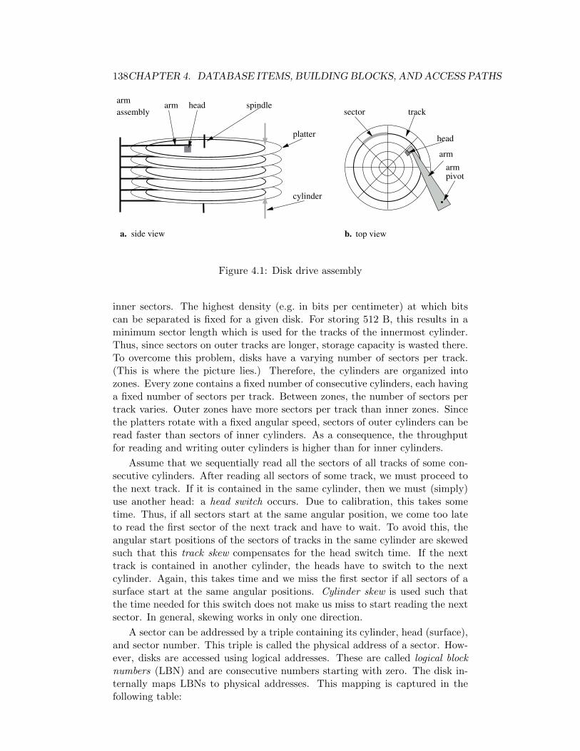
138CHAPTER 4. DATABASE ITEMS, BUILDING BLOCKS, AND ACCESS PATHS

armpivot

arm

assembly

top viewb.

platter

arm head spindle

cylinder

sector track

head

arm

side viewa.

Figure 4.1: Disk drive assembly

inner sectors. The highest density (e.g. in bits per centimeter) at which bitscan be separated is fixed for a given disk. For storing 512 B, this results in aminimum sector length which is used for the tracks of the innermost cylinder.Thus, since sectors on outer tracks are longer, storage capacity is wasted there.To overcome this problem, disks have a varying number of sectors per track.(This is where the picture lies.) Therefore, the cylinders are organized intozones. Every zone contains a fixed number of consecutive cylinders, each havinga fixed number of sectors per track. Between zones, the number of sectors pertrack varies. Outer zones have more sectors per track than inner zones. Sincethe platters rotate with a fixed angular speed, sectors of outer cylinders can beread faster than sectors of inner cylinders. As a consequence, the throughputfor reading and writing outer cylinders is higher than for inner cylinders.

Assume that we sequentially read all the sectors of all tracks of some con-secutive cylinders. After reading all sectors of some track, we must proceed tothe next track. If it is contained in the same cylinder, then we must (simply)use another head: a head switch occurs. Due to calibration, this takes sometime. Thus, if all sectors start at the same angular position, we come too lateto read the first sector of the next track and have to wait. To avoid this, theangular start positions of the sectors of tracks in the same cylinder are skewedsuch that this track skew compensates for the head switch time. If the nexttrack is contained in another cylinder, the heads have to switch to the nextcylinder. Again, this takes time and we miss the first sector if all sectors of asurface start at the same angular positions. Cylinder skew is used such thatthe time needed for this switch does not make us miss to start reading the nextsector. In general, skewing works in only one direction.

A sector can be addressed by a triple containing its cylinder, head (surface),and sector number. This triple is called the physical address of a sector. How-ever, disks are accessed using logical addresses. These are called logical blocknumbers (LBN) and are consecutive numbers starting with zero. The disk in-ternally maps LBNs to physical addresses. This mapping is captured in thefollowing table:

4.1. DISK DRIVE 139

Host sendscommand

Controllerdecodes it

Rotationallatency

Data transfer off mechanism

Status message to host

Read service time for disk 1

Read service time for disk 2

Disk 3

Disk 2

Disk 1

SCSI bus

Seek

Data transfer to host

Time

Figure 4.2: Disk drive read request processing

cylinder track LBN number of sectors per track

0 0 0 5731 573 573

. . . . . . . . . . . .5 2865 573

1 0 3438 573. . . . . . . . . . . .

15041 0 35841845 253. . . . . . . . . . . .

However, this ideal view is disturbed by the phenomenon of bad blocks. Abad block is one with a defect and it cannot be read or written. After a blockwith a certain LBN is detected to be bad, it is assigned to another sector. Theabove mapping changes. In order to be able redirect LBNs, extra space on thedisk must exist. Hence, some cylinders, tracks, and sectors are reserved for thispurpose. They may be scattered all over the platters. Redirected blocks causehiccups during sequential read.

Building (see e.g. [619]) and modeling (see e.g. [564, 720, 782, 783, 847, 893])disk drives is challenging. Whereas the former is not really important whenbuilding query compiler, the latter is, as we have to attach costs to query eval-uation plans. These costs reflect the amount of time we occupy the resourcedisk. Since disks are relatively slow, they may become the bottleneck of adatabase server. Modeling and minimizing disk access (time) is thus an im-portant topic. Consider the case where we want to read a block from a SCSIdisk. Simplified, the following actions take place and take their time (see alsoFig. 4.2):

1. The host sends the SCSI command.

2. The disk controller decodes the command and calculates the physicaladdress.

140CHAPTER 4. DATABASE ITEMS, BUILDING BLOCKS, AND ACCESS PATHS

3. During the seek the disk drive’s arm is positioned such that the accord-ing head is correctly placed over the cylinder where the requested blockresides. This step consists of several phases.

(a) The disk controller accelerates the arm.

(b) For long seeks, the arm moves with maximum velocity (coast).

(c) The disk controller slows down the arm.

(d) The disk arm settles for the desired location. The settle times differfor read and write requests. For reads, an aggressive strategy is used.If, after all, it turns out that the block could not be read correctly,we can just discard it. For writing, a more conservative strategy isin order.

4. The disk has to wait until the sector where the requested block residescomes under the head (rotation latency).

5. The disk reads the sector and transfers data to the host.

6. Finally, it sends a status message.

Note that the transfers for different read requests are interleaved. This is pos-sible since the capacity of the SCSI bus is higher than the read throughput ofthe disk. Also note that we did not mention the operating system delay andcongestions on the SCSI bus.

Disk drives apply several strategies to accelerate the above-mentioned round-trip time and access patterns like sequential read. Among them are caching,read-ahead, and command queuing. (discuss interleaving?)ToDo

The seek and rotation latency times highly depend on the head’s positionon the platter surface. Let us consider seek time. A good approximation of theseek time where d cylinders have to be travelled is given by

seektime(d) =

c1 + c2

√d d <= c0

c3 + c4d d > c0

where the constants ci are disk-specific. The constant c0 indicates the maximumnumber of cylinders where no coast takes place: seeking over a distance of morethan c0 cylinders results in a phase where the disk arm moves with maximumvelocity.

For disk accesses, the database system must be able to estimate the timethey take to be executed. First of all, we need the parameters of the disk. Itis not too easy to get hold of them, but we can make use of several tools toextract them from a given disk [234, 300, 834, 742, 905, 906]. However, then wehave a big problem: when calculating I/O costs, the query compiler has no ideawhere the head will be when the query evaluation plan emits a certain read (orwrite) command. Thus, we have to find another solution. In the following, wewill discuss a rather simplistic cost model that will serve us to get a feeling fordisk behavior. Later, we develop a more realistic model (Section 4.17).

The solution is rather trivial: we sum up all command sending and inter-preting times as well the times for positioning (seek and rotation latency) which

4.1. DISK DRIVE 141

form by far the major part. Let us call the result latency time. Then, we assumean average latency time. This, of course, may result in large errors for a singlerequest. However, on average, the error can be as “low” as 35% [720]. The nextparameter is the sustained read rate. The disk is assumed to be able to delivera certain amount of bytes per second while reading data stored consecutively.Of course, considering multi-zone disks, we know that this is oversimplified,but we are still in our simplistic model. Analogously, we have a sustained writerate. For simplicity, we will assume that this is the same as the sustained readrate. Last, the capacity is of some interest. A hypothetical disk (inspired bydisks available in 2004) then has the following parameters:

Model 2004

Parameter Value Abbreviated Name

capacity 180 GB Dcapaverage latency time 5 ms Dlatsustained read rate 100 MB/s Dsrrsustained write rate 100 MB/s Dswr

The time a disk needs to read and transfer n bytes is then approximated byDlat + n/Dsrr. Again, this is overly simplistic: (1) due to head switches andcylinder switches, long reads have lower throughput than short reads and (2)multiple zones are not modelled correctly. However, let us use this very sim-plistic model to get some feeling for disk costs.

Database management system developers distinguish between sequentialI/O and random I/O. For sequential I/O, there is only one positioning at thebeginning and then, we can assume that data is read with the sustained readrate. For random I/O, one positioning for every unit of transfer—typically apage of say 8 KB—is assumed. Let us illustrate the effect of positioning by asmall example. Assume that we want to read 100 MB of data stored consecu-tively on a disk. Sequential read takes 5 ms plus 1 s. If we read in blocks of8 KB where each block requires positioning then reading 100 MB takes 65 s.

Assume that we have a relation of about 100 MB in size, stored on a disk,and we want to read it. Does it take 1 s or 65 s? If the blocks on which it isstored are randomly scattered on disk and we access them in a random order,65 s is a good approximation. So let us assume that it is stored on consecutiveblocks. Assume that we read in chunks of 8 KB. Then,

• other applications,

• other transactions, and

• other read operations of the same query evaluation plan

could move the head away from our reading position. (Congestion on the SCSIbus may also be problem.) Again, we could be left with 65 s. Reading thewhole relation with one read request is a possibility but may pose problemsto the buffer manager. Fortunately, we can read in chunks much smaller than100 MB. Consider Figure 4.3. If we read in chunks of 100 8 KB blocks we arealready pretty close to one second (within a factor of two).

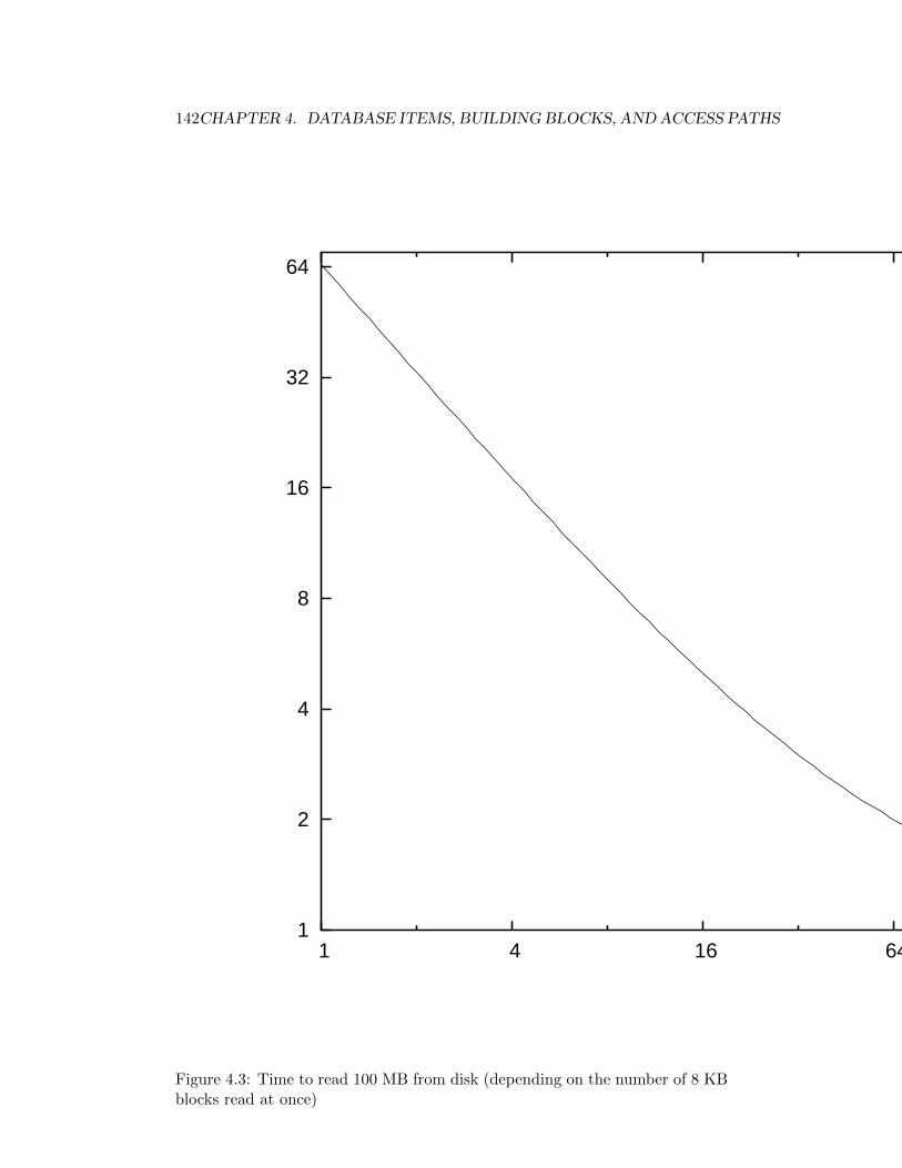
142CHAPTER 4. DATABASE ITEMS, BUILDING BLOCKS, AND ACCESS PATHS

1

2

4

8

16

32

64

1 4 16 64 256 1024

Figure 4.3: Time to read 100 MB from disk (depending on the number of 8 KBblocks read at once)

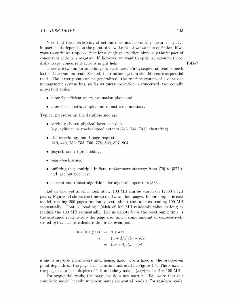
4.1. DISK DRIVE 143

Note that the interleaving of actions does not necessarily mean a negativeimpact. This depends on the point of view, i.e. what we want to optimize. If wewant to optimize response time for a single query, then obviously the impact ofconcurrent actions is negative. If, however, we want to optimize resource (here:disk) usage, concurrent actions might help. ToDo?

There are two important things to learn here. First, sequential read is muchfaster than random read. Second, the runtime system should secure sequentialread. The latter point can be generalized: the runtime system of a databasemanagement system has, as far as query execution is concerned, two equallyimportant tasks:

• allow for efficient query evaluation plans and

• allow for smooth, simple, and robust cost functions.

Typical measures on the database side are

• carefully chosen physical layout on disk(e.g. cylinder or track-aligned extents [743, 744, 741], clustering),

• disk scheduling, multi-page requests[219, 440, 752, 753, 760, 778, 809, 897, 904],

• (asynchronous) prefetching,

• piggy-back scans,

• buffering (e.g. multiple buffers, replacement strategy from [70] to [577]),and last but not least

• efficient and robust algorithms for algebraic operators [333].

Let us take yet another look at it. 100 MB can be stored on 12800 8 KBpages. Figure 4.4 shows the time to read n random pages. In our simplistic costmodel, reading 200 pages randomly costs about the same as reading 100 MBsequentially. That is, reading 1/64th of 100 MB randomly takes as long asreading the 100 MB sequentially. Let us denote by a the positioning time, sthe sustained read rate, p the page size, and d some amount of consecutivelystored bytes. Let us calculate the break-even point

n ∗ (a+ p/s) = a+ d/s

n = (a+ d/s)/(a+ p/s)

= (as+ d)/(as+ p)

a and s are disk parameters and, hence, fixed. For a fixed d, the break-evenpoint depends on the page size. This is illustrated in Figure 4.5. The x-axis isthe page size p in multiples of 1 K and the y-axis is (d/p)/n for d = 100 MB.

For sequential reads, the page size does not matter. (Be aware that oursimplistic model heavily underestimates sequential reads.) For random reads,

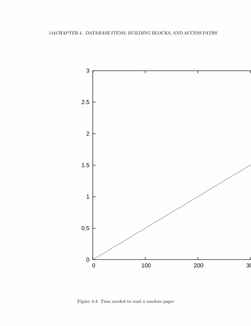
144CHAPTER 4. DATABASE ITEMS, BUILDING BLOCKS, AND ACCESS PATHS

0

0.5

1

1.5

2

2.5

3

0 100 200 300 400 500

Figure 4.4: Time needed to read n random pages

4.1. DISK DRIVE 145

8

16

32

64

128

256

512

1 2 4 8 16 32 64

Figure 4.5: Break-even point in fraction of total pages depending on page size

146CHAPTER 4. DATABASE ITEMS, BUILDING BLOCKS, AND ACCESS PATHS

as long as a single page is read, it matters neither: reading a single page of 1 KBlasts 5.0097656 ms, for an 8 KB page the number is 5.0781250 ms. From allthis, we could draw the conclusion that the larger the page the better. However,this is only true for the disk, not, e.g., for the buffer or the SCSI bus. If we needto access only 500 B of a page, then the larger the page the higher the fractionthat is wasted. This is not as severe as it sounds. Other queries or transactionsmight need other parts of the page during a single stay in the buffer. Let uscall the fraction of the page that is read by some transaction during a stay inthe buffer by utilization. Obviously, the higher the utilization the better is ourusage of the main memory in which the buffer resides. For smaller pages, theutilization is typically higher than for larger pages. The frequency by whichpages are used is another factor. [353, 354].

Excursion. Consider the root page of a B-tree. It is accessed quite frequentlyand most of its parts will be used, no matter how large it is. Hence, utilizationis always good. Thus, the larger the root page of a B-tree the better. On theother hand, consider a leaf page of a B-tree that is much bigger than mainmemory. During a single stay of it, only a small fraction of the page will beused. That is, smaller leaf pages are typically better. By converting everythingto money instead of time, Gray and Graefe [353] as well as Lomet [546] cometo the conclusion that a page size between 8 and 16 KB was a good choice atthe end of the last century.

For the less simplistic model of disk access costs developed in Section 4.17,we need to describe a disk drive by a set of parameters. These parameters aresummarized in Table 4.1.

Let us close this section by giving upper bounds on seek time and rotationallatency. Qyang proved the following theorem which gives a tight upper boundof disk seek time if several cylinders of a consecutive range of cylinders have tobe visited [677].

Theorem 4.1.1 (Qyang) If the disk arm has to travel over a region of Ccylinders, it is positioned on the first of the C cylinders and has to stop at s−1of them, then sDseek(C/s) is an upper bound for the seek time.

The time required for s consecutive sectors in a track of zone i to pass bythe head is

Drot(s, i) = sDZscan(i) = sDrot

DZspt(i)(4.1)

A trivial upper bound for the rotational delay is a full rotation.

4.2 Database Buffer

The database buffer

1. is a finite piece of memory,

2. typically supports a limited number of different page sizes (mostly one ortwo),

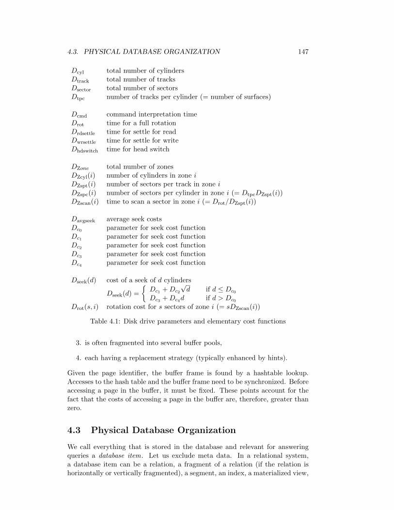
4.3. PHYSICAL DATABASE ORGANIZATION 147

Dcyl total number of cylindersDtrack total number of tracksDsector total number of sectorsDtpc number of tracks per cylinder (= number of surfaces)

Dcmd command interpretation timeDrot time for a full rotationDrdsettle time for settle for readDwrsettle time for settle for writeDhdswitch time for head switch

DZone total number of zonesDZcyl(i) number of cylinders in zone iDZspt(i) number of sectors per track in zone iDZspc(i) number of sectors per cylinder in zone i (= DtpcDZspt(i))DZscan(i) time to scan a sector in zone i (= Drot/DZspt(i))

Davgseek average seek costsDc0 parameter for seek cost functionDc1 parameter for seek cost functionDc2 parameter for seek cost functionDc3 parameter for seek cost functionDc4 parameter for seek cost function

Dseek(d) cost of a seek of d cylinders

Dseek(d) =

Dc1 +Dc2

√d if d ≤ Dc0

Dc3 +Dc4d if d > Dc0

Drot(s, i) rotation cost for s sectors of zone i (= sDZscan(i))

Table 4.1: Disk drive parameters and elementary cost functions

3. is often fragmented into several buffer pools,

4. each having a replacement strategy (typically enhanced by hints).

Given the page identifier, the buffer frame is found by a hashtable lookup.Accesses to the hash table and the buffer frame need to be synchronized. Beforeaccessing a page in the buffer, it must be fixed. These points account for thefact that the costs of accessing a page in the buffer are, therefore, greater thanzero.

4.3 Physical Database Organization

We call everything that is stored in the database and relevant for answeringqueries a database item. Let us exclude meta data. In a relational system,a database item can be a relation, a fragment of a relation (if the relation ishorizontally or vertically fragmented), a segment, an index, a materialized view,

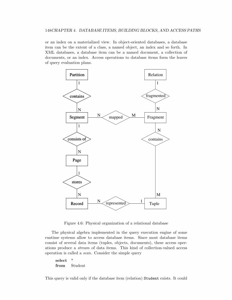
148CHAPTER 4. DATABASE ITEMS, BUILDING BLOCKS, AND ACCESS PATHS

or an index on a materialized view. In object-oriented databases, a databaseitem can be the extent of a class, a named object, an index and so forth. InXML databases, a database item can be a named document, a collection ofdocuments, or an index. Access operations to database items form the leavesof query evaluation plans.

Partition

Segment

Page

contains

consists of

Record

stores

Partition

Segment

Page

contains

consists of

Record

stores

Relation

Fragment

fragmented

contains

Tuplerepresented

mapped

1

N

1

1

M

N

1

N

N 1

M

N

N

N

Figure 4.6: Physical organization of a relational database

The physical algebra implemented in the query execution engine of someruntime systems allow to access database items. Since most database itemsconsist of several data items (tuples, objects, documents), these access oper-ations produce a stream of data items. This kind of collection-valued accessoperation is called a scan. Consider the simple query

select *from Student

This query is valid only if the database item (relation) Student exists. It could

4.3. PHYSICAL DATABASE ORGANIZATION 149

be accessible via a relation scan operation rscan(Student). However, inreality we have to consider the physical organization of the database.

Figure 4.6 gives an overview of how relations can be stored in a relationaldatabase system. Physical database items can be found on the left-hand side,logical database items on the right-hand side. A fraction of a physical disk isa partition. It can be an operating system file or a raw partition. A partitionis organized into several segments. A segment consists of several pages. Thepages within a segment are typically accessible by a non-negative integer in[0, n[, where n is the number of pages of the segment2. Iterative access to allpages of a segment is typically possible. The access is called a scan. As thereare several types of segments (e.g. data segments, index segments), several kindsof scans exist. Within a page, physical records are stored. Each physical recordrepresents a (part of a) tuple of a fragment of a relation.

Fragments are mapped to segments and relations are partitioned into frag-ments. In the simplest and most common organization, every relation has onlyone fragment with a one-to-one mapping to segments, and for every tuple thereexists exactly one record representing only this tuple. Hence, both of relation-ships mapped and represented are one-to-one. However, this organization doesnot scale well. A relation could be larger than a disk. Even if a large relation,say 180 GB fits on a disk, scanning it takes half an hour (Model 2004). Hori-zontal partitioning and allocation of the fragments on several disks reduces thescan time by allowing for parallelism. Vertical partitioning is another means ofreducing I/O [198]. Here, a tuple is represented by several physical records, eachone containing a subset of the tuple’s attributes. Since the relationship mappedis N:M, tuples from different relations can be stored in the same segment. Fur-thermore, in distributed database systems some fragments might be stored re-dundantly at different locations to improve access times [131, 494, 678, 638].Some systems support clustering of tuples of different relations. For exam-ple, department tuples can be clustered with employee tuples such that thoseemployees belonging to the department are close together and close to theirdepartment tuple. Such an organization speeds up join processing.

To estimate costs, we need a model of a segment. We assume an extent-based implementation. That is, a segment consists of several extents3. Eachextent occupies consecutive sectors on disk. For simplicity, we assume thatwhole cylinders belong to a segment. Then, we can model segments as follows.Each segment consists of a sequence of extents. Each extent is stored on con-secutive cylinders. Cylinders are exclusively assigned to a segment. We thendescribe each extent j as a pair (Fj , Lj) where Fj is the first and Lj the lastcylinder of a consecutive sequence of cylinders. A segment can then be describedby a sequence of such pairs. We assume that these pairs are sorted in ascendingorder. In such a description, an extent may include a zone boundary. Since costfunctions are dependent on the zone, we break up cylinder ranges that are notcontained in a single zone. The result can be described by a sequence of triples

2This might not be true. Alternatively, the pages of a partition can be consecutivelynumbered.

3Extents are not shown in Fig. 4.6. They can be included between Partitions and Segments.

150CHAPTER 4. DATABASE ITEMS, BUILDING BLOCKS, AND ACCESS PATHS

827

273 827

1

273 2

Figure 4.7: Slotted pages and TIDs

(Fi, Li, zi) where Fi and Li mark a range of consecutive cylinders in a zone zi.Although the zi’s can be inferred from the cylinder numbers, we include themfor clarity. Also of interest are the total number of sectors in a segment and thenumber of cylinders Scpe(i) in an extent i. Summarizing, we describe a segmentby the parameter given in Table 4.2.

Sext number of extents in the segment

Ssec total number of sectors in the segment (=∑Sext

i=1 Scpe(i)DZspc(Szone(i)))Sfirst(i) first cylinder in extent iSlast(i) last cylinder in extent iScpe(i) number of cylinders in extent i (= Slast(i)− Sfirst(i) + 1)Szone(i) zone of extent i

Table 4.2: Segment parameters

4.4 Slotted Page and Tuple Identifier (TID)

Let us briefly review slotted pages and the concept of tuple identifiers (TIDs)(see Figure 4.7) [41, 40, 547, 816]. Sometimes, record identifer or row identifier(RID) is used in the literature. A TID consists of (at least) two parts. Thefirst part identifies a page, the second part a slot on a slotted page. The slotcontains—among other things, e.g. the record’s size—a (relative) pointer to theactual record. This way, the record can be moved within the page withoutinvalidating its TID. When a record grows beyond the available space, it ismoved to another page and leaves a forward pointer (again consisting of a pageand a slot identifier) in its original position. This happened to the TID [273, 1]in Figure 4.7. If the record has to be moved again, the forward pointer isadjusted. This way, at most two page accesses are needed to retrieve a record,given its TID. For evaluating the costs of record accesses, we will assume that

4.5. PHYSICAL RECORD LAYOUTS 151

827

273 827

1

273 2

Figure 4.8: Various physical record layouts

the fraction of moved records is known.

4.5 Physical Record Layouts

A physical record represents a tuple, object, or some other logical entity orfraction thereof. In case it represents a tuple, it consists of several fields, eachrepresenting the value of an attribute. These values can be integers, floatingpoint numbers, or strings. In case of object-oriented or object-relational sys-tems, the values can also be of a complex type. Tuple identifiers are also possibleas attribute values [701]. This can, for example, speed up join processing.

In any case, we can distinguish between types whose values all exhibit thesame fixed length and those whose values may vary in length. In a physicalrecord, the values of fixed-length attributes are concatenated and the offsetfrom the beginning of the record to the value of some selected attribute canbe inferred from the types of the values preceding it. This differs for valuesof varying length. Here, several encodings are possible. Some simple ones aredepicted in Figure 4.8. The topmost record encodes varying length values as asequence of pairs of the form [size, value]. This encoding has the disadvantagethat access to an attribute of varying length is linear in the number of thosepreceding it. This disadvantage is avoided in the solution presented in themiddle. Instead of storing the sizes of the individual values, there is an arraycontaining relative offsets into the physical record. They point to the start ofthe values. The length of the values can be inferred from these offsets and,in case of the last value, from the total length of the physical record, which istypically stored in its slot. Access to a value of varying size is now simplified toan indirect memory access plus some length calculations. Although this might

152CHAPTER 4. DATABASE ITEMS, BUILDING BLOCKS, AND ACCESS PATHS

be cheaper than the first solution, there is still a non-negligible cost associatedwith an attribute access.

The third physical record layout can be used to represent compressed at-tribute values and even compressed length information for parts of varying size.Note that if fixed size fields are compressed, their length becomes varying. Ac-cess to an attribute now means decompressing length/offset information anddecompressing the value itself. The former is quite cheap: it boils down to anindirect memory access with some offset taken from a matrix [888]. The costof the latter depends on the compression scheme used. It should be clear thataccessing an attribute value now is even more expensive. To make the costs ofan attribute access explicit was the sole purpose of this small section.

Remark Westmann et al. discuss an efficient implementation of compres-sion and evaluate its performance [888]. Yiannis and Zobel report on experi-ments with several compression techniques used to speed up the sort operator.For some of them, the CPU usage is twice as large [?].

4.6 Physical Algebra (Iterator Concept)

Physical algebraic operators are mostly implemented as iterators. This meansthat they support the the interface operations open, next, and close. Withopen, the stream of items (e.g. tuples) is initialized. With next, the next itemon the stream is fetched. When no more items are available, e.g. next returnsfalse, close can be called to clean up things. The iterator concept is explainedin many text books (e.g. [305, 389, 464]) and the query processing survey byGraefe [333]. This basic iterator concept has been extended to better copewith nested evaluation by Westmann in his thesis [886], Westmann et al. [888],and Graefe [337]. The two main issues are separation of storage allocation andinitialization, and batched processing. The former splits open into resourceallocation, initialization of the operator, and initialization of the iterator.

4.7 Simple Scan

Let us come back to the scan operations. A logical operation for scanning rela-tions (which could be called rscan) is rarely supported by relational databasemanagement systems. Instead, they provide (physical) scans on segments. Sincea (data) segment is sometimes called file, the correct plan for the above queryis often denoted by fscan(Student). Several assumptions must hold: theStudent relation is not fragmented, it is stored in a single segment, the nameof this segment is the same as the relation name, and no tuples from otherrelations are stored in this segment. Until otherwise stated, we will assumethat relations are not partitioned, are stored in a single segment and that thesegment can be inferred from the relation’s name. Instead of fscan(Student),we could then simply use Student to denote leaf nodes in a query executionplan. If we want to use a variable that is bound subsequently to each tuple ina relation, the query

select *

4.8. SCAN AND ATTRIBUTE ACCESS 153

from Student

can be expressed as Student[s] instead of Student. In this notation, the outputstream contains tuples having a single attribute s bound to a tuple. Physically,s will not hold the whole tuple but, for example, a pointer into the buffer wherethe tuple can be found. An alternative is a pointer to a slot of a slotted pagecontained in the buffer.

A simple scan is an example for a building block . In general, a buildingblock is something that is used as a bottommost operator in a query evaluationplan. Hence, every leaf node of a query evaluation plan is a building block ora part thereof. This is not really a sharp definition, but is sometimes usefulto describe the behavior of a query compiler: after their determination, it willleave building blocks untouched even if reorderings are hypothetically possible.Although a building block can be more than a leaf node (scan) of a queryevaluation plan, it will never include more than a single database item. Assoon as more database items are involved, we use the notion of access path, aterm which will become more precise later on when we discuss index usage.

The disk access costs for a simple scan can be derived from the considera-tions in Section 4.1 and Section 4.17.

4.8 Scan and Attribute Access

Strictly speaking, a plan like σage>30(Student[s]) is invalid, since the tuplestream produced by Student[s] contains tuples with a single attribute s. Wehave a choice. Either we assume that attribute access takes place implicitly, orwe make it explicit. Whether this makes sense or not depends on the databasemanagement system for which we generate plans. Let us discuss the advantagesof explicit attribute retrieval. Assume s.age retrieves the age of a student.Then we can write σs.age>30(Student[s]), where there is some non-neglectablecost for s.age. The expression σs.age>30∧s.age<40(Student[s]) executes s.age

twice. This is a bad idea. Instead, we would like to retrieve it once and reuseit later.

This purpose is well-served by the map operator (χ). It adds new attributesto a given tuple and is defined as

χa1:e1,...,an:en(e) := t [a1 : c1, . . . , an : cn]|t ∈ e, ci = ei(t) ∀ (1 ≤ i ≤ n)

where denotes tuple concatenation and the ai must not be in A(e). (Remem-ber that A(e) is the set of attributes produced by e.) Every input tuple t isextended by new attributes ai, whose values are computed by evaluating theexpression ei, in which free variables (attributes) are bound to the attributes(variables) provided by t.

The above problem can now be solved by

σage>30∧age<40(χage:s.age(Student[s])).

154CHAPTER 4. DATABASE ITEMS, BUILDING BLOCKS, AND ACCESS PATHS

In general, it is beneficial to load attributes as late as possible. The latest pointat which all attributes must be read from the page is typically just before apipeline breaker4.

To see why this is useful, consider the simple query

select namefrom Studentwhere age > 30

The plan

Πn(χn:s.name(σa>30(χa:s.age(Student[s]))))

makes use of this feature, while

Πn(σa>30(χn:s.name,a:s.age(Student[s])))

does not. In the first plan the name attribute is only accessed for those studentswith age over 30. Hence, it should be cheaper to evaluate. If the databasemanagement system does not support this selective access mechanism, we oftenfind the scan enhanced by a list of attributes that is projected and included inthe resulting tuple stream.

In order to avoid copying attributes from their storage representation tosome main memory representation, some database management systems applyanother mechanism. They support the evaluation of some predicates directlyon the storage representation. These are boolean expressions consisting of sim-ple predicates of the form Aθc for attributes A, comparison operators θ, andconstants c. Instead of a constant, c could also be the value of some attributeor expression thereof given that it can be evaluated before the access to A.

Predicates evaluable on the disk representation are called SARGable whereSARG is an acronym for search argument . Note that SARGable predicatesmay also be good for index lookups. Then they are called index SARGable.In case they can not be evaluated by an index, they are called data SARGable[755, 832, 311].

Since relation or segment scans can evaluate predicates, we have to extendour notation for scans. Let I be a database item like a relation or segment.Then, I[v; p] scans I, binds each item in I successively to v and returns onlythose items for which p holds. I[v; p] is equivalent to σp(I[v]), but cheaper toevaluate. If p is a conjunction of predicates, the conjuncts should be orderedsuch that the attribute access cost reductions described above are reflected(for details see Chapter ??). Syntactically, we express this by separating thepredicates by a comma as in Student[s; age > 30, name like ‘%m%′]. If we wantto make a distinction between SARGable and non-SARGable predicates, wewrite I[v; ps; pr], with ps being the SARGable predicate and pr a non-SARGablepredicate. Additional extensions like a projection list are also possible.

4The page on which the physical record resides must be fixed until all attributes are loaded.Hence, an earlier point in time might be preferable.

4.9. TEMPORAL RELATIONS 155

4.9 Temporal Relations

Scanning a temporal relation or segment also makes sense. Whenever the resultof some (partial) query evaluation plan is used more than once, it might beworthwhile to materialize it in some temporary relation. For this purpose, atmp operator evaluates its argument expression and stores the result relation ina temporary segment. Consider the following example query.

select e.name, d.namefrom Emp e, Dept dwhere e.age > 30 and e.age < 40 and e.dno = d.dno

It can be evaluated by

Dept[d] Bnle.dno=d.dno σe.age>30∧e.age<40(Emp[d]).

Since the inner (right) argument of the nested-loop join is evaluated severaltimes (once for each department), materialization may pay off. The plan thenlooks like

Dept[d] Bnle.dno=d.dno Tmp(σe.age>30∧e.age<40(Emp[d])).

If we choose to factorize and materialize a common subexpression, the queryevaluation plan becomes a DAG. Alternatively, we could write a small “pro-gram” that has some statements materializing some expressions which are thenused later on. The last expression in a program determines its result. For ourexample, the program looks as follows.

1. Rtmp = σe.age>30∧e.age<40(Emp[d]);

2. Dept[d] Bnle.dno=d.dno Rtmp[e]

The disk costs of writing and reading temporary relations can be calculatedusing the considerations of Section 4.1.

4.10 Table Functions

A table function is a function that returns a relation [554]. An example isPrimes(int from, int to), which returns all primes between from and to,e.g. via a sieve-method. It can be used in any place where a relation name canoccur. The query

select *from TABLE(Primes(1,100)) as p

returns all primes between 1 and 100. The attribute names of the resultingrelation are specified in the declaration of the table function. Let us assumethat for Primes a single attribute prime is specified. Note that table func-tions may take parameters. This does not pose any problems, as long as we

156CHAPTER 4. DATABASE ITEMS, BUILDING BLOCKS, AND ACCESS PATHS

know that Primes is a table function and we translate the above query intoPrimes(1, 100)[p]. Although this looks exactly like a table scan, the implemen-tation and cost calculations are different.

Consider the following query where we extract the years in which we expecta special celebration of Anton’s birthday.

select *from Friends f,

TABLE(Primes(CURRENT YEAR, EXTRACT(YEAR FROM f.birthday) + 100)) as p

where f.name = ‘Anton’

The result of the table function depends on our friend Anton. Hence, a joinis no solution. Instead, we have to introduce a new kind of join, the d-joinwhere the d stands for dependent. It is defined as

R < S >= t s|t ∈ T, s ∈ S(t).

The above query can now be evaluted as

χb:EXTRACT Y EAR(f.birthday)+100(σf.name=‘Anton′(Friends[f ])) < Primes(c, b)[p] >

where we assume that some global entity c holds the value of CURRENT YEAR.Let us do the above query for all friends. We just have to drop the where

clause. Obviously, this results in many redundant computations of primes. Atthe SQL level, using the birthday of the youngest friend is beneficial:

select *from Friends f,

TABLE(Primes(CURRENT YEAR, (select max(birthday) from Friends) + 100)) as p

where p.prime ≥ f.birthday

At the algebraic level, this kind of optimizations will be considered in Section ??.Things can get even more involved if table functions can consume and pro-

duce relations, i.e. arguments and results can be relations.ToDo?Little can be said about the disk costs of table functions. They can be zero

if the function is implemented such that it does not access any disks (files storedthere), but it can also be very expensive if large files are scanned each time it iscalled. One possibility is to let the database administrator specify the numbersthe query optimizer needs. However, since parameters are involved, this isnot really an easy task. Another possibility is to measure the table function’sbehavior whenever it is executed, and learn about its resource consumption.

4.11 Indexes

There exists a plethora of different index structures. In the context of relationaldatabase management systems, the most versatile and robust index is the B-tree or variants/improvements thereof (e.g. []). It is implemented in almost

4.11. INDEXES 157

Figure 4.9: Clustered vs. non-clustered index

every commercial database management system. Some support hash-indexes(e.g. []). Other data models or specific applications need specialized indexes.There exist special index structures for indexing path expressions in object-oriented databases (e.g. []) and XML databases (e.g. []). Special purpose indexesinclude join indexes (e.g. [387, 859]) multi-dimensional indexes (e.g. []), variant(projection) indexes [624], small materialized aggregates [591], bitmap indexes[], and temporal indexes (e.g. []). We cannot discuss all indexes and theirexploitations for efficient query evaluation. This fills more than a single book.Instead, we concentrate on B-tree indexes. In general, a B-tree can be usedto index several relations. We only discuss cases where B-trees index a singlerelation.

The search key (or key for short) of an index is the sequence of attributesof the indexed relation over which the index is defined. A key is a simple key ifit consists of a single attribute. Otherwise, it is a complex key . Each entry inthe B-tree’s leaf page consists of pairs containing the key values and a sequenceof tuple identifiers (typically sorted by increasing page number). Every tuplewith a TID in this list satisfies the condition that its indexed attribute’s valuesare equal to the key values. If for every sequence of key values there is at mostone such tuple, we have a unique index, otherwise a non-unique index .

The leaf entries may contain values from additional (non-key) attributes.Then we call the index attribute data added and the additional attributes dataattributes. If the index contains all attributes of the indexed relation—in itskey or data attributes—storing the relation is no longer necessary. The result isan index-only relation. In this case, the concept of tuple identifiers is normallyno longer used since tuples can now be moved frequently, e.g. due to a leaf pagesplit. This has two consequences. First, the data part does not longer containthe TID. Second, other indexes on the index-only relation cannot have tupleidentifiers in their data part either. Instead, they use the key of the index-onlyrelation to uniquely reference a tuple. For this to work, we must have a uniqueindex.

B-trees can be either clustered or non-clustered indexes. In a clustered index,the tuple identifiers in the list of leaf pages are ordered according to their page

158CHAPTER 4. DATABASE ITEMS, BUILDING BLOCKS, AND ACCESS PATHS

numbers. Otherwise, it is a non-clustered index5. Figure 4.9 illustrates this.Range queries result in sequential access for clustered indexes and in randomaccess for non-clustered indexes.

4.12 Single Index Access Path

4.12.1 Simple Key, No Data Attributes

Consider the exact match query

select namefrom Empwhere eno = 1077

If there exists a unique index on the key attribute eno, we can first access theindex to retrieve the TID of the employee tuple satisfying eno = 1077. Anotherpage access yields the tuple itself which constitutes the result of the query. LetEmpeno be the index on eno, then we can descend the B-tree, using 1077 as thesearch key. A predicate that can be used to descend the B-tree or, in general,governing search within an index structure, is called an index sargable predicate.

For the example query, the index scan, denoted as Empeno[x; eno = 1077],retrieves a single leaf node entry with attributes eno and TID. Similar to theregular scan, we assume x to be a variable holding a pointer to this indexentry. We use the notations x.eno and x.TID to access these attributes. Todereference the TID, we use the map (χ) operator and a dereference functionderef (or ∗ for short). It turns a TID into a pointer in the buffer area. This ofcourse requires the page to be loaded, if it is not in the buffer yet. The completeplan for the query is

Πname(χe:∗(x.TID),name:e.name(Empeno[x; eno = 1077]))

where we computed several new attributes with one χ operator. Note thatthey are dependent on previously computed attributes and, hence, the order ofevaluation does matter.

We can make the dependency of the map operator more explicit by applyinga d-join. Denote by 2 an operator that returns a single empty tuple. Then

Πname(Empeno[x; eno = 1077] < χe:∗(x.TID),name:e.name(2) >)

is equivalent to the former plan. Joins and indexes will be discussed in Sec-tion 4.14.

A range query like

select namefrom Empwhere age ≥ 25 and age ≤ 35

5Of course, any degree of clusteredness may occur and has to be taken into account in costcalculations.

4.12. SINGLE INDEX ACCESS PATH 159

specifies a range for the indexed attribute. It is evaluated by an index scanwith start and stop conditions. In our case, the start condition is age ≥ 25,and the stop condition is age ≤ 35. The start condition is used to retrieve thefirst tuple satisfying it by searching within the B-tree. In our case, 25 is used todescend from the root to the leaf page containing the key 25. Then, all recordswith keys larger than 25 within the page are searched. Since entries in B-treepages are sorted on key values, this is very efficient. If we are done with theleaf page that contains 25 and the stop key has not been found yet, we proceedto the next leaf page. This is possible since leaf pages of B-trees tend to bechained. Then all records of the next leaf page are scanned and so on until wefind the stop key. The complete plan then is

Πname(χe:∗(x.TID),name:e.name(Empage[x; 25 ≤ age; age ≤ 35]))

If the index on age is non-clustered, this plan results in random I/O. Wecan turn random I/O into sequential I/O by sorting the result of the index scanon its TID attribute before dereferencing it6. This results in the following plan:

Πname(χe:∗(TID),name:e.name(SortTID(Empage[x; 25 ≤ age; age ≤ 35; TID])))

Here, we explicitly included the TID attribute of the index into the projectionlist.

Consider a similar query which demands the output to be sorted:

select name, agefrom Empwhere age ≥ 25 and age ≤ 35order by age

Since an index scan on a B-tree outputs its result ordered on the indexed at-tribute, the following plan produces the perfect result:

Πname,age(χe:∗(x.TID),name:e.name(Empage[x; 25 ≤ age; age ≤ 35]))

On a clustered index this is most probably the best plan. On a non-clusteredindex, random I/O disturbs the picture. We avoid that by sorting the result ofthe index scan on the TID attribute and, after accessing the tuples, restore theorder on age as in the following plan:

Πname,age(Sortage(χe:∗(TID),name:e.name(SortTID(Empage[x; 25 ≤ age; age ≤ 35; TID]))))

An alternative to this plan is not to sort on the original indexed attribute (agein our example), but to introduce a new attribute that holds the rank in thesequence derived from the index scan. This leads to the plan

Πname,age(Sortrank(χe:∗(TID),name:e.name(

SortTID(χrank:counter++(

Empage[x; 25 ≤ age; age ≤ 35; TID])))))

6This might not be necessary, if Emp fits main memory. Then, preferably asynchronous I/Oshould be used.

160CHAPTER 4. DATABASE ITEMS, BUILDING BLOCKS, AND ACCESS PATHS

This alternative might turn out to be more efficient since sorting on an attributewith a dense domain can be implemented efficiently. (We admit that in theabove example this is not worth considering.) There is another importantapplication of this technique: XQuery often demands output in document order.If this order is destroyed during processing, it must at the latest be restoredwhen the output it produced [569]. Depending on the implementation (i.e. therepresentation of document nodes or their identifiers), this might turn out tobe a very expensive operation.

The fact that index scans on B-trees return their result ordered on theindexed attributes is also very useful if a merge-join on the same attributes (ora prefix thereof, see Chapter 23 for further details) occurs. An example followslater on.

Some predicates are not index SARGable, but can still be evaluated withthe index as in the following query

select namefrom Empwhere age ≥ 25 and age ≤ 35 and age 6= 30

The predicate age 6= 30 is an example of a residual predicate. We can oncemore extend the index scan and compile the query into

Πname(χt:x.TID,e:∗t,name:e.name(Empage[x; 25 ≤ age; age ≤ 35; age 6= 30]))

Some index scan implementations allow exclusive bounds for start and stopconditions. With them, the query

select namefrom Empwhere age > 25 and age < 35

can be evaluated using

Πname(χt:x.TID,e:∗t,name:e.name(Empage[x; 25 < age; age < 35]))

If this is not the case, two residual predicates must be used as in

Πname(χt:x.TID,e:∗t,name:e.name(Empage[x; 25 ≤ age; age ≤ 35; age 6= 25, age 6= 35]))

Especially for predicates on strings, this might be expensive.Start and stop conditions are optional. To evaluate

select namefrom Empwhere age ≥ 60

we use age ≥ 60 as the start condition to find the leaf page containing the key60. From there on, we scan all the leaf pages “to the right”.

If we have no start condition, as in

4.12. SINGLE INDEX ACCESS PATH 161

select namefrom Empwhere age ≤ 20

we descend the B-tree to the “leftmost” page, i.e. the page containing thesmallest key value, and then proceed scanning leaf pages until we encounter thekey 20.

Having neither a start nor stop condition is also quite useful. The query

select count(*)from Emp

can be evaluated by counting the entries in the leaf pages of a B-tree. Sincea B-tree typically occupies far fewer pages than the original relation, we havea viable alternative to a relation scan. The same applies to the aggregatefunctions sum and avg. The other aggregate functions min and max can beevaluated much more efficiently by descending to the leftmost or rightmost leafpage of a B-tree. This can be used to answer queries like

select min/max(salary)from Emp

much more efficiently than by a relation scan. Consider the query

select namefrom Empwhere salary = (select max(salary)

from Emp)

It can be evaluated by first computing the maximum salary and then retrievingthe employees earning this salary. This requires two descendants into the B-tree, while obviously one is sufficient. Depending on the implementation of theindex (scan), we might be able to perform this optimization.

Further, the result of an index scan, whether it uses start and/or stop con-ditions or not, is always sorted on the key. This property can be useful forqueries with no predicates. If we have neither a start nor a stop condition, theresulting scan is called full index scan. As an example consider the query

select salaryfrom Emporder by salary

which is perfectly answered by the following full index scan:

Empsalary

So far, we have only seen indexes on numerical attributes.

162CHAPTER 4. DATABASE ITEMS, BUILDING BLOCKS, AND ACCESS PATHS

select name, salaryfrom Empwhere name ≥ ’Maaa’

gives rise to a start condition ′Maaa′ ≤ name. From the query

select name, salaryfrom Empwhere name like ’M%’

we can deduce the start condition ′M′ ≤ name.To express all the different alternatives of index usage, we need a powerful

(and runtime system dependent) index scan expression. Let us first summarizewhat we can specify for an index scan:

1. the name of the variable for index entries (or pointers to them),

2. the start condition,

3. the stop condition,

4. a residual predicate, and

5. a projection list.

A projection list has entries of the form a : x.b for attribute names a and b andx being the name of the variable for the index entry. a : x.a is also allowed andoften abbreviated as a. We also often summarize start and stop conditions intoa single expression like in 25 ≤ age ≤ 35.

For a full index specification, we list all items in the subscript of the indexname separated by a semicolon. Still, we need some extensions to express thequeries with aggregation. Let a and b be attribute names, then we allow entriesof the form b : aggr(a) in the projection list and start/stop conditions of theform min/max(a). The latter tells us to minimize/maximize the value of theindexed attribute a. Only a complete enumeration gives us the full details. Onthe other hand, extracting start and stop conditions and residual predicatesfrom a given boolean expression is rather simple. Hence, we often summarizethese three under a single predicate. This is especially useful when talkingabout index scans in general. If we have a full index scan, we leave out thepredicate. We use a star ‘*’ as an abbreviated projection list that projects allattributes of the index. (So far, these are the key attribute and the TID.) Ifthe projection list is empty, we assume that only the variable/attribute holdingthe pointer to the index entry is projected.

Using this notation, we can express some plan fragments. These fragmentsare complete plans for the above queries, except that the final projection is notpresent. As an example, consider the following fragment:

χe:∗TID,name:e.name(Empsalary[x; TID, salary])

All the plan fragments seen so far are examples of access paths. An accesspath is a plan fragment with building blocks concerning a single database item.

4.12. SINGLE INDEX ACCESS PATH 163

Hence, every building block is an access path. The above plans touch twodatabase items: a relation and an index on some attribute of that relation.If we say that an index concerns the relation it indexes, such a fragment is anaccess path. For relational systems, the most general case of an access path usesseveral indexes to retrieve the tuples of a single relation. We will see examplesof these more complex access paths in the following section. An access to theoriginal relation is not always necessary. A query that can be answered solelyby accessing indexes is called an index only query .

A query with in like

select namefrom Empwhere age in 28, 29, 31, 32

can be evaluated by taking the minimum and the maximum found in the left-hand side of in as the start and stop conditions. We further need to constructa residual predicate. The residual predicate can be represented either as age =28 ∨ age = 29 ∨ age = 31 ∨ age = 32 or as age 6= 30.

An alternative is to use a d-join. Consider the example query

select namefrom Empwhere salary in 1111, 11111, 111111

Here, the numbers are far apart and separate index accesses might make sense.Therefore, let us create a temporary relation Sal equal to [s : 1111], [s :11111], [s : 111111]. When using it, the access path becomes

Sal[S] < χe:∗TID,name:e.name(Empsalary[x; salary = S.s; TID]) >

Some B-tree implementations allow efficient searches for multiple ranges andimplement gap skipping [33, 34, 162, 311, 312, 457, 524]. Gap skipping, some-times also called zig-zag skipping , continues the search for keys in a new keyrange from the latest position visited. The implementation details vary butthe main idea of it is that after one range has been completely scanned, thecurrent (leaf) page is checked for its highest key. If it is not smaller than thelower bound of the next range, the search continues in the current page. If itis smaller than the lower bound of the next range, alternative implementationsare described in the literature. The simplest is to start a new search from theroot for the lower bound. Another alternative uses parent pointers to go up apage as long as the highest key of the current page is smaller than the lowerbound of the next range. If this is no longer the case, the search continuesdownwards again.

Gap skipping gives even more opportunities for index scans and allows effi-cient implementations of various index nested loop join strategies.

4.12.2 Complex Keys and Data Attributes

In general, an index can have a complex key comprised of the key attributesk1, . . . , kn and the data attributes d1, . . . , dm. One possibility is to use a full

164CHAPTER 4. DATABASE ITEMS, BUILDING BLOCKS, AND ACCESS PATHS

index scan on such an index. Having more attributes in the index makes itmore probable that queries are index-only.

Besides a full index scan, the index can be descended to directly search forthe desired tuple(s). Let us take a closer look at this possibility.

If the search predicate is of the form

k1 = c1 ∧ k2 = c2 ∧ . . . ∧ kj = cj

for some constants ci and some j <= n, we can generate the start and stopcondition

k1 = c1 ∧ . . . ∧ kj = cj .

This simple approach is only possible if the search predicates define values forall search key attributes, starting from the first search key and then for allkeys up to the j-th search key with no key attribute unspecified in between.Predicates concerning the other key attributes after the first non-specified keyattribute and the additional data attributes only allow for residual predicates.This condition is often not necessary for multi-dimensional index structures,whose discussion is beyond the book.

With ranges things become more complex and highly dependent on theimplementation of the facilities of the B-tree. Consider a query predicate re-stricting key values as follows

k1 = c1 ∧ k2 ≥ c2 ∧ k3 = c3

Obviously, we can generate the start condition k1 = c1 ∧ k2 ≥ c2 and the stopcondition k1 = c1. Here, we neglected the condition on k3 which becomes aresidual predicate. However, with some care we can extend the start conditionto k1 = c1 ∧ k2 ≥ c2 ∧ k3 = c3: we only have to keep k3 = c3 as a residualpredicate, since for k2 values larger than c2, values different from c3 can occurfor k3.

If closed ranges are specified for a prefix of the key attributes as in

a1 ≤ k1 ≤ b1 ∧ . . . ∧ aj ≤ kj ≤ bj

we can generate the start key k1 = a1 ∧ . . . ∧ kj = aj , the stop key k1 =b1 ∧ . . . ∧ kj = bj , and

a2 ≤ k2 ≤ b2 ∧ . . . ∧ aj ≤ kj ≤ bj

as the residual predicate. If for some search key attribute kj the lower bound ajis not specified, the start condition cannot contain kj and any kj+i. If for somesearch key attribute kj the upper bound bj is not specified, the stop conditioncannot contain kj and any kj+i.

Two further enhancements of the B-tree functionality possibly allow foralternative start/stop conditions:

• The B-tree implementation allows to specify the order (ascending or de-scending) for each key attribute individually.

4.13. MULTI INDEX ACCESS PATH 165

• The B-tree implementation implements forward and backward scans (e.g.implemented in Rdb [33]).

So far, we are only able to exploit query predicates which specify valueranges for a prefix of all key attributes. Consider querying a person on his/herheight and his/her hair color: haircolor = ’blond’ and height between

180 and 190. If we have an index on sex, haircolor, height, this indexcannot be used by means of the techniques described so far. However, sincethere are only the two values male and female available for sex, we can rewritethe query predicate to (sex = ’m’ and haircolor = ’blond’ and height

between 180 and 190) or (sex = ’f’ and haircolor = ’blond’ and height

between 180 and 190) and use two accesses to the index. This approach worksfine for attributes with a small domain and is described by Antoshenkov [34].(See also the previous section for gap skipping.) Since the possible values forkey attributes may not be known to the query optimizer, Antoshenkov goesone step further and shifts the construction of search ranges to index scan time.Therefore, the index can be provided with a complex boolean expression whichis then refined (rewritten) as soon as search key values become known. Searchranges are then generated dynamically, and gap skipping is applied to skip theintervals between the qualifying ranges during the index scan.

4.13 Multi Index Access Path

We wish to buy a used digital camera and state the following query:

select *from Camerawhere megapixel > 5 and distortion < 0.05

and noise < 0.01and zoomMin < 35 and zoomMax > 105

We assume that on every attribute used in the where clause there exists anindex. Since the predicates are conjunctively connected, we can use a techniquecalled index and-ing. Every index scan returns a set (list) of tuple identifiers.These sets/lists are then intersected. This operation is also called And merge[541]. Using index and-ing, a possible plan is

((((Cameramegapixel[c; megapixel > 5; TID]∩Cameradistortion[c; distortion < 0.05; TID])∩Cameranoise[c; noise < 0.01; TID])∩CamerazoomMin[c; zoomMin < 35; TID])∩CamerazoomMax[c; zoomMax > 105; TID])

166CHAPTER 4. DATABASE ITEMS, BUILDING BLOCKS, AND ACCESS PATHS

This results in a set of tuple identifiers that only needs to be dereferenced toaccess the according Camera tuples and produce the final result.

Since the costs of the expression clearly depend on the costs of the indexscans and the size of the intermediate TID sets, two questions arise:

• In which order do we intersect the TID sets resulting from the indexscans?

• Do we really apply all indexes before dereferencing the tuple identifiers?

The answer to the latter question is clearly “no”, if the next index scan ismore expensive than accessing the records in the current TID list. It can beshown that the indexes in the cascade of intersections are ordered on increasing(fi − 1)/ci terms, where fi is the selectivity of the index and ci its accesscost. Further, we can stop as soon as accessing the original tuples in the baseEXrelation becomes cheaper than intersecting with another index and subsequentlyaccessing the base relation.

Index or-ing is used to process disjunctive predicates. Here, we take theunion of the TID sets to produce a set of TIDs containing references to allqualifying tuples. Note that duplicates must be eliminated during the process-ing of the union. This operation is also called Or merge [541]. Consider thequery

select *from Empwhere yearsOfEmployment ≥ 30

or age ≥ 65

This query can be answered by constructing a TID set using the expression

EmpyearsOfEmployment[c; yearsOfEmployment ≥ 30; TID]∪Empage[c; age ≥ 65; TID]

and then dereferencing the list of tuple identifiers. Again, the index accessingcan be ordered for better performance. Given a general boolean expressionin and and or, constructing the optimal access path using index and-ing andor-ing is a challenging task that will be discussed in Chapter ??. This taskis even more challenging, if some simple predicates occur more than once inthe complex boolean expression and factorization has to be taken into account.This issue was first discussed by Chaudhuri, Ganesan and Saragawi [143]. Wewill come back to this in Chapter ??.

The names index and-ing and or-ing become clear if bitmap indexes areconsidered. Then the bitwise and and or operations can be used to efficientlycompute the intersection and union.ToDo

Excursion on bitmap indexes. 2

There are even more possibilities to work with TID sets. Consider the query

select *from Empwhere yearsOfEmployment 6= 10

and age ≥ 65

4.14. INDEXES AND JOINS 167

This query can be evaluated by scanning the index on age and then eliminatingall employees with yearsOfEmployment = 10:

Empage[c; age ≥ 65; TID]\EmpyearsOfEmployment[c; yearsOfEmployment 6= 10; TID]

Let us call the application of set difference on index scan results index differ-encing.

Some predicates might not be very restrictive in the sense that more thanhalf the index has to be scanned. By negating these predicates and usingindex differencing, we can make sure that at most half of the index needs to bescanned. As an example consider the query

select *from Empwhere yearsOfEmployment ≤ 5

and age ≤ 65

Assume that most of our employees’ age is below 65. Then

EmpyearsOfEmployment[c; yearsOfEmployment ≤ 5; TID] \ Empage[c; age > 65; TID]

could be more efficient than

EmpyearsOfEmployment[c; yearsOfEmployment ≤ 5; TID] ∩ Empage[c; age ≤ 65; TID]

4.14 Indexes and Joins

There are two issues when discussing indexes and joins. The first is that indexescan be used to speed up join processing. The second is that index accesses canbe expressed as joins. We discuss both of these issues, starting with the latter.

In our examples, we used the map operation to (implicitly) access the re-lation by dereferencing the tuple identifiers. We can make the implicit accessexplicit by exchanging the map operator by a d-join or even a join. Then, forexample,

χe:∗TID,name:e.name(Empsalary[x; 25 ≤ age ≤ 35; TID])

becomes

Empsalary[x; 25 ≤ age ≤ 35; TID] < χe:∗TID,name:e.name(2) >

where 2 returns a single empty tuple. Assume that every tuple contains anattribute TID containing its TID. This attribute does not have to be storedexplicitly but can be derived. Then, we have the following alternative accesspath for the join (ignoring projections):

Empsalary[x; 25 ≤ age ≤ 35] Bx.TID=e.TID Emp[e]

168CHAPTER 4. DATABASE ITEMS, BUILDING BLOCKS, AND ACCESS PATHS

For the join operator, the pointer-based join implementation developed in thecontext of object-oriented databases may be the most efficient way to evaluatethe access path [776]. Obviously, sorting the result of the index scan on thetuple identifiers can speed up processing since it turns random into sequentialI/O. However, this destroys the order on the key which might itself be usefullater on during query processing or required by the query7. Sorting the tupleidentifiers was proposed by, e.g., Yao [924], Makinouchi, Tezuka, Kitakami, andToDoAdachi in the context of RDB/V1 [556]. The different variants (whether or notand where to sort, join order) can now be transparently determined by the plangenerator: no special treatment is necessary. Further, the join predicates cannot only be on the tuple identifiers but also on key attributes. This often allowsto join with other than the indexed relations (or their indexes) before accessingthe relation.

Rosenthal and Reiner proposed to use joins to represent access paths withindexes [709]. This approach is very elegant since no special treatment for indexprocessing is required. However, if there are many relations and indexes, thesearch space might become very large, as every index increases the numberof joins to be performed. This is why Mohan, Haderle, Wang, and Chengabondoned this approach and sketched a heuristics which determines an accesspath in case multiple indexes on a single table exist [602].

The query

select name,agefrom Personwhere name like ’R%’ and age between 40 and 50

is an index only query (assuming indexes on name and age) and can be trans-lated to

Πname,age(Empage[a; 40 ≤ age ≤ 50; TIDa, age]

BTIDa=TIDn

Empname[n; name ≥′ R′; name ≤′ R′; TIDn, name])

Let us now discuss the former of the two issues mentioned in the section’sintroduction. The query

select *from Emp e, Dept dwhere e.name = ‘Maier’ and e.dno = d.dno

can be directly translated to

σe.name=′Maier′(Emp[e]) Be.dno=d.dno Dept[d]

7Restoring the order may be cheaper than typical sorting since tuples can be numberedbefore the first sort on tuple identifiers, and this dense numbering leads to efficient sortalgorithms.

4.14. INDEXES AND JOINS 169

If there are indexes on Emp.name and Dept.dno, we can replace σe.name=′Maier′(Emp[e])by an index scan as we have seen previously:

χe:∗(x.TID),A(Emp):e.∗(Empname[x; name = ‘Maier′])

Here, A(Emp) : t.∗ abbreviates access to all Emp attributes. This especiallyincludes dno:t.dno. (Strictly speaking, we do not have to access the name

attribute, since its value is already known.)As we have also seen, an alternative is to use a d-join instead:

Empname[x; name = ‘Maier′] < χt:∗(x.TID),A(e)t.∗(2) >

Let us abbreviate Empname[x; name = ‘Maier′] by Ei and χt:∗(x.TID),A(e)t.∗(2) byEa.

Now, for any e.dno, we can use the index on Dept.dno to access the ac-cording department tuple:

Ei < Ea >< Deptdno[y; y.dno = dno] >

Note that the inner expression Deptdno[y; y.dno = dno] contains the free variabledno, which is bound by Ea. Dereferencing the TID of the department resultsin the following algebraic modelling which models a complete index nested loopjoin:

Ei < Ea >< Deptdno[y; y.dno = dno; dTID : y.TID] >< χu:∗dTID,A(Dept)u.∗(2) >

Let us abbreviate Deptdno[y; y.dno = dno; dTID : y.TID] byDi and χu:∗dTID,A(Dept)u.∗(2)by Da. Fully abbreviated, the expression then becomes

Ei < Ea >< Di >< Da >

Several optimizations can possibly be applied to this expression. Sortingthe outer of a d-join is useful under several circumstances since it may

• turn random I/O into sequential I/O and/or

• avoid reading the same page twice.

In our example expression,

• we can sort the result of expression Ei on TID in order to turn randomI/O into sequential I/O, if there are many employees named “Maier”.

• we can sort the result of the expression Ei < Ea > on dno for two reasons:

– If there are duplicates for dno, i.e. there are many employees named“Maier” in each department, then this guarantees that no index page(of the index Dept.dno) has to be read more than once.

– If additionally Dept.dno is a clustered index or Dept is an index-onlytable contained in Dept.dno, then large parts of the random I/O canbe turned into sequential I/O.

170CHAPTER 4. DATABASE ITEMS, BUILDING BLOCKS, AND ACCESS PATHS

– If the result of the inner is materialized (see below), then only oneresult needs to be stored. Note that sorting is not necessary, butgrouping would suffice to avoid duplicate work.

• We can sort the result of the expression Ei < Ea >< Di > on dTID forthe same reasons as mentioned above for sorting the result of Ei on TID.

The reader is advised to explicitly write down the alternatives. Another exerciseEXis to give plan alternatives for the different cases of DB2’s Hybrid Join [311]which can now be decomposed into primitives like relation scan, index scan,d-join, sorting, TID dereferencing, and access to a unique index (see below).

Let us take a closer look at materializating the result of the inner of the d-join. IBM’s DB2 for MVS considers temping (i.e. creating a temporary relation)the inner if it is an index access [311]. Graefe provides a general discussionon the subject [337]. Let us start with the above example. Typically, manyemployees will work in a single department and possibly several of them arecalled “Maier”. For everyone of them, we can be sure that there exists at mostone department. Let us assume that referential integrity has been specified.Then, there exists exactly one department for every employee. We have to finda way to rewrite the expression

Ei < Ea >< Deptdno[y; y.dno = dno; dTID : y.TID] >

such that the mapping dno−−→dTID is explicitly materialized (or, as one couldalso say, cached). For this purpose, Hellerstein and Naughton introduced amodified version of the map operator that materializes its result [398]. Let usdenote this operator by χmat. The advantage of using this operator is that itis quite general and can be used for different purposes (see e.g. [98], Chap. ??,Chap. ??). Since the map operator extends a given input tuple by some at-tribute values, which must be computed by an expression, we need one toexpress the access to a unique index. For our example, we write

IdxAccDeptdno [y; y.dno = dno]

to express the lookup of a single (unique) entry in the index on Dept.dno. Weassume that the result is a (pointer to the) tuple containing the key attributesand all data attributes including the TID of some tuple. Then, we have toperform a further attribute access (dereferenciation) if we are interested in onlyone of the attributes.

Now, we can rewrite the above expression to

Ei < Ea >< χmatdTID:(IdxAccDeptdno [y;y.dno=dno]).TID

(2) >

If we further assume that the outer (Ei < Ea >) is sorted on dno, thenit suffices to remember only the TID for the latest dno. We define the mapoperator χmat,1 to do exactly this. A more efficient plan could thus be

Sortdno(Ei < Ea >) < χmat,1dTID:(IdxAccDeptdno [y;y.dno=dno]).TID

(2) >

4.14. INDEXES AND JOINS 171

where, strictly speaking, sorting is not necessary: grouping would suffice.

Consider a general expression of the form e1 < e2 >. The free variablesused in e2 must be a subset of the variables (attributes) produced by e1, i.e.F(e2) ⊆ A(e1). Even if e1 does not contain duplicates, the projection of e1 onF(e2) may contain duplicates. If so, materialization could pay off. However, ingeneral, for every binding of the variables F(e2), the expression e2 may produceseveral tuples. This means that using χmat is not sufficient. Consider the query

select *from Emp e, Wine wwhere e.yearOfBirth = w.year

If we have no indexes, we can answer this query by a simple join where we onlyhave to decide the join method and which of the relations becomes the outer andwhich the inner. Assume we have only wines from a few years. (Alternatively,some selection could have been applied.) Then it might make sense to considerthe following alternative:

Wine[w] < σe.yearOfBirth=w.year(Emp[e]) >

However, the relation Emp is scanned once for each Wine tuple. Hence, it mightmake sense to materialize the result of the inner for every year value of Wine

if we have only a few year values. In other words, if we have many duplicatesfor the year attribute of Wine, materialization may pay off since then we haveto scan Emp only once for each year value of Wine. To achieve caching of theinner, in case every binding of its free variables possibly results in many tuples,requires a new operator. Let us call this operator memox and denote it byM [337, 98]. For the free variables of its only argument, it remembers the setof result tuples produced by its argument expression and does not evaluate itagain if it is already cached. Using memox, the above plan becomes

Wine[w] <M(σe.yearOfBirth=w.year(Emp[e])) >

It should be clear that for more complex inners, the memox operator can beapplied at all branches, giving rise to numerous caching strategies. Analogouslyto the materializing map operator, we are able to restrict the materializationto the results for a single binding for the free variables if the outer is sorted (orgrouped) on the free variables:

Sortw.yearOfBirth(Wine[w]) <M1(σe.yearOfBirth=w.year(Emp[e])) >

Things can become even more efficient if there is an index on Emp.yearOfBirth:

Sortw.yearOfBirth(Wine[w])<M1(EmpyearOfBirth[x; x.yearOfBirth = w.year] < χe:∗(x.TID),A(Emp):∗e(2) >) >

So far we have seen different operators which materialize values: Tmp, M,and χmat. The latter in two variants. As an exercise, the reader is advised todiscuss the differences between them. EX

172CHAPTER 4. DATABASE ITEMS, BUILDING BLOCKS, AND ACCESS PATHS

Assume, we have indexes on both Emp.yearOfBirth and Wine.year. Be-sides the possibilities to use either Emp or Wine as the outer, we now also havethe possibility to perform a join on the indexes before accessing the actual Empand Wine tuples. Since the index scan produces its output ordered on the keyattributes, a simple merge join suffices (and we are back at the latter):

EmpyearOfBirth[x] Bmergex.yearOfBirth=y.year Wineyear[y]

This example makes clear that the order provided by an index scan can be usedto speed up join processing. After evaluating this plan fragment, we have toaccess the actual Emp and Wine tuples. We can consider zero, one, or two sortson their respective tuple identifiers. If the join is sufficiently selective, one ofEXthese alternatives may prove more sufficient than the ones we have consideredso far.

4.15 Remarks on Access Path Generation

A last kind of optimization we briefly want to mention is sideways informationpassing . Consider a simple join between two relations: R BR.a=S.b S. If wedecide to perform a sort merge join or a hash join, we can implement it by firstsorting/partitioning R before looking at S. While doing so, we can rememberthe minimum and maximum value of R.a and use these as a restriction on Ssuch that fewer tuples of S have to be sorted/partitioned. In case we perform ablockwise nested loop join, after the first scan of S we know the minimum andmaximum value of S.b and can use these to restrict R.

If the number of distinct values of R.a is small, we could also decide toremember all these values and evaluate perform a semi-join before the actualjoin. Algebraically, this could be expressed as

RBR.a=S.b (S NS.b=R.a ΠR.a(R))

An alternative is to use a bitmap to represent the projection of R on a.

The semi-join technique should be well-known from distributed databasesystems. In deductive database systems, this kind of optimization often carriesthe attribute magic. We will more deeply discuss this issue in Chapter ??.

The following problem is not discussed in the book. Assume that we havefully partitioned a relation vertically into a set of files which are chronologicallyordered. Then, the attribute ai of the j-th tuple can be found at the j-thposition of the i-th file. This organizion is called partitioned transposed file [55].(Compare this with variant (projection) indexes [624] and small materializedaggregates [591].) The problem is to find an access strategy to all the attributerequired by the query given a collection of restriction on some of the relation’sattributes. This problem has been discussed in depth by Batory [55]. Fullvertical partitioning is also used as the organizing principle of Monet []. Lately,it also gained some interest in the US [].

4.16. COUNTING THE NUMBER OF ACCESSES 173

4.16 Counting the Number of Accesses

4.16.1 Counting the Number of Direct Accesses

After the index scan, we have a set of (distinct) tuple identifiers for which wehave to access the original tuples. The question we would like to answer is:

How many pages do we have to read?

Let R be the relation for which we have to retrieve the tuples. Then we use thefollowing abbreviations

N |R| number of tuples in the relation Rm ||R|| number of pages on which tuples of R are storedB N/m number of tuples per page (blocking factor)k number of (distinct) TIDs for which tuples have to be retrieved

We assume that the tuples are uniformly distributed among the m pages. Then,each page stores B = N/m tuples. B is called blocking factor .

Let us consider some borderline cases. If k > N −N/m or m = 1, then allpages are accessed. If k = 1 then exactly one page is accessed. The answer tothe general question will be expressed in terms of buckets (pages in the abovecase) and items contained therein (tuples in the above case). Later on, we willalso use extents, cylinders, or tracks as buckets and tracks or sectors/blocks asitems.

We assume that a bucket contains items. The total number of items will beN and the number of requested items will be k. The above question can thenbe reformulated to how many buckets contain at least one of the k requesteditems, i.e. how many qualifying buckets exist. We start out by investigatingthe case where the items are uniformly distributed among the buckets. Twosubcases will be distinguished:

1. k distinct items are requested

2. k non-distinct items are requested.

We then discuss the case where the items are non-uniformly distributed.

In any case, the underlying access model is random access. For example,given a tuple identifier, we can directly access the page storing the tuple. Otheraccess models are possible. The one we will subsequently investigate is sequen-tial access where the buckets have to be scanned sequentially in order to findthe requested items. After that, we are prepared to develop a model for diskaccess costs.

Throughout this section, we will further assume that the probability thatwe request a set with k items is 1

(Nk )for all of the

(Nk

)possibilities to select

a k-set.8 We often make use of established equalities for binomial coefficients.For convenience, the most frequently used equalities are listed in Appendix D.

8A k-set is a set with cardinality k.

174CHAPTER 4. DATABASE ITEMS, BUILDING BLOCKS, AND ACCESS PATHS

Selecting k distinct items

Our first theorem was discovered independently by Waters [880] and Yao [921].We formulate it in terms of buckets containing items. We say a bucket qualifiesif it contains at least one of the k items we are looking for.

Theorem 4.16.1 (Waters/Yao) Consider m buckets with n items each. Thenthere is a total of N = nm items. If we randomly select k distinct items fromall items, then the number of qualifying buckets is

YN,mn (k) = m ∗ YNn (k) (4.2)

where YNn (k) is the probability that a bucket contains at least one item. Thisprobability is equal to

YNn (k) =

[1− p] k ≤ N − n1 k > N − n

where p is the probability that a bucket contains none of the k items. Thefollowing alternative expressions can be used to calculate p:

p =

(N−nk

)(Nk

) (4.3)

=k−1∏

i=0

N − n− iN − i (4.4)

=

n−1∏

i=0

N − k − iN − i (4.5)

The second expression (4.4) is due to Yao, the third (4.5) is due to Waters.Palvia and March proved both formulas to be equal [642] (see also [38]). Thefraction m = N/n may not be an integer. For these cases, it is advisable tohave a Gamma-function based implementation of binomial coeffcients at hand(see [674] for details).

Depending on k and n, either the expression of Yao or the one of Waters isfaster to compute. After the proof of the above formulas and the discussion ofsome special cases, we will give several approximations for p.

Proof The total number of possibilities to pick the k items from all N items is(Nk

). The number of possibilities to pick k items from all items not contained in

a fixed single bucket is(N−nk

). Hence, the probability p that a bucket does not

qualify is p =(N−nk

)/(Nk

). Using this result, we can do the following calculation

p =

(N−nk

)(Nk

)

=(N − n)! k!(N − k)!

k!((N − n)− k)! N !

=

k−1∏

i=0

N − n− iN − i

4.16. COUNTING THE NUMBER OF ACCESSES 175

which proves the second expression. The third follows from

p =

(N−nk

)(Nk

)

=(N − n)! k!(N − k)!

k!((N − n)− k)! N !

=(N − n)! (N − k)!

N ! ((N − k)− n)!

=n−1∏

i=0

N − k − iN − i

2

Let us list some special cases:

If then YNm (k) =

n = 1 k/Nn = N 1k = 0 0k = 1 B/N = (N/m)N = 1/mk = N 1

We examine a slight generalization of the first case in more detail. Let N itemsbe distributed over N buckets such that every bucket contains exactly one item.Further let us be interested in a subset of m buckets (1 ≤ m ≤ N). If we pickk items, then the number of buckets within the subset of size m that qualify is

mYN1 (k) = mk

N(4.6)

In order to see that the two sides are equal, we perform the following calculation:

YN1 (k) = (1−(N−1k

)(Nk

) )

= (1−(N−1)!

k!((N−1)−k)!

N !k!(N−k)!

)

= (1− (N − 1)!k!(N − k)!

N !k!((N − 1)− k)!)

= (1− N − kN

)

= (N

N− N − k

N)

=N −N + k

N

=k

N

176CHAPTER 4. DATABASE ITEMS, BUILDING BLOCKS, AND ACCESS PATHS

Since the computation of YNn (k) can be quite expensive, several approxima-tions have been developed. The first one was given by Waters [879, 880]:

p ≈ (1− k/N)n

This approximation (also described elsewhere [306, 642]) turns out to be prettygood. However, below we will see even better approximations.

For YN,mn (k) Whang, Wiederhold, and Sagalowicz gave the following ap-proximation for faster calculation [892]:

m ∗ [ (1− (1− 1/m)k)+(1/(m2n) ∗ k(k − 1)/2 ∗ (1− 1/m)k−1)+(1.5/(m3n4) ∗ k(k − 1)(2k − 1)/6 ∗ (1− 1/m)k−1) ]

A rough estimate is presented by Bernstein, Goodman, Wong, Reeve, and Roth-nie [75]:

YN,mn (k) ≈

k if k < m2

k+m2 if m

2 ≤ k < 2mm if 2m ≤ k

An interesting and useful result was derived by Dihr and Saharia [232]. Theygive two formulas and show that they are lower and upper bounds to Waterand Yao’s formula. The upper and lower bounds for p are

plower = (1− k

N − n−12

)n

pupper = ((1− k

N) ∗ (1− k

N − n+ 1))n/2

for n = N/m. Dihr and Saharia claim that the maximal difference resultingfrom the use of the lower and the upper bound to compute the number of pageaccesses is 0.224—far less than a single page access.

Selecting k non-distinct items

So far, we assumed that we retrieve k distinct items. We could ask the samequestion for k non-distinct items. This question demands a different urn mod-el. In urn model terminology, the former case is an urn model with a non-replacement assumption, while the latter case is one with a replacement as-sumption. (Deeper insight into urn models is given by Drmota, Gardy, andGittenberger [239].)

Before presenting a theorem discovered by Cheung [166], we repeat a the-orem from basic combinatorics. We know that the number of subsets of sizek of a set with N elements is

(Nk

). The following lemma gives us the number

of k-multisets9 (see, e.g. [800]). The number of k-multisets taken from a set S

with |S| elements is denoted by

((Nk

)).

9A k-multiset is a multiset with k elements.

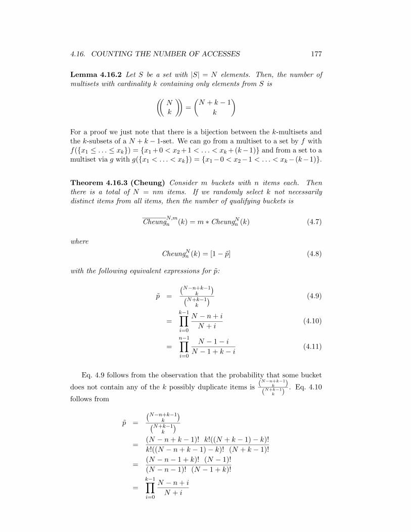
4.16. COUNTING THE NUMBER OF ACCESSES 177

Lemma 4.16.2 Let S be a set with |S| = N elements. Then, the number ofmultisets with cardinality k containing only elements from S is

((Nk

))=

(N + k − 1

k

)

For a proof we just note that there is a bijection between the k-multisets andthe k-subsets of a N + k− 1-set. We can go from a multiset to a set by f withf(x1 ≤ . . . ≤ xk) = x1 +0 < x2 +1 < . . . < xk +(k−1) and from a set to amultiset via g with g(x1 < . . . < xk) = x1−0 < x2−1 < . . . < xk− (k−1).

Theorem 4.16.3 (Cheung) Consider m buckets with n items each. Thenthere is a total of N = nm items. If we randomly select k not necessarilydistinct items from all items, then the number of qualifying buckets is

CheungN,mn (k) = m ∗ CheungNn (k) (4.7)

where

CheungNn (k) = [1− p] (4.8)

with the following equivalent expressions for p:

p =

(N−n+k−1

k

)(N+k−1

k

) (4.9)

=

k−1∏

i=0

N − n+ i

N + i(4.10)

=n−1∏

i=0

N − 1− iN − 1 + k − i (4.11)

Eq. 4.9 follows from the observation that the probability that some bucket

does not contain any of the k possibly duplicate items is(N−n+k−1

k )(N+k−1

k ). Eq. 4.10

follows from

p =

(N−n+k−1

k

)(N+k−1

k

)

=(N − n+ k − 1)! k!((N + k − 1)− k)!

k!((N − n+ k − 1)− k)! (N + k − 1)!

=(N − n− 1 + k)! (N − 1)!

(N − n− 1)! (N − 1 + k)!

=

k−1∏

i=0

N − n+ i

N + i

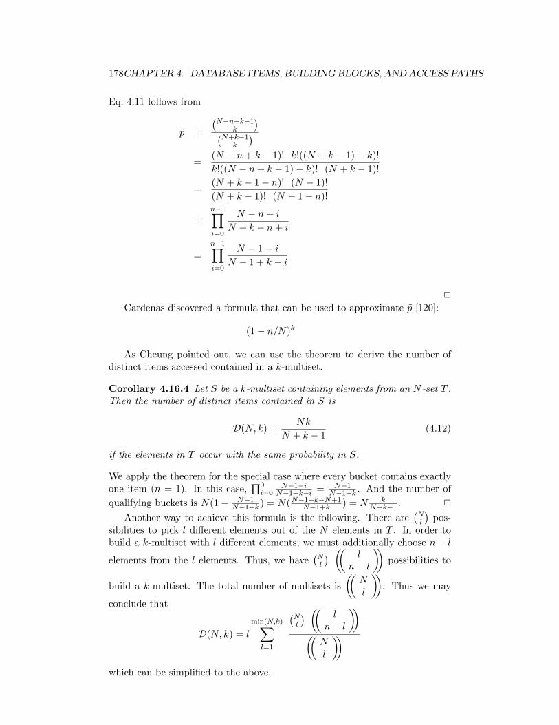
178CHAPTER 4. DATABASE ITEMS, BUILDING BLOCKS, AND ACCESS PATHS

Eq. 4.11 follows from

p =

(N−n+k−1

k

)(N+k−1

k

)

=(N − n+ k − 1)! k!((N + k − 1)− k)!

k!((N − n+ k − 1)− k)! (N + k − 1)!

=(N + k − 1− n)! (N − 1)!

(N + k − 1)! (N − 1− n)!

=n−1∏

i=0

N − n+ i

N + k − n+ i

=

n−1∏

i=0

N − 1− iN − 1 + k − i

2

Cardenas discovered a formula that can be used to approximate p [120]:

(1− n/N)k

As Cheung pointed out, we can use the theorem to derive the number ofdistinct items accessed contained in a k-multiset.

Corollary 4.16.4 Let S be a k-multiset containing elements from an N -set T .Then the number of distinct items contained in S is

D(N, k) =Nk

N + k − 1(4.12)

if the elements in T occur with the same probability in S.

We apply the theorem for the special case where every bucket contains exactlyone item (n = 1). In this case,

∏0i=0

N−1−iN−1+k−i = N−1

N−1+k . And the number of

qualifying buckets is N(1− N−1N−1+k ) = N(N−1+k−N+1

N−1+k ) = N kN+k−1 . 2

Another way to achieve this formula is the following. There are(Nl

)pos-

sibilities to pick l different elements out of the N elements in T . In order tobuild a k-multiset with l different elements, we must additionally choose n− lelements from the l elements. Thus, we have

(Nl

) (( ln− l

))possibilities to

build a k-multiset. The total number of multisets is

((Nl

)). Thus we may

conclude that

D(N, k) = l

min(N,k)∑

l=1

(Nl

) (( ln− l

))

((Nl

))

which can be simplified to the above.

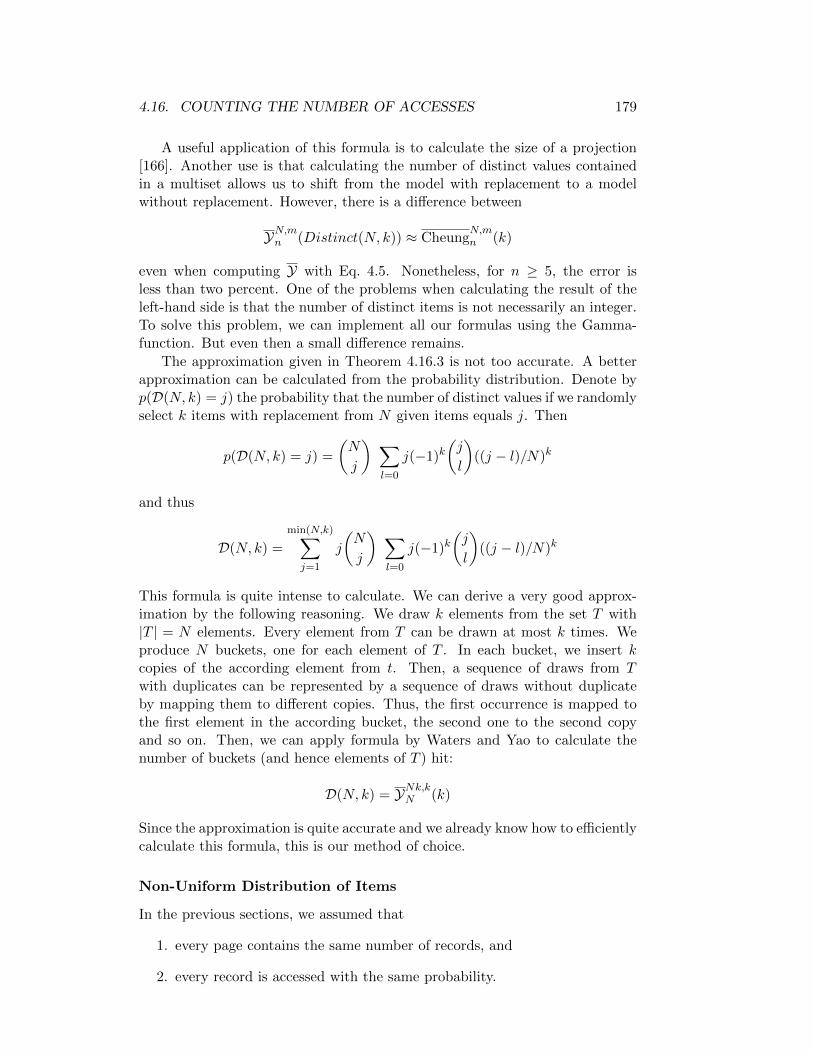
4.16. COUNTING THE NUMBER OF ACCESSES 179

A useful application of this formula is to calculate the size of a projection[166]. Another use is that calculating the number of distinct values containedin a multiset allows us to shift from the model with replacement to a modelwithout replacement. However, there is a difference between

YN,mn (Distinct(N, k)) ≈ CheungN,mn (k)

even when computing Y with Eq. 4.5. Nonetheless, for n ≥ 5, the error isless than two percent. One of the problems when calculating the result of theleft-hand side is that the number of distinct items is not necessarily an integer.To solve this problem, we can implement all our formulas using the Gamma-function. But even then a small difference remains.

The approximation given in Theorem 4.16.3 is not too accurate. A betterapproximation can be calculated from the probability distribution. Denote byp(D(N, k) = j) the probability that the number of distinct values if we randomlyselect k items with replacement from N given items equals j. Then

p(D(N, k) = j) =

(N

j

) ∑

l=0

j(−1)k(j

l

)((j − l)/N)k

and thus

D(N, k) =

min(N,k)∑

j=1

j

(N

j

) ∑

l=0

j(−1)k(j

l

)((j − l)/N)k

This formula is quite intense to calculate. We can derive a very good approx-imation by the following reasoning. We draw k elements from the set T with|T | = N elements. Every element from T can be drawn at most k times. Weproduce N buckets, one for each element of T . In each bucket, we insert kcopies of the according element from t. Then, a sequence of draws from Twith duplicates can be represented by a sequence of draws without duplicateby mapping them to different copies. Thus, the first occurrence is mapped tothe first element in the according bucket, the second one to the second copyand so on. Then, we can apply formula by Waters and Yao to calculate thenumber of buckets (and hence elements of T ) hit:

D(N, k) = YNk,kN (k)

Since the approximation is quite accurate and we already know how to efficientlycalculate this formula, this is our method of choice.

Non-Uniform Distribution of Items

In the previous sections, we assumed that

1. every page contains the same number of records, and

2. every record is accessed with the same probability.

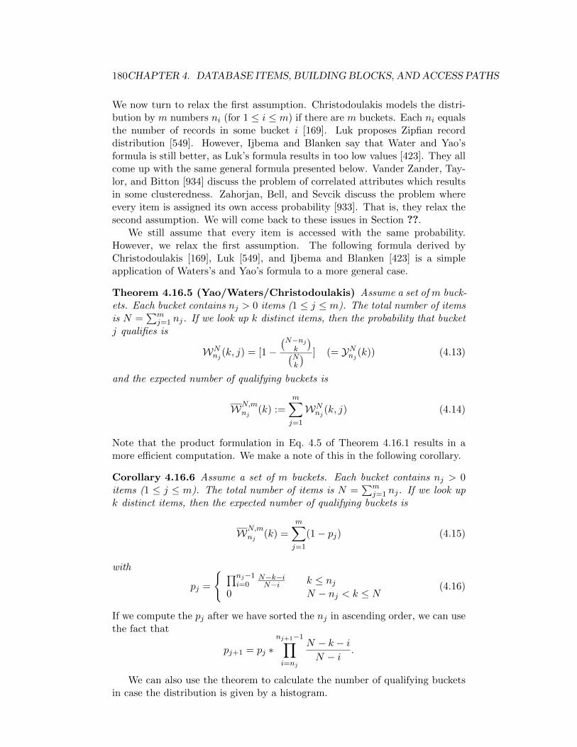
180CHAPTER 4. DATABASE ITEMS, BUILDING BLOCKS, AND ACCESS PATHS

We now turn to relax the first assumption. Christodoulakis models the distri-bution by m numbers ni (for 1 ≤ i ≤ m) if there are m buckets. Each ni equalsthe number of records in some bucket i [169]. Luk proposes Zipfian recorddistribution [549]. However, Ijbema and Blanken say that Water and Yao’sformula is still better, as Luk’s formula results in too low values [423]. They allcome up with the same general formula presented below. Vander Zander, Tay-lor, and Bitton [934] discuss the problem of correlated attributes which resultsin some clusteredness. Zahorjan, Bell, and Sevcik discuss the problem whereevery item is assigned its own access probability [933]. That is, they relax thesecond assumption. We will come back to these issues in Section ??.

We still assume that every item is accessed with the same probability.However, we relax the first assumption. The following formula derived byChristodoulakis [169], Luk [549], and Ijbema and Blanken [423] is a simpleapplication of Waters’s and Yao’s formula to a more general case.

Theorem 4.16.5 (Yao/Waters/Christodoulakis) Assume a set of m buck-ets. Each bucket contains nj > 0 items (1 ≤ j ≤ m). The total number of itemsis N =

∑mj=1 nj. If we look up k distinct items, then the probability that bucket

j qualifies is

WNnj (k, j) = [1−

(N−njk

)(Nk

) ] (= YNnj (k)) (4.13)

and the expected number of qualifying buckets is

WN,mnj (k) :=

m∑

j=1

WNnj (k, j) (4.14)

Note that the product formulation in Eq. 4.5 of Theorem 4.16.1 results in amore efficient computation. We make a note of this in the following corollary.

Corollary 4.16.6 Assume a set of m buckets. Each bucket contains nj > 0items (1 ≤ j ≤ m). The total number of items is N =

∑mj=1 nj. If we look up

k distinct items, then the expected number of qualifying buckets is

WN,mnj (k) =

m∑

j=1

(1− pj) (4.15)

with

pj =

∏nj−1i=0

N−k−iN−i k ≤ nj

0 N − nj < k ≤ N (4.16)

If we compute the pj after we have sorted the nj in ascending order, we can usethe fact that

pj+1 = pj ∗nj+1−1∏

i=nj

N − k − iN − i .

We can also use the theorem to calculate the number of qualifying bucketsin case the distribution is given by a histogram.

4.16. COUNTING THE NUMBER OF ACCESSES 181

Corollary 4.16.7 For 1 ≤ i ≤ L let there be li buckets containing ni items.Then the total number of buckets is m =

∑Li=1 li, and the total number of items

in all buckets is N =∑L

i=1 lini. For k randomly selected items, the number ofqualifying buckets is

WN,mnj (k) =

L∑

i=1

liYNnj (k) (4.17)

Last in this section, let us calculate the probability distribution for thenumber of qualifying items within a bucket. The probability that x ≤ nj itemsin a bucket j qualify can be calculated as follows. The number of possibilitiesto select x items in bucket nj is

(njx

). The number of possibilites to draw the

remaining k − x items from the other buckets is(N−njk−x

). The total number

of possibilities to distribute k items over the buckets is(Nk

). This shows the

following:

Theorem 4.16.8 Assume a set of m buckets. Each bucket contains nj > 0items (1 ≤ j ≤ m). The total number of items is N =

∑mj=1 nj. If we look up

k distinct items, the probability that x items in bucket j qualify is

XNnj (k, x) =

(njx

) (N−njk−x

)(Nk

) (4.18)

Further, the expected number of qualifying items in bucket j is

XN,mnj (k) =

min(k,nj)∑

x=0

xXNnj (k, x) (4.19)

In standard statistics books the probability distribution XNnj (k, x) is called hy-pergeometric distribution.

Let us consider the case where all nj are equal to n. Then we can calculatethe average number of qualifying items in a bucket. With y := min(k, n) we

182CHAPTER 4. DATABASE ITEMS, BUILDING BLOCKS, AND ACCESS PATHS

have

XN,mnj (k) =

min(k,n)∑

x=0

xXNn (k, x)

=

min(k,n)∑

x=1

xXNn (k, x)

=1(Nk

)y∑

x=1

x

(n

x

)(N − nk − x

)

=1(Nk

)y∑

x=1

(x

1

)(n

x

)(N − nk − x

)

=1(Nk

)y∑

x=1

(n

1

)(n− 1

x− 1

)(N − nk − x

)

=

(n1

)(Nk

)y−1∑

x=0

(n− 1

0 + x

)(N − n

(k − 1)− x

)

=

(n1

)(Nk

)(n− 1 +N − n

0 + k − 1

)

=

(n1

)(Nk

)(N − 1

k − 1

)

= nk

N=

k

m

Let us consider the even more special case where every bucket contains asingle item. That is, N = m and ni = 1. The probability that a bucket containsa qualifying item reduces to

XN1 (k, x) =

(1x

) (N−1k−1

)(Nk

)

=

(N−1k−1

)(Nk

)

=k

N(=

k

m)

Since x can then only be zero or one, the average number of qualifying items abucket contains is also k

N .The formulas presented in this section can be used to estimate the number

of block/page accesses in case of random direct accesses. As we will see next,other kinds of accesses occur and need different estimates.

4.16.2 Counting the Number of Sequential Accesses

Vector of Bits

When estimating seek costs, we need to calculate the probability distributionfor the distance between two subsequent qualifying cylinders. We model the

4.16. COUNTING THE NUMBER OF ACCESSES 183

situation as a bitvector of length B with b bits set to 1. Then B correspondsto the number of cylinders and a 1 indicates that a cylinder qualifies.

Theorem 4.16.9 Assume a bitvector of length B. Within it b ones are uni-formly distributed. The remaining B − b bits are zero. Then the probabilitydistribution of the number j of zeros

1. between two consecutive ones,

2. before the first one, and

3. after the last one

is given by

BBb (j) =

(B−j−1b−1

)(Bb

) (4.20)

A more general theorem (see Theorem 4.16.13) was first presented by Yao [922].The above formulation is due to Christodoulakis [172].

To see why the formula holds, consider the total number of bitvectors havinga one in position i followed by j zeros followed by a one. This number is

(B−j−2b−2

).

We can chose B − j − 1 positions for i. The total number of bitvectors is(Bb

)

and each bitvector has b − 1 sequences of the form that a one is followed by asequence of zeros is followed by a one. Hence,

BBb (j) =(B − j − 1)

(B−j−2b−2

)

(b− 1)(Bb

)

=

(B−j−1b−1

)(Bb

)

Part 1. of the theorem follows. To prove part 2., we count the number ofbitvectors that start with j zeros before the first one. There are B − j − 1positions left for the remaining b−1 ones. Hence, the number of these bitvectorsis(B−j−1b−1

)and part 2 follows. Part 3 follows by symmetry.

184CHAPTER 4. DATABASE ITEMS, BUILDING BLOCKS, AND ACCESS PATHS

We can derive a less expensive way to evaluate the formula for BBb (j) asfollows. For j = 0, we have BBb (0) = b

B . If j > 0, then

BBb (j) =

(B−j−1b−1

)(Bb

)

=

(B−j−1)!(b−1)!((B−j−1)−(b−1))!

B!b!(B−b)!

=(B − j − 1)! b!(B − b)!

(b− 1)!((B − j − 1)− (b− 1))! B!

= b(B − j − 1)! (B − b)!

((B − j − 1)− (b− 1))! B!

= b(B − j − 1)! (B − b)!

(B − j − b)! B!

=b

B − j(B − j)! (B − b)!(B − b− j)! B!

=b

B − j

j−1∏

i=0

(1− b

B − i)

This formula is useful when BBb (j) occurs in sums over j because we can computethe product incrementally.

Corollary 4.16.10 Using the terminology of Theorem 4.16.9, the expected val-ue for the number of zeros

1. before the first one,

2. between two successive ones, and

3. after the last one

is

BBb =

B−b∑

j=0

jBBb (j) =B − bb+ 1

(4.21)

4.16. COUNTING THE NUMBER OF ACCESSES 185

Let us calculate:

B−b∑

j=0

j

(B − j − 1

b− 1

)=

B−b∑

j=0

(B − (B − j))(B − j − 1

b− 1

)

= B

B−b∑

j=0

(B − j − 1

b− 1

)−B−b∑

j=0

(B − j)(B − j − 1

b− 1

)

= B

B−b∑

j=0

(b− 1 + j

b− 1

)− b

B−b∑

j=0

(B − jb

)

= B

B−b∑

j=0

(b− 1 + j

j

)− b

B−b∑

j=0

(b+ j

b

)

= B

((b− 1) + (B − b) + 1

(b− 1) + 1

)− b(b+ (B − b) + 1

b+ 1

)

= B

(B

b

)− b(B + 1

b+ 1

)

= (B − bB + 1

b+ 1)

(B

b

)

With

B − bB + 1

b+ 1=

B(b+ 1)− (Bb+ b)

b+ 1

=B − bb+ 1

the claim follows.

Corollary 4.16.11 Using the terminology of Theorem 4.16.9, the expected to-tal number of bits from the first bit to the last one, both included, is

Btot(B, b) =Bb+ b

b+ 1(4.22)

To see this, we subtract from B the average expected number of zeros betweenthe last one and the last bit:

B − B − bb+ 1

=B(b+ 1)

b+ 1− B − bb+ 1

=Bb+B −B + b

b+ 1

=Bb+ b

b+ 1

An early approximation of this formula was discovered by Kollias [487].

186CHAPTER 4. DATABASE ITEMS, BUILDING BLOCKS, AND ACCESS PATHS

Corollary 4.16.12 Using the terminology of Theorem 4.16.9, the number ofbits from the first one and the last one, both included, is

B1-span(B, b) =Bb−B + 2b

b+ 1(4.23)

We have two possibilities to argue here. The first subtracts from B the numberof zeros at the beginning and the end:

B1-span(B, b) = B − 2B − bb+ 1

=Bb+B − 2B + 2b

b+ 1

=Bb−B + 2b

b+ 1

The other possibility is to add the number of zeros between the first and thelast one and the number of ones:

B1-span(B, b) = (b− 1)BBb + b

= (b− 1)B − bb+ 1

+b(b+ 1

b+ 1

=Bb− b2 −B + b+ b2 + b

b+ 1

=Bb−B + 2b

b+ 1

The number of bits from the first bit to the last one including both . . . Thedistance between the first and the last one . . .EX or Cor?

Let us have a look at some possible applications of these formulas. If welook up one record in an array of B records and we search sequentially, howmany array entries do we have to examine on average if the search is successful?

In [562] we find these formulas used for the following scenario. Let a fileconsist of B consecutive cylinders. We search for k different keys, all of whichoccur in the file. These k keys are distributed over b different cylinders. Ofcourse, we can stop as soon as we have found the last key. What is the expectedtotal distance the disk head has to travel if it is placed on the first cylinder ofthe file at the beginning of the search?

Another interpretation of these formulas can be found in [412, 563]. Assumewe have an array consisting of B different entries. We sequentially go throughall entries of the array until we have found all the records for b different keys.We assume that the B entries in the array and the b keys are sorted. Further,all b keys occur in the array. On the average, how many comparisons do weneed to find all keys?

Vector of Buckets

A more general scenario is as follows. Consider a sequence of m buckets con-taining ni items each. Yao [922] developed the following theorem.

4.16. COUNTING THE NUMBER OF ACCESSES 187

Theorem 4.16.13 (Yao) Consider a sequence of m buckets. For 1 ≤ i ≤ m,let ni be the number of items in a bucket i. Then there is a total of N =

∑mi=1 ni

items. Let ti =∑i

l=0 ni be the number of items in the first i buckets. If thebuckets are searched sequentially, then the number of buckets that have to beexamined until k distinct items have been found is

CN,mni (k, j) =

(tjk

)−(tj−1

k

)(Nk

) (4.24)

Thus, the expected number of buckets that need to be examined in order toretrieve k distinct items is

CN,mni (k) =m∑

j=1

jCN,mni (k, j) = m−∑m

j=1

(tj−1

k

)(Nk

) (4.25)

Applications of this formula can be found in [169, 172, 562, 564, 847]. Manolopou-los and Kollias describe the analogue for the replacement model [562].

Lang, Driscoll, and Jou discovered a general theorem which allows us toestimate the expected number of block accesses for sequential search.

Theorem 4.16.14 (Lang/Driscoll/Jou) Consider a sequence of N items.For a batched search of k items, the expected number of accessed items is

A(N, k) = N −N−1∑

i=1

Prob[Y ≤ i] (4.26)

where Y is a random variable for the last item in the sequence that occurs amongthe k items searched.

proof? ?

With the help of this theorem, it is quite easy to derive many averagesequential accesses for different models. Cor or EX?

4.16.3 Pointers into the Literature

Segments containing records can be organized differently. Records can be placedrandomly in the segment, they can be ordered according to some key, or thesegment is organized as a tree. Accordingly, the segment is called random,sequential, or tree-structure. From a segment, records are to be retrieved fora given bag of k keys. The general question then is: how many pages do wehave to access? The answer depends on whether we assume the replacementor non-replacement model. Six cases occur. For sequential and tree-structuredsegments, it also makes sense to distinguish between successful, partially (un-)successful, and (totally) unsuccessfull searches. These notions capture the dif-ferent possibilities where for all, some, none of the k keys records are found.The following table provides some entry points into the literature. It is rough-ly organized around the above categories. (Remember that we discussed therandom file organization at length in Section 4.16.1.)

188CHAPTER 4. DATABASE ITEMS, BUILDING BLOCKS, AND ACCESS PATHS

non-replacement replacement

random [166, 169, 549, 659, 892, 921] [120, 169, 642, 659]sequential [62, 169, 506, 564, 642, 641, 781, 922] [169, 506, 564, 781]tree-structured [506, 505, 564, 641, 664] [506, 505, 564, 781]

4.17 Disk Drive Costs for N Uniform Accesses

The goal of this section is to derive estimates for the costs (time) for retrievingN cache-missed sectors of a segment S from disk. We assume that the N sectorsare read in their physical order on disk. This can be enforced by the DBMS,by the operating system’s disk scheduling policy (SCAN policy), or by the diskdrive controller.

Remembering the description of disk drives, the total costs can be describedas

Cdisk = Ccmd + Cseek + Csettle + Crot + Cheadswitch (4.27)

For brevity, we omitted the parameter N and the parameters describing thesegment and the disk drive on which the segment resides. Subsequently, wedevote a (sometimes tiny) section to each summand. Before that, we have tocalculate the number of qualifying cylinders, tracks, and sectors. These numberswill be used later on.

4.17.1 Number of Qualifying Cylinders, Tracks, and Sectors

If N sectors are to be retrieved, we have to find the number of cylinders qual-ifying in an extent i. Let Ssec denote the total number of sectors our segmentcontains and Scpe(i) = Li−Fi+1 be the number of cylinders of the extent. If theN sectors we want to retrieve are uniformly distributed among the Ssec sectorsof the segment, the number of cylinders that qualifies in (Fi, Li, zi) is Scpe(i)times 1 minus the probability that a cylinder does not qualify. The probabilitythat a cylinder does not qualify can be computed by deviding the total num-ber of possibilities to chose the N sectors from sectors outside the cylinder bythe total number of possibilities to chose N sectors from all Ssec sectors of thesegment. Hence, the number of qualifying cylinders in the considered extent is:

Qc(i) = Scpe(i)YSsec

DZspc(i)(N) = Scpe(i)(1−(Ssec−DZspc(i)

N

)(Ssec

N

) ) (4.28)

We could also have used Theorem 4.16.13.Let us also calculate the number of qualifying tracks in a partion i. It

can be calculated by Scpe(i)Dtpc(1 − Prob(a track does not qualify)). Theprobability that a track does not qualify can be computed by dividing thenumber of ways to pick N sectors from sectors not belonging to a track dividedby the number of possible ways to pick N sectors from all sectors.

Qt(i) = Scpe(i)DtpcYSsec

DZspt(i)(N) = Scpe(i)Dtpc(1−

(Ssec−DZspt(i)N

)(Ssec

N

) ) (4.29)

4.17. DISK DRIVE COSTS FOR N UNIFORM ACCESSES 189

Just for fun, we calculate the number of qualifying sectors of an extent inzone i. It can be approximated by

Qs(i) = Scpe(i)DZspc(i)N

Ssec(4.30)

Since all Scpe(i) cylinders are in the same zone, they have the same number ofsectors per track, and we could also use Waters/Yao to approximate the numberof qualifying cylinders by

Qc(i) = YScpe(i)DZspc(Szone(i)),Scpe(i)

DZspc(Szone(i)) (Qs(i)) (4.31)

This is a good approximation, as long as Qs(i) is not too small (e.g. > 4).

4.17.2 Command Costs

The command costs Ccmd are easy to compute. Every read of a sector requiresthe execution of a command. Hence

Ccmd = NDcmd

estimates the total command costs.

4.17.3 Seek Costs

We give different alternative possibilities to estimate seek costs. We start withan upper bound by exploring Theorem 4.1.1. The first cylinder we have to visitrequires a random seek with cost Davgseek. (Well this does not really give us anupper bound. For a true upper bound we should use Dseek(Dcyl − 1).) Afterthat, we have to visit the remaining Qc(i)−1 qualifying cylinders. The segmentspans a total of Slast(Sext)−Sfirst(1) + 1 cylinders. Let us assume that the firstqualifying cylinder is the first cylinder and the last qualifying cylinder is thelast cylinder of the segment. Then applying Theorem 4.1.1 gives us the upperbound

Cseek(i) ≤ (Qc(i)− 1)Dseek(Slast(Sext)− Sfirst(1) + 1

Qc(i)− 1)

after we have found the first qualifying cylinder.We can be a little more precise by splitting the seek costs into two com-

ponents. The first component Cseekgap expresses the costs of finding the firstqualifying cylinder and jumping from the last qualifying cylinder of extent i tothe first qualifying cylinder of extent i + 1. The second component Cseekext(i)calculates the seek costs within an extent i. Figure 4.10 illustrates the situation.The total seek costs then are

Cseek(i) = Cseekgap +

Sext∑

i=1

Cseekext(i)

Since there is no estimate in the literature for Cseekgap, we have to calculate itourselves. After we have done so, we present several alternatives to calculateCseekext(i).

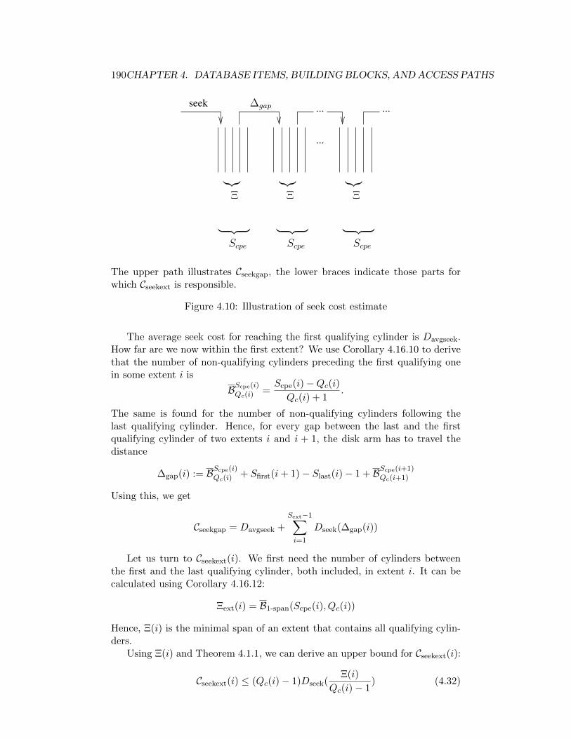
190CHAPTER 4. DATABASE ITEMS, BUILDING BLOCKS, AND ACCESS PATHS

...

...seek

...

︸︷︷︸Ξ

︸︷︷︸Ξ

︸︷︷︸Ξ

︸ ︷︷ ︸Scpe

︸ ︷︷ ︸Scpe

︸ ︷︷ ︸Scpe

∆gap

The upper path illustrates Cseekgap, the lower braces indicate those parts forwhich Cseekext is responsible.

Figure 4.10: Illustration of seek cost estimate

The average seek cost for reaching the first qualifying cylinder is Davgseek.How far are we now within the first extent? We use Corollary 4.16.10 to derivethat the number of non-qualifying cylinders preceding the first qualifying onein some extent i is

BScpe(i)Qc(i)

=Scpe(i)−Qc(i)Qc(i) + 1

.

The same is found for the number of non-qualifying cylinders following thelast qualifying cylinder. Hence, for every gap between the last and the firstqualifying cylinder of two extents i and i + 1, the disk arm has to travel thedistance

∆gap(i) := BScpe(i)Qc(i)

+ Sfirst(i+ 1)− Slast(i)− 1 + BScpe(i+1)Qc(i+1)

Using this, we get

Cseekgap = Davgseek +

Sext−1∑

i=1

Dseek(∆gap(i))

Let us turn to Cseekext(i). We first need the number of cylinders betweenthe first and the last qualifying cylinder, both included, in extent i. It can becalculated using Corollary 4.16.12:

Ξext(i) = B1-span(Scpe(i), Qc(i))

Hence, Ξ(i) is the minimal span of an extent that contains all qualifying cylin-ders.

Using Ξ(i) and Theorem 4.1.1, we can derive an upper bound for Cseekext(i):

Cseekext(i) ≤ (Qc(i)− 1)Dseek(Ξ(i)

Qc(i)− 1) (4.32)

4.17. DISK DRIVE COSTS FOR N UNIFORM ACCESSES 191

Alternatively, we could formulate this as

Cseekext(i) ≤ (Qc(i)− 1)Dseek(BScpe(i)Qc(i)

) (4.33)

by applying Corollary 4.16.10.A seemingly more precise estimate for the expected seek cost within the

qualifying cylinders of an extent is derived by using Theorem 4.16.9:

Cseekext(i) = Qc(i)

Scpe(i)−Qc(i)∑

j=0

Dseek(j + 1)BScpe(i)Qc(i)

(j) (4.34)

There are many more estimates for seek times. Older ones rely on a lineardisk model but also consider different disk scan policies. A good entry point isthe work by Theorey and Pinkerton [839, 840].

4.17.4 Settle Costs

The average settle cost is easy to calculate. For every qualifying cylinder, onehead settlement takes place:

Csettle(i) = Qc(i)Drdsettle (4.35)

4.17.5 Rotational Delay Costs

Let us turn to the rotational delay. For some given track in zone i, we want toread the Qt(i) qualifying sectors contained in it. On average, we would expectthat the read head is ready to start reading in the middle of some sector of atrack. If so, we have to wait for 1

2DZscan(Szone(i)) before the first whole sectoroccurs under the read head. However, due to track and cylinder skew, thisevent does not occur after a head switch or a cylinder switch. Instead of beingoverly precise here, we ignore this half sector pass by time and assume that we EXare always at the beginning of a sector. This is also justified by the fact thatwe model the head switch time explicitly.

Assume that the head is ready to read at the beginning of some sectorof some track. Then, in front of us is a — cyclic, which does not matter —bitvector of qualifying and non-qualifying sectors. We can use Corollary 4.16.11to estimate the total number of qualifying and non-qualifying sectors that haveto pass under the head until all qualifying sectors have been seen. The totalrotational delay for the tracks of zone i is

Crot(i) = Qt(i) DZscan(Szone(i)) Btot(DZspt(Szone(i)), Qspt(i)) (4.36)

where Qspt(i) = WSsec,DZspt(Szone(i))1 (N) = DZspt(Szone(i))

NSsec

is the expectednumber of qualifying sectors per track in extent i. In case Qspt(i) < 1, we setQspt(i) := 1.

A more precise model is derived as follows. We sum up for all j the productof (1) the probability that j sectors in a track qualify and (2) the average numberof sectors that have to be read if j sectors qualify. This gives us the number of

192CHAPTER 4. DATABASE ITEMS, BUILDING BLOCKS, AND ACCESS PATHS

sectors that have to pass the head in order to read all qualifying sectors. Weonly need to multiply this number by the time to scan a single sector and thenumber of qualifying tracks. We can estimate (1) using Theorem 4.16.8. For(2) we again use Corollary 4.16.11.

Crot(i) = Scpe(i) Dtpc DZscan(Szone(i))

·min(N,DZspt(Szone(i)))∑

j=1

X Ssec

DZspt(Szone(i))(N, j) Btot(DZspt(Szone(i)), j)(4.37)

Another approach is taken by Triantafillou, Christodoulakis, and Georgiadis[847]. They split the total rotational delay into two components. The firstcomponent (Crotpass) measures the time needed to skip unqualifying sectors andthe second (Crotread) that for (scanning and transferring) the qualifying sectorsto the host.

Let us deal with the first component. Assume that j sectors of a track inextent i qualify. The expected position on a track where the head is ready toread is the middle between two qualifying sectors. Since the expected number ofsectors between two qualifying sectors is DZspt(Szone(i))/j, the expected numberof sectors scanned before the first qualifying sector comes under the head isDZspt(Szone(i))

2j . The expected positions of j qualifying sectors on the same trackis such that the number of non-qualifying sectors between two successivelyqualifying sectors is the same. Hence, after having read a qualifying sector,DZspt(Szone(i))

j unqualifying sectors must pass by until the next qualifying sectorshows up. The total number of unqualifying sectors to be passed if j sectorsqualify in a track of zone i is

Ns(j, i) =DZspt(Szone(i))

2j+ (j − 1)

DZspt(Szone(i))− jj

(4.38)

Using again Theorem 4.16.8, the expected rotational delay for the unquali-fying sectors then is

Crotpass(i) = Scpe(i) Dtpc DZscan(Szone(i))

·min(N,DZspt(Szone(i)))∑

j=1

X Ssec

DZspt(Szone(i))(N, j)Ns(j, i) (4.39)

We have to sum up this number for all extents and then add the time neededto scan the N sectors. Hence

Crot =

Sext∑

i=1

Crotpass(i) + Crotread(i)

where the total transfer cost for the qualifying sectors of an extent can beestimated as

Crotread(i) = Qs(i) DZscan(Szone(i))

4.17. DISK DRIVE COSTS FOR N UNIFORM ACCESSES 193

4.17.6 Head Switch Costs

The average head switch cost is equal to the average number of head switchesthat occur times the average head switch cost. The average number of headswitch is equal to the number of tracks that qualify minus the number of cylin-ders that qualify since a head switch does not occur for the first track of eachcylinder. Summarizing

Cheadswitch =

Sext∑

i=1

(Qt(i)−Qc(i)) Dhdswitch (4.40)

where Qt is the average number of tracks qualifying in an extent.

4.17.7 Discussion

The disk drive cost model derived depends on many parameters. The first bunchof parameters concerns the disk drive itself. These parameters can (and mustbe) extracted from disk drives by using (micro-) benchmarking techniques [300,834, 582, 742]. The second bunch of parameters concerns the layout of a segmenton disk. The database system is responsible for providing these parameters.The closer it is to the disk, the easier these parameters are extracted. Buildinga runtime system atop the operating system’s file system is obviously a badidea from the cost model perspective. If instead the storage manager of theruntime system implements cylinder aligned extents (or at least track alignedextents) using a raw I/O interface, the cost model will be easier to develop andmuch more precise. Again, providing reliable cost models is one of the mostimportant tasks of the runtime system.

We have neglected many problems in our disk access model: partially filledcylinders, pages larger than a block, disk drive’s cache, remapping of bad blocks,non-uniformly distributed accesses, clusteredness, and so on. Whereas the firsttwo items are easy to fix, the rest is not so easy. In general, database systemsignore the disk drive cache. The justifying argument is that the database bufferis much larger than the disk drive’s cache and, hence, it is very unlikely that weread a page that is not in the database buffer but in the disk cache. However,this argument falls short for non-random accesses. Nevertheless, we will ignorethe issue in this book. The interested reader is referred to Shriver’s thesis fordisk cache modeling [782].

Remapping of bad sectors to other sectors really prevents the developmentof a precise cost model for disk accesses. Modelling disk drives becomes alreadya nightmare since a nice partitioning of the disk into zones is no longer possiblesince some sectors, tracks and even cylinders are reserved for the remapping. Soeven if no remapping takes place (which is very unlikely), having homogeneouszones of hundreds of cylinders is a dream that will never come true. Theresult is that we do not have dozens of homogeneous zones but hundreds (ifnot thousands) of zones of medium homogeneity. These should be reduced toa model of dozens of homogeneous zones such that the error does not becometoo large. The remaining issues will be discussed later in the book. EX

194CHAPTER 4. DATABASE ITEMS, BUILDING BLOCKS, AND ACCESS PATHS

There is even more to say about our cost model. A very practical issuearises if the number of qualifying cylinders is small. Then for some extent i,the expected number of qualifying cylinders could be Qc(i) = 0.38. For someof our formulas this is a big problem. As a consequence, special cases for smallN , small Qc, small Qt have to be developed and implemented.EX

Another issue is the performance of the cost model itself. The query com-piler might evaluate the cost model’s formulas thousands or millions of times.Hence, they should be fast to evaluate.

So far, we can adequately model the costs ofN disk accesses. Some questionsremain. For example, how do we derive the number N of pages we have toaccess? Do we really need to fetch all N pages from disk or will we find someof them in the buffer? If yes, how many? Further, CPU costs are also animportant issue. Deriving a cost model for CPU costs is even more tediousthan modelling disk drive costs. The only choice available is to benchmark allparts of a system and then derive a cost model using the extracted parameters.To give examples of parameters to be extracted: we need the CPU costs foraccessing a page present in the buffer, for accessing a page absent in the buffer,for a next call of an algebraic operator, for executing an integer addition, andso on. Again, this cannot be done without tools [46, 235, 396, 445, 658].

The bottom line is that a cost model does not have to be accurate, but mustlead to correct decisions. In that sense, it must be accurate at the break evenpoints between plan alternatives. Let us illustrate this point by means of ourmotivating example. If we know that the index returns a single tuple, it is quitelikely that the sequential scan is much more expensive. The same might be truefor 2, 3, 4, and 5 tuples. Hence, an accurate model for small N is not reallynecessary. However, as we come close to the costs of a sequential scan, both thecost model for the sequential scan and the one for the index-based access mustbe correct since the product of their errors is the factor a bad choice is off thebest choice. This is a crucial point, since it is easy to underestimate sequentialaccess costs by a factor of 2-3 and overestimate random access cost by a factorof 2-5.

4.18 Concluding Remarks

Learned:

Open Cost: I/O costs: non-uniform stuff, CPU costs: nothing done

Wrong cardinality estimates: Open, leads to dynamic qo

4.19 Bibliography

ToDo:

• CPU Costs for B-tree search within inner and leaf pages [502]

• Index/Relations: only joins between building blocks [709]

4.19. BIBLIOGRAPHY 195

• RDB/V1: predicate push down (views), 2 phase optimization (local: tra-ditional, global: sharing of tables), five categories for predicates, nestedloops evaluation for nested correlated subqueries, use of transitivity ofequality, conjunctive normal form, use of min/max value of join columnto reduce join cardinality by adding another selection to the other relation(min(a) <= b <= max(a)) for join predicate a=b.

• K accesses to unique index: how many page faults if buffer has size b?[722]

• buffer mgmt: [248]

• buffer mgmt: [780]

• buffer mgmt: [507]

• buffer mgmt: [723, 724]

• buffer mgmt: [105]

• buffer mgmt: [168]

• structured, semi-structured, unstructured data: [323] cited in Dono76

• B-trees and their improvements [205]

• Vertical partitioning: [252, 565, 55]

• Horizontal and vertical partitioning: [130]

• set oriented disk access to large complex objects [885, 884], assemblyoperator: [463],

• large objects: [85, 121, 521]

196CHAPTER 4. DATABASE ITEMS, BUILDING BLOCKS, AND ACCESS PATHS

Part II

Foundations

197

Chapter 5

Logic, Null, and BooleanExpressions

5.1 Two-valued logic

The Boolean algebra with its operations not (¬), and (∧), and or (∨) is well-known. The truth tables for these operations is given in Figure 5.1.

5.2 NULL values and three valued logic

Many database management systems (in particular all SQL based relationalsystems) support a concept of undefined or unknown values, commonly calledNULL values. These NULL values represent the fact that an attribute valueis unknown, and consequently the result of operations on this attribute can beunknown, too.

As a consequence, NULL values induce a three valued logic, as illustrated bythe truth table on the left-hand side of Figure ??: When comparing two valuesx and y for equality, the result is true if both values are not NULL and x = y(using standard equality), false if both values are not NULL and not x = y,and unknown (⊥) if any of the two values is NULL, as then no comparison ispossible. These three possible outcomes (true, false, and ⊥) propagate throughlogical operators, and induce a three-valued logic, as shown in Figure 5.5.

While the three-valued logic correctly captures the uncertainty caused byNULL values, and a result of ⊥ can be reported back to the user as booleanNULL, it is often necessary to convert three-valued logic results into two-valuedlogic. For the special case of equality comparisons it is sometimes useful to in-

¬ true false

false true∨ true false

true true truefalse true false

∧ true false

true true falsefalse false false

Figure 5.1: Truth tables for two-valued logic

199

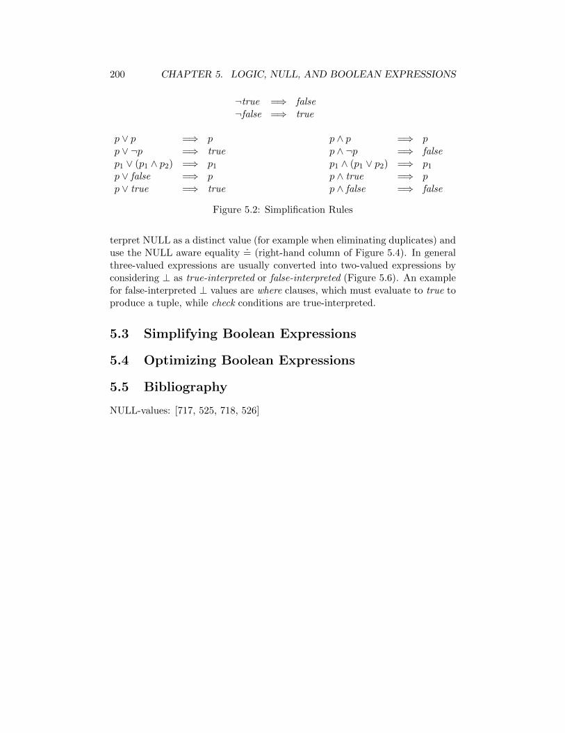
200 CHAPTER 5. LOGIC, NULL, AND BOOLEAN EXPRESSIONS

¬true =⇒ false¬false =⇒ true

p ∨ p =⇒ pp ∨ ¬p =⇒ truep1 ∨ (p1 ∧ p2) =⇒ p1

p ∨ false =⇒ pp ∨ true =⇒ true

p ∧ p =⇒ pp ∧ ¬p =⇒ falsep1 ∧ (p1 ∨ p2) =⇒ p1

p ∧ true =⇒ pp ∧ false =⇒ false

Figure 5.2: Simplification Rules

terpret NULL as a distinct value (for example when eliminating duplicates) anduse the NULL aware equality

.= (right-hand column of Figure 5.4). In general

three-valued expressions are usually converted into two-valued expressions byconsidering ⊥ as true-interpreted or false-interpreted (Figure 5.6). An examplefor false-interpreted ⊥ values are where clauses, which must evaluate to true toproduce a tuple, while check conditions are true-interpreted.

5.3 Simplifying Boolean Expressions

5.4 Optimizing Boolean Expressions

5.5 Bibliography

NULL-values: [717, 525, 718, 526]

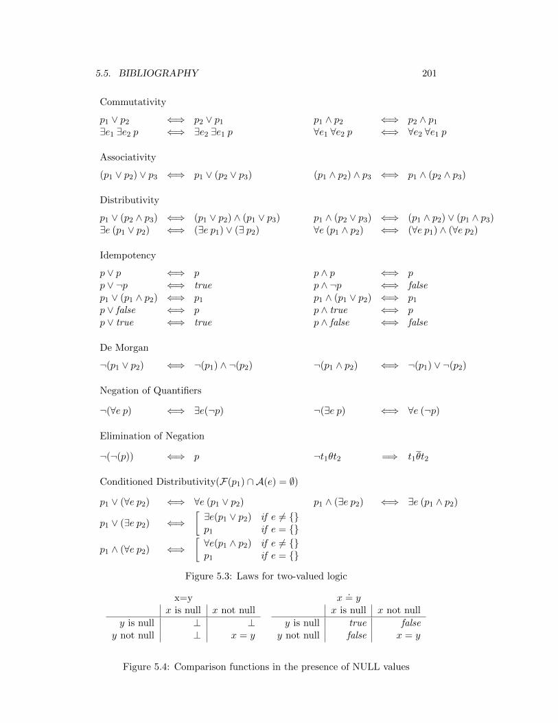
5.5. BIBLIOGRAPHY 201

Commutativity

p1 ∨ p2 ⇐⇒ p2 ∨ p1 p1 ∧ p2 ⇐⇒ p2 ∧ p1

∃e1 ∃e2 p ⇐⇒ ∃e2 ∃e1 p ∀e1 ∀e2 p ⇐⇒ ∀e2 ∀e1 p

Associativity

(p1 ∨ p2) ∨ p3 ⇐⇒ p1 ∨ (p2 ∨ p3) (p1 ∧ p2) ∧ p3 ⇐⇒ p1 ∧ (p2 ∧ p3)

Distributivity

p1 ∨ (p2 ∧ p3) ⇐⇒ (p1 ∨ p2) ∧ (p1 ∨ p3) p1 ∧ (p2 ∨ p3) ⇐⇒ (p1 ∧ p2) ∨ (p1 ∧ p3)∃e (p1 ∨ p2) ⇐⇒ (∃e p1) ∨ (∃ p2) ∀e (p1 ∧ p2) ⇐⇒ (∀e p1) ∧ (∀e p2)

Idempotency

p ∨ p ⇐⇒ p p ∧ p ⇐⇒ pp ∨ ¬p ⇐⇒ true p ∧ ¬p ⇐⇒ falsep1 ∨ (p1 ∧ p2) ⇐⇒ p1 p1 ∧ (p1 ∨ p2) ⇐⇒ p1

p ∨ false ⇐⇒ p p ∧ true ⇐⇒ pp ∨ true ⇐⇒ true p ∧ false ⇐⇒ false

De Morgan

¬(p1 ∨ p2) ⇐⇒ ¬(p1) ∧ ¬(p2) ¬(p1 ∧ p2) ⇐⇒ ¬(p1) ∨ ¬(p2)

Negation of Quantifiers

¬(∀e p) ⇐⇒ ∃e(¬p) ¬(∃e p) ⇐⇒ ∀e (¬p)

Elimination of Negation

¬(¬(p)) ⇐⇒ p ¬t1θt2 =⇒ t1θt2

Conditioned Distributivity(F(p1) ∩ A(e) = ∅)

p1 ∨ (∀e p2) ⇐⇒ ∀e (p1 ∨ p2) p1 ∧ (∃e p2) ⇐⇒ ∃e (p1 ∧ p2)

p1 ∨ (∃e p2) ⇐⇒[∃e(p1 ∨ p2) if e 6= p1 if e =

p1 ∧ (∀e p2) ⇐⇒[∀e(p1 ∧ p2) if e 6= p1 if e =

Figure 5.3: Laws for two-valued logic

x=y x.= y

x is null x not null

y is null ⊥ ⊥y not null ⊥ x = y

x is null x not null

y is null true falsey not null false x = y

Figure 5.4: Comparison functions in the presence of NULL values

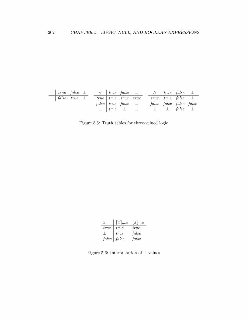
202 CHAPTER 5. LOGIC, NULL, AND BOOLEAN EXPRESSIONS

¬ true false ⊥false true ⊥

∨ true false ⊥true true true truefalse true false ⊥⊥ true ⊥ ⊥

∧ true false ⊥true true false ⊥false false false false⊥ ⊥ false ⊥

Figure 5.5: Truth tables for three-valued logic

x dxenull bxcnull

true true true⊥ true falsefalse false false

Figure 5.6: Interpretation of ⊥ values

Chapter 6

Functional Dependencies

In many query results attribute values are not independent of each other buthave certain dependencies. Keeping track of these dependencies is very usefulfor many optimizations, for example in the following query

select c.id, n.namefrom customers c, nations nwhere c.nid=n.idorder byc.id, n.name

the order by clause can be simplified to c.id without affecting the result:c.id is the key of customers, and thus determines c.nid. c.nid is joined withn.id, which is the key of nations and determines n.name, thus transitively c.iddetermines n.name.

These functional dependencies between attributes have been studied primar-ily in the context of database design, but many optimization steps like orderoptimization (Chapter 23) and query unnesting (Chapter 14) profit greatly fromknown functional dependencies. In the following we first study functional de-pendencies when all attributes are not NULL, then extend this to attributeswith NULL values, and finally discuss how functional dependencies are effectedby relational operators.

6.1 Functional Dependencies

As illustrated by the previous example, a functional dependency describes howattribute values depend on other attribute values. More formally, a relation R(with A1, A2 ⊆ A(R)) satisfies a functional dependency

f : A1 → A2

if and only if the following condition holds:

∀t1, t2([t1 ∈ R ∧ t2 ∈ R ∧ t1.A1 = t2.A1 ]⇒ [t1.A2 = t2.A2 ]).

For base relations functional dependencies can be derived from the schema,in particular key constraints and check conditions [?]. For intermediate results

203

204 CHAPTER 6. FUNCTIONAL DEPENDENCIES

additional function dependencies can be induced by algebraic operators, as wewill see below.

Once some functional dependencies are known to hold, further function-al dependencies can be derived by using Armstrong’s axioms [?] (assumingA1, A2, A3 ⊆ A(R)):

1. A2 ⊆ A1 ⇒ A1 → A2

2. A1 → A2 ⇒ (A1 ∪A3)→ (A2 ∪A3)3. A1 → A2 ∧A2 → A3 ⇒ A1 → A3

The Armstrong axioms are sound and complete, i.e., it is possible to deriveall valid functional dependencies by applying these three axioms. For practicalpurposes it is often convenient to include three additional rules which can bederived from the original axioms:

4. A1 → A2 ∧A1 → A3 ⇒ A1 → (A2 ∪A3)5. A1 → (A2 ∪A3) ⇒ A1 → A2 ∧A1 → A3

6. A1 → A2 ∧ (A2 ∪A4)→ A3 ⇒ (A1 ∪A4)→ A3

Given a set of functional dependencies F , we denote with F+ the closureof F , i.e., the set of all functional dependencies that can be derived from F byusing the inference rules shown above.

Closely related to the concept of functional dependencies is the concept ofkeys: Given a relation R and an attribute set A ⊆ A(R), A is a super key ofR if A → A(R) holds in R. Further A is a key of R if the following conditionholds:

∀A(A′ ⊂ A⇒ ¬(A′ → A(R))).

6.2 Functional Dependencies in the presence of NULLvalues

In the presence of NULL values, a relation R (with A1, A2 ⊆ A(R)) satisfies afunctional dependency

f : A1 → A2

if and only if the following condition holds:

∀t1, t2([t1 ∈ R ∧ t2 ∈ R ∧ t1.A1

.= t2.A1 ]⇒ [t1.A2

.= t2.A2 ]).

XXX explain why, discuss lax dependencies

6.3 Deriving Functional Dependencies over algebra-ic operators

XXX dependency graphs

6.4 Bibliography

Chapter 7

An Algebra for Sets, Bags,and Sequences

This section summarizes a logical algebra that is sufficent to express querieswritten in SQL, OQL and XPath/XQuery. The algebra is based upon substan-tial work by many people [67, 69, 181, 183, 188, 467, 468, 523, 791]. The mostprominent features of the algebra are:

• All operators are polymorphic and can deal with (almost) any kind ofcomplex arguments.

• The operators take arbitrary complex expressions as subscripts. This in-cludes algebraic expressions. The advantage is that nested queries candirectly be expressed as nested algebraic expressions and unnesting pos-sibilities can be represented at the algebraic level, which allows rigorouscorrectness proofs.

• The algebra is redundant, since some special cases of the operators canbe implemented more efficiently.

This chapter is organized as follows. First, we preprare some background ma-terial by discussing sets, bags, and sequences, as well as aggregation functions.Then we are ready to present the algebraic operators. This is done in two steps.First, we introduce their signatures and then their semantics. ToDo

7.1 Sets, Bags, and Sequences

7.1.1 Sets

A set contains elements drawn from some domain D. In our case, the domainwill often be tuples and we only consider finite sets. The set operations we areinterested in are union (∪s), intersection (∩s), and difference (\s). If the domainconsists of tuples, we assume that both arguments have the same schema. Thatis, the attributes and their domains are the same in both arguments. Other-wise, the expression is not well-typed. In any case, set union and intersectionare commutative and associative. Set difference is neither of them. Expressions

205

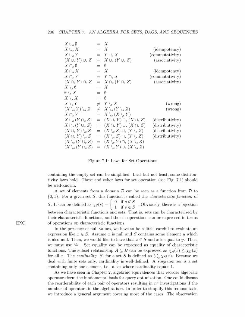
206 CHAPTER 7. AN ALGEBRA FOR SETS, BAGS, AND SEQUENCES

X ∪s ∅ = XX ∪s X = X (idempotency)X ∪s Y = Y ∪s X (commutativity)(X ∪s Y ) ∪s Z = X ∪s (Y ∪s Z) (associativity)X ∩s ∅ = ∅X ∩s X = X (idempotency)X ∩s Y = Y ∩s X (commutativity)(X ∩s Y ) ∩s Z = X ∩s (Y ∩s Z) (associativity)X \s ∅ = X∅ \s X = ∅X \s X = ∅X \s Y 6= Y \s X (wrong)(X \s Y ) \s Z 6= X \s (Y \s Z) (wrong)X ∩s Y = X \s (X \s Y )X ∪s (Y ∩s Z) = (X ∪s Y ) ∩s (X ∪s Z) (distributivity)X ∩s (Y ∪s Z) = (X ∩s Y ) ∪s (X ∩s Z) (distributivity)(X ∪s Y ) \s Z = (X \s Z) ∪s (Y \s Z) (distributivity)(X ∩s Y ) \s Z = (X \s Z) ∩s (Y \s Z) (distributivity)(X \s (Y ∪s Z) = (X \s Y ) ∩s (X \s Z)(X \s (Y ∩s Z) = (X \s Y ) ∪s (X \s Z)

Figure 7.1: Laws for Set Operations

containing the empty set can be simplified. Last but not least, some distribu-tivity laws hold. These and other laws for set operation (see Fig. 7.1) shouldbe well-known.

A set of elements from a domain D can be seen as a function from D to0, 1. For a given set S, this function is called the characteristic function of

S. It can be defined as χS(s) =

0 if s 6∈ S1 if s ∈ S . Obviously, there is a bijection

between characteristic functions and sets. That is, sets can be characterized bytheir characteristic functions, and the set operations can be expressed in termsof operations on characteristic functions.EXC

In the presence of null values, we have to be a little careful to evaluate anexpression like x ∈ S. Assume x is null and S contains some element y whichis also null. Then, we would like to have that x ∈ S and x is equal to y. Thus,we must use ‘

.=’. Set equality can be expressed as equality of characteristic

functions. The subset relationship A ⊆ B can be expressed as χA(x) ≤ χB(x)for all x. The cardinality |S| for a set S is defined as

∑x χS(x). Because we

deal with finite sets only, cardinality is well-defined. A singleton set is a setcontaining only one element, i.e., a set whose cardinality equals 1.

As we have seen in Chapter 2, algebraic equivalences that reorder algebraicoperators form the fundamental basis for query optimization. One could discussthe reorderability of each pair of operators resulting in n2 investigations if thenumber of operators in the algebra is n. In order to simplify this tedious task,we introduce a general argument covering most of the cases. The observation

7.1. SETS, BAGS, AND SEQUENCES 207

will be that set-linearity of set operators implies their reorderability easily.A unary function f from sets to sets is called set-linear (or homomorph), if

and only if the following two conditions hold for all sets X and Y :

f(∅) = ∅,f(X ∪s Y ) = f(X) ∪s f(Y ).

An n-ary mapping from sets to a set is called set-linear in its i-th argument , ifand only if for all sets X1, . . . , Xn and X ′i the following conditions hold:

f(X1, . . . , Xi−1, ∅, Xi+1, . . . , Xn) = ∅,f(X1, . . . , Xi−1, Xi ∪X ′i, Xi+1, . . . , Xn) = f(X1, . . . , Xi−1, Xi, Xi+1, . . . , Xn)

∪sf(X1, . . . , Xi−1, X′i, Xi+1, . . . , Xn).

It is called set-linear , if it is set-linear in all its arguments. For a binary functionor operator where we can distinguish between the left and the right argument,we call it left (right) set-linear if it is set-linear in its first (second) argument.Note that if an equivalence with linear mappings on both sides has to be proven,it suffices to proof it for singleton sets, i.e. sets with one element only.

Using the commutativity of set union and set intersection as well as theobservations above, we see that for a non-empty set X

(∅ ∪s X) 6= ∅,(∅ ∩s X) = ∅,(∅ \s X) = ∅,(X \s ∅) 6= ∅,

and for arbitrary sets X, Y , and Z

(X ∪s Y ) ∪s Z = (X ∪s Z) ∪s (Y ∪s Z),

(X ∪s Y ) ∩s Z = (X ∩s Z) ∪s (Y ∩s Z),

(X ∪s Y ) \s Z = (X \s Z) ∪s (Y \s Z),

X \s (Y ∪s Z) 6= (X \s Y ) ∪s (X \s Z).

We can conclude that set union is neither left nor right set-linear, set intersectionis set-linear, and set difference is left set-linear but not right set-linear.

7.1.2 Duplicate Data: Bags

A bag or multiset can contain every element more than once. It cannot containan element less than zero times. A typical bag is a, b, bb, for which we alsowrite a1, b2b. Another example is a, bb. The latter bag does not containany duplicates. Hence, it could also be considered a set. We will only considerfinite bags.

For a given bag B, the characteristic function for bags maps every elementof a domain D to the set of non-negative integers IN0. The characteristic func-tion gives the number of occurrences of each element in the bag. The number

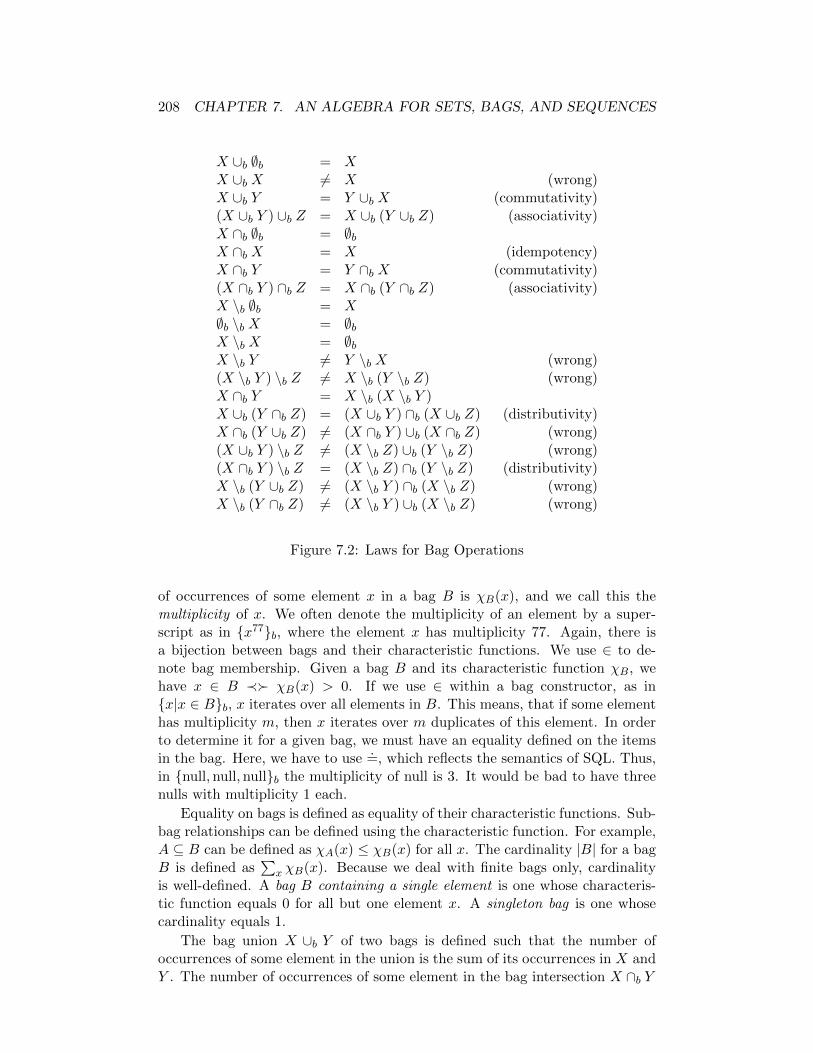
208 CHAPTER 7. AN ALGEBRA FOR SETS, BAGS, AND SEQUENCES

X ∪b ∅b = XX ∪b X 6= X (wrong)X ∪b Y = Y ∪b X (commutativity)(X ∪b Y ) ∪b Z = X ∪b (Y ∪b Z) (associativity)X ∩b ∅b = ∅bX ∩b X = X (idempotency)X ∩b Y = Y ∩b X (commutativity)(X ∩b Y ) ∩b Z = X ∩b (Y ∩b Z) (associativity)X \b ∅b = X∅b \b X = ∅bX \b X = ∅bX \b Y 6= Y \b X (wrong)(X \b Y ) \b Z 6= X \b (Y \b Z) (wrong)X ∩b Y = X \b (X \b Y )X ∪b (Y ∩b Z) = (X ∪b Y ) ∩b (X ∪b Z) (distributivity)X ∩b (Y ∪b Z) 6= (X ∩b Y ) ∪b (X ∩b Z) (wrong)(X ∪b Y ) \b Z 6= (X \b Z) ∪b (Y \b Z) (wrong)(X ∩b Y ) \b Z = (X \b Z) ∩b (Y \b Z) (distributivity)X \b (Y ∪b Z) 6= (X \b Y ) ∩b (X \b Z) (wrong)X \b (Y ∩b Z) 6= (X \b Y ) ∪b (X \b Z) (wrong)

Figure 7.2: Laws for Bag Operations

of occurrences of some element x in a bag B is χB(x), and we call this themultiplicity of x. We often denote the multiplicity of an element by a super-script as in x77b, where the element x has multiplicity 77. Again, there isa bijection between bags and their characteristic functions. We use ∈ to de-note bag membership. Given a bag B and its characteristic function χB, wehave x ∈ B ≺ χB(x) > 0. If we use ∈ within a bag constructor, as inx|x ∈ Bb, x iterates over all elements in B. This means, that if some elementhas multiplicity m, then x iterates over m duplicates of this element. In orderto determine it for a given bag, we must have an equality defined on the itemsin the bag. Here, we have to use

.=, which reflects the semantics of SQL. Thus,

in null,null,nullb the multiplicity of null is 3. It would be bad to have threenulls with multiplicity 1 each.

Equality on bags is defined as equality of their characteristic functions. Sub-bag relationships can be defined using the characteristic function. For example,A ⊆ B can be defined as χA(x) ≤ χB(x) for all x. The cardinality |B| for a bagB is defined as

∑x χB(x). Because we deal with finite bags only, cardinality

is well-defined. A bag B containing a single element is one whose characteris-tic function equals 0 for all but one element x. A singleton bag is one whosecardinality equals 1.

The bag union X ∪b Y of two bags is defined such that the number ofoccurrences of some element in the union is the sum of its occurrences in X andY . The number of occurrences of some element in the bag intersection X ∩b Y

7.1. SETS, BAGS, AND SEQUENCES 209

is the minimum of the number of its occurrences in X and Y . In the bagdifference X \b Y , the number of occurrences of some element is the difference(−) of its occurrences in X and Y , where a−b is defined as max(0, a−b). Usingcharacteristic functions, we can define

χX∪bY (z) = χX(z) + χY (z)

χX∩bY (z) = min(χX(z), χY (z))

χX\bY (z) = χX(z)−χY (z)

The laws for sets do not necessarily hold for bags (see Figure 7.2). We havethat bag union and bag intersection are both commutative and associative. Bagdifference is neither of them. Let us take a closer look at the different distribu-tivity laws. Therefore, denote by LHS the left-hand side of an equivalence andby RHS its right-hand side. Let us first prove

X ∪b (Y ∩b Z) = (X ∪b Y ) ∩b (X ∪b Z).

Since for all x we have

χLHS(x) = χX(x) + min(χY (x), χZ(x))

= min(χX(x) + χY (x), χX(x) + χZ(x))

= χRHS(x),

the claim follows.For the bags X = 15b, Y = 13b, and Z = 13b, we get

X ∩b (Y ∪b Z) = 15b ∩b 16b = 15b,

but(X ∩b Y ) ∪b (X ∩b Z) = 13b ∪b 13b = 16b.

For the bags X = 15b, Y = 13b, and Z = 12b, we calculate

(X ∪b Y ) \b Z = 18b \b 12b = 16b,

but(X \b Z) ∪b (Y \b Z) = 13b ∪b 11b = 14b.

Consider(X ∩b Y ) \b Z = (X \b Z) ∩b (Y \b Z).

This holds, since

χLHS(x) = min(χX(x), χY (x))−χZ(x)

= min(χX(x)−χZ(x), χY (x)−χZ(x))

= χRHS(x).

For the bags X = 12b, Y = 11b, and Z = 11b, we calculate

X \b (Y ∪b Z) = 12b \b 12b = ∅b,

210 CHAPTER 7. AN ALGEBRA FOR SETS, BAGS, AND SEQUENCES

but(X \b Y ) ∩b (X \b Z) = 11b ∩b 11b = 11b,

andX \b (Y ∩b Z) = 12b \b 11b = 11b,

but(X \b Y ) ∪b (X \b Z) = 11b ∪b 11b = 12b.

Remark. Our definition of bag union is not the usual definition. Thestandard set theoretic definition of the bag union operator ∪max is defined suchthat

χX∪maxY (x) = max(χX(x), χY (x))

holds [21, 212]. With this definition, the laws for sets carry over to bags. Wedecided to use the non-standard definition, since this is the semantics of bagunion in SQL and other query languages. Dayal, Goodman, and Katz [212] andAlbert [21] also investigate the non-standard bag union in their papers, althoughunder a different name. For example, Albert calls it bag concatenation. As a sideremark, it is interesting to note that Albert showed that bag concatenation cannot be expressed using ∪max, ∩b, \b [21]. Thus, any query language featuring ∪bis strictly more expressive, since ∪max can be expressed using \b and ∪b becausethe equivalence

X ∪max Y ≡ (X \b Y ) ∪b Yholds. Two other laws involving ∪max are

X ∪max Y ≡ (X ∪b Y ) \b (X ∩b Y ),

X ∩b Y ≡ (X ∪b Y ) \b (X ∪max Y ).

We introduce linearity for bags in Sec. 7.4.

7.1.3 Explicit Duplicate Control

Having every operation twice, once for bags and once for sets is quite inconve-nient. Fortunately, for some operations we only need the one for bags. We canget rid of some set operations as follows. Every set can be seen as a bag whosecharacteristic function never exceeds one. Let I(S) turn a set S into a bag withidentical characteristic function. The partial function I−1(B) turns a bag intoa set if the bag’s characteristic function does not exceed one. Otherwise let I−1

be undefined. Let X and Y be two sets. For the intersection function, we thenhave

I−1(I(X) ∩b I(Y )) = X ∩s Y.That is, for any two sets X and Y bag intersection and set intersection are thesame. Thus, we only need one intersection operation, which is defined on bagsand which we will denote by ∩.

The above observation gives rise to the notion of set-faithfulness. We call aunary function on sets f set-faithful if and only if

I−1(f(I(X))) = f(X)

7.1. SETS, BAGS, AND SEQUENCES 211

holds for all sets X. Analogously, we call binary functions g set-faithful if andonly if

I−1(g(I(X), I(Y ))) = g(X,Y )

holds for all sets X and Y .\b and ∩b are set-faithful. Hence, we can (and often will) simply use \ and

∩ to denote bag difference and intersection. If the arguments happen to be sets,the resulting bag will not contain any duplicates, i.e., it is a set.

Note that ∪b is not set-faithful. One possibility is to carefully distinguishbetween ∪b and ∪s. However, this does not solve our problem for query process-ing. A relation can be a set (e.g. if a primary key is defined) or a bag. Assumewe have two relations (or intermediate results) R1, which is a set, and R2, whichis a bag. Obviously, R1 ∪s R2 is not valid since R2 is a bag. By treating setsas special bags, R1 ∪bR2 is valid. However, we cannot control duplicates in theresult as demanded by SQL, where there is a fundamental difference betweenunion all and union distinct. We could thus use two different union oper-ators. Both take bags as input but one preserves duplicates, as does the bagunion, and the other eliminates duplicates. Let us denote the former by ∪ andthe latter by ∪d.

To go from a bag to a set, we have to eliminate duplicates. Let us denoteby ΠD the duplicate elimination operation. For a given bag B, we then haveχΠD(B)(z) = min(1, χB(z)). Using ΠD, we can define ∪d as

R1 ∪d R2 := ΠD(R1 ∪R2).

However, the right-hand side is our preferred way to take care of duplicatehandling: we will always use the bag operator, denoted by ∪ and then, ifnecessary, eliminate duplicates explicitly.

Summarizing, instead of working with sets and bags, we can work with bagsonly by identifying every set S with the bag I(S). To keep track of (possible)duplicates, we can annotate all bags with a property indicating whether itcontains duplicates or not. If at some place a set is required and we cannotinfer that the bag in that place is duplicate free, we can use ΠD as an enforcerof the set property. Note that for every set S we have ΠD(S) = S. Hence, ΠD

does not do any harm except for the resources it takes. The reasoning whethera given expression produces duplicates or not is very important. Below, we willindicate on the fly how reasoning about duplicates can be performed.

7.1.4 Ordered Data: Sequences

A sequence is ordered and may contain duplicates. An example sequence is〈a, b, b, c, b〉. The length of the sequence is the number of elements it contains.For any sequence S, the length of the sequence is denoted by |S|. The abovesequence has length five. The empty sequence (ε) contains zero elements andhas length zero.

As we consider only finite sequences, a sequence of length n ≥ 0 has acharacteristic function χ from an interval [0, n[ to a domain D. Outside [0, n[,χ is undefined (⊥). Let S be a sequence. Then α(S) gives us the first element of

212 CHAPTER 7. AN ALGEBRA FOR SETS, BAGS, AND SEQUENCES

the sequence, i.e., α(S) = χS(0). For our example sequence, α(〈a, b, b, c, b〉) = a.The rest or tail of a sequence S of length n is denoted by τ(S) and containsall but the first element in the sequence. That is χτ(S)(i) = χS(i+ 1). For ourexample sequence, τ(〈a, b, b, c, b〉) = 〈b, b, c, b〉.

Concatenation of two sequences is denoted by ⊕. The characteristic functionof the concatenation of two sequences S and T is

χS⊕T (i) =

χS(i) if i < |S|,χT (i− |S|) if i ≥ |S|.

As an example, 〈a, b, b, c, b〉 ⊕ 〈a, b, c〉 = 〈a, b, b, c, b, a, b, c〉.We can easily go from a sequence to a bag by just forgetting the order. To

convert a bag into a sequence, we typically have to apply a Sort operator. Inreality, however, bags are often represented as (ordered) streams, i.e., they aresequences. This is due to the fact that most physical algebras are implementedusing the iterator concept introduced in Section 4.6.

Analogously to set and bag linearity, we can introduce sequence linearityof unary and n-ary functions on sequences. In the definition, we only have toexchange the set union operator by concatentation. A unary function f fromsequences to sequences is called sequence-linear , if and only if the following twoconditions hold for all sequences X and Y :

f(ε) = ε,

f(X ⊕ Y ) = f(X)⊕ f(Y ).

An n-ary mapping from sequences to a sequence is called sequence-linear in itsi-th argument if and only if for all sequences X1, . . . , Xn and X ′i the followingconditions hold:

f(X1, . . . , Xi−1, ε,Xi+1, . . . , Xn) = ε

f(X1, . . . , Xi−1, Xi ⊕X ′i, Xi+1, . . . , Xn) = f(X1, . . . , Xi−1, Xi, Xi+1, . . . , Xn)

⊕f(X1, . . . , Xi−1, X′i, Xi+1, . . . , Xn)

It is called sequence-linear , if it is sequence-linear in all its arguments. For abinary function or operator where we can distinguish between the left and theright argument, we call it left (right) sequence-linear if it is sequence-linear inits first (second) argument. Note that if an equivalence with linear mappingson both sides has to be proven, it suffices to proof it for singleton sequences,i.e. sequences with one element only.

7.2 Aggregation Functions

SQL and other query languages support at least five aggregation functions.These are min, max, count, sum, and avg. In addition, SQL allows to qualifywhether duplicates are removed before computing the aggregate or whether theyare also considered by the aggregation function. For example, we may specifysum(distinct a) or sum(all a) for some attribute a. The term sum(a) is

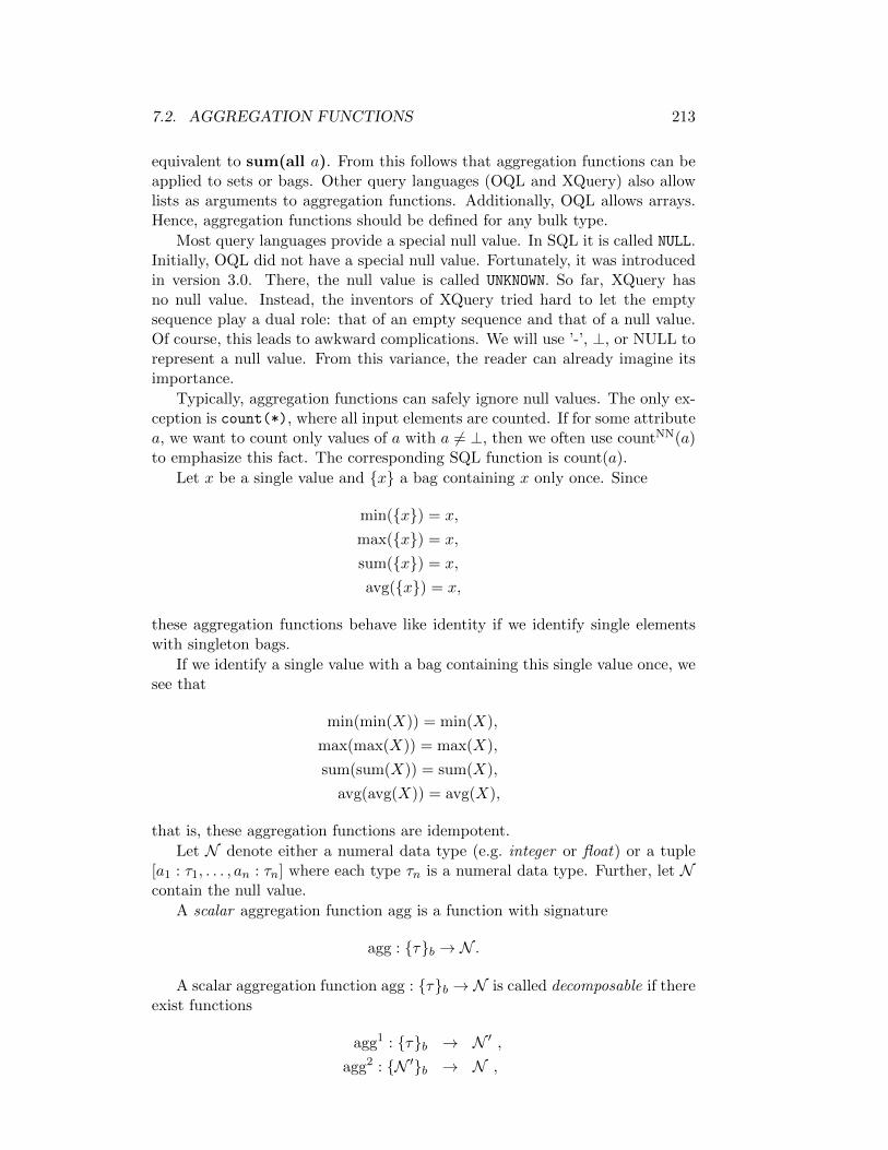
7.2. AGGREGATION FUNCTIONS 213

equivalent to sum(all a). From this follows that aggregation functions can beapplied to sets or bags. Other query languages (OQL and XQuery) also allowlists as arguments to aggregation functions. Additionally, OQL allows arrays.Hence, aggregation functions should be defined for any bulk type.

Most query languages provide a special null value. In SQL it is called NULL.Initially, OQL did not have a special null value. Fortunately, it was introducedin version 3.0. There, the null value is called UNKNOWN. So far, XQuery hasno null value. Instead, the inventors of XQuery tried hard to let the emptysequence play a dual role: that of an empty sequence and that of a null value.Of course, this leads to awkward complications. We will use ’-’, ⊥, or NULL torepresent a null value. From this variance, the reader can already imagine itsimportance.

Typically, aggregation functions can safely ignore null values. The only ex-ception is count(*), where all input elements are counted. If for some attributea, we want to count only values of a with a 6= ⊥, then we often use countNN(a)to emphasize this fact. The corresponding SQL function is count(a).

Let x be a single value and x a bag containing x only once. Since

min(x) = x,

max(x) = x,

sum(x) = x,

avg(x) = x,

these aggregation functions behave like identity if we identify single elementswith singleton bags.

If we identify a single value with a bag containing this single value once, wesee that

min(min(X)) = min(X),

max(max(X)) = max(X),

sum(sum(X)) = sum(X),

avg(avg(X)) = avg(X),

that is, these aggregation functions are idempotent.

Let N denote either a numeral data type (e.g. integer or float) or a tuple[a1 : τ1, . . . , an : τn] where each type τn is a numeral data type. Further, let Ncontain the null value.

A scalar aggregation function agg is a function with signature

agg : τb → N .

A scalar aggregation function agg : τb → N is called decomposable if thereexist functions

agg1 : τb → N ′ ,agg2 : N ′b → N ,

214 CHAPTER 7. AN ALGEBRA FOR SETS, BAGS, AND SEQUENCES

with

agg(Z) = agg2(agg1(X), agg1(Y )b)

for all X and Y (not empty) with Z = X ∪ Y . This condition assures thatagg(Z) can be computed on arbitrary subsets (-lists, -bags) of Z independentlyand the (partial) results can be aggregated to yield the correct total result. Ifthe condition holds, we say that agg is decomposable with inner agg1 and outeragg2.

A decomposable scalar aggregation function agg : τb → N is called re-versible if for aggO there exists a function (aggO)−1 : N ′,N ′ → N ′ with

agg(X) = γ((aggO)−1(aggI(Z), aggI(Y )))

for all X, Y , and Z with Z = X ∪ Y . This condition assures that we cancompute agg(X) for a subset (-list, -bag) X of Z by “subtracting” its aggregatedcomplement Y from the “total” aggO(aggI(Z)) by using (aggO)−1.

The fact that scalar aggregation functions can be decomposable and re-versible is the basic observation upon which builds the efficient evaluation ofaggregation functions.

As an example, consider the scalar aggregation avg : [a : float]b → floataveraging the values of the attributes a of a bag of tuples with a single attributea. It is reversible with

aggI : [a : float] → [sum : float, count : float],

aggO : [sum : float, count : float], [sum : float, count : float] → [sum : float, count : float],

(aggO)−1 : [sum : float, count : float], [sum : float, count : float] → [sum : float, count : float],

γ : [sum : float, count : float] → float,

where

aggI(X) = [sum : sum(X.a), count : |X|],aggO([sum : s1, count : c1], [sum : s2, count : c2]) = [sum : s1 + s2, count : c1 + c2],

(aggO)−1([sum : s1, count : c1], [sum : s2, count : c2]) = [sum : s1 − s2, count : c1 − c2],

γ([sum : s, count : c]) = s/c.

Here, sum(X.a) denotes the sum of all values of attribute a of the tuples in X,and |X| denotes the cardinality of X. Note that aggI(∅) = [sum : 0, count : 0],and γ([sum : 0, count : 0]) is undefined as is avg(∅).

In statistics, the variance of a bag of numbers is often calculated. For a bagB, it is defined as s2 = 1

n−1

∑x∈B(x− x)2, where x is the average of the values

in B, i.e., x = 1n

∑x∈B x. As an exercise, the reader should show that variance

is decomposable and reversible.

Not all aggregation functions are decomposable and reversible. For instance,min and max are decomposable but not reversible. If an aggregation functionis applied to a bag that has to be converted to a set, then decomposabili-ty is jeopardized for sum and count. That is, in SQL sum(distinct) andcount(distinct) are not decomposable.

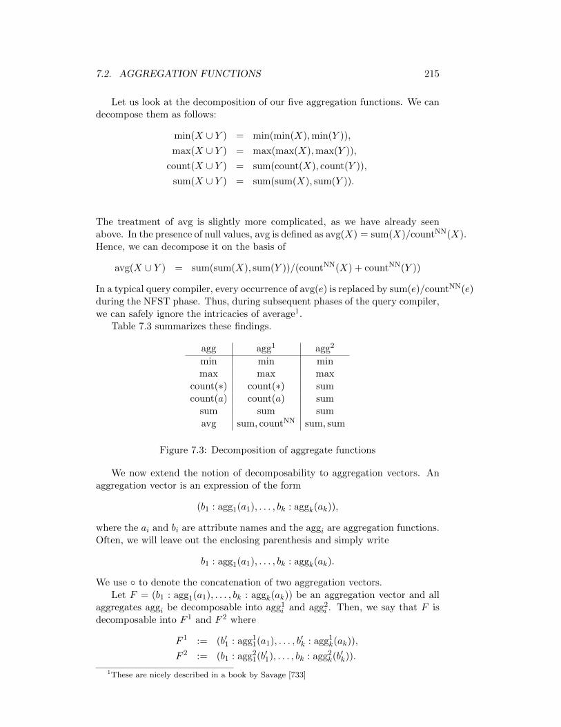
7.2. AGGREGATION FUNCTIONS 215

Let us look at the decomposition of our five aggregation functions. We candecompose them as follows:

min(X ∪ Y ) = min(min(X),min(Y )),

max(X ∪ Y ) = max(max(X),max(Y )),

count(X ∪ Y ) = sum(count(X), count(Y )),

sum(X ∪ Y ) = sum(sum(X), sum(Y )).

The treatment of avg is slightly more complicated, as we have already seenabove. In the presence of null values, avg is defined as avg(X) = sum(X)/countNN(X).Hence, we can decompose it on the basis of

avg(X ∪ Y ) = sum(sum(X), sum(Y ))/(countNN(X) + countNN(Y ))

In a typical query compiler, every occurrence of avg(e) is replaced by sum(e)/countNN(e)during the NFST phase. Thus, during subsequent phases of the query compiler,we can safely ignore the intricacies of average1.

Table 7.3 summarizes these findings.

agg agg1 agg2

min min minmax max max

count(∗) count(∗) sumcount(a) count(a) sum

sum sum sumavg sum, countNN sum, sum

Figure 7.3: Decomposition of aggregate functions

We now extend the notion of decomposability to aggregation vectors. Anaggregation vector is an expression of the form

(b1 : agg1(a1), . . . , bk : aggk(ak)),

where the ai and bi are attribute names and the aggi are aggregation functions.Often, we will leave out the enclosing parenthesis and simply write

b1 : agg1(a1), . . . , bk : aggk(ak).

We use to denote the concatenation of two aggregation vectors.Let F = (b1 : agg1(a1), . . . , bk : aggk(ak)) be an aggregation vector and all

aggregates aggi be decomposable into agg1i and agg2

i . Then, we say that F isdecomposable into F 1 and F 2 where

F 1 := (b′1 : agg11(a1), . . . , b′k : agg1

k(ak)),

F 2 := (b1 : agg21(b′1), . . . , bk : agg2

k(b′k)).

1These are nicely described in a book by Savage [733]

216 CHAPTER 7. AN ALGEBRA FOR SETS, BAGS, AND SEQUENCES

Note that in all cases, we have that if F is decomposable into F 1 and F 2,then F 1 is decomposable into F 1,1 and F 1,2, and F 2 is decomposable into F 2,1

and F 2,2. Further, we have

F 1,1 = F 1,

F 1,2 = F 2,

F 2,1 = F 2,

F 2,1 = F 2.

Let e1 and e2 be arbitrary expressions. We say that an aggregation vectorF is splittable into F1 and F2 with respect to e1 and e2 if F = F1 F2, F(F1)∩A(e2) = ∅ and F(F2) ∩ A(e1) = ∅. Assume that F contains an aggregationfunction aggi applied to some attribute ai. If a ∈ A(e1), then clearly aggi(ai)belongs to F1, if a ∈ A(e2) then aggi(ai) belongs to F2. There are other caseswhere F is splittable. Consider, for example, sum(a1 +a2) for ai ∈ A(ei). Sincesum(a1 +a2) = sum(a1)+sum(a2), this does not hinder splittability. The sameholds for subtraction.

The correct handling of duplicates, i.e., bags, is essential for the correctnessof the query compiler and requires some care. We will therefore classify our ag-gregation functions into those which are sensitive to duplicates and those whichare not. An aggregation function is called duplicate agnostic if the multiplicityof the elements in the bag does not influence its result. It is called duplicatesensitive otherwise. For our aggregation functions we have

• min, max, sum(distinct), count(distinct), avg(distinct) are duplicate ag-nostic and

• sum, count, avg are duplicate sensitive.

Yan and Larson used the term Class C aggregation function for duplicate sensi-tive aggregation functions and Class D for duplicate agnostic aggregation func-tions [913].

Finally, note that for all aggregate functions except count(∗), we haveagg(a) = a for arbitrary elements a. Thus, if we are sure that we deal withonly one tuple, we can apply the following rewrite. Let ai and bi be attributes.Then, if F = (b1 : agg1(a1), . . . , bm : aggm(am)), we define F = (b1 : a1, . . . , bm :am).

7.3 Operators

The bag operators as well as other typical operators like selection and join arewell-known. As we will see, the only difference in the definitions used hereis that they are extended to express nested queries. In order to enable this,we allow the subscripts (predicates, expressions) of these operators to containalgebraic expressions.

In this section, we define all our operators on bags. Besides duplicate elim-ination, only projection will have explicit control over duplicates.

7.3. OPERATORS 217

Sometimes, the left outerjoin needs some additional tuning. The standarddefinition of the left outerjoin demands that if some tuple from its left argumentdoes not have a join partner in its right argument, the attributes from the rightargument are given null values. We extend the left outerjoin such that valuesother than null can be given to attributes of the right hand side. Similarily,the full outerjoin will be extended to carry two superscripts for this kind ofdefaults.

The d-join operation is used for performing a join between two bag valueditems, where the second one is dependent on the first one. One use is to expressqueries with table functions (see Sec. 4.10). Another is to access index structures(see Sec. 4.14). The d-join can also be used to unnest nested queries. It is oftenequivalent to a join between two bags with a membership predicate [775]. Insome cases, it corresponds to an unnest operation.

The map operator χ ([467]) is well-known from the functional programminglanguage context. A special case of it, where it adds derived information inform of an added attribute with an according value (e.g. by object-base lookupor by method calls) to each tuple of a bag has been proposed in [466, 467].Later, this special case was given the name materialization operator [89].

The unnest operator is known from NF2 [736, 716]. It will come in two dif-ferent flavors allowing us to perform unnesting not only on nested relations butalso on attributes whose value is a bag of elements which are not tuples. Thereverse operator is the nest operator, which can be generalized to a groupingoperator. In our algebra, there exist two grouping operators: one unary group-ing operator and one binary grouping operator (called groupjoin). The unarygrouping operator groups one bag of tuples according to a grouping condition.Further, it can apply an arbitrary expression to the newly formed group. Thegroupjoin adds a group to each element in the first argument bag. This groupis formed from the second argument. The groupjoin will exploit the fact thatin the object-oriented context objects can have bag-valued attributes. As wewill see, this is useful for both, unnesting nested queries and producing nestedresults. We will even use nesting a a useful tool for processing SQL queries.

7.3.1 Preliminaries

As already mentioned, our algebraic operators not only deal with standardrelations but are polymorphic in the general sense. In order to fix the domainof the operators, we need some technical abbreviations and notations. Let usintroduce these first.

Since our operators are polymorphic, we need variables for types. We use τpossibly with a subscript to denote types. To express that a certain expressionis of type e, we write e :: τ . Starting from concrete names for types andtype variables, we can build type expressions the standard way by using typeconstructors to build tuple types ([·]), set types ·s, bag types ·b and sequencetypes < · >. Having two type expressions t1 and t2, we denote by t1 ≤ t2 thatt1 is a subtype of t2. It is important to note that this subtype relationship is notbased on the sub-/superclass hierarchy found in most object-oriented models.Instead, it simply denotes substitutability. That is, type t1 provides at least all

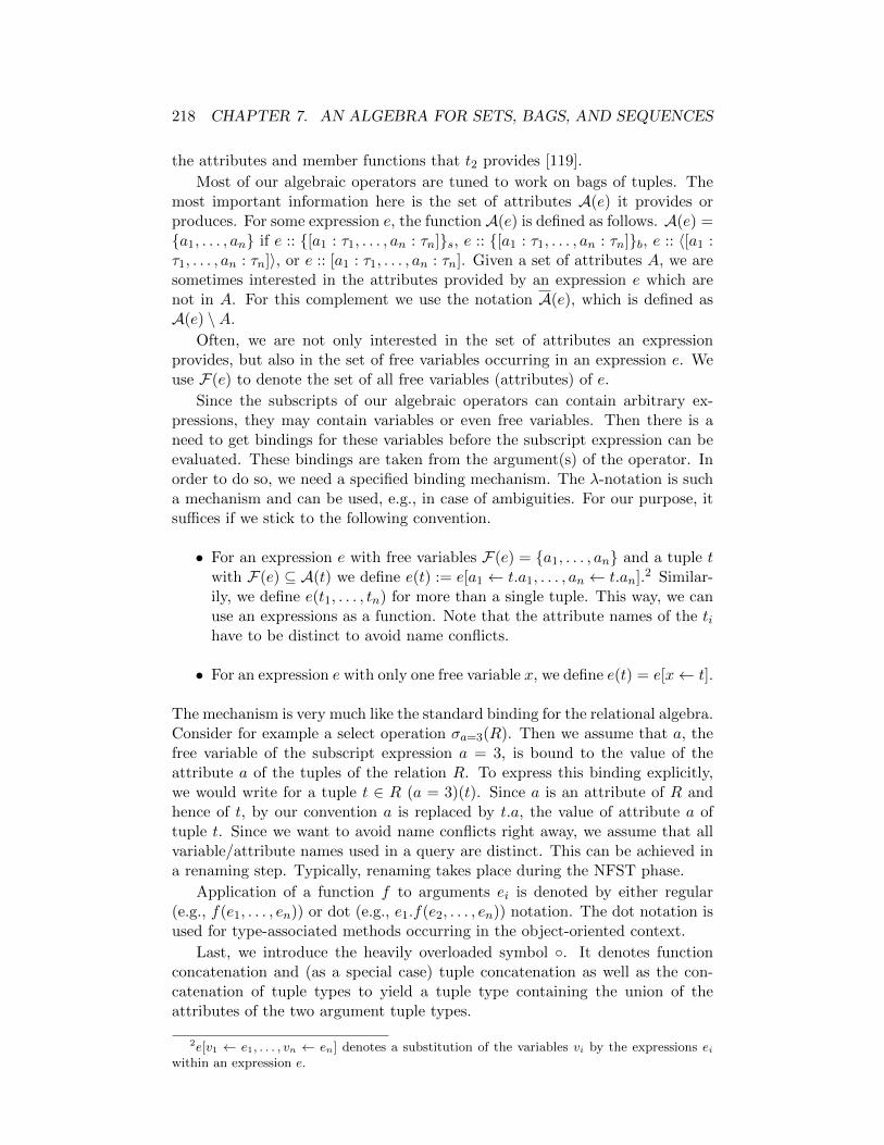
218 CHAPTER 7. AN ALGEBRA FOR SETS, BAGS, AND SEQUENCES

the attributes and member functions that t2 provides [119].

Most of our algebraic operators are tuned to work on bags of tuples. Themost important information here is the set of attributes A(e) it provides orproduces. For some expression e, the function A(e) is defined as follows. A(e) =a1, . . . , an if e :: [a1 : τ1, . . . , an : τn]s, e :: [a1 : τ1, . . . , an : τn]b, e :: 〈[a1 :τ1, . . . , an : τn]〉, or e :: [a1 : τ1, . . . , an : τn]. Given a set of attributes A, we aresometimes interested in the attributes provided by an expression e which arenot in A. For this complement we use the notation A(e), which is defined asA(e) \A.

Often, we are not only interested in the set of attributes an expressionprovides, but also in the set of free variables occurring in an expression e. Weuse F(e) to denote the set of all free variables (attributes) of e.

Since the subscripts of our algebraic operators can contain arbitrary ex-pressions, they may contain variables or even free variables. Then there is aneed to get bindings for these variables before the subscript expression can beevaluated. These bindings are taken from the argument(s) of the operator. Inorder to do so, we need a specified binding mechanism. The λ-notation is sucha mechanism and can be used, e.g., in case of ambiguities. For our purpose, itsuffices if we stick to the following convention.

• For an expression e with free variables F(e) = a1, . . . , an and a tuple twith F(e) ⊆ A(t) we define e(t) := e[a1 ← t.a1, . . . , an ← t.an].2 Similar-ily, we define e(t1, . . . , tn) for more than a single tuple. This way, we canuse an expressions as a function. Note that the attribute names of the tihave to be distinct to avoid name conflicts.

• For an expression e with only one free variable x, we define e(t) = e[x← t].

The mechanism is very much like the standard binding for the relational algebra.Consider for example a select operation σa=3(R). Then we assume that a, thefree variable of the subscript expression a = 3, is bound to the value of theattribute a of the tuples of the relation R. To express this binding explicitly,we would write for a tuple t ∈ R (a = 3)(t). Since a is an attribute of R andhence of t, by our convention a is replaced by t.a, the value of attribute a oftuple t. Since we want to avoid name conflicts right away, we assume that allvariable/attribute names used in a query are distinct. This can be achieved ina renaming step. Typically, renaming takes place during the NFST phase.

Application of a function f to arguments ei is denoted by either regular(e.g., f(e1, . . . , en)) or dot (e.g., e1.f(e2, . . . , en)) notation. The dot notation isused for type-associated methods occurring in the object-oriented context.

Last, we introduce the heavily overloaded symbol . It denotes functionconcatenation and (as a special case) tuple concatenation as well as the con-catenation of tuple types to yield a tuple type containing the union of theattributes of the two argument tuple types.

2e[v1 ← e1, . . . , vn ← en] denotes a substitution of the variables vi by the expressions eiwithin an expression e.

7.3. OPERATORS 219

Sometimes it is useful to be able to produce a bag containing only a singletuple with no attributes. This is done by the singleton scan operator denotedby 2. Thus, 2 ≡ []b.

Very often, we are given some database item which is a bag of other items.Binding these to variables or, equivalently, embedding the items into a tuple,we use the notation e[x] for an expression e and a variable/attribute name x.For bag-valued expressions e, e[x] is defined as e[x] = [x : y]|y ∈ e. Forsequence-valued expressions e, we define e[a] = ε if e is empty and e[a] = 〈[a :α(e)]〉 ⊕ τ(e)[a] otherwise.

By id we denote the identity function.

7.3.2 Signatures

We are now ready to define the signatures of the operators of our algebra.Their semantics is defined in a subsequent step. Remember that we consider alloperators as being polymorphic. Hence, their signatures are polymorphic andcontain type variables, denoted by τ , often with an index. As mentioned before,we define all operators on bags. Let us start by typing our bag operators

∪ : τb, τb → τb,∩ : τb, τb → τb,\ : τb, τb → τb,

ΠD : τb → τb.

The unary operators we use have the following signatures, where B denotes

220 CHAPTER 7. AN ALGEBRA FOR SETS, BAGS, AND SEQUENCES

the type boolean:

ΠA : τb → τ ′bif τ ≤ τ ′ = [a1 : τ1, . . . , an : τn], A = a1, . . . , an,

ΠDA : τb → τ ′b

if τ ≤ τ ′ = [a1 : τ1, . . . , an : τn], A = a1, . . . , an,σp : τb → τb

if p : τ → B,χf : τ1b → τ2b

if f : τ1 → τ2,

χa:f : τ1b → τ1 [a : τ2]bif f : τ1 → τ2,

ΓθG;g:f : τ1 τ2b → τ1 [g : τ ′]bif τi ≤ [], f : τ2b → τ ′, G = A(τ1),

νG;g : τ1 τ2b → τ1 [g : τ2b]bif τi ≤ [], G = A(τ1),

µg : τb → τ ′bif τ = [a1 : τ1, . . . , an : τn, g : τ0b],τ0 ≤ [],

τ ′ = [a1 : τ1, . . . , an : τn] τ0,

µg;c : τb → τ ′bif τ = [a1 : τ1, . . . , an : τn, g : τ0b],τ ′ = [a1 : τ1, . . . , an : τn] [c : τ0].

One special operator is needed to translate OQL, which exhibits an explicitflatten operator to unnest bags of bags. An according algebraic operator isdefined easily:

flatten : τbb → τb.

7.3. OPERATORS 221

The following is a list of signatures of some binary operators.

A : τ1b, τ2b → τ1 τ2b,Bq : τ1b, τ2b → τ1 τ2b

if τi ≤ [], q : τ1, τ2 → B,Nq : τ1b, τ2b → τ1b

if τi ≤ [], q : τ1, τ2 → B,Tq : τ1b, τ2b → τ1b

if τi ≤ [], q : τ1, τ2 → B,Eq : τ1b, τ2b → τ+

1 τ2bif τi < [], q : τ1, τ2 → B,

Kq : τ1b, τ2b → τ+1 τ+

2 bif τi < [], q : τ1, τ2 → B,

C : τ1b, τ2b → τ1 τ2bif τi ≤ [],

ZA1θA2;g:f : τ1b, τ2b → τ1 [g : τ ′]bif τ1 ≤ [], f : τ2b → τ ′, Ai ⊆ A(τi) for i = 1, 2.

Using some special min/max operators to retrieve the element(s) whosevalue becomes minimal/maximal often results in more efficient plans:

maxg;m;f : τb → [m : τa, g : τf ]

if τ ≤ [a : τa], f : τab → τf .

7.3.3 Projection

Let A a1, . . . , an be a set of attributes. We define the two projection operators

ΠA(e) := [a1 : x.a1, . . . , an : x.an]|x ∈ eb,ΠDA (e) := ΠD(ΠA(e)).

The result of ΠD is always duplicate-free. In concordance with the characteristicfunction of bags, we use

.= to determine whether two elements are equal or

not. Thus, ΠDA is defined such that the characteristic function of ΠD

A (e) yieldsmax(1, χΠA(e)(x)) for all x ∈ ΠA(e).

Thus, it is set-faithful. Typically, the result of ΠA is not duplicate-free, evenif its input is duplicate-free. Thus, we need explicit duplicate control here. Oneexception occurs in the presence of functional dependencies. If A → A(e) ande is duplicate-free, then ΠA(e) is duplicate-free.

Sometimes, we want to eliminate a single attribute or a set of attributes.This is denoted by

ΠA(e) := ΠA(e)\A(e)

ΠDA

(e) := ΠDA(e)\A(e)

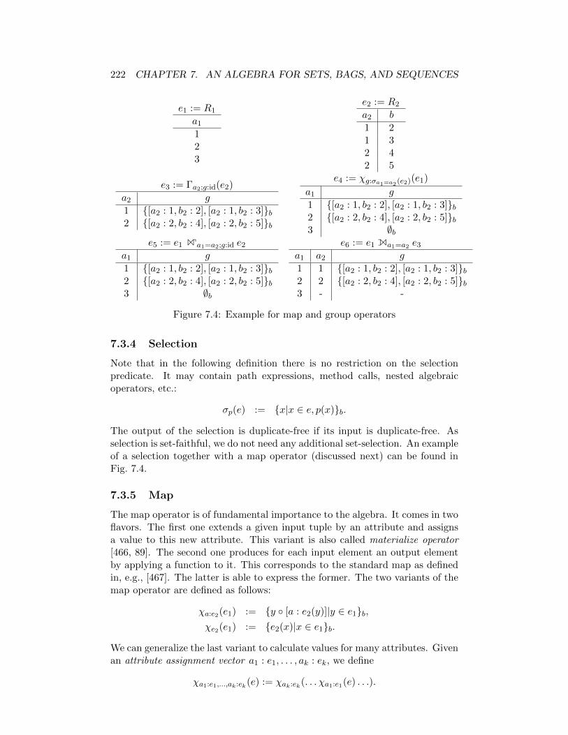
222 CHAPTER 7. AN ALGEBRA FOR SETS, BAGS, AND SEQUENCES

e1 := R1

a1

123

e2 := R2

a2 b

1 21 32 42 5

e3 := Γa2;g:id(e2)

a2 g

1 [a2 : 1, b2 : 2], [a2 : 1, b2 : 3]b2 [a2 : 2, b2 : 4], [a2 : 2, b2 : 5]b

e4 := χg:σa1=a2 (e2)(e1)

a1 g

1 [a2 : 1, b2 : 2], [a2 : 1, b2 : 3]b2 [a2 : 2, b2 : 4], [a2 : 2, b2 : 5]b3 ∅b

e5 := e1 Za1=a2;g:id e2

a1 g

1 [a2 : 1, b2 : 2], [a2 : 1, b2 : 3]b2 [a2 : 2, b2 : 4], [a2 : 2, b2 : 5]b3 ∅b

e6 := e1 Ea1=a2 e3

a1 a2 g

1 1 [a2 : 1, b2 : 2], [a2 : 1, b2 : 3]b2 2 [a2 : 2, b2 : 4], [a2 : 2, b2 : 5]b3 - -

Figure 7.4: Example for map and group operators

7.3.4 Selection

Note that in the following definition there is no restriction on the selectionpredicate. It may contain path expressions, method calls, nested algebraicoperators, etc.:

σp(e) := x|x ∈ e, p(x)b.

The output of the selection is duplicate-free if its input is duplicate-free. Asselection is set-faithful, we do not need any additional set-selection. An exampleof a selection together with a map operator (discussed next) can be found inFig. 7.4.

7.3.5 Map

The map operator is of fundamental importance to the algebra. It comes in twoflavors. The first one extends a given input tuple by an attribute and assignsa value to this new attribute. This variant is also called materialize operator[466, 89]. The second one produces for each input element an output elementby applying a function to it. This corresponds to the standard map as definedin, e.g., [467]. The latter is able to express the former. The two variants of themap operator are defined as follows:

χa:e2(e1) := y [a : e2(y)]|y ∈ e1b,χe2(e1) := e2(x)|x ∈ e1b.

We can generalize the last variant to calculate values for many attributes. Givenan attribute assignment vector a1 : e1, . . . , ak : ek, we define

χa1:e1,...,ak:ek(e) := χak:ek(. . . χa1:e1(e) . . .).

7.3. OPERATORS 223

If we demand that ai 6∈ A(e), then the ai are new attributes. Then, the ma-terialize operator and its special single-attribute case χa:e are called extending,because it extends a given input tuple with new attributes while it does notmodify the values of the input attributes. Many equivalences only hold for thisspecialization of the map operator, which, at the same time, is the predominantvariant used. In fact, it is sufficient for SQL. An example of an extending mapoperator can be found in Fig. 7.4.

Note that the map operator for the object-oriented and object-relationalcontext obviates the need of a relational projection. Sometimes the map oper-ator is equivalent to a renaming. In this case, we will use ρ instead of χ. LetA = a1, . . . , an and B = b1, . . . , bn be two sets with n attributes each. Wethen define

ρA←B(e) := ΠA(χb1:a1,...,bn:an(e))

The result of the extending variant of the map operator is duplicate-free ifand only if its input is. Thus, the extending map operator is set-faithful.

7.3.6 Unary Grouping

Two grouping operators are contained in our algebra. The first one, discussedhere and called (unary) grouping , is defined on a bag and its subscript indicatesthe (i) grouping criterions and (ii) a new attribute name as well as a functionwhich is used to calculate its value.

ΓθG;g:f (e) := y [g : x] | y ∈ ΠDG(e), x = f(z|z ∈ e, z.G θ y.Gb)s

for some set of attributes G, an attribute g and a function f . The comparisonoperator θ must be a null-extended comparison operator like ‘

.=’. Note that the

result is a set, but f is applied to a bag. An example for the grouping operatorcan be found in Fig. 7.4.

The grouping criterion may be defined on several attributes. Then, G andθ represent sequences of attributes and comparators. In case all θ equal ’

.=’, we

abbreviate Γ .=G;g:f by ΓG;g:f .

We can extend the above definition to calculate several new attribute valuesby defining

ΓθG;b1:f1,...,bk:fk(e) := y[b1 : x1, . . . , bk : xk] | y ∈ ΠDG(e), xi = fi(z|z ∈ e, z.G θ y.Gb)s.

We also introduce two variants of the grouping operator, which can be usedto abbreviate small expressions. Let F = b1 : e1, . . . , bk : ek and F(ei) = gfor all i = 1, . . . , k. Then we define

ΓG;F (e) := Πg(χF (ΓG;g:id(e))).

Here, the free attribute g is implicit. If we wish to make it explicit, we writeΓG;g;F instead of simply ΓG;F . Note that g plays the same role as partition

in OQL ([128, p. 114]).

224 CHAPTER 7. AN ALGEBRA FOR SETS, BAGS, AND SEQUENCES

Let us also introduce a SQL-notation based variant. Let F be an aggregationvector of the form

F = b1 : agg1(a1), . . . , bk : aggk(ak)

for attributes ai. Then we define Fg as

Fg = b1 : agg1(g.a1), . . . , bk : aggk(g.ak)

and introduce the following abbreviation:

ΓG;F (e) := ΓG;g;Fg(e).

This is the version we have to use for SQL.The traditional nest operator ν [736], which nests a relation R given a set

of attributes G ⊂ A(e), can be defined as an abbreviation of the groupingoperator:

νG;g(e) := ΓG;g:ΠG(e),

where G abbreviates A(e) \G.The results of Γ and ν are always duplicate-free. Thus, these operators are

set-faithful.

7.3.7 Unnest Operators

The unnest operator comes in two different flavors. The first one is responsiblefor unnesting a set of tuples on an attribute being a set/bag/sequence of tuplesitself. The second one unnests sets of tuples on an attribute not being a bulk oftuples but a set of something else, e.g., integers. The according definitions are

µg(e) := y.[A(y) \ g] x|y ∈ e, x ∈ y.gb,µa:g(e) := y.[A(y) \ g] [a : x]|y ∈ e, x ∈ y.gb.

If the bag-valued attribute is not stored explicitly but derived by the evaluationof an expression, we use the unnest map operator to unnest it:

Υe2(e1) := Πg(µg(χg:e2(e1))),

Υa:e2(e1) := Πg(µa:g(χg:e2(e1))).

The motivation for the unnest map operator is that it saves the explicit mate-rialization of the result of the evaluation of the expression e2.

The results of µg(e) and µa:g are duplicate-free, if and only if the followingtwo conditions hold.

1. The input e is duplicate-free.

2. For each tuple t ∈ e we have that t.g is duplicate-free.

Hence, explicit duplicate control for the unnest operator is in order. The sameholds for the unnest map operator.

7.3. OPERATORS 225

7.3.8 Flatten Operator

The flatten operator flattens a bag of bags by unioning the elements of the bagscontained in the outer bag.

flatten(e) = y|x ∈ e, y ∈ xb

The flatten operator’s result is duplicate-free if and only if the bags it containsare duplicate-free and they have a pairwise empty intersection. Thus, explicitduplicate control is very much in order.

7.3.9 Join Operators

The algebra features many different join operators. The first five, namely join,semijoin, antijoin, left outerjoin, and full outerjoin – are rather standard:

e1 A e2 := y x|y ∈ e1, x ∈ e2b,e1 Bp e2 := y x|y ∈ e1, x ∈ e2, p(y, x)b,e1 Np e2 := y|y ∈ e1, ∃x ∈ e2, p(y, x)b,e1 Tp e2 := y|y ∈ e1,¬∃x ∈ e2 p(y, x)b,e1 Ep e2 := (e1 Bp e2) ∪ ((e1 Tp e2) A ⊥A(e2)),e1 Kp e2 := (e1 Bp e2)

∪((e1 Tp e2) A ⊥A(e2))∪(⊥A(e1)A (e2 Tp e1)).

An example for the left outerjoin can be found in Fig. 7.4. More examples forjoin, left outerjoin, and full outerjoin can be found in Fig. 7.6 for the predicateqij := (bi = bj) and in Fig. 7.7 for the predicate q′ij := (bi

.= bj) .

Regular joins were already present in Codd’s original proposal of a relationalalgebra [188]. Outerjoins were invented by Lacroix and Pirotte [503].

The next join operator to come is called dependency join, or d-join, and isdenoted by C. It is a join between two bags, where the evaluation of the secondbag may depend on the first bag. The filled triangle thus shows the directioninto which information has to flow in order to evaluate the d-join. It is used totranslate from clauses containing table functions with parameters (see Sec. 4.10for an example) and lateral derived tables into the algebra. Whenever possible,d-joins will be rewritten into standard joins. The definition of the d-join is

e1 C e2 := y x|y ∈ e1, x ∈ e2(y)b.

The result of a d-join is duplicate-free if e1 is duplicate-free and if for eacht1 ∈ e1 we have that e2(t1) is duplicate-free. Example applications of the d-joincan be found in Sec. 4.10 and Sec. 4.14.

For the left outerjoin and the full outerjoin, we need a variant which allowsus to set some attribute values to constants other than null for tuples with no

226 CHAPTER 7. AN ALGEBRA FOR SETS, BAGS, AND SEQUENCES

join partner. Let Di = di1 : ci1, . . . , dik : cik (i = 1, 2) be two vectors assigning

constants cij to attributes dij . We then define

e1 ED2

p e2 := (e1 Bp e2)

∪((e1 Tp e2) A ⊥A(e2)\A(D2) [D2],e1 K

D1;D2

p e2 := (e1 Bp e2)

∪((e1 Tp e2) A ⊥A(e2)\A(D2) [D2]),∪((e2 Tp e1) A ⊥A(e1)\A(D1) [D1]),

If one of D1 or D2 is empty, we use − to denote this.

As can already be seen from the definitions, this set of join operators ishighly redundant. As is well-known, the (regular) join can be expressed as asequence of selection and cross product:

e1 Bq e2 ≡ σq(e1 A e2).

For an expression e2 and a predicate q, define the predicate p as p = (σq(e2) 6=∅). Therewith, the semijoin can be be expressed as a selection:

e1 Nq e2 ≡ σp(e1).

If we define p as p = (σq(e2) = ∅), then the antijoin can be expressed as

e1 Tq e2 ≡ σq(e1).

The outerjoins were already defined using these three operators, which in turncan be expressed using only selection and cross product.

We observe that:

• The results of cross product, (regular) join, left outerjoin and full outerjoinare duplicate-free if and only if both of their inputs are duplicate-free.

• The results of a semi- and an antijoin are duplicate-free if and only if theirleft-input is duplicate-free.

Thus, it follows that these operators are set-faithful.

7.3.10 Groupjoin

The second grouping operator — called groupjoin or binary grouping — is de-fined on two input bags. It is more than 20 years old, but there is still nocommon name for it. It was first introduced by von Bultzingsloewen [868, 869]under the name of outer aggregation. Nakano calls the same operator gen-eral aggregate formation [614], since unary grouping is called aggregate for-mation by Klug [482]. Steenhagen, Apers, Blanken, and de By call a vari-ant of the groupjoin nest-join [802]. The groupjoin is quite versatile and westrongly believe that no DBMS can do without it. For example, it has been

7.3. OPERATORS 227

successfully applied to the problem of unnesting nested queries in the con-text of SQL [87, 100, 101, 614, 868, 869], OQL [181, 182, 183], and XQuery[574]. Chatziantoniou, Akinde, Johnson, and Kim apply the groupjoin to effi-ciently evaluate data warehouse queries which feature a cube-by or group-by

grouping sets clause [140]. They call the groupjoin MD-Join.

The groupjoin is defined as follows:

e1 ZA1θA2;g:f e2 := y [g : G]|y ∈ e1, G = f(x|x ∈ e2, y.A1θx.A2b)b.

Thus, each tuple t1 in e1 is extended by a new attribute g, whose value is theresult of applying a function f to a bag. This bag contains all tuples from e2

which join on A1θA2 with e1. An example for the groupjoin can be found inFig. 7.4. In fact, we do not have to rely on a comparison-based predicate. Wecan generalize the groupjoin to any join predicate:

e1 Zq;g:f e2 := y [g : G]|y ∈ e1, G = f(x|x ∈ e2, q(x, y)b)b.

Similar to unary grouping, we will use Zq;g;F to abbreviate Πg(χF (e1 Zq;g:id

e2)), and Zq;F to abbreviate ZA;g;F . In both cases, F must be an aggregationvector with F(F ) = g. An SQL notation variant of the groupjoin is definedas e1 Zq;F e2 := e1 Zq;Fg e2, where the requirements for F and Fg are the sameas for unary grouping.

Since the reader is most likely not familiar with groupjoin, let us give someremarks and pointers on its implementation. Obviously, implementation tech-niques for the equijoin and the nest operator can be used if θ stands for equality.For the other cases, implementations based on sorting seem promising. Onecould also consider implementation techniques for non-equi joins, e.g., thosedeveloped for the band-width join [230]. An alternative is to use θ-tables,which were developed for efficient aggregate processing [184]. Implementationtechniques for groupjoin have also been discussed in [140, 575].

Note that the groupjoin produces a duplicate-free result if and only if itsleft input is duplicate-free. It is thus set-faithful.

7.3.11 Min/Max Operators

The max operator has a very specific use that will be explained in the sequel.The following definition is a generalization of the Max operator as defined in[181]. Defining a min operator is left to the reader.

Maxm;g;a;f (e) := [m : max(x.a|x ∈ eb), g : f(x|x ∈ e, x.a = mb)]

The max operator successively performs three tasks. First, it calculates themaximum (m) of all elements contained in e.a for some attribute a ∈ A(e).Second, it uses this maximum (m) to select exactly those elements t from e suchthat t.a = m, i.e., their a value is maximal. Third, these maximizing elementst from e are collected into a bag and the result of applying the function f to itis stored as the value for the attribute g. In a real implementation, at least thefirst two phases will be merged. Thus, max requires only a single scan over e.

228 CHAPTER 7. AN ALGEBRA FOR SETS, BAGS, AND SEQUENCES

The sole purpose of these two operators is to efficiently evaluate expressionswhich demand to select a maximizing or minimizing element:

f(σa=agg(χa(e2))(e1)) ≡ aggm;g;a;f (e1).g (7.1)

if Πa(e1) = ρb←a(Πb(e2)),

χg:f(σa=m(e2))(χm:agg(e1)(e)) ≡ χaggm;g;a;f (e1)(e) (7.2)

if Πa(e1) = ρb←a(Πb(e2)),

where agg can stand for min or max. Clearly, in case e1 = e2 the conditionsare fulfilled.

This can be very useful also in the nested case.ToDo

7.3.12 Other Dependent Operators

Similar to the d-join, we can introduce a d-semijoin, d-antijoin, and so forth.Before we introduce them, let us first make an important observation on thed-join. Therefore, let e1 and e2 be two expressions and let J = F(e2) ∩ A(e1).Then

e1 C e2 ≡ e1 B (ρJ←J ′(ΠDJ (e1) C e2)). (7.3)

Thus, we can evaluate the d-join by first evaluating it for all distinct attributecombinations contained in ΠD

J (e1) and then joining the result with e1. Thissaves redundant evaluations of expression e2 for the same attribute combination.The motivation for the memox operator (M) followed exactly this reasoning (seeSec. 4.14). The expression (ρJ←J ′(ΠD

J (e1) C e2)) will be used quite frequently.Thus, we abbreviate it by e2(e1) and even by e2 if e1 is clear from the context.So far, the d-join had no selection predicate. We can simply add one, by defining

e1 Cq e2 := e1 C σq(e2).

Now, we can give alternative expressions for the d-join:

e1 Cq e2 ≡ e1 C σq(e2),

e1 Cq e2 ≡ e1 BJ=J ′ σq(e2),

e1 Cq e2 ≡ e1 BJ=J ′ (ρJ←J ′(ΠDJ (e1) Cq e2)),

e1 Cq e2 ≡ e1 BJ=J ′∧q e2,

e1 Cq e2 ≡ e1 Bq e2,

where J = F(e2) ∩ A(e1) and q = ((J = J ′) ∧ q).As for the d-join, the filled triangle points into the direction of the informa-

tion flow for all subsequently defined dependent operators. Let us start withthe d-semijoin and d-antijoin. They can be defined using the selection:

e1 Oq e2 := σσq(e2) 6=∅(e1),

e1 Uq e2 := σσq(e2)=∅(e1).

We observe that

e1 Oq e2 ≡ e1 Nq e2,

e1 Uq e2 ≡ e1 Tq e2,

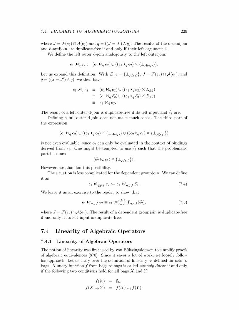
7.4. LINEARITY OF ALGEBRAIC OPERATORS 229

where J = F(e2) ∩A(e1) and q = ((J = J ′) ∧ q). The results of the d-semijoinand d-antijoin are duplicate-free if and only if their left argument is.

We define the left outer d-join analogously to the left outerjoin:

e1 Fq e2 := (e1 Cq e2) ∪ ((e1 Uq e2) A ⊥A(e2)).

Let us expand this definition. With E⊥2 = ⊥A(e2), J = F(e2) ∩ A(e1), andq = ((J = J ′) ∧ q), we then have

e1 Fq e2 ≡ (e1 Cq e2) ∪ ((e1 Uq e2) A E⊥2)

≡ (e1 Bq e2) ∪ ((e1 Tq e2) A E⊥2)

≡ e1 Eq e2.

The result of a left outer d-join is duplicate-free if its left input and e2 are.

Defining a full outer d-join does not make much sense. The third part ofthe expression

(e1 Cq e2) ∪ ((e1 Uq e2) A ⊥A(e2) ∪ ((e2 Tq e1) A ⊥A(e1))

is not even evaluable, since e2 can only be evaluated in the context of bindingsderived from e1. One might be tempted to use e2 such that the problematicpart becomes

(e2 Tq e1) A ⊥A(e1)).However, we abandon this possibility.

The situation is less complicated for the dependent groupjoin. We can defineit as

e1 [q;g:f e2 := e1 Zq;g:f e2. (7.4)

We leave it as an exercise to the reader to show that

e1 [q;g:f e2 ≡ e1 Eg:f(∅)J=J ′ Γq;g:f (e2), (7.5)

where J = F(e2)∩A(e1). The result of a dependent groupjoin is duplicate-freeif and only if its left input is duplicate-free.

7.4 Linearity of Algebraic Operators

7.4.1 Linearity of Algebraic Operators

The notion of linearity was first used by von Bultzingsloewen to simplify proofsof algebraic equivalences [870]. Since it saves a lot of work, we loosely followhis approach. Let us carry over the definition of linearity as defined for sets tobags. A unary function f from bags to bags is called strongly linear if and onlyif the following two conditions hold for all bags X and Y :

f(∅b) = ∅b,f(X ∪b Y ) = f(X) ∪b f(Y ).

230 CHAPTER 7. AN ALGEBRA FOR SETS, BAGS, AND SEQUENCES

An n-ary mapping from bags to a bag is called strongly linear in its i-th ar-gument if and only if for all bags X1, . . . , Xn and X ′i the following conditionshold:

f(X1, . . . , Xi−1, ∅b, Xi+1, . . . , Xn) = ∅bf(X1, . . . , Xi−1, Xi ∪b X ′i, Xi+1, . . . , Xn) = f(X1, . . . , Xi−1, Xi, Xi+1, . . . , Xn)

∪bf(X1, . . . , Xi−1, X′i, Xi+1, . . . , Xn)

It is called strongly linear if it is strongly linear in all its arguments. For abinary function or operator where we can distinguish between the left and theright argument, we call it strongly left (right) linear if it is strongly linear in itsfirst (second) argument.

Using the commutativity of bag union and bag intersection as well as theobservations that in general

(∅b ∪b X) 6= ∅b,(∅b ∩b X) = ∅b,(∅b \b X) = ∅b,(X \b ∅b) 6= ∅b

and

(X ∪b Y ) ∪b Z 6= (X ∪b Z) ∪b (Y ∪b Z),

(X ∪b Y ) ∩b Z 6= (X ∩b Z) ∪b (Y ∩b Z),

(X ∪b Y ) \b Z 6= (X \b Z) ∪b (Y \b Z),

X \b (Y ∪b Z) 6= (X \b Y ) ∪b (X \b Z),

we can conclude that bag union is neither strongly left nor strongly right linear,bag intersection is neither strongly left nor strongly right bag-linear, and bagdifference is neither strongly left nor strongly right linear.

We can relax the definition of strongly linear by the additional assumptionthat the intersection of the two unioned bags is empty. A unary function f frombags to bags is called weakly linear if and only if the following two conditionshold for all bags X and Y with X ∩b Y = ∅b:

f(∅b) = ∅b,f(X ∪b Y ) = f(X) ∪b f(Y ).

An n-ary mapping from bags to a bag is called weakly linear in its i-th argumentif and only if for all bags X1, . . . , Xn and X ′i with Xi ∩b X ′i = ∅b the followingconditions hold:

f(X1, . . . , Xi−1, ∅b, Xi+1, . . . , Xn) = ∅b,f(X1, . . . , Xi−1, Xi ∪b X ′i, Xi+1, . . . , Xn) = f(X1, . . . , Xi−1, Xi, Xi+1, . . . , Xn)

∪bf(X1, . . . , Xi−1, X′i, Xi+1, . . . , Xn).

It is called weakly linear , if it is weakly linear in all its arguments. For a binaryfunction or operator where we can distinguish between the left and the right

7.4. LINEARITY OF ALGEBRAIC OPERATORS 231

unary binary

operator linear operator left lin. right lin.ΠD ∪ - -ΠA + ∩ ΠDA \ -σp + A + +χa:e + Bp + +χf + Np + -

ΓθG;F - Tp + -νG;g - Ep + -µg + Kp - -µa:g + Zp;F + -Υf + C + does not apply

Υa:f +flatten +

Table 7.1: Linearity of algebraic operators

argument, we call it weakly left (right) linear if it is weakly linear in its first(second) argument.

Using the commutativity of bag union and bag intersection as well as theobservations that in general

(∅b ∪b X) 6= ∅b,(∅b ∩b X) = ∅b,(∅b \b X) = ∅b,(X \b ∅b) 6= ∅b

and

(X ∪b Y ) ∪b Z 6= (X ∪b Z) ∪b (Y ∪b Z),

(X ∪b Y ) ∩b Z = (X ∩b Z) ∪b (Y ∩b Z),

(X ∪b Y ) \b Z = (X \b Z) ∪b (Y \b Z),

Z \b (X ∪b Y ) 6= (Z \b X) ∪b (Z \b Y )

for X∩bY = ∅b, we can conclude that bag union is neither weakly left nor weaklyright linear, bag intersection is weakly linear, and bag difference is weakly leftbut not weakly right linear.

For the whole algebra, Table 7.1 summarizes the linearity properties for allof our algebraic operators. Thereby, a ’+’ denotes strong linearity, ’’ denotesweak linearity, and ’-’ denotes neither of them.

Let us take a closer look at the gap between weak and strong linearity. Forsome bag B, define the unary function f on bags such that

χf(B)(x) =

3 if x ∈ B,0 if x 6∈ B

232 CHAPTER 7. AN ALGEBRA FOR SETS, BAGS, AND SEQUENCES

holds. Then, f is weakly linear but not strongly linear. The problem is thatf manipulates the multiplicity of the elements. We can make the differencebetween weakly and strongly linear explicit. Therefore, we remember thatthe only difference in the definition was the disjointness we required for weaklinearity. Consequently, we consider now the special case of bags containinga single element multiple times. We say that a unary function f is duplicatefaithful if and only if for all x

f(xmb) = ∪mi=1f(xb)holds. Then, a unary function is strongly bag linear if and only if it is weaklybag linear and duplicate faithful. The same holds for n-ary functions if weextend the property duplicate faithful to multiple arguments.

To see that the left semijoin is not even weakly right linear, consider thefollowing example:

[a : 1]b = [a : 1]b Na=b [b : 1, c : 1], [b : 1, c : 2]b= [a : 1]b Na=b ([b : 1, c : 1]b ∪ [b : 1, c : 2]b)6= ([a : 1]b Na=b [b : 1, c : 1]b) ∪ ([a : 1]b Na=b [b : 1, c : 2]b)= [a : 1]2b.

This is the reason why some equivalences valid for sets do not hold for bagsanymore. For example, ΠA(e1)(e1 Bq12 e2) ≡ e1 Nq12 e2 holds for sets but not forbags. If we eliminate duplicates explicitly, we still have

ΠDA(e1)(e1 Bq12 e2) ≡ ΠD

A(e1)(e1 Nq12 e2). (7.6)

Similiarily, we have

ΠDA(e1)(e1 Eq12 e2) ≡ ΠD

A(e1)(e1), (7.7)

ΠDA(e1)(e1 Kq12 e2) ≡ ΠD

A(e1)(e1). (7.8)

Let us now present some sample proofs of linearity. All proofs are by induc-tion on the number of distinct elements contained in the argument bags.

χf is strongly linear.

χf (∅b) = ∅bχf (xmb) = ∪mi=1f(xb)χf (e1 ∪ e2) = f(x)|x ∈ e1 ∪ e2b

= f(x)|x ∈ e1b ∪ f(x)|x ∈ e2b= χf (e1) ∪ χf (e2)

E is strongly left linear.

∅b Eq e2 = ∅bxmb Eq e2 = ∪mi=1(xb Eq e2)

(e′1 ∪ e′′1) Eq e2 = ((e′1 ∪ e′′1) Bq e2) ∪ (((e′1 ∪ e′′1) Tq e2) A ⊥A(e2)b)= (e′1 Bq e2) ∪ (e′′1 Bq e2) ∪ ((e′1 Tq e2) A ⊥A(e2)b) ∪ ((e′′1 Tq e2) A ⊥A(e2)b)= (e1 Eq e) ∪ (e2 Eq e)

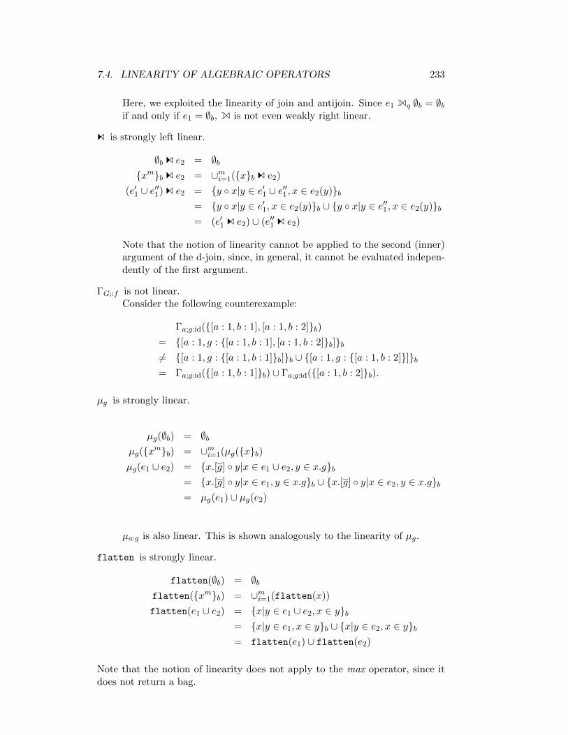
7.4. LINEARITY OF ALGEBRAIC OPERATORS 233

Here, we exploited the linearity of join and antijoin. Since e1 Eq ∅b = ∅bif and only if e1 = ∅b, E is not even weakly right linear.

C is strongly left linear.

∅b C e2 = ∅bxmb C e2 = ∪mi=1(xb C e2)

(e′1 ∪ e′′1) C e2 = y x|y ∈ e′1 ∪ e′′1, x ∈ e2(y)b= y x|y ∈ e′1, x ∈ e2(y)b ∪ y x|y ∈ e′′1, x ∈ e2(y)b= (e′1 C e2) ∪ (e′′1 C e2)

Note that the notion of linearity cannot be applied to the second (inner)argument of the d-join, since, in general, it cannot be evaluated indepen-dently of the first argument.

ΓG;:f is not linear.Consider the following counterexample:

Γa;g:id([a : 1, b : 1], [a : 1, b : 2]b)= [a : 1, g : [a : 1, b : 1], [a : 1, b : 2]b]b6= [a : 1, g : [a : 1, b : 1]b]b ∪ [a : 1, g : [a : 1, b : 2]]b= Γa;g:id([a : 1, b : 1]b) ∪ Γa;g:id([a : 1, b : 2]b).

µg is strongly linear.

µg(∅b) = ∅bµg(xmb) = ∪mi=1(µg(xb)µg(e1 ∪ e2) = x.[g] y|x ∈ e1 ∪ e2, y ∈ x.gb

= x.[g] y|x ∈ e1, y ∈ x.gb ∪ x.[g] y|x ∈ e2, y ∈ x.gb= µg(e1) ∪ µg(e2)

µa:g is also linear. This is shown analogously to the linearity of µg.

flatten is strongly linear.

flatten(∅b) = ∅bflatten(xmb) = ∪mi=1(flatten(x))

flatten(e1 ∪ e2) = x|y ∈ e1 ∪ e2, x ∈ yb= x|y ∈ e1, x ∈ yb ∪ x|y ∈ e2, x ∈ yb= flatten(e1) ∪ flatten(e2)

Note that the notion of linearity does not apply to the max operator, since itdoes not return a bag.

234 CHAPTER 7. AN ALGEBRA FOR SETS, BAGS, AND SEQUENCES

7.4.2 Exploiting Linearity

The concatenation of two weakly (strongly) linear mappings is again a weakly(strongly) linear mapping. Assume f and g to be weakly (strongly) linearmappings. Then

f(g(∅b)) = ∅b,f(g(xmb)) = ∪mi=1f(g(xb)),f(g(X ∪ Y )) = f(g(X) ∪ g(Y ))

= f(g(X)) ∪ f(g(Y )),

where the second line only applies for strongly linear mappings, and the bagsX and Y are disjoint in case of weakly linear mappings.

From the linearity considerations of the previous subsection, it is easy toderive reorderability laws.

Let f : τ f1 → τ f2 and g : τ g1 → τ g2 be two strongly linear mappings.If f(g(xb)) = g(f(xb)) for all bags xb containing a single element, then

f(g(e)) = g(f(e)) (7.9)

This is proven by induction on the number of distinct elements contained in abag e. If e is empty, the statement follows directly from the linearity of f andg. For the induction, let e = e1 ∪ e2. Then

f(g(e)) = f(g(e1 ∪ e2))

= f(g(e1)) ∪ f(g(e2))

=I.H. g(f(e1)) ∪ g(f(e2))

= g(f(e1 ∪ e2))

= g(f(e)).

2

For strongly linear algebraic operators working on bags of tuples, we canreplace the semantic condition f(g(xb)) = g(f(xb)) by a syntactic criterion.The main issue here is to formalize that two operations do not interfere in theirconsumer/producer/modifier relationship on attributes. Let us first get ridof modifications. There are only a few algebraic operators which are capableof modifying an attribute’s value. One of them is the map operator. By aproper renaming of attributes, we can assume without loss of generality thatno operator modifes an existing attribute value. For the map operator (sayχa:e2(e1)), it would mean that it only introduces new attributes (thus a 6∈A(e1)). This renaming step is an essential part of the NFST phase.

This leaves us with checking the consumer/producer relationships. Consid-er, for example, the algebraic equivalence

σp(e1 Bq12 e2) ≡ (σp(e1)) Bq12 e2.

It is well-typed if and only if the predicate p does not access any attributesfrom e2, i.e., F(p) ∩ A(e2) = ∅.

Now, for most of our operators we can be sure that f(g(e)) = g(f(e)) forsingleton bags e. This holds if and only if the following two conditions hold:

7.5. REPRESENTATIONS 235

unary binary

operator produced deleted operator produced deletedΠD ∅ ∅ ∪ ∅ ∅ΠA ∅ A ∩ ∅ ∅ΠDA ∅ A \ ∅ A(e2)σp ∅ ∅ A ∅ ∅χa:e a ∅ Bq ∅ ∅

ΓθG;F A(F ) G Nq ∅ A(e2)

νG;g g G Tq ∅ A(e2)µg A(g) g Eq A(e2) ∅µa:g a g Kq A(e1) ∪ A(e2) ∅Υa:f a ∅ Zq;g:F g ∅

Table 7.2: Produced and deleted attributes of algebraic operators

1. g does not access attributes produced by f , and

2. f does not access attributes produced by g.

We can formalize this as follows. We denote by P the set of produced attributesand by D the set of destroyed attributes (e.g., projected away). Given a unaryoperator f and an expression e, and a binary operator and expressions e1 ande2, we can define

P(f) := A(f(e)) \ A(e),

D(f) := A(e) \ A(f(e)),

P() := A(e1 e2) \ (A(e1) ∪ A(e2)),

D() :=∗ (A(e1) ∪ A(e2)) \ A(e1 e2).

A special case concerns the produced attributes of outerjoins. Since attributevalues are assigned in case of null-padding a tuple with no join partner, we haveto add the attributes of the preserved side(s) to the set of produced attributes.Table 7.2 shows the sets of produced and deleted attributes for some selectedalgebraic operators.

Using this notation, the condition f(g(xb)) = g(f(xb)) is satisfied if thetwo conditions

F(f) ∩ P(g) = P(f) ∩ F(g) = ∅b,F(f) ∩ D(g) = D(f) ∩ F(g) = ∅b

hold and if f and g are any of our unary operators. This statement is validbecause we excluded attribute modifications.

7.5 Representations

7.5.1 Three Different Representations

In this section, we discuss different representations for sets, bags, and sequences.Let us start with bags. Fig. 7.5 shows three different representations for bags.

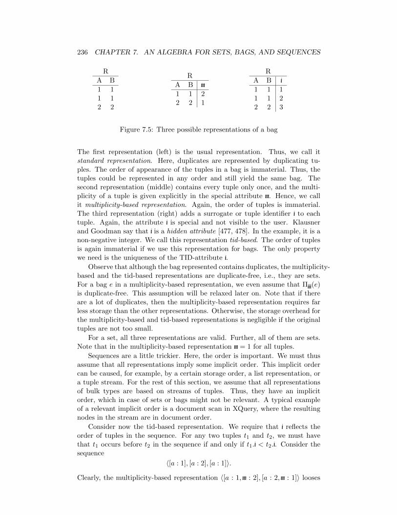
236 CHAPTER 7. AN ALGEBRA FOR SETS, BAGS, AND SEQUENCES

R

A B

1 11 12 2

R

A B m

1 1 22 2 1

R

A B i

1 1 11 1 22 2 3

Figure 7.5: Three possible representations of a bag

The first representation (left) is the usual representation. Thus, we call itstandard representation. Here, duplicates are represented by duplicating tu-ples. The order of appearance of the tuples in a bag is immaterial. Thus, thetuples could be represented in any order and still yield the same bag. Thesecond representation (middle) contains every tuple only once, and the multi-plicity of a tuple is given explicitly in the special attribute m. Hence, we callit multiplicity-based representation. Again, the order of tuples is immaterial.The third representation (right) adds a surrogate or tuple identifier i to eachtuple. Again, the attribute i is special and not visible to the user. Klausnerand Goodman say that i is a hidden attribute [477, 478]. In the example, it is anon-negative integer. We call this representation tid-based. The order of tuplesis again immaterial if we use this representation for bags. The only propertywe need is the uniqueness of the TID-attribute i.

Observe that although the bag represented contains duplicates, the multiplicity-based and the tid-based representations are duplicate-free, i.e., they are sets.For a bag e in a multiplicity-based representation, we even assume that Πm(e)is duplicate-free. This assumption will be relaxed later on. Note that if thereare a lot of duplicates, then the multiplicity-based representation requires farless storage than the other representations. Otherwise, the storage overhead forthe multiplicity-based and tid-based representations is negligible if the originaltuples are not too small.

For a set, all three representations are valid. Further, all of them are sets.Note that in the multiplicity-based representation m = 1 for all tuples.

Sequences are a little trickier. Here, the order is important. We must thusassume that all representations imply some implicit order. This implicit ordercan be caused, for example, by a certain storage order, a list representation, ora tuple stream. For the rest of this section, we assume that all representationsof bulk types are based on streams of tuples. Thus, they have an implicitorder, which in case of sets or bags might not be relevant. A typical exampleof a relevant implicit order is a document scan in XQuery, where the resultingnodes in the stream are in document order.

Consider now the tid-based representation. We require that i reflects theorder of tuples in the sequence. For any two tuples t1 and t2, we must havethat t1 occurs before t2 in the sequence if and only if t1.i < t2.i. Consider thesequence

〈[a : 1], [a : 2], [a : 1]〉.

Clearly, the multiplicity-based representation 〈[a : 1, m : 2], [a : 2, m : 1]〉 looses

7.5. REPRESENTATIONS 237

the order. One way to remedy this situation is to keep not only the multiplicityof an element but its positions. This results in

〈[a : 1]1,3, [a : 2]2〉

or in

〈[a : 1, p : 1, 3s], [a : 2, p : 2s]〉if we represent the set of positions at which a tuple occurs in an extra attributep. We call this a position-based representation. It is duplicate free and in caseof multiple duplicates in the original sequence, it saves some memory.

7.5.2 Conversion between Representations

Assume that the bag e is given in standard representation, and we wish toconvert it to a multiplicity-based representation. Then ΓA(e);p;m:|p|(e) does thejob. To go into the other direction, we need a special unnest operator, which,for a given attribute m in non-negative integers, produces m copies of a tuple.Since it looks like a special unnest operator, we use µm to denote it. It is definedas

µm(e) := Πm(tm|t ∈ eb)for attributes m in non-negative integers. Then, µm(e) converts a bag e frommultiplicity-based to standard representation.

To go from a standard representation of a bag to a tid-based representation,we apply a special tid-operator TIDi, which produces distinct TIDs (numbers)for every input tuple and stores this number in the attribute i. Assume someglobal variable c is initialized with 0, then TIDi(e) could be defined as χi:++c(e),mixing algebra and C++ code. The reverse direction is easily specified by Π

i.

Let us now turn to sets. Converting a set e in standard notation to amultiplicity-based representation is performed by χm:1(e). Converting a set ein multiplicity-based representation to one in standard representation can besimplified to Πm(e). The other conversions for sets are the same as for bags.

Given a sequence e in standard representation with implicit ordering, wecan apply the above TID-operator to convert e into a tid-based representationwith TIDi(e). The reverse conversion is not simply Π

i(e), except if we are sure

that e is already sorted on i. Otherwise, since sorting on i will restore the order,we can convert a sequence e in tid-based representation with Π

i(Sorti(e)), where

we again must assume an implicit ordering.

We can construct a position-based representation of a sequence given in atid-based representation with ΓA(e)\i;g:Πi

(e). The opposite direction is spec-

ified by Sorti(µg(e)). As an exercise, the reader should design an algorithmwhich allows to calculate the combination Sorti µg efficiently. EXC

7.5.3 Conversion between Bulk Types

Given a set e in some representation, the same representation is a valid bagrepresentation. Hence, this conversion is a no-op.

238 CHAPTER 7. AN ALGEBRA FOR SETS, BAGS, AND SEQUENCES

The opposite direction is also simple. Given a bag e in standard repre-sentation, ΠD produces a set in standard representation. This is expensive.Given a bag e in tid-based representation, ΠD

A(e)\i(e) produces a set in stan-

dard representation. This is expensive, too. Given a bag e in multiplicity-basedrepresentation, Πm(e) produces a set in standard representation. This is cheap.

Going from a sequence to a bag is simple. If the sequence is given in standardrepresentation with implicit order or in tid-based representation, the conversionto a bag is the identity function. If a sequence e is given in the position-basedrepresentation with attribute p containing the set of positions, then Πp(χm:|p|(e))converts it to a bag in multiplicity-based representation. From there, we can goanywhere. Obviously, going from a bag to a sequence requires explicit sorting.

7.5.4 Adjusting the Algebra

Implicitly, we have defined our algebra on the standard representation. This isnot coercive. Consider two bags e1 and e2 in a multiplicity-based representation.We can define a special counting cross product by

e1 Am12:m1∗m2 e2 := Πm1,m2(t1 t2 [m : t1.m1 ∗ t2.m2]|ti ∈ ei)

Doing the same exercise with the regular join operator results in the so-calledcounting join [911].

Luckily, it is not necessary to introduce a special counting cross product, ascan be seen from

e1 Am12:m1∗m2 e2 ≡ Πm1,m2(χm12:m1∗m2(e1 A e2),

which can be generalized to

Πmi(χm:∏i mi

(e1 A . . .A en))

if we want to take the counting cross product of n bags ei.Similarily, we can handle a cross product of sequences in a position-based

representation, which is left as an exercise to the reader.EXCLet us turn to projection. Consider the bag

[a : 1, b : 2, m : 3], [a : 2, b : 3, m : 4], [a : 1, b : 4, m : 2]b

in the multiplicity-based representation. Applying Πa carelessly results in

[a : 1, m : 3], [a : 2, m : 4], [a : 1, m : 2]b,

which is no longer a multiplicity-based representation, as it is not a set anymore.More specifically, Πa of the above bag contains duplicates. We use this repre-sentation as an alternative fourth representation. We call it multiplicity-basedrepresentation with duplicates. First, note that in terms of conversions and al-gebraic operators like join, the duplicates do not imply problems. We just loosesome compression of the data. Second, observe that performing a Γa;m:sum(m)

fixes this problem, i.e., it turns a bag in multiplicity-based representation withduplicates into the regular, duplicate-free multiplicity-based representation.

7.6. A NOTE ON EQUIVALENCES 239

7.5.5 Partial Preaggregation

To illustrate partial preaggregation (or partial pregrouping) we use a hash-basedimplementation of the grouping operator as an example. Assume that it haslimited buffer space and can keep k groups. If the buffer overflows, some groupis ejected from the buffer to produce new free space for a new group. We denotesuch a special implementation of the grouping operator by Γpre(k) and call itpartial preaggregation or partial pregrouping.

We illustrate it by applying it in the form of Γpre(1)a;g;m:|g| to the following bag

B := [a : 1], [a : 1], [a : 2], [a : 1], [a : 1]b.

The result is

Bpre := [a : 1, m : 2], [a : 2, m : 1], [a : 1, m : 2]b,

where we assumed that the implicit order in which the pregrouping operatorsees the tuples is from left to right. Calculating Γa;g;m:sum(m) gives with

Bm := [a : 1, m : 4], [a : 2, m : 1]b

the regular duplicate-free multiplicity-based representation. This observationalso holds for sets of attributes, as in

ΓG;m:count(∗)(e) ≡ ΓG;m:sum(m′)(Γpre(k)G;m′:count(∗)(e) (7.10)

for any k ≥ 0, where we used the SQL-notation based variant of grouping.Recall that aggregation functions and vectors can be decomposable. Then

it is easy to generalize the above equivalence. Let F be an aggregation vectordecomposable into F 1 and F 2. Then

ΓG;F (e) ≡ ΓG;F 2(Γpre(k)G;F 1 (e) (7.11)

holds. If the grouping operator is pushed into a join or any other binary op-erator and still some outer grouping is present (see Sec. 7.11), then the innergrouping can be replaced by a pregrouping. General partial pregrouping orpreaggregation is discussed in several papers [409, 513]. They also discuss theexpected resulting number of tuples of partial pregrouping.

7.6 A Note on Equivalences

We have already seen expressions like E1 ≡ E2, where the expressions Ei containalgebraic operators and other symbols. Typically, they contain variables ei todenote base tables or other database items or even algebraic expressions. Theyalso contain p or q for predicates. These are essentially variables for predicates.Also attributes names a or b can be contained in the Ei. Again, these areessentially place holders for ‘real’ attribute names. Sometimes constants c areused. Let us collectively call all these underspecified symbols variables. Wewill then say that E1 ≡ E2 if and only if the following condition holds: For all

240 CHAPTER 7. AN ALGEBRA FOR SETS, BAGS, AND SEQUENCES

bindings for all variables in E1 and E2, if E′1 and E′2, which result from applyingthese bindings to them, are well-typed, then the evaluation of E′1 and E′2 yieldsthe same result.

Equivalence of relational expressions is discussed, e.g., by Aho, Saviv, andUllman [19, 18]. In fact, they discuss weak and strong equivalence. We usestrong equivalence. Weak equivalence is defined on universal relations and isnot sufficent for our purpose.

7.7 Simple Reorderability

7.7.1 Unary Operators

The simplest property we are interested in is the idempotency of unary op-erators. A unary operator f is called idempotent, if f(f(x)) = f(x) for allx. Since ΠD(x) = ΠD(ΠD(x)), ΠA(x) = ΠA(ΠA(x)), ΠD

A (x) = ΠDA (ΠD

A (x)),and σp(x) = σp(σp(x)), these operators are idempotent. Our other operatorsare not. For projections, we also have some generalized idempotency. LetA and B be two attribute sets with A ⊆ B. Then ΠA(x) = ΠA(ΠB(x)),ΠDA (x) = ΠD

A (ΠDB (x)), and ΠD

A (x) = ΠDA (ΠB(x)).

As can be seen from the definition of the grouping operator, it is a gen-eralization of duplicate elimination. If we apply a grouping with an emptyaggregation vector, then it is equivalent to a duplicate elimination. In otherwords,

ΠDA (e) ≡ ΓA;()(e) (7.12)

holds for any set of attributes A with A ⊆ A(e). As a consequence, we haveto ask ourselves whether there exists a property generalizing idempotency thatholds for grouping. Indeed there is one. Let F be an aggregation vector which isdecomposable into F 1 and F 2, and G and G+ be two sets of grouping attributeswith G ⊆ G+. Then

ΓG;F (e) ≡ ΓG;F 2(ΓG+;F 1(e)) (7.13)

holds, since we can first group at a finer granularity and then combine finergroups to the groups derived from the grouping by G. We can even go astep further in the presence of functional dependencies. Assume the functionaldependency G→ G′ holds for two sets of grouping attributes G and G′. Then,the equivalence

ΓG;F (e) ≡ ΠG∪A(F )(ΓG∪G′;F (e)) (7.14)

holds, since the groups and their contents are the same in both cases. Thisequivalence can also be found under the name simplify group-by in a paper byTsois and Sellis [849]. A slightly more general version for any function f alsoholds:

ΓG;g:f (e) ≡ ΠG∪g(ΓG∪G′;g:f (e)). (7.15)

Eqv. 7.14 can be simplified if, in addition to G→ G′, G ⊆ G′ holds:

ΓG;F (e) ≡ ΠG∪A(F )(ΓG′;F (e)). (7.16)

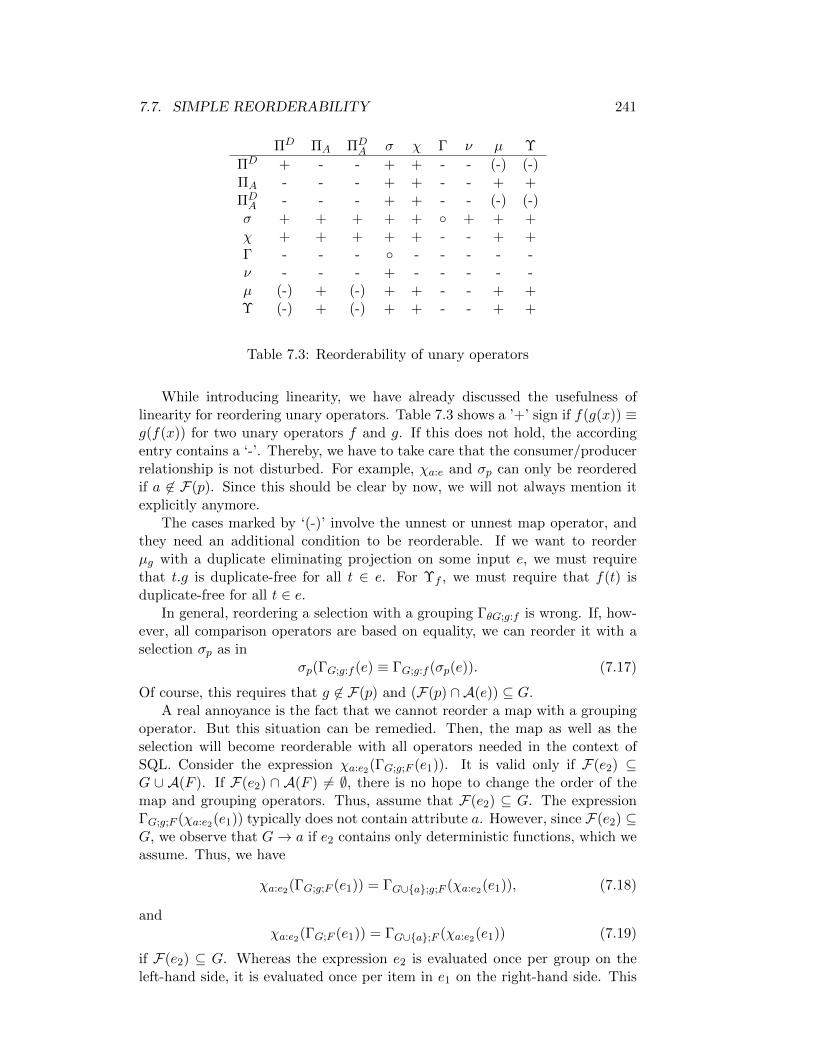
7.7. SIMPLE REORDERABILITY 241

ΠD ΠA ΠDA σ χ Γ ν µ Υ

ΠD + - - + + - - (-) (-)ΠA - - - + + - - + +ΠDA - - - + + - - (-) (-)σ + + + + + + + +χ + + + + + - - + +Γ - - - - - - - -ν - - - + - - - - -µ (-) + (-) + + - - + +Υ (-) + (-) + + - - + +

Table 7.3: Reorderability of unary operators

While introducing linearity, we have already discussed the usefulness oflinearity for reordering unary operators. Table 7.3 shows a ’+’ sign if f(g(x)) ≡g(f(x)) for two unary operators f and g. If this does not hold, the accordingentry contains a ‘-’. Thereby, we have to take care that the consumer/producerrelationship is not disturbed. For example, χa:e and σp can only be reorderedif a 6∈ F(p). Since this should be clear by now, we will not always mention itexplicitly anymore.

The cases marked by ‘(-)’ involve the unnest or unnest map operator, andthey need an additional condition to be reorderable. If we want to reorderµg with a duplicate eliminating projection on some input e, we must requirethat t.g is duplicate-free for all t ∈ e. For Υf , we must require that f(t) isduplicate-free for all t ∈ e.

In general, reordering a selection with a grouping ΓθG;g:f is wrong. If, how-ever, all comparison operators are based on equality, we can reorder it with aselection σp as in

σp(ΓG;g:f (e) ≡ ΓG;g:f (σp(e)). (7.17)

Of course, this requires that g 6∈ F(p) and (F(p) ∩ A(e)) ⊆ G.A real annoyance is the fact that we cannot reorder a map with a grouping

operator. But this situation can be remedied. Then, the map as well as theselection will become reorderable with all operators needed in the context ofSQL. Consider the expression χa:e2(ΓG;g;F (e1)). It is valid only if F(e2) ⊆G ∪ A(F ). If F(e2) ∩ A(F ) 6= ∅, there is no hope to change the order of themap and grouping operators. Thus, assume that F(e2) ⊆ G. The expressionΓG;g;F (χa:e2(e1)) typically does not contain attribute a. However, since F(e2) ⊆G, we observe that G→ a if e2 contains only deterministic functions, which weassume. Thus, we have

χa:e2(ΓG;g;F (e1)) = ΓG∪a;g;F (χa:e2(e1)), (7.18)

andχa:e2(ΓG;F (e1)) = ΓG∪a;F (χa:e2(e1)) (7.19)

if F(e2) ⊆ G. Whereas the expression e2 is evaluated once per group on theleft-hand side, it is evaluated once per item in e1 on the right-hand side. This

242 CHAPTER 7. AN ALGEBRA FOR SETS, BAGS, AND SEQUENCES

∪ ∩ \ A B N T C E K Z

ΠD / +/+ +/ / / +/- +/- /- /- / +/-ΠA -/- -/- -/- -/- -/- +/- +/- -/- -/- -/- -/-ΠDA -/- -/- -/- -/- -/- +/- +/- -/- -/- -/- -/-σ -/- +/+ +/- +/+ +/+ +/- +/- +/+ +/- -/- +/-χ -/- -/- -/- +/+ +/+ +/- +/- +/+ +/ / +/-Γ -/- -/- -/- -/- -/- +/- +/- -/- -/- -/- -/-ν -/- -/- -/- -/- -/- +/- +/- -/- -/- -/- -/-µ -/- -/- -/- +/+ +/+ +/- +/- +/+ +/- -/- +/-Υ -/- -/- -/- +/+ +/ +/- +/- +/+ +/- -/- +/-

Table 7.4: Left/right push-down

is unfortunate if we want to apply the equation from left to right. Rememberthat A(g) = A(e1) in ΓG;g;F (e1). Thus, A(e2) ⊆ G ⊆ A(g), and we can addthe calculation of e2 to F . Therefore, we need the function pick, which picksan arbitrary element out of a bag. This is deterministic, since all tuples in agroup g have the same values for all attributes contained in G. Then, we have

χa:e2(ΓG;g;F (e1)) = ΓG;g;F(a:(e2(pick(g))))(e1) (7.20)

if F(e2) ⊆ G. In our SQL-notation variant of Γ, this reads like

χa:e2(ΓG;F (e1)) = ΓG;g;F(a:e2(pick(g)))(e1) (7.21)

if F(e2) ⊆ G.

7.7.2 Push-Down/Pull-Up of Unary into/from Binary Opera-tors

In this section, we consider pushing down (pulling up) unary operators into(from) the arguments of binary operators. Thus, we are interested in equiva-lences of the form f(e1 e2) ≡ f(e1) e2 and f(e1 e2) ≡ e1 f(e2). First,let us see how linearity helps in this context. Let f be a unary, strongly linearmapping and a binary mapping that is strongly linear in its left argument.If for all expressions e1 and e2 and for all xi ∈ ei we have f(x1b x2b) =(f(x1b) x2b), then

f(e1 e2) ≡ f(e1) e2.

If e1 is empty, f(e1 e2) and f(e1) e2 are also empty. If e1 is a singleton bag,the claim follows from the prerequisite. For the induction step, we observe that

f(e1 e2) = f((e′1 e2) ∪ (e′′1 e2))

= f(e′1 e2) ∪ f(e′′1 e2)

=I.H. (f(e′1) e2) ∪ (f(e′′1) e2)

= f(e1) e2

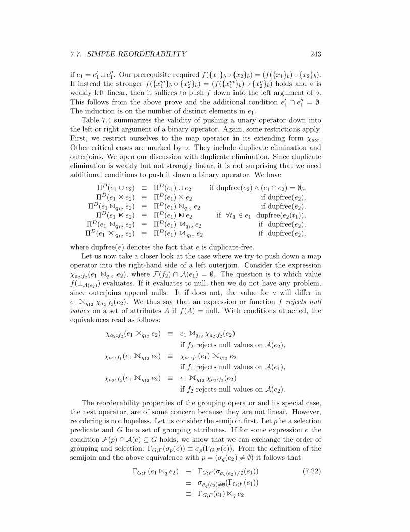
7.7. SIMPLE REORDERABILITY 243

if e1 = e′1 ∪ e′′1. Our prerequisite required f(x1b x2b) = (f(x1b) x2b).If instead the stronger f(xm1 b xn2b) = (f(xm1 b) xn2b) holds and isweakly left linear, then it suffices to push f down into the left argument of .This follows from the above prove and the additional condition e′1 ∩ e′′1 = ∅.The induction is on the number of distinct elements in e1.

Table 7.4 summarizes the validity of pushing a unary operator down intothe left or right argument of a binary operator. Again, some restrictions apply.First, we restrict ourselves to the map operator in its extending form χa:e.Other critical cases are marked by . They include duplicate elimination andouterjoins. We open our discussion with duplicate elimination. Since duplicateelimination is weakly but not strongly linear, it is not surprising that we needadditional conditions to push it down a binary operator. We have

ΠD(e1 ∪ e2) ≡ ΠD(e1) ∪ e2 if dupfree(e2) ∧ (e1 ∩ e2) = ∅b,ΠD(e1 A e2) ≡ ΠD(e1) A e2 if dupfree(e2),

ΠD(e1 Bq12 e2) ≡ ΠD(e1) Bq12 e2 if dupfree(e2),ΠD(e1 C e2) ≡ ΠD(e1) C e2 if ∀t1 ∈ e1 dupfree(e2(t1)),

ΠD(e1 Eq12 e2) ≡ ΠD(e1) Eq12 e2 if dupfree(e2),ΠD(e1 Kq12 e2) ≡ ΠD(e1) Kq12 e2 if dupfree(e2),

where dupfree(e) denotes the fact that e is duplicate-free.Let us now take a closer look at the case where we try to push down a map

operator into the right-hand side of a left outerjoin. Consider the expressionχa2:f2(e1 Eq12 e2), where F(f2) ∩ A(e1) = ∅. The question is to which valuef(⊥A(e2)) evaluates. If it evaluates to null, then we do not have any problem,since outerjoins append nulls. It if does not, the value for a will differ ine1 Eq12 χa2:f2(e2). We thus say that an expression or function f rejects nullvalues on a set of attributes A if f(A) = null. With conditions attached, theequivalences read as follows:

χa2:f2(e1 Eq12 e2) ≡ e1 Eq12 χa2:f2(e2)

if f2 rejects null values on A(e2),

χa1:f1(e1 Kq12 e2) ≡ χa1:f1(e1) Kq12 e2

if f1 rejects null values on A(e1),

χa2:f2(e1 Kq12 e2) ≡ e1 Kq12 χa2:f2(e2)

if f2 rejects null values on A(e2).

The reorderability properties of the grouping operator and its special case,the nest operator, are of some concern because they are not linear. However,reordering is not hopeless. Let us consider the semijoin first. Let p be a selectionpredicate and G be a set of grouping attributes. If for some expression e thecondition F(p) ∩ A(e) ⊆ G holds, we know that we can exchange the order ofgrouping and selection: ΓG;F (σp(e)) ≡ σp(ΓG;F (e)). From the definition of thesemijoin and the above equivalence with p = (σq(e2) 6= ∅) it follows that

ΓG;F (e1 Nq e2) ≡ ΓG;F (σσq(e2)6=∅(e1)) (7.22)

≡ σσq(e2)6=∅(ΓG;F (e1))

≡ ΓG;F (e1) Nq e2

244 CHAPTER 7. AN ALGEBRA FOR SETS, BAGS, AND SEQUENCES

ΠD ΠA ΠDA σ χ Γ ν µ Υ

∪ - + - + + - - + +∩ + - - + + - - + +\ + - - + + - - + +

Table 7.5: Simultaneous push-down

if (F(q) ∩ A(e1)) ⊆ G. Analogously, we can derive

ΓG;F (e1 Tq e2) ≡ ΓG;F (e1) Tq e2 (7.23)

if (F(q)∩A(e1)) ⊆ G. Pushing down a grouping into one of the arguments of ajoin, outerjoin, d-join, or groupjoin is a little more complex. Thus, we devoteda whole section to this problem (see Sec. 7.11).

Since the bag operators ∪, ∩, \ require the same schema for both arguments,it is quite natural to ask for a simultaneous push-down into both arguments.Thus, we are interested in equivalences of the form f(e1 e2) ≡ f(e1) f(e2)for the bag operators above. Table 7.5 summarizes the valid instances of thisequivalence pattern. Again, we must restrict the map operator to its extendingform χa:e.

And again, problems occur for duplicate eliminination and grouping as wellas its special case nest. Consider duplicate elimination first. Evaluating theexpression ΠD(e1 ∪ e2) will never result in any duplicates. ΠD(e1) ∪ ΠD(e2),however, might contain duplicates, e.g., if e1 = e2 = [a : 1]b, the result is[a : 1]2b. Since this is the only problem, we immediately conclude that

ΠD(e1 ∪ e2) ≡ ΠD(ΠD(e1) ∪ΠD(e2)), (7.24)

ΠDA (e1 ∪ e2) ≡ ΠD

A (ΠDA (e1) ∪ΠD

A (e2)). (7.25)

We now turn our attention to the grouping operator. Let e1 and e2 be twoexpressions with A(e1) = A(e2). Further, let G ⊆ A(e1) be a set of groupingattributes and F an aggregation vector. If (ΠG(e1) ∩ΠG(e2)) = ∅, then

ΓG;F (e1 ∪ e2) ≡ ΓG;F (e1) ∪ ΓG;F (e2). (7.26)

If (ΠG(e1) ∩ΠG(e2)) 6= ∅, and F is decomposable into F 1 and F 2, then

ΓG;F (e1 ∪ e2) ≡ ΓG;F 2(ΓG;F 1(e1) ∪ ΓG;F 1(e2)). (7.27)

Of course, this equivalence also holds if (ΠG(e1) ∩ΠG(e2)) = ∅.The cases of pushing grouping down an intersection or difference are dis-

cussed in Sec. 7.11.8.

7.7.3 Binary Operators

Reordering binary operators is the core operation of any plan generator. Wehave already devoted a whole chapter to the problem of finding the optimaljoin order (Chap. 3). The search space for join ordering is huge since the joinis commutative and associative. Thus, there was no restriction on the valid

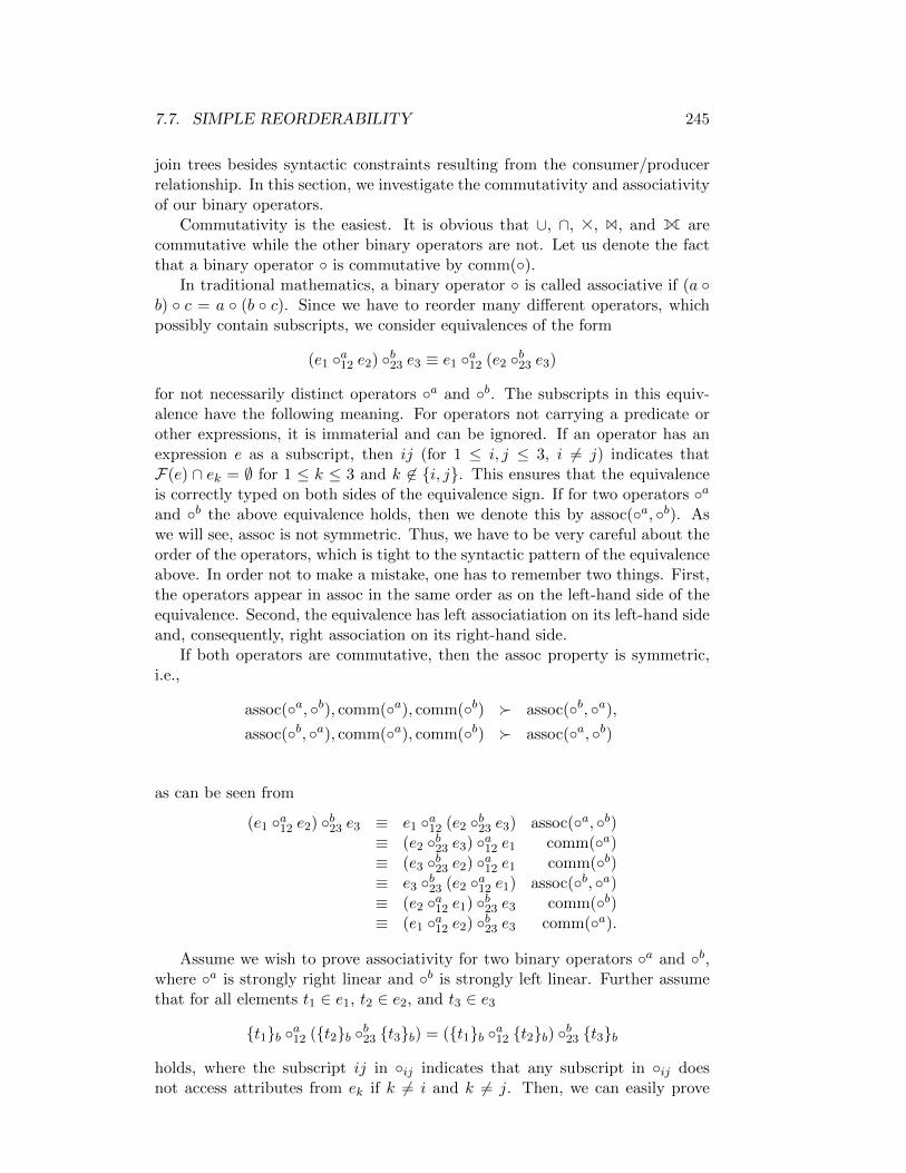
7.7. SIMPLE REORDERABILITY 245

join trees besides syntactic constraints resulting from the consumer/producerrelationship. In this section, we investigate the commutativity and associativityof our binary operators.

Commutativity is the easiest. It is obvious that ∪, ∩, A, B, and K arecommutative while the other binary operators are not. Let us denote the factthat a binary operator is commutative by comm().

In traditional mathematics, a binary operator is called associative if (a b) c = a (b c). Since we have to reorder many different operators, whichpossibly contain subscripts, we consider equivalences of the form

(e1 a12 e2) b23 e3 ≡ e1 a12 (e2 b23 e3)

for not necessarily distinct operators a and b. The subscripts in this equiv-alence have the following meaning. For operators not carrying a predicate orother expressions, it is immaterial and can be ignored. If an operator has anexpression e as a subscript, then ij (for 1 ≤ i, j ≤ 3, i 6= j) indicates thatF(e) ∩ ek = ∅ for 1 ≤ k ≤ 3 and k 6∈ i, j. This ensures that the equivalenceis correctly typed on both sides of the equivalence sign. If for two operators aand b the above equivalence holds, then we denote this by assoc(a, b). Aswe will see, assoc is not symmetric. Thus, we have to be very careful about theorder of the operators, which is tight to the syntactic pattern of the equivalenceabove. In order not to make a mistake, one has to remember two things. First,the operators appear in assoc in the same order as on the left-hand side of theequivalence. Second, the equivalence has left associatiation on its left-hand sideand, consequently, right association on its right-hand side.

If both operators are commutative, then the assoc property is symmetric,i.e.,

assoc(a, b), comm(a), comm(b) assoc(b, a),assoc(b, a), comm(a), comm(b) assoc(a, b)

as can be seen from

(e1 a12 e2) b23 e3 ≡ e1 a12 (e2 b23 e3) assoc(a, b)≡ (e2 b23 e3) a12 e1 comm(a)≡ (e3 b23 e2) a12 e1 comm(b)≡ e3 b23 (e2 a12 e1) assoc(b, a)≡ (e2 a12 e1) b23 e3 comm(b)≡ (e1 a12 e2) b23 e3 comm(a).

Assume we wish to prove associativity for two binary operators a and b,where a is strongly right linear and b is strongly left linear. Further assumethat for all elements t1 ∈ e1, t2 ∈ e2, and t3 ∈ e3

t1b a12 (t2b b23 t3b) = (t1b a12 t2b) b23 t3b

holds, where the subscript ij in ij indicates that any subscript in ij doesnot access attributes from ek if k 6= i and k 6= j. Then, we can easily prove

246 CHAPTER 7. AN ALGEBRA FOR SETS, BAGS, AND SEQUENCES

∪ ∩ \ A B N T C E K Z

∪ + - - - - - - - - - -∩ - + - - - + + - - - -\ - - - - - - - - - - -A - - - + + + + + + - +B - - - + + + + + + - +N - - - - - - - - - - -T - - - - - - - - - - -C - - - + + + + + + - +E - - - - - - - - - -K - - - - - - - - -Z - - - - - - - - - - -

Table 7.6: The assoc-property for binary operators

associativity by induction on the number of elements in the bag e2. If e2 isempty, then (e1 a12 e2) b23 e3 and e1 a12 (e2 b23 e3) are also empty. For singletonbags, we apply the prerequisite above, and for e2 = e′2 ∪ e′′2,

(e1 a12 e2) b23 e3) ≡ (e1 a12 (e′2 ∪ e′′2)) b23 e3

≡ ((e1 a12 e′2) ∪ (e1 a12 e

′′2)) b23 e3)

≡ ((e1 a12 e′2) b23 e3) ∪ ((e1 a12 e

′′2) b23 e3)

≡I.H. (e1 a12 (e′2 b23 e3)) ∪ (e1 a12 (e′′2 b23 e3))

≡ (e1 a12 ((e′2 b23 e3) ∪ (e′′2 b23 e3))

≡ e1 a12 (e2 b23 e3)

provides the induction step.Table 7.6 summarizes the associativities that hold. Be careful to determine

assoc(a, b) from this table by looking up the row with a and the columnwith b. Almost all ’+’ entries’ proofs benefit from the strong linearity of bothoperators. Some of the exceptions benefit from the fact that semi- and antijoincan be expressed as selections and we already know how to push down/pullup selections. The final set of exceptions deals with outerjoins. Here, we alsofind most of the asymmetries. Since the reader might not be familiar with thed-join, reordering the d-join is discussed in Sec. 7.9. Since reordering outerjoinsis complicated, the discussion is deferred to Sec. 7.10.

Now, imagine the operators a and b access other attributes than in theassociativity pattern above. For example, let b possibly access e1 and e3 butnot e2. Then, the associativity pattern becomes

(e1 a12 e2) b13 e3 ≡ e1 a12 (e2 b13 e3).

Obviously, the right-hand side is ill-typed. However, we could rewrite the pat-tern to

(e1 a12 e2) b13 e3 ≡ (e1 b13 e3) a12 e2

because then both sides are well-typed. Let us call instances of this patternleft asscom property and denote by l-asscom(a, b) the fact that the accord-

7.7. SIMPLE REORDERABILITY 247

ing equivalence holds. Analogously, we can define a right asscom property (r-asscom):

e1 a13 (e2 b23 e3) ≡ e2 b23 (e1 a13 e3).

First note that l-asscom and r-asscom are symmetric properties, i.e.,

l-asscom(a, b) ≺ l-asscom(b, a),r-asscom(a, b) ≺ r-asscom(b, a).

Then, the calculation

(e1 a12 e2) b23 e3 ≡ (e2 a12 e1) b23 e3 if comm(a12)≡ (e2 b23 e3) a12 e1 if l-asscom(a12, b23)≡ e1 a12 (e2 b23 e3) if comm(a12)≡ (e1 a12 e2) b23 e3 if assoc(a12, b23)

implies that

comm(a12), assoc(a12, b23) l-asscom(a12, b23),

comm(a12), l-asscom(a12, b23) assoc(a12, b23).

Thus, the l-asscom property is implied by associativity and commutativity,which explains its name. We leave it to the reader to show that

comm(b23), assoc(a12, b23) r-asscom(a12, b23),

comm(b23), r-asscom(a12, b23) assoc(a12, b23).

The important question is whether there are instances of l/r-asscom which donot follow from the commutativity and associativity properties. The answer isyes, as the following investigation shows. Assume e a e′ can be expressed as aselection σp(a,e′)(e), then

(e1 a12 e2) b13 e3 ≡ σp(a12,e2)(e1) b13 e3 assumption

≡ σp(a12,e2)(e1 b13 e3) l-pushable(σ, b13)

≡ (e1 b13 e3) a12 e2 assumption

Thus,

isLikeSelection(a), l-pushable(a, b) l-asscom(a, b).

We leave the symmetric case for r-asscom to the reader.

Another important exception is l-asscom(E, Z), which follows from thefact that both operators are strongly left linear. Assume that

(t1b a12 t2b) b13 t3b ≡ (t1b b13 t3b) a12 t2b

for all ti and that a and b are strongly left linear. Then l-asscom(a, b)holds. The proof is by induction on the number of elements contained in e1.First observe that if e1 is empty, then (e1 a12 e2) b13 e3 and (e1 b13 e3) a12 e2 are

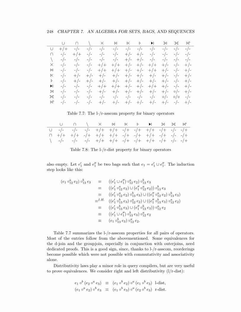
248 CHAPTER 7. AN ALGEBRA FOR SETS, BAGS, AND SEQUENCES

∪ ∩ \ A B N T C E K Z

∪ +/+ -/- -/- -/- -/- -/- -/- -/- -/- -/- -/-∩ -/- +/+ -/- -/- -/- +/- +/- -/- -/- -/- -/-\ -/- -/- -/- -/- -/- +/- +/- -/- -/- -/- -/-A -/- -/- -/- +/+ +/+ +/- +/- +/+ +/- -/- +/-B -/- -/- -/- +/+ +/+ +/- +/- +/+ +/- -/- +/-N -/- +/- +/- +/- +/- +/- +/- +/- +/- -/- +/-T -/- +/- +/- +/- +/- +/- +/- +/- +/- -/- +/-C -/- -/- -/- +/+ +/+ +/- +/- +/+ +/- -/- +/-E -/- -/- -/- +/- +/- +/- +/- +/- +/- /- +/-K -/- -/- -/- -/- -/- -/- -/- -/- /- / -/-Z -/- -/- -/- +/- +/- +/- +/- +/- +/- -/- +/-

Table 7.7: The l-/r-asscom property for binary operators

∪ ∩ \ A B N T C E K Z

∪ -/- -/- -/- +/+ +/+ -/+ -/+ +/+ -/+ -/- -/+∩ +/+ +/+ -/+ +/+ +/+ -/+ -/+ +/+ -/+ -/- -/+\ -/- -/- -/- +/+ +/+ -/+ -/+ +/+ -/+ -/- -/+

Table 7.8: The l-/r-dist property for binary operators

also empty. Let e′1 and e′′1 be two bags such that e1 = e′1 ∪ e′′1. The inductionstep looks like this:

(e1 a12 e2) b13 e3 ≡ ((e′1 ∪ e′′1) a12 e2) b13 e3

≡ ((e′1 a12 e2) ∪ (e′′1 a12 e2)) b13 e3

≡ ((e′1 a12 e2) b13 e3) ∪ ((e′′1 a12 e2) b13 e3)

≡I.H. ((e′1 b13 e3) a12 e2) ∪ ((e′′1 b13 e3) a12 e2)

≡ ((e′1 b13 e3) ∪ (e′′1 b13 e3)) a12 e2

≡ ((e′1 ∪ e′′1) b13 e3) a12 e2

≡ (e1 b13 e3) a12 e2.

Table 7.7 summarizes the l-/r-asscom properties for all pairs of operators.Most of the entries follow from the abovementioned. Some equivalences forthe d-join and the groupjoin, especially in conjunction with outerjoins, needdedicated proofs. This is a good sign, since, thanks to l-/r-asscom, reorderingsbecome possible which were not possible with commutativity and associativityalone.

Distributivity laws play a minor role in query compilers, but are very usefulto prove equivalences. We consider right and left distributivity (l/r-dist):

e1 b (e2 a e3) ≡ (e1 b e2) a (e1 b e3) l-dist,

(e1 a e2) b e3 ≡ (e1 b e3) a (e2 b e3) r-dist.

7.8. PREDICATE DETACHMENT AND ATTACHMENT 249

With these definitions, it is easy to show that

comm(b), r-dist(a, b) l-dist(a, b),comm(b), l-dist(a, b) r-dist(a, b).

Table 7.8 summarizes the distributivity laws for a ∈ ∪,∩, \.

7.8 Predicate Detachment and Attachment

In most cases, an operator with a conjunctive selection predicate allows tomove a part of it to a newly introduced selection operator. We call this processpredicate detachment. Predicate attachment denotes the opposite rewrite.

Let q, qi be join predicates and p and pi be selection predicates. Further, werequire that F(pi) ∩ A(e3−i) = ∅ for i = 1, 2. Then, the following equivalenceshold

σq∧p(e) ≡ σq(σp(e)), (7.28)

e1 Bq∧p1 e2 ≡ σp1(e1) Bq e2, (7.29)

e1 Bq∧p2 e2 ≡ e1 Bq σp2(e2), (7.30)

e1 Nq∧p1 e2 ≡ σp1(e1) Nq e2, (7.31)

e1 Nq∧p2 e2 ≡ e1 Nq σp2(e2), (7.32)

e1 Tq∧p2 e2 ≡ e1 Tq σ¬p2(e2), (7.33)

e1 Eq∧p2 e2 ≡ e1 Eq σp2(e2), (7.34)

e1 Zq∧p2;g:f e2 ≡ e1 Zq;g:f σp2(e2). (7.35)

There is no possibility to move a part of a conjunctive predicate, which onlyaccesses attributes from one side, into or out of a full outerjoin.

In case of a disjunction, we have a nice equivalence for the antijoin.

e1 Tq1∨q2 e2 ≡ (e1 Tq1 e2) Tq2 e2 (7.36)

and the equivalence

e1 Tq∨p1 e2 ≡ σ¬p1(e1) Tq e2 (7.37)

holds if e2 6= ∅.Assume that the whole predicate of a binary operator references only at-

tributes from its left or its right argument. Then, some simplifications/rewrites

250 CHAPTER 7. AN ALGEBRA FOR SETS, BAGS, AND SEQUENCES

are possible:

e1 Bp1 e2 ≡ σp1(e1) A e2, (7.38)

e1 Np1 e2 ≡ σp1(e1) Ntrue e2 ≡ σe2 6=∅(σp1(e1)), (7.39)

e1 Np2 e2 ≡ e1 Ntrue σp2(e2) ≡ σσp2 (e2)6=∅(e1), (7.40)

e1 Tp1 e2 ≡ σ(e2=∅)∨(¬p1)(e1), (7.41)

e1 Tp2 e2 ≡ e1 Ttrue σp2(e2) ≡ σσp2 (e2)=∅(e1), (7.42)

e1 Ep1 e2 ≡ (σp1(e1) A e2) ∪ ((σ(e2=∅)∨(¬p1)(e1)) A ⊥A(e2)), (7.43)

e1 Ep2 e2 ≡ e1 Etrue σp2(e2) (7.44)

≡ (e1 A σp2(e2)) ∪ ((σσp2 (e2)=∅(e1)) A ⊥A(e2)) (7.45)

e1 Kp1 e2 ≡ (σp1(e1) A e2) ∪ (σe2=∅∨¬p1(e1) A ⊥A(e2)) (7.46)

∪(σσp1 (e1)=∅(e1) A ⊥A(e1)) (7.47)

e1 Zp1;g:f e2 ≡ e1 [true;g:f σp1(e2) (7.48)

e1 Zp2;g:f e2 ≡ e1 Ztrue;g:fσp2 e2

≡ e1 Ztrue;g:f σp2e2

≡ χg:f(σp2 (e2)(e1)

≡ e1 A [g : f(σp2(e2))], (7.49)

where we left out symmetric cases, which are possible due to commutativity.Let us consider the semijoin. If F(p1) ∩ A(e2) = ∅, then

e1 Np1 e2 =

σp1(e1) if e2 6= ∅,∅ if e2 = ∅,

which can be summarized to σe2 6=∅(σp1(e1)). If F(p2) ∩ A(e1) = ∅, then

e1 Np2 e2 =

e1 if σp2(e2) 6= ∅,∅ if σp2(e2) = ∅,

which can be summarized to σσp2 (e2)6=∅(e1).Let us consider the antijoin. If F(p1) ∩ A(e2) = ∅, then

e1 Tp1 e2 =

e1 if e2 = ∅,σ¬p1(e1) if e2 6= ∅,

which can be summarized to σe2=∅∨¬p1(e1). If F(p2) ∩ A(e1) = ∅, then

e1 Tp2 e2 =

e1 if σp2(e2) = ∅∅ if σp2(e2) 6= ∅,

which can be summarized to σσp2 (e2)=∅(e1).For the semi- and the antijoin, we have the expression e2 in the subscript

of some operator on the left-hand side of the equivalences. This could meannested-loop evaluation. However, since the evaluation of e2 is independent ofe1, we can easily apply unnesting techniques, and evaluate e2 only once andonly as far as necessary to evaluate the expressions for the semi- and antijoin.

7.9. BASIC EQUIVALENCES FOR D-JOIN 251

To consider the different cases for the left and full outerjoin, it is convenientto define E⊥i = ⊥A(ei) for i = 1, 2 and given expressions ei. If F(p1)∩A(e2) =∅, we can reason as follows for the left outerjoin:

e1 Ep1 e2 ≡ (e1 Bp1 e2) ∪ ((e1 Tp1 e2) A E⊥2)

≡ (σp1(e1) A e2) ∪ ((σ(e2=∅)∨(¬p1)(e1)) A E⊥2).

If F(p2) ∩ A(e1) = ∅, we have

e1 Ep2 e2 ≡ (e1 Bp2 e2) ∪ ((e1 Tp2 e2) A E⊥2)

≡ (e1 A σp2(e2)) ∪ ((e1 Ttrue σp2(e2)) A E⊥2)

≡ (e1 Etrue σp2(e2))

or, alternatively,

e1 Ep2 e2 ≡ (e1 Bp2 e2) ∪ ((e1 Tp2 e2) A E⊥2)

≡ (e1 A σp2(e2)) ∪ ((σσp2 (e2)=∅(e1)) A E⊥2).

Next, we consider the full outerjoin. Assume F(p1) ∩ A(e2) = ∅, then

e1 Kp1 e2 ≡ (e1 Bp1 e2) ∪ ((e1 Tp1 e2) A E⊥2) ∪ ((e2 Tp1 e1) A E⊥1)

≡ (σp1(e1) A e2) ∪ (σ(e2=∅)∨(¬p1)(e1) A E⊥2) ∪ ((σσp1 (e1)=∅(e2)) A E⊥1).

Finally, let us consider groupjoin. If F(q) ∩ A(e2) = ∅, there is not muchwe can do. If F(q) ∩ A(e1) = ∅, the expression can be considerably simplified.This is due to the fact that now every item in e1 has the same members of e1

in its group. In other words, in the result of e1 Ztrue;g:id e2 all tuples have thesame value for g.

7.9 Basic Equivalences for D-Join

From the definition of the d-join follows that

e1 C e2 ≡ ∪t1∈e1(t1b A e2(t1)). (7.50)

Assume e2 depends on some attributes provided by a tuple t1. Then

e2(t1) C e3 ≡ (e2 C e3)(t1). (7.51)

That is, it is immaterial where we feed in the bindings contained in t1. Ofcourse, this only holds as long as F(e3) ∩ A(t1) = ∅.

Let us prove that C is associative:

(e1 C e2) C e3 ≡ (∪t1∈e1(t1b A e2(t1))) C e3

≡ ∪t1∈e1((t1b A e2(t1)) C e3)

≡ ∪t1∈e1(t1b A (e2(t1) C e3))

≡ ∪t1∈e1(t1b A (e2 C e3)(t1))

≡ e1 C (e2 C e3)

252 CHAPTER 7. AN ALGEBRA FOR SETS, BAGS, AND SEQUENCES

In a sense, the d-join is strongly right linear. If for all t1 ∈ e1 e2(t1) = ∅,then e1 C e2 = ∅. Assume e2 has the form e′2 ∪ e′′2. Then

e1 C e2 = e1 C (e′2 ∪ e′′2)

= e1 BJ=J ′ (e′2 ∪ e′′2)

= (e1 BJ=J ′ e′2) ∪ (e1 BJ=J e′′2)

= (e1 C e′2) ∪ (e1 C e′′2)

for J = A(e1) ∩ F(e2)).The d-join and the unnest operators are closely related:

e1 C e2 ≡ µg(χg:e2(e1)). (7.52)

Between flatten and the d-join, there also exists a correspondence:

flatten(χe2(e1)) ≡ ΠA(e2)(e1 C e2). (7.53)

Sometimes a d-join can be expressed as a cross product or a join:

e1 C e2 ≡ e1 × e2 (7.54)

if F(e2) ∩ A(e1) = ∅,e1 C σq(e2) ≡ e1 Bq e2 (7.55)

if F(e2) ∩ A(e1) = ∅.

Denote by e ↓ the fact that some expression e is defined, i.e., returns a validresult. Then, we call a function f extending, if and only if

∀x, y : (f(x) y) ↓=⇒ f(x y) = f(x) y

and we call it restricting, if and only if

∀x, y : f(x) ↓, (x y) ↓=⇒ f(x y) = f(x)

Let us give an example of a function that is neither extending nor restricting.It returns a tuple with a single attribute c, whose value is bound to the numberof attributes of its input tuple.

Unnesting of operations buried in the d-join can be performed by applyingthe following equivalence:

eC f(σA=A′(ρA←A′(e))) ≡ µg(ΓA;g:f (e)) (7.56)

if A ⊆ A(e),

e1 C (e2 B e3) ≡ (e1 C e2) B e3 (7.57)

if F(e3) ∩ A(e1) = ∅,e1 C χf (e2) ≡ χf (e1 C e2) (7.58)

if f extending,

ΠA(e1 C χf (e2)) ≡ ΠA(χf (e1 C e2)) (7.59)

if A ⊆ A(χf (e2)), and f restricting.

7.10. EQUIVALENCES FOR OUTERJOINS 253

e1 := R1

a1 b11 12 43 54 -

e2 := R2

a2 b21 22 43 64 -

e3 := R3

a3 b31 32 53 64 -

ej12 := e1 Bq12 e2

a1 b1 a2 b22 4 2 4

ej13 := e1 Bq13 e3

a1 b1 a3 b33 5 2 5

ej23 := e2 Bq23 e3

a2 b2 a3 b33 6 3 6

elo12 := e1 Eq12 e2

a1 b1 a2 b21 1 - -2 4 2 43 5 - -4 - - -

elo13 := e1 Eq13 e3

a1 b1 a3 b31 1 - -2 4 - -3 5 2 54 - - -

elo23 := e2 Eq23 e3

a2 b2 a3 b31 2 - -2 4 - -3 6 3 64 - - -

efo12 := e1 Kq12 e2

a1 b1 a2 b21 1 - -2 4 2 43 5 - -4 - - -- - 1 2- - 3 6- - 4 -

efo13 := e1 Kq13 e3

a1 b1 a3 b31 1 - -2 4 - -3 5 2 54 - - -- - 1 3- - 3 6- - 4 -

efo23 := e2 Kq23 e3

a2 b2 a3 b31 2 - -2 4 - -3 6 3 64 - - -- - 1 3- - 2 5- - 4 -

Figure 7.6: Example for outerjoin reorderability (for strict q)

We have to be careful if we exchange a d-join with a join. The dependencycan move. In the following equivalences we provide the dependencies explicitlyin parenthesis.

e1 C p12(e2(e1) Bp23 e3(e1)) ≡ (e1 C p12e2(e1)) C p23e3(e1) (7.60)

e1 C p12(e2 Bp23 e3(e1)) ≡ (e1 Bp12 e2) C p23e3(e1) (7.61)

In the first equivalence, the join between e2 and e3 on the left-hand side must beturned into a dependent join on the right-hand side. In the second equivalence,the first dependent join between e1 and e2 becomes a regular join between e1

and e2 on the right-hand side and the regular join between e2 and e3 on theleft-hand side becomes a dependent join on the right-hand side.

7.10 Equivalences for Outerjoins

Outerjoins are a little brittle. Long papers have already been written on thissubject. In this section, we summarize the most important findings, which areuseful in the context of query optimization. For a full account on outerjoinsthe reader is referred to the literature [706, 288, 297]. The occurrence of an

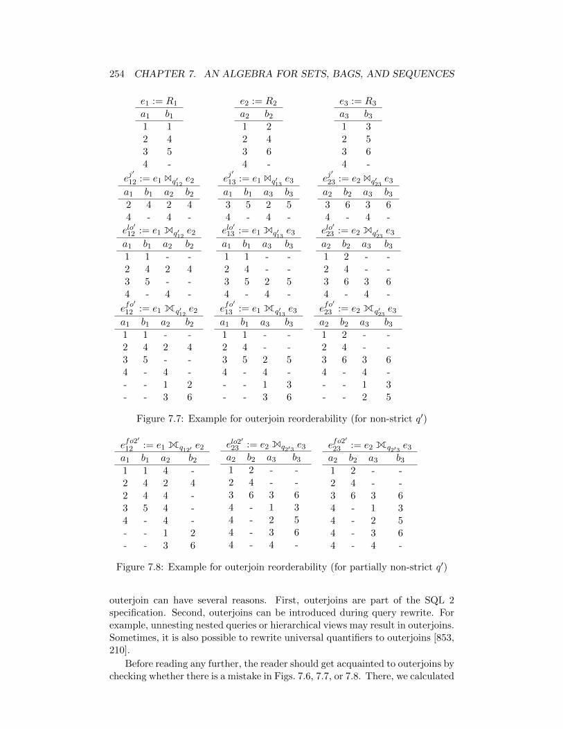
254 CHAPTER 7. AN ALGEBRA FOR SETS, BAGS, AND SEQUENCES

e1 := R1

a1 b11 12 43 54 -

e2 := R2

a2 b21 22 43 64 -

e3 := R3

a3 b31 32 53 64 -

ej′

12 := e1 Bq′12e2

a1 b1 a2 b22 4 2 44 - 4 -

ej′

13 := e1 Bq′13e3

a1 b1 a3 b33 5 2 54 - 4 -

ej′

23 := e2 Bq′23e3

a2 b2 a3 b33 6 3 64 - 4 -

elo′

12 := e1 Eq′12e2

a1 b1 a2 b21 1 - -2 4 2 43 5 - -4 - 4 -

elo′

13 := e1 Eq′13e3

a1 b1 a3 b31 1 - -2 4 - -3 5 2 54 - 4 -

elo′

23 := e2 Eq′23e3

a2 b2 a3 b31 2 - -2 4 - -3 6 3 64 - 4 -

efo′

12 := e1 Kq′12e2

a1 b1 a2 b21 1 - -2 4 2 43 5 - -4 - 4 -- - 1 2- - 3 6

efo′

13 := e1 Kq′13e3

a1 b1 a3 b31 1 - -2 4 - -3 5 2 54 - 4 -- - 1 3- - 3 6

efo′

23 := e2 Kq′23e3

a2 b2 a3 b31 2 - -2 4 - -3 6 3 64 - 4 -- - 1 3- - 2 5

Figure 7.7: Example for outerjoin reorderability (for non-strict q′)

efo2′

12 := e1 Kq12′ e2

a1 b1 a2 b21 1 4 -2 4 2 42 4 4 -3 5 4 -4 - 4 -- - 1 2- - 3 6

elo2′

23 := e2 Eq2′3 e3

a2 b2 a3 b31 2 - -2 4 - -3 6 3 64 - 1 34 - 2 54 - 3 64 - 4 -

efo2′

23 := e2 Kq2′3 e3

a2 b2 a3 b31 2 - -2 4 - -3 6 3 64 - 1 34 - 2 54 - 3 64 - 4 -

Figure 7.8: Example for outerjoin reorderability (for partially non-strict q′)

outerjoin can have several reasons. First, outerjoins are part of the SQL 2specification. Second, outerjoins can be introduced during query rewrite. Forexample, unnesting nested queries or hierarchical views may result in outerjoins.Sometimes, it is also possible to rewrite universal quantifiers to outerjoins [853,210].

Before reading any further, the reader should get acquainted to outerjoins bychecking whether there is a mistake in Figs. 7.6, 7.7, or 7.8. There, we calculated

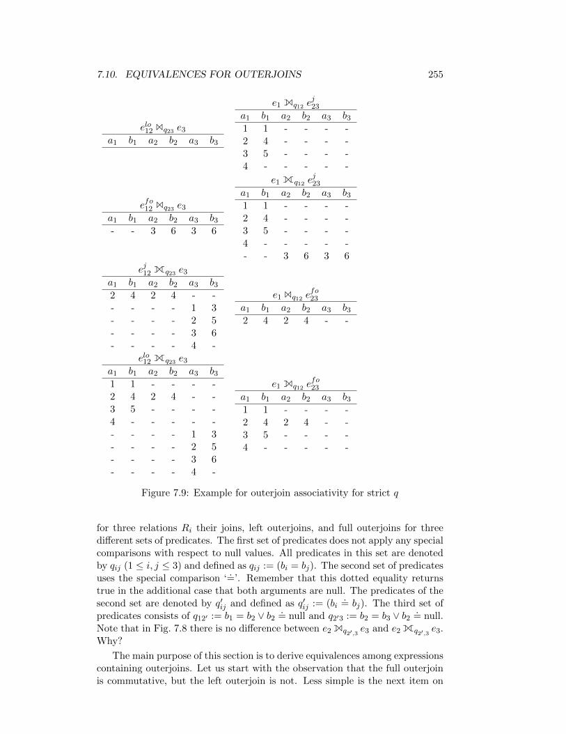
7.10. EQUIVALENCES FOR OUTERJOINS 255

elo12 Bq23 e3

a1 b1 a2 b2 a3 b3

e1 Eq12 ej23

a1 b1 a2 b2 a3 b31 1 - - - -2 4 - - - -3 5 - - - -4 - - - - -

efo12 Bq23 e3

a1 b1 a2 b2 a3 b3- - 3 6 3 6

e1 Kq12 ej23

a1 b1 a2 b2 a3 b31 1 - - - -2 4 - - - -3 5 - - - -4 - - - - -- - 3 6 3 6

ej12 Kq23 e3

a1 b1 a2 b2 a3 b32 4 2 4 - -- - - - 1 3- - - - 2 5- - - - 3 6- - - - 4 -

e1 Bq12 efo23

a1 b1 a2 b2 a3 b32 4 2 4 - -

elo12 Kq23 e3

a1 b1 a2 b2 a3 b31 1 - - - -2 4 2 4 - -3 5 - - - -4 - - - - -- - - - 1 3- - - - 2 5- - - - 3 6- - - - 4 -

e1 Eq12 efo23

a1 b1 a2 b2 a3 b31 1 - - - -2 4 2 4 - -3 5 - - - -4 - - - - -

Figure 7.9: Example for outerjoin associativity for strict q

for three relations Ri their joins, left outerjoins, and full outerjoins for threedifferent sets of predicates. The first set of predicates does not apply any specialcomparisons with respect to null values. All predicates in this set are denotedby qij (1 ≤ i, j ≤ 3) and defined as qij := (bi = bj). The second set of predicatesuses the special comparison ‘

.=’. Remember that this dotted equality returns

true in the additional case that both arguments are null. The predicates of thesecond set are denoted by q′ij and defined as q′ij := (bi

.= bj). The third set of

predicates consists of q12′ := b1 = b2 ∨ b2 .= null and q2′3 := b2 = b3 ∨ b2 .

= null.Note that in Fig. 7.8 there is no difference between e2 Eq2′,3 e3 and e2 Kq2′,3 e3.Why?

The main purpose of this section is to derive equivalences among expressionscontaining outerjoins. Let us start with the observation that the full outerjoinis commutative, but the left outerjoin is not. Less simple is the next item on

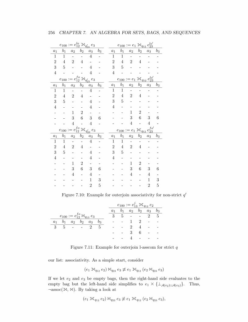
256 CHAPTER 7. AN ALGEBRA FOR SETS, BAGS, AND SEQUENCES

e100 := elo12 Eq′23e3

a1 b1 a2 b2 a3 b31 1 - - 4 -2 4 2 4 - -3 5 - - 4 -4 - - - 4 -

e100 := e1 Eq12 elo′23

a1 b1 a2 b2 a3 b31 1 - - - -2 4 2 4 - -3 5 - - - -4 - - - - -

e100 := efo12 Eq′23e3

a1 b1 a2 b2 a3 b31 1 - - 4 -2 4 2 4 - -3 5 - - 4 -4 - - - 4 -- - 1 2 - -- - 3 6 3 6- - 4 - 4 -

e100 := e1 Kq12 elo′23

a1 b1 a2 b2 a3 b31 1 - - - -2 4 2 4 - -3 5 - - - -4 - - - - -- - 1 2 - -- - 3 6 3 6- - 4 - 4 -

e100 := efo12 Kq′23e3

a1 b1 a2 b2 a3 b31 1 - - 4 -2 4 2 4 - -3 5 - - 4 -4 - - - 4 -- - 1 2 - -- - 3 6 3 6- - 4 - 4 -- - - - 1 3- - - - 2 5

e100 := e1 Kq12 efo′23

a1 b1 a2 b2 a3 b31 1 - - - -2 4 2 4 - -3 5 - - - -4 - - - - -- - 1 2 - -- - 3 6 3 6- - 4 - 4 -- - - - 1 3- - - - 2 5

Figure 7.10: Example for outerjoin associativity for non-strict q′

e100 := efo12 Bq13 e3

a1 b1 a2 b2 a3 b33 5 - - 2 5

e100 := ej13 Kq12 e2

a1 b1 a2 b2 a3 b33 5 - - 2 5- - 1 2 - -- - 2 4 - -- - 3 6 - -- - 4 - - -

Figure 7.11: Example for outerjoin l-asscom for strict q

our list: associativity. As a simple start, consider

(e1 Eq12 e2) Bq23 e3 6≡ e1 Eq12 (e2 Bq23 e3)

If we let e2 and e3 be empty bags, then the right-hand side evaluates to theempty bag but the left-hand side simplifies to e1 A ⊥A(e2)∪A(e3). Thus,¬assoc(E, B). By taking a look at

(e1 Kq12 e2) Bq23 e3 6≡ e1 Kq12 (e2 Bq23 e3),

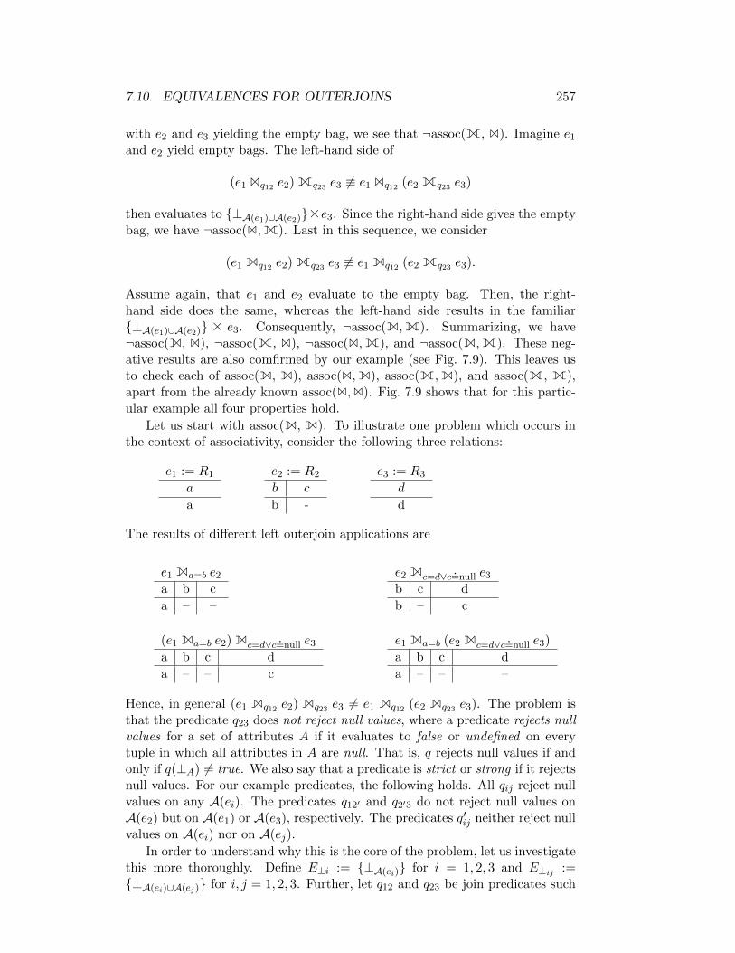
7.10. EQUIVALENCES FOR OUTERJOINS 257

with e2 and e3 yielding the empty bag, we see that ¬assoc(K, B). Imagine e1

and e2 yield empty bags. The left-hand side of

(e1 Bq12 e2) Kq23 e3 6≡ e1 Bq12 (e2 Kq23 e3)

then evaluates to ⊥A(e1)∪A(e2)Ae3. Since the right-hand side gives the emptybag, we have ¬assoc(B,K). Last in this sequence, we consider

(e1 Eq12 e2) Kq23 e3 6≡ e1 Eq12 (e2 Kq23 e3).

Assume again, that e1 and e2 evaluate to the empty bag. Then, the right-hand side does the same, whereas the left-hand side results in the familiar⊥A(e1)∪A(e2) A e3. Consequently, ¬assoc(E,K). Summarizing, we have¬assoc(E, B), ¬assoc(K, B), ¬assoc(B,K), and ¬assoc(E,K). These neg-ative results are also comfirmed by our example (see Fig. 7.9). This leaves usto check each of assoc(E, E), assoc(B,E), assoc(K,E), and assoc(K, K),apart from the already known assoc(B,B). Fig. 7.9 shows that for this partic-ular example all four properties hold.

Let us start with assoc(E, E). To illustrate one problem which occurs inthe context of associativity, consider the following three relations:

e1 := R1

a

a

e2 := R2

b c

b -

e3 := R3

d

d

The results of different left outerjoin applications are

e1 Ea=b e2

a b c

a – –

e2 Ec=d∨c .=null e3

b c d

b – c

(e1 Ea=b e2) Ec=d∨c .=null e3

a b c d

a – – c

e1 Ea=b (e2 Ec=d∨c .=null e3)

a b c d

a – – –

Hence, in general (e1 Eq12 e2) Eq23 e3 6= e1 Eq12 (e2 Eq23 e3). The problem isthat the predicate q23 does not reject null values, where a predicate rejects nullvalues for a set of attributes A if it evaluates to false or undefined on everytuple in which all attributes in A are null. That is, q rejects null values if andonly if q(⊥A) 6= true. We also say that a predicate is strict or strong if it rejectsnull values. For our example predicates, the following holds. All qij reject nullvalues on any A(ei). The predicates q12′ and q2′3 do not reject null values onA(e2) but on A(e1) or A(e3), respectively. The predicates q′ij neither reject nullvalues on A(ei) nor on A(ej).

In order to understand why this is the core of the problem, let us investigatethis more thoroughly. Define E⊥i := ⊥A(ei) for i = 1, 2, 3 and E⊥ij :=⊥A(ei)∪A(ej) for i, j = 1, 2, 3. Further, let q12 and q23 be join predicates such

258 CHAPTER 7. AN ALGEBRA FOR SETS, BAGS, AND SEQUENCES

that F(q12) ∩ A(e3) = ∅ and F(q23) ∩ A(e1) = ∅. For the left-hand side ofassociativity, we have

(e1 Eq12 e2) Eq23 e3 ≡ ((e1 Bq12 e2) ∪ ((e1 Tq12 e2) A E⊥2)) Eq23 e3

≡ (((e1 Bq12 e2) ∪ ((e1 Tq12 e2) A E⊥2)) Bq23 e3)

∪(((((e1 Bq12 e2) ∪ ((e1 Tq12 e2) A E⊥2)) Tq23 e3)) A E⊥3)

≡ ((e1 Bq12 e2) Bq23 e3)

∪(((e1 Tq12 e2) A E⊥2) Bq23 e3)

∪(((e1 Bq12 e2) Tq23 e3) A E⊥3)

∪((((e1 Tq12 e2) A E⊥2) Tq23 e3) A E⊥3)

≡ (e1 Bq12 (e2 Bq23 e3))

∪((e1 Tq12 e2) A (E⊥2 Bq23 e3))

∪(e1 Bq12 ((e2 Tq23 e3) A E⊥3))

∪((e1 Tq12 e2) A (E⊥2 Tq23 e3) A E⊥3)

≡ (e1 Bq12 ((e2 Bq23 e3) ∪ ((e2 Tq23 e3) A E⊥3))

∪((e1 Tq12 e2) A ((E⊥2 Bq23 e3)) ∪ (E⊥2 Tq23 e3) A E⊥3)

≡ (e1 Bq12 (e2 Eq23 e3))

∪((e1 Tq12 e2) A (E⊥2 Eq23 e3)).

The right part of the cross product on the right-hand side of the union, (E⊥2Eq23

e3), does look suspicious. Note that if q23 rejects nulls on A(e2), this part sim-plifies to E⊥23. To confirm our suspicion, we take a look at the other side ofassociativity:

e1 Eq12 (e2 Eq23 e3) ≡ (e1 Bq12 (e2 Eq23 e3)

∪ ((e1 Tq12 (e2 Eq23 e3)) A E⊥23

≡ (e1 Bq12 (e2 Eq23 e3)

∪ ((e1 Tq12 e2) A E⊥23).

The last step is true, since e2Eq23 e3 preserves e2 and F(q12)∩A(e3) = ∅. Thus,the left outerjoin is associative if and only if

((e1 Tq12 e2) A (E⊥2 Eq23 e3)) ≡ (e1 Tq12 e2) A E⊥23.

But this holds if q23 rejects nulls on A(e2). Thus, without any effort we havejust proven the second of the following equivalences:

(e1 Bq12 e2) Eq23 e3 ≡ e1 Bq12 (e2 Eq23 e3), (7.62)

(e1 Eq12 e2) Eq23 e3 ≡ e1 Eq12 (e2 Eq23 e3) (7.63)

if q23 rejects nulls on A(e2),

(e1 Kq12 e2) Eq23 e3 ≡ e1 Kq12 (e2 Eq23 e3) (7.64)

if q23 rejects nulls on A(e2),

(e1 Kq12 e2) Kq23 e3 ≡ e1 Kq12 (e2 Kq23 e3) (7.65)

if q12 and q23 reject nulls on A(e2).

7.10. EQUIVALENCES FOR OUTERJOINS 259

As an exercise, the reader should prove the remaining equivalences. This isnecessary since the proofs of Galindo-Legaria [287] are valid for sets only.

Let us now come to l-asscom. Fig. 7.11 shows that for our example l-asscom(K,B)does not hold. Bearing the symmetry of l-asscom in mind, the equivalences

(e1 Eq12 e2) Bq13 e3 ≡ (e1 Bq13 e3) Eq12 e2, (7.66)

(e1 Eq12 e2) Eq13 e3 ≡ (e1 Eq13 e3) Eq12 e2, (7.67)

(e1 Eq12 e2) Kq13 e3 ≡ (e1 Kq13 e3) Eq12 e2 (7.68)

if q12 rejects nulls on A(e1),

(e1 Kq12 e2) Kq13 e3 ≡ (e1 Kq13 e3) Kq12 e2 (7.69)

if q12 and q13 reject nulls on A(e1)

cover all combinations of B, E, and K except the well-known case for regu-lar joins. Since comm(B) and assoc(B,E) hold without restrictions, Eqv. 7.66holds without restrictions. Since E is strongly left linear and the consumer/producerrelationship is not disturbed because q12 does not access attributes from e3 andq13 does not access attributes from e2, Eqv. 7.67 holds without restrictions.From Eqv. 7.64 and the fact that the full outerjoin is commutative, Eqv. 7.68follows. Some care is just needed to see how the necessary restriction for asso-ciativity carries over to the l-asscom equivalence. Similarily, Eqv. 7.69 followsfrom Eqv.7.65. In all cases, the necessity of the restrictions is due to the factthat commutativity and l-asscom imply associativity.

The r-asscom property is handled quickly. The only valid equivalence wehave is

e1 Kq13 (e2 Kq23 e3) ≡ e2 Kq23 (e1 Kq13 e3), (7.70)

which follows directly from comm(K) and assoc(K,K) if q13 and q23 are bothstrict on A(e3).

7.10.1 Outerjoin Simplification

Sometimes, a left or full outerjoin can be turned into a regular or one-sidedouterjoin if it is followed a unary or binary algebraic operator with a strictpredicate. These simplifications are important and should be applied beforeplan generation.

In [297, 287], we find the the first two of the following equivalences.

e1 Bp (e2 Eq e3) ≡ e1 Bp (e2 Bq e3) (7.71)

e1 Np (e2 Eq e3) ≡ e1 Np (e2 Bq e3) (7.72)

e1 Tp (e2 Eq e3) ≡ e1 Tp (e2 Bq e3) (7.73)

e1 Ep (e2 Eq e3) ≡ e1 Ep (e2 Bq e3) (7.74)

e1 Zp (e2 Eq e3) ≡ e1 Zp (e2 Bq e3) (7.75)

These equivalences hold under the condition that p rejects nulls on A(e3). Theycan be prove to use the semijoin reducer equivalences 7.197-7.201. Similarly,

260 CHAPTER 7. AN ALGEBRA FOR SETS, BAGS, AND SEQUENCES

the equivalences

e1 Bp (e2 Kq e3) ≡ e1 Bp (e2 Eq e3) (7.76)

e1 Np (e2 Kq e3) ≡ e1 Np (e2 Eq e3) (7.77)

e1 Tp (e2 Kq e3) ≡ e1 Tp (e2 Eq e3) (7.78)

e1 Ep (e2 Kq e3) ≡ e1 Ep (e2 Eq e3) (7.79)

e1 Zp (e2 Kq e3) ≡ e1 Zp (e2 Eq e3) (7.80)

hold if p rejects nulls on A(e2). Commutatitvity of the full outerjoin givessymmetric equivalences if p rejects nulls on A(e3).

Further, we can rewrite an outerjoin to a regular join whenever null-paddedtuples are eliminated by some selection predicate. Equivalences that allow todo so and some further ones are given next.

σp1(e1 Eq e2) ≡ σp1(e1) Eq e2 (7.81)

e1 Eq∧p2 e2 ≡ e1 Eq σp2(e2), (7.82)

σp(e1 Eq e2) ≡ σp(e1 Bq e2) if p rejects nulls on A(e2), (7.83)

σp(e1 Kq e2) ≡ σp(e1 Eq e2) if p rejects nulls on A(e1), (7.84)

σp(e1 Kq e2) ≡ σp(e1 Hq e2) if p rejects nulls on A(e2). (7.85)

We can extend the last two equivalences to outerjoins with default values:

σp(e1 ED2q e2) ≡ σp(e1 Bq e2) if ¬p(D2), (7.86)

σp(e1 KD1,D2q e2) ≡ σp(e1 Eq e2) if ¬p(D1), (7.87)

σp(e1 KD1,D2q e2) ≡ σp(e1 Hq e2) if ¬p(D2). (7.88)

7.10.2 Generalized Outerjoin

As pointed out by Galindo-Legaria and Rosenthal [706, 288, 297], the differentouterjoins can be defined using the outer union operator, which in turn wasintroduced by Codd [192]. Let e1 and e2 be two relations and A1 and A2 theircorresponding attributes. The outer union is then defined by padding the unionof the relations with null values to the schema A1 ∪A2:

e1+∪ e2 := (e1 A ⊥A2\A1

) ∪ (e2 A ⊥A1\A2). (7.89)

Given this definition of the outer union operator, we can define the outerjoinoperations as follows:

e1 Eq e2 := e1 Bq e2+∪ (e1 \ΠA1(e1 Bq e2)), (7.90)

e1 Kq e2 := e1 Bq e2+∪ (e1 \ΠA1(e1 Bq e2))

+∪ (e2 \ΠA2(e1 Bq e2)).(7.91)

The expression e1Eq12 (e2Bq23 e3) cannot be reordered given the equivalences sofar. In order to allow reorderability of this expression, the generalized outerjoinwas introduced by Dayal [211]. Here, we follow Rosenthal and Galindo-Legaria

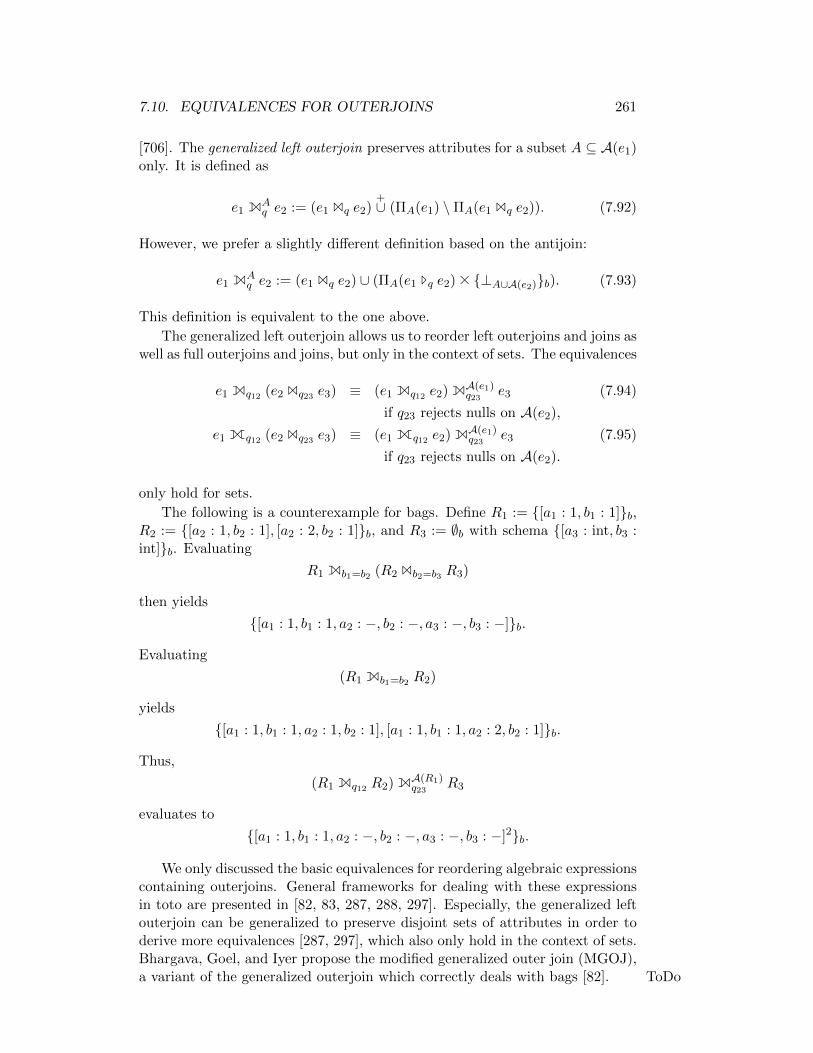
7.10. EQUIVALENCES FOR OUTERJOINS 261

[706]. The generalized left outerjoin preserves attributes for a subset A ⊆ A(e1)only. It is defined as

e1 EAq e2 := (e1 Bq e2)

+∪ (ΠA(e1) \ΠA(e1 Bq e2)). (7.92)

However, we prefer a slightly different definition based on the antijoin:

e1 EAq e2 := (e1 Bq e2) ∪ (ΠA(e1 Tq e2) A ⊥A∪A(e2)b). (7.93)

This definition is equivalent to the one above.

The generalized left outerjoin allows us to reorder left outerjoins and joins aswell as full outerjoins and joins, but only in the context of sets. The equivalences

e1 Eq12 (e2 Bq23 e3) ≡ (e1 Eq12 e2) EA(e1)q23 e3 (7.94)

if q23 rejects nulls on A(e2),

e1 Kq12 (e2 Bq23 e3) ≡ (e1 Kq12 e2) EA(e1)q23 e3 (7.95)

if q23 rejects nulls on A(e2).

only hold for sets.

The following is a counterexample for bags. Define R1 := [a1 : 1, b1 : 1]b,R2 := [a2 : 1, b2 : 1], [a2 : 2, b2 : 1]b, and R3 := ∅b with schema [a3 : int, b3 :int]b. Evaluating

R1 Eb1=b2 (R2 Bb2=b3 R3)

then yields

[a1 : 1, b1 : 1, a2 : −, b2 : −, a3 : −, b3 : −]b.

Evaluating

(R1 Eb1=b2 R2)

yields

[a1 : 1, b1 : 1, a2 : 1, b2 : 1], [a1 : 1, b1 : 1, a2 : 2, b2 : 1]b.

Thus,

(R1 Eq12 R2) EA(R1)q23 R3

evaluates to

[a1 : 1, b1 : 1, a2 : −, b2 : −, a3 : −, b3 : −]2b.

We only discussed the basic equivalences for reordering algebraic expressionscontaining outerjoins. General frameworks for dealing with these expressionsin toto are presented in [82, 83, 287, 288, 297]. Especially, the generalized leftouterjoin can be generalized to preserve disjoint sets of attributes in order toderive more equivalences [287, 297], which also only hold in the context of sets.Bhargava, Goel, and Iyer propose the modified generalized outer join (MGOJ),a variant of the generalized outerjoin which correctly deals with bags [82]. ToDo

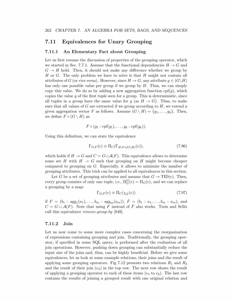
262 CHAPTER 7. AN ALGEBRA FOR SETS, BAGS, AND SEQUENCES

7.11 Equivalences for Unary Grouping

7.11.1 An Elementary Fact about Grouping

Let us first resume the discussion of properties of the grouping operator, whichwe started in Sec. 7.7.1. Assume that the functional dependencies H → G andG → H hold. Then, it should not make any difference whether we group byH or G. The only problem we have to solve is that H might not contain allattributes ofG (or vice versa). However, sinceH → G, any attribute g ∈ (G\H)has only one possible value per group if we group by H. Thus, we can simplycopy this value. We do so by adding a new aggregation function cpf(g), whichcopies the value g of the first tuple seen for a group. This is deterministic, sinceall tuples in a group have the same value for g (as H → G). Thus, to makesure that all values of G are extracted if we group according to H, we extend agiven aggregation vector F as follows. Assume (G \H) = g1, . . . , gk. Then,we define F (G \H) as

F (g1 : cpf(g1), . . . , gk : cpf(gk)).

Using this definition, we can state the equivalence

ΓG;F (e) ≡ ΠC(ΓH;F(G\H)(e)), (7.96)

which holds if H → G and C = G∪A(F ). This equivalence allows to determinesome set H with H → G such that grouping on H might become cheapercompared to grouping on G. Especially, it allows to minimize the number ofgrouping attributes. This trick can be applied to all equivalences in this section.

Let G be a set of grouping attributes and assume that G→ TID(e). Then,every group consists of only one tuple, i.e., ΠD

G(e) = ΠG(e), and we can replacea grouping by a map:

ΓG;F (e) ≡ ΠC(χF (e)) (7.97)

if F = (b1 : agg1(a1), . . . , bm : aggm(am)), F = (b1 : a1, . . . , bm : am), andC = G ∪ A(F ). Note that using F instead of F also works. Tsois and Selliscall this equivalence remove-group-by [849].

7.11.2 Join

Let us now come to some more complex cases concerning the reorganizationof expressions containing grouping and join. Traditionally, the grouping oper-ator, if specified in some SQL query, is performed after the evaluation of alljoin operations. However, pushing down grouping can substantially reduce theinput size of the joins and, thus, can be highly beneficial. Before we give someequivalences, let us look at some example relations, their joins and the result ofapplying some grouping operators. Fig 7.12 presents two relations R1 and R2

and the result of their join (e3) in the top row. The next row shows the resultof applying a grouping operator to each of these items (e4 to e6). The last rowcontains the results of joining a grouped result with one original relation and

7.11. EQUIVALENCES FOR UNARY GROUPING 263

the result of joining the two grouped results given in e4 and e5. Let us assumethat our original expression

Γg1,g2;c:count(∗),b1:sum(a1),b2:sum(a2)(e1 Bj1=j2 R2)

is equivalent to the original query we have to evaluate. The result of thisexpression is given in expression e6 of Fig 7.12. The question is whether any ofe7, e8, or e9 can be used to provide the same result. Let us start with e7. Wehave sum(c1) = 4 and sum(b′1) = 16, which is perfect. However, sum(a2) = 14,but according to e6 we should have 22. How can we fix that? Note that thedifference is 8, which is exactly the value we see in the last row of e7. Further,the count in c1 is 2. It indicates that for g1 = 1 and j1 = 2 two tuples wheregrouped. Each of these tuples joins with the tuple (1, 2, 8) of R2. This is whatwe missed. This point is illustrated in the example in Fig. 7.13, where we addedone more tuple to e2, which is marked by a ∗. All tuples to which this tuplecontributes are also marked by a ∗ later on. The reader should carefully followthe stars.

Let us return to e7 in Fig. 7.12. We have to apply some correction forthe fact that (1, 2, 8) of R2 has two (= c1) join partners. Thus, we calculatesum(c1 ∗ a2) in e7 instead of the plain sum(a2) and get the correct result 22.Let us turn to e8 in Fig. 7.12. There, we calculate sum(a1) = 16, sum(b′2) = 22,and sum(c2) = 4, which are all correct results. However, in e8 of Fig. 7.13,the tuples (1, 2, 4) and (1, 2, 8) of R1 now find two join partners in R2, sincewe added the tuple marked by the asterisk. We should expect problems! Andthere are some, since sum(a1) in e8 gives 14 but should result in 28, accordingto e6. Again, c2 holds the number of join partners the R1 tuples find in R2.Thus calculating sum(a2 ∗ c2) = 28 solves the problem.

Turning our attention to e9 of Fig. 7.12, we see that sum(b′1 ∗ c2) = 16 andsum(b′2 ∗ c1) = 22 give the correct results (compare these values to b1 and b2 ofe6). However, sum(c1) = sum(c2) = 3 but c of e6 indicates that 4 is the correctresult. The reader might guess that we have to take sum(c1 ∗ c2) = 4, whichindeed is what has to be calculated.

These observations give rise to the following definition. Let F = (b1 :agg1(a1), . . . , bm : aggm(am)) be an aggregation vector. We define F ⊗ c forsome attribute c, which will typically contain the result of some count(∗), asF ⊗ c = (b1 : agg′1(e1), . . . , bm : agg′m(em)) with

agg′i(ei) =

aggi(ei) if aggi is duplicate agnostic,aggi(ei ∗ c) if aggi is the duplicate sensitive sum,sum(c) if aggi(ei) = count(∗),sum(ei = NULL ? 0 : c) if aggi(ei) = count(ei), ei 6= ’*’.

The goal now is to exploit the decomposability of aggregation functions andthis definition to push a grouping down a join.

Let us start with an equivalence, which Rosenthal, Rich, and Scholl [712,699] used to speed up join processing. They noted that an ordinary join canbe calculated by unnesting the result of a join of two nested relations. Let q

264 CHAPTER 7. AN ALGEBRA FOR SETS, BAGS, AND SEQUENCES

e1 := R1

g1 j1 a1

1 1 21 2 41 2 8

e2 := R2

g2 j2 a2

1 1 21 1 41 2 8

e3 := R1 1j1=j2 R2

g1 j1 a1 g2 j2 a2

1 1 2 1 1 21 1 2 1 1 41 2 4 1 2 81 2 8 1 2 8

e4 := Γg1,j1;F1(e1)

g1 j1 c1 b′11 1 1 21 2 2 12

e5 := Γg2,j2;F2(e2)

g2 j2 c2 b′21 1 2 61 2 1 8

e6 := Γg1,g2;F (e3)

g1 c b1 b21 4 16 22

e7 := e4 1j1=j2 e2

g1 j1 c1 b′1 g2 j2 a2

1 1 1 2 1 1 21 1 1 2 1 1 41 2 2 12 1 2 8

e8 := e1 1j1=j2 e5

g1 j1 a1 g2 j2 c2 b′21 1 2 1 1 2 61 2 4 1 2 1 81 2 8 1 2 1 8

e9 := e4 1j1=j2 e5

g1 j1 c1 b′1 g2 j2 c2 b′21 1 1 2 1 1 2 61 2 2 12 1 2 1 8

where

F = c : count(∗), b1 : sum(a1), b2 : sum(a2)

F1 = c1 : count(∗), b′1 : sum(a1)

F2 = c2 : count(∗), b′2 : sum(a2)

Figure 7.12: Example for grouping and join

be a join predicate and e1 and e2 be two expressions to be joined. Denote byJi = F(q) ∩ A(ei) the join attributes from ei for i = 1, 2. Then

e1 Bq e2 ≡ µg2(µg1(ΓJ1;g1:ΠA(e1)\J1(e1) Bq ΓJ2;g2:ΠA(e2)\J2

(e2))). (7.98)

We need the projections ΠA(ei)\Ji to prevent the duplication of attributes inthe result.

J1 and J2 are the minimal sets of grouping attributes we can use, butnothing hinders us from using larger grouping sets. Let G+

1 and G+2 be two sets

of attributes with Ji ⊆ G+i for i = 1, 2. Then

e1 Bq e2 ≡ µg2(µg1(ΓG+1 ;g1:ΠA(e1)\J1

(e1) Bq ΓG+2 ;g2:ΠA(e2)\J2

(e2))) (7.99)

holds. Unnesting two nested attributes g1 and g2 in a row, as done in the aboveequivalences, is like generating the cross product of the items contained in g1

and g2. Under the above assumptions, we can thus state the following two

7.11. EQUIVALENCES FOR UNARY GROUPING 265

e1 := R1

g1 j1 a1

1 1 21 2 41 2 8

e2 := R2

g2 j2 a2

1 1 21 1 41 2 81 2 16 ∗

e3 := e1 1j1=j2 e2

g1 j1 a1 g2 j2 a2

1 1 2 1 1 21 1 2 1 1 41 2 4 1 2 81 2 4 1 2 16 ∗1 2 8 1 2 81 2 8 1 2 16 ∗

e4 := Γg1,j1;F1(e1)

g1 j1 c1 b′11 1 1 21 2 2 12

e5 := Γg2,j2;F2(e2)

g2 j2 c2 b′21 1 2 61 2 2 24 ∗

e6 := Γg1,g2;F (e3)

g1 c b1 b21 6 28 54 ∗

e7 := e4 1j1=j2 e2

g1 j1 c1 b′1 g2 j2 a2

1 1 1 2 1 1 21 1 1 2 1 1 41 2 2 12 1 2 81 2 2 12 1 2 16 ∗

e8 := e1 1j1=j2 e5

g1 j1 a1 g2 j2 c2 b′21 1 2 1 1 2 61 2 4 1 2 2 24 ∗1 2 8 1 2 2 24 ∗

e9 := e4 1j1=j2 e5

g1 j1 c1 b′1 g2 j2 c2 b′21 1 1 2 1 1 2 61 2 2 12 1 2 2 24 ∗where

F = c : count(∗), b1 : sum(a1), b2 : sum(a2)

F1 = c1 : count(∗), b′1 : sum(a1)

F2 = c2 : count(∗), b′2 : sum(a2)

Figure 7.13: Extended example for grouping and join

equivalences

e1 Bq e2 ≡ Πg1,g2(µg(χg:g1Ag2( (7.100)

ΓJ1;g1:ΠA(e1)\J1(e1) Bq ΓJ2;g2:ΠA(e2)\J2

(e2)))),

e1 Bq e2 ≡ Πg1,g2(µg(χg:g1Ag2( (7.101)

ΓG+1 ;g1:ΠA(e1)\G+

1

(e1) Bq ΓG+2 ;g2:ΠA(e2)\G+

2

(e2)))).

In the next step, we want to get rid of g. Assume we apply some aggregationfunction agg(g.ai) to g of the latter equivalence, where ai is an attribute of g1,i.e., ai ∈ A(g1) or, by definition, ai ∈ A(e1) \G+

1 . It should be clear that

agg(g.ai) =

sum(g1.ai) ∗ |g2| if agg = sum,count(g1.ai) ∗ |g2| if agg = count,min(g1.ai) if agg = min,max(g1.ai) if agg = max,

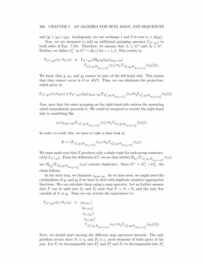
266 CHAPTER 7. AN ALGEBRA FOR SETS, BAGS, AND SEQUENCES

and |g| = |g1| ∗ |g2|. Analogously, we can exchange 1 and 2 in case ai ∈ A(g2).

Now, we are prepared to add an additional grouping operator ΓG+;g;F toboth sides of Eqv. 7.101. Therefore, we assume that J1 ⊆ G+ and J2 ⊆ G+.Further, we define G+

i as G+ ∩ A(ei) for i = 1, 2. This results in

ΓG+;g;F (e1 Bq e2) ≡ ΓG+;g;F (Πg1,g2(µg(χg:g1Ag2(

ΓG+1 ;g1:ΠA(e1)\G+

1

(e1) Bq ΓG+2 ;g2:ΠA(e2)\G+

2

(e2))))).

We know that g, g1, and g2 cannot be part of the left-hand side. This meansthat they cannot occur in G or A(F ). Thus, we can eliminate the projection,which gives us

ΓG+;g;F (e1Bqe2) ≡ ΓG+;g;F (µg(χg:g1Ag2(ΓG+1 ;g1:ΠA(e1)\G+

1

(e1)BqΓG+2 ;g2:ΠA(e2)\G+

2

(e2))))

Now, note that the outer grouping on the right-hand side undoes the unnestingwhich immediately proceeds it. We could be tempted to rewrite the right-handside to something like

χF (χg:g1Ag2(ΓG+1 ;g1:ΠA(e1)\G+

1

(e1) Bq ΓG+2 ;g2:ΠA(e2)\G+

2

(e2))).

In order to verify this, we have to take a close look at

E := (ΓG+1 ;g1:ΠA(e1)\G+

1

(e1) Bq ΓG+2 ;g2:ΠA(e2)\G+

2

(e2)).

We must make sure that E produces only a single tuple for each group construct-ed by ΓG+;g;F . From the definition of Γ, we see that neither ΠG+

1(ΓG+

1 ;g1:ΠA(e1)\G+1

(e1))

nor ΠG+2

(ΓG+2 ;g2:ΠA(e2)\G+

2

(e2)) contain duplicates. Since G+ = G+1 ∪ G+

2 , the

claim follows.

In the next step, we eliminate χg:g1Ag2 . As we have seen, we might need thecardinalities of g1 and g2 if we have to deal with duplicate sensitive aggregationfunctions. We can calculate them using a map operator. Let us further assumethat F can be split into F1 and F2 such that F = F1 F2 and the only freevariable of Fi is gi. Then we can rewrite the equivalence to

ΓG+;g;F (e1 Bq e2) ≡ χF2⊗c1(

χF1⊗c2(

χc1:|g1|(

χc2:|g2|(

ΓG+1 ;g1:ΠA(e1)\G+

1

(e1) Bq ΓG+2 ;g2:ΠA(e2)\G+

2

(e2))))).

Next, we should start moving the different map operators inwards. The onlyproblem occurs since F1 ⊗ c2 and F2 ⊗ c1 need elements of both parts of thejoin. Let F1 be decomposable into F 1

1 and F 21 and F2 be decomposable into F 1

2

7.11. EQUIVALENCES FOR UNARY GROUPING 267

and F 22 . Then, we have

ΓG+;g;F (e1 Bq e2) ≡ χF 22⊗c1(

χF 21⊗c2(

χF 11(

χF 12(

χc1:|g1|(

χc2:|g2|(

ΓG+1 ;g1:ΠA(e1)\G+

1

(e1) Bq ΓG+2 ;g2:ΠA(e2)\G+

2

(e2))))))).

Pushing down the last four χ operators yields

ΓG+;g;F (e1 Bq e2) ≡ χF 22⊗c1(

χF 21⊗c2(

χF 11(χc1:|g1|(ΓG+

1 ;g1:ΠA(e1)\G+1

(e1)))

Bq

χF 12(χc2:|g2|(ΓG+

2 ;g2:ΠA(e2)\G+2

(e2))))),

which can now easily be rewritten to the following equivalence by observingthat g1 and g2 are not needed outside the join:

ΓG+;g;F (e1 Bq e2) ≡ χF 21⊗c2,F 2

2⊗c1( (7.102)

ΓG+1 ;g1;F 1

1 (c1:|g1|)(e1) Bq ΓG+2 ;g2;F 1

2 (c2:|g2|)(e2)).

In our SQL-notation based variant of Γ, this equivalence reads

ΓG+;F (e1 Bq e2) ≡ χF 21⊗c2,F 2

2⊗c1( (7.103)

ΓG+1 ;F 1

1 (c1:count(∗))(e1) Bq ΓG+2 ;F 1

2 (c2:count(∗))(e2))

and it holds if F is splittable into F1 and F2 such that F(Fi) ⊆ A(ei) andF = F1 F2, and Fi is splittable and decomposable into F 1

i and F 2i .

Consider the expression ΓG;g;F (e1Bqe2). We denote the set of join attributesof q from ei as Ji = F(q) ∩ A(ei) for i = 1, 2, and the set of all join attributesby J = J1 ∪ J2. If J ⊆ G, we have the above case. Assume J 6⊆ G. DefineG+ = G ∪ J , Gi = G ∩ A(ei) and G+

i = Gi ∪ JI for i = 1, 2. Let F bean aggregation vector splittable into F1 and F2 such that F(Fi) ⊆ A(ei) andF = F1 F2. Further, let Fi be decomposable into F 1

i and F 2i . Then Eqvs. 7.13

and 7.103, together with the properties of aggregation functions and vectorsdiscussed in Sec. 7.2, give us the following

ΓG;F (e1 Bq e2) ≡ ΓG;F 21 ,F

22(ΓG+;F 1

1 ,F12(e1 Bq e2)),

≡ ΓG;F 21 ,F

22(χF 1,21 ⊗c2,F

1,22 ⊗c1

(

ΓG+

1 ;F 1,11 (c1:count(∗))(e1) Bq Γ

G+2 ;F 1,1

2 (c2:count(∗))(e2))),

≡ ΓG;F 21⊗c2,F 2

2⊗c1(

ΓG+1 ;F 1

1 (c1:count(∗))(e1) Bq ΓG+2 ;F 1

2 (c2:count(∗))(e2)),

268 CHAPTER 7. AN ALGEBRA FOR SETS, BAGS, AND SEQUENCES

where C = G ∪ A(F ). It should be obvious that the expression on the right-hand side can be cleaned up in case it contains several count(∗), or no count(∗)is needed because all aggregation functions in some Fi are duplicate agnostic.

By now, the reader should be prepared to understand and prove the equiva-lences provided by Yan and Larson, which we present next. Let e1 and e2 be twoexpressions and q a join predicate for them. Define for i = 1, 2 the following setsof join attributes Ji = F(q) ∩ A(ei). Let F1 = (b1 : agg1(a1), . . . , bk : aggk(ak))and F2 = (bk+1 : aggk+1(ak+1), . . . , bm : aggm(am)) be two aggregation vectors.Define A1 = a1, . . . , ak, A2 = ak+1, . . . , am, F = F1 F2, A = A1 ∪A2, andB = b1, . . . , bm. Let G be a set of grouping attributes and define Gi ∩A(ei).We denote by G+

i the union of the grouping and join attributes of ei, that is,G+i = Gi ∪ Ji.

Eager/Lazy Groupby-Count

The following equivalence corresponds to the main theorem of Yan and Larson[914]. It states that

ΓG;F (e1 Bq e2) ≡ ΓG;(F2⊗c1)F 21(ΓG+

1 ;F 11 (c1:count(∗))(e1) Bq e2) (7.104)

holds if F is splittable and F1 is decomposable into F 11 and F 2

1 . The proof of itcan be found in [914].

From Eqv. 7.104 several other equivalences can be derived easily. First,since the join is commutative,

ΓG;F (e1 Bq e2) ≡ ΓG;(F1⊗c2)F 22(e1 Bq ΓG+

2 ;F 12 (c2:count(∗))(e2)) (7.105)

holds if F is splittable and F2 is decomposable into F 12 and F 2

2 .

Eager/Lazy Group-by

If F2 is empty, that is F2 = (), then Eqv. 7.104 simplifies to

ΓG;F (e1 Bq e2) ≡ ΓG;F 21(ΓG+

1 ;F 11(e1) Bq e2). (7.106)

This equivalence holds if F1 is decomposable into F 11 and F 2

1 .If F1 is empty, then Eqv. 7.105 simplifies to

ΓG;F (e1 Bq e2) ≡ ΓG;F 22(e1 Bq ΓG+

2 ;F 12(e2)). (7.107)

This equivalence holds if F2 is decomposable into F 12 and F 2

2 .

Eager/Lazy Count

If F1 = (), then Eqv. 7.104 simplifies to

ΓG;F (e1 Bq e2) ≡ ΓG;(F2⊗c1)(ΓG+1 ;c1:count(∗)(e1) Bq e2). (7.108)

If F2 = (), then Eqv. 7.105 simplifies to

ΓG;F (e1 Bq e2) ≡ ΓG;(F1⊗c2)(e1 Bq ΓG+2 ;c2:count(∗)(e2)). (7.109)

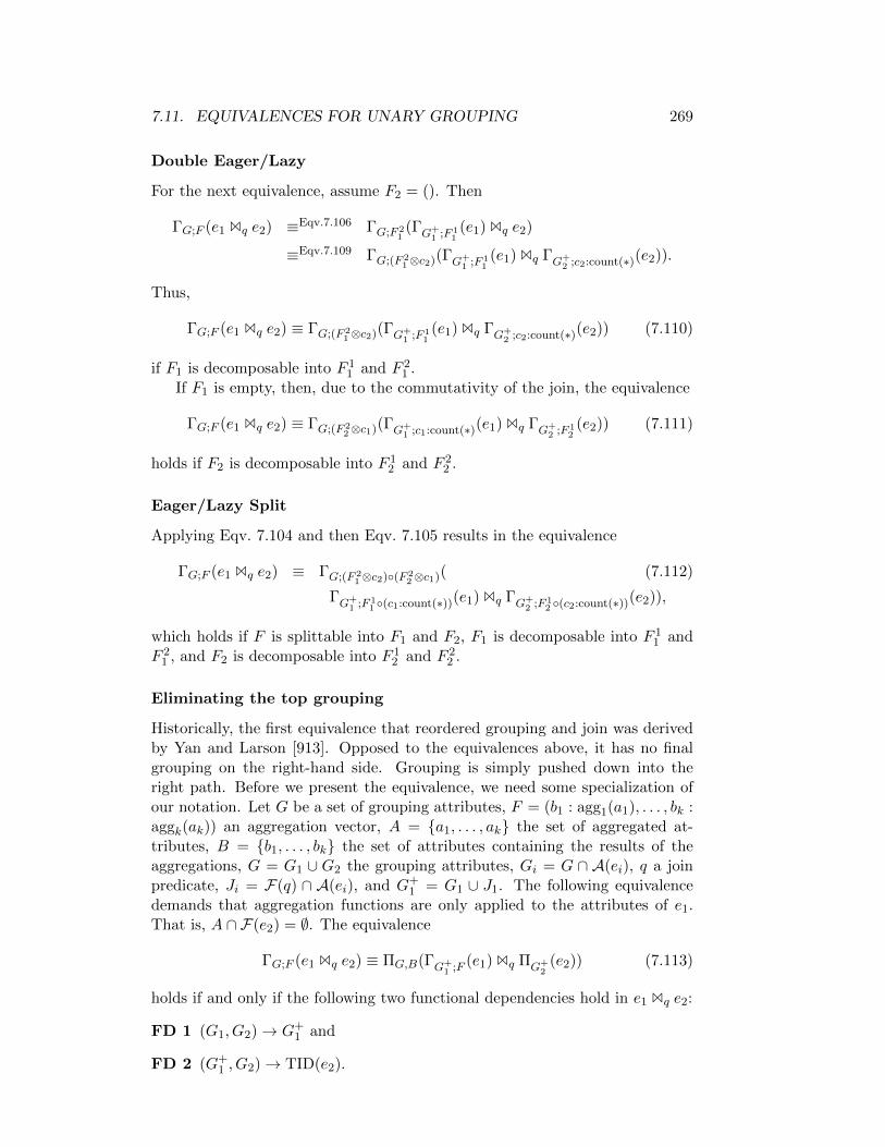
7.11. EQUIVALENCES FOR UNARY GROUPING 269

Double Eager/Lazy

For the next equivalence, assume F2 = (). Then

ΓG;F (e1 Bq e2) ≡Eqv.7.106 ΓG;F 21(ΓG+

1 ;F 11(e1) Bq e2)

≡Eqv.7.109 ΓG;(F 21⊗c2)(ΓG+

1 ;F 11(e1) Bq ΓG+

2 ;c2:count(∗)(e2)).

Thus,

ΓG;F (e1 Bq e2) ≡ ΓG;(F 21⊗c2)(ΓG+

1 ;F 11(e1) Bq ΓG+

2 ;c2:count(∗)(e2)) (7.110)

if F1 is decomposable into F 11 and F 2

1 .If F1 is empty, then, due to the commutativity of the join, the equivalence

ΓG;F (e1 Bq e2) ≡ ΓG;(F 22⊗c1)(ΓG+

1 ;c1:count(∗)(e1) Bq ΓG+2 ;F 1

2(e2)) (7.111)

holds if F2 is decomposable into F 12 and F 2

2 .

Eager/Lazy Split

Applying Eqv. 7.104 and then Eqv. 7.105 results in the equivalence

ΓG;F (e1 Bq e2) ≡ ΓG;(F 21⊗c2)(F 2

2⊗c1)( (7.112)

ΓG+1 ;F 1

1 (c1:count(∗))(e1) Bq ΓG+2 ;F 1

2 (c2:count(∗))(e2)),

which holds if F is splittable into F1 and F2, F1 is decomposable into F 11 and

F 21 , and F2 is decomposable into F 1

2 and F 22 .

Eliminating the top grouping

Historically, the first equivalence that reordered grouping and join was derivedby Yan and Larson [913]. Opposed to the equivalences above, it has no finalgrouping on the right-hand side. Grouping is simply pushed down into theright path. Before we present the equivalence, we need some specialization ofour notation. Let G be a set of grouping attributes, F = (b1 : agg1(a1), . . . , bk :aggk(ak)) an aggregation vector, A = a1, . . . , ak the set of aggregated at-tributes, B = b1, . . . , bk the set of attributes containing the results of theaggregations, G = G1 ∪ G2 the grouping attributes, Gi = G ∩ A(ei), q a joinpredicate, Ji = F(q) ∩ A(ei), and G+

1 = G1 ∪ J1. The following equivalencedemands that aggregation functions are only applied to the attributes of e1.That is, A ∩ F(e2) = ∅. The equivalence

ΓG;F (e1 Bq e2) ≡ ΠG,B(ΓG+1 ;F (e1) Bq ΠG+

2(e2)) (7.113)

holds if and only if the following two functional dependencies hold in e1 Bq e2:

FD 1 (G1, G2)→ G+1 and

FD 2 (G+1 , G2)→ TID(e2).

270 CHAPTER 7. AN ALGEBRA FOR SETS, BAGS, AND SEQUENCES

R1

g1 j1 a1

1 1 21 2 41 2 8

Rgood2

g2 j21 12 2

Rbad2

g2 j21 11 2

Rugly2

g2 j2 k2

1 1 12 1 22 1 3

eg12 := R1 1j1=j2 Rgood2

g1 j1 a1 g2 j21 1 2 1 11 2 4 2 21 2 8 2 2

Eg1 := Γg1,g2;F (eg12)

g1 g2 c1 b11 1 1 21 2 2 12

eb12 := R1 1j1=j2 Rbad2

g1 j1 a1 g2 j21 1 2 1 11 2 4 1 21 2 8 1 2

Eb1 := Γg1,g2;F (eb12)

g1 g2 c1 b11 1 3 14

eu12 := R1 1j1=j2 Rugly2

g1 j1 a1 g2 j2 k2

1 1 2 1 1 11 1 2 2 1 21 1 2 2 1 3

Eu1 := Γg1,g2;F (eu12)

g1 g2 c1 b11 1 1 21 2 2 4

G1 := Γg1,j1;F (R1)

g1 j1 c1 b11 1 1 21 2 2 12

Eg2 := G1 1j1=j2 Rgood2

g1 j1 c1 b1 g2 j21 1 1 2 1 11 2 2 12 2 2

G1 := Γg1,j1;F (R1)

g1 j1 c1 b11 1 1 21 2 2 12

Eb2 := G1 1j1=j2 Rbad2

g1 j1 c1 b1 g2 j21 1 1 2 1 11 2 2 12 1 2

G1 := Γg1,j1;F (R1)

g1 j1 c1 b11 1 1 21 2 2 12

Eu2 := G1 1j1=j2 Rugly2

g1 j1 c1 b1 g2 j2 k2

1 1 1 2 1 1 11 1 1 2 2 1 21 1 1 2 2 1 3

where F = [c1 : count(∗), b1 : sum(a1)].

Figure 7.14: Example for Eqv. 7.113

For FD 2, we use an artificial attribute TID for expression e2. It can be presentexplicitly or just in the mind of the query compiler. Its purpose is to uniquelyidentify a tuple in e2. A consequence of FD 2 is that e2 cannot contain duplicates(without the TID attribute!). This point is illustrated in the example below.Further, since it does not contain duplicates (again, if TID is ignored), wemight assume that e2 has a key (either an artificially generated one using thetid operator or, in case it is a base relation, a user-specified primary key). Then,we can replace the TID on the right-hand side by the key.

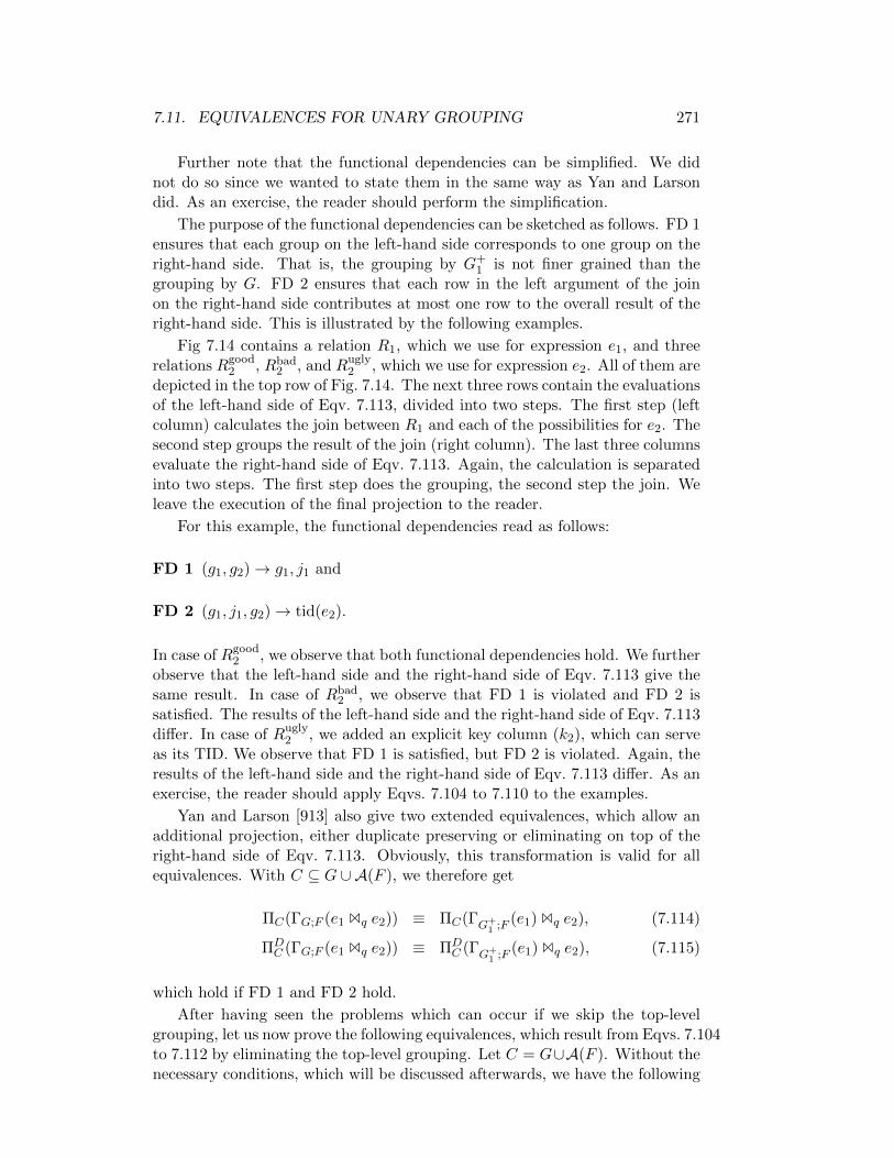
7.11. EQUIVALENCES FOR UNARY GROUPING 271

Further note that the functional dependencies can be simplified. We didnot do so since we wanted to state them in the same way as Yan and Larsondid. As an exercise, the reader should perform the simplification.

The purpose of the functional dependencies can be sketched as follows. FD 1ensures that each group on the left-hand side corresponds to one group on theright-hand side. That is, the grouping by G+

1 is not finer grained than thegrouping by G. FD 2 ensures that each row in the left argument of the joinon the right-hand side contributes at most one row to the overall result of theright-hand side. This is illustrated by the following examples.

Fig 7.14 contains a relation R1, which we use for expression e1, and threerelations Rgood

2 , Rbad2 , and Rugly

2 , which we use for expression e2. All of them aredepicted in the top row of Fig. 7.14. The next three rows contain the evaluationsof the left-hand side of Eqv. 7.113, divided into two steps. The first step (leftcolumn) calculates the join between R1 and each of the possibilities for e2. Thesecond step groups the result of the join (right column). The last three columnsevaluate the right-hand side of Eqv. 7.113. Again, the calculation is separatedinto two steps. The first step does the grouping, the second step the join. Weleave the execution of the final projection to the reader.

For this example, the functional dependencies read as follows:

FD 1 (g1, g2)→ g1, j1 and

FD 2 (g1, j1, g2)→ tid(e2).

In case of Rgood2 , we observe that both functional dependencies hold. We further

observe that the left-hand side and the right-hand side of Eqv. 7.113 give thesame result. In case of Rbad

2 , we observe that FD 1 is violated and FD 2 issatisfied. The results of the left-hand side and the right-hand side of Eqv. 7.113differ. In case of Rugly

2 , we added an explicit key column (k2), which can serveas its TID. We observe that FD 1 is satisfied, but FD 2 is violated. Again, theresults of the left-hand side and the right-hand side of Eqv. 7.113 differ. As anexercise, the reader should apply Eqvs. 7.104 to 7.110 to the examples.

Yan and Larson [913] also give two extended equivalences, which allow anadditional projection, either duplicate preserving or eliminating on top of theright-hand side of Eqv. 7.113. Obviously, this transformation is valid for allequivalences. With C ⊆ G ∪ A(F ), we therefore get

ΠC(ΓG;F (e1 Bq e2)) ≡ ΠC(ΓG+1 ;F (e1) Bq e2), (7.114)

ΠDC (ΓG;F (e1 Bq e2)) ≡ ΠD

C (ΓG+1 ;F (e1) Bq e2), (7.115)

which hold if FD 1 and FD 2 hold.

After having seen the problems which can occur if we skip the top-levelgrouping, let us now prove the following equivalences, which result from Eqvs. 7.104to 7.112 by eliminating the top-level grouping. Let C = G∪A(F ). Without thenecessary conditions, which will be discussed afterwards, we have the following

272 CHAPTER 7. AN ALGEBRA FOR SETS, BAGS, AND SEQUENCES

equivalences:

ΓG;F (e1 Bq e2) ≡ ΠC(χ (F2⊗c1)F 21

(ΓG+1 ;F 1

1 (c1:count(∗))(e1) Bq e2)), (7.116)

ΓG;F (e1 Bq e2) ≡ ΠC(χ (F1⊗c2)F 22

(e1 Bq ΓG+2 ;F 1

2 (c2:count(∗))(e2))), (7.117)

ΓG;F (e1 Bq e2) ≡ ΠC(ΓG+1 ;F (e1) Bq e2) (7.118)

ΓG;F (e1 Bq e2) ≡ ΠC(e1 Bq ΓG+2 ;F (e2)) (7.119)

ΓG;F (e1 Bq e2) ≡ ΠC(χF2⊗c1(ΓG+

1 ;c1:count(∗)(e1) Bq e2)), (7.120)

ΓG;F (e1 Bq e2) ≡ ΠC(χF1⊗c2(e1 Bq ΓG+

2 ;c2:count(∗)(e2))), (7.121)

ΓG;F (e1 Bq e2) ≡ ΠC(χF 21⊗c2

(ΓG+1 ;F 1

1(e1) Bq ΓG+

2 ;c2:count(∗)(e2))), (7.122)

ΓG;F (e1 Bq e2) ≡ ΠC(χF 22⊗c1

(ΓG+1 ;c1:count(∗)(e1) Bq ΓG+

2 ;F 12(e2))), (7.123)

ΓG;F (e1 Bq e2) ≡ ΠC(χF 21⊗c2F 2

2⊗c1(

ΓG+1 ;F 1

1 (c1:count(∗))(e1) Bq ΓG+2 ;F 1

2 (c2:count(∗))(e2))).(7.124)

We can prove Eqv. 7.117 by eliminating the top-most grouping operator onthe right-hand side of Eqv. 7.105 via an application of Eqv. 7.16 followed by anapplication of remove-group-by (Eqv. 7.97):

ΓG;F (e1 Bq e2)

≡7.105 ΓG;(F1⊗c2)F 22(e1 Bq ΓG+

2 ;F 12 (c2:count(∗))(e2))

≡7.16 ΠC(ΓG1,G+2 ;(F1⊗c2)F 2

2(e1 Bq ΓG+

2 ;F 12 (c2:count(∗))(e2)))

≡7.97 ΠC(χ (F1⊗c2)F 22

(

e1 Bq ΓG+2 ;F 1

2 (c2:count(∗))(e2)))

Let us now come to the conditions attached to the equivalences. For our dis-cussion, we denote by I the join with its (grouped) arguments, i.e.,

I = e1 Bq ΓG+2 ;F 1

2 (c2:count(∗))(e2)).

The precondition of Eqv. 7.16 requires G→ G1, G+2 to hold. Thus, a grouping

by G1, G+2 is not finer grained than a grouping by G. We still have to make

sure that the precondition required by Eqv. 7.97 holds. In our context, theprecondition is that G1, G

+2 → TID(I) holds in I, or, equivalently, ΠG1,G

+2

(I) is

duplicate-free. Clearly, ΠG+2

(ΓG+2 ;F 1

2 (c2:count(∗))(e2)) is duplicate-free. It follows

that ΠG1,G+2

(I) is duplicate-free if G1, G+2 → TID(e1) holds in I. Summarizing,

Eqv. 7.117 holds if G→ G+ and G1, G+2 → TID(e1) both hold in I.

Eqv. 7.117 can be further simplified. If F1 is empty, some simplificationyields Eqv.7.119:

ΓG;F (e1 Bq e2)

≡7.117 ΠC(χ (F1⊗c2)F 22

(e1 Bq ΓG+2 ;F 1

2 (c2:count(∗))(e2)))

≡ ΠC(e1 Bq ΓG+2 ;F (e2)).

7.11. EQUIVALENCES FOR UNARY GROUPING 273

By symmetry, Eqvs. 7.116 and 7.118 hold. Since Eqvs. 7.120 and 7.121 arealso simplifications of Eqvs. 7.116 and 7.117, they can be proven similarily.

Let us turn to Eqv. 7.124. Since

ΠG+1

(ΓG+1 ;F 1

1 (c1:count(∗))(e1))

andΠG+

2(ΓG+

2 ;F 12 (c2:count(∗))(e2))

are duplicate-free, Eqv. 7.124 holds if G → G+. Eqvs. 7.122 and 7.123 followby simplifications from Eqv.7.124, if F1 or F2 is empty.

7.11.3 Left Outerjoin

Consider a left outerjoin followed by a grouping operator. The goal is to pushdown the grouping operator into the arguments of the outerjoin. In order todo so, we will first mirror (and apply) Eqv. 7.104. The definition of the leftouterjoin gives us

ΓG;F (e1 Eq e2) ≡ ΓG;F ((e1 Bq e2) ∪ ((e1 Tq e2) A ⊥A(e2))).

As before, we define Ji = F(q)∩A(ei), J = J1∪J2, Gi = G∩A(ei), G+i = Gi∪Ji,

G+ = G ∪ J . We further demand that F is a splittable and decomposableaggregation vector. Define C = G ∪ A(F ). We also define abbreviations forsome subexpressions:

Ej = (e1 Bq e2),

Ea = ((e1 Tq e2) A ⊥A(e2)),E⊥ = ⊥A(e2).

We could consider two cases to push down the grouping operator into the ar-guments of the outerjoin. Case 1 requires ΠG(Ej) ∩ ΠG(Ea) = ∅, and case 2requires ΠG(Ej)∩ΠG(Ea) 6= ∅. The former condition is fulfilled, e.g., if G→ J1.Then, we can apply Eqv. 7.26 in case 1 and Eqv. 7.27 in case 2. Since Eqv. 7.27also holds if ΠG(Ej) ∩ ΠG(Ea) = ∅, it suffices to apply it. As an exercise, thereader should consider case 1 explicitly.

Eqv. 7.27 gives us

ΓG;F1,F2((e1 Bq e2) ∪ ((e1 Tq e2) A E⊥))≡ ΓG;F 2

1 ,F22(ΓG;F 1

1 ,F12(e1 Bq e2) ∪ ΓG;F 1

1 ,F12((e1 Tq e2) A E⊥))

where we expanded F to F1, F2. Applying Eqv. 7.104 to the left branch of theunion gives us

ΓG;F 11 ,F

12(e1 Bq e2) ≡ ΠC(Γ

G;(F 12⊗c1)F 1,2

1(ΓG+

1 ;F 1,11 (c1:count(∗))(e1) Bq e2))

Applying Eqv. 7.104 and then Eqv. 7.23 to the right branch of the union givesus:

ΓG;F 11 ,F

12((e1 Tq e2) A E⊥)

≡ ΠC(ΓG;(F 1

2⊗c1)F 1,21

(ΓG+

1 ;F 1,11 (c1:count(∗))(e1 Tq e2) A E⊥))

≡ ΠC(ΓG;(F 1

2⊗c1)F 1,21

((ΓG+

1 ;F 1,11 (c1:count(∗))(e1) Tq e2) A E⊥))

274 CHAPTER 7. AN ALGEBRA FOR SETS, BAGS, AND SEQUENCES

Putting these two things together yields

ΓG;F (e1 Eq e2)≡ ΓG;F 2

1 ,F22(

ΓG;(F 1

2⊗c1)F 1,21

(ΓG+

1 ;F 1,11 (c1:count(∗))(e1) Bq e2)

∪ΓG;(F 1

2⊗c1)F 1,21

((ΓG+

1 ;F 1,11 (c1:count(∗))(e1) Tq e2) A E⊥))

≡ ΓG;(F2⊗c1)F 21(

(ΓG+

1 ;F 1,11 (c1:count(∗))(e1) Bq e2)

∪((Γ

G+1 ;F 1,1

1 (c1:count(∗))(e1) Tq e2) A E⊥))

≡ ΓG;(F2⊗c1)F 21(ΓG+

1 ;F 1,11 (c1:count(∗))(e1) Eq e2)

where in the first step we could omit the ΠC due to the subsequent grouping.The second step pulls the two Γ

G;(F 12⊗c1)F 1,2

1operators out of the two union

branches and merges them with the outer ΓG;F 21 ,F

22. This is possible due to the

properties of the aggregation vectors involved and the fact that both group onthe same set G of grouping attributes.

Eager/Lazy Groupby-Count

Summarizing, we have the equivalence

ΓG;F (e1 Eq e2) ≡ ΓG;(F2⊗c1)F 21(ΓG+

1 ;F 11 (c1:count(∗))(e1) Eq e2), (7.125)

which holds if F is splittable into F1 and F2 with respect to e1 and e2, and Fiis decomposable into F 1

i and F 2i .

The companion of Eqv. 7.105 is

ΓG;F (e1 Eq e2) ≡ ΓG;(F1⊗c2)F 22(e1 E

F 12 (∅),c2:1q ΓG+

2 ;F 12 (c2:count(∗))(e2)). (7.126)

To prove it, we start with

ΓG;F (e1 Eq e2) ≡ ΓG;F ((e1 Bq e2) ∪ ((e1 Tq e2) A E⊥))

≡ ΓG;F 21 ,F

22(ΓG;F 1

1 ,F12(e1 Bq e2) ∪ ΓG;F 1

1 ,F12((e1 Tq e2) A E⊥)),

where E⊥ = ⊥A(e2). Applying Eqv. 7.105 to the left argument of the unionresults in

ΓG;F 11 ,F

12(e1 Bq e2) ≡ ΓG;(F 1

1⊗c2)F 22(e1 Bq ΓG+

2 ;F 12 (c2:count(∗))(e2)).

Applying Eqv. 7.105 to the right argument of the union yields

ΓG;F 11 ,F

12((e1 Tq e2) A E⊥)) ≡ ΓG;(F 1

1⊗c2)F 22((e1 Tq e2) A ΓG+

2 ;F 12 (c2:count(∗))(E⊥))

≡ ΓG;(F 11⊗c2)F 2

2((e1 Tq ΓG+

2 ;F 12 (c2:count(∗))(e2))

A ΓG+2 ;F 1

2 (c2:count(∗))(E⊥))

≡ ΓG;(F 11⊗c2)F 2

2((e1 Tq ΓG+

2 ;F 12 (c2:count(∗))(e2))

A ΠG+2 ∪A(F )∪c2(χF 1

2 (∅),c2:1(E⊥))),

and the claim follows.

7.11. EQUIVALENCES FOR UNARY GROUPING 275

Eager/Lazy Group-by

If F2 = (), Eqv. 7.125 simplifies to

ΓG;F (e1 Eq e2) ≡ ΓG;F 21(ΓG+

1 ;F 11(e1) Eq e2) (7.127)

This equivalence holds if F1 is decomposable into F 11 and F 2

1 .

If F1 = (), Eqv. 7.126 simplifies to

ΓG;F (e1 Eq e2) ≡ ΓG;F 22(e1 E

F 12 (∅)q ΓG+

2 ;F 12(e2)), (7.128)

which holds if F2 is decomposable.

Eager/Lazy Count

If F1 = (), Eqv. 7.125 simplifies to

ΓG;F (e1 Eq e2) ≡ ΓG;(F2⊗c1)(ΓG+1 ;(c1:count(∗))(e1) Eq e2). (7.129)

This equivalence holds if F2 is decomposable into F 12 and F 2

2 .

If F2 = (), Eqv. 7.126 simplifies to

ΓG;F (e1 Eq e2) ≡ ΓG;(F1⊗c2)(e1 Ec2:1q ΓG+

2 ;c2:count(∗)(e2)). (7.130)

Double Eager/Lazy

For the next equivalence assume F2 = (). We would like to derive an equivalencesimilar to Eqv. 7.110. Here it is:

ΓG;F (e1 Eq e2) ≡ ΓG;(F 21⊗c2)(ΓG+

1 ;F 11(e1) Ec2:1

q ΓG+2 ;c2:count(∗)(e2)), (7.131)

which holds if F1 is decomposable into F 11 and F 2

1 .

If F1 = () and F2 is decomposable into F 12 and F 2

2 , the equivalence

ΓG;F (e1 Eq e2) ≡ ΓG;(F 22⊗c1)(ΓG+

1 ;c1:count(∗)(e1) EF 12 (∅)q ΓG+

2 ;F 12(e2)) (7.132)

holds.

Eager/Lazy Split

The companion of Eqv. 7.112 for the left outerjoin is

ΓG;F (e1 Eq e2) ≡ ΓG;(F 21⊗c2)(F 2

2⊗c1)( (7.133)

ΓG+1 ;F 1

1 (c1:count(∗))(e1) EF 12 (∅),c2:1q ΓG+

2 ;F 12 (c2:count(∗))(e2)),

which holds if F1 is decomposable into F 11 and F 2

1 , and F2 is decomposable intoF 1

2 and F 22 .

276 CHAPTER 7. AN ALGEBRA FOR SETS, BAGS, AND SEQUENCES

Eliminating the top grouping

We can eliminate the top grouping in the above equivalences for the outerjoinby the same arguments as for the join. The resulting equivalences are

ΓG;F (e1 Eq e2) ≡ ΠC(χ (F2⊗c1)F 21

(ΓG+1 ;F 1

1 (c1:count(∗))(e1) Eq e2)), (7.134)

ΓG;F (e1 Eq e2) ≡ ΠC(χ (F1⊗c2)F 22

(e1 EF 12 (∅),c2:1q ΓG+

2 ;F 12 (c2:count(∗))(e2))),(7.135)

ΓG;F (e1 Eq e2) ≡ ΠC(ΓG+1 ;F (e1) Eq e2), (7.136)

ΓG;F (e1 Eq e2) ≡ ΠC(e1 EF (∅)q ΓG+

2 ;F (e2)), (7.137)

ΓG;F (e1 Eq e2) ≡ ΠC(χF2⊗c1(ΓG+

1 ;(c1:count(∗))(e1) Eq e2)), (7.138)

ΓG;F (e1 Eq e2) ≡ ΠC(χF1⊗c2(e1 E

c2:1q ΓG+

2 ;c2:count(∗)(e2))), (7.139)

ΓG;F (e1 Eq e2) ≡ ΠC(χF 21⊗c2

(ΓG+1 ;F 1

1(e1) Ec2:1

q ΓG+2 ;c2:count(∗)(e2))), (7.140)

ΓG;F (e1 Eq e2) ≡ ΠC(χF 22⊗c1

(ΓG+1 ;c1:count(∗)(e1) E

F 12 (∅)q ΓG+

2 ;F 12(e2)), (7.141)

ΓG;F (e1 Eq e2) ≡ ΠC(χG;F 2

1⊗c2F 22⊗c1

(

ΓG+1 ;F 1

1 (c1:count(∗))(e1) EF 12 (∅),c2:1q ΓG+

2 ;F 12 (c2:count(∗))(e2))).(7.142)

These equivalences hold if in addition to the according conditions concerningsplittability, decomposability, and emptyness, the following functional depen-dencies hold:

Eqv. 7.134 G→ G1, G+2 , G1, G

+2 → TID(e1),

Eqv. 7.135 G→ G1, G+2 , G1, G

+2 → TID(e1),

Eqv. 7.136 G→ G1, G+2 , G1, G

+2 → TID(e1),

Eqv. 7.137 G→ G1, G+2 , G1, G

+2 → TID(e1),

Eqv. 7.138 G→ G1, G+2 , G1, G

+2 → TID(e1),

Eqv. 7.139 G→ G1, G+2 , G1, G

+2 → TID(e1),

Eqv. 7.140 G→ G1, G+2 ,

Eqv. 7.141 G→ G1, G+2 ,

Eqv. 7.142 G→ G1, G+2 .

7.11.4 Left Outerjoin with Default

Main Equivalences

Let us next consider the outerjoin with default. For a set of attributes d1, . . . , dl ⊆A(e2) of e2, constants c1, . . . , cl and a vector

D = d1 : c1, . . . dl : cl,

we now consider the expression

ΓG;F (e1 EDq e2).

If we take a close look at the proof of Eqv. 7.125 and think of E⊥ as beingdefined as

E⊥ := (⊥A(e2)\A(D) A D),

7.11. EQUIVALENCES FOR UNARY GROUPING 277

we see that the proof remains valid. Thus, we have the following equivalences:

ΓG;F (e1 EDq e2) ≡ ΓG;(F2⊗c1)F 2

1(ΓG+

1 ;F 11 (c1:count(∗))(e1) Eq e2), (7.143)

ΓG;F (e1 EDq e2) ≡ ΓG;(F1⊗c2)F 2

2(e1 E

D,F 12 (∅),c2:1

q ΓG+2 ;F 1

2 (c2:count(∗))(e2)), (7.144)

ΓG;F (e1 EDq e2) ≡ ΓG;F 2

1(ΓG+

1 ;F 11(e1 E

Dq e2)) (7.145)

if F2 is empty,

ΓG;F (e1 EDq e2) ≡ ΓG;F 2

2(e1 E

D,F 12 (∅)

q ΓG+2 ;F 1

2(e2)) (7.146)

if F1 is empty,

ΓG;F (e1 EDq e2) ≡ ΓG;(F2⊗c1)(ΓG+

1 ;(c1:count(∗))(e1) EDq e2) (7.147)

if F1 is empty,

ΓG;F (e1 EDq e2) ≡ ΓG;(F1⊗c2)(e1 E

D,c2:1q ΓG+

2 ;c2:count(∗)(e2)) (7.148)

if F2 is empty,

ΓG;F (e1 EDq e2) ≡ ΓG;(F1⊗c2)(ΓG+

1 ;F 11(e1) ED,c2:1

q ΓG+2 ;c2:count(∗)(e2)) (7.149)

if F2 is empty,

ΓG;F (e1 EDq e2) ≡ ΓG;(F 2

2⊗c1)(ΓG+1 ;c1:count(∗)(e1) E

D,F 12 (∅)

q ΓG+2 ;F 1

2(e2)) (7.150)

if F1 is empty,

ΓG;F (e1 EDq e2) ≡ ΓG;(F1⊗c2)(F2⊗c1)( (7.151)

ΓG+1 ;F 1

1 (c1:count(∗))(e1) ED,F 1

2 (∅),c2:1q ΓG+

2 ;F 12 (c2:count(∗))(e2)).

These equivalences hold under the same conditions as their corresponding equiv-alences for the outerjoin with no default.

Eliminating the top grouping

This can be performed analogously to the left outerjoin without default.

7.11.5 Full Outerjoin

The next expression we consider is

ΓG;F (e1 Kq e2).

In order to deal with this expression, we will need the full outerjoin with defaultsfor both sides. Define E1⊥ = ⊥A(e1) and let us start by observing

ΓG;F (e1 Kq e2) ≡ ΓG;F ((e1 Eq e2) ∪ ((e2 Tq e1) A E1⊥))

≡ ΓG;F 2(ΓG;F 1(e1 Eq e2) ∪ ΓG;F 1((e2 Tq e1) A E1⊥)).

Applying Eqv. 7.125 to the left-hand side of the union results in

ΓG;F 1(e1 Eq e2) ≡ ΓG;(F 1

2⊗c1)F 1,21

(ΓG+

1 ;F 1,11 (c1:count(∗))(e1) Eq e2)

≡ ΓG;(F 1

1⊗c2)F 1,22

(e1 EF 1,12 (∅),c2:1q Γ

G+2 ;F 1,1

2 (c2:count(∗))(e2)).

278 CHAPTER 7. AN ALGEBRA FOR SETS, BAGS, AND SEQUENCES

Applying Eqvs. 7.104 and 7.23 to the right-hand side of the union yields

ΓG;F 1((e2 Tq e1) A E1⊥) ≡ ΓG;(F 1

1⊗c2)F 1,22

(ΓG+

2 ;F 1,12 (c2:count(∗))(e2 Tq e1) A E1⊥)

≡ ΓG;(F 1

1⊗c2)F 1,22

((ΓG+

2 ;F 1,12 (c2:count(∗))(e2) Tq e1) A E1⊥).

Putting these things together, we have

ΓG;F (e1 Kq e2)

≡ ΓG;F 2(

ΓG;(F 1

1⊗c2)F 1,22

(e1 EF 1,12 (∅),c2:1q Γ

G+2 ;F 1,1

2 (c2:count(∗))(e2))

∪(ΓG;(F 1

1⊗c2)F 1,22

((ΓG+

2 ;F 1,12 (c2:count(∗))(e2) Tq e1) A E1⊥)))

≡ ΓG;(F1⊗c2)F 22(

(e1 EF 1,12 (∅),c2:1q Γ

G+2 ;F 1,1

2 (c2:count(∗))(e2))

∪((Γ

G+2 ;F 1,1

2 (c2:count(∗))(e2) Tq e1) A E1⊥))

≡ ΓG;(F1⊗c2)F 22(e1 K

−;F 1,12 (∅),c2:1

q ΓG+

2 ;F 1,12 (c2:count(∗))(e2)).

Eager/Lazy Groupby-Count

Due to the commutativity of the full outerjoin, we thus have

ΓG;F (e1Kq e2) ≡ ΓG;(F2⊗c1)F 21(ΓG+

1 ;F 11 (c1:count(∗))(e1)K

F 11 (∅),c1:1;−q e2) (7.152)

if F is splittable and F1 is decomposable into F 11 and F 2

1 .If F is splittable and F2 is decomposable into F 1

2 and F 22 ,

ΓG;F (e1Kq e2) ≡ ΓG;(F1⊗c2)F 22(e1K

−;F 12 (∅),c2:1

q ΓG+2 ;F 1

2 (c2:count(∗))(e2)) (7.153)

holds.

Eager/Lazy Group-by

If F2 is empty, then Eqv. 7.152 simplifies to

ΓG;F (e1 Kq e2) ≡ ΓG;F 21(ΓG+

1 ;F 11(e1) K

F 11 (∅);−q e2). (7.154)

This equivalence holds if F1 is decomposable into F 11 and F 2

1 . If F1 is empty,then Eqv. 7.153 simplifies to

ΓG;F (e1 Kq e2) ≡ ΓG;F 22(e1 K

−;F 12 (∅)

q ΓG+2 ;F 1

2(e2)). (7.155)

This equivalence holds if F2 is decomposable into F 12 and F 2

2 .

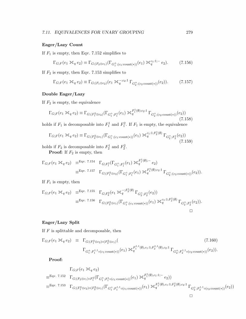
7.11. EQUIVALENCES FOR UNARY GROUPING 279

Eager/Lazy Count

If F1 is empty, then Eqv. 7.152 simplifies to

ΓG;F (e1 Kq e2) ≡ ΓG;(F2⊗c1)(ΓG+1 ;(c1:count(∗))(e1) Kc1:1;−

q e2). (7.156)

If F2 is empty, then Eqv. 7.153 simplifies to

ΓG;F (e1 Kq e2) ≡ ΓG;(F1⊗c2)(e1 K−;c2:1q ΓG+

2 ;(c2:count(∗))(e2)). (7.157)

Double Eager/Lazy

If F2 is empty, the equivalence

ΓG;F (e1 Kq e2) ≡ ΓG;(F 21⊗c2)(ΓG+

1 ;F 11(e1) K

F 11 (∅);c2:1q ΓG+

2 ;(c2:count(∗))(e2))

(7.158)holds if F1 is decomposable into F 1

1 and F 21 . If F1 is empty, the equivalence

ΓG;F (e1 Kq e2) ≡ ΓG;(F 22⊗c1)(ΓG+

1 ;(c1:count(∗))(e1) Kc1:1;F 1

2 (∅)q ΓG+

2 ;F 12(e2))

(7.159)holds if F2 is decomposable into F 1

2 and F 22 .

Proof: If F2 is empty, then

ΓG;F (e1 Kq e2) ≡Eqv. 7.154 ΓG;F 21(ΓG+

1 ;F 11(e1) K

F 11 (∅);−q e2)

≡Eqv. 7.157 ΓG;(F 21⊗c2)(ΓG+

1 ;F 11(e1) K

F 11 (∅);c2:1q ΓG+

2 ;(c2:count(∗))(e2)).

If F1 is empty, then

ΓG;F (e1 Kq e2) ≡Eqv. 7.155 ΓG;F 22(e1 K

−;F 12 (∅)

q ΓG+2 ;F 1

2(e2))

≡Eqv. 7.156 ΓG;(F 22⊗c1)(ΓG+

1 ;(c1:count(∗))(e1) Kc1:1;F 1

2 (∅)q ΓG+

2 ;F 12(e2)).

2

Eager/Lazy Split

If F is splittable and decomposable, then

ΓG;F (e1 Kq e2) ≡ ΓG;(F 21⊗c2)(F 2

2⊗c1)( (7.160)

ΓG+

1 ;F 1,11 (c1:count(∗))(e1) K

F 1,11 (∅),c1:1;F 1,1

2 (∅),c2:1q Γ

G+2 ;F 1,1

2 (c2:count(∗))(e2)).

Proof:

ΓG;F (e1 Kq e2)

≡Eqv. 7.152 ΓG;(F2⊗c1)F 21(ΓG+

1 ;F 11 (c1:count(∗))(e1) K

F 11 (∅),c1:1;−q e2))

≡Eqv. 7.153 ΓG;(F 21⊗c2)(F 2

2⊗c1)(ΓG+1 ;F 1,1

1 (c1:count(∗))(e1) KF 11 (∅),c1:1;F 1

2 (∅),c2:1q Γ

G+2 ;F 1,1

2 (c2:count(∗))(e2))

2

280 CHAPTER 7. AN ALGEBRA FOR SETS, BAGS, AND SEQUENCES

Eliminating the top grouping

Under the same conditions under which their counterparts are valid, the fol-lowing equivalences hold for the full outerjoin:

ΓG;F (e1 Kq e2) ≡ ΠC(χ (F2⊗c1)F 21

(ΓG+1 ;F 1

1 (c1:count(∗))(e1) KF 11 (∅),c1:1;−q e2)),(7.161)

ΓG;F (e1 Kq e2) ≡ ΠC(χ (F1⊗c2)F 22

(e1 K−;F 1

2 (∅),c2:1q ΓG+

2 ;F 12 (c2:count(∗))(e2))),(7.162)

ΓG;F (e1 Kq e2) ≡ ΠC(ΓG+1 ;F (e1) KF (∅);−

q e2), (7.163)

ΓG;F (e1 Kq e2) ≡ ΠC(e1 K−;F (∅)q ΓG+

2 ;F (e2)), (7.164)

ΓG;F (e1 Kq e2) ≡ ΠC(χG;F2⊗c1(ΓG+

1 ;(c1:count(∗))(e1) Kc1:1;−q e2)), (7.165)

ΓG;F (e1 Kq e2) ≡ ΠC(χF1⊗c2(e1 K

−;c2:1q ΓG+

2 ;(c2:count(∗))(e2))), (7.166)

ΓG;F (e1 Kq e2) ≡ ΠC(χF 21⊗c2

(ΓG+1 ;F 1

1(e1) K

F 11 (∅);c2:1q ΓG+

2 ;(c2:count(∗))(e2))),(7.167)

ΓG;F (e1 Kq e2) ≡ ΠC(χG;F 2

2⊗c1(ΓG+

1 ;(c1:count(∗))(e1) Kc1:1;F 1

2 (∅)q ΓG+

2 ;F 12(e2))),(7.168)

ΓG;F (e1 Kq e2) ≡ ΠC(χG;F 2

1⊗c2F 22⊗c1

(

ΓG+

1 ;F 1,11 (c1:count(∗))(e1)

KF 1,11 (∅),c1:1;F 1,1

2 (∅),c2:1q Γ

G+2 ;F 1,1

2 (c2:count(∗))(e2))).(7.169)

7.11.6 D-Join

Next, let us turn to the d-join. The outline of this subsection mirrors the onefor regular joins. Indeed, all equivalences that hold for regular joins will alsohold for d-joins.

Eager/Lazy Groupby-Count

The equivalence

ΓG;F (e1 Cq e2) ≡ ΓG;(F2⊗c1)F 21(ΓG+

1 ;F 11 (c1:count(∗))(e1) Cq e2) (7.170)

holds if F1 is splittable into F1 and F2, and F1 is decomposable into F 11 and

F 21 .

The equivalence

ΓG;F (e1 Cq e2) ≡ ΓG;(F1⊗c2)F 22(e1 Cq ΓG+

2 ;F 12 (c2:count(∗))(e2)) (7.171)

holds if F2 is splittable into F1 and F2, and F2 is decomposable into F 12 and

F 22 .

Eager/Lazy Group-by

If F2 is empty, that is F2 = (), Eqv. 7.170 simplifies to

ΓG;F (e1 Cq e2) ≡ ΓG;F 21(ΓG+

1 ;F 11(e1) Cq e2). (7.172)

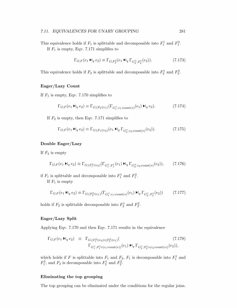
7.11. EQUIVALENCES FOR UNARY GROUPING 281

This equivalence holds if F1 is splittable and decomposable into F 11 and F 2

1 .

If F1 is empty, Eqv. 7.171 simplifies to

ΓG;F (e1 Cq e2) ≡ ΓG;F 22(e1 Cq ΓG+

2 ;F 12(e2)). (7.173)

This equivalence holds if F2 is splittable and decomposable into F 12 and F 2

2 .

Eager/Lazy Count

If F1 is empty, Eqv. 7.170 simplifies to

ΓG;F (e1 Cq e2) ≡ ΓG;(F2⊗c1)(ΓG+1 ;c1:count(∗)(e1) Cq e2). (7.174)

If F2 is empty, then Eqv. 7.171 simplifies to

ΓG;F (e1 Cq e2) ≡ ΓG;(F1⊗c2)(e1 Cq ΓG+2 ;c2:count(∗)(e2)). (7.175)

Double Eager/Lazy

If F2 is empty

ΓG;F (e1 Cq e2) ≡ ΓG;(F 21⊗c2)(ΓG+

1 ;F 11(e1) Cq ΓG+

2 ;c2:count(∗)(e2)), (7.176)

if F1 is splittable and decomposable into F 11 and F 2

1 .

If F1 is empty

ΓG;F (e1 Cq e2) ≡ ΓG;(F 22⊗c1)(ΓG+

1 ;c1:count(∗)(e1) Cq ΓG+2 ;F 1

2(e2)) (7.177)

holds if F2 is splittable decomposable into F 12 and F 2

2 .

Eager/Lazy Split

Applying Eqv. 7.170 and then Eqv. 7.171 results in the equivalence

ΓG;F (e1 Cq e2) ≡ ΓG;(F 21⊗c2)(F 2

2⊗c1)( (7.178)

ΓG+1 ;F 1

1 (c1:count(∗))(e1) Cq ΓG+2 ;F 1

2 (c2:count(∗))(e2)),

which holds if F is splittable into F1 and F2, F1 is decomposable into F 11 and

F 21 , and F2 is decomposable into F 1

2 and F 22 .

Eliminating the top grouping

The top grouping can be eliminated under the conditions for the regular joins.

282 CHAPTER 7. AN ALGEBRA FOR SETS, BAGS, AND SEQUENCES

7.11.7 Groupjoin

Simple Facts about the Groupjoin

Last in this section, we consider the groupjoin and thus the expressions of theform

ΓG;F (e1 Zq;F e2).

Before we start, we discuss some equivalences for the groupjoin. Since σ and χare linear and Z is linear in its left argument, it is easy to show that

σp(e1 ZG1θG2;g:f e2) ≡ σp(e1) ZG1θG2;g:f e2, (7.179)

χa:e(e1 ZG1θG2;g:f e2) ≡ χa:e(e1) ZG1θG2;g:f e2. (7.180)

Then, we note that unary grouping can be expressed with the help of thegroupjoin.

ΓθG;f (e) ≡ ΠC(ρA(e1)′←A(e1)(ρA(e1)←A(e1)′(ΠDG(e)) ZG′θG;f e)),

ΓθG;g;F (e) ≡ ΠC(ρA(e1)′←A(e1)(ρA(e1)←A(e1)′(ΠDG(e)) ZG′θG;g;F e)),

ΓθG;F (e) ≡ ΠC(ρA(e1)′←A(e1)(ρA(e1)←A(e1)′(ΠDG(e)) ZG′θG;F e)),

where C on the right-hand side of an equivalence contains all attributes providedin the result of the left-hand side of the equivalence.

The groupjoin itself can be expressed with the help of unary grouping anda left outerjoin:

e1 ZG1θG2;f e2 ≡ ΠC(e1 Ef(∅)G1=G2

ΓθG2;f (e2)), (7.181)

e1 ZG1θG2;g;F e2 ≡ ΠC(e1 EF (∅)G1=G2

ΓθG2;g;F (e2)), (7.182)

e1 ZG1θG2;F e2 ≡ ΠC(e1 EF (∅)G1=G2

ΓθG2;F (e2)), (7.183)

where C = G∪A(F ). We need to attach a small correction to these equivalences.Consider for example Eqv. 7.183. It only holds if F (∅) = F (⊥A(e2)). This istrue in SQL-92 for min, max, sum, count(a), but not count(*). More precisely,count(*) yields 0 if the input is the empty set, and 1 if it is applied to some null-tuple. Thus, the right-hand side yields 0 for empty groups, whereas it shouldproduce 1. Obviously, this problem can easily be fixed in the left outerjoin byusing the correct default value of 1 for all attributes containing the result of acount(*). Hence, we define count(∗)(∅) := 1 in the context of default values forouterjoins. Thus, the above equivalences now read

e1 ZG1θG2;f e2 ≡ ΠC(e1 Ef(⊥A(e2)

)G1=G2

ΓθG2;f (e2)), (7.184)

e1 ZG1θG2;g;F e2 ≡ ΠC(e1 EF (⊥A(e2)

)G1=G2

ΓθG2;g;F (e2)), (7.185)

e1 ZG1θG2;F e2 ≡ ΠC(e1 EF (⊥A(e2)

)G1=G2

ΓθG2;F (e2)). (7.186)

Apart from this detail, these equivalences follow directly from the definition ofthe groupjoin.

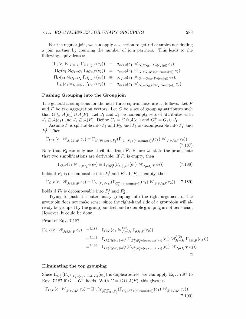
7.11. EQUIVALENCES FOR UNARY GROUPING 283

For the regular join, we can apply a selection to get rid of tuples not findinga join partner by counting the number of join partners. This leads to thefollowing equivalences:

ΠC(e1 BG1=G2 ΓθG2;g;F (e2)) ≡ σc2>0(e1 ZG1θG2;g;F(c2:|g|) e2),

ΠC(e1 BG1=G2 ΓθG2;F (e2)) ≡ σc2>0(e1 ZG1θG2;F(c2:count(∗)) e2),

ΠC(e1 BG1=G2 ΓG2;g;F (e2)) ≡ σc2>0(e1 ZG1=G2;g;F(c2:|g|) e2),

ΠC(e1 BG1=G2 ΓG2;F (e2)) ≡ σc2>0(e1 ZG1=G2;F(c2:count(∗)) e2).

Pushing Grouping into the Groupjoin

The general assumptions for the next three equivalences are as follows. Let Fand F be two aggregation vectors. Let G be a set of grouping attributes suchthat G ⊆ A(e1) ∪ A(F ). Let J1 and J2 be non-empty sets of attributes withJ1 ⊆ A(e1) and J2 ⊆ A(F ). Define G1 = G ∩ A(e1) and G+

1 = G1 ∪ J1.Assume F is splittable into F1 and F2, and F1 is decomposable into F 1

1 andF 2

1 . Then

ΓG;F (e1 ZJ1θJ2;F e2) ≡ ΓG;(F2⊗c1)F 21(ΓG+

1 ;F 11 (c1:count(∗))(e1) ZJ1θJ2;F e2)).

(7.187)Note that F2 can only use attributes from F . Before we state the proof, notethat two simplifications are derivable: If F2 is empty, then

ΓG;F (e1 ZJ1θJ2;F e2) ≡ ΓG;F 21(ΓG+

1 ;F 11(e1) ZJ1θJ2;F e2)) (7.188)

holds if F1 is decomposable into F 11 and F 2

1 . If F1 is empty, then

ΓG;F (e1 ZJ1θJ2;F e2) ≡ ΓG;(F2⊗c1)(ΓG+1 ;(c1:count(∗))(e1) ZJ1θJ2;F e2)) (7.189)

holds if F2 is decomposable into F 12 and F 2

2 .Trying to push the outer unary grouping into the right argument of the

groupjoin does not make sense, since the right-hand side of a groupjoin will al-ready be grouped by the groupjoin itself and a double grouping is not beneficial.However, it could be done.

Proof of Eqv. 7.187:

ΓG;F (e1 ZJ1θJ2;F e2) ≡7.183 ΓG;F (e1 EF (∅)J1=J2

ΓθJ2,F (e2))

≡7.143 ΓG;(F2⊗c1)F 21(ΓG+

1 ;F 11 (c1:count(∗))(e1) E

F (∅)J1=J2

ΓθJ2,F (e2)))

≡7.183 ΓG;(F2⊗c1)F 21(ΓG+

1 ;F 11 (c1:count(∗))(e1) ZJ1θJ2;F e2))

2

Eliminating the top grouping

Since ΠG+1

(ΓG+1 ;F 1

1 (c1:count(∗))(e1)) is duplicate-free, we can apply Eqv. 7.97 to

Eqv. 7.187 if G→ G+ holds. With C = G ∪ A(F ), this gives us

ΓG;F (e1 ZJ1θJ2;F e2) ≡ ΠC(χF2⊗c1F 2

1

(ΓG+1 ;F 1

1 (c1:count(∗))(e1) ZJ1θJ2;F e2)).

(7.190)

284 CHAPTER 7. AN ALGEBRA FOR SETS, BAGS, AND SEQUENCES

Simplifications result in the following equivalences, which also hold if G→ G+

holds:

ΓG;F (e1 ZJ1θJ2;F e2) ≡ ΠC(ΓG+1 ;F (e1) ZJ1θJ2;F e2), (7.191)

ΓG;F (e1 ZJ1θJ2;F e2) ≡ ΠC(χF2⊗c1(ΓG+

1 ;(c1:count(∗))(e1) ZJ1θJ2;F e2)).(7.192)

The first equivalence additionally needs that F2 is empty, the second that F1 isempty.

Important Operator Conversions

We now introduce two equivalences which allow us to replace a sequence of agrouping operator and a left-outerjoin/join by a single groupjoin [598].

For i = 1, 2, let ei be algebraic expressions and J1 = J2 be a join predi-cate, such that for the join attributes Ji ⊆ A(ei) holds. For a set of groupingattributes G, define Gi = G ∩ A(ei) and G+

i = Gi ∪ Ji. Further, let F be asplittable and decomposable aggregation vector with F(F ) ⊆ A(e2). We denoteby C the set of attributes occurring in the result, i.e., C = G ∪ A(F ). Then,the equivalence

ΓG;F (e1 EJ1=J2 e2) ≡ ΠC(e1 ZJ1=J2;F e2) (7.193)

holds under the conditions that

1. G→ G+2 and G1, G

+2 → TID(e1) hold in e1 EJ1=J2 e2,

2. J2 → G+2 holds in e2,

3. F(F ) ⊆ A(e2), and

4. F (∅) = F (⊥A(e2)).

We discuss these conditions to provide the intuition behind them. The twoconditions under 1. stem from the main theorem of Yan and Larson in [913].They assure that a grouping can be pushed into a regular join. In our context,the condition G1, G

+2 → TID(e1) assures that no two tuples from e1 belong to

the same group. This is necessary since the groupjoin on the right-hand sideprovides exactly one output tuple for each input tuple of e1. The conditionG→ G+

2 implies that grouping by G+2 is not finer grained than grouping by G,

which would lead to problems.In case the second condition (J2 → G+

2 ) is not fulfilled, we would have moregroups on the left-hand side than on the right-hand side of our equivalence,which would violate it. This is easy to see if we add to G an evil attributefrom e2, which is not functionally determined by J2. The importance of thefunctional dependencies is illustrated in the examples below.

The third condition (F(F ) ⊆ A(e2)) can actually be relaxed if we maintaina final map operator (see Eqvs. 7.117 and 7.135). The fourth condition followsfrom the discussion of Eqv. 7.183.

Eqv. 7.193 is important since it allows us to replace a unary grouping anda left outerjoin by a groupjoin. This is very beneficial in several scenarios.

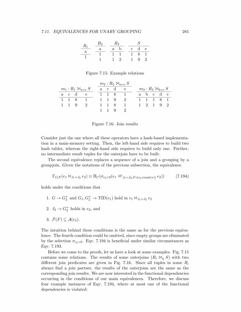
7.11. EQUIVALENCES FOR UNARY GROUPING 285

R1

a

1

R2

a

11

R3

a b

1 11 2

S

c d e

1 8 11 9 2

Figure 7.15: Example relations

m1 : R1 Ea=c S

a c d e

1 1 8 11 1 9 2

m2 : R2 Ea=c S

a c d e

1 1 8 11 1 9 21 1 8 11 1 9 2

m3 : R3 Eb=e S

a b c d e

1 1 1 8 11 2 1 9 2

Figure 7.16: Join results

Consider just the one where all these operators have a hash-based implementa-tion in a main-memory setting. Then, the left-hand side requires to build twohash tables, whereas the right-hand side requires to build only one. Further,no intermediate result tuples for the outerjoin have to be built.

The second equivalence replaces a sequence of a join and a grouping by agroupjoin. Given the notations of the previous subsection, the equivalence

ΓG;F (e1 BJ1=J2 e2) ≡ ΠC(σc2>0(e1 ZJ1=J2;F(c2:count(∗)) e2)) (7.194)

holds under the conditions that

1. G→ G+2 and G1, G

+2 → TID(e1) hold in e1 BJ1=J2 e2

2. J2 → G+2 holds in e2, and

3. F(F ) ⊆ A(e2).

The intuition behind these conditions is the same as for the previous equiva-lence. The fourth condition could be omitted, since empty groups are eliminatedby the selection σc2>0. Eqv. 7.194 is beneficial under similar circumstances asEqv. 7.193.

Before we come to the proofs, let us have a look at some examples. Fig. 7.15contains some relations. The results of some outerjoins (Ri Eq S) with twodifferent join predicates are given in Fig. 7.16. Since all tuples in some Rialways find a join partner, the results of the outerjoins are the same as thecorresponding join results. We are now interested in the functional dependenciesoccurring in the conditions of our main equivalences. Therefore, we discussfour example instances of Eqv. 7.194, where at most one of the functionaldependencies is violated:

286 CHAPTER 7. AN ALGEBRA FOR SETS, BAGS, AND SEQUENCES

l1 : Γa;sum(d)(R1 Ea=c S)

a sum(d)

1 17

r1 : R1 Za=c;sum(d) S

a sum(d)

1 17l2 : Γa,e;sum(d)(R1 Ea=c S)

a e sum(d)

1 1 81 2 9

r2 : R1 Za=c;sum(d) S

a sum(d)

1 17

l3 : Γa;sum(d)(R2 Ea=c S)

a sum(d)

1 34

r3 : R2 Za=c;sum(d) S

a sum(d)

1 171 17

l4 : Γa;sum(d)(R3 Eb=e S)

a sum(d)

1 17

r4 : R3 Zb=e;sum(d) S

a b sum(d)

1 1 81 2 9

Figure 7.17: Left- and right-hand sides

G→ G+2 G1, G

+2 → TID(e1) J2 → G+

2

1 + + +2 + + -3 + - +4 - + +

The according instances of the left-hand and right-hand side of Eqv. 7.194 are:

LHS RHS

1 Γa;sum(d)(R1 Ea=c S) R1 Za=c;sum(d) S

2 Γa,e;sum(d)(R1 Ea=c S) R1 Za=c;sum(d) S

3 Γa;sum(d)(R2 Ea=c S) R2 Za=c;sum(d) S

3 Γa;sum(d)(R3 Eb=e S) R3 Zb=e;sum(d) S

The functional dependencies have to be checked on the join results given inFig. 7.16. In order to help the reader to check the functional dependencies,we provide the following table holding the main attribute sets occurring in ourmain equivalences:

G G1 G2 J2 G+2

1 a a ∅ c c2 a, e a e c c, e3 a a ∅ c c4 a a ∅ e e

Taking a look at Fig. 7.17, we see that both sides of the equivalence give thesame result only if none of the functional dependencies is violated.

7.12. ELIMINATING REDUNDANT JOINS 287

Proof of Eqv. 7.193 We now give the proof of Eqv. 7.193. We start withthe right-hand side and transform it until we get the left-hand side:

ΠC(e1 ZJ1=J2;F e2)

≡7.183 ΠC(e1 EF (∅)J1=J2

ΓJ2;F (e2))

≡7.14 ΠC(e1 EF (∅)J1=J2

ΓG+2 ;F (e2))

≡7.137 ΓG;F (e1 EJ1=J2 e2)).

The preconditions follow from collecting the preconditions of the different equiv-alences applied. 2

Proof of Eqv. 7.194 Eqv. 7.194 follows directly from Eqv. 7.193. An alter-native is to modify the above proof by using Eqv. 7.187 instead of Eqv. 7.183and Eqv. 7.117 instead of Eqv. 7.137.

Remark Often, we encounter expression of the form ΓG;F (e1) ZJ1=J2 e2. IfG = J1, the hash table for the grouping can be reused by the groupjoin. Simi-larily, if G ⊇ J1, any sorting produced to perform a sort-based grouping can bereused for a a sort-based groupjoin.

7.11.8 Intersection and Difference

There is not much we can do in terms of pushing a unary grouping operatordown an intersection or set difference. We can only change an explicit bagrepresentation into a multiplicity-based bag representation. This gives us thefollowing two equivalences:

ΓG;F (e1 ∩ e2) ≡ ΓG;(F⊗m)(χm:min(c1,c2)( (7.195)

E1 BA(e1)=A(e2)′ ρA(e2)←A(e2)′(E2))),

ΓG;F (e1 \ e2) ≡ ΓG;(F⊗m)(χm:c1−c2( (7.196)

E1 Ec2:0A(e1)=A(e2)′ ρA(e2)←A(e2)′(E2))),

where Ei is defined as

ΓA(ei);ci:count(∗)(ei)

for i = 1, 2.

7.12 Eliminating Redundant Joins

Since the join operation is very expensive, it makes sense to investigate possi-bilities to elimininate redundant joins. These often occur if queries use views[631, 632] or if queries are generated by some programs. One possibility stud-ied intensively is to use tableaux techniques to detect and eliminate redundantjoins [19, 18, 555, 631, 632, 730]. The techniques discussed there only work onsets and not for bags.

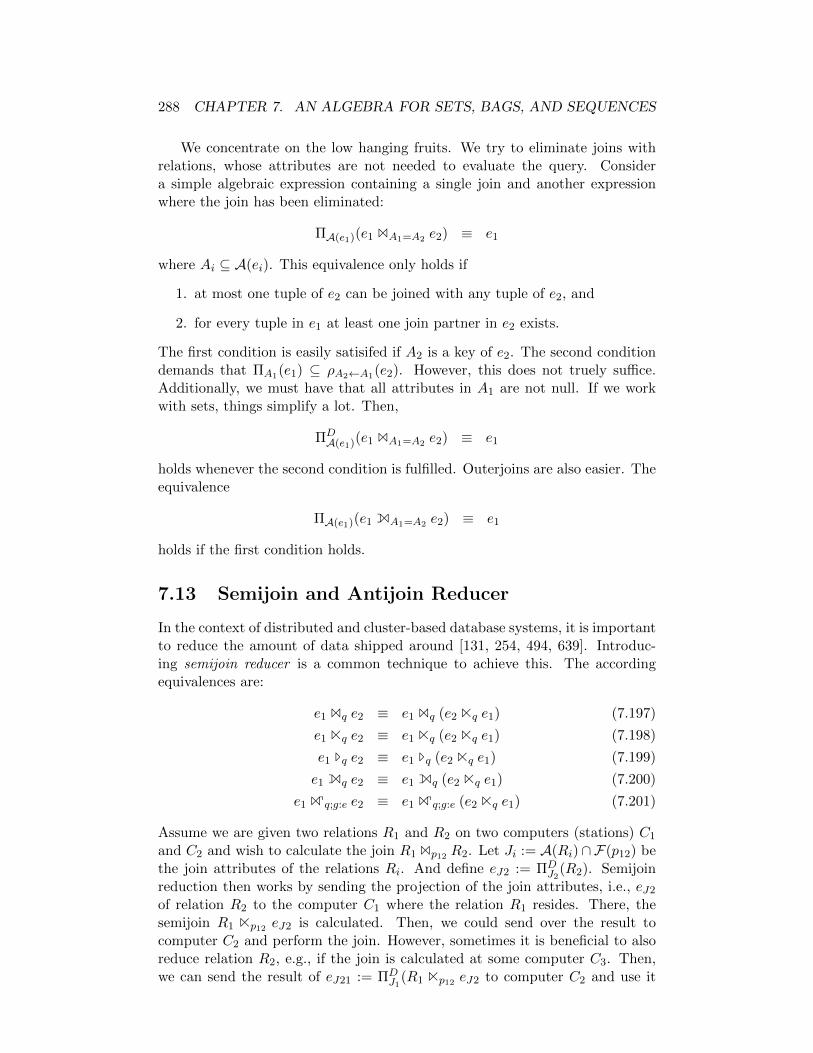
288 CHAPTER 7. AN ALGEBRA FOR SETS, BAGS, AND SEQUENCES

We concentrate on the low hanging fruits. We try to eliminate joins withrelations, whose attributes are not needed to evaluate the query. Considera simple algebraic expression containing a single join and another expressionwhere the join has been eliminated:

ΠA(e1)(e1 BA1=A2 e2) ≡ e1

where Ai ⊆ A(ei). This equivalence only holds if

1. at most one tuple of e2 can be joined with any tuple of e2, and

2. for every tuple in e1 at least one join partner in e2 exists.

The first condition is easily satisifed if A2 is a key of e2. The second conditiondemands that ΠA1(e1) ⊆ ρA2←A1(e2). However, this does not truely suffice.Additionally, we must have that all attributes in A1 are not null. If we workwith sets, things simplify a lot. Then,

ΠDA(e1)(e1 BA1=A2 e2) ≡ e1

holds whenever the second condition is fulfilled. Outerjoins are also easier. Theequivalence

ΠA(e1)(e1 EA1=A2 e2) ≡ e1

holds if the first condition holds.

7.13 Semijoin and Antijoin Reducer

In the context of distributed and cluster-based database systems, it is importantto reduce the amount of data shipped around [131, 254, 494, 639]. Introduc-ing semijoin reducer is a common technique to achieve this. The accordingequivalences are:

e1 Bq e2 ≡ e1 Bq (e2 Nq e1) (7.197)

e1 Nq e2 ≡ e1 Nq (e2 Nq e1) (7.198)

e1 Tq e2 ≡ e1 Tq (e2 Nq e1) (7.199)

e1 Eq e2 ≡ e1 Eq (e2 Nq e1) (7.200)

e1 Zq;g:e e2 ≡ e1 Zq;g:e (e2 Nq e1) (7.201)

Assume we are given two relations R1 and R2 on two computers (stations) C1

and C2 and wish to calculate the join R1 Bp12 R2. Let Ji := A(Ri)∩F(p12) bethe join attributes of the relations Ri. And define eJ2 := ΠD

J2(R2). Semijoin

reduction then works by sending the projection of the join attributes, i.e., eJ2

of relation R2 to the computer C1 where the relation R1 resides. There, thesemijoin R1 Np12 eJ2 is calculated. Then, we could send over the result tocomputer C2 and perform the join. However, sometimes it is beneficial to alsoreduce relation R2, e.g., if the join is calculated at some computer C3. Then,we can send the result of eJ21 := ΠD

J1(R1 Np12 eJ2 to computer C2 and use it

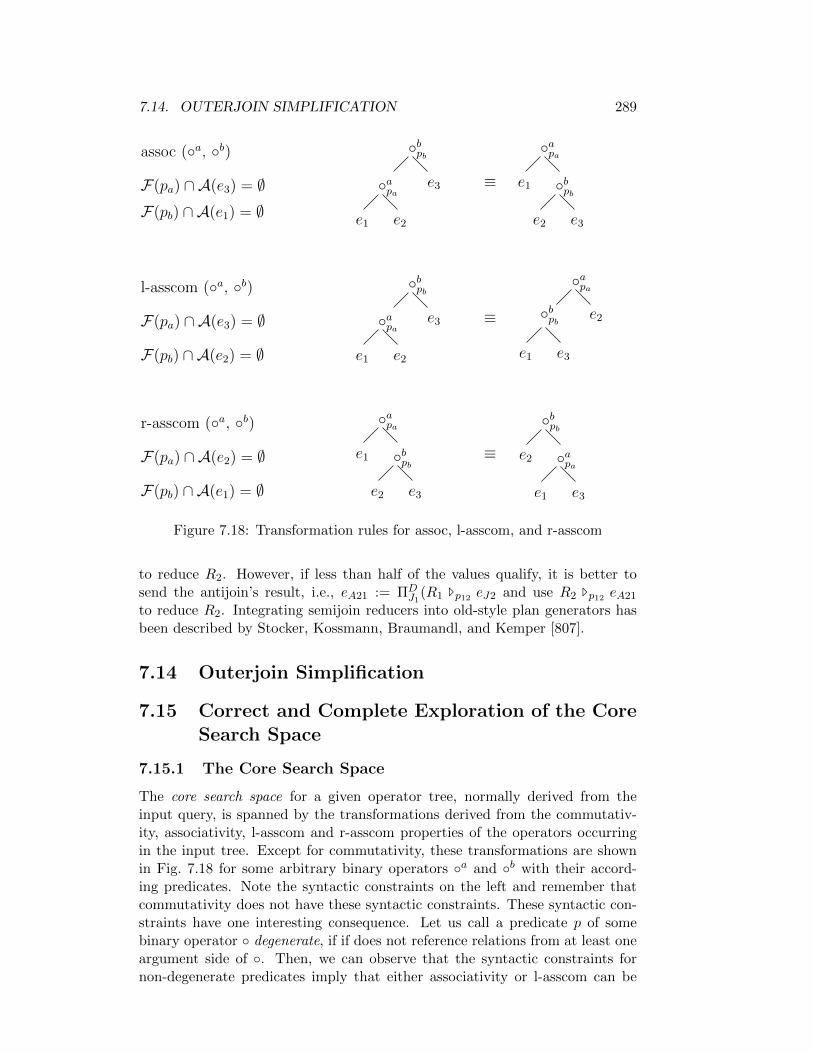
7.14. OUTERJOIN SIMPLIFICATION 289

bpbe3

e1 e2

apa

bpbe3

e1 e2

apa

e2 e3

bpb

apae1

e2 e3

bpb

bpbe2

e1 e3

apa

r-asscom (a, b)

l-asscom (a, b)

F(pa) ∩ A(e3) = ∅

F(pb) ∩ A(e2) = ∅

assoc (a, b)

≡

≡

≡F(pb) ∩ A(e1) = ∅

F(pa) ∩ A(e2) = ∅

F(pb) ∩ A(e1) = ∅

F(pa) ∩ A(e3) = ∅

apae1

apa

e1 e3

bpb e2

Figure 7.18: Transformation rules for assoc, l-asscom, and r-asscom

to reduce R2. However, if less than half of the values qualify, it is better tosend the antijoin’s result, i.e., eA21 := ΠD

J1(R1 Tp12 eJ2 and use R2 Tp12 eA21

to reduce R2. Integrating semijoin reducers into old-style plan generators hasbeen described by Stocker, Kossmann, Braumandl, and Kemper [807].

7.14 Outerjoin Simplification

7.15 Correct and Complete Exploration of the CoreSearch Space

7.15.1 The Core Search Space

The core search space for a given operator tree, normally derived from theinput query, is spanned by the transformations derived from the commutativ-ity, associativity, l-asscom and r-asscom properties of the operators occurringin the input tree. Except for commutativity, these transformations are shownin Fig. 7.18 for some arbitrary binary operators a and b with their accord-ing predicates. Note the syntactic constraints on the left and remember thatcommutativity does not have these syntactic constraints. These syntactic con-straints have one interesting consequence. Let us call a predicate p of somebinary operator degenerate, if if does not reference relations from at least oneargument side of . Then, we can observe that the syntactic constraints fornon-degenerate predicates imply that either associativity or l-asscom can be

290 CHAPTER 7. AN ALGEBRA FOR SETS, BAGS, AND SEQUENCES

comm (ob)e3 o

b13 (e2 o

a12 e1)(e2 o

a12 e1) o

b13 e3

comm (ob)(e1 o

a12 e2) o

b13 e3 e3 o

b13 (e1 o

a12 e2)

comm (oa)

l-asscomm (oa, ob)

comm (oa)(e1 o

b13 e3) o

a12 e2 e2 o

a12 (e1 o

b13 e3)

comm (ob)

comm (oa)(e3 o

b13 e1) o

a12 e2 e2 o

a12 (e3 o

b13 e1)

comm (oa)

comm (ob)

r-asscomm (oa, ob)

assoc (ob, oa)

assoc (oa, ob)

Figure 7.19: Core search space example

applied for left nesting but not both, and either associativity or r-asscom canbe applied for right-nesting but not both.

Fig. 7.19 shows an example of the seach space for an expression (e1a12e2)b13

e3, where the subscripts of the operators indicate which arguments are refer-enced in their predicate. We observe that any expression in this search spacecan be reached by a sequence of at most two applications of commutativity, atmost one application of associativity, l-asscom, or r-asscom, finally followed byat most two applications of commutativity. The total number of applicationsof commutativity can be restricted to 2. The case (e1 a12 e2) b23 e3 is left to thereader.

The last observation only holds if there are no degenerate predictates andno cross products in the original plan. Fig. 7.20 shows all possible plans fortwo binary operators a and b. One can think of them as cross products. Theplans are generated by applying assoc, l-asscom, r-asscom, and commutativityrewrites. Assume that the initial plan is the one in row 1 and column 3. Theother plans in the first row are generated by using all rewrites but commuta-tivity. The second row shows the plans derived from the plan above them by

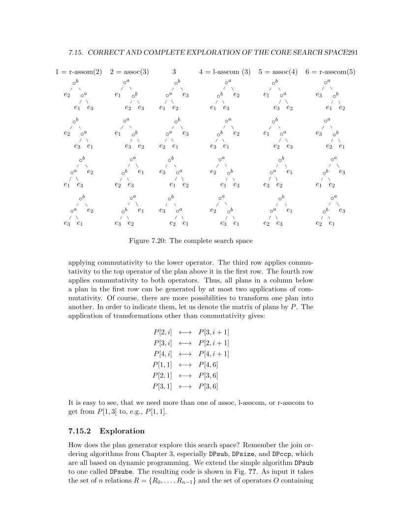
7.15. CORRECT AND COMPLETE EXPLORATIONOF THE CORE SEARCH SPACE291

1 = r-assom(2) 2 = assoc(3) 3 4 = l-asscom (3) 5 = assoc(4) 6 = r-asscom(5)

be2 a

e1 e3

a

e1 be2 e3

b

a

e1 e2

e3

a

be1 e3

e2

be1 a

e3 e2

a

e3 be1 e2

be2 a

e3 e1

a

e1 be3 e2

b

a

e2 e1

e3

a

be3 e1

e2

be1 a

e2 e3

a

e3 be2 e1

b

a

e1 e3

e2

a

be2 e3

e1

be3 a

e1 e2

a

e2 be1 e3

b

a

e3 e2

e1

a

be1 e2

e3

b

a

e3 e1

e2

a

be3 e2

e1

be3 a

e2 e1

a

e2 be3 e1

b

a

e2 e3

e1

a

be2 e1

e3

Figure 7.20: The complete search space

applying commutativity to the lower operator. The third row applies commu-tativity to the top operator of the plan above it in the first row. The fourth rowapplies commutativity to both operators. Thus, all plans in a column belowa plan in the first row can be generated by at most two applications of com-mutativity. Of course, there are more possibilities to transform one plan intoanother. In order to indicate them, let us denote the matrix of plans by P . Theapplication of transformations other than commutativity gives:

P [2, i] ←→ P [3, i+ 1]

P [3, i] ←→ P [2, i+ 1]

P [4, i] ←→ P [4, i+ 1]

P [1, 1] ←→ P [4, 6]

P [2, 1] ←→ P [3, 6]

P [3, 1] ←→ P [3, 6]

It is easy to see, that we need more than one of assoc, l-asscom, or r-asscom toget from P [1, 3] to, e.g., P [1, 1].

7.15.2 Exploration

How does the plan generator explore this search space? Remember the join or-dering algorithms from Chapter 3, especially DPsub, DPsize, and DPccp, whichare all based on dynamic programming. We extend the simple algorithm DPsub

to one called DPsube. The resulting code is shown in Fig. ??. As input it takesthe set of n relations R = R0, . . . , Rn−1 and the set of operators O containing

292 CHAPTER 7. AN ALGEBRA FOR SETS, BAGS, AND SEQUENCES

n − 1 operators which DPsube has to use in order to build a plan. First, itconstructs plan for single relations. Then, it enumerates all subsets S of re-lations by decoding an integer, which represents a bitvector. For each set ofrelations S, DPsube then enumerates all subsets S1 of S and their complementsS2. Both of them must be non-empty. For each pair (S1, S2), all operators in O are then tested for applicability via a call to applicable. If the operatoris applicable, then the best plans p1 for S1 and p2 for S2 are recalled from thedynamic programming table BestPlan and combined into the plan p1 p2 forS. The costs of this plan are then calculated and it is possibly added to theDP-table. Since this piece of code is straight forward, we did not detail on it.Note that only if an operator is applicable then DPsube also considers p2 p1 if is commutative. The rest of the section deals with different implementationsof applicable.

Two implementations of applicable are described in the literature. Each ofthem uses a set of relations as a short-hand representation of possible reorder-ing conflicts. The first set is called EEL, and is presented by Rao, Lindsay,Lohman, Pirahesh, and Simmen [689, 688]. The second set is called TES, andis presented by Moerkotte and Neumann [597, 596]. The first approach is lim-ited to B, T, and E. Both approaches generate invalid plans, i.e., plans whichare not equivalent to the input operator tree. Thus, we will present an alter-native test. The main properties are that it will be correct and complete. Animplementation of applicable is correct, if only valid plans are generated. It iscomplete, if all valid plans are generated.

Preliminaries

In order to open our approach for new algebraic operators, we use a table drivenapproach. We use four tables which contain the properties of the algebraicoperators. These contain the information of Tables 7.6 and 7.7 together withthe information about the commutativity of the operators. Thus, extendingour approach only requires to extend these tables.

We develop our final approach in three steps. At each step, we present acomplete bundle consisting of three components:

1. a representation for conflicts

2. a conflict detection (CD) algorithm, which detects the conflicts from aninitial operator tree and produces a conflict represention for this operator,and

3. the implementation of applicable, which uses the conflict representationfor an operator and then determines whether the operator can be appliedin a given context.

Each of the subsequently discussed bundles is correct, but only the last one iscomplete.

The main idea in the following (and in the literature cited above) is to ex-tend the consumer/producer constraints. Therefore, we first introduce syntacticeligibility sets (SES for short), which are attached to operators and contain the

7.15. CORRECT AND COMPLETE EXPLORATIONOF THE CORE SEARCH SPACE293

Algorithm DPsube

Input: a set of relations R = R0, . . . , Rn−1a set of operators O with associated conflict descriptors

Output: an optimal bushy operator tree

for all Ri ∈ RBestPlan(Ri) = Ri;

for 1 ≤ i < 2n − 1 ascendingS = Rj ∈ R|(bi/2jcmod 2) = 1if (|S| = 1) continuefor all S1 ⊂ S, S1 6= ∅ do

S2 = S \ S1;for all ∈ O do

if (applicable(, S1, S2))build and handle the plans BestPlan(S1) BestPlan(S2)if ( is commutative)

build and handle the plans BestPlan(S2) BestPlan(S1)return BestPlan(R);

Figure 7.21: Algorithm DPsube

set of relations that must be present before the operator can be applied. Some-times, SES is called NEL.

For every operator , SES() is thus a set of relations. Then, a plan of theform plan(S1)plan(S2) is only considered if the test SES() ⊆ S1∪S2 succeeds.Hence, SES checks for a consumer/producer relationships.

Some operators like the groupjoin or map operator introduce new attributes.These are treated as if they belong to a new artificial relation. This new relationis present in the set of accessible relations after the groupjoin or map operatorhas been applied.

We assume that an initial operator tree is given and refer to it as the operatortree. We need some notation. For a set of attributes A, we denote by REL(A)the set of relations to which these attributes belong. We abbreviate REL(F(e))by FT(e). Let be an operator in the initial operator tree. We denote by left()(right()) its left (right) descendants. STO() denotes the operators contained inthe operator subtree rooted at . REL() denotes the set of relations containedin the subtree rooted at .

The syntactic eligibility set (SES) is used to express the syntactic con-straints: all referenced attributes/relations must be present before an expressioncan be evaluated. First of all, it contains the relations referenced by a predicate.Further, as we also deal with table functions and dependent join operators aswell as groupjoins, we need the following extensions. Let R be a relation, Ta table-valued function call, p any of our binary or unary operators except a

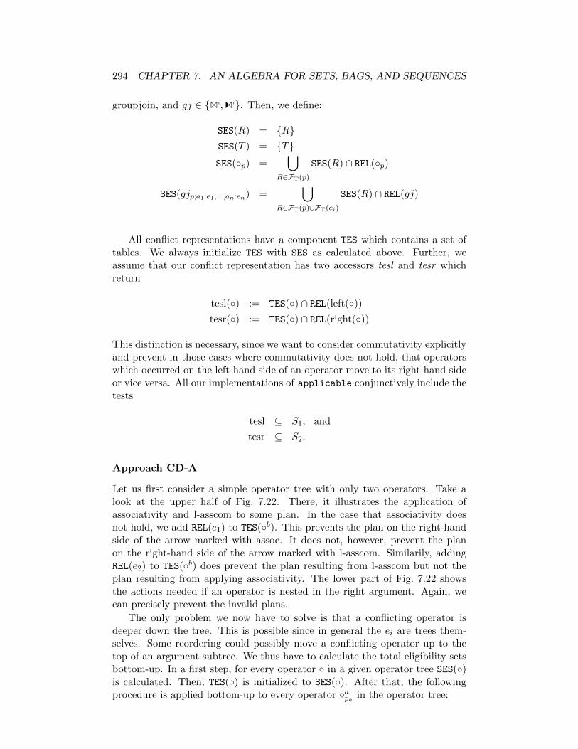
294 CHAPTER 7. AN ALGEBRA FOR SETS, BAGS, AND SEQUENCES

groupjoin, and gj ∈ Z,[. Then, we define:

SES(R) = RSES(T ) = TSES(p) =

⋃

R∈FT(p)

SES(R) ∩ REL(p)

SES(gjp;a1:e1,...,an:en) =⋃

R∈FT(p)∪FT(ei)

SES(R) ∩ REL(gj)

All conflict representations have a component TES which contains a set oftables. We always initialize TES with SES as calculated above. Further, weassume that our conflict representation has two accessors tesl and tesr whichreturn

tesl() := TES() ∩ REL(left())tesr() := TES() ∩ REL(right())

This distinction is necessary, since we want to consider commutativity explicitlyand prevent in those cases where commutativity does not hold, that operatorswhich occurred on the left-hand side of an operator move to its right-hand sideor vice versa. All our implementations of applicable conjunctively include thetests

tesl ⊆ S1, and

tesr ⊆ S2.

Approach CD-A

Let us first consider a simple operator tree with only two operators. Take alook at the upper half of Fig. 7.22. There, it illustrates the application ofassociativity and l-asscom to some plan. In the case that associativity doesnot hold, we add REL(e1) to TES(b). This prevents the plan on the right-handside of the arrow marked with assoc. It does not, however, prevent the planon the right-hand side of the arrow marked with l-asscom. Similarily, addingREL(e2) to TES(b) does prevent the plan resulting from l-asscom but not theplan resulting from applying associativity. The lower part of Fig. 7.22 showsthe actions needed if an operator is nested in the right argument. Again, wecan precisely prevent the invalid plans.

The only problem we now have to solve is that a conflicting operator isdeeper down the tree. This is possible since in general the ei are trees them-selves. Some reordering could possibly move a conflicting operator up to thetop of an argument subtree. We thus have to calculate the total eligibility setsbottom-up. In a first step, for every operator in a given operator tree SES()is calculated. Then, TES() is initialized to SES(). After that, the followingprocedure is applied bottom-up to every operator apa in the operator tree:

7.15. CORRECT AND COMPLETE EXPLORATIONOF THE CORE SEARCH SPACE295

b

a

e1 e2

e3

assoc−−→

a

e1 be2 e3

¬assoc(a, b)TES(b) ∪= REL(e1)

l-asscom−−→

a

be1 e3

e2

¬l-asscom(a, b)TES(b) ∪= REL(e2)

be3 a

e1 e2

assoc−−→

a

be3 e1

e2

¬assoc(b, a)TES(b) ∪= REL(e2)

r-asscom−−→

a

e1 be3 e2

¬r-asscom(a, b)TES(b) ∪= REL(e1)

Figure 7.22: Calculating TES for simple operator trees

CD-A(bpb) // operator b and its predicate pb

for ∀ a ∈ STO(left(b))if ¬assoc(a, b) then TES(b) ∪= REL(left(a))if ¬l-asscom(a, b) then TES(b) ∪= REL(right(a))

for ∀ a ∈ STO(right(b))if ¬assoc(b, a) then TES(b) ∪= REL(right(a))if ¬r-asscom(a, b) then TES(b) ∪= REL(left(a))

If we do not have degenerate predicates and cross products among the operatorsin the initial operator tree, we can safely use TES instead of REL.

The conflict representation comprises the TES for every operator. The defi-nition of applicable is

applicable(, S1, S2) := tesl() ⊆ S1 ∧ tesr() ⊆ S2.

Let us now see why applicable is correct. We have to show that it preventsthe generation of bad plans. Take the ¬ assoc case with nesting on the left.Let the original operator tree contain (e1 a12 e2) b23 e3. Define the set of tablesR2 := FT(b23) ∩ REL(left(b23)) and R3 := FT(b23) ∩ REL(right(b23)). ThenSES(b23) = R2 ∪R3. Further, since ¬assoc(a12, b23), we have

TES(b23) ⊇ SES(b23) ∪ REL(e1).

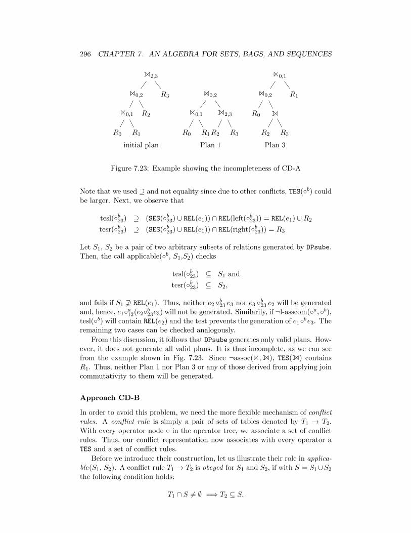
296 CHAPTER 7. AN ALGEBRA FOR SETS, BAGS, AND SEQUENCES

E2,3

B0,2

N0,1

R0 R1

R2

R3 B0,2

N0,1

R0 R1

E2,3

R2 R3

N0,1

B0,2

R0 E

R2 R3

R1

initial plan Plan 1 Plan 3

Figure 7.23: Example showing the incompleteness of CD-A

Note that we used ⊇ and not equality since due to other conflicts, TES(b) couldbe larger. Next, we observe that

tesl(b23) ⊇ (SES(b23) ∪ REL(e1)) ∩ REL(left(b23)) = REL(e1) ∪R2

tesr(b23) ⊇ (SES(b23) ∪ REL(e1)) ∩ REL(right(b23)) = R3

Let S1, S2 be a pair of two arbitrary subsets of relations generated by DPsube.Then, the call applicable(b, S1,S2) checks

tesl(b23) ⊆ S1 and

tesr(b23) ⊆ S2,

and fails if S1 6⊇ REL(e1). Thus, neither e2 b23 e3 nor e3 b23 e2 will be generatedand, hence, e1a12(e2b23e3) will not be generated. Similarily, if ¬l-asscom(a, b),tesl(b) will contain REL(e2) and the test prevents the generation of e1be3. Theremaining two cases can be checked analogously.

From this discussion, it follows that DPsube generates only valid plans. How-ever, it does not generate all valid plans. It is thus incomplete, as we can seefrom the example shown in Fig. 7.23. Since ¬assoc(N,E), TES(E) containsR1. Thus, neither Plan 1 nor Plan 3 or any of those derived from applying joincommutativity to them will be generated.

Approach CD-B

In order to avoid this problem, we need the more flexible mechanism of conflictrules. A conflict rule is simply a pair of sets of tables denoted by T1 → T2.With every operator node in the operator tree, we associate a set of conflictrules. Thus, our conflict representation now associates with every operator aTES and a set of conflict rules.

Before we introduce their construction, let us illustrate their role in applica-ble(S1, S2). A conflict rule T1 → T2 is obeyed for S1 and S2, if with S = S1∪S2

the following condition holds:

T1 ∩ S 6= ∅ =⇒ T2 ⊆ S.

7.15. CORRECT AND COMPLETE EXPLORATIONOF THE CORE SEARCH SPACE297

b

a

e1 e2

e3

assoc−−→

a

e1 be2 e3

¬assoc(a, b)CR(b) + = REL(e2)→ REL(e1)

l-asscom−−→

a

be1 e3

e2

¬l-asscom(a, b)CR(b) + = REL(e1)→ REL(e2)

be3 a

e1 e2

assoc−−→

a

be3 e1

e2

¬assoc(b, a)CR(b) + = REL(e1)→ REL(e2)

r-asscom−−→

a

e1 be3 e2

¬r-asscom(a, b)CR(b) + = REL(e2)→ REL(e1)

Figure 7.24: Calculating conflict rules for simple operator trees

Thus, if T1 contains a single relation from S, then S must contain all relationsin T2. Keeping this in mind, it is easy to see that the invalid plans are indeedprevented by the rules shown in Fig. 7.24 if they are obeyed.

As before, we just need to generalize it to arbitrary trees:

CD-B(bpb) // operator b and its predicate pb

for ∀ a ∈ STO(left(b))if ¬assoc(a, b) then CR(b) + = REL(right(a))→ REL(left(a))if ¬l-asscom(a, b) then CR(b) + = REL(left(a))→ REL(right(a))

for ∀ a ∈ STO(right(b))if ¬assoc(b, a) then CR(b) + = REL(left(a))→ REL(right(a))if ¬r-asscom(a, b) then CR(b) + = REL(right(a))→ REL(left(a))

The test applicable(, S1, S2) checks two conditions:

1. tesl ⊆ S1 ∧ tesr ⊆ S2 must hold, and

2. all rules in the rule set of must be obeyed.

Again, this implementation of applicable is correct but not complete, as theexample in Fig. 7.25 shows. Since assoc(B,N) and l-asscom(B,N), the onlyconflict occurs due to r-asscom(B,N). Thus,

REL(R3)→ REL(R1, R2) ∈ CR(B0,1)

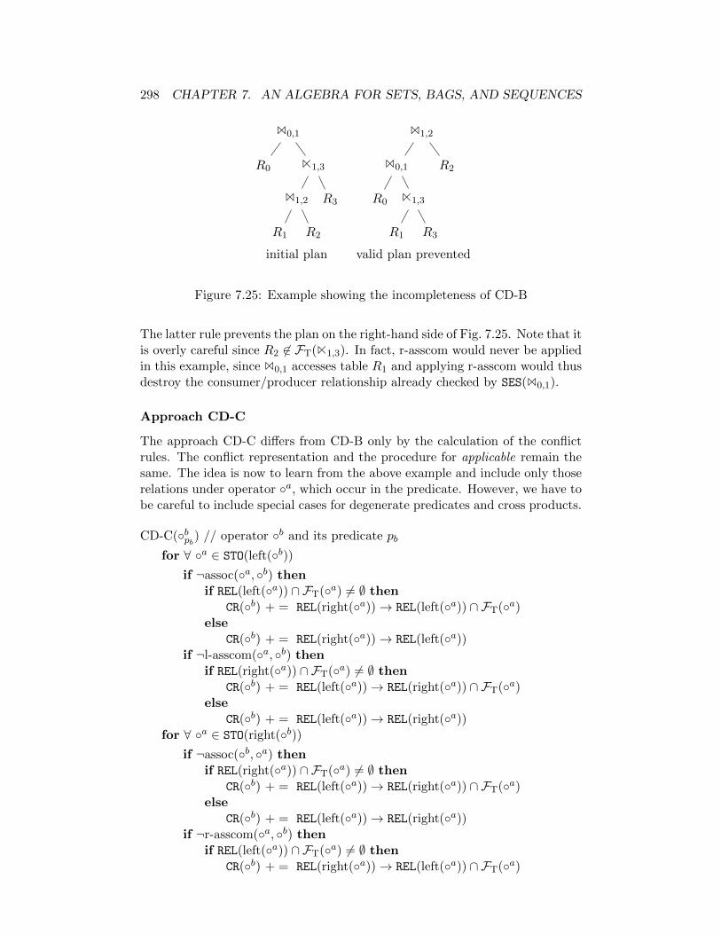
298 CHAPTER 7. AN ALGEBRA FOR SETS, BAGS, AND SEQUENCES

B0,1

R0 N1,3

B1,2

R1 R2

R3

B1,2

B0,1

R0 N1,3

R1 R3

R2

initial plan valid plan prevented

Figure 7.25: Example showing the incompleteness of CD-B

The latter rule prevents the plan on the right-hand side of Fig. 7.25. Note that itis overly careful since R2 6∈ FT(N1,3). In fact, r-asscom would never be appliedin this example, since B0,1 accesses table R1 and applying r-asscom would thusdestroy the consumer/producer relationship already checked by SES(B0,1).

Approach CD-C

The approach CD-C differs from CD-B only by the calculation of the conflictrules. The conflict representation and the procedure for applicable remain thesame. The idea is now to learn from the above example and include only thoserelations under operator a, which occur in the predicate. However, we have tobe careful to include special cases for degenerate predicates and cross products.

CD-C(bpb) // operator b and its predicate pb

for ∀ a ∈ STO(left(b))if ¬assoc(a, b) then

if REL(left(a)) ∩ FT(a) 6= ∅ thenCR(b) + = REL(right(a))→ REL(left(a)) ∩ FT(a)

elseCR(b) + = REL(right(a))→ REL(left(a))

if ¬l-asscom(a, b) thenif REL(right(a)) ∩ FT(a) 6= ∅ then

CR(b) + = REL(left(a))→ REL(right(a)) ∩ FT(a)else

CR(b) + = REL(left(a))→ REL(right(a))for ∀ a ∈ STO(right(b))

if ¬assoc(b, a) thenif REL(right(a)) ∩ FT(a) 6= ∅ then

CR(b) + = REL(left(a))→ REL(right(a)) ∩ FT(a)else

CR(b) + = REL(left(a))→ REL(right(a))if ¬r-asscom(a, b) then

if REL(left(a)) ∩ FT(a) 6= ∅ thenCR(b) + = REL(right(a))→ REL(left(a)) ∩ FT(a)

7.15. CORRECT AND COMPLETE EXPLORATIONOF THE CORE SEARCH SPACE299

elseCR(b) + = REL(right(a))→ REL(left(a))

Rule Simplification

Large TES make the search space to be explored by the plan generator smallerand, thus, lead to more efficiency, at least if an advanced plan generator likeDPhyp is used. Further, reducing the number of rules slightly decreases plangeneration time. Thus, applying laws like

R1 → R2, R1 → R3 ≡ R1 → R2 ∪R3

R1 → R2, R3 → R2 ≡ R1 ∪R3 → R2

can be used to rearrange the rule set for efficient evaluation. However, we aremuch more interested in eliminated rules altogether by adding their right-handside to the TES. For some operator , consider a conflict rule R1 → R2. IfR1∩TES() 6= ∅, then we can add R2 to TES due to the existential quantifier onthe left-hand side of a rule in the definition of obey. Further, if R2 ⊆ TES(), wecan safely eliminate the rule. Applying these rearrangements is often possiblesince both REL(left(a))∩FT() and REL(right(a))∩FT() will be non-empty.

7.15.3 More Issues

Unary Operators

Not all unary operators are freely reorderable (see Table 7.3). Fortunately,handling conflicts for unary operators is quite simple. We associate a newartificial relation with every unary operator (that needs one). For a given unaryoperator a, denote this relation by AREL(a). Then, whenever a conflict witha unary operator b above a occurs, we add AREL(a) to TES(b). The resultis that they will never be reordered. This is captured in the following codefragment:

CD-C

for each unary operator (b)for each unary operator a in STO(b)

if ¬reorderable(a, b)TES(b) + = AREL(a)

Mixing Unary and Binary Operators

A unary operator maybe left- or right-pushable into some binary operator (seeTable 7.4). In the given original operator tree, a unary operator may occurabove or below a binary operator. Accordingly, we extend CD-C by two morecases.

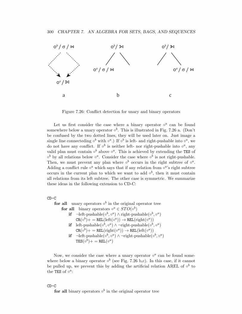
300 CHAPTER 7. AN ALGEBRA FOR SETS, BAGS, AND SEQUENCES

0b / σ /

0a /

a

0b/

0a / σ /

b

0a / σ /

c

0b/

Figure 7.26: Conflict detection for unary and binary operators

Let us first consider the case where a binary operator a can be foundsomewhere below a unary operator b. This is illustrated in Fig. 7.26 a. (Don’tbe confused by the two dotted lines, they will be used later on. Just image asingle line connecteding b with a.) If b is left- and right-pushable into a, wedo not have any conflict. If b is neither left- nor right-pushable into a, anyvalid plan must contain b above a. This is achieved by extending the TES ofb by all relations below a. Consider the case where b is not right-pushable.Then, we must prevent any plan where b occurs in the right subtree of a.Adding a conflict rule a which says that if any relation from a’s right subtreeoccurs in the current plan to which we want to add b, then it must containall relations from its left subtree. The other case is symmetric. We summarizethese ideas in the following extension to CD-C:

CD-C

for all unary operators b in the original operator treefor all binary operators a ∈ STO(b)

if ¬left-pushable(b, a) ∧ right-pushable(b, a)CR(b)+ = REL(left(a))→ REL(right(a))

if left-pushable(b, a) ∧ ¬right-pushable(b, a)CR(b)+ = REL(right(a))→ REL(left(a))

if ¬left-pushable(b, a) ∧ ¬right-pushable(b, a)TES(b)+ = REL(a)

Now, we consider the case where a unary operator a can be found some-where below a binary operator b (see Fig. 7.26 b,c). In this case, if it cannotbe pulled up, we prevent this by adding the artificial relation AREL of b tothe TES of a:

CD-C

for all binary operators b in the original operator tree

7.15. CORRECT AND COMPLETE EXPLORATIONOF THE CORE SEARCH SPACE301

for all unary operators a ∈ STO(left(b))if ¬left-pushable(a, b)

TES(b)+ = AREL(b)for all unary operators a ∈ STO(right(b))

if ¬right-pushable(a, b)TES(b)+ = AREL(b)

A selection operator can be changed into a join if its predicate references twoor more relations. In this case, a conflict between the resulting join and someother binary operator might occur. We can handle these potential conflicts asfollows. Consider Fig. 7.26 a. By b/σ/B we denote our selection that can beturned into a join. By a/E we denote a binary operator below our selection.The case that it might be a left outerjoin is used in a subsequent example.The Figure shows the trick we perform. We assume that a selection that canbe turned into a join has two arguments, a left and a right subtree. Both ofwhich point to the (only) child node of the selection. Thus, the left outerjoin isonce the left child of the selection/join and once the right one. Then, the usualCD-C procedure can be run in addition to the above conflict handling. Let usdo so for the example. In case we treat the left outerjoin as the left child of theouterjoin, we derive from ¬assoc(E,B)

CR(b)+ = REL(right(a))→ REL(left(a))

possibly with ∩FT(a) on the right-hand side. In the other case, we get due tothe fact that ¬r-asscom(B,E)

CR(b)+ = REL(right(a))→ REL(left(a)),

possibly with ∩FT(a) on the right-hand side. In any case, both conflicts resultin the same conflict rule. Further, both are subsumed by the above conflicthandling for the unary/binary operator mix. The reader should validate thatthis is the case for all the operators in our algebra. However, since we want tobe purely table driven, we simply add these (redundant) conflict rules and relyon rule simplification.

Cross Products and Degenerate Predicates

Cross products and degenerate predicates require more care as the comparisonbetween Fig. 7.19 and Fig. 7.20 shows. They lack the syntactic constraints dueto attribute accesses, which highly restrict the number of syntactically validplans. Consider an example like

(R1 AR2) B1,3 (R3 N3,4 R4).

So far, nothing prevents DPsube to consider invalid plans like

R1 B1,3 (R3 N3,4 (R2 AR4)).

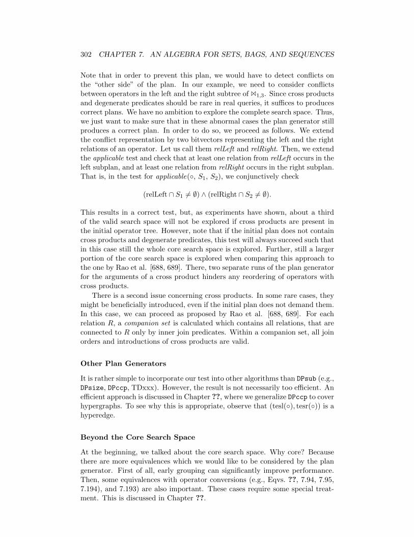
302 CHAPTER 7. AN ALGEBRA FOR SETS, BAGS, AND SEQUENCES

Note that in order to prevent this plan, we would have to detect conflicts onthe “other side” of the plan. In our example, we need to consider conflictsbetween operators in the left and the right subtree of B1,3. Since cross productsand degenerate predicates should be rare in real queries, it suffices to producescorrect plans. We have no ambition to explore the complete search space. Thus,we just want to make sure that in these abnormal cases the plan generator stillproduces a correct plan. In order to do so, we proceed as follows. We extendthe conflict representation by two bitvectors representing the left and the rightrelations of an operator. Let us call them relLeft and relRight. Then, we extendthe applicable test and check that at least one relation from relLeft occurs in theleft subplan, and at least one relation from relRight occurs in the right subplan.That is, in the test for applicable(, S1, S2), we conjunctively check

(relLeft ∩ S1 6= ∅) ∧ (relRight ∩ S2 6= ∅).

This results in a correct test, but, as experiments have shown, about a thirdof the valid search space will not be explored if cross products are present inthe initial operator tree. However, note that if the initial plan does not containcross products and degenerate predicates, this test will always succeed such thatin this case still the whole core search space is explored. Further, still a largerportion of the core search space is explored when comparing this approach tothe one by Rao et al. [688, 689]. There, two separate runs of the plan generatorfor the arguments of a cross product hinders any reordering of operators withcross products.

There is a second issue concerning cross products. In some rare cases, theymight be beneficially introduced, even if the initial plan does not demand them.In this case, we can proceed as proposed by Rao et al. [688, 689]. For eachrelation R, a companion set is calculated which contains all relations, that areconnected to R only by inner join predicates. Within a companion set, all joinorders and introductions of cross products are valid.

Other Plan Generators

It is rather simple to incorporate our test into other algorithms than DPsub (e.g.,DPsize, DPccp, TDxxx). However, the result is not necessarily too efficient. Anefficient approach is discussed in Chapter ??, where we generalize DPccp to coverhypergraphs. To see why this is appropriate, observe that (tesl(), tesr()) is ahyperedge.

Beyond the Core Search Space

At the beginning, we talked about the core search space. Why core? Becausethere are more equivalences which we would like to be considered by the plangenerator. First of all, early grouping can significantly improve performance.Then, some equivalences with operator conversions (e.g., Eqvs. ??, 7.94, 7.95,7.194), and 7.193) are also important. These cases require some special treat-ment. This is discussed in Chapter ??.

7.16. LOGICAL ALGEBRA FOR SEQUENCES 303

7.16 Logical Algebra for Sequences

7.16.1 Introduction

The algebra (NAL) we use here extends the SAL-Algebra [69] developed byBeeri and Tzaban. SAL is the order-preserving counterpart of the algebra usedin [181, 183] and in this book.

SAL and NAL work on sequences of sets of variable bindings, i.e., sequencesof unordered tuples where every attribute corresponds to a variable. We allownested tuples, i.e. the value of an attribute may be a sequence of tuples. Singletuples are constructed by using the standard [·] brackets. The concatenationof tuples and functions is denoted by . The set of attributes defined for anexpression e is defined as A(e). The set of free variables of an expression e isdefined as F(e).

The projection of a tuple on a set of attributes A is denoted by |A. For anexpression e1 possibly containing free variables, and a tuple e2, we denote bye1(e2) the result of evaluating e1 where bindings of free variables are taken fromvariable bindings provided by e2. Of course this requires F(e1) ⊆ A(e2). For aset of attributes A, we define the tuple constructor ⊥A such that it returns atuple with attributes in A initialized to NULL.

For sequences e we use α(e) to denote the first element of a sequence. Weidentify single element sequences and elements. The function τ retrieves thetail of a sequence, and ⊕ concatenates two sequences. We denote the emptysequence by ε. As a first application, we construct from a sequence of non-tuple values e a sequence of tuples denoted by e[a]. It is empty if e is empty.Otherwise, e[a] = [a : α(e)]⊕ τ(e)[a].

By id we denote the identity function. In order to avoid special cases duringthe translation of XQuery into the algebra, we use the special algebraic operator(2) that returns a singleton sequence consisting of the empty tuple, i.e., a tuplewith no attributes.

We will only define order-preserving algebraic operators. For the unorderedcounterparts see [183]. Typically, when translating a more complex XQuery intoour algebra, a mixture of order-preserving and not order-preserving operatorswill occur. In order to keep the section readable, we only employ the order-preserving operators and use the same notation for them that has been used in[181, 183], SAL [69], and this book.

Again, our algebra will allow nesting of algebraic expressions. For example,within a selection predicate of a select operator we allow the occurrence offurther nested algebraic expressions. Hence, a join within a selection predicate ispossible. This simplifies the translation procedure of nested XQuery expressionsinto the algebra. However, nested algebraic expressions force a nested loopevaluation strategy. Thus, the goal of the paper will be to remove nestedalgebraic expressions. As a result, we perform unnesting of nested queries notat the source level, but at the algebraic level. This approach is more versatileand less error-prone.

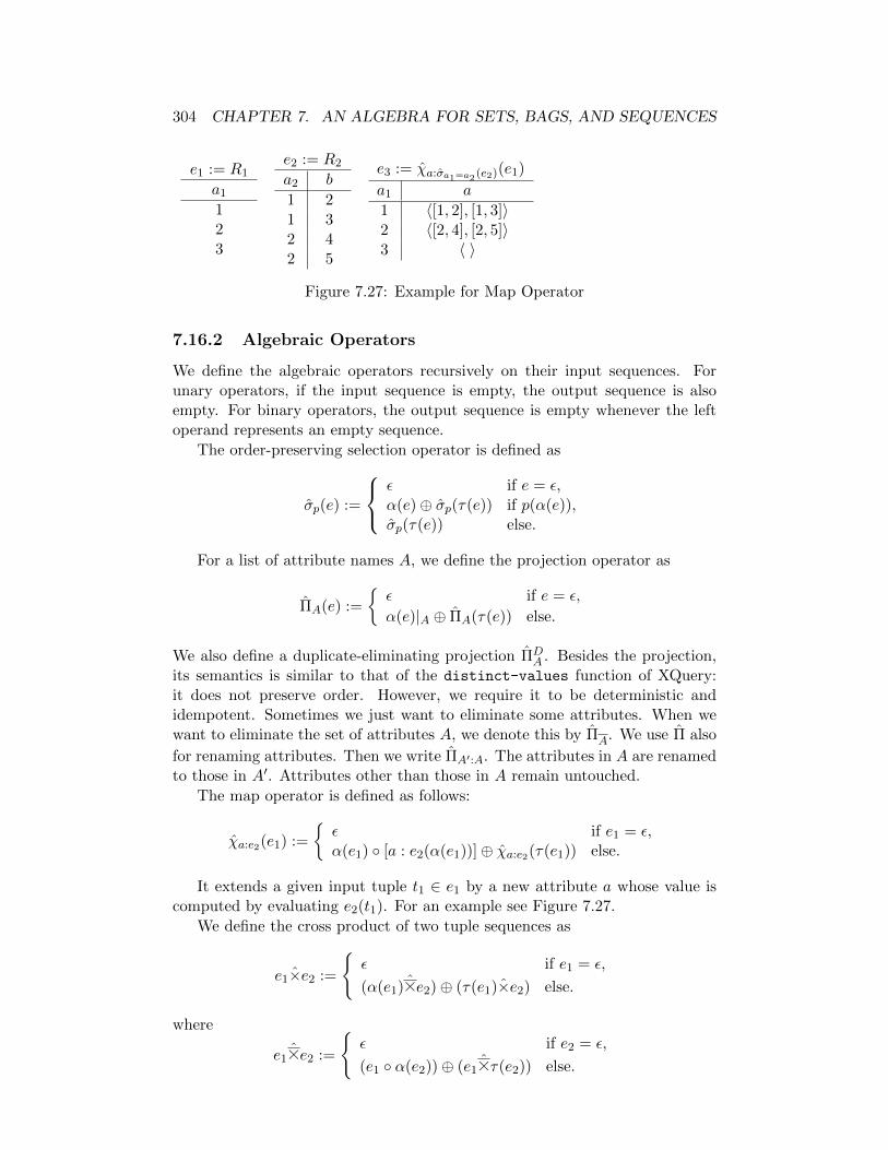
304 CHAPTER 7. AN ALGEBRA FOR SETS, BAGS, AND SEQUENCES

e1 := R1

a1

123

e2 := R2

a2 b

1 21 32 42 5

e3 := χa:σa1=a2 (e2)(e1)

a1 a

1 〈[1, 2], [1, 3]〉2 〈[2, 4], [2, 5]〉3 〈 〉

Figure 7.27: Example for Map Operator

7.16.2 Algebraic Operators

We define the algebraic operators recursively on their input sequences. Forunary operators, if the input sequence is empty, the output sequence is alsoempty. For binary operators, the output sequence is empty whenever the leftoperand represents an empty sequence.

The order-preserving selection operator is defined as

σp(e) :=

ε if e = ε,α(e)⊕ σp(τ(e)) if p(α(e)),σp(τ(e)) else.

For a list of attribute names A, we define the projection operator as

ΠA(e) :=

ε if e = ε,

α(e)|A ⊕ ΠA(τ(e)) else.

We also define a duplicate-eliminating projection ΠDA . Besides the projection,

its semantics is similar to that of the distinct-values function of XQuery:it does not preserve order. However, we require it to be deterministic andidempotent. Sometimes we just want to eliminate some attributes. When wewant to eliminate the set of attributes A, we denote this by ΠA. We use Π also

for renaming attributes. Then we write ΠA′:A. The attributes in A are renamedto those in A′. Attributes other than those in A remain untouched.

The map operator is defined as follows:

χa:e2(e1) :=

ε if e1 = ε,α(e1) [a : e2(α(e1))]⊕ χa:e2(τ(e1)) else.

It extends a given input tuple t1 ∈ e1 by a new attribute a whose value iscomputed by evaluating e2(t1). For an example see Figure 7.27.

We define the cross product of two tuple sequences as

e1×e2 :=

ε if e1 = ε,

(α(e1)Ae2)⊕ (τ(e1)×e2) else.

where

e1Ae2 :=

ε if e2 = ε,

(e1 α(e2))⊕ (e1Aτ(e2)) else.

7.16. LOGICAL ALGEBRA FOR SEQUENCES 305

We are now prepared to define the join operation on ordered sequences:

e1Bpe2 := σp(e1×e2).

We define the semijoin as

e1Npe2 :=

α(e1)⊕ (τ(e1)Npe2) if ∃x ∈ e2 p(α(e1) x),τ(e1)Npe2 else.

and the anti-join as

e1Tpe2 :=

α(e1)⊕ (τ(e1)Tpe2) if 6 ∃x ∈ e2 p(α(e1) x),(τ(e1)Tpe2) else.

The left outer join, which will play an essential role in unnesting, is definedas e1E

g:ep e2 :=

(α(e1)Bpe2)⊕ (τ(e1)Eg:e

p e2) if (α(e1)Bpe2) 6= ε,(α(e1) ⊥A(e2)\g [g : e]) else.

⊕(τ(e1)Eg:e

p e2)

where g ∈ A(e2). Our definition deviates slightly from the standard left outerjoin operator, as we want to use it in conjunction with grouping and (aggregate)functions. Consider the relations R1 and R2 in Figure 7.28. If we want to joinR1 (via a left outerjoin) with e3, which is grouped on a2, we need to be ableto handle empty groups (as for the tuple with a1 = 3 in e1 in the example). Inthe definition of the left outerjoin with default, the expression e then definesthe value given to the attribute g for all those elements in e1 that do not find

a join partner in e2. In our example, it would specify Eg=0

.We define the dependency join (d-join for short) as

e1<e2> :=

ε if e1 = ε

α(e1)Ae2(e1)⊕ τ(e1)<e2> else

Let θ ∈ =,≤,≥, <,>, 6= be a comparison operator on atomic values. Thegrouping operator which produces a sequence-valued new attribute containing“the group” is defined by using a groupjoin.

ΓθA;g:f (e) := ΠA:A′(ΠDA′:A(ΠA(e)) ZA′θA;g:fe)

where the groupjoin operator (sometimes called nest-join [802]) is defined as

e1 ZA1θA2;e:fe2 :=

ε if e1 = ε

α(e1) [g : G(α(e1))]⊕ (τ(e1) ZA1θA2;g:fe2)

Here, G(x) := f(σx|A1θA2

(e2)), and function f assigns a meaningful value toempty groups. See also Figure 7.28 for an example. The unary grouping oper-ator processes a single relation and obviously groups only on those values thatare present. The groupjoin works on two relations and uses the left-hand oneto determine the groups. This will become important for the correctness of theunnesting procedure.

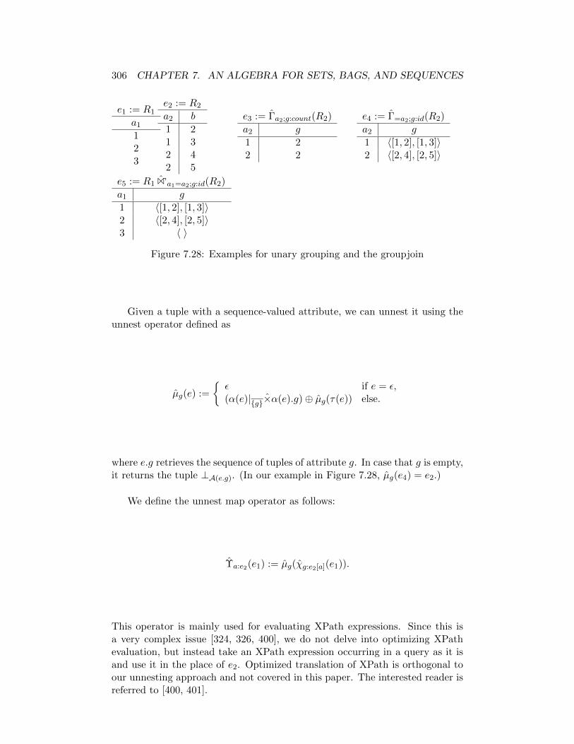
306 CHAPTER 7. AN ALGEBRA FOR SETS, BAGS, AND SEQUENCES

e1 := R1

a1

123

e2 := R2

a2 b

1 21 32 42 5

e3 := Γa2;g:count(R2)

a2 g

1 22 2

e4 := Γ=a2;g:id(R2)

a2 g

1 〈[1, 2], [1, 3]〉2 〈[2, 4], [2, 5]〉

e5 := R1 Za1=a2;g:id(R2)

a1 g

1 〈[1, 2], [1, 3]〉2 〈[2, 4], [2, 5]〉3 〈 〉

Figure 7.28: Examples for unary grouping and the groupjoin

Given a tuple with a sequence-valued attribute, we can unnest it using theunnest operator defined as

µg(e) :=

ε if e = ε,(α(e)|g×α(e).g)⊕ µg(τ(e)) else.

where e.g retrieves the sequence of tuples of attribute g. In case that g is empty,it returns the tuple ⊥A(e.g). (In our example in Figure 7.28, µg(e4) = e2.)

We define the unnest map operator as follows:

Υa:e2(e1) := µg(χg:e2[a](e1)).

This operator is mainly used for evaluating XPath expressions. Since this isa very complex issue [324, 326, 400], we do not delve into optimizing XPathevaluation, but instead take an XPath expression occurring in a query as it isand use it in the place of e2. Optimized translation of XPath is orthogonal toour unnesting approach and not covered in this paper. The interested reader isreferred to [400, 401].

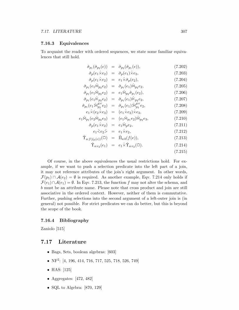
7.17. LITERATURE 307

7.16.3 Equivalences

To acquaint the reader with ordered sequences, we state some familiar equiva-lences that still hold.

σp1(σp2(e)) = σp2(σp1(e)), (7.202)

σp(e1×e2) = σp(e1)×e2, (7.203)

σp(e1×e2) = e1×σp(e2), (7.204)

σp1(e1Bp2e2) = σp1(e1)Bp2e2, (7.205)

σp1(e1Bp2e2) = e1Bp2 σp1(e2), (7.206)

σp1(e1Np2e2) = σp1(e1)Np2e2, (7.207)

σp1(e1Eg:ep2 e2) = σp1(e1)E

g:ep2 e2, (7.208)

e1×(e2×e3) = (e1×e2)×e3, (7.209)

e1Bp1(e2Bp2e3) = (e1Bp1e2)Bp2e3, (7.210)

σp(e1×e2) = e1Bpe2, (7.211)

e1<e2> = e1×e2, (7.212)

Υa:f(χb(e))(2) = Πa:b(f(e)), (7.213)

Υa:e2(e1) = e1×Υa:e2(2). (7.214)

(7.215)

Of course, in the above equivalences the usual restrictions hold. For ex-ample, if we want to push a selection predicate into the left part of a join,it may not reference attributes of the join’s right argument. In other words,F(p1) ∩ A(e2) = ∅ is required. As another example, Eqv. 7.214 only holds ifF(e1)∩A(e1) = ∅. In Eqv. 7.213, the function f may not alter the schema, andb must be an attribute name. Please note that cross product and join are stillassociative in the ordered context. However, neither of them is commutative.Further, pushing selections into the second argument of a left-outer join is (ingeneral) not possible. For strict predicates we can do better, but this is beyondthe scope of the book.

7.16.4 Bibliography

Zaniolo [515]

7.17 Literature

• Bags, Sets, boolean algebras: [603]

• NF2: [4, 196, 414, 716, 717, 525, 718, 526, 749]

• HAS: [125]

• Aggregates: [472, 482]

• SQL to Algebra: [870, 129]

308 CHAPTER 7. AN ALGEBRA FOR SETS, BAGS, AND SEQUENCES

• Calculus to Algebra: [870, 614] Nakano: without duplicates

• BAGs: [21], [212]

• OO Algebra of Steenhagen et al. [802, 803, 801, 804]

• OO Algebra of Cluet and Moerkotte [181, 183].

• OO Algebra [165]

• OO Algebra [180]

• OO Algebra [366]

• OO Algebra [540]

• OO Algebra [731]

• OO Algebra [774, 773, 772, 775]

• OO Algebra [866, 867]

• OO Algebra [930]

• SAL [69]: works on lists. Intended for semistructured data. SAL can bethought of as the order-preserving counterpart of the algebra presentedin [181, 183] extended to handle semistructured data. These extensionsare similar to those proposed in [5, 173]

• TAX [444]: The underlying algebra’s data model is based on sets of or-dered labeled trees. Intended for XML.

• XML: Construction: [271, 272]

• no-name [791]: order preserving algebra for OLAP-style queries

• [355]

• Document Processing Algebras: [174, 370]

• Geo: [371]

• Mumick, Pirahesh, and Ramakrishnan introduce a variant of Datalog withbag semantics [610]. Further, they show that the magic set transformationretains the correct number of duplicates.

7.18 ToDo

Grouping Mapping and Commutativity Comment on ΠA(R1∩R2) 6≡ ΠA(R1)∩ToDoToDo ΠA(R2) ΠA(R1 \R2) 6≡ ΠA(R1) \ΠA(R2)

[689]pregrouping Tsois, Sellis: [849]bulktypes: Albert: [21]bulktypes: Dayal: [212]

Chapter 8

Declarative QueryRepresentation

8.1 Calculus Representations

relational calculus originally introduced by Codd: [190, 189].Variant for embedding in Pascal/R: [747]calculus for complex objects: [48]

8.2 Datalog

8.3 Tableaux Representation

Tableaus have been introduced by [17, 18, 19] Tableaus are able to represent aparticuar kind of queries, the so called conjunctive queries ([138], [703]).

Expressions containing disjunction (set union) and negation (set difference)can be represented by sets of tableaus ([729],[453]).

query processing with tables: [633]

8.4 Monoid Comprehension

[114, 268, 269]

8.5 Expressiveness

transitivity: [663]. aggregates: [482]. complex object and nested relations: [3].

8.6 Bibliography

309

310 CHAPTER 8. DECLARATIVE QUERY REPRESENTATION

Chapter 9

Translation and Lifting

9.1 Query Language to Calculus

9.2 Query Language to Algebra

9.3 Calculus to Algebra

9.4 Algebra to Calculus

9.5 Bibliography

311

312 CHAPTER 9. TRANSLATION AND LIFTING

Chapter 10

Query Equivalence,Containment, Minimization,and Factorization

This chapter is devoted to three related problems. Let q be a query and d be adatabase. We denote by q(d) the result of evaluating the query on the database.Two queries q1 and q2 are by definition equivalent (q1 ≡ q2), if q1(d) = q2(d) forall databases d. The problem of deciding whether two queries are equivalentis the query equivalence problem. We define q1 ⊆ q2 if q1(d) ⊆ q2(d) for alldatabases d. The problem of deciding whether for two q1 ⊆ q2 holds is thequery containment problem. Obviously, q1 ≡ q2 ≺ q1 ⊆ q2 ∧ q2 ⊆ q1.

The third problem is query minimization. Consider the following conjunc-tive query written as a rule in datalog:

q(X,Y ) : −p(X,Y ), p(X,Y ).

Obviously, this query is equivalent to

q(X,Y ) : −p(X,Y ).

under set semantics. The latter query now contains fewer body literals. Queryminimization now asks for an equivalent query with the least possible numberof body literals. One possible approach is to successively delete a body literaluntil no more body literal can be deleted without violating equivalence to theoriginal query.

The above example is also illustrative since it shows that query equiva-lence (and thus query containment) differs under different semantics: whereasthe above two queries are equivalent under set semantics, they are not underbag semantics. To see this, consider the extensional database p(a, b), p(a, b).The result of the first query contains p(a, b) four times whereas the last querycontains is only 2 times.

313

314CHAPTER 10. QUERY EQUIVALENCE, CONTAINMENT, MINIMIZATION, AND FACTORIZATION

10.1 Set Semantics

10.1.1 Conjunctive Queries

A conjunctive query may contain literals where the predicate is built-in. Forexample, it applies comparison operators =, <,>,≤,≥, 6=. Any explicit useof equality can be eliminated as follows. For any literal of the form X = c,any occurrence of X is replaced by c and the equality literal is dropped fromthe query clause. For any literal of the form X = Y , any occurrence of Yis replaced by X and the equality literal is dropped from the query clause.This procedure is not possible for the other comparison operators <,>,≤,≥, 6=which we call inequality opertors. An inequality is any literal literal using aninequality operator.

Containment and minimization for conjunctive queries without inequalitiesare NP-complete Problems. First note that a tableaux directly correspondsto a conjunctive queries with all body literals having a common predicate.From that and the NP-completeness results for tableaux containment whichin turn follows immediately from first order subsumption [64, 308], it followsimmediately that containment of conjunctive queries is NP-complete. Chandraand Merlin proved that minimization is NP-complete [138]. The complexity ofchecking for equivalence of conjunctive queries is related to graph isomorphism.

EXThe procedure for checking query containment builds upon mappings from

queries to queries1. These mappings have two different names: homomorphismand containment mapping .

Let q1 and q2 be the two queries for which we want to check containment.Assume the qi are of the form

q1 : r1 : − l1, . . . , lkq2 : r2 : − l′1, . . . , l

′m

Let V(qi) be the set of variables occurring in qi, and C(qi) be the set of constantsoccurring in qi. Further, let h be a substitution h : V(q2) → (V(q1) ∪ C(q1)).We call h a containment mapping from q2 to q1, if and only if the followingconditions are fulfilled:

1. h(r2) = r1 for the head literals, and

2. for all i (1 ≤ i ≤ m) there exists a j (1 ≤ j ≤ k) such that h(l′i) = lj .

The latter condition states that for each body literal l′i in q2 there is a bodyliteral lj in q1 such that h(li) = l′i. Note that this does not imply that h isinjective or surjective.

The following theorem connects containment mappings with the contain-ment problem:

Theorem 10.1.1 Let q1 and q2 be two conjunctive queries. Then q1 ⊆ q2 ifand only if there is a containment mapping h mapping q2 to q1.

1In fact, Chandra and Merlin mapped natural models which is essentially the same.

10.1. SET SEMANTICS 315

Consider the following example:

q1 : p(X1, X2) : − q(X2, X1), q(X1, X3)q2 : p(Y1, Y2) : − q(Y2, Y1), q(Y3, Y1), q(Y1, Y4)

Consider h with h(Y1) = X1, h(Y2) = X2, h(Y3) = X2, and h(Y4) = X3. Then

l : p(Y1, Y2) q(Y2, Y1) q(Y3, Y1) q(Y1, Y4)h(l) : p(X1, X2) q(X2, X1) q(X2, X1) q(X1, X3)

and, hence, q1 ⊆ q2.A query q is minimal, if it contains the minimal possible number of body

literals. More formally, q is minimal , if for any query q′ with q ≡ q′ the numberof body literals in q′ greater than or equal to the number of body literals inq. The following theorem shows that our initial thoughts on minimization arecorrect for conjunctive queries.

Theorem 10.1.2 Let q be a conjunctive query. Then there is a minimal queryq′ equivalent to q such that q′ results from q by deleting zero or more bodyliterals.

This suggests a simple procedure for minimizing a given query q. For everybody literal check whether some containment mapping h exists such that it issubsumed by some other body literal. Note that this containment mappingmust not rename head variables.

Let q and q′ be two conjunctive queries. If q can be derived from q′ solelyby reordering body literals and renaming variables, then q and q′ are calledisomorphic. Minimal queries are unique up to some isomorphism. Obviously,minimizing conjunctive queries is also NP-complete.

Let us now come to unions of conjunctive queries. Let Q = Q1 ∪ . . . ∪ Qkand Q′ = Q′1 ∪ . . . ∪Q′l be two unions of conjunctive queries Qi and Q′j with acommon head predicate. A containment mapping h from Q to Q′ maps each Qito some Q′j such that h(Qi) ⊆ Q′j . Sagiv and Yannakakis showed the followingtheorem [729].

Theorem 10.1.3 Let Q = Q1 ∪ . . .∪Qk and Q′ = Q′1 ∪ . . .∪Q′l be two unionsof conjunctive queries Qi and Q′j with a common head predicate. Then Q ⊆ Q′if and only if there is a containment mapping from Q to Q′.

This theorem gives us a corollary which allows us minimizing unions ofconjunctive queries by a pairwise checking of containment [729] (see also [854]).

Corollary 10.1.4 Let Q = Q1 ∪ . . .∪Qk be a union of conjunctive queries Qiwith common head predicate. Then there exists a subset R of Q such that

1. R ≡ Q

2. ¬∃ R′ ⊂ R R′ ≡ Q

3. If Qm is any equivalent to Q, then there is a containment mapping fromQm to R but none from Qm to any proper subset R′ of R.

316CHAPTER 10. QUERY EQUIVALENCE, CONTAINMENT, MINIMIZATION, AND FACTORIZATION

This corollary implies that we can minimize a query that is a union of con-junctive queries by eliminating those conjunctive queries Qi from it that arecontained in some Qj .

For conjunctive queries the problems of containment, equivalence, and min-imization are

The problems of containment, equivalence, and minimization of conjunctivequeries are most difficitult if all body literals have a common predicate p. Thisis quite an unrealistic assumption as typical conjunctive queries will not onlyself-join the same relation. A first question is thus whether there exist specialcases where there are polynomial algorithms for containment checking. Anotherstrain of work is devoted to more complex queries. As it turns out, the resultsbecome less nice and more restricted.

10.1.2 . . . with Inequalities

We now turn to conjunctive queries with inequalities in their body. For thissection, we assume that the domain is totally ordered and dense. That is, forall x and y with x < y, there exists a z with x < z < y. In this context, wehave the following theorem:

Theorem 10.1.5 Assume the two conjunctive queries q1 and q2 are of the form

q1 : p1 : − l1, . . . , lk, e1, . . . , elq2 : p2 : − l′1, . . . , l

′m, e

′1, . . . , e

′n

where pi are the head literals, li and l′i are ordinary subgoals and ei and e′iare inequalities. Let h be a containment mapping from q2 to q1 where both arerestricted to their ordinary literals. If additionally for all i = 1, . . . , n we have

e1, . . . , el =⇒ h(e′i)

then q1 ⊆ q2.

This result is due to Klug [483] who used the following procedure to reasonabout inequalities using comparison operators in =, <,≤. Given a set ofinequalities L, an directed graph G is defined whose nodes are the variablesand constants in L. Whenever for all x < y or x ≤ y in L, the edge (x, y) isadded to G. For all constants c and c′ in L, if c < c′ then we add an edge(c, c′). Edges are labeled with the according comparison operator. For equalitypredicates, an edge in both direction is added. Given the graph G, we concludethat x ≤ y if there is a path from x to y and x < y only if additionally at leastone edge is labelled by <. An alternative is to use the procedure presented inSection 11.2.3 to solve the inequality inference problem. It also allows for thecomparison operator 6=.

To see why a dense domain is important consider the domain of integers.From 1 < x < 3 we can easily conclude that x = 2, a fact we can deriveneither from the procedure above nor from the axioms and inference procedurepresented in Section 11.2.3.

10.2. BAG SEMANTICS 317

Unfortunately, the other direction of Theorem ?? is wrong as the followingexample shows:

q1 : p(X1, X2) : − q(X1, X2), r(X3, X4), r(X4, X3)q2 : p(Y1, Y2) : − q(Y1, Y2), r(Y3, Y4), Y3 ≤ Y4

Obviously, Y3 ≤ Y4 cannot be implied by any non-existing inequalities from q1.However, for q1 to be non-empty, we must have r(a, b) and r(b, a) for some aand b. We also have a ≤ b or b ≤ a. In the former case, we can chose Y3 = aand Y4 = b and in the latter Y3 = b and Y4 = a to satisfy r(Y3, Y4) and Y3 ≤ Y4.

Klug provides an alternative method to solve the containment problem. Itbuilds upon canonical models. He then shows that if the containment testsucceeds for all canonical models then and only then query containment holds[483]. Klug does not give an explicit algorithm for constructing these canonicalmodels but these can be found in the literature []. He also gives two simplesubclasses of inequality queries, where constants are allowed only on the left-or only on the right-hand side. For these subclasses if and only if holds in theabove Theorem ??.

Although the theorem is stated in terms of conjunctive queries with in-equalities, it holds for any predicate p. Assume two queries of the followingform:

q1 : p1 : − l1, . . . , lk, Pq2 : p2 : − l′1, . . . , l

′m, P

′

where P and P ′ are arbitrary formulas. If there is a containment mapping fromq2 to q1 where both are restricted to their ordinary literals and P =⇒ h(P ′),then q1 ⊆ q2.

10.1.3 . . . with Negation

The first incarnation of negation we consider is set difference. Here, Sagiv andYannakakis where the first to derive some results [729].

[193]

10.1.4 . . . under Constraints

constraints: [451, 452, 422]negation+constraints: [260, 261, 262, 263]

10.1.5 . . . with Aggregation

[194, 195]

10.2 Bag Semantics

10.2.1 Conjunctive Queries

• definition bag-containment, bag-equivalence [212, 477]

– characterizations [153, 432] (no proofs in [154])

318CHAPTER 10. QUERY EQUIVALENCE, CONTAINMENT, MINIMIZATION, AND FACTORIZATION

– complexity results [153]

• definition bag-set containment, bag-set equivalence [153]

10.3 Sequences

10.3.1 Path Expressions

XPath constructs and their short-hands to denote XPath sublanguages.

• branching (’[]’)

• wild cards (’*’)

• descendant axis (’//’)

• disjunction : only binary or branching, (’—’) (or-branching)

Otherwise XPath only contains the child axis and node name tests. Thesesublanguages are represented as tree patterns.

Query containment for certain subclasses:

• XP[],∗,// is coNP-complete [583]

Consider we have to answer p ⊆ p′. Then

– if p ∈ P [],// and p ∈ P [],∗,// then query containment is coNP-complete.

– in PTIME if number of ’//’ is restricted by d which then gives thedegree of the polynomial describing the time complexity

– remains coNP-complete if p contains no ’*’ p′ contains at most two’*’s

– remains coNP-complete if p contains at most 5 branches and p′ con-tains at most 3 branches.

• P[],∗ is in PTIME (follows from work on conjunctive acyclic queries [918],also noted by Wood [901])

• P[],// is in PTIME [28]

• P∗,// is in PTIME (these are related to a fragment of regular expressions[584])

• Por is in PTIME

• P[],or is coNP-complete

• P| is coNP-complete [583][618] showed that P[],∗,//,| is coNP-complete for infinite alphabets and inPSPACE for finite alphabets.

10.4. MINIMIZATION 319

• P//,| is PSPACE-complete

• P[],∗,// with variable binding and equivality tests is Πp2- hard [226]

A PTIME algorithm for the fragment P// can be found in [113]

Florescu, Levy, and Suciu showed that for a language quite similar to P[],//

containment is NP-complete if evaluated on a graph-based data model insteadof a tree-based one [280].

Calvanese et al. also consider a graph-based data model and more expressivequeries [117].

[618] also contains work on languages with variable bindings with differentsemantics.

More result: [226]

query containment with DTDs: [902]

Schwentick gives a very good overview over complexity results for contain-ment checking [750]. We should repeat his table here.

10.4 Minimization

minimization: [501]

10.5 Detecting common subexpressions

[273, 379, 377]

10.5.1 Simple Expressions

Simple Non-Expensive Expressions

Simple Expensive Expressions

10.5.2 Algebraic Expressions

10.6 Bibliography

In a pair of papers Aho, Sagiv, and Ullmann [15, 16] study equivalence, con-tainment, and minimization problems for tableaux. More specifically, theyintroduce a restricted variant of relational expressions containing projection,natural join, and selection with predicates that only compare attributes withconstants. They further assume the existence of a universal relation. Thatis, every relation R is the projection of the universal relation on A(R). Now,these restricted conjunctive queries can be expressed with tableaux. The au-thors tableaux equivalence, containment, and minimization problems also inthe presence of functional dependences. The investigated problems are all NP-complete. Since the practical usefulness is limited we do not give the concreteresults of this pair of papers.

[152, 155] contains (complexity) results for deciding query equivalence inthe case of recursive and nonrecursive datalog.

320CHAPTER 10. QUERY EQUIVALENCE, CONTAINMENT, MINIMIZATION, AND FACTORIZATION

View selection problem (just pointers): . . .[449, 446, 447][159]

• conjunctive queries: equivalence and minimization are NP-complete [138,16]In [16] tableaux are used.

• polynomial algorithms for equivalence and minimization for simple tableaux:[16, 15]

• union of elementary differences: Πp2 complete: remark in [729] and a

pointer to the thesis of Sagiv [726].

• acyclic conjunctive queries: PTIME [918]

• equivalence (σ, B, π, ∪), equivalence (σ, B, π, ∪, \): ΠP2 -complete [729]

• Recursive Datalog: [95]

Part III

Rewrite Techniques

321

Chapter 11

Simple Rewrites

11.1 Simple Adjustments

11.1.1 Rewriting Simple Expressions

Constant Folding

Constant subexpressions are evaluated and the result replaces the subexpres-sion. For example an expression 1/100 is replaced by 0.01. Other expressionslike a− 10 = 50 can be rewritten to a = 40. However, the latter kind of rewriteis rarely performed by commercial systems.

Eliminate Between

A predicate of the form Y BETWEEN X AND Z is replaced by X <= Y AND Y <=Z. This step not only eliminates syntactic sugar but also enables transitivityreasoning to derive new predicates (see ).

Eliminate IN

A predicate of the form x IN (c1,...,cn) is rewritten to x = c1 OR ...OR x

= cn. This eliminates on form of the IN predicate and enables multikey indexaccess.

Another possibility is to use a table function that produces a table with onecolumn whose values are exactly those in the IN-list. From thereon, regularoptimization takes place. This possibility is also investigated when severalcomparisons of a column with a constants are disjunctively connected.

Eliminating LIKE

A predicate of the form a LIKE ’Guy’ can only be rewritten to a = ’Guy’ ifa is of type varchar. This is due to the different white space padding rules forLIKE and =.

323

324 CHAPTER 11. SIMPLE REWRITES

Start and Stop conditions derived from LIKE predicates

A predicate of the form a LIKE ‘bla%‘ gives rise to a start condition a >=‘bla‘. Which can enable subsequent index usage. A stop predicate of the forma < ’blb’ can also be derived. completing a range predicate for an index scan.Start and stop conditions can only be derived if there is no leading ‘%‘ in thepattern.

Pushing NOT operations down and eliminating them

NOT operations need to be pushed downwards for correctness reasons. At-tention has to be paid to the IS NOT NULL and IS NULL predicates. XXXcomplete set of rules go into some table.

Merge AND, OR, and other associative operations

While parsing, AND and OR operations are binary. For simpler processing theyare often n-ary in the internal representation. Therefor (p AND (q AND r)) isrewritten to (AND p q r).

In general, associative nested operations should be merged. Examples ofother associative operations are + and ∗.

Normalized Argument Order for Commutative Operations

enabling factorization, constant folding: move constants to the left Speed upToDoevaluation of equal.

Eliminate - and /

(x− y) ; x+ (−y) x/y ; x ∗ (1/y)

Adjust join predicates

A = B +C becomes A−C = B if AandB are from one relation and C is fromanother.

Simplifying boolean expressions

The usual simplification rules for boolean expressions can be applied. For ex-ample, if a contradiction can be derived.

Eliminating ANY, SOME, and ALL

ANY and SOME operators in conjunction with a comparison operator arerewritten into disjunction of comparison predicates. For example a > ANY

(c1, c2) is rewritten to a > c1 OR a > c2. Correspondingly, an ALL oper-ator with a constant list is rewritten into a conjunction of comparisons. Forexample, a > ALL(c1, c2) is rewritten to a > c1 AND a > c2.

If a subquery occurs, then the ANY or SOME expression is rewritten toa correlated subquery in an EXIST predicate. Consider the query a > ANY

11.2. DERIVING NEW PREDICATES 325

(SELECT b FROM ...WHERE p). It is rewritten to EXISTS(SELECT ...FROM

...WHERE p AND a > b).Correspondingly, a subquery within an ALL operator is rewritten into a

NOT EXISTS subquery. For example, a > (SELECT b FROM ...WHERE p) isrewritten into NOT EXISTS (SELECT b FROM ...WHERE p and a <= b)

• CASE ¡==¿ UNION

11.1.2 Normal forms for queries with disjunction

Another step of the NFST component or the first step of the rewriting compo-nent can be the transformation of boolean expressions found in where clausesin order to account for NULL values. Pushing not operators inside the booleanexpression allows to use two-valued logic instead of three-valued logic. If wemiss this step, we can get wrong results.

Another possible step is the subsequent transformation of the boolean ex-pressions in where clauses into disjunctive normal form (DNF) or conjunctivenormal form (CNF). This step is not always necessary and really depends onwhich plan generation approach is taken. Hence, this step could take place aslate as in a preparatory step for plan generation. It is (obviously) only neces-sary if the query contains disjunctions. We discuss plan generation for querieswith disjunctions in Section ??.

11.2 Deriving new predicates

Given a set of conjunctive predicates, it is often possible to derive new predicateswhich might be helpful during query plan generation.

This section discusses ways to infer new predicates.

11.2.1 Collecting conjunctive predicates

A query predicate may not only contain the and connector, but also or or not.For the inference rules in this section we need base predicates that occur

conjunctively.We say that a (base) predicate q occurs conjunctively in a (complex) pred-

icate p if p [q ← false] can be simplified to false. That is, if we replace everyoccurrence of q by true, the simplification rules in Figure 11.1 (Fig. ??) simplifyp [q ← true] to false.

These simplification rules can be used to implement a simple member func-tion occursConjunctively to determine whether a predicate occurs conjunctivelyin a predicate or not. Together with a member function or visitor Collect-BasePredicates, we can compute the set of conjunctively occurring predicates.This set will form the basis for the next subsections.

11.2.2 Equality

Equality is a reflexive, symmetric and transitive binary relationship (see Fig. 11.2).Such a relation is called an equivalence relation Hence, a set of conjunctively

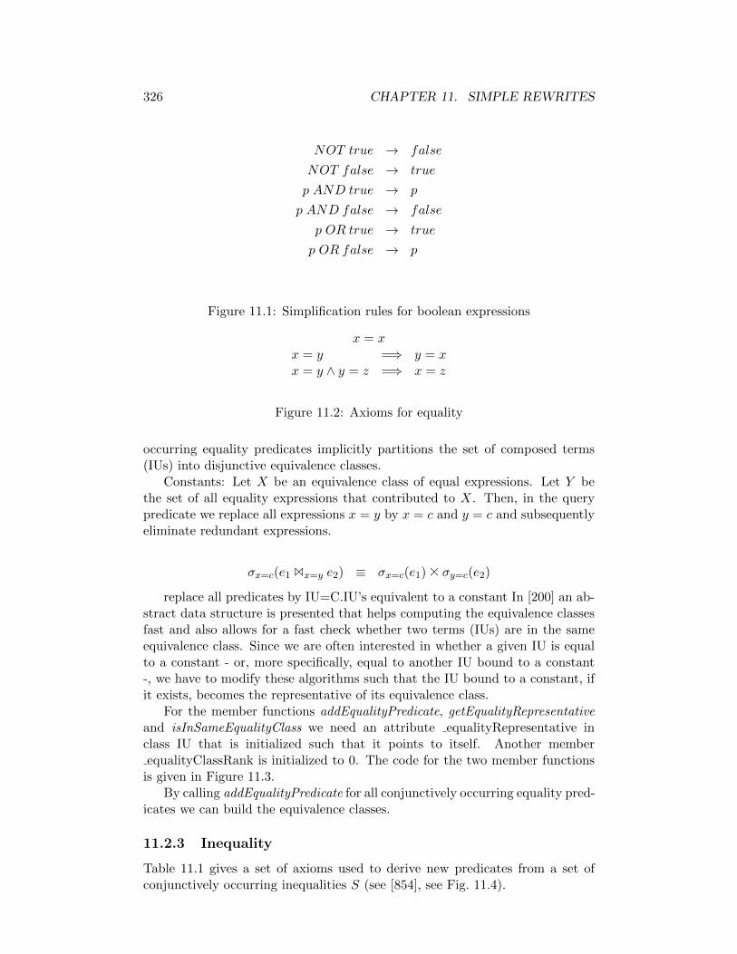
326 CHAPTER 11. SIMPLE REWRITES

NOT true → false

NOT false → true

p AND true → p

p AND false → false

p OR true → true

p OR false → p

Figure 11.1: Simplification rules for boolean expressions

x = xx = y =⇒ y = xx = y ∧ y = z =⇒ x = z

Figure 11.2: Axioms for equality

occurring equality predicates implicitly partitions the set of composed terms(IUs) into disjunctive equivalence classes.

Constants: Let X be an equivalence class of equal expressions. Let Y bethe set of all equality expressions that contributed to X. Then, in the querypredicate we replace all expressions x = y by x = c and y = c and subsequentlyeliminate redundant expressions.

σx=c(e1 Bx=y e2) ≡ σx=c(e1) A σy=c(e2)

replace all predicates by IU=C.IU’s equivalent to a constant In [200] an ab-stract data structure is presented that helps computing the equivalence classesfast and also allows for a fast check whether two terms (IUs) are in the sameequivalence class. Since we are often interested in whether a given IU is equalto a constant - or, more specifically, equal to another IU bound to a constant-, we have to modify these algorithms such that the IU bound to a constant, ifit exists, becomes the representative of its equivalence class.

For the member functions addEqualityPredicate, getEqualityRepresentativeand isInSameEqualityClass we need an attribute equalityRepresentative inclass IU that is initialized such that it points to itself. Another memberequalityClassRank is initialized to 0. The code for the two member functions

is given in Figure 11.3.By calling addEqualityPredicate for all conjunctively occurring equality pred-

icates we can build the equivalence classes.

11.2.3 Inequality

Table 11.1 gives a set of axioms used to derive new predicates from a set ofconjunctively occurring inequalities S (see [854], see Fig. 11.4).

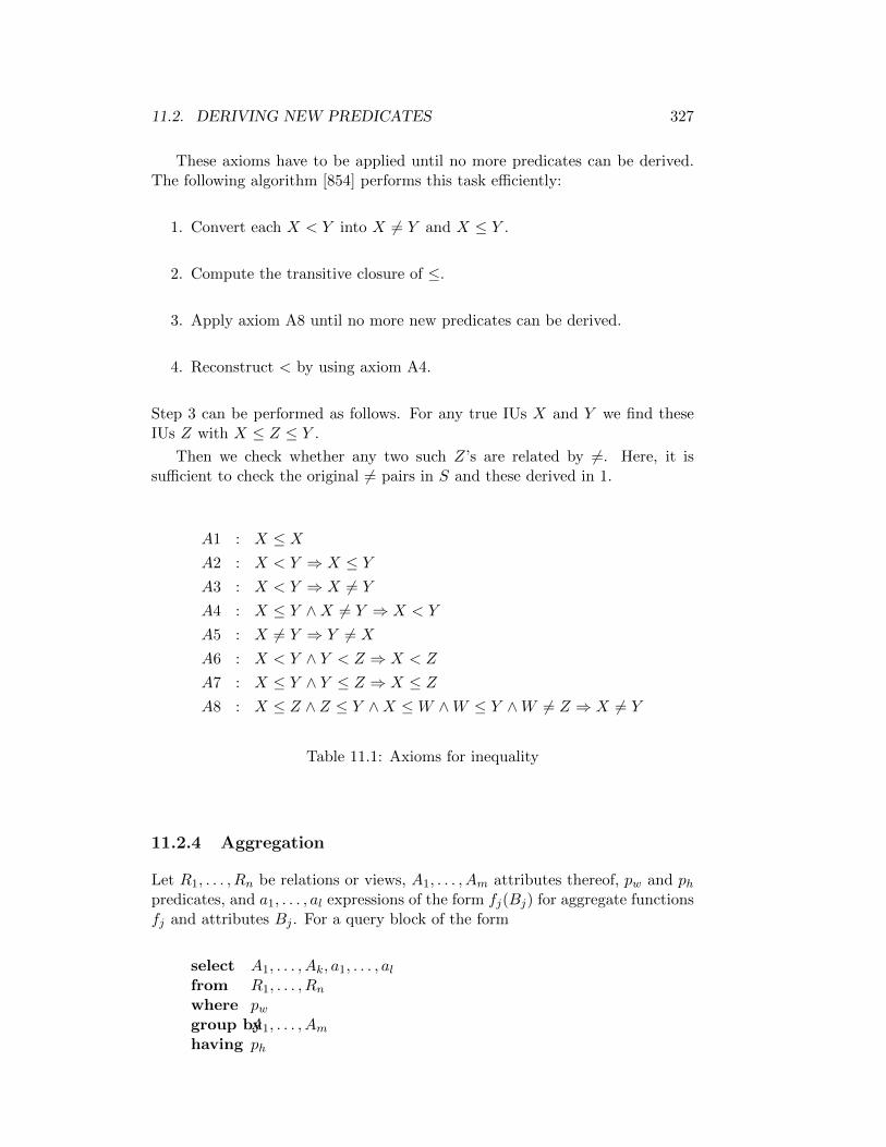
11.2. DERIVING NEW PREDICATES 327

These axioms have to be applied until no more predicates can be derived.The following algorithm [854] performs this task efficiently:

1. Convert each X < Y into X 6= Y and X ≤ Y .

2. Compute the transitive closure of ≤.

3. Apply axiom A8 until no more new predicates can be derived.

4. Reconstruct < by using axiom A4.

Step 3 can be performed as follows. For any true IUs X and Y we find theseIUs Z with X ≤ Z ≤ Y .

Then we check whether any two such Z’s are related by 6=. Here, it issufficient to check the original 6= pairs in S and these derived in 1.

A1 : X ≤ XA2 : X < Y ⇒ X ≤ YA3 : X < Y ⇒ X 6= Y

A4 : X ≤ Y ∧X 6= Y ⇒ X < Y

A5 : X 6= Y ⇒ Y 6= X

A6 : X < Y ∧ Y < Z ⇒ X < Z

A7 : X ≤ Y ∧ Y ≤ Z ⇒ X ≤ ZA8 : X ≤ Z ∧ Z ≤ Y ∧X ≤W ∧W ≤ Y ∧W 6= Z ⇒ X 6= Y

Table 11.1: Axioms for inequality

11.2.4 Aggregation

Let R1, . . . , Rn be relations or views, A1, . . . , Am attributes thereof, pw and phpredicates, and a1, . . . , al expressions of the form fj(Bj) for aggregate functionsfj and attributes Bj . For a query block of the form

select A1, . . . , Ak, a1, . . . , alfrom R1, . . . , Rnwhere pwgroup byA1, . . . , Amhaving ph

328 CHAPTER 11. SIMPLE REWRITES

we consider the derivation of new predicates [530]. Obviously, the followingpredicates are true:

min(B) ≤ B

max(B) ≥ B

max(B) ≥ min(B)

min(B) ≤ avg(B)

avg(B) ≤ max(B)

If pw contains conjunctively a predicate Bθc for some constant c, we can fur-

ther infermin(B) θ c if θ ∈ >,≥max(B) θ c if θ ∈ <,≤avg(B) θ c if θ ∈ <,≤, >,≥

These predicates can then

be used to derive further predicates. The original and the derive predicatesare usefule when the query block is embedded in another query block sincewe are allowed to add them to the embedding query block conjunctively (seeSection 12.3).

If we know restrictions on the aggregates from some embedding query block,we might be able to add predicates to pw. The following table contains the re-strictions on an aggregate we know in the left column and the predicates we can

infer in the right column:

max(B) ≥ c ; B ≥ c if no other aggregation occursmax(B) > c ; B > c if no other aggregation occursmin(B) ≤ c ; B ≤ c if no other aggregation occursmin(B) < c ; B < c if no other aggregation occurs

Note that the aggregation occurring in the left column must be the only aggre-gation found in the query block. That is, l = 1 and ph contains no aggregationother than a1. To see why this is necessary, consider the following query

select deptNo, max(salary), min(salary)from Employeegroup bydeptNo

Even if we know that max(salary) > 100.000, the above query block is notequivalent to

select deptNo, max(salary), min(salary)from Employeewhere salary ¿ 100.000group bydeptNo

Neither is

select deptNo, max(salary)from Employeegroup bydeptNohaving avg(salary) ¿ 50.000

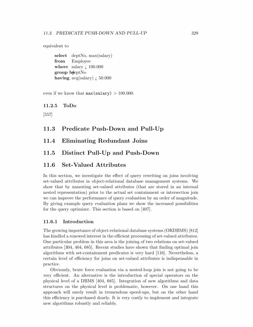
11.3. PREDICATE PUSH-DOWN AND PULL-UP 329

equivalent to

select deptNo, max(salary)from Employeewhere salary ¿ 100.000group bydeptNohaving avg(salary) ¿ 50.000

even if we know that max(salary) > 100.000.

11.2.5 ToDo

[557]

11.3 Predicate Push-Down and Pull-Up

11.4 Eliminating Redundant Joins

11.5 Distinct Pull-Up and Push-Down

11.6 Set-Valued Attributes

In this section, we investigate the effect of query rewriting on joins involvingset-valued attributes in object-relational database management systems. Weshow that by unnesting set-valued attributes (that are stored in an internalnested representation) prior to the actual set containment or intersection joinwe can improve the performance of query evaluation by an order of magnitude.By giving example query evaluation plans we show the increased possibilitiesfor the query optimizer. This section is based on [407].

11.6.1 Introduction

The growing importance of object-relational database systems (ORDBMS) [812]has kindled a renewed interest in the efficient processing of set-valued attributes.One particular problem in this area is the joining of two relations on set-valuedattributes [304, 404, 685]. Recent studies have shown that finding optimal joinalgorithms with set-containment predicates is very hard [116]. Nevertheless, acertain level of efficiency for joins on set-valued attributes is indispensable inpractice.

Obviously, brute force evaluation via a nested-loop join is not going to bevery efficient. An alternative is the introduction of special operators on thephysical level of a DBMS [404, 685]. Integration of new algorithms and datastructures on the physical level is problematic, however. On one hand thisapproach will surely result in tremendous speed-ups, but on the other handthis efficiency is purchased dearly. It is very costly to implement and integratenew algorithms robustly and reliably.

330 CHAPTER 11. SIMPLE REWRITES

We consider an alternative approach to support set-containment and non-empty intersection join queries by compiling these join predicates away. Themain idea is to unnest the set-valued attributes prior to the join. Thereby, weassume a nested internal representation [684]. This is also the underlying rep-resentation for the specific join algorithms proposed so far [404, 685]. Whereas[685] concentrates on set-containment joins, we also consider joins based onnon-empty intersections. Ramasamy et al. also present a query rewrite for con-tainment queries in [685], but on an unnested external representation, which(as shown there) exhibits very poor performance. Further, the special case ofempty sets was not dealt with.

The goal of our paper is to show that by rewriting queries we can compileaway the original set-containment or intersection join. As our experiments withDB2 show, our rewrite results in speed-up factors that grow linearly in the sizeof the input relations as compared to quadratic growth for brute-force nested-loop evaluation. The advantage of this approach—as compared to [404, 685]—isthat no new join algorithms have to be added to the database system.

11.6.2 Preliminaries

In this section we give an overview of the definition of the set type. Due to thedeferral of set types to SQL-4 [281], we use a syntax similar to that of Informix1. A possible example declaration of a table with a set-valued attribute is:

create table ngrams (

setID integer not null primary key,

content set<char(3)>

);

setID is the key of the relation, whereas content stores the actual set. Thecomponents of a set can be any built-in or user-defined type. In our case weused set<char(3)>, because we wanted to store 3-grams (see also Section ??).We further assume that on set-valued attributes the standard set operationsand comparison operators are available.

Our rewriting method is based on unnesting the internal nested representa-tion. The following view defining the unnested version of the above table keepsour representation more concise:

create view view_ngrams(setID, d, card) as (

(select ngrams.setID, d.value, count(ngrams.content)

from ngrams, table(unnest<char(3)>(ngrams.content)) d)

union all

(select ngrams.setID, NULL, 0)

from ngrams

where count(ngrams.content) = 0)

);

1http://www.informix.com/documentation/

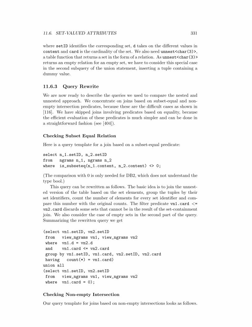
11.6. SET-VALUED ATTRIBUTES 331

where setID identifies the corresponding set, d takes on the different values incontent and card is the cardinality of the set. We also need unnest<char(3)>,a table function that returns a set in the form of a relation. As unnest<char(3)>returns an empty relation for an empty set, we have to consider this special casein the second subquery of the union statement, inserting a tuple containing adummy value.

11.6.3 Query Rewrite

We are now ready to describe the queries we used to compare the nested andunnested approach. We concentrate on joins based on subset-equal and non-empty intersection predicates, because these are the difficult cases as shown in[116]. We have skipped joins involving predicates based on equality, becausethe efficient evaluation of these predicates is much simpler and can be done ina straightforward fashion (see [404]).

Checking Subset Equal Relation

Here is a query template for a join based on a subset-equal predicate:

select n_1.setID, n_2.setID

from ngrams n_1, ngrams n_2

where is_subseteq(n_1.content, n_2.content) <> 0;

(The comparison with 0 is only needed for DB2, which does not understand thetype bool.)

This query can be rewritten as follows. The basic idea is to join the unnest-ed version of the table based on the set elements, group the tuples by theirset identifiers, count the number of elements for every set identifier and com-pare this number with the original counts. The filter predicate vn1.card <=vn2.card discards some sets that cannot be in the result of the set-containmentjoin. We also consider the case of empty sets in the second part of the query.Summarizing the rewritten query we get

(select vn1.setID, vn2.setID

from view_ngrams vn1, view_ngrams vn2

where vn1.d = vn2.d

and vn1.card <= vn2.card

group by vn1.setID, vn1.card, vn2.setID, vn2.card

having count(*) = vn1.card)

union all

(select vn1.setID, vn2.setID

from view_ngrams vn1, view_ngrams vn2

where vn1.card = 0);

Checking Non-empty Intersection

Our query template for joins based on non-empty intersections looks as follows.

332 CHAPTER 11. SIMPLE REWRITES

select n_1.setID, n_2.setID

from ngrams n_1, ngrams n_2

where intersects(n_1.content, n_2.content) <> 0;

The formulation of the unnested query is much simpler than the unnestedquery in Section 11.6.3. Due to our view definition, not much rewriting isnecessary. We just have to take care of empty sets again, although this time ina different, simpler way.

select distinct vn1.setID, vn2.setID

from view_ngrams vn1, view_ngrams vn2

where vn1.d = vn2.d

and vn1.card > 0;

11.7 Bibliography

This section is based on the investigations by Helmer and Moerkotte [407].There, we also find a performance evaluation indicating that that the rewritesdepending on the relation sizes result in speed-up factors between 5 and 50 evenfor moderately sized relations. Nevertheless, it is argued their, that support forset-valued attributes must be build into the DBMS. A viable alternative to therewrites presented here is the usage of special join algorithms for join predicatesinvolving set-valued attributes [304, 403, 404, 559, 578, 579, 685]. Nevertheless,as has been shown by Cai, Chakaravarthy, Kaushik, and Naughton, dealingwith set-valued attributes in joins theoretically (and of course practical) difficultissue [116]. Last, to efficiently support simple selection predicates on set-valuedattributes, special index structures should be incorporated into the DBMS [405,406, 408].

11.7. BIBLIOGRAPHY 333

IU::addEqualityClassUnderThis(IU* lIU)

IU*lRepresentativeThis = this -> getEqualityRepresentativeIU;

IU*lRepresentativeArg = aIU -> getEqualityRepresentativeIU;

lRepresentativeArg -> _equalityRepresentative =

lRepresentativeThis;

if(lRepresentativeArg -> _equalityClassRank >=

lRepresentativeThis -> _equalityClassRank)

lRepresentativeThis -> _equalityClassRank =

lRepresentativeArg -> _equalityClass Rank + 1;

IU::addEqualityPredicate(Compositing* p)

IU*lLeft = p -> leftIU;

IU*lRight = p -> rightIU;

if (p -> isEqualityPredicateIU &&

lLeft -> getEqualityRepresentativeIU ==

lRight -> getEqualityRepresentativeIU)

if(lLeft - > isBoundToConstantIU)

lLeft -> addEqualityClassUnderThis(lRight);

else

if(lRight -> isBoundToConstantIU)

lRight -> addEqualityClassUnderThis(lLeft),

else

if (lLeft -> _equalityClassRank > lRight ->

_equalityClassRank)

lLeft -> addEqualityClassUnderThis(lRight)

else

lright -> addEqualityClassUnderThis(lLeft)

IU* IU:: getEqualityRepresentativeIU()

if (this == _equalityRepresentative)

_equalityRepresentative = _equalityRepresentative ->

getEqualityRepresentativeIU;

return_equalityRepresentative;

Figure 11.3:

334 CHAPTER 11. SIMPLE REWRITES

A1 X ≤ XA2 X < Y ⇒ X ≤ YA3 X < Y ⇒ X 6= YA4 X ≤ Y ∧X 6= Y ⇒ X < YA5 X 6= Y ⇒ Y 6= XA6 X < Y ∧ Y < Z ⇒ X < ZA7 X ≤ Y ∧ Y ≤ Z ⇒ X ≤ ZA8 X ≤ Z ∧ Z ≤ Y ∧X ≤W ∧W ≤ Y ∧W 6= Z ⇒ X 6= Y

Figure 11.4: Axioms for inequality

Chapter 12

View Merging

12.1 View Resolution

View merging can be as simple as replacing the view name in the from clauseof a query by the view definition. We would like to call this step view reso-lution. This then results in a query with nesting in the from clause that cansubsequently be unnested (see ??). Consider the following example: XXX Ex-ample Other examples are given below. One must be careful not to producevariable clashes. Especially if a view is referenced several times, variables mustbe renamed.

12.2 Simple View Merging

Of course, these two steps can be merged into one step. The overall effect isthen that the view name is replaced by all the entries in the from clause of theview definition and the predicate contained in the where clause of the viewdefinition is conjunctively added to where clause of the query block whosefrom clause contained the view name. Consider the following view definition

create view

which is refenced in the following query:

View merging resuls in

However, there are a few pitfalls. This simple version of view merging canonly be applied to simple select-project-join queries not containing duplicateelimination, set operations, grouping or aggregation. In these cases, complexview merging must be applied.

335

336 CHAPTER 12. VIEW MERGING

12.3 Predicate Move Around (Predicate pull-up andpush-down)

If unnesting is not implemented or not possible, several techniques like predicatemove around, semi-join techniques and magic rewriting allow the copying ofpredicates from one block into another block in order to reduce the number ofqualifying tuples [530, 608, 609, 610, 763].

Let us briefly illustrate the main idea by means of a simple example query

select e.namefrom Employee e,

(select d.name, d.dnofrom Department dwhere d.dno = e.dno and

d.boss.name = e.name andd.boss.name like ’%S’) as D(dname,ddno)

where e.dno between 1 and 10

which can be rewritten by predicate move around to

select e.namefrom Employee e,

(select d.name, d.dnofrom Department dwhere d.dno = e.dno and

d.boss.name = e.name andd.dno between 1 and 10 andd.boss.name like ’%S’) as D(dname,dd no)

where e.dno between 1 and 10 ande.name like ’%S’

Predicate push-down and pull-up often occurs in conjunction with views.Let us therefore consider some examples. The following view that cannot besimply merged because it contains a union operator. Consider the case wherethere are two different employee tables that are unioned in a view.

create view Emp(eno, name, salary, dno) asselect e1.eno, e1.name, e1.salary, e1.dnofrom Emp1[e1]union allselect e2.eno, e2.name, e2.salary, e2.dnofrom Emp2[e2]

Simple view merging cannot be applied to the query

select e.eno, e.namefrom Emp[e]where e.salary > 150000

12.4. COMPLEX VIEW MERGING 337

but view resolution with a subsequent push-down of the predicate e.salary >150.000 will result in

select e.eno, e.namefrom ( select e1.eno, e1.name, e1.salary, e1.dno

from Emp1[e1]where e1.salary > 150000)

union all( select e2.eno, e2.name, e2.salary, e2.dnofrom Emp2[e2]where e2.salary > 150000)

Note that we did not eliminate unneeded columns/attributes. Further notethat we can now exploit possible indexes on Emp1.salary and Emp2.salary.In case union would have been used in the view definition, the rewritten querywould also contain union requiring a duplicate elimination.

Here is another example where pushing a predicate down results in muchmore efficient plans. Given the view

define view EmpStat asselect e.dno, min(e.salary) minSal, max(e.salary) maxSal, avg(e.salary) avgSalfrom Emp[e]group by e.dno

the query

select *from EmpStat[e]where e.dno = 10

can be rewritten to

select e.dno, min(e.salary) minSal, max(e.salary) maxSal, avg(e.salary) avgSalfrom Emp[e]where e.dno = 10group by e.dno

which can be further simplified to

select e.dno, min(e.salary) minSal, max(e.salary) maxSal, avg(e.salary) avgSalfrom Emp[e]where e.dno = 10

12.4 Complex View Merging

12.4.1 Views with Distinct

XXX TODO views with distinct

338 CHAPTER 12. VIEW MERGING

12.4.2 Views with Group-By and Aggregation

Consider the following view with a group-by clause and aggregation:

create view AvgSalary asselect e.dno, avg(e.salary) as avgSalaryfrom Emp[e]group by e.dno

The following query uses this view:

select d.name, s.avgSalary)from Dept[d], AvgSalary[s]where d.location = ‘Paris‘ and

d.dno = s.dno

Using the view definition, this query can be rewritten to

select d.name, avg(e.salary) as avgSalaryfrom Dept[d], Emp[e]where d.location = ‘Paris‘ and

d.dno = e.dnogroup by d.ROWID, d.name

where d.ROWID is a either a key-attribute like d.dno or a unique row identifier ofthe tuples in Dept. Or course, this transformation is not valid in general. Theprimary condition here is that we have a key-foreign key join. More specifically,d.dno must be the key of the Dept table or it must be a unique attribute.

Applying simple view resolution results in:

select d.name, s.avgSalary)from Dept[d], (select e.dno, avg(salary) as avgSalary

from Emp[e]group by e.dno) [s]

where d.location = ‘Paris‘ andd.dno = s.dno

This query can then be unnested using the techniques of Section ??.Sometimes strange results occur. Consider for example the view

define view EmpStat asselect e.dno, min(e.salary) minSal, max(e.salary) maxSal, avg(e.salary) avgSalfrom Emp[e]group by e.dno

If the user issues the query

12.4. COMPLEX VIEW MERGING 339

select avg(minSal), avg(maxSal), avg(avgSal)from EmpStat

view merging results in

select avg(min(e.salary)), avg(max(e.salary)), avg(avg(e.salary))from Emp[e]group by e.dno

This is perfectly o.k. You just need to think twice about it. The resulting planwill contain two group operations: XXX Plan

12.4.3 Views in IN predicates

Consider a view that contains the minimum salary for each department

create view MinSalary asselect e.dno, min(e.salary) as minSalaryfrom Emp[e]group by e.dno

and a query asking for all those employees together with their salaries in Parisiandepartments earning the minimum salary:

select e.name, e.salaryfrom Emp[e], Dept[d]where e.dno = d.dno and

d.location = ‘Paris‘ and(e.dno, e.sal) in MinSalary

This query can be rewritten to:

select e.name, e.salaryfrom Emp[e], Dept[d], Emp[e2]where e.dno = d.dno and

d.location = ‘Paris‘ ande.dno = e2.dno

group by e.ROWID, d.ROWID, e.name, e.salaryhaving e.salary = min(e2.sal)

Note that the employee relation occurs twice. Avoiding to scan the employeerelation twice can be done as follows:

12.4.4 Final Remarks

Not all views can be merged. If for example a rownum function that numbersrows in a table is used in a view definition for a result column, then the viewcannot be merged. Unmerged views will remain as nested subqueries with

340 CHAPTER 12. VIEW MERGING

two alternative evaluation strategies: Either they will be evaluated as nestedqueries, that is for every row produced by some outer producer the view isevaluated, or the view will be materialized into a temporary table. Whateveris more efficient must be chosen by the plan generator. However, techniquesfor deriving additional predicates and subsequent techniques such as predicatemove around (predicate pull-down, push-down) are still applicable.

12.5 Bibliography

Chapter 13

Quantifier treatment

13.1 Pseudo-Quantifiers

Again, the clue to rewrite subqueries with a ANY or ALL predicate is to applyaggregate functions [303]. A predicate of the form

< ANY (select . . .from . . .where . . . )

can be transformed into the equivalent predicate

< (select max(. . . )from . . .where . . . )

Analogously, a predicate of the form

< ALL (select . . .from . . .where . . . )

can be transformed into the equivalent predicate

< (select min(. . . )from . . .where . . . )

In the above rewrite rules, the predicate < can be replaced by =, ≤, etc. If thepredicate is > or ≥ then the above rules are flipped. For example, a predicateof the form >ANY becomes >select min and >ALL becomes >select max.

After the rewrites have been applied, the Type A or Type JA unnestingtechniques can be applied, depending on the details of the inner query block.

341

342 CHAPTER 13. QUANTIFIER TREATMENT

13.2 Existential quantifier

Existential quantifiers can be seen as special aggregate functions and queryblocks exhibiting an existential quantifier can be unnested accordingly [211].For example, an independent existential subquery can be treated the same wayas a Type A query. Nested existential quantifiers with a correlation predi-cate can be unnested using a semi-join. Other approaches rewrite (existential)quantifiers using the aggregate function count [303]. Consider the partial querypattern

. . .where exists (select . . .from . . .where . . . )

It is equivalent to

. . .where 0 > (select count(. . . )from . . .where . . . )

A not exists like in

. . .where not exists (select . . .from . . .where . . . )

is equivalent to

. . .where 0 = (select count(. . . )from . . .where . . . )

After these rewrites have been applied, the Type A or Type JA unnestingtechniques can be applied, depending on the details of the inner query block.

13.3 Universal quantifier

Universal quantification is a little more complex. An overview is provided in[176]. Here is the prototypical OQL query pattern upon which our discussion

13.3. UNIVERSAL QUANTIFIER 343

Case-No. 1 2 3 4 5 6 7 8

p() p() p() p() p(e1) p(e1) p(e1) p(e1)q() q(e1) q(e2) q(e1, e2) q() q(e1) q(e2) q(e1, e2)

Case-No. 9 10 11 12 13 14 15 16

p(e2) p(e2) p(e2) p(e2) p(e1, e2) p(e1, e2) p(e1, e2) p(e1, e2)q() q(e1) q(e2) q(e1, e2) q() q(e1) q(e2) q(e1, e2)

Table 13.1: Classification Scheme According to the Variable Bindings

of universal quantifiers nested within a query block is based:

Q ≡ select e1

from e1 in E1

where for all e2 in select e2

from e2 in E2

where p:q

where p (called the range predicate) and q (called the quantifier predicate) arepredicates in a subset of the variables e1, e2. This query pattern is denotedby Q.

In order to emphasize the (non-)occurrence of variables in a predicate p, wewrite p(e1, . . . , en) if p depends on the variables e1, . . . , en. Using this conven-tion, we can list all the possible cases of variable occurrence. Since both e1 ande2 may or may not occur in p or q, we have to consider 16 cases (see Table 13.1).All cases but 12, 15, and 16 are rather trivial. Class 12 queries can be unnestedby replacing the universal quantifier by a division, set difference, anti-semijoin,or counting. Class 15 queries are treated by set difference, anti-semijoin orgrouping with count aggregation. For Class 16 queries, the alternatives are setdifference, anti-semijoin, and grouping with count aggregation. In all cases,special care has to be taken regarding NULL values. For details see [176].

Class 12 Let us first consider an example of a Class 12 query.

select al.namefrom al in Airlinewhere for all ap in (select ap

from ap in Airportwhere apctry = ’USA’):

ap in al.lounges

Define U ≡ πap(σapctry=′USA′(Airport[ap, apctry])). Then the three alternativealgebraic expressions equivalent to this query are

• plan with division:if U = ∅

344 CHAPTER 13. QUANTIFIER TREATMENT

then Airline[name]else µap:lounges(Airline[name, lounges])÷ U

• plan with set difference:

Airline[name] \ (πname(U Nap 6∈lounges Airline[name, lounges]))

• plan with anti-semijoin:

πname(U Tap 6∈lounges Airline[name, lounges])

This plan is only valid, if the projected attributes of Airline form a su-perkey.

The plan with the anti-semijoin is typically the most efficient.

In general, the plan with division is [614, 341]:

ifσp(e2)(E2[e2])6=∅(((E1[e1] Bq(e1,e2) E2[e2])÷ σp(e2)(E2[e2])), E1[e1])

In case the selection σp(e2)(E2[e2]) yields at least a one tuple or object, we canapply the prediate p to the divident, as in

ifσp(e2)(E2[e2])6=∅(((E1[e1] Bq(e1,e2) σp(e2)(E2[e2]))÷ σp(e2)(E2[e2])), E1[e1]).

If the quantifier predicate q(e1, e2) is of the form e2 ∈ e1.SetAttribute, then thejoin can be replaced by an unnest operator:

ifσp(e2)(E2[e2])6=∅((µe2:SetAttribute(E1[e1,SetAttribute])÷ σp(e2)(E2[e2])), E1[e1])

Using set difference, the translation is

E1[e1] \ πe1((E1[e1]× σp(e2)(E2[e2])) \ (E1[e1] Bq(e1,e2) σp(e2)(E2[e2])))

which can be optimized to

E1[e1] \ E1[e1] N¬q(e1,e2) σp(e2)(E2[e2])

This plan is mentioned in [801], however using a regular join instead of a semi-join.

The anti-semijoin can be employed to eliminate the set difference yieldingthe following plan:

E1[e1] T¬q(e1,e2) σp(e2)(E2[e2])

This plan is in many cases the most efficient plan. However, the correctness ofthis plan depends on the uniqueness of e1, i.e., the attribute(s) e1 must be a(super) key of E1. This is especially fulfilled in the object-oriented context ife1 consists of or contains the object identifier.

We do not present the plans based group and count operations (see [176]).

13.3. UNIVERSAL QUANTIFIER 345

Class 15 Here is an example query of Class 15:

select al.namefrom al in Airlinewhere for all f in (

select ffrom f in Flightwhere al = f.carrier):f.to.apctry != “Libya”

The quantifier’s range formulat σp(e1,e2)(E2[e2]) is obviously not closed. Itcontains the free variable e1. According to the reduction algorithm of Codd[191], the division plan is

(E1[e1] B¬p(e1,e2)∨q(e2) E2[e2])÷ E2[e2].

The plan with set difference is

E1[e1] \ πe1((E1[e1] Bp(e1,e2) E2[e2]) \ (E1[e1] Bp(e1,e2) σq(e2)(E2[e2])))

and the most efficient plan using the antijoin is

E1[e1] Tp(e1,e2) σ¬q(e2)(E2[e2]).

Class 16 Here is an example Class 16 query:

select al.namefrom al in Airlinewhere for all ap in (

select apfrom ap in Airportwhere apctry = alctry):ap in al.lounges

The range predicate again depends on the outer level variable e1. A validdivision plan looks similar to the one for Class 15. A plan with set difference is

E1[e1] \ πe1((E1[e1] Bp(e1,e2) E2[e2]) \ (E1[e1] Bp(e1,e2)∧q(e1,e2) E2[e2])).

This plan can first be refined by replacing the seet difference of the two joinexpression by a semijoin resultint in

E1[e1] \ (E1[e1] Np(e1,e2)∧¬q(e1,e2) E2[e2])

Finally, the remaining set difference is transformed into an anti-semijoin whichalso covers the semijoin:

E1[e1] Tp(e1,e2)∧¬q(e1,e2) E2[e2].

Again, the uniqueness constraing on E2[e2] is required for this most efficientplan to be valid.

For all discussed classes, problems with NULL values might occur. In thatcase, the plans have to refined [176].

346 CHAPTER 13. QUANTIFIER TREATMENT

13.4 Bibliography

[448] [211] [176] [687, 680]

Chapter 14

Unnesting Nested Queries

347

348 CHAPTER 14. UNNESTING NESTED QUERIES

Chapter 15

Optimizing Queries withMaterialized Views

15.1 Conjunctive Views

15.2 Views with Grouping and Aggregation

15.3 Views with Disjunction

15.4 Bibliography

materialized view with aggregates: [799],materialized view with disjunction: [11],SQL Server: [320]other: [12, 145, 146, 157, 528, 814, 848, 915] [134, 138, 158, 148, 273, 462,

514, 649, 679, 756]some more including maintenance etc: [10, 14, 52, 90, 145, 151, 197, 369, 384]

[417, 461, 527, 676, 719, 256, 799] [814, 823, 822, 939, 916] [6, 243, 244, 391]Overview: [376][529]performance eval: [88]Stacked views: [216]recursion: [246]with patterns (integration): [679], [245, 247], [225]

349

350CHAPTER 15. OPTIMIZING QUERIESWITHMATERIALIZED VIEWS

Chapter 16

Semantic Query Rewrite

16.1 Constraints and their impact on query opti-mization

Using Constraints: [318, 360]

16.2 Semantic Query Rewrite

Semantic query rewrite exploits knowledge (semantic information) about thecontent of the object base. This knowledge is typically specified by the user.We already saw one example of user-supplied information: inverse relationships.As we already saw, inverse relationships can be exploited for more efficient queryevaluation.

Another important piece of information is knowledge about keys. In con-junction with type inference, this information can be used during query rewriteto speed up query execution. A typical example is the following query

select distinct *from Professor p1, Professor p2where p1.university.name = p2.university.name

By type inference, we can conclude that the expressions p1.university andp2.university are of type University. If we further knew that the name of uni-versities are unique, that is the name is a candidate key for universities, thenthe query could be simplified to

select distinct *from Professor p1, Professor p2where p1.university = p2.university

Evaluating this query does no longer necessitate accessing the universities toretrieve their name.

Some systems consider even more general knowledge in form of equivalencesholding over user-defined functions [1, 279]. These equivalences are then usedto rewrite the query. Thereby, alternatives are generated all of which are sub-sequently optimized.

351

352 CHAPTER 16. SEMANTIC QUERY REWRITE

Semantic Query Optimization: [134]

16.3 Exploiting Uniqueness in Query Optimization

[653]

16.4 Bibliography

[79] [71] [910] Foreign functions semantic rules rewrite: [148] Conjunctive Queries,Branch Minimization: [713]

Part IV

Plan Generation

353

Chapter 17

Current Search Space and ItsLimits

17.1 Plans with Outer Joins, Semijoins and Anti-joins

outer join reordering [289, 288, 706, 297], outer join/antijoin plan generation[689], semijoin reducer [807],

17.2 Expensive Predicates and Functions

17.3 Techniques to Reduce the Search Space

• join single row tables first

• push down SARGable predicates

• For large join queries do not apply transitivity of equality to derive newpredicates and disable cross products and possibly bushy trees.

17.4 Bibliography

355

356 CHAPTER 17. CURRENT SEARCH SPACE AND ITS LIMITS

Chapter 18

Dynamic Programming-BasedPlan Generation

18.1 Introduction

So far, we treated predicates that reference a single relation as selection predi-cates and predicates that reference two relations as join predicates. In general,a predicate can reference more than two relations. In this case, it can be treatedas a join predicate. Consider for example the query

select * from R, S, T, where R.A = S.B AND S.C = T.D and R.E+ S.F = T.G

A query graph as defined in Section ?? does not suffice to capture thesepredicates. What is needed are hypergraphs.

There exists a second reason why hypergraphs are needed. In Section 7.15,we introduced several conflict handling mechanisms, which allow for the correctenumeration of the core search space. Every operator within some operatortree has a set of relations TES associated with it. This set of relations was asubset of all the relations in the leaf nodes below the operator subtree rootedat . Hence, some relations occurred on ’s left side, others on its right side.Thus, we splitted TES into TESleft and TESright. Then, the pair (TESleft, TESright)is a hyperedge.

Algorithm DPsube was used to calculate the best plan bottom-up. Theapplicability test, among other things, assured that only connected componentsand connected complements thereof were formed. The test often fails. This issimilar to the manner the tests of DPsub and DPsize (see Section ??) failedfor regular graphs. There, this fact lead us to the development of DPccp, whichenumerates CCPs for regular graphs quite efficiently.

The first goal of this section is to build an equally efficient enumerator forCCPs for hypergraphs. Then, this basic algorithm is extended such that it isable to deal with more operators than those handled in the core search space.

357

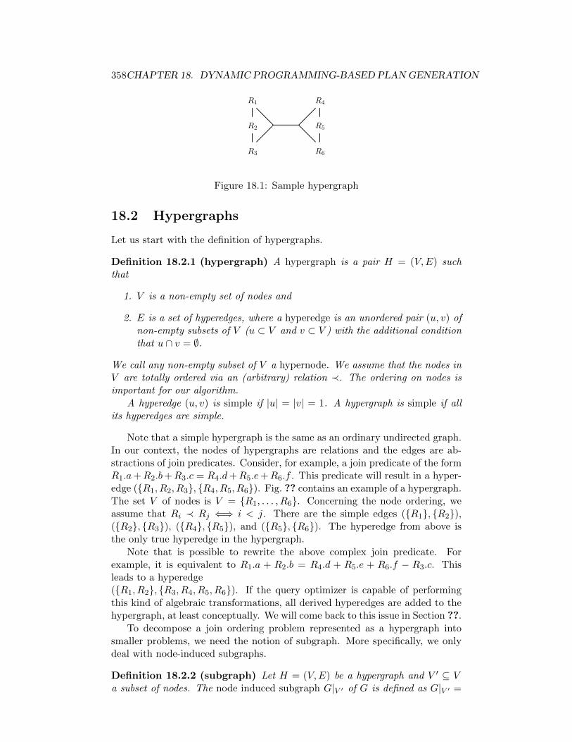
358CHAPTER 18. DYNAMIC PROGRAMMING-BASED PLANGENERATION

R1

R2

R3

R4

R5

R6

Figure 18.1: Sample hypergraph

18.2 Hypergraphs

Let us start with the definition of hypergraphs.

Definition 18.2.1 (hypergraph) A hypergraph is a pair H = (V,E) suchthat

1. V is a non-empty set of nodes and

2. E is a set of hyperedges, where a hyperedge is an unordered pair (u, v) ofnon-empty subsets of V (u ⊂ V and v ⊂ V ) with the additional conditionthat u ∩ v = ∅.

We call any non-empty subset of V a hypernode. We assume that the nodes inV are totally ordered via an (arbitrary) relation ≺. The ordering on nodes isimportant for our algorithm.

A hyperedge (u, v) is simple if |u| = |v| = 1. A hypergraph is simple if allits hyperedges are simple.

Note that a simple hypergraph is the same as an ordinary undirected graph.In our context, the nodes of hypergraphs are relations and the edges are ab-stractions of join predicates. Consider, for example, a join predicate of the formR1.a+R2.b+R3.c = R4.d+R5.e+R6.f . This predicate will result in a hyper-edge (R1, R2, R3, R4, R5, R6). Fig. ?? contains an example of a hypergraph.The set V of nodes is V = R1, . . . , R6. Concerning the node ordering, weassume that Ri ≺ Rj ⇐⇒ i < j. There are the simple edges (R1, R2),(R2, R3), (R4, R5), and (R5, R6). The hyperedge from above isthe only true hyperedge in the hypergraph.

Note that is possible to rewrite the above complex join predicate. Forexample, it is equivalent to R1.a + R2.b = R4.d + R5.e + R6.f − R3.c. Thisleads to a hyperedge(R1, R2, R3, R4, R5, R6). If the query optimizer is capable of performingthis kind of algebraic transformations, all derived hyperedges are added to thehypergraph, at least conceptually. We will come back to this issue in Section ??.

To decompose a join ordering problem represented as a hypergraph intosmaller problems, we need the notion of subgraph. More specifically, we onlydeal with node-induced subgraphs.

Definition 18.2.2 (subgraph) Let H = (V,E) be a hypergraph and V ′ ⊆ Va subset of nodes. The node induced subgraph G|V ′ of G is defined as G|V ′ =

18.3. CCPS: CSG-CMP-PAIRS FOR HYPERGRAPHS 359

(V ′, E′) with E′ = (u, v)|(u, v) ∈ E, u ⊆ V ′, v ⊆ V ′. The node ordering onV ′ is the restriction of the node ordering of V .

As we are interested in connected subgraphs, we give

Definition 18.2.3 (connected) Let H = (V,E) be a hypergraph. H is con-nected if |V | = 1 or if there exists a partitioning V ′, V ′′ of V and a hyperedge(u, v) ∈ E such that u ⊆ V ′, v ⊆ V ′′, and both G|V ′ and G|V ′′ are connected.

If H = (V,E) is a hypergraph and V ′ ⊆ V is a subset of the nodes such that thenode-induced subgraph G|V ′ is connected, then we call V ′ a connected subgraphor csg for short. The number of connected subgraphs is important for dynamicprogramming: it directly corresponds to the number of entries in the dynamicprogramming table. If a node set V ′′ ⊆ (V \ V ′) induces a connected subgraphG|V ′′ , we call V ′′ a connected complement of V ′ or cmp for short.

For the purpose of this chapter, we assume that all hypergraphs are con-nected. This way, we can make sure that no (additional) cross products areneeded. This condition can easily be assured by adding according hyperedges:for every pair of connected components, we can add a hyperedge whose hypern-odes contain exactly the relations of the connected components. By consideringthese hyperedges as A operators. As we saw in Section 7.15, cross products canbe handled by our conflict detectors can be handled

18.3 CCPs: Csg-Cmp-Pairs for Hypergraphs

With these notations, we can move closer to the heart of dynamic programmingby defining a csg-cmp-pair, or ccp for short.

Definition 18.3.1 (csg-cmp-pair, ccp) Let H = (V,E) be a hypergraph andS1, S2 two subsets of V such that S1 ⊆ V and S2 ⊆ (V \ S1) are a connect-ed subgraph and a connected complement. If there further exists a hyperedge(u, v) ∈ E such that u ⊆ S1 and v ⊆ S2, we call (S1, S2) a csg-cmp-pair.

Note that if (S1, S2) is a csg-cmp-pair, then (S2, S1) is one as well. Outof these two possibilities, only one will be enumerated by our subsequent al-gorithm. More specifically, we will restrict the enumeration of csg-cmp-pairsto those (S1, S2) which satisfy the condition that min(S1) ≺ min(S2), wheremin(S) = s such that s ∈ S and ∀s′ ∈ S : s 6= s′ =⇒ s ≺ s′. Since thisrestriction will hold for all csg-cmp-pairs enumerated by our procedure, we aresure that no duplicate csg-cmp-pairs are calculated. As a consequence, we haveto take some care in order to ensure that our dynamic programming procedureis complete: if the binary operator we apply is commutative, the procedure tobuild a plan for S1 ∪ S2 from plans for S1 and S2 has to take commutativityinto account. However, this is not really a challenge.

Obviously, in order to be correct, any dynamic programming algorithm hasto consider all csg-cmp-pairs [595]. Further, only these have to be considered.Thus, the minimal number of cost function calls of any dynamic programmingalgorithm is exactly the number of csg-cmp-pairs for a given hypergraph. Note

360CHAPTER 18. DYNAMIC PROGRAMMING-BASED PLANGENERATION

that the number of connected subgraphs is far smaller than the number of csg-cmp-pairs. The problem now is to enumerate the csg-cmp-pairs efficiently andin an order acceptable for dynamic programming. The latter can be expressedmore specifically. Before enumerating a csg-cmp-pair (S1, S2), all csg-cmp-pairs(S′1, S

′2) with S′1 ⊆ S1 and S′2 ⊆ S2 have to be enumerated.

18.4 Neighborhood

The main idea to generate csg-cmp-pairs is to incrementally expand connectedsubgraphs by considering new nodes in the neighborhood of a subgraph. Infor-mally, the neighborhood N(S) under an exclusion set X consists of all nodesreachable from S that are not in X. We derive an exact definition below.

When choosing subsets of the neighborhood for inclusion, we have to treata hypernode as a single instance: either all of its nodes are inside an enumer-ated subset or none of them. Since we want to use the fast subset enumerationprocedure introduced by Vance and Maier [865], we must have a single bitrepresenting a hypernode and also single bits for relations occurring in simpleedges. Since these may overlap, we are constrained to choose one unique rep-resentative of every hypernode occurring in a hyperedge. We choose the nodethat is minimal with respect to ≺. Accordingly, we define:

min(S) = s|s ∈ S, ∀s′ ∈ S s 6= s′ =⇒ s ≺ s′

Note that if S is empty, then min(S) is also empty. Otherwise, it contains a sin-gle element. Hence, if S is a singleton set, then min(S) equals the only elementcontained in S. For our hypergraph in Fig. ?? and with S = R4, R5, R6, wehave min(S) = R4.

Let S be a current set, which we want to expand by adding further relations.Consider a hyperedge (u, v) with u ⊆ S. Then, we will add min(v) to theneighborhood of S. However, we have to make sure that the missing elementsof v, i.e. v \min(v), are also contained in any set emitted. We thus define

min(S) = S \min(S)

For our hypergraph in Fig. ?? and with S = R4, R5, R6, we have min(S) =R5, R6.

We define the set of non-subsumed hyperedges as the minimal subset E ↓of E such that for all (u, v) ∈ E there exists a hyperedge (u′, v′) ∈ E ↓ withu′ ⊆ u and v′ ⊆ v. Additionally, we make sure that none of the nodes of ahypernode are contained in a set X, which is to be excluded from neighborhoodconsiderations. We thus define a set containing the interesting hypernodes forgiven sets S and X. We do so in two steps. First, we collect the potentiallyinteresting hypernodes into a set E ↓′ (S,X) and then minimize this set toeliminate subsumed hypernodes. This step then results in E ↓ (S,X), withwhich the algorithm will work.

E ↓′ (S,X) = v|(u, v) ∈ E, u ⊆ S, v ∩ S = ∅, v ∩X = ∅

18.5. THE CCP ENUMERATOR BUENUMCPPHYP 361

Define E ↓ (S,X) to be the minimal set of hypernodes such that for all v ∈E ↓′ (S,X) there exists a hypernode v′ in E ↓ (S,X) such that v′ ⊆ v. Notethat apart from the connectedness, we test exactly the conditions given inDef. 18.3.1. For our hypergraph in Fig. ?? and with X = S = R1, R2, R3, wehave E ↓ (S,X) = R4, R5, R6.

We are now ready to define the neighborhood of a hypernode S, given a setof excluded nodes X.

IN(S,X) =⋃

v∈E↓(S,X)

min(v) (18.1)

For our hypergraph in Fig. ?? and with X = S = R1, R2, R3, we haveIN(S,X) = R4. Assuming a bit vector representation of sets, the neighbor-hood can be efficiently calculated bottom-up.

18.5 The CCP Enumerator BuEnumCppHyp

Before starting with the algorithm description we give a high-level overview ofthe general principles used in the algorithm:

1. The algorithm constructs ccps by enumerating connected subgraphs froman increasing part of the query graph;

2. both the primary connected subgraphs and its connected complement arecreated by recursive graph traversals;

3. during traversal, some nodes are forbidden to avoid creating duplicates.More precisely, when a function performs a recursive call it forbids allnodes it will investigate itself;

4. connected subgraphs are increased by following edges to neighboring nodes.For this purpose hyperedges are interpreted as n : 1 edges, leading fromn of one side to one (specific) canonical node of the other side (cmp.Eq. 18.1).

Summarizing the above, the algorithm traverses the graph in a fixed order andrecursively produces larger connected subgraphs. The main challenge relativeto DPccp is the traversal of hyperedges: First, the ”starting” side of the edgecan require multiple nodes, which complicates neighborhood computation. Inparticular the neighborhood can no longer be computed as a simple bottom-upunion of local neighborhoods. Second, the ”ending” side of the edge can leadto multiple nodes at once, which disrupts the recursive growth of components.Consider a set S1, which we want to extend by a hyperedge (u,w). Even ifu ⊆ S1, there is no guarantee that S1 ∪ w will be connected.

To overcome these problems, the algorithm picks a representative end node.In our exmaple, it picks the 1 in the n : 1 of item 4 (see also Eq. 18.1). Withit, it starts the recursive growth and exploits the DP table to check if a validconstellation has been reached, i.e., the constructed hypernode induces a con-nected subgraph. This exploitation builds on the fact that our DP strategies

362CHAPTER 18. DYNAMIC PROGRAMMING-BASED PLANGENERATION

enumerate subsets before supersets. We are now prepared to discuss the detailsof the algorithm.

We give the implementation of our join ordering algorithm for hypergraphsby means of the pseudocode for member functions of a class BuEnumCcpHyp.This allows us to minimize the number of parameters by assuming that thisclass contains references to the query hypergraph (G = (V,E)) and to thedynamic programming table (DpTable).

The whole algorithm is distributed over five subroutines. The top-level rou-tine BuEnumCcpHyp initializes the DpTable with access plans for single relationsand then calls EmitCsg and EnumerateCsgRec for each set containing exactlyone relation. In a real implementation, the DpTable should be initialized beforecalling BuEnumCcpHyp.

The member function EnumerateCsgRec is responsible for enumerating con-nected subgraphs. It does so by calculating the neighborhood and iteratingover each of its subset. For each such subset S1, it calls EmitCsg. This memberfunction is responsible for finding suitable complements. It does so by callingEnumerateCmpRec, which recursively enumerates the complements S2 for theconnected subgraph S1 found before. The pair (S1, S2) is a csg-cmp-pair. Forevery such pair, EmitCsgCmp is called. Its main responsibility is to consider aplan built up from the plans for S1 and S2. The following subsections discussthese five member functions in detail. We illustrate them with the examplehypergraph shown in Fig. ??. The corresponding traversal steps are shown inFig. 18.2, we will illustrate them during the description of the algorithm.

18.5.1 BuEnumCcpHyp

The pseudocode for BuEnumCcpHyp looks as follows:

BuEnumCcpHyp()for each v ∈ V // initialize DpTable

DpTable[v] = plan for vfor each v ∈ V descending according to ≺

EmitCsg(v) // process singleton setsEnumerateCsgRec(v,Bv) // expand singleton sets

return DpTable[V ]

In the first loop, it initializes the dynamic programming table with plans for sin-gle relations. In the second loop, it calls for every node in the query graph, in de-creasing order (according to≺) the two subroutines EmitCsg and EnumerateCsgRec.In Fig. 18.2, we find the call stack of our algorithm. The calls generated byBuEnumCcpHyp correspond to those with stack-depth zero, where the stack-depth is indicated in the second column from the left. For convenience, we notonly give the parameters, but also the neighborhood IN. The algorithm callsEmitCsg(v) for single nodes v ∈ V to generate all csg-cmp-pairs (v, S2) viacalls to EnumerateCsgCmp and EmitCsgCmp, where v ≺ min(S2) holds. This con-dition implies that every csg-cmp-pair is generated only once, and no symmetricpairs are generated. In Fig. 18.2, this corresponds to single vertex graphs, e.g.step 1 and 2. The calls to EnumerateCsgRec extend the initial set v to larger

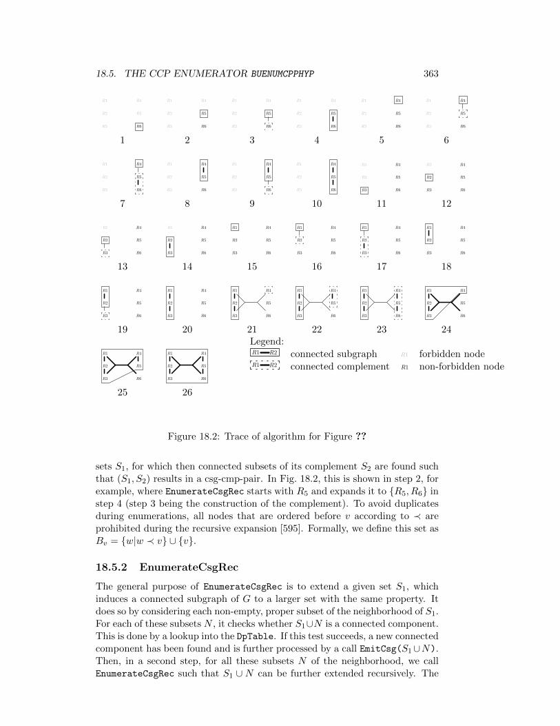
18.5. THE CCP ENUMERATOR BUENUMCPPHYP 363

. .

..

R1

R2

R3

R4

R5

R6

. .

..

R1

R2

R3

R4

R5

R6

. .

..

R1

R2

R3

R4

R5

R6

. .

..

R1

R2

R3

R4

R5

R6

. .

..

R1

R2

R3

R4

R5

R6

. .

..

R1

R2

R3

R4

R5

R6

1 2 3 4 5 6

. .

..

R1

R2

R3

R4

R5

R6

. .

..

R1

R2

R3

R4

R5

R6

. .

..

R1

R2

R3

R4

R5

R6

. .

..

R1

R2

R3

R4

R5

R6

. .

..

R1

R2

R3

R4

R5

R6

. .

..

R1

R2

R3

R4

R5

R6

7 8 9 10 11 12

. .

..

R1

R2

R3

R4

R5

R6

. .

..

R1

R2

R3

R4

R5

R6

. .

..

R1

R2

R3

R4

R5

R6

. .

..

R1

R2

R3

R4

R5

R6

. .

..

R1

R2

R3

R4

R5

R6

. .

..

R1

R2

R3

R4

R5

R6

13 14 15 16 17 18

. .

..

R1

R2

R3

R4

R5

R6

. .

..

R1

R2

R3

R4

R5

R6

. .

..

R1

R2

R3

R4

R5

R6

. .

..

R1

R2

R3

R4

R5

R6

. .

..

R1

R2

R3

R4

R5

R6

. .

..

R1

R2

R3

R4

R5

R6

19 20 21 22 23 24

. .

..

R1

R2

R3

R4

R5

R6

. .

..

R1

R2

R3

R4

R5

R6

Legend:R2R1 connected subgraph R1 forbidden nodeR2R1 connected complement R1 non-forbidden node

25 26

Figure 18.2: Trace of algorithm for Figure ??

sets S1, for which then connected subsets of its complement S2 are found suchthat (S1, S2) results in a csg-cmp-pair. In Fig. 18.2, this is shown in step 2, forexample, where EnumerateCsgRec starts with R5 and expands it to R5, R6 instep 4 (step 3 being the construction of the complement). To avoid duplicatesduring enumerations, all nodes that are ordered before v according to ≺ areprohibited during the recursive expansion [595]. Formally, we define this set asBv = w|w ≺ v ∪ v.

18.5.2 EnumerateCsgRec

The general purpose of EnumerateCsgRec is to extend a given set S1, whichinduces a connected subgraph of G to a larger set with the same property. Itdoes so by considering each non-empty, proper subset of the neighborhood of S1.For each of these subsets N , it checks whether S1∪N is a connected component.This is done by a lookup into the DpTable. If this test succeeds, a new connectedcomponent has been found and is further processed by a call EmitCsg(S1∪N).Then, in a second step, for all these subsets N of the neighborhood, we callEnumerateCsgRec such that S1 ∪ N can be further extended recursively. The

364CHAPTER 18. DYNAMIC PROGRAMMING-BASED PLANGENERATION

reason why we first call EmitCsg and then EnumerateCsgRec is that in orderto have an enumeration sequence valid for dynamic programming, smaller setsmust be generated first. Summarizing, the code looks as follows:

EnumerateCsgRec(S1, X)for each N ⊆ IN(S1, X): N 6= ∅

if DpTable[S1 ∪N ]6= ∅EmitCsg(S1 ∪N)

for each N ⊆ IN(S1, X): N 6= ∅EnumerateCsgRec(S1 ∪N,X ∪ IN(S1, X))

Take a look at step 12. This call was generated by BuEnumCcpHyp on S1 =R2. The neighborhood consists only of R3, since R1 is in X (R4, R5, R6

are not in X either, but not reachable). EnumerateCsgRec first calls EmitCsg,which will create the joinable complement (step 13). It then tests R2, R3for connectedness. The according DpTable entry was generated in step 13.Hence, this test succeeds, and R2, R3 is further processed by a recursive call toEnumerateCsgRec (step 14). Now the expansion stops, since the neighborhoodof R2, R3 is empty, because R1 ∈ X.

18.5.3 EmitCsg

EmitCsg takes as an argument a non-empty, proper subset S1 of V , whichinduces a connected subgraph. It is then responsible to generate the seeds forall S2 such that (S1, S2) becomes a csg-cmp-pair. Not surprisingly, the seedsare taken from the neighborhood of S1. All nodes that have ordered before thesmallest element in S1 (captured by the set Bmin(S1)) are removed from theneighborhood to avoid duplicate enumerations [595]. Since the neighborhoodalso contains min(v) for hyperedges (u, v) with |v| > 1, it is not guaranteed thatS1 is connected to v. To avoid the generation of false csg-cmp-pairs, EmitCsgchecks for connectedness. However, each single neighbor might be extended toa valid complement S2 of S1. Hence, no such test is necessary before callingEnumerateCmpRec, which performs this extension. The pseudocode looks asfollows:

EmitCsg(S1)X = S1 ∪Bmin(S1)

N = IN(S1, X)for each v ∈ N descending according to ≺

S2 = vif ∃(u, v) ∈ E : u ⊆ S1 ∧ v ⊆ S2

EmitCsgCmp(S1, S2)EnumerateCmpRec(S1, S2, X ∪Bv(N))

where Bv(W ) = w|w ∈W,w ≤ v is defined as in Section 3.2.4 for DPccp.Take a look at step 20. The current set S1 is S1 = R1, R2, R3, and the

neighborhood is IN = R4. As there is no hyperedge connecting these two

18.5. THE CCP ENUMERATOR BUENUMCPPHYP 365

sets, there is no call to EmitCsgCmp. However, the set R4 can be extendedto a valid complement, namely R4, R5, R6. Properly extending the seeds ofcomplements is the task of the call to EnumerateCmpRec in step 21.

18.5.4 EnumerateCmpRec

EnumerateCsgRec has three parameters. The first parameter S1 is only usedto pass it to EmitCsgCmp. The second parameter is a set S2 which is connect-ed and must be extended until a valid csg-cmp-pair is reached. Therefore, itconsiders the neighborhood of S2. For every non-empty, proper subset N ofthe neighborhood, it checks whether S2 ∪N induces a connected subset and isconnected to S1. If so, we have a valid csg-cmp-pair (S1, S2) and can start planconstruction (done in EmitCsgCmp). Irrespective of the outcome of the test, werecursively try to extend S2 such that this test becomes successful. Overall, theEnumerateCmpRec behaves very much like EnumerateCsgRec. Its pseudocodelooks as follows:

EnumerateCmpRec(S1, S2, X)for each N ⊆ IN(S2, X): N 6= ∅

if DpTable[S2 ∪N ]6= ∅ ∧∃(u, v) ∈ E : u ⊆ S1 ∧ v ⊆ S2 ∪N

EmitCsgCmp(S1, S2 ∪N)X = X ∪ IN(S2, X)for each N ⊆ IN(S2, X): N 6= ∅

EnumerateCmpRec(S1, S2 ∪N,X)

Take a look at step 21 again. The parameters are S1 = R1, R2, R3 andS2 = R4. The neighborhood consists of the single relation R5. The setR4, R5 induces a connected subgraph. It was inserted into DpTable in step 6.However, there is no hyperedge connecting it to S1. Hence, there is no call toEmitCsgCmp. Next is the recursive call in step 22 with S2 changed to R4, R5.Its neighborhood is R6. The set R4, R5, R6 induces a connected subgraph.The according test via a lookup into DpTable succeeds, since the accordingentry was generated in step 7. The second part of the test also succeeds, as ouronly true hyperedge connects this set with S1. Hence, the call to EmitCsgCmp

in step 23 takes place and generates the plans containing all relations.

18.5.5 EmitCsgCmp

The procedure EmitCsgCmp(S1,S2) is called for every S1 and S2 such that(S1, S2) forms a csg-cmp-pair. It is the (call back) interface for BuEnumCcpHyp.Its only task is to call BuildPlan, which then builds the optimal plan(s) for(S1, S2).

18.5.6 Neighborhood Calculation

The formulation of neighborhood we used, is only one possibility. In fact, anyneighborhood satisfying the following condition will do. Let G = (V,E) be a

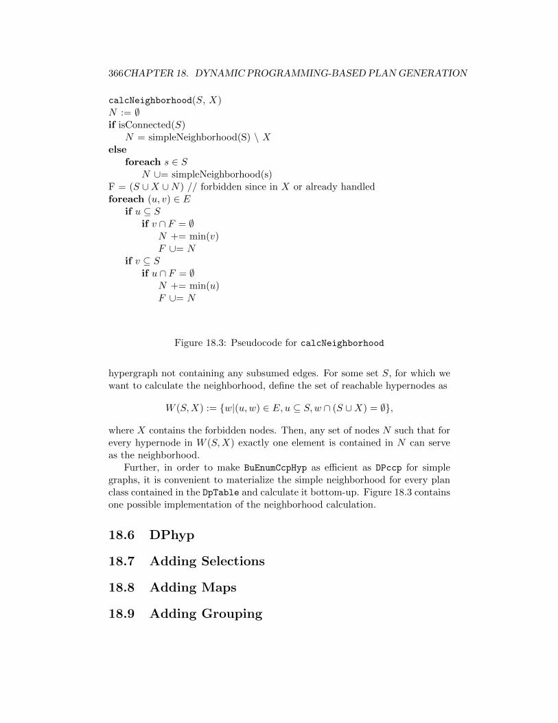
366CHAPTER 18. DYNAMIC PROGRAMMING-BASED PLANGENERATION

calcNeighborhood(S, X)N := ∅if isConnected(S)

N = simpleNeighborhood(S) \ Xelse

foreach s ∈ SN ∪= simpleNeighborhood(s)

F = (S ∪X ∪N) // forbidden since in X or already handledforeach (u, v) ∈ E

if u ⊆ Sif v ∩ F = ∅

N += min(v)F ∪= N

if v ⊆ Sif u ∩ F = ∅

N += min(u)F ∪= N

Figure 18.3: Pseudocode for calcNeighborhood

hypergraph not containing any subsumed edges. For some set S, for which wewant to calculate the neighborhood, define the set of reachable hypernodes as

W (S,X) := w|(u,w) ∈ E, u ⊆ S,w ∩ (S ∪X) = ∅,

where X contains the forbidden nodes. Then, any set of nodes N such that forevery hypernode in W (S,X) exactly one element is contained in N can serveas the neighborhood.

Further, in order to make BuEnumCcpHyp as efficient as DPccp for simplegraphs, it is convenient to materialize the simple neighborhood for every planclass contained in the DpTable and calculate it bottom-up. Figure 18.3 containsone possible implementation of the neighborhood calculation.

18.6 DPhyp

18.7 Adding Selections

18.8 Adding Maps

18.9 Adding Grouping

Chapter 19

Optimizing Queries withDisjunctions

19.1 Introduction

Simple rewrites as indicated in Section ?? for IN and OR predicates that boildown to comparisons of a column with a set of constants can eliminate disjunc-tion from the plan or push it into a multirange index access.

Another possibility that can be used for disjunctions on single columns isto use DISJOINT UNION of plans. This is a special form of UNION whereconditions ensure that no phantom duplicates are produced. The DISJOINTUNION operator merely concatenates the result tables without any furtheroverhead like duplicate elimination.

For example a predicate of the form x = c1 or y = c2 where x and y arecolumns of the same table results in two predicates

1. x = c1

2. x <> c1 AND y = c2

Obviously, no row can satisfy both conditions. Hence, the query select *

from R where x = c1 or y = c2 can be safely rewritten to

(select * from R where x = c1) DISJOINT UNION (select * from

R where x <> c1 AND y = c2

In case there are indexes on x and y efficient plans do exist. If they don’t thetable R needs to be scanned twice. This problem is avoided by using bypassplans.

DISJOIN UNIONs can also be used for join predicates. Consider the follow-ing example query: select * from R, S where R.a = S.a OR R.b = S.a Thisquery can be rewritten to (select * from R, S where R.a = S.a) DISJOINT

UNION (select * from R, S where R.a <> S.a and R.b = S.b) The gen-eral condition here is that all equality predicates have one side identical. Notethat both tables are scanned and joined twice. Bypass plans will eliminate thisproblem.

367

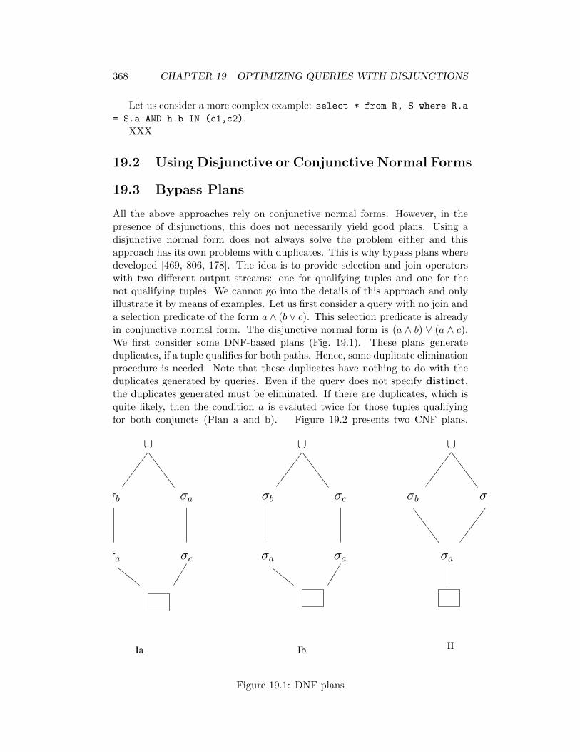
368 CHAPTER 19. OPTIMIZING QUERIES WITH DISJUNCTIONS

Let us consider a more complex example: select * from R, S where R.a

= S.a AND h.b IN (c1,c2).XXX

19.2 Using Disjunctive or Conjunctive Normal Forms

19.3 Bypass Plans

All the above approaches rely on conjunctive normal forms. However, in thepresence of disjunctions, this does not necessarily yield good plans. Using adisjunctive normal form does not always solve the problem either and thisapproach has its own problems with duplicates. This is why bypass plans wheredeveloped [469, 806, 178]. The idea is to provide selection and join operatorswith two different output streams: one for qualifying tuples and one for thenot qualifying tuples. We cannot go into the details of this approach and onlyillustrate it by means of examples. Let us first consider a query with no join anda selection predicate of the form a ∧ (b ∨ c). This selection predicate is alreadyin conjunctive normal form. The disjunctive normal form is (a ∧ b) ∨ (a ∧ c).We first consider some DNF-based plans (Fig. 19.1). These plans generateduplicates, if a tuple qualifies for both paths. Hence, some duplicate eliminationprocedure is needed. Note that these duplicates have nothing to do with theduplicates generated by queries. Even if the query does not specify distinct,the duplicates generated must be eliminated. If there are duplicates, which isquite likely, then the condition a is evaluted twice for those tuples qualifyingfor both conjuncts (Plan a and b). Figure 19.2 presents two CNF plans.

IbII

Ia

∪ ∪ ∪

σb σb σb

σa σa σaσc

σc σcσa

σa

Figure 19.1: DNF plans

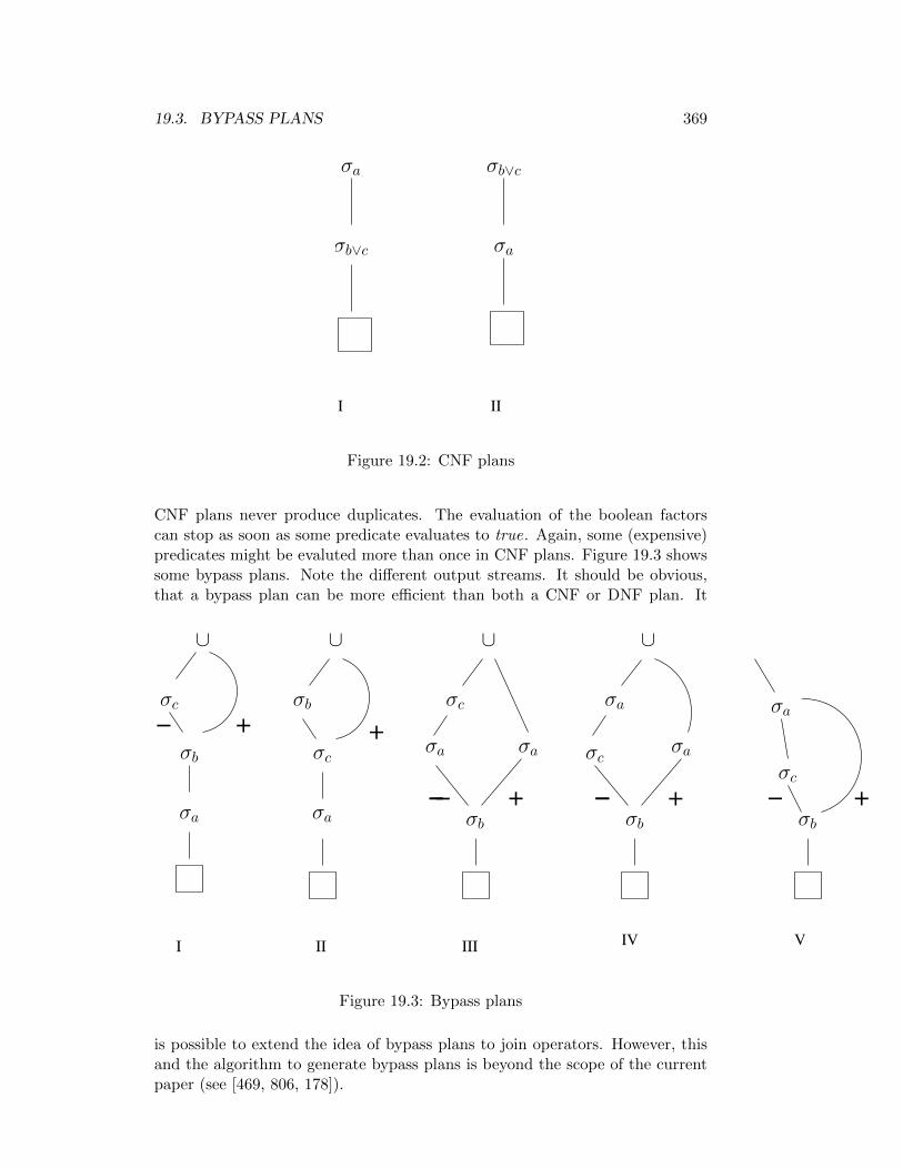
19.3. BYPASS PLANS 369

I II

σa

σaσb∨c

σb∨c

Figure 19.2: CNF plans

CNF plans never produce duplicates. The evaluation of the boolean factorscan stop as soon as some predicate evaluates to true. Again, some (expensive)predicates might be evaluted more than once in CNF plans. Figure 19.3 showssome bypass plans. Note the different output streams. It should be obvious,that a bypass plan can be more efficient than both a CNF or DNF plan. It

I II IIIIV V

−− −−− −+ +

+− +

+

∪ ∪ ∪ ∪

σa σa

σaσa

σa

σa

σa

σb

σb

σb σb σb

σc

σc

σc

σcσc

Figure 19.3: Bypass plans

is possible to extend the idea of bypass plans to join operators. However, thisand the algorithm to generate bypass plans is beyond the scope of the currentpaper (see [469, 806, 178]).

370 CHAPTER 19. OPTIMIZING QUERIES WITH DISJUNCTIONS

19.4 Implementation remarks

The internal representation of execution plans during plan generation typicallydiffers from that used in Rewrite I. The reason is that many plans have to begenerated and space efficiency is a major concern. As in the query representa-tion discussed earlier, the physical algebraic operators can be organized into ahierarchy. Besides their arguments, they possibly contain backpointers to theoriginal query representation (e.g. for predicates). Sharing is a must for plangeneration. Hence, subplans are heavily shared. The plan nodes are enhancedby so-called property vectors. These contain information about the plan:

• logical information

– the set of relations joined

– the set of predicates applied so far

– the set of IUs computed so far

– order information

• physical information

– costs

– cardinality information

For fast processing, the first three set-valued items in the logical informationblock are represented as bit-vectors. However, the problem is that an upperbound on the size of these bitvectors is not reasonable. Hence, they are ofvariant size. It is recommendable, to have a plan node factory that generatesplan nodes of different length such that the bit-vectors are included in the plannode. A special interpreter class then knows the offsets and lengths of thedifferent bitvectors and supplies the operations needed to deal with them. Thisbit-vector interpreter can be attached to the plan generator’s control block asindicated in Fig. 25.3.

19.5 Other plan generators/query optimizer

There are plenty of other query optimizers described in the literatur. Some ofmy personal favorites not mentioned so far are the Blackboard query optimzer[468], the Epoq optimizer [589, 588], the Genesis optimizer [56, 61], the Gralquery optimizer [66], the Lanzelotte query optimizer [508, 509, 510], the Orionoptimizer [49, 50, 473], the Postgres optimizer [450, 386, 384, 385], the Primaoptimizer [390, 388], the Probe optimizer [214, 213, 628], the Straube optimizer[821, 856, 818, 819, 817, 820]. Highly recommended is a description of the DB2query optimizer(s) [311].

Also interesting to read is the first proposal for a rule-based query optimizercalled Squirel [794] and other proposals for rule-based query optimizers [285,751, 466, 465, 558].

19.6. BIBLIOGRAPHY 371

19.6 Bibliography

Disjunctive queries: P. Ciaccia and M. Scalas: Optimization Strategy for Re-lational Queries. IEEE Transaction on Software Engineering 15 (10), pp 1217-1235, 1989.

Kristofer Vorwerk, G. N. Paulley: On Implicate Discovery and Query Op-timization. International Database Engineering and Applications Symposium(IDEAS’02)

Jack Minker, Rita G. Minker: Optimization of Boolean Expressions-HistoricalDevelopments. IEEE Annals of the History of Computing 2 (3), pp 227-238,1980.

Chaudhuri: SIGMOD 03: [143]Conjunctive Queries, Branch Minimization: [713]Also Boolean Difference Calculus (?): [795]

372 CHAPTER 19. OPTIMIZING QUERIES WITH DISJUNCTIONS

Chapter 20

Generating Plans for the FullAlgebra

373

374 CHAPTER 20. GENERATING PLANS FOR THE FULL ALGEBRA

Chapter 21

Generating DAG-structuredPlans

@misc roy-optimization,

author = "Prasan Roy",

title = "Optimization of DAG-Structured Query Evaluation Plans",

url = "citeseer.nj.nec.com/roy98optimization.html"

375

376 CHAPTER 21. GENERATING DAG-STRUCTURED PLANS

Chapter 22

Simplifying the Query Graph

[This chapter was written by Thomas Neumann]

22.1 Introduction

As we have seen in Chapter 3, computing the the optimal join for large queries isa very hard problem. Most hand-written queries join just a few (<15) relations,but in general join queries can become quite large: Some systems like SAP R/3store their data in thousands of relations, and subsequently generate large joinqueries. Other examples include data warehousing, where a fact table is joinedwith a large number of dimension tables, forming a star join, and databases thatmake heavy use of views to simplify query formulation (where the views thenimplicitly add joins). Existing database management systems have difficultiesoptimizing very large join queries, falling back to heuristics when they cannotsolve them exactly anymore. This is unfortunate, as it does not offer a smoothtransition. Ideally, one would optimize a query as much as possible under giventime constraints.

When optimizing join queries, the optimal join order is usually determinedusing some variant of dynamic programming (DP). However finding the opti-mal join is NP-hard in general, which means that large join queries becomeintractable at some point. On the other hand, the complexity of the problemdepends heavily upon the structure of the query (see Chapter 3), where somequeries can be optimized exactly even for a large number of relations whileother queries quickly become too difficult. As computing the optimal join orderbecomes intractable at some point, the standard technique of handling largejoin queries resorts to some heuristics. Some commercial database systems firsttry to solve the problem exactly using DP, and then fall back to greedy heuris-tics when they run out memory. As we have seen in Chapter 3, a wide rangeof heuristics has been proposed in the literature. Most of them integrate somekind of greedy processing in the optimization process, greedily building execu-tion plan fragments that seem plausible. The inherent problem of this approachis that it is quite likely to greedily make a decision that one would regret hav-ing more information about the complete execution plan. For example greedilydeciding which two relations should be joined first is very hard, as it depends

377

378 CHAPTER 22. SIMPLIFYING THE QUERY GRAPH

on all other joins involved in the query.

Here, we follow a different approach presented in [?]: If a query is toocomplex to optimize exactly, we simplify it using a greedy heuristic until itbecomes tractable using DP. The simplification step does not build executionplans but modifies the join graph of the query to make it more restrictive,ruling out join orders that it considers unlikely. In a way this is the oppositeof the standard greedy plan building techniques: Instead of greedily choosingjoins (which is very hard), we choose joins that must be avoided. The greatadvantage of this approach is that we can start with the ’easy’ decisions (i.e.,the relatively obvious ones) using the heuristic and then leave the hard executionplan building to the DP algorithm once the problem is simplified enough. Theresulting optimization algorithm adapts naturally to the query complexity andthe given time budget, simplifying the query just as much as needed and thenoptimizing the simplified query exactly.

22.2 On Optimizing Join Queries

Optimizing the join order is one of the most important steps of query optimiza-tion, as changes in the join order can affect the query execution times by ordersof magnitudes. Unfortunately computing the optimal join order is NP-hard ingeneral, and the standard technique of using dynamic programming fails if thequery is large enough.

Still, there are large differences in problem complexity even for queries of thesame size. When disregarding cross products, the join predicates included in thequery induce a query graph, and the structure of that query graph determinesthe complexity of the problem. Clique queries for example, where there is a joinpredicate between any two relations involved in the query, are the worst-casescenario for join ordering. Here any combination of relations is joinable, all joinsaffect each other through redundant join edges, and both the space complexityand the runtime complexity of the best known algorithm increases exponentially(in the order of O(2n) and O(4n), where n is the number of relations). For cliquequeries there is little hope of ever finding a good algorithm, but fortunately largeclique queries never occur in practice. Chain queries on the other hand, whererelations are joined sequentially, are quite common in practice and much easierto optimize: Any join tree without cross products must only consist of relationsthat are neighboring in the chain, i.e., that form a subchain. As there are lessthan n2 subchains of a chain of length n, and we can join a subchain only withless than n other (neighboring) subchains, we get a space complexity of O(n2)and a time complexity of O(n3). Other graph structures are between these twoextremes. Star queries, which are common in data warehouse applications wheredimension tables are joined to a central fact table, have a space complexity ofO(2n) and a time complexity of O(n2n).

The practical impact of these complexity differences can be seen in Fig-ure 22.1. It shows the optimization time using DPhyp and the setup discussedin Section [?]. One observation here is that while small queries (<10 relations)can be optimized quickly regardless of the graph structure, larger queries soon

22.3. GRAPH SIMPLIFICATION ALGORITHM 379

1

10

100

1000

10000

100000

1e+06

1e+07

1e+08

1e+09

4 6 8 10 12 14 16 18 20

optim

izat

ion

time

[ms]

number of relations

chainscycles

starsgrids

cliques

Figure 22.1: Runtimes for Different Query Graphs

become too expensive for everything except chain and cycle queries. Cliquequeries are particular bad, of course, but even the data warehousing star queriesare too complex relatively soon. For really large queries (e.g., 50 relations),finding the optimal solution using DP is out of question for most query types.

Now the basic idea of graph simplification stems from the fact that somegraph easier to solve than others: If the problem is too difficult to solve exactly,we change the query graph to make it easier to solve. We will look at thissimplification strategy in the next section.

22.3 Graph Simplification Algorithm

After examining the impact of the query graph structure on optimization time,we now study an algorithm to simplify the query graph as much as needed toallow for a dynamic programming solution. We first discuss the simplificationitself, then how this can be used to simplify a query graph as much as needed,and then one edge selection heuristic (which is orthogonal to the main simpli-fication algorithm). Finally we show that the approach is plausible by provingoptimality for star queries and certain classes of cost functions.

During this section we assume that the query has been brought into properquery (hyper-)graph form. In particular we assume that all non-inner joins havebeen expressed as hyperedges, as suggested in [?]. This allows us to reason aboutgraph structures alone without violating proper query semantics.

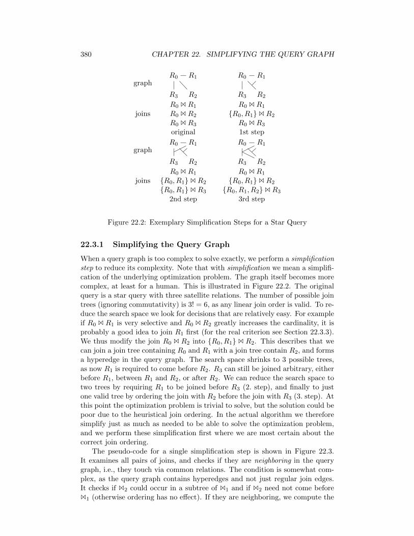
380 CHAPTER 22. SIMPLIFYING THE QUERY GRAPH

graphR0 R1

R3 R2

R0 R1

R3 R2

R0 BR1 R0 BR1

joins R0 BR2 R0, R1BR2

R0 BR3 R0 BR3

original 1st step

graphR0 R1

R3 R2

R0 R1

R3 R2

R0 BR1 R0 BR1

joins R0, R1BR2 R0, R1BR2

R0, R1BR3 R0, R1, R2BR3

2nd step 3rd step

Figure 22.2: Exemplary Simplification Steps for a Star Query

22.3.1 Simplifying the Query Graph

When a query graph is too complex to solve exactly, we perform a simplificationstep to reduce its complexity. Note that with simplification we mean a simplifi-cation of the underlying optimization problem. The graph itself becomes morecomplex, at least for a human. This is illustrated in Figure 22.2. The originalquery is a star query with three satellite relations. The number of possible jointrees (ignoring commutativity) is 3! = 6, as any linear join order is valid. To re-duce the search space we look for decisions that are relatively easy. For exampleif R0 B R1 is very selective and R0 B R2 greatly increases the cardinality, it isprobably a good idea to join R1 first (for the real criterion see Section 22.3.3).We thus modify the join R0 B R2 into R0, R1 B R2. This describes that wecan join a join tree containing R0 and R1 with a join tree contain R2, and formsa hyperedge in the query graph. The search space shrinks to 3 possible trees,as now R1 is required to come before R2. R3 can still be joined arbitrary, eitherbefore R1, between R1 and R2, or after R2. We can reduce the search space totwo trees by requiring R1 to be joined before R3 (2. step), and finally to justone valid tree by ordering the join with R2 before the join with R3 (3. step). Atthis point the optimization problem is trivial to solve, but the solution could bepoor due to the heuristical join ordering. In the actual algorithm we thereforesimplify just as much as needed to be able to solve the optimization problem,and we perform these simplification first where we are most certain about thecorrect join ordering.

The pseudo-code for a single simplification step is shown in Figure 22.3.It examines all pairs of joins, and checks if they are neighboring in the querygraph, i.e., they touch via common relations. The condition is somewhat com-plex, as the query graph contains hyperedges and not just regular join edges.It checks if B2 could occur in a subtree of B1 and if B2 need not come beforeB1 (otherwise ordering has no effect). If they are neighboring, we compute the

22.3. GRAPH SIMPLIFICATION ALGORITHM 381

SimplifyGraph(G = (V,E))j1 = ∅, j2 = ∅, M = −∞// Find the most beneficial simplificationfor each SL1 B1 S

R1 ∈ E

for each SL2 B2 SR2 ∈ E, B1 6= B2

// Does B1 neighbor B2?if ((SL2 ⊆ SL1 ∨ SR2 ⊆ SL1 ) ∧ (SL2 ∪ SR2 6⊆ SL1 ))∨

((SL2 ⊆ SR1 ∨ SR2 ⊆ SR1 ) ∧ (SL2 ∪ SR2 6⊆ SR1 ))b =orderingBenefit(SL1 B1 S

R1 ,SL2 B2 S

R2 )

if b > M ∧ (B2 could be ordered before B1)j1 = SL1 B1 S

R1 , j2 = SL2 B2 S

R2 , M = b

// No further simplification possible?if j1 = ∅ return G// Order j2 = SL2 B2 S

R2 before j1 = SL1 B1 S

R1

if (SL2 ⊆ SL1 ∨ SR2 ⊆ SL1 ) ∧ (SL2 ∪ SR2 6⊆ SL1 ))return (V,E \ j1 ∪ (SL1 ∪ SL2 ∪ SR2 ) B1 S

R1 )

elsereturn (V,E \ j1 ∪ SL1 B1 (SR1 ∪ SL2 ∪ SR2 ))

Figure 22.3: Pseudo-Code for a Single Simplification Step

expected benefit of ordering B2 before B1. The implementation of ordering-Benefit is orthogonal to the simplification itself, it should predict how likely itis that B2 must come before B1 (see Section 22.3.3). We restrict ourselves toordering neighboring joins as it is hard to make useful predictions about arbi-trary unrelated joins. Note that through a series of simplification steps the joinneighborhoods increase, such that the algorithm can ultimately order all joinsif needed. The algorithm remembers the join pair (j1, j2) with the maximumestimated benefit, and modifies the query graph such that j2 must come beforej1. This creates an hyperedge in the query graph, as now j1 ’requires’ all rela-tions involved in j2 to guarantee the ordering, effectively shrinking the searchspace.

A detail of the pseudo-code not discussed yet is the condition ’B2 could beordered before B1’ in the first loop. So far we have assumed that it is indeedpossible to order B2 before B1, but this might not be the case: First, the querymight contain non-inner joins, which are not freely reorderable. Second, if thequery is cyclic, a series of simplification steps could lead to a contradiction,demanding (transitively) that B1 must come before B2 and B2 before B1. Toavoid this, we build a partial ordering of joins as a directed graph, deriving theinitial one from the original query hypergraph and then ordering the joins asindicated by the simplification step. The condition ’B2 could be ordered beforeB1’ is effectively a check if an edge B2 → B1 would create a cycle in our graph.

In general the performance of SimplifyGraph can be improved significantlyby maintaining proper data structures. As we will see in the next section, thealgorithm is applied repeatedly to simplify a query graph, thus it pays off toremember already computed results. We therefore materialize all neighbors of a

382 CHAPTER 22. SIMPLIFYING THE QUERY GRAPH

join, and update the neighbors when a join is modified. Further, we rememberthe estimated benefit for each neighbor, and keep all joins in a priority queueordered by the maximum benefit they can get from ordering a neighbor. Thiseliminates the two nested loops in the algorithm, and greatly improves runtime.

22.3.2 The Full Algorithm

The full algorithms works in two phases: First, it repeatedly performs sim-plification steps until the problem complexity has decreased enough, and thenit runs a dynamic programming algorithm to find the optimal solution for thesimplified graph. To check if the graph has been simplified enough, we can reusethe DPccp algorithm [?], where the complexity of the dynamic programmingalgorithm depends on the number of connected subgraphs in the query graph.More precisely, the number of connected subgraphs is identical to the size ofthe DP table after the optimization is finished. We can therefore simplify thequery graph until the number of connected subgraphs decreased sufficiently.

Counting the number of connected subgraphs is not that trivial, but analgoruthm follows naturally from graph-based query optimization: The DPhypalgorithm [?] solves the join ordering problem by enumerating all connectedsubgraphs of the query graph and joining them with all connected subgraphsthat are disjoint from but connected to the first subgraph. By simply eliminat-ing the enumeration of the second subgraph we get an algorithm that producesall connected subgraphs. Note that the algorithm does not have to fill a DPtable, as we are only interested in the number of connected subgraphs, and wecan stop as soon as we have enumerated more than our maximum number ofconnected subgraphs. Howver, enumerating 10,000 subgraphs in a query graphwith 100 relations takes roughly 5ms. This means that while checking the prob-lem complexity is not that expensive, we cannot afford to check it after eachsimplifications step, as there may be thousands of simplification steps.

The full algorithm therefore operates as depicted in Figure 22.4. It is in-voked by giving a query graph G and a maximum complexity budget b. Itfirst generates all possible simplifications G by applying the SimplifyGraph steprepeatedly. The complexity of these graphs decreases monotonically, as eachsimplification step adds more restrictions. Then, it performs a binary searchover the list of graphs, and computes the complexity just for the currently ex-amined graph. The graph with the least number of simplification steps thathas a complexity ≤ b is stored in Gb. Note that Gb could be equal to G, i.e.,the original problem, if the graph is simple enough. After the binary search,the optimal solution for Gb is computed by using DPhyp [?].

Again the pseudo-code is simplified. In particular it is not advisable to re-ally materialize all query graphs in G, as this becomes noticeably expensive forqueries with more than 50 relations. Instead, we just remember the two joins(j1, j2) selected for merging by the SimplifyGraph step. Then we materializethe graphs examined by the binary search by replaying the merge steps basedupon these (j1, j2) values relative to the last materialized graph. Using thesetechniques, the full algorithm (including the final DPhyp call) takes less thanone second for a star query with 50 relations and a complexity budget of 10, 000

22.3. GRAPH SIMPLIFICATION ALGORITHM 383

GraphSimplificationOptimizer(G = (V,E),b)// Input: A query graph G and a complexity budget b// Output: The best plan found under the budget b

// Compute all possible simplification stepsG = a list of query graphs, G′ = Gdo

append G′ to GG = G′, G′ =SimplifyGraph(G)

while G 6= G′

// Use binary search to find the necessary simplificationsl = 0, r = |G|, v = r,Gb = G[r − 1]while l < r

m = b l+r2 cc =#connected subgraphs in G[m] (count at most b+ 1)if c > bl = c+ 1

elser = cif c < vv = c,Gb = G[m]

// Solve the simplified graphreturn DPhyp(Gb)

Figure 22.4: The Full Optimization Algorithm

in experiments [?]. Note that we can even avoid generating all possible mergesteps: By using search techniques for unbounded search (e.g., [?]) we can gen-erate merging steps as required by the search strategy. This does not changethe asymptotic complexity, but it is more efficient if most queries require fewor no simplification steps (which is probably the case in practice).

22.3.3 Join Ordering Criterion

So far we have assumed that the simplification algorithm can somehow estimatethe benefit of ordering B2 before B1. In principle this is orthogonal to thesimplification algorithm, and different kinds of ordering criterion could be used.The experiments in [?] used the following estimation function, which comparesthe relative costs of the join orders, and gave very good results:

orderingBenefit(X B1 R1, X B2 R2) =C((X B1 R1) B2 R2)

C((X B2 R2) B1 R1)

The rational here is that if joining first R2 and then R1 is orders of magni-tude cheaper than first joining R1 and then R2, it is very likely that the joinwith R2 will come before the join with R1 in the optimal solution, regardless ofthe other relations involved. As the simplification algorithms orders the highest

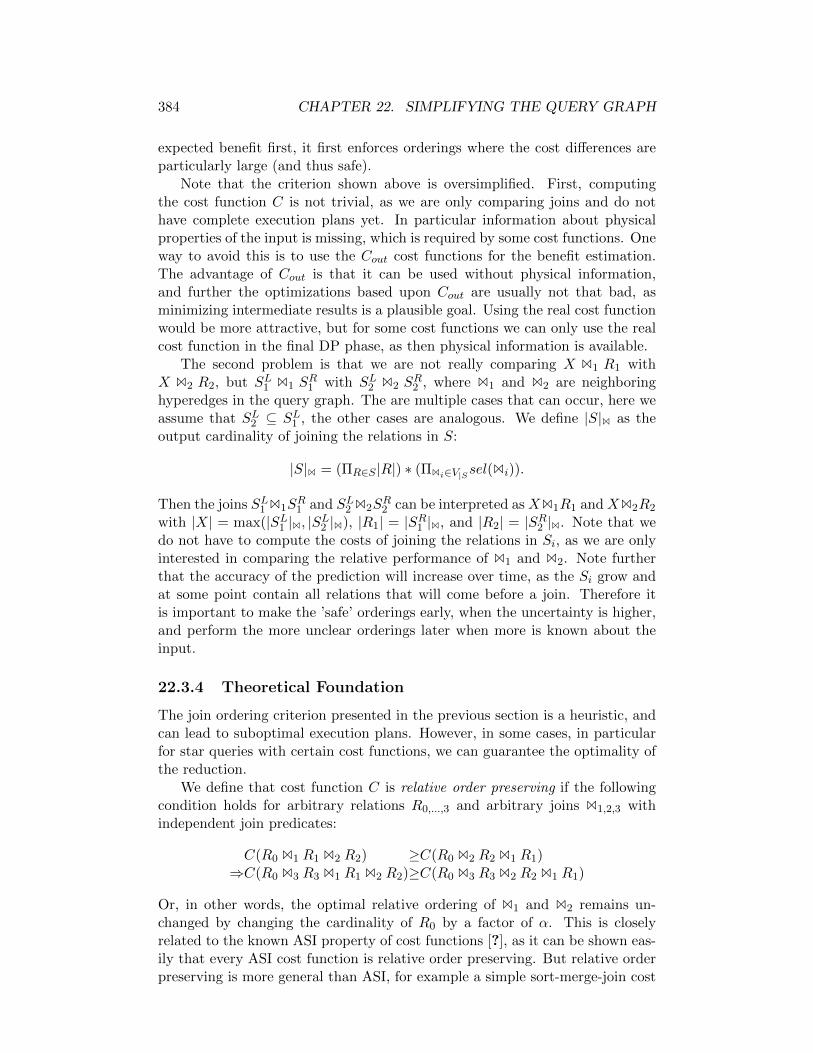
384 CHAPTER 22. SIMPLIFYING THE QUERY GRAPH

expected benefit first, it first enforces orderings where the cost differences areparticularly large (and thus safe).

Note that the criterion shown above is oversimplified. First, computingthe cost function C is not trivial, as we are only comparing joins and do nothave complete execution plans yet. In particular information about physicalproperties of the input is missing, which is required by some cost functions. Oneway to avoid this is to use the Cout cost functions for the benefit estimation.The advantage of Cout is that it can be used without physical information,and further the optimizations based upon Cout are usually not that bad, asminimizing intermediate results is a plausible goal. Using the real cost functionwould be more attractive, but for some cost functions we can only use the realcost function in the final DP phase, as then physical information is available.

The second problem is that we are not really comparing X B1 R1 withX B2 R2, but SL1 B1 S

R1 with SL2 B2 S

R2 , where B1 and B2 are neighboring

hyperedges in the query graph. The are multiple cases that can occur, here weassume that SL2 ⊆ SL1 , the other cases are analogous. We define |S|B as theoutput cardinality of joining the relations in S:

|S|B = (ΠR∈S |R|) ∗ (ΠBi∈V|Ssel(Bi)).

Then the joins SL1 B1SR1 and SL2 B2S

R2 can be interpreted as XB1R1 and XB2R2

with |X| = max(|SL1 |B, |SL2 |B), |R1| = |SR1 |B, and |R2| = |SR2 |B. Note that wedo not have to compute the costs of joining the relations in Si, as we are onlyinterested in comparing the relative performance of B1 and B2. Note furtherthat the accuracy of the prediction will increase over time, as the Si grow andat some point contain all relations that will come before a join. Therefore itis important to make the ’safe’ orderings early, when the uncertainty is higher,and perform the more unclear orderings later when more is known about theinput.

22.3.4 Theoretical Foundation

The join ordering criterion presented in the previous section is a heuristic, andcan lead to suboptimal execution plans. However, in some cases, in particularfor star queries with certain cost functions, we can guarantee the optimality ofthe reduction.

We define that cost function C is relative order preserving if the followingcondition holds for arbitrary relations R0,...,3 and arbitrary joins B1,2,3 withindependent join predicates:

C(R0 B1 R1 B2 R2) ≥C(R0 B2 R2 B1 R1)⇒C(R0 B3 R3 B1 R1 B2 R2)≥C(R0 B3 R3 B2 R2 B1 R1)

Or, in other words, the optimal relative ordering of B1 and B2 remains un-changed by changing the cardinality of R0 by a factor of α. This is closelyrelated to the known ASI property of cost functions [?], as it can be shown eas-ily that every ASI cost function is relative order preserving. But relative orderpreserving is more general than ASI, for example a simple sort-merge-join cost

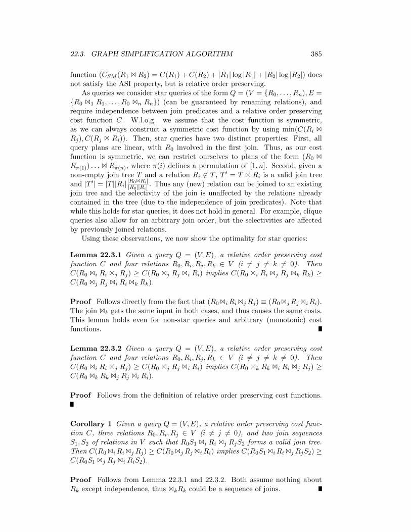
22.3. GRAPH SIMPLIFICATION ALGORITHM 385

function (CSM (R1 B R2) = C(R1) + C(R2) + |R1| log |R1|+ |R2| log |R2|) doesnot satisfy the ASI property, but is relative order preserving.

As queries we consider star queries of the form Q = (V = R0, . . . , Rn), E =R0 B1 R1, . . . , R0 Bn Rn) (can be guaranteed by renaming relations), andrequire independence between join predicates and a relative order preservingcost function C. W.l.o.g. we assume that the cost function is symmetric,as we can always construct a symmetric cost function by using min(C(Ri BRj), C(Rj B Ri)). Then, star queries have two distinct properties: First, allquery plans are linear, with R0 involved in the first join. Thus, as our costfunction is symmetric, we can restrict ourselves to plans of the form (R0 B

Rπ(1)) . . . B Rπ(n), where π(i) defines a permutation of [1, n]. Second, given anon-empty join tree T and a relation Ri 6∈ T , T ′ = T B Ri is a valid join treeand |T ′| = |T ||Ri| |R0BRi|

|R0||Ri| . Thus any (new) relation can be joined to an existingjoin tree and the selectivity of the join is unaffected by the relations alreadycontained in the tree (due to the independence of join predicates). Note thatwhile this holds for star queries, it does not hold in general. For example, cliquequeries also allow for an arbitrary join order, but the selectivities are affectedby previously joined relations.

Using these observations, we now show the optimality for star queries:

Lemma 22.3.1 Given a query Q = (V,E), a relative order preserving costfunction C and four relations R0, Ri, Rj , Rk ∈ V (i 6= j 6= k 6= 0). ThenC(R0 Bi Ri Bj Rj) ≥ C(R0 Bj Rj Bi Ri) implies C(R0 Bi Ri Bj Rj Bk Rk) ≥C(R0 Bj Rj Bi Ri Bk Rk).

Proof Follows directly from the fact that (R0BiRiBjRj) ≡ (R0BjRjBiRi).The join Bk gets the same input in both cases, and thus causes the same costs.This lemma holds even for non-star queries and arbitrary (monotonic) costfunctions.

Lemma 22.3.2 Given a query Q = (V,E), a relative order preserving costfunction C and four relations R0, Ri, Rj , Rk ∈ V (i 6= j 6= k 6= 0). ThenC(R0 Bi Ri Bj Rj) ≥ C(R0 Bj Rj Bi Ri) implies C(R0 Bk Rk Bi Ri Bj Rj) ≥C(R0 Bk Rk Bj Rj Bi Ri).

Proof Follows from the definition of relative order preserving cost functions.

Corollary 1 Given a query Q = (V,E), a relative order preserving cost func-tion C, three relations R0, Ri, Rj ∈ V (i 6= j 6= 0), and two join sequencesS1, S2 of relations in V such that R0S1 Bi Ri Bj RjS2 forms a valid join tree.Then C(R0 BiRiBj Rj) ≥ C(R0 Bj RjBiRi) implies C(R0S1 BiRiBj RjS2) ≥C(R0S1 Bj Rj Bi RiS2).

Proof Follows from Lemma 22.3.1 and 22.3.2. Both assume nothing aboutRk except independence, thus BkRk could be a sequence of joins.

386 CHAPTER 22. SIMPLIFYING THE QUERY GRAPH

Theorem 1 Given a star query Q = (V,E) and a relative order preserving costfunction C. Then for any optimal optimal join tree T and pairs of relationsRi, Rj neighbored in T (i.e., T has the form R0S1 Bi RiBj RjS2) the followingcondition holds: Either C(R0 Bi Ri Bj Rj) ≤ C(R0 Bj Rj Bi Ri) or T ′ =R0S1 Bj Rj Bi RiS2 is optimal, too.

Proof By contradiction. We assume that C(R0BiRiBjRj) > C(R0BjRjBiRi)and T ′ is not optimal. By Corollary 1 we can deduce that C(R0 BiRiBj Rj) >C(R0BjRjBiRi)⇒ C(T ′) = C(R0S1BjRjBiRiS2) ≤ C(R0S1BiRiBiRiS2) =C(T ). This is a contradiction to the assumption that T ′ is not optimal

This theorem is a strong indication that our simplification algorithm is plau-sible, as we know that one of the optimal solutions will satisfy the ordering con-straints used by the algorithm. Unfortunately the authors of [?] were only ableto prove the optimality by restricting the cost function some more (perhaps un-necessarily): A cost function C is fully relative order preserving if it is relativeorder preserving and the following condition holds for arbitrary relations R0,...,3

and arbitrary joins B1,2,3 with independent join predicates: C(R0B1R1B2R2) ≥C(R0 B2 R2 B1 R1) ⇒ C(R0 B1 R1 B3 R3 B2 R2) ≥ C(R0 B2 R2 B3 R3 B1 R1).Again, this property is satisfied by all ASI cost functions. Using this definition,we can show the optimality as follows.

Lemma 22.3.3 Given a query Q = (V,E), a fully relative order preservingcost function C, three relations R0, Ri, Rj ∈ V (i 6= j 6= 0), and three joinsequences S1, S2, S3 of relations in V such that R0S1 Bi RiS2 Bj RjS3 forms avalid join tree. Then C(R0BiRiBjRj) ≥ C(R0BjRjBiRi) implies C(R0S1Bi

RiS2 Bj RjS3) ≥ C(R0S1 Bj RjS2 Bi RiS3).

Proof Follows from Corollary 1 and the definition of fully relative order pre-serving cost functions.

Theorem 2 Given a star query Q = (V,E) and a fully relative order pre-serving cost function C. Applying the GraphSimplificationOptimizer algorithmrepeatedly leads to the optimal execution plan.

Proof As Q is a star query, any linear join order is valid, thus join ordering isdone purely based upon costs. The algorithm repeatedly orders the two joinswith the largest quotient, which is guaranteed to be ≥ 1 due to the lack of joinordering constraints. Lemma 22.3.3 shows joins can be ordered relative to eachother regardless of other relations, thus if the algorithm orders Bi before Bj

there exists an optimal solution with Bi before Bj (analogue to Theorem 1).The algorithm simplified the graph until the joins are in a total order, whichuniquely describes one optimal execution plan.

22.4. THE TIME/QUALITY TRADE-OFF 387

0 5

10

0 20 40 60 80 100 120 140 160

cost

s

number of simplification steps

0 2000 4000 6000 8000

10000 12000 14000

time

[ms]

0

100000

200000

300000

400000

500000#s

ubgr

aphs

Figure 22.5: The Effect of Simplification Steps for a Star Query with 20 Rela-tions

22.4 The Time/Quality Trade-Off

One particular interesting propery of the simplification algorithm is that itoffers a direct trade-off between time and result quality. We therefore repeatsome experimental results from [?] here that illustrate this trade-off.

Clearly, each simplification step decreases the search space, i.e., the numberof connected subgraphs. Ideally the optimization time goes down analogous-ly, and, unfortunately, the costs will go up if the heuristic makes mistakes.Figure 22.5 shows how the number of connected subgraphs, the optimizationtime, and the scaled costs (relative to the optimal solution) change during sim-plification of a star query with 20 relations. As predicted, the search spaceshrinks monotonically with simplification. It does not shrink strictly mono-tonically, as the simplification algorithm sometimes adds restrictions that arealready implied through other restrictions, but this is not an issue for the fullalgorithm due to the binary search. The optimization time follows the searchspace size, although there are some local peaks. Apparently they are causedby the higher costs of hyperedges for the DPhyp algorithm relative to normaledges. The scaled costs are constantly 1 here, i.e., the algorithm produces theoptimal solution regardless of the number of simplification steps. This is due tothe theoretical properties of the ordering heuristic (see Section 22.3.4), whichin this case is optimal.

For grid queries the general situation is similar as shown in Figure 22.6.Search space and optimization time decrease similar to star queries, the costs

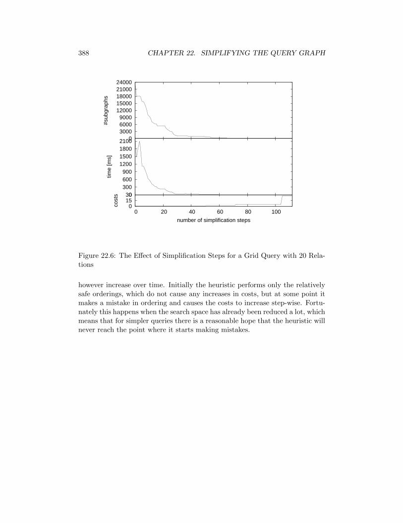
388 CHAPTER 22. SIMPLIFYING THE QUERY GRAPH

0 15 30

0 20 40 60 80 100

cost

s

number of simplification steps

0 300 600 900

1200 1500 1800 2100

time

[ms]

0 3000 6000 9000

12000 15000 18000 21000 24000

#sub

grap

hs

Figure 22.6: The Effect of Simplification Steps for a Grid Query with 20 Rela-tions

however increase over time. Initially the heuristic performs only the relativelysafe orderings, which do not cause any increases in costs, but at some point itmakes a mistake in ordering and causes the costs to increase step-wise. Fortu-nately this happens when the search space has already been reduced a lot, whichmeans that for simpler queries there is a reasonable hope that the heuristic willnever reach the point where it starts making mistakes.

Chapter 23

Deriving and Dealing withInteresting Orderings andGroupings

[This chapter was written by Thomas Neumann and Guido Moerkotte]

23.1 Introduction

The most expensive operations (e.g. join, grouping, duplicate elimination) dur-ing query evaluation can be performed more efficiently if the input is orderedor grouped in a certain way. Therefore, it is crucial for query optimization torecognize cases where the input of an operator satisfies the ordering or group-ing requirements needed for a more efficient evaluation. Since a plan generatortypically considers millions of different plans – and, hence, operators –, thisrecognition easily becomes a performance bottleneck for plan generation, oftenleading to heuristic solutions.

The importance of exploiting available orderings has already been recog-nized in the seminal work of Selinger et al [755]. They presented the concept ofinteresting orderings and showed how redundant sort operations could be avoid-ed by reusing available orderings, rendering sort-based operators like sort-mergejoin much more interesting.

Along these lines, it is beneficial to reuse available grouping properties, forexample for hash-based operators. While heuristic techniques to avoid redun-dant group-by operators have been given [149], for a long time groupings havenot been treated as thoroughly as orderings. One reason might be that whileorderings and groupings are related (every ordering is also a grouping), group-ings behave somewhat differently. For example, a tuple stream grouped on theattributes a, b need not be grouped on the attribute a. This is differentfrom orderings, where a tuple stream ordered on the attributes (a, b) is alsoordered on the attribute (a). Since no simple prefix (or subset) test exists forgroupings, optimizing groupings even in a heuristic way is much more difficultthan optimizing orderings. Still, it is desirable to combine order optimizationand the optimization of groupings, as the problems are related and treated sim-

389

390CHAPTER 23. DERIVING ANDDEALINGWITH INTERESTINGORDERINGS ANDGROUPINGS

ilarly during plan generation. Recently, some work in this direction has beenpublished [878]. However, this only covers a special case of grouping. Instead,in this chapter we follow the approach presented by Neumann and Moerkotte[617, 616]

Other existing frameworks usually consider only order optimization, andexperimental results have shown that the costs for order optimization can havea large impact on the total costs of query optimization [617]. Therefore, somecare is needed when adding groupings to order optimization, as a slowdown ofplan generation would be unacceptable.

In this chapter, we present a framework to efficiently reason about orderingsand groupings. It can be used for the plan generator described in Chapter ??,but is actually an independent component that could be used in any kind of plangenerator. Experimental results show that it efficiently handles orderings andgroupings at the same time, with no additional costs during plan generation andonly modest one time costs. Actually, the operations needed for both orderingand grouping optimization during plan generation can be performed in O(1),basically allowing to exploit groupings for free.

23.2 Problem Definition

The order manager component used by the plan generator combines order op-timization and the handling of grouping in one consistent set of algorithms anddata structures. In this section, we give a more formal definition of the prob-lem and the scope of the framework. First, we define the operations of orderingand grouping (Section 23.2.1 and 23.2.2). Then, we briefly discuss functionaldependencies (Section 23.2.3) and how they interact with algebraic operators(Section 23.2.4). Finally, we explain how the component is actually used duringplan generation (Section 23.2.5).

23.2.1 Ordering

During plan generation, many operators require or produce certain orderings.To avoid redundant sorting, it is required to keep track of the orderings a certainplan satisfies. The orderings that are relevant for query optimization are calledinteresting orders [755]. The set of interesting orders for a given query consistsof

1. all orderings required by an operator of the physical algebra that may beused in a query execution plan for the given query, and

2. all orderings produced by an operator of the physical algebra that maybe used in a query execution plan for the given query.

This includes the final ordering requested by the given query, if this is specified.The interesting orders are logical orderings. This means that they specify a

condition a tuple stream must meet to satisfy the given ordering. In contrast,the physical ordering of a tuple stream is the actual succession of tuples inthe stream. Note that while a tuple stream has only one physical ordering,

23.2. PROBLEM DEFINITION 391

it can satisfy multiple logical orderings. For example, the stream of tuples((1, 1), (2, 2)) with schema (a, b) has one physical ordering (the actual stream),but satisfies the logical orderings a, b, ab and ba.

Some operators, like sort, actually influence the physical ordering of atuple stream. Others, like select, only influence the logical ordering. Forexample, a sort[a] produces a tuple stream satisfying the ordering (a) byactually changing the physical order of tuples. After applying select[a=b] tothis tuple stream, the result satisfies the logical orderings (a), (b), (a, b), (b, a),although the physical ordering did not change. Deduction of logical orderingscan be described by using the well-known notion of functional dependency (FD)[789]. In general, the influence of a given algebraic operator on a set of logicalorderings can be described by a set of functional dependencies.

We now formalize the problem. Let R = (t1, . . . , tr) be a stream (orderedsequence) of tuples in attributes A1, . . . , An. Then R satisfies the logical order-ing o = (Ao1 , . . . , Aom) (1 ≤ oi ≤ n) if and only if for all 1 ≤ i < j ≤ r thefollowing condition holds:

(ti.Ao1 ≤ tj .Ao1)

∧ ∀1 < k ≤ m (∃1 ≤ l < k(ti.Aol < tj .Aol)) ∨((ti.Aok−1

= tj .Aok−1) ∧

(ti.Aok ≤ tj .Aok))

Next, we need to define the inference mechanism. Given a logical orderingo = (Ao1 , . . . , Aom) of a tuple stream R, then R obviously satisfies any logicalordering that is a prefix of o including o itself.

Let R be a tuple stream satisfying both the logical ordering o = (A1, . . . , An)and the functional dependency f = B1, . . . , Bk → Bk+1

1 with Bi ∈ A1 . . . An.Then R also satisfies any logical ordering derived from o as follows: add Bk+1

to o at any position such that all of B1, . . . , Bk occurred before this positionin o. For example, consider a tuple stream satisfying the ordering (a, b); afterinducing the functional dependency a, b→ c, the tuple stream also satisfies theordering (a, b, c), but not the ordering (a, c, b). Let O′ be the set of all logicalorderings that can be constructed this way from o and f after prefix closure.Then, we use the following notation: o `f O′. Let e be the equation Ai = Aj .Then, o `e O′, where O′ is the prefix closure of the union of the following threesets. The first set is O1 defined as o `Ai→Aj O1, the second is O2 defined aso `Aj→Ai O2, and the third is the set of logical orderings derived from o where apossible occurrence of Ai is replaced by Aj or vice versa. For example, considera tuple stream satisfying the ordering (a); after inducing the equation a = b,the tuple stream also satisfies the orderings (a, b), (b) and (b, a). Let e be anequation of the form A = const. Then O′ (o `e O′) is derived from o by insertingA at any position in o. This is equivalent to o `∅→A O′. For example, consider atuple stream satisfying the ordering (a, b); after inducing the equation c = constthe tuple stream also satisfies the orderings (c, a, b), (a, c, b) and (a, b, c).

1Any functional dependency which is not in this form can be normalized into a set of FDsof this form.

392CHAPTER 23. DERIVING ANDDEALINGWITH INTERESTINGORDERINGS ANDGROUPINGS

Let O be a set of logical orderings and F a set of functional dependen-cies (and possibly equations). We define the sets of inferred logical orderingsΩi(O,F ) as follows:

Ω0(O,F ) := O

Ωi(O,F ) := Ωi−1(O,F ) ∪⋃

f∈F,o∈Ωi−1(O,F )

O′ with o `f O′

Let Ω(O,F ) be the prefix closure of⋃∞i=0 Ωi(O,F ). We write o `F o′ if and

only if o′ ∈ Ω(O,F ).

23.2.2 Grouping

It was shown in [878] that, similar to order optimization, it is beneficial tokeep track of the groupings satisfied by a certain plan. Traditionally, group-byoperators are either applied after the rest of the query has been processed orare scheduled using some heuristics [149]. However, the plan generator couldtake advantage of grouping properties produced e.g. by avoiding re-hashing ifsuch information was easily available.

Analogous to order optimization, we call this grouping optimization anddefine that the set of interesting groupings for a given query consists of

1. all groupings required by an operator of the physical algebra that may beused in a query execution plan for the given query

2. all groupings produced by an operator of the physical algebra that maybe used in a query execution plan for the given query.

This includes the grouping specified by the group-by clause of the query, if anyexists.

These groupings are similar to logical orderings, as they specify a conditiona tuple stream must meet to satisfy a given grouping. Likewise, functionaldependencies can be used to infer new groupings.

More formally, a tuple stream R = (t1, . . . , tr) in attributes A1, . . . , Ansatisfies the grouping g = Ag1 . . . , Agm (1 ≤ gi ≤ n) if and only if for all1 ≤ i < j < k ≤ r the following condition holds:

∀1 ≤ l ≤ m ti.Agl = tk.Agl⇒ ∀1 ≤ l ≤ m ti.Agl = tj .Agl

Two remarks are in order here. First, note that a grouping is a set ofattributes and not – as orderings – a sequence of attributes. Second, notethat given two groupings g and g′ ⊂ g and a tuple stream R satisfying thegrouping g, R need not satisfy the grouping g′. For example, the tuple stream((1, 2), (2, 3), (1, 4)) with the schema (a, b) is grouped by a, b, but not by a.This is different from orderings, where a tuple stream satisfying an ordering oalso satisfies all orderings that are a prefix of o.

23.2. PROBLEM DEFINITION 393

New groupings can be inferred by functional dependencies as follows: Let Rbe a tuple stream satisfying both the grouping g = A1, . . . , An and the func-tional dependency f = B1, . . . , Bk → Bk+1 with B1, . . . , Bk ⊆ A1, . . . , An.Then R also satisfies the grouping g′ = A1, . . . , An ∪ Bk+1. Let G′ be theset of all groupings that can be constructed this way from g and f . Then weuse the following notation: g `f G′. For example a, b `a,b→c a, b, c. Let ebe the equation Ai = Aj . Then g `e G′ where G′ is the union of the follow-ing three sets. The first set is G1 defined as g `Ai→Aj G1, the second is G2

defined as g `Aj→Ai G2, and the third is the set of groupings derived from gwhere a possible occurrence of Ai is replaced by Aj or vice versa. For example,a, b `b=c a, c. Let e be an equation of the form A = const. Then g `e G′ isdefined as g `∅→A G′. For example, a, b `c=const a, b, c.

Let G be a set of groupings and F be a set of functional dependencies (andpossibly equations). We define the set of inferred groupings Ωi(G,F ) as follows:

Ω0(G,F ) := G

Ωi(G,F ) := Ωi−1(G,F ) ∪⋃

f∈F,g∈Ωi−1(G,F )

G′ with g `f G′

Let Ω(G,F ) be⋃∞i=0 Ωi(G,F ). We write g `F g′ if and only if g′ ∈ Ω(G,F ).

23.2.3 Functional Dependencies

The reasoning about orderings and groupings assumes that the set of func-tional dependencies is known. The process of gathering the relevant functionaldependencies is described in detail in [789, 790]. Predominantly, there are threesources of functional dependencies:

1. key constraints

2. join predicates [references constraints]

3. filter predicates

4. simple expressions

However, the algorithm makes no assumption about the functional dependen-cies. If for some reason an operator induces another kind of functional depen-dency (e.g., when using TID-based optimizations [566]), this can be handledthe same way. The only important fact is that we provide the set of functionaldependencies as input to the algorithm.

23.2.4 Algebraic Operators

To illustrate the propagation of orderings and groupings during query optimiza-tion, we give some rules for concrete (physical) operators in Figure 23.1. As a

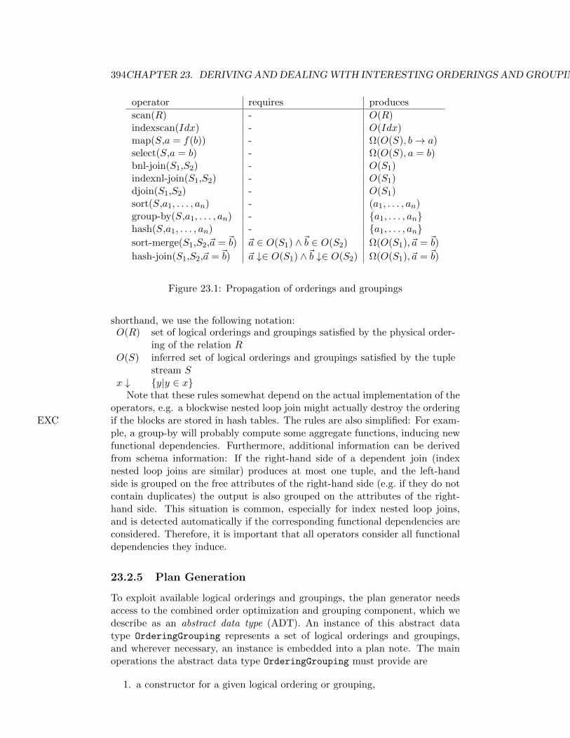
394CHAPTER 23. DERIVING ANDDEALINGWITH INTERESTINGORDERINGS ANDGROUPINGS

operator requires produces

scan(R) - O(R)indexscan(Idx) - O(Idx)map(S,a = f(b)) - Ω(O(S), b→ a)select(S,a = b) - Ω(O(S), a = b)bnl-join(S1,S2) - O(S1)indexnl-join(S1,S2) - O(S1)djoin(S1,S2) - O(S1)sort(S,a1, . . . , an) - (a1, . . . , an)group-by(S,a1, . . . , an) - a1, . . . , anhash(S,a1, . . . , an) - a1, . . . , ansort-merge(S1,S2,~a = ~b) ~a ∈ O(S1) ∧~b ∈ O(S2) Ω(O(S1),~a = ~b)

hash-join(S1,S2,~a = ~b) ~a ↓∈ O(S1) ∧~b ↓∈ O(S2) Ω(O(S1),~a = ~b)

Figure 23.1: Propagation of orderings and groupings

shorthand, we use the following notation:O(R) set of logical orderings and groupings satisfied by the physical order-

ing of the relation RO(S) inferred set of logical orderings and groupings satisfied by the tuple

stream Sx ↓ y|y ∈ x

Note that these rules somewhat depend on the actual implementation of theoperators, e.g. a blockwise nested loop join might actually destroy the orderingif the blocks are stored in hash tables. The rules are also simplified: For exam-EXCple, a group-by will probably compute some aggregate functions, inducing newfunctional dependencies. Furthermore, additional information can be derivedfrom schema information: If the right-hand side of a dependent join (indexnested loop joins are similar) produces at most one tuple, and the left-handside is grouped on the free attributes of the right-hand side (e.g. if they do notcontain duplicates) the output is also grouped on the attributes of the right-hand side. This situation is common, especially for index nested loop joins,and is detected automatically if the corresponding functional dependencies areconsidered. Therefore, it is important that all operators consider all functionaldependencies they induce.

23.2.5 Plan Generation

To exploit available logical orderings and groupings, the plan generator needsaccess to the combined order optimization and grouping component, which wedescribe as an abstract data type (ADT). An instance of this abstract datatype OrderingGrouping represents a set of logical orderings and groupings,and wherever necessary, an instance is embedded into a plan note. The mainoperations the abstract data type OrderingGrouping must provide are

1. a constructor for a given logical ordering or grouping,

23.3. OVERVIEW 395

2. a membership test (called containsOrdering(LogicalOrdering)) whichtests whether the set contains the logical ordering given as parameter,

3. a membership test (called containsGrouping(Grouping)) which testswhether the set contains the grouping given as parameter, and

4. an inference operation (called infer(set<FD>)). Given a set of functionaldependencies and equations, it computes a new set of logical orderings andgroupings a tuple stream satisfies.

These operations can be implemented by using the formalism describedbefore: containsOrdering tests for o ∈ O, containsGrouping tests for o ∈ Gand infer(F) calculates Ω(O,F ) respectively Ω(G,F ). Note that the intuitiveapproach to explicitly maintain the set of all logical orderings and groupingsis not useful in practice. For example, if a sort operator sorts a tuple streamon (a, b), the result is compatible with logical orderings (a, b), (a). After aselection operator with selection predicate x = const is applied, the set of logicalorderings changes to (x, a, b), (a, x, b), (a, b, x), (x, a), (a, x), (x). Since thesize of the set increases quadratically with every additional selection predicateof the form v = const, a naive representation as a set of logical orderings isproblematic. This led Simmen et al. to introduce a more concise representation,which is discussed in the related work section. Note that Simmen’s technique isnot easily applicable to groupings, and no algorithm was proposed to efficientlymaintain the set of available groupings. The order optimization componentdescribed here closes this gap by supporting both orderings and groupings.The problem of quadatic growth is avoided by only implicitly representing theset.

23.3 Overview

As we have seen, explicit maintenance of the set of logical orderings and group-ings can be very expensive. However, the ADT OrderingGrouping requiredfor plan generation does not need to offer access to this set: It only allows totest if a given interesting order or grouping is in the set and changes the setaccording to new functional dependencies. Hence, it is not required to explicitlyrepresent this set; an implicit representation is sufficient as long as the ADToperations can be implemented atop of it. In other words, we need not be ableto reconstruct the set of logical orderings and groupings from the state of theADT. This gives us room for optimizations.

The initial idea (see [617]) was to represent sets of logical orderings as statesof a finite state machine (FSM). Roughly, a state of the FSM represents acurrent physical ordering and the set of logical orderings that can be inferredfrom it given a set of functional dependencies. The edges (transitions) in theFSM are labeled by sets of functional dependencies. They lead from one stateto another, if the target state of the edge represents the set of logical orderingsthat can be derived from the orderings the edge’s source node represents byapplying the set of functional dependencies the edge is labeled with. We have

396CHAPTER 23. DERIVING ANDDEALINGWITH INTERESTINGORDERINGS ANDGROUPINGS

a

abdabdc

abcd

abc

b→ d b→ d

b→ d

ε

εab

ε

ε

ε

Figure 23.2: Possible FSM for orderings

to use sets of functional dependencies, since a single algebraic operator mayintroduce more than one functional dependency.

Let us illustrate the idea by a simple example and then discuss some prob-lems. In Figure 23.2, an FSM for the interesting order (a, b, c) and its prefixes(remember that we need prefix closure) and the set of functional dependenciesb → d is given. When a physical ordering satisfies (a, b, c), it also satisfiesits prefixes (a, b) and (a). This is indicated by the ε transitions. The func-tional dependency b → d allows to derive the logical orderings (a, b, c, d) and(a, b, d, c). This is handled by assuming that the physical ordering changes toeither (a, b, c, d) or (a, b, d, c). Hence, these states have to be added to the FSM.We further add the transitions induced by b → d. Note that the resultingFSM is a non-deterministic finite state machine (NFSM).

Assume we have an NFSM as above. Then (while ignoring groupings) thestate of the ADT is a state of the NFSM and the operations of the ADT caneasily be mapped to the FSM. Testing for a logical ordering can be performedby checking if the node with the ordering is reachable from the current stateby following ε edges. If the set must be changed because of a functional de-pendency the state is changed by following the edge labeled with the functionaldependency. Of course, the non-determinism is in our way.

While remembering only the active state of the NFSM avoids the problemof maintaining a set of orderings, the NFSM is not really useful from a prac-tical point of view, since the transitions are non-deterministic. Nevertheless,the NFSM can be considered as a special non-deterministic finite automaton(NFA), which consumes the functional dependencies and ”recognizes” the pos-sible physical orderings. Further, an NFA can be converted into a deterministicfinite automaton (DFA), which can be handled efficiently. Remember that theconstruction is based on the power set of the NFA’s states. That is, the statesof the DFA are sets of states of the NFA [532]. We do not take the deviationover the finite automaton but instead lift the construction of deterministic finiteautomatons from non-deterministic ones to finite state machines. Since this isnot a traditional conversion, we give a proof of this step in Section ??.

Yet another problem is that the conversion from an NFSM to a deterministicFSM (DFSM) can be expensive for large NFSMs. Therefore, reducing the sizeof the NFSM is another problem we look at. We introduce techniques forreducing the set of functional dependencies that have to be considered and

23.3. OVERVIEW 397

abcdabc

b→ d

Figure 23.3: Possible FSM for groupings

a

abdabdc

abcd

abc

abc abcd

b→ d b→ d

b→ d

ε

εab

ε

ε

ε

ε

ε

b→ d

Figure 23.4: Combined FSM for orderings and groupings

further techniques to prune the NFSM in Section 23.4.7.

The idea of a combined framework for orderings and groupings was presentedin [616]. Here, the main point is to construct a similar FSM for groupings andintegrate it into the FSM for orderings, thus handling orderings and groupingsat the same time. An example of this is shown in Figure 23.3. Here, theFSM for the grouping a, b, c and the functional dependency b → c is shown.We represent states for orderings as rounded boxes and states for groupingsas rectangles. Note that although the FSM for groupings has a start nodesimilar to the FSM for orderings, it is much smaller. This is due to the factthat groupings are only compatible with themselves, no nodes for prefixes arerequired. However, the FSM is still non-deterministic: given the functionaldependency b → c, the grouping a, b, c, d is compatible with a, b, c, d itselfand with a, b, c; therefore, there exists an (implicit) edge from each groupingto itself.

The FSM for groupings is integrated into the FSM for orderings by addingε edges from each ordering to the grouping with the same attributes; this isdue to the fact that every ordering is also a grouping. Note that although theordering (a, b, c, d) also implies the grouping a, b, c, no edge is required forthis, since there exists an ε edge to (a, b, c) and from there to a, b, c.

After constructing a combined FSM as described above, the full ADT sup-porting both orderings and groupings can easily be mapped to the FSM: The

a,ab,abc

abd,abcd,a,ab,abc,ab

abdc,abd

b→ d

Figure 23.5: Possible DFSM for Figure 23.4

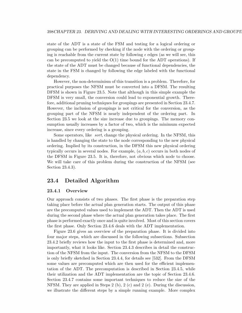
398CHAPTER 23. DERIVING ANDDEALINGWITH INTERESTINGORDERINGS ANDGROUPINGS

state of the ADT is a state of the FSM and testing for a logical ordering orgrouping can be performed by checking if the node with the ordering or group-ing is reachable from the current state by following ε edges (as we will see, thiscan be precomputed to yield the O(1) time bound for the ADT operations). Ifthe state of the ADT must be changed because of functional dependencies, thestate in the FSM is changed by following the edge labeled with the functionaldependency.

However, the non-determinism of this transition is a problem. Therefore, forpractical purposes the NFSM must be converted into a DFSM. The resultingDFSM is shown in Figure 23.5. Note that although in this simple example theDFSM is very small, the conversion could lead to exponential growth. There-fore, additional pruning techniques for groupings are presented in Section 23.4.7.However, the inclusion of groupings is not critical for the conversion, as thegrouping part of the NFSM is nearly independent of the ordering part. InSection 23.5 we look at the size increase due to groupings. The memory con-sumption usually increases by a factor of two, which is the minimum expectedincrease, since every ordering is a grouping.

Some operators, like sort, change the physical ordering. In the NFSM, thisis handled by changing the state to the node corresponding to the new physicalordering. Implied by its construction, in the DFSM this new physical orderingtypically occurs in several nodes. For example, (a, b, c) occurs in both nodes ofthe DFSM in Figure 23.5. It is, therefore, not obvious which node to choose.We will take care of this problem during the construction of the NFSM (seeSection 23.4.3).

23.4 Detailed Algorithm

23.4.1 Overview

Our approach consists of two phases. The first phase is the preparation steptaking place before the actual plan generation starts. The output of this phaseare the precomputed values used to implement the ADT. Then the ADT is usedduring the second phase where the actual plan generation takes place. The firstphase is performed exactly once and is quite involved. Most of this section coversthe first phase. Only Section 23.4.6 deals with the ADT implementation.

Figure 23.6 gives an overview of the preparation phase. It is divided intofour major steps, which are discussed in the following subsections. Subsection23.4.2 briefly reviews how the input to the first phase is determined and, moreimportantly, what it looks like. Section 23.4.3 describes in detail the construc-tion of the NFSM from the input. The conversion from the NFSM to the DFSMis only briefly sketched in Section 23.4.4, for details see [532]. From the DFSMsome values are precomputed which are then used for the efficient implemen-tation of the ADT. The precomputation is described in Section 23.4.5, whiletheir utilization and the ADT implementation are the topic of Section 23.4.6.Section 23.4.7 contains some important techniques to reduce the size of theNFSM. They are applied in Steps 2 (b), 2 (c) and 2 (e). During the discussion,we illustrate the different steps by a simple running example. More complex

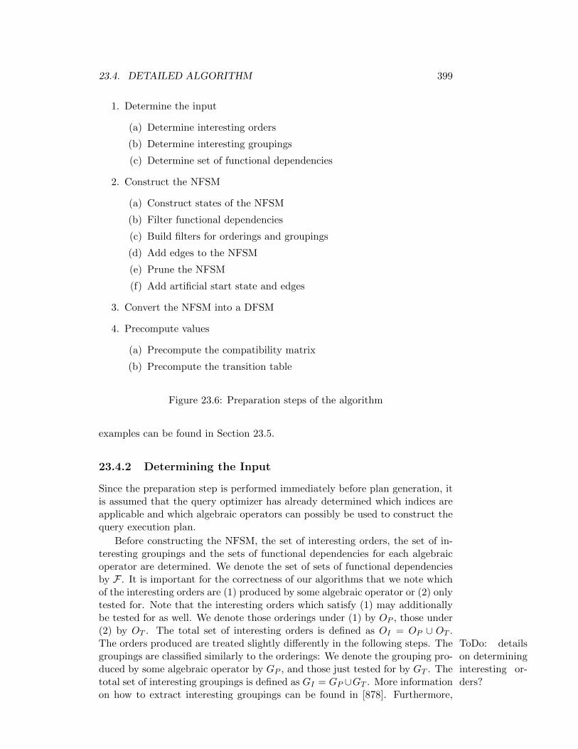
23.4. DETAILED ALGORITHM 399

1. Determine the input

(a) Determine interesting orders

(b) Determine interesting groupings

(c) Determine set of functional dependencies

2. Construct the NFSM

(a) Construct states of the NFSM

(b) Filter functional dependencies

(c) Build filters for orderings and groupings

(d) Add edges to the NFSM

(e) Prune the NFSM

(f) Add artificial start state and edges

3. Convert the NFSM into a DFSM

4. Precompute values

(a) Precompute the compatibility matrix

(b) Precompute the transition table

Figure 23.6: Preparation steps of the algorithm

examples can be found in Section 23.5.

23.4.2 Determining the Input

Since the preparation step is performed immediately before plan generation, itis assumed that the query optimizer has already determined which indices areapplicable and which algebraic operators can possibly be used to construct thequery execution plan.

Before constructing the NFSM, the set of interesting orders, the set of in-teresting groupings and the sets of functional dependencies for each algebraicoperator are determined. We denote the set of sets of functional dependenciesby F . It is important for the correctness of our algorithms that we note whichof the interesting orders are (1) produced by some algebraic operator or (2) onlytested for. Note that the interesting orders which satisfy (1) may additionallybe tested for as well. We denote those orderings under (1) by OP , those under(2) by OT . The total set of interesting orders is defined as OI = OP ∪ OT .The orders produced are treated slightly differently in the following steps. The ToDo: details

on determininginteresting or-ders?

groupings are classified similarly to the orderings: We denote the grouping pro-duced by some algebraic operator by GP , and those just tested for by GT . Thetotal set of interesting groupings is defined as GI = GP ∪GT . More informationon how to extract interesting groupings can be found in [878]. Furthermore,

400CHAPTER 23. DERIVING ANDDEALINGWITH INTERESTINGORDERINGS ANDGROUPINGS

for a sample query the extraction of both interesting orders and groupings isillustrated in Section 23.5.

To illustrate subsequent steps, we assume that the set of sets of functionaldependencies

F = b→ c, b→ d,the interesting groupings

GI = b ∪ b, c

and the interesting orders

OI = (b), (a, b) ∪ (a, b, c)

have been extracted from the query. We assume that those in OT = (a, b, c)and GT = b, c are tested for but not produced by any operator, whereasthose in OP = (b), (a, b) and GP = b may be produced by some algebraicoperators.

23.4.3 Constructing the NFSM

An NFSM consists of a tuple (Σ, Q,D, qo), where

• Σ is the input alphabet,

• Q is the set of possible states,

• D ⊆ Q× (Σ ∪ ε)×Q is the transition relation, and

• q0 is the initial state.

Coarsely, Σ consists of the functional dependencies, Q of the relevant or-derings and groupings, and D describes how the orderings or groupings changeunder a given functional dependency. Some refinements are needed to provideefficient ADT operations. The details of the construction are described now.

For the order optimization part the states are partitioned in Q = QI ∪QA∪q0, where q0 is an artificial state to initialize the ADT, QI is the set of statescorresponding to interesting orderings and QA is a set of artificial states onlyrequired for the algorithm itself. QA is described later. Furthermore, the setQI is partitioned in QPI and QTI , representing the orderings in OP and OT ,respectively. To support groupings, we add to QPI states corresponding to thegroupings in GP and to QTI states corresponding to the groupings in GT .

The initial NFSM contains the states QI of interesting groupings and order-ings. For the example, this initial construction not including the start state qo isshown in Figure 23.7. The states representing groupings are drawn as rectanglesand the states representing orderings are drawn with rounded corners.

When considering functional dependencies, additional groupings and order-ings can occur. These are not directly relevant for the query, but have to berepresented by states to handle transitive changes. Since they have no directconnection to the query, these states are called artificial states. Starting with

23.4. DETAILED ALGORITHM 401

b,c

b

a,b,c

a,b

b

Figure 23.7: Initial NFSM for sample query

the initial states QI , artificial states are constructed by considering functionaldependencies

QA = (Ω(OI ,F) \OI) ∪ (Ω(GI ,F) \GI).In our example, this creates the states (b, c) and (a), as (b, c) can be inferredfrom (b) when considering b→ c and (a) can be inferred from (a, b), since (a)is a prefix of (a, b). The result is show in Figure 23.8 (ignore the edges).

Sometimes the ADT has to be explicitly initialized with a certain orderingor grouping (e.g. after a sort). To support this, artificial edges are addedlater on. These point to the requested ordering or grouping (states in QPI ) andare labeled with the state that they lead to. Therefore, the input alphabetΣ consists of the sets of functional dependencies and produced orderings andgroupings:

Σ = F ∪QPI ∪ ε.In our example, Σ = b→ c, b→ d, (b), (a, b), b.

Accordingly, the domain of the transition relation D is

D ⊆ ((Q \ q0)× (F ∪ ε)× (Q \ q0))∪ (qo ×QPI ×QPI ).

The edges are formed by the functional dependencies and the artificial edges.Furthermore, ε edges exist between orderings and the corresponding groupings,as orderings are a special case of grouping:

DFD = (q, f, q′) | q ∈ Q, f ∈ F ∪ ε, q′ ∈ Q, q ` fq′

DA = (q0, q, q) | q ∈ QPI

DOG = (o, ε, g) | o ∈ Ω(OI ,F), g ∈ Ω(GI ,F), o ≡ gD = DFD ∪DA ∪DOG

First, the edges corresponding to functional dependencies are added (DFD).In our example, this results in the NFSM shown in Figure 23.8.

Note that the functional dependency b → d has been pruned, since d doesnot occur in any interesting order or grouping. The NFSM can be furthersimplified by pruning the artificial state (b, c), which cannot lead to a newinteresting order. The result is shown in Figure 23.9. A detailed description ofthese pruning techniques can be found in Section 23.4.7.

402CHAPTER 23. DERIVING ANDDEALINGWITH INTERESTINGORDERINGS ANDGROUPINGS

b

a,b

a,b,c

b

b,c

b,c

a

b→ c ε

ε

ε

b→ c

b→ c

q0

Figure 23.8: NFSM after adding DFD edges

b

a,b

a,b,c

b

b,ca

b→ c ε

ε

b→ c

q0

Figure 23.9: NFSM after pruning artificial states

The artificial start state q0 has emanating edges incident to all states rep-resenting interesting orders in OPI and interesting groupings in GPI (DA). Also,the states representing orderings have edges to their corresponding groupingstates (DOG), as every ordering is also a grouping. The final NFSM for theexample is shown in Figure 23.10. Note that the states representing (a, b, c)and b, c are not linked by an artificial edge since it is only tested for, as theyare in QTI .

a b,c

b

a,b,c

a,b

b

(a,b)

(b)

b

qo

b→ cε

εb→ c

ε

Figure 23.10: Final NFSM

23.4. DETAILED ALGORITHM 403

b

(b)

(a,b)

6:(a),(a,b),(a,b,c)

5:(b),b,b,c

4:b,b,c

3:(a),(a,b)

2:(b),b

1:b

b→ c

b→ c

b→ c

qo

Figure 23.11: Resulting DFSM

state 1: 2: 3: 4: 5: 6:(a) (a,b) (a,b,c) (b) b b,c

1 0 0 0 0 1 02 0 0 0 1 1 03 1 1 0 0 0 04 0 0 0 0 1 15 0 0 0 1 1 16 1 1 1 0 0 0

Figure 23.12: contains Matrix

23.4.4 Constructing the DFSM

The construction of the DFSM from the NFSM follows the standard powerset construction that is used to translate an NFA into a DFA [532]. A formaldescription and a proof of correctness is given in Section ??. It is importantto note that this construction preserves the start state and the artificial edges.The resulting DFSM for the example is shown in Figure 23.11.

state 1: 2: 3: 4:b→ c (a, b) (b) b

qo - 3 2 11 4 - - -2 5 - - -3 6 - - -4 4 - - -5 5 - - -6 6 - - -

Figure 23.13: transition Matrix

404CHAPTER 23. DERIVING ANDDEALINGWITH INTERESTINGORDERINGS ANDGROUPINGS

23.4.5 Precomputing Values

To allow for an efficient precomputation of values, every occurrence of an inter-esting order, interesting grouping or set of functional dependencies is replacedby integers. This allows comparisons in constant time (equivalent entries aremapped to same integer). Further, the DFSM is represented by an adjacencymatrix.

The precomputation step itself computes two matrices. The first matrixdenotes whether an NFSM state in QI is active, i.e. an interesting order or aninteresting grouping, is contained in a specific DFSM state. This matrix canbe represented as a compact bit vector, allowing tests in O(1). For our runningexample, it is given (in a more readable form) in Figure 23.12. The secondmatrix contains the transition table for the DFSM relation D. Using it, edgesin the DFSM can be followed in O(1). For the example, the transition matrixis given in Figure 23.13.

23.4.6 During Plan Generation

During plan generation, larger plans are constructed by adding algebraic op-erators to existing (sub-)plans. Each subplan contains the available orderingsand groupings in the form of the corresponding DFSM state. Hence, the stateof the DFSM, a simple integer, is the state of our ADT OrderingGrouping.

When applying an operator to subplans, the ordering and grouping require-ments are tested by checking whether the DFSM state of the subplan containsthe required ordering or grouping of the operator. This is done by a simplelookup in the contains matrix.

If the operator introduces a new set of functional dependencies, the newstate of the ADT is computed by following the according edge in the DFSM.This is performed by a quick lookup in the transition matrix.

For “atomic” subplans like table or index scans, the ordering and groupingis determined explicitly by the operator. The state of the DFSM is determinedby a lookup in the transition matrix with start state qo and the edge annotatedby the produced ordering or grouping. For sort and group-by operators thestate of the DFSM is determined as before by following the artificial edge forthe produced ordering or grouping and then reapplying the set of functionaldependencies that currently hold.

In the example, a sort on (b) results in a subplan with ordering/groupingstate 2 (the state 2 is active in the DFSM), which satisfies the ordering (b)and the grouping b. After applying an operator which induces b → c, theordering/grouping changes to state 5 which also satisfies b, c.

23.4.7 Reducing the Size of the NFSM

Reducing the size of the NFSM is important for two reasons: First, it reducesthe amount of work needed during the preparation step, especially the con-version from NFSM to DFSM. Even more important is that a reduced NFSMresults in a smaller DFSM. This is crucial for plan generation, since it reduces

23.4. DETAILED ALGORITHM 405

the search space: Plans can only be compared and pruned if they have compa-rable ordering and a comparable set of functional dependencies (see [789, 790]for details). Reducing the size of the DFSM removes information that is notrelevant for plan generation and, therefore, allows a more aggressive pruning ofplans.

At first, the functional dependencies are pruned. Here, functional dependen-cies which can never lead to a new interesting order or grouping are removed.For convenience, we extend the definition of Ω(O,F ) and define

Ω(O, ε) := Ω(O, ∅).

Then the set of prunable functional dependencies FP can be described by

ΩN (o, f) := Ω(o, f) \ Ω(o, ε)FP := f |f ∈ F ∧ ∀o ∈ OI ∪GI :

(Ω(ΩN (o, f), F ) \ Ω(o, ε)) ∩ (OI ∪GI) = ∅.

Pruning functional dependencies is especially useful, since it also prunes artifi-cial states that would be created because of the dependencies. In the example,this removed the functional dependency b → d, since d does not appear inany interesting order or grouping. This step also removes the artificial statescontaining d.

The artificial states are required to build the NFSM, but they are not visibleoutside the NFSM. Therefore, they can be pruned and merged without affectingplan generation. Two heuristics are used to reduce the set of artificial states:

1. All artificial nodes that behave exactly the same (that is, their edges leadto the same states given the same input) are merged and

2. all edges to artificial states that can reach states in QI only through εedges are replaced with corresponding edges to the states in QI .

More formally, the following pairs of states can be merged:

(o1, o2) | o1 ∈ QA, o2 ∈ QA ∧ ∀f ∈ F :

(Ω(o1, f) \ Ω(o1, ε)) =

(Ω(o2, f) \ Ω(o2, ε)).

The following states can be replaced with the next state reachable by an ε edge:

o | o ∈ QA ∧ ∀f ∈ F :

Ω(Ω(o, ε), f) \ o =

Ω(Ω(o, ε) \ o, f).

In the example, this removed the state (b, c), which was artificial and only ledto the state (b).

These techniques reduce the size of the NFSM, but still most states areartificial states, i.e. they are only created because they can be reached by con-sidering functional dependencies when a certain ordering or grouping is avail-able. But many of these states are not relevant for the actual query processing.

406CHAPTER 23. DERIVING ANDDEALINGWITH INTERESTINGORDERINGS ANDGROUPINGS

For example, given a set of interesting orders which consists only of a singleordering (a) and a set of functional dependencies which consists only of a→ b,the NFSM will contain (among others) two states: (a) and (a, b). The state(a, b) is created since it can be reached from (a) by considering the functionaldependency, however, it is irrelevant for the plan generation, since (a, b) is notan interesting order and is never created nor tested for. Actually, in the ex-ample above, the whole functional dependency would be pruned (since b neveroccurs in an interesting order), but the problem remains for combinations ofinteresting orders: Given the interesting orders (a), (b) and (c) and the func-tional dependencies a→ b, b→ a, b→ c, c→ b, the NFSM will contain statesfor all permutations of a, b and c. But these states are completely useless, sinceall interesting orders consist only of a single attribute and, therefore, only thefirst entry of an ordering is ever tested.

Ideally, the NFSM should only contain states which are relevant for thequery; since this is difficult to ensure, a heuristic can be used which greatlyreduces the size of the NFSM and still guarantees that all relevant states areavailable: When considering a functional dependency of the form a → b andan ordering o1, o2, . . . , on with oi = a for some i (1 ≤ i ≤ n), the b can beinserted at any position j with i < j ≤ n+ 1 (for the special case of a conditiona = b, i = j is also possible). So, an entry of an ordering can only affect entrieson the right of its own position. This means that it is unnecessary to considerthose parts of an ordering which are behind the length of the longest interestingorder; since that part cannot influence any entries relevant for plan generation,it can be omitted. Therefore, the orderings created by functional dependenciescan be cut off after the maximum length of interesting orders, which results inless possible combinations and a smaller NFSM.

The space of possible orderings can be limited further by taking into accountthe prefix of the ordering: before inserting an entry b in an ordering o1, o2, . . . , onat the position i, check if there is actually an interesting order with the prefixo1, o2, ...oi−1, b and stop inserting if no interesting order is found. Also limit thenew ordering to the length of the longest matching interesting order; furtherattributes will never be used. If functional dependencies of the form a = b occur,they might influence the prefix of the ordering and the simple test describedabove is not sufficient. Therefore, a representative is chosen for each equivalenceclass created by these dependencies, and for the prefix test the attributes arereplaced with their representatives. Since the set of interesting orders witha prefix of o1, . . . , on is a superset of the set for the prefix o1, ...on, on+1, thisheuristic can be implemented very efficiently by iterating over i and reducingthe set as needed.

Additional techniques can be used to avoid creating superfluous artificalstates for groupings: First, in Step 2.3 (see Figure 23.6) the set of attributesoccurring in interesting groupings is determined:

AG = a | ∃g ∈ GI : a ∈ g

Now, for every attribute a occurring on the right-hand side of a functional

23.4. DETAILED ALGORITHM 407

dependency the set of potentially reachable relevant attributes is determined:

r(a, 0) = ar(a, n) = r(a, n− 1) ∪

a′ | ∃(a1 . . . am → a′) ∈ F :

a1 . . . am ∩ r(a, n− 1) 6= ∅r(a) = r(a, |F|) ∩AG

This can be used to determine if a functional dependency actually addsuseful attributes. Given a functional dependency a1 . . . an → a and a groupingg with a1 . . . an ⊆ g, a should only be added to g if r(a) 6⊆ g, i.e. theattribute might actually lead to a new interesting grouping. For example, giventhe interesting groupings a, a, b and the functional dependencies a→ c, a→d, d = b. When considering the grouping a, the functional dependency a→ ccan be ignored, as it can only produce the attribute c, which does not occur inan interesting grouping. However, the functional dependency a→ d should beadded, since transitively the attribute b can be produced, which does occur inan interesting grouping.

Since there are no ε edges between groupings, i.e. groupings are not com-patible with each other, a grouping can only be relevant for the query if it isa subset of an interesting ordering (as further attributes could be added byfunctional dependencies). However, a simple subset test is not sufficient, asequations of the form a = b are also supported; these can effectively renameattributes, resulting in a slightly more complicated test:

In Step 2.3 (see Figure 23.6) the equivalence classes induced by the equationsin F are determined and for each class a representative is chosen (a and a1 . . . anare attributes occuring in the GI):

E(a, 0) = aE(a, n) = E(a, n− 1) ∪

a′ | ((a = a′) ∈ F) ∨ ((a′ = a) ∈ F)E(a) = E(a, |F|)e(a) = a representative choosen from E(A)

e(a1 . . . an) = e(a1) . . . e(an).

Using these equivalence classes, a mapped set of interesting groupings isproduced that will be used to test if a grouping is relevant:

GEI = e(g) | g ∈ GI

Now a grouping g can be pruned if 6 ∃g′ ∈ GEI : e(g) ⊆ g′. For example,given the interesting grouping a and the equations a = b, b = c, the groupingd can be pruned, as it will never lead to an interesting grouping; however, thegroupings b and c have to be kept, as they could change to an interestinggrouping later on.

408CHAPTER 23. DERIVING ANDDEALINGWITH INTERESTINGORDERINGS ANDGROUPINGS

Note that although they appear to test similar conditions, the first pruningtechnique (using r(a)) is not dominated by the second one (using e(a)). Con-sider e.g. the interesting grouping a, the equation a = b and the functionaldependency a→ b. Using only the second technique, the grouping a, b wouldbe created, although it is not relevant.

23.4.8 Complex Ordering Requirements

Specifying the ordering requirements of an operator can be surprisingly difficult.Consider the following SQL query:

select *

from S s, R r

where r.a=s.a and r.b=s.b and

r.c=s.c and r.d=s.d

When answering this query using a sort-merge join, the operator has torequest a certain odering. But there are many orderings that could be used:The intuitive ordering would be abcd, but adcb or any other premutation couldhave been used as well. This is problematic, as checking for an exponentialnumber of possibilities is not acceptable in general. Note that this problem isnot specific to our approach, the same is true, e.g., for Simmen’s approach.

The problem can be solved by defining a total ordering between the at-tributes, such that a canonical ordering can be constructed. We give some ruleshow to derive such an ordering below, but it can happen that such an order-ing is unavailable (or rather the construction rules are ambiguous). Given, forexample, two indices, one on abcd and one on adcb, both orderings would be areasonable choice. If this happens, the operators have two choices: Either theyaccept all reasonable orderings (which could still be an exponential number,but most likely only a few orderings remaing) or they limit themselves to oneordering, which could induce unnecessary sort operators. Probably the secondchoice is preferable, as the ambiguous case should be rare and does not justifythe complex logic of the first solution.

The attribute ordering can be derived by using the following heuristicalrules:

1. Only attributes that occur in sets without natural ordering (i.e. complexjoin predicates or grouping attributes) have to be ordered.

2. Orderings that are given (e.g., indices, user-requested orderings etc.) or-der some attributes.

3. Small orderings should be considered first. If an operator requires an or-dering with the attributes abc, and another operator requires an orderingwith the attributes bc, the attributes b and c should come before a.

4. The attributes should be ordered according to equivalence classes. If ais ordered before b, all orderings in E(a) should be ordered before allorderings in E(b).

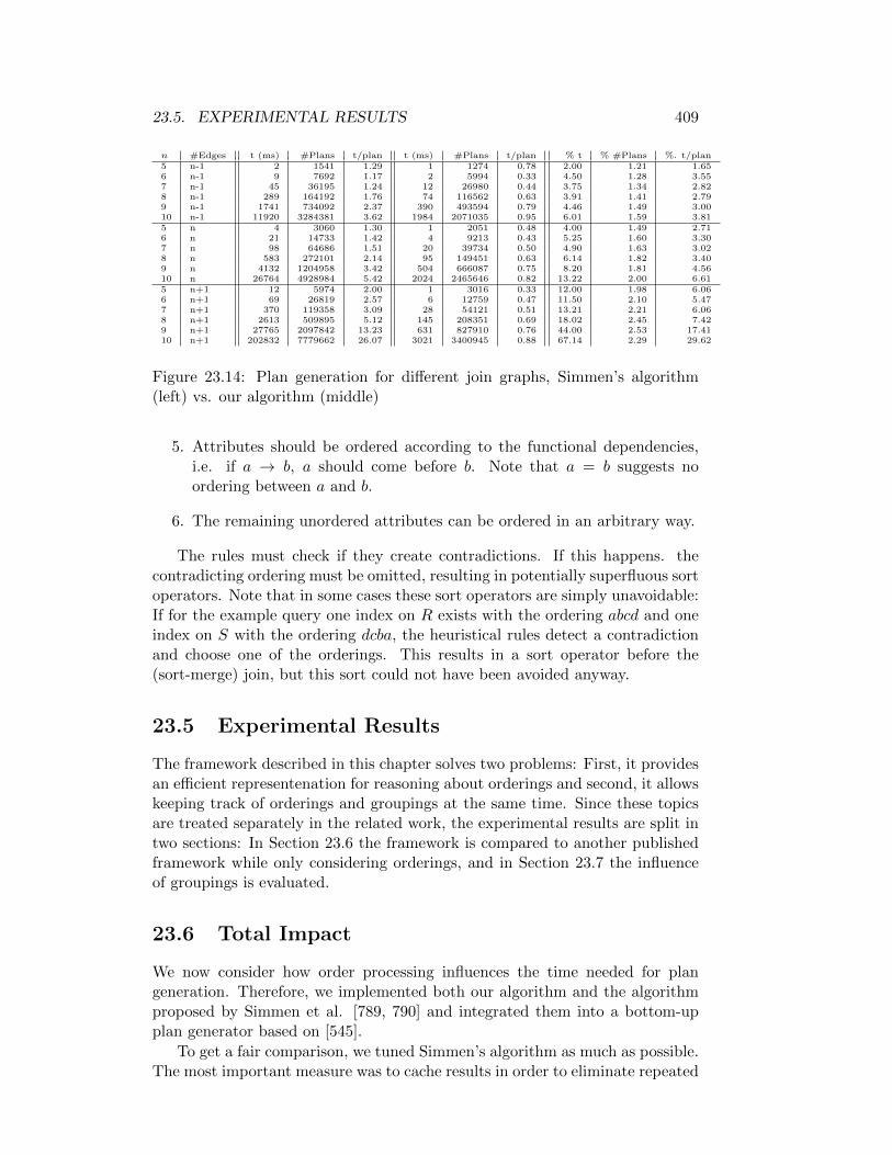
23.5. EXPERIMENTAL RESULTS 409

n #Edges t (ms) #Plans t/plan t (ms) #Plans t/plan % t % #Plans %. t/plan5 n-1 2 1541 1.29 1 1274 0.78 2.00 1.21 1.656 n-1 9 7692 1.17 2 5994 0.33 4.50 1.28 3.557 n-1 45 36195 1.24 12 26980 0.44 3.75 1.34 2.828 n-1 289 164192 1.76 74 116562 0.63 3.91 1.41 2.799 n-1 1741 734092 2.37 390 493594 0.79 4.46 1.49 3.0010 n-1 11920 3284381 3.62 1984 2071035 0.95 6.01 1.59 3.815 n 4 3060 1.30 1 2051 0.48 4.00 1.49 2.716 n 21 14733 1.42 4 9213 0.43 5.25 1.60 3.307 n 98 64686 1.51 20 39734 0.50 4.90 1.63 3.028 n 583 272101 2.14 95 149451 0.63 6.14 1.82 3.409 n 4132 1204958 3.42 504 666087 0.75 8.20 1.81 4.5610 n 26764 4928984 5.42 2024 2465646 0.82 13.22 2.00 6.615 n+1 12 5974 2.00 1 3016 0.33 12.00 1.98 6.066 n+1 69 26819 2.57 6 12759 0.47 11.50 2.10 5.477 n+1 370 119358 3.09 28 54121 0.51 13.21 2.21 6.068 n+1 2613 509895 5.12 145 208351 0.69 18.02 2.45 7.429 n+1 27765 2097842 13.23 631 827910 0.76 44.00 2.53 17.4110 n+1 202832 7779662 26.07 3021 3400945 0.88 67.14 2.29 29.62

Figure 23.14: Plan generation for different join graphs, Simmen’s algorithm(left) vs. our algorithm (middle)

5. Attributes should be ordered according to the functional dependencies,i.e. if a → b, a should come before b. Note that a = b suggests noordering between a and b.

6. The remaining unordered attributes can be ordered in an arbitrary way.

The rules must check if they create contradictions. If this happens. thecontradicting ordering must be omitted, resulting in potentially superfluous sortoperators. Note that in some cases these sort operators are simply unavoidable:If for the example query one index on R exists with the ordering abcd and oneindex on S with the ordering dcba, the heuristical rules detect a contradictionand choose one of the orderings. This results in a sort operator before the(sort-merge) join, but this sort could not have been avoided anyway.

23.5 Experimental Results

The framework described in this chapter solves two problems: First, it providesan efficient representenation for reasoning about orderings and second, it allowskeeping track of orderings and groupings at the same time. Since these topicsare treated separately in the related work, the experimental results are split intwo sections: In Section 23.6 the framework is compared to another publishedframework while only considering orderings, and in Section 23.7 the influenceof groupings is evaluated.

23.6 Total Impact

We now consider how order processing influences the time needed for plangeneration. Therefore, we implemented both our algorithm and the algorithmproposed by Simmen et al. [789, 790] and integrated them into a bottom-upplan generator based on [545].

To get a fair comparison, we tuned Simmen’s algorithm as much as possible.The most important measure was to cache results in order to eliminate repeated

410CHAPTER 23. DERIVING ANDDEALINGWITH INTERESTINGORDERINGS ANDGROUPINGS

calls to the very expensive reduce operation. Second, since Simmen’s algorithmrequires dynamic memory, we implemented a specially tailored memory man-agement. This alone gave us a speed up by a factor of three. We further tunedthe algorithm by thoroughly profiling it until no more improvements were possi-ble. For each order optimization framework the plan generator was recompiledto allow for as many compiler optimizations as possible. We also carefully ob-served that in all cases both order optimization algorithms produced the sameoptimal plan.

We first measured the plan generation times and memory usage for TPC-R Query 8. A detailed discussion of this query follows in Section 23.7, herewe ignored the grouping properties to compare it with Simmen’s algorithm.The result of this experiment is summarized in the following table. Since or-der optimization is tightly integrated with plan generation, it is impossible toexactly measure the time spent just for order optimization during plan gener-ation. Hence, we decided to measure the impact of order optimization on thetotal plan generation time. This has the advantage that we can also (for thefirst time) measure the impact order optimization has on plan generation time.This is important since one could argue that we are optimizing a problem withno significant impact on plan generation time, hence solving a non-problem. Aswe will see, this is definitely not the case.

In subsequent tables, we denote by t(ms) the total execution time for plangeneration measured in milliseconds, by #Plans the total number of subplansgenerated, by t/plan the average time (in microseconds) needed to introduceone plan operator, i.e. the time to produce a single subplan, and by Memorythe total memory (in KB) consumed by the order optimization algorithms.

Simmen Our algorithm

t (ms) 262 52#Plans 200536 123954t/plan (µs) 1.31 0.42Memory (KB) 329 136

From these numbers, it becomes obvious that order optimization has a signif-icant influence on total plan generation time. It may come as a surprise thatfewer plans need to be generated by our approach. This is due to the factthat the (reduced) FSM only contains the information relevant to the query,resulting in fewer states. With Simmen’s approach, the plan generator can onlydiscard plans if the ordering is the same and the set of functional dependen-cies is equal (respectively a subset). It does not recognize that the additionalinformation is not relevant for the query.

In order to show the influence of the query on the possible gains of ouralgorithm, we generated queries with 5-10 relations and a varying number ofjoin predicates —that is, edges in the join graph. We always started froma chain query and then randomly added some edges. For small queries weaveraged the results of 100 queries and averaged 10 queries for large queries.The results of the experiment can be found in Fig. 23.14. In the second column,we denote the number of edges in terms of the number of relations (n) given inthe first column. The next six columns contain (1) the total time needed for

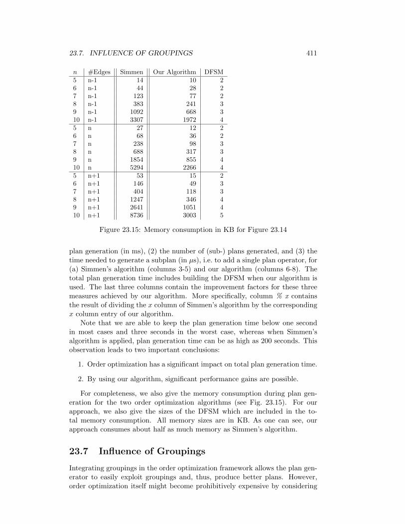
23.7. INFLUENCE OF GROUPINGS 411

n #Edges Simmen Our Algorithm DFSM5 n-1 14 10 26 n-1 44 28 27 n-1 123 77 28 n-1 383 241 39 n-1 1092 668 310 n-1 3307 1972 45 n 27 12 26 n 68 36 27 n 238 98 38 n 688 317 39 n 1854 855 410 n 5294 2266 45 n+1 53 15 26 n+1 146 49 37 n+1 404 118 38 n+1 1247 346 49 n+1 2641 1051 410 n+1 8736 3003 5

Figure 23.15: Memory consumption in KB for Figure 23.14

plan generation (in ms), (2) the number of (sub-) plans generated, and (3) thetime needed to generate a subplan (in µs), i.e. to add a single plan operator, for(a) Simmen’s algorithm (columns 3-5) and our algorithm (columns 6-8). Thetotal plan generation time includes building the DFSM when our algorithm isused. The last three columns contain the improvement factors for these threemeasures achieved by our algorithm. More specifically, column % x containsthe result of dividing the x column of Simmen’s algorithm by the correspondingx column entry of our algorithm.

Note that we are able to keep the plan generation time below one secondin most cases and three seconds in the worst case, whereas when Simmen’salgorithm is applied, plan generation time can be as high as 200 seconds. Thisobservation leads to two important conclusions:

1. Order optimization has a significant impact on total plan generation time.

2. By using our algorithm, significant performance gains are possible.

For completeness, we also give the memory consumption during plan gen-eration for the two order optimization algorithms (see Fig. 23.15). For ourapproach, we also give the sizes of the DFSM which are included in the to-tal memory consumption. All memory sizes are in KB. As one can see, ourapproach consumes about half as much memory as Simmen’s algorithm.

23.7 Influence of Groupings

Integrating groupings in the order optimization framework allows the plan gen-erator to easily exploit groupings and, thus, produce better plans. However,order optimization itself might become prohibitively expensive by considering

412CHAPTER 23. DERIVING ANDDEALINGWITH INTERESTINGORDERINGS ANDGROUPINGS

groupings. Therefore, we evaluated the costs of including groupings for differentqueries.

Since adding support for groupings has no effect on the runtime behaviorof the plan generator (all operations are still one table lookup), we measuredthe runtime and the memory consumption of the preparation step both withand without considering groupings. When considering groupings, we treatedeach interesting ordering also as an interesting grouping, i.e. we assumed thata grouping-based (e.g. hash-based) operator was always available as an alter-native. Since this is the worst-case scenario, it should give an upper bound forthe additional costs. All experiments were performed on a 2.4 GHz PentiumIV, using the gcc 3.3.1.

To examine the impact for real queries, we choose a more complex queryfrom the well-known TPC-R benchmark ([846], Query 8):

selecto year,sum(case when nation = ’[NATION]’

then volumeelse 0

end) / sum(volume) as mkt sharefrom

(selectextract(year from o orderdate) as o year,l extendedprice * (1-l discount) as volume,n2.n name as nation

from part,supplier,lineitem,orders,customer,nation n1,nation n2,region

wherep partkey = l partkey ands suppkey = l suppkey andl orderkey = o orderkey ando custkey = c custkey andc nationkey = n1.n nationkey andn1.n regionkey = r regionkey andr name = ’[REGION]’ ands nationkey = n2.n nationkey ando orderdate between date ’1995-01-01’ and

date ’1996-12-31’ andp type = ’[TYPE]’

) as all nationsgroup by o yearorder by o year;

When considering this query, all attributes used in joins, group-by andorder-by clauses are added to the set of interesting orders. Since hash-basedsolutions are possible, they are also added to the set of interesting groupings.

23.7. INFLUENCE OF GROUPINGS 413

This results in the sets

OPI = (o year), (o partkey), (p partkey),

(l partkey), (l suppkey), (l orderkey),

(o orderkey), (o custkey), (c custkey),

(c nationkey), (n1.n nationkey),

(n2.n nationkey), (n regionkey),

(r regionkey), (s suppkey), (s nationkey)OTI = ∅GPI = o year, o partkey, p partkey,

l partkey, l suppkey, l orderkey,o orderkey, o custkey, c custkey,c nationkey, n1.n nationkey,n2.n nationkey, n regionkey,r regionkey, s suppkey, s nationkey

GTI = ∅

Note that here OTI and GTI are empty, as we assumed that each orderingand grouping would be produced if beneficial. For example, we might assumethat it makes no sense to intentionally group by o year: If a tuple stream isalready grouped by o year it makes sense to exploit this, however, instead ofjust grouping by o year it could make sense to sort by o year, as this is requiredanyway (although here it only makes sense if the sort operator performs earlyaggregation). In this case, o year would move from GPI to GTI , as it wouldbe only tested for, but not produced.

The set of functional dependencies (and equations) contains all join condi-tions and constant conditions:

F = p partkey = l partkey, ∅ → p type,o custkey = c custkey, ∅ → r name,c nationkey = n1.n nationkey,s nationkey = n2.n nationkey,l orderkey = o orderkey,s suppkey = l suppkey,n1.n regionkey = r regionkey

To measure the influence of groupings, the preparation step was executedtwice: Once with the data as given above and once with GPI = ∅ (i.e. groupingswere ignored). The space and time requirements are shown below:

With Groups Without Groups

Duration [ms] 0.6ms 0.3msDFSM [nodes] 63 32Memory [KB] 5 2

414CHAPTER 23. DERIVING ANDDEALINGWITH INTERESTINGORDERINGS ANDGROUPINGS

0

2

4

6

8

10

4 5 6 7 8 9 10 11

dura

tion

(ms)

no of relations

preparation time

o+g (n-1)o (n-1)o+g (n)

o (n)o+g (n+1)

o (n+1)

Figure 23.16: Time requirements for the preparation step

Here time and space requirements both increase by a factor of two. Sinceall interesting orderings are also treated as interesting groupings, a factor ofabout two was expected.

While Query 8 is one of the more complex TPC-R queries, it is not overlycomplex when looking at order optimization. It contains 16 interesting order-ings/groupings and 8 functional dependencies, but they cannot be combined inmany reasonable ways, resulting in a comparatively small DFSM. In order toget more complex examples, we produced randomized queries with 5− 10 rela-tions and a varying number of join predicates. We always started from a chainquery and then randomly added additional edges to the join graph. The resultsare shown for n− 1, n and n+ 1 additional edges. In the case of 10 relations,this means that the join graph consisted of 18, 19 and 20 edges, respectively.

The time and space requirements for the preparation step are shown inFigure 23.16 and Figure 23.17, respectively. For each number of relations, therequirements for the combined framework (o+g) and the framework ignoringgroupings (o) are shown. The numbers in parentheses (n− 1, n and n+ 1) arethe number of additional edges in the join graph.

As with Query 8, the time and space requirements roughly increase by afactor of two when adding groupings. This is a very positive result, given that afactor of two can be estimated as a lower bound (since every interesting orderingis also an interesting grouping here). Furthermore, the absolute time and spacerequirements are very low (a few ms and a few KB), encouraging the inclusionof groupings in the order optimization framework.

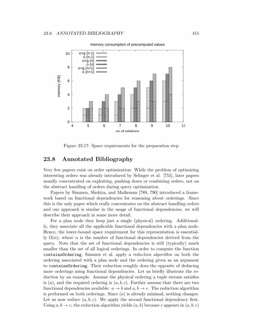
23.8. ANNOTATED BIBLIOGRAPHY 415

0

2

4

6

8

10

4 5 6 7 8 9 10 11

mem

ory

(KB

)

no of relations

memory consumption of precomputed values

o+g (n-1)o (n-1)o+g (n)

o (n)o+g (n+1)

o (n+1)

Figure 23.17: Space requirements for the preparation step

23.8 Annotated Bibliography

Very few papers exist on order optimization. While the problem of optimizinginteresting orders was already introduced by Selinger et al. [755], later papersusually concentrated on exploiting, pushing down or combining orders, not onthe abstract handling of orders during query optimization.

Papers by Simmen, Shekita, and Malkemus [789, 790] introduced a frame-work based on functional dependencies for reasoning about orderings. Sincethis is the only paper which really concentrates on the abstract handling ordersand our approach is similar in the usage of functional dependencies, we willdescribe their approach in some more detail.

For a plan node they keep just a single (physical) ordering. Additional-ly, they associate all the applicable functional dependencies with a plan node.Hence, the lower-bound space requirement for this representation is essential-ly Ω(n), where n is the number of functional dependencies derived from thequery. Note that the set of functional dependencies is still (typically) muchsmaller than the set of all logical orderings. In order to compute the functioncontainsOrdering, Simmen et al. apply a reduction algorithm on both theordering associated with a plan node and the ordering given as an argumentto containsOrdering. Their reduction roughly does the opposite of deducingmore orderings using functional dependencies. Let us briefly illustrate the re-duction by an example. Assume the physical ordering a tuple stream satisfiesis (a), and the required ordering is (a, b, c). Further assume that there are twofunctional dependencies available: a→ b and a, b→ c. The reduction algorithmis performed on both orderings. Since (a) is already minimal, nothing changes.Let us now reduce (a, b, c). We apply the second functional dependency first.Using a, b→ c, the reduction algorithm yields (a, b) because c appears in (a, b, c)

416CHAPTER 23. DERIVING ANDDEALINGWITH INTERESTINGORDERINGS ANDGROUPINGS

after a and b. Hence, c is removed. In general, every occurrence of an attributeon the right-hand side of a functional dependency is removed if all attributesof the left-hand side of the functional dependency precede the occurrence. Re-duction of (a, b) by a → b yields (a). After both orderings are reduced, thealgorithm tests whether the reduced required ordering is a prefix of the reducedphysical ordering. Note that if we applied a → b first, then (a, b, c) would re-duce to (a, c) and no further reduction would be possible. Hence, the rewritesystem induced by their reduction process is not confluent. This problem is notmentioned by Simmen et al., but can have the effect that containsOrdering

returns false whereas it should return true. The result is that some orderingsremain unexploited; this could be avoided by maintaining a minimal set of func-tional dependencies, but the computation costs would probably be prohibitive.This problem does not occur with our approach. On the complexity side, everyfunctional dependency has to be considered by the reduction algorithm at leastonce. Hence, the lower time bound is Ω(n).

In case all functional dependencies are introduced by a single plan node andall of them have to be inserted into the set of functional dependencies associatedwith that plan node, the lower bound for inferNewLogicalOrderings is alsoΩ(n).

Overall, Simmen et al. proposed the important framework for order opti-mization utilizing functional dependencies and nice algorithms to handle order-ings during plan generation, but the space and time requirements are unfortu-nate since plan generation might generate millions of subplans. Also note thatthe reduction algorithm is not applicable for groupings (which, of course, wasnever intended by Simmen): Given the grouping a, b, c and the functionaldependencies a → b and b → c, the grouping would be reduced to a, c orto a, depending on the order in which the reductions are performed. Thisproblem does not occur with orderings, as the attributes are sorted and can bereduced back to front.

A recent paper by Wang and Cherniack [878] presented the idea of combiningorder optimization with the optimization of groupings. Based upon Simmen’sframework, they annotated each attribute in an ordering with the informationwhether it is actually ordered by or grouped by. For a single attribute a, theywrite OaO(R) to denote that R is ordered by a, OaG(R) to denote that R isgrouped by a and OaO→bG to denote that R is first ordered by a and thengrouped by b (within blocks of the same a value). Before checking if a requiredordering or grouping is satisfied by a given plan, they use some inference rules toget all orderings and groupings satisfied by the plan. Basically, this is Simmen’sreduction algorithm with two extra transformations for groupings. In theirpaper the check itself is just written as ∈, however, at least one reduction onthe required ordering would be needed for this to work (and even that wouldnot be trivial, as the stated transformations on groupings are ambiguous). Thepromised details in the cited technical report are currently not available, as thereport has not appeared yet. Also note that, as explained above, the reductionapproach is fundamentally not suited for groupings. In Wang’s and Cherniack’spaper, this problem does not occur, as they only look at a very specializedkind of grouping: As stated in their Axiom 3.6, they assume that a grouping

23.8. ANNOTATED BIBLIOGRAPHY 417

OaG→bG is first grouped by a and then (within the block of tuples with the samea value) grouped by b. However, this is a very strong condition that is usuallynot satisfied by a hash-based grouping operator. Therefore, their work is notgeneral enough to capture the full functionality offered by a state-of-the-artquery execution engine.

In this chapter, we followed [617, 616].

418CHAPTER 23. DERIVING ANDDEALINGWITH INTERESTINGORDERINGS ANDGROUPINGS

Chapter 24

Cardinality and CostEstimation

24.1 Introduction

The plan generator relies on a cost function to evaluate the different plans and todetermine the cheapest one. This chapter is concerned with the development ofcost functions. The main input to cost functions are cardinalities. For example,assume a scan of a relation, which also applies a selection predicate. Clearly,the cost of scanning the relation depends on the physical layout of the relationon disk. Further, the CPU cost for evaluating the predicate depends on thenumber of tuples in the relation. Note that the cardinality of a relation isindependent of its physical layout.

In general, the cost of an algebraic operator is estimated by using a profile ofthe database. The profile must be small, e.g., a couple of kilobytes per relation1.We distuinguish between the logical and the physical profile. For each databaseitem and its constituents, there exist specialized logical and physical profiles.They exist for relations, indices, attributes, and sets of attributes. Consider arelation R. Its cardinality |R| belongs to its logical profile, whereas the numberof pages ||R|| it occupies belongs to its physical profile. In Chapter 4, we sawmore advanced physical profiles.

The DBMS must be capable to perform several operations to derive profilesand to deal with them. Fig. 24.1 gives an overview. This figure roughly followsthe approach of Mannino et al. [561, 560]. The first operation is the build op-eration, that takes as input a specification of the profiles to be build (becausethere are many different alternatives, as we will see) and the database. Fromthat, it builds the according profiles for all database items of all the differentgranularities. When updates arrive, the profiles must be updated. This caneither be done by a complete recalculation or by an incremental update opera-tion on the profiles themselves. The latter is reflected in the operation update.Unfortunately, not all profiles can have an update operation. Within this book,we will not be too concerned with building and updating profiles. At the end

1Given today’s cost for main memory, it may also be reasonable to use a couple ofmegabytes.

419

420 CHAPTER 24. CARDINALITY AND COST ESTIMATION

cardinalityestimation

costestimation

establishingphysicalprofiles

calculus oralgebraic expression

calculus oralgebraic expression

profile specification

update

profile

logical profile

cardinality estimation

physical profiles

algebraic expression

logical profile

physical profile

logical profile(s)

algebraic operator

logical profile

cardinality estimate

physical profile

logical profile

physical profile(s)

update

build

profile

cost

profile

propagation

Figure 24.1: Overview of operations for cardinality and cost estimations

of this chapter, we will provide some references (See [202] for an overview).

The main operations this chapter deals with are among the remaining ones.The first of them is cardinality estmation. Given an algebraic expression or acalculus expression together with a logical profile of the database, we estimatethe output/result cardinality of the expression. Why do we say algebraic orcalculus expression? Remember that plan generators generate plans for planclasses. Each plan class corresponds to a set of equivalent plans. They all pro-duce the same result and, hence, the same number of output tuples. Thus, intheory, one arbitrary representative of the class of equivalent algebraic expres-sions should suffice to calculate the logical profile, as a logical profile dependsonly on the outcome. On the other hand, the plan class more directly corre-sponds to a calculus expression. Hence, estimating the result cardinality of acalculus expression is a viable alternative. In the literature, most papers dealwith the first approach while only a few deal with the latter (e.g., [218]).

The second operation we will be concerned with is cost estimation. Givenlogical and physical profiles for all inputs and an algebraic operator (tree), thisoperation calculates the actual costs. Chapter 4 contains a detailed discussionabout disk access cost calculation. Hence, this part is considered done forbuilding blocks and access paths.

The third major task is profile propagation. Given a logical or physicalprofile and an expression, we must be able to calculate the profile of the result,since this may be the input to other expressions and thus be needed for furthercardinality estimates. The estimation of a physical profile occurs mostly in

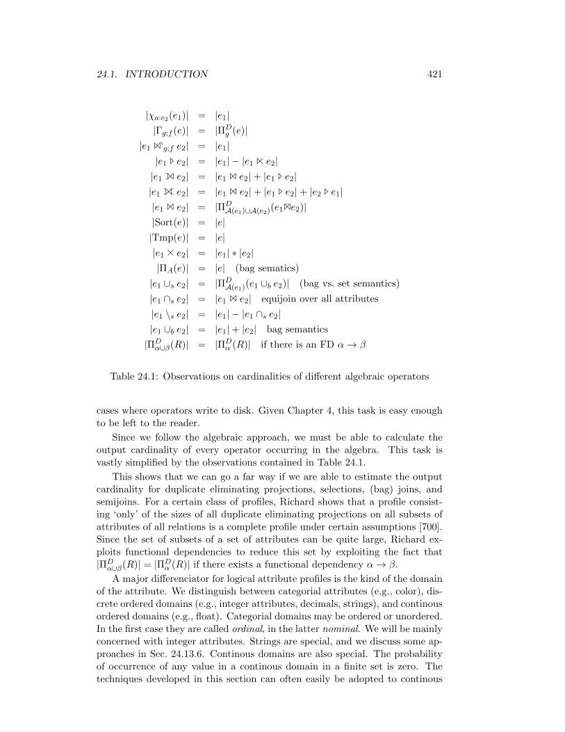
24.1. INTRODUCTION 421

|χa:e2(e1)| = |e1||Γg;f (e)| = |ΠD

g (e)||e1 Zg;f e2| = |e1||e1 T e2| = |e1| − |e1 N e2||e1 E e2| = |e1 B e2|+ |e1 T e2||e1 K e2| = |e1 1 e2|+ |e1 T e2|+ |e2 T e1||e1 1 e2| = |ΠD

A(e1)∪A(e2)(e11e2)||Sort(e)| = |e||Tmp(e)| = |e||e1 A e2| = |e1| ∗ |e2||ΠA(e)| = |e| (bag sematics)

|e1 ∪s e2| = |ΠDA(e1)(e1 ∪b e2)| (bag vs. set semantics)

|e1 ∩s e2| = |e1 1 e2| equijoin over all attributes

|e1 \s e2| = |e1| − |e1 ∩s e2||e1 ∪b e2| = |e1|+ |e2| bag semantics

|ΠDα∪β(R)| = |ΠD

α (R)| if there is an FD α→ β

Table 24.1: Observations on cardinalities of different algebraic operators

cases where operators write to disk. Given Chapter 4, this task is easy enoughto be left to the reader.

Since we follow the algebraic approach, we must be able to calculate theoutput cardinality of every operator occurring in the algebra. This task isvastly simplified by the observations contained in Table 24.1.

This shows that we can go a far way if we are able to estimate the outputcardinality for duplicate eliminating projections, selections, (bag) joins, andsemijoins. For a certain class of profiles, Richard shows that a profile consist-ing ‘only’ of the sizes of all duplicate eliminating projections on all subsets ofattributes of all relations is a complete profile under certain assumptions [700].Since the set of subsets of a set of attributes can be quite large, Richard ex-ploits functional dependencies to reduce this set by exploiting the fact that|ΠD

α∪β(R)| = |ΠDα (R)| if there exists a functional dependency α→ β.

A major differenciator for logical attribute profiles is the kind of the domainof the attribute. We distinguish between categorial attributes (e.g., color), dis-crete ordered domains (e.g., integer attributes, decimals, strings), and continousordered domains (e.g., float). Categorial domains may be ordered or unordered.In the first case they are called ordinal, in the latter nominal. We will be mainlyconcerned with integer attributes. Strings are special, and we discuss some ap-proaches in Sec. 24.13.6. Continous domains are also special. The probabilityof occurrence of any value in a continous domain in a finite set is zero. Thetechniques developed in this section can often easily be adopted to continous

422 CHAPTER 24. CARDINALITY AND COST ESTIMATION

domains, even if we do not mention this explicitly.

24.2 A First Approach

The first approach to cost and cardinality estimation integrated into a dynamicprogramming-based plan generator was presented by Selinger et al. [755]. Wewill use it as the basis for this section.

24.2.1 Top-Most Cost Formula (Overall Costs)

Their top-most cost formula states that the total cost of a query evaluationplan equals the weighted sum of the I/O and CPU costs:

C = CI/O + wCcpu (24.1)

where w is the weight which can be adapted to different situations. If, forexample, the system is CPU bound, we should increase w and if it is I/Obound, we decrease w.

However, it is not totally clear what we are going to optimize under this costformula. One interpretation could be the following. Assume w = 0.5. Then,we could interprete the total costs as response time under the assumption thatfifty percent of the CPU time can be executed in parallel with I/O. Accordingly,we find other top-most cost formulas. For example, the weight is sometimesdropped [392]:

C = CI/O + Ccpu (24.2)

Under the above interpretation, this would mean that concurrency is totallyabsent. The opposite, total concurrency between I/O and CPU, can also befound [162]:

C = max(CI/O, Ccpu) (24.3)

In these green days, an alternative is to calculate the power consumptionduring query execution. Therefore, we convert CPU time to Watts consumedby the CPU and disk time to Watts consumed by the disks and simply add upthese number to get an estimate of the power consumption of the plan.

24.2.2 Summation of Operator Costs

Given a query evaluation plan, the task is to calculate its I/O and CPU costs.This can be done by calculating the costs for each operator (op) occurring inthe query evaluation plan (QEP) and adding up the according costs:

CI/O =∑

op∈QEP

CI/O(op)

Ccpu =∑

op∈QEP

Ccpu(op)

However, these formulae sometimes raise a problem. For example, the nestedloop join method requires multiple evalutions of its inner part.

24.2. A FIRST APPROACH 423

Further, in order to count the I/O cost correctly, it is necessary to makesome assumptions when intermediate results are written to and read from disk.We will use the following assumption: Every operator is responsible for passingits result to the next operator via main memory. For example, a sort mergejoin may require sorting its inputs. The sort operators are then responsible forhanding over their result to the merge join via main memory. This means thatthe merge join may not require any I/O if the merge can be done purely inmain memory.

24.2.3 CPU Cost

To get an estimate of the CPU costs, Selinger et al. simply count the numberof calls to the tuple oriented interface (called RSI). This roughly correspondsto the number of next calls in an iterator-based implementation of algebraicoperators (for details on the Research Storage Engine (RSS) and its interfaceRSI see [41]). Hence, what needs to be known is the output cardinality of eachoperator in the query plan.

Given the input and output cardinalities, it is often quite straightforwardto calculate the CPU costs. Take, for example, a selection operator. Clearly,the selection predicate is called n times if n is the input cardinality. The selec-tion predicate itself consists of several calls to comparison functions, Booleanoperators, arithmetic operators and the like. The CPU cost of each of theseoperators can easily be determined (by counting CPU cycles or measurements),and thus the total CPU cost of a selection operator can be determined easily.Other operators are also straightforward. A problem only arises if functionsare called whose CPU costs can not easily be determined since they depend ontheir parameters. A typical example are string comparisons, where the CPUcosts depend on the length of the string. Another example are user-definedfunctions. The framework presented in [395] can be used for all more complexfunctions. Another possibility is to use simplifying assumptions. The functionswe are talking about are executed on a per tuple basis. As there are typicallymany tuples, using the average execution time for cost calculations is not a badidea.

24.2.4 Abbreviations

We need some abbreviations to state our cost formulas. A first bunch of themis summarized in Table 24.2. There, we assume that an index is always a B+

tree.

24.2.5 I/O Costs

Selinger et al. measure I/O costs in the number of pages read. Let us first discussthe different possible access paths to a single relation. Clearly, for a simple scanof a relation R, ||R|| pages have to be read. The next access path is composedof an access to a non-clustered index I to retrieve the tuple identifiers of thosetuples that satisfy a predicate p followed by an access to the base relation R.Let F (p) be the fraction of tuples satisfying a certain predicate p. F (p) is called

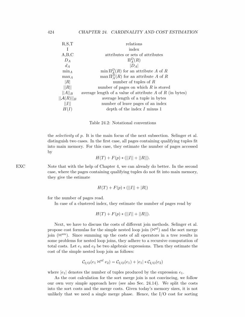
424 CHAPTER 24. CARDINALITY AND COST ESTIMATION

R,S,T relationsI index

A,B,C attributes or sets of attributesDA ΠD

A (R)dA |DA|

minA min ΠDA (R) for an attribute A of R

maxA max ΠDA (R) for an attribute A of R

|R| number of tuples of R||R|| number of pages on which R is stored||A||B average length of a value of attribute A of R (in bytes)||A(R)||B average length of a tuple in bytes||I|| number of leave pages of an indexH(I) depth of the index I minus 1

Table 24.2: Notational conventions

the selectivity of p. It is the main focus of the next subsection. Selinger et al.distinguish two cases. In the first case, all pages containing qualifying tuples fitinto main memory. For this case, they estimate the number of pages accessedby

H(T ) + F (p) ∗ (||I||+ ||R||).

Note that with the help of Chapter 4, we can already do better. In the secondEXCcase, where the pages containing qualifying tuples do not fit into main memory,they give the estimate

H(T ) + F (p) ∗ (||I||+ |R|)

for the number of pages read.

In case of a clustered index, they estimate the number of pages read by

H(T ) + F (p) ∗ (||I||+ ||R||).

Next, we have to discuss the costs of different join methods. Selinger et al.propose cost formulas for the simple nested loop join (1nl) and the sort mergejoin (1sm). Since summing up the costs of all operators in a tree results insome problems for nested loop joins, they adhere to a recursive computation oftotal costs. Let e1 and e2 be two algebraic expressions. Then they estimate thecost of the simple nested loop join as follows:

CI/O(e1 1nl e2) = CI/O(e1) + |e1| ∗ CI/O(e2)

where |e1| denotes the number of tuples produced by the expression e1.

As the cost calculation for the sort merge join is not convincing, we followour own very simple approach here (see also Sec. 24.14). We split the costsinto the sort costs and the merge costs. Given today’s memory sizes, it is notunlikely that we need a single merge phase. Hence, the I/O cost for sorting

24.2. A FIRST APPROACH 425

consists of writing and reading the result of ei if it needs to be sorted. This canbe estimated as

CI/O(sort(ei)) = CI/O(ei) + 2 ∗ d1.2||A(ei)||B ∗ |ei|/pagesizee

where pagesize is the page size in bytes. The factor 1.2 is called the universalfudge factor . In the above case, it takes care of the storage overhead incurredby using slotted pages. If we assume that the merge phase of the sort mergejoin can be performed in main memory, no additional I/O costs occur and weare done.

Clearly, in the light of Chapter 4, counting the numbers of pages read is notsufficient as the discrepancy between random and sequential I/O is tremendous.Thus, better cost functions should use a more elaborate I/O cost model alongthe lines of Chapter 4. In any case, note that the calculation of the I/O or CPUcosts of any operator highly depends on its input and output cardinalities.

24.2.6 Cardinality Estimates

Given a predicate p, we want to estimate its selectivity, which is defined as thefraction of qualifying tuples. If p is a selection predicate applied to a relationR, the selectivity of p is defined as

s(p) =|σp(R)||R| .

If we know the selectivity of p, we can then easily calculate the result size of aselection:

|σp(R)| = s(p)|R|Similarly for joins. Given a join predicate p and two relations R and S, wedefine the selectivity of p as

s(p) =|R 1p S||R× S| =

|R 1p S||R| ∗ |S|

and can calculate the result size of a join by

|R 1p S| = s(p) |R| |S|.

The idea of the approach of Selinger et al. is to calculate the result cardinal-ity for a plan class by the following procedure. First, the sizes of all relationsrepresented by the plan class are multiplied. This is the result of their crossproduct. In a second step, they take a look at the predicate p applied to therelations in the plan class. For p they calculate a selectivity estimate s(p) andmultiply it with the result of the first step. This then gives the result. Hence,if a plan class represents the algebraic expression

σp(Ani=1Ri),

the cardinality estimate is

s(p)

n∏

i=1

|Ri|.

426 CHAPTER 24. CARDINALITY AND COST ESTIMATION

predicate s(p) comment

not(p1) 1− s(p1)p1 ∧ p2 s(p1) ∗ s(p2) independencep1 ∨ p2 s(p1) + s(p2)− s(p1)s(p2)A = c 1/dA if dA is known, uniformity

1/10 elseA = B 1/max(dA, dB) if dA and dB are known, uniformity

1/dX if only dX , X ∈ A,B is known1/10 else

A > c maxA−cmaxA−minA

if min and max are known, uniformity

1/3 else

c1 ≤ A ≤ c2c2−c1

maxA−minAif min and max are known, uniformity

1/4 elseA IN L min(1/2, s(A = c)|L|)A IN Q |Q| ∗ |X| X is cross product of all relations

in Q’s from clause

Table 24.3: Selectivity estimation as proposed by Selinger et al.[755]

Since p can be a complex predicate involving boolean operators, they have todeal with them. Table 24.3 summarizes the proposed selectivity estimation. Aand B denote attributes, c, c1, c2 denote constants, L denotes a list of values, Qdenotes a subquery. In System R, the number of distinct values for an attribute(dA, dB) is only known if there exists an according index on the attribute. Letus give some rational for the selectivity estimation of A IN Q for an attribute Aand a subquery Q. Assume that A is an attribute of relation R and the subqueryQ is of the form select B from S .... Further assume that ΠA(R) ⊆ ΠB(S),i.e., referential integrity holds. Clearly, if all tuples of S are in the result of Q,the selectivity is equal to 1. If the output cardinality of Q is restricted by afactor s′ = |Q|/|S|, then we may assume that the number of distinct values inQ’s result is restricted by the same factor. Hence, the selectivity factor of thetotal predicate is also s′. Selinger et al. now continue as follows: “With a littleoptimism, we can extend this reasoning to include subqueries which are joinsand subqueries in which column [B] is replaced by an arithmetic expressioninvolving column names. This leads to the formula given above.”

Discussion Taking a broad view at the above model, we see that

• the estimates for CPU and I/O times are quite rough,

• the approach is not complete, especially projection and semijoin are nottreated,

• profile propagation is not discussed.

Further, the uniformity and independence assumptions are applied. This hasbeen shown to be quite inaccurate in many cases. More specifically, apply-

24.3. A FIRST LOGICAL PROFILE AND ITS PROPAGATION 427

ing these and other assumptions often leads to an overestimate of real resultcardinalities [169, 171].

How bad is it in terms of plan generation if we under- or overestimate thecardinalities of intermediate results? As Ioannidis and Christodoulakis pointedout, errors propagate multiplicatively through joins [433]. Assume we want tojoin eight relations R1, . . . , R8 and that the cardinality estimates of Ri are eacha factor of 5 off. Then the cardinality estimation of R1 1 R2 1 R3 will be afactor of 125 off. Clearly, this can affect the subsequent join ordering. If wewere only a factor of 2 off, the cardinality estimation of R1 1 R2 1 R3 could beonly a factor of eight off. This shows that minimizing the multiplicative erroris a serious intention.

The effect of misestimating cardinalities on plan quality has not been thor-oughly investigated. There exists a study by Kumar and Stonebraker, whichconcludes that it does not matter [500]. However, we do not trust this conclu-sion. Swami and Schiefer give a query and its profiles for which bad cardinalityestimates lead to a very bad plan [833]. A very impressive example query ispresented in [851]. The plan produced for the query under cardinality estima-tion errors runs 40 minutes while the plan produced with better cardinalityestimates takes less than 2 seconds. Later, we will give two further examplesshowing that good cardinality estimation is vital for generation of good plans.Hence, we are very sure that accurate estimation is vital for plan generation.We suggest to the reader to find examples, using the simple Cout cost function,where wrong cardinality estimates lead to bad plans. EXC

24.3 A First Logical Profile and its Propagation

We call a logical profile complete if it allows us to perform cardinality estima-tion and logical profile propagation for all algebraic operators. In this section,we present an almost complete logical profile and describe the procedure ofprofile propagation. The main components are the cumulated frequency, i.e.,the number of tuples, and the number of distinct values for each attribute in arelation. It is easy to see that we cannot do without either of them. Further,an upper and lower bound for values of an attribute is needed. Again, we willsee that we cannot do without them. Hence, the following profile is minimal.

24.3.1 The Logical Profile

For every attribute A of a relation, we define its logical profile as a four tuple

bA = [lA, uA, fA, dA]

where lA is a lower and uA is an upper bound for the values of A. Further, fA isthe cumulated frequency, i.e., the number of tuples with an A value within thebounds, and dA is the number of distinct values occurring as A’s values withinthe given bounds.

428 CHAPTER 24. CARDINALITY AND COST ESTIMATION

For the purpose of this section, we can define

lA = min(ΠA(R))

uA = max(ΠA(R))

fA = |R|dA = |ΠD

A (R)|

If the attribute A is implicit from the context or does not matter, we may omitit.

24.3.2 Assumptions

The first two assumptions we make are:

1. All attribute values are uniformely distributed, and

2. the values of all attributes are drawn independently.

Other assumptions will follow.Often in the formulas developed below, we talk about the universe (U) or

domain of the attributes. This is the potential set of values from which agiven attribute takes its values. In case of integer attributes, it is easy to seethat the domain of attribute A is [lA, uA]. The size of the domain, denotedby nA, then is nA = uA − lA + 1. For real values, the size of the domain is(almost) infinite. Thus, only some of the formulas given below may carry overto attributes whose type is real. Please do not confuse the universe/domain ofan attribute A with the active domain of an attribute A, which contains theactual values DA = ΠD

A (R) occurring for A in relation R.Let us take a closer look at the assumptions. The uniform distribution

assumption means that every value occurs about the same number of times.However, this cannot mean that every value of the domain does so, since dA maybe much smaller than nA. Hence, we refine the uniform distribution assumption(UDA) by assuming that every distinct value occurs about fA/dA times.

The second assumption is called attribute value independence assumption(AVI) or simply independence assumption. Assume we have two predicates p1

and p2 and wish to calculate the selectivity of p1 ∧ p2. Independence tells usthat we can do so by multiplying the selectivities of p1 and p2. Thus, underindependence sel(p1 ∧ p2) = sel(p1) ∗ sel(p2).

We still need another assumption: the equal spread assumption (ESA), alsocalled uniform spread assumption (USA) [202, 672]. It is used to answer thequestion where the occurring distinct values are in the domain. The equalspread assumption states that they occur at equal distance. Let us elaborate alittle on this.

For integers, we know the number nA of possible values from which A canbe drawn. It is nA = uA − lA + 1. Let us assume that we have only a fewdistinct values, that is dA << nA. This is not strictly necessary but is good forour intuition. We can now define the spread between two values occurring in A.Let DA = ΠD

A (R) = x1, . . . , xdA where xi < xi+1 be the sorted set of values

24.3. A FIRST LOGICAL PROFILE AND ITS PROPAGATION 429

occuring for attribute A, also known as active domain. Then we can define thespread as

∆i = xi+1 − xiThe equal spread assumption (ESA) states that ∆i = ∆j for all 1 ≤ i, j < dA.Denote this value by ∆A.

There are three subtypes of the equal spread assumption, depending onwhether we assume the lower and upper bounds lA and uA belong to DA. TypeI assumes lA, uA ∈ DA. Then ∆A becomes (uA − lA)/(dA − 1). In case of typeII, where lA ∈ DA and uA 6∈ DA holds, we have ∆A = (uA − lA)/dA. For typeIII, where lA 6∈ DA and uA 6∈ DA we get ∆A = (uA − lA)/(dA + 1). As anexample, take lA = 1, uA = 13, and dA = 3. Then for the three types we havethe different values 12/2 = 6, 12/3 = 4, and 12/4 = 3. It should be clear thatthe difference is small if dA is sufficiently large. If dA is small, we can storethe frequency of each value explicitly. Otherwise, it is large, and it does notmatter which type we use. In case of integers, the above numbers may resultin non-integers. Thus, we prefer to define in this case

∆A = buq − lq + 1

dAc.

An alternative to the uniform distribution assumption and the equal spreadassumption is the continous-value assumption. Here, we assume that all valuesin the (discrete and finite) domain occur with frequency fA/nA.

Different assumptions can lead to different estimates. To see this, we firstfix some notation. Then, we provide estimation procedures under the contin-ues value assumption and under the equal spread assumption. Afterwards, wepresent an example. Assume we are given a relation R and one of its attributesA. The possible values for attribute A as implied by its type is called universeand abbreviated by UA. The set of possible values is the active domain DA,which we already saw. The total number of tuples in R is typically called itscardinality and denoted by |R|. However, in this chapter we prefer to call thisvalue cumulated frequency and denote it by fA. Remember that we denote theminimum of DA by lA and the maximum by uA.

For attribute A, we consider range queries and try to estimate the resultcardinality thereof. Thus, we are interested in queries Q of the form

select count(*) from R where lq ≤ A ≤ uq.We denote the result of this range query by fq.

We describe frequency densities of some attribute A by sets of points (xi, fi),where xi is a domain value and fi is the frequency of the domain value. Thus,the frequency density is the result of the query

select A, count(*) from R group by A.

Here is our example for a frequency density:

(1, 7), (5, 4), (7, 2), (8, 1).

Thus, the integer value 1 occurs 7 times and the value 7 occurs 2 times.

430 CHAPTER 24. CARDINALITY AND COST ESTIMATION

To estimate the result cardinality of a range query Q with bounds lq anduq under the continous value assumption, we use the formula

fq(cva) :=uq − lq + 1

ua − la + 1∗ fA.

Let us first recall the spread under the equal spread assumptions. For integervalues, we defined

∆A := buq − lq + 1

dAc.

Using this definition, we provide an estimate for fq(esa) by applying the fol-lowing formula:

fq(esa) := bqu − ql + 1

∆Ac ∗ fA

dA.

Note that if the active domain is dense, i.e., all possible values within [lA, uA]occur in the database, then the estimation under cva and esa coincide.EXC

Fig. 24.2 shows the results for 28 different range queries specified by theirlower bound (lq) and upper bound (uq) for the frequency density given above.The true cumulated frequency within the given query range is given in thecolumn fq. The estimates determined under CVA and ESA are presented aswell as a column indicating the better assumption for that particular query. Aswe can see, in most cases ESA wins. However, experiments by Wang and Sevcik[873] came to the conclusion that the opposite is true and CVA is superior toESA. (We can follow this claim at least for some of their data sets). Sinceestimates using CVA are easier to calculate and easily extendible to contineousdomains, we prefer them.

Given the above assumptions (and one more to come), the task is to establishthe operations cardinality estimation and logical profile propagation. The latterimplies that we can calculate the logical profile of all attributes of any resultrelation established by applying some algebraic operator. Assume we havesolved this task. Then it is clear that the cumulated frequency fA, whichequals |R| in this section, solves the task of cardinality estimation. Hence,we will not mention the cardinality estimation task explicitly any more. Theuse of the cumulated frequency fA instead of the seemingly simpler cardinalitynotation |R| is motivated by the fact that a single attribute will have multiple(small, piecewise) profiles if histograms are applied. To make the formulas ofthis section readily available for histogram use is the main motivation for usingthe cumulated frequency.

24.3.3 Profile Propagation for Selection

We start with the selection operation. Let R be a relation and A,C ∈ A(R)be two attributes of R. We are given the profiles bA = [lA, uA, fA, dA] andbC = [lC , uC , fC , dC ] and have to calculate the profiles b′A = [l′A, u

′A, f

′A, d

′A]

and b′C = [l′C , u′C , f

′C , d

′C ] for σp(A)(R) for various selection predicates p(A) in

attribute A. We assume that the attribute values of A and C are uniformlydistributed and that A and C are independent. If a selection predicate uses

24.3. A FIRST LOGICAL PROFILE AND ITS PROPAGATION 431

no lq uq fq fq(cva) fq(esa) winner

1 1 2 7 3.5 3.52 1 3 7 5.25 3.5 cva3 1 4 7 7 74 1 5 11 8.75 7 cva5 1 6 11 10.5 10.56 1 7 13 12.25 10.5 cva7 1 8 14 14 148 2 3 0 3.5 3.59 2 4 0 5.25 3.5 esa

10 2 5 4 7 711 2 6 4 8.75 7 esa12 2 7 6 10.5 10.513 2 8 7 12.25 10.5 esa14 3 4 0 3.5 3.515 3 5 4 5.25 3.5 esa16 3 6 4 7 717 3 7 6 8.75 7 esa18 3 8 7 10.5 10.519 4 5 4 3.5 3.520 4 6 4 5.25 3.5 esa21 4 7 6 7 722 4 8 7 8.75 7 esa23 5 6 4 3.5 3.524 5 7 6 5.25 3.5 cva25 5 8 7 7 726 6 7 2 3.5 3.527 6 8 3 5.25 3.5 esa28 7 8 3 3.5 3.5

Figure 24.2: Sample for range query result estimation under CVA and ESA.

two attributes A and B, we again need to give the profile propagation for allattributes C, which are different from them.

Exact match queries The first case we consider is σA=c for a constant c.Clearly, l′A = c, u′A = c. Further,

d′A =

1 if c ∈ ΠA(R)0 else

We cannot be sure whether the first or second case occurs. Since no reasonablecardinality estimation should ever return zero, we always assume c ∈ ΠA(R).More generally, we assume that all constants in a query are contained in thedatabase in the according attributes.

As every distinct value occurs about fA/dA times, we conclude that f ′A =

432 CHAPTER 24. CARDINALITY AND COST ESTIMATION

fA/dA. A special case occurs if A is the key. Then, we can immediately concludethat f ′A = 1.

Let us now consider another attribute C ∈ A(R), C 6= A. Since f ′C = f ′A,we only need to establish d′C . For the lack of any further knowledge, we keepthe lower and upper bounds, i.e. l′C = lC and u′C = uC . To derive the number ofdistinct values remaining for attribute B, we can use the formula by Yao/Waters(see Sec. 4.16.1) Denote by s(p) = |σA=c(R)|/|R| = f ′A/fA the fraction of tuplesthat survives the selection with predicate p ≡ A = c. Fix a distinct value forC. Using the uniform distribution assumption, it occurs in fC/dC tuples of R.

Then, for this value we have(fA−fC/dC

f ′A

)possibilities to chose f ′A tuples without

it. The total number of possibilities to chose f ′A tuples is(fAf ′A

). Thus, we may

conclude thatd′C = dCYfAfC/dC (f ′A)

Alternatively, we could use

d′C = dC ∗ (1− (1− s(p))fC/dC )

or any other good approximation (see Section 4.16.1).

Range queries Let us now turn to range queries, i.e. selection predicates ofthe form c1 ≤ A ≤ c2, where lA ≤ c1 < c2 ≤ uA. In all of them, the lowerand upper bounds are given by the range, i.e. l′A = c1 and u′A = c2. Using theSystem R approach, we can estimate

f ′A =c2 − c1

uA − lA∗ fA

d′A =c2 − c1

uA − lA∗ dA

This estimate is good for real values.We could also rewrite the above estimate for the number of distinct values

d′A to

d′A =c2 − c1

∆A

As soon as we have estimated the number of distinct values in a given range,we can easily derive the cumulated frequency, as every distinct value occurs asoften as it did in R. Thus f ′A = fA ∗ (d′A/dA).

For another attribute C, C 6= A, the profile propagation is the same as inthe case for A = c. We only need to define s(p) = |σc1≤A≤c2(R)|/|R|.

Equality-based correlation The next case we consider is a predicate of theform A = B. If uA < lB or uB < lA, the result is empty. If lA 6= lB or uA 6= uB,we first apply a selection with predicate max(lA, lB) ≤ A ≤ min(uA, uB) andmax(lA, lB) ≤ B ≤ min(uA, uB). So assume w.l.o.g. that lA = lB and uA = uB.Note that fA = fB. Denote this number by f . Define n to be the numberof values in the domain of attributes A and B. For integers, this number is

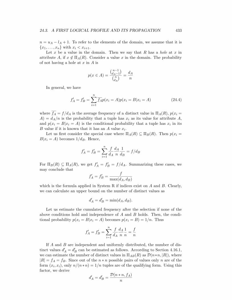
24.3. A FIRST LOGICAL PROFILE AND ITS PROPAGATION 433

n = uA − lA + 1. To refer to the elements of the domain, we assume that it isx1, . . . , xn with xi < xi+1.

Let x be a value in the domain. Then we say that R has a hole at x inattribute A, if x 6∈ ΠA(R). Consider a value x in the domain. The probabilityof not having a hole at x in A is

p(x ∈ A) =

(n−1dA−1

)(ndA

) =dAn

In general, we have

f ′A = f ′B =n∑

i=1

fAp(xi = A)p(xi = B|xi = A) (24.4)

where fA = f/dA is the average frequency of a distinct value in ΠA(R), p(xi =A) = dA/n is the probability that a tuple has xi as its value for attribute A,and p(xi = B|xi = A) is the conditional probability that a tuple has xi in itsB value if it is known that it has an A value xi.

Let us first consider the special case where ΠA(R) ⊆ ΠB(R). Then p(xi =B|xi = A) becomes 1/dB. Hence,

f ′A = f ′B =n∑

i=1

f

dA

dAn

1

dB= f/dB

For ΠB(R) ⊆ ΠA(R), we get f ′A = f ′B = f/dA. Summarizing these cases, wemay conclude that

f ′A = f ′B =f

max(dA, dB)

which is the formula applied in System R if indices exist on A and B. Clearly,we can calculate an upper bound on the number of distinct values as

d′A = d′B = min(dA, dB).

Let us estimate the cumulated frequency after the selection if none of theabove conditions hold and independence of A and B holds. Then, the condi-tional probability p(xi = B|xi = A) becomes p(xi = B) = 1/n. Thus

f ′A = f ′B =n∑

i=1

f

dA

dAn

1

n=f

n

If A and B are independent and uniformly distributed, the number of dis-tinct values d′A = d′B can be estimated as follows. According to Section 4.16.1,we can estimate the number of distinct values in ΠAB(R) as D(n∗n, |R|), where|R| = fA = fB. Since out of the n ∗ n possible pairs of values only n are of theform (xi, xi), only n/(n ∗n) = 1/n tuples are of the qualifying form. Using thisfactor, we derive

d′A = d′B =D(n ∗ n, fA)

n

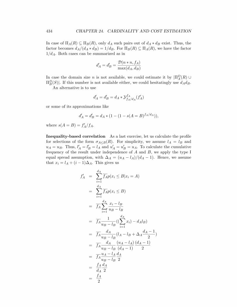
434 CHAPTER 24. CARDINALITY AND COST ESTIMATION

In case of ΠA(R) ⊆ ΠB(R), only dA such pairs out of dA ∗ dB exist. Thus, thefactor becomes dA/(dA ∗ dB) = 1/dB. For ΠB(R) ⊆ ΠA(R), we have the factor1/dA. Both cases can be summarized as in

d′A = d′B =D(n ∗ n, fA)

max(dA, dB)

In case the domain size n is not available, we could estimate it by |ΠDA (R) ∪

ΠDB (S)|. If this number is not available either, we could hesitatingly use dAdB.

An alternative is to use

d′A = d′B = dA ∗ YfAfA/dA(f ′A)

or some of its approximations like

d′A = d′B = dA ∗ (1− (1− s(A = B)fA/dA)),

where s(A = B) = f ′A/fA.

Inequality-based correlation As a last exercise, let us calculate the profilefor selections of the form σA≤B(R). For simplicity, we assume lA = lB anduA = uB. Thus, l′A = l′B = lA and u′A = u′B = uA. To calculate the cumulativefrequency of the result under independence of A and B, we apply the type Iequal spread assumption, with ∆A = (uA − lA)/(dA − 1). Hence, we assumethat xi = lA + (i− 1)∆A. This gives us

f ′A =

dA∑

i=1

fAp(xi ≤ B|xi = A)

=

dA∑

i=1

fAp(xi ≤ B)

= fA

dA∑

i=1

xi − lBuB − lB

= fA1

uB − lB((

dA∑

i=1

xi)− dAlB)

= fAdA

uB − lB(lA − lB + ∆A

dA − 1

2)

= fAdA

uB − lB(uA − lA)

(dA − 1)

(dA − 1)

2

= fAuA − lAuB − lB

dA2

=fAdA

dA2

=fA2

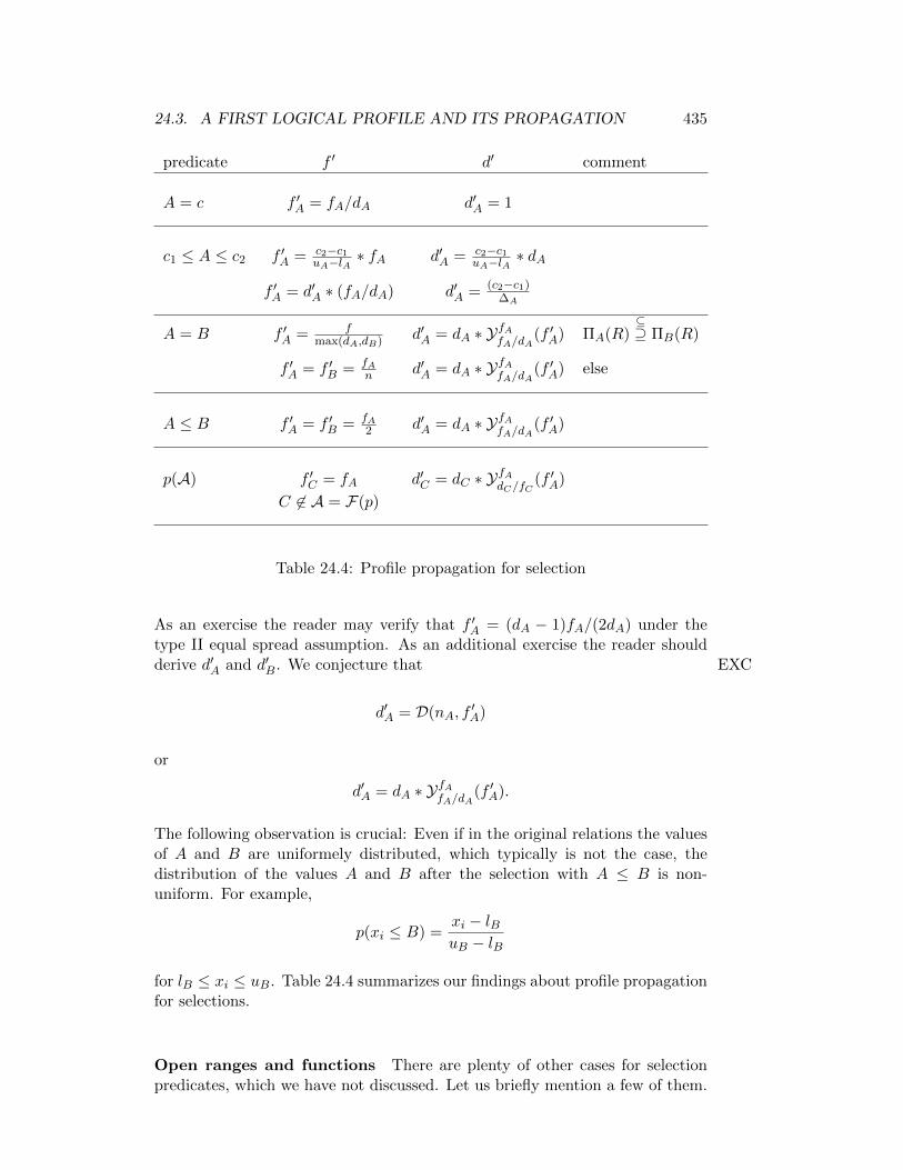
24.3. A FIRST LOGICAL PROFILE AND ITS PROPAGATION 435

predicate f ′ d′ comment

A = c f ′A = fA/dA d′A = 1

c1 ≤ A ≤ c2 f ′A = c2−c1uA−lA ∗ fA d′A = c2−c1

uA−lA ∗ dA

f ′A = d′A ∗ (fA/dA) d′A = (c2−c1)∆A

A = B f ′A = fmax(dA,dB) d′A = dA ∗ YfAfA/dA(f ′A) ΠA(R)

⊆⊇ ΠB(R)

f ′A = f ′B = fAn d′A = dA ∗ YfAfA/dA(f ′A) else

A ≤ B f ′A = f ′B = fA2 d′A = dA ∗ YfAfA/dA(f ′A)

p(A) f ′C = fA d′C = dC ∗ YfAdC/fC (f ′A)

C 6∈ A = F(p)

Table 24.4: Profile propagation for selection

As an exercise the reader may verify that f ′A = (dA − 1)fA/(2dA) under thetype II equal spread assumption. As an additional exercise the reader shouldderive d′A and d′B. We conjecture that EXC

d′A = D(nA, f′A)

or

d′A = dA ∗ YfAfA/dA(f ′A).

The following observation is crucial: Even if in the original relations the valuesof A and B are uniformely distributed, which typically is not the case, thedistribution of the values A and B after the selection with A ≤ B is non-uniform. For example,

p(xi ≤ B) =xi − lBuB − lB

for lB ≤ xi ≤ uB. Table 24.4 summarizes our findings about profile propagationfor selections.

Open ranges and functions There are plenty of other cases for selectionpredicates, which we have not discussed. Let us briefly mention a few of them.

436 CHAPTER 24. CARDINALITY AND COST ESTIMATION

Clearly, we have:

|σA 6=c(R)| = |R| − |σA=c(R)||σc1<A≤c2(R)| = |σc1≤A≤c2(R)| − |σA=c1(R)||σc1≤A<c2(R)| = |σc1≤A≤c2(R)| − |σA=c2(R)||σc1<A<c2(R)| = |σc1≤A≤c2(R)| − |σA=c1(R)| − |σA=c2(R)||σc1≤A(R)| = |σc1≤A≤uA(R)||σc1<A(R)| = |σc1≤A<uA(R)||σA≤c2(R)| = |σlA≤A≤c2(R)||σA<c2(R)| = |σlA≤A<c2(R)|

This helps to estimate the f ′A. The d′A are left to the reader.EXC

Estimating selectivities for (user defined) functions and expressions can bedone by using computed attributes. For example, cardinalities for selectionswith predicates like g(A) = c for a function g can be treated by introducing anadditional attribute gA for which a profile can be established.

24.3.4 Profile Propagation for Join

As for equality-based correlation, we assume for this subsection that the upperand lower bounds of the join attributes A and B are the same. If this is notthe case, we apply the according selections first.

Semijoin Let us now turn to the join operator and its variants. We start withthe left-semijoin and consider expressions of the type R NA=B S. If ΠA(R) ⊆ΠB(S), then R NA=B S = R, and no profiles change. If ΠA(R) ⊇ ΠB(S), thenf ′A = fAdB/dA and d′A = dB. If A and B are independent, we calculate

f ′A =

n∑

i=1

fAdAp(xi = A)p(xi ∈ B) =

n∑

i=1

fAdA

dAn

dBn

=fAdBn

.

and

d′A =dAdBn

.

For an attribute C ∈ A(R) \ A,B, we have f ′C = f ′A and

d′C = dC ∗ YfAfC/dC (f ′A).

Regular Join For the regular join R 1A=B S. Let us start with an at-tribute C ∈ A(R)\A,B. We can apply the formulas for the semijoin becauseΠDC (R 1A=B S) = ΠD

C (R N S). For attributes C ∈ A(S) \ A,B rememberthat the join commutes.

We turn to the case where ΠA(R) ⊆ ΠB(S). In this case, it is easy to seethat f ′A = f ′B = fAfB/dB and d′A = d′B = dA. If ΠA(R) ⊇ ΠB(S), we have justto exchange the roles of R and S.

24.3. A FIRST LOGICAL PROFILE AND ITS PROPAGATION 437

If A and B are independent, we proceed as follows. Denote again by n thedomain size of A and B and the values of DA = ΠA(R) by x1, . . . , xdA. Then,we can argue that

f ′A = f ′B =n∑

i=1

fAdA

fBdBp(xi = A)p(xi ∈ B) =

n∑

i=1

fAdA

fBdB

dAn

dBn

=fAfBn

.

Rosenthal showed that this result also holds if the condition of fairness holdsfor at least one relation [704]. A relation is called fair with respect to anattribute A if for the expected value E(|σA=x(R)|) = |R|/nA holds. In thiscase, the expected value for the result of the join is (|R||S|)/n. Note thatΠDA (R 1A=B S) = ΠD(R NA=B S). Thus, we can estimate the number of

distinct values as

d′A = d′B =dAdBn

.

Selfjoin The above formulas only apply if we are not dealing with a selfjoin.Of course, R 1A=B R does not pose any problems. However, R 1A=A R does,because all tuples find a join partner. The estimates are easy to derive:

f ′A =fAfAdA

d′A = dA

For all attributes C other than A, f ′C = f ′A and d′C = dC .As pointed out by [23], selfjoin sizes can be used to derive an upper bound

for general joins:

|RBA=B S| ≤|RBA=A R|+ |S BB=B S|

2.

This bound, which is an immediate consequence of the Cauchy Schwarz in-equality, can be used as a sanity check. Table 24.5 summarizes our findings forjoins.

24.3.5 Profile Propagation for Projection

The next operator we deal with is the duplicate eliminating projection. Givenour work from Chapter 4, it is not surprising, that we simply have to apply theD function. For single attributes A, we have

f ′A = d′A = dA

For a set of attributes A = A1, . . . , An, the result cardinality of ΠDA(R) is

D(n∏

i=1

nAi , |R|),

if nAi , the size of the domain of Ai, is known. Otherwise, we can use theestimate

D(n∏

i=1

dAi , |R|)

438 CHAPTER 24. CARDINALITY AND COST ESTIMATION

join f’ d’ comment

RNA=B S f ′A = fA d′A = dA ΠA(R) ⊆ ΠB(S)

f ′A = fAdBdA

d′A = dB ΠA(R) ⊇ ΠB(S)

f ′A = fAdBn d′A = dAdB

n else

f ′C = f ′A d′C = dC ∗ YfAdC/fC (f ′A) for C ∈ A(R) \ A,B

RBA=B S f ′A = fAfBdB

d′A = dA ΠA(R) ⊆ ΠB(S)

f ′A = fAfBn d′A = dAdB

n else

RBA=A R f ′A = fAfAdA

d′A = dA

Table 24.5: Profile propagation for joins

The number of distinct values in any attribute does not change, i.e. d′Ai = dAi .

If we have a functional dependencies and κ → A for a set of attributes Aand κ ⊂ A, then

ΠDA(R) = ΠD

κ (R).

Further, if |ΠDA(R)| = |R|, we have |ΠD

A′(R)| = |R| for all A′ with A′ ⊇ A.

The above estimates for the result size of a duplicate eliminating projectionassumes that the attribute values are uniformly distributed, i.e., every distinctvalue occurs with the same probability. As we will not deal with projectionsany more in this part of the book, let us complete the subject by giving anapproach where each attribute value can have its own probability of occurrence.This is not unlikely, and for attributes with few possible values the followingapproach proposed by Yu, Zuzarte, and Sevcik is quite reasonable [932]. Theassumptions are that the attributes are independent and the values of eachof them are drawn by independent Bernoulli trials. Under these assumptions,they derive the following three results: a lower bound, an upper bound, and anestimate for the expected number of distinct values in the projection. In orderto state these results, we need some additional notation. Let R be a relationand define N = |R|. Further let G = A1, . . . , An be a subset of the attributesof R. Define di = |ΠD

Ai(R)| to be the number of distinct values occurring in

attribute Ai. We denote values of Ai by ai,1, . . . , ai,di .

We wish to derive an estimate for DG = |ΠDG(R)|. Therefore, we model each

attribute Ai by a frequency vector fi = (fi,1, . . . , fi,di) where fi,j is the numberof occurrences of the j-th distinct value ai,j of Ai divided by N . If, for example,A1 has three distinct values which occur 90, 9, and 1 times in a relation withN = 100 elements, then f1 becomes (0.9, 0.09, 0.01).

Let us first look at bounds for DG. Trivially, DG is bounded from above by

DG ≤ minN,n∏

i=1

di

24.3. A FIRST LOGICAL PROFILE AND ITS PROPAGATION 439

and from below byDG ≥

nmaxi=1

di.

These bounds are very rough. This motivated Yu et al. to derive better ones.Before we proceed, let us consider another example. Assume we have three

attributes A1, A2, and A3 all with frequency vectors fi = (0.9, 0.09, 0.01) for arelation of size N = 100. Since we assume attribute independence, the proba-bility of (a1,3, a2,3, a3,3) is 0.01∗0.01∗0.01. Thus, its occurrence in a relation ofsize 100 is highly unlikely. Hence, we expect DG to be less than 27 = 3*3*3. Ingeneral, we observe that the probability of occurrence of a tuple (a1,j1 , . . . , an,jn)is the product of the relative frequencies f1,j1 ∗ . . . ∗ fn,jn . From this, the ba-sic idea of the approach of Yu et al. becomes clear: we have to systematicallyconsider all the different possibilities to multiply relative frequencies. This isnicely captured by the Kronecker product (tensor product).

Before we proceed, let us state the upper and lower bounds in case of twoattributes by giving two theorems developed by Yu et al. [932].

Theorem 24.3.1 (lower bound) For a set of attributes A1, A2 of a rela-tion R and its frequency vectors, we define li,j for i = 1, 2 and 1 ≤ j ≤ di as theminimum number of different values that have to be combined with fi,j giventhe marginals, i.e.

li,j = min|F | | F ⊆ 1, . . . , di′, ∀q 6∈ F S(F ) ≤ fi,j < S(F ) + fi′,q

where i′ = 3− i and S(F ) =∑

p∈F fi′,p. Further define

D⊥G = maxi=1,2

di∑

j=1

li,j .

Then D⊥G is a lower bound for DG and D⊥G ≥ maxd1,d2.

Theorem 24.3.2 (upper bound) For a set of attributes A1, A2 of a rela-tion R and its frequency vectors, we define ui,j for i = 1, 2 and 1 ≤ j ≤ di asthe maximum number of different values that can be combined with fi,j giventhe marginals, i.e.

ui,j = mindi′ , fi,jNwhere i′ = 3− i. Further define

D>G = mini=1,2

di∑

j=1

ui,j .

Then D>G is a lower bound for DG and D>G ≤ minN,∏ni=1 di.

The algorithm in Fig. 24.3 calculates the lower bound D⊥G. Calculating theupper bound D>G is much easier. For each fi,j , we compute ui,j by simplycomparing fi,jN and di′ . Adding up the ui,j for each attribute and taking thelesser of the two sums gives the desired result.

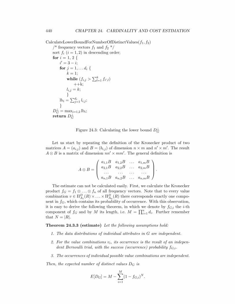
440 CHAPTER 24. CARDINALITY AND COST ESTIMATION

CalculateLowerBoundForNumberOfDistinctValues(f1, f2)/* frequency vectors f1 and f2 */sort fi (i = 1, 2) in descending order;for i = 1, 2

i′ = 3− i;for j = 1, . . . di

k = 1;

while (fi,j >∑k

l=1 fi′,l)++k;

li,j = k;

lbi =∑di

j=1 li,j ;

D⊥G = maxi=1,2 lbi;return D⊥G

Figure 24.3: Calculating the lower bound D⊥G

Let us start by repeating the definition of the Kronecker product of twomatrices A = (ai,j) and B = (bi,j) of dimension n×m and n′ ×m′. The resultA⊗B is a matrix of dimension nn′ ×mm′. The general definition is

A⊗B =

a1,1B a1,2B . . . a1,mBa2,1B a2,2B . . . a2,mB. . . . . . . . . . . .an,1B an,2B . . . an,mB

.

The estimate can not be calculated easily. First, we calculate the Kroneckerproduct fG = f1 ⊗ . . . ⊗ fn of all frequency vectors. Note that to every valuecombination v ∈ ΠD

A1(R)× . . .×ΠD

An(R) there corresponds exactly one compo-

nent in fG, which contains its probability of occurrence. With this observation,it is easy to derive the following theorem, in which we denote by fG,i the i-thcomponent of fG and by M its length, i.e. M =

∏ni=1 di. Further remember

that N = |R|.

Theorem 24.3.3 (estimate) Let the following assumptions hold:

1. The data distributions of individual attributes in G are independent.

2. For the value combinations vi, its occurrence is the result of an indepen-dent Bernoulli trial, with the success (occurrence) probability fG,i.

3. The occurrences of individual possible value combinations are independent.

Then, the expected number of distinct values DG is

E[DG] = M −M∑

i=1

(1− fG,i)N .

24.3. A FIRST LOGICAL PROFILE AND ITS PROPAGATION 441

EstimateNumberOfDistinctValues(f1, . . . , fn)/* frequency vectors fi *//* step 1: calculate fG = f1 ⊗ . . .⊗ fn */fG = f1;for (i = 2; i ≤ n; ++i)

fold = fG;fG = ε; // empty vectorfor (j = 1; j ≤ |fold|; ++j)

for (k = 1; k ≤ di; ++k) fG = push back(fG, f

oldj × fi,j); // append a value to a vector

/* step 2: compute the expected number of distinct value combinations */S = 0;for (j = 1, j ≤M ; ++j) // M = length(fG)

S += (1− fj)N ;DG = M − S;

return DG;

Figure 24.4: Calculating the estimate for DG

The algorithm for computing the estimate is given in Fig. 24.4. In the first,most expensive phase, it constructs the Kronecker product. Then, the simplecalculations according to the theorem follow. A more efficient implementationwould calculate the Kronecker product only implicitly. Further, the frequencyvectors may not be completely known but only a part of it via some histogram.As was also shown by Yu et al., end-biased histograms (coming soon) are opti-mal under the following error metrics. Let DG,hist be the estimate derived fora histogram. The error function they consider is

Eabs = |DG − DG,hist|.

24.3.6 Profile Propagation for Division

As a starting point, we use an observation made by Merrett and Otoo [580].Assume we are given two sets X and Y , which are both subsets of a finitedomain D with |D| = n elements. Then |X| < |Y | implies that X 6⊆ Y .Otherwise, we can calculate the probability of X ⊇ Y as

p(X ⊇ Y ) =

(|X||Y |

)/

(n

|Y |

)

Now let R and S be two relations with A(R) = A,B and A(S) = B. Avalue a ∈ ΠD

A (R) is contained in the result ofR÷B if and only if ΠB(σA=a(R)) ⊇

442 CHAPTER 24. CARDINALITY AND COST ESTIMATION

S. Hence, for any such a, fA = fA/dA and nB equal to the size of the commondomain of R.B and S.B, we can calculate the survival probability as

(fA|S|

)/

(nB|S|

)

provided that fA ≥ |S| and R is a set. Denote by f ′A and d′A the cumulatedfrequency and the number of distinct values for attribute A in the result ofR÷ S. Then we have the estimate

f ′A = d′A = dA ∗(fA|S|

)/

(nB|S|

)

in case R is a set.

If R is a bag, we must be prepared to see duplicates in σA=a(R). In thiscase we can adjust the above formula to

f ′A = d′A = dA ∗(xA|S|

)/

(n

|S|

)

where xA = D(xA, nA), and nA is the size of the domain of R.A.

If there is some variance among the number of distinct values associatedwith the a ∈ ΠD

A (R), the estimate will be rough. To cure this, we need betterinformation. Define for each a ∈ ΠD

A (R) the number ha to be the number ofdistinct b values occurring for it, i.e. ha = |ΠD

B (σA=a(R))|. Then we couldestimate f ′A and d′A as follows:

f ′A = d′A =∑

a∈ΠDA (R)

(ha|S|

)/

(n

|S|

)

Keeping ha for every possible a may not be practical. However, if the numberof distinct values in H = ha|a ∈ ΠD

A (R) is small, we can keep the number ofdistinct a values for each possible ha. Assume H = h1, . . . , hk and define

gi = |a ∈ ΠDA (R)|ha = hi|,

then we have the estimate

f ′A = d′A =

k∑

i=0,hi≥|S|gi

(hi|S|

)/

(n

|S|

).

24.3.7 Remarks

NULL Values Our profile is not really complete for attributes which canhave NULL values. To deal with these, we need to extend our profiles by thefrequency d⊥A with which NULL occurs in an attribute A of some relation. It isstraightforward to extend the above profile to deal with this additional count.

24.4. APPROXIMATION OF A SET OF VALUES 443

Name Definition Error minimized

median(x)

x(n+1)/2 n odd

(xn/2 + xn/2+1)/2 n evenE1 =

∑ni=1 |xi − x|

mean(x) 1/n∑n

i=1 xi E2 =√∑n

i=1(xi − x)2

middle (max(x) + min(x))/2 E∞ = maxni=1 |xi − x|

q-value√

max(X) min(X) Eq = maxni=1 maxxi/x, x/xi

Table 24.6: Approximations of a set of numbers by a single number

Uniformity is not sufficient As we have seen, even if all attributes areuniformly distributed, which is rarely the case in practice, the result of algebraicoperators may no longer be uniformly distributed. As a consequence, we needto be concerned with the approximation of the true distribution of values.

Sets of Attributes Note that nothing prevents us to use the formulas de-veloped above for selections and joins if A and B are attribute sets instead ofsingle attributes. We just have to know or calculate dA for sets of attributes A.

24.4 Approximation of a Set of Values

24.4.1 Approximations and Error Metrics

Assume we have a set of values x = x1, . . . , xn. The task we want to tackleis to approximate this set of values by a single value. The left two columnsof Table 24.6 show the names and definitions of some possible approximations.Whereas mean and median are well known, the other two may be not. Themiddle is defined as the value exactly between the minimum and maximum ofX. Hence, the distance from the middle to either extreme is the same. The q-value needs some further restriction: the values in X must be larger than zero.For our purposes, this restriction is not bad since execution costs are typicallylarger than zero and frequencies are mostly larger than zero if they are notexactly zero. The latter case needs some special attention if we use somethinglike the q-value, which we could also term geometric or multiplicative middle.

Let us take a look at a simple example. Assume X = 1, 2, 9. Then wecan easily calculate the approximations summarized in the following table:

median mean middle q-value

2 4 5 3

Which of these approximations is the best one? The answer depends on the errorfunction we wish to minimize. Therefore, the rightmost column of Table 24.6shows some error functions, which are minimized by the approximation definedin the same line. The variable x denotes the estimate whose error is to be

444 CHAPTER 24. CARDINALITY AND COST ESTIMATION

calculated. For E2 there exist plenty of equivalent formulations, where we thinkof two error measures as being equivalent, if and only if they result in the sameminimum. Some important alternatives are 1/n

∑(xi−x)2, 1/(n−1)

∑(xi−x)2

(empirical variance), and simply∑

(xi − x)2.A nice property half of the approximations give us are error bounds. These

are E∞ and Eq. Define the spread s of x as max(x)−min(x). Then, given themiddle m of x, we have for every xi ∈ x that

m− s/2 ≤ xi ≤ m+ s/2.

Thus, we have a symmetric, additive error bound for all elements in x. Definethe geometric spread as s =

√max(x)/min(x). Then we have a symmetric,

multiplicative error bound for all elements xi in x given by

(1/s)q ≤ xi ≤ sq

if q is the geometric middle. The following table shows the possible errors forall approximations of our example set X = 1, 2, 9:

median mean middle geo. mean2 4 5 3

E1 8 10 11 9E2 7.1 6.2 6.4 6.4E∞ 7 5 4 6Eq 4.5 4 5 3

Which of these error metrics and, hence, which approximation is the best?Obviously, this depends on the application. In the query compiler context, E1

plays no role that we are aware of. E2 plays a predominant role as it is used toapproximate values in a given histogram bucket. This has not come by sharpreasoning about the best possibility but merely by the existence of a huge bodyof literature in this area. Currently, the other two error metrics, E∞ and Eq,play minor roles. But this will change.

24.4.2 Example Applications

Let us discuss some example applications relevant to building a query compiler.Assume we have to come up with the execution time (CPU usage) for somefunction. This could be a simple arithmetic function built into our system,a hash function executed for a hash-join, the CPU time used to dereferencea TID if the according page is in memory, the CPU time needed to search aB-tree page residing in the buffer, or the CPU time needed to load a page fromsecondary storage into the buffer. Careful as we are, we measure the function’sexecution time several times. Almost certainly, the numbers will not be samefor every execution, except maybe for the simplest functions. To come up withina single number, we need to approximate the set of numbers derived from ourmeasurements. If the function is going to be executed many times within aquery execution plan (in which it occurs), we need to cost the average caseand the mean is the approximation of choice. We will see more applications inSection 24.5.2.

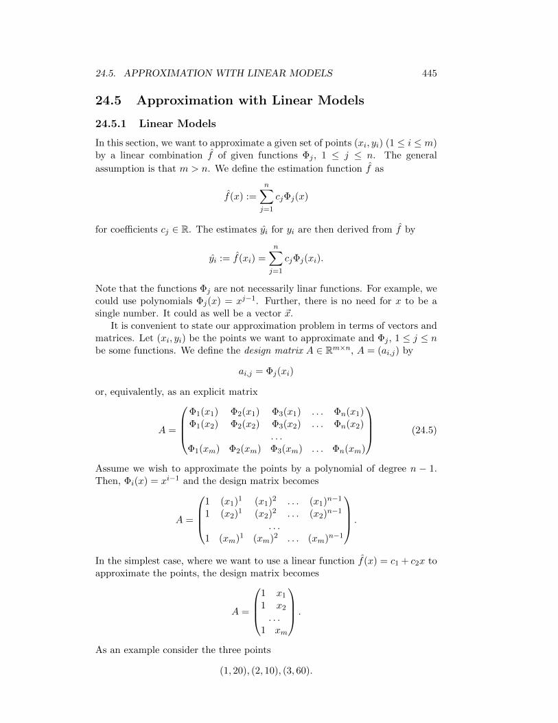
24.5. APPROXIMATION WITH LINEAR MODELS 445

24.5 Approximation with Linear Models

24.5.1 Linear Models

In this section, we want to approximate a given set of points (xi, yi) (1 ≤ i ≤ m)by a linear combination f of given functions Φj , 1 ≤ j ≤ n. The general

assumption is that m > n. We define the estimation function f as

f(x) :=n∑

j=1

cjΦj(x)

for coefficients cj ∈ R. The estimates yi for yi are then derived from f by

yi := f(xi) =

n∑

j=1

cjΦj(xi).

Note that the functions Φj are not necessarily linar functions. For example, wecould use polynomials Φj(x) = xj−1. Further, there is no need for x to be asingle number. It could as well be a vector ~x.

It is convenient to state our approximation problem in terms of vectors andmatrices. Let (xi, yi) be the points we want to approximate and Φj , 1 ≤ j ≤ nbe some functions. We define the design matrix A ∈ Rm×n, A = (ai,j) by

ai,j = Φj(xi)

or, equivalently, as an explicit matrix

A =

Φ1(x1) Φ2(x1) Φ3(x1) . . . Φn(x1)Φ1(x2) Φ2(x2) Φ3(x2) . . . Φn(x2)

. . .Φ1(xm) Φ2(xm) Φ3(xm) . . . Φn(xm)

(24.5)

Assume we wish to approximate the points by a polynomial of degree n − 1.Then, Φi(x) = xi−1 and the design matrix becomes

A =

1 (x1)1 (x1)2 . . . (x1)n−1

1 (x2)1 (x2)2 . . . (x2)n−1

. . .1 (xm)1 (xm)2 . . . (xm)n−1

.

In the simplest case, where we want to use a linear function f(x) = c1 + c2x toapproximate the points, the design matrix becomes

A =

1 x1

1 x2

. . .1 xm

.

As an example consider the three points

(1, 20), (2, 10), (3, 60).

446 CHAPTER 24. CARDINALITY AND COST ESTIMATION

The design matrix becomes

A =

1 11 21 3

(24.6)

For every column vector ~c = (c1, c2)T

A~c

gives the result of f for all points. Clearly, ~c should be determined such thatthe deviation of A~c from ~y = (y1, . . . , ym)T becomes minimal.

The deviation could be zero, that is A~c = ~y. However, remember our as-sumption that m > n. This means that we have more equations than variables.Thus, we have an overdetermined system of equations and it is quite unlikelythat a solution to this system of equations exists. This motivates our goal tofind an approximation as good as possible. Next, we formalize this goal.

Often used measures for deviations or distances of two vectors are based onnorms.

Definition 24.5.1 (norm) Let S be a linear space. Then a function ||x|| :S → R is called a norm if and only if it has the following three properties:

1. ||x|| > 0 unless x = 0

2. ||λx|| = |λ| ||x||

3. ||x+ y|| ≤ ||x||+ ||y||Various norms, called p norms can be found in the literature. Let x ∈ Rn

and p ≥ 1 where p =∞ is possible. Then

||x||p = (

n∑

i=0

|xi|p)1p .

The most important norms are the l1, l2, and l∞ norms:

||x||1 = |x1|+ . . .+ |xn|||x||2 =

√(x1)2 + . . .+ (xn)2

||x||∞ =n

maxi=1|xi|

Using these norms, we can define distance functions d1, d2, and d∞. For twovectors x and y in Rn, we define

d1(x, y) = ||x− y||1d2(x, y) = ||x− y||2d∞(x, y) = ||x− y||∞

It should be clear, that these define the error measures E1, E2, and E∞, whichwe used in Sec. 24.4. The only missing error function is Eq. We immediatelyfill this gap, and start with the one dimensional case.

24.5. APPROXIMATION WITH LINEAR MODELS 447

Definition 24.5.2 (Q-paranorm in R) Define for x ∈ R,

||x||Q =

∞ if x ≤ 01/x if 0 < x ≤ 1x if 1 ≤ x

|| · ||Q is called Q-paranorm.

Note that for x > 0, ||x||Q = max(x, 1/x). The multivariate case is a straight-forward extension using the maximum over all components:

Definition 24.5.3 (Q-paranorm in Rn) For x ∈ Rn, define

||x||Q =n

maxi=1||xi||Q.

We denote this paranorm by lq.

Definition 24.5.4 (paranorm) Let S be a linear space. Then a function||x|| : S → R is called a paranorm if and only if the following two propertieshold:

1. ||x|| ≥ 0

2. ||x+ y|| ≤ ||x||+ ||y||

The Q-paranorm is a norm, hence the name. The only missing part is thedistance function stated next. Let x and y be two vectors in Rn, where y =(y1, . . . , yn)T with yi > 0. Then we define

dq(x, y) = ||x/y||Q

where we define x/y for two column vectors x, y ∈ Rn as follows:

x/y = (x1/y1, . . . , xn/yn)T.

Between norms there exist some inequalities. For all vectors x ∈ Rn, wehave

||x||2 ≤ ||x||1 ≤ √n||x||2

||x||∞ ≤ ||x||2 ≤ √n||x||∞

||x||∞ ≤ ||x||1 ≤ n||x||∞For lq, no such inequality exists as ||x||Q approaches infinity as x approacheszero.

We can now formally state the approximation problem. Let A ∈ Rm×nbe the design matrix and (xi, yi), 1 ≤ i ≤ m be a set of points, and ~y =(y1, . . . , ym). The goal is to find a vector ~a∗ ∈ Rn minimizing d(A~a, ~y). Thatis, we look for ~a∗ ∈ Rn such that

d(A~a∗, ~y) = min~a∈Rn

d(A~a, ~y) (24.7)

~a∗ is then called solution of the approximation problem or best approximation.

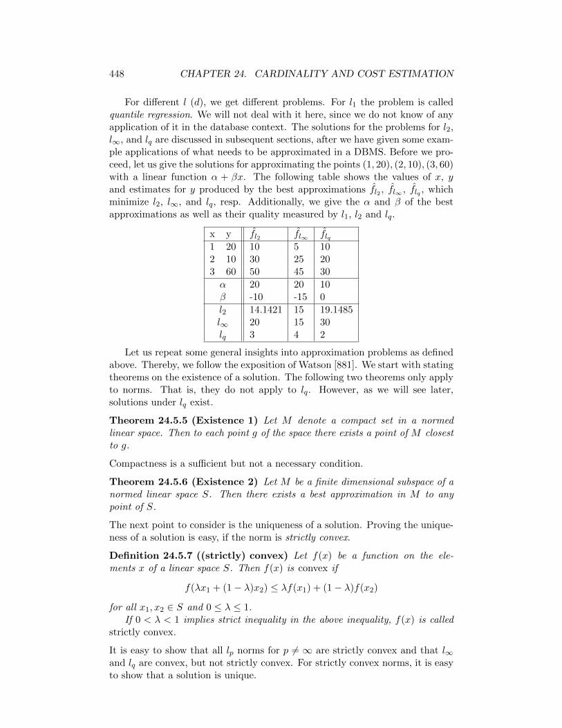
448 CHAPTER 24. CARDINALITY AND COST ESTIMATION

For different l (d), we get different problems. For l1 the problem is calledquantile regression. We will not deal with it here, since we do not know of anyapplication of it in the database context. The solutions for the problems for l2,l∞, and lq are discussed in subsequent sections, after we have given some exam-ple applications of what needs to be approximated in a DBMS. Before we pro-ceed, let us give the solutions for approximating the points (1, 20), (2, 10), (3, 60)with a linear function α + βx. The following table shows the values of x, yand estimates for y produced by the best approximations fl2 , fl∞ , flq , whichminimize l2, l∞, and lq, resp. Additionally, we give the α and β of the bestapproximations as well as their quality measured by l1, l2 and lq.

x y fl2 fl∞ flq1 20 10 5 102 10 30 25 203 60 50 45 30

α 20 20 10β -10 -15 0

l2 14.1421 15 19.1485l∞ 20 15 30lq 3 4 2

Let us repeat some general insights into approximation problems as definedabove. Thereby, we follow the exposition of Watson [881]. We start with statingtheorems on the existence of a solution. The following two theorems only applyto norms. That is, they do not apply to lq. However, as we will see later,solutions under lq exist.

Theorem 24.5.5 (Existence 1) Let M denote a compact set in a normedlinear space. Then to each point g of the space there exists a point of M closestto g.

Compactness is a sufficient but not a necessary condition.

Theorem 24.5.6 (Existence 2) Let M be a finite dimensional subspace of anormed linear space S. Then there exists a best approximation in M to anypoint of S.

The next point to consider is the uniqueness of a solution. Proving the unique-ness of a solution is easy, if the norm is strictly convex.

Definition 24.5.7 ((strictly) convex) Let f(x) be a function on the ele-ments x of a linear space S. Then f(x) is convex if

f(λx1 + (1− λ)x2) ≤ λf(x1) + (1− λ)f(x2)

for all x1, x2 ∈ S and 0 ≤ λ ≤ 1.If 0 < λ < 1 implies strict inequality in the above inequality, f(x) is called

strictly convex.

It is easy to show that all lp norms for p 6= ∞ are strictly convex and that l∞and lq are convex, but not strictly convex. For strictly convex norms, it is easyto show that a solution is unique.

24.5. APPROXIMATION WITH LINEAR MODELS 449

Theorem 24.5.8 In a strictly convex normed linear space S, a finite dimen-sional subspace M contains a unique best approximation to any point of S.

Although l∞ and lq are not strictly convex, under certain circumstances a uniquebest approximation exists for them. This is discussed in subsequent sections.

Considering the above, one might conjecture that l2 approximation is muchsimpler than l∞ or lq approximation. This is indeed the case. We will not repeatall the findings from approximation theory and the algorithms developed. Thereare plenty of excellent textbooks on this matter. We highly recommend the ex-cellent book of Golub and van Loan [322], which discusses l2 approximation andseveral algorithms to solve them (e.g. QR factorization and SVD). Other goodbooks to refresh one’s knowledge on matrix algebra are [375, 393, 415, 748].Uberhuber wrote another good book discussing l2 approximation, QR factor-ization and SVD [852]. In the context of statistics, many different regressionmodels exist to approximate a given set of data. An excellent overview is pro-vided by [?]. Another good reading, not only in this context, is the book by ToDoPress, Teukolsky, Vetterling, and Flannery [674]. Before reading these books,it might be helpful to repeat some linear algebra and some basics of matrices.An excellent book for doing so was written by Schmidt and Trenkler [748]. Theonly book we know of that discusses approximation under l∞, is the one byWatson, already cited above [881]. Approximation under lq is not discussed inany textbook. Hence, we must refer to the original articles [594, 600]. In anycase, since mathematics is quite involved at times, we give explicit algorithmsonly for the approximation by a linear function. For all other cases, we refer tothe literature.

24.5.2 Example Applications

In this section, we give some examples of approximation problems occurringin the database context. As we will see, different problems demand differentnorms. Additionally, we sketch how to use approximations. The details are leftto the reader as an exercise.

Disk seek times

There exist small benchmarks, which measure the disk seek time for travellingn cylinders (see Sec. 4.1). To cover for random errors, many measurements aretaken. The task is to find the parameters d and ci, 1 ≤ i ≤ 4, for the disk seektime formula from Sec. 4.1:

seektime(d) =

c1 + c2

√d d <= c0

c3 + c4d d > c0

Since many seeks occur during the processing of a single query, l2 is the appro-priate norm. On the surface, we seem to have a problem using a simple linearmodel. However, we can approximate the parts c1 +c2

√d and c3 +c4d for sever-

al distinct c0 either by trying a full range of values for c0 or by a binary search.The solution for c0 we then favor is the one in which the maximum of the errorson both parts becomes minimal. A second problem is the occurrence of

√d,

450 CHAPTER 24. CARDINALITY AND COST ESTIMATION

since this does not look linear. However, choosing Φ1 = 1 and Φ2(x) =√x will

work fine.

Another method is to transform a set of points (xi, yi) with two (injective)transformation functions tx and ty into the set of points (tx(xi), ty(yi)). Thenthis set is approximated and the result is transformed back. While using thisapproach, special attention has to be paid to the norm, as it can change due tothe transformation. We see examples of this later on in Sec. 24.5.6.

Functions sensitive to parameter size

Another example is to approximate the execution time of a hash function onstring values. As its calculation depends on the length of the input string,measurements can be taken for various lengths. Using l2 as a norm is perfect,because the hash function is typically executed many times during a hash joinor hash teams [338].

Approximation of frequency densities and distributions

We start by demonstrating the usage of approximating functions for cardinal-ity estimation. Then, we look at the choice of error metrics for estimatingselectivity results and the influence of cardinality estimation errors on joins.

Let R be a relation and A one of its attributes. Let (xi, fi) denote thefrequency fi with which the value xi occurs in attribute A. Typically, onlythose values xi are written down and approximated for which fi 6= 0. Wefurther assume that the xi are sorted, i.e., xi < xi+1. Using the methods tocome, we can approximate this set of points by a function f(x). To calculatethe output cardinality of a selection σA=c(R), we can simply return f(c) as anestimate. Hence it is a good choice to use lq (see below for strong arguments).

To calculate the result cardinality for a range query of the form σc1≤A≤c2(R),we distinguish several cases. First, assume that the domain of A is discrete andthe number of values between c1 and c2 is small. Then, we can calculate theresult quite efficiently by ∑

c1≤x≤c2f(x)

if the active domain of the attribute under consideration is dense, which assumein this subsection. In Section ??, we present estimation formulas without thisassumption. If the number of values between c1 and c2 is too large for anexplicit summation, we can apply speed-up techniques if the function f has asimple form. For example, if f is a linear function f(x) = α + βx, the abovesum can be calculated very efficiently . If the number of values between c1 andEXCc2 is very large and no efficient form for the above sum can be found, or if wedo not have a discrete domain, we can use the integral to approximate the sum.Thus, we use the right-hand side of

∑

c1≤x≤c2f(x) ≈

∫ c2

c1

f(x)dx

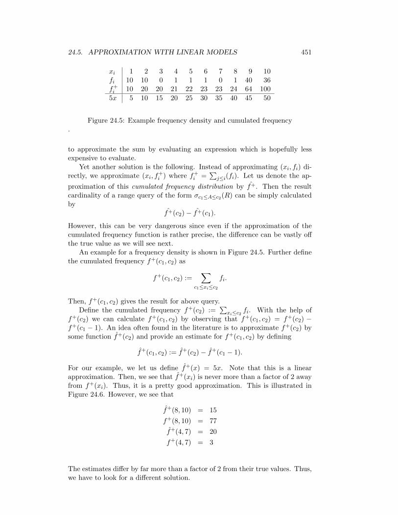
24.5. APPROXIMATION WITH LINEAR MODELS 451

xi 1 2 3 4 5 6 7 8 9 10fi 10 10 0 1 1 1 0 1 40 36f+i 10 20 20 21 22 23 23 24 64 100

5x 5 10 15 20 25 30 35 40 45 50

Figure 24.5: Example frequency density and cumulated frequency.

to approximate the sum by evaluating an expression which is hopefully lessexpensive to evaluate.

Yet another solution is the following. Instead of approximating (xi, fi) di-rectly, we approximate (xi, f

+i ) where f+

i =∑

j≤i(fi). Let us denote the ap-

proximation of this cumulated frequency distribution by f+. Then the resultcardinality of a range query of the form σc1≤A≤c2(R) can be simply calculatedby

f+(c2)− f+(c1).

However, this can be very dangerous since even if the approximation of thecumulated frequency function is rather precise, the difference can be vastly offthe true value as we will see next.

An example for a frequency density is shown in Figure 24.5. Further definethe cumulated frequency f+(c1, c2) as

f+(c1, c2) :=∑

c1≤xi≤c2fi.

Then, f+(c1, c2) gives the result for above query.Define the cumulated frequency f+(c2) :=

∑xi≤c2 fi. With the help of

f+(c2) we can calculate f+(c1, c2) by observing that f+(c1, c2) = f+(c2) −f+(c1 − 1). An idea often found in the literature is to approximate f+(c2) bysome function f+(c2) and provide an estimate for f+(c1, c2) by defining

f+(c1, c2) := f+(c2)− f+(c1 − 1).

For our example, we let us define f+(x) = 5x. Note that this is a linearapproximation. Then, we see that f+(xi) is never more than a factor of 2 awayfrom f+(xi). Thus, it is a pretty good approximation. This is illustrated inFigure 24.6. However, we see that

f+(8, 10) = 15

f+(8, 10) = 77

f+(4, 7) = 20

f+(4, 7) = 3

The estimates differ by far more than a factor of 2 from their true values. Thus,we have to look for a different solution.

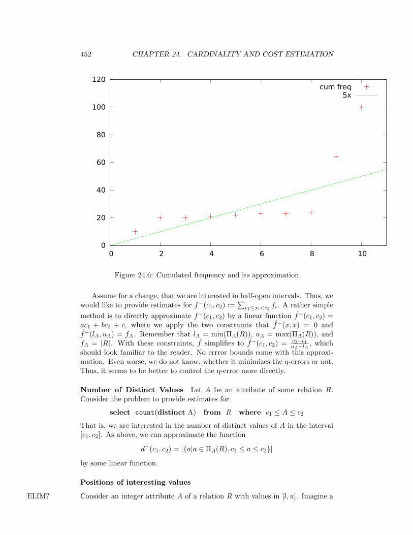
452 CHAPTER 24. CARDINALITY AND COST ESTIMATION

0

20

40

60

80

100

120

0 2 4 6 8 10

cum freq5x

Figure 24.6: Cumulated frequency and its approximation

Assume for a change, that we are interested in half-open intervals. Thus, wewould like to provide estimates for f−(c1, c2) :=

∑c1≤xi<c2 fi. A rather simple

method is to directly approximate f−(c1, c2) by a linear function f−(c1, c2) =ac1 + bc2 + c, where we apply the two constraints that f−(x, x) = 0 andf−(lA, uA) = fA. Remember that lA = min(ΠA(R)), uA = max(ΠA(R)), andfA = |R|. With these constraints, f simplifies to f−(c1, c2) = c2−c1

uA−lA , whichshould look familiar to the reader. No errror bounds come with this approxi-mation. Even worse, we do not know, whether it minimizes the q-errors or not.Thus, it seems to be better to control the q-error more directly.

Number of Distinct Values Let A be an attribute of some relation R.Consider the problem to provide estimates for

select count(distinct A) from R where c1 ≤ A ≤ c2

That is, we are interested in the number of distinct values of A in the interval[c1, c2]. As above, we can approximate the function

d+(c1, c2) = |a|a ∈ ΠA(R), c1 ≤ a ≤ c2|by some linear function.

Positions of interesting values

Consider an integer attribute A of a relation R with values in [l, u]. Imagine aELIM?

24.5. APPROXIMATION WITH LINEAR MODELS 453

situation where almost all values in [l, u] occur with some frequency in A. Onlya few holes exist. Denote by W the set of values in [l, u] that do not occur inA. Again, the selection is of the form σc1≤A≤c2(R). In the case of holes, theabove summation for range queries leads to a wrong result. It would be betterto calculate the result cardinality as in

∑

c1≤x≤c2f(x)−

∑

c1≤x≤c2,x∈Wf(x)

For this to work, we have to know where the holes in [l, u] are. If there are onlya few of them, we can memorize them. If they are to many to be stored, wecan approximate them as follows. Let W = w1, . . . , wm. Then, we can useapproximation techniques to approximate the set of points (i, wi), 1 ≤ i ≤ m.Depending on the size of the interval [l, u] either l∞ or lq is the appropriatenorm. Similarily, the peaks, i.e., the distinct values occurring in the attributeA of R, can be approximated if there are only a few of them in the domain ofA.

Why Q?

Minimizing error propagation. Let us assume that the purpose of ourapproximation is to estimate the output cardinalities of selections on relationsRi, i.e. σpi(Ri) for i = 1, . . . , n. The results of these cardinality estimationsare then used to find the optimal order of subsequent joins. More specifically,assume we have to find the optimal query execution plan for the followingexpression:

σp1(R1) 1 . . . 1 σpn(Rn), (24.8)

where we intentionally left out all the join predicates. Ioanidis and Christo-doulakis pointed out that errors propagate exponentially through joins [433].Denote by si the cardinality of σpi(Ri) and by si its estimate. Further assumethat independence holds. This means, that si can be written as fi|Ri|, wherefi is the selectivity of pi. Denote by fi,j the selectivity of the join predicatebetween Ri and Rj , if it exists. Otherwise we define fi,j = 1. The result ofjoining a subset x ⊆ R1, . . . , Rn has cardinality

sx = (∏

Ri∈xfi)(

∏

Ri,Rj∈xfi,j)(

∏

Ri∈x|Ri|)

Denote by fi the estimate for the selectivities of the pi and assume that thejoin selectivities have been estimated correctly (which, of course, is difficult inpractice). Then, the estimated cardinality of the result of joining the relations

454 CHAPTER 24. CARDINALITY AND COST ESTIMATION

in x is

sx = (∏

Ri∈xfi)(

∏

Ri,Rj∈xfi,j)(

∏

Ri∈x|Ri|)

= (∏

Ri∈xfi/fi)(

∏

Ri∈xfi)(

∏

Ri,Rj∈xfi,j)(

∏

Ri∈x|Ri|)

= (∏

Ri∈xfi/fi)(

∏

Ri∈xfi)(

∏

Ri,Rj∈xfi,j)(

∏

Ri∈x|Ri|)

= (∏

Ri∈xfi/fi)sx

where some i belong to the category with fi/fi < 1 and others to the onewith fi/fi > 1. Remember that during dynamic programming, all subsets ofrelations are considered. Especially those subsets occur in which all relationsbelong to one category only. Hence, building on the cancellation of errors bymixing them from different categories is not a true option. Instead, we shouldminimize ∏

Ri∈xmaxfi/fi, fi/fi

in order to minimize errors and error propagation. This product can be mini-mized by minimizing each of its factors. This means that if we want to minimizeerror propagation, we have to minimize the multiplicative error Eq for estimat-ing the cardinalities of selections based on equality. This finding can obviouslybe generalized to any kind of selections. Thus, for cardinality estimations forselections (and joins, or cardinality estimation in general) the q-error is theerror metrics of choice.

Error bounds guaranteeing plan optimality. Let us give another strongargument for minimizing the multiplicative error Eq. Let us consider again thejoin expression given in 24.8. Further, denote by fi the correct selectivity ofσAi=ci and by fi some estimate. If the plan generator uses the correct cardi-nalities, it produces the optimal plan. Given the estimates, it might produceanother plan. The question is, how far can the cardinality estimates deviatefrom the true cardinalities such that the opimal plan still remains the same.More formally, denote by P the optimal plan under the correct cardinalitiesf and by P the optimal plan under the estimates f . Then, we can restatethe above question to whether there exists a condition on f such that if thiscondition holds then P = P. The nice truth is that such conditions exist andthey involve the Q paranorm.

In the simplest case, let us assume that the expression given in 24.8 is usedto evaluate a star query under an ASI cost function without considering crossproducts. From Sec. 3.2.2, we can conclude that the optimal join order forstar queries starts with the center relation and orders the satellite relationsaccording to their rank. This holds if the a symmetric cost function is used likeCout. The rank of a relation R is defined as rank(Ri) = (T (Ri) − 1)/C(Ri),where C(S) are some fixed per tuple costs and T (Ri) = f0,ifi|R|, if f0,i is the

24.5. APPROXIMATION WITH LINEAR MODELS 455

join selectivity of the join of Ri with the center relation R0. Thus, P = P if fand f result in the same ordering of the relations. Since f(x) = (x − 1)/c ismonotonically increasing for constants c, we can conclude that the ordering isindeed the same as long as for all i 6= j we have

f0,ifi|Ri| < f0,jfj |Rj | ⇐⇒ f0,ifi|Ri| < f0,j fj |Rj |

which is equivalent to

firifjrj

< 1⇐⇒ firi

fjrj< 1

for ri = f0,i|Ri|. We now show that if

||fifi||Q < min

i 6=j

√|| firifjrj||Q (24.9)

for all i, then P = P . This condition implies the much weaker condition thatfor all i 6= j

|| fifi||Q ||

fjfj||Q < ||

firifjrj||Q (24.10)

To show the claim, it suffices to show that (firi)/(fjrj) < 1 implies (firi)/(fjrj) <1. This follows from

firi

fjrj=

fifi

fj

fj

firifjrj

= (fifi

fj

fj)/(|| firi

fjrj||Q) (∗)

≤ (|| fifi||Q ||

fj

fj||Q)/(|| firi

fjrj||Q)

< 1

where (*) follows from (firi)/(fjrj) < 1. Thus, we have shown that if theq-error is limited as in condition 24.9, the produced plan is still optimal.

From cardinality estimation error bounds to cost error bounds. Ifthere are cardinality estimation errors, the plan generator can accidentally pro-duce the wrong plan. This plan may be suboptimal under the true cardinalitiesbut is optimal under the estimated cardinalities. The question is, how bad isthe plan? To clarify this, assume that the optimal plan under the true cardi-nalities is P . The optimal plan under the estimated cardinalities is P . Then,we are interested in the factor by which the P is worse than P . The followingtheorem answers this question [599]:

Theorem 24.5.9 Let C = CSMJ or C = CGHJ be the cost function of thesort-merge or the Grace hash join. For a given query in n relations, let P bethe optimal plan under the true cardinalities, P be the optimal plan under the

456 CHAPTER 24. CARDINALITY AND COST ESTIMATION

0

2

4

6

8

10

12

1 1.2 1.4 1.6 1.8 2 2.2 2.4

chain querystar query

Figure 24.7: Q-error and plan optimality

estimated cardinalities, C(P ) be the true costs under C of the optimal plan,and C(P ) be the true costs under C of the plan produced under the estimatedcardinalities. Then

C(P ) ≤ q4C(P ),

where q is defined as

q = maxx⊆X||sx/sx||Q,

with X being the set of relations to be joined, and sx (sx) is the true (estimated)size of the join of the relations in x. That is, q is the maximum estimation errortaken over all intermediate results.

This bound is rather tight, as is demonstrated by the example shown in Fig. 24.7(taken from [599]). This figure shows for a chain and a star query with fourrelations the quotient cost(P )/cost(P ) for increasing q-errors. For the starquery, we see that this ratio is about 11.11, which is about 23.46. Thus, abound of the form q3C(P ) would fail.

24.5.3 Linear Models Under l2

Now that we know that the solution to our problem exists and is unique, wecontinue by characterizing it. Let S be a linear space (say R2) and s ∈ S somepoint. Further denote by G some linear subspace of S (say a straight line). Forany g ∈ G, we can define the residual vector g − f . Using residuals, we cancharacterize the unique solution quite easily and intuitively. Exactly the vectorg∗ ∈ G is closest to f whose residual f − g is orthogonal to G. Remember thattwo vectors are orthogonal if and only if their scalar product is zero. Now wecan characterize the solution to our approximation problem under l2.

Theorem 24.5.10 (Characterization) Let S be a linear space and G a sub-space. An element g∗ is the best approximation of a point s ∈ S if and onlyif

〈g∗ − f, g〉 = 0

holds. That is, if the error is orthogonal to all elements in G.

24.5. APPROXIMATION WITH LINEAR MODELS 457

Since we are used to solve equations for x, we rewrite our problem to A~x = b.That is, the vector ~x replaces the coefficient vector c. Using Theorem 24.5.10,we must have that A~x∗−b is orthogonal to the range of A. The range of a matrixA ∈ Rm×n is defined as R(A) = Ax|x ∈ Rn. Let ai be i-th column vectorof A and ~x = (x1, . . . , xn)T. Then, the best approximation can be found bysolving the following system of linear equations, which is called (Gauß) normalequations:

〈a1, a1〉x1 + 〈a2, a1〉x2 + . . . + 〈an, a1〉xn = 〈b, a1〉〈a1, a2〉x1 + 〈a2, a2〉x2 + . . . + 〈an, a2〉xn = 〈b, a2〉

......

......

...〈a1, an〉x1 + 〈a2, an〉x2 + . . . + 〈an, an〉xn = 〈b, an〉

or, using matrix notation, we get

ATA~x = AT~b (24.11)

This system of linear equations can be solved by many different approaches.Some fast and numerically stable approaches are QR decomposition and sin-gular value decomposition (SVD). Both leave the conditioning of the problemunchanged. QR decomposition can only be applied if the the matrix has fullrank (see below). Otherwise, one has to keep up with variants of QR decom-position or SVD. Hence, we will briefly discuss SVD. We will not give anyalgorithms. The interested reader is referred to [322].

Before we proceed with SVD, let us repeat some basics on matrices. Aspecial matrix is the identity matrix I ∈ Rn×n with I = (δi,j)i,j , 1 ≤ i ≤ n.Matrices can have plenty of properties. Here are some of them.

Definition 24.5.11 (rank) The rank of a matrix A, denoted by rank(A), isthe rank of the subspace R(A).

Definition 24.5.12 (full rank) A matrix A ∈ Rm×n, m > n has full rank ifits rank is n.

Definition 24.5.13 (symmetric) A matrix A ∈ Rn is symmetric if and onlyif AT = A.

Note that for all matrices A ∈ Rm×n, we always have that AAT and ATA aresymmetric.

Definition 24.5.14 (idempotent) A matrix A ∈ Rn×n is idempotent if andonly if AA = A.

Definition 24.5.15 (inverse) A Matrix A−1 ∈ Rn×n is the inverse of a ma-trix A ∈ Rn×n if and only if A−1A = AA−1 = I.

A matrix for which the uniquely determined inverse exists is called regular.

Definition 24.5.16 (orthogonal) A matrix A ∈ Rn×n is orthogonal if andonly if AAT = ATA = I.

458 CHAPTER 24. CARDINALITY AND COST ESTIMATION

Let us use a simple, operational, recursive definition of the determinant.

Definition 24.5.17 (determinant) Let A ∈ Rn×n be a matrix. We definethe determinant of A as det(A) = a1,1 if n = 1. Otherwise, we define

det(A) =

n∑

j=1

(−1)i+jai,j det(Ai,j)

where Ai,j ∈ R(n−1)×(n−1) results from A by eliminating the i-th row and thej-th column.

Definition 24.5.18 (characteristic polynomial) Let A ∈ Rn×n be a ma-trix. The characteristic polynomial is defined as

Pn(z;A) := det(A− zI) =

∣∣∣∣∣∣∣∣∣

(a1,1 − z) a1,2 . . . a1,n

a2,1 (a2,2 − z) · · · a2,n...

.... . .

...an,1 an,2 · · · (an,n − z)

∣∣∣∣∣∣∣∣∣

Definition 24.5.19 (Eigenvalue) Let A ∈ Rn×n be a matrix and Pn(z;A) itscharacteristic polynomial. Any root λi of Pn(z;A), i.e. P(z;A)(λi) = 0 is calledEigenvalue. The set of Eigenvalues is denoted by

λ(A) := λ1, . . . , λk

and is called spectrum of A.

Definition 24.5.20 (similar) Two matrices A,B ∈ Rn×n are similar if andonly if there exists a regular matrix X ∈ Rn×n such that B = X−1AX.

Two similar matrices have the same Eigenvalues, as can be seen from the fol-lowing theorem.

Theorem 24.5.21 Let A,B ∈ Rn×n be two similar matrices. Then they havethe same characteristic polynomial.

Definition 24.5.22 (generalized inverse) A matrix A− ∈ Rn×m is the gen-eralized inverse, or g-inverse, of a matrix A ∈ Rm×n, if AA−A = A holds.

Every matrix and, hence, every vector has a g-inverse. For regular matrices,the g-inverse and the inverse coincide. In general, the g-inverse is not uniquelydetermined. Adding some additional properties makes it unique.

Definition 24.5.23 (Moore-Penrose inverse) A matrix A+ ∈ Rn×m is theMoore-Penrose inverse of a matrix A ∈ Rm×n if the following conditions hold:

1. AA+A = A

2. A+AA+ = A+

24.5. APPROXIMATION WITH LINEAR MODELS 459

3. (A+A)T = A+A

4. (AA+)T = AA+

For every matrix and, hence, every vector there exists a uniquely determinedMoore-Penrose inverse. In case A is regular, A+ = A−1 holds. If A is symmetric,then A+A = AA+. If A is symmetric and idempotent, then A+ = A. Further,all of A+A, AA+, I − A+A, and I − AA+ are idempotent. Here are someequalities holding for the Moore-Penrose inverse:

(A+)+ = A (24.12)

(AT)+ = (A+)T (24.13)

(ATA)+ = A+(AT)+ (24.14)

(AAT)+ = (AT)+A+ (24.15)

ATAA+ = AT (24.16)

A+AAT = AT (24.17)

The following theorem states the existence of a decomposition of any matrixinto regular/orthogonal submatrices.

Theorem 24.5.24 (singular value decomposition) Let A ∈ Rm×n be amatrix. Then there exist an orthogonal matrix U ∈ Rm×m and an orthogo-nal matrix V ∈ Rn×n such that

UTAV = S

such that S ∈ Rm×n is of the form

S = diag(s1, . . . , sk)

with k = min(m,n) and, further

s1 ≥ s2 ≥ . . . ≥ sr > sr+1 = . . . = sk = 0

holds where r = rank(A).

For a proof and algorithms to calculate the SVD of an arbitrary matrix see thebook by Golub and Loan [322]. Another proof can be found in the book byHarville [393]. The diagonal elements si of S, which is orthogonal equivalent toA, are called singular values. From

STS = (UTAV )T(UTAV ) = V TATUUTAV = V −1ATAV

it follows that STS and ATA are similar. Since STS = diag(s21, . . . , s

2r , 0, . . . , 0)

and similar matrices have the same spectrum, it follows that

si =√λi

for λi ∈ λ(ATA), 1 ≤ i ≤ n.

460 CHAPTER 24. CARDINALITY AND COST ESTIMATION

Define S−1 = diag(1/s1, . . . , 1/sr, 0, . . . , 0) and A+ = V S−1UT. From

AA+A = (USV T)(V S−1UT)(USV T)

= USS−1SV T

= USV T

= A

and

A+AA+ = (V S−1UT)(USV T)(V S−1UT)

= V S−1SS−1UT

= V S−1UT

= A+

we see that A+ = V S−1UT is a g-inverse of A. The reader is advised to checkthe remaining conditions of the Moore-Penrose inverse.

Remember that we have to solve ATA~x = AT~b for ~x in order to find thebest approximation for our set of data points. Set ~x = A+~b. Then

ATA~x = ATAA+~b

= AT~b

where we used Eqn. 24.16. Hence, the Moore-Penrose inverse2 solves our prob-lem. Moreover, the solution can be obtained easily from the singular valuedecomposition.

Approximation by a linear function

Assume we are given m points (xi, yi), 1 ≤ i ≤ m and wish to approximatethem by a linar function f(x) = α+ βx. The design matrix, b and ~x then are

A =

1 x1

1 x2...

...1 xm

x =

(αβ

), b =

y1...ym

The resulting system of normal equations(

m∑m

i=1 xi∑mi=1 xi

∑mi=1(xi)

2

)(αβ

)=

( ∑mi=1 yi∑mi=1 xiyi

)

has the solution

α =

∑mi=1(xi)

2∑m

i=1 yi −∑m

i=1 xiyi∑m

i=1 xim∑m

i=1(xi)2 − (∑m

i=1 xi)2

, β =m∑m

i=1 xiyi −∑m

i=1 xi∑m

i=1 yim∑m

i=1(xi)2 − (∑m

i=1 xi)2

Note that this is a very nice formula as new points arrive or are deleted, onlythe sums have to be updated and the quotients to be calculated. There is noneed to look at the other points again.

2The Greville algorithm to calculate the Moore-Penrose inverse directly is described in[748].

24.5. APPROXIMATION WITH LINEAR MODELS 461

24.5.4 Linear Models Under l∞

Let A ∈ Rm×n be a matrix, where m > n, and b ∈ Rm a vector. The problemwe solve in this section is to

find ~a ∈ Rn to minimize ||r(a)||∞ (24.18)

wherer(~a) = ~b−A~a (24.19)

The components of the vector r(~a) are denoted by ri(~a).As pointed out earlier, l∞ is a convex norm. Hence, a solution exists. Since

l∞ is not strictly convex, the uniqueness of the solution is not guaranteed.To solve problem 24.18 by following the approach proposed by Watson [881].We start by characterizing the solution, continue with the conditions underwhich uniqueness holds, make some more observations, and finally derive analgorithm for the case n = 2, i.e. we find a best approximation by a linearfunction. Although only few applications in databases exist for l∞, it is veryuseful to find a best approximation under lq if we want to approximate by afunction eβ+αx (see Sec. 24.5.6).

Assume we have a best solution ~a. Then, for some indices i, ri(~a) attains themaximum, i.e. ri(~a) = ||r(~a)||∞. Otherwise, a better solution would exist. Wedenote the set of indices where the maximum is attained by I(~a). We furtherdenote by θi(~a) the sign of ri(~a). Thus ri(~a) = θi(~a)||r(~a)||∞ for all i ∈ I. Thefollowing theorem gives a characterization of the solution.

Theorem 24.5.25 A vector ~a ∈ Rn solves problem 24.18 if and only if thereexists a subset I of I with |I| ≤ n+ 1 and a vector ~λ ∈ Rm such that

1. λi = 0 for all i 6∈ I,

2. λiθi ≥ 0 for all i ∈ I, and

3. AT~λ = ~0.

The set I in the theorem is called an extremal subset of a solution ~a.There are two important corollaries to this theorem.

Corollary 24.5.26 Let ~a solve problem 24.18. Then ~a solves an l∞ approxi-mation problem in Rn+1 obtained by restricting the components of r(~a) to someparticular n+ 1 components. If A has rank t, then the components of r(~a maybe restricted to a particular t+ 1 components.

Corollary 24.5.27 Let ~a solve problem 24.18 and let I be chosen accordingto Theorem 24.5.25 such that λi 6= 0 for all i ∈ I. Further let ~d be anothersolution to 24.18. Then

ri(~d) = ri(~a).

Hence, not surprisingly, any two solutions have the same residuals for compo-nents where the maximum is attained. The theorem and its first corollary statethat we need at most t+1 solutions for a matrix A of rank t. The next theoremshows that at least t+ 1 indices exist where the maximum is attained.

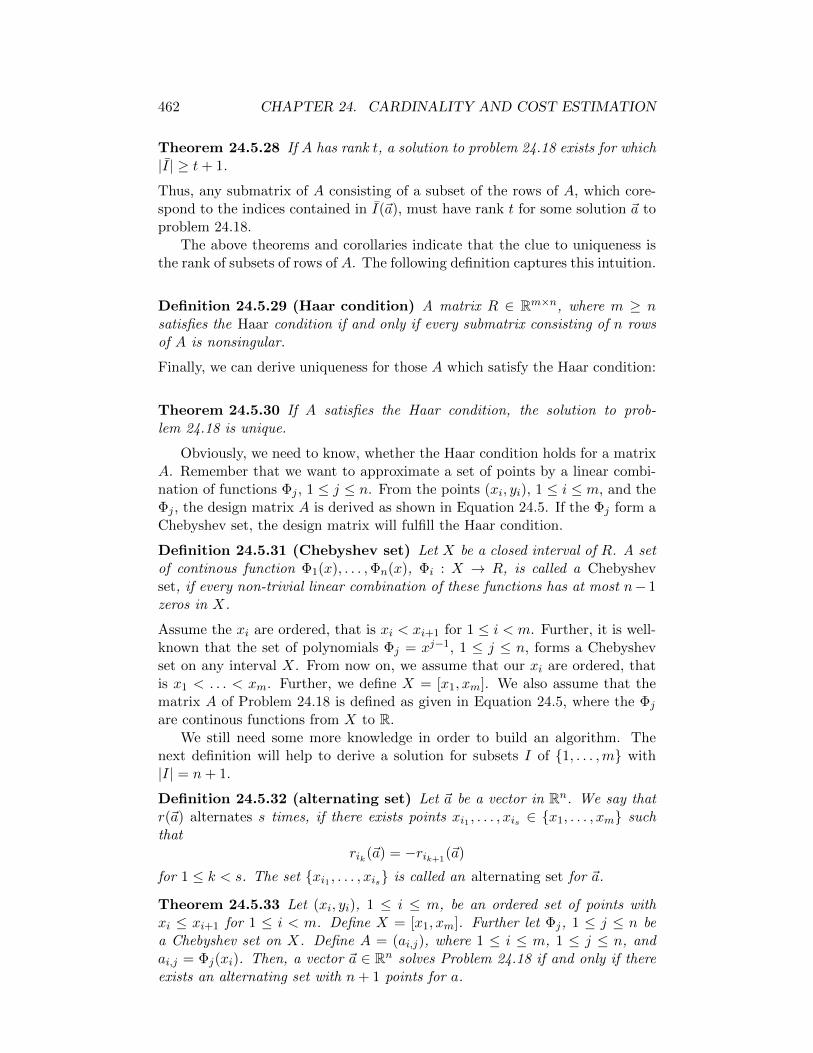
462 CHAPTER 24. CARDINALITY AND COST ESTIMATION

Theorem 24.5.28 If A has rank t, a solution to problem 24.18 exists for which|I| ≥ t+ 1.

Thus, any submatrix of A consisting of a subset of the rows of A, which core-spond to the indices contained in I(~a), must have rank t for some solution ~a toproblem 24.18.

The above theorems and corollaries indicate that the clue to uniqueness isthe rank of subsets of rows of A. The following definition captures this intuition.

Definition 24.5.29 (Haar condition) A matrix R ∈ Rm×n, where m ≥ nsatisfies the Haar condition if and only if every submatrix consisting of n rowsof A is nonsingular.

Finally, we can derive uniqueness for those A which satisfy the Haar condition:

Theorem 24.5.30 If A satisfies the Haar condition, the solution to prob-lem 24.18 is unique.

Obviously, we need to know, whether the Haar condition holds for a matrixA. Remember that we want to approximate a set of points by a linear combi-nation of functions Φj , 1 ≤ j ≤ n. From the points (xi, yi), 1 ≤ i ≤ m, and theΦj , the design matrix A is derived as shown in Equation 24.5. If the Φj form aChebyshev set, the design matrix will fulfill the Haar condition.

Definition 24.5.31 (Chebyshev set) Let X be a closed interval of R. A setof continous function Φ1(x), . . . ,Φn(x), Φi : X → R, is called a Chebyshevset, if every non-trivial linear combination of these functions has at most n− 1zeros in X.

Assume the xi are ordered, that is xi < xi+1 for 1 ≤ i < m. Further, it is well-known that the set of polynomials Φj = xj−1, 1 ≤ j ≤ n, forms a Chebyshevset on any interval X. From now on, we assume that our xi are ordered, thatis x1 < . . . < xm. Further, we define X = [x1, xm]. We also assume that thematrix A of Problem 24.18 is defined as given in Equation 24.5, where the Φj

are continous functions from X to R.We still need some more knowledge in order to build an algorithm. The

next definition will help to derive a solution for subsets I of 1, . . . ,m with|I| = n+ 1.

Definition 24.5.32 (alternating set) Let ~a be a vector in Rn. We say thatr(~a) alternates s times, if there exists points xi1 , . . . , xis ∈ x1, . . . , xm suchthat

rik(~a) = −rik+1(~a)

for 1 ≤ k < s. The set xi1 , . . . , xis is called an alternating set for ~a.

Theorem 24.5.33 Let (xi, yi), 1 ≤ i ≤ m, be an ordered set of points withxi ≤ xi+1 for 1 ≤ i < m. Define X = [x1, xm]. Further let Φj, 1 ≤ j ≤ n bea Chebyshev set on X. Define A = (ai,j), where 1 ≤ i ≤ m, 1 ≤ j ≤ n, andai,j = Φj(xi). Then, a vector ~a ∈ Rn solves Problem 24.18 if and only if thereexists an alternating set with n+ 1 points for a.

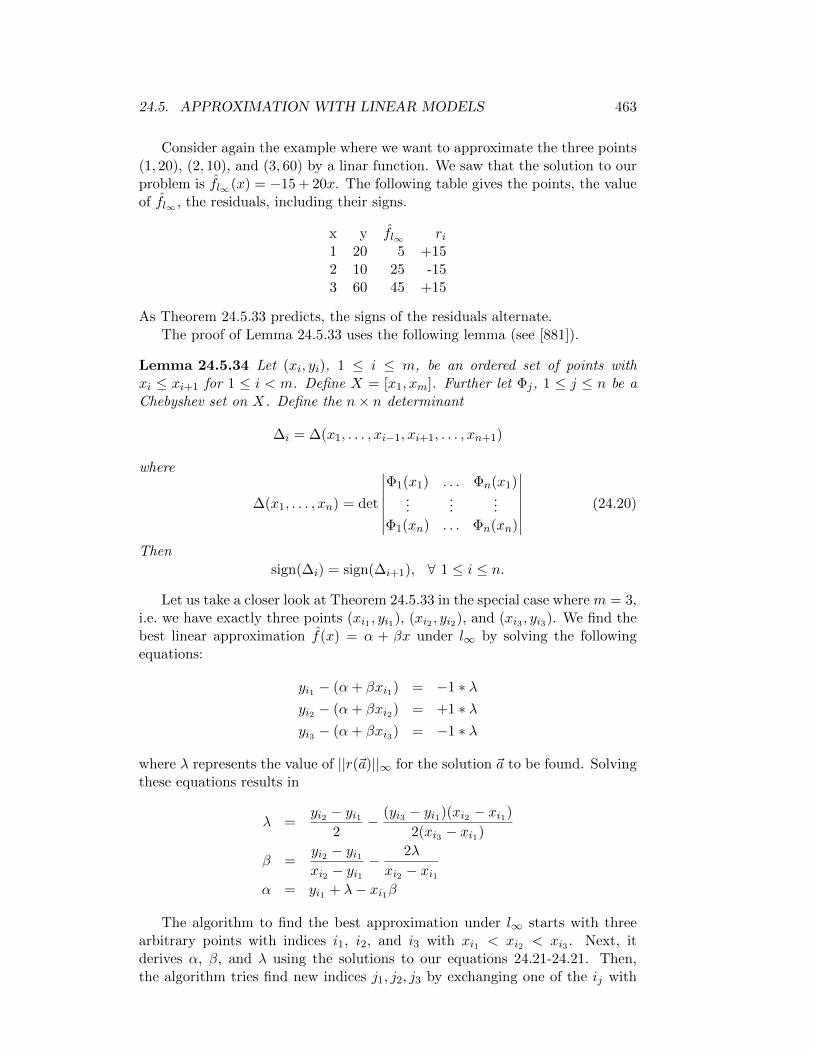
24.5. APPROXIMATION WITH LINEAR MODELS 463

Consider again the example where we want to approximate the three points(1, 20), (2, 10), and (3, 60) by a linar function. We saw that the solution to ourproblem is fl∞(x) = −15 + 20x. The following table gives the points, the valueof fl∞ , the residuals, including their signs.

x y fl∞ ri1 20 5 +152 10 25 -153 60 45 +15

As Theorem 24.5.33 predicts, the signs of the residuals alternate.

The proof of Lemma 24.5.33 uses the following lemma (see [881]).

Lemma 24.5.34 Let (xi, yi), 1 ≤ i ≤ m, be an ordered set of points withxi ≤ xi+1 for 1 ≤ i < m. Define X = [x1, xm]. Further let Φj, 1 ≤ j ≤ n be aChebyshev set on X. Define the n× n determinant

∆i = ∆(x1, . . . , xi−1, xi+1, . . . , xn+1)

where

∆(x1, . . . , xn) = det

∣∣∣∣∣∣∣

Φ1(x1) . . . Φn(x1)...

......

Φ1(xn) . . . Φn(xn)

∣∣∣∣∣∣∣(24.20)

Then

sign(∆i) = sign(∆i+1), ∀ 1 ≤ i ≤ n.

Let us take a closer look at Theorem 24.5.33 in the special case where m = 3,i.e. we have exactly three points (xi1 , yi1), (xi2 , yi2), and (xi3 , yi3). We find thebest linear approximation f(x) = α + βx under l∞ by solving the followingequations:

yi1 − (α+ βxi1) = −1 ∗ λyi2 − (α+ βxi2) = +1 ∗ λyi3 − (α+ βxi3) = −1 ∗ λ

where λ represents the value of ||r(~a)||∞ for the solution ~a to be found. Solvingthese equations results in

λ =yi2 − yi1

2− (yi3 − yi1)(xi2 − xi1)

2(xi3 − xi1)

β =yi2 − yi1xi2 − yi1

− 2λ

xi2 − xi1α = yi1 + λ− xi1β

The algorithm to find the best approximation under l∞ starts with threearbitrary points with indices i1, i2, and i3 with xi1 < xi2 < xi3 . Next, itderives α, β, and λ using the solutions to our equations 24.21-24.21. Then,the algorithm tries find new indices j1, j2, j3 by exchanging one of the ij with

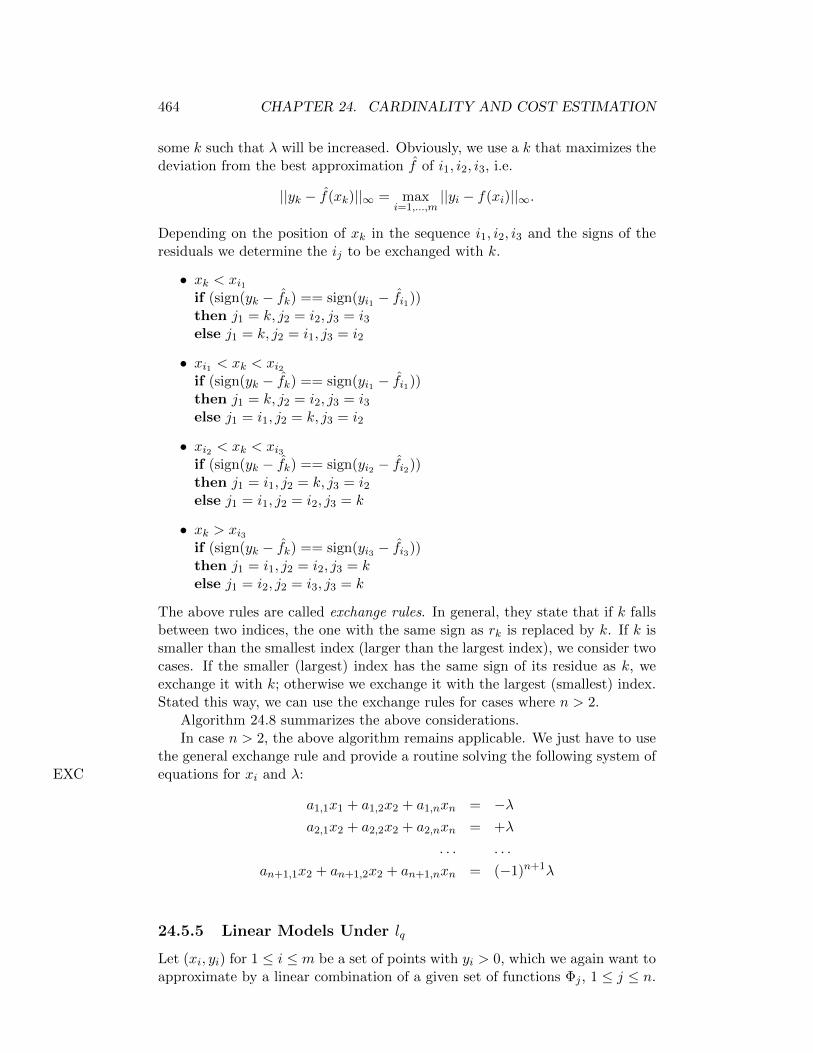
464 CHAPTER 24. CARDINALITY AND COST ESTIMATION

some k such that λ will be increased. Obviously, we use a k that maximizes thedeviation from the best approximation f of i1, i2, i3, i.e.

||yk − f(xk)||∞ = maxi=1,...,m

||yi − f(xi)||∞.

Depending on the position of xk in the sequence i1, i2, i3 and the signs of theresiduals we determine the ij to be exchanged with k.

• xk < xi1if (sign(yk − fk) == sign(yi1 − fi1))then j1 = k, j2 = i2, j3 = i3else j1 = k, j2 = i1, j3 = i2

• xi1 < xk < xi2if (sign(yk − fk) == sign(yi1 − fi1))then j1 = k, j2 = i2, j3 = i3else j1 = i1, j2 = k, j3 = i2

• xi2 < xk < xi3if (sign(yk − fk) == sign(yi2 − fi2))then j1 = i1, j2 = k, j3 = i2else j1 = i1, j2 = i2, j3 = k

• xk > xi3if (sign(yk − fk) == sign(yi3 − fi3))then j1 = i1, j2 = i2, j3 = kelse j1 = i2, j2 = i3, j3 = k

The above rules are called exchange rules. In general, they state that if k fallsbetween two indices, the one with the same sign as rk is replaced by k. If k issmaller than the smallest index (larger than the largest index), we consider twocases. If the smaller (largest) index has the same sign of its residue as k, weexchange it with k; otherwise we exchange it with the largest (smallest) index.Stated this way, we can use the exchange rules for cases where n > 2.

Algorithm 24.8 summarizes the above considerations.In case n > 2, the above algorithm remains applicable. We just have to use

the general exchange rule and provide a routine solving the following system ofequations for xi and λ:EXC

a1,1x1 + a1,2x2 + a1,nxn = −λa2,1x2 + a2,2x2 + a2,nxn = +λ

. . . . . .

an+1,1x2 + an+1,2x2 + an+1,nxn = (−1)n+1λ

24.5.5 Linear Models Under lq

Let (xi, yi) for 1 ≤ i ≤ m be a set of points with yi > 0, which we again want toapproximate by a linear combination of a given set of functions Φj , 1 ≤ j ≤ n.

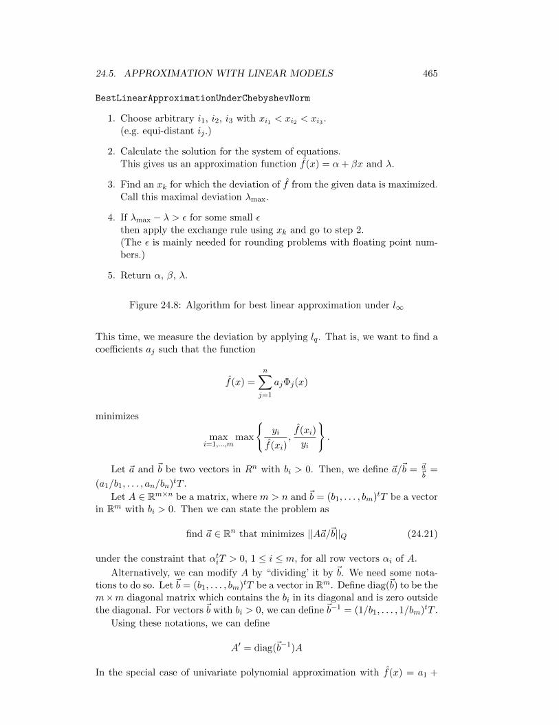
24.5. APPROXIMATION WITH LINEAR MODELS 465

BestLinearApproximationUnderChebyshevNorm

1. Choose arbitrary i1, i2, i3 with xi1 < xi2 < xi3 .(e.g. equi-distant ij .)

2. Calculate the solution for the system of equations.This gives us an approximation function f(x) = α+ βx and λ.

3. Find an xk for which the deviation of f from the given data is maximized.Call this maximal deviation λmax.

4. If λmax − λ > ε for some small εthen apply the exchange rule using xk and go to step 2.(The ε is mainly needed for rounding problems with floating point num-bers.)

5. Return α, β, λ.

Figure 24.8: Algorithm for best linear approximation under l∞

This time, we measure the deviation by applying lq. That is, we want to find acoefficients aj such that the function

f(x) =n∑

j=1

ajΦj(x)

minimizes

maxi=1,...,m

max

yi

f(xi),f(xi)

yi

.

Let ~a and ~b be two vectors in Rn with bi > 0. Then, we define ~a/~b = ~a~b

=

(a1/b1, . . . , an/bn)tT .

Let A ∈ Rm×n be a matrix, where m > n and ~b = (b1, . . . , bm)tT be a vectorin Rm with bi > 0. Then we can state the problem as

find ~a ∈ Rn that minimizes ||A~a/~b||Q (24.21)

under the constraint that αtiT > 0, 1 ≤ i ≤ m, for all row vectors αi of A.

Alternatively, we can modify A by “dividing’ it by ~b. We need some nota-tions to do so. Let~b = (b1, . . . , bm)tT be a vector in Rm. Define diag(~b) to be them×m diagonal matrix which contains the bi in its diagonal and is zero outsidethe diagonal. For vectors ~b with bi > 0, we can define ~b−1 = (1/b1, . . . , 1/bm)tT .

Using these notations, we can define

A′ = diag(~b−1)A

In the special case of univariate polynomial approximation with f(x) = a1 +

466 CHAPTER 24. CARDINALITY AND COST ESTIMATION

a2x+ . . .+ anxn−1 the matrix A′ has the form

A′ =

1/y1 x1/y1 . . . xn−11 /y1

1/y2 x2/y2 . . . xn−12 /y2

...... . . .

...1/ym xm/ym . . . xn−1

m /ym

. (24.22)

Keeping the trick with A′ in mind, it is easy to see that Problem 24.21 canbe solved, if we can solve the general problem

find~a ∈ Rnthat minimizes||A~a||Q. (24.23)

The following proposition ensures that a solution to this general problem exists.Further, since ||A~a||Q is convex, the minimum is a global one.

Proposition 24.5.1 Let A ∈ Rm,n such that R(A) ∩ Rm>0 6= ∅. Then ||A · ||Qattains its minimum.

Recall that lq is subadditive and convex. Further it is lower semi-continuous(see also [702, p. 52]). However, it is not strictly convex. Hence, as with l∞, weexpect uniqueness to hold only under certain conditions.

We need some more notation. Let A ∈ Rm,n. We denote by R(A) =A~a | ~a ∈ Rn the range of A and by N (A) = ~a ∈ Rn | A~a = 0 the nullspaceof A.

Problem (24.23) can be rewritten as the following constrained minimizationproblem:

min(~a,q)∈Rn×R

q subject to1

q≤ A~a ≤ q and q ≥ 1. (24.24)

The Lagrangian of (24.24) is given by

L(~a, q, λ+, λ−, µ) := q − (λ+)T(q −A~a)− (λ−)T(A~a− 1

q)− µ(q − 1).

Assume that R(A) ∩ Rm>0 6= ∅. Then the set (~a, q) : 1q ≤ A~a ≤ q and q ≥

1 is non-empty and closed and there exists (~a, q) for which we have stronginequality in all conditions. Then the following Karush-Kuhn-Tucker conditionsare necessary and sufficient for (~a, q) to be a minimizer of (24.24), see, e.g., [796,p. 62]: there exist λ+, λ− ∈ Rm≥0 and µ ≥ 0 such that

∇~aL(~a, q, λ+, λ−, µ) = ATλ+ −ATλ− = 0 (24.25)

∂

∂qL(~a, q, λ+, λ−, µ) = 1−

m∑

i=1

λ+i −

1

q2

m∑

i=1

λ−i − µ = 0 (24.26)

and for i = 1, . . . ,m,

λ+i

(a− (A~a)i

)= 0, (24.27)

λ−i

((A~a)i −

1

q

)= 0, (24.28)

µ(q − 1) = 0.

24.5. APPROXIMATION WITH LINEAR MODELS 467

Assume that 1m 6∈ R(A), where 1m is the vector with all components 1. Thenq > 1 and consequently µ = 0. Furthermore, it is clear that not both λ+

i and

λ−i can be positive because the conditions q = (A~a)i and 1q = (A~a)i cannot be

fulfilled at the same time, since q > 1.

Setting λ := λ+ − λ−, we can summarize our findings (24.25) - (24.28) inthe following theorem.

Theorem 24.5.35 Let A ∈ Rm,n such that R(A) ∩ Rm>0 6= ∅ and 1m 6∈ R(A).

Then (~a, q) solves (24.24) if and only if there exists λ ∈ Rm such that

i) ATλ = 0.

ii) q = q∑λi>0

λi + 1q

∑λi<0

λi.

iii) λi = 0 if 1q < (A~a)i < q.

iv) if λi > 0 then (A~a)i = q and if λi < 0 then (A~a)i = 1/q.

Remark. We see that 1 < q = (A~a)i implies sign(

(A~a)i − 1)

= 1 and that

1 > 1/q = (A~a)i implies sign(

(A~a)i − 1)

= −1; whence λi

((A~a)i − 1

)≥ 0.

For our approximation problem (24.21) this means that the residuum f(xi)−bifulfills λi (f(xi)− bi) ≥ 0.

Under certain conditions, problem (24.23) has a unique solution which canbe simply characterized. Let us start with some straightforward considerationsin this direction. IfN (A) 6= ~0, then we have for any minimizer ~a of ||A·||Q that

~a+β, β ∈ N (A) is also a minimizer. In particular, we have that N (A) 6= ~0 if

• m < n,

• m ≥ n and A is not of full range, i.e., rank(A) < n.

In these cases, we cannot have a unique minimizer. Note further, that if 1m ∈R(A), then the minimum of ||A · ||Q is 1 and the set of minimizers is given by

A+1m +N (A),

where A+ denotes the Moore-Penrose inverse of A. Of course, this can easilybe checked using the methods of Sec. 24.5.3.

In the following, we restrict our attention to the case m > n and rank(A) =n.

The following proposition considers (n+ 1, n)–matrices.

Proposition 24.5.2 Let A ∈ Rn+1,n such that R(A) ∩ Rn+1>0 6= ∅, 1m 6∈ R(A)

and rank(A) = n. Then ||A · ||Q has a unique minimizer if and only if the

Lagrange multipliers λi, i = 1, . . . , n+ 1 are not zero.

468 CHAPTER 24. CARDINALITY AND COST ESTIMATION

By spark(A) we denote the smallest number of rows of A which are linearlydependent. In other words, any spark(A)−1 rows of A are linearly independent.For the ’spark’ notation we also refer to [27].

Examples. 1. We obtain for the matrix

A :=

1 0 00 1 00 0 11 0 1

, rg(A) = 3, spark(A) = 3.

2. The matrix (m,n)–matrix A in (24.22) is the product of the diagonal ma-trix diag (1/bi)

mi=1 with positive diagonal entries and a Vandermonde matrix.

Hence, it can easily be seen that spark(A) = n+ 1. If an (m,n)–matrix A hasspark(A) = n+ 1, then A fulfills the Haar condition.

Proposition 24.5.2 can be reformulated as follows:

Corollary 24.5.36 Let A ∈ Rn+1,n such that R(A)∩Rn+1>0 6= ∅ and 1m 6∈ R(A)

. Then ||A · ||Q has a unique minimizer if and only if spark(A) = n+ 1.

The result can be generalized by the following theorem.

Theorem 24.5.37 Let A ∈ Rm,n such that R(A) ∩ Rm>0 6= ∅. Suppose thatspark(A) = n + 1. Then ||A · ||Q has a unique minimizer which is determinedby n+ 1 rows of A, i.e., there exists an index set J ⊂ 1, . . . ,m of cardinality|J | = n + 1 such that ||A · ||Q and ||A|J · ||Q have the same minimum and thesame minimizer. Here A|J denotes the restriction of A to the rows which arecontained in the index set J . We call such index set J an extremal set.

Of course the condition spark(A) = n + 1 is not necessary for ||A · ||Q tohave a unique minimizer as the following example shows.

Example. The matrices

A :=

1 00 1−1 1

2−4 2

, and A :=

1 00 1−4 4−1 1

have both spark(A) = 2. By some following considerations, we obtain forboth problems that the minimum of ||A · ||Q is q = 2. However, in the first

problem the minimizer is uniquely determined by~a = (12 , 2)T while the whole

line c(12 , 1)T + (1 − c)(3

2 , 2)T, c ∈ [0, 1] minimizes the functional in the second

case. For (12 , 1)T we have sign(λ1, λ2, λ3, λ3) = (−1, 0, 1,−1) while the pattern is

(0, 1, 1,−1) for (32 , 2)T and (0, 0, 1,−1) within the line bounded by these points.

By Theorem 24.5.37, a method for finding the minimizer of ||A · ||Q wouldbe to compute the unique minimizers of the

(mn+1

)subproblems ||A|J · ||Q for

all index sets J of cardinality n + 1 and to take the largest minimum a andthe corresponding~a as minimizer of the original problem. For our line problemthere exist

(m3

)= O(m3) of these subproblems. In the following section, we

give another algorithm which is also based on Theorem 24.5.37, but ensures

24.5. APPROXIMATION WITH LINEAR MODELS 469

that the value a enlarges for each new choice of the subset J . Since there isonly a finite number of such subsets we must reach a stage where no furtherincrease is possible and J is an extremal set. In normed spaces such methodsare known as ascent methods, see [881].

In this section, we suggest a detailed algorithm for minimizing ||A·||Q, wherewe restrict our attention to the line problem

maxi=1,...,m

max

bi

β + αxi,β + αxi

bi

. (24.29)

i.e., to the matrix A in (24.22) with n = 2.

Corollary 24.5.38 Let (xi, bi), i = 1, 2, 3 be given points with pairwise distinctxi ∈ R and positive bi, i = 1, 2, 3. Then the minimum q and the minimizer~a ∈ R2 of (24.29) are given by q = ||q1||Q and

(βα

)=

1

x2 − x1

(x2 −x1

−1 1

)(b1 q1

b2 q2

),

where

q1 :=

√r2

1−r1 if r1 < 0 and r2 > 0,√

1−r2r1

if r1 > 0 and r2 < 0,√1

r1+r2if r1 > 0 and r2 > 0,

(24.30)

q2 :=

1/q1 if r1r2 < 0,

x1 if r1r2 > 0

and

r1 :=b1(x2 − x3)

b3(x2 − x1), r2 :=

b2(x3 − x1)

b3(x2 − x1).

Remark. If the points are ordered, i.e., x1 < x2 < x3 (or alternatively indescending order), then either A~a = (q, 1/q, q)T or A~a = (1/q, q, 1/q)T. Thismeans that λ in Theorem 24.5.35 has alternating signs. In other words, thepoints f(x1), f(x3) lie above b1, b3 and f(x2) lies below b2 or conversely.

Later we will show that the alternating sign condition is true for generalbest polynomial approximation with respect to the Q-paranorm.

Corollary 24.5.38 is the basis of the Algorithm 24.9, which finds the optimalline with respect to three points in each step and chooses the next three pointsif the minimum corresponding to their line becomes larger.

Proposition 24.5.3 The algorithm computes the line f(x) = β + αx whichminimizes (24.29).

Remark. Alternatively, one can deal with ordered points b1 < b2 < b3which restricts the effort in (24.30) to q1 = r2

1−r1 but requires an ascendingordering of the points xi1 , xi2 , xj in each step of the algorithm.

Finally, we want to generalize the remark on the signs of the Lagrangemultipliers given after Corollary 24.5.38. Remember that the set of polynomialsΦi(x) = xi−1, i = 1, . . . , n forms a Chebyshev set (see Def. 24.5.31). Applyingagain Lemma 24.5.34, one can easily prove the following result.

470 CHAPTER 24. CARDINALITY AND COST ESTIMATION

Algorithm. (Best line approximation with respect to lq)Input: (xi, bi), i = 1, . . . ,m of pairwise distinct points xi ∈ R and bi > 0Set i1 := 1, i2 := 2 and stopsignal := −1.

While stopsignal = −1 do

1. For i = 1, . . . ,m; i 6= i1, i2 compute

r1,i :=bi1(xi2 − xi)bi(xi2 − xi1)

, r2,i :=bi2(xi − xi1)

bi(xi2 − xi1).

2. Compute aj = maxi||x1(r1,i, r2,i)||Q by (24.30). Let j 6= i1, i2 be an

index where the maximum is attained and x1 = x1(r1,j , r2,j).

3. Compute a := maxi||r1,ix1 + r2,ix2||Q.

Let k be an index, where the maximum is attained.

4. If a ≤ aj then stopsignal = 1 and a = aj ,

(βα

)=

1

xi2 − xi1

(xi2 −xi1−1 1

)(bi1 q1

bi2/q1

),

otherwise set i1 := j and i2 := k and return to 1.

Figure 24.9: Algorithm finding best linear approximation under lq.

Theorem 24.5.39 Let Φi : I → R, i = 1, . . . , n be a Chebyshev set and letx1 < . . . < xn+1 be points in I. Then, for

Φ := (Φj(xi))n+1,ni,j=1 ,

the Lagrange multipliers λi, i = 1, . . . , n+ 1 corresponding to the minimizer of||Φ · ||Q have alternating signs.

For our polynomial approximation problem argmin~a∈Rn ||A~a||Q with A ∈Rn+1,n defined by (24.22) and ordered points x1 < . . . < xn+1 we see thatA = diag(1/bi)

n+1i=1 Φ, where Φ is the matrix belonging to the Chebyshev set

Φi(x) = xi−1. Since the bi are positive, we obtain immediately that the La-grange multipliers λi have alternating signs. Again, this means that f(xi)− bihas alternating signs.

Using Theorem 24.5.39, we not only simplify Algorithm 24.9 but also useAlgorithm 24.8 even for approximation by arbitrary Chebyshev sets of sizen > 2. We only have to provide a routine which solves the following system ofequations:EXC

24.5. APPROXIMATION WITH LINEAR MODELS 471

a1,1x1 + a1,2x2 + a1,nxn = λ+1

a2,1x2 + a2,2x2 + a2,nxn = λ−1

. . . . . .

an+1,1x2 + an+1,2x2 + an+1,nxn = λ(−1)n

Let us illustrate this for n = 2. In this case, we can write

1

λ(α+ βx1) = y1

λ(α+ βx2) = y2

1

λ(α+ βx3) = y3

If we number the above equations from 1 to 3, then we may conclude that

3 =⇒ α = λy3 − βx3 (∗)1, (∗) =⇒ λy3 − βx3 + βx1 = λy1

=⇒ (y3 − y1)λ = (x3 − x1)β=⇒ λ = x3−x1

y3−y1 β (∗∗)=⇒ λ = q13β (∗∗)2, (∗), (∗∗) =⇒ q13β(q13y3β − βx3 + βx2) = y2

=⇒ β2(q13y3 − x3 + x2) = y2q−113

=⇒ β =√g−1y2q

−113

where

q13 :=x3 − x1

y3 − y1

g := q13y3 − x3 + x2

Caution is necessary, if β = 0. Then:

β = 0

α = λy1

λ =√y2/y1

24.5.6 Non-Linear Models under lq

In general there is a lot to say about this subject and we refer the reader to theliterature. However, let us consider two simple problems, which we can solveusing algorithms we already know:

1. Find the best approximation using ep(x) under lq, and

2. find the best approximation using ln(p(x)) under l∞,

where p(x) is a linear combination of a set of Chebyshev functions.

472 CHAPTER 24. CARDINALITY AND COST ESTIMATION

Let us start with the first problem. That is, we ask for an exponentialfunction

f = e∑nj=1 αjΦj

which best approximates under lq a given set of points (xi, yi), i = 1, . . . ,m

with pairwise distinct xi ∈ Rd and yi > 0, 1 ≤ i ≤ m. Note that f > 0 bydefinition. Since the ln function increases strictly monotone this is equivalentto minimizing

ln

(max

i=1,...,mmax

yi

f(xi),f(xi)

yi

)= max

i=1,...,mmaxln yi − ln f(xi), ln f(xi)− ln yi

= maxi=1,...,m

| ln yi −n∑

j=1

αj Φj(xi)|

= ‖(ln yi)mi=1 − Φα‖∞.

Thus, it remains to find the best function∑n

j=1 αj Φj(xi) with respect to thel∞ norm.

It is now easy to see that we can solve the second problem as follows.Let (xi, yi) be the data we want to approximate by a function of the formEXCln(p(x)) while minimizing the Chebyshev norm. We can do so by finding thebest approximation of (xi, e

yi) under lq.

24.5.7 Multidimensional Models under lq

In this section, we show that it is possible to find the best approximation underlq in the multidimensional setting. The idea is to reduce the problem to secondorder cone programming (SOCP).

In general, SOCP can be used to solve problems of the form

minx∈Rs〈c, x〉 subject to Mx+ b ∈ K

where c ∈ Rs, b ∈ Rt, M ∈ Rt,s, and K is a convex cone in Rt. For detailson SOCP, we refer to [543]. For us, it is important that software packages likeMOSEK solve SOCP problems quite efficiently.

We now show how our problem can be reduced to SOCP. Thereby, we followthe approach of Setzer et al. [764]. Assume our set of d-dimensional points isX = x1, . . . , xm ⊂ Rd. For each point xi, we have a measurement (e.g., itsfrequency) fi > 0. Further, we want to find a linear model in functions Φj ,1 ≤ j ≤ n. Then, the model can be represented by a matrix A := (Φj/fi)

m,ni,j=1.

We assume that n < m and that A has full rank. The problem to find a bestapproximation under lq can then be formulated as

α = argminα∈Rn ||Aα||Q (24.31)

This is equivalent to the constraint problem

minu∈Rm,α∈Rn

||u||Q subject to Aα = u

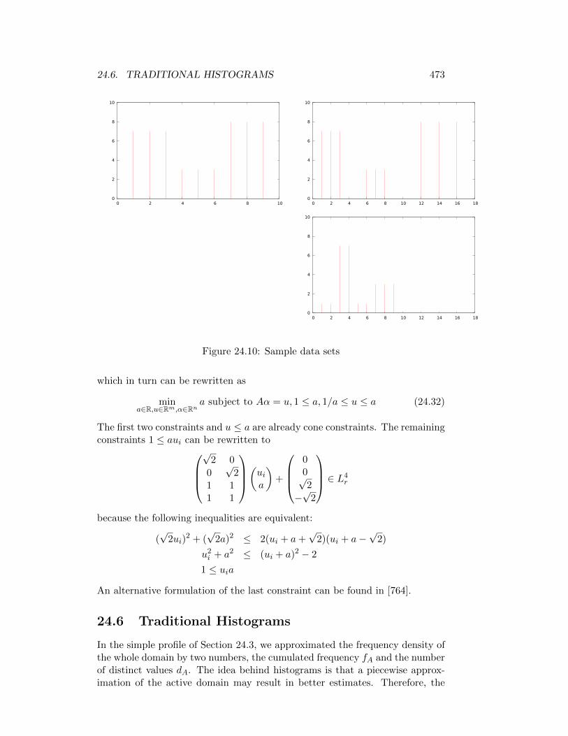
24.6. TRADITIONAL HISTOGRAMS 473

0

2

4

6

8

10

0 2 4 6 8 10 0

2

4

6

8

10

0 2 4 6 8 10 12 14 16 18

0

2

4

6

8

10

0 2 4 6 8 10 12 14 16 18

Figure 24.10: Sample data sets

which in turn can be rewritten as

mina∈R,u∈Rm,α∈Rn

a subject to Aα = u, 1 ≤ a, 1/a ≤ u ≤ a (24.32)

The first two constraints and u ≤ a are already cone constraints. The remainingconstraints 1 ≤ aui can be rewritten to

√2 0

0√

21 11 1

(uia

)+

00√2

−√

2

∈ L

4r

because the following inequalities are equivalent:

(√

2ui)2 + (

√2a)2 ≤ 2(ui + a+

√2)(ui + a−

√2)

u2i + a2 ≤ (ui + a)2 − 2

1 ≤ uia

An alternative formulation of the last constraint can be found in [764].

24.6 Traditional Histograms

In the simple profile of Section 24.3, we approximated the frequency density ofthe whole domain by two numbers, the cumulated frequency fA and the numberof distinct values dA. The idea behind histograms is that a piecewise approx-imation of the active domain may result in better estimates. Therefore, the

474 CHAPTER 24. CARDINALITY AND COST ESTIMATION

active domain [lA, uA] is partitioned into subsets called buckets. Traditionally,for each bucket Bi, the cumulated frequency f+

i of the values falling within thebucket as well as the number of distinct values d+

i of A within the bucket isstored. A histogram then consists of a sequence of buckets.

24.6.1 Bucketization

Assume we wish to partition the active domain DA (= ΠA(R)) of some attributeA of some relation R into β buckets Bi (1 ≤ i ≤ β). Then, each bucket containsa subset of values of the universe of A. That is Bi ⊆ [lA, uA]. Not any subset isused in practice. Since it is too memory consuming to store the values in eachbucket explicitly, buckets always comprise subintervals of the active domain.Further, these are typically non-overlapping. That is Bi ∩Bj = ∅ for i 6= j.

Such a partitioning of the active domain can be achieved in two steps. Ina first step, we fix a set of bucket boundaries bi ∈ [lA, ua] such that lA = b0 ≤b1 ≤ . . . ≤ bα = uA. In order to decrease the search space, the bi are typicallychosen from the active domain, that is bi ∈ DA.

In a second step, we use these values as bucket boundaries to determine thebuckets. Here, there are several alternatives. Let us first consider the case ofan integer-valued attribute A. If we use closed intervals for buckets, we candefine a bucket as comprising the values in [bi−1 + 1, bi]. Note that [bi, bi+1]does not work, since it overlaps with [bi+1, bi+2]. We could also build a bucket[bi−1, bi− 1]. But with proper choices of the bi, these two are equivalent. A notequivalent alternative is to use half-open intervals. In this case, we can definea bucket as [bi, bi+1[.

Another issue is whether the buckets completely cover the active domain,that is whether

⋃βi=1Bi = [lA, uA] holds or not. In the latter case, we can define

buckets comprising closed intervals as [bi, bi+1] if we do not define buckets for[bi−1, bi] and [bi+1, bi+2]. Thus, our histogram (the set of buckets we define)contains holes. This is typically only the case if no value from DA falls into thehole.

Summarizing, we have the following three alternatives for attribut with adiscrete, ordered domain:

1. closed-interval histogram without holes

2. closed-interval histogram with holes

3. half-open interval histogram without holes

Note that independent of the kind of histogram constructed, all the values bimust be stored.

The literature is sparse on investigations of whether holes are good or not.Most papers don’t even specify which kind of histogram they are talking about.As an exception, Wang and Sevcik consider 1) and 2) [873]. They proposeto treat these two possibilities as alternatives during the construction of thehistogram.

For a contineous domain, e.g. floating point numbers, alternative 1) is not(easily) possible. Thus, in this case, we can only choose between 2) and 3).

24.6. TRADITIONAL HISTOGRAMS 475

If most range queries use close ranges, 1) and 2) should be the preferredoptions. To see this, note that we must add or subtract the frequencies of theboundaries to convert a half-open or open inveral into a closed interval or viceversa. Further, even if we have a good approximation of the exact frequenciesof single values, we still face the problem of values not occurring in the activedomain if it is not dense. Nonetheless, the subsequent discussion applies withminor modifications to all three alternatives.

24.6.2 Heuristics to Determine Bucket Boundaries

In the sequel, we discuss some heuristics to determine the bucket boundaries.All these algorithms have a parameter β for the number of buckets to construct.Subsequently, we assume that we are given a set d of value/frequency pairsX = (xi, fi)|1 ≤ i ≤ d. We assume that the xi are sorted in increasing order,i.e., xi < xi+1 for 1 ≤ i < d. By F+ or n , we denote the cumulated frequencyF+ = n =

∑di=0 fI . The bucket boundaries will be denoted by b0, . . . , bβ, where

b0 = x0 and bβ = xd. Of course, we assume that b << d.

Equi-Width Histograms

Kooi was the first to propose histograms for selectivity estimation [492]. Thefirst type of histograms he proposed were equi-width histograms. In an equi-width histogram, the bucket boundaries are determined by

bi = x0 + iδ

where δ = (xd − x0)/β.

Equi-Width Histograms

Kooi [492] also proposed the alternative of equi-width histograms [492]. There,all buckets have about the same cumulated frequency. This can be achievedby a single scan through X and starting a new bucket as soon as the currentbucket’s cumulated frequency exceeds F+/β.

Another interesting approach to equi-width histograms has been describedby Piatetsky-Shapiro and Connell [660]. There, buckets can overlap. The con-struction is quite simple, though expensive. First, from X we construct a bag Yof cardinality n such that each value xi occurs exactly fi times in Y . Then, Y issorted by increasing values. A parameter S is used to determine the number ofvalues to be stored. S determines the distance in the sorted vector Y betweentwo stored values via N = (n − 1)/S. From the sorted vector we then pickevery value at a position 1 + iN for i = 0, . . . , S. Hence, we store S + 1 values.If (n − 1)/S is not an integer, the distance between the last two elements canbe smaller.

This approach is called distribution steps, but could also be termed quantiles.If some values occur very frequently (more often than N times), then they arestored more than once. Thus, the buckets overlap. Besides the values nothingelse is stored. Piatetsky-Shapiro and Connell then continue to give selectivityestimation formulars [660], which we do not repeat here.

476 CHAPTER 24. CARDINALITY AND COST ESTIMATION

The Heuristics Zoo

Besides the classic equi-width and equi-depth heuristics to find bucket bound-aries, a whole zoo of heuristics has been proposed. Fortunately, this zoo hasbeen classified by Poosala, Ioannidis, Haas, and Shekita [672].

Before we begin, let us recall some basic definitions. For every xi except thealst one, we define the spread si as si = xi+1−xi and the area ai as ai = fi ∗si.The motivation behind these definitions is based on the two major problems weface when approximating a given data distribution X. The problems are

1. largely varying fi and

2. largely varying si.

Any of the xi, fi, si, or ai is a parameter to the heuristics. We denote whichone of these the heuristics should apply by V (value), F (frequency), S (spread),A (area), respectively.

The first partitioning heuristics is Equi-Sum. It gives rise to Equi-Sum(V),Equi-Sum(F), Equi-Sum(S), and Equi-Sum(A) and tries to balance the sum ofits parameter such that all buckets exhibit about the same value for the sum.Thus, Equi-Sum(V) corresponds to equi-width (here, we count the number of xifalling into a bucket) and Equi-Sum(F) corresponds to equi-depth histograms.

The next bunch of heuristics are max-diff histograms. They come in theflavors of max-diff(F), max-diff(S), and max-diff(A). They put bucket boundsbetween those β − 1 values xi and xi+1 where the β − 1 highest values of thedifferences |fi+1 − fi|, |si+1 − si|, |ai+1 − ai| are found.

End-biased histograms store those values together with their frequenciesthat exhibit the β1 lowest and β2 highest frequencies with β = β1 + β2. Theremaining values are put into a single bucket. High-biased histograms onlystore the β highest values and use a single histogram for the remaining values.Compressed histograms additional use a regular histogram (e.g. equi-depth) toapproximate the frequency distribution of the remaining values.

Note that none of these histograms comes with a guarantee regarding themaximal possible q-error for range queries. Histograms that exhibit this prop-erty will be discussed in Sec. ??. But before that, we need to prepare ourselvesa little more.

24.7 More on Q

24.7.1 Properties of the Q-Error

Definition of the Q-Error

Let f ≥ 0 be a number and f ≥ 0 be an estimate for f . Then, we define theq-error of f as

||f/f ||Q,where ||x||Q := max(x, 1/x).

If for some value q ≥ 1 ||f/f ||Q ≤ q, we say that the estimate is q-acceptable.

24.7. MORE ON Q 477

Let R be a relation and A be one of its attributes. Let ΠDA (R) = x1, . . . , xd

with xi ≤ xi+1. Denote by fi the frequency of xi and by f+(c1, c2) :=∑

c1≤x<c2 fithe cumulated frequency. Let f+(x, y) be an estimation function for f+. Letq ≥ 1 be some number. We say that f+ is q-acceptable, if for all x1 ≤ c1 ≤c2 ≤ xd the estimate f+(c1, c2) is q-acceptable.

Assume we know that1

ax ≤ x′ ≤ bx

for some numbers a, b ≥ 1 and x, x′ > 0. Then, it is easy to see that

||x/x′||Q ≤ max(a, b)

holds.

Sums

For 1 ≤ i ≤ n, let fi be true values and fi be estimates with ||fi/fi||Q ≤ q forall 1 ≤ i ≤ n. Then

1/q ∗n∑

i=1

fi ≤n∑

i=1

fi ≤ q ∗n∑

i=1

fi

holds, i.e.,

||∑n

i=1 fi∑ni=1 fi

||Q ≤ q.

Products

For 1 ≤ i ≤ n, let fi be true values and fi be estimates with ||fi/fi||Q ≤ qi forall 1 ≤ i ≤ n. Then

n∏

i=1

(1/qi) ∗n∏

i=1

fi ≤n∏

i=1

fi ≤n∏

i=1

qi ∗n∏

i=1

fi

holds, i.e.,

||∏ni=1 fi∏ni=1 fi

||Q ≤n∏

i=1

qi.

Note that division behaves like multiplication.

Differences

Assume we are given a total value t > 0, which is the sum of a large valuesl > 0 and a small value s > 0. Thus, t = l + s and s ≤ l. The latter impliesthat s ≤ t/2 ≤ l.

If we know t and an estimate l of l, we can get an estimate s = t− l. Thiskind of estimation is not a good idea, as we see from the following example.Assume that t = 100, l = 90, s = 10, and l = 99. Although ||l/l||Q = 1.1, we

have s = t− l = 1 and, thus, ||s/s||Q = 10.The situation is different, if we use an estimate s of (the smaller) s to derive

an estimate l for (the larger) l as the following theorem shows.

478 CHAPTER 24. CARDINALITY AND COST ESTIMATION

Theorem 24.7.1 Let t, l, s > 0 be three numbers such that t = l+ s and s ≤ l.Let s be an estimate for s with ||s/s||Q ≤ q for some q ≥ 1. Define the estimate

l for l as l = max(t/2, t− s). Then ||l/l||Q ≤ min(2, q).

Proof: First, observe that if q = 1 the theorem trivially holds. Sec-ond, observe that ||l/l||Q ≤ 2 always holds. Thus, if for some q we have

q = ||s/s||Q >= 2 then ||l/l||Q ≤ q. Finally, we have to show that ||l/l||Q ≤ qfor 1 < q < 2.

Due to t = l + s and s ≤ l, we have

t/2 ≤ l = t− s (*),

and, thus t ≤ 2(t− s).Further remember our assumption 2 > q = ||s/s||Q. According to the

definition of l, we have to distinguish two cases.

Case 1: Assume t− s < t/2. Then

t− s < t/2

s > t− t

2

qs > t− t

2

qs >t

2

2q >t

s1

2q<

s

t(**)

Thus,

|| ll||Q = || t/2

l||Q

= || t

2(t− s) ||Q

=∗2(t− s)

t

= 2(1− s

t)

≤∗∗ 2(1− 1

2q)

= 2− 1

q≤ q

To see why the last inequality holds, we first observe that 2 − 1q is strongly

increasing in q. Further, remember that 1 ≤ q always holds and observe that(1) q − (2 − 1

q ) is strongly decreasing in q and (b) it attains its minimum in

24.7. MORE ON Q 479

the interval [1, 2] at q = 1, for which q − (2− 1q ) = 1− (2− 1

1) = 0. Thus, the

difference q− (2− 1q ) is always greater or equal to zero. This fact together with

q − (2− 1

q) ≥ 0

q ≥ 2− 1

q

finishes Case 1.

Case 2: We have to show that

(1/q)l ≤ t− s ≤ ql

under the assumptions that t/2 ≤ t− s and 1 < q < 2.

We start by showing t− s ≤ ql.

t− s ≤ ql≺ t− s ≤ q(t− s)≺ t− 1

q s ≤ q(t− s)≺ t− 1

q s ≤ qt− qs≺ qs− 1

q s ≤ qt− t≺ (q − 1

q )s ≤ (q − 1)t

≺ (q− 1q

)

(q−1) ≤ ts

We now observe that

(q − 1q )

(q − 1)=

q − 1 + 1− 1q

q − 1

= 1 +1− 1

q

q − 1≤ 2

≤ t

s

To see that1− 1

q

q−1 ≤ 1 consider

1− 1q

q−1 ≤ 1

≺ 1− 1q ≤ q − 1

≺ 2 ≤ q + 1q

The function f(x) = x + 1/x is monotonically increasing on x ∈ [1, 2], ourinterval of interest. Thus, since 1 + 1/1 = 2, the claim follows.

We now show that (1/q)l ≤ t − s under the assumptions that t/2 ≤ t − sand 1 < q < 2. If (1/q)(t− s) ≤ t/2 then (1/q)(t− s) ≤ t/2 ≤ t− s and we aredone. Thus, assume t/2 ≤ (1/q)(t− s).

480 CHAPTER 24. CARDINALITY AND COST ESTIMATION

Consider(1/q)l ≤ t− s

≺ 1/q(t− s) ≤ t− s≺ 1/q(t− s) ≤ t− qs≺ 1

q t− 1q s ≤ t− qs

≺ qs− 1q s ≤ t− 1

q t

≺ (q − 1q )s ≤ (1− 1

q )t

≺ q− 1q

1− 1q

≤ ts (*)

Observe that

q − 1q

1− 1q

=q2 − 1

q − 1

=(q + 1)(q − 1)

q − 1

= q + 1 (**)

Summarizing (*) and (**), it suffices to show

q + 1 ≤ t

s.

From our assumption t/2 ≤ 1q (t− s), we can derive

t/2 ≤ 1q (t− s)

≺ qt ≤ 2t− 2s≺ q ≤ 2 t−st≺ q ≤ 2(1− s

t )≺ q ≤ 2− 2 st≺ q + 1 ≤ 3− 2 st

Now, it suffices to show that

3− 2s

t≤ t

s.

The following inequalities are equivalent:

3− 2s

t≤ t

s3ts− 2s2 ≤ t2

0 ≤ t2 − 3ts+ 2s2

0 ≤ t2 − 2ts+ s2 − ts+ s2

0 ≤ (t− s)2 − s(t− s)0 ≤ (t− s)− s0 ≤ t− 2s

Since the latter holds, we are done with the case t/2 ≤ 1q (t− s) and, thus, with

Case 2.2

24.7. MORE ON Q 481

Theorem 24.7.2 Let t, l, s > 0 be three numbers such that t = l+ s and s ≤ l.Let t be an estimate for t with ||t/t||Q ≤ q for some q ≥ 1. Define the estimate

l for l as l = max(t/2, t− s). Then ||l/l||Q ≤ 2q.

ProofCase 1. l = t/2. Define

q∗ := || ll||Q = || t/2

t− s ||Q.

Case 1.1 t/2 ≥ t− s. Then

q∗ =t/2

t− s

≤ t/2

t/2

≤ q

Case 1.2 t− s ≥ t/2. Then

q∗ =t− st/2

≤ t

t/2

≤ 2q

Case 2. l = t− s, t− s ≥ t/2. Define

q∗ := || ll||Q = || t− s

t− s ||Q.

Case 2.1 t− s ≥ t− s. Then

q∗ =t− st− s

≤ t− t/2t− t/2

≤ t− t/2t/2

≤ 2q − 1

Case 2.2 t− s ≥ t− s. Then

q∗ =t− st− s

≤ t− st/2

≤ t

t/2

≤ 2q

482 CHAPTER 24. CARDINALITY AND COST ESTIMATION

2

Note that if we make sure that we overestimate t, i.e., t ≥ t, then only Case2.1 applies and t is quite precise.

Theorem 24.7.3 Let t, l, s > 0 be three numbers such that t = l+ s and s ≤ l.Let t be an estimate for t with ||t/t||Q ≤ qt for some qt ≥ 1. Let s be an

estimate for s with ||s/s||Q ≤ qs for some qs ≥ 1. Define l := max(t/2, t − s).Additionally, assume that (1/qt)− qss > 0. Then, ||l/l||Q ≤ max(2qt, q

2t qs).

ProofToDo

Case 1. Consider the case where t/2 > t − s and, thus, l = t/2. The firstcondition implies that s > t/2. Also, by our preconditions, t/2 ≤ t− s. Define

q∗ := || ll||Q = || t/2

t− s ||Q.

Case 1.1 Assume l ≥ l. Then

q∗ =t/2

t− s≤ qtt/2

t/2

≤ qt

Case 1.2 Assume l < l. Then

q∗ =t− st/2

=t− s

1/qtt/2

= qtt− st/2

≤ 2qt

Case 2. Consider the case where t/2 ≤ t− s and, thus, l = t− s. Define

q∗ := || ll||Q = || t− s

t− s ||Q.

Case 2.1 Assume l ≥ l. Then

q∗ =t− st− s

≤ qtt

t− s −1

qs

s

t− s≤ 2qt −

1

qs

s

t− s≤ 2qt

24.7. MORE ON Q 483

Also, we have that

q∗ =t− st− s

≤ qtt− (1/qt)s

t− s≤ qt

t− st− s

≤ qtqs

This is not too bad since qt will be close to 1 in our applications.Also

q∗ =t− st− s

≤ t− s+ (qt − 1)t

t− s≤ qs +

(qt − 1)t

t− s≤ qs + 2(qt − 1)

This is not too bad since qt will be close to 1 in our applications.Case 2.2 Assume l < l. Then

q∗ =t− st− s

≤ t− s(1/qt)t− s

≤ qtt− st− qts

≤ q2t qs

This holds if t− qtqss ≥ t/2.If qtqs < 2 then

q∗ =t− st− s

≤ t− s(1/qt)t− s

≤ t/2

(1/qt)t− qs(t/2)

≤ t

(2/qt)t− qs(t)≤ 1

(2/qt)− qs≤ qt

1

2− qtqs

das ist doof.2

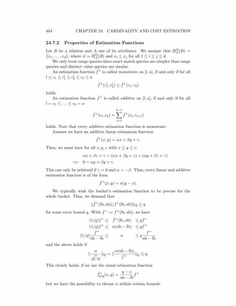
484 CHAPTER 24. CARDINALITY AND COST ESTIMATION

24.7.2 Properties of Estimation Functions

Let R be a relation and A one of its attributes. We assume that ΠDA (R) =

x1, . . . , xd, where d := ΠDA (R) and xi ≤ xj for all 1 ≤ i ≤ j ≤ d.

We only treat range queries since exact match queries are simpler than rangequeries and distinct value queries are similar.

An estimation function f+ is called monotonic on [l, u], if and only if for alll ≤ c1 ≤ c′1 ≤ c′2 ≤ c2 ≤ u

f+(c′1, c′2) ≤ f+(c1, c2)

holds.An estimation function f+ is called additive on [l, u], if and only if for all

l = c1 ≤ . . . ≤ ck = u

f+(c1, ck) =k−1∑

i=1

f+(ci, ci+1)

holds. Note that every additive estimation function is monotonic.Assume we have an additive linear estimation function

f+(x, y) = αx+ βy + γ.

Then, we must have for all x, y, z with x ≤ y ≤ z:αx+ βz + γ = (αx+ βy + γ) + (αy + βz + γ)

≺ 0 = αy + βy + γ

This can only be achieved if γ = 0 and α = −β. Thus, every linear and additiveestimation function is of the form

f+(x, y) = α(y − x).

We typically wish the bucket’s estimation function to be precise for thewhole bucket. Thus, we demand that

||f+(lb, ub)/f+(lb, ub)||Q ≤ qfor some error bound q. With f+ := f+(lb,ub), we have

(1/q)f+ ≤ f+(lb,ub) ≤ qf+

(1/q)f+ ≤ α(ub− lb) ≤ qf+

(1/q)f+

ub− lb≤ α ≤ q f+

ub− lb

and the above holds if

|| αf+

ub−lb

||Q = ||α(ub− lb)

f+||Q ≤ q.

This clearly holds, if we use the usual estimation function

f+avg(x, y) =

y − xub− lb

f+

but we have the possibility to choose α within certain bounds.

24.7. MORE ON Q 485

24.7.3 θ,q-Acceptability

One problem occurs if the cardinality estimate for some query is f ≥ 1 and thetrue cardinality is zero. This happens, since we should never return an estimateof zero, because this leads to query simplifications which may be wrong or inreorderings which may not be appropriate. To solve this dilemma, there isonly a single solution: during query optimization time, we execute buildingblocks and even access paths until the first tuple has been delivered. Fromthere on, we know for sure, wether the result will be empty or not. If thereis a tuple delivered, we buffer it, since we want to avoid its recalculation atruntime. The overhead of this method should therefore be low. Now, assumethat we are willing to buffer more tuples (say 1000). Then, if there are lessthan 1000 qualifying tuples, we now the exact answer after fetching them. If wehave to halt the evaluation of the build block since the buffer is full, we knowthat there will be ≥ 1000 qualifying tuples. Let us denote by θbuf the numberof tuples we are willing to buffer. Since we interleave query optimization andquery execution, this can be considered a small step in the direction of adaptivequery optimization [223].

However, before we can evaluate a building block or access paths, we have todetermine an optimal one, which in turn requires cardinality estimates! Beforewe proceed note that cardinality estimates may be imprecise as long as they donot influence the decisions of the query optimizer badly. This means, as longas the query optimizer produces the best plan, any estimate is o.k. Let’s forexample take the decision wether to exploit an index or not. Assume, an indexis better than a scan if less than 10% of the tuples qualify (This is a typicalvalue [99, 353]). If the relation has 10000 tuples, the threshold is at 1000 tuples.Thus, assume that for a given range query both, the estimate and the true valuedo not exceed 500. Then, no matter what the estimate is, we should use theindex. Note that the q-error can be 500 (e.g., the estimate is 1 and the truevalue is 500). Still it does not have any bad influence on our decision. Theimportant thing is that the estimate has to be precise around 1000. For a givenrelation and one of its indices, we denote by θidx the number of tuples that, ifexceeded make a table scan more efficient than the index scan.

Let us now combine these two things. Assume we want to have a maximal q-error of q. Define θ = min(θbuf−1, (1/q)θidx). Assume that f is an estimate forthe true cardinality f . Further assume that if f or f exeeds θ, then ||f/f ||Q ≤ q.Now let’s go through the optimizer. In a first step, we define our building blocksand access paths, which requires to decide on index usage. Clearly, the estimatewill be precise above (1/q)θidx, which includes the critical part. After evaluatinga building block or access path, we have precise cardinality estimates if fewerthan θbuf tuples are retrieved. Otherwise, our estimate will obey the givenq-error. Thus, we are as precise as necessary under all circumstances.

These simple observations motivate us to introduce the notion of θ, q-acceptability.Let f ≥ 0 be a number and f ≥ 0 be an estimate for f . Let q ≥ 1 and θ ≥ 1be numbers. We say that f is θ, q-acceptable if

1. f ≤ θ ∧ f ≤ θ or

486 CHAPTER 24. CARDINALITY AND COST ESTIMATION

2. ||f/f ||Q ≤ q.

Let R be a relation and A be one of its attributes. Let ΠDA (R) = x1, . . . , xd

with xi ≤ xi+1. Denote by fi the frequency of xi and by f+(c1, c2) :=∑

c1≤x<c2 fithe cumulated frequency. Let f+(x, y) be an estimation function for f+. Wesay that f+ is θ, q-acceptable, if for all x1 ≤ c1 ≤ c2 ≤ xd the estimate f+(c1, c2)is θ, q-acceptable.

Another way to look at θ is that it is a ’Bagatellgrenze’. If the cardinality isbelow it, we do not really care how large it really is. The reason is that queryexecution will be fast anyway, even if we pick the wrong plan.

24.7.4 Testing θ,q-Acceptability for Buckets

Let R be a relation and A one of its attributes. We assume that ΠDA (R) =

x1, . . . , xd, where d := ΠDA (R) and xi ≤ xj for all 1 ≤ i ≤ j ≤ d.

We only treat range queries since exact match queries are simpler than rangequeries and distinct value queries are similar.

We assume left-open bucket boundaries and range queries of the form [a, b[.

Discretization

Testing θ,q-acceptability for a given bucket for a continous domain directly isimpossible since it would involve testing θ,q-acceptability of f+(c1, c2) for allc1, c2 within the bucket. In this section, we show that a test quadratic in thenumber of distinct values in the bucket suffices.

Let c1, c2 be a query interval. Assume i, j are chosen such that [xi, xj ] ⊆[c1, c2] ⊂ [xi−1, xj+1]. Since there is no distinct value between xi and xi−1 andbetween xj and xj+1, we have that f+(c1, c2) = f+(xi, xj) < f+(xi−1, xj+1).Assume the following conditions hold:

1. f+ is monotonic.

2. || f+(xi,xj)f+(c1,c2)

||Q ≤ q

3. || f+(xi−1,xj+1)f+(c1,c2)

||Q ≤ q

Since f+(xi, xj) = f+(c1, c2) ≤ f+(xi−1, xj+1), we then have || f+(c1,c2)f+(c1,c2)

||Q ≤ q.Exploiting this fact, we can develop the following quadratic test for some

given θ and q. If for all i, j such that xi and xj are in the bucket we have that

f+(xi−1, xj+1) ≤ θ ∧ f+(xi−1, xj+1) ≤ θ

or

|| f+(xi, xj)

f+(xi, xj)||Q ≤ q ∧ ||

f+(xi−1, xj+1)

f+(xi, xj)||Q ≤ q

then the bucket is θ,q-acceptable.

24.7. MORE ON Q 487

Subtests

Still, after discretization, the number of tests is quadratic in the number ofdistinct values contained in a bucket. We can restrict this even further formonotonic and additive estimators f+. For a given, fixed θ and for any i(1 ≤ i < d), we define i′ to be the index such that

1. f+(xi, xi′) ≤ θ

2. f+(xi, xi′) ≤ θ

3. f+(xi, xi′+1) > θ or f+(xi, xi′+1) > θ

This index i′ can be found by binary search.

For a given L, assume that for all l with 1 ≤ l ≤ L

• ||f+(xi, xi′+l)/f+(xi, xi′+l)||Q ≤ q

and

• f+(xi, xi′+L) ≥ kθ and

• f+(xi, xi′+L) ≥ kθ.

That is, we stop after L tests.

Then, we will show that the bucket is θ, (q + 1k )-acceptable.

Consider the range query [xi, xj [. If f+(xi, xj) ≤ kθ, then it is θ, q-acceptablefor f+(xi, xj).

Otherwise, we can find i1, . . . , im such that

• xi = xi1 and

• xj = xim .

Also, we can achieve that (a)

• ∀ij < m− 1 f+(xij , xij+1) ≥ kθ and

• f+(xim−1 , xim) < θ

or (b)

• ∀ij < m− 1 f+(xij , xij+1) ≥ kθ.

• f+(xim−1 , xim) < θ.

In the worst case, we have m = 3.

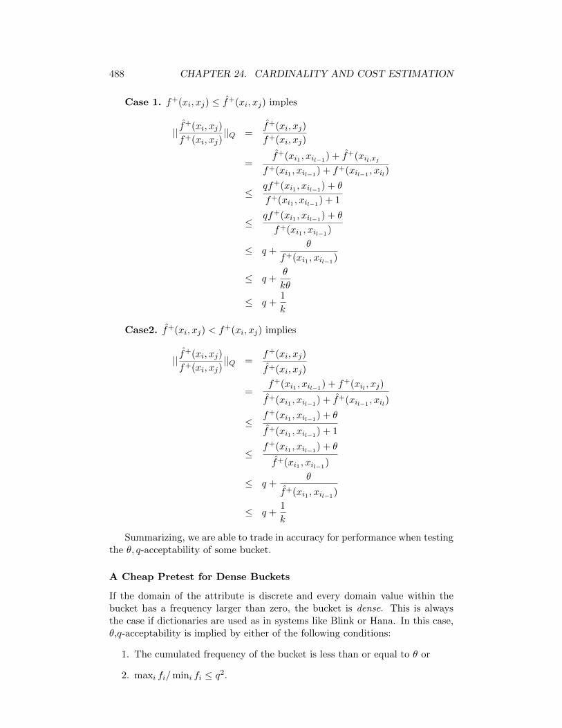
488 CHAPTER 24. CARDINALITY AND COST ESTIMATION

Case 1. f+(xi, xj) ≤ f+(xi, xj) imples

|| f+(xi, xj)

f+(xi, xj)||Q =

f+(xi, xj)

f+(xi, xj)

=f+(xi1 , xil−1

) + f+(xil,xjf+(xi1 , xil−1

) + f+(xil−1, xil)

≤ qf+(xi1 , xil−1) + θ

f+(xi1 , xil−1) + 1

≤ qf+(xi1 , xil−1) + θ

f+(xi1 , xil−1)

≤ q +θ

f+(xi1 , xil−1)

≤ q +θ

kθ

≤ q +1

k

Case2. f+(xi, xj) < f+(xi, xj) implies

|| f+(xi, xj)

f+(xi, xj)||Q =

f+(xi, xj)

f+(xi, xj)

=f+(xi1 , xil−1

) + f+(xil , xj)

f+(xi1 , xil−1) + f+(xil−1

, xil)

≤ f+(xi1 , xil−1) + θ

f+(xi1 , xil−1) + 1

≤ f+(xi1 , xil−1) + θ

f+(xi1 , xil−1)

≤ q +θ

f+(xi1 , xil−1)

≤ q +1

k

Summarizing, we are able to trade in accuracy for performance when testingthe θ, q-acceptability of some bucket.

A Cheap Pretest for Dense Buckets

If the domain of the attribute is discrete and every domain value within thebucket has a frequency larger than zero, the bucket is dense. This is alwaysthe case if dictionaries are used as in systems like Blink or Hana. In this case,θ,q-acceptability is implied by either of the following conditions:

1. The cumulated frequency of the bucket is less than or equal to θ or

2. maxi fi/mini fi ≤ q2.

24.7. MORE ON Q 489

The first condition also holds for non-dense buckets. The last condition onlyholds if we use our flexibility concerning the α in our approximation function.If we use f+

avg, we need to exchange it against

qf ≥ maxifi ∧ (1/q)f ≤ min

ifi,

where f is the average frequency of the bucket.If this cheap pretest fails, we need to apply the quadratic test or the subtest.

24.7.5 From Buckets To Histograms

As usual, let R be some relation and A be some of its attributes with ΠDA =

x1, . . . , xd, where d := |ΠDA (R)| and xi ≤ xj for 1 ≤ i ≤ j ≤ d.

In general, θ,q-acceptability does not carry over from buckets to histograms.That is, even though all buckets maybe theta, q-acceptable, the histogram mustnot be. Consider a histogram in which each bucket has the true cumulatedfrequency θ and the estimate for each bucket is 1. Then, the estimate for arange query comprising n buckets is n and the true value is nθ. Clearly, thehistogram is not θ,q-acceptable if q < θ.

Theorem 24.7.4 Let H be a histogram. Consider two neighbored buckets B1

and B2 spanning the intervals [bi, bi+1[ for i = 0, 1. Let k ≥ 2 be a number.If both buckets B1 and B2 are θ,q-acceptable then the histogram is kθ,q + q

k−1 -acceptable.

Proof: Assume we have two buckets B1 = [b0, b1[ and B2 = [b1, b2] and arange query asking for the cumulated frequency in [c1, c2[ with

b0 ≤ c1 ≤ b1 ≤ c2 ≤ b2.

For each bucket Bi, we denote by

f+i (x, y) =

∑

x≤xi<yfi

the true cumulated frequency within an interval contained in the bucket. Fur-ther, we assume that the approximation function f+

i (x, y) of every bucket Bi isθ,q-acceptable.

We introduce the following abbreviations:

f1 := f+(c1, b1)

f2 := f+(b1, c2)

f := f1 + f2

f1 := f+1 (c1, b1)

f2 := f+2 (b1, c2)

f := f1 + f2

Now, we investigate the estimation error for our range query. We distinguishseveral cases.

490 CHAPTER 24. CARDINALITY AND COST ESTIMATION

Case 1. In the first case, we assume f ≤ kθ and f ≤ kθ. In this case, theestimate is kθ,q-acceptable.

Case 2. In the second case, we assume that (f1 > θ∨f1 > θ)∧(f2 > θ∨f2 > θ).It follows that ||f/f ||Q ≤ q.Case 3. We now assume that neither the condition of Case 1 nor the conditionof Case 2 holds. Thus,

¬(f ≤ kθ ∧ f ≤ kθ) ∧ ¬((f1 > θ ∨ f1 > θ) ∧ (f2 > θ ∨ f2 > θ)),

which is equivalent to

(f > kθ ∨ f > kθ) ∧ ((f1 ≤ θ ∧ f1 ≤ θ) ∨ (f2 ≤ θ ∧ f2 ≤ θ)).

We consider four subcases, where we denote by q∗ the q-error of f , i.e.,

q∗ := || ff||Q = || f1 + f2

f1 + f2||Q.

Case 3.1 Assume

f > kθ, f1 ≤ θ, f1 ≤ θ.

From this, it follows that

kθ < f = f1 + f2 ≤ θ + f2

and thus (k − 1)θ < f2 and, since k ≥ 2

|| f2

f2||Q ≤ q.

Case 3.1.1 Assume f1 + f2 ≥ f1 + f2. A simple calculation gives us

q∗ =f1 + f2

f1 + f2

=f1

f1 + f2+

f2

f1 + f2

<θ

kθ+f2

f2

≤ q +1

k

24.7. MORE ON Q 491

Case 3.1.2 Assume f1 + f2 > f1 + f2. A simple calculation gives us

q∗ =f1 + f2

f1 + f2

≤ θ + qf2

f2

≤ q +θ

f2

≤ q +θ

(1/q)f2

≤ q +θ

(1/q)(k − 1)θ

≤ q +q

k − 1

Case 3.2 Assume

f > kθ, f2 ≤ θ, f2 ≤ θ.

This implies

kθ < f = f1 + f2 ≤ f1 + θ

and thus (k − 1)θ < f1 and, since k ≥ 2

|| f1

f1||Q ≤ q.

Case 3.2.1 Assume f1 + f2 ≥ f1 + f2. Then, f1 + f2 > kθ.

A simple calculation gives us

q∗ =f1 + f2

f1 + f2

=f1

f1 + f2+

f2

f1 + f2

≤ f1

f1+

θ

kθ

≤ q +1

k

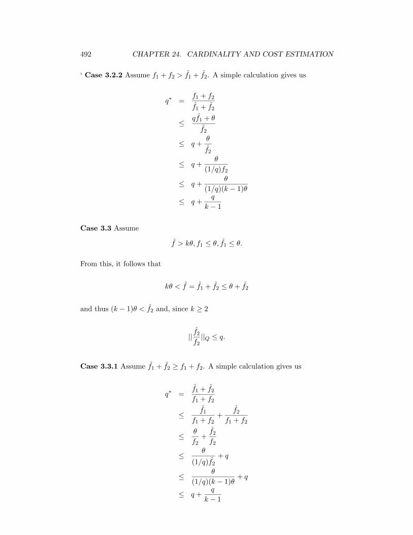
492 CHAPTER 24. CARDINALITY AND COST ESTIMATION

‘ Case 3.2.2 Assume f1 + f2 > f1 + f2. A simple calculation gives us

q∗ =f1 + f2

f1 + f2

≤ qf1 + θ

f2

≤ q +θ

f2

≤ q +θ

(1/q)f2

≤ q +θ

(1/q)(k − 1)θ

≤ q +q

k − 1

Case 3.3 Assume

f > kθ, f1 ≤ θ, f1 ≤ θ.

From this, it follows that

kθ < f = f1 + f2 ≤ θ + f2

and thus (k − 1)θ < f2 and, since k ≥ 2

|| f2

f2||Q ≤ q.

Case 3.3.1 Assume f1 + f2 ≥ f1 + f2. A simple calculation gives us

q∗ =f1 + f2

f1 + f2

≤ f1

f1 + f2+

f2

f1 + f2

≤ θ

f2+f2

f2

≤ θ

(1/q)f2

+ q

≤ θ

(1/q)(k − 1)θ+ q

≤ q +q

k − 1

24.7. MORE ON Q 493

Case 3.3.2 Assume f1 + f2 > f1 + f2. A simple calculation gives us

q∗ =f1 + f2

f1 + f2

≤ f1

f1 + f2

+f2

f1 + f2

≤ θ

kθ+f2

f2

≤ q +1

k

Case 3.4 Assumef > kθ, f2 ≤ θ, f2 ≤ θ.

From this, it follows that

kθ < f = f1 + f2 ≤ f1 + θ

and thus (k − 1)θ < f1 and, since k ≥ 2

|| f1

f1||Q ≤ q.

Case 3.4.1 Assume f1 + f2 ≥ f1 + f2.

q∗ =f1 + f2

f1 + f2

≤ f1

f1 + f2+

f2

f1 + f2

≤ f1

f1+

θ

f1

≤ q +θ

(1/q)f1

≤ q +θ

(1/q)(k − 1)θ

≤ q +q

k − 1

Case 3.4.2 Assume f1 + f2 > f1 + f2. A simple calculation gives us

q∗ =f1 + f2

f1 + f2

≤ f1

f1 + f2

+f2

f1 + f2

≤ f1

f1

+θ

kθ

≤ q +1

k

2

494 CHAPTER 24. CARDINALITY AND COST ESTIMATION

Theorem 24.7.5 Let H be a histogram. Consider n ≥ 3 consecutive bucketsBi in H spanning the intervals [bi, bi+1[ for i = 0, . . . , n. Let k ≥ 3 be a number.If every estimate for a range query spanning a whole bucket is q-acceptable andevery bucket Bi is θ,q-acceptable then the histogram is kθ,q + 2q

k−2 -acceptable.

Proof: Assume a query interval [c1, c2[ spanning the n buckets of H. Thatis b0 ≤ c1 ≤ b1 and bn−1 ≤ c2 ≤ bn.

We introduce the following abbreviations:

f1 := f+(c1, b1)

f2 := f+(b1, bn−1)

f3 := f+(bn−1, c2)

f := f1 + f2 + f3

f1 := f+1 (c1, b1)

f2 := f+2 (b1, bn−1)

f3 := f+3 (bn−1, c2)

f := f+1 + f+

2 + f+3

By assumption, we have ||f+2 /f

+2 ||Q ≤ q.

We distinguish several cases.

Case 1. If f ≤ kθ and f ≤ kθ, then the estimate is kθ, q-acceptable.

Case 2. If (f1 > θ ∨ f1 > θ) ∧ (f3 > θ ∨ f3 > θ), the estimate is q-acceptable.

Case 3. We now assume that neither the condition of Case 1 nor the conditionof Case 2 holds. Thus

¬(f ≤ kθ ∧ f ≤ kθ) ∧ ¬((f1 > θ ∨ f1 > θ) ∧ (f3 > θ ∨ f3 > θ)),

which is equivalent to

(f > kθ ∨ f > kθ) ∧ ((f1 ≤ θ ∧ f1 ≤ θ) ∨ (f3 ≤ θ ∧ f3 ≤ θ)).

We denote by q∗ the q-error of f , i.e.,

q∗ := || ff||Q = || f1 + f2 + f3

f1 + f2 + f3||Q.

Case 3.1 Assume f1 ≤ θ and f1 ≤ θ and f3 ≤ θ and f3 ≤ θ.Case 3.1.1 Assume f > kθ. From f = f1 + f2 + f3 > kθ and f1 ≤ θ andf3 ≤ θ, we get

f2 > (k − 2)θ

and

qf2 > (k − 2)θ.

24.7. MORE ON Q 495

If f ≤ f we get

q∗ =f

f

=f1 + f2 + f3

f1 + f2 + f3

=f1 + f3

f1 + f2 + f3+

f2

f1 + f2 + f3

≤ 2θ

kθ+ q

≤ q +2

k

If f ≤ f we get

q∗ =f

f

=f1 + f2 + f3

f1 + f2 + f3

≤ 2θ + f2

f2

≤ q +2θ

f2

≤ q +2θ

(1/q)(k − 2)θ

≤ q +2q

k − 2

Case 3.1.2 Assume f > kθ. From f = f1 + f2 + f3 > kθ and f1 ≤ θ andf3 ≤ θ, we get

f2 > (k − 2)θ

andqf2 > (k − 2)θ.

If f ≤ f we get

q∗ =f

f

=f1 + f2 + f3

f1 + f2 + f3

≤ q +2θ

f2

≤ q +2θ

(1/q)(k − 2)θ

≤ q +2q

k − 2

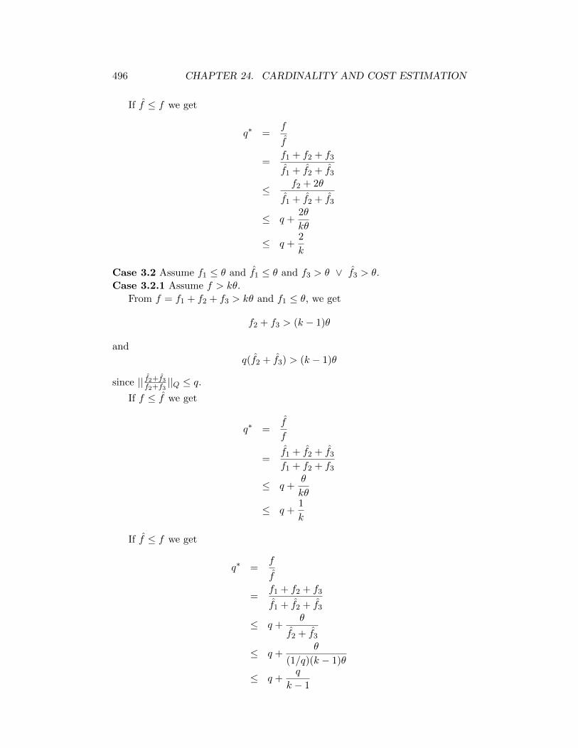
496 CHAPTER 24. CARDINALITY AND COST ESTIMATION

If f ≤ f we get

q∗ =f

f

=f1 + f2 + f3

f1 + f2 + f3

≤ f2 + 2θ

f1 + f2 + f3

≤ q +2θ

kθ

≤ q +2

k

Case 3.2 Assume f1 ≤ θ and f1 ≤ θ and f3 > θ ∨ f3 > θ.

Case 3.2.1 Assume f > kθ.

From f = f1 + f2 + f3 > kθ and f1 ≤ θ, we get

f2 + f3 > (k − 1)θ

and

q(f2 + f3) > (k − 1)θ

since || f2+f3f2+f3

||Q ≤ q.If f ≤ f we get

q∗ =f

f

=f1 + f2 + f3

f1 + f2 + f3

≤ q +θ

kθ

≤ q +1

k

If f ≤ f we get

q∗ =f

f

=f1 + f2 + f3

f1 + f2 + f3

≤ q +θ

f2 + f3

≤ q +θ

(1/q)(k − 1)θ

≤ q +q

k − 1

24.7. MORE ON Q 497

Case 3.2.2 Assume f > kθ.From f = f1 + f2 + f3 > kθ and f1 ≤ θ, we get

f2 + f3 > (k − 1)θ

andq(f2 + f3) > (k − 1)θ.

since || f2+f3f2+f3

||Q ≤ q.If f ≤ f we get

q∗ =f

f

=f1 + f2 + f3

f1 + f2 + f3

≤ q +θ

f2 + f3

≤ q +θ

(1/q)(k − 1)θ

≤ q +q

k − 1

If f ≤ f we get

q∗ =f

f

=f1 + f2 + f3

f1 + f2 + f3

≤ q +θ

f1 + f2 + f3

≤ q +θ

kθ

≤ q +1

k

Case 3.3 Assume f1 > θ ∨ f1 > θ and f3 ≤ θ and f3 ≤ θ.Case 3.3.1 Assume f > kθ. By Symmetry.Case 3.3.2 Assume f > kθ. By Symmetry.

2

In case the estimates for a whole bucket are precise, e.g., if we use f+avg, we

can refine the bounds.

Corollary 24.7.6 Let H be a histogram. Consider n ≥ 3 consecutive bucketsBi in H spanning the intervals [bi, bi+1[ for i = 0, . . . , n. Let k ≥ 3 be a number.If every estimate for a range query spanning a whole bucket is 1-acceptable andevery bucket Bi is θ,q-acceptable then the histogram is kθ,q′-acceptable, whereq′ := 2

k−2q + 1.

To see that the corollary holds, simply reconsider the above proof. Let usmention that for k ≥ 3, we never saw a q-error larger than q + 1/k.

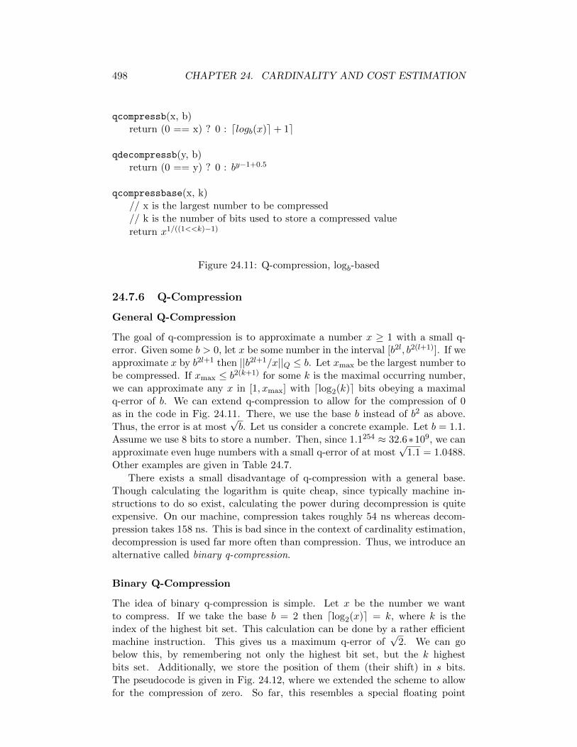
498 CHAPTER 24. CARDINALITY AND COST ESTIMATION

qcompressb(x, b)return (0 == x) ? 0 : dlogb(x)e+ 1e

qdecompressb(y, b)return (0 == y) ? 0 : by−1+0.5

qcompressbase(x, k)// x is the largest number to be compressed// k is the number of bits used to store a compressed value

return x1/((1<<k)−1)

Figure 24.11: Q-compression, logb-based

24.7.6 Q-Compression

General Q-Compression

The goal of q-compression is to approximate a number x ≥ 1 with a small q-error. Given some b > 0, let x be some number in the interval [b2l, b2(l+1)]. If weapproximate x by b2l+1 then ||b2l+1/x||Q ≤ b. Let xmax be the largest number tobe compressed. If xmax ≤ b2(k+1) for some k is the maximal occurring number,we can approximate any x in [1, xmax] with dlog2(k)e bits obeying a maximalq-error of b. We can extend q-compression to allow for the compression of 0as in the code in Fig. 24.11. There, we use the base b instead of b2 as above.Thus, the error is at most

√b. Let us consider a concrete example. Let b = 1.1.

Assume we use 8 bits to store a number. Then, since 1.1254 ≈ 32.6∗109, we canapproximate even huge numbers with a small q-error of at most

√1.1 = 1.0488.

Other examples are given in Table 24.7.

There exists a small disadvantage of q-compression with a general base.Though calculating the logarithm is quite cheap, since typically machine in-structions to do so exist, calculating the power during decompression is quiteexpensive. On our machine, compression takes roughly 54 ns whereas decom-pression takes 158 ns. This is bad since in the context of cardinality estimation,decompression is used far more often than compression. Thus, we introduce analternative called binary q-compression.

Binary Q-Compression

The idea of binary q-compression is simple. Let x be the number we wantto compress. If we take the base b = 2 then dlog2(x)e = k, where k is theindex of the highest bit set. This calculation can be done by a rather efficientmachine instruction. This gives us a maximum q-error of

√2. We can go

below this, by remembering not only the highest bit set, but the k highestbits set. Additionally, we store the position of them (their shift) in s bits.The pseudocode is given in Fig. 24.12, where we extended the scheme to allowfor the compression of zero. So far, this resembles a special floating point

24.7. MORE ON Q 499

#Bits Base Largest compressable number q-Error

4 2.5 372529 1.584 2.6 645099 1.614 2.7 1094189 1.645 1.7 8193465 1.305 1.8 45517159 1.345 1.9 230466617 1.386 1.2 81140 1.106 1.3 11600797 1.146 1.4 1147990282 1.187 1.1 164239 1.057 1.2 9480625727 1.108 1.1 32639389743 1.05

Table 24.7: Examples for q-compression

representation with only positiv mantissa and exponent.

The q-middle of 2n and 2n−1 − 1 is√

2n ∗ (2n+1 − 1). This is the estimatewe should return for n. We do not want to compute the square root duringdecompression, since this is too expensive. A little calculation helps.

√2n ∗ (2n+1 − 1) ≈

√2n ∗ 2n+1

=√

22n ∗ 2

=√

2 ∗ 2n

= 2n + (√

2− 1) ∗ 2n

The second part can be calculated by a constant (√

2 − 1) shifted by n to theleft. The pseudocode in Fig. 24.12 gives the calculation of this constant C in C.The best theoretical q-error achievable with storing k bits is

√1 + 21−k. With

our fast approximation, we get pretty close as the following table shows. Theobserved maximal q-error column was obtained experimentally. The deviationfrom the observed maximal q-error to the theoretical maximal q-error is dueto the fact that only a small portion of the digits of C are used. Further,compression (2.7 ns) and decompression (2.8 ns) are fast.

500 CHAPTER 24. CARDINALITY AND COST ESTIMATION

qcompress2(x, k, s)if 2s > xthen

bits = xshift = 0

elseshift = index-of-highest-bit-set(x) - k + 1;bits = (x >> shift)

return (bits << shift) | shift

qdecompress2(y, k, s)shift = y & (2s − 1)bits = y >> shiftx = bits << shift– assume C = (int) ((sqrt((double) 2.0) - 1.0) * 4 * (1 << 30))x |= (C >> (32 - shift))return x

Figure 24.12: Binary Q-compression

k max q-error observed max q-error theoretical (√

1 + 21−k)1 1.5 1.412 1.25 1.223 1.13 1.124 1.07 1.065 1.036 1.036 1.018 1.0167 1.0091 1.00788 1.0045 1.00399 1.0023 1.00195

10 1.0011 1.0009811 1.00056 1.0004812 1.00027 1.00024

Incremental Updates

It might come as a surprise that q-compressed numbers can be incrementallyupdated. Already in 1978, Morris observed this fact [605]. Later, Flajoletanalyzed the probabilistic counting method thoroughly [274]. The main idea israther simple. For binary q-compressed numbers, the incrementing procedureis defined as follows:

RandomIncrement(int& c)// c: the counter

24.8. ONE DIMENSIONAL SYNOPSES 501

τ1,1: 100

–

τ1,1: 100

τ1,2: 52

m1,2: 33

τ1,2: 52

τ1,4: 30

m1,4: 18

τ1,4: 30

τ1,8: 12

m1,8: 6

τ1,8: 12

τ2,8: 18

–

τ2,8: 18

τ2,4: 22

–

τ2,4: 22

τ3,8: 16

m3,8: 11

τ3,8: 16

τ4,8: 6

–

τ4,8: 6

τ2,2: 48

–

τ2,2: 48

τ3,4: 20

m3,4: 13

τ3,4: 20

τ5,8: 6

m5,8: 5

τ5,8: 7

τ6,8: 14

–

τ6,8: 13

τ4,4: 28

–

τ4,4: 28

τ7,8: 13

m7,8: 7

τ7,8: 13

τ8,8: 15

–

τ8,8: 15

Figure 24.13: FLT example 1

let δ be a binary random variable which takesvalue 1 with probability 2−c andvalue 0 with probability 1− 2−c.

c += δ

To go to an arbitrary base, we have to modify the random variable δ such thatit takes the value 1 with probability a−c and 0 with probability 1− a−c.

24.8 One Dimensional Synopses

24.8.1 Four Level Tree and Variants

The Original Four Level Tree

Four level trees were introduced by Buccafurri, Pontieri, Rosaci, and Sacca[112]. Later, Buccafurri, Lax, Sacca, Pontieri, and Rosaci discussed three, five,and N-Level level trees [110, 111]. A concise description can also be found in[202].

The basic idea is to divide a bucket into eight subbuckets (called bucklets)of equal width. Consider the following sample bucket [111]:

xi 1 2 3 4 5 6 7 8 9 10 11 12 13 14 15 16fi 7 5 18 0 6 10 0 6 0 6 9 5 13 0 8 7

This bucket is divided into 8 bucklets of width 16/8 = 2. Every bucklet τi,8summarizes the values in bucket i, 1 ≤ i ≤ 8. The next higher level of the four

502 CHAPTER 24. CARDINALITY AND COST ESTIMATION

level tree contains four values τi,4 (1 ≤ i ≤ 4) summing the frequencies in thei-th quarter of the bucket. Thus, τi,4 = τ2i−1,8 + τ2i,8 for 1 ≤ i ≤ 4. The thirdlevel of the four level tree defines the values τi,2 for i = 1, 2 summing up thefrequencies in each half of the bucket. The last level, τ1,1 contains the sum ofall frequencies fi in the bucket. This scheme is illustrated in Fig. 24.13 andformally defined as

τi,2k := τ2i−1,2k+1 + τ2i,2k+1

for k = 0, . . . , 3.

The four level tree in Fig. 24.13 is compressed into 64 bits as follows. τ1,1 isstored in the first 32 bits. Next, the τj,2k for k > 0 are only stored if j is odd.For even j = 2i, τ2i,2k+1 can be calculated given τi,2k :

τ2i,2k+1 := τi,2k − τ2i−1,2k+1

for k = 1, . . . , 3. Further, since 7 numbers have to be compressed into 32 bits,only an approximation thereof is stored. The number of bits bk used to storethe approximation of some τ2i−1,2k+1 decreases from top to bottom:

k 0 1 2 3bk 32 6 5 4

The intention is that if we make a mistake at a higher level, all lower levels areaffected. Thus, we want to be precise at higher levels.

Instead of storing τ2i−1,2k+1 directly, the ratio τ2i−1,2k+1/τi,2k is approximat-ed using bk bits:

m2i−1,2k+1 := round(τ2i−1,2k+1

τi,2k(2bk − 1)). (24.33)

The 7 mi,j values are stored in the second 32 bits:

m1,2 m1,4 m3,4 m1,8 m3,8 m5,8 m7,8

33 18 13 6 11 5 7100001 10010 01101 0110 1011 0101 0111

The number of zeros and ones in the last line is 1 ∗ 6 + 2 ∗ 5 + 4 ∗ 4 = 32.

From m2i−1,2k , we can restore an estimate for τ2i,22k by calculating

τ2i,22k := round(m2i−1,2k

2bk − 1∗ τi,2k). (24.34)

This recursion is possible, since we store τ1,1 explicitly. The τ are also given inFig. 24.13.

Now, consider the example in Fig. 24.14. It shows the four level tree for afrequency density where the eight bucklets have the following cumulated fre-quencies:

i 1 2 3 4 5 6 7 8f+i 1.000.000 100.000 10.000 1000 100 10 1 10.000

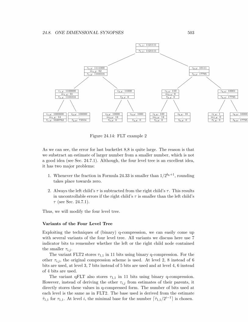
24.8. ONE DIMENSIONAL SYNOPSES 503

τ1,1: 1121111–

τ1,1: 1121111

τ1,2: 1111000m1,2: 62

τ1,2: 1103316

τ1,4: 1100000m1,4: 31

τ1,4: 1103316

τ1,8: 1000000m1,8: 14

τ1,8: 1029762

τ2,8: 100000–

τ2,8: 73554

τ2,4: 11000–

τ2,4: 0

τ3,8: 10000m3,8: 14τ3,8: 0

τ4,8: 1000–

τ4,8: 0

τ2,2: 10111–

τ2,2: 17795

τ3,4: 110m3,4: 0τ3,4: 0

τ5,8: 100m5,8: 14τ5,8: 0

τ6,8: 10–

τ6,8: 0

τ4,4: 10001–

τ4,4: 17795

τ7,8: 1m7,8: 0τ7,8: 0

τ8,8: 10000–

τ8,8: 17795

Figure 24.14: FLT example 2

As we can see, the error for last bucketlet 8,8 is quite large. The reason is thatwe substract an estimate of larger number from a smaller number, which is nota good idea (see Sec. 24.7.1). Although, the four level tree is an excellent idea,it has two major problems:

1. Whenever the fraction in Formula 24.33 is smaller than 1/2bk+1, roundingtakes place towards zero.

2. Always the left child’s τ is subtracted from the right child’s τ . This resultsin uncontrollable errors if the right child’s τ is smaller than the left child’sτ (see Sec. 24.7.1).

Thus, we will modify the four level tree.

Variants of the Four Level Tree

Exploiting the techniques of (binary) q-compression, we can easily come upwith several variants of the four level tree. All variants we discuss here use 7indicator bits to remember whether the left or the right child node containedthe smaller τi,j .

The variant FLT2 stores τ1,1 in 11 bits using binary q-compression. For theother τi,j , the original compression scheme is used. At level 2, 8 instead of 6bits are used, at level 3, 7 bits instead of 5 bits are used and at level 4, 6 insteadof 4 bits are used.

The variant qFLT also stores τ1,1 in 11 bits using binary q-compression.However, instead of deriving the other τi,j from estimates of their parents, itdirectly stores these values in q-compressed form. The number of bits used ateach level is the same as in FLT2. The base used is derived from the estimateτ1,1 for τ1,1. At level i, the minimal base for the number dτ1,1/2

i−1e is chosen.

504 CHAPTER 24. CARDINALITY AND COST ESTIMATION

24.8.2 Q-Histograms (Type I)

So far, every bucket contains the same information. Loosening this restrictionresults in heterogeneous histograms. This leads to heterogeneous histogramswhich contain different kinds of buckets. However, there are a few disadvan-tages: higher cpu and memory consumption. Further, with every bucket typeconsidered, histogram construction costs increase. Besides the bucket bound-aries and the bucket contents a bucket header has to be stored. Since this istypically only a single byte per bucket, the increased flexibility by using differ-ent bucket types by far outways the price of this byte, leading to more compactand precise histograms.

Simple Bucket Types

We now briefly summarize some possible bucket types.

standard bucket A standard bucket contains the cumulated frequency andthe number of distinct values.

standard bucket with boundary frequency Microsoft SQL Server storesfor every bucket the frequency of the lower bucket boundary [217, p208].

poly2dim, exppoly2dim Assume (xi, fi) is the frequency density of ourattribute A. For given bucket boundaries b1, b2, we can approximate the set

RGE := (xi, xj , f+(xi, xj))|b1 ≤ xi ≤ xj ≤ b2

by a 2-dimensional polynomial. It is advantageous to use only low degrees (oneor two) and find the best approximation under lq. Approximation by a ep for apolynomial p leads to another alternative.

poly1dim, exppoly1dim

Histogram Construction by Dynamic Programming

A Heuristic for Histogram Construction

24.8.3 Q-Histogram (Type II)

24.9 Sketches For Counting The Number of DistinctValues

Histograms are used to overcome deficiencies of the uniform distribution as-sumption. So far, the only way we discussed to combine selectivities derived forserveral predicates from different attributes has to be done under the attributevalue independence assumption. In this section, we discuss an approach toavoid the attribute value independence assumption. This can be done by pro-viding precise estimates on the number of distinct values in a set of attributes

24.9. SKETCHES FOR COUNTING THE NUMBEROF DISTINCT VALUES505

(sometimes called column group). Although the number of distinct values for aset of attributes is rather interesting at different points in cardinality estimation(see our simple profile), we show how to provide selectivity estimates under theuniform distribution assumption but without relying on the attribute value in-dependence assumption. The number of distinct values for a column group canbe calculated by sorting or hashing, but this is often far to expensive. Thus,we provide a set of techniques based on sketches. Sketches are small summariesof data typically calculated online, i.e., with a single scan over the data. Weconcentrate on sketches for the count distinct case. A general introduction andan overview is contained in [202].

The problem we look at in this section is to approximately answer a queryof the form

select count(distinct A1,. . . ,An)from R

Standard techniques like hashtables or red-black trees can be used to collectthe distinct values contained in the attributes A1, . . . , An of R. However, thespace consumption is linear in the number of distinct values. Sketches requirefar less space.

Before we delve into the details of the algorithms, let us recall an observationmade by Ilyas, Markl, Haas, Brown, and Aboulnaga [425]. They observedthat sometimes assuming uniformity is not as bad as assuming attribute valueindependence. In this case, keeping the number of distinct values for a set ofattributes helps to make estimates more precise. Consider their example ofa car database repeated in Fig. 24.15. Assume that we want to provide anestimate for

select count(*)from Carwhere Make = Honda and Model = Accord

Denote by p1 (p2) the first (second) predidate in the query. The selectivities ares(p1) = 1/7 and s(p2) = 1/8. Assuming AVI yields s(p1 ∧ p2) = s(p1) ∗ s(p2) =1/56. The true selectivity is 1/10. The number of distinct values in the attributegroup (Make,Model) is calculated by the following query

select count(distinct Make, Model)from Car

and results in #DV = 9. Assuming that all distinct values occur equally often(uniformity assumption) results in the selectivity estimate s(p1 ∧ p2) = 1/9,which is much better.

Throughout the rest of this section, we assume that we want to producean estimate d for the number of distinct values d of a multiset (bag) X =x1, . . . , xd.

506 CHAPTER 24. CARDINALITY AND COST ESTIMATION

Car

ID Make Model

1 Honda Accord2 Honda Civic3 Toyota Camry4 Nissan Sentra5 Toyota Corolla6 BMW 3237 Mazda 3238 Saab 95i9 Ford F150

10 Mazda 323

Figure 24.15: Car database example

24.9.1 Linear Counting

The first algorithm we look at is Linear Counting by Astrahan, Schkolnick,and Whang [39]. Later, Whang, Vander-Zanden, and Taylor analyzed the al-gorithm and proposed a slight improvement [891]. Further, they showed ana-lytically and experimentally, that linear counting still yields good results evenif the fill factor goes up to 5-12. The algorithm is rather simple: Initialize abitvector B of length b to contain only zeros. Then, for each member x in thegiven multiset X, set B[h(x)] to one, where h is a hash function. Finally, thenumber of zeros z in B is counted and the resulting estimate for the number ofdistinct values in X is d = −b ln(z/b) (or d = b ln(b/z)). If the number of onesin the bitvector is rather small, this number can be used as the estimate. Thepseudocode of LinearCounting is given in Fig. 24.16. A problem occurs, if thebitvector becomes full, i.e., all bits are set. In this case, Whang et al. proposeto run the algorithm a second time with another hash function. Further, theyshow how to keep the probability of running into a full bitvector a second timelow. However, it is better to integrate LinearCounting into other algorithmsthat are capable of counting large numbers of distinct values in far less thanlinear space.

24.9.2 DvByKMinVal

Assume the hash function h hashes the elements of our set X to the interval[0, 1[. Further, let H = hi|hi = h(xi), xi ∈ X and assume that 0 ≤ hi ≤hi+1 < 1. If the hash function spreads out the elements evenly, we expectan average distance of δ = 1/(d + 1) ≈ 1/d between two neighbored hashvalues. For some given k, consider hk, i.e., the k-th smallest value in H. Thisvalue can easily be calculated exploiting a heap to keep the lowest k distinctvalues while scanning X. Clearly, we expect the value of hk to be around kδ.Thus, δ = hk/k. If we plug this into the former equation, we get hk/k = 1/dand hence d = k/hk. This very simple algorithm (see Fig.24.17), which we

24.9. SKETCHES FOR COUNTING THE NUMBEROF DISTINCT VALUES507

LinearCounting(X, h, B)X: bag of elementsh: hash function in [0, b− 1]B: bitvector of length bkinitialize B with zerosfor all x ∈ X do B[h(i] = 1for all i ∈ [0,m[ do

if 0 = M [i] then z := z + 1if 0 = z then z := 1o := m− z // number of ones in the bitvector corresponding to Mif o <

√m

then return oelse return m ∗ ln(m/z)

Figure 24.16: Linear Counting

DvByKMinVal(X,h)input: a bag X, a hashfunction h : X → [0, 1]

output: estimtate for the number d for the number of distinct values in Xusing,e.g., a heap calculate the k-th minimal value hk in h(x)|x ∈ Xd := (k − 1)/hkreturn d

Figure 24.17: Algorithm DvByKMinVal

call DvByKMinVal, was developed and analyzed by Bar-Yossef, Jayram, Kumar,Sivikumar, Trevisan [51]. Later Beyer, Haas, Reinwald, Sismanis, and Gemullashowed that this estimator is biased. They found that an unbiased estimator isd = (k−1)/hk [81]. As the hash function they recommend using the golden-ratiomultiplicative hashing method [485].

24.9.3 Logarithmic Counting

In a series of papers, Flajolet and Martin introduced three different probabilisticcounting algorithms [276, 277, 278]. For these algorithms, the hash functionmust map the elements of X to some bit pattern of a fixed length (say 32 or 64bits).

Let us start with the simplest one called LogarithmicCounting. The ideabehind this algorithm is the observation that the probability that the first bit ina bit pattern produced by the hash function being zero is 1/2. The probabilitythat the first two bits are zero is 1/4, and so on. The algorithm calculatesnow the smallest index R, such that among the bitvectors h(xi) the R-th bit isnever set. The estimate then roughly is 2R. However, this estimate is biased.

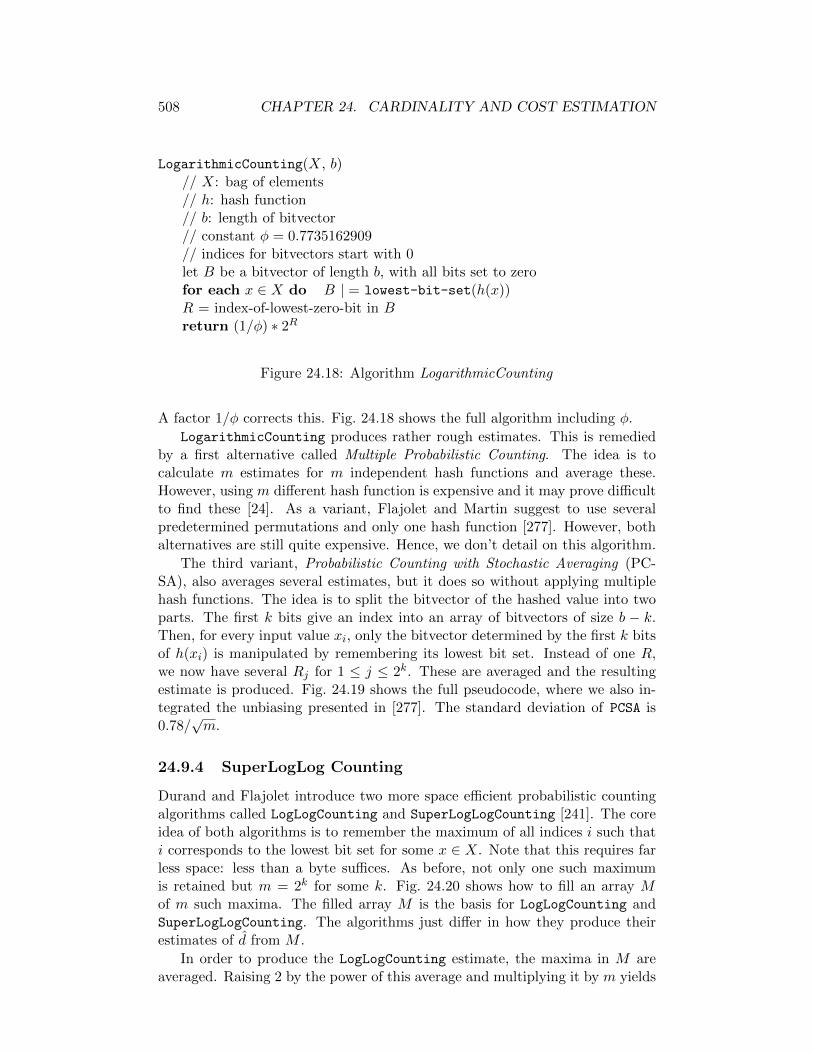
508 CHAPTER 24. CARDINALITY AND COST ESTIMATION

LogarithmicCounting(X, b)// X: bag of elements// h: hash function// b: length of bitvector// constant φ = 0.7735162909// indices for bitvectors start with 0let B be a bitvector of length b, with all bits set to zerofor each x ∈ X do B | = lowest-bit-set(h(x))R = index-of-lowest-zero-bit in Breturn (1/φ) ∗ 2R

Figure 24.18: Algorithm LogarithmicCounting

A factor 1/φ corrects this. Fig. 24.18 shows the full algorithm including φ.

LogarithmicCounting produces rather rough estimates. This is remediedby a first alternative called Multiple Probabilistic Counting. The idea is tocalculate m estimates for m independent hash functions and average these.However, using m different hash function is expensive and it may prove difficultto find these [24]. As a variant, Flajolet and Martin suggest to use severalpredetermined permutations and only one hash function [277]. However, bothalternatives are still quite expensive. Hence, we don’t detail on this algorithm.

The third variant, Probabilistic Counting with Stochastic Averaging (PC-SA), also averages several estimates, but it does so without applying multiplehash functions. The idea is to split the bitvector of the hashed value into twoparts. The first k bits give an index into an array of bitvectors of size b − k.Then, for every input value xi, only the bitvector determined by the first k bitsof h(xi) is manipulated by remembering its lowest bit set. Instead of one R,we now have several Rj for 1 ≤ j ≤ 2k. These are averaged and the resultingestimate is produced. Fig. 24.19 shows the full pseudocode, where we also in-tegrated the unbiasing presented in [277]. The standard deviation of PCSA is0.78/

√m.

24.9.4 SuperLogLog Counting

Durand and Flajolet introduce two more space efficient probabilistic countingalgorithms called LogLogCounting and SuperLogLogCounting [241]. The coreidea of both algorithms is to remember the maximum of all indices i such thati corresponds to the lowest bit set for some x ∈ X. Note that this requires farless space: less than a byte suffices. As before, not only one such maximumis retained but m = 2k for some k. Fig. 24.20 shows how to fill an array Mof m such maxima. The filled array M is the basis for LogLogCounting andSuperLogLogCounting. The algorithms just differ in how they produce theirestimates of d from M .

In order to produce the LogLogCounting estimate, the maxima in M areaveraged. Raising 2 by the power of this average and multiplying it by m yields

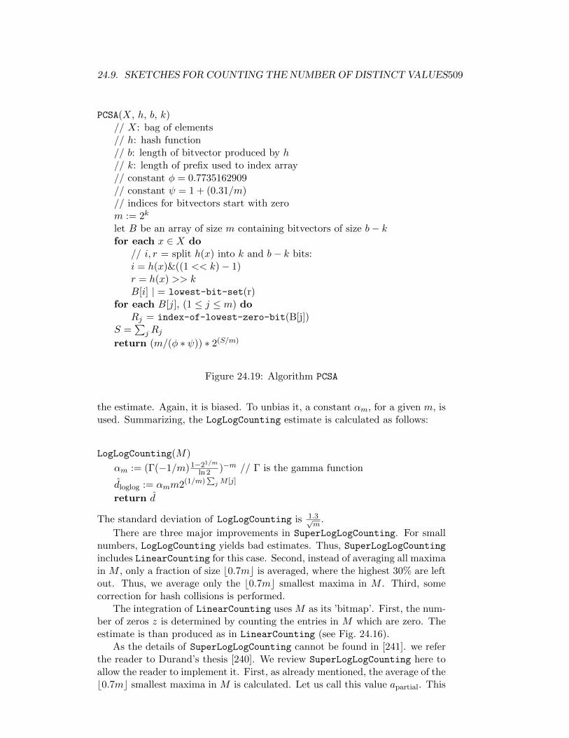
24.9. SKETCHES FOR COUNTING THE NUMBEROF DISTINCT VALUES509

PCSA(X, h, b, k)// X: bag of elements// h: hash function// b: length of bitvector produced by h// k: length of prefix used to index array// constant φ = 0.7735162909// constant ψ = 1 + (0.31/m)// indices for bitvectors start with zerom := 2k

let B be an array of size m containing bitvectors of size b− kfor each x ∈ X do

// i, r = split h(x) into k and b− k bits:i = h(x)&((1 << k)− 1)r = h(x) >> kB[i] | = lowest-bit-set(r)

for each B[j], (1 ≤ j ≤ m) doRj = index-of-lowest-zero-bit(B[j])

S =∑

j Rjreturn (m/(φ ∗ ψ)) ∗ 2(S/m)

Figure 24.19: Algorithm PCSA

the estimate. Again, it is biased. To unbias it, a constant αm, for a given m, isused. Summarizing, the LogLogCounting estimate is calculated as follows:

LogLogCounting(M)

αm := (Γ(−1/m)1−21/m

ln 2 )−m // Γ is the gamma function

dloglog := αmm2(1/m)∑jM [j]

return d

The standard deviation of LogLogCounting is 1.3√m

.

There are three major improvements in SuperLogLogCounting. For smallnumbers, LogLogCounting yields bad estimates. Thus, SuperLogLogCountingincludes LinearCounting for this case. Second, instead of averaging all maximain M , only a fraction of size b0.7mc is averaged, where the highest 30% are leftout. Thus, we average only the b0.7mc smallest maxima in M . Third, somecorrection for hash collisions is performed.

The integration of LinearCounting uses M as its ’bitmap’. First, the num-ber of zeros z is determined by counting the entries in M which are zero. Theestimate is than produced as in LinearCounting (see Fig. 24.16).

As the details of SuperLogLogCounting cannot be found in [241]. we referthe reader to Durand’s thesis [240]. We review SuperLogLogCounting here toallow the reader to implement it. First, as already mentioned, the average of theb0.7mc smallest maxima in M is calculated. Let us call this value apartial. This

510 CHAPTER 24. CARDINALITY AND COST ESTIMATION

FillM(X, h, M)// X: bag of elements// h: hash function// k: length of prefix used to index array M of maxima// indices for bitvectors start with onelet M be an array containing m small integers initialized with 0for each x ∈ X do

if 0 == xthen

M[i] := max(M [i], 33− k) // if the length of hash value is 32 bitselse

i := x & ((1 << k) - 1)j := idx-lowest-bit-set(x >> k)M [i] = max(M [i], j)

Figure 24.20: Filling M for LogLogCounting, SuperLogLogCounting, and Hy-perLogLogCounting

SuperLogLog(M)

dlinc := LinearCounting(M)

dloglog := LogLogCounting(M)

dsupll := α(dloglog)m2apartial

L := 10m/5case

when dsupll < L ∧ dlinc < L do N := dlinc

when dsupll > L ∧ dlinc > L do N := dsupll

else N := (dlinc + dsupll)/2esacH = 232 // if 32 bit is the length of a hash value

return −H ln(1− NH ) // correction of hash collisions

Figure 24.21: SuperLogLog Counting

eliminates bad accidental outliers. Then, three estimates are calculated. Thefirst is dlinc produced by LinearCounting. The second is dloglog produced byLogLogCounting. This estimate is only used to produce the next estimate viasome function α. The third is dsupll. The estimate produced by SuperLogLog

is then calculated as shown in Fig. 24.21.

The only missing piece is the calculation of the unbiasing function α givenin Fig. 24.22. As one can see, a polynomial of degree 4 is evaluated if k exceeds3. The coefficients differ for different k. They are also given in the figure. Thestandard deviation of SuperLogLogCounting is 1.05/

√m. For hashing strings,

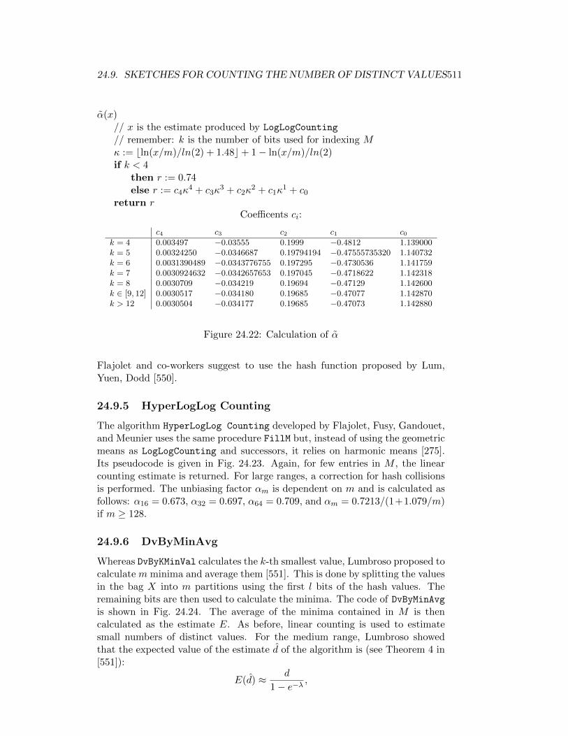
24.9. SKETCHES FOR COUNTING THE NUMBEROF DISTINCT VALUES511

α(x)// x is the estimate produced by LogLogCounting

// remember: k is the number of bits used for indexing Mκ := bln(x/m)/ln(2) + 1.48c+ 1− ln(x/m)/ln(2)if k < 4

then r := 0.74else r := c4κ

4 + c3κ3 + c2κ

2 + c1κ1 + c0

return rCoefficents ci:

c4 c3 c2 c1 c0k = 4 0.003497 −0.03555 0.1999 −0.4812 1.139000k = 5 0.00324250 −0.0346687 0.19794194 −0.47555735320 1.140732k = 6 0.0031390489 −0.0343776755 0.197295 −0.4730536 1.141759k = 7 0.0030924632 −0.0342657653 0.197045 −0.4718622 1.142318k = 8 0.0030709 −0.034219 0.19694 −0.47129 1.142600k ∈ [9, 12] 0.0030517 −0.034180 0.19685 −0.47077 1.142870k > 12 0.0030504 −0.034177 0.19685 −0.47073 1.142880

Figure 24.22: Calculation of α

Flajolet and co-workers suggest to use the hash function proposed by Lum,Yuen, Dodd [550].

24.9.5 HyperLogLog Counting

The algorithm HyperLogLog Counting developed by Flajolet, Fusy, Gandouet,and Meunier uses the same procedure FillM but, instead of using the geometricmeans as LogLogCounting and successors, it relies on harmonic means [275].Its pseudocode is given in Fig. 24.23. Again, for few entries in M , the linearcounting estimate is returned. For large ranges, a correction for hash collisionsis performed. The unbiasing factor αm is dependent on m and is calculated asfollows: α16 = 0.673, α32 = 0.697, α64 = 0.709, and αm = 0.7213/(1+1.079/m)if m ≥ 128.

24.9.6 DvByMinAvg

Whereas DvByKMinVal calculates the k-th smallest value, Lumbroso proposed tocalculate m minima and average them [551]. This is done by splitting the valuesin the bag X into m partitions using the first l bits of the hash values. Theremaining bits are then used to calculate the minima. The code of DvByMinAvgis shown in Fig. 24.24. The average of the minima contained in M is thencalculated as the estimate E. As before, linear counting is used to estimatesmall numbers of distinct values. For the medium range, Lumbroso showedthat the expected value of the estimate d of the algorithm is (see Theorem 4 in[551]):

E(d) ≈ d

1− e−λ ,

512 CHAPTER 24. CARDINALITY AND COST ESTIMATION

HyperLogLog(X, h, m)X: bag of elementsh: hash function to 0, 132m: number of entries in matrix M , m = 2l for some lFillM(X,h, M)

E := αmm2(∑

i=0 i < m2−M [i])−1 // ’raw’ estimate

if E < 5/2m

then V := number of empty entries in ME∗ := (V = 0) ? E∗ : m log(m/V )

else if E ≤ 130232

then E∗ := Eelse E∗ := −232 log(1− E/232)return E∗

Figure 24.23: HyperLogLog Counting

where d is the true number of distinct values in X and λ = d/m. In order tocorrect this bias, we set y = d/m and solve

y =λ

λ− e−λ

for λ. Let us denote this inverse function by f−1(λ). The best quadraticapproximation under lq is f−1(x) ≈ −0.0329046x2 +1.34703∗x−0.932685 witha maximal q-error of 1.0035.

24.9.7 DvByKMinAvg

Giroire proposed and algorithm we call DvByKMinAvg [317]. Alghough olderthan the approach by Lumbroso, DvByKMinAvg can easiest be understood asa combination of DvByKMin and DvByMinAvg. As can be seen in Fig. 24.25,we maintain an array M of buckets. Each bucket holds the k minimal valuesassigned to it, where k is a parameter pragmatically chosen to be 3 [317]. Thiscombines relatively low overhead with relatively high precision. After the arrayM has been filled with the minimal values of the actual estimate is calculated intwo steps. First, the sum of the negative logarithms of the k-th minimal valuesis calculated. In the algorithm, we denote by Mk[i] the k-th smallest value inbucket i. Then, the actual estimate is calculated from this sum. The estimatefound in the algorithm corresponds ot the logarithm family algorithm. Giroirepresented two more estimators, namely the inverse family algorithm and thesquare root family algorithm [317].

24.9.8 Pointers to the Literature

Gelenbe and Gardy discuss a direct estimation approach to estimate the size ofa projection [314] (see also the simple profile). In another paper, they do so in

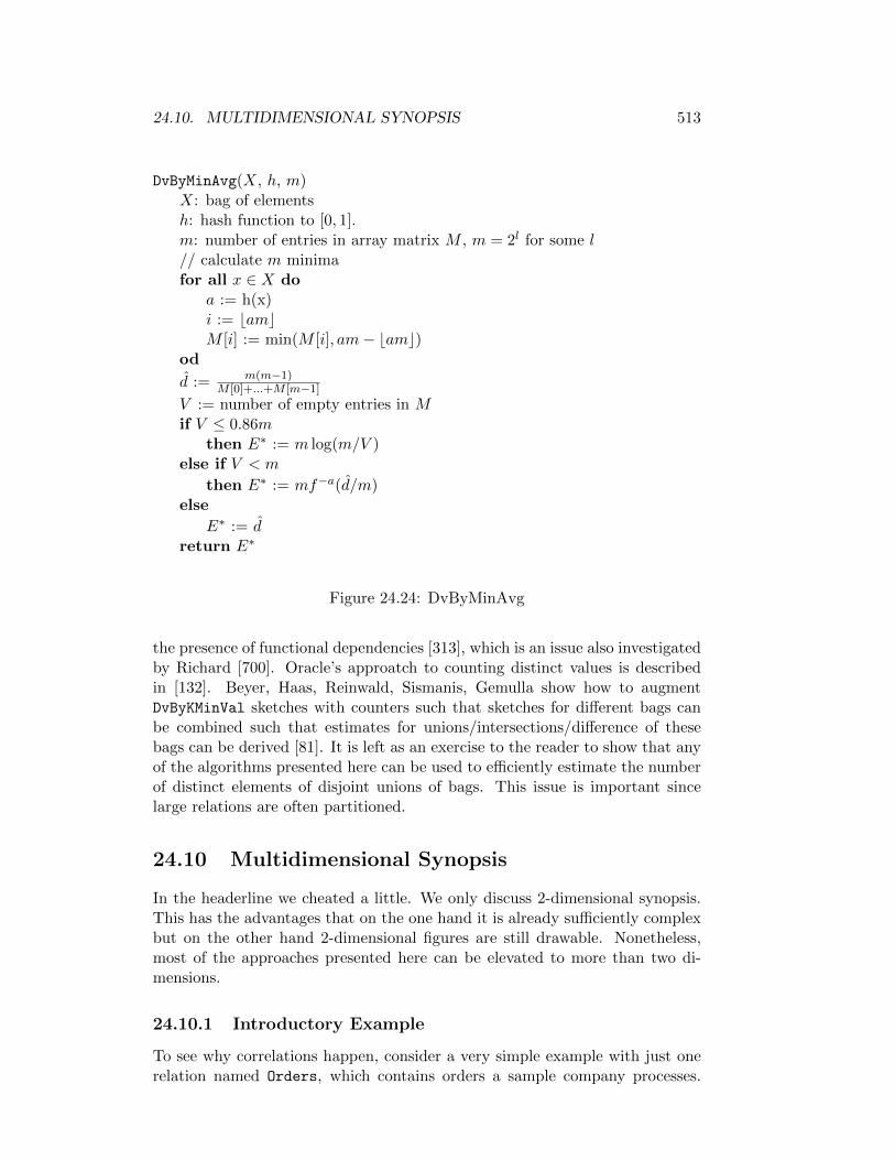
24.10. MULTIDIMENSIONAL SYNOPSIS 513

DvByMinAvg(X, h, m)X: bag of elementsh: hash function to [0, 1].m: number of entries in array matrix M , m = 2l for some l// calculate m minimafor all x ∈ X do

a := h(x)i := bamcM [i] := min(M [i], am− bamc)

od

d := m(m−1)M [0]+...+M [m−1]

V := number of empty entries in Mif V ≤ 0.86m

then E∗ := m log(m/V )else if V < m

then E∗ := mf−a(d/m)else

E∗ := dreturn E∗

Figure 24.24: DvByMinAvg

the presence of functional dependencies [313], which is an issue also investigatedby Richard [700]. Oracle’s approatch to counting distinct values is describedin [132]. Beyer, Haas, Reinwald, Sismanis, Gemulla show how to augmentDvByKMinVal sketches with counters such that sketches for different bags canbe combined such that estimates for unions/intersections/difference of thesebags can be derived [81]. It is left as an exercise to the reader to show that anyof the algorithms presented here can be used to efficiently estimate the numberof distinct elements of disjoint unions of bags. This issue is important sincelarge relations are often partitioned.

24.10 Multidimensional Synopsis

In the headerline we cheated a little. We only discuss 2-dimensional synopsis.This has the advantages that on the one hand it is already sufficiently complexbut on the other hand 2-dimensional figures are still drawable. Nonetheless,most of the approaches presented here can be elevated to more than two di-mensions.

24.10.1 Introductory Example

To see why correlations happen, consider a very simple example with just onerelation named Orders, which contains orders a sample company processes.

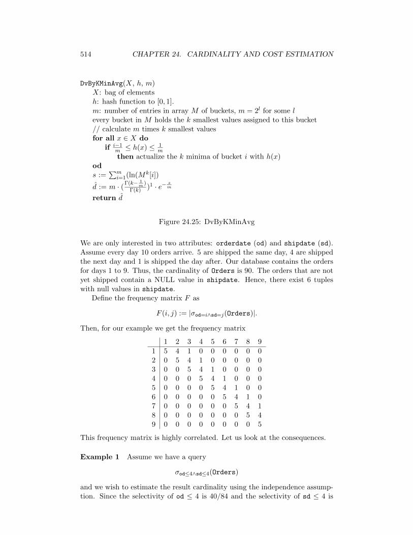
514 CHAPTER 24. CARDINALITY AND COST ESTIMATION

DvByKMinAvg(X, h, m)X: bag of elementsh: hash function to [0, 1].m: number of entries in array M of buckets, m = 2l for some levery bucket in M holds the k smallest values assigned to this bucket// calculate m times k smallest valuesfor all x ∈ X do

if i−1m ≤ h(x) ≤ 1

mthen actualize the k minima of bucket i with h(x)

ods :=

∑mi=1(ln(Mk[i])

d := m · (Γ(k− 1m

)

Γ(k) )1 · e− sm

return d

Figure 24.25: DvByKMinAvg

We are only interested in two attributes: orderdate (od) and shipdate (sd).Assume every day 10 orders arrive. 5 are shipped the same day, 4 are shippedthe next day and 1 is shipped the day after. Our database contains the ordersfor days 1 to 9. Thus, the cardinality of Orders is 90. The orders that are notyet shipped contain a NULL value in shipdate. Hence, there exist 6 tupleswith null values in shipdate.

Define the frequency matrix F as

F (i, j) := |σod=i∧sd=j(Orders)|.

Then, for our example we get the frequency matrix

1 2 3 4 5 6 7 8 9

1 5 4 1 0 0 0 0 0 02 0 5 4 1 0 0 0 0 03 0 0 5 4 1 0 0 0 04 0 0 0 5 4 1 0 0 05 0 0 0 0 5 4 1 0 06 0 0 0 0 0 5 4 1 07 0 0 0 0 0 0 5 4 18 0 0 0 0 0 0 0 5 49 0 0 0 0 0 0 0 0 5

This frequency matrix is highly correlated. Let us look at the consequences.

Example 1 Assume we have a query

σod≤4∧sd≤4(Orders)

and we wish to estimate the result cardinality using the independence assump-tion. Since the selectivity of od ≤ 4 is 40/84 and the selectivity of sd ≤ 4 is

24.10. MULTIDIMENSIONAL SYNOPSIS 515

34/84, the total selectivity under independence is 40/84 ∗ 34/84 = 0.19, andthus an estimate of 0.19 ∗ 84 ≈ 16 for our result cardinality. The true resultcardinality is 34.

Example 2 Assume we have a query

σod≤4∧sd≥6(Orders)

and we wish to estimate the result cardinality using the independence assump-tion. Since the selectivity of od ≤ 4 is 40/84 and the selectivity of sd ≥ 6 is40/84, we get that the total selectivity is 40/84 ∗ 40/84 = 0.23, and thus anestimate of 0.23 ∗ 84 = 19 for our result cardinality. The true result cardinalityis 1.

Two dimensional synopses are meant to avoid these inaccuracies.

24.10.2 Solving the Introductory Problem without 2-DimensionalSynopsis

For the example above, a special solution exploiting one dimensional histogramsexists. Instead of building a two-dimensional histogram on the attributes od

and sd, we build a one-dimensional histogram on the difference (sd− od). Theexact histogram for the introductory example looks as follows:

(sd− od) frequency

0 451 322 7

To see why this is a useful statistics to calculate estimates for the result sizesof our example queries, consider the general case of a conjunction of two rangepredicates

(c1 ≤ A ≤ c2) ∧ (d1 ≤ B ≤ d2) (24.35)

on attributes A and B. This predicate implies

A−B ≤ c2 − d1

B −A ≤ d2 − c1

which is equivalent to

A−B ≥ c1 − d2

A−B ≤ c2 − d1

and thus

(c1 − d2) ≤ (A−B) ≤ (c2 − d1). (24.36)

Using the one-dimensional histogram, we can derive an estimate for the selec-tivity of Eq. 24.36. Call this selectivity s(Eq.24.36). Additionally, denote by

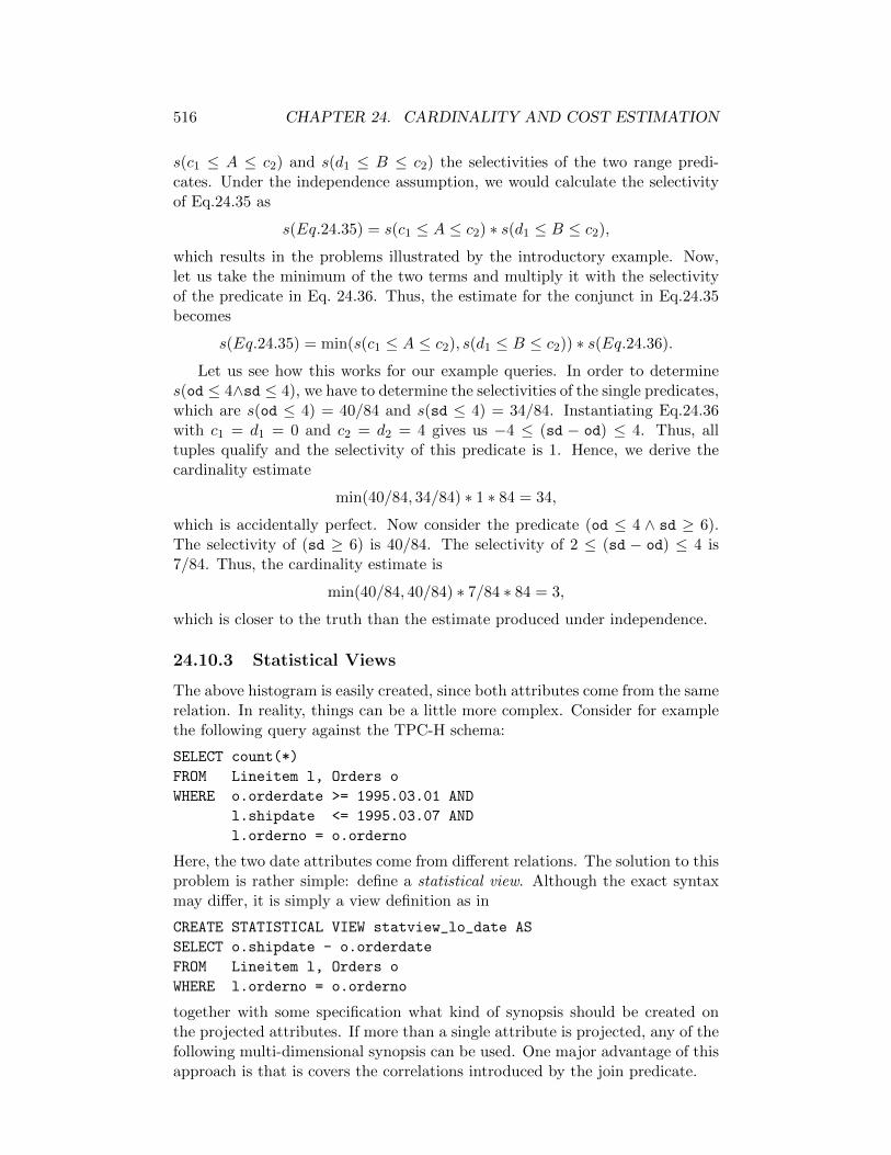
516 CHAPTER 24. CARDINALITY AND COST ESTIMATION

s(c1 ≤ A ≤ c2) and s(d1 ≤ B ≤ c2) the selectivities of the two range predi-cates. Under the independence assumption, we would calculate the selectivityof Eq.24.35 as

s(Eq.24.35) = s(c1 ≤ A ≤ c2) ∗ s(d1 ≤ B ≤ c2),

which results in the problems illustrated by the introductory example. Now,let us take the minimum of the two terms and multiply it with the selectivityof the predicate in Eq. 24.36. Thus, the estimate for the conjunct in Eq.24.35becomes

s(Eq.24.35) = min(s(c1 ≤ A ≤ c2), s(d1 ≤ B ≤ c2)) ∗ s(Eq.24.36).

Let us see how this works for our example queries. In order to determines(od ≤ 4∧sd ≤ 4), we have to determine the selectivities of the single predicates,which are s(od ≤ 4) = 40/84 and s(sd ≤ 4) = 34/84. Instantiating Eq.24.36with c1 = d1 = 0 and c2 = d2 = 4 gives us −4 ≤ (sd − od) ≤ 4. Thus, alltuples qualify and the selectivity of this predicate is 1. Hence, we derive thecardinality estimate

min(40/84, 34/84) ∗ 1 ∗ 84 = 34,

which is accidentally perfect. Now consider the predicate (od ≤ 4 ∧ sd ≥ 6).The selectivity of (sd ≥ 6) is 40/84. The selectivity of 2 ≤ (sd − od) ≤ 4 is7/84. Thus, the cardinality estimate is

min(40/84, 40/84) ∗ 7/84 ∗ 84 = 3,

which is closer to the truth than the estimate produced under independence.

24.10.3 Statistical Views

The above histogram is easily created, since both attributes come from the samerelation. In reality, things can be a little more complex. Consider for examplethe following query against the TPC-H schema:

SELECT count(*)

FROM Lineitem l, Orders o

WHERE o.orderdate >= 1995.03.01 AND

l.shipdate <= 1995.03.07 AND

l.orderno = o.orderno

Here, the two date attributes come from different relations. The solution to thisproblem is rather simple: define a statistical view. Although the exact syntaxmay differ, it is simply a view definition as in

CREATE STATISTICAL VIEW statview_lo_date AS

SELECT o.shipdate - o.orderdate

FROM Lineitem l, Orders o

WHERE l.orderno = o.orderno

together with some specification what kind of synopsis should be created onthe projected attributes. If more than a single attribute is projected, any of thefollowing multi-dimensional synopsis can be used. One major advantage of thisapproach is that is covers the correlations introduced by the join predicate.

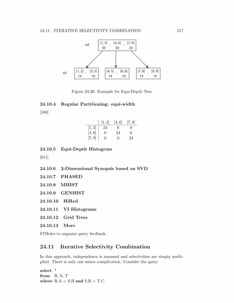
24.11. ITERATIVE SELECTIVITY COMBINATION 517

[1, 3]30

[4, 6]30

[7, 9]24

, ,

[1, 2]14

[3, 5]16

, [4, 5]14

[6, 8]16

, [7, 8]14

[9, 9]10

,

od

sd

Figure 24.26: Example for Equi-Depth Tree

24.10.4 Regular Partitioning: equi-width

[580]

[1, 3] [4, 6] [7, 9]

[1, 3] 24 6 0[4, 6] 0 24 6[7, 9] 0 0 24

24.10.5 Equi-Depth Histogram

[611]

24.10.6 2-Dimensional Synopsis based on SVD

24.10.7 PHASED

24.10.8 MHIST

24.10.9 GENHIST

24.10.10 HiRed

24.10.11 VI Histograms

24.10.12 Grid Trees

24.10.13 More

STHoles to organize query feedback.

24.11 Iterative Selectivity Combination

In this approach, independence is assumed and selectivities are simply multi-plied. There is only one minor complication. Consider the query

select *from R, S, Twhere R.A = S.B and S.B = T.C

518 CHAPTER 24. CARDINALITY AND COST ESTIMATION

The query compiler uses transitivity to derive more predicates to increase thesearch space and make it more indendent of the actual query formulation chosenby the user (Sec. 11.2.2). Thus, the query is rewritten to

select *from R, S, Twhere R.A = S.B and S.B = T.C and R.A = T.C

and all of R.A, S.B, T.C are within the same equivalence class. All of thethree equality predicates have an associated selectivity. However, after two ofthe predicates have been applied and their selectivities have been multiplied, thethird predicate is implied by the other two and, accordingly its selectivity shouldnot be used. This can easily be prevented by using a union find datastructure[201] associated with each plan class. It contains only those variables thatcontain in equivalence classes with cardinality greater than two. Initially, eachof these variables is in its own class. Then, whenever an equality predicateis about to be applied, we check whether the two variables on the left andright are already in the same equivalence class. If so, we ignore the predicate.Otherwise, we apply the predicate and union the two equivalence classes of thevariables. There remains only one open question. Assume the plan generatorhas generated the partial plan RBR.A=S.BS. Then, there are two predicates leftto join T : S.B = T.C and R.A = T.C. For this case, where several predicatesthat can be applied, Swami and Schiefer [833] showed that the following rule(called LS ) is the correct way to do it:

”Given a choice of join selectivities for a single equivalence class,always pick the largest join selectivity.

Thus, to make things more efficient, we sort the equality predicates whose vari-ables belong to equivalence classes with more than two elements by decreasingselectivity. Then, we can proceed as indicated above.

24.12 Maximum Entropy

[567, 568]

24.13 Selected Issues

24.13.1 Exploiting and Augmenting Existing DBMS Data Struc-tures

Index Structures

Assume we have an attribute A of some relation R and a B+- or B∗-Tree on A.The goal of this subsection is to show that we can use as simple procedure toproduce a cardinality estimate for a given range query A ∈ Iq, where Iq = [a, b]is some query intervall.

Let us start with some notation. Denote a node in the B+-Tree by N. Weassign a level to every node in the B+-Tree, increasing level numbers from leaf

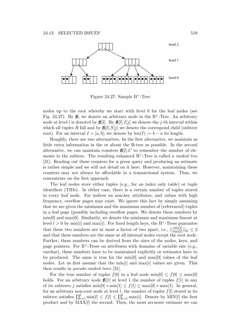
24.13. SELECTED ISSUES 519

level 2

level 1

level 0

Figure 24.27: Sample B+-Tree

nodes up to the root whereby we start with level 0 for the leaf nodes (seeFig. 24.27). By N, we denote an arbitrary node in the B+-Tree. An arbitrarynode at level l is denoted by N[l]. By N[l].I[j] we denote the j-th interval withinwhich all tuples R fall and by N[l].S[j] we denote the correspond child (subtreeroot). For an interval I = [a, b], we denote by len(I) := b− a its length.

Roughly, there are two alternatives. In the first alternative, we maintain aslittle extra information in the or about the B-tree as possible. In the secondalternative, we can maintain counters N[l].C to remember the number of ele-ments in the subtree. The resulting enhanced B+-Tree is called a ranked tree[31]. Reading out these counters for a given query and producing an estimateis rather simple and we will not detail on it here. However, maintaining thesecounters may not always be affordable in a transactional system. Thus, weconcentrate on the first approach.

The leaf nodes store either tuples (e.g., for an index only table) or tupleidentifiers (TIDs). In either case, there is a certain number of tuples storedin every leaf node. For indices on non-key attributes, and values with highfrequency, overflow pages may exist. We ignore this fact by simply assumingthat we are given the minimum and the maximum number of (referenced) tuplesin a leaf page (possibly including overflow pages. We denote these numbers bymin[0] and max[0]. Similarily, we denote the minimum and maximum fanout atlevel l > 0 by min[i] and max[i]. For fixed length keys, the B+-Trees guarantee

that these two numbers are at most a factor of two apart, i.e., ||min[i]max[i] ||Q ≤ 2

and that these numbers are the same at all internal nodes except the root node.Further, these numbers can be derived from the sizes of the nodes, keys, andpage pointers. For B+-Trees on attributes with domains of variable size (e.g.,varchar), these numbers have to be maintained explicitly or estimates have tobe produced. The same is true for the min[0] and max[0] values of the leafnodes. Let us first assume that the min[i] and max[i] values are given. Thisthen results in pseudo-ranked trees [31].

For the true number of tuples f [0] in a leaf node min[0] ≤ f [0] ≤ max[0]holds. For an arbitrary node N[1] at level 1 the number of tuples f [1] in anyof its subtrees j satisfies min[0] ∗min[1] ≤ f [1] ≤ max[0] ∗max[1]. In general,for an arbitrary non-root node at level l, the number of tuples f [l] stored in itssubtree satisfies

∏li=1 min[l] ≤ f [l] ≤ ∏l

i=1 max[i]. Denote by MIN[l] the firstproduct and by MAX[l] the second. Then, the most accurate estimate we can

520 CHAPTER 24. CARDINALITY AND COST ESTIMATION

return isq-middle(MIN[i],MAX[i])

with a maximal q-error of√

(2l) if ||min[i]max[i] ||Q ≤ 2 holds at all levels including

the leaf node level.Given a node N[l, k] at an arbitrary level l > 0 with J child nodes, we can

estimate its contribution to a range query with query interval Iq as in

J∑

j=1

len(Iq ∩ N[l, k].I[j])

len(N[l, k].I[j])q-middle(MIN[l],MAX[l]).

This procedure can now be applied to the root node only, However, it maybebeneficial to descend into child nodes for better estimates. This is especiallytrue for those child nodes, that are not fully contained in the query interval.Thus, the questions arise (1) which nodes to descend and (2) when to stop.Several traversal strategies have been defined (see [35]).

This is not too bad, but there are certain problems. As indicated above,variable length keys and overflow pages due to high skew result in certain prob-lems. Concerning the former problem. One possibility to overcome the formerproblem is to explicitly maintain the minimal and maximal fanout for each lev-el. If this is too expensive, we could maintain the number of nodes n[l] at everylevel l and use this to calculate the average fanout at level l as n[l + 1]/n[l]and use this number instead of the minmal and maximal fanout. Definitely, weloose any error bounds in this case. Consider the latter problem. The simplestsolution is to maintain the number of leaf nodes explicitly and to derive anaverage number avg[0] of tuples in the leaf nodes, which is then used instead ofmin[0] and max[0]. Obviously, we lose precision, which can only be restored bymaintaing explicit cardinality counters.

Dictionaries

Introduction Many main memory database management systems designedfor OLAP are column stores. Further, they often use ordered dictionaries tofacilitate compression of columns. Two commercial systems following theselines are Hana [], DB2 Blue [] SQL Server [].

Let A be an attribute of some relation R. Assume that the active domainDA = x1, . . . , xn with xi < xj if i < j. A dictionary then comprises twomappings:

1. a mapping of i to xi and

2. a mapping from xi to i.

We call the i dictionary indexes and the xi dictionary values. No matterwhether the domain of A is discrete or continous, the dictionary indexes arepositive integers. In a column store, the column for A then contains the (com-pressed) dictionary indexes of the original values.

If the dictionary is ordered, a range query

Q := σlq≤A≤uq(R) (24.37)

24.13. SELECTED ISSUES 521

with values lq and uq can be mapped to a range query on dictionary indexes.Depending on the use of ≤ vs. <, the lower and upper query bounds are mappedto lower (lidx) and upper (uidx) bounds on dictionary indexes as follows:

lq ≤ A → lidx := max(i|xi ≥ lq)lq < A → lidx := max(i|xi > lq)A ≤ uq → uidx := min(i|xi ≤ uq)A < uq → uidx := min(i|xi < uq)

Any range query (open or half-open or open) is then mapped to the closedrange query

Qidx := σlidx≤A≤uidx(R). (24.38)

The mapping itself can be carried out by rather efficiently by a binary searchwithin the dictionary.

Since Q and Qidx are equivalent, estimation problems can now be carriedout on Qidx. This task is simplified by the very structure of a dictionary.

Distinct Values Since the dictionary is typically dense, that is no values thatdo not occur in the active domain are stored, the number of distinct values ofA in Q can be calculated exactly:

|ΠDA (σlidx≤A≤uidx(R))| = uidx − lidx + 1. (24.39)

Cardinality Assume that every dictionary value xi occurs with frequency fi.Then, we have

|ΠA(σlidx≤A≤uidx(R))| =uidx∑

i=lidx

fi. (24.40)

This requires that the fi (4 bytes) are stored for every dictionary entry.At the expense of CPU time, we can use q-compression on the fi to diminishmemory consumption to one byte per dictionary entry. Thereby, we can bevery precise, since, e.g., 1.1255 ≈ 36 ∗ 109.

If I := (uidx − lidx + 1) is small, the above summation yields acceptableperformance. Assume, that we are willing to add 2δ frequencies. (If δ = 50,this means we are willing to add 100 frequencies.) If I > 2δ, we have to relyon alternative mechanisms. We have several options. Among the most obviousare:

• build a tree-like structure with fan out δ and height dlogδ(n)e, where n isthe number of dictionary entries, or

• build some kind of histogram on the dictionary index, where, within everybucket, we have to be precise only for ranges comprising more than δvalues (see Sec. 24.8.3).

24.13.2 Sampling

[202]

522 CHAPTER 24. CARDINALITY AND COST ESTIMATION

24.13.3 Query Feedback

24.13.4 Combining Data Summaries with Sampling

24.13.5 Wavelets

24.13.6 Selectivity of String-Valued Attributes

24.14 Cost Functions

24.14.1 Disk-based Joins

24.14.2 Main Memory Joins

24.14.3 Additional Pointers to the Literature

[929] bit-valued attributes, top-k queries.[218] Cardinality estimation at the calculus level.[169] Estimating Block Transfers and Join Sizes[170] parametric: Pearson Type 2 and 7 for symmetric, unimodal distribu-

tions.[264] Inverted files, multiple regression for Zipf distributions.[265] also gives details cost model for inverted file retrieval.[460] models relations as arrays of bits. Defines similarity function between

bitmaps, lusters homogeneous rectangles using a pyramidal scheme.[561] overview article summarizing the eighties up to 1986.[307] uses generating functions.[53] overview article (New Jersey data reduction report), several techniques.[430] Overvies article, several techniques.[671] application of histograms to load balancing for parallel joins.[670] M-dimension Histograms (MHIST)[443] optimal histograms with quality guarantees: minimum error under

given space, minimal space under given maximal error, construction algo: O(n2)if n is the number of distinct values contained in the histogram

[302] cost model for parallel query optimization[493] application of SVD to time series data[488] piecewise approximation, rough, with linear functions[91] kernel estimators[431] applies histograms to approximate query answers.[496] optimal histograms for hierarchical range queries (OLAP)[236] split and merge buckets to capture changes in variance (gives dynamic

v-optimal histograms (DVO histograms)[106, 107] STHoles multidimension histograms constructed from query feed-

back[442] constructs many histograms at once to meet global storage bounds.

this allows to give more memory to histograms for more skewed (less easyapproximatable) attributes

[362] histograms for data streams[360] discovery and application of check constraints[318] exploiting soft constraints

24.14. COST FUNCTIONS 523

[363] fast algorithm for histogram construction for hierarchical range queries(OLAP)

[842] dynamic multidimensional histograms (for data streams)[112] 4byte encoding of 4-level tree to allow refinement estimates within a

histogram bucket. (very nice idea)[489] automatic tuning of data synopsis[110] uses N-Level Tree Histograms (again bit encodings) to estimate range

queries[425, 426, 424] automatic relationship discovery: correlations and soft func-

tional dependencies[931] HASE: combines synopses-based selectivity estimation with sampling-

based sel. est.[940] fast comp. of approx. statistics[253] just-in-time statistics (todo)[615] approximation of CDF with splinesTeorey, Das: [838] physical database designSpyratos: [797] operational approach, database updates, viewsYu, Luk, Siu: [929] Estimation Number of Desired Records with Respect to

a given queryPiatetsky-Shapiro [660]: Distribution Steps [612]: DDSMArchitecture of Cardinality and Cost Estimation: Parameter systems [700];

[560]

524 CHAPTER 24. CARDINALITY AND COST ESTIMATION

Part V

Implementation

525

Chapter 25

Architecture of a QueryCompiler

25.1 Compilation process

25.2 Architecture

Figure 25.1 a path of a query through the optimizer. For every step, a singlecomponent is responsible. Providing a facade for the components results in theoverall architecture (Fig. 25.2). Every component is reentrant and stateless.The information necessary for a component to process a query is passed viareferences to control blocks. Control blocks are discussed next, then we discussmemory management. Subsequent sections describe the components in somedetail.

25.3 Control Blocks

It is very convenient to have a hierarchy of control blocks within the optimizer.Figure 25.3 shows some of the control blocks. For simplification, those blocksconcerned with session handling and transaction handling are omitted. Everyroutine call within the optimizer has a control block pointer as a parameter.The routines belonging to a specific phase have a pointer to the phase’ specificcontrol block as a parameter. For example, the routines in NFST have a NFST CB

pointer as a parameter. We now discuss the purpose of the different controlblocks.

The global control block governs the behavior of the query compiler. Itcontains boolean variables indicating which phases to perform and which phasesof the compilation process are to be traced. It also contains indicators for theindividual phases. For example, for the first rewrite phase it contains indicatorswhich rules to apply, which rules to trace and so on. These control indicatorsare manipulated by the driver which also allows to step through the differentphases. This is very important for debugging purposes. Besides this overallcontrol of the query compilers behavior, the global control block also contains

527

528 CHAPTER 25. ARCHITECTURE OF A QUERY COMPILER

parsing

nfst

rewrite I

plan generation

rewrite II

code generation

abstract syntax tree

internal representation

internal representation

internal representation

internal representation

execution plan

query

query

optimizer

CTS

Figure 25.1: The compilation process

a pointer to the schema cache. The schema cache itself allows to look up typenames, relations, extensions, indexes, and so on.

The query control block contains all the information gathered for the currentquery so far. It contains the abstract syntax tree, after its construction, theanalyzed and translated query after NFST has been applied, the rewritten plan

25.4. MEMORY MANAGEMENT 529

after the Rewrite I phase, and so on. It also contains a link to the memorymanager that manages memory for this specific query. After the control blockfor a query is created, the memory manager is initialized. During the destructorcall, the memory manager is destroyed and memory released.

Some components need helpers. These are also associated with the controlblocks. We discuss them together with the components.

25.4 Memory Management

There are three approaches to memory management in query optimizers. Thefirst approach is to use an automatic garbage collector if the language providesone. This is not necessarily the most efficient approach but by far the mostconvenient one. This approach can be imitated by an implementation based onsmart pointers. I would not recommend doing so since the treatment of cyclescan be quite tricky and it is inefficient. Another approach would be to collect allreferences to newly created objects and release these after the query has beenprocessed. This approach is easy to implement, very convenient (transparent tothe implementor), but inefficient. A better approach is to allocate bigger areasof memory by a memory manager. Factories1 then use these memory chunks togenerate objects as necessary. After the query has been processed, the chunksare freed.

Here, we consider only memory whose duration lasts for the processing of asingle query. In general, we have more kinds of memory whose validity conformsto sessions and transactions.

25.5 Tracing and Plan Visualization

25.6 Driver

25.7 Bibliography

1Design pattern.

530 CHAPTER 25. ARCHITECTURE OF A QUERY COMPILER

PlanGenerator

run(PlanGenerator_CB*)

Rewrite_I

run(Rewrite_I_CB*)

Rewrite_II

run(Rewrite_II_CB*)

CodeGenerator

run(CodeGenerator_CB*)

NFST

run(NFST_CB*)

QueryCompilerParser

parse(Query_CB*)

11..* 11..*

Scanner

Singleton, Facade

Figure 25.2: Class Architecture of the Query Compiler

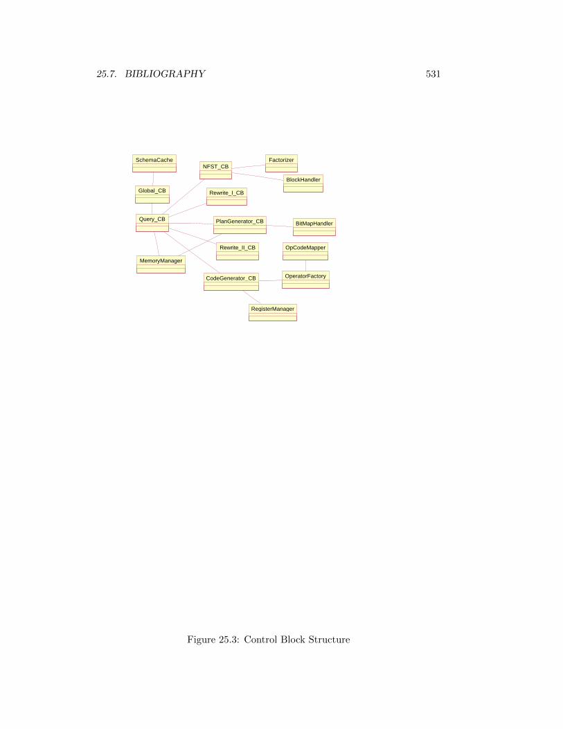
25.7. BIBLIOGRAPHY 531

SchemaCache

Global_CB Rewrite_I_CB

Rewrite_II_CB

Factorizer

BlockHandler

NFST_CB

MemoryManager

BitMapHandlerPlanGenerator_CBQuery_CB

RegisterManager

CodeGenerator_CB OperatorFactory

OpCodeMapper

Figure 25.3: Control Block Structure

532 CHAPTER 25. ARCHITECTURE OF A QUERY COMPILER

Chapter 26

Internal Representations

26.1 Requirements

easy access to information

query representation: overall design goal: methods/functions with semanticmeaning, not only syntactic meaning.

relationships: consumer/producer (occurrance) precedence order informa-tion equivalence of expressions (transitivity of equality) see also expr.h fuerandere funktionen/beziehungen die gebraucht werden

2-ebenen repraesentation. 2. ebene materialisiert einige beziehungen undfunktionen, die haeufig gebraucht werden und kompliziert zu berechnen sind an-derer grund fuer materialisierung: vermeide zuviele geschachtelte forschleifen.bsp: keycheck: gegeben eine menge von attributen und eine menge von schlues-seln, ist die menge ein schluessel? teste jeden schluessel, kommt jedes elementin schluessel in menge von attributen vor? (schon drei schleifen!!!)

modellierungsdetail: ein grosser struct mit dicken case oder feine klassen-hierarchie. wann splitten: nur wenn innerhalb des optimierers verschiedeneabarbeitung erfordert.

Representation: info captured: 1) 1st class information (information ob-vious in original query+(standard)semantic analysis) 2) 2nd class information(derived information) 3) historic information (during query optimization itself)- modified (original expression, modifier) - copied (original expression, copi-er) 4) information about the expression itselt: (e.g.: is function call, is select)5) specific representations for specific purposes (optimization algorithms, codegeneration, semantic analysis) beziehungen zwischen diesen repraesentationen

info captured for 1) different parts of the optimizer

syntactic/semantic information

garbage collection: 1) manually 2) automatic 3) semi-automatic (collectreferences, free at end of query)

26.2 Algebraic Representations

relational algebra in: [189].

533

534 CHAPTER 26. INTERNAL REPRESENTATIONS

26.2.1 Graph Representations

26.2.2 Query Graph

also called object graph: [76, 928]

26.2.3 Operator Graph

used in: [794], [924]

enhanced to represent physical properties: [709]

with outerjoins: [706], [298]

graph representation and equivalence to calculus: [634]

26.3 Query Graph Model (QGM)

26.4 Classification of Predicates

klassifikation von praedikaten

• nach stelligkeit,wertigkeit (selektion, join, nasty)

• nach funktor(=,¡,..., between, oder boolsche funktion)

• nach funktion: fuer keys in index: start/stop/range/exact/enum range(in-predicate)

• nach sel-wert: simple (col = const), komplex (col = expr) cheap/expensive

• nach join wert: fuer hj, smj, hbnlj,...

• korrelationspraedikate

26.5 Treatment of Distinct

26.6 Query Analysis and Materialization of AnalysisResults

Questions:

1. was materialisieren wir

2. was packen wir in die 1. repraesentation?

• bsp: properties: zeiger auf property oder besser inline properties

• bsp: unique number: entweder in expr oder getrennter dictionarystruktur

26.7. QUERY AND PLAN PROPERTIES 535

query analysis (purpose, determine optimization algorithm)

#input relations, #predicates, #ex-quantifiers, #all-quantifiers,

#conjunctions, #disjunctions, #joingraphkind(star,chain,tree,cyclic)

#strongly-connected-components (for crossproduct indication)

#false aggregates in projection list clause (implies grouping required)

/* remark: typical query optimizes should at least have two algorithms:

- exhaustive (for large queries)

- heuristic (for small queries)

*/

for blocks: indicator whether they should produce a null-tuple, in case theydo not produce any tuple. this is nice for some rewrite rules. other possibility:if-statement in algebra.

26.7 Query and Plan Properties

Logical and Physical Properties of PlansAusfuhrungsplanen konnen eine Reihe von Eigenschaften zugeordnet wer-

den. Diese Eigenschaften fallen in drei Klassen

1. logische Eigenschaften, also beispielsweise

(a) beinhaltete Relationen

(b) beinhaltete Attribute

(c) angewendete Pradikate

2. physische Eigenschaften, also beispielsweise

(a) Ordnung der Tupel

(b) Strom oder Materialisierung des Ergebnisses

(c) Materialisierung im Hauptspeicher oder Hintergrundspeicher

(d) Zugriffspfade auf das Ergebnis

(e) Rechnerknoten des Ergebnis (im verteilten Fall)

(f) Kompression

3. quantitative Eigenschaften, also beispielsweise

(a) Anzahl der Elemente im Ergebnis

(b) Große des Ergebnisses oder eines Ergebniselementes

(c) Auswertungskosten aufgeschlusselt nach I/O, CPU und Kommunika-tionskosten

kosten: diese sind zu berechnen und dienen als grundlage fuer die planbe-wertung ges-kosten /* gesamt kosten (ressourcenverbrauch) */ ges-kosten +=cpu-instr / inst/sek ges-kosten += seek-kosten * overhead (waiting/cpu) ges-kosten += i/o-kosten * io-weight cpu-kosten /* reine cpu-kosten */ i/o-kosten/* hintergrundspeicherzugriff ( warten auf platte + cpu fuer seitenzugriffe) */

536 CHAPTER 26. INTERNAL REPRESENTATIONS

com-kosten /* kommunikation */ com-init /* initialisierungskosten fuer kom-munikationsvorgang */ com-exit /* exitkosten fuer kommunikationsvorgang */com-cptu /* kosten fuer jede transfereinheit (z.b. byte) waehrend eines kom-munikationsvorgangs */

kostenstruktur koennte etwas sein, dass ges/cpu/io kosten enthaelt. ausser-dem waeren kosten fuer rescanning interessant, falls dies notwendig ist (puffer-probleme, indexscan und dann faellt seite raus) weiteres interessantes kosten-mass sind die kosten, bis das erste tupel berechnet wird.

dies sind die konstanten, die system-abhaengig sind. am besten sind, sie wer-den gemessen. Hardware: #cpu-instruktionen pro sekunde #cpu-instruktionenfuer block zugriff/transfer lesen/schreiben #cpu-instruktionen pro transfer init/send/exitinit/receive/exit ms fuer seek/latency/transfer pro nK block

RTS-kosten #cpu-instruktionen fuer open/next/close fuer scan operatorenunter verschiedenen voraussetzungen:mit/ohne praedikat, mit/ohne projektion(entsprechend den avm programmen) #cpu-instruktionen fuer open/next/closefuer jeden alg operator, #cpu-instruktionen fuer funktionen/operationen/praedikate/avm-befehle

statistics: first/large physical page of a relation number of pages of a relation-¿ to estimate scan cost measured sequential scan cost (no interference/plentyinterference)

–properties:

• menge der quns

• menge der attribute

• menge der praedikate

• ordnung

• boolean properties

• globale menge der gepipelineten quns

• kostenvektor

• cardinalitaeten bewiesen/geschaetzt

• gewuenschter puffer

• schluessel, fds

• #seiten, die durch ein fetch gelesen werden sollen

• menge der objekte, von denen der plan (der ja teilplan sein kann) abhaengt

• eigenschaften fuer parallele plaene

• eigenschaften fuer smp plaene

26.8. CONVERSION TO THE INTERNAL REPRESENTATION 537

das folgende ist alles blabla. aber es weisst auf den punkt hin,

das in dieser beziehung etwas getan werden muss.

--index: determine degree of clustering

- lese_rate = #gelesene_seiten / seiten_fuer_relation

ein praedikate erniedrigt die lesen_rate, ein erneutes lesen aufgrund einer verdraengung im puffer erhoeht die lese_rate

falls TIDs sortiert werden, muss fetch_ration erneut berechnet werden

- seiten koennen in gruppen z.b. auf einem zylinder zusammengefasst werden

und mit einem prefetch befehl geholt werden. anzahl seeks abschaetzen

- cluster_ration(CR)

CR = P(read(t) ohne page read) = (card - anzahl pagefetch)/card

= (card - (#pagefetch - #page))/card

das ist besonderer quark

- cluster_factor(CF)

CF = P(avoid unnecessary pagefetch) = (pagefetch/maxpagefetch)

= card -#fetch / card - #pageinrel

das ist besonderer quark

index retrieval on full key => beide faktoren auf 100% setzen, da

innerhalb eines index die TIDs pro key-eintrag sortiert werden.

Speicherung von Properties unter dynamischem Programmieren und Mem-oization: Kosten und andere Eigenschaften, die nicht vom Plan abhangen,konnen pro Planklasse gespeichert werden und brauchen nicht pro Plan gespe-ichert zu werden.

26.8 Conversion to the Internal Representation

26.8.1 Preprocessing

26.8.2 Translation into the Internal Representation

26.9 Bibliography

538 CHAPTER 26. INTERNAL REPRESENTATIONS

Chapter 27

Details on the Phases ofQuery Compilation

27.1 Parsing

Lexical analysis is pretty much the same as for traditional compilers. However,it is convenient to treat keywords as soft. This allows for example for relationnames like order which is a keyword in SQL. This might be very convenient forusers since SQL has plenty (several hundreds) of keywords. For some keywordslike select there is less danger of it being a relation name. A solution for groupand order would be to lex them as a single token together with the followingby .

Parsing again is very similar to parsing in compiler construction. For both,lexing and parsing, generators can be used to generate these components. Theparser specification of SQL is quite lengthy while the one for OQL is prettycompact. In both cases, a LALR(2) grammar suffices. The outcome of theparser should be an abstract syntax tree. Again the data structure for abstractsyntax trees (ast) as well as operations to deal with them (allocation, deletion,traversal) can be generated from an according ast specification.

During parsing already some of the basic rewriting techniques can be ap-plied. For example, between can be eliminated.

In BD II, there are currently four parsers (for SQL, OQL, NQL (a cleanversion of XQuery), XQuery). The driver allows to step through the querycompiler and allows to influence its overall behavior. For example, several tracelevels can be switched on and off while within the driver. Single rewrites canbe enabled and disabled. Further, the driver allows to switch to a differentquery language. This is quite convenient for debugging purposes. We used theCocktail tools to generate the lexer, parser, ast, and NFST component.

27.2 Semantic Analysis, Normalization, Factoriza-tion, Constant Folding, and Translation

The NFST component performs (at least) four different tasks:

539

540CHAPTER 27. DETAILS ON THE PHASES OF QUERY COMPILATION

/

IU:salary IU:budget 100

*

Figure 27.1: Expression

1. normalization of expressions,

2. factorization of common subexpressions,

3. semantic analysis, and

4. translation into the internal algebra-based query representation.

Although these are different tasks, a single pass over the abstract syntax treesuffices to perform all these tasks in one step.

Consider the following example query:

select e.name, (d.salary / d.budget) * 100from Employee e, Department dwhere e.salary > 100000 and e.dno = d.dno

The internal representation of the expression (d.salary / d.budget) * 100 in thequery is shown in Fig. 27.1. It contains two operator nodes for the operations“∗” and “/”. At the bottom, we find IU nodes. IU stands for InformationUnit. A single IU corresponds to a variable that can be bound to a value.Sample IUs are attributes of a relation or, as we will see, intermediate results.In the query representation, there are three IUs. The first two IUs are boundto attribute values for the attributes salary and budget . The third IU is boundto the constant 100.

NFST routines can be implemented using a typical compiler generator tool.It is implemented in a rule-based language. Every rule matches a specific kindof AST nodes and performs an action. The ast tree is processed in post order.

The hierarchy for organizing different kinds of expressions is shown in Fig 27.2.Here is a list of useful functions:

• occurrance of expressions in another expression

27.3. NORMALIZATION 541

Expression

Constant IU DB I term Function Call Bolean Aggregat

Relation Extent Variable Attribute Access AND OR NOT

Figure 27.2: Expression hierarchy

• for a given expression: compute the set of occurring (consumed, free) IUs

• for a given expression: compute the set of produced IUs

• for a given IU, retrieve the block producing the IU

• determine whether some block returns a single value only

• computation of the transivitity of predicates, especially equality to deriveits equivalence classes.

• determine whether some expression produces a subset of another expres-sion

• constant folding

• merge and/or (from e.g. binary to n-ary) and push not operations

• replace a certain expression by another one

• deep and shallow copy

These functions can be implemented either as member functions of expressionsor according to visitor/collector/mutator patterns. For more complex functions(consumer/producer) we recommend the latter.

Some of these functions will be called quite frequently, e.g. the consumer/producer,precedence ordering, equivalence (transivitity of equality) functions. So it mightbe convenient to compute these relationships only once and then materializethem. Since some transformation in the rewrite phases are quite complex, arecomputation of these materialized functions should be possible since theirdirect maintenance might be too complex.

27.3 Normalization

Fig. 27.3 shows the result after normalization. The idea of normalization is tointroduce intermediate IUs such that all operators take only IUs as arguments.This representation is quite useful.

27.4 Factorization

Common subexpressions are factorized by replacing them with references tosome IU. For the expressions in TPCD query 1, the result is shown in Fig. 27.4.

542CHAPTER 27. DETAILS ON THE PHASES OF QUERY COMPILATION

/

IU:salary IU:budget

IU:− IU:−

100

IU:−

*

Figure 27.3: Expression

Factorization is enabled by a factorization component that takes care of allexpressions seen so far and the IUs representing these expressions. Every ex-pression encountered by some NFST routine is passed to the factorization. Theresult is a reference to an IU. This IU can be a new IU in case of a new expres-sion, or an existing IU in case of a common subexpression. The factorizationcomponent is available to the NFST routines via the NFST control block whichis associated with a factorization component (Fig.25.3).

27.5 Constant Folding

27.6 Semantic analysis

The main purpose of semantic analysis is to attach a type to every expres-sion. For simple expressions it is very similar to traditional semantic analysisin compiler construction. The only difference occurs for references to schemaconstructs. The schema is persistence and references to e.g. relations or namedobjects have to be looked up there. For performance reasons it is convenientto have a schema cache in order to cache frequently used references. Anotheraspect complicating semantic analysis a little is that collection types are fre-quently used in the database context. Their incorporation is rather straightforward but the different collection types should be handled with care.

As programming languages, query languages provide a block structure. Con-sider for example the SQL query

. . .select a, b, cfrom A, Bwhere d > e and f = g

. . .

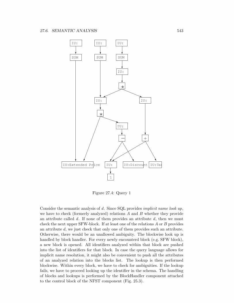
27.6. SEMANTIC ANALYSIS 543

*

IU:

IU: IU: IU:

IU:

IU:

IU:Extended Price IU:Discount IU:Tax

SUM SUMSUM

IU:

IU:

*

+-

1

Figure 27.4: Query 1

Consider the semantic analysis of d . Since SQL provides implicit name look up,we have to check (formerly analyzed) relations A and B whether they providean attribute called d . If none of them provides an attribute d , then we mustcheck the next upper SFW-block. If at least one of the relations A or B providesan attribute d, we just check that only one of them provides such an attribute.Otherwise, there would be an unallowed ambiguity. The blockwise look up ishandled by block handler. For every newly encounterd block (e.g. SFW block),a new block is opened. All identifiers analyzed within that block are pushedinto the list of identifiers for that block. In case the query language allows forimplicit name resolution, it might also be convenient to push all the attributesof an analyzed relation into the blocks list. The lookup is then performedblockwise. Within every block, we have to check for ambiguities. If the lookupfails, we have to proceed looking up the identifier in the schema. The handlingof blocks and lookups is performed by the BlockHandler component attachedto the control block of the NFST component (Fig. 25.3).

544CHAPTER 27. DETAILS ON THE PHASES OF QUERY COMPILATION

Another departure from standard semantic analysis are false aggregates asprovided by SQL.

select avg(age)from Students

I call count(age) a false aggregate since a true aggregate function operators ona collection of values and returns a single value. Here, the situation is different.The attribute age is of type integer. Hence, for the average function whithsignature avg : int −−→ int the semantic analysis would detect a typingerror. The result is that we have to treat these false aggregates as special cases.This is (mostly) not necessary for query languages like OQL.

27.7 Translation

The translation step translates the original AST representation into an internalrepresentation. There are as many internal query representations as there arequery compiler. They all build on calculus expressions, operator graphs buildover some algebra, or tableaux representations [853, 854]. A very powerfulrepresentation that also captures the subtleties of duplicate handling is thequery graph model (QGM) [661].

The representation we use here is a mixture of a typed algebra and calcu-lus. Algebraic expressions are simple operator trees with algebraic operatorslike selection, join, etc. as nodes. These operator trees must be correctly typed.For example, we are very picky about whether a selection operator returns aset or a bag. The expression that more resemble a calculus representation thanan algebraic expression is the SFWD block used in the internal representation.We first clarify our notion of block within the query representation describedhere and then give an example of an SFWD block. A block is everything thatproduces variable bindings. For example a SFWD-block that pretty directlycorresponds to a SFW-block in SQL or OQL. Other examples of blocks arequantifier expressions and grouping operators. A block has the following ingre-dients:

• a list of inputs of type collection of tuples1 (labeled from)

• a set of expressions whose top is an IU (labeled define)

• a selection predicate of type bool (labeled where)

For quantifier blocks and group blocks, the list of inputs is restricted to lengthone. The SFWD-block and the grouping block additionally have a projectionlist (labeled select) that indicates which IUs are to be projected (i.e. passed tosubsequent operators). Blocks are typed (algebraic) expressions and can thusbe mixed with other expressions and algebraic operator trees.

An example of a SFWD-block is shown in Fig. 27.5 where dashed linesindicate the produced-by relationship. The graph corresponds to the internal

1We use a quite general notion of tuple: a tuple is a set of variable (IU) bindings.

27.7. TRANSLATION 545

IU:e

IU: name IU: salary IU: budget

IU:d

Attr. Acces"budget"

Attr. Acces"salary"

Attr. Acces"name"

scan scan

select

where

define

from

key IUkey IU

Relation/Extent"Employee"

Relation/Extent"Department"

IU: IU: IU: IU:

100 100.000/

>

*

Figure 27.5: Internal representation

representation of our example query. The semantics of a SFWD-block can bedescribed as follows. First, take the cross product of the collections of tuplesfound in the list of inputs. (If this is not possible, due to dependencies, d-joinshave to be used.) Then, for every resulting tuple, compute the bindings for allthe IUs mentioned in the define clause, apply the selection predicate and returnall the bindings for the IUs mentioned in the select clause.

Although the SFWD-block looks neat, it lacks certain information that mustbe represented. This information concerns the role of the entries in the fromclause and duplicate elimination. Let us start with the latter. There are threeviews relevant to duplicate processing:

1. the user view: did the user specify distinct?

2. the context view: does the occurrence or elimination of duplicates make

546CHAPTER 27. DETAILS ON THE PHASES OF QUERY COMPILATION

a difference for the query result?

3. the processing view: does the block produce duplicates?

All this information is attached to a block. This information can then besummarized to one of three values representing

• eliminate duplicates

• preserve duplicates

• don’t care about duplicates(The optimizer can feel free to do whatever is more efficient.)

This summary is also attached to every block. Let us illustrate this by a simpleexample:

select distinct ssnofrom Employeewhere . . . and

exists( select . . . from . . . where )

For the inner block, the user specifies that duplicates are to be preserved. How-ever, duplicates or not does not modify the outcome of exists. Hence, thecontextual information indicates that the outcome for the inner block is a don’tcare. The processing view can determine whether the block produces dupli-cates. If for all the entries in the from clause, a key is projected in the selectclause, then the query does not produce duplicates. Hence, no special care hasto be taken to remove duplicates produced by the outer block if we assume thatssno is the key of Employee.

No let us consider the annotations for the arguments in the from clause.The query

select distinct e.namefrom Employee e, Department dwhere e.dno = d.dno

retrieves only Employee attributes. Such a query is most efficiently evaluated bya semi-join. Hence, we can add a semi-join (SJ) annotation to the Departmentd clause.

For queries without a distinct, the result may be wrong (e.g. in case anemployee works in several departments) since a typical semi-join just checks forexistence. A special semi-join that preserves duplicates should be used. Theaccording annotation is (SJ,PD). Another annotation occurs whenever an outer-join is used. Outer joins can (in SQL) be part of the from clause. Typicallythey have to be fully parenthesized since outer joins and regular joins not alwayscommute. But under special circumstances, they commute and hence a list ofentries in the from clause suffices [297]. Then, the entry to be preserved (the

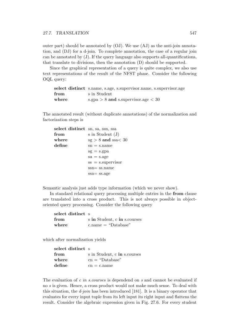
27.7. TRANSLATION 547

outer part) should be annotated by (OJ). We use (AJ) as the anti-join annota-tion, and (DJ) for a d-join. To complete annotation, the case of a regular joincan be annotated by (J). If the query language also supports all-quantifications,that translate to divisions, then the annotation (D) should be supported.

Since the graphical representation of a query is quite complex, we also usetext representations of the result of the NFST phase. Consider the followingOQL query:

select distinct s.name, s.age, s.supervisor.name, s.supervisor.agefrom s in Studentwhere s.gpa > 8 and s.supervisor.age < 30

The annotated result (without duplicate annotations) of the normalization andfactorization steps is

select distinct sn, sa, ssn, ssafrom s in Student (J)where sg > 8 and ssa< 30define sn = s.name

sg = s.gpasa = s.agess = s.supervisorssn= ss.namessa= ss.age

Semantic analysis just adds type information (which we never show).In standard relational query processing multiple entries in the from clause

are translated into a cross product. This is not always possible in object-oriented query processing. Consider the following query

select distinct sfrom s in Student, c in s.courseswhere c.name = “Database”

which after normalization yields

select distinct sfrom s in Student, c in s.courseswhere cn = “Database”define cn = c.name

The evaluation of c in s.courses is dependend on s and cannot be evaluated ifno s is given. Hence, a cross product would not make much sense. To deal withthis situation, the d-join has been introduced [181]. It is a binary operator thatevaluates for every input tuple from its left input its right input and flattens theresult. Consider the algebraic expression given in Fig. 27.6. For every student

548CHAPTER 27. DETAILS ON THE PHASES OF QUERY COMPILATION

D-JOIN [c:s.courses]SCAN [s:student]

EXPAND [cn:c.name]

SELECT [cn=”Database”]

PROJECT [s]

Figure 27.6: An algebraic operator tree with a d-join

s from its left input, the d-join computes the set s.courses. For every coursec in s.courses an output tuple containing the original student s and a singlecourse c is produced. If the evaluation of the right argument of the d-join is notdependend on the left argument, the d-join is equivalent with a cross product.The first optimization is to replace d-joins by cross products whenever possible.

Queries with a group by clause must be translated using the unary groupingoperator GROUP which we denote by Γ. It is defined as

Γg;θA;f (e) = y.A [g : G]|y ∈ e,G = f(x|x ∈ e, x.Aθy.A)

where the subscripts have the following semantics: (i) g is a new attributethat will hold the elements of the group (ii) θA is the grouping criterion for asequence of comparison operators θ and a sequence of attribute names A, and(iii) the function f will be applied to each group after it has been formed. Weoften use some abbreviations. If the comparison operator θ is equal to “=”, wedon’t write it. If the function f is identity, we omit it. Hence, Γg;A abbreviatesΓg;=A;id.

Let us complete the discussion on internal query representation. We alreadymentioned algebraic operators like selection and join. These are called logicalalgebraic operators. There implementations are called physical algebraic opera-tors. Typically, there exist several possible implementations for a single logicalalgebraic operator. The most prominent example being the join operator withimplementations like Grace join, sort-merge join, nested-loop join etc. All theoperators can be modelled as objects. To do so, we extend the expression hi-erarchy by an algebra hierarchy. Although not shown in Fig 27.7, the algebraclass should be a subclass of the expression class. This is not necessary for SQLbut is a requirement for more orthogonal query languages like OQL.

27.8. REWRITE I 549

Expression

AlgUnary AlgBinary AlgNary AlgScan Group SFWDblock

Algebraic Operator

DupElim

SortUnnestSelectChiProjection AlgIfDivisionJoin AlgSetop

Union Intersection Difference

Figure 27.7: Algebra

27.8 Rewrite I

27.9 Plan Generation

27.10 Rewrite II

27.11 Code generation

In order to discuss the tasks of code generation, it is necessary to have a littleunderstanding of the interface to the runtime system that interpretes the exe-cution plan. I have chosen AODB as an example runtime system since this isone I know. The interface to AODB is defined by the AODB Virtual Machine(AVM). For simple operations, like arithmetic operations, comparisons and soon, AVM provides assembler-like operations that are interpreted at runtime.Simple AVM operations work on registers. A single register is able to hold thecontents of exactly one IU. Additionally, AVM provides physical algebraic oper-ators. These operators take AVM programs (possibly with algebraic operators)as arguments. There is one specialty about AVM programs though. In order toefficiently support factorization of common subexpressions involving arithmeticoperations (as needed in aggregations like avg, sum), arithmetic operators inAVM can have two side effects. They are able to store the result of the opera-tion into a register and they are able to add the result of the operation to thecontents of another register. This is denoted by the result mode. If the resultmode is A, they just add the result to some register, if it is C, they copy (store)the result to some register, if it is B, they do both. This is explored in the codefor Query 1 of the TPC-D benchmark (Fig. 1.6).

Code generation has the following tasks. First it must map the physical op-erators in a plan to the operators of the AVM code. This mapping is a straightforward 1:1 mapping. Then, the code for the subscripts of the operators hasto be generated. Subscripts are for example the predicate expressions for theselection and join operators. For grouping, several AVM programs have to be

550CHAPTER 27. DETAILS ON THE PHASES OF QUERY COMPILATION

generated. First program is the init program. It initializes the registers thatwill hold the results for the aggregate functions. For example, for an averageoperation, the register is initalized with 0. The advance program is executedonce for every tuple to advance the aggregate computation. For example, foran average operations, the value of some register of the input tuple is addedto the result register holding the average. The finalize program performs post-processing for aggregate functions. For example for the average, it devides thesum by the number of tuples. For hash-based grouping, the last two programs(see Fig.1.6) compute the hash value of the input register set and compare thegroup-by attributes of the input registers with those of every group in the hashbucket.

During the code generation for the subscripts factorization of common subex-pression has to take place. Another task is register allocation and deallocation.This task is performed by the register manager. It uses subroutines to de-termine whether some registers are no longer needed. The register managermust also keep track in which register some IU is stored (if at all). Anothercomponent used during code generation is a factory that generates new AVMoperations. This factory is associated with a table driven component that mapsthe operations used in the internal query representation to AVM opcodes.

27.12 Bibliography

Chapter 28

Hard-Wired Algorithms

28.1 Hard-wired Dynamic Programming

28.1.1 Introduction

Plan generation is performed block-wise. The goal is to generate a plan forevery block. Typically, not all possible plans are generated. For example, thegroup operator (if necessary for the query) is mostly performed last (see alsoSec. ??). This mainly leaves ordering joins and selections as the task of plangeneration. A plan is an operator tree whose node consist of physical algebraicoperators, e.g. selection, sort-operator, sort-merge and other joins, relation andindex scans. The process of plan generation has received a lot of attention.Often, the term query optimization is used synonymous for the plan generationphase.

Figure 28.1 shows a plan for the block

select e.namefrom Employee e, Department dwhere e.dno = d.dno and d.name = “shoe”

The bottom level contains two table scans that scan the base tables Employeeand Department . Then, a selection operator is applied to restrict the depart-ments to those named “shoe”. A nested-loop join is used to select those employ-ees that work in the selected departments. The projection restricts the outputto the name of the employees, as required by the query block. For such a plan,a cost function is used to estimate its cost. The goal of plan generation is togenerate the cheapest possible plan. Costing is briefly sketched in Section ??.

The foundation of plan generation are algebraic equivalences. For e, e1, e2, . . .being algebraic expressions and p, q predicates, here are some example equiva-

551

552 CHAPTER 28. HARD-WIRED ALGORITHMS

Table Scan (Employee[e]) Table Scan (Department[d])

Select (d.name = "shoe")

NL−Join (e.dno = d.dno)

Project (e.name)

Figure 28.1: A sample execution plan

lences:

σp(σq(e)) ≡ σq(σp(e))

σp(e1 1q e2) ≡ (σp(e1)) 1q e2 if p is applicable to e1

e1 1p e2 ≡ e2 1p e1

(e1 1p e2) 1q e3 ≡ e1 1p (e2 1q e3)

e1 ∪ e2 ≡ e2 ∪ e1

(e1 ∪ e2) ∪ e3 ≡ e1 ∪ (e2 ∪ e3)

e1 ∩ e2 ≡ e2 ∩ e1

(e1 ∩ e2) ∩ e3 ≡ e1 ∩ (e2 ∩ e3)

σp(e1 ∩ e2) ≡ σp(e1) ∩ e2

For more equivalences and conditions that ought to be attached to the equiva-lences see the appendix ??. Note that commutativity and associativity of thejoin operator allow an arbitrary ordering. Since the join operator is the mostexpensive operation, ordering joins is the most prominent problem in plan gen-eration.

These equivalences are of course independent of the actual implementationof the algebraic operators. The total number of plans equivalent to the originalquery block is called the potential search space. However, not always is thetotal search space considered. The set of plans equivalent to the original queryconsidered by the plan generator is the actual search space. Since the System Rplan generator [755], certain restrictions are applied. The most prominent are:

• Generate only plans where selections are pushed down as far as possible.

• Do not consider cross products if not absolutely necessary.

• Generate only left-deep trees.

28.1. HARD-WIRED DYNAMIC PROGRAMMING 553

R1

R3

R4

R1 R2 R3 R4

bushy tree

R2

left−deep tree

B

B

B B

B

B

Figure 28.2: Different join operator trees

• If the query block contains a grouping operation, the group operator isperformed last.

Some comments are in order. Cross products are only necessary, if the querygraph is unconnected where a query graph is defined as follows: the nodesare the relations and the edges correspond to the predicates (boolean factors1)found in the where clause. More precisely, the query graph is a hypergraph,since a boolean factor may involve more than two relations. A left-deep tree isan operator tree where the right argument of a join operator always is a baserelation. A plan with join operators whose both arguments are derived by otherjoin operators is called bushy tree. Figure 28.2 gives an example of a left-deeptree and a bushy tree.

If we take all the above restrictions together, the problem boils down toordering the join operators or relations. This problem has been studied exten-sively. The complexity of finding the best (according to some cost function)ordering (operator tree) was first studied by Ibaraki and Kameda [421]. Theyproved that the problem of generating optimal left-deep trees with no crossproducts is NP-hard for a special block-wise nested loop join cost function.This cost function applied in the proof is quite complex. Later is was shownthat even if the cost function is very simple, the problem remains NP-hard[186]. The cost function (Cout) used there just adds up intermediate resultssizes. This cost function is interesting in that it is the kernel of many other costfunctions and it fulfills the ASI property of which we now the following: If thecost function fulfills the ASI property and the query graph is acyclic, then theproblem can be solved in polynomial time [421, 499]. Ono and Lohman gave ex-amples that considering cross products can substantially improve performance[626]. However, generating optimal left-deep trees with cross products evenfor Cout makes the problem NP-hard [186]. Generating optimal bushy trees is

1A boolean factor is a disjunction of basic predicates in a conjunctive normal form.

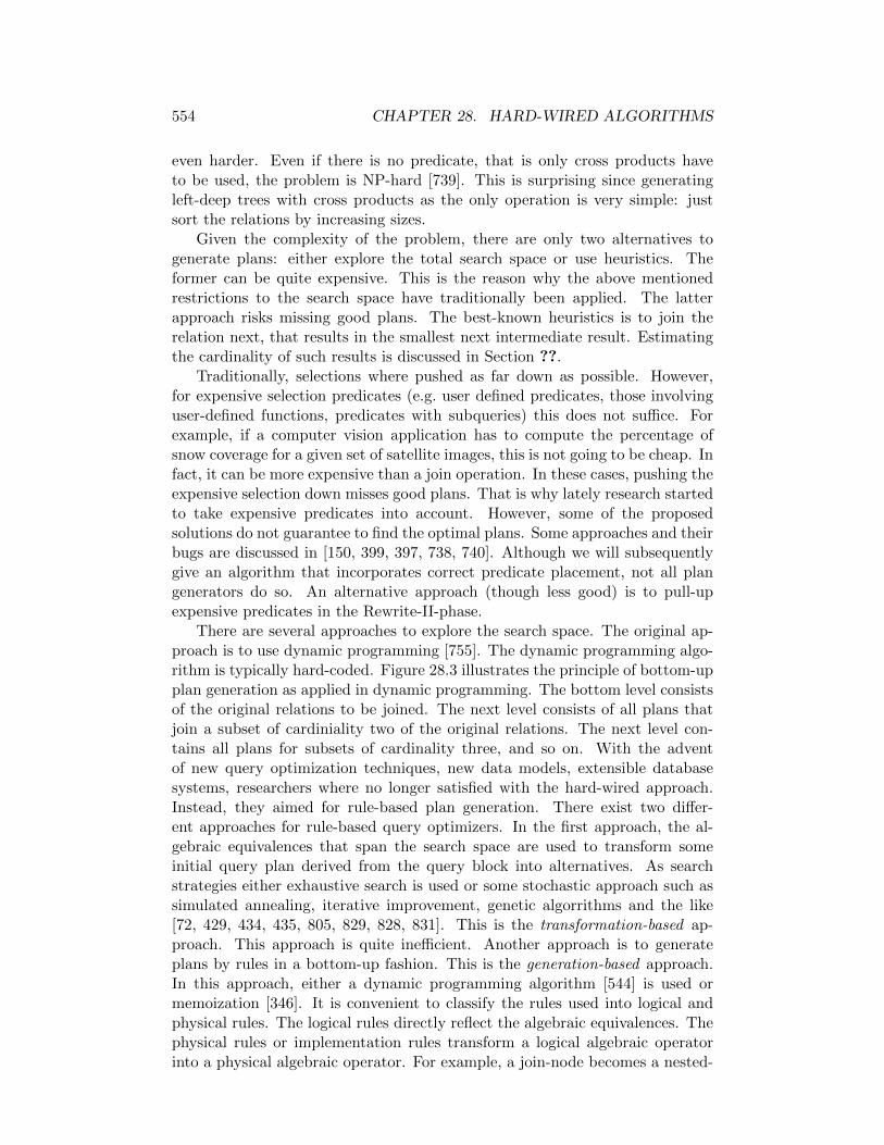
554 CHAPTER 28. HARD-WIRED ALGORITHMS

even harder. Even if there is no predicate, that is only cross products haveto be used, the problem is NP-hard [739]. This is surprising since generatingleft-deep trees with cross products as the only operation is very simple: justsort the relations by increasing sizes.

Given the complexity of the problem, there are only two alternatives togenerate plans: either explore the total search space or use heuristics. Theformer can be quite expensive. This is the reason why the above mentionedrestrictions to the search space have traditionally been applied. The latterapproach risks missing good plans. The best-known heuristics is to join therelation next, that results in the smallest next intermediate result. Estimatingthe cardinality of such results is discussed in Section ??.

Traditionally, selections where pushed as far down as possible. However,for expensive selection predicates (e.g. user defined predicates, those involvinguser-defined functions, predicates with subqueries) this does not suffice. Forexample, if a computer vision application has to compute the percentage ofsnow coverage for a given set of satellite images, this is not going to be cheap. Infact, it can be more expensive than a join operation. In these cases, pushing theexpensive selection down misses good plans. That is why lately research startedto take expensive predicates into account. However, some of the proposedsolutions do not guarantee to find the optimal plans. Some approaches and theirbugs are discussed in [150, 399, 397, 738, 740]. Although we will subsequentlygive an algorithm that incorporates correct predicate placement, not all plangenerators do so. An alternative approach (though less good) is to pull-upexpensive predicates in the Rewrite-II-phase.

There are several approaches to explore the search space. The original ap-proach is to use dynamic programming [755]. The dynamic programming algo-rithm is typically hard-coded. Figure 28.3 illustrates the principle of bottom-upplan generation as applied in dynamic programming. The bottom level consistsof the original relations to be joined. The next level consists of all plans thatjoin a subset of cardiniality two of the original relations. The next level con-tains all plans for subsets of cardinality three, and so on. With the adventof new query optimization techniques, new data models, extensible databasesystems, researchers where no longer satisfied with the hard-wired approach.Instead, they aimed for rule-based plan generation. There exist two differ-ent approaches for rule-based query optimizers. In the first approach, the al-gebraic equivalences that span the search space are used to transform someinitial query plan derived from the query block into alternatives. As searchstrategies either exhaustive search is used or some stochastic approach such assimulated annealing, iterative improvement, genetic algorrithms and the like[72, 429, 434, 435, 805, 829, 828, 831]. This is the transformation-based ap-proach. This approach is quite inefficient. Another approach is to generateplans by rules in a bottom-up fashion. This is the generation-based approach.In this approach, either a dynamic programming algorithm [544] is used ormemoization [346]. It is convenient to classify the rules used into logical andphysical rules. The logical rules directly reflect the algebraic equivalences. Thephysical rules or implementation rules transform a logical algebraic operatorinto a physical algebraic operator. For example, a join-node becomes a nested-

28.1. HARD-WIRED DYNAMIC PROGRAMMING 555

R1 R2 R3

R12 R23R13

R123R123R123 <== 2 alternatives pruned

<== input relations

<== first set of partial plans generated

Figure 28.3: Bottom up plan generation

loop join node.

28.1.2 A plan generator for bushy trees

Within the brief discussion in the last subsection, we enumerated plans suchthat first all 1-relation plans are generated, then all 2-relation plans and so on.This enumeration order is not the most efficient one. Let us consider the simpleproblem where we have to generate exactly one best plan for the subsets of then element set of relations to be joined. The empty subset is not meaningful,leaving the number of subsets to be investigated at 2n − 1. Enumerating thesesubsets can be done most efficient by enumerating them in counting order . Thatis, we initialize a n bit counter with 1 and count until have reached 2n−1. Then bits represent the subsets. Note that with this enumeration order, plans arestill generated bottom up. For a given subset R of the relations (encoded as thebit pattern a), we have to generate a plan from subsets of this subset (encodedas the bit pattern s). For example, if we only want to generate left-deep trees,then we must consider 1 element subsets and their complements. If we wantto generate bushy trees, all subsets must be considered. We can generate thesesubsets by a very fast algorithm developed by Vance and Maier [865]:

s = a & -a;

while(s)

s = a & (s - a);

process(s);

The meaning of process(s) depends on the kinds of plans we generate. If weconcentrate on join ordering neglecting selection operations (i.e. pushing them)This step essentially looks up the plans for s and its complement s and thenjoins the plans found there. Lookup is best implemented via an array with s asan index.

556 CHAPTER 28. HARD-WIRED ALGORITHMS

28.1.3 A plan generator for bushy trees and expensive selec-tions

Figure 28.4 shows the pseudocode of a dynamic programming algorithm thatgenerates plans with cross products, selections, and joins. It generates optimalbushy trees. Efficient implementation technique for the algorithm can be foundin [865, 740]. As input parameters, the algorithm takes a set of relations R anda set of predicates P . The set of relations for which a selection predicate existsis denoted by RS . We identify relations and predicates that apply to theserelations. For all subsets Mk of the relations and subsets Pl of the predicates,an optimal plan is constructed and entered into the table T . The loops rangeover all Mk and Pl. Thereby, the set Mk is split into two disjoint subsets Land L′, and the set Pl is split into three parts (line 7). The first part (V )contains those predicates that apply to relations in L only. The second part(V ′) contains those predicates that apply to relations in L′ only. The third part(p) is a conjunction of all the join predicates connecting relations in L and L′

(line 8). Line 9 constructs a plan by joining the two plans found for the pairs[L, V ] and [L′, V ′] in the table T . If this plan has so far the best costs, it ismemoized in the table (lines 10-12). Last, different possibilities of not pushingpredicates in Pl are investigated (lines 15-19).

Another issue that complicates the application of dynamic programming arecertain properties of plans. The most prominent such properties are interestingorders [755, 789, 790]. Take a look at the following query:

select d.no, e.namefrom Employee e, Department dwhere e.dno = d.dnoorder by d.dno

Here, the user requests the result to be order on d.dno. Incidentally, this is also ajoin attribute. During bottom up plan generation, we might think that a Gracehash join is more efficient than a sort-merge join since the cost of sorting therelations is too high. However, the result has to be sorted anyway so that thissort may pay off. Hence, we have have to keep both plans. The approach is thefollowing. In the example, an ordering on d.dno is called an interesting order.In general, any order that is helpful for ordering the output as requested by theuser, for a join operator, for a grouping operator, or for duplicate eliminationis called an interesting order . The dymamic programming algorithm is thenmodified such that plans are not pruned, if they produce different interestingorders.

28.1.4 A plan generator for bushy trees, expensive selectionsand functions

28.2 Bibliography

28.2. BIBLIOGRAPHY 557

proc Optimal-Bushy-Tree(R,P )1 for k = 1 to n do2 for all k-subsets Mk of R do3 for l = 0 to min(k,m) do4 for all l-subsets Pl of Mk ∩RS do5 best cost so far =∞;6 for all subsets L of Mk with 0 < |L| < k do7 L′ = Mk \ L, V = Pl ∩ L, V ′ = Pl ∩ L′;8 p =

∧pi,j | pi,j ∈ P, Ri ∈ V, Rj ∈ V ′; // p=true might hold9 T = (T [L, V ] 1p T [L′, V ′]);10 if Cost(T) < best cost so far then11 best cost so far = Cost(T);12 T [Mk, Pl] = T ;13 fi;14 od;15 for all R ∈ Pl do16 T = σR(T [Mk, Pl \ R]);17 if Cost(T) < best cost so far then18 best cost so far = Cost(T);19 T [Mk, Pl] = T ;20 fi;21 od;22 od;23 od;24 od;25 od;26 return T [R,S];

Figure 28.4: A Dynamic Programming Optimization Algorithm

558 CHAPTER 28. HARD-WIRED ALGORITHMS

Chapter 29

Rule-Based Algorithms

29.1 Rule-based Dynamic Programming

The section is beyond the scope of the paper and the reader is refered to thestarburst papers, especially [374, 519, 518, 544, 545].

29.2 Rule-based Memoization

This section is beyond the scope of the paper and the reader is refered tothe Volcano and Cascade papers [331, 336, 342, 345, 346]. Both optimizerframeworks derived from the earlier Exodus query optimizer generator [329,343].

29.3 Bibliography

559

560 CHAPTER 29. RULE-BASED ALGORITHMS

Chapter 30

Example Query Compiler

30.1 Research Prototypes

30.1.1 AQUA and COLA

30.1.2 Black Dahlia II

30.1.3 Epoq

Fur das objektorientierte Datenmodell Encore [935] wurde die AnfragespracheEqual [774, 773, 775], eine objektorientierte Algebra, die die Erzeugung von Ob-jekten erlaubt, entwickelt. Zur Optimierung von Equal-Algebra-Ausdruckensoll der Optimierer Epoq dienen. Eine Realisierung von Epoq steht nochaus. Konkretisiert wurden jedoch bereits der Architekturansatz [589] und dieKontrolle der Alternativenerzeugung [588] innerhalb dieser Architektur. EinenGesamtuberblick gibt die Dissertation von Mitchell [587].

Der Architekturvorschlag besteht aus einer generischen Architektur, diean einem Beispieloptimierer konkretisiert wurde [587, 588]. Die elementarenBausteine der Architektur sind Regionen. Sie bestehen aus einer Kontrol-lkomponente und wiederum Regionen beziehungsweise Transformationen. Dieeinfachste Region ist dabei eine Transformation/Regel, die einen Algebraaus-druck in einen aquivalenten Algebraausdruck umformt. Jede Region selbst wirdwiederum als eine Transformation aufgefaßt. Innerhalb der Architektur werdennun diese Regionen in einer Hierarchie oder auch einem gerichteten azyklis-chen Graphen, organisiert. Abbildung 30.1 zeigt eine solche Beispielorganisa-tion. Regionen selbst konnen bis auf die Kontrolle als Module im Sinne vonSciore und Sieg [751] aufgefaßt werden. Sie weisen sehr ahnliche Parameter undSchnittstellen auf. Wahrend jedoch bei Sciore und Sieg die Kontrollstrategieeines Moduls aus einer festen Menge von gegebenen Kontrollstrategien aus-gewahlt werden muß, kann sie hier freier spezifiziert werden.

Unabhangig davon, ob die Transformationen einer Region wiederum Regio-nen sind oder elementare Transformationen, wird ihre Anwendung einheitlichvon der Kontrolle der Region bestimmt. Die Aufgabe dieser Kontrolle bestehtdarin, eine Folge von Transformationen zu finden, die die gegebene Anfragein eine aquivalente uberfuhren. Sinngebend ist hierbei ein gewisses Ziel, dases zu erreichen gilt. Beispielsweise kann dieses Ziel lauten: Optimiere eine

561

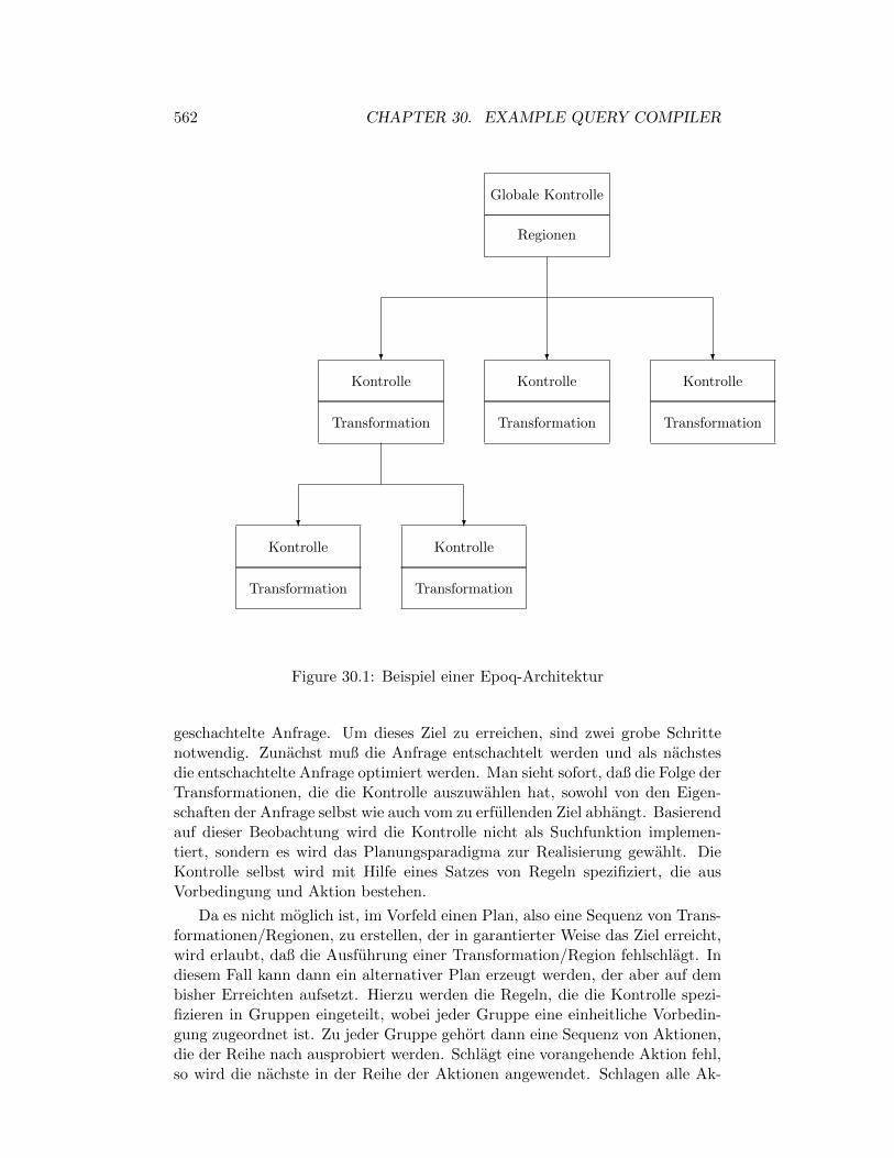
562 CHAPTER 30. EXAMPLE QUERY COMPILER

Regionen

Globale Kontrolle

? ? ?

Kontrolle Kontrolle Kontrolle

Transformation Transformation Transformation

? ?

Kontrolle Kontrolle

Transformation Transformation

Figure 30.1: Beispiel einer Epoq-Architektur

geschachtelte Anfrage. Um dieses Ziel zu erreichen, sind zwei grobe Schrittenotwendig. Zunachst muß die Anfrage entschachtelt werden und als nachstesdie entschachtelte Anfrage optimiert werden. Man sieht sofort, daß die Folge derTransformationen, die die Kontrolle auszuwahlen hat, sowohl von den Eigen-schaften der Anfrage selbst wie auch vom zu erfullenden Ziel abhangt. Basierendauf dieser Beobachtung wird die Kontrolle nicht als Suchfunktion implemen-tiert, sondern es wird das Planungsparadigma zur Realisierung gewahlt. DieKontrolle selbst wird mit Hilfe eines Satzes von Regeln spezifiziert, die ausVorbedingung und Aktion bestehen.

Da es nicht moglich ist, im Vorfeld einen Plan, also eine Sequenz von Trans-formationen/Regionen, zu erstellen, der in garantierter Weise das Ziel erreicht,wird erlaubt, daß die Ausfuhrung einer Transformation/Region fehlschlagt. Indiesem Fall kann dann ein alternativer Plan erzeugt werden, der aber auf dembisher Erreichten aufsetzt. Hierzu werden die Regeln, die die Kontrolle spezi-fizieren in Gruppen eingeteilt, wobei jeder Gruppe eine einheitliche Vorbedin-gung zugeordnet ist. Zu jeder Gruppe gehort dann eine Sequenz von Aktionen,die der Reihe nach ausprobiert werden. Schlagt eine vorangehende Aktion fehl,so wird die nachste in der Reihe der Aktionen angewendet. Schlagen alle Ak-

30.1. RESEARCH PROTOTYPES 563

tionen fehl, so schlagt auch die Anwendung der Region fehl.

Jede Aktion selbst ist wiederum eine Sequenz von elementaren Aktionen.Jede dieser elementaren Aktionen ist entweder die Anwendung einer elementarenTransformation, der Aufruf einer Region oder der rekursive Aufruf des Planersmit einem neuformulierten Ziel, dessen Teilplan dann an entsprechender Stellein die Aktion eingebaut wird.

Die Erweiterbarkeit dieses Ansatzes um neue Regionen scheint einfach moglich,da die Schnittstelle der Regionen genormt ist. Probleme konnte es lediglich beiden Kontrollstrategien geben, da nicht klar ist, ob die benutzte Regelsprachemachtig genug ist, um alle wunschenswerten Kontrollstrategien zu verwirk-lichen.

Die Frage, ob die einzelnen Komponenten des Optimierers, also die Re-gionen, evaluiert werden konnen, ist schwierig zu beantworten. Dafur sprichtjedoch, daß jede Region in einem gewissen Kontext aufgerufen wird, also zur Er-reichung eines bestimmten Zieles bei der Optimierung einer Anfrage mit ebensobestimmten Eigenschaften. Beurteilen kann man daher die Erfolgsquote einerRegion innerhalb ihrer verschiedenen Anwendungen. Da jede Region lediglicheine Alternative erzeugen darf, aufgrund des eine Region ist eine Transforma-tion-Paradigmas, ist schwer zu sagen, in wieweit sich die durch die beschriebeneBewertung gewonnene Information zur Verbesserung der Regionen oder desGesamtoptimierers einsetzen laßt.

Da auch hier der transformierende Ansatz zugrunde liegt, treffen die bereitsdiskutierten Probleme auch fur den Optimierer fur Straube zu.

Einen stetigen Leistungsabfall konnte man durch die Realisierung von al-ternativen Regionen erreichen, indem man ein Ziel OptimiereSchnell einfuhrt,das dann entsprechend weniger sorgfaltige, aber schnellere Regionen aufruft.Vorhersagen uber der Gute (bei gegebener Optimierungszeit) scheinen aberschwerlich moglich.

30.1.4 Ereq

A primary goal of the EREQ project is to define a common architecture for thenext generation of database managers. This architecture now includes

* the query language OQL (a la ODMG), * the logical algebra AQUA (a laBrown), and * the physical algebra OPA (a la OGI/PSU).

It also includes

* software to parse OQL into AQUA (a la Bolo)

and query optimizers:

* OPT++ (Wisconsin), * EPOQ (Brown), * Cascades (PSU/OGI), and *Reflective Optimizer (OGI).

In order to test this architecture, we hope to conduct a ”bakeoff” in whichthe four query optimizers will participate. The primary goal of this bakeoff isto determine whether optimizers written in different contexts can accommodatethe architecture we have defined. Secondarily, we hope to collect enough per-formance statistics to draw some conclusions about the four optimizers, whichhave been written using significantly different paradigms.

564 CHAPTER 30. EXAMPLE QUERY COMPILER

Anfrage - Synt. Analyse -

Anfrage Graph

Optimierer -

Auswertungsplan

Interpreter - Antwort

C-Compiler

?

Optimierergenerator

?

Modellbeschreibung

?

Figure 30.2: Exodus Optimierer Generator

At present, OGI and PSU are testing their optimizers on the bakeoff queries.Here is the prototype bakeoff optimizer developed at OGI. This set of Webpages is meant to report on the current progress of their effort, and to definethe bakeoff rules. Please email your suggestions for improvement to Leo Fegarasfegaras@cse.ogi.edu. Leo will route comments to the appropriate author.

http://www.cse.ogi.edu/DISC/projects/ereq/bakeoff/bakeoff.html

30.1.5 Exodus/Volcano/Cascade

Im Rahmen des Exodus-Projektes wurde ein Optimierergenerator entwickelt[343]. Einen Uberblick uber den Exodus-Optimierergenerator gibt Abbildung 30.2.Ein Model description file enthalt alle Angaben, die fur einen Optimierer notigsind. Da der Exodus-Optimierergenerator verschiedene Datenmodelle unter-stutzen soll, enthalt dieses File zunachst einmal die Definition der verfugbarenOperatoren und Methoden. Dabei werden mit Operatoren die Operatoren derlogischen Algebra bezeichnet und mit Methoden diejenigen der physischen Al-gebra, also die Implementierungen der Operatoren. Das Model description fileenthalt weiterhin zwei Klassen von Regeln. Transformationen basieren auf alge-braischen Gleichungen und fuhren einen Operatorbaum in einen anderen uber.Implementierungsregeln wahlen fur einen gegebenen Operator eine Methodeaus. Beide Klassen von Regeln haben einen linken Teil, der mit einem Teil desaktuellen Operatorgraphen ubereinstimmen muß, einen rechten Teil, der denOperatorgraphen nach Anwendung der Regel beschreibt, und eine Bedingung,die erfullt sein muß, damit die Regel angewendet werden kann. Wahrend dielinke und rechte Seite der Regel als Muster angegeben werden, wird die Be-dingung durch C-Code beschrieben. Auch fur die Tranformation lassen sichC-Routinen verwenden. In einer abschließenden Sektion des Model descriptionfiles finden sich dann die benotigten C-Routinen.

30.1. RESEARCH PROTOTYPES 565

Aus dem Model description file wird durch den Optimierergenerator einC-Programm erzeugt, das anschließend ubersetzt und gebunden wird. DasErgebnis ist dann der Anfrageoptimierer, der in der herkommlichen Art undWeise verwendet werden kann. Es wurde ein ubersetzender Ansatz fur dieRegeln gewahlt und kein interpretierender, da in einem von den Autoren vorherdurchgefuhrten Experiment sich die Regelinterpretation als zu langsam erwiesenhat.

Die Regelabarbeitung im generierten Optimierer verwaltet eine Liste OPEN,in der alle anwendbaren Regeln gehalten werden. Ein Auswahlmechanismusbestimmt dann die nachste anzuwendende Regel und entfernt sie aus OPEN.Nach deren Anwendung werden die hierdurch ermoglichten Regelanwendungendetektiert und in OPEN vermerkt. Zur Implementierung des Auswahlmecha-nismus werden sowohl die Kosten eines aktuellen Ausdrucks als auch eine Ab-schatzung des Potentials einer Regel in Betracht gezogen. Diese Abschatzungdes Potentials berechnet sich aus dem Quotienten der Kosten fur einen Opera-torbaum vor und nach Regelanwendung fur eine Reihe von vorher durchgefuhrtenRegelanwendungen. Mit Hilfe dieser beiden Angaben, den Kosten des aktuellenOperatorgraphen, auf den die Regel angewendet werden soll, und ihres Poten-tials konnen dann Abschatzungen uber die Kosten des erzeugten Operator-graphen berechnet werden. Die Suchstrategie ist Hill climbing.

Der von den Autoren vermerkte Hauptnachteil ihres Optimierergenerators,den sie jedoch fur alle transformierenden regelbasierten Optimerer geltend machen,ist die Unmoglichkeit der Abschatzung der absoluten Gute eines Operator-baumes und des Potentials eines Operatorbaumes im Hinblick auf zukunftigeOptimierungen. Dadurch kann niemals abgeschatzt werden, ob der optimaleOperatorbaum bereits erreicht wurde. Erst nach Generierung aller Alternativ-en ist die Auswahl des optimalen Operatorbaumes moglich. Weiter bedauern esdie Autoren, daß es nicht moglich ist, den A∗-Algorithmus als Suchfunktion zuverwenden, da die Abschatzung des Potentials oder der Distanz zum optimalenOperatorgraphen nicht moglich ist.

Zumindest kritisch gegenuberstehen sollte man auch der Bewertung einzel-ner Regeln, da diese, basierend auf algebraischen Gleichungen, von zu feinerGranularitat sind, als daß eine allgemeine Bewertung moglich ware. Die erfol-greiche Verwendung des Vertauschens zweier Verbundoperationen in einer An-frage bedeutet noch lange nicht, daß diese Vertauschung auch in der nachstenAnfrage die Kosten verringert. Die Hauptursache fur die kritische Einstel-lung gegenuber dieser recht ansprechenden Idee ist, daß eine Regelanwendungzu wenig Information/Kontext berucksichtigt. Wurde dieses Manko beseitigt,waren Regeln also von entschieden groberer Granularitat, so erschiene dieserAnsatz vielversprechend. Ein Beispiel ware eine Regel, die alle Verbundoper-ationen gemaß einer gegebenen Heuristik ordnet, also ein komplexer Algorith-mus, der mehr Wissen in seine Entscheidungen einbezieht.

Graefe selbst fuhrt einige weitere Nachteile des Exodus-Optimierergeneratorsan, die dann zur Entwicklung des Volcano-Optimierergenerators fuhrten [345,346]. Unzureichend unterstutzt werden

• nicht-triviale Kostenmodelle,

566 CHAPTER 30. EXAMPLE QUERY COMPILER

• Eigenschaften,

• Heuristiken und

• Transformationen von Subskripten von algebraischen Operatoren in alge-braische Operatoren.

Der letzte Punkt ist insbesondere im Bereich der Objektbanken wesentlich, umbeispielsweise Pfadausdrucke in eine Folge von Verbundoperationen umwandelnzu konnen.

Im Volcano-Optimierergenerator werden algebraische Ausdrucke wieder ineinen Operatorbaum umgewandelt. Wie im Exodus-Optimierergenerator wirdder Optimierer wieder mit einer Menge von transformierenden und implemen-tierenden Regeln beschrieben. Die Nachteile des transformierenden Ansatzwerden somit geerbt. Eine Trennung in zwei Phasen, wie bei vielen Opti-mierern anzutreffen, ist fur den Volcano-Optimierergenerator nicht notwendig.Der Entwickler des Optimierers hat die Freiheit, die Phasen selbst festzulegen.Die Probleme, die sonst bei der Kopplung der algebraischen mit der nicht-algebraischen Optimierung auftreten, konnen also vermieden werden. Die Be-handlung der Eigenschaften erfolgt zielorientiert. Die in der Anfrage gefordertenEigenschaften (bspw. Sortierung), werden der Suchfunktion als Parameter ubergeben,damit gezielt Plane erstellt werden, die diese erfullen. Wenn ein Operator odereine Methode eingebaut wird, so wird darauf geachtet, daß diese noch nichterfullten Eigenschaften durch den Operator oder die Methode erzielt werden.Die geforderten Eigenschaften dienen wieder als Zielbeschreibung fur die nach-folgenden Aufrufe der Suchfunktion. Zu diesen Eigenschaften gehoren auchKostengrenzen, mit denen die Suchfunktion dann einen Branch-and-bound-Algorithmus implementiert. Bevor ein Plan fur einen algebraischen Ausdruckgeneriert wird, wird in einer Hash-Tabelle nachgeschaut, ob ein entsprechen-der Ausdruck mit den geforderten Eigenschaften bereits existiert. Dadurchwird Doppeltarbeit vermieden. Bei beiden Optimierergeneratoren werden dieForderungen nach stetigem Leistungsabfall, fruher Bewertung von Alternativenund Evaluierbarkeit einzelner Komponenten nicht erfullt.

30.1.6 Freytags regelbasierte System R-Emulation

[285] zeigt, wie man mit Hilfe eines regelbasierten Ansatzes den Optimierer vonSystem R [755] emulieren kann. Die Eingabe besteht aus einem Lisp-ahnlichenAusdruck:

(select <proj-list><sel-pred-list><join-pred-list><table-list>)

Die Projektionsliste besteht aus Attributspezifikationen der Form

<rel-name>.<attr-name>

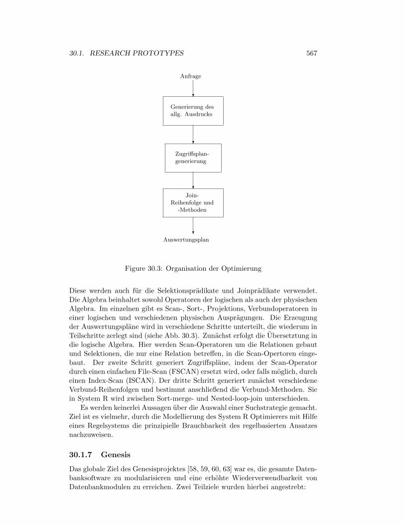
30.1. RESEARCH PROTOTYPES 567

Anfrage

?

Generierung desallg. Ausdrucks

?

Zugriffsplan-generierung

?

Join-Reihenfolge und

-Methoden

?Auswertungsplan

Figure 30.3: Organisation der Optimierung

Diese werden auch fur die Selektionspradikate und Joinpradikate verwendet.Die Algebra beinhaltet sowohl Operatoren der logischen als auch der physischenAlgebra. Im einzelnen gibt es Scan-, Sort-, Projektions, Verbundoperatoren ineiner logischen und verschiedenen physischen Auspragungen. Die Erzeugungder Auswertungsplane wird in verschiedene Schritte unterteilt, die wiederum inTeilschritte zerlegt sind (siehe Abb. 30.3). Zunachst erfolgt die Ubersetztung indie logische Algebra. Hier werden Scan-Operatoren um die Relationen gebautund Selektionen, die nur eine Relation betreffen, in die Scan-Opertoren einge-baut. Der zweite Schritt generiert Zugriffsplane, indem der Scan-Operatordurch einen einfachen File-Scan (FSCAN) ersetzt wird, oder falls moglich, durcheinen Index-Scan (ISCAN). Der dritte Schritt generiert zunachst verschiedeneVerbund-Reihenfolgen und bestimmt anschließend die Verbund-Methoden. Siein System R wird zwischen Sort-merge- und Nested-loop-join unterschieden.

Es werden keinerlei Aussagen uber die Auswahl einer Suchstrategie gemacht.Ziel ist es vielmehr, durch die Modellierung des System R Optimierers mit Hilfeeines Regelsystems die prinzipielle Brauchbarkeit des regelbasierten Ansatzesnachzuweisen.

30.1.7 Genesis

Das globale Ziel des Genesisprojektes [58, 59, 60, 63] war es, die gesamte Daten-banksoftware zu modularisieren und eine erhohte Wiederverwendbarkeit vonDatenbankmodulen zu erreichen. Zwei Teilziele wurden hierbei angestrebt:

568 CHAPTER 30. EXAMPLE QUERY COMPILER

1. Standardisierung der Schnittstellen und

2. Formulierung der Algorithmen unabhangig von der DBMS-Implementierung.

Wir interessieren uns hier lediglich fur die Erreichung der Ziele beim Bau vonOptimierern [56, 61].

Die Standardisierung der Schnittstellen wird durch eine Verallgemeinerungvon Anfragegraphen erreicht. Die Algorithmen selbst werden durch Transfor-mationen auf Anfragegraphen beschrieben. Man beachte, daß dies nicht be-deutet, daß die Algorithmen auch durch Transformationregeln implementiertwerden. Regeln werden lediglich als Beschreibungsmittel benutzt, um die Naturder Wiederverwendbarkeit von Optimierungsalgorithmen zu verstehen.

Die Optimierung wird in zwei Phasen eingeteilt, die Reduktionsphase unddie Verbundphase. Die Reduktionsphase bildet Anfragegraphen, die auf nichtreduzierten Datenmengen arbeiten, auf solche ab, die auf reduzierten Daten-mengen arbeiten. Die Reduktionsphase orientiert sich also deutlich an denHeuristiken zum Durchschieben von Selektionen und Projektionen. Die zweitePhase bestimmt Verbundordnungen. Damit ist die in den Papieren beschriebeneAuspragung des Ansatzes sehr konservativ in dem Sinne, daß nur klassischeDatenmodelle betrachtet werden. Eine Anwendung der Methodik auf objekto-rientierte oder deduktive Datenmodelle steht noch aus.

Folglich lassen sich nur die existierenden klassischen Optimierungsansatzemit diesen Mitteln hinreichend gut beschreiben. Ebenso lassen sich die ex-istierenden klassischen Optimierer mit den vorgestellten Mitteln als Zusam-mensetzung der ebenfalls im Formalismus erfaßten Algorithmen beschreiben.Die Zusammensetzung selbst wird mit algebraischen Termersetzungen beschrieben.Durch neue Kompositionsregeln lassen sich dann auch neue Optimierer beschreiben,die andere Kombinationen von Algorithmen verwenden.

Durch die formale, implementierungsunabhangige Beschreibung sowohl dereinzelnen Optimierungsalgorithmen als auch der Zusammensetzung eines Opti-mierers wird die Wiederverwendbarkeit von bestehenden Algorithmen optimalunterstutzt. Wichtig dabei ist auch die Verwendung der standardisierten An-fragegraphen. Dieser Punkt wird allerdings aufgeweicht, da auch vorgesehen ist,verschiedene Darstellungen von Anfragegraphen zu verwenden [59]. Hierdurchwird die Wiederverwendung von Implementierungen von Optimierungsalgorith-men naturlich in Frage gestellt, da diese ublicherweise nur auf einer bestimmtenDarstellung der Anfragegraphen arbeiten.

Wenn neue Optimierungsansatze entwickelt werden, so lassen sie sich eben-falls im vorgestellten Formalismus beschreiben. Gleiches gilt auch fur neue In-dexstrukturen, da auch diese formal beschrieben werden [57, 62]. Nicht abzuse-hen ist, in wieweit der standardisierte Anfragegraph Erweiterungen standhalt.Dies ist jedoch kein spezifisches Problem des Genesisansatzes, sondern gilt furalle Optimierer. Es ist noch offen, ob es gelingt, die Optimierungsalgorithmenso zu spezifizieren und zu implementieren, daß sie unabhangig von der konkretenDarstellung oder Implementierung der Anfragegraphen arbeiten. Der objekto-rientierte Ansatz kann hier nutzlich sein. Es erhebt sich jedoch die Frage, ob beiEinfuhrung eines neuen Operators die bestehenden Algorithmen so implemen-

30.1. RESEARCH PROTOTYPES 569

tierbar sind, daß sie diesen ignorieren konnen und trotzdem sinnvolle Arbeitleisten.

Die Beschrankung auf zwei Optimierungsphasen, die Reduktions- und dieVerbundphase, ist keine Einschrankung, da auch sie mittels Termersetzungsregelnfestgelegt wurde, und somit leicht geandert werden kann.

Da die Beschreibungen des Optimierers und der einzelnen Algorithmen un-abhangig von der tatsachlichen Implementierung sind, sind auch die globaleKontrolle des Optimierers und die lokalen Kontrollen der einzelnen Algorithmenvoneinander losgelost. Dieses ist eine wichtige Forderung, um Erweiterbarkeitzu erreichen. Sie wird oft bei regelbasierten Optimierern verletzt und schranktsomit deren Erweiterbarkeit ein.

Die Evaluierbarkeit, die Vorhersagbarkeit und die fruhe Bewertung von Al-ternativen sind mit dem vorgestellten Ansatz nicht moglich, da die einzelnenAlgorithmen als Transformationen auf dem Anfragegraphen aufgefaßt werden.Dieser Nachteil gilt jedoch nicht allein fur den hier vorgestellten Genesisansatz,sondern generell fur alle bis auf einen Optimierer. Es ist allerdings nicht ab-sehbar, ob dieser Nachteil aus dem verwendeten Formalismus resultiert oderlediglich aus deren Konkretisierung bei der Modellierung bestehender Optimier-er. Es ist durchaus moglich, daß der Formalismus mit leichten Erweiterungenauch andere Ansatze, insbesondere den generierenden, beschreiben kann.

Insgesamt handelt es sich beim Genesisansatz um einen sehr brauchbarenAnsatz. Leider hat er, im Gegensatz zur Regelbasierung, nicht genug Wider-hall gefunden hat. Er hat hochst wahrscheinlich mehr Moglichkeiten, die An-forderungen zu erfullen, als bisher ausgelotet wurde.

30.1.8 GOMbgo

570 CHAPTER 30. EXAMPLE QUERY COMPILER

ASR-Schema

Code Generator

Selektion und Polierung

Regelanwendung

Ubersetzung und Vorverarbeitung

GOMql-Anfrage

Kostenmodell

Regelbasis

Heuristik

Auswertungsplan

(QEP)

optimierter Term

Liste der optimierten Terme

Termreprasentation

-

?

?

?

?

?

HHHH

HHY

Figure 30.4: Ablauf der Optimierung

30.1. RESEARCH PROTOTYPES 571

optimized

query alternatives

box

tool−

pattern

matcher

cond

mgr

rule

application

transf

mgr

environment manager

Schema Manager

− access support relations

− types

heuristics transformation rules

query

heuristic

evaluator

Figure 30.5: Architektur von GOMrbo

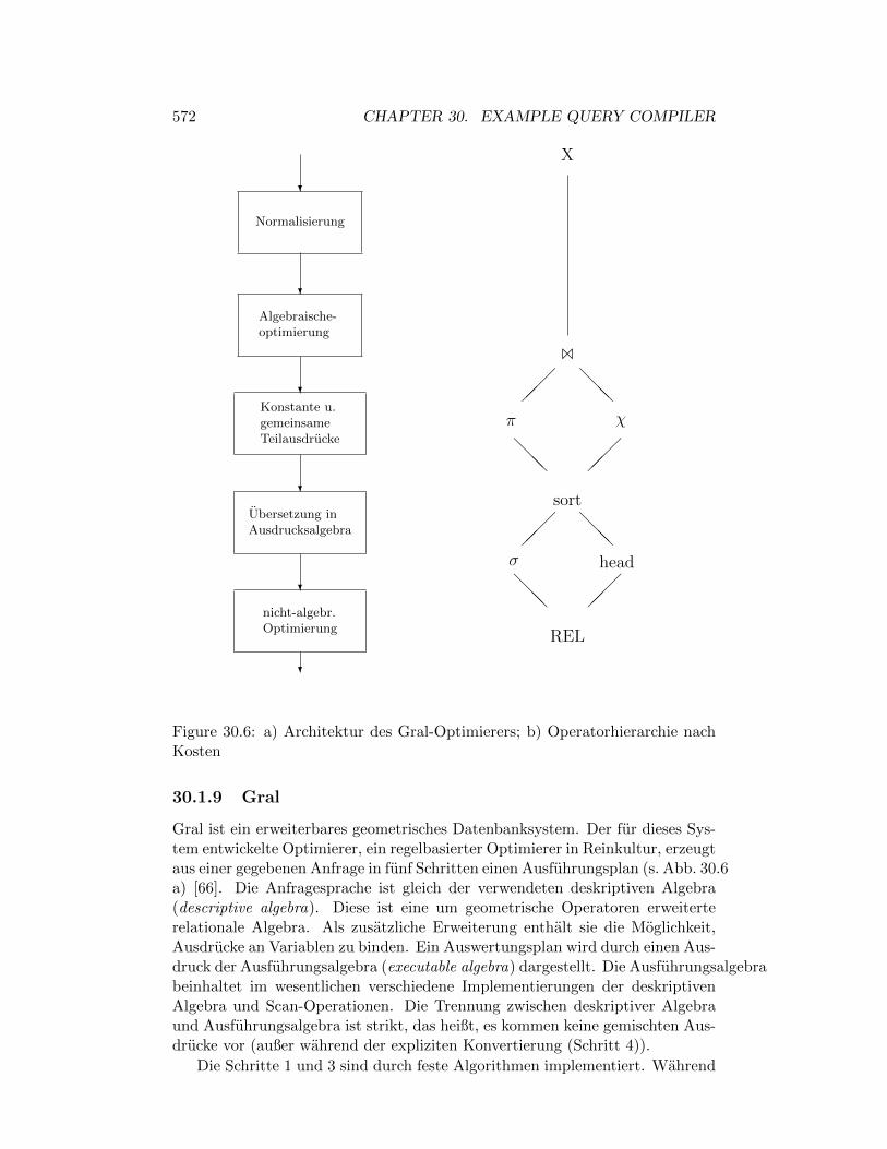
572 CHAPTER 30. EXAMPLE QUERY COMPILER

?

Normalisierung

?

Algebraische-optimierung

?

Konstante u.gemeinsameTeilausdrucke

?

Ubersetzung inAusdrucksalgebra

?

nicht-algebr.Optimierung

?

X

1

@@@

π

@@@

χ

sort

@@@

σ head

@@@

REL

Figure 30.6: a) Architektur des Gral-Optimierers; b) Operatorhierarchie nachKosten

30.1.9 Gral

Gral ist ein erweiterbares geometrisches Datenbanksystem. Der fur dieses Sys-tem entwickelte Optimierer, ein regelbasierter Optimierer in Reinkultur, erzeugtaus einer gegebenen Anfrage in funf Schritten einen Ausfuhrungsplan (s. Abb. 30.6a) [66]. Die Anfragesprache ist gleich der verwendeten deskriptiven Algebra(descriptive algebra). Diese ist eine um geometrische Operatoren erweiterterelationale Algebra. Als zusatzliche Erweiterung enthalt sie die Moglichkeit,Ausdrucke an Variablen zu binden. Ein Auswertungsplan wird durch einen Aus-druck der Ausfuhrungsalgebra (executable algebra) dargestellt. Die Ausfuhrungsalgebrabeinhaltet im wesentlichen verschiedene Implementierungen der deskriptivenAlgebra und Scan-Operationen. Die Trennung zwischen deskriptiver Algebraund Ausfuhrungsalgebra ist strikt, das heißt, es kommen keine gemischten Aus-drucke vor (außer wahrend der expliziten Konvertierung (Schritt 4)).

Die Schritte 1 und 3 sind durch feste Algorithmen implementiert. Wahrend

30.1. RESEARCH PROTOTYPES 573

der Normalisierung (Schritt 1) werden Variablenvorkommen durch die an siegebundenen Ausdrucke ersetzt. Dies ist notwendig, um das Optimierungspo-tential vollstandig erschließen zu konnen. Schritt 3 fuhrt fur konstante Aus-drucke Variablen ein. Die entspricht der Entschachtelung von Anfragen vomTyp N und A (s. Kapitel ?? und [474]). Die Behandlung von gemeinsamenTeilausdrucken ist noch nicht implementiert, aber fur Schritt 3 vorgesehen.

Die Schritte 2, 4 und 5 sind regelbasiert. Zur Formulierung der Regeln wirdeine Regelbeschreibungssprache (rule description language) verwendet. DieBeschreibungen der Regeln werden in einer Datei abgelegt. Innerhalb der Dateiwerden Regeln zu Gruppen (sections) zusammengefaßt. Diese Gruppen werdennacheinander angewandt. Daraus ergeben sich auch fur einen Schritt mehrerekleinere Schritte. Beispielsweise ist der Schritt 2 im OPTEX-Optimierer furGral in vier Teilschritte unterteilt:

1. Dekomposition von Selektionen mit komplexen Selektionspradikaten ineine Folge von Selektionen mit einfachen Selektionspradikaten und Zer-legung von Verbundoperationen in eine Folge von Selektionen und Kreuzpro-dukten.

2. Eigentlicher IMPROVING Schritt (siehe unten).

3. Teilausdrucke bestehend aus einer Selektion und einem unmittelbar fol-genden Kreuzprodukt werden in Verbundoperationen umgewandelt.

4. Bestimmung einer Ordnung zwischen den Verbundoperationen und Kreuzpro-dukten. Dabei werden Kreuzprodukte zum Schluß ausgefuhrt und kleineRelationen zuerst verbunden.

Jeder Gruppe wird eine von drei in Gral implementierten Suchstrategien zuge-ordnet.

STANDARD Fuhrt solange alle Regeln einer Gruppe aus, bis keine Regelmehr anwendbar ist. Es werden keine Vorkehrungen getroffen, um End-losschleifen zu verhindern. Die Regeln mussen also dementsprechend for-muliert werden. Diese Strategie kann fur Schritte 2 und 5 verwendetwerden.

IMPROVING Diese Strategie unterstutzt algebraische Optimierung in derdeskriptiven Algebra (Schritt 2). Das Ziel ist hierbei eine gute Ord-nung der algebraischen Operatoren zu erlangen. Hierzu wird eine partielleOrdnung der algebraischen Operatoren gemaß ihrer Kosten definiert (s.Abb. 30.6 b) fur ein Beispiel). Die IMPROVING-Strategie versucht danndie hierdurch definierte Ordnung in einem gegebenen Ausdruck zu erre-ichen. Hierzu wird sie zunachst rekursiv auf alle Teilausdrucke eines Aus-drucks angewendet. Regeln zur Umformung werden dann angewendet,wenn dadurch eine hohere Koharenz der Operatorfolge im Ausdruck mitder der Operatorkostenhierarchie erreicht werden kann. Dies entsprichteinem Bubble-sort auf dem Ausdruck. Ausdrucke mit der kleinsten An-zahl von runs werden bevorzugt. Dabei ist ein run eine Folge von Op-eratoren innerhalb des zu optimierenden Ausdrucks, dessen Operatorengemaß der Operatorkostenhierarchie geordnet sind.

574 CHAPTER 30. EXAMPLE QUERY COMPILER

TRANSLATION Regelgruppen mit dieser Strategie werden wahrend derUbersetzung von der deskriptiven Algebra in die Ausfuhrungsalgebra angewen-det (Schritt 4). Jede Regel beschreibt dabei die Ubersetzung eines einzel-nen deskriptiven Operators in einen Ausdruck der Ausfuhrungsalgebra, al-so einen, der keine deskriptiven Operatoren enthalten darf. Die Ubersetzungerfolgt lokal. Fur Parameter, also beispielsweise Selektions- und Ver-bundpradikate, konnen Regeln angegeben werden, die einen Suchraum furdie Reorganisation des Parameters erlauben. Hiermit kann man beispiel-sweise alle Permutationen einer Konjunktion erzeugen. Die Suchstrate-gie fur die Parameterbestimmung ist erschopfend und tragt Vorsorge, daßkeine Zyklen auftreten. Eine Auswahl kann mittels des valuation-Eintragsin den Regeln getroffen werden. Dieser kann beispielsweise Kosten reprasentieren.Dementsprechend werden dann Regeln mit der kleinsten valuation bevorzugt.Jede fur einen Parameter generierte Darstellung wird ubersetzt.

Die Syntax fur eine Regel ist

specificationdefinitionRULE

pattern→ result1 valuation1 if condition1

· · ·→ resultn valuationn if conditionn

wobei

specification von der Form

SPEC spec1,. . . ,specn

ist. Dabei sind die speci Range-Spezifikationen wie beispielsweise opi in <OpSet >.

definition Variablen definiert (bspw. fur Attributsequenzen). In Gral ex-istieren verschiedene Sorten von Variablen fur Attribute, Operationen,Relationen etc.

pattern ein Muster in Form eines Ausdrucks ist, der Variablen und Konstan-ten enthalten kann. Der Ausdruck kann ein Ausdruck der deskriptivenAlgebra oder der Ausfuhrungsalgebra sein.

conditioni eine Bedingung ist. Diese Bedingung ist ein allgemeiner boolescherAusdruck. Spezielle Pradikate wie ExistsIndex (existiert ein Index fur eineRelation?) werden von Gral zur Verfugung gestellt.

resulti wiederum ein Ausdruck ist, der das Ergebnis der Regel beschreibt.

valuationi ist ein arithmetischer Ausdruck, der einen numerischen Wert zuruckliefert.Dieser kann in einer (Gral unterstutzt mehrere) Auswahlstrategie herange-zogen werden: Es wird die Regel mit der kleinsten valuation bevorzugt.

30.1. RESEARCH PROTOTYPES 575

Die Auswertung einer Regel erfolgt standardmaßig. Sei E der Ausdruck aufden die Regel angewendet werden soll.

if ∃ Substitution σ, Unterausdruck E′ von E mit E′σ = patternand ∀1 ≤ i ≤ j: ¬ conditioniand conditionj

then ersetzte E′ in E durch resultjσ

Der Gral-Optimierer ist ein reiner regelbasierter Optimierer, der den Trans-formationsansatz verfolgt. Dementsprechend treffen alle vorher identifiziertenNachteile derselben zu.

Zu bemangeln sind im einzelnen folgende Punkte:

• Es erfolgt keine fruhzeitige Bewertung der Alternativen.

• Die Suchstrategien sind fest eingebaut und nicht sonderlich ausgefeilt.

• Der Einbau von hochspezialisierten Algorithmen, die besondere Opti-mierungstechniken reprasentieren, ist schwierig, wenn nicht unmoglich.

• Eine Bestimmung der Verbundreihenfolge gemaß eines komplexeren Al-gorithmus ist nicht moglich.

• Da die Ubersetzung in die Ausfuhrungsalgebra lokal ist und keine An-notationen zugelassen sind, konnen vorhandene Sortierreihenfolgen nurschwer ausgenutzt werden.

Es wird nur eine Alternative der algebraischen Optimierung zur physischenOptimierung ubergeben. Das kann zu Fallen fuhren, in denen der Optimiererniemals das Optimum finden kann. Wenngleich dies auch im allgemeinen nichtimmer moglich ist, so sollte jedoch diese Eigenschaft nicht inharent sein.

Positiv zu vermerken ist, daß fur IMPROVING und TRANSLATION derAufwand fur das Pattern-matching vermutlich gering gehalten werden kann.

30.1.10 Lambda-DB

http://lambda.uta.edu/lambda-DB/manual/overview.html

30.1.11 Lanzelotte in short

Query Language Der Lanzelotte-Optimierer verwendet keine spezielle An-fragesprache. Ausgangspunkt der Betrachtungen sind sog. Anfragegraphen(request graphs, query graphs). Einzelheiten stehen in meiner Ausar-beitung. In einem Papier ([508]) wird gezeigt wie man von einer Regel-sprache (RDL) zu Anfragegraphen kommt.

Internal Representation Die interne Repraesentation einer Anfrage ist derClass Connection Graph. Dort enthalten sind die Datenbankobjekte (Ex-tensionen), die in der Anfrage referenziert werden aus der Sicht des physikalis-chen Schemas und die in der Anfrage bedeutsamen Beziehungen zwischendiesen Extensionen (Joins, Attributpfade, Selektionen).

576 CHAPTER 30. EXAMPLE QUERY COMPILER

Query Execution Plans QEPs werden als (deep) processing trees repraesen-tiert.

Architecture Der Lanzelotte-Optimierer ist regelbasiert.

Transformation versus generation Lanzelotte bietet Regeln fuer beide Spielarten.Sie unterscheidet enumerative search (Generierung), randomized search(Transformation) und genetic search (Transformation).

Control/Search-Strategy Lanzelotte versucht von den Einzelheiten der ver-wendeten Stategien zu abstrahieren und stellt eine erweiterbare Opti-mierung vor, die die Einzelheiten ueberdeckt. Die tatsaechlich zu einembestimmten Zeitpunkt verwendete Strategie wird durch “assertions” bes-timmt. (Dazu steht nicht viel in den Papieren, vielleicht meint sie auchdie Bedingungsteile der Regeln)

Cost Model Ziemlich aehnlich dem, das wir verwenden. Sie benutzt auchsolche Sachen wie card(C), size(C), ndist(Ai), fan(Ai), share(Ai). Einzel-heiten stehen in meiner Ausarbeitung.

30.1.12 Opt++

wisconsin

30.1.13 Postgres

Postgres ist kein Objektbanksystem sondern fallt in die Klasse der erweitertenrelationalen Systeme [815]. Die wesentlichen Erweiterungen sind

• berechenbare Attribute, die als Quel-Anfragen formuliert werden [813],

• Operationen [811],

• abstrakte Datentypen [810] und

• Regeln [814].

Diese beiden Punkte sollen uns jedoch an dieser Stelle nicht interessieren. Diedort entwickelten Optimierungstechniken, insbesondere die Materialisierung derberechenbaren Attribute, sind in der Literatur beschrieben [450, 386, 384, 385].Unser Interesse richtet sich vielmehr auf eine neuere Publikation, in der eineVorschlag fur die Reihenfolgebestimmung von Selektionen und Verbundopera-tionen unterbreitet wird [399]. Diese soll im folgenden kurz vorgestellt werden.Zunachst jedoch einige Vorbemerkungen.

Wenn man eine Selektion verzogert, also nach einem Verbund ausfuhrt,obwohl dies nicht notwendig ware, so kann es passieren, daß das Selektion-spradikat auf mehr Tupeln ausgewertet werden muß. Es kann jedoch nichtpassieren, daß es auf mehr verschiedenen Werten ausgefuhrt werden muß. ImGegenteil, die Anzahl der Argumentewerte wird durch einen Verbund im allge-meinen verkleinert. Cached man also die bereits errechneten Werte des Selek-tionspradikates, so wird die Anzahl der Auswertungen des Selektionspradikates

30.1. RESEARCH PROTOTYPES 577

nach einem Verbund zumindest nicht großer. Die Auswertung wird dann durchein Nachschlagen ersetzt. Da wir hier nur teure Selektionspradikate betrachten,ist ein Nachschlagen sehr billig gegenuber der Auswertung. Die Kosten fur dasNachschlagen konnen sogar vernachlaßigt werden. Es bleibt das Problem dergroße des Caches. Liegt Eingabe sortiert nach den Argumenten des Selektion-spradikates vor, so kann der die große des Caches unter Umstanden auf 1 re-duziert werden. Er erubrigt sich ganz, wenn man eine indirekte Reprasentationdes Verbundergebnisses verwendet. Eine mogliche indirekte Reprasentation istin Abbildung ?? dargestellt, wobei die linke der abgebildeten Relationen dieArgumente fur das betrachtete Selektionspradikat enthalte.

Fur jedes Selektionspradikat p(a1, . . . , an) mit Argumenten ai bezeichne cpdie Kosten der Auswertung auf einem Tupel. Diese setzen sich aus CPU-und I/O-Kosten zusammen (s. [399]). Ein Plan ist ein Baum, dessen Blatterscan-Knoten enthalten und dessen innere Knoten mit Selektions- und Verbund-pradikaten markiert sind. Ein Strom in einem Plan ist ein Pfad von einem Blattzur Wurzel. Die zentrale Ide ist nun die Selektions- und Verbundpradikate nichtzu unterscheiden, sondern gleich zu behandeln. Dabei wird angenommen, daßalle diese Pradikate auf dem Kreuzprodukt aller Relationen der betrachtetenAnfrage arbeiten. Dies erfordert eine Anpassung der Kosten. Seien a1, . . . , andie Relationen der betrachteten Anfrage und p ein Pradikat uber den Relationena1, . . . , ak. Dann sind die globalen Kosten von p wie folgt definiert:

C(p) =cp∏n

i=k+1 |ai|

Die globalen Kosten berechnen die Kosten der Auswertung des Pradikates uberder gesamten Anfrage. Hierbei mussen naturlich diejenigen Relationen her-ausgenommen werden, die das Pradikat nicht beeinflussen. Zur Illustrationnehme man an, p sei ein Selektionspradikat auf nur einer Relation a1. Wendetman p direkt auf a1 an, so entstehen die Kosten cp ∗ |a1|. Im vereinheitlicht-en Modell wird angenommen, daß jedes Pradikat auf dem Kreuzprodukt allerin der Anfrage beteiligten Relationen ausgewertet wird. Es entstehen also dieKosten C(p)∗|a1|∗|a2|∗. . .∗|an|. Diese sind aber gleich cp∗|a1|. Dies ist naturlichnur unter der Verwendung eines Caches fur die Werte der Selektionspradikatekorrekt. Man beachte weiter, daß die Selektivitat s(p) eines Pradikates p un-abhangig von der Lage innerhalb eines Stroms ist.

Der globale Rang eines Pradikates p ist definiert als

rank(p) = s(p)C(p)

Man beachte, daß die Pradikate innerhalb eines Stroms nicht beliebig umord-bar sind, da wir gewahrleisten mussen, daß die von einem Pradikat benutztenArgumente auch vorhanden sein mussen. In [399] wir noch eine weitere Ein-schrankung vorgenommen: Die Verbundreihenfolge darf nicht angetastet wer-den. Es wird also vorausgesetzt, daß eine optimale Verbundreihenfolge bereitsbestimmt wurde und nur noch die reinen Selektionspradikate verschoben wer-den durfen.

Betrachtet man zunachst einmal nur die Umordnung der Pradikate aufeinem Strom, so erhalt man bedingt durch die Umordbarkeitseinschrankungen

578 CHAPTER 30. EXAMPLE QUERY COMPILER

das Sequentialisierungsproblem mit Vorrangbedingungen fur das Algorithmusmit Laufzeit O(nlogn) (n ist die Stromlange) eine optimale Losung bekannt ist[604].

Das in [399] vorgeschlagene Verfahren wendet diesen Algorithmus solangeauf jeden Strom an, bis keine Verbesserung mehr erzielt werden kann. DasErgebnis ist ein polynomialer Algorithmus, der die optimale Losung garantiert.Dies jedoch nur unter der Einschrankung, daß die Kosten des Joins linear sind.

Damit sind wir bereits bei einem der Nachteile des Verfahrens: Die Kostender Verbundoperation nicht mitunter nicht linear sondern sogar quadratisch.Ein weiterer Nachteil liegt in der Voraussetzung, daß die optimale Verbun-dreihenfolge schon bestimmt wurde, denn diese hangt wesentlich davon ab, anwelcher Stelle die Selektionen eingebaut werden. Ublicherweise wird bei der Bes-timmung der optimalen Verbundreihenfolge vorausgesetzt, daß alle Selektion-spradikate soweit wie moglich nach unten verschoben werden. Dies ist jedochjetzt nicht mehr der Fall. Es ist also notwendig die Selektionspradikatmigrationin die Joinreihenfolgebestimmung zu integrieren. Nur dann kann man auf guteErgebnisse hoffen. Die Integration mit einem Ansatz des dynamischen Pro-grammierens ist problematisch, da dort Losungen verworfen werden, die unterUmstanden zur Optimalen Losung fuhren, wenn ein Selektionspradikat nichtganz nach unten durchgeschoben wird [399].

Eine Teillosung wird dort auch angedeutet. Ist der Rang eines Selektion-spradikates großer als jeder Rang jedes Plans einer Menge von Verbunden, soist das Selektionspradikat in einem optimalen Baum oberhalb all dieser Ver-bundoperationen plaziert. Ein entsprechender Algorithmus hat aber, wenner beispielsweise nur Left-deep-trees erzeugt, eine Worst-case-Komplexitat vonO(n4n!).

30.1.14 Sciore & Sieg

Die Hauptidee von Sciore und Sieg ist es, die Regelmenge in Module zu or-ganisieren und jedem Modul eine eigene Suchstrategie, Kostenberechnung undRegelmenge zuzuordnen. Module konnen andere Module explizit aufrufen, oderimplizit ihre Ausgabemenge an das nachste Modul weiterleiten.

30.1.15 Secondo

Gueting

30.1.16 Squiral

Der erste Ansatz eines regelbasierten Optimierers, Squiral, kann auf das Jahr1975 zuruckgefuhrt werden [794]. Man beachte, daß dieses Papier vier Jahrealter ist als das vielleicht am haufigsten zitierte Papier uber den System ROptimierer [755], der jedoch nicht regelbasiert, sondern fest verdrahtet ist.

Abbildung 30.7 gibt einen Uberblick uber den Aufbau von Squiral. Nachder syntaktischen Analyse liegt ein Operatorgraph vor. Dieser ist in Squiralzunachst auf einen Operatorbaum beschrankt. Zur Behandlung von gemein-samen Teilausdrucken wird das Anlegen von temporaren Relationen, die den

30.1. RESEARCH PROTOTYPES 579

graphtransformations

parsing

operator

construction

database

machine

query

result

rulestransformation

cooperativeconcurrentprograms

optimizedoperator graph

transformations

proceduresbase

operator graph

Figure 30.7: Die Squiralarchitektur

gemeinsamen Teilausdrucken entsprechen, vorgeschlagen. Diese temporarenRelationen ersetzen dann die gemeinsamen Teilausdrucke. Dadurch ist es moglich,sich auf Operatorbaume zu beschranken.

Der Operatorbaum wird dann in einen optimierten Operatorbaum trans-formiert. Hierzu werden Regeln, die den algebraischen Gleichungen entsprechen,verwendet. Die Anwendung dieser Transformationsregeln ist rein heuristischgesteuert. Die Heuristik selber ist in den Transformationsanwendungsregelnabgelegt. Eine dieser Regeln sagt beispielsweise, daß Projektionen nur dannnach unten geschoben werden, wenn die Operation, uber die die Projektionals nachstes geschoben werden soll, keine Verbundoperation ist. Neben denStandardregeln, die das Vertauschen von relationalen Operatoren ermoglichen,gibt es Regeln, die es erlauben, relationale Ausdrucke in komplexe boolescheAusdrucke, die dann als Selektionspradikate Verwendung finden, zu uberfuhren.Dies ist der erste Vorschlag, nicht nur primitive Selektionspradikate in Form vonLiteralen, sondern auch komplexere Ausdrucke mit booleschen Verknupfungenzu verwenden. Auf die Optimierung dieser Ausdrucke wird jedoch nicht weiter

580 CHAPTER 30. EXAMPLE QUERY COMPILER

eingegangen.

Die wesentliche Aufgabe der Operatorkonstruktion ist die Auswahl der tatsachlichenImplementierungen der Operatoren im Operatorgraph unter optimaler Aus-nutzung gegebener Sortierreihenfolgen. Auch diese Phase der Optimierung istin Squiral nicht kostenbasiert. Sie wird durch zwei Durchlaufe durch den Op-eratorgraphen realisiert. Der erste Durchlauf berechnet von unten nach obendie moglichen Sortierungen, die ohne zusatzlichen Aufwand moglich sind, dabeispielsweise Relationen schon sortiert sind, und vorhandene Sortierungendurch Operatoren nicht zerstort werden. Im zweiten Durchlauf, von oben nachunten, werden Umsortierungen nur dann vorgenommen, wenn keine der im er-sten Durchlauf berechneten Sortierungen eine effiziente Implementierung deszu konvertierenden Operators erlaubt. Beide Durchlaufe sind mit Regelsatzenspezifiziert. Es ist bemerkenswert, daß die Anzahl der Regeln, 32 fur denAufwartspaß und 34 fur den Abwartspaß, die Anzahl der Regeln fur die Trans-formationsphase (insgesamt 7 Regeln), bei weitem ubertrifft. Auch die Kom-plexitat der Regeln ist erheblich hoher.

Beide fur uns interessante Phasen, die Operatorgraphtransformation undOperatorkonstruktion, sind mit Regeln spezifiziert. Es ist jedoch in beidenPhasen kein Suchprozeß notig, da die Regeln alle Falle sehr gezielt auflistenund somit einen eindeutigen Entscheidungsbaum beschreiben. Eine noch minu-tiosere Unterscheidung fur die Erzeugung von Ausfuhrungsplanen in der Oper-atorkonstruktionsphase gibt es nur noch bei Yao [924]. Diese haben auch denVorteil, durch Kostenrechnungen belegt zu sein.

Da die Regeln in ihren Pramissen die Heuristik ihrer Anwendung mit kodierenund keine eigene Suchfunktion zur Anwendung der Regeln existiert, ist die Er-weiterbarkeit sehr schwierig. Das Fehlen jeglicher Kostenbewertung macht eineEvaluation der Alternativen unmoglich. Daher ist es auch schwer, die einzel-nen Komponenten des Optimierers, namlich die Regeln, zu bewerten, zumal dertransformierende Ansatz gewahlt wurde. Der Forderung nach Vorhersagbarkeitund stetiger Leistungsabfall wird in diesem Ansatz ebenfalls nicht nachgegan-gen.

30.1.17 System R and System R∗

30.1.18 Starburst and DB2

Starburst [257, 373] liegt ein erweiterbares relationales Datenmodell zugrunde.Die Anfragebearbeitung ist wie in System R und System R* in die zwei SchritteAnfrageubersetzung und -ausfuhrung zergliedert [374]. Wir interessieren unsfur den ersten Schritt, die Anfrageubersetzung. Einen Uberblick gibt Abbil-dung 30.8. Nach der standardmaßigen Zerteilung liegt die Anfrage in derinternen Darstellung QGM (Query Graph Model) vor. QGM ist an die An-fragesprache Hydrogen (ahnlich SQL) von Starburst angelehnt. Der wichtigsteGrundbaustein von QGM ist der select-Operator. Dieser enthalt eine Projek-tionsliste und das Anfragepradikat in Graphform. Die Knoten sind markiertund referenzieren (gespeicherte) Relationen oder weitere QGM-Operatoren. DieMarkierung ist entweder ein Quantor (∀, ∃) oder die Mengenerzeugermarkierung

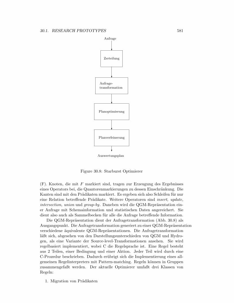
30.1. RESEARCH PROTOTYPES 581

Anfrage

?

Zerteilung

?

Anfrage-transformation

?

Planoptimierung

?

Planverfeinerung

?

Auswertungsplan

Figure 30.8: Starburst Optimierer

(F). Knoten, die mit F markiert sind, tragen zur Erzeugung des Ergebnisseseines Operators bei, die Quantorenmarkierungen zu dessen Einschrankung. DieKanten sind mit den Pradikaten markiert. Es ergeben sich also Schleifen fur nureine Relation betreffende Pradikate. Weitere Operatoren sind insert, update,intersection, union und group-by . Daneben wird die QGM-Reprasentation ein-er Anfrage mit Schemainformation und statistischen Daten angereichert. Siedient also auch als Sammelbecken fur alle die Anfrage betreffende Information.

Die QGM-Reprasentation dient der Anfragetransformation (Abb. 30.8) alsAusgangspunkt. Die Anfragetransformation generiert zu einer QGM-Reprasentationverschiedene aquivalente QGM-Reprasentationen. Die Anfragetransformationlaßt sich, abgesehen von den Darstellungsunterschieden von QGM und Hydro-gen, als eine Variante der Source-level-Transformationen ansehen. Sie wirdregelbasiert implementiert, wobei C die Regelsprache ist. Eine Regel bestehtaus 2 Teilen, einer Bedingung und einer Aktion. Jeder Teil wird durch eineC-Prozedur beschrieben. Dadurch erubrigt sich die Implementierung eines all-gemeinen Regelinterpreters mit Pattern-matching. Regeln konnen in Gruppenzusammengefaßt werden. Der aktuelle Optimierer umfaßt drei Klassen vonRegeln:

1. Migration von Pradikaten

582 CHAPTER 30. EXAMPLE QUERY COMPILER

2. Migration von Projektionen

3. Verschmelzung von Operationen

Fur die Ausfuhrung der Regeln stehen drei verschiedene Suchstrategien zurVerfugung:

1. sequentiell,

2. prioritatsgesteuert und

3. zufallig, gemaß einer gegebenen Verteilung.

Die Teilgraphen der QGM-Reprasentation, auf die Regeln anwendbar sind,konnen entweder durch eine depth-first oder eine breadth-first Suche bestimmtwerden. Falls mehrere alternative QGM-Reprasentationen existieren (was meis-tens der Fall ist), wird ein Choose-Operator [347] verwendet, der die verschiede-nen QGMs in einen QGM zusammenbaut. Die nachfolgende Phase wahlt dannkostenbasiert einen dieser alternativen QGMs aus. Dies ist nicht zwingend,die Auswahl kann auch erst zur Auswertungszeit stattfinden. Begrundet wirddieses Vorgehen damit, daß keine Kosten fur QGMs berechnet werden konnen,und somit keine Bewertung eines QGMs stattfinden kann. Wie die Autorenselbst anmerken, ist dieser Umstand sehr mißlich, da keine Alternativen ver-worfen werden konnen. Sie kundigen daher Untersuchungen an, die Transfor-mation (Schritt 2) mit der Planoptimierung (Schritt 3) zu verschmelzen. Umeine gewisse Kontrolle uber das Verhalten der Transformation zu haben, kanndiesem Schritt ein “budget” mitgegeben werden, nach dessen Ablauf der Schrittbeendet wird. Die genaue Funktionsweise des “budget” ist leider nicht erlautert.

Der Schritt der Planoptimierung (s. Abb. 30.8) kann mit der bisherigen Op-timierung verglichen werden. Sie arbeitet regelbasiert, benutzt aber nicht dentransformierenden, sondern den generierenden Ansatz [545]. Aus Basisopera-tionen – LOLEPOPs (LOw-LEvel Plan OPerator) genannt – werden mit (gram-matischen) Regeln – STARs (strategy alternative rules) genannt – (alternative)Auswertungsplane erzeugt. LOLEPOPs entstammen der um SCAN, SORTund ahnliche physische Operatoren angereicherten relationalen Algebra. EinAuswertungsplan ist dann ein Ausdruck von geschachtelten Funktionsaufrufen,wobei die Funktionen den LOLEPOPs entsprechen.

Ein STAR definiert ein benanntes parametrisiertes Objekt, das einem Nicht-terminalsymbol entspricht. Er besteht aus einer Menge von alternativen Defi-nitionen, die jede aus einer Bedingung fur die Anwendbarkeit und der Defini-tion eines Plans bestehen. Der generierte Plan kann LOLEPOPs (entsprechenTerminalsymbolen) und STARs referenzieren. Ein rootSTAR entspricht demStartsymbol der Grammatik. STARs ahneln den Regeln, die in Genesis nichtnur fur den Optimierer, sondern fur das ganze DBMS eingesetzt werden, umalternative Implementierungen zu erhalten [58, 56, 60, 59, 61]. Um erzeugteAlternativen fur einen Plan zusammenzusetzen und zu verhindern, daß dieseAlternativen die Anzahl der Plane in denen diese vorkommen, vervielfachen,wird ein Glue-Mechanismus eingesetzt. Dieser hat den Choose-Operator alsWurzel. Darunter hangen dann Alternativen, die beispielsweise einen Strom

30.1. RESEARCH PROTOTYPES 583

AlternativeAusf”uhrungs-

pl”ane

optimierterAlgebraausdruck

typkonsistenterAusdruck

Objektalgebra-ausdruck

normalisierterKalk”ulausdruck

deklarativeAnfrage

GenerierungAusf”uhrungs-

plan

Algebra-optimierung

Typ-”uberpr”ufung

Ubers. vonKalk”ul in

Algebra

Ubers. inKalk”ul

??????- - - - - -

Figure 30.9: Der Optimierer von Straube

mit gewissen Eigenschaften (Sortierung, Lokation) erzeugen. Von diesen Alter-nativen werden nur diejenigen betrachten, die die geringsten Kosten bei gleichenEigenschaften haben [520]. Die Kosten beziehen sich dabei immer nur auf denbisher erreichten Teilplan.

Der Aufbau eines Auswertungsplanes erfolgt Bottom-up. Die Menge deranwendbaren STARs wird in einer ToDo-Liste gehalten. Diese ist eine sortierteListe. Hiermit konnen dann verschiedene Suchstrategien implementiert werden,indem verschiedene Sortierungen fur die ToDo-Liste Verwendung finden [520].Ein Vorteil des STAR-Ansatzes ist die Vermeidung von Pattern-matching. Dieserlaubt es, die STARs zu interpretieren [520].

Die Beurteilung der Erweiterbarkeit ist sehr schwierig. Zum einen handelt essich um einen erweiterbaren Optimierer, da sowohl LOLEPOPs als auch STARshinzugefugt werden konnen. Der Glue-Mechanismus kann ebenfalls spezifiziertwerden, ohne in die Implementierung einzugreifen. Das Problem ist lediglichdie Komplexitat dieser Anderungen. Man kann diesen Ansatz daher vielleichtals bedingt erweiterbar kennzeichnen.

Eine Trennung der Optimierung in verschiedene Phasen wirft die damitverbundenen Probleme auf. Wie oben bereits angefuhrt, kundigen die Autorenweitere Untersuchungen an, um eine Verschmelzung der Phasen zu ermoglichen.Da keine Alternativen verworfen werden, ist es potentiell moglich, den opti-malen Auswertungsplan zu errechnen. Schwer zu sehen ist jedoch, wie einstetiger Leistungsabfall zu realisieren ist. Gleiches gilt fur die Evaluierbarkeitder einzelnen Komponenten (STARs).

More on Starburst can be found in [661, 662].

30.1.19 Der Optimierer von Straube

In seiner Dissertation stellt Straube den von ihm entwickelten Optimierer dar[821]. Die Ergebnisse dieser Arbeit flossen in eine Reihe von Veroffentlichungenein [856, 818, 819, 817, 820]. Der Aufbau des Optimierers ist in Abbildung 30.9skizziert. Eine Anfrage wird zunachst in den Objektkalkul ubersetzt und vondort in die Objektalgebra. Hier findet dann zunachst eine Typuberprufungstatt. Danach beginnt die eigentliche Optimierung. Diese besteht aus zweiPhasen, der algebraischen Optimierung und der Generierung des Ausfuhrungsplans.

Die erste Phase, die algebraische Optimierung, folgt dem Tranformation-sparadigma. Die algebraischen Ausdrucke werden mit Hilfe von Regeln in

584 CHAPTER 30. EXAMPLE QUERY COMPILER

aquivalente algebraische Ausdrucke transformiert. Straube beschrankt sichdabei im wesentlichen auf die Formulierung der Regeln. Fur die Abarbeitungder Regeln schlagt er lediglich die Verwendung des Exodus-Optimierergenerators[343] oder des Anfrageumformers von Starburst [394] vor.

Die zweite Phase, die Generierung der Ausfuhrungsplane, ist nicht regel-basiert. Ihr liegt eine sogenannte Ausfuhrungsplanschablone zu Grunde. Sie istvergleichbar mit einem Und/Oder-Baum, der alle moglichen Ausfuhrungsplaneimplizit beinhaltet. Zur Generierung eines konkreten Ausfuhrungsplans wirdder durch die Ausfuhrungsschablone aufgespannte Suchraum vollstandig durch-sucht. Der billigste Ausfuhrungsplan kommt dann zur Abarbeitung.

Da ein regelbasierten Ansatz fur die erste Phase gewahlt wurde und die Ver-wendung des Exodus-Optimierergenerators oder des Starburst-Anfrageumformersvorgeschlagen wird, verweisen wir fur die Bewertung dieser Phase auf die entsprechen-den Abschnitte.

Die zweite Phase ist voll auskodiert und damit schlecht erweiterbar. Einefruhe Bewertung der Alternativen ist nicht ausgeschlossen, wird aber nichtvorgenommen. Ein vollstandiges Durchsuchen verhindert naturlich auch denstetigen Leistungsabfall des Optimierers.

Erschwerend fur den gewahlten Ansatz kommt die Zweiphasigkeit hinzu.Es ist schwierig zu sehen, wie eine phasenubergreifende Kontrolle auszusehenhat, die zumindest potentiell Optimalitat gewahrleistet. Die Evaluierbarkeiteinzelner Komponenten des Optimierers ist nicht moglich.

30.1.20 Other Query Optimizer

Neben den in den vorangehenden Abschnitten erwahnten Optimierern gibt esnoch eine ganze Reihe anderer, die aber nicht im einzelnen vorgestellt werdensollen. Erwahnt werden sollen noch die Systeme Probe [214, 213, 628] undPrima [390, 388]. Der Schwerpunkt bei der Optimierung liegt im Primasys-tem auf dem dynamischen Zusammenbau von Molekulen. Es ware zu unter-suchen, ob ein Assembly-Operator (s. [463]) hier von Nutzen ware. Beson-ders erwahnenswert ist noch eine Arbeit, die Optimierungsmoglichkeiten furdie Datenbankprogrammiersprache FAD vorstellt [861]. Diese Arbeit stellteinen ersten Schritt in Richtung eines Optimierers fur eine General-purpose-Programmiersprache dar. Ein wesentlicher Punkt ist dabei, daß auch anderndeOperationen optimiert werden. Der Optimierer ist in zwei Module (RWR andOPT) eingeteilt. RWR ist ein Sprachmodul, das die Ubersetzung von FAD inein internes FAD vornimmt. Immer wenn RWR einen Ausdruck erkennt, derin der vom Optimierer OPT bearbeitbaren Sprache ausgedruckt werden kann,so wird dieser an den Optimierer weitergegeben und dort optimiert. Es wirdExhaustive search als Suchstrategie fur den Optimierer vorgeschlagen.

Im erweiterten O2-Kontext wurde das Zerteilen von Pfadausdrucken weit-er untersucht [179]. Es werden die Vorteile einer typisierten Algebra fur dieseZwecke herausgearbeitet. Eine graphische Notation sorgt fur eine anschaulicheDarstellung. Ihr besonderes Augenmerk richten die Autoren auf die Faktorisierunggemeinsamer Teilausdrucke. Einige der Ersetzungsregeln sind aus [774] und[773] entnommen und werden gewinnbringend eingesetzt, so beispielsweise die

30.1. RESEARCH PROTOTYPES 585

Ersetzung von Selektionen durch Verbundoperatoren.Ebenfalls erwahnt wurden bereits die Arbeiten im Orion-Kontext [49, 50,

473], die sich auf die Behandlung von Pfadausdrucken konzentrieren. Auch hierwurde ein funktionsfahiger Optimierer entwickelt.

Wie bereits erwahnt, stammt der erste regelbasierte Optimierer von Smithund Chang [794]. Doch erst die neueren Arbeiten fuhrten zu einer Blutedes regelbasierten Ansatzes. Hier ist insbesondere die Arbeit von Freytag zuerwahnen, die diese Blute mit initiierte [285]. Dort wird gezeigt, wie man mitHilfe eines regelbasierten Ansatzes den Optimierer von System R [755] emulierenkann. Die Eingabe besteht aus einem Lisp-ahnlichen Ausdruck:

(select <proj-list><sel-pred-list><join-pred-list><table-list>)

Die Projektionsliste besteht aus Attributspezifikationen der Form

<rel-name>.<attr-name>

Diese werden auch fur die Selektionspradikate und Joinpradikate verwendet.Die Algebra beinhaltet sowohl Operatoren der logischen als auch der physischenAlgebra. Im einzelnen gibt es Scan-, Sort-, Projektions, Verbundoperatoren ineiner logischen und verschiedenen physischen Auspragungen. Die Erzeugungder Auswertungsplane wird in verschiedene Schritte unterteilt, die wiederum inTeilschritte zerlegt sind (siehe Abb. 30.3).

Zunachst erfolgt die Ubersetztung in die logische Algebra. Hier werdenScan-Operatoren um die Relationen gebaut und Selektionen, die nur eine Re-lation betreffen, in die Scan-Operatoren eingebaut. Der zweite Schritt gener-iert Zugriffsplane, indem der Scan-Operator durch einen einfachen File-Scan(FSCAN) ersetzt wird oder falls moglich, durch einen Index-Scan (ISCAN).Der dritte Schritt generiert zunachst verschiedene Verbundreihenfolgen undbestimmt anschließend die Verbundmethoden. Wie in System R wird zwis-chen dem Sortiere-und-Mische-Verbund und dem Verbund durch geschachtelteSchleifen unterschieden. Es werden keinerlei Aussagen uber die Auswahl einerSuchstrategie gemacht. Ziel ist es vielmehr, durch die Modellierung des SystemR Optimierers mit Hilfe eines Regelsystems die prinzipielle Brauchbarkeit desregelbasierten Ansatzes nachzuweisen.

Man beachte auch die erwahnte Arbeit von Sciore und Sieg zur Modular-isierung von regelbasierten Optimierern [751]. Die Hauptidee von Sciore undSieg ist es, die Regelmenge in Module zu organisieren und jedem Modul eineeigene Suchstrategie, Kostenberechnung und Regelmenge zuzuordnen. Mod-ule konnen andere Module explizit aufrufen oder implizit ihre Ausgabemengean das nachste Modul weiterleiten. Der erste Optimierer des GOM-Systemsist ebenfalls regelbasiert [466, 465]. Die gesamte Regelmenge wurde hier inTeilmengen ahnlich zu den Modulen organisiert. Die Steuerung zwischen denTeilmengen erfolgt durch ein heuristisches Netz, das angibt in welchen Fallen zuwelcher weiteren Teilmenge von Regeln zu verzweigen ist. Die Strukturierungdes Optimiererwissens steht auch in [558] im Vordergrund.

586 CHAPTER 30. EXAMPLE QUERY COMPILER

In diesem Zusammenhang, der Strukturierung von Optimierern und derWiederverwendbarkeit einzelner Teile, sei noch einmal ausdrucklich auf dieArbeiten von Batory [59] aus dem Genesiskontext hingewiesen (s. auch Ab-schnitt 30.1.7). Der dort leider ein wenig zu kurz kommende Aspekt derWiederverwendbarkeit von Suchfunktionen wird in einer Arbeit von Lanzelotteund Valduriez [509] ausfuhrlicher behandelt. Hier wurde eine Typhierarchie ex-istierender Suchfunktionen entworfen und deren Schnittstellen vereinheitlicht.Die Suchfunktionen selbst wurden modularisiert. Weitere Arbeiten aus der-selben Gruppe beschaftigen sich mit der Optimierung von objektorientiertenAnfragen [508, 512], wobei hier die Behandlung von Pfaden im Vordergrundsteht. Eine neuere Arbeit beschaftigt sich mit der Optimierung von rekursivenAnfragen im objektorientierten Kontext [510].

Viele kommerzielle Systeme besitzen eine Anfragesprache und einen Opti-mierer. Einer der wenigen Optimierer, die auch in der Literatur beschriebenwerden, ist der von ObjectStore [627]. Durch die einfache Anfragesprache,die nur Teilmengenbestimmung erlaubt, und die strikte Verwendung von C-Semantik fur boolesche Ausdrucke sind die meisten Optimierungsmoglichkeitenjedoch ausgeschlossen, und der “Optimierer” ist daher sehr einfach.

30.2 Commercial Query Compiler

30.2.1 The DB 2 Query Compiler

30.2.2 The Oracle Query Compiler

Oracle still provides two modes for its optimizer. Dependent on the user spec-ified optimizer mode, a query is optimized either by the rule-based optimizer(RBO) or by the cost-based optimizer (CBO). The RBO is a heuristic optimizerthat resembles the simple optimizer of chapter 2. Here we concentrate on themore powerful CBO. The user can also determine whether the optimizer shouldoptimize for throughput or response time.

• nested loop join, nested loop outer join, index nested loop joins, sort mergejoin, sort merge outer join, hash joins, hash outer join, cartesian join, fullouter join, cluster join, anti-joins, semi-joins, uses bitmap indexes for starqueries

• sort group-by,

• bitmap indexes, bitmap join indexes

• index skip scans

• partitioned tables and indexes

• index-organized tables

• reverse key indexes

• function-based indexes

30.2. COMMERCIAL QUERY COMPILER 587

• SAMPLE clause in SELECT statement

• parallel query and parallel DML

• star transformations and star joins

• query rewrite with materialized views

• cost: considers CPU, I/O, memory

• access path: table scan, fast full index scan, index scan, ROWID scans(access ROW by ROWID), cluster scans, hash scans. [former two withprefetching] index scans:

– index unique scan (UNIQUE or PRIMARY KEY constraints)

– index range scan (one or more leading columns or key)

– index range scan descending

– index skip scan (> 1 leading key values not given)

– index full scan, index fast full scan

– index joins (joins indexes with hash join, resembles index anding)

– bitmap joins (index anding/oring)

– cluster scan: for indexed cluster to retrieve rows with the same clus-ter id

– hash scan: to locate rows in a hash cluster

CBO: parsed quer –¿ [query transformer] –¿ [estimator] –¿ [plan generator]1-16.

after parser: nested query blockssimple rewrites:

• eliminate between

• elminate x in (c1 . . . cn) (also uses IN-LIST iterator as outer table con-structor in a d-join or nested-loop join like operation.

query transformer:

• view merging

• predicate pushing

• subquery unnesting

• query rewrite using materialized views (cost based)

remaining subplans for nested query blocks are ordered in an efficient mannerplan generator:

• choose access path, join order (upper limit on number of permutationsconsidered), join method.

588 CHAPTER 30. EXAMPLE QUERY COMPILER

• generate subplan for every block in a bottom-up fashion

• (> 1 for still nested queries and unmerged views)

• stop generating more plans if there already exists a cheap plan

• starting plan: order by their effective cardinality

• considers normally only left-deep (zig-zag) trees.

• single row joins are placed first (based on unique and key constraints.

• join statement with outer join: table with outer join operator must comeafter the other table in the condition in the join order. optimizer doesnot consider join orders that violate this rule.

• NOT IN (SELECT . . . ) becomes a anti-join that is executed as a nested-loop join by default unless hints are given and various conditions are metwhich allow the transformation of the NOT IN uncorrelated subquery intoa sort-merge or hash anti-join.

• EXISTS (SELECT . . . ) becomes a semi-join. execution as index nestedloops, if there is an index. otherwise a nested-loop join is used by defaultfor EXISTS and IN subqueries that cannot be merged with the containingquery unless a hint specifies otherwise and conditions are met to allos thetransformation of the subquery into a sort-merge or hash semi-join.

• star query detection

cost:

• takes unique/key constraints into consideration

• low/high values and uniform distribution

• host variables: guess small selectivity value to favor index access

• histograms

• common subexpression optimization

• complex view merging

• push-join predicate

• bitmap access paths for tables with only B-tree indexes

• subquery unnesting

• index joins

rest:

• Oracle allows user hints in SQL statements to influence the Optimizer.for example join methods can be given explicitly

30.2. COMMERCIAL QUERY COMPILER 589

parameters:

• HASH AREA SIZE

• SORT AREA SIZE

• DB FILE MULTIBLOCK READ COUNT (number of prefetched pages)

statistics:

• table statisticsnumber of rows, number of blocks, average row length

• column statisticsnumber of distinct values, number of nulls, data distribution

• index statisticsnumber of keys, (from column statistics?) number of leaf blocks, levels,clustering factor (collocation amount of the index block/data blocks, 3-17)

• system statisticsI/O performance and utilization, cpu performance and utilization

generating statistics:

• estimation based on random data sampling(row sampling, block sampling)

• exact computation

• user-defined statistics collection methods

histograms:

• height-based histograms (approx. equal number of values per bucket)

• value-based histogramsused for number of distinct values ≤ number of buckets

• support of index-only queries

• index-organized tables

• bitmap indexes (auch fuer null-werte x <> const)

• convert b-tree result RID lists to bitmaps for further bitmap anding

• bitmaps and count

• bitmap join index

• cluster tables (cluster rows of different tables on the same block)

• hash clusters

590 CHAPTER 30. EXAMPLE QUERY COMPILER

• hint: USE CONCAT: OR ::= UNION ALL

• hint: STAR TRANSFORMATION: see Oracle9i Database Concepts

• NOT IN ::= anti-join

• EXISTS ::= special join preserving duplicates and adding no phantomduplicates (semi-join) (5-27)

• continue 5-35

30.2.3 The SQL Server Query Compiler

Part VI

Selected Topics

591

Chapter 31

Generating Plans forTop-N-Queries?

31.1 Motivation and Introduction

motivation:

• first by user (ordered)

• optimize for n rows (user/cursor)

• exist(subquery) optimize for 1 row

• having count(*) <= n

31.2 Optimizing for the First Tuple

31.3 Optimizing for the First N Tuples

• nl-join instead of sm/hash join

• index access over table scan

• disable prefetching

[122, 123, 124] [144, 237] [258, 259, 416] [533][365] (also contains inverted list algorithms under frequent updates)[533]

593

594 CHAPTER 31. GENERATING PLANS FOR TOP-N-QUERIES?

Chapter 32

Recursive Queries

595

596 CHAPTER 32. RECURSIVE QUERIES

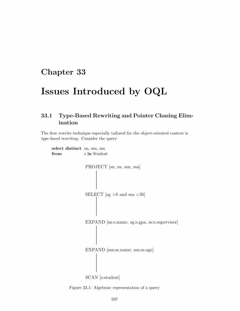
Chapter 33

Issues Introduced by OQL

33.1 Type-Based Rewriting and Pointer Chasing Elim-ination

The first rewrite technique especially tailored for the object-oriented context istype-based rewriting . Consider the query

select distinct sn, ssn, ssafrom s in Student

SCAN [s:student]

EXPAND [ssn:ss.name, ssa:ss.age]

EXPAND [sn:s.name, sg:s.gpa, ss:s.supervisor]

SELECT [sg >8 and ssa <30]

PROJECT [sn, sa, ssn, ssa]

Figure 33.1: Algebraic representation of a query

597

598 CHAPTER 33. ISSUES INTRODUCED BY OQL

where sg > 8 and ssa < 30define sn = s.name

sg = s.gpass = s.supervisorssn= ss.namessa= ss.age

The algebraic expression in Fig. 33.1 implies a scan of all students and a sub-sequent dereferentiation of the supervisor attribute in order to access the su-pervisors. If not all supervisors fit into main memory, this may result in manypage accesses. Further, if there exists an index on the supervisor’s age, andthe selection condition ssa < 30 is highly selective, the index should be appliedin order to retrieve only those supervisors required for answering the query.Type-based rewriting enables this kind of optimization. For any expression ofcertain type with an associated extent, the extent is introduced in the fromclause. For our query this results in

select distinct sn, pn, pafrom s in Student, p in Professorwhere sg > 8 and pa < 30 and ss = pdefine sn = s.name

sg = s.gpass = s.supervisorpn = ss.namepa = ss.age

As a side-effect, the attribute traversal from students via supervisor to professoris replaced by a join. Now, join-ordering allows for several new plans that couldnot be investigated otherwise. For example, we could exploit the above men-tioned index to retrieve the young professors and join them with the studentshaving a gpa greater than 8. The according plan is given in Fig. 33.2. Turningimplicit joins or pointer chasing into explicit joins which can be freely reorderedis an original query optimization technique for object-oriented queries. Notethat the plan generation component is still allowed to turn the explicit join intoan implicit join again.

Consider the query

select distinct pfrom p in Professorwhere p.room.number = 209

Straight forward evaluation of this query would scan all professors. For everyprofessor, the room relationship would be traversed to find the room where theprofessor resides. Last, the room’s number would be retrieved and tested to be209. Using the inverse relationship, the query could as well be rewritten to

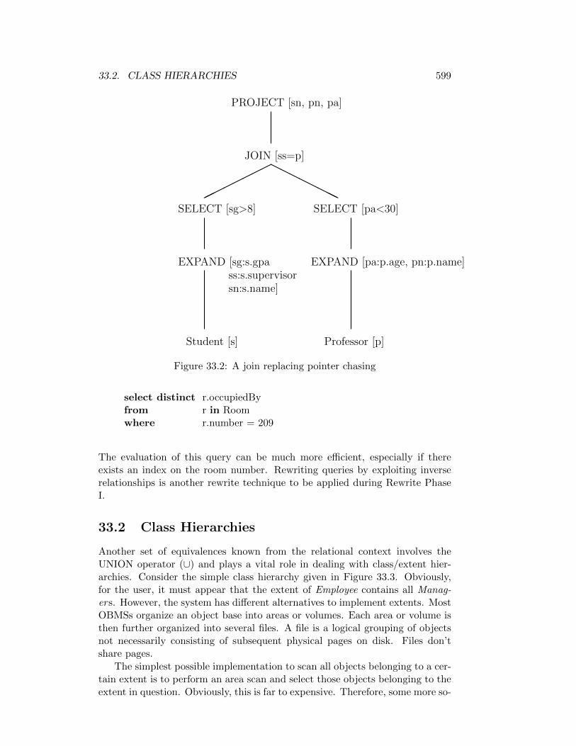
33.2. CLASS HIERARCHIES 599

HHHHHH

HH

PROJECT [sn, pn, pa]

JOIN [ss=p]

SELECT [sg>8]

EXPAND [pa:p.age, pn:p.name]

Professor [p]Student [s]

SELECT [pa<30]

EXPAND [sg:s.gpass:s.supervisorsn:s.name]

Figure 33.2: A join replacing pointer chasing

select distinct r.occupiedByfrom r in Roomwhere r.number = 209

The evaluation of this query can be much more efficient, especially if thereexists an index on the room number. Rewriting queries by exploiting inverserelationships is another rewrite technique to be applied during Rewrite PhaseI.

33.2 Class Hierarchies

Another set of equivalences known from the relational context involves theUNION operator (∪) and plays a vital role in dealing with class/extent hier-archies. Consider the simple class hierarchy given in Figure 33.3. Obviously,for the user, it must appear that the extent of Employee contains all Manag-ers. However, the system has different alternatives to implement extents. MostOBMSs organize an object base into areas or volumes. Each area or volume isthen further organized into several files. A file is a logical grouping of objectsnot necessarily consisting of subsequent physical pages on disk. Files don’tshare pages.

The simplest possible implementation to scan all objects belonging to a cer-tain extent is to perform an area scan and select those objects belonging to theextent in question. Obviously, this is far to expensive. Therefore, some more so-

600 CHAPTER 33. ISSUES INTRODUCED BY OQL

Employee name: stringsalary: intboss: Manager6

Managerboss: CEO

6

CEO

Figure 33.3: A Sample Class Hierarchy

phisticated possibilities to realize extents and scans over them are needed. Thedifferent possible implementations can be classified along two dimensions. Thefirst dimension distinguishes between logical and physical extents, the seconddistinguishes between strict and (non-strict) extents.

Logical vs. Physical ExtentsAn extent can be realized as a collection of object identifiers. A scan overthe extent is then implemented by a scan over all the object identifierscontained in the collection. Subsequently, the object identifiers are deref-erenced to yield the objects themselves. This approach leads to logicalextents. Another possibility is to implement extent membership by phys-ical containment. The best alternative is to store all objects of an extentin a file. This results in physical extents. A scan over a physical extent isthen implemented by a file scan.

Extents vs. Strict ExtentsA strict extent contains the objects (or their OIDs) of a class excludingthose of its subclasses. A non-strict extent contains the objects of a classand all objects of its subclasses.

Given a class C, any strict extent of a subclass C ′ of C is called a subextentof C.

Obviously, the two classifications are orthogonal. Applying them both re-sults in the four possibilities presented graphically in Fig. 33.4. [187] stronglyargues that strict extents are the method of choice. The reason is that onlythis way the query optimizer might exploit differences for extents. For example,there might be an index on the age of Manager but not for Employee. Thisdifference can only be exploited for a query including a restriction on age, if wehave strict extents.

However, strict extents result in initial query plans including UNION oper-ators. Consider the query

select efrom e in Employeewhere e.salary > 100.000

33.3. CARDINALITIES AND COST FUNCTIONS 601

ob1C:

ob2C1: ob3C2:

C1: id2 C1: id1, id2C2: id3 id1, id3

excluding

C1: C2:

C:

ob1, ob2

ob1

ob1, ob3

including

physical

C: id1 C: id1logical

Figure 33.4: Implementation of Extents

The initial plan is

σsa>100.000(χsa:x.salary((Employee[x] ∪Manager[x]) ∪ CEO[x]))

Hence, algebraic equivalences are needed to reorder UNION operators withother algebraic operators. The most important equivalences are

e1 ∪ e2 ≡ e2 ∪ e1 (33.1)

e1 ∪ (e2 ∪ e3) ≡ (e1 ∪ e2) ∪ e3 (33.2)

σp(e1 ∪ e2) ≡ σp(e1) ∪ σp(e2) (33.3)

χa:e(e1 ∪ e2) ≡ χa:e(e1) ∪ χa:e(e2) (33.4)

(e1 ∪ e2) 1p e3 ≡ (e1 1p e3) ∪ (e2 1p e3) (33.5)

Equivalences containing the UNION operator sometimes involve tricky typingconstraints. These go beyond the current chapter and the reader is refered to[590].

33.3 Cardinalities and Cost Functions

602 CHAPTER 33. ISSUES INTRODUCED BY OQL

Chapter 34

Issues Introduced by XPath

34.1 A Naive XPath-Interpreter and its Problems

34.2 Dynamic Programming and Memoization

[324, 326, 325]

34.3 Naive Translation of XPath to Algebra

34.4 Pushing Duplicate Elimination

34.5 Avoiding Duplicate Work

34.6 Avoiding Duplicate Generation

[400]

34.7 Index Usage and Materialized Views

[47]

34.8 Cardinalities and Costs

34.9 Bibliography

603

604 CHAPTER 34. ISSUES INTRODUCED BY XPATH

Chapter 35

Issues Introduced by XQuery

35.1 Reordering in Ordered Context

35.2 Result Construction

[271, 272] [769]

35.3 Unnesting Nested XQueries

Unnesting with error: [646][570, 572, 571, 573]

35.4 Cardinalities and Cost Functions

cardinality: [160, 908, 909, 732] [7]XPathLearner: [539]Polyzotis et al (XSKETCH): [667, 668, 665], [669]

35.5 Bibliography

[576] [850] [224]Numbering: [270] Timber [441] TAX Algebra [444], physical algebra of Tim-

ber [647]Structural Joins [20, 798]SAL: [69], TAX: [444], XAL: [283]

• XML Statistics for hidden web: [8]

• XPath selectivity for internet scale: [7]

• StatiX: [284]

• IMAX: incremental statistics [683]

• Metrics for XML Document Collections: [479]

605

606 CHAPTER 35. ISSUES INTRODUCED BY XQUERY

• output size containment join: [876]

• Bloom Histogram: [877]

View and XML: [2]Quilt: [136]Timber: [441] Monet: [745] Natix: NoK: [936]Correlated XPath: [937]Wood: [900, 901, 902]Path based approach to Storage (XRel): [927]Grust: [356, 358, 357, 359, 841]Liefke: Loop fusion etc.: [538]Benchmarking: XMach-1: [93], MBench: [721] XBench: [640, 919, 920],

XMark: [746] XOO7: [104]Rewriting: [228, 349, 350][227, 411]Incremental Schema Validation: [97, 645]Franklin (filtering): [231]

Chapter 36

Outlook

What we did not talk about: multiple query optimization, semantic queryoptimization, special techniques for optimization in OBMSs, multi-media databases, object-relational databases, spatial databases, temporal databases, andquery optimization for parallel and distributed database systems.

Multi Query Optimization? [758]

Parametric/Dynamic/Adaptive Query Optimization? [32, 33, 34, 29,347, 340] [437, 438, 455, 857]

[44]

Parallel Database Systems?

Distributed Database Systems? [494]

Recursive Queries?

Multi Database Systems?

Temporal Database Systems?

Spatial Database Systems?

Translation of Triggers and Updates?

Online Queries (Streams)?

Approximate Answers? [316]

607

608 CHAPTER 36. OUTLOOK

Appendix A

Query Languages?

A.1 Designing a query language

requirementsdesign principles for object-oriented query languages: [410] [80]

A.2 SQL

A.3 OQL

A.4 XPath

A.5 XQuery

A.6 Datalog

609

610 APPENDIX A. QUERY LANGUAGES?

Appendix B

Query Execution Engine (?)

• Overview Books: [389, 305]

• Overview: Graefe [333, 334]

• Implementation of Division [330, 339, 341]

• Implementation of Division and set-containment joins [680]

• Hash vs. Sort: [335, 344]

• Heap-Filter Merge Join: [332]

• Hash-Teams

611

612 APPENDIX B. QUERY EXECUTION ENGINE (?)

Appendix C

Glossary of Rewrite andOptimization Techniques

trivopt Triviale Auswertungen bspw. solche fur widerspruchliche Pradikatewerden sofort vorgenommen. Dies ist eine Optimierungstechnik, die oftbereits auf der Quellebene durchgefuhrt wird.

pareval Falls ein Glied einer Konjunktion zu false evaluiert, werden die restlichenGlieder nicht mehr evaluiert. Dies ergibt sich automatisch durch die Ver-wendung von hintereinanderausgefuhrten Selektionen.

pushnot Falls ein Pradikat die Form ¬(p1 ∧ p2) hat, so ist pareval nicht an-wendbar. Daher werden Negationen nach innen gezogen. Auf ¬p1 ∨ ¬p2

ist pareval dann wieder anwendbar. Das Durchschieben von Negationenist auch im Kontext von NULL-Werten unabdingbar fur die Korrektheit.Dies ist eine Optimierungstechnik, die oft bereits auf der Quellebenedurchgefuhrt wird.

bxp Verallgemeinert man die in pareval und notpush angesprochene Prob-lematik, so fuhrt dies auf die Optimierung von allgemeinen booleschenPradikaten.

trans Durch Ausnutzen der Transitivitat von Vergleichsoperationen konnenneue Selektionspradikate gewonnen und Konstanten propagiert werden.Diese Optimierungstechnik erweitert den Suchraum und wird ebenfalls aufder Quellebene durchgefuhrt. Bei manchen Systemen wir dieser Schrittnicht durchgefuhrt, falls sehr viele Relationen zu joinen sind, um denSuchraum nicht noch weiter zu vergroßern [311, 312].

selpush Selektionen werden so fruh wie moglich durchgefuhrt. Diese Technikfuhrt nicht immer zu optimalen Auswertungsplanen und stellt somit eineHeuristik dar. Diese Optimierungstechnik schrankt den Suchraum ein.

projpush Die Technik zur Behandlung von Projektionen ist nicht ganz so ein-fach wie die der Selektion. Zu unterscheiden ist hier, ob es sich um eineProjektion mit Duplikateliminierung handelt oder nicht. Je nach dem

613

614APPENDIX C. GLOSSARYOF REWRITE ANDOPTIMIZATION TECHNIQUES

ist es sinnvoll, die Projektion zur Wurzel des Operatorgraphen zu ver-schieben oder zu den Blattern hin. Die Projektion verringert den Spe-icherbedarf von Zwischenergebnissen, da die Tupel weniger Attribute en-thalten. Handelt es sich um eine duplikateliminierende Projektion, so wirdmoglicherweise auch die Anzahl der Tupel verringert. Duplikatelimina-tion als solche ist aber eine sehr teure Operation. Diese wird ublicherweisedurch Sortieren implementiert. Bei großen Datenmengen gibt es allerdingsbessere Alternativen. Auch Hash-basierte Verfahren eignen sich zur Du-plikateliminierung. Diese Optimierungstechnik schrankt den Suchraumein.

grouppush Pushing a grouping operation past a join can lead to better plans.

crossjoin Ein Kreuzprodukt, das von einer Selektion gefolgt wird, wird wennimmer moglich in eine Verbundoperation umgewandelt. Diese Optimierung-stechnik schrankt den Suchraum ein, da Plane mit Kreuzprodukten ver-mieden werden.

nocross Kreuzprodukte werden wenn immer moglich vermieden oder, wenndies nicht moglich ist, erst so spat wie moglich durchgefuhrt. DieseTechnik verringert den Suchraum, fuhrt aber nicht immer zu optimalenAuswertungsplanen.

semjoin Eine Verbundoperation kann durch eine Semiverbundoperation erset-zt werden, wenn nur die Attribute einer Relation weitere Verwendungfinden.

joinor Die Auswertungsreihenfolge von Verbundoperationen ist kritisch. Da-her wurden eine Reihe von Verfahren entwickelt, die optimale oder quasi-optimale Reihenfolge von Verbundoperationen zu bestimmen. Oft wirddabei der Suchraum auf Listen von Verbundoperationen beschrankt. DieMotivation hierbei ist das Verkleinern des Suchraums und die Beschrankungauf nur eine zu erzeugenden Zwischenrelation. Dieses Verfahren garantiertnicht mehr ein optimales Ergebnis.

joinpush Tables that are guaranteed to produce a single tuple are alwayspushed to be joined first. This reduces the search space. The single tuplecondition can be evaluated by determining whether all key attributes ofa relation are fully qualified. [311, 312].

elimredjoin Eliminate redundant join operations. See Sections. . . XXX

indnest Eine direkte Evaluierung von geschachtelten Anfragen wird durchgeschachtelte Schleifen vorgenommen. Dabei wird eine Unteranfrage furjede erzielte Bindung der außeren Anfrage evaluiert. Dies erfordert quadratis-chen Aufwand und ist deshalb sehr ineffizient. Falls die innere Anfrageunabhangig von der außeren Anfrage evaluiert werden kann, so wird dieseherausgezogen und getrennt evaluiert. Weitere Optimierungen geschachtel-ter Anfragen sind moglich.

615

unnest Entschachtelung von Anfragen [181, 183, 303, 474, 480, 481, 661, 801,803, 804]

compop Oft ist es sinnvoll, mehrere Operationen zu einer komplexeren zusam-menzufassen. Beispielsweise konnen zwei hintereinander ausgefuhrte Se-lektionen durch eine Selektion mit einem komplexeren Pradikat ersetztwerden. Ebenso kann auch das Zusammenfassen von Verbundoperatio-nen, Selektionen und Projektionen sinnvoll sein.

comsubexpr Gemeinsame Teilausdrucke werden nur einfach evaluiert. Hierunterfallen zum einen Techniken, die das mehrmalige Lesen vom Hintergrund-speicher verhindern, und zum anderen Techniken, die Zwischenergebnissevon Teilausdrucken materialisieren. Letzteres sollte nur dann angewen-det werden, falls die k-malige Auswertung teurer ist als das einmaligeAuswerten und das Erzeugen des Ergebnisses mit k-maligem Lesen, wobeik die Anzahl der Vorkommen im Plan ist.

dynminmax Dynamisch gewonnene Minima und Maxima von Attributwertenkonnen fur die Erzeugung von zusatzlichen Restriktionen herangezogenwerden. Diese Technik funktioniert auch sehr gut fur unkorrelierte An-fragen. Dabei werden min- und max-Werte herangezogen um zusatzlicheRestriktionen fur die Anfrage zu gewinnen. [480, 311, 312]

pma Predicate Move around moves predicates between queries and subqueries.Mostly they are duplicated in order to yield as many restrictions in a blockas possible [530]. As a special case, predicates will be pushed into viewdefinitions if they have to be materialized temporarily [311, 312].

exproj For subqueries with exist prune unnecessary entries in the select clause.The intention behind is that attributes projected unnecessarily might in-fluence the optimizer’s decision on the optimal access path [311, 312].

vm View merging expands the view definition within the query such that iscan be optimized together with the query. Thereby, duplicate accesses tothe view are resolved by different copies of the views definition in orderto facilitate unnesting [311, 312, 661].

inConstSet2Or A predicate of the form x ∈ a1, . . . , an is transformed intoa sequence of disjunctions x = a1 ∨ . . . ∨ x = an if the ai are constants inorder to allow index or-ing (TID list operations or bitvector operations)[311, 312].

like1 If the like predicate does not start with %, then a prefix index can beused.

like2 The pattern is analyzed to see whether a range of values can be extractedsuch that the pattern does not have to be evaluated on all tuples. Theresult is either a pretest or an index access. [311, 312].

like3 Special indexes supporting like predicates are introduced.

616APPENDIX C. GLOSSARYOF REWRITE ANDOPTIMIZATION TECHNIQUES

sort Vorhandene Sortierungen konnen fur verschiedene Operatoren ausgenutztwerden. Falls keine Sortierung vorhanden ist, kann es sinnvoll sein, diesezu erzeugen [789]. Z.B. aufeinanderfolgende joins, joins und gruppierun-gen. Dabei kann man die Gruppierungsattribute permutieren, um sie miteiner gegebenen Sortierreihenfolge in Einklang zu bringen [311, 312].

aps Zugriffspfade werden eingesetzt, wann immer dies gewinnbringend moglichist. Beispielsweise kann die Anfrage

select count(*) from R;

durch einen Indexscan effizient ausgewertet werden [163].

tmpidx Manchmal kann es sinnvoll sein, temporare Zugriffspfade anzulegen.

optimpl Fur algebraische Operatoren existieren im allgemeinen mehrere Im-plementierungen. Es sollte hier immer die fur einen Operator im vorliegen-den Fall billigste Losung ausgewahlt werden. Ebenfalls von Bedeutung istdie Darstellung des Zwischenergebnisses. Beispielsweise konnen Relatio-nen explizit oder implizit dargestellt werden, wobei letztere Darstellungnur Zeiger auf Tupel oder Surrogate der Tupel enthalt. Weitergedachtfuhrt diese Technik zu den TID-Listen-basierten Operatoren.

setpipe Die Evaluation eines algebraischen Ausdrucks kann entweder mengenori-entiert oder nebenlaufig (pipelining) erfolgen. Letzteres erspart das Erzeu-gen von großen Zwischenergebnissen.

tmplay Das temporare Andern eines Layouts eines Objektes kann durchaussinnvoll sein, wenn die Kosten, die durch diese Anderung entstehen, durchden Gewinn der mehrmaligen Verwendung dieses Layouts mehr als kom-pensiert werden. Ein typisches Beispiel ist Pointer-swizzling .

matSubQ If a query is not unnested, then for every argument combinationpassed to the subquery, the result is materialized in order to avoid du-plicate computation of the same subquery expression for the same argu-ment combination [311, 312]. This technique is favorable for detachment[816, 898, 928]

AggrJoin Joins with non-equi join predicates based on ≤ or <, can be pro-cessed more efficiently than by a cross product with a subsequent selection[185].

ClassHier Class hierarchies involve the computation of queries over a unionof extents (if implemented that way). Pushing algebraic operations pastunions allows often for more efficient plans [187].

AggrIDX Use an index to determine aggregate values like min/max/avg/count.

rid/tidsort When several tuples qualify during an index scan, the resultingTIDs can be sorted in order to guarantee sequential access to the baserelation.

617

multIDX Perform operations like union and disjunction on the outcome of anindex scan.

multIDXsplit If two ranges are queried within the same query ([1-10],[20-30])consider multIDX or use a single scan through the index [1-30] with anadditional qualification predicate.

multIDXor Queries with more conditions on indexed attributes can be evalu-ated by more complex combinations of index scans and tid-list/bitvectoroperations. (A = 5 and (B = 3 or B = 4)).

scanDirChange During multiple sequential scans of relation (e.g. for a block-wise nested loop join), the direction of the scan can be changed in orderto reuse as much of the pages in the buffer as possible.

lock The optimizer should chose the correct locks to set on tables. For example,if a whole table is scanned, a table lock should be set.

expFunMat Expensive functions can be cached during query evaluation inorder to avoid their multiple evaluation for the same arguments [398].

expFunFil Easiser to evaluate predicates that are implied by more expensivepredicates can serve as filters in order to avoid the evaluation of the ex-pensive predicate on all tuples.

stop Stop evaluation after the first tuple qualifies. This is good for existentialsubqueries, universal subqueries (disqualify), semi-joins for distinct resultsand the like.

expensive projections 1. zum Schluss, da dort am wenigsten verschiedeneWerte

2. durchschieben, falls cache fuer Funktionsergebnisse dadurch vermiedenwerden kann

OO-Kontext: problematisch: objekte muessen fuer funktionen/methodenals ganzes vorhanden sein. daher ist eine einfache strategie nicht moeglich.

distinct/sorting select distinct a,b,c

...

order by a,b

kann auch nach a,b,c sortiert werden. stoert gar nicht, vereinfacht aberdie duplikateliminierung. nur ein sortieren notwendig.

index access • by key

• by key range

• by dashed key range (set of keys/key ranges)

• index anding/oring

618APPENDIX C. GLOSSARYOF REWRITE ANDOPTIMIZATION TECHNIQUES

alternative operator implementations e.g. join: nlj bnlj hj grace-hashhybrid-hash smj diag-join star-join

distpd Push-down or Pull-up distinct.

aggregate with distinct select a, agg(distinct b)

...

group by a

===>

sort on a,b

dup elim

group a,sum(b)

alternative: aggr(distinct *) is implemented such that it uses a hashtableto eliminate duplicates this is only good, if the number of groups is smal-land the number of distinct values in each group is small.

XXX - use keys, inclusion dependencies, fds etc. (all user specified and de-rived) (propagate keys over joins as fds), (for a function call: derived IU isfunctional dependend on arguments of the function call if function is de-terministic) (keys can be represented as sets of IUs or as bitvectors(givennumbering of IUs)) (numbering inprecise: bitvectors can be used as filters(like for signatures))

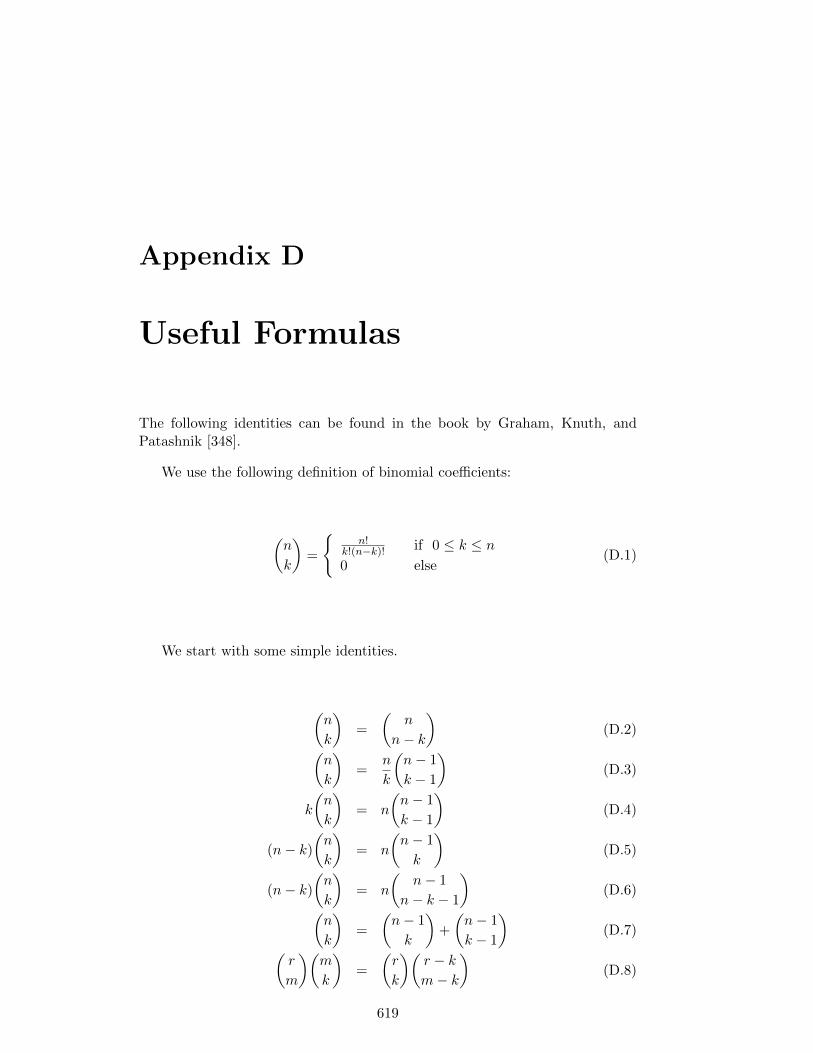
Appendix D

Useful Formulas

The following identities can be found in the book by Graham, Knuth, andPatashnik [348].

We use the following definition of binomial coefficients:

(n

k

)=

n!

k!(n−k)! if 0 ≤ k ≤ n0 else

(D.1)

We start with some simple identities.

(n

k

)=

(n

n− k

)(D.2)

(n

k

)=

n

k

(n− 1

k − 1

)(D.3)

k

(n

k

)= n

(n− 1

k − 1

)(D.4)

(n− k)

(n

k

)= n

(n− 1

k

)(D.5)

(n− k)

(n

k

)= n

(n− 1

n− k − 1

)(D.6)

(n

k

)=

(n− 1

k

)+

(n− 1

k − 1

)(D.7)

(r

m

)(m

k

)=

(r

k

)(r − km− k

)(D.8)

619

620 APPENDIX D. USEFUL FORMULAS

The following identities are good for sums of binomial coefficients.

n∑

k=0

(n

k

)= 2n (D.9)

n∑

k=0

(k

m

)=

(n+ 1

m+ 1

)(D.10)

n∑

k=0

(m+ k

k

)=

(m+ n+ 1

m+ 1

)=

(m+ n+ 1

n

)(D.11)

n∑

k=0

(m− n+ k

k

)=

(m+ 1

n

)(D.12)

From Identities D.2 and D.11 it follows that

m∑

k=0

(k + r

r

)=

(m+ r + 1

r + 1

)(D.13)

For sums of products, we have

n∑

k=0

(r

m+ k

)(s

n− k

)=

(r + s

m+ n

)(D.14)

n∑

k=0

(l − km

)(q + k

n

)=

(l + q + 1

m+ n+ 1

)(D.15)

n∑

k=0

(l

m+ k

)(s

n+ k

)=

(l + s

l −m+ n

)(D.16)

Bibliography

[1] K. Aberer and G. Fischer. Semantic query optimization for methods inobject-oriented database systems. In Proc. IEEE Conference on DataEngineering, pages 70–79, 1995.

[2] S. Abiteboul. On Views and XML. In Proc. ACM SIGMOD/SIGACTConf. on Princ. of Database Syst. (PODS), pages 1–9, 1999.

[3] S. Abiteboul, C. Beeri, M. Gyssens, and D. Van Gucht. An introductionto the completeness of languages for complex objects and nested relations.In S. Abiteboul, P.C. Fischer, and H.-J. Schek, editors, Nested Relationsand Complex Objects in Databases, pages 117–138. Lecture PAGESs inComputer Science 361, Springer, 1987.

[4] S. Abiteboul and N. Bidoit. Non first normal form relations: An alge-bra allowing restructuring. Journal of Computer Science and Systems,33(3):361, 1986.

[5] S. Abiteboul, S. Cluet, V. Christophides, T. Milo, G. Moerkotte, andJ. Simeon. Querying documents in object databases. International Jour-nal on Digital Libraries, 1(1):5–19, April 1997.

[6] S. Abiteboul and O. Duschka. Complexity of answering queries usingmaterialized views. In Proc. ACM SIGMOD/SIGACT Conf. on Princ.of Database Syst. (PODS), pages 254–263, 1998.

[7] A. Aboulnaga, A. Alameldeen, and J. Naughton. Estimating the selectiv-ity of XML path expressions for internet scale applications. In Proc. Int.Conf. on Very Large Data Bases (VLDB), pages 591–600, 2001.

[8] A. Aboulnaga and J. Naughton. Building XML statistics for the hiddenweb. In Int. Conference on Information and Knowledge Management(CIKM), pages 358–365, 2003.

[9] W. Abu-Sufah, D. J. Kuch, and D. H. Lawrie. On the performance en-hancement of paging systems through program analysis and transforma-tions. IEEE Trans. on Computers, C-50(5):341–355, 1981.

[10] B. Adelberg, H. Garcia-Molina, and J. Widom. The STRIP rule systemfor efficiently maintaining derived data. In Proc. of the ACM SIGMODConf. on Management of Data, pages 147–158, 1997.

621

622 BIBLIOGRAPHY

[11] F. Afrati, M. Gergatsoulis, and T. Kavalieros. Answering queries usingmaterialized views with disjunctions. In Proc. Int. Conf. on DatabaseTheory (ICDT), pages 435–452, 1999.

[12] F. Afrati, C. Li, and J. Ullman. Generating efficient plans for queriesusing views. In Proc. of the ACM SIGMOD Conf. on Management ofData, pages 319–330, 2001.

[13] F. Afrati and C. Papadimitriou. The parallel complexity of simple chainqueries. In Proc. ACM SIGMOD/SIGACT Conf. on Princ. of DatabaseSyst. (PODS), pages 210–?, 1987.

[14] D. Agrawal, A. Abbadi, A. Singh, and T. Yurek. Efficient view main-tenance at data warehouses. In Proc. of the ACM SIGMOD Conf. onManagement of Data, pages 417–427, 1997.

[15] A. Aho, Y. Sagiv, and J. Ullman. Efficient optimization of a class ofrelational expressions. ACM Trans. on Database Systems, 4(4):435–454,1979.

[16] A. Aho, Y. Sagiv, and J. Ullman. Equivalence of relational expressions.SIAM J. on Computing, 8(2):218–246, 1979.

[17] A. V. Aho, C. Beeri, and J. D. Ullman. The theory of joins in relationaldatabases. ACM Trans. on Database Systems, 4(3):297–314, 1979.

[18] A. V. Aho, Y. Sagiv, and J. D. Ullman. Efficient optimization of a classof relational expression. ACM Trans. on Database Systems, 4(4):435–454,1979.

[19] A.V. Aho, Y. Sagiv, and J.D. Ullman. Equivalence among relationalexpressions. SIAM Journal on Computing, 8(2):218–246, 1979.

[20] S. Al-Khalifa, H. Jagadish, N. Koudas, J. Patel, D. Srivastava, and Y. Wu.Structural joins: A primitive for efficient XML query pattern matching.In Proc. IEEE Conference on Data Engineering, pages 141–152, 2002.

[21] J. Albert. Algebraic properties of bag data types. In Proc. Int. Conf. onVery Large Data Bases (VLDB), pages 211–219, 1991.

[22] F. E. Allen and J. Cocke. A catalogue of optimizing transformations.In R. Rustin, editor, Design and optimization of compilers, pages 1–30.Prentice Hall, 1971.

[23] N. Alon, P. Gibbons, Y. Matias, and M. Szegedy. Tracking join and self-join sizes in limited storage. J. Comput System Sciences, 35(4):391–432,2002.

[24] N. Alon, Y. Matias, and M. Szegedy. The space complexity of approx-imating the frequency moments. J. of Computer and System Sciences,58(1):137–147, 1999.

BIBLIOGRAPHY 623

[25] J. Alsabbagh and V. Rahavan. Analysis of common subexpression ex-ploitation models in multiple-query processing. In Proc. IEEE Conferenceon Data Engineering, pages 488–497, 1994.

[26] P. Alsberg. Space and time savings through large database compressionand dynamic restructuring. In Proc IEEE 63,8, Aug. 1975.

[27] D. Donoho amd M. Elad. Optimally sparse representation in general(non-orthogonal) dictionaries via `1 minimization. Proc. of the NationalAcademy of Sciences, 100(5):2197–2202, 2003.

[28] S. Amer-Yahia, S. Cho, L. Lakshmanan, and D. Srivastava. Efficientalgorithms for minimizing tree pattern queries. In Proc. of the ACMSIGMOD Conf. on Management of Data, pages 497–508, 2001.

[29] L. Amsaleg, M. Franklin, A. Tomasic, and T. Urhan. Scrambling queryplans to cope with unexpected delay. In 4th Int. Conference on Paralleland Distributed Information Systems (PDIS), Palm Beach, Fl, 1996.

[30] O. Anfindsen. A study of access path selection in DB2. Technical report,Norwegian Telecommunication Administration and University of Oslo,Norway, Oct. 1989.

[31] G. Antoshenkov. Random sampling from pseudo-ranked b+-trees. In Proc.Int. Conf. on Very Large Data Bases (VLDB), pages 375–382, 1992.

[32] G. Antoshenkov. Dynamic query optimization in RDB/VMS. In Proc.IEEE Conference on Data Engineering, pages 538–547, Vienna, Apr.1993.

[33] G. Antoshenkov. Query processing in DEC Rdb: Major issues and futurechallenges. IEEE Data Engineering Bulletin, 16:42–52, Dec. 1993.

[34] G. Antoshenkov. Dynamic optimization of index scans restricted bybooleans. In Proc. IEEE Conference on Data Engineering, pages 430–440, 1996.

[35] P. Aoki. Algorithms for index-assisted selectivity estimation. TechnicalReport UCB/CSD-98-1021, University of California, Berkeley, Oct 1998.

[36] P.M.G. Apers, A.R. Hevner, and S.B. Yao. Optimization algorithms fordistributed queries. IEEE Trans. on Software Eng., 9(1):57–68, 1983.

[37] P.M.G. Apers, A.R. Hevner, and S.B. Yao. Optimization algorithms fordistributed queries. IEEE Trans. on Software Eng., 9(1):57–68, 1983.

[38] R. Ashenhurst. Acm forum. Communications of the ACM, 20(8):609–612,1977.

[39] M. Astrahan, M. Schkolnick, and K. Whang. Counting unique values ofan attribute without sorting. Information Systems, 12(1):11–15, 1987.

624 BIBLIOGRAPHY

[40] M. M. Astrahan and D. D. Chamberlin. Implementation of a structuredEnglish query language. Communications of the ACM, 18(10):580–588,1975.

[41] M.M. Astrahan, M.W. Blasgen, D.D. Chamberlin, K.P. Eswaran, J.N.Gray, P.P. Griffiths, W.F. King, R.A. Lorie, P.R. Mc Jones, J.W. Mehl,G.R. Putzolu, I.L. Traiger, B.W. Wade, and V. Watson. System R:relational approach to database management. ACM Transactions onDatabase Systems, 1(2):97–137, June 1976.

[42] R. Avnur and J. Hellerstein. Eddies: Continiously adaptive query opti-mization. In Proc. of the ACM SIGMOD Conf. on Management of Data,2000.

[43] B. Babcock and S. Chaudhuri. Towards a robust query optimizer: Aprincipled and practical approach. In Proc. of the ACM SIGMOD Conf.on Management of Data, pages 119–130, 2005.

[44] S. Babu, P. Bizarro, and D. DeWitt. Proactive re-optimization. In Proc.of the ACM SIGMOD Conf. on Management of Data, pages 107–118,2005.

[45] L. Baekgaard and L. Mark. Incremental computation of nested relationalquery expressions. ACM Trans. on Database Systems, 20(2):111–148,1995.

[46] T. Baer. Iperfex: A hardware performance monitor for Linux/IA32 sys-tems. perform internet search for this or similar tools.

[47] A. Balmin, F. Ozcan, K. Beyer, R. Cochrane, and H. Pirahesh. A frame-work for using materialized XPath views in XML query processing. InProc. Int. Conf. on Very Large Data Bases (VLDB), pages 60–71, 2004.

[48] F. Bancilhon and K. Koshafian. A calculus for complex objects. In ACMSymp. on Principles of Database Systems, pages 53–59, 1986.

[49] J. Banerjee, W. Kim, and K.-C. Kim. Queries in object-oriented databas-es. MCC Technical Report DB-188-87, MCC, Austin, TX 78759, June1987.

[50] J. Banerjee, W. Kim, and K.-C. Kim. Queries in object-oriented databas-es. In Proc. IEEE Conference on Data Engineering, pages 31–38, 1988.

[51] Z. Bar-Yossef, T. Jayram, R. Kumar, D. Sivikumar, and L. Trevisan.Counting distinct elements in a data stream. In 6th Int. Workshop RAN-DOM 2002, pages 1–10, 2002.

[52] E. Baralis, S. Paraboschi, and E. Teniente. Materialized views selectionin a multidimensional database. In Proc. Int. Conf. on Very Large DataBases (VLDB), pages 156–165, 1997.

BIBLIOGRAPHY 625

[53] D. Barbar‘a, W. DuMouchel, C. Faloutsos, P. Haas, J. Hellerstein,Y. Ioannidis, H. Jagadish, T. Johnson, R. Ng, V. Poosala, K. Ross, andK. Sevcik. The New Jersey data reduction report. IEEE Data EngineeringBulletin, 20(4):3–45, 1997.

[54] M. Bassiouni. Data compression in scientific and statistical databases.IEEE Trans. on Software Eng., 11(10):1047–1058, 1985.

[55] D. Batory. On searching transposed files. ACM Trans. on DatabaseSystems, 4(4):531–544, 1979.

[56] D. Batory. Extensible cost models and query optimization in Genesis.IEEE Database Engineering, 9(4), Nov 1986.

[57] D. S. Batory. Modeling the storage architecture of commercial databasesystems. ACM Trans. on Database Systems, 10(4):463–528, Dec. 1985.

[58] D. S. Batory. A molecular database systems technology. Tech. ReportTR-87-23, University of Austin, 1987.

[59] D. S. Batory. Building blocks of database management systems. TechnicalReport TR-87-23, University of Texas, Austin, TX, Feb. 1988.

[60] D. S. Batory. Concepts for a database system compiler. In Proc. of the17nth ACM SIGMOD, pages 184–192, 1988.

[61] D. S. Batory. On the reusability of query optimization algorithms. Infor-mation Sciences, 49:177–202, 1989.

[62] D. S. Batory and C. Gotlieb. A unifying model of physical databases.ACM Trans. on Database Systems, 7(4):509–539, Dec. 1982.

[63] D. S. Batory, T. Y. Leung, and T. E. Wise. Implementation concepts foran extensible data model and data language. ACM Trans. on DatabaseSystems, 13(3):231–262, Sep 1988.

[64] L. Baxter. TheComplexity of Unification. PhD thesis, University of Wa-terloo, 1976.

[65] L. Becker and R. H. Guting. Rule-based optimization and query process-ing in an extensible geometric database system. ACM Trans. on DatabaseSystems (to appear), 1991.

[66] L. Becker and R. H. Guting. Rule-based optimization and query process-ing in an extensible geometric database system. ACM Trans. on DatabaseSystems, 17(2):247–303, June 1992.

[67] C. Beeri and Y. Kornatzky. Algebraic optimization of object-orientedquery languages. In Proc. Int. Conf. on Database Theory (ICDT), pages72–88, 1990.

[68] C. Beeri and Y. Kornatzky. Algebraic optimization of object-orientedquery languages. Theoretical Computer Science, 116(1):59–94, 1993.

626 BIBLIOGRAPHY

[69] C. Beeri and Y. Tzaban. SAL: An algebra for semistructured data andXML. In ACM SIGMOD Workshop on the Web and Databases (WebDB),1999.

[70] L. A. Belady. A study of replacement algorithms for virtual storage com-puters. IBM Systems Journal, 5(2):78–101, 1966.

[71] D. Beneventano, S. Bergamaschi, and C. Sartori. Description logic forsemantic query optimization in object-oriented database systems. ACMTrans. on Database Systems, 28(1):1–50, 2003.

[72] K. Bennett, M. Ferris, and Y. Ioannidis. A genetic algorithm for databasequery optimization. Technical Report Tech. Report 1004, University ofWisconsin, 1990.

[73] K. Bennett, M. Ferris, and Y. Ioannidis. A genetic algorithm for databasequery optimization. In Proc. 4th Int. Conf. on Genetic Algorithms, pages400–407, 1991.

[74] A. Bernasconi and B. Codenetti. Measures of boolean function complexitybased on harmonic analysis. In M. Bonuccelli, P. Crescenzi, and R. Pe-treschi, editors, Algorithms and Complexity (2nd. Italien Converence),pages 63–72, Rome, Feb. 1994. Springer (Lecture Notes in Computer Sci-ence 778).

[75] P. Bernstein, E. Wong, C. Reeve, and J. Rothnie. Query processing ina system for distributed databases (sdd-1). ACM Trans. on DatabaseSystems, 6(4):603–625, 1981.

[76] P. A. Bernstein and D. M. W. Chiu. Using semi-joins to solve relationalqueries. Journal of the ACM, 28(1):25–40, 1981.

[77] P. A. Bernstein and N. Goodman. The power of inequality semijoin.Information Systems, 6(4):255–265, 1981.

[78] P. A. Bernstein and N. Goodman. The power of natural semijoin. SIAMJ. Comp., 10(4):751–771, 1981.

[79] E. Bertino and D. Musto. Query optimization by using knowledge aboutdata semantics. Data & Knowledge Engineering, 9(2):121–155, 1992.

[80] E. Bertino, M. Negri, G. Pelagatti, and L. Sbattella. Object-orientedquery languages: The notion and the issues. IEEE Trans. on Knowledgeand Data Eng., 4(3):223–237, June 1992.

[81] K. Beyer, P. Haas, B. Reinwald, Y. Sismanis, and R. Gemulla. On syn-opses for distinct-value estimation under multiset operations. In Proc. ofthe ACM SIGMOD Conf. on Management of Data, pages 199–210, 2007.

[82] G. Bhargava, P. Goel, and B. Iyer. Hypergraph based reorderings of outerjoin queries with complex predicates. In Proc. of the ACM SIGMOD Conf.on Management of Data, pages 304–315, 1995.

BIBLIOGRAPHY 627

[83] G. Bhargava, P. Goel, and B. Iyer. No regression algorithm for the enu-meration of projections in SQL queries with joins and outer joins. In IBMCentre for Advanced Studies Conference (CASCOM), 1995.

[84] G. Bhargava, P. Goel, and B. Iyer. Efficient processing of outer joins andaggregate functions. In Proc. IEEE Conference on Data Engineering,pages 441–449, 1996.

[85] A. Biliris. An efficient database storage structure for large dynamic ob-jects. In Proc. IEEE Conference on Data Engineering, pages 301–308,1992.

[86] D. Bitton and D. DeWitt. Duplicate record elimination in large data files.ACM Trans. on Database Systems, 8(2):255–265, 1983.

[87] S. Bitzer. Design and implementation of a query unnesting module innatix. Master’s thesis, University of Mannheim, 2007.

[88] J. Blakeley and N. Martin. Join index, materialized view, and hybridhash-join: a performance analysis. In Proc. IEEE Conference on DataEngineering, pages 256–236, 1990.

[89] J. Blakeley, W. McKenna, and G. Graefe. Experiences building the OpenOODB query optimizer. In Proc. of the ACM SIGMOD Conf. on Man-agement of Data, pages 287–295, 1993.

[90] J. A. Blakeley, P. A. Larson, and F. W. Tompa. Efficiently updatingmaterialized views. In Proc. of the ACM SIGMOD Conf. on Managementof Data, pages 61–71, Washington, D.C., 1986.

[91] B. Blohsfeld, D. Korus, and B. Seeger. A comparison of selectivity es-timators for range queries on metric attributes. In Proc. of the ACMSIGMOD Conf. on Management of Data, pages 239–250, 1999.

[92] P. Bodorik and J.S. Riordon. Distributed query processing optimizationobjectives. In Proc. IEEE Conference on Data Engineering, pages 320–329, 1988.

[93] T. Bohme and E. Rahm. Xmach-1: A benchmark for XML data manage-ment. In BTW, pages 264–273, 2001.

[94] A. Bolour. Optimal retrieval for small range queries. SIAM J. of Comput.,10(4):721–741, 1981.

[95] P. Bonatti. On the decidability of containment of recursive datalog queries- preliminary report. In Proc. ACM SIGMOD/SIGACT Conf. on Princ.of Database Syst. (PODS), pages 297–306, 2004.

[96] P. Boncz, A. Wilschut, and M. Kersten. Flattening an object algebra toprovide performance. In Proc. IEEE Conference on Data Engineering,pages 568–577, 1998.

628 BIBLIOGRAPHY

[97] B. Bouchou, M. Halfeld, and F. Alves. Updates and incremental vali-dation of XML documents. In Int. Workshop on Database ProgrammingLanguages, pages 216–232, 2003.

[98] M. Brantner, S. Helmer, C.-C. Kanne, and G. Moerkotte. Full-fledgedalgebraic XPath processing in Natix. In Proc. IEEE Conference on DataEngineering, pages 705–716, 2005.

[99] M. Brantner, S. Helmer, C-C. Kanne, and G. Moerkotte. Index vs. navi-gation in XPath evaluation. In Int. XML Database Symp. (XSym), pages16–30, 2006.

[100] M. Brantner, N. May, and G. Moerkotte. Unnesting SQL queries in thepresence of disjunction. Technical Report TR-2006-013, University ofMannheim, 2006.

[101] M. Brantner, N. May, and G. Moerkotte. Unnesting scalar SQL queriesin the presence of disjunction. In Proc. IEEE Conference on Data Engi-neering, 2007. 46-55.

[102] K. Bratbergsengen and K. Norvag. Improved and optimized partitioningtechniques in database query procesing. In Advances in Databases, 15thBritish National Conference on Databases, pages 69–83, 1997.

[103] Y. Breitbart and A. Reiter. Algorithms for fast evaluation of booleanexpressions. Acta Informatica, 4:107–116, 1975.

[104] S. Bressan, M. Lee, Y. Li, Z. Lacroix, and U. Nambiar. The XOO7 XMLManagement System Benchmark. Technical Report TR21/00, NationalUniversity of Singapore, 2001.

[105] K. Brown, M. Carey, and M. Livny. Goal-oriented buffer managementrevisited. In Proc. of the ACM SIGMOD Conf. on Management of Data,pages 353–364, Montreal, Canada, Jun 1996.

[106] N. Bruno, S. Chaudhuri, and L. Gravano. STHoles: a multidimension-al workload-aware histogram. In Proc. of the ACM SIGMOD Conf. onManagement of Data, pages 211–222, 2001.

[107] N. Bruno, S. Chaudhuri, and L. Gravano. STHoles: a multidimension-al workload-aware histogram. Technical Report MSR-TR-2001-36, Mi-crosoft Research, 2001.

[108] F. Bry. Logical rewritings for improving the evaluation of quantifiedqueries. In 2nd. Symp. on Mathematical Fundamentals of Database Sys-tems, pages 100–116, June 1989, Visegrad, Hungary, 1989.

[109] F. Bry. Towards an efficient evaluation of general queries: Quantifiers anddisjunction processing revisited. In Proc. of the ACM SIGMOD Conf. onManagement of Data, pages 193–204, 1989.

BIBLIOGRAPHY 629

[110] F. Buccafurri and G. Lax. Fast range query estimation by n-level treehistograms. Data & Knowledge Engineering, 51:257–275, 2004.

[111] F. Buccafurri, G. Lax, D. Sacca, L. Pontieri, and D. Rosaci. Enhancinghistograms by tree-like bucket indices. The VLDB Journal, 17:1041–1061,2008.

[112] F. Buccafurri, L. Pontieri, D. Rosaci, and D. Sacca. Improving rangequery estimation on histograms. In Proc. IEEE Conference on Data En-gineering, pages 628–638, 2002.

[113] P. Buneman, S. Davidson, W. Fan, C. Hara, and W. Tan. Keys for XML.In WWW Conference, pages 201–210, 2001.

[114] P. Buneman, L. Libkin, D. Suciu, V. Tannen, and L. Wong. Comprehen-sion syntax. SIGMOD Record, 23(1):87–96, 1994.

[115] L. Cabibbo and R. Torlone. A framework for the investigation of aggregatefunctions in database queries. In Proc. Int. Conf. on Database Theory(ICDT), pages 383–397, 1999.

[116] J.-Y. Cai, V. Chakaravarthy, R. Kaushik, and J. Naughton. On the com-plexity of join predicates. In Proc. ACM SIGMOD/SIGACT Conf. onPrinc. of Database Syst. (PODS), pages 207–214, 2001.

[117] D. Calvanese, G. DeGiacomo, M. Lenzerini, and M. Vardi. View-basedquery answering and query containment over semistructured data. In Int.Workshop on Database Programming Languages, pages 40–61, 2001.

[118] B. Cao and A. Badia. A nested relational approach to processing sqlsubqueries. In Proc. of the ACM SIGMOD Conf. on Management ofData, pages 191–202, 2005.

[119] L. Cardelli and P. Wegner. On understanding types, data abstraction,and polymorphism. JOURNAL of the ACM, Computing Surveys:471–522, 1985.

[120] A. F. Cardenas. Analysis and performance of inverted data base struc-tures. Communications of the ACM, 18(5):253–263, 1975.

[121] M. Carey, D. DeWitt, J. Richardson, and E. Shikita. Object and filemanagement in the EXODUS extensible database system. In Proc. Int.Conf. on Very Large Data Bases (VLDB), pages 91–100, 1986.

[122] M. Carey and D. Kossmann. On saying “enough already!” in SQL. InProc. of the ACM SIGMOD Conf. on Management of Data, pages 219–230, 1997.

[123] M. Carey and D. Kossmann. Processing top N and bottom N queries.IEEE Data Engineering Bulletin, 20(3):12–19, 1997.

630 BIBLIOGRAPHY

[124] M. Carey and D. Kossmann. Reducing the braking distance of an SQLquery engine. In Proc. Int. Conf. on Very Large Data Bases (VLDB),pages 158–169, 1998.

[125] J. Carlis. HAS: A relational algebra operator, or devide is not to conquer.In Proc. IEEE Conference on Data Engineering, pages 254–261, 1986.

[126] L. Carlitz, D. Roselle, and R. Scoville. Some remarks on ballot-typesequences of positive integers. Journal of Combinatorial Theory, 11:258–271, 1971.

[127] C. R. Carlson and R. S. Kaplan. A generalized access path model andits application to a relational database system. In Proc. of the ACMSIGMOD Conf. on Management of Data, pages 143–154, 1976.

[128] R. Cattell, D. Barry, M. Berler, J. Eastman, D. Jordan, C. Russel,O. Schadow, T. Stanienda, and F. Velez, editors. The Object DatabaseStandard: ODMG 3.0. Morgan Kaufmann, 1999. Release 3.0.

[129] S. Ceri and G. Gottlob. Translating SQL into relational algebra: Op-timization, semantics and equivalence of SQL queries. IEEE Trans. onSoftware Eng., 11(4):324–345, Apr 1985.

[130] S. Ceri and G. Pelagatti. Correctness of query execution strategies indistributed databases. ACM Trans. on Database Systems, 8(4):577–607,Dec. 1983.

[131] S. Ceri and G. Pelagatti. Distributed Databases: Principles and Systems.McGraw-Hill, 1985.

[132] S. Chakkappen, T. Curanes, B. Dageville, L. Jiang, U. Shaft, H. Su, andM. Zait. Efficient statistics gathering for large databases in Oracle 11g.In Proc. of the ACM SIGMOD Conf. on Management of Data, pages1053–1064, 2008.

[133] S. Chakravarthy. Devide and conquer: a basis for augmenting a con-ventional query optimizer with multiple query processing capabilities. InProc. IEEE Conference on Data Engineering, 1991.

[134] U. S. Chakravarthy, J. Grant, and J. Minker. Logic-based approach to se-mantic query optimization. ACM Trans. on Database Systems, 15(2):162–207, 1990.

[135] U. S. Chakravarthy and J. Minker. Multiple query processing in deductivedatabases using query graphs. In Proc. Int. Conf. on Very Large DataBases (VLDB), pages ?–?, 1986.

[136] D. Chamberlin, J. Robie, and D. Florescu. Quilt: An XML query languagefor heterogeneous data sources. In ACM SIGMOD Workshop on the Weband Databases (WebDB), 2000.

BIBLIOGRAPHY 631

[137] C. Chan and B. Ooi. Efficient scheduling of page accesses in index-basedjoin processing. IEEE Trans. on Knowledge and Data Eng., 9(6):1005–1011, 1997.

[138] A. Chandra and P. Merlin. Optimal implementation of conjunctive queriesin relational data bases. In Proc. ACM SIGACT Symp. on the Theory ofComputing, pages 77–90, 1977.

[139] S. Chatterji, S. Evani, S. Ganguly, and M. Yemmanuru. On the complexi-ty of approximate query optimization. In Proc. ACM SIGMOD/SIGACTConf. on Princ. of Database Syst. (PODS), pages 282–292, 2002.

[140] D. Chatziantoniou, M. Akinde, T. Johnson, and S. Kim. The MD-Join:An Operator for Complex OLAP. In Proc. IEEE Conference on DataEngineering, pages 524–533, 2001.

[141] D. Chatziantoniou and K. Ross. Querying multiple features in relationaldatabases. In Proc. Int. Conf. on Very Large Data Bases (VLDB), pages295–306, 1996.

[142] D. Chatziantoniou and K. Ross. Groupwise processing of relationalqueries. In Proc. Int. Conf. on Very Large Data Bases (VLDB), pages476–485, 1997.

[143] S. Chaudhuri, P. Ganesan, and S. Sarawagi. Factorizing complex predi-cates in queries to exploit indexes. In Proc. of the ACM SIGMOD Conf.on Management of Data, pages 361–372, 2003.

[144] S. Chaudhuri and L. Gravano. Evaluating top-k selection queries. In Proc.Int. Conf. on Very Large Data Bases (VLDB), pages 397–410, 1999.

[145] S. Chaudhuri, R. Krishnamurthy, S. Potamianos, and K. Shim. Optimiz-ing queries with materialized views. In Proc. IEEE Conference on DataEngineering, pages 190–200, 1995.

[146] S. Chaudhuri, R. Krishnamurthy, S. Potamianos, and K. Shim. Optimiz-ing Queries with Materialized Views, pages 77–92. MIT Press, 1999.

[147] S. Chaudhuri, V. Narasayya, and R. Ramamurthy. Estimating progressof long running sql queries. In Proc. of the ACM SIGMOD Conf. onManagement of Data, pages 803–814, 2004.

[148] S. Chaudhuri and K. Shim. Query optimization in the presence of foreignfunctions. In Proc. Int. Conf. on Very Large Data Bases (VLDB), pages529–542, 1993.

[149] S. Chaudhuri and K. Shim. Including group-by in query optimization.In Proc. Int. Conf. on Very Large Data Bases (VLDB), pages 354–366,1994.

632 BIBLIOGRAPHY

[150] S. Chaudhuri and K. Shim. Optimization of queries with user-definedpredicates. In Proc. Int. Conf. on Very Large Data Bases (VLDB), pages87–98, 1996.

[151] S. Chaudhuri and K. Shim. Optimizing queries with aggregate views. InProc. of the Int. Conf. on Extending Database Technology (EDBT), pages167–182, 1996.

[152] S. Chaudhuri and M. Vardi. On the equivalence of recursive and nonre-cursive datalog programs. In Proc. ACM SIGMOD/SIGACT Conf. onPrinc. of Database Syst. (PODS), pages 55–66, 1992.

[153] S. Chaudhuri and M. Vardi. Optimization of real conjunctive queries.In Proc. ACM SIGMOD/SIGACT Conf. on Princ. of Database Syst.(PODS), pages 59–70, 1993.

[154] S. Chaudhuri and M. Vardi. Optimization of real conjunctive queries.Technical Report HPL-93-26, HP Software Technology Laboratory, 1993.

[155] S. Chaudhuri and M. Vardi. On the complexity of equivalence be-tween recursive and nonrecursive datalog programs. In Proc. ACM SIG-MOD/SIGACT Conf. on Princ. of Database Syst. (PODS), pages 55–66,1994.

[156] P. Cheeseman, B. Kanefsky, and W. Taylor. Where the really hard prob-lems are. In Int. Joint Conf. on Artificial Intelligence (IJCAI), pages331–337, 1991.

[157] C. Chekuri and A. Rajaraman. Conjunctive query containment revisited.In Proc. Int. Conf. on Database Theory (ICDT), pages 56–70, 1997.

[158] C. Chen and N. Roussopoulos. The implementation and performanceevaluation of the ADMS query optimizer: Integrating query result cachingand matching. In Proc. of the Int. Conf. on Extending Database Technol-ogy (EDBT), pages 323–336, 1994.

[159] Z. Chen, J. Gehrke, and F. Korn. Query optimization in compresseddatabase systems. In Proc. of the ACM SIGMOD Conf. on Managementof Data, pages 271–282, 2001.

[160] Z. Chen, H. V. Jagadish, F. Korn, N. Koudas, S. Muthukrishnan, R. Ng,and D. Srivastava. Counting twig matches in a tree. In Proc. IEEEConference on Data Engineering, pages 595–604, 2001.

[161] Z. Chen and V. Narasayya. Efficient computation of multiple group byqueries. In Proc. of the ACM SIGMOD Conf. on Management of Data,pages 263–274, 2005.

[162] J. Cheng, D. Haderle, R. Hedges, B. Iyer, T. Messenger, C. Mohan, andY. Wang. An efficient hybrid join algorithm: A DB2 prototype. In Proc.IEEE Conference on Data Engineering, pages 171–180, 1991.

BIBLIOGRAPHY 633

[163] J. Cheng, C. Loosley, A. Shibamiya, and P. Worthington. IBM DB2 Per-formance: design, implementation, and tuning. IBM Sys. J., 23(2):189–210, 1984.

[164] Q. Cheng, J. Gryz, F. Koo, T. Y. Cliff Leung, L. Liu, X. Quian, andB. Schiefer. Implementation of two semantic query optimization tech-niques in DB2 universal database. In Proc. Int. Conf. on Very LargeData Bases (VLDB), pages 687–698, 1999.

[165] M. Cherniack and S. Zdonik. Rule languages and internal algebras forrule-based optimizers. In Proc. of the ACM SIGMOD Conf. on Manage-ment of Data, pages 401–412, 1996.

[166] T.-Y. Cheung. Estimating block accesses and number of records in filemanagement. Communications of the ACM, 25(7):484–487, 1982.

[167] D. M. Chiu and Y. C. Ho. A methodology for interpreting tree queriesinto optimal semi-join expressions. In Proc. of the ACM SIGMOD Conf.on Management of Data, pages 169–178, 1980.

[168] H.-T. Chou and D. DeWitt. An evaluation of buffer management strate-gies for relational database systems. In Proc. Int. Conf. on Very LargeData Bases (VLDB), pages 127–141, 1985.

[169] S. Christodoulakis. Estimating block transfers and join sizes. In Proc. ofthe ACM SIGMOD Conf. on Management of Data, pages 40–54, 1983.

[170] S. Christodoulakis. Estimating record selectivities. Information Systems,8(2):105–115, 1983.

[171] S. Christodoulakis. Implications of certain assumptions in database per-formance evaluation. ACM Trans. on Database Systems, 9(2):163–186,1984.

[172] S. Christodoulakis. Analysis of retrieval performance for records andobjects using optical disk technology. ACM Trans. on Database Systems,12(2):137–169, 1987.

[173] V. Christophides, S. Cluet, and G. Moerkotte. Evaluating queries withgeneralized path expressions. In Proc. of the ACM SIGMOD Conf. onManagement of Data, pages 413–422, 1996.

[174] C. Clarke, G. Cormack, and F. Burkowski. An algebra for structured textsearch and a framework for its implementation. The Computer Journal,38(1):43–56, 1995.

[175] J. Claussen, A. Kemper, and D. Kossmann. Order-preserving hash joins:Sorting (almost) for free. Technical Report MIP-9810, University of Pas-sau, 1998.

634 BIBLIOGRAPHY

[176] J. Claussen, A. Kemper, G. Moerkotte, and K. Peithner. Optimiz-ing queries with universal quantification in object-oriented and object-relational databases. In Proc. Int. Conf. on Very Large Data Bases(VLDB), pages 286–295, 1997.

[177] J. Claussen, A. Kemper, G. Moerkotte, and K. Peithner. Optimiz-ing queries with universal quantification in object-oriented and object-relational databases. Technical Report MIP–9706, University of Passau,Fak. f. Mathematik u. Informatik, Mar 1997.

[178] J. Claussen, A. Kemper, G. Moerkotte, K. Peithner, and M. Steinbrunn.Optimization and evaluation of disjunctive queries. IEEE Trans. onKnowledge and Data Eng., 12(2):238–260, 2000.

[179] S. Cluet and C. Delobel. A general framework for the optimization ofobject-oriented queries. In Proc. of the ACM SIGMOD Conf. on Man-agement of Data, pages 383–392, 1992.

[180] S. Cluet, C. Delobel, C. Lecluse, and P. Richard. Reloop, an algebrabased query language for an object-oriented database system. In Proc.Int. Conf. on Deductive and Object-Oriented Databases (DOOD), 1989.

[181] S. Cluet and G. Moerkotte. Nested queries in object bases. In Proc. Int.Workshop on Database Programming Languages, pages 226–242, 1993.

[182] S. Cluet and G. Moerkotte. Classification and optimization of nestedqueries in object bases. In BDA, pages 331–349, 1994.

[183] S. Cluet and G. Moerkotte. Classification and optimization of nestedqueries in object bases. Technical Report 95-6, RWTH Aachen, 1995.

[184] S. Cluet and G. Moerkotte. Efficient evaluation of aggregates on bulktypes. Technical Report 95-5, RWTH-Aachen, 1995.

[185] S. Cluet and G. Moerkotte. Efficient evaluation of aggregates on bulktypes. In Proc. Int. Workshop on Database Programming Languages,1995.

[186] S. Cluet and G. Moerkotte. On the complexity of generating optimalleft-deep processing trees with cross products. In Proc. Int. Conf. onDatabase Theory (ICDT), pages 54–67, 1995.

[187] S. Cluet and G. Moerkotte. Query optimization techniques exploitingclass hierarchies. Technical Report 95-7, RWTH-Aachen, 1995.

[188] E. Codd. A relational model of data for large shared data banks. Com-munications of the ACM, 13(6):377–387, 1970.

[189] E. Codd. Database Systems - Courant Computer Science Symposium.Prentice Hall, 1972.

BIBLIOGRAPHY 635

[190] E. F. Codd. A database sublanguage founded on the relational calculus. InProc. ACM-SIGFIDET Workshop, Datadescription, Access, and Control,pages 35–68, San Diego, Calif., 1971. ACM.

[191] E. F. Codd. Relational completeness of data base sublanguages. InCourant Computer Science Symposia No. 6: Data Base Systems, pages67–101, New York, 1972. Prentice Hall.

[192] E. F. Codd. Extending the relational database model to capture moremeaning. ACM Trans. on Database Systems, 4(4):397–434, Dec. 1979.

[193] S. Cohen, W. Nutt, and Y. Sagiv. Equivalences among aggregate querieswith negation. In Proc. ACM SIGMOD/SIGACT Conf. on Princ. ofDatabase Syst. (PODS), pages 215–226, 2001.

[194] S. Cohen, W. Nutt, and Y. Sagiv. Containment of aggregate queries (ex-tended version). Technical report, Hebrew University of Jerusalem, 2002.available at www.cs.huji.ac.il/ sarina/papers/agg-containment-long.ps.

[195] S. Cohen, W. Nutt, and Y. Sagiv. Containment of aggregate queries. InProc. Int. Conf. on Database Theory (ICDT), pages 111–125, 2003.

[196] L. Colby. A recursive algebra and query optimization for nested relationalalgebra. In Proc. of the ACM SIGMOD Conf. on Management of Data,pages 273–283, 1989.

[197] L. Colby, A. Kawaguchi, D. Lieuwen, I. Mumick, and K. Ross. Supportingmultiple view maintenance policies. In Proc. of the ACM SIGMOD Conf.on Management of Data, pages 405–416, 1997.

[198] G. Copeland and S. Khoshafian. A decomposition storage model. InProc. of the ACM SIGMOD Conf. on Management of Data, pages 268–279, Austin, TX, 1985.

[199] G. Cormack. Data compression on a database system. Communicationsof the ACM, 28(12):1336–1342, 1985.

[200] T. Cormen, C. Leiserson, and R. Rivest. Introduction to Algorithms. MITPress, 1990.

[201] T. Cormen, C. Leiserson, R. Rivest, and C. Stein. Introduction to Algo-rithms. MIT Press, 2001. 2nd Edition.

[202] G. Cormode, M. Garofalakis, P. Haas, and C. Jermaine. Synopses forMassive Data: Samples, Histograms, Wavelets, Sketches. NOW Press,2012.

[203] D. Cornell and P. Yu. Integration of buffer management and query op-timization in relational database environments. In Proc. Int. Conf. onVery Large Data Bases (VLDB), pages 247–255, 1989.

636 BIBLIOGRAPHY

[204] J. Crawford and L. Auton. Experimental results on the crossover pointin satisfiability problems. In Proc. National Conference on Artificial In-telligence, pages 21–27, 1993.

[205] K. Culik, T. Ottmann, and D. Wood. Dense multiway trees. ACM Trans.on Database Systems, 6(3):486–512, 1981.

[206] M. Dadashzadeh. An improved division operator for relational algebra.Information Systems, 14(5):431–437, 1989.

[207] D. Daniels. Query compilation in a distributed database system. TechnicalReport RJ 3432, IBM Research Laboratory, San Jose, CA, 1982.

[208] D. Das and D. Batory. Praire: A rule specification framework for queryoptimizers. In Proc. IEEE Conference on Data Engineering, pages 201–210, 1995.

[209] C. J. Date. The outer join. In Proc. of the Int. Conf. on Databases,Cambridge, England, 1983.

[210] U. Dayal. Processing queries with quantifiers: A horticultural approach.In ACM Symp. on Principles of Database Systems, pages 125–136, 1983.

[211] U. Dayal. Of nests and trees: A unified approach to processing queriesthat contain nested subqueries, aggregates, and quantifiers. In VLDB,pages 197–208, 1987.

[212] U. Dayal, N. Goodman, and R.H. Katz. An extended relational al-gebra with control over duplicate elimination. In Proc. ACM SIG-MOD/SIGACT Conf. on Princ. of Database Syst. (PODS), pages 117–123, 1982.

[213] U. Dayal, F. Manola, A. Buchman, U. Chakravarthy, D. Goldhirsch,S. Heiler, J. Orenstein, and A. Rosenthal. Simplifying complex object:The PROBE approach to modelling and querying them. In H.J. Schekand G. Schlageter (eds.) Proc. BTW, pages 17–37, 1987.

[214] U. Dayal and J. Smith. PROBE: A knowledge-oriented database manage-ment system. In Proc. Islamorada Workshop on Large Scale KnowledgeBase and Reasoning Systems, 1985.

[215] G. de Balbine. Note on random permutations. Mathematics of Compu-tation, 21:710–712, 1967.

[216] D. DeHaan, P.-A. Larson, and J. Zhou. Stacked index views in MicrosoftSQL server. In Proc. of the ACM SIGMOD Conf. on Management ofData, pages 179–190, 2005.

[217] K. Delaney. Inside Microsoft SQL Server 2005: Query Tuning and Opti-mization. Microsoft Press, 2008.

BIBLIOGRAPHY 637

[218] R. Demolombe. Estimation of the number of tuples satisfying a queryexpressed in predicate calculus language. In Proc. Int. Conf. on VeryLarge Data Bases (VLDB), pages 55–63, 1980.

[219] P. Denning. Effects of scheduling on file memory operations. In Proc.AFIPS, pages 9–21, 1967.

[220] N. Derrett and M.-C. Shan. Rule-based query optimization in IRIS. Tech-nical report, Hewlard-Packard Laboratories, 1501 Page Mill Road, PaloAlto, CA94303, 1990.

[221] B. Desai. Performance of a composite attribute and join index. IEEETrans. on Software Eng., 15(2):142–152, Feb. 1989.

[222] A. Deshpande, M. Garofalakis, and R. Rastogi. Independence is good:Dependency-based histogram synopses for high-dimensional data. InProc. of the ACM SIGMOD Conf. on Management of Data, pages 199–210, 2001.

[223] A. Deshpande, Z. Ives, and V. Raman. Adaptive Query Optimization.NOW, 2007.

[224] A. Deutsch, M. Fernandez, D. Florescu, A. Levy, D. Maier, and D. Suciu.Querying XML data. IEEE Data Engineering Bulletin, 22(3):10–18, 1999.

[225] A. Deutsch, B. Ludascher, and A. Nash. Rewriting queries using viewswith access patterns under integrity constraints. In Proc. Int. Conf. onDatabase Theory (ICDT), pages 352–367, 2005.

[226] A. Deutsch and V. Tannen. Containment and integrity constraints forXPath. In Int. Workshop on Knowledge Representation meets Databases(KRDB), 2001.

[227] A. Deutsch and V. Tannen. Optimization properties for classes of con-junctive regular path queries. In Int. Workshop on Database ProgrammingLanguages, pages 21–39, 2001.

[228] A. Deutsch and V. Tannen. Reformulation of XML queries and con-straints. In Proc. Int. Conf. on Database Theory (ICDT), pages 225–241,2003.

[229] D. DeWitt, R. Katz, F. Olken, L. Shapiro, M. Stonebraker, and D. Wood.Implementation techniques for main memory database systems. In Proc.Int. Conf. on Very Large Data Bases (VLDB), pages 151–1??, 1984.

[230] D. DeWitt, J. Naughton, and D. Schneider. An evaluation of non-equijoinalgorithms. In Proc. Int. Conf. on Very Large Data Bases (VLDB), pages443–452, 1991.

[231] Y. Diao, M. Altinel, M. Franklin, H. Zhang, and P. Fischer. Path sharingand predicate evaluation for high-performance xml filtering. ACM Trans.on Database Systems, 28(4):367–516, 2003.

638 BIBLIOGRAPHY

[232] G. Diehr and A. Saharia. Estimating block accesses in database organi-zations. IEEE Trans. on Knowledge and Data Engineering, 6(3):497–499,1994.

[233] P. Dietz. Optimal algorithms for list indexing and subset ranking. InWorkshop on Algorithms and Data Structures (LNCS 382), pages 39–46,1989.

[234] Z. Dimitrijevic, R. Rangaswami, E. Chang, D. Watson, and A. Acharya.Diskbench: User-level disk feature extraction tool. Technical report, Uni-versity of California, Santa Barbara, 2004.

[235] J. Dongarra, K. London, S. Moore, P. Mucci, and D. Terpstra. UsingPAPI for hardware performance monitoring on Linux systems. performinternet search for this or similar tools.

[236] D. Donjerkovic, Y. Ioannidis, and R. Ramakrishnan. Dynamic his-tograms: Capturing evolving data sets. In Proc. IEEE Conference onData Engineering, page 86, 2000.

[237] D. Donjerkovic and R. Ramakrishnan. Probabilistic optimization of Topn queries. In Proc. Int. Conf. on Very Large Data Bases (VLDB), pages411–422, 1999.

[238] J. Donovan. Database system approach to management of decision sup-port. ACM Trans. on Database Systems, 1(4):344–368, 1976.

[239] M. Drmota, D. Gardy, and B. Gittenberger. A unified presentation ofsome urn models. Algorithmica, 29:120–147, 2001.

[240] M. Durand. Combinatoire analytique et algorithmique des ensembles dedonnees. PhD thesis, Ecole Polytechnique, 2004.

[241] M. Durand and P. Flajolet. Loglog counting of large cardinalities. InAlgorithms - ESA 2003, Annual European Symposium, pages 605–617.Springer LNCS 2832, 2003.

[242] R. Durstenfeld. Algorithm 235: Random permutation. Communicationsof the ACM, 7(7):420, 1964.

[243] O. Duschka. Query Planning and Optimization in Information Integra-tion. PhD thesis, Stanford University, 1997.

[244] O. Duschka and M. Genesereth. Answering recursive queries using views.In Proc. ACM SIGMOD/SIGACT Conf. on Princ. of Database Syst.(PODS), pages 109–116, 1997.

[245] O. Duschka and M. Genesereth. Query planning with disjunctive sources.In AAAI Workshop on AI and Information Integration, 1998.

[246] O. Duschka and M. Gensereth. Answering recursive queries using views.In Proc. ACM SIGMOD/SIGACT Conf. on Princ. of Database Syst.(PODS), pages 109–116, 1997.

BIBLIOGRAPHY 639

[247] O. Duschka and A. Levy. Recursive plans for information gathering. InInt. Joint Conf. on Artificial Intelligence (IJCAI), 1997.

[248] W. Effelsberg and T. Harder. Principles of database buffer management.ACM Trans. on Database Systems, 9(4):560–595, 1984.

[249] S. Eggers, F. Olken, and A. Shoshani. A compression technique for largestatistical data bases. In Proc. Int. Conf. on Very Large Data Bases(VLDB), pages 424–434, 1981.

[250] S. Eggers and A. Shoshani. Efficient access of compressed data. In Proc.Int. Conf. on Very Large Data Bases (VLDB), pages 205–211, 1980.

[251] J. F. Egler. A procedure for converting logic table conditions into anefficient sequence of test instructions. Communications of the ACM,6(9):510–514, 1963.

[252] M. Eisner and D. Severance. Mathematical techniques for efficient recordsegmentation in large shared databases. Journal of the ACM, 23(4):619–635, 1976.

[253] A. El-Helw, I. Ilyas, W. Lau, V. Markl, and C. Zuzarte. Collecting andmaintaining just-in-time statistics. In Proc. IEEE Conference on DataEngineering, pages 526–525, 2007.

[254] R. Elmasri and S. Navathe. Fundamentals of Database Systems. Addison-Wesley, 2000. 3rd Edition.

[255] G. Lohman et al. Optimization of nested queries in a distributed relationaldatabase. In Proc. Int. Conf. on Very Large Data Bases (VLDB), 1984.

[256] N. Roussopoulos et al. The maryland ADMS project: Views R Us. IEEEData Engineering Bulletin, 18(2), 1995.

[257] P. Schwarz et al. Extensibility in the starburst database system. In Proc.Int. Workshop on Object-Oriented Database Systems, 1986.

[258] R. Fagin. Combining fuzzy information from multiple systems. In Proc.ACM SIGMOD/SIGACT Conf. on Princ. of Database Syst. (PODS),pages 216–226, 1996.

[259] R. Fagin, A. Lotem, and M. Naor. Optimal aggregation algorithmsfor middleware. In Proc. ACM SIGMOD/SIGACT Conf. on Princ. ofDatabase Syst. (PODS), pages ?–?, 2001.

[260] C. Farr’e, E. Teniente, and T. Urp’i. Query containment checking as aview updating problem. In Inf. Conf. on Database and Expert SystemsApplications (DEXA), pages 310–321, 1998.

[261] C. Farr’e, E. Teniente, and T. Urp’i. The constructive method for querycontainment checking. In Inf. Conf. on Database and Expert SystemsApplications (DEXA), pages 583–593, 1999.

640 BIBLIOGRAPHY

[262] C. Farr’e, E. Teniente, and T. Urp’i. Query containment with negatedIDB predicates. In ABDIS, pages 583–593, 2003.

[263] C. Farr’e, E. Teniente, and T. Urp’i. Checking query containment withthe cqc method. Data & Knowledge Engineering, 53:163–223, 2005.

[264] J. Fedorowicz. Database evaluation using multiple regression techniques.In Proc. of the ACM SIGMOD Conf. on Management of Data, pages70–76, 1984.

[265] J. Fedorowicz. Database performance evaluation in an indexed file envi-ronment. ACM Trans. on Database Systems, 12(1):85–110, 1987.

[266] L. Fegaras. Optimizing large OODB queries. In Proc. Int. Conf. onDeductive and Object-Oriented Databases (DOOD), pages 421–422, 1997.

[267] L. Fegaras. A new heuristic for optimizing large queries. In DEXA, pages726–735, 1998.

[268] L. Fegaras and D. Maier. Towards an effective calculus for object querylanguages. In Proc. of the ACM SIGMOD Conf. on Management of Data,pages 47–58, 1995.

[269] L. Fegaras and D. Maier. Optimizing object queries using an effectivecalculus. ACM Trans. on Database Systems, 25(4):457–516, 2000.

[270] T. Fiebig and G. Moerkotte. Evaluating Queries on Structure with eX-tended Access Support Relations. In WebDB 2000, 2000.

[271] T. Fiebig and G. Moerkotte. Algebraic XML construction in Natix. InProc. Int. Conf. on Web Information Systems Engineering (WISE), pages212–221, 2001.

[272] T. Fiebig and G. Moerkotte. Algebraic XML construction and its opti-mization in Natix. World Wide Web Journal, 4(3):167–187, 2002.

[273] S. Finkelstein. Common expression analysis in database applications. InProc. of the ACM SIGMOD Conf. on Management of Data, pages 235–245, 1982.

[274] P. Flajolet. Approximate counting: A detailed analysis. BIT, 25(1):113–134, 1985.

[275] P. Flajolet, E. Fusy, O. Gandouet, and F. Meunier. HyperLogLog: theanalysis of a near-optimal cardinality estimation algorithm. In Conf.on Analysis of Algorithms (AofA). Discrete Mathematics and TheoreticalComputer Science, pages 127–146, 2007.

[276] P. Flajolet and G. Martin. Probabilistic counting. In Annual Symposiumon Foundations of Computer Science (FOCS), pages 76j–82, 1983.

[277] P. Flajolet and G. Martin. Probabilistic counting algorithms for data baseapplications. Rapports de Recherche 313, INRIA Rocquencourt, 1984.

BIBLIOGRAPHY 641

[278] P. Flajolet and G. Martin. Probabilistic counting algorithms for data baseapplications. J. Comput. Syst. Sci., 31(2):182–209, 1985.

[279] D. Florescu. Espaces de Recherche pour l’Optimisation de Requetes Objet(Search Spaces for Query Optimization). PhD thesis, Universite de ParisVI, 1996. in French.

[280] D. Florescu, A. Levy, and D. Suciu. Query containment for conjunctivequeries with regular expressions. In Proc. ACM SIGMOD/SIGACT Conf.on Princ. of Database Syst. (PODS), pages 139–148, 1998.

[281] P. Fortier. SQL-3, Implementing the SQL Foundation Standard. McGrawHill, 1999.

[282] F. Fotouhi and S. Pramanik. Optimal secondary storage access sequencefor performing relational join. IEEE Trans. on Knowledge and Data Eng.,1(3):318–328, 1989.

[283] F. Frasincar, G.-J. Houben, and C. Pau. XAL: An algebra for XML queryoptimization. In Australasian Database Conference (ADC), 2002.

[284] J. Freire, J. Haritsa, M. Ramanath, P. Roy, and J. Simeon. StatiX: makingXML count. In Proc. of the ACM SIGMOD Conf. on Management ofData, pages 181–191, 2002.

[285] J. C. Freytag. A rule-based view of query optimization. In Proc. of theACM SIGMOD Conf. on Management of Data, pages 173–180, 1987.

[286] J. C. Freytag and N. Goodman. On the translation of relational queriesinto iterative programs. ACM Trans. on Database Systems, 14(1):1–27,1989.

[287] C. Galindo-Legaria. Outerjoin Simplification and Reordering for QueryOptimization. PhD thesis, Harvard University, 1992.

[288] C. Galindo-Legaria. Outerjoins as disjunctions. In Proc. of the ACMSIGMOD Conf. on Management of Data, pages 348–358, 1994.

[289] C. Galindo-Legaria. Outerjoins as disjunctions. In Proc. of the ACMSIGMOD Conf. on Management of Data, pages 348–538, 1994.

[290] C. Galindo-Legaria and M. Joshi. Orthogonal optimization of subqueriesand aggregation. In Proc. of the ACM SIGMOD Conf. on Managementof Data, pages 571–581, 2001.

[291] C. Galindo-Legaria, A. Pellenkoft, and M. Kersten. Cost distribution ofsearch spaces in query optimization. Technical Report CS-R9432, CWI,Amsterdam, NL, 1994.

[292] C. Galindo-Legaria, A. Pellenkoft, and M. Kersten. Fact, randomizedjoin-order selection — why use transformations? In Proc. Int. Conf. onVery Large Data Bases (VLDB), pages 85–95, 1994.

642 BIBLIOGRAPHY

[293] C. Galindo-Legaria, A. Pellenkoft, and M. Kersten. Fast, randomizedjoin-order selection — why use transformations? Technical Report CS-R–9416, CWI, Amsterdam, NL, 1994.

[294] C. Galindo-Legaria, A. Pellenkoft, and M. Kersten. The impact of cat-alogs and join algorithms on probabilistic query optimization. TechnicalReport CS-R9459, CWI, Amsterdam, NL, 1994.

[295] C. Galindo-Legaria, A. Pellenkoft, and M. Kersten. Uniformly-distributedrandom generation of join orders. Technical Report CS-R9431, CWI,Amsterdam, NL, 1994.

[296] C. Galindo-Legaria, A. Pellenkoft, and M. Kersten. Cost distribution ofsearch spaces in query optimization. In Proc. Int. Conf. on DatabaseTheory (ICDT), pages 280–293, 1995.

[297] C. Galindo-Legaria and A. Rosenthal. Outerjoin simplification and re-ordering for query optimization. ACM Trans. on Database Systems,22(1):43–73, Marc 1997.

[298] C. Galindo-Legaria, A. Rosenthal, and E. Kortright. Expressions, graphs,and algebraic identities for joins, 1991. working paper.

[299] S. Ganapathy and V. Rajaraman. Information theory applied to theconversion of decision tables to computer programs. Communications ofthe ACM, 16:532–539, 1973.

[300] S. Gandeharizadeh, J. Stone, and R. Zimmermann. Techniques to quanti-fy SCSI-2 disk subsystem specifications for multimedia. Technical Report95-610, University of Southern California, 1995.

[301] S. Ganguly. On the complexity of finding optimal join order sequence forstar queries without cross products. personal correspondance, 2000.

[302] S. Ganguly, A. Goel, and A. Silberschatz. Efficient and accurate costmodel for parallel query optimization. In Proc. ACM SIGMOD/SIGACTConf. on Princ. of Database Syst. (PODS), pages 172–181, 1996.

[303] R. Ganski and H. Wong. Optimization of nested SQL queries revisited. InProc. of the ACM SIGMOD Conf. on Management of Data, pages 23–33,1987.

[304] G. Garani and R. Johnson. Joining nested relations and subrelations.Information Systems, 25(4):287–307, 2000.

[305] H. Garcia-Molina, J. Ullman, and J. Widom. Database System Imple-mentation. Prentice Hall, 2000.

[306] D. Gardy and L. Nemirovski. Urn models and yao’s formula. In Proc.Int. Conf. on Database Theory (ICDT), pages 100–112, 1999.

BIBLIOGRAPHY 643

[307] D. Gardy and C. Puech. On the effect of join operations on relation sizes.ACM Trans. on Database Systems, 14(4):574–603, 1989.

[308] M. Garey and D. Johnson. Computers and Intractability: A Guide to theTheory of NP-Completeness. Freeman, 1978.

[309] M. R. Garey and D. S. Johnson. Computers and Intractability: a Guideto the Theory of NP-Completeness. Freeman, San Francisco, 1979.

[310] M. Garofalakis and P. Gibbons. Wavelet synopses with error guarantees.In Proc. of the ACM SIGMOD Conf. on Management of Data, pages476–487, 2002.

[311] P. Gassner, G. Lohman, and K. Schiefer. Query optimization in the IBMDB2 family. IEEE Data Engineering Bulletin, 16:4–18, Dec. 1993.

[312] P. Gassner, G. Lohman, K. Schiefer, and Y. Wang. Query optimizationin the IBM DB2 family. Technical report rj 9734, IBM, 1994.

[313] E. Gelenbe and D. Gardy. On the size of projections: I. InformationProcessing Letters, 14:1, 1982.

[314] E. Gelenbe and D. Gardy. The size of projections of relations satisfyinga functional dependency. In Proc. Int. Conf. on Very Large Data Bases(VLDB), pages 325–333, 1982.

[315] I. Gent and T. Walsh. Towards an understanding of hill-climbing proce-dures for SAT. In Proc. National Conference on Artificial Intelligence,pages 28–33, 1993.

[316] P. Gibbons and Y. Matias. New sampling-based summary statistics forimproving approximate query answers. In Proc. of the ACM SIGMODConf. on Management of Data, pages 331–342, 1998.

[317] F. Giroire. Order statistics and estimating cardinalities of massive datasets. Discrete Applied Mathematics, 157:406–427, 2009.

[318] P. Godfrey, J. Gryz, and C. Zuzarte. Exploiting constraint-like datacharacterizations in query optimization. In Proc. of the ACM SIGMODConf. on Management of Data, pages 582–592, 2001.

[319] D. Goldberg. Genetic Algorithms in Search, Optimization and MachineLearning. Addison-Wesley, 1989.

[320] J. Goldstein and P. Larson. Optimizing queries using materialized views:A practical, scalable solution. In Proc. of the ACM SIGMOD Conf. onManagement of Data, pages 331–342, 2001.

[321] J. Goldstein, R. Ramakrishnan, and U. Shaft. Compressing relations andindexes. In Proc. IEEE Conference on Data Engineering, 1998. to appear.

[322] G. Golub and C. van Loan. Matrix Computations. The John HopkinsUniversity Press, 1996. Third Edition.

644 BIBLIOGRAPHY

[323] G. Gorry and S. Morton. A framework for management information sys-tems. Sloan Management Review, 13(1):55–70, 1971.

[324] G. Gottlob, C. Koch, and R. Pichler. Efficient algorithms for processingXPath queries. In Proc. Int. Conf. on Very Large Data Bases (VLDB),pages 95–106, 2002.

[325] G. Gottlob, C. Koch, and R. Pichler. XPath processing in a nutshell.SIGMOD Record, 2003.

[326] G. Gottlob, C. Koch, and R. Pichler. XPath query evaluation: Improvingtime and space efficiency. In Proc. IEEE Conference on Data Engineering,page to appear, 2003.

[327] M. Gouda and U. Dayal. Optimal semijoin schedules for query processingin local distributed database systems. In Proc. of the ACM SIGMODConf. on Management of Data, pages 164–175, 1981.

[328] P. Goyal. Coding methods for text string search on compressed databases.Information Systems, 8(3):231–233, 1983.

[329] G. Graefe. Software modularization with the exodus optimizer generator.IEEE Database Engineering, 9(4):37–45, 1986.

[330] G. Graefe. Relational division: Four algorithms and their performance.In Proc. IEEE Conference on Data Engineering, pages 94–101, 1989.

[331] G. Graefe. Encapsulation of parallelism in the Volcano query processingsystem. In Proc. of the ACM SIGMOD Conf. on Management of Data,pages ?–?, 1990.

[332] G. Graefe. Heap-filter merge join: A new algorithm for joining medium-size inputs. IEEE Trans. on Software Eng., 17(9):979–982, 1991.

[333] G. Graefe. Query evaluation techniques for large databases. ACM Com-puting Surveys, 25(2), June 1993.

[334] G. Graefe. Query evaluation techniques for large databases. Shortenedversion: [333], July 1993.

[335] G. Graefe. Sort-merge-join: An idea whose time has(h) passed? In Proc.IEEE Conference on Data Engineering, pages 406–417, 1994.

[336] G. Graefe. The cascades framework for query optimization. IEEE DataEngineering Bulletin, 18(3):19–29, Sept 1995.

[337] G. Graefe. Executing nested queries. In BTW, pages 58–77, 2003.

[338] G. Graefe, R. Bunker, and S. Cooper. Hash joins and hash teams inMicrosoft SQL Server. In Proc. Int. Conf. on Very Large Data Bases(VLDB), pages 86–97, 1998.

BIBLIOGRAPHY 645

[339] G. Graefe and R. Cole. Fast algorithms for universal quantification inlarge databases. Internal report, Portland State University and Universityof Colorado at Boulder, 19??

[340] G. Graefe and R. Cole. Dynamic query evaluation plans. In Proc. of theACM SIGMOD Conf. on Management of Data, pages ?–?, 1994.

[341] G. Graefe and R. Cole. Fast algorithms for universal quantification inlarge databases. ACM Trans. on Database Systems, ?(?):?–?, ? 1995?

[342] G. Graefe, R. Cole, D. Davison, W. McKenna, and R. Wolniewicz. Exten-sible query optimization and parallel execution in Volcano. In DagstuhlQuery Processing Workshop, pages 337–380, 1991.

[343] G. Graefe and D. DeWitt. The EXODUS optimizer generator. In Proc. ofthe ACM SIGMOD Conf. on Management of Data, pages 160–172, 1987.

[344] G. Graefe, A. Linville, and L. Shapiro. Sort versus hash revisited. IEEETrans. on Knowledge and Data Eng., 6(6):934–944, Dec. 1994.

[345] G. Graefe and W. McKenna. The Volcano optimizer generator. Tech.Report 563, University of Colorado, Boulder, 1991.

[346] G. Graefe and W. McKenna. Extensibility and search efficiency in thevolcano optimizer generator. In Proc. IEEE Conference on Data Engi-neering, pages 209–218, 1993.

[347] G. Graefe and K. Ward. Dynamic query evaluation plans. In Proc. of theACM SIGMOD Conf. on Management of Data, pages 358–366, 1989.

[348] R. Graham, D. Knuth, and O. Patashnik. Concrete Mathematics.Addison-Wesley, 2002.

[349] G. Grahne and A. Thomo. Algebraic rewritings for optimizing regularpath queries. In Proc. Int. Conf. on Database Theory (ICDT), pages301–315, 2001.

[350] G. Grahne and A. Thomo. New rewritings and optimizations for regularpath queries. In Proc. Int. Conf. on Database Theory (ICDT), pages242–258, 2003.

[351] J. Grant, J. Gryz, J. Minker, and L. Raschid. Semantic query optimizationfor object databases. In Proc. IEEE Conference on Data Engineering,pages 444–453, 1997.

[352] J. Gray, editor. The Benchmark Handbook. Morgan Kaufmann Publishers,San Mateo, CA, 1991.

[353] J. Gray and G. Graefe. The five-minute rule ten years later, and othercomputer storage rules of thumb. ACM SIGMOD Record, 26(4):63–68,1997.

646 BIBLIOGRAPHY

[354] J. Gray and F. Putzolu. The 5 minute rule for trading memory for diskaccesses and the 10 byte rule for trading memory for CPU time. In Proc.of the ACM SIGMOD Conf. on Management of Data, pages 395–398,1987.

[355] P. Grefen and R. de By. A multi-set extended relational algebra – aformal approach to a practical issue. In Proc. IEEE Conference on DataEngineering, pages 80–88, 1994.

[356] T. Grust. Accelerating XPath location steps. In Proc. of the ACM SIG-MOD Conf. on Management of Data, pages 109–120, 2002.

[357] T. Grust and M. Van Keulen. Tree awareness for relational databasekernels: Staircase join. In Intelligent Search on XML Data, pages 231–245, 2003.

[358] T. Grust, M. Van Keulen, and J. Teubner. Staircase join: Teach a rela-tional dbms to watch its (axis) steps. In Proc. Int. Conf. on Very LargeData Bases (VLDB), pages 524–525, 2003.

[359] T. Grust, M. Van Keulen, and J. Teubner. Accelerating XPath evaluationin any RDBMS. ACM Trans. on Database Systems, 29(1):91–131, 2004.

[360] J. Gryz, B. Schiefer, J. Zheng, and C. Zuzarte. Discovery and applica-tion of check constraints in DB2. In Proc. IEEE Conference on DataEngineering, pages 551–556, 2001.

[361] E. Gudes and A. Reiter. On evaluating boolean expression. SoftwarePractice and Experience, 3:345–350, 1973.

[362] S. Guha, N. Koudas, and K. Shim. Data-streams and histograms. InAnnual ACM Symposium on Theory of Computing (STOC), pages 471–475, 2001.

[363] S. Guha, N. Koudas, and D. Srivastava. Fast algorithms for hierarchicalrange histogram construction. In Proc. ACM SIGMOD/SIGACT Conf.on Princ. of Database Syst. (PODS), pages 180–187, 2002.

[364] H. Gunadhi and A. Segev. Query processing algorithms for temporalintersection joins. In Proc. IEEE Conference on Data Engineering, pages336–344, 1991.

[365] L. Guo, K. Beyer, J. Shanmugasundaram, and E. Shekita. Efficient in-verted lists and query algorithms for structured value ranking in update-intense relational databases. In Proc. IEEE Conference on Data Engi-neering, pages 298–309, 2005.

[366] M. Guo, S. Y. W. Su, and H. Lam. An association algebra for processingobject-oriented databases. In Proc. IEEE Conference on Data Engineer-ing, pages ?–?, 1991.

BIBLIOGRAPHY 647

[367] A. Gupta, V. Harinarayan, and D. Quass. Aggregate-query processing indata warehousing environments. In Proc. Int. Conf. on Very Large DataBases (VLDB), pages 358–369, 1995.

[368] A. Gupta, V. Harinarayan, and D. Quass. Generalized projections: Apowerful approach to aggregation. Technical Report, 1995.

[369] A. Gupta and I. Mumick. Maintenance of materialized views: problems,techniques and applications. IEEE Data Engineering Bulletin, 18(2):3–19,1995.

[370] R. Guting, R. Zicari, and D. Choy. An algebra for structured office doc-uments. ACM Trans. on Information Systems, 7(4):123–157, 1989.

[371] R. H. Guting. Geo-relational algebra: A model and query language forgeometric database systems. In J. W. Schmidt, S. Ceri, and M. Missikoff,editors, Proc. of the Intl. Conf. on Extending Database Technology, pages506–527, Venice, Italy, Mar 1988. Springer-Verlag, Lecture Notes in Com-puter Science No. 303.

[372] R. H. Guting. Second-order signature: A tool for specifying data models,query processing, and optimization. Informatik-Bericht 12/1992, ETHZurich, 1992.

[373] L. Haas, W. Chang, G. Lohman, J. McPherson, P. Wilms, G. Lapis,B. Lindsay, H. Pirahesh, M. Carey, and E. Shekita. Starbust mid-flight:As the dust clears. IEEE Trans. on Knowledge and Data Eng., 2(1):143–160, 1990.

[374] L. Haas, J. Freytag, G. Lohman, and H. Pirahesh. Extensible query pro-cessing in starburst. In Proc. of the ACM SIGMOD Conf. on Managementof Data, pages 377–388, 1989.

[375] A. Hadi. Matrix Algebra as a Tool. Duxbury Press, 1996.

[376] A. Halevy. Answering queries using views: A survey. The VLDB Journal,10(4):270–294, Dec. 2001.

[377] P. A. V. Hall. Common subexpression identification in general algebra-ic systems. Tech. rep. uksc 0060, IBM UK Scientific Center, Peterlee,England, 1974.

[378] P. A. V. Hall. Optimization of single expressions in a relational databasesystem. IBM J. Res. Devel., 20(3):244–257, 1976.

[379] P. A. V. Hall and S. Todd. Factorization of algebraic expressions. Tech.Report UKSC 0055, IBM UK Scientific Center, Peterlee, England, 1974.

[380] C. Hamalainen. Complexity of query optimisation and evaluation. Mas-ter’s thesis, Griffith University, Queensland, Australia, 2002.

648 BIBLIOGRAPHY

[381] M. Hammer and B. Niamir. A heuristic approach to attribute partition-ing. In Proc. of the ACM SIGMOD Conf. on Management of Data, pages93–101, 1979.

[382] J. Han. Smallest-first query evaluation for database systems. In AustralianDatabase Conference, pages ?–?, Christchurch, New Zealand, Jan. 1994.

[383] M. Z. Hanani. An optimal evaluation of boolean expressions in an onlinequery system. Communications of the ACM, 20(5):344–347, 1977.

[384] E. Hanson. A performance analysis of view materialization strategies.In Proc. of the ACM SIGMOD Conf. on Management of Data, pages440–453, 1987.

[385] E. Hanson. Processing queries against database procedures. In Proc. ofthe ACM SIGMOD Conf. on Management of Data, pages ?–?, 1988.

[386] E.N. Hanson, M. Chaabouni, C.-H. Kim, and Y.-W. Wang. A predi-cate matching algorithm for database rule systems. In Proc. of the ACMSIGMOD Conf. on Management of Data, pages 271–?, 1990.

[387] T. Harder. Implementing a generalized access path structure for a rela-tional database system. ACM Trans. on Database Systems, 3(3):285–298,1978.

[388] T. Harder, B. Mitschang, and H. Schoning. Query processing for complexobjects. Data and Knowledge Engineering, 7(3):181–200, 1992.

[389] T. Harder and E. Rahm. Datenbanksysteme. Springer, 1999.

[390] T. Harder, H. Schoning, and A. Sikeler. Parallelism in processing querieson complex objects. In International Symposium on Databases in Paralleland Distributed Systems, Ausgin, TX, August 1988.

[391] V. Harinarayan and A. Gupta. Generalized projections: a powerful queryoptimization technique. Technical Report STAN-CS-TN-94-14, StanfordUniversity, 1994.

[392] E. Harris and K. Ramamohanarao. Join algorithm costs revisited. TheVLDB Journal, 5(1):?–?, Jan 1996.

[393] D. Harville. Matrix Algebra from a Statistician’s Perspective. Springer,2008.

[394] W. Hasan and H. Pirahesh. Query rewrite optimization in starburst.Research Report RJ6367, IBM, 1988.

[395] Z. He, B. Lee, and R. Snapp. Self-tuning cost modeling of user-definedfunctions in an object-relational DBMS. ACM Trans. on Database Sys-tems, 30(3):812–853, 2005.

[396] Heller. Rabbit: A performance counter library for Intel/AMD processorsand Linux. perform internet search for this or similar tools.

BIBLIOGRAPHY 649

[397] J. Hellerstein. Practical predicate placement. In Proc. of the ACM SIG-MOD Conf. on Management of Data, pages 325–335, 1994.

[398] J. Hellerstein and J. Naughton. Query execution techniques for cachingexpensive methods. In Proc. of the ACM SIGMOD Conf. on Managementof Data, pages 423–434, 1996.

[399] J. Hellerstein and M. Stonebraker. Predicate migration: Optimizingqueries with expensive predicates. In Proc. of the ACM SIGMOD Conf.on Management of Data, pages 267–277, 1993.

[400] S. Helmer, C.-C. Kanne, and G. Moerkotte. Optimized translation ofXPath expressions into algebraic expressions parameterized by programscontaining navigational primitives. In Proc. Int. Conf. on Web Informa-tion Systems Engineering (WISE), 2002. 215-224.

[401] S. Helmer, C.-C. Kanne, and G. Moerkotte. Optimized translation ofXPath expressions into algebraic expressions parameterized by programscontaining navigational primitives. Technical Report 11, University ofMannheim, 2002.

[402] S. Helmer, B. Konig-Ries, and G. Moerkotte. The relational differencecalculus and applications. Technical report, Universitat Karlsruhe, 1993.(unpublished manuscript).

[403] S. Helmer and G. Moerkotte. Evaluation of main memory join algorithmsfor joins with set comparison join predicates. Technical Report 13/96,University of Mannheim, Mannheim, Germany, 1996.

[404] S. Helmer and G. Moerkotte. Evaluation of main memory join algorithmsfor joins with set comparison join predicates. In Proc. Int. Conf. on VeryLarge Data Bases (VLDB), pages 386–395, 1997.

[405] S. Helmer and G. Moerkotte. Index structures for databases containingdata items with set-valued attributes. Technical Report 2/97, Universityof Mannheim, 1997.

[406] S. Helmer and G. Moerkotte. A study of four index structures for set-valued attributes of low cardinality. Technical Report 02/99, Universityof Mannheim, 1999.

[407] S. Helmer and G. Moerkotte. Compiling away set containment and inter-section joins. Technical Report 4, University of Mannheim, 2002.

[408] S. Helmer and G. Moerkotte. A performance study of four index structuresfor set-valued attributes of low cardinality. VLDB Journal, 12(3):244–261,2003.

[409] S. Helmer, T. Neumann, and G. Moerkotte. Early grouping gets the skew.Technical Report 9, University of Mannheim, 2002.

650 BIBLIOGRAPHY

[410] A. Heuer and M. H. Scholl. Principles of object-oriented query languages.In Proc. der GI-Fachtagung Datenbanksysteme fur Buro, Technik undWissenschaft (BTW). Springer, 1991.

[411] J. Hidders and P. Michiels. Avoiding unnecessary ordering operations inXPath. In Int. Workshop on Database Programming Languages, pages54–70, 2003.

[412] D. Hirschberg. On the complexity of searching a set of vectors. SIAM J.Computing, 9(1):126–129, 1980.

[413] T. Hogg and C. Williams. Solving the really hard problems with coopera-tive search. In Proc. National Conference on Artificial Intelligence, pages231–236, 1993.

[414] L. Hong-Cheu and K. Ramamohanarao. Algebraic equivalences amongnested relational expressions. In CIKM, pages 234–243, 1994.

[415] R. Horn and C. Johnson. Matrix Analysis. Cambridge University Press,2007.

[416] V. Hristidis, N. Koudas, and Y. Papakonstantinou. PREFER: A systemfor the efficient execution of multi-parametric ranked queries. In Proc. ofthe ACM SIGMOD Conf. on Management of Data, pages ?–?, 2001.

[417] N. Huyn. Multiple-view self-maintenance in data warehousing environ-ments. In Proc. Int. Conf. on Very Large Data Bases (VLDB), pages26–35, 1997.

[418] F. Hwang and G. Chang. Enumerating consecutive and nested partitionsfor graphs. Technical Report DIMACS Technical Report 93-15, RutgersUniversity, 1993.

[419] H.-Y. Hwang and Y.-T. Yu. An analytical method for estimating andinterpreting query time. In Proc. Int. Conf. on Very Large Data Bases(VLDB), pages 347–358, 1987.

[420] L. Hyafil and R. Rivest. Constructing optimal binary decision trees isNP-complete. Information Processing Letters, 5(1):15–17, 1976.

[421] T. Ibaraki and T. Kameda. Optimal nesting for computing n-relationaljoins. ACM Trans. on Database Systems, 9(3):482–502, 1984.

[422] O. Ibarra and J. Su. On the containment and equivalence of databasequeries with linear constraints. In Proc. ACM SIGMOD/SIGACT Conf.on Princ. of Database Syst. (PODS), pages 32–43, 1997.

[423] A. IJbema and H. Blanken. Estimating bucket accesses: A practicalapproach. In Proc. IEEE Conference on Data Engineering, pages 30–37,1986.

BIBLIOGRAPHY 651

[424] I. Ilyas, V. Markl, P. Haas, P. Brown, and A. Aboulnaga. Automaticrelationship discovery in self-managing database systems. In Proc. Int.Conf. on Automatic Computing (ICAC), pages 340–341, 2004.

[425] I. Ilyas, V. Markl, P. Haas, P. Brown, and A. Aboulnaga. Cords: Auto-matic discovery of correlations and soft functional dependencies. In Proc.of the ACM SIGMOD Conf. on Management of Data, pages 647–658,2004.

[426] I. Ilyas, V. Markl, P. Haas, P. Brown, and A. Aboulnaga. Cords: Auto-matic generation of correlation statistics in db2. In Proc. Int. Conf. onVery Large Data Bases (VLDB), 2004.

[427] I. Ilyas, J. Rao, G. Lohman, D. Gao, and E. Lin. Estimating compilationtime of a query optimizer. In Proc. of the ACM SIGMOD Conf. onManagement of Data, pages 373–384, 2003.

[428] Y. Ioannidis. Query optimization. ACM Computing Surveys, 28(1):121–123, 1996.

[429] Y. Ioannidis. A. Tucker (ed.): The Computer Science and EngineeringHandbook, chapter Query Optimization, pages 1038–1057. CRC Press,1997.

[430] Y. Ioannidis. The history of histograms (abridged). In Proc. Int. Conf.on Very Large Data Bases (VLDB), pages 19–30, 2003.

[431] Y. Ioannidis and V. Poosala. Histogram-based approximation of set-valued query answers. In Proc. Int. Conf. on Very Large Data Bases(VLDB), pages 174–185, 1999.

[432] Y. Ioannidis and R. Ramakrishnan. Containment of conjunctive queries:Beyond relations and sets. ACM Trans. on Database Systems, 20(3):288–324, 1992.

[433] Y. E. Ioannidis and S. Christodoulakis. On the propagation of errors in thesize of join results. In Proc. of the ACM SIGMOD Conf. on Managementof Data, pages 268–277, 1991.

[434] Y. E. Ioannidis and Y. C. Kang. Randomized algorithms for optimizinglarge join queries. In Proc. of the ACM SIGMOD Conf. on Managementof Data, pages 312–321, 1990.

[435] Y. E. Ioannidis and Y. C. Kang. Left-deep vs. bushy trees: An analysisof strategy spaces and its implications for query optimization. In Proc. ofthe ACM SIGMOD Conf. on Management of Data, pages 168–177, 1991.

[436] Y. E. Ioannidis, Y. C. Kang, and T. Zhang. Cost wells in random graphs.personal communication, Dec. 1996.

[437] Y. E. Ioannidis, R. T. Ng, K. Shim, and T. K. Sellis. Parametric queryoptimization. Tech. report, University of Wisconsin, Madison, 1992.

652 BIBLIOGRAPHY

[438] Y. E. Ioannidis, R. T. Ng, K. Shim, and T. K. Sellis. Parametric queryoptimization. In Proc. Int. Conf. on Very Large Data Bases (VLDB),pages 103–114, 1992.

[439] Y. E. Ioannidis and E. Wong. Query optimization by simulated annealing.In Proc. of the ACM SIGMOD Conf. on Management of Data, pages 9–22, 1987.

[440] D. Jacobsen and J. Wilkes. Disk scheduling algorithms based on rota-tional position. Technical Report HPL-CSP-91-7, Hewlett-Packard Lab-oratories, 1991.

[441] H. V. Jagadish, S. Al-Khalifa, A. Chapman, L.V.S. Lakshmanan, A. Nier-man, S. Paparizos, J. Patel, D. Srivastava, N. Wiwatwattana, Y. Wu, andC. Yu. TIMBER: A Native XML Database. VLDB Journal, 2003. to ap-pear.

[442] H. V. Jagadish, H. Jin, B. C. Ooi, and K.-L. Tan. Global optimizationof histograms. In Proc. of the ACM SIGMOD Conf. on Management ofData, pages 223–234, 2001.

[443] H. V. Jagadish, N. Koudas, S. Muthukrishnan, V. Poosala, K. C. Sevcik,and T. Suel. Optimal histograms with quality guarantees. In Proc. Int.Conf. on Very Large Data Bases (VLDB), pages 275–286, 1998.

[444] H. V. Jagadish, L. V. S. Lakshmanan, D. Srivastava, and K. Thompson.TAX: A tree algebra for XML. In Proc. Int. Workshop on DatabaseProgramming Languages, pages 149–164, 2001.

[445] C. Janssen. The visual profiler. perform internet search for this or similartools.

[446] M. Jarke. Common subexpression isolation in multiple query optimiza-tion. In W. Kim, D. Reiner, and D. Batory, editors, Topics in InformationSystems. Query Processing in Database Systems, pages 191–205, 1985.

[447] M. Jarke. Common subexpression isolation in multiple query optimiza-tion. In Query Processing in Database Systems, W. Kim, D. Reiner, D.Batory (Eds.), pages 191–205, 1985.

[448] M. Jarke and J.Koch. Range nesting: A fast method to evaluate quantifiedqueries. In Proc. of the ACM SIGMOD Conf. on Management of Data,pages 196–206, 1983.

[449] M. Jarke and J. Koch. Query optimization in database systems. ACMComputing Surveys, pages 111–152, Jun 1984.

[450] A. Jhingran. A performance study of query optimization algorithms ona database system supporting procedures. In Proc. Int. Conf. on VeryLarge Data Bases (VLDB), pages 88–99, 1988.

BIBLIOGRAPHY 653

[451] D. Johnson and A. Klug. Testing containment of conjunctive queriesunder functional and inclusion dependencies. In Proc. ACM SIG-MOD/SIGACT Conf. on Princ. of Database Syst. (PODS), pages 164–168, 1982.

[452] D. Johnson and A. Klug. Testing containment of conjunctive queries un-der functional and inclusion dependencies. J. Comp. Sys. Sci., 28(1):167–189, 1984.

[453] D. S. Johnson and A. Klug. Optimizing conjunctive queries that containuntyped variables. SIAM J. Comput., 12(4):616–640, 1983.

[454] B. Jonsson, M. Franklin, and D. Srivastava. Interaction of query evalu-ation and buffer management for information retrieval. In Proc. of theACM SIGMOD Conf. on Management of Data, pages 118–129, 1998.

[455] N. Kabra and D. DeWitt. Efficient mid-query re-optimization of sub-optimal query execution plans. In Proc. of the ACM SIGMOD Conf. onManagement of Data, pages 106–117, 1998.

[456] J. Kahn, G. Kalai, and N. Linial. The influence of variables on booleanfunctions. In IEEE ???, pages 68–80, 1988.

[457] M. Kamath and K. Ramamritham. Bucket skip merge join: A scalablealgorithm for join processing in very large databases using indexes. Tech-nical Report 20, University of Massachusetts at Amherst, Amherst, MA,1996.

[458] Y. Kambayashi. Processing cyclic queries. In W. Kim, D. Reiner, andD. Batory, editors, Query Processing in Database Systems, pages 62–78,1985.

[459] Y. Kambayashi and M. Yoshikawa. Query processing utilizing dependen-cies and horizontal decomposition. In Proc. of the ACM SIGMOD Conf.on Management of Data, pages 55–68, 1983.

[460] N. Kamel and R. King. A model of data distribution based on textureanalysis. In Proc. of the ACM SIGMOD Conf. on Management of Data,pages 319–325, 1985.

[461] A. Kawaguchi, D. Lieuwen, I. Mumick, and K. Ross. Implementing incre-mental view maintenance in nested data models. In Proc. Int. Workshopon Database Programming Languages, 1997.

[462] A. Keller and J. Basu. A predicate-based caching scheme for client-serverdatabase architectures. In PDIS, pages 229–238, 1994.

[463] T. Keller, G. Graefe, and D. Maier. Efficient assembly of complex objects.In Proc. of the ACM SIGMOD Conf. on Management of Data, pages 148–157, 1991.

654 BIBLIOGRAPHY

[464] A. Kemper and A. Eickler. Datenbanksysteme. Oldenbourg, 2001. 4thEdition.

[465] A. Kemper and G. Moerkotte. Advanced query processing in object bases:A comprehensive approach to access support, query transformation andevaluation. Technical Report 27/90, University of Karlsruhe, 1990.

[466] A. Kemper and G. Moerkotte. Advanced query processing in object basesusing access support relations. In Proc. Int. Conf. on Very Large DataBases (VLDB), pages 294–305, 1990.

[467] A. Kemper and G. Moerkotte. Query optimization in object bases: Ex-ploiting relational techniques. In Proc. Dagstuhl Workshop on QueryOptimization (J.-C. Freytag, D. Maier und G. Vossen (eds.)). Morgan-Kaufman, 1993.

[468] A. Kemper, G. Moerkotte, and K. Peithner. A blackboard architecturefor query optimization in object bases. In Proc. Int. Conf. on Very LargeData Bases (VLDB), pages 543–554, 1993.

[469] A. Kemper, G. Moerkotte, K. Peithner, and M. Steinbrunn. Optimiz-ing disjunctive queries with expensive predicates. In Proc. of the ACMSIGMOD Conf. on Management of Data, pages 336–347, 1994.

[470] A. Kemper, G. Moerkotte, and M. Steinbrunn. Optimierung BoolescherAusdrucke in Objektbanken. In Grundlagen von Datenbanken (Eds. U.Lipeck, R. Manthey), pages 91–95, 1992.

[471] A. Kemper, G. Moerkotte, and M. Steinbrunn. Optimization of booleanexpressions in object bases. In Proc. Int. Conf. on Very Large Data Bases(VLDB), pages 79–90, 1992.

[472] W. Kiessling. On semantic reefs and efficient processing of correlationqueries with aggregates. In Proc. Int. Conf. on Very Large Data Bases(VLDB), pages 241–250, 1985.

[473] K. C. Kim, W. Kim, D. Woelk, and A. Dale. Acyclic query processingin object-oriented databases. In Proc. of the Entity Relationship Conf.,1988.

[474] W. Kim. On optimizing an SQL-like nested query. ACM Trans. onDatabase Systems, 7(3):443–469, Sep 82.

[475] J. J. King. Exploring the use of domain knowledge for query processingefficiency. Technical Report STAN-CS-79-781, Computer Science Depart-ment, Stanford University, 1979.

[476] J. J. King. Quist: A system for semantik query optimization in relationaldatabases. In Proc. Int. Conf. on Very Large Data Bases (VLDB), pages510–517, 1981.

BIBLIOGRAPHY 655

[477] A. Klausner. Multirelations in Relational Databases. PhD thesis, HarvardUniversity, Cambridge, 1986.

[478] A. Klausner and N. Goodman. Multirelations – semantics and languages.In Proc. Int. Conf. on Very Large Data Bases (VLDB), pages 251–258,1985.

[479] M. Klettke, L. Schneider, and A. Heuer. Metrics for XML Document Col-lections. In EDBT Workshop XML-Based Data Management (XMLDM),pages 15–28, 2002.

[480] A. Klug. Calculating constraints on relational expressions. ACM Trans.on Database Systems, 5(3):260–290, 1980.

[481] A. Klug. Access paths in the “ABE” statistical query facility. In Proc. ofthe ACM SIGMOD Conf. on Management of Data, pages 161–173, 1982.

[482] A. Klug. Equivalence of relational algebra and relational calculus querylanguages having aggregate functions. Journal of the ACM, 29(3):699–717, 1982.

[483] A. Klug. On conjunctive queries containing inequalities. Journal of theACM, 35(1):146–160, 1988. Written 1982 and published posthumously.

[484] D. Knuth. The Art of Computer Programming, Volume 1: FundamentalAlgorithms. Addison-Wesley, 1997.

[485] D. Knuth. The Art of Computer Programming; Volume 3: Sorting andSearching. Addison Wesley, 2000.

[486] J. Koch. Relationale Anfragen: Zerlegung und Optimierung. Informatik-Fachberichte 101. Springer-Verlag, 1985.

[487] J. Kollias. An estimate for seek time for batched searching of random orindex sequential structured files. The Computer Journal, 21(2):132–133,1978.

[488] A. Konig and G. Weikum. Combining histograms and parametric curvefitting for feedback-driven query result-size estimation. In Proc. Int. Conf.on Very Large Data Bases (VLDB), pages 423–434, 1999.

[489] A. Konig and G. Weikum. Automatic tuning of data synopsis. Informa-tion Systems, 28:85–109, 2003.

[490] B. Konig-Ries, S. Helmer, and G. Moerkotte. An experimental studyon the complexity of left-deep join ordering problems for cyclic queries.Working Draft, 1994.

[491] B. Konig-Ries, S. Helmer, and G. Moerkotte. An experimental studyon the complexity of left-deep join ordering problems for cyclic queries.Technical Report 95-4, RWTH-Aachen, 1995.

656 BIBLIOGRAPHY

[492] R. Kooi. The Optimization of Queries in Relational Databases. PhDthesis, Case Western Reserve University, 1980.

[493] F. Korn, H.V. Jagadish, and C. Faloutsos. Efficiently supporting ad hocqueries in large datasets of time sequences. In Proc. of the ACM SIGMODConf. on Management of Data, pages 289–300, 1997.

[494] D. Kossmann. The state of the art in distributed query processing. ACMComputing Surveys, 32(4):422–469, 2000.

[495] D. Kossmann and K. Stocker. Iterative dynamic programming: a newclass of query optimization algorithms. ACM Trans. on Database Systems,25(1):43–82, 2000.

[496] N. Koudas, S. Muthukrishnan, and D. Srivastava. Optimal histogramsfor hierarchical range queries. In Proc. ACM SIGMOD/SIGACT Conf.on Princ. of Database Syst. (PODS), pages 196–204, 2000.

[497] W. Kowarschick. Semantic optimization: What are disjunctive residuesuseful for? SIGMOD Record, 21(3):26–32, September 1992.

[498] D. Kreher and D. Stinson. Combinatorial Algorithms: Generation, Enu-meration, and Search. CRC Press, 1999.

[499] R. Krishnamurthy, H. Boral, and C. Zaniolo. Optimization of nonrecur-sive queries. In Proc. Int. Conf. on Very Large Data Bases (VLDB), pages128–137, 1986.

[500] A. Kumar and M. Stonebraker. The effect of join selectivities on optimalnesting order. SIGMOD Record, 16(1):28–41, 1987.

[501] I. Kunen and D. Suciu. A scalable algorithm for query minimization. askDan for more information, year.

[502] S. Kwan and H. Strong. Index path length evaluation for the researchstorage system of system r. Technical Report RJ2736, IBM ResearchLaboratory, San Jose, 1980.

[503] M. Lacroix and A. Pirotte. Generalized joins. SIGMOD Record, 8(3):14–15, 1976.

[504] L. Lakshman and R. Missaoui. Pushing semantics inside recursion: Ageneral framework for semantic optimization of recursive queries. In Proc.IEEE Conference on Data Engineering, pages 211–220, 1995.

[505] S. Lang and Y. Manolopoulos. Efficient expressions for completely andpartly unsuccessful batched search of tree-structured files. IEEE Trans.on Software Eng., 16(12):1433–1435, 1990.

[506] S.-D. Lang, J. Driscoll, and J. Jou. A unified analysis of batched searchingof sequential and tree-structured files. ACM Trans. on Database Systems,14(4):604–618, 1989.

BIBLIOGRAPHY 657

[507] T. Lang, C. Wood, and I. Fernandez. Database buffer paging in virtualstorage systems. ACM Trans. on Database Systems, 2(4):339–351, 1977.

[508] R. Lanzelotte and J.-P. Cheiney. Adapting relational optimisation tech-nology for deductive and object-oriented declarative database languages.In Proc. Int. Workshop on Database Programming Languages, pages 322–336, 1991.

[509] R. Lanzelotte and P. Valduriez. Extending the search strategy in a queryoptimizer. In Proc. Int. Conf. on Very Large Data Bases (VLDB), pages363–373, 1991.

[510] R. Lanzelotte, P. Valduriez, and M. Zait. Optimization of object-orientedrecursive queries using cost-controlled stragegies. In Proc. of the ACMSIGMOD Conf. on Management of Data, pages 256–265, 1992.

[511] R. Lanzelotte, P. Valduriez, and M. Zait. On the effectiveness of opti-mization search strategies for parallel execution. In Proc. Int. Conf. onVery Large Data Bases (VLDB), pages 493–504, 1993.

[512] R. Lanzelotte, P. Valduriez, M. Ziane, and J.-P. Cheiney. Optimizationof nonrecursive queries in OODBMs. In Proc. Int. Conf. on Deductiveand Object-Oriented Databases (DOOD), pages 1–21, 1991.

[513] P.-A. Larson. Data reduction by partial preaggregation. In Proc. IEEEConference on Data Engineering, pages 706–715, 2002.

[514] P.-A. Larson and H. Yang. Computing queries from derived relations.In Proc. Int. Conf. on Very Large Data Bases (VLDB), pages 259–269,1985.

[515] Y.-N. Law, H. Wang, and C. Zaniolo. Query languages and data modelsfor database sequences and data streams. In VLDB, pages 492–503, 2004.

[516] E. Lawler. Sequencing jobs to minimize total weighted completion timesubject to precedence constraints. Ann. Discrete Math., 2:75–90, 1978.

[517] C. Lee, C.-S. Shih, and Y.-H. Chen. Optimizing large join queries usinga graph-based approach. IEEE Trans. on Knowledge and Data Eng.,13(2):298–315, 2001.

[518] M. K. Lee, J. C. Freytag, and G. M. Lohman. Implementing an interpreterfor functional rules in a query optimizer. In Proc. Int. Conf. on Very LargeData Bases (VLDB), pages 218–239, 1988.

[519] M. K. Lee, J. C. Freytag, and G. M. Lohman. Implementing an optimizerfor functional rules in a query optimizer. Technical Report RJ 6125, IBMAlmaden Research Center, San Jose, CA, 1988.

[520] M.K. Lee, J.C, Freytag, and G.M. Lohman. Implementing an interpreterfor functional rules in a query optimizer. Research report RJ 6125, IBM,1988.

658 BIBLIOGRAPHY

[521] T. Lehman and B. Lindsay. The Starburst long field manager. In Proc.Int. Conf. on Very Large Data Bases (VLDB), pages 375–383, 1989.

[522] K. Lehnert. Regelbasierte Beschreibung von Optimierungsverfahren fur re-lationale Datenbankanfragesprachen. PhD thesis, Technische UniversitatMunchen, 8000 Munchen, West Germany, Dec 1988.

[523] A. Lerner and D. Shasha. AQuery: query language for ordered data,optimization techniques, and experiments. In Proc. Int. Conf. on VeryLarge Data Bases (VLDB), pages 345–356, 2003.

[524] H. Leslie, R. Jain, D. Birdsall, and H. Yaghmai. Efficient search ofmulti-dimensional B-trees. In Proc. Int. Conf. on Very Large Data Bases(VLDB), pages 710–719, 1995.

[525] M. Levene and G. Loizou. Correction to null values in nested relationaldatabases by m. roth and h. korth and a. silberschatz. Acta Informatica,28(6):603–605, 1991.

[526] M. Levene and G. Loizou. A fully precise null extended nested relationalalgebra. Fundamenta Informaticae, 19(3/4):303–342, 1993.

[527] A. Levy, A. Mendelzon, and Y. Sagiv. Answering queries using views.In Proc. ACM SIGMOD/SIGACT Conf. on Princ. of Database Syst.(PODS), pages ?–?, 1995.

[528] A. Levy, A. Mendelzon, Y. Sagiv, and D. Srivastava. Answering QueriesUsing Views, pages 93–106. MIT Press, 1999.

[529] A. Levy, A. Mendelzon, D. Srivastava, and Y. Sagiv. Answering queriesusing views. In Proc. ACM SIGMOD/SIGACT Conf. on Princ. ofDatabase Syst. (PODS), pages 95–104, 1995.

[530] A. Levy, I. Mumick, and Y. Sagiv. Query optimization by predicate move-around. In Proc. Int. Conf. on Very Large Data Bases (VLDB), pages96–107, 1994.

[531] A.Y. Levy and I.S. Mumick. Reasoning with aggregation constraints. InP. Apers, M. Bouzeghoub, and G. Gardarin, editors, Proc. European Conf.on Extending Database Technology (EDBT), Lecture Notes in ComputerScience, pages 514–534. Springer, March 1996.

[532] H. Lewis and C. Papadimitriou. Elements of the Theory of Computation.Prentice Hall, 1981.

[533] C. Li, K. Chang, I. Ilyas, and S. Song. RankSQL: Query algebra andoptimization for relational top-k queries. In Proc. of the ACM SIGMODConf. on Management of Data, pages 131–142, 2005.

[534] D. Lichtenstein. Planar formulae and their uses. SIAM J. Comp.,11(2):329–343, 1982.

BIBLIOGRAPHY 659

[535] J. Liebehenschel. Ranking and unranking of lexicographically orderedwords: An average-case analysis. J. of Automata, Languages, and Com-binatorics, 2:227–268, 1997.

[536] J. Liebehenschel. Lexicographical generation of a generalized dyck lan-guage. Technical Report 5/98, University of Frankfurt, 1998.

[537] J. Liebehenschel. Lexikographische Generierung, Ranking und Unrankingkombinatorisher Objekt: Eine Average-Case Analyse. PhD thesis, Uni-versity of Frankfurt, 2000.

[538] H. Liefke. Horizontal query optimization on ordered semistructured data.In ACM SIGMOD Workshop on the Web and Databases (WebDB), 1999.

[539] L. Lim, M. Wang, S. Padmanabhan, J. Vitter, and R. Parr. XPathLearn-er: An on-line self-tuning Markov histogram for XML path selectivityestimation. In Proc. Int. Conf. on Very Large Data Bases (VLDB), pages442–453, 2002.

[540] J. Lin and M. Ozsoyoglu. Processing OODB queries by O-algebra. In Int.Conference on Information and Knowledge Management (CIKM), pages134–142, 1996.

[541] J. W. S. Liu. Algorithms for parsing search queries in systems with in-verted file organization. ACM Trans. on Database Systems, 1(4):299–316,1976.

[542] M.-L. Lo and C. Ravishankar. Towards eliminating random I/O in hashjoins. In Proc. IEEE Conference on Data Engineering, pages 422–429,1996.

[543] M. Lobo, L. Vandenberghe, S. Boyd, and H. Lebret. Applications ofsecond-order cone programming. Linear Algebra and its Applications,284:192–228, 1998.

[544] G. Lohman. Grammar-like functional rules for representing query opti-mization alternatives. Research report rj 5992, IBM, 1987.

[545] G. M. Lohman. Grammar-like functional rules for representing queryoptimization alternatives. In Proc. of the ACM SIGMOD Conf. on Man-agement of Data, pages 18–27, 1988.

[546] D. Lomet. B-tree page size when caching is considered. ACM SIGMODRecord, 27(3):28–32, 1998.

[547] R. Lorie. XRM - an extended (N-ary) relational model. Technical Report320-2096, IBM Cambridge Scientific Center, 1974.

[548] H. Lu and K.-L. Tan. On sort-merge algorithms for band joins. IEEETrans. on Knowledge and Data Eng., 7(3):508–510, Jun 1995.

660 BIBLIOGRAPHY

[549] W. S. Luk. On estimating block accesses in database organizations. Com-munications of the ACM, 26(11):945–947, 1983.

[550] V. Lum, P. Yuen, and M. Dodd. Key-to-address transform techniques.Communications of the ACM, 14:228–239, 1971.

[551] J. Lumbroso. An optimal cardinality estimation algorithm based on orderstatistics and its full analysis. In Conf. on Analysis of Algorithms (AofA).Discrete Mathematics and Theoretical Computer Science, pages 491–506,2010.

[552] G. Luo, J. Naughton, C. Ellmann, and M. Watzke. Toward a progressindicator for database queries. In Proc. of the ACM SIGMOD Conf. onManagement of Data, pages 791–802, 2004.

[553] G. Luo, J. Naughton, C. Ellmann, and M. Watzke. Increasing the accu-racy and coverage of SQL progress indicators. In Proc. IEEE Conferenceon Data Engineering, pages 853–864, 2005.

[554] D. Maier and D. S. Warren. Incorporating computed relations in relationaldatabases. In Proc. of the ACM SIGMOD Conf. on Management of Data,pages 176–187, 1981.

[555] M. Majster-Cederbaum. Elimination of redundant operations in relationalqueries with general selection operators. Computing, 34(4):303–323, 1984.

[556] A. Makinouchi, M. Tezuka, H. Kitakami, and S. Adachi. The optimizationstrategy for query evaluation in RDB/V1. In Proc. IEEE Conference onData Engineering, pages 518–529, 1981.

[557] T. Malkemus, S. Padmanabhan, and B. Bhattacharjee. Predicate deriva-tion and monotonicity detection in DB2 UDB. In Proc. IEEE Conferenceon Data Engineering, pages ?–?, 2005.

[558] C. V. Malley and S. B. Zdonik. A knowledge-based approach to queryoptimization. In Proc. Int. Conf. on Expert Database Systems, pages329–344, 1987.

[559] N. Mamoulis. Efficient processing of joins on set-valued attributes. InProc. of the ACM SIGMOD Conf. on Management of Data, pages 157–168, 2003.

[560] M. Mannino and A. Rivera. An extensible model of selectivity estimation.Information Sciences, 49:225–247, 1989.

[561] M. V. Mannino, P. Chu, and T. Sager. Statistical profile estimation indatabase systems. ACM Computing Surveys, 20(3):191–221, 1988.

[562] Y. Manolopoulos and J. Kollias. Estimating disk head movement inbatched searching. BIT, 28:27–36, 1988.

BIBLIOGRAPHY 661

[563] Y. Manolopoulos, J. Kollias, and M. Hatzopoulos. Sequential vs. binarybatched search. The Computer Journal, 29(4):368–372, 1986.

[564] Y. Manopoulos and J. Kollias. Performance of a two-headed disk systemwhen serving database queries under the scan policy. ACM Trans. onDatabase Systems, 14(3):425–442, 1989.

[565] S. March and D. Severence. The determination of efficient record segmen-tation and blocking factors for shared data files. ACM Trans. on DatabaseSystems, 2(3):279–296, 1977.

[566] R. Marek and E. Rahm. TID hash joins. In Int. Conference on Informa-tion and Knowledge Management (CIKM), pages 42–49, 1994.

[567] V. Markl, P. Haas, M. Kutsch, N. Meggido, U. Srivastava, and T. Tran.Consistent selectivity estimation via maximum entropy. The VLDB Jour-nal, 16:55–76, 2006.

[568] V. Markl, N. Megiddo, M. Kutsch, T. Tran, P. Haas, and U. Srivastava.Consistently estimating the selectivity of conjuncts of predicates. In Proc.Int. Conf. on Very Large Data Bases (VLDB), pages 373–384, 2005.

[569] N. May, S. Helmer, C.-C. Kanne, and G. Moerkotte. Xquery process-ing in natix with an emphasis on join ordering. In Int. Workshop onXQuery Implementation, Experience and Perspectives (XIME-P), pages49–54, 2004.

[570] N. May, S. Helmer, and G. Moerkotte. Nested queries and quantifiers inan ordered context. Technical report, University of Mannheim, 2003.

[571] N. May, S. Helmer, and G. Moerkotte. Quantifiers in XQuery. In Proc.Int. Conf. on Web Information Systems Engineering (WISE), pages 313–316, 2003.

[572] N. May, S. Helmer, and G. Moerkotte. Three Cases for Query Decorre-lation in XQuery. In Int. XML Database Symp. (XSym), pages 70–84,2003.

[573] N. May, S. Helmer, and G. Moerkotte. Nested queries and quantifiersin an ordered context. In Proc. IEEE Conference on Data Engineering,pages 239–250, 2004.

[574] N. May, S. Helmer, and G. Moerkotte. Strategies for query unnestingin XML databases. ACM Trans. on Database Systems, 31(3):968–1013,2006.

[575] N. May and G. Moerkotte. Main memory implementations for binarygrouping. In Int. XML Database Symp. (XSym), pages 162–176, 2005.

[576] J. McHugh and J. Widom. Query optimization for XML. In Proc. Int.Conf. on Very Large Data Bases (VLDB), pages 315–326, 1999.

662 BIBLIOGRAPHY

[577] N. Megiddo and D. Modha. Outperforming LRU with an adpative re-placement cache algorithm. IEEE Computer, 37(4):58–65, 2004.

[578] S. Melnik and H. Garcia-Molina. Divide-and-conquer algorithm for com-puting set containment joins. In Proc. of the Int. Conf. on ExtendingDatabase Technology (EDBT), pages 427–444, 2002.

[579] S. Melnik and H. Garcia-Molina. Adaptive algorithms for set containmentjoins. ACM Trans. on Database Systems, 28(1):56–99, 2003.

[580] T. Merrett and E. Otoo. Distribution models of relations. In Proc. Int.Conf. on Very Large Data Bases (VLDB), pages 418–425, 1979.

[581] T. H. Merrett, Y. Kambayashi, and H. Yasuura. Scheduling of page-fetches in join operations. In Proc. Int. Conf. on Very Large Data Bases(VLDB), pages 488–498, 1981.

[582] R. Van Meter. Observing the effects of multi-zone disks. In USENIXAnnual Technical Conference, 1997.

[583] G. Miklau and D. Suciu. Containment and equivalence of XPath expres-sions. Journal of the ACM, 51(1):2–45, 2002.

[584] T. Milo and D. Suciu. Index structures for path expressions. In Proc. Int.Conf. on Database Theory (ICDT), pages 277–295, 1999.

[585] M. Minoux. Mathematical Programming. Theory and Algorithms. Wiley,1986.

[586] D. Mitchell, B. Selman, and H. Levesque. Hard and easy distributions ofSAT problems. In Proc. National Conference on Artificial Intelligence,pages 459–465, 1992.

[587] G. Mitchell. Extensible Query Processing in an Object-Oriented Database.PhD thesis, Brown University, Providence, RI 02912, 1993.

[588] G. Mitchell, U. Dayal, and S. Zdonik. Control of an extensible queryoptimizer: A planning-based approach. In Proc. Int. Conf. on Very LargeData Bases (VLDB), pages ?–?, 1993.

[589] G. Mitchell, S. Zdonik, and U. Dayal. An architecture for query processingin persistent object stores. In Proc. of the Hawaiian Conf. on Computerand System Sciences, pages 787–798, 1992.

[590] G. Mitchell, S. Zdonik, and U. Dayal. A. Dogac and M. T. Ozsu and A.Biliris, and T. Sellis: Object-Oriented Database Systems, chapter Opti-mization of Object-Oriented Queries: Problems and Applications, pages119–146. NATO ASI Series F: Computer and Systems Sciences, Vol. 130.Springer, 1994.

[591] G. Moerkotte. Small materialized aggregates: A light weight index struc-ture for data warehousing. In Proc. Int. Conf. on Very Large Data Bases(VLDB), pages 476–487, 1998.

BIBLIOGRAPHY 663

[592] G. Moerkotte. Constructing Optimal Bushy Trees Possibly ContainingCross Products for Order Preserving Joins is in P. Technical Report 12,University of Mannheim, 2003.

[593] G. Moerkotte. Dp-counter analytics. Technical Report 2, University ofMannheim, 2006.

[594] G. Moerkotte. Best approximation under a convex paranorm. TechnicalReport MA-08-07, University of Mannheim, 2008.

[595] G. Moerkotte and T. Neumann. Analysis of two existing and one newdynamic programming algorithm for the generation of optimal bushy treeswithout cross products. In Proc. Int. Conf. on Very Large Data Bases(VLDB), pages 930–941, 2006.

[596] G. Moerkotte and T. Neumann. Dynamic programming strikes back. InProc. of the ACM SIGMOD Conf. on Management of Data, pages 539–552, 2008.

[597] G. Moerkotte and T. Neumann. Faster join enumeration for complexqueries. In Proc. IEEE Conference on Data Engineering, pages 1430–1432, 2008.

[598] G. Moerkotte and T. Neumann. Accelerating queries with group-by andjoin by groupjoin. In Proc. of the VLDB Endowment (PVLDB), pages843–851, 2011.

[599] G. Moerkotte, T. Neumann, and G. Steidl. Preventing bad plans bybounding the impact of cardinality estimation errors. Proc. of the VLDBEndowment (PVLDB), 2(1):982–993, 2009.

[600] G. Moerkotte and G. Steidl. Best approximation with respect to a quo-tient functional. Technical Report X, University of Mannheim, 2008.

[601] C. Mohan. Interactions between query optimization and concurrencycontrol. In Int. Workshop on RIDE, 1992.

[602] C. Mohan, D. Haderle, Y. Wang, and J. Cheng. Single table access usingmultiple indexes: Optimization, execution, and concurrency control tech-niques. In Int. Conf. on Extended Database Technology (EDBT), pages29–43, 1990.

[603] J. Monk and R. Bonnett, editors. Handbook of Boolean Algebras. NorthHolland, 1989.

[604] C. Monma and J. Sidney. Sequencing with series-parallel precedence con-straints. Math. Oper. Res., 4:215–224, 1979.

[605] R. Morris. Counting large numbers of events in small registers. Commu-nications of the ACM, 21(10):840–842, 1978.

664 BIBLIOGRAPHY

[606] T. Morzy, M. Matyasiak, and S. Salza. Tabu search optimization of largejoin queries. In Proc. of the Int. Conf. on Extending Database Technology(EDBT), pages 309–322, 1994.

[607] L. Moses and R. Oakland. Tables of Random Permutations. StanfordUniversity Press, 1963.

[608] I. Mumick, S. Finkelstein, H. Pirahesh, and R. Ramakrishnan. Magic isrelevant. In Proc. of the ACM SIGMOD Conf. on Management of Data,pages 247–258, 1990.

[609] I. Mumick and H. Pirahesh. Implementation of magic sets in a relationaldatabase system. In Proc. of the ACM SIGMOD Conf. on Managementof Data, pages 103–114, 1994.

[610] I. Mumick, H. Pirahesh, and R. Ramakrishnan. The magic of duplicatesand aggregates. In Proc. Int. Conf. on Very Large Data Bases (VLDB),pages 264–277, 1990.

[611] M. Muralikrishna and D.J. DeWitt. Equi-depth histograms for estimatingselectivity factors for multi-dimensional queries. In Proc. of the ACMSIGMOD Conf. on Management of Data, pages 28–36, 1988.

[612] B. Muthuswamy and L. Kerschberg. A detailed statistical model for re-lational query optimization. In ACM Annual Conference - The range ofcomputing: mid-80’s perspective, pages 439–447, 1985.

[613] W. Myrvold and F. Ruskey. Ranking and unranking permutations inlinear time. Information Processing Letters, 79(6):281–284, 2001.

[614] R. Nakano. Translation with optimization from relational calculus torelational algebra having aggregate funktions. ACM Trans. on DatabaseSystems, 15(4):518–557, 1990.

[615] T. Neumann and S. Michel. Smooth interpolation histograms with er-ror guarantees. In British National Conference on Databases (BNCOD),pages ?–?, 2008.

[616] T. Neumann and G. Moerkotte. A combined framework for groupingand order optimization. In Proc. Int. Conf. on Very Large Data Bases(VLDB), pages 960–971, 2004.

[617] T. Neumann and G. Moerkotte. An efficient framework for order opti-mization. In Proc. IEEE Conference on Data Engineering, pages 461–472,2004.

[618] F. Neven and T. Schwentick. XPath containment in the presence of dis-junction, dtds, and variables. In Proc. Int. Conf. on Database Theory(ICDT), pages 315–329, 2003.

[619] S. Ng. Advances in disk technology: Performance issues. IEEE Computer,31(5):75–81, 1998.

BIBLIOGRAPHY 665

[620] W. Ng and C. Ravishankar. Relational database compression using aug-mented vector quantization. In Proc. IEEE Conference on Data Engi-neering, pages 540–549, 1995.

[621] S. Nigam and K. Davis. A semantic query optimization algorithm forobject-oriented databases. In Second International Workshop on Con-straint Database Systems, pages 329–344, 1997.

[622] E. Omicienski. Heuristics for join processing using nonclustered indexes.IEEE Trans. on Software Eng., 15(1):18–25, Feb. 1989.

[623] P. O’Neil. Database Principles, Programming, Performance. MorganKaufmann, 1994.

[624] P. O’Neil and D. Quass. Improved query performance with variant index-es. In Proc. of the ACM SIGMOD Conf. on Management of Data, pages38–49, 1997.

[625] K. Ono and G. Lohman. Extensible enumeration of feasible joins forrelational query optimization. Technical Report RJ 6625, IBM AlmadenResearch Center, 1988.

[626] K. Ono and G. Lohman. Measuring the complexity of join enumerationin query optimization. In Proc. Int. Conf. on Very Large Data Bases(VLDB), pages 314–325, 1990.

[627] J. A. Orenstein, S. Haradhvala, B. Margulies, and D. Sakahara. Queryprocessing in the ObjectStore database system. In Proc. of the ACMSIGMOD Conf. on Management of Data, pages 403–412, 1992.

[628] J. A. Orenstein and F. A. Manola. PROBE spatial data modeling andquery processing in an image database application. IEEE Trans. on Soft-ware Eng., 14(5):611–629, 1988.

[629] M. Ortega-Binderberger, K. Chakrabarti, and S. Mehrotra. An approachto integrating query refinement in sql. In Proc. of the Int. Conf. onExtending Database Technology (EDBT), pages 15–33, 2002.

[630] S. Osborn. Identity, equality and query optimization. In Proc. OODB,1989.

[631] N. Ott. On the problem of removing redundant join operations. TechnicalReport TR 80.01.002, IBM Scientific Center, Heidelberg, 1980.

[632] N. Ott and K. Horlaender. Removing redundant joins in queries involvingviews. Technical Report TR-82.03.003, IBM Scientific Center, Heidelberg,1982.

[633] G. Ozsoyoglu, V. Matos, and Z. M. Ozsoyoglu. Query processingtechniques in the Summary-Table-by-Example database query language.ACM Trans. on Database Systems, 14(4):526–573, 1989.

666 BIBLIOGRAPHY

[634] G. Ozsoyoglu and H. Wang. A relational calculus with set operators, itssafety and equivalent graphical languages. IEEE Trans. on Software Eng.,SE-15(9):1038–1052, 1989.

[635] T. Ozsu and J. Blakeley. W. Kim (ed.): Modern Database Systems, chap-ter Query Processing in Object-Oriented Database Systems, pages 146–174. Addison Wesley, 1995.

[636] T. Ozsu and D. Meechan. Finding heuristics for processing selectionqueries in relational database systems. Information Systems, 15(3):359–373, 1990.

[637] T. Ozsu and D. Meechan. Join processing heuristics in relational databasesystems. Information Systems, 15(4):429–444, 1990.

[638] T. Ozsu and P. Valduriez. Principles of Distributed Database Systems.Prentice-Hall, 1999.

[639] T. Ozsu and P. Valduriez. Principles of Distributed Database Systems.Springer, 2011.

[640] T. Ozsu and B. Yao. Evaluation of DBMSs using XBench benchmark.Technical Report CS-2003-24, University of Waterloo, 2003.

[641] P. Palvia. Expressions for batched searching of sequential and hierarchicalfiles. ACM Trans. on Database Systems, 10(1):97–106, 1985.

[642] P. Palvia and S. March. Approximating block accesses in database orga-nizations. Information Processing Letters, 19:75–79, 1984.

[643] S. Papadimitriou, H. Kitagawa, P. Gibbons, and C. Faloutsos. LOCI:Fast outlier detection using local correlation integral. In ICDE, pages315–, 2003.

[644] V. Papadimos and D. Maier. Mutant query plans. Information & SoftwareTechnology, 44(4):197–206, 2002.

[645] Y. Papakonstantinou and V. Vianu. Incremental validation of XML doc-uments. In Proc. Int. Conf. on Database Theory (ICDT), pages 47–63,2003.

[646] S. Paparizos, S. Al-Khalifa, H. V. Jagadish, L. V. S. Lakshmanan, A. Nier-man, D. Srivastava, and Y. Wu. Grouping in XML. In EDBT Workshops,pages 128–147, 2002.

[647] S. Paparizos, S. Al-Khalifa, H. V. Jagadish, A. Niermann, and Y. Wu.A physical algebra for XML. Technical report, University of Michigan,2002.

[648] J. Paredaens and D. Van Gucht. Converting nested algebra expressionsinto flat algebra expressions. ACM Trans. on Database Systems, 17(1):65–93, Mar 1992.

BIBLIOGRAPHY 667

[649] C.-S. Park, M. Kim, and Y.-J. Lee. Rewriting OLAP queries using materi-alized views and dimension hierarchies in data. In Proc. IEEE Conferenceon Data Engineering, pages 515–523, 2001.

[650] J. Patel, M. Carey, and M. Vernon. Accurate modeling of the hybrid hashjoin algorithm. In Proc. ACM SIGMETRICS Conf. on Measurement andModeling of Computer Systems, pages 56–66, 1994.

[651] R. Patterson, G. Gibson, E. Ginting, D. Stodolsky, and J. Zelenka.Informed prefetching and caching. Technical Report CMU-CS-95-134,Carnegie Mellon University, 1995.

[652] R. Patterson, G. Gibson, and M. Sayanarayanan. A status report onresearch in transparent informed prefetching. Technical Report CMU-CS-93-113, Carnegie Mellon University, 1993.

[653] G. Paulley and P.-A. Larson. Exploiting uniqueness in query optimization.In Proc. IEEE Conference on Data Engineering, pages 68–79, 1994.

[654] J. Pearl. Heuristics: Intelligent Search Strategies for Computer ProblemSolving. Addison Wesley, 1984.

[655] A. Pellenkoft, C. Galindo-Legaria, and M. Kersten. Complexity oftransformation-based optimizers and duplicate-free generation of alter-natives. Technical Report CS-R9639, CWI, 1996.

[656] A. Pellenkoft, C. Galindo-Legaria, and M. Kersten. The complexity oftransformation-based join enumeration. In Proc. Int. Conf. on Very LargeData Bases (VLDB), pages 306–315, 1997.

[657] A. Pellenkoft, C. Galindo-Legaria, and M. Kersten. Duplicate-free gener-ation of alternatives in transformation-based optimizers. In Proceedingsof the International Conference on Database Systems for Advanced Ap-plications (DASFAA), pages 117–124, 1997.

[658] M. Pettersson. Linux x86 performance monitoring counters driver. per-form internet search for this or similar tools.

[659] M. Pezarro. A note on estimating hit ratios for direct-access storagedevices. The Computer Journal, 19(3):271–272, 1976.

[660] B. Piatetsky-Shapiro and C. Connell. Accurate estimation of the numberof tuples satisfying a condition. In Proc. of the ACM SIGMOD Conf. onManagement of Data, pages 256–276, 1984.

[661] H. Pirahesh, J. Hellerstein, and W. Hasan. Extensible/rule-based queryrewrite optimization in Starburst. In Proc. of the ACM SIGMOD Conf.on Management of Data, pages 39–48, 1992.

[662] H. Pirahesh, T. Leung, and W. Hassan. A rule engine for query transfor-mation in Starburst and IBM DB2 C/S DBMS. In Proc. IEEE Conferenceon Data Engineering, pages 391–400, 1997.

668 BIBLIOGRAPHY

[663] A. Pirotte. Fundamental and secondary issues in the design of non-procedural relational languages. In Proc. Int. Conf. on Very Large DataBases (VLDB), pages 239–250, 1979.

[664] M. Piwowarski. Comments on batched searching of sequential and tree-structured files. ACM Trans. on Database Systems, 10(2):285–287, 1985.

[665] N. Plyzotis and M. Garofalakis. XSKETCH synopsis for XML. In HellenicData Management Symposium 02, 2002.

[666] S. L. Pollack. Conversion of limited entry decision tables to computerprograms. Communications of the ACM, 8(11):677–682, 1965.

[667] N. Polyzotis and M. Garofalakis. Statistical synopses for graph-structuredXML databases. In Proc. of the ACM SIGMOD Conf. on Managementof Data, pages 358–369, 2002.

[668] N. Polyzotis and M. Garofalakis. Structure and value synopsis for XMLdata graphs. In Proc. Int. Conf. on Very Large Data Bases (VLDB),pages 466–477, 2002.

[669] N. Polyzotis, M. Garofalakis, and Y. Ioannidis. Selectivity estimationfor XML twigs. In Proc. IEEE Conference on Data Engineering, pages264–275, 2002.

[670] V. Poosala and Y. Ioannidis. Selectivity estimation without the attributevalue independence assumption. In Proc. Int. Conf. on Very Large DataBases (VLDB), pages 486–495, 1997.

[671] V. Poosola and Y. Ioannidis. Estimation of query-result distribution andits application to parallel-join load balancing. In Proc. Int. Conf. on VeryLarge Data Bases (VLDB), pages 448–459, 1996.

[672] V. Poosola, Y. Ioannidis, P. Haas, and E. Shekita. Improved histogramsfor selectivity estimates of range predicates. In Proc. of the ACM SIG-MOD Conf. on Management of Data, pages 294–305, 1996.

[673] S. Pramanik and D. Ittner. Use of graph-theoretic models for optimalrelational database accesses to perform joins. ACM Trans. on DatabaseSystems, 10(1):57–74, 1985.

[674] W. Press, S. Teukolsky, W. Vetterling, and B. Flannery. NumericalRecipes. Cambridge University Press, 2007. Third Edition.

[675] X. Qian. Query folding. In Proc. IEEE Conference on Data Engineering,pages 48–55, 1996.

[676] D. Quass and J. Widom. On-line warehouse view maintenance. In Proc.of the ACM SIGMOD Conf. on Management of Data, pages 393–404,1997.

BIBLIOGRAPHY 669

[677] Y.-J. Qyang. A tight upper bound for the lumped disk seek time for theSCAN disk scheduling policy. Information Processing Letters, 54:355–358,1995.

[678] E. Rahm. Mehrrechner-Datenbanksysteme: Grundlagen der verteilten undparallelen Datenbankverwaltung. Addison-Wesley, 1994.

[679] A. Rajaraman, Y. Sagiv, and J.D. Ullman. Answering queries using tem-plates with binding patterns. In Proc. ACM SIGMOD/SIGACT Conf.on Princ. of Database Syst. (PODS), PODS, 1995.

[680] Bernhard Mitschang Ralf Rantzau, Leonard D. Shapiro and Quan Wang.Algorithms and applications for universal quantification in relationaldatabases. Information Systems, 28(1-2):3–32, 2003.

[681] R. Ramakrishnan and J. Gehrke. Database Management Systems. Mc-Graw Hill, 2000. 2nd Edition.

[682] K. Ramamohanarao, J. Lloyd, and J. Thom. Partial-match retrieval usinghashing descriptors. ACM Trans. on Database Systems, 8(4):552–576,1983.

[683] M. Ramanath, L. Zhang, J. Freire, and J. Haritsa. IMAX: Incrementalmaintenance of schema-based xXML statistics. In Proc. IEEE Conferenceon Data Engineering, pages 273–284, 2005.

[684] K. Ramasamy, J. Naughton, and D. Maier. High performance implemen-tation techniques for set-valued attributes. Technical report, Universityof Wisconsin, Wisconsin, 2000.

[685] K. Ramasamy, J. Patel, J. Naughton, and R. Kaushik. Set containmentjoins: The good, the bad, and the ugly. In Proc. Int. Conf. on Very LargeData Bases (VLDB), pages 351–362, 2000.

[686] S. Ramaswamy and P. Kanellakis. OODB indexing by class division. InProc. of the ACM SIGMOD Conf. on Management of Data, pages 139–150, 1995.

[687] R. Rantzau, L. Shapiro, B. Mitschang, and Q. Wang. Universal quantifi-cation in relational databases: A classification of data and algorithms. InProc. of the Int. Conf. on Extending Database Technology (EDBT), pages445–463, 2002.

[688] J. Rao, B. Lindsay, G. Lohman, H.Pirahesh, and D. Simmen. Using EELs:A practical approach to outerjoin and antijoin reordering. Technical Re-port RJ 10203, IBM, 2000.

[689] J. Rao, B. Lindsay, G. Lohman, H. Pirahesh, and D. Simmen. UsingEELs: A practical approach to outerjoin and antijoin reordering. In Proc.IEEE Conference on Data Engineering, pages 595–606, 2001.

670 BIBLIOGRAPHY

[690] J. Rao and K. Ross. Reusing invariants: A new strategy for correlatedqueries. In Proc. of the ACM SIGMOD Conf. on Management of Data,pages 37–48, Seattle, WA, 1998.

[691] S. Rao, A. Badia, and D. Van Gucht. Providing better support for aclass of decision support queries. In Proc. of the ACM SIGMOD Conf.on Management of Data, pages 217–227, 1996.

[692] G. Ray, J. Haritsa, and S. Seshadri. Database compression: A perfor-mance enhancement tool. In COMAD, 1995.

[693] D. Reiner and A. Rosenthal. Strategy spaces and abstract target machinesfor query optimization. Database Engineering, 5(3):56–60, Sept. 1982.

[694] D. Reiner and A. Rosenthal. Querying relational views of networks. InW. Kim, D. Reiner, and D. Batory, editors, Query Processing in DatabaseSystems, pages 109–124, 1985.

[695] E. Reingold, J. Nievergelt, and N. Deo. Combinatorial Algorithms: The-ory and Practice. Prentice Hall, 1977.

[696] L. T. Reinwald and R. M. Soland. Conversion of limited entry decisiontables to optimal computer programs I: minimum average processing time.Journal of the ACM, 13(3):339–358, 1966.

[697] F. Reiss and T. Kanungo. A characterization of the sensitivity of queryoptimization to storage access cost parameters. In Proc. of the ACMSIGMOD Conf. on Management of Data, pages 385–396, 2003.

[698] A. Reiter, A. Clute, and J. Tenenbaum. Representation and execution ofsearches over large tree-structured data bases. In Proc. IFIP Congress,Booklet TA-3, pages 134–144, 1971.

[699] C. Rich, A. Rosenthal, and M. Scholl. Reducing duplicate work in rela-tional join(s): A unified approach. In CISMOD, pages 87–102, 1993.

[700] P. Richard. Evaluation of the size of a query expressed in relationalalgebra. In Proc. of the ACM SIGMOD Conf. on Management of Data,pages 155–163, 1981.

[701] R. Van De Riet, A. Wassermann, M. Kersten, and W. De Jonge. High-level programming features for improving the efficiency of a relationaldatabase system. ACM Trans. on Database Systems, 6(3):464–485, 1981.

[702] R. Rockafellar. Convex Analysis. Princeton University Press, 1970.

[703] D.J. Rosenkrantz and M.B. Hunt. Processing conjunctive predicates andqueries. In Proc. Int. Conf. on Very Large Data Bases (VLDB), pages64–74, 1980.

[704] A. Rosenthal. Note on the expected size of a join. SIGMOD Record,11(4):19–25, 1981.

BIBLIOGRAPHY 671

[705] A. Rosenthal and U. S. Chakravarthy. Anatomy of a modular multiplequery optimizer. In Proc. Int. Conf. on Very Large Data Bases (VLDB),pages 230–239, 1988.

[706] A. Rosenthal and C. Galindo-Legaria. Query graphs, implementing trees,and freely-reorderable outerjoins. In Proc. of the ACM SIGMOD Conf.on Management of Data, pages 291–299, 1990.

[707] A. Rosenthal, S. Heiler, U. Dayal, and F. Manola. Traversal recursion: apractical approach to supporting recursive applications. In Proc. of theACM SIGMOD Conf. on Management of Data, pages 166–167, 1986.

[708] A. Rosenthal and P. Helman. Understanding and extendingtransformation-based optimizers. IEEE Data Engineering, 9(4):44–51,1986.

[709] A. Rosenthal and D. Reiner. An architecture for query optimization. InProc. of the ACM SIGMOD Conf. on Management of Data, pages 246–255, 1982.

[710] A. Rosenthal and D. Reiner. Extending the algebraic framework of queryprocessing to handle outerjoins. In Proc. Int. Conf. on Very Large DataBases (VLDB), pages 334–343, 1984.

[711] A. Rosenthal and D. Reiner. Querying relational views of networks. InW. Kim, D. Reiner, and D. Batory, editors, Query Processing in DatabaseSystems, New York, 1984. Springer.

[712] A. Rosenthal, C. Rich, and M. Scholl. Reducing duplicate work in re-lational join(s): a modular approach using nested relations. Technicalreport, ETH Zurich, 1991.

[713] K. Ross. Conjunctive selection conditions in main memory. In Proc. ofthe ACM SIGMOD Conf. on Management of Data, pages 108–120, 2002.

[714] K. Ross, D. Srivastava, and D. Chatziantoniou. Complex aggregation atmultiple granularities. In Proc. of the Int. Conf. on Extending DatabaseTechnology (EDBT), pages 263–278, 1998.

[715] M. Roth and S. Horn. Database compression. SIGMOD Record, 22(3):31–39, 1993.

[716] M. Roth, H. Korth, and A. Silberschatz. Extended algebra and calcu-lus for nested relational databases. ACM Trans. on Database Systems,13(4):389–417, 1988. see also [836].

[717] M. Roth, H. Korth, and A. Silberschatz. Null values in nested relationaldatabases. Acta Informatica, 26(7):615–642, 1989.

[718] M. Roth, H. Korth, and A. Silberschatz. Addendum to null values innested relational databases. Acta Informatica, 28(6):607–610, 1991.

672 BIBLIOGRAPHY

[719] N. Roussopoulos. View indexing in relational databases. ACM Trans. onDatabase Systems, 7(2):258–290, 1982.

[720] C. Ruemmler and J. Wilkes. An introduction to disk drive modeling.IEEE Computer, 27(3):17–29, 1994.

[721] K. Runapongsa, J. Patel, H. Jagadish, and S. AlKhalifa. The michiganbenchmark. Technical report, University of Michigan, 2002.

[722] G. Sacco. Index access with a finite buffer. In Proc. Int. Conf. on VeryLarge Data Bases (VLDB), pages 301–309, 1887.

[723] G. Sacco and M. Schkolnick. A technique for managing the buffer pool ina relational system using the hot set model. In Proc. Int. Conf. on VeryLarge Data Bases (VLDB), pages 257–262, 1982.

[724] G. Sacco and M. Schkolnick. Buffer management in relational databasesystems. ACM Trans. on Database Systems, 11(4):473–498, 1986.

[725] G. M. Sacco. Fragmentation: A technique for efficient query processing.ACM Trans. on Database Systems, 11(2):?–?, June 1986.

[726] Y. Sagiv. Optimization of queries in relational databases. PhD thesis,Princeton University, 1978.

[727] Y. Sagiv. Optimization of Queries in Relational Databases. UMI ResearchPress, Ann Arbor, Michigan, 1981.

[728] Y. Sagiv. Quadratic algorithms for minimizing joins in restricted rela-tional expressions. SIAM J. Comput., 12(2):321–346, 1983.

[729] Y. Sagiv and M. Yannakakis. Equivalence among expressions with theunion and difference operators. Journal of the ACM, 27(4):633–655, 1980.

[730] Y. Sagiv and M. Yannakakis. Equivalences among relational expressionswith the union and difference operator. Journal of the ACM, 27(4):633–655, 1980.

[731] V. Sarathy, L. Saxton, and D. Van Gucht. Algebraic foundation andoptimization for object based query languages. In Proc. IEEE Conferenceon Data Engineering, pages 113–133, 1993.

[732] C. Sartiani. A general framework for estimating XML query cardinality.In Int. Workshop on Database Programming Languages, pages 257–277,2003.

[733] S. Savage. The Flaw of Average. John Wiley & Sons, 2009.

[734] F. Scarcello, G. Greco, and N. Leone. Weighted hypertree decompositionand optimal query plans. In Proc. ACM SIGMOD/SIGACT Conf. onPrinc. of Database Syst. (PODS), pages 210–221, 2004.

BIBLIOGRAPHY 673

[735] J. Scheible. A survey of storage options. IEEE Computer, 35(12):42–46,2002.

[736] H.-J. Schek and M. Scholl. The relational model with relation-valuedattributes. Information Systems, 11(2):137–147, 1986.

[737] W. Scheufele. Algebraic Query Optimization in Database Systems. PhDthesis, Universitat Mannheim, 1999.

[738] W. Scheufele and G. Moerkotte. Optimal ordering of selections andjoins in acyclic queries with expensive predicates. Technical Report 96-3,RWTH-Aachen, 1996.

[739] W. Scheufele and G. Moerkotte. On the complexity of generating optimalplans with cross products. In Proc. ACM SIGMOD/SIGACT Conf. onPrinc. of Database Syst. (PODS), pages 238–248, 1997.

[740] W. Scheufele and G. Moerkotte. Efficient dynamic programming algo-rithms for ordering expensive joins and selections. In Proc. of the Int.Conf. on Extending Database Technology (EDBT), pages 201–215, 1998.

[741] J. Schindler, A. Ailamaki, and G. Ganger. Lachesis: Robust databasestorage management based on device-specific performance characteristics.In Proc. Int. Conf. on Very Large Data Bases (VLDB), pages 706–717,2003.

[742] J. Schindler and G. Ganger. Automated disk drive characterization. Tech-nical Report CMU-CS-99-176, Carnegie Mellon University, 1999.

[743] J. Schindler, J. Griffin, C. Lumb, and G. Ganger. Track-aligned extents:Matching access patterns to disk drive characteristics. Technical ReportCMU-CS-01-119, Carnegie Mellon University, 2001.

[744] J. Schindler, J. Griffin, C. Lumb, and G. Ganger. Track-aligned extents:Matching access patterns to disk drive characteristics. In Conf. on Fileand Storage Technology (FAST), pages 259–274, 2002.

[745] A. Schmidt, M. Kersten, M. Windhouwer, and F. Waas. Efficient relation-al storage and retrieval of XML documents. In ACM SIGMOD Workshopon the Web and Databases (WebDB), 2000.

[746] A. Schmidt, F. Waas, M. Kersten, D. Florescu, I. Manolescu, M. Carey,and R. Busse. The XML Benchmark Project. Technical Report INS-R0103, CWI, Amsterdam, 2001.

[747] J. W. Schmidt. Some high level language constructs for data of typerelation. ACM Trans. on Database Systems, 2(3):247–261, 1977.

[748] K. Schmidt and G. Trenkler. Moderne Matrix Algebra. Springer, 2006.Second Edition.

674 BIBLIOGRAPHY

[749] M. Scholl. Theoretical foundation of algebraic optimization utilizing un-normalized relations. In Proc. Int. Conf. on Database Theory (ICDT),pages ?–?, 1986.

[750] T. Schwentick. XPath query containment. ACM SIGMOD Record,33(1):101–109, 2004.

[751] E. Sciore and J. Sieg. A modular query optimizer generator. In Proc.IEEE Conference on Data Engineering, pages 146–153, 1990.

[752] B. Seeger. An analysis of schedules for performing multi-page requests.Information Systems, 21(4):387–407, 1996.

[753] B. Seeger, P.-A. Larson, and R. McFadyen. Reading a set of disk pages.In Proc. Int. Conf. on Very Large Data Bases (VLDB), pages 592–603,1993.

[754] A. Segev. Optimization of join operations in horizontally partitioneddatabase systems. ACM Trans. on Database Systems, 11(1):48–80, 1986.

[755] P. Selinger, M. Astrahan, D. Chamberlin, R. Lorie, and T. Price. Accesspath selection in a relational database management system. In Proc. ofthe ACM SIGMOD Conf. on Management of Data, pages 23–34, 1979.

[756] T. Sellis. Intelligent caching and indexing techniques for relationaldatabase systems. Information Systems, 13(2):175–185, 1988.

[757] T. Sellis. Intelligent caching and indexing techniques for relationaldatabase systems. Information Systems, 13(2):175–186, 1988.

[758] T. Sellis. Multiple-query optimization. ACM Trans. on Database Systems,13(1):23–52, 1988.

[759] T. K. Sellis. Global query optimization. In Proc. of the ACM SIGMODConf. on Management of Data, pages 191–205, 1986.

[760] M. Seltzer, P. Chen, and J. Ousterhout. Disk scheduling revisited. InUSENIX, pages 313–323, 1990.

[761] V. Sengar and J. Haritsa. PLASTIC: Reducing query optimization over-heads through plan recycling. In Proc. of the ACM SIGMOD Conf. onManagement of Data, page 676, 2003.

[762] K. Seppi, J. Barnes, and C. Morris. A bayesian approach to databasequery optimization. ORSA Journal of Computing, 5(4):410–418, 1993.

[763] P. Seshadri, J. Hellerstein, H. Pirahesh, T. Leung, R. Ramakrishnan,D. Srivastava, P. Stuckey, and S. Sudarshan. Cost-based optimizationfor magic: Algebra and implementation. In Proc. of the ACM SIGMODConf. on Management of Data, pages 435–446, 1996.

BIBLIOGRAPHY 675

[764] S. Setzer, G. Steidl, T. Teuber, and G. Moerkotte. Approximation relatedto quotient functionals. Journal of Approximation Theory, 162(3):545–558, 2010.

[765] K. Sevcik. Data base system performance prediction using an analyticalmodel. In Proc. Int. Conf. on Very Large Data Bases (VLDB), pages182–198, 1981.

[766] D. Severance. A practitioner’s guide to data base compression. Informa-tion Systems, 8(1):51=62, 1983.

[767] D. Severance and G. Lohman. Differential files: their application tothe maintenance of large databases. ACM Trans. on Database Systems,1(3):256–267, Sep 1976.

[768] M. C. Shan. Optimal plan search in a rule-based query optimizer. In J. W.Schmidt, S. Ceri, and M. Missikoff, editors, Proc. of the Intl. Conf. onExtending Database Technology, pages 92–112, Venice, Italy, Mar 1988.Springer-Verlag, Lecture Notes in Computer Science No. 303.

[769] J. Shanmugasundaram, R. Barr E. J. Shekita, M. J. Carey, B. G. Lindsay,H. Pirahesh, and B. Reinwald. Efficiently Publishing Relational Data asXML Documents. In Proc. Int. Conf. on Very Large Data Bases (VLDB),pages 65–76, 2000.

[770] L. Shapiro, D. Maier, P. Benninghoff, K. Billings, Y. Fan, K. Hatwal,Q. Wang, Y. Zhang, H.-M. Wu, and B. Vance. Exploiting upper andlower bounds in top-down query optimization. In IDEAS, pages 20–33,2001.

[771] L. Shapiro and A. Stephens. Bootstrap percolation, the schroder numbersand the n-kings problem. SIAM J. Discr. Math., 4(2):275–280, 1991.

[772] G. M. Shaw and S.B. Zdonik. Object-oriented queries: Equivalence andoptimization. In 1st Int. Conf. on Deductive and Object-Oriented Databas-es, pages 264–278, 1989.

[773] G. M. Shaw and S.B. Zdonik. A query algebra for object-oriented databas-es. Tech. report no. cs-89-19, Department of Computer Science, BrownUniversity, 1989.

[774] G.M. Shaw and S.B. Zdonik. An object-oriented query algebra. In 2nd Int.Workshop on Database Programming Languages, pages 111–119, 1989.

[775] G.M. Shaw and S.B. Zdonik. A query algebra for object-oriented databas-es. In Proc. IEEE Conference on Data Engineering, pages 154–162, 1990.

[776] E. Shekita and M. Carey. A performance evaluation of pointer-basedjoins. In Proc. of the ACM SIGMOD Conf. on Management of Data,pages 300–311, 1990.

676 BIBLIOGRAPHY

[777] E. Shekita, H. Young, and K.-L. Tan. Multi-join optimization for sym-metric multiprocessors. In Proc. Int. Conf. on Very Large Data Bases(VLDB), pages 479–492, 1993.

[778] P. Shenoy and H. Cello. A disk scheduling framework for next generationoperating systems. In Proc. ACM SIGMETRICS Conf. on Measurementand Modeling of Computer Systems, pages 44–55, 1998.

[779] S. T. Shenoy and Z. M. Ozsoyoglu. A system for semantic query opti-mization. In Proc. of the ACM SIGMOD Conf. on Management of Data,pages 181–195, 1987.

[780] S. Sherman and R. Brice. Performance of a database manager in a virtualmemory system. ACM Trans. on Database Systems, 1(4):317–343, 1976.

[781] B. Shneiderman and V. Goodman. Batched searching of sequential andtree structured files. ACM Trans. on Database Systems, 1(3):208–222,1976.

[782] E. Shriver. Performance Modeling for Realistic Storage Devices. PhDthesis, University of New York, 1997.

[783] E. Shriver, A. Merchant, and J. Wilkes. An analytical behavior modelfor disk drives with readahead caches and request reordering. In Proc.ACM SIGMETRICS Conf. on Measurement and Modeling of ComputerSystems, pages 182–191, 1998.

[784] A. Shrufi and T. Topaloglou. Query processing for knowledge bases usingjoin indices. In Int. Conference on Information and Knowledge Manage-ment (CIKM), 1995.

[785] K. Shwayder. Conversion of limited entry decision tables to computerprograms — a proposed modification to Pollack’s algorithm. Communi-cations of the ACM, 14(2):69–73, 1971.

[786] M. Siegel, E. Sciore, and S. Salveter. A method for automatic rule deriva-tion to support semantic query optimization. ACM Trans. on DatabaseSystems, 17(4):53–600, 1992.

[787] A. Silberschatz, H. Korth, and S. Sudarshan. Database System Concepts.McGraw Hill, 1997. 3rd Edition.

[788] D. Simmen, C. Leung, and H. Pirahesh. Exploitation of uniqueness prop-erties for the optimization of SQL queries using a 1-tuple condition. Re-search Report RJ 10008 (89098), IBM Almaden Research Division, Feb.1996.

[789] D. Simmen, E. Shekita, and T. Malkemus. Fundamental techniques fororder optimization. In Proc. of the ACM SIGMOD Conf. on Managementof Data, pages 57–67, 1996.

BIBLIOGRAPHY 677

[790] D. Simmen, E. Shekita, and T. Malkemus. Fundamental techniques fororder optimization. In Proc. of the Int. Conf. on Extending DatabaseTechnology (EDBT), pages 625–62, 1996.

[791] G. Slivinskas, C. Jensen, and R. Snodgrass. Bringing order to queryoptimization. SIGMOD Record, 13(2):5–14, 2002.

[792] D. Smith and M. Genesereth. Ordering conjunctive queries. ArtificialIntelligence, 26:171–215, 1985.

[793] J. A. Smith. Sequentiality and prefetching in database systems. ACMTrans. on Database Systems, 3(3):223–247, 1978.

[794] J. M. Smith and P. Y.-T. Chang. Optimizing the performance of arelational algebra database interface. Communications of the ACM,18(10):568–579, 1975.

[795] R. Sosic, J. Gu, and R. Johnson. The Unison algorithm: Fast evalua-tion of boolean expressions. ACM Transactions on Design Automation ofElectronic Systems (TODAES), 1:456 – 477, 1996.

[796] P. Spellucci. Numerische Verfahren der Nichtlinearen Optimierung.Birkhauser, 1993.

[797] N. Spyratos. An operational approach to data bases. In Proc. ACMSIGMOD/SIGACT Conf. on Princ. of Database Syst. (PODS), pages212–220, 1982.

[798] D. Srivastava, S. Al-Khalifa, H. V. Jagadish, N. Koudas, J. Patel, andY. Wu. Structural joins: A primitive for efficient XML query patternmatching. In Proc. IEEE Conference on Data Engineering, 2002.

[799] D. Srivastava, S. Dar, J. Jagadish, and A. Levy. Answering queries withaggregation using views. In Proc. Int. Conf. on Very Large Data Bases(VLDB), pages 318–329, 1996.

[800] R. Stanley. Enumerative Combinatorics, Volume I, volume 49 of Cam-bridge Studies in Advanced Mathematics. Cambridge University Press,1997.

[801] H. Steenhagen. Optimization of Object Query Languages. PhD thesis,University of Twente, 1995.

[802] H. Steenhagen, P. Apers, and H. Blanken. Optimization of nested queriesin a complex object model. In Proc. of the Int. Conf. on ExtendingDatabase Technology (EDBT), pages 337–350, 1994.

[803] H. Steenhagen, P. Apers, H. Blanken, and R. de By. From nested-loopto join queries in oodb. In Proc. Int. Conf. on Very Large Data Bases(VLDB), pages 618–629, 1994.

678 BIBLIOGRAPHY

[804] H. Steenhagen, R. de By, and H. Blanken. Translating OSQL queries intoefficient set expressions. In Proc. of the Int. Conf. on Extending DatabaseTechnology (EDBT), pages 183–197, 1996.

[805] M. Steinbrunn, G. Moerkotte, and A. Kemper. Heuristic and randomizedoptimization for the join ordering problem. The VLDB Journal, 6(3):191–208, Aug. 1997.

[806] M. Steinbrunn, K. Peithner, G. Moerkotte, and A. Kemper. Bypassingjoins in disjunctive queries. In Proc. Int. Conf. on Very Large Data Bases(VLDB), pages 228–238, 1995.

[807] K. Stocker, D. Kossmann, R. Braumandl, and A. Kemper. Integratingsemi-join reducers into state-of-the-art query processors. In Proc. IEEEConference on Data Engineering, pages 575–584, 2001.

[808] L. Stockmeyer and C. Wong. On the number of comparisons to find theintersection of two relations. Technical report, IBM Watson ResearchCenter, 1978.

[809] H. Stone and H. Fuller. On the near-optimality of the shortest-latency-time-first drum scheduling discipline. Communications of the ACM,16(6):352–353, 1973.

[810] M. Stonebraker. Inclusion of new types in relational database systems.In Proc. IEEE Conference on Data Engineering, pages ?–?, 1986.

[811] M. Stonebraker, J. Anton, and E. Hanson. Extending a database systemwith procedures. ACM Trans. on Database Systems, 12(3):350–376, Sep1987.

[812] M. Stonebraker and P. Brown. Object-Relational DBMSs, Tracking theNext Great Wave. Morgan Kaufman, 1999.

[813] M. Stonebraker et al. QUEL as a data type. In Proc. of the ACM SIG-MOD Conf. on Management of Data, Boston, MA, June 1984.

[814] M. Stonebraker, A. Jhingran, J. Goh, and S. Potamios. On rules, pro-cedures, caching and views in data base systems. In Proc. of the ACMSIGMOD Conf. on Management of Data, pages 281–290, 1990.

[815] M. Stonebraker and L. A. Rowe. The design of postgres. In Proc. of the15nth ACM SIGMOD, pages 340–355, 1986.

[816] M. Stonebraker, E. Wong, P. Kreps, and G. Held. The design and imple-mentation of INGRES. ACM Trans. on Database Systems, 1(3):189–222,1976.

[817] D. Straube and T. Ozsu. Access plan generation for an object algebra.Technical Report TR 90-20, Department of Computing Science, Univer-sity of Alberta, June 1990.

BIBLIOGRAPHY 679

[818] D. Straube and T. Ozsu. Queries and query processing in object-orienteddatabase systems. Technical report, Department of Computing Science,University of Alberta, Edmonton, Alberta, Canada, 1990.

[819] D. Straube and T. Ozsu. Queries and query processing in object-orienteddatabase systems. ACM Trans. on Information Systems, 8(4):387–430,1990.

[820] D. Straube and T. Ozsu. Execution plan generation for an object-orienteddata model. In Proc. Int. Conf. on Deductive and Object-OrientedDatabases (DOOD), pages 43–67, 1991.

[821] D. D. Straube. Queries and Query Processing in Object-OrientedDatabase Systems. PhD thesis, The University of Alberta, Edmonton,Alberta, Canada, Dec 1990.

[822] S. Subramanian and S. Venkataraman. Cost-based optimization of deci-sion support queries using transient views. In Proc. of the ACM SIGMODConf. on Management of Data, pages 319–330, Seattle, WA, 1998.

[823] D. Suciu. Query decomposition and view maintenance for query languagesfor unconstrained data. In Proc. Int. Conf. on Very Large Data Bases(VLDB), pages 227–238, 1996.

[824] N. Sudkamp and V. Linnemann. Elimination of views and redundantvariables in an SQL-like database language for extended NF2 structures.In Proc. Int. Conf. on Very Large Data Bases (VLDB), pages 302–313,1990.

[825] K. Sutner, A. Satyanarayana, and C. Suffel. The complexity of the resid-ual node connectedness reliability problem. SIAM J. Comp., 20(1):149–155, 1991.

[826] P. Svensson. On search performance for conjunctive queries in com-pressed, fully transposed ordered files. In Proc. Int. Conf. on Very LargeData Bases (VLDB), pages 155–163, 1979.

[827] A. Swami. Optimization of Large Join Queries. PhD thesis, StanfordUniversity, 1989. Technical Report STAN-CS-89-1262.

[828] A. Swami. Optimization of large join queries: Combining heuristics andcombinatorial techniques. In Proc. of the ACM SIGMOD Conf. on Man-agement of Data, pages 367–376, 1989.

[829] A. Swami and A. Gupta. Optimization of large join queries. In Proc. ofthe ACM SIGMOD Conf. on Management of Data, pages 8–17, 1988.

[830] A. Swami and B. Iyer. A polynomial time algorithm for optimizing joinqueries. Technical Report RJ 8812, IBM Almaden Research Center, 1992.

680 BIBLIOGRAPHY

[831] A. Swami and B. Iyer. A polynomial time algorithm for optimizing joinqueries. In Proc. IEEE Conference on Data Engineering, pages 345–354,1993.

[832] A. Swami and B. Schiefer. Estimating page fetches for index scans withfinite LRU buffers. In Proc. of the ACM SIGMOD Conf. on Managementof Data, pages 173–184, 1994.

[833] A. Swami and B. Schiefer. On the estimation of join result sizes. In Proc.of the Int. Conf. on Extending Database Technology (EDBT), pages 287–300, 1994.

[834] N. Talagala, R. Arpaci-Dusseau, and D. Patterson. Microbenchmark-based extraction of local and global disk characteristics. Technical ReportUCB-CSD-99-1063, University of Berkeley, 2000.

[835] K.-L. Tan and H. Lu. A note on the strategy space of multiway join queryoptimization problem in parallel systems. SIGMOD Record, 20(4):81–82,1991.

[836] A. Tansel and L. Garnett. On roth, korth, and silberschatz’s extendedalgebra and calculus for nested relational databases. ACM Trans. onDatabase Systems, 17(2):374–383, 1992.

[837] Y. C. Tay. On the optimality of strategies for multiple joins. Journal ofthe ACM, 40(5):1067–1086, 1993.

[838] T. Teorey and K. Das. Application of an analytical model to evaluatestorage structures. In Proc. of the ACM SIGMOD Conf. on Managementof Data, pages 9–19, 1976.

[839] T. Teorey and T. Pinkerton. A comparative analysis of disk schedulingpolicies. In Proc. of the AFIPS Fall Joint Computer Conference, pages1–11, 1972.

[840] T. Teorey and T. Pinkerton. A comparative analysis of disk schedulingpolicies. Communications of the ACM, 15(3):177–184, 1972.

[841] J. Teubner, T. Grust, and M. Van Keulen. Bridging the gap betweenrelational and native XML storage with staircase join. Grundlagen vonDatenbanken, pages 85–89, 2003.

[842] N. Thaper, S. Guha, P. Indyk, and N. Koudas. Dynamic multidimensionalhistograms. In Proc. of the ACM SIGMOD Conf. on Management ofData, pages 428–439, 2002.

[843] C. Tompkins. Machine attacks on problems whose variables are permuta-tions. Numerical Analysis (Proc. of Symposia in Applied Mathematics),6, 1956.

[844] R. Topor. Join-ordering is NP-complete. Draft, personal communication,1998.

BIBLIOGRAPHY 681

[845] Transaction Processing Council (TPC). TPC Benchmark D.http://www.tpc.org, 1995.

[846] Transaction Processing Performance Council, 777 N. First Street, Suite600, San Jose, CA, USA. TPC Benchmark R, 1999. Revision 1.2.0.http://www.tpc.org.

[847] P. Triantafillou, S. Christodoulakis, and C. Georgiadis. A comprehensiveanalytical performance model for disk devices under random workloads.IEEE Trans. on Knowledge and Data Eng., 14(1):140–155, 2002.

[848] O. Tsatalos, M. Solomon, and Y. Ioannidis. The GMAP: A versatile toolfor physical data independence. In Proc. Int. Conf. on Very Large DataBases (VLDB), pages 367–378, 1994.

[849] A. Tsois and T. Sellis. The generalized pre-grouping transformation:Aggregate-query optimization in the presence of dependencies. In Proc.Int. Conf. on Very Large Data Bases (VLDB), pages 644–655, 2003.

[850] K. Tufte and D. Maier. Aggregation and accumulation of XML data.IEEE Data Engineering Bulletin, 24(2):34–39, 2001.

[851] K. Tzoumas, A. Deshpande, and C. Jensen. Efficiently adapting graphicalmodels for selectivity estimation. Proc. Int. Conf. on Very Large DataBases (VLDB), 22:3–27, 2013.

[852] Uberhuber. Computer Numerik 2. Springer, 1995.

[853] J.D. Ullman. Database and Knowledge Base Systems, volume Volume 1.Computer Science Press, 1989.

[854] J.D. Ullman. Database and Knowledge Base Systems, volume Volume 2.Computer Science Press, 1989.

[855] J.D. Ullman. Database and Knowledge Base Systems. Computer SciencePress, 1989.

[856] D. Straube und T. Ozsu. Query transformation rules for an object al-gebra. Technical Report TR 89-23, Department of Computing Science,University of Alberta, Sept. 1989.

[857] T. Urhan, M. Franklin, and L. Amsaleg. Cost based query scrambling forinitial delays. In Proc. of the ACM SIGMOD Conf. on Management ofData, pages 130–141, 1998.

[858] M. Uysal, G. Alvarez, and A. Merchant. A modular analytical throughputmodel for modern disk arrays. In MASCOTS, pages 183–192, 2001.

[859] P. Valduriez. Join indices. ACM Trans. on Database Systems, 12(2):218–246, 1987.

682 BIBLIOGRAPHY

[860] P. Valduriez and H. Boral. Evaluation of recursive queries using joinindices. In Proc. Int. Conf. on Expert Database Systems (EDS), pages197–208, 1986.

[861] P. Valduriez and S. Danforth. Query optimization in database program-ming languages. In Proc. Int. Conf. on Deductive and Object-OrientedDatabases (DOOD), pages 516–534, 1989.

[862] L. Valiant. The complexity of computing the permanent. TheoreticalComp. Science, 8:189–201, 1979.

[863] L. Valiant. The complexity of enumeration and reliability problems. SIAMJ. Comp., 8(3):410–421, 1979.

[864] B. Vance. Join-order Optimization with Cartesian Products. PhD thesis,Oregon Graduate Institute of Science and Technology, 1998.

[865] B. Vance and D. Maier. Rapid bushy join-order optimization with carte-sian products. In Proc. of the ACM SIGMOD Conf. on Management ofData, pages 35–46, 1996.

[866] S. L. Vandenberg and D. DeWitt. An algebra for complex objects witharrays and identity. Internal report, Computer Sciences Department, Uni-versity of Wisconsin, Madison, WI 53706, USA, 1990.

[867] S. L. Vandenberg and D. DeWitt. Algebraic support for complex objectswith arrays, identity, and inheritance. In Proc. of the ACM SIGMODConf. on Management of Data, pages 158–167, 1991.

[868] G. von Bultzingsloewen. Optimizing SQL queries for parallel execution.ACM SIGMOD Record, 1989.

[869] G. von Bultzingsloewen. Optimierung von SQL-Anfragen fur paralleleBearbeitung (Optimization of SQL-queries for parallel processing). PhDthesis, University of Karlsruhe, 1990. in German.

[870] G. von Bultzingsloewen. SQL-Anfragen: Optimierung fur parallele Bear-beitung. FZI-Berichte Informatik. Springer, 1991.

[871] F. Waas and A. Pellenkoft. Probabilistic bottom-up join order selection– breaking the curse of NP-completeness. Technical Report INS-R9906,CWI, 1999.

[872] F. Waas and A. Pellenkoft. Join order selection - good enough is easy. InBNCOD, pages 51–67, 2000.

[873] H. Wang and K. Sevcik. Histograms based on the minimum descriptionlength principle. The VLDB Journal, 17:419–442, 2008.

[874] J. Wang, J. Li, and G. Butler. Implementing the PostgreSQL queryoptimzier within the OPT++ framework. In Asia-Pacific Software Engi-neering Conference (APSEC), pages 262–272, 2003.

BIBLIOGRAPHY 683

[875] J. Wang, M. Maher, and R. Topor. Rewriting unions of general conjunc-tive queries using views. In Proc. of the Int. Conf. on Extending DatabaseTechnology (EDBT), pages 52–69, 2002.

[876] W. Wang, H. Jiang, H. Lu, and J. Yu. Containment join size estima-tion: Models and methods. In Proc. of the ACM SIGMOD Conf. onManagement of Data, pages 145–156, 2003.

[877] W. Wang, H. Jiang, H. Lu, and J. Yu. Bloom histogram: Path selectivityestimation for xml data with updates. In Proc. Int. Conf. on Very LargeData Bases (VLDB), pages 240–251, 2004.

[878] X. Wang and M. Cherniack. Avoiding ordering and grouping in queryprocessing. In Proc. Int. Conf. on Very Large Data Bases (VLDB), pages826–837, 2003.

[879] S. Waters. File design fallacies. The Computer Journal, 15(1):1–4, 1972.

[880] S. Waters. Hit ratio. Computer Journal, 19(1):21–24, 1976.

[881] G. Watson. Approximation Theory and Numerical Methods. Addison-Wesley, 1980.

[882] H. Wedekind and G. Zorntlein. Prefetching in realtime database appli-cations. In Proc. of the ACM SIGMOD Conf. on Management of Data,pages 215–226, 1986.

[883] M. Wedekind. On the selection of access paths in a database system.In J. Klimbie and K. Koffeman, editors, IFIP Working Conference DataBase Management, pages 385–397, Amsterdam, 1974. North-Holland.

[884] G. Weikum. Set-oriented disk access to large complex objects. In Proc.IEEE Conference on Data Engineering, pages 426–433, 1989.

[885] G. Weikum, B. Neumann, and H.-B. Paul. Konzeption und Realisierungeiner mengenorientierten Seitenschnittstelle zum effizienten Zugriff aufkomplexe Objekte. In Proc. der GI-Fachtagung Datenbanksysteme furBuro, Technik und Wissenschaft (BTW), pages 212–230, 1987.

[886] T. Westmann. Effiziente Laufzeitsysteme fur Datenlager. PhD thesis,University of Mannheim, 2000.

[887] T. Westmann, D. Kossmann, S. Helmer, and G. Moerkotte. The imple-mentation and performance of compressed databases. Technical Report03/98, University of Mannheim, 1998.

[888] T. Westmann, D. Kossmann, S. Helmer, and G. Moerkotte. The imple-mentation and performance of compressed databases. SIGMOD Record,29(3):55–67, 2000.

[889] T. Westmann and G. Moerkotte. Variations on grouping and aggrega-tions. Technical Report 11/99, University of Mannheim, 1999.

684 BIBLIOGRAPHY

[890] K.-Y. Whang, A. Malhotra, G. Sockut, and L. Burns. Supporting uni-versal quantification in a two-dimensional database query language. InProc. IEEE Conference on Data Engineering, pages 68–75, 1990.

[891] K.-Y. Whang, B. Vander-Zanden, and H. Taylor. A linear-time prob-abilistic counting algorithm for database applications. ACM Trans. onDatabase Systems, 15(2):208–229, 1990.

[892] K.-Y. Whang, G. Wiederhold, and D. Sagalowicz. Estimating block ac-cesses in database organizations: A closed noniterative formula. Commu-nications of the ACM, 26(11):940–944, 1983.

[893] N. Wilhelm. A general model for the performance of disk systems. Journalof the ACM, 24(1):14–31, 1977.

[894] D. E. Willard. Efficient processing of relational calculus queries usingrange query theory. In Proc. of the ACM SIGMOD Conf. on Managementof Data, pages 164–175, 1984.

[895] C. Williams and T. Hogg. Using deep structure to locate hard problems.In Proc. National Conference on Artificial Intelligence, pages 472–477,1992.

[896] J. Wolf, R. Iyer, K. Pattipati, and J. Turek. Optimal buffer partitioningfor the nested block join algorithm. In Proc. IEEE Conference on DataEngineering, pages 510–519, 1991.

[897] C. Wong. Minimizing expected head movement in one-dimensionaland two-dimensional mass storage systems. ACM Computing Surveys,12(2):167–177, 1980.

[898] F. Wong and K. Youssefi. Decomposition – a strategy for query process-ing. ACM Trans. on Database Systems, 1(3):223–241, 1976.

[899] H. Wong and J. Li. Transposition algorithms on very large compresseddatabases. In Proc. Int. Conf. on Very Large Data Bases (VLDB), pages304–311, 1986.

[900] P. Wood. On the equivalence of XML patterns. In CL 2000, 2000.

[901] P. Wood. Minimizing simple XPath expressions. In Int. Workshop onDatabase Programming Languages, pages 13–18, 2001.

[902] P. Wood. Containment for XPath fragments under dtd constraints. InProc. Int. Conf. on Database Theory (ICDT), pages 300–314, 2003.

[903] W. A. Woods. Procedural semantics for question-answering systems. InFJCC (AFIPS Vol. 33 Part I), pages 457–471, 1968.

[904] B. Worthington, G. Ganger, Y. Patt, and J. Wilkes. Scheduling algo-rithms for modern disk drives. In Proc. ACM SIGMETRICS Conf. onMeasurement and Modeling of Computer Systems, pages 241–251, 1994.

BIBLIOGRAPHY 685

[905] B. Worthington, G. Ganger, Y. Patt, and J. Wilkes. On-line extractionof SCSI disk drive parameters. In Proc. ACM SIGMETRICS Conf. onMeasurement and Modeling of Computer Systems, pages 146–156, 1995.

[906] B. Worthington, G. Ganger, Y. Patt, and J. Wilkes. On-line extraction ofSCSI disk drive parameters. Technical Report CSE-TR-323-96, Universityof Michigan, 1996.

[907] M.-C. Wu. Query optimization for selections using bitmaps. In Proc. ofthe ACM SIGMOD Conf. on Management of Data, pages 227–238, 1999.

[908] Y. Wu, J. Patel, and H.V. Jagadish. Estimating answer sizes for XMLqueries. In Proc. of the Int. Conf. on Extending Database Technology(EDBT), pages 590–608, 2002.

[909] Y. Wu, J. Patel, and H.V. Jagadish. Estimating answer sizes for XMLqueries. Information Systems, 28(1-2):33–59, 2003.

[910] Z. Xie. Optimization of object queries containing encapsulated methods.In Proc. 2nd. Int. Conf. on Information and Knowledge Management,pages 451–460, 1993.

[911] Z. Xie and J. Han. Join index hierarchies for supporting efficient naviga-tion in object-oriented databases. In Proc. Int. Conf. on Very Large DataBases (VLDB), pages 522–533, 1994.

[912] G. D. Xu. Search control in semantic query optimization. TechnicalReport 83-09, COINS, University of Massachusetts, Amherst, MA, 1983.

[913] W. Yan and P.-A. Larson. Performing group-by before join. In Proc.IEEE Conference on Data Engineering, pages 89–100, 1994.

[914] W. Yan and P.-A. Larson. Eager aggregation and lazy aggregation. InProc. Int. Conf. on Very Large Data Bases (VLDB), pages 345–357, 1995.

[915] H. Yang and P.-A. Larson. Query transformation for PSJ-queries. In Proc.Int. Conf. on Very Large Data Bases (VLDB), pages 245–254, 1987.

[916] J. Yang, K. Karlapalem, and Q. Li. Algorithms for materialized viewdesign in data warehousing environment. In Proc. Int. Conf. on VeryLarge Data Bases (VLDB), pages 136–145, 1997.

[917] Qi Yang. Computation of chain queries in distributed database systems.In Proc. of the ACM SIGMOD Conf. on Management of Data, pages348–355, 1994.

[918] M. Yannakakis. Algorithms for acyclic database schemes. In Proc. Int.Conf. on Very Large Data Bases (VLDB), pages 82–94, 1981.

[919] B. Yao and T. Ozsu. XBench – A Family of Benchmarks for XML DBMSs.Technical Report CS-2002-39, University of Waterloo, 2002.

686 BIBLIOGRAPHY

[920] B. Yao, T. Ozsu, and N. Khandelwal. Xbench benchmark and perfor-mance testing of XML DBMSs. In Proc. IEEE Conference on Data En-gineering, pages 621–632, 2004.

[921] S. B. Yao. Approximating block accesses in database organizations. Com-munications of the ACM, 20(4):260–261, 1977.

[922] S. B. Yao. An attribute based model for database access cost analysis.ACM Trans. on Database Systems, 2(1):45–67, 1977.

[923] S. B. Yao and D. DeJong. Evaluation of database access paths. In Proc.of the ACM SIGMOD Conf. on Management of Data, pages 66–77, 1978.

[924] S.B. Yao. Optimization of query evaluation algorithms. ACM Trans. onDatabase Systems, 4(2):133–155, 1979.

[925] S.B. Yao, A.R. Hevner, and H. Young-Myers. Analysis of database sys-tem architectures using benchmarks. IEEE Trans. on Software Eng.,SE-13(6):709–725, 1987.

[926] Y. Yoo and S. Lafortune. An intelligent search method for query optimiza-tion by semijoins. IEEE Trans. on Knowledge and Data Eng., 1(2):226–237, June 1989.

[927] M. Yoshikawa, T. Amagasa, T. Shimura, and S. Uemura. Xrel: A path-based approach to storage and retrieval of XML documents using relation-al databases. ACM Transactions on Internet Technology, 1(1):110–141,June 2001.

[928] K. Youssefi and E. Wong. Query processing in a relational database man-agement system. In Proc. Int. Conf. on Very Large Data Bases (VLDB),pages 409–417, 1979.

[929] C. T. Yu, W. S. Luk, and M. K. Siu. On the estimation of the number ofdesired records with respect to a given query. ACM Trans. on DatabaseSystems, 3(1):41–56, 1978.

[930] L. Yu and S. L. Osborn. An evaluation framework for algebraic object-oriented query models. In Proc. IEEE Conference on Data Engineering,1991.

[931] X. Yu, N. Koudas, and C. Zuzarte. HASE: a hybrid approach to selec-tivity estimation for conjunctive predicates. In Proc. of the Int. Conf. onExtending Database Technology (EDBT), pages 460–477, 2006.

[932] X. Yu, C. Zuzarte, and K. Sevcik. Towards estimating the number ofdistinct value combinations for a set of attributes. In CIKM, pages 656–663, 2005.

[933] J. Zahorjan, B. Bell, and K. Sevcik. Estimating block transfers whenrecord access probabilities are non-uniform. Information Processing Let-ters, 16(5):249–252, 1983.

BIBLIOGRAPHY 687

[934] B. T. Vander Zander, H. M. Taylor, and D. Bitton. Estimating blockaccesses when attributes are correlated. In Proc. Int. Conf. on Very LargeData Bases (VLDB), pages 119–127, 1986.

[935] S. Zdonik and G. Mitchell. ENCORE: An object-oriented approachto database modelling and querying. IEEE Data Engineering Bulletin,14(2):53–57, June 1991.

[936] N. Zhang, V. Kacholia, and T. Ozsu. A succinct physical storage schemefor efficient evaluation of path queries in XML. In Proc. IEEE Conferenceon Data Engineering, pages 54–65, 2004.

[937] N. Zhang and T. Ozsu. Optimizing correlated path expressions in XMLlanguages. Technical Report CS-2002-36, University of Waterloo, 2002.

[938] Y. Zhao, P. Deshpande, J. Naughton, and A. Shukla. Simultaneous opti-mization and evaluation of multiple dimensional queries. In Proc. of theACM SIGMOD Conf. on Management of Data, pages 271–282, 1998.

[939] Y. Zhuge, H. Garcia-Molina, J. Hammer, and J. Widom. View mainte-nance in a warehouse environment. In Proc. of the ACM SIGMOD Conf.on Management of Data, 1995.

[940] C. Zuzarte and X. Yu. Fast approximate computation of statistics onviews. In Proc. of the ACM SIGMOD Conf. on Management of Data,page 724, 2006.

688 BIBLIOGRAPHY

Bibliography

[1] K. Aberer and G. Fischer. Semantic query optimization for methods inobject-oriented database systems. In Proc. IEEE Conference on DataEngineering, pages 70–79, 1995.

[2] S. Abiteboul. On Views and XML. In Proc. ACM SIGMOD/SIGACTConf. on Princ. of Database Syst. (PODS), pages 1–9, 1999.

[3] S. Abiteboul, C. Beeri, M. Gyssens, and D. Van Gucht. An introductionto the completeness of languages for complex objects and nested relations.In S. Abiteboul, P.C. Fischer, and H.-J. Schek, editors, Nested Relationsand Complex Objects in Databases, pages 117–138. Lecture PAGESs inComputer Science 361, Springer, 1987.

[4] S. Abiteboul and N. Bidoit. Non first normal form relations: An alge-bra allowing restructuring. Journal of Computer Science and Systems,33(3):361, 1986.

[5] S. Abiteboul, S. Cluet, V. Christophides, T. Milo, G. Moerkotte, andJ. Simeon. Querying documents in object databases. International Jour-nal on Digital Libraries, 1(1):5–19, April 1997.

[6] S. Abiteboul and O. Duschka. Complexity of answering queries usingmaterialized views. In Proc. ACM SIGMOD/SIGACT Conf. on Princ.of Database Syst. (PODS), pages 254–263, 1998.

[7] A. Aboulnaga, A. Alameldeen, and J. Naughton. Estimating the selectiv-ity of XML path expressions for internet scale applications. In Proc. Int.Conf. on Very Large Data Bases (VLDB), pages 591–600, 2001.

[8] A. Aboulnaga and J. Naughton. Building XML statistics for the hiddenweb. In Int. Conference on Information and Knowledge Management(CIKM), pages 358–365, 2003.

[9] W. Abu-Sufah, D. J. Kuch, and D. H. Lawrie. On the performance en-hancement of paging systems through program analysis and transforma-tions. IEEE Trans. on Computers, C-50(5):341–355, 1981.

[10] B. Adelberg, H. Garcia-Molina, and J. Widom. The STRIP rule systemfor efficiently maintaining derived data. In Proc. of the ACM SIGMODConf. on Management of Data, pages 147–158, 1997.

689

690 BIBLIOGRAPHY

[11] F. Afrati, M. Gergatsoulis, and T. Kavalieros. Answering queries usingmaterialized views with disjunctions. In Proc. Int. Conf. on DatabaseTheory (ICDT), pages 435–452, 1999.

[12] F. Afrati, C. Li, and J. Ullman. Generating efficient plans for queriesusing views. In Proc. of the ACM SIGMOD Conf. on Management ofData, pages 319–330, 2001.

[13] F. Afrati and C. Papadimitriou. The parallel complexity of simple chainqueries. In Proc. ACM SIGMOD/SIGACT Conf. on Princ. of DatabaseSyst. (PODS), pages 210–?, 1987.

[14] D. Agrawal, A. Abbadi, A. Singh, and T. Yurek. Efficient view main-tenance at data warehouses. In Proc. of the ACM SIGMOD Conf. onManagement of Data, pages 417–427, 1997.

[15] A. Aho, Y. Sagiv, and J. Ullman. Efficient optimization of a class ofrelational expressions. ACM Trans. on Database Systems, 4(4):435–454,1979.

[16] A. Aho, Y. Sagiv, and J. Ullman. Equivalence of relational expressions.SIAM J. on Computing, 8(2):218–246, 1979.

[17] A. V. Aho, C. Beeri, and J. D. Ullman. The theory of joins in relationaldatabases. ACM Trans. on Database Systems, 4(3):297–314, 1979.

[18] A. V. Aho, Y. Sagiv, and J. D. Ullman. Efficient optimization of a classof relational expression. ACM Trans. on Database Systems, 4(4):435–454,1979.

[19] A.V. Aho, Y. Sagiv, and J.D. Ullman. Equivalence among relationalexpressions. SIAM Journal on Computing, 8(2):218–246, 1979.

[20] S. Al-Khalifa, H. Jagadish, N. Koudas, J. Patel, D. Srivastava, and Y. Wu.Structural joins: A primitive for efficient XML query pattern matching.In Proc. IEEE Conference on Data Engineering, pages 141–152, 2002.

[21] J. Albert. Algebraic properties of bag data types. In Proc. Int. Conf. onVery Large Data Bases (VLDB), pages 211–219, 1991.

[22] F. E. Allen and J. Cocke. A catalogue of optimizing transformations.In R. Rustin, editor, Design and optimization of compilers, pages 1–30.Prentice Hall, 1971.

[23] N. Alon, P. Gibbons, Y. Matias, and M. Szegedy. Tracking join and self-join sizes in limited storage. J. Comput System Sciences, 35(4):391–432,2002.

[24] N. Alon, Y. Matias, and M. Szegedy. The space complexity of approx-imating the frequency moments. J. of Computer and System Sciences,58(1):137–147, 1999.

BIBLIOGRAPHY 691

[25] J. Alsabbagh and V. Rahavan. Analysis of common subexpression ex-ploitation models in multiple-query processing. In Proc. IEEE Conferenceon Data Engineering, pages 488–497, 1994.

[26] P. Alsberg. Space and time savings through large database compressionand dynamic restructuring. In Proc IEEE 63,8, Aug. 1975.

[27] D. Donoho amd M. Elad. Optimally sparse representation in general(non-orthogonal) dictionaries via `1 minimization. Proc. of the NationalAcademy of Sciences, 100(5):2197–2202, 2003.

[28] S. Amer-Yahia, S. Cho, L. Lakshmanan, and D. Srivastava. Efficientalgorithms for minimizing tree pattern queries. In Proc. of the ACMSIGMOD Conf. on Management of Data, pages 497–508, 2001.

[29] L. Amsaleg, M. Franklin, A. Tomasic, and T. Urhan. Scrambling queryplans to cope with unexpected delay. In 4th Int. Conference on Paralleland Distributed Information Systems (PDIS), Palm Beach, Fl, 1996.

[30] O. Anfindsen. A study of access path selection in DB2. Technical report,Norwegian Telecommunication Administration and University of Oslo,Norway, Oct. 1989.

[31] G. Antoshenkov. Random sampling from pseudo-ranked b+-trees. In Proc.Int. Conf. on Very Large Data Bases (VLDB), pages 375–382, 1992.

[32] G. Antoshenkov. Dynamic query optimization in RDB/VMS. In Proc.IEEE Conference on Data Engineering, pages 538–547, Vienna, Apr.1993.

[33] G. Antoshenkov. Query processing in DEC Rdb: Major issues and futurechallenges. IEEE Data Engineering Bulletin, 16:42–52, Dec. 1993.

[34] G. Antoshenkov. Dynamic optimization of index scans restricted bybooleans. In Proc. IEEE Conference on Data Engineering, pages 430–440, 1996.

[35] P. Aoki. Algorithms for index-assisted selectivity estimation. TechnicalReport UCB/CSD-98-1021, University of California, Berkeley, Oct 1998.

[36] P.M.G. Apers, A.R. Hevner, and S.B. Yao. Optimization algorithms fordistributed queries. IEEE Trans. on Software Eng., 9(1):57–68, 1983.

[37] P.M.G. Apers, A.R. Hevner, and S.B. Yao. Optimization algorithms fordistributed queries. IEEE Trans. on Software Eng., 9(1):57–68, 1983.

[38] R. Ashenhurst. Acm forum. Communications of the ACM, 20(8):609–612,1977.

[39] M. Astrahan, M. Schkolnick, and K. Whang. Counting unique values ofan attribute without sorting. Information Systems, 12(1):11–15, 1987.

692 BIBLIOGRAPHY

[40] M. M. Astrahan and D. D. Chamberlin. Implementation of a structuredEnglish query language. Communications of the ACM, 18(10):580–588,1975.

[41] M.M. Astrahan, M.W. Blasgen, D.D. Chamberlin, K.P. Eswaran, J.N.Gray, P.P. Griffiths, W.F. King, R.A. Lorie, P.R. Mc Jones, J.W. Mehl,G.R. Putzolu, I.L. Traiger, B.W. Wade, and V. Watson. System R:relational approach to database management. ACM Transactions onDatabase Systems, 1(2):97–137, June 1976.

[42] R. Avnur and J. Hellerstein. Eddies: Continiously adaptive query opti-mization. In Proc. of the ACM SIGMOD Conf. on Management of Data,2000.

[43] B. Babcock and S. Chaudhuri. Towards a robust query optimizer: Aprincipled and practical approach. In Proc. of the ACM SIGMOD Conf.on Management of Data, pages 119–130, 2005.

[44] S. Babu, P. Bizarro, and D. DeWitt. Proactive re-optimization. In Proc.of the ACM SIGMOD Conf. on Management of Data, pages 107–118,2005.

[45] L. Baekgaard and L. Mark. Incremental computation of nested relationalquery expressions. ACM Trans. on Database Systems, 20(2):111–148,1995.

[46] T. Baer. Iperfex: A hardware performance monitor for Linux/IA32 sys-tems. perform internet search for this or similar tools.

[47] A. Balmin, F. Ozcan, K. Beyer, R. Cochrane, and H. Pirahesh. A frame-work for using materialized XPath views in XML query processing. InProc. Int. Conf. on Very Large Data Bases (VLDB), pages 60–71, 2004.

[48] F. Bancilhon and K. Koshafian. A calculus for complex objects. In ACMSymp. on Principles of Database Systems, pages 53–59, 1986.

[49] J. Banerjee, W. Kim, and K.-C. Kim. Queries in object-oriented databas-es. MCC Technical Report DB-188-87, MCC, Austin, TX 78759, June1987.

[50] J. Banerjee, W. Kim, and K.-C. Kim. Queries in object-oriented databas-es. In Proc. IEEE Conference on Data Engineering, pages 31–38, 1988.

[51] Z. Bar-Yossef, T. Jayram, R. Kumar, D. Sivikumar, and L. Trevisan.Counting distinct elements in a data stream. In 6th Int. Workshop RAN-DOM 2002, pages 1–10, 2002.

[52] E. Baralis, S. Paraboschi, and E. Teniente. Materialized views selectionin a multidimensional database. In Proc. Int. Conf. on Very Large DataBases (VLDB), pages 156–165, 1997.

BIBLIOGRAPHY 693

[53] D. Barbar‘a, W. DuMouchel, C. Faloutsos, P. Haas, J. Hellerstein,Y. Ioannidis, H. Jagadish, T. Johnson, R. Ng, V. Poosala, K. Ross, andK. Sevcik. The New Jersey data reduction report. IEEE Data EngineeringBulletin, 20(4):3–45, 1997.

[54] M. Bassiouni. Data compression in scientific and statistical databases.IEEE Trans. on Software Eng., 11(10):1047–1058, 1985.

[55] D. Batory. On searching transposed files. ACM Trans. on DatabaseSystems, 4(4):531–544, 1979.

[56] D. Batory. Extensible cost models and query optimization in Genesis.IEEE Database Engineering, 9(4), Nov 1986.

[57] D. S. Batory. Modeling the storage architecture of commercial databasesystems. ACM Trans. on Database Systems, 10(4):463–528, Dec. 1985.

[58] D. S. Batory. A molecular database systems technology. Tech. ReportTR-87-23, University of Austin, 1987.

[59] D. S. Batory. Building blocks of database management systems. TechnicalReport TR-87-23, University of Texas, Austin, TX, Feb. 1988.

[60] D. S. Batory. Concepts for a database system compiler. In Proc. of the17nth ACM SIGMOD, pages 184–192, 1988.

[61] D. S. Batory. On the reusability of query optimization algorithms. Infor-mation Sciences, 49:177–202, 1989.

[62] D. S. Batory and C. Gotlieb. A unifying model of physical databases.ACM Trans. on Database Systems, 7(4):509–539, Dec. 1982.

[63] D. S. Batory, T. Y. Leung, and T. E. Wise. Implementation concepts foran extensible data model and data language. ACM Trans. on DatabaseSystems, 13(3):231–262, Sep 1988.

[64] L. Baxter. TheComplexity of Unification. PhD thesis, University of Wa-terloo, 1976.

[65] L. Becker and R. H. Guting. Rule-based optimization and query process-ing in an extensible geometric database system. ACM Trans. on DatabaseSystems (to appear), 1991.

[66] L. Becker and R. H. Guting. Rule-based optimization and query process-ing in an extensible geometric database system. ACM Trans. on DatabaseSystems, 17(2):247–303, June 1992.

[67] C. Beeri and Y. Kornatzky. Algebraic optimization of object-orientedquery languages. In Proc. Int. Conf. on Database Theory (ICDT), pages72–88, 1990.

[68] C. Beeri and Y. Kornatzky. Algebraic optimization of object-orientedquery languages. Theoretical Computer Science, 116(1):59–94, 1993.

694 BIBLIOGRAPHY

[69] C. Beeri and Y. Tzaban. SAL: An algebra for semistructured data andXML. In ACM SIGMOD Workshop on the Web and Databases (WebDB),1999.

[70] L. A. Belady. A study of replacement algorithms for virtual storage com-puters. IBM Systems Journal, 5(2):78–101, 1966.

[71] D. Beneventano, S. Bergamaschi, and C. Sartori. Description logic forsemantic query optimization in object-oriented database systems. ACMTrans. on Database Systems, 28(1):1–50, 2003.

[72] K. Bennett, M. Ferris, and Y. Ioannidis. A genetic algorithm for databasequery optimization. Technical Report Tech. Report 1004, University ofWisconsin, 1990.

[73] K. Bennett, M. Ferris, and Y. Ioannidis. A genetic algorithm for databasequery optimization. In Proc. 4th Int. Conf. on Genetic Algorithms, pages400–407, 1991.

[74] A. Bernasconi and B. Codenetti. Measures of boolean function complexitybased on harmonic analysis. In M. Bonuccelli, P. Crescenzi, and R. Pe-treschi, editors, Algorithms and Complexity (2nd. Italien Converence),pages 63–72, Rome, Feb. 1994. Springer (Lecture Notes in Computer Sci-ence 778).

[75] P. Bernstein, E. Wong, C. Reeve, and J. Rothnie. Query processing ina system for distributed databases (sdd-1). ACM Trans. on DatabaseSystems, 6(4):603–625, 1981.

[76] P. A. Bernstein and D. M. W. Chiu. Using semi-joins to solve relationalqueries. Journal of the ACM, 28(1):25–40, 1981.

[77] P. A. Bernstein and N. Goodman. The power of inequality semijoin.Information Systems, 6(4):255–265, 1981.

[78] P. A. Bernstein and N. Goodman. The power of natural semijoin. SIAMJ. Comp., 10(4):751–771, 1981.

[79] E. Bertino and D. Musto. Query optimization by using knowledge aboutdata semantics. Data & Knowledge Engineering, 9(2):121–155, 1992.

[80] E. Bertino, M. Negri, G. Pelagatti, and L. Sbattella. Object-orientedquery languages: The notion and the issues. IEEE Trans. on Knowledgeand Data Eng., 4(3):223–237, June 1992.

[81] K. Beyer, P. Haas, B. Reinwald, Y. Sismanis, and R. Gemulla. On syn-opses for distinct-value estimation under multiset operations. In Proc. ofthe ACM SIGMOD Conf. on Management of Data, pages 199–210, 2007.

[82] G. Bhargava, P. Goel, and B. Iyer. Hypergraph based reorderings of outerjoin queries with complex predicates. In Proc. of the ACM SIGMOD Conf.on Management of Data, pages 304–315, 1995.

BIBLIOGRAPHY 695

[83] G. Bhargava, P. Goel, and B. Iyer. No regression algorithm for the enu-meration of projections in SQL queries with joins and outer joins. In IBMCentre for Advanced Studies Conference (CASCOM), 1995.

[84] G. Bhargava, P. Goel, and B. Iyer. Efficient processing of outer joins andaggregate functions. In Proc. IEEE Conference on Data Engineering,pages 441–449, 1996.

[85] A. Biliris. An efficient database storage structure for large dynamic ob-jects. In Proc. IEEE Conference on Data Engineering, pages 301–308,1992.

[86] D. Bitton and D. DeWitt. Duplicate record elimination in large data files.ACM Trans. on Database Systems, 8(2):255–265, 1983.

[87] S. Bitzer. Design and implementation of a query unnesting module innatix. Master’s thesis, University of Mannheim, 2007.

[88] J. Blakeley and N. Martin. Join index, materialized view, and hybridhash-join: a performance analysis. In Proc. IEEE Conference on DataEngineering, pages 256–236, 1990.

[89] J. Blakeley, W. McKenna, and G. Graefe. Experiences building the OpenOODB query optimizer. In Proc. of the ACM SIGMOD Conf. on Man-agement of Data, pages 287–295, 1993.

[90] J. A. Blakeley, P. A. Larson, and F. W. Tompa. Efficiently updatingmaterialized views. In Proc. of the ACM SIGMOD Conf. on Managementof Data, pages 61–71, Washington, D.C., 1986.

[91] B. Blohsfeld, D. Korus, and B. Seeger. A comparison of selectivity es-timators for range queries on metric attributes. In Proc. of the ACMSIGMOD Conf. on Management of Data, pages 239–250, 1999.

[92] P. Bodorik and J.S. Riordon. Distributed query processing optimizationobjectives. In Proc. IEEE Conference on Data Engineering, pages 320–329, 1988.

[93] T. Bohme and E. Rahm. Xmach-1: A benchmark for XML data manage-ment. In BTW, pages 264–273, 2001.

[94] A. Bolour. Optimal retrieval for small range queries. SIAM J. of Comput.,10(4):721–741, 1981.

[95] P. Bonatti. On the decidability of containment of recursive datalog queries- preliminary report. In Proc. ACM SIGMOD/SIGACT Conf. on Princ.of Database Syst. (PODS), pages 297–306, 2004.

[96] P. Boncz, A. Wilschut, and M. Kersten. Flattening an object algebra toprovide performance. In Proc. IEEE Conference on Data Engineering,pages 568–577, 1998.

696 BIBLIOGRAPHY

[97] B. Bouchou, M. Halfeld, and F. Alves. Updates and incremental vali-dation of XML documents. In Int. Workshop on Database ProgrammingLanguages, pages 216–232, 2003.

[98] M. Brantner, S. Helmer, C.-C. Kanne, and G. Moerkotte. Full-fledgedalgebraic XPath processing in Natix. In Proc. IEEE Conference on DataEngineering, pages 705–716, 2005.

[99] M. Brantner, S. Helmer, C-C. Kanne, and G. Moerkotte. Index vs. navi-gation in XPath evaluation. In Int. XML Database Symp. (XSym), pages16–30, 2006.

[100] M. Brantner, N. May, and G. Moerkotte. Unnesting SQL queries in thepresence of disjunction. Technical Report TR-2006-013, University ofMannheim, 2006.

[101] M. Brantner, N. May, and G. Moerkotte. Unnesting scalar SQL queriesin the presence of disjunction. In Proc. IEEE Conference on Data Engi-neering, 2007. 46-55.

[102] K. Bratbergsengen and K. Norvag. Improved and optimized partitioningtechniques in database query procesing. In Advances in Databases, 15thBritish National Conference on Databases, pages 69–83, 1997.

[103] Y. Breitbart and A. Reiter. Algorithms for fast evaluation of booleanexpressions. Acta Informatica, 4:107–116, 1975.

[104] S. Bressan, M. Lee, Y. Li, Z. Lacroix, and U. Nambiar. The XOO7 XMLManagement System Benchmark. Technical Report TR21/00, NationalUniversity of Singapore, 2001.

[105] K. Brown, M. Carey, and M. Livny. Goal-oriented buffer managementrevisited. In Proc. of the ACM SIGMOD Conf. on Management of Data,pages 353–364, Montreal, Canada, Jun 1996.

[106] N. Bruno, S. Chaudhuri, and L. Gravano. STHoles: a multidimension-al workload-aware histogram. In Proc. of the ACM SIGMOD Conf. onManagement of Data, pages 211–222, 2001.

[107] N. Bruno, S. Chaudhuri, and L. Gravano. STHoles: a multidimension-al workload-aware histogram. Technical Report MSR-TR-2001-36, Mi-crosoft Research, 2001.

[108] F. Bry. Logical rewritings for improving the evaluation of quantifiedqueries. In 2nd. Symp. on Mathematical Fundamentals of Database Sys-tems, pages 100–116, June 1989, Visegrad, Hungary, 1989.

[109] F. Bry. Towards an efficient evaluation of general queries: Quantifiers anddisjunction processing revisited. In Proc. of the ACM SIGMOD Conf. onManagement of Data, pages 193–204, 1989.

BIBLIOGRAPHY 697

[110] F. Buccafurri and G. Lax. Fast range query estimation by n-level treehistograms. Data & Knowledge Engineering, 51:257–275, 2004.

[111] F. Buccafurri, G. Lax, D. Sacca, L. Pontieri, and D. Rosaci. Enhancinghistograms by tree-like bucket indices. The VLDB Journal, 17:1041–1061,2008.

[112] F. Buccafurri, L. Pontieri, D. Rosaci, and D. Sacca. Improving rangequery estimation on histograms. In Proc. IEEE Conference on Data En-gineering, pages 628–638, 2002.

[113] P. Buneman, S. Davidson, W. Fan, C. Hara, and W. Tan. Keys for XML.In WWW Conference, pages 201–210, 2001.

[114] P. Buneman, L. Libkin, D. Suciu, V. Tannen, and L. Wong. Comprehen-sion syntax. SIGMOD Record, 23(1):87–96, 1994.

[115] L. Cabibbo and R. Torlone. A framework for the investigation of aggregatefunctions in database queries. In Proc. Int. Conf. on Database Theory(ICDT), pages 383–397, 1999.

[116] J.-Y. Cai, V. Chakaravarthy, R. Kaushik, and J. Naughton. On the com-plexity of join predicates. In Proc. ACM SIGMOD/SIGACT Conf. onPrinc. of Database Syst. (PODS), pages 207–214, 2001.

[117] D. Calvanese, G. DeGiacomo, M. Lenzerini, and M. Vardi. View-basedquery answering and query containment over semistructured data. In Int.Workshop on Database Programming Languages, pages 40–61, 2001.

[118] B. Cao and A. Badia. A nested relational approach to processing sqlsubqueries. In Proc. of the ACM SIGMOD Conf. on Management ofData, pages 191–202, 2005.

[119] L. Cardelli and P. Wegner. On understanding types, data abstraction,and polymorphism. JOURNAL of the ACM, Computing Surveys:471–522, 1985.

[120] A. F. Cardenas. Analysis and performance of inverted data base struc-tures. Communications of the ACM, 18(5):253–263, 1975.

[121] M. Carey, D. DeWitt, J. Richardson, and E. Shikita. Object and filemanagement in the EXODUS extensible database system. In Proc. Int.Conf. on Very Large Data Bases (VLDB), pages 91–100, 1986.

[122] M. Carey and D. Kossmann. On saying “enough already!” in SQL. InProc. of the ACM SIGMOD Conf. on Management of Data, pages 219–230, 1997.

[123] M. Carey and D. Kossmann. Processing top N and bottom N queries.IEEE Data Engineering Bulletin, 20(3):12–19, 1997.

698 BIBLIOGRAPHY

[124] M. Carey and D. Kossmann. Reducing the braking distance of an SQLquery engine. In Proc. Int. Conf. on Very Large Data Bases (VLDB),pages 158–169, 1998.

[125] J. Carlis. HAS: A relational algebra operator, or devide is not to conquer.In Proc. IEEE Conference on Data Engineering, pages 254–261, 1986.

[126] L. Carlitz, D. Roselle, and R. Scoville. Some remarks on ballot-typesequences of positive integers. Journal of Combinatorial Theory, 11:258–271, 1971.

[127] C. R. Carlson and R. S. Kaplan. A generalized access path model andits application to a relational database system. In Proc. of the ACMSIGMOD Conf. on Management of Data, pages 143–154, 1976.

[128] R. Cattell, D. Barry, M. Berler, J. Eastman, D. Jordan, C. Russel,O. Schadow, T. Stanienda, and F. Velez, editors. The Object DatabaseStandard: ODMG 3.0. Morgan Kaufmann, 1999. Release 3.0.

[129] S. Ceri and G. Gottlob. Translating SQL into relational algebra: Op-timization, semantics and equivalence of SQL queries. IEEE Trans. onSoftware Eng., 11(4):324–345, Apr 1985.

[130] S. Ceri and G. Pelagatti. Correctness of query execution strategies indistributed databases. ACM Trans. on Database Systems, 8(4):577–607,Dec. 1983.

[131] S. Ceri and G. Pelagatti. Distributed Databases: Principles and Systems.McGraw-Hill, 1985.

[132] S. Chakkappen, T. Curanes, B. Dageville, L. Jiang, U. Shaft, H. Su, andM. Zait. Efficient statistics gathering for large databases in Oracle 11g.In Proc. of the ACM SIGMOD Conf. on Management of Data, pages1053–1064, 2008.

[133] S. Chakravarthy. Devide and conquer: a basis for augmenting a con-ventional query optimizer with multiple query processing capabilities. InProc. IEEE Conference on Data Engineering, 1991.

[134] U. S. Chakravarthy, J. Grant, and J. Minker. Logic-based approach to se-mantic query optimization. ACM Trans. on Database Systems, 15(2):162–207, 1990.

[135] U. S. Chakravarthy and J. Minker. Multiple query processing in deductivedatabases using query graphs. In Proc. Int. Conf. on Very Large DataBases (VLDB), pages ?–?, 1986.

[136] D. Chamberlin, J. Robie, and D. Florescu. Quilt: An XML query languagefor heterogeneous data sources. In ACM SIGMOD Workshop on the Weband Databases (WebDB), 2000.

BIBLIOGRAPHY 699

[137] C. Chan and B. Ooi. Efficient scheduling of page accesses in index-basedjoin processing. IEEE Trans. on Knowledge and Data Eng., 9(6):1005–1011, 1997.

[138] A. Chandra and P. Merlin. Optimal implementation of conjunctive queriesin relational data bases. In Proc. ACM SIGACT Symp. on the Theory ofComputing, pages 77–90, 1977.

[139] S. Chatterji, S. Evani, S. Ganguly, and M. Yemmanuru. On the complexi-ty of approximate query optimization. In Proc. ACM SIGMOD/SIGACTConf. on Princ. of Database Syst. (PODS), pages 282–292, 2002.

[140] D. Chatziantoniou, M. Akinde, T. Johnson, and S. Kim. The MD-Join:An Operator for Complex OLAP. In Proc. IEEE Conference on DataEngineering, pages 524–533, 2001.

[141] D. Chatziantoniou and K. Ross. Querying multiple features in relationaldatabases. In Proc. Int. Conf. on Very Large Data Bases (VLDB), pages295–306, 1996.

[142] D. Chatziantoniou and K. Ross. Groupwise processing of relationalqueries. In Proc. Int. Conf. on Very Large Data Bases (VLDB), pages476–485, 1997.

[143] S. Chaudhuri, P. Ganesan, and S. Sarawagi. Factorizing complex predi-cates in queries to exploit indexes. In Proc. of the ACM SIGMOD Conf.on Management of Data, pages 361–372, 2003.

[144] S. Chaudhuri and L. Gravano. Evaluating top-k selection queries. In Proc.Int. Conf. on Very Large Data Bases (VLDB), pages 397–410, 1999.

[145] S. Chaudhuri, R. Krishnamurthy, S. Potamianos, and K. Shim. Optimiz-ing queries with materialized views. In Proc. IEEE Conference on DataEngineering, pages 190–200, 1995.

[146] S. Chaudhuri, R. Krishnamurthy, S. Potamianos, and K. Shim. Optimiz-ing Queries with Materialized Views, pages 77–92. MIT Press, 1999.

[147] S. Chaudhuri, V. Narasayya, and R. Ramamurthy. Estimating progressof long running sql queries. In Proc. of the ACM SIGMOD Conf. onManagement of Data, pages 803–814, 2004.

[148] S. Chaudhuri and K. Shim. Query optimization in the presence of foreignfunctions. In Proc. Int. Conf. on Very Large Data Bases (VLDB), pages529–542, 1993.

[149] S. Chaudhuri and K. Shim. Including group-by in query optimization.In Proc. Int. Conf. on Very Large Data Bases (VLDB), pages 354–366,1994.

700 BIBLIOGRAPHY

[150] S. Chaudhuri and K. Shim. Optimization of queries with user-definedpredicates. In Proc. Int. Conf. on Very Large Data Bases (VLDB), pages87–98, 1996.

[151] S. Chaudhuri and K. Shim. Optimizing queries with aggregate views. InProc. of the Int. Conf. on Extending Database Technology (EDBT), pages167–182, 1996.

[152] S. Chaudhuri and M. Vardi. On the equivalence of recursive and nonre-cursive datalog programs. In Proc. ACM SIGMOD/SIGACT Conf. onPrinc. of Database Syst. (PODS), pages 55–66, 1992.

[153] S. Chaudhuri and M. Vardi. Optimization of real conjunctive queries.In Proc. ACM SIGMOD/SIGACT Conf. on Princ. of Database Syst.(PODS), pages 59–70, 1993.

[154] S. Chaudhuri and M. Vardi. Optimization of real conjunctive queries.Technical Report HPL-93-26, HP Software Technology Laboratory, 1993.

[155] S. Chaudhuri and M. Vardi. On the complexity of equivalence be-tween recursive and nonrecursive datalog programs. In Proc. ACM SIG-MOD/SIGACT Conf. on Princ. of Database Syst. (PODS), pages 55–66,1994.

[156] P. Cheeseman, B. Kanefsky, and W. Taylor. Where the really hard prob-lems are. In Int. Joint Conf. on Artificial Intelligence (IJCAI), pages331–337, 1991.

[157] C. Chekuri and A. Rajaraman. Conjunctive query containment revisited.In Proc. Int. Conf. on Database Theory (ICDT), pages 56–70, 1997.

[158] C. Chen and N. Roussopoulos. The implementation and performanceevaluation of the ADMS query optimizer: Integrating query result cachingand matching. In Proc. of the Int. Conf. on Extending Database Technol-ogy (EDBT), pages 323–336, 1994.

[159] Z. Chen, J. Gehrke, and F. Korn. Query optimization in compresseddatabase systems. In Proc. of the ACM SIGMOD Conf. on Managementof Data, pages 271–282, 2001.

[160] Z. Chen, H. V. Jagadish, F. Korn, N. Koudas, S. Muthukrishnan, R. Ng,and D. Srivastava. Counting twig matches in a tree. In Proc. IEEEConference on Data Engineering, pages 595–604, 2001.

[161] Z. Chen and V. Narasayya. Efficient computation of multiple group byqueries. In Proc. of the ACM SIGMOD Conf. on Management of Data,pages 263–274, 2005.

[162] J. Cheng, D. Haderle, R. Hedges, B. Iyer, T. Messenger, C. Mohan, andY. Wang. An efficient hybrid join algorithm: A DB2 prototype. In Proc.IEEE Conference on Data Engineering, pages 171–180, 1991.

BIBLIOGRAPHY 701

[163] J. Cheng, C. Loosley, A. Shibamiya, and P. Worthington. IBM DB2 Per-formance: design, implementation, and tuning. IBM Sys. J., 23(2):189–210, 1984.

[164] Q. Cheng, J. Gryz, F. Koo, T. Y. Cliff Leung, L. Liu, X. Quian, andB. Schiefer. Implementation of two semantic query optimization tech-niques in DB2 universal database. In Proc. Int. Conf. on Very LargeData Bases (VLDB), pages 687–698, 1999.

[165] M. Cherniack and S. Zdonik. Rule languages and internal algebras forrule-based optimizers. In Proc. of the ACM SIGMOD Conf. on Manage-ment of Data, pages 401–412, 1996.

[166] T.-Y. Cheung. Estimating block accesses and number of records in filemanagement. Communications of the ACM, 25(7):484–487, 1982.

[167] D. M. Chiu and Y. C. Ho. A methodology for interpreting tree queriesinto optimal semi-join expressions. In Proc. of the ACM SIGMOD Conf.on Management of Data, pages 169–178, 1980.

[168] H.-T. Chou and D. DeWitt. An evaluation of buffer management strate-gies for relational database systems. In Proc. Int. Conf. on Very LargeData Bases (VLDB), pages 127–141, 1985.

[169] S. Christodoulakis. Estimating block transfers and join sizes. In Proc. ofthe ACM SIGMOD Conf. on Management of Data, pages 40–54, 1983.

[170] S. Christodoulakis. Estimating record selectivities. Information Systems,8(2):105–115, 1983.

[171] S. Christodoulakis. Implications of certain assumptions in database per-formance evaluation. ACM Trans. on Database Systems, 9(2):163–186,1984.

[172] S. Christodoulakis. Analysis of retrieval performance for records andobjects using optical disk technology. ACM Trans. on Database Systems,12(2):137–169, 1987.

[173] V. Christophides, S. Cluet, and G. Moerkotte. Evaluating queries withgeneralized path expressions. In Proc. of the ACM SIGMOD Conf. onManagement of Data, pages 413–422, 1996.

[174] C. Clarke, G. Cormack, and F. Burkowski. An algebra for structured textsearch and a framework for its implementation. The Computer Journal,38(1):43–56, 1995.

[175] J. Claussen, A. Kemper, and D. Kossmann. Order-preserving hash joins:Sorting (almost) for free. Technical Report MIP-9810, University of Pas-sau, 1998.

702 BIBLIOGRAPHY

[176] J. Claussen, A. Kemper, G. Moerkotte, and K. Peithner. Optimiz-ing queries with universal quantification in object-oriented and object-relational databases. In Proc. Int. Conf. on Very Large Data Bases(VLDB), pages 286–295, 1997.

[177] J. Claussen, A. Kemper, G. Moerkotte, and K. Peithner. Optimiz-ing queries with universal quantification in object-oriented and object-relational databases. Technical Report MIP–9706, University of Passau,Fak. f. Mathematik u. Informatik, Mar 1997.

[178] J. Claussen, A. Kemper, G. Moerkotte, K. Peithner, and M. Steinbrunn.Optimization and evaluation of disjunctive queries. IEEE Trans. onKnowledge and Data Eng., 12(2):238–260, 2000.

[179] S. Cluet and C. Delobel. A general framework for the optimization ofobject-oriented queries. In Proc. of the ACM SIGMOD Conf. on Man-agement of Data, pages 383–392, 1992.

[180] S. Cluet, C. Delobel, C. Lecluse, and P. Richard. Reloop, an algebrabased query language for an object-oriented database system. In Proc.Int. Conf. on Deductive and Object-Oriented Databases (DOOD), 1989.

[181] S. Cluet and G. Moerkotte. Nested queries in object bases. In Proc. Int.Workshop on Database Programming Languages, pages 226–242, 1993.

[182] S. Cluet and G. Moerkotte. Classification and optimization of nestedqueries in object bases. In BDA, pages 331–349, 1994.

[183] S. Cluet and G. Moerkotte. Classification and optimization of nestedqueries in object bases. Technical Report 95-6, RWTH Aachen, 1995.

[184] S. Cluet and G. Moerkotte. Efficient evaluation of aggregates on bulktypes. Technical Report 95-5, RWTH-Aachen, 1995.

[185] S. Cluet and G. Moerkotte. Efficient evaluation of aggregates on bulktypes. In Proc. Int. Workshop on Database Programming Languages,1995.

[186] S. Cluet and G. Moerkotte. On the complexity of generating optimalleft-deep processing trees with cross products. In Proc. Int. Conf. onDatabase Theory (ICDT), pages 54–67, 1995.

[187] S. Cluet and G. Moerkotte. Query optimization techniques exploitingclass hierarchies. Technical Report 95-7, RWTH-Aachen, 1995.

[188] E. Codd. A relational model of data for large shared data banks. Com-munications of the ACM, 13(6):377–387, 1970.

[189] E. Codd. Database Systems - Courant Computer Science Symposium.Prentice Hall, 1972.

BIBLIOGRAPHY 703

[190] E. F. Codd. A database sublanguage founded on the relational calculus. InProc. ACM-SIGFIDET Workshop, Datadescription, Access, and Control,pages 35–68, San Diego, Calif., 1971. ACM.

[191] E. F. Codd. Relational completeness of data base sublanguages. InCourant Computer Science Symposia No. 6: Data Base Systems, pages67–101, New York, 1972. Prentice Hall.

[192] E. F. Codd. Extending the relational database model to capture moremeaning. ACM Trans. on Database Systems, 4(4):397–434, Dec. 1979.

[193] S. Cohen, W. Nutt, and Y. Sagiv. Equivalences among aggregate querieswith negation. In Proc. ACM SIGMOD/SIGACT Conf. on Princ. ofDatabase Syst. (PODS), pages 215–226, 2001.

[194] S. Cohen, W. Nutt, and Y. Sagiv. Containment of aggregate queries (ex-tended version). Technical report, Hebrew University of Jerusalem, 2002.available at www.cs.huji.ac.il/ sarina/papers/agg-containment-long.ps.

[195] S. Cohen, W. Nutt, and Y. Sagiv. Containment of aggregate queries. InProc. Int. Conf. on Database Theory (ICDT), pages 111–125, 2003.

[196] L. Colby. A recursive algebra and query optimization for nested relationalalgebra. In Proc. of the ACM SIGMOD Conf. on Management of Data,pages 273–283, 1989.

[197] L. Colby, A. Kawaguchi, D. Lieuwen, I. Mumick, and K. Ross. Supportingmultiple view maintenance policies. In Proc. of the ACM SIGMOD Conf.on Management of Data, pages 405–416, 1997.

[198] G. Copeland and S. Khoshafian. A decomposition storage model. InProc. of the ACM SIGMOD Conf. on Management of Data, pages 268–279, Austin, TX, 1985.

[199] G. Cormack. Data compression on a database system. Communicationsof the ACM, 28(12):1336–1342, 1985.

[200] T. Cormen, C. Leiserson, and R. Rivest. Introduction to Algorithms. MITPress, 1990.

[201] T. Cormen, C. Leiserson, R. Rivest, and C. Stein. Introduction to Algo-rithms. MIT Press, 2001. 2nd Edition.

[202] G. Cormode, M. Garofalakis, P. Haas, and C. Jermaine. Synopses forMassive Data: Samples, Histograms, Wavelets, Sketches. NOW Press,2012.

[203] D. Cornell and P. Yu. Integration of buffer management and query op-timization in relational database environments. In Proc. Int. Conf. onVery Large Data Bases (VLDB), pages 247–255, 1989.

704 BIBLIOGRAPHY

[204] J. Crawford and L. Auton. Experimental results on the crossover pointin satisfiability problems. In Proc. National Conference on Artificial In-telligence, pages 21–27, 1993.

[205] K. Culik, T. Ottmann, and D. Wood. Dense multiway trees. ACM Trans.on Database Systems, 6(3):486–512, 1981.

[206] M. Dadashzadeh. An improved division operator for relational algebra.Information Systems, 14(5):431–437, 1989.

[207] D. Daniels. Query compilation in a distributed database system. TechnicalReport RJ 3432, IBM Research Laboratory, San Jose, CA, 1982.

[208] D. Das and D. Batory. Praire: A rule specification framework for queryoptimizers. In Proc. IEEE Conference on Data Engineering, pages 201–210, 1995.

[209] C. J. Date. The outer join. In Proc. of the Int. Conf. on Databases,Cambridge, England, 1983.

[210] U. Dayal. Processing queries with quantifiers: A horticultural approach.In ACM Symp. on Principles of Database Systems, pages 125–136, 1983.

[211] U. Dayal. Of nests and trees: A unified approach to processing queriesthat contain nested subqueries, aggregates, and quantifiers. In VLDB,pages 197–208, 1987.

[212] U. Dayal, N. Goodman, and R.H. Katz. An extended relational al-gebra with control over duplicate elimination. In Proc. ACM SIG-MOD/SIGACT Conf. on Princ. of Database Syst. (PODS), pages 117–123, 1982.

[213] U. Dayal, F. Manola, A. Buchman, U. Chakravarthy, D. Goldhirsch,S. Heiler, J. Orenstein, and A. Rosenthal. Simplifying complex object:The PROBE approach to modelling and querying them. In H.J. Schekand G. Schlageter (eds.) Proc. BTW, pages 17–37, 1987.

[214] U. Dayal and J. Smith. PROBE: A knowledge-oriented database manage-ment system. In Proc. Islamorada Workshop on Large Scale KnowledgeBase and Reasoning Systems, 1985.

[215] G. de Balbine. Note on random permutations. Mathematics of Compu-tation, 21:710–712, 1967.

[216] D. DeHaan, P.-A. Larson, and J. Zhou. Stacked index views in MicrosoftSQL server. In Proc. of the ACM SIGMOD Conf. on Management ofData, pages 179–190, 2005.

[217] K. Delaney. Inside Microsoft SQL Server 2005: Query Tuning and Opti-mization. Microsoft Press, 2008.

BIBLIOGRAPHY 705

[218] R. Demolombe. Estimation of the number of tuples satisfying a queryexpressed in predicate calculus language. In Proc. Int. Conf. on VeryLarge Data Bases (VLDB), pages 55–63, 1980.

[219] P. Denning. Effects of scheduling on file memory operations. In Proc.AFIPS, pages 9–21, 1967.

[220] N. Derrett and M.-C. Shan. Rule-based query optimization in IRIS. Tech-nical report, Hewlard-Packard Laboratories, 1501 Page Mill Road, PaloAlto, CA94303, 1990.

[221] B. Desai. Performance of a composite attribute and join index. IEEETrans. on Software Eng., 15(2):142–152, Feb. 1989.

[222] A. Deshpande, M. Garofalakis, and R. Rastogi. Independence is good:Dependency-based histogram synopses for high-dimensional data. InProc. of the ACM SIGMOD Conf. on Management of Data, pages 199–210, 2001.

[223] A. Deshpande, Z. Ives, and V. Raman. Adaptive Query Optimization.NOW, 2007.

[224] A. Deutsch, M. Fernandez, D. Florescu, A. Levy, D. Maier, and D. Suciu.Querying XML data. IEEE Data Engineering Bulletin, 22(3):10–18, 1999.

[225] A. Deutsch, B. Ludascher, and A. Nash. Rewriting queries using viewswith access patterns under integrity constraints. In Proc. Int. Conf. onDatabase Theory (ICDT), pages 352–367, 2005.

[226] A. Deutsch and V. Tannen. Containment and integrity constraints forXPath. In Int. Workshop on Knowledge Representation meets Databases(KRDB), 2001.

[227] A. Deutsch and V. Tannen. Optimization properties for classes of con-junctive regular path queries. In Int. Workshop on Database ProgrammingLanguages, pages 21–39, 2001.

[228] A. Deutsch and V. Tannen. Reformulation of XML queries and con-straints. In Proc. Int. Conf. on Database Theory (ICDT), pages 225–241,2003.

[229] D. DeWitt, R. Katz, F. Olken, L. Shapiro, M. Stonebraker, and D. Wood.Implementation techniques for main memory database systems. In Proc.Int. Conf. on Very Large Data Bases (VLDB), pages 151–1??, 1984.

[230] D. DeWitt, J. Naughton, and D. Schneider. An evaluation of non-equijoinalgorithms. In Proc. Int. Conf. on Very Large Data Bases (VLDB), pages443–452, 1991.

[231] Y. Diao, M. Altinel, M. Franklin, H. Zhang, and P. Fischer. Path sharingand predicate evaluation for high-performance xml filtering. ACM Trans.on Database Systems, 28(4):367–516, 2003.

706 BIBLIOGRAPHY

[232] G. Diehr and A. Saharia. Estimating block accesses in database organi-zations. IEEE Trans. on Knowledge and Data Engineering, 6(3):497–499,1994.

[233] P. Dietz. Optimal algorithms for list indexing and subset ranking. InWorkshop on Algorithms and Data Structures (LNCS 382), pages 39–46,1989.

[234] Z. Dimitrijevic, R. Rangaswami, E. Chang, D. Watson, and A. Acharya.Diskbench: User-level disk feature extraction tool. Technical report, Uni-versity of California, Santa Barbara, 2004.

[235] J. Dongarra, K. London, S. Moore, P. Mucci, and D. Terpstra. UsingPAPI for hardware performance monitoring on Linux systems. performinternet search for this or similar tools.

[236] D. Donjerkovic, Y. Ioannidis, and R. Ramakrishnan. Dynamic his-tograms: Capturing evolving data sets. In Proc. IEEE Conference onData Engineering, page 86, 2000.

[237] D. Donjerkovic and R. Ramakrishnan. Probabilistic optimization of Topn queries. In Proc. Int. Conf. on Very Large Data Bases (VLDB), pages411–422, 1999.

[238] J. Donovan. Database system approach to management of decision sup-port. ACM Trans. on Database Systems, 1(4):344–368, 1976.

[239] M. Drmota, D. Gardy, and B. Gittenberger. A unified presentation ofsome urn models. Algorithmica, 29:120–147, 2001.

[240] M. Durand. Combinatoire analytique et algorithmique des ensembles dedonnees. PhD thesis, Ecole Polytechnique, 2004.

[241] M. Durand and P. Flajolet. Loglog counting of large cardinalities. InAlgorithms - ESA 2003, Annual European Symposium, pages 605–617.Springer LNCS 2832, 2003.

[242] R. Durstenfeld. Algorithm 235: Random permutation. Communicationsof the ACM, 7(7):420, 1964.

[243] O. Duschka. Query Planning and Optimization in Information Integra-tion. PhD thesis, Stanford University, 1997.

[244] O. Duschka and M. Genesereth. Answering recursive queries using views.In Proc. ACM SIGMOD/SIGACT Conf. on Princ. of Database Syst.(PODS), pages 109–116, 1997.

[245] O. Duschka and M. Genesereth. Query planning with disjunctive sources.In AAAI Workshop on AI and Information Integration, 1998.

[246] O. Duschka and M. Gensereth. Answering recursive queries using views.In Proc. ACM SIGMOD/SIGACT Conf. on Princ. of Database Syst.(PODS), pages 109–116, 1997.

BIBLIOGRAPHY 707

[247] O. Duschka and A. Levy. Recursive plans for information gathering. InInt. Joint Conf. on Artificial Intelligence (IJCAI), 1997.

[248] W. Effelsberg and T. Harder. Principles of database buffer management.ACM Trans. on Database Systems, 9(4):560–595, 1984.

[249] S. Eggers, F. Olken, and A. Shoshani. A compression technique for largestatistical data bases. In Proc. Int. Conf. on Very Large Data Bases(VLDB), pages 424–434, 1981.

[250] S. Eggers and A. Shoshani. Efficient access of compressed data. In Proc.Int. Conf. on Very Large Data Bases (VLDB), pages 205–211, 1980.

[251] J. F. Egler. A procedure for converting logic table conditions into anefficient sequence of test instructions. Communications of the ACM,6(9):510–514, 1963.

[252] M. Eisner and D. Severance. Mathematical techniques for efficient recordsegmentation in large shared databases. Journal of the ACM, 23(4):619–635, 1976.

[253] A. El-Helw, I. Ilyas, W. Lau, V. Markl, and C. Zuzarte. Collecting andmaintaining just-in-time statistics. In Proc. IEEE Conference on DataEngineering, pages 526–525, 2007.

[254] R. Elmasri and S. Navathe. Fundamentals of Database Systems. Addison-Wesley, 2000. 3rd Edition.

[255] G. Lohman et al. Optimization of nested queries in a distributed relationaldatabase. In Proc. Int. Conf. on Very Large Data Bases (VLDB), 1984.

[256] N. Roussopoulos et al. The maryland ADMS project: Views R Us. IEEEData Engineering Bulletin, 18(2), 1995.

[257] P. Schwarz et al. Extensibility in the starburst database system. In Proc.Int. Workshop on Object-Oriented Database Systems, 1986.

[258] R. Fagin. Combining fuzzy information from multiple systems. In Proc.ACM SIGMOD/SIGACT Conf. on Princ. of Database Syst. (PODS),pages 216–226, 1996.

[259] R. Fagin, A. Lotem, and M. Naor. Optimal aggregation algorithmsfor middleware. In Proc. ACM SIGMOD/SIGACT Conf. on Princ. ofDatabase Syst. (PODS), pages ?–?, 2001.

[260] C. Farr’e, E. Teniente, and T. Urp’i. Query containment checking as aview updating problem. In Inf. Conf. on Database and Expert SystemsApplications (DEXA), pages 310–321, 1998.

[261] C. Farr’e, E. Teniente, and T. Urp’i. The constructive method for querycontainment checking. In Inf. Conf. on Database and Expert SystemsApplications (DEXA), pages 583–593, 1999.

708 BIBLIOGRAPHY

[262] C. Farr’e, E. Teniente, and T. Urp’i. Query containment with negatedIDB predicates. In ABDIS, pages 583–593, 2003.

[263] C. Farr’e, E. Teniente, and T. Urp’i. Checking query containment withthe cqc method. Data & Knowledge Engineering, 53:163–223, 2005.

[264] J. Fedorowicz. Database evaluation using multiple regression techniques.In Proc. of the ACM SIGMOD Conf. on Management of Data, pages70–76, 1984.

[265] J. Fedorowicz. Database performance evaluation in an indexed file envi-ronment. ACM Trans. on Database Systems, 12(1):85–110, 1987.

[266] L. Fegaras. Optimizing large OODB queries. In Proc. Int. Conf. onDeductive and Object-Oriented Databases (DOOD), pages 421–422, 1997.

[267] L. Fegaras. A new heuristic for optimizing large queries. In DEXA, pages726–735, 1998.

[268] L. Fegaras and D. Maier. Towards an effective calculus for object querylanguages. In Proc. of the ACM SIGMOD Conf. on Management of Data,pages 47–58, 1995.

[269] L. Fegaras and D. Maier. Optimizing object queries using an effectivecalculus. ACM Trans. on Database Systems, 25(4):457–516, 2000.

[270] T. Fiebig and G. Moerkotte. Evaluating Queries on Structure with eX-tended Access Support Relations. In WebDB 2000, 2000.

[271] T. Fiebig and G. Moerkotte. Algebraic XML construction in Natix. InProc. Int. Conf. on Web Information Systems Engineering (WISE), pages212–221, 2001.

[272] T. Fiebig and G. Moerkotte. Algebraic XML construction and its opti-mization in Natix. World Wide Web Journal, 4(3):167–187, 2002.

[273] S. Finkelstein. Common expression analysis in database applications. InProc. of the ACM SIGMOD Conf. on Management of Data, pages 235–245, 1982.

[274] P. Flajolet. Approximate counting: A detailed analysis. BIT, 25(1):113–134, 1985.

[275] P. Flajolet, E. Fusy, O. Gandouet, and F. Meunier. HyperLogLog: theanalysis of a near-optimal cardinality estimation algorithm. In Conf.on Analysis of Algorithms (AofA). Discrete Mathematics and TheoreticalComputer Science, pages 127–146, 2007.

[276] P. Flajolet and G. Martin. Probabilistic counting. In Annual Symposiumon Foundations of Computer Science (FOCS), pages 76j–82, 1983.

[277] P. Flajolet and G. Martin. Probabilistic counting algorithms for data baseapplications. Rapports de Recherche 313, INRIA Rocquencourt, 1984.

BIBLIOGRAPHY 709

[278] P. Flajolet and G. Martin. Probabilistic counting algorithms for data baseapplications. J. Comput. Syst. Sci., 31(2):182–209, 1985.

[279] D. Florescu. Espaces de Recherche pour l’Optimisation de Requetes Objet(Search Spaces for Query Optimization). PhD thesis, Universite de ParisVI, 1996. in French.

[280] D. Florescu, A. Levy, and D. Suciu. Query containment for conjunctivequeries with regular expressions. In Proc. ACM SIGMOD/SIGACT Conf.on Princ. of Database Syst. (PODS), pages 139–148, 1998.

[281] P. Fortier. SQL-3, Implementing the SQL Foundation Standard. McGrawHill, 1999.

[282] F. Fotouhi and S. Pramanik. Optimal secondary storage access sequencefor performing relational join. IEEE Trans. on Knowledge and Data Eng.,1(3):318–328, 1989.

[283] F. Frasincar, G.-J. Houben, and C. Pau. XAL: An algebra for XML queryoptimization. In Australasian Database Conference (ADC), 2002.

[284] J. Freire, J. Haritsa, M. Ramanath, P. Roy, and J. Simeon. StatiX: makingXML count. In Proc. of the ACM SIGMOD Conf. on Management ofData, pages 181–191, 2002.

[285] J. C. Freytag. A rule-based view of query optimization. In Proc. of theACM SIGMOD Conf. on Management of Data, pages 173–180, 1987.

[286] J. C. Freytag and N. Goodman. On the translation of relational queriesinto iterative programs. ACM Trans. on Database Systems, 14(1):1–27,1989.

[287] C. Galindo-Legaria. Outerjoin Simplification and Reordering for QueryOptimization. PhD thesis, Harvard University, 1992.

[288] C. Galindo-Legaria. Outerjoins as disjunctions. In Proc. of the ACMSIGMOD Conf. on Management of Data, pages 348–358, 1994.

[289] C. Galindo-Legaria. Outerjoins as disjunctions. In Proc. of the ACMSIGMOD Conf. on Management of Data, pages 348–538, 1994.

[290] C. Galindo-Legaria and M. Joshi. Orthogonal optimization of subqueriesand aggregation. In Proc. of the ACM SIGMOD Conf. on Managementof Data, pages 571–581, 2001.

[291] C. Galindo-Legaria, A. Pellenkoft, and M. Kersten. Cost distribution ofsearch spaces in query optimization. Technical Report CS-R9432, CWI,Amsterdam, NL, 1994.

[292] C. Galindo-Legaria, A. Pellenkoft, and M. Kersten. Fact, randomizedjoin-order selection — why use transformations? In Proc. Int. Conf. onVery Large Data Bases (VLDB), pages 85–95, 1994.

710 BIBLIOGRAPHY

[293] C. Galindo-Legaria, A. Pellenkoft, and M. Kersten. Fast, randomizedjoin-order selection — why use transformations? Technical Report CS-R–9416, CWI, Amsterdam, NL, 1994.

[294] C. Galindo-Legaria, A. Pellenkoft, and M. Kersten. The impact of cat-alogs and join algorithms on probabilistic query optimization. TechnicalReport CS-R9459, CWI, Amsterdam, NL, 1994.

[295] C. Galindo-Legaria, A. Pellenkoft, and M. Kersten. Uniformly-distributedrandom generation of join orders. Technical Report CS-R9431, CWI,Amsterdam, NL, 1994.

[296] C. Galindo-Legaria, A. Pellenkoft, and M. Kersten. Cost distribution ofsearch spaces in query optimization. In Proc. Int. Conf. on DatabaseTheory (ICDT), pages 280–293, 1995.

[297] C. Galindo-Legaria and A. Rosenthal. Outerjoin simplification and re-ordering for query optimization. ACM Trans. on Database Systems,22(1):43–73, Marc 1997.

[298] C. Galindo-Legaria, A. Rosenthal, and E. Kortright. Expressions, graphs,and algebraic identities for joins, 1991. working paper.

[299] S. Ganapathy and V. Rajaraman. Information theory applied to theconversion of decision tables to computer programs. Communications ofthe ACM, 16:532–539, 1973.

[300] S. Gandeharizadeh, J. Stone, and R. Zimmermann. Techniques to quanti-fy SCSI-2 disk subsystem specifications for multimedia. Technical Report95-610, University of Southern California, 1995.

[301] S. Ganguly. On the complexity of finding optimal join order sequence forstar queries without cross products. personal correspondance, 2000.

[302] S. Ganguly, A. Goel, and A. Silberschatz. Efficient and accurate costmodel for parallel query optimization. In Proc. ACM SIGMOD/SIGACTConf. on Princ. of Database Syst. (PODS), pages 172–181, 1996.

[303] R. Ganski and H. Wong. Optimization of nested SQL queries revisited. InProc. of the ACM SIGMOD Conf. on Management of Data, pages 23–33,1987.

[304] G. Garani and R. Johnson. Joining nested relations and subrelations.Information Systems, 25(4):287–307, 2000.

[305] H. Garcia-Molina, J. Ullman, and J. Widom. Database System Imple-mentation. Prentice Hall, 2000.

[306] D. Gardy and L. Nemirovski. Urn models and yao’s formula. In Proc.Int. Conf. on Database Theory (ICDT), pages 100–112, 1999.

BIBLIOGRAPHY 711

[307] D. Gardy and C. Puech. On the effect of join operations on relation sizes.ACM Trans. on Database Systems, 14(4):574–603, 1989.

[308] M. Garey and D. Johnson. Computers and Intractability: A Guide to theTheory of NP-Completeness. Freeman, 1978.

[309] M. R. Garey and D. S. Johnson. Computers and Intractability: a Guideto the Theory of NP-Completeness. Freeman, San Francisco, 1979.

[310] M. Garofalakis and P. Gibbons. Wavelet synopses with error guarantees.In Proc. of the ACM SIGMOD Conf. on Management of Data, pages476–487, 2002.

[311] P. Gassner, G. Lohman, and K. Schiefer. Query optimization in the IBMDB2 family. IEEE Data Engineering Bulletin, 16:4–18, Dec. 1993.

[312] P. Gassner, G. Lohman, K. Schiefer, and Y. Wang. Query optimizationin the IBM DB2 family. Technical report rj 9734, IBM, 1994.

[313] E. Gelenbe and D. Gardy. On the size of projections: I. InformationProcessing Letters, 14:1, 1982.

[314] E. Gelenbe and D. Gardy. The size of projections of relations satisfyinga functional dependency. In Proc. Int. Conf. on Very Large Data Bases(VLDB), pages 325–333, 1982.

[315] I. Gent and T. Walsh. Towards an understanding of hill-climbing proce-dures for SAT. In Proc. National Conference on Artificial Intelligence,pages 28–33, 1993.

[316] P. Gibbons and Y. Matias. New sampling-based summary statistics forimproving approximate query answers. In Proc. of the ACM SIGMODConf. on Management of Data, pages 331–342, 1998.

[317] F. Giroire. Order statistics and estimating cardinalities of massive datasets. Discrete Applied Mathematics, 157:406–427, 2009.

[318] P. Godfrey, J. Gryz, and C. Zuzarte. Exploiting constraint-like datacharacterizations in query optimization. In Proc. of the ACM SIGMODConf. on Management of Data, pages 582–592, 2001.

[319] D. Goldberg. Genetic Algorithms in Search, Optimization and MachineLearning. Addison-Wesley, 1989.

[320] J. Goldstein and P. Larson. Optimizing queries using materialized views:A practical, scalable solution. In Proc. of the ACM SIGMOD Conf. onManagement of Data, pages 331–342, 2001.

[321] J. Goldstein, R. Ramakrishnan, and U. Shaft. Compressing relations andindexes. In Proc. IEEE Conference on Data Engineering, 1998. to appear.

[322] G. Golub and C. van Loan. Matrix Computations. The John HopkinsUniversity Press, 1996. Third Edition.

712 BIBLIOGRAPHY

[323] G. Gorry and S. Morton. A framework for management information sys-tems. Sloan Management Review, 13(1):55–70, 1971.

[324] G. Gottlob, C. Koch, and R. Pichler. Efficient algorithms for processingXPath queries. In Proc. Int. Conf. on Very Large Data Bases (VLDB),pages 95–106, 2002.

[325] G. Gottlob, C. Koch, and R. Pichler. XPath processing in a nutshell.SIGMOD Record, 2003.

[326] G. Gottlob, C. Koch, and R. Pichler. XPath query evaluation: Improvingtime and space efficiency. In Proc. IEEE Conference on Data Engineering,page to appear, 2003.

[327] M. Gouda and U. Dayal. Optimal semijoin schedules for query processingin local distributed database systems. In Proc. of the ACM SIGMODConf. on Management of Data, pages 164–175, 1981.

[328] P. Goyal. Coding methods for text string search on compressed databases.Information Systems, 8(3):231–233, 1983.

[329] G. Graefe. Software modularization with the exodus optimizer generator.IEEE Database Engineering, 9(4):37–45, 1986.

[330] G. Graefe. Relational division: Four algorithms and their performance.In Proc. IEEE Conference on Data Engineering, pages 94–101, 1989.

[331] G. Graefe. Encapsulation of parallelism in the Volcano query processingsystem. In Proc. of the ACM SIGMOD Conf. on Management of Data,pages ?–?, 1990.

[332] G. Graefe. Heap-filter merge join: A new algorithm for joining medium-size inputs. IEEE Trans. on Software Eng., 17(9):979–982, 1991.

[333] G. Graefe. Query evaluation techniques for large databases. ACM Com-puting Surveys, 25(2), June 1993.

[334] G. Graefe. Query evaluation techniques for large databases. Shortenedversion: [333], July 1993.

[335] G. Graefe. Sort-merge-join: An idea whose time has(h) passed? In Proc.IEEE Conference on Data Engineering, pages 406–417, 1994.

[336] G. Graefe. The cascades framework for query optimization. IEEE DataEngineering Bulletin, 18(3):19–29, Sept 1995.

[337] G. Graefe. Executing nested queries. In BTW, pages 58–77, 2003.

[338] G. Graefe, R. Bunker, and S. Cooper. Hash joins and hash teams inMicrosoft SQL Server. In Proc. Int. Conf. on Very Large Data Bases(VLDB), pages 86–97, 1998.

BIBLIOGRAPHY 713

[339] G. Graefe and R. Cole. Fast algorithms for universal quantification inlarge databases. Internal report, Portland State University and Universityof Colorado at Boulder, 19??

[340] G. Graefe and R. Cole. Dynamic query evaluation plans. In Proc. of theACM SIGMOD Conf. on Management of Data, pages ?–?, 1994.

[341] G. Graefe and R. Cole. Fast algorithms for universal quantification inlarge databases. ACM Trans. on Database Systems, ?(?):?–?, ? 1995?

[342] G. Graefe, R. Cole, D. Davison, W. McKenna, and R. Wolniewicz. Exten-sible query optimization and parallel execution in Volcano. In DagstuhlQuery Processing Workshop, pages 337–380, 1991.

[343] G. Graefe and D. DeWitt. The EXODUS optimizer generator. In Proc. ofthe ACM SIGMOD Conf. on Management of Data, pages 160–172, 1987.

[344] G. Graefe, A. Linville, and L. Shapiro. Sort versus hash revisited. IEEETrans. on Knowledge and Data Eng., 6(6):934–944, Dec. 1994.

[345] G. Graefe and W. McKenna. The Volcano optimizer generator. Tech.Report 563, University of Colorado, Boulder, 1991.

[346] G. Graefe and W. McKenna. Extensibility and search efficiency in thevolcano optimizer generator. In Proc. IEEE Conference on Data Engi-neering, pages 209–218, 1993.

[347] G. Graefe and K. Ward. Dynamic query evaluation plans. In Proc. of theACM SIGMOD Conf. on Management of Data, pages 358–366, 1989.

[348] R. Graham, D. Knuth, and O. Patashnik. Concrete Mathematics.Addison-Wesley, 2002.

[349] G. Grahne and A. Thomo. Algebraic rewritings for optimizing regularpath queries. In Proc. Int. Conf. on Database Theory (ICDT), pages301–315, 2001.

[350] G. Grahne and A. Thomo. New rewritings and optimizations for regularpath queries. In Proc. Int. Conf. on Database Theory (ICDT), pages242–258, 2003.

[351] J. Grant, J. Gryz, J. Minker, and L. Raschid. Semantic query optimizationfor object databases. In Proc. IEEE Conference on Data Engineering,pages 444–453, 1997.

[352] J. Gray, editor. The Benchmark Handbook. Morgan Kaufmann Publishers,San Mateo, CA, 1991.

[353] J. Gray and G. Graefe. The five-minute rule ten years later, and othercomputer storage rules of thumb. ACM SIGMOD Record, 26(4):63–68,1997.

714 BIBLIOGRAPHY

[354] J. Gray and F. Putzolu. The 5 minute rule for trading memory for diskaccesses and the 10 byte rule for trading memory for CPU time. In Proc.of the ACM SIGMOD Conf. on Management of Data, pages 395–398,1987.

[355] P. Grefen and R. de By. A multi-set extended relational algebra – aformal approach to a practical issue. In Proc. IEEE Conference on DataEngineering, pages 80–88, 1994.

[356] T. Grust. Accelerating XPath location steps. In Proc. of the ACM SIG-MOD Conf. on Management of Data, pages 109–120, 2002.

[357] T. Grust and M. Van Keulen. Tree awareness for relational databasekernels: Staircase join. In Intelligent Search on XML Data, pages 231–245, 2003.

[358] T. Grust, M. Van Keulen, and J. Teubner. Staircase join: Teach a rela-tional dbms to watch its (axis) steps. In Proc. Int. Conf. on Very LargeData Bases (VLDB), pages 524–525, 2003.

[359] T. Grust, M. Van Keulen, and J. Teubner. Accelerating XPath evaluationin any RDBMS. ACM Trans. on Database Systems, 29(1):91–131, 2004.

[360] J. Gryz, B. Schiefer, J. Zheng, and C. Zuzarte. Discovery and applica-tion of check constraints in DB2. In Proc. IEEE Conference on DataEngineering, pages 551–556, 2001.

[361] E. Gudes and A. Reiter. On evaluating boolean expression. SoftwarePractice and Experience, 3:345–350, 1973.

[362] S. Guha, N. Koudas, and K. Shim. Data-streams and histograms. InAnnual ACM Symposium on Theory of Computing (STOC), pages 471–475, 2001.

[363] S. Guha, N. Koudas, and D. Srivastava. Fast algorithms for hierarchicalrange histogram construction. In Proc. ACM SIGMOD/SIGACT Conf.on Princ. of Database Syst. (PODS), pages 180–187, 2002.

[364] H. Gunadhi and A. Segev. Query processing algorithms for temporalintersection joins. In Proc. IEEE Conference on Data Engineering, pages336–344, 1991.

[365] L. Guo, K. Beyer, J. Shanmugasundaram, and E. Shekita. Efficient in-verted lists and query algorithms for structured value ranking in update-intense relational databases. In Proc. IEEE Conference on Data Engi-neering, pages 298–309, 2005.

[366] M. Guo, S. Y. W. Su, and H. Lam. An association algebra for processingobject-oriented databases. In Proc. IEEE Conference on Data Engineer-ing, pages ?–?, 1991.

BIBLIOGRAPHY 715

[367] A. Gupta, V. Harinarayan, and D. Quass. Aggregate-query processing indata warehousing environments. In Proc. Int. Conf. on Very Large DataBases (VLDB), pages 358–369, 1995.

[368] A. Gupta, V. Harinarayan, and D. Quass. Generalized projections: Apowerful approach to aggregation. Technical Report, 1995.

[369] A. Gupta and I. Mumick. Maintenance of materialized views: problems,techniques and applications. IEEE Data Engineering Bulletin, 18(2):3–19,1995.

[370] R. Guting, R. Zicari, and D. Choy. An algebra for structured office doc-uments. ACM Trans. on Information Systems, 7(4):123–157, 1989.

[371] R. H. Guting. Geo-relational algebra: A model and query language forgeometric database systems. In J. W. Schmidt, S. Ceri, and M. Missikoff,editors, Proc. of the Intl. Conf. on Extending Database Technology, pages506–527, Venice, Italy, Mar 1988. Springer-Verlag, Lecture Notes in Com-puter Science No. 303.

[372] R. H. Guting. Second-order signature: A tool for specifying data models,query processing, and optimization. Informatik-Bericht 12/1992, ETHZurich, 1992.

[373] L. Haas, W. Chang, G. Lohman, J. McPherson, P. Wilms, G. Lapis,B. Lindsay, H. Pirahesh, M. Carey, and E. Shekita. Starbust mid-flight:As the dust clears. IEEE Trans. on Knowledge and Data Eng., 2(1):143–160, 1990.

[374] L. Haas, J. Freytag, G. Lohman, and H. Pirahesh. Extensible query pro-cessing in starburst. In Proc. of the ACM SIGMOD Conf. on Managementof Data, pages 377–388, 1989.

[375] A. Hadi. Matrix Algebra as a Tool. Duxbury Press, 1996.

[376] A. Halevy. Answering queries using views: A survey. The VLDB Journal,10(4):270–294, Dec. 2001.

[377] P. A. V. Hall. Common subexpression identification in general algebra-ic systems. Tech. rep. uksc 0060, IBM UK Scientific Center, Peterlee,England, 1974.

[378] P. A. V. Hall. Optimization of single expressions in a relational databasesystem. IBM J. Res. Devel., 20(3):244–257, 1976.

[379] P. A. V. Hall and S. Todd. Factorization of algebraic expressions. Tech.Report UKSC 0055, IBM UK Scientific Center, Peterlee, England, 1974.

[380] C. Hamalainen. Complexity of query optimisation and evaluation. Mas-ter’s thesis, Griffith University, Queensland, Australia, 2002.

716 BIBLIOGRAPHY

[381] M. Hammer and B. Niamir. A heuristic approach to attribute partition-ing. In Proc. of the ACM SIGMOD Conf. on Management of Data, pages93–101, 1979.

[382] J. Han. Smallest-first query evaluation for database systems. In AustralianDatabase Conference, pages ?–?, Christchurch, New Zealand, Jan. 1994.

[383] M. Z. Hanani. An optimal evaluation of boolean expressions in an onlinequery system. Communications of the ACM, 20(5):344–347, 1977.

[384] E. Hanson. A performance analysis of view materialization strategies.In Proc. of the ACM SIGMOD Conf. on Management of Data, pages440–453, 1987.

[385] E. Hanson. Processing queries against database procedures. In Proc. ofthe ACM SIGMOD Conf. on Management of Data, pages ?–?, 1988.

[386] E.N. Hanson, M. Chaabouni, C.-H. Kim, and Y.-W. Wang. A predi-cate matching algorithm for database rule systems. In Proc. of the ACMSIGMOD Conf. on Management of Data, pages 271–?, 1990.

[387] T. Harder. Implementing a generalized access path structure for a rela-tional database system. ACM Trans. on Database Systems, 3(3):285–298,1978.

[388] T. Harder, B. Mitschang, and H. Schoning. Query processing for complexobjects. Data and Knowledge Engineering, 7(3):181–200, 1992.

[389] T. Harder and E. Rahm. Datenbanksysteme. Springer, 1999.

[390] T. Harder, H. Schoning, and A. Sikeler. Parallelism in processing querieson complex objects. In International Symposium on Databases in Paralleland Distributed Systems, Ausgin, TX, August 1988.

[391] V. Harinarayan and A. Gupta. Generalized projections: a powerful queryoptimization technique. Technical Report STAN-CS-TN-94-14, StanfordUniversity, 1994.

[392] E. Harris and K. Ramamohanarao. Join algorithm costs revisited. TheVLDB Journal, 5(1):?–?, Jan 1996.

[393] D. Harville. Matrix Algebra from a Statistician’s Perspective. Springer,2008.

[394] W. Hasan and H. Pirahesh. Query rewrite optimization in starburst.Research Report RJ6367, IBM, 1988.

[395] Z. He, B. Lee, and R. Snapp. Self-tuning cost modeling of user-definedfunctions in an object-relational DBMS. ACM Trans. on Database Sys-tems, 30(3):812–853, 2005.

[396] Heller. Rabbit: A performance counter library for Intel/AMD processorsand Linux. perform internet search for this or similar tools.

BIBLIOGRAPHY 717

[397] J. Hellerstein. Practical predicate placement. In Proc. of the ACM SIG-MOD Conf. on Management of Data, pages 325–335, 1994.

[398] J. Hellerstein and J. Naughton. Query execution techniques for cachingexpensive methods. In Proc. of the ACM SIGMOD Conf. on Managementof Data, pages 423–434, 1996.

[399] J. Hellerstein and M. Stonebraker. Predicate migration: Optimizingqueries with expensive predicates. In Proc. of the ACM SIGMOD Conf.on Management of Data, pages 267–277, 1993.

[400] S. Helmer, C.-C. Kanne, and G. Moerkotte. Optimized translation ofXPath expressions into algebraic expressions parameterized by programscontaining navigational primitives. In Proc. Int. Conf. on Web Informa-tion Systems Engineering (WISE), 2002. 215-224.

[401] S. Helmer, C.-C. Kanne, and G. Moerkotte. Optimized translation ofXPath expressions into algebraic expressions parameterized by programscontaining navigational primitives. Technical Report 11, University ofMannheim, 2002.

[402] S. Helmer, B. Konig-Ries, and G. Moerkotte. The relational differencecalculus and applications. Technical report, Universitat Karlsruhe, 1993.(unpublished manuscript).

[403] S. Helmer and G. Moerkotte. Evaluation of main memory join algorithmsfor joins with set comparison join predicates. Technical Report 13/96,University of Mannheim, Mannheim, Germany, 1996.

[404] S. Helmer and G. Moerkotte. Evaluation of main memory join algorithmsfor joins with set comparison join predicates. In Proc. Int. Conf. on VeryLarge Data Bases (VLDB), pages 386–395, 1997.

[405] S. Helmer and G. Moerkotte. Index structures for databases containingdata items with set-valued attributes. Technical Report 2/97, Universityof Mannheim, 1997.

[406] S. Helmer and G. Moerkotte. A study of four index structures for set-valued attributes of low cardinality. Technical Report 02/99, Universityof Mannheim, 1999.

[407] S. Helmer and G. Moerkotte. Compiling away set containment and inter-section joins. Technical Report 4, University of Mannheim, 2002.

[408] S. Helmer and G. Moerkotte. A performance study of four index structuresfor set-valued attributes of low cardinality. VLDB Journal, 12(3):244–261,2003.

[409] S. Helmer, T. Neumann, and G. Moerkotte. Early grouping gets the skew.Technical Report 9, University of Mannheim, 2002.

718 BIBLIOGRAPHY

[410] A. Heuer and M. H. Scholl. Principles of object-oriented query languages.In Proc. der GI-Fachtagung Datenbanksysteme fur Buro, Technik undWissenschaft (BTW). Springer, 1991.

[411] J. Hidders and P. Michiels. Avoiding unnecessary ordering operations inXPath. In Int. Workshop on Database Programming Languages, pages54–70, 2003.

[412] D. Hirschberg. On the complexity of searching a set of vectors. SIAM J.Computing, 9(1):126–129, 1980.

[413] T. Hogg and C. Williams. Solving the really hard problems with coopera-tive search. In Proc. National Conference on Artificial Intelligence, pages231–236, 1993.

[414] L. Hong-Cheu and K. Ramamohanarao. Algebraic equivalences amongnested relational expressions. In CIKM, pages 234–243, 1994.

[415] R. Horn and C. Johnson. Matrix Analysis. Cambridge University Press,2007.

[416] V. Hristidis, N. Koudas, and Y. Papakonstantinou. PREFER: A systemfor the efficient execution of multi-parametric ranked queries. In Proc. ofthe ACM SIGMOD Conf. on Management of Data, pages ?–?, 2001.

[417] N. Huyn. Multiple-view self-maintenance in data warehousing environ-ments. In Proc. Int. Conf. on Very Large Data Bases (VLDB), pages26–35, 1997.

[418] F. Hwang and G. Chang. Enumerating consecutive and nested partitionsfor graphs. Technical Report DIMACS Technical Report 93-15, RutgersUniversity, 1993.

[419] H.-Y. Hwang and Y.-T. Yu. An analytical method for estimating andinterpreting query time. In Proc. Int. Conf. on Very Large Data Bases(VLDB), pages 347–358, 1987.

[420] L. Hyafil and R. Rivest. Constructing optimal binary decision trees isNP-complete. Information Processing Letters, 5(1):15–17, 1976.

[421] T. Ibaraki and T. Kameda. Optimal nesting for computing n-relationaljoins. ACM Trans. on Database Systems, 9(3):482–502, 1984.

[422] O. Ibarra and J. Su. On the containment and equivalence of databasequeries with linear constraints. In Proc. ACM SIGMOD/SIGACT Conf.on Princ. of Database Syst. (PODS), pages 32–43, 1997.

[423] A. IJbema and H. Blanken. Estimating bucket accesses: A practicalapproach. In Proc. IEEE Conference on Data Engineering, pages 30–37,1986.

BIBLIOGRAPHY 719

[424] I. Ilyas, V. Markl, P. Haas, P. Brown, and A. Aboulnaga. Automaticrelationship discovery in self-managing database systems. In Proc. Int.Conf. on Automatic Computing (ICAC), pages 340–341, 2004.

[425] I. Ilyas, V. Markl, P. Haas, P. Brown, and A. Aboulnaga. Cords: Auto-matic discovery of correlations and soft functional dependencies. In Proc.of the ACM SIGMOD Conf. on Management of Data, pages 647–658,2004.

[426] I. Ilyas, V. Markl, P. Haas, P. Brown, and A. Aboulnaga. Cords: Auto-matic generation of correlation statistics in db2. In Proc. Int. Conf. onVery Large Data Bases (VLDB), 2004.

[427] I. Ilyas, J. Rao, G. Lohman, D. Gao, and E. Lin. Estimating compilationtime of a query optimizer. In Proc. of the ACM SIGMOD Conf. onManagement of Data, pages 373–384, 2003.

[428] Y. Ioannidis. Query optimization. ACM Computing Surveys, 28(1):121–123, 1996.

[429] Y. Ioannidis. A. Tucker (ed.): The Computer Science and EngineeringHandbook, chapter Query Optimization, pages 1038–1057. CRC Press,1997.

[430] Y. Ioannidis. The history of histograms (abridged). In Proc. Int. Conf.on Very Large Data Bases (VLDB), pages 19–30, 2003.

[431] Y. Ioannidis and V. Poosala. Histogram-based approximation of set-valued query answers. In Proc. Int. Conf. on Very Large Data Bases(VLDB), pages 174–185, 1999.

[432] Y. Ioannidis and R. Ramakrishnan. Containment of conjunctive queries:Beyond relations and sets. ACM Trans. on Database Systems, 20(3):288–324, 1992.

[433] Y. E. Ioannidis and S. Christodoulakis. On the propagation of errors in thesize of join results. In Proc. of the ACM SIGMOD Conf. on Managementof Data, pages 268–277, 1991.

[434] Y. E. Ioannidis and Y. C. Kang. Randomized algorithms for optimizinglarge join queries. In Proc. of the ACM SIGMOD Conf. on Managementof Data, pages 312–321, 1990.

[435] Y. E. Ioannidis and Y. C. Kang. Left-deep vs. bushy trees: An analysisof strategy spaces and its implications for query optimization. In Proc. ofthe ACM SIGMOD Conf. on Management of Data, pages 168–177, 1991.

[436] Y. E. Ioannidis, Y. C. Kang, and T. Zhang. Cost wells in random graphs.personal communication, Dec. 1996.

[437] Y. E. Ioannidis, R. T. Ng, K. Shim, and T. K. Sellis. Parametric queryoptimization. Tech. report, University of Wisconsin, Madison, 1992.

720 BIBLIOGRAPHY

[438] Y. E. Ioannidis, R. T. Ng, K. Shim, and T. K. Sellis. Parametric queryoptimization. In Proc. Int. Conf. on Very Large Data Bases (VLDB),pages 103–114, 1992.

[439] Y. E. Ioannidis and E. Wong. Query optimization by simulated annealing.In Proc. of the ACM SIGMOD Conf. on Management of Data, pages 9–22, 1987.

[440] D. Jacobsen and J. Wilkes. Disk scheduling algorithms based on rota-tional position. Technical Report HPL-CSP-91-7, Hewlett-Packard Lab-oratories, 1991.

[441] H. V. Jagadish, S. Al-Khalifa, A. Chapman, L.V.S. Lakshmanan, A. Nier-man, S. Paparizos, J. Patel, D. Srivastava, N. Wiwatwattana, Y. Wu, andC. Yu. TIMBER: A Native XML Database. VLDB Journal, 2003. to ap-pear.

[442] H. V. Jagadish, H. Jin, B. C. Ooi, and K.-L. Tan. Global optimizationof histograms. In Proc. of the ACM SIGMOD Conf. on Management ofData, pages 223–234, 2001.

[443] H. V. Jagadish, N. Koudas, S. Muthukrishnan, V. Poosala, K. C. Sevcik,and T. Suel. Optimal histograms with quality guarantees. In Proc. Int.Conf. on Very Large Data Bases (VLDB), pages 275–286, 1998.

[444] H. V. Jagadish, L. V. S. Lakshmanan, D. Srivastava, and K. Thompson.TAX: A tree algebra for XML. In Proc. Int. Workshop on DatabaseProgramming Languages, pages 149–164, 2001.

[445] C. Janssen. The visual profiler. perform internet search for this or similartools.

[446] M. Jarke. Common subexpression isolation in multiple query optimiza-tion. In W. Kim, D. Reiner, and D. Batory, editors, Topics in InformationSystems. Query Processing in Database Systems, pages 191–205, 1985.

[447] M. Jarke. Common subexpression isolation in multiple query optimiza-tion. In Query Processing in Database Systems, W. Kim, D. Reiner, D.Batory (Eds.), pages 191–205, 1985.

[448] M. Jarke and J.Koch. Range nesting: A fast method to evaluate quantifiedqueries. In Proc. of the ACM SIGMOD Conf. on Management of Data,pages 196–206, 1983.

[449] M. Jarke and J. Koch. Query optimization in database systems. ACMComputing Surveys, pages 111–152, Jun 1984.

[450] A. Jhingran. A performance study of query optimization algorithms ona database system supporting procedures. In Proc. Int. Conf. on VeryLarge Data Bases (VLDB), pages 88–99, 1988.

BIBLIOGRAPHY 721

[451] D. Johnson and A. Klug. Testing containment of conjunctive queriesunder functional and inclusion dependencies. In Proc. ACM SIG-MOD/SIGACT Conf. on Princ. of Database Syst. (PODS), pages 164–168, 1982.

[452] D. Johnson and A. Klug. Testing containment of conjunctive queries un-der functional and inclusion dependencies. J. Comp. Sys. Sci., 28(1):167–189, 1984.

[453] D. S. Johnson and A. Klug. Optimizing conjunctive queries that containuntyped variables. SIAM J. Comput., 12(4):616–640, 1983.

[454] B. Jonsson, M. Franklin, and D. Srivastava. Interaction of query evalu-ation and buffer management for information retrieval. In Proc. of theACM SIGMOD Conf. on Management of Data, pages 118–129, 1998.

[455] N. Kabra and D. DeWitt. Efficient mid-query re-optimization of sub-optimal query execution plans. In Proc. of the ACM SIGMOD Conf. onManagement of Data, pages 106–117, 1998.

[456] J. Kahn, G. Kalai, and N. Linial. The influence of variables on booleanfunctions. In IEEE ???, pages 68–80, 1988.

[457] M. Kamath and K. Ramamritham. Bucket skip merge join: A scalablealgorithm for join processing in very large databases using indexes. Tech-nical Report 20, University of Massachusetts at Amherst, Amherst, MA,1996.

[458] Y. Kambayashi. Processing cyclic queries. In W. Kim, D. Reiner, andD. Batory, editors, Query Processing in Database Systems, pages 62–78,1985.

[459] Y. Kambayashi and M. Yoshikawa. Query processing utilizing dependen-cies and horizontal decomposition. In Proc. of the ACM SIGMOD Conf.on Management of Data, pages 55–68, 1983.

[460] N. Kamel and R. King. A model of data distribution based on textureanalysis. In Proc. of the ACM SIGMOD Conf. on Management of Data,pages 319–325, 1985.

[461] A. Kawaguchi, D. Lieuwen, I. Mumick, and K. Ross. Implementing incre-mental view maintenance in nested data models. In Proc. Int. Workshopon Database Programming Languages, 1997.

[462] A. Keller and J. Basu. A predicate-based caching scheme for client-serverdatabase architectures. In PDIS, pages 229–238, 1994.

[463] T. Keller, G. Graefe, and D. Maier. Efficient assembly of complex objects.In Proc. of the ACM SIGMOD Conf. on Management of Data, pages 148–157, 1991.

722 BIBLIOGRAPHY

[464] A. Kemper and A. Eickler. Datenbanksysteme. Oldenbourg, 2001. 4thEdition.

[465] A. Kemper and G. Moerkotte. Advanced query processing in object bases:A comprehensive approach to access support, query transformation andevaluation. Technical Report 27/90, University of Karlsruhe, 1990.

[466] A. Kemper and G. Moerkotte. Advanced query processing in object basesusing access support relations. In Proc. Int. Conf. on Very Large DataBases (VLDB), pages 294–305, 1990.

[467] A. Kemper and G. Moerkotte. Query optimization in object bases: Ex-ploiting relational techniques. In Proc. Dagstuhl Workshop on QueryOptimization (J.-C. Freytag, D. Maier und G. Vossen (eds.)). Morgan-Kaufman, 1993.

[468] A. Kemper, G. Moerkotte, and K. Peithner. A blackboard architecturefor query optimization in object bases. In Proc. Int. Conf. on Very LargeData Bases (VLDB), pages 543–554, 1993.

[469] A. Kemper, G. Moerkotte, K. Peithner, and M. Steinbrunn. Optimiz-ing disjunctive queries with expensive predicates. In Proc. of the ACMSIGMOD Conf. on Management of Data, pages 336–347, 1994.

[470] A. Kemper, G. Moerkotte, and M. Steinbrunn. Optimierung BoolescherAusdrucke in Objektbanken. In Grundlagen von Datenbanken (Eds. U.Lipeck, R. Manthey), pages 91–95, 1992.

[471] A. Kemper, G. Moerkotte, and M. Steinbrunn. Optimization of booleanexpressions in object bases. In Proc. Int. Conf. on Very Large Data Bases(VLDB), pages 79–90, 1992.

[472] W. Kiessling. On semantic reefs and efficient processing of correlationqueries with aggregates. In Proc. Int. Conf. on Very Large Data Bases(VLDB), pages 241–250, 1985.

[473] K. C. Kim, W. Kim, D. Woelk, and A. Dale. Acyclic query processingin object-oriented databases. In Proc. of the Entity Relationship Conf.,1988.

[474] W. Kim. On optimizing an SQL-like nested query. ACM Trans. onDatabase Systems, 7(3):443–469, Sep 82.

[475] J. J. King. Exploring the use of domain knowledge for query processingefficiency. Technical Report STAN-CS-79-781, Computer Science Depart-ment, Stanford University, 1979.

[476] J. J. King. Quist: A system for semantik query optimization in relationaldatabases. In Proc. Int. Conf. on Very Large Data Bases (VLDB), pages510–517, 1981.

BIBLIOGRAPHY 723

[477] A. Klausner. Multirelations in Relational Databases. PhD thesis, HarvardUniversity, Cambridge, 1986.

[478] A. Klausner and N. Goodman. Multirelations – semantics and languages.In Proc. Int. Conf. on Very Large Data Bases (VLDB), pages 251–258,1985.

[479] M. Klettke, L. Schneider, and A. Heuer. Metrics for XML Document Col-lections. In EDBT Workshop XML-Based Data Management (XMLDM),pages 15–28, 2002.

[480] A. Klug. Calculating constraints on relational expressions. ACM Trans.on Database Systems, 5(3):260–290, 1980.

[481] A. Klug. Access paths in the “ABE” statistical query facility. In Proc. ofthe ACM SIGMOD Conf. on Management of Data, pages 161–173, 1982.

[482] A. Klug. Equivalence of relational algebra and relational calculus querylanguages having aggregate functions. Journal of the ACM, 29(3):699–717, 1982.

[483] A. Klug. On conjunctive queries containing inequalities. Journal of theACM, 35(1):146–160, 1988. Written 1982 and published posthumously.

[484] D. Knuth. The Art of Computer Programming, Volume 1: FundamentalAlgorithms. Addison-Wesley, 1997.

[485] D. Knuth. The Art of Computer Programming; Volume 3: Sorting andSearching. Addison Wesley, 2000.

[486] J. Koch. Relationale Anfragen: Zerlegung und Optimierung. Informatik-Fachberichte 101. Springer-Verlag, 1985.

[487] J. Kollias. An estimate for seek time for batched searching of random orindex sequential structured files. The Computer Journal, 21(2):132–133,1978.

[488] A. Konig and G. Weikum. Combining histograms and parametric curvefitting for feedback-driven query result-size estimation. In Proc. Int. Conf.on Very Large Data Bases (VLDB), pages 423–434, 1999.

[489] A. Konig and G. Weikum. Automatic tuning of data synopsis. Informa-tion Systems, 28:85–109, 2003.

[490] B. Konig-Ries, S. Helmer, and G. Moerkotte. An experimental studyon the complexity of left-deep join ordering problems for cyclic queries.Working Draft, 1994.

[491] B. Konig-Ries, S. Helmer, and G. Moerkotte. An experimental studyon the complexity of left-deep join ordering problems for cyclic queries.Technical Report 95-4, RWTH-Aachen, 1995.

724 BIBLIOGRAPHY

[492] R. Kooi. The Optimization of Queries in Relational Databases. PhDthesis, Case Western Reserve University, 1980.

[493] F. Korn, H.V. Jagadish, and C. Faloutsos. Efficiently supporting ad hocqueries in large datasets of time sequences. In Proc. of the ACM SIGMODConf. on Management of Data, pages 289–300, 1997.

[494] D. Kossmann. The state of the art in distributed query processing. ACMComputing Surveys, 32(4):422–469, 2000.

[495] D. Kossmann and K. Stocker. Iterative dynamic programming: a newclass of query optimization algorithms. ACM Trans. on Database Systems,25(1):43–82, 2000.

[496] N. Koudas, S. Muthukrishnan, and D. Srivastava. Optimal histogramsfor hierarchical range queries. In Proc. ACM SIGMOD/SIGACT Conf.on Princ. of Database Syst. (PODS), pages 196–204, 2000.

[497] W. Kowarschick. Semantic optimization: What are disjunctive residuesuseful for? SIGMOD Record, 21(3):26–32, September 1992.

[498] D. Kreher and D. Stinson. Combinatorial Algorithms: Generation, Enu-meration, and Search. CRC Press, 1999.

[499] R. Krishnamurthy, H. Boral, and C. Zaniolo. Optimization of nonrecur-sive queries. In Proc. Int. Conf. on Very Large Data Bases (VLDB), pages128–137, 1986.

[500] A. Kumar and M. Stonebraker. The effect of join selectivities on optimalnesting order. SIGMOD Record, 16(1):28–41, 1987.

[501] I. Kunen and D. Suciu. A scalable algorithm for query minimization. askDan for more information, year.

[502] S. Kwan and H. Strong. Index path length evaluation for the researchstorage system of system r. Technical Report RJ2736, IBM ResearchLaboratory, San Jose, 1980.

[503] M. Lacroix and A. Pirotte. Generalized joins. SIGMOD Record, 8(3):14–15, 1976.

[504] L. Lakshman and R. Missaoui. Pushing semantics inside recursion: Ageneral framework for semantic optimization of recursive queries. In Proc.IEEE Conference on Data Engineering, pages 211–220, 1995.

[505] S. Lang and Y. Manolopoulos. Efficient expressions for completely andpartly unsuccessful batched search of tree-structured files. IEEE Trans.on Software Eng., 16(12):1433–1435, 1990.

[506] S.-D. Lang, J. Driscoll, and J. Jou. A unified analysis of batched searchingof sequential and tree-structured files. ACM Trans. on Database Systems,14(4):604–618, 1989.

BIBLIOGRAPHY 725

[507] T. Lang, C. Wood, and I. Fernandez. Database buffer paging in virtualstorage systems. ACM Trans. on Database Systems, 2(4):339–351, 1977.

[508] R. Lanzelotte and J.-P. Cheiney. Adapting relational optimisation tech-nology for deductive and object-oriented declarative database languages.In Proc. Int. Workshop on Database Programming Languages, pages 322–336, 1991.

[509] R. Lanzelotte and P. Valduriez. Extending the search strategy in a queryoptimizer. In Proc. Int. Conf. on Very Large Data Bases (VLDB), pages363–373, 1991.

[510] R. Lanzelotte, P. Valduriez, and M. Zait. Optimization of object-orientedrecursive queries using cost-controlled stragegies. In Proc. of the ACMSIGMOD Conf. on Management of Data, pages 256–265, 1992.

[511] R. Lanzelotte, P. Valduriez, and M. Zait. On the effectiveness of opti-mization search strategies for parallel execution. In Proc. Int. Conf. onVery Large Data Bases (VLDB), pages 493–504, 1993.

[512] R. Lanzelotte, P. Valduriez, M. Ziane, and J.-P. Cheiney. Optimizationof nonrecursive queries in OODBMs. In Proc. Int. Conf. on Deductiveand Object-Oriented Databases (DOOD), pages 1–21, 1991.

[513] P.-A. Larson. Data reduction by partial preaggregation. In Proc. IEEEConference on Data Engineering, pages 706–715, 2002.

[514] P.-A. Larson and H. Yang. Computing queries from derived relations.In Proc. Int. Conf. on Very Large Data Bases (VLDB), pages 259–269,1985.

[515] Y.-N. Law, H. Wang, and C. Zaniolo. Query languages and data modelsfor database sequences and data streams. In VLDB, pages 492–503, 2004.

[516] E. Lawler. Sequencing jobs to minimize total weighted completion timesubject to precedence constraints. Ann. Discrete Math., 2:75–90, 1978.

[517] C. Lee, C.-S. Shih, and Y.-H. Chen. Optimizing large join queries usinga graph-based approach. IEEE Trans. on Knowledge and Data Eng.,13(2):298–315, 2001.

[518] M. K. Lee, J. C. Freytag, and G. M. Lohman. Implementing an interpreterfor functional rules in a query optimizer. In Proc. Int. Conf. on Very LargeData Bases (VLDB), pages 218–239, 1988.

[519] M. K. Lee, J. C. Freytag, and G. M. Lohman. Implementing an optimizerfor functional rules in a query optimizer. Technical Report RJ 6125, IBMAlmaden Research Center, San Jose, CA, 1988.

[520] M.K. Lee, J.C, Freytag, and G.M. Lohman. Implementing an interpreterfor functional rules in a query optimizer. Research report RJ 6125, IBM,1988.

726 BIBLIOGRAPHY

[521] T. Lehman and B. Lindsay. The Starburst long field manager. In Proc.Int. Conf. on Very Large Data Bases (VLDB), pages 375–383, 1989.

[522] K. Lehnert. Regelbasierte Beschreibung von Optimierungsverfahren fur re-lationale Datenbankanfragesprachen. PhD thesis, Technische UniversitatMunchen, 8000 Munchen, West Germany, Dec 1988.

[523] A. Lerner and D. Shasha. AQuery: query language for ordered data,optimization techniques, and experiments. In Proc. Int. Conf. on VeryLarge Data Bases (VLDB), pages 345–356, 2003.

[524] H. Leslie, R. Jain, D. Birdsall, and H. Yaghmai. Efficient search ofmulti-dimensional B-trees. In Proc. Int. Conf. on Very Large Data Bases(VLDB), pages 710–719, 1995.

[525] M. Levene and G. Loizou. Correction to null values in nested relationaldatabases by m. roth and h. korth and a. silberschatz. Acta Informatica,28(6):603–605, 1991.

[526] M. Levene and G. Loizou. A fully precise null extended nested relationalalgebra. Fundamenta Informaticae, 19(3/4):303–342, 1993.

[527] A. Levy, A. Mendelzon, and Y. Sagiv. Answering queries using views.In Proc. ACM SIGMOD/SIGACT Conf. on Princ. of Database Syst.(PODS), pages ?–?, 1995.

[528] A. Levy, A. Mendelzon, Y. Sagiv, and D. Srivastava. Answering QueriesUsing Views, pages 93–106. MIT Press, 1999.

[529] A. Levy, A. Mendelzon, D. Srivastava, and Y. Sagiv. Answering queriesusing views. In Proc. ACM SIGMOD/SIGACT Conf. on Princ. ofDatabase Syst. (PODS), pages 95–104, 1995.

[530] A. Levy, I. Mumick, and Y. Sagiv. Query optimization by predicate move-around. In Proc. Int. Conf. on Very Large Data Bases (VLDB), pages96–107, 1994.

[531] A.Y. Levy and I.S. Mumick. Reasoning with aggregation constraints. InP. Apers, M. Bouzeghoub, and G. Gardarin, editors, Proc. European Conf.on Extending Database Technology (EDBT), Lecture Notes in ComputerScience, pages 514–534. Springer, March 1996.

[532] H. Lewis and C. Papadimitriou. Elements of the Theory of Computation.Prentice Hall, 1981.

[533] C. Li, K. Chang, I. Ilyas, and S. Song. RankSQL: Query algebra andoptimization for relational top-k queries. In Proc. of the ACM SIGMODConf. on Management of Data, pages 131–142, 2005.

[534] D. Lichtenstein. Planar formulae and their uses. SIAM J. Comp.,11(2):329–343, 1982.

BIBLIOGRAPHY 727

[535] J. Liebehenschel. Ranking and unranking of lexicographically orderedwords: An average-case analysis. J. of Automata, Languages, and Com-binatorics, 2:227–268, 1997.

[536] J. Liebehenschel. Lexicographical generation of a generalized dyck lan-guage. Technical Report 5/98, University of Frankfurt, 1998.

[537] J. Liebehenschel. Lexikographische Generierung, Ranking und Unrankingkombinatorisher Objekt: Eine Average-Case Analyse. PhD thesis, Uni-versity of Frankfurt, 2000.

[538] H. Liefke. Horizontal query optimization on ordered semistructured data.In ACM SIGMOD Workshop on the Web and Databases (WebDB), 1999.

[539] L. Lim, M. Wang, S. Padmanabhan, J. Vitter, and R. Parr. XPathLearn-er: An on-line self-tuning Markov histogram for XML path selectivityestimation. In Proc. Int. Conf. on Very Large Data Bases (VLDB), pages442–453, 2002.

[540] J. Lin and M. Ozsoyoglu. Processing OODB queries by O-algebra. In Int.Conference on Information and Knowledge Management (CIKM), pages134–142, 1996.

[541] J. W. S. Liu. Algorithms for parsing search queries in systems with in-verted file organization. ACM Trans. on Database Systems, 1(4):299–316,1976.

[542] M.-L. Lo and C. Ravishankar. Towards eliminating random I/O in hashjoins. In Proc. IEEE Conference on Data Engineering, pages 422–429,1996.

[543] M. Lobo, L. Vandenberghe, S. Boyd, and H. Lebret. Applications ofsecond-order cone programming. Linear Algebra and its Applications,284:192–228, 1998.

[544] G. Lohman. Grammar-like functional rules for representing query opti-mization alternatives. Research report rj 5992, IBM, 1987.

[545] G. M. Lohman. Grammar-like functional rules for representing queryoptimization alternatives. In Proc. of the ACM SIGMOD Conf. on Man-agement of Data, pages 18–27, 1988.

[546] D. Lomet. B-tree page size when caching is considered. ACM SIGMODRecord, 27(3):28–32, 1998.

[547] R. Lorie. XRM - an extended (N-ary) relational model. Technical Report320-2096, IBM Cambridge Scientific Center, 1974.

[548] H. Lu and K.-L. Tan. On sort-merge algorithms for band joins. IEEETrans. on Knowledge and Data Eng., 7(3):508–510, Jun 1995.

728 BIBLIOGRAPHY

[549] W. S. Luk. On estimating block accesses in database organizations. Com-munications of the ACM, 26(11):945–947, 1983.

[550] V. Lum, P. Yuen, and M. Dodd. Key-to-address transform techniques.Communications of the ACM, 14:228–239, 1971.

[551] J. Lumbroso. An optimal cardinality estimation algorithm based on orderstatistics and its full analysis. In Conf. on Analysis of Algorithms (AofA).Discrete Mathematics and Theoretical Computer Science, pages 491–506,2010.

[552] G. Luo, J. Naughton, C. Ellmann, and M. Watzke. Toward a progressindicator for database queries. In Proc. of the ACM SIGMOD Conf. onManagement of Data, pages 791–802, 2004.

[553] G. Luo, J. Naughton, C. Ellmann, and M. Watzke. Increasing the accu-racy and coverage of SQL progress indicators. In Proc. IEEE Conferenceon Data Engineering, pages 853–864, 2005.

[554] D. Maier and D. S. Warren. Incorporating computed relations in relationaldatabases. In Proc. of the ACM SIGMOD Conf. on Management of Data,pages 176–187, 1981.

[555] M. Majster-Cederbaum. Elimination of redundant operations in relationalqueries with general selection operators. Computing, 34(4):303–323, 1984.

[556] A. Makinouchi, M. Tezuka, H. Kitakami, and S. Adachi. The optimizationstrategy for query evaluation in RDB/V1. In Proc. IEEE Conference onData Engineering, pages 518–529, 1981.

[557] T. Malkemus, S. Padmanabhan, and B. Bhattacharjee. Predicate deriva-tion and monotonicity detection in DB2 UDB. In Proc. IEEE Conferenceon Data Engineering, pages ?–?, 2005.

[558] C. V. Malley and S. B. Zdonik. A knowledge-based approach to queryoptimization. In Proc. Int. Conf. on Expert Database Systems, pages329–344, 1987.

[559] N. Mamoulis. Efficient processing of joins on set-valued attributes. InProc. of the ACM SIGMOD Conf. on Management of Data, pages 157–168, 2003.

[560] M. Mannino and A. Rivera. An extensible model of selectivity estimation.Information Sciences, 49:225–247, 1989.

[561] M. V. Mannino, P. Chu, and T. Sager. Statistical profile estimation indatabase systems. ACM Computing Surveys, 20(3):191–221, 1988.

[562] Y. Manolopoulos and J. Kollias. Estimating disk head movement inbatched searching. BIT, 28:27–36, 1988.

BIBLIOGRAPHY 729

[563] Y. Manolopoulos, J. Kollias, and M. Hatzopoulos. Sequential vs. binarybatched search. The Computer Journal, 29(4):368–372, 1986.

[564] Y. Manopoulos and J. Kollias. Performance of a two-headed disk systemwhen serving database queries under the scan policy. ACM Trans. onDatabase Systems, 14(3):425–442, 1989.

[565] S. March and D. Severence. The determination of efficient record segmen-tation and blocking factors for shared data files. ACM Trans. on DatabaseSystems, 2(3):279–296, 1977.

[566] R. Marek and E. Rahm. TID hash joins. In Int. Conference on Informa-tion and Knowledge Management (CIKM), pages 42–49, 1994.

[567] V. Markl, P. Haas, M. Kutsch, N. Meggido, U. Srivastava, and T. Tran.Consistent selectivity estimation via maximum entropy. The VLDB Jour-nal, 16:55–76, 2006.

[568] V. Markl, N. Megiddo, M. Kutsch, T. Tran, P. Haas, and U. Srivastava.Consistently estimating the selectivity of conjuncts of predicates. In Proc.Int. Conf. on Very Large Data Bases (VLDB), pages 373–384, 2005.

[569] N. May, S. Helmer, C.-C. Kanne, and G. Moerkotte. Xquery process-ing in natix with an emphasis on join ordering. In Int. Workshop onXQuery Implementation, Experience and Perspectives (XIME-P), pages49–54, 2004.

[570] N. May, S. Helmer, and G. Moerkotte. Nested queries and quantifiers inan ordered context. Technical report, University of Mannheim, 2003.

[571] N. May, S. Helmer, and G. Moerkotte. Quantifiers in XQuery. In Proc.Int. Conf. on Web Information Systems Engineering (WISE), pages 313–316, 2003.

[572] N. May, S. Helmer, and G. Moerkotte. Three Cases for Query Decorre-lation in XQuery. In Int. XML Database Symp. (XSym), pages 70–84,2003.

[573] N. May, S. Helmer, and G. Moerkotte. Nested queries and quantifiersin an ordered context. In Proc. IEEE Conference on Data Engineering,pages 239–250, 2004.

[574] N. May, S. Helmer, and G. Moerkotte. Strategies for query unnestingin XML databases. ACM Trans. on Database Systems, 31(3):968–1013,2006.

[575] N. May and G. Moerkotte. Main memory implementations for binarygrouping. In Int. XML Database Symp. (XSym), pages 162–176, 2005.

[576] J. McHugh and J. Widom. Query optimization for XML. In Proc. Int.Conf. on Very Large Data Bases (VLDB), pages 315–326, 1999.

730 BIBLIOGRAPHY

[577] N. Megiddo and D. Modha. Outperforming LRU with an adpative re-placement cache algorithm. IEEE Computer, 37(4):58–65, 2004.

[578] S. Melnik and H. Garcia-Molina. Divide-and-conquer algorithm for com-puting set containment joins. In Proc. of the Int. Conf. on ExtendingDatabase Technology (EDBT), pages 427–444, 2002.

[579] S. Melnik and H. Garcia-Molina. Adaptive algorithms for set containmentjoins. ACM Trans. on Database Systems, 28(1):56–99, 2003.

[580] T. Merrett and E. Otoo. Distribution models of relations. In Proc. Int.Conf. on Very Large Data Bases (VLDB), pages 418–425, 1979.

[581] T. H. Merrett, Y. Kambayashi, and H. Yasuura. Scheduling of page-fetches in join operations. In Proc. Int. Conf. on Very Large Data Bases(VLDB), pages 488–498, 1981.

[582] R. Van Meter. Observing the effects of multi-zone disks. In USENIXAnnual Technical Conference, 1997.

[583] G. Miklau and D. Suciu. Containment and equivalence of XPath expres-sions. Journal of the ACM, 51(1):2–45, 2002.

[584] T. Milo and D. Suciu. Index structures for path expressions. In Proc. Int.Conf. on Database Theory (ICDT), pages 277–295, 1999.

[585] M. Minoux. Mathematical Programming. Theory and Algorithms. Wiley,1986.

[586] D. Mitchell, B. Selman, and H. Levesque. Hard and easy distributions ofSAT problems. In Proc. National Conference on Artificial Intelligence,pages 459–465, 1992.

[587] G. Mitchell. Extensible Query Processing in an Object-Oriented Database.PhD thesis, Brown University, Providence, RI 02912, 1993.

[588] G. Mitchell, U. Dayal, and S. Zdonik. Control of an extensible queryoptimizer: A planning-based approach. In Proc. Int. Conf. on Very LargeData Bases (VLDB), pages ?–?, 1993.

[589] G. Mitchell, S. Zdonik, and U. Dayal. An architecture for query processingin persistent object stores. In Proc. of the Hawaiian Conf. on Computerand System Sciences, pages 787–798, 1992.

[590] G. Mitchell, S. Zdonik, and U. Dayal. A. Dogac and M. T. Ozsu and A.Biliris, and T. Sellis: Object-Oriented Database Systems, chapter Opti-mization of Object-Oriented Queries: Problems and Applications, pages119–146. NATO ASI Series F: Computer and Systems Sciences, Vol. 130.Springer, 1994.

[591] G. Moerkotte. Small materialized aggregates: A light weight index struc-ture for data warehousing. In Proc. Int. Conf. on Very Large Data Bases(VLDB), pages 476–487, 1998.

BIBLIOGRAPHY 731

[592] G. Moerkotte. Constructing Optimal Bushy Trees Possibly ContainingCross Products for Order Preserving Joins is in P. Technical Report 12,University of Mannheim, 2003.

[593] G. Moerkotte. Dp-counter analytics. Technical Report 2, University ofMannheim, 2006.

[594] G. Moerkotte. Best approximation under a convex paranorm. TechnicalReport MA-08-07, University of Mannheim, 2008.

[595] G. Moerkotte and T. Neumann. Analysis of two existing and one newdynamic programming algorithm for the generation of optimal bushy treeswithout cross products. In Proc. Int. Conf. on Very Large Data Bases(VLDB), pages 930–941, 2006.

[596] G. Moerkotte and T. Neumann. Dynamic programming strikes back. InProc. of the ACM SIGMOD Conf. on Management of Data, pages 539–552, 2008.

[597] G. Moerkotte and T. Neumann. Faster join enumeration for complexqueries. In Proc. IEEE Conference on Data Engineering, pages 1430–1432, 2008.

[598] G. Moerkotte and T. Neumann. Accelerating queries with group-by andjoin by groupjoin. In Proc. of the VLDB Endowment (PVLDB), pages843–851, 2011.

[599] G. Moerkotte, T. Neumann, and G. Steidl. Preventing bad plans bybounding the impact of cardinality estimation errors. Proc. of the VLDBEndowment (PVLDB), 2(1):982–993, 2009.

[600] G. Moerkotte and G. Steidl. Best approximation with respect to a quo-tient functional. Technical Report X, University of Mannheim, 2008.

[601] C. Mohan. Interactions between query optimization and concurrencycontrol. In Int. Workshop on RIDE, 1992.

[602] C. Mohan, D. Haderle, Y. Wang, and J. Cheng. Single table access usingmultiple indexes: Optimization, execution, and concurrency control tech-niques. In Int. Conf. on Extended Database Technology (EDBT), pages29–43, 1990.

[603] J. Monk and R. Bonnett, editors. Handbook of Boolean Algebras. NorthHolland, 1989.

[604] C. Monma and J. Sidney. Sequencing with series-parallel precedence con-straints. Math. Oper. Res., 4:215–224, 1979.

[605] R. Morris. Counting large numbers of events in small registers. Commu-nications of the ACM, 21(10):840–842, 1978.

732 BIBLIOGRAPHY

[606] T. Morzy, M. Matyasiak, and S. Salza. Tabu search optimization of largejoin queries. In Proc. of the Int. Conf. on Extending Database Technology(EDBT), pages 309–322, 1994.

[607] L. Moses and R. Oakland. Tables of Random Permutations. StanfordUniversity Press, 1963.

[608] I. Mumick, S. Finkelstein, H. Pirahesh, and R. Ramakrishnan. Magic isrelevant. In Proc. of the ACM SIGMOD Conf. on Management of Data,pages 247–258, 1990.

[609] I. Mumick and H. Pirahesh. Implementation of magic sets in a relationaldatabase system. In Proc. of the ACM SIGMOD Conf. on Managementof Data, pages 103–114, 1994.

[610] I. Mumick, H. Pirahesh, and R. Ramakrishnan. The magic of duplicatesand aggregates. In Proc. Int. Conf. on Very Large Data Bases (VLDB),pages 264–277, 1990.

[611] M. Muralikrishna and D.J. DeWitt. Equi-depth histograms for estimatingselectivity factors for multi-dimensional queries. In Proc. of the ACMSIGMOD Conf. on Management of Data, pages 28–36, 1988.

[612] B. Muthuswamy and L. Kerschberg. A detailed statistical model for re-lational query optimization. In ACM Annual Conference - The range ofcomputing: mid-80’s perspective, pages 439–447, 1985.

[613] W. Myrvold and F. Ruskey. Ranking and unranking permutations inlinear time. Information Processing Letters, 79(6):281–284, 2001.

[614] R. Nakano. Translation with optimization from relational calculus torelational algebra having aggregate funktions. ACM Trans. on DatabaseSystems, 15(4):518–557, 1990.

[615] T. Neumann and S. Michel. Smooth interpolation histograms with er-ror guarantees. In British National Conference on Databases (BNCOD),pages ?–?, 2008.

[616] T. Neumann and G. Moerkotte. A combined framework for groupingand order optimization. In Proc. Int. Conf. on Very Large Data Bases(VLDB), pages 960–971, 2004.

[617] T. Neumann and G. Moerkotte. An efficient framework for order opti-mization. In Proc. IEEE Conference on Data Engineering, pages 461–472,2004.

[618] F. Neven and T. Schwentick. XPath containment in the presence of dis-junction, dtds, and variables. In Proc. Int. Conf. on Database Theory(ICDT), pages 315–329, 2003.

[619] S. Ng. Advances in disk technology: Performance issues. IEEE Computer,31(5):75–81, 1998.

BIBLIOGRAPHY 733

[620] W. Ng and C. Ravishankar. Relational database compression using aug-mented vector quantization. In Proc. IEEE Conference on Data Engi-neering, pages 540–549, 1995.

[621] S. Nigam and K. Davis. A semantic query optimization algorithm forobject-oriented databases. In Second International Workshop on Con-straint Database Systems, pages 329–344, 1997.

[622] E. Omicienski. Heuristics for join processing using nonclustered indexes.IEEE Trans. on Software Eng., 15(1):18–25, Feb. 1989.

[623] P. O’Neil. Database Principles, Programming, Performance. MorganKaufmann, 1994.

[624] P. O’Neil and D. Quass. Improved query performance with variant index-es. In Proc. of the ACM SIGMOD Conf. on Management of Data, pages38–49, 1997.

[625] K. Ono and G. Lohman. Extensible enumeration of feasible joins forrelational query optimization. Technical Report RJ 6625, IBM AlmadenResearch Center, 1988.

[626] K. Ono and G. Lohman. Measuring the complexity of join enumerationin query optimization. In Proc. Int. Conf. on Very Large Data Bases(VLDB), pages 314–325, 1990.

[627] J. A. Orenstein, S. Haradhvala, B. Margulies, and D. Sakahara. Queryprocessing in the ObjectStore database system. In Proc. of the ACMSIGMOD Conf. on Management of Data, pages 403–412, 1992.

[628] J. A. Orenstein and F. A. Manola. PROBE spatial data modeling andquery processing in an image database application. IEEE Trans. on Soft-ware Eng., 14(5):611–629, 1988.

[629] M. Ortega-Binderberger, K. Chakrabarti, and S. Mehrotra. An approachto integrating query refinement in sql. In Proc. of the Int. Conf. onExtending Database Technology (EDBT), pages 15–33, 2002.

[630] S. Osborn. Identity, equality and query optimization. In Proc. OODB,1989.

[631] N. Ott. On the problem of removing redundant join operations. TechnicalReport TR 80.01.002, IBM Scientific Center, Heidelberg, 1980.

[632] N. Ott and K. Horlaender. Removing redundant joins in queries involvingviews. Technical Report TR-82.03.003, IBM Scientific Center, Heidelberg,1982.

[633] G. Ozsoyoglu, V. Matos, and Z. M. Ozsoyoglu. Query processingtechniques in the Summary-Table-by-Example database query language.ACM Trans. on Database Systems, 14(4):526–573, 1989.

734 BIBLIOGRAPHY

[634] G. Ozsoyoglu and H. Wang. A relational calculus with set operators, itssafety and equivalent graphical languages. IEEE Trans. on Software Eng.,SE-15(9):1038–1052, 1989.

[635] T. Ozsu and J. Blakeley. W. Kim (ed.): Modern Database Systems, chap-ter Query Processing in Object-Oriented Database Systems, pages 146–174. Addison Wesley, 1995.

[636] T. Ozsu and D. Meechan. Finding heuristics for processing selectionqueries in relational database systems. Information Systems, 15(3):359–373, 1990.

[637] T. Ozsu and D. Meechan. Join processing heuristics in relational databasesystems. Information Systems, 15(4):429–444, 1990.

[638] T. Ozsu and P. Valduriez. Principles of Distributed Database Systems.Prentice-Hall, 1999.

[639] T. Ozsu and P. Valduriez. Principles of Distributed Database Systems.Springer, 2011.

[640] T. Ozsu and B. Yao. Evaluation of DBMSs using XBench benchmark.Technical Report CS-2003-24, University of Waterloo, 2003.

[641] P. Palvia. Expressions for batched searching of sequential and hierarchicalfiles. ACM Trans. on Database Systems, 10(1):97–106, 1985.

[642] P. Palvia and S. March. Approximating block accesses in database orga-nizations. Information Processing Letters, 19:75–79, 1984.

[643] S. Papadimitriou, H. Kitagawa, P. Gibbons, and C. Faloutsos. LOCI:Fast outlier detection using local correlation integral. In ICDE, pages315–, 2003.

[644] V. Papadimos and D. Maier. Mutant query plans. Information & SoftwareTechnology, 44(4):197–206, 2002.

[645] Y. Papakonstantinou and V. Vianu. Incremental validation of XML doc-uments. In Proc. Int. Conf. on Database Theory (ICDT), pages 47–63,2003.

[646] S. Paparizos, S. Al-Khalifa, H. V. Jagadish, L. V. S. Lakshmanan, A. Nier-man, D. Srivastava, and Y. Wu. Grouping in XML. In EDBT Workshops,pages 128–147, 2002.

[647] S. Paparizos, S. Al-Khalifa, H. V. Jagadish, A. Niermann, and Y. Wu.A physical algebra for XML. Technical report, University of Michigan,2002.

[648] J. Paredaens and D. Van Gucht. Converting nested algebra expressionsinto flat algebra expressions. ACM Trans. on Database Systems, 17(1):65–93, Mar 1992.

BIBLIOGRAPHY 735

[649] C.-S. Park, M. Kim, and Y.-J. Lee. Rewriting OLAP queries using materi-alized views and dimension hierarchies in data. In Proc. IEEE Conferenceon Data Engineering, pages 515–523, 2001.

[650] J. Patel, M. Carey, and M. Vernon. Accurate modeling of the hybrid hashjoin algorithm. In Proc. ACM SIGMETRICS Conf. on Measurement andModeling of Computer Systems, pages 56–66, 1994.

[651] R. Patterson, G. Gibson, E. Ginting, D. Stodolsky, and J. Zelenka.Informed prefetching and caching. Technical Report CMU-CS-95-134,Carnegie Mellon University, 1995.

[652] R. Patterson, G. Gibson, and M. Sayanarayanan. A status report onresearch in transparent informed prefetching. Technical Report CMU-CS-93-113, Carnegie Mellon University, 1993.

[653] G. Paulley and P.-A. Larson. Exploiting uniqueness in query optimization.In Proc. IEEE Conference on Data Engineering, pages 68–79, 1994.

[654] J. Pearl. Heuristics: Intelligent Search Strategies for Computer ProblemSolving. Addison Wesley, 1984.

[655] A. Pellenkoft, C. Galindo-Legaria, and M. Kersten. Complexity oftransformation-based optimizers and duplicate-free generation of alter-natives. Technical Report CS-R9639, CWI, 1996.

[656] A. Pellenkoft, C. Galindo-Legaria, and M. Kersten. The complexity oftransformation-based join enumeration. In Proc. Int. Conf. on Very LargeData Bases (VLDB), pages 306–315, 1997.

[657] A. Pellenkoft, C. Galindo-Legaria, and M. Kersten. Duplicate-free gener-ation of alternatives in transformation-based optimizers. In Proceedingsof the International Conference on Database Systems for Advanced Ap-plications (DASFAA), pages 117–124, 1997.

[658] M. Pettersson. Linux x86 performance monitoring counters driver. per-form internet search for this or similar tools.

[659] M. Pezarro. A note on estimating hit ratios for direct-access storagedevices. The Computer Journal, 19(3):271–272, 1976.

[660] B. Piatetsky-Shapiro and C. Connell. Accurate estimation of the numberof tuples satisfying a condition. In Proc. of the ACM SIGMOD Conf. onManagement of Data, pages 256–276, 1984.

[661] H. Pirahesh, J. Hellerstein, and W. Hasan. Extensible/rule-based queryrewrite optimization in Starburst. In Proc. of the ACM SIGMOD Conf.on Management of Data, pages 39–48, 1992.

[662] H. Pirahesh, T. Leung, and W. Hassan. A rule engine for query transfor-mation in Starburst and IBM DB2 C/S DBMS. In Proc. IEEE Conferenceon Data Engineering, pages 391–400, 1997.

736 BIBLIOGRAPHY

[663] A. Pirotte. Fundamental and secondary issues in the design of non-procedural relational languages. In Proc. Int. Conf. on Very Large DataBases (VLDB), pages 239–250, 1979.

[664] M. Piwowarski. Comments on batched searching of sequential and tree-structured files. ACM Trans. on Database Systems, 10(2):285–287, 1985.

[665] N. Plyzotis and M. Garofalakis. XSKETCH synopsis for XML. In HellenicData Management Symposium 02, 2002.

[666] S. L. Pollack. Conversion of limited entry decision tables to computerprograms. Communications of the ACM, 8(11):677–682, 1965.

[667] N. Polyzotis and M. Garofalakis. Statistical synopses for graph-structuredXML databases. In Proc. of the ACM SIGMOD Conf. on Managementof Data, pages 358–369, 2002.

[668] N. Polyzotis and M. Garofalakis. Structure and value synopsis for XMLdata graphs. In Proc. Int. Conf. on Very Large Data Bases (VLDB),pages 466–477, 2002.

[669] N. Polyzotis, M. Garofalakis, and Y. Ioannidis. Selectivity estimationfor XML twigs. In Proc. IEEE Conference on Data Engineering, pages264–275, 2002.

[670] V. Poosala and Y. Ioannidis. Selectivity estimation without the attributevalue independence assumption. In Proc. Int. Conf. on Very Large DataBases (VLDB), pages 486–495, 1997.

[671] V. Poosola and Y. Ioannidis. Estimation of query-result distribution andits application to parallel-join load balancing. In Proc. Int. Conf. on VeryLarge Data Bases (VLDB), pages 448–459, 1996.

[672] V. Poosola, Y. Ioannidis, P. Haas, and E. Shekita. Improved histogramsfor selectivity estimates of range predicates. In Proc. of the ACM SIG-MOD Conf. on Management of Data, pages 294–305, 1996.

[673] S. Pramanik and D. Ittner. Use of graph-theoretic models for optimalrelational database accesses to perform joins. ACM Trans. on DatabaseSystems, 10(1):57–74, 1985.

[674] W. Press, S. Teukolsky, W. Vetterling, and B. Flannery. NumericalRecipes. Cambridge University Press, 2007. Third Edition.

[675] X. Qian. Query folding. In Proc. IEEE Conference on Data Engineering,pages 48–55, 1996.

[676] D. Quass and J. Widom. On-line warehouse view maintenance. In Proc.of the ACM SIGMOD Conf. on Management of Data, pages 393–404,1997.

BIBLIOGRAPHY 737

[677] Y.-J. Qyang. A tight upper bound for the lumped disk seek time for theSCAN disk scheduling policy. Information Processing Letters, 54:355–358,1995.

[678] E. Rahm. Mehrrechner-Datenbanksysteme: Grundlagen der verteilten undparallelen Datenbankverwaltung. Addison-Wesley, 1994.

[679] A. Rajaraman, Y. Sagiv, and J.D. Ullman. Answering queries using tem-plates with binding patterns. In Proc. ACM SIGMOD/SIGACT Conf.on Princ. of Database Syst. (PODS), PODS, 1995.

[680] Bernhard Mitschang Ralf Rantzau, Leonard D. Shapiro and Quan Wang.Algorithms and applications for universal quantification in relationaldatabases. Information Systems, 28(1-2):3–32, 2003.

[681] R. Ramakrishnan and J. Gehrke. Database Management Systems. Mc-Graw Hill, 2000. 2nd Edition.

[682] K. Ramamohanarao, J. Lloyd, and J. Thom. Partial-match retrieval usinghashing descriptors. ACM Trans. on Database Systems, 8(4):552–576,1983.

[683] M. Ramanath, L. Zhang, J. Freire, and J. Haritsa. IMAX: Incrementalmaintenance of schema-based xXML statistics. In Proc. IEEE Conferenceon Data Engineering, pages 273–284, 2005.

[684] K. Ramasamy, J. Naughton, and D. Maier. High performance implemen-tation techniques for set-valued attributes. Technical report, Universityof Wisconsin, Wisconsin, 2000.

[685] K. Ramasamy, J. Patel, J. Naughton, and R. Kaushik. Set containmentjoins: The good, the bad, and the ugly. In Proc. Int. Conf. on Very LargeData Bases (VLDB), pages 351–362, 2000.

[686] S. Ramaswamy and P. Kanellakis. OODB indexing by class division. InProc. of the ACM SIGMOD Conf. on Management of Data, pages 139–150, 1995.

[687] R. Rantzau, L. Shapiro, B. Mitschang, and Q. Wang. Universal quantifi-cation in relational databases: A classification of data and algorithms. InProc. of the Int. Conf. on Extending Database Technology (EDBT), pages445–463, 2002.

[688] J. Rao, B. Lindsay, G. Lohman, H.Pirahesh, and D. Simmen. Using EELs:A practical approach to outerjoin and antijoin reordering. Technical Re-port RJ 10203, IBM, 2000.

[689] J. Rao, B. Lindsay, G. Lohman, H. Pirahesh, and D. Simmen. UsingEELs: A practical approach to outerjoin and antijoin reordering. In Proc.IEEE Conference on Data Engineering, pages 595–606, 2001.

738 BIBLIOGRAPHY

[690] J. Rao and K. Ross. Reusing invariants: A new strategy for correlatedqueries. In Proc. of the ACM SIGMOD Conf. on Management of Data,pages 37–48, Seattle, WA, 1998.

[691] S. Rao, A. Badia, and D. Van Gucht. Providing better support for aclass of decision support queries. In Proc. of the ACM SIGMOD Conf.on Management of Data, pages 217–227, 1996.

[692] G. Ray, J. Haritsa, and S. Seshadri. Database compression: A perfor-mance enhancement tool. In COMAD, 1995.

[693] D. Reiner and A. Rosenthal. Strategy spaces and abstract target machinesfor query optimization. Database Engineering, 5(3):56–60, Sept. 1982.

[694] D. Reiner and A. Rosenthal. Querying relational views of networks. InW. Kim, D. Reiner, and D. Batory, editors, Query Processing in DatabaseSystems, pages 109–124, 1985.

[695] E. Reingold, J. Nievergelt, and N. Deo. Combinatorial Algorithms: The-ory and Practice. Prentice Hall, 1977.

[696] L. T. Reinwald and R. M. Soland. Conversion of limited entry decisiontables to optimal computer programs I: minimum average processing time.Journal of the ACM, 13(3):339–358, 1966.

[697] F. Reiss and T. Kanungo. A characterization of the sensitivity of queryoptimization to storage access cost parameters. In Proc. of the ACMSIGMOD Conf. on Management of Data, pages 385–396, 2003.

[698] A. Reiter, A. Clute, and J. Tenenbaum. Representation and execution ofsearches over large tree-structured data bases. In Proc. IFIP Congress,Booklet TA-3, pages 134–144, 1971.

[699] C. Rich, A. Rosenthal, and M. Scholl. Reducing duplicate work in rela-tional join(s): A unified approach. In CISMOD, pages 87–102, 1993.

[700] P. Richard. Evaluation of the size of a query expressed in relationalalgebra. In Proc. of the ACM SIGMOD Conf. on Management of Data,pages 155–163, 1981.

[701] R. Van De Riet, A. Wassermann, M. Kersten, and W. De Jonge. High-level programming features for improving the efficiency of a relationaldatabase system. ACM Trans. on Database Systems, 6(3):464–485, 1981.

[702] R. Rockafellar. Convex Analysis. Princeton University Press, 1970.

[703] D.J. Rosenkrantz and M.B. Hunt. Processing conjunctive predicates andqueries. In Proc. Int. Conf. on Very Large Data Bases (VLDB), pages64–74, 1980.

[704] A. Rosenthal. Note on the expected size of a join. SIGMOD Record,11(4):19–25, 1981.

BIBLIOGRAPHY 739

[705] A. Rosenthal and U. S. Chakravarthy. Anatomy of a modular multiplequery optimizer. In Proc. Int. Conf. on Very Large Data Bases (VLDB),pages 230–239, 1988.

[706] A. Rosenthal and C. Galindo-Legaria. Query graphs, implementing trees,and freely-reorderable outerjoins. In Proc. of the ACM SIGMOD Conf.on Management of Data, pages 291–299, 1990.

[707] A. Rosenthal, S. Heiler, U. Dayal, and F. Manola. Traversal recursion: apractical approach to supporting recursive applications. In Proc. of theACM SIGMOD Conf. on Management of Data, pages 166–167, 1986.

[708] A. Rosenthal and P. Helman. Understanding and extendingtransformation-based optimizers. IEEE Data Engineering, 9(4):44–51,1986.

[709] A. Rosenthal and D. Reiner. An architecture for query optimization. InProc. of the ACM SIGMOD Conf. on Management of Data, pages 246–255, 1982.

[710] A. Rosenthal and D. Reiner. Extending the algebraic framework of queryprocessing to handle outerjoins. In Proc. Int. Conf. on Very Large DataBases (VLDB), pages 334–343, 1984.

[711] A. Rosenthal and D. Reiner. Querying relational views of networks. InW. Kim, D. Reiner, and D. Batory, editors, Query Processing in DatabaseSystems, New York, 1984. Springer.

[712] A. Rosenthal, C. Rich, and M. Scholl. Reducing duplicate work in re-lational join(s): a modular approach using nested relations. Technicalreport, ETH Zurich, 1991.

[713] K. Ross. Conjunctive selection conditions in main memory. In Proc. ofthe ACM SIGMOD Conf. on Management of Data, pages 108–120, 2002.

[714] K. Ross, D. Srivastava, and D. Chatziantoniou. Complex aggregation atmultiple granularities. In Proc. of the Int. Conf. on Extending DatabaseTechnology (EDBT), pages 263–278, 1998.

[715] M. Roth and S. Horn. Database compression. SIGMOD Record, 22(3):31–39, 1993.

[716] M. Roth, H. Korth, and A. Silberschatz. Extended algebra and calcu-lus for nested relational databases. ACM Trans. on Database Systems,13(4):389–417, 1988. see also [836].

[717] M. Roth, H. Korth, and A. Silberschatz. Null values in nested relationaldatabases. Acta Informatica, 26(7):615–642, 1989.

[718] M. Roth, H. Korth, and A. Silberschatz. Addendum to null values innested relational databases. Acta Informatica, 28(6):607–610, 1991.

740 BIBLIOGRAPHY

[719] N. Roussopoulos. View indexing in relational databases. ACM Trans. onDatabase Systems, 7(2):258–290, 1982.

[720] C. Ruemmler and J. Wilkes. An introduction to disk drive modeling.IEEE Computer, 27(3):17–29, 1994.

[721] K. Runapongsa, J. Patel, H. Jagadish, and S. AlKhalifa. The michiganbenchmark. Technical report, University of Michigan, 2002.

[722] G. Sacco. Index access with a finite buffer. In Proc. Int. Conf. on VeryLarge Data Bases (VLDB), pages 301–309, 1887.

[723] G. Sacco and M. Schkolnick. A technique for managing the buffer pool ina relational system using the hot set model. In Proc. Int. Conf. on VeryLarge Data Bases (VLDB), pages 257–262, 1982.

[724] G. Sacco and M. Schkolnick. Buffer management in relational databasesystems. ACM Trans. on Database Systems, 11(4):473–498, 1986.

[725] G. M. Sacco. Fragmentation: A technique for efficient query processing.ACM Trans. on Database Systems, 11(2):?–?, June 1986.

[726] Y. Sagiv. Optimization of queries in relational databases. PhD thesis,Princeton University, 1978.

[727] Y. Sagiv. Optimization of Queries in Relational Databases. UMI ResearchPress, Ann Arbor, Michigan, 1981.

[728] Y. Sagiv. Quadratic algorithms for minimizing joins in restricted rela-tional expressions. SIAM J. Comput., 12(2):321–346, 1983.

[729] Y. Sagiv and M. Yannakakis. Equivalence among expressions with theunion and difference operators. Journal of the ACM, 27(4):633–655, 1980.

[730] Y. Sagiv and M. Yannakakis. Equivalences among relational expressionswith the union and difference operator. Journal of the ACM, 27(4):633–655, 1980.

[731] V. Sarathy, L. Saxton, and D. Van Gucht. Algebraic foundation andoptimization for object based query languages. In Proc. IEEE Conferenceon Data Engineering, pages 113–133, 1993.

[732] C. Sartiani. A general framework for estimating XML query cardinality.In Int. Workshop on Database Programming Languages, pages 257–277,2003.

[733] S. Savage. The Flaw of Average. John Wiley & Sons, 2009.

[734] F. Scarcello, G. Greco, and N. Leone. Weighted hypertree decompositionand optimal query plans. In Proc. ACM SIGMOD/SIGACT Conf. onPrinc. of Database Syst. (PODS), pages 210–221, 2004.

BIBLIOGRAPHY 741

[735] J. Scheible. A survey of storage options. IEEE Computer, 35(12):42–46,2002.

[736] H.-J. Schek and M. Scholl. The relational model with relation-valuedattributes. Information Systems, 11(2):137–147, 1986.

[737] W. Scheufele. Algebraic Query Optimization in Database Systems. PhDthesis, Universitat Mannheim, 1999.

[738] W. Scheufele and G. Moerkotte. Optimal ordering of selections andjoins in acyclic queries with expensive predicates. Technical Report 96-3,RWTH-Aachen, 1996.

[739] W. Scheufele and G. Moerkotte. On the complexity of generating optimalplans with cross products. In Proc. ACM SIGMOD/SIGACT Conf. onPrinc. of Database Syst. (PODS), pages 238–248, 1997.

[740] W. Scheufele and G. Moerkotte. Efficient dynamic programming algo-rithms for ordering expensive joins and selections. In Proc. of the Int.Conf. on Extending Database Technology (EDBT), pages 201–215, 1998.

[741] J. Schindler, A. Ailamaki, and G. Ganger. Lachesis: Robust databasestorage management based on device-specific performance characteristics.In Proc. Int. Conf. on Very Large Data Bases (VLDB), pages 706–717,2003.

[742] J. Schindler and G. Ganger. Automated disk drive characterization. Tech-nical Report CMU-CS-99-176, Carnegie Mellon University, 1999.

[743] J. Schindler, J. Griffin, C. Lumb, and G. Ganger. Track-aligned extents:Matching access patterns to disk drive characteristics. Technical ReportCMU-CS-01-119, Carnegie Mellon University, 2001.

[744] J. Schindler, J. Griffin, C. Lumb, and G. Ganger. Track-aligned extents:Matching access patterns to disk drive characteristics. In Conf. on Fileand Storage Technology (FAST), pages 259–274, 2002.

[745] A. Schmidt, M. Kersten, M. Windhouwer, and F. Waas. Efficient relation-al storage and retrieval of XML documents. In ACM SIGMOD Workshopon the Web and Databases (WebDB), 2000.

[746] A. Schmidt, F. Waas, M. Kersten, D. Florescu, I. Manolescu, M. Carey,and R. Busse. The XML Benchmark Project. Technical Report INS-R0103, CWI, Amsterdam, 2001.

[747] J. W. Schmidt. Some high level language constructs for data of typerelation. ACM Trans. on Database Systems, 2(3):247–261, 1977.

[748] K. Schmidt and G. Trenkler. Moderne Matrix Algebra. Springer, 2006.Second Edition.

742 BIBLIOGRAPHY

[749] M. Scholl. Theoretical foundation of algebraic optimization utilizing un-normalized relations. In Proc. Int. Conf. on Database Theory (ICDT),pages ?–?, 1986.

[750] T. Schwentick. XPath query containment. ACM SIGMOD Record,33(1):101–109, 2004.

[751] E. Sciore and J. Sieg. A modular query optimizer generator. In Proc.IEEE Conference on Data Engineering, pages 146–153, 1990.

[752] B. Seeger. An analysis of schedules for performing multi-page requests.Information Systems, 21(4):387–407, 1996.

[753] B. Seeger, P.-A. Larson, and R. McFadyen. Reading a set of disk pages.In Proc. Int. Conf. on Very Large Data Bases (VLDB), pages 592–603,1993.

[754] A. Segev. Optimization of join operations in horizontally partitioneddatabase systems. ACM Trans. on Database Systems, 11(1):48–80, 1986.

[755] P. Selinger, M. Astrahan, D. Chamberlin, R. Lorie, and T. Price. Accesspath selection in a relational database management system. In Proc. ofthe ACM SIGMOD Conf. on Management of Data, pages 23–34, 1979.

[756] T. Sellis. Intelligent caching and indexing techniques for relationaldatabase systems. Information Systems, 13(2):175–185, 1988.

[757] T. Sellis. Intelligent caching and indexing techniques for relationaldatabase systems. Information Systems, 13(2):175–186, 1988.

[758] T. Sellis. Multiple-query optimization. ACM Trans. on Database Systems,13(1):23–52, 1988.

[759] T. K. Sellis. Global query optimization. In Proc. of the ACM SIGMODConf. on Management of Data, pages 191–205, 1986.

[760] M. Seltzer, P. Chen, and J. Ousterhout. Disk scheduling revisited. InUSENIX, pages 313–323, 1990.

[761] V. Sengar and J. Haritsa. PLASTIC: Reducing query optimization over-heads through plan recycling. In Proc. of the ACM SIGMOD Conf. onManagement of Data, page 676, 2003.

[762] K. Seppi, J. Barnes, and C. Morris. A bayesian approach to databasequery optimization. ORSA Journal of Computing, 5(4):410–418, 1993.

[763] P. Seshadri, J. Hellerstein, H. Pirahesh, T. Leung, R. Ramakrishnan,D. Srivastava, P. Stuckey, and S. Sudarshan. Cost-based optimizationfor magic: Algebra and implementation. In Proc. of the ACM SIGMODConf. on Management of Data, pages 435–446, 1996.

BIBLIOGRAPHY 743

[764] S. Setzer, G. Steidl, T. Teuber, and G. Moerkotte. Approximation relatedto quotient functionals. Journal of Approximation Theory, 162(3):545–558, 2010.

[765] K. Sevcik. Data base system performance prediction using an analyticalmodel. In Proc. Int. Conf. on Very Large Data Bases (VLDB), pages182–198, 1981.

[766] D. Severance. A practitioner’s guide to data base compression. Informa-tion Systems, 8(1):51=62, 1983.

[767] D. Severance and G. Lohman. Differential files: their application tothe maintenance of large databases. ACM Trans. on Database Systems,1(3):256–267, Sep 1976.

[768] M. C. Shan. Optimal plan search in a rule-based query optimizer. In J. W.Schmidt, S. Ceri, and M. Missikoff, editors, Proc. of the Intl. Conf. onExtending Database Technology, pages 92–112, Venice, Italy, Mar 1988.Springer-Verlag, Lecture Notes in Computer Science No. 303.

[769] J. Shanmugasundaram, R. Barr E. J. Shekita, M. J. Carey, B. G. Lindsay,H. Pirahesh, and B. Reinwald. Efficiently Publishing Relational Data asXML Documents. In Proc. Int. Conf. on Very Large Data Bases (VLDB),pages 65–76, 2000.

[770] L. Shapiro, D. Maier, P. Benninghoff, K. Billings, Y. Fan, K. Hatwal,Q. Wang, Y. Zhang, H.-M. Wu, and B. Vance. Exploiting upper andlower bounds in top-down query optimization. In IDEAS, pages 20–33,2001.

[771] L. Shapiro and A. Stephens. Bootstrap percolation, the schroder numbersand the n-kings problem. SIAM J. Discr. Math., 4(2):275–280, 1991.

[772] G. M. Shaw and S.B. Zdonik. Object-oriented queries: Equivalence andoptimization. In 1st Int. Conf. on Deductive and Object-Oriented Databas-es, pages 264–278, 1989.

[773] G. M. Shaw and S.B. Zdonik. A query algebra for object-oriented databas-es. Tech. report no. cs-89-19, Department of Computer Science, BrownUniversity, 1989.

[774] G.M. Shaw and S.B. Zdonik. An object-oriented query algebra. In 2nd Int.Workshop on Database Programming Languages, pages 111–119, 1989.

[775] G.M. Shaw and S.B. Zdonik. A query algebra for object-oriented databas-es. In Proc. IEEE Conference on Data Engineering, pages 154–162, 1990.

[776] E. Shekita and M. Carey. A performance evaluation of pointer-basedjoins. In Proc. of the ACM SIGMOD Conf. on Management of Data,pages 300–311, 1990.

744 BIBLIOGRAPHY

[777] E. Shekita, H. Young, and K.-L. Tan. Multi-join optimization for sym-metric multiprocessors. In Proc. Int. Conf. on Very Large Data Bases(VLDB), pages 479–492, 1993.

[778] P. Shenoy and H. Cello. A disk scheduling framework for next generationoperating systems. In Proc. ACM SIGMETRICS Conf. on Measurementand Modeling of Computer Systems, pages 44–55, 1998.

[779] S. T. Shenoy and Z. M. Ozsoyoglu. A system for semantic query opti-mization. In Proc. of the ACM SIGMOD Conf. on Management of Data,pages 181–195, 1987.

[780] S. Sherman and R. Brice. Performance of a database manager in a virtualmemory system. ACM Trans. on Database Systems, 1(4):317–343, 1976.

[781] B. Shneiderman and V. Goodman. Batched searching of sequential andtree structured files. ACM Trans. on Database Systems, 1(3):208–222,1976.

[782] E. Shriver. Performance Modeling for Realistic Storage Devices. PhDthesis, University of New York, 1997.

[783] E. Shriver, A. Merchant, and J. Wilkes. An analytical behavior modelfor disk drives with readahead caches and request reordering. In Proc.ACM SIGMETRICS Conf. on Measurement and Modeling of ComputerSystems, pages 182–191, 1998.

[784] A. Shrufi and T. Topaloglou. Query processing for knowledge bases usingjoin indices. In Int. Conference on Information and Knowledge Manage-ment (CIKM), 1995.

[785] K. Shwayder. Conversion of limited entry decision tables to computerprograms — a proposed modification to Pollack’s algorithm. Communi-cations of the ACM, 14(2):69–73, 1971.

[786] M. Siegel, E. Sciore, and S. Salveter. A method for automatic rule deriva-tion to support semantic query optimization. ACM Trans. on DatabaseSystems, 17(4):53–600, 1992.

[787] A. Silberschatz, H. Korth, and S. Sudarshan. Database System Concepts.McGraw Hill, 1997. 3rd Edition.

[788] D. Simmen, C. Leung, and H. Pirahesh. Exploitation of uniqueness prop-erties for the optimization of SQL queries using a 1-tuple condition. Re-search Report RJ 10008 (89098), IBM Almaden Research Division, Feb.1996.

[789] D. Simmen, E. Shekita, and T. Malkemus. Fundamental techniques fororder optimization. In Proc. of the ACM SIGMOD Conf. on Managementof Data, pages 57–67, 1996.

BIBLIOGRAPHY 745

[790] D. Simmen, E. Shekita, and T. Malkemus. Fundamental techniques fororder optimization. In Proc. of the Int. Conf. on Extending DatabaseTechnology (EDBT), pages 625–62, 1996.

[791] G. Slivinskas, C. Jensen, and R. Snodgrass. Bringing order to queryoptimization. SIGMOD Record, 13(2):5–14, 2002.

[792] D. Smith and M. Genesereth. Ordering conjunctive queries. ArtificialIntelligence, 26:171–215, 1985.

[793] J. A. Smith. Sequentiality and prefetching in database systems. ACMTrans. on Database Systems, 3(3):223–247, 1978.

[794] J. M. Smith and P. Y.-T. Chang. Optimizing the performance of arelational algebra database interface. Communications of the ACM,18(10):568–579, 1975.

[795] R. Sosic, J. Gu, and R. Johnson. The Unison algorithm: Fast evalua-tion of boolean expressions. ACM Transactions on Design Automation ofElectronic Systems (TODAES), 1:456 – 477, 1996.

[796] P. Spellucci. Numerische Verfahren der Nichtlinearen Optimierung.Birkhauser, 1993.

[797] N. Spyratos. An operational approach to data bases. In Proc. ACMSIGMOD/SIGACT Conf. on Princ. of Database Syst. (PODS), pages212–220, 1982.

[798] D. Srivastava, S. Al-Khalifa, H. V. Jagadish, N. Koudas, J. Patel, andY. Wu. Structural joins: A primitive for efficient XML query patternmatching. In Proc. IEEE Conference on Data Engineering, 2002.

[799] D. Srivastava, S. Dar, J. Jagadish, and A. Levy. Answering queries withaggregation using views. In Proc. Int. Conf. on Very Large Data Bases(VLDB), pages 318–329, 1996.

[800] R. Stanley. Enumerative Combinatorics, Volume I, volume 49 of Cam-bridge Studies in Advanced Mathematics. Cambridge University Press,1997.

[801] H. Steenhagen. Optimization of Object Query Languages. PhD thesis,University of Twente, 1995.

[802] H. Steenhagen, P. Apers, and H. Blanken. Optimization of nested queriesin a complex object model. In Proc. of the Int. Conf. on ExtendingDatabase Technology (EDBT), pages 337–350, 1994.

[803] H. Steenhagen, P. Apers, H. Blanken, and R. de By. From nested-loopto join queries in oodb. In Proc. Int. Conf. on Very Large Data Bases(VLDB), pages 618–629, 1994.

746 BIBLIOGRAPHY

[804] H. Steenhagen, R. de By, and H. Blanken. Translating OSQL queries intoefficient set expressions. In Proc. of the Int. Conf. on Extending DatabaseTechnology (EDBT), pages 183–197, 1996.

[805] M. Steinbrunn, G. Moerkotte, and A. Kemper. Heuristic and randomizedoptimization for the join ordering problem. The VLDB Journal, 6(3):191–208, Aug. 1997.

[806] M. Steinbrunn, K. Peithner, G. Moerkotte, and A. Kemper. Bypassingjoins in disjunctive queries. In Proc. Int. Conf. on Very Large Data Bases(VLDB), pages 228–238, 1995.

[807] K. Stocker, D. Kossmann, R. Braumandl, and A. Kemper. Integratingsemi-join reducers into state-of-the-art query processors. In Proc. IEEEConference on Data Engineering, pages 575–584, 2001.

[808] L. Stockmeyer and C. Wong. On the number of comparisons to find theintersection of two relations. Technical report, IBM Watson ResearchCenter, 1978.

[809] H. Stone and H. Fuller. On the near-optimality of the shortest-latency-time-first drum scheduling discipline. Communications of the ACM,16(6):352–353, 1973.

[810] M. Stonebraker. Inclusion of new types in relational database systems.In Proc. IEEE Conference on Data Engineering, pages ?–?, 1986.

[811] M. Stonebraker, J. Anton, and E. Hanson. Extending a database systemwith procedures. ACM Trans. on Database Systems, 12(3):350–376, Sep1987.

[812] M. Stonebraker and P. Brown. Object-Relational DBMSs, Tracking theNext Great Wave. Morgan Kaufman, 1999.

[813] M. Stonebraker et al. QUEL as a data type. In Proc. of the ACM SIG-MOD Conf. on Management of Data, Boston, MA, June 1984.

[814] M. Stonebraker, A. Jhingran, J. Goh, and S. Potamios. On rules, pro-cedures, caching and views in data base systems. In Proc. of the ACMSIGMOD Conf. on Management of Data, pages 281–290, 1990.

[815] M. Stonebraker and L. A. Rowe. The design of postgres. In Proc. of the15nth ACM SIGMOD, pages 340–355, 1986.

[816] M. Stonebraker, E. Wong, P. Kreps, and G. Held. The design and imple-mentation of INGRES. ACM Trans. on Database Systems, 1(3):189–222,1976.

[817] D. Straube and T. Ozsu. Access plan generation for an object algebra.Technical Report TR 90-20, Department of Computing Science, Univer-sity of Alberta, June 1990.

BIBLIOGRAPHY 747

[818] D. Straube and T. Ozsu. Queries and query processing in object-orienteddatabase systems. Technical report, Department of Computing Science,University of Alberta, Edmonton, Alberta, Canada, 1990.

[819] D. Straube and T. Ozsu. Queries and query processing in object-orienteddatabase systems. ACM Trans. on Information Systems, 8(4):387–430,1990.

[820] D. Straube and T. Ozsu. Execution plan generation for an object-orienteddata model. In Proc. Int. Conf. on Deductive and Object-OrientedDatabases (DOOD), pages 43–67, 1991.

[821] D. D. Straube. Queries and Query Processing in Object-OrientedDatabase Systems. PhD thesis, The University of Alberta, Edmonton,Alberta, Canada, Dec 1990.

[822] S. Subramanian and S. Venkataraman. Cost-based optimization of deci-sion support queries using transient views. In Proc. of the ACM SIGMODConf. on Management of Data, pages 319–330, Seattle, WA, 1998.

[823] D. Suciu. Query decomposition and view maintenance for query languagesfor unconstrained data. In Proc. Int. Conf. on Very Large Data Bases(VLDB), pages 227–238, 1996.

[824] N. Sudkamp and V. Linnemann. Elimination of views and redundantvariables in an SQL-like database language for extended NF2 structures.In Proc. Int. Conf. on Very Large Data Bases (VLDB), pages 302–313,1990.

[825] K. Sutner, A. Satyanarayana, and C. Suffel. The complexity of the resid-ual node connectedness reliability problem. SIAM J. Comp., 20(1):149–155, 1991.

[826] P. Svensson. On search performance for conjunctive queries in com-pressed, fully transposed ordered files. In Proc. Int. Conf. on Very LargeData Bases (VLDB), pages 155–163, 1979.

[827] A. Swami. Optimization of Large Join Queries. PhD thesis, StanfordUniversity, 1989. Technical Report STAN-CS-89-1262.

[828] A. Swami. Optimization of large join queries: Combining heuristics andcombinatorial techniques. In Proc. of the ACM SIGMOD Conf. on Man-agement of Data, pages 367–376, 1989.

[829] A. Swami and A. Gupta. Optimization of large join queries. In Proc. ofthe ACM SIGMOD Conf. on Management of Data, pages 8–17, 1988.

[830] A. Swami and B. Iyer. A polynomial time algorithm for optimizing joinqueries. Technical Report RJ 8812, IBM Almaden Research Center, 1992.

748 BIBLIOGRAPHY

[831] A. Swami and B. Iyer. A polynomial time algorithm for optimizing joinqueries. In Proc. IEEE Conference on Data Engineering, pages 345–354,1993.

[832] A. Swami and B. Schiefer. Estimating page fetches for index scans withfinite LRU buffers. In Proc. of the ACM SIGMOD Conf. on Managementof Data, pages 173–184, 1994.

[833] A. Swami and B. Schiefer. On the estimation of join result sizes. In Proc.of the Int. Conf. on Extending Database Technology (EDBT), pages 287–300, 1994.

[834] N. Talagala, R. Arpaci-Dusseau, and D. Patterson. Microbenchmark-based extraction of local and global disk characteristics. Technical ReportUCB-CSD-99-1063, University of Berkeley, 2000.

[835] K.-L. Tan and H. Lu. A note on the strategy space of multiway join queryoptimization problem in parallel systems. SIGMOD Record, 20(4):81–82,1991.

[836] A. Tansel and L. Garnett. On roth, korth, and silberschatz’s extendedalgebra and calculus for nested relational databases. ACM Trans. onDatabase Systems, 17(2):374–383, 1992.

[837] Y. C. Tay. On the optimality of strategies for multiple joins. Journal ofthe ACM, 40(5):1067–1086, 1993.

[838] T. Teorey and K. Das. Application of an analytical model to evaluatestorage structures. In Proc. of the ACM SIGMOD Conf. on Managementof Data, pages 9–19, 1976.

[839] T. Teorey and T. Pinkerton. A comparative analysis of disk schedulingpolicies. In Proc. of the AFIPS Fall Joint Computer Conference, pages1–11, 1972.

[840] T. Teorey and T. Pinkerton. A comparative analysis of disk schedulingpolicies. Communications of the ACM, 15(3):177–184, 1972.

[841] J. Teubner, T. Grust, and M. Van Keulen. Bridging the gap betweenrelational and native XML storage with staircase join. Grundlagen vonDatenbanken, pages 85–89, 2003.

[842] N. Thaper, S. Guha, P. Indyk, and N. Koudas. Dynamic multidimensionalhistograms. In Proc. of the ACM SIGMOD Conf. on Management ofData, pages 428–439, 2002.

[843] C. Tompkins. Machine attacks on problems whose variables are permuta-tions. Numerical Analysis (Proc. of Symposia in Applied Mathematics),6, 1956.

[844] R. Topor. Join-ordering is NP-complete. Draft, personal communication,1998.

BIBLIOGRAPHY 749

[845] Transaction Processing Council (TPC). TPC Benchmark D.http://www.tpc.org, 1995.

[846] Transaction Processing Performance Council, 777 N. First Street, Suite600, San Jose, CA, USA. TPC Benchmark R, 1999. Revision 1.2.0.http://www.tpc.org.

[847] P. Triantafillou, S. Christodoulakis, and C. Georgiadis. A comprehensiveanalytical performance model for disk devices under random workloads.IEEE Trans. on Knowledge and Data Eng., 14(1):140–155, 2002.

[848] O. Tsatalos, M. Solomon, and Y. Ioannidis. The GMAP: A versatile toolfor physical data independence. In Proc. Int. Conf. on Very Large DataBases (VLDB), pages 367–378, 1994.

[849] A. Tsois and T. Sellis. The generalized pre-grouping transformation:Aggregate-query optimization in the presence of dependencies. In Proc.Int. Conf. on Very Large Data Bases (VLDB), pages 644–655, 2003.

[850] K. Tufte and D. Maier. Aggregation and accumulation of XML data.IEEE Data Engineering Bulletin, 24(2):34–39, 2001.

[851] K. Tzoumas, A. Deshpande, and C. Jensen. Efficiently adapting graphicalmodels for selectivity estimation. Proc. Int. Conf. on Very Large DataBases (VLDB), 22:3–27, 2013.

[852] Uberhuber. Computer Numerik 2. Springer, 1995.

[853] J.D. Ullman. Database and Knowledge Base Systems, volume Volume 1.Computer Science Press, 1989.

[854] J.D. Ullman. Database and Knowledge Base Systems, volume Volume 2.Computer Science Press, 1989.

[855] J.D. Ullman. Database and Knowledge Base Systems. Computer SciencePress, 1989.

[856] D. Straube und T. Ozsu. Query transformation rules for an object al-gebra. Technical Report TR 89-23, Department of Computing Science,University of Alberta, Sept. 1989.

[857] T. Urhan, M. Franklin, and L. Amsaleg. Cost based query scrambling forinitial delays. In Proc. of the ACM SIGMOD Conf. on Management ofData, pages 130–141, 1998.

[858] M. Uysal, G. Alvarez, and A. Merchant. A modular analytical throughputmodel for modern disk arrays. In MASCOTS, pages 183–192, 2001.

[859] P. Valduriez. Join indices. ACM Trans. on Database Systems, 12(2):218–246, 1987.

750 BIBLIOGRAPHY

[860] P. Valduriez and H. Boral. Evaluation of recursive queries using joinindices. In Proc. Int. Conf. on Expert Database Systems (EDS), pages197–208, 1986.

[861] P. Valduriez and S. Danforth. Query optimization in database program-ming languages. In Proc. Int. Conf. on Deductive and Object-OrientedDatabases (DOOD), pages 516–534, 1989.

[862] L. Valiant. The complexity of computing the permanent. TheoreticalComp. Science, 8:189–201, 1979.

[863] L. Valiant. The complexity of enumeration and reliability problems. SIAMJ. Comp., 8(3):410–421, 1979.

[864] B. Vance. Join-order Optimization with Cartesian Products. PhD thesis,Oregon Graduate Institute of Science and Technology, 1998.

[865] B. Vance and D. Maier. Rapid bushy join-order optimization with carte-sian products. In Proc. of the ACM SIGMOD Conf. on Management ofData, pages 35–46, 1996.

[866] S. L. Vandenberg and D. DeWitt. An algebra for complex objects witharrays and identity. Internal report, Computer Sciences Department, Uni-versity of Wisconsin, Madison, WI 53706, USA, 1990.

[867] S. L. Vandenberg and D. DeWitt. Algebraic support for complex objectswith arrays, identity, and inheritance. In Proc. of the ACM SIGMODConf. on Management of Data, pages 158–167, 1991.

[868] G. von Bultzingsloewen. Optimizing SQL queries for parallel execution.ACM SIGMOD Record, 1989.

[869] G. von Bultzingsloewen. Optimierung von SQL-Anfragen fur paralleleBearbeitung (Optimization of SQL-queries for parallel processing). PhDthesis, University of Karlsruhe, 1990. in German.

[870] G. von Bultzingsloewen. SQL-Anfragen: Optimierung fur parallele Bear-beitung. FZI-Berichte Informatik. Springer, 1991.

[871] F. Waas and A. Pellenkoft. Probabilistic bottom-up join order selection– breaking the curse of NP-completeness. Technical Report INS-R9906,CWI, 1999.

[872] F. Waas and A. Pellenkoft. Join order selection - good enough is easy. InBNCOD, pages 51–67, 2000.

[873] H. Wang and K. Sevcik. Histograms based on the minimum descriptionlength principle. The VLDB Journal, 17:419–442, 2008.

[874] J. Wang, J. Li, and G. Butler. Implementing the PostgreSQL queryoptimzier within the OPT++ framework. In Asia-Pacific Software Engi-neering Conference (APSEC), pages 262–272, 2003.

BIBLIOGRAPHY 751

[875] J. Wang, M. Maher, and R. Topor. Rewriting unions of general conjunc-tive queries using views. In Proc. of the Int. Conf. on Extending DatabaseTechnology (EDBT), pages 52–69, 2002.

[876] W. Wang, H. Jiang, H. Lu, and J. Yu. Containment join size estima-tion: Models and methods. In Proc. of the ACM SIGMOD Conf. onManagement of Data, pages 145–156, 2003.

[877] W. Wang, H. Jiang, H. Lu, and J. Yu. Bloom histogram: Path selectivityestimation for xml data with updates. In Proc. Int. Conf. on Very LargeData Bases (VLDB), pages 240–251, 2004.

[878] X. Wang and M. Cherniack. Avoiding ordering and grouping in queryprocessing. In Proc. Int. Conf. on Very Large Data Bases (VLDB), pages826–837, 2003.

[879] S. Waters. File design fallacies. The Computer Journal, 15(1):1–4, 1972.

[880] S. Waters. Hit ratio. Computer Journal, 19(1):21–24, 1976.

[881] G. Watson. Approximation Theory and Numerical Methods. Addison-Wesley, 1980.

[882] H. Wedekind and G. Zorntlein. Prefetching in realtime database appli-cations. In Proc. of the ACM SIGMOD Conf. on Management of Data,pages 215–226, 1986.

[883] M. Wedekind. On the selection of access paths in a database system.In J. Klimbie and K. Koffeman, editors, IFIP Working Conference DataBase Management, pages 385–397, Amsterdam, 1974. North-Holland.

[884] G. Weikum. Set-oriented disk access to large complex objects. In Proc.IEEE Conference on Data Engineering, pages 426–433, 1989.

[885] G. Weikum, B. Neumann, and H.-B. Paul. Konzeption und Realisierungeiner mengenorientierten Seitenschnittstelle zum effizienten Zugriff aufkomplexe Objekte. In Proc. der GI-Fachtagung Datenbanksysteme furBuro, Technik und Wissenschaft (BTW), pages 212–230, 1987.

[886] T. Westmann. Effiziente Laufzeitsysteme fur Datenlager. PhD thesis,University of Mannheim, 2000.

[887] T. Westmann, D. Kossmann, S. Helmer, and G. Moerkotte. The imple-mentation and performance of compressed databases. Technical Report03/98, University of Mannheim, 1998.

[888] T. Westmann, D. Kossmann, S. Helmer, and G. Moerkotte. The imple-mentation and performance of compressed databases. SIGMOD Record,29(3):55–67, 2000.

[889] T. Westmann and G. Moerkotte. Variations on grouping and aggrega-tions. Technical Report 11/99, University of Mannheim, 1999.

752 BIBLIOGRAPHY

[890] K.-Y. Whang, A. Malhotra, G. Sockut, and L. Burns. Supporting uni-versal quantification in a two-dimensional database query language. InProc. IEEE Conference on Data Engineering, pages 68–75, 1990.

[891] K.-Y. Whang, B. Vander-Zanden, and H. Taylor. A linear-time prob-abilistic counting algorithm for database applications. ACM Trans. onDatabase Systems, 15(2):208–229, 1990.

[892] K.-Y. Whang, G. Wiederhold, and D. Sagalowicz. Estimating block ac-cesses in database organizations: A closed noniterative formula. Commu-nications of the ACM, 26(11):940–944, 1983.

[893] N. Wilhelm. A general model for the performance of disk systems. Journalof the ACM, 24(1):14–31, 1977.

[894] D. E. Willard. Efficient processing of relational calculus queries usingrange query theory. In Proc. of the ACM SIGMOD Conf. on Managementof Data, pages 164–175, 1984.

[895] C. Williams and T. Hogg. Using deep structure to locate hard problems.In Proc. National Conference on Artificial Intelligence, pages 472–477,1992.

[896] J. Wolf, R. Iyer, K. Pattipati, and J. Turek. Optimal buffer partitioningfor the nested block join algorithm. In Proc. IEEE Conference on DataEngineering, pages 510–519, 1991.

[897] C. Wong. Minimizing expected head movement in one-dimensionaland two-dimensional mass storage systems. ACM Computing Surveys,12(2):167–177, 1980.

[898] F. Wong and K. Youssefi. Decomposition – a strategy for query process-ing. ACM Trans. on Database Systems, 1(3):223–241, 1976.

[899] H. Wong and J. Li. Transposition algorithms on very large compresseddatabases. In Proc. Int. Conf. on Very Large Data Bases (VLDB), pages304–311, 1986.

[900] P. Wood. On the equivalence of XML patterns. In CL 2000, 2000.

[901] P. Wood. Minimizing simple XPath expressions. In Int. Workshop onDatabase Programming Languages, pages 13–18, 2001.

[902] P. Wood. Containment for XPath fragments under dtd constraints. InProc. Int. Conf. on Database Theory (ICDT), pages 300–314, 2003.

[903] W. A. Woods. Procedural semantics for question-answering systems. InFJCC (AFIPS Vol. 33 Part I), pages 457–471, 1968.

[904] B. Worthington, G. Ganger, Y. Patt, and J. Wilkes. Scheduling algo-rithms for modern disk drives. In Proc. ACM SIGMETRICS Conf. onMeasurement and Modeling of Computer Systems, pages 241–251, 1994.

BIBLIOGRAPHY 753

[905] B. Worthington, G. Ganger, Y. Patt, and J. Wilkes. On-line extractionof SCSI disk drive parameters. In Proc. ACM SIGMETRICS Conf. onMeasurement and Modeling of Computer Systems, pages 146–156, 1995.

[906] B. Worthington, G. Ganger, Y. Patt, and J. Wilkes. On-line extraction ofSCSI disk drive parameters. Technical Report CSE-TR-323-96, Universityof Michigan, 1996.

[907] M.-C. Wu. Query optimization for selections using bitmaps. In Proc. ofthe ACM SIGMOD Conf. on Management of Data, pages 227–238, 1999.

[908] Y. Wu, J. Patel, and H.V. Jagadish. Estimating answer sizes for XMLqueries. In Proc. of the Int. Conf. on Extending Database Technology(EDBT), pages 590–608, 2002.

[909] Y. Wu, J. Patel, and H.V. Jagadish. Estimating answer sizes for XMLqueries. Information Systems, 28(1-2):33–59, 2003.

[910] Z. Xie. Optimization of object queries containing encapsulated methods.In Proc. 2nd. Int. Conf. on Information and Knowledge Management,pages 451–460, 1993.

[911] Z. Xie and J. Han. Join index hierarchies for supporting efficient naviga-tion in object-oriented databases. In Proc. Int. Conf. on Very Large DataBases (VLDB), pages 522–533, 1994.

[912] G. D. Xu. Search control in semantic query optimization. TechnicalReport 83-09, COINS, University of Massachusetts, Amherst, MA, 1983.

[913] W. Yan and P.-A. Larson. Performing group-by before join. In Proc.IEEE Conference on Data Engineering, pages 89–100, 1994.

[914] W. Yan and P.-A. Larson. Eager aggregation and lazy aggregation. InProc. Int. Conf. on Very Large Data Bases (VLDB), pages 345–357, 1995.

[915] H. Yang and P.-A. Larson. Query transformation for PSJ-queries. In Proc.Int. Conf. on Very Large Data Bases (VLDB), pages 245–254, 1987.

[916] J. Yang, K. Karlapalem, and Q. Li. Algorithms for materialized viewdesign in data warehousing environment. In Proc. Int. Conf. on VeryLarge Data Bases (VLDB), pages 136–145, 1997.

[917] Qi Yang. Computation of chain queries in distributed database systems.In Proc. of the ACM SIGMOD Conf. on Management of Data, pages348–355, 1994.

[918] M. Yannakakis. Algorithms for acyclic database schemes. In Proc. Int.Conf. on Very Large Data Bases (VLDB), pages 82–94, 1981.

[919] B. Yao and T. Ozsu. XBench – A Family of Benchmarks for XML DBMSs.Technical Report CS-2002-39, University of Waterloo, 2002.

754 BIBLIOGRAPHY

[920] B. Yao, T. Ozsu, and N. Khandelwal. Xbench benchmark and perfor-mance testing of XML DBMSs. In Proc. IEEE Conference on Data En-gineering, pages 621–632, 2004.

[921] S. B. Yao. Approximating block accesses in database organizations. Com-munications of the ACM, 20(4):260–261, 1977.

[922] S. B. Yao. An attribute based model for database access cost analysis.ACM Trans. on Database Systems, 2(1):45–67, 1977.

[923] S. B. Yao and D. DeJong. Evaluation of database access paths. In Proc.of the ACM SIGMOD Conf. on Management of Data, pages 66–77, 1978.

[924] S.B. Yao. Optimization of query evaluation algorithms. ACM Trans. onDatabase Systems, 4(2):133–155, 1979.

[925] S.B. Yao, A.R. Hevner, and H. Young-Myers. Analysis of database sys-tem architectures using benchmarks. IEEE Trans. on Software Eng.,SE-13(6):709–725, 1987.

[926] Y. Yoo and S. Lafortune. An intelligent search method for query optimiza-tion by semijoins. IEEE Trans. on Knowledge and Data Eng., 1(2):226–237, June 1989.

[927] M. Yoshikawa, T. Amagasa, T. Shimura, and S. Uemura. Xrel: A path-based approach to storage and retrieval of XML documents using relation-al databases. ACM Transactions on Internet Technology, 1(1):110–141,June 2001.

[928] K. Youssefi and E. Wong. Query processing in a relational database man-agement system. In Proc. Int. Conf. on Very Large Data Bases (VLDB),pages 409–417, 1979.

[929] C. T. Yu, W. S. Luk, and M. K. Siu. On the estimation of the number ofdesired records with respect to a given query. ACM Trans. on DatabaseSystems, 3(1):41–56, 1978.

[930] L. Yu and S. L. Osborn. An evaluation framework for algebraic object-oriented query models. In Proc. IEEE Conference on Data Engineering,1991.

[931] X. Yu, N. Koudas, and C. Zuzarte. HASE: a hybrid approach to selec-tivity estimation for conjunctive predicates. In Proc. of the Int. Conf. onExtending Database Technology (EDBT), pages 460–477, 2006.

[932] X. Yu, C. Zuzarte, and K. Sevcik. Towards estimating the number ofdistinct value combinations for a set of attributes. In CIKM, pages 656–663, 2005.

[933] J. Zahorjan, B. Bell, and K. Sevcik. Estimating block transfers whenrecord access probabilities are non-uniform. Information Processing Let-ters, 16(5):249–252, 1983.

BIBLIOGRAPHY 755

[934] B. T. Vander Zander, H. M. Taylor, and D. Bitton. Estimating blockaccesses when attributes are correlated. In Proc. Int. Conf. on Very LargeData Bases (VLDB), pages 119–127, 1986.

[935] S. Zdonik and G. Mitchell. ENCORE: An object-oriented approachto database modelling and querying. IEEE Data Engineering Bulletin,14(2):53–57, June 1991.

[936] N. Zhang, V. Kacholia, and T. Ozsu. A succinct physical storage schemefor efficient evaluation of path queries in XML. In Proc. IEEE Conferenceon Data Engineering, pages 54–65, 2004.

[937] N. Zhang and T. Ozsu. Optimizing correlated path expressions in XMLlanguages. Technical Report CS-2002-36, University of Waterloo, 2002.

[938] Y. Zhao, P. Deshpande, J. Naughton, and A. Shukla. Simultaneous opti-mization and evaluation of multiple dimensional queries. In Proc. of theACM SIGMOD Conf. on Management of Data, pages 271–282, 1998.

[939] Y. Zhuge, H. Garcia-Molina, J. Hammer, and J. Widom. View mainte-nance in a warehouse environment. In Proc. of the ACM SIGMOD Conf.on Management of Data, 1995.

[940] C. Zuzarte and X. Yu. Fast approximate computation of statistics onviews. In Proc. of the ACM SIGMOD Conf. on Management of Data,page 724, 2006.

756 BIBLIOGRAPHY

Appendix E

ToDo

• size of a query in rel alg: [700]

• [875]

• Integrating Buffer Issues into Query Optimization: [203, 454]

• Integrating concurrency control issues into query optimization: [601, 602]

• [96]

• where do we put ”counting page accesses”?

• control, A∗, ballooning: [588, 587]

• Bypass Plans

• Properties (rather complete list, partial ordering, plan independent prop-erties: store them somewhere else (dpstructure or memostructure))

• describe prep-phase of plan generator

• reuse plans: [761]

• estimating query compilation time: [427]

• cost model [765]

• sensivitity of QO to storage access cost parameters [697] (and join selec-tivities on join order: [500] [papier ist nicht ernst zu nehmen])

• magic set and semi join reducers [76, 78, 77, 167, 327, 610, 608, 610, 609,763, 807, 926]

• join indexes and clustering tuples of different relations with 1:n relation-ship [221, 387, 859, 860, 784]

• B-Trees with space filling curves (Bayer)

• Prefetching [882]

757

758 APPENDIX E. TODO

• feedback to optimizer [488]

• compression [26, 54, 159, 199, 250, 249, 321, 328] [620, 692, 715, 766, 767,826, 887, 899]

• semantic QO SQO: [1, 79, 164, 318, 351, 475, 476, 497, 504] [621, 629,630, 653, 779, 786, 788, 912] [531]

• join processing with nonclustered indexes: [622]

• join+buffer: [896]

• removal/elimination of redundant joins [632, 824]

• benchmark(ing): Gray Book: [352]; papers: [93, 104, 640, 721, 746, 925,919, 920]

• dynamic qo: [644] [29, 857] [42] [455]

• unnesting: [648, 690]

• prefetching: [652, 651, 793, 882]

• Starburst: [661, 662]

• BXP: [103, 251, 299, 361, 383, 420, 471, 666, 696, 785, 792, 795, 470]BXP complexity: [74] BXP var infl: [456]

• joins: [673]

• query folding: [675]

• quantification: [109, 108, 177, 178, 687, 680, 890] [448]

• outerjoins: [82, 84, 209, 297, 289, 288, 689, 706]

• partial match + hashing: [682]

• OODB indexing by class division: [185, 686]

• decision support [691]

• tree structured databases: [698]

• Rosenthal: [709, 693, 710, 711, 694, 705, 708, 707]

• conj. queries [703]

• aggregation/(generalized proj): [115, 185, 290, 714] [367, 368, 391]

• do nest/unnest to optimize duplicate work: [712]e1 BA1=A2 e2 ≡ µg(e1 BA1=A2 Γg;=A2;id(e2))

• join size: [704]

• fragmentation: [725]

759

• eqv: [19, 18]

• alg eqvs union/difference: [729] [875]

• other sagiv: [727, 728]

• bayesian approach to QO: [762]

• cache query plans: [761]

• joins for horizontally fragmentation: [754]

• partitioning: [55, 102, 381, 459, 624]

• MQO: [25, 135, 133, 759, 758, 938]

• indexing+caching: [757]

• rule-based QO: [768, 65, 66, 285]

• rule-based IRIS: [220]

• cost: [808] [858]

• search space: [835], join ordering: [837]

• access path: [127, 883, 923, 94]

• eff aggr: [286] [889]

• misc: [894] [9] [13]

• access paths: bitmaps [907]

• dist db: [36, 37, 92, 207, 917] Donald’s state of the art: [494]

• [141, 142]

• eqv: bags [21, 212]

• eqvs old: [22]

• DB2: norwegian analysis: [30]

• nested: [45]

• Genesis/Praire/Batory: [56, 60, 59, 61, 208]

• eqvs OO: [67, 68]

• dupelim: [86]

• (generalized) division: [125, 206, 341, 330]

• early aggregation

• chunks-wise processing [222, 337]

760 APPENDIX E. TODO

• temporal intersection join: [364]

• 2nd ord sig: Guting: [372]

• classics: [378]

• smallest first: [382]

• Hwang/Yu: [419]

• Kambayashi: [458]

• Koch [486], Lehnert [522]

• I/O cost reduction for (hash) joins: [542, 581]

• dist nest: [255]

• band join: [548]

• Donovan (TODS 76,1,4) Decision Support: [238]

• whenever materialize something (sort, hash join, etc) compute min/maxof some attributes and use these as additional selection predicates

• determine optimal page access sequence and buffer size to access pairs(x,y) of pages where join partners of one relation lie on x and of theother on y (Fotouhi, Pramanik [282], Merret, Kambayashi, Yasuura [581],Omiecinski [622], Pramanik, Ittner [673], Chan, Ooi [137])

• Scarcello, Greco, Leone: [734]

• Sigmod05:

– proactive reoptimization [44]

– robust query optimizer [43]

– stacked indexed views [216]

– NF2-approach to processing nested sql queries [118]

– efficient computatio of multiple groupby queries [161]

• LOCI: [643]

• Wavelet synopses: [310]

• Progress Indicators: [147, 552, 553]

• PostgresExperience: [874]

• Chaudhuri sigmod 05: [43]

• Cesar on testing sql server [?]