BUILDING AND SIMULATING DYNAMIC MODELS OF DISTRICT HEATING NETWORKS WITH MODELICA

Using Matlab to process data and automate modelling and simulation

KRISTOFFER HERMANSSON

CRISTOFFER KOS

School of Business, Society and Engineering Energy Engineering Master Thesis 30 credits Masters Program in Engineering, Energy System ERA403

Supervisors: Konstantinos Kyprianidis Fredrik Starfelt Nathan Zimmerman Examiner: Raza Naqvi Date: 2017-06-06 Email: Kristoffer Hermansson Khn12003@student.mdh.se Cristoffer Kos Cks12001@student.mdh.se

ABSTRACT

District heating systems are common in Nordic countries today and accounts for a great

portion of the heat demand. In Sweden, total district heating end use in the last years has been

around 50 TWh and district heating accounts for roughly 50 % of the total heat demand.

Suppliers of district heating must balance demand and supply, often in large and complex

networks. Heat propagation can be in the range of hours and it is not known in detail how the

heat will propagate during transient conditions. A dynamic model has been developed in

OpenModelica and a method for modeling, handling data, simulating and visualizing the

results of a district heating network was developed using Matlab as core. Data from

Mälarenergi AB, a district heating producer and grid operator, was used for validation of the

model. Validation shows that the model works well in predicting heat propagation and

temperature distribution in the network and that the model can be scaled up to a large number

of heat exchangers and pipes. The model is robust and can handle bi-directional and reversing

flows in complex ring structures. It was concluded that OpenModelica together with Matlab is

a good combination for creating models of district heating networks, as a high degree of

standardization and automation can be achieved. This, together with visualization of the heat

propagation, makes it useful for the understanding of the district heating network during

transient conditions.

Keywords

Heat losses, flow reversal, heat propagation, visualization, CAD, components, object-oriented,

bi-directional

FOREWORD

We would like to thank our supervisors, Prof. Konstantinos Kyprianidis (Mälardalen

university), Dr. Fredrik Starfelt (Sigholm konsult AB) and Nathan Zimmerman (Mälardalen

university) for supporting us in this degree project. They have provided us with knowledge,

ideas and motivation.

We would also like to thank Mälarenergi AB for providing us with data on their network, they

have been very kind and helpful and their data has been very valuable for the study.

It has been our ambition to create a model that can be a useful tool for both academia and

industry for understanding, analysis, control and optimization. We believe that this will be

critical for the developments of next generation district heating and hope this model and

method can be a part of that development.

Cristoffer Kos

Kristoffer Hermansson

Västerås, Sweden

2017-06-06

SAMMANFATTNING

Fjärrvärmesystem är vanliga i Norden idag och står för en stor del av värmebehovet. I Sverige

har den totala fjärrvärmeanvändningen under de senaste åren varit cirka 50 TWh och

fjärrvärme står för cirka 50% av det totala värmebehovet. Fokuset för framtidens

fjärrvärmesystem ligger i att göra systemet mer effektivt genom att sänka temperaturerna i

nätet och därmed minska förlusterna och möjliggöra integration av alternativa energikällor.

Leverantörer av fjärrvärme måste hela tiden balansera produktion med konsumtion, ofta i

stora och komplexa nätverk. I och med att värmeutbredningens fördröjning i nätet kan uppgå

till flera timmar och att det oftast inte finns någon information om hur nätet beter sig under

dynamiska förhållanden, är det svårt att hålla en jämn last och undvika överproduktion.

För att skapa en bättre förståelse för hur ett fjärrvärmenät kan bete sig under dynamiska

förhållanden, så har syftet med denna studie varit att ta fram en metod för hur fjärrvärmenät

kan modelleras och visualiseras. Detta har gjorts med hänsyn till att fånga värmeutbredningen

i stora komplexa nät och därav så har förenklingar gjorts för att minska belastningarna på

värmeberäkningarna för värmeförluster och konsumenter, vilket också gör modellen mer

generell.

Ett bibliotek av standardkomponenter har utvecklats i OpenModelica och en metod för

modellering, hantering av data, simulering och visualisering av ett fjärrvärmenät utvecklades

med Matlab som bas. För uppbyggnaden av modellen så har CAD-ritningar använts där

dimensionerna av den undersökta delen i fjärrvärmenätet funnits beskriven. Driftdata från

Mälarenergi AB, fjärrvärmeproducent och nätoperatör, användes för validering av biblioteket

där en enklare modell av nätet byggdes upp. Validering visar att modellen fungerar bra för att

förutsäga värmeutbredningen och temperaturfördelningen i nätet. Vidare så byggdes modellen

mer detaljerat, där den beskriver distributionsledningarna inuti en avgränsad del av nätet. För

den detaljerade modellen så användes uppmäta kunddata för energi- och flödesförbrukning,

dock så fanns inte all data tillgängligt och en extrapolering av data var nödvändig. Detta gjorde

att den mer detaljerade modellen inte kunde valideras fullt ut.

Det konstaterades att OpenModelica tillsammans med Matlab är en bra kombination för att

skapa modeller för fjärrvärmenät, eftersom en hög grad av standardisering och automatisering

kan uppnås. Vidare så är möjligheten till visualisering god och modellen kan användas för att

studera värmeutbredning i fjärrvärmenät under dynamiska förhållanden. Detta öppnar upp

möjligheten att enkelt kunna identifiera delar av nätet där stora värmeförluster uppstår, samt

kunder som har en lång fördröjning av den levererade framledningstemperaturen från

produktionsanläggningen.

Nyckelord

Värmeförluster, reversibelt flöde, värmeutbredning, visualisering, CAD, komponenter, objekt-

orienterat, riktningsoberoende

i

TABLE OF CONTENT

1. INTRODUCTION ............................................................................................................................. 1

ISSUES ...................................................................................................................................... 1

PURPOSE AND RESEARCH QUESTIONS ........................................................................................ 2

SCOPE AND DELIMITATION .......................................................................................................... 2

CONTRIBUTION TO CURRENT RESEARCH ..................................................................................... 2

2. LITERATURE REVIEW ................................................................................................................... 3

TEMPERATURE PREDICTION MODELS .......................................................................................... 3

COMPUTATION STRATEGIES ....................................................................................................... 4

HEAT LOAD AND LOSSES ............................................................................................................ 5

UNCONVENTIONAL CONCEPTS .................................................................................................... 6

SUMMARY ................................................................................................................................. 6

3. METHOD ......................................................................................................................................... 7

MODELICA DYNAMIC MODEL LIBRARY ......................................................................................... 8

3.1.1. Flow connector ................................................................................................................ 9

3.1.2. Pipe model ..................................................................................................................... 10

3.1.3. Heat load ....................................................................................................................... 13

3.1.4. Pump ............................................................................................................................. 14

VALIDATION ............................................................................................................................. 15

3.2.1. Simple model of Hallstahammar .................................................................................... 17

3.2.2. Aggregated model of Hallstahammar ............................................................................ 17

AUTOMATION OF MODEL BUILDING, SIMULATION AND VISUALIZATION .......................................... 21

4. RESULTS AND DISCUSSION ...................................................................................................... 22

SIMPLE MODEL OF HALLSTAHAMMAR (ONE CUSTOMER, TWO CULVERTS) .................................... 22

AGGREGATED MODEL OF HALLSTAHAMMAR (37 CUSTOMERS, 54 CULVERTS) ............................. 25

4.2.1. Temperature distribution ................................................................................................ 25

4.2.2. Pressure and flow .......................................................................................................... 29

4.2.3. Visualization of heat propagation .................................................................................. 32

AUTOMATION OF MODEL BUILDING, SIMULATION AND VISUALIZATION .......................................... 33

UTILIZATION OF MODEL ............................................................................................................ 34

5. CONCLUSIONS ............................................................................................................................ 35

6. FURTHER WORK ......................................................................................................................... 36

REFERENCES ...................................................................................................................................... 37

APPENDIX 1 – AVAILABLE DATA

APPENDIX 2 – CUSTOMER AREAS

ii

LIST OF FIGURES

Figure 1 Method for data handling, modeling, simulation and visualization ............................ 7

Figure 2 Alternative method, used in the study for building up and validating a DHN ............ 8

Figure 3 Data inputs and outputs into model ............................................................................ 8

Figure 4 Pipe model, dimension definitions ............................................................................. 11

Figure 5 Heat load model from OME graphical interface ......................................................... 13

Figure 6 Model of pump with outlet pressure given from input data .......................................14

Figure 7 Model of pump with inlet pressure given from input data ......................................... 15

Figure 8 District heating grid in Hallstahammar, courtesy of Mälarenergi AB .......................16

Figure 9 Operational data of outdoor temperature and heat supply for simulation period .....16

Figure 10 One heat exchanger model of Hallstahammar for validation, made in OME .......... 17

Figure 11 Aggregation principles .............................................................................................. 18

Figure 12 Filtering of customers ...............................................................................................19

Figure 13 Aggregated model of Hallstahammar ...................................................................... 20

Figure 14 Simplified CAD-drawing of Hallstahammar for automation ....................................21

Figure 15 Pressure after first transit pipe, both measured and predicted by model ............... 22

Figure 16 Temperature after first transit pipe, both measured and predicted by model ........ 23

Figure 17 Temperature on return side before A, both measured and predicted by model ...... 23

Figure 18 Pressure on return side at B, both measured and predicted by model .................... 24

Figure 19 Temperature on return side at B, both measured and predicted by model ............. 25

Figure 20 Temperatures at flow ports of all return and supply pipes ..................................... 26

Figure 21 Return and supply temperatures of all areas ........................................................... 27

Figure 22 Return temperature at B .......................................................................................... 28

Figure 23 Supply temperature at customer in area 7 ............................................................... 29

Figure 24 Difference pressure of all areas with measured supply pressure at A ..................... 29

Figure 25 Total volume flow rate from Hallstahammar .......................................................... 30

Figure 26 Difference pressure of all areas with controlled supply pressure at A ..................... 31

Figure 27 Supply pressure at A with measured pressure given at the return inlet ................... 31

Figure 28 Supply heat propagation from hour 28 to 34 in aggregated model ........................ 32

Figure 29 Heat propagation illustration generated in Matlab from CAD-file and data input 33

Figure 30 Suggestions for further work on model and method ............................................... 36

iii

ABBREVIATIONS AND ACRONYMS

DHS District Heating System

DHN District Heating Network

CHP Combined Heat and Power

GIS Geographic Information System

NTU Number of Transfer Units

CAD Computer-Aided Design

OME OpenModelica connection Editor

DXF Drawing Exchange Format

iv

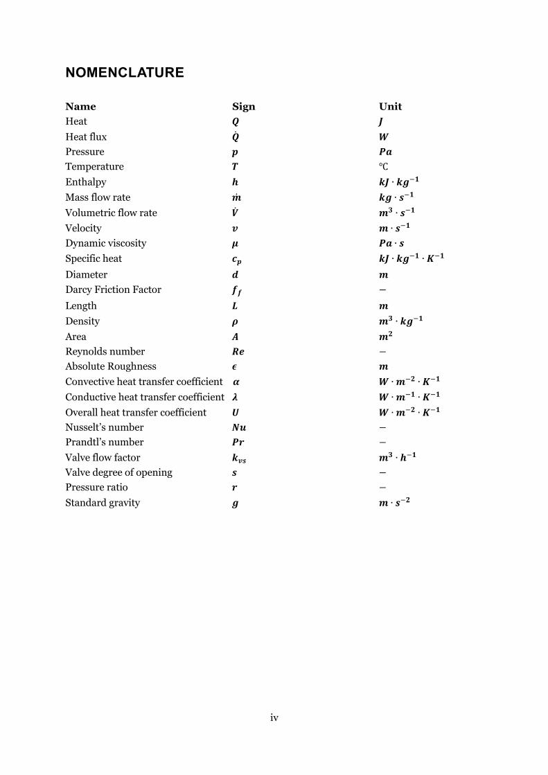
NOMENCLATURE

Name Sign Unit

Heat 𝑸 𝑱

Heat flux �� 𝑾

Pressure 𝒑 𝑷𝒂

Temperature 𝑻 ℃

Enthalpy 𝒉 𝒌𝑱 ∙ 𝒌𝒈−𝟏

Mass flow rate �� 𝒌𝒈 ∙ 𝒔−𝟏

Volumetric flow rate �� 𝒎𝟑 ∙ 𝒔−𝟏

Velocity 𝒗 𝒎 ∙ 𝒔−𝟏

Dynamic viscosity 𝝁 𝑷𝒂 ∙ 𝒔

Specific heat 𝒄𝒑 𝒌𝑱 ∙ 𝒌𝒈−𝟏 ∙ 𝑲−𝟏

Diameter 𝒅 𝒎

Darcy Friction Factor 𝒇𝒇 −

Length 𝑳 𝒎

Density 𝝆 𝒎𝟑 ∙ 𝒌𝒈−𝟏

Area 𝑨 𝒎𝟐

Reynolds number 𝑹𝒆 −

Absolute Roughness 𝝐 𝒎

Convective heat transfer coefficient 𝜶 𝑾 ∙𝒎−𝟐 ∙ 𝑲−𝟏

Conductive heat transfer coefficient 𝝀 𝑾 ∙𝒎−𝟏 ∙ 𝑲−𝟏

Overall heat transfer coefficient 𝑼 𝑾 ∙𝒎−𝟐 ∙ 𝑲−𝟏

Nusselt’s number 𝑵𝒖 −

Prandtl’s number 𝑷𝒓 −

Valve flow factor 𝒌𝒗𝒔 𝒎𝟑 ∙ 𝒉−𝟏

Valve degree of opening 𝒔 −

Pressure ratio 𝒓 −

Standard gravity 𝒈 𝒎 ∙ 𝒔−𝟐

1

1. INTRODUCTION

Focus on environmental challenges have during the last decades increased and one of the

major issues is anthropogenic global warming, where mitigation of the deleterious greenhouse

gases is vital. Energy systems can be made more sustainable by lowering demand, integrating

more renewable energy sources and increasing efficiency in production, transmissions and end

use. Using combined heat and power (CHP) together with a district heating system (DHS),

many of these aspects can be addressed at the same time.

DHS are common in the Nordic countries today and accounts for a great portion of the heat

supply. In Sweden, total district heating end use in the last years has been around 50 TWh

according to Energimyndigheten (2016) and district heating accounts for about 50 % of the

total heat demand (Danielewicz, Śniechowska, Sayegh, Fidorów, & Jouhara, 2016).

The aim for future DHS is a higher integration of energy efficient and low energy buildings,

heat recovery, renewable energy sources and more efficient production of power and heat. This

could be achieved by decreasing the supply and return temperature of the network and

increasing the overall efficiency of the system. By lowering the temperature of the DHS, grid

losses are reduced, more electricity can be produced by CHP plants, more heat from lower

temperature heat sources can be used such as flue gas condensation, geothermal and solar, the

performance for heat pumps can be increased and thermal heat storages will have a higher

capacity (Lund et al., 2014).

Issues

Suppliers of District heating must balance demand and supply, often in large and complex

networks. Peak loads can be problematic for suppliers which often leads to use of fossil fuels

such as coal, oil or gas with negative environmental and economic impact. Heat propagation

can be in the range of many hours throughout a DHS and will vary with operational conditions,

furthermore, the flow can change direction during transient conditions in parts of the network.

For heat suppliers to optimally plan the production subject to heat demand, losses and delays,

reliable data e.g. temperature at critical points and knowledge of how the flow propagate

through the network is required (Pinson, Nielsen, Nielsen, Poulsen, & Madsen, 2009). A

dynamic model can be used for this purpose.

2

Purpose and research questions

The purpose of this study is to develop a dynamic model of the district heating network and a

method for building, simulating and visualizing the network. The model will be used to answer

the following research questions

• How can a dynamic model of a district heating network be used to better understand the system

in transient conditions?

• Is Modelica and Matlab a good combination for modelling and simulating district heating

networks?

Scope and delimitation

Because the model should be able to depict characteristics of a large DHn, a more robust and

simpler model approach has been chosen for most parts instead of very detailed models. In

particular, many simplifications were made with regards to heat transfer, since very detailed

heat transfer calculations become complex and demanding.

Because focus have been on heat propagation in the network, all heat loads have been made

empirical and no production units were included.

Contribution to current research

From the literature review presented below it was concluded that most models have limitations

to them, often due to sequential solvers that makes it hard to handle flow reversals and ring

network structures. The focus of this study is therefore to build a library of robust standalone

components using object oriented programming and show how it can be used to model and

simulate district heating networks.

3

2. LITERATURE REVIEW

As DHS becomes more complex, connected to distributed energy sources and thermal storages,

models need to be designed to handle bi-directional flows, closed circuits and transients in the

network. Most models and tools today focus on dimensioning energy systems or uses linear

programming for optimizing production planning and there is need for fully dynamic models

for complex systems (Allegrini et al., 2015). Using Open-source Object oriented dynamic

models such as a library in OpenModelica, district heating networks can be built by inputs of

GIS data directly, drastically reducing manual work (Wetter, Treeck, & IEA EBC, 2015).

Temperature prediction models

Having accurate forecasts of the temperature distribution in district heating networks is crucial

to be able to minimize the production cost while fulfilling the needs of the customers, where

dynamic models is one solution. Pinson et al. (2009) have developed a conditional finite

impulse response model (cFIR) which is an extension of the finite impulse response model

(FIR), and instead of static coefficients they have included nonparametric coefficient functions.

The model showed a high accuracy of temperature prediction compared to statistical methods,

but it has issues regarding how the regularization should be tuned optimally. Stevanovic et al.

(2009) developed a model using Lagrange interpolation which has a high accuracy of the front

wave propagation due to there being no numerical diffusion. The results corresponds to real

measured values. Both models have assumed nondynamic hydraulic models, as it is shown that

the pressure dynamics are much faster than the thermal dynamics and do not affect heat

propagation significantly.

Relative attenuation degree and lag time are two parameters that can be used to describe the

dynamics of a constant flow in a pipe without branches, that is the time it takes for a change of

inlet temperature to establish a steady outlet temperature and the change of inlet temperature

that gives a 1 °C change on the outlet temperature. Jie, Tian, Yuan, & Zhu (2012) have made a

model based on Fourier series that describes these characteristics with the focus on the pipe

model as it has the largest impact on these parameters. The model was validated against

operational data computed with the peak valley method and was concluded to have the small

relative errors, thereby showing a potential to be able to estimate the lag time.

A building strategy that could be applied is a network where all customers have an equal length

of pipes, including both the return and supply. Instead of the customers having an own control

valve for the primary flow, the flow would be equally distributed for everyone. Kuosa et al.

(2014) have modeled such system with plate heat exchangers and studied how the primary and

secondary flow should be matched, to lower the return temperature to the production plant. It

was shown that almost equal heat capacity flows gave the highest performance in terms of

number of transfer units (NTU) and effectiveness in the heat exchangers. The strategy could

however only be used in new grids of isolated extensions of a present grid.

4

Modelica have been used in numerous studies for dynamic simulations, often in combination

with a graphical user interface and integration with other software for pre- and post-

processing. Velu, Larsson, Windahl, Saarinen, & Boman (2014) used the results from Modelica

simulations together with nonlinear optimization techniques to maximize the benefits of heat

and electricity production. Giraud, Bavière, Cédric, Vallée, & Robin (2015) developed a

dynamic model for district heating and experimentally validated it against a virtual district

heating network. At the 11th international Modelica conference Giraud, Bavière, Vallée, &

Paulus (2015) presented their district heating library based on modified components from the

Modelica standard library. The modification was mainly that they simplified the fluid to a

liquid and made two pipe models; one with nodes by discretization and one with spatial

distribution, hence reducing the number of equations significantly in comparison to the

standard library.

Computation strategies

To calculate thermal transients and capture information along a network, it can be discretized.

Zhou, Tian, Zhau, & Guo (2014) discretized their model with finite difference by expanding

their equation with the first order Tailor series and solved it by using an explicit forward

scheme. The calculation with this method have a restriction in time step size due to stability,

and to ensure a stable solution they restricted their time step to fulfill the Courant-Friedrichs-

Lewy condition. Ikonen, Selek, Kovács, & Neuvonen (2016) discretized their model using a

spatial distribution and only calculated the temperatures at the vertex locations, thereby

excluding the temperature distribution along the pipes. The equations were written with a

transport delay term and solved using the decoupled pseudo-steady-state framework.

Gabrielaitienė, Bøhm, & Sundén (2011) made a comparison of a node model, developed at

Technical University of Denmark by Benonysson (1991), and the commercial software Termis.

The node model accounted for thermal accumulation in the pipes while Termis neglects it.

Comparison was made with the results from simulations in two different cases in Denmark

and it was concluded that there was no significant difference in the prediction between the

models. It could be seen that the models gave a high accuracy for small and slow changes of

the supply temperature, but high errors were given for large and sudden changes.

Furthermore, the amount of disturbances of the flow such as bends and valves, contributed to

a higher spreading of the temperature wave and would affect the temperature before and after

the disturbances.

5

Aggregating district heating networks in models is an efficient way to reduce the computing

time of simulations. Larsen, Pálsson, Bøhm, & Ravn (2002) proposed a method that can reduce

large networks of thousand pipes into a small model of just a few pipes, with the assumptions

that aggregated branches have proportional mass flows, equal return temperatures and that

they are not looped. They further show that the simplified network could maintain the

characteristics of the original network with significantly faster simulation time. Guelpa et al.

(2016) developed a reduced model which was based on Proper Orthogonal Decomposition

(POD) and Radial Basis Function (RBF). They compare the model to a full fluid dynamic model

and concludes that the model can reduce the computational time of the simulation of a large

district heating network up to 95 %, thereby making it more suitable for optimization purposes.

Heat load and losses

The heat loss from the distribution pipes has an direct impact on the supply temperature level,

thus it is of importance to include in district heating models. Perpar, Rek, Bajric, & Zun (2012)

have studied the soil thermal conductivity in detail by experimental and numerical analysis of

pre-insulated pipelines in operation. The analysis is conducted from three groups of variables;

geometry, material properties and time dependent data of supply, return and ambient air

temperature. Varying soil thermal conductivity between 0.4 to 1.0 W/m, K gave an increase of

about 30 % in the heat losses locally. The impact in large scale simulations is low and varying

the thermal conductivity could then be used for fine tuning purposes.

To capture the detailed dynamics in a district heating system the heat demand models of

consumers play an important role as they will determine the mass flow and the drop in

temperature. Some are physical while others are completely statistical, and some are gray-box

models which combines some physical elements with statistical analysis. Ma et al. (2014)

studied energy consumption patterns using time and type of building along with outdoor

temperature as prediction factors to heat demand. Commercial, apartment and office building

was used as types and described by a Gaussian mixture model. It was seen that the outdoor

temperature had a strong correlation to the heat demand, but to be able to predict it accurately,

both the type of building and time was needed.

Idowu, Saguna, Åhlund, & Schelén, (2016) studied how machine learning could be used for

load forecasting by using parameters of outdoor temperature, historical heat load, temporal

aspects and physical properties in the sub stations. They evaluated several machine learning

methods and concluded that support vector machine, feed forward neural network and

multiple linear regression was most suitable for describing district heating loads. However,

buildings with a higher unpredictability could not be described and had large performance

errors in comparison to the other buildings. Powell, Sriprasad, Cole, & Edgar (2014) also

evaluated several methods but only using weather and time data as input. They concluded that

a nonlinear autoregressive model with exogenous inputs was the best to use.

6

Unconventional concepts

Having prosumers in a district heating network is a concept where the customers can both

utilize heat from the network and give back excess heat to it. Brange, Englund, & Lauenburg,

(2016) investigated the potential of having prosumers in an area located in Sweden and

concluded that there is a potential of environmental and primary energy savings. Olsthoorn,

Haghighat, & Mirzaei (2016) reviewed the potential of integrating storage and renewable

energy into the district heating system. They concluded that there is a potential for storage

both short term, diurnal and long term seasonal storage with the correct integration.

Evening out the heat load at the production plant and thereby increasing the efficiency could

potentially be achieved by short term thermal energy storage. A district heating system could

be loaded by temporarily increasing the supply temperature, but that could also lower the

efficiencies of production units and lead to fatigue of the distribution pipes. Kensby, Trüschel,

& Dalenbäck (2015) have looked at the potential to evening out the heat demand from buildings

by controlling the radiator supply temperature within the building. The supply temperature is

increased for a period and then decreased for a period, and the thermal mass of the building is

used to even out the indoor temperature so that the indoor climate remains comfortable.

Summary

Development of district heating models has been done by different approaches and ideas, most

of the models aim to be able to conduct accurate temperature prediction in the network both

with regards to the time lag and heat loss of the supply temperature. Much weight is often put

on whether methods of aggregation, heat losses and pressure losses can simplify models in

such a way that the results still represent the reality accurately enough. The reason is to make

the computing time fast enough so that the model can be used for optimization and further be

used for forecasting. To do this there is also a need of accurate customer models, with a high

predictability of their consumption and different models have been made to forecast these.

Building these types of district heating system models requires specific data of the modeled

system and by using an object-oriented language such as Modelica, a library of generic

components makes the building process easier and allows for the model to change with the

system easily. Other types of studies have been made on how for example thermal capacity of

buildings could be used to even out the demand for one customer, but the studies have not

included the effects on the district heating network.

7

3. METHOD

Two things were developed in this study, a library of components in Modelica and a method of

building and simulating district heating networks (DHN) with Matlab as core. The purpose of

this combination is to create an automated procedure in which any DHN can be built from

CAD-drawings as well as an environment where DHN can be built manually and easily

simulated and visualized.

OpenModelica connection editor (OME) was used to build the object oriented dynamic model

library, because it is open source and the model can be built to handle ring networks and bi-

directional flow in a robust way. Furthermore, the DHN is a constantly evolving system where

customers, pipes, valves, temperature levels etc. changes with time and new business models

and price models are developed. This makes an object oriented dynamic model library a very

suitable method to ensure that the model can evolve together with the system.

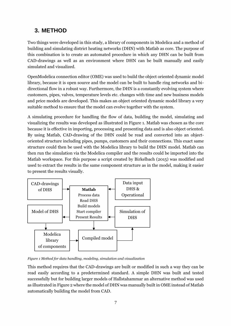
A simulating procedure for handling the flow of data, building the model, simulating and

visualizing the results was developed as illustrated in Figure 1. Matlab was chosen as the core

because it is effective in importing, processing and presenting data and is also object oriented.

By using Matlab, CAD-drawing of the DHN could be read and converted into an object-

oriented structure including pipes, pumps, customers and their connections. This exact same

structure could then be used with the Modelica library to build the DHN model. Matlab can

then run the simulation via the Modelica compiler and the results could be imported into the

Matlab workspace. For this purpose a script created by Birkelbach (2015) was modified and

used to extract the results in the same component structure as in the model, making it easier

to present the results visually.

Figure 1 Method for data handling, modeling, simulation and visualization

This method requires that the CAD-drawings are built or modified in such a way they can be

read easily according to a predetermined standard. A simple DHN was built and tested

successfully but for building larger models of Hallstahammar an alternative method was used

as illustrated in Figure 2 where the model of DHN was manually built in OME instead of Matlab

automatically building the model from CAD.

Modelica

library

of components

Model of DHS

Data input

DHS &

Operational

Simulation of

DHS

Matlab

Process data

Read DHS

Build models

Start compiler

Present Results

CAD-drawings

of DHS

Compiled model

8

Figure 2 Alternative method, used in the study for building up and validating a DHN

Measured data from network can be inputted and the dynamic model would simulate the DHN

dynamic behavior as illustrated in Figure 3. Because the flow and thermal model is physical it

requires input on pressure and temperature at certain point in the DHN. The heat load models

(customers) is empirical and not physical, meaning they require data on heat load and mass

flow, this needs to be pre-processed and injected into the model upon simulation. By using this

approach, the simulation can show how the DHN behaves in different transient conditions and

be useful for detecting weaknesses and unexpected behaviors in the system.

Figure 3 Data inputs and outputs into model

Modelica dynamic model library

The principle followed for all objects in the model library has been that an object can only

interact with variables and data available internally and at its boundaries. Hence, no system

characteristics are built into any of the components, rather this is a result of connecting several

objects together.

Data input

Operational

Simulation of

DHS

Matlab

Process data

Start compiler

Present Results

CAD-drawings

of DHS OME

Graphical

Interface for

building model

Data input

DHS

Physical Flow &

Thermal model

Empirical Heat

Load Model

Dynamic

DHN Model

��, ��

𝑇, 𝑝

𝑇, 𝑝…

Modelica

library

of components

Model of DHS

Compiled model

9

Generally, the following assumptions have been made to ensure robustness and simulation

speed:

• Model is quasi-dynamic, i.e. temperature is considered dynamic but pressure is considered

static

• Specific heat of water and pipe material is constant throughout the entire model

• Heat accumulates in pipe wall but not insulation

• Water, Pipe wall and Insulation are all separate lumped systems in radial direction and

discretized axially (1-dimensional model)

• No heat flows between pipes in culverts

• Temperature outside of pipe wall is a parameter and not variable

Below a brief description of the model and its key equations is presented.

3.1.1. Flow connector

All objects can be connected to each other via connectors. This allows information to be

transferred between objects. There are three different types of variables that can be defined for

a connector, potential, flow and stream variables.

From thermodynamics, it is known that a difference in intensive properties drives a flow of

extensive properties, the same is true in Modelica where potential variables are intensive

properties and flow variables are extensive properties.

A flow of an extensive property such as mass also carries specific properties with them, e.g.

enthalpy. In Modelica this is denoted as a Stream variable.

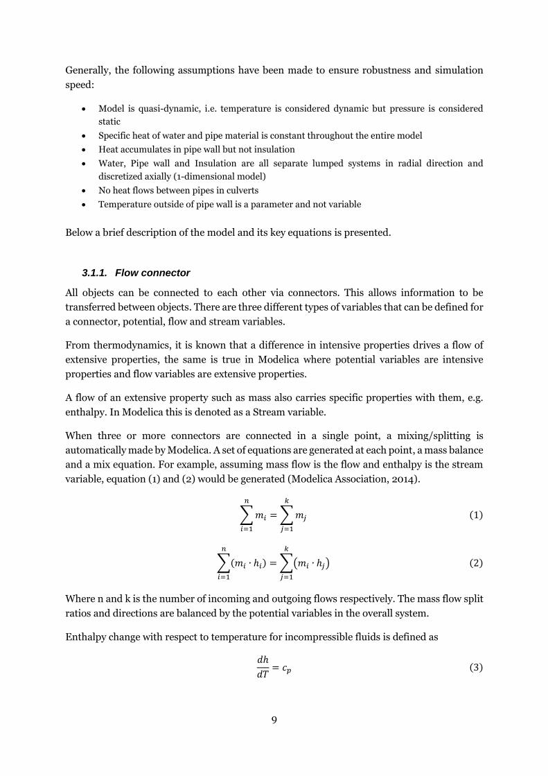
When three or more connectors are connected in a single point, a mixing/splitting is

automatically made by Modelica. A set of equations are generated at each point, a mass balance

and a mix equation. For example, assuming mass flow is the flow and enthalpy is the stream

variable, equation (1) and (2) would be generated (Modelica Association, 2014).

∑𝑚𝑖

𝑛

𝑖=1

=∑𝑚𝑗

𝑘

𝑗=1

(1)

∑(𝑚𝑖 ∙ ℎ𝑖)

𝑛

𝑖=1

=∑(𝑚𝑖 ∙ ℎ𝑗)

𝑘

𝑗=1

(2)

Where n and k is the number of incoming and outgoing flows respectively. The mass flow split

ratios and directions are balanced by the potential variables in the overall system.

Enthalpy change with respect to temperature for incompressible fluids is defined as

𝑑ℎ

𝑑𝑇= 𝑐𝑝 (3)

10

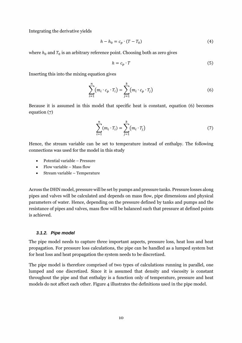
Integrating the derivative yields

ℎ − ℎ0 = 𝑐𝑝 ∙ (𝑇 − 𝑇0) (4)

where ℎ0 and 𝑇0 is an arbitrary reference point. Choosing both as zero gives

ℎ = 𝑐𝑝 ∙ 𝑇 (5)

Inserting this into the mixing equation gives

∑(𝑚𝑖 ∙ 𝑐𝑝 ∙ 𝑇𝑖)

𝑛

𝑖=1

=∑(𝑚𝑖 ∙ 𝑐𝑝 ∙ 𝑇𝑗)

𝑘

𝑗=1

(6)

Because it is assumed in this model that specific heat is constant, equation (6) becomes

equation (7)

∑(𝑚𝑖 ∙ 𝑇𝑖)

𝑛

𝑖=1

=∑(𝑚𝑖 ∙ 𝑇𝑗)

𝑘

𝑗=1

(7)

Hence, the stream variable can be set to temperature instead of enthalpy. The following

connections was used for the model in this study

• Potential variable – Pressure

• Flow variable – Mass flow

• Stream variable – Temperature

Across the DHN model, pressure will be set by pumps and pressure tanks. Pressure losses along

pipes and valves will be calculated and depends on mass flow, pipe dimensions and physical

parameters of water. Hence, depending on the pressure defined by tanks and pumps and the

resistance of pipes and valves, mass flow will be balanced such that pressure at defined points

is achieved.

3.1.2. Pipe model

The pipe model needs to capture three important aspects, pressure loss, heat loss and heat

propagation. For pressure loss calculations, the pipe can be handled as a lumped system but

for heat loss and heat propagation the system needs to be discretized.

The pipe model is therefore comprised of two types of calculations running in parallel, one

lumped and one discretized. Since it is assumed that density and viscosity is constant

throughout the pipe and that enthalpy is a function only of temperature, pressure and heat

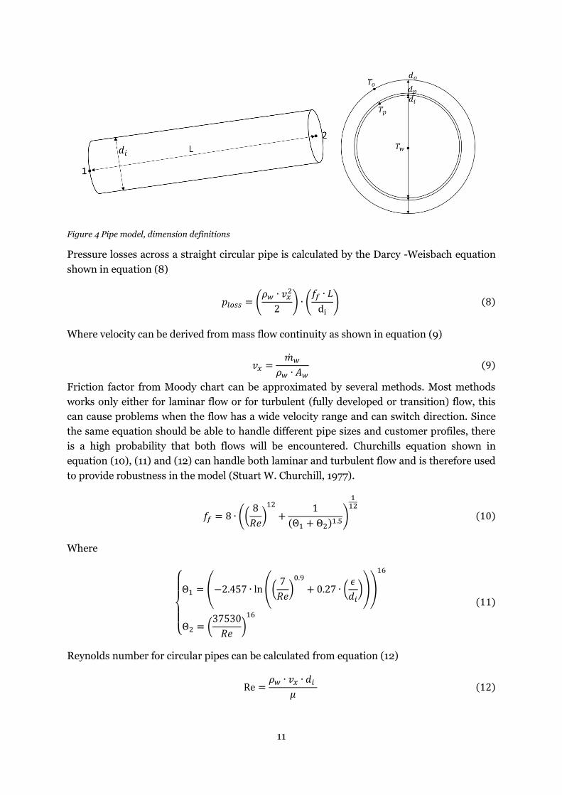
models do not affect each other. Figure 4 illustrates the definitions used in the pipe model.

11

Figure 4 Pipe model, dimension definitions

Pressure losses across a straight circular pipe is calculated by the Darcy -Weisbach equation

shown in equation (8)

𝑝𝑙𝑜𝑠𝑠 = (𝜌𝑤 ∙ 𝑣𝑥

2

2) ∙ (

𝑓𝑓 ∙ 𝐿

di) (8)

Where velocity can be derived from mass flow continuity as shown in equation (9)

𝑣𝑥 =��𝑤

𝜌𝑤 ∙ 𝐴𝑤(9)

Friction factor from Moody chart can be approximated by several methods. Most methods

works only either for laminar flow or for turbulent (fully developed or transition) flow, this

can cause problems when the flow has a wide velocity range and can switch direction. Since

the same equation should be able to handle different pipe sizes and customer profiles, there

is a high probability that both flows will be encountered. Churchills equation shown in

equation (10), (11) and (12) can handle both laminar and turbulent flow and is therefore used

to provide robustness in the model (Stuart W. Churchill, 1977).

𝑓𝑓 = 8 ∙ ((8

𝑅𝑒)12

+1

(Θ1 + Θ2)1.5)

112

(10)

Where

{

Θ1 = (−2.457 ∙ ln ((

7

𝑅𝑒)0.9

+ 0.27 ∙ (𝜖

𝑑𝑖)))

16

Θ2 = (37530

𝑅𝑒)16

(11)

Reynolds number for circular pipes can be calculated from equation (12)

Re =𝜌𝑤 ∙ 𝑣𝑥 ∙ 𝑑𝑖

𝜇(12)

12

Heat loss and heat propagation can both be considered by adding heat losses to the standard

advection equation. Assuming convection from water to pipe wall, heat accumulation in pipe

wall and conduction from pipe wall to outer layer of insulation, equation (13) and (14) are

obtained where (13) determines the water temperature and (14) determines pipe wall

temperature.

𝛼 ∙ 𝜋 ∙ 𝑑𝑖 ∙ 𝑑𝑥 ∙ (𝑇𝑝 − 𝑇𝑤) = 𝜌𝑤 ∙𝜋 ∙ 𝑑𝑖

2

4∙ 𝑐𝑝,𝑤 ∙ 𝑑𝑥 ∙ (

𝜕𝑇𝑤𝜕𝑡

+ 𝑣𝑥 ∙𝜕𝑇𝑤𝜕𝑥

) (13)

𝛼 ∙ 𝜋 ∙ 𝑑𝑖 ∙ 𝑑𝑥 ∙ (𝑇𝑤 − 𝑇𝑝) + Utot ∙ 𝜋 ∙ 𝑑𝑖 ∙ 𝑑𝑥 ∙ (𝑇𝑜 − 𝑇𝑝) = 𝜌𝑝 ∙𝜋 ∙ (𝑑𝑝

2 − 𝑑𝑖2)

4∙ 𝑐𝑝,𝑝 ∙ 𝑑𝑥 ∙

𝜕𝑇𝑝

𝜕𝑡(14)

Derivatives with regards to time will be handled by Modelica, however Modelica does not

handle derivatives with regards to any other variable, hence discretization in space needs to be

done manually or handled otherwise. Using upwind method to discretize equation (13) will

yield a high degree of numerical (false) diffusion which leads to heat propagation being late

and displaying characteristics of diffusion even though it should not. Therefore QUICKEST

method, developed by Leonard (1979) was used which gives less false diffusion. Equation (13)

then becomes (15) where i denotes a node within the pipe.

𝛼 ∙ 𝜋 ∙ 𝑑𝑖 ∙ 𝑑𝑥 ∙ (𝑇𝑝 − 𝑇𝑤) =

𝜌𝑤 ∙𝜋 ∙ 𝑑𝑖

2

4∙ 𝑐𝑝,𝑤 ∙ 𝑑𝑥 ∙ (

𝜕𝑇𝑤𝜕𝑡

+ 𝑣𝑥 ∙(𝑇𝑤

𝑖+1 − 𝑇𝑤𝑖−1)

2 ∙ 𝑑𝑥− 𝑣𝑥

2 ∙(𝑇𝑤

𝑖−1 + 𝑇𝑤𝑖+1 − 2 ∙ 𝑇𝑤

𝑖 )

2 ∙ 𝑑𝑥2) (15)

In order to make the pipe standalone and to allow flow to reverse, the first and last node was

made to interact with the flow port connections using the upwind method. This was due to that

the pipe has no information on what it is connected to and it is not always connected to another

component that is discretized. It is important that the derivatives of the internal nodes are

continuous, but as the temperature in the flow port is set depending on the flow direction, it

will not be continues when the flow reverses. To handle this, the incoming flow port is used as

an extended node and the outgoing flow port is set by the last node.

Thermal transmittance through pipe wall and insulation can be calculated by equation (16)

𝑈𝑡𝑜𝑡 =1

𝑑𝑖 ∙ ln (𝑑𝑝𝑑𝑖)

2 ∙ 𝜆𝑝+𝑑𝑖 ∙ ln (

𝑑𝑜𝑑𝑝)

2 ∙ 𝜆𝑖

(16)

The convective heat transfer coefficient 𝛼 can be calculated by a number of different methods

available in literature. Mainly it will be a function of Reynold’s and Prandtl’s number,

temperature of water and pipe properties. Usually it is calculated from Nusselt’s number

𝛼 =𝑁𝑢 ∙ 𝜆𝑤𝑑𝑖

(17)

13

Equation (18) for turbulent(including transition range) flow in smooth circular tubes is valid

over a wide range of Reynold’s and Prandtl’s numbers and gives errors of less than 10%

(Incropera, DeWitt, Bergman, & Lavine, 2013).

𝑁𝑢 =(𝑓8) ∙ (𝑅𝑒 − 1000) ∙ 𝑃𝑟

1 + 12.7 ∙ (𝑓8)

12∙ (𝑃𝑟

23 − 1)

(18)

Where Prandtl’s number is defined from equation (19)

𝑃𝑟 =𝜇 ∙ 𝑐𝑝

𝜆𝑤(19)

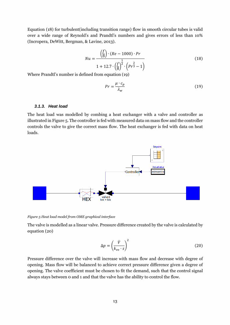
3.1.3. Heat load

The heat load was modelled by combing a heat exchanger with a valve and controller as

illustrated in Figure 5. The controller is fed with measured data on mass flow and the controller

controls the valve to give the correct mass flow. The heat exchanger is fed with data on heat

loads.

Figure 5 Heat load model from OME graphical interface

The valve is modelled as a linear valve. Pressure difference created by the valve is calculated by

equation (20)

Δ𝑝 = (𝑉

𝑘𝑣𝑠 ∙ 𝑠

)

2

(20)

Pressure difference over the valve will increase with mass flow and decrease with degree of

opening. Mass flow will be balanced to achieve correct pressure difference given a degree of

opening. The valve coefficient must be chosen to fit the demand, such that the control signal

always stays between 0 and 1 and that the valve has the ability to control the flow.

14

For every customer, a start value of mass is also given, this helps Modelica to initialize the

entire system. To get reasonable starting values for the valves, the control signal is initialized

by assuming a pressure difference of 3 bar and using the starting value for the customer, as

shown in equation (21)

𝑠𝑖𝑛𝑖𝑡 =𝑚𝑖𝑛𝑖𝑡 ∙ 3.6

√3 ∙ 𝑘𝑣𝑠(21)

Temperature on the return side is calculated from equation (22)

�� = �� ∙ 𝑐𝑝 ∙ (𝑇𝑠 − 𝑇𝑅) (22)

3.1.4. Pump

A generic and basic pump model was designed that is fed with an input signal for the pressure

ratio as shown in equation (23)

pout𝑝𝑖𝑛

= 𝑟 (23)

From the pressure ratio, the outlet pressure is calculated and upheld.

In larger district heating systems, there are many different pumps that are controlled by

different signals, e.g. with the purpose to control the pressure difference of a customer at far

end of the grid. Because information on how pumps were controlled was not available and

measured data on pressure is available, different pumps were designed to allow the physical

model to converge.

Two additional pumps were designed and used for validation. The first pump, illustrated in

Figure 6, has measured outlet pressure as input via datafiles, and calculates pressure ratio

necessary based on the incoming pressure.

Figure 6 Model of pump with outlet pressure given from input data

15

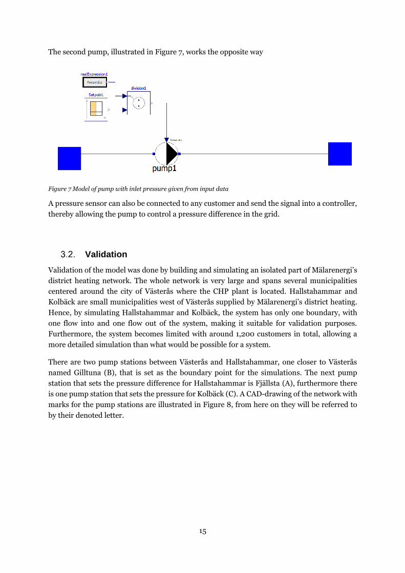
The second pump, illustrated in Figure 7, works the opposite way

Figure 7 Model of pump with inlet pressure given from input data

A pressure sensor can also be connected to any customer and send the signal into a controller,

thereby allowing the pump to control a pressure difference in the grid.

Validation

Validation of the model was done by building and simulating an isolated part of Mälarenergi’s

district heating network. The whole network is very large and spans several municipalities

centered around the city of Västerås where the CHP plant is located. Hallstahammar and

Kolbäck are small municipalities west of Västerås supplied by Mälarenergi’s district heating.

Hence, by simulating Hallstahammar and Kolbäck, the system has only one boundary, with

one flow into and one flow out of the system, making it suitable for validation purposes.

Furthermore, the system becomes limited with around 1,200 customers in total, allowing a

more detailed simulation than what would be possible for a system.

There are two pump stations between Västerås and Hallstahammar, one closer to Västerås

named Gilltuna (B), that is set as the boundary point for the simulations. The next pump

station that sets the pressure difference for Hallstahammar is Fjällsta (A), furthermore there

is one pump station that sets the pressure for Kolbäck (C). A CAD-drawing of the network with

marks for the pump stations are illustrated in Figure 8, from here on they will be referred to

by their denoted letter.

16

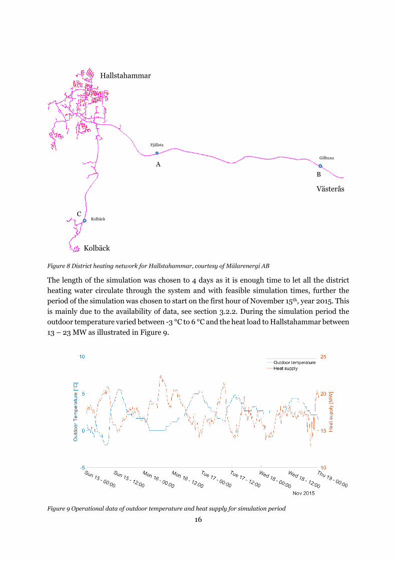
Figure 8 District heating network for Hallstahammar, courtesy of Mälarenergi AB

The length of the simulation was chosen to 4 days as it is enough time to let all the district

heating water circulate through the system and with feasible simulation times, further the

period of the simulation was chosen to start on the first hour of November 15th, year 2015. This

is mainly due to the availability of data, see section 3.2.2. During the simulation period the

outdoor temperature varied between -3 °C to 6 °C and the heat load to Hallstahammar between

13 – 23 MW as illustrated in Figure 9.

Figure 9 Operational data of outdoor temperature and heat supply for simulation period

Hallstahammar

Kolbäck

Västerås

Gilltuna

Fjällsta

Kolbäck

B A

C

17

3.2.1. Simple model of Hallstahammar

Validation was done in two steps, first focus was put into validating pressure losses and then

heat propagation. For this purpose a model was made which incorporated pump station A and

the transit line between station B and Hallstahammar, which was modelled as one heat load.

The model is illustrated in Figure 10.

Figure 10 One heat exchanger model of Hallstahammar for validation, made in OME

Temperature and pressure on supply side after B was inputted as boundary data, shown as B1

in Figure 10. Outlet supply pressure for pump station A was inputted into the pump model

which was translated into a pressure ratio based on inlet pressure. Inlet and outlet pressure at

the return side of pump station A was given. Mass flow measured on the return side was

inputted into the controller which set the mass flow in the system to the same. The total heat

demand of Hallstahammar and Kolbäck was inputted into the heat exchanger. Validation was

then done by simulating the model and comparing temperature and pressure at calculated

points in the system.

The model was manually tuned to fit the measured data as good as possible. Pressure was tuned

by changing the relative roughness and number of minor losses of the individual pipes.

3.2.2. Aggregated model of Hallstahammar

To demonstrate how the library can handle larger and more complex models, a more detailed

model of Hallstahammar was created with the aim to capture the dynamics of the distribution

pipelines and to be validated against one of the customers. Building and simulating the specific

part of the network required inputs of data, firstly the dimensions of the district heating

network to build the model and then operational data for simulation and validation.

A1

A2

18

Dimensions of the network was given in a Drawing Interchange Format (DXF) which

contained dimensions, type and positions of the pipes and positions of the customers. As the

number of pipes and customers are large, a first approach was to extract data from the DXF-

file by a script. However, many uncertainties were found in the drawing which would require

a lot of filtering before a model could be generated. Instead the necessary pipe data was

extracted manually using a CAD software. To make the amount of manual work feasible and

keep the number of equations low, the system was aggregated to only include the major

pipelines and excluding minor pipelines to individual customers.

The aggregated model of Hallstahammar was reduced to 108 pipes (54 supply and 54 return)

and 37 areas with customers, see APPENDIX 2 for an overview of the areas. It included four

pumps in total, two pumps at station C and two pumps at station A. In addition to the inputs

given to the simple model, pressure data available for pump station C was also inputted. The

boundaries towards Västerås are set up as a set point on the supply outlet and a sink on the

return inlet of pump station B. Figure 13 shows the graphics of the model taken from OME.

The pipes that were included in the model where those which had the same diameter between

connections to areas. If the diameter changed between connections, a new pipe was introduced

in series. In Figure 11 two examples of aggregation are illustrated, where several customers

have been aggregated to represent one customer in the model, shown with a mark. To the left

is an area where customers are connected in parallel along a major pipe and were aggregated

to one load in the middle, thereby assumed to cancel out the pressure losses due to the reduced

flow along the path. To the right is an area where several customers that had a common

connection to a major pipe were aggregated to one load.

Figure 11 Aggregation principles

19

Data of the customers were given as raw databases of MWh and m3 on hourly averages for the

whole year. The data was given together with metadata that contained information about all

the customers. It was given as a Json-string with information on a customer basis, included

their location in World Geodetic System 1984 (WSG84) format. To sort out the id’s for all

customers within Hallstahammar a filtering was made by using two WSG84 positions as

boundaries and include everything within. To ensure that all customer id’s were found the

number of customers id’s that were found were compared to the number that were found

within the .DXF file and furthermore they were plotted in a figure to ensure that the correct

id’s were found. To determine which customers that belonged to the different areas, CAD was

used where positions of two corners in a square were used to limit the areas and for some areas

several squares were needed, see Figure 12. To sort out the customers with the drawing

coordinates a conversion between WSG84 and Swedish Reference Frame 1999 (SWEREF 99)

was necessary.

Figure 12 Filtering of customers

The databases were searched for the id’s to extract their correlated data, whereas the found

data was stored in text files on a customer basis. Around 50 % of customers could not be found

within the provided databases and some of the customers found only had data from 2015-11-

12, thereby it was decided that the simulation would start from the first hour 2015-11-15.

Furthermore, the missing data was linearly extrapolated with calculated normalized values for

different customer categories. Weighted values were added to the areas depending on which

categories that were missing. For more statistics of the data see APPENDIX 1.

20

Operational data of the district heating network was collected from the monitoring system at

the production plant, which had available measurements from fixed pressure, temperature and

flow sensors at the pump stations. It also included measurements of the outdoor temperature

and heat delivered to the specific location. The availability of operational data within the

municipality was limited to the supply temperature that was available at one customer.

Selecting the correct start values for a large and complex model is time consuming and might

not even be possible. Therefore, to make it easier for the solver to converge, density, convective

heat transfer coefficient and viscosity was treated as constants rather than varying by functions

of temperature and pressure.

Figure 13 Aggregated model of Hallstahammar

21

Automation of model building, simulation and visualization

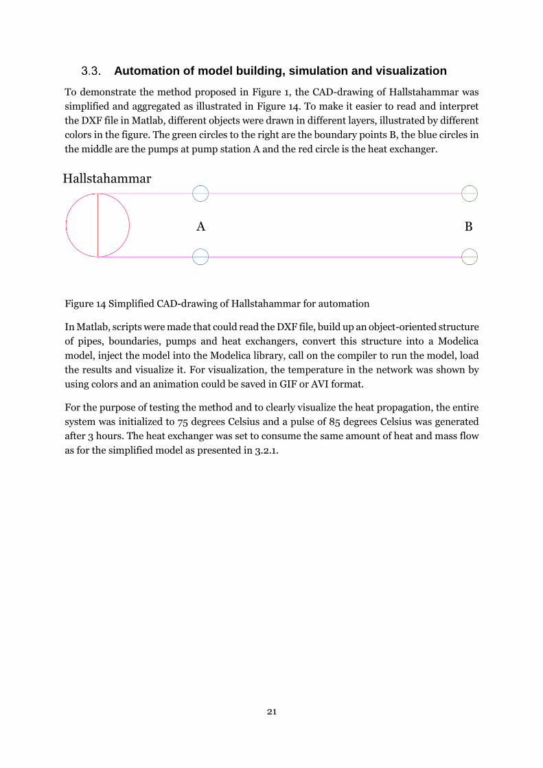
To demonstrate the method proposed in Figure 1, the CAD-drawing of Hallstahammar was

simplified and aggregated as illustrated in Figure 14. To make it easier to read and interpret

the DXF file in Matlab, different objects were drawn in different layers, illustrated by different

colors in the figure. The green circles to the right are the boundary points B, the blue circles in

the middle are the pumps at pump station A and the red circle is the heat exchanger.

Figure 14 Simplified CAD-drawing of Hallstahammar for automation

In Matlab, scripts were made that could read the DXF file, build up an object-oriented structure

of pipes, boundaries, pumps and heat exchangers, convert this structure into a Modelica

model, inject the model into the Modelica library, call on the compiler to run the model, load

the results and visualize it. For visualization, the temperature in the network was shown by

using colors and an animation could be saved in GIF or AVI format.

For the purpose of testing the method and to clearly visualize the heat propagation, the entire

system was initialized to 75 degrees Celsius and a pulse of 85 degrees Celsius was generated

after 3 hours. The heat exchanger was set to consume the same amount of heat and mass flow

as for the simplified model as presented in 3.2.1.

B A

Hallstahammar

22

4. RESULTS AND DISCUSSION

Simple model of Hallstahammar (one customer, two culverts)

The results of the simulation and comparison with measured data is presented below. For all

pipes, a step size of 20 meters and a time step of 10 seconds was used. Because exact

initialization cannot be done in pipes, the thermal dynamics will take some hours to be in tune

with the system, pressure model is not affected since it is modelled as steady state.

It should be noted that for the simulations with one heat exchanger, operational data was used,

which comes from the same system, where the heat supply is calculated based on mass flow

and temperature. The mass flow is also measured and hence the pressure losses can be tuned

to correlate well. This is one of the reasons why the model can so accurately depict the system

behavior.

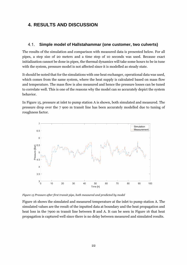
In Figure 15, pressure at inlet to pump station A is shown, both simulated and measured. The

pressure drop over the 7 900 m transit line has been accurately modelled due to tuning of

roughness factor.

Figure 15 Pressure after first transit pipe, both measured and predicted by model

Figure 16 shows the simulated and measured temperature at the inlet to pump station A. The

simulated values are the result of the inputted data at boundary and the heat propagation and

heat loss in the 7900 m transit line between B and A. It can be seen in Figure 16 that heat

propagation is captured well since there is no delay between measured and simulated results.

23

Figure 16 Temperature after first transit pipe, both measured and predicted by model

Figure 17 illustrates the return temperature at A. The online measured temperature has a

pattern which suggest that it shows a mean temperature over longer periods of time or that the

sensitivity of the meter is low. Simulated temperature varies more, but seems to be at the right

level. Simulated temperature can also vary more than actual temperature since only one heat

exchanger has been used which means that no delay times inside Hallstahammar is taken into

consideration. Including more heat exchangers and pipes would result in mixings of

temperatures and most likely a more constant return temperature.

Figure 17 Temperature on return side before A, both measured and predicted by model

24

Figure 18 below shows pressure at B. Since pressure at outlet of A was inputted from measured

data, this pressure is the result of pressure drop over the 7 900 m transit line between A and

B, same as on supply side. Using the same roughness yields a less accurate pressure

determination then on the supply side. This difference in pressure loss could be due to several

reasons; pressure data could have errors, the flow on supply side and return side could be

different due to leakage, if temperature is estimated wrongly this would affect physical

properties of the water and hence pressure drop, roughness of pipes could differ etc. A more

detailed tuning of the model could be done to minimize the total error. It is also interesting to

note that around 45 – 55 hours into the simulation, measured and simulated data are almost

identical, the reason for this is unknown.

Figure 18 Pressure on return side at B, both measured and predicted by model

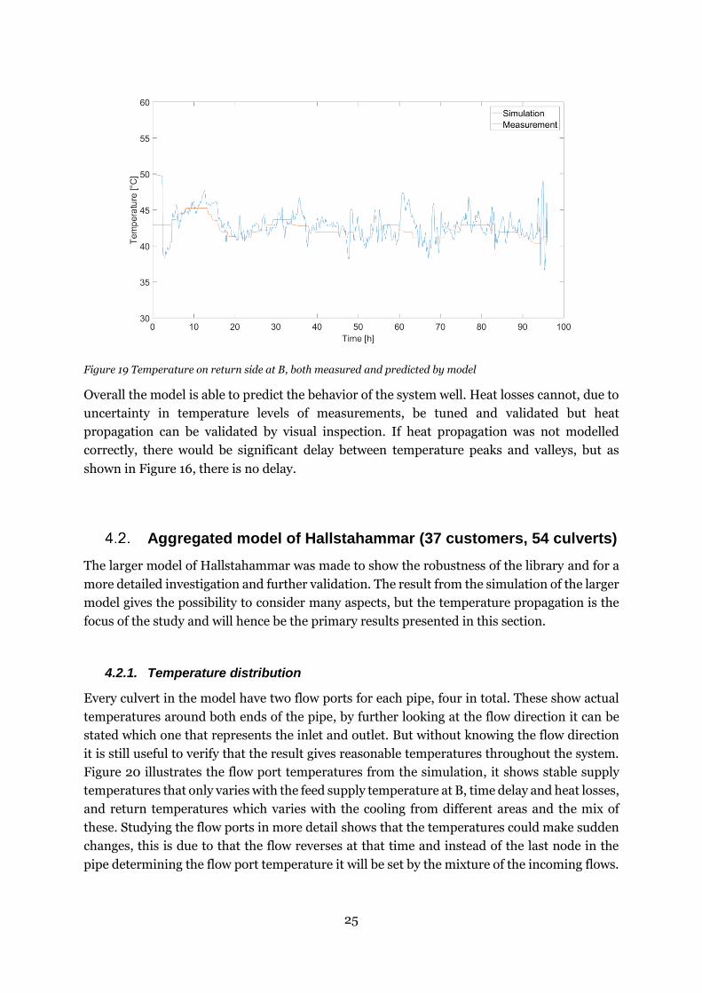
The temperature at B is shown below in Figure 19. Just as the temperature at A’s return pipe,

the temperature at B seems to be measured in mean values but simulation and measurements

are in the same level. The heat loss and propagation between A and B, which corresponds to

the transit line of 7900 m, could be estimated by identifying a peak and comparing time and

level. By doing that, the temperature loss could be tuned and validated in more detail, however

due to the uncertainty in measured temperature this would not be reliable in this case. The

temperature error in measurements could very well be larger than the temperature drop due

to heat losses, which usually are small, making it difficult to validate heat loss against provided

data.

25

Figure 19 Temperature on return side at B, both measured and predicted by model

Overall the model is able to predict the behavior of the system well. Heat losses cannot, due to

uncertainty in temperature levels of measurements, be tuned and validated but heat

propagation can be validated by visual inspection. If heat propagation was not modelled

correctly, there would be significant delay between temperature peaks and valleys, but as

shown in Figure 16, there is no delay.

Aggregated model of Hallstahammar (37 customers, 54 culverts)

The larger model of Hallstahammar was made to show the robustness of the library and for a

more detailed investigation and further validation. The result from the simulation of the larger

model gives the possibility to consider many aspects, but the temperature propagation is the

focus of the study and will hence be the primary results presented in this section.

4.2.1. Temperature distribution

Every culvert in the model have two flow ports for each pipe, four in total. These show actual

temperatures around both ends of the pipe, by further looking at the flow direction it can be

stated which one that represents the inlet and outlet. But without knowing the flow direction

it is still useful to verify that the result gives reasonable temperatures throughout the system.

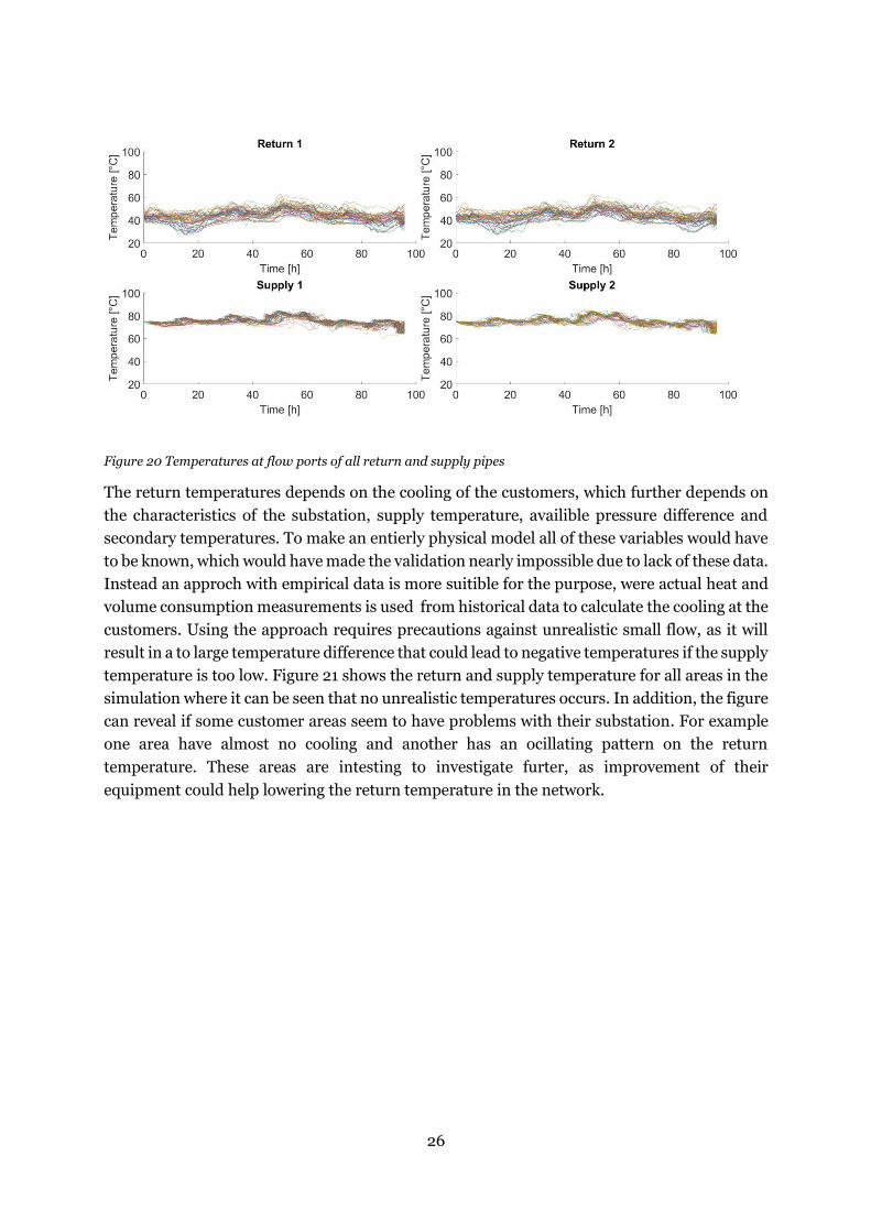
Figure 20 illustrates the flow port temperatures from the simulation, it shows stable supply

temperatures that only varies with the feed supply temperature at B, time delay and heat losses,

and return temperatures which varies with the cooling from different areas and the mix of

these. Studying the flow ports in more detail shows that the temperatures could make sudden

changes, this is due to that the flow reverses at that time and instead of the last node in the

pipe determining the flow port temperature it will be set by the mixture of the incoming flows.

26

Figure 20 Temperatures at flow ports of all return and supply pipes

The return temperatures depends on the cooling of the customers, which further depends on

the characteristics of the substation, supply temperature, availible pressure difference and

secondary temperatures. To make an entierly physical model all of these variables would have

to be known, which would have made the validation nearly impossible due to lack of these data.

Instead an approch with empirical data is more suitible for the purpose, were actual heat and

volume consumption measurements is used from historical data to calculate the cooling at the

customers. Using the approach requires precautions against unrealistic small flow, as it will

result in a to large temperature difference that could lead to negative temperatures if the supply

temperature is too low. Figure 21 shows the return and supply temperature for all areas in the

simulation where it can be seen that no unrealistic temperatures occurs. In addition, the figure

can reveal if some customer areas seem to have problems with their substation. For example

one area have almost no cooling and another has an ocillating pattern on the return

temperature. These areas are intesting to investigate furter, as improvement of their

equipment could help lowering the return temperature in the network.

27

Figure 21 Return and supply temperatures of all areas

Validation of the model was done against two temperatures, the boundary return temperature

at B and a customer internally located within Hallstahammar. In Figure 22 the simulated

return temperature is presented as blue and the measurement as red. In comparison to the

single heat exchanger model the return temperature is much smoother due the introduction of

several heat loads with different time delays. The simulated results give a maximal absolute

error of 10 °C occurring around hour 53, but is within 2.5 °C during the rest of the simulation.

The two curves have the same characteristics even though the simulated curve have a higher

amplitude. There could be several reasons to the deviation, but most likely it is due to that

nearly 40 % of the customers consumption were extrapolated and that the use of mean values

from the same categories was not accurate enough to describe the consumer patterns.

The extrapolation of data was necessary to be able to model and simulate Hallstahammar in

detail, but even though customers are in the same category they will not have the same heat

and flow consumption. This leads to both an effect on the flow and the return temperature,

even though it was found that the extrapolation gave the same magnitude as the total flow. The

return temperature of the area which had the largest flow consumption was also plotted in

Figure 22, as a yellow line, and it has the same characteristic as the simulated return

temperature but with a time delay for its location. This indicates that the return temperature

from this area has a significant impact on the return temperature at B, and as all the data was

available from this area, the validation of the return temperature is then highly depending on

that the data is correct.

28

Figure 22 Return temperature at B

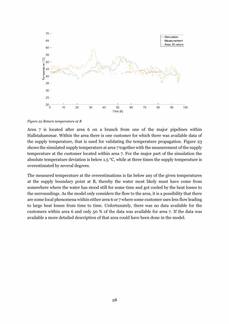
Area 7 is located after area 6 on a branch from one of the major pipelines within

Hallstahammar. Within the area there is one customer for which there was available data of

the supply temperature, that is used for validating the temperature propagation. Figure 23

shows the simulated supply temperature at area 7 together with the measurement of the supply

temperature at the customer located within area 7. For the major part of the simulation the

absolute temperature deviation is below 1.5 °C, while at three times the supply temperature is

overestimated by several degrees.

The measured temperature at the overestimations is far below any of the given temperatures

at the supply boundary point at B, thereby the water most likely must have come from

somewhere where the water has stood still for some time and got cooled by the heat losses to

the surroundings. As the model only considers the flow to the area, it is a possibility that there

are some local phenomena within either area 6 or 7 where some customer uses less flow leading

to large heat losses from time to time. Unfortunately, there was no data available for the

customers within area 6 and only 50 % of the data was available for area 7. If the data was

available a more detailed description of that area could have been done in the model.

29

Figure 23 Supply temperature at customer in area 7

4.2.2. Pressure and flow

When it comes to ring networks the pressure losses becomes important as it will determine

how the flow will propagate depending on lengths, diameters and roughness, thereby deciding

the velocities in the pipes and hence also the speed of the temperature propagation. In the

model, the pressure distribution is steady state in each time step, hence the neglection of water

acceleration/retardation could have some impact on the flow. But as the temperature

propagation is much slower than the pressure propagation the impact will not be significant,

which then would have given errors in the temperature validation of area 7.

Figure 24 Pressure difference of all areas with measured supply pressure at A

30

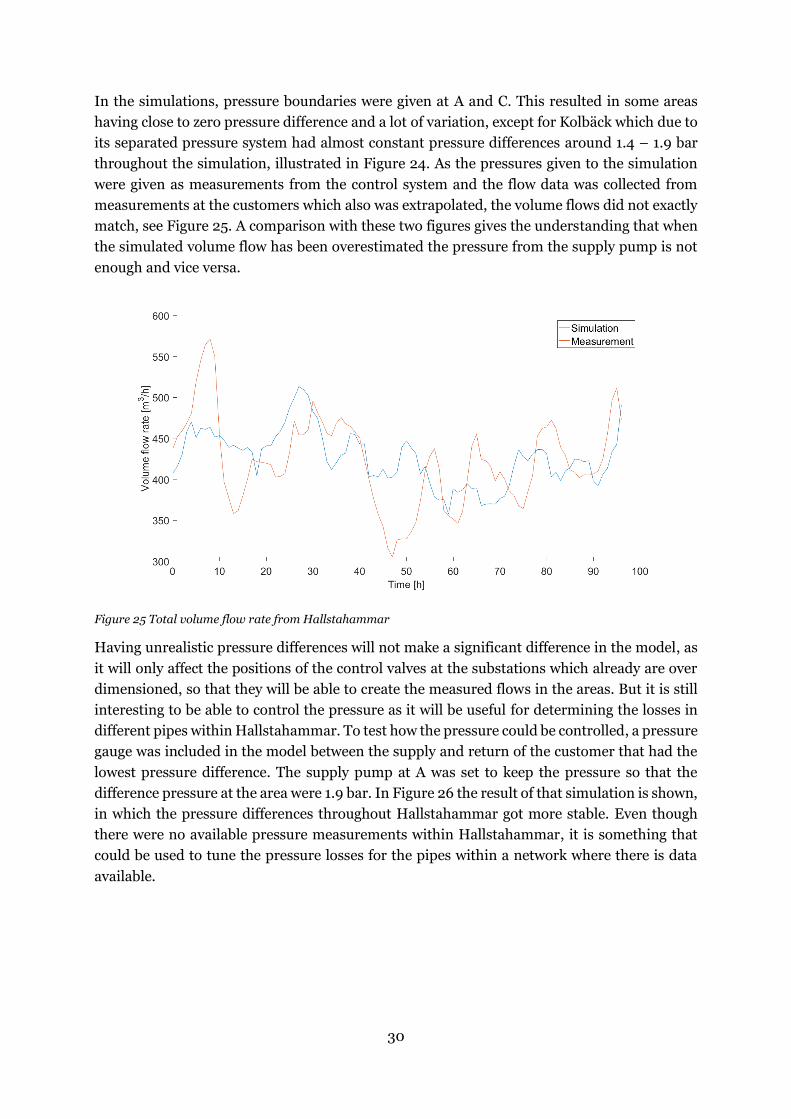
In the simulations, pressure boundaries were given at A and C. This resulted in some areas

having close to zero pressure difference and a lot of variation, except for Kolbäck which due to

its separated pressure system had almost constant pressure differences around 1.4 – 1.9 bar

throughout the simulation, illustrated in Figure 24. As the pressures given to the simulation

were given as measurements from the control system and the flow data was collected from

measurements at the customers which also was extrapolated, the volume flows did not exactly

match, see Figure 25. A comparison with these two figures gives the understanding that when

the simulated volume flow has been overestimated the pressure from the supply pump is not

enough and vice versa.

Figure 25 Total volume flow rate from Hallstahammar

Having unrealistic pressure differences will not make a significant difference in the model, as

it will only affect the positions of the control valves at the substations which already are over

dimensioned, so that they will be able to create the measured flows in the areas. But it is still

interesting to be able to control the pressure as it will be useful for determining the losses in

different pipes within Hallstahammar. To test how the pressure could be controlled, a pressure

gauge was included in the model between the supply and return of the customer that had the

lowest pressure difference. The supply pump at A was set to keep the pressure so that the

difference pressure at the area were 1.9 bar. In Figure 26 the result of that simulation is shown,

in which the pressure differences throughout Hallstahammar got more stable. Even though

there were no available pressure measurements within Hallstahammar, it is something that

could be used to tune the pressure losses for the pipes within a network where there is data

available.

31

Figure 26 Pressure difference of all areas with controlled supply pressure at A

In pressure flow network the losses can be calculated from the flow and vice versa, but the

absolute pressure in some point will have to be determined. In reality, it would most likely be

a pressurized point at a production facility or an accumulator tank, while in this model it is in

the inlet to A, as the model is a part of a larger system for which the dynamics are set by

unknown variables. Therefor the usage of a pump controller might not reflect the reality in

absolute values. Figure 27 shows the measured supply pressure at A and the simulated with a

controlled pump, where it suggests that the simulated pressure would almost be as high as 10

bar at the highest flow while the measured only gets up to 9 bar at its highest flow, see Figure

25. This is a result from that the return pressure varies due to the rest of the network.

Figure 27 Supply pressure at A with measured pressure given at the return inlet

32

4.2.3. Visualization of heat propagation

The temperature propagation in the supply distribution pipes is illustrated in Figure 28, in

accordance to the pipes included in the model. The figure is not made to scale, but rather to

illustrate the figure presented from OME, illustrated in Figure 13. At hour 28, the system has

an even temperature distribution and it can be seen that the temperature at the boundary point

located at Västerås is starting to rise as the color is starting to shift to red. Further, at hour 30,

the temperature wave has reached the beginning of Hallstahammar, seen by the red line to the

right. By hour 32 the temperature has started to reach most parts of Hallstahammar and is

closing in to Kolbäck, it can also be seen that the supply temperature from the boundary is

starting to decrease. At hour 34 it can be clearly seen which pipes that have the longest delay

of supply temperature, as these have not yet got the supply temperature that entered at hour

28.

Figure 28 Supply heat propagation from hour 28 to 34 in aggregated model

Some examples from the Hallstahammar simulations of issues that can be found with a

dynamic model is that the flow can behave in unexpected ways during off-design and transient

conditions. It was found that in 7 of the pipes, 3 return and 4 supply pipes, the flow reversed

direction during the simulation. This is because the flows to the areas varies over time, which

causes the pressure losses to vary and hence the path of least resistance for the flow. The model

does not capture the dynamic change of flow and pressure; hence the acceleration/retardation

of the flow is not accounted for which brings an uncertainty for the exact change of flow

direction. Also, as the pressures within Hallstahammar could not be validated against any

internal nodes, the pressure losses of the pipes could not be fully tuned nor was it known if

there were any closed valves or booster pumps within the system.

33

Another result of the pressure differences balancing in ring structures in the network is that

some pipes got low velocities which resulted in large heat losses. Having large heat losses does

not only cause a need for more production at the production facility, it also affects the supply

temperature, which for some customers is crucial to meet their demand. As in the earlier

example with the customer in area 7, that at certain times gets much colder supply than what

is delivered from Västerås. There can be multiple of different solutions to solve these issues,

such as installing pumps or bypass valves to make the flow velocity higher during the these

occasions, dynamic simulations are then a valuable tool to analyze what effect the different

solutions would have on the system. Furthermore, the results could be used to investigate if

the environmental, economic and social benefits would make up for the cost of the investment.

Automation of model building, simulation and visualization

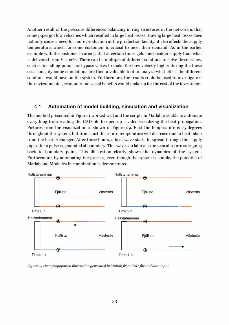
The method presented in Figure 1 worked well and the scripts in Matlab was able to automate

everything from reading the CAD-file to open up a video visualizing the heat propagation.

Pictures from the visualization is shown in Figure 29. First the temperature is 75 degrees

throughout the system, but from start the return temperature will decrease due to heat taken

from the heat exchanger. After three hours, a heat wave starts to spread through the supply

pipe after a pulse is generated at boundary. This wave can later also be seen at return side going

back to boundary point. This illustration clearly shows the dynamics of the system.

Furthermore, by automating the process, even though the system is simple, the potential of

Matlab and Modelica in combination is demonstrated.

Figure 29 Heat propagation illustration generated in Matlab from CAD-file and data input

34

Building a library of generic components is good for systems that changes often and can take

on different forms, such as district heating systems. Modelica was an effective way of building

such a library and because of its structure and shell, models could be build and simulated

externally using the library and compiler. This is critical because this allows the model building

to be automated and updated from other IT-systems of the DHS, e.g. CAD drawing. This way,

the DHS owner only have to redraw the CAD-drawings, and the dynamic model would then

easily be updated in accordance.

OME was a good tool for designing and verifying the model library. However, handling data

was not easily done in OME and hence should be pre-processed in some other program, e.g.

Matlab or some other language that supports an object-oriented structure.

Utilization of model

A dynamic model is useful because it shows how the system behaves at all times, not only for

certain states of equilibrium. Because the district heating system is very dynamic in its nature

due to varying heat loads, weather conditions and production, a dynamic model is well suited

for a variety of applications. It can be used for training purposes for operators that can try

different strategies and learn how to optimally control the system in a safe environment.

Analyses of the system can be made to better understand how it behaves and how changes such

as new loads, pumps, valves, control strategies, temperature levels etc. would affect the system.

A dynamic model that is accurate enough can also be used for diagnostics, seeking anomalies

and warning when something is out of order, e.g. a leakage. A dynamic model can also be used

for real time control and optimization of the system.

By introducing production units and more details into model that can quantify the total pump

work, heat losses and heat & electricity production, the model can be used for optimizing

production and distribution planning. Real time optimization would however require that

model can be simulated relatively fast, this is possible by increasing discretization grid and

reducing the number of variables such as density, viscosity and heat transfer coefficients. A

sensitivity analysis would have to be made to ensure that the results are accurate enough for

optimizations to be carried out. Since district heating systems tends to be large and stands for

a significant part of the energy system, optimization can yield great economic benefits.

Using a physical model for very large systems can give issues of convergence when input data

such as pressure and temperature is inserted. This becomes a problem especially when there

is lack of good and accurate data. However, by making some variables into parameters, such

as density, viscosity and heat loss factors, the dynamic model can more easily converge, even

for larger systems and without too much effect on the result. Again, using a generic object

oriented library as base, the user can get the option of what factors to have as variables and

what to set as parameters, as well as where to input data (which then determines what is

simulated), a flexibility that is very good.

35

5. CONCLUSIONS

A library of components was developed in Modelica together with a method for building and

simulating district heating networks with Matlab as core. Validation of the component library

was done by simulating an isolated part of Mälarenergi’s DHN by aggregating a municipality

to one heat exchanger and comparing simulated temperature and pressure with online

measurements. It was concluded that the components can describe the characteristic of the

system and in particular the heat propagation.

The model was then scaled to describe the major distribution pipes within the municipality

with 37 heat exchangers describing the heat load from different areas. Simulation of the model

was feasible but due to insufficient data it could not be fully validated. Furthermore, a

demonstration was made were a CAD drawing together with the component library was used

to build, simulate and visualize a model of a district heating network.

From the visualization of the simulation results, heat propagation and temperature

distribution in the district heating network was clearly shown. This gives a better

understanding of how the system behaves under transient conditions. It also reveals parts of

the network that have high heat losses and which customers that has the longest delays of

supply temperature.

The use of an external program such as Matlab in combination with Modelica’s object oriented

structure suits the purpose of building models of district heating networks well, as large system

can be built by a few standard components with a high degree of automation.

36

6. FURTHER WORK

A complete dynamic model of a DHS which includes physical models of customers and

production units would be useful for forecasting, control and optimization of the system. The

model developed in this study uses an empirical model of heat loads and making a physical

model that calculates the heat transfer according to temperature and mass flow would be the

next step. This would allow heat demand to be the only input data into the model, and

depending on supply temperature and heat exchanger conditions at customer, the flow would

be controlled by customer to achieve the correct heat. This would allow the model to be used

for more applications, e.g. investigating how a different supply temperatures would affect

customers and DHS. The physical heat load model could also be extended with models of

forecasting, then the model would require input on weather conditions and other factors

affecting heat demand.

It would also be interesting to demonstrate the method of automating the entire process on a

large scale. This would require the CAD-drawings of the DHS to be made according to a certain

structure. By doing this and applying the method shown in Figure 30, the entire process of

building a dynamic model of any DHS and inputting data and visualizing results, could be

made automatic and hence evolve with the DHS.

Figure 30 Suggestions for further work on model and method

Or

Physical Flow &

Thermal model

Empirical Heat

Load Model

Physical Heat Load

Model

Dynamic model

library

CHP/heat-plant

model

Model of DHS

Data input DHS &

Operational

Simulation of

DHS

Matlab

Process data

Read DHS

Build models

Start compiler

Present Results

CAD-drawings of

DHS

Compiled model

37

REFERENCES

Allegrini, J., Orehounig, K., Mavromatidis, G., Ruesch, F., Dorer, V., & Evins, R. (2015). A

review of modelling approaches and tools for the simulation of district-scale energy

systems. Renewable and Sustainable Energy Reviews, 52, 1391–1404.

https://doi.org/10.1016/j.rser.2015.07.123

Benonysson, A. (1991). Dynamic modelling and operational optimization of district heating

systems. Thesis (Ph.D.) Danmarks Tekniske Hoejskole, Lyngby (Denmark).

Birkelbach, F. (2015). Modelica result file parser (Version Version 1.0). Retrieved from

https://se.mathworks.com/matlabcentral/fileexchange/49015-modelica-result-file-

parser

Brange, L., Englund, J., & Lauenburg, P. (2016). Prosumers in district heating networks – A

Swedish case study. Applied Energy, 164, 492–500.

https://doi.org/10.1016/j.apenergy.2015.12.020

Danielewicz, J., Śniechowska, B., Sayegh, M. A., Fidorów, N., & Jouhara, H. (2016). Three-

dimensional numerical model of heat losses from district heating network pre-

insulated pipes buried in the ground. Energy, 108, 172–184.

https://doi.org/10.1016/j.energy.2015.07.012

Energimyndigheten. (2016, February 18). Energiläget i siffror 2016. Energimyndigheten.

Gabrielaitienė, I., Bøhm, B., & Sundén, B. (2011). Dynamic temperature simulation in district

heating systems in Denmark regarding pronounced transient behaviour. Journal of

Civil Engineering and Management, 17(1), 79–87.

https://doi.org/10.3846/13923730.2011.553936

Giraud, L., Bavière, R., Cédric, P., Vallée, M., & Robin, J.-F. (2015). Dynamic Modelling,

Experimental Validation and Simulation of a Virtual District Heating Network.

Retrieved from

https://www.researchgate.net/publication/277007243_Dynamic_Modelling_Experi

mental_Validation_and_Simulation_of_a_Virtual_District_Heating_Network

38

Giraud, L., Bavière, R., Vallée, M., & Paulus, C. (2015). Presentation, Validation and

Application of the DistrictHeating Modelica Library. Retrieved from

http://www.ep.liu.se/ecp/118/008/ecp1511879.pdf

Guelpa, E., Toro, C., Sciacovelli, A., Melli, R., Sciubba, E., & Verda, V. (2016). Optimal

operation of large district heating networks through fast fluid-dynamic simulation.

Energy, 102, 586–595. https://doi.org/10.1016/j.energy.2016.02.058

Idowu, S., Saguna, S., Åhlund, C., & Schelén, O. (2016). Applied machine learning:

Forecasting heat load in district heating system. Energy and Buildings, 133, 478–

488. https://doi.org/10.1016/j.enbuild.2016.09.068

Ikonen, E., Selek, I., Kovács, J., & Neuvonen, M. (2016). Examination of operational

optimization at Kemi district heating network. Thermal Science, 20(2), 667–678.

Incropera, F. P., DeWitt, D. P., Bergman, T. L., & Lavine, A. S. (Eds.). (2013). Principles of

heat and mass transfer (7. ed., international student version). Singapore: Wiley.

Jie, P., Tian, Z., Yuan, S., & Zhu, N. (2012). Modeling the dynamic characteristics of a district

heating network. Energy, 39(1), 126–134.

https://doi.org/10.1016/j.energy.2012.01.055

Kensby, J., Trüschel, A., & Dalenbäck, J.-O. (2015). Potential of residential buildings as

thermal energy storage in district heating systems – Results from a pilot test. Applied

Energy, 137, 773–781. https://doi.org/10.1016/j.apenergy.2014.07.026

Kuosa, M., Aalto, M., El Haj Assad, M., Mäkilä, T., Lampinen, M., & Lahdelma, R. (2014).

Study of a district heating system with the ring network technology and plate heat

exchangers in a consumer substation. Energy and Buildings, 80, 276–289.

https://doi.org/10.1016/j.enbuild.2014.05.016

Larsen, H. V., Pálsson, H., Bøhm, B., & Ravn, H. F. (2002). Aggregated dynamic simulation

model of district heating networks. Energy Conversion and Management, 43(8),

995–1019. https://doi.org/10.1016/S0196-8904(01)00093-0

39

Leonard, B. P. (1979). A stable and accurate convective modelling procedure based on

quadratic upstream interpolation. Computer Methods in Applied Mechanics and

Engineering, 19(1), 59–98. https://doi.org/10.1016/0045-7825(79)90034-3

Lund, H., Werner, S., Wiltshire, R., Svendsen, S., Thorsen, J. E., Hvelplund, F., & Mathiesen,

B. V. (2014). 4th Generation District Heating (4GDH): Integrating smart thermal

grids into future sustainable energy systems. Energy, 68, 1–11.

https://doi.org/10.1016/j.energy.2014.02.089

Ma, Z., Li, H., Sun, Q., Wang, C., Yan, A., & Starfelt, F. (2014). Statistical analysis of energy

consumption patterns on the heat demand of buildings in district heating systems.

Energy and Buildings, 85, 464–472. https://doi.org/10.1016/j.enbuild.2014.09.048

Modelica Association. (2014). Modelica® - A Unified Object-Oriented Language for

Physical Systems Modeling. Language Specification. Version 3.3. Revision 1 (pp.

183–188). Retrieved from

https://www.modelica.org/documents/ModelicaSpec33_withRevisionMarks.pdf

Olsthoorn, D., Haghighat, F., & Mirzaei, P. A. (2016). Integration of storage and renewable

energy into district heating systems: A review of modelling and optimization. Solar

Energy, 136, 49–64. https://doi.org/10.1016/j.solener.2016.06.054

Perpar, M., Rek, Z., Bajric, S., & Zun, I. (2012). Soil thermal conductivity prediction for

district heating pre-insulated pipeline in operation. Energy, 44(1), 197–210.

https://doi.org/10.1016/j.energy.2012.06.037

Pinson, P., Nielsen, T. S., Nielsen, H. A., Poulsen, N. K., & Madsen, H. (2009). Temperature

prediction at critical points in district heating systems. European Journal of

Operational Research, 194(1), 163–176. https://doi.org/10.1016/j.ejor.2007.11.065

Powell, K. M., Sriprasad, A., Cole, W. J., & Edgar, T. F. (2014). Heating, cooling, and

electrical load forecasting for a large-scale district energy system. Energy, 74, 877–

885. https://doi.org/10.1016/j.energy.2014.07.064

Stevanovic, V. D., Zivkovic, B., Prica, S., Maslovaric, B., Karamarkovic, V., & Trkulja, V.

(2009). Prediction of thermal transients in district heating systems. Energy

40

Conversion and Management, 50(9), 2167–2173.

https://doi.org/10.1016/j.enconman.2009.04.034

Stuart W. Churchill. (1977). Friction-factor equation spans all fluid-flow regimes.

Velu, S., Larsson, P.-O., Windahl, J., Saarinen, L., & Boman, K. (2014). Short-term

production planning for district heating networks with JModelica.org.

https://doi.org/10.3384/ECP14096959

Wetter, M., Treeck, C. van, & IEA EBC. (2015). New Generation Computational Tools for

Building and Community Energy Systems based on the Modelica and Functional

Mockup Interface Standards. Retrieved February 8, 2017, from http://www.iea-

ebc.org/fileadmin/user_upload/docs/TD1511/10_IEA-

EBC_Technical_Day_November_2015_-_EBC_Annex_60.pdf

Zhou, S., Tian, M., Zhau, Y., & Guo, M. (2014). Dynamic modeling of thermal conditions for

hot-water district-heating networks. Journal of Hydrodynamics, Ser. B, 26(4), 531–

537. https://doi.org/10.1016/S1001-6058(14)60060-3

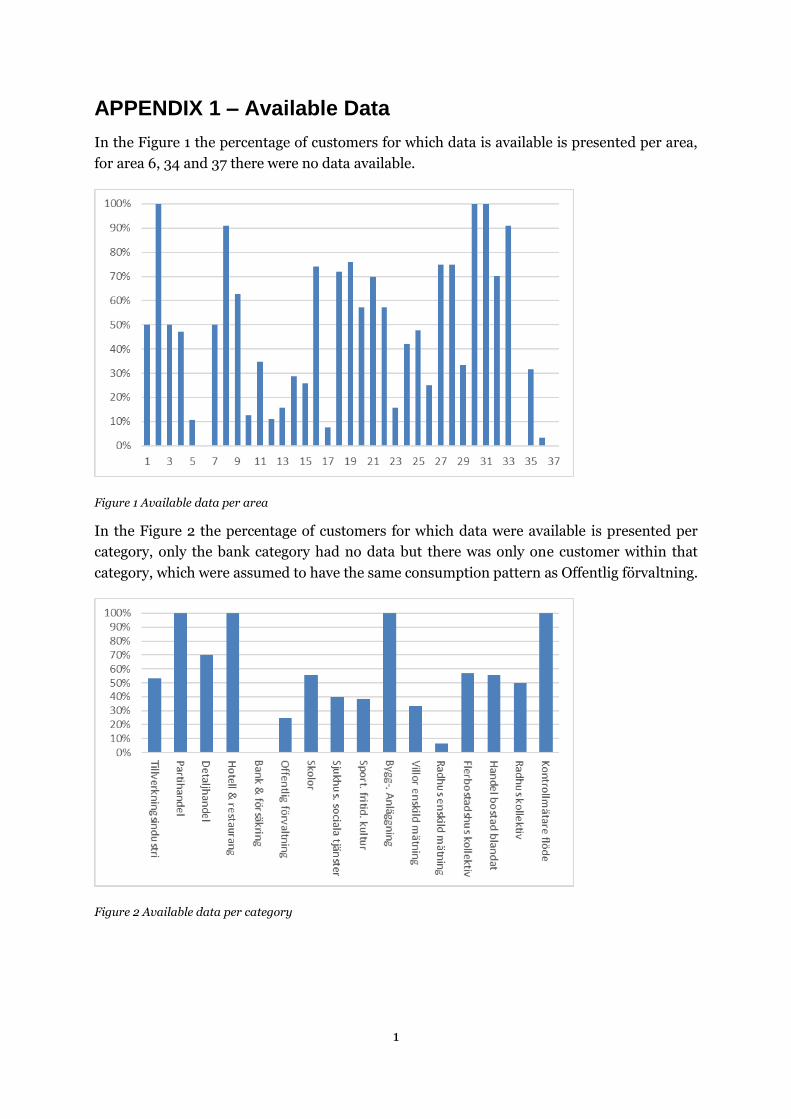
1

APPENDIX 1 – Available Data

In the Figure 1 the percentage of customers for which data is available is presented per area,

for area 6, 34 and 37 there were no data available.

Figure 1 Available data per area

In the Figure 2 the percentage of customers for which data were available is presented per

category, only the bank category had no data but there was only one customer within that

category, which were assumed to have the same consumption pattern as Offentlig förvaltning.

Figure 2 Available data per category

1

APPENDIX 2 – Customer areas

The Figure 1 shows how the areas have been selected, without numbering due to integrity.

Figure 1 Customer areas

P.O. Box 883, SE-721 23 Västerås, Sweden Phone: +46 21 101 300 P.O. Box 325, SE-631 05 Eskilstuna, Sweden Phone: +46 16 153 600

E-mail: info@mdh.se Webb: www.mdh.se