BUSINESS CYCLE AND MARKOV SWITCHING MODELS WITH

DISTRIBUTED LAGS: A COMPARISON BETWEEN US AND EURO AREA

by Monica Billio ∗ and Maddalena Cavicchioli †

FOR PhD SESSION

Abstract. This paper shows that well-known State Space systems used to analyse business

cycle phases in several empirical works can be comprised into a broad class of non linear

models, the MSI-VARMA. These processes are M -state Markov switching VARMA(p, q)

models for which the intercept term depends not only on the actual regime but also on

the last r regimes. We give stable finite order VARMA(p∗,q∗) representations for these

processes, where upper bounds for p∗ and q∗ are elementary functions of the dimension K

of the process, the number M of regimes, the number of regimes r on the intercept and the

orders p and q. If there is no cancellation, the bounds become equalities, and this solves the

identification problem. This result allows us to study US and European business cycles and

to determine the number of regimes most appropriate for the description of the economic

systems. Two regimes are confirmed for the US economy; the European business cycle

exhibits, instead, strong non-linearities and more regimes are necessary. This is taken

into account when performing estimation and regime identification.

Keywords: Time series, Varma models, Markov chains, changes in regime, regime number,

business cycle models.

JEL Classification: C01, C50, C32, E32.

∗Department of Economics, ”Ca Foscari” University of Venice, Cannaregio 873, 30121

Venice, Italy. E-mail: billio@unive.it†Advanced School of Economics, Department of Economics, ”Ca Foscari” University

of Venice, Cannaregio 873, 30121 Venice, Italy. E-mail: maddalena.cavicchioli@unive.it

(corresponding author)

1

2

1. Introduction

In this paper we consider a generalization of dynamic models denoted as Markov Switch-

ing Vector Autoregressive Moving Average (in short, MS(M)-VARMA(p, q)), which are

models for time series where we allow the parameters to change as a result of the outcome

of an observed Markov chain. In particular, one may also assume that the intercept term

depends not only on the actual regime, as in the baseline case (see Cavicchioli (2013)),

but also on the last r regimes and we we denote it as MSI(M, r)-VARMA(p, q). It turns

out that this is a useful representation of a dynamic economic system since some business

cycle models can be comprised in this framework. As a consequence, a key problem is

the determination of the number of states which best describes the observed data. Our

method for the determination of the number of regimes relies on the computation of the au-

tocovariance function and on finite order (or stable) VARMA representation of the initial

switching model (see Krolzig (1997) and Cavicchioli (2013)). More precisely, the param-

eters of the VARMA representation can be determined by evaluating the autocovariance

function of the Markov-switching model. It turns out that the orders p∗ and q∗ of the

finite order VARMA representations are elementary functions of the dimension K of the

process, the number M of regimes, the number of lags r on the intercept and the orders p

and q of the initial swiching model. Moreover, if there is no cancellation among the roots

of the autoregressive and moving average polynomials, the bounds become equalities, and

this solves the identification problem.

We note that well-known State-Space models of business cycle can be rewritten into the

MSI-VARMA framework. This is convenient since it allows simpler inference and gives

a way to determine the number of regimes which better describes the economic system.

Business cycle analysis takes its first steps from the main empirical facts establishing that

during a postwar period, contraction has typically been followed by a high-growth recovery

that quickly boosts output to its prerecession level. This two phase pattern was initially

proposed by Hamilton (1989) and Lam (1990) and we call it the Lam-Hamilton-Kim

model. An alternative description was initiated by Friedman (1964; 1993) who observes

that postwar fluctuations in real output should be thought of as having three phases

rather than two - contractions, high-growth recoveries and moderate-growth subsequent

recoveries (see also DeLong and Summers (1988) and Kim and Nelson (1999)). In the

sequel we will refer to this alternative model as Friedman-Kim-Nelson. In recent years,

interest has increased in the ability of business cycle models to forecast economic growth

rates and turning points or structural breaks in economic activity (see Krolizig (2001,2004),

Billio and Casarin (2010) or Billio, Ferrara, Guegan and Mazzi (2013)). However, in

empirical applications where such non-linear specifications are employed, the number of

regimes is sometimes dictated by the particular application or is determined in an informal

3

manner by visual inspection of plots. Since Hamilton (1989) and his application, for the

study of US cycles, two regimes have been considered in many studies. On the contrary,

in some recent papers which analyze the Euro area dynamics, more regimes have been

suggested. For example, Billio, Casarin, Ravazzolo and Van Dijk (2012) considered Markov

Switching models and in their application to US and EU industrial production data, for a

period of time including the last recession, they find that four regimes (strong-recession,

contraction, normal-growth, and high-growth) are necessary to identify some important

features of the cycle.

The main contributions of our paper are twofold. Firstly, we show that the most used

models for business cycle analysis can be comprised into a broad class of non linear model,

the MSI-VARMA, and we obtain new results related to it. Specifically, we give its stable

VARMA(p∗, q∗) representation and the orders can be determined by evaluating the auto-

covariance function of the initial switching model. Secondly, we propose a new and more

rigorous way for the determination of the number of regimes and apply it to analyse the

US and Euro business cycles. In particular, we are able to assess that two regimes are

sufficient when modeling the US business cycle but more regimes are necessary when we

consider the Euro area. This is the preliminary stage to obtain correct estimation and to

identify regimes.

The rest of the paper is organized as follows. In Section 2 we review some facts linking

Markov switching models to business cycle analysis and thus we introduce the MS-VAR

model. In Section 3 we study a generalization denoted as MSI-VARMA starting from

the baseline case of an hidden Markov chain process with distributed lags in the regime

(in short, MSI(M, r)-VAR(0)); here we give upper bounds for the stable VARMA order

both via autocovariance function and via explicit determination of the stable VARMA.

Then we extend these results in Section 4 where theorems are stated for every MSI(M, r)-

VARMA(p, q) model in which the regime variable is uncorrelated with the observable.

Section 5 introduces the Lam-Hamilton-Kim and the Friedman-Kim-Nelson models of

business cycle fluctuations and shows that these State Space models can be expressed as

MSI-VARMA. Finally, an application on the determination of the number of regimes for

the US and Euro real GDP is conducted in Section 6, followed by estimation and regime

identification. Section 7 concludes. Proofs are given in the Appendix.

2. Markov Switching Models and Business Cycle

Many economic time series occasionally exhibit dramatic breaks in their behavior, associ-

ated with events such as financial crises, abrupt changes in government policy or in the

price of production factors. Of particular interest for economists is the statistical mea-

surement and forecasting of business cycles. Since the early work of Bruns and Mitchell

(1946), many attempts have been made to identify cycles and to provide a turning-point

4

chronology that dates the cycle for a given country or economic area. The modern tools

to deal with business cycle analysis refer to nonlinear parametric modelling, which are

flexible enough to take into account certain stylized facts, such as asymmetries in the

phase of the cycle. In fact, there is a large literature that uses Markov switching (MS)

models to recognize business cycle phases. The starting point of this strand of litera-

ture is the recognition that there is a relationship between the concepts of changes in

cyclical phases and changes in regime. The most representative works are the univari-

ate regime-switching model proposed by Hamilton (1989) and its multivariate extension

allowing both for co-movement of macroeconomic variables and switching regime as in

Kim and Nelson (1999). The relationship between turning point and change in regime

has been confirmed by a number of empirical studies, as Krolzig (2001, 2004) and Billio,

Ferrara, Guegan and Mazzi (2013) among the others. When using parametric models to

analyze the cycle, the most used models are certainly MS-VAR. This approach do not

assume any a priori definition of the business cycle: by means of the switching approach,

different regimes are identified. Indeed, these regimes differ in terms of average growth

rates and/or growth volatilities. Let us now introduce the MS-VAR model. Consider the

K-dimensional second-order stationary dynamic process y = (yt) satisfying the following

Markov switching autoregressive model

(2.1) φst(L)yt = νst + Σstut

where ut ∼ IID(0, IK) and φst(L) =∑pi=0 φst,iL

i with φst,0 = Ik and φst,p 6= 0. As

usual, we assume that the polynomials |φst(z)| have all their roots strictly outside the

unit circle. Sufficient conditions ensuring second-order stationarity for Markov-switching

VAR models and Markov-switching VARMA models can be found, for example, in Francq

and Zakoıan (2001), respectively. The regime (st) follows an M -state ergodic irreducible

Markov chain with P = (pij) being the (M × M) matrix of transition probabilities

pij = Pr(st = j|st−1 = i), for i, j = 1, . . . ,M . In general, from a statistical point of

view, the order p, the number of states M , the parameters and the transition matrix P

are unknown. However, it is established in the literature that such models admit finite-

order VARMA(p∗; q∗) representations. Several authors (Krolzig (1997), Zhang and Stine

(2001), Francq and Zakoan (2001,2002), Cavicchioli (2013) have looked at the problem of

finding upper bounds for p∗ and q∗, expressed as functions of various parameters of the

initial switching model. One possible application of such bounds are corresponding lower

bounds for M which in principle could be useful in real data situation. Another method

for the determination of regimes’ number refers to complexity-penalized likelihood crite-

ria, such as AIC, BIC, HQC (see Psaradakis and Spagnolo 2003, Olteanu and Rynkiewicz

2007, Rios and Rodriguez 2008). However, these criteria are not widely used in empirical

literature, possibly for the computational burder required. The sample autocovariances

5

are instead more easily calculated than maximum (penalized) likelihood estimates of the

model parameters and the bounds arising from the above-mentioned elementary func-

tions are very useful for selecting the number of regimes and the orders of the switching

autoregression. In the sequel we will consider a generalization of these models where the

intercept depends not only on the actual regime but also on the some previous regimes and

we propose a method for the determination of regimes number. This is interesting since

well-known models used for business cycle analysis can be recomprised in this framework,

thus having a rigorous way for detection of regimes and estimation.

3. The MSI(M, r) - VAR(0) Model

Let us consider a generalization of the MS(M)-VAR(p) model (see Cavicchioli (2013)), for

which we assume that the intercept term depends not only on the actual regime but also

on the last r (r ≥ 0) regimes

νt = νst,st−1,...,st−r =

r∑j=0

νj,st−j =

r∑j=0

M∑m=1

νjmI(st−j = m)

where the indicator function I(st = · ) takes on the value 1 if st = m and zero otherwise.

This specification is called MSI(M, r) - VAR(p) model. Here we treat the case r > 0 (for

r = 0 see Cavicchioli (2013)). (The basic reference for our arguments and techniques is the

Krolzig book (1997)). First we consider the K-dimensional MSI(M, r)-VAR(0) process:

(3.1) yt =

r∑j=0

νj,st−j + Σstut

where ut ∼ IID(0, IK) and (st) follows an M -state ergodic irreducible Markov chain. The

Markov chain follows an AR(1) process

ξt = P′ξt−1 + vt.

where P = (pij) is the (M ×M) matrix of transition probabilities pij = Pr(st = j|st−1 =

i), for i, j = 1, . . . ,M , and ξt denotes the random (M × 1) vector whose mth element is

equal to 1 if st = m and zero otherwise. Here the innovation process (vt) is a martingale

difference sequence defined by vt = ξt − E(ξt|ξt−1); it is uncorrelated with ut and past

values of u, ξ or y. The (M × 1) vector of the ergodic probabilities is denoted by π =

E(ξt) = (π1, . . . , πM )′. It turns out to be the eigenvector of P associated with the unit

eigenvalue, that is, the vector π satisfies P′π = π. The eigenvector π is normalized so

that its elements sum to unity. Irreducibility implies that πm > 0, for m = 1, . . . ,M ,

meaning that all unobservable states are possible.

6

The process in (3.1) has a first State-Space representation as follows

(3.2)

yt =∑rj=0 Λjξt−j + Σ(ξt ⊗ IK)ut

ξt = P′ξt−1 + vt

where Λj = (νj1 . . . νjM ), for j = 0, . . . , r, and Σ = (Σ1 . . . ΣM ).

Theorem 3.1 For every h ≥ r > 0, the autocovariance function of the process (yt) in

(3.1) satisfies

Γy(h) = A′(Q′)hB

where

A′

=

r∑i=0

Λi(P′)−i B =

r∑j=0

(P′)jDΛ

′

j Q = P−P∞ P∞ = limn Pn.

We can always obtain a second State-Space representation in the following way:

yt =

r∑j=0

Λj(ξt−j − π) + (

r∑j=0

Λj)π + Σ((ξt − π)⊗ IK)ut + Σ(π ⊗ IK)ut

or equivalently

yt = (

r∑j=0

Λj)π +

r∑j=0

Λjδt−j + Σ(δt ⊗ IK)ut + Σ(π ⊗ IK)ut

where

Λj = (νj1 − νjM . . . νjM−1 − νjM ) Σ = (Σ1 −ΣM . . . ΣM−1 −ΣM ).

Here δt is the (M − 1) × 1 vector formed by the columns, but the last one, of ξt − π.

Of course, the last formula is obtained by using the restrictions i′

Mξt = 1 and i′

Mπ = 1,

where i′

M denotes the (M × 1) vector of ones. So we get

(3.3)

yt = (∑rj=0 Λj)π +

∑rj=0 Λjδt−j + Σ(δt ⊗ IK)ut + Σ(π ⊗ IK)ut

δt = Fδt−1 + wt

where E(wtw′

t) = D− FDF′, E(wtw

′

τ ) = 0 for t 6= τ ,

D =

π1(1− π1) −π1π2 · · · −π1πM−1−π1π2 π2(1− π2) · · · −π2πM−1

......

...

−πM−1π1 −πM−1π2 · · · πM−1(1− πM−1)

7

and

F =

p11 − pM1 · · · pM−1,1 − pM1

......

p1,M−1 − pM,M−1 · · · pM−1,M−1 − pM,M−1

which is an (M − 1) × (M − 1) matrix with all eigenvalues inside the unit circle. Since

δt has zero mean, the unconditional expectation of the initial process is given by E(yt) =

µy = (∑rj=0 Λj)π, as before. By iteration of the transition equation in (3.3), we also

obtain E(δtδ′

t+h) = D(F′)h for every h ≥ 0.

For Model (3.1), we obtain the following main result:

Theorem 3.2. The second-order stationary dynamic process defined in (3.1), with r > 0,

has a stable VARMA(p∗, q∗) representation, where p∗ ≤M − 1 and q∗ ≤M + r− 2. If the

lag polynomials of the AR and MA parts of the VARMA(p∗, q∗) have no roots in common,

equalities hold in the previous relations, and the identification problem is completely solved,

that is, M = p∗ + 1 and r = q∗ − p∗ + 1 (in this case, we have q∗ ≥ p∗).

Now we also determine explicitly a stable VARMA(p∗, q∗) representation for the process

(yt) in (3.1), with r > 0. In our computation, the autoregressive lag polynomial of such a

stable VARMA is shown to be scalar.

Theorem 3.3. The second-order stationary dynamic process defined in (3.1), with r > 0,

has a stable VARMA(p∗, q∗) representation, with p∗ ≤M − 1 and q∗ ≤M + r − 2,

γ(L)(yt − µy) = C(L)εt

where γ(L) = |F (L)| is a scalar polynomial of degree M − 1 in L (that is, the determinant

of the matrix F (L) = IM−1 − FL, where L is the lag operator) and C(L) is the [K ×(KM +M − 1)]-dimensional lag polynomial matrix of degree M + r − 2 in L given by

C(L) = [

r∑j=0

ΛjF (L)∗Lj Σ(F (L)∗ ⊗ IK) |F (L)|Σ(π ⊗ IK)]

where F (L)∗ is the adjoint matrix of F (L). Furthermore, εt = (w′

t u′

t(w′

t⊗IK) u′

t)′

is a zero mean white noise process with var(εt) = diag(D−FDF′, (D−FDF

′)⊗ IK , IK).

If γ(L) and C(L) are coprime, then p∗ = M−1 and q∗ = M+r−2, and the identification

problem is completely solved.

4. The MSI(M, r)-VARMA(p, q) Model

Firstly, we consider the followingK-dimensional second-order stationary MSI(M, r)-VAR(p)

process, with r > 0 and p > 0,

(4.1) φst(L)yt =

r∑j=0

νj,st−j+ Σstut

8

where ut ∼ IID(0, IK) and φst(L) = φ0,st + φ1,stL + · · · + φp,stLp with φ0,st = IK

and φp,st 6= 0 . As usual, we assume that the polynomials |φst(z)| have all their roots

strictly outside the unit circle. Sufficient conditions ensuring second-order stationarity

for Markov-switching VARMA models can be found, for example, in Francq and Zakoıan

(2001) .

For every j = 0, . . . , r, define Λj = (νj1 . . . νjM ). Then define Σ = (Σ1 . . . ΣM ) and

φ(L) = [IK + φ1,1L+ · · ·+ φp,1Lp . . . IK + φ1,ML+ · · ·+ φp,MLp].

The process in (4.1) has a first State-Space representation as follows

(4.2)

φ(L)(ξt ⊗ IK)yt =∑rj=0 Λjξt−j + Σ(ξt ⊗ IK)ut

ξt = P′ξt−1 + vt

Moreover, we can always obtain a second State-Space representation:

(4.3)

φ(L)(δt ⊗ IK)yt + φ(L)(π ⊗ IK)yt

= (

r∑j=0

Λj)π +

r∑j=0

Λjδt−j + Σ(δt ⊗ IK)ut + Σ(π ⊗ IK)ut

δt = Fδt−1 + wt

where δt, Λj and Σ are defined as in the previous section, and

φ(L) = [(φ1,1−φ1,M )L+· · ·+(φp,1−φp,M )Lp . . . (φ1,M−1−φ1,M )L+· · ·+(φp,M−1−φp,M )Lp].

Theorem 4.1. For every h ≥ r > 0, assume that the regime variable ξt+h is uncorrelated

with yt. Then the autocovariance function of the second-order stationary process in (4.1)

satisfies

B(L)Γy(h) = A′FhB

where A′

=∑rj=0 ΛjF

−j and B = E(δty′

t), which are assumed to be nonzero matrices.

Now, applying Theorem 2.2 from Cavicchioli (2013) for q = r and taking in mind that F

is (M − 1)× (M − 1), we have the following main result for model (4.1):

Theorem 4.2. Under the hypothesis that the regime variable is uncorrelated with the

observable, the K-dimensional second-order stationary process in (4.1), with r > 0 and

p > 0, admits a stable VARMA(p∗, q∗) representation with p∗ ≤ M + p − 1 and q∗ ≤M + r− 2. If we require that autoregressive lag polynomial of such a stable representation

is scalar, then the bounds become p∗ ≤ M + Kp − 1 and q∗ ≤ M + (K − 1)p + r − 2. If

the lag polynomials of the AR and MA parts of the former VARMA(p∗, q∗) representation

9

have no roots in common, equalities hold in the previous relations, that is, p∗ = M + p− 1

and q∗ = M + r − 2.

To end the section we compute explicitly a VARMA representation for a general MSI-

VARMA. This gives a new proof of Theorem 3.3 (case q = 0) and extends Proposition

5 from Krolzig (1997), Section 10.2.2. We start with the more simple case in which the

autoregressive lag polynomial of the initial process is state independent.

Theorem 4.3. Let y = (yt) be an K–dimensional second-order stationary MSI(M, r)-

VARMA(p, q) process, with r > 0,

A(L)yt =

r∑j=0

νj,st−j+

q∑i=0

Θst(L)ut

where A(L) =∑p`=0 A`L

` with A0 = IK , |Ap| 6= 0, and Θst(L) =∑qi=0 Θst,iL

i,

with Θst,0 = Σst (nonsingular symmetric K × K matrix) and |Θst,q| 6= 0 are full rank

matrix lag polynomials. Under quite general regularity conditions, the dynamic process

y = (yt) admits a stable VARMA(p∗, q∗) representation, with p∗ ≤ M + Kp − 1 and

q∗ ≤M + (K − 1)p+ max{r, q + 1} − 2,

γ(L)(yt − µy) = C(L)εt

where γ(L) = |F (L)||A(L)| is the scalar AR operator of degree M + Kp − 1, C(L) is a

matrix lag polynomial of degree M + (K − 1)p+ max{r, q + 1} − 2, and εt is a zero mean

vector white noise process.

In the general case in which the autoregression part of the process in Theorem 4.3 is state

dependent but the regime variable is uncorrelated with the observable, we can proceed

as follows. By Theorem 4.1 the autocovariances of the process satisfy a finite difference

equation of order p∗ = M + p − 1 and rank q∗ + 1 = M + max{r, q + 1} − 1. Then the

process can be represented by a stable VARMA(p∗, q∗). Given the process (yt), we can

estimate the coefficients of the stable VARMA(p∗, q∗) with usual procedures. If there is

no cancellation between the AR and MA part of the estimated VARMA(p∗, q∗), then we

get the representation as in Theorem 4.3 with equalities.

5. Business Cycle Models

In this Section we show that business cycle models widely used in empirical works can be

rewritten as MSI-VARMA. Therefore, we can formally test the number of regimes as well

as lags in the intercept or autoregressive lags, given the above results. This avoids informal

determination of regimes’ number by the researcher and leads to correct estimation results

and possibly to reliable forecasting conclusions.

10

(5.1) The Lam-Hamilton-Kim model. In modeling the time series behaviour of real

Gross National Product (GNP) of United States, Hamilton (1989) considered the case in

which real GNP is generated by the sum of two independent unobserved components, one

following an autoregressive process with a unit root, and the other following a random

walk with a Markov switching error term. Lam (1990) generalized the Hamilton model to

the case in which the autoregressive component need not contain a unit root. Finally, Kim

(1994) showed that the Lam-Hamilton model can be written in the following State-Space

form, which we shall call the Lam-Hamilton-Kim model :

(5.1)

{yt = Hxt + βst

xt = Φxt−1 + et

where yt is scalar (K = 1), xt = (xt xt−1 · · ·xt−r+1)′

and et = (ut 0 · · · 0)′

are r× 1, with

ut ∼ IID(0, σ2), H = (1 − 1 0 · · · 0) is 1× r and

Φ =

φ1 φ2 φ3 · · · φr

1 0 0 · · · 0

0 1 0 · · · 0...

......

...

0 0 0 · · · 0

with φi ∈ R, i = 1, . . . , r, (r ≥ 2). Here βst = δ0 + δ1st, where δj ∈ R, j = 0, 1,

and (st) is an M -state Markov chain. Kim (1994) estimated this model by using suitable

(filtering and smoothing) algorithms that he also constructed for more general State-Space

representations with Markov switching. Now we are going to show that Model (5.1) can

be interpreted as a model with distributed lags in the regime. Then we give a stable

VARMA representation of it. This allows us to estimate the model via MLE, i.e., a very

simple procedure which is alternative to that employed by Kim (1994). From the transition

equation in (5.1) we get

Φ(L)xt = et

hence

(5.2) |Φ(L)|xt = Φ(L)∗et

where Φ(L) = Ir −ΦL. Substituting (5.2) into the measurement equation in (5.1) after

premultiplying by the determinant of Φ(L) gives

(5.3) |Φ(L)|yt = |Φ(L)|βst + HΦ(L)∗et

which is an MSI(M, r)-VARMA(p, q) model in the sense of Section 4, where p = r and

q = r−1 (recall r ≥ 2). So Theorem 4.3 directly implies that the Lam-Hamilton-Kim model

11

admits a stable VARMA(p∗, q∗) representation (whose autoregressive lag polynomial is

scalar) with p∗ ≤M + r − 1 and q∗ ≤M + max{p, p} − 2 = M + p− 2.

We now determine explicitly the final form of this stable VARMA and we need some

notation. Define β = (β1 · · ·βM ), where βm = δ0 + δ1m for every m = 1, . . . ,M . Then we

get βst = βξt. Substituting this relation into (5.3) yields

|Φ(L)|yt = |Φ(L)|βξt + HΦ(L)∗et

= |Φ(L)|β(ξt − π) + |Φ(1)|βπ + HΦ(L)∗et

= |Φ(L)|βδt + |Φ(1)|βπ + HΦ(L)∗et

where β = (β1 − βM · · ·βM−1 − βM ). Then we get the State-Space representation

(5.4)

{|Φ(L)|(yt − µy) = |Φ(L)|βδt + HΦ(L)∗et

δt = Fδt−1 + wt

where |Φ(L)|µy = |Φ(1)|βπ (in fact, µy = βπ). Substituting δt = F (L)−1wt into the

measurement equation in (5.4) and premultiplying by |F (L)| yield

|F (L)||Φ(L)|(yt − µy) = β|Φ(L)|F (L)∗wt + H|F (L)|Φ(L)∗et

which is a stable VARMA(p∗, q∗) with p∗ ≤ M + r − 1 and q∗ ≤ M + r − 2, and whose

autoregressive lag polynomial is scalar. Summarizing we have the following result:

Theorem 5.1. The Lam-Hamilton-Kim model for US real GNP admits a stable VARMA(p∗,

q∗) representation

γ(L)(yt − µy) = C(L)εt

with p∗ ≤ M + r − 1 and q∗ ≤ M + r − 2. Under quite general regularity conditions,

γ(L) = |F (L)||Φ(L)| is the scalar AR operator of degree M + r − 1 in the lag operator L

and C(L) is a [1× (M + r− 1)]-dimensional matrix lag polynomial of degree M + r− 2 in

L given by

C(L) = [H|F (L)|Φ(L)∗ β|Φ(L)|F (L)∗]

and εt = (e′

t w′

t)′

is a zero mean (M + r− 1)× 1 vector white noise process. If γ(L) and

C(L) are coprime, then equalities hold in the previous relations, hence p∗ = M + r − 1

and q∗ = p∗ − 1.

(5.2) The Friedman-Kim-Nelson model. Friedman’s plucking model (1964) of business

fluctuations suggests that output cannot exceed a ceiling level, and it is occasionally

plucked downward by recession. The model implies that business fluctuations are asym-

metric, that recessions have only a temporary effect on output, and that recessions are

duration dependent while expansions are not. Subsequent literature has provided copious

12

empirical support for these statements. See, for example, De Simone and Clarke (2007)

and its references. Kim and Nelson (1998) showed that the Friedman model can be written

in the following State-Space form, which we shall call the Friedman-Kim-Nelson model :

(5.5)

{yt = Hxt

xt = µst + Φxt−1 + Σstet

where yt is scalar (K = 1), xt, µst and et are 4 × 1 with et ∼ IID(0, I4), Σst is a 4 × 4

diagonal matrix, H = (1 1 0 0), and

Φ =

1 0 0 1

0 φ1 φ2 0

0 1 0 0

0 0 0 1

with φi ∈ R, i = 1, 2; here (st) is an M -state Markov chain (M = 2 in the quoted papers).

Kim and Nelson (1998) estimated the model by using Kim’s approximate MLE. See also

Kim (1994). We show that Model (5.5) can be viewed as a model with distributed lags in

the regime and then we give a stable VARMA representation of it. From the transition

equation in (5.5) we get

Φ(L)xt = µst + Σstet

where

Φ(L) = I4 −ΦL =

1− L 0 0 −L

0 1− φ1L −φ2L 0

0 −L 1 0

0 0 0 1− L

hence |Φ(L)| = (1−L)2(1−φ1L−φ2L2). Premultiplying by the adjoint matrix Φ(L)∗ we

obtain

(5.6) |Φ(L)|xt = Φ(L)∗µst + Φ(L)∗Σstet

where

Φ(L)∗ =

(1− L)(1− φ1L− φ2L2) 0 0 L(1− φ1L− φ2L2)

0 (1− L)2 φ2L(1− L)2 0

0 L(1− L)2 (1− φ1L)(1− L)2 0

0 0 0 (1− L)(1− φ1L− φ2L2)

.

Substituting (5.6) into the measurement equation in (5.5) gives

|Φ(L)|yt = HΦ(L)∗µst + HΦ(L)∗Σstet

13

which is an MSI(M, r)-VARMA(p, q) with p = 4 and r = q = 3. So Theorem 4.3 implies

that such a model has a stable VARMA(p∗, q∗) representation, with p∗ ≤M+p−1 = M+3

and q∗ ≤M + max{r, q + 1} − 2 = M + 2. We now determine explicitly the final form of

this stable VARMA. Model (5.5) has the following State-Space representation

(5.7)

yt = Hxt

xt = µδt + µπ + Φxt−1 + Σ(δt ⊗ I4)et + Σ(π ⊗ I4)et

δt = Fδt−1 + wt

where µ = (µ1 · · ·µM ) is 4×M , Σ = (Σ1 · · ·ΣM ) is 4× (4M), and µ and Σ are defined

in the usual way. Furthermore, we have E(yt) = HE(xt) and Φ(L)E(xt) = µπ, hence

yt − E(yt) = H(xt − E(xt)). From (5.7) we get

Φ(L)(xt − E(xt)) = µδt + Σ(δt ⊗ I4)et + Σ(π ⊗ I4)et

= µF (L)−1wt + Σ(F (L)−1wt ⊗ I4)et + Σ(π ⊗ I4)et

hence

|F (L)|Φ(L)(xt − E(xt)) = µF (L)∗wt + Σ(F (L)∗wt ⊗ I4)et + Σ|F (L)|(π ⊗ I4)et.

Premultiplying by the determinant of Φ(L) yields

|F (L)||Φ(L)|(xt−E(xt)) = Φ(L)∗µF (L)∗wt+Φ(L)∗Σ(F (L)∗wt⊗I4)et+Φ(L)∗Σ|F (L)|(π⊗I4)et.

Assuming µy = E(yt) time invariant, we obtain

|F (L)||Φ(L)|(yt − µy) = H|F (L)||Φ(L)|(xt − E(xt))

= HΦ(L)∗µF (L)∗wt + HΦ(L)∗Σ(F (L)∗ ⊗ I4)(wt ⊗ I4)et + HΦ(L)∗Σ|F (L)|(π ⊗ I4)et

which is a stable VARMA(p∗, q∗) with p∗ ≤ M + 3 and q∗ ≤ M + 2, and whose autore-

gressive lag polynomial is scalar. Summarizing we have the following result:

Theorem 5.2. The Friedman-Kim-Nelson model of business fluctuations admits a stable

VARMA(p∗, q∗) representation

γ(L)(yt − µy) = C(L)εt

with p∗ ≤ M + 3 and q∗ ≤ M + 2. Under quite general regularity conditions, γ(L) =

|F (L)||Φ(L)| is the scalar AR operator of degree M + 3 in the lag operator L and C(L) is

a [1× (5M − 1)]-dimensional matrix lag polynomial of degree M + 2 in L given by

C(L) = [HΦ(L)∗µF (L)∗ HΦ(L)∗Σ(F (L)∗ ⊗ I4) HΦ(L)∗Σ|F (L)|(π ⊗ I4)]

14

and εt = (w′

t e′

t(w′

t⊗I4) e′

t)′

is a zero mean (5M−1)×1 vector white noise process. If

γ(L) and C(L) are coprime, then equalities hold in the previous relations, hence p∗ = M+3

and q∗ = p∗ − 1.

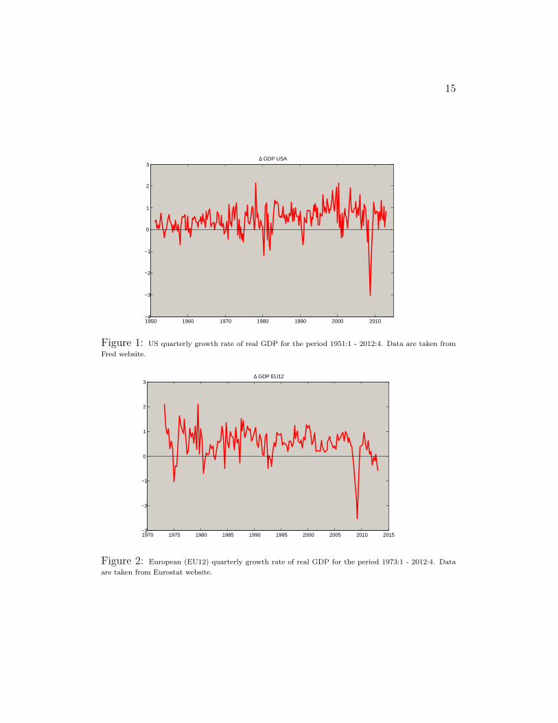
6. Empirical Application

In our study we consider the Gross Domestic Product (GDP) from FRED at a quarterly

frequency for the United States (US), from 1951:1 to 2012:4, and from EUROSTAT for

the European Union (EU 12), from 1973:1 to 2012:4 1. The presence of unit root in the

data has been checked by augmented Dickey-Fuller (ADF) test which points out the non-

stationarity of both series. For the null hypothesis of unit roots, the test statistic gives

1.724 (with p = 12) for US GDP and -0.4037 (with p=5) for EU GDP. In both cases the

null hypothesis of a unit root cannot be rejected. For differenced time series, the ADF

test rejects the unit root hypothesis on the 1% significance level (with test statistics of

-4.4853 for US and -5.3384 for EU). In the following analysis we consider the growth rate

of quarterly real GDP data for US and EU and the series are plotted in Figure 1 and

Figure 2.

We model both series as a MSI(M,r)-AR(0), with state-dependent mean and variance and

no autoregressive part. This follows from several empirical studies which find that most

part of the forecast errors is due to time changes in some parameters of the prediction

models. In particular, we follow Krolzig (2000) and Anas et al. (2008) where only intercept

and volatility are assumed to be driven by a regime-switching variable. In fact, with

regards to the Euro area, Anas et al. (2008) and Billio et al. (2013) find that allowing

regime switching-autoregressive coefficients deteriorates the detection of the business cycle

turning points. Note that we can now apply the bounds proposed in Section 3 which

simultaneously define number of regimes and lags in the intercept. Those can be obtained

having estimates of the stable VARMA orders p∗ and q∗ as followsM = p∗ + 1

r = 1− p∗ + q∗.

For the computation of the orders of the stable VARMA we use the 3-pattern method

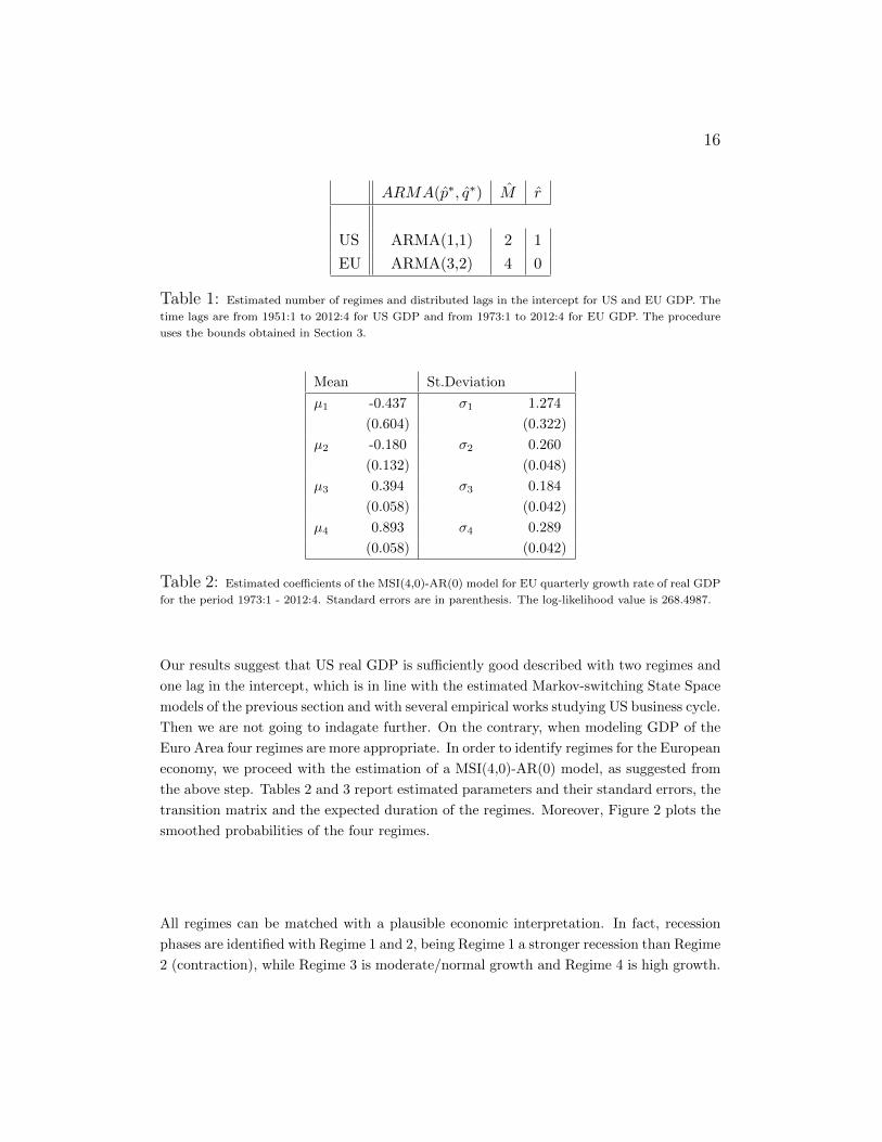
(TPM) proposed by Choi (1992). This gives the results reported in Table 1.

1Data are taken from Fred website: < research.stlouisfed.org > and from Eurostat website: < http :

//epp.eurostat.ec.europa.eu/portal/page/portal/eurostat/home/ >. Data are seasonally adjusted.

15

1950 1960 1970 1980 1990 2000 2010−4

−3

−2

−1

0

1

2

3∆ GDP USA

Figure 1: US quarterly growth rate of real GDP for the period 1951:1 - 2012:4. Data are taken from

Fred website.

1970 1975 1980 1985 1990 1995 2000 2005 2010 2015−3

−2

−1

0

1

2

3∆ GDP EU12

Figure 2: European (EU12) quarterly growth rate of real GDP for the period 1973:1 - 2012:4. Data

are taken from Eurostat website.

16

ARMA(p∗, q∗) M r

US ARMA(1,1) 2 1

EU ARMA(3,2) 4 0

Table 1: Estimated number of regimes and distributed lags in the intercept for US and EU GDP. The

time lags are from 1951:1 to 2012:4 for US GDP and from 1973:1 to 2012:4 for EU GDP. The procedure

uses the bounds obtained in Section 3.

Mean St.Deviation

µ1 -0.437 σ1 1.274

(0.604) (0.322)

µ2 -0.180 σ2 0.260

(0.132) (0.048)

µ3 0.394 σ3 0.184

(0.058) (0.042)

µ4 0.893 σ4 0.289

(0.058) (0.042)

Table 2: Estimated coefficients of the MSI(4,0)-AR(0) model for EU quarterly growth rate of real GDP

for the period 1973:1 - 2012:4. Standard errors are in parenthesis. The log-likelihood value is 268.4987.

Our results suggest that US real GDP is sufficiently good described with two regimes and

one lag in the intercept, which is in line with the estimated Markov-switching State Space

models of the previous section and with several empirical works studying US business cycle.

Then we are not going to indagate further. On the contrary, when modeling GDP of the

Euro Area four regimes are more appropriate. In order to identify regimes for the European

economy, we proceed with the estimation of a MSI(4,0)-AR(0) model, as suggested from

the above step. Tables 2 and 3 report estimated parameters and their standard errors, the

transition matrix and the expected duration of the regimes. Moreover, Figure 2 plots the

smoothed probabilities of the four regimes.

All regimes can be matched with a plausible economic interpretation. In fact, recession

phases are identified with Regime 1 and 2, being Regime 1 a stronger recession than Regime

2 (contraction), while Regime 3 is moderate/normal growth and Regime 4 is high growth.

17

Regime 1 Regime 2 Regime 3 Regime 4

Regime 1 0.49 0.00 0.09 0.00

(0.45) (0.01) (0.06) (0.01)

Regime 2 0.51 0.58 0.02 0.05

(0.33) (0.26) (0.02) (0.03)

Regime 3 0.00 0.20 0.68 0.18

(0.01) (0.12) (0.16) (0.07)

Regime 4 0.00 0.22 0.22 0.76

(0.01) (0.12) (0.09) (0.13)

Table 3: Transition probability matrix of the estimated MSI(4,0)-AR(0) model for EU quarterly growth

rate of real GDP for the period 1973:1 - 2012:4. Standard errors are in parenthesis.

19731975197719791981198319851987198919911993199519971999200120032005200720092011 20130

0.5

1

Pro

babi

litie

s of

Reg

ime

1

19731975197719791981198319851987198919911993199519971999200120032005200720092011 20130

0.5

1

Pro

babi

litie

s of

Reg

ime

2

19731975197719791981198319851987198919911993199519971999200120032005200720092011 20130

0.5

1

Pro

babi

litie

s of

Reg

ime

3

19731975197719791981198319851987198919911993199519971999200120032005200720092011 20130

0.5

1

Pro

babi

litie

s of

Reg

ime

4

Figure 3: Smoothed probabilities from the estimated MSI(4,0)-AR(0) model for EU quarterly growth

rate of real GDP for the period 1973:1 - 2012:4. Data are taken from Eurostat. Regime 1 corresponds to

strong recession, Regime 2 to contraction, Regime 3 to moderate/normal growth and Regime 4 to high

growth.

18

The expansionary regimes are more persistent than the others, in fact probabilities of

staying in those regimes are 0.68 and 0.76. Note also that all volatility coefficients are

significant at 1% level. The expected duration of recession phases is 4/5 quarters, while

expansionary regimes cover about 7 quarters. Here we detect turning points as the last

quarter of each regime phase and the following recession periods can be inferred from the

estimation: 1974:1 - 1975:3, 1979:1 - 1981:3, 1982:1 - 1983:1, 1991:1 - 1993:3, 2008:1 -

2010:1 and 2011:1 - 2012:4. These conclusions are in line with well-recognised recession

phases, see, for instance, Anas et al.(2007).

7. Conclusion

In this paper, for a general class of Markov-switching VARMA models with distributed lags

in the regime, in symbols MSI(M, r)- VARMA(p, q), we give finite order VARMA(p∗, q∗)

representations where the parameters can be determined by evaluating the autocovariance

function of the Markov-switching models. It turns out that upper bounds for p∗ and q∗

are elementary functions of the dimension K of the process, the number M of regimes, the

number of regimes r on the intercept and the orders p and q. If there is no cancellation,

the bounds become equalities, and this solves the identification problem. This result

produces an easy method for setting a lower bound on the number of regimes from the

estimated autocovariance function. Of particular interest is how some well-known State

Space systems, introduced in the literature for business cycle analysis, are shown to be

comprised in this general MSI-VARMA model, such as the Lam-Hamilton-Kim and the

Friedman-Kim-Nelson models of business fluctuations. In the application we determine

the number of regimes which turns out to be more appropriate for the description of US

and EU economic systems by using the bounds obtained in this work. In particular, US

real GDP is better described with two regimes, as is usually assumed in the estimation of

such State Space systems. However, EU business cycle exhibits strong non-linearities and

more regimes are necessary. This is taken into account when performing estimation and

regime identification.

19

References

[1] Anas, J., Billio, M., Ferrara, L., LoDuca, M. (2007) Business Cycle Analysis with

Multivariate Markov Switching Models, in Growth and Cycle in the Euro Zone,

Mazzi GL and Savio G (eds), Palgrave Macmillan: New York, 249–260.

[2] Anas, J., Billio, M., Ferrara, L., LoDuca, M. (2008) A system for dating and de-

tecting turning points in the Euro area, The Manchester School, 76, 549–577.

[3] Billio, M., and Casarin, R. (2010) Identifying business cycle turning points with

sequential monte carlo methods: an online and real-time application to Euro area,

Journal of Forecasting, 29, 145–167.

[4] Billio, M., Casarin, R., Ravazzolo, F., and Van Dijk, H.K. (2012) Combination

scheme for turning point predictions, The Quartely Review of Economics and Fi-

nance, 52, 402–412.

[5] Billio, M., Ferrara, L., Gugan, D., and Mazzi, G.L. (2013) Evaluation of regime

switching models for real-time business cycle analysis of the Euro area, Journal of

Forecasting, DOI: 10.1002/for.2260, 2013.

[6] Burns, A.F. and Mitchell, W.C. (1946), Measuring Business Cycles, New York:

National Bureau of Economic Research.

[7] Cavicchioli, M. (2012) Determining the number of regimes in Markov-Switching

Varma models, Working Paper Series Unive N.03/2013.

[8] Choi, B. S. (1992) ARMA Model Identification, New York, Springer-Verlag.

[9] DeLong B., and Summers, L. (1988) How does macroeconomic policy affect output?,

Brookings paper on economic activity 2, 433–494.

[10] Francq, C. and Zakoıan, J.M. (2001) Stationarity of Multivariate Markov-Switching

ARMA Models, Journal of Econometrics 102, 339–364.

[11] Francq, C. and Zakoıan, J.M. (2002) Autocovariance Structure of Powers of Switching-

Regime ARMA Processes, ESAIM: Probability and Statistics 6, 259–270.

[12] Friedman, M. (1964) Monetary Studies of the National Bureau , The National Bu-

reau Enters Its 45th Year, 44th Annual Report, 7-25; Reprinted in Milton Friedman

(1969). The Optimum Quantity of Money and Other Essays. Chicago: Aldine, Chp.

12, 261–284.

[13] Friedman, M. (1993) The ”plucking model” of business fluctuations Revisited , Eco-

nomic Inquiry 31, 171–177.

20

[14] Hamilton, J. (1989) A new approach to the economic analysis of nonstationary time

series and the business cycle, Econometrica 57, 357–384.

[15] Kim, C.J. (1994) Dynamic linear models with Markov-switching, Journal of Econo-

metrics 60, 1–22.

[16] Kim, C.J. and Nelson, C.R. (1999) Friedman’s plucking model of business fluctu-

ations: tests and estimates of permanent and transitory components, Journal of

Money, Credit, and Banking 31 (3), 317–334.

[17] Kim, C.J. and Nelson, C.R. (1999) State-Space models with regime switching: clas-

sical and Gibbs-sampling approaches with applications, The MIT Press.

[18] Krolzig, H.M. (1997) Markov-Switching Vector Autoregressions: Modelling, Statis-

tical Inference and Application to Business Cycle Analysis, Springer Verlag, Berlin-

Heidelberg-New York.

[19] Krolzig, H.M. (2000) Predicting Markov Switching vector autoregressive processes,

Nuffield College Economics Working Papers, 2000-WP31.

[20] Krolzig, H.M. (2001) Markov Switching procedures for dating the Euro-zone business

cycle, Quarterly Journal of Economic Research, 3, 339–351.

[21] Krolzig, H.M. (2004) Constructing turning point chronologies with Markov-switching

vector autoregressive models: the euro-zone business cycle, in Mazzi GL and Savio

G (eds), Monographs of Official Statistics, Luxembourg: European Commission,

147–190.

[22] Lam, P.S. (1990) The Hamilton model with a general autoregressive component:

estimation and comparison with other models of economic time series, Journal of

Monetary Economics 26, 409–432.

[23] Sichel, D.E. (1994) Inventories and the three phases of business cycle, Journal of

Business and Economic Statistics, 12 (3), 269–277.

21

Appendix

Proof of Theorem 3.1. Using the measurement equation in (3.2) , we can easily compute

E(yt) =

r∑j=0

ΛjE(ξt−j) = (

r∑j=0

Λj)π

and

E(yt)E(y′

t+h) = (

r∑j=0

Λj)ππ′(

r∑j=0

Λ′

j) = (

r∑j=0

Λj)DP∞(

r∑j=0

Λ′

j)

where D = diag(π1, . . . , πM ). For every h ≥ r > 0, we get

E(yty′

t+h) = E[

r∑j=0

Λjξt−j + Σ(ξt ⊗ IK)ut,

r∑i=0

ξ′

t+h−iΛ′

i + u′

t+h(ξ′

t+h ⊗ IK)Σ′]

=

r∑i=0

r∑j=0

ΛjE(ξt−jξ′

t+h−i)Λ′

i

=

r∑i=0

r∑j=0

ΛjE(ξt−jξ′

t−j+h−i+j)Λ′

i

=

r∑i=0

r∑j=0

ΛjDPh−i+jΛ′

i

=

r∑i=0

r∑j=0

ΛjDQh−i+jΛ′

i +

r∑i=0

r∑j=0

ΛjDP∞Λ′

i

because h + r ≥ h − i + j ≥ h − r ≥ 0 for every i, j = 0, . . . , r. Here we have used the

well-known property E(ξtξ′

t+h) = DPh for every h ≥ 0 (where we set Ph = IM for h = 0).

Thus

Γy(−h) = cov(yt,yt+h) = E(yty′

t+h)− E(yt)E(y′

t+h) = (

r∑j=0

ΛjDPj)Qh(

r∑i=0

P−iΛ′

i)

for every h ≥ r > 0, and taking the transpose gives the result. Here we have used the

relations Qh−i+j = Ph−i+j−P∞ = Pj(Ph−P∞)P−i = PjQhP−i as PnP∞ = P∞Pn =

P∞ and Qn = Pn −P∞ for every n ≥ 1. �

Proof of Theorem 3.3. For every h ≥ r > 0, we get

Γy(−h) = E(yty′

t+h)− (

r∑j=0

Λj)DP∞(

r∑i=0

Λ′

i)

and

E(yty′

t+h) = (

r∑j=0

Λj)DP∞(

r∑j=0

Λ′

j) +

r∑j=0

r∑i=0

ΛjE(δt−jδ′

t−j+h−i+j)Λ′

i,

22

by using the State-Space representation in (3.3). Then it follows that

Γy(−h) =

r∑j=0

r∑i=0

ΛjD(F′)h−i+jΛ

′

i = (

r∑j=0

ΛjD(F′)j)(F

′)h(

r∑i=0

(F′)−iΛ

′

i)

hence

Γy(h) = A′FhB

where A′

=∑ri=0 ΛiF

−i and B =∑rj=0 FjDΛ

′

j , which we assume to be nonzero matrices.

Now apply Theorem 3.2 with p = 0, q = r > 0 and M − 1 instead of M as F is (M − 1)×(M − 1). �

Proof of Theorem 3.4. The stable VAR(1) process (δt) possesses the vector MA(∞)

representation δt = F (L)−1wt. Since the inverse matrix polynomial can be reduced to

the inverse of the determinant, that is, |F (L)|−1, and the adjoint matrix F (L)∗, we have

δt = |F (L)|−1F (L)∗wt. Inserting this transformed state equation into the measurement

equation in (3.3) and multiplying by the determinant of F (L) yield

|F (L)|(yt−µy) =

r∑j=0

ΛjF (L)∗Ljwt + Σ(F (L)∗⊗ IK)(wt⊗ IK)ut + |F (L)|Σ(π⊗ IK)ut

which is a stable VARMA whose autoregressive lag polynomial is scalar, and where the

orders of the stable VARMA are as in the statement. �

Proof of Theorem 4.1. Set xt =∑rj=0 Λjξt−j + Σ(ξt ⊗ IK)ut. For every h ≥ r > 0,

we have

(A.1)

cov(xt+h,yt) = cov(φ(L)(ξt+h ⊗ IK)yt+h,yt)

= φ(L)[E(ξt+h)⊗ cov(yt+h,yt)]

= φ(L)(π ⊗ IK)[1⊗ cov(yt+h,yt)]

= B(L)Γy(h)

where B(L) = φ(L)(π ⊗ IK) is a K × K matrix lag polynomial of degree p. Since

the process is second-order stationary, the above formula implies that cov(xt+h,yt) is

time invariant. Using the unrestricted State-Space representation (4.3) and the relation

δt+h = Fhδt +∑h−1j=0 Fjwt+h−j , we have

(A.2)

xt+h =(

r∑j=0

Λj)π +

r∑j=0

ΛjFhδt−j +

h−1∑i=0

r∑j=0

ΛjFiwt+h−i−j + Σ[(Fhδt)⊗ IK ]ut+h

+

h−1∑i=0

Σ[(Fiwt+h−i)⊗ IK ]ut+h + Σ(π ⊗ IK)ut+h

23

By (A.2), for every h ≥ r > 0, we obtain

(3.6)

cov(xt+h,yt) = cov((

r∑j=0

Λj)π +

r∑j=0

ΛjFhδt−j ,yt) =

r∑j=0

ΛjFhcov(δt−j ,yt)

=

r∑j=0

ΛjFh−jE(δty

′

t) = A′FhB

where A′

=∑rj=0 ΛjF

−j and B = E(δty′

t), as requested. Now we see that E(δty′

t) is

time invariant as cov(xt+h,yt) is. Collecting formulae (A.1) and (A.3) gives the result. �

Proof of Theorem 4.3. We have δt = F (L)−1wt as usual. Substituting the last formula

in the State-Space representation of the initial process obtained in the same manner as in

(4.3), we get

(A.4)

A(L)(yt − µy) =

r∑j=0

ΛjF (L)−1Ljwt +

q∑i=0

Θi(F (L)−1 ⊗ IK)(wt ⊗ IK)Liut

+

q∑i=0

Θi(π ⊗ IK)Liut

where Θi is given by the usual construction applied to Θi = (Θ1i . . .ΘMi) for i = 0, . . . , q.

Premultiplying (A.4) by |F (L)| yields

(A.5)

|F (L)|A(L)(yt − µy) =

r∑j=0

ΛjF (L)∗Ljwt +

q∑i=0

Θi(F (L)∗ ⊗ IK)(wt ⊗ IK)Liut

+ |F (L)|q∑i=0

Θi(π ⊗ IK)Liut.

Now the regularity conditions of the statement mean that A(L) is invertible, that is,

A(L)∗A(L) = |A(L)|IK . Premultiplying (A.5) by A(L)∗, we get the VARMA(p∗, q∗)

representation, with p∗ ≤ M + Kp − 1 and q∗ ≤ M + (K − 1)p + max{r, q + 1} − 2 (use

the fact that the degree of |A(L)| is Kp):

|F (L)||A(L)|(yt − µy) =

r∑j=0

A(L)∗ΛjF (L)∗Ljwt

+

q∑i=0

A(L)∗Θi(F (L)∗ ⊗ IK)(wt ⊗ IK)Liut + |F (L)|A(L)∗q∑i=0

Θi(π ⊗ IK)Liut

which is a stable model as required in the statement. �