business cycles: facts and theory - georgetown...
TRANSCRIPT
Business Cycles
Business Cycles: Facts and Theory
Mark Huggett1
1Georgetown
March 8, 2017

Business Cycles
One of the most controversial questions inmacroeconomics is what explains business-cyclefluctuations?
Economists largely agree on what are the key factsdescribing business-cycle fluctuations. Thus, it isfairly clear what business-cycle theorists are tryingto explain. However, a unifying explanation forthese facts is still hotly debated. Business-cyclepolicy is also hotly debated for the same reason.

Business Cycles
Business-Cycle Facts
According to Burns and Mitchell (1946, p. 3), business cyclesare
“... a type of fluctuation found in the aggregate economic activityof nations that organize their work mainly in business enterprises:a cycle consists of expansions occuring at about the same time inmany economic activities, followed by similarly general recessions,contractions, and revivals which merge into the expansion phase ofthe next cycle; this sequence of changes is recurrent but notperiodic; in duration business cycles vary from more than one yearto ten or twelve years; they are not divisible into shorter cycles ofsimilar character with amplitudes approximating their own.”

Business Cycles
Business-Cycle Facts
Economists nowadays characterize business-cyclefacts quite differently from Burns and Mitchell. Acommon approach is to divide a time series(y1, y2, ..., yn) into trend and cycle components.Business-cycle facts are then properties of the cyclecomponent ycyclet :
yt = ytrendt + ycyclet

Business Cycles
Business-Cycle Facts
Modern view: What are the key facts?Business-cycle facts describe the statistical regularities ofthe cycle component.
Key properties1. amplitude of fluctuations2. comovements3. lead and lag patterns

Business Cycles
work/e301/BusCycle-1.png
‐9.2
‐9
‐8.8
‐8.6
‐8.4
‐8.2
‐8
‐7.8
‐7.61940 1950 1960 1970 1980 1990 2000 2010 2020
Log Units
Year
US Log GDP 1948‐2012: Data and Trend
Log GDP Trend

Business Cycles
Business-Cycle Facts
How to define the smooth trend line?
We will follow the literature and use the Hodrick-Prescottfilter to define the smooth trend line. Intuitively, this is away to extract the long-run growth portion of a series. Itcan also be viewed as a way to take away “low frequency”components from the data.

Business Cycles
Business-Cycle Facts
How to define the smooth trend line?
Given data (y1, ..., yT ), Hodrick and Prescott defined thetrend (ytrend1 , ..., ytrendT ) as the values for the trend thatminimize the objective below when λ = 1600:
T∑t=1
(yt − ytrendt )2 + λT−1∑t=2
[(ytrendt+1 − ytrendt )− [(ytrendt − ytrendt−1 )]2
This is a mechanical procedure that passes a trend throughdata.
Business Cycles
Business-Cycle Facts
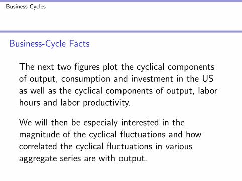
The next two figures plot the cyclical componentsof output, consumption and investment in the USas well as the cyclical components of output, laborhours and labor productivity.
We will then be especialy interested in themagnitude of the cyclical fluctuations and howcorrelated the cyclical fluctuations in variousaggregate series are with output.

Business Cycles
work/e301/BusCycle-2.png
‐0.15
‐0.1
‐0.05
0
0.05
0.1
0.15
1940 1950 1960 1970 1980 1990 2000 2010 2020
Busin
ess Cycle Co
mpo
nent
Year
US Business Cycles: Output Components
Consumption Investment Output

Business Cycles
work/e301/BusCycle-3.png
‐0.08
‐0.06
‐0.04
‐0.02
0
0.02
0.04
0.06
1940 1950 1960 1970 1980 1990 2000 2010 2020
Busin
ess C
ycle Com
pone
nt
Year
US Business Cycles: Output, Labor and Productivity
Output Labor Hours Labor Productivity
Business Cycles
Business-Cycle Facts
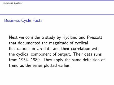
Next we consider a study by Kydland and Prescottthat documented the magnitude of cyclicalfluctuations in US data and their correlation withthe cyclical component of output. Their data runsfrom 1954- 1989. They apply the same definition oftrend as the series plotted earlier.

Business Cycles
work/e301/BCfacts1.png

Business Cycles
work/e301/BCfacts2.png

Business Cycles
work/e301/BCfacts3.png

Business Cycles
Key US Facts:
1. Labor hours are about as variable as output and arestrongly procyclical. The standard deviation of output is1.71, whereas labor is 1.47. Thus, a typical deviation fromtrend for output is 1.71 percent.2. Labor productivity is procyclical.3. Consumption is less variable than output but investmentis much more variable than output.4. Consumption and investment are procyclical.Government spending is acyclical.5. Measures of money are procyclical but prices arecountercyclical.

Business Cycles
Business-Cycle Facts
Other Data Issues:1. Have business-cycle fuctuations changed in magnitude ornature over time in US data?
There is a literature that debates whether business-cyclefluctuations in the US were larger before the GreatDepression than after WW II. There is also a literaturethat documents smaller business-cycle fluctuations in theUS after 1984 but before the Great Recession.
2. Is the systematic movement in quarterly GDP (theseasonal cycle) smaller or larger than business-cyclefluctuations?

Business Cycles
Business-Cycle Theory
A good place to begin discussing business-cycle theory is bydiscussing the procyclical productivity puzzle.
Procyclical Productivity Puzzle:
The data tell us that at business-cycle frequencies laborhours move alot (SD=1.5 percent) and are procyclical butthat capital input moves little and is acyclical. If we adopta theory that features a neoclassical aggregate productionfunction, then what are some different possibilities toproduce procyclical labor productivity (Y/L)?

Business Cycles
A Problem:
Any theory with an unchanging, CRS production functionYt = F (Kt, Lt) with diminishing marginal products will beproblematic. We will see that this holds regardless of whatare the fundamental shocks (e.g. animal spirits,government spending shocks, ...) driving business cyclesother than technology shocks and regardless of whether ornot consumer behavior in the face of such shocks is rationalor irrational.
Qualifying Proviso: capital input varies little in percentageterms.

Business Cycles
work/e301/labor-prod1.png

Business Cycles
Two Possible Solutions:
1. Yt = AtF (Kt, Lt) and At varies.
2. Yt = F (Kt, Lt) w/ increasing returns to labor
The next slide plots the same two data points on twographs. The data points are consistent with procyclicalproductivity. The possible “solutions” proposed involve theaggregate production function passing through the datapoints, holding capital input unchanged.

Business Cycles
work/e301/labor-prod2.png

Business Cycles
Business-Cycle Theory
A large class of business-cycle theories are based on“impulses” or shocks on the one hand and“propagation mechanisms” on the other hand. Thisfollows Knut Wicksell who reportedly said:
“If you hit a wooden rocking horse with a club, themovement of the horse will be very different to thatof the club.”
Business Cycles
Business-Cycle Theory
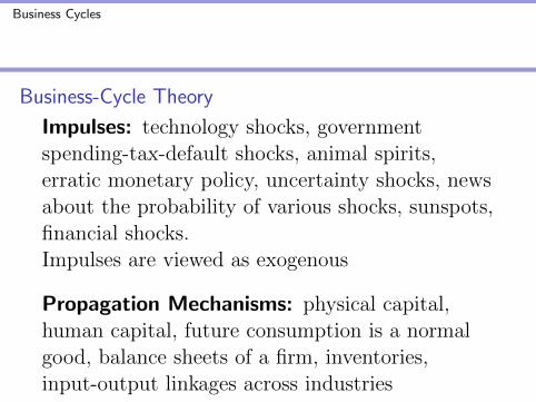
Impulses: technology shocks, governmentspending-tax-default shocks, animal spirits,erratic monetary policy, uncertainty shocks, newsabout the probability of various shocks, sunspots,financial shocks.Impulses are viewed as exogenous
Propagation Mechanisms: physical capital,human capital, future consumption is a normalgood, balance sheets of a firm, inventories,input-output linkages across industries

Business Cycles
Business-Cycle Theory
While there are many different business-cycletheories to consider, we will consider just two. Theywill be vastly different in theoretical structure and inpolicy implications.
* Theory 1: Technology Shock Theory
* Theory 2: Keynesian Animal Spirits Theory

Business Cycles
Theory 1: Life-Cycle Model w/ TechnologyShocks
Main Ingredients:- rational choice: Yes ... consumers optimize- technology: Yt = AtF (Kt, Lt) = AtK
βt L
1−βt
- impulses: At - technology shocks- shock propagation: capital accumulation +future consumption is a normal good

Business Cycles
Theory 1: A Permanent Increase in Technology Assume:
1. The Life-Cycle Model is the way the economy works.2. Economy is at steady state at t = 13. Assume A1 = 1, A2 = 2, A3 = 2, A4 = 2, ...
To figure out what happens ... graph the law of motion.

Business Cycles
work/e301/law-of-motion2.png

Business Cycles
work/e301/perm-shock.png
Permanent Technology Shock: Life‐Cycle Model
30
35
20
25
tle
10
15Axis Ti
0
5
0 2 4 6 8 10 12
Axis Title
Output Capital Wage Investment Technology
Business Cycles
Theory 1: Basic Story
The growth rate of technology At (as measured by theSolow residual) is variable in data. This theory implies highA is associated with high output Y , high wage W and highY/L. This pattern is supported in data.
The life-cycle model abstracts from a labor-leisure choice.Thus, it does not get labor hours to vary. Procyclical laborhours can be achieved by adding such a choice to themodel. However, much of the cyclical variation in laborhours in the data comes via changes in employment-unemployment. Modeling unemployment is way beyondwhat we can do in this course.

Business Cycles
Theory 1: Policy
If the Life-Cycle model with shocks is the theoryof business cycles, then attempts to smooth outbusiness cycle fluctuations will not (with positivereal interest rates) lead to Pareto improvements.Recall the Proposition established in the chapteron the life-cycle model.

Business Cycles
Theory 2: Old-Time Keynesian Story
Main Ingedients:
- rational choice: None ... Keynes abandonsmicroeconomics- technology: no production function- impulses: animal spirits of investors areexogenous impulses- shock propagation: unclear as the model isstatic and does not model time periods
Business Cycles
Rational Choice: None
“The fundamental psychological law, upon whichwe are entitled to depend with great confidenceboth a priori and from our knowledge of humannature and from the detailed facts of experience,is that men are disposed, as a rule and on theaverage, to increase their consumption as theirincome increases, but not by as much as theincrease in their income.” - Keynes (1936,Chapter 8, p. 96.).
Business Cycles
Source of Shocks: Animal Spirits“Even apart from the instability due to speculation, thereis the instability due to the characteristic of human naturethat a large proportion of our positive activities depend onspontaneous optimism rather than on a mathematicalexpectation, whether moral or hedonistic or economic.Most, probably, of our decisions to do something positive,the full consequences of which will be drawn out over manydays to come, can only be taken as a result of animalspirits - of a spontaneous urge to action rather thaninaction, and not as the outcome of a weighted average ofquantitative benefits multiplied by quantitativeprobabilities.” - Keynes (1936, Chapter 12, p. 161)

Business Cycles
Stylized Keynesian Model
C + I +G = Y - NIPA identityC = a+ b(Y − T ) - consumption (a > 0 and0 < b < 1)I - determined by animal spiritsT = G - assumption of a balanced budget
Solve for Output Y :a+ b(Y −G) + I +G = Y or Y = a+I+(1−b)G
1−b

Business Cycles
Theory 2: Basic Story
The economy is buffeted by animal spirits ofinvestors. Thus, investment moves exogenously.Times of low investment are times of low outputas the model implies (under the assumptions
above): Y = a+I+(1−b)G1−b .
Times of low output are taken to be indicative ofa poorly functioning economy. A formal welfareanalysis is not undertaken (as it would in otherareas of economics) using the Pareto criteria andthe utility functions of the consumers.

Business Cycles
Theory 2: Policy
Typical advice: increase government spending (orreduce taxes) in a recession.
Balanced Budget Multiplier: ∆Y∆G = 1−b
1−b = 1
Y = a+I+(1−b)G1−b ⇒ ∆Y = (1−b)∆G
1−b
Unbalanced Budget Multiplier: ∆Y∆G = 1
1−b > 1
Y = a−bT+I+G1−b ⇒ ∆Y = ∆G
1−b

Business Cycles
Government Spending Multipliers:
Keynesian Model: An increase in government spending(whether balanced budget or deficit financed) increasescurrent output as both multipliers are POSITIVE. If themultiplier is positive but less than 1 then (G, Y ) go up butC falls. Model does not have dynamic multipliers as themodel is static.
Business Cycles
Government Spending Multipliers:
Life-Cycle Model: A multiplier is defined as the change inoutput (at some horizon) due to the increased spending dividedby the change in government spending. To determinemultipliers, the output path under two different governmentspending plans must be calculated. Basic Conclusion: currentmultiplier is ZERO but the multiplier is NEGATIVE in allfuture periods as the taxes/borrowing financing extra spendingdepresses the capital stock.
NOTE: If a labor-leisure decision is added to the life-cyclemodel, then the output multiplier could be POSITIVE. Thiscould occur if the negative income effect (from the increasedtaxes funding government spending) leads to an increase inlabor that is sufficiently strong to offset the fall in savings fromthe increase in taxes.

Business Cycles
Multipliers: Empirical Work
It is not surprising that different theories havecompletely different multipliers or that onetheory could produce either positive or negativemultipliers under different assumptions.
Romer and Romer (2010) argue, using US data,that the contemporaneous tax multiplier isroughly zero but is negative at longer horizons.Thus, an exogenous increase in taxes leads tolower future output. We will discuss their work inchaper 7.

Business Cycles
Gains to Business-Cycle Smoothing
Are Gains to Business-cycle Smoothing Large?
Although the source(s) of business-cycle fluctuations arecontroversial, could we figure out whether the maximumpotential gain to (somehow) eliminating these fluctuationsis large?
Robert Lucas’ back-of-the-envelope calculation was that themaximum potential gain was worth about $8.50 per personper year! We will review the logic behind his calculation.
Business Cycles
Gains to Business-Cycle Smoothing
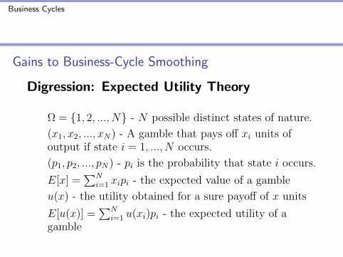
Digression: Expected Utility Theory
Ω = 1, 2, ..., N - N possible distinct states of nature.
(x1, x2, ..., xN) - A gamble that pays off xi units ofoutput if state i = 1, ..., N occurs.
(p1, p2, ..., pN) - pi is the probability that state i occurs.
E[x] =∑N
i=1 xipi - the expected value of a gamble
u(x) - the utility obtained for a sure payoff of x units
E[u(x)] =∑N
i=1 u(xi)pi - the expected utility of agamble

Business Cycles
Example 1: [Coin Toss]
Ω = H,T(xH , xT ) = (90, 110)
(pH , pT ) = (0.5, 0.5)
u(x) = log(x)
Expected utility:u(xH)pH + u(xT )pT = log(90)× 0.5 + log(110)× 0.5

Business Cycles
Example 1: [Coin Toss]
If the utility function u displays diminishing marginal utility,then getting the expected value (or mean) of a gamble as asure payout is strictly prefered to taking the gamble. Utilityfunctions with this property display risk aversion.How valuable is geting the mean for sure?
log(100) = log(90(1 + λ))× .5 + log(110(1 + λ))× .5
log(1+λ) = log(100)−log(90)×0.5+log(110)×0.5 = 0.00218
λ = 0.005 implies getting the mean is worth 1/2 percent ofconsumption

Business Cycles
A Simplified Version of Lucas’ Argument:
1. Assume the government engineers the smooth trendconsumption rather than a risky consumption process withthe same period-by-period mean.2. Assume agents are risk averse.3. Quantify the gain achieved by such business-cyclesmoothing.4. Need to measure consumption variation. A one standarddeviation movement of the cyclical component of aggregateconsumption from trend is about a 1.25 percent movementover 1954-89.5. Need knowledge of u.

Business Cycles
Specific Assumptions:
E[u(c)] = u(clow)P (low) + u(chigh)P (high)Probability: P (low) = P (high) = 1/2
Utility: u(c) = c1−γ
1−γ , where γ > 1
Consumption: clow = 98 and chigh = 102

Business Cycles
Gain (λ) to getting c = 100 for sure?
E[U((1 + λ)c)] = U(100)
(102(1+λ))1−γ
1−γ (1/2) + (98(1+λ))1−γ
1−γ (1/2) = (100)1−γ
1−γ
⇒ (1 + λ)1−γ =1001−γ
1021−γ(1/2) + 981−γ(1/2)
⇒ λ = [1001−γ
1021−γ(1/2) + 981−γ(1/2)]1/(1−γ) − 1
Business Cycles
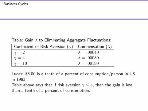
Table: Gain λ to Eliminating Aggregate Fluctuations:
Coefficient of Risk Aversion (γ) Compensation (λ)
γ = 2 λ = .00040γ = 4 λ = .00080γ = 10 λ = .00199
Lucas: $8.50 is a tenth of a percent of consumption/person in USin 1983.Table above says that if risk aversion γ ≤ 4, then the gain is lessthan a tenth of a percent of consumption.

Business Cycles
How Risk Averse Are You?Pick the row best matching your risk aversion. Each row describesthe maximum percentage of total wealth that a consumer withutility function U(c) = c1−γ
1−γ is willing to give up to avoid aneven-odds gamble of gaining or losing a fraction α of total wealth.
Percentage of Wealth Given Up to Avoid a Proportional WealthGamble of Size α
Coefficient of Risk Aversion (γ) α = 10% α = 30%
γ = 1 0.5% 4.6%γ = 4 2.0% 16.0%γ = 10 4.4% 24.4%γ = 40 8.4% 28.7%
Business Cycles
Potential Reasons Why Lucas’ number is sosmall:
1. Aggregate consumption movements over thebusiness cycle are small after WWII.2. Individual households experience much largerconsumption fluctuations than those in aggregatedata.3. Eliminating or reducing aggregate fluctuationsmay reduce (but not eliminate) individualfluctuations. If so, should start calculations withthe magnitude of individual fluctuations notaggregate fluctuations.