business cycles: i - georgetown...
TRANSCRIPT

Business Cycles
Business Cycles: I
Mark Huggett2
2Georgetown
November, 2015
Business Cycles
Business Cycles: A Very Short HistoryI Theory: Shocks and Propagation Mechanisms
Wicksell analogy: a club and a rocking horseCandidate Shocks: technology shocks, animal spirits, govtspending or tax shocks, erratic monetary policy, news (i.e.signals about other candidate shocks), uncertainty shocks
Propagation Mechanisms: physical capital + futureconsumption a normal good, balance sheet, ...
I Facts: Burns and Mitchell (1946) vs Hodrick and Prescott(1980) vs other methods
I BC Theory: Post Kydland and Prescott (1982)I BC Theory- rooted in growth modelsI GE models centralI Models judged on quantitative groundsI policy analysis done w/in model - GE analysis
Business Cycles
Business Cycles: Agenda for these Slides
I Focus on three things
I BC Facts: apply HP filter
I Candidate Shock: Solow residual
I BC Theory: Employ aggregate prod fn w/ Solow residual asthe only shock. Evaluate model in the style of KP (1982)
Business Cycles
Business Cycles: Facts
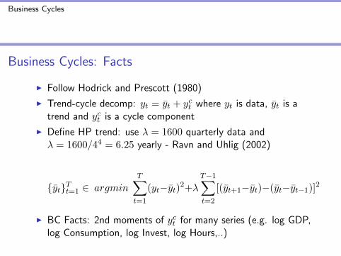
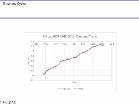
I Follow Hodrick and Prescott (1980)
I Trend-cycle decomp: yt = yt + yct where yt is data, yt is atrend and yct is a cycle component
I Define HP trend: use λ = 1600 quarterly data andλ = 1600/44 = 6.25 yearly - Ravn and Uhlig (2002)
{yt}Tt=1 ∈ argmin
T∑t=1
(yt−yt)2+λ
T−1∑t=2
[(yt+1−yt)−(yt−yt−1)]2
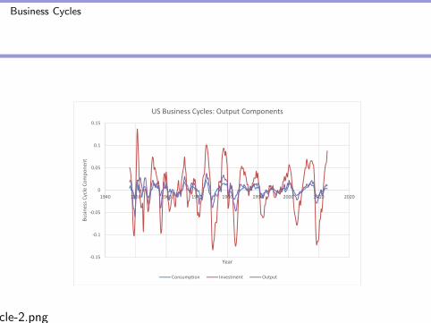
I BC Facts: 2nd moments of yct for many series (e.g. log GDP,log Consumption, log Invest, log Hours,..)
Business Cycles
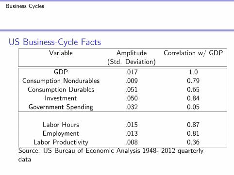
US Business-Cycle FactsVariable Amplitude Correlation w/ GDP
(Std. Deviation)
GDP .017 1.0Consumption Nondurables .009 0.79
Consumption Durables .051 0.65Investment .050 0.84
Government Spending .032 0.05
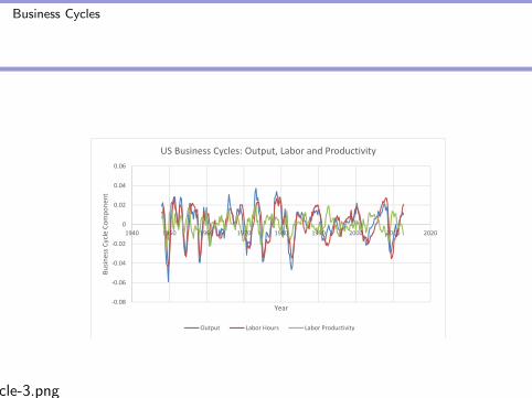
Labor Hours .015 0.87Employment .013 0.81
Labor Productivity .008 0.36Source: US Bureau of Economic Analysis 1948- 2012 quarterlydata
Business Cycles
work/macro1/slides/BusCycle-1.png
‐9.2
‐9
‐8.8
‐8.6
‐8.4
‐8.2
‐8
‐7.8
‐7.61940 1950 1960 1970 1980 1990 2000 2010 2020
Log Units
Year
US Log GDP 1948‐2012: Data and Trend
Log GDP Trend
Business Cycles
work/macro1/slides/BusCycle-2.png
‐0.15
‐0.1
‐0.05
0
0.05
0.1
0.15
1940 1950 1960 1970 1980 1990 2000 2010 2020
Busin
ess Cycle Co
mpo
nent
Year
US Business Cycles: Output Components
Consumption Investment Output
Business Cycles
work/macro1/slides/BusCycle-3.png
‐0.08
‐0.06
‐0.04
‐0.02
0
0.02
0.04
0.06
1940 1950 1960 1970 1980 1990 2000 2010 2020
Busin
ess C
ycle Com
pone
nt
Year
US Business Cycles: Output, Labor and Productivity
Output Labor Hours Labor Productivity

Business Cycles
Facts:
Read Kydland-Prescott (1990) for a broader set of facts based onthe same procedure and some perspective on the history ofthought.
Business Cycles
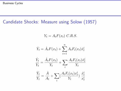
Candidate Shocks: Measure using Solow (1957)
Yt = AtF (xt) C.R.S.
Yt = AtF (xt) +
n∑i=1
AtFi(xt)xit
YtYt
=AtF (xt)
Yt+∑i
AtFi(xt)xit
Yt
YtYt
=A
At+∑i
(AtFi(xt)x
it
Yt)xitxit

Business Cycles
Solow Growth Accounting Equation w/ two Inputs:
YtYt
=AtAt
+ βtKt
Kt+ (1− βt)
LtLt
An Approximation (also follows from C-D Prod Fn):
∆YtYt
=∆AtAt
+ β∆Kt
Kt+ (1− β)
∆LtLt
Two Points: (1) an accounting decomp of output growth intofactor input growth components and a technology component, (2)view technology component (under the theory) as true realizedshock plus measurement error in inputs and output.
Business Cycles
Solow (1957) Findings: US 1909- 1949
1. Output per unit of labor input grows by about 100 percent.
2. The capital-labor ratio grows by about 30 percent over theperiod. So there is “capital deepening”.
3. Technology grows by about 80 percent. Thus, about 80percent of the growth in output per unit of labor input overthe period is accounted for by growth in the technology andthe remaining 20 by increases in the capital-labor ratio.
4. The measure of the technology level falls in a number ofrecession and depression years and tends to increase inexpansions. Thus, measured technology growth rates are “procyclical”.
Business Cycles
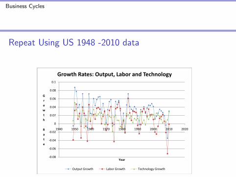
Repeat Using US 1948 -2010 data
3-fig1.pdf work/macro1/slides/hwk 3-fig1.pdf
0.02
0.04
0.06
0.08
0.1
Growt
Growth Rates: Output, Labor and Technology
‐0.08
‐0.06
‐0.04
‐0.02
0
0 0
1940 1950 1960 1970 1980 1990 2000 2010 2020
h
Rate
Year
Output Growth Labor Growth Technology Growth

Business Cycles
Repeat Using US 1948 -2010 dataApply At+1 = At(1 + ∆At
At)
3-fig2.pdf work/macro1/slides/hwk 3-fig2.pdf
0
0.5
1
1.5
2
2.5
1940 1950 1960 1970 1980 1990 2000 2010 2020
Level
Year
Technology: US 1948‐2010
Technology Level

Business Cycles
Repeat Using US 1948 -2010 data
3-fig3.pdf work/macro1/slides/hwk 3-fig3.pdf
‐0.06
‐0.04
‐0.02
0
0.02
0.04
0.06
0.08
0.1
1940 1950 1960 1970 1980 1990 2000 2010 2020
Growth
Rate
Year
Procyclical Labor Productivity
Labor Productivity Growth Output Growth Ttechnology Growth
Business Cycles
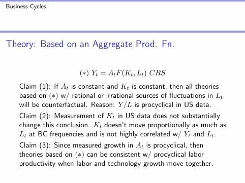
Theory: Based on an Aggregate Prod. Fn.
(∗) Yt = AtF (Kt, Lt) CRS
Claim (1): If At is constant and Kt is constant, then all theoriesbased on (∗) w/ rational or irrational sources of fluctuations in Ltwill be counterfactual. Reason: Y/L is procyclical in US data.
Claim (2): Measurement of Kt in US data does not substantiallychange this conclusion. Kt doesn’t move proportionally as much asLt at BC frequencies and is not highly correlated w/ Yt and Lt.
Claim (3): Since measured growth in At is procyclical, thentheories based on (∗) can be consistent w/ procyclical laborproductivity when labor and technology growth move together.

Business Cycles
Theory: Based on an Aggregate Prod. Fn.
Preferences: E[∑∞
t=0 βtu(ct, 1− lt)]
Technology: yt = exp(zt)F (kt, lt) and ct + xt = yt
kt+1 = kt(1− δ) + xt
zt = ρzt−1 + εt, εt ∼ N(0, σ2ε )
Endowments: k0 > 0 and 1 unit of labor time
Business Cycles
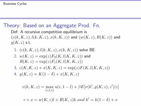
Theory: Based on an Aggregate Prod. Fn.Def: A recursive competitive equilibrium is(c(k,K, z), l(k,K, z), x(k,K, z)) and (w(K, z), R(K, z)) andg(K, z) s.t.
1. (c(k,K, z), l(k,K, z), x(k,K, z)) solve BE
2. w(K, z) = exp(z)F2(K, l(K,K, z)) andR(K, z) = exp(z)F1(K, l(K,K, z))
3. c(K,K, z) + x(K,K, z) = exp(z)F (K, l(K,K, z))
4. g(K, z) = K(1− δ) + x(K,K, z)
v(k,K, z) = max(c,l,x)
u(c, 1− l) + βE[v(k′, g(K, z), z′)|z]
c+ x = w(K, z)l +R(K, z)k and k′ = k(1− δ) + x
Business Cycles
Evaluating the Model
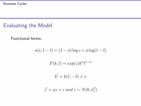
Functional forms:
u(c, 1− l) = (1− φ) log c+ φ log(1− l)
F (k, l) = exp(z)kαl1−α
k′ = k(1− δ) + x
z′ = ρz + ε and ε ∼ N(0, σ2ε )
Business Cycles
Theory: Based on an Aggregate Prod. Fn.
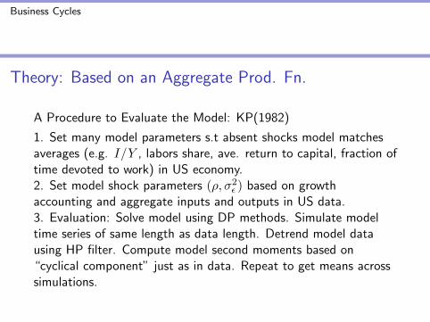
A Procedure to Evaluate the Model: KP(1982)
1. Set many model parameters s.t absent shocks model matchesaverages (e.g. I/Y , labors share, ave. return to capital, fraction oftime devoted to work) in US economy.2. Set model shock parameters (ρ, σ2
ε ) based on growthaccounting and aggregate inputs and outputs in US data.3. Evaluation: Solve model using DP methods. Simulate modeltime series of same length as data length. Detrend model datausing HP filter. Compute model second moments based on“cyclical component” just as in data. Repeat to get means acrosssimulations.
Business Cycles
Evaluating the Model
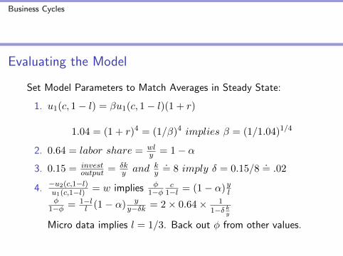
Set Model Parameters to Match Averages in Steady State:
1. u1(c, 1− l) = βu1(c, 1− l)(1 + r)
1.04 = (1 + r)4 = (1/β)4 implies β = (1/1.04)1/4
2. 0.64 = labor share = wly = 1− α
3. 0.15 = investoutput = δk
y and ky.= 8 imply δ = 0.15/8
.= .02
4. −u2(c,1−l)u1(c,1−l) = w implies φ
1−φc
1−l = (1− α)ylφ
1−φ = 1−ll (1− α) y
y−δk = 2× 0.64× 11−δ k
y
Micro data implies l = 1/3. Back out φ from other values.

Business Cycles
Evaluating the Model
How to Solve the Model, Given All Parameters?
MANY METHODS:
1. Solve Planning Problem using Finite DP methods
2. Solve Planning Problem using linear approx to policy functionabout deterministic steady. Use first-order Taylor Seriesapprox in (k, z)
3. Write FOC and resource constraint to Planning Problem orComp. Equil. and then linearize or log-linearize all equations.Get linear system in deviations from steady state quantities.
4. Nowadays, estimation, solution and simulation of (standard)BC models are done w/in packages such as DYNARE.
Business Cycles
Model Implications: Cooley and Prescott (1995)
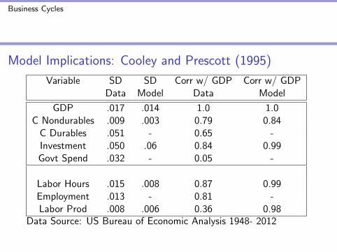
Variable SD SD Corr w/ GDP Corr w/ GDPData Model Data Model
GDP .017 .014 1.0 1.0C Nondurables .009 .003 0.79 0.84
C Durables .051 - 0.65 -Investment .050 .06 0.84 0.99Govt Spend .032 - 0.05 -
Labor Hours .015 .008 0.87 0.99Employment .013 - 0.81 -Labor Prod .008 .006 0.36 0.98
Data Source: US Bureau of Economic Analysis 1948- 2012
Business Cycles
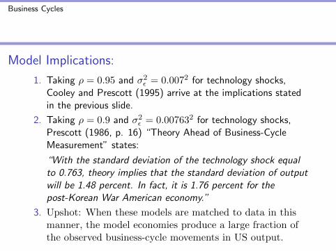
Model Implications:
1. Taking ρ = 0.95 and σ2ε = 0.0072 for technology shocks,
Cooley and Prescott (1995) arrive at the implications statedin the previous slide.
2. Taking ρ = 0.9 and σ2ε = 0.007632 for technology shocks,
Prescott (1986, p. 16) “Theory Ahead of Business-CycleMeasurement” states:
“With the standard deviation of the technology shock equalto 0.763, theory implies that the standard deviation of outputwill be 1.48 percent. In fact, it is 1.76 percent for thepost-Korean War American economy.”
3. Upshot: When these models are matched to data in thismanner, the model economies produce a large fraction ofthe observed business-cycle movements in US output.

Business Cycles
Discussion
1. So far these notes have described an approach to documentbusiness-cycle fluctuations and to build a quantitative modelbased on technology shocks as the only shocks.
2. There is substantial lore developed around trying tounderstand what is important in such a model for producingthe SD and Corr structure of US aggregates.
3. Disagreements over theory and measurement: (1) InterpretSolow residuals as exog. shocks or as aggregation issues ofother shocks across production units?, (2) How doesaggregate hours variability at business-cycle frequencies ariseand how is it tied to properties of utility functions at microlevel? We address (2) next.
Business Cycles
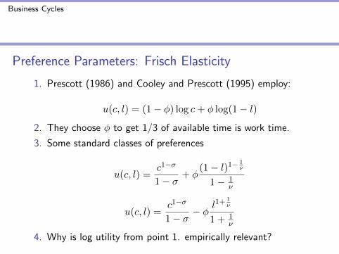
Preference Parameters: Frisch Elasticity
1. Prescott (1986) and Cooley and Prescott (1995) employ:
u(c, l) = (1− φ) log c+ φ log(1− l)
2. They choose φ to get 1/3 of available time is work time.
3. Some standard classes of preferences
u(c, l) =c1−σ
1− σ+ φ
(1− l)1− 1ν
1− 1ν
u(c, l) =c1−σ
1− σ− φ l
1+ 1ν
1 + 1ν
4. Why is log utility from point 1. empirically relevant?
Business Cycles
Preference Parameters: Frisch Elasticity
1. Following MaCurdy (1982), labor economists have tried tomeasure different notions of labor hours elasticity. Onepotentially useful elasticity is the Frisch elasticity becauseestimation of this elasticity relates in a fairly direct way topreference parameters.
2. Typical View: Frisch labor hours elasticity for prime-age males(age 25-55) is well below one.
3. Casual argument: Average (log) hours and wage rates areroughly hump-shaped over working lifetime but wages vary inpercentage terms more than hours.
Business Cycles
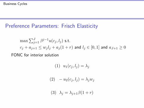
Preference Parameters: Frisch Elasticity
max∑J
j=1 βj−1u(cj , lj) s.t.
cj + aj+1 ≤ wjlj + aj(1 + r) and lj ∈ [0, 1] and aJ+1 ≥ 0
FONC for interior solution
(1) u1(cj , lj) = λj
(2) − u2(cj , lj) = λjwj
(3) λj = λj+1β(1 + r)
Business Cycles
Preference Parameters: Frisch Elasticity
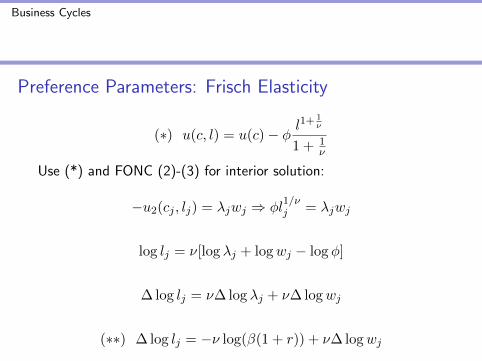
(∗) u(c, l) = u(c)− φ l1+ 1
ν
1 + 1ν
Use (*) and FONC (2)-(3) for interior solution:
−u2(cj , lj) = λjwj ⇒ φl1/νj = λjwj
log lj = ν[log λj + logwj − log φ]
∆ log lj = ν∆ log λj + ν∆ logwj
(∗∗) ∆ log lj = −ν log(β(1 + r)) + ν∆ logwj
Business Cycles
Preference Parameters: Frisch Elasticity
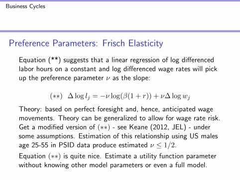
Equation (**) suggests that a linear regression of log differencedlabor hours on a constant and log differenced wage rates will pickup the preference parameter ν as the slope:
(∗∗) ∆ log lj = −ν log(β(1 + r)) + ν∆ logwj
Theory: based on perfect foresight and, hence, anticipated wagemovements. Theory can be generalized to allow for wage rate risk.Get a modified version of (∗∗) - see Keane (2012, JEL) - undersome assumptions. Estimation of this relationship using US malesage 25-55 in PSID data produce estimated ν ≤ 1/2.
Equation (∗∗) is quite nice. Estimate a utility function parameterwithout knowing other model parameters or even a full model.

Business Cycles
Preference Parameters: Frisch Elasticity
Some standard classes of preferences. First function is constantFrisch elasticity of leisure, Second function is hte constant Frischelasticity of labor.
u(c, l) = u(c) + φ(1− l)1− 1
ν
1− 1ν
u(c, l) = u(c)− φ l1+ 1
ν
1 + 1ν
We will now figure out theory-based Frisch elasticities for these twoclasses.
Business Cycles
Preference Parameters: Frisch Elasticity
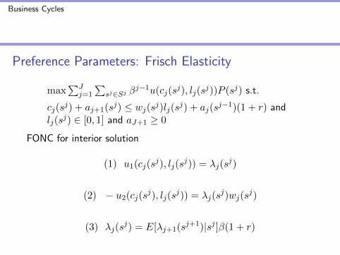
max∑J
j=1
∑sj∈Sj β
j−1u(cj(sj), lj(s
j))P (sj) s.t.
cj(sj) + aj+1(sj) ≤ wj(sj)lj(sj) + aj(s
j−1)(1 + r) andlj(s
j) ∈ [0, 1] and aJ+1 ≥ 0
FONC for interior solution
(1) u1(cj(sj), lj(s
j)) = λj(sj)
(2) − u2(cj(sj), lj(s
j)) = λj(sj)wj(s
j)
(3) λj(sj) = E[λj+1(sj+1)|sj ]β(1 + r)

Business Cycles
Define Frisch demand functions (c(λ,w), l(λ,w), n(λ,w)) assolutions to system below:
(1) u1(c(λ,w), l(λ,w)) = λ
(2) − u2(c(λ,w), l(λ,w)) = λw
(3) l(λ,w) + n(λ,w) = 1
Define labor εl and leisure εn elasticities as follows:
εl(λ,w) ≡ ∂l(λ,w)
∂w
w
l(λ,w)and εn(λ,w) ≡ ∂n(λ,w)
∂w
w
n(λ,w)
εl(λ,w) =−∂n(λ,w)
∂w
w
1− n(λ,w)= −εn(λ,w)
n(λ,w)
1− n(λ,w)
Business Cycles
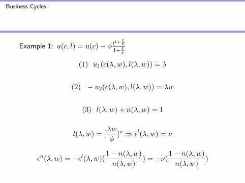
Example 1: u(c, l) = u(c)− φ l1+ 1
ν
1+ 1ν
(1) u1(c(λ,w), l(λ,w)) = λ
(2) − u2(c(λ,w), l(λ,w)) = λw
(3) l(λ,w) + n(λ,w) = 1
l(λ,w) = [λw
φ]ν ⇒ εl(λ,w) = ν
εn(λ,w) = −εl(λ,w)(1− n(λ,w)
n(λ,w)) = −ν(
1− n(λ,w)
n(λ,w))

Business Cycles
Example 2: u(c, l) = u(c) + φ (1−l)1−1ν
1− 1ν
(1) u1(c(λ,w), l(λ,w)) = λ
(2) − u2(c(λ,w), l(λ,w)) = λw
(3) l(λ,w) + n(λ,w) = 1
n(λ,w) = [λw
φ]−ν ⇒ εn(λ,w) = −ν
εl(λ,w) = −εn(λ,w)n(λ,w)
1− n(λ,w)= ν
n(λ,w)
1− n(λ,w)

Business Cycles
Example 3: u(c, l) = u(c) + φ log(1− l)A limiting case of Example 2
n(λ,w) = [λw
φ]−1 ⇒ εn(λ,w) = −1
εl(λ,w) = −εn(λ,w)n(λ,w)
1− n(λ,w)= 1
n(λ,w)
1− n(λ,w)
Prescott : εl(λ,w) = 1(n(λ,w)
1− n(λ,w)) = 1× 2 = 2
Upshot: Frisch labor Elasticity of total work hours of 2 is severaltimes the estimated Frisch elasticity for prime-age males w/substantial attachment to the labor force.

Business Cycles
More Discussion of Example 3: u(c, l) = u(c) + φ log(1− l)
1. The discussion of Example 3 up to this point is meant to getyou up to speed in interpreting evidence on a key preferenceparameter from one theoretical perspective.
2. See ”Micro and Macro Labor Supply Elasticities: AReassessment of Conventional Wisdom.” - Keane andRogerson (2012, JEL) - for a recent review.
3. KR(2012): BC agg. hours fluctuations involve a largemovement in and out of employment (extensive margin) andsmaller agg. movement from varying hours worked per worker(intensive margin). Thus, BC agg. hours fluctuations needtheoretical models where agg. hours variation involvesextensive margin decisions (e.g. models w/ search, homeproduction, multi-member households, retirement,...).