business economics group
TRANSCRIPT

MSc Thesis Business Economics
Business Economics Group
Data Envelopment Analysis in determining
factors that influence technical efficiency
levels on Dutch dairy farms
Which cow specific expressions can influence farm performances
P.H.M. Rooijakkers
18-06-2018


Data Envelopment Analysis in
determining factors that influence
technical efficiency levels on Dutch
dairy farms
Which cow specific expressions can influence farm performances
Name course : MSc Thesis Business Economics
Number : BEC-80436
Study load : 36 credits
Date : xx-06-2019
Student : P.H.M. (Pieter) Rooijakkers
Registration number : 95-04-07-708-120
Study programme : MSc . Management, Economics and Consumer Studies
Supervisor(s) : dr. M (Mariska) van der Voort
dr. C (Claudia) Kamphuis
Examiner : prof.dr.ir. H (Henk) Hogeveen
Group : Business Economics Group
Hollandseweg 1 (Building 201)
6706 KN Wageningen
T: 0317-(4)84065

MSc. Thesis | P.H.M. Rooijakkers 4
DISCLAIMER
This report is written by a student of Wageningen University as part of his/her master programme
under the supervision of the chair Business Economics.
It is not an official publication of Wageningen University and Research and the content herein does not
represent any formal position or representation by Wageningen University and Research.
It is not allowed to reproduce or distribute the information from this report without the prior consent
of the Business Economics group of the Wageningen University ([email protected])

5 MSc. Thesis | P.H.M. Rooijakkers
Preface
For Dutch dairy farmers, increasing herd size to maximize profits is not a common trend anymore.
Dairy farmers are restricted by their outputs and must be creative in their inputs to get the best out of
their herds. Besides growing consumer concerns on animal welfare and environmental responsible
productivity, efficiency plays a big role in the life of a farmer. Feed costs have grown substantially in
the last years, but knowledge on how to use this feed correctly has also made big improvements. I
hope that this study can contribute to even more efficient dairy farms. I think many developments
have already be made on for example improved cow health, increased productive fitness or feed
efficiency, but I think the dairy sector is still in progress to become even more input source efficient.
This thesis is part of the Horizon 2020 GenTORE project. A project that will develop innovative tools to
optimize resilience and efficiency. The project consists of multiple European stakeholders and partners
that are all active in the dairy and beef cattle industry. I am glad that the results of this thesis not only
will be used on national scale but are also included into an international programme.
Regarding the GenTORE project I want to thank Claudia Kamphuis for her critical and pragmatic point
of view. It was nice to discuss with someone which is critical with knowledge from another discipline.
I want to furthermore thank her for giving me the opportunity and the confidence to present the
results of my thesis at the annual project meeting in Basel. For me, it was received as a compliment to
present my work in front of researchers from all kinds of disciplines in the dairy and beef cattle
industry.
Fortunately, Mariska van der Voort was always willing to help in improving the content of this thesis. I
want to thank her for the elaborate brainstorm sessions through the whole research process and for
giving me the opportunity to always be critical on my own results and findings. I also want to thank my
fellow students and friends for the many discussions we had regarding this research and for showing
interest into this study.
Enjoy reading!
Pieter Rooijakkers
Wageningen, 29th of May 2019

MSc. Thesis | P.H.M. Rooijakkers 6


MSc. Thesis | P.H.M. Rooijakkers 4
Summary
Milk production per cow has increased substantially in the past decades. Subsequent to the intensification of the dairy sector, consumers have growing concern on aspects like welfare and environmental friendly production. Also due to health and safety demands of food production, a shift in focus on the genetic selection for breeding goals next to milk production has grown.
Focussing on functional traits next to milk production can be both economically beneficial as socially accepted. They contribute to the functionality and the fitness of an individual cow. Furthermore, these so-called hybrid cows have a long-life expectancy which will lead to reduced costs due to savings on health and replacement costs caused by involuntary culling. Functional traits can be divided into several categories which all have specific indicators. For this study, the most important traits were selected from literature concerning health, fertility, longevity, and feed efficiency.
It is known that managerial choices are closely related to farm efficiency, however it is not known how this efficiency is related to the expression of functional traits by an individual cow. Therefore, the question arises, in which extent cows can express their functional traits can be influenced by a change in farm management.
In this study, efficiency measures are based on productive efficiency, indicated by a technical efficiency score. Technical efficiency can be interpreted as a relative measure between decision making units (farms) for managerial capacity on a technology level which is in this case milk production. The method that was used in this study to measure technical efficiency is Data Envelopment Analysis, or DEA, which is an econometric, non-parametric linear programming approach capable in measuring whole-farm efficiency. Information of functional traits was used to select a set of variables that does both relate to the production of milk and to functional traits of a dairy herd for the efficiency analysis. In a subsequent comparison between different technical efficient scoring groups, all variables relating to functional traits were included to indicate significant differences between efficient and low(er) efficient farms.
From a dataset of 846 farms it was found that between the years 2013 and 2016 farms were relatively efficient to each other having an average technical efficiency score of around 0.93. Inefficiency means that there is room for input improvement, which are in this case related to functional traits on cow level. Around 23% of all assessed farms remained in the same efficiency range over all years. When one consecutive year is concerned, approximately 50% of the farms seem to remain in the same efficiency range and about an equal amount (approximately 25%) of the farms increase or decrease in technical efficiency groups which were based on the distribution of technical efficiency scores per year.
At last it was found that from the DEA significant differences were found for technical efficiency scores for the variables which are related to the traits of individual cows. Efficient farms include cows that are healthy and fertile, having both low health and breeding and controlling costs. Furthermore, at these efficient farms cows were fed significantly lower concentrates and had significantly higher milk yield per hectare of feeding area. In contrary on having high performance for the functional traits health, fertility and feed efficiency, farms that are efficient had cows present with a significantly lower average age than the cows that were found on farms with low(er) efficiency. Concerning productivity, fully efficient farms produce less milk yield per cow than highly efficient farms but significantly more than on low efficient farms.
It could be concluded that DEA is a suitable method in examining the performance of a farm while focussing on cow specific traits. Despite it was not suitable to include every variable, interesting results of efficiency differences relation to functional traits were found. Other efficiency analysis methods were not used but could give interesting insights for the validation of this study. Results are still on farm level; however, they give insights in where the focus should be when analysis on cow level is performed. In a subsequent study, studies on farm and cow level could be combined to correct for high performing cows on low performing farms and vice versa.

5 MSc. Thesis | P.H.M. Rooijakkers

MSc. Thesis | P.H.M. Rooijakkers 4
Table of Contents
Preface ..................................................................................................................................................... 5
Summary ................................................................................................................................................. 4
Table of tables ......................................................................................................................................... 6
Table of figures ........................................................................................................................................ 6
Abbreviations .......................................................................................................................................... 7
1. Introduction ..................................................................................................................................... 8
1.1. Current situation of efficiency in Dutch dairy farming ............................................................ 8
1.2. Desired situation of efficiency in Dutch dairy farming ............................................................ 9
1.3. Problem definition ................................................................................................................... 9
1.4. Research questions................................................................................................................ 10
1.5. Demarcation .......................................................................................................................... 10
1.6. Outline ................................................................................................................................... 10
2. Literature ....................................................................................................................................... 12
2.1. Introduction to data envelopment analysis .......................................................................... 12
2.1.1. Efficiency analyses in literature ..................................................................................... 13
2.1.2. Efficiency analyses in Dutch dairy farming .................................................................... 14
2.2. Functional traits ..................................................................................................................... 16
2.2.1. Functional traits in data recording systems .................................................................. 16
2.2.2. Overview functional traits ............................................................................................. 19
2.3. Literature summary ............................................................................................................... 20
3. Material and Methods ................................................................................................................... 22
3.1. Data description .................................................................................................................... 22
3.1.1. Data summary ............................................................................................................... 22
3.2. Data Envelopment Analysis ................................................................................................... 24
3.3 Variable selection .................................................................................................................. 27
3.2.1. Correlations ................................................................................................................... 27
3.2.2. Multicollinearity ............................................................................................................ 29
3.2.3. Best subset selection ..................................................................................................... 30
3.4. Comparison of results ........................................................................................................... 32
4. Results ........................................................................................................................................... 34
4.1. Data summary ....................................................................................................................... 34
4.1.1. Cows .............................................................................................................................. 34

5 MSc. Thesis | P.H.M. Rooijakkers
4.1.2. Land ............................................................................................................................... 35
4.1.3. Costs .............................................................................................................................. 36
4.2. Data Envelopment Analysis ................................................................................................... 38
4.2.1. Summary of efficiency scores ........................................................................................ 38
4.2.2. TE score group dynamics through 2013-2016 ............................................................... 39
4.2.3. In- and output variable variation between TE score groups ......................................... 41
5. Discussion ...................................................................................................................................... 45
6. Conclusion ..................................................................................................................................... 49
7. Recommendations......................................................................................................................... 51
8. Bibliography ................................................................................................................................... 53
Appendices ............................................................................................................................................... I
Appendix I: Elaborated overview of Dutch efficiency analyses in dairy farming ................................. I
Appendix II: Selected variables from original dataset (Dutch) ........................................................... III
Appendix III: Best subset selection ..................................................................................................... VI

MSc. Thesis | P.H.M. Rooijakkers 6
Table of tables
Table 1: Overview efficiency studies in Dutch dairy farming ................................................................................. 15 Table 2: Overview of functional traits and their indicator together with their availability in the used dataset ... 19 Table 3: Subset of selected variables .................................................................................................................... 23 Table 4: Correlation table between in- and output variables based on Pearson's r correlation coefficient. Blue
coloured cells contain strongly positive correlations, red cells contain strongly negative correlations within a
range between 1 and -1. ....................................................................................................................................... 28 Table 5: Multicollinearity by VIF scores ................................................................................................................. 30 Table 6: Ranges of comparison groups based on TE score .................................................................................... 32 Table 7: Overview of variables used for statistical comparison based on TE scores ............................................. 32 Table 8: Summary of selected variables in chapter 3.1.1 in the cow related category ......................................... 35 Table 9: Summary of selected variables in chapter 3.1.1 in the land related category ........................................ 36 Table 10: Summary of selected variables in chapter 3.1.1 in the costs related category ..................................... 37 Table 11: Summary of TE scores ............................................................................................................................ 38 Table 12: Composition of TE score groups based on the distribution per year in Table 12 ................................... 39 Table 13: Dynamics of TE scores between ranking groups, brief overview ........................................................... 39 Table 14: Dynamics of TE scores between ranking groups, elaborated overview. TE score groups overview is
given in Table 12 and Table 13 .............................................................................................................................. 40 Table 15: Variables to compare different TE score groups. Means are displayed with significant differences
between groups marked with '*' ........................................................................................................................... 41 Table 16: Between group differences for both input and output variables for the panel 2013-2016 ................... 42 Table I: Overview of studies on technical efficiency in Dutch dairy farming. ........................................................... I Table II: Selected variables from original dataset .................................................................................................. III Table III: Variables included in the best subset selection. Variable Cows is forced in, which means that this
variable will always be included ............................................................................................................................. VI Table IV: Best subset composition with set numbers indicating which variables will be included in the designated
set ........................................................................................................................................................................... VI
Table of figures
Figure 1: Frontier estimation methods as in Mareth et al. (2016) ........................................................................ 12 Figure 2: Visualisation of scale efficiency measurements with efficient farm R and inefficient farms G and P, q
represents outputs and x represents inputs as in (Coelli et al., 2005) ................................................................... 25 Figure 3: Constant returns to scale frontier assuming multiple inputs. Point 1 is projected on the best-practice
frontier .................................................................................................................................................................. 26 Figure 4: Summaries of Mean Squared Errors returning from the selected variables from the best subset
selection with on the y-axis the MSE of each set of variables (x-axis) between the predicted and actual Milk
yield). Sets of variables are shown in (Appendix III, Table 2) ................................................................................ 31 Figure 5: Overview of feeding cost structure ........................................................................................................ 36 Figure 6: Histogram plots of the TE score distribution per year ............................................................................ 38

7 MSc. Thesis | P.H.M. Rooijakkers
Abbreviations
AMS Automatic Milking System
CRS Constant Returns to Scale
DEA Data Envelopment Analysis
LP Linear Programming
PLF Precision Livestock Farming
SFA Stochastic Frontier Analysis
TE Technical Efficiency
TFP Total Factor Productivity
VRS Variable Returns to Scale

MSc. Thesis | P.H.M. Rooijakkers 8
1. Introduction
Over the years the Dutch dairy cow population has decreased from a total of 2.55 million milking cows
in 1984 to 1.6 million milking cows in 2018 (CBS, 2017). Almost 60 years ago, the same amount of
milking cows was recorded, however in the meantime milk production has more than doubled from
around 4200 kg per cow per year in the 1960’s to around 9100 kg per cow per year in 2018 (CRV, 2019;
van Dijk, Schukking, & van der Berg, 2015). Besides the intensification of the dairy sector, more and
more social pressure also has led to a shift in the genetic selection for other breeding goals instead of
milk production increase (Cook & Nordlund, 2009; Pritchard, Coffey, Mrode, & Wall, 2013). Due to
healt demands and growing concerns about safe products in combination with high animal welfare,
novel functional traits of cow health information receive increasing attention by dairy producers
(Egger-Danner, Willam, Fuerst, Schwarzenbacher, & Fuerst-Waltl, 2012). These traits can both be
economically beneficial as socially accepted. Furthermore will these breeding goals lead to more
sustainable dairy products and increase animal welfare due to its higher robustness (Pritchard et al.,
2013). According to Groen (2004) functional traits are characteristics of animals that can increase
efficiency by reduced costs of input instead of higher outputs.
Efficiency can have multiple definitions, furthermore focus can be specified on different levels. In this
study, efficiency will be approached at farm level. Efficiency can be measured in multiple ways, this
study will focus on the technical efficiency of Dutch dairy farms which examines the inefficient use of
resources in the production process or the ability of farms to use minimum inputs to produce a given
level of output (Allendorf & Wettemann, 2015; Davis, 2018; Korver, 1988). Focussing on the efficiency
of an individual cow, a definition by Friggens & Thorup (2015) was found. Individual cow efficiency
could be divided into two components, digestive efficiency (for example variations in digestibility or
feeding behaviour) and metabolic efficiency (for example quantifying absorbed nutrients in different
metabolic functions such as activity, maintenance and production). Farms can have a mix of both
inefficient and efficient cows according to the definition of Friggens & Thorup (2015).
1.1. Current situation of efficiency in Dutch dairy farming
Traditional breeding goals in the 20th century was mainly focussed to feed a growing world population.
In the dairy sector, milk yield increased by increasing the number of animals per farm. The number of
cows was at its highest in the year 1984 with 2.5 million milk and calf cows. This was just before the
introduction of the European milk quota to protect the dairy market for overproduction. At that time,
there were around 60 000 dairy farms in the Netherlands with a total production of around 13.2 billion
kilograms of milk per year. Just before the abolition of the European milk quota, Dutch dairy farms
started growing again in milk production with its peak in 2016 where a total of around 14.3 billion
kilograms of milk was produced by only around 16 500 dairy farms (CBS, 2017; CRV, 2019). Due to an
overproduction of phosphate by the Dutch livestock sector in 2015 in contrast to European regulations,
at 1 January 2018 new regulations were introduced to decrease the production of phosphate by
limiting the amount of kilograms of phosphate produced per farm (Rijksdienst voor Ondernemend
Nederland, 2019). This has a direct effect at the current milk production, but also in the determination
of farm specific breeding goals.
Not only farm sizes have increased during the past decades, also the amount of technologies available
at the farms have become increasingly popular in dairy farming. Data is being monitored more as ever
before and therefore the number of sources of data have increased too. Traditional scoring methods
9 MSc. Thesis | P.H.M. Rooijakkers
are being replaced by novel sensors, like for example oestrus observing in cows. Tools that record on
farm data mostly focus on the identification of events of key features such as for example locomotion
in a way of using individual measures for one animal and a single event such as increased activity to
detect oestrus (Rutten, Velthuis, Steeneveld, & Hogeveen, 2013). These ‘first-generation precision
livestock farming’ (PLF) tools can be described with a single-event monitoring approach and should be
combined into a combined-event monitoring system to perform more precise precision phenotyping
by combining several single events (for example increased activity and ruminant activity) together to
predict for example oestrus.
With the help of these first-generation PLF’s it is possible to record on farm data in datasets that can
be used to measure the efficiency of a sector, in this case the Dutch dairy sector. Nowadays efficiency
is mostly measured from a productive (technical), allocative or environmental aspect. In this study, the
focus will be on the efficient levels of the input to output ratio relative to a set of farms, which can be
seen as measuring the technical efficiency. Technical efficiency (TE) measures in the Netherlands were
already performed by Reinhard, Lovell, & Thijssen (1999), Brümmer, Glauben, & Thijssen (2002),
Kovacs & Emvalomatis (2011) and Dandi (2017). These studies found high mean TE scores between 80
and 91% for the Dutch dairy sector concerning inputs like fixed and variable costs, labour, land and
number of cows.
1.2. Desired situation of efficiency in Dutch dairy farming
With the help of variables that are recorded with precision livestock farming tools and existing
datasets, it is possible to measure relative efficiencies of a selected group of farms. However, the
results of a TE score are not related to individual cows. Today, more and more cow specific data will
be recorded and the first generation PLF tools can be replaced by second generation PLF tools for a
more precise measurement of farm and cow performances. These tools combine single-event
monitoring to predictions on cow states in for example fertility or lameness detection in an early stage
(Friggens, Kaya, & Roozen, 2017). With the help of these early warnings, a farmer can have a better
success rate of for example inseminations and can prevent diseases more easily which will eventually
lead to reduced costs. These enhanced data recordings could furthermore be used to measure a farms’
efficiency not only on its financial position, but also on the health status, viability and performance of
the dairy herd. In a desired situation, a farmer knows the status of every individual cow and the relation
to his whole farm performance. Every farmer should keep track of the advantages and shortcomings
of his dairy herd so that deliberate farm management adjustments can be made.
1.3. Problem definition
In which extent cows can express their functional traits can be influenced by farm management (Egger-
Danner et al., 2014). Because farm management is closely related to farm efficiency, improving farm
efficiency can help farmers to optimize their dairy herds. However, it is not known how farm efficiency
(and therefore farm management change) is related to this expression of functional traits by individual
cows and in what extent the variables that influence farm efficiency are related to functional traits.
Both in international and in Dutch literature on dairy farming, many studies estimate or measure farm
efficiency, but do not make the translation from farm efficiency to individual cow expression.

MSc. Thesis | P.H.M. Rooijakkers 10
1.4. Research questions
How can on farm level efficiency indicate differences related to cow specific traits?
1. Which indicators of farm level efficiency can influence the performance of individual cows and therefore change the expression of traits related to farm performance?
2. What are the technical efficiency differences between Dutch dairy farms? 3. How are influencing variables on farm efficiency related to traits of individual cows?
1.5. Demarcation
In this report, data between 2013 and 2016 from Flynth Advisors & Accountants will be used. With the
help of information from literature, preliminary knowledge and statistical selection methods, variables
will be chosen for further research. Only the variables that are chosen will be used for making up the
results.
1.6. Outline
This thesis consists of a literature study and a data analyses part. Chapter 1 gives a brief introduction
of the current and desired situation. Also, the problem is stated, and the research questions are given
that should be answered in this thesis. Chapter 2 is a literature review of efficiency analyses in Dutch
and international dairy farming, functional cow traits and the relation of these traits with economics
values. Chapter 3 consists of the Material and Methods and gives an explanation about the practices
that were used to construct this report. In Chapter 4, variable selection takes place, a stepwise
explanation is given in towards the final set of variables that are used for DEA. Furthermore, this
chapter gives a visual overview and explanation of the results from the performed DEA. Chapter 5
discusses the results and in Chapter 6 a conclusion is given. In Chapter 7 recommendations are given
that are useful for further research. Furthermore, references and appendices are reported.

11 MSc. Thesis | P.H.M. Rooijakkers

MSc. Thesis | P.H.M. Rooijakkers 12
2. Literature
2.1. Introduction to data envelopment analysis
Several studies have shown that dairy farmers are able to improve their farm efficiency. Productive
efficiency can be indicated by Technical Efficiency (TE). In this thesis, Decision Making Units (DMU’s)
will be represented by farms. Furthermore TE can be interpreted as a relative measure for managerial
capacity on a technology level, such as milk production (Mareth, Thomé, Cyrino Oliveira, & Scavarda,
2016).
Statistically, methodologies which can measure or predict relative TE, can be divided in a parametric
and a non-parametric approach. The two approaches differ in pre-defined assumptions and model
structures. Non-parametric models can be subdivided in deterministic and probabilistic methods.
Parametric methods need functional forms (such as Cobb-Douglas or translog models) and error
distributions or can be estimated statistically. When a farm is assumed as efficient, it has efficient input
use or output production and is operating on a best practice frontier. Because efficiency is measured
relatively, between all selected farms, farms that are operating under efficient conditions and use their
inputs in the best way possible relatively to the other farms (or produce relatively the most output
possible from a given set of inputs). Farms operating on an efficient level, are located on a so-called
best practice production frontier. Deterministic models assume that inefficiency is caused by an
deviation from a best practice frontier, probabilistic models encounter inefficiency with the use of an
error term and random noise (Mareth et al., 2016). Many studies have estimated TE using multiple
methods with different results based on different types of data, however there is no clear advantage
of using one method over the other (Resti, 1999). Frontier estimation methods can be visualised as in
Figure 1.
Figure 1: Frontier estimation methods as in Mareth et al. (2016)

13 MSc. Thesis | P.H.M. Rooijakkers
Data Envelopment Analysis (DEA), which is the method that will be used in this study, is a
non-parametric approach that measures productive efficiency of an industry. DEA is an econometric
linear programming (LP) approach which is capable of measuring whole-farm efficiency by measuring
relative efficiencies between DMU’s which are specialised dairy farms in this study. Because the DEA
approach is non-parametric, it requires very few assumptions and makes it useful to examine multiple
inputs and multiple outputs that are considered by the DMU’s without being restricted by complex
and unknown pre-established model structures. Other than performance measurement that only
measures performances of farms based on partial productivity indicators like for example feed
efficiency, DEA is able to consider all inputs and outputs that are related to a farms’ efficiency (Avkiran,
2011).
2.1.1. Efficiency analyses in literature
Mareth et al. (2016) performed a systematic review of 85 papers to indicate the differences between
frontier estimation methods and their results in dairy farming. Mareth et al. (2016) concluded that the
mean TE varied between the method of estimation and also according to the functional form but did
not find that the mean TE varied between cross-sectional or panel data that was used. This finding is,
however, contradicting with other reviews on this topic which also looked into frontier estimation
methods in dairy farming (Bravo-Ureta et al., 2007; Rivas, 2003). In all review studies, mean TE varied
according to the geographical location of the countries that were assessed and mean TE also varied
according to the herd size on the farm. In the review studies that were found, it was not confirmed
that mean TE varied according to the income level of the country or on the land size which is used by
a farm.
Of all papers that were assessed, studies that used a non-parametric method yielded an average mean
TE of 79.9%. For parametric studies this was somewhat lower, namely 78.8%. This indicates that it does
matter which method is chosen for measuring technical efficiency. Furthermore Bravo-Ureta et al.
(2007), Mareth et al. (2016) and Rivas (2003) found that the dimensionality of a model showed
significant variations between the assessed papers. It does therefore matter which amount of in- and
output variables is chosen, because this can influence efficiency scores substantially. Including too
many variables in the selection will lead to an overestimation of TE scores. This finding was also
indicated by Wagner & Shimshak (2007).
Within the studies of Bravo-Ureta et al. (2007) and Mareth et al. (2016) differences were made for six
global regions within these regions, also a difference was made between Western and Eastern Europe.
Results on papers on Oceanian data were merged with papers on Western European dairy farming.
The region where the Netherlands is located (Western Europe and Oceania) showed statistically higher
results than other geographical regions such as Asia, Latin America or Africa. Significant differences
between different global and European regions were found, based on various types of data, methods
and variables which were used but also between the amounts of cases that were assessed. Most cases
were found for studies on Asian, North American and European and Oceanian dairy farms. Because
there were significant differences found between multiple geographical regions, it does not make
sense to compare the results of this study with results from studies of other regions. In the
Netherlands, multiple studies measuring TE scores were found, these studies will be consulted in
chapter 2.1.2.
MSc. Thesis | P.H.M. Rooijakkers 14
2.1.2. Efficiency analyses in Dutch dairy farming In Dutch dairy farming several efficiency analyses have been performed to indicate the technical
efficiency score of the sector. Various methods have been used and will be summarized below. Results
of studies on Dutch dairy farming are represented in Table 1.
In 1999, Reinhard et al. (1999) estimated environmental efficiency by performing a parametric
stochastic translog production frontier. Both with an input and an output orientation. In their model,
nitrogen surplus was treated as a detrimental input. The authors mentioned that farms can only be
competitive in the agricultural sector when outputs are produced with marketable inputs efficiently as
possible. By knowing the technical efficiency level of Dutch dairy farming, it is possible to indicate how
competitive this sector is. Furthermore, by including multiple years technical (or environmental)
improvement or deterioration can be measured.
In 2000, Reinhard, Knox Lovell, & Thijssen extended the approach of measuring TE and added another
detrimental input, namely phosphorus surplus. The model was formed in a way that the environmental
effects (phosphorus and nitrogen surplus and energy use) were used as conventional inputs rather
than undesirable outputs. Also, energy use was considered. In this subsequent study, Reinhard et al.
(2000) extended the research with technical and environmental efficiency scores using data
envelopment analysis (DEA) in addition to the already performed stochastic frontier analysis (SFA),
both input and output oriented. For the DEA, a variable returns to scale approach is used. This means
that technical levels of farms with equal size are compared relatively to each other, an approach that
will also be used in this study. The conventional inputs in this case consisted of three categories, labour,
capital and variable inputs. Output was defined in a single index of dairy farm output containing milk,
livestock and roughage sold. Waste emissions were treated as another factor of production besides
conventional production outputs. Reductions in these emissions resulted in a reduced output and
therefore it was able to measure the environmentally detrimental input usage. Technical and
environmental efficiency with SFA and DEA for the years 1991 until 1994.
Brümmer et al. (2002) also used this timeframe, however he estimated the total factor productivity
(TFP) growth which was decomposed in technical change, technical efficiency, allocative efficiency
regarding inputs and outputs and scale efficiency. In this study, farms from Germany, Poland and the
Netherlands were analysed. The part of TFP change is represented by allocative effects caused by
market or behavioural conditions. For this research, four categories of inputs were used namely,
capital, labour, land and intermediate inputs (such as concentrates, roughage, fertilizer and other
purchases). Outputs were divided into milk production and other outputs. Dutch dairy farms were
found with very high technological levels, which were only subject to modest rates of change. Growth
should depend on allocative components more than increasing the level of technology, more than was
the case for farms located in Germany or Poland. Because in this study also multiple years are assessed,
technical change through the years will be examined by comparing mean TE scores, like in the study
of Reinhard et al. (2000).
Kovács & Emvalomatis (2011) measured technical efficiency of Dutch dairy farms with the help of DEA
and compared this score with Hungarian and German dairy farms. The authors indicated that farms
that are inefficient are wasting inputs because they do not produce the maximum attainable output
with the quantity of inputs used and the possibility of reducing costs concerning a timeframe of 2001
until 2005. Inputs were divided into six categories namely, capital, labour, material inputs (deflated
farm specific costs), livestock and purchased feed (as deflated monetary value). Outputs were divided
into milk production and other outputs (such as beef and veal and other outputs). Scale efficiencies
were calculated by indicating the difference between constant returns to scale (CRS) and variable
returns to scale (VRS), further explained in chapter 3.2. Focussing on Dutch dairy farms, this scale

15 MSc. Thesis | P.H.M. Rooijakkers
efficiency was found high, on average 0.96. This means that adjusting scale can only improve efficiency
with 4% on average while maintaining the best practices that are already performed by an efficient
farm.
Dandi (2017) did his thesis on the effects of scale on productivity and technical efficiency. Technical
efficiency was estimated using SFA. Farms were studied concerning the same data set that is used in
this thesis for the years 2011 to 2014. In this study it was concluded that intensification had a negative
correlation with technical efficiency, and that the use of an automatic milking robot showed a positive
correlation with technical efficiency. Furthermore, there were no much differences found in terms of
technical efficiency between different size classes of farms. In his model Dandi (2017) use one output
(milk income) and three inputs (labour costs, capital and other costs). To analyse the effects of scale
production on efficiency, several explanatory variables were included namely, intensification, pasture
size, automatic milking robot availability, concentrate costs, age of first calving, and age of farm
manager.
From the studies that measured or predicted efficiency levels of Dutch dairy farming it becomes clear
that dairy farms in the Netherlands reached high scores on efficiency in the past. In comparison with
the findings in Mareth et al. (2016), who found a mean TE level for western European countries of 0.80,
dairy farms in the Netherlands are performing on a high technical level relatively of which an overview
is summarized in Table 1.
Table 1: Overview efficiency studies in Dutch dairy farming
MTE = Mean Technical Efficiency, SFA = Stochastic Frontier Analysis, DEA = Data Envelopment Analysis, VRS = Variable Returns to Scale, CRS = Constant Returns to Scale, TFP = Total Factor Productivity
From Table 1 it becomes clear studies on the technical efficiency levels in Dutch dairy farming used
various inputs. In Appendix I, a more elaborated table is shown including in- and output variables. The
variables capital, labour, land and variable inputs are returning variables and are used in the studies
performed on Dutch dairy farming. Variable inputs is an input which is composed by various costs or
quantities that occur on variable basis, varying between the studies. Some studies included extra
variables to measure for example environmental effects (Reinhard et al., 2000, 1999), or to measure
the effect from a given technology like implementing an automatic milking system (AMS) (Dandi,
2017). With exception of the findings in Reinhard et al. (2000), TE scores of around 0.90 were found.
Multiple methods of efficiency analyses were used, and differences in TE score were found which was
already indicated by Mareth et al. (2016), written in chapter 2.1.1. These differences could not only
occur by the method or in- and outputs that are used but can also occur due to technology
Authors Year Panel Method(s) Orientation MTE Sample size
Reinhard et al. 1999 1991 - 1994 Stochastic translog production frontier
Input 0.903 613
Output 0.894
Reinhard et al. 2000 1991 - 1994
SFA Input 0.889
613 SFA Output 0.899
DEA (VRS) Input 0.811
DEA (VRS) Output 0.784
Brümmer et al. 2002 1991 - 1994 TFP Output 0.896 141
Kovács & Emvalomatis
2011 2001 - 2005 DEA (CRS) Output 0.89
178 DEA (VRS) Output 0.92
Dandi 2017 2011 - 2014 SFA Output 0.91 2046

MSc. Thesis | P.H.M. Rooijakkers 16
improvement throughout the years. This can however not be confirmed because no similar methods,
sample sizes or in- and outputs were found between the found studies in Table 1.
2.2. Functional traits
Functional traits, traits that contribute to the functionality and fitness of an individual cow, rather than
production characteristics, began to raise attention when negative genetic correlations were observed
in the 90’s between milk yield and fitness traits. Increasing milk yield led to involuntary losses and an
increase in veterinary visits. Due to the findings of the loss in milk yield and increase in veterinary visits,
together with an increased importance of growing concerns about animal welfare and consumer
demands for healthy and natural products, breeding goals started to include functional traits (Egger-
Danner et al., 2014). Nowadays, milk yield is no longer ranked as the most important trait to select for
in a breeding programme. From a survey of (Egger-Danner et al., 2014), respondents indicated that
so-called hybrid cows that are healthy, have a long life expectancy but are also highly productive are
desired. According to Bo (2009), breeding goals should include aspects that lead to an increased
income, reduced costs, easier management and advantages the sales of products. This is possible when
besides traits for a higher production of milk or beef, traits for a better fertility, fewer diseases and a
higher live expectancy lead to reduced costs are considered due to savings on health and replacement
costs. Cow temperament and milking speed lead to an improvement of management.
Pritchard et al. (2013) mentions that a farm income only can be sustained when an optimal balance
between maximum production and minimal costs is realized. Reduced profitability is associated with
costs related to health problems that eventually lead to involuntary culling. However, they also
mentioned that health traits tend to have low heritability, which means that slow genetic gain implies
and breeding effects will most likely be visible in the long term. Therefore yearly attention on breeding
results for health traits should lead to moderate positive improvements in a cumulative way. Brickell
& Wathes (2011) suggest that the increase of economic feasible life of cows also improves the
efficiency of dairy production by lowering replacement costs. Fuerst-Waltl & Baumung (2010) divided
the selection for traits into two categories; production and functional traits. Production traits are
related to the production of output products such as milk or beef and functional traits to include both
economic and socio-economic impact by improving animal welfare but also production sustainability.
Within functional traits, several categories can be composed (Groen et al., 1997): health, fertility,
calving ease, feed efficiency and milkability. Within Groen et al. (1997) longevity is not included as
functional trait. Pritchard et al.(2013), indicated a somewhat similar set of functional traits, health (feet
and legs or udder), longevity and fertility (calving interval, days to first service) as most common. Also
in the earlier mentioned review about novel traits and phenotyping strategies in dairy cattle by Egger-
Danner et al. (2014) similar categories on functional traits were found, however they also included
metabolism. General characteristics of functional traits are that they are negatively correlated to milk
production. Selecting for production levels solely will therefore lead to a deterioration of functional
traits. However, improving functional traits can contribute to higher farm income by for example a
prolonged economic cow life, or a reduction on veterinary costs.
2.2.1. Functional traits in data recording systems Traits (both functional and production) are nowadays widely recorded by sophisticated data collection
systems. Recently more and more collection systems arise that collect phenotypic data, which are
closely related to functional traits (Cole, 2014). Information on these traits can be automatic or
manually recorded on farm or in laboratories. Results of the information are often stored in databases

17 MSc. Thesis | P.H.M. Rooijakkers
that can be made available for research. In the next paragraphs, economic indicators and currently
available sensor data on functional traits together with an explanation on the feed efficiency functional
trait will be described which contribute to the selection of variables in chapter 3.3.
Economic indicators of functional traits Economic values of health can be found in losses of future income when replacing animals before
reaching the optimal economic age before culling. Unhealthy cows are often not productive and are
therefore temporarily not providing income (Groen et al., 1997). Besides losses on future income,
reduced slaughter values occur with unhealthy cows. Also, veterinary costs are higher, together with
costs before disposal in unhealthy dairy herds. For fertility economic values can be find in insemination
costs (including additional inseminations) and in the replacement policy of the farmer. Also (just like
health) veterinary costs are higher at unfertile farms and increased culling rates can be observed.
Lactation cycles will be increased which will reduce the optimal utility of a cow’s milk production.
Calving ease can be economically defined in calf losses and also in veterinary fees (Korver, 1988). For
feed efficiency body weight measures and composition is an important indicator dependent on
assumed feed prices and the intake of roughage and concentrates. Also the dynamics of residual feed
intake have been indicated as an important economic value by several studies (Lu et al., 2018). Milking
speed can be economically defined in labour and electricity costs. Furthermore, the presence of
automatic milking systems (AMS) is an economic indicator for this functional trait. Longevity increases
the average herd yield because there is a higher proportion of cows in the higher producing age-groups
available. Also, replacement costs will be reduced which allows an increase in milking herd size, if no
further restrictions are present. However, this depends on the costs of growing new animals versus
the salvage value of a cow. Furthermore an increase in herd size can also lead to an increase in culling
rates (Groen et al., 1997; Lu et al., 2018)
Functional traits and data collection systems Besides economic indicators of functional traits, functional traits can also be related to other
information available from on farm data collection systems such as for example AMS. For example,
mastitis is the most common trait related to udder health. Mastitis can be indirectly measured by an
prolonged elevated Somatic Cell Count (SCC) but also Electrical Conductivity (EC) which can be
integrated in an AMS can be used as an indicator for mastitis (Pritchard et al., 2013). Feet and leg
health is often recorded by linear type classification systems manually. Locomotion measures, either
manually by farmers, breeding associations or veterinaries or by activity sensors are indicators for feet
and leg conditions. Behaviour sensors track the position of cows which gives information on feeding
and lying time but also on visit frequencies of AMS systems. Also information from hoof trimming could
be an information source on feet and leg conformation traits (Egger-Danner et al., 2014). Calving dates,
insemination dates and natural mating dates, pregnancy test results and hormone assays are
information for fertility disorders. When a cow shows oestrus behaviour, a change in physical activity
can be observed such as standing heat and mounting behaviour. Fertility indicators can be find in
techniques that use for example pedometers to monitor physical activity or measuring body condition
score which has a favourable relationship with fertility (Pryce et al., 2015). Furthermore, the type of
farm bedding, flooring type and herd density in the housing system add information on factors that
influence animal health (Egger-Danner et al., 2014).
Feed efficiency Functional traits can be found in health, fertility and longevity characteristics and influence the
efficiency of an individual cow. However reflecting to the definition of Friggens & Thorup (2015),
efficiency of an individual cow can be divided into a digestive efficiency component including feeding
behaviour and digestibility, and a metabolic efficiency component where the different metabolic

MSc. Thesis | P.H.M. Rooijakkers 18
functions (maintenance, production and activity) are included. Therefore, feeding efficiency is an
important factor to include searching for useful variables for further analyses. Good fitness in
functional traits like health, fertility and longevity relate to an improved feeding efficiency. For
example, a negative energy balance is generally related to poorer health and fertility (Veerkamp,
2010). Because feed costs cover a large amount of a farms’ variable costs, selecting for feed efficient
dairy cattle is an important topic (Pryce, Wales, De Haas, Veerkamp, & Hayes, 2014). Feed efficient
cows not only contribute to cost savings, also environmental impact of a dairy farm will decrease due
to a more efficient use of raw materials and a lower greenhouse gas production. Most important
factors for feed intake are energy needs for milk production and maintenance of the body (de Haas &
Veerkamp, 2001). Feed rations for Dutch dairy mostly consist of hay, grass and corn silage and added
concentrates
In the Netherlands, grasslands contribute to about 50% of all agricultural soils. The remainder soils
contain mostly potatoes, fruits or other vegetables, but feeding crops such as corn and grain are also
widely grown. Dairy farmers are often self-sufficient in feed, however there exist regional differences.
For example, at peat soils, less arable crops such as corn or grains are cultivated due to bad cultivation
circumstances for these crops. At sand, and clay most arable crops are cultivated (Plomp, Prins, van
Schooten, & Pinxterhuisse, 2010). Farmers that are not able to cultivate or are low on their own feeding
crops, but still want to provide their cows with mixed rations of grass, roughage and concentrates are
able to purchase roughage. The purchasing behaviour of farmers of roughage can therefore be
different according to different regions in the Netherlands depending mostly on soil type (Kool, 2017).

19 MSc. Thesis | P.H.M. Rooijakkers
2.2.2. Overview functional traits In Table 2, an overview is given for indicators that can be found from current data recording systems.
Indicators for functional traits are based on the results from the performed literature study.
Furthermore, availability in the dataset that is used in this study is given. With the help of this
information, variable selection can take place.
Table 2: Overview of functional traits and their indicator together with their availability in the used dataset
Trait Indicator Explanation Available
Hea
lth
Replacement rates Indicator of frequent disposal Yes
Slaughter revenues Indicator of reduced quality and weight No
Veterinary costs Indicator of frequent veterinary visits Yes
Disposal costs Indicator of frequent disposal No
(Increased) SCC Indicator for udder health Yes
EC Indicator for udder health No
Locomotion measures Indicator for lameness No
AMS visits Indicator for lameness No
Hoof trimming information Indicator for lameness No
Floor type, farm bedding Indicator for cow welfare No
Herd density Indicator for cow welfare No
Fert
ility
Insemination costs Indicator of succeeded inseminations Yes
Calving interval Indicator for fertility Yes
Culling rates Indicator of disposal of unfertile cows Yes
Calf losses Indicator of unsuccessful births No
Veterinary costs Indicator of frequent veterinary visits Yes
Insemination and calving dates Indicator of succeeded inseminations No
Pregnancy tests Indicator of succeeded inseminations No
Pedometer results Indicator of oestrus No
Lon
gev
ity
Replacement rates Indicator of herd age management Yes
Culling rates Indicator of herd age management Yes
Age Indicator of herd age management Yes
Disposal costs Indicator of herd age management No
Herd size Indicator of herd age management Yes
Feed
eff
icie
ncy
Land area Indicator of extensiveness of farming Yes
Purchased feed Indicator of extensiveness of farming Yes
Concentrate application Indicator of feed additives Yes
Body condition score Indicator for cow fitness No
Milk production Indicator of returns from feed application
Yes
SCC = Somatic Cell Count, EC – Electrical Conductivity

MSc. Thesis | P.H.M. Rooijakkers 20
2.3. Literature summary
In literature, already multiple efficiency analyses (including DEA) were performed in dairy farming
globally. Average TE scores were found in Western European countries at around 0.80. Studies that
were performed in the Netherlands showed higher average TE scores, around 0.90. These scores give
a relative indication of all farms in a dataset, high average TE scores represent an efficient sample of
farms relatively to each other. This means that the farms that were included in the Dutch were
relatively highly efficient. The studies used multiple analysis methods and both input and output
orientated approaches. Differences were found in the method of analysis that will be used in reviews
on efficiency analysis in dairy farming from Bravo-Ureta et al. (2007), Mareth et al. (2016) and Rivas
(2003), but also in which geographical location is used for analysis. Furthermore, differences between
papers having various dimensions were found in the assessed reviews. It is therefore important that
not only the right variables are included in the model, but also the number of variables must be
considered to prevent overestimation or loss of information. In literature, it was not suggested
concretely how many variables should be selected, however stepwise variable selection will give
information on how adding or removing input or output influence the model (Wagner & Shimshak,
2007).
Variables that are selected in this study must have a link with the performance of individual cows. In
Dutch dairy farming, former studies found that Dutch dairy farmers are at a highly technical efficient
level relatively to each other. From the literature study on functional traits these variables have been
found and multiple indicators for functional traits appear on the dataset that can be used for this study.
Next to production traits like milk yield, functional traits arise awareness from breeders and dairy
farmers. The functional traits can be subdivided into four categories: health, fertility, longevity and
feed efficiency.

21 MSc. Thesis | P.H.M. Rooijakkers
MSc. Thesis | P.H.M. Rooijakkers 22
3. Material and Methods
DEA will be performed with a reduced set of variables from the original accounting dataset. The
selection of variables is based on literature findings on functional traits and production traits chapter
2.2.1, earlier research on farm efficiency measures in Dutch dairy farms chapter 2.1.2 and previous
knowledge of the dairy sector. Prior to a description of the data, variables are selected from the original
dataset which contribute to cow health, fertility and longevity and furthermore relate to the
production of milk from the original dataset. With this selection of variables, a sub-set will be made
which will be used for the DEA. Data is processed with the help of Microsoft Excel 2016 and R Studio
1.1.414 together with R 3.5.2.
3.1. Data description
The original accounting data set that was provided by Flynth advisers & accountants, the dataset
contained financial and farm specific information of 3432 unique dairy farm ID’s for panel 2004-2016.
Variables contained information from for example investments, financial statements or labour, but
also farm specific herd information like cow age, and calving interval.
3.1.1. Data summary Unbalanced panel data was selected for the years between 2013-2016. This means that not every year
contained similar amounts of information concerning the assessed farms. Within this range, data was
summarised based on several selection criteria (prior knowledge, functional traits literature and earlier
research on dairy farm efficiency). Because only between 10 and 25 organic farms were found on a
data panel of more than a thousand farms, organic farms were excluded from this research because
of lack of data. Organic dairy farms could use different levels of inputs than conventional farms and
can influence the results. Furthermore, only specialised dairy farms were selected from the provided
data. This means that farms that also perform in other sectors such as arable farming are excluded
from this research. Including only specialized dairy farms means that results only occur for in- and
outputs that are used with the focus on milk production. Effects of other extra farm activities are
therefore excluded. Specialized dairy farms that were selected all had information available on breed
type that is present on the farm. Eventually, 846 farms had information available for a balanced panel
of 2013-2016. Information of fixed costs and labour will not be used for further research because the
focus in this study is on the relation of efficiency and functional traits. Information on variable costs
will be subdivided in only relevant costs for this study. For data description, variables were subdivided
into three categories containing information on variables for Cows, Land and Costs.
Former studies (Asmild et al., 2003; Brümmer et al., 2002; Dandi, 2017; Kovács & Emvalomatis, 2011;
Lopez, 2006; Mugera, 2013; Reinhard et al., 2000, 1999; Theodoridis, 2015) emphasise besides the
variable costs and feed application also on fixed costs like investments for machinery, buildings and
land. Because fluctuating effects on yearly farm efficiency will appear, in this study fixed costs were
not included in the selection of data variables. Furthermore, the focus in this study is on the technical
efficiency explaining differences on cow level and not on investment efficiencies. Also labour can be
an influencing factor of farm efficiency and is often implemented in studies that measure technical
efficiencies (Mareth et al., 2016). However, because farm labour is weakly registered and mostly
consists of household labour or hired labour, variables containing labour information were not
included in this study for further research.

23 MSc. Thesis | P.H.M. Rooijakkers
From the original accounting dataset, a set of suitable variables was selected which is shown in
Appendix II. From the set of variables shown in Appendix II, the following subset was selected:
Table 3: Subset of selected variables
Variable Unit Description
Co
ws
Number of cows - Average number of cows present at a farm
Total milk production kg Total milk production of a year
Average age years Average age of the cows
Replacement rate % Average replacement rate
Calving interval days Average calving interval of all cows
Ratio of cows died % Percentage of died milking cows in one year
Average culling age years Average age of culling
Total concentrate application kg Total concentrate application
Average SCC cells/ml Average Stomatic Cell Count (SCC) on a farm
Lan
d
Area of grass ha Area of grass used for feed production or grazing
Area of corn ha Area of corn used for feed production
Area of other ha Area of other feed crops used
Total area ha Total area feed crops
Co
sts
Concentrate costs € Concentrate costs per year
Purchased roughage € Purchased roughage costs per year
Total feed costs € Total feed costs per year
Health costs € Health related costs per year
Breeding and controlling costs € Costs related to breeding and controlling per year SCC = Somatic Cell Count
The variable Total concentrate application is calculated from the original dataset as the product of the
Number of cows and the application concentrates per cow per day for one year (365 days).
Per year summaries of the selected variables are given in the Results chapter 4.1. Of each variable, the
number of data points, minimum, maximum, mean and standard deviation are given divided over the
data panel for 2013-2016. To compare the heterogeneous variables, a coefficient of variation (𝐶𝑂𝑉) is
calculated for every variable according to the following formula:
𝐶𝑂𝑉 = 𝜇
𝜎 (3.1)
where:
𝜇 = mean of the samples of one variable
𝜎 = standard deviation of the samples of one variable
With the help of COV, a direct representation of the variance within a variable can be shown, easier
interpretable than the standard deviation because COV is given in a range from 0 to 1 relative to the
mean value. With the help of this parameter, highly fluctuating variables between the selected farms
can be indicated directly in relation to variables that are used at a more constant rate.

MSc. Thesis | P.H.M. Rooijakkers 24
3.2. Data Envelopment Analysis
The DEA methodology forms a best-practice frontier from the most efficient DMU’s. DEA (and other
efficiency analyses tools) can be approached with an input or an output orientation. Due to restrictions
on milk production by the phosphate rights system, initiated in January 2018, an input oriented DEA
will be performed. Dutch dairy farmers are assigned a given measure of phosphate rights, suitable to
the dairy herd that was available on a farm at the 2nd of July 2015 (Rijksdienst voor Ondernemend
Nederland, 2019). It is possible to buy phosphate rights from other farmers in the Netherlands, which
allows farmers to increase their dairy herd and subsequently their milk production. Another, more
sustainable, approach is to produce the same amount of milk with decreasing inputs, this latter
orientation will be used in this study.
Full efficiency is attained by DMU’s who are not able to improve their inputs so that outputs remain
the same (concerning an input oriented approach). The best-practice frontier defines a relationship
between the input and output and represents the maximum output attainable with given input(s). It
reflects the current state of technology that is available at the time of assessment. Technical efficiency
is determined by the DMU’s that are operating on the frontier. Inefficient DMU’s could attain the same
output by reducing their inputs if an input-oriented approach is adopted. In this study, DEA analysis
will be performed in R.
With the use of linear programming, the non-parametric surface can be derived from the selected
data. The efficiency measures of the concerned DMU’s can be measured relative to this surface. A DEA
model can be assumed with constant or variable returns to scale (CRS and VRS respectively). By
measuring both efficiency scores with CRS and VRS assumptions, scale efficiencies can be calculated
which indicate the utility for farms to increase in scale concerning selected inputs and outputs. A CRS
assumption can therefore be appropriate when all DMU’s are operating at an optimal scale. When this
is not the case, measures of technical efficiencies (TE) can be confounded with scale efficiencies (SE).
Therefore, it could be better to use a VRS approach when SE’s are high. SE can be calculated by
examining the difference between the TE measures of both VRS and CRS (Coelli, Rao, O’Donnel, &
Batesse, 2005).

25 MSc. Thesis | P.H.M. Rooijakkers
With the help of Figure 2, SE can be made visible. When the farm P is concerned, it can be assumed as
inefficient because it has a distance to the best-practice frontier. This distance however is unequal
when a VRS approach is compared with a CRS approach. Technical inefficiency under VRS is in Figure
2 represented by PPV, under CRS this distance is larger and represented by the distance PPC.
Visualisation of both (CRS and VRS) assumptions is done in Figure 2. Farm R is operating in a full
efficient way, meaning that improvements in inputs or on scale will not lead to any progress in
efficiency.
In Figure 2 an input-oriented approach is assumed. This is similar to the approach used in this study.
An input-oriented approach identifies technical efficiency as a proportional reduction in input usage
without changing the level of output production. A linear programming model for CRS and VRS
assumptions are somewhat different to each other. Equation (3.1) represents a general equivalent
form where the objective is to minimize inputs while maintaining the same output. VRS is taken into
account by adding an extra constraint, I1′𝜆 = 1:
min𝜃,𝜆 st
𝜃, −𝑞𝑖 + 𝑄𝜆 ≥ 0, 𝜃𝑥𝑖 − 𝑋𝜆 ≥ 0, I1′𝜆 = 1 𝜆 ≥ 0,
(3.1)
Figure 2: Visualisation of scale efficiency measurements with efficient farm R and inefficient farms G and P, q represents outputs and x represents inputs as in (Coelli et al., 2005)

MSc. Thesis | P.H.M. Rooijakkers 26
where 𝜃 is a scalar and 𝜆 is a 𝐼 ∗ 1 vector of constants. Data is represented by 𝑁 inputs and 𝑀 outputs
for each of 𝐼 farms. For every farm (with index 𝑖) in- and outputs are represented by column vectors
𝑥𝑖 and 𝑞𝑖 respectively. All 𝐼 farms are subsequently represented by the 𝑁 ∗ 𝐼 input matrix, 𝑋, and the
𝑀 ∗ 𝐼 output matrix, 𝑄. Where 𝜃 ≤ 1, a farm is technically efficient when a value of 1 is measured
because 𝜃 is the TE score which is obtained 𝐼 times. The problem in equation (3.1) uses the feasible
area represented by the constraints to radially move the input vector 𝑥. This movement projects a
point on the best-practice surface (𝑋𝜆, 𝑄𝜆). Every point represents one farm and is a linear projection
of the observed data points in the production area.
When considering multiple inputs, slack values occur because the projected value consists of the
original value, radial movement to the best practice frontier and some slack movement to efficient
farms that are used as benchmarks. A multiple input situation with associated slacks are visualised in
Figure 3. When concerning slacks, a farm on the best-practice frontier can therefore improve its inputs
by reducing slack. This is done by projecting the observed data point to a farm on the frontier that uses
less inputs and is used as a benchmark. It has no radial movement because it already operates on the
frontier. Input slacks are non-occurring when −𝑞𝑖 + 𝑄𝜆 = 0. Calculating slacks can only be performed
when multiple linear programs are performed additional to the original technical efficiency
calculations.
Coelli et al. (2005) suggest that slacks are essentially considered as allocative efficiency. For the analysis
of technical efficiency, it is suggested to concentrate on the radial movement of the first stage DEA-LP
described under (3.1). In this study, only technical efficiency is considered and focus will be on the
Figure 3: Constant returns to scale frontier assuming multiple inputs. Point 1 is projected on the best-practice frontier

27 MSc. Thesis | P.H.M. Rooijakkers
differences between farms with different efficiency scores, based on statistical analyses. Therefore
slack values will not be considered in this study.
3.3 Variable selection
From the list of variables that are represented in Table 3 a final set of variables are selected with the
help of selection methods in 3.2.1 and 3.2.3.
3.2.1. Correlations To check whether there is multicollinearity and collinearity between the selected variables from the
data set, a correlation matrix was built in R. With the information of the correlation matrix (Table 4)
first insights are gained (together with the information from literature and the information from the
descriptive statistics) on the final selection of variables for the data envelopment analysis. When strong
correlations occur between several of the selected variables, multicollinearity tests can be performed.
It is therefore not necessary to include all of the selected variables from the correlation matrix.
A Pearsons’ correlation matrix was built to determine the correlation between the input and output
variables. Because all variables are continuous from a large sample volume, this matrix can be used.
The Pearson’s r correlation coefficient (𝑟) between two variables can be calculated as follows:
𝑟 = ∑ (𝑥𝑖 − 𝑥)(𝑦𝑖 − 𝑦)/(𝑛 − 1)𝑖
𝑠(𝑥)(𝑦) (3.2)
with:
𝑟 = Pearson' s r correlation coefficient
𝑥, 𝑦 = unique sample of variable x or y
𝑥, 𝑦 = mean values of x and y
𝑠 = standard deviations with
𝑠(𝑥) = √1
(𝑛 − 1)∑(𝑥𝑖 − 𝑥)2
𝑛
𝑖=1
and 𝑠(𝑦) = √1
(𝑛−1)∑ (𝑦𝑖 − 𝑦)2𝑛
𝑖=1
In Table 4 on the next page a correlation table is represented with variables that can be found in Table
3. The variables have correlating values based on equation 3.2 above.

MSc. Thesis | P.H.M. Rooijakkers 28
In Table 4 variables were ranked from having the least collinearity to having the most collinearity with
other variables. The variable Total milk production was found with highest correlations in respect to
the other variables. It is almost perfect positively correlated with the number of cows, which is no
surprising result. Total milk production is a variable that can be classified as a production trait and
therefore functions as an output for the following DEA. As shown in Figure 5 in chapter 4.1.3, Total
feed costs consists for around 74% of Concentrate costs. This leads to an almost perfect positive
correlation between total feed costs and costs for concentrates. It is therefore unnecessary to include
both variables into the analysis. The variable Purchased roughage is moderately positive correlated
with Total feed costs. Health costs and Breeding controlling costs also has strong positive correlations
with Total feed costs, Total milk production and Number of cows in general. A higher number of cows
results in a higher milk production, as expected. Furthermore, costs on feed, health and breeding
increase. Higher concentrate application has a weakly positive correlation with the replacement rate
SCC = Somatic Cell Count
Table 4: Correlation table between in- and output variables based on Pearson's r correlation coefficient. Blue coloured cells contain strongly positive correlations, red cells contain strongly negative correlations within a range between 1 and -1.
29 MSc. Thesis | P.H.M. Rooijakkers
and has weak negative correlation with SCC and Age. This could indicate that higher concentrate
application leads to higher health issues, resulting in a lower average age. However, due to this weak
correlation, this cannot be clarified based on only these results. Total concentrate application is almost
perfectly positive correlated with Concentrate costs, for further analyses only one of the two variables
will be selected, preferably Total concentrate application because this value is not affected by
fluctuating concentrate prices. Only a moderately positive correlation is found between Area of grass
is strongly positive correlated with the number of cows, which indicates the grass-based way of farming
which is common in the Netherlands. Area of corn is moderately positive correlated with the number
of cows and milk production. This finding is an indicator of the variability in feeding from own soil
management by the selected farmers. Area of other almost has no correlation with other variables.
Culling age is moderately correlated with Age, for further analyses only one of these two variables will
be selected, preferably Age because more information is available for this variable. Both variables have
a moderately negative correlation with Replacement rate which indicates that farms having cows with
a higher average age have lower replacement rates.
3.2.2. Multicollinearity Multicollinearity can exist between two or more variables or a linear combination between one
variable and all other variables. In this case, multicollinearity is tested with Total milk production as
dependent variable, because this is also assumed as output in the DEA. Multicollinearity can create
difficulties when linear models are built between response variable y and explanatory variables xi.
Because DEA is also a linear representation of dependent and explanatory variables, a multicollinearity
test can be informative in the selection of variables. To determine if multicollinearity problems occur
in the data set, Variance Inflation Factors (VIF) can be calculated after calculating a Pearson’s
correlation matrix, because the latter method only describes the correlations between two
independent variables. VIF values measure the increase in the standard deviation in a case of
multicollinearity relative to the variance in a case when no multicollinearity would occur. Large values
of VIF represent the way a standard deviation is inflated and indicate the involvement of a variable to
linear dependency. The threshold between large and small values for VIF is generally taken as 10, which
means that variables including higher values deserve attention for inclusion because these variables
can be indicators for multicollinearity problems for a data set (Alin, 2010). Values between 5 and 10
are questionable. VIF can be calculated as follows:
𝑉𝐼𝐹𝑖 =1
1 − 𝑅𝑖2 for 𝑖 = 1,2, … , 𝑘
(3.3)
where 𝑅𝑖2 is the coefficient for multiple determination of a variable 𝑥𝑖 on the other selected
explanatory variables.
Multicollinearity is shown in Table 5. Variables Number of cows, Total concentrate application,
Concentrate costs and Total feed costs contain high values of VIF and require therefore attention. Total
concentrate application is most informative for the concentrate use on a farm. Including also roughage
costs reflect the majority of the total feed composition of a farm. Therefore, the variables
Concentrate costs and Total feed costs can be eliminated. Because the number of cows is an important
explanatory variable when measuring the efficiency of dairy farms, this variable will be included
despite the high value of VIF. Excluding variables that give double information or result in high VIF
values, reduces the mean VIF from 7.95 to 3.62. Only the variable Number of cows still has a value
above 10.
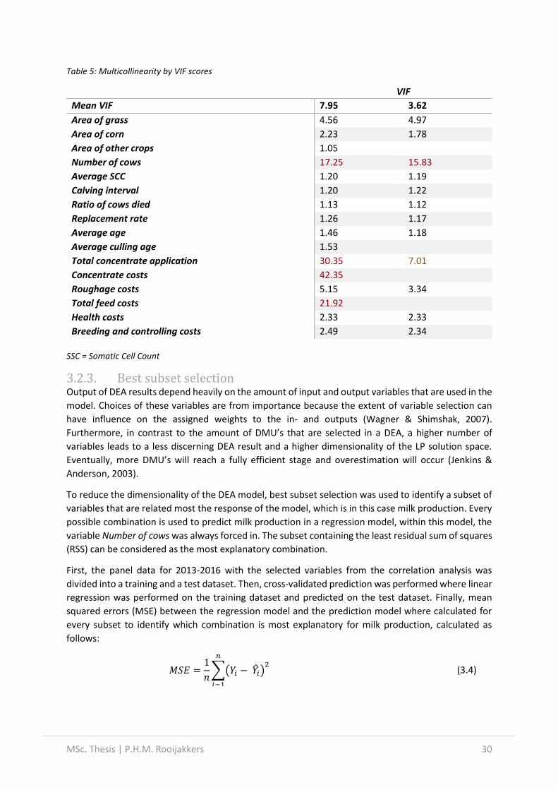
MSc. Thesis | P.H.M. Rooijakkers 30
Table 5: Multicollinearity by VIF scores
VIF
Mean VIF 7.95 3.62
Area of grass 4.56 4.97
Area of corn 2.23 1.78
Area of other crops 1.05
Number of cows 17.25 15.83
Average SCC 1.20 1.19
Calving interval 1.20 1.22
Ratio of cows died 1.13 1.12
Replacement rate 1.26 1.17
Average age 1.46 1.18
Average culling age 1.53
Total concentrate application 30.35 7.01
Concentrate costs 42.35
Roughage costs 5.15 3.34
Total feed costs 21.92
Health costs 2.33 2.33
Breeding and controlling costs 2.49 2.34
SSC = Somatic Cell Count
3.2.3. Best subset selection Output of DEA results depend heavily on the amount of input and output variables that are used in the
model. Choices of these variables are from importance because the extent of variable selection can
have influence on the assigned weights to the in- and outputs (Wagner & Shimshak, 2007).
Furthermore, in contrast to the amount of DMU’s that are selected in a DEA, a higher number of
variables leads to a less discerning DEA result and a higher dimensionality of the LP solution space.
Eventually, more DMU’s will reach a fully efficient stage and overestimation will occur (Jenkins &
Anderson, 2003).
To reduce the dimensionality of the DEA model, best subset selection was used to identify a subset of
variables that are related most the response of the model, which is in this case milk production. Every
possible combination is used to predict milk production in a regression model, within this model, the
variable Number of cows was always forced in. The subset containing the least residual sum of squares
(RSS) can be considered as the most explanatory combination.
First, the panel data for 2013-2016 with the selected variables from the correlation analysis was
divided into a training and a test dataset. Then, cross-validated prediction was performed where linear
regression was performed on the training dataset and predicted on the test dataset. Finally, mean
squared errors (MSE) between the regression model and the prediction model where calculated for
every subset to identify which combination is most explanatory for milk production, calculated as
follows:
𝑀𝑆𝐸 =1
𝑛∑(𝑌𝑖 − �̂�𝑖)
2𝑛
𝑖−1
(3.4)

31 MSc. Thesis | P.H.M. Rooijakkers
where the mean (1
𝑛∑ ) 𝑛
𝑖−1 of the squares of the errors (𝑌𝑖 − �̂�𝑖)2
is calculated and where 𝑌𝑖 represents
the observed values for the regression on the training dataset and �̂�𝑖 represents the observed
predicted values on the test dataset.
Sets of variables and outcomes of the best subset selection are summarised in Appendix III. Set 5
contains six variables which is suitable for performing a DEA. These variables are most explanatory
considering the whole set of variables leading from the correlation analysis. The variables that will be
selected for performing DEA are (ordered from most explanatory to least explanatory for milk
production):
• Number of cows
• Calving interval
• Total concentrate application
• Health costs
• Breeding and controlling costs
• Ratio of cows died
Because these variables all declare the milk production and variables on feed are not well represented
in the model by these six variables, one variable will be dropped from the selection (Ratio of cows died)
and will be substituted with a variable which is not explanatory for milk yield but does give some
information on feed intake:
• Total feed crop area (Sum of area of grass, corn and other feed crops)
With these six variables, DEA will be performed per year for the years 2013, 2014, 2015 and 2016 on
the 846 DMU’s. MSE’s are summarized in Figure 4:
In Figure 4 it is made visible that including more variables in a set of variables (Appendix III), the mean
squared error (MSE) will be reduced until a given amount. Variables that were included first explain
milk production the most. In this case that are the variables listed above. Including all variables will
Figure 4: Summaries of Mean Squared Errors returning from the selected variables from the best subset selection with on the y-axis the MSE of each set of variables (x-axis) between the predicted and actual Milk yield). Sets of variables are shown in (Appendix III, Table 2)

MSc. Thesis | P.H.M. Rooijakkers 32
lead to a worse prediction of the milk yield than including the six variables represented by set 5 because
than a larger MSE is shown.
3.4. Comparison of results
Results of the DEA are compared using several statistical tests and post-hoc tests. Comparison will be
performed on different groups of efficiency levels. These groups will be based on the distribution of
efficiency scores per year, shown in Table 6:
Table 6: Ranges of comparison groups based on TE score
Group Range
1 Maximum TE score (1) 2 3rd Quartile < Maximum TE score 3 Mean < 3rd Quartile 4 1st Quartile < Mean 5 Minimum TE score < 1st Quartile
TE = Technical Efficiency
Because the group containing efficient farms could have a substantially large size, this group is taken
as one separate group. Furthermore, whit this distribution of groups, it is possible to compare fully
efficient farms with lower efficient farms.
Variables that were compared are a mixture of input variables, farm specific variables and derived
variables from milk output. The variables that will be compared using statistical tests are shown in
Table 7 which is a subset of the variables shown in Table 3. In Table 7 variables were derived per unit
of output when this was found useful to compare different efficient scoring classes on their
performance per output:
Table 7: Overview of variables used for statistical comparison based on TE scores
Variable Unit Description
Number of cows no. Average number of cows present at a farm
Calving interval days Interval between birth of a calf and a subsequent calf
Ratio of cows died % Percentage of cows that has died in one year at a farm
Replacement rate % Replacement percentage of cows at a farm
Average age years Average age of the production cows at a farm
Average culling age years Average culling age of the production cows at a farm
Milk production per total area kg/ha Amount of milk produced per total feeding area
Milk production per cow kg/cow Amount of milk produced per cow present at a farm
Concentrate application per unit of milk
kg/100 kg Average amount of concentrates applied to a cow per 100 kg of produced kilograms of milk
Purchased roughage per unit of milk
€/100 kg Average costs of purchased roughage per 100 kg of produced kilograms of milk
Health costs per unit of milk €/100 kg Average costs of health-related activities per 100 kg of produced kilograms of milk
Breeding and controlling costs per unit of milk
€/100 kg Average costs of breeding and controlling related activities per 100 kg of produced kilograms of milk

33 MSc. Thesis | P.H.M. Rooijakkers
To compare variables, they were first examined if they are normally distributed with the help of a
Shapiro-Wilks test. This test assesses if the mean observations for a concerning variable are normal
distributed. When variables were found normally distributed, TE scores were compared using a one-
way ANOVA, divided into five TE score groups (Table 6). Variations between the groups were compared
and examination of statistical difference between these groups was performed. When variables were
found not normally distributed, the same procedure was performed using a non-parametric Kruskal-
Wallis test. This test analyses if TE score groups are equal to each other, equal to a One-way ANOVA,
however in this case non-distributed variables are assessed and makes assumptions based on median
values instead of mean values. These tests indicate if there are significant differences between the
assessed groups (Table 6) but do not give information for between group differences. To get this
information, a post-hoc test will be performed. When a variable was normally distributed, a Tukey
range test will be performed. When a variable is not normally distributed, a Wilcoxon signed rank test
will be performed to compare the five groups. These post-hoc tests analyse the differences between
two paired groups.

MSc. Thesis | P.H.M. Rooijakkers 34
4. Results
4.1. Data summary
All variables that were selected in chapter 3.1.1 are summarized in three categories: Cows, Land and
Costs for every year between 2013 and 2016.
4.1.1. Cows From Table 8 at the next page it becomes clear that most missing values arise from the average Somatic
Cell Count (SCC) variable. The variables average cow age, replacement rate, calving interval and
percentage of cows died all contain between 300 and 325 missing values. From a more in-depth
examination of the dataset it becomes clear that farms that miss one of the above variables, often also
miss data of the others. This makes these farms less informative if one or several of these variables are
selected for further research. Information on total milk production and the number of cows present at
the farm is available of all the selected farms. The coefficient of variance (COV) gives information of
the ratio of the variation of the data relative to the mean. With the help of the COV, variation is
standardized and easier to interpret the magnitude of variation concerning the different variables.
Standard deviations were found high on the percentage of cows died. Moderate variation was found
in the variables average number of cows, total milk production and total concentrates applied.

35 MSc. Thesis | P.H.M. Rooijakkers
Table 8: Summary of selected variables in chapter 3.1.1 in the cow related category
N N blank Mean Min Max Std. Dev. COV
20
13
Number of cows [-] 1223 0 95.7 14.4 621.1 46.4 0.5
Total milk production [kg] 1223 0 794599 83452 4766903 397755 0.5
Avg. age [years] 886 337 4.2 3.1 7.0 0.5 0.1
Replacement rate [%] 872 351 25.9 6.0 73.0 7.5 0.3
Calving interval [days] 889 334 411.9 352.0 635.0 25.5 0.1
Ratio of cows died [%] 882 341 3.0 0.0 16.0 2.5 0.8
Avg. Culling age [years] 874 349 5.3 3.1 10.1 0.8 0.2
Total conc. application [kg] 1204 19 205957 27193 1926963 111504 0.5
Average SCC [cells/ml] 282 941 172.7 67.0 409.0 54.3 0.3
20
14
Number of cows [-] 1223 0 97.7 14.5 686.3 48.6 0.5
Total milk production [kg] 1223 0 816585 90889 5307904 416534 0.5
Avg. age [years] 901 322 4.2 3.1 7.0 0.4 0.1
Replacement rate [%] 889 334 26.9 1.0 69.0 7.5 0.3
Calving interval [days] 904 319 409.3 352.0 592.0 24.5 0.1
Ratio of cows died [%] 899 324 3.3 0.0 25.0 2.8 0.9
Avg. Culling age [years] 888 335 5.3 3.1 20.6 0.8 0.2
Total conc. application [kg] 1210 13 209777 25404 2003996 117766 0.6
Average SCC [cells/ml] 298 925 166.2 76.0 328.0 48.2 0.3
20
15
Number of cows [-] 1223 0 102.9 16.9 879.9 55.2 0.5
Total milk production [kg] 1223 0 872159 99125 6737981 486145 0.6
Avg. age [years] 916 307 4.2 3.1 6.1 0.4 0.1
Replacement rate [%] 900 323 24.0 2.0 62.0 7.0 0.3
Calving interval [days] 917 306 409.6 356.0 594.0 24.9 0.1
Ratio of cows died [%] 910 313 2.9 0.0 18.0 2.4 0.8
Avg. Culling age [years] 902 321 5.3 3.1 11.0 0.9 0.2
Total conc. application [kg] 1211 12 226854 18834 2472959 142736 0.6
Average SCC [cells/ml] 349 874 158.5 40.0 403.0 52.4 0.3
201
6
Number of cows [-] 1223 0 109.4 10.8 1043.9 62.2 0.6
Total milk production [kg] 1223 0 941984 97843 8315824 557098 0.6
Avg. age [years] 921 302 4.2 3.1 6.1 0.4 0.1
Replacement rate [%] 909 314 26.9 2.0 89.0 7.5 0.3
Calving interval [days] 918 305 404.9 356.0 617.0 23.8 0.1
Ratio of cows died [%] 914 309 3.6 0.0 22.0 3.1 0.8
Avg. Culling age [years] 904 319 5.3 3.1 10.1 0.8 0.2
Total conc. application [kg] 1202 21 254139 11884 3810235 183716 0.7
Average SCC [cells/ml] 308 915 159.4 40.0 351.0 52.8 0.3
SCC = Somatic Cell Count
4.1.2. Land Selected farmers vary in cropland area. Not only because farms vary in size farmers need more land to
provide their animals of feed, but also management and availability of farmland can play a role in the
distribution and presence of land on farm. Furthermore, in some areas in the Netherlands it is only
possible to farm grasslands. Farms can be very extensive or intensive, depending on management
styles. Furthermore, rations can vary between dairy farmers in the Netherlands from very grass

MSc. Thesis | P.H.M. Rooijakkers 36
(protein) based to rations that include more cereals such as corn. From the Table 9, most variation is
found in maize and other cropland. It is made visible that farmers almost don’t cultivate other crops
than maize and grass, which are also the most common components in Dutch dairy rations (Plomp et
al., 2010). Availability of information on land availability on the selected farms was found for every
assessed farm.
Table 9: Summary of selected variables in chapter 3.1.1 in the land related category
N N blank Mean Min Max Std. Dev. COV
20
13
Area of grass [ha] 1223 0 38.7 0.0 298.4 18.8 0.5
Area of corn [ha] 1223 0 9.0 0.0 58.0 6.7 0.7
Area of other crops [ha] 1223 0 0.3 0.0 21.8 1.5 5.7
20
14
Area of grass [ha] 1223 0 40.5 0.0 345.2 20.1 0.5
Area of corn [ha] 1223 0 7.9 0.0 58.0 6.0 0.8
Area of other crops [ha] 1223 0 0.2 0.0 21.8 1.2 6.2
20
15
Area of grass [ha] 1223 0 42.3 0.0 387.2 21.7 0.5
Area of corn [ha] 1223 0 7.4 0.0 58.0 5.8 0.8
Area of other crops [ha] 1223 0 0.1 0.0 15.7 1.0 7.0
20
16
Area of grass [ha] 1223 0 43.5 8.1 463.5 23.9 0.6
Area of corn [ha] 1223 0 7.5 0.0 69.4 5.9 0.8
Area of other crops [ha] 1223 0 0.3 0.0 21.7 1.5 6.1
4.1.3. Costs The availability of data for the selected variables on costs were found good. Variations within cost
related variables was almost found similar between the variables, representing moderate variations
between the farm for all costs, except for the variable Roughage costs. Roughage costs vary most
between farms because of availability of land and crop strategies (chapter 2.2.1). Some farmers are
therefore high in roughage purchases and some farmers are able to cultivate their own feeding crops.
Moderate variation was found in total feed costs, which also includes the costs for concentrates. Total
feed costs consist of; concentrate costs, vitamins and minerals, milk products, purchased roughage
and stock change, wet by-products and grazing rents. In Figure 5 the contribution of these costs to the
total feed costs are visualised.
Figure 5: Overview of feeding cost structure

37 MSc. Thesis | P.H.M. Rooijakkers
Total feed costs consist for almost three quarters of concentrates, which is varying moderately
between farmers as seen in Table 10. It is therefore possible that some variation in efficiency can be
found from concentrate use. Costs of roughage contribute to 12% of the total feed costs on average,
this can vary between farms as can be observed from Table 10.
Table 10: Summary of selected variables in chapter 3.1.1 in the costs related category
N N blank Mean Min Max Std. Dev. COV
20
13
Concentrate costs [€] 1223 0 64066 7899 391839 33380 0.5
Roughage costs [€] 1223 0 14404 0 136585 15392 1.1
Total feed costs [€] 1223 0 90300 8931 483364 51503 0.6
Health costs [€] 1223 0 7393 510 38333 4306 0.6
Breed. and contr. costs [€] 1223 0 7171 327 30778 3563 0.5
20
14
Concentrate costs [€] 1223 0 59985 6495 414017 32270 0.5
Roughage costs [€] 1223 0 17025 0 133529 17582 1.0
Total feed costs [€] 1223 0 84873 6639 485142 51215 0.6
Health costs [€] 1223 0 7651 700 55202 4609 0.6
Breed. and contr. costs [€] 1223 0 7573 188 31027 3769 0.5
20
15
Concentrate costs [€] 1223 0 62558 6113 497263 36908 0.6
Roughage costs [€] 1223 0 17301 0 199528 19368 1.1
Total feed costs [€] 1223 0 90194 3030 590513 58832 0.7
Health costs [€] 1223 0 8045 765 55925 5012 0.6
Breed. and contr. costs [€] 1223 0 7553 487 35855 3978 0.5
20
16
Concentrate costs [€] 1223 0 68406 3314 706013 44952 0.7
Roughage costs [€] 1223 0 16362 0 204434 18568 1.1
Total feed costs [€] 1223 0 95016 2701 824098 66415 0.7
Health costs [€] 1223 0 8415 580 62369 5289 0.6
Breed. and contr. costs [€] 1223 0 7997 150 36625 4345 0.5

MSc. Thesis | P.H.M. Rooijakkers 38
4.2. Data Envelopment Analysis
4.2.1. Summary of efficiency scores Based on the selection of the best subset variable selection method, five input variables and one
output variable were selected which is explained in chapter 3.2.3. Variables that were selected for DEA
are; Number of cows, Calving interval, Total concentrate application, Breeding and Controlling costs,
Health costs and Total area as input variables and Total milk production as output variable.
TE scores and their distribution resulting from the DEA, performed per year are shown in Table 11.
Most efficient farms were found in the year 2014 concerning these six input variables. Mean TE scores
were found to be 0.93 for all assessed years. Mean TE scores were found high and indicate that the
846 selected Dutch dairy farms operate near or on the best practice frontier. Almost no increase in
mean TE was found between the assessed years (with 2013 containing the lowest and 2015 containing
the highest meant TE score), however the number of efficient farms were substantially lower in the
year 2016. This means that almost no improvement was made in input use relatively to the produced
output on average over consequent years between 2013 and 2016.
Table 11: Summary of TE scores
Min. 1st Qu. Median Mean 3rd Qu. Max.
2013 0.743 0.901 0.929 0.927 0.958 1
2014 0.697 0.904 0.935 0.932 0.965 1
2015 0.705 0.905 0.935 0.933 0.966 1
2016 0.718 0.904 0.933 0.929 0.956 1
The scores are not normal distribution because many farms have a TE score of 1. Most farms have an
efficiency between 0.9 and 1.
Figure 6: Histogram plots of the TE score distribution per year

39 MSc. Thesis | P.H.M. Rooijakkers
The histograms in Figure 6 indicate that there are no large differences on TE scores between the years.
Not many outliers were found in the lower region, but there are some farms found that have a
substantially lower TE score relative to the other farms in the selected data set. This finding shows that
farms are technical efficient relative to each other. Farms that have the lowest TE score, use there
inputs approximately 30% less efficient than the most efficient farms in the dataset, having TE scores
of 0.70.
4.2.2. TE score group dynamics through 2013-2016 To compare TE scores during the years, farms were ranked on their TE score within five groups. Groups
and their group sizes are shown in Table 12. For further comparison, ranks are divided based on the
same quartiles as in Table 11. The TE score groups can be used to compare significant differences of
the selected variables that are linked to functional traits. Furthermore, a more in-depth examination
of the in- and decrease of TE gives an indication of the technical level (or input/output use), which is
relevant to examine if farms fluctuate a lot in TE or remain the same score every year relatively to the
other farms.
Table 12: Composition of TE score groups based on the distribution per year in Table 12
TE score group Range Rank 2013 2014 2015 2016
1 Max. Fully efficient 90 98 99 77 2 3rd Qu. – Max. Highly efficient 121 114 113 134 3 Mean – 3rd Qu. Moderately efficient 225 236 223 233 4 1st Qu. – Mean Lower efficient 198 186 199 189 5 Min. – 1st Qu. Low efficient 212 212 212 213
From Table 12 it can be seen that in the years 2014 and 2015 most efficient farms were found. In these
years, also mean efficiency as found highest (Table 11). To analyse the in- and decrease of efficiency
score, changes in ranks between groups were recorded and compared per year. Most farms
maintained an equal rank between two consecutive years. In 2013-2014, more farms decreased in rank
than increased, however in 2015-2016 the opposite was observed. In 2014-2015, approximately an
equal number of farms decreased and increased in TE group. No farms subsequently increased in rank.
There were 165 that maintained the same rank every year. Most of the farms that subsequently were
in the same ranking group were found in group 5 low scoring farms. The dynamics of ranking change
during the years summarised in Table 13 only give a brief overview of TE changes during the years. A
more precise overview is given in Table 14.
Table 13: Dynamics of TE scores between ranking groups, brief overview
2013-2014 2014-2015 2015-2016
Increase 219 224 210 Equal 396 402 425 Decrease 231 220 211
Constant increase 2 Constant equal 165 Constant decrease 3 Other 676
From Table 14, it can be derived that a high number of farms that are ranked in group 1 stay in group
1 in a consecutive year. Remarkable results were found in the changes from group 1 to 5 or the

MSc. Thesis | P.H.M. Rooijakkers 40
opposite, a minor number of farms change from the highest to the lowest ranking group (or the
opposite) within one year. Most changes in ranking group were found from one rank to a rank that is
one grade higher or lower.
Table 14: Dynamics of TE scores between ranking groups, elaborated overview. TE score groups overview is given in Table 12 and Table 13
TE score groups 2013-2014 2014-2015 2015-2016
Increase
5 > 4 45 55 54
5 > 3 27 21 14
5 > 2 3 0 8
5 > 1 1 0 0
4 > 3 62 56 57
4 > 2 10 8 11
4 > 1 4 5 6
3 > 2 45 45 40
3 > 1 12 13 4
2 > 1 22 17 17
Equal
5 > 5 136 136 136
4 > 4 72 67 74
3 > 3 92 95 116
2 > 2 37 56 49
1 > 1 59 64 50
Decrease
1 > 2 19 20 26
1 > 3 7 11 10
1 > 4 2 2 7
1 > 5 3 1 6
2 > 3 48 40 36
2 > 4 11 16 8
2 > 5 3 1 3
3 > 4 56 59 46
3 > 5 20 24 17
4 > 5 50 50 51
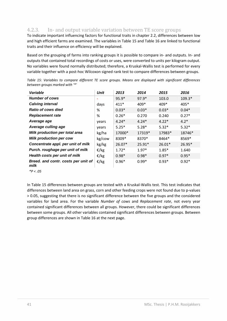
41 MSc. Thesis | P.H.M. Rooijakkers
4.2.3. In- and output variable variation between TE score groups To indicate important influencing factors for functional traits in chapter 2.2, differences between low
and high efficient farms are examined. The variables in Table 15 and Table 16 are linked to functional
traits and their influence on efficiency will be explained.
Based on the grouping of farms into ranking groups it is possible to compare in- and outputs. In- and
outputs that contained total recordings of costs or uses, were converted to units per kilogram output.
No variables were found normally distributed; therefore, a Kruskal-Wallis test is performed for every
variable together with a post-hoc Wilcoxon signed rank test to compare differences between groups.
Table 15: Variables to compare different TE score groups. Means are displayed with significant differences between groups marked with '*'
Variable Unit 2013 2014 2015 2016
Number of cows - 95.9* 97.9* 103.0 109.3*
Calving interval days 411* 409* 409* 405*
Ratio of cows died % 0.03* 0.03* 0.03* 0.04*
Replacement rate % 0.26* 0.270 0.240 0.27*
Average age years 4.24* 4.24* 4.22* 4.2*
Average culling age years 5.25* 5.28* 5.32* 5.32*
Milk production per total area kg/ha 17000* 17319* 17983* 18746*
Milk production per cow kg/cow 8309* 8370* 8464* 8569*
Concentrate appl. per unit of milk kg/kg 26.07* 25.91* 26.01* 26.95*
Purch. roughage per unit of milk €/kg 1.72* 1.97* 1.85* 1.640
Health costs per unit of milk €/kg 0.98* 0.98* 0.97* 0.95*
Breed. and contr. costs per unit of milk
€/kg 0.96* 0.99* 0.93* 0.92*
*P < .05
In Table 15 differences between groups are tested with a Kruskal-Wallis test. This test indicates that
differences between land area on grass, corn and other feeding crops were not found due to p-values
> 0.05, suggesting that there is no significant difference between the five groups and the considered
variables for land area. For the variable Number of cows and Replacement rate, not every year
contained significant differences between all groups. However, there could be significant differences
between some groups. All other variables contained significant differences between groups. Between
group differences are shown in Table 16 at the next page.

MSc. Thesis | P.H.M. Rooijakkers 42
Table 16: Between group differences for both input and output variables for the panel 2013-2016
a-d within row significant differences between TE score groups occur with different superscripts (P < .05)
Unit
2013 2014 2015 2016
TE score group
1 2 3 4 5 1 2 3 4 5 1 2 3 4 5 1 2 3 4 5
Cows no. 116.9 ab
92.4 ab
99.6 a
93.7 ab
87.0
b
122.3 a
95.5 ab
97.2 ab
97.7 ab
88.8 b
128.4 a
102.9 a
102.7 a
98.9 a
95.4 a
131.6 ab
118.4
a
108.6 ab
110.5 a
95.4 b
Calving int. days 403 ab
396 a
403 b
410 c
434 d
403 a
396 a
399 a
408 b
431 c
401 ab
393 a
400 b
409
c
431 d
398 ab
389 a
395 b
405 c
427 d
Cows died. % 0.03 a
0.03 a
0.02 a
0.03 a
0.04 b
0.04 ab
0.02 a
0.03 a
0.03 a
0.04 b
0.03 ab
0.02 b
0.03 b
0.03 ab
0.03 a
0.04 ab
0.03 b
0.03 b
0.04 b
0.05 a
Repl. rate % 0.26 ab
0.27 a
0.26 ab
0.26 ab
0.25 b
0.28 a
0.27 a
0.27 a
0.27 a
0.27 a
0.25 a
0.24 a
0.24 a
0.24 a
0.23 a
0.3 a
0.27 b
0.26 b
0.27 ab
0.27 ab
Age years 4.16 a
4.17 a
4.19 a
4.25 ac
4.35 c
4.23 ab
4.16 ab
4.15 b
4.29 ac
4.35 c
4.15 ab
4.16 b
4.17 b
4.23 bc
4.33 c
4.16 a
4.12 a
4.19 a
4.18 a
4.3 b
Culling age years 5.02
a
5.09 ab
5.15 ab
5.28 bc
5.5 c
5.2 ab
5.15 a
5.14 a
5.39 b
5.46 b
5.15 a
5.07 ab
5.38 bc
5.3 ac
5.49 c
5.2 ab
5.18 a
5.31 ab
5.3 ab
5.49 b
Milk p. area kg/ha 20531
ab
18775 a
17475 bc
16329 c
14610 d
20941
a
18177a
18272a
16504
b
14838 c
22550a
19566a
18473a
16797b
15604c
22975
ab
20326
a
19061
ab
18514 b
16085 c
Milk p. cow kg/cow 8630 ab
8865 a
8548 b
8230 c
7676 d
8644 ab
8867 a
8622 a
8362 b
7703 c
8719 ab
8906 a
8737 a
8442 b
7844 c
8853 ab
8915 a 8806 a 8600 b
7964 c
Concentrate kg/100kg 23.56 a
24.17 a
25.65 b
26.68 c
28.1 d
23.74 a
23.61 a
25.52 b
26.33 b
28.21 c
24.63 a
24.63 a
25.47 ab
26.31 b
27.69 c
25.35 a
25.44 a
26.14 a
27.66
b
28.72
c
Roughage €/100kg 1.80 ab
2.09 a
1.71 ab
1.71 ab
1.50 b
2.18 ab
2.19 ab
2.16 a
1.78 ab
1.70 b
2.02 a
2.04 a
1.99 a
1.72 a
1.66 a
1.79 a
1.71 a
1.74 a
1.67 a
1.40 a
Health €/100kg 0.77 a
0.95 ab
0.95 b
1.02 bc
1.09 c
0.79 a
0.94 b
1.01 b
0.99 b
1.06 b
0.80 a
0.84 a
0.96 b
1.03 bc
1.07 c
0.68 a
0.93 b
0.96 bc
0.98 bc
1.03 c
Breeding €/100kg 0.80 a
0.91 ab
0.97 bc
0.98 bc
1.04 c
0.79 a
0.93 b
0.97 bc
1.05 cd
1.08 d
0.78 a
0.84 a
0.96 b
0.97 b
1.00 b
0.72 a
0.86 b
0.94 c
0.94 bc
0.99 c

43 MSc. Thesis | P.H.M. Rooijakkers
Differences between the groups of high and low efficient farms are significant for all variables except
the variables Number of cows (except for 2014), Ratio of cows died, Replacement rate and Purchased
roughage. The number of cows differs a lot within group 1, with a standard deviation from 80 to 97
cows during the panel of years. The variable Replacement rate was relatively lower in 2015 than in the
other years, but not varying between the groups in general. The variable Ratio of cows died also does
not vary between the first four groups and remains equal over the years. Also, no significant
differences were found between fully efficient farms (group 1) and low efficient farms (group 5) for
every year except 2013. Also, significant differences between efficiency groups for Purchased
roughage were not found in general.
The variable Total concentrate application has significant differences between fully efficient farms
(group 1) and lower efficient groups (4 and 5) for every year. Also, highly efficient farms (group 2) has
significant differences with lower efficient groups (4 and 5) for every year. Highly efficient farms do
not differ significantly from fully efficient farms for every assessed year. For the output variable Milk
production per total area and Milk production per cow, significant differences between highly efficient
groups (1 and 2) and low efficient group 5 were found every year. For both output variables, the first
two groups do not differ from each other significantly during all the assessed years. Also, no significant
differences between groups 1 and 3 were found, however group 3 significantly differs from group 2
and 4 for some years. Group 3 differs from group 5 significantly for every year for both output
variables. From these results, efficient farms are represented by farms that are significantly more area
intensive and use significantly less concentrates than farms with lower efficiency. Furthermore, the
efficient farms have also significantly higher milk yields per cow which could indicate that these farms
have cows that perform significantly better for feed efficiency, a functional trait which was selected in
chapter 2.2.
For Health and Breeding and controlling costs significant differences were found between the highly
efficient groups. The group containing fully efficient farms did differ significantly from groups 3, 4 and
5 in every assessed year. For these two variables, no significant differences were found between lower
efficient groups (4 and 5) and for some years (depending on the variable health or breeding and
controlling costs). For the variable Calving interval significant differences were found between groups
containing lower and moderate efficient scores (2, 3, 4, 5), but also between fully efficient farms (group
1) and lower efficient groups (4 and 5). In every year that was assessed, fully efficient, highly efficient
and moderately efficient farms (groups 1, 2 and 3) differed significantly from lower and low efficient
farms (groups 4 and 5). Both relating to functional traits health and fertility these results indicate that
efficient farms could have significantly healthier and fertile cows than cows that are present on lower
efficient farms due to lower costs that are spend on health and fertility related costs. Furthermore,
efficient farms have a significant lower calving interval which could indicate that cows at efficient farms
have higher success rates of inseminations and gestation.
For the variable Age, shows significant differences between fully efficient farms (group 1) and low
efficient farms for every year, age of cows is significantly higher at lower efficient farms. The fully
efficient farms do not differ significant from other groups. Between groups 2, 3 and 4 there is some
variation between significant differences with other groups. Concerning the variable Culling age,
significant differences highly vary between the assessed years. For every year, group 2 differs
significantly from group 5. Furthermore, no significant differences were found between groups 1 and
2, groups 2 and 3 and between groups 4 and 5 for every year. For the functional trait longevity, farms
that have lower efficiency contain cows that have a higher average age than the cows that are present
on high efficient farms. Also, lower culling ages were found at fully efficient farms in comparison with
lower efficient farms, however this was not found significant.

MSc. Thesis | P.H.M. Rooijakkers 44
45 MSc. Thesis | P.H.M. Rooijakkers
5. Discussion
In economics, efficiency analysis can be performed by applying different methods. Also, in dairy
farming, several methods were performed to measure or estimate technical efficiency. An overview of
methods that are used in the past is given in the review of Mareth et al. (2016). Studies on Dutch dairy
farming are given in chapter 2.1.2. Technical efficiency is always a relative measure between DMU’s
and it is therefore difficult to compare various studies with each other. Not only variations in
performed method occur, within these various methods the amount and type of in- and outputs could
be approached differently. Inputs that are used to measure or estimate technical efficiency consist
mostly of land, herd size, labour, capital and variable inputs, however based on the focus of a study
(for example animal welfare or environmental impact) a set of chosen in- and output variables can
change. The selection of variables depends on the goal of the study, for example determining the
impact of environmental inputs like in Reinhard et al. (2000). In this study, focus was set on the
performance of an individual cow influencing farm performance. With the help of a literature study,
influencing factors were found and selected from the used accounting dataset.
DEA uses a non-parametric approach and is therefore not restricted by parametrical assumptions and
needs functional forms to relate the inputs to the outputs. DEA is a useful method when multiple inputs
are handled with a single output, but it does not account for random noise in these variables. This
means that assumptions are made in relation to statistical noise or measurement errors. DEA is in
contrast to SFA more sensible for outliers, however this effect will be reduced when sample sizes are
enlarged. DEA does treat all variables equal, it is therefore easily possible to include various variables
which do not have to be in an equal range or have the same probabilistic behaviour. Because technical
efficiency scores are approached completely different besides the two methods, results are likely to
be different and both methods have their advantages and disadvantages. However, in Resti (1999) no
clear advantages were found using one method above the other. In this study, only the non-
parametrical deterministic approach (DEA) was performed, due to its advantage of approaching all
variables equally by not adding any weights to the variables.
The variables that were selected in this study are different from other studies. For example, the
variables labour and capital were not included. All variables except Total area land were found
explainable for milk production. Because DEA makes no difference between variable weights, Total
area land was chosen as a variable not explainable for milk production and included in the set of chosen
inputs. The variable is however an indicator for roughage feed input and therefore for importance for
this study. Furthermore, because land area is a common selected variable in efficiency analysis in dairy
farming according to the assessed literature, this variable was chosen with a higher priority relative to
Purchased roughage. This will result in other results, because the selected variables are not similar to
other studies. The focus of this study is not to compare the TE scores with other studies, however
studies found in literature with similar approaches give an indication of the TE level of Dutch dairy
farming.
To explain functional traits in the DEA, variables have been chosen that include information of the
traits health, fertility, longevity and feed efficiency. The set of variables that was chosen include Total
land area and Total concentrate application concerning the functional trait Feed efficiency, variables
Calving interval and Breeding and controlling costs concerning the functional trait Fertility and the
variable Health costs concerning the functional trait Health. Furthermore, the variable Number of cows
was included to measure the farm production performance explanatory for the output variable Total
milk production. Within this set of in- and output variables, no variables explaining the functional trait

MSc. Thesis | P.H.M. Rooijakkers 46
Longevity were included. Because the variables Age and Replacement rate were not found explanatory
for Total milk production and only a limited set of variables could be selected, the variables Age and
Replacement rate were excluded from the DEA analysis. They were however included in the
comparison study.
Besides selecting the right set of in- and output variables, the amount of variables that will be chosen
heavily depend the output of DEA results (Wagner & Shimshak, 2007). Selecting too many variables
will lead to overestimation of the TE scores and lead to a shift of the mean TE score. When too many
variables are chosen, the possibility for a DMU to be efficient in some way will be enlarged. Therefore,
in this study a maximum of six input variables and one output variable was restricted. A balance
between information loss and overestimation was found sufficient with this set of variables because
the variables explaining milk yield and variables in relation with functional traits were included, having
a mean TE score of all years of 0.93. The set of six variables was eventually found best from a selection
of several sets that differed in variable size and composition.
This mean TE score is higher than that was found in literature about Dutch dairy farming (Brümmer et
al., 2002; Dandi, 2017; Kovács & Emvalomatis, 2011; Reinhard et al., 2000, 1999) performed in the
past. Scores between 0.78 and 0.92 were found from the performed literature study where different
methods with different sets of variables were used. It is therefore not assumable to compare these
scores with each other. However, relatively to each other, Dutch dairy farmers are very efficient in
input use, not regarding which set of variables are used. The conclusion that Dutch dairy farmers are
relatively very efficient to each other was found both in literature and in this study. However different
methods were used to find TE scores.
From the dataset, information onwards 2004 was available. This study only gives results for the years
between 2013 and 2016. A similar approach (four year panel) was found in literature (Brümmer et al.,
2002; Dandi, 2017; Kovács & Emvalomatis, 2011; Reinhard et al., 2000, 1999). It was chosen to only
include the most recent years that were made available and to exclude all other years. For these four
years the panel was balanced, including multiple years would lead to loss in data because not all farms
have data available for multiple years. For dairy farmers in the Netherlands farm characteristics could
be somewhat affected during the years that were assessed due to the abortion of milk quota in 2014
and preparations for the initiation of the phosphate regulation in 2018. The average number of cows
present on a farm does not stagnate from 2015 (reference year for phosphate regulation), however
the replacement rate is lower in 2015 relative to the other years. Also, average milk production per
cow increased substantially which could indicate that farmers focus on a reduced feed use per kilogram
of milk, however the application of concentrates per cow have also increased during the years. This
could indicate that farmers are more focussing on functional traits like in this finding feed efficiency
instead of increasing their dairy herd.
In the review of Mareth et al. (2016) on efficiency analysis in dairy farming it was found that mean TE
scores varied according to herd size and that it did not vary according to land size. In this study, no
significant differences according herd size were found between efficient and lower efficient farms.
However, farms that were efficient used a rather intensive land management, having significantly
higher milk yields per hectare of land. From the results it can be seen that farms which have high
production levels per cow, are found in the group with farms which are highly efficient. Fully efficient
farms have still a significant higher milk yield than lower efficient farms, however do not contain the
cows which reach the highest production levels on average. Subsequent to these somewhat lower milk
yields, these farms use significantly less concentrates per cow than farms with moderate and low(er)
efficiency and less concentrates per cow than on farms which are highly efficient. Also, farms that are
fully efficient use less health and breeding and controlling costs than the highly efficient farms,

47 MSc. Thesis | P.H.M. Rooijakkers
resulting in 2016 with significant lower costs on health and breeding and controlling. Concerning age
and culling age, fully and highly efficient farms do not differ significantly. Farms that have low(er) TE
scores do have significant differences concerning the two variables on age. These farms have cows
present that reach a higher age on average. Reasons for having a herd with on average lower age could
not be found in this study, however it could be suggested that farms only want to keep their most
productive cows due to phosphate production restrictions. Also calving intervals were found
significantly higher on the lower performing farms which could indicate that cows that are present
there are less fertile, having higher insemination failures, having increased gestation failures, or that
cows are held in lactation for a longer period, resulting in a lower year-round milk yield. This indicates
that fully efficient farms perform slightly lower in production performance than highly efficient farms,
however focussing on functional traits fully efficient farms perform better than lower efficient farms
relating to feed efficiency, health and fertility. In comparison with low(er) efficient farms, fully efficient
farms perform worse for the functional trait longevity.
Results were compared based on the distribution of the technical efficiency scores for every year.
Similar patterns were found for all variables between the farms with the highest and the farms
containing the lowest efficiency scores. There were differences found between the other groups
concerning the assessed years. It was chosen to compare groups based on their distributions above
comparing various clusters. Cluster analyses were performed per year, but it was not made clear how
many clusters should be assessed. Furthermore, no clear patterns were found between the various
years. Cluster analysis was performed based on the in- and output variables, however the composition
of clusters and farms varied highly between the years. Comparison was therefore performed based on
the distribution of efficiency scores and results of the cluster analyses were excluded from the report.
From Figure 6 it is made visible that similar patterns occur, but only change in magnitude. This is not a
remarkable result because on average farms will only slightly change their in- and output levels
between the years. From Table 12 it becomes clear that group sizes remain approximately equal over
the years, but looking into Table 13 and Table 14 it is also observed that technical efficiency scores can
be highly dynamic for a farm relatively to the other assessed farms. Because the farms are classified
based on their distribution, it makes it however possible to compare the farm characteristics (based
on the variables in Table 3) of various years, other than for example a cluster analysis.
DEA was found as an applicable method to relate farm performance to functional traits because
significant differences could be found between high and low efficient farms in relation to functional
traits. These functional traits are related to individual cows and a farmer could reduce the use of inputs
by selecting for cows that have suitable characteristics for the important functional traits. Efficient
farms only perform less on longevity; however, this could also be affected by the initiation of the
phosphate regulation. Within farm differences could not be indicated with the help of the dataset that
was used for this study, however the dataset was found sufficient with indicators for the most
important functional traits found in literature (Egger-Danner et al., 2012; Fuerst-Waltl & Baumung,
2010; Groen et al., 1997; Pritchard et al., 2013). Because efficiency analysis methods like DEA are
restricted to only a limited set of in- and output variables, it is found difficult to include every aspect
of functional traits. In the subsequent comparison study between the various TE score groups, it
however became clear that some significant differences were found between efficient and low
efficient farms in relation to the indicators for functional traits. Based on this information, DEA was
found as an appropriate tool for this study. With the help of the results of this study, future studies
could focus on the within farm differences relating to the indicators for functional traits that were
selected in this study and could examine if cows on efficient farms have significantly different
characteristics than cows on low(er) efficient farms. It could be possible that characteristics at farm
level could influence the functional and productive characteristics of an individual cow.

MSc. Thesis | P.H.M. Rooijakkers 48

49 MSc. Thesis | P.H.M. Rooijakkers
6. Conclusion
From literature study it became clear that Dutch dairy farmers are relatively efficient. Studies
concluded high TE scores, between 0.78 and 0.92 with multiple methods and orientations (both input
and output orientated studies). In this study, a mean TE score of around 0.93 was found for every
assessed year. What can be concluded by both the found literature and this study is that Dutch dairy
farms are efficient relative to each other. Between 7 and 99 fully efficient farms were found, which
represents that approximately 10% of the assessed farms use their inputs at an optimal level.
Difference in TE score between Dutch dairy farms was found for every year. Concerning one
consecutive year, it is shown that most farms remain in the same TE score group and approximately
the same number of farms increase or decrease to one or more groups containing a higher or lower
efficiency score. Almost no farms constantly in- or decrease in TE score group subsequently between
the years 2013-2016. However, this is also affected by the cause that only farms that are in the highest
or lowest groups could perform a constant in- or decrease. Around 23% of all farms remain in the same
TE score group every year. Furthermore, it becomes clear that farms mostly switch between one group
which is higher or lower in efficiency.
To answer the question of which indicators of farm level efficiency can influence the performance of
individual cows and therefore change the expression of traits related to farm performance, functional
traits were classified into four groups; health, fertility, longevity and feed efficiency. From DEA analysis,
significant differences in TE were found for variables which are all related to traits of an individual cow.
From an accountancy dataset, it was possible to find variables that had significant differences between
various TE score groups and are indicators for functional traits. These variables are Calving interval,
Age, Culling age, Concentrate application, Health costs and Breeding and controlling costs also for
production traits like Milk production per area and Milk production per cow significant differences
between efficient and low efficient farms were found. Farm level efficiency differences could therefore
be explained by cows that are healthy and fertile, having both low health and breeding and controlling
costs. Furthermore, cows at efficient farms were found feed efficient, using significantly lower
amounts of concentrates to reach a given quantity of milk output. On the other hand, cows on efficient
farms have on average a significantly lower age, and lower calving intervals which could indicate that
old cows are replaced earlier at a given age or after a certain number of lactations. The same trend
was found for every assessed year from 2013 to 2016. Concerning productivity, fully efficient farms
produce a lower milk yield per cow than highly efficient farms. It can be concluded that fully efficient
farms perform well on the functional traits health, fertility, and feed efficiency but perform worse on
the functional trait longevity.
It can be concluded that with using DEA it is possible to include cow specific traits to examine farm
performances. However, with the dataset that was used for this study, results are still on farm level
but give insights in cow specific characteristics which need further consideration on cow level.
Significant differences between fully efficient and low(er) efficient farms were found and indicate
where low(er) efficient farms could improve in relation to functional traits.

MSc. Thesis | P.H.M. Rooijakkers 50

51 MSc. Thesis | P.H.M. Rooijakkers
7. Recommendations
This study only contains results based on data of Dutch dairy farming. It would be interesting to also
apply the same study on other countries using the same way of farming to examine if the same findings
occur for other countries. In the Netherlands, dairy farmers are relatively efficient to each other,
however what would be the case for countries where differences in TE scores are much higher?
Furthermore, can the findings of this study be validated by applying the same study for similar
countries or will other significant differences be found. Countries in similar regions could be compared
on management and differences between regions could be indicated. When differences between
countries are made visible, it could be possible for farmers or breeders to focus on the indicators that
need attention by learning from countries that perform well on similar indicators. However, climate
and geographical and income differences should always be considered.
Furthermore, in this study only DEA is concerned, and no other efficiency analysis methods were
performed. It would be interesting do examine the results of a similar study in SFA and to compare the
differences between the two methods. In literature, no clear advantages were found using the one
method over the other, however, there were differences found which would be interesting to validate
the findings in this study.
These recommendations relate to the validation of this study. Another recommendation is to
investigate farm data and compare herd efficiencies to indicate the high and low performing cows. By
combining the information of this study, and examination of individual cow traits and performances,
correction factors could be created for high performing cows on low efficient farms or vice versa so
that the comparison of cows is not affected by the TE level of a farm.

MSc. Thesis | P.H.M. Rooijakkers 52

53 MSc. Thesis | P.H.M. Rooijakkers
8. Bibliography
Alin, A. (2010). Multicollinearity, 2, 370–374. https://doi.org/10.1002/wics.84
Allendorf, J. J., & Wettemann, P. J. C. (2015). Does animal welfare influence dairy farm efficiency? A two-stage approach. Journal of Dairy Science, 98(11), 7730–7740. https://doi.org/10.3168/jds.2015-9390
Asmild, M., Hougaard, J. L., Kronborg, D., & Kvist, H. K. (2003). Measuring Inefficiency via Potential Improvements. Journal of Productivity Analysis (Vol. 19). https://doi.org/10.1023/A:1021822103696
Avkiran, N. K. (2011). Applications of data envelopment analysis in the service sector. International Series in Operations Research and Management Science (Vol. 164). https://doi.org/10.1007/978-1-4419-6151-8_15
Bo, N. (2009). Practical cattle breeding in the future – commercialised or co-operative, across borderlines between countries and organizations. Proceedings of the 2009 - Interbull Meeting - Barcelona, Spain, AUGUST 21-24, 2009 (Vol. 40). Retrieved from https://journal.interbull.org/index.php/ib/article/viewFile/1122/1113
Bravo-Ureta, B. E., Solís, D., Moreira López, V. H., Maripani, J. F., Thiam, A., & Rivas, T. (2007). Technical efficiency in farming: A meta-regression analysis. Journal of Productivity Analysis, 27(1), 57–72. https://doi.org/10.1007/s11123-006-0025-3
Brickell, J. S., & Wathes, D. C. (2011). A descriptive study of the survival of Holstein-Friesian heifers through to third calving on English dairy farms. Journal of Dairy Science, 94(4), 1831–1838. https://doi.org/10.3168/jds.2010-3710
Brümmer, B., Glauben, T., & Thijssen, G. (2002). Decomposition of productivity growth using distance functions: The case of dairy farms in three European countries. American Journal of Agricultural Economics, 84(3), 628–644. https://doi.org/10.1111/1467-8276.00324
CBS. (2017). Nederlandse landbouwproductie 1950-2015. Retrieved January 9, 2019, from https://www.cbs.nl/nl-nl/nieuws/2017/05/nederlandse-landbouwproductie-1950-2015
Coelli, T. J., Rao, D. S. P., O’Donnel, C. J., & Batesse, G. E. (2005). An Introduction To Efficiency. An Introduction to Efficiency and Productivity Analysis (2nd ed.). New York: Springer Science & Business Media. https://doi.org/10.1007/978-1-4615-5493-6
Cole, J. B. (2014). Phenotypes for novel functional traits of dairy cattle. Retrieved from https://www.icar.org/wp-content/uploads/2016/07/Berlin-2014-Cole-Phenotypes-for-novel-functional-traits-of-dairy-cattle.pdf
Cook, N. B., & Nordlund, K. V. (2009). The influence of the environment on dairy cow behavior, claw health and herd lameness dynamics. Veterinary Journal, 179(3), 360–369. https://doi.org/10.1016/j.tvjl.2007.09.016
CRV. (2019). Bedrijven en koeien in cijfers - Coöperatie CRV. Retrieved January 9, 2019, from https://www.cooperatie-crv.nl/downloads/stamboek/bedrijven-en-koeien-in-cijfers/
Dandi, E. (2017). Economic Analysis of Scale and Technical Efficiencies of Dairy Farms. Retrieved from https://edepot.wur.nl/423246
Davis, H. S. (2018). the Measurement of Productive Efficiency. The Industrial Study of Economic Progress (Vol. 120). https://doi.org/10.2307/j.ctv5rdxd5.7

MSc. Thesis | P.H.M. Rooijakkers 54
de Haas, Y., & Veerkamp, R. F. (2001). Fokwaarde voeropname Introductie. Praktijkonderzoek Veehouderij. Retrieved from https://library.wur.nl/WebQuery/wurpubs/reports/486019
Egger-Danner, C., Cole, J. B., Pryce, J. E., Gengler, N., Heringstad, B., Bradley, A., & Stock, K. F. (2014). Invited review: overview of new traits and phenotyping strategies in dairy cattle with a focus on functional traits. Animal, 9(02), 191–207. https://doi.org/10.1017/s1751731114002614
Egger-Danner, C., Willam, A., Fuerst, C., Schwarzenbacher, H., & Fuerst-Waltl, B. (2012). Hot topic: Effect of breeding strategies using genomic information on fitness and health. Journal of Dairy Science, 95(8), 4600–4609. https://doi.org/10.3168/jds.2012-5323
Friggens, N. C., & Thorup, V. M. (2015). From Monitoring to Precision Phenotyping: Towards a Systemic Use of Precision Livestock Measures in Dairy Herds. In New Zealand Society of Animal Production (Vol. 75, pp. 145–148).
Friggens, N., Kaya, C., & Roozen, A. (2017). GenTORE: Genomic Management Tools to Optimise Resilience and Efficiency. GenTORE - "GENomic management Tools to Optimize Resilience and Efficiency (Vol. 0). Interbull Centre. Retrieved from https://journal.interbull.org/index.php/ib/article/view/1436
Fuerst-Waltl, B., & Baumung, R. (2010). Economic values for performance and functional traits in dairy sheep. Italian Journal of Animal Science, 8(3), 341–357. https://doi.org/10.4081/ijas.2009.341
Groen, A. F. (2004). Advances in Selection for Functional Traits. Paris. Retrieved from http://edepot.wur.nl/27415
Groen, A. F., Steine, T., Colleau, J. J., Pedersen, J., Pribyl, J., & Reinsch, N. (1997). Economic values in dairy cattle breeding, with special reference to functional traits. Report of an EAAP-working group. Livestock Production Science, 49(1), 1–21. https://doi.org/10.1016/S0301-6226(97)00041-9
Jenkins, L., & Anderson, M. (2003). A multivariate statistical approach to reducing the number of variables in data envelopment analysis. European Journal of Operational Research (Vol. 147). https://doi.org/10.1016/S0377-2217(02)00243-6
Kool, D. (2017). Optimaal benutten van eigen voer. Retrieved March 20, 2019, from https://www.ppp-agro.nl/Projecten/optimaal-benutten-van-eigen-voer
Korver, S. (1988). Genetic aspects of feed intake and feed efficiency in dairy cattle: A review. Livestock Production Science, 20(1), 1–13. https://doi.org/10.1016/0301-6226(88)90049-8
Kovács, K., & Emvalomatis, G. (2011). Dutch, Hungarian And German Dairy Farms Technical Efficiency Comparison. Applied Studies In Agribusiness And Commerce (Vol. 5). Budapest. https://doi.org/10.19041/apstract/2011/1-2/15
Lopez, V. H. M. (2006). Dairy farm technical efficiency and milk total factor productivity growth in three South American countries. Doctoral Dissertations. Retrieved from https://opencommons.uconn.edu/dissertations/AAI3239568
Lu, Y., Vandehaar, M. J., Spurlock, D. M., Weigel, K. A., Armentano, L. E., Connor, E. E., … Tempelman, R. J. (2018). Genome-wide association analyses based on a multiple-trait approach for modeling feed efficiency. Journal of Dairy Science, 101(4), 3140–3154. https://doi.org/10.3168/jds.2017-13364
Mareth, T., Thomé, A. M. T., Cyrino Oliveira, F. L., & Scavarda, L. F. (2016). Systematic review and meta-regression analysis of technical efficiency in dairy farms. International Journal of Productivity and Performance Management, 65(3), 279–301. https://doi.org/10.1108/IJPPM-02-2015-0027

55 MSc. Thesis | P.H.M. Rooijakkers
Mugera, A. W. (2013). Measuring technical efficiency of dairy farms with imprecise data: A fuzzy data envelopment analysis approach. Australian Journal of Agricultural and Resource Economics, 57(4), 501–520. https://doi.org/10.1111/1467-8489.12008
Plomp, M., Prins, U., van Schooten, H., & Pinxterhuisse, I. J. (2010). Regionale rantsoenen voor melkvee. Wageningen. Retrieved from www.biokennis.nl.
Pritchard, T., Coffey, M., Mrode, R., & Wall, E. (2013). Genetic parameters for production, health, fertility and longevity traits in dairy cows. Animal, 7(1), 34–46. https://doi.org/10.1017/S1751731112001401
Pryce, J. E., Gonzalez-Recio, O., Nieuwhof, G., Wales, W. J., Coffey, M. P., Hayes, B. J., & Goddard, M. E. (2015). Hot topic: Definition and implementation of a breeding value for feed efficiency in dairy cows. Journal of Dairy Science, 98(10), 7340–7350. https://doi.org/10.3168/jds.2015-9621
Pryce, J. E., Wales, W. J., De Haas, Y., Veerkamp, R. F., & Hayes, B. J. (2014). Genomic selection for feed efficiency in dairy cattle. Animal, 8(1), 1–10. https://doi.org/10.1017/S1751731113001687
Reinhard, S., Knox Lovell, C. A., & Thijssen, G. J. (2000). Environmental efficiency with multiple environmentally detrimental variables; estimated with SFA and DEA. European Journal of Operational Research, 121(2), 287–303. https://doi.org/10.1016/S0377-2217(99)00218-0
Reinhard, S., Lovell, C. A. K., & Thijssen, G. (1999). Econometric Estimation of Technical and Environmental Efficiency: An Application to Dutch Dairy Farms. American Journal of Agricultural Economics (Vol. 81). https://doi.org/10.2307/1244449
Resti, A. (1999). Efficiency measurement for multi-product industries: a comparison of classic and recent techniques based on simulated data. European Journal of Operational Research, 121(3), 559–578. https://doi.org/10.1016/S0377-2217(99)00054-5
Rijksdienst voor Ondernemend Nederland. (2019). Fosfaat gebruiksnorm en gebruiksruimte | RVO.nl. Retrieved January 9, 2019, from https://www.rvo.nl/onderwerpen/agrarisch-ondernemen/mest-en-grond/gebruiksruimte-berekenen/fosfaat-gebruiksnorm-en-ruimte
Rivas, T. E. (2003). Dairy farm efficiency and the analysis of milk production growth: Evidence from Vermont. Doctoral Dissertations. Retrieved from https://opencommons.uconn.edu/dissertations/AAI3080927
Rutten, C. J., Velthuis, A. G. J., Steeneveld, W., & Hogeveen, H. (2013). Invited review: Sensors to support health management on dairy farms. Journal of Dairy Science, 96(4), 1928–1952. https://doi.org/10.3168/jds.2012-6107
Theodoridis, A. M. (2015). A Restricted Data Envelopment Analysis Application to Dairy Farming. Data Envelopment Analysis Journal, 1(2), 171–193. https://doi.org/10.1561/103.00000007
van Dijk, H., Schukking, S., & van der Berg, R. (2015). Ontwikkeling voedervoorziening op melkveebedrijven in Nederland.
Veerkamp, R. F. (2010). Selection for Economic Efficiency of Dairy Cattle Using Information on Live Weight and Feed Intake: A Review. Journal of Dairy Science, 81(4), 1109–1119. https://doi.org/10.3168/jds.s0022-0302(98)75673-5
Wagner, J. M., & Shimshak, D. G. (2007). Stepwise selection of variables in data envelopment analysis: Procedures and managerial perspectives. European Journal of Operational Research, 180(1), 57–67. https://doi.org/10.1016/j.ejor.2006.02.048

MSc. Thesis | P.H.M. Rooijakkers 56

I MSc. Thesis | P.H.M. Rooijakkers
Appendices
Appendix I: Elaborated overview of Dutch efficiency analyses in dairy farming
Table I: Overview of studies on technical efficiency in Dutch dairy farming.
Authors Year Panel Method(s) Orientation MTE Sample size Variables In- output Unit
Reinhard, Lovell, & Thijssen
1999 1991 - 1994
Stochastic translog production frontier
Input 0.903
613
Dairy farm output (aggregated) Output NLG
Labour Input hours
Output 0.894
Capital Input NLG
Variable inputs Input NLG
Nitrogen surplus Input kg N
Reinhard, Knox Lovell, & Thijssen
2000 1991 - 1994
SFA Input 0.889
613
Dairy farm output (aggregated) Output NLG
Labour Input hours
SFA Output 0.899 Capital Input NLG
Variable inputs Input NLG
DEA (VRS) Input 0.811 Nitrogen surplus Input kg N
Phosphorus surplus Input kg P
DEA (VRS) Output 0.784 Energy Input Gigajoule
Brümmer, Glauben, & Thijssen
2002 1991-1994 TFP Output 0.896 141
Milk output Output *1000 DM
Other outputs Output *1000 DM
Intermediate inputs Input *1000 DM
Labour Input hours
Capital Input *1000 DM
Land Input hectares
Kovács & Emvalomatis
2011 2001-2005 DEA (CRS) Output 0.89 178 Milk revenues Output €
Other revenues Output €

MSc. Thesis | P.H.M. Rooijakkers II
Capital Input €
Labour Input AWU
DEA (VRS) Output 0.92
Land Input UAA
Material inputs Input €
Livestock Input amount
Purchased feed Output €
Dandi & Rao 2017 2011-2014 SFA Output 0.91 2046
Milk income Output €
Labour cost Input €
Capital Input €
Other costs Input €
Intensification Input €
AFC Input years
Age Input years
Concentrate Input €
Pasture size Input hectares
Milking robot Input dummy
MTE = Mean Technical Efficiency, SFA = Stochastic Frontier Analysis, DEA = Data Envelopment Analysis, VRS = Variable Returns to Scale, CRS = Constant Returns to Scale, TFP
= Total Factor Productivity, AFC = Age at First Calving, NLG = Dutch Guilders, N = Nitrogen, P = Phosphorus, DM = German Mark, AWU = Annual Working Unit, UAA = Utilised
Agricultural Area.

III MSc. Thesis | P.H.M. Rooijakkers
Appendix II: Selected variables from original dataset (Dutch)
Table II: Selected variables from original dataset
Eenheid Type Soort Noodzakelijk Interessant Misschien Niet noodzakelijk
Boekjaar begin Jaar Discrete Filter - - - -
Periode begin Maand Discrete Filter - - - -
Boekjaar einde Jaar Discrete Filter - - - -
Periode einde Maand Discrete Filter - - - -
gemengd of zuiver - Dichotomous Filter - - - -
biologisch - Dichotomous Input
x
melkrobot aanwezig ja / nee 0 = nee 1 = ja - Dichotomous Input
x
ligplaatsen per melkkoe - Continuous Input
x
beweinden koeien 0=nee 1=ja blank=NB - Nominal Input
x
veeslag - Nominal Input x
oppervlakte grasland in ha ha Continuous Input x
voederoppervlakte mais in ha ha Continuous Input x
oppervlakte overige voedergewassen in ha ha Continuous Input x
Kg melk totaal bedrijf kg/jaar Discrete Output x
melkkoeien - Continuous Input x
gemiddeld aanwezig vrl. jongvee 1-2 jaar - Continuous Input
x
gemiddeld aanwezig vrl. jongvee 0-1 jaar - Continuous Input
x
gemiddeld aanwezig mnl. jongvee 0-1 jaar - Continuous Input
x
kg melk per koe kg/jaar Discrete Output
x
vetgehalte in % % Continuous Input
x
eiwitgehalte in % % Continuous Input
x
meetmelk FPCM geproduceerd/koe kg/jaar Discrete Output
x
celgetal cellen/ml Discrete Input
x
gemiddelde tussenkalftijd dagen Discrete Input
x
percentage gestorv kalv <14 dagen % Continuous Input
x
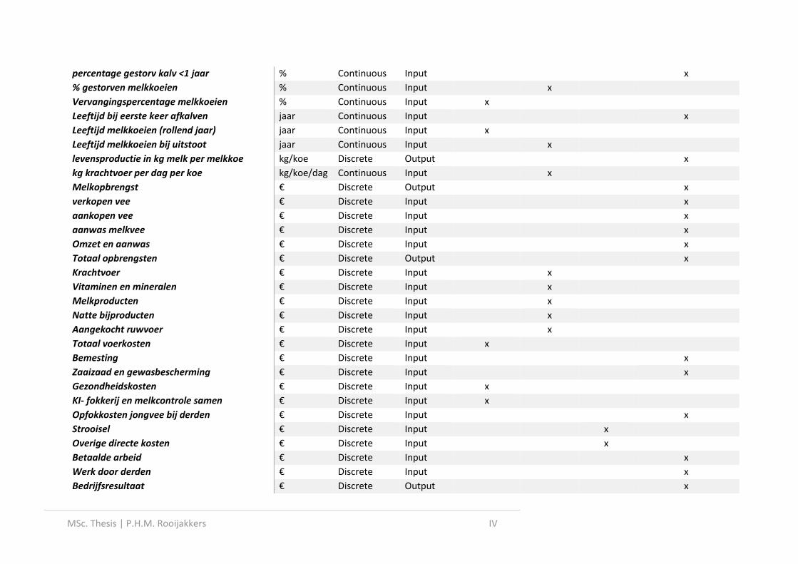
MSc. Thesis | P.H.M. Rooijakkers IV
percentage gestorv kalv <1 jaar % Continuous Input
x
% gestorven melkkoeien % Continuous Input
x
Vervangingspercentage melkkoeien % Continuous Input x
Leeftijd bij eerste keer afkalven jaar Continuous Input
x
Leeftijd melkkoeien (rollend jaar) jaar Continuous Input x
Leeftijd melkkoeien bij uitstoot jaar Continuous Input
x
levensproductie in kg melk per melkkoe kg/koe Discrete Output
x
kg krachtvoer per dag per koe kg/koe/dag Continuous Input
x
Melkopbrengst € Discrete Output
x
verkopen vee € Discrete Input
x
aankopen vee € Discrete Input
x
aanwas melkvee € Discrete Input
x
Omzet en aanwas € Discrete Input
x
Totaal opbrengsten € Discrete Output
x
Krachtvoer € Discrete Input
x
Vitaminen en mineralen € Discrete Input
x
Melkproducten € Discrete Input
x
Natte bijproducten € Discrete Input
x
Aangekocht ruwvoer € Discrete Input
x
Totaal voerkosten € Discrete Input x
Bemesting € Discrete Input
x
Zaaizaad en gewasbescherming € Discrete Input
x
Gezondheidskosten € Discrete Input x
KI- fokkerij en melkcontrole samen € Discrete Input x
Opfokkosten jongvee bij derden € Discrete Input
x
Strooisel € Discrete Input
x
Overige directe kosten € Discrete Input
x
Betaalde arbeid € Discrete Input
x
Werk door derden € Discrete Input
x
Bedrijfsresultaat € Discrete Output
x
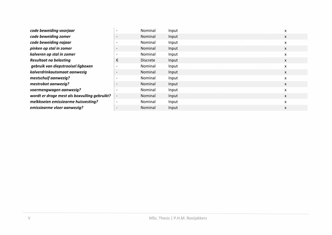
V MSc. Thesis | P.H.M. Rooijakkers
code beweiding voorjaar - Nominal Input
x
code beweiding zomer - Nominal Input
x
code beweiding najaar - Nominal Input
x
pinken op stal in zomer - Nominal Input
x
kalveren op stal in zomer - Nominal Input
x
Resultaat na belasting € Discrete Input
x
gebruik van diepstrooisel ligboxen - Nominal Input
x
kalverdrinkautomaat aanwezig - Nominal Input
x
mestschuif aanwezig? - Nominal Input
x
mestrobot aanwezig? - Nominal Input
x
voermengwagen aanwezig? - Nominal Input
x
wordt er droge mest als boxvulling gebruikt? - Nominal Input
x
melkkoeien emissiearme huisvesting? - Nominal Input
x
emissiearme vloer aanwezig? - Nominal Input
x

MSc. Thesis | P.H.M. Rooijakkers VI
Appendix III: Best subset selection
Table III: Variables included in the best subset selection. Variable Cows is forced in, which means that this variable will always be included
Forced in Forced out
Calving_int FALSE FALSE
Area_total FALSE FALSE
Cows TRUE FALSE
Cows_died FALSE FALSE
Repl_rate FALSE FALSE
Age FALSE FALSE
Total_concentrate FALSE FALSE
Roughage_costs FALSE FALSE
Health_costs FALSE FALSE Breeding_controlling_costs FALSE FALSE
Table IV: Best subset composition with set numbers indicating which variables will be included in the designated set
Set Cows Calv. int.
Conc. BC Health
Cows died
Roughage
Age Area total
Repl. rate
1 "*" "*" " " " " " " " " " " " " " " " "
2 "*" "*" "*" " " " " " " " " " " " " " "
3 "*" "*" "*" "*" " " " " " " " " " " " "
4 "*" "*" "*" "*" "*" " " " " " " " " " "
5 "*" "*" "*" "*" "*" "*" " " " " " " " "
6 "*" "*" "*" "*" "*" "*" "*" " " " " " "
7 "*" "*" "*" "*" "*" "*" "*" "*" " " " "