business statistics -mu

8/22/2019 Business Statistics -MU

http://slidepdf.com/reader/full/business-statistics-mu 1/59

Business Statistics

Sem I



IMPORTANCE OF STATISTICS

• Competition, Globalization and Liberalization has focused onQuantitative Techniques in Management

• Application of Q.T. involves fixation of basic parameters.

• Theses parameters are objectively based on Data collected innumerical terms

•

Hence Data Collection, Analysis and Inference is important.• So Statistics is the first step for Q.T. in management.

• Data also used for Decision-making

• All of us are either Data Producer or Data User.

• Extract relevant information and become effective Data user.

• Statistics --- Status --- State --- Political State and• So closely linked with Administrative affairs



Statistics

Descriptive

Statistics

Inferential

Statistics

Collecting

OrganizingSummarizing

Presenting Data

Making Inference

Hypothesis TestingDetermining relationships

Making predictions



BASIC CONCEPTS

-------------------



WHAT IS STATISTICS

• Statistics in plural form means

– Numerical Facts about Objects.

• Statistic in singular form means

–Science of Collection, Organization, Analysis and Interpretation

of Numerical Facts



Characteristics of Statistics

Characteristics of statistics

• Aggregate of facts – Collection of facts. Facts can be analyzedstatistically only when they are more than one.

•Affected to a marked extent by multiplicity of causes.

• Numerically expressed –only numerical facts can bestatistically analyzed.

• Enumerated / Estimated according to reasonable standard of accuracy.

• Collected in systematic manner.• Collected for pre-determined purpose.

• Statistics are placed in relation to each other.



Functions of Statistics

• Simplifies complexity of the Data

• Reduces bulk of the Data

• Adds precision to thinking

• Helps in comparing different sets of figures

• Guides formulation of policies & helps in planning

• Indicates trends & tendencies

• Helps in studying relationship between differentfactors



Branches and Scope

Branches of Statistics1. Statistical Methods

2. Applied Statistics – Biometry

Demography

EconometricsStatistical Quality Control

Psychometry

Scope and Application of Statistics

• Biology Agriculture• Medicine Business

• Economics Commerce



Limitations of Statistics

• Does not deal with qualitative data

• Does not deal with individual fact

•

Statistical inferences are not exact.These are probabilistic statements.

• Statistics can be misused

• Common people can not handle statisticsproperly.



Some Basic Definitions

• Units / Individuals / Elements – These are Objects whose

characteristics we study.• Population / Universe – Collection of all Units.

• Finite Population – contains finite number of Units.

• Infinite Population – contains infinite number of Units.

• Quantitative Characteristic – Numerically measurable

• Qualitative Characteristic – Numerically not measurable

• Variable - Quantitative Characteristics which varies from unitto unit.

• Attribute – Qualitative Characteristics which varies from unitto unit.

• Discrete Variable – Assumes some specified values in range.

• Continuous Variable – assumes all the values in the givenrange.



Classification and Tabulation

Units having common characteristics are grouped together.Functions of Classifications

• Reduces the bulk of data

• Simplifies the data

•

Facilitates comparison of characteristics• Renders data ready for statistical analysis

Types of classification –

• Quantitative (with regard to variable)

• Qualitative (with regard to attribute)

• Spatial (Geographical)• Temporal (Chronological)

• Classification of units on the basis of a characteristic into twoclasses is called Dichotomy (Men / Women)



Classification and TabulationTypes of classification –

• Quantitative (with regard to variable)

• Qualitative (with regard to attribute)

• Spatial (Geographical)

• Temporal (Chronological)

• Classification of units on the basis of a characteristic into twolasses is called Dichotomy (Men / Women)

• Classification on the basis of

– Single characteristic is called Simple or One-way

classification. – Two characteristic is called Two-way classification and

– More characteristics is called Manifold classification



Summarization of Data

Frequency Distribution

• Frequency is the number of units associated with each valueof variable

• Frequency Distribution is systematic presentation of values

taken by variable and the corresponding frequencies• Values may be discrete or continuous

• If the number of values is more,

range of variable is divided into

mutually exclusive sub-ranges called class intervals.

• Lower Class Limit Upper Class Limit

• Width of class – Difference between the class limits.



Frequency Distribution• Class mark or Class Mid-value – Central value of class interval.

•Continuous Frequency Distribution

• Discrete Frequency Distribution

• Inclusive Class Interval – Lower & Upper limits of class intervalare included in the same class interval.

•

Exclusive Class Interval – Lower class limit is included in thesame class interval & upper class limit is included insucceeding class interval.

• While analyzing Frequency Distribution Inclusive class intervalshould be converted into Exclusive class interval. (0—9, 10—

19, 20—29 will become -0.5—9.5, 9.5—19.5, 19.5—29.5 )• Values 0.5, 9.5, etc. are called Class Boundaries




• Open End Class – when class intervals at extremities

do not have one limit.

• Univariate Frequency Distribution – Single variable

• Bivariate Frequency Distribution – Two variables

• Multivariate Frequency Distribution – More than one

variables

• Frequency density of the class = Frequency of the

Class / Width of the Class



Graphical Presentation

Graphs -

• Bar GraphsSimple Sub-divided (Component) Multiple

• Dot Chart

•

Pictograph• Pie Chart

– Percentage share of each category is represented aspercentage of 360 degrees on a circle

–

Segments are drawn in order of their size from largest tosmallest in clockwise direction

• Line Graph



Graphic Representation of


Histogram

• On X-axis class limits / class marks are marked.

• On Y-axis class frequencies are marked.

• Rectangular bars are drawn for each class interval

and its frequency.

• For unequal class interval Y-axis measures Frequency

Density and not Class Frequency.• So if one class interval is three times the others, then

its height is reduced to 1/3.





Frequency Polygon

• Mark dots on the mid-point of top of each rectangle of histogram

• Join these points by straight lines.

•

Polygon thus formed, is closed by joining to the mid-point falling onthe X-axis of the next outlyinginterval with zero frequency.

• It can be drawn without drawingHistogram by only marking thepoints.

0

10

20

30

40

5060

70

80

90

100

1 s t Q

t r

2 n d Q t r

3 r d Q t r

4 t h

Q t r

No. of patients





Cumulative Frequency Curve or Ogive

• Less than Type or More than Type

• Y-axis represents total frequency

• X-axis is labeled with upper class limit in case of Less than

Ogive

and with lower class limit in case of More than Ogive

• Cumulative curve has quick adaptability for interpretation.

• Point of intersection of two curve is Median.

• Two sets of Ogives can be compared on percentage basis.



Graphic Representation of Frequency Distribution

f fc f fc

• Less than 59 6 6 50 or more 6 80

• Less than 69 9 15 60 or more 9 74

•Less than 79 15 30 70 or more 15 65

• Less than 89 25 55 80 or more 25 50

• Less than 99 13 68 90 or more 13 25

• Less than 109 7 75 100 or more 7 12

• Less than 119 5 80 110 or more 5 5



MEASURE OF CENTRAL TENDENCY• Generally in a Frequency Distribution values cluster around a

central value.• This is called as Central Tendency.

• The central value around which there is a concentration iscalled Measure of Central Tendency or average

•

Averaging is done to arrive at a single value representingentire data.

Objectives of Averaging –

• To find out one value that represents the whole data.

• To enable comparison

• To establish relationship

• To derive inferences about a universe from a sample



MEASURE OF CENTRAL TENDENCY

These Measures of central tendency are –

• Mathematical Averages – Arithmetic Mean

– Geometric Mean

–Harmonic Mean

• Positional Averages

– Median

–

Mode• Arithmetic Mean, Median & Mode are most

widely used.



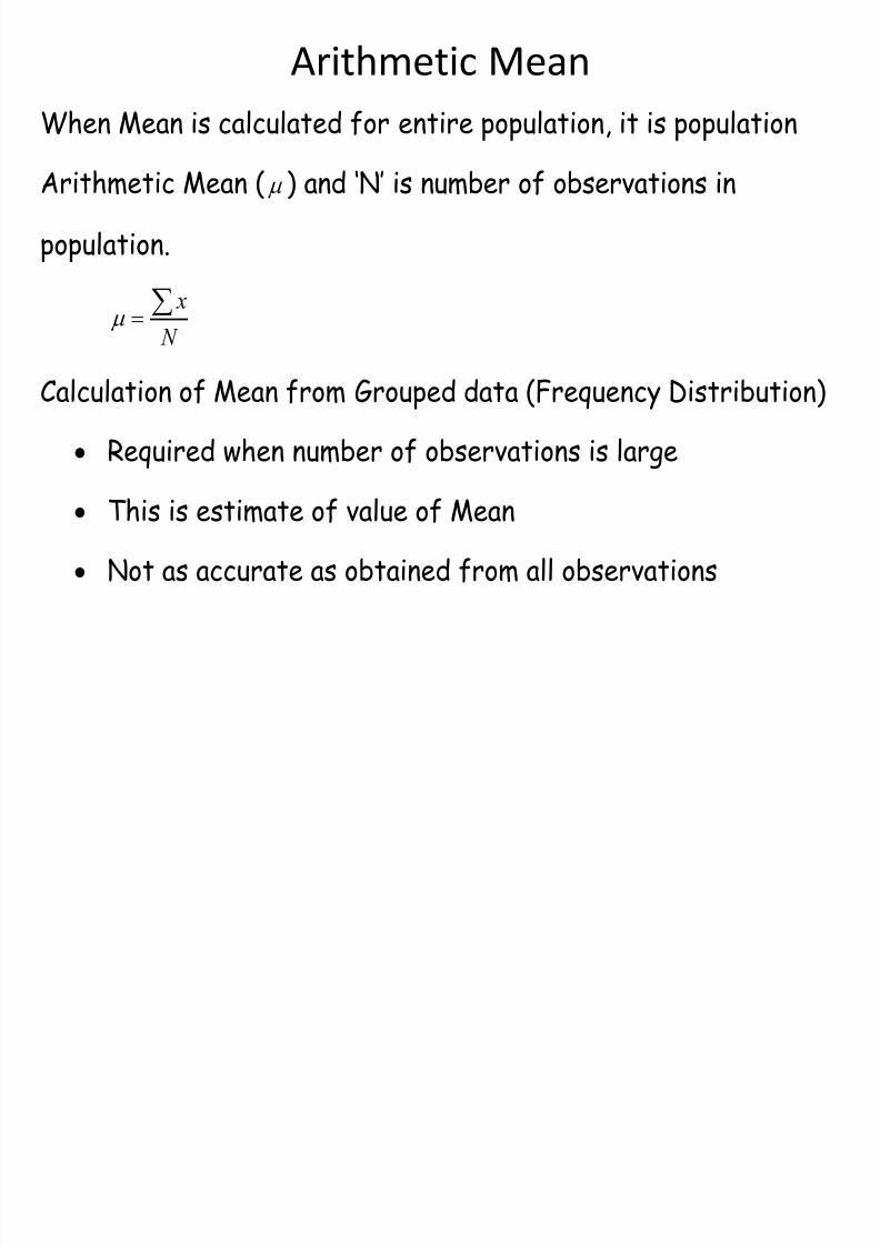
Arithmetic Mean

When Mean is calculated for entire population, it is population

Arithmetic Mean ( ) and ‘N’ is number of observations in

population.

N

x

Calculation of Mean from Grouped data (Frequency Distribution)

Required when number of observations is large This is estimate of value of Mean

Not as accurate as obtained from all observations



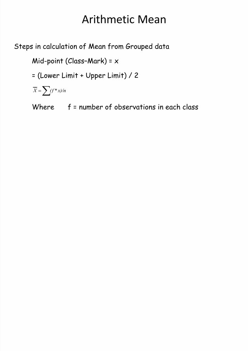
Arithmetic Mean

Steps in calculation of Mean from Grouped data

Mid-point (Class–Mark) = x

= (Lower Limit + Upper Limit) / 2

x)/n*(f X

Where f = number of observations in each class



Example

• Calculate the Mean

weight of the

population

=63.79

Wt inkg Frequency(f)

Class-mark (X)

f*X

60-61 10 60.5 605

61-62 20 61.5 1230

62-63 45 62.5 2812.5

63-64 50 63.5 3175

64-65 60 64.5 3870

65-66 40 65.5 2620

66-67 15 66.5 997.5

Total 240 15310

240

15310

f

Xf X



Arithmetic MeanChange of origin and scale

If origin is shifted to ‘A’ & scale changed by ‘c’, then

d = (x – A) / c or X = A + cu and uc A x

This formula is used for avoiding calculations with large figures.

Properties of Arithmetic Mean –

1. 0)( X X

2. Sum of squares of deviations of set of values is minimum

when deviations are taken around arithmetic mean.

3. Arithmetic Mean of two sets =Combined arithmetic Mean =

21

2211

nn

xn xn

X



Arithmetic MeanAdvantages of Mean• Familiarity

• Easy to understand• Easy to calculate• It is rigidly defined• Good basis for comparison• Adaptable for further statistical analysis

• Based on all values• More stable• Can be calculated even if some values are zero or negative.Disadvantages of Mean• Extreme isolated observation affects mean; hence sometimes

extreme values are omitted.• It may be a value not assumed by any variable• Can not be calculated even if one value is missing



Weighted Arithmetic Mean

Considers relative importance of each value

Ex. Labour rate for a product using three classes of labour

Weighted Arithmetic Mean wS X ww X /*

w = weight allocated

Sw = Sum of all weights



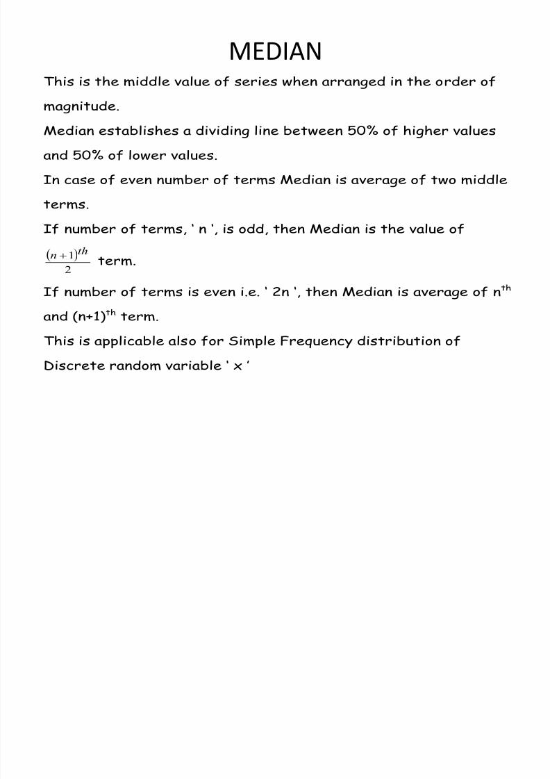
MEDIANThis is the middle value of series when arranged in the order of

magnitude.

Median establishes a dividing line between 50% of higher values

and 50% of lower values.

In case of even number of terms Median is average of two middle

terms.

If number of terms, ‘ n ‘, is odd, then Median is the value of

2

1thn term.

If number of terms is even i.e. ‘ 2n ‘, then Median is average of nth

and (n+1)th term.

This is applicable also for Simple Frequency distribution of

Discrete random variable ‘ x ’



Median for Grouped Data

Locate the class in which Median lies.

Median = L m + [(N/2) -F] * w/ F m

Where, L m = Lower limit of Median class

W = Width of class interval

F = Cumulative frequency up - to lower limit of Median

class

F m = Fr equency of the Median class

N = total Frequency



Median

• The sum of the deviations from Median, ignoring signs, is theleast.

• Advantages and Disadvantages of Median –

• Not strongly affected by extreme values

• Easy to understand

• Easy to calculate

• Can also be used for qualitative data

• But

• Time-consuming in arranging data in order

• Difficult to arrange data for large number of observations



MODE

Mode is the value of variable which occurs most frequently.

For ungrouped data, check value that occurs most frequently.

For Grouped data Mode is located in the class with maximum

frequency

Mode = Mo = LMo + wd d

d

*21

1

Where, LMo = Lower limit of the Modal class

d1 = Frequency of Modal class – frequency of the class

preceding modal class

d2 = Frequency of Modal class – frequency of the class

succeeding modal class

w = Width of Modal class



MODE

Advantages & Disadvantages of Mode –

• Can be used for qualitative data

• Not affected by extreme values

•

In case of symmetrical distribution, Mean, Median & Modecoincide.

• If the distribution is moderately asymmetrical, then

3 (Mean- Median) = Mean – Mode

Or 3 Median = 2 Mean + Mode



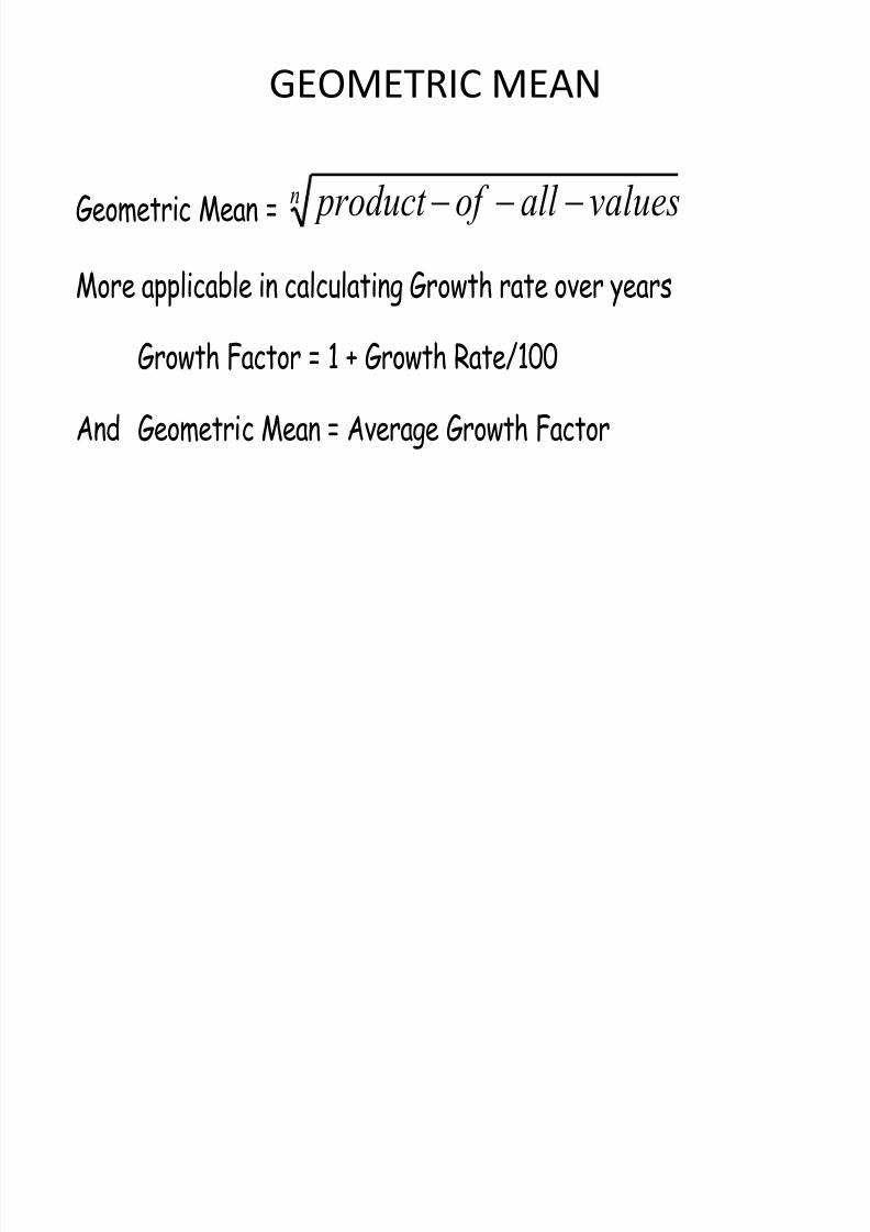
GEOMETRIC MEAN

Geometric Mean = n valuesall of product

More applicable in calculating Growth rate over years

Growth Factor = 1 + Growth Rate/100

And Geometric Mean = Average Growth Factor



HARMONIC MEAN

H. M. is the Reciprocal of Arithmetic Mean of a series formed byreciprocals of given values.

H.M. =

n x x x

N

1...

11

21

Ex.–

When equal distances are traveled at different speeds, the

average speed of total travel is given by harmonic Mean of all the

speeds.

Weighted Harmonic Mean WHM =

X W

W

/

Foe any set of positive values of variables

A. M. G. M. H. M.

A.M. x H.M. = (G.M.) 2



Appropriate Situations for

Use of various Averages

Arithmetic Mean• In depth study of the variable is needed

• The variable is continuous and additive in nature

• The data are in the interval or ratio scale

•The distribution is symmetrical

Geometric Mean

• The rate of growth, ratios and percentages are to be studied

• The variable is of multiplicative nature

Harmonic Mean

• The study is related to speed , time

• Average of rates which produces equal effects are to be found



Appropriate Situations for

Use of various Averages

Median• The variable is discrete

• There exists abnormal values

• The distribution is skewed

•The extreme values are missing

• The characteristics studied are qualitative

• The data are on the ordinal scale

Mode

• The variable is discrete

• There exists abnormal values



• The characteristics studied are qualitative



Positional Averages

• Lower Quartile Q 1 = th observation.

• Upper Quartile Q 3 = 3 th observation.

• For grouped Data

•Q 1 = L 1 + Q 3 = L 3 +

• L 1 = Lower boundary of first quartile class

• L 3 = Lower boundary of third quartile class

• N = Total cumulative frequency

• f = Frequency of quartile class

• h = Class interval (width)

• c = cumulative frequency of the class just above the quartileclass

4

1 N

4

1 N

h F

C N

4

1

h F

C N

4

3



Percentile

• They are values of the variables which divide

the total observations by an imaginary line

into two parts, expressed in percentage as 10

% and 90 %, etc.

• It can be used for comparing one percentile

value of two samples/ populations



Percentile

0

20

40

60

80

100

120

7 8 9 10 11

Indian

American



MEASURE OF DISPERSION

• One more Characteristic of Dataset is

How it is distributed?

How far each element is from Measure of Centraltendency

The Measures for this Dispersion are• RANGE

• INTER-QUARTILE RANGE

• QUARTILE DEVIATIONS

• MEAN DEVIATION• VARIANCE

• STANDARD DEVIATION



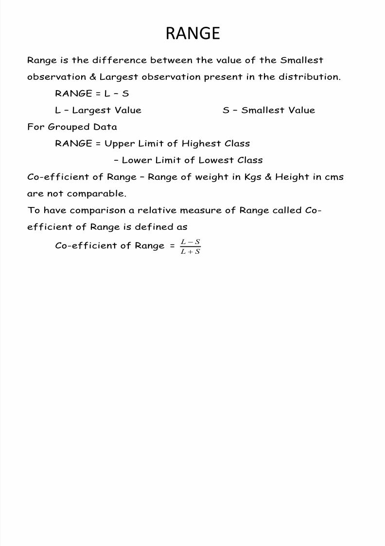
RANGE Range is the difference between the value of the Smallest

observation & Largest observation present in the distribution.

RANGE = L – S

L – Largest Value S – Smallest Value

For Grouped Data

RANGE = Upper Limit of Highest Class

– Lower Limit of Lowest Class

Co-efficient of Range – Range of weight in Kgs & Height in cms

are not comparable.

To have comparison a relative measure of Range called Co-

efficient of Range is defined as

Co-efficient of Range =S L

S L



Merits & Limitations of Range• Merits

– Simple to understand

– Easy to calculate

• Demerits – Not based on all the observations

– Influenced by extreme values

– Can not be computed for Frequency Distribution withOpen end class

– No indication about Characteristics of distribution

within L & S.• Use of Range

– For Quality Control



INTER-QUARTILE RANGE

• Inter-quartile Range is the Range calculatedbased on middle 50% of the observations.

• INTER-QUARTILE RANGE = Q 3 – Q 1• Q 1, Q 2, Q 3 are highest value in each of the

first three quartile.

• QUARTILE DEVIATION

= (Q 3 – Q 1)/2



QUARTILE DEVIATION

Co-efficient of Quartile Deviation =13

13

QQ

QQ

Lower Quartile Q 1 =4

1 N th observation.

Upper Quartile Q 3 = 34

1 N th observation.

For grouped Data

Q1= L

1+ h

F

C N

4

1

Q 3 = L 3 + h F

C N

4

3



QUARTILE DEVIATION

L1

= Lower boundary of first quartile class

L 3 = Lower boundary of third quartile class

N = Total cumulative frequency

f = Frequency of quartile classh = Class interval (width)

c = cumulative frequency of the class just

above the quartile class



Merits and Limitations of

Quartile Deviation

• Merits

– Can be used for Open-ended Class distribution

– Better measure for highly skewed distribution or

distribution with extreme values

• Limitations

– Since it uses only 50 % observations, it can not be

considered as good measure – Q.D. is only positional and not real measure.



MEAN DEVIATION

This is Absolute Mean Deviation of each observation from Mean.

Absolute Mean Deviation = N

x for population, and

Absolute Mean Deviation =n

x X for sample

Where, x = value of observation

= The Mean of population

N = number of observations in population

x = sample mean

N = number of observations in sample



Mean Deviation

M. D. (about the mean x ) = x x f N

1

= d f N

1

X = mid-value of the class interval

f = corresponding frequency

d = deviation

Merits and De-merits of absolute Mean Deviation–

Simple and Easy

More comprehensive as it depends on all observations

True measure as it averages all deviations

But

Less reliable as it ignores sign

Not conducive to algebraic operation

Not useful for open end class



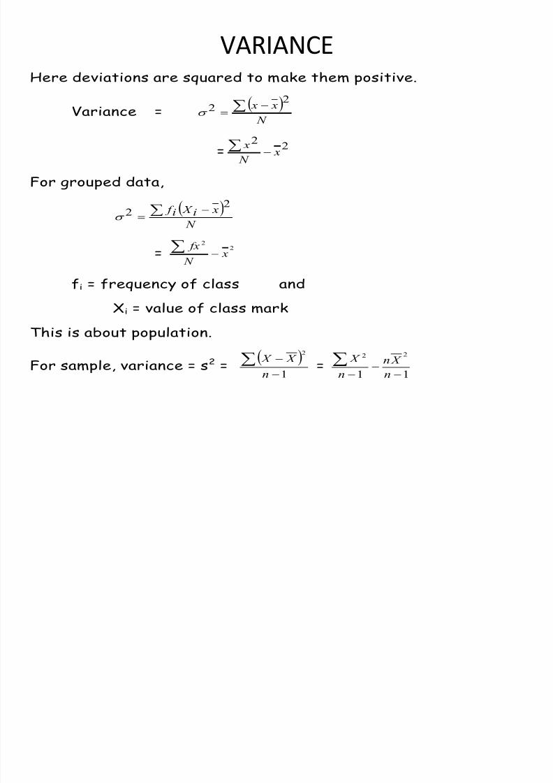
VARIANCE Here deviations are squared to make them positive.

Variance = N

x x

22

= 22

x N

x

For grouped data,

N

xi X i f

22

=2

2

x N

fx

fi = frequency of class and

Xi = value of class mark

This is about population.

For sample, variance = s2 =

1

2

n

X X =

11

22

n

X n

n

X



STANDARD DEVIATION

S.D.=

Variance

Properties of standard deviation –

S.D. is independent of change of origin i.e. if all the

observation values are increased / decreased by a constantquan tity, S.D. does not change.

S.D. is dependent on change of scale i. e. if each observation

value is multiplied / divided by a constant quantity, S.D. will

also be similarly affected.



STANDARD DEVIATION

Combined S.D. of two or more groups ( 12 )

21

2

22

2

11

2

22

2

11

12

nn

d nd nnn

d1 = x X 1

; d2 = x X 2 and

212211

/ nn xn xn x

Co-efficient of variation = S.D. / Mean

This is generally expressed in percentage.

E l



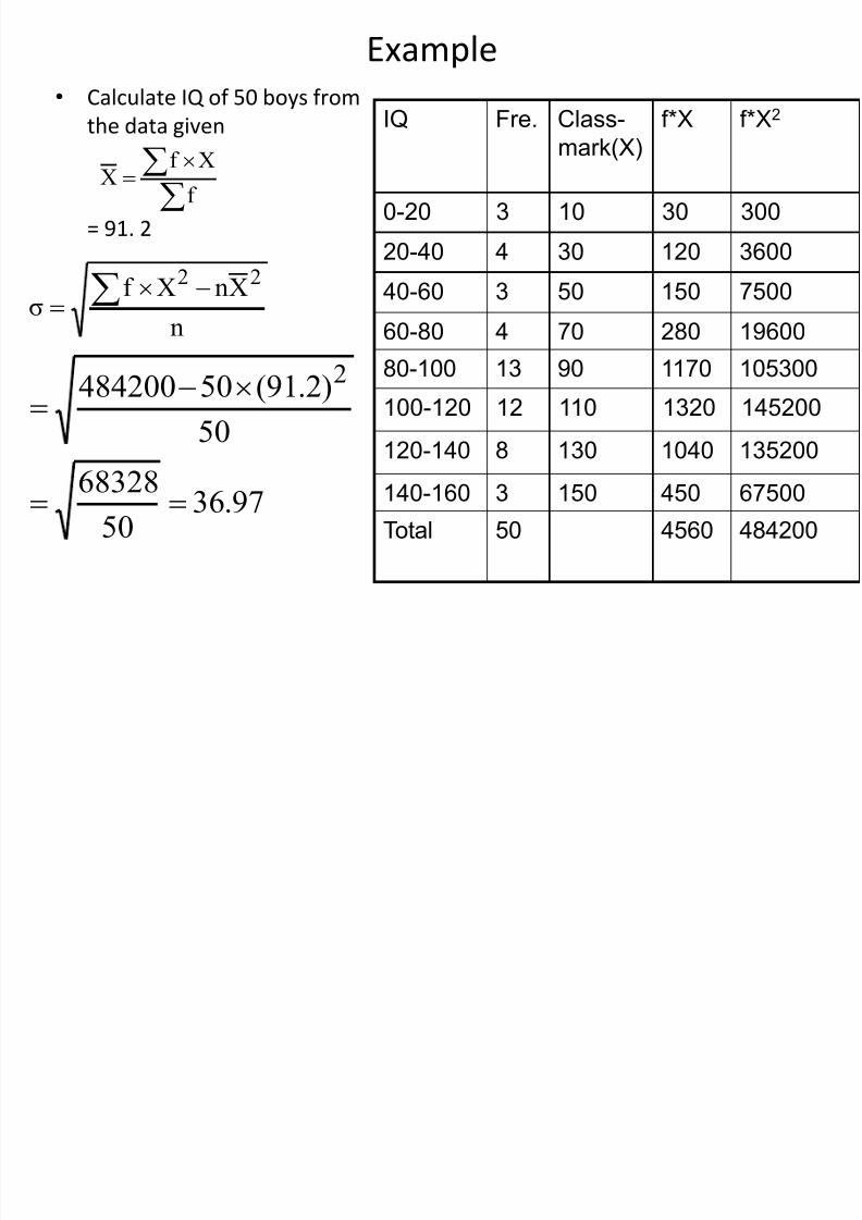
Example

• Calculate IQ of 50 boys from

the data given

= 91. 2

IQ Fre. Class-

mark(X)

f*X f*X2

0-20 3 10 30 300

20-40 4 30 120 3600

40-60 3 50 150 7500

60-80 4 70 280 19600

80-100 13 90 1170 105300

100-120 12 110 1320 145200

120-140 8 130 1040 135200140-160 3 150 450 67500

Total 50 4560 484200

f

Xf X

n

XnXf σ

22

97.3650

68328

50

)2.91(50484200 2



RELATIVE DISPERSION

• Absolute Measures are expressed in same

units as original data

• To compare dispersion of data in different

units, Relative Measures of dispersion are

used

• Relative Measures are Absolute measures

expressed as percentage of Measure of Central tendency



SKEWNESS

• The Measure of Central tendency and Measure of Dispersionare characteristics of Frequency Distribution

• Third important characteristic of Frequency Distribution is itsShape

•A Frequency Distribution is said to be Symmetrical when thevalues of the variable equidistant from mean have equalfrequencies

• When F.D. is not Symmetrical, it is said to be Asymmetrical orSkewed

• Amy deviation from symmetry is called Skewness

• Skewness may be Positive or Negative



SKEWNESS

• Positively skewed

– If the frequency curve has a longer tail towards

the higher values of X

– In positively Skewed distribution Mode is

minimum and Mean is maximum out of Mean,Median and Mode.

• Negatively skewed

– If the frequency curve has a longer tail towards

the lower values of X

– In Negatively skewed distribution, mean is

minimum and Mode is maximum



Positively Skewed Negatively skewed



Measures of Skewness

• Pearson’s first measure

Skewness = (Mean – Mode) / S.D.

• Pearson’s second measure

Skewness = 3(Mean – Median) / S.D.



Bienayme Chebyshev’s Rule

• It states that whatever may be the shape of distribution, at

least 75 % of the values in the population will fall within + 2standard deviation from the mean and at least 89 per cent willfall within + 3 standard deviation from the mean.

• The rule states that the percentage of the data observationlying within +/- ‘k’ standard deviation of the mean is at least(1 – 1 / k2)*100

In case of symmetrical bell-shaped distribution, we can say that

• Approximately 68 % of the observations in the population fallwithin +/- 1 s.d. from the mean

• Approximately 95 % of the observations in the population fall

within +/- 2 s.d. from the mean• Approximately 99 % of the observations in the population fall

within +/- 3 s.d. from the mean

business statistics -mu

Documents