bvri photometry of sn 2011fe in m101 - aavso.org · 872 richmond and smith, jaavso volume 40, 2012...

Richmond and Smith, JAAVSO Volume 40, 2012872

BVRI Photometry of SN 2011fe in M101

Michael W. RichmondPhysics Department, Rochester Institute of Technology, 84 Lomb Memorial Drive, Rochester, NY, 14623; [email protected]

Horace A. SmithDepartment of Physics and Astronomy, Michigan State University, East Lansing, MI 48824; [email protected]

Received March 19, 2012; revised April 4, 2012; accepted April 11, 2012

Abstract We present BVRI photometry of Supernova 2011fe in M101, starting 2.9 days after the explosion and ending 179 days later. The light curves and color evolution show that SN 2011fe belongs to the “normal’’ subset of type Ia supernovae, with a decline parameter Dm15(B) = 1.21 ± 0.03 mag. After correcting for the small amount of extinction in the line of sight, and adopting a distance modulus of (m – M ) = 29.10 mag to M101, we derive absolute magnitudes MB = –19.21, MV = –19.19, MR = –19.18, and MI = –18.94. We compare the voluminous record of visual measurements of this event to our CCD photometry and find evidence for a systematic difference which depends on color.

1. Introduction

Supernova (SN) 2011fe in the galaxy M101 (NGC 5457) was discovered by the Palomar Transient Factory (Law et al. 2009; Rau et al. 2009) in images taken on UT 2012 Aug 24 and announced later that day (Nugent et al. 2011a). As the closest and brightest type Ia SN since SN 1972E (Kirshner et al. 1973), and moreover as one which appears to suffer relatively little interstellar extinction, this event should provide a wealth of information on the nature of thermonuclear supernovae. We present here photometry of SN 2011fe in the BVRI passbands obtained at two sites, starting one day after the discovery and continuing for a span of 179 days. Section 2 describes our observational procedures, our reduction of the raw images, and the methods we used to extract instrumental magnitudes. In section 3, we explain how the instrumental quantities were transformed to the standard Johnson-Cousins magnitude scale. We illustrate the light curves and color curves of SN 2011fe in section 4, comment briefly on their properties, and discuss extinction along the line of sight. In section 5, we examine the rich history of distance measurements to M101 in order to choose a representative value with which we then compute absolute magnitudes. Using a very large set of visual measurements from the AAVSO, we compare the visual and CCD V-band observations in section 6. We present our conclusions in section 7.

Richmond and Smith, JAAVSO Volume 40, 2012 873

2. Observations

This paper contains measurements made at the RIT Observatory, near Rochester, New York, and the Michigan State University (MSU) Campus Observatory, near East Lansing, Michigan. We will describe below the acquisition and reduction of the images into instrumental magnitudes from each site in turn. The RIT Observatory is located on the campus of the Rochester Institute of Technology, at longitude 77:39:53 West, latitude +43:04:33 North, and an elevation of 168 meters above sea level. The city lights of Rochester make the northeastern sky especially bright, which at times affected our measurements of SN 2011fe. We used a Meade LX200 f /10 30-cm telescope and SBIG ST-8E camera, which features a Kodak KAF1600 CCD chip and astronomical filters made to the Bessell prescription; with 3 × 3 binning, the plate scale is 1.85 seconds per pixel. To measure SN 2011fe, we took a series of 60-second unguided exposures through each filter; the number of images per filter ranged from 10, at early times, to 15 or 20 at late times. We typically discarded a few images in each series due to trailing. We acquired dark and flatfield images each night, switching from twilight sky flats to dome flats in late October. The filter wheel often failed to return to its proper location in the R-band, so, when necessary, we shifted the R-band flats by a small amount in one dimension in order to match the R-band target images. We combined 10 dark images each night to create a master dark frame, and 10 flatfield images in each filter to create a master flatfield frame. After applying the master dark and flatfield images in the usual manner, we examined each cleaned target image by eye. We discarded trailed and blurry images and measured the FWHM of those remaining. The XVista (Treffers and Richmond 1989) routines stars and phot were used to find stars and to extract their instrumental magnitudes, respectively, using a synthetic aperture with radius slightly larger than the FWHM (which was typically 4" to 5"). As Figure 1 shows, SN 2011fe lies in a region relatively free of light from M101 (see also Supplementary Figure 1 of Li et al. 2011). As a check that simple aperture photometry would yield accurate results, we examined high-resolution HST images of the area, using ACS WFC data in the F814W filter originally taken as part of proposal GO-9490 (PI: Kuntz). The brightest two sources within a 5" radius of the position of the SN, R.A. = 14h 03m 05.733s, Dec, = +54˚ 16' 25.18" (J2000) (Li et al. 2011), have apparent magnitudes of mI ~_ 21.8 and mI ~_ 22.2. Thus, even when the SN is at its faintest, in our final I-band measurements, it is more than one hundred times brighter than nearby stars which might contaminate our measurements. Between August and November 2011, we measured instrumental magnitudes from each exposure and applied inhomogeneous ensemble photometry (Honeycutt 1992) to determine a mean value in each passband. Starting in December 2011, the SN grew so faint in the I-band that we combined


the good images for each passband using a pixel-by-pixel median procedure, yielding a single image with lower noise levels. We then extracted instrumental magnitudes from this image in the manner described above. In order to verify that this change in procedure did not cause any systematic shift in the results, we also measured magnitudes from the individual exposures, reduced them using ensemble photometry, and compared the results to those measured from the median-combined images. As Figure 2 shows, there were no significant systematic differences. The Michigan State University Campus Observatory lies on the MSU campus, at longitude 05:37:56 West, latitude +42:42:23 North, and an elevation of 273 meters above sea level. The f /8 60-cm Boller and Chivens reflector focuses light on an Apogee Alta U47 camera and its e2V CCD47-10 back-illuminated CCD, yielding a plate scale of 0.56 arcsecond per pixel. Filters closely approximate the Bessell prescription. Exposure times ranged between 30 and 180 seconds. We acquired dark, bias, and twilight sky flatfield frames on most nights. On a few nights, high clouds prevented the taking of twilight sky flatfield exposures, so we used flatfields from the preceding or following nights. The I-band images show considerable fringing which cannot always be removed perfectly. We extracted instrumental magnitudes for all stars using a synthetic aperture of radius 5.4 seconds.

3. Photometric calibration

In order to transform our instrumental measurements into magnitudes in the standard Johnson-Cousins BVRI system, we used a set of local comparison stars. The AAVSO kindly supplied measurements for stars in the field of M101 (Henden 2012) based on data from the K35 telescope at Sonoita Research Observatory (Simonsen 2011). We list these magnitudes in Table 1; note that they are slightly different from the values in the AAVSO’s on-line sequences which appeared in late 2011. Figure 1 shows the location of the three comparison stars. The AAVSO calibration data included many other stars in the region near M101. In order to check for systematic errors, we compared the AAVSO data to photoelectric BV measurements in Sandage and Tammann (1974). For the five stars listed as A, B, C, D, and G in Sandage and Tammann (1974), which range 12.01 < V < 16.22, we find mean differences of –0.013 ± 0.038 mag in B-band, and –0.009 ± 0.022 mag in V-band. We conclude that the AAVSO calibration set suffers from no systematic error in B or V at the level of two percent. Unfortunately, we could not find any independent measurements to check the R and I passbands in a similar manner. In order to convert the RIT measurements to the Johnson-Cousins system, we analyzed images of the standard field PG1633+009 (Landolt 1992) to determine the coefficients in the transformation equations


B = b + 0.238 (043) * (b – v) + ZB (1)

V = v – 0.077 (010) * (v – r) + ZV (2)

R = r – 0.082 (038) * (r – i) + ZR (3)

I = i + 0.014 (013) * (r – i) + ZI (4)

In the equations above, lower-case symbols represent instrumental magnitudes, upper-case symbols Johnson-Cousins magnitudes, terms in parentheses the uncertainties in each coefficient, and Z the zeropoint in each band. We used stars A, B, and G to determine the zeropoint for each image (except in a few cases for which G fell outside the image). Table 2 lists our calibrated measurements of SN 2011fe made at RIT. The first column shows the mean Julian Date of all the exposures taken during each night. In most cases, the span between the first and last exposures was less than 0.04 day, but on a few nights, clouds interrupted the sequence of observations. Contact the first author for a dataset providing the Julian Date of each measurement individually. The uncertainties listed in Table 2 incorporate the uncertainties in instrumental magnitudes and in the offset to shift the instrumental values to the standard scale, added in quadrature. As a check on their size, we chose a region of the light curve, 875 < JD – 2455000 < 930, in which the magnitude appeared to be a linear function of time. We fit a straight line to the measurements in each passband, weighting each point based on its uncertainty; the results are shown in Table 3. The reduced c2 values, between 0.9 and 1.6, indicate that our uncertainties accurately reflect the scatter from one night to the next. The decline rate is smallest in the blue, but it is still, at roughly 130 days after explosion, significantly faster than the 0.0098 mag/day produced by the decay of 56Co. The MSU data were transformed in a similar way, using only stars A and B. The transformation equations for MSU were

B = b + 0.25 (0.03) * (b – v) + ZB (5)

V = v – 0.08 (0.02) * (b – v) + ZV (6)

I = i + 0.03 (0.02) * (v – i) + ZI (7)

In the equations above, lower-case symbols represent instrumental magnitudes, upper-case symbols Johnson-Cousins magnitudes, terms in parentheses the uncertainties in each coefficient, and Z the zeropoint in each band. Table 4 lists our calibrated measurements of SN 2011fe made at MSU. Due to the larger aperture of the MSU telescope, exposure times were short enough


that the range between the first and last exposures on each night was less than 0.01 day.

4. Light curves

We adopt the explosion date of JD 2455796.687 ± 0.014 deduced by Nugent et al. (2011b) in the following discussion. Figure 3 shows our light curves of SN 2011fe, which start 2.9 days after the explosion and 1.1 days after Nugent et al. (2011a) announced their discovery. In order to determine the time and magnitude at peak brightness, we fit polynomials of order 2 and 3 to the light curves near maximum in each passband, weighting the fits by the uncertainties in each measurement. We list the results in Table 5, including the values for the secondary maximum in I-band. We again use low-order polynomial fits to measure the decline in the B-band 15 days after the peak, finding D15(B) = 1.21 ± 0.03. This value is similar to that of the “normal’’ SNe Ia 1980N (Hamuy et al. 1991), 1989B (Wells et al. 1994), 1994D (Richmond et al. (1995), and 2003du (Stanishev et al. 2007). The location of the secondary peak in I-band, 26.6 ± 0.5 days after and 0.45 ± 0.03 mag below the primary peak, also lies close to the values for those other SNe. Although there is as yet little published analysis of the spectra of SN 2011fe, (Nugent et al. 2011b) state that the optical spectrum on UT 2011 Aug 25 resembles that of the SN 1994D; on the other hand, (Marion 2011) reports that a near-infrared spectrum on UT 2011 Aug 26 resembles that of SNe Ia with fast decline rates and Dm15 (B) > 1.3. We must wait for detailed analysis of spectra of this event as it evolves to and past maximum light for a secure spectral classification, but this very preliminary information may support the photometric evidence that SN 2011fe falls into the normal subset of type Ia SNe. We turn now to the evolution of SN 2011fe in color. In order to compare its colors easily to those of other supernovae, we must remove the effects of extinction due to gas and dust within the Milky Way and within M101. Fortunately, there appears to be little intervening material. Schlegel et al. (1998) use infrared maps of dust in the Milky Way to estimate E(B–V) = 0.009 in the direction of M101. Patat et al. (2011) acquired high-resolution spectroscopy of SN 2011fe and identified a number of narrow Na I D2 absorption features; they use radial velocities to assign some to the Milky Way and some to M101. They convert the total equivalent width of all components, 85mÅ, to a reddening of E(B–V) = 0.025 ± 0.003 using the relationship given in Munari and Zwitter (1997). Note, however, that this total equivalent width is considerably smaller than that of all but a single star in the sample used by Munari and Zwitter (1997), so we have decided to double the quoted uncertainty. Adopting the conversions from reddening to extinction given in Schlegel et al. (1998), we compute the extinction toward SN 2011fe to be AB = 0.11 ± 0.03, AV = 0.08 ± 0.02, AR = 0.07 ± 0.02, and AI = 0.05 ± 0.01.


After removing this extinction from our measurements, we show the color evolution of SN 2011fe in Figures 4 through 6. The shape and extreme values of these colors are similar to those of the normal Type Ia SNe 1994D and 2003du. In Figure 4, we have drawn a line to represent the relationship (Lira (1995); Phillips et al. (1999)) for a set of four type Ia SNe which suffered little or no extinction. The (B−V) locus of SN 2011fe lies slightly (0.05 to 0.10 mag) to the red side of this line, especially near the time of maximum (B−V) color. Given our estimates of the extinction to SN 2011fe, this small difference is unlikely to be due to our underestimation of the reddening.

5. Absolute magnitudes

In order to compute the peak absolute magnitudes of SN 2011fe, we must remove the effects of extinction and apply the appropriate correction for its distance. The previous section discusses the extinction to this event, and we now examine the distance to M101. Since the first identification of Cepheids in this galaxy 26 years ago (Cook et al. 1986), astronomers have acquired ever deeper and larger collections of measurements. Shappee and Stanek (2011) provide a list of recent efforts, which suggests that Cepheid-based measurements are converging on a relative distance modulus (m – M) = 10.63 mag between the LMC and M101. If we adopt a distance modulus of (m – M)LMC = 18.50 mag to the LMC, this implies a distance modulus (m – M)M101 = 29.13 to M101. This is similar to one of the two results based on the luminosity of the tip of the red giant branch, (m – M)M101 = 29.05 ± 0.06 (rand) ± 0.12 (sys) mag (Shappee and Stanek 2011), though considerably less than the other, (m – M)M101 = 29.42 ± 0.11 mag (Sakai et al. 2004). We therefore adopt a value of (m – M)M101 = 29.10 ± 0.15 mag to convert our apparent to absolute magnitudes. Note that the uncertainty in this distance modulus is our rough average, based on a combination of the random and systematic errors quoted by other authors and the scatter between their values. This uncertainty in the distance to M101 will dominate the uncertainties in all absolute magnitudes computed below. Using this distance modulus, and the extinction derived earlier for each band, we can convert the apparent magnitudes at maximum light into absolute magnitudes. We list these values in Table 6. Phillips (1993) found a connection between the absolute magnitude of a type Ia SN and the rate at which it declines after maximum: quickly-declining events are intrinsically less luminous. Further investigation (Hamuy et al. 1996; Riess et al. 1996; Perlmutter et al. 1997) confirmed this relationship and spawned several different methods to quantify it. We adopt the Dm15(B) method, which characterizes an event by the change in its B-band luminosity in the 15 days after maximum light. The light curve of SN 2011fe yields Dm15(B) = 1.21 ± 0.03 mag, placing it in the middle of the range of values for SNe Ia. Prieto et al. (2006) compute linear relationships between the Dm15(B) and


peak absolute magnitudes for a large sample of SNe. If we insert our value of Dm15(B) into the equations from their Table 3 for host galaxies with small reddening, we derive the absolute magnitudes shown in the rightmost column of Table 6. The excellent agreement with the observed values suggests that our choice of distance modulus to M101 may be a good one.

6. Comparison with visual measurements

Perhaps because it was the brightest SN Ia to appear in the sky since 1972, SN 2011fe was observed intensively by many astronomers. The AAVSO received over 900 visual measurements of the event within six months of the explosion. Since it was observed so well with both human eyes and CCDs, this star provides an ideal opportunity to compare the two detectors quantitatively. We acquired visual measurements made by a large set of observers from the AAVSO; note that these have not yet been validated. We removed a small number of obvious outliers, leaving 880 measurements over the range 799 < JD – 2455000 < 984. For each of our CCD V-band measurements, we estimated a simultaneous visual magnitude by fitting an unweighted low-order polynomial to the visual measurements within N days; due to the decreasing frequency of visual measurements and the less sharply changing light curve at late times, we increased N from 5 days to 8 days at JD 2455840 and again to 30 days at JD 2455865. We then computed the difference between the polynomial and the V-band measurement. Figure 7 shows our results: there is a clear trend for the visual measurements to be relatively fainter when the object is red. If we make an unweighted linear fit to all the differences, we find

(visual – V)2011fe = – 0.09 + 0.19 (04) * (B – V) (8)

where the number in parentheses represents the uncertainty in the coefficient. We know of two other cases in which visual and other measurements of type Ia SNe are compared. Pierce and Jacoby (1995) retrieved photographic films of SN 1937C, which were originally described in Baade and Zwicky (1938), re-measured them with a photodensitometer, and calibrated the results to the Johnson V-band using a set of local standards. They compared their results to the visual measurements of SN 1937C made by Beyer (1939) and found

(visual – V)1937C = – 0.63 + 0.53 * (B – V) (9)

We plot this relationship in Figure 7 using a dotted line. Jacoby and Pierce (1996) discussed the differences between visual measurements of SN 1991T from the AAVSO to CCD V-band measurements made by Phillips et al. (1992). We have extracted the measurements of Phillips et al. (1992) from their Figure 2 and compared them to the visual measurements, using the median of all visual


measurements within a range of 0.5 day to define a value corresponding to each CCD measurement. We show these differences as circular symbols in Figure 7; an unweighted linear fit yields

(visual – V)1991T = – 0.28 + 0.68(10) * (B – V) (10)

We find the slope to be the more interesting quantity in these relationships, since the constant offset term may depend on the choice of comparison stars for visual observers. Although at first blush the slopes appear to be quite different, if one examines Figure 7 carefully, one will see that the trend is quite similar for all three SNe if one restricts the color range to (B – V) > 0.5. The main difference between these three events, then, lies in the measurements made when the SNe were relatively blue. Could that difference be real? We note that SNe 1991T (definitely) and 1937C (probably) were events with slowly declining light curves and higher than average luminosities, while SN 2011fe declined at an average rate and, for our assumed distance to M101, was of average luminosity. As Phillips et al. (1992) describes, the spectrum of SN 1991T was most different from that of ordinary SNe Ia at early times, before and during its maximum luminosity; it is also at these early times that SNe shine with blue light. Could the combination of photometry by the human eye and photometry by CCD really distinguish ordinary and superluminous SNe Ia at early times? The evidence is far too weak at this time to support such a conclusion, but we look forward to testing the idea with future events. Stanton (1999) undertook a more general study, comparing the measurements of a set of roughly twenty stars near SS Cyg made by many visual observers to the Johnson V as a function of (B – V). He found a relationship

(visual – V) = 0.21 * (B – V) (11)

which we plot with a dash-dotted line in Figure 7. The slope of this relationship is consistent with that derived from the entire SN 2011fe dataset.

7. Conclusion

Our multicolor photometry suggests that SN 2011fe was a “normal’’ type Ia SN, with a decline parameter Dm15(B) = 1.21 ± 0.03 mag. After correcting for extinction and adopting a distance modulus to M101 of (m – M) = 29.10 mag, we find absolute magnitudes of MB = –19.21, MV = –19.19, MR = –19.18, and MI = –18.94, which provide further evidence that this event was “normal’’ in its optical properties. As such, it should serve as an exemplar of the SNe which can act as standardizable candles for cosmological studies. A comparison of the visual and CCD V-band measurements of SN 2011fe reveals systematic differences as a function of color which are similar to those found for other type Ia SNe and for stars in general.


8. Acknowledgements

We acknowledge with thanks the variable star observations from the AAVSO International Database contributed by observers worldwide and used in this research. We thank Arne Henden and the staff at AAVSO for making special efforts to provide a sequence of comparison stars near M101, and for helping to coordinate efforts to study this particular variable star. MWR is grateful for the continued support of the RIT Observatory by RIT and its College of Science. Without the Palomar Transient Factory, the astronomical community would not have received such early notice of this explosion. We thank the anonymous referee for his comments.

References

Baade, W., and Zwicky, F. 1938, Astrophys. J., 88, 411.Beyer, M. 1939, Astron. Nachr., 268, 341.Cook, K. H., Aaronson, M., and Illingworth, G. 1986, Astrophys. J., Lett. Ed.,

301, L45.Hamuy, M., Phillips, M. M., Maza, J., Wischnjewsky, M., Uomoto, A., Landolt,

A. U., and Khatwani, R. 1991, Astron. J., 102, 208.Hamuy, M., Phillips, M. M., Suntzeff, N. B., Schommer, R. A., Maza, J., and

Aviles, R. 1996, Astron. J., 112, 2391.Henden, A. A. 2012, Observations from the AAVSO International Database,

private communication.Honeycutt, R. K. 1992, Publ. Astron. Soc. Pacific, 104, 435.Jacoby, G. H., and Pierce, M. J. 1996, Astron. J., 112, 723.Kirshner, R. P., Willner, S. P., Becklin, E. E., Neugebauer, G., and Oke, J. B.

1973, Astrophys. J., Lett. Ed., 180, L97.Landolt, A. U. 1992, Astron. J., 104, 340.Law, N. M., et al. 2009, Publ. Astron. Soc. Pacific, 121, 1395.Li, W., et al. 2011, Nature, 480, 348.Lira, P. 1995, Master’s thesis, Univ. Chile.Marion, H. 2011, Astron. Telegram, No. 3599, 1.Munari, U., and Zwitter, T. 1997, Astron. Astrophys., 318, 269.Nugent, P., Sullivan, M., Bersier, D., Howell, D. A., Thomas, R., and James, P.

2011a, Astron. Telegram, No. 3581, 1.Nugent, P. E., et al. 2011b, Nature, 480, 344.Patat, F., et al. 2011, arXiv, 1112.0247.Perlmutter, S., et al. 1997, Astrophys. J., 483, 565.Pierce, M. J., and Jacoby, G. H. 1995, Astron. J., 110, 2885.Phillips, M. M. 1993, Astrophys. J., Lett. Ed., 413, L105.Phillips, M. M., Wells, L. A., Suntzeff, N. B., Hamuy, M., Leibundgut, B.,

Kirshner, R. P., and Foltz, C. B. 1992, Astron. J., 103, 1632.


Phillips, M. M., et al. 1999, Astron. J., 118, 1776.Prieto, J. L., Rest, A., and Suntzeff, N. B. 2006, Astrophys. J., 647, 501.Rau, A., et al. 2009, Publ. Astron. Soc. Pacific, 121, 1334.Richmond, M. W., et al. 1995, Astron. J., 109, 2121.Riess, A. G., Press, W. H., and Kirshner, R. P. 1996, Astrophys. J., 473, 88.Sakai, S., Ferrarese, L., Kennicutt, R. C., Saha, A. 2004, Astrophys. J., 608, 42.Sandage, A., and Tammann, G. A. 1974, Astrophys. J., 194, 223.Schlegel, D. J., Finkbeiner, D. P., and Davis, M. 1998, Astrophys. J., Suppl Ser.,

500, 525.Shappee, B. J., and Stanek, K. Z. 2011, Astrophys. J., 733, 124.Simonsen, M. 2011, Bull. Amer. Astron. Soc., 43, 218.Stanishev, V., et al. 2007, Astron. Astrophys., 469, 645.Stanton, R. H. 1999, J. Amer. Assoc. Var. Star Obs., 27, 97.Treffers, R. R., and Richmond, M. W. 1989, Publ. Astron. Soc. Pacific, 101, 725.Wells, L. A., et al. 1994, Astron. J., 108, 2233.

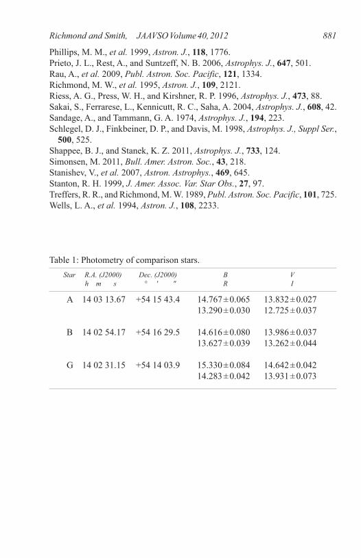
Table 1: Photometry of comparison stars. Star R.A. (J2000) Dec. (J2000) B V h m s ° ' " R I

A 14 03 13.67 +54 15 43.4 14.767 ± 0.065 13.832 ± 0.027 13.290 ± 0.030 12.725 ± 0.037

B 14 02 54.17 +54 16 29.5 14.616 ± 0.080 13.986 ± 0.037 13.627 ± 0.039 13.262 ± 0.044

G 14 02 31.15 +54 14 03.9 15.330 ± 0.084 14.642 ± 0.042 14.283 ± 0.042 13.931 ± 0.073


799.56 14.072 ± 0.038 13.776 ± 0.016 13.728 ± 0.011 13.696 ± 0.022 * 800.58 13.321 ± 0.046 13.025 ± 0.013 12.955 ± 0.024 12.942 ± 0.026 802.56 12.148 ± 0.028 12.049 ± 0.011 11.941 ± 0.020 11.882 ± 0.022 803.55 11.690 ± 0.023 11.643 ± 0.016 11.512 ± 0.015 11.471 ± 0.024 804.56 11.310 ± 0.025 11.300 ± 0.009 11.170 ± 0.012 11.147 ± 0.017 806.54 — 10.659 ± 0.020 10.572 ± 0.028 10.569 ± 0.052 * 808.54 10.346 ± 0.045 10.466 ± 0.029 10.336 ± 0.011 10.402 ± 0.025 814.53 10.034 ± 0.039 10.014 ± 0.003 10.042 ± 0.084 10.260 ± 0.030 * 815.53 9.981 ± 0.015 10.012 ± 0.012 10.011 ± 0.025 10.320 ± 0.027 816.53 10.072 ± 0.052 9.998 ± 0.008 10.006 ± 0.035 10.362 ± 0.036 817.58 10.060 ± 0.072 9.903 ± 0.059 10.031 ± 0.031 10.307 ± 0.019 * 820.53 10.171 ± 0.010 10.082 ± 0.013 10.080 ± 0.014 10.505 ± 0.018 * 822.52 10.326 ± 0.017 10.134 ± 0.006 10.181 ± 0.002 10.630 ± 0.026 823.53 10.405 ± 0.015 10.185 ± 0.014 10.283 ± 0.015 10.691 ± 0.013 825.52 10.623 ± 0.030 10.311 ± 0.009 10.428 ± 0.027 10.840 ± 0.018 827.51 10.829 ± 0.028 10.459 ± 0.016 10.580 ± 0.024 10.918 ± 0.025 829.51 11.043 ± 0.057 10.574 ± 0.019 10.655 ± 0.017 10.898 ± 0.020 830.52 11.167 ± 0.014 10.629 ± 0.011 10.672 ± 0.021 10.894 ± 0.015 832.51 11.423 ± 0.058 10.739 ± 0.011 10.731 ± 0.012 10.855 ± 0.018 * 839.53 12.228 ± 0.016 11.116 ± 0.016 10.850 ± 0.008 10.699 ± 0.033 * 840.50 12.312 ± 0.039 11.180 ± 0.013 10.865 ± 0.024 10.661 ± 0.026 841.50 12.407 ± 0.049 11.237 ± 0.011 10.925 ± 0.016 10.672 ± 0.031 842.50 12.503 ± 0.038 11.294 ± 0.006 10.958 ± 0.015 10.680 ± 0.026 844.50 12.688 ± 0.035 11.430 ± 0.016 11.054 ± 0.016 10.738 ± 0.045 * 852.90 13.098 ± 0.021 11.921 ± 0.014 11.615 ± 0.033 11.255 ± 0.022 858.48 13.314 ± 0.034 12.144 ± 0.020 11.862 ± 0.013 11.564 ± 0.024 * 859.49 13.290 ± 0.016 12.157 ± 0.010 11.879 ± 0.012 11.634 ± 0.047 * 864.90 13.340 ± 0.037 12.332 ± 0.012 12.085 ± 0.013 11.884 ± 0.010 868.49 13.364 ± 0.017 12.441 ± 0.014 12.190 ± 0.016 12.038 ± 0.040 870.90 13.375 ± 0.011 12.478 ± 0.016 12.256 ± 0.008 12.141 ± 0.005 872.88 13.371 ± 0.041 12.509 ± 0.016 12.343 ± 0.021 12.179 ± 0.008 * 883.92 13.584 ± 0.006 12.826 ± 0.010 12.688 ± 0.011 12.676 ± 0.014 887.92 13.598 ± 0.012 12.927 ± 0.006 12.796 ± 0.005 12.832 ± 0.013 889.92 13.699 ± 0.037 12.968 ± 0.019 12.904 ± 0.026 12.909 ± 0.012 890.93 13.658 ± 0.021 12.988 ± 0.019 12.902 ± 0.011 12.957 ± 0.018 898.91 13.761 ± 0.037 13.217 ± 0.014 13.155 ± 0.019 13.245 ± 0.027 905.94 13.831 ± 0.033 13.398 ± 0.013 13.353 ± 0.017 13.470 ± 0.036 907.92 13.877 ± 0.026 13.442 ± 0.018 13.445 ± 0.027 13.580 ± 0.039 913.89 13.919 ± 0.035 13.559 ± 0.019 13.624 ± 0.027 13.732 ± 0.025 * 924.92 14.078 ± 0.036 13.811 ± 0.016 13.945 ± 0.025 14.066 ± 0.032 *

Table 2. RIT photometry of SN 2011fe. JD–2455000 B V R I note

table continued on next page


932.94 14.191 ± 0.032 14.006 ± 0.022 14.145 ± 0.020 14.256 ± 0.045 * 935.98 14.219 ± 0.041 14.054 ± 0.017 14.280 ± 0.027 14.384 ± 0.039 * 937.92 14.253 ± 0.026 14.124 ± 0.015 14.325 ± 0.026 14.423 ± 0.036 942.72 14.298 ± 0.038 14.204 ± 0.025 14.402 ± 0.058 14.506 ± 0.043 * 945.89 14.377 ± 0.033 14.272 ± 0.033 14.523 ± 0.036 14.627 ± 0.045 * 948.86 14.420 ± 0.036 14.336 ± 0.023 14.639 ± 0.031 14.702 ± 0.050 954.82 14.524 ± 0.044 14.465 ± 0.021 14.757 ± 0.028 14.803 ± 0.040 966.90 14.716 ± 0.033 14.623 ± 0.024 14.951 ± 0.032 15.034 ± 0.053 973.67 14.792 ± 0.044 14.754 ± 0.039 15.165 ± 0.060 15.174 ± 0.056 978.67 14.884 ± 0.046 14.894 ± 0.026 15.340 ± 0.048 15.242 ± 0.054

Table 2. RIT photometry of SN 2011fe, cont. JD–2455000 B V R I note

* clouds

Table 3. Linear fit to light curves 2455875 < JD < 2455930. Passband Slope (mag/day) reduced c2

B 0.0117 ± 0.0006 1.2 V 0.0247 ± 0.0004 1.6 R 0.0312 ± 0.0004 0.9 I 0.0346 ± 0.0006 1.0

801.58 12.66 ± 0.02 12.42 ± 0.02 12.36 ± 0.03 803.56 11.69 ± 0.01 11.60 ± 0.01 11.48 ± 0.02 806.58 10.80 ± 0.01 10.74 ± 0.01 10.66 ± 0.02 809.56 10.36 ± 0.02 10.30 ± 0.01 10.28 ± 0.02 811.56 10.17 ± 0.03 10.08 ± 0.03 10.22 ± 0.02 * 820.54 10.13 ± 0.02 10.06 ± 0.01 10.44 ± 0.02 822.53 10.27 ± 0.02 10.10 ± 0.01 10.55 ± 0.01 825.54 10.55 ± 0.03 10.27 ± 0.02 10.87 ± 0.02 * 837.52 11.93 ± 0.02 10.97 ± 0.02 10.66 ± 0.03 851.50 13.04 ± 0.03 11.83 ± 0.02 11.16 ± 0.03 857.90 13.18 ± 0.05 12.09 ± 0.04 11.42 ± 0.04 * 867.48 13.27 ± 0.04 12.37 ± 0.03 11.96 ± 0.03 889.46 13.61 ± 0.03 12.92 ± 0.03 12.89 ± 0.03 898.47 13.67 ± 0.10 13.14 ± 0.06 13.22 ± 0.08

Table 4. MSU photometry of SN 2011fe. JD–2455000 B V I note

* clouds


B 816.0 ± 0.3 10.00 ± 0.02 V 817.0 ± 0.3 9.99 ± 0.01 R 816.6 ± 0.4 9.99 ± 0.02 I 813.1 ± 0.4 10.21 ± 0.03 I (sec) 839.7 ± 0.5 10.66 ± 0.01

Table 5. Apparent magnitudes at maximum light. Passband JD–2455000 Magnitude

B –19.21 ± 0.15 –19.25 ± 0.03 V –19.19 ± 0.15 –19.18 ± 0.03 R –19.18 ± 0.15 –19.19 ± 0.04 I –18.94 ± 0.15 –18.92 ± 0.03 I (sec) –18.49 ± 0.15 —

Table 6. Absolute magnitudes at maximum light, corrected for extinction. Passband Observed Based on Dm15

b magnitude a

a Based on (m – M)M101 = 29.10 ± 0.15 mag.b Using the relationship from Prieto et al. (2006).

Figure 1. A V-band image of M101 from RIT, showing stars used to calibrate measurements of SN 2011fe. North is up, East to the left. The field of view is roughly 13 by 9 arcminutes.


Figure 2. Difference between instrumental magnitudes extracted from median-combined images and from individual images at RIT. The values have been shifted for clarity by 0.4, 0.0, –0.4, –0.8 magnitude in B, V, R, I, respectively.

Figure 3. Light curves of SN 2011fe in BVRI. The data for each passband have been offset vertically for clarity.

Figure 4. (B–V) color evolution of SN 2011fe, after correcting for extinction.


Figure 5. (V–R) color evolution of SN 2011fe, after correcting for extinction.

Figure 6. (R–I) color evolution of SN 2011fe, after correcting for extinction.

Figure 7. The difference between visual and CCD or photographic measurements, as a function of (B–V) color, for SNe Ia and for variable stars in general.

bvri photometry of sn 2011fe in m101 - aavso.org · 872 richmond and smith, jaavso volume 40, 2012...

Documents