by brandon hanson - university of toronto
TRANSCRIPT

Character Sum Estimates in Finite Fields and Applications
by
Brandon Hanson
A thesis submitted in conformity with the requirementsfor the degree of Doctor of PhilosophyGraduate Department of Mathematics
University of Toronto
c© Copyright 2015 by Brandon Hanson
Abstract
Character Sum Estimates in Finite Fields and Applications
Brandon Hanson
Doctor of Philosophy
Graduate Department of Mathematics
University of Toronto
2015
In this thesis we present a number of character sum estimates for sums of various types occurring in finite
fields. The sums in question generally have an arithmetic combinatorial flavour and we give applications
of such estimates to problems in arithmetic combinatorics and analytic number theory. Conversely,
we demonstrate ways in which the theory of arithmetic combinatorics can be used to obtain certain
character sum estimates.
ii

Dedication
To my friends, for all the laughs. To my family, for their support. To my teachers, for inspiring me. To
John, for his patience and commitment. To Michelle, for everything.
iii

Acknowledgements
First and foremost I must thank John Friedlander, my thesis advisor, for giving me so much of his
time and patience. This thesis would not have been possible without all of the helpful discussions
we had. I also want to thank Leo Goldmakher for getting me interested in the field and providing
much encouragement along the way. Thanks to Kumar Murty and Antal Balog for being a part of my
thesis committee and providing fruitful discussion. Finally, like every graduate student in math at the
University of Toronto, I am indebted to Ida Bulat and Jemima Merisca. They made my life in the
graduate program so much easier. I want to thank them for ensuring that my headaches were purely
mathematical ones.
iv

Contents
1 Introduction and Motivation 1
1.1 Primes in arithmetic progressions: A fundamental example of equidistribution in number
theory . . . . . . . . . . . . . . . . . . . . . . . . . . . . . . . . . . . . . . . . . . . . . . . 1
1.2 Random oscillatory sums and the square-root law: The nature of random sequences . . . . 2
1.3 Weyl’s Equidistribution Criterion: Fourier analysis enters the scene . . . . . . . . . . . . 3
1.4 The Sum-Product Phenomenon: A source of equidistribution . . . . . . . . . . . . . . . . 5
1.5 Character sums: The star of the show . . . . . . . . . . . . . . . . . . . . . . . . . . . . . 6
1.6 An outline of this thesis . . . . . . . . . . . . . . . . . . . . . . . . . . . . . . . . . . . . . 8
2 Notation and relevant background 10
2.1 Asymptotic Notation . . . . . . . . . . . . . . . . . . . . . . . . . . . . . . . . . . . . . . . 10
2.2 Fourier analysis on finite abelian groups . . . . . . . . . . . . . . . . . . . . . . . . . . . . 10
2.3 Finite fields . . . . . . . . . . . . . . . . . . . . . . . . . . . . . . . . . . . . . . . . . . . . 13
2.4 Additive combinatorics and the Sum-Product Phenomenon . . . . . . . . . . . . . . . . . 14
2.5 Bohr sets and their structure . . . . . . . . . . . . . . . . . . . . . . . . . . . . . . . . . . 18
2.6 Character sums . . . . . . . . . . . . . . . . . . . . . . . . . . . . . . . . . . . . . . . . . . 21
3 Capturing forms in dense subsets of finite fields 25
3.1 Introduction . . . . . . . . . . . . . . . . . . . . . . . . . . . . . . . . . . . . . . . . . . . . 25
3.2 Statement of results . . . . . . . . . . . . . . . . . . . . . . . . . . . . . . . . . . . . . . . 26
3.3 Upper Bound . . . . . . . . . . . . . . . . . . . . . . . . . . . . . . . . . . . . . . . . . . . 27
3.4 Lower Bound . . . . . . . . . . . . . . . . . . . . . . . . . . . . . . . . . . . . . . . . . . . 29
3.5 Remarks for Composite Modulus . . . . . . . . . . . . . . . . . . . . . . . . . . . . . . . . 31
4 Character sum estimates for Bohr sets and applications 33
4.1 Introduction . . . . . . . . . . . . . . . . . . . . . . . . . . . . . . . . . . . . . . . . . . . . 33
4.2 Statement of Results and Applications . . . . . . . . . . . . . . . . . . . . . . . . . . . . . 33
4.2.1 Main Results . . . . . . . . . . . . . . . . . . . . . . . . . . . . . . . . . . . . . . . 33
4.2.2 Applications . . . . . . . . . . . . . . . . . . . . . . . . . . . . . . . . . . . . . . . 34
4.3 The Polya-Vinogradov Argument . . . . . . . . . . . . . . . . . . . . . . . . . . . . . . . . 35
4.4 The Burgess Argument . . . . . . . . . . . . . . . . . . . . . . . . . . . . . . . . . . . . . . 36
4.5 Application to Polynomial Recurrence . . . . . . . . . . . . . . . . . . . . . . . . . . . . . 38
v

5 Character sum estimates for various convolutions 41
5.1 Introduction . . . . . . . . . . . . . . . . . . . . . . . . . . . . . . . . . . . . . . . . . . . . 41
5.2 Statement of Results . . . . . . . . . . . . . . . . . . . . . . . . . . . . . . . . . . . . . . . 43
5.3 Trivariate sums . . . . . . . . . . . . . . . . . . . . . . . . . . . . . . . . . . . . . . . . . . 44
5.4 Mixed multivariate sums . . . . . . . . . . . . . . . . . . . . . . . . . . . . . . . . . . . . . 47
Bibliography 49
vi

Chapter 1
Introduction and Motivation
Much of this thesis is concerned with equidistribution as it pertains to arithmetic. This notion is a
fundamental one in number theory which measures the extent to which an object behaves randomly.
In the next five sections we illustrate some results in number theory, old and new, which will motivate
the thesis. The hope is that through this exposition, our train of thought will be made clear, so
that the reader has context for the results of the following chapters. In the first section we present
the quintessential example of equidistribution in analytic number theory - the distribution of primes
in arithmetic progressions. Though not explicitly related to the results of this thesis, the problem of
understanding the distribution of primes seems like the most natural starting point for any discussion
about equidistribution in number theory. In the second section we digress a bit in order to recall some
of the properties of uniform random sequences. We hope this diversion will suggest which qualities a
deterministic object should have in order to deem it random-like. The third section of this introduction
is devoted to Weyl’s Equidistribution Criterion. This is a basic result which relates the problem of
measuring the uniformity of a sequence with its Fourier analytic behaviour. As the criterion suggests,
Fourier analysis plays a large role, in analytic number theory and it will be used at length in this
book. In the fourth section of the introduction we discuss the Sum-Product Problem of combinatorial
number theory. This problem seeks to quantify the extent to which additive structure and multiplicative
structure are uncorrelated. The spirit of the Sum-Product Problem was the motivation for work on
the character sum estimates proved in Chapters 4 and 5. In the fifth section, we hope to capture the
reader’s interest in the question of character sum estimates. Such questions began with Dirichlet’s work
on the distribution of primes in arithmetic progressions, but we hope that throughout this chapter we
can convince the reader that these estimates are interesting in their own right. In the final section of
this introduction we give an outline for the rest of this thesis and a statement of the results to come.
1.1 Primes in arithmetic progressions: A fundamental example
of equidistribution in number theory
The first, and perhaps most famous instance of equidistribution of arithmetic objects is the equidistri-
bution of the primes into arithmetic progressions. While we do not investigate the distribution of primes
in this thesis, the question provides a good starting point for our exposition. The primes are mysterious
numbers, mostly because they are defined by what they are not rather than by what they are. As such,
1
Chapter 1. Introduction and Motivation 2
stating facts about primes is rarely easy.
We begin by examining some basic properties. Certainly, each prime other than 2 is odd. And no
primes other than 3 and 5 should have a common factor with 15. In general, when we divide p by
q, which is to say we write p = nq + a with 0 ≤ a ≤ q − 1, the remainder a is necessarily relatively
prime with q. Indeed, if q and a had a factor in common, that factor would also divide p. In short,
if p = a mod q then (a, q) = 1. Beyond this obvious pattern, it is hard to deduce anything structural
about the number a. Arguments going back to Euclid tell us that if we divide the odd primes by 4 then
the remainders 1 and 3 occur infinitely often (0 and 2 are forbidden). This fact was famously generalized
by Dirichlet, who proved that each of the eligible remainders that come from dividing a prime p by a
number q also occur infinitely often as we run over the primes. His work and subsequent work in analytic
number theory lead to the Prime Number Theorem in Arithmetic Progressions, which says that each
eligible remainder occurs with roughly the same frequency. In other words, primes fall uniformly into
the φ(q) eligible residue classes modulo q.
Theorem (Prime Number Theorem in Arithmetic Progressions). Let π(x, q, a) denote the number of
primes up to x which have remainder a when divided by q, and let π(x) denote to total number of primes
up to x. Then as x→∞ we haveπ(x, q, a)
π(x)→ 1
φ(q).
Suppose we were given a large prime and asked which residue class p lies in modulo q. Without any
further information this task seems hopeless - the prime is really, really big. We should not be to hard
on ourselves however, because the above theorem is telling us we might do just as well to choose one
class at random. So, it is not the case that we do not understand patterns in the distribution of primes
beyond the obvious ones, but rather that (at least at this scope) there aren’t any.
The main tool for the study of primes in arithmetic progressions is the Dirichlet character. These
characters will be of central interest in Chapter 4 and Chapter 5. We will give further exposition to
Dirichlet characters in Section 1.5.
1.2 Random oscillatory sums and the square-root law: The na-
ture of random sequences
Most of the equidistribution problems investigated in this thesis are concerned with points on the unit
circle in the complex plane,
S1 = {z ∈ C : |z| = 1}.
We identify the circle S1 with the group R/Z = [0, 1], the group operation being addition modulo 1.
This identification is via the map e : R/Z → S1 defined by e(θ) = e2πiθ. Given a real number α, the
expression α mod 1 means the fractional part {α} of α up to translation by integers. We now divert
briefly from the topic of equidistribution to discuss what we might expect on random grounds when
summing complex unit vectors.
Suppose we choose N numbers θ1, . . . , θN uniformly at random from [0, 1] and send them to the circle
by the map e defined above. These new points have uniformly distributed angles and so are likely to
point in all sorts of directions. In particular, given an arc C of length l(C) on the circle, we would expect
that a proportion l(C)/2π - the proportion of the circle occupied by C - of the points lie in the arc C.

Chapter 1. Introduction and Motivation 3
The (probabilistic) expectation of e(θn) is E(e(θn)) = 0. The numbers e(θn) are all unit vectors and
pointing in various directions and so when adding them, we expect to see a lot of cancellation - their
total expectation is ∑n≤N
E(e(θn)) = 0.
How close to this expectation is the sum typically? Well, while the sum
SN =
N∑n=1
e(θn)
could be as large as N , being a sum of N complex numbers of unit modulus, by Chebychev’s inequality
we have
P(|SN | > k√N) ≤ 1
k2NE(|SN |2) =
1
k2N
∑1≤m,n≤N
E(e(θm)e(θn)).
Since θm is independent of θn when m 6= n we have
E(e(θm)e(θn)) = E(e(θm))E(e(θn)) = 0.
Thus
P(|SN | > k√N) ≤ 1
k2
and so we typically have SN �√N . In fact, the Central Limit Theorem tells us that
P(a <
SN√N
< b
)→ 1√
2π
∫ b
a
e−t2/2dt.
When considering the distribution of complex unit vectors, a quantitative way to measure their random-
ness is to see cancellation in their sum. The “Holy Grail” of this business is to prove that these sums
exhibit the same square-root cancellation as random sums do. We call this the square-root law. With
all of this in mind, let us continue with our discussion of equidistribution.
1.3 Weyl’s Equidistribution Criterion: Fourier analysis enters
the scene
Suppose we are given a sequence of numbers (αn) in R/Z, which appear to have no obvious patterns.
The sequence is a deterministic one, and in our case, will usually have a number theoretic origin. We
would like to quantify how close to a uniform random sequence these numbers are and we will do this
by comparing their distributions. The basic tool for doing this sort of thing is Fourier analysis, which is
illustrated by the Weyl Criterion. Recall that e was the function from the reals modulo 1 (R/Z) to the
circle (S1), defined by e(θ) = e2πiθ. How often do the points e(αn) lie in the right side of the circle and
how often do they lie in the left side? If the sequence were unbiased, then we would expect the answer
two be half and half. In general and as was discussed in Section 1.2, given an arc C of length l(C) on
the circle, we expect that the proportion of elements of the sequence which lie in C is about l(C)/2π, the

Chapter 1. Introduction and Motivation 4
proportion of the circle occupied by C. To be precise, we would expect that
limN→∞
|{n ≤ N : e(αn) ∈ C}|N
=l(C)2π
.
If this holds for any arc C, we say the sequence (αn) is equidistributed. Weyl’s Criterion turns the problem
of showing a sequence is equidistributed into a question about estimating oscillatory sums.
Theorem (Weyl’s Criterion). A sequence (αn) in R/Z is equidistributed if and only if for each integer
k 6= 0, we have
limN→∞
1
N
∑n≤N
e(kαn) = 0.
It is simple consequence of Weyl’s Criterion that the sequence αn = nα mod 1 is equidistributed
if and only if the number α is irrational - that is if α doesn’t satisfy any rational linear equation.
This suggests that predicting the long-term behaviour of consecutive translation by α is a complicated
problem. Given a huge number N and limited computing power, it would be tough to figure out where
e(Nα) is on the circle. On the other hand, when α is rational, say α = a/q, then the sequence of numbers
nα mod 1 begins with 0, 1/q, 2/q, . . . , (q−1)/q and repeats, so that long-term behaviour is pretty simple:
to find e(Nα) on S1 we just need to work out N mod q. Our best guess for where Nα lands when N is
large and α is irrational, according to Weyl’s Criterion, is to choose uniformly at random on the circle.
We remark here that there are plenty of number theoretic sequences whose distribution mod 1 is the
subject of ongoing research. Complicated sequences like bnπ, which is concerned with the distribution
of the digits of π in base b, remain a mystery still today.
Here is a rough idea of the proof of Weyl’s Criterion. The basic strategy is a common one and
highlights the usefulness of Fourier analysis in analytic number theory. The theory of Fourier analysis,
at least as far as finite abelian groups are concerned, is developed in Section 2.2. We warn that our
argument is quite imprecise, but the ideas can be made rigorous. Let (a, b) be an interval in R/Z (which
can be identified with an arc on the circle S1). Our task is to show that the proportion of n ≤ N for
which a < αn < b is the length of (a, b) (which we denote l(a, b)) if and only if for each k 6= 0 we have
limN→∞
1
N
∑n≤N
e(kαn) = 0.
In essence we approximate the indicator function 1(a,b) by a trigonometric polynomial
F (θ) =∑|m|≤M
cme(mθ)
with c0 approximately l(a, b). That one can make such an approximation is usually proved in a standard
first course in Fourier analysis. The number of n for which a < αn < b is about
∑n≤N
F (αn) =∑|m|≤M
cm1
N
∑n≤N
e(mαn) ≈ l(a, b) +∑|m|≤Mm 6=0
cm1
N
∑n≤N
e(mαn)
and the right hand side tends to l(a, b) as N tends to infinity, which is what we wanted. On the other
hand, for any k 6= 0, we divide S1 into arcs Cm of length 2πM around the points e2πim/kM with M very
large and relatively prime to k. Each of these arcs contains NM +Em points e(αn) were Em is an error and

Chapter 1. Introduction and Motivation 5
Em/N → 0. Since k and M are relatively prime, the complex numbers e2πikm/M are just a permutation
of the complex numbers e2πim/M . Thus we would expect
1
N
∑n≤N
e(kαn) ≈ 1
N
M∑m=1
e2πim/M
(N
M+ Em
)→ 0
as N →∞.
Actually, Weyl’s Criterion provides more than just a way of measuring the randomness of a sequence.
If we can estimate the necessary exponential sums, the criterion allows us to approximate our sequence
by a random one. This means we can analyse the sequence based on random heuristics which is usually
a much easier problem. If we have a certain special configuration, such as an arithmetic progression, and
wanted to estimate how often it occurred in the given sequence, we can do so by counting the expected
number of occurrences. We will make use of this idea in Chapter 3 and in Chapter 4.
1.4 The Sum-Product Phenomenon: A source of equidistribu-
tion
Many interesting questions in number theory are concerned with the additive structure of multiplicative
objects or vice versa. For instance, Goldbach’s Conjecture asks whether each even number at least four is
a sum of two primes. This question is difficult because the natural questions about primes are concerned
with their multiplicative properties rather than their additive properties. It is a general phenomenon
that the interaction of addition and multiplication is a complicated one. One way of quantifying this
complexity leads a famous and unsolved problem of Erdos and Szemeredi [ES]. For a finite set A of
integers, we define the sumset of A to be
A+A = {a+ a′ : a, a′ ∈ A}
and the productset to be
A ·A = {a · a′ : a, a′ ∈ A}.
There are potentially |A|(|A|+1)/2 different sums that could occur in A+A, accounting for the identity
a+ a′ = a′ + a. On the other hand if A was very structured, like an arithmetic progression, then many
of these sums would repeat, and so |A+A| could be as small as 2|A| − 1. A similar analysis shows that
2|A| − 1 ≤ |A ·A| ≤ |A|(|A|+ 1)/2
though the sets A for which |A · A| is small look like geometric progressions rather than arithmetic
progressions. Erdos and Szemeredi conjectured that while one of the quantities |A+A| and |A ·A| could
be small, it is impossible for both quantities to be small simultaneously. Erdos and Szemeredi even went
as far as to conjecture that:
Conjecture (Erdos-Szemeredi). For finite sets A ⊂ Z and ε > 0,
max{|A+A|, |A ·A|} �ε |A|2−ε

Chapter 1. Introduction and Motivation 6
so that one of the two should be almost as big as possible. The ε above is to some extent necessary as
the set A = {1, . . . , n} has sumset {2, . . . , 2n} which has size 2n − 1 and a product set which is of size
o(n2), as was proved by Erdos in [E]. The study of the Erdos-Szemeredi Conjecture is referred to as the
Sum-Product Problem. Currently the best-known result, which holds not only for sets A consisting of
integers but also for sets of complex numbers, is
max{|A+A|, |A ·A|} � |A|4/3−ε.
This was proved in the case of real sets A by Solymosi in [So] with a beautiful, and completely elementary
geometric argument. The argument was cleverly extended to complex sets A in [KR].
The Sum-Product Problem is equally sensible in the finite field setting, however the possible presence
of finite subfields (which are obstructions to the conjecture) makes the problem more difficult. We restrict
our attention to prime fields Fp in order to get around this, though it is true that certain Sum-Product
type statements are valid in extensions of Fq under additional hypotheses, see for instance [LRN].
The Sum-Product Phenomenon essentially tells us that additive sequences (or elements of additively
structured sets) should appear random from a multiplicative point of view. Most of the work in this
thesis can be interpreted in this spirit. In Chapter 4 and Chapter 5 we will make use of the known
Sum-Product results in finite fields to estimate certain character sums.
1.5 Character sums: The star of the show
In the last section of this chapter we introduce the principal object of study in this thesis, the character
sum. We will give a more extensive introduction to abstract characters in Section 2.2, but for now by
a character we mean a multiplicative character over a prime field Fp. This is a function on the group
of units F×p satisfying χ(ab) = χ(a)χ(b) which takes values in S1. We extend this function to all of Fpby setting χ(0) = 0. These very useful functions were introduced by Dirichlet in his work on primes in
arithmetic progressions, which we discussed in Section 1.1.
A character sum is just a quantity of the form
S =∑a∈A
w(a)χ(a)
where χ is a character and w : A → C is some weight function. Of course, since χ takes values in the
unit disc we always have what we shall call the trivial estimate
|S| ≤∑a∈A|w(a)|.
The goal of studying character sums is to understand when this estimate can be improved. It is sometimes
impossible to improve this bound, which happens when A possesses too much multiplicative structure.
A non-trivial estimate is then evidence that A is unstructured. To motivate the need for character sum
estimates, we consider the following classical problem in analytic number theory:
Problem. Let p be a prime and consider the complete set of non-zero residue classes modulo p given
by {1, 2, . . . , p − 1}. Of these, precisely half are quadratic residues and half are not. Let np denote the
smallest integer in this set which is not a quadratic residue. In terms of p, how big is np?

Chapter 1. Introduction and Motivation 7
The most famous instance of a multiplicative character is the Legendre symbol which is defined by
(a
p
)=
0 if a ≡ 0 mod p
1 if a 6≡ 0 mod p and a is a quadratic residue modulo p
−1 if a 6≡ 0 mod p and a is not a quadratic residue modulo p.
It follows the np is the smallest positive integer N satisfying(Np
)= −1, or equivalently the smallest
value of N for which we can improve upon the trivial estimate in the sum
S =∑
1≤n≤N
(n
p
).
There is a classical estimate for S going back to Polya and Vinogradov, which also holds for other
characters as well.
Theorem (Polya-Vinogradov). Let χ be a non-trivial multiplicative character modulo p. Then∑M≤n≤M+N
χ(n)� √p log p.
This estimate is better than the trivial estimate provided N � √p log p and is simple to prove. A
remarkable feature of this bound is that it is uniform in the length of the interval of summation. In [P],
Paley proved that the bound is in fact nearly sharp for longer sums.
One needs to work harder to get non-trivial estimates for shorter intervals. One reason for this is
that many of the methods we have to estimate character sums extend to sums over arbitrary finite fields.
This is problematic because in finite fields which are not prime, certain characters may not oscillate on
an interval. It could be the case that the variable of summation ranges over some subfield to which a
non-trivial character restricts trivially. Because the subfields of a finite field with q elements have at
most√q elements, sums with
√q or fewer terms tend to be much more difficult to estimate even when
we expect a lot of cancellation. This obstacle has come to be known as the square-root barrier. In the
early 1960’s ([Bu1], [Bu2]), D. A. Burgess gave an ingenious argument to break the square-root barrier.
Theorem (Burgess). Let χ be a non-trivial multiplicative character modulo p. Then for any positive
integer k and ε > 0 we have ∑M≤n≤M+N
χ(n)�k,ε N1−1/kp(k+1)/4k2+ε.
This result is better than trivial provided N � p1/4+δ which can be seen by taking the parameter k
to be sufficiently large. Obtaining estimates for even shorter intervals remains a major open problem in
analytic number theory. Further reading can be found in Chapter 12 of [IK].
Both the Polya-Vinogradov and the Burgess estimates are leveraging the additive structure of the
integers in an interval. Multiplicative characters are just the multiplicative analogs of the exponential
functions which were used in Weyl’s Criterion. Since the Sum-Product Phenomenon tells us that such
additively structured sets should appear random from the point of view of the multiplicative group F×p ,
we expect non-trivial estimates for these sums to hold. In this thesis we find other settings in which the
methods of Burgess and Polya-Vinogradov prove fruitful. The basic Burgess method will be given in

Chapter 1. Introduction and Motivation 8
Section 2.6. In Chapter 5 we use Burgess’ ideas to estimate certain smoother, combinatorial character
sums. In Chapter 4 we prove Burgess and Polya-Vinogradov type estimates for character sums on a
Bohr set.
1.6 An outline of this thesis
The next chapter is devoted to the necessary background needed for Chapters 3, 5 and 4. While many
of these well-known results quoted without proof, we hope the exposition is still enlightening. Where
appropriate, we attempt to give context and intuition for these facts in order to further motivate the
results of subsequent chapters.
Chapter 3 gives a first taste of the application of character sums to combinatorial number theory.
The results of that chapter represent progress toward a finite field analog to a long standing and open
conjecture of Hindman. This conjecture is as follows. Suppose the natural numbers are each coloured
by any of r possible colours. Must there always be two numbers x, y ∈ N for which x + y and xy are
coloured the same? We ask a similar question over finite fields Fq where the theory of characters can be
used. We give estimates on the size of a subset A ⊂ Fq needed to guarantee the existence of x, y ∈ Fqsatisfying xy, x + y ∈ A. We also construct a subset A ⊂ Fq of size on the order of log q for which
xy, x + y ∈ A has no solutions. In fact, the result is slightly more general in that, provided certain
non-degeneracy conditions, one can replace x+ y with a linear form in x and y, and one can replace xy
with a quadratic form in x and y. Our main theorem of Chapter 3 is:
Theorem. Let Fq be a finite field of odd order. Let Q ∈ Fq[X,Y ] be a binary quadratic form with
non-zero discriminant and let L ∈ Fq[X,Y ] be a binary linear form not dividing Q. Then we have
log q � Nq(L,Q)� √q.
Chapter 4 contains estimates analogous to the classical estimates of Polya-Vinogradov and Burgess
for character sums over Bohr sets. In addition, we provide applications of these estimates to discrete
analogs of questions in Diophantine approximation. Our first main theorem in Chapter 4:
Theorem (Polya-Vinogradov for Bohr sets). Let B = B(Γ, ε) be a Bohr set with |Γ| = d. Then for any
non-trivial multiplicative character χ ∣∣∣∣∣∑x∈B
χ(x)
∣∣∣∣∣�d√p(log p)d.
This estimate is non-trivial for Bohr sets which are larger than√p in size. For smaller sets, we have
the second main theorem of Chapter 4:
Theorem (Burgess for Bohr sets). Let B = B(Γ, ε) be a regular Bohr set with |Γ| = d. Let k ≥ 1 be an
integer and let χ be non-trivial multiplicative character. When |B| ≥ √p we have the estimate∣∣∣∣∣∑x∈B
χ(x)
∣∣∣∣∣�k,d |B| · p5d/16k2+o(1)
(|B|εdp
)5/16k (p
|B|
)−1/8k
.

Chapter 1. Introduction and Motivation 9
When |B| < √p we have the estimate∣∣∣∣∣∑x∈B
χ(x)
∣∣∣∣∣�k,d |B| · p5d/16k2+o(1)
(|B|εdp
)5/16k ( |B|5p2
)−1/8k
.
From here we move on to our applications - discrete analogs of Schmidt’s Theorem on approximation
by squares. Our first application is the recurrence of small powers:
Theorem (Recurrence of k’th powers). Let Γ be a set of d integers, let p be a prime and let k be a
positive integer. There is an integer x ≤ p for which
maxr∈Γ
{∥∥∥∥xk rp∥∥∥∥}�d p
−1/2d log p · k1/d.
Next we move on to recurrence of generators of F×p :
Theorem (Recurrence of primitive roots). Let Γ be a set of d integers and let p be a prime. There is
an integer 1 < x < p which generates F×p and such that
maxr∈Γ
{∥∥∥∥xrp∥∥∥∥}�d
p1/2d log p
φ(p− 1)1/d.
Chapter 5 is concerned with estimates for character sums of three and four variables. The sums
under investigation are smoother versions of well-known sums where breaking the square-root barrier is
thought to be quite difficult. This work was originally motivated by the character sum estimates used
in Chapter 3, however the general problem is well-known.
The first main theorem of Chapter 5 is that we are able to breach the square-root barrier for triple
convolutions:
Theorem. Given subsets A,B,C ⊂ Fp each of size |A|, |B|, |C| ≥ δ√p, for some δ > 0, and a non-trivial
character χ, then we have
|Sχ(A,B,C)| = oδ(|A||B||C|).
Unfortunately, we are unable to save a power of p in the above sum, which is usually what one seeks.
By introducing a multiplicative fourth variable, we can obtain such a saving:
Theorem. Suppose A,B,C,D ⊂ Fp are sets with |A|, |B|, |C|, |D| > pδ, |C| < √p and |D|4|A|56|B|28|C|33 ≥p60+ε for some δ, ε > 0. There is a constant τ > 0 depending only on δ and ε such that
|Hχ(A,B,C,D)| � |A||B||C||D|p−τ .
In the case that |A|, |B|, |D| > pδ, |C| ≥ √p and |D|8|A|112|B|56 ≥ p87+ε then there is a constant τ > 0
depending only on δ and ε such that
|Hχ(A,B,C,D)| � |A||B||C||D|p−τ .

Chapter 2
Notation and relevant background
2.1 Asymptotic Notation
We will usually be interested in studying a quantity asymptotically with respect to some parameter.
To do so we introduce the following standard notation. Given a complex valued function f and a real,
non-negative function g of some variable t tending to infinity, we say f = O(g) if |f(t)| ≤ Cg(t) for
|t| sufficiently large and some constant C independent of t. We sometimes write f � g to mean the
same thing. In the case that there is a dependence on one or more further parameters u1, . . . , uk, i.e.
if |f(t)| ≤ Cu1,...,ukg(t) for sufficiently large t but the constant Cu1,...,uk
depends on u1, . . . , uk, then we
write f = Ou1,...,uk(g) or f �u1,...,uk
g. In the case that f(t)/g(t)→ 0 as t→∞ we write f = o(g), and
f = ou1,...,uk(g) if there is a dependence on other parameters.
2.2 Fourier analysis on finite abelian groups
In this section we develop the basic theory of Fourier analysis on a finite abelian group. The books [TV]
and [N] give a nice treatment of the subject.
We will make use of the theory of Lp spaces on finite sets, though because we shall reserve the letter
p for a prime number, we will denote the spaces by Lu. For a finite set X, the space Lu(X) is the set
of functions f : X → C endowed with the norm
‖f‖uu =1
|X|∑x∈X|f(x)|u.
The case u = 2 is of particular interest because by setting 〈f, g〉 =∑x∈X f(x)g(x), we endow L2(X)
with the structure of an inner product space. Given a subset X ′ ⊂ X we define the indicator function
of X ′ by
1X′(x) =
1 if x ∈ X ′
0 if x /∈ X ′.
We also write δx = 1{x}.
Definition (Character). Let G be an abelian group. A character on G to be a function γ : G→ S1 such
that for each x, y ∈ G we have γ(x+ y) = γ(x)γ(y).
10

Chapter 2. Notation and relevant background 11
The set of characters on G is called the dual group of G and denoted G. It is in fact a group under
pointwise multiplication
(γγ′)(x) = γ(x)γ′(x)
and its identity is the constant function 1G(x) = 1, which will be called the trivial character. A crucial
property of characters is that they are orthogonal as functions in L2(G).
Proposition 2.1 (Orthogonality relations). Let γ, γ′ ∈ G then
∑x∈G
γ(x)γ′(x) =
|G| if γ = γ′,
0 if γ 6= γ′.
Let x, x′ ∈ G then ∑γ∈G
γ(x)γ(x′) =
|G| if x = x′,
0 if x 6= x′.
The characters of the cyclic group Z/NZ are given by the functions x 7→ e2πikx/N where k ∈ Z/NZ.
These functions are well-defined since they have period dividing N . We obtain all characters of Z/NZin this fashion as k varies over the elements of Z/NZ thus producing an isomorphism Z/NZ→ Z/NZ.
Given a direct sum of cyclic groups (Z/N1Z)⊕ · · ·⊕ (Z/NlZ) and characters γ1, . . . , γl on the individual
groups, we define a character γ on the direct sum by
γ (x1 ⊕ · · · ⊕ xl) = γ1(x1) · · · γl(xl).
In fact all characters on the direct sum are produced in this way. From the classification of finite abelian
groups we deduce the following theorem.
Theorem 2.1. For any finite abelian group G we have an isomorphism G ∼= G.
Usually, we shall be interested in some quantitative statement about the structure of a subset of
an abelian group. For instance, we may wish to count the number of solutions to a + b = c + d with
a, b, c, d ∈ A ⊂ G. This quantity is called the additive energy of A, denoted E+(A,A) and will be
discussed further in Section 2.4. While counting typically is done with indicator functions, such as
E+(A,A) =∑
a+b=c+d
1A(a)1A(b)1A(c)1A(d),
characters provide a basis of functions that capture (using the orthogonality relations) the identity
a + b = c + d. Thus the expression of an indicator function as linear combinations of characters gives
a useful method for estimating such quantities. The fact that we can express any function as a linear
combination of characters is called Fourier inversion.
Definition (Fourier Transform). Given a function f : G → C and a character γ ∈ G, we define the
Fourier transform of f at γ to be
f(γ) =∑x∈G
f(x)γ(x) = 〈f, γ〉.
Recall that the convolution of functions is defined as:
Chapter 2. Notation and relevant background 12
Definition (Convolution). For functions f, g : G→ C we define their convolution f ∗ g : G→ C by
f ∗ g(x) =∑y∈G
f(x− y)g(y).
Perhaps the most useful property of the Fourier transform is that it turns convolution into multipli-
cation. We record this and some other useful properties here.
Lemma 2.1 (Properties of the Fourier Transform). Let f, g : G→ C, then we have
1. Fourier inversion: f(x) = 1|G|∑γ∈G f(γ)γ(x).
2. Parseval’s identity:∑x∈G f(x)g(x) = 1
|G|∑γ∈G f(γ)g(γ).
3. Plancherel’s identity:∑x∈G |f(x)|2 = 1
|G|∑γ∈G |f(γ)|2.
4. Convolution to multiplication: f ∗ g(γ) = f(γ)g(γ).
When A is a subset of G and 1A is the indicator function of A then the number of solutions to
x = a+ b with a, b ∈ A is just the convolution 1A ∗1A(x). Using the properties of the Fourier transform,
we have a neat formula for additive energy:
E+(A,A) =∑x∈G
1A ∗ 1A(x)2 =1
|G|∑γ∈G
| 1A ∗ 1A(γ)|2 =1
|G|∑γ∈G
|1A(γ)|4.
The first equality here is Plancherel’s identity, the second follows from the convolution to multiplication
property.
Weyl’s Criterion in the finite group setting can be viewed as a simple identity. Recall that Weyl’s
Criterion in Section 1.3 said that a sequence of numbers (αn) modulo 1 was equidistributed if and only
if we have cancellation in the exponential sums∑n≤N
e(kαn) = o(N)
when k ∈ Z is non-zero. The functions θ 7→ e(kθ) are just the characters on the group R/Z and those with
k 6= 0 are the non-trivial characters. Thus Weyl’s Criterion says that we have equidistribution provided
there is cancellation when non-trivial characters are summed over the elements of the sequence. In the
finite abelian group setting, we can establish the same fact easily from Fourier inversion. Suppose (αn)n
is a sequence in G. We would like to say the sequence is equidistributed if the number of αn with n ≤ Nwith αn = x ∈ G is about N/|G|. Let
AN (x) = |{n ≤ N : αn = x}| − N
|G|,
then we have by Plancherel’s identity,
∑x∈G
(AN (x))2
=1
|G|∑γ∈G
∣∣∣AN (γ)∣∣∣2 .

Chapter 2. Notation and relevant background 13
When γ is trivial,
AN (γ) =∑x∈G
AN (x) = 0.
Thus we see that we get closer to uniform distribution of the sequence as we get more cancellation of
the Fourier transform at the non-trivial characters.
We end with the Poisson Summation Formula, which further illustrates how correlation with group
structure leads to a concentration in the Fourier transform. Given a subgroup H ⊂ G, any character on
G can be viewed as a character on H by restriction. We let
H⊥ = {γ ∈ G : γ|H = 1}
be the set of characters which restrict trivially to H.
Proposition 2.2 (Poisson Summation Formula). Let f : G→ C be a function. Then
1
|H|∑x∈H
f(x) =1
|G|∑γ∈H⊥
f(γ).
This will be used in Section 4.5 to deduce an application of character sums over Bohr sets.
2.3 Finite fields
In this section we set the stage for the problems that are investigated in this thesis, covering the basic
facts concerning finite fields. All of the work in subsequent chapters concern problems in this context.
These facts can be found in the first 3 Chapters of [LN].
A finite field is of course a field containing finitely many elements. The basic example is Fp = Z/pZ,
the field of residue classes modulo a prime integer p. Other examples (in fact, all other examples) are
the algebraic extensions Fp(α) of Fp, obtained from Fp by adjoining an element α which satisfies some
polynomial relation αn + cn−1αn−1 + . . .+ c1α+ c0 = 0 with coefficients ci ∈ Fp. The characteristic of
a field F with multiplicative identity 1 is the smallest integer p > 0 (if it exists) such that p · 1 = 0, and
it is necessarily a prime number. Otherwise we say the field has characteristic 0.
Theorem 2.2 (The Structure of Finite Fields). We have the following facts concerning finite fields.
1. Any finite field F has characteristic p with p prime. Such a field necessarily contains q = pn
elements for some integer n > 0. Each element a ∈ F then satisfies the relation aq = a.
2. Conversely, given a prime power q = pn, there is a finite field Fq containing exactly q elements
which is unique up to field isomorphism. It is the splitting field of the polynomial Xq−X ∈ Fp[X].
Given the above theorem, we will henceforth denote all finite fields by Fq where q = pn is some prime
power.
Theorem 2.3 (The Subfield Criterion). The subfields of Fq with q = pn consist precisely of the finite
fields Fr with r = pm and m|n.
The Subfield Criterion tells us that there are no subfields of Fq of size bigger than√q. This is the
source of the so-called square-root barrier that arises in the estimation of character sums. We will talk
about this barrier in Section 2.6.

Chapter 2. Notation and relevant background 14
Theorem 2.4 (The Structure of Units). The set of non-zero elements of Fq, denoted F×q , is a group
which we call the multiplicative group of Fq. It is a cyclic group of order q − 1.
Definition (Primitive Roots). The generators of the group F×q are called primitive roots. There are
exactly φ(q − 1) of primitive roots, where φ is the Euler totient function.
Having discussed the theory of Fourier analysis on an arbitrary finite abelian group in the previous
section, we now review the theory tailored specifically to finite fields. In this setting there are two groups
with respect to which we perform Fourier analysis, namely the additive group Fq and the multiplicative
group F×q . First we recall the trace map on an extension field.
Definition (Trace). Suppose m ≥ 0 and Fqm is the finite field of qm elements extending the finite field
Fq, then the trace map is the Fq-linear map TrFqm/Fq: Fqm → Fq defined by
TrFqm/Fq(a) =
m−1∑j=0
aqj
.
With this in mind, we describe the characters of Fq, which will be called additive characters or
exponentials. They are parametrized by the elements of Fq: all additive characters of Fq are of the form
x 7→ ep(Tr(ax)) = e2πiTr(ax)/p with a ∈ Fq, where Tr = TrFq/Fpis the trace map. We will henceforth
abbreviate this with the notation eq(ax) = ep(Tr(ax)). The element a ∈ Fq is sometimes referred to as
the frequency of the additive character.
The characters of the multiplicative group F×q will be called multiplicative characters, or sometimes
just characters if there is no risk of ambiguity. We also extend multiplicative characters χ to the whole
of Fq by setting χ(0) = 0. The multiplicative characters of a prime field are extended to a completely
multiplicative function on the integers given by first reducing modulo p. These multiplicative functions
are the Dirichlet characters, which were introduced in his work on primes in arithmetic progressions and
are objects of great interest in analytic number theory.
2.4 Additive combinatorics and the Sum-Product Phenomenon
Additive combinatorics is a fairly young subject that is starting to see many applications in analytic
number theory. It can loosely be thought of as the conversion of combinatorial information into algebraic
information. One of its aims is to understand the nature of sumsets and the like. Most of the material
here can be found in the standard reference [TV] except for the quoted version of the Balog-Szemeredi-
Gowers Theorem, in which case references are supplied.
Definition (Sumset, difference set and partial analogs). Let A and B be finite subsets of an abelian
group G. Their sumset is the set
A+B = {a+ b : a ∈ A, b ∈ B}.
The difference set of A and B is the set
A−B = {a− b : a ∈ A, b ∈ B}.

Chapter 2. Notation and relevant background 15
If E ⊂ A×B then we define the partial sumset with respect to E to be
AE+ B = {a+ b : (a, b) ∈ E}
and the partial difference set with respect to E to be
AE− B = {a− b : (a, b) ∈ E}.
We are often interested in combinatorial information about A+B. How large is A+B? The quantity
|A + A|/|A| is referred to as the doubling constant of A and much of additive combinatorics seeks to
understand the sets A for which have small doubling constant. Closely related to the sumset of two sets
is their additive energy:
Definition (Additive energy). Let A and B be finite subsets of an abelian group G. The additive energy
between A and B is the quantity
E+(A,B) = |{(a, a′, b, b′) ∈ A×A×B ×B : a+ b = a′ + b′}| .
Let r(s) denote the number of ways an element s ∈ A+B can be represented as s = a+ b with a ∈ Aand b ∈ B. We have the simple identities
|A||B| =∑
s∈A+B
r(s)
and
E+(A,B) =∑
s∈A+B
r(s)2.
A simple application of the Cauchy-Schwarz inequality shows that the size of A+B is tied to the additive
energy between A and B.
Lemma 2.2. Let A and B be finite subsets of an abelian group G. Then we have
|A|2|B|2 ≤ |A+B| · E+(A,B).
Proof. We have
|A||B| =∑
s∈A+B
r(s),
so by Cauchy-Schwarz we have
|A|2|B|2 =
( ∑s∈A+B
1 · r(s)
)2
≤ |A+B|∑
s∈A+B
r(s)2 = |A+B| · E+(A,B).
In fact, a converse to this result holds too, and comes in the form of the following theorem.

Chapter 2. Notation and relevant background 16
Theorem 2.5 (Balog-Szemeredi-Gowers). Suppose A is a finite subset of an abelian group G and
E+(A,A) ≥ |A|3
K.
Then there is a subset A′ ⊂ A of size |A′| � |A|K(log(e|A|))2 with
|A′ −A′| � K4 |A′|3(log(|A|))8
|A|2.
The implied constants are absolute.
We remark here that it is sometimes necessary to pass to subsets A′ and B′ in order to obtain a small
sumset. Indeed, suppose we take A = B = {1, . . . , N}∪ {21, . . . , 2N}. Then the interval part {1, . . . , N}will cause the additive energy of A to be large, while the geometric progression part {21, . . . , 2N} will
produce a large sumset. The version of the Balog-Szemeredi-Gowers Theorem we have quoted has very
good explicit bounds, and is due Bourgain and Garaev. The proof is essentially a combination of the
following two lemmas from [BG], and we shall record it for convenience. It was communicated to us by
O. Roche-Newton.
Lemma 2.3. Let G be an abelian group and A,B ⊂ G finite subsets. Suppose E ⊂ A× B is such that
|E| ≥ |A||B|K . There is a subset A′ ⊂ A of size |A′| ≥ 110K |A| with
|AE− B|4 ≥ |A
′ −A′||A||B|2
104K5.
The second lemma, below, is stated in [BG] with AE+ B but works just as well with A
E− B.
Lemma 2.4. Let G be an abelian group and A,B ⊂ G finite subsets. There is a subset E ⊂ A×B such
that
E+(A,B) ≤ 8|E|2
|AE− B|
(log(e|A|))2.
Proof of Theorem 2.5. Let E ⊂ A× A be any subset (which has size |E| = |E||A|2 |A|
2). Then by Lemma
2.3, there is a subset A′ ⊂ A of size at least |E|10|A|2 |A| and such that
|AE− A|4 ≥ |A
′ −A′||A|3|E|5
104|A|10=|A′ −A′||E|5
104|A|7. (2.1)
By Lemma 2.4 there is a subset E ⊂ A×A with
E+(A,A) ≤ 8|E|2
|AE− A|
(log(e|A|))2.
Using this bound for |AE− A| in (2.1) gives
|A′ −A′| � |A|7|E|3 log(|A|)8
E+(A,A)4� K4|E|3 log(|A|)8
|A|5

Chapter 2. Notation and relevant background 17
after using our lower bound on E+(A,A). Now we have that
|E| � |A||A′|
so upon inserting this we have
|A′ −A′| � K4|A′|3 log(|A|)8
|A|2
which is what we wanted. We just need to check the lower bound on |A′|. Since any element of AE− A
can be represented in at most |A| ways, we have
|AE− A| ≥ |E|
|A|.
On the other hand we have
|AE− A| � |E|
2(log(|A|))2
E+(A,A)
showing that
|E| � E+(A,A)
|A|(log(|A|))2� E+(A,A)
|A|(log(|A|))2=
|A|2
K(log(|A|))2.
This gives the desired bound on |A′|.
One useful tool for working with sumsets and difference sets is Ruzsa’s Triangle Inequality.
Lemma 2.5 (Ruzsa’s Triangle Inequality). Let A,B,C be finite subsets of an abelian group G. Then
|A−B| ≤ |A− C||C −B|/|C|.
Proof. We produce an injection i : C × (A − B) → (A − C) × (C − B). For each element d ∈ A − Bfix a representation d = ad − bd for some ad ∈ A and bd ∈ B. Then we define i(c, d) = (ad − c, c − bd).The sum of the two co-ordinates in the image of i is d. From d we recover ad and bd since each d was
assigned fixed summands. We can then recover c, and so i is indeed invertible.
Since we shall usually prefer to work with sumsets rather than difference sets, we also need the
following lemma, which is a simple and standard consequence of the Ruzsa Triangle Inequality.
Lemma 2.6. Suppose A is a finite subset of an abelian group G. Then
|A−A| ≤(|A+A||A|
)2
|A|.
Proof. In the Triangle Inequality, take A = B and C = −A.
It is sometimes easier to work with the energy between a set and itself rather than between distinct
sets. Fortunately, the following lemma allows us to reduce to this scenario.
Lemma 2.7. We have
E+(A,B)2 ≤ E+(A,A)E+(B,B)
Chapter 2. Notation and relevant background 18
Proof. Let rA(d) denote the number of ways d = a1 − a2 with a1, a2 ∈ A and rB(d) denote the number
of ways d = b1 − b2 with b1, b2 ∈ B. We have
E+(A,B)2 =
(∑d
rA(d)rB(d)
)2
≤
(∑d
rA(d)2
)(∑d
rB(d)2
)
by Cauchy-Schwarz. The right hand side above is just E+(A,A)E+(B,B).
In order to execute a Burgess-type argument for character sums, we will need estimates on multi-
plicative energy. This is the same thing as additive energy, but in the context of the multiplicative group
F×p . For two sets A,B ⊂ Fp we call
E×(A,B) = | {(a1, a2, b1, b2) ∈ A×A×B ×B : a1b1 = a2b2} |
the multiplicative energy between A and B. We observe that if
r×(x) = |{(a, b) ∈ A×B : ab = x}|
then
E×(A,B) =∑x∈Fp
r×(x)2.
As with additive energy, such quantities appear regularly in additive combinatorics, particularly in
reference to the Sum-Product Problem. For our purposes, we need to bound the multiplicative energy
between two sets with additive structure. We achieve this by using of the following Sum-Product estimate
from [R]1. The estimate presented here is not explicitly written, but it is proved on the way to proving
Theorem 1 of that article.
Theorem 2.6 (Rudnev). Let A ⊂ Fp satisfy |A| < √p. Then
E×(A,A)� |A||A+A| 74 log |A|.
There is often a restriction like in the above theorem that |A| < √p for otherwise it is impossible for
the sets A ·A and A+A to have size |A|2. Thus one cannot hope for estimates as strong as the Erdos-
Szemeredi Conjecture 1.4 for integers. On the other hand one can prove very strong and nearly-optimal
Sum-Product estimates for |A| ≥ √p using Fourier analytic methods, as was shown in [G2].
2.5 Bohr sets and their structure
The material here can be found in section 4.4 of [TV]. We begin by defining Bohr sets in the setting
of an arbitrary abelian group and then refine the theory to the more specific setting of a finite field.
These sets were introduced into additive combinatorics and number theory by Bourgain in his work on
arithmetic progressions in sumsets and improvements to Roth’s Theorem on three-term progressions,
see [Bou1] and [Bou2] respectively. Suppose G is a finite abelian group and Γ ⊂ G is some collection of
1Recently, Rudnev’s sum-product estimate was improved in [RNRS]. Turning this bound into an energy estimate maygive a small improvement to our Burgess-type estimates. However, sum-product estimates are still far from optimal andare likely to see further improvement.

Chapter 2. Notation and relevant background 19
characters. The kernel of γ ∈ Γ is the subset Ker(γ) of G on which γ restricts to the trivial character.
Since γ is a group homomorphism, Ker(γ) is a subgroup of G. We extend this definition and define the
kernel of the set Γ to be the subset Ker(Γ) of G on which each character γ ∈ Γ restricts to the trivial
character. It is straightforward that
Ker(Γ) =⋂γ∈Γ
Ker(γ)
and hence that Ker(Γ) is also a subgroup. It may be the case, for instance when G is the group Fpwhich is the situation we are interested in, that there are no non-trivial subgroups. In this case Ker(Γ)
is the trivial subgroup unless Γ consists solely of the trivial character. Hence we need to settle for a
weaker structure - an approximate kernel. The Bohr sets fill this role. Given a set of characters Γ and a
parameter ε > 0, the Bohr set B(Γ, ε) is the set on which each character in Γ is approximately trivial:
Definition (Bohr set, abelian group version). Let G be an abelian group, let Γ ⊂ G be a finite set of
characters and let ε > 0 be a real number. Then we define the Bohr set to be
B(Γ, ε) = {x ∈ G : |γ(x)− 1| ≤ ε for each γ ∈ Γ} .
The size of Γ is called the rank of the Bohr set and the parameter ε is called the radius.
Remarkably, a Bohr set retains quite a bit of the group structure of G. For instance, Bohr sets are
symmetric in the sense that B(Γ, ε) = −B(Γ, ε), and they contain the identity element of the group G.
Furthermore, from the triangle inequality it is straightforward that
B(Γ, ε) +B(Γ, ε) ⊂ B(Γ, 2ε).
It follows that if B(Γ, 2ε) is not too much bigger than B(Γ, ε), then the Bohr set is closed under addition
in a weak sense. Sets with these properties are referred to in the literature as “approximate groups”,
and are discussed in more detail in Section 2.4 of [TV].
We now refine our discussion of Bohr sets to the additive group of Fp. Such sets are quite useful in
additive combinatorics. For instance it is often the case that one will transfer a problem in Z to a problem
in Fp, where one has a simpler version of Fourier analysis and a legal division operation. The drawback
to working in Fp is that there are no subgroups, so one needs to work with the weaker structure of a
Bohr set. As we saw in Section 2.3, the additive characters of Fp are given by exponentials x 7→ ep(rx)
with r ∈ Fp. We identify a set Γ of exponentials with their frequencies r. Thus for a subset Γ ⊂ Fp, the
Bohr set B(Γ, ε) consists of elements x ∈ Fp for which |ep(rx)− 1| ≤ ε for each r ∈ Γ. What is roughly
equivalent (after renormalizing ε) is that B(Γ, ε) is the set of x ∈ Fp for which ‖rx/p‖ ≤ ε where ‖ · ‖ is
the distance to the nearest integer, and we have interpreted x as an integer up to equivalence modulo p.
Here we have just used the fact that ‖rx/p‖ and |ep(rx)− 1| are comparable. This is the definition we
shall take in the Fp setting.
Definition (Bohr set, finite field version). Let Γ ⊂ Fp and let ε > 0 be a real number. Then we define
the Bohr set to be
B(Γ, ε) = {x ∈ Fp : ‖rx/p‖ ≤ ε for each r ∈ Γ} .
Again, the size of Γ is called the rank of the Bohr set and the parameter ε is called the radius.
This definition of a Bohr set should be somewhat reminiscent of Dirichlet’s Theorem on rational

Chapter 2. Notation and relevant background 20
approximation:
Theorem (Dirichlet approximation). For real numbers α1, . . . , αd there is an integer n ≤ Q so that
max{‖nαk‖ : 1 ≤ k ≤ d} ≤ Q−1/d.
Bohr sets consist of the numbers guaranteed by Dirichlet’s theorem, though we are working with
discrete approximation - rational numbers with denominator p. In fact, using Dirichlet’s box principle
we get the following estimates on the size of a Bohr set.
Lemma 2.8 (The size of Bohr sets). Let Γ ⊂ Fp with |Γ| = d and ε > 0. Then
|B(Γ, ε)| ≥ εdp
and
|B(Γ, 2ε)| ≤ 4d|B(Γ, ε)|.
As we mentioned above, B(Γ, ε) + B(Γ, ε) ⊂ B(Γ, 2ε) by the triangle inequality, and we can imme-
diately deduce the following bound.
Corollary 2.1. Let Γ ⊂ Fp with |Γ| = d and ε > 0. Then
|B(Γ, ε) +B(Γ, ε)| ≤ 4d|B(Γ, ε)|.
Given Γ ⊂ Fp, there are certain values of ε for which |B(Γ, ε + κ)| varies nicely for small values κ.
More precisely, we define a regular Bohr set as follows.
Definition (Regular values and regular Bohr sets). Suppose Γ ⊂ Fp is a set of size d, we say ε is a
regular value for Γ if whenever |κ| < 1100d we have
1− 100d|κ| ≤ |B(Γ, (1 + κ)ε)||B(Γ, ε)|
≤ 1 + 100d|κ|.
We say the Bohr set B(Γ, ε) is regular.
The natural first question to ask is if a given Γ has any regular values. As it turns out, one can
always find a regular value close to any desired radius. The following results are due to Bourgain.
Lemma 2.9. Let Γ be a set of size d and let δ ∈ (0, 1). There is an ε ∈ (δ, 2δ) which is regular for Γ.
The crucial property of regular Bohr sets is that they are almost invariant under translation by
Bohr sets of small radius. This will allow us to replace a character sum over a Bohr set by something
“smoother” in the next chapter.
Corollary 2.2. Let B(Γ, ε) be a regular Bohr set with |Γ| = d. If η ≤ δε/200d for some 0 < δ < 1 then
for any natural number n ≥ 1 and y1, . . . , yn ∈ B(Γ, η) we have∑x∈Fp
|1B(Γ,ε)(x+ y1 + . . .+ yn)− 1B(Γ,ε)(x)| ≤ nδ|B(Γ, ε)|.
Proof. By the triangle inequality it suffices to prove the result for n = 1. For y = y1, the value of
|1B(Γ,ε)(x+ y)− 1B(Γ,ε)(x)| is 0 unless exactly one of x and x+ y lies in B(Γ, ε) in which case there is

Chapter 2. Notation and relevant background 21
a contribution of 1. However, if the latter happens then x ∈ B(Γ, ε + η) \ B(Γ, ε − η). Owing to the
regularity of B(Γ, ε), for any y ∈ B(Γ, η), there is a contribution of at most∣∣∣∣B(Γ, ε
(1 +
δ
200d
))∣∣∣∣− ∣∣∣∣B(Γ, ε
(1− δ
200d
))∣∣∣∣ ≤ δ |B(Γ, ε)| .
2.6 Character sums
Here we recall well-known facts concerning character sums over finite fields. For details, we refer to
chapter 11 of [IK]. Multiplicative characters are the characters χ of the group F×q which are extended
to Fq by setting χ(0) = 0. For example, in the next chapter we will be particularly interested in the
quadratic character on Fq that is the character given by
χ(c) =
1 if c 6= 0 is a square
−1 if c 6= 0 is not a square
0 if c = 0.
Suppose χ is a non-trivial multiplicative character. For a ∈ Fq the Fourier transform of χ at a is
τ(χ,−a) =∑y∈Fq
χ(y)eq(−ay)
which is known as the Gauss sum. By expanding the square modulus, it is not hard to prove the
following.
Lemma 2.10. For non-zero a ∈ Fq we have
|τ(χ,−a)| = √q
and τ(χ, 0) = 0.
Proof. That τ(χ, 0) = 0 is immediate from orthogonality on F×q . Suppose then that a 6= 0. Then
|τ(χ,−a)|2 =∑
y1,y2∈Fq
y2 6=0
χ(y1/y2)eq(a(y1 − y2)) =∑z1∈Fq
χ(z1)∑z2∈F×q
eq(az2(z1 − 1)).
In the second step here we have made the change of variables z1 = y1/y2 and z2 = y2. Since z2 ranges
over all non-zero elements of Fq, then provided z1 6= 1 orthogonality tells us that then inner sum is −1.
If z1 = 1 then the inner sum is q − 1, and χ(z1) = 1. Thus we have
|τ(χ,−a)|2 = q −∑z1∈Fq
χ(z1) = q
by orthogonality on F×q .
The exponential sums over the squares in Fq are also called Gauss sums by abuse of notation. This

Chapter 2. Notation and relevant background 22
can be reconciled with the identity:
Lemma 2.11. Suppose a ∈ F×q and χ is the quadratic character on Fq. We have
τ(χ, a) =∑x∈Fq
eq(ax2).
Proof. It is easy to see that x2 = y has exactly χ(y) + 1 solutions x. So the right hand side above is∑x∈Fq
eq(ax2) =
∑y∈Fq
eq(ay)(χ(y) + 1) = τ(χ, a) +∑y∈Fq
eq(ay) = τ(χ, a)
by orthogonality.
This is a pretty remarkable result. It says that the squares in Fq are perfectly equidistributed. We
hit the square-root law right on the nose. Estimates of this strength are quite rare in the character sums
business, and the strength of this is what allows us to prove the Polya-Vinogradov bound.
In order to carry out the proof of a Burgess-type estimate, we shall need Weil’s bound for character
sums with polynomial arguments. Recall that the subgroups of F×q consist of the l’th powers for some
l dividing q − 1, owing to the fact that F×q is a cyclic group. Weil’s bound tells us that a polynomial
cannot take on values in such a subgroup unless the polynomial is itself an l’th power, in which case it
clearly must.
Theorem 2.7 (Weil). Let f ∈ Fp[x] be a polynomial with r distinct roots over Fp. Then if χ has order
l and provided f is not an l’th power over Fp[x] we have∣∣∣∣∣∣∑x∈Fp
χ(f(x))
∣∣∣∣∣∣ ≤ r√p.We now record a general version of Burgess’ argument which is an application of Holder’s inequality
and Weil’s bound. This proof is distilled from the proof of Burgess’s original estimate in Chapter 12 of
[IK]. The first ingredient we need is a basic consequence of Weil’s bound.
Lemma 2.12. Let k be a positive integer and χ a non-trivial multiplicative character. Then for any
subset A ⊂ Fp we have ∑x∈Fq
∣∣∣∣∣∑a∈A
χ(a+ x)
∣∣∣∣∣2k
≤ |A|2k2k√p+ (2k|A|)kp.
Proof. Expanding the 2k’th power and using that χ(y) = χ(yp−2), we have∑a1,...,a2k∈A
∑x
χ((x− a1) · · · (x− ak)(x− ak+1)p−2 · · · (x− a2k)p−2)
=∑
a∈A2k
∑x
χ(fa(x)).
Here fa(t) is the polynomial
fa(X) = (X − a1) · · · (X − ak)(X − ak+1)p−2 · · · (X − a2k)p−2.
Chapter 2. Notation and relevant background 23
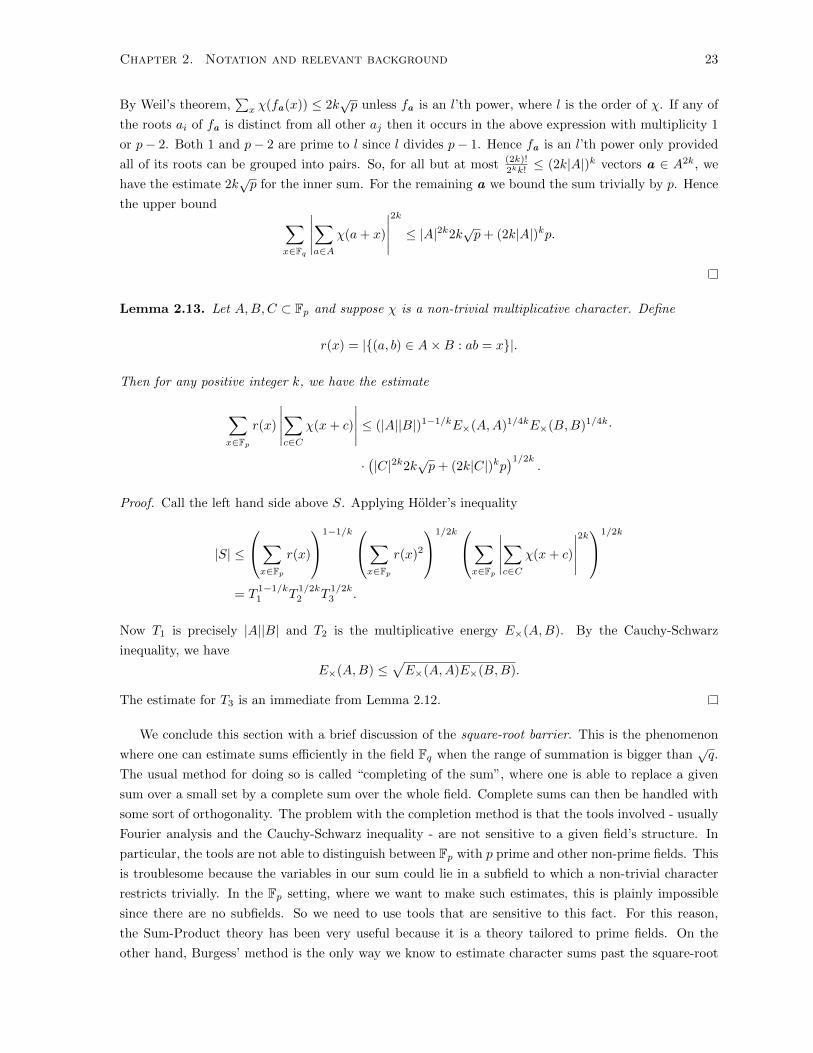
By Weil’s theorem,∑x χ(fa(x)) ≤ 2k
√p unless fa is an l’th power, where l is the order of χ. If any of
the roots ai of fa is distinct from all other aj then it occurs in the above expression with multiplicity 1
or p− 2. Both 1 and p− 2 are prime to l since l divides p− 1. Hence fa is an l’th power only provided
all of its roots can be grouped into pairs. So, for all but at most (2k)!2kk!
≤ (2k|A|)k vectors a ∈ A2k, we
have the estimate 2k√p for the inner sum. For the remaining a we bound the sum trivially by p. Hence
the upper bound ∑x∈Fq
∣∣∣∣∣∑a∈A
χ(a+ x)
∣∣∣∣∣2k
≤ |A|2k2k√p+ (2k|A|)kp.
Lemma 2.13. Let A,B,C ⊂ Fp and suppose χ is a non-trivial multiplicative character. Define
r(x) = |{(a, b) ∈ A×B : ab = x}|.
Then for any positive integer k, we have the estimate
∑x∈Fp
r(x)
∣∣∣∣∣∑c∈C
χ(x+ c)
∣∣∣∣∣ ≤ (|A||B|)1−1/kE×(A,A)1/4kE×(B,B)1/4k·
·(|C|2k2k
√p+ (2k|C|)kp
)1/2k.
Proof. Call the left hand side above S. Applying Holder’s inequality
|S| ≤
∑x∈Fp
r(x)
1−1/k∑x∈Fp
r(x)2
1/2k∑x∈Fp
∣∣∣∣∣∑c∈C
χ(x+ c)
∣∣∣∣∣2k1/2k
= T1−1/k1 T
1/2k2 T
1/2k3 .
Now T1 is precisely |A||B| and T2 is the multiplicative energy E×(A,B). By the Cauchy-Schwarz
inequality, we have
E×(A,B) ≤√E×(A,A)E×(B,B).
The estimate for T3 is an immediate from Lemma 2.12.
We conclude this section with a brief discussion of the square-root barrier. This is the phenomenon
where one can estimate sums efficiently in the field Fq when the range of summation is bigger than√q.
The usual method for doing so is called “completing of the sum”, where one is able to replace a given
sum over a small set by a complete sum over the whole field. Complete sums can then be handled with
some sort of orthogonality. The problem with the completion method is that the tools involved - usually
Fourier analysis and the Cauchy-Schwarz inequality - are not sensitive to a given field’s structure. In
particular, the tools are not able to distinguish between Fp with p prime and other non-prime fields. This
is troublesome because the variables in our sum could lie in a subfield to which a non-trivial character
restricts trivially. In the Fp setting, where we want to make such estimates, this is plainly impossible
since there are no subfields. So we need to use tools that are sensitive to this fact. For this reason,
the Sum-Product theory has been very useful because it is a theory tailored to prime fields. On the
other hand, Burgess’ method is the only way we know to estimate character sums past the square-root

Chapter 2. Notation and relevant background 24
barrier, and it is inefficient for sums shorter than p1/4. This is because the Burgess method makes use
of completion again, but replaces the use of orthogonality with the Weil bound. Perhaps if one could
handle incomplete Weil type sums, non-trivial estimates could be made in a broader range.

Chapter 3
Capturing forms in dense subsets of
finite fields
3.1 Introduction
Ramsey theory is concerned with finding small, structured objects inside of large objects. For instance,
if you flip a coin enough times, you are likely to see a sequence of one hundred consecutive heads. The
prototypical result in the area is appropriately named Ramsey’s Theorem.
Theorem 3.1 (Ramsey’s Theorem). Let G = (V,E) be the complete graph with vertices V indexed
by the natural numbers. Suppose we have a function c : E → {1, . . . , r} on the edges of G for some
finite integer r ≥ 1. Then there is an infinite set of vertices V ′ ⊂ V and a number i such that for any
v1, v2 ∈ V ′ the edge c({v1, v2}) = i.
We typically think of the edges of G in Ramsey’s Theorem as having been coloured by r different
colours. The theorem then says that if we colour the edges of G with finitely many colours then there is
an infinite subset of the vertices such that the induced graph on that subset has monochromatic edges,
i.e. they all have the same colour.
In arithmetic Ramsey theory, we are interested in finding configurations of numbers satisfying some
arithmetic relation. For instance, it is a simple consequence of Ramsey’s Theorem that if we colour the
natural numbers by c : N→ {1, . . . , r}, we can find a pair (and in fact infinitely many pairs) of numbers
x, y with each of x, y and x + y the same colour. To see this consider the complete graph with vertex
set N, and colour the edge {x, y} by the same colour as c(|x − y|). Then by Ramsey’s Theorem, we
can certainly find three vertices in the graph a < b < c such that all edges on these three vertices are
coloured the same. But then the numbers a− b, a− c and b− c are coloured the same so that x = a− band y = b− c are the desired pair.
From this, we can give a similar result concerning pairs x, y with x, y and xy coloured the same.
Define a new colouring of the natural numbers given by colouring k the same way we coloured 2k in the
original colouring. Finding x′ and y′ with x′, y′ and x′ + y′ all the same colour in this new colouring
gives the pair x = 2x′, y = 2y
′with x, y and xy monochromatic.
An open problem of Hindman asks if we can satisfy both equations monochromatically at the same
time. That is, given a colouring of the natural numbers with finitely many colours, can we find x, y
25

Chapter 3. Capturing forms in dense subsets of finite fields 26
with x, y, x+ y and xy monochromatic. Even the easier question of finding x and y with x+ y and xy
the same colour (never mind the colours of x and y) seems intractable. The problem is difficult largely
because we have a hard time controlling the additive structure and multiplicative structure of integers
at the same time.
As a first step we can reduce the question to one about solving quadratic equations. Indeed, suppose
we want to find x and y with xy and x+ y of a fixed colour i. Let A be the set of all natural numbers
n with c(n) = i. Then we want to find a, b ∈ A with x + y = a and xy = b. This is equivalent to x
and y being the roots of the quadratic polynomial Q(X) = X2 − aX + b. So our question is reduced
to asking if any of the quadratic polynomials X2 − aX + b with a, b ∈ A have natural roots. Which as
we learned in high school is equivalent to knowing when (a ±√a2 − 4b)/2 is a natural number. There
are two obstructions to this. First, the numerator needs to be even. The second and much more severe
obstruction is that the discriminant a2 − 4b needs to be a perfect square. In this chapter we ask a
question similar to Hindman’s conjecture, but in a setting were dividing by 2 is legal and perfect squares
are easier to come by - a finite field of odd characteristic.
Before proceeding to the problem, we remark that the similar question of colouring x + y and x/y
the same with x, y ∈ N and y dividing x is much easier. As we shall see, this question is a linear one.
Proposition 3.1. Let c : N→ {1, . . . , r} be a finite colouring of the natural numbers. Then there exist
x, y ∈ N with y|x and c(x+ y) = c(x/y).
Proof. Write z = x/y, so that x = yz - thus x is linear in y. We want to have c(z) = c(x+y) = c(y(z+1)).
Now just take numbers ai with c(ai) = i for i = 1, . . . , r. Then if the colour of (a1 + 1) · · · (ar + 1) is k,
we can take z = ak and y =∏i6=k(ai + 1). Letting x = yz gives the desired pair.
3.2 Statement of results
One might suspect that in fact a stronger result than Hindman’s Conjecture might hold, namely that
any sufficiently dense set of natural numbers contains the elements x+ y and xy for some x and y. This
would immediately solve the problem since one of the colours in any finite colouring must be sufficiently
dense. Such a result is impossible however, since the odd numbers provide a counter example and are
fairly dense in many senses of the word. This simple parity obstruction disappears in the finite field
setting. In [Shk], the following was proved.1
Theorem (Shkredov). Let p be a prime number, and A1, A2, A3 ⊂ Fp be any sets, |A1||A2||A3| ≥ 40p52 .
Then there are x, y ∈ Fp such that x+ y ∈ A1, xy ∈ A2 and x ∈ A3.
Now, let q = pn be an odd prime power and Fq a finite field of order q. Given a binary linear form
L(X,Y ) and a binary quadratic form Q(X,Y ), define Nq(L,Q) to be the smallest integer k such that
for any subset A ⊂ Fq with |A| ≥ k, there exists (x, y) ∈ F2q with L(x, y), Q(x, y) ∈ A. That is,
Nq(L,Q) = min{k : ∀ A ⊂ Fq with |A| ≥ k, ∃ (x, y) ∈ F2
q with L(x, y), Q(x, y) ∈ A}.
In this chapter we give estimates on the size of Nq(L,Q). We will prove the following theorem.
1This result was communicated to us by J. Solymosi after the results of this section were made available.
Chapter 3. Capturing forms in dense subsets of finite fields 27
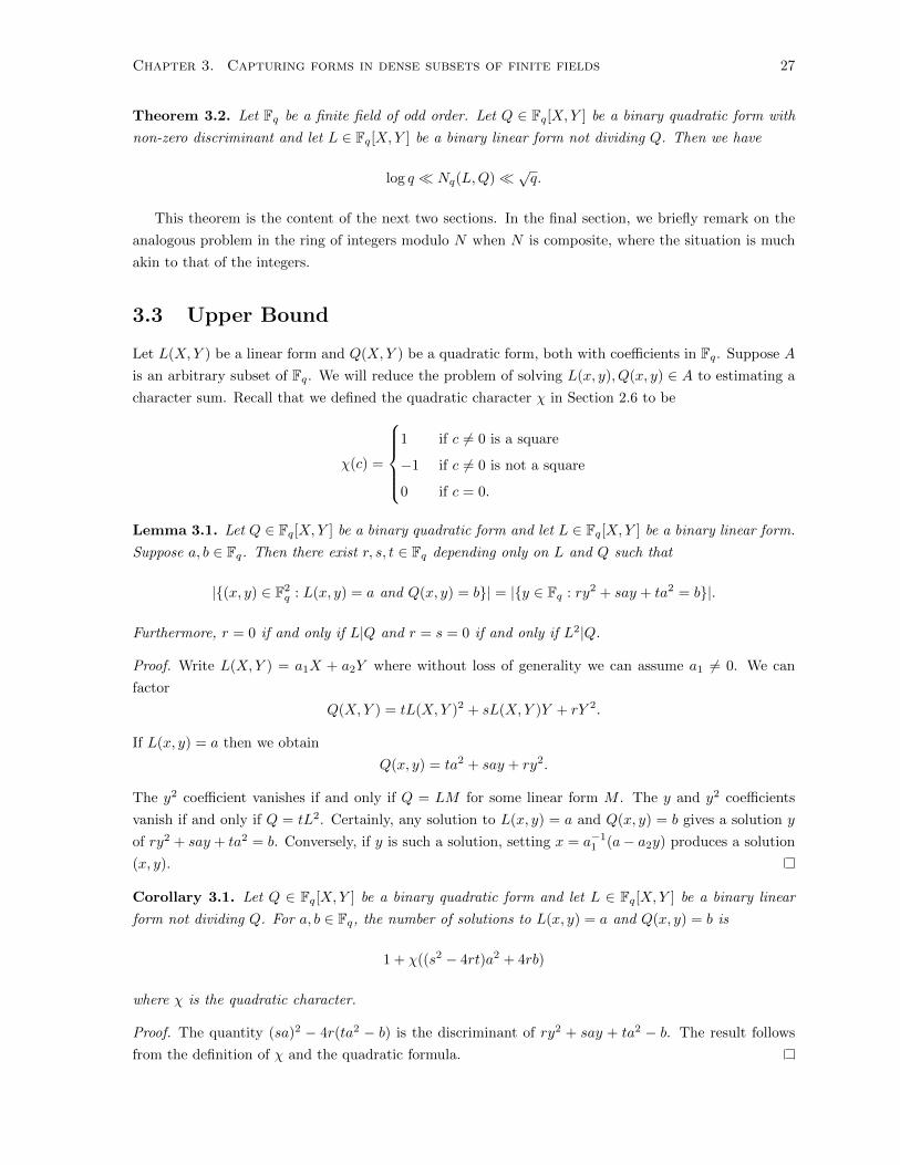
Theorem 3.2. Let Fq be a finite field of odd order. Let Q ∈ Fq[X,Y ] be a binary quadratic form with
non-zero discriminant and let L ∈ Fq[X,Y ] be a binary linear form not dividing Q. Then we have
log q � Nq(L,Q)� √q.
This theorem is the content of the next two sections. In the final section, we briefly remark on the
analogous problem in the ring of integers modulo N when N is composite, where the situation is much
akin to that of the integers.
3.3 Upper Bound
Let L(X,Y ) be a linear form and Q(X,Y ) be a quadratic form, both with coefficients in Fq. Suppose A
is an arbitrary subset of Fq. We will reduce the problem of solving L(x, y), Q(x, y) ∈ A to estimating a
character sum. Recall that we defined the quadratic character χ in Section 2.6 to be
χ(c) =
1 if c 6= 0 is a square
−1 if c 6= 0 is not a square
0 if c = 0.
Lemma 3.1. Let Q ∈ Fq[X,Y ] be a binary quadratic form and let L ∈ Fq[X,Y ] be a binary linear form.
Suppose a, b ∈ Fq. Then there exist r, s, t ∈ Fq depending only on L and Q such that
|{(x, y) ∈ F2q : L(x, y) = a and Q(x, y) = b}| = |{y ∈ Fq : ry2 + say + ta2 = b}|.
Furthermore, r = 0 if and only if L|Q and r = s = 0 if and only if L2|Q.
Proof. Write L(X,Y ) = a1X + a2Y where without loss of generality we can assume a1 6= 0. We can
factor
Q(X,Y ) = tL(X,Y )2 + sL(X,Y )Y + rY 2.
If L(x, y) = a then we obtain
Q(x, y) = ta2 + say + ry2.
The y2 coefficient vanishes if and only if Q = LM for some linear form M . The y and y2 coefficients
vanish if and only if Q = tL2. Certainly, any solution to L(x, y) = a and Q(x, y) = b gives a solution y
of ry2 + say + ta2 = b. Conversely, if y is such a solution, setting x = a−11 (a− a2y) produces a solution
(x, y).
Corollary 3.1. Let Q ∈ Fq[X,Y ] be a binary quadratic form and let L ∈ Fq[X,Y ] be a binary linear
form not dividing Q. For a, b ∈ Fq, the number of solutions to L(x, y) = a and Q(x, y) = b is
1 + χ((s2 − 4rt)a2 + 4rb)
where χ is the quadratic character.
Proof. The quantity (sa)2 − 4r(ta2 − b) is the discriminant of ry2 + say + ta2 − b. The result follows
from the definition of χ and the quadratic formula.

Chapter 3. Capturing forms in dense subsets of finite fields 28
In fact, from Lemma 3.1, we can essentially handle the situation when L|Q.
Corollary 3.2. Let Q ∈ Fq[X,Y ] be a binary quadratic form and let L ∈ Fq[X,Y ] be a binary linear
form dividing Q. Then Nq(L,Q) = 1 if L2 does not divide Q, otherwise Nq(L,Q) ≥ q+12 .
Proof. Let A ⊂ Fq. The number of pairs (x, y) with L(x, y), Q(x, y) ∈ A is∑x,y
1A(L(x, y))1A(Q(x, y)) =∑a∈A
∑y∈Fq
1A(say + ta2)
by the above lemma. If sa 6= 0 then say+ ta2 ranges over Fq as y, and the inner sum is |A|. In this case
there are in fact |A|2 solutions (x, y). If a = 0 then 0 ∈ A and we can take (x, y) = (0, 0). If s = 0 then
the sum is q∑a∈A 1A(a2t). If we set
A =
t ·N = {tn : n ∈ N} if t 6= 0
N if t = 0
where N is the set of non-squares in Fq, then there are no solutions. This shows that Nq(L,Q) ≥ q+12 .
We now handle the case that L does not divide Q. The following estimate is essentially due to
Vinogradov (see for instance the exercises of Chapter 6 in [V] for the analogous result for exponentials).
Lemma 3.2. Let A,B ⊂ Fq and suppose χ is a non-trivial multiplicative character. Then if u, v ∈ F×q∑a∈A
∑b∈B
χ(ua2 + vb) ≤ 2√q|A||B|.
Proof. Let S denote the sum in question. Then
|S| ≤∑b∈B
∣∣∣∣∣∑a∈A
χ(ua2 + vb)
∣∣∣∣∣ ≤ |B| 12∑b∈Fq
∣∣∣∣∣∑a∈A
χ(ua2 + vb)
∣∣∣∣∣2 1
2
by Cauchy’s inequality. Expanding the sum in the second factor, we get
∑a1,a2∈A
∑b∈Fq
ua22+vb6=0
χ
(ua2
1 + vb
ua22 + vb
)=
∑a1,a2∈A
∑b∈Fq
ua22+vb6=0
χ
(1 +
u(a21 − a2
2)
ua22 + vb
)
=∑
a1,a2∈A
∑b∈F×q
χ(1 + u(a2
1 − a22)b)
after the change of variables (ua22 + vb)−1 7→ b. When a2
1 6= a22, the values of 1 + u(a2
1 − a22)b range over
all values of Fq save 1 as b traverses F×q . Hence, in this case, the sum amounts to −1. It follows that the
total is at most 4q|A|.
Recall that the discriminant of a quadratic form Q(X,Y ) = b1X2 + b2XY + b3Y
2 is defined to be
disc(Q) = b22 − 4b1b3.
Proposition 3.2. Let Q ∈ Fq[X,Y ] be a binary quadratic form and let L ∈ Fq[X,Y ] be a binary linear
form not dividing Q. Then Nq(L,Q) ≤ 2√q + 1 if disc(Q) 6= 0 otherwise Nq(L,Q) ≥ q−1
2 .

Chapter 3. Capturing forms in dense subsets of finite fields 29
Proof. Let A ⊂ Fq. By Corollary 3.1, the number of pairs (x, y) with L(x, y), Q(x, y) ∈ A is∑x,y
1A(L(x, y))1A(Q(x, y)) =∑a,b∈A
(1 + χ(Da2 + 4rb))
where D = s2 − 4rt. One can check that in fact D = a−21 disc(Q).
If D = 0 then χ(Da2 + 4rb) + 1 = χ(r)χ(b) + 1. This will be identically zero if A is chosen to be the
squares or non-squares according to the value of χ(r). Hence, if disc(Q) = 0 then Nq(L,Q) ≥ q−12 .
Now assume D 6= 0. Summing over a, b ∈ A the number of solutions is
|A|2 +∑a,b∈A
χ(Da2 + 4rb) = |A|2 + E(A).
By Lemma 3.2, E(A) < |A|2 when |A| ≥ 2√q + 1 and the result follows.
In the case that A has particularly nice structure, we can improve the upper bound. Suppose q = p
is prime and A is an interval. Then as above the number of pairs (x, y) with L(x, y), Q(x, y) ∈ A is
|A|2 +∑a,b∈A
χ(Da2 + 4rb).
Now ∑a,b∈A
χ(Da2 + 4rb) ≤∑a∈A
∣∣∣∣∣∑b∈A
χ(Da2/4r + b)
∣∣∣∣∣ .Using the classical Burgess estimate, the inner sum (which is also over an interval) is o(|A|) whenever
|A| � p14 +ε.
3.4 Lower Bound
In this section we give a lower bound for Nq(L,Q) in the case that L does not divide Q and disc(Q) 6= 0.
To do so we need to produce a set A such that L(x, y) and Q(x, y) are never both elements of A.
Equivalently, we need to produce a set A for which χ(Da2 + 4rb) = −1 for all pairs (a, b) ∈ A×A.
Let a ∈ Fq and define
Xa(b) =
1 if χ(Da2 + 4rb) = χ(Db2 + 4ra) = −1
0 otherwise.
Thus the desired set A will have Xa(b) = 1 for a, b ∈ A. The idea behind our argument is probabilistic.
Suppose we create a graph Γ with vertex set
V = {a ∈ Fq : Xa(a) = 1}
and edge set
E = {{a, b} : Xa(b) = Xb(a) = 1}.
These edges appear to be randomly distributed and occur with probability roughly 14 . In this setting,
Nq(L,Q) is one more than the clique number of Γ (ie. the size of the largest complete subgraph of

Chapter 3. Capturing forms in dense subsets of finite fields 30
Γ). Let G(n, δ) be the graph with n vertices that is the result of connecting two vertices randomly and
independently with probability δ. Such a graph has clique number roughly log n (see [AS], chapter 10).
One is tempted to treat Γ as such a graph and construct a clique by greedily choosing vertices, and
indeed this is how the set A is constructed. It is worth mentioning that this model suggests that the
right upper bound for Nq(L,Q) is closer to log q in magnitude.
Lemma 3.3. Let B ⊂ Fq. Then for a ∈ Fq, we have
∑b∈B
Xa(b) =1
4
∑b∈B
(1− χ(Da2 + 4rb))(1− χ(Db2 + 4ra)) +O(1).
Proof. The summands on the right are
(1− χ(Da2 + 4rb))(1− χ(Db2 + 4ra)) =
4 if χ(Da2 + 4rb) = χ(Db2 + 4ra) = −1
2 if {χ(Da2 + 4rb), χ(Db2 + 4ra)} = {0,−1}
1 if χ(Da2 + 4rb) = χ(Db2 + 4ra) = 0
0 otherwise.
For fixed a, the second and third cases can only occur for O(1) values of b.
Proposition 3.3. Let A,B ⊂ Fq with |A|, |B| > √q. Then
∑a∈A
∑b∈B
Xa(b) =|A||B|
4+O(|A||B| 12 q 1
4 ).
Proof. By the preceding lemma, it suffices to estimate
∑a∈A
1
4
(∑b∈B
(1− χ(Da2 + 4rb))(1− χ(Db2 + 4ra))
)+O(1)
=|A||B|
4− 1
4
∑a∈A
∑b∈B
χ(Da2 + 4rb)− 1
4
∑a∈A
∑b∈B
χ(Db2 + 4ra)
+1
4
∑a∈A
∑b∈B
χ((Da2 + 4rb)(Db2 + 4ra)) +O(|A|).
By Lemma 1 of the previous section, the first two sums above are O(√q|A||B|) = O(|A||B| 12 q 1
4 ). By
Cauchy’s inequality, the final sum is bounded by
|B| 12
∑b∈Fq
∣∣∣∣∣∑a∈A
χ((Da2 + 4rb)(Db2 + 4ra))
∣∣∣∣∣2 1
2
.
Expanding the square modulus, the second factor is the square-root of∑a1,a2∈A
∑b∈Fq
χ((Da21 + 4rb)(Db2 + 4ra1)(Da2
2 + 4rb)(Db2 + 4ra2)).

Chapter 3. Capturing forms in dense subsets of finite fields 31
By Weil’s Theorem, the inner sum is bounded by 6√q when the polynomial
f(b) = (Da21 + 4rb)(Db2 + 4ra1)(Da2
2 + 4rb)(Db2 + 4ra2)
is not a square. This happens for all but O(|A|) pairs (a1, a2). Hence the bound is O(|A|q + |A|2√q).Since |A| > √q, this is O(|A|2√q) and the overall bound is O(|A||B| 12 q 1
4 ).
We immediately deduce the following.
Corollary 3.3. There is an absolute constant c > 0 such that if B ⊂ Fq with |B| ≥ c√q then there is
an element a ∈ B such that
|{b ∈ B : Xa(b) = 1}| ≥ 1
8|B|.
Proof. Indeed, taking A = B in the preceding theorem,
maxa∈B
{∑b∈B
Xa(b)
}≥ 1
|B|∑a,b∈B
Xa(b) =|B|4
+O(q14 |B| 12 ) ≥ |B|
8
when |B| > c√q for some appropriately chosen c.
Proposition 3.4. Let Q ∈ Fq[X,Y ] be a binary quadratic form and let L ∈ Fq[X,Y ] be a binary linear
form not dividing Q. Then if disc(Q) 6= 0 we have Nq(L,Q)� log q.
Proof. We will construct a clique in the graph Γ introduced above. First we claim that |V | = q−12 +O(1).
Indeed ∑a∈F×q
χ(Da2 + 4ra) =∑a∈F×q
χ(a−2)χ(Da2 + 4ra) =∑a∈F×q
χ(D + 4ra−1) = O(1)
by orthogonality. The final term is O(1) and the claim follows since χ takes on the values ±1 on F×q .
Now set V0 = V and assume q is large. Write |V0| = c′q > c√q (with c as in the preceeding corollary
and c′ ≈ 12 ). For a ∈ V0, let N(a) denote the neighbours of a (ie. those b which are joined to a by
an edge). Then there is an a1 ∈ V0 such that |N(a1)| ≥ c′q/8. Let A1 = {a1}, let V1 = N(a1) ⊂ V0,
and for a ∈ V1 let N1(a) = N(a) ∩ V1. By choice, all elements of V1 are connected to a1. Now
|V1 \ A1| ≥ c′q/8 − 1 ≥ c′q/16 so, provided this is at least c′q/16, there is some element a2 of V1 \ A1
such that |N1(a2)| ≥ |V1 \A1|/8. Let A2 = A1 ∪ {a2}, V2 = N1(a2) ⊂ V1 and define N2(a) = N(a)∩ V2.
Once again each element of V2 is connected to each element of A2. We repeat this process provided that
at stage i there exists an element ai+1 ∈ Vi \Ai with |Ni(ai+1)| ≥ |Vi \Ai|/8. We set Ai+1 = Ai∪{ai+1}and observe that Ai+1 induces a clique. We may iterate provided |Vi \ Ai| > c
√q which is guaranteed
for i� log q. The final set Ai (which has size i) will be the desired set A.
The combination of this proposition and Proposition 3.2 completes the proof of Theorem 3.2.
3.5 Remarks for Composite Modulus
Consider the analogous question in the ring Z/NZ with N odd. Let L(X,Y ) = a1X+a2Y with (a1, N) =
1 and Q(X,Y ) = b1X2 + b2XY + b3Y
2. We then let A ⊂ Z/NZ and wish to find (x, y) ∈ (Z/NZ)2 such
that L(x, y), Q(x, y) ∈ A. As before, this amounts to finding a solution to
Q(a−11 (a− a2Y ), Y ) = b
Chapter 3. Capturing forms in dense subsets of finite fields 32
for some a, b ∈ A. In general, one cannot find a solution based on the size of A alone unless A is very
large. Indeed, if p is a small prime dividing N and t mod p is chosen such that the discriminant of
Q(a−11 (t− a2Y ), Y )− t
is a non-residue modulo p then taking A = {a mod N : a ≡ t mod p} provides a set of density 1/p which
fails admit a solution.

Chapter 4
Character sum estimates for Bohr
sets and applications
4.1 Introduction
In Chapter 1 we discussed the Sum-Product Problem. This problem seeks to quantify the extent to
which additive structure and multiplicative structure are independent phenomena. In this section we
establish a result which is dual to this: if one can control additive characters on a given set, one cannot
hope to control multiplicative characters on that set. Recall that in Section 2.5 we defined the Bohr set
B(Γ, ε) = {x ∈ Fp : max{‖rx/p‖ : r ∈ Γ} ≤ ε}.
Thus B(Γ, ε) is the set on which the exponentials with frequencies in Γ approximate the trivial character.
We think of B(Γ, ε) as behaving like a kernel for this set of characters (there are of course no actual
kernels since Fp has no non-trivial subgroups). Can such a set also behave like a kernel for a multi-
plicative character? In this chapter we show that the answer is no. We will prove that any non-trivial
multiplicative character must oscillate on a Bohr set.
4.2 Statement of Results and Applications
4.2.1 Main Results
In Section 2.5 we discussed several facts concerning Bohr sets, and in particular we stressed that they
possess a lot of additive structure. Indeed, elements x ∈ B(Γ, ε) dilate Γ into a short interval, and much
of the additive structure of this interval carries over to B. We shall put this structure to use in order
to obtain very strong estimates on large Bohr sets. In Section 4.3 we obtain the following analog of the
Polya-Vinogradov estimate which is non-trivial for large Bohr sets.
Theorem 4.1 (Polya-Vinogradov for Bohr sets). Let B = B(Γ, ε) be a Bohr set with |Γ| = d. Then for
33

Chapter 4. Character sum estimates for Bohr sets and applications 34
any non-trivial multiplicative character χ∣∣∣∣∣∑x∈B
χ(x)
∣∣∣∣∣�d√p(log p)d.
This result is comparable to [Sh] in which a Polya-Vingradov estimate is established for generalized
arithmetic progressions of rank d, which is a set of the form
A = {a0 + x1a1 + · · ·+ xdad : 1 ≤ xi ≤ Ni}
for some integers Ni. For non-trivial estimates when the Bohr set is on the order of√p or smaller, we
appeal to Burgess’ method. We are able to prove non-trivial results provided the Bohr set satisfies a
certain niceness condition known as regularity, see Definition 2.5.
Theorem 4.2 (Burgess for Bohr sets). Let B = B(Γ, ε) be a regular Bohr set with |Γ| = d. Let k ≥ 1
be an integer and let χ be non-trivial multiplicative character. When |B| ≥ √p we have the estimate∣∣∣∣∣∑x∈B
χ(x)
∣∣∣∣∣�k,d |B| · p5d/16k2+o(1)
(|B|εdp
)5/16k (p
|B|
)−1/8k
.
When |B| < √p we have the estimate∣∣∣∣∣∑x∈B
χ(x)
∣∣∣∣∣�k,d |B| · p5d/16k2+o(1)
(|B|εdp
)5/16k ( |B|5p2
)−1/8k
.
The statement appears complicated, but usually one has |B| ≈ εdp so the middle factor in the
estimate is harmless. If the rank d is bounded, one can take k much larger than d and obtain a non-
trivial estimate in the range |B| � p2/5+δ for some positive δ. This is comparable to character sum
estimates of M.-C. Chang for generalized arithmetic progressions of similar rank, proved in [C1]. As in
her proof, we make use of Sum-Product Phenomena in Fp.
4.2.2 Applications
Recall Dirichlet’s approximation theorem states that for real numbers α1, . . . , αd there is an integer
n ≤ Q so that maxk{‖nαk‖} ≤ Q−1/d. Schmidt proved in [Sch] that, at the cost of weakening the
approximation, we can take n to be a perfect square. Specifically, he proved the following.
Theorem (Schmidt). Given real numbers α1, . . . , αd and Q a positive integer, there is an integer 1 ≤n ≤ Q and a positive absolute constant c such that
max{‖n2αk‖ : 1 ≤ k ≤ d} � dQ−c/d2
.
This result was also proved by Green and Tao in [GT] and extended to different systems of polynomials
in [LM]. An elementary proof of a slightly weaker estimate was also given in [CLR].
When Γ is a subset of Fp and ε > 0 then the elements of B(Γ, ε) are precisely the elements guaranteed
by Dirichlet’s approximation theorem. Here we are replacing approximation in the continuous torus R/Zwith approximation in the discrete torus Fp. We will prove the following Fp analog of Schmidt’s theorem.
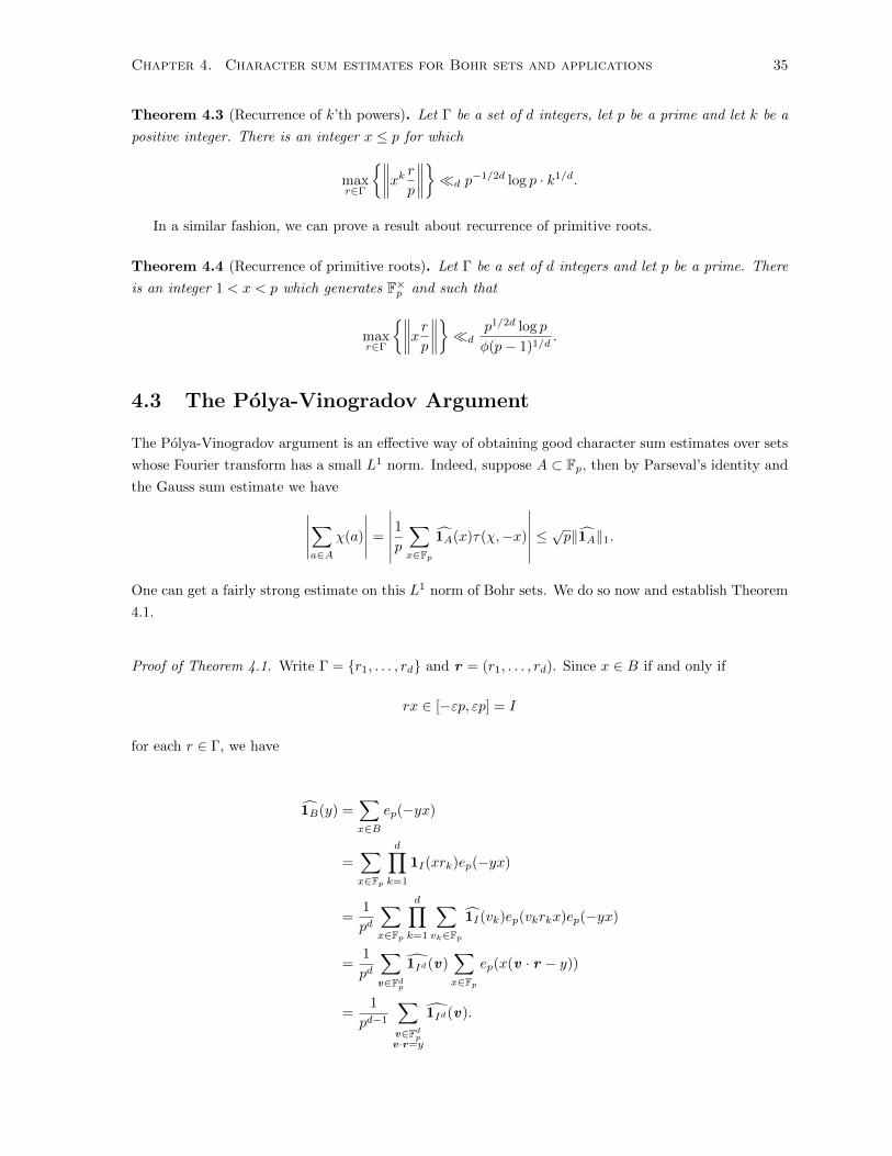
Chapter 4. Character sum estimates for Bohr sets and applications 35
Theorem 4.3 (Recurrence of k’th powers). Let Γ be a set of d integers, let p be a prime and let k be a
positive integer. There is an integer x ≤ p for which
maxr∈Γ
{∥∥∥∥xk rp∥∥∥∥}�d p
−1/2d log p · k1/d.
In a similar fashion, we can prove a result about recurrence of primitive roots.
Theorem 4.4 (Recurrence of primitive roots). Let Γ be a set of d integers and let p be a prime. There
is an integer 1 < x < p which generates F×p and such that
maxr∈Γ
{∥∥∥∥xrp∥∥∥∥}�d
p1/2d log p
φ(p− 1)1/d.
4.3 The Polya-Vinogradov Argument
The Polya-Vinogradov argument is an effective way of obtaining good character sum estimates over sets
whose Fourier transform has a small L1 norm. Indeed, suppose A ⊂ Fp, then by Parseval’s identity and
the Gauss sum estimate we have∣∣∣∣∣∑a∈A
χ(a)
∣∣∣∣∣ =
∣∣∣∣∣∣1p∑x∈Fp
1A(x)τ(χ,−x)
∣∣∣∣∣∣ ≤ √p‖1A‖1.One can get a fairly strong estimate on this L1 norm of Bohr sets. We do so now and establish Theorem
4.1.
Proof of Theorem 4.1. Write Γ = {r1, . . . , rd} and r = (r1, . . . , rd). Since x ∈ B if and only if
rx ∈ [−εp, εp] = I
for each r ∈ Γ, we have
1B(y) =∑x∈B
ep(−yx)
=∑x∈Fp
d∏k=1
1I(xrk)ep(−yx)
=1
pd
∑x∈Fp
d∏k=1
∑vk∈Fp
1I(vk)ep(vkrkx)ep(−yx)
=1
pd
∑v∈Fd
p
1Id(v)∑x∈Fp
ep(x(v · r − y))
=1
pd−1
∑v∈Fd
pv ·r=y
1Id(v).

Chapter 4. Character sum estimates for Bohr sets and applications 36
Here we have set Id = I×d
× . . .× I and
1Id((v1, . . . , vd)) = 1I(v1) · · · 1I(vd).
Plugging this in, we obtain
‖1B‖1 ≤1
pd
∑y∈Fp
∑v∈Fd
pv ·r=y
|1Id(v)| = 1
pd
∑v∈Fd
p
|1Id(v)| = ‖1I‖d1.
As in the classical proof of the Polya-Vinogradov inequality,
|1I(v)| =
∣∣∣∣∣N∑
k=−N
ep(−kv)
∣∣∣∣∣ =
∣∣∣∣∣2N+1∑k=0
ep(−kv)
∣∣∣∣∣ =
∣∣∣∣ep(v(2N + 2)− 1
ep(v)− 1
∣∣∣∣� p
v.
It follows that ‖1I‖1 � log p and the theorem is proved.
Remark. If one takes Γ = {1} and ε = N/p for some positive integer N then B(Γ, ε) = [−N,N ],
thought of as a subset of Fp. This recovers the classical Polya-Vinogradov estimate∑|n|≤N
χ(n)� √p log p.
4.4 The Burgess Argument
In this section we prove Theorem 4.2. The method is the same as in the proof of Burgess’ estimate
for character sums over an interval, which can be found in Chapter 12 of [IK]. The main difference
lies in estimating the multiplicative energy between two Bohr sets and for this we use Rudnev’s Sum-
Product result quoted in Section 2.4. Sum-Product estimates were used for the same purpose in [C1]
with methods taken from [KS]. It is likely that the argument presented here is not efficient. Indeed,
Bohr sets are highly structured and the current Sum-Product estimates are weaker than expected, and
certainly weaker than what is predicted by the Erdos-Szemeredi Conjecture. For example, one of the
energy estimates proved in [C1] was improved in [K] using the geometry of numbers. We were unable
to adapt that argument to the present situation.
Proof of Theorem 4.2. Suppose Γ ⊂ Fp has size d and ε is a regular value for Γ. We may as well assume
that Γ 6= 0 for otherwise B = Fp and the result is trivial. Write B = B(Γ, ε) and let χ be a non-trivial
character of F×p . Then we wish to estimate
S(χ) =∑x∈B
χ(x).
We begin by first using Corollary 2.2. Let η = p−1/kε/(200d) and let y ∈ B(Γ, η). For any natural
number n ≤ p1/2k we have

Chapter 4. Character sum estimates for Bohr sets and applications 37
S(χ) =∑x∈Fp
1B(x)χ(x)
=∑x∈Fp
1B(x+ ny)χ(x) +O(n|B|p−1/k
)=∑x∈B
χ(x− ny) +O(n|B|p−1/k
).
Averaging this over all values 1 ≤ n ≤ p1/2k and over all values y ∈ B′ = B(Γ, η) \ {0} we obtain
S(χ) =1
p1/2k|B′|∑x∈B
∑y∈B′
∑1≤n≤p1/2k
χ(x− ny) +O(|B|p−1/2k
).
It remains to estimate
T (χ) =1
p1/2k|B′|∑x∈B
∑y∈B′
∑1≤n≤p1/2k
χ(x− ny).
We begin by assuming that |B| < √p. Then, applying Lemma 2.13 (where r(x) is now the number
of ways of writing x as ab with a ∈ B and b ∈ (B′)−1), we have
|T (χ)| � 1
p1/2k|B′|∑x∈Fp
r(x)
∣∣∣∣∣∣∑
1≤n≤p1/2kχ(x− n)
∣∣∣∣∣∣≤ (|B||B′|)1−1/kE×(B,B)1/4kE×(B′, B′)1/4k
p1/2k|B′|·
·(
2kp3/2 + (2k)kp3/2)1/2k
≤ |B|(|B||B′|)−3/4k(|B +B||B′ +B′|)7/16k(log p)1/2k√kp1/4k
after applying Theorem 2.6. Applying Corollary 2.1, we get the bound
|T (χ)| � |B|(|B||B′|)−5/16k47d/8k(log p)1/2k√kp1/4k.
Using Lemma 2.8,
|B′| ≥ ηdp =
(ε
p1/k200d
)dp
so that
|T (χ)| �d,k |B| · p5d/16k2+o(1)
(|B|εdp
)5/16k ( |B|5/2p
)−1/4k
.
Now if |B| ≥ √p, first split B into disjoint sets Bi with√p� |Bi| <
√p. Then
|T (χ)| � |B|√p· 1
p1/2k|B′|maxi
∑x∈Bi
∑y∈B′
∣∣∣∣∣∣∑
1≤n≤p1/2kχ(x− ny)
∣∣∣∣∣∣ .
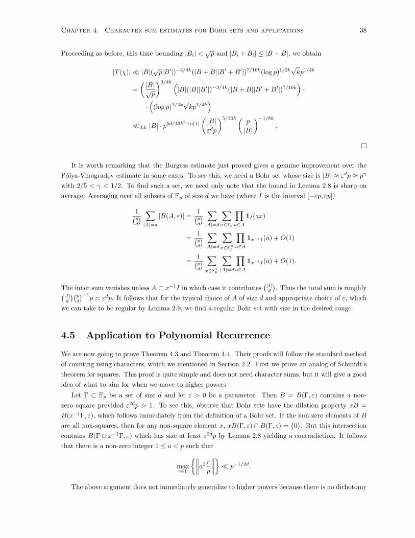
Chapter 4. Character sum estimates for Bohr sets and applications 38
Proceeding as before, this time bounding |Bi| <√p and |Bi +Bi| ≤ |B +B|, we obtain
|T (χ)| � |B|(√p|B′|)−3/4k(|B +B||B′ +B′|)7/16k(log p)1/2k√kp1/4k
=
(|B|√p
)3/4k (|B|(|B||B′|)−3/4k(|B +B||B′ +B′|)7/16k
)·
·(
(log p)1/2k√kp1/4k
)�d,k |B| · p5d/16k2+o(1)
(|B|εdp
)5/16k (p
|B|
)−1/8k
.
It is worth remarking that the Burgess estimate just proved gives a genuine improvement over the
Polya-Vinogradov estimate in some cases. To see this, we need a Bohr set whose size is |B| ≈ εdp ≈ pγ
with 2/5 < γ < 1/2. To find such a set, we need only note that the bound in Lemma 2.8 is sharp on
average. Averaging over all subsets of Fp of size d we have (where I is the interval [−εp, εp])
1(pd
) ∑|A|=d
|B(A, ε)| = 1(pd
) ∑|A|=d
∑x∈Fp
∏a∈A
1I(ax)
=1(pd
) ∑|A|=d
∑x∈F×p
∏a∈A
1x−1I(a) +O(1)
=1(pd
) ∑x∈F×p
∑|A|=d
∏a∈A
1x−1I(a) +O(1).
The inner sum vanishes unless A ⊂ x−1I in which case it contributes(|I|d
). Thus the total sum is roughly(|I|
d
)(pd
)−1p � εdp. It follows that for the typical choice of A of size d and appropriate choice of ε, which
we can take to be regular by Lemma 2.9, we find a regular Bohr set with size in the desired range.
4.5 Application to Polynomial Recurrence
We are now going to prove Theorem 4.3 and Theorem 4.4. Their proofs will follow the standard method
of counting using characters, which we mentioned in Section 2.2. First we prove an analog of Schmidt’s
theorem for squares. This proof is quite simple and does not need character sums, but it will give a good
idea of what to aim for when we move to higher powers.
Let Γ ⊂ Fp be a set of size d and let ε > 0 be a parameter. Then B = B(Γ, ε) contains a non-
zero square provided ε2dp > 1. To see this, observe that Bohr sets have the dilation property xB =
B(x−1Γ, ε), which follows immediately from the definition of a Bohr set. If the non-zero elements of B
are all non-squares, then for any non-square element x, xB(Γ, ε) ∩ B(Γ, ε) = {0}. But this intersection
contains B(Γ ∪ x−1Γ, ε) which has size at least ε2dp by Lemma 2.8 yielding a contradiction. It follows
that there is a non-zero integer 1 ≤ a < p such that
maxr∈Γ
{∥∥∥∥a2 r
p
∥∥∥∥}� p−1/2d.
The above argument does not immediately generalize to higher powers because there is no dichotomy

Chapter 4. Character sum estimates for Bohr sets and applications 39
- an element can be in any of the k cosets of the set of k’th powers. Instead, we will use Theorem 4.1 to
find higher powers and primitive roots in Bohr sets.
Proof of Theorem 4.3. Write B for B(Γ, ε). Observe that when (k, p − 1) = l then the k’th powers are
the same as the l’th powers. So we suppose k|(p− 1) and K is the subgroup of F×p consisting of the k’th
powers. This group has index k. The problem is then showing that B(Γ, ε) ∩K is non-empty. Let K⊥
be the group of multiplicative characters which restrict to the trivial character on K. This group has
size |K⊥| = k. The Poisson Summation Formula, Proposition 2.2, states that
1K(x) =1
k
∑χ∈K⊥
χ(x).
Thus,
|K ∩B| = 1
k
∑χ∈K⊥
∑b∈B
χ(b).
After extracting the contribution from the trivial character χ0 this we have∣∣∣∣|K ∩B| − |B|k∣∣∣∣ ≤ max
χ|S(χ)|
where S(χ) =∑b∈B χ(b) and the maximum is taken over all non-trivial characters χ ∈ K⊥. Thus if we
can show that the maximum value of |S(χ)| is at most |B|k then B must contain an element of K. By
Theorem 4.1, B contains a k’th powers provided |B| �d kp1/2(log p)d which is certainly the case when
εd �d kp−1/2(log p)d in view of Lemma 2.8. Thus
maxr∈Γ
{∥∥∥∥xk rp∥∥∥∥}�d p
−1/2d log p · k1/d.
We now turn to primitive roots.
Proof of Theorem 4.4. We can also find primitive roots in a Bohr set. Recall that the group F×p is cyclic
and a primitive element of Fp is a generator of this group. Denote the primitive roots of Fp by P. The
characteristic function of P has a nice expansion in terms of characters, due to Vinogradov, see exercise
5.14 of [LN]:
1P(x) =φ(p− 1)
p− 1
∑d|(p−1)
µ(d)
φ(d)
∑χd
χ(x)
where φ is Euler’s totient function and∑χd
is the sum over all characters with order exactly d. Summing
over the elements of a Bohr set B and extracting the contribution from the trivial character, we obtain∣∣∣∣|B ∩ P| − |B|φ(p− 1)
p− 1
∣∣∣∣�d√p(log p)d.
We deduce that B will contain a primitive root whenever ε� p1/2d
φ(p−1)1/d· log p. Thus there is a primitive
root 1 < x < p with
maxr∈Γ
{∥∥∥∥xrp∥∥∥∥}�d
p1/2d log p
φ(p− 1)1/d.

Chapter 4. Character sum estimates for Bohr sets and applications 40
We close by mentioning that use of Theorem 4.2 would allow for smaller choices of ε but for the
factor(|B|εdp
)kappearing in the estimate. As we mentioned in the preceding section, this factor is usually
harmless, but we wanted uniform results for all sets Γ which comes more easily by way of Theorem 4.1.

Chapter 5
Character sum estimates for various
convolutions
5.1 Introduction
This chapter is motivated by the following question of Sarkozy:
Problem. Are the quadratic residues modulo p a sumset? That is, do there exist sets A,B ⊂ Fp, each
of size at least two with the set A+B equal to the set of quadratic residues?
The general consensus is that the answer to the above question is no. Indeed, if B contains two
elements b, b′ then we would require that A + b and A + b′ are both subsets of the quadratic residues.
But we expect that a + b is a quadratic residue half of the time, and we expect that a + b′ also be a
residue half of the time, independent of whether or not a+b is a quadratic residue. So if A+B consisted
entirely of quadratic residues then many unlikely events must have occurred. For A+B to consist of all
the quadratic residues would be shocking. In [Shk2], Shkredov showed that one could not take A = B.
By estimating certain character sums, Sarkozy [Sar] and later Shparlinski [Shp] were able to prove that:
Theorem. If A,B ⊂ Fp, each of size at least two with the set A+B equal to the set of quadratic residues
then |A| and |B| are within a constant factor of√p.
This provides a bit of tension since |A+B| ≤ |A||B| � p but on the other hand A+B must contain
at least (p− 1)/2 elements.
A tempting way to approach the question is to understand the sum
∑a∈A
∑b∈B
(a+ b
p
).
Using the Cauchy-Schwarz inequality and orthogonality it is not too hard to show that this sum is at
most√|A||B|p which is non-trivial for |A||B| > p. This argument was used in proof of Lemma 3.2. This
estimate just fails to answer our question. Thus improving upon it even by a constant factor (1/4 would
suffice, for instance) would be worthwhile. Unfortunately, the proof of this estimate is not sensitive to
the fact that Fp is a prime field - this is the square-root barrier that was discussed at the end of Section
2.6. And in general finite fields, the presence of subfields makes this estimate sharp. In this Chapter we
41

Chapter 5. Character sum estimates for various convolutions 42
show that if one is willing to accept a sum which is made smoother by introducing more variables, then
we can leverage the structure of Fp and obtain non-trivial estimates past the square-root barrier.
Suppose χ is a non-trivial multiplicative character of the finite field Fp with p prime. Then given
subsets A,B ⊂ Fp we wish to estimate sums of the form
Sχ(A,B) =∑a∈A
∑b∈B
χ(a+ b).
As was mentioned earlier, there is a simple estimate that comes from the Cauchy-Schwarz inequality.
We have already seen what is essentially the same result in Chapter 3, Lemma 3.2.
Lemma 5.1. Given subsets A,B ⊂ Fp and a non-trivial character χ we have
|Sχ(A,B)| ≤√p|A||B|.
Proof. We have
|Sχ(A,B)|2 ≤
(∑a∈A
∣∣∣∣∣∑b∈B
χ(a+ b)
∣∣∣∣∣)2
≤ |A|
∑x∈Fp
∣∣∣∣∣∑b∈B
χ(x+ b)
∣∣∣∣∣2 .
Expanding the second factor, we get
∑b1,b2∈B
∑−b2 6=x∈Fp
χ(x+ b1)χ(x+ b2) =∑
b1,b2∈B
∑−b2 6=x∈Fp
χ
(x+ b1x+ b2
)
The inner sum over x is −1 when b1 6= b2, so we are left with the contribution when b1 = b2 which is at
most p. Thus the double sum is at most |B|p and the lemma follows.
This bound is non-trivial provided |A||B| > p and improving it for smaller sets is a difficult open
problem. With various further assumptions on the sets A and B, Friedlander and Iwaniec improved the
range in which one can obtain non-trivial estimates, see [FI]. However, the additional constaints on the
sets A and B in their work are quite rigid. These constraints were weakened by Mei-Chu Chang in [C1],
allowing us to estimate sums Sχ(A,B) when |A+A| is very small.
Theorem (Chang). Suppose A,B ⊂ Fp with |A|, |B| ≥ pα for some α > 49 and such that |A+A| ≤ K|A|.
Then there is a constant τ = τ(K,α) such that for p sufficiently large and any non-trivial character χ,
we have
|Sχ(A,B)| ≤ |A||B|p−τ .
We remark that in light of Freiman’s Theorem, which we will discuss a bit later, the condition that
|A+A| has to be so small is still very limiting.
In this chapter we aim to establish non-trivial bounds for sums with more variables. These results are
different from those mentioned above since they hold for all sets which are sufficiently large - there are no
further assumptions made about their structure. There is precedent for such results: by interchanging
the roles of addition and multiplication one can also prove that∣∣∣∣∣∑a∈A
∑b∈B
ep(xab)
∣∣∣∣∣ ≤√p|A||B|.

Chapter 5. Character sum estimates for various convolutions 43
This inequality is non-trivial in the range |A||B| > p but is in fact nearly sharp, even in prime fields, since
one can take A = B = {1, . . . , p1/2−ε} and x = 1 and see very little cancellation. However, Bourgain
[Bou3] proved that with more variables one can extend the range in which the estimate is non-trivial.
Theorem. There is a constant C such that the following holds. Suppose δ > 0 and k ≥ Cδ−1, then for
A1, . . . , Ak ⊂ Fp with |Ai| ≥ pδ and x ∈ F×p , we have∣∣∣∣∣ ∑a1∈Ai
· · ·∑ak∈Ak
ep(xa1 · · · ak)
∣∣∣∣∣ < |A1| · · · |Ak|p−τ
where τ > C−k.
We cannot prove results of this strength. The reason is that non-trivial additive characters are
parameterized by elements of F×p acting on Fp. Thus there is tension between the inherently additive
structure of the frequencies for which the sum is large and the multiplicative nature of the variables of
summation. We can then utilize Sum-Product estimates to exploit this tension and conclude something
about how large the exponential sum can be. This property of additive characters (i.e. that they have
frequencies) is simply not present in the case of multiplicative characters, and we must rely on Burgess’
method instead.
5.2 Statement of Results
In Section 5.3 we investigate the trivariate analog of Lemma 5.1. We consider the problem of estimating
the sum
Sχ(A,B,C) =∑a∈A
∑b∈B
∑c∈C
χ(a+ b+ c).
Using Chang’s estimate, we are able to give bounds for trivariate sums which are non-trivial just past
the square-root barrier:
Theorem 5.1. Given subsets A,B,C ⊂ Fp each of size |A|, |B|, |C| ≥ δ√p, for some δ > 0, and a
non-trivial character χ, then we have
|Sχ(A,B,C)| = oδ(|A||B||C|).
Typically, in the estimation of character sums one really seeks a power saving. In Theorem 5.1
we would prefer a bound of the form |Sχ(A,B,C)| ≤ |A||B||C|p−τ for some positive τ . However, our
estimate relies on Chang’s Theorem which only allows one to estimate Sχ(A,B) past the square-root
barrier under the hypothesis that |A+A| ≤ K|A| for some constant K. This hypothesis plays a crucial
part in the proof of her bound because it allows one to appeal to Freiman’s Classification Theorem:
Theorem (Freiman’s Theorem). Suppose A is a finite set of integers such that |A+ A| ≤ K|A|. Then
there is a generalized arithmetic progression P containing A and such that P is of dimension at most K
and log(|P |/|A|)� Kc for some absolute constant c.
Using this classification theorem, one can make a change of variables a 7→ a + bc which is the first
step in a Burgess type argument. To see this in action, see the proof of Theorem 4.2 in Chapter 4.
Freiman’s Theorem is simply unable to accommodate the situation |A + A| ≤ |A|1+δ, even for small

Chapter 5. Character sum estimates for various convolutions 44
values of δ > 0. This creates a barrier which prevents us from extending Chang’s estimates for Sχ(A,B)
to such sets A. However, this is the sort of estimate we would need in order to get a power saving in our
bound for three variable sums. To circumvent the use of Freiman’s Theorem, in Section 5.4 we replace
triple sums with sums of four variables. This time, by incorporating both additive and multiplicative
convolutions we arrive at sums of the form
Hχ(A,B,C,D) =∑a∈A
∑b∈B
∑c∈C
∑d∈D
χ(a+ b+ cd).
In this way we have essentially forced a scenario where we can make use of the Burgess argument. While
such sums may seem contrived, we believe they are worth studying. Indeed, even for these sums it is
only by using very recent ideas from additive combinatorics that we are able to obtain estimates beyond
the square-root barrier. By introducing both arithmetic operations, we are able to weigh the additive
structure in one of the variables against the multiplicative structure of that variable in order to use a
Sum-Product estimate. We are able to prove the following theorem.
Theorem 5.2. Suppose A,B,C,D ⊂ Fp are sets with |A|, |B|, |C|, |D| > pδ, |C| < √p and |D|4|A|56|B|28|C|33 ≥p60+ε for some δ, ε > 0. There is a constant τ > 0 depending only on δ and ε such that
|Hχ(A,B,C,D)| � |A||B||C||D|p−τ .
In the case that |A|, |B|, |D| > pδ, |C| ≥ √p and |D|8|A|112|B|56 ≥ p87+ε then there is a constant τ > 0
depending only on δ and ε such that
|Hχ(A,B,C,D)| � |A||B||C||D|p−τ .
5.3 Trivariate sums
We begin this section by giving a simple estimate which is non-trivial past the square-root barrier
provided we can control certain additive energy.
Corollary 5.1. Given subsets A,B,C ⊂ Fp and a non-trivial character χ we have
|Sχ(A,B,C)| ≤ √p (|A||B||C|)2/3.
Proof. By the above lemma, we have
|Sχ(A,B,C)| ≤∑a∈A|Sχ(a+B,C)| ≤ |A|
√p|B||C|.
Interchanging the roles of A,B,C and taking geometric averages gives the result.
Once again this bound is only non-trivial with |A||B||C| ≥ p3/2, and so says nothing for sets A,B,C
of size√p. This is yet another instance the square-root barrier: this estimate is also sharp in the presence
of subfields. However, using Sum-Product theory (which is not valid for Fp2 without modification) we
may be able to improve upon the estimate. First we show that if there are not too many additive
relations among the sets, then we obtain something non-trivial.

Chapter 5. Character sum estimates for various convolutions 45
Lemma 5.2. Given subsets A,B,C ⊂ Fp and a non-trivial character χ we have
|Sχ(A,B,C)| ≤√p|A|E+(B,C).
Proof. Let r(x) be the number of ways in which x ∈ Fp is a sum x = b+ c with b ∈ B and c ∈ C. Then
|S(A,B,C)| ≤∑x∈Fp
r(x)
∣∣∣∣∣∑a∈A
χ(a+ x)
∣∣∣∣∣ ≤∑x∈Fp
r(x)2
1/2∑x∈Fp
∣∣∣∣∣∑a∈A
χ(a+ x)
∣∣∣∣∣21/2
.
It is straightforward to check that the first factor above is√E+(B,C) and as before, the second factor
is√p|A|.
Now E+(B,C) ≤ min{|B|2|C|, |C|2|B|} so that we recover Corollary 5.1. On the other hand,
E+(B,C) may be much smaller, in which case we have a better estimate. So in order to improve
upon Corollary 5.1, we may assume that E+(B,C) � min{|B|2|C|, |C|2|B|}, which tells us the sets in
question have a lot of additive structure. Using the Balog-Szemeredi-Gowers theorem, we can therefore
deduce a doubling bound for B and C. We shall only in fact need the symmetric version of the theorem
when the sets are identical. Before proceeding, we record a technical lemma.
Lemma 5.3. Let z1, . . . , zn be complex numbers with | arg z1 − arg zj | ≤ δ. Then
|z1 + . . .+ zn| ≥ (1− δ)(|z1|+ . . .+ |zn|).
Proof. We have
|z1|+ . . .+ |zn| = θ1z1 + . . .+ θnzn = θ1(z1 + . . .+ zn) + (θ2 − θ1)z2 + . . .+ (θn − θ1)zn
for some complex numbers θk of modulus 1 with |θ1 − θj | ≤ δ. Thus by the triangle inequality
|z1|+ . . .+ |zn| ≤ |z1 + . . .+ zn|+ δ(|z2|+ . . .+ |zn|)
and the result follows.
We are now able to make an improvement to estimates for Sχ(A,B,C). The idea of the proof is
pretty simple. Ignoring technical details for the moment, either we are in a situation where Lemma 5.2
improves upon the trivial estimate, or else we can appeal to the Balog-Szemeredi-Gowers Theorem and
deduce that A has a subset with small sumset. In the latter case we can make use of Chang’s Theorem
and also arrive at a non-trivial estimate, even saving a power of p. Unfortunately, this scenerio does
not come in to play until one of the sets has a lot of additive energy. This means that the saving from
Lemma 5.2 will become quite poor before we are rescued by Chang’s estimate. We proceed with the
proof proper.
Proof of Theorem 5.1. Suppose, by way of contradiction, that the theorem does not hold. This means
that there is some positive constant ε > 0 such that for p arbitrarily large, we have sets A,B,C ⊂ Fpwith |A|, |B|, |C| ≥ δ√p, and a non-trivial character χ of F×p satisfying
|Sχ(A,B,C)| ≥ ε|A||B||C|.

Chapter 5. Character sum estimates for various convolutions 46
It follows that
ε|A||B||C| ≤∑a∈A|Sχ(B, a+ C)|.
If we let
A′ = {a ∈ A : |Sχ(B, a+ C)| ≥ ε
2|B||C|}
thenε
2|A||B||C| ≤
∑a∈A′
|Sχ(B, a+ C)|
and |A′| ≥ |A|ε/2. Now by the same argument as in the proof of Lemma 5.2, we must have
ε2
4|A|2|B|2|C|2 ≤ p|C|E+(A′, B) ≤ p|C|E+(A′, A′)1/2E+(B,B)1/2,
the last inequality being a consequence of Lemma 2.7. So, using that |A|, |B|, |C| ≥ δ√p and E+(B,B) ≤|B|3, we have
E+(A′, A′) ≥ ε4δ4
16|A′|3
and so by Theorem 2.5 and Lemma 2.6 we can find a subset A′′ ⊂ A′, with size at least (εδ)t√p and
such that |A′′ +A′′| ≤ (εδ)−t|A′′| for some t = O(1). Now since A′′ ⊂ A′, we have
ε
2|A′′||B||C| ≤
∑a∈A′′
|Sχ(B, a+ C)|.
By the pigeon-hole principle, after passing to a subset of A′′′ of size |A′′|/16, we can assume that the
complex numbers Sχ(B, a+C) all have argument within 12 of each other. Thus, by Lemma 5.3, we have
ε
4|A′′′||B||C| ≤ |Sχ(A′′′, B,C)| ,
we have |A′′′| ≥ (εδ)t√p/16, and we have
|A′′′ +A′′′| ≤ |A′′ +A′′| ≤ (εδ)−t|A′′| ≤ 16(εδ)−t|A′′′|.
However, by the triangle inequality, this implies that
ε
4|A′′′||B + c| ≤ max
c∈C|Sχ(A′′′, B + c)| .
This is in clear violation of Theorem 5.1 provided p is sufficiently large in terms of δ and ε. Thus we
have arrived at the desired contradiction.
It is likely, provided |A| > pδ for some positive δ, that we have |Sχ(A,A)| = o(|A|). Some such size
requirement is necessary, for if χ were the Legendre symbol, then we could take A to be an arithmetic
progression contained in the quadratic residues of size log p which are known to exist. However, one
might suspect that for a given set A there is a “smooth enough” sum in which one can find cancellation.
Problem. Suppose A ⊂ Fp has size |A| = pδ. Then there is an integer k depending only on δ such that
Sχ(A; k) =∑
a1,...,ak∈Aχ(a1 + . . .+ ak) = o(|A|k).
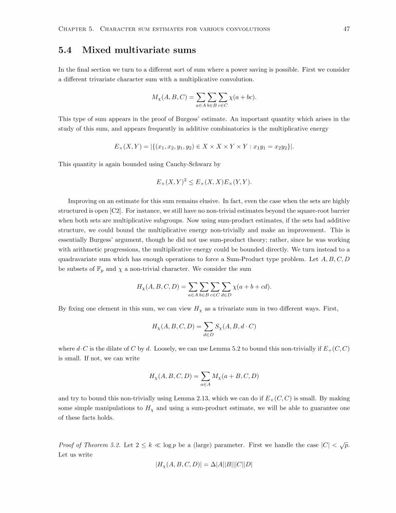
Chapter 5. Character sum estimates for various convolutions 47
5.4 Mixed multivariate sums
In the final section we turn to a different sort of sum where a power saving is possible. First we consider
a different trivariate character sum with a multiplicative convolution.
Mχ(A,B,C) =∑a∈A
∑b∈B
∑c∈C
χ(a+ bc).
This type of sum appears in the proof of Burgess’ estimate. An important quantity which arises in the
study of this sum, and appears frequently in additive combinatorics is the multiplicative energy
E×(X,Y ) = |{(x1, x2, y1, y2) ∈ X ×X × Y × Y : x1y1 = x2y2}|.
This quantity is again bounded using Cauchy-Schwarz by
E×(X,Y )2 ≤ E×(X,X)E×(Y, Y ).
Improving on an estimate for this sum remains elusive. In fact, even the case when the sets are highly
structured is open [C2]. For instance, we still have no non-trivial estimates beyond the square-root barrier
when both sets are multiplicative subgroups. Now using sum-product estimates, if the sets had additive
structure, we could bound the multiplicative energy non-trivially and make an improvement. This is
essentially Burgess’ argument, though he did not use sum-product theory; rather, since he was working
with arithmetic progressions, the multiplicative energy could be bounded directly. We turn instead to a
quadravariate sum which has enough operations to force a Sum-Product type problem. Let A,B,C,D
be subsets of Fp and χ a non-trivial character. We consider the sum
Hχ(A,B,C,D) =∑a∈A
∑b∈B
∑c∈C
∑d∈D
χ(a+ b+ cd).
By fixing one element in this sum, we can view Hχ as a trivariate sum in two different ways. First,
Hχ(A,B,C,D) =∑d∈D
Sχ(A,B, d · C)
where d ·C is the dilate of C by d. Loosely, we can use Lemma 5.2 to bound this non-trivially if E+(C,C)
is small. If not, we can write
Hχ(A,B,C,D) =∑a∈A
Mχ(a+B,C,D)
and try to bound this non-trivially using Lemma 2.13, which we can do if E×(C,C) is small. By making
some simple manipulations to Hχ and using a sum-product estimate, we will be able to guarantee one
of these facts holds.
Proof of Theorem 5.2. Let 2 ≤ k � log p be a (large) parameter. First we handle the case |C| < √p.Let us write
|Hχ(A,B,C,D)| = ∆|A||B|||C||D|

Chapter 5. Character sum estimates for various convolutions 48
so that our purpose is to estimate ∆. Let
C1 =
{c ∈ C : |Sχ(A,B, c ·D)| ≥ ∆|A||B||D|
2
}.
We have1
2|Hχ(A,B,C,D)| ≤
∑c∈C1
|Sχ(A,B, c ·D)|,
and using that the inner quantities are at most |A||B||D|, we have
|C1| ≥∆
2|C|.
Now, passing to a subset C2 of C1 of size at least |C1|16 ≥
∆32 |C|, we can assume that the complex numbers
Sχ(A,B, c ·D) with c ∈ C2 all have arguments within 12 of each other, so that for any C ′2 ⊂ C2 we have
|C ′2|2|C||Hχ(A,B,C,D)| = |C ′2|
∆|A||B||D|2
≤∑c∈C′2
|Sχ(A,B, c ·D)|
and so by Lemma 5.3 we have
|C ′2|4|C||Hχ(A,B,C,D)| ≤
∣∣∣∣∣∣∑c∈C′2
Sχ(A,B, c ·D)
∣∣∣∣∣∣ = |Hχ(A,B,C ′2, D)|. (5.1)
In particular, if C ′2 = C2 we have
∆2
128|A||B||C||D| ≤ |C
′2|
4|C||Hχ(A,B,C,D)| ≤
∑d∈D
|Sχ(A,B, d · C2)|.
Now in view of Lemma 5.2, we see that
∆2
128|A||B||C||D| ≤ |D|max
d∈D
√p|A|E+(B, d · C2) ≤ √p|D||A|1/2|B|3/4E+(C2, C2)1/4.
Thus
E+(C2, C2) ≥ ∆8
1284|A|2|B||C|4p−2 ≥
(∆8
1284|A|2|B||C|p−2
)|C2|3.
For convenience, write K−1 = ∆8
1284 |A|2|B||C|p−2. By Theorem 2.5 there is a subset C3 ⊂ C2 of size at
least |C2|K(log p)2 and such that
|C3 − C3| � K4 |C3|2(log p)8
|C2|2|C3|.
In particular, by Theorem 2.6 we have
E×(C3, C3)� |C3|K7
(|C3|2(log p)8
|C2|2
)7/4
|C3|7/4 log p = K7|C3|25/4|C2|−7/2(log p)15.

Chapter 5. Character sum estimates for various convolutions 49
Now we take C ′2 = C3 in equation (5.1) so that we get
∆
4|A||B||C3||D| =
|C3|4|C||Hχ(A,B,C,D)| ≤ |Hχ(A,B,C3, D)| ≤
∑a∈A|Mχ(a+B,C3, D)|.
Now we apply Lemma 2.13 to obtain that
∆
4|A||B||C3||D| � |A|(|D||C3|)1− 1
k (E×(D,D)E×(C3, C3))1/4k(|B|2k2k
√p+ (2k|B|)kp
)1/2kwhich implies (after bounding E×(D,D) trivially by |D|3)
∆4k � |D|−1|C3|−4E×(C3, C3)(2k√p+ (2k|B|−1)kp
)2.
Since 2 ≤ k � log p and |B| ≥ pδ, the final factor is at most O(p(log p)2k) as long as k > 12δ , and after
inserting the upper bound for E×(C3, C3) we have
∆4k � |D|−1K7|C3|9/4|C2|−7/2(log p)2k+15p.
Now we substitute K−1 = ∆8
1284 |A|2|B||C|p−2 and see
∆4k+56 � |D|−1|A|−14|B|−7|C|−7|C3|9/4|C2|−7/2(log p)2k+15p15.
Bounding |C3| ≤ |C2| and |C2| � ∆|C| we get
∆4k+ 2294 � |D|−1|A|−14|B|−7|C|− 33
4 (log p)2k+15p15.
Upon taking 4k’th roots we have
∆1+229/16k �(|D|−1|A|−14|B|−7|C|− 33
4 p15)1/4k
(log p)1/2+15/4k.
Since
|D|4|A|56|B|28|C|33 ≥ p60+ε,
the quantity in brackets on the right is at most p−ε/4. This shows that we must have ∆ < p−τ for some
τ > 0 depending only on ε and δ. This is because we only needed k to be sufficiently large in terms of δ.
If |C| > √p then we can break C into a disjoint union of m ≈ |C|√p sets C1, . . . , Cm of size at most
√p. Then
|Hχ(A,B,C,D)| ≤∑j
|Hχ(A,B,Cj , D)|.
We obtain a savings of p−τ for each Hχ(A,B,Cj , D) and hence for Hχ(A,B,C,D) provided
|D|4|A|56|B|28|Cj |33 � |D|4|A|56|B|28p33/2 ≥ p60+ε
which is guaranteed by hypothesis (with 2ε in place of ε).

Bibliography
[AS] N. Alon and J. Spencer, The Probabilistic Method, 3rd edition, John Wiley and Sons, Inc., 2008.
[Bou1] J. Bourgain, On arithmetic progressions in sums of sets of integers, A tribute to Paul Erds,
105-109, Cambridge Univ. Press, Cambridge, 1990.
[Bou2] J. Bourgain,On triples in arithmetic progression, Geom. Funct. Anal. 9 (1999), no. 5, 968-984.
[Bou3] J. Bourgain,Multilinear exponential sums in prime fields under optimal entropy condition on the
sources, Geom. Funct. Anal. 18 (2009), no. 5, 1477-1502.
[BG] J. Bourgain and M.Z. Garaev,On a variant of sum-product estimates and explicit exponential sum
bounds in prime fields, Math. Proc. Cambridge Philos. Soc. 146 (2009), no. 1, 1-21.
[BGK] J. Bourgain, A. A. Glibichuk and S. V. Konyagin, Estimates for the number of sums and products
and for exponential sums in fields of prime order, J. Lond. Math. Soc. (2) 73 (2006), no. 2, 380-398.
[BKT] J. Bourgain, N. Katz and T. Tao, A sum-product estimate in finite fields, and applications, Geom.
Funct. Anal. 14 (2004), no. 1, 27-57.
[Bu1] D. A. Burgess, On character sums and L-series, Proc. London Math. Soc. (3) 12 1962 193-206.
[Bu2] D. A. Burgess, On character sums and L-series. II, Proc. London Math. Soc. (3) 13 1963 524-536.
[C1] M.-C. Chang, On a question of Davenport and Lewis and new character sum bounds in finite fields,
Duke Math. J. 145 (2008), no. 3, 409-442.
[C2] M.-C. Chang, Character sums in finite fields, Finite fields: theory and applications, 83-98, Con-
temp. Math., 518, Amer. Math. Soc., Providence, RI, 2010.
[CLR] E. Croot, N. Lyall and A. Rice, A purely combinatorial approach to simultaneous polynomial
recurrence modulo 1, arXiv:1307.0779.
[E] P. Erdos, An asymptotic inequality in the theory of numbers, (Russian. English summary) Vestnik
Leningrad. Univ. 15 1960 no. 13, 41-49.
[ES] P. Erdos and E. Szemeredi, On sums and products of integers, Studies in pure mathematics, 213-
218, Birkhuser, Basel, 1983.
50

Bibliography 51
[FI] J. Friedlander and H. Iwaniec, Estimates for character sums, Proc. Amer. Math. Soc. 119 (1993),
no. 2, 365-372.
[G1] M. Z. Garaev, An explicit sum-product estimate in Fp, Int. Math. Res. Not. IMRN 2007, no. 11,
Art. ID rnm035, 11 pp.
[G2] M. Z. Garaev, The sum-product estimate for large subsets of prime fields, Proc. Amer. Math. Soc.
136 (2008), no. 8, 2735-2739.
[GT] B. Green and T. Tao, New bounds for Szemeredis theorem. II. A new bound for r4(N), Analytic
number theory, 180-204, Cambridge University Press, Cambridge, 2009.
[HLS] N. Hindman, I. Leader, I. and D. Strauss, Open Problems in Partition Regularity, Combinatorics,
Probability and Computing, no. 12, 571-583.
[IK] H. Iwaniec and E. Kowalski, Analytic Number Theory, American Mathematical Society Colloquium
Publications. Amer. Math. Soc., Providence, RI, 2004.
[KS] N. H. Katz and C.-Y. Shen, A slight improvement to Garaevs sum product estimate, Proc. Amer.
Math. Soc. 136 (2008), 2499-2504.
[K] S.V. Konyagin, Estimates for character sums in finite fields, (Russian) Mat. Zametki 88 (2010),
no. 4, 529–542; translation in Math. Notes 88 (2010), no. 3-4, 503-515
[KR] S.V. Konyagin and M. Rudnev, On new sum-product-type estimates, SIAM J. Discrete Math. 27
(2013), no. 2, 973-990.
[LN] R. Lidl and H. Neiderreiter, Finite fields, Encyclopedia of mathematics and its applications. Cam-
bridge University Press, 1997.
[LM] N. Lyall and A. Magyar, Simultaneous polynomial recurrence, Bull. Lond. Math. Soc. 43 (2011),
no. 4, 765-785.
[LRN] L. Li and O. Roche-Newton, An improved sum-product estimate for general finite fields, SIAM J.
Discrete Math. 25 (2011), no. 3, 1285-1296.
[N] M. B. Nathanson, Elementary Methods in Number Theory, Graduate Texts in Mathematics.
Springer, 2000.
[P] R. E. A. C. Paley, A theorem on characters, J. Lond. Math. Soc. 7 (1932), 28-32.
[RNRS] O. Roche-Newton, M. Rudnev and I. Shkredov, New sum-product type estimates over finite
fields, arXiv:1408.0542v1.
[R] M. Rudnev, An improved sum-product inequality in fields of prime order, Int. Math. Res. Not.
IMRN 2012, no. 16, 3693-3705.

Bibliography 52
[Sar] A. Sarkozy, On additive decompositions of the set of quadratic residues modulo p, Acta Arith. 155
(2012), no. 1, 41-51.
[Sch] W. M. Schmidt, Small fractional parts of polynomials, CBMS Regional Conference Series in Math.,
32, Amer. Math. Soc., 1977.
[Sh] X. Shao, On character sums and exponential sums over generalized arithmetic progressions, Bull.
Lond. Math. Soc. (2013) 45 (3): 541-550.
[Shk] I. D. Shkredov, On monochromatic solutions of some nonlinear equations in Z/pZ, Mathematical
Notes, 88,(2010), no. 3-4, 603611.
[Shk2] I. D. Shkredov, Sumsets in quadratic residues, Acta Arith. 164 (2014), no. 3, 221-243.
[So] J. Solymosi, Bounding multiplicative energy by the sumset, Adv. Math. 222 (2009), no. 2, 402-408.
[Shp] I. Shparlinski, Additive decompositions of subgroups of finite fields, SIAM J. Discrete Math. 27
(2013), no. 4, 1870-1879.
[TV] T. Tao and V. Vu, Additive Combinatorics, Cambridge Studies in Advanced Mathematics, 105.
Cambridge University Press, Cambridge, 2006.
[V] I. M. Vinogradov, An Introduction to the Theory of Numbers, 6th edition (translated from Russian),
Pergamon Press, 1952.