by juan nicol as quesada mej a - university of toronto t-space · patrik, robert, juliette au...
TRANSCRIPT

Very Nonlinear Quantum Optics
by
Juan Nicolas Quesada Mejıa
A thesis submitted in conformity with the requirementsfor the degree of Doctor of Philosophy
Graduate Department of PhysicsUniversity of Toronto
c© Copyright 2015 by Juan Nicolas Quesada Mejıa

Abstract
Very Nonlinear Quantum Optics
Juan Nicolas Quesada Mejıa
Doctor of Philosophy
Graduate Department of Physics
University of Toronto
2015
This thesis presents a study of photon generation and conversion processes in nonlinear
optics. Our results extend beyond the first order perturbative regime, in which only
pairs of photons are generated in spontaneous parametric down-conversion or four wave
mixing. They also allow us to identify the limiting factors for achieving unit efficiency
frequency conversion, and to correctly account for the propagation of bright nonclassi-
cal photon states generated in the nonlinear material. This is done using the Magnus
expansion, which allows us to incorporate corrections due to time-ordering effects in the
time evolution of the state, while also respecting the quantum statistics associated with
squeezed states (in photon generation) and single photons or coherent states (in pho-
ton conversion). We show more generally that this expansion should be the preferred
strategy when dealing with any type of time-dependent Hamiltonian that is a quadratic
form in the creation and annihilation operators of the fields involved. Using the Mag-
nus expansion, simple figures of merit to estimate the relevance of these time-ordering
corrections are obtained. These quantities depend on the group velocities of the modes
involved in the nonlinear process and provide a very simple physical picture of the in-
teractions between the photons at different times. These time-ordering effects are shown
to be important only when the photons and pump beam overlap within the nonlinear
material for a significant amount of time. We also discuss the possibility of preparing
Fock states with many photons using parametric down-conversion sources and realistic
photon-number-resolving detectors. After discussing photon generation processes, we
study photon conversion processes in which a nonlinear material and a classical strong
ii

pump field are used modify the frequency of a second incoming low-intensity field. We
show that time-ordering effects limit the efficiency of this conversion process, re-examine
strategies to get around this problem, and show that it should be possible to have a clear
observation of modified upconversion probabilities due to these effects, and thus have an
experimental demonstration of time-ordering effects in nonlinear optics.
iii

Acknowledgements
This is the first or second page to be read, but the last one written. I will try to thank
all the people that made my five years in Toronto a fantastic experience, but I will forget
something; so, in the best of Canadian manners, this is a preemptive “I am sorry”.
First of all, I would like to thank the members of my supervisory committee, Prof.
Daniel F.V. James, Prof. John. E. Sipe and Prof. Aephraim M. Steinberg. I learned a
lot from you all regarding physics, but you also taught me about the tortuous ways of the
English language, how to present my ideas coherently, and how to be a better scientist
and person in general.
I would also like to thank Prof. Anna Sanpera and Prof. Andrew White for their
kind hospitality during my visits to Barcelona and Brisbane respectively, and also extend
my gratitude to Prof. Christine Silberhorn, Benjamin Brecht, Vahid Ansari and John
Donohue for many valuable conversations over Skype and for sharing their experimental
insight with this clueless theorist.
I would like to thank the people of Canada for the generous support they provide
to basic scientific research. J’aimerais remercier les gens du Canada pour leur genereux
soutien envers la recherche scientifique fondamentale.
Five years is a long time, during which I have learned a lot, in physics, English (I still
have a lot to learn about these two), and cryogenics (thanks Canadian winter). Even
more importantly, I have made friends that are by now family. I will start this list
chronologically, but I am bound to skip around sooner or later.
Juan Mi and Aleks, seeing you always makes me realize that the world out there is
always full of possibilities for joy and happiness. I hope that never changes!
Sir Shreyas and Juan Matincito, you are two of the finest physicists I have ever met
and also the best possible company for a pint after the daily grind of grad school.
Liebe Sigrid, not only did you introduce me to a certain Canadienne, but you also
made a deep impression on me with your awesome Austrian hospitality. I can only look
forward to my next visit to Graz. Also, I should thank your grandpa’s company for
furnishing great supplies for theoretical physics research ;).
Thanks to all the Toronto people: Mariu (and her friends and family in Madrid),
Patrik, Robert, Juliette au chocolat...
Muchas gracias a mi familia navidena adoptiva Mexicana-Torontoniana: Marıa de
Avi, Emi, Pablo, Itzel, Alejandro y Lina, los extranaremos mucho. Por ustedes sabemos
que siempre tendremos que volver a Toronto (e ir a Bruselas o donde sea que andes
Marıa).
iv

My deepest gratitude also goes to my lunch companions over the years: the muppets
from the 10th floor (Praheen, Zanai, Zachary, Steve “T. Rex” Foster, Ciaran).
Thanks a lot MattheW: I will miss our conversations over lunch time and your careful
debunking of my crazy ideas.
I would also like to thank the members of my group, the “senior” students, Asma,
Omar and Kero, and especially the “junior” ones, Jas, Kevin, Mike and Dave; you taught
me a lot, and I look forward to future encounters!
Thank you Aggie for being so generous with your ideas and friendship. I look forward
to future collaborations :P.
Tanya and Matt, my favourite real and fake Ukrainians, I am grateful for all the great
times. I can only wish you the best in your future with your loved ones!
Dr. Federico, Dra. Cata y Dr. Caja, muchas, muchas gracias por su amistad, siempre
fue lindo encontrar gente en el departamento con quien ejercitar el espanol del terruno
(o el parlache).
Muchas gracias mama y papa, a pesar de la distancia su apoyo incondicional siempre
lo sentı muy cerca. Los quiero mucho!
Ma Catou, sans toi, tout ceci aurait non seulement ete extremement difficile mais ca
n’aurait egalement eu aucun sens. Je t’aime.
v

Preface
This preface contains a list of the peer reviewed articles and conference proceedings that
I have authored or coauthored during my Ph.D. studies.
List of publications in peer reviewed journals
• Nicolas Quesada and J.E. Sipe. Time-ordering effects in the generation of entangled
photons using nonlinear optical processes. Phys. Rev. Lett., 114(9):093903, 2015.
• Jaspreet Sahota and Nicolas Quesada. Quantum correlations in optical metrology:
Heisenberg-limited phase estimation without mode entanglement. Phys. Rev. A,
91(1):013808, 2015.
• Nicolas Quesada and J.E. Sipe. Effects of time-ordering in quantum nonlinear
optics. Phys. Rev. A, 90(6):063840, 2014.
• Nicolas Quesada and Anna Sanpera. Bound entanglement in the Jaynes–Cummings
model. J. Phys. B: At. Mol. Opt. Phys., 46(22):224002, 2013.
• Nicolas Quesada, Agata M. Branczyk, and Daniel F.V. James. Self-calibrating
tomography for multidimensional systems. Phys. Rev. A, 87(6):062118, 2013.
• Nicolas Quesada, Asma Al-Qasimi, and Daniel F.V. James. Quantum properties
and dynamics of X states. J. Mod. Opt., 59(15):1322–1329, 2012.
• Nicolas Quesada. Strong coupling of two quantum emitters to a single light mode:
The dissipative Tavis-Cummings ladder. Phys. Rev. A, 86(1):013836, 2012.
• Paulo C. Cardenas, Nicolas Quesada, Herbert Vinck-Posada, and Boris A. Rodrıguez.
Strong coupling of two interacting excitons confined in a nanocavity–quantum dot
system. J. Phys. Condens. Matter, 23(26):265304, 2011.
List of publications in peer reviewed conference proceedings
• Nicolas Quesada and J.E. Sipe. Observing the effects of time-ordering in single
photon frequency conversion. In CLEO: Science and Innovations, pages JTu5A–3.
Optical Society of America, 2015.
• Nicolas Quesada and Jaspreet Sahota. Particle vs. mode entanglement in opti-
cal quantum metrology. In CLEO: QELS Fundamental Science, pages FM1A–3.
Optical Society of America, 2015.
vi
• Nicolas Quesada, Agata M. Branczyk, and Daniel F.V. James. Holistic quantum
state and process tomography. In Frontiers in Optics, pages FW1C–6. Optical
Society of America, 2013.
• Nicolas Quesada. Quantum correlations in a mixed full rank qubit-qudit system:
Discord and entanglement in the Jaynes-Cummings model. In Quantum Informa-
tion and Measurement, pages W6–33. Optical Society of America, 2013.
• Nicolas Quesada, Daniel F.V. James, and Agata M. Branczyk. Self-calibrating
tomography for non-unitary processes. In Quantum Information and Measurement,
pages W6–38. Optical Society of America, 2013.
• Nicolas Quesada, Paulo C. Cardenas, Boris A. Rodrıguez, and Herbert Vinck-
Posada. Strong coupling criterion for two interacting excitons in a nanocavity. In
Frontiers in Optics, page JTuA22. Optical Society of America, 2011.
• Nicolas Quesada and Daniel F.V. James. An equation of motion for the concurrence
of 2 qubit pure states. In Frontiers in Optics, page FThS3. Optical Society of
America, 2011.
vii

En el buen tiempo viejo, un senor trabajaba un ano en un escritorio,haciendo calculos, y luego enviaba un telegrama a un observatorio: “Dirijanel telescopio a la posicion tal y veran un planeta desconocido”. Los planetaseran muy corteses y tomaban lugar donde se les indicaba, como en un balletbien organizado. Hoy, las partıculas atomicas aparecen de subito y como porescotillon, haciendo piruetas. La fısica de antano tenıa algo de fiesta de saloncon musica de Mozart, mientras que ahora parece una feria de diversiones,con salas de espejos, laberintos de sorpresas, tiro al blanco y hombres quepregonan fenomenos. Y a la astronomıa, que era una recatada nina de suhogar, laboriosa y modesta, le ha salido ahora un hermano menor que ensuciala casa, convierte el altillo en polvorın, hace preguntas insoportables e inventacuentos descabellados.
Ernesto Sabato, Fısica Escandalosa, Uno y el universo
viii

Contents
1 Introduction 1
2 Quantum Mechanics of the Harmonic Oscillator 10
2.1 The Harmonic Oscillator . . . . . . . . . . . . . . . . . . . . . . . . . . . 10
2.1.1 Classical Mechanics . . . . . . . . . . . . . . . . . . . . . . . . . . 10
2.1.2 Quantum Mechanics . . . . . . . . . . . . . . . . . . . . . . . . . 11
2.1.3 The Forced Harmonic Oscillator: Time-Ordering Effects . . . . . 15
2.2 Two Harmonic Oscillators: Squeezing and Beam Splitters . . . . . . . . . 17
2.2.1 Beam-splitter transformations . . . . . . . . . . . . . . . . . . . . 17
2.2.2 Squeezing transformations . . . . . . . . . . . . . . . . . . . . . . 19
2.2.3 Generating functions and Gaussian states . . . . . . . . . . . . . 20
2.2.4 Lossy two-mode squeezed vacuum states . . . . . . . . . . . . . . 21
2.3 Continuous variable Gaussian transformations and states . . . . . . . . . 23
2.3.1 Multimode Beam Splitters and Squeezers . . . . . . . . . . . . . . 24
3 Nonlinear optics 29
3.1 Classical Fields . . . . . . . . . . . . . . . . . . . . . . . . . . . . . . . . 29
3.2 Quantization . . . . . . . . . . . . . . . . . . . . . . . . . . . . . . . . . 31
3.3 The nonlinear interaction . . . . . . . . . . . . . . . . . . . . . . . . . . . 31
3.4 The interaction Hamiltonian for a χ2 process . . . . . . . . . . . . . . . . 32
3.5 The interaction Hamiltonian for a χ3 process . . . . . . . . . . . . . . . . 36
4 The Magnus expansion 40
4.1 Introduction . . . . . . . . . . . . . . . . . . . . . . . . . . . . . . . . . . 40
4.2 Properties of the Magnus expansion . . . . . . . . . . . . . . . . . . . . . 42
4.3 Time ordering in Parametric Down-Conversion and Four Wave Mixing . 46
4.4 Time ordering in Frequency Conversion . . . . . . . . . . . . . . . . . . . 52
4.5 Disentangling the Magnus expansion . . . . . . . . . . . . . . . . . . . . 54
ix

4.6 Time-ordering corrections in broadly phase-matched Processes . . . . . . 60
4.7 Relation between this work and that of Christ et al. . . . . . . . . . . . . 61
5 Generation of bright non-classical light 64
5.1 Introduction . . . . . . . . . . . . . . . . . . . . . . . . . . . . . . . . . . 64
5.2 Model . . . . . . . . . . . . . . . . . . . . . . . . . . . . . . . . . . . . . 65
5.3 Time-ordering effects in spontaneous photon generation . . . . . . . . . . 68
5.4 Time-ordering effects in stimulated photon generation . . . . . . . . . . . 70
5.5 Experimental proposal . . . . . . . . . . . . . . . . . . . . . . . . . . . . 72
5.6 Measuring the effects of the time-ordering corrections . . . . . . . . . . . 74
5.7 Heralded generation of Fock states . . . . . . . . . . . . . . . . . . . . . 79
6 Highly efficient frequency conversion 88
6.1 Introduction . . . . . . . . . . . . . . . . . . . . . . . . . . . . . . . . . . 88
6.2 Ideal frequency conversion . . . . . . . . . . . . . . . . . . . . . . . . . . 89
6.3 Time ordering in Frequency Conversion . . . . . . . . . . . . . . . . . . . 91
6.4 Achieving near unit efficiency in Frequency Conversion . . . . . . . . . . 94
7 Conclusions and future directions 98
A Energy in an Electromagnetic pulse 102
B Numerical calculation of the Schmidt decomposition 105
C The Magnus library 107
C.1 Gaussian approximation for the third order Magnus term . . . . . . . . . 107
C.2 General calculation of the Second and Third order Magnus terms . . . . 109
D Analytical calculation of the third order Magnus correction 111
Bibliography 118
x

List of Tables
2.1 In this table we summarize how the annihilation operators transform under
different Gaussian operations. In all cases the operators are mapped to
linear combinations of creation and annihilation operators of the modes. . 21
2.2 Transformation of the annihilation operators for the different multimode
operations considered in Eq. (2.75) and Eq. (2.77). Note the similarities
with Table 2.1 and the fact that annihilation operators are mapped to
linear combinations of creation and annihilation operators. . . . . . . . . 28
5.1 Parameters for Periodically poles Lithium Niobate (PPLN) to observe sig-
nificant time-ordering effects. To obtain zeroth order phase-matching a
periodicity of Λ = 1/|ne(λp)/λp − no(λa)/λa − ne(λb)/λb| = 58.25µm is
required. no/e are the indices of refraction of the two different polarizations. 73
xi

List of Figures
2.1 This diagram illustrates how to model losses for a two-mode squeezed
vacuum state. First the TMSV state is prepared, generating entanglement
(symbolized by the loop). Then each mode is sent to a beam splitter
where the other input is vacuum. We then trace out the extra harmonic
oscillators (symbolized by the trash bin) and look at the resultant state
in modes a and b which is in general less entangled and represented by a
mixed density matrix ρ. . . . . . . . . . . . . . . . . . . . . . . . . . . . 22
4.1 Diagrams representing the first, second and third order Magnus terms for
PDC. Dashed lines are used to represent pump photons, full lines are used
to represent lower energy down converted ones. (a) depicts a photon of
frequency ωp being converted to two photons of frequencies ωa and ωb.
(b) depicts the second order Magnus term in which one of the photons
from a down-conversion event is, with the help of a low energy photon
previously present, up converted to a pump photon. Finally, (c) depicts
the third order Magnus term in which a pair of photons from two previous
down-conversion events is converted to a pump photon. . . . . . . . . . 49
4.2 Diagrams representing the first, second and third order Magnus terms for
FC. Dashed lines are used to represent pump photons, full lines are used to
represent photons in fields a and b. (a) depicts a photon from the classical
beam ωp being fused with a photon with frequency ωa to create a photon
of energy ωb. (b) depicts the second order Magnus term in which one of
the up-converted photons decays into to two photons one in field a and one
in the classical pump field p. Finally, (c) depicts the third order Magnus
term in which two up-conversion processes with a down-conversion process
in the middle occur. . . . . . . . . . . . . . . . . . . . . . . . . . . . . . 54
5.1 Comparison of a sinc function and the gaussian fit exp(−γx2). . . . . . 65
xii

5.2 First and third order Magnus terms for the parameters from Table 5.1.
Note that the function J1 has been normalized by ετ and J3, K3 by ε3τ 3/µaµb.
For the case when when the lowest order JSA (J1) is round one has
µa = µb =√
2τ . . . . . . . . . . . . . . . . . . . . . . . . . . . . . . . . . 73
5.3 Mean number of photons and Schmidt number for the parameters of the
JSA in Fig. 5.2 as a function of s0ε in A and B. In C we plot the Schmidt
number as a function of s0ε including (continuous lines) and excluding
(dashed lines) time-ordering effects. Note that there are two continu-
ous lines precisely because the time-ordering corrections generate an extra
Schmidt mode. In the limit ε 1 this Schmidt mode disappears because
its Schmidt number becomes zero. . . . . . . . . . . . . . . . . . . . . . 77
5.4 Asymmetry parameter A as a function of ε. If time-ordering effects where
ignored this parameter would be zero. . . . . . . . . . . . . . . . . . . . . 78
5.5 Schematic representation of the heralded preparation of a Fock state with
N photons using an inefficient detector, modeled as a perfect detector
preceded by a loss channel. . . . . . . . . . . . . . . . . . . . . . . . . . . 80
5.6 Probabilities of obtaining the results N = 1, 5, 10 when measuring the
photon number in field a for the state Eq. (5.34) ignoring time-ordering
corrections. The probability is plotted as a function of the squeezing pa-
rameter s0ε and the transmissivity T used to parametrize the finite effi-
ciency of the detector. The case T = 1 corresponds to ideal detectors. . . 82
5.7 Mandel Q parameter and purity of field b for the heralding outcomes N =
1, 5, 10 when measuring the photon number for field a in the state Eq.
(5.34) ignoring time-ordering corrections. These parameters are plotted
as a function of the squeezing parameter s0ε and the transmissivity T
used to parametrize the finite efficiency of the detector. The case T = 1
corresponds to ideal detectors. . . . . . . . . . . . . . . . . . . . . . . . . 82
5.8 Probabilities of obtaining the results N = 1, 5, 10 when detecting the pho-
ton number in field a for the state Eq. (5.40) including time-ordering
corrections. The probability is plotted as a function of the squeezing pa-
rameter s0ε and the transmissivity T used to parametrize the finite effi-
ciency of the detector. The case T = 1 corresponds to ideal detectors. . . 86
xiii
5.9 Mandel Q parameter and purity of field b for the heralding outcomes N =
1, 5, 10 when measuring the photon number in field a for the state Eq.
(5.40) including time-ordering corrections. These parameters are plotted
as a function of the squeezing parameter s0ε and the transmissivity T
used to parametrize the finite efficiency of the detector. The case T = 1
corresponds to ideal detectors. . . . . . . . . . . . . . . . . . . . . . . . . 86
6.1 In A we plot the probability of upconversion as a function of the in-
teraction strength r0ε, for a single photon in the Gaussian wave packet
f(α) including and excluding time-ordering corrections. In B we plot
the Schmidt numbers of J including (dashed lines) and excluding (full
line) time-ordering corrections. In the inset we plot the overlap between
the time ordered corrected Schmidt functions and the Gaussian profile of
the incoming single photon. Finally in C and D we plot the real and
imaginary parts of the Schmidt functions for different values of r0ε. For
r0ε = 0.02, 0.5 1 they are very similar to the Gaussian shape of the
input single photon. . . . . . . . . . . . . . . . . . . . . . . . . . . . . . . 96
xiv

List of Acronyms
BS: Beam splitter
FC: Frequency conversion
FWHM: Full width at half maximum
FWM: Four wave mixing
JCA: Joint conversion amplitude
JSA: Joint spectral amplitude
ME: Magnus expansion
PDC: Parametric down-conversion
PPLN: Periodically Poled Lithium Niobate
PVM: Projective-valued Measure
QIP: Quantum information processing
RA: Rotation in field a
RB: Rotation in field b
SFWM: Spontaneous four wave mixing
SPDC: Spontaneous parametric down-conversion
SQ: Squeezer/Squeezing
TMSV: Two-mode squeezed vacuum
xv

Chapter 1
Introduction
Etenim cognitio contemplatioque naturae manca quodam modo atque in-choata sit, si nulla actio rerum consequatur.
Cicero, De Officiis, 1.153
Nonlinear photonic materials are some of the most versatile sources of nonclassical
light. They allow the production of entangled states of light [1, 2, 3, 4] with very strong
correlations beyond what any local realist theory could allow [5, 6]. Aided with high
efficiency light detectors, they can be used to generate (to a very good approximation)
states with a well defined number of light quanta; that is, states having no fluctuations
in photon number [7, 8, 9, 10, 11, 12]. These photons can then be used as ultra-secure
information carriers [13] or as information processors in their own right [14, 15, 16].
Moreover, the flexibility of these sources allows us to use them to teach experimental
quantum physics to undergraduate students [17], yet also perform stringent tests of the
strong non-classical correlations that entangled states can exhibit [4].
Besides being useful for generating quantum states of light, these materials have
proven very useful for transforming and manipulating different degrees of freedom of
light, in particular to change the central frequency and spectral profile [18, 19, 20]. For
instance, nonlinear photonic materials can be used to double or halve the frequency of a
single photon by borrowing or dumping the extra energy into a classical co-propagating
electromagnetic field [21, 22, 23]; this process is known as frequency conversion (FC)
[24, 25, 26]. FC is an important building block in several quantum information appli-
cations like deterministic implementations of controlled Z gates [27] and quantum pulse
gates [20] between single photons. It is also useful in converting signals in regions of
the electromagnetic spectrum where there are no good detectors, (for example around
telecommunication wavelengths), to regions where there are good detectors (for example
1

Chapter 1. Introduction 2
the visible) [26, 28]. In the same way that frequency conversion can be thought as a fusion
process, one can also understand the photon generation processes described in the previ-
ous paragraph as a photon fission process in which a high energy photon spontaneously
“decays” into two low energy photons. This process is called Spontaneous Parametric
Down-Conversion (SPDC). Because energy and linear momentum are preserved in the
fission process, the two daughter photons have frequencies and wavevectors that add to
the frequency and wavevector of the original photon. The two daughter photons are also
born almost at the same time; this combination of constraints is precisely what gives
these photons their non-classical correlations.
SPDC is not the only process that can give birth to very correlated photons. One can
also consider the case of a pair of identical pump photons that transform into photons at
different frequencies; this process is called Spontaneous Four Wave Mixing (SFWM). As
we shall show later, SFWM has many similarities with SPDC; in particular, both involve
destroying photons from a classical field and creating pairs of quantum-correlated light
particles [29, 30].
The properties of the photons generated by SPDC and SFWM are extremely interest-
ing, and one might wonder what allows these nonlinear materials to mediate interactions
between photons, particles that hardly interact amongst themselves? The reason why
this is possible is that the induced macroscopic polarization in these materials ~P (~r) is a
nonlinear function of the applied electric fields ~E(~r) (or equivalently of the displacement
field ~D(~r)). Thus, very generally one can write
P i(~r) = ε0χij1 (~r)Ej(~r) + ε0χ
ijk2 (~r)Ej(~r)Ek(~r) + . . . (1.1)
≈ Γij1 (~r)Dj(~r) + Γijk2 Dj(~r)Dk(~r) + . . . (1.2)
where ε0 is the permittivity of free space, χ2 is the 2nd order electric susceptibility, and
Ei(~r) is the ith Cartesian component of the electric field. In the second line, we rewrote
the polarization in terms of the displacement vector D, and introduced the Γ tensors
relating the polarization and the different powers of the displacement field; in both equa-
tions we have used the Einstein summation convention. If we assume that there are two
incident fields in the material at frequencies ωa and ωb, Eq. (1.1) tells us that the dipoles
in the material can oscillate and radiate at frequencies ωa ± ωb. This fact allows the
matter degrees of freedom to generate harmonics, which were observed in the pioneering
work of Franken et al. in 1961 [31]. Note that if there are only fields at one frequency
ω, one can only expect to see radiation in multiples nω in this classical picture. As we
shall argue later, this will change once we consider the quantum mechanical picture and

Chapter 1. Introduction 3
include vacuum fluctuations.
Having the polarization written as in Eq. (1.1), we can write the nonlinear part of
the Hamiltonian as[32]
HNL = − 1
3ε0
ˆd~rΓijk2 Di(~r)Dj(~r)Dk(~r). (1.3)
After quantization, the displacement field in the structure can be written as a linear
combination of creation and annihilation operators for photons at different frequencies.
If we assume that the three displacement fields a, b, p in the crystal have the initial state
|0〉a ⊗ |0〉b ⊗ |α〉p (where |0〉 is the vacuum representing no photons in the field and |α〉is a coherent state representing the quantum analogue of a classical field), then it is not
hard to show that to first order in perturbation theory, there will be a correction to the
initial state due to the nonlinear Hamiltonian that will be given by
HNL |0〉a ⊗ |0〉b ⊗ |α〉p ∼(χ2a
† ⊗ b† ⊗ c)(|0〉a ⊗ |0〉b ⊗ |α〉p
)= χ2α |1〉a ⊗ |1〉b ⊗ |α〉p .
(1.4)
In the last equality we used the facts that the creation operators a† and b† create one pho-
ton when acting on vacuum and, that coherent states are eigenstates of the destruction
operator c. These states and the action of the different operators on them will be intro-
duced in the next chapter. Eq. (1.4) explicitly shows that to first order in perturbation
theory a pair of photons in fields a and b will be created.
The use of this type of interaction as a source of pairs of photons was first theoretically
proposed by Zel’dovich and Klyshko in 1969 [33] and experimentally demonstrated by
Burnham and Weinberg [34] a year later. In the decade that followed these experiments,
new sources of entangled photon pairs based on atomic transitions were used to perform
experimental tests of local realism based on the ideas of John S. Bell [5] refined by John F.
Clauser and coworkers [6]. In particular, Freedman and Clauser [35] used photons emit-
ted from an atomic cascade in calcium to show violations of restrictions imposed by local
realism on the correlations between polarization detectors in two distant locations. These
violations were put on even stronger footing by the work of Alain Aspect and coworkers
[36]. Two years after Aspect’s experiments, Brassard and Bennett proposed using entan-
gled pairs of photons to generate a secure secret key for the exchange of cryptographic
messages [13] using pairs of polarization-entangled photons. Quantum cryptography is
by now the most established quantum technology with commercial applications already

Chapter 1. Introduction 4
in the market. Interestingly, Acın et al. showed in 2006 that the security of quantum
key distribution relies on the fact that the data used to construct the key also violates a
Bell inequality [37].
Even though the original experiments on Bell’s inequalities were performed using
atomic sources of polarization-entangled photon pairs, nowadays the most advanced
sources of such photons are provided by nonlinear crystal schemes developed by P. Kwiat
and coworkers [2, 3, 4]. Finally, as mentioned at the beginning of this chapter, nonlinear
photonic materials can also be aided with photon detectors to generate pure heralded
single photons in a probabilistic manner as proposed and experimentally demonstrated
by I. Walmsley and coworkers [7, 8, 9, 10].
In the previous paragraph, we described how nonlinear photonic materials can be
used to generate single photons. Although these materials are by now one of the most
mature sources of single photons they will likely be superseded by solid state sources
[38, 39, 40]. The reason why this will probably happen is because the number purity
of a single photon state generated in SPDC decreases with the probability of generating
one in a heralded nondeterministic source. Even though nonlinear optical materials
might not be the optimal source of single photons they might be an excellent source
of bright non classical states of light. These states are typically squeezed states, which
have been shown to be extremely useful in quantum metrology [41, 42, 43] and quantum
computing [44, 45]. However, the theory describing the generation of bright states of
light in a nonlinear material is less developed than its counterpart for single or pairs
of photons. There are of course theoretical descriptions of the propagation of light in
nonlinear materials beyond the perturbative regime necessary to describe pair generation
or low efficiency frequency conversion. These treatments typically describe the evolution
of the electric field operators in the Heisenberg picture and have been used by McGuiness
et al. to treat frequency conversion [46, 47], by Lvovsky et al. for Type I degenerate
SPDC [48, 49], by Gatti et al. for Type I and II SPDC [50, 51], and by Christ et al. [52]
for Type II SPDC and FC. In the Heisenberg picture one will find equations of motion for
the spatio-temporal field operators. For example, in the case of SPDC in the undepleted
pump approximation and ignoring group velocity dispersion these equations are
∂ψa(z, t)
∂t+ va
∂ψa(z, t)
∂z+ iωaψa(z, t) = iζ(z)ψp(z, t)ψ
†b(z, t), (1.5)
∂ψb(z, t)
∂t+ vb
∂ψb(z, t)
∂z+ iωbψb(z, t) = iζ(z)ψp(z, t)ψ
†a(z, t) (1.6)
where the field operators ψ†(z, t)a,b create photons in the space time location (z, t), the

Chapter 1. Introduction 5
classical pump field ψp(z, t) = ψp(z − vpt, 0) evolves freely (this fact is equivalent to
the undepleted pump approximation in this regime), va,b,p(ωa,b,p) are the group velocities
(central frequencies) of the different fields and ζ(z) describes the nonlinear interaction
between the different fields. This last quantity is zero for space locations outside the
length of the crystal. The important property of Eq. (1.5) is that the equations are
linear in the quantum fields ψ†(z, t)a/b, ψ(z, t)a/b and thus the quantum operators of the
outgoing field operators must be linear combinations of the incoming operators. This
linearity allows the authors to develop efficient numerical methods (or Green function
techniques) to find the state generated in SPDC and this is precisely the property that
is exploited in most of the studies just mentioned. These methods have the advantage
that they are numerically exact. They have the disadvantage that one cannot separate
the ideal operation of an SPDC device, given by the first order Magnus terms, from the
time ordering corrections and thus it is hard to understand how to minimize them.
In this thesis we take a different route to study the generation of bright states of
light and very high efficiency frequency conversion. Instead of propagating the equation
of motion for the quantum operators, we calculate the unitary time evolution operator
for the problem. Once we obtain this operator, we can reproduce the results obtained
before by propagating the electric field operators or we can instead directly propagate
the quantum state of the system. This approach has the added advantage of being much
closer to the formalism of quantum information where one likes to think of multipartite
states being modified by entangling and local operations [14]. Once having the state of
the generated photons we can also investigate how using recently developed technology
like photon-number resolving detectors [53] one can generate non-deterministically Fock
states with more than one photon[54]. These states can be useful for implementing
quantum enhanced metrology schemes [55] and also as bright non-Gaussian resource
states in continuous variable quantum computation [56].
The main difficulty in obtaining the unitary evolution operator for the nonlinear
processes we have considered is that the Hamiltonian describing this processes is typically
time dependent and does commute with itself at different times. To understand this
complication, let us consider the following interaction-picture Hamiltonian, which can be
derived from the one in Eq. (1.3):
HI(t) = ε
ˆdωadωbdωpe
i(ωa+ωb−ωc)tc(ωc)a†(ωa)b
†(ωb)Φ
(∆k(ωa, ωb, ωc)L
2
)+ H.c., (1.7)
Here, field c is the field where the strong coherent pump is injected and fields a and b
are the ones where photons will be generated. The quantity Φ (∆k(ωa, ωb, ωc)L/2) =
Chapter 1. Introduction 6
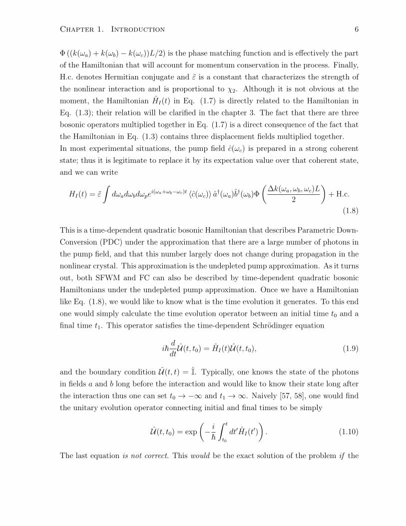
Φ ((k(ωa) + k(ωb)− k(ωc))L/2) is the phase matching function and is effectively the part
of the Hamiltonian that will account for momentum conservation in the process. Finally,
H.c. denotes Hermitian conjugate and ε is a constant that characterizes the strength of
the nonlinear interaction and is proportional to χ2. Although it is not obvious at the
moment, the Hamiltonian HI(t) in Eq. (1.7) is directly related to the Hamiltonian in
Eq. (1.3); their relation will be clarified in the chapter 3. The fact that there are three
bosonic operators multiplied together in Eq. (1.7) is a direct consequence of the fact that
the Hamiltonian in Eq. (1.3) contains three displacement fields multiplied together.
In most experimental situations, the pump field c(ωc) is prepared in a strong coherent
state; thus it is legitimate to replace it by its expectation value over that coherent state,
and we can write
HI(t) = ε
ˆdωadωbdωpe
i(ωa+ωb−ωc)t 〈c(ωc)〉 a†(ωa)b†(ωb)Φ(
∆k(ωa, ωb, ωc)L
2
)+ H.c.
(1.8)
This is a time-dependent quadratic bosonic Hamiltonian that describes Parametric Down-
Conversion (PDC) under the approximation that there are a large number of photons in
the pump field, and that this number largely does not change during propagation in the
nonlinear crystal. This approximation is the undepleted pump approximation. As it turns
out, both SFWM and FC can also be described by time-dependent quadratic bosonic
Hamiltonians under the undepleted pump approximation. Once we have a Hamiltonian
like Eq. (1.8), we would like to know what is the time evolution it generates. To this end
one would simply calculate the time evolution operator between an initial time t0 and a
final time t1. This operator satisfies the time-dependent Schrodinger equation
i~d
dtU(t, t0) = HI(t)U(t, t0), (1.9)
and the boundary condition U(t, t) = I. Typically, one knows the state of the photons
in fields a and b long before the interaction and would like to know their state long after
the interaction thus one can set t0 → −∞ and t1 →∞. Naively [57, 58], one would find
the unitary evolution operator connecting initial and final times to be simply
U(t, t0) = exp
(− i~
ˆ t
t0
dt′HI(t′)
). (1.10)
The last equation is not correct. This would be the exact solution of the problem if the

Chapter 1. Introduction 7
Hamiltonian commuted at different times
[HI(t), HI(t′)] = 0. (1.11)
It is straightforward to confirm that the Hamiltonian in Eq. (1.8) does not satisfy Eq.
(1.11) and thus Eq. (1.10) is not the solution to the Schrodinger equation. The correct
solution should precisely take into account the fact that Eq. (1.11) is not satisfied; thus,
formally one writes
U(t, t0) = T exp
(− i~
ˆ t
t0
dt′HI(t′)
), (1.12)
where T is the time-ordering operator.
Typically, the quantum optics community approximates the unitary evolution opera-
tor U(t, t0) using a power series of the Hamiltonian known as the Dyson series
U(t, t0) ≈ I− i
~
ˆ t
t0
dt′HI(t′) +
(−i~
)2 ˆ t
t0
dt′ˆ t′
t0
dt′′HI(t′)HI(t
′′) + . . . (1.13)
If the interaction were very weak so that first order perturbation theory were sufficient to
describe the output state, then the last equation would show directly that for very weak
pump intensities the output state would indeed be a pair of photons in fields a and b (see
Eq. (1.4)). One could hope that by including higher order terms in the series, one would
get an increasingly better approximation of the exact solution of the problem [59, 60].
As we shall show in detail in chapter 4, the Magnus expansion provides a much better
approximation strategy that is unitary at any truncation order and that respects the
underlying physics of the exact solution. In the Magnus expansion, one writes a unitary
approximation to U(t, t0) that explicitly separates the time-ordering contribution from
the result that would be obtained if Eq. (1.11) held:
U(t, t0) ≈ exp
(− i~
ˆ t
t0
dt′HI(t′) +
(−i)2
2~2
ˆ t
t0
dt′ˆ t′
t0
dt′′[HI(t
′), HI(t′′)]
+ . . .
). (1.14)
The extra terms in the last equation relative to Eq. (1.10) are the time-ordering correc-
tions. They are only relevant if one is considering the generation of bright states of light
or when one is approaching unit conversion efficiency in frequency conversion. They also
cause the generator (the operator inside the exponential) of the dynamics to be a nonlin-
ear function of the pump electric field, and thus render the evolution of these quantum
optical models very nonlinear. To the best of our knowledge this thesis is the first work

Chapter 1. Introduction 8
where the Magnus expansion is used to thoroughly examinate the dynamics of photon
generation and conversion in nonlinear optics.
Using the Magnus expansion in the following chapters we explore how the time-
ordering corrections manifest in the processes of photon generation in SPDC and SFWM
and in photon frequency conversion. The results presented in this thesis allow us to
understand what are the limitations imposed by the time-ordering corrections in the
generation of pure bright squeezed states and in highly efficient frequency conversion.
At the same time the methods developed in this work allows us to separate very cleanly
the “ideal” operation of an SPDC/SFWM source/Frequency conversion device from the
“undesirable” effects of time-ordering. Thus we will be able to explicitly write the opera-
tion of an SPDC/SFWM/FC gate, in a language very close to the one used in Quantum
Information, as a unitary operation USPDC/SFWM/FC = exp(Ω1 + Ω2 + Ω3 . . .) that con-
sists of a desired generator Ω1 and time-ordering corrections Ω2, Ω3, . . . that modify the
operation of the gate. Having this separation will help us understand when the time-
ordering corrections are small and perhaps more interestingly, how to make them small.
The understanding of this imperfections will give insights into how to generate bright
squeezed light and bright Fock states and also how to perfectly upconvert single photons.
As mentioned before, bright non classical light will lead to better metrology schemes
and enhanced computational capabilities. Highly efficient frequency conversion will also
have several applications. It can be used to move weak signals from a region of the
spectrum where there are no efficient detectors to another where there are [28, 61]; it
can modify in a controlled manner the properties of weak signals, a useful component
of several quantum information processing protocols [20, 21, 22, 23, 27]; and it can be
used to modify the spectral profile of single photons to make them more compatible with
quantum memories [18, 19].
This thesis is organized as follows: In Chapter 2, we introduce some notions from
quantum mechanics and basic operations and states from quantum optics (such as the
coherent, squeezed and number states already mentioned) and a useful mathematical
technique known as the Schmidt decomposition. In Chapter 3, as promised, we de-
rive the nonlinear SPDC Hamiltonian Eq. (1.3) from the Maxwell equations and the
constitutive relation Eq. (1.1), and we do the same for SFWM and FC. In Chapter 4
we introduce the Magnus expansion and derive some of its useful properties. We also
compare it with the Dyson series and argue why it should be the preferred method for
dealing with problems in nonlinear optics. We also apply the Magnus expansion to the
problems that will be addressed in the next two chapters, namely photon generation and
photon frequency conversion. These results have been published in N. Quesada and J.E.

Chapter 1. Introduction 9
Sipe, “Effects of time-ordering in quantum nonlinear optics”, Phys. Rev. A 90 063840
(2014). Then, in Chapter 5 we explore the effects of time-ordering in SPDC and SFWM.
Using the Magnus expansion we obtain a simple intuitive picture of when time-ordering
effects are important in photon generation. These effects are relevant only when the
pump and the generated signal travel together for a significant amount of time in the
nonlinear material. We also study how the photons generated in SPDC can be used
to probabilistically generate Fock states using realistic photon-number-resolving detec-
tors. These results correspond roughly to the material published in N. Quesada and J.E.
Sipe, “Time-Ordering Effects in the Generation of Entangled Photons Using Nonlinear
Optical Processes”, Phys. Rev. Lett. 114 093903 (2015) and N. Quesada, J.E. Sipe.
and A.M. Branczyk, “Optimized generation of bright squeezed and heralded-Fock states
using parametric down-conversion” (in preparation). In Chapter 6 we look at frequency
conversion and show how time-ordering effects limit the conversion efficiency of single
photons. We also comment on how these effects can be attenuated and how they can be
experimentally observed. This material corresponds to the results published in N. Que-
sada and J.E. Sipe, “Observing the effects of time-ordering in Single Photon Frequency
Conversion”, CLEO:2015 Conf. Proc. and “Limits in high efficiency frequency conver-
sion” (submitted to Optics Letters, arXiv preprint 1508.03361). Finally, conclusions and
future directions are presented in Chapter 7.

Chapter 2
Quantum Mechanics of the
Harmonic Oscillator
Two types of problems exist in quantum mechanics, those that you cannotsolve and the harmonic oscillator. The trick is to push a problem from onecategory to the other.
Marcos Moshinsky
In this chapter we discuss some basic notions of quantum mechanics applied to the
simple harmonic oscillator. These ideas are later used to build some important states
and operations in quantum optics such as squeezed and coherent states and squeezers
and beam splitters. The discussion of quantum mechanics and quantum optics in this
chapter is by no means exhaustive and the reader is referred to, for example, the books
by Sakurai [62] and Gerry and Knight [63] respectively.
2.1 The Harmonic Oscillator
2.1.1 Classical Mechanics
The dynamics of a simple harmonic oscillator can be described by a classical Hamiltonian
function in terms of its position q and canonical momentum p (which specify its state)
as follows
H0 =p2
2m+mω2q2
2, (2.1)
10

Chapter 2. Quantum Mechanics of the Harmonic Oscillator 11
where m is the mass of the oscillator and ω is the frequency of oscillation. The dynamics
of this system is given by Hamilton’s equations [64]
d
dtq = q,Hq,p =
p
m,
d
dtp = p,Hq,p = −mω2q, (2.2)
where f, gq,p ≡ ∂f∂q
∂g∂p− ∂f
∂p∂g∂q
is the Poisson bracket of f and g. The variables q and p
are said to be canonical because by definition they satisfy
q, pq,p = 1. (2.3)
There are infinitely many canonical variables. One particular handy set is the one defined
by the amplitude a and its complex conjugate a∗
a =mωq + ip√
2mω, a∗ =
mωq − ip√2mω
. (2.4)
These variables are also canonical because they satisfy a, ia∗p,q = 1. We then rewrite
the Hamiltonian Eq. (2.1) as H = ωa∗a. Because a and ia∗ are canonical variables, we
can easily find their equations of motion
d
dta = a,H0a,ia∗ = −iωa, d
dta∗ = a∗, H0a,ia∗ = iωa∗, (2.5)
and integrate them immediately to get
a(t) = ae−iωt and a∗(t) = a∗eiωt. (2.6)
With these solutions, or by directly integrating Hamilton’s Eqs. (2.2), we find the solution
for the dynamics of q and p
q(t) = q cos(ωt) +p
mωsin(ωt), p(t) = p cos(ωt)−mωq sin(ωt). (2.7)
2.1.2 Quantum Mechanics
Upon quantization, the canonical variables q and p no longer specify the state of the sys-
tem; instead they become Hermitian operators q and p acting on an infinite dimensional
Hilbert space. These operators satisfy the canonical commutation relation
[q, p] ≡ qp− pq = i~, (2.8)

Chapter 2. Quantum Mechanics of the Harmonic Oscillator 12
where ~ ≈ 1.054571726 × 10⁻³⁴ Js is Planck’s constant. Note the similarity between
the canonical commutation relation and Eq. (2.3). One can heuristically make the
correspondence [62]
, p,q →[, ]
i~. (2.9)
The eigenfunctions of the operators q and p form continuous (as opposed to discrete),
orthonormal, and complete sets of functions,
q |q〉 = q |q〉 , p |p〉 = p |p〉 , 〈q|p〉 =1√2π~
eiqp/~. (2.10)
Because they form a continuous set, applications involving degrees of freedom that behave
like harmonic oscillators are often termed “continuous variable” applications.
The state in quantum mechanics is specified by a vector |ψ〉 in a Hilbert space that
evolves in time according to
|ψ(t)〉 = U(t, t0) |ψ(t0)〉 , (2.11)
where U(t, t0) is the unitary time evolution operator satisfying the Schrodinger equation
i~d
dtU(t, t0) = H(t)U(t, t0) (2.12)
and H(t) is the (in general time-dependent) Hamiltonian of the system. Expectation
values of operators in a given quantum mechanical state are determined by the following
rule
〈O(t)〉ψ = 〈ψ(t)| O(t0) |ψ(t)〉 = 〈ψ(t0)| U(t, t0)†O(t0)U(t, t0) |ψ(t0)〉 . (2.13)
Typically it is understood from the context which state is being used to calculate the
expectation value, and thus from now we will drop the subindex indicating the state.
This rule suggests that instead of using U(t, t0) to propagate the initial state |ψ(t0)〉 we
can use it to propagate the operators in the following manner
O(t) = U(t, t0)†O(t0)U(t, t0), (2.14)
while leaving the initial state fixed. These two ideas — propagating states versus prop-
agating operators — are called the Schrodinger and Heisenberg pictures of quantum

Chapter 2. Quantum Mechanics of the Harmonic Oscillator 13
mechanics, respectively. In either picture the expectation values of quantities will clearly
be the same. If we take the time derivative of Eq. (2.14) and use Eq. (2.12), we obtain
d
dtO(t) =
[O(t), H(t)]
i~, (2.15)
which is precisely what one would have guessed by combining Hamilton’s equations with
the heuristic Eq. (2.9). Besides being able to define expectation values, we can also
introduce the variance of an operator in a given state |ψ〉. It is defined as
∆2O ≡ 〈O2〉 − 〈O〉2. (2.16)
An important property of two non-commuting observables is that the product of their
variances is bounded from below; this bound is known as the Heisenberg uncertainty
relation [62]
∆2A∆2B ≥ 1
4| 〈[A, B]〉 |2, (2.17)
and in particular ∆q∆p ≥ ~/2 where ∆x =√
∆2x.
The quantized version of the Hamiltonian of the harmonic oscillator can be obtained
by replacing the canonical variables with operators in Eq. (2.1)
H =p2
2m+mω2q2
2. (2.18)
Given the operator H one would like to find its eigenvalues En and eigenfunctions |n〉satisfying H |n〉 = En |n〉. The simplest way to obtain such quantities is to introduce
operators analogous to the amplitudes introduced in Eq. (2.4),
a =mωq + ip√
2mω~, a† =
mωq − ip√2mω~
. (2.19)
These operators are called annihilation and creation operators, and satisfy
[a, a†] = 1. (2.20)
We can now write the Hamiltonian Eq. (2.18) as
H = ~ω(n+
1
2
)= ~ω
(a†a+
1
2
). (2.21)

Chapter 2. Quantum Mechanics of the Harmonic Oscillator 14
In the last line, we introduced the Hermitian positive semidefinite number operator n =
a†a. With the Hamiltonian in this form, it is easy to show that there is an eigenstate of
lowest energy |0〉 with eigenenergy ~ω/2 and eigennumber 0, and that all the eigenstates
of H are given by |n〉 =(a†)
n
√n!|0〉 with n a positive integer. The eigenvalues are given by
~ω(n + 1/2) for H and n for n. The states |n〉 are called number states. These states
are analogous to states of the electromagnetic field containing a well defined number
of photons. They are sometimes called Fock states, and the state |0〉 containing no
photons is called the vacuum. Number states |n〉 satisfy ∆q∆p = (n + 1/2)~, hence
the only number state that saturates the uncertainty relation Eq. (2.17) is |0〉, for
which ∆q∆p = ~/2. Having the eigenstates and eigenvalues of the Hamiltonian, we can
immediately solve the Schrodinger equation. Since in this case the Hamiltonian is time
independent, the time evolution operator is simply
U0(t, t0) = exp
(− i~
ˆ t
t0
dt′H0
)= exp (−iω(t− t0)(n+ 1/2))
=∞∑n=0
e−iω(t−t0)(n+1/2) |n〉 〈n| . (2.22)
It is now straightforward to show that the operators a and a† evolve in the Heisenberg
picture exactly like their classical counterparts a and a∗ in Eq. (2.6)
U †0(t, 0)aU0(t, 0) = ae−iωt and U †0(t, 0)a†U0(t, 0) = a†eiωt. (2.23)
It was mentioned before that the vacuum state for the harmonic oscillator |0〉 satu-
rated the uncertainty relation. Another set of states that saturates this relation for all
times under the evolution given by Eq. (2.22) are the set of coherent states. They are
parametrized by a complex number α and are defined as follows
|α〉 = D(α) |0〉 = exp(αa† − α∗a) |0〉 = e−|α|2/2eαa
†e−α
∗a |0〉 = e−|α|2/2
∞∑n=0
αn√n!|n〉 .
(2.24)
In the last line we introduced the displacement operator D(α) and decomposed the
coherent state in the number basis. To obtain this decomposition we used the well
known Baker-Campbell-Hausdorff formula [65]
eA+B = eAeBe−[A,B]/2, (2.25)

Chapter 2. Quantum Mechanics of the Harmonic Oscillator 15
which is valid if [A, B] commutes with A and B. The displacement operator transforms
the creation and annihilation operators as follows
D†(α)aD(α) = a+ α, D†(α)a†D(α) = a† + α∗. (2.26)
Coherent states are right eigenstates of a and left eigenstates of a†
a |α〉 = α |α〉 , 〈α| a† = α∗ 〈α| . (2.27)
These states provide the closest analogue to the classical dynamics of the variables a
and a∗ because the expectation value of the operators a and a† evolves exactly like the
classical variables a = α and a∗ = α∗. If we evaluate their expectation values with
number states instead, we would get 0.
2.1.3 The Forced Harmonic Oscillator: Time-Ordering Effects
Let us study now how the coherent states introduced at the end of the last subsection can
be generated. This study will also lead naturally to encounter time-ordering effects in a
very simple context where we can study both the exact solution and an approximated
solution ignoring time-ordering corrections.
Let us assume that our harmonic oscillator is being driven by some external force
−F (t). To account for this new force we write the Hamiltonian as
H(t) =p2
2m+mω2q2
2+ qF (t) = ~ω
(a†a+
1
2
)︸ ︷︷ ︸
≡H0
+
√~
2mω
(a+ a†
)F (t)︸ ︷︷ ︸
≡V (t)
. (2.28)
To study the dynamics of the problem let us consider what is the equation of motion
obeyed by a modified time evolution operator UI related to the original time evolution
operator U via
UI(t, t0) ≡ eiH0(t−t0)/~U(t, t0). (2.29)
Using the Schrodinger equation for U in Eq. (2.12) we find that
i~d
dtUI(t, t0) =
(eiH0(t−t0)/~V (t)e−iH0(t−t0)/~
)UI(t, t0) = VI(t)UI(t, t0). (2.30)
In the last line we introduced the interaction picture Hamiltonian VI(t). If we apply this

Chapter 2. Quantum Mechanics of the Harmonic Oscillator 16
procedure to the forced Harmonic oscillator we find
VI(t) =
√~
2mω
(ae−iωt + a†eiωt
)F (t). (2.31)
Now, we would like to solve the Schrodinger Eq. (2.30) for UI(t, t0) with VI(t) in Eq.
(2.31). Our first guess would be to put
UI(t, t0) = exp
(−i
ˆ t
t0
dt′VI(t′)/~
). (2.32)
This is incorrect because
[VI(t), VI(t′)] = i
~mω
F (t)F (t′) sin(ω(t− t′)) 6= 0. (2.33)
The correct formal solution is given by the time-ordered version of Eq. (2.32) [62]
UI(t, t0) = T exp
(−i
ˆ t
t0
dt′VI(t′)/~
), (2.34)
where T is the time-ordering operator. In Chapter 4 we will show using the Magnus
expansion that the exact solution to Eq. (2.30) for the Forced Harmonic oscillator is
UI(t, t0) = exp
(− i~
ˆ t
t0
dt′VI(t′) +
(−i)2
2~2
ˆ t
t0
dt′ˆ t′
t0
dt′′[VI(t
′), VI(t′′)])
(2.35)
= exp
[− i√
2mω~
ˆ t
t0
dt′eiωt′F (t′)
]︸ ︷︷ ︸
≡α(t)
a† − H.c.
×
exp
− i
2~mω
ˆ t
t0
dt′ˆ t′
t0
dt′′F (t′)F (t′′) sin(ω(t′′ − t′))︸ ︷︷ ︸≡φ(t)
= D(α(t))eiφ(t).
In the last line, we used the definition of the displacement operator in Eq. (2.24).
Now we see that if at time t0 = 0 the Harmonic oscillator is prepared in the ground state
|0〉 it will evolve at later times to
|ψ(t)〉 = U(t, 0) |0〉 = e−iH0t/~UI(t, 0) |0〉 = e−iH0t/~UI(t, 0)eiH0t/~e−iH0t/~ |0〉 (2.36)
= eiφ(t)e−iωt/2e−iH0t/~D(α(t))eiH0t/~ |0〉 = ei(φ(t)−ωt/2)D(α(t)eiωt
)|0〉 , (2.37)
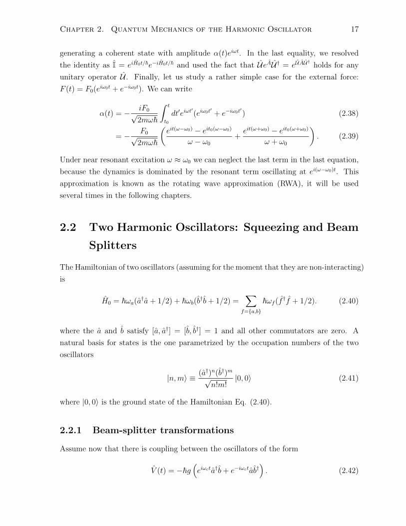
Chapter 2. Quantum Mechanics of the Harmonic Oscillator 17
generating a coherent state with amplitude α(t)eiωt. In the last equality, we resolved
the identity as I = eiH0t/~e−iH0t/~ and used the fact that UeAU † = eUAU†
holds for any
unitary operator U . Finally, let us study a rather simple case for the external force:
F (t) = F0(eiω0t + e−iω0t). We can write
α(t) = − iF0√2mω~
ˆ t
t0
dt′eiωt′(eiω0t′ + e−iω0t′) (2.38)
= − F0√2mω~
(eit(ω−ω0) − eit0(ω−ω0)
ω − ω0
+eit(ω+ω0) − eit0(ω+ω0)
ω + ω0
). (2.39)
Under near resonant excitation ω ≈ ω0 we can neglect the last term in the last equation,
because the dynamics is dominated by the resonant term oscillating at ei(ω−ω0)t. This
approximation is known as the rotating wave approximation (RWA), it will be used
several times in the following chapters.
2.2 Two Harmonic Oscillators: Squeezing and Beam
Splitters
The Hamiltonian of two oscillators (assuming for the moment that they are non-interacting)
is
H0 = ~ωa(a†a+ 1/2) + ~ωb(b†b+ 1/2) =∑
f=a,b
~ωf (f †f + 1/2). (2.40)
where the a and b satisfy [a, a†] = [b, b†] = 1 and all other commutators are zero. A
natural basis for states is the one parametrized by the occupation numbers of the two
oscillators
|n,m〉 ≡ (a†)n(b†)m√n!m!
|0, 0〉 (2.41)
where |0, 0〉 is the ground state of the Hamiltonian Eq. (2.40).
2.2.1 Beam-splitter transformations
Assume now that there is coupling between the oscillators of the form
V (t) = −~g(eiωcta†b+ e−iωctab†
). (2.42)

Chapter 2. Quantum Mechanics of the Harmonic Oscillator 18
The interaction picture version of this Hamiltonian with respect to H0 is
VI(t) = −~g(ei(ωc+ωa−ωb)ta†b+ e−i(ωc+ωa−ωb)tab†
)(2.43)
If we take ωc = ωb − ωa then VI(t) is time independent. Under this condition the time
evolution operator is
UI = exp(ir(a†b+ ba†) (2.44)
with r = g(t − t0). This last operator induces a beam-splitter (BS) transformation. It
can be shown that it transforms the canonical operators a and b according to [63]
e−ir(a†b+H.c.)aeir(a
†b+H.c.) = cos(r)a+ i sin(r)b, (2.45)
e−ir(a†b+H.c.)beir(a
†b+H.c.) = i sin(r)a+ cos(r)b. (2.46)
In the Schrodinger picture a state with one excitation (a single photon) in harmonic
oscillator a and zero in harmonic oscillator b will evolve to
|ψ〉 = U0UI |1, 0〉 = U0UI a† |0, 0〉 = U0
(cos(r)a† + i sin(r)b†
)|0, 0〉 (2.47)
= U0(cos(r) |1, 0〉+ i sin(r) |0, 1〉) = cos(r)e−i(3ωat)/2 |1, 0〉+ i sin(r)e−i(3ωbt)/2 |0, 1〉 .
This last state is entangled unless r = nπ/2 with n ∈ Z. It is entangled because we
cannot write it as |ψ(t)〉 = |µa〉 |νb〉, a separable state . Note that if a state is separable
(not entangled) we can assign a state vector to each subsystem, for instance |µa〉 for a
and |νb〉 for b in the last example. Even though we cannot assign state vectors to the
subsystems of an entangled system, we can assign density matrices to them . These are
constructed by tracing out the subsystems that are not of interest; for example,
ρa = trb (|ψ〉 〈ψ|) =∞∑m=0
〈mb| |ψ〉 〈ψ| |mb〉 = cos2(r) |1a〉 〈1a|+ sin2(r) |0a〉 〈0a| . (2.48)
Once we have a density matrix for a subsystem, we can calculate expectation values
with a slightly modified rule. Instead of using Eq. (2.13), the expectation values for an
operator in system a are obtained according to 〈Oa〉 = tr(ρaOa). In the case where the
composite system is separable |ψ〉 = |µa〉 |νb〉, the density matrix is simply a projector
into the corresponding subsystem vector, ρa = |µa〉 〈µa| and ρb = |νb〉 〈νb|.

Chapter 2. Quantum Mechanics of the Harmonic Oscillator 19
2.2.2 Squeezing transformations
Another interesting coupling Hamiltonian that we will find later on is
V (t) = −~g(e−iωcta†b† + eiωctab
). (2.49)
In the interaction picture with respect to H0, this Hamiltonian becomes
VI(t) = −~g(ei(−ωc+ωa+ωb)ta†b† + e−i(ωc−ωa−ωb)tab
). (2.50)
We will now assume that ωc = ωa + ωb, and then we again get a time independent
interaction Hamiltonian with evolution operator
UI = exp(is(a†b† + ab)), (2.51)
with s = g(t− t0). This operator is known as a two-mode squeezing (SQ) operator and
transforms the canonical operators according to
e−is(a†b†+H.c.)aeis(a
†b†+H.c.) = cosh(s)a+ i sinh(s)b†, (2.52)
e−is(a†b†+H.c.)beis(a
†b†+H.c.) = i sinh(s)a† + cosh(s)b. (2.53)
When this operator acts on vacuum, one obtains a two-mode squeezed vacuum (TMSV)
state
|s〉 = exp(is(a†b† + ab)) |0, 0〉 =∞∑n=0
in tanhn s
cosh s|n, n〉 . (2.54)
One direct way of obtaining the last decomposition in terms of number states is by using
the following identity (see Appendix 5 of [65])
exp(is(a†b† + ab
))=eia
†b† tanh se−(a†a+b†b+1) log cosh seiab tanh s. (2.55)
The two-mode squeezed vacuum is also entangled. The reduced density matrix of system
a is
ρa =∞∑n=0
tanh2n(s)
cosh2(s)|na〉 〈na| . (2.56)
Density matrices of the form Eq. (2.56) that are diagonal in the number basis and
that have coefficients that follow a geometric distribution in n are called thermal states.

Chapter 2. Quantum Mechanics of the Harmonic Oscillator 20
We can use this density operator to calculate for example the expectation value of the
number operator na. If the states |n〉 label different Fock states this is the mean number
of photons and is given by
〈na〉 = tr(ρana) = sinh2(s). (2.57)
2.2.3 Generating functions and Gaussian states
In quantum mechanics the states, represented by a vector |ψ〉 or a density matrix ρ,
contain all the information necessary to make predictions about the outcome of an exper-
iment. In classical mechanics a probability density function over the canonical variables
will play an analogous role to the state in quantum mechanics. In the same way that one
can completely describe a probability distribution by its moments, encoded in their mo-
ment generating function, a continuous variable (CV) quantum state can be described by
its moment generating function (also called characteristic function). The normal ordered
generating function is defined as
χ(α, α∗, β, β∗) = tr(ρeαa
†+βb†eα∗a+β∗b
), (2.58)
where ρ = |ψ〉 〈ψ| is the density matrix of the system. There is a special category of
quantum states called Gaussian states. They are characterized by the fact that their
generating function (any one of them) is gaussian in (α, α∗, β, β∗) [66]. In this thesis we
will be mostly interested in Gaussian states with zero mean, for which 〈a〉 = 〈b〉 = 0 and
we can write the normal ordered generating function as (See Chapter 3 of Ref. [65])
χ(α, α∗, β, β∗) = χ(z) = exp(S) = exp
(−1
2z†V z
), (2.59)
z = (α∗, α, β∗, β)T , (2.60)
V =
⟨a†a⟩−⟨(a†)2
⟩ ⟨a†b⟩−⟨a†b†
⟩−〈a2〉
⟨a†a⟩
−⟨ab⟩ ⟨
b†a⟩⟨
b†a⟩−⟨a†b†
⟩ ⟨b†b⟩−⟨
(b†)2⟩
−⟨ab⟩ ⟨
a†b⟩
−⟨b2⟩ ⟨
b†b⟩
. (2.61)
V is called the covariance matrix of the state, and it contains all the information necessary
to characterize a Gaussian state with zero mean. Examples of Gaussian states with zero
mean are |0, 0〉, the thermal state and the two-mode squeezed vacuum state. The second

Chapter 2. Quantum Mechanics of the Harmonic Oscillator 21
Transformation Action on the annihilation operators
Beam Splitter e−ir(a†b+H.c.)aeir(a
†b+H.c.) = cos(r)a+ i sin(r)b,
e−ir(a†b+H.c.)beir(a
†b+H.c.) = i sin(r)a+ cos(r)b,
Two-mode squeezing e−is(a†b†+H.c.)aeis(a
†b†+H.c.) = cosh(s)a+ i sinh(s)b†
e−is(a†b†+H.c.)beis(a
†b†+H.c.) = i sinh(s)a† + cosh(s)b
Rotations e−iua†aaeiua
†a = aeiu
e−ivb†bbeivb
†b = beiv
Table 2.1: In this table we summarize how the annihilation operators transform underdifferent Gaussian operations. In all cases the operators are mapped to linear combina-tions of creation and annihilation operators of the modes.
moments of the TMSV are
〈(a†)2〉 = 〈a2〉 = 〈b2〉 = 〈(b†)2〉 = 〈a†b〉 = 〈ab†〉 = 0 (2.62)
〈a†a〉 = 〈b†b〉 = sinh2(s), 〈ab〉 = (〈a†b†〉)∗ = i sinh(s) cosh(s), (2.63)
and the same moments for vacuum are all 0. Besides Gaussian states there are also Gaus-
sian transformations sometimes also called linear Bogoliubov transformations. These are
transformations that map Gaussian states to Gaussian states. An alternative charac-
terization of these transformations is that they map the canonical operators a, a†, b, b†
to linear combinations of those operators. The two-mode squeezing operator and the
beam-splitter operators generate Gaussian transformations of the states. In Table 2.1 we
summarize the action of different Gaussian transformations over the annihilation opera-
tors.
2.2.4 Lossy two-mode squeezed vacuum states
As an application of the relations we derived in the last sections, let us consider what
happens to a TMSV state that undergoes losses. Losses are typically modeled by a beam
splitter in which one of the inputs is the system that will undergo loss and the other input
is vacuum. We can model losses in mode a (b) by sending it through a BS operation
where the other arm c (d) is in vacuum. Thus we need to consider
eir′(b†d+H.c.)eir(a
†c+H.c.)eis(a†b†+H.c.) |0, 0, 0, 0〉 , (2.64)
where c and d are annihilation operators satisfying the usual commutation relations and
|0, 0, 0, 0〉 ≡ |0〉a |0〉b |0〉c |0〉d. We are now interested in the density matrix of systems

Chapter 2. Quantum Mechanics of the Harmonic Oscillator 22
Figure 2.1: This diagram illustrates how to model losses for a two-mode squeezedvacuum state. First the TMSV state is prepared, generating entanglement (symbolizedby the loop). Then each mode is sent to a beam splitter where the other input is vacuum.We then trace out the extra harmonic oscillators (symbolized by the trash bin) and lookat the resultant state in modes a and b which is in general less entangled and representedby a mixed density matrix ρ.
a and b. To obtain this quantity we need to trace out modes c and d. Note neverthe-
less that the operations and initial state in Eq. (2.64) are Gaussian thus a complete
characterization of such a state is contained in the second moments that determine the
covariance matrix
〈(a†)2〉 = 〈a2〉 = 〈b2〉 = 〈(b†)2〉 = 〈a†b〉 = 〈ab†〉 = 0, (2.65)
〈a†a〉 = T sinh2(s), 〈b†b〉 = T ′ sinh2(s), 〈ab〉 = (〈a†b†〉)∗ =√TT ′i sinh(s) cosh(s),
where√T = | cos(r)| and
√T ′ = | cos(r′)|. These moments contain all the information
necessary to write the covariance matrix and thus the state. It can be shown [54] that
the following density matrix for systems a and b
ρ = eis′(a†b†+H.c.)
(1
1 + n
1
1 + m
∞∑n,m=0
(n
1 + n
)n(m
1 + m
)m|n,m〉 〈n,m|
)e−is
′(a†b†+H.c.)
(2.66)

Chapter 2. Quantum Mechanics of the Harmonic Oscillator 23
is Gaussian and has the same second moments Eq. (2.65) provided that
tanh(2s′) =2√TT ′ sinh(s) cosh(s)
sinh2(s)(T + T ′) + 1, (2.67)
n+ m =
√(sinh2(s)(T + T ′) + 1
)2 − 4TT ′ sinh2(s) cosh2(s)− 1, (2.68)
n− m = (T − T ′) sinh2(s). (2.69)
Since covariance matrices specify a Gaussian state (or density matrix) uniquely we con-
clude that the density matrix in Eq. (2.66) is the one corresponding to systems a and b
when systems c and d are traced out in Eq. (2.64). Eq. (2.66) is useful because it allows
one to express a TMSV state after loss as a product of thermal states that undergoes
squeezing. An interesting special case of Eqs. (2.67) is when only one of the modes
undergoes losses, that is one of T and T ′ is equal to one. In that case n = 0 if T ′ = 1
and m = 0 if T = 1.
2.3 Continuous variable Gaussian transformations and
states
In this section we generalize some of the results from the previous section to a continuum
of harmonic oscillators (a continuum of continuous variable systems). To this end, we
introduce creation and annihilation operators labeled by a continuous index ω. They will
now satisfy the commutation relations
[a(ω), a†(ω′)] = δ(ω − ω′), [a(ω), a(ω′)] = 0. (2.70)
and will create photons at a single sharply defined frequency ω. In this thesis we will
assume that the states of a photon can be specified by its frequency. This is a simplifi-
cation that is only valid in a quasi 1-D situation. More generally states will be specified
by wavevectors ~k in 3-D space.
The noninteracting Hamiltonian of these oscillators is given by H0 =´dω~ωa†(ω)a(ω),
where we have omitted the factor of 1/2 that corresponds to the zero point energy of the
state with no photons. At this point we will start to refer to the collection of oscillators
as a field. The first state of the field that we will care about is the vacuum |vac〉. This
state satisfies
a(ω) |vac〉 = 0 ∀ω. (2.71)

Chapter 2. Quantum Mechanics of the Harmonic Oscillator 24
We can now introduce normalized broadband states containing a single excitation,
|1g(ω)〉 =
ˆdωg(ω)a†(ω) |vac〉 ,
ˆdω|g(ω)| = 1, (2.72)
analogous to the state studied in Eq. (2.47). Broadband coherent states are defined as
|g(ω)〉 = exp
(√N
ˆdωg(ω)a†(ω)− H.c.
)|vac〉 . (2.73)
where N =´dωa 〈a†(ωa)a(ωa)〉 is the mean number of photons in |g(ω)〉.
2.3.1 Multimode Beam Splitters and Squeezers
Next we would like to construct operations analogous to the BS and SQ operations for
the fields. To this end another field b(ω) is introduced
[b(ω), b†(ω′)] = δ(ω − ω′), [b(ω), b(ω′)] = 0. (2.74)
The field operators b(ωb), b†(ωb) commute with all the a(ω) and a†(ω). With these two
sets, the beam-splitter and squeezing operators are generalized to
USQ = exp
(i
ˆdωadωbK(ωa, ωb)a
†(ωa)b(ωb) + H.c.
), (2.75)
UBS = exp
(i
ˆdωadωbF (ωa, ωb)a
†(ωa)b†(ωb) + H.c.
). (2.76)
For future convenience we will also study the following operators
URA = exp
(i
ˆdωadω
′aG(ωa, ω
′a)a†(ωa)a(ω′a)
), (2.77)
URB = exp
(i
ˆdωbdω
′bH(ωb, ω
′b)b†(ωb)b(ω
′b)
). (2.78)
Here, the subindices RA and RB stand for rotation operation in the a and b modes,
and the functions G and H are assumed to be hermitian, G(ω, ω′) = G∗(ω′, ω) and
H(ω, ω′) = H∗(ω′, ω).
As we shall show in the next chapters, operations like the ones just mentioned can
be performed over the electromagnetic field using nonlinear optical materials. For the
moment we would like to know how operations like BS, RA, RB and SQ transform
different states. To learn how to apply these transformations, the Schmidt decompositions

Chapter 2. Quantum Mechanics of the Harmonic Oscillator 25
of F and K are introduced
F (ωa, ωb) =∑λ
sλfλ(ωa)jλ(ωb), K(ωa, ωb) =∑θ
rθkθ(ωa)l∗θ(ωb). (2.79)
The quantities sλ and rθ are positive and the functions f, j, k, l satisfy the following
orthonormality and completeness relations:
ˆ ∞−∞
dωafλ(ωa)f∗λ′(ωa) =
ˆ ∞−∞
dωakλ(ωa)k∗λ′(ωa) = δλλ′ , (2.80)∑
λ
fλ(ωa)f∗λ(ω′a) =
∑λ
kλ(ωa)k∗λ(ω
′a) = δ(ωa − ω′a), (2.81)
ˆ ∞−∞
dωbjλ(ωb)j∗λ′(ωb) =
ˆ ∞−∞
dωblλ(ωb)l∗λ′(ωb) = δλλ′ , (2.82)∑
λ
jλ(ωb)j∗λ(ω
′b) =
∑λ
lλ(ωb)l∗λ(ω
′b) = δ(ωb − ω′b). (2.83)
Likewise for the functions F and H, one introduces their eigendecompositions
G(ωa, ω′a) =
∑α
uαgα(ωa)g∗α(ω′a), H(ωb, ω
′b) =
∑β
vβhβ(ωb)h∗β(ω′b), (2.84)
where the numbers uα and vβ are real numbers and the functions g and h satisfy
ˆ ∞−∞
dωag∗α(ωa)gα′(ωa) =
ˆ ∞−∞
dωbh∗α(ωb)hα′(ωb) = δαα′ , (2.85)∑
α
g∗α(ω)gα(ω′) =∑β
h∗β(ω)hβ(ω′) = δ(ω − ω′). (2.86)
These decompositions exist if the functions are square integrable. In Appendix B we
show how one can numerically approximate the Schmidt decomposition using the singular
value decomposition (SVD) of matrices. With these definitions one introduces broadband
creation and annihilation operators
Aλ =
ˆdωaf
∗λ(ωa)a(ωa), Aλ =
ˆdωak
∗λ(ωa)a(ωa), Aλ =
ˆdωag
∗λ(ωa)a(ωa), (2.87)
Bλ =
ˆdωbj
∗λ(ωb)b(ωb), Bλ =
ˆdωbl
∗λ(ωb)b(ωb), Bλ =
ˆdωbh
∗λ(ωb)b(ωb). (2.88)

Chapter 2. Quantum Mechanics of the Harmonic Oscillator 26
One can then easily rewrite
USQ = exp
(i∑λ
sλA†λB†λ + H.c.
)=⊗λ
exp(isλA
†λB†λ + H.c.
), (2.89)
UBS = exp
(i∑θ
rθA†θBθ + H.c.
)=⊗θ
exp(irθA†θBθ + H.c.
), (2.90)
URA = exp
(i∑α
uαA†αAα
)=⊗α
exp(iuαA
†αAα
), (2.91)
URB = exp
(i∑β
vβB†βBβ
)=⊗β
exp(ivβB
†βBβ
). (2.92)
where we have used the completeness and orthogonality relations.
The Schmidt decompositions just introduced will play an important role in the fol-
lowing chapters. By using the completeness and orthogonality of the Schmidt functions
we can study what is the effect of the multimode field operators on arbitrary field states.
The Schmidt coefficients will play the role of the squeezing parameters s or rotation
angles r introduced in Sec. 2.2. For example, using the Schmidt decomposition we can
investigate how an annihilation operator for a photon of frequency ω, a(ω) transforms
under a BS transformation
U †BSa(ωa)UBS = U †BS
ˆdω′aδ(ωa − ω′a)a(ω′a)UBS = U †BS
ˆdω′a
∑θ
f ∗θ (ω′a)kθ(ωa)a(ω′a)UBS
=∑θ
kθ(ωa)U †BSAθUBS =∑θ
kθ(ωa)(Aθ cos(rθ) + i sin(rθ)Bθ
)=∑θ
kθ(ωa)
(ˆdω′af
∗θ (ω′a)a(ω′a) cos(rθ) + i
ˆdω′b sin(rθ)lθ(ω
′b)b(ω
′b)
)
=
ˆdω′a
(∑θ
kθ(ωa)f∗θ (ω′a) cos(rθ)
)a(ω′a)
+ i
ˆdω′b
(∑θ
kθ(ωa)lθ(ω′b) sin(rθ)
)b(ω′b) (2.93)
In Table 2.2 we summarize the transformations of the annihilation operators for the
different transformations. With these decompositions, we can investigate how multimode

Chapter 2. Quantum Mechanics of the Harmonic Oscillator 27
states transform. For instance, let us look at
UBS |1α(ω)〉 = UBS
ˆdωα(ω)a†(ω) |vac〉 =
ˆdωα(ω)UBSa
†(ω)U †BS |vac〉 (2.94)
=∑θ
(ˆdωk∗θ(ω)α(ω)
)(cos(rθ)A†θ + i sin(rθ)B†θ
)|vac〉 . (2.95)
This is almost like the result in Eq. (2.47). These equations can in fact be made
completely identical if we take α(ω) = kθ′(ω) since in that case the last equation becomes
UBS |1kθ′ (ω)〉 =(
cos(rθ′)A†θ′ + i sin(rθ′)B†θ′)|vac〉 (2.96)
The results in Table 2.2 are also useful because they allow us to calculate moments of
the operators, for instance the following expectation values of interest:
Na(ωa) = 〈vac| U †SQa†(ωa)a(ωa)USQ |vac〉 =
∑λ
sinh2(sλ)|fλ(ωa)|2 (2.97)
Nb(ωb) = 〈vac| U †SQb†(ωb)b(ωb)USQ |vac〉 =
∑λ
sinh2(sλ)|jλ(ωb)|2. (2.98)
These results are again very similar to the ones obtained for discrete modes in Eq. (2.57).
In the limit of sinh(sλ) ≈ sλ 1 this allows us to confirm that, for example,
ˆdωb|F (ωa, ωb)|2 =
∑λ
s2λ|fλ(ωa)|2 ≈ 〈vac| USQa
†(ωa)a(ωa)USQ |vac〉 . (2.99)
Finally, let us introduce a useful quantity called the Schmidt number [67]. If we write
the Schmidt decomposition of the function F as in Eq. (2.79) then the Schmidt number
of the function F is
S =(∑
λ s2λ)
2∑λ s
4λ
. (2.100)
Note that if the function F is normalized´dωadωb|F (ωa, ωb)|2 =
∑λ s
2λ = 1 then the
numerator of the last equation is simply 1. The Schmidt number of a separable function
F (ωa, ωb) = sf(ωa)j(ωb) is 1. Functions that are not separable have a Schmidt number
greater than 1 and the bigger it is the more terms its Schmidt decomposition has.
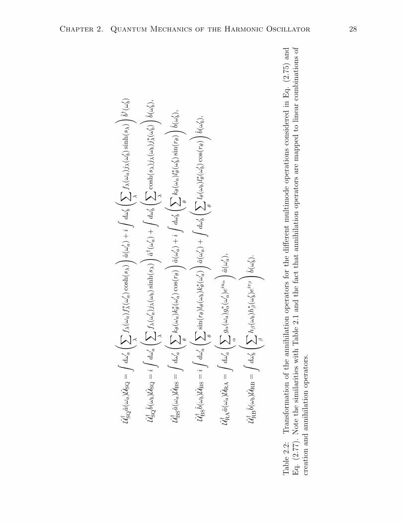
Chapter 2. Quantum Mechanics of the Harmonic Oscillator 28
U† SQa(ωa)U
SQ=
ˆdω′ a
( ∑ λ
f λ(ωa)f∗ λ(ω′ a)cosh(sλ)) a
(ω′ a)
+i
ˆdω′ b
( ∑ λ
f λ(ωa)jλ(ω′ b)sinh(sλ)) b†
(ω′ b)
U† SQb(ωb)U
SQ=
i
ˆdω′ a
( ∑ λ
f λ(ω′ a)j λ(ωb)sinh(sλ)) a
† (ω′ a)
+
ˆdω′ b
( ∑ λ
cosh(sλ)jλ(ωb)j∗ λ(ω′ b)
) b(ω′ b),
U† B
Sa(ωa)U
BS=
ˆdω′ a
( ∑ θ
kθ(ωa)k∗ θ(ω′ a)cos(r θ)) a
(ω′ a)
+i
ˆdω′ b
( ∑ θ
kθ(ωa)l∗ θ(ω′ b)sin(rθ)) b(
ω′ b),
U† B
Sb(ωb)U
BS=
i
ˆdω′ a
( ∑ θ
sin(rθ)lθ(ωb)k∗ θ(ω′ a)
) a(ω′ a)
+
ˆdω′ b
( ∑ θ
l θ(ωb)l∗ θ(ω′ b)cos(r θ)) b(
ω′ b),
U† R
Aa(ωa)U
RA=
ˆdω′ a
( ∑ α
g α(ωa)g∗ α(ω′ a)eiuα
) a(ω′ a),
U† R
Bb(ωb)U
RB=
ˆdω′ b
∑ β
hβ(ωb)h∗ β(ω′ b)eivβ
b(ω′ b).
Tab
le2.
2:T
ransf
orm
atio
nof
the
annih
ilat
ion
oper
ator
sfo
rth
ediff
eren
tm
ult
imode
oper
atio
ns
consi
der
edin
Eq.
(2.7
5)an
dE
q.
(2.7
7).
Not
eth
esi
milar
itie
sw
ith
Tab
le2.
1an
dth
efa
ctth
atan
nih
ilat
ion
oper
ator
sar
em
app
edto
linea
rco
mbin
atio
ns
ofcr
eati
onan
dan
nih
ilat
ion
oper
ator
s.

Chapter 3
Nonlinear optics
c©Joaquın Salvador Lavado (QUINO) Toda Mafalda — Ediciones de La Flor, 1993
In this chapter we will quantize the electromagnetic field in a medium and will write
the interaction picture Hamiltonians for the nonlinear processes that will be studied in the
thesis. It will be shown that the mathematical structure used to describe the quantized
electromagnetic field is completely analogous to the one corresponding to a collection of
quantum harmonic oscillators. For the derivation of the nonlinear Hamiltonian we will
essentially follow the approach of Sipe et al. [68, 69, 32].
3.1 Classical Fields
Before studying the nonlinear Hamiltonian we will quantize the electromagnetic field. To
this end we will write Maxwell’s equations for the Displacement ~D(~r) and Magnetic ~B(~r)
fields in a non-magnetic medium as follows
~∇ · ~D (~r) = 0, ~∇ · ~B (~r) = 0, (3.1)
−iω ~B (~r) = −~∇×
(~D(~r)
ε0n2(x, y;ω)
), − iω ~D(~r) = ~∇×
(~B(~r)
µ0
).
29

Chapter 3. Nonlinear optics 30
In the last equation we assumed that fields vary harmonically and thus we used
f(~r, t) = f(~r)e−iωt + c.c. (3.2)
where f is any scalar or vector function. The electric and magnetizing fields are related
to the displacement and magnetic fields via
~E(~r) =~D(~r)
ε0n2(x, y;ω), ~H(~r) =
~B(~r)
µ0
, (3.3)
where we assumed the refractive index n(x, y;ω) to be frequency dependent and space
dependent in the directions x, y orthogonal to the direction of propagation z. We are
interested in solving Eqs. (3.1) for a set of spatial modes that behave like exp(ikz) and
that can be labeled by their wavevector k and another index (or set of indices) J . The
solutions to Eqs. (3.1) can be found by solving the “Master-equation” commonly used
in photonic crystal studies [70, 69, 32],
~∇×
(~∇× ~BJk(~r)
n2(x, y;ωJk)
)=ω2Jk
c2~BJk(~r). (3.4)
Once the solutions to the Master equation have been found one can directly obtain the
displacement field from the last of Eqs. (3.1). Because of the form we assumed for ~BJk(~r)
we can automatically write for the other fields
~BJk(~r) = ~bJk(x, y)eikz√
2π, ~DJk(~r) = ~dJk(x, y)
eikz√2π, (3.5)
~HJk(~r) = ~hJk(x, y)eikz√
2π, ~EJk(~r) = ~eJk(x, y)
eikz√2π. (3.6)
Having the modes we can now write the classical fields as
~B(~r, t) =∑J
ˆdk AJk ~BJk(~r)e
−iωJkt + c.c., (3.7)
~D(~r, t) =∑J
ˆdk AJk ~DJk(~r)e
−iωJkt + c.c.,
~H(~r, t) =∑J
ˆdk AJk ~HJk(~r)e
−iωJkt + c.c.,
~E(~r, t) =∑J
ˆdk AJk ~EJk(~r)e
−iωJkt + c.c.

Chapter 3. Nonlinear optics 31
We can in principle choose any normalization for the transverse part of the fields. One
that turns out to be convenient when dealing with dispersive media [69] is
ˆdxdy
~d∗Jk(x, y) · ~dJk(x, y)
ε0n2(x, y;ωJk)
vp(x, y;ωJk)
vg(x, y;ωJk)= 1. (3.8)
where vp and vg are the local phase and group velocities in the medium.
3.2 Quantization
To quantize the fields we turn the amplitudes AJk into operators aJk modulo some pref-
actors (these appear because of the normalization used in Eq. (3.8)). This is analogous
to how we turned the amplitudes a and a∗ into the operators a and a† in the last chapter.
Now the Schrodinger operators are
~B(~r) =∑J
ˆdk
√~ωJk
2aJk ~BJk(~r) + H.c., (3.9)
~D(~r) =∑J
ˆdk
√~ωJk
2aJk ~DJk(~r) + H.c.,
~H(~r) =∑J
ˆdk
√~ωJk
2aJk ~HJk(~r) + H.c.,
~E(~r) =∑J
ˆdk
√~ωJk
2aJk ~EJk(~r) + H.c.
The annihilation operators aJk and their adjoints a†Jk satisfy
[aIk, aI′k′ ] = 0,[aIk, a
†I′k′
]= δII′δ(k − k′) (3.10)
and their dynamics is dictated by the linear Hamiltonian
HL =∑J
ˆdk ~ωJka†JkaJk. (3.11)
3.3 The nonlinear interaction
Writing the polarization in the material like we did in the introduction Eq. (1.1)
P i(~r, t) = Γij(1)(~r)Dj(~r, t) + Γijk(2) (~r)Dj(~r, t)Dk(~r, t) + . . . (3.12)
Chapter 3. Nonlinear optics 32
we can write the nonlinear part of the Hamiltonian as
HNL = − 1
3ε0
ˆd~r Γijk(2)(~r)D
i(~r)Dj(~r)Dk(~r) + . . . (3.13)
It can be shown that the Γ(2) tensor is related to the more commonly used nonlinear
tensor χ(2) via [32]
Γijk(2)(~r)→χijk(2)(~r)
ε0n2(~rωPkP )n2(~r, ωSkS)n2(~r, ωIkI )(3.14)
and assuming there are only three modes of interest labeled S, I, P and doing the rotating
wave approximation we obtain the following Hamiltonian
HNL =− 2ε0
ˆdkPdkSdkI
√~ωPk4π
~ωSk4π
~ωIk4π
a†SkS a†IkIaPkP
ˆdzei(kP−kS−kI)z× (3.15)
ˆdxdy χijk(2)(x, y)
(diSkS(x, y)
)∗ (djIkI (x, y)
)∗dkPkP (x, y)
ε30n2(x, y;ωSkS)n2(x, y;ωIkI )n
2(x, y;ωPkP )+ H.c. + . . .
Up to this point we have developed a very general theory of the interaction of photons
mediated by a nonlinear structure. In what follows we will specialize this theory to the
case of an effective one dimensional structure where the states of the photons can be
specified by their frequency ω.
3.4 The interaction Hamiltonian for a χ2 process
The nonlinear Hamiltonian in the Schrodinger picture Eq. (3.15) can be rewritten as
HNL = −ˆk
dkadkbdkcSI(kc, ka, kb)c(kc)a†(ka)b
†(kb) + H.c., (3.16)
where we have relabeled aPkP → c(k), aIkI → b(k), aSkS → a(k) and these operators
satisfy [c(k), c†(k′)] = [b(k), b†(k′)] = [a(k), a†(k′)] = δ(k− k′) and any other commutator
between operators equal to zero. We assume that the wavenumber ranges and/or the
polarizations of the pump photons (destruction operator c(kc)) and the down-converted
photons (destruction operators a(ka) and b(kb)) are distinct. Letting the frequency as-
sociated with kl be ωl, where l = a, b, or c, the coupling coefficient SI(kc, ka, kb) is given

Chapter 3. Nonlinear optics 33
by
SI(kc, ka, kb) =2
ε0
√~ωc~ωa~ωb
(4π)3
χ2
ε0n2c (ωc)n2
a(ωa)n2b(ωb)ˆ
A
dxdy dc(x, y)d∗a(x, y)d∗b(x, y)
ˆ L/2
−L/2dz ei(kc−ka−kb)z, (3.17)
where we have put nl(ωl) for n(~r, ωKk) as the effective index of the indicated mode type.
Here we have simplified the expression from the last section for the nonlinear Hamiltonian
Eq. (3.15) by neglecting the tensor nature of χ2 and the vector nature of the dl(x, y),
which characterize the mode profiles of the displacement field; in our expression Eq.
(3.17) for SI(kc, ka, kb) the parameter χ2 can be taken to characterize the strength of the
nonlinearity, which we assume to be present only from −L/2 to L/2, and we take the
dl(x, y) to be uniform over an area A. The vectors ~dl(x, y) are normalized according to
Eq. (3.8) which can be simplified to
ˆdxdy
~d∗l (x, y) · ~dl(x, y)
ε0n2l (ωl)
vp(l)
vg(l)= 1, (3.18)
where vp(l) = c/nl(ωl) and vg(l) = dωl/dkl are the phase and group velocities (assumed
to be constant in the area A), this leads to
dl =
√vg(l)n2
l (ωl)ε0vp(l)A
, (3.19)
and using this in Eq. (3.17) we have
SI(kc, ka, kb) = 2Lχ2
√~ωc~ωa~ωbvg(a)vg(b)vg(c)
(4π)3ε0Avp(a)vp(b)vp(c)n2an
2bn
2c
sinc
(L
2(kc − ka − kb)
). (3.20)
In the last equation sinc(L2(kc − ka − kb)
)is the so called phase matching function.
For fields propagating in a single direction it is conventional to work with frequency rather
than wavenumber labels; hence we take, for example, c(kc)→√dωc/dkcc(ωc), such that

Chapter 3. Nonlinear optics 34
[c(ωa), c
†(ω′a)]
= δ(ωa−ω′a). Then changing to frequency variables in Eq. (3.17) we have
HI(t) = −2
ˆ ∞0
dωadωbdωcLχ2c(ωc)a†(ωa)b
†(ωb)ei∆t
√~ωc~ωa~ωb
(4π)3ε0Ac3na(ωa)nb(ωb)nc(ωc)
× sinc
(L
2(k(ωc)− k(ωa)− kb(ωb))
)+ H.c., (3.21)
where we have also moved to the interaction picture defined by linear evolution, HNL →HI(t), with c(ωc)a
†(ωa)b†(ωb) picking up the phase factor exp(i∆t), where ∆ = ωa+ωb−
ωc. Eq. (3.21) shows explicitly that there will be a significant interaction between fields
a, b and c only if the central frequencies ω and central wavevectors satisfy
ωa + ωb − ωc ≈ 0, (3.22)
k(ωa) + k(ωb)− k(ωc) ≈ 0. (3.23)
These two constraints give precisely the energy and momentum conservation rules men-
tioned in Chapter 1. Note that one can modify the momentum conservation rule if the
nonlinearity in the material is also modulated at some spatial periodicity Λ. In that
case the χijk(2)(x, y) in Eq. (3.15) should be changed to χijk(2)(x, y)e±i2πz/Λ consequently the
argument of the sinc function in Eq. (3.21) is L2(k(ωc)− k(ωa)− kb(ωb)± 2π/Λ) and the
momentum conservation rule is k(ωa) + k(ωb)− k(ωc) ≈ ±2π/Λ [71, 72].
In the same interaction picture mentioned before the electric field operator can be
related to the displacement field operator in the usual way Eq. (3.3); using this expression
and our expression for the transverse displacement vector Eq. (3.19) we find
~E(~r, t) =∑l
ˆ ∞0
dωlnl
√~ωl
4πε0vp(l)Aql(ωl)e
ik(ωl)z−iωlt + H.c. (3.24)
where l is summed over a, b, and c, ql(ωl) ranges over the destruction operators a(ωa),
b(ωb), and c(ωc). Taking the expectation value of the above operator with respect to a
coherent state for the pump field (and vacuum for the down-converted photon frequencies)
turns c(ωc) into a c-number β(ω), where we drop the subscript c. Now we can compare
this with a classical pulse with energy U0, centered at ωl and frequency variance σ2 (See

Chapter 3. Nonlinear optics 35
Eq. A.11)
~E(~r, t) = E0
ˆ ∞0
dωei(k(ω)z−ωt) 1√2πσ
e−(ω−ωl)2/2σ2
=
ˆ ∞0
dω
√(U0/√π)σ
2ε0n(ω)cAei(k(ω)z−ωt) 1√
2πσe−(ω−ωl)2/2σ2
, (3.25)
and identify
β(ω) =
√U0/√π
~ωσe−(ω−ω)2/2σ2
. (3.26)
It is convenient to replace σ by the inverse standard deviation of the time-dependent
pump intensity, τ = 1/√
2σ = 2√
2 ln 2 FWHM,(where FWHM is the full width at half
maximum of a Gaussian distribution) and write
β(ω) =
√U0/√π/2
~τωτe−τ
2(ω−ω)2
. (3.27)
With this in hand we can return to the nonlinear Hamiltonian Eq. (3.21) and write
HI(t) = −~εˆ ∞
0
dωadωbdωcsinc
(L
2(k(ωc)− ka(ωa)− kb(ωb))
)ei∆tα(ωc)a
†(ωa)b†(ωb)
+ H.c., (3.28)
for an PDC process with a classically described undepleted pump field c, where we
introduced the dimensionless perturbation parameter ε
ε = 2Lχ2
√ √2U0πωbωa√
π(4π)3ε0Ac3na(ωa)nb(ωb)nc(ωc)τ(3.29)
and in benign frequency factors (like the refractive indices and the nonlinear coefficient
χ(2)) we have evaluated ωa, ωb, ωc at the central frequencies ωa, ωb, ωc. These are the
frequencies where the phase-matching condition is assumed to be satisfied exactly. We
also introduced
α(ωc) =τ√πe−τ
2(ωc−ωc)2
, (3.30)
which is essentially the shape of the pulse used to pump the crystal and which has units
of time. Eq. (3.28) is the final form of the Hamiltonian we will use in the rest of the

Chapter 3. Nonlinear optics 36
thesis for χ2 processes.
3.5 The interaction Hamiltonian for a χ3 process
For a third order process, the straightforward extension of the nonlinear Hamiltonian Eq.
(3.16) [32] in the Schrodinger picture is given by
HNL = − 1
4ε0
ˆV
d~rΓijkl3 Di(~r)Dj(~r)Dk(~r)Dl(~r), (3.31)
where indices refer to Cartesian components and are to be summed over when repeated;
Γijkl3 can be written in terms of the more usual third order optical susceptibility χijkl3
and the linear indices at the appropriate frequency components involved [73]; as in the
subsection above we use the symbol χ3 (without tensor indices) to indicate the size of
the component(s) that are important when the relevant fields are used in the different
Di(~r). For Four Wave Mixing (FWM) we require destruction operators for the pump
fields (c(ωc) and c(ω′c)) and creation operators for the photons generated described by
a (ωa) and b(ωb), and in analogy with the result of the last chapter we find
HI(t) = −ˆ L/2
−L/2dz
ˆ ∞0
dωcdω′cdωbdωa
3χ3
ε30n2c(ωc)n
2c(ω
′c)n
2b(ωb)n
2a(ωa)
√~ωc4π
~ω′c4π
~ωa4π
~ωb4π
Ana(ωa)nb(ωb)nc(ωc)nc(ω′c)√
vg(a)vg(b)vg(c)vg(c′)
√vg(c′)ε0vp(c′)A
vg(c)ε0vp(c)A
√vg(a)ε0vp(a)A
vg(b)ε0vp(b)A
(3.32)
a†(ωa)b†(ωb)c(ωc)c(ω
′c)e−i(ωc+ω′c−ωa−ωb)tei(kc(ωc)+kc(ω
′c)−ka(ωa)−kb(ωb))z + H.c.
The factor of 3 in the fraction containing χ3 is (4!/2!)/4, with (4!/2!) the number of
permutations involving the ordering of the creation and annihilation operators; note that
this is twice the corresponding factor appearing in [73] because here we assume that
the creation operators a†(ωa) and b†(ωb) involve different ranges of frequency and/or
polarization. The refractive index factors in the denominator, and the appearance of
ε30, arise because of the conversion from Γijkl to χijkl3 and the prefactor of ε−10 in Eq.
(3.31); compare with the corresponding terms in Eq. (3.17). The terms of the form√~ωl/4π arise from the expansion of the displacement field in terms of raising and
lowering operators, and again find their correspondence in terms in Eq. (3.17). The
factor of A comes from integrating over the area in our “toy model” for our waveguide
and its modes; the factor (vg(a)vg(b)vg(c)vg(c′))−1/2 arises from the change of variables
from wave numbers to frequencies; and the next terms are the expressions for the mode
Chapter 3. Nonlinear optics 37
profiles Eq. (3.19). Supposing that all the frequency prefactors vary slowly relative to
the harmonic dependence in space and time due to the phase factors, in those prefactors
we set ωc and ω′c at the center frequency ωc of the pump, and evaluate ωa and ωb at the
frequencies ωa and ωb where the phase-matching is optimum; Eq. (3.32) then reduces to
HI(t) = − 3χ3~2
ε0A(4π)2c2
√(ωc
nc(ωc)
)2ωa
na(ωa)
ωbnb(ωb)
ˆ L/2
−L/2dz
ˆ ∞0
dωcdω′cdωbdωa (3.33)
× a†(ωa)b†(ωb)c(ωc)c(ω′c)e−i(ωc+ω′c−ωa−ωb)tei(kc(ωc)+kc(ω
′c)−ka(ωa)−kb(ωb))z + H.c.
As in the last subsection we replace the c operators by classical functions (see Eq. (3.27))
and assume that σ ωc, which allows us to extend the range of the ωc and ω′c integrals
to −∞ to ∞, and we find
HI(t) = − 3χ3~2
ε0A(4π)2c2
√(ωc
nc(ωc)
)2ωa
na(ωa)
ωbnb(ωb)
U0/√π/2
~ωcσ
ˆ L/2
−L/2dz
ˆdωcdω
′cdωbdωa
e−(ωc−ωc)2/2σ2
e−(ω′c−ωc)2/2σ2
ei(kc(ωc)+kc(ω′c)−ka(ωa)−kb(ωb))ze−i(ωc+ω
′c−ωa−ωb)t
a†(ωa)b†(ωb) + H.c. (3.34)
To simplify this further we look at the integrals over ωc and ω′c,
I =
ˆdωcdω
′cei(kc(ωc)+kc(ω′c))z−i(ωc+ω′c)te−(ωc−ωc)2/2σ2
e−(ω′c−ωc)2/2σ2
. (3.35)
Expanding kc(ωc) and kc(ω′c) as
k(ω) = k(ω) + (ω − ω)/vg +1
2κω(ω − ω)2, (3.36)
with κω = (d2k/dω2)ω=ω, vg being the group velocity and introducing ω± = ωc ± ω′c, we
find that Eq. (3.35) equals
I =
ˆdω+e
ik+(ω+)ze−iω+te−(ω+−2ωc)2/4σ2
ˆdω−
2e−
ω2−4 ( 1
σ2−iκωcz), (3.37)
where
k+(ω+) = 2kc(ωc) + (ω+ − 2ωc)/vc +κωc4
(ω+ − 2ωc)2. (3.38)

Chapter 3. Nonlinear optics 38
We can formally perform the integral over ω− to get
ˆdω−
2e−
ω2−4 ( 1
σ2−iκωcz) =√πσg(z), (3.39)
where
g(z) ≡ 1√1− iκωczσ2
. (3.40)
Although the square root in the last equation produces two different complex numbers one
can always go back to the defining integral Eq. (3.39) which is completely unambiguous.
We can then finally write the Hamiltonian as
HI(t) = −~εˆdω+
ˆdωb
ˆdωaΦ(∆k)ei∆ta†(ωa)b
†(ωb)α(ω+) + H.c.,
where
α(ω+) ≡ τ e−τ2(ω+−2ωc)2
√π
, (3.41)
(with units of time) characterizes the bandwidth of the pump, and we have introduced
τ = 1/(2σ) and ∆ ≡ ωa + ωb − ω+, (note the difference between these quantities and
the corresponding α, τ , and ∆ from the last subsection); the dimensionless perturbation
parameter
ε =6√
2πχ3U0Lσ
ε0A(4π)2ncc2
√ωana
ωbnb, (3.42)
which characterizes the strength of the nonlinear interaction, and the modified phase
matching function is
Φ(∆k) ≡ˆ L/2
−L/2
dz
Lei(ka(ωa)+kb(ωb)−k+(ω+))zg(z). (3.43)
If the effect of group velocity dispersion on the pump pulse is negligible over the length
L of the nonlinear region, for all relevant z we have |κωczσ2| 1, we can set g(z) → 1,
k+(ω+) = 2kc(ω+/2) and Φ(∆k) = sinc(∆kL/2). Finally, note that we can rewrite
expression Eq. (3.41) in a slightly more suggestive manner,
HI(t) = −~εˆdω+
ˆdωb
ˆdωaΦ(∆k)ei∆ta†(ωa)b
†(ωb)ζ(ω+/2− ωc)2
2σ+ H.c. (3.44)

Chapter 3. Nonlinear optics 39
where ζ(ω) = exp(−ω2/(2σ2)) is proportional to the electric field amplitude, explicitly
displaying the dependence of HI(t) on the square of that amplitude. Of course, the details
of the argument given here rely on the assumed Gaussian nature of the pump. But we
can expect that the general form Eq. (3.41) will survive even for more general pump
pulses, as long as the effect of group velocity dispersion on the pump pulse is negligible.
In the following chapters we will treat the evolution generated by the Hamiltonians Eq.
(3.28) and Eq. (3.41) in a non-perturbative way. For the case of SPDC, this implies that
we will consider higher powers of the nonlinear susceptibility χ2, which naturally leads
to the question of whether higher order susceptibilities like χ3 need to be considered. To
address this question one should remember that to have a significant nonlinear interaction
requires not only intense fields, but also satisfying energy and momentum conservation.
Thus if energy and linear momentum are conserved for photon generation via SPDC (see
Eq. (3.22)), it is easy to see that one cannot have photon generation via a χ3 process
since this process will not be phase matched and will not preserve energy. The same
argument allows us to rule out photon generation through higher order susceptibilities
for phase-matched χ2 and χ3 processes.
The argument just presented allows us to ignore the photon generation component of
a χ3 process if we design a structure for SPDC. Nevertheless there are other χ3 processes
that are automatically phase-matched and preserve energy. Two such processes are self-
phase modulation of the pump pulse and cross-phase modulation of the pump on the
down-converted photons [74]. The interplay of the time ordering effects to be discussed
in the following chapters and the self- and cross- phase modulation just mentioned is
under active study [75].

Chapter 4
The Magnus expansion
Wigner also describes Pauli as giving the label die Gruppenpest (“the grouppestilence”) to the increasing use of group theory in quantum mechanics
Peter Wolt in Not even Wrong.
4.1 Introduction
Spontaneous parametric down-conversion (SPDC), spontaneous four-wave mixing (SFWM),
and frequency conversion (FC) are three of the most common nonlinear processes used
in quantum optics. In the first two a nonlinear medium is used to convert photons from
a pump laser into pairs of quantum correlated photons [12]. In the third, the frequency
of a photon is increased or decreased after it interacts with a strong pump field inside a
nonlinear medium. Pair generation is often modeled in a straightforward manner using
the first order of a Dyson series, or the first term in a Taylor-like series that results if
consequences of time ordering are ignored [57]. But when the nonlinear interaction be-
comes sufficiently strong a more involved theoretical treatment is required. In particular,
the Taylor-like series is suspect beyond a few orders because the interaction Hamiltonian
does not commute with itself at different times.
In previous work [59, 60] the Dyson series has been used to investigate parametric
down-conversion (PDC), and it was shown that when the initial state of the down-
converted fields is vacuum (SPDC), the Taylor-like and Dyson series give identical results
up to second order. In a subsequent study, Christ et al. [52] used the Heisenberg picture
to investigate time-ordering issues in both SPDC and FC. They noticed that when the
pump is approximated as undepleted and treated classically, the Hamiltonian is quadratic
in the bosonic operators of the down-converted fields, and thus the equations of motion of
the operators are necessarily linear. This implies that the outgoing fields are related to the
40

Chapter 4. The Magnus expansion 41
incoming fields by a linear Bogoliubov transformation [76]. They used this observation to
build an ansatz solution, and develop a numerical algorithm that permits the calculation
of the linear transformation relating output to input. Another consequence of the linear
Bogoliubov relation between output and input is that the state of the down-converted
photons in SPDC cannot be more complicated than a two-mode squeezed vacuum. This
is at odds with a result of Branczyk et al. [60], who found that the third order correction
to the SPDC state contains a six photon energy correlated state. As we shall show, this
discrepancy is related to the fact that the Dyson series does not retain the Gaussian
preserving nature of the quadratic Hamiltonian, or equivalently the linear Bogoliubov
nature of the transformation relating input and output fields.
In this chapter we employ the Magnus Expansion (ME), which is able to deal properly
with time ordering at each level, and thus is unitary to all orders. Yet, unlike the
Dyson series, it respects the Gaussian preserving nature of the process for the class of
Hamiltonians that are quadratic in bosonic operators, giving rise to a linear Bogoliubov
transformation to whatever order it is taken. Thus we feel it should be the preferred
strategy for the description of photon generation and conversion in nonlinear quantum
optics.
In section 4.2 we introduce the ME and mention some of its important properties, de-
riving a useful simplification of its terms when dealing with a broad class of Hamiltonians
used in quantum optics; we also show why the ME automatically respects the Gaussian
nature of usual nonlinear quantum optical processes. In section 4.3 we apply the ME to
the PDC and FWM Hamiltonians. While the ME has been used in the past in quantum
nonlinear optics (see e.g. Yang et al. [32] and references cited therein), usually only the
first term in the expansion has been kept. We calculate the second and third order terms,
and also introduce diagrams akin to Feynman diagrams that allow for a simple tabulation
of the higher order processes in the ME. Using these diagrams we easily demonstrate why
it is necessary to go to third order in the expansion to see a correction to the SPDC and
SFWM states. In section 4.4 we extend these ideas to FC processes. We show that the
expansion formulas derived for FC are completely analogous to those derived for PDC
and FWM. In section 4.5 we show how the ME can be taken to a form more amenable to
direct calculation and develop a expansion for the joint spectral amplitude (JSA) of the
down converted photons in SPDC and SFWM. In section 4.6 we show that for perfect
phase matching the second and third order Magnus terms vanish.

Chapter 4. The Magnus expansion 42
4.2 Properties of the Magnus expansion
In quantum mechanics it is often necessary to solve the time-dependent Schrodinger
equation for the time evolution operator U(t, t0),
i~d
dtU(t, t0) = HI(t)U(t, t0), (4.1)
where HI(t) is the interaction picture Hamiltonian. One common way to approximate
the solution of Eq. (4.1) is to use the Dyson series in which the evolution operator is
expanded as a power series
U(t1, t0) = I+ T1(t1, t0) + T2(t1, t0) + . . . (4.2)
= I+ (−i)ˆ t1
t0
dt′HI(t
′)
~+ (−i)2
ˆ t1
t0
dt′ˆ t′
t0
dt′′HI(t
′)HI(t′′)
~2+ . . .
Often after time ordering some of the terms appearing, depicted as Feynman diagrams,
can be grouped into classes and summed. Here instead we use the Magnus expansion
[77, 78] in which a series expansion is developed as the argument of an exponential,
U(t1, t0) = exp(Ω1(t1, t0) + Ω2(t1, t0) + Ω3(t1, t0) + . . .
), (4.3a)
Ω1(t1, t0) = − i~
ˆ t1
t0
dtHI(t), (4.3b)
Ω2(t1, t0) =(−i)2
2~2
ˆ t1
t0
dt
ˆ t
t0
dt′[HI(t), HI(t
′)], (4.3c)
Ω3(t1, t0) =(−i)3
6~3
ˆ t1
t0
dt
ˆ t
t0
dt′ˆ t′
t0
dt′′( [HI(t),
[HI(t
′), HI(t′′)]]
(4.3d)
+[[HI(t), HI(t
′)], HI(t
′′)] ).
in general all the terms of the Magnus series are time-ordered integrals of commutators
of the Hamiltonian at different times [78]. This series will terminate at the second order
for the case of the forced harmonic oscillator considered in section 2.1.3 because the
commutator of the Hamiltonian at two different times for that problem is a number (see
Eq. (2.33)). Thus Eq. (2.35) is indeed the exact propagator for this problem.
In the rest of the thesis we will take unless otherwise indicated t0 → −∞ and t1 →∞. In the following we calculate the terms in such a series for a rather broad class of
Hamiltonians relevant to nonlinear quantum optics. We write the time dependence of

Chapter 4. The Magnus expansion 43
the interaction Hamiltonian as
HI(t) = ~ˆdω(h(ω)ei∆t + h†(ω)e−i∆t
), (4.4)
where we use the shorthand notation
h(ω) = h(ω1, ω2, . . . , ωn), (4.5)
dω = dω1dω2 . . . dωn,
∆ = ∆(ω1, ω2, . . . , ωn).
For the moment we leave the integration limits of the frequencies ω unspecified; in the
next sections we will specify them for particular cases. For the first order Magnus term
one simply finds
Ω1 =− i
~
ˆdtHI(t) = −2πi
ˆdω(h(ω) + H.c.
)δ(∆). (4.6)
In the last equation we have adopted the convention that whenever the lower (or upper)
limit of an integral over time is not specified it is meant to be understood as −∞ (or
+∞). The term in Eq. (4.6), exponentiated, corresponds to the sum of the Taylor-like
series for U that could be constructed by time ordering the series Eq. (4.2) and ignoring
the fact that the Hamiltonians HI(t) at different times t need not commute. In fact,
if [HI(t), HI(t′)] = 0 for all t and t′, then exp Ω1 constitutes the exact solution of the
problem, since all the higher order Magnus terms vanish. Hence we refer to terms in the
Magnus expansion beyond Ω1 as “time-ordering corrections”.
In general no simplifications can be made to the higher order Magnus terms if no
further assumptions are made about HI(t). We make the following assumption:
[h(ω), h(ω′)] = [h†(ω), h†(ω′)] = 0, (4.7)
which is indeed valid for the Hamiltonians usually employed to describe both type I and
II parametric down-conversion, four wave mixing, and frequency conversion, either if the
pump is treated classically or if it is treated quantum mechanically. Using property Eq.
(4.7) and the fact that
ˆdt
ˆ t
dt′ei∆t−i∆′t′ = 2π2δ(∆)δ(∆′) + 2πiδ(∆−∆′)
P∆, (4.8)
with P indicating a principal value, the second order Magnus term, generally given by

Chapter 4. The Magnus expansion 44
Eq. (4.3c) can be simplified to
Ω2 = −2πi
dωdω′
[h(ω), h†(ω′)
] δ(∆−∆′)
∆. (4.9)
In the last equation we have used the principal value integral symbolffl
. This is necessary
because the result Eq. (4.8) is only valid under a principal value integration sign. Only
the second term of Eq. (4.8) contributes to the second order term. This is to be expected
since the first term is just
2π2δ(∆)δ(∆′) =1
2
ˆdt
ˆdt′ei∆t−i∆
′t′ , (4.10)
which is the expression that would be obtained from Eq. (4.8) ignoring the time ordering;
note the difference in limits between Eq. (4.10) and Eq. (4.8).
Now let us look at the third order Magnus term Eq. (4.3d). Here the relevant time
integrals take the form
ˆdt
ˆ t
dt′ˆ t′
dt′′eiµt+iνt′+iξt′′ = 2π3δ (µ) δ (ν) δ (ξ)− 2π2iδ (ν + ξ) δ (µ+ ν + ξ)
Pξ
+ 2π2iδ (µ+ ν) δ (µ+ ν + ξ)Pµ− 2πδ (µ+ ν + ξ)
Pµ+ ν
Pµ. (4.11)
Because of the condition Eq. (4.7) the only term that contributes to Ω3 in Eq. (4.11) is
the last one, and then upon relabeling one obtains:
Ω3 = −2πi
dωdω′dω′′
([h(ω), [h(ω′), h†(ω′′)]] + H.c.
)× δ (∆ + ∆′ −∆′′)
3
(1
∆∆′′+
1
∆∆′
). (4.12)
We emphasize that the simple form obtained for Ω3 critically depends on assumption
Eq. (4.7). If this did not hold, then the second and third terms in Eq. (4.11) would
also contribute, leading to a much more complicated expression. However, even if Eq.
(4.7) were not to hold the first term of Eq. (4.11) would never contribute to Ω3, which
is related to the fact that it is proportional to terms that would arise if time order were
ignored, and their effects have all been included in Ω1.
Finally, let us note that the Magnus expansion is more robust in preserving qualitative
features of the exact solution for U than the Dyson expansion, particularly for problems in
nonlinear quantum optics. Generally, of course, the Magnus expansion truncated at any

Chapter 4. The Magnus expansion 45
level will always give rise to a unitary evolution operator if the Hamiltonian is Hermitian,
as is assumed when writing Eq. (4.4), while a truncated Dyson expansion will not. More
specifically, the Magnus expansion truncated at any level will always give rise, in the
Heisenberg picture, to a linear Bogoliubov transformation of the bosonic operators if the
Hamiltonian is quadratic in them. Since such quadratic bosonic Hamiltonians (QBH)
often appear in nonlinear quantum optics, and since for such a Hamiltonian the exact
solution for the Heisenberg picture evolution of the bosonic operators indeed takes the
form of a linear Bogoliubov transformation [76], this is a very desirable feature of the
Magnus approximation. Here is the proof that any Magnus approximation displays this
feature: From the general commutator identity
[AB, CD] = [A, C]BD + A[B, C]D + C[A, D]B + CA[B, D]. (4.13)
we see that if A, B, C, D are all bosonic operators then the commutators on the right
hand side are all c−numbers, and in fact if they do not vanish they are delta functions,
either Kronecker or Dirac. Since all the terms Ω1, Ω2 etc., in the Magnus series involve
commutators, it is clear that for a QBH all the terms Ωi will be quadratic functions of
the bosonic operators, and the M th order approximation to the Magnus expansion
UM(tf , t0) = exp(Ω1(tf , t0) + Ω2(tf , t0) + . . .+ ΩM(tf , t0)) = exp(OM(tf , t0)), (4.14)
where we reinstate general initial and final times, t0 and tf respectively, is characterized
by an operator O(tf , t0) that is anti-Hermitian and a quadratic function of the boson
operators. Now in the Heisenberg picture and initial operator A(t0) evolves to a later
operator A(tf ) according to
A(tf ) = U †(tf , t0)A(t0)U(tf , t0). (4.15)
Using the approximation given by Eq. (4.14) and the Baker-Campbell-Hausdorff (BCH)
lemma
eX Y e−X = Y +[X, Y
]+
1
2!
[X,[X, Y
]]+ · · · , (4.16)
we find
A(tf ) = A(t0) + [A(t0), OM(tf , t0)] +1
2![[A(t0), OM(tf , t0)], OM(tf , t0)] + . . . (4.17)

Chapter 4. The Magnus expansion 46
Using the general commutator identity
[A, BC] = [A, B]C + B[A, C], (4.18)
we see that if A(t0) is a bosonic operator the commutators on the right hand side of
Eq. (4.17) will all be bosonic operators, and thus the Heisenberg bosonic operators at
tf are indeed linear functions of the Heisenberg bosonic operators at t0. This completes
the proof. In the Schrodinger picture, the result implies that any Magnus approximation
for evolution under a QBH will share the property of the exact solution that the general
Gaussian nature of an initial state will be preserved; that is, the exact evolution con-
stitutes a unitary Gaussian channel, and any Magnus approximation for the evolution
constitutes a unitary Gaussian channel as well [66].
4.3 Time ordering in Parametric Down-Conversion
and Four Wave Mixing
In type II SPDC an incoming photon at frequency ωp is transformed into two photons of
different polarizations at frequencies ωa and ωb which are roughly half the frequency of
the incoming photon. Within the usual rotating wave and undepleted pump approxima-
tions, the interaction Hamiltonian governing this process in an effectively one-dimensional
structure with all relevant fields propagating in the same direction, such as a channel or
ridge waveguide, is (see section 3.5)
HI(t) = −~εˆdωadωbdωpe
i∆tΦ(ωa, ωb, ωp)α(ωp)a†(ωa)b
†(ωb) + H.c., (4.19)
∆ = ωa + ωb − ωp. (4.20)
where a(ωa) and b(ωb) are photon destruction operators associated with the wavevectors
ka(ωa) and kb(ωb), constructed to satisfy the commutation relations
[a(ω), a†(ω′)] = [b(ω), b†(ω′)] = δ(ω − ω′), (4.21)
and all other commutators between destruction and creation operators vanishing; α (ωp)
is a classical function proportional to the electric field amplitude of the undepleted pump
field with wavevector k(ωp). The assumption Eq. (4.21) is well justified because for

Chapter 4. The Magnus expansion 47
type II SPDC the down converted photons appear in orthogonal polarizations, and their
frequency support is far away from the frequency support of the pump field characterized
by α (ωp). Because of this the limits of integration for the frequencies of the fields will
range from 0 to ∞. Nevertheless, since the bandwidth of the photons is much smaller
than their central frequencies these integrals can be safely extended in their lower limit
to −∞.
The phase matching function Φ incorporates the spatial dependence of the fields and
the nonlinearity profile; It takes the form
Φ(ωa, ωb, ωp) = sinc
(∆kL
2
), ∆k = ka(ωa) + kb(ωb)− kp(ωp), (4.22)
when the nonlinearity is assumed to be uniform in a region of space from −L/2 to L/2,
and in Eq. (4.19) ε is a dimensionless constant incorporating parameters such as the
strength of the nonlinearity profile and the effective cross sectional area of the crystal.
There will be corrections to the integrand of Eq. (4.19) depending in a benign way on
the frequencies (see Eq. (3.29)), and for simplicity we neglect them here.
In SFWM a pair of photons from a pump field at frequencies ωp and ω′p are converted
into a pair of photons of different frequencies ωp ±∆ωp. The description of this process
is inherently more complicated than that of SPDC, but we show in Sec. 3.5 that if the
pump field is treated classically and undepleted, then the Hamiltonian governing the
process is formally identical to Eq. (4.19) if the effects of group velocity dispersion on
the propagation of the pump pulse can be neglected. In that limit we find
HI(t) = −~εˆdωadωbdω+e
i∆tΦ(ωa, ωb, ω+)α(ω+)a†(ωa)b†(ωb) + H.c., (4.23)
where here ∆ = ωa + ωb − ω+, ωp + ω′p = ω+ and
Φ(ωa, ωb, ω+) = sinc
(∆kL
2
), ∆k = ka(ωa) + kb(ωb)− 2kp
(ω+
2
), (4.24)
and now α(ω+) is proportional to the square of the amplitude of the electric field of the
pump. Again we have assumed that the generated photons at ωa and ωb are characterized
by distinct polarizations and/or frequency ranges – the latter, for example, might arise
due to phase matching constraints [79] – and thus the only nonvanishing commutation
relations are given by Eq. (4.21).
While the approach introduced in this chapter can be applied to more complicated
scenarios for SFWM, we restrict ourselves here to situations where Eq. (4.23) is appli-
Chapter 4. The Magnus expansion 48
cable; then the analysis of SPDC and SFWM is essentially the same. The interaction
Hamiltonian HI(t) takes the form Eq. (4.4) with
h(ωa, ωb, ωp) = F (ωa, ωb, ωp)a†(ωa)b
†(ωb), (4.25)
F (ωa, ωb, ωp) = −εα(ωp)Φ(ωa, ωb, ωp), (4.26)
for SPDC; for SFWM we simply replace ωp by ω+, α(ωp) by α(ω+), ε by ε and Φ(ωa, ωb, ωc)
by Φ(ωa, ωb, ω+). So although in the calculations below we explicitly use the notation
for SPDC, the generalization to SFWM is trivial.
With the notation introduced in the paragraphs above, the first order Magnus term
is
Ω1 = −2πi
ˆdωadωb
(J1(ωa, ωb)a
†(ωa)b†(ωb) + H.c.
), (4.27)
with
J1(ωa, ωb) = F (ωa, ωb, ωa + ωb). (4.28)
This process can be represented by the diagram (a) in Fig. 4.1 in which a photon of
frequency of ωp (or two photons of frequency ωp for SFWM) is converted to two photons
of frequency ωa and ωb; we associate it with the term J1 (ωa, ωb) a†(ωa)b
†(ωb). To have
a Hermitian Hamiltonian, the reverse process needs to be possible and this is associated
with J∗1 (ωa, ωb) a(ωa)b(ωb) where x∗ is the complex conjugate of x. We note that with
the approximation of keeping only the first term in the Magnus expansion, as well as the
assumption that its effect is small, we have
|ψ(∞)〉 = U |ψ(−∞)〉 ≈ eΩ1 |ψ(−∞)〉 ≈ (I+ Ω1) |ψ(−∞)〉 = (I+ T1) |ψ(−∞)〉 , (4.29)
where T1 is the first term of the Dyson series Eq. (4.2), this is, as shown in the last
equation, identical to the first order Magnus term Ω1.
For the second order Magnus term we need the following:[h(ω), h†(ω′)
]=− δ(ω′b − ωb)F (ωa, ωb, ωp)F
∗ (ω′a, ω′b, ω′p) a†(ωa)a(ω′a)
− δ(ω′a − ωa)F (ωa, ωb, ωp)F∗ (ω′a, ω′b, ω′p) b†(ωb)b(ω′b). (4.30)

Chapter 4. The Magnus expansion 49
Figure 4.1: Diagrams representing the first, second and third order Magnus terms forPDC. Dashed lines are used to represent pump photons, full lines are used to representlower energy down converted ones. (a) depicts a photon of frequency ωp being convertedto two photons of frequencies ωa and ωb. (b) depicts the second order Magnus term inwhich one of the photons from a down-conversion event is, with the help of a low energyphoton previously present, up converted to a pump photon. Finally, (c) depicts the thirdorder Magnus term in which a pair of photons from two previous down-conversion eventsis converted to a pump photon.

Chapter 4. The Magnus expansion 50
After some relabeling the second order Magnus term is
Ω2 = −2πi(ˆ
dωadω′aG
a2(ωa, ω
′a)a† (ωa) a (ω′a) +
ˆdωbdω
′bG
b2(ωb, ω
′b)b† (ωb) b (ω′b)
),
(4.31)
with
Ga2(ωa, ω
′a) =
ˆdωd
dωpωp
F (ωa, ωd, ωa + ωp + ωd)F∗ (ω′a, ωd, ω
′a + ωp + ωd) , (4.32a)
Gb2(ωb, ω
′b) =
ˆdωc
dωpωp
F (ωc, ωb, ωb + ωc + ωp)F∗ (ωc, ω
′b, ω
′b + ωp + ωc) . (4.32b)
The last expression shows that the second order term corresponds to a frequency con-
version process in which a photon of frequency ω′a (ω′b) is converted to one of frequency
ωa (ωb) with probability amplitude Ga2(Gb
2). These terms once exponentiated correspond
to rotation operators URA and URB. If one recognizes that F is associated with down-
conversion and F ∗ with up conversion, then Eqs. (4.32) can be read as follows: first a
photon at the pump energy (or two photons for the case of SFWM) is down converted to
two photons of energies ωa (ωb) and ωd(ωc). Later the photon of energy ωd(ωc) interacts
with a photon of energy ω′a (ω′b) to be up converted to another photon of energy close to
the pump energy (or a pair of photons for SFWM), which effectively gives a frequency
conversion process from ω′a(ω′b) to ωa (ωb). This is sketched in diagram (b) in Fig. 4.1.
For the third order Magnus term we need to calculate the following:
[h(ω), [h(ω′), h†(ω′′)]] = F (ωa, ωb, ωp)F(ω′a, ω
′b, ω
′p
)F ∗(ω′′a , ω
′′b , ω
′′p
)× (4.33)(
δ (ω′′a − ω′a) δ (ω′′b − ωb) b† (ω′b) a† (ωa) + δ (ω′′a − ωa) δ (ω′′b − ω′b) b† (ωb) a
† (ω′a)).
Using Eq. (4.12), after some rearranging of the dummy integration variables we obtain
Ω3 =− 2πi
ˆdωadωba
†(ωa)b†(ωb)
dωcdωddωpdωq
F ∗ (ωd, ωc,−ωa − ωb + ωp + ωq)
3
× F (ωa, ωc, ωp)F (ωd, ωb, ωq) 2
(ωa + ωc − ωp) (ωb + ωd − ωq)
+1
(ωa + ωc − ωp) (ωa + ωb + ωc + ωd − ωp − ωq)
+1
(ωb + ωd − ωq) (ωa + ωb + ωc + ωd − ωp − ωq)
.

Chapter 4. The Magnus expansion 51
Switching ωp → ωp + ωa + ωc and ωq → ωq + ωb + ωd the innermost integral becomes
ˆdωcdωd
dωpdωq
F ∗ (ωd, ωc, ωc + ωd + ωp + ωq)
3F (ωa, ωc, ωa + ωc + ωp)
× F (ωd, ωb, ωb + ωd + ωq) 2
ωpωq+
1
ωp + ωq
(1
ωp+
1
ωq
). (4.34)
At this point we use the identity (for a proof see Appendix 7 of Ref. [65])
Pωp + ωq
(Pωp
+Pωq
)=Pωp
Pωq
+ π2δ(ωp)δ(ωq), (4.35)
which is valid under the assumption that the test function over which the principal values
are being calculated is well behaved. We can then write
Ω3 = −2πi
ˆdωadωb
(J3(ωa, ωb)a
†(ωa)b†(ωb) + H.c.
), (4.36)
with
J3(ωa, ωb) =
ˆdωcdωd
π2
3F ∗ (ωc, ωd, ωc + ωd)F (ωa, ωd, ωa + ωd)F (ωc, ωb, ωb + ωc)
+
dωpωp
dωqωq
F ∗ (ωc, ωd, ωc + ωd + ωp + ωq)×
F (ωa, ωd, ωa + ωd + ωp)F (ωc, ωb, ωb + ωc + ωq). (4.37)
As before, a diagram representing the third order processes can be drawn. This corre-
sponds to two down-conversion processes in which one of the converted photons from
each process is later used for up-conversion, as is seen in diagram (c) of Fig. 4.1.
Note that the treatment for type I degenerate PDC follows easily from what was done
above. One needs only to replace b by a to characterize the fact that both down converted
photons are generated with the same polarization and in the same frequency range; the
quantity F in Eq. (4.25) will be symmetric in the first two arguments, F (x, y, z) =
F (y, x, z), and the expression for ε will differ by a factor of two.
Finally, let us mention that we have developed a numerical library [80] that uses the
cubature software package [81] to numerically approximate the different Magnus terms
for PDC and FWM within the approximations introduced in this chapter.

Chapter 4. The Magnus expansion 52
4.4 Time ordering in Frequency Conversion
Frequency conversion (FC) is another nonlinear process in which three fields interact.
In this section we explicitly consider FC employing a χ2 nonlinearity, but the extension
to treat FC by a χ3 nonlinearity follows in the same way the description of photon
generation by SFWM followed from the description of photon generation by SPDC. For
a χ2 nonlinearity, FC occurs when a pump photon with frequency ωp fuses with a photon
with frequency ωa to create a higher energy photon with frequency ωb = ωa + ωp. The
Hamiltonian governing this process is derived in a completely analogous manner to the
way Eq. (4.19) is derived in Section 3.5. The Hamiltonian governing the process is
HI(t) = −~εˆdωadωbdωpe
i∆tΦ(ωa, ωb, ωp)α(ωp)a(ωa)b†(ωb) + H.c., (4.38)
where all the variables have the same meaning as in Eq. (4.19) except that now the phase
matching function for uniform non-linearity in the region −L/2 to L/2 is given by
Φ(ωa, ωb, ωp) = sinc
(∆kL
2
), ∆k = kb(ωb)− ka(ωa)− kp(ωp), (4.39)
and
∆ = ωb − ωa − ωp. (4.40)
The interaction Hamiltonian Eq. (4.38) can be rewritten as
HI(t) =
ˆdωadωbdωp
(ei∆th(ωa, ωb, ωp) + H.c.
), (4.41)
with
h(ωa, ωb, ωp) = a(ωa)b†(ωb)F (ωa, ωb, ωp) , (4.42)
F (ωa, ωb, ωp) = −εα(ωp)Φ(ωa, ωb, ωp). (4.43)
Note that for the functions associated with FC we used an overbar. The classical pump
is described in the same manner for both PDC, FWM and FC and thus we do not use
an overbar for it.

Chapter 4. The Magnus expansion 53
For FC the first Magnus term is
Ω1 = −2πi
ˆdωadωb
(J1(ωa, ωb)a(ωa)b
†(ωb) + H.c.). (4.44)
with
J1(ωa, ωb) = F (ωa, ωb, ωb − ωa). (4.45)
For the higher order terms we find:
Ω2 = −2πi(ˆ
dωadω′aG
a2(ωa, ω
′a)a† (ωa) a (ω′a) +
ˆdωbdω
′bG
b2(ωb, ω
′b)b† (ωb) b (ω′b)
).
(4.46)
with
Ga2(ωa, ω
′a) = −
ˆdωq
dωpωp
F (ω′a, ωq, ωq − ω′a + ωp) F∗ (ωa, ωq, ωq − ωa + ωp) , (4.47)
Gb2(ωb, ω
′b) =
ˆdωq
dωpωp
F (ωq, ωb, ωb − ωq + ωp) F∗ (ωq, ω
′b, ω
′b + ωp − ωq) , (4.48)
and
Ω3 = −2πi
ˆdωadωb
(J3(ωa, ωb)a(ωa)b
†(ωb) + H.c.), (4.49)
with
J3(ωa, ωb) =
ˆdωcdωd
−π2
3F ∗ (ωc, ωd, ωd − ωc) F (ωa, ωd, ωd − ωa) F (ωc, ωb, ωb − ωc)
+
dωpωp
dωqωq
F ∗ (ωc, ωd, ωd − ωc + ωp − ωq)×
F (ωa, ωd, ωd − ωa − ωq) F (ωc, ωb, ωb − ωc + ωp). (4.50)
In the last equation it has been assumed again that the function F is well behaved.
Note the very elegant connection the Magnus series provides between FC and PDC.
To obtain the Hamiltonian of FC from that of SPDC it suffices to make the substitutions
a(ωa) → a†(ωa), a†(ωa) → a(ωa) and ωa → −ωa. The corresponding Magnus terms of
FC are obtained by performing exactly the same substitutions in the SPDC terms, and
rearranging the sign of the variables in the principal value integrals over ωq and ωp.
They can also be represented by diagrams as shown in Figure 4.2. They follow similar

Chapter 4. The Magnus expansion 54
Figure 4.2: Diagrams representing the first, second and third order Magnus terms forFC. Dashed lines are used to represent pump photons, full lines are used to representphotons in fields a and b. (a) depicts a photon from the classical beam ωp being fusedwith a photon with frequency ωa to create a photon of energy ωb. (b) depicts the secondorder Magnus term in which one of the up-converted photons decays into to two photonsone in field a and one in the classical pump field p. Finally, (c) depicts the third orderMagnus term in which two up-conversion processes with a down-conversion process inthe middle occur.
rules to the ones derived for the PDC diagrams shown in Figure 4.1. We shall show in
Chapter 6 that an even more explicit connection exists for certain simple models of the
phasematching function Φ and the pump function α in section 6.4.
4.5 Disentangling the Magnus expansion
The calculations for photon generation used the fact that the commutator of two two-
mode squeezing Hamiltonians gives rotation terms terms,[a† (ωp) b
† (ωq) + H.c., a† (ωr) b† (ωs) + H.c.
]= (4.51)
δ(ωq − ωs)a† (ωr) a (ωp) + δ(ωp − ωr)b† (ωs) b (ωq)− H.c.,

Chapter 4. The Magnus expansion 55
and the fact that the commutator of a rotation term with a two-mode squeezing term is
again a two-mode squeezing term,[a† (ωs) a (ωr) + H.c., a† (ωp) b
† (ωq) + H.c.]
= (4.52)
δ(ωs − ωp)b† (ωq) a† (ωr) + δ(ωr − ωp)b† (ωq) a
† (ωs)− H.c.
Likewise for FC they used the fact that the commutator of beam-splitter terms gives
rotation terms,[a (ωp) b
† (ωq) + H.c. , a (ωr) b† (ωs) + H.c.
]= (4.53)
δ(ωq − ωs)a† (ωp) a (ωr) + δ(ωp − ωr)b† (ωq) b (ωs)− H.c.,
and that the commutator of a beam-splitter term and a rotation term gives again a
beam-splitter term,[a† (ωs) a (ωr) + H.c., a† (ωp) b (ωq) + H.c.
]= (4.54)
δ(ωs − ωp)a† (ωr) b (ωq) + δ(ωr − ωp)a† (ωs) b (ωq)− H.c.
These results can be used to inductively show that the unitary that connects states at
t0 → −∞ and t→∞ has to be of the form:
UPDC(t, t0) = exp(− 2πi
ˆdω1dω2
Ga(ω1, ω2)a†(ω1)a(ω2) + Gb(ω1, ω2)b†(ω1)b(ω2)
+ (J(ω1, ω2)a†(ω1)b†(ω2) + H.c.)), (4.55)
with
J =∑i
J2i+1; Ga =∑i
Ga2i; Gb =
∑i
Gb2i, (4.56)
for PDC and FWM. For FC one only needs to change
a†(ω1)b†(ω2)⇒ a†(ω1)b(ω2) (4.57)
in Eq. (4.55) and put bars over the functions J,Ga, Gb. The result Eq. (4.55) confirms
in detail the proof given at the end of section II. Eq. (4.55) shows the great utility of
the Magnus expansion. It provides us with the general form of the solution. One only
needs to calculate the higher corrections to the coefficients that appear in front of the
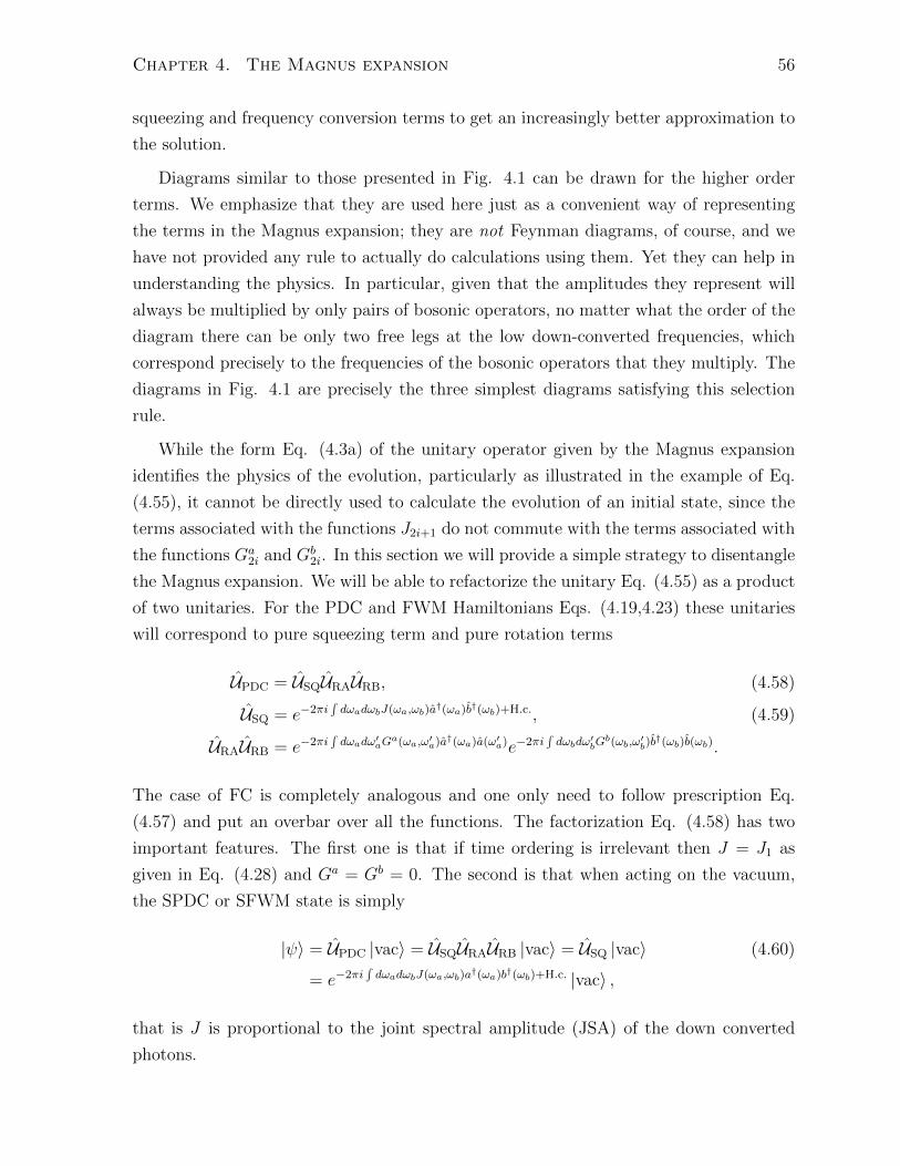
Chapter 4. The Magnus expansion 56
squeezing and frequency conversion terms to get an increasingly better approximation to
the solution.
Diagrams similar to those presented in Fig. 4.1 can be drawn for the higher order
terms. We emphasize that they are used here just as a convenient way of representing
the terms in the Magnus expansion; they are not Feynman diagrams, of course, and we
have not provided any rule to actually do calculations using them. Yet they can help in
understanding the physics. In particular, given that the amplitudes they represent will
always be multiplied by only pairs of bosonic operators, no matter what the order of the
diagram there can be only two free legs at the low down-converted frequencies, which
correspond precisely to the frequencies of the bosonic operators that they multiply. The
diagrams in Fig. 4.1 are precisely the three simplest diagrams satisfying this selection
rule.
While the form Eq. (4.3a) of the unitary operator given by the Magnus expansion
identifies the physics of the evolution, particularly as illustrated in the example of Eq.
(4.55), it cannot be directly used to calculate the evolution of an initial state, since the
terms associated with the functions J2i+1 do not commute with the terms associated with
the functions Ga2i and Gb
2i. In this section we will provide a simple strategy to disentangle
the Magnus expansion. We will be able to refactorize the unitary Eq. (4.55) as a product
of two unitaries. For the PDC and FWM Hamiltonians Eqs. (4.19,4.23) these unitaries
will correspond to pure squeezing term and pure rotation terms
UPDC = USQURAURB, (4.58)
USQ = e−2πi´dωadωbJ(ωa,ωb)a
†(ωa)b†(ωb)+H.c., (4.59)
URAURB = e−2πi´dωadω′aG
a(ωa,ω′a)a†(ωa)a(ω′a)e−2πi´dωbdω
′bG
b(ωb,ω′b)b†(ωb)b(ωb).
The case of FC is completely analogous and one only need to follow prescription Eq.
(4.57) and put an overbar over all the functions. The factorization Eq. (4.58) has two
important features. The first one is that if time ordering is irrelevant then J = J1 as
given in Eq. (4.28) and Ga = Gb = 0. The second is that when acting on the vacuum,
the SPDC or SFWM state is simply
|ψ〉 = UPDC |vac〉 = USQURAURB |vac〉 = USQ |vac〉 (4.60)
= e−2πi´dωadωbJ(ωa,ωb)a
†(ωa)b†(ωb)+H.c. |vac〉 ,
that is J is proportional to the joint spectral amplitude (JSA) of the down converted
photons.

Chapter 4. The Magnus expansion 57
To obtain the factorization Eq. (4.58) we will use the Baker-Campbell-Hausdorff
lemma Eq. (4.16) and the generalized Baker-Campbell-Hausdorff formula [82],
eX+Y = eXeY e−12
[X,Y ]e16
(2[Y ,[X,Y ]]+[X,[X,Y ]])···. (4.61)
The lowest order factorization that can be obtained by just going to second order in the
Magnus expansion is to write
UPDC = eΩ1+Ω2 ≈ eΩ1eΩ2 = USQURAURB. (4.62)
When applied to vacuum one simply obtains
|ψ2〉 = UPDC |vac〉 = eΩ1 |vac〉 , (4.63)
that is, up to second order the state is not modified by time ordering (since Ω2 |vac〉 = 0),
reminiscent of what happens when the Dyson series is used for this same problem [60].
Nevertheless, in the Magnus expansion the meaning of the null contribution of the second
order in SPDC and SFWM is transparent: this second order term requires at least
one down-converted photon to be present and hence it will vanish when applied to the
vacuum.
Thus it is clear that to see time-ordering corrections to the expression for the state of the
generated photons it is necessary to go to at least to third order. In this case one finds
eΩ1+Ω2+Ω3 ≈ eΩ1+Ω3eΩ2e−12
[Ω1+Ω3,Ω2] ≈ eΩ1+Ω3eΩ2e−12
[Ω1,Ω2]
= eΩ1+Ω3eΩ2e−12
[Ω1,Ω2]e−Ω2eΩ2 ≈ eΩ1+Ω3e−12eΩ2 [Ω1,Ω2]e−Ω2eΩ2
≈ eΩ1+Ω3e−12
([Ω1,Ω2]+[Ω2,[Ω1,Ω2]])eΩ2 ≈ eΩ1+Ω3e−12
[Ω1,Ω2]eΩ2
≈ eΩ1+Ω3− 12
[Ω1,Ω2]eΩ2 . (4.64)
Here we ignore any fourth order term, resolved the identity as I = e−Ω2eΩ2 , used the
Baker-Campbell-Hausdorff lemma and formula and the following relation eW eV e−W ≡eeW V e−W . From the last derivation is seen that to calculate the first non-vanishing correc-
tion to the JSA we not only need Ω3 but also [Ω1, Ω2]. This extra third order correction is
easy to understand: The diagram corresponding to Ω2 needs an incoming photon, which
can only be provided by a previous down-conversion process event included in Ω1. This
process will be of course of third order since it includes two down-conversion events and
one up conversion event. If Ω1 is a squeezing term and Ω2 is a rotation term for a and b,

Chapter 4. The Magnus expansion 58
then, their commutator is another two-mode squeezing operator
[Ω1, Ω2]
2= −2πi2
ˆdωadωb(K3(ωa, ωb)a
†(ωa)b†(ωb)− H.c.), (4.65)
with
K3(ωa, ωb) = π
ˆdω(J1 (ωa, ω)Gb
2 (ωb, ω) +Ga2 (ωa, ω) J1 (ω, ωb)
).
Eq. (4.64) provides a compact formula accounting for the effects of time ordering, and
leads to an identification of the form of the joint spectral amplitude, which to this level
of approximation is proportional to
J(ωa, ωb) = J1(ωa, ωb) + (J3(ωa, ωb)− iK3(ωa, ωb)) , (4.66)
where the first contribution J1(ωa, ωb) neglects effects of time ordering, while the addi-
tional terms take corrections into account to all orders lower than the fifth (this last fact
we shall prove shortly). This illustrates that as the intensity of the pump field increases
and the corrections become larger not only are more squeezed photons generated in the
same modes, but their spectral properties change. In particular, if the functions char-
acterizing the pump pulse and the phase-matching functions are real, then as the pump
intensity is increased the phase structure of the joint spectral amplitude evolves from
trivial to nontrivial.
For FC one will also need the commutator of the first two Magnus terms which is
[Ω1, Ω2]
2= −(2π)i2
ˆdωadωb(K3(ωa, ωb)a(ωa)b
†(ωb)− H.c.),
where we defined
K3(ωa, ωb) = π
ˆdω(J1(ωa, ω)Gb
2(ωb, ω)− Ga2(ω, ωa)J1(ω, ωb)
). (4.67)
From the general properties of the Magnus expansion, i.e. the fact that the nth order
Magnus terms is made of n− 1 commutators, we know that all even Magnus terms will
be rotation operators for a and b, whereas all odd terms will be two-mode squeezing
operators. This fact can be used to show that the commutator of two Magnus terms
[Ωi, Ωj] (which is an i + j order term) will be a rotation term if i + j is even and a
squeezing term if i + j is odd. With these two facts and after some algebra it can be

Chapter 4. The Magnus expansion 59
shown, that the extension of Eq. (4.64) to fifth order is
UPDC = exp(Ω1 + Ω2 + Ω3 + Ω4 + Ω5) = USQURAURB, (4.68)
where the squeezing and rotation unitaries USQ, URAURB are
USQ = exp
(Ω1 +
(Ω3 −
1
2[Ω1, Ω2]
)+(
Ω5 −1
2[Ω1, Ω4] (4.69)
− 1
2[Ω3, Ω2] +
5
6[Ω2, [Ω2, Ω1]] +
1
2[Ω1, [Ω1, Ω3]]
)),
URAURB = exp
(Ω2 +
(Ω4 +
1
2[Ω1, [Ω1, Ω2]]
)). (4.70)
We now consider difference frequency generation, where besides an injected pump
pulse that is treated classically we also seed the modes at ωa and/or ωb, with injected
pulses described by coherent states. Here the output state can be written as
|ψ3〉 = eΩ1+Ω3− 12
[Ω1,Ω2]eΩ2ei∑c=a,b(
´dωcgc(ωc)c†(ωc)+H.c.) |vac〉 (4.71)
=(eΩ1+Ω3− 1
2[Ω1,Ω2]
)(eΩ2ei
∑c=a,b(
´dωcgc(ωc)c†(ωc)+H.c.)e−Ω2
)|vac〉 . (4.72)
Keeping only terms up to third order, we find
eΩ2ei∑c=a,b(
´dωcgc(ωc)c†(ωc)+H.c.)e−Ω2 = ei
∑c=a,b(
´dωcgc(ωc)eΩ2 c†(ωc)e−Ω2+H.c.) (4.73)
= ei∑c=a,b(
´dωcgc(ωc)(c†(ωc)+[Ω2,c†(ωc)])+H.c.). (4.74)
The commutator inside the exponential in Eq. (4.74) can be easily calculated to be
[Ω2, a†(ω′a)] = −2πi
ˆdωaa
†(ωa)Ga2(ωa, ω
′a), (4.75)
[Ω2, b†(ω′b)] = −2πi
ˆdωbb
†(ωb)Gb2(ωb, ω
′b). (4.76)
This shows that the first effect due to time-ordering corrections in stimulated processes is
to modify the shape of the injected seed pulses, since we can incorporate the time-ordering
corrections to second order by imagining that the shape of the incoming coherent state
(or single photon) is modified according to gc(ωc) → gc(ωc) − 2πi´dω′cgc(ω
′c)G
c2(ωc, ω
′c).
Although the discussion in this section was phrased in terms of the PDC and FWM
Hamiltonian all its conclusions are directly applicable to the case of FC.

Chapter 4. The Magnus expansion 60
4.6 Time-ordering corrections in broadly phase-matched
Processes
Here we consider time-ordering corrections in the special limit that the phase matching
function is independent of is variables,
Φ(ωa, ωb, ωp) ∝ 1, (4.77)
in Eqs. (4.22) and (4.39). This implies that the function F in Eqs. (4.25) and (4.43) is
a function only of its last argument, F (x, y, z) = F (z). We show below that if this holds
the second and third order Magnus terms vanish. Recently Donohue et al. [19] showed
that all the time-ordering corrections vanish for a flat phase matching function.
To proceed, we look at Ga2(ωa, ω
′a) as a typical term. For PDC, in the limit Eq. (4.77)
it becomes
Ga2(ωa, ω
′a) =
ˆdωq
dωpωp
F (ωa + ωp + ωq)F∗ (ω′a + ωp + ωq) .
In the last equation we are free to move the origin of the integral in ωq by ωp to get:
Ga2 =
ˆdωqF (ωa + ωq)F
∗ (ω′a + ωq)
dωpωp
, (4.78)
using the identityffl
dxx+y
= 0, the innermost integral is identically zero. The same kind
of argument shows that Gb2 vanishes. Finally, to show that the third order term is also
zero we proceed along similar lines. Using expression Eq. (4.34), with F (x, y, z) = F (z)
we obtain:
ˆdωcdωd
dωpdωqF
∗ (ωc + ωd + ωp + ωq)F (ωa + ωc + ωp)F (ωb + ωd + ωq)
×1
3
2
ωpωq+
1
ωp + ωq
(1
ωp+
1
ωq
). (4.79)
As before, we shift the integration axes, in this case, ωc → ωc− ωq, ωd → ωd− ωp to get:
ˆdωcdωdF
∗ (ωc + ωd)F (ωa + ωd)F (ωb + ωc)
dωpdωq
2
ωpωq+
1
ωp + ωq
(1
ωp+
1
ωq
)= 0. (4.80)

Chapter 4. The Magnus expansion 61
4.7 Relation between this work and that of Christ et
al.
In the previous sections we have argued that the exact propagator of PDC is given by
UPDC = USQURAURB. In the work of Christ et al. [52] the authors study the properties
of PDC by looking at the action of the propagator on the canonical operators for the
different polarizations. In particular they set to solve for functions Ua, Va, Ub, Vb that
satisfy
U †PDCa(ωa)UPDC =
ˆdω′aUa(ωa, ω
′a)a(ω′a) +
ˆdω′bVa(ωa, ω
′b)b†(ω′b), (4.81)
U †PDCb(ωb)UPDC =
ˆdω′bUb(ωb, ω
′b)b(ω
′b) +
ˆdω′aVb(ωb, ω
′a)a†(ω′a). (4.82)
To link the two approaches one only needs to use the results from this chapter and
concatenate the results regarding the transformations of single frequency operators under
multimode transformations Table 2.2 and let F → J , G→ Ga and H → Gb in Eq. (2.79)
and Eq. (2.84) to get
U †PDCa(ωa)UPDC = U †RBU†RAU
†SQa(ωa)USQURAURB (4.83)
=
ˆdω′′a
ˆdω′a
(∑λ
fλ(ωa)f∗λ(ω′a) cosh(sλ)
)(∑α
gα(ω′α)g∗α(ω′′α)eiuα
)︸ ︷︷ ︸
Ua(ωa,ω′′a )
a(ω′′a)
+
ˆdω′′b
i
ˆdω′b
(∑λ
fλ(ωa)jλ(ω′b) sinh(sλ)
)(∑β
h∗β(ω′b)hβ(ω′′b )e−ivβ
)︸ ︷︷ ︸
Va(ωa,ω′′b )
b†(ω′′b ).
In an analogous manner one finds for b(ωb)
U †PDCb(ωb)UPDC = (4.84)ˆdω′′a
i
ˆdω′a
(∑λ
fλ(ω′a)j(ωb) sinh(sλ)
)(∑α
g∗α(ω′a)gα(ω′′a)e−iuα
)︸ ︷︷ ︸
Vb(ωb,ω′′a )
a†(ω′′a)
+
ˆdω′′b
ˆdω′b
(∑λ
cosh(sλ)jλ(ωb)j∗λ(ω
′b)
)(∑β
hβ(ω′b)h∗β(ω′′b )eivβ
)︸ ︷︷ ︸
Ub(ωb,ω′′b )
b(ω′′b ).

Chapter 4. The Magnus expansion 62
Similarly to what was done for PDC we showed that the exact propagator for FC can be
written as UFC = UBSURAURB. Likewise in [52] it is proposed that the canonical operators
at the input and output are related via
UFCa(ωa)U †FC =
ˆdω′aUa(ωa, ω
′a)a(ω′a) +
ˆdω′bVa(ωa, ω
′b)b(ω
′b), (4.85)
UFCb(ωb)U †FC =
ˆdω′bUb(ωb, ω
′b)b(ω
′b) +
ˆdω′aVb(ωb, ω
′a)a(ω′a). (4.86)
Using again the results in Table 2.2 and letting K → J , G → Ga and H → Gb in Eq.
(2.79) the two approaches can be related in the following way:
UFCa(ωa)U †FC = (4.87)ˆdω′′a
ˆdω′a
(∑θ
k∗θ(ωa)kθ(ω′a) cos(rθ)
)(∑α
g∗α(ω′a)gα(ω′′a)eiuα
)︸ ︷︷ ︸
Ua(ωa,ω′′a )
a(ω′′a)
+
ˆdω′′b
i
ˆdω′b
(∑θ
k∗θ(ωa)lθ(ω′b) sin(rθ)
)(∑β
h∗β(ω′b)hβ(ω′′b )eivβ
)︸ ︷︷ ︸
Va(ωa,ω′′a )
b(ω′′b ),
UFCb(ωb)U †FC = (4.88)ˆdω′′a
i
ˆdω′a
(∑θ
sin(rθ)l∗θ(ωb)kθ(ω
′a)
)(∑α
g∗α(ω′a)gα(ω′′a)eiuα
)︸ ︷︷ ︸
Vb(ωb,ω′′a )
a(ω′′a)
+
ˆdω′′b
ˆdω′b
(∑θ
lθ(ωb)l∗θ(ω
′b) cos(rθ)
)(∑β
hβ(ω′b)h∗β(ω′′b )eivβ
)︸ ︷︷ ︸
Ub(ωb,ω′′b )
b(ω′′b ).
So far we have only shown how to calculate the transformation functions in the Heisenberg
picture starting from the unitary evolution operator. In general the inverse mapping is
much harder since it is essentially a deconvolution problem. Yet for the special case of
SPDC it is possible to invert. In SPDC the state generated by the nonlinear interaction
is UPDC |vac〉 = USQURAURB |vac〉 = USQ |vac〉. Note that URA and URB disappear from

Chapter 4. The Magnus expansion 63
the problem. With this in mind we can calculate
〈vac| U †PDCa(ωa)b(ωb)UPDC |vac〉 = 〈vac| U †SQa(ωa)b(ωb)USQ |vac〉 (4.89)
= i∑λ
sinh(2sλ)
2fλ(ωa)jλ(ωb) (4.90)
= i
ˆdωUa(ωa, ω)Vb(ωb, ω). (4.91)
Note that the last quantity can be calculated from the results in [52] and the last equation
provides the recipe to obtain the JSA from this last second moment; if we write the
Schmidt decomposition
i
ˆdωUa(ωa, ω)Vb(ωb, ω) = i
∑λ
sλfλ(ωa)jλ(ωb), (4.92)
then we can immediately reconstruct the JSA as
−2πJ(ωa, ωb) =∑λ
sλfλ(ωa)jλ(ωb) =∑λ
sinh−1 (2sλ)
2fλ(ωa)jλ(ωb), (4.93)
and identify the Schmidt values sλ and functions fλ, jλ of the JSA. The consistency of
the reconstruction Eq. (4.89) can be checked by verifying the following relations
〈vac| U †PDCa†(ωa)a(ω′a)UPDC |vac〉 = 〈vac| U †SQa
†(ωa)a(ω′a)USQ |vac〉 (4.94)
=∑λ
sinh2 sλ f∗λ(ωa)fλ(ω
′a) (4.95)
=
ˆdωV ∗a (ωa, ω)Va(ω
′a, ω), (4.96)
〈vac| U †PDCb†(ωb)b(ω
′b)UPDC |vac〉 = 〈vac| U †SQb
†(ωb)b(ω′b)USQ |vac〉 (4.97)
=∑λ
sinh2 sλ j∗λ(ωb)jλ(ω
′b) (4.98)
=
ˆdωV ∗b (ωb, ω)Vb(ω
′b, ω). (4.99)
The only reason why one can invert for the JSA of the squeezed state is because we are
looking at SPDC, which implies that we take vacuum expectation values that make the
contribution from URA and URB disappear. If they were present one would be dealing
with much harder deconvolution problem.

Chapter 5
Generation of bright non-classical
light
“Not gaussian” = “An ass outing.” A useful anagram?
Stephen “T. Rex” Foster
5.1 Introduction
Particles exhibiting strong, non-classical correlations play a central role in the imple-
mentation of quantum-enhanced information processing tasks. As mentioned in the
introduction, nonlinear photonic materials provide some of the most versatile sources
of these particles. The interactions that give rise to the quantum correlated photons
are typically rather weak, but by using a strong classical pump field they can be en-
hanced by orders of magnitude. Thus the theoretical treatment of photon generation
usually involves a time-dependent Hamiltonian in the interaction picture. Because this
Hamiltonian generally does not commute with itself at different times, the time evolu-
tion operator in these types of problems is not just a simple exponential involving the
time integral of the Hamiltonian, and so-called “time-ordering” corrections arise in the
description of the quantum state evolution [57, 59, 60].
In this chapter, we introduce an analytical model that describes the effects of time
ordering in several non-linear quantum optical processes. The model automatically cap-
tures the photon statistics and unitary evolution that characterize the exact solution of the
problem. With this model we provide a simple explanation of when time-ordering effects
become important: As long as the generated photons do not significantly copropagate
(i.e., reside in the same spatial region at the same time) with the pump photons, time-
64

Chapter 5. Generation of bright non-classical light 65
Figure 5.1: Comparison of a sinc function and the gaussian fit exp(−γx2).
ordering effects are irrelevant for the description of the generated quantum state. Based
on this intuitive idea we propose an experiment using periodically poled lithium niobate
where these corrections can be observed. Then we use our simple model to study how
the properties of the quantum light produced by the nonlinear material are modified by
the time-ordering corrections and we derive useful observables that capture the departure
from the first order Magnus correction. Finally, we also study what are the effects of the
time-ordering correction in the heralded generation of Fock states using realistic number
resolution detectors.
5.2 Model
We consider the following interaction picture Hamiltonian, which can be used to model
both spontaneous parametric down-conversion (SPDC) and spontaneous four-wave mix-
ing (SFWM) in a one dimensional geometry, within the undepleted pump and rotating
wave approximations:
HI(t) = −~εˆdωpdωadωbe
i∆tΦ(ωa, ωb, ωp)α(ωp)a†(ωa)b
†(ωb) + H.c. (5.1)
Here a†(ω) and b†(ω) are creation operators for two different fields, and Φ is the phase
matching function, which we take to be a Gaussian function,
Φ(ωa, ωb, ωp) = exp(−(saδωa + sbδωb − spδωp)2
). (5.2)

Chapter 5. Generation of bright non-classical light 66
When we take si =√γL/(2vi) > 0, where vi is the group velocity at frequency ωi,
this provides a good approximation to the usual sinc function resulting from a uniform
nonlinearity over a region of length L, under the neglect of dispersion effects; the choice
of γ = 0.193 guarantees that the full width at half maximum of the sinc and Gaussian
functions agree (See Fig. 5.1). We should mention that by using poling techniques [83]
it is possible to engineer approximately the phase matching function in Eq. (5.2). In
Eq. (5.2) δωi = ωi − ωi; in SPDC the central frequencies ωi are constrained by energy
conservation, ωa + ωb = ωp , and momentum conservation, ka(ωa) + kb(ωb) = kp(ωp),
while for SFWM ωp is twice the frequency of the pump and momentum conservation
reads ka(ωa) +kb(ωb) = 2kp(ωp/2) [84]. The parameter ε is a dimensionless constant that
characterizes the strength of the interaction (see Eq. (3.28) and Eq. (3.41)); it depends
on physical properties such as the effective non-linearity of the medium and the area of
the interaction region. We also assume that the classical pump can be described by a
Gaussian function,
α(ωp) =τ√π
exp(−τ 2δω2
p
), (5.3)
with τ characterizing the temporal duration of the pump pulse. Finally ∆ = ωa+ωb−ωp,and in Eq. (5.1) we adopt the convention (used throughout the thesis) that whenever
the limits of an integral are not specified they range from −∞ to ∞. We will frame
the discussion in terms of photon generation using SPDC but as argued in the previous
Chapters the results translate almost immediately to SFWM.
Using the Magnus expansion, we showed in the previous chapter that the unitary
evolution operator generated by the Hamiltonian Eq. (5.1) can be factored as UPDC =
USQURAURB with USQ a pure two-mode squeezing term (generated by terms that are
extensions of a†b† + H.c.) and URAURB pure “rotation” terms (generated by terms that
are extensions of a†a+ b†b),
UPDC = exp
(−2πi
ˆdωadωb
∑n
(Jn − iKn)a†(ωa)b†(ωb) + H.c.
)(5.4)
∏c=a,b
exp
(−2πi
ˆdωcdωc′
∑m
Gcm(ωc, ωc′)c
†(ωc)c(ω′c)
),
with n odd and m even. Each of these indices labels the order of the expansion in ε; e.g.,
n = 1 is a term ∝ ε and m = 2 is a term ∝ ε2. If a spontaneous process is considered,
where the unitary operator UPDC is applied to the vacuum, it is readily seen that the

Chapter 5. Generation of bright non-classical light 67
second exponential in Eq. (5.4) does not modify the initial state; URAURB |vac〉 = |vac〉,and hence the output state |ψout〉 = UPDC |vac〉 = USQ |vac〉 is generated solely by the
squeezing part USQ. With these observations it is easy to identify J =∑
n(Jn − iKn) as
proportional to the Joint Spectral Amplitude (JSA) of the photons generated in modes
a and b in a spontaneous process. The first term of the Magnus expansion for the
Hamiltonian Eq. (5.1) is obtained by integrating the Hamiltonian from −∞ to ∞;
K1 = 0, and the result for J1 can be written in the following simple form using the
derivations from Sec. 4.3:
J1(δωa, δωb) = − ετ√π
exp(−uNuT
), (5.5)
N =
(µ2a µ2
µ2 µ2b
), u = (δωa, δωb), (5.6)
ηa,b = sp − sa,b, µ2 = τ 2 + ηaηb, µ2a,b = τ 2 + η2
a,b.
If time-ordering effects were ignored, K1 would vanish, and J1 would be the only con-
tribution to J ; J1 would thus completely describe the properties of the state, and would
identify the joint spectral amplitude of the generated photons. A measure of entangle-
ment is the Schmidt number introduced in [67] and studied in Chapter 2, which for the
state characterized by J1 is [49, 85]
S = µaµb/√µ2aµ
2b − µ4. (5.7)
In the limit that the matrix N is diagonal, µ → 0 and the down converted photons are
uncorrelated; here S = 1. If in this limit N were also proportional to the identity matrix,
then the photons would not only be uncorrelated but would share the same spectral
characteristics; for this to happen we require ηa = −ηb = ±τ . In the opposite limit, i.e.
τ |ηa,b|, (5.8)
N becomes rank deficient, the photons generated in the modes a and b are strongly
correlated, and S →∞. A simple way to understand the physics in the limit Eq. (5.8)
is to rewrite the inequality as
vpτ
|va,b − vp| L
va,b. (5.9)
That is, in this limit the time the down converted photons spend with the pump photons
Chapter 5. Generation of bright non-classical light 68
is much less than the time they spend in the nonlinear structure. The down converted
photons once created thus escape the nonlinear structure without spending appreciable
time in the same region as the pump photons, and if the pump intensity is high enough
to generate a number of pairs of photons then the stream of pairs is spread over a long
time; equivalently, their frequencies are tightly constrained.
5.3 Time-ordering effects in spontaneous photon gen-
eration
For the simple Gaussian model considered in this chapter, the real part of the first non-
vanishing correction to the JSA due to time ordering is given by
J3(ωa, ωb) = W (ωa, ωb)− Z(ωa, ωb)V (ωa, ωb), (5.10)
W (ωa, ωb) =2π3/2ε3τ 3
3R2exp
(−uQuT/R4
), (5.11)
Z(ωa, ωb) = 4√πτ 3ε3 exp
(−uNuT/3
), (5.12)
V (ωa, ωb) =
ˆ ∞0
dp
ˆ ∞0
dq exp(−(p, q)M(p, q)T
)cos(
4τηab(δωaq + δωbp)/√
3),
(5.13)
with
Q =
(M4µ2
a µ6
µ6 M4µ2b
), M =
(2µ2
a µ2
µ2 2µ2b
), (5.14)
R4 = 4µ2aµ
2b − µ4 = 4η2
abτ2 + 3µ4,
M4 = 4µ2aµ
2b − 3µ4, ηab = −ηba = ηa − ηb.
The imaginary part of the correction K3 is given by
K3(ωa, ωb) = −ε3π3/2 τ3
R2exp(−uQuT/R4) (erfi(yab) + erfi(yba)) ,
yab =
√2
3
τηba (2δωaµ2a − δωbµ2)
R2µa(5.15)
and erfi(z) = erf(iz)/i, with erf being the standard error function. Details of the calcula-
tion are given in Appendix D. A useful feature of using Gaussian functions to model both
the phase-matching function and the pump pulse is that estimates of the relative sizes of
the corrections due to time ordering in SPDC and SFWM can be easily extracted; this
Chapter 5. Generation of bright non-classical light 69
also holds for the time-ordering corrections to frequency conversion. We demonstrate
this all below, introducing figures of merit which characterize the size of the time-ordering
corrections relative to the uncorrected prediction that would follow from the first order
Magnus calculation. Some of the mathematical details are relegated to Appendix D.
To estimate the effects of time ordering on SPDC and SFWM we introduce the
following figure of merit,
r =maxωa,ωb |J3(ωa, ωb)|maxωa,ωb |J1(ωa, ωb)|
=
√π
ετmaxωa,ωb|J3(ωa, ωb)|. (5.16)
In Appendix D we show that
|J3(ωa, ωb)| ≤2π3/2ε3τ 3
R2, (5.17)
and so we identify the bound
r ≤ 2π2ε2
(τ 2
R2
). (5.18)
There are two interesting limits of the important ratio τ 2/R2 that appears in Eq. (5.18).
We find
τ |ηa,b| ⇒τ 2
R2∼ 1√
3
τ
|ηa|τ
|ηb|≪ 1, (5.19)
µ = 0⇒ τ 2
R2=
τ
2|ηab|.
From this we can see that the importance of the time-ordering corrections depends
strongly on the entanglement of the photons in modes a and b, and we can also un-
derstand this scaling physically. As discussed in the previous section, if the generated
photons are highly entangled with a large Schmidt number, the time they overlap the
pump field is short. We would then expect on physical grounds that time-ordering
corrections should be small, and indeed we see from the first of Eq. (5.19) and Eq.
(5.18) that a very large interaction strength ε would be necessary for the time-ordering
corrections to come into play. In the reverse limit, the second of Eq. (5.19), the group
velocities of the generated photons satisfy ηaηb = −τ 2 (µ = 0). To have a significant
time-ordering correction, we have from the second of Eq. (5.19) that the group velocities
of the downconverted photons must be similar. Note that if the velocities were equal J3
would vanish identically; see Appendix D. It can also be shown that the maximum of

Chapter 5. Generation of bright non-classical light 70
τ 2/R2 under the constraint of having µ = 0 is obtained for
ηa = −ηb = ±τ ⇒ vpτ
|va,b − vp|=
√γ
2
L
va,b. (5.20)
In such a case τ 2/R2 equals 1/4. Eq. (5.20) simply tell us that the time the down-
converted photons spend with the pump is comparable with the time they spend in the
crystal. Note that the entanglement in the downconverted state as predicted by using J1
for J and the condition Eq. (5.20) is very small, but because of the continued presence of
photons being generated with the pump pulse, time-ordering corrections would be phys-
ically expected to come into play at a smaller interaction strength ε; this is confirmed by
using Eq. (5.20) in Eq. (5.18). Furthermore, besides being simply larger, time-ordering
corrections can be expected to be of greater significance here, since they can qualitatively
modify the very small entanglement that the approximation of J by J1 would imply.
When appropriate values of ε are used in Eq. (5.18), we see that our results are
consistent with what was found by Christ et al. [52], in which simulations showed that
extremely high pump intensities are necessary to obtain observable time-ordering effects
for very entangled JSAs.
5.4 Time-ordering effects in stimulated photon gen-
eration
In this section we turn our attention to stimulated parametric down-conversion/four wave
mixing processes, in which the unitary rotation operators URAURB in Eq. (5.4) charac-
terizing single mode frequency conversion become important. The first contribution to
the frequency conversion unitary is given by
Ga2(ωa, ω
′a) = ε2
√π
2
τ 2
µbe−x
2−−x2
+erfi(x+), x+ =τηba (δω′a + δωa)√
2µb, x− =
(ωa − ω′a)µa√2
.
(5.21)
To obtain the last equation one needs to use Eq. (4.32a) and the following identity
dx
xe−ax
2+bx+c = 2
ˆ ∞0
dx
xe−ax
2+c sinh(bx) = ecπerfi
(b
2√a
). (5.22)
An analogous formula to Eq. (5.21) can be found for Gb2(ωb, ω
′b) by simply switching
a↔ b in Eq. (5.21). We consider the scenario of a process seeded by a coherent state in
Chapter 5. Generation of bright non-classical light 71
field a, described by the state
|g(ωa)〉 = exp
(i√N
ˆdωa
(g(ωa)a
†(ωa) + h.c.))|vac〉 . (5.23)
where´dωa|g(ωa)|2 = 1 and N is the mean number of photons in the state (see Sec.
2.3). Using Eq. (5.4) and the results from the previous chapter we see that the lowest
(second) order effect associated with time ordering is
|ψout〉 = USQURAURA |g(ωa)〉 = USQ × ei√N
´dωa(g(ωa)+δg(ωa))a†(ωa)+h.c. |vac〉 ,
δg(ωa) = −2πi
ˆdω′ag(ω′a)G2(ωa, ω
′a). (5.24)
The last equation can be interpreted as follows: the first effect (∝ ε) of the interaction is
that the nonlinear medium acts as a two mode squeezer, generating pairs of photons in
fields a and b. The second order effect (∝ ε2), which appears solely due to time ordering,
describes the “dressing” of the seed photons by the pump. That is, the frequency
amplitudes of the photons of polarization a are no longer described by g(ωa) but rather
by g(ωa) + δg(ωa). Finally, note that if instead the seed were prepared in a single photon
state |1g(ωa)〉 =´dωag(ωa)a
†(ωa) |vac〉, the effect of time ordering would be to dress it
according to |1g(ωa)〉 → |1g(ωa)+δg(ωa)〉.
To quantify the effects of time ordering we estimate the correction given by the second
term of Eq. (5.24) relative to the first term. If we take g(ωa) = ν exp(−τ 2a δω
2a), in the
limit τa τ, |ηa|,ˆdω′ag(ω′a)G2(ωa, ω
′a) = ε2ν
π2τ 2
N 2exp(−q2)erfi(q), (5.25)
q =√
2ωaηabτµa/N 2, N 4 = µ4 + 2τ 2η2ab. (5.26)
Note that the maximum value the function exp(−q2)erfi(q) attains is ξ ≈ 0.610503 and
that the function is identically zero if q = 0 (which only occurs for the unphysical situation
ηa = ηb). As before, we can compare the relative strengths of the amplitudes of the
coherent state with and without including time-ordering effects to obtain the following
figure of merit:
ρ =maxωa |δg(ωa)|maxωa g(ωa)
= 2π3ξ(ε2τ 2/N 2). (5.27)
This quantity measures how much the pump is dressed by the time-ordering effects of the
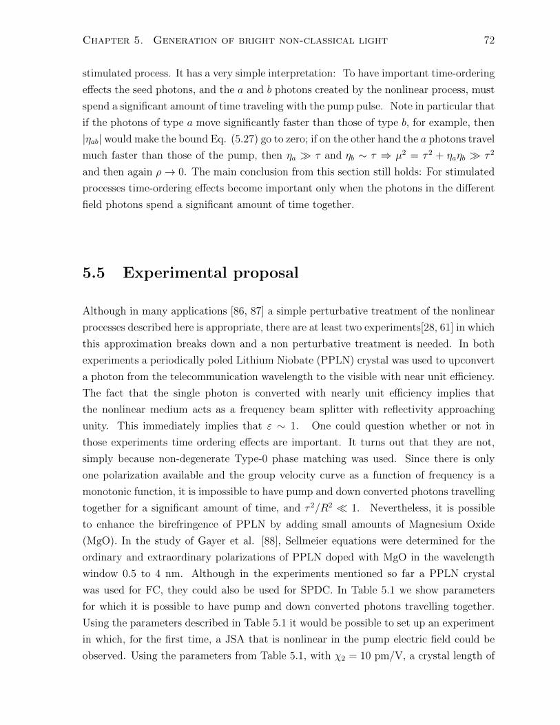
Chapter 5. Generation of bright non-classical light 72
stimulated process. It has a very simple interpretation: To have important time-ordering
effects the seed photons, and the a and b photons created by the nonlinear process, must
spend a significant amount of time traveling with the pump pulse. Note in particular that
if the photons of type a move significantly faster than those of type b, for example, then
|ηab| would make the bound Eq. (5.27) go to zero; if on the other hand the a photons travel
much faster than those of the pump, then ηa τ and ηb ∼ τ ⇒ µ2 = τ 2 + ηaηb τ 2
and then again ρ→ 0. The main conclusion from this section still holds: For stimulated
processes time-ordering effects become important only when the photons in the different
field photons spend a significant amount of time together.
5.5 Experimental proposal
Although in many applications [86, 87] a simple perturbative treatment of the nonlinear
processes described here is appropriate, there are at least two experiments[28, 61] in which
this approximation breaks down and a non perturbative treatment is needed. In both
experiments a periodically poled Lithium Niobate (PPLN) crystal was used to upconvert
a photon from the telecommunication wavelength to the visible with near unit efficiency.
The fact that the single photon is converted with nearly unit efficiency implies that
the nonlinear medium acts as a frequency beam splitter with reflectivity approaching
unity. This immediately implies that ε ∼ 1. One could question whether or not in
those experiments time ordering effects are important. It turns out that they are not,
simply because non-degenerate Type-0 phase matching was used. Since there is only
one polarization available and the group velocity curve as a function of frequency is a
monotonic function, it is impossible to have pump and down converted photons travelling
together for a significant amount of time, and τ 2/R2 1. Nevertheless, it is possible
to enhance the birefringence of PPLN by adding small amounts of Magnesium Oxide
(MgO). In the study of Gayer et al. [88], Sellmeier equations were determined for the
ordinary and extraordinary polarizations of PPLN doped with MgO in the wavelength
window 0.5 to 4 nm. Although in the experiments mentioned so far a PPLN crystal
was used for FC, they could also be used for SPDC. In Table 5.1 we show parameters
for which it is possible to have pump and down converted photons travelling together.
Using the parameters described in Table 5.1 it would be possible to set up an experiment
in which, for the first time, a JSA that is nonlinear in the pump electric field could be
observed. Using the parameters from Table 5.1, with χ2 = 10 pm/V, a crystal length of
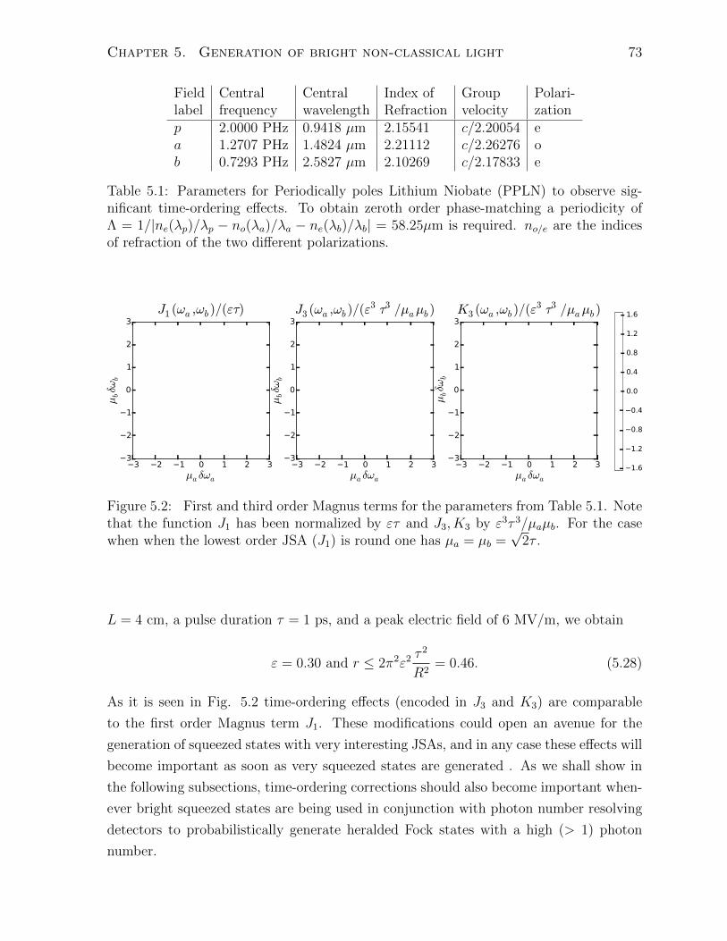
Chapter 5. Generation of bright non-classical light 73
Field Central Central Index of Group Polari-label frequency wavelength Refraction velocity zationp 2.0000 PHz 0.9418 µm 2.15541 c/2.20054 ea 1.2707 PHz 1.4824 µm 2.21112 c/2.26276 ob 0.7293 PHz 2.5827 µm 2.10269 c/2.17833 e
Table 5.1: Parameters for Periodically poles Lithium Niobate (PPLN) to observe sig-nificant time-ordering effects. To obtain zeroth order phase-matching a periodicity ofΛ = 1/|ne(λp)/λp − no(λa)/λa − ne(λb)/λb| = 58.25µm is required. no/e are the indicesof refraction of the two different polarizations.
Figure 5.2: First and third order Magnus terms for the parameters from Table 5.1. Notethat the function J1 has been normalized by ετ and J3, K3 by ε3τ 3/µaµb. For the casewhen when the lowest order JSA (J1) is round one has µa = µb =
√2τ .
L = 4 cm, a pulse duration τ = 1 ps, and a peak electric field of 6 MV/m, we obtain
ε = 0.30 and r ≤ 2π2ε2 τ2
R2= 0.46. (5.28)
As it is seen in Fig. 5.2 time-ordering effects (encoded in J3 and K3) are comparable
to the first order Magnus term J1. These modifications could open an avenue for the
generation of squeezed states with very interesting JSAs, and in any case these effects will
become important as soon as very squeezed states are generated . As we shall show in
the following subsections, time-ordering corrections should also become important when-
ever bright squeezed states are being used in conjunction with photon number resolving
detectors to probabilistically generate heralded Fock states with a high (> 1) photon
number.

Chapter 5. Generation of bright non-classical light 74
5.6 Measuring the effects of the time-ordering cor-
rections
Before considering how to measure the effects of time ordering lets us look at what are
the consequences of including time-ordering corrections in the state generated in SPDC.
If they were ignored then we could write very generally
J(ωa, ωb) = J1(ωa, ωb) =∑λ
(−εsλ)2π
fλ(ωa)jλ(ωb). (5.29)
Because we assumed that the only contribution to J comes from J1 then ε, the constant
characterizing the strength of the interaction, can be factored out and the Schmidt values
sλ(ε) = εsλ become linear functions of ε and the Schmidt functions are independent of
ε. We can write the squeezed state generated by the interaction as
|ψout〉 = ei∑λ(εsλ)(A†λB
†λ+H.c.) |vac〉 =
⊗λ
ei(εsλ)(A†λB†λ+H.c.) |vac〉 , (5.30)
where we used the notation introduced in Eq. (2.87). The last equation tells us that
as we increase the energy in the pump pulse (as we increase ε) we simply increase the
squeezing parameter εsλ linearly and we do not modify the spectral shape of the Schmidt
modes. We can contrast this with the case where we include time-ordering corrections
J(ωa, ωb) = J1(ωa, ωb)︸ ︷︷ ︸∝ε
+ (J3(ωa, ωb)− iK3(ωa, ωb))︸ ︷︷ ︸∝ε3
=∑λ
−sλ(ε)2π
fλ(ωa; ε)jλ(ωa; ε).
(5.31)
In the last equation we cannot simply factor out the ε dependence and thus because of
time-ordering effects the Schmidt coefficients are now nonlinear functions of ε and the
Schmidt functions will change as ε is changed.
We have argued that the ideal parameter region for having significant modifications
of the JSA is when one has a nearly uncorrelated JSA for ε 1 (µ = 0 in Eq. 5.5). In
this parameter region J1 can be written as an uncorrelated Gaussian
−2πJ1(ωa, ωb) =2πετ√π
exp(−α2 − β2) (5.32)
=√
2πτεf(α)f(β), α = µaδωa, β = µbδωb, (5.33)
where f(x) = exp(−x2)/ 4√π/2 is a normalized Gaussian function. If we ignored time

Chapter 5. Generation of bright non-classical light 75
ordering then
|ψout〉 = eis0ε´dαdβ(f(α)f(β)a†(α)b†(β)+H.c.) |vac〉 = eis0εA
†0B†0+H.c. |vac〉 (5.34)
where the parameter
s0 =
√2πτ√µaµb
. (5.35)
tells us the rate of change of the squeezing parameter with respect to the dimensionless
coupling constant ε. This parameter has another very important physical meaning. Un-
der the separability constraint 0 = µ2 = ηaηb + τ 2 the quantity s0 tells us how much
our low energy JSA, J1 departs from being round. Indeed, for a perfectly round and
separable J1, for which µa = µb =√
2τ , the quantity s0 takes its maximum value π. For
a more eccentric J1 the quantity s0 will be less than π and will tend to zero for a J1 with
an aspect ratio tending to zero or infinity.
For the state in Eq. (5.34) the mean number of photons in field a (or b) is
〈Na〉 = 〈Nb〉 = sinh2(s0ε), (5.36)
Na =
ˆdωaa
†(ωa)a(ωa), Nb =
ˆdωbb
†(ωb)b(ωb), (5.37)
and the Schmidt number S = 1 for all values of ε.
Once time ordering is included we need to calculate the corrections J3 and K3. As shown
in Appendix D for µ = 0 these functions are
J3(ωa, ωb) =π3/2τ 3ε3e−α
2−β2(
3erfi(√
23β)
erfi(√
23α)− 1)
6µaµb, (5.38)
K3(ωa, ωb) = ±π3/2τ 3ε3e−α
2−β2(
erfi(√
23β)− erfi
(√23α))
2µaµb, (5.39)
and now the Schmidt functions depend on ε and the Schmidt coefficients are no longer
Chapter 5. Generation of bright non-classical light 76
linear functions of ε. The state including time-ordering corrections will be now
|ψout〉 = exp
(i
ˆdαdβ
(s0ε)f(α)f(β) +
(s0ε)3
4× (5.40)
f(α)f(β)
[erfi(√
2/3β)
erfi(√
2/3α)− 1/3
± i(
erfi(√
2/3β)− erfi
(√2/3α
))]a†(α)b†(β) + H.c.
)|vac〉
The expression shows a very interesting feature of the Gaussian model. For the low
energy uncorrelated case µ = 0 the corrected JSA is only a function of s0ε. The last
expression shows explicitly that for s0ε 1 this quantity is precisely the Schmidt number
of the mode, but more importantly even when the condition s0ε 1 is not satisfied
this quantity still solely determines the Schmidt numbers and functions. This is not so
surprising once one realizes that the correction should be just a function of the aspect
ratio of the JSA in the ωa, ωb and this information is encoded in s0.
Expressions Eq. (5.32) and Eq. (5.38) can be further specialized to the case discussed
in the last section for which J1 is round by putting µa = µb =√
2τ and ηab = ±2τ .
In Fig. 5.3 we plot the mean number of photons including and ignoring time-ordering
corrections. It is seen that as soon as the mean number of photons generated Na ≥ 1
the two theories predict very different results. Thus observing a faster than sinh2(s0ε)
growth in the intensity of the down converted fields could we used as a witness of the
nonlinear behaviour of the JSA when time-ordering corrections become important.
Another way of revealing time-ordering effects is by noticing that the time-ordering
corrections do not share the following symmetry of J1 in the limit µ = 0
J1(δωa, δωb) = J1(−δωa, δωb) = J1(δωa,−δωb). (5.41)
Thus one could also measure correlation functions like
〈a†(ωa)a(ωa)b†(ωb)b(ωb)〉 = 〈a†(ωa)a(ωa)〉 〈b†(ωb)b(ωb)〉+ 〈a†(ωa)b†(ωb)〉 〈a(ωa)b(ωb)〉 .
(5.42)
to detect the presence of time-ordering corrections. Incidentally, the last equation ex-
plicitly shows that for a Gaussian state (like TMSV) the higher order moments of the
creation and annihilation operators are functions of the second moments of the same
operators.

Chapter 5. Generation of bright non-classical light 77
A B
C
Figure 5.3: Mean number of photons and Schmidt number for the parameters of theJSA in Fig. 5.2 as a function of s0ε in A and B. In C we plot the Schmidt number asa function of s0ε including (continuous lines) and excluding (dashed lines) time-orderingeffects. Note that there are two continuous lines precisely because the time-orderingcorrections generate an extra Schmidt mode. In the limit ε 1 this Schmidt modedisappears because its Schmidt number becomes zero.

Chapter 5. Generation of bright non-classical light 78
Figure 5.4: Asymmetry parameter A as a function of ε. If time-ordering effects whereignored this parameter would be zero.
It is more convenient to consider only the correlated part of the the expectation value
Eq. (5.42) and thus we subtract the uncorrelated part to get
| 〈a†(ωa)b†(ωb)〉 |2 = 〈a†(ωa)a(ωa)b†(ωb)b(ωb)〉 − 〈a†(ωa)a(ωa)〉 〈b†(ωb)b(ωb)〉 . (5.43)
We can evaluate what is the value of this quantity integrated over the four different
quadrants
Q1 =
ˆδωa>0,δωb>0
dωadωb| 〈a†(ωa)b†(ωb)〉 |2, Q2 =
ˆδωa>0,δωb<0
dωadωb| 〈a†(ωa)b†(ωb)〉 |2,
Q3 =
ˆδωa<0,δωb<0
dωadωb| 〈a†(ωa)b†(ωb)〉 |2, Q4 =
ˆδωa>0,δωb<0
dωadωb| 〈a†(ωa)b†(ωb)〉 |2.
(5.44)
The quantities Qi are the number of correlated photons in each of the quadrants of the
(ωa, ωb) space centered at ωa = ωa and ωb = ωb (δωa = δωb = 0). Let us introduce the
following asymmetry parameter
A =|Q1 −Q2 +Q3 −Q4|Q1 +Q2 +Q3 +Q4
. (5.45)
This quantity satisfies 0 ≤ A ≤ 1 and should be measurable by inserting frequency filters
before intensity detectors. In this idealized situation the filters correspond to sharp
Heaviside functions in frequency space.

Chapter 5. Generation of bright non-classical light 79
The quantity A has two very desirable features. The first one is that for JSAs of the form
Eq. (5.32) it vanishes. The second one is that for any JSA that has only one non-zero
Schmidt coefficient it is independent of the value of ε. In Fig. 5.4 we plot this parameter
as a function of ε. It takes a maximum value of around 4%. Although this value is
small, this result illustrates the general idea that any change in the shape of the JSA will
indicate the appearance of time-ordering contributions.
5.7 Heralded generation of Fock states
With the development of photon number resolving detectors [89, 90] it becomes possible
to generate Fock states with more than one photon by doing measurements in one field
of a TMSV state. In the very ideal case of a TMSV with just one non-zero Schmidt
coefficient
|ψi〉 = eisi(A†i B†i+H.c.) |vac〉 , (5.46)
and considering ideal detectors modeled by the projection-valued measure (PVM) ele-
ments
ΠaN =
1
N !
(ˆ N∏i=1
dωj a†(ωj)
)|vac〉 〈vac|
(ˆ N∏i=1
dωj a(ωj)
), (5.47)
where Πan is an ideal N -photon projector in field a. One can easily show (see Sec. 2.2.2)
that the state of field b when N photons are detected in a is
ρb =tra
(ΠaN |ψi〉 〈ψi| Πa
N
)pN
=tra (|Na
i 〉 〈Nai | |ψi〉 〈ψi| |Na
i 〉 〈Nai |)
pN= |N b
i 〉 〈N bi | , (5.48)
|N bi 〉 =
(B†i
)N√N !|vac〉 , |Na
i 〉 =
(A†i
)N√N !|vac〉 , pn =
tanh2N si
cosh2 si. (5.49)
The state in Eq. (5.48) is a spectrally pure Fock state |N bi 〉 having N photons in field
b in Schmidt mode i. This outcome of the measurement will occur with probability
pN = tanh2N(si)/ cosh2(si). The probability pN for fixed N attains its maximum value
when the squeezing parameter satisfies sinh2 si = N bi = 〈Nb〉 and is equal to
p(max)N =
1
N
(1 +
1
N
)−N→N1
1
eN. (5.50)
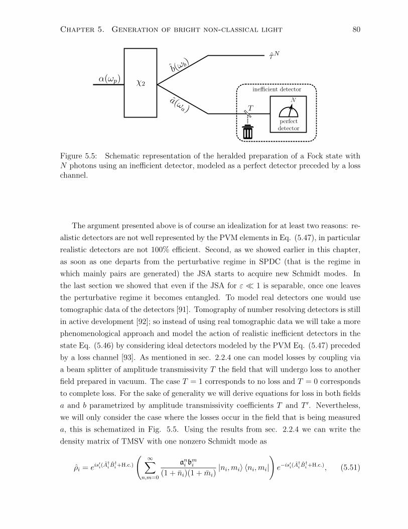
Chapter 5. Generation of bright non-classical light 80
Figure 5.5: Schematic representation of the heralded preparation of a Fock state withN photons using an inefficient detector, modeled as a perfect detector preceded by a losschannel.
The argument presented above is of course an idealization for at least two reasons: re-
alistic detectors are not well represented by the PVM elements in Eq. (5.47), in particular
realistic detectors are not 100% efficient. Second, as we showed earlier in this chapter,
as soon as one departs from the perturbative regime in SPDC (that is the regime in
which mainly pairs are generated) the JSA starts to acquire new Schmidt modes. In
the last section we showed that even if the JSA for ε 1 is separable, once one leaves
the perturbative regime it becomes entangled. To model real detectors one would use
tomographic data of the detectors [91]. Tomography of number resolving detectors is still
in active development [92]; so instead of using real tomographic data we will take a more
phenomenological approach and model the action of realistic inefficient detectors in the
state Eq. (5.46) by considering ideal detectors modeled by the PVM Eq. (5.47) preceded
by a loss channel [93]. As mentioned in sec. 2.2.4 one can model losses by coupling via
a beam splitter of amplitude transmissivity T the field that will undergo loss to another
field prepared in vacuum. The case T = 1 corresponds to no loss and T = 0 corresponds
to complete loss. For the sake of generality we will derive equations for loss in both fields
a and b parametrized by amplitude transmissivity coefficients T and T ′. Nevertheless,
we will only consider the case where the losses occur in the field that is being measured
a, this is schematized in Fig. 5.5. Using the results from sec. 2.2.4 we can write the
density matrix of TMSV with one nonzero Schmidt mode as
ρi = eis′i(A†i B†i+H.c.)
(∞∑
n,m=0
ani bmi
(1 + ni)(1 + mi)|ni,mi〉 〈ni,mi|
)e−is
′i(A†i B†i+H.c.), (5.51)

Chapter 5. Generation of bright non-classical light 81
where
|ni,mi〉 =
(A†i
)n (B†i
)m√n!m!
|vac〉 , ai =ni
1 + ni, bi =
mi
1 + mi
(5.52)
We can now use this lossy state and the ideal PVM elements in Eq. (5.47) to mimic the
statistics of the pure state Eq. (5.46) being measured by realistic inefficient detectors. If
the measurement gives us the outcome N then our state will be projected to
ρi =⇒ ρNi =
(ΠaN
)ρ(
ΠaN
)p
(i)N
, (5.53)
p(i)N = tr
(ΠN ρi
). (5.54)
This outcome will occur with probability p(i)N . We want to know now what is the state of
the photons in mode b given that we measured N in mode a. We can do this by simply
tracing out mode a in the last equation. The normalized state for b conditioned on result
N in a is
τNi =1
p(i)N
∞∑M=0
ci,N,M |M bi 〉 〈M b
i | .
where
ci,N,M =∞∑
n,m=0
ani bmi
(1 + ni)(1 + mi)
∣∣∣〈Ni,Mi|eis′i(A†i B†i+H.c.)|ni,mi〉
∣∣∣2 (5.55)
and p(i)N =
∑∞M=0 ci,N,M . In Fig. 5.6 we plot this probability as a function of the squeezing
parameter and the efficiency of the detector. We see that its behaviour is not strongly
modified by losses.
We can evaluate the matrix elements of the two-mode squeezing operator in the
number basis using the disentangling identity from Eq. (2.55)
〈n′k,m′k|eis′k(A
†kB†k+H.c.)|nk,mk〉 = δm′−m,n′−nsn′,m′;n,m (5.56)

Chapter 5. Generation of bright non-classical light 82
Figure 5.6: Probabilities of obtaining the results N = 1, 5, 10 when measuring thephoton number in field a for the state Eq. (5.34) ignoring time-ordering corrections. Theprobability is plotted as a function of the squeezing parameter s0ε and the transmissivityT used to parametrize the finite efficiency of the detector. The case T = 1 correspondsto ideal detectors.
Figure 5.7: Mandel Q parameter and purity of field b for the heralding outcomesN = 1, 5, 10 when measuring the photon number for field a in the state Eq. (5.34)ignoring time-ordering corrections. These parameters are plotted as a function of thesqueezing parameter s0ε and the transmissivity T used to parametrize the finite efficiencyof the detector. The case T = 1 corresponds to ideal detectors.

Chapter 5. Generation of bright non-classical light 83
where
sn′,m′;n,m = idtanhd s′i
coshm+n+1 s′i
√m!n!m′!n′!× (5.57)
min(m,n)∑j=max(0,−d)
(−1)j sinh2j s′i
j!(j + d)!√
(m− j)!(n− j)!(m′ − j − d)!(n′ − j − d)!
and d = m′ −m = n′ − n. We can use the selection rule in Eq. (5.56) to rewrite
ci,N,M = bM−Ni
∞∑n=max(0,N−M)
(aibi)n
(1 + ni)(1 + mi)|sN,M ;n,n−(N−M)|2. (5.58)
In the case when only field a undergoes losses we know that ni = 0 = ai (see Sec. 2.2.4)
and then
ci,N,M =
bM−Ni
1+mi|sN,M ;0,M−N |2 if M ≥ N,
0 otherwise,(5.59)
and sN,M ;0,M−N = iN√
M !N !(M−N)!
tanhN s′icoshM−N+1 s′i
. We can write the density matrix for this
case as
τNi =1
p(i)N
∞∑M=N
(bM−Ni
1 + mi
M !
N !(M −N)!
tanh2N s′icosh2M−2N+2 s′i
)|M b
i 〉 〈M bi | (5.60)
=(1− ri)
N+1r−NiN !
∞∑M=N
M !
(M −N)!rMi |M b
i 〉 〈M bi | ,
p(i)N =
1
1 + mi
tanh2N s′icosh2 s′i(1− ri)N+1
, (5.61)
where we introduced the parameter
ri =bi
cosh2 s′i. (5.62)
Using these results, in Fig. 5.7 we plot the purity and Mandel Q parameter of the state
when the measurement outcomes in field a are N = 1, 5, 10. The Mandel Q parameter
is defined as [94]
Q =〈N2
b 〉 − 〈Nb〉2
〈Nb〉− 1 (5.63)

Chapter 5. Generation of bright non-classical light 84
and characterizes the departure of a field from Poissonian counting statistics. It has the
nice feature that for Fock states other than vacuum it takes the value -1. We see that for
a transmissivity of T < 0.9 one can only find Q parameters close to -1 in regions where
the probability (as plotted in Fig. 5.6) is very small. The purity on the other hand tell
us about the mixedness of our state τNi . For an arbitrary, but normalized, quantum state
ρ it is defined as
P (ρ) = tr(ρ2). (5.64)
The purity is one for pure states and approaches zero for very mixed states. For the state
in Eq. (5.60) we can easily calculate the Q parameter, and the mean number of photons
Q =ri
1− ri− N
N + ri, (5.65)
〈Nb〉 = N +ri
1− ri(N + 1). (5.66)
With some extra tap dancing of the dummy indices we can also write the purity as
P = (1− ri)2(N+1)
2F1
(N + 1, N + 1; 1; r2
i
)(5.67)
where 2F1 is the Gauss Hypergeometric function (see Sec. 15.2 of [95, 96]). From Fig.
5.7 we see that the purity and the Mandel Q parameter are strongly correlated and give
roughly the same information about our state. This is to be expected since the only source
of mixedness if there is only one Schmidt mode is the one related to the photon number.
One might wonder whether considering one Schmidt mode is a good approximation. In
the following paragraphs we will generalize these results but we should also mention that
one can fight the time-ordering corrections that cause the appearance of extra Schmidt
modes by using cascaded generation devices. This will be explained in detail in Sec. 6.3.
We have so far only considered the case of one Schmidt mode. From the findings of
the previous section we know that even if the JSA for low pump energy is separable (has
only one Schmidt mode) as soon as one starts to get more than one pair of downconverted
photons on average, new Schmidt modes will appear. The case of many Schmidt modes
is a straightforward generalization of the previous result. More generally one would have
the state
|ψ〉 =⊗i
eisi(A†i B†i+H.c.) |vac〉 . (5.68)

Chapter 5. Generation of bright non-classical light 85
To calculate the effect of realistic detectors we need to obtain the multi Schmidt mode
lossy density matrix and write the action of the Πan in such state. The first part of this
calculation is trivial since the multimode Schmidt state after loss is simply
ρ =⊗i
ρi (5.69)
where ρi is the single mode Schmidt mode lossy state in Eq. (5.51). The last equation
simply tell us that losses affect all the Schmidt modes in the same way. The second part
of this strategy is to write the action of the projector Eq. (5.47) in state Eq. (5.69). One
can write this action for an arbitrary number of Schmidt modes but we will only do it
for two (since to first approximation time-ordering corrections only generate one extra
Schmidt mode). Assuming there are only two Schmidt modes that we label 0 and 1 we
have ρ = ρ0 ⊗ ρ1 and we can write
(ΠaN)ρ(Πa
N) = (5.70)(N∑l=0
|la0〉 〈la0 | ⊗ |(N − l)a1〉 〈(N − l)a1|
)ρ
(N∑l=0
|la0〉 〈la0 | ⊗ |(N − l)a1〉 〈(N − l)a1|
)
|la0〉 =
(A†0
)l√l!|vac〉 , |(N − l)a1〉 =
(A†1
)N−l√
(N − l)!|vac〉 . (5.71)
We can now trace out mode a and find the density matrix for mode b conditioned on the
detection of N photons
τN =1
pN
∞∑M,M ′=0
(N∑l=0
c0,l,Mc1,N−l,M ′
)|M b
0〉 〈M b0 | ⊗ |(M ′)b1〉 〈(M ′)b1| , (5.72)
where now
pN =∞∑
M,M ′=0
(N∑l=0
c0,l,Mc1,N−l,M ′
). (5.73)
In Fig. 5.8 and Fig. 5.9 we plot the probabilities, Mandel Q parameter and purity for
the case when time-ordering corrections are included and allow for the possibility of more
than one Schmidt mode. We note that the probabilities and Mandel Q parameter do
not differ significantly from the case without time-ordering corrections. Yet, the overall
purity is significantly different from the case without time ordering shown in Figs. 5.6
and 5.7. This result is easy to understand if we realize that time ordering will cause an
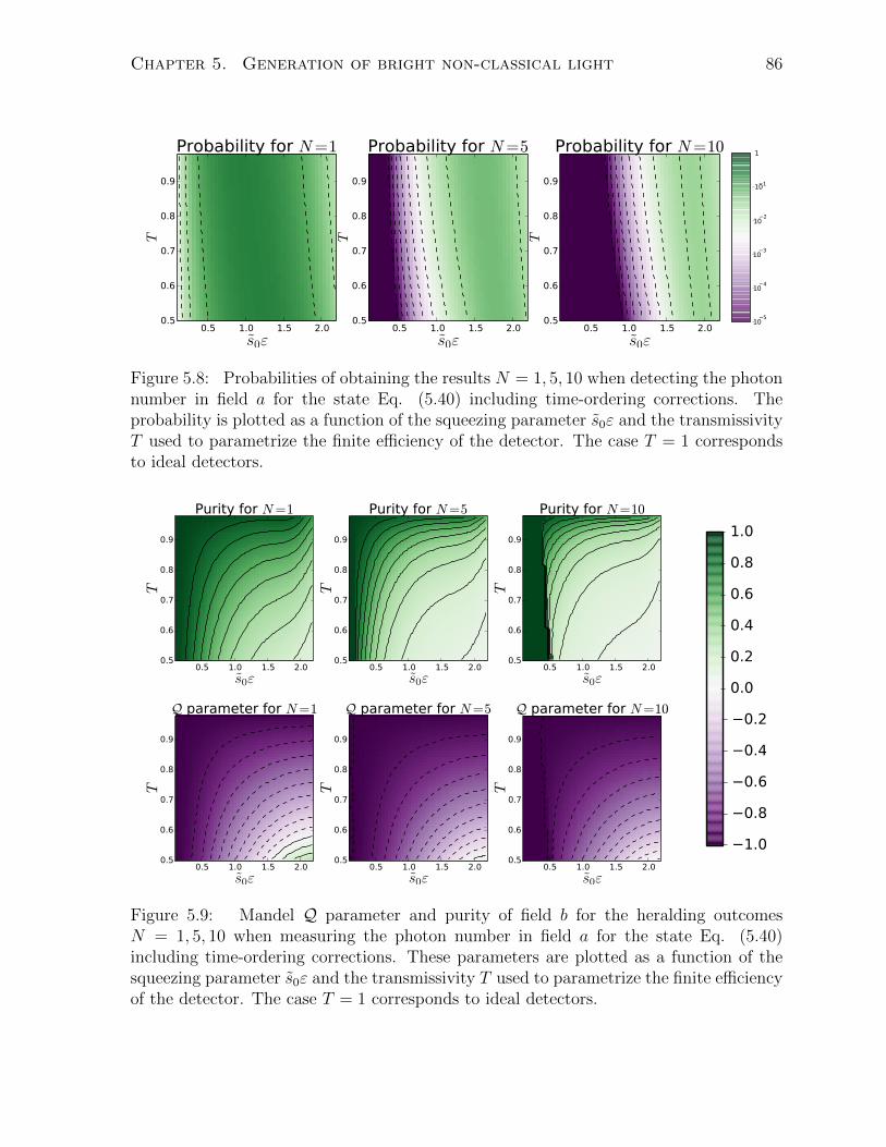
Chapter 5. Generation of bright non-classical light 86
Figure 5.8: Probabilities of obtaining the results N = 1, 5, 10 when detecting the photonnumber in field a for the state Eq. (5.40) including time-ordering corrections. Theprobability is plotted as a function of the squeezing parameter s0ε and the transmissivityT used to parametrize the finite efficiency of the detector. The case T = 1 correspondsto ideal detectors.
Figure 5.9: Mandel Q parameter and purity of field b for the heralding outcomesN = 1, 5, 10 when measuring the photon number in field a for the state Eq. (5.40)including time-ordering corrections. These parameters are plotted as a function of thesqueezing parameter s0ε and the transmissivity T used to parametrize the finite efficiencyof the detector. The case T = 1 corresponds to ideal detectors.

Chapter 5. Generation of bright non-classical light 87
extra Schmidt mode to appear, allowing for the possibility of mixedness in that degree
of freedom.
The results of this section show that to prepare highly pure Fock states with more
than one photon it is necessary to use very high efficiency photon number resolving
detectors or wait for exceedingly long times in order to get at least one detection event
in the heralding arm. On the other hand the preparation of single photons does not
seem to be constrained by this compromise relation. Using inefficient number resolving
detectors one can prepare highly pure single photons with heralding probabilities that are
not vanishingly small. This can be contrasted with the case of bucket detectors (binary
detectors that distinguish only between having no photons and having any number of
photons) where the probability of preparing a single photon with purity 1− r (r 1) is
roughly r/2.

Chapter 6
Highly efficient frequency conversion
You can’t always get what you wantBut if you try some time, you just might findYou get what you need
The Rolling Stones
6.1 Introduction
Nonlinear photonic materials provide some of the most advanced platforms for manip-
ulating the frequency and spectral profile of photons. This manipulation is typically
achieved using a process known as frequency conversion (FC) [24, 25]. In FC, two pho-
tons (one of them typically coming from a bright classical field) are fused into another
photon with a higher energy. FC has several important applications. First, it can be
used to move weak signals from a region of the spectrum where there are no good detec-
tors to another region where there are [28, 61]. A second application is to modify in a
controlled manner the properties of weak signals, in particular single photons, for quan-
tum information processing (QIP) tasks. Brecht et al. have recently proposed encoding
information in large Hilbert spaces using temporal/frequency modes of single photons
[20, 21, 22, 23]. One of the components of this and several other [27] QIP protocols
using single photons is the ability to completely upconvert a single frequency mode of a
given spectral profile while leaving all the other orthogonal frequency profiles untouched.
Finally, FC is useful for modifying the spectral profile of single photons, making their
sources compatible with existing or proposed quantum memories [18, 19]. For all these
applications it is important to have conversion efficiency near unity, and for some of them
it is also important to have selectivity in the frequency profiles that are converted.
88

Chapter 6. Highly efficient frequency conversion 89
In this chapter, we examine limitations to highly efficient FC arising from its fun-
damental quantum mechanical nature. These limitations are due to time-ordering cor-
rections that appear because the interaction picture Hamiltonian that describes the χ2
interaction between the different fields does not commute with itself at different times.
Our study allows us to separate very cleanly the “ideal” operation of an FC device from
the “undesirable” effects of time ordering. Thus, we can explicitly write the operation
of an FC gate, in a language very close to the one used in quantum information, as a
unitary operation UFC = exp(Ω1 + Ω2 + Ω3 + . . .) that consists of a desired generator
Ω1 and time-ordering corrections Ω2, Ω3, . . . that modify the operation of the gate. This
separation is obtained using the Magnus expansion (ME) studied in Chapter 4. Using
the ME allows us to understand the scaling of the time-ordering corrections as a func-
tion of the energy of the classical pump pulse. Based on this model, we propose a new
scheme to achieve highly efficient FC harnessing the until now undesirable time-ordering
corrections; this model also allows us to explain, using simple scaling arguments, why the
double pass scheme introduced by Reddy et al. [23] succeeds in achieving high efficiency
FC.
6.2 Ideal frequency conversion
We begin with the Hamiltonian describing a second-order nonlinear optical FC process
in the undepleted pump approximation, occurring in a quasi one-dimensional structure
of length L and characterized by a nonlinear coefficient χ2 (Sec. 4.4)
HI(t) =− ~εˆdωpdωadωb
(ei∆tΦ(ωa, ωb, ωp)α(ωp)a(ωa)b
†(ωb) + H.c.), (6.1)
where ωp refers to a pump frequency, and the shape of the classical pump function α(ωp)
is taken to be a Gaussian,
α(ωp) = τe−τ2δω2
p/√π, δωp = ωp − ωp, (6.2)
where ωp identifies the center pump frequency; τ identifies the duration of the pump
pulse, and we specify its energy by U0. In the FC process frequency components ωa
can be destroyed and frequency components ωb can be created; associated with this are
bosonic destruction and creation operators a(ωa) and b†(ωb) respectively. We assume
that the phase-matching function (PMF) Φ(ωa, ωb, ωp), restricts the destroyed and cre-
ated photons to be in nonoverlapping frequency regions, and/or of different mode profiles

Chapter 6. Highly efficient frequency conversion 90
or polarizations; then we can take [a(ωa), b†(ωb)] = 0. We reference the frequencies ωa
and ωb to center frequencies ωa and ωb respectively, defined so that energy and momen-
tum conservation are exactly satisfied for the center frequencies, ωb − ωa − ωp = 0 and
∆k(ωa, ωb, ωp) = 0 (see Eq. (4.39)). Finally, ∆ = ωb − ωa − ωp, and
ε = 2Lχ2
√ √2U0πωbωa√
π(4π)3ε0Ac3na(ωa)nb(ωb)nc(ωc)τ(6.3)
is a dimensionless constant that characterizes the strength of the interaction; the ni(ωi)
are the indices of refraction at the central frequencies ωi, and A is the effective overlap
area of the spatial fields. We will considered conversion using a χ2 material. With
correspondences presented in the previous chapters, this results can be generalized to the
use of χ3 materials as well.
Ignoring time-ordering corrections, the unitary evolution operator connecting states
at t→ −∞ to states at t→∞ is
U1 = eΩ1 = e−i~´∞−∞ dtHI(t) (6.4a)
= e−2πi´dωadωb(J1(ωa,ωb)a(ωa)b†(ωb)+H.c.), (6.4b)
where the quantity J1 is, to this level of approximation, the joint conversion amplitude
(JCA) and is given by
J1(ωa, ωb) = −εα(ωb − ωa)Φ(ωa, ωb, ωb − ωa).
To understand how this operator transforms a given input state, let us first introduce
the Schmidt decomposition of the function J1
−J1(ωa, ωb) =∑θ
rθ(ε)
2πk∗θ(ωa)lθ(ωb), rθ(ε) = εrθ, (6.5)
where the Schmidt functions kθ(ω) (lθ(ω)) are assumed to form a complete and orthonor-
mal set, and the positive quantities rθ(ε) = εrθ are the Schmidt numbers of the function
J1. In Eq. (6.5) we have explicitly used the fact that ε is only a multiplicative constant
in this approximation of the JCA; accordingly, the Schmidt numbers are linear func-
tions of this quantity and the Schmidt functions are independent of it. Because of the
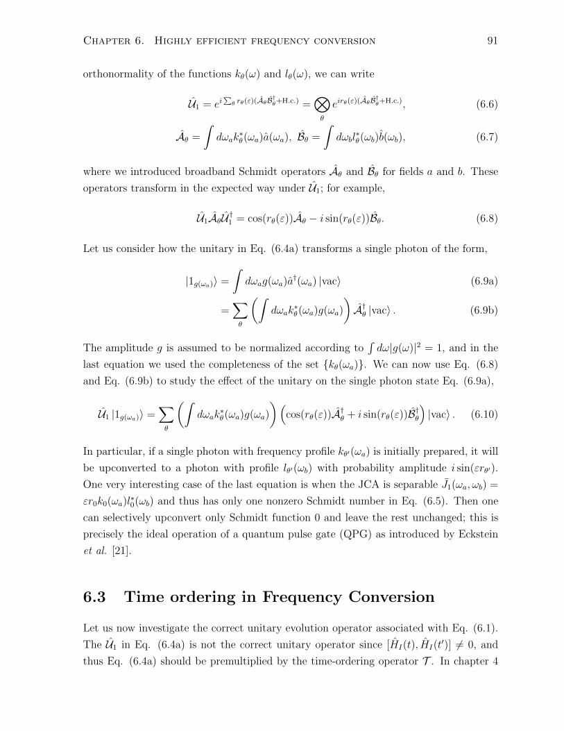
Chapter 6. Highly efficient frequency conversion 91
orthonormality of the functions kθ(ω) and lθ(ω), we can write
U1 = ei∑θ rθ(ε)(AθB†θ+H.c.) =
⊗θ
eirθ(ε)(AθB†θ+H.c.), (6.6)
Aθ =
ˆdωak
∗θ(ωa)a(ωa), Bθ =
ˆdωbl
∗θ(ωb)b(ωb), (6.7)
where we introduced broadband Schmidt operators Aθ and Bθ for fields a and b. These
operators transform in the expected way under U1; for example,
U1AθU †1 = cos(rθ(ε))Aθ − i sin(rθ(ε))Bθ. (6.8)
Let us consider how the unitary in Eq. (6.4a) transforms a single photon of the form,
|1g(ωa)〉 =
ˆdωag(ωa)a
†(ωa) |vac〉 (6.9a)
=∑θ
(ˆdωak
∗θ(ωa)g(ωa)
)A†θ |vac〉 . (6.9b)
The amplitude g is assumed to be normalized according to´dω|g(ω)|2 = 1, and in the
last equation we used the completeness of the set kθ(ωa). We can now use Eq. (6.8)
and Eq. (6.9b) to study the effect of the unitary on the single photon state Eq. (6.9a),
U1 |1g(ωa)〉 =∑θ
(ˆdωak
∗θ(ωa)g(ωa)
)(cos(rθ(ε))A†θ + i sin(rθ(ε))B†θ
)|vac〉 . (6.10)
In particular, if a single photon with frequency profile kθ′(ωa) is initially prepared, it will
be upconverted to a photon with profile lθ′(ωb) with probability amplitude i sin(εrθ′).
One very interesting case of the last equation is when the JCA is separable J1(ωa, ωb) =
εr0k0(ωa)l∗0(ωb) and thus has only one nonzero Schmidt number in Eq. (6.5). Then one
can selectively upconvert only Schmidt function 0 and leave the rest unchanged; this is
precisely the ideal operation of a quantum pulse gate (QPG) as introduced by Eckstein
et al. [21].
6.3 Time ordering in Frequency Conversion
Let us now investigate the correct unitary evolution operator associated with Eq. (6.1).
The U1 in Eq. (6.4a) is not the correct unitary operator since [HI(t), HI(t′)] 6= 0, and
thus Eq. (6.4a) should be premultiplied by the time-ordering operator T . In chapter 4

Chapter 6. Highly efficient frequency conversion 92
we have shown that the ME provides a particularly appealing way of approximating the
time evolution operator for time-dependent quadratic Hamiltonians [84] like the one in
Eq. (6.1). Using the ME, the correct unitary time evolution operator is [84, 97, 98]
UFC = T e−i~´∞−∞ dtHI(t) = eΩ1+Ω2+Ω3+.... (6.11)
In the last equation, the odd order terms are beam-splitter-like operators
Ω2n+1 = −2πi
ˆdωadωb
(J2n+1(ωa, ωb)a(ωa)b
†(ωb) + H.c.), (6.12)
and the even order terms are rotation-like operators
Ω2n = −2πi∑c=a,b
ˆdωcdω
′cG
c2n(ωc, ω
′c)c†(ωc)c(ω
′c). (6.13)
As explained in Chapter 4 the functions J2n+1, G2n can be reduced to quadratures of the
pump and PMFs.
One can break the RHS of Eq. (6.11) into a unitary involving only beam-splitter
terms and one involving only rotation terms UFC = URAURBUBS where URA and URB
are generated by operators such as Eq. (6.13) and UBS is generated by operators such
as Eq. (6.12). The lowest order example of this factorization is obtained by using the
Baker-Campbell-Hausdorff formula
UFC =(URAURB
)(UBS
)≈ eΩ2 eΩ1+Ω3+
[Ω1,Ω2]2 , (6.14)
where
[Ω1, Ω2]
2=(2π)
ˆdωadωb(K3(ωa, ωb)a(ωa)b
†(ωb)− H.c.), (6.15)
K3(ωa, ωb) =π
ˆdω(J1(ωa, ω)Gb
2(ωb, ω)− Ga2(ω, ωa)J1(ω, ωb)
). (6.16)
The factorization Eq. (6.14) is useful because we can write the unitary for FC as an
entangling operation for fields a and b postmultiplied by local unitaries. These local
unitaries cannot alter the entanglement between a and b, and because they involve rota-
tion operators of the form given in Eq. (6.13), they cannot change the total number of
photons in fields a and b. Thus the unitary UBS contains all the information necessary

Chapter 6. Highly efficient frequency conversion 93
to calculate the probability of upconversion. The JCA associated with UBS is now
J = J1︸︷︷︸∝ε
+ J3 + iK3︸ ︷︷ ︸∝ε3
+ . . . (6.17)
We can introduce the Schmidt decomposition of J just as was done in Eq. (6.5), except
that now the Schmidt numbers are not linear functions of ε, and the Schmidt functions
now depend on ε; thus we must replace
kθ(ωa)→ kθ(ωa; ε), lθ(ωb)→ lθ(ωb; ε), (6.18a)
Aθ → Aθ(ε), Bθ → Bθ(ε), (6.18b)
in Eq. (6.6). Note that Eqs. (6.6,6.9a,6.10) will still hold after the rules Eq. (6.18) are
applied. In principle 100% efficiency FC could be achieved were ri(ε) = π/2 for some i
and ε and the single photon A†i (ε) |vac〉 =´dωakθ(ωa; ε)a
†(ωa) |vac〉 sent to the frequency
converter. Of course, this could be hard to attain experimentally, since time-ordering
corrections make the JCA a complicated function of ωa and ωb, and certainly introduce
an imaginary component (see Eq. (6.17)); thus the kθ(ωa; ε) can become complicated as
well.
Another way of achieving highly efficient FC is by eliminating the time-ordering cor-
rections. To this end note that the nth Magnus term Ωn scales with εn. Now let us
imagine that instead of sending our single photon once through an FC device together
with a pump pulse of energy U0, the effect of which is characterized by UFC(ε), we send
it sequentially through N copies of the original FC device, each with the same pump
pulse shape but with pump energy U0/N2 (equivalently scaling ε by 1/N). Then the
time evolution operator is
(UFC(ε/N))N = eΩ1+Ω2/N+Ω3/N2+...; (6.19)
thus by having more than one FC device the time-ordering corrections can be reduced.
This observation neatly explains the results of Reddy et al. [23], where highly efficient-
mode selective FC is achieved using cascaded nonlinear crystals. Note that this scheme
does not assume anything about the nature of the time-ordering corrections except their
scaling; thus this method should also allow to attenuate time-ordering corrections in
SPDC. One complication with this scheme is the fact that it requires multiple FC devices,
which typically will imply stabilizing and controlling more complex interferometers.

Chapter 6. Highly efficient frequency conversion 94
6.4 Achieving near unit efficiency in Frequency Con-
version
Let us now consider the possibility of achieving near unit efficiency FC by harnessing
the up to now undesirable time-ordering corrections. That is, can we turn a bug into a
feature? We begin by considering for simplicity that the JCA is separable and Gaussian
if time-ordering corrections are ignored. This can be achieved by engineering a Gaussian
PMF [83]. Gaussian functions can also be used as a simple approximation to the more
common sinc function one would encounter for a uniform nonlinearity in over a region
of length L. One can match the FWHM of e−γx2
to the FWHM of sinc(x) by setting
γ ≈ 0.193 (see Fig. 5.1). Assuming a Gaussian PMF, we expand the phase mismatch
around the central frequencies of the fields involved to get
Φ(ωa, ωb, ωp) = e−(sbδωb−saδωa−spδωp)2
, (6.20)
where si =√γL/(2vi),
1vi
= dki(ωi)dωi|ωi=ωi is the inverse group velocity of the ith field, and
we have assumed that group velocity dispersion is negligible. Under these approxima-
tions, ignoring time-ordering corrections the JCA is
J1(ωa, ωb) = −ετ e2µ2δωaδωb−µ2aδω
2a−µ2
bδω2b/√π, (6.21)
µ2 = τ 2 + (sp − sa)(sp − sb), µ2a,b = τ 2 + (sp − sa,b)2.
The necessary and sufficient condition for a separable Gaussian J1 is µ = 0. This will
give an ideal QPG,
U1 = ei´dαdβ(r0εf(α)f(β)a(α)b†(β)+H.c.), (6.22)
r0 =
√2πτ√µaµb
, α = µaδωa, β = µbδωb, f(x) =e−x
2
4√π/2
,
for the photon |1f(α)〉 = A†0 |vac〉 =´dαf(α)a†(α) |vac〉, mapping it to the photon
|1f(β)〉 = B†0 |vac〉 =´dβf(β)b†(β) |vac〉. In Eq. (6.22) we have used the fact that
the Schmidt functions of Eq. (6.21) with µ = 0 are
k0(ωa) =√µaf
∗(α) and l0(ωb) =√µbf(β). (6.23)
As soon as one starts to approach a FC efficiency near unity, one needs to include the
time-ordering corrections. The unitary connecting inputs and outputs is given by Eq.
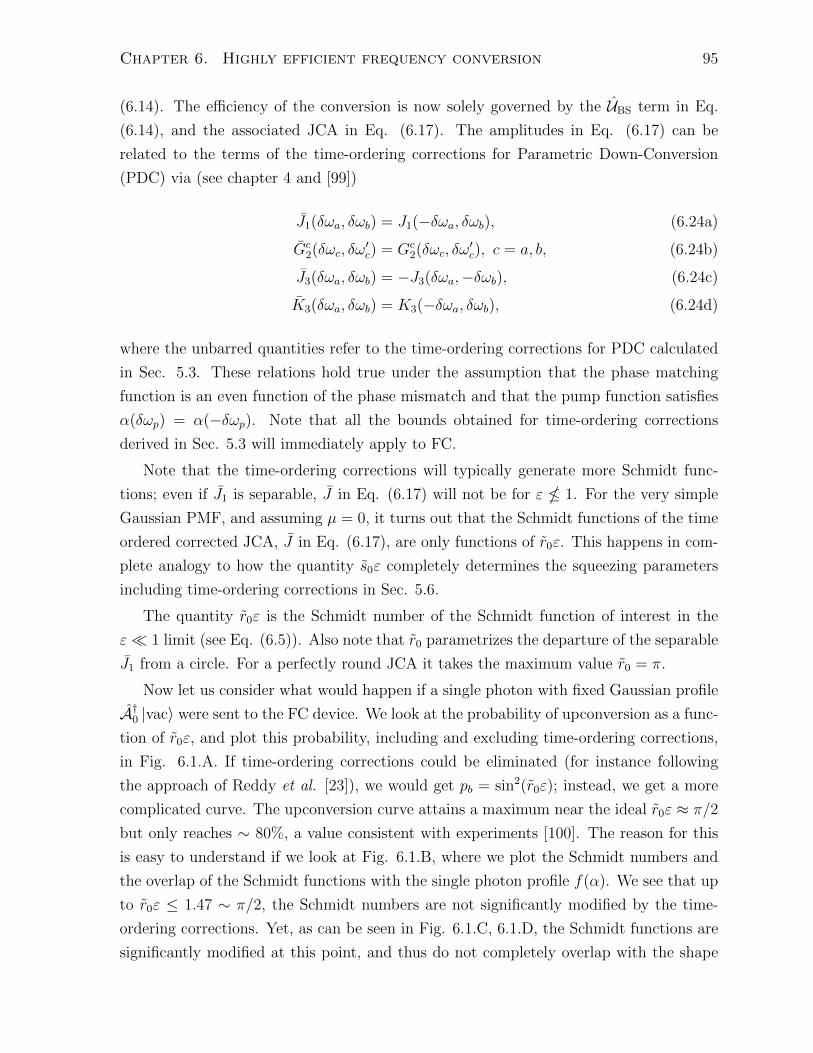
Chapter 6. Highly efficient frequency conversion 95
(6.14). The efficiency of the conversion is now solely governed by the UBS term in Eq.
(6.14), and the associated JCA in Eq. (6.17). The amplitudes in Eq. (6.17) can be
related to the terms of the time-ordering corrections for Parametric Down-Conversion
(PDC) via (see chapter 4 and [99])
J1(δωa, δωb) = J1(−δωa, δωb), (6.24a)
Gc2(δωc, δω
′c) = Gc
2(δωc, δω′c), c = a, b, (6.24b)
J3(δωa, δωb) = −J3(δωa,−δωb), (6.24c)
K3(δωa, δωb) = K3(−δωa, δωb), (6.24d)
where the unbarred quantities refer to the time-ordering corrections for PDC calculated
in Sec. 5.3. These relations hold true under the assumption that the phase matching
function is an even function of the phase mismatch and that the pump function satisfies
α(δωp) = α(−δωp). Note that all the bounds obtained for time-ordering corrections
derived in Sec. 5.3 will immediately apply to FC.
Note that the time-ordering corrections will typically generate more Schmidt func-
tions; even if J1 is separable, J in Eq. (6.17) will not be for ε 1. For the very simple
Gaussian PMF, and assuming µ = 0, it turns out that the Schmidt functions of the time
ordered corrected JCA, J in Eq. (6.17), are only functions of r0ε. This happens in com-
plete analogy to how the quantity s0ε completely determines the squeezing parameters
including time-ordering corrections in Sec. 5.6.
The quantity r0ε is the Schmidt number of the Schmidt function of interest in the
ε 1 limit (see Eq. (6.5)). Also note that r0 parametrizes the departure of the separable
J1 from a circle. For a perfectly round JCA it takes the maximum value r0 = π.
Now let us consider what would happen if a single photon with fixed Gaussian profile
A†0 |vac〉 were sent to the FC device. We look at the probability of upconversion as a func-
tion of r0ε, and plot this probability, including and excluding time-ordering corrections,
in Fig. 6.1.A. If time-ordering corrections could be eliminated (for instance following
the approach of Reddy et al. [23]), we would get pb = sin2(r0ε); instead, we get a more
complicated curve. The upconversion curve attains a maximum near the ideal r0ε ≈ π/2
but only reaches ∼ 80%, a value consistent with experiments [100]. The reason for this
is easy to understand if we look at Fig. 6.1.B, where we plot the Schmidt numbers and
the overlap of the Schmidt functions with the single photon profile f(α). We see that up
to r0ε ≤ 1.47 ∼ π/2, the Schmidt numbers are not significantly modified by the time-
ordering corrections. Yet, as can be seen in Fig. 6.1.C, 6.1.D, the Schmidt functions are
significantly modified at this point, and thus do not completely overlap with the shape

Chapter 6. Highly efficient frequency conversion 96
0.15
A
0.15
B
C D
Figure 6.1: In A we plot the probability of upconversion as a function of the interactionstrength r0ε, for a single photon in the Gaussian wave packet f(α) including and excludingtime-ordering corrections. In B we plot the Schmidt numbers of J including (dashedlines) and excluding (full line) time-ordering corrections. In the inset we plot the overlapbetween the time ordered corrected Schmidt functions and the Gaussian profile of theincoming single photon. Finally in C and D we plot the real and imaginary parts ofthe Schmidt functions for different values of r0ε. For r0ε = 0.02, 0.5 1 they are verysimilar to the Gaussian shape of the input single photon.
of the incoming single photon; see inset of Fig. 6.1.B, where we plot the overlap of the
Gaussian wave packet with the two Schmidt functions. As we increase r0ε further, the
probability of upconversion oscillates faster; this is just a reflection of the fact that past
r0ε = π/2 the Schmidt numbers are modified by the time-ordering corrections and grow
much faster than linearly, as seen in Fig. 6.1.B. This feature could be used as direct
experimental evidence of the contribution of the time-ordering corrections to the JCA
in FC. The final, most interesting feature of Fig. 6.1.A is that the probability reaches
unity for a value near r0ε near 2.79. This happens because the two non-zero Schmidt
numbers of J become odd multiples of π/2 at the same time. This allows the two Schmidt
functions to cooperate and attain 100% efficiency.
The results presented in this chapter give us a very simple picture of the physical
mechanisms associated with time-ordering that limit the efficiency of frequency conver-

Chapter 6. Highly efficient frequency conversion 97
sion using sum-frequency generation. The use of the Magnus expansion to calculate the
unitary evolution operator allowed us to understand what was the effect of these correc-
tions, explain how certain protocols can overcome them, and how they can also be used
to our advantage to increase conversion efficiency.

Chapter 7
Conclusions and future directions
Let’s just say we’d like to avoid any Imperial entanglements.
Obi-wan Kenobi
In this thesis we have studied the quantum dynamics of photon generation and con-
version. To undertake this study we have looked directly at the properties of the time-
evolution operator. This approach is complementary to the approach commonly taken
by the nonlinear optics community where one instead looks at the equations of motion
for the relevant quantum (or classical) field operators. We believe that the approach in
this thesis is very suitable for the study of quantum information applications of non-
linear optics since the description of the transformation of states is written precisely in
the language of this discipline. The formalism developed here becomes especially useful
when one is interested in understanding, manipulating, minimizing and profiting from
the time-ordering corrections (TOCs) associated with time dependent Hamiltonians.
To understand the nature of the TOCs in a very general setting, in Chapter 4 we have
used the Magnus expansion to construct solutions to the time-dependent Schrodinger
equation describing several nonlinear processes governed by quadratic bosonic Hamilto-
nians that do not commute at different times: spontaneous parametric down-conversion,
spontaneous four wave mixing, and frequency conversion. In the derivation of the Magnus
terms for these three processes we found a rather simple form for the second and third
order Magnus terms for a broad class of Hamiltonians. The Magnus expansion solution
that we found for the time evolution operator was shown to be Gaussian preserving;
equivalently, when the unitary operator is used to transform input and output bosonic
operators the transformation is Bogoliubov linear. With the expansion we developed, it
was easy to explain why the second order effect due to the time ordering in SPDC van-
ishes: Essentially the second order process needs to be stimulated by a previous photon.
98

Chapter 7. Conclusions and future directions 99
We also showed how to calculate corrections to the Joint Spectral Amplitude (JSA) of
the photons in SPDC and SFWM and to the Joint Conversion Amplitude (JCA) in FC,
and how even when the phase matching function and pump functions are real the JSA
or JCA acquires a non-trivial phase structure due to time ordering; this structure can be
investigated via tomographic methods. We also explored how the effect of time order-
ing acts in stimulated PDC; in particular, we looked at the case when the lower energy
photons are prepared in coherent states and showed that the first correction due to time
ordering is to modify their spectral structure. The Magnus expansion also allowed us to
argue that time ordering is irrelevant if the phase matching function is infinitely broad.
With the very general results from the preceding chapter, in Chapter 5 we presented
a theory that allows us to understand the effects of time ordering in photon genera-
tion processes. We introduced a figure of merit quantifying the effects of time ordering,
and it was shown that these effects are only sizable whenever the photons in the down-
converted/frequency converted modes copropagate with the pump photons. This agrees
with the simple physical intuition that the only way the effect of the Hamiltonian at some
posterior time H(tf ) can be influenced by the former version of itself H(ti), under the
assumption of an undepleted pump, is if the fields associated with the pump photons,
any seed photons, and the generated photons spend a significant amount of time in the
same regions of space. Under these conditions the time-ordering corrections will also
have the most significant qualitative effect, since they will modify the Schmidt number
of the quantum correlated photons from the uncorrected value of close to unity. We have
used Gaussian functions to approximately describe both the pump pulse and the phase-
matching functions that enter the description of the photon generation or conversion.
This led to the possibility of constructing analytic expressions for the figures of merit.
Nonetheless, the general approach of the Magnus expansion described earlier could be
applied to the use of arbitrary functions to model the pump pulse and phase matching.
A general result of our investigations here, that strong pump pulses are required for any
deviation from the first order Magnus term to be relevant, can be expected to hold more
generally. There is thus a wide range of problems where an elementary first order pertur-
bative approach would fail, but a calculation using the first order Magnus term would be
sufficient. Yet working at pump intensities high enough that time-ordering corrections
appear should lead to new strategies for producing novel quantum states.
In addition to clarifying the physical regimes in which the time-ordering corrections
are expected to be relevant we also proposed relevant observables that can be used to
witness the contribution of the corrections to the joint spectral amplitude of the generated
photons. Finally, in Chapter 5 we also studied how using inefficient detectors one can

Chapter 7. Conclusions and future directions 100
probabilistically generate heralded Fock states with many quanta.
In Chapter 6 we have studied the effects of the time-ordering corrections on frequency
conversion. We have considered conversion using a χ2 material and, with correspondences
presented in Chapter 3, this can be generalized to the use of χ3 materials as well. We
have shown how the time-ordering corrections modify the ideal operation of a quantum
pulse gate and how they can be used to achieve near unity FC using the extra Schmidt
functions that are generated by them. Finally, we provided a simple scaling argument
that explains the results of Reddy et al. [23], in which time-ordering corrections are
attenuated by using cascaded FC devices and argued that the same ideas could be used
to attenuate time-ordering corrections in photon generation.
The results presented in this thesis allow us to present a simple tool-kit that an
experimentalist or a theorist can easily use to assess whether time ordering effects will
have any role in their experiment or calculation. First one needs to use the results
in Eqs. (3.29) and (3.42) to estimate the value of the dimensionless constants ε or ε
characterizing the strength of the χ2 or χ3 process. If this constant is very small, one
can ignore time-ordering effects and simply use the first order Magnus term. If they are
bigger or close to one, then one can either use the simple analytical bounds summarized
in Eq. (5.18) or perform a full numerical calculation of the JSA or JCA using the Magnus
library documented in Appendix C. Even though the bounds and the numerical library
are presented/documented in terms of photon generation, they can easily be mapped to
results for frequency conversion using the equivalences in Eq. (6.24). Finally, the results
presented in Figs. 5.6, 5.7, 5.8, 5.9 allow us to evaluate the quality of the Fock states
generated by heralding using an imperfect photon-number-resolving detector.
In chapters 4,5 and 6 we showed that there is a very strong parallel between the results
of photon generation and photon conversion. This parallel became evident once we used
the Magnus expansion to explore the contributions of the time-ordering corrections to
the unitary evolution. This parallel would have been extremely hard to unravel using the
more commonly used Dyson series. Nonlinear quantum optics is probably not the only
area of physics that would benefit from using improved expansions for time-dependent
problems. In particular one can show that results related to time averaged dynamics can
be understood through the lens of the Magnus expansion and that the effective Hamilto-
nian discussed in e.g. [101] is nothing but the second order Magnus term[102]. Another
field where the Magnus expansion could be employed is relativistic quantum informa-
tion. A typical problem in this field is to study the properties of detectors in different
space-time regions that interact with quantum fields[103]. These interactions are typ-
ically time-dependent and thus the Magnus expansion should provide a useful method
Chapter 7. Conclusions and future directions 101
to evaluate the effects of the fields on the detectors and vice-versa especially in the case
when one can model the detectors as harmonic oscillators.
Finally, we should mention that there are of course very interesting questions not ad-
dressed with the formalism presented in this thesis, and also questions for which this
formalism will probably be insufficient. Chief among the former set, is the inverse prob-
lem; that is, given a target time-ordering corrected JSA or JCA what type of pump
pulse or phase-matching functions should be engineered to obtain such JSA or JCA. In
the latter set is the question of a full quantum mechanical treatment of the nonlinear
problem. Even though the dynamics studied here was termed “very” nonlinear (in the
sense that the shape of the Schmidt modes in photon generation or conversion is modified
significantly by the time-ordering corrections) it is still linear in the quantum operators
considered. This linearity is a result of the fact that we are treating the pump field as a
classical entity; this approximation is warranted by the experimental conditions in which
these questions are investigated. A very interesting question that will soon become rel-
evant for experimentalist and theorists studying microwave photons in superconducting
waveguides is how to describe this dynamics when all three (or more) fields involved in
the nonlinear interaction must be treated quantum mechanically.

Appendix A
Energy in an Electromagnetic pulse
In this appendix we construct an estimate of the energy of an electromagnetic pulse
propagating in vacuum. Since our purpose here is not to give a precise calculation for
any particular system, but rather to identify the characteristic size and form of the terms
needed in our calculations, we simply approximate the relevant field at each frequency
in the linear regime as if it consisted of an area A “cut out” of a linearly polarized plane
wave propagating in a direction perpendicular to the plane of the area; this can be taken
as a “toy model” of a waveguide mode.
To construct our “toy model” we start with a solution to Maxwell’s equations in a medium
with index of refraction n(ω)
~E(z, t) =(~xE0e
i(kz−ωt))+ c.c., (A.1)
~B(z, t) =(~yB0e
i(kz−ωt))+ c.c., (A.2)
with E0/B0 = c/n(ω) and k = k(ω). To construct pulses we take superpositions,
~E(z, t) = ~x
ˆ ∞0
dωE0(ω)ei(kz−ωt) + c.c., (A.3)
~B(z, t) = ~y
ˆ ∞0
dωB0(ω)ei(kz−ωt) + c.c.
In what follows we will assume that the amplitude functions E(ω) and B(ω) are very
narrowly peaked around some central frequency ω and thus over the relevant integration
range to good approximation we can write E(ω) = E0f(ω) and B(ω) = B0f(ω), where
E0/B0 = c/n(ω), taking f(ω) to vanish for ω < 0. With this in mind, in a non-magnetic
102

Appendix A. Energy in an Electromagnetic pulse 103
medium the Poynting vector is
~S (z, t) =~E(z, t) × ~B(z, t)
µ0
(A.4)
= ~zE0B0
µ0
ˆ ∞0
dωdω′ × (A.5)(f(ω)f(ω′)ei(k(ω)+k(ω′))z−(ω+ω′)t + f(ω)f ∗(ω′)ei(k(ω)−k(ω′))z−(ω−ω′)t
)+ c.c.
Writing a directed element of area d ~A as ~zdA, from Poynting’s theorem the energy carried
in the pulse over an area A is then given by
U0 =
ˆ ∞−∞
dt
ˆA
d ~A · ~S(z, t) (A.6)
=2πAE0B0
µ0
ˆ ∞0
dω(f(ω)f(−ω)ei(k(ω)+k(−ω))z|f(ω)|2 + c.c.
). (A.7)
The first term is identically zero since f(ω) = 0 if ω < 0; if we then, for example,
approximate f(ω) for ω > 0 by
f(ω) =1√2πσ
ζ(ω − ω), ζ(ω) = exp(−ω2/(2σ2)),
and take
k(ω) = k(ω) + (ω − ω)/vg, (A.8)
with vg the group velocity at frequency ω, we have
~E(z, t) = 2~xE0e− 1
2σ2(t−z/vg)2
cos(k(ω)z − ωt), (A.9)
~B(z, t) = 2~yB0e− 1
2σ2(t−z/vg)2
cos(k(ω)z − ωt), (A.10)
where we have assumed that ω σ and thus one can safely extend the lower integration
limit in Eq. (A.3) from 0 to −∞. Averaged over the period 2π/ω, the Poynting vector
following from Eq. (A.4) has a standard deviation√
2σ, leading to a full width at half
maximum (FWHM) of the intensity of the pulse given by FWHM = 2√
2 ln 2(√
2σ),
or σ = FWHM/4√
ln 2 ≈ 0.3 FWHM. From (A6,A7), under the same approximations
leading to (A10,A11) we have U0 = 2Aε0n(ω)cE20
√πσ
. This is a useful result that allows
to relate the peak amplitude of the electric field E0 to the net energy in the pulse U0:
E0 =
√(U0/√π)σ
2ε0n(ω)cA. (A.11)

Appendix A. Energy in an Electromagnetic pulse 104
Note that even if group dispersion were included in Eq. (A.8):
k(ω) = k(ω) + (ω − ω)/vg +1
2κω(ω − ω)2, (A.12)
with κω = (d2k/dω2)ω=ω, we would still obtain the same relation between E0 and U0.

Appendix B
Numerical calculation of the
Schmidt decomposition
Typically the Schmidt decompositions in Eq. (2.79) and Eq. (2.84) cannot be found
analytically unless one is dealing with Gaussians [85]. Yet, one can obtain excellent
numerical approximations by using the matrix version of the Schmidt decomposition,
the singular value decomposition (SVD). To this end let us sample the function F(x, y)
at the n+ 1×m+ 1 points xi = x0 + i∆x|ni=0 and yj = y0 + j∆y|mj=0
Mi,j = F(xi, yj). (B.1)
The question is now, assuming that F(x, y) =∑
k λk uk(x) v∗k(y) how can λk, uk, vk be
approximated from the knowledge of the singular value decomposition of M ,
M = Udiag(µl)V†. (B.2)
To connect the SVD of M and the Schmidt decomposition of F let us note first that
typically F has units, for instance for all the functions considered previously [F(x, y)] =
(xy)−1/2. From the normalization chosen for the functions uλ and vλ we have
ˆdx u∗λ(x)uλ′(x) =
ˆdy v∗λ(y)vλ′(y) = δλ,λ′ , (B.3)
from which we deduce that [u(x)] = x−1/2, [v(y)] = y−1/2. Simply from the definition of
Mi,j we have
F(xi, yj) = Mi,j =∑l
µlUi,lV∗j,l. (B.4)
105

Appendix B. Numerical calculation of the Schmidt decomposition 106
The identification between the terms of the SVD and the Schmidt decomposition is as
follows
λk = µk√
∆x∆y, uk(xi) = Ui,k/√
∆x, vk(yj) = Vj,k/√
∆y. (B.5)
This will automatically yield the correct normalizations
ˆdx(u∗k(x) uk′(x)) ≈
N∑i=0
∆x (u∗k(xi) uk′(xi)) =N∑i=0
∆x
(U∗i,k√∆x
)(Ui,k′√
∆x
)
=N∑i=0
U∗i,k Ui,k′ = δk,k′ . (B.6)
In the last equality we used the fact that the columns of U are orthogonal to each other
and are normalized. One can find a similar result for v and V (again assuming that the
columns of V are orthonormal).

Appendix C
The Magnus library
The Magnus library comprises two different and independent software pieces. Both of
them perform numerical integration using the fantastic Cubature library developed by
Steven G. Johnson at MIT (http://ab-initio.mit.edu/wiki/index.php/Cubature). The
Magnus library is freely available at https://github.com/nquesada/magnus.
C.1 Gaussian approximation for the third order Mag-
nus term
The first application, completely contained in the file gauss_magnus.c, calculates the
third order Magnus correction for Gaussian phase matching and pump functions of the
form given in Eq. (5.2) and Eq. (5.3). The third order Magnus term can be written as in
Eq. (5.10). The functions in this equation depend on the parameters introduced in Eq.
(5.14). They are all functions of the slowness of the modes sa, sb, sp, the time duration
of the pump τ and the interaction strength ε. In what follows we fix ε = −1 and use
units where the pulse duration is τ = 1. The library computes numerically the integral V
defined in Eq. (5.10) using the hcubature routine from cubature. The user is required
to provide values for 4 macros at the beginning of the file. The first three of them
#define MAX_EVAL_INT 10000000 //Maximum number of evaluations
#define REQ_ABS_ERROR 1e-10 //Required absolute error
#define REQ_REL_ERROR 1e-8 //Required relative error
give the maximum number of times the function being integrated can be evaluated, the
second one is the required absolute error in the integration and the third is the required
relative error. To calculate numerical integrals extending to infinity one must perform
107

Appendix C. The Magnus library 108
the following changes of variables:
ˆ ∞−∞
dx f(x) =
ˆ 1
−1
dtf
(t
1− t2
)1 + t2
(1− t2)2, (C.1)
ˆ ∞0
dx f(x) =
ˆ 1
0
f
(t
1− t
)1
(1− t)2.
We can now write V in Eq. (5.10) in following way:
V (ωa, ωb) =
ˆ 1
0
dtr
ˆ 1
0
dtqg
(ωa, ωb,
tr1− tr
,tq
1− tq
)1
(1− tr)2
1
(1− tq)2(C.2)
=
ˆ 1
0
dtr
ˆ 1
0
dtqg(ωa, ωb, tr, tq), (C.3)
g(ωa, ωb, r, q) = exp(−(r, q)M(r, q)T
)cos(
4τηab(ωaq + ωbr)/√
3), (C.4)
where M is defined in Eq. (5.14). With this definitions we now list the different func-
tions in gauss_magnus.c where the arguments of the function have the following mean-
ing: int gaussianarg(unsigned ndim, const double *x, void *fdata, unsigned
fdim, double *fval) calculates precisely g(ωa, ωb, tr, tq):
• unsigned ndim should be set to 2, since we are dealing with two dimensional
integrals.
• const double *x is a two dimensional array containing the values of the variables
being integrated, x[0]= tr, x[1]= tq.
• void *fdata is a two dimensional array containing the values of the other variables,
fdata[0]= ωa, fdata[1]= ωb.
• unsigned fdim should be set to 1 since we are integrating a scalar function.
• double *fval is a one dimensional array, fval[0]= g(ωa, ωb, tr, tq).
The next function in gauss_magnus.c, is int gaussianval(double fdata[2], double
*res), it uses gaussianarg and cubature to calculate the integral Eq. (C.2). Its
arguments are:
• double fdata[2] is a two dimensional array containing the values of the other
variables, fdata[0]= ωa, fdata[1]= ωb.
• double *res contains the values of the integral in res[0] and the estimated error
res[1].

Appendix C. The Magnus library 109
Finally the function double J3(double wa,double wb) calculates J3 as given in Eq.
5.10. It first calculates the analytical bound
|J3(ωa, ωb)| ≤2π3/2ε3τ 3
3R2
(exp
(−uQuT/R4
)+ 2 exp
(−uNuT/3
)). (C.5)
If this bound is less than the macro eps the integral is approximated to 0. If it is bigger
than 0 then it is calculated using gaussianval and combined with W and Z to give J3.
To test the correctness of the calculation one can check the results for the following set
of numerical values
sc = 0, sa = 1, sb = −1, J3(0, 0) = 0.19635, J3(1, 1) = −0.0530724. (C.6)
C.2 General calculation of the Second and Third or-
der Magnus terms
This routines calculate numerically the second and third order Magnus terms for the
Hamiltonian in Eq. (4.19) using the function F defined in Eq. (4.25). We use the
convention´≡
´∞−∞. The Magnus correction terms can be written in terms of the
functions G2, H2, J3, K3 introduced in Eqs. (4.32a,4.37,4.66). The first Magnus term is
given by J1(ωa, ωb) = F (ωa, ωb, ωa + ωb). In what follows it is assumed that F ∗ = F .
Note that any principal value integral can be written as:
dx
xf(x) =
ˆ ∞0
dx
x(f(x)− f(−x)). (C.7)
To calculate the Magnus correction three different files are provided. The first one
functionF.c provides the function F (ωa, ωb, ωp). The evaluation of F should be as
efficient as possible since this function will be called many times during the calculation
of any Magnus term. In the file magnus.c functions that calculate the integrands asso-
ciated with each magnus term are provided. They nevertheless evaluate the functions in
the transformed variables according to Eq. (C.1) and Eq. (C.7).
The functions int magnusNx(unsigned ndim, const double *x, void *fdata,
unsigned fdim, double *fval) take the same arguments
• unsigned ndim the number of dimensions that need to be integrated.
• const double *x the values of dummy integration variables.
• void *fdata the variables of the actual arguments of the Magnus functions.
Appendix C. The Magnus library 110
• unsigned fdim is al always equal to one since the functions being integrated are
scalar.
• double *fval is where the value of the integrand is returned.
A simple example clarifies the notation. Let us look at
G2(ωa, ω′a) =
ˆdωd
dωpωp
F (ωa, ωd, ωa + ωp + ωd) f∗ (ω′a, ωd, ω
′a + ωp + ωd) (C.8)
=
ˆ ∞−∞
dωd
ˆ ∞0
dωp1
ωp
(F (ωa, ωd, ωa + ωp + ωd)F
∗ (ω′a, ωd, ω′a + ωp + ωd)
−F (ωa, ωd, ωa − ωp + ωd)F∗ (ω′a, ωd, ω
′a − ωp + ωd)
). (C.9)
In the last equation identity Eq. (C.7) was used. To perform the integral we need to
switch variables again using Eq. (C.1), ωd = td/(1− td), ωp = tp/(1− t2p) to obtain:
G2(ωa, ω′a) =
ˆ 1
0
dtd
ˆ 1
−1
dtp
1
(1− td)2
1 + t2p(1− t2p)2
1tp
1−t2p
× (C.10)(F
(ωa,
td1− td
, ωa +td
1− td+
tp1− t2p
)F ∗(ω′a,
td1− td
, ω′a +td
1− td+
tp1− t2p
)
− F(ωa,
td1− td
, ωa +td
1− td− tp
1− t2p
)F ∗(ω′a,
td1− td
, ω′a +td
1− td− tp
1− t2p
)).
The term inside the is the Jacobian of the transformation. In this example then
x[0]=td, x[1]= tp, fdata[0]= ωa, fdata[1]= ω′a. Having explained the use of the
function in magnus.c explaining magnusint.c is easy. Each function then calls the cor-
responding function in magnus.c and performs the integrals using cubature. So for in-
stance int magnus2aint(double wa, double waa, double *res) calls magnus2a and
performs the integral for the values wa= ωa, waa= ω′a returning the value of the integral
and its error in res[0] and res[1]. One final clarification, magnus2a calculates G2,
magnus2b calculates H2, magnus3s calculates the first term (the one which requires a 2
dimensional integration) that defines J3 omitting the prefactor of π2/3 in Eq. (4.37),
magnus3 calculates the second term in J3 (which requires a 4 dimensional integration)
and finally magnus3w calculates K3 omitting the prefactor of π in Eq. (4.67).

Appendix D
Analytical calculation of the third
order Magnus correction
In this Appendix we calculate the third order Magnus term Ω3 and associated JSA
contribution J3 for the Hamiltonian considered in the main Chapter 5. Note that the
second order correction Ω2 (and associated functions Ga2, G
b2) and the imaginary part of
the third order correction K3 can be calculated directly from the results in Sec. 4.3. For
the calculation of J3 we will not use the results presented in Sec. 4.3. The reason is
that integrals of the formffl
dxxdyyf(x, y), which are the ones necessary to calculate the
third order correction, are hard to bound and cannot be computed analytically for the
situation when f is a Gaussian function. To circumvent this difficulty we assume that
the Hamiltonian can be written as a function of the frequencies of the down-converted
photons and time (ωa, ωb, t) but without any explicit dependence of the pump frequency
(ωp) which will be assumed to have been integrated out. This can be done analytically for
Gaussian pump profiles and phase-matching functions, as we shall show shortly. Because
the time dependence of the Hamiltonian will no longer be harmonic but Gaussian, the
time order integrations will not involve any principal value integrals but rather incomplete
(i.e. not extending over the whole real line) Gaussian integrals.
We will consider the Hamiltonian given by Eq. (5.1) with phase matching function
Eq. (5.2) and pump function Eq. (5.3). We remind the reader that the detuning can be
written as
∆ = ωa + ωb − ωp = δωa + δωb − δωp.
Given the simplicity of the pump and phase matching functions we can perform analyt-
111

Appendix D. Analytical calculation of the third order Magnus correction112
ically the integral over ωp
F (ωa, ωb, t) = −εˆdωpe
i∆tα(ωp)Φ(ωa, ωb, ωp) = (D.1)
− ετ√
1
s2p + τ 2
exp
((−2sp (saδωa + sbδωb) + it) 2
4(s2p + τ 2
) + it (δωa + δωb)− (saδωa + sbδωb)2
).
After the integration the Hamiltonian is now
HI(t) = ~ˆdωadωbF (ωa, ωb, t)a
†(ωa)b†(ωb) + H.c. (D.2)
For the third order Magnus term we get
Ω3 =(−i)3
6~3
ˆdt
ˆ t
dt′ˆ t′
dt′′[HI(t),
[HI(t
′), HI(t′′)]]
+[[HI(t), HI(t
′)], HI(t
′′)]
=i
6
ˆdt
ˆ t
dt′ˆ t′
dt′′ˆdωodωedω
′odω
′edω
′′odω
′′e (D.3)
×(δ (ω′′e − ωe) δ (ω′′o − ω′o)F (ωo, ωe, t)F (ω′o, ω
′e, t′)F ∗ (ω′′o , ω
′′e , t′′) a†(ωo)b
†(ω′e)
− 2δ (ω′e − ωe) δ (ω′o − ω′′o )F (ωo, ωe, t)F (ω′′o , ω′′e , t′′)F ∗ (ω′o, ω
′e, t′) a†(ωo)b
†(ω′′e )
+ δ (ω′′e − ω′e) δ (ω′′o − ωo)F (ωo, ωe, t)F (ω′o, ω′e, t′)F ∗ (ω′′o , ω
′′e , t′′) a†(ω′o)b
†(ωe)
+ δ (ωe − ω′e) δ (ωo − ω′′o )F (ω′o, ω′e, t′)F (ω′′o , ω
′′e , t′′)F ∗ (ωo, ωe, t) a
†(ω′o)b†(ω′′e )
− 2δ (ω′e − ω′′e ) δ (ω′o − ωo)F (ωo, ωe, t)F (ω′′o , ω′′e , t′′)F ∗ (ω′o, ω
′e, t′) a†(ω′′o )b†(ωe)
+ δ (ωe − ω′′e ) δ (ωo − ω′o)F (ω′o, ω′e, t′)F (ω′′o , ω
′′e , t′′)F ∗ (ωo, ωe, t) a
†(ω′′o )b†(ω′e))− H.c.
In the last equation we use δ for the Dirac distribution. To simplify this expression we
perform the following changes of variables in each of the six terms in the last equation
ωe → ωd ω′′e → ωd ω′o → ωc ω′′o → ωc ω′e → ωb ωo → ωa
ωe → ωd ω′e → ωd ω′o → ωc ω′′o → ωc ω′′e → ωb ωo → ωa
ω′e → ωd ω′′e → ωd ωo → ωc ω′′o → ωc ωe → ωb ω′o → ωa
ωe → ωd ω′e → ωd ωo → ωc ω′′o → ωc ω′′e → ωb ω′o → ωa
ω′e → ωd ω′′e → ωd ωo → ωc ω′o → ωc ωe → ωb ω′′o → ωa
ωe → ωd ω′′e → ωd ωo → ωc ω′o → ωc ω′e → ωb ω′′o → ωa,
(D.4)
Appendix D. Analytical calculation of the third order Magnus correction113
to get
Ω3 =i
6
ˆdt
ˆ t
dt′ˆ t′
dt′′ˆdωadωbdωcdωda
†(ωa)b†(ωb)× (D.5)(
F (ωa, ωd, t)F (ωc, ωb, t′)F ∗ (ωc, ωd, t
′′)− 2F (ωa, ωd, t)F (ωc, ωb, t′′)F ∗ (ωc, ωd, t
′)
+ F (ωa, ωd, t′)F (ωc, ωb, t)F
∗ (ωc, ωd, t′′) + F (ωa, ωd, t
′)F (ωc, ωb, t′′)F ∗ (ωc, ωd, t)
− 2F (ωa, ωd, t′′)F (ωc, ωb, t)F
∗ (ωc, ωd, t′) + F (ωa, ωd, t
′′)F (ωc, ωb, t′)F ∗ (ωc, ωd, t)
)− H.c..
We can now perform the change of variables t = q+ 2r+ s, t′ = q− r+ s, t′′ = q− r−2s
that transforms the integral according to´dt´ tdt′
´ t′dt′′ = 9
´dq
´∞0dr
´∞0ds, and also
use the fact that F (ωa, ωb,−t) = F ∗(ωa, ωb, t), where x∗ denotes the complex conjugate
of x, to obtain
Ω3 =3i
2
ˆdq
ˆ ∞0
dr
ˆ ∞0
ds
ˆdωadωbdωcdωda
†(ωa)b†(ωb)× (D.6)(
F (ωa, ωd, q + 2r + s)F (ωc, ωb, q − r + s)F (ωc, ωd,−q + r + 2s)
− 2F (ωa, ωd, q + 2r + s)F (ωc, ωb, q − r − 2s)F (ωc, ωd,−q + r − s)
+ F (ωa, ωd, q − r + s)F (ωc, ωb, q + 2r + s)F (ωc, ωd,−q + r + 2s)
+ F (ωa, ωd, q − r + s)F (ωc, ωb, q − r − 2s)F (ωc, ωd,−q − 2r − s)
− 2F (ωa, ωd, q − r − 2s)F (ωc, ωb, q + 2r + s)F (ωc, ωd,−q + r − s)
+ F (ωa, ωd, q − r − 2s)F (ωc, ωb, q − r + s)F (ωc, ωd,−q − 2r − s))− H.c.
Note the following: First, r and s can always be swapped since they have the same
integration ranges and second, the change q → −q can always be performed since´∞−∞ dqf(q) =
´∞−∞ dqf(−q). Because of this it is easily seen that in the last equation the
sixth term is the complex conjugate of the first, the fifth is the complex conjugate of the
second and the fourth is the complex conjugate of the third. So we can more compactly

Appendix D. Analytical calculation of the third order Magnus correction114
write
Ω3 = −2πi
ˆdωadωba
†(ωa)b†(ωb)J3(ωa, ωb)− H.c. (D.7)
= −2πi
ˆdωadωba
†(ωa)b†(ωb)
(− 3
4π
ˆdqdωcdωd(L1 − 2L2 + L3 + c.c.)
)− H.c.
(D.8)
L1 =
ˆ ∞0
dr
ˆ ∞0
ds F (ωa, ωd, q + 2r + s)F (ωc, ωb, q − r + s)F (ωc, ωd,−q + r + 2s)
(D.9)
L2 =
ˆ ∞0
dr
ˆ ∞0
ds F (ωa, ωd, q + 2r + s)F (ωc, ωb, q − r − 2s)F (ωc, ωd,−q + r − s)
(D.10)
L3 =
ˆ ∞0
dr
ˆ ∞0
ds F (ωa, ωd, q − r + s)F (ωc, ωb, q + 2r + s)F (ωc, ωd,−q + r + 2s) .
(D.11)
To get a simpler expression we can perform the following changes of variables: For L1 in
the last equation we put r → r′ + s′, s→ −s′ to obtain:
L1 =
ˆ 0
−∞ds′
ˆ ∞−s′
dr′F (ωa, ωd, q + 2r′ + s′)F (ωc, ωb, q − r′ − 2s′)F (ωc, ωd,−q + r′ − s′) .
(D.12)
Likewise for L3 we change r → −r′ − s′ and s→ r′ to obtain:
L3 =
ˆ ∞0
dr′ˆ −r′−∞
ds′F (ωa, ωd, q + 2r′ + s′)F (ωc, ωb, q − r′ − 2s′)F (ωc, ωd,−q + r′ − s′) .
(D.13)
Note that now the integrands of L1, L2 and L3 are identical and that´ 0
−∞ ds′ ´∞−s′ dr
′ +´∞0dr′
´ −r′−∞ ds
′ =´∞
0dr′
´ 0
−∞ ds′ so we can write more simply
L1 − 2L2 + L3 =
(ˆ ∞0
dr
ˆ 0
−∞ds− 2
ˆ ∞0
dr
ˆ ∞0
ds
)× (D.14)
F (ωa, ωd, q + 2r + s)F (ωc, ωb, q − r − 2s)F (ωc, ωd,−q + r − s) ,

Appendix D. Analytical calculation of the third order Magnus correction115
we can now write J3 as
J3(ωa, ωb) = − 3
4π
ˆdqdωcdωd
(ˆ ∞0
dr′ˆ 0
−∞ds− 2
ˆ ∞0
dr′ˆ ∞
0
ds
)× (D.15)
F (ωa, ωd, q + 2r + s)F (ωc, ωb, q − r − 2s)F (ωc, ωd,−q + r − s) .
Up to this point we have not used the fact that F is Gaussian; now we will use it: The
product of three F ’s is a Gaussian function in q, r, s, ωa, ωb, ωc, ωd and hence the integrals
over q, ωc, ωd are complete (i.e. extending over the whole real line) Gaussian integrals
and thus can be done analytically, leaving us with a Gaussian function in r, s, ωa, ωb.
Doing these integrals we obtain
ˆdqdωcdωdF (ωa, ωd, q + 2r + s)F (ωc, ωb, q − r − 2s)F (ωc, ωd,−q + r − s) = (D.16)
− 2π3/2τε3
3sasbe−uNuT /3(f(r, s) + c.c.),
with
f(r, s) = exp(xTAx + ivTx), A = − 3
4τ 2
(2µ2b
s2b
µ2
sasbµ2
sasb
2µ2a
s2a
), vT = 2ηab
(δωasb,δωbsa
).
(D.17)
and N and u being defined in Eq. (5.14). With this result we can write
J3(ωa, ωb) =
√πτε3
2sasbexp
(−uNuT/3
)I (D.18)
I =
(ˆ ∞0
dr′ˆ 0
−∞ds− 2
ˆ ∞0
dr′ˆ ∞
0
ds
)f(r, s) + c.c. (D.19)
Now we will add and subtract the quantity´∞
0dr
´∞0ds f(r, s) + c.c. to I to get
I =
(ˆ ∞0
dr
ˆ 0
−∞ds f(r, s) +
ˆ ∞0
dr
ˆ ∞0
ds f(r, s) + c.c.
)−(
3
ˆ ∞0
dr
ˆ ∞0
ds f(r, s) + c.c.
)= I1 − I2. (D.20)

Appendix D. Analytical calculation of the third order Magnus correction116
Notice that the term in parenthesis, I1, can be evaluated since:
I1 =
ˆ ∞0
dr
ˆ 0
−∞ds f(r, s) +
ˆ ∞0
dr
ˆ ∞0
ds f(r, s) + c.c. =
ˆ ∞−∞
dr
ˆ ∞−∞
ds f(r, s)
(D.21)
=4πsasbτ
2
3R2exp
(−4τ 2η2
ab
3R4uWuT
), W =
(2µ2
a −µ2
−µ2 2µ2b
). (D.22)
As for I2, we can proceed as follows:
I2 = 3
ˆ ∞0
dr
ˆ ∞0
ds f(r, s) + c.c. = 6
ˆ ∞0
dr
ˆ ∞0
ds exp(xTAx
)cos(vTx
). (D.23)
But now we can let s→ 2saτq/√
3 and r → 2sbτp/√
3 to get:
I2 = 8sasbτ2
ˆ ∞0
dq
ˆ ∞0
dp exp(−(p, q)M(p, q)T
)cos(
4τηab(δωaq + δωbp)/√
3).(D.24)
Now we can put all these results together to obtain
J3 =
√πτε3
2sasbexp (−uNu/3)
4πsasbτ
2
3R2exp
(−4τ 2η2
ab
3R4uWuT
)(D.25)
− 8sasbτ2
ˆ ∞0
dq
ˆ ∞0
dp exp(−(p, q)M(p, q)T
)cos
(4τηab(δωaq + δωbp)√
3
).
Simplifying and noting that N/3 + W = Q/R4 where Q and R are defined in Eq. 5.14,
we obtain
J3 =2π3/2τ 3ε3
3R2exp
(−uQuT/R4
)− 4√πτ 3ε3 exp
(−uNuT/3
)× (D.26)ˆ ∞
0
dq
ˆ ∞0
dp exp(−(p, q)M(p, q)T
)cos(
4τηab(δωaq + δωbp)/√
3).
This last equation can be rewritten as Eqs. (5.10) using the definitions of Eq. 5.14 in the
main text. We now obtain a bound for J3. First note that |J3| ≤ |W |+|V Z| = W+|V |Z;
the only term that is hard to bound from the last inequality is |V |, and to this end we
note the following chain of inequalities:
exp(−(p, q)M(p, q)T
) ∣∣∣cos(
4τηab(δωaq + δωbp)/√
3)∣∣∣ ≤ exp
(−(p, q)M(p, q)T
)(D.27)

Appendix D. Analytical calculation of the third order Magnus correction117
ˆ ∞0
dp
ˆ ∞0
dq exp(−(p, q)M(p, q)T
) ∣∣∣cos(
4τηab(δωaq + δωbp)/√
3)∣∣∣
≤ˆ ∞
0
dp
ˆ ∞0
dq exp(−(p, q)M(p, q)T
). (D.28)
Now note that for any function g(p, q), |´∞
0dp
´∞0dq g(p, q)| ≤
´∞0dp
´∞0dq|g(p, q)| and
thus we can finally write
|V (ωa, ωb)| =∣∣∣∣ˆ ∞
0
dp
ˆ ∞0
dq exp(−(p, q)M(p, q)T
)cos(
4τηab(δωaq + δωbp)/√
3)∣∣∣∣
≤ˆ ∞
0
dp
ˆ ∞0
dq exp(−(p, q)M(p, q)T
)= V (ωa, ωb). (D.29)
The right hand side of the last inequality can be easily evaluated
V (ωa, ωb) =
π+tan−1(R2/µ2)
2R2 , if µ2 < 0
tan−1(R2/µ2)2R2 , if µ2 > 0.
(D.30)
Note from Eq. (5.10) of the main text that R4 ≥ 3µ4 this immediately implies that
V (ωa, ωb) < π/(3R2) and the general bound
|J3(ωa, ωb)| <2π3/2ε3τ 3
3R2
(exp
(−uQuT/R4
)+ 2 exp
(−uNuT/3
))≤ 2π3/2ε3τ 3
R2, (D.31)
which is Eq. (5.16) The last bound is obtained by taking u = 0. Note that maxηa,ηb τ2/R2 =
1/√
3 is achieved for ηa = ηb = 0. Nevertheless note that for this parameter values
(ηab = ηa − ηb = 0) J3 is identically zero. To show this note that if ηab = 0 then
R4 = 3µ4, M4 = µ4, µ2 > 0, Q/R4 = N/3 and
V (ωa, ωb) = V (ωa, ωb) =π
6R2. (D.32)
Finally, let us note that for µ = 0 one can obtain an analytical expression for V ,
V (ωa, ωb)|µ=0 = −πe− 2
3τ2η2
ab
(δω2a
µ2b
+δω2b
µ2a
)(erfi
(√23τηabδωbµa
)erfi
(√23τδωaηabµb
)− 1
)8µaµb
,(D.33)
and with this an analytical expression for J3
J3(ωa, ωb) =π3/2τ 3ε3
6µaµbe−µ
2aδω
2a−µ2
bδω2b
(3erfi
(√2
3µbδωb
)erfi
(√2
3µaωa
)− 1
)(D.34)
Appendix D. Analytical calculation of the third order Magnus correction118
where we used the fact that
µ = 0 =⇒ −τ 2η2ab + µ2
aµ2b = 0 =⇒
∣∣∣∣ τηabµaµb
∣∣∣∣ = 1. (D.35)
Using the last equation we can simplify also the expression for K3,
K3(ωa, ωb) = ±π3/2τ 3ε3
2µaµbe−δω
2aµ
2a−δω2
bµ2b
(erfi
(√2
3µbδωb
)− erfi
(√2
3µaδωa
))(D.36)
where the sign is + if ηab > 0 and - otherwise.
Bibliography
[1] Y. H. Shih and C. O. Alley. New type of Einstein-Podolsky-Rosen-Bohm experi-
ment using pairs of light quanta produced by optical parametric down conversion.
Phys. Rev. Lett., 61:2921–2924, 1988.
[2] Paul G. Kwiat, Klaus Mattle, Harald Weinfurter, Anton Zeilinger, Alexander V.
Sergienko, and Yanhua Shih. New high-intensity source of polarization-entangled
photon pairs. Phys. Rev. Lett., 75(24):4337, 1995.
[3] Paul G. Kwiat, Edo Waks, Andrew G. White, Ian Appelbaum, and Philippe H.
Eberhard. Ultrabright source of polarization-entangled photons. Phys. Rev. A,
60(2):R773, 1999.
[4] B. G. Christensen, K. T. McCusker, J. B. Altepeter, B. Calkins, T. Gerrits, A. E.
Lita, A. Miller, L. K. Shalm, Y. Zhang, S. W. Nam, N. Brunner, C. C. W. Lim,
N. Gisin, and P. G. Kwiat. Detection-loophole-free test of quantum nonlocality,
and applications. Phys. Rev. Lett., 111:130406, 2013.
[5] John S. Bell. On the Einstein-Podolsky-Rosen paradox. Physics, 1(3):195–200,
1964.
[6] John F. Clauser, Michael A. Horne, Abner Shimony, and Richard A. Holt. Proposed
experiment to test local hidden-variable theories. Phys. Rev. Lett., 23(15):880, 1969.
[7] W.P. Grice, A.B. U’Ren, and I.A. Walmsley. Eliminating frequency and space-time
correlations in multiphoton states. Phys. Rev. A, 64(6):063815, 2001.
[8] Alfred B. U’Ren, Reinhard K. Erdmann, Manuel de La Cruz-Gutierrez, and Ian A.
Walmsley. Generation of two-photon states with an arbitrary degree of entangle-
ment via nonlinear crystal superlattices. Phys. Rev. Lett., 97(22):223602, 2006.
119

Bibliography 120
[9] Alfred B. U’Ren, Yasser Jeronimo-Moreno, and Hipolito Garcia-Gracia. Generation
of fourier-transform-limited heralded single photons. Phys. Rev. A, 75(2):023810,
2007.
[10] Peter J. Mosley, Jeff S. Lundeen, Brian J. Smith, Piotr Wasylczyk, Alfred B. U’Ren,
Christine Silberhorn, and Ian A. Walmsley. Heralded generation of ultrafast single
photons in pure quantum states. Phys. Rev. Lett., 100(13):133601, 2008.
[11] Thomas Gerrits, Martin J. Stevens, Burm Baek, Brice Calkins, Adriana Lita, Scott
Glancy, Emanuel Knill, Sae Woo Nam, Richard P Mirin, Robert H. Hadfield,
et al. Generation of degenerate, factorizable, pulsed squeezed light at telecom
wavelengths. Opt. Express, 19(24):24434–24447, 2011.
[12] Andreas Christ, Alessandro Fedrizzi, Hannes Hubel, Thomas Jennewein, and Chris-
tine Silberhorn. Chapter 11 - parametric down-conversion. In Jingyun Fan
Alan Migdall, Sergey V. Polyakov and Joshua C. Bienfang, editors, Single-Photon
Generation and Detection Physics and Applications, volume 45 of Experimental
Methods in the Physical Sciences, pages 351 – 410. Academic Press, 2013.
[13] Charles H. Bennett and Gilles Brassard. Quantum cryptography: Public key dis-
tribution and coin tossing. Theoretical Computer Science, 2011.
[14] Michael A. Nielsen and Isaac L. Chuang. Quantum computation and quantum
information. Cambridge university press, 2010.
[15] Emanuel Knill, Raymond Laflamme, and Gerald J. Milburn. A scheme for efficient
quantum computation with linear optics. Nature, 409(6816):46–52, 2001.
[16] Robert Raussendorf, Daniel E. Browne, and Hans J. Briegel. Measurement-based
quantum computation on cluster states. Phys. Rev. A, 68(2):022312, 2003.
[17] Dietrich Dehlinger and M. W. Mitchell. Entangled photons, nonlocality, and Bell
inequalities in the undergraduate laboratory. Am. J. Phys., 70(9):903–910, 2002.
[18] Jonathan Lavoie, John M. Donohue, Logan G. Wright, Alessandro Fedrizzi, and
Kevin J. Resch. Spectral compression of single photons. Nat. Photonics, 7(5):363–
366, 2013.
[19] John M. Donohue, Michael D. Mazurek, and Kevin J. Resch. Theory of high-
efficiency sum-frequency generation for single-photon waveform conversion. Phys.
Rev. A, 91:033809, 2015.
Bibliography 121
[20] B. Brecht, Dileep V. Reddy, C. Silberhorn, and M.G. Raymer. Photon temporal
modes: a complete framework for quantum information science. arXiv preprint
arXiv:1504.06251, 2015.
[21] Andreas Eckstein, Benjamin Brecht, and Christine Silberhorn. A quantum pulse
gate based on spectrally engineered sum frequency generation. Opt. Express,
19(15):13770–13778, 2011.
[22] Michael G. Raymer and Kartik Srinivasan. Manipulating the color and shape of
single photons. Phys. Today, 65(11):32–37, 2012.
[23] Dileep V. Reddy, Michael G. Raymer, and Colin J. McKinstrie. Efficient sorting
of quantum-optical wave packets by temporal-mode interferometry. Opt. Lett.,
39(10):2924–2927, 2014.
[24] Prem Kumar. Quantum frequency conversion. Opt. Lett., 15(24):1476–1478, 1990.
[25] Jianming Huang and Prem Kumar. Observation of quantum frequency conversion.
Phys. Rev. Lett., 68(14):2153, 1992.
[26] Aaron P. VanDevender and Paul G. Kwiat. Quantum transduction via frequency
upconversion. J. Opt. Soc. Am. B: Opt. Phys., 24(2):295–299, 2007.
[27] T. C. Ralph, I. Sollner, S. Mahmoodian, A. G. White, and P. Lodahl. Photon
sorting, efficient Bell measurements, and a deterministic controlled-z gate using a
passive two-level nonlinearity. Phys. Rev. Lett., 114:173603, 2015.
[28] Carsten Langrock, Eleni Diamanti, Rostislav V. Roussev, Yoshihisa Yamamoto,
Martin M. Fejer, and Hiroki Takesue. Highly efficient single-photon detection at
communication wavelengths by use of upconversion in reverse-proton-exchanged
periodically poled linbo3 waveguides. Opt. Lett., 30(13):1725–1727, 2005.
[29] Offir Cohen, Jeff S. Lundeen, Brian J. Smith, Graciana Puentes, Peter J. Mosley,
and Ian A. Walmsley. Tailored photon-pair generation in optical fibers. Phys. Rev.
Lett., 102:123603, 2009.
[30] M. Halder, J. Fulconis, B. Cemlyn, A. Clark, C. Xiong, W. J. Wadsworth, and J. G.
Rarity. Nonclassical 2-photon interference with separate intrinsically narrowband
fibre sources. Opt. Express, 17(6):4670–4676, 2009.
[31] P.A. Franken, A.E. Hill, C.W. Peters, and G. Weinreich. Generation of optical
harmonics. Phys. Rev. Lett., 7(4):118–119, 1961.

Bibliography 122
[32] Zhenshan Yang, Marco Liscidini, and J. E. Sipe. Spontaneous parametric down-
conversion in waveguides: A backward Heisenberg picture approach. Phys. Rev. A,
77:033808, 2008.
[33] B. Ya Zel’Dovich and D.N. Klyshko. Field statistics in parametric luminescence.
ZhETF Pisma Redaktsiiu, 9:69, 1969.
[34] David C. Burnham and Donald L. Weinberg. Observation of simultaneity in para-
metric production of optical photon pairs. Phys. Rev. Lett., 25:84–87, 1970.
[35] Stuart J. Freedman and John F. Clauser. Experimental test of local hidden-variable
theories. Phys. Rev. Lett., 28(14):938, 1972.
[36] Alain Aspect, Jean Dalibard, and Gerard Roger. Experimental test of Bell’s in-
equalities using time-varying analyzers. Phys. Rev. Lett., 49(25):1804, 1982.
[37] Antonio Acın, Nicolas Gisin, and Lluis Masanes. From Bell’s theorem to secure
quantum key distribution. Phys. Rev. Lett., 97:120405, 2006.
[38] Christian Kurtsiefer, Sonja Mayer, Patrick Zarda, and Harald Weinfurter. Stable
solid-state source of single photons. Phys. Rev. Lett., 85:290–293, 2000.
[39] Charles Santori, David Fattal, Jelena Vuckovic, Glenn S. Solomon, and Yoshi-
hisa Yamamoto. Indistinguishable photons from a single-photon device. Nature,
419(6907):594–597, 2002.
[40] K.D. Jons, P. Atkinson, M. Muller, M. Heldmaier, S.M. Ulrich, O.G. Schmidt, and
P. Michler. Triggered indistinguishable single photons with narrow line widths from
site-controlled quantum dots. Nano Lett., 13(1):126–130, 2012.
[41] Carlton M. Caves. Quantum-mechanical noise in an interferometer. Phys. Rev. D,
23:1693–1708, 1981.
[42] Jaspreet Sahota and Nicolas Quesada. Quantum correlations in optical metrology:
Heisenberg-limited phase estimation without mode entanglement. Phys. Rev. A,
91:013808, 2015.
[43] Nicolas Quesada, Jaspreet Sahota, and Daniel F.V. James. Physical resources for
quantum-enhanced phase estimation. in preparation, 2015.
[44] Seth Lloyd and Samuel L. Braunstein. Quantum computation over continuous
variables. Phys. Rev. Lett., 82:1784–1787, 1999.

Bibliography 123
[45] Christian Weedbrook, Stefano Pirandola, Raul Garcıa-Patron, Nicolas J. Cerf, Tim-
othy C. Ralph, Jeffrey H. Shapiro, and Seth Lloyd. Gaussian quantum information.
Rev. Mod. Phys., 84:621–669, 2012.
[46] H. J. McGuinness, M. G. Raymer, C. J. McKinstrie, and S. Radic. Quantum
frequency translation of single-photon states in a photonic crystal fiber. Phys. Rev.
Lett., 105:093604, 2010.
[47] H.J. McGuinness, M.G. Raymer, and C.J. McKinstrie. Theory of quantum fre-
quency translation of light in optical fiber: application to interference of two pho-
tons of different color. Opt. Express, 19(19):17876–17907, 2011.
[48] Wojciech Wasilewski, A. I. Lvovsky, Konrad Banaszek, and Czes law Radzewicz.
Pulsed squeezed light: Simultaneous squeezing of multiple modes. Phys. Rev. A,
73:063819, 2006.
[49] A. I. Lvovsky, Wojciech Wasilewski, and Konrad Banaszek. Decomposing a pulsed
optical parametric amplifier into independent squeezers. J. Mod. Opt., 54(5):721–
733, 2007.
[50] A. Gatti, R. Zambrini, M. San Miguel, and L. A. Lugiato. Multiphoton multimode
polarization entanglement in parametric down-conversion. Phys. Rev. A, 68:053807,
2003.
[51] L. Caspani, E. Brambilla, and A. Gatti. Tailoring the spatiotemporal structure
of biphoton entanglement in type-I parametric down-conversion. Phys. Rev. A,
81:033808, 2010.
[52] Andreas Christ, Benjamin Brecht, Wolfgang Mauerer, and Christine Silberhorn.
Theory of quantum frequency conversion and type-II parametric down-conversion
in the high-gain regime. New. J. Phys., 15(5):053038, 2013.
[53] Danna Rosenberg, Adriana E. Lita, Aaron J. Miller, and Sae Woo Nam. Noise-free
high-efficiency photon-number-resolving detectors. Phys. Rev. A, 71:061803, 2005.
[54] Nicolas Quesada, J.E. Sipe, and Agata M. Branczyk. Optimized generation of
bright squeezed and heralded-Fock states using parametric down-conversion. in
preparation, 2015.
[55] M.J. Holland and K. Burnett. Interferometric detection of optical phase shifts at
the Heisenberg limit. Phys. Rev. Lett., 71(9):1355, 1993.

Bibliography 124
[56] Ulrik L. Andersen and Timothy C. Ralph. High-fidelity teleportation of continuous-
variable quantum states using delocalized single photons. Phys. Rev. Lett.,
111:050504, 2013.
[57] W. P. Grice and I. A. Walmsley. Spectral information and distinguishability in
type-II down-conversion with a broadband pump. Phys. Rev. A, 56(2):1627, 1997.
[58] Mayukh Lahiri, Radek Lapkiewicz, Gabriela Barreto Lemos, and Anton
Zeilinger. Theory of quantum imaging with undetected photons. arXiv preprint
arXiv:1504.00402, 2015.
[59] Agata M. Branczyk. Non-classical States of Light. PhD thesis, The University of
Queensland, 2010.
[60] Agata M. Branczyk, Thomas M. Stace, and T.C. Ralph. Time ordering in sponta-
neous parametric down-conversion. In AIP Conference Proceedings, volume 1363,
page 335, 2011.
[61] Aaron P. Vandevender and Paul G. Kwiat. High efficiency single photon detection
via frequency up-conversion. J. Mod. Opt., 51(9-10):1433–1445, 2004.
[62] Jun John Sakurai. Modern quantum mechanics. Addison-Wesley, 2011.
[63] Christopher Gerry and Peter Knight. Introductory quantum optics. Cambridge
university press, 2005.
[64] Herbert Goldstein. Classical mechanics. Pearson Education, 1957.
[65] Stephen Barnett and Paul M Radmore. Methods in theoretical quantum optics,
volume 15. Oxford University Press, 2002.
[66] J. Eisert and M. M. Wolf. Gaussian quantum channels. eprint arXiv:quant-
ph/0505151, 2005.
[67] C. K. Law and J. H. Eberly. Analysis and interpretation of high transverse en-
tanglement in optical parametric down conversion. Phys. Rev. Lett., 92:127903,
2004.
[68] J. E. Sipe, Navin A. R. Bhat, Philip Chak, and Suresh Pereira. Effective field theory
for the nonlinear optical properties of photonic crystals. Phys. Rev. E, 69:016604,
2004.

Bibliography 125
[69] Navin A. R. Bhat and J. E. Sipe. Hamiltonian treatment of the electromagnetic
field in dispersive and absorptive structured media. Phys. Rev. A, 73:063808, 2006.
[70] John D. Joannopoulos, Steven G. Johnson, Joshua N. Winn, and Robert D. Meade.
Photonic crystals: molding the flow of light. Princeton university press, 2011.
[71] M.M. Fejer, G.A. Magel, Dieter H. Jundt, and R.L. Byer. Quasi-phase-matched
second harmonic generation: tuning and tolerances. IEEE J. Quantum Electron.,
28(11):2631–2654, 1992.
[72] G. Imeshev, M. M. Fejer, A. Galvanauskas, and D. Harter. Pulse shaping by
difference-frequency mixing with quasi-phase-matching gratings. J. Opt. Soc. Am.
B: Opt. Phys., 18(4):534–539, 2001.
[73] Lukas G. Helt, Marco Liscidini, and John E. Sipe. How does it scale? comparing
quantum and classical nonlinear optical processes in integrated devices. J. Opt.
Soc. Am. B, 29(8):2199–2212, 2012.
[74] John E. Sipe. SFWM in birefrigent fibers. Unpublished, 2014.
[75] Nicolas Quesada and John E. Sipe. In preparation, 2015.
[76] Samuel L. Braunstein. Squeezing as an irreducible resource. Phys. Rev. A,
71:055801, 2005.
[77] Wilhelm Magnus. On the exponential solution of differential equations for a linear
operator. Commun. Pure Appl. Math., 7(4):649–673, 1954.
[78] Sergio Blanes, F. Casas, J. A. Oteo, and Jose Ros. The Magnus expansion and
some of its applications. Phys. Rep., 470(5):151–238, 2009.
[79] Jamy Moreno. Spontaneous four-wave mixing in standard birefringent fiber. Mas-
ter’s thesis, University of Delaware, 2012.
[80] Nicolas Quesada. SPDC Magnus library. https://github.com/nquesada/magnus.
[81] Steven G. Johnson. Cubature (multi-dimensional integration). http://
ab-initio.mit.edu/wiki/index.php/Cubature.
[82] Fernando Casas, Ander Murua, and Mladen Nadinic. Efficient computation of the
Zassenhaus formula. Comput. Phys. Commun., 183(11):2386 – 2391, 2012.
Bibliography 126
[83] Annamaria Dosseva, Lukasz Cincio, and Agata M. Branczyk. Shaping the spec-
trum of downconverted photons through optimized custom poling. arXiv preprint
arXiv:1410.7714, 2014.
[84] Nicolas Quesada and J. E. Sipe. Effects of time ordering in quantum nonlinear
optics. Phys. Rev. A, 90:063840, 2014.
[85] Wolfgang Mauerer, Malte Avenhaus, Wolfram Helwig, and Christine Silberhorn.
How colors influence numbers: Photon statistics of parametric down-conversion.
Phys. Rev. A, 80:053815, 2009.
[86] Hannes Hubel, Deny R. Hamel, Alessandro Fedrizzi, Sven Ramelow, Kevin J.
Resch, and Thomas Jennewein. Direct generation of photon triplets using cas-
caded photon-pair sources. Nature, 466(7306):601–603, 2010.
[87] Christoph Soller, Offir Cohen, Brian J. Smith, Ian A. Walmsley, and Christine Sil-
berhorn. High-performance single-photon generation with commercial-grade optical
fiber. Phys. Rev. A, 83:031806, 2011.
[88] O. Gayer, Z. Sacks, E. Galun, and A. Arie. Temperature and wavelength depen-
dent refractive index equations for mgo-doped congruent and stoichiometric linbo3.
Appl. Phys. B, 91(2):343–348, 2008.
[89] Aaron J. Miller, Sae Woo Nam, John M. Martinis, and Alexander V. Sergienko.
Demonstration of a low-noise near-infrared photon counter with multiphoton dis-
crimination. Appl. Phys. Lett., 83(4):791–793, 2003.
[90] Adriana E. Lita, Aaron J. Miller, and Sae Woo Nam. Counting near-infrared
single-photons with 95% efficiency. Opt. Express, 16(5):3032–3040, 2008.
[91] J.S. Lundeen, A. Feito, H. Coldenstrodt-Ronge, K.L. Pregnell, C. Silberhorn, T.C.
Ralph, J. Eisert, M.B. Plenio, and I.A. Walmsley. Tomography of quantum detec-
tors. Nat. Phys., 5(1):27–30, 2009.
[92] Peter C. Humphreys, Benjamin J. Metcalf, Thomas Gerrits, Thomas Hiemstra,
Adriana E. Lita, Joshua Nunn, Sae Woo Nam, Animesh Datta, W. Steven Koltham-
mer, and Ian A. Walmsley. Tomography of photon-number resolving continuous-
output detectors. arXiv preprint arXiv:1502.07649, 2015.
[93] Pieter Kok, W. J. Munro, Kae Nemoto, T. C. Ralph, Jonathan P. Dowling, and
G. J. Milburn. Linear optical quantum computing with photonic qubits. Rev. Mod.
Phys., 79:135–174, 2007.

Bibliography 127
[94] Leonard Mandel. Sub-poissonian photon statistics in resonance fluorescence. Optics
Lett., 4(7):205–207, 1979.
[95] NIST Digital Library of Mathematical Functions. http://dlmf.nist.gov/, Release
1.0.9 of 2014-08-29. Online companion to [96].
[96] F. W. J. Olver, D. W. Lozier, R. F. Boisvert, and C. W. Clark, editors. NIST
Handbook of Mathematical Functions. Cambridge University Press, New York,
NY, 2010. Print companion to [95].
[97] N. Quesada and J. E. Sipe. Limits in high efficiency quantum frequency conversion.
arXiv preprint arXiv:1508.03361, 2015.
[98] Nicolas Quesada and John E. Sipe. Observing the effects of time ordering in single
photon frequency conversion. In CLEO: 2015, page JTu5A.3. Optical Society of
America, 2015.
[99] Nicolas Quesada and J. E. Sipe. Time-ordering effects in the generation of entangled
photons using nonlinear optical processes. Phys. Rev. Lett., 114:093903, 2015.
[100] Benjamin Brecht, Andreas Eckstein, Raimund Ricken, Viktor Quiring, Hubertus
Suche, Linda Sansoni, and Christine Silberhorn. Demonstration of coherent time-
frequency Schmidt mode selection using dispersion-engineered frequency conver-
sion. Phys. Rev. A, 90:030302, 2014.
[101] Omar Gamel and Daniel F. V. James. Time-averaged quantum dynamics and the
validity of the effective Hamiltonian model. Phys. Rev. A, 82:052106, 2010.
[102] Nicolas Quesada. On the relation between the effective Hamiltonian and the Mag-
nus expansion. in preparation, 2015.
[103] Alejandro Pozas-Kerstjens and Eduardo Martin-Martinez. Harvesting correlations
from the quantum vacuum. arXiv preprint arXiv:1506.03081, 2015.