A FORTRAN COMPUTER PROGRAM FOR CALCULATING THE GINI RATIO FOR

UNGROUPED DATA

By

Marcia ·M. Gowen Linda Buttel

Richard L. Meyer

\. ESO #446

Department of Agricultural Economics and Rural Sociology The Ohio State University

Columbus, Ohio January 3, 1978

A FORTRAN COMPUTER PROGRAM FOR CALCULATING THE GINI RATIO OF

UNGROUPED DATA

Introduction

Recent interest in income distribution has encouraged the creation of

alternative measures of income inequality. The Gini Ratio, or Gini Index of

Concentration, is one commonly accepted measure of income inequality. This

paper presents (1) how the index is calculated based on theory and (2) a com-

puter program designed to calculate the Gini Ratio for ungrouped data. Though

vital to a full understanding of the applicability of this index, a discussion

1/ of the limitations of this index is not included but may be found elsewhere.-

This paper is limited to a discussion of the concepts involved in calculating

the ratio and a Fortran computer program for the Gini for income inequality

using ungrouped data. The example shown is for rural household income distri-

bution in Taiwan. The approach would be similar if the distribution of

another variable, say, farm area, was desired.

The Calculation of the Gini Ratio

The Gini Ratio represents the proportion of the triangular area in a unit

square falling below the Lorenz curve. Therefore, to conceptually understand

the Gini Ratio, the Lorenz curve must first be understood.

A Lorenz curve may be derived by plotting the cumulative fraction of units

(income earners in the case reported in this paper) arrayed in order from the

smallest to the largest income (the X-axis) against the cumulative share of

the aggregate income accounted for by these units (Y-axis). Within a unit

square, a 45° diagonal line is drawn, known as the Line of Equality (Figure

1). Perfect equality of incomes among all units or income earners would re-

sult in such a line. Similarily if each income group's or percentile's income

share of the total income exactly equaled their proportion of the population

such a line would exist.

. .._ . .

Cumulative Fraction of Income

- 2 -

Figure 1. Lorenz Curve

0 1.0 x

Cumulative Fraction of Units (Income Earners)

- 3 -

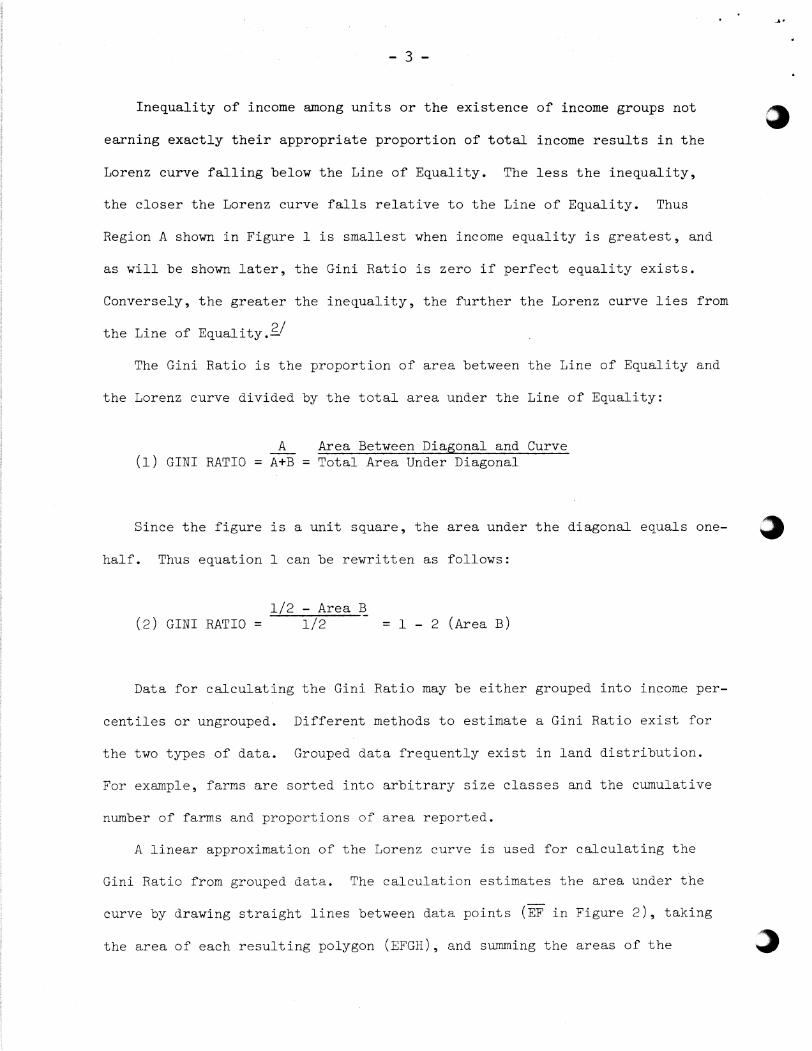
Inequality of income among units or the existence of income groups not

earning exactly their appropriate proportion of total income results in the

Lorenz curve falling below the Line of Equality. The less the inequality,

the closer the Lorenz curve falls relative to the Line of Equality. Thus

Region A shown in Figure 1 is smallest when income equality is greatest, and

as will be shown later, the Gini Ratio is zero if perfect equality exists.

Conversely, the greater the inequality, the further the Lorenz curve lies from

the Line of Equality.£/

The Gini Ratio is the proportion of area between the Line of Equality and

the Lorenz curve divided by the total area under the Line of Equality:

A Area Between Diagonal and Curve (1) GIN! RATIO = A+B = Total Area Under Diagonal

Since the figure is a unit square, the area under the diagonal equals one-

half. Thus equation 1 can be rewritten as follows:

1/2 - Area B (2) GINI RATIO = 1/2 = 1 - 2 (Area B)

Data for calculating the Gini Ratio may be either grouped into income per-

centiles or ungrouped. Different methods to estimate a Gini Ratio exist for

the two types of data. Grouped data frequently exist in land distribution.

For example, farms are sorted into arbitrary size classes and the cumulative

number of farms and proportions of area reported.

A linear approximation of the Lorenz curve is used for calculating the

Gini Ratio from grouped data. The calculation estimates the area under the

curve by drawing straight lines between data points (EF in Figure 2), taking

the area of each resulting polygon (EFGH), and summing the areas of the

....

Cumulative Fraction of Income

- 4 -

Figure 2. Lorenz Curve

x. 1.-l

G

x· 1. 1.0 x

Cumulative Fraction of Units (Income Earners)

- 5 -

several polygons to approximate the area under the curve. Because the

straight lines connecting these data points lie above the curve, a Gini Ratio

results which underestimates the true concentration index. Obviously, the

greater the number of polygons created from a data set i.e., the greater

the number of groups or percentiles the closer will be the estimate of the

areas to the true area.l/

The calculation of the Gini Ratio using the linear approximation method

can be expressed as follows:

Area under any line segment equals:

(3) Area EFGH = (Yi + Yi-1)

2 (Xi - Xi-1)

Where: Yi = Cumulative fraction of income

Xi = Cumulative fraction of units (income earners)

Summing over all the intervals to approximate the area under the curve

gives:

( 4) s = ~ i ~ i = 1

Where: K = the number of intervals.

Through substitution of equation (4) into equation (2), a formula for estimating

the Gini Ratio results:

( 5) GIIH RATIO = 1 - 2 ~ (Y. + yi-1) l i = 1 (x. - X· 1) 2

l l-

k = 1 - £ (y. + yi-1) (x. - xi-1) l l

i - 1

.. - 6 -

Similar presentations are given by Riemenschneider, Morgan, Bonnen, and

Manke. Also, Gastwirth gives a somewhat different, though, in essence parallel

presentation.

Several methods exist for calculating the Gini Ratio from ungrouped data.

One such method uses the cumulative number of recipients (Wi) and the cumula-

tive income (Zi). The equation is as follows:

}t (6) GINI RATIO = 1 - Z, (zi + zi-1) (wi - wi-1)

WN • ZN i = 1

Where: i = 1, 2, 3 • • • N

= # of recipients

Other methods for determining the Gini Ratio from ungrouped data are given by

Riemenschneider.

A Fortran Program for Calculating the Gini Ratio

This computer program calculates the Gini Ratio from ungrouped data using

equation (5) instead of equation (6) because income data is most commonly

expressed as income shares for income groups. The program (1) takes unordered,

ungrouped observations, (2) orders them from lowest to highest income level,

(3) divides the resulting list into separate groups representing income groups

or percentiles (Xi's), (4) calculates the cumulative income for each group,

(5) divides this cumulative group income by the number of observations in each

group to obtain a mean _group income, often called the income share (Yi's),

then (6) calculates the Gini Ratio using equation (5).

Several characteristics of the program are unique to this study and need

elaboration. First, the number of observations varies from one year to the

- 7 -

next for the data analyzed with this program. It was necessary to ensure that

no observations would be dropped when dividing them into income groups. The

program, thus, groups observations by taking the cumulative number of observa­

tions for one cumulative percentile and subtracts from it the number of obser­

vations in the previous cumulative percentile. For instance, to obtain the

number of observations in the 51-60 percent group, the first 60 percent of the

total number of observations in a given year is determined, then from it is

subtracted the cumulative number of observations in the last 50 percent of the

sample, i.e., number of observations in 51-60 percent= (.60N) - (.SON) where

:rr = total number of observations.

Some control cards for the program will need adjustment depending on the

specific data. They include the year of the sample, and the specification of

income groups. The cards which pertain to these characteristics are designated

..

on the program deck printout. Missing data is not accounted for in the program. ~

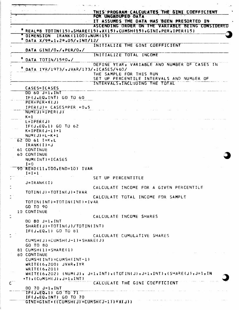
The printout of the program deck and parts of one program printout follow.

The input comes from unit 11 and output is on unit 6 (which is universally the

printer). Brief explanations of the program results are found on the printout.

- 8 -

Printout of Computer Program

*those items possibly to be changed

'

'

_- ,J,_ -~ . - .:'ii( . -.. ·- , .....

"'. FM· UHGIDUPEO· ·GATA , · · : · · ;. • IT ·ASSUME·S 'TME OA:t'l··KA'S' 'BEEN PRESORTED IN-lsC'ENDtNG ORDER ON nfE VARll'BlE BEING CONSIDERED

* REAL*8 TOTINC15JtSHAREfl5J,X(l5),CUMSHU,1tGlNitPER.tIPERl15) ,,... *DIMENSION IRANKC1100),NUMC15J ~ *DATA X/9*•lt2*.05/tINT/l2/

- IN I'""'T-=I-A-,-L-=-1-=-z--e--=1..,..,H=e G I NI c 0 E FF I c IE NT DATA GINI/O./,PER/O./

INITIALIZE TOTAL INCOME * DATA TDTIN/15*0./

-~---·---·--------··----DEF.INE-Y~-AR-;--VARIA.BLE·-;u.fo·-NUMBER-OF-C-ASES.-TN ·-· *DATA IYR/1973/,JVAR/173/tICASES/460/

.- ---- ----- ... - THE- SAMPLE FOR THIS RUN SET UP PERCENTILE INTERVALS AND NUMBER OF

·-----------·m·-·--lNTERVALS 9INCL'1)0ING THt· TOTAL ______ ----~ ----~-----~-· --CASES=ICASES ------------ _______ ,. _________ ,, ____ ---------- --····-----·. - ---·----·----- -- -- --·-- - ·-- - ---- -DO 60 J=ltINT IF(J.EQ.INT) GO TO 60

----PE-R-=PE-R-+X-t J > --·-- -- -- -------

IPER CJ I= CASES*PER +0.5 ----- ·-NUMTJT:TPERf J f . . .. . ...

K=l ·- -· --· v- ·- ....... .

L=IPER(JI If(J.EQ.l) GO TO 62 i<=lPER(J-lJ+l NUM(Jt=L-K+l

-· ··i;-2···00 61 r =K, L IRANKCl)=J

61 CONiI'NUE 60 CONTINUE

NUMCINT>=ICASES I=O

-~lrr"AD ( 11,TOO, END='lOT IVAR I=I+l

c·

SET UP PERCENTITLE J=IRANK(I)

CALCULATE INCOME FOR A GIVEN PERCENTILE TOTINCJl=TOTINCJl+IVAR

CALCULATE TOTAL INCOME FOR SAMPLE TOTINllNT>=TDTINCINTl+IVAR GO TO 90

10 CONTINUE CALCULATE INCOME SHARES

DO 80 J=l,INT SHARECJl=TOTIN<Jl/TOTINCINT) IFCJ.EQ.ll GO TO 81

CALCULATE CUMULATIVE SHARES CU~SHCJl=CUMSHCJ-ll+SHARECJ)

GO TO 80 81 CUMSHClJ=SHARECll 80 CONTINUE

CUMS~(INT>=CUMSHCINT-11

WRITEC6,200) JVARtlYR WRITEC6,20U WR I TE C 6 , 2 O 2 > C NU M ( J I , J = l , I NT) , C T OT I N C J I , J = 1 , 1 "I Tl , C SH AR. E ( J ) , J = 1 , I N

+T),CCUMSHCJJ,J=l,INTI . --· ·--·-·- ·-- - - c·ATCU[ A r·E THE G 1 NT- CO E~FTCT ENT'

DO 70 J=ltlNT - --- -TFT:r;-e-0--;1 r· GOTd--=rr---------- --· --- -···--· .. - ----

IF CJ. EQ. INT> GO TO 70 ·-· -- -'GIN1 =GI Nl+-fTCUM'SHT IT+CUR SHTJ.;;. lTl .:t>U J l >

- 10 -

.c (Continued}

--·-·------ _GQ __ TQ_ J_Q__ _ __ _ _ _ _. 71 GINl=GINI+CCUHSHCJJ*XCJJ) 70 CONTINUE ·--------------GINl=l.-GINI

WRITE(6,300) GINI 100 FORMAT C 250X, 2 50X-,2 sffx;2 50X·, l 77 X ~-I if_____ ------- -- -··-·-- ----- ----------- -- ·------ ---200 FORMATC'l't45X,•VARIABLE = •,13,1ox,•vEAR = 'tl4/'0')

-201--FORMAT_fi_ 0•;·24x-;·- -f.:1-0·-~-4-x, • l i = 2o ,--,4>(, -,- 21.::.. 3o' '4-,(-;. 31-40' '4X' '41 =so•·--------+ ,4X, '5l-60't4X t '61-70', 4X, '7 l-80' ,4X t '8l-90',4X t '9l-q5•,3x, • 96- l OO ·-- --- -·-.-i-; =rx-~·•nf'fAL • /; -.--, - · · ·-· · - · - ·

202 FORMAT('ONUMBER OF CASES •,5x,1111a,1x1,2x,19/'0INCOME TOTAL',9Xtl ------ ·- +Uf:a~·o';ixT,zx,F9~-o/ -

+ '0INCOME SHARE't9X,ll(F8.5tlXJ,2XtF9.5/'0CUMULATIVE SHARE', +5}f,-+ l l ( f 8. 5, 1X J, 2XtF9.5/' 0')

----"3'0U~ FORi"IAI ( •o I HE -crnT--COEPFI-e~1-e-N-r--·TS"-T";Fro;;~~-__,,...,.,.--,,-:--·-·

STOP

Printout of Program Results

Percentiles

___ NUM~R Of CA.SES

INC04E TOTAL

INCOME SHARE

CUMULATIVE SHARE

. :-1 .. 0

46

16q72~ R.

Q .. 036 ~~

0.03852

11-20

46

2403743.

Q. C"i~55

0.09307

THE GINI C.OEFFJEIENT lS 0.27490

VARIABLE = 173

21-30 31-40 41-50

46 46 ' ll6. , .... .,;.,

z7q7q90. 31 7133~. 3601136.~

Ci • N:2 °" :2 0 0.07191 o.n°l72 0.15656 0.22853 0.31025

-·--------·-·-------------·------------------~-----·------------------------------------- --·-----·---

51-6 Ci t-1-70 71-f:.(i R 1-40 TCTAL

\4--cl.-:;.·~-·~tL. -· 4~-702-9-·~. -~3 .. -L,._'.:. ',·•.' 1-~ •. ...,."¥1'. o _ ,. _, '"' , ~ 6464 78"'. <+O!...:. ~ l ~'. :·':! •. <1~'-· ·.i •

. c.c<n10 c1. J'·'PZ .D...a.J.?J7C>

. ____ i,,,£... ___ ..... _ -~_:,!._ .. -----~·--... - -.. - .. -4._.c,S ....... O __

1. GC C·OC.

I . ~·~~~~~~~~~~~~

- 12 -

Footnotes

1. A thorough discussion of the limitations of the Gini Ratio may be found

in Riemenschneider. Also Eric Monke makes a comparison of different income

measures. Paglin modifies the calculations in an attempt to take into account

the life-cycle effects on an income distribution from a sample population

which contains income earners of various ages.

2. It is obvious that the Gini Ratio does not give complete information

concerning the distribution of the variable. Other statistics such as the

mean, mode, ~edian, coefficient of skewness, Kurtosis, and the coefficient

of variation provide further illustrative information to describe the dis­

tribution.

3. Riemenschneider sets the minimum number of percentile groups at eight to

obtain the closest approximation of the true area. Unfortunately most income

data from countries exist in groups ranging from the lowest twenty percent of

income earners to the top five percent (0-20 percent, 21-40 percent, 41-60

percent, 61-80 percent, 81-95 percent, 96-100 percent). Felix Paukeit's contro­

versial study on income distribution (1973) based on an extensive data collec­

tion helped to set this pattern. To reduce possible underestimates of the Gini

Ratio it is advisable to have at least eight groups.

- 13 -

References

Bonner, Jam.es T., 11The Distribution of Benefits from Selected U.S. Farm Pro­

grams", Rural Poverty in the United States, A report by the President's

National Advisory Commission on Rural Poverty, Washington, D. C., May,

1968.

Gastwirth, J. L., "The Estimation of the Lorenz Curve and Gini Index", The

Review of Economics and Statistics, Vol. 54, No. 3, August, 1972, pp.

306-316.

:.fonke, Eric, "Income Distribution in Tai wan: A Panel Study of Agricultural

Farm Families", unpublished paper, Food Research Institute, Stanford

University, August 1, 1975.

:.Jorgan, James, "The Anatomy of Income Distribution", Review of Economics and

Statistics, Vol. 44, No. 3, August, 1962, pp. 207-283.

Paukert, Felix, "Income Distribution at Different Levels of Development: A

Survey of Evidence", International Labour Review, August-September, 1973,

pp. 97-125.

. .

:leir.ienschneider, Charles, "The Use of the Gini Ratio in Measuring Distributionai

Impacts", unpublished paper, Department of Agricultural Economics, Michigan

State University, circa 1976.