by matthew s. jaremski - electronic theses &...
TRANSCRIPT

FREE BANKING: A REASSESSMENT USING BANK-LEVEL DATA
By
Matthew S. Jaremski
Dissertation
Submitted to the Faculty of the
Graduate School of Vanderbilt University
in partial fulfillment of the requirements
for the degree of
DOCTOR OF PHILOSOPHY
in
Economics
August 2010
Nashville, Tennessee
Approved:
Professor Peter Rousseau
Professor Jeremy Atack
Professor Mario Crucini
Professor Robert Driskill
Professor David Parsley

ii
Copyright © 2010 by Matthew S. Jaremski
All Rights Reserved

iii
ACKNOWLEDGEMENTS
First and foremost, I would like to thank my family, especially my parents, for their
unwavering support in all my endeavors. If not for their understanding and encouragement, I
might not have pursued my PhD and definitely would not have completed it.
I am also grateful for all my advisors and mentors throughout the years. At Austin
College, Kevin Simmons and Danny Nuckols gave me the unique opportunity as an
undergraduate to experience research and economic theory at a high level. At Vanderbilt, Peter
Rousseau and Jeremy Atack provided constant feedback on my ideas and writing. Quite simply,
the dissertation would not have been completed without their patience and selflessness. I would
also like to thank Warren Weber for introducing me to free banking and providing me the
necessary data to pursue my ideas. I am also deeply indebted to Robert Driskill and the rest of
my committee members, Mario Crucini and David Parsley, for their helpful suggestions.
The dissertation has also benefited greatly from the comments received from students at
Vanderbilt, especially Susan Carter, Kan Chen, PJ Glandon, Greg Niemesh, Ayse Sapci,
Shabana Singh, Lola Soumonni, and Caleb Stroup. Participants at the Economic History
Association and Cliometrics Society meetings, as well as Howard Bodenhorn, John James, and
Joel Moen have also offered invaluable feedback on earlier drafts of the chapters. I also
gratefully acknowledge funding from the Economic History Association and Vanderbilt
University.

iv
TABLE OF CONTENTS
Page
ACKNOWLEDGEMENTS............................................................................................................iii
LIST OF TABLES..........................................................................................................................vi
LIST OF FIGURES.......................................................................................................................vii
CHAPTERS
I. INTRODUCTION........................................................................................................................1
Introduction to Free Banking (1837-1862.....................................................................3
Free Bank Compositions & Instability..........................................................................6
The Decline of Free Banking.......................................................................................11
II. FREE BANK FAILURES: RISKY BONDS VS. UNDIVERSIFIED PORTFOLIOS............12
The Cause of Free Bank Failures.................................................................................14
Falling Asset Price Hypothesis .............................................................................15
Undiversified Portfolio Hypothesis.......................................................................17
Data..............................................................................................................................18
Empirical Analysis ......................................................................................................23
Results – Systematic Failure Risk .........................................................................25
Results – Idiosyncratic Failure Risk......................................................................27
Robustness Checks Using Alternate Bank Samples .............................................32
Conclusion...................................................................................................................35
Appendix A. The Proportional-Hazard Model ...........................................................37
III. BANK-SPECIFIC DEFAULT RISK IN THE PRICING OF BANK NOTE DISCOUNTS.39
Bank Notes in the Antebellum United States..............................................................42
Stylized Bank Note Discount Facts.....................................................................44
Data .............................................................................................................................46
Examining the Determinants of Individual Note Discounts .......................................49
Redemption Costs ...............................................................................................50
Default Risks .......................................................................................................51
Empirical Analysis ......................................................................................................53
Determinants of Note Discounts When Open......................................................56
Determinants of Note Discounts When Closed...................................................60
Conclusion...................................................................................................................61
Appendix B. Construction of Passenger Cost Index...................................................63
Historical Sources..................................................................................................63
Method of Construction.........................................................................................65
v
Appendix C. Non-linear Model of Note Discounts.....................................................70
IV. STATE BANKS AND THE NATIONAL BANKING ACTS: A CAUTIONARY TALE OF
CREATIVE DESTRUCTION.................................................................................................73
State and National Banking ........................................................................................74
National Banking Act of 1863.............................................................................76
National Banking Act of 1864.............................................................................80
State Bank Note Tax (1865-1868) ......................................................................84
Data..............................................................................................................................85
Consequences of National Banking Legislation..........................................................86
Determinants of State Bank Decline....................................................................86
Determinants of New National Banks.................................................................94
Counterfactual Analysis.......................................................................................96
Conclusion...................................................................................................................98
V. CONCLUSION................................................................................................................ .......101
REFERENCES ...........................................................................................................................103

vi
LIST OF TABLES
Table Page
CHAPTER I
1. Table 1-1: Sample of Free Bank Requirements By State…………..............................4
2. Table 1-2: Summary of Antebellum Banking Systems (1790-1861)………................5
3. Table 1-3: Sample Balance Sheets................................................................................8
4. Table 1-4: Comparison of Average Free Bank Balance Sheet Positions.....................10
CHAPTER II
5. Table 2-1 Bond Prices Used in Average………………..............................................20
6. Table 2-2: Determinants of Bank Failure (1835-1861) ..............................................26
7. Table 2-3: Determinants of Free Bank Failure (1835-1861) ......................................29
8. Table 2-4: Average Balance Sheets of Banks With Differing Probabilities of
Failure..................................................................................................................... .....31
9. Table 2-5: Robustness Checks Using Specified Samples of Banks............................33
CHAPTER III
10. Table 3-1: Comparison of Free Bank Balance Sheets and Discounts.........................54
11. Table 3-2: Determinants of Note Discounts While Free Bank Was Open..................57
12. Table 3-3: Determinants of Note Discounts While Free Bank Was Closed................61
13. Table B1: Comparison of Historical Stagecoach Fares...............................................66
14. Table B2: Estimates of Passenger Fares on Various Modes of Transportation...........66
15. Table C1: Nonlinear Determinants of Free Bank Note Discounts..............................71
CHAPTER IV
16. Table 4-1: Outcomes of State Banks Present in 1863..................................................85
17. Table 4-2: Multinomial Determinants of State Bank Outcomes (1863-1868) ...........89
18. Table 4-3: Determinants of New National Banks (1863-1866) ..................................94
19. Table 4-4: Counterfactual Distribution of Banks Without State Bank Note Tax........97

vii
LIST OF FIGURES
Figures Page
CHAPTER I
1. Figure 1-1: Distribution of Free and Charter Banks .....................................................7
CHAPTER II
2. Figure 2-1: Bank Failures And Bond Prices (1837-1861) ..........................................16
CHAPTER III
3. Figure 3-1: Sample Bank Notes...................................................................................42
4. Figure 3-2: Average Bank Note Discounts By State (1837-1860) .............................45
5. Figure 3-3: Average Bank Note Discounts in New York City and Philadelphia........50
6. Figure 3-4: Note Discounts vs. Bond Prices (1832-1860) ..........................................52
7. Figure B1: Sample Hub-and-Spoke Network..............................................................67
8. Figure B2: Transportation Hubs Used In Each Year...................................................69
CHAPTER IV
9. Figure 4-1: # Of Banks By Type (1858-1868) ............................................................75
10. Figure 4-2: State Bank Closures By Region (1861 – 1868) .......................................79
11. Figure 4-3: State Bank Conversions By Region (1863-1866) ....................................82
12. Figure 4-4: Average Capital By Bank Type................................................................83
13. Figure 4-5: Locations of State Bank Closures and Conversions.................................92
14. Figure 4-6: Locations of New National Banks (1863-1868) ......................................96
15. Figure 4-7: Distribution of Banks................................................................................99

1
CHAPTER I
INTRODUCTION
Evidence from Sylla (1998), Rousseau and Sylla (2005), and Wright (2002) has shown
that the connection between finance and growth has been present in the United States since its
inception. However, high entry barriers initially restricted capital to developed parts of the
county and those banks that could be established were prone to default and instability. The
nation’s first evolutionary step towards the modern banking sector was a series of state “free
banking” laws starting in 1837. These laws standardized entry requirements within a state and
helped spread banking throughout the developing nation.
Despite doubling the number of banks within a quarter of a decade, free banking was
infamous for its instability. Fewer than half of all free banks remained in operation by 1863 and
the majority of closed banks were not able to repay the full value of their notes. Whether true or
not, politicians and the proponents of the National Banking System (1863-1913) took this
instability as evidence of lax regulations and “wildcat banks”, i.e. unsound banks operating
outside of populated areas. Also focusing on legal restrictions and anecdotal evidence, early
studies of antebellum banking such as Knox (1900), Hammond (1957), and Cagan (1963) did
little to disprove or test these assertions.
Recent studies such as Rockoff (1972, 1974) and Rolnick and Weber (1983, 1984, 1985)
have pushed back against the wildcat interpretation, but the lack of data has prevented a
complete view of the period. Instead, studies draw conclusions from small sets of banks
(Economopoulos 1988), years (Dwyer and Hasan 2007), and variables (Rolnick and Weber
1984). Building on the wave of empirical studies, this dissertation provides a comprehensive

2
reassessment of free banking by assembling a bank-level database. The database includes an
annual balance sheet and quarterly note discount for almost every antebellum bank, as well as an
estimate of their note redemption cost and bond portfolio value.
Following the “new financial history” literature, the unique compositional and
environmental data allows me to unpack free banking’s most controversial aspects. This
introductory chapter starts with a brief summary of free banking, providing the background
material for the rest of the dissertation. The second chapter addresses the causes of free
banking’s systematic (or regulatory) instability and idiosyncratic (or bank-level) instability. After
determining why free banks were unstable, the third chapter examines whether private brokers
were able to efficiently price the default risk of each bank and thus mitigate note holder losses.
Finally, the fourth chapter illustrates the results of the legislative “solution” to free banking’s
instability: the National Banking Acts of 1863 and 1864. On the surface, the legislation
nationalized free banking, but their additional restrictions ultimately broke its spirit, leaving
fewer than 56 free banks in operation in 1869.
The dissertation might focus on a historical period, but its conclusions have ramifications
for modern bank regulations. First, it highlights the unintended consequences associated with
reactionary regulations, and shows that the most successful regulations are those that are
gradually amended as problems occurred. Second, it shows that the individuals are able to adjust
to changes in risk and regulation even when there is no federal oversight or modern security
exchanges. The Free Banking System is thus an important study of the complications and
unexpected consequences of bank regulations, as well as, the market’s ability to adjust to those
regulations.
3
Introduction to Free Banking (1837-1862)
The U.S. banking system before 1837 was governed by a loose collection of rules with
few standards even within states. Each bank petitioned for a unique charter from its state
legislature, and approval depended as much on political influence as personal resources.1 A
series of “free banking” laws changed this by replacing the need for legislative approval with a
well-defined set of capital, reserve, and note requirements. Therefore contrary to its name, free
banking was far from laissez-faire; rather, the term “free” refers to the idea that any person who
met the state’s requirements was “free” to open a bank.2
The sample of free banking laws in Table 1-1 illustrates that requirement levels varied by
state but each contained a bond-secured note requirement.3 Unlike charter banks, the requirement
stipulated that free banks purchase state or federal debt (or other specified assets) as security for
each note. The bank then deposited those bonds with a state representative and received an equal
value of bank notes in return. The state representative held the bonds as note collateral and only
relinquished them when the bank returned an equal number of notes. If even a single request for
note redemption was unmet by a bank, the state representative would close the bank and
liquidate the collateral bonds to redeem any outstanding notes.
Table 1-2 shows that 18 of the 32 states passed a free banking law and 872 free banks
were established before 1861. However, despite the large number of banks established, free
banks seemed to be unnecessary in Northeast (with the exception of New York) given the high
1 For convenience, I define “charter banks” to be any institution established by direct order of the state legislature.
This distinction is necessary because charter banks continued to operate even after free bank laws were passed.
Hammond (1957) and Bodenhorn (2003) provide detailed summaries of the political and economic forces behind
free banking. 2 The laws typically stated that any single or group of residents who met the requirements was allowed to found a
bank. By the letter of the law, they do not explicitly exclude women, children, or slaves. 3 Most laws specified that the government debt used for note backing had to be paying full interest. When allowed,
other assets typically included real estate (Michigan, New Jersey), but some states also allowed unique assets such
as slaves in Georgia.

4
Table 1-1: Sample of Free Bank Requirements By State
Capital
Stock
Assets
Allowed For
Note
Security*
Accepted
Bond Value
Additional
Note
Security
Note Reserve
Requirements
Damages
for Non-
payment
Stockholder
Liability
Alabama
(1849)
$100,000 to
$500,000 U.S. bonds
Par value
-
-
15%
-
Illinois
(1851)
Over
$50,000
Any public
bonds
Not over par
or market
value
-
-
12%
Double
Indiana
(1852)
Over
$50,000
Any public
bonds
Not over par
or market
value
-
12.5% of notes
outstanding -
Single
Michigan
(1837)
$50,000 to
$300,000
Any public
bonds, MI
mortgages, other personal
bonds
-
0.5% of
capital paid
into security fund
Notes, loans and
discounts under
2.5x capital stock
20%
Single
Minnesota
(1858)
Over
$25,000
Any public
bonds
Not over par
or market
25% of notes
or 10% in
Public stock
-
-
Double
New Jersey
(1850)
$50,000 to
$500,000
U.S., NJ, &
MA bonds or
mortgages
Not over par
or market
value
-
-
12%
Single
New York
(1838)
Over
$100,000
Any public
bonds or NY
mortgages
Not over par
value -
12.5% of notes
outstanding in
specie
14%
Not
personally
liable
Ohio
(1851)
$25,000 to
$500,000
US or OH
bonds
Not over par
or market
value
Notes cannot
be 3x capital
or less than
third of
liabilities
30% of notes
outstanding; 15%
Single
Wisconsin
(1852) -
Any public
bonds &
Wisconsin
railroad bonds
Not over par
or market 1/4th of notes
Security for
notes over
$25,000
5% Single
Notes: Sample comes from original state law requirements. Any additions or changes to the laws were not added. "-" denotes non-specified values. *Almost all state laws required that any bond used was currently paying full interest. "Public bonds" are defined as any state or national bond
paying full interest.

5
Table 1-2: Summary of Antebellum Banking Systems (1790-1862)
Free Bank States
Free Bank Law Passed Charter Banks Free Banks
Alabama
1849 11
1
Connecticut
1852 83
14
Florida
1853 14
0
Georgia
1838 53
0
Illinois
1851 8
132
Indiana
1852 4
96
Iowa
1858 2
0
Louisiana
1853 25
0
Massachusetts
1851 225
4
Michigan
1837 33
46
Minnesota
1858 0
16
New Jersey
1850 70
26 New York*
1838 109
377 Ohio
1851 110
14
Pennsylvania
1860 114
0 Tennessee
1852 42
2
Vermont
1851 50
1 Wisconsin
1852 3
143
States With Bond Secured Note Issues
Kentucky
1850 28
0
Missouri
1858 12
0
Virginia
1851 30
0
States Without Free Banks
Arkansas
- 2
0
Delaware
- 11
0 Kansas
- 1
0 Maine
- 124
0 Maryland
- 55
0
Mississippi
- 27
0 Nebraska
- 8
0 New Hampshire
- 69
0 North Carolina
- 16
0 Rhode Island
- 104
0 South Carolina
- 20
0 Total 1,463 872
Notes: Year passed was taken from Rockoff (1974, pp. 3, 125-130). Number of banks was obtained
from Weber (2005b). State with "Bond secured note issues" did not have other free bank requirements.
*New York charter banks which eventually operated as free banks are counted as charter banks.

6
population and large number of pre-existing charter banks and unwanted in the South as the
region set high bank requirements relative to its rural population. Excluding New York, only 42
free banks were established in those two regions compared to 1,107 charter banks. Therefore, the
New York and Midwest free banking laws saw the most use. Midwest laws seem to be
successful because their requirements were low and their low population prevented charter bank
entry, whereas New York’s requirements fit their growing population.
The impact of the new legislation on the country’s bank distribution is seen in Figure 1-1.
Before free banking, banks were concentrated in Northeast, particularly along the Atlantic Ocean
and Great Lakes. As railroads and population expanded westward, so did the banking system.
However, the expansion consisted primarily of free banks as charter banks remained
concentrated in the Northeast. In 1860, 46.5 percent of free banks were located in the Midwest,
compared to 8.5 percent of charter banks. Free banks seem to be attracted to communities that
were beginning their development, whereas, larger charter banks were primarily in developed
areas.
Free Bank Compositions & Instability
The first step to understanding of free banking is to examine an individual bank’s balance
sheet. For the sake of illustration, let us assume that a potential banker with $50,000 in capital
wished to start a free bank. The banker would use the capital to buy $50,000 worth of
government bonds.4 The bonds were then deposited with the state representative in exchange for
$50,000 worth of bank notes. As the bank’s primary source of liquidity, these notes were then
used to make investments and carry out day-to-day operations.
4 While this example bank invested the full amount of capital in notes, it is not an unrealistic generalization as free
banks heavily relied on circulation for liquidity.

7

8
Table 1-3: Sample Balance Sheets
Bank A: Safe Bank
Specie 25,000 Circulation 50,000
Loans 25,000 Deposits 0
Government Bonds 50,000 Capital 50,000
Total Assets 100,000 Total Liabilities 100,000
Bank B: Risky Bank
Specie 25,000 Circulation 100,000
Loans 25,000 Deposits 0
Government Bonds 100,000 Capital 50,000
Total Assets 150,000 Total Liabilities 150,000
Notes: This table provides two possible portfolios that could be achieved from an initial
capital level of $50,000. The safe/risky labels are derived from the bank’s ability to meet its
note obligations during negative shocks to bonds and loans.
Table 1-3 illustrates two possible portfolios a bank could achieve. Bank A used its notes
to make loans and purchase specie, whereas Bank B leveraged its notes to purchase additional
bonds and deposited them with the state representative for more notes.5 Bank B still used its
additional notes to purchase specie and make loans, but the additional notes and bonds make it
more risky. For example, if bonds and loans depreciated by 50 percent, Bank A would still have
enough assets ($50,000) to meet its outstanding circulation ($50,000). Yet under the same shock,
better equipped to handle negative shocks than the Bank B.
As seen in the example, free banking’s unique note requirements meant that the security
of a note was tied to the government bond price level. When bond prices fell, the value of the
bank’s note backing declined while its notes maintained the same face value. Moreover, a free
bank could not have quickly sold its bonds to generate liquidity because they were held by a state
representative. Even if a bank had available bonds to sell, any effort to sell them quickly would
further depress their price and increase capital losses. The bond-secured note issue thus exposed
5 This second bank would traditionally be labeled as a wildcat bank.

9
free banks to negative bond shocks and prevented them from redeeming notes when shocks did
occur.
Free banks could avoid bond price declines and remain solvent in several ways. First,
they could decide invest some of their capital into loans or specie, rather than fully investing in
bonds for notes. This restraint would limit the amount of redemption required during a bank run.
Second, they could diversify their liabilities with non-demandable deposits and their assets with
short-term loans and specie.6 Deposits would provide extra liquidity that was not subject to bank
runs, whereas short-term loans and specie would provide assets that were not susceptible to bond
price declines.7
Table 1-4 shows that stable free banks achieved this type of diversification. On the asset-
side of the balance sheet, the average failed bank invested 44.8 percent of its assets in bonds,
compared to the average stable bank had only 5.5 percent. Stable banks, however, did not invest
in more specie, as the level of specie to assets was approximately the same across bank types.
Instead, they invested in loans, potentially replacing one interest-earning asset with another. On
the liabilities-side, failed banks issued roughly the same number of notes as stable banks but had
only half the assets in which to reimburse note holders. To put it another way, the average failed
free bank had to liquidate half of its assets to meet its outstanding circulation compared to stable
banks that only had to liquidate a sixth.
The dissertation’s second and third chapters build upon these balance sheet comparisons
by addressing why free banks were instable and whether the market responded in the short-term.
Lending support to Rolnick and Weber (1984), the second chapter confirms that the new note
6 This type of diversification was studied by Economopoulos (1990). 7 As argued by Rolnick and Weber (1984) and Dwyer and Hafer (2004), free banks could also diversify their bond
portfolio with less risky bonds, such as New York or US bonds.

10
Table 1-4: Comparison of Average Free Bank Balance Sheet Positions
Assets
Liabilities
Non-
Failed
Failed
Non-
Failed
Failed
Specie 73,383
28,277
Circulation 72,319
80,401
Due from Other Banks 25,106
17,017
Deposits 123,467
12,785
Other Banks Bills 7,514
3,231
Due to Other Banks 37,426
3,081
Bonds 23,051
76,540
Other Liabilities 14,519
4,945
Loans 231,468
31,884
Real Estate 8,710
1,015 Expenses 2,767
864
Capital 165,778
77,998
Other Assets 45,569
12,021
Profit/Loss 12,290
779
Total Assets 417,568
170,850
Total Liabilities 425,799
179,988
Specie/Assets 17.6%
16.6%
Circulation/Assets 17.3%
47.1%
Bonds/Assets 5.5%
44.8%
Deposits/Assets 29.6%
7.5%
Loans/Assets 55.4%
18.7%
Capital/Assets 38.9%
43.3%
Notes: Table presents the average balance sheet of free banks. Banks are equally weighted. Measurement error
prevents assets from equaling liabilities. “Failed” denote banks that did not fully redeem their notes upon closure.
requirements seem to be the underlying cause of the free banking system’s high failure rate
relative to the charter banking system. However, as discussed by Economopoulos (1990), solvent
free banks seemed to diversify their assets away from bonds with loans and reduced their note
circulation. Regulation therefore seems to be responsible for the high free bank failure rate, but
banks could have decreased their probability of failure through diversification.
The third chapter tests whether the market was able to effective monitor the risky
behavior of free banks. It shows that the market priced bank notes according to their systematic
risk (specie suspensions) and idiosyncratic risk (falling bond prices and a bank’s proportion of
loans). Moreover, the discounts after a bank closed changed to reflect the market’s value of a
bank’s debt (circulation) and assets (bond prices and a bank’s asset size). In this way, note
discounts before closure corresponded to the probability that a bank would default, whereas after

11
closure, they corresponded to its ability to pay off its debt. The market thus mitigated the real
value of losses and allowed free bank notes to circulate throughout the country.
The Decline of Free Banking
Shrinking from 513 to 56 banks during the 1860’s, the nation’s experiment with free
banking came to a virtual end with the Civil War and the National Banking Acts of 1863 and
1864. The new legislation attempted to reform the free banking system on the national level. The
goal was to replace risky free and charter banks (i.e. state-chartered banks) with safe nationally-
chartered free banks; however, the new “safer” regulations came with a high cost that not every
bank was able to pay.
First, national banks avoided free bank’s attachment to risky state debt by only allowing
federal debt to back notes. Second, a ceiling was placed on aggregate circulation of national bank
notes encouraging banks to restrict their note issues and pursue deposits. Third, New York’s
already high capital requirement was increased for densely populated areas. Fourth, a reserve
was required on both reserves and deposits. Finally, a prohibitive 10 percent tax was passed on
state bank notes meant to eliminate the free (and charter) bank notes.
The dissertation’s fourth chapter show that the decline of free banks was not simply due
to a switch to national charters. Rather, a third of state banks closed permanently between 1863
and 1869 and half of national banks were created from new capital. The chapter goes on to show
that the high capital requirements of national banks prevented existing banks from converting to
a national charter, whereas the state bank note tax destroyed many of the small banks which
remains. Overall, the legislation created large banks in developed areas and destroyed the access
to capital in rural areas, effectively breaking the spirit of free banking.
12
CHAPTER II
FREE BANK FAILURES: RISKY BONDS VS. UNDIVERSIFIED PORTFOLIOS
The Free Banking System (1837-1862) was the United States’ first step towards a
uniform banking system, but instead of adding stability to the existing system, the new laws led
to even greater problems. By the time the National Banking Acts were passed, almost a third of
all free banks were considered failures, unable to reimburse note holders for the full value of
their bank notes upon closure. However, despite the infamous reputation, there is no general
consensus on the cause of the failures. Because most samples have been limited to groups of
banks or years, papers written on the topic have typically focused on one of two general
explanations for their failure. Either banks were subject to poorly designed regulation or did not
sufficiently diversify their asset and liability portfolios. Using almost the entire population of
antebellum banks, this chapter attempts to draw clearer conclusions about the system’s collapse
by testing both theories within a single hazard model.
Rolnick and Weber (1984, 1985) believe that free banks were as much victims as villains,
done in by sudden exogenous bond price depreciations and counter-productive bank regulations.
Without exception, banks are more likely to fail when their assets depreciate. Rolnick and Weber
argue that free bank laws further exposed banks to bond price depreciations by forcing them to
back notes with government debt. Under this falling asset price hypothesis, low bond prices
should correspond to a higher degree of free bank failures than charter bank failures.
Instead of focusing on specific regulations, Economopoulos (1990) addresses the
operational choices made by free banks. He argues that individual free banks could have limited

13
their exposure to bond prices through diversification. Free banks which sufficiently diversified
their assets with loans and their liabilities with deposits would have been more likely to survive
bond market declines than other free banks. The undiversified portfolio hypothesis therefore
asserts that free banks needed to hold more loans and deposits but fewer bonds and circulation to
remain solvent.1
The two hypotheses are straight-forward, but testing them separately is unlikely to
provide conclusive results. A comparison of bank failures and collateral bond prices would
identify the negative correlation between the two, but not prove that properly diversified banks
also failed. To account for relationships between explanatory variables, I employ the multivariate
proportional-hazard model with time varying covariates developed by Cox (1972). The model
uses both a bank’s financial (cross-sectional) and environmental (time series) information to
estimate the roles that nature (bank structure) and nurture (market fluctuations) had in bank
failure. Although similar to a panel logit or probit, the model gains additional efficiency from the
use of imbedded duration information such as the bank’s time-to-failure.
Recent studies such as Modlina (2002) and Wheelock and Wilson (1995, 2000) have
shown the hazard model’s usefulness in modeling bank failures, but the lack of consistent micro-
level bank information has prevented its application in free banking studies. Without large panel
samples, previous studies have examined smaller sets of banks (Economopoulos, 1990), years
(Hasan and Dwyer, 1994), or variables (Rolnick and Weber, 1984). Only Dwyer and Hafer
(2004) and Dwyer and Hasan (2007) have incorporated bank portfolios and bond market
information within a single model.
1 It is also helpful to note that this hypothesis is a more general version of Rockoff’s (1972, 1974) wildcat banking hypothesis, namely that failed free banks issued more notes than they could conceivably redeem.

14
To overcome this deficiency, I have assembled the necessary panel by merging and
expanding the two antebellum bank databases collected by Warren Weber (2005b, 2008). The
later database is a set of over 20,000 bank balance sheets stretching from 1790 to 1861. The
balance sheets were then matched with Weber’s separate listing of banks to add each bank’s
type, location, operation dates, and whether it failed.2 The merged database was then extended
using Hunts’ Merchants’ Magazine and Banker’s Magazine to document the over 120 banks that
failed after Weber’s listing ends in 1860 and construct a quarterly price database for 14 state
bonds and a U.S. Treasury bond. The extended database provides the annual financial structure
and failure date of almost every bank in operation before the Civil War, in addition to an
indicator of relevant market fluctuations.
I use this micro-database to examine two questions: (1) what made a free bank more
likely to fail than a charter bank (systematic risk) and (2) what made one free bank more likely to
fail than another free bank (idiosyncratic risk). My results suggest that free banking’s systematic
risk was due almost entirely to its bond-secured note issue. On the other hand, individual free
banks seemed to avoid failure by diversifying their assets with loans and reducing their
circulation.
The Cause of Free Bank Failures
As discussed in the previous chapter, free banking’s requirement that notes be fully
backed by government debt (or other specified assets) was often insufficient to fully cover their
note circulation. Consequently, bank notes were redeemed at cents on the dollar. Some losses
were minimal (most Indiana banks, for example, redeemed at 95 cents on the dollar) whereas
other losses were nearly total (Minnesota “railroad” banks repaid less than 35 cents of each 2 I owe a great deal to Weber who made an expanded version of his databases available.

15
dollar).3 Following Rolnick and Weber (1984), “failed banks” are defined as those institutions
that did not reimburse the full value of their notes, whereas “closed banks” ceased operation but
repaid their notes at par.4 Based on this distinction, 29 percent of the 872 free banks failed. In
comparison, only 19 percent of the 1,463 charter banks failed, even though they were allowed to
back their notes with any type of asset.5
The high failure rate of free bank is traditionally attributed to either inefficient regulatory
design or improper banking practices. In the following section, I discuss each of these theories
individually drawing attention to their empirical strengths and weaknesses before moving to a
more rigorous empirical test.
Falling Asset Price Hypothesis
The falling asset hypothesis in Rolnick and Weber (1984, 1985) argues that free bank
failures were a natural reaction to exogenous bond price declines.6 Because bond prices were
published weekly or monthly, a bond price decline might trigger a bank note run.7 Knowing that
their note security portfolio was worth less in the short run than their notes in circulation in the
short-run, banks could either (1) redeem their notes at par taking capital losses or (2) refuse their
notes, close their doors, and forfeit their security portfolio. At some bond price, the losses on
redemption would exceed the value of the security, and the bank would voluntarily cease
operation rather than experience additional losses.
3 Rolnick and Weber (1983) 4 Due to lack of data this definition does not include losses on deposits. 5 These failure rates were taken from Weber (2005b) which is described in the Data section. 6 Although the hypothesis clearly applies all assets, the literature has focused on the bonds deposited with the state as they experienced the largest fluctuations during the period and were the primary source of note backing. 7 Many newspapers published the bond prices of states such as New York, Pennsylvania, and Ohio every week. Less traded bonds were published monthly in Hunts’ Merchants’ Magazine or Banker’s Magazine.

16
Rolnick and Weber test the hypothesis by illustrating the negative correlation between
free bank failures and bond prices. As seen in Figure 2-1, 158 of 242 free bank failures (or 65
percent) occurred when bond prices were low.8 Moreover, free banks that failed during the 1839
western bond crisis and the 1861 southern bond crisis held a larger proportion of their portfolio
in these depressed bonds than banks that survived. For example, failed free banks in New York
during the early 1840’s held 95 percent of their note security portfolios in defaulted bonds
whereas solvent banks held only 75.2 percent.9 The evidence therefore suggests that free banks
were susceptible to bond price depressions.
8 Bond periods were defined using the prices of Indiana 5% bonds and Missouri 6% bonds. These bonds were chosen for their large variation. The conclusions are robust to slight changes in the periods. 9 Rolnick and Weber (1985, Table 3 and 4). Economopoulos (1988) finds similar results in Illinois.

17
This falling asset price hypothesis has not gone unchallenged. Hasan and Dwyer (1994)
question the exogeneity of bond prices. During a bank run, solvent banks sold assets to obtain
liquidity, and state representatives liquidated the assets of closed banks. Even if bond prices were
not already declining, they could fall in response to the sudden liquidation of bonds. Although
this represents an important criticism, the average bond portfolio of a bank was small compared
to the total amount of state debt. For instance, the total amount of state debt in 1841 was
$189,910,399 but the average free bank only held $74,737 with the state representative to cover
its circulation.10 Thus individual bond prices might have been endogenous, but it would take a
large number of failures to dramatically affect the entire bond market.
Undiversified Portfolio Hypothesis
Economopoulos (1990) argues that free banks which diversified their asset and liability
portfolios were better equipped to remain in operation during bond price depressions. Because
free banks started in an unstable financial position, tied to a single asset (government bonds) and
a single liability (note circulation), the undiversified portfolio hypothesis argues that free banks
needed to hold a larger proportion of loans and specie in order to offset bond price declines,
whereas deposits were needed to offset large circulations. The theory can potentially explain the
84 free bank failures that occurred during periods of stable or rising prices, as well as those
during bond price depressions.11
10 Total state debt was obtained from Wallis (2005, Table 1). Average free bank circulation was calculated from the bank database described in Data section. 11 It is worth noting the undiversified portfolio hypothesis typically focuses on comparing the probability of failure amongst free banks. It assumes that banks needed to diversify away from risky bonds and circulation because of the bond-secured note regulations. On the other hand, the falling asset price hypothesis explains the failure rate among free banks and between free and charter banks.

18
The undiversified portfolio hypothesis encompasses Rockoff’s wildcat bank definition.
Rockoff (1974, p. 142) defines wildcat banks as those with “note issues of far greater volume
than they could hope to continuously redeem”. A wildcat bank’s portfolio should thus have had a
large note circulation and little specie or other assets with which to redeem them.
Economopoulos tests the undiversified hypothesis by comparing the balance sheets of
solvent and closed free banks in New York and Wisconsin. He shows that the more deposits,
loans, or bonds a bank had, the more likely the bank would be solvent. While the positive
relationship between solvency and bonds seems to challenge his hypothesis, Economopoulos
argues that bond holdings were less risky when supported by other earning assets.
Data
Whereas most studies rely on samples containing a handful of banks or years, I have
constructed a new dataset that provides financial and biographical information for almost every
bank in operation before 1861.12 The dataset is built upon the two antebellum databases collected
by Warren Weber (2005b, 2008).
Weber’s earlier database contains a complete census of the approximately 2,450 banks
created before 1861. Constructed from published balance sheets and note reporters, the census
provides each bank’s location and dates of operation, as well as, its type (i.e. free or charter) and
whether it failed or closed before 1861. The census matches well with contemporaneous
accounts in periodicals in 1861, as well as previous bank estimates.
In order to extend the census through 1862, I used Hunts’ Merchants’ Magazine and
Banker’s Magazine to document which banks failed after Weber’s listing ends in 1860. The
extension is necessary because over 120 free banks closed between 1860 and 1863. If these 12 The databases have been conveniently published on Weber’s webpage and summarized in Weber (2006a, 2006b).

19
failures are excluded, then the failure rate of free banks is halved, making free banks appear
much more stable. I determine which banks failed by comparing the reported list of banks in
operation. A bank that was included in the list in the beginning of 1861 but not the beginning of
1863 is considered to be failed. The list was also reexamined in 1864 to correct for any missing
banks that quickly reappeared.
Weber’s second database contains almost 26,000 individual bank balance sheets from
1790 to 1861. Data before 1835 is less frequently available, but after 1837 the database contains
annual account most banks. In total, balance sheets are available for 2,056 individual banks.
Missing banks generally closed before they published their first annual balance sheet making this
sample slightly biased toward stable and nonfraudlent banks. For the sake of the statistical
analysis, I restrict the sample to bank observations after 1834 to avoid measurement error from
missing bank entries. The balance sheets were then merged with the census to provide the bank
type and when the bank failed or closed.
I also constructed a quarterly price database consisting of 14 state bonds and a U.S.
Treasury bond. Prices of the more traded notes were collected from quarterly publications in
Hunt’s Merchant Magazine and Commercial Review or Banker’s Magazine, but I have relied on
large amounts of data collected by Dwyer, Hafer, and Weber (1999) to fill gaps after 1850 and
Sylla, Wilson, and Wright’s Price Quotations to fill gaps before 1845. Due to the low number of
observations of some states, weekly and monthly prices were averaged to give a quarterly market
price for each bond. Seen in Table 2-1 the database does not contain every state bond issued
during the period, but it does provide the most comprehensive collection of bond available.

20
Table 2-1: Bond Prices Used in Average State of Issue Coupon Rate Beginning Year Beginning Quarter
US* 6 1834 1 NY 6 1834 1 OH 6 1834 1 PA 5 1834 1 MD 6 1834 3 IL 6 1838 2 SC 6 1839 3 IN 5 1839 4 KY 6 1840 3 VA 6 1842 1 TN 6 1843 4 GA 6 1854 3 MO 6 1854 3 NC 6 1854 3 LA 6 1855 1
Notes: This table lists the state bonds that were used to make up the bond price average. * denotes U.S. Treasury bond rather than a state bond.
Because the balance sheets do not contain the types of bonds held by each bank, I
assigned each bank a portfolio of bonds defined by its state law. 13 Recalling Table 1-1, most
states allowed any type of state or national debt that was paying full interest to back debt,
whereas Alabama, New Jersey, New York, and Ohio only allowed banks to use certain state
bonds. Banks not subject to a bond constraint are assumed to hold equal proportions of the 14
state bonds, Alabama and New Jersey banks hold U.S. Treasury bonds, and Ohio holds its own
state bond. 14 Based on the change in its free banking law, New York observations hold equal
proportions of the 14 state bonds before 1842 but only New York bonds afterward. The average
13 The results are robust when I weight the portfolio by state debt in 1880 or assign portfolios by region. On the other hand, the bond price variables are insignificant when I ignore state requirements or weight the portfolio in by state debt in 1840. 14 I use the price of NY bonds to fill the missing US bond prices before 1841 because they closely match fluctuations in US bond price during the rest of the period. However, bond prices remain significant when I use the full 14 bond price average instead.
21
price of each bank’s portfolio is then defined as the average of price its bonds over the following
year, in order to cover the period of potential failure.
Without information on a bank’s composition of assets, management quality, or
profitability, I am unable to estimate a full set of CAMELS measures used by modern regulators
in assessing banks, but I have constructed as many as possible.15 As described below, the
variables can be separated both by their modern interpretations and their connection to the
hypotheses summarized in the previous section.
The falling asset price hypothesis or a bank’s “Sensitivity to market risk” is captured by
two variables: Average Bond Price and Cumulative Bond Value.16 The Average Bond Price is the
average bond price of the bank’s constructed portfolio over the year following the publication of
the balance sheet. The measure captures that degree that the nominal price of bonds mattered.
For instance, a 10 percent decline from par would most likely be less problematic than the same
decline from a bond that was already selling at 70 percent of its par value. While the forward-
looking average for a single bond could be endogenous to a large number of failures, it is
unlikely that any bank or group of banks possessed a sufficient bond portfolio to influence all 14
allowable bonds. The assumption that a bank holds an equal amount of all available bonds
suppresses the possible endogeneity of future bond prices.
The Cumulative Bond Value is total appreciation or depreciation of a bond portfolio since
the bank was in operation.17 Because bonds were deposited with the state comptroller at some
fixed initial value, this variable measures the degree that bond prices have moved against or in
15 The CAMELS ratings are a modern measure of a bank’s quality. Each letter stands for a factor in rating: C for capital adequacy, A for asset quality, M for management quality, E for earnings, L for liquidity, and S for sensitivity to market risk. 16 Note I explicitly assume that circulation was backed primarily with bonds. As most states did not allow other assets, this is not a significantly biased assumption. An examination of balance sheets also shows that free bank circulation is strongly correlated (0.69) with bonds. 17 Lacking information on specific bank portfolios, I assume that a bank’s bond portfolio did not change over time.

22
favor of the bank’s portfolio over time. The variable is calculated by subtracting the bond price
average when the bank entered from the average over the next year.
I test the undiversified portfolio hypothesis using five different variables.18 The
log(Assets) captures size differences among banks. Capital (defined as the ratio of Capital to
Total Assets) measures “Capital adequacy”. Specie (defined as Specie divided by Total
Circulation) is an index of bank “Liquidity”, measuring the bank’s capacity to meet bank runs in
specie. Deposits (defined as the ratio of Deposits to Total Assets) measures the bank’s liability
diversity, whereas asset diversity is measured by Loans (defined as the ratio of Loans and
Discounts to Total Assets) and Bonds (defined as the ratio of state and U.S. government assets on
the bank’s balance sheet to total Assets). Contrary to modern studies where government debt is
safe, Loans can also be thought of as a crude measure of “Asset quality” due to their high return
and short maturity compared to bonds during the period. Finally, the level of potential future
redemption is measured by the Circulation (defined as the ratio of Circulation to Total Assets).
Based on the previously hypotheses, we would expect the variables to have the following
relationships with the probability of failure in the data:
; ; ; ; ; ; ; 1
where (-)/(+) denotes the expected sign of the variable’s correlation with the probability of
failure. The rest of the chapter describes and estimates this probability using a hazard function.
18 The balance sheet variables have been averaged across all years the bank was in operation in order to avoid sudden endogenous changes just prior to failure.

23
Empirical Analysis
I employ the multivariate proportional-hazard model with time varying covariates
proposed by Cox (1972, 1974). This approach models the probability of failure of bank i given
survival to the period t as:
, , , lim |
2
where T is the failure date, is the baseline hazard function common to all banks, and the
exponential function captures the effects of the explanatory variables . All explanatory
variables enter the exponential function linearly with , a vector of coefficients that are
interpreted as the variable’s effect on the instantaneous probability of failure. 19 Standard errors
are clustered by state to account for possible within group correlation of errors.20
In addition to variables discussed above, contains several other explanatory variables.
The first is a free bank dummy which takes the value “1” if the observation came from a free
bank and “0” otherwise. The dummy variable captures the differential failure rate between the
bank types, or in other words, the intercept difference in terms of the hazard function itself. Each
explanatory variable is also interacted with the free bank dummy to provide approximate slope
differences. also contains state effects to account for constant heterogeneity across states, such
as regulation enforcement, and year dummies to account for financial panics and specie
suspensions.21
As detailed in Appendix B, Cox’s method is a semi-parametric “partial likelihood”
approach which requires the specification of the scale function (exponential) but not the baseline
19 To calculate the marginal effect of each variable, one would need to make additional assumptions on the initial hazard function. Rather than introducing more uncertainty, I only report the raw coefficients. 20 According to Petersen (2009), the existence of residual correlation across groups and time can be corrected for by adding a time fixed effects and clustering the standard error by groups. 21 Note that state effects limit the sample to states with more than a few observations. However, the few observations that are dropped do not largely influence the results.

24
hazard function. Like a panel probit or logit, the hazard treats each year a balance sheet was
published (t) as a unique observation linked to the individual bank. Each bank enters the hazard
at the date of its first balance sheet and exits when it ceased operation. In this way, the model
examines the lifespan of each bank rather than just the point at which it failed, identifying the s
from variation across starting and failure dates.22 This method gains further efficiency over other
binary choice models by explicitly taking into account survival time.
The imprecise timing of observations relative to failure dates is a common problem for
studies using the hazard model. The model makes use of the definition of a derivative by
assuming that the observation periods are very small. Therefore if possible, the model needs to
observe the bank immediately prior to its failure; however, a bank’s final balance sheet was often
published several quarters before its failure. Following other studies, I define failure to occur at
the date of the last balance sheet publication. The definition assumes that there are no changes
in-between the observed date and failure but does not results in any significant way because I use
a forward-looking bond price and only use the average balance sheet of each bank.
Even though the undiversified portfolio hypothesis focuses on a narrow set of balance
sheet variables, there is still a possibility of multicollinearity.23 A correlation matrix shows that
no pair of variables has more than a 0.65 correlation, but I tested the precision of the hazard
coefficients in two additional ways.24 First, I followed Mitra and Golder (2002) and Poel and
Lariviere (2004) and looked for any large coefficient changes when variables are sequentially
subtracted from the model. Second, I computed the variance inflation factors (VIFs) on a simple
22 The model treats banks which were solvent at the end of 1862 or which closed during the period as censored observations. 23 While most hazard models are sensitive to time-varying correlations (see Leeflang et al., 2000), the use of balance sheet averages eliminates this problem. The model therefore only needs to be tested for cross-sectional correlations. 24 As long as correlations are not perfect, standard estimators remain consistent in most cases.

25
linear panel. Both tests indicate that the model’s precision is not significantly affected by
multicollinearity and therefore I proceed to estimate the fully-specified hazard models.
Results – Systematic Failure Risk
The falling asset and undiversified portfolio hypothesis have typically focused on what
made a free bank more likely to fail than another free bank (idiosyncratic risk), but it is helpful to
start by determining what made a free bank more likely to fail than a charter bank (systematic
risk). This comparison is achieved by examining the free bank interaction terms. If the
coefficient of the free bank interaction term is significant, it suggests that free banks were more
or less likely to fail than a charter bank given an equal level of that variable. Alternatively, an
insignificant interaction term does not imply that the variable is an insignificant indicator of
idiosyncratic failure risk, only that the slope coefficient cannot be statistically distinguished
between the two bank types.
Column (1) of Table 2-2 provides a comparison point by estimating the model with only
a free bank dummy. As expected, free banks are more likely to fail than chartered banks. The
coefficient is not statistically significant, but still provides some indication of relative insolvency
of free banks. Starting at 0.332, the coefficient falls to 0.131 and 0.0973 when the explanatory
variables enter the model without interaction terms. This decline suggests that the high failure
rate of free banks relative to charter banks might be caused by the explanatory variables.
Forcing the coefficients to be equal across both bank types provides some information,
but the interaction terms help determine whether free bank failures differed from charter banks.
Immediately evident is that free banks seem to be much more likely to fail when bond prices
were low. The coefficients on the level of each bond price variable are positive and insignificant,

26
Table 2-2: Determinants of Bank Failure (1835-1861) (1) (2) (3) (4) (5) Free Bank Dummy 0.332 0.131 3.373 0.0973 -3.736
[0.281] [0.294] [3.358] [0.282] [2.410]
Average Bond Price -0.023 0.012 [0.015] [0.020]
Cumulative Bond Value -0.004 0.006 [0.012] [0.014]
Bonds/Assets 0.243 -0.271 0.256 -0.561 [0.955] [1.684] [0.962] [1.491]
Circulation/Assets 0.686*** 0.966 0.719*** 1.205 [0.215] [1.152] [0.221] [1.060]
ln(Assets) -0.355*** -0.411*** -0.356*** -0.387*** [0.100] [0.149] [0.098] [0.135]
Capital/Assets 0.372 0.148 0.438 0.157 [0.652] [1.152] [0.628] [1.010]
Specie/Assets -1.024 -6.805*** -1.095 -6.623*** [1.395] [2.450] [1.433] [2.321]
Loans/Assets -0.003 0.061 0.003 0.201 [0.328] [0.748] [0.332] [0.686]
Deposits/Assets -3.910** -7.036** -3.852** -6.683** [1.586] [2.983] [1.542] [2.676]
Average Bond Price*Free -0.071*** [0.020]
Cumulative Bond Value*Free -0.062*** [0.016]
Bonds/Assets*Free 0.505 0.996 [1.654] [1.352]
Circulation/Assets*Free -0.362 -0.519 [1.083] [0.985]
ln(Assets)*Free 0.262 0.250 [0.202] [0.167]
Capital/Assets*Free 0.300 0.570 [1.926] [1.792]
Specie/Assets*Free 6.976*** 6.289*** [2.498] [2.436]
Loans/Assets*Free -0.466 -0.721 [0.780] [0.726]
Deposits/Assets*Free 4.529 4.332 [4.533] [4.083]
Observations 20,073 20,073 20,073 20,073 20,073 Pseudo R-squared 0.154 0.175 0.183 0.175 0.181 Notes: The model is a proportional-hazard partial likelihood model. The dependent variable is the whether the bank failed during the next year. The model treats each year’s balance sheet as a unique observation but links them under the individual bank. Balance sheet variables have been averaged across years to prevent endogeneity. Fixed effects for state and year have been added to all specifications. Standard errors have been clustered by state and are listed below the coefficients in brackets. * denotes significance at 10%; ** at 5% level and *** at 1% level.

27
whereas the coefficients on the interaction terms are negative, large, and significant. These stark
results lend weight to the falling asset price hypothesis: free banks were more likely to fail in a
given year because of their bond-secured debt issue.
Charter banks, on the other hand, are more likely to fail due to low specie levels than free
banks. This result is shown when the significant interaction term (6.976) is added to the
significant level (-6.805). As charter banks were generally located in developed and accessible
locations, they might have needed to hold more specie to meet redemption demand. However,
without an explicit model of charter bank regulations, I am unable to confirm this assertion.
The remaining interaction terms indicate that idiosyncratic free bank failures were more
correlated with circulation and loans, whereas idiosyncratic charter bank failures were more
correlated with assets, deposits, and specie. However, because bond prices are the only
statistically significant cause of free bank failures over charter bank failures, the results suggest
that the free banking system’s bond-secured note issue was the only factor responsible for its
high systematic failure risk.
Results – Idiosyncratic Failure Risk
The previous section showed that free banking’s high failure rate relative to charter
banking was most likely the result of the bond-secured note issue. This result lends weight to the
falling asset hypothesis at the aggregate level, but does not shed light on why only certain free
banks failed during the bond price depressions. As idiosyncratic risk is at the center of the
undiversified portfolio hypothesis, this section addresses the free-bank-specific coefficients.
Rather than estimating the model using only free bank observations, I calculate the free bank
coefficients by adding each variable’s level and interaction term from the hazard models in
28
Columns (3) and (5) of Table 2-2.25 This process keeps state and year fixed effects constant
across both bank types and allows for a clear reference to the charter bank coefficients.
The free-bank-specific coefficients in Table 2-3 confirm the previous results. A low
average bond price or cumulative bond value is associated with a higher probability of failure for
free banks. This correlation is not surprising given that the majority of free banks failed during
periods of bond declines. Even so, the sizes of the bond price coefficients are not large enough to
completely nullify the balance sheet effects for free banks. To put it another way, a free bank
could counter the increased probability of failure associated with a bond price decline by
increasing the relative quantity of loans and reducing circulation. These results suggest that the
falling asset price hypothesis holds, but free banks are not helpless.
Not all balance sheet items are significantly correlated with the probability of failure.
Asset size, for example, has little to do with failure. If anything, large free banks are more likely
to fail. A bank’s ratio of capital to assets is also insignificant. As previously described, a large
proportion of free bank capital is typically invested in bonds, and thus a large capitalization leads
to an even more undiversified portfolio. The ratios of deposits and bonds to assets have their
expected signs but no significant statistical effect on the probability of failure.
The coefficient on circulation is positive and statistically significant. The more notes, the
more likely a bank would fail. On the other hand, it does not seem like specie reserves helped to
stabilize a free bank. This does not imply that wildcat banking (i.e. too much circulation to
consistently redeem) was widespread, but does provide evidence that note over-issues are
empirically important.
25 Note that like the coefficients in the previous table, these coefficients are not the marginal effects, but rather the coefficients within the scale function.

29
Table 2-3: Determinants of Free Bank Failure (1835-1861) (3) (5) Average Bond Price -0.059***
[0.020]
Cumulative Bond Value -0.055*** [0.017]
Bonds/Assets 0.234 0.435 [1.280] [1.179]
Circulation/Assets 0.604** 0.685*** [0.301] [0.270]
ln(Assets) -0.149 -0.137 [0.141] [0.107]
Capital/Assets 0.448 0.727 [1.209] [1.125]
Specie/Assets 0.171 -0.333 [0.514] [0.786]
Loans/Assets -0.404* -0.520* [0.227] [0.287]
Deposits/Assets -2.507 -2.350 [2.518] [2.229]
Observations 20,073 20,073 Pseudo R-squared 0.183 0.181 Notes: This table displays the free bank coefficients implied by Columns (3) and (5) of Table 2-2. The model is a proportional-hazard partial likelihood model. The dependent variable is the whether the bank failed during the next year. Balance sheet variables have been averaged across years to prevent endogeneity. The model treats each year’s balance sheet as a unique observation but links them under the individual bank. Fixed effects for state and year have been added to all specifications. Standard errors have been clustered by state and are listed in brackets. * denotes significance at 10%; ** at 5% level and *** at 1% level.
The proportion of loans is also a significant indicator of whether a free bank would fail.
The larger a bank’s loan portfolio, the more likely it would remain solvent. The fact that loans
seem to be free bank’s most stabilizing asset should not be surprising. Although of highest value

30
to the current holder, loans were typically short-term with maturities of 3-6 months. 26 Temin
(1975) finds that New York City banks adjusted their loan portfolios to meet anticipated demand.
The short maturity combined with the fact that loan rates (6%) were slightly above bond yields
(5%) suggests that loans would not only have offset the level of bonds but also would have
brought in needed revenue.27
A comparison of charter bank coefficients in Table 2-2 to the free bank coefficients in
Table 2-3 shows that idiosyncratic risk is very different for each bank type.28 Whereas individual
free bank failures were correlated with circulation and loans, individual charter bank failures
were correlated with asset size, specie, and deposits. This difference provides evidence for the
undiversified portfolio hypothesis. Free banks needed to diversify their portfolio to respond to
the bond-secured note issue whereas charter banks did not.
Based upon the coefficients of the hazard model in Column (3) of Table 2-3, we can
determine which free banks are more or less likely to fail. As a demonstration, Table 2-4
provides the balance sheets of four Wisconsin banks with differing probabilities of failure.29 The
first bank (Marine Bank) is the solvent bank which the model labeled as the least likely to fail,
whereas the last bank (Portage County Bank) is the failed bank which was most likely to fail.
The other two columns provide the balance sheets of a solvent bank (Corn Exchange Bank) with
an average probability of failure amongst solvent banks and a failed bank (Manitouwoc County
26 Bodenhorn (2003) studies the loan portfolios of a small sample of banks across the nation. He first finds that there was an average maturity of about 85 days, but the number varied from 58 (Black River Bank in NY) to 116.9 (Branch & Sons in VA). Next he shows that many banks renewed loans over time, but several such as Branch & Sons in Virginia renewed very few. He concludes by illustrating that banks usually held diversified loan portfolios, representing the underlying industrial distribution of the surrounding area. For instance, the Memphis Branch of the Bank of Tennessee issued more loans to Merchant and Service sectors, while the Branch & Sons Bank issued more loans to the Manufacturing sector. Putting the results together, loans were short-term, often not renewed, and diversified against some idiosyncratic risk. 27 Bodenhorn (2003) and Homer and Sylla (2005). 28 The charter bank coefficients are simply the coefficients on each variable’s level in Table 2-2. 29 Selection of banks was limited to Wisconsin to keep state effects constant.

31
Table 2-4: Average Balance Sheets of Banks With Differing Probabilities of Failure Non-Failed Free Banks Failed Free Banks
Lowest Probability Avg. Probability Avg. Probability
Highest Probability
Bank Marine Bank Corn Exchange
Bank Manitouwoc County Bank
Portage County Bank
County Milwaukee Waupun Two Rivers Jordan State WI WI WI WI
Specie 5,294 4,891 2,736 1,142 Real Estate 2,073 4,649 300 0 Loans 133,183 50,336 15,653 0
Circulation 19,555 39,735 36,551 48,372 Capital 50,000 50,000 50,000 50,000 Deposits 51,736 40,076 2,138 0 Total Assets 181,695 141,265 88,689 106,109
Specie/Assets 2.9% 3.5% 3.1% 1.1% Real Estate/Assets 1.1% 3.3% 0.3% 0.0% Loans/Assets 73.7% 34.3% 17.3% 0.0% Circulation/Assets 10.8% 28.1% 41.2% 45.6% Deposits/Assets 28.5% 28.4% 2.4% 0.0% Notes: Banks of each type have been sorted using the predictions of the proportional-hazard partial likelihood model in Table 2-3, Column (5). Only banks in Wisconsin have been used. All balance sheet items are averages over the bank's years in operation.
Bank) with an average probability of failure amongst failed banks. By reading from left to right,
the table starts with the “best” bank and ends with the “worst”.
Immediately, loans stand out as the important asset for stable banks, falling from 73 to 0
percent as the probability of failure increases, whereas circulation stands out as the important
liability rises from 11 to 45 percent. Next, we see that all the banks have the same capital level,
suggesting that many held only the state requirement. Finally, we see there is non-linear
relationship between specie reserves and probability of failure, as the “average” banks both held
greater reserves than the “best” bank.
In summary, bond prices and the ratio of loans to assets are negatively and significantly
correlated with the probability of free bank failure, whereas the ratio of circulation to assets is

32
positively and significantly correlated. The rest of the balance sheet variables generally have
their expected sign but are never significant. The results suggest that the note requirements of
free banks were a significant source of instability but individual free banks could eliminate at
least some of the idiosyncratic risk by diversifying their portfolios.
Robustness Checks Using Alternate Bank Samples
The approach in Table 2-3 does not rule out the possibility of bias due to outliers or
fraud. This section examines these possibilities by restricting the bank panel in various ways.
Once again, the full interaction model is estimated using the sample of charter and free banks,
but only the free bank coefficients are reported in Table 2-5.
The first outlier is the larger number of failures in Illinois and Wisconsin in 1861 and
1862. While Dwyer and Hafer (2004) and Dwyer and Hasan (2007) show that these failures were
the result of depressed bond prices, it is possible that they are driving the results in some other
way. I correct for this by dropping all observations after 1860 and re-estimating the hazard
model. After removing these observations, the average bond price remains statistically
significant at the 5 percent level but the cumulative bond value losses its significance. The rise in
standard errors is expected when treating so many failed banks as stable banks, but the lack of
any large coefficient changes provides some support for the previous conclusions. The
coefficients therefore suggest that large number of failures in Illinois and Wisconsin reinforce
the falling asset price theory’s explanatory power but the underlying relationship seems intact.
The previous hazard specifications also do not account for the possibility that fraudulent,
short-lived banks had large reserves and few loans. If a banker wanted to defraud his customers,
he would not loan them money; instead, he would buy liquid assets that he could carry with him

33

34
when bond prices declined. This type of behavior could lead to the significant coefficient on
loans and the insignificant coefficient on specie. Because short lived-banks often did not remain
open long enough to publish their first annual report, the original sample is already biased
towards safe banks; however, I take selection a step further and drop any bank that was in
operation less than two years. This selection should purge the sample of fraudulent banks, greatly
leaving only stable banks in the sample. Once short-lived banks are removed, specie gains
statistical significance, but the bond price variables, loans, and circulation remain generally
significant.
The large number of New York banks could also bias the hazard’s results. Because New
York had a strong financial system and the most restrictive bank requirements, it is possible that
its free banks operated differently from “frontier” banks. For instance, Sylla (1969) argues that
country banks operated as virtual monopolies extracting high interest rates on loans, whereas,
competition in cities drove down interest rates. I examine this possibility by regressing New
York banks separately from the banks of all other states. If a country and city interest rate
dichotomy exists, loans should be more correlated with solvency in non-NY banks reflecting
their high return while specie should be more correlated with NY bank solvency. While the
probability of failure in all free banks is correlated with circulation and bond prices, failures in
New York are more correlated with low asset sizes and failures in other states are more
correlated with small loans portfolios.
The comparison of New York and frontier free banks also suggests that bank balance
sheet solvency depended on a state’s bond requirement. While frontier banks could use any type
of public debt to back their note circulation, New York banks could only use New York bonds
after the early 1840’s. Due to price variability of other state’s bonds relative to New York’s,
35
frontier banks with risky bonds might need more loans to offset them, while at the same time,
additional loans might be inefficient in a bank with stable bonds. Therefore, banks could also
lower their risk of failure through their bond choice. This result is confirmed by Dwyer and
Hafer (2004). They show that Illinois, Indiana, and Wisconsin free banks with risky portfolios
(defined as those with high standard deviations and low returns) were more likely to fail during
the 1861 bond price decline. I conclude that diversification seems to be important not just across
asset classes but within them as well.
Conclusion
Free banking laws created competitive state banking systems by standardizing the
requirements of banks; unfortunately, the laws were characterized by instability. Economic
historians have typically blamed the instability on the laws themselves or inefficient bank
management. By requiring notes to be backed with government securities, the laws left new free
banks intimately tied to the price of a single type of asset (bonds). At the same time, however,
banks could have diversified their portfolios in such a way as to avoid bond price declines. I test
both of these hypotheses using the annual balance sheets of almost every antebellum bank.
First, I find that the new note requirements seem to be the underlying cause of the free
banking system’s high failure rate relative to the charter banking system. While bond prices
declines were significantly correlated with free bank failures, they were not correlated with the
failure rate of charter banks. Therefore, those banks that did not have to back notes with bonds
did not fail because of depressed bond prices. Furthermore, the statistical relationship was not the
result of general declines in bond prices. Banks were sensitive only to those bond prices that they
could purchase for note backing, instead of the market price of all bonds. For example, New

36
York banks that could only use New York bonds avoided the failures associated with the price
declines of Kentucky and Missouri bonds. In this way, some states limited the exposure of their
banks to more risky bonds, at least ex post.
Second, solvent free banks seemed to diversify their assets away from bonds and
liabilities away from note circulation. Although the addition of balance sheet variables to the
hazard model does not reduce the statistical significance of the bond price effect, their combined
effect would have been sufficient to a least partially shield banks from bond price declines. Free
banks therefore were not helpless and could have decreased their probability of failure.
Solvent free banks also seemed to respond to the specific risks of their state regulations.
Frontier free banks which could hold a range of risky bonds needed a larger proportion of loans
to fully diversify their assets, whereas, more loans would have been inefficient for New York
bank which had less risky bonds. As such, frontier free bank failures were correlated with loans
and circulation while New York failures were correlated with specie and asset size.
Putting these results into a broader perspective, the National Banking Acts of 1863 and
1864 focused on the specific weaknesses of the free banking system. The legislation reformed
the bond-secured note issue by requiring U.S. Treasury bonds instead of state debt. Federal
bonds were still subject to default and inflation risk, but their prices were generally less variable
than state bonds before (and after) 1860. On the other hand, a ceiling on the aggregate circulation
of national bank notes encouraged banks to restrict their note issues, and a reserve requirement
on both circulation and deposits encouraged banks to hold safer portfolios. The legislation thus
took free banking’s structure but put requirements in place to avoid its systematic and
idiosyncratic risk.

37
Appendix A. The Proportional-Hazard Model
Although I use a proportional-hazard model in the chapter, it is helpful to first describe a
typical hazard model. The standard hazard model measures the probability that a bank would fail
within a short time period. Each bank (i) is observed for j periods (with 1 … ). Because I
have only used data before 1862, is defined by either the last observed period of bank i before
failure or the bank’s 1861 balance sheet. The failure time for each bank is then defined as , .
Before we construct the hazard function itself, we must define a cumulative distribution
function for the duration T. The CDF is given by , with the corresponding
density function . The survivor function gives the probability that a bank will
survive the period, and is defined as S t 1 F t . The hazard function for T is then:
lim |
1ln
3
The hazard is then the probability of failure within the interval , conditional on the bank
surviving to time t. This probability is often called the instantaneous rate of failure per unit of
time.
In order to measure the impact of explanatory variables upon the hazard, we multiple the
initial hazard function by some function , . This function scales up or down the
initial hazard rate, leading us to the proportional hazard function:
, , , , 4
The initial or baseline hazard is common to all banks, but the scale function brings in the
variation across banks and time. Typically, an exponential function with linear arguments is
used, the baseline hazard however is usually carefully specified. Using the semi-parametric
“partial likelihood” approach proposed by Cox (1972, 1974), I can estimate the β’s without

38
having to specify either the baseline hazard or density function. Compared to full parametric
techniques, there are some efficiency losses, but most studies have found it to be minimal.30
Cox’s approach starts by ranking the duration by time, , and defining a
“risk set” for each bank i as : , , . We consider this set to be all the banks which
did not fail before bank i’s failure. The collection of all failures and censoring is defined as
, . Using these definitions, the conditional probability of bank i failing at , , given the
history is:
,
, , ,
∑ , , , 5
This equation relates the contribution of each observation to the likelihood function.
However it can be simplified if we take account of the censored data. To this extent, we create a
dummy variable, , taking the value “1” if the bank failed and “0” otherwise. By using this in
the numerator, non-failed banks do not contribute to the numerator. We can also drop out the
baseline hazard function to give:
exp
∑ 6
By taking a log and substituting, we eventually obtain a log-likelihood function of the form
ln exp 7
From this equation, we can estimate the coefficients. Z-values can be obtained because the
distribution is asymptotically pivotal.
30 For a more in-depth discussion, consult Cox and Oakes (1984). Efron (1977) and Oakes (1977) are two studies that argue the efficiency losses are small.
39
CHAPTER III
BANK-SPECIFIC DEFAULT RISK IN THE PRICING OF BANK NOTE DISCOUNTS
Bank notes played a controversial role in the antebellum economy. On one hand, the
asset-backed liabilities satisfied the public’s need for portable, non-metallic money and quickly
became the largest component of the domestic money supply. While on the other, estimates of
aggregate note holder losses range from 2 to 5 percent per year and the losses on an individual
note issue could be as high as 60 percent.1 If note issues were so variable, then why were they so
readily accepted? I propose that the market reduced the real value losses ex ante by pricing bank
notes based upon the issuer’s default risk. Whereas previous studies have shown a connection
between discounts and systematic risk, I test whether discounts accurately represented the default
risk of individual notes.
Starting with the savings and loan crisis and continuing through the subprime mortgage
crisis, the past two decades have seen a renewed interest in determining whether the market
monitors individual bank behavior. Studies such as Whalen (1991), Wheelock and Wilson
(1995), and Bongini, Claessens and Ferri (2001) show that riskiness can be monitored through
balance sheet indicators such as return on equity, whereas Avery, Belton, and Goldberg (1988),
Gorton and Santomero (1990), and Flannery and Sorescu (1996) show that prices do respond to
these indicators.2 Because these studies focus on banks after the development of modern
1 Estimates vary by author. Knox’s (1900) puts losses at 5 percent per year; King (1983) puts New York’s losses at 4 percent or more before 1842 but finds that that new banking laws limited losses later in the period; Rockoff (1974) is only able to justify a 2 percent annual loss rate across the available data. Rockoff (1974) and Rolnick and Weber (1988) find that individual note losses could be over 60 percent. 2 These are just a sample of the large literature on monitoring bank risk. Older examples include, Meyer and Pifer (1970), Sinkey (1978), and Pettaway and Sinkey (1980).

40
regulations, the Free Banking Period (1837-1862) offers a unique testing environment. Not only
were there no federal bank regulations during the period, but over 2,500 individual bank notes
were priced by small local brokers and not by large exchanges. This chapter therefore considers
the open historical question of whether the market efficiently price bank risk without federal
oversight and modern security exchanges.
Examining the timing of bank closure and note discounts, Bodenhorn (1998) provides
evidence that note discounts adjusted to changes in risk. Not only did discounts increase up to
two years before a bank defaulted, but temporary increases were also seen for solvent banks.
Bodenhorn argues that the increased note discount signaled that a bank was at risk. Banks
heeding the signal took action and the market rewarded them with lower discounts, whereas
those that did not often defaulted. Drawing on studies of free bank default, I determine whether
these patterns match the two most significant indicators of bank-specific risk: the market value of
a bank’s collateral assets and the degree of diversity in its portfolio.
Rolnick and Weber (1984, 1985) use depressed government bond prices as indicators of
default risk. By design, free bank capital was primary invested in government debt to back note
issues. A drop in bond prices would depreciate the value of a bank’s capital stock and note
backing, but leave the value of the notes outstanding unchanged. Consequently, banks were more
likely to default and should have had higher note discounts during periods of bond price declines.
Economopoulos (1990) argues that free banks could have limited their exposure to falling
bond prices through portfolio diversification. Additional empirical tests in the previous chapter
show that free banks that diversified their assets with loans and limited the size of their note
circulations were more likely to remain solvent regardless of bond price declines. The banks

41
achieving this diversification required a lower risk premium, and therefore should have had a
lower note discount.
To date, the lack of micro-level data has only allowed the study of systematic risk.
Gorton (1996, 1999), for example, focuses on state regulations and note insurance programs,
whereas Weber (2005a) examines specie suspensions. However, the recent publication of
Weber’s bank database (2008) removes this constraint by providing the annual balance sheet of
almost every free bank.3 By matching a bank’s composition with its redemption cost and note
discount in New York City (1817-1860) and Philadelphia (1830-1858), I construct a quarterly
panel from which to measure the relationship between discounts and bank-specific default risk
for 596 free banks.
The data indicate that the note discounts of banks that were in operation are strongly
related to those factors that increased the probability of bank failure: specie suspensions, bond
prices, and the share of loans to assets of the underlying bank. Alternatively, discounts after bank
closure reflected the market value of a bank’s assets and the relative size of its obligations. Even
in the absence of modern regulations or reporting, the market-determined discounts seemed to
shield note holders from default risk, thereby lessening the value of losses and increasing note
demand.
3 Weber (2006a, 2006b) contains a detailed description of the database.

42
Bank Notes in the Antebellum United States
Unlike today, deposits during the antebellum period were not demandable or a high debt
priority. Therefore to obtain liquidity, states gave banks the right to monetize their assets.4 By
promising to pay the full value in specie whenever demanded, banks split large illiquid assets
into smaller liquid ones. As seen in Figure 3-1, bank notes were denominated in dollars and
resemble modern paper currency. The name and location of the issuing bank were prominently
displayed alongside an image meant to differentiate the notes and protect against counterfeiting.
Each note also described the type of assets used to back it. For instance, the Dayton Bank note
4 While individual deposits were increasing in commercial centers throughout the period, more than two-thirds of free banks had more circulation then deposits in 1860.

43
was “secured by the pledge of public stocks and real estate”, whereas the People’s Bank was
“secured by pledge of public stocks”. Each note thus provided the relevant information whether
for its use in transactions or redemption at the originating bank.
The notes of early antebellum banks (called charter banks) were subject to few
operational standards. Some northeastern states developed insurance programs (e.g. the Safety
Fund) or banking coalitions (e.g. the Suffolk System) to limit charter note losses, but
participation was often not part of a bank’s charter. Starting in 1837, a series of free banking
laws altered this trend. Rather than subjecting free banks to indirect or informal note regulations,
the new laws required the purchase of government debt (and occasionally other assets) as
security for each note.5 The bonds were then deposited with the state comptroller in exchange for
an equal value of notes. If any request for note redemption went unmet, the state comptroller
would close the bank and liquidate the collateral bonds to redeem outstanding notes.
With over 2,500 unique bank notes in circulation, it was difficult to decipher which notes
should be accepted. A merchant had to determine that the note was legitimate and then trust that
it would be redeemed at face value if presented for repayment. Private note brokers stepped in to
alleviate these problems by identifying and purchasing notes at a percentage discount from their
par or face value.6 Similar to modern currency exchangers, brokers advertised the prices and
notes that they were willing to buy and sell. Merchants could then quickly exchange out-of-town
bank notes for local currency, leaving the broker to return the note to the issuer. Accepting the
risk of default, brokers also had an incentive to monitor bank activity and quickly adjust prices.
As the number of brokers and traded notes grew, note reporters began to collect the
prevailing note discounts in an area and sell them as a monthly or quarterly periodical. The
5 Most laws specified that the government debt had to be paying full interest. When allowed, other assets typically included real estate (Michigan, New Jersey), but some states also allowed unique assets such as slaves in Georgia. 6 Dillistin (1949) and Gorton (1989a) provide a more detailed description of note brokers and reporters.
44
reporters reduced transactions costs by providing all the information a merchant needed: each
bank note’s current discount, physical description, originating location, and a description of any
similar counterfeit notes. Rather than consulting a broker directly, a merchant could thus
confidently verify any note’s provenance and discount by comparing it to its physical description
in the reporter.
Because there were at least two paper dollars for every dollar of specie in the money
supply after 1840, sudden bank failures posed a potential problem for the economy.7 On an
aggregate-level, losses were not excessive. King (1983) finds that the annual losses of New York
free bank notes were 4 percent before 1842 but less after additional regulations were installed,
whereas Rockoff (1974) finds annual losses of about 2 percent across the entire free banking
system. On the bank-level, note holder loses were much more significant. Rockoff (1974) and
Rolnick and Weber (1988) find that individual note losses could be over 60 percent. Cagan
(1963) suggests that the liquidity benefits of bank notes simply outweighed the losses, but an
efficient market would also have limited the real value of the losses by appropriately discounting
the notes before default. The remainder of the chapter determines whether discounts were
correlated with a bank’s probably of default.
Stylized Bank Note Discount Facts
Figure 3-2 shows that discounts varied across states from approximately zero in New
York to 17.5 percent in Michigan but display the same tendencies across note reporters.8
Comparing reporters from Cincinnati, Cleveland, New York City, and Philadelphia, Ales,
7 Temin (1969) 8 As discussed in detail in the next section, the two samples contain different bank notes and thus the differences in discounts could be the result of sample selection.

45
Carapella, Maziero, and Weber (2008) highlight several stylized discount facts. The facts are as
follows:
1) “Local” bank notes almost always traded at par, because note holders could easily
demand payment from a local bank. As banks were required to redeem their notes at par, a local
discount could only exist if the bank was closed or suspended. In the case of closed or suspended
banks, the market value of the bank’s assets and collateral should ultimately determine its
discount.
2) Most, but not all, “foreign” notes circulated at a discount. For example, Indiana notes
were discounted in New York City (NYC) and Philadelphia, whereas NYC notes were not
discounted in Philadelphia. Furthermore, foreign discounts varied across redemption locations.
In terms of the previous example, Indiana notes would have different discounts in NYC than
Philadelphia.

46
3) Discounts were asymmetric across locations. If discounts were only a function of
distance, then the discount of NYC notes in Cleveland should have been the same as the discount
of Cleveland notes in NYC. However, this was not the case. Instead, NYC notes circulated
around par in Cleveland, and Cleveland notes circulated at large discounts in NYC. As arbitrage
did not eliminate these differentials, there must have been some asymmetry between bank notes.
Data
I examine the quarterly discount of bank notes traded in New York City (1817-1860) and
Philadelphia (1830-1858). The data made public by Gorton and Weber are the longest and most
inclusive sample of bank notes available.9 Discounts in Philadelphia come from Bicknell’s
Reporter, Counterfeit Detector, and General Prices Current before 1839 and Van Court’s
Counterfeit Detector and Bank Note List thereafter. Whereas, discounts in New York City come
primarily from the Shipping & Commercial List, New York Price Current, and to a lesser extent
Taylor’s United States Money Reporter and Gold and Silver Coin Examiner and Thompson’s
Bank Note and Commercial Reporter. Notes enter the sample around the date of first issue and
exit when no longer traded. Discounts thus vary over time for a specific bank and from quarter to
quarter between banks.
The discount samples contain charter bank notes, but I focus on free bank notes for two
reasons. First, free banks within a state were subject to the same capital, reserve, and note
requirements, whereas charter banks had unique requirements that often varied within a state.10
This within-state variation makes balance sheet and note-security comparisons difficult as they
9 Discounts from other cities such as Cleveland and Cincinnati contain few notes and periods in which to compare. 10 Most importantly, almost every free bank backed its notes with some type of government debt, whereas charter banks could back their notes with any asset. Therefore I can estimate the value of a note’s security in each period for free banks but not for charter banks.

47
were restricted in unobservable ways. Second, free banks were not generally subject to note
insurance programs or bank coalitions. As described by Gorton (1996, 1999), the Safety Fund
and the Suffolk Banking System virtually eliminated the note discounts of all member banks.
While these institutions are important for note pricing, the absence of discounts leaves no
variation to be explained. Therefore by focusing on free banks, I examine the underlying roles of
redemption cost and default risk rather than the efficiency of external institutions.
The New York City sample consists of 495 unique free bank notes and the Philadelphia
sample consists of 520 notes.11 The size difference is the result of reporters not publishing local
notes and Pennsylvania having no free banks until after 1860. The Philadelphia sample is
therefore larger because it has more New York bank notes than the New York City sample.
When New York free banks are excluded, the New York City sample has more notes than
Philadelphia. Because of these differences, I regress the two samples separately but focus on the
New York City sample’s diversity and longer period. However, to provide a closer comparison
of note reporters, I also report the regression results when New York City bank notes are
dropped from the Philadelphia sample.
I obtain the annual balance sheet of almost every free bank in operation during the period
from Weber (2008), but must make an assumption before matching them with the quarterly
discounts. Namely, I assume that it would take note reporters two quarters to update their
discounts in response to a new balance sheet examination.12 Balance sheet examinations were
required by law, but there was an initial delay between the time the bank examined its balance
11 A sample selection regression shows that banks were selected into the sample by staying open. The longer a bank was is in operation, the more likely that it would be present in the reporters. The size of the bank is significant predictor for New York’s sample but not Philadelphia. 12 The assumption also allows me to extend the balance sheet data to fill missing balance sheet information.

48
sheet and the time it was published in a banking periodical.13 For example, balance sheets
examined at the end of the year were not published until the following March edition of
Merchant’s Magazine. Once publicly available, there was an additional delay as note reporters
waited for reporters to update their prices using the new information. These delays would lead to
the assumed two-quarter lag from the examination date until the note reporters were fully
updated, but the results also hold with a one or three quarter lag.14
Because notes had to be physically returned to the issuing bank, I construct an annual
passenger travel cost index to account for each bank note’s redemption cost.15 Described in
detail in Appendix B, the index uses a hub-and-spoke network to estimate the travel cost from
New York City and Philadelphia to each bank location. Each hub is a central city to which the
travel costs from New York City and Philadelphia are known with reasonable certainty in 1836,
1849, 1856, or 1859, whereas the spokes are typically smaller locations to which the costs are
unknown. A reasonable estimate of travel cost is then generated by minimizing the cost of
traveling to the 376 free bank locations either directly or indirectly through a hub. Because the
years represent major U.S. transportation waves, I am able to reasonable fill the missing years
with a linear trend.
The combination of data provides 15,998 quarterly observations from 597 free banks
located in 376 cities. Each observation contains a bank’s lagged balance sheet, its quarterly note
discount in New York City and Philadelphia and the travel cost to return its notes.
13 Note that the date of each balance sheet is the date of examination and not the date of publication. 14 The delay also ensures that a bank’s composition exogenous to changes in discounts. 15 Compared to travel time and distance, cost is available for a large number of cities, varies over time, and does not depend on timetables or weather. As shown by Gorton (1989b), this choice should not significantly bias the results as travel costs are strongly correlated with travel time (0.94) and distance (0.89).
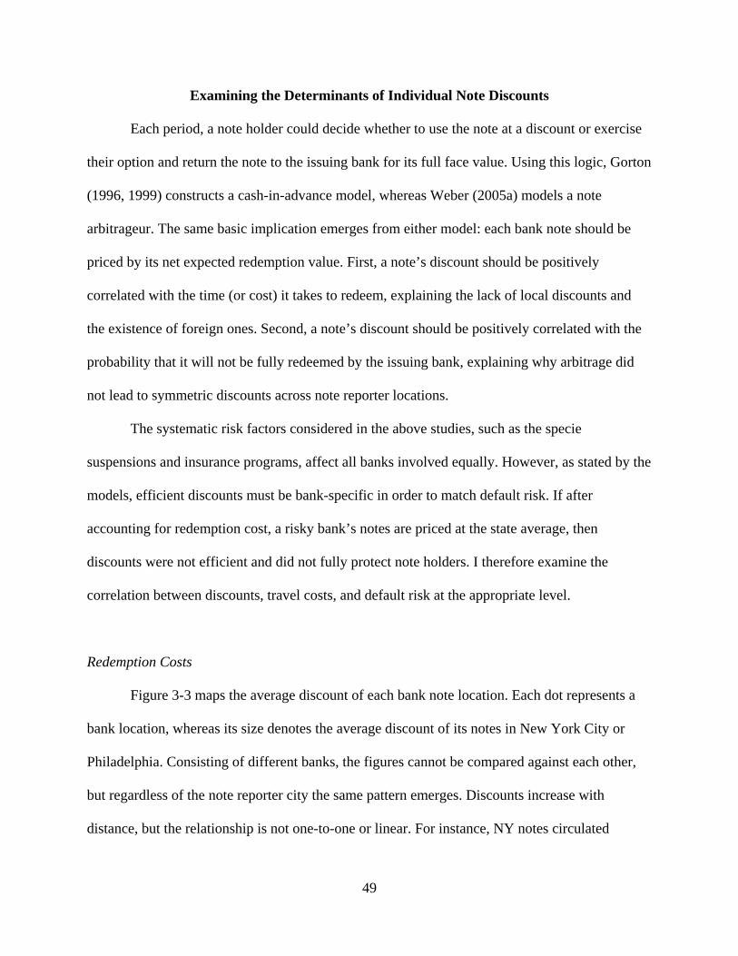
49
Examining the Determinants of Individual Note Discounts
Each period, a note holder could decide whether to use the note at a discount or exercise
their option and return the note to the issuing bank for its full face value. Using this logic, Gorton
(1996, 1999) constructs a cash-in-advance model, whereas Weber (2005a) models a note
arbitrageur. The same basic implication emerges from either model: each bank note should be
priced by its net expected redemption value. First, a note’s discount should be positively
correlated with the time (or cost) it takes to redeem, explaining the lack of local discounts and
the existence of foreign ones. Second, a note’s discount should be positively correlated with the
probability that it will not be fully redeemed by the issuing bank, explaining why arbitrage did
not lead to symmetric discounts across note reporter locations.
The systematic risk factors considered in the above studies, such as the specie
suspensions and insurance programs, affect all banks involved equally. However, as stated by the
models, efficient discounts must be bank-specific in order to match default risk. If after
accounting for redemption cost, a risky bank’s notes are priced at the state average, then
discounts were not efficient and did not fully protect note holders. I therefore examine the
correlation between discounts, travel costs, and default risk at the appropriate level.
Redemption Costs
Figure 3-3 maps the average discount of each bank note location. Each dot represents a
bank location, whereas its size denotes the average discount of its notes in New York City or
Philadelphia. Consisting of different banks, the figures cannot be compared against each other,
but regardless of the note reporter city the same pattern emerges. Discounts increase with
distance, but the relationship is not one-to-one or linear. For instance, NY notes circulated

50

51
around par and Indiana notes did not, but some Indiana notes have greater discounts than those
from Minnesota. Travel costs therefore seem to explain the general trends in discounts but not
the volatility.
Default Risks
The data allow the examination of three types of default risk: systematic (specie
suspensions), state-specific (falling bond prices), and bank-specific (undiversified balance
sheets). With the exception of missing information on “Management quality” and “Earnings”,
these default risk measures correspond to the CAMELS ratings used to measure modern bank
quality. The balance sheet variables measure “Capital adequacy” (Capital/Assets) and
“Liquidity” (Specie/Assets), whereas specie suspensions and bond prices measure the note’s
“Sensitivity to market risk.” Contrary to modern studies where government debt is very safe,
loans can be thought of as a crude measure of “Asset quality”, due to their high return and short
maturity compared to bonds during the period.
Specie suspensions relieved banks of their redemption requirements without forcing
closure and should have led to uniformly higher discounts. As seen in Figure 3-4, discounts
double during each of the three shaded suspension periods: May 1837-Aug. 1838, Oct. 1839-
June 1842, and late 1857.16 The only exception comes in the Philadelphia sample during the
early 1840’s when the average discount decreases as a result of non-suspended New York bank
notes trading at a premium.17 When non-suspended notes are ignored, the average discount
always increases during a suspension.
16 New York banks did not suspend between October 1839 and June 1842. 17 During specie suspensions, foreign bank notes were only traded for local notes. A premium does not suggest that paper was worth more than specie but instead that it was worth more than local bank notes.

52
Rolnick and Weber’s (1984, 1985) falling asset price hypothesis states that free banks
were more likely to default during periods of low bond prices.18 As notes were backed by
government debt, a bond price decline signaled that a bank’s collateral was insufficient to
redeem its notes in the short run. This signal often resulted in a bank run. Knowing their
collateral was worth less than their notes in circulation in the short-run, banks could either: (1)
redeem their notes at par and take capital losses or (2) refuse their notes and forfeit their security
portfolio. Discounts therefore needed to be higher during periods of low bond prices to
compensate for the depreciated note backing and increased probability of failure. Figure 3-4
illustrates this negative correlation: bond prices are at their lowest when note discounts are at
their highest. 18 While not directly addressing the backing requirements, Gorton (1996, 1999) argues that bank regulations or lack thereof led to different levels of default risk. Using both free and charter bank notes, Gorton finds that insurance programs and branch banking regulations dramatically affected discounts. Because free banks were not subject to these regulations, I focus on the other balance sheet and note restrictions present in the laws.

53
While bond depressions were events outside of their immediate control, Economopoulos
(1990) argues that banks could have diversified their asset and liability portfolios in order to
remain solvent during negative shocks. Found in Chapter II, free banks with large proportions of
bank notes (Circulation/Assets) and small proportions of loans (Loans/Assets) were more likely
to default during the antebellum period. Because diversified banks are less likely to default, they
should have had lower note discounts. Table 3-1 shows that a bank’s proportion of specie, loans,
and circulation are significantly correlated with discounts, whereas its asset size and leverage are
insignificantly correlated. Discounts thus seem to reflect the bank-level factors associated with
default.
Empirical Analysis
Similar to studies of modern bank subordinated debt, I estimate the note discount panel
within a linear model.19 Each observation is a single bank-quarter allowing identification across
differences between banks and over time. The dependant variable ( , ) is the percentage
discount on a note from bank i in period t, and the explanatory variables enter the regression
equation linearly with a vector of coefficients. In keeping with the previous section, I measure
redemption costs with the logarithm of travel cost from bank i’s to the redemption city at time t
19 Among others, Avery, Belton, and Goldberg (1988) assume a linear relationship between a bank’s default risk and its market spread (i.e. discount). Despite criticism by Gorton and Santomero (1990), if one accounts for a bank’s leverage, even the market spread of the standard non-linear Black and Cox model (1979) is either monotonically increasing or decreasing with risk. Using this fact, Flannery and Sorescu (1996) argue that a linear model could lead to better results as it does not rely on the strong assumptions necessary for traditional non-linear finance models. I therefore test the linear assumption’s robustness using a non-linear specification in the appendix.

54

55
( , )20, the effects of specie suspensions using a dummy variable ( , ), the falling
asset price hypothesis with the average quarterly bond price ( , ) 21, bank size using the
logarithm of , capital adequacy and leverage using Capital/Assets ( , ), asset
quality using Loans/Assets ( , ), liquidity using Specie/Assets ( , ), and note
overissues using Circulation/Assets ( , ).The general model is as follows:
, , Assets 1
, ,
where denotes the random effects by bank22, , denotes the error term, and , is a vector of
control variables. The control variables included but not reported are the number of years a bank
has been in operation (reputation effects), Davis’ (2004) annual industrial production index
(business cycles), and year-quarter dummies. Standard errors are clustered by state to account for
the possibility that errors are serially correlated within each state and across time.23
I estimate all regressions with and without state fixed effects. When included, these
effects account for constant heterogeneity across states, such as relative population or regulatory
enforcement. The state effects are also particularly useful for comparing balance sheets but do
substantially reduce travel cost variation. The presence of state effects does not preclude travel
costs from being significant, but must be kept in mind when interpreting the results of the model.
20 The logarithm of travel costs accounts for the non-linear relationship between distance and discounts. 21 The bond price variable was constructed from the 14 different state bonds outlined in Table 2-1. The bond price variable is defined as the average quarterly price of equally-weighted bonds allowed by each state’s law. Most states allowed any type of state or national debt that was paying full interest to back notes, whereas Alabama, New Jersey, New York, and Ohio only allowed banks to the use of certain state bonds. Banks not subject to a bond constraint take the average price of all 14 state bonds, Alabama and New Jersey take the price of a US Treasury bond, and Ohio takes its own state bond price. The price of NY bonds fills missing US bond prices before 1841. Due to a law change, New York takes the average price of all 14 state bonds before 1842 but only its own bond price afterward. 22 A Hausman test fails to reject the random effects assumption for the full model. I therefore use random effects because the database does not contain sufficient observations to cluster standard errors under fixed effects. 23 Petersen (2009) shows that the existence of residual correlation across groups and time can be corrected for by adding a time fixed effects and clustering the standard error by groups.
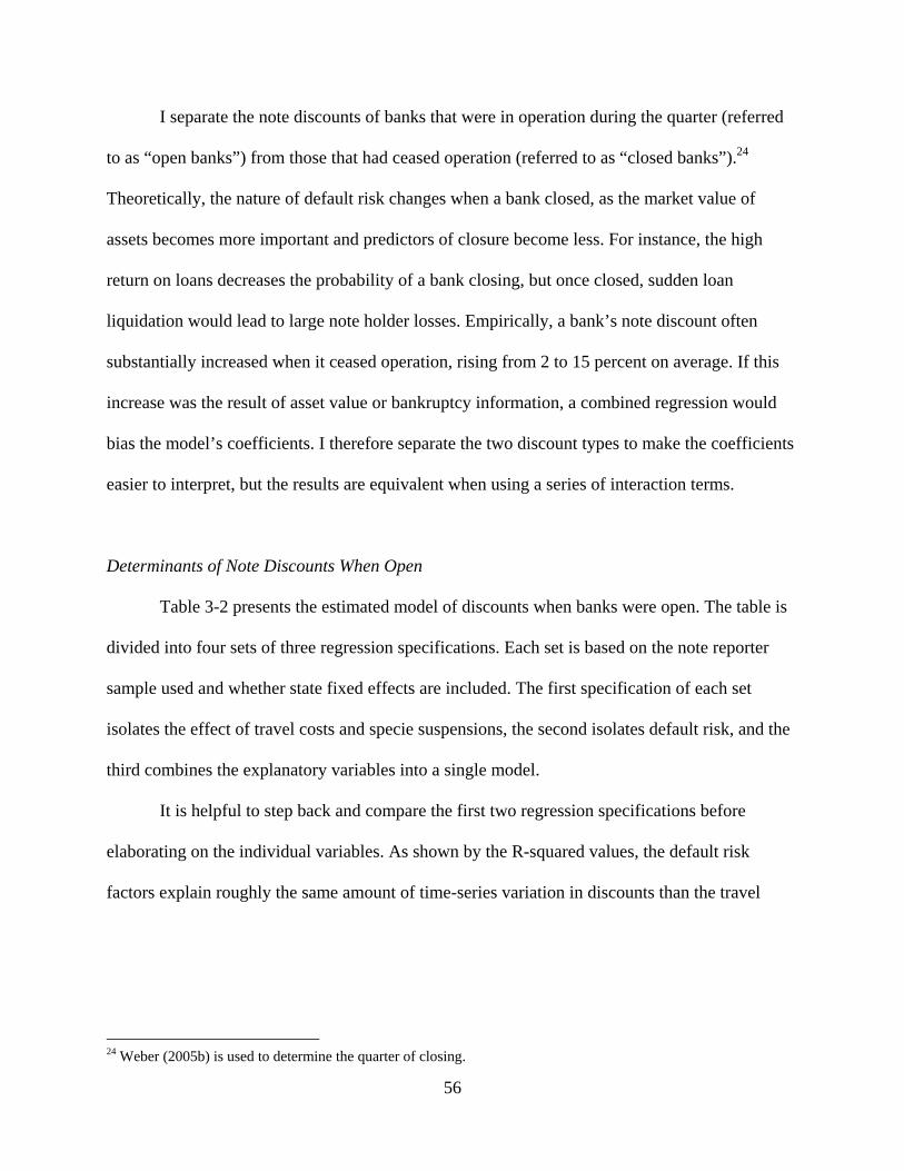
56
I separate the note discounts of banks that were in operation during the quarter (referred
to as “open banks”) from those that had ceased operation (referred to as “closed banks”).24
Theoretically, the nature of default risk changes when a bank closed, as the market value of
assets becomes more important and predictors of closure become less. For instance, the high
return on loans decreases the probability of a bank closing, but once closed, sudden loan
liquidation would lead to large note holder losses. Empirically, a bank’s note discount often
substantially increased when it ceased operation, rising from 2 to 15 percent on average. If this
increase was the result of asset value or bankruptcy information, a combined regression would
bias the model’s coefficients. I therefore separate the two discount types to make the coefficients
easier to interpret, but the results are equivalent when using a series of interaction terms.
Determinants of Note Discounts When Open
Table 3-2 presents the estimated model of discounts when banks were open. The table is
divided into four sets of three regression specifications. Each set is based on the note reporter
sample used and whether state fixed effects are included. The first specification of each set
isolates the effect of travel costs and specie suspensions, the second isolates default risk, and the
third combines the explanatory variables into a single model.
It is helpful to step back and compare the first two regression specifications before
elaborating on the individual variables. As shown by the R-squared values, the default risk
factors explain roughly the same amount of time-series variation in discounts than the travel
24 Weber (2005b) is used to determine the quarter of closing.

57
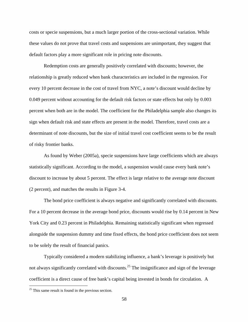
58
costs or specie suspensions, but a much larger portion of the cross-sectional variation. While
these values do not prove that travel costs and suspensions are unimportant, they suggest that
default factors play a more significant role in pricing note discounts.
Redemption costs are generally positively correlated with discounts; however, the
relationship is greatly reduced when bank characteristics are included in the regression. For
every 10 percent decrease in the cost of travel from NYC, a note’s discount would decline by
0.049 percent without accounting for the default risk factors or state effects but only by 0.003
percent when both are in the model. The coefficient for the Philadelphia sample also changes its
sign when default risk and state effects are present in the model. Therefore, travel costs are a
determinant of note discounts, but the size of initial travel cost coefficient seems to be the result
of risky frontier banks.
As found by Weber (2005a), specie suspensions have large coefficients which are always
statistically significant. According to the model, a suspension would cause every bank note’s
discount to increase by about 5 percent. The effect is large relative to the average note discount
(2 percent), and matches the results in Figure 3-4.
The bond price coefficient is always negative and significantly correlated with discounts.
For a 10 percent decrease in the average bond price, discounts would rise by 0.14 percent in New
York City and 0.23 percent in Philadelphia. Remaining statistically significant when regressed
alongside the suspension dummy and time fixed effects, the bond price coefficient does not seem
to be solely the result of financial panics.
Typically considered a modern stabilizing influence, a bank’s leverage is positively but
not always significantly correlated with discounts.25 The insignificance and sign of the leverage
coefficient is a direct cause of free bank’s capital being invested in bonds for circulation. A 25 This same result is found in the previous section.

59
larger capitalization rate implies a larger bond portfolio and therefore a higher probability of
default.
While circulation is strongly correlated with the probability of default, a bank’s
circulation is also insignificantly correlated with discounts. The insignificance seems to be the
result of large circulations being more readily available to be shipped together. Weber (2005a)
suggests that the presence of economies of scale in note return lowers the redemption cost per
note or per dollar and compensates note brokers for some risk. Unfortunately, the lack of
redemption data prevents me from confirming this suggestion.
The coefficient on loans is always significant, negative, and large. Although of highest
value to the current holder, loans were typically short-term with maturities of 3-6 months. 26
Temin (1975) also finds that New York City banks adjusted their loan portfolios to meet
anticipated demand. The short maturity combined with the fact that loan rates (6 percent) were
equivalent to bond yields (5 percent) suggests that loans helped to avoid bank runs without
sacrificing revenue.27 Loans therefore might have been a way for brokers to identify the
profitability and diversity of a free bank.
In summary, discounts on the notes of open banks are closely related to travel costs and
default risk, but not the other balance sheet variables. The effect of travel costs, however,
significantly declines when controlling for default risk. In other words, brokers seem to price
notes based on the issuing bank’s fundamentals rather than its location.
26 Bodenhorn (2003, pp. 96-110) 27 Homer and Sylla (2005) and Bodenhorn (2003, Table 4.2 and 4.3).

60
Determinants of Note Discounts When Closed
I regress the note discounts of closed banks in Table 3-3. 28 Not only does this examine
what factors mattered to discounters after a bank closed, but it also implicitly measures which
factors allowed a bank to fulfill their note obligations upon closure.
Travel costs and specie suspensions are no longer robustly correlated with note discounts.
The fact that the coefficient on travel costs is negative or insignificantly positive is likely
because a note holder only had to redeem the note at the state representative’s office and usually
had a year or two to do so. On the other hand, the statistical insignificance of the suspension
coefficient is understandable given that closed banks were not required to redeem notes on
demand.
Upon closure, a bank liquidated both the bonds used to back notes and those held on its
balance sheet. The current market price of bonds therefore would determine the losses associated
with bond liquidation. The signs reflect that this relationship, but it is only statistically significant
when state effects are not included.
The coefficients on assets, circulation, and leverage are large and statically significant,
whereas those on loans are insignificant. In the sense that a bank’s circulation represents the size
of its redemption obligations and its assets represents the potential size of sudden liquidation
losses, the note discounts of closed banks reflect the ability of the bank to repay its note
obligations. The results differ significantly from the pricing of the note discounts of open free
banks, seeming to capture the changing nature of risk.
28 Because notes were removed from the reporters when they no longer circulated, the discount samples only contain about 170 unique notes.

61
Table 3-3: Determinants of Note Discounts While Free Bank Was Closed Note Discounts of Closed Banks
New York City (1837-1860) Philadelphia (1837-1858) Without
NYC Notes ln(Travel Cost) -3.832*** -2.285*** -0.002 0.651 -1.726
[1.263] [0.695] [1.116] [0.647] [5.450]
Suspended 10.780 11.060* -19.512*** -19.501*** -21.765*** [7.079] [6.020] [4.913] [4.342] [4.669]
Avg. Bond Price -0.867*** -1.145 -0.367* -0.142 -0.056 [0.311] [0.736] [0.210] [0.171] [0.179]
ln(Assets) 6.853*** 6.611*** 2.512*** 2.411*** 2.758*** [2.208] [2.558] [0.815] [0.907] [0.748]
Capital/Assets 22.310* 27.060* 15.886* 17.299** 21.937*** [12.490] [15.770] [8.114] [8.748] [5.744]
Circulation/Assets 32.950* 29.460** 12.009 6.550 9.796 [18.65] [14.85] [16.210] [14.383] [11.134]
Specie/Assets 21.880 30.980 4.170 5.406 14.178 [36.030] [42.770] [16.487] [16.842] [19.853]
Loans/Assets -2.913 -5.918** -5.313 -11.232** -8.702 [4.912] [2.930] [5.739] [4.799] [7.154]
State Effects No Yes No Yes Yes
Observations 908 908 1,684 1,684 1,494 R-squared :
Within 0.2704 0.2755 0.177 0.1783 0.2146 Between 0.3467 0.4799 0.1997 0.3714 0.3834
Combined 0.2761 0.3651 0.1888 0.2907 0.3065 Notes: Linear panel regression with random effects taking the bank's note discount as the dependent variable. Only discounts of banks that were currently closed were used. Different columns represent the present of state fixed effects of discount sample used. All regressions include time (quarter-year) effects, a index of industrial production, and the cumulative number of years a bank was open. Standard errors are provided in brackets and clustered by state. * denotes significance at 10%; ** at 5% level and *** at 1% level.
Conclusion
This chapter shows that the market effectively monitored the risky behavior of
antebellum banks despite significant travel costs, informational asymmetries, and limited

62
government involvement. Specifically, the market priced bank notes according to their
redemption costs and default risk. While travel costs were able to separate note discounts across
different states, they were highly correlated with a bank’s default risk. The results suggest that
systematic risk (specie suspensions) and idiosyncratic risk (falling bond prices and a bank’s
proportion of loans) were the primary determinants of discounts.
I also show that the market discounted the notes of open and closed banks differently.
While open bank discounts were sensitive to default risk, closed bank discounts reflected the
current market value of a bank’s debt (circulation) and assets (bond prices and a bank’s asset
size). In this way, note discounts before closure corresponded to the probability that a bank
would default, but after closure, they corresponded to its ability to pay off its debt.
The analysis provides a reason why risky bank notes circulated in the antebellum
economy. It was not only that the benefits of bank notes simply outweighed the nominal losses,
but that market discounts also mitigated the value of those losses. Combined with the fact that
specie and other types of money during the period were also highly variable, the discounting
process might have made bank notes the safest and most liquid currency.29
29 Discussed in Bodenhorn (1998, p. 21), most coins in circulation were worn and not denominated in dollars thus making it hard to immediately exchange or decipher their value.

63
Appendix B. Construction of Passenger Cost Index
Over 30,000 miles of railroad and 4,000 miles of canals were constructed in the United
States between 1815 and 1861. This “transportation revolution” greatly lowered the cost of
passenger travel and facilitated the nation’s westward migration.30 The lack of antebellum travel
records, however, has prevented studies from examining the impact of these changes on most
locations. Historical studies such as Dunbar (1937) and Taylor (1951) illustrate the travel costs,
times, and distances between major cities such as New York City or Philadelphia, but not
subsidiary or developing cities such as Cleveland or Louisville. Even the most comprehensive
study to date, Gorton (1989), is limited to 30 major cities. This appendix enables the study of
antebellum travel improvements by constructing a hub-and-spoke network that is capable of
estimating the cost of passenger travel to any US city in 1836, 1849, 1856, or 1859.
Historical Sources
I take the historical passenger costs from New York City and Philadelphia to a large
number of “hub” cities from two travel guides.31 Each guide assembled maps, schedules, costs,
and distances for major transportation routes. Data for 1836 and 1849 come from Gorton’s
(1989) summary of Disturnell’s A Guide Between Washington, Philadelphia, etc., whereas 1856
and 1859 come directly from Appletons’ Railway and Steam Navigation Guide.32 These
particular years were chosen both for their availability and association with the major antebellum
transportation waves. As the majority of canals were not finished and railroads had not yet truly 30 The term “transportation revolution” was first popularized by Taylor (1951). 31 While travel costs, times, and distances are highly correlated, costs are the most comprehensive and available measure of transportation advances. Costs are exact, whereas reported times are approximate guesses and actual times would vary depending on weather conditions and other factors. Moreover, costs reflect technological improvements in both speed and efficiency, whereas times reflect only the former and distances reflect neither. 32 Some additional hubs were taken from Weber (2005a) in the late 1840s. Similar in nature, Disturnell’s guide focuses on the chief routes of travel, while Appletons’ provides most available options. Despite the different approaches, a comparison of Disturnell’s 1862 and Appleton’s 1859 yields only minimal differences.

64
begun, roads and rivers were the most common avenue of travel before 1837. The 1840’s saw a
distinct rise in canals and the beginning of railroads. Finally, the spread of railroads through the
Midwest and South surpassed water travel during the 1850’s. In this way, the network provides
an estimate of travel costs during each transportation wave and lowers the size of cost changes
between observations.33
The problem with obtaining a complete summary of passenger costs from the guides is
their general lack of stagecoach and minor water routes. Consequently, most cities unconnected
to major rail or water transportation (referred to as a “spokes”) are not present in the guides.34 To
reach these spokes from New York City or Philadelphia, one would have to travel by rail or
water to a nearby location and then take a road or minor waterway the remaining distance.
Obtaining the most efficient route to each spoke would therefore require additional knowledge of
every water and road route between the several thousand spoke-hub pairs. The lack of
information currently rules out such a detailed approach and forces the use of a simplifying
assumption, namely that travel between each hub and spoke was by stagecoach on straight roads.
This assumption admittedly ignores available water transportation as well as any
mountains, rivers, or other obstacles that roads would avoid. The choice of roads over rivers can
be partially defended using historical evidence. Taylor (1951, p. 71-72) highlights some of the
drawbacks of river transport:
But even more important, especially in the West, was the directness of rail as again river routes…But the meandering western rives greatly handicapped water transportation…While railroads operated the year round, the lakes and rivers of the North were closed by ice from two to five month during the winter season and in the West frequently for long periods during the rest of the year by low water…Finally, river position was predetermined, where rails might be laid over the most convenience routes for commerce…irregularity of sailing and the lack of interline agreements made [non-direct travel] arrangements unusual for river trips…
33 This later result allows a linear trend to reasonably fill the intervening years. 34 In the cases where stagecoach or wagon routes are listed, they generally lack consistent cost and time estimates.

65
Even though Taylor is comparing river travel to railroads, similar principles also apply to
stagecoach travel. Relative to steamboats, stagecoaches were less reliant on weather (could travel
year round), more direct (major roads were straight compared to rivers), and costs did not depend
on direction of travel (upstream vs. downstream). The increased mileage and seasonality of river
travel mitigates some of the per-mile cost advantage, and therefore, the stagecoach assumption
might not greatly bias my cost estimate especially for travel in winter and summer months.
Assuming that stagecoaches were used to travel between every hub and spoke pair, the
final piece of necessary historical information is an estimate of stagecoach costs. Seen in Table
B1, stagecoach costs varied across locations, as the diffusion of road, bridge, and stagecoach
improvements took time. The costs of stagecoaches within the developed Northeast were
therefore generally inexpensive after 1840, but still expensive and declining everywhere else.
Summarized in Table B2, I have chosen to use the median estimates of stagecoach costs
proposed by Gorton (1989).35 The estimates are expensive for developed areas such as the
Northeast, but because the average travel distance between Northeast hubs and spokes are also
small, the choice minimizes measurement error across the entire country.
Method of Construction
The hub-and-spoke network minimizes the travel cost based on available transportation
options. Seen in Figure B1, if an individual from New York City was traveling to a city on a
railroad (e.g. Indianapolis or Richmond), they would simply take a train. However, if the
destination was not on a railroad (e.g. Nashville), the individual would first travel as far as
possible by rail and then take a stagecoach the rest of the way.
35 The network can also be adjusted to incorporate another set of cost estimates when necessary.

66
Table B1: Comparison of Historical Stagecoach Fares
Year Passenger-
Mile Rate ($) Mileage
1812 Philadelphia to Pittsburg 0.09 297
1832 Philadelphia to New York 0.067 90*
1846 Montgomery to Mobile 0.05 200
1848 Tuscaloosa to Mobile 0.018 676 Philadelphia to Baltimore 0.023 128 Baltimore to Richmond 0.026 378 Baltimore to Wheeling 0.044 271 Indianapolis to Madison 0.047 86 Philadelphia to Pittsburg 0.05 300 Lexington to Louisville 0.056 75 Louisville to St. Louis 0.056 75 Wheeling to Columbus 0.057 140 St. Augustine to New Orleans 0.058 600 Columbus to Cincinnati 0.059 110 Columbus to Cleveland 0.06 177 Augusta to Montgomery 0.062 300 Richmond to Knoxville 0.064 444 Louisville to Nashville 0.067 180 Montgomery to Mobile 0.067 180 Nashville to Memphis 0.067 224 Pittsburg to Wheeling 0.068 59
Mobile to New Orleans 0.075 160 Notes: From Warren (1849) and Dunbar (1937). Partially reprinted in Fishlow (1965, Table 8) and Gorton (1989, Tables 5 and 6) . *in snow, on sleigh
Table B2: Estimates of Passenger Fares on Various Modes of Transportation Passenger-Mile Cost ($)
1839 1849 1856 1859 Stagecoach 0.07 0.06 0.06 0.06 Steamboat 0.043 0.04 0.03 0.03 Railroad 0.03 0.03 0.03 0.03 Notes: These estimates were first proposed by Gorton (1989). Railroad costs have been averaged between North and South.

67
For the sake of explanation, the optimization problem can be described in four steps.
First, the network obtains the passenger costs to known transportation hubs from the travel
guides described above. Second, the network calculates the distance in miles between each hub-
spoke pair. Third, the network calculates the total direct and indirect travel costs to Philadelphia
and New York City. Finally, the network compares all routes to a city and selects the lowest cost.
The foundation of the hub-and-spoke network is a historical database containing the
passenger costs from New York City and Philadelphia to a large number of cities in 1836, 1849,
1856, and 1859. Although railroads were generally more direct than rivers and less expensive
than stagecoaches, I selected the shortest and least costly route of all available methods of travel.

68
Corresponding to the expansion of canals and railroads, Figure B2 illustrates how the number of
hubs increased over time: 44 in 1836, 52 in 1849, 124 in 1856, and 132 in 1859.36
Putting the hub travel information aside temporarily, I create a separate spoke database.
Each row is a single city’s global position system (GPS) coordinates, whereas the columns
correspond to each hub’s coordinates. In this way, each cell pairs one spoke with one hub. I then
use the Haversine Formula to calculate the distance in miles on a sphere between each hub-spoke
pair. Assuming the coordinates of the two locations are (long1, lat1) and (long2, lat2), the
Haversine Formula is:37
dlong = long2 - long1 dlat = lat2 - lat1 (2) X = [sin(dlat/2)]^2 + cos(lat1) * cos(lat2) * [sin(dlong/2)]^2 Distance (in miles) = {2 * atan2[sqrt(X), sqrt(1-X)]} * 3956
I convert the distance into passenger costs by multiplying it by the median per mile stagecoach
cost estimates in Table B2.
I combine the hub and spoke databases to minimize the total cost of travel to each city.
The total cost of each route is simply the sum of the cost from Philadelphia and New York City
to a hub and the cost from that hub to the spoke. Because the origin cities are hubs with a zero
travel cost, this process calculates the direct travel to a city as well as every possible indirect path
through a hub. By comparing all routes, I select the minimum total cost of travel to each city in
each year.38
36 Care was given to select the same hubs across time, but they do vary based on availability. The increase in hubs substantially reduces the distance between hubs and spokes which in turn reduces the estimation error over time. 37 See Sinnott (1984) for more details. 38 For simplicity, I assume that costs could not increase over time and replace any which do with their previous value.

69

70
Appendix C. Non-linear Model of Note Discounts
The chapter used a simple linear panel approach to approximate the determinants of
discounts. Responding to Gorton and Santomero’s (1999) criticism that the relationship between
risk and discounts (or market spread) is non-linear in leverage, this section estimates an
alternative non-linear model suggested by Flannery and Sorescu (1996). Keeping the control
variables, a bank’s size, and the travel cost the same, this model differs from the last in that the
risk variables are interacted with the sum of the leverage variable ( ) and its square. The
interaction creates a non-linear relationship between risk, leverage, and discounts similar to that
argued by Gorton and Santomero (1999). Keeping the previously defined variables, the model is:
, , Assets , 3
, , , , ,
, , , ,
With this model there are two things to note. First, the level coefficient on leverage must
be constrained to unity in order to identify the other coefficients. Second, the raw coefficients are
not the standard marginal effects. Instead, the marginal effect of each variable depends on at
least one other variable. For example, the marginal effect of each risk variable is of the form:
,
,, ,
(4)
while the marginal effect of leverage is:
,
,, , , , 5
, 1 2 ,
To make results comparable, I only report these marginal effects evaluated at the mean.

71
Table C1: Nonlinear Determinants of Note Discounts When Bank was Open Note Discounts of Open Banks
NYC Philadelphia ln(Travel Cost) 0.375** 0.031*** 1.085*** -0.089
[0.148] [0.010] [0.094] [0.230]
Suspended 4.779 4.593 -0.791 -1.237 [2.825] [2.726] [1.333] [1.191]
Avg. Bond Price -0.013* -0.005 0.013** 0.009** [0.006] [0.006] [0.005] [0.004]
ln(Assets) 0.016 -0.038 -0.197 -0.386 [0.110] [0.053] [0.224] [0.233]
Capital/Assets 0.435 -0.066 -5.748 -1.416 [1.228] [0.274] [6.628] [1.469]
Circulation/Assets 1.115 0.007 -1.121 -0.855 [0.669] [0.519] [0.765] [0.542]
Specie/Assets 6.845 -1.922 10.050 -1.873 [5.619] [1.539] [8.085] [1.661]
Loans/Assets -1.263* -0.332 -2.023*** -0.703** [0.658] [0.223] [0.611] [0.260]
State Effects No Yes No Yes
Observations 4,641 4,641 8,868 8,868 Adj. R-squared 0.3264 0.4015 0.2197 0.2936
Notes: This non-linear model interacts a bank's leverage with its balance sheet risk factors. Different columns represent the present of state fixed effects of discount sample used. All regressions include time (quarter-year) effects, a index of industrial production, and the cumulative number of years a bank was open. Standard errors are provided in brackets and clustered by state. * denotes significance at 10%; ** at 5% level and *** at 1% level.
Table C1 reports the regressions using the note discounts of open banks. Although it is
not a rigorous comparison, the adjusted R-squared terms suggest that the non-linear panel
actually fits discounts roughly the same if not worse than the linear model. The non-linear model
produces the same basic marginal effects with lower significance levels, further suggesting that

72
the non-linearity is less important for antebellum bank notes.39 The proportions of loans remains
negatively correlated with discounts. Suspensions and travel costs generally remain positive,
whereas the average bond price changes sign in Philadelphia. Leverage is now generally
negative, while Asset size and circulation remain insignificant. I conclude that the linear model’s
results are generally robust to this non-linearity, particularly in the New York City sample.
39The increased standard errors are largely due to the insignificance of leverage.

73
CHAPTER IV
STATE BANKS AND THE NATIONAL BANKING ACTS: A TALE OF CREATIVE
DESTRUCTION
Bank regulators walk a delicate tightrope. On the one hand, they must stabilize the
financial system and prevent future crises; while on the other, they must keep banking incentives
in place to facilitate future growth. The National Banking Acts of 1863 and 1864 failed to
achieve either of these goals. The legislation attempted to reform the free banking system, but its
methods have been heavily criticized. Cagan (1963), West (1974), and Livingston (1986) argue
that it created an inelastic money supply and a risky reserve structure. Whereas, Davis (1965),
Sylla (1969), and James (1978) argue that the high requirements prevented liquidity from
reaching rural areas. Using a new bank-level census, this chapter examines how the legislation
changed the antebellum distribution of banking services through the destruction of state banks
and creation of national banks.
There were over 1,650 state-chartered banks (i.e. free and charter banks) in 1859.
However, only 235 remained a decade later, whereas 1,630 nationally-chartered banks had been
established. The sudden decline in state banks and rise in national banks have been illustrated in
many studies, but the limited amount of data has forced key studies of the National Banking
Period such as Barnett (1911), James (1978), and White (1983) to focus on growth after 1876. A
few recent studies have began to analyze bank level data for Georgia and Indiana (Redenius
2002) and New York City (Weiman and James 2006), but have yet to provide an examination of
the entire geographic and economic distribution of banks.

74
I overcome these data gaps by constructing a census of banks from 1860 to 1869.
Specifically, I use the annual editions of Merchants and Bankers’ Directory to determine the
name, dates of operation, location, and capital level of every bank in operation during the
decade, as well as whether they converted to a national charter. I then link the census to Warren
Weber’s antebellum databases (2005b, 2008) to provide the beginning date and balance sheet of
banks in operation before 1860. The combined data enable the comparison of state banks that
continued to operate with those that closed or converted to a national bank, as well as, new
national banks that opened during the period.
The data show that the decline of state banks was not simply due to their adoption of
national charters. Rather, many could meet the high national bank requirements, and nearly a
third closed permanently between 1863 and 1869. The legislation therefore not only changed the
distribution of the country’s banking services, but had a differential effect on banks based on
composition and location. A set of bank-level regressions similar to White (1983) and Carlson
and Mitchener (2009) indicate the legislation stripped bank capital from rural areas and
redistributed it to developed areas. In particular, the high national bank capital requirements
prevented existing state banks from converting and new national banks from opening in rural
areas, whereas the state bank note tax drove many of the small banks operating in rural areas out
of business.
State and National Banking
The total number of banks displays steady but slow growth over time, but charter, free,
and national banks all experienced a unique growth pattern. Separated for the first time in Figure
1, the number of free banks experienced an early decline in 1861 and stayed flat until a second
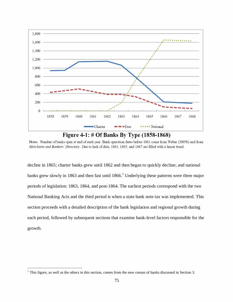
75
decline in 1865; charter banks grew until 1862 and then began to quickly decline; and national
banks grew slowly in 1863 and then fast until 1866.1 Underlying these patterns were three major
periods of legislation: 1863, 1864, and post-1864. The earliest periods correspond with the two
National Banking Acts and the third period is when a state bank note tax was implemented. This
section proceeds with a detailed description of the bank legislation and regional growth during
each period, followed by subsequent sections that examine bank-level factors responsible for the
growth.
1 This figure, as well as the others in this section, comes from the new census of banks discussed in Section 3.

76
National Banking Act of 1863
Secretary of the Treasury Salmon Chase was given the task of financing the war under
Lincoln. Chase, a Jeffersonian democrat, was skeptical of the state banking systems, but did not
take action until after the Midwest free banking defaults and the specie suspension of 1861.2
Seeking to secure bank notes and create a market for national debt, Chase pushed for a federally-
controlled banking system. The resulting National Banking Act of 1863 (also known as the
National Currency Act) adopted the language and approach of New York’s relatively stable free
banking law, but it also homogenized bank notes and took explicit steps to prevent the note
holder losses seen during the Civil War.3
First, it avoided free banking’s attachment to risky state debt by only allowing the use of
federal debt. Second, it only allowed notes to be issued up to 90 percent of a bank’s total bond
value.4 Third, it forced banks to restrict their circulations by placing a $300 million ceiling on the
aggregate number of national notes. Fourth, it placed a 25 percent reserve requirement on both
circulation and deposits.
The reserve requirements were structured in such a way as to reduce the burden on banks.
Specially, only banks in nine large “reserve cities” 5
were required to hold the full 25 percent
reserve in vault cash. The remaining banks (called country banks) were allowed to deposit up to
three-fifths of the reserves in a reserve city national bank. In this way, country banks received
interest on their reserves and reserve city banks received additional deposits.
Despite never being subjected to a deposit reserve, an examination of bank balance sheets
shows that the tiered-reserve requirements enabled existing banks to continue keep their
2 Davis (1910) discusses the anti-bank statements made by Chase during his time as governor of Ohio. 3 Chapter II discusses the targeted nature of the National Banking Acts in more detail. 4 This requirement had the addition benefit of creating a demand for federal debt. 5 The original redemption cities were Baltimore, Boston, Chicago, Cincinnati, New Orleans, New York City,
Philadelphia, Providence, and St. Louis.
77
allocation of funds when they converted to a national charter. In 1860, the average ratio of specie
to circulation and deposits was 5 percent for free banks and 11 percent for charter banks, but was
20 and 25 percent respectively when interbank deposits were included. The new requirements
therefore would not have been an entry barrier for state banks as long as they held their funds in
a national bank.
The Act also forbade national banks from issuing real estate loans. The intention was to
prevent the losses due to land speculation seen during the antebellum period; however, it would
also have the unintended consequence of preventing lending in communities where wealth was
concentrated in land. As few states explicitly prevented real estate loans before 1863, Barnett
(1911) argues that the constraint discouraged rural and agricultural banks from adopting a
national charter.
New York’s high capital requirement was lowered for rural areas, but was kept high for
densely populated areas. Specifically, banks in a city with over 10,000 people had to maintain a
capital level of at least $100,000, whereas those in less populated cities had a $50,000
minimum.6 Recalling the sample of free bank laws in Table 1-1, very few banks required
$100,000.7 The capital requirements therefore fell most heavily on high population areas and
western states such as Minnesota and Wisconsin which had low capital requirements.
Senator Harris of New York added a last-minute amendment when the Act stalled in
Congress. The amendment allowed state banks that held 50 percent or more of their capital in
federal bonds to issue national notes without converting to a national charter. State banks could
only issue notes up to 80 percent of their bonds’ market value, i.e. 10 percent less than national
6 To provide additional demand for national debt, the Act required much of the capital to be submitted in US bonds. 7 White (1984) illustrates that states lowered their requirements over time to further increase the differences between
state and national banking requirements.

78
banks, but the loophole still gave them the primary benefit of a national charter, homogenous
bank notes, without subjecting them to the costly requirements.
The response to national banking was less than enthusiastic by any metric: number,
location, or capital. During the year, 182 national banks were established and only 7 were former
state banks.8 Moreover, the national banks that were established typically did not locate in the
country’s financial centers. For example, there was one national bank in Philadelphia and three
in New York City, but at least three in both Cincinnati and Syracuse. The lack of national banks
in urban areas also corresponded to the lowest average capital level ($125,000) of any bank type.
The aggregate number of state banks declined by 95 in 1863; however, the National
Banking Act does not seem to be responsible. First, as seen in Figure 4-2, the closures were
almost entirely in the Confederate South. During 1863 and 1864, 179 of 277 southern banks
closed, compared to 27 of 1,173 non-southern banks. 9 The fact that 22 new state banks were
created also suggests that state banking was still a viable option in other areas. Second, southern
banks that survived the Civil War were located in areas quickly retaken by the Union, i.e.
Louisiana, Tennessee, and Virginia.10
Third, contemporary accounts such as the Merchants and
Bankers’ Directory (1864, p. 19; 1865, p. 21) illustrates that the war interrupted southern
banking, stating “The Bank of Tennessee is in the hands of the rebels, and removed South”. The
8 Weiman and James (2006, p. 4) argue that most of the new banks were founded by private bankers that believed they might lose part of their note broker business. 9 1863 corresponds to the Battle of Gettysburg and the Surrender of Vicksburg, whereas, 1864 corresponds to
Sherman’s march to the sea. 10 While it is possible that southern banks simply did not report to the Merchant and Bankers’ Directory during the
war, it seems unlikely given that they did not begin to report again after the war.
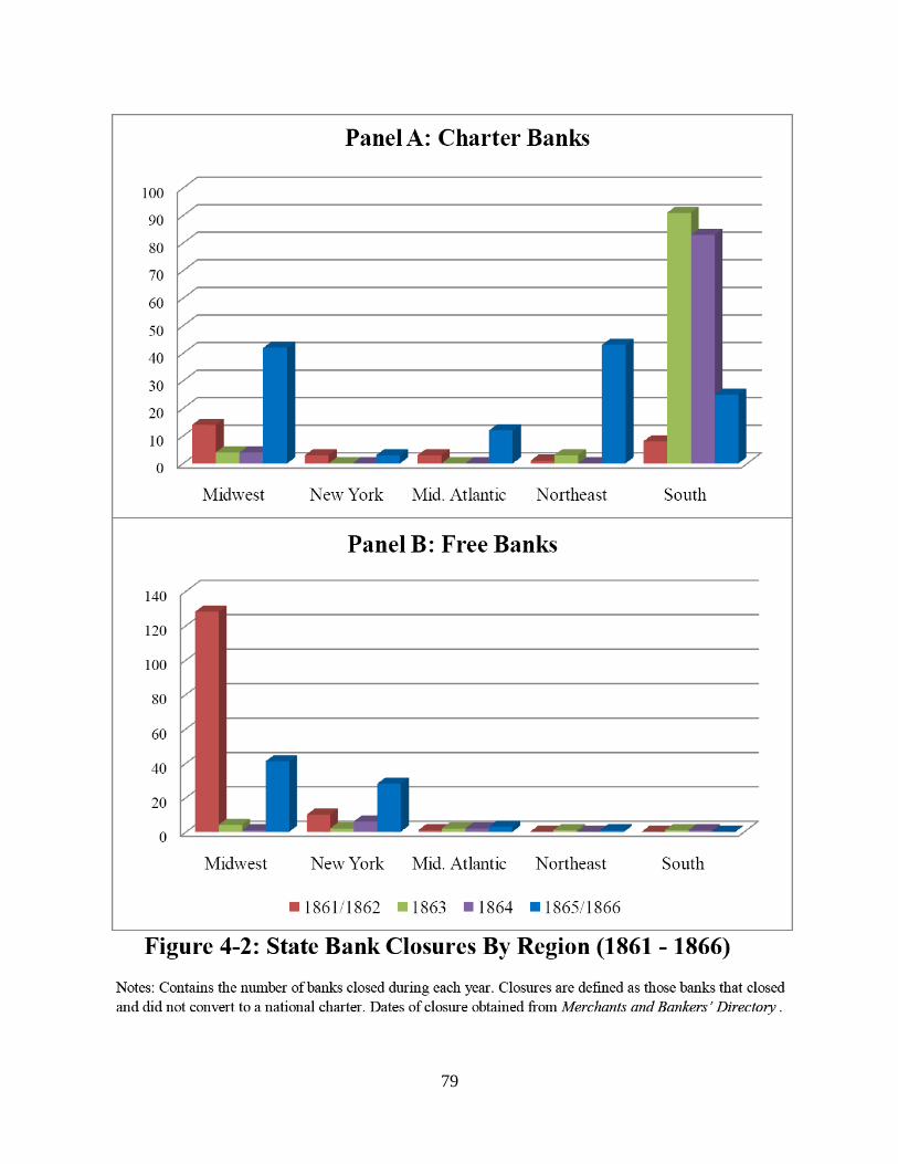
79
80
evidence suggests that the Civil War was the primary cause of state bank closures in 1863, and
the National Banking Act left the distribution of state banks roughly unchanged.11
National Banking Act of 1864
The lack of state bank conversions and large national banks in financial centers left Chase
and his supporters troubled.12
The primary cause of both problems was the lack of New York
City bank conversions. New York City banks provided a safe place to earn interest on reserves.
Over time, interior banks developed correspondent relationships in the city, and by 1860, almost
40 percent of all interbank deposits were in New York City banks.13
However, because the Act
did not count deposits placed in a state bank as reserves, interior banks that wanted to convert to
a national charter would have to cancel their correspond relationships and move their deposits to
another city. In this way, many banks were discouraged from becoming national banks.
The New York holdout also stemmed from the new reserves requirements. While the
legislation encouraged country banks to place deposits in reserve city banks, it did not provide
the same incentive for reserve city banks. In fact, reserve city banks might have to withdraw their
deposits from other banks just to meet their reserve requirements. Rather than losing their main
source of liquidity, New York City banks united in opposition to the new legislation, hoping to
prevent the spread of national banking.14
To end the New York City holdout, the National Banking Act of 1864 restructured the
reserve requirements. First, the reserve requirement of country banks was reduced to 15 percent.
11 I have not excluded these closures in the econometric analysis of Sections 4 and 5. When southern banks are
excluded, the main results become stronger, suggesting that the bank closures were not the result of instability. 12 Samuel Hooper, the Massachusetts congressman who introduced the first National Banking Act in the House, wrote to Chase in November of 1863, “I do not like having only small banks organized under the new law, and
regret that no large banks are yet organized in the principle commercial cities to be made depositories of public
money, as it seems to me very desirable”. Quoted in Davis (1910, p. 168) and Gische (1979, p 45). 13 For comparison, Boston had 15 percent and Philadelphia had 5 percent of the countries interbank deposits. 14 Gische (1979) and Weiman and James (2006) describe the holdout in more detail.
81
Second, the number of reserve cities was raised to 16 and their banks were now allowed to hold
up to half of their reserve in a New York City national bank.15
Third, New York City was
designated as the only central reserve city and its banks were required to hold their entire 25
percent reserve in vault cash. Finally, all non-central reserve city banks were required to redeem
their notes at par in a larger city. The structure forced other banks to place reserves in other
banks and established New York City as the official center of the banking world.16
Preventing state banks from enjoying the benefit of national banking without enduring its
requirements, the Act revoked the ability of state banks to issue national bank notes. State banks
could still issue their own unique notes, but they were, in many ways, inferior to the homogenous
national notes. For the first time, banks had to decide between issuing state or national notes.
Capital requirements were also increased in an effort to establish banks capable of
serving as depositories. National banks in a city with more than 50,000 people now needed
$200,000 in capital, those with 6,000 to 49,999 people needed $100,000, and those in smaller
cities still needed $50,000. As no state previously required a capital level of $200,000. the Act
greatly raised entry barriers for new national banks and existing state banks.
The changes successfully broke New York City’s holdout by converting its largest bank,
Bank of Commerce ($10 million in capital), to a national charter.17
By the end of 1864, 282 new
national banks had been established and an additional 242 state banks converted. Seen in Figure
4-2, national bank expansion was still greatest in the Middle Atlantic and Northeast, but it was
15 The reserve cities were St. Louis, Louisville, Chicago, Detroit, Milwaukee, New Orleans, Cincinnati, Cleveland, Pittsburgh, Baltimore, Philadelphia, Boston, Albany, Leavenworth, San Francisco, and Washington. Charleston and
Richmond were added after the war. 16 Weiman and James (2006) confirm that New York not only remained primary holder of interbank deposits but the
size of those deposits also dramatically increased over time. 17 The Bank of Commerce of New York was exempted (by name) from the double liability requirement.
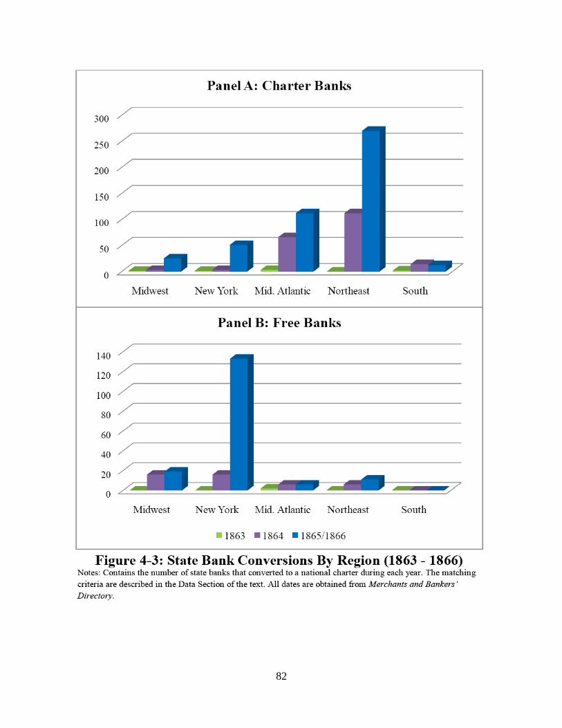
82

83
now concentrated in financial centers. For example, 36 banks were established in Boston, 14 in
New York City, and 27 in Philadelphia. Seen in Figure 4-4, the average capital level of national
banks also dramatically grew from $126,000 to $205,000. The capital growth, however, was due
not to increased requirements, but rather to the conversion of state banks with an average capital
level of $325,000.
State banks were beginning to convert at a high level, but 1,126 still remained at the end
of the year. Corresponding to Sherman’s march to the sea, the large number of closures in 1864
once again seems to be the result of the Civil War. Of the 97 closures, only 13 were outside of
the South. State banks thus seemed capable of continuing under their state charter despite the
National Banking Acts.
84
State Bank Note Tax (1865-1868)
While James (1978), Gische (1979), and Weiman and James (2006) argue that the wave
of state bank conversions had only started to gain momentum, economic historians such as
Hammond (1957) and White (1983) argue that the 10 percent state bank note tax passed in 1865
was responsible for the collapse of state banking. Instead of encouraging banks to convert to a
more secured note issue, Gische (1979, p. 58) states, “The tax was seen by both its supporters
and opponents as the final and conclusive blow to the circulation of state bank notes”. The tax
would not only drive state bank notes out of the market, but it would also force the majority of
state banks to reevaluate their charter, as two-thirds still had more circulation than deposits.
The years after 1864 saw an explosion of national bank growth: 291 new national banks
were established and 651 state banks converted. The average capital of national banks also grew
to $255,000, making them comparable to charter banks and larger than free banks. By 1869,
1,650 national banks had been established and roughly half were former state banks. The
national banking system was therefore constructed using a large amount of new capital.
The state bank note tax seems to be the only piece of legislation capable of closing state
banks. Almost one-fourth of existing state banks closed between 1864 and 1869, leaving only
179 charter banks and 56 free banks in operation. Seen in Table 4-1, closures were concentrated
in the Midwest where capital and reserve requirements were particularly low. On the other hand,
free banks remained in New York and populated western cities such as Chicago and Madison,
and surviving charter banks remained in the Northeast and populated southern cities such as
Louisville and New Orleans. The data thus indicate that state banks stripped of note issue could
only survive within densely populated areas where deposits were most likely prevalent.
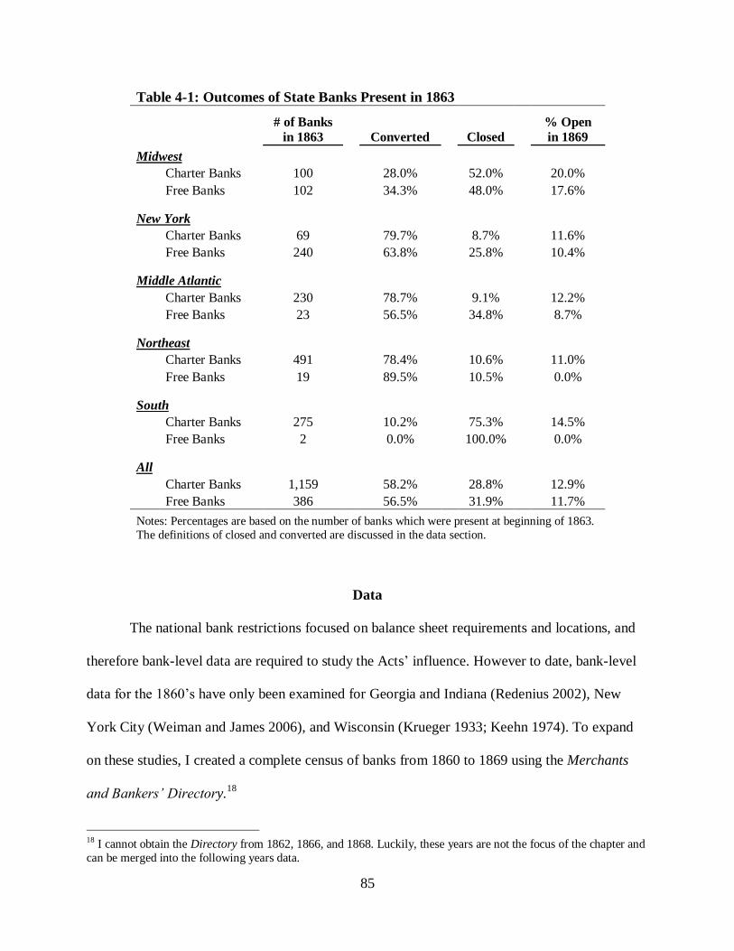
85
Table 4-1: Outcomes of State Banks Present in 1863
# of Banks
in 1863
Converted
Closed
% Open
in 1869
Midwest
Charter Banks 100
28.0%
52.0%
20.0%
Free Banks 102
34.3%
48.0%
17.6%
New York
Charter Banks 69
79.7%
8.7%
11.6%
Free Banks 240
63.8%
25.8%
10.4%
Middle Atlantic
Charter Banks 230
78.7%
9.1%
12.2%
Free Banks 23
56.5%
34.8%
8.7%
Northeast
Charter Banks 491
78.4%
10.6%
11.0%
Free Banks 19
89.5%
10.5%
0.0%
South
Charter Banks 275
10.2%
75.3%
14.5%
Free Banks 2
0.0%
100.0%
0.0%
All
Charter Banks 1,159
58.2%
28.8%
12.9%
Free Banks 386 56.5% 31.9% 11.7%
Notes: Percentages are based on the number of banks which were present at beginning of 1863.
The definitions of closed and converted are discussed in the data section.
Data
The national bank restrictions focused on balance sheet requirements and locations, and
therefore bank-level data are required to study the Acts’ influence. However to date, bank-level
data for the 1860’s have only been examined for Georgia and Indiana (Redenius 2002), New
York City (Weiman and James 2006), and Wisconsin (Krueger 1933; Keehn 1974). To expand
on these studies, I created a complete census of banks from 1860 to 1869 using the Merchants
and Bankers’ Directory.18
18 I cannot obtain the Directory from 1862, 1866, and 1868. Luckily, these years are not the focus of the chapter and
can be merged into the following years data.

86
The annual directories provide the name and location of every bank in operation at the
end of each year, as well as their president, cashier, and capital level. I determine when banks
opened and closed by comparing the directories in successive years. The bank’s characteristics
then allow me to determine whether a state bank converted to a national charter when it did
close.19
I define a state bank as “converted” if its closing year, location, and at least two of four
other characteristics (name, president, cashier, and capital level) match those of an opening
national bank.20
Finally, the census is linked to Weber’s antebellum databases (2005b, 2008) to
determine each existing bank’s balance sheet, establishment date, and type (i.e. charter or free).
Consequences of National Banking Legislation
The National Banking Acts and state bank note tax had two opposite effects on the
banking system. On the one hand, they converted or closed existing state banks, while on the
other, they established new national banks. This section examines the pattern of creation and
destruction at the bank-level to determine how and why the distribution of banks changed over
time.
Determinants of State Bank Decline
I begin by modeling the destruction of the existing state banking system using a
multinomial logit function. The dependent variable denotes a bank’s outcome (survived, closed,
converted) by a certain date, and the model identifies the conditional probability of each outcome
through cross-sectional balance sheet variation across banks. I have chosen to use survival as the
19 Because the National Banking Act of 1863 required banks to adopt a name based on their entry order (e.g. First
National Bank of Buffalo), the name and location of a closing state bank are often not sufficient to determine
whether it converted to a national charter. While the requirement was repealed by the National Banking Act of 1864,
there were still 634 First National Banks (about 33 percent of all national banks) in 1869. 20 A match is generally made on three of the other characteristics. Looser restrictions lead to few additional matches.

87
base outcome, as the raw coefficients measure the probability of moving from the steady-state,
but the choice does not affect the main results.21
However, rather than reporting the raw
coefficients which measure relative risk, I report the explanatory variables’ marginal effect on
the probability of each outcome to make the interpretation clearer.
Because banks would alter their behavior in response to new standards, I compare each
state bank’s composition in 1860. 22
The explanatory variables are thus observed prior to the
Civil War and National Banking Acts, making them at least weakly exogenous to the events.
Fitting the multinomial approach, the explanatory variables match both a bank’s probability of
closure and its ability to convert to a national charter.23
The logarithm of capital measures the
bank’s size and ability to meet the national capital requirements. Reserves (defined as specie and
due from other banks divided by circulation and deposits) measures the bank’s ability to redeem
notes and meet the national reserve requirements.24
The ratio of circulation to circulation and
deposits determines the bank’s primary source of liquidity and the extent that the bank note tax
would have affected it. The ratio of loans to assets measures whether loans were the bank’s
primary source of revenue and the extent that the prohibition of real estate loans would have
affected it.
The regressions contain several independent variables in addition to the balance sheet
items. The first is a free bank dummy which takes the value “1” if the observation came from a
free bank and “0” otherwise. The dummy variable captures the differential outcome rate between
the bank types. The interaction between the other independent variables and the dummy provides
21 A Hausman test also fails to reject the independence of irrelevance alternatives. 22 The resulting database contains about 80 percent of banks open in 1860. The missing banks generally had recently
opened or were in the process of closing. 23 I do not deflate capital and reserves based on population because I am jointly addressing closures and conversions.
Such a deflation would help identify conversion coefficients, but bias those of closure. 24 Deposits are composed of individual deposits and interbank deposits.

88
approximate slope differences. The number of years a bank had been in operation (controlling
for a bank’s reputation) and state dummies (controlling for the original state regulations and
population) are also included in all regressions.
Whereas Chapter II illustrated a bank’s probability of closure before 1863, Table 4-2
illustrates the probability of closure, survival, and conversion during the rest of the period.25
Each regression is reported in three columns, one for each outcome. The first two regressions
examine the outcomes for banks present in 1863, whereas the third isolates the effect of the state
bank note tax by regressing only the outcomes of banks present in 1865.
Before looking at individual coefficients, a key result is visible by looking at the
regression as a whole. State banks which survived the period seem very different than those that
closed or converted. In every case but circulation, the absolute values of the closed and
converted coefficients are almost indistinguishable. This stark result illustrates the birth of
savings banks. While some savings banks existed in the Northeast before 1860, it was not until
after the state bank note tax that they began to see widespread use. In fact, several of the
surviving state banks changed their name to reflect their roles as savings or deposit institutions,
and there were several hundred savings banks in operation across the country by 1875. The state
bank note tax seemed to force the evolution of state banking by destroying those banks which
could not survive as savings banks.
The free bank coefficient is statistically significant across all regressions. In a given state,
a free bank is about 8 percent more likely to close and less likely to convert then charter banks,
but not more or less likely to survive. The significance of the free bank coefficient for conversion
is most likely due to the fact that free banks had more state debt than national debt.26
A free bank
25 The results are very similar when closures before 1863 are included or when southern states are excluded. 26 See Rolnick and Weber (1984) for a breakdown of bond portfolios.
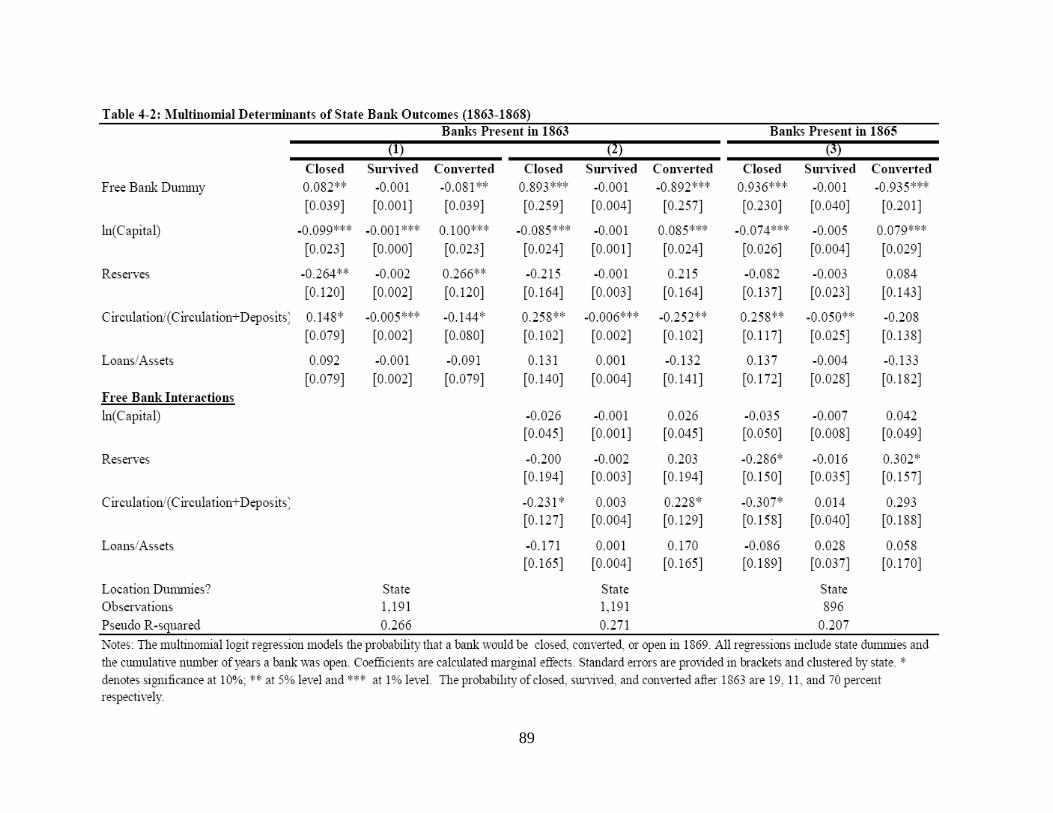
89

90
would therefore have to sell less expensive state bonds and purchase national bonds before
converting to a national charter.
The circulation variable is a significant determinant of all three outcomes. The more
circulation a bank had relative to its deposits, the more likely that it would close and the less
likely that it would convert to a national charter or remain open. However, the coefficient on
survival is slightly reduced and loses statistical significance for outcomes of banks present in
1865. The reduction of the coefficient suggests that the state bank note tax might have
encouraged a small number of banks to convert but the number was insignificant compared to
the number of banks that it closed. The pattern indicates that the state bank note tax’s primary
effect was bank destruction not conversion.
An increase in circulation relative to deposits seems to have larger effect on the
probability of closure (or conversion) for a charter bank than a free bank, but the effect is only
marginally significant. The sum of the level and interaction coefficients retains its sign for
outcomes of banks present in 1863, but loses it for banks present in 1865. Circulation, therefore,
increases a free bank’s probability of closure at a reduced rate for the full period, but has little
effect on free banks after 1865.
Reserves and loans are not robustly correlated with any bank outcome. The insignificant
coefficient on reserves provides evidence that banks already had sufficient interbank deposits,
whereas the high standard errors on the loan coefficients are not surprising given that I cannot
isolate real estate loans. The signs on the loan coefficients at least suggest that the prohibition on
real estate lending was not an entry barrier for conversion.
Banks with a large amount of capital seem the most likely to convert. A state bank’s
capital level is negatively correlated with closure and positively correlated with conversion. On

91
the other hand, large capital levels are not correlated with survival. The coefficients are also
economically significant. Increasing a bank’s capital from $50,000 to $100,000 would decrease
the probability of closure and increase the probability of conversion by 8 percentage points.
Because the coefficients on the other two national bank requirements, loans and reserves, are
statistically insignificant, the high capital requirements seem to be the primary entry barrier for
state bank conversion.
These results lend weight to the arguments of James (1978), Gische (1979), and Weiman
and James (2006). Converted banks are associated with high capital levels, closed banks with
high circulations, and surviving banks with large amounts of deposits. In this way, the capital
requirements of the National Banking Acts prevented small state banks from converting, whereas
the state bank note tax prevented the remaining banks of circulation from operating under their
original charter. The note tax also seems to be primarily associated with bank closure and could
have reduced the number of banks unnecessarily.
Figure 4-5 displays these conclusions from a geographic perspective. Panel A shows that
the majority of closed banks were located in the Midwest or South. On the other hand, Panel B
shows that bank conversions were almost entirely in the Northeast. Matching the regression
results, areas with high circulation and low capital requirements (Midwest and South) lost a large
number of state banks, and areas with high capital requirements (Northeast) saw a large number
of conversions.
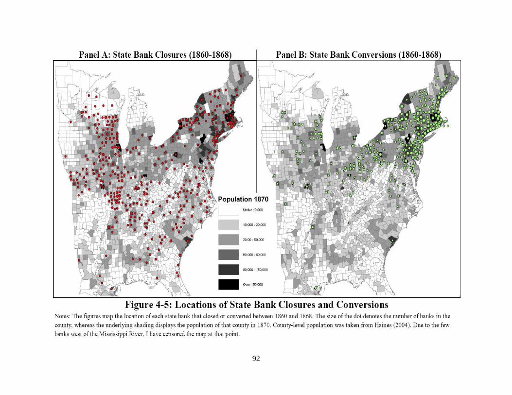
92

93
Determinants of New National Banks
The National Banking Acts created 784 new banks by 1869. However, unlike the
previous section, the compositions of these new banks are endogenous to its entry decision and
cannot be compared. Therefore to study the creation of new banks, I model the number of new
national banks that enter county i in year t as a linear function of the composition of each
county.27
The size of a county is measured by the logarithm of population in 1860 and the change
in the log of population between 1850 and 1860 to avoid any endogenous changes caused by
bank entry.28
The county’s industrial composition is measured by the share of its population in
manufacturing in 1860,29
and its banking composition is measured by the number of state banks
in year t, the number of closed state banks since 1860, and the number of national banks in year
t-1. Presented in Table 4-3, the regression is estimated separately for 1863, 1864, and 1865/1866
to allow each piece of legislation to affect entry decisions differently.
The coefficients on population are always positive and statistically significant. New
national banks were attracted to populated areas, but not necessarily the fastest growing areas.
Matching the conclusions of Sylla (1969), national bank capital requirements seemed to need the
support of a large population and prevented banks from entering areas which had not yet reached
some threshold. In fact, only 24 national banks were located in counties with fewer than 10,000
people in 1869 even though almost half of the country had fewer.
27 This approach is similar to that found in Carlson and Mitchener (2009). All non-bank information comes from
Haines (2004). State dummies are included in all regressions. 28 Using the urban population instead of total population leads to the same results only larger coefficients. 29 When I account for agricultural production, land, or value instead of manufacturing, the results remain the same
with a changed sign.
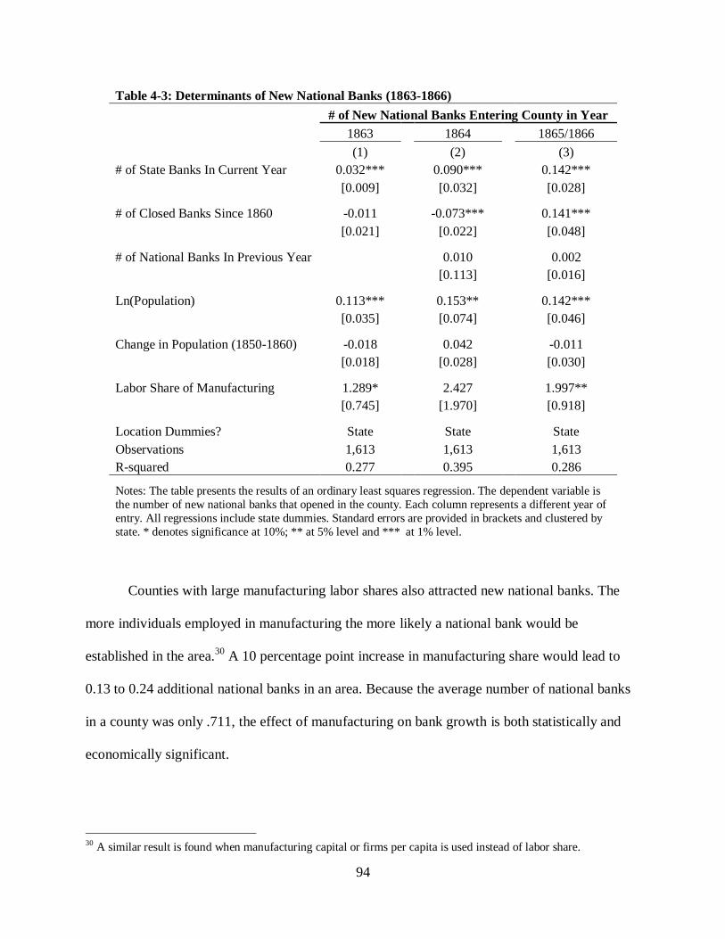
94
Table 4-3: Determinants of New National Banks (1863-1866)
# of New National Banks Entering County in Year
1863
1864
1865/1866
(1)
(2)
(3)
# of State Banks In Current Year 0.032***
0.090***
0.142***
[0.009]
[0.032]
[0.028]
# of Closed Banks Since 1860 -0.011
-0.073***
0.141***
[0.021]
[0.022]
[0.048]
# of National Banks In Previous Year
0.010
0.002
[0.113]
[0.016]
Ln(Population) 0.113***
0.153**
0.142***
[0.035]
[0.074]
[0.046]
Change in Population (1850-1860) -0.018
0.042
-0.011
[0.018]
[0.028]
[0.030]
Labor Share of Manufacturing 1.289*
2.427
1.997**
[0.745]
[1.970]
[0.918]
Location Dummies? State
State
State
Observations 1,613
1,613
1,613
R-squared 0.277
0.395
0.286
Notes: The table presents the results of an ordinary least squares regression. The dependent variable is
the number of new national banks that opened in the county. Each column represents a different year of
entry. All regressions include state dummies. Standard errors are provided in brackets and clustered by
state. * denotes significance at 10%; ** at 5% level and *** at 1% level.
Counties with large manufacturing labor shares also attracted new national banks. The
more individuals employed in manufacturing the more likely a national bank would be
established in the area.30
A 10 percentage point increase in manufacturing share would lead to
0.13 to 0.24 additional national banks in an area. Because the average number of national banks
in a county was only .711, the effect of manufacturing on bank growth is both statistically and
economically significant.
30 A similar result is found when manufacturing capital or firms per capita is used instead of labor share.
95
The banking coefficients show no evidence of crowding out. In fact, the coefficient on
state banks is positive and significant, suggesting that national banks were attracted to counties
with state banks. The complementary is most likely the result of a bank’s demand for depositors.
As seen in the previous section, surviving state banks were located in large deposit areas, a trait
also desired by national banks.31
National banks also had an incentive to replace the circulation
lost when state banks were stripped of their note issue capability. In this way, state banks
evolved into savings banks whereas national banks filled the need for banks of circulation.
Alternatively, the coefficients on closed state banks are all significantly below 1
suggesting that national banks did not fully replace state banks. In fact, they seem to avoid those
places with closed banks before 1865. Even in 1865/1866, at most 1 national bank would be
established for every 7 closed state banks. Because the capital of new national banks was roughly
the same as closing state banks, one national bank could not replace the capital of several state
banks.
These results indicate that new national banks located in densely populated counties with
large manufacturing sectors. Confirmed in Figure 4-6, there was a large number of new national
banks in the Midwest and South, but very few in low population areas. Instead, new bank growth
primarily occurred in counties with the largest populations (e.g. Chicago and St. Louis). The
maps also indicate that the National Banking Acts concentrated new capital in previously
developed areas, particularly along what would come to be known as the “Manufacturing Belt”.
31 James (1979) discusses the growth in the importance of deposits during the National Banking Era. Krueger (1944)
shows that national banks had a large number of deposits relative to state banks in Wisconsin.

96
Counterfactual Analysis
The conclusions from the previous sections have implied that the state bank tax might
have unnecessarily reduced the number of banks. This section attempts to determine the full
effect of the tax by describing the distribution of banks if the state bank note tax was not passed.
Specifically, I assume that the closures during 1865 and 1866 did not occur. This choice
purposely keeps the new national banks that opened in response to state bank closures for two
reasons. First, the number of banks that entered in response to the closures was small, about 28

97
Table 4-4: Counterfactual Distribution of Banks Without State Bank Note Tax
Actual # of
Banks in
1868
# of Banks If No
State Bank Note
Tax
% Difference
All Counties 1,865
2,067
10.8%
Region
Midwest 367
453
23.4%
South 146
171
17.1%
New York 342
373
9.1%
Northeast 547
591
8.0%
Middle Atlantic 463
479
3.5%
Population
Less than 10,000 24
37
54.2%
10,000 to 49,999 946
1,063
12.4%
50,000 to 99,999 328
361
10.1%
100,000 to 299,999 410
443
8.0%
More than 300,000 157
163
3.8%
Avg. Capital Level
Less than 50,000 32
94
193.8%
$50,000 to 99,999 398
450
13.1%
$100,000 to 199,999 766
816
6.5%
$200,000 to 999,999 576
608
5.6%
More than $1,000,000 93 99 6.5%
Notes: Table presents the counterfactual distribution of banks if there had been no closures during
1855 and 1856. When examining the population results it is helpful to note that 48 percent of counties had less than 10,000 people, 47 percent had 10,000 to 49,999, leaving about 1.5 percent in the
remaining population categories. The 5 banks without capital records are listed as "Less than 50,000".
new banks. Second, national banks that did respond would have done so in high population areas
therefore only biasing the numbers against finding a large difference between rural and urban
regions.
Table 4-4 shows that the tax had the greatest effect on the Midwest, but most regions
were affected. However, to view the full impact of the tax, the counterfactual must be broken
down county population. In this case, the results are much clearer: the state bank note tax
primarily stripped capital from rural areas. If the tax was not imposed, there would have been
over 50 percent more banks in areas with less than 10,000 people, around 11 percent more for

98
areas with 10,000 to 99,999, and less than 10 percent more for more populated counties.
Therefore most geographic regions were affected by the state bank note tax, but the loss of banks
was concentrated in the rural counties of those regions.
Another important result is seen when the counterfactual is displayed relative to bank
capital levels: only the smallest banks were destroyed. The note tax destroyed roughly two-thirds
of all banks with capital levels of less than $50,000, but only 6.5 percent of banks with more than
$100,000. As suggested by the multinomial coefficients, the state bank note tax greatly shifted
the distribution towards large banks.
Conclusion
The National Banking Acts of 1863 and 1864 and the state bank note tax of 1865 were
conceived as a way to secure the banking sector, but they ultimately caused a dramatic
redistribution of bank capital. Over the course of the decade, 589 state banks closed and 879
converted to a national charter, whereas 752 new national banks were established. Using a newly
created bank census, this chapter isolates the bank-level causes behind these radical changes.
Figure 4-7 illustrates how the geographic distribution of banks changed. In 1860, banks
do not seem to be restricted to high population areas and many were located in less populated
counties. However, over the course of the decade, there was a shift towards high population
areas. Densely populated areas such as Southern Michigan gained a large number of banks,
whereas rural areas such as Alabama, Missouri, and Wisconsin lost a large number of banks. The
legislation thus created bank capital around the Midwest’s “Manufacturing Belt” and destroyed it
in other areas. The question for future studies is whether this redistribution benefited or harmed
the country’s development.

99

100
A comparison of existing state banks shows that the National Banking Acts’ capital
restrictions prevented small state banks from converting, whereas the state bank note tax
prevented them from continuing to operate under their original charter. On the other hand, new
national banks did not simply replace closing state banks, locating instead in densely populated
counties with large manufacturing sectors. Even though the legislation attempted to emulate the
free banking spirit, the results show that it ultimately destroyed the small banks in rural areas that
free banking had established.
State banks that survived the period were fundamentally different from those that
converted or closed in one respect: they held large numbers of deposits. The note tax thus seems
to have the unintended benefit of forcing state banks to evolve into savings bank. Savings banks
existed within the Northeast before 1860, but it was not until the decade after the note tax that
savings and deposits banks spread throughout the country.

101
CHAPTER V
CONCLUSION
Through a unique collection of compositional (e.g. balance sheets and note discounts)
and environmental (e.g. bond portfolio values and passenger travel costs) data for almost every
antebellum bank, this dissertation provides the first bank-level view of the U.S. Free Banking
System. The depth of the data not only augments previous descriptive studies, but also enables a
modern econometric reassessment of free banking’s most controversial topics. Following the
“new financial history” literature, the dissertation conclusions transcend the historical context
and shed light on many continuing problems in finance.
The lessons most clearly learned from free banking are the problems associated with
reactionary and near-sighted bank regulations. States believing their banking capital was
insufficient sought to lower entry barriers and encourage growth. In the rush to liberalize,
however, states did not take proper precautions to create stable banks. Instead the underlying
security requirement of the entire banking system failed to take the variability of state debt into
account. On the other hand, the “solution” to free banking, the National Banking Acts, raised
requirements too far, preventing even stable banks from operating in rural areas. Therefore,
despite radically different goals, both regulations over-reacted and by doing so limited the
benefits of the entire system. This type of oscillation between strict (e.g. Glass-Steagall Act of
1933) and loose (e.g. Gramm-Leach-Bliley Act of 1999) regulations continues to create
unforeseen problems even in the modern system.

102
On the other hand, the period’s most successful regulations were those that gradually
amended problems as they occurred and adapted to changing market risk. For instance, New
York and Indiana free banks experienced few failures after they adjusted their bond
requirements, whereas the lowering of national bank capital requirements in 1900 led to
tremendous bank growth. Attentive and flexible legislatures were able to create stable financial
systems and encourage growth by adjusting regulations as needed, rather than waiting until an
entire new set of rules was seen as the only option. The outcomes of small careful adjustments
are much easier to predict, and therefore seem to avoid the unexpected consequences that
accompany large changes in regulations.
The dissertation’s final lesson is that individuals and banks are able to adjust quickly to
changes in risk and regulation. During the antebellum period, private note brokers were able to
efficiently price over 2,500 unique bank notes without federal regulators or modern security
exchanges. Through their efforts, the secondary note market protected individuals from losses
and potentially allowed bank notes to circulate around the country. Similarly, stable banks
diversified their portfolios around the free banking’s bond-secure note issue. Even stripped of
their note issue capacity, some free banks were able to evolve into savings banks. In this light, it
is even more important for legislatures to continuously adapt bank regulations over time to match
current market conditions and the bank behavior, rather than allow regulations to become out of
date.
103
REFERENCES
Ales, Laurence, Francesca Carapella, Pricila Maziero, and Warren E. Weber. 2008. “Model of
Banknote Discounts”. Journal of Economic Theory 142, 5-27.
Appletons’ Railway and Steam Navigation Guide. Vol. III (Sept. 1956) and Vol. VI (September
1959). New York: D. Appleton & Co.
Avery, R., Terrence M. Belton, and Michael A. Goldberg. 1988. “Market Discipline in
Regulating Bank Risk: New evidence from the capital markets”. Journal of Money,
Credit, and Banking 20, 597-610.
Barnett, George. 1911. State Banks and Trust Companies since the Passage of the National-Bank
Act. Washington: Government Printing Office.
Black, Fischer and John C. Cox. 1976. “Valuing Corporate Securities: Some effects of bond
indentures”. Journal of Finance 31, 351-367.
Bodenhorn, Howard. 1998. “Quis Custodiet Ipsos Custodes?”. Eastern Economic Journal 24, 7-
24.
Bodenhorn, Howard. 2003. State Banking in Early America: A New Economic History. New
York: Oxford University Press.
Bongini, Paola, Stijn Claessens, and Giovanni Ferri. 2001. “The political economy of distress in
East Asian financial institutions”, Journal of Financial Services Research 19, 5-25.
Cagan, Philip. 1963. “The First Fifty years of the national banking system: An historical
appraisal”. In: Carson, D. (Ed.), Banking and Monetary Studies. Homewood, Illinois:
Richard D. Irwin, 15-42.
Carlson, Mark, and Kris Mitchener. 2009."Branch Banking as a Device for Discipline:
Competition and Bank Survivorship during the Great Depression". Journal of Political
Economy 117, 165-210.
Cox, D.R. “Partial Likelihood”. 1974. Biometrika 62, 269-276.
Cox, D.R. “Regression Models and Life-Tables”. (1972). Journal of Royal Statistical Society
34B, 187-220.
Cox, D.R. and D. Oakes. 1984. Analysis of Survival Data. London: Chapman and Hall.
Davis, Andrew. 1910. The Origin of the National Banking System. Washington: US Government
Printing Office.

104
Davis, Joseph. 2004. “An Annual Index of U. S. Industrial Production, 1790–1915”. Quarterly
Journal of Economics 119, 1177-1215.
Davis, Lance. 1965. “The Investment Market, 1870-1914: The Evolution of a National Market.”
Journal of Economic History 25, 355-399.
Dillistin, William H. 1949. Bank Note Reporters and Counterfeit Detectors, 1826-1866.
Numismatic Notes and Monographs, no. 114. New York: American Numismatic Soc.
Disturnell’s A Guide Between Washington, Baltimore, Philadelphia, New York, Boston, etc.
Various years. New York: John Disturnell.
Dunbar, Seymour. 1937. History of Travel in America. New York: Tudor Publishing Company.
Dwyer, Jr., Gerald P., W. R. Hafer, and Warren E. Weber. 1999. “Weekly U.S. and State Bond
Prices.” Historical Methods 32, 37-42.
Dwyer, Jr., Gerald P. and W. R. Hafer. 2004. "Bank Failures in Banking Panics: Risky Banks or
Road Kill?". In Bank and Financial Market Efficiency: Global Perspectives, Volume 5
(Research in Banking and Finance), Edited by Iftekhar Hasan and William C. Hunter.
Amsterdam : Elsevier, 2004
Dwyer, Jr., Gerald P. and Iftekhar Hasan. 2007. “Suspension of Payments, Bank Failures, and
the Nonbank Public‟s Losses”. Journal of Monetary Economics 54, 565-580.
Economopoulos, Andrew. 1988. “Illinois Free Banking Experience”. Journal of Money, Credit
and Banking 20, 249-264.
Economopoulos, Andrew. 1990. “Free Bank Failures in New York and Wisconsin: A Portfolio
Analysis.” Explorations in Economic History 27, 421-441.
Efron, Bradley. 1977. “The Efficiency of Cox‟s Likelihood Function for Censored Data”.
Journal of the American Statistical Association 72, 557-565.
Fishlow, Albert. 1965. American Railroads and the Transformation f of the Antebellum
Economy. Cambridge: Harvard University Press.
Flannery, Mark J. and Sorin M. Sorescu. 1996. “Evidence of Bank Market Discipline in
Subordinated Debenture Yields: 1983-1991”. Journal of Finance 51, 1347-1377.
Gische, David. 1979. "The New York City Banks and the Development of the National Banking
System 1860-1870". American Journal of Legal History 23, 21-67.
Gorton, Gary. 1989a. “An Introduction to Van Court's Bank Note Reporter and Counterfeit
Detector”. The Wharton School, University of Pennsylvania. Working paper.
105
Gorton, Gary. 1989b. “Ante Bellum Transportation Indices”. The Wharton School, University of
Pennsylvania. Working paper.
Gorton, Gary. 1996. “Reputation formation in early bank note markets”. Journal of Political
Economy 104, 346-397.
Gorton, Gary. 1999. “Pricing free bank notes”. Journal of Monetary Economics 44, 33-64.
Gorton, Gary and Anthony M. Santomero. 1990. “Market Discipline and Bank Subordinated
Debt”. Journal of Money, Credit, and Banking 22, 119-128.
Gorton, Gary and Weber, Warren E. Quoted Discounts on State Bank Notes in Philadelphia,
1832-1858. Research Department, Federal Reserve Bank of Minneapolis.
http://minneapolisfed.org/research/economists/wewproj.html.
Haines, Michael R. 2004. Historical, Demographic, Economic, and Social Data: The United
States, 1790-2000. ICPSR Study 2896. Ann Arbor, MI: Inter-university Consortium for
Political and Social Research.
Hammond, Bray. 1957. Banks and Politics in America: From the Revolution to the Civil War.
Princeton: Princeton University Press.
Hasan, Iftekhar and Gerald P. Dwyer, Jr. 1994. “Bank Runs in the Free Banking Period”.
Journal of Money, Credit & Banking 26, 271-288.
Homer, Sidney and Richard Sylla. 2005. A History of Interest Rates, 4th
edition. Hoboken, NJ:
John Wiley & Sons, Inc.
James, John. 1978. Money and Capital Markets in Postbellum America. Princeton: Princeton
University Press.
Keehn, Richard. 1974. “Federal Bank Policy, Bank Market Structure, and Bank Performance:
Wisconsin 1863-1914”. Business History Review 48, pp. 1-21.
King, Robert. 1983. "On the economics of private money". Journal of Monetary Economics 12,
127-158.
Knox, John Jay. 1900. A History of Banking In the United States. New York: Bradford, Rhodes,
& Co.
Krueger, Leonard. 1933. History of Commercial Banking in Wisconsin. Madison: University of
Wisconsin Press.
Leeflang, Peter S.H., Dick R. Wittink, Michel Wedel, and Philippe A. Naert. 2000. Building
Models For Marketing Decisions. Dordrecht, NL: Kluwer Academic Publishers.

106
Livingston, James. 1986. Origins of the Federal Reserve System: Money, Class, and Corporate
Capitalism, 1890-1913. Ithaca: Cornell University Press.
Merchants and Bankers’ Directory (also called Merchants and Bankers’ Almanac). Various
years. New York: Bankers‟ Magazine Office.
Merchants’ Magazine and Commercial Review. (also called Hunt’s Merchants’ Magazine) Vol.
19, no. 1 (July 1848) through v. 44, no. 3 (Mar. 1861). Edited by Freeman Hunt. New
York.
Meyer Paul A. and Howard W. Pifer. 1970. “Prediction of banking failures", Journal of Finance
25, 853-68.
Mitra, Debanjan and Peter N. Golder. 2002. “Whose Culture Matters? Near-market knowledge
and its impact on foreign market entry timing”. Journal of Marketing Research 12, 27-35.
Molina, Carlos. 2002. “Predicting Bank Failures Using A Hazard Model: The Venezuelan
banking crisis”. Emerging Markets Review 3, 31-50.
Oakes, David. 1977. “The Asymptotic Information In Censored Survival Data”. Biometrika 64,
441-448.
Petersen, Mitchell A. 2009. “Estimating Standard Errors in Finance Panel Data Sets: Comparing
Approaches”. The Review of Financial Studies 22, p 435-480.
Pettaway, Richard H. and Joseph F. Sinkey. 1980. "Establishing on-site bank examination
priorities: an early warning system using accounting and market information", Journal of
Finance 35, 137-50.
Poel, Dirk Van den and Bart Lariviere. 2004. “Customer Attrition Analysis For Financial
Services Using Proportional Hazard Models”. European Journal of Operational
Research 157, 196-217
Redenius, Scott. 2002. Between Reforms: The U.S. Banking System in the Postbellum Period.
Ph.D. dissertation, Yale University.
Redenius, Scott. 2007. “Designing a National Currency: Antebellum Payment Networks and the
Structure of the National Banking System”. Financial History Review 14, 207-228.
Rockoff, Hugh. 1972. The Free Banking Era: A Reexamination. Dissertations in American
history (rev. Ph.D. diss., University of Chicago). New York; Arno Press.
Rockoff, Hugh. 1974. “The Free Banking Era: A Reexamination”. Journal of Money, Credit, and
Banking 6, 141-167.

107
Rolnick, Arthur J. and Warren E. Weber. 1983. “New Evidence on the Free Banking Era”. The
American Economic Review 73, 1080-1091.
Rolnick, Arthur J. and Warren E. Weber. 1984. “The Causes of Free Bank Failures: A Detailed
Examination”. Journal of Monetary Economics 14, 269-291.
Rolnick, Arthur J. and Warren E. Weber. 1985. “Banking Instability and Regulation in the U.S.
Free Banking Era”. Federal Reserve Bank of Minneapolis Quarterly Review.
Rolnick, Arthur J. and Warren E. Weber. 1988. “Explaining the Demand for Free Bank Notes”.
Journal of Monetary Economics 21, 47-71.
Rousseau, Peter, and Richard Sylla. 2005. “Emerging financial markets and early US growth”.
Explorations in Economic History 42, 1-26.
Sinkey, Joseph F. 1978. “Identifying „Problem‟ Banks: How Do the Banking Authorities
Measure A Bank‟s Risk Exposure?”, Journal of Money, Credit and Banking 10, 184-193.
Sinnott, R. W. 1984. "Virtues of the Haversine", Sky and Telescope 68, p. 159.
Sylla, Richard, Jack Wilson, and Robert Wright. Early U.S. Securities Prices.
http://eh.net/databases/early-us-securities-prices.
Sylla, Richard. 1969. “Federal Policy, Banking Market Structure, and Capital Mobilization in the
United States, 1863-1913”. Journal of Economic History 29, 657-686.
Sylla, Richard. 1998. “U.S Securities Markets and the Banking System, 1790-1840”. Federal
Reserve of St. Louis Review.
Taylor, George. 1951. The Transportation Revolution. White Planes, NY: M.E. Sharpe, Inc.
Temin, Peter. 1969. The Jacksonian Economy. New York: W.W. Norton & Company.
Temin, Peter. 1975. “The Panic of 1857”. Intermountain Economic Review 6, 21-36.
The Bankers' magazine, and state financial register. Vol. 1, no. 1 (July 1846) through v. 3, no.
12 (June 1849). Baltimore: J. Smith Homans.
Wallis, John Joseph. 2005. “Constitutions, Corporations, and Corruption: American States and
Constitutional Change, 1842 to 1852”. The Journal of Economic History 65, 211-256.
Warren, Isaac W. 1849. The Immigrant’s Guide and Citizen’s Manual. New York.
Weber, Warren E. 2005a. “Were U.S. State Banknotes Priced as Securities?” Federal Reserve
Bank of Minneapolis, Research Department Staff Report #344.
108
Weber, Warren E. 2005b. Listing of all State Banks with Beginning and Ending Dates. Research
Department, Federal Reserve Bank of Minneapolis.
http://research.mpls.frb.fed.us/research/economists/wewproj.html.
Weber, Warren E. 2006a. “Early State Banks in the United States: How Many Were There and
Where Did They Exist?”. Journal of Economic History 66, 433–455.
Weber, Warren E. 2006b. “New Evidence on State Banking Before the Civil War”. Research
Department, Federal Reserve Bank of Minneapolis Working Paper #642
Weber, Warren E. 2008. Balance sheets for U.S. Antebellum State Banks. Research Department,
Federal Reserve Bank of Minneapolis.
http://research.mpls.frb.fed.us/research/economists/wewproj.html.
Weber, Warren E. Quoted Discounts on State Bank Notes in New York, selected dates, 1827-
1858. Research Department, Federal Reserve Bank of Minneapolis.
http://minneapolisfed.org/research/economists/wewproj.html.
Weiman, David, and John James. 2006. “New National Banks and the Restructuring of New
York Banking after the Civil War.” Unpublished working paper.
West, Robert C. 1974. Banking Reform and the Federal Reserve, 1863-1923. Ithaca: Cornell
University Press.
Whalen, Gary. 1991. "A proportional hazard model of bank failure: an examination of its
usefulness as an early warning tool", Federal Reserve Bank of Cleveland, Economic
Review 27(1), 21-31.
Wheelock, David and Paul Wilson. 1995. “Explaining Bank Failures: Deposit Insurance,
Regulation, and Efficiency”. Review of Economics and Statistics 77, 689-700.
Wheelock, David and Paul Wilson. 2000. “Why Do Bank Disappear: The Determinants of U.S.
Bank Failures and Acquisitions”. Review of Economics and Statistics 82, 127-138.
White, Eugene. 1983. The Regulation and Reform of the American Banking System, 1900-1929.
Princeton: Princeton University Press.
Wright, Robert. 2002. The Wealth of Nations Rediscovered: Integration and Expansion in
American Financial Markets, 1780–1850. New York: Cambridge University Press.