by viktor todorov northwestern university · 2019-04-12 · by viktor todorov northwestern...

NONPARAMETRIC SPOT VOLATILITY FROM OPTIONS

By Viktor Todorov

Northwestern University

We propose a nonparametric estimator of spot volatility fromnoisy short-dated option data. The estimator is based on formingportfolios of options with different strikes that replicate the (risk-neutral) conditional characteristic function of the underlying price ina model-free way. The separation of volatility from jumps is done bymaking use of the dominant role of the volatility in the conditionalcharacteristic function over short time intervals and for large valuesof the characteristic exponent. The latter is chosen in an adaptiveway in order to account for the time-varying volatility. We show thatthe volatility estimator is near rate-optimal in minimax sense. Wefurther derive a feasible joint Central Limit Theorem for the proposedoption-based volatility estimator and existing high-frequency return-based volatility estimators. The limit distribution is mixed-Gaussianreflecting the time-varying precision in the volatility recovery.

1. Introduction. Options provide a natural source of information forstudying volatility. Indeed, following the seminal work of [14] and [33], anyoption written on an asset can be used to back out the unknown volatilityof the asset. The resulting estimator of volatility is typically referred toas Black-Scholes Implied Volatility (BSIV). Unfortunately, the assumptionsbehind the model of [14] and [33], mainly constant volatility and no jumprisk, are too simple for such volatility extraction to work in practice, seee.g., [19], [21] and [40]. Indeed, BSIV backed out from available optionswith strikes that are far from the current price level are typically too highwhen compared to historical averages based on returns data. These elevatedimplied volatility levels are a reflection of the importance of time-varyingvolatility and jump risk for investors. The goal of this paper is to developnonparametric spot volatility estimator from options that works in generalsettings when jumps are present and volatility can vary over time.

Recent developments in financial markets make the construction of option-based nonparametric volatility estimates practically feasible. In particular,the availability and liquidity of very short-maturity options with a wide

AMS 2000 subject classifications: Primary 60F05, 60E10; secondary 60J60, 60J75.Keywords and phrases: Ito Semimartingale, jumps, nonparametric inference, options,

stable convergence, stochastic volatility.

1

http://www.imstat.org/aos/

2 VIKTOR TODOROV

range of strikes has significantly increased over the last few years, see e.g.,[6].

We use these short-dated options in the construction of our estimator. Anatural candidate for a spot volatility estimator is provided by the BSIV ofoptions with strikes that are close to the current price level. The short timeto expiration limits the effect of the time-varying volatility on these options.Similarly, the proximity of their strikes to the current price limits the effectof jumps on them. Nevertheless, we show that jumps cause an upward bias inthe recovery of volatility from the BSIV of short-dated options with strikesclose to the price level. This bias is nontrivial and cannot be ignored inpractice.

In this paper, we take a different approach for estimating spot volatil-ity from options, which allows for an efficient separation of volatility fromjumps. Our approach makes use of the fact that the expected value of smoothfunctions of the price of the underlying asset at expiration can be replicatedby portfolios of options with continuum of strike levels, see e.g., [15] as wellas the earlier work of [26] and [38]. Using this insight, we construct port-folios of options which replicate the conditional risk-neutral characteristicfunction of the price at expiration. If the time to expiration is short, thenthe time variation in volatility has a negligible effect on the latter and canbe ignored. The effect of the jumps on the characteristic function, on theother hand, is more subtle. If the value of the characteristic exponent isclose to zero, then the jumps have a non-negligible effect. However, theireffect diminishes for higher values of the characteristic exponent. We showthat asymptotically (as the time to maturity shrinks) optimal separation ofvolatility from jumps can be achieved when the characteristic exponent isgrowing at a rate proportional to the square root of the time to expirationof the options. This leads to a volatility estimator which is significantly lessbiased in presence of jumps than the BSIV of options with strikes close tothe current price.

We establish consistency of the proposed volatility estimator in an asymp-totic setting in which options are observed with error, their maturity goesto zero together with shrinking mesh of the available strike grid. We fur-ther derive a Central Limit Theorem (CLT) for our volatility estimator.The limiting distribution is determined by the asymptotic behavior of theobservation error in the available options. The convergence is stable and itsasymptotic limit is mixed Gaussian. That is, the limit is centered Gaussianwhen conditioning on the sigma algebra on which the return and optiondata are defined. This allows for the asymptotic variance of the volatility es-timator to depend, in particular, on the current level of volatility and more

NONPARAMETRIC SPOT VOLATILITY FROM OPTIONS 3

generally on any other variable that determines the quality of the optiondata. Hence, the precision in estimation will typically differ over differentpoints in time. For feasible inference, we develop a simple estimator of theasymptotic variance which is based on an option portfolio that measures thesensitivity of the observed option prices to changes in their strikes.

There are many asymptotically valid choices for the characteristic expo-nent of the volatility estimator. However, for the successful performance ofthe estimator in practice, this choice matters a lot. Therefore, we develop anadaptive procedure for setting this tuning parameter by using an initial con-sistent estimator of volatility constructed from the option data. Our initialconsistent estimator is the option analogue of the truncated high-frequencyreturn volatility estimator of [31]. It is based on integrating the availableoptions in a portfolio which spans a truncated second moment of the priceat expiration (i.e., a function which behaves like the square function aroundzero and diminishes to zero for values of the argument diverging from zero).

We show that our estimator is near-rate optimal. In particular, in thespecialized setting of Levy jump-diffusion dynamics for the underlying priceand Gaussian observation errors proportional to the true unobserved optionprices, we show that the efficient rate (in a minimax sense) of recoveringvolatility from the noisy short-maturity option data coincides with the rateof convergence of our estimator up to a log term (the rate of convergenceof our estimator is some power of the time to maturity). This is unlike avolatility estimator based on the average of close-to-money BSIV.

The nonparametric spot volatility estimator developed in this paper canbe viewed as the option counterpart of the high-frequency return-basedvolatility estimators. In pioneering work, [9, 10] propose so-called multi-power variation statistics as a way to separate volatility from jumps while[31, 32] develops truncated variance estimator that achieves the same goal.More recently, [30] propose the use of the empirical characteristic functionof returns as a way to measure volatility in a jump-robust way, which allowsalso to deal with jumps of arbitrary high activity in an efficient way.

The high-frequency return-based volatility estimators use an asymptoti-cally increasing number of increments in a local window of time to estimatevolatility in a way similar to estimating volatility from a sequence of i.i.d.returns in classical settings. By contrast, the newly-proposed option-basedestimator uses an asymptotically increasing number of short-dated optionswith different strikes to identify the expectation about the future volatil-ity embodied in them. In turn, this conditional expectation of volatilityconverges to the spot volatility when the time to maturity of the optionsshrinks. We show that the convergence of the option-based and return-based

4 VIKTOR TODOROV

volatility estimators holds jointly. This allows one to construct an optimalmixture of the two types of estimators which has the lowest asymptoticvariance for measuring spot volatility from return and option data.

We evaluate the performance of the option-based volatility estimator in aMonte Carlo experiment whose setup mimics key features of available optiondata. The Monte Carlo shows satisfactory finite sample properties of the de-veloped estimator and the inference about it. In an empirical application toshort-dated S&P 500 index options, we find that the option-based volatilityestimator is on average very close to an estimator based on high-frequencyreturns on the S&P 500 index but it is significantly more accurate.

The current paper is related to two strands of literature on volatility in-ference from option data. First, there is a large body of work that considersshort-maturity expansions of at-the-money options or options which becomeat-the-money in the limit, see e.g., [12], [23], [24], [36], [35]. Unlike this bodyof work, we consider a portfolio of options across strikes which is importantto reduce the asymptotic bias of the estimator. We further allow for obser-vation error, derive a stable CLT for our estimator and establish its nearrate-optimality. Second, [11], [20], [41], [42], [43, 44] consider nonparametricinference for the diffusive volatility in the class of exponential-Levy modelsfrom options with fixed maturity. The major difference between the currentpaper and this strand of work is that our analysis applies to general Itosemimartingales and the asymptotic setup here is one with shrinking matu-rity of the options. The latter difference leads to a significantly faster rate ofconvergence of the volatility estimator in the current asymptotic setting asthe shrinking maturity aids the separation of diffusive volatility from jumps.

The rest of the paper is organized as follows. In Section 2 we develop non-parametric methods for recovering volatility from options in the infeasiblescenario where a continuum of short-maturity options with strikes spanningthe positive real line are available. Section 3 adapts these procedures to thefeasible setting where only a finite number of noisy option observations areavailable instead. In this section we further characterize the rate of conver-gence of the volatility estimator, derive a feasible CLT for it, and developan adaptive method for selecting the tuning parameter used in its construc-tion. Section 4 derives the minimax risk of recovering spot volatility fromnoisy short-dated options in the special Levy case and Gaussian observationerrors. Section 5 contains a Monte Carlo study and Section 6 an empiricalapplication. The proofs are given in Section 7.

2. Option Portfolios and Volatility. We begin our analysis withshowing how to identify volatility in the infeasible setting where short-dated


options with arbitrary strikes are available and further when the options areobserved without error. We will relax these assumptions about the optionobservation scheme in the next section.

The underlying asset price is denoted by X and is defined on the fil-

tered probability space(Ω(0),F (0), (F (0)

t )t≥0,P(0)). Since our focus in this

paper is on extracting information from options, we will specify here onlythe behavior of X under the so-called risk-neutral measure Q, which un-der no-arbitrage is locally equivalent to P(0). For the return-based volatilityestimates, which we use later on to compare the option-based volatility esti-mator with, we will need to impose some structure on the P(0) dynamics ofX as well (see assumption A6 in Section 3.2). The dynamics of the log-pricex = ln(X) under Q is given by

(2.1) xt =

∫ t

0asds+

∫ t

0σsdWs +

∫ t

0

∫Rxµ(ds, dx),

where W is a Brownian motion, µ is an integer-valued random measure onR+ × R, counting the jumps in x, with compensator νt(x)dt ⊗ dx and µis the martingale measure associated with µ (W and νt are defined withrespect to Q). The regularity conditions for the above quantities are givenin Section 3.2.

Although equation (2.1) describes the dynamics of x under Q, under no-arbitrage, σt continues to be the diffusive volatility of x under P(0). Ourgoal here is to estimate the spot diffusive variance Vt ≡ σ2

t under generalconditions, i.e., with minimal regularity assumptions about (at, σt, νt).

For the recovery of Vt, we will use options written on X at time t, whichexpire at t + T , for some T > 0. Since t will be fixed throughout, we willhenceforth suppress the dependence on t in the notation of the option pricesand other related quantities. For simplicity, we will further assume thatthe dividend yield associated with X and the risk-free interest rate are bothequal to zero as their effect on short-dated options is known to be negligible.With these normalizations, the theoretical values of the options we will usein our analysis are given by

(2.2) κT (k) =

EQt (ek − ext+T )+, if k ≤ xt,

EQt (ext+T − ek)+, if k > xt.

κT (k) is the price of an out-of-the-money (OTM) option (i.e., an optionwhich will be worth zero if it were to expire today). This is a call contract(an option to buy the asset) if k > xt and a put contract (an option to sellthe asset) if k ≤ xt. In what follows, we will refer to K ≡ ek and k as thestrike and log-strike, respectively, of the option.

6 VIKTOR TODOROV

To simplify analysis, in this section, we will assume that jumps are offinite activity, i.e., that

(2.3)

∫ t+T

t

∫Rνs(dx)ds <∞, a.s.

Many jump models used in financial applications satisfy the above finiteactivity assumption and we will further relax it in the derivation of theformal results presented in the next section.

Henceforth, for a generic sequence of random variables YT and some de-terministic sequence RT , YT = Op(RT ) will mean that YT /RT is bounded inprobability and YT = op(RT ) will mean that YT /RT converges in probabilityto zero, with both statements being for T ↓ 0, see e.g., Section 2.2 in [46].

Since the volatility accounts for the small moves in the asset price, anatural candidate for a spot volatility estimator is the at-the-money (ATM)Black-Scholes option implied volatility. Indeed, the ATM BSIV has oftenbeen used as a proxy for spot volatility in empirical work. When (2.3) holdsand under some weak regularity type assumptions for (at, σt, νt), it is easyto show that

(2.4) κT (0) =

√T√2πσt +Op(T ), as T ↓ 0.

This bound on the error for recovering σt from κT (0) is sharp and a largecomponent of it is due to the jumps in X. This can be illustrated usingthe seminal Merton jump-diffusion model ([34]) for which a higher-orderexpansion of κT (0) can be derived. In the Merton model the volatility isconstant and the jumps are compound Poisson with intensity λ and theirsize is drawn from a normal distribution with mean µj and variance σ2

j . Inthis case, by directly expanding the option price by considering the leadingcases of no jump or one jump in X until expiration, we get for the ATMoption price, κMT (0), the following as T ↓ 0:

κMT (0) =

√T√2πσ − Tσ2

4

+ λT

(Φ

(−µjσj

)− eµj+

σ2j2 Φ

(−µjσj− σj

))+Op(T

3/2),

(2.5)

where Φ denotes the cdf of a standard normal random variable. The firsttwo terms on the right-hand side of (2.5) are the leading terms of the optionprice when conditioning on no jumps in X until expiration. The third termis the leading component of the option price when conditioning on exactlyone jump occurring during the life of the option.


The above parametric example shows that the bound in (2.4) is sharp.Using the ATM option price expansion in (2.4), we have

(2.6) Vt =2π

Tκ2T (0) +Op(

√T ), as T ↓ 0,

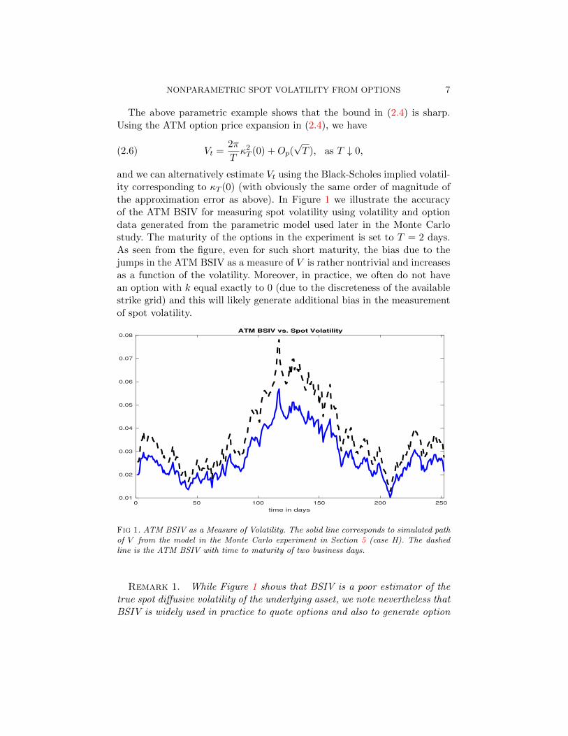
and we can alternatively estimate Vt using the Black-Scholes implied volatil-ity corresponding to κT (0) (with obviously the same order of magnitude ofthe approximation error as above). In Figure 1 we illustrate the accuracyof the ATM BSIV for measuring spot volatility using volatility and optiondata generated from the parametric model used later in the Monte Carlostudy. The maturity of the options in the experiment is set to T = 2 days.As seen from the figure, even for such short maturity, the bias due to thejumps in the ATM BSIV as a measure of V is rather nontrivial and increasesas a function of the volatility. Moreover, in practice, we often do not havean option with k equal exactly to 0 (due to the discreteness of the availablestrike grid) and this will likely generate additional bias in the measurementof spot volatility.

0 50 100 150 200 250

time in days

0.01

0.02

0.03

0.04

0.05

0.06

0.07

0.08ATM BSIV vs. Spot Volatility

Fig 1. ATM BSIV as a Measure of Volatility. The solid line corresponds to simulated pathof V from the model in the Monte Carlo experiment in Section 5 (case H). The dashedline is the ATM BSIV with time to maturity of two business days.

Remark 1. While Figure 1 shows that BSIV is a poor estimator of thetrue spot diffusive volatility of the underlying asset, we note nevertheless thatBSIV is widely used in practice to quote options and also to generate option

8 VIKTOR TODOROV

prices for strikes which are not available via interpolation in BSIV space. Inaddition, if one is interested solely in modeling the options, then (misspec-ified) diffusive stochastic volatility models which generate option prices freeof arbitrage can be used. However, there is a large nonparametric evidencefor presence of jumps in the underlying asset from return data (see e.g., [1])as well as from option data (see e.g., [16]). Therefore, if one is interested inthe joint modeling of the underlying asset and the derivatives written on itin a dynamically consistent way, then the nonparametric recovery of the spotdiffusive volatility is important. Moreover, the volatility of the underlying as-set is interesting in itself for addressing various practical risk managementand theoretical asset pricing questions.

We now develop an alternative strategy for recovering spot volatility fromshort-dated options which will have much smaller approximation error thanthe ATM BSIV. Our strategy builds on the fact that the conditional expec-tation (under Q) of any sufficiently smooth functions of xt+T can be spannedby a portfolio of options with continuum of strikes, κT (k)k∈R, see e.g., [15].We note that this spanning result lies also behind the construction of thepopular volatility VIX index computed by the CBOE options exchange.

The idea of our estimation strategy is to pick a function of the terminalprice which will allow us to efficiently separate the volatility from the jumps.We will use the characteristic function to achieve this. Using κT (k)k∈R,we can recover EQ

t

(eiu(xt+T−xt)

)(see the expression in (3.11) below for the

explicit formula). For an appropriate choice of u, as we now show, we candisentangle volatility from jumps using EQ

t

(eiu(xt+T−xt)

).

To help intuition, lets first assume that xt+T − xt is, Ft-conditionally, aLevy process under Q (i.e., a process with i.i.d. increments). In this case,the Levy-Khintchine formula ([39], Theorem 8.1) implies

EQt

(eiu(xt+T−xt)/

√T)

= exp

(iu√Tat −

u2

2Vt + T

∫R

(eiuT−1/2x − 1− iuT−1/2x)νt(x)dx

).

(2.7)

Using our finite activity jump assumption in (2.3), we easily have that∫R(cos(uT−1/2x)− 1)νt(x)dx = Op(1), and therefore

(2.8) Vt = − 2

u2<(

ln(EQt

(eiu(xt+T−xt)/

√T)))

+Op(T ), as T ↓ 0.

As we show in the appendix, the above approximation continues to hold evenwhen xt+T−xt is not Ft-conditionally a Levy process but it can instead have


time-varying volatility and jump intensity. Comparing (2.6) and (2.8), wecan see that the characteristic function based approach has asymptoticallysmaller error than the ATM BSIV for estimating the spot volatility.

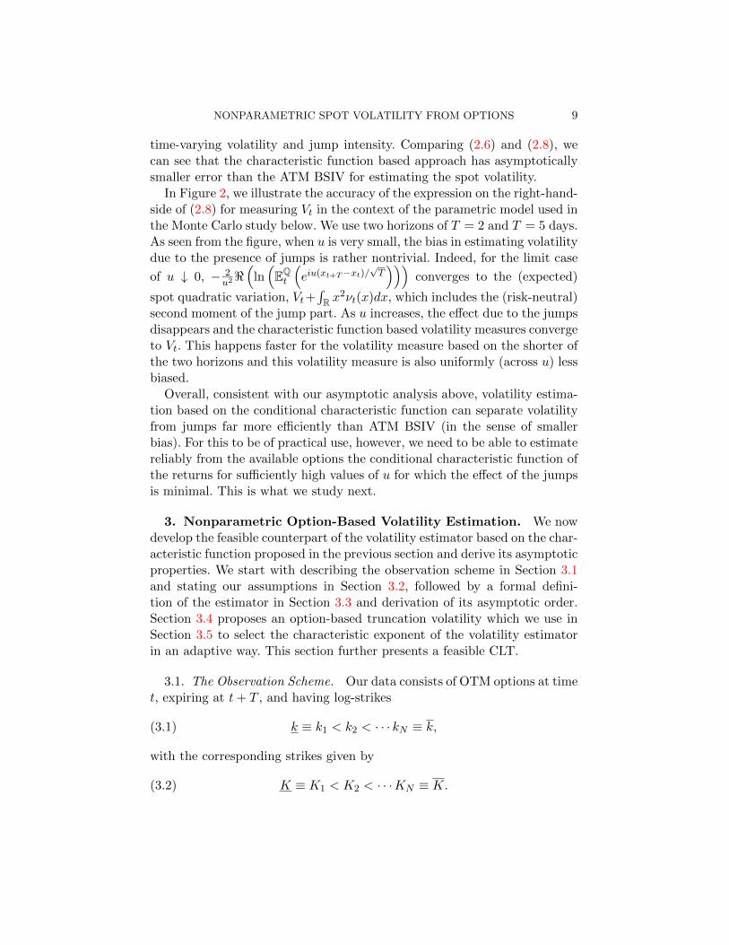
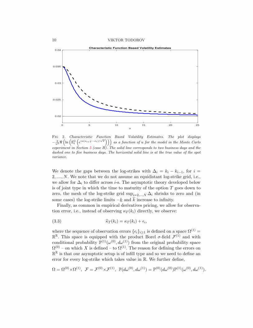
In Figure 2, we illustrate the accuracy of the expression on the right-hand-side of (2.8) for measuring Vt in the context of the parametric model used inthe Monte Carlo study below. We use two horizons of T = 2 and T = 5 days.As seen from the figure, when u is very small, the bias in estimating volatilitydue to the presence of jumps is rather nontrivial. Indeed, for the limit case

of u ↓ 0, − 2u2<(

ln(EQt

(eiu(xt+T−xt)/

√T)))

converges to the (expected)

spot quadratic variation, Vt+∫R x

2νt(x)dx, which includes the (risk-neutral)second moment of the jump part. As u increases, the effect due to the jumpsdisappears and the characteristic function based volatility measures convergeto Vt. This happens faster for the volatility measure based on the shorter ofthe two horizons and this volatility measure is also uniformly (across u) lessbiased.

Overall, consistent with our asymptotic analysis above, volatility estima-tion based on the conditional characteristic function can separate volatilityfrom jumps far more efficiently than ATM BSIV (in the sense of smallerbias). For this to be of practical use, however, we need to be able to estimatereliably from the available options the conditional characteristic function ofthe returns for sufficiently high values of u for which the effect of the jumpsis minimal. This is what we study next.

3. Nonparametric Option-Based Volatility Estimation. We nowdevelop the feasible counterpart of the volatility estimator based on the char-acteristic function proposed in the previous section and derive its asymptoticproperties. We start with describing the observation scheme in Section 3.1and stating our assumptions in Section 3.2, followed by a formal defini-tion of the estimator in Section 3.3 and derivation of its asymptotic order.Section 3.4 proposes an option-based truncation volatility which we use inSection 3.5 to select the characteristic exponent of the volatility estimatorin an adaptive way. This section further presents a feasible CLT.

3.1. The Observation Scheme. Our data consists of OTM options at timet, expiring at t+ T , and having log-strikes

(3.1) k ≡ k1 < k2 < · · · kN ≡ k,

with the corresponding strikes given by

(3.2) K ≡ K1 < K2 < · · ·KN ≡ K.

10 VIKTOR TODOROV

0 5 10 15 20 25

u

0.02

0.025

0.03

0.035

0.04

Characteristic Function Based Volatility Estimates

Fig 2. Characteristic Function Based Volatility Estimates. The plot displays

− 2u2<

(ln(EQt

(eiu(xt+T−xt)/

√T)))

as a function of u for the model in the Monte Carlo

experiment in Section 5 (case H). The solid line corresponds to two business days and thedashed one to five business days. The horizontal solid line is at the true value of the spotvariance.

We denote the gaps between the log-strikes with ∆i = ki − ki−1, for i =2, ...., N . We note that we do not assume an equidistant log-strike grid, i.e.,we allow for ∆i to differ across i-s. The asymptotic theory developed belowis of joint type in which the time to maturity of the option T goes down tozero, the mesh of the log-strike grid supi=2,...,N ∆i shrinks to zero and (in

some cases) the log-strike limits −k and k increase to infinity.Finally, as common in empirical derivatives pricing, we allow for observa-

tion error, i.e., instead of observing κT (ki) directly, we observe:

(3.3) κT (ki) = κT (ki) + εi,

where the sequence of observation errors εii≥1 is defined on a space Ω(1) =RR. This space is equipped with the product Borel σ-field F (1) and withconditional probability P(1)(ω(0), dω(1)) from the original probability spaceΩ(0) – on which X is defined – to Ω(1). The reason for defining the errors onRR is that our asymptotic setup is of infill type and so we need to define anerror for every log-strike which takes value in R. We further define,

Ω = Ω(0)×Ω(1), F = F (0)×F (1), P(dω(0), dω(1)) = P(0)(dω(0))P(1)(ω(0), dω(1)).


We will assume E(εi|F (0)

)= 0 and that εi and εj are F (0)-conditionally

independent for i 6= j. At the same time, we will allow for a general form ofF (0)-conditional heteroskedasticity in the observation error.

3.2. Assumptions. We continue with our formal assumptions for the pro-cess x, the option observation scheme as well as the observation error.

A1. Vt > 0 and the process σ has the following dynamics under Q for s ≥ t:

(3.4) σs = σt +

∫ s

t

budu+

∫ s

t

ηudWu +

∫ s

t

ηudWu +

∫ s

t

∫Rδσ(u, z)µσ(du, dz),

where W is a Brownian motion independent of W ; µσ is a Poisson randommeasure on R+×R with compensator νσ(du, dz) = du⊗dz, having arbitrarydependence with the random measure µ; b, η and η are processes with cadlagpaths and δσ(u, z) : R+ × R→ R is left-continuous in its first argument.

A2-r. With the notation of A1 and for some r ∈ [0, 1], there exists an Ft-adapted random variable t > t such that for s ∈ [t, t]:

(3.5) EQt |as|4 + EQ

t |σs|6 + EQt (e4|xs|) + EQ

t

(∫R[(e3|z| − 1) ∨ |z|r]νs(z)dz

)4

< Ct,

for some Ft-adapted random variable Ct, and in addition for some ι > 0:

(3.6) EQt

(∫R

(|δσ(s, z)|4 ∨ |δσ(s, z)|)dz)1+ι

≤ Ct.

A3. With the notation of A1, there exists an Ft-adapted random variablet > t such that for s ∈ [t, t]:

EQt |as − at|p + EQ

t |σs − σt|p + EQt |ηs − ηt|p + EQ

t |ηs − ηt|p ≤ Ct|s− t|, p ∈ [2, 4],

(3.7)

(3.8) EQt

(∫R

(ez∨0|z| ∨ |z|2)|νs(z)− νt(z)|dz)p≤ Ct|s− t|, p ∈ [2, 3],

(3.9) EQt

(∫R

(δσ(s, z)− δσ(t, z))2dz

)≤ Ct|s− t|,

for some Ft-adapted random variable Ct.

12 VIKTOR TODOROV

A4. The log strike grid kiNi=1 is F (0)t -adapted and on a set with probability

approaching one, we have

(3.10) η∆ ≤ infi=2,...,N

∆i ≤ supi=2,...,N

∆i ≤ ∆,

where η ∈ (0, 1) is some positive constant and ∆ is a deterministic sequencewith ∆→ 0.

A5. We have: (1) E(εi∣∣F (0)

)= 0, (2) E

(ε2i∣∣F (0)

)= κT (ki)

2σ2t,i where

σt,i ≡ σt(ki) with infk∈R σt(k) and supk∈R σt(k) being finite-valued, posi-

tive and F (0)t -adapted random variables, (3) E

(|εi|4|F (0)

)≤ ζtκT (ki)

4 for

some finite-valued F (0)t -adapted random variable ζt, and (4) εi and εj are

F (0)-conditionally independent whenever i 6= j.

A6. The dynamics of X and σ under P is as (2.1) and (3.4) but with W , Wand µσ defined with respect to P, and with µ having a compensator under P ofthe form νPt (x)dt⊗dx. The drift coefficient of X is locally bounded. Moreover,for a sequence of stopping times (τn) increasing to infinity and a sequence offunctions Γn(z) satisfying

∫R Γn(z)dz <∞, we have

∫R(|z| ∧ 1)νPt (dx) <∞

and |δσ(t, z)| ≤ Γn(z) for t ≤ τn.

Assumption A1 imposes σt to be an Ito semimartingale under Q, whichis the case for many applications, e.g., for models in the popular affine class,see e.g., [22]. Assumption A2 imposes existence of conditional moments.This assumption also assumes that the so-called jump activity of X (seee.g., Section 3.2 of [27]) is bounded by r ∈ [0, 1]. Assumption A3 imposes“smoothness in expectation” type conditions which are satisfied for examplewhen the corresponding processes are Ito semimartingales. Assumption A4is a weak condition on the strike grid and Assumption A5 is about theobservation error. The latter is F (0)-conditionally centered at zero and itcan have F (0)-conditional heteroskedasticity. The F (0)-conditional standarddeviation of the observation error is proportional to the option price it isattached to and this determines the asymptotic order of the error as T ↓ 0.Finally, assumption A6 is only needed for the high-frequency return-basedvolatility estimator and is taken from [27] (Assumption H in Section 9.1).

3.3. Construction of the Volatility Estimator and its Rate of Convergence.We proceed with formally defining our characteristic function based volatil-ity estimator. Using Appendix 1 of [15], the conditional characteristic func-tion of the log return, EQ

t (eiu(xt+T−xt)), can be spanned by the following


portfolio of options

(3.11) 1− (u2 + iu)

∫Re(iu−1)k−iuxtκT (k)dk, u ∈ R.

The integral in the above expression is not computable, given available data,because we do not have option observations over a continuum of strikes andfurthermore we do not observe directly κT (k). The computable counterpartof the expression in (3.11) is formed by using a Riemann sum approxima-tion of the integral in (3.11) constructed from the available noisy optionobservations:

(3.12) ft,T (u) = 1− (u2 + iu)

N∑j=2

e(iu−1)kj−1−iuxt κT (kj−1)∆j , u ∈ R.

While in general xt+T −xt is not F (0)t -conditionally the increment of a Levy

process, when T is small, the expression for the characteristic function in(2.7) nevertheless holds approximately true. This motivates the followingestimator of the volatility:

(3.13) Vt,T (u) =2

Tu2Rt,T (u),

where Rt,T (u) is given by

(3.14) Rt,T (u) = −<(

ln(ft,T (u) ∨ T

)).

For Vt,T (u) to be a consistent estimator of Vt, we will need ft,T (u) to convergein probability to the expression in (3.11) and for this we will need the meshof the discrete strike price grid in (3.1) to go to zero and the time to maturityT of the options to shrink. The formal result for the consistency and rate ofconvergence of Vt,T (u) is given in the next theorem.

Theorem 1. Suppose assumptions A1-A5 in Section 3.2 hold for somer ∈ [0, 1] and in addition ∆ Tα, K T−β, K T γ for some α > 1

2 ,

β ≥ 0 and γ ≥ 0. Let (uT ) be an F (0)t -adapted sequence such that

(3.15) u2TT

a.s.−→ u, where u is a finite nonnegative random variable.

Then, we have

(3.16) Vt,T (uT )− Vt = Op

(ur−2T

∨ √∆

T 1/4

∨u−1T e−2(|k|∨k)

).

14 VIKTOR TODOROV

Since the order of magnitude of the increment xt+T − xt shrinks asymp-totically as T ↓ 0, it is intuitively clear that we need to consider sequences(uT ) which go to infinity. We look only at the case where uT increases asfast as 1/

√T because for sequences (uT ) going at a faster rate to infinity,

the limit of ft,T (u) will be zero (recall (2.7)) and hence the signal about thevolatility will be smaller.

The rate of convergence result in (3.16) reveals the role of the differentsources of error in the volatility estimation. The first term on the right-handside of (3.16) is a bias due to the presence of jumps in X. The parameterr controls the so-called jump activity (see assumption A2-r), with highervalues of r implying more concentration of small jumps in X which in turnare harder to separate from the diffusive component. The case of finite activ-ity jumps that we considered in the previous section corresponds to r = 0.Similar to earlier work on recovering volatility from high-frequency returndata (e.g., [9, 10] and [31, 32]) and in line with earlier empirical evidencein [4] and [18], here we consider only the case of finite variation jumps, i.e.,r ≤ 1. For the infinite variation case, the bias due to the jumps becomeslarger and a bias correction analogous to the one in [30] for the return-basedestimator is probably needed for satisfactory performance of the volatilityestimator in practice. Finally, from (3.16), it is clear that better separationof volatility from jumps is achieved for higher values of uT .

The second term on the right-hand side of (3.16) is due to the observationerror, i.e., due to the fact that we use κT (k) in the estimation instead ofκT (k). The conditional volatility of the observation error is assumed to beof the same order of magnitude as the option price it is associated with(see assumption A5). This is intuitive and is motivated by the empiricalevidence in [4] regarding the size of the relative bid-ask spread in availableoption data sets. The asymptotic order of magnitude of the option pricesdiffer depending on the strike (and hence the same applies for the observationerrors attached to the options). In particular, for log-strikes which are withina range from the current log-price of order Op(

√T ), the option prices are

of asymptotic order Op(√T ). On the other hand, for log-strikes which are

of fixed size (different from the current log-price), the option prices are ofasymptotic order Op(T ) only. That is, for time-to-maturity T shrinking tozero, the option prices whose strikes are close to the current price level areof larger asymptotic order than the ones whose strikes are further away fromit. Note that in (3.12) we use options with all available strikes (provided βand γ are strictly positive). The above discussion suggests that the effect ofthe observation error on the recovery of volatility will be determined by theoption observations whose strikes are in the vicinity of the current price.


The third term on the right-hand side of (3.16) is due to the finite log-strike range of the available option data (k, k) used in the estimation. Intu-itively, the order of magnitude of this error will depend on the probability

mass in the tails of the risk-neutral F (0)t -conditional distribution of xt+T−xt.

With stronger assumptions for the latter, than what is currently assumed inassumption A2, the order of magnitude of this error can be further relaxed.From a practical point of view, this error is likely to have little impact on theestimation, as for the typical option data sets, the deepest available OTMoption prices are very close to zero. This implies that the “effective” supportof the conditional return distribution is covered by the available log-strikerange (k, k). Indeed, earlier empirical work has documented that the effectof the finite strike range of the available options on the precision of the VIXindex (which is another portfolio of options with different strikes) is typi-cally small. We further note that since the argument of the characteristicfunction uT is asymptotically drifting to infinity, we have that Vt,T (uT ) is aconsistent estimator of Vt even when the strike range of the options remainsfinite.

Finally, the recovery of the spot volatility from the short-dated optionscontains an error due to the time-variation in the volatility and the jumpintensity over the interval [t, t + T ]. The effect of this error on the volatil-ity estimation is of order Op(T ) and hence it is asymptotically dominatedby the first term on the right-hand side of (3.16) (which recall is due tothe separation of volatility from jumps and is present even if volatility isconstant). We note in this regard that our interest here is in the effect ofthe error due to the time-variation in volatility and jump intensity on therecovery of the option portfolio in (3.11) and not on an individual option.The former is much smaller than what we can show for the latter. We alsomention that it is only the stochastic changes in the volatility and the jumpintensity which cause the above-mentioned bias in the estimation. Indeed,if conditional on Ft the process V has deterministic time-variation over theinterval [t, t + T ], then Vt,T (uT ) is an estimate of 1

T

∫ t+Tt Vsds without any

bias due to the time-variation in V .

3.4. Data-driven Choice of uT and Option-Based Truncated Volatility.From Theorem 1, it is clear that in order to minimize the impact of thejumps on the volatility recovery, it is optimal to set uT to be of asymptoticorder Op(1/

√T ). This, of course, is an asymptotic statement and it does not

give a specific guidance regarding the choice of uT in finite samples. At thesame time, from the expression for the log-characteristic function in (2.7), itis clear that its behavior is governed by the product T ×u2

T ×Vt. Therefore,

16 VIKTOR TODOROV

one would like to set uT such that T ×u2T ×Vt is some fixed constant. To do

this, we will need a preliminary estimator of volatility and further we willhave to show that our estimator Vt,T (uT ) can be made adaptive, i.e., thatuT can be replaced with an estimate uT based on the data.

In this section we tackle the first problem, i.e., the construction of apreliminary volatility estimator from the option data, and in the next sectionwe deal with making Vt,T (uT ) adaptive. One natural choice of a preliminaryvolatility estimator is the ATM BSIV which has the additional advantageof being free of tuning parameters. However, given the documented largebias in the ATM BSIV, we propose an alternative one. Our initial consistentvolatility estimator can be viewed as the option analogue of the truncatedvolatility estimator of [31] and is given by

(3.17) T V t,T (η) =1

T

N∑j=2

hη(kj−1)κT (kj−1)∆j , η ≥ 0,

where we denote

hη(k) = e−k−η(k−xt)2[4η2(k − xt)4

+ 2− 10η(k − xt)2 + 2η(k − xt)3 − 2(k − xt)].

T V t,T (η) is a consistent estimator of EQt (e−η(xt+T−xt)2(xt+T −xt)2) from the

available options. In the special case when η = 0 we denote

(3.18) QV t,T ≡ T V t,T (0),

and we note that QV t,T is an estimator of the expected risk-neutral spotquadratic variation

(3.19) QVt,T = Vt +

∫Rx2νt(x)dx.

Thus, QV t,T is the option counterpart of the realized variance computedfrom return data ([2] and [7, 8]). We note however a fundamental difference.The realized variance is an estimator of

∫ t+τt Vsds+

∑s∈[t,t+τ ](∆xs)

2 for some

τ > 0. By contrast, QVt,T can be viewed as the risk-neutral F (0)t -conditional

expectation of this quantity for τ small (and further standardized, i.e., di-vided, by τ). While for small τ we have Vt ≈ EQ

t (Vt+τ ), the same does nothold for the expected and realized jumps no matter how small τ is and re-gardless of whether the jump intensity varies over time or not (i.e., whetherνt depends on t or not).


When η is a positive number, then T V t,T (η) estimates a truncated (con-ditional) second moment of the increment xt+T − xt with the degree oftruncation determined by η. When η is replaced with an increasing functiondepending on T , i.e., when the degree of truncation changes as we get moreshort-dated option data, then we can use T V t,T (η) to separate volatilityfrom jumps. This is analogous to the truncated volatility estimator basedon return data proposed by [31], with the difference being that, unlike [31],we use a smooth truncated square function here.

To implement the option-based truncated volatility estimator, we need tochoose the truncation level. The tradeoff we face here is similar to the one forthe return-based counterpart of our estimator. On one hand we would like toset the truncation as high as possible to minimize the impact of the jumpson the statistic. On the other hand, a more severe truncation will cause adownward bias in the recovery of volatility since such severe truncation willstart eliminating even the contribution coming from the continuous partof the process in the second moment of the return. Therefore, an adaptiveversion of T V t,T (η) is necessary. We use the following data-driven choice forthe cutoff parameter

(3.20) ηT =ηTT

1

QV t,T ∨ T,

for some deterministic sequence ηT that depends only on T and which goesto zero, but at a rate slower than the one at which T decreases. The reasonfor setting the truncation parameter this way is that the downward bias inT V t,T (η) caused by the truncation depends on the product η × T ×QVt,T .In the next theorem we present the consistency result for our truncationvolatility estimator.


2 ,β > 0 and γ > 0. We have

(3.21) QV t,TP−→ QVt,T .

Suppose in addition that for ηT in (3.20):

(3.22)ηT√T→ 0 and

ηTT→∞.

Then, we also have

(3.23) T V t,T (ηT )P−→ Vt.

18 VIKTOR TODOROV

The result in (3.21) is of independent interest and can be used for makinginference for the jump part of X. We note that we can further derive a CLTassociated with the convergence in (3.21) which will allow us to assess theprecision in the recovery of the jump part of the quadratic variation.

3.5. Feasible CLT for the Characteristic Function Based Volatility Esti-mator. Theorem 1 allows for the sequence (uT ) to be random. However,

it restricts (uT ) to be F (0)t -adapted and this rules out the case where (uT )

depends on the option data used in the construction of Vt,T (uT ). The goalof this section is to make the volatility estimator adaptive by making uT afunction of our preliminary truncated volatility T V t,T (ηT ). In particular, we

set the characteristic exponent in the construction of Vt,T (u) in the followingdata-driven way (recall our discussion at the beginning of Section 3.4)

(3.24) uT =u√T

1√T V t,T (ηT )

,

where u is some fixed positive number that does not depend on the data.We will further derive a feasible CLT for Vt,T (uT ) and for this we will

need a consistent estimator for its conditional asymptotic variance. We nowintroduce the necessary notation for this. First, our estimates for the varianceof the observation error are based on

(3.25) εj = κT (kj)−1

2(κT (kj−1) + κT (kj+1)) , j = 2, ..., N − 1 and j 6= j∗,

where j∗ ∈ 1, ..., N with |kj∗ − xt| ≤ |kj − xt|, for j = 1, ..., N , and

ε1 = ε2 and εN−1 = εN ,

εj∗ = κT (kj∗)− κT (kj∗−1)− (κT (kj∗−1)− κT (kj∗−2))Kj∗ −Kj∗−1

Kj∗−1 −Kj∗−2, if kj∗ ≤ xt,

εj∗ = κT (kj∗)− κT (kj∗+1)− (κT (kj∗+1)− κT (kj∗+2))Kj∗ −Kj∗+1

Kj∗+1 −Kj∗+2, if kj∗ > xt.

Since the true option price is smooth in k, then for j = 2, ..., N − 1 andj 6= j∗, εj is an estimate of εj − 1

2 (εj−1 + εj+1). We use a different estimatefor the error associated with the available option with strike closest to thecurrent price level. This is done so that we can incorporate the no-arbitragerestriction that the option price is a monotone function of its strike (de-creasing for calls and increasing for puts).


Given εjj=2,...,N , we set

Ct,T (u) =2

3

N∑j=2

ζj−1(u)ζj−1(u)>e−2kj−1 ε2j−1∆2j ,(3.26)

ζj(u) =

(u2 cos (ukj − uxt)− u sin (ukj − uxt)u cos (ukj − uxt) + u2 sin (ukj − uxt)

), j = 1, ...., N,

and with it our estimate for the asymptotic variance is given by

Avar(Vt,T (u)) =4

T 2u4

1

|ft,T (u)|4

(<ft,T (u)

=ft,T (u)

)>Ct,T (u)

(<ft,T (u)

=ft,T (u)

).(3.27)

Theorem 3 gives a feasible CLT for Vt,T (uT ). Below, L − s denotes stableconvergence, i.e., convergence in law that holds jointly with any boundedpositive random variable defined on the probability space, see e.g., [28] forfurther details.


2 ,β > 0 and γ > 0. If (3.22) holds and

(3.28) α <

(1

2+ 2− r

)∧(1

2+ 4(β ∧ γ)

),

then

(3.29)Vt,T (uT )− Vt√Avar(Vt,T (uT ))

L−s−→ N(0, 1),

where the limit is defined on an extension of the original probability spaceand is independent of F .

The condition in (3.28) ensures that the leading term in the differenceVt,T (uT ) − Vt is due to the option observation error, and in particular thatthe biases in the estimation due to the separation of volatility from jumpsand the finiteness of the strike range are of higher asymptotic order.

We note that the asymptotic limit of Avar(Vt,T (uT )) (after appropriately

rescaling it) is in general random. That is, the asymptotic limit of Vt,T (uT )−Vt is mixed Gaussian. This reflects the fact that the precision in the recoveryof the random Vt is itself random. This mirrors the limit behavior of thereturn-based volatility estimators ([9, 10] and [31, 32]).

20 VIKTOR TODOROV

We further point out that the limit above is of self-normalizing type.That is, we do not establish the limit of appropriately scaled Vt,T (uT )− Vtand

√Avar(Vt,T (uT )) but only of their ratio. This allows, in particular, to

incorporate general setups for the observed strike grid.We finish this section by comparing the performance of our estimator

with one constructed from high-frequency return data. We will use a local(in time) version of the truncated variance of [31, 32] in the comparison,but the results extend also to other return-based volatility estimators, e.g.,the multipower variations of [9, 10]. The return-based truncated volatilityestimator is given by

(3.30) V hft =

n

kn

∑i∈Int

(∆ni x)21|∆n

i x|≤αn−$, α > 0 and $ ∈ (0, 1/2),

where Int = i = 1, ..., kn : btnc − i denotes a local window used for thecalculation of the volatility and ∆n

i x = x in− x i−1

n. An estimator for the

asymptotic variance of V hft can be constructed as follows

(3.31) Avar(V hft,T ) =

2

3

n2

k2n

∑i∈Int

(∆ni x)41|∆n

i x|≤αn−$.

For the successful application of V hft , it is important to set α in a data-driven

way that accounts for the current level of volatility. In the next theorem, weshow that the convergence of Vt,T (uT ) holds jointly with that of V hf

t .

Theorem 4. In addition to the conditions of Theorem 3 suppose alsothat assumption A6 in Section 3.2 holds and kn

√n. Then

(3.32)V hft − Vt√Avar(V hf

t,T )

L−s−→ N(0, 1),

and this convergence holds jointly with the convergence in (3.29), with thelimits defined on an extension of the original probability space and beingindependent of each other and of F .

We note that Vt,T (uT ) and V hft are only F-conditionally independent

of each other but, due to connections between their conditional asymptoticvariances (which recall are random), they can have dependence uncondition-ally. The result of Theorem 4 suggests that we can benefit from combiningthe two volatility estimators. Indeed, we can optimally weight them (note


that the weights given below are in general random variables and hence weneed to use the fact that the convergence of the two estimators holds stably)according to their F-conditional asymptotic variances, to get(3.33)

V mixt = wtVt,T (uT ) + (1− wt)V hf

t , wt =Avar(V hf

t,T )

Avar(V hft,T ) + Avar(Vt,T (uT ))

.

The noisier one of the two volatility estimators is, the less weight it receives inthe combined estimator V mix

t . In fact, if one of the two estimators convergesat a faster rate, then asymptotically the weight it receives in V mix

t convergesto one, i.e., it receives all the weight. A convenient feature of V mix

t is thatthe user does not need to take a stand on whether options or high-frequencyreturns are more efficient for recovering volatility at any point in time. Theoptimally weighted V mix

t automatically “adapts” to the situation at hand.

4. Minimax Risk for Recovering Volatility from Noisy Short-Dated Options. We will now derive a lower bound for the minimax riskfor recovering the spot volatility from noisy short-dated option data. Thisresult will show that our nonparametric estimator Vt,T (uT ) is near rate-efficient. We first introduce the necessary notation for stating the formalresult. We will specialize attention to the case where x is a Levy process(under the risk-neutral measure) with finite activity jumps, and hence wewill drop the subscript t in the notation of the diffusive volatility and thejump compensator here. We will define the set G(R) of risk-neutral proba-bility measures Q (under which the true option prices κT (k) are computedaccording to (2.2)) for which x is a Levy process with characteristics tripletwith respect to the identity truncation function ([39], Definition 8.2) givenby

(4.1)

(−1

2σ2 −

∫R

(ez − 1− z)ν(z)dz, σ2, F (z)

),

where F (dz) = ν(z)dz and we further have

(4.2)1

R≤ |σ| ≤ R,

∫R

((e3|z| − 1) ∨ 1

)ν(z)dz ≤ R,

for some constant R > 0.The option observations are given by

(4.3) κT (ki) = κT (ki) + (κT (ki) ∨ T )εi, i = 1, ..., N,

22 VIKTOR TODOROV

where εi≥1 is a sequence of i.i.d. N(0, 1) random variables defined on a

product extension of (Ω(0),F (0), (F (0)t )t≥0,P(0)) and independent of F (0).

One can show that the option prices for every strike are of order Op(T ).Therefore, the truncation from below in the scale of the option error doesnot change its asymptotic order.

In what follows, we will denote with ET expectations under which thetrue (unobservable) option prices κT (k) are computed according to the risk-neutral probability measure T .

Theorem 5. In the setting of (4.1)-(4.3), assume further that η∆ ≤∆i ≤ ∆, for i = 1, ..., N and some η ∈ (0, 1] and ∆ > 0. Let ∆ Tα,K T−β and K T γ, for 1

2 < α < 52 and β, γ > 0 as T ↓ 0.

We then have

(4.4) infσ

supT ∈G(R)

ET

(√T | lnT |5/2

∆|σ − σ|2

)≥ c,

for some c > 0 and where σ is any estimator of σ based on the option dataκT (ki)i=1,...,N .

Under the conditions of Theorem 3, one can show that Vt,T (uT ) − Vt =

Op

(√∆

T 1/4

). Comparing this result with the efficient rate of convergence in

Theorem 5 (in the special setting of that theorem), we see that Vt,T (uT ) isnear rate-optimal, i.e., its rate convergence is slower than the optimal oneonly by a log term.

5. Monte Carlo Study. We now test the performance of the developednonparametric techniques on simulated data. In order to generate optiondata, we need a parametric model for the risk-neutral dynamics of X. Weuse the following specification:

(5.5) Xt = X0 +

∫ t

0

√VsdWs +

∫ t

0

∫R

(ex − 1)µ(ds, dx),

with W being a Brownian motion and V having the dynamics

(5.6) dVt = 3.6(0.02− Vt)dt− 0.1√VtdWt + 0.2

√0.75

√VtdWt,

where W is a Brownian motion orthogonal to W . The jump measure µ hasa compensator νt(x)dt⊗ dx with νt given by

(5.7) νt(x) = c−Vte−20|x|

|x|0.51x<0 + c+Vt

e−100|x|

|x|0.51x>0.


The specification in (5.5)-(5.7) belongs to the affine class of models ([22])commonly used in empirical option pricing work. Consistent with existingempirical evidence, the jumps have time-varying jump intensity. The jumpsize distribution is like the one of a tempered stable process which is foundto provide good fit to observed option data. We set the model parameters ina way that results in option prices similar to observed equity index options.In particular, the parameter specification of V implies average annualizedvolatility of around 15% (our unit of time is one year) and negative correla-tion between the innovations in price and stochastic volatility (also knownas leverage effect).

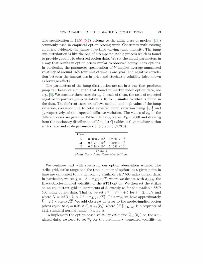
The parameters of the jump distribution are set in a way that producesjump tail behavior similar to that found in market index option data, seee.g., [5]. We consider three cases for c±. In each of them, the ratio of expectednegative to positive jump variation is 10 to 1, similar to what is found inthe data. The different cases are of low, medium and high value of the jumpvariation, corresponding to total expected jump variation being 1

4 , 12 and

34 , respectively, of the expected diffusive variation. The values of c± in thedifferent cases are given in Table 1. Finally, we set X0 = 2000 and draw V0

from the stationary distribution of Vt under Q (which is Gamma distributionwith shape and scale parameters of 3.6 and 0.02/3.6).

Case c− c+

L 0.3058× 103 1.7097× 103

M 0.6177× 103 3.4194× 103

H 0.9174× 103 5.1291× 103

Table 1Monte Carlo Jump Parameter Settings.

We continue next with specifying our option observation scheme. Thestrike grid, strike range and the total number of options at a given point intime are calibrated to match roughly available S&P 500 index option data.In particular, we set k = −8 × σATM

√T , where we denote with σATM the

Black-Scholes implied volatility of the ATM option. We then set the strikeson an equidistant grid in increments of 5, exactly as for the available S&P500 index option data. That is, we set eki = eki−1 + 5 for i = 2, ..., N andwhere N = infi : ki > 2.5 × σATM

√T. This way, we have approximately

k = 2.5× σATM√T . We add observation error to the model-implied option

prices equal to εi = 0.05 × Zi × κT (ki), where Zii=1,...,N is a sequence ofi.i.d. standard normal random variables.

To implement the option-based volatility estimator Vt,T (uT ) on the sim-ulated data, we need to set ηT for the preliminary truncated volatility as

24 VIKTOR TODOROV

well as u for the adaptive characteristic exponent uT in (3.24). Recall thatηT is a deterministic sequence converging to zero. We put ηT = T 0.51, whichfor T = 2/252 takes value of approximately 0.085 and for T = 5/252 takesvalue of approximately 0.135. Our choice for ηT is motivated by the maxi-mum downward bias in the measurement of volatility. By first-order Taylorexpansion, in the case of no jumps, 3ηT is equal approximately to the relative

negative bias in the measurement of the spot variance by T V t,T (ηT ).Turning next to u, we would like to pick this constant as low as possi-

ble to guard against the effect of the jumps while at the same time highenough so that the estimation is not too noisy. We experiment with twovalues, u =

√2 ln(1/0.1) and u =

√2 ln(1/0.085), which correspond to

|EQt

(eiu(xt+T−xt)

)| having values of 0.1 and 0.085, respectively (recall from

the discussion in Section 2 that for high u we have |EQt

(eiu(xt+T−xt)

)| ≈

e−u2 VtT

2 ). Finally, to guard against potential finite sample distortions inthe data-driven choice of u, if the above choice of uT exceeds umin =argminu∈[0,400]|fT (u)|, we set uT equal to the latter.

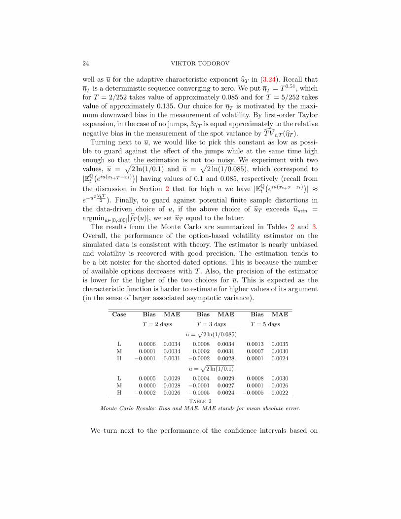
The results from the Monte Carlo are summarized in Tables 2 and 3.Overall, the performance of the option-based volatility estimator on thesimulated data is consistent with theory. The estimator is nearly unbiasedand volatility is recovered with good precision. The estimation tends tobe a bit noisier for the shorted-dated options. This is because the numberof available options decreases with T . Also, the precision of the estimatoris lower for the higher of the two choices for u. This is expected as thecharacteristic function is harder to estimate for higher values of its argument(in the sense of larger associated asymptotic variance).

Case Bias MAE Bias MAE Bias MAE

T = 2 days T = 3 days T = 5 days

u =√

2 ln(1/0.085)

L 0.0006 0.0034 0.0008 0.0034 0.0013 0.0035M 0.0001 0.0034 0.0002 0.0031 0.0007 0.0030H −0.0001 0.0031 −0.0002 0.0028 0.0001 0.0024

u =√

2 ln(1/0.1)

L 0.0005 0.0029 0.0004 0.0029 0.0008 0.0030M 0.0000 0.0028 −0.0001 0.0027 0.0001 0.0026H −0.0002 0.0026 −0.0005 0.0024 −0.0005 0.0022

Table 2Monte Carlo Results: Bias and MAE. MAE stands for mean absolute error.

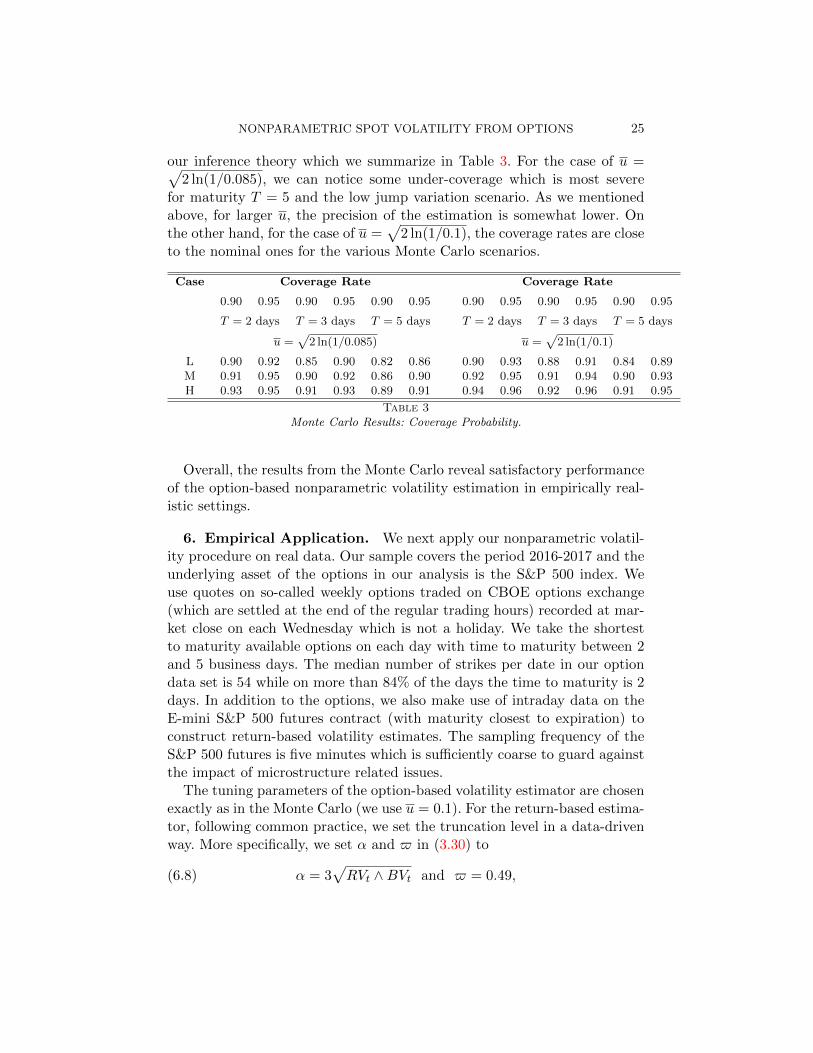
We turn next to the performance of the confidence intervals based on


our inference theory which we summarize in Table 3. For the case of u =√2 ln(1/0.085), we can notice some under-coverage which is most severe

for maturity T = 5 and the low jump variation scenario. As we mentionedabove, for larger u, the precision of the estimation is somewhat lower. Onthe other hand, for the case of u =

√2 ln(1/0.1), the coverage rates are close

to the nominal ones for the various Monte Carlo scenarios.

Case Coverage Rate Coverage Rate

0.90 0.95 0.90 0.95 0.90 0.95 0.90 0.95 0.90 0.95 0.90 0.95

T = 2 days T = 3 days T = 5 days T = 2 days T = 3 days T = 5 days

u =√

2 ln(1/0.085) u =√

2 ln(1/0.1)

L 0.90 0.92 0.85 0.90 0.82 0.86 0.90 0.93 0.88 0.91 0.84 0.89M 0.91 0.95 0.90 0.92 0.86 0.90 0.92 0.95 0.91 0.94 0.90 0.93H 0.93 0.95 0.91 0.93 0.89 0.91 0.94 0.96 0.92 0.96 0.91 0.95

Table 3Monte Carlo Results: Coverage Probability.

Overall, the results from the Monte Carlo reveal satisfactory performanceof the option-based nonparametric volatility estimation in empirically real-istic settings.

6. Empirical Application. We next apply our nonparametric volatil-ity procedure on real data. Our sample covers the period 2016-2017 and theunderlying asset of the options in our analysis is the S&P 500 index. Weuse quotes on so-called weekly options traded on CBOE options exchange(which are settled at the end of the regular trading hours) recorded at mar-ket close on each Wednesday which is not a holiday. We take the shortestto maturity available options on each day with time to maturity between 2and 5 business days. The median number of strikes per date in our optiondata set is 54 while on more than 84% of the days the time to maturity is 2days. In addition to the options, we also make use of intraday data on theE-mini S&P 500 futures contract (with maturity closest to expiration) toconstruct return-based volatility estimates. The sampling frequency of theS&P 500 futures is five minutes which is sufficiently coarse to guard againstthe impact of microstructure related issues.

The tuning parameters of the option-based volatility estimator are chosenexactly as in the Monte Carlo (we use u = 0.1). For the return-based estima-tor, following common practice, we set the truncation level in a data-drivenway. More specifically, we set α and $ in (3.30) to

(6.8) α = 3√RVt ∧BVt and $ = 0.49,

26 VIKTOR TODOROV

where

(6.9) RVt =

btnc∑i=b(t−1)nc+1

(∆ni x)2, BVt =

π

2

btnc∑i=b(t−1)nc+2

|∆ni−1x||∆n

i x|,

with RVt being the realized volatility and BVt being the Bipower Variationof [9, 10] over the trading day. The latter is a nonparametric jump-robustmeasure of integrated volatility that is free of tuning parameters. Finally,our local window for V hf

t consists of kn = 48 five-minute returns beforemarket close (which is the time when the option data is recorded).

In Figure 3, we plot the two spot volatility estimators. As seen from thefigure, the two series are very close to each other on average. Indeed, thesample median of the option-based volatility estimate is within 1.5% of thatof the return-based volatility estimator while the correlation between thetwo time series is 0.9. At the same time, though, we can note that thevolatility estimate from the high-frequency data is significantly noisier. In-deed, the standard deviation of the return-based volatility estimate is over32% higher than that of its option-based counterpart. In addition, the cor-relation between the first differences of the two estimators, for which themeasurement error plays bigger role, is only 0.6 (first differences are used inthe computation of measures of variation such as the quadratic variation).Also, the efficiency gains offered by the option-based estimator (based on theestimated asymptotic variances) are particularly pronounced at the begin-ning of the sample when the volatility was very high. This is to be expectedas during such episodes the separation of volatility from the realization ofjumps from return data is particularly challenging. Finally, V mix

t in (3.33)that combines optimally the option and return-based volatility estimators isvery close to the former, with correlation between Vt,T (uT ) and V mix

t of over

0.99. This is due to the high weight assigned to Vt,T (uT ) in forming V mixt ,

particularly in the high volatility period.Overall, the empirical analysis reveals nontrivial gains in measuring spot

volatility by the use of short-dated options. The newly-proposed nonpara-metric volatility estimator should therefore greatly improve the precisionin studying various features of the volatility process, e.g., the roughness ofthe volatility path (see e.g., [25]) as well as the presence of jumps in thevolatility and their connection with those in the underlying price (see e.g.,[29] and [3]). Answering these questions regarding the volatility trajectoryfrom return data alone is known to be very difficult as the volatility is notdirectly observed and has to be filtered out from the data. This can beparticularly challenging in the presence of persistent microstructure-related


01/2016 07/2016 01/2017 07/2017

time

0

0.05

0.1

0.15

0.2

0.25

0.3

0.35

0.4Option and Return Based Measures of Spot Volatility

Fig 3. Option and Return Based Measures of Volatility. The solid line corresponds to the

option based one,

√Vt,T (uT ), and the stars to the one based on five-minute returns of the

underlying asset,

√V hft . The x-axis ticks are at the beginning of the corresponding month.

distortions in the high-frequency returns, see e.g., the recent work of [17].In addition, the option-based spot volatility estimates should be of directuse for the purposes of volatility forecasting and risk management where amore precise volatility proxy is known to provide efficiency gains, see e.g.,[2] in the case of volatility forecasting. In current work in progress I showthis to be the case when using the newly-developed option-based volatilityestimator for forecasting the future volatility of various assets.

7. Proofs. In the proofs we will denote with Ct a finite-valued and Ft-adapted random variable which might change from line to line. If the variabledepends on some parameter q, then we will use the notation Ct(q). Further,without loss of generality, in the proofs, we will set Xt = 1 or equivalentlyxt = 0.

7.1. Decomposition, Notation and Auxiliary Results. The jump part ofthe process xt can be represented as an integral with respect to a Poissonrandom measure under Q. In particular, using the so-called Grigelionis rep-resentation of the jump part of a semimartingale (Theorem 2.1.2 of [27])

28 VIKTOR TODOROV

and upon suitably extending the probability space, we can write

(7.1)

∫ t

0

∫Rµ(ds, dx) ≡

∫ t

0

∫Eδx(s, z)µx(ds, dz),

where µx(ds, dz) is a Poisson measure on R+×E with compensator dt⊗λ(dz)for some sigma-finite measure λ on E, µx is the martingale counterpart ofµx, and δx is a predictable and R-valued function on Ω×R+ ×E such thatνt(z)dz is the image of the measure λ(dz) under the map z → δx(t, z) onthe set z : δx(ω, t, z) 6= 0.

There are different choices for E and the function δx. For the analysishere it will be convenient to use E = R+×R and δx(t, z) = z21z1≤νt(z2) forz = (z1, z2), with λ being the Lebesgue measure on E.

We proceed with introducing some notation that will be used throughoutthe proofs. By noting that xt = 0, we can split xs into

(7.2) xcs =

∫ s

taudu+

∫ s

tσudWu, xds =

∫ s

t

∫Eδx(u, z)µx(du, dz), s ≥ t.

We now introduce two approximations for xs. The first is xs = xcs + xds ,where for s ≥ t

(7.3) xcs = at(s− t) + σt(Ws −Wt), xds =

∫ s

t

∫Eδx(t, z)µx(du, dz).

The second approximation is given by xs = xcs + xds , where for s ≥ t(7.4)

xcs = at(s− t)+

∫ s

tσuWu, xds = xds , σs = σt+ηt(Ws−Wt)+ηt(W s−W t).

The OTM option prices at time t associated with log-terminal value xt+Tare denoted by κT (k), the ones with log-terminal value of xt+T are denotedby κT (k), and the ones with log-terminal value of σt(Wt+T−Wt) with κcT (k).

Lemma 1. Suppose assumptions A1-A3 hold. There exist Ft-adaptedrandom variables t > t and Ct > 0 that do not depend on k, k1, k2 andT , such that for T < t we have

(7.5) κT (k) ≤ CtT

e2k

e−k−1, if k < 0,

1ek−1

, if k > 0,

(7.6) |κT (k)− κT (k)| ≤ Ct| lnT |T 3/2,


(7.7) |κT (k)− κT (k)| ≤ Ct(T

32

∨(T 3/2

|ek − 1|∧T

)),

(7.8) κT (k) ≤ Ct(√

T∧ T

|ek − 1|

),

(7.9)

k < kl,t =⇒ κT (k) ≤ Ct e2k

(e−k−kl,t−1)2T, kl,t = −σt

√T | lnT |,

k > kh,t =⇒ κT (k) ≤ Ct 1

(ek−kh,t−1)2T, kh,t = σt

√T | lnT |,

|κT (k1)− κT (k2)| ≤ Ct[(

T

k22

∧1

)1|k2|≤1 +

T

k42

1|k2|>1

] ∣∣ek1 − ek2∣∣ ,(7.10)

|κT (k1)− κT (k2)| ≤ Ct[(

T

k22

∧1

)1|k2|≤1 +

T

k42

1|k2|>1

] ∣∣ek1 − ek2∣∣ ,(7.11)

where k1 < k2 < 0 or k1 > k2 > 0.

Proof of Lemma 1. All bounds but the last one are proved in Lemmas 2-7of [37]. The bound in (7.11) can be proved exactly as Lemma 7 of [37] usingthe integrability assumptions in A2-r. 2

Lemma 2. Suppose assumptions A1-A3 hold. There exist Ft-adaptedrandom variables t > t and Ct > 0 that do not depend on k and T , such thatfor T < t we have

(7.12) |κT (k)− κcT (k)| ≤ CtT,

∣∣∣∣κcT (k)− f(k − atT√Tσt

)√Tσt − (ek − 1)Φ

(k − atT√Tσt

)∣∣∣∣ ≤ CtT, if k ≤ 0,∣∣∣∣κcT (k)− f(k − atT√Tσt

)√Tσt + (ek − 1)

(1− Φ

(k − atT√Tσt

))∣∣∣∣ ≤ CtT, if k > 0,

(7.13)

where f and Φ are the pdf and cdf, respectively, of a standard normal randomvariable.

Proof of Lemma 2. We look only at the case k > 0, with the proof for thecase k ≤ 0 being done in analogous way. First, we have∣∣∣∣∣∣∣ext+T − ek∣∣∣+ − ∣∣∣eσt(Wt+T−Wt) − ek

∣∣∣+∣∣∣∣ ≤ eσt(Wt+T−Wt)|eatT+xdt+T − 1|.

From here we can use the Ft-conditional independence of Wt+T −Wt andxdt+T and apply Lemma 1 of [37] to obtain the result in (7.12).

30 VIKTOR TODOROV

We continue with the bounds in (7.13). Direct calculation shows for k > 0

κcT (k) = eatT+σ2t T/2

(1− Φ

(k − atT√Tσt

−√Tσt

))−ek

(1− Φ

(k − atT√Tσt

)).

From here the result of (7.13) follows by using Taylor expansion and thefact that the function f is bounded. 2

7.2. Proof of Theorem 1. We introduce the following notation

ft,T (u) = EQt

(eiu(xt+T−xt)

), ft,T (u) = EQ

t

(eiu(xt+T−xt)

).

Using Appendix 1 of [15], ft,T (u) equals the expression in (3.11). We furthernote that by Levy-Khintchine formula

(7.14) ft,T (u) = exp

(iTuat − T

u2

2Vt + T

∫R

(eiux − 1− iux)νt(x)dx

).

We start the proof with establishing a bound for the difference ft,T (u)−ft,T (u). In the proof we will denote with ζt,T (u) a random variable thatdepends on u and further satisfies

|ζt,T (u)| ≤ Ct(|u|T 3/2 ∨ |u|4T 3),

where Ct is Ft-adapted random variable that does not depend on u. Thisvariable can change from one line to another.

We first study the real part of the difference <(ft,T (u)−ft,T (u)). ApplyingIto’s lemma, using the normalization xt = 0 and the integrability assumptionA2, we have

EQt (cos(uxt+T ))− 1 = −EQ

t

(∫ t+T

t

u sin(uxs)asds+1

2

∫ t+T

t

u2 cos(uxs)σ2sds

)

+ EQt

(∫ t+T

t

∫R

(cos(uxs)(cos(uz)− 1)− sin(uxs)(sin(uz)− u sin(z))) νs(z)dzds

).

We have an analogous expression for EQt (cos(uxt+T )) − 1. Then, using as-

sumption A3 as well as EQt |xs − xs| ≤ CtT for s ∈ [t, t + T ] and Ct being

Ft-adapted random variable (which follows from using Doob’s inequalityand A3), we can write

EQt (cos(uxt+T ))− 1 = −EQ

t

(∫ t+T

t

u sin(uxs)atds+1

2

∫ t+T

t

u2 cos(uxs)σ2sds

)

+ EQt

(∫ t+T

t

∫R

(cos(uxs)(cos(uz)− 1)− sin(uxs)(sin(uz)− u sin(z))) νt(z)dzds

)+ ζt,T (u).


Therefore, we have

EQt (cos(uxt+T ))− EQ

t (cos(uxt+T ))

=1

2EQt

(∫ t+T

t

u2(cos(uxs)σ2t − cos(uxs)σ

2s)ds

)+ ζt,T (u).

Using the proof of Lemma 3 in [37] as well as (3.9) of A3, we have EQt |xs−

xs| ≤ CtT3/2 for s ∈ [t, t + T ] and Ct being Ft-adapted random variable.

In addition, using assumptions A1-A3 and Doob’s inequality, we also have

EQt |σs − σs| ≤ CtT for s ∈ [t, t + T ] and Ct as before. Using these results

and Cauchy-Schwartz inequality, we can write

EQt (cos(uxt+T ))− EQ

t (cos(uxt+T ))

=1

2EQt

(∫ t+T

t

u2(cos(uxs)σ2t − cos(uxs)σ

2s)ds

)+ ζt,T (u).

(7.15)

Next, we can decompose

cos(uxs)σ2s − cos(uxs)σ

2t = (cos(uxs)− cos(uxs))σ

2t + cos(uxs)(σs − σt)2

+ 2(cos(uxs)− cos(uxs))(σs − σt)σt + 2 cos(uxs)(σs − σt)σt.(7.16)

For the second and third terms on the right-hand side of the above equalitywe can use EQ

t (σs−σt)2 ≤ CtT and EQt (xs−xs)2 = EQ

t

(∫ st (σs − σt)dWu

)2 ≤CtT

2, for s ∈ [t, t+ T ] and Ct being Ft-adapted random variable as well asCauchy-Schwartz inequality, and conclude

u2TEQt (σs − σt)2 + u2T

∣∣∣EQt [(cos(uxs)− cos(uxs))(σs − σt)]

∣∣∣ = ζt,T (u).

For the forth term on the right-hand side of (7.16), we can decomposecos(uxs) = cos(uxcs) cos(uxds)− sin(uxcs) sin(uxds). Then, using the symmetryof the density of the standard normal distribution as well as the indepen-dence of W and W , we have

EQt (cos(uxcs) cos(uxds)(σs − σt))

= − sin(uat(s− t))EQt (sin(uσt(Ws −Wt)) cos(uxds)(σs − σt)),

which is ζt,T (u) because EQt |σs − σt| ≤ Ct

√T for s ∈ [t, t + T ]. Using the

Ft-conditional independence of xds and σs − σt, we also have

EQt | sin(uxcs) sin(uxds)(σs − σt)| ≤ |u|E

Qt (|xds ||σs − σt|)

= |u|EQt |xds |E

Qt |σs − σt| = ζt,T (u).

32 VIKTOR TODOROV

Combining these bounds, we have

EQt (cos(uxs)(σs − σt)) = ζt,T (u).

Finally, for the first term on the right-hand side of (7.16) using the indepen-

dence of W and W and integration by parts, we can write

EQt (cos(uxs)− cos(uxs)) = −EQ

t (sin(uxs) sin(uxs − uxs)) + ζt,T (u)

= −uEQt (sin(uxs)(xs − xs)) + ζt,T (u) = −u

2ηtEQ

t (sin(uxs)(Ws −Wt)2) + ζt,T (u)

= −u2ηtEQ

t (sin(uσt(Ws −Wt))(Ws −Wt)2) + ζt,T (u) = ζt,T (u),

where for the last two equalities we have made use of the Ft-conditional in-dependence of xcs and xds as well as the symmetry of the density of the stan-

dard normal distribution. Altogether we get that EQt

(∫ t+Tt u2(cos(uxs)σ

2s−

cos(uxs)σ2t )ds

)is ζt,T (u). Combining this result with (7.15), we have

(7.17) <(ft,T (u)− ft,T (u)) = ζt,T (u).

Turning to =(ft,T (u) − ft,T (u)), by making use of EQt |xt+T − xt+T | ≤ CtT ,

we have

(7.18) |EQt (sin(uxt+T ))− EQ

t (sin(uxt+T ))| ≤ Ct|u|T.

The results in (7.17) and (7.18), together with the rate condition for thesequence uT in (3.15), imply

(7.19) <(ft,T (uT ))−<(ft,T (uT )) = Op(T ), =(ft,T (uT ))−=(ft,T (uT )) = Op(√T ).

From (7.14), we also have

(7.20) <(ft,T (uT )) = Op(1), =(ft,T (uT )) = Op(√T ).

From here, using Taylor expansion, we have

(7.21) < (ln (ft,T (uT )))−<(

ln(ft,T (uT )

))= Op(T ).

Furthermore, for r being the constant in assumption A2-r, we have

(7.22)

∣∣∣∣<(ln(ft,T (uT )

))+ T

u2T

2σ2t

∣∣∣∣ ≤ 2T |uT |r∫R|x|rνt(x)dx.


Altogether, we have

(7.23) − 2

Tu2T

< (ln (ft,T (uT )))− σ2t = Op(u

r−2T ).

We next decompose ft,T (uT )− ft,T (uT ) =∑3

j=1 f(j)t,T , where f

(j)t,T = −(u2

T +

iuT )Tf(j)t,T and

f(1)t,T =

1

T

N∑j=2

e(iuT−1)kj−1εj−1∆j ,

f(2)t,T =

1

T

N∑j=2

∫ kj

kj−1

(e(iuT−1)kj−1κT (kj−1)− e(iuT−1)kκT (k)

)dk,

f(3)t,T = − 1

T

∫ k

−∞e(iuT−1)kκT (k)dk − 1

T

∫ ∞k

e(iuT−1)kκT (k)dk.

Using the bounds of Lemma 1 and assumption A5 for the observation error,we have

(7.24) f(1)t,T = Op

(√∆

T 1/4

), f

(2)t,T = Op

(∆√T| lnT |

).

Turning to f(3)t,T , using integration by parts and Lemma 1, we get∫ k

−∞e(iuT−1)kκT (k)dk =

i

uT

∫ k

−∞e(iuT−1)k(κ′T (k)− κT (k))dk

− i

uTe(iuT−1)kκT (k).

(7.25)

Using Lebesgue dominated convergence and the integrability conditions inAssumption A2, we have

κ′T (k) = ekQt (xt+T < k) = ekQt

(e−xt+T − 1 < e−k − 1

)≤ Ctek

T

(e−k − 1)3, k < 0.

(7.26)

From here by application of Lemma 1, we obtain∫ k−∞ e

(iuT−1)kκT (k)dk =

Op(u−1T Te−2|k|). Exactly the same analysis can be done for the second inte-

gral in f(3)t,T , and thus altogether we have

(7.27) f(3)t,T = Op

(u−1T e−2(|k|∧|k|)

).

34 VIKTOR TODOROV

Combining the bounds in (7.23), (7.24) and (7.27), using Taylor expansionand the rate condition in (3.15) as well as the conditions for the asymptoticbehavior of T , ∆, k and k in the theorem, we have (3.16).

7.3. Proof of Theorem 2. We set fη(x) = e−ηx2x2 for η ≥ 0, and we

denote

(7.28) ηT =ηTT

1

QVt,

which is an Ft-adapted random variable. Using Appendix 1 of [15], for everyfinite-valued, nonnegative and Ft-adapted random variable η, we have

(7.29) EQt (fη(xt+T − xt)) =

∫ ∞−∞

hη(k)κT (k)dk.

We will first show that EQt (f0(xt+T − xt)) and EQ

t (fηT (xt+T − xt)) are closeto QVt and Vt, respectively. Applying Ito’s lemma, taking expectations andusing the integrability conditions of assumption A2-r, we have

EQt (fη(xt+T − xt)) = atEQ

t

(∫ T

0

f ′η(xt+s − xt)ds

)+Vt2EQt

(∫ T

0

f′′

η (xt+s − xt)ds

)

+ EQt

(∫ T

0

∫R

(fη(xt+s − xt + z)− fη(xt+s − xt)− f ′η(xt+s − xt)z

)dsνt(z)dz

),

(7.30)

for any Ft-adapted η. Using then the fact that (which follows by (7.3) andthe integrability conditions in A2-r)

(7.31) |EQt (xt+s − xt)| ≤ CtT, for s ∈ [t, t+ T ],

we have

(7.32)

∣∣∣∣ 1

TEQt (f0(xt+T − xt))− Vt −

∫Rz2νt(z)dz

∣∣∣∣ = Op (T ) .

Next, for some constant C that does not depend on η and x, we have forη ∈ R+ and x ∈ R:

(7.33) |f ′η(x)| ≤ C|x| and |f ′′η (x)− 2| ≤ Cηx2,

|fη(x+ z)− fη(x)− f ′η(x)z − fη(z)|

≤ C(|x||z|+ η|x|2|z|2 + η|x|3|z|+ e−

η2|z|2 |z|2

).

(7.34)


Using the above bounds and (7.30), the inequality |x|e−|x|2 ≤ C, the fact that∫R |z|νt(z)dz <∞ (due to A2-r), the bound EQ

t (|xs− xt|2∨|xs− xt|3) ≤ CtTfor s ∈ [t, t + T ], as well as the integrability assumptions in A2-r, we havefor ηT in (7.28):

(7.35)∣∣ 1

TEQt (fηT (xt+T − xt))− Vt

∣∣ = Op

(√T ∨ ηTT

∨ 1√ηT

).

Given the results in (7.32) and (7.35), to prove the claims of Theorem 2, we

need to show the asymptotic negligibility of QV t,T − 1T

∫∞−∞ h0(k)κT (k)dk

and T V t,T (ηT )− 1T

∫∞−∞ hηT (k)κT (k)dk.

First, using the bounds of Lemma 1 and assumption A5 for the observa-tion error, we can easily conclude

(7.36) QV t,T −1

T

∫ ∞−∞

h0(k)κT (k)dk = Op

(√∆

T 1/4

∨e−2(|k|∨k)(|k| ∨ k)

).

In addition, using Ito’s lemma as well as assumptions A1-A3, we have

(7.37)∣∣∣EQt (f0(xt+T − xt))− EQ

t (f0(xt+T − xt))∣∣∣ = Op(T

√T ).

The bounds in (7.36)-(7.37) together with (7.32) establish the consistency

of QV t,T . We continue with T V t,T (ηT ). For its analysis, we first introducethe set

Ω =

ω : |QV t,T −QVt| ≤

1

5QVt

.

We will further make use of two algebraic inequalities. For η ∈ R+, a ∈ R+

with |a− η| ≤ η4 , and k ∈ R, we have

(7.38) |hη(k)| ≤ Ce−k−η2k2(|k| ∨ 1),

(7.39) |ha(k)− hη(k)| ≤ C|a− η|k2e−k−η2k2(k2 ∨ 1 + η2k4

),

for some C that does not depend on η, a and k (recall that xt = 0).Using the bounds of Lemma 1 and assumption A5 for the observation error

as well as (7.32) and (7.36), we have for T being below some F (0)t -adapted

and positive random variable ζt (so that P(T > ζt)→ 0 as T → 0):

(7.40) P (Ωc|T < ζt) ≤ Ct∆√T,

36 VIKTOR TODOROV

and therefore 1(Ωc) is Op

(∆√T

). Further, using the inequality in (7.38), the

bounds of Lemma 1 as well as assumption A5 for the observation error, wehave T V t,T (ηT )− T V t,T (ηT ) = Op(1). Therefore, altogether

(7.41)(T V t,T (ηT )− T V t,T (ηT )

)1Ωc = Op

(∆√T

).

Next, since on the set Ω we have |ηT − ηT | ≤ ηT4 for T small enough, we can

apply (7.39) and bound∣∣∣T V t,T (ηT )− T V t,T (ηT )∣∣∣ 1Ω ≤ CtηT |QV t,T −QVt,T |

× 1

T 2

N∑j=1

k2j−1e

−kj−1−ηT2 k2j−1

(k2j−1 ∨ 1 + η2

T k4j−1

)κT (kj−1)∆j ,

(7.42)

for some finite-valued Ct > 0 (note that because of A1 we have QVt,T > 0).Using the bounds of Lemma 1 and assumption A5 for the observation error,we have

(7.43)1

T 2

N∑j=1

k2j−1e

−kj−1−ηT2 k2j−1

(k2j−1 ∨ 1 + η2

T k4j−1

)κT (kj−1)∆j = Op(1),

and taking into account the bounds for QV t,T in (7.32) and (7.36), we havealtogether(7.44)(T V t,T (ηT )− T V t,T (ηT )

)1Ω = Op

(ηT

√∆

T 1/4

∨ηT√T∨ηT e

−2(|k|∨k)(|k| ∨ k)

).

We continue next with T V t,T (ηT )− 1T

∫∞−∞ hηT (k)κT (k)dk which we split

into T V(1)

t,T , T V(2)

t,T and T V(3)

t,T defined as

T V(1)

t,T =1

T

N∑j=2

hηT (kj−1)εj−1∆j ,

T V(2)

t,T =1

T

N∑j=2

∫ kj

kj−1

(hηT (kj−1)κT (kj−1)− hηT (k)κT (k))dk,

TV(3)

t,T = − 1

T

∫ k1

−∞hηT (k)κT (k)dk − 1

T

∫ ∞kN

hηT (k)κT (k)dk.

Using assumption A5 and the bounds of Lemma 1, we have

(7.45) E(T V

(1)

t,T

∣∣F (0))2

= Op

(∆√T

), T V

(3)

t,T = Op

(e−(k2∧k2) 1

4QVt

ηTT

).


For T V(2)

t,T we make use of the following algebraic inequality

|hη(k2)− hη(k1)| ≤ Ct|k2 − k1|e|k2|−η2 k

22 (1 + |k2|η)

(1 + k2

2 + η2k42

),(7.46)

for |k1| ≤ 12 |k2| and where Ct is a finite-valued Ft-adapted random variable

that does not depend on k1, k2 and η. Using this inequality, (7.38) as wellas Lemma 1, we get

(7.47) T V(2)

t,T = Op

(∆√T

).

Combining the bounds in (7.45) and (7.47), we have altogether (the boundbelow is not sharp and can be further relaxed)

(7.48) T V t,T (ηT )− 1

T

∫ ∞−∞

hηT (k)κT (k)dk = Op

( √∆

T 1/4

∨e−2(|k|∧|k|)(|k| ∧ |k|)

).

This result, together with (7.35), (7.41) and (7.44) as well as

(7.49) EQt |fηT (xt+T − xt)− fηT (xt+T − xt)| ≤ CtT 3/2,

implies the consistency of T V t,T (ηT ).

7.4. Proof of Theorem 3. We use the notation in (7.14). Using the resultin (7.23) in the proof of Theorem 1, the fact that uT is Ft-adapted, the con-

sistency of T V t,T (ηT ) for Vt from Theorem 2 as well as the strict positivityof Vt from assumption A1, we have

(7.50) − 2

T u2T

< (ln (ft,T (uT )))− σ2t = Op(T

1−r/2).

We denote

uT =u√T

1√T V t,T (ηT )

, uT =u√T

1√Vt.

Using the fact that ft,T (u) equals the expression in (3.11), we then decom-

pose ft,T (uT )− ft,T (uT ) =∑4

j=1 f(j)t,T , where f

(j)t,T = −(u2

T + iuT )Tf(j)t,T and

f(1)t,T =

1

T

N∑j=2

e(iuT−1)kj−1εj−1∆j ,

f(2)t,T =

1

T

N∑j=2

(e(iuT−1)kj−1 − e(iuT−1)kj−1)εj−1∆j ,

38 VIKTOR TODOROV

f(3)t,T =

1

T

N∑j=2

∫ kj

kj−1

(e(iuT−1)kj−1κT (kj−1)− e(iuT−1)kκT (k)

)dk,

f(4)t,T = − 1

T

∫ k

−∞e(iuT−1)kκT (k)dk − 1

T

∫ ∞k

e(iuT−1)kκT (k)dk.

We analyze each of the terms in the above decomposition. We start with

f(2)t,T . We denote

(7.51) ξt,T (u) =1

T

N∑j=2

e

(iu√T√Vt−1

)kj−1

εj−1∆j , u ∈ R.

Taking into account the F (0)-conditional independence of the observationerrors and applying Lemma 1, we have for some sufficiently small T :

(7.52) E(|ξt,T (u)|2|F (0)

)≤ Ct

∆√T,

where Ct is F (0)t -adapted random variable that does not depend on u. Fur-

ther, by application of Burkholder-Gundy-Davis inequality and the algebraicinequality |

∑j ai|p ≤

∑i |ai|p for p ∈ (0, 1] as well as the boundedness of

the trigonometric functions, we have for some ι ∈ (0, 1):

E(|ξt,T (u)− ξt,T (v)|2+ι

∣∣F (0))

≤ Ct|u− v|1+ιN∑j=2

e−(2+ι)kj−1|kj−1|1+ι

T 5/2+3ι/2|κT (kj−1)|2+ι∆2+ι

j , u, v ∈ R,

(7.53)

where Ct is F (0)t -adapted random variable that does not depend on u and

v. From here, for T sufficiently small so that the bounds of Lemma 1 apply,we get

(7.54) E(|ξt,T (u)− ξt,T (v)|2+ι

∣∣F (0))≤ Ct|u− v|1+ι

(∆√T

)1+ι

| lnT |,

and here again Ct is F (0)t -adapted random variable that does not depend on u

and v. Since by the rate conditions of the theorem, ∆/√T → 0, we can apply

Theorem 12.3 of [13] and conclude that T 1/4√∆ξt,T (u) is F (0)

t -conditionally tight

in the space of continuous functions of u for any arbitrary bounded interval


on R. Using the established tightness result, we can apply Theorem 8.2 of[13] and conclude that for arbitrary small ε > 0 and η > 0, we have for T

below some value and for some δ > 0 (both being F (0)t -adapted):

(7.55) P

(T 1/4

√∆

sup|u−u|≤δ

|ξt,T (u)− ξt,T (u)| ≥ ε∣∣∣∣F (0)

)≤ η,

where u is the constant used in defining uT in (3.24). Now, if we have asequence u which F (0)-conditionally converges in probability to u, then wecan pick T sufficiently small, such that

(7.56) P(|u− u| > δ|F (0)

)≤ η.

In turn, for T smaller than the values for which the above two results hold,we have

(7.57) P

(T 1/4

√∆|ξt,T (u)− ξt,T (u)| ≥ ε

∣∣∣∣F (0)

)≤ 2η.

Therefore,

(7.58) ξt,T (u)− ξt,T (u) = op

(√∆

T 1/4

).

Applying this result with u = u√

VtT V t,T (ηT )

and taking into account that

from the proof of Theorem 2, we have that T V t,T (ηT ) converges in proba-bility F (0)-conditionally to Vt, we get

(7.59) f(2)t,T = op

(√∆

T 1/4

).

Next, using the bounds of Lemma 1 as well as the consistency result forT V t,T (ηT ) of Theorem 2, we have

(7.60) f(4)t,T = Op

(∆√T| lnT |

), f

(5)t,T = Op

(e−2(|k|∧|k|)

).

Overall, taking into account the rate condition in (3.28), we have

(7.61)4∑j=2

f(j)t,T = op

(√∆

T 1/4

).

40 VIKTOR TODOROV

We are left with f(1)t,T . First, using assumption A5 and the bounds of Lemma 1,

we have

(7.62) E((<f (1)

t,T

)2 ∣∣F (0)

)+ E

((=f (1)

t,T

)2 ∣∣F (0)

)≤ Ct

∆√T.

Using again assumption A5 for the observation errors and the bounds ofLemma 1, we have

(7.63) E((<f (1)

t,T =f (1)t,T

)> (<f (1)

t,T =f (1)t,T

) ∣∣∣∣F (0)

)= Vt,T ,

(7.64)1

T 4E

N∑j=2

e−4kj−1ε4j−1∆4j

∣∣∣∣F (0)

= Op

(∆

3

T 3/2

),

where Vt,T is 2× 2 matrix with elements given as follows

Vlmt,T =

1

T 2

N∑j=2

χlm(uTkj−1)e−2kj−1σ2t,j−1κ

2T (kj−1)∆2

j ,

with χlm(x) = cos2(x) for l = m = 1, χlm(x) = sin2(x) for l = m = 2 andχlm(x) = cos(x) sin(x) for l = 1 and m = 2. Therefore,

E

( Tu2T<f

(1)

t,T − TuT=f(1)

t,T

TuT<f(1)

t,T + Tu2T=f

(1)

t,T

)(Tu2

T<f(1)

t,T − TuT=f(1)

t,T

TuT<f(1)

t,T + Tu2T=f

(1)

t,T

)> ∣∣∣∣F (0)

= Ct,T (uT ),

(7.65)

where for u ∈ R we denote (recall the notation in (3.26))

Ct,T (u) =N∑j=2

ζj−1(u)ζj−1(u)>e−2kj−1σ2t,j−1κ

2T (kj−1)∆2

j .

Further, since ft,T (uT ) is F (0)-adapted, if we set

χt,T =<ft,T (uT )

|ft,T (uT )|2(Tu2

T<f(1)

t,T − TuT=f(1)

t,T

)+=ft,T (uT )

|ft,T (uT )|2(TuT<f

(1)

t,T + Tu2T=f

(1)

t,T

),

we have for V Tχ = E

(χ2t,T |F (0)

):

(7.66)

V Tχ =

1

|ft,T (uT )|4(<ft,T (uT ) =ft,T (uT ))Ct,T (uT ) (<ft,T (uT ) =ft,T (uT ))> .


Using (7.19) and (7.62), we have

V Tχ =u4

V 2t

1

|ft,T (uT )|4(<ft,T (uT ) =ft,T (uT )

)Vt,T

(<ft,T (uT ) =ft,T (uT )

)>+Op

(∆)

=u4

TV 2t

1

|ft,T (uT )|2N∑j=2

cos2

(ukj−1√Tσt

− ψt,T)e−2kj−1σ2

t,j−1κ2T (kj−1)∆2

j +Op(∆),

(7.67)

where we use the notation

ψt,T =uat√T

σt+ T

∫R

(sin

(ux√Tσt

)− ux√

Tσt

)νt(x)dx.

Note that, given assumption A2-r, we have |ψt,T | ≤ Ct√T . If we denote with

VTχ the expression in the second line of (7.67), then by using assumption A5

as well as the bounds of Lemmas 1 and 2, we have

VTχ ≥

Ct∆

T 2

∑j:|kj−1|≤

√T

cos2(uTkj−1 − ψt,T )κ2T (kj−1)∆j

≥ Ct∆

T 2

∑j:|kj−1|≤

√T

cos2(uTkj−1 − ψt,T )κcT (kj−1)2∆j +Op(∆)

≥ Ct∆

T 2

∫ √T−√T

cos2(uTk − ψt,T )κcT (k)2dk +Op

(∆ ∨ ∆

2

T

).

From here, using Lemma 2 and by a change of the variable of integration,we further have

VTχ ≥

Ct∆√T

∫ 1

−1cos2

(uk

σt− ψt,T

)(f

(k

σt

)− |k|σt

Φ

(−|k|σt

))2

dk

+Op

(∆ ∨ ∆

2

T

).

(7.68)

We note that the function f(k) − |k|Φ(−|k|) is strictly positive obtainingits maximum at k = 0 and decaying to zero in the tails. Therefore, for

T sufficiently small,√T

∆V Tχ is bounded from below by an Ft-adapted and

positive-valued random variable. This shows that ∆√T

is the sharp order of

magnitude of V Tχ (and not an upper bound for it).

42 VIKTOR TODOROV

Using (7.64) and (7.66)-(7.68) as well as the F (0)-conditional indepen-dence of the observation errors from assumption A5, we can apply Theo-rem VIII.5.7 of [28] and get

(7.69)χt,T√V Tχ

L−s−→ N (0, 1),

where in the limit result above the notation L−s means convergence that isstable in law and further the limit is defined on an extension of the originalprobability space and independent of F .

From the bounds on the terms f (j)t,T j=1,...,5 as well as the asymptotic

negligibility of T V t,T (ηT )− Vt by Theorem 2, we have

<(ft,T (uT ))/<(ft,T (uT ))P−→ 1 and =(ft,T (uT ))−=(ft,T (uT ))

P−→ 0.

Therefore, by an application of delta method from the convergence result in(7.69) and upon taking into account (7.67) and (7.68) as well as (7.61), weget(7.70)

Avar(Vt,T (uT ))−1/2 2

Tu2T

(<(ln(ft,T (uT )))−< (ln(ft,T (uT )))

)L−s−→ N (0, 1) ,

where Avar(Vt,T (uT )) denotes the analogous expression as Avar(Vt,T (uT ))

in which Ct,T (uT ) is replaced with Ct,T (uT ), ft,T (uT ) with ft,T (uT ) and uTwith uT . We would like to extend the above result to(7.71)

Avar(Vt,T (uT ))−1/2 2

T u2T

(<(ln(ft,T (uT )))−< (ln(ft,T (uT )))

)L−s−→ N (0, 1) .

For this, we need to show that Avar(Vt,T (uT ))/Avar(Vt,T (uT ))P−→ 1 and

uT /uTP−→ 1. Given the asymptotic negligibility of T V t,T (ηT ) − Vt and

<(ft,T (uT ))/<(ft,T (uT ))P−→ 1 and =(ft,T (uT )) − =(ft,T (uT ))

P−→ 0

(established above), we only need to show that Ct,T (uT ) − Ct,T (uT ) =

op

(∆√T

). First, using the bounds in Lemma 1 as well as assumption A5

for the observation error, we have Ct,T (uT )− Ct,T (uT ) = Op

(αT

∆√T

)where

T V t,T (ηT ) − Vt = Op(αT ). Second, for Ct,T (uT ) − Ct,T (uT ) we can use as-sumption A5 for the observation error and apply Burkholder-Davis-Gundy

inequality and conclude Ct,T (uT ) − Ct,T (uT ) = op

(∆√T

). Thus, altogether,

Ct,T (uT )− Ct,T (uT ) = op

(∆√T

), and from here the result in (7.71) follows.


Combining this result with (7.50) and taking into account the rate conditionin (3.28), we have the convergence result (3.29) of the theorem.

7.5. Proof of Theorem 4. Under assumption A6 and our rate conditionfor kn, the conditions of Theorem 13.3.3 of [27] are satisfied. Therefore, wecan apply this theorem and a counterpart to Theorem 9.3.2 of [27] for fourthpower local truncated variations, and get

(7.72)V hft − Vt√Avar(V hf

t,T )

L−s−→ Z,

with Z being a standard normal random variable defined on an extension ofthe original probability space and independent from F . Lets denote Zn1 =

Vt,T (uT )−Vt√Avar(Vt,T (uT ))

and Zn2 =

√kn(V hft −Vt

)√

2V hft, where Avar(Vt,T (u)) is defined as in

the proof of Theorem 3 above and as in that proof we set uT = u√T

1√Vt

. From

the proof of Theorem 3 we haveVt,T (uT )−Vt√Avar(Vt,T (uT ))

− Zn1 = op(1) and hence to

prove the result of Theorem 4 we need to establish the joint convergence of(Zn1 , Z

n2 ).

We further denote with Z1 and Z2 two independent standard normalvariables, which are defined on an extension of the original probability spaceand independent of F , and with g and h two bounded continuous functionson R. Now, using our results from the proof of Theorem 3 for the term

f(1)t,T , we can apply Theorem VIII.5.25 of [28] (using assumption A5 for the

observation errors and the separability of F (0)) and conclude that

(7.73) E(g (Zn1 )

∣∣F (0))−→ E(g(Z1)), a.s.,

and therefore since g and h are bounded functions

(7.74) E((

E(g (Zn1 )

∣∣F (0))− E(g(Z1))

)h(Zn2 )

)−→ 0.

Therefore, using (7.72), we have for every bounded random variable Y on F

(7.75) E (Y g(Zn1 )h(Zn2 )) −→ E(Y )E(g(Z1))E(h(Z2)),

and this establishes (Zn1 , Zn2 )

L−s−→ (Z1, Z2).

44 VIKTOR TODOROV

7.6. Proof of Theorem 5. Since T ↓ 0, it is no restriction to assumeT < t, for t being the random variable of Lemmas 1 and 2, and we will doso in the proof without further mention. We will further define with C somepositive constant which can change from line to line and depends on R in(4.2). Finally, we will use the notation an & bn and an . bn to mean therespective inequality up to a constant independent of the parameter n.

The idea of the proof is to perturb locally σ and then derive the orderof magnitude of the Kullback-Leibler divergence of the resulting two proba-bility distributions of the observed option prices. Applying Theorem 2.2 in[45], we then have

(7.76) infσ

supT ∈G(R)

ET

(√T | lnT |5/2

∆|σ − σ|2

)≥ V (α),

where α is an upper bound on the Kullback-Leibler divergence of two proba-bility distributions in G(R) with diffusive volatilities σ(1) and σ(2) such that

|σ(1) − σ(2)| =√

∆T 1/4| lnT |5/4 and |a(1) − a(2)| ≤ |σ(1) − σ(2)|, and V (α) is some

strictly positive function of α.The KL divergence between the probability measures for the observed

noisy option prices, corresponding to T with σ(1) and σ(2) and the same ν,both of which belong to G(R), is given by

KL(σ(1), σ(2)) =N∑i=1

(κT,1(ki)− κT,2(ki))2

2(κT,2(ki) ∨ T )2

+1

2

N∑i=1

((κT,1(ki) ∨ TκT,2(ki) ∨ T

)2

− 1− ln

(κT,1(ki) ∨ TκT,2(ki) ∨ T

)2),

(7.77)

where the option prices corresponding to σ(j) are denoted by OT,j(k), forj = 1, 2.

In order to analyze the KL divergence, we will first establish lower andupper bounds on κT,1(k) and κT,2(k). In what follows we will use the notationof Section 7.2. For Q ∈ G(R), we can decompose

κT (k) = κcT (k) + EQt [(ext+T − ek)+1µ([t,t+T ]×R)≥1]

− EQt [(ex

ct+T − ek)+1µ([t,t+T ]×R)≥1],

(7.78)

for k > 0 and a similar decomposition holds for the case k ≤ 0. Then usingthe independence of xct+T and xdt+T (recall x is a Levy process under Q), the


fact that F (R) <∞ (recall notation in (4.1)) as well as Holder’s inequalityand the integrability assumptions for ν in (4.2), we have

(7.79) |κT (k)− κcT (k)| ≤ CT,

for some positive constant C which does not depend on k and T , and is acontinuous function of σ.

We will henceforth concentrate on the case k ≤ 0 with the other casek > 0 being treated analogously. Now, we can make use of Lemma 2, andhence it suffices to look at

(7.80) f

(k − aT√Tσ

)√Tσ + (ek − 1)Φ

(k − aT√Tσ

).

We have −xΦ(x) ∼ f(x) for x ↓ −∞, and using this fact and Taylor expan-sion, we have

(7.81)

∣∣∣∣κT (k)− f(k − aT√Tσ

)√Tσ − kΦ

(k − aT√Tσ

)∣∣∣∣ ≤ CT,for some positive constant C which does not depend on k and T , and is acontinuous function of σ. The function f(x)+xΦ(x) is increasing with valueat zero of f(0) > 0 and limx↓−∞(f(x) + xΦ(x)) = 0. Furthermore, we have

(7.82) limx↓−∞

f(x) + xΦ(x)

f(x)/x2= 1.

Therefore, for some ε ∈ (0, 1), there exists large in absolute value x∗ < 0such that for x < x∗, we have

(7.83) (1− ε)f(x)

x2≤ f(x) + xΦ(x) ≤ (1 + ε)

f(x)

x2.

As a result, we have the following lower bounds for Q ∈ G(R):

κT (k) ∨ T ≥ C1

[f

(k − aT√Tσ

)T 3/2

|k|2∨T

], for k < x∗σ

√T + aT ,

κT (k) ∨ T ≥ C2

√T , for k ∈ [x∗σ

√T + aT, 0],

(7.84)

and we note that x∗ does not depend on σ while the constants 1 ≥ C1 > 0and C2 > 0 do. We similarly have the upper bounds for Q ∈ G(R):

κT (k) ≤ C1

[f

(k − aT√Tσ

)T 3/2

|k|2∨T

], for k < x∗σ

√T + aT ,

κT (k) ≤ C2

√T , for k ∈ [x∗σ

√T + aT, 0],

(7.85)

46 VIKTOR TODOROV

for some finite constants C1 > 0 and C2 > 0 which depend on σ. We notethat C1, C2, C1 and C2 remain bounded both from below and above forQ ∈ G(R). Further, for T sufficiently small, we have

(7.86)

k < −√

2Tσ√

ln(1/√T ) =⇒ f

(k−aT√Tσ

)T 3/2

|k|2 < T,

k > −√

2Tσ =⇒ f(k−aT√Tσ

)T 3/2

|k|2 > T.

As a result, for two risk-neutral probability laws Q ∈ G(R) with the same νand |σ(1) − σ(2)| ≤ CT η (and |a(1) − a(2)| ≤ |σ(1) − σ(2)|) with some positiveη > 0, we have

k ∈(−√

2Tσ(1)√

ln(1/√T ),−

√2Tσ(2)

)=⇒

1− ι < f

(k − a(1)T√Tσ(1)

)/f

(k − a(2)T√Tσ(2)

)< 1 + ι,

(7.87)

for some ι ∈ (0, 1) and where without loss of generality we have assumedσ(1) ≤ σ(2). Therefore,

(7.88) 0 < R ≤κT,1(k) ∨ TκT,2(k) ∨ T

≤ R <∞,

for some R and R that depend on R.Given this bound and using second-order Taylor expansion, we have

(7.89) KL(σ(1), σ(2)) .N∑i=1

(κT,1(ki)− κT,2(ki))2

κT,2(ki)2 ∨ T 2.

To proceed further, we need to analyze the difference κT,1(k)− κT,2(k). Bylooking separately at the sets at which there is no jump in x on the interval[t, t+ T ] and on which there is, we have

|κT,1(k)− κT,2(k)| ≤ |κcT,1(k)− κcT,2(k)|

+ 2EQt

[(ex

dt+T ∨ 1)|ex

(c,1)t+T − ex

(c,2)t+T |1µ([t,t+T ],R)≥1

],

(7.90)

and therefore, taking into account the independence of xct+T and xdt+T aswell as ν(R) <∞ and the tail decay of ν, we have

(7.91) |κT,1(k)− κT,2(k)| ≤ |κcT,1(k)− κcT,2(k)|+ CT 3/2|σ(1) − σ(2)|.


In what follows, we consider the case k ≤ 0 with k > 0 analyzed in a similarway. Direct calculation yields for k ≤ 0:

(7.92) κcT (k) = ekΦ

(k − aT√Tσ

)− eaT−σ2T/2Φ

(k − aT√Tσ

−√Tσ

),

and therefore using Taylor expansion, we can make the follow decomposition

κcT (k) =∑6

j=1A(j)T (k) where with the shorthand kT = k−aT√

Tσ, we denote

(7.93) A(1)T (k) = σ

√T[kTΦ(kT ) + f(kT )

], A

(2)T (k) = aTΦ(kT ),

(7.94) A(3)T (k) =

1

2f ′(kT )σ2T, A

(4)T (k) = (ek − 1− k)Φ(kT ),

(7.95) A(5)T (k) = −

(eaT−σ

2T/2 − 1)

Φ(kT − σ√T ),

and A(6)T (k) is such that we have

(7.96)∣∣∣A(6)

T (k)∣∣∣ ≤ CT 3/2(|kT − σ

√T |2 ∨ 1)f(kT ).

For l = 1, 2, we denote with kT,l and A(j)T,l(k) the counterparts of kT and

A(j)T (k) where a and σ are replaced with a(l) and σ(l). Using Taylor expansion

and the monotonicity of f and Φ, we then have for k ≤ 0

|A(1)T,1(k)−A(1)

T,2(k)| ≤ C√T(kT,1Φ(kT,1) + f(kT,1)

)|σ(1) − σ(2)|

+ C√T

(|k|√T

∨√T

)Φ(kT,1 ∨ kT,2)|σ(1) − σ(2)|,

(7.97)

(7.98) |A(2)T,1(k)−A(2)

T,2(k)| ≤ CT(|k|√T

∨√T

)f(kT,1 ∨ kT,2)|σ(1) − σ(2)|,

(7.99)

|A(3)T,1(k)−A(3)

T,2(k)| ≤ CT(|k|√T

∨ |k|3

T 3/2

∨√T

)f(kT,1 ∨ kT,2)|σ(1) − σ(2)|,

(7.100)

|A(4)T,1(k)−A(4)

T,2(k)| ≤ C(|k|2 ∧ |k|)(|k|√T

∨√T

)f(kT,1 ∨ kT,2)|σ(1) − σ(2)|,

48 VIKTOR TODOROV

(7.101) |A(5)T,1(k)−A(5)

T,2(k)| ≤ CT(|k|√T

∨√T

)f(kT,1 ∨ kT,2)|σ(1) − σ(2)|,

and these bounds continue to hold for k > 0. Using them, the lower boundsfor κT (k) derived earlier, the fact that −x

∫ x−∞ f

2(u)du ∼ f2(x) for x ↓ −∞,the asymptotic behavior of Φ(x) and f(x)+xΦ(x) for x ↓ −∞, and splittingthe summations below into two sums according to whether |k| is above or

below√

2Tσ(2)√

ln(1/√T ), we have

(7.102)5∑j=1

N∑i=1

|A(j)T,1(ki)−A(j)

T,2(ki)|2

κT,2(ki)2 ∨ T 2.

√T

∆η2T | lnT |5/2,

and further

(7.103)N∑i=1

|A(6)T,1(ki)−A(6)

T,2(ki)|2

κT,2(ki)2 ∨ T 2.T 5/2

∆| lnT |9/2.

Therefore, taking into account also the bound in (7.90), we have

(7.104)N∑i=1

|κT,1(ki)− κT,2(ki)|2

κT,2(ki)2 ∨ T 2.

√T

∆η2T | lnT |5/2 +

T 5/2

∆| lnT |9/2,

where we denote ηT = σ(1) − σ(2). Evaluating the above bounds with ηT =√∆

T 1/4| lnT |5/4 (and making use of the fact that α < 5/2 by assumption), we

get the result of the theorem.

Acknowledgements. The work is partially supported by NSF GrantSES-1530748. I would like to thank the Editor, Associate Editor, an anony-mous referee, my discussants Dobrislav Dobrev, Marcel Rindisbacher andDacheng Xiu, as well as seminar participants at various conferences andseminars for many comments and suggestions which have led to significantimprovements.

References.

[1] Aıt-Sahalia, Y. and J. Jacod (2014). High-Frequency Financial Econometrics. Prince-ton University Press.

[2] Andersen, T. G., T. Bollerslev, F. X. Diebold, and P. Labys (2003). Modeling andForecasting Realized Volatility. Econometrica 71, 579–625.

[3] Andersen, T. G., O. Bondarenko, and M. T. Gonzalez-Perez (2015). Exploring returndynamics via corridor implied volatility. The Review of Financial Studies 28 (10), 2902–2945.


[4] Andersen, T. G., N. Fusari, and V. Todorov (2015a). Parametric Inference and Dy-namic State Recovery from Option Panels. Econometrica 83, 1081–1145.

[5] Andersen, T. G., N. Fusari, and V. Todorov (2015b). The Risk Premia Embedded inIndex Options. Journal of Financial Economics 117, 558–584.

[6] Andersen, T. G., N. Fusari, and V. Todorov (2017). The Pricing of Short-Term MarketRisk: Evidence from Weekly Options. Journal of Finance 72, 1335–1386.

[7] Barndorff-Nielsen, O. and N. Shephard (2002). Econometric Analysis of RealizedVolatility and its Use in Estimating Stochastic Volatility Models. Journal of the RoyalStatistical Society Series B, 64, 253280.

[8] Barndorff-Nielsen, O. and N. Shephard (2004a). Econometric analysis of realizedcovariation: High frequency based covariance, regression, and correlation in financialeconomics. Econometrica 72 (3), 885 – 925.

[9] Barndorff-Nielsen, O. and N. Shephard (2004b). Power and Bipower Variation withStochastic Volatility and Jumps. Journal of Financial Econometrics 2, 1–37.

[10] Barndorff-Nielsen, O. and N. Shephard (2006). Econometrics of Testing for Jumpsin Financial Economics using Bipower Variation. Journal of Financial Econometrics 4,1–30.

[11] Belomestny, D. and M. Reiß (2006). Spectral Calibration of Exponential Levy Mod-els. Finance and Stochastics 10, 449–474.

[12] Bentata, A. and R. Cont (2012). Short-Time Asymptotics for Marginal Distributionsof Semimartingales. Working paper.

[13] Billingsley, P. (1968). Convergence of Probability Measures. New York: Wiley.[14] Black, F. and M. Scholes (1973). The Pricing of Options and Corporate Liabilities.

Journal of Political Economy 81, 637–654.[15] Carr, P. and D. Madan (2001). Optimal Positioning in Derivative Securities. Quan-

titiative Finance 1, 19–37.[16] Carr, P. and L. Wu (2003). What Type of Process Underlies Options? A Simple

Robust Test. Journal of Finance 58, 2581–2610.[17] Christensen, K., R. Oomen, and R. Reno (2018). The Drift Burst Hypothesis. Work-

ing paper.[18] Cont, R. and C. Mancini (2011). Nonparametric Tests for Pathwise Properties of

Semimartingales. Bernoulli 17, 781–813.[19] Cont, R. and P. Tankov (2004a). Financial Modelling with Jump Processes. Boca

Raton, Florida, U.S.A.: Chapman and Hall.[20] Cont, R. and P. Tankov (2004b). Nonparametric Calibration of Jump-Diffusion Op-

tion Pricing Models. Journal of Computational Finance 7, 1–49.[21] Duffie, D. (2001). Dynamic Asset Pricing Theory (3rd ed.). Princeton University

Press.[22] Duffie, D., J. Pan, and K. Singleton (2000). Transform Analysis and Asset Pricing

for Affine Jump-Diffusions. Econometrica 68, 1343–1376.[23] Figueroa-Lopez, J., S. Gong, and C. Houdre (2016). High-Order Short-Time Expan-

sions for ATM Option Prices of Exponential Levy Models. Mathematical Finance 26,516–557.

[24] Figueroa-Lopez, J. and S. Olafsson (2016). Short-time Expansions for Close-to-the-money Options under a Levy Jump Model with Stochastic Volatility. Finance andStochastics 20, 219–265.

[25] Gatheral, J., T. Jaisson, and M. Rosenbaum (2018). Volatility is Rough. QuantitativeFinance, forthcoming .

[26] Green, R. and R. Jarrow (1987). Spanning and Completeness in Markets with Con-tingent Claims. Journal of Economic Theory 41, 202–210.

50 VIKTOR TODOROV

[27] Jacod, J. and P. Protter (2012). Discretization of Processes. Berlin: Springer-Verlag.[28] Jacod, J. and A. Shiryaev (2003). Limit Theorems For Stochastic Processes (2nd

ed.). Berlin: Springer-Verlag.[29] Jacod, J. and V. Todorov (2010). Do Price and Volatility Jump Together? Annals

of Applied Probability 20, 1425–1469.[30] Jacod, J. and V. Todorov (2014). Efficient Estimation of Integrated Volatility in

Presence of Infinite Variation Jumps. Annals of Statistics 42, 1029–1069.[31] Mancini, C. (2001). Disentangling the Jumps of the Diffusion in a Geometric Jumping

Brownian Motion. Giornale dell’Istituto Italiano degli Attuari LXIV, 19–47.[32] Mancini, C. (2009). Non-parametric Threshold Estimation for Models with Stochastic

Diffusion Coefficient and Jumps. Scandinavian Journal of Statistics 36, 270–296.[33] Merton, R. (1973). Theory of Rational Option Pricing. Bell Journal of Economics

and Management Science 4, 141–183.[34] Merton, R. (1976). Option Pricing when Underlying Asset Returns are Discontinuous.

Journal of Financial Economics 3, 125–144.[35] Mijatovic, A. and P. Tankov (2016). A New Look at Short-Term Implied Volatility

in Asset Price Models with Jumps. Mathematical Finance 26, 149–183.[36] Muhle-Karbe, J. and M. Nutz (2011). Small-Time Asymptotics of Option Prices and

First Absolute Moments. Journal of Applied Probability 48, 1003–1020.[37] Qin, L. and V. Todorov (2018). Nonparametric Implied Levy Densities. Annals of

Statistics, forthcoming .[38] Ross, S. (1976). Options and Efficiency. Quarterly Journal of Economics 90, 75–89.[39] Sato, K. (1999). Levy Processes and Infinitely Divisible Distributions. Cambridge,

UK: Cambridge University Press.[40] Singleton, K. (2006). Empirical Dynamic Asset Pricing. Princeton University Press.[41] Sohl, J. (2014). Confidence Sets in Nonparametric Calibration of Exponential Levy

Models. Finance and Stochastics 18, 617–649.[42] Sohl, J. and M. Trabs (2014). Option Calibration of Exponential Levy Models:

Confidence Intervals and Empirical Results. Journal of Computational Finance 18,91–119.

[43] Trabs, M. (2014). Calibration of Self-Decomposable Levy Models. Bernoulli 20,109–140.

[44] Trabs, M. (2015). Quantile Estimation for Levy Measures. Stochastic Processes andtheir Applications 125, 3484–3521.

[45] Tsybakov, A. (2009). Introduction to Nonparametric Estimation. Springer-Verlag.[46] van der Vaart, A. (1998). Asymptotic Statistics. Cambridge: Cambridge University

Press.

Department of FinanceNorthwestern UniversityEvanston, IL 60208E-mail: [email protected]

mailto:[email protected]

by viktor todorov northwestern university · 2019-04-12 · by viktor todorov northwestern...

Documents