Working Paper Series WP 2015-4

School of Economic Sciences

Analysis of Technical Change, Efficiency Change,

and Total Factor Productivity Change

in U.S. Agriculture

By

Darlington Sabasi and C.

Richard Shumway

April 2015

1

Analysis of Technical Change, Efficiency Change, and Total Factor Productivity Change

in U.S. Agriculture

Darlington Sabasi and C. Richard Shumway

Abstract

This article examines factors driving technical change, technical efficiency change, and scale and

mix efficiency change – all components of total factor productivity change – in U.S. agriculture. We

use economic theory and previous literature to identify explanatory variables that could affect each

component and examine some potentially important factors of total factor productivity change

which have received less attention in the literature. Results show that technical change comes

primarily from increased innovation through public research and improvements made in human

capital. Technical efficiency change is driven by education, extension, the ratio of family-to-total

labor, and some weather variables, while scale and mix efficiency change is significantly affected by

farm size, all weather variables, and agro-temperature. Additionally, results show that some

previously overlooked factors such as health care access play a crucial role in total factor

productivity growth through its significant impact on technical change.

Keywords: scale and mix efficiency, technical change, technical efficiency, total factor productivity,

U.S. agriculture

JEL Classification: D24, Q16

_________________________________________________________________________________________________________________

Darlington Sabasi is a Ph.D. Graduate Research Assistant, and C. Richard Shumway is a Regents Professor in the School of Economic Sciences, Washington State University. The authors thank Christopher J. O’Donnell, Michael J. Roberts, Daniel K. N. Johnson, V. Eldon Ball, Wallace E. Huffman, and Yucan Liu for the data they provided. The authors also thank Christopher J. O’Donnell, Hayley H. Chouinard, Jonathan K. Yoder, Sansi Yang, Tristan D. Skolrud, and Vine Mutyasira for helpful comments on an earlier draft. This project was supported by the Washington Agricultural Research Center and by the USDA National Institute of Food and Agriculture, Hatch grant WPN000275.

2

Analysis of Technical Change, Efficiency Change, and Total Factor Productivity Change

in U.S. Agriculture

Despite consistent growth in U.S. agricultural total factor productivity (TFP) over the last century,

evidence of a recent slowdown in productivity growth has been observed (Fuglie 2008; Alston et al.

2010, p. 110; Ball, Schimmelpfennig and Wang 2013). For example, James et al. (2009) find a

statistically significant slowdown in productivity growth after 1990 in their study focusing on

agricultural productivity between 1949 and 2002. More alarming is the rate of slowdown – they

further note that agricultural productivity growth has plummeted to half the rate that had been

sustained for much of the 20th century.

Understanding sources of TFP growth and how it can be sustained is vital to ensure current

and future food security, preserve the environment, mitigate the impact of climate change, and

improve the U.S. agricultural industry’s competitiveness internationally. Regarding the latter and

despite the overall slowdown in agricultural productivity growth, Key and McBride (2007)

conclude that live hog prices were nearly a third lower than they would have been without the

productivity growth that occurred between 1992 and 2004. This decrease in price due to increased

productivity help to give U.S. agriculture a competitive advantage in the export market where the

U.S. is a net exporter of agricultural commodities.

The objective of this article is to examine factors driving total factor productivity change

(TFPC) components for U.S. agriculture. We report the first analysis of how such factors as

education, health care access, public and private research, extension, weather, and climate change

affect technical change (TC), technical efficiency change (TEC), and scale and mix efficiency change

(SMEC) for the entire U.S. agricultural industry in the 48 contiguous states.

These components of TFPC can be illustrated by reference to the concept of a production

frontier. The production frontier identifies the maximum output that can be produced from given

inputs and technology. A shift (which also results in a change in the maximum possible TFP) in the

3

production frontier over time is referred to as technical change (Cummins and Xie 2013). Farrell

(1957) defines technical efficiency as a ratio of actual production to production on the frontier. That

is, any production not on the production frontier is technically inefficient production. Scale and mix

efficiency measures the movement around the production frontier to capture economies of scale

and movement from a production frontier where the input or output mix is restricted to another

production frontier with no restrictions on input or output mix to capture economies of scope

(O’Donnell 2012).

A major focus of previous research on TFP has been to examine the elasticity of TFP with

respect to factors such as research and development (R&D) which provides vital information for

understanding causal linkages. For example, R&D, education, and experience have been

documented as major factors that affect agricultural TFP in the U.S. (e.g., Jorgenson and Griliches

1967; Ball et al. 1997; Ball et al. 1999; Alston, Craig and Pardey 1998; Huffman and Evenson 2006;

Alston et al. 2011; Plastina and Fulginiti 2012). TFP change can be decomposed into technical

change and efficiency measures (Farrell 1957; Capalbo 1988; Kuosmanen et al. 2009; O’Donnell

2012), and Jin et al. (2010) document that the magnitude of TFP is determined by changes both in

efficiency and technical change. However, analysis of overall TFP provides little understanding of

driving forces for these individual components of TFP.

Since TFP components ultimately determine TFP growth, decomposition of TFP provides a

potentially fruitful avenue for more detailed understanding of the underlying sources of TFP

growth, including some that have been largely ignored in the literature. Technical change is the

main component pulling TFP upward (Ruttan 2002; O’Donnell 2012). Technical inefficiency leads

to increased production costs and decreased TFP. Tian and Wan (2000) note that analyzing

efficiency determinants is more important than presenting efficiency indices. That is,

decomposition of TFP into its components is a first and necessary step but not sufficient. As

Stewart, Veeman and Unterschultz (2009) note, decomposition of TFP into components permits

4

evaluation of how TFP growth occurs, which is distinct from the causal assessments of why TFP

growth happens. Whereas previous studies have examined why overall TFP growth occurs, this

study differs by focusing on why growth of TFP components occurs.

Although some research has examined driving forces of technical change or efficiency

measures for U.S. agriculture (e.g. Paul et al. 2004; Mayen, Balagtas and Alexander 2010; Key and

Sneeringer 2014), none of these has explicitly calculated TFP first and then decomposed it into

these components before examining the forces of change. An important weakness in calculating

technical efficiency without decomposing TFP, for example, is the frequently imposed restrictive

assumption of no technical change. Further, these studies have focused on particular sectors of the

agricultural industry and to certain geographical regions. Consequently, they are unable to provide

policy makers with comprehensive policy prescription for the entire agricultural industry. Our

study differs first by addressing the prior weakness as we use technical change and efficiency

measures decomposed from TFP change without additional restrictive assumptions. This is a three-

stage approach where the first stage is calculation of TFPC, the second stage is decomposition of

TFPC, and the third stage is examination of the decomposed TFPC components. Second, we examine

the entire agricultural industry for the 48 contiguous states.

An important challenge, as Kuosmanen and Sipiläinen (2009) and O’Donnell (2012)

highlight, has been a lack of coherent information on TFP change components. In addition, they

note that prior decompositions calculated using the axiomatic approach have been inexact due to

mixing of prices and quantities from different periods and failing to satisfy economically sound and

5

relevant axioms from index number theory, i.e. the identity and transitivity axioms. 1 O’Donnell

(2012) addresses these concerns in his calculation of U.S. agricultural TFP indices and

decomposition into TC, TEC, and SMEC.

The contributions of this research are twofold. First, we use the components of TFPC (TC,

TEC and SMEC) recently calculated by O’Donnell (2012) and examine factors affecting them using a

state-level panel data series for the contiguous 48 states. Second, we examine overall TFPC utilizing

a broader range of potential drivers, including health care access and agro-climatic conditions,

which have not been previously examined.

Results indicate that education, health care access, both private and public research and

their spill-ins are the main factors affecting TC. TEC is affected by education, extension, the ratio of

family-to-total labor, and some of the weather variables. SMEC is significantly affected by farm size,

all weather variables, and agro-temperature. Additionally, results show that some previously

overlooked factors such as health care access play a crucial role in TFPC through its significant

impact on technical change.

The article proceeds as follows. We first briefly present the theory of total factor

productivity, its decomposition, and the empirical models along with justification for our choice of

regressors for each component. We discuss the panel data and method of estimation in the

following section. Empirical results from diagnostic tests and the TC, TEC, SMEC, and TFPC models

are presented in the subsequent section. The final section concludes.

1 The axiomatic approach postulates a number of properties that any meaningful index number should

satisfy, and then tries to construct an ideal index number formula to meet the axioms. These indices assume

very little about the economic objectives of the firms or their production technology. All that is required is

price and quantity data of inputs and outputs, e.g. Fisher and Törnqvist indexes (Kuosmanen and Sipiläinen

2009).

6

Theory and Empirical Models

TFP can be defined as the ratio of the total output level to total factor (or input) level. O’Donnell

(2008) shows that TFP for state i in period t can be expressed mathematically as: 𝑇𝑇𝑇𝑖𝑖 = 𝑌𝑖𝑖/𝑋𝑖𝑖,

where 𝑌𝑖𝑖 ≡ 𝑌(𝒚𝑖𝑖) is aggregate output, 𝒚𝑖𝑖 ∈ 𝑖+𝑀 is a vector of output quantities, 𝑋𝑖𝑖 ≡ 𝑋(𝒙𝑖𝑖) is

aggregate input, and 𝒙𝑖𝑖 ∈ 𝑖+𝑁 is a vector of input quantities. Output quantities are measures of

quantities sold plus on-farm consumption and net changes in inventories, and input quantities are

measures of purchased inputs and those inputs provided on the farm (O’Donnell 2012). The

functions 𝑌(·) and 𝑋(·) are aggregators required to be nonnegative, nondecreasing, and linearly

homogeneous. Productivity change for state i from time 𝑡 − 1 to 𝑡 is:

(1) 𝑇𝑇𝑇𝑖𝑖𝑇𝑇𝑇𝑖𝑖−1

= �𝑌𝑖𝑖𝑋𝑖𝑖� / �𝑌𝑖𝑖−1

𝑋𝑖𝑖−1� = �𝑌𝑖𝑖,𝑖𝑖−1

𝑋𝑖𝑖,𝑖𝑖−1�,

where 𝑌𝑖𝑖,𝑖𝑖−1 ≡ � 𝑌𝑖𝑖𝑌𝑖𝑖−1

� is an output index (measuring the change in aggregate output level between

periods t – 1 and t) and 𝑋𝑖𝑖,𝑖−1 ≡ � 𝑋𝑖𝑖𝑋𝑖𝑖−1

� is an input index (measuring the change in aggregate input

level between periods t – 1 and t). In order for the TFP indexes to satisfy the basic index axioms,

appropriate vectors of reference output and input prices, p0 and w0, must be used as weights.2

Thus, equation (1) can be re-written as

(2) 𝑇𝑇𝑇𝑖𝑖𝑇𝑇𝑇𝑖𝑖−1

= � 𝒑0𝒚𝑖𝑖𝒑0𝒚𝑖𝑖−1

� × �𝒘0𝒙𝑖𝑖−1𝒘0𝒙𝑖𝑖

�.

O’Donnell (2008, 2012) shows that TFPC can be decomposed into TC, TEC and SMEC as:

(3) 𝑇𝑇𝑇𝑖𝑖𝑇𝑇𝑇𝑖𝑖−1

= � 𝑇𝑇𝑇𝑖𝑖∗

𝑇𝑇𝑇𝑖𝑖−1∗ � × � 𝑂𝑇𝑂𝑖𝑖

𝑂𝑇𝑂𝑖𝑖−1� × � 𝑂𝑂𝑀𝑂𝑖𝑖

𝑂𝑂𝑀𝑂𝑖𝑖−1�,

where 𝑇𝑇𝑇𝑖𝑖∗ ≡ �𝑌𝑖𝑖∗

𝑋𝑖𝑖∗ � and 𝑇𝑇𝑇𝑖𝑖−1∗ ≡ �𝑌𝑖𝑖−1

∗

𝑋𝑖𝑖−1∗ � represent maximum possible TFP for state i in period t

and t – 1, respectively, using the available technology in each period (measure of technical change); 2 O’Donnell (2012) notes that p0 and w0 can be any price vector representative of the price vector faced by all

firms in the dataset. He uses sample means of prices in all states (I) in all periods (T), i.e. 𝒑0 = 𝒑 � =

(𝐼𝑇)−1 ∑ ∑ 𝒑𝑖𝑖𝑖𝑖 and 𝒘0 = 𝒘� = (𝐼𝑇)−1 ∑ ∑ 𝒘𝑖𝑖𝑖𝑖 .

7

𝑌𝑖𝑖∗ and 𝑋𝑖𝑖∗ are output and input levels at the maximum TFP point; 𝑂𝑇𝑂𝑖𝑖 ≡ 𝑌𝑖𝑖/𝑌�𝑖𝑖 (a measure of

technical efficiency), and 𝑌�𝑖𝑖 is the maximum aggregate output level possible for a fixed observed

input level and output mix; 𝑂𝑂𝑂𝑂𝑖𝑖 = 𝑂𝑂𝑂𝑖𝑖 × 𝑅𝑂𝑂𝑂𝑖𝑖(a measure of scale and mix efficiency),

𝑂𝑂𝑂𝑖𝑖 is output-oriented mix efficiency defined as 𝑂𝑂𝑂𝑖𝑖 ≡ 𝑌�𝑖𝑖/𝑌�𝑖𝑖(measure of potential gains that

can be achieved through economies of scope), 𝑌�𝑖𝑖 is the maximum output level that can be produced

with no restriction on output mix using 𝑋𝑖𝑖 units of inputs; 𝑅𝑂𝑂𝑂𝑖𝑖 is residual output-oriented scale

efficiency defined as 𝑅𝑂𝑂𝑂𝑖𝑖 ≡ �𝑌�𝑖𝑖𝑋𝑖𝑖� / �𝑌𝑖𝑖

∗

𝑋𝑖𝑖∗ �, a movement around an unrestricted production

frontier, i.e., a movement from one mix-efficient point to another (scale effect), and the term

residual refers to potential residual mix effect in this scale effect. Thus, equation (3) can be

rewritten in terms of 𝑌𝑖𝑖 and 𝑋𝑖𝑖 as:

(4) 𝑇𝑇𝑇𝑖𝑖𝑇𝑇𝑇𝑖𝑖−1

= � 𝑌𝑖𝑖∗/𝑋𝑖𝑖

∗

𝑌𝑖𝑖−1∗ /𝑋𝑖𝑖−1

∗ � × � 𝑌𝑖𝑖/𝑌�𝑖𝑖𝑌𝑖𝑖−1/𝑌�𝑖𝑖−1

� × � 𝑌�𝑖𝑖/𝑌�𝑖𝑖𝑌�𝑖𝑖−1/𝑌�𝑖𝑖−1

� × � [𝑌�𝑖𝑖/𝑋𝑖𝑖]/[𝑌𝑖𝑖∗/𝑋𝑖𝑖

∗ ][𝑌�𝑖𝑖−1/𝑋𝑖𝑖−1]/[𝑌𝑖𝑖−1

∗ /𝑋𝑖𝑖−1∗ ]

�,

which simplifies to equation (1).

From equation (3) the relationship between TFPC and its components is multiplicative and

can be represented as:

(5) 𝑇𝑇𝑇𝑇𝑖𝑖 = 𝑇𝑇𝑖𝑖 × 𝑇𝑂𝑇𝑖𝑖 × 𝑂𝑂𝑂𝑇𝑖𝑖,

where TCit is technical change, and TECit and SMECit are output-oriented technical efficiency change

and scale and mix efficiency change measures, respectively.3

We analyze how each of these components is affected by various factors that potentially

affect TFPC. Letting 𝑇𝑇𝑇𝑇𝑖𝑖 = 𝑓(𝑍) + 𝜀𝑖𝑖 , where 𝑍 = {𝑅𝑖𝑖,𝑊𝑖𝑖 , 𝑂𝑖𝑖} represent the regressors, R are

3 O’Donnell (2012) calculates output-oriented efficiency measures. Efficiency components can be split into

sub-components for inputs (input-oriented) and outputs (output-oriented), offering a detailed picture of the

constituents of productivity change (Kuosmanen and Sipiläinen, 2009). Chen and Huffman (2003) note that

output-oriented and input-oriented measures of technical efficiency agree if and only if the technology

exhibits constant returns to scale. The output-oriented measures are more common in empirical work.

8

research variables, W are weather variables, S are other variables that affect overall TFPC, we

identify factors expected to affect each of the components. That is, we select a subset of

regressors, 𝑔(𝑧), from set 𝑍 for each component. So 𝑇 = {𝑔(𝑧) ∈ 𝑍} + 𝜀𝑖𝑖 , where C is the

component, 𝑇𝑇𝑖𝑖, 𝑇𝑂𝑇𝑖𝑖 or 𝑂𝑂𝑂𝑇𝑖𝑖, and 𝜀𝑖𝑖 is the random disturbance term with expected mean of

zero for each equation. We present the TFPC component models below and justify the choice of our

regressors after presenting each model. One of the important challenges is the ex-ante difficulty of

identifying potential factors affecting the components. We rely on economic theory, previous

literature, and logic to identify factors that potentially drive each of the components. We allow for

the possibility that some regressors are drivers for more than one component.4

Technical Change

(6) 𝑙𝑙𝑇𝑇𝑖𝑖 = 𝛼1 + 𝛼2𝑙𝑙𝑂𝑙𝑖𝑖 + 𝛼3𝑙𝑙𝑙𝑙𝑖𝑖 + 𝛼4𝑙𝑙𝑅𝑙𝑙𝑙𝑖𝑖 + 𝛼5𝑙𝑙𝑅𝑙𝑙𝑙𝑂𝑖𝑖 + 𝛼6𝑙𝑙𝑅𝑙𝑙𝑖𝑖𝑖

+𝛼7𝑙𝑙𝑅𝑙𝑙𝑖𝑂𝑖𝑖 + 𝛼8(𝑙𝑙𝑅𝑙𝑙𝑖𝑖𝑖)𝐷96 + 𝛼9(𝑙𝑙𝑅𝑙𝑙𝑖𝑂𝑖𝑖)𝐷96 + �𝛽𝑟

6

𝑟=1

𝐷𝑟 + 𝜀𝑖𝑖 ,

where TC is the technical change component of TFPC, Ed is farmers’ education level, Hs is rural

health care access, Rpub is the stock of public agricultural research investments, RpubS is public

agricultural research spill-in, Rpri is the stock of private agricultural research investments, RpriS is

private agricultural research spill-in, 𝐷96 is a dummy variable for method of data calculation for

Rpri that changed after 1996 (the period 1997 to 2003 gets the value of 1), Dr are regional dummy

4 O’Donnell (2014) notes that TFPC can be further decomposed to include an environmental efficiency

measure. With no environmental efficiency component, we include environmental variables in the TEC

estimation equation and both environmental and agro-climatic variables in the SMEC equation. Our logic for

this selection is provided after presenting each of the models. Education and health care access are the other

regressors in more than one component model. Both are included in the TC and TEC models.

9

variables that are included based on the results of the Hausman test for regional fixed effects

(reported later), α and β are parameters to be estimated.

TC is the shift in the production frontier over time which also results in a change in the

maximum possible TFP. Ruttan (2002), Stewart, Veeman and Unterschultz (2009), O’Donnell

(2010), and Jin et al. (2010) all note that investments in research and technology help develop

innovations that potentially result in TC. R&D brings advances in physical technologies as well as

more knowledge which in turn can lead to improvement in planning and decision making. For

example, Fuglie and Heisey (2007) found that every $1 invested in public agricultural research

expenditures in the U.S. generated $10 in return. Examining agricultural production in China, Jin at

al. (2010) identified technology, research, and the introduction of new crop varieties as factors

behind TC-based TFP in the crop and livestock sectors. Mullen (2007) found that public and private

investments in research significantly contributed to TC that improved agricultural productivity in

Australia. We account for the impacts of both public and private research on technical change in U.S.

agriculture.

Huffman and Evenson (2006) document that public funds invested in one state have direct

benefits in that state and also can indirectly benefit other states within the same geo-climatic region

as the state making the investment. That is, there is a spill-in effect from research conducted in

contiguous states which contributes to each state’s productivity. Pardey and Alston (2011) estimate

that roughly one-third of the benefits of state-level agricultural R&D are generated through spill-in

of research conducted in other states. Thus, R&D in one state is nonexcludable and potentially

contributes to TC not only within the state the research is conducted but in nearby states.

As farmers are typically the end users of agricultural R&D innovations, their human capital

is potentially a contributing factor to TC. Human capital of the labor force is a measure of its quality

and includes skill level and health status (Fuglie and Rada 2013). Skill is enhanced through

education. McCunn and Huffman (2000) and Reimers and Klasen (2013) note that farmers’

10

education has been shown to affect farmers’ decisions to adopt and make maximum use of new

inventions. That is, farmers’ level of education potentially contributes to TC by enabling the farmer

to adopt and use these innovations from private and public research. The labor data used by

O’Donnell (2012) to identify the components of TFPC (TC, TEC and SMEC), our dependent variables,

were adjusted for quality changes. The quality changes included those based on educational

differences. Consequently, if a significant effect of education level on TC is found in this study, it can

be interpreted as a residual effect beyond that incorporated into the labor series as quality

adjustments.

Additionally, a healthier work force can contribute to TC not only through greater physical

productivity but also by being better able to assimilate new production practices and innovations.

Further, a healthy farmer is more willing and may have more resources to invest in new

technologies than an unhealthy farmer who may be limited due to spending resources and time on

resolving a poor health condition. Thus, in addition to a farmer’s education level, her health status

potentially affects TC. For instance, looking at the health status of Norwegian farmers and its impact

on productivity, Loureiro (2009) finds that including health status is necessary to properly model

productivity gains from capital and technological improvements. Lacking data on health status of

agricultural labor, we use a measure of health care access as a proxy variable.

Technical Efficiency Change

(7) 𝑙𝑙𝑇𝑂𝑇𝑖𝑖 = 𝛼1 + 𝛼2𝑙𝑙𝑂𝑙𝑖𝑖 + 𝛼3𝑙𝑙𝑙𝑙𝑖𝑖 + 𝛼4𝑙𝑙𝑂𝑙𝑡𝑖𝑖 + 𝛼5𝑙𝑙𝑇𝑙𝑖𝑖 + 𝛼6𝑙𝑙𝑇𝑡𝑙𝑙𝑙𝑡𝑖𝑙𝑖𝑖

+ 𝛼7𝑙𝑙𝑇𝑙𝑙𝑙𝑙𝑖𝑖 + 𝛼8𝑙𝑙𝑙𝐷𝐷𝑖𝑖 + 𝛼9𝑙𝑙𝐷𝐷𝐷𝑖𝑖 + 𝛼10(𝑙𝑙𝑙𝐷𝐷𝑖𝑖)𝐷𝑠 + 𝛼11(𝑙𝑙𝑙𝐷𝐷𝑖𝑖)𝐷𝑛 + 𝛼12(𝑙𝑙𝐷𝐷𝐷𝑖𝑖)𝐷𝑠 + 𝛼13(𝑙𝑙𝐷𝐷𝐷𝑖𝑖)𝐷𝑛 + 𝜀𝑖𝑖 , where TEC is the technical efficiency change component of TFPC, Fs is farm size, Ext is the stock of

public extension investments, Ftlratio is the ratio of family labor to total labor, Precp is annual total

rainfall, GDD is growing degree days, DDD is damaging degree days, Ds, and Dn are indicator

variables for Southern and Northern states, respectively.

11

While adoption of new production practices has the potential to impact TC, the farmer’s

ability to use and improve the method of applying the available technology has potential to increase

technical efficiency. Tian and Wan (2000) state that technical inefficiencies are likely to be affected

by a wide variety of factors which include biological and human capital. The latter can be increased

through formal education and training and improved health. They can be complemented by

external services and socioeconomic conditions influenced by public policy. O’Donnell (2010) notes

that complementary policies designed to increase technical efficiency include education, training,

and extension programs. As with TC, a significant effect of education level on TEC would be

interpreted as a residual effect beyond that accounted for in the adjustments for labor quality.

Farmers receiving more extension services are expected to develop better management

skills, i.e., the ability to do the right things at the right time in the right way in order to better utilize

existing technologies to increase their technical efficiency. Mullen (2007) notes that extension plays

a critical role by giving farmers reliable information on new technologies and understanding how

these technologies can be used to their fullest. Useful information, theoretical or practical, has the

potential to help farmers move from inefficient production toward production on the frontier. This

is further documented by Jin et al. (2010) who conclude that deterioration of the extension system

almost certainly will have a negative effect on TFPC mainly through affecting the efficiency of

farming by not teaching farmers how to use newly available technologies.

Average farm size in the U.S. has increased dramatically and consistently over the past

century. Cummins and Xie (2013) note that expansion of firms has potential to create inefficiencies

primarily due to management inefficiency and decreasing productivity of variable inputs. On the

other hand, Paul et al. (2004) find that small family farms are generally less efficient in terms of

both their scale of operations and technical aspects of production than are large farms. Thus, farm

size is a potentially important factor for TEC. Although not an unambiguous theoretical hypothesis,

12

larger farms (over the range of state-level average farm sizes) are expected to be more efficient

than smaller farms and so have a positive effect on TEC.

How much time the farmer spends on the farm or how heavily the farmer relies on hired

labor potentially affects her managerial ability. Yee, Ahearn and Huffman (2004) note that the

majority of workers on U.S. farms are the operators and their families. They contribute at least two

thirds of the hours worked. The ratio of family-to-total labor is included as a measure of farmers’

self-sufficiency. The expected impact of this variable is ambiguous. It can either positively or

negatively affect TEC. For example, having more hired labor may enable the family labor to focus

more on management activities thereby positively impacting TEC. Alternatively, the hired labor

may be more experienced than some of the family labor, in which case relying on family labor can

be detrimental to TEC. On the other hand, hired labor may have different objectives than family

labor which could create a moral hazard problem, in which case having more hired labor relative to

family labor may negatively affect TEC.

Technical inefficiency in agricultural production can also be attributed to undesirable

events beyond the farmer’s control such as poor weather. Although changes in management

practices can counter the effects of a changing environment on TEC, unexpected weather conditions

potentially affect TEC in the short run. For example, Key and Sneeringer (2014) find a negative

relationship between expected heat stress and the technical efficiency of dairies across the U.S. We

include three variables in our TEC equation. Rainfall is included as total annual precipitation. Two

temperature variables are included to capture a twofold effect. First, crops have a range of

temperatures that enhance their growth. Second, there are extreme temperatures that negatively

affect growth. For instance, optimal growing temperature for corn is 8 - 29◦C and any temperature

above 29◦C has a damaging effect on growth (Roberts, Schlenker and Eyer 2012). We capture these

two effects of temperature through growing degree days and damaging degree days (explained in

the data section). We also acknowledge the existence of heterogeneous weather conditions effects

13

on TEC between the Northern, Central and Southern bands of states and we include growing degree

day and damaging degree day interaction terms to identify this difference. However, we do not

include any interaction terms for precipitation because of prior evidence of little difference in their

effect across regions (McCarl et al. 2008).

Scale and Mix Efficiency Change

(8) 𝑙𝑙𝑂𝑂𝑂𝑇𝑖𝑖 = 𝛼1 + 𝛼2𝑙𝑙𝑇𝑙𝑖𝑖 + 𝛼3𝑙𝑙𝑇𝑇𝑖𝑖 + 𝛼4𝑙𝑙𝑇𝑙𝑙𝑙𝑙𝑖𝑖 + 𝛼5𝑙𝑙𝑙𝐷𝐷𝑖𝑖 + 𝛼6𝑙𝑙𝐷𝐷𝐷𝑖𝑖

+ 𝛼7𝑙𝑙𝑙𝑔𝑙𝑙𝑡𝑙𝑙𝑙𝑖𝑖 + 𝛼8𝑙𝑙𝑙𝑔𝑙𝑙𝑙𝑙𝑙𝑙𝑙𝑖𝑖 + 𝛼9(𝑙𝑙𝑙𝐷𝐷𝑖𝑖)𝐷𝑠 + 𝛼10(𝑙𝑙𝑙𝐷𝐷𝑖𝑖)𝐷𝑛

+ 𝛼11(𝑙𝑙𝐷𝐷𝐷𝑖𝑖)𝐷𝑠 + 𝛼12(𝑙𝑙𝐷𝐷𝐷𝑖𝑖)𝐷𝑛 + 𝛼13(𝑙𝑙𝑙𝑔𝑙𝑙𝑡𝑙𝑙𝑙𝑖𝑖)𝐷𝑠 + 𝛼14(𝑙𝑙𝑙𝑔𝑙𝑙𝑡𝑙𝑙𝑙𝑖𝑖)𝐷𝑛

+ 𝛼15(𝑙𝑙𝑙𝑔𝑙𝑙𝑙𝑙𝑙𝑙𝑙𝑖𝑖)𝐷𝑠 + 𝛼16(𝑙𝑙𝑙𝑔𝑙𝑙𝑙𝑙𝑙𝑙𝑙𝑖𝑖)𝐷𝑛 + 𝛼17𝐷83 + �𝛽𝑟

6

𝑟=1

𝐷𝑟 + 𝜀𝑖𝑖 ,

where SMEC is the scale and mix efficiency change component of TFPC, TT is the ratio of aggregate

output price to aggregate input price, Agrotemp is the 50-year rolling average for temperature,

Agroprecp is the 50-year rolling average for rainfall, and D83 is an indicator variable for the 1983

Payment In Kind (PIK) program.

Economic and related incentives largely bring about the movement from one technically

efficient point to another through changing total input and output levels or their combinations.

O’Donnell (2012) argues that subsidies and tax policies have an impact on SMEC. Policies mainly

alter incentives and change expectations. For example, the 1983 Payment-In-Kind (PIK) program

through which the Federal Government encouraged farmers to reduce crop production in order to

lower accumulated government-held commodity surpluses potentially affected SMEC in different

ways than did policies that were in place for longer periods.

As Coelli et al. (2005, p. 4) point out, a firm may be technically efficient but may still be able

to improve its productivity by exploiting scale economies through increasing output or by

exploiting economies of scope through changes in the output or input mix. Farm size potentially

impacts a farm’s SMEC through both scale and scope. Previous research found that large farms are

more scale efficient than small farms. For example, Paul et al. (2004) examined the trend toward

14

consolidation in U.S. agriculture and found significant scale and efficiency advantages for large

farms. Input and output combinations often change as farm size changes. Unless production is

homothetic, profit-maximizing input ratios and output ratios are both functions of output level

which in turn is affected by farm size.

O’Donnell (2010) notes that improvements in terms of trade (our variable TT which is the

ratio of aggregate output to input prices) encourage technically efficient optimizing firms to expand

their operations (further) into the region of decreasing returns to scale (and scope), with the result

that increases in profitability can be associated with falls in productivity. Thus, terms of trade

potentially have an impact on farmers’ decisions of scale, mix of inputs, and mix of outputs. Yet, the

speed of adjustment may be quite slow. A major limitation in changing scale or mix of inputs or

outputs is what Chhetri et al. (2010) refer to as the inertia of sunk costs. Farmers willing to add new

inventions that could alter their scale or input or output mix may have limited resources to do so

because of high investment in prior technology.

Agricultural production is a biological process heavily affected by weather and agro-climatic

conditions. Weather (precipitation and temperature in our case) can be a deterrent or motivation

for farmers to use more inputs in production that could affect SMEC. Consequently, as in the TEC

equation, we include precipitation, growing degree days, and damaging degree days, as well as

regional dummy interaction terms for the two temperature variables in this equation.

Additionally, agro-climatic conditions also play an important role in determining the

magnitude of production and can also play an ex ante role in affecting input and output

combinations and thus SMEC. Deschênes and Greenstone (2007) highlight that, in response to a

change in climate, farmers may alter their use of fertilizers, change their mix of crops, or even

decide to use their farmland for another activity. The impact of the agro-climatic conditions likely

differ between the Southern, Central, and Northern bands of states. We include interaction terms to

determine this difference.

15

Total Factor Productivity Change

For comparison with the component models and with previous literature, we estimate the TFP

model including all explanatory variables hypothesized to affect individual components.

(9) 𝑙𝑙𝑇𝑇𝑇𝑇𝑖𝑖 = 𝛼0 + ∑ 𝛼𝑘𝑙𝑙25𝑘=1 𝑙𝑖𝑖 + 𝛼26𝐷83 +∑ 𝛽𝑟6

𝑟=1 𝐷𝑟 + 𝜀𝑖𝑖 ,

where 𝑙𝑖𝑖 are all the variables and interaction terms in the component models.

Data and Empirical Approach

We use a balanced panel annual data set with 2,064 observations that covers the 48 contiguous

states for the period 1961 to 2003. TFPC, TC, TEC and SMEC were calculated by O'Donnell (2012)

using an annual state-level panel dataset of prices and quantities for three outputs (crops, livestock

and other outputs) and four inputs (land, labor, capital and materials) compiled by the USDA/ERS

for the years 1960-2004 (USDA 2013).5 We make use of the same dataset for some of our variables

(described below) but drop years 1960 and 2004 due to the lack of observations in those years for

some of our other regressors.

TFP was calculated by O’Donnell (2012) as a ratio of output to input values with outputs

and inputs aggregated using the functions 𝒀(𝒚𝑖𝑖) ∝ 𝒑0′ 𝒚𝑖𝑖 and 𝑿(𝒙𝑖𝑖) ∝ 𝒘0′ 𝒙𝑖𝑖. TC, TEC and SMEC

were estimated using data envelope analysis (DEA) methodology. TC was estimated by solving

𝑇𝑇𝑇𝑖∗ = max𝜽,𝜔,𝒗{𝒑0′ 𝝎:𝝎 ≤ 𝒀𝜽;𝑿𝜽 ≤ 𝒗; 𝒘0′ 𝒗 = 1; 𝜽′𝜾 = 1; 𝜽,𝝎,𝒗 ≥ 0} where 𝝎 ≤ 𝒀𝜽 and

𝑿𝜽 ≤ 𝒗 are the constraints to the production possibilities set, 𝜽 is a 𝐽𝑖 × 1 vector, 𝜾 is a 𝐽𝑖 × 1 unit

vector, and 𝐽𝑖 is the number of observations used to estimate the frontier in period t. TEC was

estimated by solving 𝑌𝑖𝑖/𝑌�𝑖𝑖=min𝜆,𝜽{𝜆−1: 𝜆𝒚𝑖𝑖 ≤ 𝒀𝜽;𝑿𝜽 ≤ 𝒙𝑖𝑖; 𝜽′𝜾 = 1; 𝜆,𝜽 ≥ 0} where 𝜆−1 =

𝒀(𝒚𝑖𝑖)/𝒀(𝜆𝒚𝑖𝑖). Scale efficiency change was computed by taking the ratio of [min𝜆,𝜽{𝜆−1: 𝜆𝒚𝑖𝑖 ≤

5 The term change (C) in TFPC, TEC, and SMEC refers to changes in TFP, technical efficiency, and scale and mix

efficiency in comparison to California in 1960 which had TFP = 1, was fully technically efficient and scale and

mix efficient. For TC, the comparison was to the Pacific region (one of the ten USDA ERS farm production

regions) which had TC = 1 in 1960).

16

𝒀𝜽;𝑿𝜽 ≤ 𝒙𝑖𝑖;𝜆,𝜽 ≥ 0}]/[min𝜆,𝜽{𝜆−1: 𝜆𝒚𝑖𝑖 ≤ 𝒀𝜽;𝑿𝜽 ≤ 𝒙𝑖𝑖; 𝜽′𝜾 = 1; 𝜆,𝜽 ≥ 0}] where the numerator

is an estimate of TEC under constant returns to scale, the denominator is an estimate of TEC under

variable returns to scale. Mix efficiency change was computed by solving 𝑌𝑖𝑖/𝑌�𝑖𝑖 = min𝜽,𝑧{𝒑0′ 𝒚𝑖𝑖/

𝒑0′ 𝝎:𝝎 ≤ 𝒀𝜽;𝑿𝜽 ≤ 𝒙𝑖𝑖; 𝜽′𝜾 = 1; 𝜽,𝝎 ≥ 0}.

Liu et al. (2009) developed data for health care access and farmers’ education level by state

for 1961 to 1999. We updated them to 2003 using the same procedures. Health care access was

proxied by Medical Doctors (MDs) per 10,000 population in rural counties of each state. County-

level data on the number of MDs and population in each state were from the Bureau of Health

Professions National Center for Health Workforce Analysis (2012). For identification of rural

counties, the Urban Influence Code (UIC) developed by USDA/ERS (2003) which divides counties

into metropolitan counties and nonmetropolitan (rural) counties was used. State-level data for MDs

per 10,000 population was then calculated as a simple average of total MDs in all rural counties in

each state per 10,000 population.

Farmers' education level was approximated by an index of weighted average weekly

working hours across various education levels and types of employment for each state. The index

was constructed by Liu et al. (2009) using data from Ball (2005), and we updated it using data from

Ball (2013).

Public agricultural research and public agricultural extension stock data were from

Huffman (2012). The stock of public agricultural research was calculated using state-level

expenditure data for agricultural research on agricultural productivity. These data came from the

USDA’s Current Research Information System (CRIS). The stock variable was the sum of

expenditures based on a 35-year trapezoidal knowledge decay function (Wang et al. 2013). The

stock of public agricultural extension (Huffman 2012) was calculated as a stock of full-time-

equivalent professional extension staff. The stock was calculated based on a 5-year exponentially

declining weight. The private research stock data was measured from the inventory of patents for

17

agriculture as the source of use industry (Johnson 2013) and considering a 19-year trapezoidal

decay function (Wang et al. 2013).

We measured spill-in for both public and private research using spatial weights derived by

Huffman (2009). The spatial weights were calculated as a share of all agricultural production for

each state in the geo-climatic region relative to the sum of all agricultural production for all states

in the region. Public research spill-in for state i was then calculated as the sum of the weighted

public agriculture research capital for all other states, except state i, in the same geo-climatic

region. This method is similar to that used by Liu et al. (2009) but uses Huffman’s (2009) 16 geo-

climatic regions rather than the 10 ERS regions. Huffman found that spill-in variables based on the

geo-climatic regions performed significantly better (based on t-values and R2) than the variables

based on the ERS regions.

Average farm size for each state was measured as the real gross value of farm assets per

farm. Yee and Ahearn (2005) argue that this measure is preferred to acreage since it accounts for

the productive capacity of land. We use the Farm Balance Sheet data from USDA/ERS (1961-2003)

and deflate the gross value of farm assets to 2003 dollars using the Bureau of Economic Analysis’

chain-type GDP deflator from the St. Louis Federal Reserve Bank’s Alfred service (series

B191RG3A086NBEA). This is the same deflator used by the ERS.

We used the USDA (2013) state-level data to calculate the ratio of family-to-total labor.

Using the same data set, terms of trade was measured as a ratio of aggregate output price to

aggregate input price following O’Donnell (2008).

Precipitation, in centimeters, was measured as the accumulated total per calendar year.

Monthly averages for each state were from the National Climatic Data Center/National Oceanic and

Atmospheric Administration (NCDC/NOAA).

Temperature was proxied by growing degree days and damaging degree days. These are

measures of crops’ accumulated exposure to optimal growing temperature or extreme temperature,

18

respectively, during the growing season. The county-level data for both growing degree days and

damaging degree days for the months April to November (the period which encompasses the

growing season for most crops) each year were from Roberts (2013). Deschênes and Greenstone

(2007) document that the effect of heat accumulation is nonlinear since temperature must be above

a threshold for plants to absorb heat and below a ceiling since plants cannot absorb extra heat

when temperature is too high. While the upper bound and lower bound vary by crop, previous

literature (e.g., Schlenker, Hanemann and Fisher 2006; Deschênes and Greenstone 2007; Roberts,

Schlenker and Eyer 2012) generally follows Ritchie and NeSmith (1991, pp. 5-29) who suggested

characterizing the entire agricultural sector using a base of 8oC and a ceiling of 32oC. Growing

degree days were measured by summing 𝑙𝑖𝑙 �𝑇ℎ+𝑇𝑙2

,𝑇𝑚� − 𝑇𝑏 across days between April 1 and

November 30, where 𝑇ℎ is the day’s maximum temperature, 𝑇𝑙 is the day’s minimum temperature,

𝑇𝑚 is the upper bound growing temperature (32oC), and 𝑇𝑏 is the lower bound growing

temperature (8oC). Damaging degree days were calculated using the sum across days of �𝑇ℎ+𝑇𝑙2

−

𝑇𝑚� when 𝑇ℎ+𝑇𝑙2

> 𝑇𝑚. State-level data were computed as the simple average for all counties in each

state.

Fifty-year rolling averages (starting from 1911) for precipitation and temperature were

used as proxies for agro-climatic conditions (agro-precipitation and agro-temperature). Agro-

temperature was calculated as the 50-year average temperature during the growing season from

April to November, and agro-precipitation was calculated as the 50-year average total annual

rainfall. Monthly averages for each state were from the National Climatic Data Center/National

Oceanic and Atmospheric Administration (NCDC/NOAA).

We present summary data statistics in Table 1. They show that states vary greatly in terms

of farm size, extension professional staff, public and private research investment, private research

19

spill-in, and damaging degree days. Health care access also varies considerably across states but not

as much as the above variables.

Figure 1 shows the relationship between TFPC and its components between 1961 and 2003.

TFPC and TC have an upward trend, TEC is relatively flat and smooth, and SMEC fluctuates

throughout the period of study. Most of the growth in TFPC is due to technical change.

Results

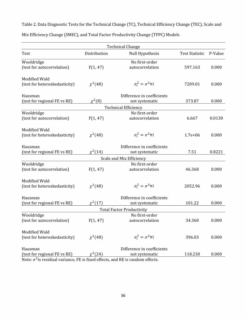
Our dataset is likely to be subject to heteroskedasticity, contemporaneous correlation across

panels, and auto-correlation within panels. We test for heteroskedasticity and autocorrelation for

each model using the Modified Wald test and Wooldridge test, respectively. Results show that we

cannot reject the presence of heteroskedasticity or autocorrelation in our dataset for any of the four

models. In addition, we perform the Hausman specification test (Hausman 1978), to determine

whether to use a random or fixed effects panel data estimator. Hausman test results support using a

fixed-effects estimator for three of our models (TC, SMEC and TFPC) and a random-effects

estimator for the TEC model. Results for these diagnostic tests are presented in Table 2. Following

Huffman and Evenson (2006) and Huffman (2009), we use regional (rather than state) fixed effects,

in the three models using the fixed-effects estimator, for seven geographic regions (Northeast,

Southeast, Central, Northern Plains, Southern Plains, Mountain, Pacific). These regions are based on

the 10 ERS regions with the New England region combined with the Northeast region, the

Appalachian region combined with the Southeast region, and the Lake States region combined with

the Corn Belt region. The Corn Belt region is treated as the baseline for comparison with the other

regions, so no dummy variable is included for this region.

We estimate all three component and TFPC models using the Prais-Winsten panel corrected

standard errors (PCSE) estimator with AR1 autocorrelation. As Beck and Katz (1995) document,

this approach works well with panel data when correcting for heteroskedasticity,

contemporaneous correlation across panels, and autocorrelation within panels.

20

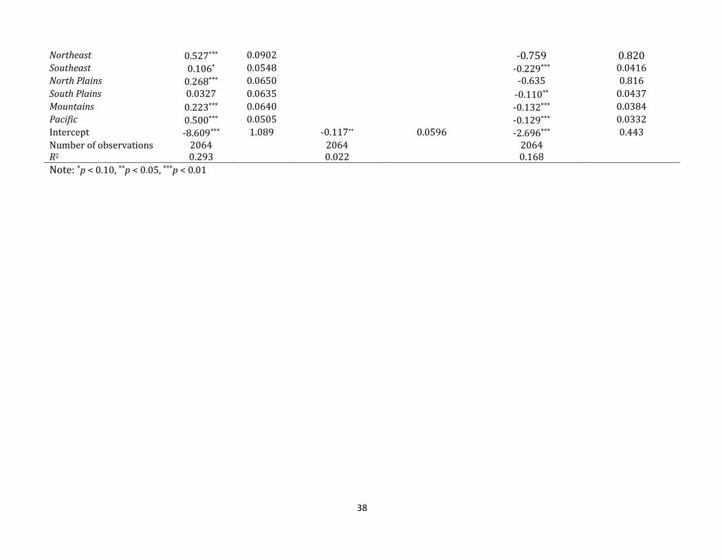
Results from the TFPC component models are reported in Table 3. The estimates are

reported in the three columns, technical change (TC), technical efficiency change (TEC) and scale

and mix efficiency change (SMEC), respectively.

Coefficient estimates of explanatory variables in the TC model are all significant at the 0.05

level except for education which is significant at the 0.10 level. These results show that education,

health care access, public research, public research spill-in, and private research all have a positive

effect on TC while private research spill-in has a negative effect on TC. Except for the Southern

Plains region, results show a statistically significant and positive difference between each of the

other regions and the Corn Belt region. These results show that public research conducted in other

states within the same geo-climate region (public research spill-in) has the largest effect on the

state’s TC. A 1 percent increase in public research spill-in results in a 0.42 percent increase in TC.

The next largest impact on TC comes from education with an elasticity of 0.16. This large education

elasticity is particularly noteworthy since it only measures the residual effect of education after

adjusting for educational differences in the labor force. These large elasticities are followed in turn

by public research, health care access, and private research. The negative elasticity of private

research spill-in on TC is quite large, -0.14.

These findings are consistent with Reimers and Klasen’s (2013) finding that education plays

an important role in productivity growth through enhancing better decision skills for farmers,

improved access to information, and faster adoption of new technologies. Our finding that research

investment, both within the state and public research by its regional neighbors, promote technical

change is consistent with Alston et al.’s (2011) and Plastina and Fulginiti’s (2012) findings of the

importance of public research and public research spill-in on agricultural productivity. What is new

about our findings is the discovery that health care access also plays a positive and significant role

in enhancing technical change. This broadens the set of options available to policy makers for

stimulating technical change and productivity growth in the agricultural sector.

21

Results from the TEC model show a negative and statistically significant effect of health care

access, family-to-total labor ratio, and damaging degree days in the central band of states and a

positive and statistically significant effect of extension and precipitation on TEC. Education, farm

size, and growing degree days do not have a significant effect. Although the estimated impacts of

health care access, family-to-total labor ratio, and damaging degree days are small, their negative

effects on TEC imply that it is positively affected by a decrease in health care access, relatively

larger hired labor work force, and less extreme temperatures. A possible explanation for the first

finding could be that limited health care access results in farmers hiring additional labor or other

service providers who may be in better health than they are. Although conjectural, this explanation

can be supported by the second finding which implies that family labor contributes more to

technical efficiency when it is augmented by additional hired labor. This could be due to less burden

on family labor enabling it to focus more on management thereby improving managerial efficiency

and improving decision making skills. Another possible explanation could be the level of

specialization – hired labor may be more skilled in the tasks they are hired to do and hence may be

more efficient than family labor. The negative relationship between damaging degree days and TEC

is consistent with Key and Sneeringer’s (2014) finding that heat stress has a negative effect on

technical efficiency on dairies in the U.S.

The SMEC model estimates reveal that farm size, precipitation (at the 0.10 level of

significance), growing degree days, and agro-temperature all have positive and statistically

significant impact on scale and mix efficiency change. Damaging degree days has a small but

significant negative impact on SMEC in the central band of states and a greater negative impact in

the southern band of states. Agro-precipitation also has a large and significant negative impact on

SMEC in the southern band of states. Agro-temperature has the largest impact on SMEC with a 1

percent increase resulting in 0.34 percent increase in SMEC in the central band of states. This

implies that an increase in long-term (50-year) average temperature has been beneficial for SMEC

22

in the mid-latitude states. This finding is not significantly different in either of the other bands of

states. This could be a result of farmers moving to more nearly optimal scale as the temperature has

increased (a little less than 2oF over the last century). Since growing degree days have a much

greater positive effect on SMEC than the negative effect of damaging degree days, another possible

explanation could be that the effect of additional growing degree days caused by the increase in

agro-temperature has more than offset the effect of additional damaging degree days.

The large positive impact on SMEC of agro-temperature is followed in turn by the negative

impact of agro-precipitation in the southern band of states, the positive impacts of growing degree

days, farm size, and precipitation, and the negative impact of damaging degree days. As expected,

growing degree days have a positive and statistically significant effect on SMEC as crops have more

exposure to optimal growing temperature while damaging degree days have a negative and

statistically significant effect on SMEC as exposure to adverse temperatures inhibits growth.

Damaging degree days have a larger effect in the warmer southern band than in the central band of

states. Additional precipitation generally contributes to plant growth and has a positive and

significant effect on SMEC. But in the southern band of states, where precipitation has been

increasing over the past century, additional long-term precipitation (agro-precipitation) has a

pronounced negative impact. An increase in average farm size increases SMEC by moving toward

more optimal scale. This finding is similar to the result of Paul et al. (2004) that small family farms

are generally less efficient in terms of their scale of operations than are large farms. Our results also

show that the 1983 PIK program negatively and significantly affected SMEC. The R2 values for all

our component models are low – 0.29, 0.02, and 0.17 for TC, TEC and SMEC respectively.

Estimates for the TFPC model are reported in Table 4. The TFPC model includes all

explanatory variables included in the component models. As with the component models, most

parameters are statistically significant. An increase in agro-temperature for the northern and

southern bands of states has the greatest impact on TFPC with elasticities of 0.73 and 0.65,

23

respectively. They are followed by decreasing the family-to-total labor ratio and terms of trade,

with elasticities of -0.28 and -0.27, respectively. Increasing growing degree days in the northern

band of states and agro-temperature in the central band have a positive impact on TFPC, each with

an elasticity of 0.23. Increases in public research, public research spill-in, growing degree days as

well as agro-precipitation and precipitation in the central band of states, and health care access also

have positive impacts on TFPC, with elasticities ranging from 0.05 to 0.15. Private research and

damaging degree days in the southern and central bands of states have negative impacts on TFPC,

with elasticities of -0.01 to -0.04.

Health care access, public research, and public research spill-in all have plausible signs –

positive and statistically significant. Public research and public research spill-in results are

consistent with prior findings of the pivotal role public research plays in increasing agricultural

productivity (Huffman and Evenson 2006; Plastina and Fulginiti 2012). Health care access results

are consistent with our expectation of the impact of human capital on agricultural productivity

through enabling farmers to embrace new innovations as well as to avoid disruption to their

decision making skills due to inadequate access to health care.

Although somewhat surprising, the finding that a decrease in private research results in an

increase in TFP is similar to results from Huffman (2009). Since private research is conducted

mainly by agricultural input suppliers, farmers’ investment in these innovations is more costly and

their adoption may limit the scale and mix of inputs farmers use. Huffman (2009) finds that private

and public research are substitutes. Since innovations from public research are likely to be more

affordable than those from private research, less private research and more public research

appears to be beneficial to productivity of the agricultural sector. A decrease in the terms of trade

(output to input price ratio) creates incentive to conserve inputs and increase average productivity,

a finding that is consistent with O’Donnell (2010). The findings of both the TFPC and TEC equations

are consistent in finding that an increase in hired labor makes all labor more productive.

24

Parameter estimates for most of the weather and agro-climate variables are statistically

significant and have generally plausible signs. The only exception, which is the same as in the SMEC

model, is that agro-temperature has a very large positive effect on TFPC for all bands of states.

Some prior research (e.g. Lobell and Field 2007; Hatfield et al. 2011) find a negative relationship

between an increase in average growing temperature and yields. However, adaptation such as early

planting, conservation tillage, and improved planting equipment may be helping to drive gains in

yields from this long-term increase in temperature. For example, Sacks and Kucharik (2011) note

that corn and soybeans have been planted increasingly earlier over the past 30 years. As expected,

an increase in growing degree days (in the northern and central bands) results in an increase in

TFPC as crops have more exposure to optimal growth temperature. Also the negative and

statistically significant effect of damaging degree days on TFPC is consistent with expectations.

Damaging degree days hinder crop growth and lead to a decrease in output. And, the marginal

effect is greatest in the warmest region. This result is similar to McCarl et al.’s (2008) finding.

Neither education nor extension have a significant effect on TFPC. With regard to education,

this implies that the adjustment of the labor input series to account for changes in education fully

exhausts the educational effect on TFPC. The insignificant effect of extension is a greater surprise.

Comparing TFPC elasticities

We next compare TFPC elasticities calculated from the component models to those obtained

directly from the estimated TFPC model. These elasticities are presented in Table 5. We report

elasticities only for the 15 continuous variables without dummy variable interaction.

Most of the qualitative implications of the elasticities from the components are consistent

with those from the elasticities calculated directly from the TFPC model. Parameter estimates for

health care access, public research, public research spill-in, family-to-total labor ratio, precipitation,

growing degree days, damaging degree days, and agro-temperature all have the same sign and are

statistically significant in both approaches. Private research is statistically significant in both

25

approaches but has a different sign, and education, private research spill-in, farm size, terms of

trade, and agro-precipitation are significant in only one of the two approaches. Extension remains

insignificant regardless of which approach is used. Additionally, there is a big difference in

magnitude of a few elasticities between the two approaches. For example, public research spill-in

has the highest elasticity from the component models and is over four times as large as when it is

computed directly from the TFPC model. The opposite is true for the family-to-total labor ratio and

precipitation which are 28 and eight times as large, respectively, in the directly estimated TFPC

model than when calculated from the component models.

To check the robustness of our results to the choice of functional form, we also re-estimate

the TFPC model in linear form and calculate elasticities at the data means to compare with

elasticities from the logarithmic TFPC model. Results are presented in Table 6. Again, most of the

qualitative implications are the same. Eight elasticities are statistically significant in both models

and have the same sign, four elasticities are insignificant in both specifications, three elasticities are

significant in only one model and one elasticity is significant in both models but has a different sign.

With the exception of public research spill-in, the elasticity estimates that are significant in both

specifications with the same sign are similar in magnitude. Thus, the results do not appear to be

highly sensitive to our choice of functional form.

Conclusions

This article has sought a deeper understanding of the drivers of total factor productivity change

(TFPC) in U.S. agriculture by examining the drivers of the components of TFPC – technical change,

technical efficiency change, and scale and mix efficiency change. Building on O’Donnell’s (2012)

recent decomposition of U.S. agricultural TFPC into these components, we use economic theory,

previous literature, and logic to identify factors potentially driving each component. We also

include a broader set of factors potentially driving TFPC than most previous analyses by including

health care access, weather, and agro-climatic conditions. We use a state-level panel dataset for the

26

48 contiguous states for the period 1961-2003 and examine the robustness of implications from the

component models with a directly estimated TFPC model using alternative functional forms.

We find that public research conducted within the state as well as spill-ins from the same

geo-climatic region, education, and health care access are the main factors driving technical change,

which in turn is the dominant component of TFP change. In fact, technical change has much greater

impact on TFP change than profit-maximizing output and input choices of firms. These results are

consistent with the notion that technical change comes from innovation resulting from R&D and

improved human capital which helps in adoption of new innovations. We find private research to

have mixed effects on technical change, depending on whether it is patented within the state or in

other states in the same geo-climatic region.

Although technical efficiency change is very stable over the data period, changes that do

occur are driven primarily by extension, the ratio of family-to-total labor, health care access, and

weather (except growing degree days). Technical efficiency change increases as health care access

decreases. This unexpected result could be due to farmers hiring additional labor or other service

providers who may be in better health than they are. Although theoretical expectations are

ambiguous, the impact of the ratio of family-to-total labor is also opposite to conventional wisdom

in that technical efficiency change increases as this ratio decreases. This could be because hired

labor provides higher skill levels in specialized tasks than do family labor, and/or because family

labor focuses more on management thereby improving managerial efficiency and decision making

skills when more labor is hired. Education, farm size, and growing degree days do not significantly

affect technical efficiency.

Scale and mix efficiency change exhibits considerable fluctuation over the data period but,

like technical efficiency change, has little trend. It is affected most by farm size, weather, and agro-

climatic conditions. Rising long-term temperatures and larger farm size are both beneficial for scale

27

and mix efficiency change. Government policies such as the 1983 PIK program also have an impact

on farmers’ scale and mix efficiency change.

With few exceptions, elasticities estimated with the TFPC model are qualitatively the same

and similar in magnitude to those calculated from the component models. They are also largely

consistent with elasticities computed at data means from a linear TFP model. These results

substantiate the important role of public research, health care access, family-to-total labor ratio,

weather, and agro-climatic conditions on TFPC of U.S. agriculture.

The results from this study contribute to the policy debate about how to surmount the

recent downturn in agricultural productivity. Technical change is the primary component driving

total factor productivity growth. Public policy can impact its growth rate most through investment

in public research and facilitating additional education and health care access in rural areas.

28

References

Alston, J.M., M.A. Andersen, J.S. James, and P.G. Pardey. 2010. Persistence Pays: U.S. Agricultural Productivity

Growth and the Benefits from Public R&D Spending. New York: Springer.

——. 2011. The Economic Returns to U.S. Public Agricultural Research. American Journal of Agricultural

Economics 93(5):1257-1277.

Alston, J.M., B. Craig, and P.G. Pardey. 1998. Dynamics in the Creation and Depreciation of Knowledge, and

the Returns to Research. International Food Policy Research Institute EPTD Discussion Paper No. 35.

Ball, V.E. 2005. Detailed Agricultural Labor Data by State, 1960-1999. Unpublished. U.S. Department of

Agriculture. ERS, Washington.

——. 2013. Detailed Agricultural Labor Data by State, 1960-2004. Unpublished. U.S. Department of

Agriculture. ERS, Washington.

Ball, V.E., J-C. Bureau, R. Nehring, and A. Somwaru. 1997. Agricultural Productivity Revisited. American

Journal of Agricultural Economics 79(4):1045-1063.

Ball, V.E., F. Gollop, A. Kelly-Hawke, and G. Swinand. 1999. Patterns of Productivity Growth in the U.S. Farm

Sector: Linking State and Aggregate Model. American Journal of Agricultural Economics 81(1):164-

79.

Ball, V.E., D. Schimmelpfennig, and S.L. Wang. 2013. Is U.S. Agricultural Productivity Growth Slowing?

Applied Economic Perspectives and Policy 35(3):435-450.

Beck, N. and J.N. Katz. 1995. What to Do (and Not to Do) with Time-Series Cross-Section Data. American

Political Science Review 89:634-647.

Bureau of Health Professions/National Center for Health Workforce Analysis. 2013. The Area Health

Resource File (ARHF), Rockville, Maryland.

Capalbo, S.M. 1988. Measuring the Components of Aggregate Productivity Growth in U.S. Agriculture.

Western Journal of Agricultural Economics 13(1): 53-62.

29

Chen, A. Z., W.E Huffman, and S. Rozelle. 2003. Technical Efficiency of Chinese Grain Production: A

Stochastic Production Frontier Approach. Paper presented at the American Agricultural Economics

Association Annual Meeting, Montreal, Canada, July 27-30.

Chhetri, N. B., W.E. Easterling, A. Ternando, and L. Mearns. 2010. Modeling Path Dependence in Agricultural

Adaptation to Climate Variability and Change. Annals of the Association of American Geographers

100:894–907.

Coelli, T. J., D. S. P. Rao, C. J. O’Donnell, and G. E. Battese. 2005. An Introduction to Efficiency and Productivity

Analysis, 2nd ed. New York: Springer.

Cummins, D.J. and X. Xie. 2013. Efficiency, Productivity, and Scale Economies in the U.S. Property-Liability

Insurance Industry. Journal of Productivity Analysis 39:141-164.

Deschênes, O. and M. Greenstone. 2007. The Economic Impacts of Climate Change: Evidence from

Agricultural Output and Random Fluctuations in Weather. American Economic Review 97(1):354-

385.

Farrell, M.J. 1957. The Measurement of Productive Efficiency. Journal of the Royal Statistical Society Series A

(General) 120(3):253-282.

Fuglie, K.O. and P.W. Heisey. 2007. Economic Returns to Public Agricultural Research. Economic Brief

Number 10. U.S. Department of Agriculture, Economic Research Service.

Fuglie, K.O., J.M. MacDonald, and V.E. Ball. 2007. Productivity Growth in U.S. Agriculture. Economic Brief

Number 9. U.S. Department of Agriculture, Economic Research Service.

Hatfield, J.L., K.J. Boote, B.A. Kimball, L.H. Ziska, R.C. Izaurralde, D. Ort, A.M. Thomson, and D. Wolfe, 2011.

Climate Impacts on Agriculture: Implications for Crop Production. Agronomy Journal 103(2): 351-

370.

Hausman, J.A. 1978. Specification Tests in Econometrics. Econometrica 46(6):1251-1271.

30

Huffman W.E. 2009. “Measuring Public Agricultural Research Capital and Its Contribution to State

Agricultural Productivity.” Iowa State University, Department of Economics, Working Paper No.

09022.

Huffman, W.E. and R.E. Evenson. 2006. Do Formula or Competitive Grant Funds Have Greater Impacts On

State Agricultural Productivity? American Journal of Agricultural Economics 88(4): 783-798.

Huffman, W.E. and P. Orazem. 2004. “The Role of Agriculture and Human Capital in Economic Growth:

Farmers, Schooling, and Health.” Iowa State University, Department of Economics, Working Paper

No. 04016.

James, J.S., J.M. Alston, P.G. Pardey, and M.A. Andersen. 2009. Structural Changes in U.S. Agricultural

Production and Productivity. Choices 24 (4).

Jin, S., H. Ma, J. Huang, R. Hu, and S. Rozelle. 2010. Productivity, Efficiency and Technical Change: Measuring

the Performance of China’s Manufacturing Agriculture. Journal of Productivity Analysis 33(3):191-

207.

Johnson, D.K.N. 2013. USHiPS: The U.S. Historical Patent Set. (February). Personal communication.

Key, N. and S. Sneeringer. 2014. Potential Effects of Climate Change on the Productivity of U.S. Dairies.

American Journal of Agricultural and Applied Economics doi:10.1093/ajae/aau002.

Key, N. and W. McBride. 2007. The Changing Economics of U.S. Hog Production. Economic Research Report

52. U.S. Department of Agriculture, Economic Research Service.

Kuosmanen, T. and T. Sipiläinen. 2009. Exact decomposition of the Fisher ideal total factor productivity

index. Journal of Productivity Analysis 31:137-150.

Liu, Y., C.R. Shumway, R. Rosenman, and V.E. Ball. 2009. Productivity Growth and Convergence in US

Agriculture: New Cointegration Panel Data Results. Applied Economics 43(1):91-102.

Lobell, D.B. and C.B. Field, 2007. Global Scale Climate–Crop Yield Relationships and the Impacts of Recent

Warming. Environmental Research Letters 2(1): 014002.

Loureiro, M. L. 2009. Farmers' Health and Agricultural Productivity. The Journal of the International

Association of Agricultural Economists 40(4):381-388.

31

Mayen, C.D., J.V. Balagtas, and C.E. Alexander. 2010. Technology Adoption and Technical Efficiency:

Organic and Conventional Dairy Farms in the United States. American Journal of Agricultural

Economics 92(1): 181-195.

McCarl, B. A., X. Villavicencio, and X. Wu. 2008. Climate Change and Future Analysis: Is Stationarity

Dying? American Journal of Agricultural Economics 90(5):1241-1247.

McCunn, A. and W.E. Huffman. 2000. Convergence in U.S. Productivity Growth for Agriculture: Implications

of Interstate Research Spillovers for Funding Agricultural Research. American Journal of

Agricultural Economics 82(2):370-388.

Mullen, J. 2007. Productivity Growth and the Returns from Public Investment in R&D in Australian

Broadacre Agriculture. Australian Journal of Agricultural and Resource Economics 51 (4): 359–84.

National Climatic Data Center/National Oceanic and Atmospheric Administration (NCDC/NOAA). 2013.

http://www1.ncdc.noaa.gov/pub/data/cirs/. Accessed March.

O’Donnell, C.J. 2008. An Aggregate Quantity-Price Framework for Measuring and Decomposing Productivity

and Profitability Change. Centre for Efficiency and Productivity Analysis, University of Queensland,

Working Paper Series No. WP07/2008.

——. 2010. Measuring and Decomposing Agricultural Productivity and Profitability Change. Australian

Journal of Agricultural and Resource Economics 54:527-560.

——. 2012. Non-Parametric Estimates of the Components of Productivity and Profitability Change in U.S.

Agriculture. American Journal of Agricultural Economics 94(4):873-890.

——.2014. An Economic Approach to Identifying the Drivers of Productivity Change in the Market Sectors

of the Australian Economy, University of Queensland, Working Paper Series No. WP02/2014.

Paul, C.M., R. Nehring, D. Banker, and A. Somwaru. 2004. Scale Economies and Efficiency in U.S. Agriculture:

Are Traditional Farms History? Journal of Productivity Analysis 22:185–205

Plastina, A. and L. Fulginiti. 2012. Rates of Return to Public Agricultural Research in 48 U.S. States. Journal

of Productivity Analysis 37(2):95-113.

32

Reimers, M. and S. Klasen. 2013. Revisiting the Role of Education for Agricultural Productivity. American

Journal of Agricultural Economics 95(1):131-152.

Ritchie, J. T. and D.S. NeSmith. 1991. Temperature and Crop Development. In J. Hanks and J.T. Ritchie ed.

Modeling Plant and Soil Systems. Madison WI: American Society of Agronomy, pp. 5-29.

Roberts, M.J. 2013. Personal Communication. County-Level Degree Day Aggregates of Fine-Scale Data

Available at http://www2.hawaii.edu/~mjrobert/main/Links.html Accessed August.

Roberts, M.J., W. Schlenker, and J. Eyer. 2012. Agronomic Weather Measures in Econometric Models of Crop

Yield with Implications for Climate Change. American Journal of Agricultural Economics 95(2):236-

243.

Ruttan, V.W. 2002. Productivity Growth in World Agriculture: Sources and Constraints. The Journal of

Economic Perspectives 16(4):161-184.

Sacks, W.J. and C.J. Kucharik, 2011. Crop Management and Phenology Trends in the U.S. Corn Belt: Impacts

on Yields, Evapotranspiration and Energy Balance. Agricultural and Forest Meteorology 151(7):

882-894.

Schlenker, W., W.M. Hanemann, and A.C. Fisher. 2006. The Impact of Global Warming on U.S. Agriculture:

An Econometric Analysis of Optimal Growing Conditions. Review of Economics and Statistics 88(1):

113-125.

Stewart, B., T. Veeman, and J. Unterschutz. 2009. Crops and Livestock Productivity Growth in the Praires:

The Impacts of Technical Change and Scale. Canadian Journal of Agricultural Economics 57:379-394.

Tian, W. and G. H. Wan. 2000. Technical Efficiency and Its Determinants in China’s Grain Production.

Journal of Productivity Analysis 13:159–174.

U.S. Department of Agriculture/Economic Research Service (USDA/ERS). 1960-2003. Farm Balance Sheets

Annual Series. http://www.ers.usda.gov/Data/FarmBalanceSheets/50STBSHT.htm.

——. 2003. Urban Influence Codes. http://www.ers.usda.gov/Data/UrbanInfluenceCodes/.

33

——. 2013. Table 23. Price Indices and Implicit Quantities of Farm Outputs and Inputs by State, 1960-

2004. Available at http://www.ers.usda.gov/data-products/agricultural-productivity-in-the-

us.aspx#.U366yNJdX_k. Accessed March, 2013.

Wang, S.L., P.W. Heisey, W.E. Huffman and K.O. Fuglie. 2013. Public R&D, Private R&D, and U.S. Agricultural

Productivity Growth: Dynamic and Long-Run Relationships. American Journal of Agricultural

Economics 95(5):1287-1293.

Yee, J. and M.C. Ahearn. 2005. Government Policies and Farm Size: Does the Size Concept Matter? Applied

Economics 37: 2231-2238.

Yee, J., M.C. Ahearn, and W. Huffman. 2004. Links Among Farm Size Productivity, Off-Farm Work, and Farm

Size in the Southeast. Journal of Agricultural and Applied Economics 36:591-603.

34

Figure 1. U.S. agricultural total factor productivity (TFPC), technical change (TC), technical efficiency

change (TEC) and scale and mix efficiency change (SMEC) 1961-2003

0.6

0.7

0.8

0.9

1

1.1

1.2

1.3

1.4

1.519

61

1963

1965

1967

1969

1971

1973

1975

1977

1979

1981

1983

1985

1987

1989

1991

1993

1995

1997

1999

2001

2003

Inde

x

Year

TFPC

TC

TEC

SMEC

35

Table 1. Summary Statistics

Variable Variable Code Unit Mean

Standard Deviation

Minimum Value

Maximum Value

Total factor productivity change

TFPC index 0.982 0.301 0.401 2.155

Technical change TC index 1.072 0.272 0.626 1.869 Technical efficiency change TEC index 0.990 0.034 0.710 1.000 Scale and mix efficiency change

SMEC index 0.904 0.159 0.407 1.123

Education Ed index 2.860 0.587 1.411 3.830 Health care access Hs index 12.013 5.210 4.757 37.318 Public research investment Rpub $M 15.349 13.775 1.040 101.167 Public research spill-in RpubS $M 63.947 34.027 5.960 171.737 Private research Rpri patents 24.187 36.128 0.138 227.997 Private research spill-in RpriS patents 103.880 93.571 0.773 352.382 Extension Ext FTE prof. staff 137.157 97.077 0.028 562.310 Farm size Fs $1,000 per farm 353.230 312.637 15.116 3496.001 Family-to-total labor ratio Ftlratio index 0.706 0.161 0.112 0.934 Terms of trade TT index 0.751 0.264 0.279 1.363 Precipitation Precp cm 36.188 14.958 5.370 80.580 Growing degree days GDD oF days 2317.183 722.394 1152.947 4456.675 Damaging degree days DDD oF days 16.586 29.677 0.0001 235.083 Agro-temperature Agrotemp oF 60.969 6.534 50.616 75.663 Agro-precipitation Agroprecp cm 35.233 13.605 8.180 58.220

36

Table 2. Data Diagnostic Tests for the Technical Change (TC), Technical Efficiency Change (TEC), Scale and

Mix Efficiency Change (SMEC), and Total Factor Productivity Change (TFPC) Models

Technical Change Test Distribution Null Hypothesis Test Statistic P-Value

Wooldridge (test for autocorrelation) F(1, 47)

No first-order autocorrelation 597.163 0.000

Modified Wald (test for heteroskedasticity) 𝜒2(48) 𝜎𝑖2 = 𝜎2∀𝑖 7209.01 0.000 Hausman (test for regional FE vs RE) 𝜒2(8)

Difference in coefficients not systematic 373.87 0.000

Technical Efficiency Wooldridge (test for autocorrelation) F(1, 47)

No first-order autocorrelation 6.667 0.0130

Modified Wald (test for heteroskedasticity) 𝜒2(48) 𝜎𝑖2 = 𝜎2∀𝑖 1.7e+06 0.000

Hausman (test for regional FE vs RE) 𝜒2(14)

Difference in coefficients not systematic 7.51 0.8221

Scale and Mix Efficiency Wooldridge (test for autocorrelation) F(1, 47)

No first-order autocorrelation 46.368 0.000

Modified Wald (test for heteroskedasticity) 𝜒2(48) 𝜎𝑖2 = 𝜎2∀𝑖 2052.96 0.000

Hausman (test for regional FE vs RE) 𝜒2(17)

Difference in coefficients not systematic 101.22 0.000

Total Factor Productivity Wooldridge (test for autocorrelation) F(1, 47)

No first-order autocorrelation 34.360 0.000

Modified Wald (test for heteroskedasticity) 𝜒2(48) 𝜎𝑖2 = 𝜎2∀𝑖 396.03 0.000

Hausman (test for regional FE vs RE) 𝜒2(24)

Difference in coefficients not systematic 118.230 0.000

Note: 𝜎2is residual variance, FE is fixed effects, and RE is random effects.

37

Table 3. Prais-Winsten Estimates for Technical Change (TC), Technical Efficiency (TEC), and Scale and Mix Efficiency (SMEC)

Regressor

Dependent Variable: ln(TC)

Dependent Variable: ln(TEC)

Dependent Variable: ln(SMEC)

Estimated Coefficient

Standard Error

Estimated Coefficient

Standard Error Estimated Coefficient Standard Error

ln(Education) 0.155* 0.0864 -0.00488 0.00823 ln(Health care access) 0.0345** 0.0152 -0.00830* 0.00434 ln(Public research) 0.0799*** 0.0142 ln(Public research spill-in)

0.416*** 0.0625

ln(Private research) 0.0277*** 0.00976 ln(Private research spill-in)

-0.137*** 0.0348

ln(Extension) 0.00353* 0.00208 ln(Farm size) 0.00122 0.00321 0.0470** 0.0201 ln(Family-to-total labor ratio)

-0.0103** 0.00427

ln(Terms of trade) 0.00142 0.0295 ln(Precipitation) 0.00604** 0.00282 0.0262* 0.0146 ln(Growing degree days) 0.0112 0.00793 0.110*** 0.0307 ln(Damaging degree days) -0.00290*** 0.000602 -0.00897*** 0.00216 ln(Agro-temperature) 0.337** 0.142 ln(Agro-precipitation) 0.0251 0.0365 ln(Private research) *D96 -0.0129*** 0.00397 ln(Private research spill-in) *D96

0.0110** 0.00539

(lnGDD)*Ds -0.000529 0.000716 -0.0292 0.119 (lnGDD)*Dn 0.00000441 0.000508 -0.0460 0.0605 (lnDDD)*Ds 0.00221** 0.00107 -0.0230*** 0.00800 (lnDDD)*Dn 0.00267*** 0.000779 0.00384 0.00355 ln(Agro-precipitation)*Ds -0.247*** 0.0794 ln(Agro-precipitation)*Dn -0.000618 0.182 ln(Agro-temperature)*Ds 0.286 0.233 ln(Agro-temperature)*Dn 0.251 0.244 D83 -0.0797*** 0.0187

38

Northeast 0.527*** 0.0902 -0.759 0.820 Southeast 0.106* 0.0548 -0.229*** 0.0416 North Plains 0.268*** 0.0650 -0.635 0.816 South Plains 0.0327 0.0635 -0.110** 0.0437 Mountains 0.223*** 0.0640 -0.132*** 0.0384 Pacific 0.500*** 0.0505 -0.129*** 0.0332 Intercept -8.609*** 1.089 -0.117** 0.0596 -2.696*** 0.443 Number of observations 2064 2064 2064 R2 0.293 0.022 0.168 Note: *p < 0.10, **p < 0.05, ***p < 0.01

39

Table 4. Prais-Winsten Estimates for Total Factor Productivity Change (TFPC) Regressor

Dependent Variable: ln(TFPC)

Estimated Coefficient

Standard Error ln(Education) 0.0883 0.0643 ln(Health care access) 0.0532** 0.0221 ln(Public research) 0.149*** 0.0148 ln(Public research spill-in) 0.0931** 0.0405 ln(Private research) -0.0275*** 0.00767 ln(Private research spill-in) 0.0148 0.0215 ln(Extension) 0.00461 0.00737 ln(Farm size) 0.0248 0.0227 ln(Family-to-total labor ratio) -0.284*** 0.0252 ln(Terms of trade) -0.271*** 0.0442 ln(Precipitation) 0.0534*** 0.0175 ln(Growing degree days) 0.121*** 0.0316 ln(Damaging degree days) -0.0104*** 0.00259 ln(Agro-temperature) 0.232* 0.132 ln(Agro-precipitation) 0.0957** 0.0413 ln(Private research) *D96 -0.00469 0.00658 ln(Private research spill-in) *D96 0.00827 0.00710 (lnGDD)*Ds -0.121 0.114 (lnGDD)*Dn 0.109* 0.0558 (lnDDD)*Ds -0.0309*** 0.00728 (lnDDD)*Dn 0.000826 0.00332 ln(Agro-precipitation)*Ds -0.174** 0.0705 ln(Agro-precipitation)*Dn -0.104 0.143 ln(Agro-temperature)*Ds 0.420* 0.226 ln(Agro-temperature)*Dn 0.499*** 0.172 D83 -0.0854*** 0.0261 Northeast -2.384*** 0.728 Southeast -0.0953*** 0.0367 North Plains -2.368*** 0.716 South Plains -0.189*** 0.0452 Mountains 0.0238 0.0491 Pacific 0.0413 0.0369 Intercept -6.972*** 0.886 Number of observations 2064 R2 0.643 Note: *p < 0.10, **p < 0.05, ***p < 0.01

40

Table 5. TFPC Elasticities Calculated from Component Models and Estimated Directly from the Total

Factor Productivity Change Model

Component Models TFPC Model Elasticity

Standard

Error Elasticity

Standard

Error ln(Education) 0.150* 0.0864 0.0883 0.0643 ln(Health care access) 0.0262* 0.0158 0.0532** 0.0221 ln(Public research) 0.0799*** 0.0142 0.149*** 0.0148 ln(Public research spill-in) 0.416*** 0.0625 0.0931** 0.0405 ln(Private research) 0.0277*** 0.00976 -0.0275*** 0.00767 ln(Private research spill-in) -0.137*** 0.0348 0.0148 0.0215 ln(Extension) 0.00353 0.00208 0.00461 0.00737 ln(Farm size) 0.0482** 0.0204 0.0248 0.0227 ln(Family-to-total labor ratio) -0.0103** 0.00427 -0.284*** 0.0252 ln(Terms of trade) 0.000239 0.03 -0.271*** 0.0442 ln(Precipitation) 0.00604** 0.00282 0.0534*** 0.0175 ln(Growing degree days) 0.121*** 0.0317 0.121*** 0.0316 ln(Damaging degree days) -0.0119*** 0.00224 -0.0104*** 0.00259 ln(Agro-temperature) 0.337** 0.142 0.232* 0.132 ln(Agro-precipitation) 0.0251 0.0365 0.0957** 0.0413 Note: *p < 0.10, **p < 0.05, ***p < 0.01

41

Table 6. TFPC Elasticities Estimated Directly from the Logarithmic TFPC Model and Calculated at

Data Means from the Linear TFP Model

ln(TFPC) Model Linear TFPC Model Elasticity Standard

Error Elasticity Standard

Error Education 0.0883 0.0643 -0.0054 0.0773 Health care access 0.0532** 0.0221 0.0735*** 0.0223 Public research 0.149*** 0.0148 0.1558*** 0.0159 Public research spill-in 0.0931** 0.0405 0.1972*** 0.0430 Private research -0.0275*** 0.00767 -0.0228*** 0.0083 Private research spill-in 0.0148 0.0215 -0.0458 0.0282 Extension 0.00461 0.00737 0.0132 0.0146 Farm size 0.0248 0.0227 0.0055 0.0041 Family-to-total labor ratio -0.284*** 0.0252 -0.3535*** 0.0355 Terms of trade -0.271*** 0.0442 -0.2034*** 0.0416 Precipitation 0.0534*** 0.0175 0.0493*** 0.0187 Growing degree days 0.121*** 0.0316 -0.0383 0.0364 Damaging degree days -0.0104*** 0.00259 0.0057 0.0045 Agro-temperature 0.232* 0.132 0.1169 0.1350 Agro-precipitation 0.0957** 0.0413 0.1577*** 0.0600 Note: *p < 0.10, **p < 0.05, ***p < 0.01