c© 2011 Abhishek Gupta

CONTROL IN THE PRESENCE OF AN INTELLIGENT JAMMER WITH LIMITEDACTIONS

BY

ABHISHEK GUPTA

THESIS

Submitted in partial fulfillment of the requirementsfor the degree of Master of Science in Aerospace Engineering

in the Graduate College of theUniversity of Illinois at Urbana-Champaign, 2011

Urbana, Illinois

Advisers:

Professor Tamer BasarAssistant Professor Cedric Langbort

ABSTRACT

In this thesis, we consider three different problems related to control using communication channel as a

medium to transfer control signal in a networked control system. In particular, we are interested in control

in the presence of an intelligent and strategic jammer who is maliciously altering the control signal or

observation signal in the communication network connecting the controller and the plant.

The first formulation considers a dynamic zero-sum game between a controller and a jammer for two

different scenarios. The first player acts as a controller for a discrete time LTI plant, while the second player

acts to jam the communication between the controller and the plant. The number of jamming actions is

limited, which captures the energy constraint of the jammer. In the first scenario, the state of the plant is

unconstrained, while in the second scenario, the state of the plant is constrained by a threshold at all time

steps, and both the jammer and the controller try to maintain the state of the plant below that threshold.

We determine saddle-point equilibrium control and jamming strategies for these two games under the full

state, total recall information structure for both players, and show that the jammer acts according to a

threshold-based policy at each decision step. Various properties of the threshold functions are derived and

complemented by numerical simulation studies.

The next problem considers a model of stealthy attack on a networked control system by formulating

a static zero-sum game among four players. The three players constitute a team of encoder, decoder and

controller for a scalar discrete time linear plant, while the fourth player acts to flip the bits of the binary

encoded observation signal of the communication channel between the plant and the controller. We are inter-

ested in characterizing the possible encoding/decoding/control defense strategies available to the controller

and for simplicity, we model it for a scalar discrete time system with only one time step. We further assume

that the communication channel has finite bandwidth, and that the observation and control signals have

finite codelengths. We determine the saddle-point equilibrium control and jamming strategies for this game

when the controller’s strategy space is restricted to quantization-based policies, and show that the resulting

performance compares favorably to universal lower bounds obtained from rate-distortion theory. We also

provide a necessary and sufficient condition on the minimum number of bits that are required to drive the

cost to zero for this one step control problem in the presence of a jammer.

ii

There are three births of a man; first as a child, second after education and third after death.

Dr. S. Radhakrishnan

Indian Philosophy - Vol. I

To my parents, sister Shubham and brother Shubhankar

iii

ACKNOWLEDGMENTS

I would like to thank my advisors Prof. Tamer Basar and Prof. Cedric Langbort for their constant advice and

feedback throughout my research. Our meetings were insightful and thought provoking and I have learned

a lot about research from them. I could deepen my understanding of control theory, refresh motivations

towards research and acquire new insights through these meetings.

Prof. Langbort has always amazed me with his patience. His constructive feedback on various facets of

research have made my thought process more structured and clear. Prof. Basar’s book - “Dynamic Non-

cooperative Game Theory” has been an excellent reference for me throughout my research. I am also indebted

to the professors at IIT Bombay and here at UIUC, from whom I have learned a lot in the classes as well as

through personal interaction during leisure hours.

I would like to acknowledge AFOSR Grant FA9550-09-1-0249 and AFOSR grant for MURI - ”Multi-Layer

and Multi-Resolution Networks of Interacting Agents in Adversarial Environments” for full support during

my Master’s degree.

I am very thankful to my research group Nathan, Ali, Sourabh, Takashi and Albert for helping me out

at various stages of my research and being an excellent company. Ankur, Anupama, Ashish, Aditya, Dar-

shan, Zeba and Nihal are great friends and a constant source of motivation in the past two years. I couldn’t

have done so much without their support. Himanshu, Harshad, Amod, Ankita, Aditi and Vandana have

been always supportive which makes me lucky to have them as my friends. I am deeply indebted to my

parents, sister and brother for their love and support in my life.

iv

TABLE OF CONTENTS

LIST OF FIGURES . . . . . . . . . . . . . . . . . . . . . . . . . . . . . . . . . . . . . . . . . . . . . . vi

CHAPTER 1 INTRODUCTION . . . . . . . . . . . . . . . . . . . . . . . . . . . . . . . . . . . . . . 11.1 Previous Work . . . . . . . . . . . . . . . . . . . . . . . . . . . . . . . . . . . . . . . . . . . . 31.2 Overview of Chapters . . . . . . . . . . . . . . . . . . . . . . . . . . . . . . . . . . . . . . . . 4

CHAPTER 2 JAMMING ATTACKS . . . . . . . . . . . . . . . . . . . . . . . . . . . . . . . . . . . . 62.1 Problem Formulation . . . . . . . . . . . . . . . . . . . . . . . . . . . . . . . . . . . . . . . . . 62.2 Solution Approach . . . . . . . . . . . . . . . . . . . . . . . . . . . . . . . . . . . . . . . . . . 92.3 Notation . . . . . . . . . . . . . . . . . . . . . . . . . . . . . . . . . . . . . . . . . . . . . . . . 11

CHAPTER 3 OPTIMAL CONTROL WITHOUT STATE CONSTRAINTS . . . . . . . . . . . . . . 133.1 The M = 1, N = 3 case . . . . . . . . . . . . . . . . . . . . . . . . . . . . . . . . . . . . . . . 133.2 A General Case with M = 1 . . . . . . . . . . . . . . . . . . . . . . . . . . . . . . . . . . . . . 193.3 General Case . . . . . . . . . . . . . . . . . . . . . . . . . . . . . . . . . . . . . . . . . . . . . 263.4 Multidimensional State Space . . . . . . . . . . . . . . . . . . . . . . . . . . . . . . . . . . . . 293.5 Numerical Simulations . . . . . . . . . . . . . . . . . . . . . . . . . . . . . . . . . . . . . . . . 31

CHAPTER 4 OPTIMAL CONTROL WITH STATE CONSTRAINTS . . . . . . . . . . . . . . . . . 344.1 Main Result . . . . . . . . . . . . . . . . . . . . . . . . . . . . . . . . . . . . . . . . . . . . . . 344.2 The M=1, N=2 case . . . . . . . . . . . . . . . . . . . . . . . . . . . . . . . . . . . . . . . . . 364.3 Discussion on Earlier Results . . . . . . . . . . . . . . . . . . . . . . . . . . . . . . . . . . . . 394.4 Numerical Simulations . . . . . . . . . . . . . . . . . . . . . . . . . . . . . . . . . . . . . . . . 44

CHAPTER 5 ONE STEP CONTROL WITH FINITE CODELENGTH . . . . . . . . . . . . . . . . 475.1 Problem Formulation . . . . . . . . . . . . . . . . . . . . . . . . . . . . . . . . . . . . . . . . . 475.2 Binning Based Strategies and an Upper Bound . . . . . . . . . . . . . . . . . . . . . . . . . . 495.3 A Lower Bound using Rate Distortion Theory . . . . . . . . . . . . . . . . . . . . . . . . . . . 615.4 Summary . . . . . . . . . . . . . . . . . . . . . . . . . . . . . . . . . . . . . . . . . . . . . . . 64

CHAPTER 6 CONCLUSION . . . . . . . . . . . . . . . . . . . . . . . . . . . . . . . . . . . . . . . . 656.1 Future Work . . . . . . . . . . . . . . . . . . . . . . . . . . . . . . . . . . . . . . . . . . . . . 65

CHAPTER 7 REFERENCES . . . . . . . . . . . . . . . . . . . . . . . . . . . . . . . . . . . . . . . . 67

v

LIST OF FIGURES

2.1 Control in the presence of an intelligent jammer. . . . . . . . . . . . . . . . . . . . . . . . . . 72.2 A portion of the extended state space. . . . . . . . . . . . . . . . . . . . . . . . . . . . . . . . 10

3.1 Graph of function τ(1,3)(x) for A = 2.5 and σw = 1. . . . . . . . . . . . . . . . . . . . . . . . . 193.2 Extended state space for a general stage. Here “J” means that the jammer is active at

this time instant and “C” means that the controller is active at this time instant. . . . . . . . 263.3 Region showing the union of the sets in which the jammer jams and does not jam as a

function of horizon length N . . . . . . . . . . . . . . . . . . . . . . . . . . . . . . . . . . . . . 323.4 Variations in τ(1,t)(x(1,t)) as a function of state x(1,t) for an unstable system with A = 2.5,

σw = 1 and for a stable system with A = 0.5, σw = 1 for t = 3, 5, 10. . . . . . . . . . . . . . . 32

4.1 The value function at stage (1, 2) with state constraint parameter % = 40 and systemparameters A = 2 and σw = 2. The red region denotes the values of x, where the jammer jams. 45

4.2 The threshold variation as a function of σw. Here, superscript u denote threshold forunconstrained game considered in Chapter 3 and superscript c denotes threshold for con-strained game. The region between dotted lines is the region where jamming is optimal atstage (1, 2) for the constrained game. . . . . . . . . . . . . . . . . . . . . . . . . . . . . . . . . 45

4.3 The ratio of value function with a jammer and without a jammer with state constraintactive in both cases. . . . . . . . . . . . . . . . . . . . . . . . . . . . . . . . . . . . . . . . . . 46

5.1 Control in the presence of an intelligent jammer. The lightly shaded blocks belong toone player (referred to as controller) and the darker shaded block is the other player (thejammer). See text for details. . . . . . . . . . . . . . . . . . . . . . . . . . . . . . . . . . . . . 48

5.2 The binning based strategy in the presence of a jammer. . . . . . . . . . . . . . . . . . . . . . 495.3 The graph shows the region on channel rate n - log2N plot where the state cannot be

guaranteed to be within a given bound with probability 1 (red region), saddle-point equi-librium may achieve a better performance than the worst case (blue region), and wherethe jammer is ineffective (green region) due to error correcting coding algorithms. . . . . . . . 54

5.4 Various bounds on the channel rate when the jammer can flip at most t = 2 bits in codeword. 555.5 The change in value of the game P{x+ 6∈ I|x ∈ I} with increase in the channel rate n

as obtained from Theorem 5.6 using the Hamming bound and the Gilbert bound. Thesimulation parameters are A = 10, t = 5, ∆ = 0. The actual cost lies between the twocurves and depends on necc(N, t). . . . . . . . . . . . . . . . . . . . . . . . . . . . . . . . . . . 58

5.6 Two-bins case with λ1, λ2 ≤ 0. The shaded portion denotes the indifference set S = T1 ∩ T2. . 595.7 An equivalent representation of the control problem posed as a communication problem

with distortion. . . . . . . . . . . . . . . . . . . . . . . . . . . . . . . . . . . . . . . . . . . . . 625.8 A plot of rate n obtained from Theorem 5.4 using the Hamming bound and the Gilbert

bound and necessary condition on rate n obtained from Theorem 5.9 using rate distortiontheory (RDT) for the controller to incur zero cost as a function of A. The simulationparameters are t = 5 and ∆ = 0. . . . . . . . . . . . . . . . . . . . . . . . . . . . . . . . . . . 64

vi

CHAPTER 1

INTRODUCTION

Communication theory mainly deals with exact reconstruction of a message which has been transmitted

from a distant location. A typical communication task involves encoding the message into bits, sending it

across a wired/wireless channel and decoding the received bits which may be erroneous due to inherent noise

in the medium. Control theory, on the other hand, assumes in general that the control signal received at the

plant end from the controller is free of errors, and the received signal is applied to the plant.

Using communication channel as a medium to transfer control signal restricts the controller’s ability to

stabilize the system or achieve optimality in closed loop. Limitations of a communication channel include

limited data rate and channel capacity, stochastic packet drops and delays, and bounded signal-to-noise

ratio. The adverse effects of such communication channel-induced limitations on control systems have been

intensively studied in the past decade. For example, a number of papers have considered the minimum chan-

nel rate necessary for stabilization (see, e.g. [1, 2, 3]) or achieving optimal quadratic closed-loop performance

[4, 5, 6].

In some communication protocols, acknowledgement packets are sent by the receiver to the transmitter to

acknowledge the successful error-free transmission of the message. In control systems, when such acknowl-

edgements are sent by the receiver to the transmitter1, then it results in a classical information pattern

for the controller and separation holds for the optimal controller in the classical linear-quadratic Gaussian

problem. Non-classical information patterns arise in the case when the acknowledgement is not sent to the

controller or the plant (see, e.g. [7, 8]). In such cases, the optimal control policy for the linear-quadratic

Gaussian problem has no closed form solution and is a non-linear function of state.

Delay may occur in the communication systems if the message is to be transferred error-free across the

channel or the message to be transferred has long codelength. In fact, most of the proofs of information

theory which bounds the probability of error in the transmission of a message rely on arbitrarily large

codelength, which entails large delays. Delay is typically directly proportional to codelength for a message

- larger the codelength, larger is the delay associated with the transfer of message. Typical communication

process can tolerate some delay as long as the message is transmitted error-free (would it matter to you if an

email sent to you comes after a delay of say, one minute?). However, the performance of the control systems

degrades rapidly with an increase in delay in transferring control or observation signal. Delay can increase

the cost to the controller beyond an acceptable level or even worse, make the system unstable.

Most of the work in the field of networked control system has concentrated on the problem where the

channel behavior is assumed independent of the controller’s action or plant’s state. In papers [4, 5, 9, 10], the

channel induced limitations like dropping of control and observation packets are posed as a Bernoulli i.i.d.

1Here, receiver or transmitter may be a controller or a plant.

1

process which are uncorrelated in time. However, this is not true in the case where a malicious agent is trying

to intentionally and strategically drop the control signal or alter the data in the communication network

to deceive the controller. Such a scenario may arise in the battlefield where the enemies frequently jam

to disrupt the communication channel or in large industrial networks where the data sent through wireless

channels may be intercepted by malicious intruders.

In the absence of appropriate security measures, networked control systems are highly vulnerable to

attack. Two types of attack on such systems have been considered in the past, namely denial of service

(DoS) attack and deception (or integrity) attacks [11, 12, 13]. Under DoS attack, the communication link

is jammed in order to break the information exchange between the subsystems, while in deception attacks,

the data of the subsystems are tampered with in order to deceive the controller and harm the system.

These strategic moves by an antagonistic agent not only correlate the loss of information across time, but

they also couple them with state of the system in cases where the antagonist has access to the state infor-

mation. Of course, the problem formulation and the corresponding solution is dependent on the constraints

on the action set and information structure of the antagonist in the system.

In addition to attacks on control systems by altering the crucial data, attacks have been reported in which

the enemy hacks the system to obtain crucial data [14] or infect the software of control system with worms

like STUXNET [15, 16]. However, these attacks are out of the realm of the study done in this thesis. Analysis

of these attacks and measures to prevent such attacks require a complete understanding of communication,

controls, computing, cryptography, security in wireless systems and their interplay from a systems-theoretic

viewpoint and for a specific cyber-physical system. We consider very specific attacks in this thesis and more

importantly, our analysis is done in a game-theoretic framework.

In the thesis, we consider three problems which arise in networked control systems. The first two problems

deal with a strategic adversary who maliciously drops the control signal in order to cause harm to the system

by increasing the cost to the controller, while the third problem deals with the jammer altering the observation

signal for a one step control problem.

The first problem models the adversary as a jammer, who is maliciously trying to drop the control packet

in order to increase the cost to the controller by using a finite number of jamming actions over a horizon of

N time steps. This constraint on the number of jamming actions is similar to that introduced in [17, 18]

in the case of optimal control (without an adversary), and in [19] in the case of estimation (again without

an adversary). It is introduced in the present problem to capture the fact that, since jamming is a power

intensive activity and available energy on-board a jammer is typically limited, continuous action throughout

the entire decision horizon is not possible. The second problem introduces a safety critical observation

constraint on the system, which both the controller and the jammer strive to maintain.

However, in digital systems, real numbers need to be quantized and binary codewords are sent across

a channel. Limited bandwidth also prohibits the controller to send large amount of data over the network

within a short span of time. This means that the quantization bin cannot be made arbitrarily small, so as

to emulate the process of sending real numbers in finite time. Hence, in the third problem, we consider the

scenario where the observation and control signals are sent in binary codewords with limited codelengths.

The jammer, instead of blocking the signal completely, can only flip a limited number of bits in the codewords

to corrupt the data. Jammer’s role is similar to a binary symmetric channel, but is different in the sense

that the jammer flips the bit deterministically and strategically to alter the data.

Let us first glance over the main references in the field of networked control systems involving wireless

2

communication as a medium to transfer information.

1.1 Previous Work

1.1.1 Control over Communication Channels

One of the first papers to consider control and observation with communication constraints is [20]. In this

paper, Borkar and Mitter considered optimal control of a stochastic LQG discrete-time system with finite

alphabet codeword and a constant delay between the plant and the controller. They showed that instead

of quantizing and transmitting the state, if the plant encodes and transmits the innovation process along

the lines of [21] in the unquantized case, then the controller has separation property2. Since then, a lot of

research has been done in understanding the effect of quantization, packet losses, delay and limited data rate

on the observability, stabilizability, control policy and corresponding system performance.

One of the problems associated with wireless channels is packet losses. In [9], the problem of Kalman

filtering with intermittent observation is considered. In this scenario, the observation vector is received

intermittently (modeled as an i.i.d. Bernoulli process) at the filter. The authors derived necessary and

sufficient conditions on the packet arrival probability under which the second moment of the error in the

estimate is bounded. The authors of [4, 5] considered the problem of LQG control over channels where

the packet drop across the channel is modeled as i.i.d. Bernoulli process. If the controller and the plant

receive acknowledgement packets, like in TCP protocols of the internet, then they show that the separation

property holds for the system. Moreover, they derived necessary and sufficient conditions under which the

modified Riccati equation, which takes into account control packet losses, converges in such a scenario. When

the acknowledgement packets are not sent to the controller and the plant, like in UDP protocols, then the

separation property does not hold and the system has a non-linear control policy.

Many authors (see e.g. [1, 25, 3, 26]) considered the problem of minimum channel rate required for a

linear discrete-time system to be stabilizable when the observation or/and control packets are sent across a

communication channel with limited capacity. Nair et.al. [2] compared the relative impacts of delay, data

rate, open loop instability and process noise on the steady state control performance and stabilizability of the

plant. They also show that optimal controller for linear discrete-time systems features certainty equivalence

property even if the state information is sent across a channel with delay. Yuksel and Basar [26] considered

both the feedforward and the feedback channel to be noisy and shown that for an invariant distribution of

the state, the packet drop probability of the feedback channel must be greater than or equal to the packet

drop probability of the feedforward channel.

1.1.2 Security in Control Systems

Jamming attacks have been considered in wireless communication for a long time under different channel

characteristics [27, 28, 29]. It is frequently employed in battlefield for blocking the enemy signal and disrupt

their communication network. Not all jamming is intentional; for example, large scale jamming can happen

2For more information regarding certainty equivalence and separation property of a controller, the reader is referred to[22, 23, 24].

3

in upper atmosphere in the event of solar flares [30]. However, coordinated and planned malicious jamming

attacks may result in a complete failure of the control system.

In control systems, cyber attacks have been considered in numerous papers [13, 11, 31, 32] and the

references therein. Amin et. al. [11] considered a random DoS attack on a control system, which is equipped

with a quadratic cost function and a scalar constraint on the state and input in a probabilistic sense. They

restricted the control strategy to be affine in the entire history of estimate of the state and obtained optimal

control for such an attack as a solution to a convex problem.

In contrast to the random attack model in Amin et. al. [11], we consider here a strategic attack, since

we believe that the jammer has no incentive to randomize his strategy if he could launch a denial of service

attack in a planned fashion across time and make use of the information available to him at each instant

of decision step. This also allows us to put a limited energy constraint on the jammer, that of limited

number of actions in the entire horizon. We also consider the control strategies as measurable mappings of

the controller’s information set, instead of restricting them to be affine in the history of estimate. However,

these generalization in the model comes at a cost, since the analysis of such attacks is difficult even for scalar

linear systems with quadratic cost.

1.2 Overview of Chapters

The first problem considered in this thesis is that of a jammer who is maliciously and strategically dropping

the control packets in the communication network connecting the controller to the plant. The precise

problem is formulated in Chapter 2. We modeled the communication as an analog channel, which can pass

real numbers (in the form of control signal) over the network. This falls in the category of denial of service

attack, in which an intelligent jammer jams the communication link between the controller and the plant.

The jammer’s goal was to optimally block the control signal by using a finite number of jamming actions

over a horizon of N time steps. The restriction on the number of times the jammer can jam captures the

limited on-board energy with the jammer.

Our formulation, detailed in Chapter 2, naturally results in a dynamic zero-sum game between the jammer

and the controller. We show that saddle-point equilibrium strategies exist by computing the value function

of the game at each time step of the game and use dynamic programming to compute the value functions.

In particular, we show that the jammer saddle-point equilibrium strategy is threshold-based, which means

that at every time step, the jammer jams if and only if the plant’s state is larger than an off-line computable

and time-varying threshold. We start by investigating the situation in Chapter 3, in which there is no

constraint on the state or observation. In Chapter 4, we introduce a safety critical observation constraint

for the controller as well as the jammer. Both strive to maintain the observation below this constraint with

the jammer trying to increase the cost to the controller.

We then look into the problem where the jammer flips a limited number of bits in the codeword for

observation in Chapter 5. The cost to the controller is chosen to be the probability with which the state

goes out of the bounded interval in the next time step given that the state started from that bounded set at

the beginning of the game. This is formulated as a static game between the team of encoder, controller and

decoder against a jammer for a linear discrete-time system. This results in wrong observation signal to reach

the controller, which may result in control being different from what was intended. The study in Chapter

4

5 falls within the class of deception attacks as described above. We provide a necessary and a sufficient

condition on the number of bits required by the controller to keep the state bounded when the state starts

from a bounded set.

The thesis concludes with the concluding remarks of Chapter 6, which also identifies some future directions

of research.

5

CHAPTER 2

JAMMING ATTACKS

A wireless network is built upon a shared medium which is accessible to many others. This makes it easier

for adversaries to launch an eavesdropping or a jamming-type attack. In eavesdropping, the attacker only

steals the information which is being transfered over the communication channel. This gives an informational

advantage to the attacker in a combat scenario. Jamming type attacks, on the other hand, affect the quality

of the service to the authorized traffic.

Jamming may not always be intentional. Some natural events like solar flares may jam the communication

link between satellites and the ground station. Another kind of jamming can occur if there is interference by

other devices that operate at the same frequency band as the system under consideration. Sometimes, just

changing the frequency at which the communication is takes place may be sufficient to avoid jamming due to

interference. Changing frequency of communication may not always work when powerful natural events like

solar flares jam the signal. Most often, it may also be difficult to distinguish between a malicious jammer

and a source of interference. If the antagonist is adaptive and strategic, then changing the frequency is not

an appropriate strategy and one needs to take into account its presence in any strategy development.

In networked control systems, intelligent jamming actions can disrupt communication among critical

elements of a control system, resulting in failure of one or more actuators to act at the intended time.

Hence, a jamming attack can severely restrict the ability of a control system to perform in the desired (and

expected) fashion. Consequently, mechanisms are needed to cope with jamming attacks on control systems.

2.1 Problem Formulation

The class of problems considered in this formulation can be viewed as the standard discrete-time linear-

quadratic-Gaussian (LQG) control problem with state feedback, but with one major difference: as a net-

worked control system, the link connecting the output of the controller to the plant is unreliable due to the

presence of adversarial jamming, with a possibility of the control signal being intercepted by the jammer and

not reaching the plant. Instead of limiting the jammer’s action through an energy constraint, we instead

allow the jammer only M possibilities of interception in problem of horizon N , where M < N . Further,

if the control signal is intercepted, that the input to the plant is zero. It would be possible to adopt an

alternate formulation where whenever the control signal is intercepted, the actuator generates an input that

is based on the most recently received control signal, but this will not be pursued in this thesis.

Using scalar system dynamics, the scenario above can be captured through the following mathematical

6

formulation: The state equation under adversarial jamming evolves as

xk+1 = Axk + αkuk + wk , k = 0, 1, ..., N − 1 , (2.1)

where xk ∈ R is the state of the plant, uk ∈ R is the control signal, {wk} is a discrete-time zero mean Gaussian

white noise process with variance σ2w (i.e. wk ∼ N (0, σ2

w)), and x0 is also a zero mean Gaussian random

variable, with variance σ20 , and independent of the noise process {wk}. The sequence {αk ∈ {0, 1}} is the

PlantController

CommunicationChannel

Jammer

uk

yk = xk

αk ∈ {0, 1}αkuk

Figure 2.1: Control in the presence of an intelligent jammer.

control of the jammer, where αk = 0 means that the jammer is active at time k, whereas αk = 1 means that

the jammer is inactive and the control signal reaches the plant. The assumption that the jammer is allowed

to intercept at most M times (in a horizon of N), is captured by the jammer constraint∑N−1k=0 (1−αk) = M .

Note that here we actually use an equality rather than an inequality because, as it will be clear from the

analysis later, since the jammer does not incur any cost during each jamming instance, there is no incentive

for it not to use all M allotments for interception. In fact, given any strategy for the jammer that involves

fewer than M jamming instances, the optimum value of the cost function introduced below can be made

strictly higher by allowing the jammer to intercept during any one of the non-jamming instances as dictated

by the strategy.

The cost function associated with this problem is

J = E

{N−1∑k=0

(x2k + αku

2k) + x2

N

}(2.2)

which is to be minimized by the controller and maximized by the jammer. Note that when the control signal

is intercepted (that is, αk = 0), the controller accrues no cost for control.

This is clearly a zero-sum dynamic game, but to make the problem precise we have to specify the

underlying information structure, and the equilibrium solution concept to be adopted. Toward this end, let

x[0,k] := {x0, . . . , xk},with a similar definition applying to α[0,k], and let us introduce

I0 := {x0} , Ik := {x[0,k], α[0,k−1]} for k ≥ 1

as the information available to both the controller and the jammer at time k. We introduce control policies

(strategies) for the controller and the jammer as measurable mappings, {γk} and {µk}, respectively, from

their information sets (which are the same for both) to their action sets; more precisely, uk = γk(Ik) and

7

αk = µk(Ik), where

γk : Rk+1 × {0, 1}k → R and µk : Rk+1 × {0, 1}k → {0, 1} .

We further restrict µ := {µ0, . . . , µN−1} to those maps that satisfy the jammer constraint, with αk = µk(Ik);

let us denote the class of all such policies for the jammer by M and for controller by Γ. At each point in

time, the controller has access to the current value of the state and recalls the past values, and also has full

memory on whether any of the previous control signal transmissions were intercepted or not. This latter

information could be made available to the controller through acknowledgement messages sent from the

plant, as in TCP of the Internet. Likewise, the jammer has access to full state information, and recalls its

past actions. There could, of course, be various variations of this information structure.

Now, given the information structure introduced above, and the feasible policies of the controller and

the jammer, we rewrite the cost function as J(γ, µ), in terms of the policies γ and µ, and seek a pair

(γ∗ ∈ Γ, µ∗ ∈M) with the property:

J(γ∗, µ) ≤ J(γ∗, µ∗) ≤ J(γ, µ∗) ∀γ ∈ Γ, µ ∈M .

This is a saddle-point solution for the underlying game, where the controller is the minimizer and the jammer

the maximizer, and the order in which they determine their policies is immaterial (that is, the upper and

lower values are equal). Of course, this has not been established as yet, and one of the goals of the thesis is

to show that this is indeed the case, and also to obtain the saddle-point solution.

When M = 0, this is precisely the standard LQG problem with perfect state measurements, and for

M = N , the controller signal is always intercepted and hence any pair of the form (γ, 0) with γ ∈ Γ is

trivially a saddle-point solution; it is the intermediate case that is of interest.

2.1.1 Problem without State Constraint

In the problem formulated above, there is no hard bound on the state. Since the plant is modeled as a linear

system, the state of the plant cannot grow arbitrarily large in finite horizon. Also, due to the cost on state,

the controller always tries to keep the state as close to zero as possible.

Consider the scenario in which the initial state is large and the system is unstable. With high probability,

the jammer will exhaust all his jamming actions at the beginning of the horizon, since it increases the cost

for the state while the jammer is active as well as the control at later stages when jammer is inactive. This

will increase the state to a very high value. However, in many applications, it is desired that the state be

bounded, which motivates us put a hard constraint on the system state.

2.1.2 Problem with State Constraint

We assume that the reason why the jammer has an opportunity to intercept an incoming input signal from

the controller is because the controller lets it do so, under particular circumstances. More precisely, we

posit that it is willing to tolerate a small number of interceptions, say M in a decision horizon of length N

(M < N), as long as it can ensure that no “critical event” will result from them. However, if it expects the

safety critical constraints to be violated or observes more than M interceptions, the controller will (i) switch

8

to a different, secure actuation channel that is not accessible to the jammer and, (ii) apply the requisite

input to ensure that the critical event does not occur. The result of this controller response behavior, which

we assume to be known to both players, is that the jammer is in effect constrained to act at most M times,

and so as to not violate the safety critical constraint, if it wants to have any influence on the outcome of the

game.

For the sake of definiteness and simplicity, we restrict ourselves here (and in Chapter 4) to a safety critical

constraint of the form

|E(xk+1|Ik)| ≤ % for all k = 0, ..., N − 1 (2.3)

for some pre-specified alert level %. As a result, if, given its information state Ik, the controller expects the

state at the next time step to leave the safe interval [−%, %], it will in effect force the jammer to remain

inactive, and apply the control input that achieves equality in (2.3).

While the description above results in a mathematically well-posed dynamic game in the sense that

the controller’s and jammer’s strategy spaces are well-defined, there is still some ambiguity as to why the

controller would decide to act in this way. If it does have the ability to isolate itself from the effects of the

jammer’s actions, why would it ever decide to join the game and tolerate any interception? Possible answers

are: (i) that it may find it to its benefit to do so, e.g., if switching to the secure channel is particularly costly,

or (ii) that, if it expects the basic control channel to be unreliable regardless of whether the packet drops

are intelligently planned or not, it has no good reason to reject a channel subject to strategic jamming, as

long as it cannot a priori distinguish the strategic and non-strategic situations (when the total number of

interceptions is the same in both cases). In that case, requiring the jammer to use only M jamming instances

can be seen as conferring it some degree of stealthiness, by allowing it to “masquerade” as a non-strategic

channel.

Therefore, at the game level, there is a mutual cooperation between the controller and the jammer to

keep the state bounded. The jammer is free to jam strategically in the region below the state constraint. It

can be viewed as a scenario in which the jammer is reaping benefit from blocking the control signal, while

maintaining the safety constraint in order to remain in the system and derive benefit from it for as long as

possible.

2.2 Solution Approach

In order to establish the existence of and compute saddle-point equilibrium strategies, it is easiest to extend

the game’s state space so as to keep track of the jammer’s options at a particular time step, and redefine

the dynamics on this state space. An extented state of the dynamic zero-sum game defined by cost function

J , information sets {Ik} and evolution equation (2.1) is a triple (x, s, t) ∈ E := R × {0, ...,M} × {0, ..., N},where x is the state of the controlled plant, t = N −k can be thought of as the number of remaining decision

steps, and s can be thought of as the number of remaining jamming instances available to the jammer. We

will also say that “x is the state of the plant at stage (s, t)” and write x(s,t) to denote this. We will denote

the jammer’s action space at stage (s, t) by A(s,t) ⊆ {0, 1}.From an extended state (x, s, t) ∈ E such that A(s,t) = {0, 1}, the system can transition to two extended

states, depending on jammer’s and controller’s actions at that state: (Ax+u+w, s, t−1) or (Ax+w, s−1, t−1).

9

The first state is reached when the controller is applying input u and the jammer is inactive (α = 1), while

the second is reached when the jammer is active (α = 0), regardless of the controller’s action. When A(s,t)

is a strict subset of {0, 1}, only one of those two transitions is possible. The projection of the extended state

space onto the (s, t)− space thus has the structure of the graph of Figure 2.2. In the figure, ‘J’ denotes that

the jammer is active in that stage and ‘C’ denotes that the jammer is idle (and control signal is received by

the plant). Depending on the value of M , some of the depicted transitions may not be possible.

Forw

ardin

time

(0, 0)

CC JJ

C J

C J C J C J

(3, 3)(2, 3)(0, 3) (1, 3)

(0, 2) (1, 2) (2, 2)

(0, 1) (1, 1)

Figure 2.2: A portion of the extended state space.

The original zero-sum dynamic game introduced previously naturally induces a zero-sum dynamic game

on the extended state space E by keeping the same cost function J as in (2.2) and using the extended state

transition rule defined above. A controller feedback policy on E is a map γ : E → R and, likewise, a jammer

feedback policy on E is a map µ : E → {0, 1}. Given a controller policy γ on E , we can define a feasible

policy γ ∈ Γ for the original game by

γk(x[0,k], α[0,k−1]) := γ(xk,M − card{i ∈ [0, k − 1] |αi = 0 }, N − k)

for all k. Similarly, we can associate a jammer policy µ ∈ M with a feedback jammer policy on E . As a

result, if the zero-sum game defined on the extended state space has a saddle-point equilibrium in feedback

strategies, the original zero-sum game admits a saddle-point equilibrium (γ∗ ∈ Γ, µ∗ ∈ M). Note, however,

that the converse may not be true, as a feasible strategy γ for the original game does not always uniquely

correspond to a feedback strategy γ on E (since, e.g., some γk could depend on the exact jamming sequence

α[0,k−1] instead of just the number of jamming events so far). As a first approach to the problem of control

in the presence of an intelligent jammer, we focus here exclusively on saddle-point equilibrium strategies

corresponding to feedback strategies defined on E .

A straightforward generalization of Corollary 6.2 on page 282 of [33], establishes that strategies γ∗ and

µ∗ are feedback saddle-point equilibrium strategies defined on E if and only if, for all (s, t) ∈ {1, ...,M} ×{1, ..., N} there exist functions V(s,t) : R→ R such that the following recursive equations hold for all x ∈ R:

V(0,0)(x) = x2, V(s,t)(x) = infu

maxα∈A(s,t)

(E{x2 + αu2 + V(s+(α),t−1)(Ax+ αu+ w)}

). (2.4)

In (2.4), we have let s+(α) =

{s if α = 1

s− 1 if α = 0.

In the next two chapters, we explicitly compute such functions V(s,t), thus effectively and constructively

10

proving the existence of feedback saddle-point equilibrium strategies defined on E , and, in turn, of saddle-

point equilibrium strategies in Γ×M for the original game with and without state constraints. At this point,

it is worth emphasizing that the equality between inf-max and max-inf does indeed hold in (2.4), i.e., that

the game has a value. This follows directly from the facts that the function u 7→ E{x2 +V(s−1,t−1)(Ax+w)}(which appears in the right hand-side of (2.4) when α = 0) is a constant and the following lemma.

Lemma 2.1 Let f be a function and M be a constant. Then infu

max(f(u),M) = max (infuf(u),M).

Proof: Let U := {u|f(u) < M}. Then we have two cases: U = ∅ and U 6= ∅. When U = ∅,

f(u) ≥M for all u, (2.5)

and hence max(f(u),M) = f(u) for all u and infu

max(f(u),M) = infuf(u). Besides, inequality (2.5) also

implies that infuf(u) ≥ M , so that max (inf

uf(u),M) = inf

uf(u). Now, if U 6= ∅, then inf

uf(u) < M and

max (infuf(u),M) = M . On the other hand, by definition, max (f(u),M) ≥ M for all u and, since U 6= ∅,

there exists u0 such that max (f(u0),M) = M . Hence, infu

max(f(u),M) = M .

2.3 Notation

We now introduce some notations. We denote the jammer’s and controller’s best response costs at stage

(s, t), respectively as

J(s,t)(x, u, α) := E{x2 + αu2 + V(s+(α),t−1)(Ax+ αu+ w)},

JJ(s,t)(x) := x2 + E{V(s−1,t−1)(Ax+ w)},

J C(s,t)(x, u) := E{x2 + u2 + V(s,t−1)(Ax+ u+ w)}

JC(s,t)(x) := infu

J C(s,t)(x, u) = inf

uE{x2 + u2 + V(s,t−1)(Ax+ u+ w)}.

With these notations, feedback saddle-point equilibrium strategies defined on E are characterized by the

fact that, when the plant state is x at stage (s, t), the controller’s action minimizes J(s,t)(x, u, α) over u,

while the jammer is choosing the action corresponding to the largest of the two costs between JC(s,t)(x) and

JJ(s,t)(x) when A(s,t) = {0, 1}. As we will see, this results in a threshold-based policy in which the action of

the jammer at (s, t) depends on the sign of the quantity |x| − τ(s,t)(x) for an off-line computable threshold

function τ(s,t)(x).

Another object that we will make frequent use of in the next two chapters is the conditional probability

density function of the state at a given stage. When a transition from stage (s, t) to stage (s′, t′) is possible

in Figure 2.2, and control action u is applied at stage (s, t), we denote this conditional probability density

function of the state x(s′,t′) given the state x(s,t) and u by f(x(s′,t′)|x(s,t), u). If the jammer was inactive

during the stage (s, t), then s′ = s, t′ = t − 1, and x(s′,t′) = Ax(s,t) + u + wN−t. Since the noise {wk} is a

sequence of i.i.d. Gaussian random variables, the conditional probability density function follows a normal

distribution, given by

f(x(s,t−1)|x(s,t), u

)= N

(Ax(s,t) + u, σ2

w

). (2.6)

11

If the jammer is active at stage (s, t), s′ = s − 1, t′ = t − 1, and x(s′,t′) = Ax(s,t) + wN−t so that the

conditional probability density function is

f(x(s−1,t−1)|x(s,t), u

)= N

(Ax(s,t), σ

2w

). (2.7)

Note that it does not depend on control action u in this case.

Let Γ ∈ Rn×n be a positive semi-definite matrix, i.e. Γ ≥ 0. Denote two Riccati-type mappings RC (Γ)

and RJ (Γ) on Γ as

RC (Γ) =(ATΓA+Q−ATΓB(R+BTΓB)−1BTΓA

), (2.8)

RJ (Γ) =(ATΓA+Q

). (2.9)

For the case with state constraint treated in Chapter 4, we write the cost function as JJ(s,t,%) and JC(s,t,%) for

the case when the jammer is assumed to be active and for the case when the jammer is inactive respectively.

This is done to emphasize the fact that the cost functions in this case are dependent on the state constraint

%. The value function for the game is denoted by V(s,t,%) at each stage (s, t).

With these notations, we now study jamming attack without state constraint in the next chapter. In

Chapter 4, we derive the saddle-point strategy for the zero-sum game under the state constraint.

12

CHAPTER 3

OPTIMAL CONTROL WITHOUT STATE CONSTRAINTS

Our formulation, detailed in the previous Chapter 2, naturally results in a dynamic zero-sum game between

the jammer and the controller. Here, we address the game without state constraints. We show that saddle-

point equilibrium strategies exist and use dynamic programming to compute them. In particular, we show

that the jammer saddle-point equilibrium strategy is threshold-based, which means that at every time step,

the jammer jams if and only if the plant’s state is larger than an off-line computable and time-varying

threshold. We start by investigating a simple situation in Section 3.1, in which the jammer can only act

once over a 3-steps horizon. We derive the threshold functions analytically in this case. The case of general

N with M = 1 is then treated in Section 3.2. Then, we extend the analysis to the general case of any pair

of (M,N), M < N in Section 3.3. We investigate the case of jamming attack on multi-dimensional system

in Section 3.4 and discuss challenges in obtaining the solution for this class of games in multi-dimensional

system. Finally, we provide numerical simulations in the Section 3.5, which complement the theoretical

results obtained in the chapter. Parts of this chapter have been reported in our conference publication [34].

3.1 The M = 1, N = 3 case

In order to illustrate the main steps of our derivations while keeping notation to a minimum, we start

by computing feedback saddle-point equilibrium strategies (γ∗, µ∗) for the extended game in the simple

case where N = 3 and M = 1 (i.e., the jammer can only jam once in three time steps). By definition,

V(0,0)(x) = x2. At the next step, we can be in either of the two stages (0, 1) and (1, 1), depending upon

whether the jammer was active in the last decision period or not (see Figure 2.2). At stage (0, 1), the jammer

has no chance left to jam and his action space is reduced to A(0,1) = {1}. The jammer’s best response cost

is thus

J C(0,1)(x, u) = E{(Ax+ u+ w2)2 + x2 + u2},

where expectation is taken over the noise added to the system at this time step. This is a convex function

in control u and therefore, first order necessary condition for optimality is also sufficient for the control to

be optimal. Using the first order necessary condition for optimality, we find that the optimal control action

γ∗(x, 0, 1) satisfies

∂J C(0,1)

∂u= 2(Ax+ γ∗(x, 0, 1)) + 2γ∗(x, 0, 1) = 0,

13

i.e., γ∗(x, 0, 1) = −A2 x. The value function at this stage is

V(0,1)(x) =

(1 +

A2

2

)x2 + σ2

w. (3.1)

In stage (1, 1), the jammer must always jam, otherwise the jammer constraint is violated. The value

function at (1, 1) is

V(1,1)(x) = JJ(1,1)(x) = (1 +A2)x2 + σ2w. (3.2)

Clearly, the value function with control in (3.1) is lower than the expected cost without control in (3.2).

Let us now move on to stages (0, 2) and (1, 2). Note that the noise w1 in these stages is independent from

the noise w2 occurring in the next stage. Applying the same approach as above, we find that the optimal

control for stage (0, 2) is

γ∗(x, 0, 2) = −A

(1 + A2

2

2 + A2

2

)x

and that the corresponding value function is given by

V(0,2)(x) =

(1 +A2 − 2A2

4 +A2

)x2 +

(2 +

A2

2

)σ2w.

Define κ1,C(0,2) =

(1 +A2 − 2A2

4+A2

)and κ2,C

(0,2) =(

2 + A2

2

). The case of stage (1, 2) requires more effort since

the jammer has two options, i.e., A(1,2) = {0, 1}. At this stage, the two options of the jammer corresponds

to - (i) either jam at this stage to reach stage (0, 1) and remain idle at the next stage (t = 1), or (ii) remain

idle at this stage to reach stage (1, 1) and jam at the next stage. The controller’s best response costs are

found to be

JJ(1,2)(x) = κ1,J(1,2)x

2 + κ2,J(1,2)σ

2w (3.3)

JC(1,2)(x) = κ1,C(1,2)x

2 + κ2,C(1,2)σ

2w, (3.4)

where κ1,J(1,2) = 1 +A2

(1 +

A2

2

), κ2,J

(1,2) = 2 +A2

2, (3.5)

κ1,C(1,2) = 1 +A2 − A2

2 +A2, κ2,C

(1,2) = 2 +A2. (3.6)

For a given state x, the jammer can enforce the higher of the two costs by choosing to jam if the difference

between these costs JJ(1,2)(x) − JC(1,2)(x) is non-negative and not to jam if the difference is negative. The

difference in the cost with jamming and with control is

JJ(1,2)(x)− JC(1,2)(x) =

(A6 + 2A4 − 2A2

2(2 +A2)

)x2 − A2

2σ2w

The threshold for this stage is calculated by solving for x such that this difference in cost is greater than

14

zero i.e. {x : JJ(1,2)(x)− JC(1,2)(x) ≥ 0}. This yields

|x| ≥

√(2 +A2

A4 + 2A2 + 2

)σw.

Define τ(1,2) =

√(2+A2

A4+2A2+2

)σw to be the threshold for this stage (1, 2). In order to increase the cost to

the controller, the jammer will jam if the state is above threshold τ(1,2) as defined in the previous equation.

The value at stage (1, 2) is

V(1,2)(x) =

{JJ(1,2)(x) if |x| ≥ τ(1,2)

JC(1,2)(x) if |x| < τ(1,2)

(3.7)

where we defined τ(1,2) :=

√(2+A2

A4+2A2+2

)σw. The feedback saddle-point equilibrium strategies (γ∗, µ∗) is

µ∗(x, 1, 2) =

{0 if |x| ≥ τ(1,2)

1 if |x| < τ(1,2)

,

and γ∗(x, 1, 2) = −A(

1 +A2

2 +A2

)x ∀ x.

It can be observed that the value function V(1,2) is an even and convex function of state x, since it is maximum

of two convex functions JJ(1,2) and JC(1,2). We will make use of this fact in proving the convexity of value

function in the next stage.

Let us now consider stage (1, 3), the initial stage. The controller’s cost if the jammer decides to jam at

this stage is

JJ(1,3)(x) = κ1,J(1,3)x

2 + κ2,J(1,3)σ

2w

where κ1,J(1,3) =

(1 +A2κ1,C

(0,2)

), κ2,J

(1,3) = κ1,C(0,2) + κ2,C

(0,2)

If the jammer chooses not to jam at stage (1, 3), then the controller incurs a cost J C(1,3)(x, u). In one

case, the state in the next stage (1, 2) can fall into the region |x1| ≥ τ(1,2). This means that the jammer

will choose to jam at that stage. Second case is that the state falls into the region |x1| < τ(1,2) and the

jammer will jam at a later step. We need to analyze the cost to the controller in both the cases separately.

The conditional probability of x1 given x0 is f(x1|x) = N (Ax + u, σ2w). To compute the controller’s best

response cost when the jammer is idle, JC(1,3), we need to calculate E(V(1,2)(x1)), where x1 = Ax+ u+w for

a given controller action u. According to (3.7), and recalling the definition of f(.|.) introduced in Section

2.3, we see that

E(V(1,2)(x1)) =

∫|x1|≥τ1,2

f(x1|x, u)JJ(1,2)(x1)dx1 +

∫|x1|<τ1,2

f(x1|x, u)JC(1,2)(x1)dx1. (3.8)

Let us introduce P(1,3)(x, u) as the conditional probability that |x(1,2)| lies above the threshold τ1,2, given

15

that the state at stage (1, 3) is x and the control action at stage (1, 3) is u,

P(1,3)(x, u) =

∫|x1|≥τ(1,2)

f(x1|x, u)dx1. (3.9)

Let us also write P (1,3)(x, u) = 1 − P(1,3)(x, u) for the conditional probability that |x(1,2)| < τ(1,2), and

introduce the following two second moments of x1

R(1,3)(x, u) =

∫|x1|≥τ(1,2)

x21f(x1|x,u)dx1

(Ax+ u)2 + σ2w

(3.10)

and R(1,3)(x, u) := 1−R(1,3)(x, u). The cost at stage (1, 3) with control is

J C(1,3)(x, u) = x2 + u2 + E(V(1,2)(Ax+ u+ w0)|x). (3.11)

Using the notation introduced above, the cost at stage (1, 3) is given by

J C(1,3)(x, u) = x2 + u2 + (Ax+ u)2

(R(1,3)κ

1,J(1,2) +R(1,3)κ

1,C(1,2)

)+ σ2

w

(R(1,3)κ

1,J(1,2) +R(1,3)κ

1,C(1,2)

+P(1,3)κ2,J(1,2) + P (1,3)κ

2,C(1,2)

). (3.12)

Next, we state a proposition, which proves that the cost function is convex in state and control variables.

Proposition 3.1 Let h be a (strictly) convex function and w be a random variable. Then x 7→ Ew{h(x+w)}is a (strictly) convex function in x, where Ew{·} denotes the expectation with respect to the random variable

w.

Proof: Since h(x) is convex, we have

h(λx1 + (1− λ)x2) ≤ λh(x1) + (1− λ)h(x2).

Therefore, using this inequality in the expression for the expectation, we get

Ew{h(λx1 + (1− λ)x2 + w)} ≤ Ew{λh(x1 + w) + (1− λ)h(x2 + w)},

= λEw{h(x1 + w)}+ (1− λ)Ew{h(x2 + w)}.

Here, the first inequality follows from the definition of convex function and positivity of probability distribu-

tion of random variable w. Hence, if the random variable is added linearly to the state, then the expectation

value of a convex function is also be a convex function. The proof for strictly convex case is the same with

strict inequality in the first relationship above.

From the proposition above, we know that the cost function in (3.11) is convex in control u. Therefore, first

order necessary condition for optimality is also sufficient for obtaining the optimal control γ∗(x, 1, 3). To

16

obtain the optimal control, we differentiate the cost function in (3.11) with respect to u to get

dJ C(1,3)

du= H(x, u) := 2u+ 2(Ax+ u)

(R(1,3)κ

1,J(1,2) +R(1,3)κ

1,C(1,2)

)+((Ax+ u)2 + σ2

w

)(κ1,J

(1,2) − κ1,C(1,2)

) dR(1,3)

du+ σ2

w

(κ2,J

(1,2) − κ2,C(1,2)

) dP(1,3)

du, (3.13)

and set it equal to zero. This gives an implicit equation H(x, u) = 0 characterizing γ∗(x, 1, 3). Now, letting

L(1,3)(x) := −γ∗(x, 1, 3)/(Ax) and plugging the obtained value of γ∗(x, 1, 3) back into (3.11), yields

JC(1,3)(x) = κ1,C(1,3)(x)x2 + κ2,C

(1,3)(x)σ2w (3.14)

where P(1,3) := P(1,3)(x, γ∗(x, 1, 3)), R(1,3) := R(1,3)(x, γ

∗(x, 1, 3)) and

κ1,C(1,3)(x) = 1 +A2L2

(1,3)(x) +A2(1− L(1,3)(x))2(R(1,3)κ

1,J(1,2) +R(1,3)κ

1,C(1,2)

), (3.15)

κ2,C(1,3)(x) =

(R(1,3)κ

1,J(1,2) +R(1,3)κ

1,C(1,2) + P(1,3)κ

2,J(1,2) + P (1,3)κ

2,C(1,2)

). (3.16)

Once both functions JJ(1,3)(x) and JC(1,3)(x) have been determined, the value function at stage (1, 3) is

V(1,3)(x) =

{JJ(1,3)(x) if |x| ≥ τ(1,3)(x)

JC(1,3)(x) if |x| < τ(1,3)(x), (3.17)

where the threshold function τ(1,3)(x) is defined such that JJ(1,3)(x)−JC(1,3)(x) ≥ 0 if and only if |x| ≥ τ(1,3)(x).

Analytically, we find that

τ(1,3)(x) =

√√√√κ2,C(1,3)(x)− κ2,J

(1,3)

κ1,J(1,3) − κ

1,C(1,3)(x)

σw. (3.18)

Note that, unlike τ(1,2), threshold function τ(1,3) is not constant, and that its computation requires

determining γ(., 1, 3). Also note that κ1,C(1,3)(x) and κ2,C

(1,3)(x) are even functions, i.e., that κ1,C(1,3)(−x) = κ1,C

(1,3)(x)

and κ2,C(1,3)(−x) = κ2,C

(1,3)(x). This is because P(1,3)(−x,−u) = P(1,3)(x, u) and the same property holds for

R(1,3)(x, u). As a result, τ(1,3)(x) is even.

We will make use of the following proposition to prove that the value function in (3.17) is a convex

function of state.

Proposition 3.2 Let h be a non-negative convex function in (x, u) ∈ R × R. Then H(x) := infu h(x, u) is

a convex function in x.

Proof: For proof, the reader is referred to [35], pp 102.

Letting h = J C(1,3) in the proposition above, we find that the optimal cost with control JC(1,3) is a convex

function of state x. Again, the value function in (3.17) is the maximum of two convex functions, and is

therefore, a convex function.

We are now in a position to prove two results, which give us an insight into the nature of threshold

function τ(1,3). In the next lemma, we prove that the control policy can never be a deadbeat policy. Then

we make use of this fact to prove that the threshold function has a limit as the state tends to infinity.

17

Lemma 3.3 L(1,3)(x) 6= 1 ∀ x 6= 0.

Proof: We prove this by contradiction. If L(1,3)(x) = 1, then the optimal control u∗(x) = −Ax and (3.13)

vanishes at u = −Ax. Therefore, it is sufficient to prove that (3.13) doesn’t vanish at u = −Ax. Consider

the derivative of R(1,3)(x, u) and P(1,3)(x, u) with respect to u.

dR(1,3)(x, u)

du=

∫|x1|≥τ(1,2)

x21 exp

(− (x1 − (Ax+ u))2

2σ2w

) (x1−(Ax+u)σ2w

− 2(Ax+u)(Ax+u)2+σ2

w

)(Ax+ u)2 + σ2

w

dx1 (3.19)

dP(1,3)(x, u)

du=

∫|x1|≥τ(1,2)

(x1 − (Ax+ u))

σ2w

exp

(− (x1 − (Ax+ u))2

2σ2w

)dx1 (3.20)

If we put u = −Ax in (3.19) and (3.20), the function being integrated becomes odd and the interval in which

it is being integrated is (−∞,−τ(1,2)) ∪ (τ(1,2),∞). Thus, they vanish at u = −Ax. Using this relation in

(3.13) for x 6= 0, we get

dJ C(1,3)

du

∣∣∣∣∣u=−Ax

= 2u = −2Ax 6= 0 (3.21)

Therefore, the optimal control u∗(x) can never be equal to −Ax. This proves L(1,3)(x) = −u∗(x)/(Ax) 6= 1

and the optimal control strategy can never be deadbeat.

Proposition 3.4 As the state x tends to infinity, lim|x|→∞ τ(1,3)(x) exists.

Proof: From Lemma 3.3, we know that L(1,3)(x) 6= 1 ∀ x 6= 0. Define u∗(x) := γ∗(x, 1, 3) 6= −Ax.

Therefore, as state |x| → ∞, |Ax+ u∗(x)| → ∞ also holds. We are interested in limiting value of L(1,3)(x).

Taking the limit |x| → ∞ in (3.9) and (3.10), we get

lim|x|→∞

P(1,3)(x, u∗(x)) = 1, lim

|x|→∞P (1,3)(x, u

∗(x)) = 0

lim|x|→∞

R(1,3)(x, u∗(x)) = 1, lim

|x|→∞R(1,3)(x, u

∗(x)) = 0

Also, derivative of P(1,3)(x, u∗(x)) in (3.20) vanish as |x| → ∞. The derivative term of R(1,3)(x, u

∗(x)) in

(3.13) in the limit is

lim|x|→∞

((Ax+ u)2 + σ2

w

) dR(1,3)(x, u)

du

∣∣∣∣u=u∗(x)

= 0

If we divide (3.13) by Ax at optimal control u∗(x), it still remains 0. Using these relations, we get

lim|x|→∞

1

Ax

dJ C(1,3)

du

∣∣∣∣∣u=u∗(x)

= 0

which simplifies to

lim|x|→∞

−2L(1,3)(x) + 2(1− L(1,3)(x))κ1,J(1,2) = 0

18

Figure 3.1: Graph of function τ(1,3)(x) for A = 2.5 and σw = 1.

This relation yields

lim|x|→∞

L(1,3)(x) =κ1,J

(1,2)

1 + κ1,J(1,2)

(3.22)

Putting this limiting value of L(1,3) in (3.15) and (3.16), we get

lim|x|→∞

κ1,C(1,3)(x) = 1 +A2

κ1,J(1,2)

1 + κ1,J(1,2)

(3.23)

lim|x|→∞

κ2,C(1,3)(x) = κ1,J

(1,2) + κ2,J(1,2) (3.24)

Taking the limit in (3.18) and substituting (3.23) and (3.24),

lim|x|→∞

τ(1,3)(x) =

√√√√√√ κ1,J(1,2) + κ2,J

(1,2) − κ2,J(1,3)

κ1,J(1,3) − (1 +A2

κ1,J(1,2)

1+κ1,J(1,2)

)

σw (3.25)

which proves the lemma.

Figure 3.1 shows the graph of the threshold function τ(1,3)(x). As predicted by Lemma 3.4, we observe that

the threshold τ(1,3)(x) reaches the limiting value given by (3.25) when the state value x is sufficiently large.

Also notice that when the state is sufficiently large, the value of |x| − τ(1,3)(x) is greater than 0, and it is

beneficial for jammer to jam in this region. In the dark-colored narrow strip, absolute value of state |x|is less than the threshold τ(1,3)(x), while the reversed inequality holds in the white region. The jammer is

active at stage (1, 3) if x belongs to the white region.

3.2 A General Case with M = 1

Before we compute the optimal strategies for the controller and the jammer, let us first prove the following

theorem.

Theorem 3.5 The value function V(s,t) at all stages (s, t) is strictly convex in state x for all 0 ≤ s ≤ t.

19

Proof: This statement can be proved using induction on t and then by induction on s. The base case is

stage (0, 0), at which the value function is V(0,0)(x) = x2, which is a strictly convex function of state. Using

optimal control theory, we know that at each stage (0, t), t ≥ 1, the value function is quadratic in state (see

Theorem 3.7). Hence, the value function V(0,t) is strictly convex function of state. We also know that the

value functions at stage (t, t) is strictly convex (and in fact, quadratic in state x). In the previous section,

we showed that the value function is strictly convex in state at stage (1, 2). Let us assume that the value

function is strictly convex at stage (1, t). Then at stage (1, t+ 1), the cost functions are

JJ(1,t+1)(x) = E{x2 + V(0,t)(Ax+ w)},

JC(1,t+1)(x) = infuE{x2 + u2 + V(1,t)(Ax+ u+ w)}.

By Propositions 3.1 and 3.2, the cost functions are strictly convex functions of state. The value function

V(1,t+1)(x) = max{JJ(1,t+1)(x), JC(1,t+1)(x)}

is the maximum of these two cost functions. Hence, the value function V(1,t+1) is a strictly convex function.

Hence for a fixed t, all the value functions are strictly convex in state for all values of s ≤ t. Similar to

the steps above, we can prove that the value function V(s+1,t+1) is convex if the value functions V(s,t) and

V(s+1,t) is convex. This completes the induction step and we get the proof of the statement.

Next, we have following lemma which shows that as a result of Theorem 3.5 proved above, we also have

a unique control action at each decision step.

Lemma 3.6 The optimal control at each stage (s, t) exists and is unique.

Proof: Using Proposition 3.1 and Theorem 3.5, we can infer that the cost function is strictly convex in

the control. Also, we have following observation

lim|u(s,t)|→∞

J C(s,t)(x(s,t), u(s,t)) =∞.

Then, there is a unique control value which minimizes the cost. Therefore, the first order necessary condition

for optimality is also sufficient in this case.

Now, building on the intuition drawn from the results of Section 3.1, we can prove the following theorem

regarding the existence and characterization of feedback saddle-point equilibrium strategies defined on E in

the case where M = 1 and N is arbitrary. The result is proved by induction on t.

Theorem 3.7 Let M = 1 and N > 1. Let the coefficients be defined according to the following recursion:

κ1,C(0,0) = 1, κ2,C

(0,0) = 0,

κ1,C(0,t) = 1 +A2 κ1,C

(0,t−1)

1+κ1,C(0,t−1)

, κ2,C(0,t) = κ1,C

(0,t−1) + κ2,C(0,t−1),

κ1,J(1,t) = 1 +A2κ1,C

(0,t−1), κ2,J(1,t) = κ1,C

(0,t−1) + κ2,C(0,t−1),

κ1,C(1,t)(x) = 1 +A2

(L2

(1,t)(x) + (1− L(1,t)(x))2ψ1(1,t)(x, γ

∗(x, 1, t))),

κ2,C(1,t)(x) = ψ1

(1,t)(x, γ∗(x, 1, t)) + ψ2

(1,t)(x, γ∗(x, 1, t)),

20

for all t ≥ 1 and all x, where, the set X(1,t) is defined as

X(1,t) ={x(1,t) ∈ R : x2

(1,t) − τ2(1,t)(x(1,t)) ≥ 0

},

the threshold τ(1,t)(x(1,t)) and ψ(x, u)’s are defined as

τ(1,t)(x(1,t)) =

√√√√κ2,C(1,t)(x(1,t))− κ2,J

(1,t)

κ1,J(1,t) − κ

1,C(1,t)(x(1,t))

σw,

ψ1(1,t)(x, u) =

∫X c

(1,t−1)

κ1,C(1,t−1)(x)x2

(Ax+ u)2 + σ2w

f(x|x, u)dx+R(1,t)(x, u)κ1,J(1,t−1)

ψ2(1,t)(x, u) =

∫X c

(1,t−1)

κ2,C(1,t−1)(x)f(x|x, u)dx+ P(1,t)(x, u)κ2,J

(1,t−1),

conditional probability and second moment defined as

P(1,t)(x(1,t), u(1,t)) = Pr{x(1,t−1) ∈ X(1,t−1)|x(1,t), u(1,t)

},

R(1,t)(x(1,t), u(1,t)) =

∫X(1,t−1)

x2f(x|x(1,t), u(1,t))dx

(Ax(1,t) + u(1,t))2 + σ2w

,

and optimal control γ∗(x, 1, t) is

γ∗(x, 1, t) = arg infu

[x2 + u2 + (Ax+ u)2ψ1

(1,t)(x, u) + σ2w

(ψ1

(1,t)(x, u) + ψ2(1,t)(x, u)

)].

Then, the strategies (γ∗, µ∗) given below are feedback saddle-point equilibrium strategies defined on E:

γ∗(x, 0, t) = −

(Aκ1,C

(0,t−1)

1 + κ1,C(0,t−1)

)x; µ∗(x, 0, t) = 1 ∀ t, x,

µ∗(x, 1, t) =

{0 if x ∈ X(1,t)

1 if x ∈ X c(1,t)

and γ∗(x, 1, t) as obtained above.

Proof: This theorem can be proved using induction. As shown in the Section 3.1, the theorem holds for

the base case of induction, i.e. for stage (0, 0), (0, 1) and (1, 1). We denote the cost function of the game at

stage (1, t− 1) as

JJ(1,t−1)(x(1,t−1)) = κ1,J(1,t−1)x

2(1,t−1) + κ2,J

(1,t−1)σ2w,

JC(1,t−1)(x(1,t−1)) = κ1,C(1,t−1)(x(1,t−1))x

2(1,t−1) + κ2,C

(1,t−1)(x(1,t−1))σ2w,

with the value function as

V(1,t−1)(x(0,t−1)) = max{JJ(1,t−1)(x(1,t−1)), J

C(1,t−1)(x(1,t−1))

}.

21

At stage (0, t− 1), the value of the game is denoted by

V(0,t−1)(x(0,t−1)) = κ1,C(0,t−1)x

2(0,t−1) + κ2,C

(0,t−1)σ2w,

where κ1,J(1,t−1), κ

2,J(1,t−1), κ

1,C(0,t−1) and κ2,C

(0,t−1) are known constants at step t − 1 and κ1,C(1,t−1)(x(1,t−1)) and

κ2,C(1,t−1)(x(1,t−1)) are nonlinear functions of the state at that stage. Now, we derive the coefficients for the

value of the game at the next stage, in terms of these quantities.

Consider stage (0, t), where the jammer has 0 chances left to jam and t time steps left to go. The next stage

is (0, t− 1). The cost in this case is

J C(0,t)(x(0,t), u(0,t)) = E

{κ1,C

(0,t−1)(Ax(0,t) + u(0,t) + w(0,t))2 + κ2,C

(0,t−1)σ2w

}+ x2

(0,t) + u2(0,t),

where the actuation noise w(0,t) is independent of state and previous noise. Rewriting the equation after

expansion:

J C(0,t)(x(0,t), u(0,t)) = (1 +A2κ1,C

(0,t−1))x2(0,t) + (1 + κ1,C

(0,t−1))u2(0,t) + 2Aκ1,C

(0,t−1)x(0,t)u(0,t)

+(κ1,C

(0,t−1) + κ2,C(0,t−1)

)σ2w. (3.26)

We differentiate the cost with respect to u(0,t) and set it equal to zero to get the optimal control γ∗(x, 0, t):

dJ C(0,t)

du(0,t)= 2(1 + κ1,C

(0,t−1))u(0,t) + 2Aκ1,C(0,t−1)x(0,t),

γ∗(x, 0, t) = −A

(κ1,C

(0,t−1)

1 + κ1,C(0,t−1)

)x(0,t).

Putting this value of optimal control in (3.26), the value of the game V C(0,t) is

JC(0,t)(x(0,t)) = κ1,C(0,t)x

2(0,t) + κ2,C

(0,t)σ2w,

where κ1,C(0,t) = 1 +A2

κ1,C(0,t−1)

1 + κ1,C(0,t−1)

,

κ2,C(0,t) = κ1,C

(0,t−1) + κ2,C(0,t−1).

At stage (1, t), the jammer can choose to jam. The cost with jamming in this case is

JJ(1,t) = E{κ1,C

(0,t−1)(Ax(1,t) + w(1,t))2 + κ2,C

(0,t−1)σ2w

}+ x2

(1,t),

which upon simplification yields

κ1,J(1,t) = 1 +A2κ1,C

(0,t−1),

κ2,J(1,t) = κ1,C

(0,t−1) + κ2,C(0,t−1).

22

If the jammer chooses not to jam at stage (1, t), then there would be two cases. The jammer may choose

to jam at the next stage (1, t− 1) or not jam, depending upon the threshold τ(1,t−1)(x(1,t−1)) at that stage.

Notice that the threshold is a function of state x(1,t−1) at next stage. Therefore, the cost at this stage J C(1,t)

consists of a cost of state and control at this stage, and the expected cost for both the cases conditioned on

the state x(1,t) at this stage :

J C(1,t)(x(1,t), u(1,t)) = x2

(1,t) + u2(1,t) + E

{V(1,t−1)(x(1,t−1))|x(1,t), u(1,t)

}.

Let X(1,t−1) denote the set of all states in stage (1, t− 1), in which jamming is the cost maximizing strategy

for the jammer :

X(1,t−1) ={x(1,t−1) ∈ R : x2

(1,t−1) − τ2(1,t−1)(x(1,t−1)) ≥ 0

}. (3.27)

The probability P(1,t) is the probability that the state x(1,t−1) falls in the set X(1,t−1) conditioned on the

information about the current state x(1,t) i.e.

P(1,t)(x(1,t), u(1,t)) = P{x(1,t−1) ∈ X(1,t−1)|x(1,t), u(1,t)}. (3.28)

Similarly, define R(1,t)(x(1,t), u(1,t)) as the second moment of the state x(1,t−1) ∈ X(1,t−1) conditioned on the

state x(1,t) :

R(1,t)(x(1,t), u(1,t)) =

∫X(1,t−1)

x2(1,t−1)f(x(1,t−1)|x(1,t), u(1,t))dx(1,t−1)

(Ax(1,t) + u(1,t))2 + σ2w

. (3.29)

Let us define ψ1(1,t)(x(1,t), u(1,t)) and ψ2

(1,t)(x(1,t), u(1,t)) as follows :

ψ1(1,t)(x(1,t), u(1,t)) =

∫X c

(1,t−1)

κ1,C(1,t−1)(x(1,t−1))x

2(1,t−1)

(Ax(1,t) + u(1,t))2 + σ2w

f(x(1,t−1)|x(1,t), u(1,t))dx(1,t−1)

+R(1,t)(x(1,t), u(1,t))κ1,J(1,t−1), (3.30)

ψ2(1,t)(x(1,t), u(1,t)) =

∫X c

(1,t−1)

κ2,C(1,t−1)(x(1,t−1))f(x(1,t−1)|x(1,t), u(1,t))dx(1,t−1)

+P(1,t)(x(1,t), u(1,t))κ2,J(1,t−1). (3.31)

Notice that the integral is taken over the set X c(1,t−1), which is the complementary set of X(1,t−1) in R,

X c(1,t−1) = R\X(1,t−1). The cost to the controller is given by

J C(1,t)(x(1,t), u(1,t)) = x2

(1,t) + u2(1,t) +

(Ax(1,t) + u(1,t)

)2ψ1

(1,t)(x(1,t), u(1,t))

+σ2w

(ψ1

(1,t)(x(1,t), u(1,t)) + ψ2(1,t)(x(1,t), u(1,t))

).

Using Proposition 3.1 and Theorem 3.5, we know that the cost function J C(1,t) is a strictly convex function

of control u(1,t). Hence, first order necessary condition is also sufficient for optimality of control action.

23

Differentiating it with respect to u(1,t), we get

dJ C(1,t)

du(1,t)= 2u(1,t) + 2

(Ax(1,t) + u(1,t)

)ψ1

(1,t) +(Ax(1,t) + u(1,t)

)2 dψ1(1,t)

du(1,t)+ σ2

w

(dψ1

(1,t)

du(1,t)+dψ2

(1,t)

du(1,t)

), (3.32)

which vanish at the optimal value of control γ∗(x, 1, t)

dJ C(1,t)

du(1,t)(x, γ∗(x, 1, t)) = 0.

This way, we get the optimal control as a function of the state at this stage. Again, define L(1,t)(x(1,t)) =

−γ∗(x, 1, t)(x(1,t))/(Ax(1,t)). Then the coefficient for the optimal cost at stage (1, t) if the jammer chooses

not to jam is given by

κ1,C(1,t)(x(1,t)) = 1 +A2

(L2

(1,t)(x(1,t)) + (1− L(1,t)(x(1,t)))2ψ1

(1,t)(x(1,t))), (3.33)

κ2,C(1,t)(x(1,t)) = ψ1

(1,t)(x(1,t)) + ψ2(1,t)(x(1,t)). (3.34)

The threshold at this stage is given by

τ(1,t)(x(1,t)) =

√√√√κ2,C(1,t)(x(1,t))− κ2,J

(1,t)

κ1,J(1,t) − κ

1,C(1,t)(x(1,t))

σw. (3.35)

Again, we can compute the set

X(1,t) ={x(1,t) : x2

(1,t) − τ2(1,t)(x(1,t)) ≥ 0

},

where the optimal expected cost with jamming is more than the optimal expected cost with control. As we

go down the steps, we compute the thresholds at stage (1, t) as a function of state. Then we identify the

set X(1,t) such that if the state lies in this set, then it is beneficial for the jammer to jam the control signal.

Then we move on the next step t+ 1 until the entire horizon N is covered.

The following proposition can be proved, in complete analogy to Proposition 3.4.

Proposition 3.8 lim|x|→∞ τ(1,t)(x) exists and is equal to√√√√√√ κ1,J(1,t−1) + κ2,J

(1,t−1) − κ2,J(1,t)

κ1,J(1,t) −

(1 +A2

κ1,J(1,t−1)

1+κ1,J(1,t−1)

)σw.Proof: Using the same technique as in Lemma 3.3, we can prove

dJ C(1,t)

du(1,t)

∣∣∣∣∣u(1,t)=−Ax(1,t)

= 2u(1,t) = −2Ax(1,t) 6= 0, (3.36)

24

which implies L(1,t)(x(1,t)) 6= 1 ∀ x(1,t) 6= 0. Therefore, as state |x(1,t)| → ∞, |Ax(1,t) + γ∗(x(1,t), 1, t)∗| → ∞

also holds. Let us see the behavior of L(1,t)(x(1,t)) as state x(1,t) becomes large. Taking the limit |x(1,t)| → ∞in (3.28) and (3.29), we get

lim|x(1,t)|→∞

P(1,t)(x(1,t), γ∗(x(1,t), 1, t)) = 1,

lim|x(1,t)|→∞

R(1,t)(x(1,t), γ∗(x(1,t), 1, t)) = 1.

We know from our discussion in the last section, that κ1,C(1,t) and κ2,C

(1,t) are even functions of the state x(1,t).

We exploit this symmetry and take the limit in (3.30) and (3.31), the values of ψ1(1,t)(x(1,t), γ

∗(x(1,t), 1, t))

and ψ2(1,t)(x(1,t), γ

∗(x(1,t), 1, t)) are

lim|x(1,t)|→∞

ψ1(1,t)(x(1,t), γ

∗(x(1,t), 1, t)) = κ1,J(1,t−1),

lim|x(1,t)|→∞

ψ2(1,t)(x(1,t), γ

∗(x(1,t), 1, t)) = κ2,J(1,t−1).

The derivative terms in (3.32) converge to 0 in the limit

lim|x(1,t)|→∞

((Ax(1,t) + u(1,t))

2 + σ2w

) dψ1(1,t)

du(1,t)

∣∣∣∣∣u(1,t)=γ∗(x(1,t),1,t)

= 0,

lim|x(1,t)|→∞

dψ2(1,t)

du(1,t)

∣∣∣∣∣u(1,t)=γ∗(x(1,t),1,t)

= 0.

Using these relations in (3.32) at optimal control u∗(1,t), we get

lim|x(1,t)|→∞

1

Ax(1,t)

dJ C(1,t)(x(1,t), u(1,t))

du(1,t)

∣∣∣∣∣u(1,t)=γ∗(x(1,t),1,t)

= 0,

lim|x(1,t)|→∞

−2L(1,t)(x(1,t)) + 2(1− L(1,t)(x(1,t)))κ1,J(1,t−1) = 0.

This relation yields

lim|x(1,t)|→∞

L(1,t)(x(1,t)) =κ1,J

(1,t−1)

1 + κ1,J(1,t−1)

. (3.37)

Putting this limiting value of L(1,t) in (3.33) and (3.34), we get

lim|x(1,t)|→∞

κ1,C(1,t)(x(1,t)) = 1 +A2

κ1,J(1,t−1)

1 + κ1,J(1,t−1)

, (3.38)

lim|x(1,t)|→∞

κ2,C(1,t)(x(1,t)) = κ1,J

(1,t−1) + κ2,J(1,t−1). (3.39)

25

Taking the limit in (3.35) and substituting (3.38) and (3.39)

lim|x(1,t)|→∞

τ(1,t)(x(1,t)) =

√√√√√√ κ1,J(1,t−1) + κ2,J

(1,t−1) − κ2,J(1,t)

κ1,J(1,t) −

(1 +A2

κ1,J(1,t−1)

1+κ1,J(1,t−1)

)σw. (3.40)

This completes the proof.

3.3 General Case

We now consider the general case, as in Figure 3.2. The current stage is (s, t), which means that there are t

time steps to go from now and the jammer can jam s times till the end of the game. If the jammer chooses

to jam at stage (s, t), then the next stage is (s− 1, t− 1). If the jammer chooses not to jam, then the next

stage is going to be (s, t− 1) (see Figure 3.2). From our previous discussion, we know following facts :

• All κ’s are even function of state x for all (s, t)

• As a result, τ ’s are also even function of state x

• The set X(s,t) is symmetric with respect to x = 0 line

(s, t)

(s, t+ 1)

C J

J C Increasing timeDecreasing t

(s+ 1, t+ 1)

(s, t− 1)(s− 1, t− 1)

Figure 3.2: Extended state space for a general stage. Here “J” means that the jammer is active at thistime instant and “C” means that the controller is active at this time instant.

3.3.1 Cost with Control at stage (s, t)

Let X(s,t−1) denote the set of all states at stage (s, t − 1), in which jamming is a better strategy for the

jammer:

X(s,t−1) ={x(s,t−1) ∈ R : x2

(s,t−1) − τ2(s,t−1)(x(s,t−1)) ≥ 0

}. (3.41)

26

Let us define ψ1,C(s,t)(x(s,t), u(s,t)) and ψ2,C

(s,t)(x(s,t), u(s,t)) as follows

ψ1,C(s,t)(x(s,t), u(s,t)) =

∫X c

(s,t−1)

κ1,C(s,t−1)(x(s,t−1))x

2(s,t−1)

(Ax(s,t) + u(s,t))2 + σ2w

× f(x(s,t−1)|x(s,t), u(s,t))dx(s,t−1)

+

∫X(s,t−1)

κ1,J(s,t−1)(x(s,t−1))x

2(s,t−1)

(Ax(s,t) + u(s,t))2 + σ2w

f(x(s,t−1)|x(s,t), u(s,t))dx(s,t−1), (3.42)

ψ2,C(s,t)(x(s,t), u(s,t)) =

∫X c

(s,t−1)

κ2,C(s,t−1)(x(s,t−1))× f(x(s,t−1)|x(s,t), u(s,t))dx(s,t−1)

+

∫X(s,t−1)

κ2,J(s,t−1)(x(s,t−1))× f(x(s,t−1)|x(s,t), u(s,t))dx(s,t−1). (3.43)

The cost to the controller is given by

J C(s,t)(x(s,t), u(s,t)) = x2

(s,t) + u2(s,t) +

(Ax(s,t) + u(s,t)

)2ψ1,C

(s,t)(x(s,t), u(s,t))

+σ2w

(ψ1,C

(s,t)(x(s,t), u(s,t)) + ψ2,C(s,t)(x(s,t), u(s,t))

).

From Lemma 3.6 above, first order necessary condition for optimality is also sufficient. Differentiating it

with respect to u(s,t), we get

dJ C(s,t)

du(s,t)= 2u(s,t) + 2

(Ax(s,t) + u(s,t)

)ψ1,C

(s,t) +(Ax(s,t) + u(s,t)

)2 dψ1,C(s,t)

du(s,t)+ σ2

w

(dψ1,C

(s,t)

du(s,t)+dψ2,C

(s,t)

du(s,t)

), (3.44)

which vanish at the optimal value of control γ∗(x(s,t), s, t),

dJ C(s,t)

du(s,t)

(x(s,t), γ

∗(x(s,t), s, t))

= 0.

This way, we get the optimal control as a function of the state at this stage. Again, define L(s,t)(x(s,t)) =

−γ∗(x(s,t), s, t)/(Ax(s,t)). Then the coefficient for the optimal cost at stage (s, t) if the jammer chooses not

to jam is given by

κ1,C(s,t)(x(s,t)) = 1 +A2

(L2

(s,t)(x(s,t)) + (1− L(s,t)(x(s,t)))2ψ1,C

(s,t)

(x(s,t), γ

∗(x(s,t), s, t))), (3.45)

κ2,C(s,t)(x(s,t)) = ψ1,C

(s,t)

(x(s,t), γ

∗(x(s,t), s, t))

+ ψ2,C(s,t)

(x(s,t), γ

∗(x(s,t), s, t)). (3.46)

27

3.3.2 Cost with Jamming at stage (s, t)

Let us define ψ1,J(s,t)(x(s,t)) and ψ2,J

(s,t)(x(s,t)) as follows :

ψ1,J(s,t)(x(s,t)) =

∫X c

(s−1,t−1)

κ1,C(s−1,t−1)(x(s−1,t−1))x

2(s−1,t−1)

(Ax(s,t))2 + σ2w

× f(x(s−1,t−1)|x(s,t))dx(s−1,t−1)

+

∫X(s−1,t−1)

κ1,J(s−1,t−1)(x(s−1,t−1))x

2(s−1,t−1)

(Ax(s,t))2 + σ2w

× f(x(s−1,t−1)|x(s,t))dx(s−1,t−1), (3.47)

ψ2,J(s,t)(x(s,t)) =

∫X c

(s−1,t−1)

κ2,C(s−1,t−1)(x(s−1,t−1))× f(x(s−1,t−1)|x(s,t))dx(s−1,t−1)

+

∫X(s−1,t−1)

κ2,J(s−1,t−1)(x(s−1,t−1))× f(x(s−1,t−1)|x(s,t))dx(s−1,t−1). (3.48)

The cost to the controller is given by

JJ(s,t)(x(s,t)) = x2(s,t) +

(Ax(s,t)

)2ψ1,J

(s,t)(x(s,t)) + σ2w

(ψ1,J

(s,t)(x(s,t)) + ψ2,J(s,t)(x(s,t))

).

Then the coefficient for the optimal cost at stage (s, t) if the jammer chooses to jam is given by

κ1,J(s,t)(x(s,t)) = 1 +A2ψ1,J

(s,t)(x(s,t)), (3.49)

κ2,J(s,t)(x(s,t)) = ψ1,J

(s,t)(x(s,t)) + ψ2,J(s,t)(x(s,t)). (3.50)

3.3.3 Threshold at stage (s, t)

The threshold at this stage is given by

τ(s,t)(x(s,t)) =

√√√√κ2,C(s,t)(x(s,t))− κ2,J

(s,t)(x(s,t))

κ1,J(s,t)(x(s,t))− κ1,C

(s,t)(x(s,t))σw. (3.51)

Again, we can find the set

X(s,t) ={x(s,t) : x2

(s,t) − τ2(s,t)(x(s,t)) ≥ 0

}.

It should be noted that the constraint on the number of actions the jammer can take during the game is

upper bounded by M . It is intuitive that it is in the best interest of the jammer to exhaust all his jamming

actions by the end of the horizon. By jamming, the jammer increases the state of the system which adds to

the cost of the system. We now prove this intuitive result which explains why the jammer exhausts all his

jamming actions available to him at the beginning of the game.

Lemma 3.9 The value functions are increasing functions of t and 0 ≤ s ≤ t, i.e.

V(s,t)(x) < V(s+1,t)(x) for 0 ≤ s ≤ t− 1,

V(s,t)(x) < V(s,t+1)(x) for t ≥ s

28

for all values of x ∈ R.

Proof: We again employ the principle of induction to prove this lemma. The base case is that of (0, 1)

and (1, 1). We showed in the Section 3.1, V(0,1)(x) < V(1,1)(x) for all values of x ∈ R. Also note that the

value function is increasing as t increases for stages (0, t) and (t, t) as shown below

V(0,t+1)(x) = infux2 + u2 + E

{V(0,t)(Ax+ u+ w)

}=

(1 +A2

κ1,C(0,t)

1 + κ1,C(0,t)

)x2 +

(κ1,C

(0,t) + κ2,C(0,t)

)σ2w

> κ1,C(0,t)x

2 + κ2,C(0,t)σ

2w = V(0,t)(x),

V(t+1,t+1)(x) = x2 + E{V(t,t)(Ax+ w)

}=(

1 +A2κ1,J(t,t)

)x2 +

(κ1,J

(t,t) + κ2,J(t,t)

)σ2w

> κ1,J(t,t)x

2 + κ2,J(t,t)σ

2w = V(t,t)(x).

Next, we prove that V(0,t)(x) < V(1,t)(x) for t ≥ 2.

V(1,t)(x) = max{x2 + E{V(0,t−1)(Ax+ w)}, infux2 + u2 + E{V(1,t−1)(Ax+ u+ w)}},

> infux2 + u2 + E{V(0,t−1)(Ax+ u+ w)} = V(0,t)(x).

This holds from the property of maximum and the fact that the cost with control is always better than the

cost without control. Now let us assume that V(s−1,t−1)(x) < V(s,t−1)(x) < V(s+1,t−1)(x) for all x ∈ R and

for s ≥ 1. Then, from the positivity of probability distribution, we get

V(s+1,t)(x) = max{JJ(s+1,t)(x), JC(s+1,t)(x)},

= max{x2 + E{V(s,t−1)(Ax+ w)}, infux2 + u2 + E{V(s+1,t−1)(Ax+ u+ w)}},

> max{x2 + E{V(s−1,t−1)(Ax+ w)}, infux2 + u2 + E{V(s,t−1)(Ax+ u+ w)}},

= V(s,t)(x).

Using similar argument, we can prove that V(s,t)(x) < V(s,t+1)(x) for all x ∈ R and 2 ≤ s ≤ t. This completes

the induction step and we prove the lemma.

3.4 Multidimensional State Space

Let us consider the case when the state and control actions of the plant are multi-dimensional. The state

equation under adversarial jamming evolves as

xk+1 = Axk + αkBuk + wk , k = 0, 1, ..., N − 1 , (3.52)

where xk ∈ Rn is the state of the plant, uk ∈ Rm is the control signal, {wk} is an n-dimensional discrete-time

zero mean Gaussian random vector with variance Σw (i.e. wk ∼ N (0,Σw)). The initial state x0 is also an

n-dimensional zero mean Gaussian random vector with variance Σ0, and is assumed to be independent of

the noise process {wk}. Here, A ∈ Rn×n, B ∈ Rn×m are matrices with real entries.

29

Similar to the formulation in Chapter 2, the sequence {αk ∈ {0, 1}} is the control of the jammer, where

αk = 0 means that the jammer is active at time k and no control action is applied to the plant, whereas

αk = 1 means that the jammer is inactive and the control action is applied to the plant. The assumption

that the jammer is allowed to intercept at most M times (in a horizon of N), is captured by the jammer

constraint∑N−1k=0 (1− αk) = M .

Again, we consider a quadratic cost function for the plant, which is given by

J =

N−1∑k=1

(xTkQxk + αku

TkRuk

)+ xTNQxN ,

where Q ≥ 0 and R > 0 are matrices of appropriate dimensions.

In this section, we derive the underlying equations for the case when M = 1 and N = 2. At stage (0, 0),

the cost is

J(0,0)(x2) = xT2 Qx2.

At stage (0, 1), the jammer has no chance to jam and the controller’s signal is applied to the system. The

expected cost is

J(0,1)(x1) = xT1(ATQA+Q−ATQB(R+BTQB)−1BTQA

)x1 + tr (QΣw) .

The control signal at this stage is

γ∗(x, 0, 1) = −((R+BTQB)−1BTQA

)x.

Let us denote

κ1,C(0,1) =

(ATQA+Q−ATQB(R+BTQB)−1BTQA

), κ2,C

(0,1) = Q,

such that the cost at this stage becomes

J(0,1)(x1) = xT1 κ1,C(0,1)x1 + tr

(κ2,C

(0,1)Σw

).

At stage (1, 1), the expected cost is

J(1,1)(x1) = xT1(ATQA+Q

)x1 + tr (QΣw) .

Similarly, define

κ1,J(1,1) =

(ATQA+Q

), κ2,J

(1,1) = Q,

and the cost is

J(1,1)(x1) = xT1 κ1,J(1,1)x1 + tr

(κ2,J

(1,1)Σw

).

30

Consider stage (1, 2). We will have two cases. The cost with jamming at stage (1, 2) is

JJ(1,2)(x0) = xT0RJ(κ1,C

(0,1)

)x0 + tr

((κ1,C

(0,1) + κ2,C(0,1)

)Σw

),

and without jamming is

JC(1,2)(x0) = xT0RC(κ1,J

(1,1)

)x0 + tr

((κ1,J

(1,1) + κ2,J(1,1)

)Σw

).

The optimal control at this stage is given by

γ∗(x, 1, 2) = −(

(R+BTκ1,J(1,1)B)−1BTκ1,J

(1,1)A)x.

The difference in the cost gives us the threshold hyper-surface for each stage which is the set of all x0 ∈ Rn

such that

xT0

(RJ(κ1,C

(0,1)

)−RC

(κ1,J

(1,1)

))x0 + tr

((κ1,C

(0,1) − κ1,J(1,1)

)Σw

)= 0. (3.53)

This surface denotes an ellipsoid in the n-dimensional state space with the center at origin. In the interior

of the ellipsoid (which contains the origin), the expected cost with control is greater than the expected cost

with jamming. Hence, the jammer chooses to remain inactive and the controller controls the plant. Outside

the region which extends to infinity, the optimal expected cost with jamming is greater than the expected

cost with control. Therefore, the jammer chooses to jam if the state lies outside the ellipsoid.

We considered the case M = 1 and N = 2 in this section. For a general (M,N), we can proceed in a

similar way to calculate the region of jamming and not jamming at all stages. However, it is not hard to

see that after stage (1, 2), the computation of optimal expected cost and optimal control strategies requires

integration over n-dimensional space, which is computationally intensive.

3.5 Numerical Simulations

As a result of using dynamic programming for this problem, we get a strongly time consistent strategy for

both the players. By strong time consistency, we mean that the solution of the problem remains unchanged

from any stage (s, t) till the stage (0, 0), and the strategy does not depend on the history of jamming and

control actions until the stage (s, t).

In this section, we discuss some simulation results which we obtained for various values of parameters A

and σw for the scalar case as studied in Section 3.2. All simulations were performed in MATLAB. Integration

of value functions were performed using the standard ode45 function of MATLAB. Since the integration can

not be performed till ∞, the upper limit of integration was taken to be |Ax + u| + 10σw (and lower limit

was −(|Ax + u| + 10σw)). The maximum step size for integration was limited to 5σw to achieve desired

accuracy. For calculating the infimum of the cost function, differentiation was performed numerically and

fzero function was invoked to find the control value at infimum. Then the threshold was calculated using

the algorithm described in this chapter.

Figure 3.3 shows the set X(1,t) for t ranging from 2 to 12 for an unstable system with A = 2.5 and σw = 1.

31

In Figure 3.3, at a fixed integer N , the darker region indicates the set X(1,N) and lighter region indicates

the set X c(1,N). The bold line in the graph is the boundary of the set X(1,N). The vertical line extends to ∞above and −∞ below. This set can be computed off line and stored with the jammer.

Figure 3.3: Region showing the union of the sets in which the jammer jams and does not jam as a functionof horizon length N .

−50 0 50

0.8

1

1.2

1.4

1.6

State x

τ(x)

A = 2.5, M = 1

t = 3t = 5t = 10

−50 0 501

1.5

2

State x

τ(x)

A = 0.5, M = 1

t = 3t = 5t = 10

Figure 3.4: Variations in τ(1,t)(x(1,t)) as a function of state x(1,t) for an unstable system with A = 2.5,σw = 1 and for a stable system with A = 0.5, σw = 1 for t = 3, 5, 10.

The two sets of graphs of Figure 3.4 show the values of τ(1,t)(x) for various values of t and x. It should

be noted that for an N -stage problem, the threshold function τ(1,t)(x), t < N , is the same as τ(1,t)(x) for

a t-stage problem. As can be observed from these curves, and similarly to the M = 1, N = 3 case, these

threshold functions have a limit as the state goes to infinity.

Expanding the present analysis to M ≥ 2 seems to be quite challenging numerically. As derived in this

chapter, κ1,J(s,t) and κ2,J

(s,t) are functions of state x(s,t) for this case. The values of ψ1(s,t) and ψ1

(s,t) involve

multiple integrals over the set X(s,t) and X c(s,t) (see (3.42), (3.43), (3.47) and (3.48)). Due to the nonlinear

nature of the integrals and differentiation, closed-form solution for the threshold is not possible even for the

simple case of M = 1 and N = 3. One has to switch to computational methods to compute the set X(s,t), in

which the jammer must jam in order to increase the cost. It is seen that the jammer’s policy is not to jam

32

when the state is “small”, and to jam when the state is “large”. This result holds true for M ≥ 2 case too.

For intermediate values of state, the accurate value of the threshold is needed.

In multi-dimensional state space, the regions of jamming and not jamming are separated by a hyper-

surface, and their analysis involves integrating the Gaussian distribution in a multi-dimensional space over

the regions within the hyper-surface and outside the hyper-surface. This makes the computation and analysis

of jammer’s policy even more difficult than in the scalar case. Extending the result from single dimension

to the multi-dimensional state space, the jammer must jam if the state is “large”, and not jam if the state

is sufficiently “small”.

In this chapter, we studied the jamming problem for the case when there was no constraint on the state

of the system. In the next chapter, we will consider the jamming problem with a state constraint on the

system at each time step.

33

CHAPTER 4

OPTIMAL CONTROL WITH STATE CONSTRAINTS

This chapter is an extension of the previous chapter. Our formulation, detailed in Chapter 2, considers a

dynamic zero-sum game between the jammer and the controller with a constraint on the state. We show that

saddle-point equilibrium strategies exist and use dynamic programming to compute them. In particular, we

show that the jammer saddle-point equilibrium strategy is threshold-based, which means that at every time

step, the jammer jams if and only if the plant’s state is larger than an off-line computable and time-varying

threshold. Our main result is given in Section 4.1. We calculate the value functions and the optimal strategy

for a simple situation in Section 4.2, in which the jammer can only act once over a 2-steps horizon. In Section

4.3, we discuss the relationship with the results of Chapter 3. In Section 4.4, we compute the threshold values

numerically for various cases.

4.1 Main Result

In this section, we start with calculating the expected cost and optimal strategy for each of the players for

the game formulated in Chapter 2. Let us assume that the game is currently at stage (s, t), where 0 < s < t.

Then the next stage of the game could be (s − 1, t − 1) or (s, t − 1) depending upon whether the jammer

was active or not.

Let us consider the case that the jammer is inactive. Denote the current state as x and the control

variable as u. The expected cost of the game given the information IN−t is

J(s,t,%)(x, u, 1) = E{x2 + u2 + V(s,t−1,%)(Ax+ u+ w)|IN−t}

We wish to minimize the cost using some control action u subjected to the constraint

|E{x(s,t−1)|IN−t}| = |Ax+ u| ≤ %.

The Lagrangian of the underlying optimization problem is given by

L(x, u, λ1, λ2) = J(s,t,%)(x, u, 1) + λ1(Ax+ u− %)− λ2(Ax+ u+ %).

34

The Karush-Kuhn-Tucker conditions for this optimization problem is

∂L

∂u(x, u∗, λ1, λ2) = 0,

λi ≥ 0 for i = 1, 2,

λ1(Ax+ u∗ − %) = 0,

λ2(Ax+ u∗ + %) = 0.

When the constraint is not active, the optimal control is

u∗(x) = u∗(s,t)(x) = arg minuJ(s,t,%)(x, u, 1)

and λ1 = λ2 = 0. When the constraint is active, then

u∗(x) =

{%−Ax if Ax+ u∗(s,t)(x) > %,

−%−Ax if Ax+ u∗(s,t)(x) < −%.

Therefore, the controller’s optimal strategy is

γ∗(x, %, s, t) =

u∗(s,t)(x) if |Ax+ u∗(s,t)(x)| ≤ %%−Ax if Ax+ u∗(s,t)(x) > %

−%−Ax if Ax+ u∗(s,t)(x) < −%. (4.1)

As introduced in the Section 2.3 in Chapter 2, the expected cost with optimal control u∗(s,t)(x) is denoted

by JC(s,t,%)(x). Now, let us consider that the jammer is active. The expected cost of the game is

JJ(s,t,%)(x) = x2 + E{V(s−1,t−1),%)(Ax+ w)}.

Additionally, the state constraint restricts the jammer to be active only when

|E{x(s−1,t−1)|IN−t}| = |Ax| ≤ %.

Therefore, the jammer’s optimal strategy is given by

µ∗(x, %, s, t) =

{0 if JJ(s,t,%)(x) ≥ JC(s,t,%)(x) and |Ax| ≤ %1 if JJ(s,t,%)(x) < JC(s,t,%)(x) or |Ax| > %

.

The jammer chooses to jam when the cost with jamming JJ(s,t,%)(x) is greater than the cost with control

JC(s,t,%)(x) and also when he satisfies the state constraint. Notice that the set of values of state x where the

jammer jams is a subset of the set of values of x where the controller applies optimal control without active

constraint. This is because u∗(s,t)(x) is minimizing a quadratic cost and driving the state of the system to

zero resulting in |Ax+ u∗(s,t)(x)| < |Ax|. The value function of the game is calculated to be

V(s,t,%)(x) =

{JJ(s,t,%)(x) if |Ax| ≤ % andJJ(s,t,%)(x) ≥ JC(s,t,%)(x)

J(s,t,%)(x, u∗(x), 1) otherwise

,

35

where u∗(x) = γ∗(x, %, s, t). Now let us consider the case when the jammer has no chance left to jam and

s = 0. The optimal control in this case remains the same as calculated earlier in (4.1) with s replaced by 0.

The jammer remains inactive and the value function is given by

V(0,t,%)(x) = J(0,t,%)(x, γ∗(x, %, 0, t), 1).

When the jammer has s = t jamming instances left, then he can jam the system till the end of the horizon.

However, he must also satisfy the state constraint. On instances when the jammer could not exercise his

jamming action due to active constraint, the next stage considered is (t− 1, t− 1) (instead of (t, t− 1), since

the jammer can jan t− 1 times only). The optimal strategy for the jammer is

µ∗(x, %, t, t) =

{0 if |Ax| ≤ %1 if |Ax| > %

.

Again, the controller’s strategy can be calculated in a similar manner as above and remains the same as

given in (4.1) with the value of s replaced by the value of t. The value of the game is given by

V(t,t,%)(x) =

{JJ(t,t,%)(x) if |Ax| ≤ %J(s,t,%)(x, u

∗, 1) otherwise,

where u∗ = γ∗(x, %, t, t). Starting from V(0,0,%)(x) = x2, one can recursively compute the value functons and

the strategies of the players in this game. This completes the derivation of saddle-point equilibrium strategy

for the jammer and the controller playing the zero-sum game formulated in Chapter 2 with state constraint.

In the next section, we will derive the cost and value functions explicitly for the case when the jammer has

one chance to jam and the horizon is of length two, i.e. M = 1 and N = 2.

4.2 The M=1, N=2 case

In this section, we start by computing feedback saddle-point equilibrium strategies (γ∗, µ∗) for the extended

game in the simple case where N = 2 and M = 1 (i.e., the jammer can only jam once in two time steps). For

simplicity sake, we assume that A > 0. Let us start with the stage (0, 0), which is the end of the horizon.

At this stage, by definition, the value function is

V(0,0,%)(x) = x2.

At stage (0, 1), the jammer has no chance left to jam. The controller has to choose the optimal control such

that it satisfies the state constraint at the next time step. The unconstrained optimal control for the stage

is

u∗(0,1)(x) = −A2x.

36

However, with this control, the expected state at the next stage is

y(0,0)(x) = E{Ax+ u∗(0,1)(x) + w} =A

2x.

If the expected state is above the threshold %, then the controller applies a control so as to satisfy the

constraint. Therefore, the saddle-point strategy for the controller in this game at stage (0, 1) is

γ∗(x, %, 0, 1) =

−A2 x if − 2%

A ≤ x ≤2%A

%−Ax if x > 2%A

−%−Ax if x < − 2%A

,

and the saddle-point value function is given by

V(0,1,%)(x) =

{V 1

(0,1,%)(x) if −2%A ≤ x ≤ 2%

A

V 2(0,1,%)(x) otherwise

,

where,

V 1(0,1,%)(x) =

(1 +

A2

2

)x2 + σ2

w

V 2(0,1,%)(x) = (1 +A2)x2 − 2%A|x|+ 2%2 + σ2

w

Since the jammer has no chance left to jam, the strategy of the jammer is trivially given by

µ∗(x, %, 0, 1) = 0. (4.2)

Next, we consider the stage (1, 1). At stage (1, 1), the jammer choses to jam if it does not violate the state

constraint. Therefore, with an active jammer, the value function is

V(1,1,%)(x) = x2 + E{(Ax+ w)2|I1} = (1 +A2)x2 + σ2w,

where we used the zero mean property and independence of the noise variable w. However, the jammer can

only jam if Ax ≤ %. Therefore, the value function is

V(1,1,%)(x) =

V 1

(1,1,%)(x) if −%A ≤ x ≤%A

V 1(0,1,%)(x) if %

A < |x| ≤ 2%A

V 2(0,1,%)(x) otherwise

,

where

V 1(1,1,%)(x) = (1 +A2)x2 + σ2

w.

37

The optimal strategy for the controller remains the same as in (0, 1) case, i.e.,

γ∗(x, %, 1, 1) =

−A2 x if − 2%

A ≤ x ≤2%A

%−Ax if x > 2%A

−%−Ax if x < − 2%A

,

while the jammer’s strategy is

µ∗(x, %, 1, 1) =

{0 if x ≤ %

A

1 otherwise.

Next, we consider the stage (1, 2), which is the initial step of the game. The jammer can either choose to

jam now, or jam later in the next step. It must be noted that if the jammer decides to jam now, then he

must also satisfy the state constraint. The expected cost at this stage is

JJ(1,2,%)(x) = x2 + E{V(0,1,%)(Ax+ w)|I0}. (4.3)

The expectation value of the cost at next stage is calculated by following integration

E{V(0,1,%)(Ax+ w)|I0} =

∫ 2%/A

−2%/A

V 1(0,1,%)(x)f(x|x)dx+

∫ −2%/A

−∞V 2

(0,1,%)(x)f(x|x)dx

+

∫ ∞2%/A

V 2(0,1,%)(x)f(x|x)dx,

where f(x|x) = N (Ax, σ2w) as defined in the earlier section.

Now, let us consider the case when the controller applies the control at the stage (1, 2). In this case, the

next stage is (1, 1), i.e. the jammer has a chance to jam in the future. Therefore, the expected cost for this

stage with active controller and inactive jammer is

JC(1,2,%)(x) = infux2 + u2 + E{V(1,1,%)(Ax+ u+ w)}. (4.4)

Using the first order necessary condition for optimality, the infimum is calculated by taking the first

derivative of the cost function and equating it to zero :

∂J(1,2,%)(x, u, α = 1)

∂u

∣∣∣∣u∗(1,2)

(x)

= 0.

Since the cost function is convex in u from Proposition 3.1, this is also a sufficient condition to obtain the

optimal control. This results in the optimal controller’s strategy as

γ∗(x, %, 1, 2) =

u∗(1,2)(x) if |Ax+ u∗(1,2)(x)| ≤ %,%−Ax if Ax+ u∗(1,2)(x) > %

−%−Ax if Ax+ u∗(1,2)(x) < −%,

38

and the jammer’s strategy as

µ∗(x, %, 1, 2) =

{0 if JJ(1,2,%)(x) ≥ JC(1,2,%)(x) and |Ax| ≤ %1 if JJ(1,2,%)(x) < JC(1,2,%)(x) or |Ax| > %

(4.5)

Let us define threshold function for the jammer as

τ c(1,2),l := {x ∈ R : JJ(1,2,%)(x) = JC(1,2,%)(x)}, (4.6)

τ c(1,2),u :=%

A. (4.7)

Here, τ c(1,2),l denotes the lower threshold and τ c(1,2),u denotes the upper threshold for the jammer for the

constrained game. The jammer’s strategy is then to jam if the state falls in between these two thresholds.

Now, let us consider the case when the jammer has no choice of jamming and there are two time steps

left for the game to end. This corresponds to the stage (0, 2). At this stage, the controller controls in order

to minimize the expected cost without the jammer’s action, but still maintaining the state constraint. The

expected cost is

JC(0,2,%)(x) = infux2 + u2 + E{V(0,1,%)(Ax+ u+ w)|I0}, (4.8)

subject to state constraint. Let u∗(0,2)(x) denote the optimal control as a function of the state x in (4.8).

Similar to the derivation for optimal control at stage (1, 2), the first-order necessary condition for optimality

requires that the derivative of J(0,2,%)(x, u, α = 1) with respect to u vanish at optimal control u∗(0,2)(x), i.e.

∂J(0,2,%)(x, u, α = 1)

∂u

∣∣∣∣u∗(0,2)

(x)

= 0.

The optimal control is then given by

γ∗(x, %, 0, 2) =

u∗(0,2)(x) if |Ax+ u∗(0,2)(x)| ≤ %,%−Ax if Ax+ u∗(0,2)(x) > %,

−%−Ax if Ax+ u∗(0,2)(x) < −%.

Having derived the saddle point equilibrium solutions for the controller and the jammer with a constraint

on the state, we next discuss the similarity and differences in the solution obtained above and the one obtained

in Chapter 3, for the unconstrained state case.

4.3 Discussion on Earlier Results

4.3.1 Characterization of Threshold

The lower threshold as given by (4.6) can only be computed numerically. However, in this sub-section, we

compare the lower threshold τ c(1,2),l with the unconstrained threshold τ(1,2) while varying the state constraint

and noise variance. At first, we recover the unconstrained threshold as a special case of constrained game

39

by taking the limit %→∞. This follows from the three propositions proved below.

Proposition 4.1 Let IX := [−X,X] and IU := [−U,U ] be two bounded subsets of R. Define

J(1,2,∞)(x, u, 1) := x2 + u2 +

∫ ∞−∞

V 1(1,1,%)(x)f(x|x, u)dx,

J(1,2,∞)(x, u, 0) := x2 +

∫ ∞−∞

V 1(0,1,%)(x)f(x|x, u)dx.

Then for every ε > 0, there exists %1, %2 ∈ R, such that the cost function with control and without control for

the constrained case satisfies

|J(1,2,∞)(x, u, 1)− J(1,2,%)(x, u, 1)| < ε ∀% > %1

|J(1,2,∞)(x, u, 0)− J(1,2,%)(x, u, 0)| < ε ∀% > %2

for all x ∈ IX and u ∈ IU .

Proof: Consider ε > 0, x ∈ IX and u ∈ IU . The cost function at stage (1, 2) with control is

J(1,2,%)(x, u, 1) = x2 + u2 + E{V(1,1,%)(Ax+ u+ w)|I0}.

Let us consider the difference between the two cost functions |J(1,2,∞)(x, u, 1) − J(1,2,%)(x, u, 1)|. After

cancellations and using traingle inequality, the difference is

|J(1,2,∞)(x, u, 1)− J(1,2,%)(x, u, 1)| ≤∫ −%/A−2%/A

A2x2

2f(x|x, u)dx+

∫ 2%/A

%/A

A2x2

2f(x|x, u)dx

+

∫ −2%/A

−∞|(2%A|x| − 2%2)|f(x|x, u)dx

+

∫ ∞2%/A

|(2%A|x| − 2%2)|f(x|x, u)dx.

The first term in the integration is bounded above by

∫ −%/A−2%/A

A2x2

2f(x|x, u)dx ≤ 2%2

√2πσw

e

(− (%/A−|AX+U|)2

2σ2w

)

< ε/4 ∀% > %1 ∈ R,

for x ∈ IX and u ∈ IU . This holds because the upper bound converges to zero as % → ∞. Similarly, the

second term is bounded by ∫ 2%/A

%/A

A2x2

2f(x|x, u)dx < ε/4 ∀% > %2 ∈ R.

The last two integrals are converging integrals, since each is an integration of product of a polynomial function

with an exponentially decaying function. Hence, the values must get arbitrarily small as the interval of the

40

integration is increased from 2%/A :

∫ −2%/A

−∞|(2%A|x| − 2%2)|f(x|x, u)dx < ε/4, ∀% > %3 ∈ R,∫ ∞

2%/A

|(2%A|x| − 2%2)|f(x|x, u)dx < ε/4, ∀% > %4 ∈ R.

Now, consider %1 = max{%1, %2, %3, %4}, x ∈ IX and u ∈ IU . Then, the difference in the cost is

|J(1,2,∞)(x, u, 1)− J(1,2,%)(x, u, 1)| < ε ∀% > %1.

Using similar techniques as employed above, we can prove the following result for the cost without control

|J(1,2,∞)(x, u, 0)− J(1,2,%)(x, u, 0)| < ε ∀% > %2.

Hence, the cost function for the constrained game converges to the cost function for unconstrained game as

%→∞ when x and u belongs to a compact subset of real line.

Proposition 4.2 Let h : R × R → R and H : R → R be continuous functions and I ⊂ R be a closed and

bounded set. Assume that for every ε > 0, there exists %ε ∈ R such that

|h(u, %)−H(u)| < ε ∀% > %ε

holds for all u ∈ I. Then,

lim%→∞

infuh(u, %) = inf

uH(u), (4.9)

i.e., the order of limit and infimum can be interchanged.

Proof: From the statement above, for ε > 0, there exists %ε ∈ R such that

H(u)− ε < h(u, %) < H(u) + ε (4.10)

holds for all % > %ε and for all u ∈ I. Since I is compact and the function H(u) and h(u, %) is continuous

in u, the infimum is attained. Let u∗ be the point in I which achieves the minimum of H(u) and u∗% be the

point in I which achieves the minimum of h(u, %). Then, for all % > Nε,

H(u∗) ≤ H(u∗%) < h(u∗%, %) + ε,

h(u∗%, %) ≤ h(u∗, %) < H(u∗) + ε.

These two sets of inequalities gives

|H(u∗)− h(u∗%, %)| < ε

for all % > %ε. Since this holds for every ε > 0, the proposition is proved.

41

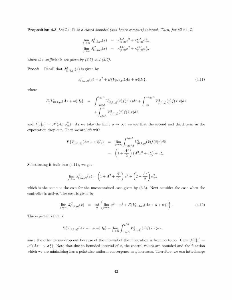
Proposition 4.3 Let I ⊂ R be a closed bounded (and hence compact) interval. Then, for all x ∈ I:

lim%→∞

JJ(1,2,%)(x) = κ1,J(1,2)x

2 + κ2,J(1,2)σ

2w,

lim%→∞

JC(1,2,%)(x) = κ1,C(1,2)x

2 + κ2,C(1,2)σ

2w,

where the coefficients are given by (3.5) and (3.6).

Proof: Recall that JJ(1,2,%)(x) is given by

JJ(1,2,%)(x) = x2 + E{V(0,1,%)(Ax+ w)|I0}, (4.11)

where

E{V(0,1,%)(Ax+ w)|I0} =

∫ 2%/A

−2%/A

V 1(0,1,%)(x)f(x|x)dx+

∫ −2%/A

−∞V 2

(0,1,%)(x)f(x|x)dx

+

∫ ∞2%/A

V 2(0,1,%)(x)f(x|x)dx,

and f(x|x) = N (Ax, σ2w). As we take the limit % → ∞, we see that the second and third term in the

expectation drop out. Then we are left with

E{V(0,1,%)(Ax+ w)|I0} = lim%→∞

∫ 2%/A

−2%/A

V 1(0,1,%)(x)f(x|x)dx

=

(1 +

A2

2

)(A2x2 + σ2

w

)+ σ2

w.

Substituting it back into (4.11), we get

lim%→∞

JJ(1,2,%)(x) =

(1 +A2 +

A4

2

)x2 +

(2 +

A2

2

)σ2w,

which is the same as the cost for the unconstrained case given by (3.3). Next consider the case when the

controller is active. The cost is given by

lim%→∞

JC(1,2,%)(x) = infu

(lim%→∞

x2 + u2 + E{V(1,1,%)(Ax+ u+ w)}). (4.12)

The expected value is

E{V(1,1,%)(Ax+ u+ w)|I0} = lim%→∞

∫ %/A

−%/AV 1

(1,1,%)(x)f(x|x)dx,

since the other terms drop out because of the interval of the integration is from ∞ to ∞. Here, f(x|x) =

N (Ax + u, σ2w). Note that due to bounded interval of x, the control values are bounded and the function

which we are minimizing has a pointwise uniform convergence as % increases. Therefore, we can interchange

42

the limit and the infimum. Again, simplifying the equation gives

E{V(1,1,%)(Ax+ u+ w)|I0} = (1 +A2)((Ax+ u)2 + σ2w) + σ2

w.

Since this is a quadratic function of u, the first derivative gives the optimal value of control action u, and it

is

u∗(1,2)(x) = −A(

1 +A2

2 +A2

)x.

Putting this optimal control value back in (4.12), we get

lim%→∞

JC(1,2,%)(x) =

(1 +A2 − A2

2 +A2

)x2 +

(2 +A2

)σ2w.

This proves the proposition. The main technical step in this proof consists in guaranteeing that the “infu”

and “lim%→∞” terms can be swapped in the computation of lim%→∞ JC(1,2,%)(x), for a fixed x ∈ I. This

follows directly from Propositions 4.1 and 4.2 proved above.

In the proposition above, we proved that as the constraint is relaxed, we recover the same cost function

and value functions as in the game with unconstrained state. As a result of this, we also find that the

threshold function for the jammer is same as that derived in (3.7) in Chapter 3.

Next, we prove a proposition which gives the lower threshold as a linear function of noise variance when

the ratio %/σw is a constant.

Proposition 4.4 If %/σw = υ, then τ c(1,2),l = g(υ,A)σw where g(.) is satisfies

JJ(1,2)(g(υ,A))− JC(1,2)(g(υ,A)) = 0. (4.13)

The cost calculated above is for the system that has zero mean unit variance noise (σw = 1) and υ as its

state constraint.

Proof: Let us transform our state variable x to ξ := x/σw. At first, we prove that if %/σw = υ, then the

optimal control at (1, 2) is a linear function of σw. The optimal control value is

u∗(1,2)(x) = arg minux2 + u2 + E{V(1,1,%)(Ax+ u+ w)|I0}, (4.14)

= arg minuσ2w

(ξ2 +

u2

σ2w

+ E

{V(1,1,%)

(Aξ +

u

σw+

w

σw

)|I0})

. (4.15)

Define u := u/σw, change the variable of integration to x = x/σw and interval of integration, we get the

minimizing function as

u∗(1,2) (ξ) = arg minu

(ξ2 + u2 + E

{V(1,1)

(Aξ + u+

w

σw

)|I0})

. (4.16)

Here V(1,1,υ) is the value function for the game with state constraint υ and unit noise variance. Minimizing

with respect to u in (4.14) is the same as minimizing with respect to u in (4.16). Now, the expression in

(4.16) is independent of σw and %, and is dependent only on the value of υ, A and ξ. Given the value of

43

u∗(1,2)(ξ), we transform the system back to the original game to get u∗(1,2)(x) = u∗(1,2)(ξ)σw. Therefore, the

optimal control is a linear function in σw.

Let us consider the difference in the cost with jamming and the cost with controlling. It is given by

JJ(1,2,%)(x)− JC(1,2,%)(x) = E{V(0,1,%)(Ax+ w)|I0} − u∗2(1,2)(x)− E{V(1,1,%)(Ax+ u∗(1,2)(x) + w)|I0}.

Again, applying the transformation and changing the limits in the integration terms appropriately, we get

this difference as

JJ(1,2,%)(x)− JC(1,2,%)(x) = σ2w

(JJ(1,2,υ)(ξ)− J

C(1,2,υ)(ξ)

). (4.17)

By definition, lower threshold τ c(1,2),l is defined as the value where the difference in the cost with jamming is

equal to the cost with control, i.e. it is a zero of (4.17). The zero of the right hand side of (4.17) is g(υ,A).

Using this fact and transforming the system back to x = ξσw, we complete the proof of the proposition.

In the proposition above, we have seen that for a system with a given A, the threshold is a constant

dependent on the ratio %/σw multiplied with the noise variance σw. System designers can use this result to

get an acceptable value of the constraint % as a function of the noise variance σw.

4.4 Numerical Simulations

In this section, we discuss some simulation results which we obtained for various values of the parameters A,

% and σw. The results obtained are for x ≥ 0, but similar results hold for x < 0 also. We have normalized

our x-axis to be equal to Ax/%, so that the jammer is active only when Ax/% ≤ 1. All simulations were

performed in MATLAB. Integration of value functions were performed using the standard ode45 function

of MATLAB. Since the integration can not be performed till ∞, the upper limit of integration was taken

to be |Ax + u| + 2%/A + 10σw (and lower limit was −(|Ax + u| + 2%/A + 10σw)). The maximum step size

for integration was limited to 5σw to achieve desired accuracy. For calculating the infimum of the cost

function, differentiation was performed numerically and fzero function was invoked to find the infimum.

Lower threshold was calculated by interpolating the cost function between two values of state x1 and x2 at

which JC(1,2,%)(x1) > JJ(1,2,%)(x1) and JC(1,2,%)(x2) < JJ(1,2,%)(x2) to find the point where the two costs are equal

JC(1,2,%)(τc(1,2)l) = JJ(1,2,%)(τ

c(1,2)l).

In Figure 4.1, we see that when the state is small, the actuator noise on the system in this stage will

increase the state of the system. Therefore it is optimal for the jammer to jam at the next step. This is

the reason why we see that the jammer’s optimal policy requires the jammer to not jam when the state is

small. After the lower threshold, the cost function with jamming is always higher than the cost function

with control. Hence, the jammer jams up to x ≤ %/A and after that the state constraint becomes active and

the jammer cannot jam the channel.

In Figure 4.2, we notice that the lower threshold for the jammer in the constrained case is always lower

than the threshold for the unconstrained case. In the unconstrained game, the jammer’s policy is to jam

when the state x is above that threshold. However, in the constrained case, the jammer is forced to reduce

the lower threshold in order to satisfy the state constraint, as well as increase the cost to the controller

44

0 1 2 3 4 5

102

103

104

105

Ax/ρV

(1,2

)(x)

A = 2, σw

= 2, ρ = 40

Jammer InactiveJammer Active

Figure 4.1: The value function at stage (1, 2) with state constraint parameter % = 40 and systemparameters A = 2 and σw = 2. The red region denotes the values of x, where the jammer jams.

0 20 40 60 800

5

10

15

20

25

30

35

40

σw

Sta

te x

A = 2, ρ = 40

τ(1,2)u

τ(1,2),lc

τ(1,2),uc

Figure 4.2: The threshold variation as a function of σw. Here, superscript u denote threshold forunconstrained game considered in Chapter 3 and superscript c denotes threshold for constrained game. Theregion between dotted lines is the region where jamming is optimal at stage (1, 2) for the constrained game.

strategically. We also see that when the threshold for the unconstrained game τ(1,2) is much smaller than

the upper threshold for the constrained game τ c(1,2),u := %/A (this happens when σw is small), the lower

threshold curve overlaps the threshold curve for the unconstrained game. This is due to the fact that the

tail of the Gaussian probability distribution goes to zero very rapidly for small σw. This reduces the effect

of state constraint when state and noise variance is small. Also, as the noise variance becomes larger, the

lower threshold reduces to zero.

In Figure 4.3, we compare the increase in cost the system suffers due to the action of jammer. We plot

the ratio of value function for stage (1, 2) and stage (0, 2) in this figure. At stage (0, 2), the jammer has no

chance left to jam till the end of the horizon. Therefore, the value function is the optimal cost for constrained

optimization (note that the state constraint is still active). For the same noise variance, we see that the

presence of the jammer inflicts higher cost to the unstable system if the constraint is relaxed. Notice that for

A = 4, % = 100 has a value function ratio exceeding 11 while for % = 20, the ratio is less than 8. Therefore,

if the system is unstable and the jammer is present, the designer should try to keep the state constraint as

45

small as possible.

0 1 2 3 4 50

2

4

6

8

10

12

Ax/ρ

V(1

,2)(x

)/V

(0,2

)(x)

σw

= 5, ρ = 20

A = 0.75A = 2A = 4

0 1 2 3 4 50

2

4

6

8

10

12

Ax/ρ

V(1

,2)(x

)/V

(0,2

)(x)

σw

= 5, ρ = 100

A = 0.75A = 2A = 4

(a) (b)

Figure 4.3: The ratio of value function with a jammer and without a jammer with state constraint active inboth cases.

The case of M ≥ 2 and for a general state space can also be solved using the techniques discussed in

this chapter. However, the exact calculation of the set of states when the jammer jams is difficult to obtain.

For the case when M ≥ 2, we need to calculate the threshold for all the nodes which is in the path from

(M,N) to (0, 0) in the tree given in Figure 2.2. In the multi-dimensional case, it is not hard to see that the

expectation value of the value functions at the next stage would require integration in n-dimension. Also,

instead of thresholds that we get for the scalar case, we get hyperplanes separating the region where the

jammer is active and where the controller is active.

Therefore, computation of saddle-point strategy for general cases requires significant computational effort

even for simple games. If M is large, or the state dimension is large, then obtaining the accurate strategy

for the jammer and the controller is very difficult from a computational perspective. Therefore, one must

switch to approximation schemes in order to compute the saddle-point equilibrium strategy for the controller

and the jammer. However, intuitively, the jammer would jam if the state is “large” but below the upper

threshold and not jam if the state is “small”. It is the intermediate values of state where the jammer needs

to know the exact values of thresholds (or hypersurfaces in case of multi dimensional state space) to have

strategic advantage.

In this chapter, we assumed that the communication channel can transmit control signal in the form of

an analog signal, which can send real numbers. Also, jamming is assumed to completely block the control

signal. However, in digital systems, the control signal (and observation signal) needs to be quantized and

the quantized signal is encoded into bits, which are then sent across the communication channel. We treat a

class of jamming attacks in such systems, where instead of blocking the signal completely, the jammer flips

limited number of bits in the encoded signal.

46

CHAPTER 5

ONE STEP CONTROL WITH FINITE CODELENGTH

We consider in this chapter a type of deception attack on a control system, where a jammer flips a limited

number of bits in the observation signal, which is assumed to be of finite codelength. However, to gain

insight into the problem and for simplicity of exposition, we restrict our attention to a noisy scalar system

playing a static game with the jammer. We provide precise problem formulation in Section 5.1. In Section

5.2, we restrict our attention to binning based control strategy for the controller in order to obtain an upper

bound on the minimum cost that the controller incurs due to the presence of the jammer. We also discuss

relevant tools from error correcting coding theory for the problem in this section. In the Section 5.3, we

explore the theory of rate distortion from information theory to arrive at the ultimate lower bound on the

codelength that is required to keep the state bounded. We provide some concluding remarks in Section 5.4.

The results discussed in this chapter have been reported in [36].

5.1 Problem Formulation

Using scalar system dynamics, the scenario can be captured through the following mathematical formulation:

The state equation evolves as (note that we have one stage problem)

x+ = Ax+ u+ w, (5.1)

where x, x+ ∈ R is the state of the plant, u ∈ R is the control signal, w is a discrete-time zero mean

uniformly distributed random variable with bound ∆ (i.e. w ∼ U (−∆,∆)). Initial state x is also a zero

mean uniformly distributed random variable in the interval I := [−1, 1] and independent of process noise w.

What we consider is a prototype of a scenario where the controller and the plant are far from each other,

such that the plant sends the state information to the controller and the controller sends the control signal

to the plant via a communication channel. For the analysis, the channel is assumed to be perfect (but

unsecured) and it does not induce any error on the received bit at the controller or the plant end (only

jammer can induce errors). The plant and the controller can send at most n bits across the channel. The

signal sent over the channel from the plant to the controller is intercepted by a jammer, which can flip

at most t bits of the codewords of the observation signal. We assume that the jammer jams the channel

from the plant to the controller, while the channel from the controller to the plant is not intercepted by the

jammer. We refer to n as the channel rate1 in this chapter.

Figure 5.1 provides a schematic description of the interconnections and the flow of information in the

1Note that this definition of channel rate differs from the usual meaning of channel rate in information theory.

47

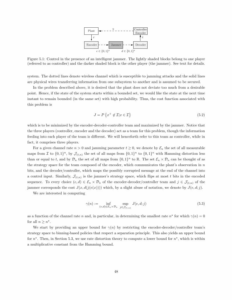
Plant ControllerEncoder

u

x x

Encoder Jammer Decoder

e ∈ {0, 1}n d ∈ {0, 1}n

Figure 5.1: Control in the presence of an intelligent jammer. The lightly shaded blocks belong to one player(referred to as controller) and the darker shaded block is the other player (the jammer). See text for details.

system. The dotted lines denote wireless channel which is susceptible to jamming attacks and the solid lines

are physical wires transferring information from one subsystem to another and is assumed to be secured.

In the problem described above, it is desired that the plant does not deviate too much from a desirable

point. Hence, if the state of the system starts within a bounded set, we would like the state at the next time

instant to remain bounded (in the same set) with high probability. Thus, the cost function associated with

this problem is

J = P{x+ 6∈ I|x ∈ I

}(5.2)

which is to be minimized by the encoder-decoder-controller team and maximized by the jammer. Notice that

the three players (controller, encoder and the decoder) act as a team for this problem, though the information

feeding into each player of the team is different. We will henceforth refer to this team as controller, while in

fact, it comprises three players.

For a given channel rate n > 0 and jamming parameter t ≥ 0, we denote by En the set of all measurable

maps from I to {0, 1}n, by J(t,n) the set of all maps from {0, 1}n to {0, 1}n with Hamming distortion less

than or equal to t, and by Dn the set of all maps from {0, 1}n to R. The set En ×Dn can be thought of as

the strategy space for the team composed of the encoder, which communicates the plant’s observation in n

bits, and the decoder/controller, which maps the possibly corrupted message at the end of the channel into

a control input. Similarly, J(t,n) is the jammer’s strategy space, which flips at most t bits in the encoded

sequence. To every choice (e, d) ∈ En × Dn of the encoder-decoder/controller team and j ∈ J(t,n) of the

jammer corresponds the cost J(x, d(j(e(x)))) which, by a slight abuse of notation, we denote by J(e, d; j).

We are interested in computing

γ(n) := inf(e,d)∈En×Dn

supj∈J(t,n)

J(e, d; j) (5.3)

as a function of the channel rate n and, in particular, in determining the smallest rate n? for which γ(n) = 0

for all n ≥ n?.We start by providing an upper bound for γ(n) by restricting the encoder-decoder/controller team’s

strategy space to binning-based policies that respect a separation principle. This also yields an upper bound

for n?. Then, in Section 5.3, we use rate distortion theory to compute a lower bound for n?, which is within

a multiplicative constant from the Hamming bound.

48

5.2 Binning Based Strategies and an Upper Bound

Intuitively, when there is finite length encoding of a real number, the most obvious solution strategy is to

use quantization and binning based strategy for the controller. The interval I is divided into N intervals

(henceforth, termed as bins). The encoder takes x as the input, determines which bin x belongs to, and

outputs the codeword corresponding to that bin. Therefore, we force the controller to use a binning based

strategy, which naturally restricts encoding strategies to code and send the bin index across the channel.

Note that our problem formulation in the previous section does not enforce this structure on the controller.

This specific solution strategy is chosen to find a constructive upper bound on γ(n) as defined in the previous

section and an upper bound on the number of bits n required to drive the cost to zero.

We consider the case for A > 1, since for |A| ≤ 1, a trivial control strategy is to use zero. The case of

A < −1 yields the same value with A replaced by |A|.

Plant

Encoder Jammer Decoder

Q ∈J

e ∈ {0, 1}n d ∈ {0, 1}n

x

u Controller

Figure 5.2: The binning based strategy in the presence of a jammer.

The flow of information in the system is as follows (see Figure 5.2). The state information x of the plant

is sent to the encoder, which encodes the bin index corresponding to the state into e ∈ {0, 1}n. The jammer

flips at most t bits in this sequence to produce d ∈ {0, 1}n. The decoder at the controller end receives

this jammed sequence d and determines which bin index Q this sequence belongs to using nearest neighbor

search. This information is then used by the controller to compute the control value for the plant and the

index corresponding to the control value is sent to the plant over the communication channel. Therefore,

in this scenario, the three players (encoder, decoder and controller) act as a team (collectively called the

controller) and the jammer acts as the fourth player. The codeword associated with each bin index and the

codeword associated with each control action is known to everyone, including the jammer.

5.2.1 Notation

In order to obtain an upper bound on γ(n) under the restriction of using binning based control strategy,

we need to introduce some additional notation. Let H(·, ·) denote the Hamming distance [37] between two

codewords. We say that an encoding strategy e ∈ En is N bin-based if there exists a partition (B1, ...,BN )

of the interval I such that

I =⋃i∈J

Bi

49

and corresponding to each bin Bi, there exists a codeword εi ∈ {0, 1}n such that

e(x) = εi for all x ∈ Bi.

If, in addition, the codewords satisfy

H(εi, εk) ≥ 2s+ 1 for all i 6= k, s ∈ N ∪ {0}, (5.4)

we say that the encoding strategy En is s-error free. Let ε ∈ {0, 1}n be the codeword received by the decoder

and define h(ε) by the following relation:

h(ε) := arg mini∈J

H(εi, ε). (5.5)

We will denote h(ε) by Q which lies in the set J . We say that a decoding strategy d ∈ Dn is N bin-based

if there exist N codewords εi ∈ {0, 1}n (i ∈J ) and N control inputs u1, ..., uN ∈ R such that

d(ε) = uh(ε) for all ε ∈ {0, 1}n.

The set of points Ti ⊂ I where the control ui keeps the state within the interval I is given by

Ti =

[−1 + ∆− ui

A,

1−∆− uiA

]∩ I. (5.6)

We define Ni ⊆J as the set of bin indices whose codewords are less than or equal to 2t Hamming distance

away from the codeword for bin i :

Ni = {k ∈J : k = h(j(e(x))), x ∈ Bi, j ∈ J(t,n)}, (5.7)

where h(·) is defined in (5.5). Clearly, the set Ni for each bin index i ∈ J is dependent on the encoding

strategy. Since the jammer flips at most t bits, the set Ni consists of all bin indices corresponding to the

nearest neighbors of all 0 to t flips in the codeword for ith bin. Denote pik, k ∈ Ni to be the probability with

which the jammer flips the bits in the codeword corresponding to ith bin such that the resulting codeword

corresponds to the codeword of the kth bin.

We say that N bin-based encoding and decoding strategies are adapted if the codewords {ε1, ..., εN} are

the same for both strategies, and refer to the pair (e, d) as s-error free. The set of all adapted N bin-based,

s-error free encoding and decoding strategy pairs with codelength n is denoted by S(n,N,s).

Although an N bin-based decoding strategy may not be well-defined over {0, 1}n (because there may

be more than one index satisfying (5.5)), the expression d(j(e(x))) is well defined for every x ∈ I, every N

bin-based encoding strategy e that is adapted to d and t-error free, and every j ∈ J(t,n). Indeed, in this

case, condition (5.4) ensures that every codeword used by the encoding and decoding strategies is uniquely

recovered by the nearest neighbor rule (5.5), regardless of which t out of its n bits are flipped. In addition,

for every (e, d) ∈ S(n,N,t),

d(j(e(x))) = ui ⇔ x ∈ Bi

50

for all j ∈ J(t,n) and all x ∈ I.

In words, when the encoder-decoder/controller team uses a pair of strategies in S(n,N,t), it is guaranteed

that system (5.1) will receive the input signal corresponding to the actual bin in which the state lies,

regardless of the action of the jammer. The goal of the team is to achieve a cost supj∈J(t,n)J(e, d; j) of zero

by appropriately choosing control inputs corresponding to each bin.

It is clear that for all (e, d) ∈ S(n,N,t) and all j ∈ J(t,n)

γ(n) ≤ inf(e,d)∈S(n,N,t)

supj∈J(t,n)

J(e, d; j),

since we are restricting the strategy space of the controller to binning-based control strategies.

The following result, which is classical in the theory of error correcting codes, provides conditions for the

(non) existence of s-error free N bin based encoding strategies.

Lemma 5.1 (Gilbert & Hamming bounds [37]) If

N ≤ 2n∑2tj=0

(n

j

) , (5.8)

then there exists a t-error free N bin-based encoding strategy. However, if

N >2n∑t

j=0

(n

j

) , (5.9)

there does not exist a t-error free N bin-based encoding strategy.

Lemma 5.1 implies that, for every N and t, the set of all rates n for which there exists a t-error free N

bin based encoding strategy is non-empty. In addition, its minimal element, denoted by necc(N, t), satisfies

nHamming(N, t) ≤ necc(N, t) ≤ nGilbert(N, t), (5.10)

where nHamming(N, t) and nGilbert(N, t) are given by

nHamming(N, t) = 1 + max

n ∈ N : N >2n∑t

j=0

(n

j

)

nGilbert(N, t) = min

n ∈ N : N ≤ 2n∑2tj=0

(n

j

)

Hence, an upper bound on the value of γ(n) can be obtained by considering a zero-sum game between

the jammer and encoder-decoder/controller team, with the strategy space of the latter restricted to S(n,N,t).

51

5.2.2 Control Without Jammer

We consider the case without a jammer and obtain a binning and control strategy. The main purpose of the

Lemma below is to come up with a necessary condition on the number of bins which are required to keep

the state bounded in the next time step.

Lemma 5.2 Let n, N , and t be such that N bin-based, t-error free encoding strategies exist. Then there

exist (e, d) ∈ S(n,N,t) such that J(e, d; j) = 0 for all j ∈ J(t,n) if and only if

N ≥⌈|A|

1−∆

⌉. (5.11)

In addition, when (5.11) holds, e and d can be constructed with the following choice of bins (B1, ...,BN ) and

control inputs u1, ..., uN :

• if N is odd:

Bk =

[2k − 1

N,

2k + 1

N

), uk = −2kA

N, (5.12)

for all −N−12 ≤ k ≤ N−1

2

• if N is even,

Bk =

[2(k − 1)

N,

2k

N

), uk = − (2k − 1)A

N, (5.13)

for all −N2 + 1 ≤ k ≤ N2 .

In both cases, any set of codewords ε1, ..., εN ∈ {0, 1}n which renders e t-error free can be chosen.

Proof: Let there exist (e, d) ∈ S(n,N,t) such that J(e, d; j) = 0. Consider a bin Bi, x1 := inf Bi, x2 := supBiand assume the control for this bin to be u and A > 0. Since the state at the next step is bounded, we need

the following to hold:

Ax1 + u ≥ −1 + ∆

Ax2 + u ≤ 1−∆.

Subtracting the first from the second, we get x2 − x1 ≤ 2(1−∆)A . Hence, the maximum bin size cannot be

greater than 2(1 −∆)/A in order to keep the state bounded. The number of bins N required to cover the

interval I is d2/(2(1 −∆)/A)e =⌈

A1−∆

⌉. Again, the result for negative values of A can be obtained using

similar steps.

If N =⌈|A|

1−∆

⌉, then the binning and control strategy given by (5.12) for odd N and (5.13) for even N in

the lemma above keeps the state in the interval.

Substituting the control value uk for x corresponding to bin Bk keeps the state within the interval I.

Note that this control strategy works for equispaced bins only.

When noise is not present in the system, then ∆ = 0. The length of codeword in this case is log2d|A|e.The result is not surprising, since it has been shown in [1, 2, 3] that the channel rate has to be (strictly)

52

greater than log2 |A| for the system to be stabilizable. Although our goal here is a little different (the state

has to remain in the interval I instead of stabilizable), the results are essentially the same (without the strict

inequality) as those obtained in these references. This is, however, not true for a system which has bounded

noise as shown in the Lemma above.

If the noise is unbounded (as in the case of Gaussian process noise), then there is no control strategy

with the finite channel rate scheme which can keep the state within the given bound with probability 1.

The essence of the results in this section is that there are certain minimum number of bins required (as

proved in Lemma 5.2) for the system state to remain in the same interval in the next time step. This number

of bins are dependent of the system parameter A and the maximum magnitude of noise ∆. Now, we are

prepared to consider the problem with the jammer in the next subsection.

5.2.3 Jamming and Error Correcting Code

In Lemma 5.2, we noticed that a certain minimum number of bins is necessary for the controller to be able

to keep the state bounded even without a jammer. If the number of bins is less than that, then there is no

hope of being able to keep the state within the interval I in the next time step. The number of bits that are

required to send codewords for N bins is dlog2(N)e.In the presence of a jammer which can flip at most t bits, the codelength n above which the errors can

be corrected is bounded below by the Hamming bound and above by the Gilbert bound [37] (see Lemma

5.1). Establishing the Hamming and Gilbert bounds do not involve a constructive proof and rely on random

coding strategy for constructing codewords. Recall that the minimum n for which t errors can be corrected

by decoder for the N bin case is necc(N, t). It is clear from (5.10) that necc(N, t) lies between the Hamming

bound and the Gilbert bound. However, currently, it is not known how close necc(N, t) is to the Hamming

bound or the Gilbert bound [37]. There are only a few coding strategies for which the Hamming bound is

tight, and they are known as perfect codes [37].

It is clear that the number of bits required for the specific number of bins is going to be much larger than

log2(N) in the presence of the jammer. Therefore, when the channel rate n < necc(N, t) but n ≥ log2(N),

then the only way to design the control strategy is by computing saddle-point equilibrium strategy for the

zero-sum game between the controller and the jammer. Towards this end, we need to compute (e∗, d∗) ∈En ×Dn and j∗ ∈ J(t,n) such that

J(e∗, d∗; j) ≤ J(e∗, d∗; j∗) ≤ J(e, d; j∗),

which holds for all (e, d) ∈ En × Dn and j ∈ J(t,n). This means that the binning, encoding and control

strategies have to be chosen intelligently to mitigate the adverse effect of jamming. This is addressed in

next subsection. Figure 5.3 shows the various regions where each solution concept works for this class of

problems. In the figure, necc is the minimum channel rate at which t-flips in the codewords can be corrected

for N bins by using an appropriate error correcting algorithm.

In the following theorem, we present a sufficient condition on the channel rate n, such that the error

correction coding technique can be applied to the problem so as to mitigate the error resulting due to the

adversarial action by the jammer. Since the proof is constructive, we also obtain a coding scheme and a

decoding scheme which achieve this bound.

53

������������������������������������������

������������������������������������������

�����������������������������������������������������������������

�����������������������������������������������������������������

������������������������������������������������

������������������������������������������������

necc

log

2N

Channel Rate n

log2d|A|e

Figure 5.3: The graph shows the region on channel rate n - log2N plot where the state cannot beguaranteed to be within a given bound with probability 1 (red region), saddle-point equilibrium mayachieve a better performance than the worst case (blue region), and where the jammer is ineffective (greenregion) due to error correcting coding algorithms.

Theorem 5.3 Let N be the number of bins and n be the codelength, and assume that the jammer can flip at

most t bits. Then, a sufficient condition on the codelength n for the jammer to have no effect on the control

signal is

n ≥ tncr + dlog2Ne , (5.14)

where ncr ∈ N satisfies

ncr = min

{n ∈ N : N ≤

(n

0

)+

(n− 1

1

)+ · · ·+

(dn/2ebn/2c

)}.

Proof: If two different codewords are sent and the jammer has flipped t bits in the codewords, then to

be able to decode it without error, the two codewords should be 2t + 1 bit apart. With this idea, we now

construct a set of codewords, such that the difference between any two codewords is of 2 bits. After this is

done, we will extend the algorithm to 2t+ 1 bit case by padding it with another set of codewords.

Let us suppose that ncr number of bits are required to have a difference of 2 bits in any two codewords.

Assume first codeword to be 000...(ncr times). Now fix the first bit in the codeword to be 1 and put 1 at

any of the ncr − 1 places. There are

(ncr − 1

1

)ways of doing this. Then the difference between any

two codewords is 2. Now, fix the first two bits to 1 and put two 1’s at the remaining of the ncr − 2 places.

There are

(ncr − 2

2

)ways of doing this. Repeat this process until all the first bncr/2c bits are fixed to 1

and the rest of the dncr/2e bits have a combination of bncr/2c number of 1’s. This way, we constructed the

codewords for N bins and any two codewords in the set have a minimum distance of 2 bits. If the number

of codewords required to control the plant reliably is N , then ncr must satisfy

N ≤

(ncr

0

)+

(ncr − 1

1

)+ ...+

(dncr/2ebncr/2c

).

54

If the jammer has the ability to flip t bits, then we can replace each 0 in the codeword with a sequence

of t 0’s and 1 with a sequence of t 1’s. This keeps the codewords a minimum of 2t bits apart.

Now “pad” the ith codeword with the binary expansion of integer i. This will ensure that each of the two

codewords have an additional distance of 1. This will require dlog2Ne number of additional bits. Summing

the two expressions, we get the inequality in (5.14).

100

101

102

0

5

10

15

20

25

30

Number of bins N

Num

ber

of b

its r

equi

red

n

Hamming BoundBound in Theorem 2Gilbert Boundlog

2 N

Figure 5.4: Various bounds on the channel rate when the jammer can flip at most t = 2 bits in codeword.

In Figure 5.4, we see the performance of the coding strategy in Theorem 5.3 with the Hamming bound

and the Gilbert bound [37]. We notice that for up to N = 8 bins, our coding strategy is within the Hamming

and Gilbert bounds. After that, the codelength of our coding strategy exceeds the Gilbert bound. Therefore,

the coding scheme given by Theorem 5.3 can be improved to obtain a codelength below the Gilbert bound.

When the channel rate n ≥ necc(N, t), then we can separately design the quantization, encoding and

control policies. In that case, N bins (where N is given by Lemma 5.2) can be designed such that the

information of the bin is reconstructed exactly at the controller end and it can send the correct control

signal. The encoder is free to choose its policy independent of the control policy2. The cost in this case is

zero, that is, the state will remain in the set I with probability 1. The following Theorem summarizes the

result and provides a sufficient condition on rate n for which the cost is zero.

Theorem 5.4 For the problem formulated in section 5.1 with binning-based control strategy, let there be

N =⌈|A|

1−∆

⌉bins and the jammer can flip at most t bits. Then, the value of the game is zero if n ≥ necc(N, t),

i.e.,

γ(n) = 0, for all n ≥ necc(N, t).

As a result, we get n? ≤ necc(N, t).

Proof: If n ≥ necc(N, t), then there is an encoding policy with N codewords such that any pair of

codewords have a Hamming distance greater than or equal to 2t + 1. From Lemma 5.2, we know that if

2The depenence of encoding policy on the control policy is addressed in the next subsection, where we consider the gamescenario.

55

N =⌈|A|

1−∆

⌉and n ≥ necc(N, t), then there exists (e, d) ∈ S(n,N,t) such that J(e, d; j) = 0 for all j ∈ J(t,n).

Then, the policy given in Lemma 5.2 controls the plant such that the state remains in the interval I in the

next time step. Hence, we achieve a value of zero for all jamming strategies. This results in γ(n) = 0 for all

n ≥ necc(N, t).

If n < necc(N, t), then there is no encoding-decoding strategy which can correct all t flips by the jammer.

Hence, there will always be “confusion” in a few bin indices sent by the encoder at the decoder’s end. Using

nearest neighbor search, the decoder may obtain wrong bin index, and hence, wrong control input is sent to

the plant. Thus, the value of zero cannot be achieved by binning-based control strategy if n < necc(N, t).

Until now, we fixed the number of bins N and number of flips t to get the required channel rate n for

zero cost. However, a more practical scenario is the one where the number of bits that can be transferred

across a channel is limited by n. Therefore, we look into the case when channel rate n < necc(N, t) now. To

do this, we need the following lemma which simplifies the cost function to make it easier to analyze.

Lemma 5.5 The cost function of the game for the binning based control strategy is equivalent to

P{x+ 6∈ I

∣∣x ∈ I} =

N∑i=1

∑k∈Ni

pikP{x ∈ Bi ∩ T ′k},

with the constraint pik ≥ 0 and ∑k∈Ni

pik = 1,∀ i ∈ {1, 2, ..., N},

where Ni and Ti is defined for all i ∈J in (5.7) and (5.6) respectively.

Proof: Using Bayes’ theorem repeatedly, we can write the cost function as

P{x+ 6∈ I

∣∣x ∈ I} =

N∑i=1

P {x ∈ Bi|x ∈ I}

(∑k∈Ni

pikP{x+ 6∈ I

∣∣x ∈ Bi, Q = k})

,

where pik = P{

Q = k∣∣∣x ∈ Bi} for all k ∈ Ni with the constraint

∑k∈Ni

pik = 1, (5.15)

and Q = h(j(e(x))). Now, recall the following identities

P{x+ 6∈ I

∣∣x ∈ Bi, Q = k}

=P{x ∈ Bi ∩ T ′k}P{x ∈ Bi}

,

P {x ∈ Bi|x ∈ I} = P{x ∈ Bi}.

Using these expressions, the cost function is rewritten as

P{x+ 6∈ I

∣∣x ∈ I} =

N∑i=1

∑k∈Ni

pikP{x ∈ Bi ∩ T ′k}.

56

Next, we fix the rate n and the number of flips t, and define Ncr to be

Ncr = max{N ∈ N : n ≥ necc(N, t)}. (5.16)

In this case, we can obtain Ncr number of codewords, each of codelength n, which are 2t + 1 bits apart.

Using these set of codewords, we can obtain an upper bound on the cost function and as a consequence, an

upper bound on γ(n). Following theorem establishes an upper bound on the cost as a function of n.

Theorem 5.6 Let Ncr be given by (5.16). If Ncr < d|A|/(1−∆)e, then the cost to the controller is

J(e, d; j) =

(1− Ncr(1−∆)

|A|

),

it is achievable by infinitely many binning and control strategies.

Proof: By the definition of Ncr in (5.16), there exists an encoding and decoding strategy pair (e, d) ∈S(n,Ncr,t) such that the codewords for the bins can be coded in such a manner that the two bins are 2t+ 1

bits apart and t flips by jammer will have no effect on the decoded bin. Therefore, Q = h(j(e(x))) = i for

x ∈ Bi. Using this in Lemma 5.5, we see that

P{x+ 6∈ I

∣∣x ∈ I} =

N∑i=1

P{x ∈ Bi ∩ T ′i },

which has to be minimized by the controller by choosing appropriate binning and control strategies. Recall

that for A > 0

Ti =

[−1 + ∆− ui

A,

1−∆− uiA

]∩ I.

Now, construct bin Bi and Ti such that Ti ⊆ Bi for all i = 1, 2, ..., Ncr which implies P{x ∈ Bi ∩ T ′i } =

(l(Bi)− l(Ti)) /2 where l(·) is the length of the interval. Clearly,

Ncr∑i=1

l(Bi) = 2 and

Ncr∑i=1

l(Ti) = Ncr2(1−∆)

A.

A simple calculation yields (holds for A < 0 also)

P{x+ 6∈ I

∣∣x ∈ I} = 1− Ncr(1−∆)

|A|,

which proves the theorem. There are multiple binning and control strategies which achieve this value by

restricting Ti ⊆ Bi for all i = 1, 2, ..., Ncr and l(Bi) ≥ 2(

1−∆|A|

).

The set of strategies discussed in this section lead to a constructive upper bound on the cost J(e, d; j) and

γ(n) for a given n. In the next section, we explore the possibility of reducing the cost by considering a game

between the controller team and the jammer and solving for the saddle-point control and jamming strategies.

57

0 5 10 15 20 25 300

0.1

0.2

0.3

0.4

0.5

0.6

0.7

0.8

0.9

1

Channel rate n

Val

ue o

f the

gam

e J

A = 10, t = 5, ∆ = 0

Hamming BoundGilbert Bound

Figure 5.5: The change in value of the game P{x+ 6∈ I|x ∈ I} with increase in the channel rate n asobtained from Theorem 5.6 using the Hamming bound and the Gilbert bound. The simulation parametersare A = 10, t = 5, ∆ = 0. The actual cost lies between the two curves and depends on necc(N, t).

5.2.4 Saddle-Point Solution for the Two-Bin Case

Recall that when the channel rate n < necc(N, t) but n ≥ log2(N), then we need to compute (e∗, d∗) ∈ En×Dnand j∗ ∈ J(t,n) such that

J(e∗, d∗; j) ≤ J(e∗, d∗; j∗) ≤ J(e, d; j∗),

which holds for all (e, d) ∈ En × Dn and j ∈ J(t,n). Consider the case when A > 1 and only one bit (i.e.,

n = 1) is available to the controller. The saddle-point solution for the jammer and the controller is derived

in the following theorem.

Theorem 5.7 Let ε ∈ {0, 1} be the received codeword at the decoder’s end and Q := h(ε) = ε. For the game

described above, the set of saddle-point solutions for the controller is given by

u =

{(A− 1) + λ1A if Q = 1,

−(A− 1)− λ2A if Q = 2,

with λ1, λ2 ≤ 0 and λ1 + λ2 = 2/A− 2, and for the jammer, the probability that the jammer flips the bit is

1. The value of the game is

J(e∗, d∗; j∗) = 1− 1

A.

Proof: The cost function for the game is rewritten as

P{x+ 6∈ I|x ∈ I

}= P

{x+ 6∈ I|x ∈ B1

}P {x ∈ B1|x ∈ I}+ P

{x+ 6∈ I|x ∈ B2

}P {x ∈ B2|x ∈ I} . (5.17)

58

The quantity P {x+ 6∈ I|x ∈ Bi} is given by the expression

P{x+ 6∈ I|x ∈ Bi

}=

2∑j=1

P{x+ 6∈ I|x ∈ Bi, Q = j

}P{

Q = j|x ∈ Bi}

for i = 1, 2. For notational simplicity, let us denote the P{

Q = j|x ∈ Bi}

by pij , which is the probability

with which the jammer flips the bit corresponding to ith bin to jth bin. Now let us parameterize control

values with the parameters λ1, λ2 such that

u1 = (A− 1) + λ1A,

u2 = −(A− 1)− λ2A.

Let us separate the two bins at k, i.e. B1 = [−1, k] and B2 = (k, 1]. Firstly, we need to compute the following

quantities

P{x+ 6∈ I|x ∈ B1, Q = 1

}= 1− P

{−1 ≤ ax+ u1 ≤ 1|x ∈ B1, Q = 1

},

= 1− P{x ∈ T1|x ∈ B1, Q = 1

},

= P{x ∈ T ′1 ∩ B1|x ∈ B1, Q = 1

}, (5.18)

where T1 =[−(1 + λ1),

(2A − 1− λ1

)]and

P{x+ 6∈ I|x ∈ B1, Q = 2

}= 1− P

{−1 ≤ ax+ u2 ≤ 1|x ∈ B1, Q = 2

},

= P{x ∈ T ′2 ∩ B1|x ∈ B1, Q = 2

}, (5.19)

where T2 =[(

1 + λ2 − 2A

), (1 + λ2)

]and T ′ := I\T denotes the complement of the set T . It should be

noted that the length of each Ti is 2A . By changing the values of λi, we are translating the set Ti within the

interval I as shown in Figure 5.6.

������������( 2A − 1− λ1)

−1(1 + λ2)(1 + λ2 − 2

A )1

−(1 + λ1) k

Figure 5.6: Two-bins case with λ1, λ2 ≤ 0. The shaded portion denotes the indifference set S = T1 ∩ T2.

Now, consider the indifference set S := T1 ∩ T2 ⊆ I which is the set of points in I which remains within

the bound I with both the control values u1 and u2. The indifference set is S = [1 + λ2 − 2/A, 2/A− 1− λ1]

if −(1+λ1) ≤ 1+λ2−2/A or equivalently, λ1 +λ2 ≥ 2/A−2 and S = [−(1+λ1), (1+λ2)] if λ1 +λ2 < 2/A−2

(see Figure 5.6).

59

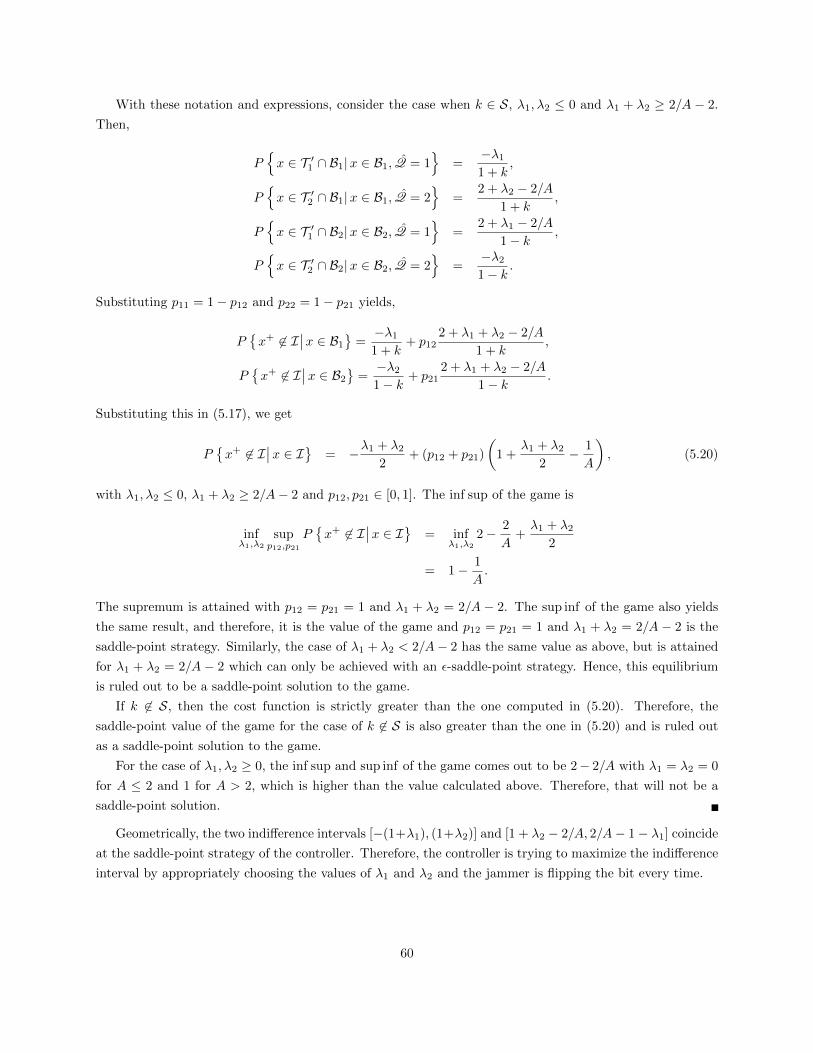
With these notation and expressions, consider the case when k ∈ S, λ1, λ2 ≤ 0 and λ1 + λ2 ≥ 2/A − 2.

Then,

P{x ∈ T ′1 ∩ B1|x ∈ B1, Q = 1

}=

−λ1

1 + k,

P{x ∈ T ′2 ∩ B1|x ∈ B1, Q = 2

}=

2 + λ2 − 2/A

1 + k,

P{x ∈ T ′1 ∩ B2|x ∈ B2, Q = 1

}=

2 + λ1 − 2/A

1− k,

P{x ∈ T ′2 ∩ B2|x ∈ B2, Q = 2

}=

−λ2

1− k.

Substituting p11 = 1− p12 and p22 = 1− p21 yields,

P{x+ 6∈ I

∣∣x ∈ B1

}=−λ1

1 + k+ p12

2 + λ1 + λ2 − 2/A

1 + k,

P{x+ 6∈ I

∣∣x ∈ B2

}=−λ2

1− k+ p21

2 + λ1 + λ2 − 2/A

1− k.

Substituting this in (5.17), we get

P{x+ 6∈ I

∣∣x ∈ I} = −λ1 + λ2

2+ (p12 + p21)

(1 +

λ1 + λ2

2− 1

A

), (5.20)

with λ1, λ2 ≤ 0, λ1 + λ2 ≥ 2/A− 2 and p12, p21 ∈ [0, 1]. The inf sup of the game is

infλ1,λ2

supp12,p21

P{x+ 6∈ I

∣∣x ∈ I} = infλ1,λ2

2− 2

A+λ1 + λ2

2

= 1− 1

A.

The supremum is attained with p12 = p21 = 1 and λ1 + λ2 = 2/A − 2. The sup inf of the game also yields

the same result, and therefore, it is the value of the game and p12 = p21 = 1 and λ1 + λ2 = 2/A − 2 is the

saddle-point strategy. Similarly, the case of λ1 + λ2 < 2/A− 2 has the same value as above, but is attained

for λ1 + λ2 = 2/A − 2 which can only be achieved with an ε-saddle-point strategy. Hence, this equilibrium

is ruled out to be a saddle-point solution to the game.

If k 6∈ S, then the cost function is strictly greater than the one computed in (5.20). Therefore, the

saddle-point value of the game for the case of k 6∈ S is also greater than the one in (5.20) and is ruled out

as a saddle-point solution to the game.

For the case of λ1, λ2 ≥ 0, the inf sup and sup inf of the game comes out to be 2− 2/A with λ1 = λ2 = 0

for A ≤ 2 and 1 for A > 2, which is higher than the value calculated above. Therefore, that will not be a

saddle-point solution.

Geometrically, the two indifference intervals [−(1+λ1), (1+λ2)] and [1 + λ2 − 2/A, 2/A− 1− λ1] coincide

at the saddle-point strategy of the controller. Therefore, the controller is trying to maximize the indifference

interval by appropriately choosing the values of λ1 and λ2 and the jammer is flipping the bit every time.

60

5.2.5 Analysis for the N -Bin Case

Let us assume that there are N bins Bi, i ∈J = {1, · · · , N} and the system has process noise. We can get

an idea of the saddle-point solution to the game using Lemma 5.5. The value of the game is defined if the

inf sup is equal to the sup inf of the cost function [33]. The inf sup for this game is

infui,1≤i≤N

suppik, k∈Ni,∑k∈Ni

pik=1

N∑i=1

∑k∈Ni

pikP{x ∈ Bi ∩ T ′k} = infui,1≤i≤N

N∑i=1

supk∈Ni

P{x ∈ Bi ∩ T ′k}, (5.21)

where the supremum is attained by

pik =

1 if k = arg supl∈Ni

P{x ∈ Bi ∩ T ′l },

0 otherwise.(5.22)

i.e., the jammer always flips the bits in such a manner, so as to produce the codeword for k which has least

overlap between Bi and Tk. If arg supl∈NiP{x ∈ Bi ∩ T ′l } is a set with more than one element, then the

jammer has uniform probability over the entire set.

The sup inf can also be computed for this game, but is dependent on the set Ni. The quantity in (5.21)

gives the upper bound on the value of the game [33]. If inf sup of the cost function is equal to the sup inf

(subject to the constraint (5.15)), then saddle-point exist and the jammer’s strategy is given by (5.22).

At this point, it is a natural question to ask if the cost can be driven to zero even if n < necc(N, t). We

will use rate distortion theory to find an answer to this question in the next section. This gives us a lower

bound on n?.

5.3 A Lower Bound using Rate Distortion Theory

In this section, we use information theory to find the minimum number of bits (the ultimate lower bound)

required to control the plant reliably in the presence of the jammer. Our problem can be posed as a rate

distortion problem [38], which is widely studied in the field of information theory. The key observation here

is that the controller needs the value of the state (and not that of quantization bin) in order to compute

the control value for the plant. In order to keep the state within the interval I, the controller needs the

information about the state within an error of (1 − ∆)/|A|. Therefore, the maximum allowable difference

between the state of the plant x and the estimate of the state x must be less than (1 −∆)/|A|. With this

idea, we can provide a lower bound (albeit loose) on the number of bits using rate distortion theory. The

following lemma will establish the connection between our original problem and information theory.

Lemma 5.8 Consider the problem formulated in Section 5.1. The cost P{x+ 6∈ I|x ∈ I} is zero for all

jamming strategies if and only if there exists encoding and decoding policies such that

supp(j|e)

|x− x| ≤ 1−∆

|A|for almost all x ∈ I. (5.23)

61

Proof: If the inequality in (5.23) holds for some encoding and decoding policy pair, then the controller

can send u = −Ax which keeps the state |x+| = |Ax−Ax| ≤ 1−∆ within the interval I.

Now, if the value of the game is zero for all jamming strategies, then |Ax+u| ≤ 1−∆ for some encoding

and decoding policy and for all x ∈ I. Pick x = −u/A. Since this holds for all jamming strategies, we get

supp(j|e) |x− x| ≤ (1−∆)/|A|.

EncoderxUniformSource +

eDecoder

d x

Jammer

j

Figure 5.7: An equivalent representation of the control problem posed as a communication problem withdistortion.

This problem is different in three ways from the one usually studied in information theory. First, due to

the constraint on the number of bits to transfer the state information, our result does not rely on results with

arbitrarily large codelength. Second, we are sending a real number over a channel with finite codelength and

some information is lost in encoding the real number. Third difference is the presence of a jammer, who is

observing the input codewords and strategically flipping the bits in order to alter the estimate of the state.

Therefore, the distortion in this case has to take care of both, the jammer and the information lost due to

encoding a real number. Now, let us define distortion function as

d(x, x) = (x− x)2,

whose expected value is to be minimized by the controller by choosing p(x|x) and maximized by the jammer

by choosing p(j|e). The distortion rate function is defined as

D(R) = infp(x|x)

I(X;X)≤R

EX{d(X; X)},

where I(X; X) is the mutual information between the random variables X and X (see [38] for the definition of

mutual information). The following theorem characterizes the minimum value of the rate n, say nrdt(A,∆, t),

for the system to have zero cost in terms of distortion rate function. It must be noted that if n < nrdt(A,∆, t),

then there is no encoding-decoding policy whatsoever which can ensure zero cost to the controller.

Theorem 5.9 If the value of the game J(e, d; j) is zero for some encoding and decoding policy pair (e, d) ∈En ×Dn and for all jamming strategies j ∈ J(t,n), then n satisfies

D(CJ(n, t)) ≤ (1−∆)2

A2, (5.24)

where CJ(n, t) := n− log2

(t∑i=0

(n

i

)). (5.25)

Proof: From Lemma 5.8, if the value of the game is zero, then there exists an encoding and decoding policy

pair such that supp(j|e) d(x, x) ≤ (1−∆)2

A2 for almost all x ∈ I. Now assume that the jammer fixes its strategy

62

such that it flips i ≤ t bits at random with uniform probability. Then, there exists an encoding-decoding

policy pair such that the EX{d(X, X)} ≤ (1−∆)2

A2 . With this jamming strategy, the mutual information is

bounded by

I(X; X) ≤ I(e; d) = H(d)−H(d|e)

≤ n−H(j|e) = CJ(n, t),

where the first inequality holds due to data processing inequality [38] and the second inequality holds by

taking uniform distribution over the received bits at decoder. Hence, there exists an x such that I(X; X) ≤CJ(n, t) and EX{d(X, X)} ≤ (1−∆)2

A2 for almost all x ∈ I. As a result, we get

D(CJ(n, t)) = infp(x|x),

I(X;X)≤CJ (n,t)

EX{d(X; X)} ≤ (1−∆)2

A2.

Hence, the jammer chooses the strategy which minimizes the mutual information and then the encoder

and decoder minimize the mean-squared distortion by choosing appropriate p(x|x). This gives a necessary

condition on the number of bits n required by the controller to achieve the required distortion as derived in

Lemma 5.8 which ensures zero cost. It is clear that nrdt(A,∆, t) ≤ necc(N, t), but to ascertain the tightness

of necc(N, t), numerical simulations are done to find the value of nrdt(A,∆, t) and check the difference

necc(N, t)−nrdt(A,∆, t). The following lower bound on rate-distortion function [39] can be used to compute

nrdt(A,∆, t):

R(D) ≥ 1

2log2

(4

2πeD

).

This gives the lower bound on the channel rate R(D) at which expected mean-squared distortionD is achieved

for a uniform source taking values in the interval [−1, 1] for all codelengths. Substituting R(D) = CJ(n, t),

we get a lower bound on the distortion D :

2

πe22CJ (n,t)≤ D(CJ(n, t)) ≤ (1−∆)2

A2.

The minimum n for which this inequality holds gives us a lower bound on nrdt(A,∆, t). Substituting the

value of CJ(n, t) from (5.25) and rearranging, we see that

|A|(1−∆)

≤√πe

2

2n(∑tj=0

(n

j

)) ,

which is a restatement of the Hamming bound with a multiplicative constant√

πe2 ≈ 2.1. As a result of this,

nrdt(A,∆, t) ≤ nHamming(N, t).The following theorem summarizes the main result of the chapter and gives the necessary and sufficient

condition on n? for γ(n) = 0 for the original problem formulated in Section 5.1.

63

5 10 15 20 25 300

5

10

15

20

25

30

A

Rat

e n

t = 5, ∆ = 0

Gilbert BoundHamming BoundRDT bound

Figure 5.8: A plot of rate n obtained from Theorem 5.4 using the Hamming bound and the Gilbert boundand necessary condition on rate n obtained from Theorem 5.9 using rate distortion theory (RDT) for thecontroller to incur zero cost as a function of A. The simulation parameters are t = 5 and ∆ = 0.

Theorem 5.10 Consider the problem formulated in Section 5.1 where the jammer can flip at most t bits in

the codeword. Recall that n? = min{n ∈ N : γ(n) = 0}, nrdt(A,∆, t) satisfies

nrdt(A,∆, t) = min

n ∈ N :|A|

(1−∆)≤√πe

2

2n(∑tj=0

(n

j

)) ,

and N = d|A|/(1−∆)e. Then n? satisfies

nrdt(A,∆, t) ≤ n? ≤ necc(N, t) ≤ nGilbert(N, t).

Proof: Follows from the discussion up to this point.

5.4 Summary

We considered a deception attack on a networked control system in the presence of an intelligent and strategic

jammer, which flips at most t bits in the observation codeword. We restricted our attention to binning based

control strategy to obtain an upper bound on the cost to the controller and a sufficient condition on the

codelength required to drive the cost to zero. We then posed the problem as a zero-sum game between the

team of encoder-decoder-controller and the jammer for the case when the codelength is small. We derived

the saddle-point strategy for the controller and the jammer for the case when the jammer can flip one bit

and the controller has one bit to transfer state information. We derived a necessary and sufficient condition

on the channel rate n for which the cost is zero, i.e., state leaves the bounded set I with probability zero.

Note that in this chapter, we focused our attention to one stage control system. We would like to extend

the result to a dynamic system, which evolves over time. This will be addressed in our future work.

64

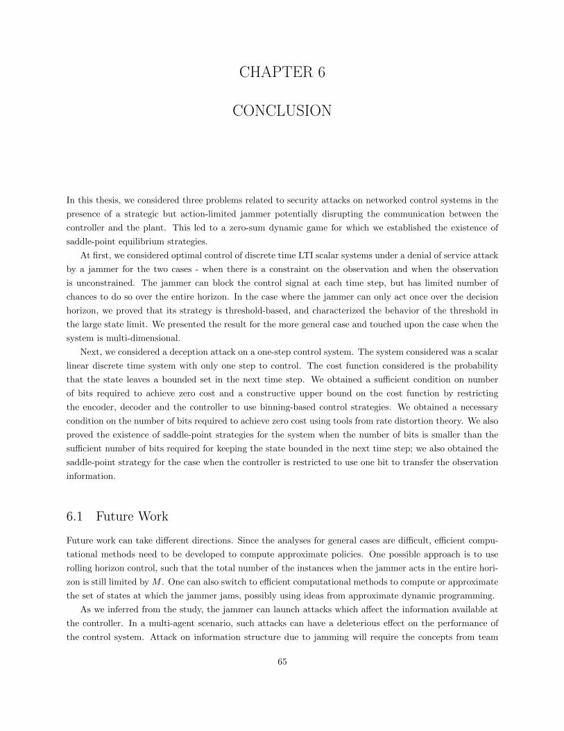
CHAPTER 6

CONCLUSION

In this thesis, we considered three problems related to security attacks on networked control systems in the

presence of a strategic but action-limited jammer potentially disrupting the communication between the

controller and the plant. This led to a zero-sum dynamic game for which we established the existence of

saddle-point equilibrium strategies.

At first, we considered optimal control of discrete time LTI scalar systems under a denial of service attack

by a jammer for the two cases - when there is a constraint on the observation and when the observation

is unconstrained. The jammer can block the control signal at each time step, but has limited number of

chances to do so over the entire horizon. In the case where the jammer can only act once over the decision

horizon, we proved that its strategy is threshold-based, and characterized the behavior of the threshold in

the large state limit. We presented the result for the more general case and touched upon the case when the

system is multi-dimensional.

Next, we considered a deception attack on a one-step control system. The system considered was a scalar

linear discrete time system with only one step to control. The cost function considered is the probability

that the state leaves a bounded set in the next time step. We obtained a sufficient condition on number

of bits required to achieve zero cost and a constructive upper bound on the cost function by restricting

the encoder, decoder and the controller to use binning-based control strategies. We obtained a necessary

condition on the number of bits required to achieve zero cost using tools from rate distortion theory. We also

proved the existence of saddle-point strategies for the system when the number of bits is smaller than the

sufficient number of bits required for keeping the state bounded in the next time step; we also obtained the

saddle-point strategy for the case when the controller is restricted to use one bit to transfer the observation

information.

6.1 Future Work

Future work can take different directions. Since the analyses for general cases are difficult, efficient compu-

tational methods need to be developed to compute approximate policies. One possible approach is to use

rolling horizon control, such that the total number of the instances when the jammer acts in the entire hori-

zon is still limited by M . One can also switch to efficient computational methods to compute or approximate

the set of states at which the jammer jams, possibly using ideas from approximate dynamic programming.

As we inferred from the study, the jammer can launch attacks which affect the information available at

the controller. In a multi-agent scenario, such attacks can have a deleterious effect on the performance of

the control system. Attack on information structure due to jamming will require the concepts from team

65

theory as well as communication theory, and it will be exciting to see various concepts leading to a new class

of problems being solved.

Another extension of the work can be to extend the result of Chapter 5 to a dynamic setting, where

the codelength is constrained in the presence of the jammer. It will be interesting to obtain the minimum

codelength at which the state remains bounded with probability one. The optimal binning and control

strategies may also evolve over time in such a scenario.

66

CHAPTER 7

REFERENCES

[1] S. Tatikonda and S. Mitter, “Control under Communication Constraints,” IEEE Transactions on Au-tomatic Control, vol. 49, no. 7, pp. 1056–1068, 2004.

[2] G. Nair, F. Fagnani, S. Zampieri, and R. Evans, “Feedback control under data rate constraints: anoverview,” Proceedings of the IEEE, vol. 95, no. 1, pp. 108–137, 2007.

[3] S. Yuksel and T. Basar, “Minimum Rate Coding for LTI Systems over Noiseless Channels,” IEEETransactions on Automatic Control, vol. 51, no. 12, pp. 1878–1887, 2006.

[4] L. Schenato, B. Sinopoli, M. Franceschetti, K. Poolla, and S. Sastry, “Foundations of control andestimation over lossy networks,” Proceedings of the IEEE, vol. 95, no. 1, pp. 163–187, 2007.

[5] O. Imer, S. Yuksel, and T. Basar, “Optimal control of LTI systems over unreliable communicationlinks,” Automatica, vol. 42, no. 9, pp. 1429–1439, 2006.

[6] E. Garone, B. Sinopoli, and A. Casavola, “LQG control over lossy TCP-like networks with probabilisticpacket acknowledgements,” International Journal of Systems, Control and Communications, vol. 2,no. 1, pp. 55–81, 2010.

[7] P. Antsaklis and J. Baillieul, “Special issue on technology of networked control systems,” Proceedingsof the IEEE, vol. 95, no. 1, pp. 5–8, 2007.

[8] C. Hadjicostis, C. Langbort, N. Martins, and S. Yuksel, “Special issue on information processing anddecision making in distributed control systems,” Int. Journal of Systems, Control, and Communications,vol. 2, no. 1/2/3, 2010.

[9] B. Sinopoli, L. Schenato, M. Franceschetti, K. Poolla, M. Jordan, and S. Sastry, “Kalman Filtering withIntermittent Observations,” IEEE Transactions on Automatic Control, vol. 49, no. 9, pp. 1453–1464,2004.

[10] T. Katayama, “On the matrix Riccati equation for linear systems with random gain,” Automatic Control,IEEE Transactions on, vol. 21, no. 5, pp. 770–771, 1976.

[11] S. Amin, A. Cardenas, and S. Sastry, “Safe and Secure Networked Control Systems under Denial-of-Service Attacks,” Hybrid Systems: Computation and Control, pp. 31–45, 2009.

[12] H. Sandberg, A. Teixeira, and K. Johansson, “On security indices for state estimators in power net-works,” in Preprints of the First Workshop on Secure Control Systems, CPSWEEK, 2010.

[13] A. Cardenas, S. Amin, and S. Sastry, “Research challenges for the security of control systems,” inProceedings of the 3rd conference on Hot topics in security, 2008, pp. 1–6.

[14] S. Gorman, Y. J. Dreazen, and A. Cole, “Insurgents hack U.S. drones,” December 2009, http://online.wsj.com/article/SB126102247889095011.html.

[15] P. Marks, “Stuxnet: the new face of war,” The New Scientist, vol. 208, no. 2781, pp. 26–27, 2010.

67

[16] T. Chen, “Stuxnet, the real start of cyber warfare?” IEEE Network, vol. 24, no. 6, pp. 2–3, 2010.

[17] P. Bommannavar and T. Basar, “Optimal control with limited control actions and lossy transmissions,”in 47th IEEE Conference on Decision and Control (CDC), 2008, pp. 2032–2037.

[18] O. Imer and T. Basar, “Optimal control with limited controls,” in Proceedings of the 2006 AmericanControl Conference. Citeseer, 2006, pp. 298–303.

[19] O. Imer and T. Basar, “Optimal estimation with limited measurements,” Int. J. Systems, Control, andCommunications (Special Issue on Information Processing and Decision Making in Distributed ControlSystems), vol. 2, no. 1/2/3, pp. 5–29, 2010.

[20] V. Borkar and S. Mitter, “LQG control with communication constraints,” Laboratory for Informationand Decision Systems, Massachusetts Institute of Technology, 1995.

[21] R. Bansal and T. Basar, “Simultaneous design of measurement and control strategies for stochasticsystems with feedback,” Automatica, vol. 25, no. 5, pp. 679–694, 1989.

[22] H. Witsenhausen, “Separation of estimation and control for discrete time systems,” Proceedings of theIEEE, vol. 59, no. 11, pp. 1557–1566, 1971.

[23] Y. Bar-Shalom and E. Tse, “Dual effect, certainty equivalence, and separation in stochastic control,”IEEE Transactions on Automatic Control, vol. 19, no. 5, pp. 494–500, 1974.

[24] D. Bertsekas, Dynamic Programming and Optimal Control, vol. I & II. Athena Scientific, 2007.

[25] G. Nair and R. Evans, “Stabilizability of stochastic linear systems with finite feedback data rates,”SIAM Journal on Control and Optimization, vol. 43, no. 2, pp. 413–436, 2005.

[26] S. Yuksel and T. Basar, “Control over noisy forward and reverse channels,” IEEE Transactions onAutomatic Control, no. 99.

[27] T. Basar, “The Gaussian test channel with an intelligent jammer,” IEEE Transactions on InformationTheory, vol. 29, no. 1, pp. 152–157, 1983.

[28] A. Kashyap, T. Basar, and R. Srikant, “Correlated jamming on MIMO Gaussian fading channels,”IEEE Transactions on Information Theory, vol. 50, no. 9, pp. 2119–2123, 2004.

[29] W. Xu, W. Trappe, Y. Zhang, and T. Wood, “The feasibility of launching and detecting jammingattacks in wireless networks,” in Proceedings of the 6th ACM international symposium on Mobile ad hocnetworking and computing. ACM, 2005, pp. 46–57.

[30] “Monster solar flare jams radio signals,” February 2011, http://news.discovery.com/space/solar-flare-radio-communications-disruption-110217.html.

[31] R. Turk, Cyber incidents involving control systems. Idaho National Engineering and EnvironmentalLaboratory, 2005.

[32] E. Byres and J. Lowe, “The myths and facts behind cyber security risks for industrial control systems,”in Proceedings of the VDE Kongress, vol. 116, 2004.

[33] T. Basar and G. Olsder, Dynamic Noncooperative Game Theory. Society for Industrial Mathematics(SIAM) Series in Classics in Applied Mathematics, Philadelphia, 1999.

[34] A. Gupta, C. Langbort, and T. Basar, “Optimal control in the presence of an intelligent jammer withlimited actions,” in 49th IEEE Conference on Decision and Control (CDC), December 2010, pp. 1096–1101.

68

[35] S. Boyd and L. Vandenberghe, Convex Optimization. Cambridge University Press, New York, USA,2004.

[36] A. Gupta, P. Grover, C. Langbort, and T. Basar, “One-Stage control over an adversarial channel withfinite codewords,” in Submitted to IEEE Conference on Decision and Control, 2011.

[37] S. Wicker, Error Control Systems for Digital Communication and Storage. Prentice Hall, New Jersey,1995.

[38] T. Cover and J. Thomas, Elements of Information Theory. Wiley-Interscience, 2006.

[39] S. Azami, O. Rioul, and P. Duhamel, “Performance bounds for joint source-channel coding of uniformmemoryless sources using a binary decomposition,” in Proceedings of European Workshop on EmergingTechniques for Communication Terminals, 1997, pp. 259–263.

69