c© 2011 Rishabh Kumar Jain

AN EFFICIENT MULTINOMIAL SAMPLING ALGORITHM FORSPATIALLY DISTRIBUTED STOCHASTIC PARTICLE SIMULATIONS

BY

RISHABH KUMAR JAIN

THESIS

Submitted in partial fulfillment of the requirementsfor the degree of Master of Science in Mechanical Engineering

in the Graduate College of theUniversity of Illinois at Urbana-Champaign, 2011

Urbana, Illinois

Adviser:

Assistant Professor Matthew West

ABSTRACT

This study develops a new particle-resolved method (PGM) for stochastically

simulating the transport of particles by advection and diffusion processes.

This particle-resolved method is based on a multinomial sampling algorithm

which calculates the number of particles transferred between adjacent sub-

volumes in the domain at each time-step. The particle-resolved method is

compared with the traditional finite volume and Monte Carlo methods. Sta-

bility and convergence of the particle method are also investigated. We ex-

tend the particle grid method (PGM) to the large time-step particle grid

method (LTPGM) which allows us to use bigger time-steps even when the

grid is made finer. Errors between different methods have been rigorously

derived. Results from the numerical simulations have been shown to confirm

the mathematically derived results.

ii

To my parents and brother, for their love and support.

iii

ACKNOWLEDGMENTS

This project would not have been possible without the support of many

people. Many thanks to my advisor, Prof. Matthew West, who read my nu-

merous revisions and helped make some sense of the confusion. He has been

a source of assistance and inspiration throughout. Also thanks to PartMC

Group members, Prof. Nicole Riemer, Prof. Tami Bond and Prof. Lee Dev-

ille who offered guidance and support. The PartMC group of the University

of Illinois at Urbana-Champaign is a great place to work and I thank its

present and former members for providing a pleasant atmosphere; they are

Prof. Matthew West, Prof. Nicole Riemer and Prof. Lee DeVille whom I

have already mentioned, and Peter Maginnis, Mahbub Ashraf Choudhary,

Pradeep Gudla, Laura Fierce, Joseph Ching, Jeff Curtis, Jian Tian, Jef-

frey Beck, Christina Hahn, Alex Lakocy, Lauraleigh Heffner and Matthew D

Michelotti. I am especially grateful for the company of Peter, with whom I

shared an office for two years. He went through his Masters at the same time

and was a great support for me.

I thank Department of Energy (DOE) and National Science Foundation

(NSF) for their financial support. And finally, thanks to my brother, parents,

and numerous friends who endured this long process with me, always offering

support and love.

Thanks to all of you.

iv

TABLE OF CONTENTS

LIST OF ABBREVIATIONS . . . . . . . . . . . . . . . . . . . . . . . vii

LIST OF SYMBOLS . . . . . . . . . . . . . . . . . . . . . . . . . . . . viii

CHAPTER 1 INTRODUCTION . . . . . . . . . . . . . . . . . . . . 1

CHAPTER 2 TRADITIONAL METHODS . . . . . . . . . . . . . . . 62.1 Finite Volume Method (FVM) . . . . . . . . . . . . . . . . . 62.2 Particle Grid Free Method (PGFM) . . . . . . . . . . . . . . . 9

CHAPTER 3 PARTICLE GRID METHOD (PGM) . . . . . . . . . . 123.1 Convergence of Particle Grid Method . . . . . . . . . . . . . . 133.2 Stability of Particle Grid Method . . . . . . . . . . . . . . . . 183.3 Implementation and Computational Cost . . . . . . . . . . . 203.4 Large Time-step Particle Grid Method (LTPGM) . . . . . . . 21

CHAPTER 4 GENERALIZED CONVERGENCE PROOF . . . . . . 264.1 Strong Proof for Convergence of Particle Grid Method . . . . 26

CHAPTER 5 ERROR ANALYSIS . . . . . . . . . . . . . . . . . . . 315.1 Error Induced by Assuming Constant Diffusivity in each ∆t . 315.2 Error Between Traditional FV Solution and Exact Solution . . 37

CHAPTER 6 NUMERICAL RESULTS . . . . . . . . . . . . . . . . . 386.1 Convergence of Finite Volume Solution to Exact Solution . . . 386.2 Convergence of Particle Grid Solution to Finite Volume

Solution . . . . . . . . . . . . . . . . . . . . . . . . . . . . . . 406.3 Convergence of Particle Grid Free Solution to Exact Solution . 426.4 Convergence of Particle Grid Solution to Exact Solution . . . 426.5 Comparison Between Finite Volume Method, Particle Grid

Method and Particle Grid Free Method . . . . . . . . . . . . . 46

CHAPTER 7 CONCLUSIONS . . . . . . . . . . . . . . . . . . . . . 47

v

APPENDIX A MATHEMATICAL RESULTS . . . . . . . . . . . . . 48A.1 Spectral Norm of Diffusion and Advection Matrices . . . . . . 48A.2 Binomial-Poisson Hierarchy Model . . . . . . . . . . . . . . . 50A.3 Conditional Distribution of Multinomial Variables . . . . . . . 51

REFERENCES . . . . . . . . . . . . . . . . . . . . . . . . . . . . . . . 53

AUTHOR’S BIOGRAPHY . . . . . . . . . . . . . . . . . . . . . . . . 57

vi

LIST OF ABBREVIATIONS

SDE Stochastic Differential Equation

PDE Partial Differential Equation

FVM Finite Volume Method

PGM Particle Grid Method

PGFM Particle Grid Free Method

LTPGM Large Time-step Particle Grid Method

vii

LIST OF SYMBOLS

p Exact solution

p Finite Volume solution

p̃ Particle grid solution

p̂ Particle grid free solution

N Total number of computational particles

m Number of grid cells along each dimension

∆t Time-step for simulation

nt Number of time-steps for simulation

τ Time step for sub-cycling

nτ Number of time steps for sub-cycling

κ(~x, t) Diffusivity at location ~x and time t

~w(~x, t) Velocity field at location ~x and time t

T Total time for simulation

∆x Characteristic length of a grid cell

viii

CHAPTER 1

INTRODUCTION

Interacting particles in fluid suspensions occur in many mechanical science

and engineering problems. Some of the applications which involve fluid trans-

ported particles are sintering [Sander et al., 2009], combustion [Smallbone

et al., 2011], biological applications [Resat et al., 2009, Griesemer et al.,

2009], and atmospheric pollution [Zaveri et al., 2008, 2010, Riemer et al.,

2010, 2009].

The transport of particles due to fluid velocity and diffusion can be de-

scribed by the diffusion-advection PDE

pt +∇ · (~w(~x, t)p)︸ ︷︷ ︸advection term

= ∇ · (κ(~x, t)∇p)︸ ︷︷ ︸diffusion term

. (1.1)

Where p(~x, t), ~w(~x, t) and κ(~x, t) denote the density of particles, the velocity

field and diffusivity at position ~x and time t respectively.

Exact analytic solutions solving this PDE exist only for some special cases.

Common methods of solution are finite volume and finite difference meth-

ods. In these methods, the PDE is discretized on a grid based on various

Figure 1.1: Diagram representing advection and diffusion of aerosol particles be-tween box models stacked together.

1

discretization schemes and then the equations for each grid cell are all as-

sembled to form a matrix equation which is then solved using efficient linear

solvers. The discretization schemes can be classified into the explicit and im-

plicit schemes. Explicit schemes use only the data at neighboring grid cells

from previous time step to calculate the data in a grid cell at the current time

step whereas in implicit scheme, the data in a grid cell at the current time

step depends on the data at neighboring grid cells at the previous time step

as well as the current time step. Implicit schemes usually require inversion

of a matrix and hence are more costly, but they are also more stable and

more accurate than explicit schemes. The Crank-Nicholson [Leveque, 2002,

Ch. 4, p. 67; Moin, 2001, Ch. 5, p. 108] scheme involves taking the average

of implicit and explicit discretization. The Crank-Nicholson scheme turns

out to be unconditionally stable and more accurate while costing the same

as other implicit methods.

One important application is the atmospheric simulation for weather fore-

casting. New climate models need accurate representation of the properties

of aerosols including their number concentration, size of particles, chemical

composition, solubility, hygroscopicity, optical properties and the ability to

act as cloud condensation nuclei (CCN) [Ghan and Schwartz, 2007]. The

aerosol particles can vary from a few nanometers to a few microns in size

and so, the particles will have different rates of condensation and coagu-

lation since these processes are size dependent. The composition of these

particles also varies a lot and depends on their source and interaction with

other particles.

Existing aerosol models represent the particle population as a function of

only a single variable like total particle mass, diameter or similar. In these

models it is assumed that all the particles consist of a single species and

that all the particles in the same mode or size bin have identical chemical

composition. Common models which use this approach are sectional, modal

and moment models. Sectional models [Adams et al., 1999, Jacobson, 1997,

Wexler et al., 1994, Zaveri et al., 2008] discretize the variable space into

grids and store the number distribution or mass distribution in each grid

cell. Modal models [Binkowski and Shankar, 1995, Stier et al., 2005, Whitby

and McMurry, 1997, Wilson et al., 2001] represent the particle distribution

as a sum of modes, each having a lognormal size distribution described by a

few parameters like size, mass and number. Moment models [McGraw, 1997]

2

track a few low-order moments of the distribution.

The sectional models can be extended to handle multivariate distributions

also [Fassi-Fihri et al., 1997], but the computational cost and storage memory

scale exponentially with number of variables. On the other hand, particle-

resolved methods scale with the number of particles and not the number of

variables.

The Monte Carlo approach was used by Gillespie [1975] for simulation of

the evolution of the particle distribution. He later developed the Stochas-

tic Simulation Algorithm (SSA) [Gillespie, 1976, 1977, 1992] for stochastic

collision-coalescence process in clouds. He also developed the tau-leaping

method [Gillespie, 2001] for efficient generation of many events with near

constant rates.

A particle-resolved box model for atmospheric aerosol simulation called

PartMC-MOSAIC (Particle Monte Carlo model-Model for Simulating Aerosol

Interactions and Chemistry) [Zaveri et al., 2010] has been developed. MO-

SAIC [Zaveri et al., 2008] simulates the gas and particle phase chemistries,

particle phase thermodynamics, and dynamic gas-particle mass transfer in

a deterministic manner. The PartMC-MOSAIC model predicts the number,

mass and composition of aerosol particles and tracks their evolution due to

processes like condensation, emission, coagulation, dilution, evaporation, etc.

The results from this model showed the multidimensional structure of par-

ticle composition for the first time, which was usually lost in sectional and

modal models [Riemer et al., 2009, 2010].

Particle-based fluid simulations [Muller et al., 2003] have been used in the

past for virtual surgery simulations, computer games, drug delivery simula-

tion etc. All these applications are small scaled and require very few particles

and so, tracking their evolution is not very costly. The same method can-

not be used for simulating advection and diffusion of aerosol particles in the

atmosphere because a large number of particles need to be tracked and com-

putational cost will become infeasible. So, for this large scale application, we

developed a new method for which the computational cost does not depend

on the total number of particles used.

The main objective for our work is to simulate the reaction-diffusion master

equation [Gardiner et al., 1976] for aerosol particles. We focus on the simu-

lation of transport of particles by advection and diffusion and this code will

then be integrated with the already existing reaction simulation code. The

3

Stochastic Simulation Algorithm (SSA) was implemented for simulating the

reaction-diffusion master equation in a well mixed volume. Inhomogeneous

Stochastic Simulation Algorithm (ISSA) [Hanusse and Blanche, 1981, Fange

and Elf, 2006, Lampoudi et al., 2009, Isaacson and Peskin, 2006] divides

the inhomogeneous volume into homogeneous sub-volumes and the chemical

reactions in these sub-volumes are augmented with the transfer of particles

between neighboring sub-volumes. ISSA is slow when the transfer of particles

occurs more frequently than the chemical reactions. A multinomial sampling

algorithm (MSA) for stochastic simulation of reaction-diffusion systems was

developed by Lampoudi et al. [2009]. MSA outperforms ISSA when the trans-

fer of particles is more frequent than chemical reactions in the sub-volumes.

MSA conserves the total number of particles. In MSA, particles from one

sub-volume are transferred to neighboring sub-volumes using multinomial

probabilities.

The PartMC-MOSAIC box model moves along a specified trajectory and

the number concentrations and chemical compositions of the aerosol particles

get modified by processes like evaporation, condensation, coagulation, emis-

sion, etc. We would like to extend the box model into a column model. For

that, we stack the box models together and we need to simulate transport

of particles from one box to another as shown in Figure 1.1. The transport

of aerosol particles can occur by advection and diffusion. The work done in

this thesis focusses mainly on developing an efficient numerical algorithm for

the transport of particles by advection and diffusion. MSA assumed constant

diffusivity but our new particle grid method (PGM) is applicable even when

the diffusivity varies with space and time. PGM is an extension of MSA for

spatially distributed stochastic particle simulations with varying diffusivity

and velocity field. Similar to ISSA, we also divide the domain into sub-

volumes since we want to integrate it with existing grid based methods. We

assume the particles in each sub-volume to be uniformly distributed. The

PGM method is successfully implemented and is found to be more accurate

and efficient than other commonly used particle methods. We also develop

the large time-step particle grid method (LTPGM) which allows us to use

bigger time-steps even when the grid is made finer. Its computational cost

is even less than the particle grid method.

In chapter 2, we discuss the traditional methods used for solving the

advection-diffusion PDE such as finite volume methods and particle grid

4

free method (PGFM). Then we introduce the particle grid method (PGM)

in chapter 3 and discuss the convergence and stability of this method. We

also discuss the computational cost associated with this method and how it

is implemented efficiently in our code. Then we focus on using large time

steps for simulation and explain the assumptions for developing the Large

Time-step Particle Grid Method (LTPGM). We present a generalized con-

vergence proof for the particle grid method in chapter 4. In chapter 5, we

compare different methods and error bounds for different methods are ob-

tained. In chapter 6, we present the results from numerical simulation of

the diffusion-advection PDE using the above mentioned methods. Finally

we conclude our work in chapter 6. Proofs of some of the theorems included

in this thesis are given in the Appendix.

5

CHAPTER 2

TRADITIONAL METHODS

We will now discuss the traditional methods which are used for solving the

diffusion-advection PDE. We will discuss two methods. The first method

is a deterministic method called the finite volume method. In this method,

we divide the domain into grid cells and the particles are assumed to be

uniformly distributed within each grid cell. So we only store the number

of particles within each grid cell and the particle density is calculated by

normalizing the number of particles within each grid cell. The second method

is a stochastic method and we call it the particle grid free method. In this

method, we track the evolution of each particle by advection and diffusion

processes. For comparing it with finite volume method, we impose a grid on

the domain and count the number of particles within each grid cell based on

their location at the final time. We then normalize the number concentration

to obtain the particle density.

2.1 Finite Volume Method (FVM)

We integrate and then discretize the diffusion-advection PDE (1.1) to get the

discretized diffusion-advection equation. For example, in two dimension, the

discretized diffusion-advection equation is given by

qk+1ij − qk

ij

∆t=

F ki+ 1

2,j− F k

i− 12,j

∆x+

F ki,j+ 1

2

− F ki,j− 1

2

∆y. (2.1)

Here F represent fluxes in the x and y direction and qkij is the concentration

of particles in the grid cell (i, j) at time t = k∆t. Figure 2.1 shows the flux

terms on a 2D grid. Here i, j = 1, 2, . . . ,m where m is the number of grid

6

cells in the x and y direction and

qkij =

xi+1∫xi

yj+1∫yj

p(x, y, k∆t)dxdy.

Note that ~w = (u, v) in two dimensions. The advective fluxes are given by

F ki± 1

2,j

= −(uk

i± 12,j± |uk

i± 12,j|)qk

i,j + (uki± 1

2,j∓ |uk

i± 12,j|)qk

i±1,j

2and

F ki,j± 1

2= −

(vki,j± 1

2

± |vki,j± 1

2

|)qki,j + (vk

i,j± 12

∓ |vki,j± 1

2

|)qki,j±1

2.

Here uki+ 1

2,j

represents the velocity component along x direction, calculated

at the midpoint of common edge of cells (i, j) and (i + 1, j) at time t = k.

And vki,j+ 1

2

represents the velocity component along y direction, calculated

at the midpoint of common edge of cells (i, j) and (i, j + 1) at time t = k.

For diffusion, fluxes are given by

F ki± 1

2,j

= κki± 1

2,j

(±qki±1,j ∓ qk

i,j

∆x

)and

F ki,j± 1

2= κk

i,j± 12

(±qki,j±1 ∓ qk

i,j

∆y

).

Here κki+ 1

2,j

represents the diffusivity calculated at the midpoint of the com-

mon edge of cells (i, j) and (i + 1, j) at time t = k.

We use forward differencing [Moin, 2001, Ch. 2, p. 13] for time discretiza-

tion and central differencing [Moin, 2001, Ch. 2, p. 14] for space discretiza-

tion. Note that we use explicit fluxes, i.e. we use flux term only at time t = k.

We apply periodic boundary conditions on the boundary cells and assemble

all the equations to form a matrix equation of the form

qk+1 = [Bk+1]qk. (2.2)

Here Bk+1 represents the coefficient matrix constructed using κ(~x, k∆t) and

∆t. Multiplication by this coefficient matrix causes evolution from time

t = k∆t to time t = (k + 1)∆t. We solved the above equation to obtain the

number concentration of particles at each time step.

7

qi−1,j qi+1,j

qi,j−1

qi,j+1

qi,j

Fi− 12,j Fi+ 1

2,j

Fi,j− 12

Fi,j+ 12

Figure 2.1: Diagram showing flux terms on a 2D grid.

The averaged density of particles pki,j in the cell (i, j) is given by

pki,j =

qki,j

∆x∆y. (2.3)

We are using a hyper-cubic domain and also equal number of grid cells

along each dimension. The grid cell length along each dimension is equal.

We will refer to it as the characteristic length ∆x of the grid cell and all

formulae for the multidimensional case will be expressed in terms of this

characteristic length.

The explicit method is conditionally stable which can be easily verified

using the Von Neumann stability analysis [Moin, 2001, Ch. 5, p. 101]. The

CFL stability criterion [Leveque, 2002, Ch. 4, p. 69] leads to a critical time

step. The CFL stability criterion for a hyper-cubic d-dimensional system for

advection is given by

∆t ≤ ∆tc =∆x

max ‖~w‖1=⇒ nt ∝ m, (2.4)

And for diffusion,

∆t ≤ ∆tc =∆x2

2κmaxd=⇒ nt ∝ m2. (2.5)

8

Where nt represents the number of time steps in the simulation and d is the

dimensionality of the problem.

The truncation error that results due to the explicit discretization of the

diffusion-advection equation is O(∆x2, ∆t) which implies that as ∆x is de-

creased, the truncation error decreases quadratically. In other words, as

∆x → 0 and ∆t → 0, finite volume solution will converge to the exact

analytical solution of the diffusion-advection PDE.

One disadvantage of using finite volume method for atmospheric aerosol

simulation is that in finite volume method, we only deal with number concen-

tration of the particles in each grid cell. Aerosol particles can have different

sizes and different chemical compositions. We would like to be able to also

track these properties of aerosol particles. So we need to develop a new

method which allows us to track the number concentrations as well as other

properties associated with aerosol particles.

2.2 Particle Grid Free Method (PGFM)

The stochastic differential equation (SDE) for diffusion-advection of the par-

ticles is

dZt = ~w(Zt, t)dt + β(Zt, t)dBt. (2.6)

Here ββT

2= κId is the diffusion coefficient, Bt represents the d-dimensional

Brownian motion and Id is the identity matrix. This equation should be inter-

preted as an informal way of expressing the corresponding integral equation

Zt = Zt−∆t +

∫ t

t−∆t

~w(Zs, s)ds +

∫ t

t−∆t

β(Zs, s)dBs.

A large population of real atmospheric aerosol particles is represented by

N computational particles in the code. The advection and diffusion of each

individual computational particle is governed by the above equation. Instead,

if we are interested in the evolution of particle density, then it is obtained by

solving the Fokker-Planck equation which is same as the advection-diffusion

PDE in our case. Let the solution of this SDE be denoted by Zt. For

numerical simulation, let the location of a particle at time t = k∆t be denoted

by random variable Xk. The initial location X0 of the particle is sampled

9

from the pdf p(~x, 0).

X0 ∼ p(~x, 0).

Then the random variable Xk representing the location of the particle at

time t = k∆t is distributed as

Xk ∼ N(R∆t(Xk−1), 2κ(Xk−1, (k − 1)∆t)∆t).

Where R∆t(~x) is the Runge-Kutta 4 (RK4) solution of the equation

~̇x = ~w(~x, t).

In the Particle grid free method, we track each particle and store its lo-

cation as well as other properties associated with it. We store the particle

locations and other properties only for two consecutive time steps to reduce

storage memory. The Runge-Kutta 4 (RK4) scheme is used for advection

time-stepping. Then noise is added to simulate the effect of diffusion and we

obtain the new location Xk of the particle.

Xk = R∆t(Xk−1) + ζ√

2κ(Xk−1, (k − 1)∆t)∆t (2.7)

where ζ is N(0, 1). All the particles are then grouped on a grid based on their

location and the number of particles in each grid cell is counted to obtain

particle concentration. Then we divide the solution vector by N∆x to obtain

particle density by particle grid free method.

We also know that E[|Xk − Zt|] → 0 as ∆t → 0 [Higham, 2001]. This

implies the convergence of numerical solution to exact solution of SDE. Also

refer to Figure 6.4 for numerical result.

Although the RK4 method is fourth order accurate, our solution is overall

only first order accurate because of the noise added to simulate the diffusion

process. We could get the same accuracy by using Euler method, but we still

used RK4 scheme to accurately capture the evolution in advection dominant

problems.

Let X ik denote the location of the i-th particle at time t = k∆t. The

10

particle density in cell I at time t = k∆t is computed as

p̂kI =

1

VIN

N∑i=1

χI(Xik). (2.8)

Where χI is the indicator function for grid cell I and VI is the volume of

cell I. A single run of code generates only one sample path corresponding to

each particle. We need to generate many sample paths and compute their

sample mean to converge to the exact solution. We run the code nr times

to generate nr observations for particle density. Then sample mean p̂kI of the

particle density is computed as

p̂kI =

1

nr

nr∑r=1

(p̂kI )r. (2.9)

We expect the standard deviation σ of the sample mean [Hogg et al., 2005,

Ch. 4, p. 199] of particle density p̂k to vary as

σ(p̂k) ∝ 1√

nr

. (2.10)

And by the Law of Large Numbers [Hogg et al., 2005, Ch. 4, p. 204],

σ(p̂k)→ 0 and p̂k → E[p̂k] as nr →∞.

11

CHAPTER 3

PARTICLE GRID METHOD (PGM)

We would like to develop a new particle method which is more efficient than

the particle grid free method discussed in the previous chapter. We would

like to integrate this method with the existing grid based codes [Michalakes

et al., 1999]. So, we develop a method which is a hybrid of the finite volume

method and the particle grid free method. In this method, all the particles

are initially randomly distributed on a grid according to the initial particle

density. Then these particles are advected and diffused randomly to other

grid cells by multinomial sampling based on a transition matrix [Norris, 1998].

This transition matrix depends on the coefficient matrix that we derived in

the FV method. In this way, the computational cost is not proportional to

the total number of particles, but only to the number of particles which move

between the grid cells at each time-step.

The FV matrix equation based on the explicit discretization can be written

as

qk+1 = [Bk+1]qk.

The matrix B is used as a transition probability matrix in the particle

grid method. B is a sparse matrix based on the stencil used for the FV

discretization of the advection-diffusion PDE. We will denote the particle

grid solution at time t = k∆t by Qk.

Initially, the particle grid solution Qk at time t = 0 is calculated as

Q0I = Poisson

(∫DI

c(~x, 0)d~x)

for all cell I = 1, 2, . . . , Ncell. (3.1)

Where ~x represents the n-tuple (x1, x2, . . . , xd), d~x is the d-dimensional vol-

ume differential dx1dx2 . . . dxd and DI ∈ Rd is the domain of the cell I. The

12

domain D of our simulation is then

D =⋃I

DI .

Also, the concentration of particle is given by

c(~x, 0) = Np(~x, 0).

Where N is the total number of computational particles which are assumed

to be identical and p(~x, 0) is the probability density of particles at time t = 0.

Since we used hyper-cubic domain and equal number of grid cells along each

dimension, so Ncell = md.

Then the particle grid solution Qk at time t = k∆t is calculated as

Qk =

Ncell∑I=1

multinomial(Qk−1I , Bk

I ). (3.2)

The averaged density of particles p̃kI in the cell I is given by

p̃kI =

QkI

NVI

. (3.3)

Where VI is the volume of cell I.

VI =

∫DI

d~x.

See Algorithm 1 for details of PGM.

3.1 Convergence of Particle Grid Method

We will now prove that the particle grid method converges to the finite

volume method for large number of particles. But first, we must state the

following theorems.

Theorem 1. If Y is Poisson(λ) and X is binomial(Y, p), then X is Poisson(λp).

For proof of this theorem, see Section A.2 in Appendix A or refer to Casella

and Berger [2001, Ch. 4, p. 153].

13

Algorithm 1 Particle Grid Method (PGM) for advection and diffusion ofparticles.

1: m is the number of grid cells along each dimension2: d is the dimensionality of the problem3: Ncell ← md is the total number of grid cells4: N is the total number of computational particles5: p(~x, 0) is the initial particle density

6: ∆t← 0.5/(

max ‖~w‖1∆x

+ 2κmaxd∆x2

)is the time-step

7: Calculate the number of time-steps nt ← T∆t

8: VI and DI are the volume and domain of grid cell I where I = 1, . . . , Ncell

9: QkI is the number of particles in grid cell I at time k∆t

10: p̃kI is the particle density in grid cell I at time k∆t

11: for nr repetitions do12: for all cells I do13: randomly choose Q0

I ∼ Poisson( ∫

DI

N p(~x, 0)d~x)

14: end for15: for time-step k = 1, 2, . . . , nt do16: Construct the combined advection-diffusion matrix Ck based on ex-

plicit discretization of diffusion-advection PDE with time-step ∆t17: Compute Qk ←

∑Ncell

I=1 multinomial(Qk−1I , Ck

I )18: p̃k

I ← QkI/(N VI)

19: end for20: end for21: Compute the sample mean of particle density p̃k

I ← 1nr

∑nr

r=1(p̃kI )r

14

Theorem 2. If X1, X2, . . . , Xk are independent random variables where Xi =

Poisson(λi) and i = 1, 2, . . . , k, then X1 +X2 + . . .+Xk is Poisson(λ1 +λ2 +

. . . + λk).

Proof. Refer to Hogg et al. [2005, Ch. 3, p. 146] for proof.

We will now try to prove that the particle grid solution converges in mean

square to the finite volume solution for large number of particles. Conver-

gence in mean square also implies convergence in probability and convergence

in mean. Also refer to Figure 6.3 for numerical result showing the conver-

gence of PGM solution to FVM solution as the number of particles increase.

Theorem 3. Particle grid solution (p̃N)k at time-step k converges in mean

square to finite volume solution p̄k at time-step k as N →∞.

(p̃N)k L2

−→ p̄k as N →∞ for all k = 1, 2, . . . , nt.

Here (p̃N)k denotes the particle grid solution at time-step k calculated using

N particles. That is,

limN→∞

E(‖(p̃N)k − p̄k‖2) = 0 for all k = 1, 2, . . . , nt.

Proof. We know that

Q0I = Poisson

(∫DI

c(~x, 0)d~x)

for all I = 1, 2, . . . , Ncell

= Poisson(∫

DI

Np(~x, 0)d~x)

= Poisson(Nq0I ).

We will now use mathematical induction for this proof. We assume that

QkI = Poisson(Nqk

I ) for all k = 1, 2, . . . , nt − 1.

And we will try to prove that

Qk+1I = Poisson(Nqk+1

I ).

15

Now, we know that

Qk+1 =

Ncell∑J=1

multinomial(QkJ , Bk+1

J ).

We can rewrite it as

Qk+1I =

Ncell∑J=1

binomial(QkJ , Bk+1

I,J ).

Using Theorem 1, we get

Qk+1I =

Ncell∑J=1

Poisson(NBk+1I,J qk

J).

And Theorem 2 suggests that

Qk+1I = Poisson

(Ncell∑J=1

NBk+1I,J qk

J

)= Poisson(Nqk+1

I ) for all k = 0, 1, 2, . . . , nt − 1.

Hence, QkI = Poisson(Nqk

I ) for all k = 0, 1, 2, . . . , nt.

Now, for any time-step k, the expectation of the particle grid solution is

E[(p̃NI )k] = E

[ QkI

NVI

]=

1

NVI

NqkI

= p̄kI . (3.4)

And the variance of the particle grid solution is

Var[(p̃NI )k] = Var

[ QkI

NVI

]=

1

(NVI)2Nqk

I

=qkI

NV 2I

N→∞−→ 0. (3.5)

16

Therefore, the mean square error is

E(‖(p̃N)k − p̄k‖2) = E(‖(p̃N)k − E[(p̃N)k]‖2)

= tr[Cov[(p̃N)k]]

=

Ncell∑I=1

Var[(p̃NI )k]

N→∞−→ 0. (3.6)

Hence, the particle grid solution p̃k converges in mean square to the finite

volume solution p̄k as N →∞ for all k = 1, 2, . . . , nt.

For completeness, we will now state the well known result that the FVM

solution converges to the exact analytical solution as both the grid cell length

∆x and the time-step ∆t are made smaller. Note that in our simulation, we

use ∆t ≤ ∆tc where ∆tc ∝ ∆x for advection and ∆tc ∝ ∆x2 for diffusion.

So as ∆x → 0, ∆t automatically tends to 0. Also refer to Figure 6.2 for

numerical result.

Theorem 4. The finite volume solution p̄k at time-step k converges to the

exact solution pk at time-step k as ∆x → 0 and ∆t → 0 where ∆t ≤ ∆tc =

c0∆xa and c0 and a are constants.

p̄k → pk as ∆x→ 0 and ∆t→ 0 for all k = 1, 2, . . . , nt. (3.7)

In other words, if we let

e = ‖p̄k − pk‖2

=

∫D

(p̄k(~x)− pk(~x))2d~x

=

Ncell∑

I=1

(p̄kI − pk

I )2VI .

Then e→ 0 as ∆x→ 0 and ∆t→ 0.

Proof. Refer to Cockburn et al. [1991] and Strikwerda [2004, Ch. 10, p. 262]

for proof.

Combining Theorem 3 and Theorem 4, we can easily deduce that the PGM

17

solution will also converge to exact solution if we first let N →∞ and then

let ∆x→ 0 and ∆t→ 0. See Figure 6.5 for numerical result.

Theorem 5. The particle grid solution (p̃N)k at time-step k calculated using

N particles, converges in mean square to the exact analytical solution pk at

time-step k if we first let N → ∞ and then let ∆x → 0 and ∆t → 0 where

∆t ≤ ∆tc = c0∆xa and c0 and a are constants.

lim∆x→0,∆t→0

limN→∞

E[‖(p̃N)k − pk‖2] = 0 for all k = 1, 2, . . . , nt. (3.8)

Proof. For any time-step k,

E[‖(p̃N)k − pk‖2] ≤ E[‖(p̃N)k − p̄k‖2 + ‖p̄k − pk‖2]

= E[‖(p̃N)k − p̄k‖2] + ‖p̄k − pk‖2.

By theorem 3, we know that the first term on RHS goes to 0 in the limit

N →∞. So, we get

0 ≤ limN→∞

E[‖(p̃N)k − pk‖2] ≤ ‖p̄k − pk‖2.

Theorem 4 suggests that the upper bound tends to 0 as ∆x → 0 and

∆t→ 0. So, using sandwich rule of limits, we get

lim∆x→0,∆t→0

limN→∞

E[‖(p̃N)k − pk‖2] = 0.

3.2 Stability of Particle Grid Method

The particle grid method has the same stability restrictions as the explicit FV

method since we are using the same coefficient matrix as transition matrix.

The transition probability matrix is required to be non-negative at every time

step and a large time step will cause the diagonal elements of B to become

negative. This limits the time step for simulation.

18

We decided to use explicit discretization instead of Crank-Nicholson dis-

cretization for particle grid method because we did not observe unconditional

stability in particle grid method although we used the same coefficient ma-

trices as in FV method with Crank-Nicholson discretization. So we do not

get the benefit of using any arbitrary time step and also we would like to

save the computational cost associated with calculating the inverse of the

coefficient matrix that results from Crank-Nicholson discretization.

Consider the one-dimensional problem. Number of time steps, nt is given

by

nt =⌈ T

∆t

⌉.

And grid spacing is calculated as

∆x =L

m.

The Courant number condition for 1D advection is∣∣∣u∆t

∆x

∣∣∣ ≤ 1.

Therefore, the critical time step is given by

∆tc =∆x

|umax|.

Hence, the number of time-steps is

nt ∝ m if ∆t ∝ ∆tc. (3.9)

The Courant number condition for 1D diffusion is∣∣∣ κ∆t

(∆x)2

∣∣∣ ≤ 1

2

which implies that

∆tc =(∆x)2

2κmax

.

Hence, the number of time-steps for diffusion process is

nt ∝ m2 if ∆t ∝ ∆tc. (3.10)

19

3.3 Implementation and Computational Cost

We use SPARSKIT [Saad, 1994] package for storing the sparse coefficient

matrices in our code. SPARSKIT is a tool package for working with sparse

matrices. All coefficient matrices are stored in CSR (Compressed Sparse

Row) format using SPARSKIT to reduce the storage memory.

We will now estimate the total computational cost associated with the

particle grid method based on the explicit discretization of the 1D advection-

diffusion PDE. After each time step, we need to do multinomial sampling

from each element of the solution vector according to a probability vector

which is the corresponding column of our transition matrix B. Refer to

Lampoudi et al. [2009] for details. This multinomial sampling is the most

expensive part at each time step. So, we can estimate the total computational

cost as

Cost ≈ ntCost multinomial sampling.

The code for generating multinomial sample uses the fact that the condi-

tional distribution of the multinomial random variables is a binomial distribu-

tion. This has been proved in Section A.3. So, for generating a multinomial

random sample of size m, we need to generate m binomial random samples.

The multinomial sampling code depends on binomial random number gen-

eration which is implemented based on the BTPE [Kachitvichyanukul and

Schmeiser, 1988] algorithm. The computational cost for BTPE is a com-

plicated expression in terms of N , the total number of trials and p, the

probability. For large number of trials, i.e. as N → ∞, the cost of BTPE

reduces to a constant which does not depend on p.

The transition probability matrix B is a sparse matrix. The number of

non-zero elements in its each column is equal to the size of stencil used for

discretization of 1D advection-diffusion PDE. So, the number of categories

for multinomial sampling is equal to stencil size. The number of iterations for

each binomial random variate generation using BTPE, on average, is equal

to 1.159 for large number of particles. So the total cost for multinomial

sampling is 1.159m(δ − 1) where δ is the stencil size expressed it in terms

of the number of grid cells. The last category gets all the particles which

are left after allocation to the other (δ − 1) categories. So, we can say that

the total cost is O(m3) for 1D diffusion and the total cost is O(m2) for 1D

20

advection.

The cost of the particle grid free method depends on the total number of

particles used in simulation, but the cost associated with the particle grid

method is much less since it depends only on the number of grid cells and

not directly on the number of particles.

3.4 Large Time-step Particle Grid Method (LTPGM)

The stability criterion for the combined 1-D diffusion-advection problem puts

a restriction on the time-step given by

∆t ≤ ∆tc =1(

umax

∆x+ 2κmax

∆x2

) .

We would like to use larger time steps than permitted by this stability crite-

rion. This will also reduce the computational cost as larger time steps imply

less number of time steps to reach the final time and the computational cost

is directly proportional to the number of time steps. So we decided to use a

time-step based on stability criteria for advection only process, i.e. ∆ta ∝ ∆x.

We decided that we will evolve the state of the system by first implementing

advection and then diffusion within each time-step ∆ta.

The stability criterion for the diffusion only process dictates that the time

step should be given by

∆td ≤ ∆tc =(∆x)2

2κmax

.

The stability curve is a parabola as shown in the Figure 3.1. This time-step

is usually smaller than the advection time-step. So for diffusion, if we use

the advective time step ∆ta > ∆td keeping the grid spacing constant, then

we will have to use a larger stencil radius to maintain accuracy because if

we are a using a big time step then it is likely that the particles from the

source cell can even move to cells which are farther away from the source cell

in that time step.

But we don’t want to discretize the advection-diffusion PDE at each time

step using a different sized stencil and construct the coefficient matrix all

over again. We are interested in using a fixed stencil radius for constructing

21

our coefficient matrices and would like to maintain the accuracy also. So we

devise a new way to increase the stencil size without having to construct the

coefficient matrix all over again.

We use time steps ∆t = ∆ta for our aerosol simulations. In other words, we

will use the time step dictated by the stability criterion for advection only

problem, as our time step ∆t for solving the advection-diffusion problem.

And within each ∆t, we will sub-cycle the diffusion process with time step

τ = ∆td.

We also assume that the diffusivity κ and velocity u do not vary signifi-

cantly in the big time step ∆t. This assumption depends on the application

and is not valid in all situations. We believe this assumption is acceptable

for the simulation of atmospheric aerosol particles.

We will denote the compounded diffusion coefficient matrix based on the

big time step ∆t by C∆t. In each ∆t, [Bnτ ] = [Bnτ−1] = . . . = [B2] = [B1]

where nτ = ∆tτ

. So,

C∆t = [Bnτ ][Bnτ−1] . . . [B1]

= [B1]nτ .

In general,

Cj∆t = [B(j−1)∆t+τ ]nτ for all j = 1, 2, . . . , nt. (3.11)

Here Cj∆t is the compounded coefficient matrix which causes the evolution

from time t = (j − 1)∆t to t = j∆t. Sometimes, we may already know the

diffusivity at the start and the end of the big time-step ∆t. In that case,

we may approximate the diffusivity values at the sub-cycling time-steps by

linear interpolation of the known values.

For each time step ∆t, repeated multiplication of matrix B with itself

has the effect of increasing the number of non-zeros in the transition matrix

which is the same effect as produced by an increase in the stencil radius.

So, in the large time-step particle grid method with big time steps ∆t, the

solution vector at next time-step is calculated as

Qk∆t =

Ncell∑J=1

multinomial(Q(k−1)∆tJ , Ck∆t

J ) for all k = 1, 2, . . . , nt.

According to the stability curve, a bigger critical time step requires a

22

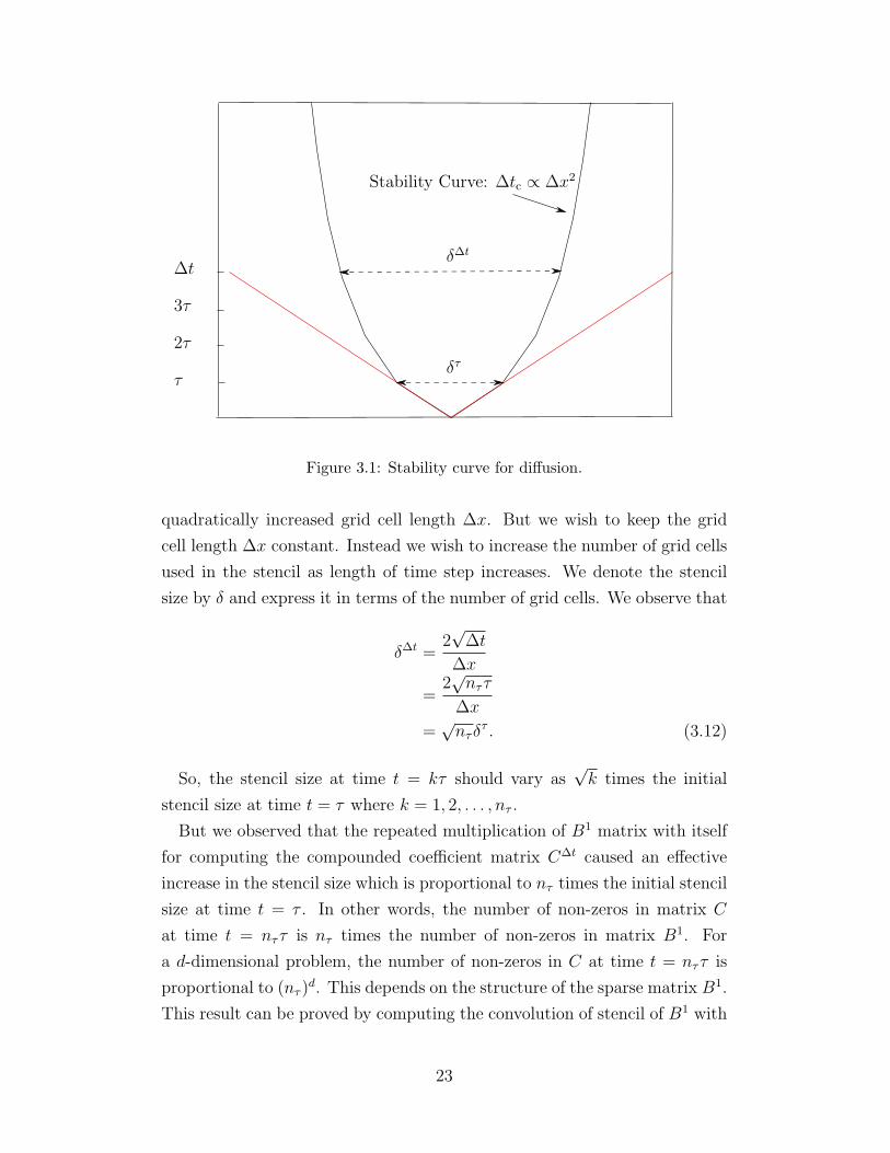
δ∆t

δτ

τ

2τ

3τ

∆t

Stability Curve: ∆tc ∝ ∆x2

Figure 3.1: Stability curve for diffusion.

quadratically increased grid cell length ∆x. But we wish to keep the grid

cell length ∆x constant. Instead we wish to increase the number of grid cells

used in the stencil as length of time step increases. We denote the stencil

size by δ and express it in terms of the number of grid cells. We observe that

δ∆t =2√

∆t

∆x

=2√

nττ

∆x

=√

nτδτ . (3.12)

So, the stencil size at time t = kτ should vary as√

k times the initial

stencil size at time t = τ where k = 1, 2, . . . , nτ .

But we observed that the repeated multiplication of B1 matrix with itself

for computing the compounded coefficient matrix C∆t caused an effective

increase in the stencil size which is proportional to nτ times the initial stencil

size at time t = τ . In other words, the number of non-zeros in matrix C

at time t = nττ is nτ times the number of non-zeros in matrix B1. For

a d-dimensional problem, the number of non-zeros in C at time t = nττ is

proportional to (nτ )d. This depends on the structure of the sparse matrix B1.

This result can be proved by computing the convolution of stencil of B1 with

23

the stencil of C. The red curve in the Figure 3.1 indicates this observation.

This happens due to numerical diffusion. The stencil size becomes very large

very quickly and so the computational cost also increases because number of

non-zeros in each column of the transition matrix increases and hence the

cost of multinomial sampling increases.

So we can further reduce the computational cost if we adjust the stencil size

δkτ after each time step τ to be proportional to√

k times the initial stencil

size where k = 1, 2, . . . , nτ . We will denote the number of non-zeros in a

matrix by nnz. See Algorithm 2 and Algorithm 3 for details. The LTPGM

(Algorithm 2) differs from PGM (Algorithm 1) only in points 6, 16, 17, and

18.

Algorithm 2 Large Time-step Particle Grid Method (LTPGM) for advec-tion and diffusion of particles.

1: m is the number of grid cells along each dimension2: d is the dimensionality of the problem3: Ncell ← md is the total number of grid cells4: N is the total number of computational particles5: p(~x, 0) is the initial particle density

6: ∆t← (0.5)∆xmax ‖~w‖1 is the time-step

7: Calculate the number of time-steps nt ← T∆t

8: VI and DI are the volume and domain of grid cell I where I = 1, . . . , Ncell

9: QkI is the number of particles in grid cell I at time k∆t

10: p̃kI is the particle density in grid cell I at time k∆t

11: for nr repetitions do12: for all cells I do13: randomly choose Q0

I ∼ Poisson( ∫

DI

N p(~x, 0)d~x)

14: end for15: for time-step k = 1, 2, . . . , nt do16: Construct the advection matrix Ak based on explicit discretization

of advection PDE17: Construct the diffusion matrix Dk by sub-cycling within each ∆t

time-step18: Compute the transition matrix Ck ← DkAk

19: Compute Qk ←∑Ncell

I=1 multinomial(Qk−1I , Ck

I )20: p̃k

I ← QkI/(N VI)

21: end for22: end for23: Compute the sample mean of particle density p̃k

I ← 1nr

∑nr

r=1(p̃kI )r

24

Algorithm 3 Construction of diffusion matrix by sub-cycling in each ∆t.

1: nτ is the number of sub-cycling time-steps2: τ is the sub-cycling time-step3: for each ∆t do4: κmax = max κ(~x, (k − 1)∆t)

5: Calculate τ ← (0.5) ∆x2

2κmaxd

6: Calculate nτ ← ∆tτ

7: Construct the diffusion matrix Bk using τ and κ(~x, (k − 1)∆t) basedon explicit discretization of diffusion PDE

8: Construct Dk ← J where J is the identity matrix9: for i = 1, 2, . . . , nτ do

10: Dk ← Bk Dk

11: a← nnz((Dk)column 1)− b√

i nnz((Bk)column 1)c12: if a > 0 then13: remove a outer diagonals from Dk matrix14: for all columns j of Dk do15: Dk

j ← Dkj /sum(Dk

j )16: end for17: end if18: end for19: end for

25

CHAPTER 4

GENERALIZED CONVERGENCE PROOF

In this chapter, we will present a generalized proof for the convergence of

the particle grid method (PGM) to the finite volume method (FVM). In

the earlier proof in Section 3.1, we assumed the initial distribution to be

poisson sampled. This proof makes no such assumption, but the convergence

is weaker as it proves convergence only in probability and not the convergence

in mean square. Also refer to Figure 6.3 for numerical result.

4.1 Strong Proof for Convergence of Particle Grid

Method

Theorem 6. The particle grid solution (p̃N)k at time-step k converges in

probability to the finite volume solution p̄k at time-step k as N →∞.

(p̃N)k P−→ p̄k as N →∞ for all k = 1, 2, . . . , nt.

where (p̃N)k denotes the particle grid solution at time-step k calculated using

N particles .

Proof. Consider the finite volume solution for the 1-D diffusion-advection

problem. We have a domain of length L which is divided into m grid cells.

p(x, t) denotes the particle density at location x and time t. qk is the finite

volume solution at time t = k. Given the initial particle density p(x, 0), we

can calculate the solution vector at initial time t = 0 as

q0i =

∫ xi+1

xi

p(x, 0)dx for all i = 1, 2, . . . ,m. (4.1)

The solution at next time step q1 is calculated by multiplying a coefficient

matrix B1 to the initial solution vector. Here B1 denotes the coefficient

26

matrix calculated using the diffusivity and wind velocity at time t = 0.

q1 = B1q0.

Since we are using the periodic boundary conditions, so the total number of

particles should remain constant. This implies that the sum of each column

of matrix B1 is 1. In general, the solution at the k-th time step is given by

qk = Bkqk−1.

So,

qk = BkBk−1Bk−2 . . . B1q0. (4.2)

where Bk denotes the coefficient matrix calculated using the diffusivity and

wind velocity at time t = (k − 1)∆t.

For the particle grid solution with N particles, we define the concentration

of particles as

c(x, t) = Np(x, t).

Since p(x, t) is a probability density function [Hogg et al., 2005, Ch. 1, p.

45], we also know that ∫ L

0

p(x, t)dx = 1.

And hence, the total number of particles is

N =

∫ L

0

c(x, t)dx.

Let Qk be the particle grid solution at time t = k∆t. Assume that we

know the particle solution at the initial time t = 0. For any time step k =

1, 2, . . . , nt, the particle grid solution at the current time step Qk is obtained

from the previous particle grid solution Qk−1 by multinomial sampling based

on the matrix Bk containing the probabilities of transfer of particles from

one grid cell to another grid cell.

Qk =m∑

j=1

multinomial(Qk−1j , Bk

j ).

Here Bkj denotes the j-th column of the coefficient matrix B calculated at

27

the time t = (k − 1)∆t and Qk−1j denotes the j-th element of the particle

grid solution vector at time t = (k − 1)∆t.

We will now prove that the PGM particle density converges in probability

to the FV particle density at each time-step k as N →∞.

(p̃k)N P−→ p̄k as N → 0 or

Qk

N∆x

P−→ qk

∆xas N → 0.

From Hogg et al. [2005, Ch. 4, p. 205], we know that if (p̃k)N P−→ p̄k, then

a(p̃k)N P−→ ap̄k where a is any constant. We choose a = ∆x, so to prove

Qk

N∆x

P−→ qk

∆xas N → 0

We only need to proveQk

N

P−→ qk as N → 0.

We claim that this is a stronger proof for convergence because we will

now show that irrespective of how we sample the initial particle distribu-

tion, ifQ0

N

P−→ q0 as N → ∞, thenQk

N

P−→ qk as N → ∞ for any

k = 1, 2, . . . , nt. GivenQ0

N

P−→ q0, we now use mathematical induction

to prove thatQk+1

N

P−→ qk+1 as N → ∞ assumingQk

N

P−→ qk as N → ∞.

By Chebyshev’s Inequality [Hogg et al., 2005, Ch. 1, p. 69], this is equivalent

to proving that

If E[Qk

N

]N→∞−→ qk and Cov

[Qk

N

]N→∞−→ 0,

then E[Qk+1

N

]N→∞−→ qk+1 and Cov

[Qk+1

N

]N→∞−→ 0. (4.3)

Using Law of Total Expectation, we can write

E[ 1

NQk+1

]= E

[E[ 1

NQk+1

∣∣∣Qk]]

(4.4)

= E[ 1

NBk+1Qk

].

Since mathematical expectation E is a linear operator [Hogg et al., 2005, Ch.

28

4, p. 198],

E[ 1

NBk+1Qk

]= Bk+1E

[ 1

NQk]

N→∞−→ Bk+1qk

= qk+1. (4.5)

Hence,

E[ 1

NQk+1

]N→∞−→ qk+1.

Law of Total Covariance can used to decompose the covariance as

Cov[ 1

NQk+1

]= Cov

[E[ 1

NQk+1

∣∣∣Qk]]

+ E[Cov

[ 1

NQk+1

∣∣∣Qk]]

= Cov[E[ 1

NQk+1

∣∣∣Qk]]

+ E[ 1

N2Cov

[Qk+1

∣∣∣Qk]]

. (4.6)

The first term on RHS of (4.6) is

Cov[E[ 1

NQk+1

∣∣∣Qk]]

= Cov[ 1

NBk+1Qk

]= [Bk+1]Cov

[ 1

NQk][Bk+1]T

N→∞−→ 0.(since Cov

[Qk

N

]N→∞−→ 0

)(4.7)

Consider the second term on RHS of (4.6)

Cov[Qk+1

∣∣∣Qk]

i,j= Cov

[Qk+1

i , Qk+1j

∣∣∣Qk]

for all i, j = 1, 2, 3 . . . , m

= Cov[ m∑

r=1

Qk+1i,r ,

m∑s=1

Qk+1j,s

∣∣∣Qk]

=m∑

s=1

m∑r=1

Cov[Qk+1

i,r , Qk+1j,s

∣∣∣Qk]

=

{0 if r 6= s∑m

r=1 Qkra

rij if r = s.

where

arij =

{−birbjr if i 6= j

bir(1− bir) if i = j.

29

Here Qk+1i,r denotes the number of particles transferred from the cell r to the

cell i. If r 6= s, then Qk+1i,r and Qk+1

j,s are independent because they are derived

from different multinomial distributions.

E[ 1

N2Cov

[Qk+1

i , Qk+1j

∣∣∣Qk]]

=

{0 if r 6= s∑m

r=1 E[

1N2 Q

kra

rij

]if r = s

=

{0 if r 6= s∑m

r=11N

arijE[

Qkr

N

]if r = s

N→∞−→ 0.(since E

[Qkr

N

]N→∞−→ qk

)So the second term on RHS of (4.6)

E[Cov

[ 1

NQk+1

∣∣∣Qk]]

N→∞−→ 0. (4.8)

From (4.6), (4.7) and (4.8), we conclude that Cov[Qk+1

N

]N→∞−→ 0. Thus,

Qk+1

N

P−→ qk+1 for all k = 0, 1, 2, . . . , nt − 1. And hence, (p̃k+1)N P−→p̄k+1 for all k = 0, 1, 2, . . . , nt − 1.

Thus, we proved that the particle grid solution converges to the finite vol-

ume solution for large number of particles. This proof can be easily extended

to multi-dimensional systems as well.

30

CHAPTER 5

ERROR ANALYSIS

We will now present a detailed mathematical derivation of upper bounds for

errors between the various methods used for solving the diffusion-advection

PDE.

5.1 Error Induced by Assuming Constant Diffusivity in

each ∆t

In LTPGM, we assume the diffusivity to remain constant within each time-

step ∆t. But in PGM, no such assumption is made. We would like to compare

the LTPGM method with the PGM method. Since both the methods are

stochastic methods, so it makes sense to calculate the error between these

two methods after they have converged to their mean solution. Since both

these particle methods converge to the corresponding FV solution for large

number of particles so we will calculate the error caused by the assumption of

constant diffusivity in each ∆t time-step by comparing the corresponding two

finite volume methods for solving the diffusion equation. In both methods,

we compute the diffusion matrix at ∆t by sub-cycling within each ∆t.

The first finite volume method computes the diffusion coefficient matrix

at each sub-cycling time step τ and then computes the product matrix D of

all these diffusion matrices. Multiplication by matrix D causes evolution of

solution vector from time t = (i−1)∆t to time t = i∆t where i = 1, 2, . . . , nt.

The second finite volume method uses the assumption that diffusivity re-

mains constant in each ∆t. So we first compute the diffusion matrix in the

first sub-cycling time-step τ . The diffusion matrix for all the rest of the sub-

cycling time steps will also be the same since diffusivity is constant. So the

compounded matrix, denoted by C will be calculated by raising the diffusion

matrix in the first sub-cycling time-step to the power nτ . Again, Multipli-

31

cation by the matrix C will cause evolution of the solution vector from time

t = (i− 1)∆t to time t = i∆t where i = 1, 2, . . . , nt. Let us now introduce a

useful theorem which we will use later for proof of Theorem 8.

Theorem 7 ([Apostal, 1962, Ch. 9, p. 460]). If a function κ ∈ C1, that is,

κ is continuous and differentiable and [a, b] is compact, then κ is Lipschitz

on [a, b]. Hence,

maxt∈[t0,t1]

|κ(t)− κ(t0)| ≤ L|t1 − t0|.

Theorem 8. The local error at time-step ∆t is O(∆t2) and the global error

at t = T is O(∆t). In other words,

‖(Ci −Di)qi−1‖2 = c2∆t2 and∥∥∥( nt∏i=1

Ci −nt∏i=1

Di)q0∥∥∥

2= c3∆t

where c2 and c3 are constants.

Proof. Let the transition matrix be Bk where k = 1, 2, . . . , nτ and nτ be

the number of small time steps τ within big time step ∆t. The exact finite

volume solution after nτ small time steps is given by

qnτ = Bnτ Bnτ−1Bnτ−2 . . . B1q0.

And the approximate finite volume solution is given by

q̆nτ = [B1]nτ q0. (5.1)

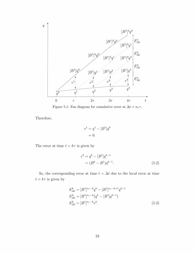
Figure 5.1 depicts the fan diagram [Niesen, 2010] for calculating the error

committed in a single time step ∆t = 4τ . We are interested in estimating

the error caused by our approximate finite volume method compared to the

exact finite volume solution. ek denotes the local error at time t = kτ and

Ek∆t denotes the global error at time t = ∆t due to the evolution of local

error ek at time t = kτ . Note that

qk = [Bk]qk−1.

32

q0 q1 q2 q3 q4

[B1]q0

[B1]2q0

[B1]3q0

[B1]4q0

[B1]q1 [B1]q2 [B1]q3

[B1]2q1

[B1]3q1

[B1]2q2

e1 e2 e3 e4 E4∆t

E3∆t

E2∆t

E1∆t

0 τ 2τ 3τ 4τ

q

t

Figure 5.1: Fan diagram for cumulative error at ∆t = nττ .

Therefore,

e1 = q1 − [B1]q0

= 0.

The error at time t = kτ is given by

ek = qk − [B1]qk−1

= (Bk −B1)qk−1. (5.2)

So, the corresponding error at time t = ∆t due to the local error at time

t = kτ is given by

Ek∆t = [B1]nτ−kqk − [B1]nτ−k+1qk−1

Ek∆t = [B1]nτ−k(qk − [B1]qk−1)

Ek∆t = [B1]nτ−kek. (5.3)

33

So, if we take the 2-norm of the error, we get

‖Ek∆t‖2 ≤ ‖[B1]nτ−k‖2‖ek‖2

≤ ‖B1‖nτ−k2 ‖ek‖2.

The vector-induced matrix norm used here is the spectral norm, which is

equal to the largest singular value of a matrix. Also, the 2-norm of the local

error is

‖ek‖2 ≤ ‖(Bk −B1)‖2‖qk−1‖2.

Note that for all time-step k, we have

Bk =

1− 2κkτ κkτ 0 . . . κkτ

κkτ 1− 2κkτ κkτ . . . 0

0 κkτ 1− 2κkτ . . . 0...

......

. . ....

κkτ 0 . . . κkτ 1− 2κkτ

.

And since B1 is a real symmetric stochastic [Norris, 1998] matrix, so its

spectral norm is 1. Refer to Section A.1 for proof. So,

‖B1‖2 = 1. (5.4)

It is clear that

‖(Bk −B1)‖2 = c1|κk − κ1|τ. (5.5)

So, the error

‖Ek∆t‖2 ≤ ‖B1‖nτ−k

2 ‖ek‖2≤ ‖ek‖2≤ ‖(Bk −B1)‖2‖qk−1‖2= c1|κk − κ1|τ‖qk−1‖2.

Let us denote the maximum change in the diffusivity in time-step ∆t by

∆κ = max1≤k≤nτ

(|κk − κ1|).

34

Then

‖E∆t‖2 ≤nτ∑

k=1

‖Ek∆t‖2

≤ (c1∆κτ)nτ∑

k=1

‖qk−1‖2

≤ (c1∆κτ)(nτ‖q0‖2).

So, the relative error can be written as

‖E∆t‖2‖q0‖2

≤ c1∆κ(nττ)

= c1∆κ∆t.

By Theorem 7, we know that

∆κ ≤ L∆t.

Using this, we get

‖E∆t‖2‖q0‖2

≤ c1L∆t2

= c2∆t2. (5.6)

Now for the global error at time t = T , look at the fan diagram in Fig-

ure 5.2. For simplicity, we assume that each time-step ∆t contains the same

number of sub-cycling time-steps nτ . Let

Ci = (B(i−1)∆t+τ )nτ for all i = 1, 2, . . . , nt and (5.7)

Di =nτ∏j=1

B(i−1)∆t+jτ for all i = 1, 2, . . . , nt. (5.8)

Now, the evolved error Ei′T at time T corresponding to the error committed

35

q0 D1 D2 D3 D4

C1

C2

C3

C4

C2 C3 C4

C3

C4

C4

E1′∆t E2′

∆tE3′

∆tE4′

∆tE4′

T

E3′T

E2′T

E1′T

0 ∆t 2∆t 3∆t 4∆t

q

t

Figure 5.2: Fan diagram for global error at T = nt∆t.

at time t = i∆t is

Ei′

T =( nt∏

j=i+1

Cj)(Ci −Di)

( i−1∏k=1

Di)q0. (5.9)

‖Ei′

T ‖2 ≤∥∥∥( nt∏

j=i+1

Cj)∥∥∥

2

∥∥∥(Ci −Di)( i−1∏

k=1

Di)q0

∥∥∥2

=∥∥∥( nt∏

j=i+1

Cj)∥∥∥

2‖Ei′

∆t‖2.

where Ei′∆t is the error at time t = i∆t. Since (

∏nt

j=i+1 Cj) is also a real sym-

metric stochastic matrix, hence its spectral norm is 1. Refer to Section A.1

for proof. ∥∥∥( nt∏j=i+1

Cj)∥∥∥

2= 1. (5.10)

36

Therefore, we get

‖Ei′

T ‖2 ≤ ‖Ei′

∆t‖2.

‖ET‖2 ≤nt∑i=1

‖Ei′

T ‖2

≤nt∑i=1

‖Ei′

∆t‖2

Since ‖Ei′∆t‖2 ≤ c2∆t2‖q0‖2, we can write

‖ET‖2 ≤ ntc2∆t2‖q0‖2= c2T∆t‖q0‖2= c3∆t‖q0‖2.

Hence,‖ET‖2‖q0‖2

≤ c3∆t. (5.11)

5.2 Error Between Traditional FV Solution and Exact

Solution

The global error between exact analytical solution and finite volume solution

based on explicit discretization at time t = T is O(∆x2). It can be proved

with the help of the Lady Windermere’s fan diagram [Hairer et al., 2008, Ch.

II, p. 160; Niesen, 2010]. See Figure 6.2.

37

CHAPTER 6

NUMERICAL RESULTS

We will now present the results from the numerical simulation of the one-

dimensional diffusion-advection equation (1.1) by various methods. We con-

sidered a domain of length L = 1 and divided it into m uniformly spaced

grid cells. We performed simulation for a total time T = 1. We assumed

initial particle density to be

p(x, 0) = 1 + sin(2π(x− 0.5)).

We used diffusivity given by

κ(x, t) = 0.05(1

2+

1

πtan−1

(2t− 2

3

)),

and velocity u(x, t) = 1. We solved the 1-D advection-diffusion equation

with different methods and the results are shown in Figure 6.1. The blue

curve shows the initial particle density and the red curve shows the particle

density at final time. The solution by all the given methods looks good and

is very close to the exact analytical solution.

6.1 Convergence of Finite Volume Solution to Exact

Solution

The 1-D diffusion-advection was solved with the finite volume method with

increasing number of grid cells and was compared with the exact analytical

solution. The error was calculated as

‖p̄T − pT‖2 =

√√√√ m∑I=1

(p̄TI − pT

I )2∆x.

38

0 0.5 10

0.5

1

1.5

2

x

Par

ticle

den

sity

FV

0 0.5 10

0.5

1

1.5

2

x

Par

ticle

den

sity

Analytic

0 0.5 10

0.5

1

1.5

2

x

Par

ticle

den

sity

PGM

0 0.5 10

0.5

1

1.5

2

x

Par

ticle

den

sity

LTPGM

0 0.5 10

0.5

1

1.5

2

x

Par

ticle

den

sity

PGFM

Figure 6.1: Solution of 1-D diffusion-advection PDE by various methods. Thedomain length L = 1 was divided into m = 20 grid cells. The number of particlesused for particle methods is N = 100000. The PGFM method used same numberof time-steps nt as FV and PGM. The blue curve shows the initial particle densityand the red curve shows the particle density at the final time T = 1.

39

10 20 30 40 50 60 70 80 90 10010

−5

10−4

10−3

10−2

m

Err

or

(FV

− E

xa

ct)

|| FV − Exact ||2

slope= -2

Figure 6.2: Convergence of finite volume solution to exact solution for 1-Ddiffusion-advection equation. The y-axis shows the error between FV and exact

particle density. The error is calculated as ‖p̄T − pT ‖2 =√∑m

I=1(p̄TI − pT

I )2∆x.

From Figure 6.2, we observe that as ∆x decreases, the error decreases with

slope = −2 as predicted in Section 5.2 and Theorem 4.

6.2 Convergence of Particle Grid Solution to Finite

Volume Solution

We also compared the particle grid solution with the finite volume solution.

The error was calculated as

E(‖(p̃N)T − p̄T‖2) =1

nr

nr∑r=1

(√√√√ m∑I=1

((p̃NI )T

r − p̄TI )2∆x

).

According to Theorem 3, the error between these two methods should de-

crease as number of particles used for particle grid method increase. Fig-

40

102

103

104

105

106

107

10−4

10−3

10−2

10−1

100

N

Err

or

(PG

M −

FV

)

|| PGM − FV ||2

slope= -0.5

Figure 6.3: Convergence of PGM solution to FV solution for 1D diffusion-advectionequation. Both solutions used m = 10 grid cells. We used nr = 50 repe-titions for the PGM method. The y-axis shows the error between PGM andFV solution at final time. The error was calculated as E(‖(p̃N )T − p̄T ‖2) =1nr

∑nrr=1

(√∑mI=1((p̃

NI )T

r − p̄TI )2∆x

).

ure 6.3 shows the result from numerical simulation with m = 10 grid cells

and nr = 50 repetitions of the particle grid solution. For all particle methods,

we expect the error to decrease with increase in number of particles with a

slope = −0.5. The numerical results agree with the mathematically derived

results.

41

6.3 Convergence of Particle Grid Free Solution to

Exact Solution

We solved the 1-D diffusion-advection equation with particle grid free method

and compared it with exact analytical solution. The error was calculated as

E(‖(p̂N)T − p̄T‖2) =1

nr

nr∑r=1

(√√√√ m∑I=1

((p̂NI )T

r − p̄TI )2∆x

).

We expect that the error between these two methods should decrease as

the number of particles used for particle grid free method increase with a

slope = −0.5. The error should also decrease when a smaller time-step is

used for simulation. Refer to Section 2.2. Figure 6.3 shows the result from

numerical simulation with m = 5 grid cells and nr = 50 repetitions and

increasing number of particles. The blue curve shows the error with a time-

step ∆t = 0.1 and the red curve shows the error with a time-step ∆t = 0.01.

The results from numerical simulation agree with the mathematically derived

results.

6.4 Convergence of Particle Grid Solution to Exact

Solution

In this section, we investigate the convergence of particle grid solution to

the exact analytical solution of 1-D diffusion-advection equation. We expect

that the error between these two methods should decrease as the number of

particles N and the number of grid cells m are increased. Refer to Theorem 5.

Figure 6.5 shows the result from numerical simulation. The red curve shows

the error with m = 10 grid cells and the blue curve shows the error with

m = 5 grid cells. In this figure, we also observe that the error increases if

we use small number of particles and increase the number of grid cells. To

investigate this behavior in detail, we plotted the error between the particle

grid method and exact analytical solution for N = 100 particles and we

increased the number of grid cells m. We again observe increase in error as

m is increased for small N in Figure 6.6. As the total number of particles

is relatively small, so each grid cell will get very few particles on average.

42

102

103

104

105

106

107

10−4

10−3

10−2

10−1

100

N

err

or

(PG

FM

− E

xa

ct)

dt=0.1dt=0.01

slope = -0.5

Figure 6.4: Convergence of PGFM solution to exact solution for 1D diffusion-advection equation. Both solutions used m = 5 grid cells. We used nr = 50repetitions for the PGFM method. The y-axis shows the error between PGFMand exact solution at final time. The error was calculated as E(‖(p̂N )T − p̄T ‖2) =1nr

∑nrr=1

(√∑mI=1((p̂

NI )T

r − p̄TI )2∆x

). The blue curve shows the result with nt =

10 time-steps and the red curve shows the result with nt = 100 time-steps forPGFM method.

43

102

103

104

105

106

107

10−3

10−2

10−1

100

N

err

or

(PG

M −

Exa

ct)

m=5m=10

slope = -0.5

Figure 6.5: Convergence of PGM solution to exact solution for 1D diffusion-advection equation. We used nr = 100 repetitions for the PGM method. They-axis shows the error between PGM and exact solution at final time. The error

was calculated as E(‖(p̃N )T − pT ‖2) = 1nr

∑nrr=1

(√∑mI=1((p̃

NI )T

r − pTI )2∆x

).The

blue curve shows the result with m = 5 grid cells and the red curve shows theresult with m = 10 grid cells.

Since the particle grid method is a stochastic method, so some grid cells

may get more particles while others may not get any. So the deviation from

exact solution will be large. Since we are calculating the mean of the errors

and not the error between the mean particle grid solution and the exact

analytic solution, so we expect the error to increase as the number of grid

cells increase for the simulation with small N . We can mathematically show

the error to be proportional to√

mN

. So the observed slope of 0.5 agrees well

with mathematically expected result.

44

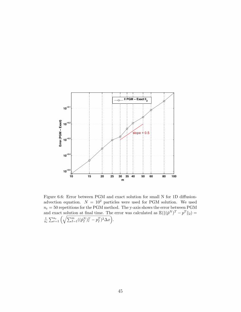
10 15 20 25 30 35 40 50 60 80 100

10−0.5

10−0.4

10−0.3

10−0.2

10−0.1

Err

or

(PG

M −

Exa

ct)

m

|| PGM − Exact ||2

slope = 0.5

Figure 6.6: Error between PGM and exact solution for small N for 1D diffusion-advection equation. N = 102 particles were used for PGM solution. We usednr = 50 repetitions for the PGM method. The y-axis shows the error between PGMand exact solution at final time. The error was calculated as E(‖(p̃N )T − pT ‖2) =1nr

∑nrr=1

(√∑mI=1((p̃

NI )T

r − pTI )2∆x

).

45

100

101

102

10−4

10−3

10−2

10−1

m

Err

or

|| FV − Exact ||2

|| PGM − Exact ||2

|| PGFM − Exact ||2

slope= -2

Figure 6.7: Comparison of various solution methods. The y-axis shows error be-tween the given method and the exact solution. N = 107 particles and nr = 50repetitions were used for particle methods.

6.5 Comparison Between Finite Volume Method,

Particle Grid Method and Particle Grid Free

Method

We also calculated the error between the finite volume method, the particle

grid method and the particle grid free method with N = 107 particles with

respect to the exact solution as number of grid cells is increased. Figure 6.7

shows the result from numerical simulation. All the three errors decrease as

the number of grid cells is increased as we discussed in Section 2.2, Section 5.2

and Theorem 5. The finite volume method is the most accurate among all the

three methods. Among the particle methods, the particle grid method is more

accurate than the particle grid free method. The slope of the error curves for

the particle methods increases for large m because as m is increased, we need

more particles to converge to accurate solution. See Figure 6.6 for numerical

result.

46

CHAPTER 7

CONCLUSIONS

We developed a particle-resolved method for large scale simulation of the

transport of particles by advection and diffusion. It is called the particle

grid method (PGM). In ISSA by Lampoudi et al. [2009], the population of

particles in the neighboring sub-volumes are coupled by diffusive transfers

which are treated as unimolecular reactions. MSA [Lampoudi et al., 2009] is

a stochastic method which outperforms ISSA when the transfer of particles is

more frequent than the chemical reactions in the sub-volumes but it assumes

constant diffusivity. The PGM method does not make any such assumption.

PGM is an extension of MSA for spatially distributed stochastic particle sim-

ulations with varying diffusivity and velocity field. PGM is based on transfer

of particles between homogeneous grid cells with multinomial probabilities.

It converges to the finite volume solution if large number of particles are used

and also converges to exact solution if we then also make the grid finer. We

found that the particle grid method is more accurate and computationally

cheaper than the particle grid free method. The LTPGM method, which is

a variant of the PGM method, was derived based on assumptions which we

believe are acceptable for large scale simulation of fluid transported parti-

cles. The error between LTPGM and exact solution is approximately the

same as the error between PGM and exact solution if a very fine grid is used.

Its computational cost is also less than the PGM method as less number of

time-steps are involved. Hence, we conclude that it is a suitable method for

large scale simulation of transport of particles by advection and diffusion.

47

APPENDIX A

MATHEMATICAL RESULTS

A.1 Spectral Norm of Diffusion and Advection

Matrices

The advection and the diffusion coefficient matrices are used as the transi-

tion probability matrix in the particle grid method. We now know that the

transition probability matrix B is always non-negative, symmetric and its

row sum is 1. The matrix B is also called a stochastic matrix [Norris, 1998].

The spectral norm of a matrix is equal to the maximum singular value of

that matrix. We will now prove that the spectral norm of B is always 1.

Theorem 9. One of the eigenvalue associated with a stochastic matrix is

always 1.

Proof. Since the row sum of a stochastic matrix is always 1, so we can choose

an eigenvector with all the elements equal to 1 and we always get a corre-

sponding eigenvalue equal to 1.

Theorem 10 (Perron Frobenius Theorem). The largest eigenvalue associated

with a stochastic matrix is always 1.

Proof. Let v be the right eigenvector of the stochastic matrix P . Let vi be

48

the largest coordinate in the modulus. Then

λvi = (Pv)i =k∑

j=1

Pijvj.

|λvi| = |k∑

j=1

Pijvj|

≤k∑

j=1

Pij|vj|

≤k∑

j=1

Pij|vi|

Since∑k

j=1 Pij = 1, we get

|λvi| ≤ |vi|.

⇒ |λ| ≤ 1 for all λ. (A.1)

Since one of the eigenvalue is always 1 and all the eigenvalues are less than

or equal to 1, so λ = 1 is the largest eigenvalue of a stochastic matrix.

For alternate proof of the above theorem, refer to Lancaster and Tismenet-

sky [1985, Ch. 15, p. 547].

Theorem 11. For a real symmetric stochastic matrix, the maximum singular

value is always 1. In other words, the spectral norm of a real symmetric

stochastic matrix is always 1.

Proof. Let σ denote the singular value of a matrix. Then

σ(P ) = eig(P T P )

Since P is real symmetric, so

σ(P ) = eig(P 2).

49

Let λ be an eigenvalue of P . Then

P 2x = PPx

= λPx

= λ2x.

⇒ σ(P ) = eig(P 2)

= λ2.

Thus,

σmax(P ) = (λmax)2

And by Perron Frobenius Theorem,

σmax(P ) = 1. (A.2)

A.2 Binomial-Poisson Hierarchy Model

Theorem 12. If Y is Poisson(λ) and X is binomial(Y, p), then X is Poisson(λp).

Proof. Since Y is Poisson(λ),

P (Y = y) =λye−λ

y!.

By the definition of conditional probability,

P (X = x|Y = y) =P (X = x; Y = y)

P (Y = y).

P (X = x; Y = y) = P (Y = y)P (X = x|Y = y).

The marginal distribution of X is then given by

P (X = x) =∞∑

y=x

P (X = x; Y = y)

=∞∑

y=x

λye−λ

y!

(y

x

)px(1− p)y−x

50

=∞∑

y=x

λye−λ

x!(y − x)!px(1− p)y−x

=px(1− p)−xe−λ

x!

∞∑y=x

λy(1− p)y

(y − x)!

=px(1− p)−xe−λ

x!eλ(1−p)λx(1− p)x

=(λp)xe−λp

x!.

So X is Poisson(λp).

A.3 Conditional Distribution of Multinomial Variables

Theorem 13. Suppose X1, X2, . . . , Xk, . . . , Xm are multinomial random vari-

ables with the corresponding probabilities p1, p2, . . . , pk, . . . , pm.

(X1, X2, . . . , Xk, . . . , Xm) ∼ multinomial(N, p1, p2, . . . , pk, . . . , pm).

Hence,m∑

i=1

Xi = N

andm∑

i=1

pi = 1.

Then,

P(Xk = nk|Xk−1 = nk−1, . . . , X2 = n2, X1 = n1)

= binomial

(N −

k−1∑i=1

ni,pk

1−k−1∑i=1

pi

).

Proof. By the definition of conditional probability,

P(Xk = nk|Xk−1 = nk−1, . . . , X1 = n1)

=P(Xk = nk, Xk−1 = nk−1, . . . , X1 = n1)

P(Xk−1 = nk−1, . . . , X1 = n1).

51

Since

P(Xk−1 = nk−1, Xk−2 = nk−2, . . . , X1 = n1)

=N !(

Πk−1i=1 ni!

)(N −

k−1∑i=1

ni

)!

(Πk−1

i=1 pnii

)(1−

k−1∑i=1

pi

)(N−k−1Pi=1

ni

)

And

P(Xk = nk, Xk−1 = nk−1, . . . , X1 = n1)

=N !(

Πki=1ni!

)(N −

k∑i=1

ni

)!

(Πk

i=1pnii

)(1−

k∑i=1

pi

)(N−kP

i=1ni

).

So, by dividing the above two equations, we get

P(Xk = nk|Xk−1 = nk−1, . . . , X1 = n1)

=

(N −

k−1∑i=1

ni

nk

)(pk

1−k−1∑i=1

pi

)nk( 1−

k∑i=1

pi

1−k−1∑i=1

pi

)(N−kP

i=1ni

).

Hence,

P(Xk = nk|Xk−1 = nk−1, . . . , X1 = n1)

= binomial

(N −

k−1∑i=1

ni,pk

1−k−1∑i=1

pi

).

52

REFERENCES

P. J. Adams, J. H. Seinfeld, and D. M. Koch. Global concentration of tropo-spheric sulphate, nitrate and ammonium simulated in a general circulationmodel. Journal of Geophysical Research, 104, 1999.

T. M. Apostal. Calculus. Blaisdell Publishing Company, first edition, 1962.

F. S. Binkowski and U. Shankar. The regional particulate matter model:I. Model description and preliminary results. Journal of Geophysical Re-search, 100, 1995.

G. Casella and R. L. Berger. Statistical Inference. Duxbury Press, secondedition, 2001.

B. Cockburn, F. Coquel, Ph. LeFloch, and C. W. Shu. Convergenceof finite volume methods. IMA preprint series 771, available athttp://www.ima.umn.edu/preprints/Feb91Series/771.pdf, 1991.

D. Fange and J. Elf. Noise-induced min phenotypes in E. coli. PLoS Com-putational Biolgy, 2(6), 2006.

A. Fassi-Fihri, K. Suhre, and R. Rosset. Internal and external mixing inatmospheric aerosols by coagulation: Impact on the optical and hygro-scopic properties of the sulphate-soot system. Atmospheric Environment,31, 1997.

C. W. Gardiner, K. J. McNeil, D. F. Walls, and I. S. Matheson. Correlationsin stochastic theories of chemical reactions. Journal of Statistical Physics,14(1), 1976.

S. J. Ghan and S. E. Schwartz. Aerosol properties and processes– A path fromfield and laboratory measurements to global climate models. AmericanMeteorological Society, 88, 2007.

D. T. Gillespie. An exact method for numerically simulating the stochasticcoalescence process in a cloud. Journal of Atmospheric Science, 32, 1975.

D. T. Gillespie. A general method for numerically simulating the stochastictime evolution of coupled chemical reactions. Journal of ComputationalPhysics, 22, 1976.

53

D. T. Gillespie. Exact stochastic simulation of coupled chemical reactions.Journal of Physical Chemistry, 81, 1977.

D. T. Gillespie. Markov Processes: An Introduction for Physical Scientists.Academic Press, San Diego, Calif., 1992.

D. T. Gillespie. Approximate accelerated stochastic simulation of chemicallyreacting systems. Journal of Chemical Physics, 115, 2001.

M. B. Griesemer, C. L. Young, D. Raden, F. J. Doyle III, A. S. Robinson,and L. R. Petzold. Modeling the impact of spatial localization of proteinfunction in the endoplasmic reticulum of yeast. In Proc. 2009 FOSBEConference, 2009.

E. Hairer, S. P. Norsett, and G. Wanner. Solving Ordinary Differential Equa-tions I. Nonstiff Problems. Springer, second edition, 2008.

P. Hanusse and A. Blanche. A Monte-Carlo method for large reaction-diffusion systems. Journal of Chemical Physics, 74(11), 1981.

D. J. Higham. An algorithmic introduction to numerical simulation ofstochastic differential equations. SIAM REVIEW, 43(3), 2001.

R. V. Hogg, J. W. McKean, and A. T. Craig. Introduction to MathematicalStatistics. Pearson Prentice Hall, sixth edition, 2005.

S. A. Isaacson and C. S. Peskin. Incorporating diffusion in complex ge-ometries into stochastic chemical kinetics simulations. SIAM Journal ofScientific Computing, 28, 2006.

M. Z. Jacobson. Development and application of a new air pollution modelingsystem: II. Aerosol module structure and design. Atmospheric Environ-ment, 31, 1997.

V. Kachitvichyanukul and B. W. Schmeiser. Binomial random variate gen-eration. Communications of the ACM, 31(2), 1988.

S. Lampoudi, D. Gillespie, and L. Petzold. The multinomial simulation al-gorithm for discrete stochastic simulation of reaction-diffusion systems.Journal of Chemical Physics, 130(9), 2009.

P. Lancaster and M. Tismenetsky. The Theory of Matrices. Academic Press,second edition, 1985.

R. J. Leveque. Finite Volume Methods for Hyperbolic Problems. CambridgeUniversity Press, 2002.

R. McGraw. Description of aerosol dynamics by the quadrature method ofmoments. Aerosol Science and Technology, 27, 1997.

54

J. Michalakes, J. Dudhia, D. Gill, J. Klemp, and W. Skamarock. Designof a next-generation regional weather research and forecast model. InTowards Teracomputing, pages 117–124, River Edge, New Jersey, 1999.World Scientific.

P. Moin. Fundamentals of Engineering Numerical Analysis. Cambridge Uni-versity Press, first edition, 2001.

M. Muller, D. Charypar, and M. Gross. Particle-based fluid simulation forinteractive applications. Eurographics/SIGGRAPH Symposium on Com-puter Animation, 2003.

J. Niesen. On the Global Error of Discretization Methods for Ordinary Dif-ferential Equations. PhD thesis, University of Cambridge, 2010.

J. R. Norris. Markov Chains. Cambridge University Press, first edition, 1998.

H. Resat, L. Petzold, and M. F. Pettigrew. Kinetic modeling of biologicalsystems. Computational Systems Biology, 541, 2009.

N. Riemer, M. West, R. A. Zaveri, and R. C. Easter. Simulating the evolutionof soot mixing state with a particle-resolved aerosol model. Journal ofGeophysical Research, 114, 2009.

N. Riemer, M. West, R. Zaveri, and R. Easter. Estimating black carbonaging time-scales with a particle-resolved aerosol model. Aerosol Science,41, 2010.

Y. Saad. SPARSKIT: A basic tool kit for sparse matrix computations, ver-sion 2. CSRD (University of Illinois) and RIACS (NASA Ames ResearchCenter), 1994.

M. Sander, R. H. West, M. S. Celnik, and M. Kraft. A detailed model forthe sintering of polydispersed nanoparticle agglomerates. Aerosol Scienceand Technology, 43, 2009.

A. J. Smallbone, A. R. Coble, A. N. Bhave, S. Mosbach, M. Kraft, N. Morgan,and G. Kalghatgi. Simulating PM emissions and combustion stability ingasoline/diesel fuelled engines. Technical report, SAE 2011 World Congressand Exhibition, 2011.

P. Stier, J. Feichter, S. Kinne, S. Kloster, E. Vignati, J. Wilson, L. Ganzeveld,I. Tegen, M. Werner, Y. Balkanski, M. Schulz, O. Boucher, A. Minikin,and A. Petzold. The aerosol-climate model ECHAM5-HAM. AtmosphericChemistry and Physics, 5(4), 2005.

J. C. Strikwerda. Finite Difference Schemes and Partial Differential Equa-tions. SIAM: Society for Industrial and Applied Mathematics, second edi-tion, 2004.

55

A. S. Wexler, F. W. Lurmann, and J. H. Seinfeld. Modelling urban aerosols–I.Model development. Atmospheric Environment, 28, 1994.

E. R. Whitby and P. H. McMurry. Modal aerosol dynamics modeling. AerosolScience and Technology, 27, 1997.

J. Wilson, C. Cuvelier, and F. Raes. A modeling study of global mixedaerosol fields. Journal of Geophysical Research, 106, 2001.

R. A. Zaveri, R. C. Easter, J. D. Fast, and L. K. Peters. Model for simulatingaerosol interactions and chemistry (MOSAIC). Journal of GeophysicalResearch, 113, 2008.

R. A. Zaveri, J. C. Barnard, R. C. Easter, N. Riemer, and M. West. Particle-resolved simulation of aerosol size, composition, mixing state, and theassociated optical and cloud condensation nuclei activation properties inan evolving urban plume. Journal of Geophysical Research, 115, 2010.

56

AUTHOR’S BIOGRAPHY

Rishabh Kumar Jain was born in Rajasthan, India, on April 9th, 1988. He

completed his school education from Atomic Energy Central School no. 4

in Rawatbhata in 2005. The following July, he joined Indian Institute of

Technology, Bombay and in August 2009, received the degree of Bachelor

of Technology in Mechanical Engineering. He joined University of Illinois

at Urbana-Champaign in August 2009 and is a candidate for the Master of

Science Degree in Mechanical Engineering.

57