c 2015 zhenyu hu - ideals

DYNAMIC PRICING WITH REFERENCE PRICE EFFECTS

BY

ZHENYU HU

DISSERTATION

Submitted in partial fulfillment of the requirementsfor the degree of Doctor of Philosophy in Industrial Engineering

in the Graduate College of theUniversity of Illinois at Urbana-Champaign, 2015

Urbana, Illinois

Doctoral Committee:

Associate Professor Xin Chen, ChairAssistant Professor Alex OlshevskyAssociate Professor Nicholas PetruzziAssociate Professor Qiong Wang

Abstract

This dissertation mainly focuses on the models and the corresponding dy-

namic pricing problems that incorporate reference price effects, a concept

developed in economics and marketing literature that try to capture the de-

pendency of consumers purchasing behavior on past prices.

Conceptually, reference price is a price expectation consumers develop from

their observations of historical prices. Since it can not be physically ob-

served, various models have been proposed to operationalize its formation.

We empirically compare some of the models in the literature and extend the

literature by proposing a new reference price model. In addition, we present

analysis on the dynamic pricing problems under these models assuming con-

sumers are loss/gain neutral or loss-averse. We find that constant pricing

strategies are a robust solution to the problem regardless of which reference

price models one may choose.

Empirical evidences, however, indicate that loss/gain neutral or loss-averse

behavior may not be a universal phenomenon. We analyze the dynamic

pricing problem when consumers exhibit gain-seeking behavior. In sharp

contrast to the loss-averse case, even myopic pricing strategies can result

in complicated cyclic price paths. We show for a special case that a cyclic

skimming pricing strategy is optimal and provide conditions to guarantee the

optimality of high-low pricing strategies.

With the understanding of the qualitative behavior of the optimal pricing

strategies under various settings, we develop efficient algorithms to compute

the optimal prices in both loss-averse and gain-seeking case. We demon-

strate the efficiency and robustness of our algorithms by applying them to a

practical problem with real data.

Finally, we extend the above considered single-product setting to multi-

product setting and analyze the corresponding dynamic pricing problems.

ii

To my parents, for their love and support.

iii

Acknowledgments

First and foremost, I would like to express my deepest gratitude to my ad-

visor Prof. Xin Chen. As a student, the financial support and tremendous

guidance I received from Prof. Chen is what make this thesis and the com-

pletion of my study possible. His quick and sharp observations have always

been a source of ideas and breakthroughs. His patience, on the other hand,

enables me to step out of a specific problem and to explore the related ar-

eas in order to have a big picture and better understanding of the problem

at hand. As a researcher, I believe the invaluable experiences of working

so closely with Prof. Chen for the past four years has a profound and far-

reaching influence on my future career. I get to know how a research idea

is brought up and developed; I become to recognize the importance in an

intuitive understanding of a certain result and I learn to keep my interests

wide and open. I am eternally grateful for all the time and effort he has put

in over the years to guide and teach me how to do research and how to enjoy

research.

I would like to thank my thesis committee members Prof. Alex Olshevsky,

Prof. Nicholas Petruzzi and Prof. Qiong Wang for their time, efforts and

valuable suggestions. I would also like to thank Prof. Peng Hu for the

discussions and his contributions to Chapter 3 and Chapter 4, and Yuhan

Zhang for his input in Chapter 2.

During my study at the University of Illinois, I am fortunate to meet and

discuss with many brilliant professors across the departments. I want to

thank Prof. Enlu Zhou, Prof. Qiong Wang, Prof. Angelia Nedich and many

others members of the IESE faculty for all their teachings over the years. I

also want to thank Prof. Daniel Liberzon at the ECE department for the

discussion in switched systems and Prof. Xiaofeng Shao at the Statistic-

s department for his comments and suggestions on the empirical study in

Chapter 3. Finally, I would like to thank Prof. Nicholas Petruzzi at the

iv

Business Administration department for inviting me to his review team of

an academic journal paper, which is a valuable experience.

I would also like to thank the staff members at the IESE, especially Holly

Kizer, Barbara Bohlen, Amy Summers. Not only they have made the offices

for PhD students much more pleasant places, their dedicated works also allow

me to concentrate on my studies and research.

I am grateful to the countless discussions as well as the time spent with my

colleagues as well as friends in my research group, including Xiangyu Gao,

Shuanglong Wang, Limeng Pan and Wenbo Chen. I am also grateful to my

other friends at the University of Illinois such as Kai Jin, Fei Ji, Xinyu Ma,

Haoxiang Wang, Binyang Zhang, Jingnan Chen, Fan Ye, Tao Zhu, Hao Jiang,

Helin Zhu and many others for making my PhD life much more enjoyable

and fun.Finally, I am indebted to my parents for their unconditional support and

encouragement. I am also indebted to my girl friend Moying Li, for her care,tolerance and love.

v

Table of Contents

List of Tables . . . . . . . . . . . . . . . . . . . . . . . . . . . . . . . . viii

List of Figures . . . . . . . . . . . . . . . . . . . . . . . . . . . . . . . ix

Chapter 1 Introduction . . . . . . . . . . . . . . . . . . . . . . . . . . 11.1 Motivations . . . . . . . . . . . . . . . . . . . . . . . . . . . . 11.2 Organization of the thesis . . . . . . . . . . . . . . . . . . . . 4

Chapter 2 Reference Price Models: Empirical Comparisons andDynamic Pricing Problems . . . . . . . . . . . . . . . . . . . . . . . 62.1 Introduction . . . . . . . . . . . . . . . . . . . . . . . . . . . . 62.2 Reference Price and Demand Models . . . . . . . . . . . . . . 92.3 Model Comparison . . . . . . . . . . . . . . . . . . . . . . . . 122.4 Dynamic Pricing under the Exponential Smoothing Model . . 172.5 Dynamic Pricing under the Peak-End Model . . . . . . . . . . 202.6 Dynamic Pricing under the Adaptation-Rate-Based Model . . 212.7 Stochastic Reference Price Model . . . . . . . . . . . . . . . . 252.8 Conclusion . . . . . . . . . . . . . . . . . . . . . . . . . . . . . 32

Chapter 3 Dynamic Pricing Problem with Gain-Seeking ReferencePrice Effect . . . . . . . . . . . . . . . . . . . . . . . . . . . . . . . 343.1 Introduction . . . . . . . . . . . . . . . . . . . . . . . . . . . . 343.2 Model . . . . . . . . . . . . . . . . . . . . . . . . . . . . . . . 393.3 Dynamics of the Myopic Pricing Strategy . . . . . . . . . . . . 423.4 Optimal Pricing Strategy . . . . . . . . . . . . . . . . . . . . . 463.5 Numerical Study . . . . . . . . . . . . . . . . . . . . . . . . . 553.6 Conclusion . . . . . . . . . . . . . . . . . . . . . . . . . . . . . 61

Chapter 4 Efficient Algorithms for Dynamic Pricing Problem . . . . . 644.1 Introduction . . . . . . . . . . . . . . . . . . . . . . . . . . . . 644.2 Model . . . . . . . . . . . . . . . . . . . . . . . . . . . . . . . 664.3 Loss-averse Consumers . . . . . . . . . . . . . . . . . . . . . . 674.4 Numerical Study . . . . . . . . . . . . . . . . . . . . . . . . . 814.5 Conclusion . . . . . . . . . . . . . . . . . . . . . . . . . . . . . 86

vi

Chapter 5 Dynamic Pricing of Multiple Products . . . . . . . . . . . 885.1 Introduction . . . . . . . . . . . . . . . . . . . . . . . . . . . . 885.2 Model . . . . . . . . . . . . . . . . . . . . . . . . . . . . . . . 905.3 Analysis . . . . . . . . . . . . . . . . . . . . . . . . . . . . . . 915.4 Conclusion . . . . . . . . . . . . . . . . . . . . . . . . . . . . . 101

Chapter 6 Future research . . . . . . . . . . . . . . . . . . . . . . . . 103

Appendix A . . . . . . . . . . . . . . . . . . . . . . . . . . . . . . . 105A.1 Proof of Proposition 2.5 . . . . . . . . . . . . . . . . . . . . . 105A.2 Proof of Proposition 2.6 . . . . . . . . . . . . . . . . . . . . . 109

Appendix B . . . . . . . . . . . . . . . . . . . . . . . . . . . . . . . . 110B.1 Proof of Lemma 3.1 . . . . . . . . . . . . . . . . . . . . . . . . 110B.2 Proof of Proposition 3.1 . . . . . . . . . . . . . . . . . . . . . 111B.3 Proof of Proposition 3.2 . . . . . . . . . . . . . . . . . . . . . 112B.4 Proof of Lemma 3.2 . . . . . . . . . . . . . . . . . . . . . . . . 113B.5 Proof of Lemma 3.3 . . . . . . . . . . . . . . . . . . . . . . . . 113B.6 Proof of Proposition 3.3 . . . . . . . . . . . . . . . . . . . . . 114B.7 Proof of Proposition 3.4 . . . . . . . . . . . . . . . . . . . . . 116B.8 Proof of Proposition 3.5 . . . . . . . . . . . . . . . . . . . . . 117B.9 Proof of Proposition 3.6 . . . . . . . . . . . . . . . . . . . . . 118

Appendix C . . . . . . . . . . . . . . . . . . . . . . . . . . . . . . . . 120C.1 Proof of Proposition 4.1 . . . . . . . . . . . . . . . . . . . . . 120C.2 Proof of Lemma 4.1 . . . . . . . . . . . . . . . . . . . . . . . . 120C.3 Proof of Proposition 4.2 . . . . . . . . . . . . . . . . . . . . . 121C.4 Proof of Lemma 4.2 . . . . . . . . . . . . . . . . . . . . . . . . 121C.5 Proof of Proposition 4.3 . . . . . . . . . . . . . . . . . . . . . 121C.6 Proof of Proposition 4.5 . . . . . . . . . . . . . . . . . . . . . 123C.7 Proof of Lemma 4.3 . . . . . . . . . . . . . . . . . . . . . . . . 124C.8 Proof of Proposition 4.6 . . . . . . . . . . . . . . . . . . . . . 125C.9 Proof of Proposition 4.7 . . . . . . . . . . . . . . . . . . . . . 126

Appendix D . . . . . . . . . . . . . . . . . . . . . . . . . . . . . . . 127D.1 Proof of Lemma 5.1 . . . . . . . . . . . . . . . . . . . . . . . . 127D.2 Proof of Proposition 5.1 . . . . . . . . . . . . . . . . . . . . . 127D.3 Proof of Proposition 5.2 . . . . . . . . . . . . . . . . . . . . . 131D.4 Proof of Lemma 5.2 . . . . . . . . . . . . . . . . . . . . . . . . 132D.5 Proof of Lemma 5.3 . . . . . . . . . . . . . . . . . . . . . . . . 133D.6 Proof of Proposition 5.3 . . . . . . . . . . . . . . . . . . . . . 135

References . . . . . . . . . . . . . . . . . . . . . . . . . . . . . . . . . . 136

vii

List of Tables

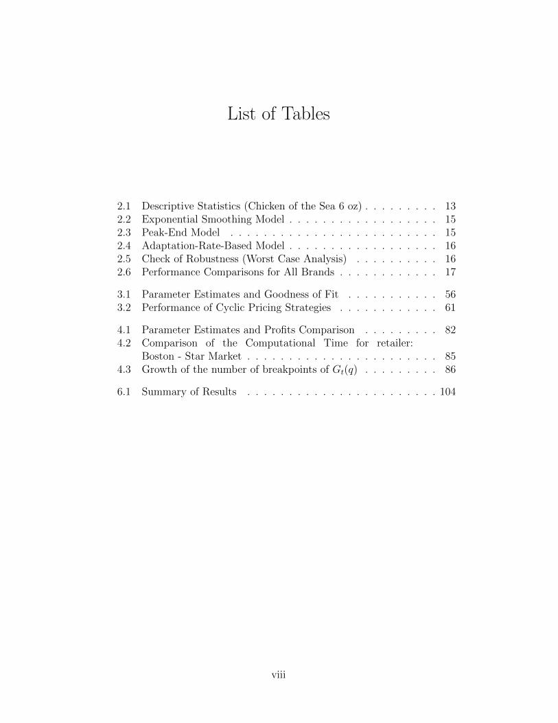
2.1 Descriptive Statistics (Chicken of the Sea 6 oz) . . . . . . . . . 132.2 Exponential Smoothing Model . . . . . . . . . . . . . . . . . . 152.3 Peak-End Model . . . . . . . . . . . . . . . . . . . . . . . . . 152.4 Adaptation-Rate-Based Model . . . . . . . . . . . . . . . . . . 162.5 Check of Robustness (Worst Case Analysis) . . . . . . . . . . 162.6 Performance Comparisons for All Brands . . . . . . . . . . . . 17

3.1 Parameter Estimates and Goodness of Fit . . . . . . . . . . . 563.2 Performance of Cyclic Pricing Strategies . . . . . . . . . . . . 61

4.1 Parameter Estimates and Profits Comparison . . . . . . . . . 824.2 Comparison of the Computational Time for retailer:

Boston - Star Market . . . . . . . . . . . . . . . . . . . . . . . 854.3 Growth of the number of breakpoints of Gt(q) . . . . . . . . . 86

6.1 Summary of Results . . . . . . . . . . . . . . . . . . . . . . . 104

viii

List of Figures

2.1 Convergence result for benchmark model . . . . . . . . . . . . 202.2 Ratio of steady state ranges . . . . . . . . . . . . . . . . . . . 242.3 E[r(t)] and sample paths of r(t) under pH and pL . . . . . . . 272.4 Shape of fR∗s (r) under different α . . . . . . . . . . . . . . . . 302.5 Comparisons of r∗s and r∗D . . . . . . . . . . . . . . . . . . . . 31

3.1 Possible patterns of a periodic orbit . . . . . . . . . . . . . . . 423.2 Discontinuous map (3.6) and periodic orbits for the myopic

pricing strategies when α = 0.8 and α = 0.85 respectively . . . 443.3 Optimal pricing strategy when α = 0.8, η− = 0 and γ = 0.9 . . 473.4 Periodic orbits for the optimal pricing strategies when α =

0.8 and α = 0.85 respectively . . . . . . . . . . . . . . . . . . 483.5 Optimal pricing strategy and a periodic orbit . . . . . . . . . 523.6 Profit comparison of simple pricing strategies . . . . . . . . . . 593.7 Relative profit under different parameter combinations . . . . 603.8 The optimal pricing strategies when α = 0 and η−/η+ ∈

{0.16, 0.18, 0.20, 0.22, 0.24, 0.26} . . . . . . . . . . . . . . . . . 62

4.1 Illustration of r∗(q) . . . . . . . . . . . . . . . . . . . . . . . . 734.2 Illustration of r2(q) . . . . . . . . . . . . . . . . . . . . . . . . 804.3 Comparison of the price paths for retailer: Boston - Star

Market . . . . . . . . . . . . . . . . . . . . . . . . . . . . . . 844.4 Comparison of the price paths for retailer: Chicago - Omni . 84

5.1 State space regions and a switching path . . . . . . . . . . . . 985.2 Steady state region and reference price paths . . . . . . . . . . 101

D.1 Illustration of the proof . . . . . . . . . . . . . . . . . . . . . . 134

ix

Chapter 1

Introduction

1.1 Motivations

Over the last two decades, dynamic pricing has attracted considerable at-

tention from industry as well as academia. On the one hand, the scope of

industries that adopt dynamic pricing strategies has widened remarkably,

with examples ranging from airline, hotel industries whose use of dynamic

pricing has long been a well established practice to many other industries

such as retailing, manufacturing, cloud computing and energy, etc. In retail

industry, for instance, new information technology has enabled the retailers

to collect information about the sales and provided them the decision-support

tools for analyzing the collected data. E-commerce retailers with virtually

no cost in making price changes, in particular, have brought the practice of

dynamic pricing strategies to a new level. It is reported that Amazon.com,

a leading e-commerce retailer, can “adjust the prices of identical goods to

correspond to a customer’s willingness to pay (Weiss and Mehrotra, 2001)”.

On the other hand, the on-going research in academia has led the prac-

tice of dynamic pricing to grow more sophisticated over the years (see, for

example, Elmaghraby and Keskinocak, 2003; Chen and Simchi-Levi, 2012,

for a review). Major efforts have been devoted to several issues. First, how

to capture the relationship between demand and price accurately? A recent

progress in this direction is the incorporation of consumers’ behavior into

consideration, such as strategic or bounded rational behavior of consumers.

Second, in different business contexts, different pricing optimization models

need to be developed. As an example, the stream of literature that incorpo-

rates network effects into the pricing optimization models strives to tackle

various pricing problems associated with the emerging social networks such

as Facebook. The third issue is the coordination of pricing decisions with

1

other operations management decisions. A bulk of existing literature has

been focusing on the coordination of pricing and inventory decisions. Fi-

nally, associated with various models and problems mentioned above is the

computational issue. While the models with more realistic consumer behav-

iors or that incorporate other operations management decisions can bring up

lots of new managerial insights, these models usually lead to very complex

optimal solutions. Fortunately, the development of computational optimiza-

tion techniques in mathematical programming has significantly improved the

efficiency in finding optimal solutions or effective heuristics.

This thesis contributes to the existing literature in dynamic pricing through

an extensive analysis of the reference price models and the corresponding dy-

namic pricing problems. Traditionally, it is usually assumed that the demand

in a period only depends on the selling price of the current period. However,

in a market with repeated purchases such as supermarkets, intertemporal

changes in prices would have significant impacts on consumers’ perception of

the price and in turn influence consumers’ purchasing decisions. The concept

of reference price, developed in economics and marketing literature, is then

used to capture such relationship between demand and past prices. It argues

that consumers form price expectations and use them to judge the current

selling price. That is, reference price is used as an internal anchor formed

in consumers’ minds as a result of experience based on information such as

prices in observed periods (Kalyanaram and Little, 1994). Consumers then

make their purchasing decisions based on the relative magnitude of the ref-

erence price and the selling price. Here, a purchasing instance is perceived

by consumers as gains or losses based on whether the selling price is consid-

ered as discounts or surcharges relative to reference prices. Naturally, gains

induce consumers to buy while losses deter them from purchasing.

Chapter 2 provides an overview of the common reference price models used

in the literature. We empirically compare different reference price models,

present existing results in the dynamic pricing problems and extend those re-

sults. We provide answers to several important and practical questions. First,

can reference price help us to capture the relationship between demand and

prices more accurately? Are such findings consistent over different reference

price model specifications and robust to errors in estimations? Second, what

are the differences among various reference price models, both in terms of

empirical performance as well as managerial implications? Finally, what are

2

the missing elements in the current reference price models and how will such

elements change the pricing strategies of the firm?

In addition to reference price effects, behavioral asymmetry is another

important consideration in modeling consumers’ behavior. A common belief

is that people are loss-averse (Tversky and Kahneman, 1991) and existing

literature in dynamic pricing with reference price effects has been exclusively

focusing on this side of asymmetry. However, the assumption of loss-aversion

is not granted to hold in every pricing context. On the contrary, many

evidences including our empirical studies in Chapter 2 points to the other

side of asymmetry, the gain-seeking behavior. In Chapter 3, we argue that it

is necessary and important for researchers as well as practitioners to realize

the existence of gain-seeking behavior. We provide analytical as well as

numerical results on the dynamic pricing problem that can guide the firm in

choosing its pricing strategies if it faces gain-seeking demands.

In Chapter 4, we consider the computational issues in the dynamic pric-

ing problems with reference price effects. On the one hand, reference price

effects link all the intertemporal pricing decisions together. On the other

hand, behavioral asymmetry creates non-smooth optimization problems. In

order to apply reference price models in practice, where pricing decisions

for thousands of products are made and coordinated with other operations

management decisions, how to compute the optimal prices efficiently and ac-

curately becomes a critical question. Facing with such dynamic non-smooth

optimization problems, we develop a strongly polynomial time algorithm that

solves the optimal prices exactly. We identify general structural properties in

the problem that make such efficient algorithm possible and many of our tech-

niques are potentially applicable to other dynamic non-smooth optimization

problems as well. Our algorithm is shown to be very efficient when applied

to a practical problem with real data.

Most of the studies on dynamic pricing problems with reference price ef-

fects in the literature (including our results in previous chapters) are in a

single-product setting. While dynamic pricing problems with multiple prod-

ucts are inherently difficult due to curse of dimensionality, they are, never-

theless, practically relevant. Firms in retail industries, where most evidences

on reference price effects are found, usually manage hundreds and thousands

of products. In most cases, the demands for those products are interdepen-

dent through cross-price effects. Thus, it is crucial to understand whether

3

the results in the single-product setting can be generalized to multi-product

setting or not and if the answer is no, whether there is a simple heuristic

to the problem. Chapter 5 pushes our understanding to the dynamic pric-

ing problems with multiple products in this regard. We derive an explicit

solution to the multi-product problem and provide a confirmative answer to

the question of generalizing the results in the single-product setting for the

case where no behavioral asymmetry is present. When behavioral asymme-

try is considered, we provide a simple heuristic and prove several desirable

properties of the heuristic.

1.2 Organization of the thesis

Chapter 2 reviews and extends the existing results by comparing the empiri-

cal performance as well as managerial implications of different reference price

models and proposing new models to overcome the limitations in the existing

models. Section 2.1 gives a review of the empirical studies on reference price

models in the literature. Section 2.2 introduces the three memory-based ref-

erence price models used in the literature and the demand model to be used

throughout this thesis. In Section 2.3, we give an empirical comparison of

the three memory-based reference price models using real data from canned

tuna category. Section 2.4-2.6 present and compare the results in the dynam-

ic pricing problems under the three reference price models. A new reference

price model is proposed and analyzed in Section 2.7.

Chapter 3 examines the dynamic pricing problem when the demand is

gain-seeking. The evidences in the gain-seeking behavior and the relevant

literature is presented in Section 3.1. Section 3.2 briefly reminds the read-

ers of the mathematical formulation of the dynamic pricing problem. The

dynamics of the myopic pricing strategy is analyzed in Section 3.3 and that

of the optimal pricing strategy is analyzed in Section 3.4. Section 3.5 gives

an empirical study to examine the assumptions we made and numerically

examines the performance of simple pricing strategies.

Chapter 4 looks into the computational issue of the dynamic pricing prob-

lems with reference price effects. Section 4.2 gives the model for the finite

horizon problem. A strongly polynomial time algorithm is presented for the

loss-averse demands in Section 4.3. The efficiency and robustness of the al-

4

gorithm is examined through solving a practical industry problem in Section

4.4.

Chapter 5 considers the dynamic pricing problem with multiple products.

Section 5.1 reviews the models used in the literature for the multi-product

setting and Section 5.2 introduces the model we use in a continuous time

framework. In Section 5.3, we analyze the dynamic pricing problem with

multiple products and give an explicit solution for the loss/gain-neutral case.

For the loss-averse case, we construct a heuristic and prove some of the nice

properties of the heuristic with two products.

Finally, the last chapter concludes this thesis by summarizing the directions

for future research.

5

Chapter 2

Reference Price Models: EmpiricalComparisons and Dynamic Pricing Problems

2.1 Introduction

The concept of reference price, as introduced in Chapter 1, postulates that

consumers form price expectations and use them to judge the current selling

price. However, reference prices cannot be physically observed and conse-

quently a large amount of literature is devoted to modeling the formation

of reference prices and investigating the impact of reference prices on con-

sumers’ purchasing behavior. This stream of literature can be divided into

two categories based on whether the study conducted is at an individual lev-

el or an aggregate level. Specifically, empirical studies based on individual

level can differ in terms of models, types of data and potentially implications

from the studies based on aggregate level. In most studies at the individual

level, a brand choice model in multi-product setting (usually a multinomial

logit model) is employed. That is, consumers’ utility function is dependent

on reference price and the utility will then determine purchase probability

and demands. In comparison, studies at the aggregate level demand usual-

ly impose a specific demand-price function form. Correspondingly, the data

used at the individual level is scanner panel data which tracks the purchasing

behavior of each household while the the data used at the aggregate level is

simply time series data containing price and demand pairs. Although at both

levels, there are abundant evidences of reference price effects, further impli-

cations on the model parameters can be different at the two levels. Readers

are referred to Chapter 3 for more details on the differences.

Although the focus of this thesis is not on individual level models, we give

a brief discussion of the reference price models in the literature at the indi-

vidual level here for completeness. Literature in this area has differed consid-

erably in how reference prices are formed and many alternative models have

6

been proposed and compared. There are two major different perspectives

in viewing the formation of reference price. One is called the memory-based

or temporal reference price, which is assumed by a majority of researchers.

They argue that reference price is based on the historical prices consumers

encountered during past purchasing occasions and have operationalized ref-

erence price as a weighted average of past encountered prices. For example,

Mayhew and Winer (1992) and Krishnamurthi et al. (1992) have simply tak-

en the price encountered in the last purchase occasion as the reference price.

On the other hand, Lattin and Bucklin (1989) and Kalyanaram and Little

(1994) use an exponentially smoothed prices which depend on consumer’s

whole purchasing history (we refer to as the exponentially smoothing model).

The other one is called the stimulus-based or contextual reference price. It

assumes that the current prices of certain brands serve as the reference price.

The underlying argument is that consumers may not have a strong memory

for past prices and the information provided by current prices of the brands

available in the store is most salient and convenient for consumers. For in-

stance, Hardie et al. (1993) use the current price of the brand that consumers

have purchased in latest occasion as the reference price while Mazumdar and

Papatla (1995) average the current prices of all brands by the weight based

on the loyalties to the respective brands. Briesch et al. (1997) provide com-

prehensive review of the above mentioned models and empirically compare

them using scanner panel data for peanut butter, liquid detergent, ground

coffee and tissue. They find that in four categories the memory-based refer-

ence price model performs the best. Rajendran and Tellis (1994) postulate

that a combination of both memory-based and stimulus-based reference price

model may be more realistic and provide empirical evidences to support their

premise.

Empirical studies at the aggregate level are relatively scarce, even though

most analytical analysis in the literature is based on aggregate level models

due to their simplicity. As pointed out above, aggregate level models focus

more on single-product settings and even if they are generalized to multi-

product settings, the brand choice behavior is not modeled explicitly. As a

result, the literature at the aggregate level usually assumes a memory-based

reference price model. Within the context of memory-based reference price,

various operationalizations have been proposed. Similar to the individual

level model, Raman and Bass (2002) use the price from the previous period

7

as the reference price, and Greenleaf (1995) and Kopalle et al. (1996) employ

the more general exponentially smoothing model. More recently, different

memory-based models have been explored. Nasiry and Popescu (2011) pro-

pose a reference price model based on the peak-end rule (we refer to as the

peak-end model), which suggests that consumers remember the lowest (peak)

and most recent prices (end). Such a model is conceptually supported by sub-

stantial research in psychology, however, “an empirical investigation of the

peak-end rule in the pricing context is still lacking (Nasiry and Popescu,

2011)”. Nevertheless, they analyze the dynamic pricing problem under the

peak-end model and show that a constant pricing strategy is optimal with

loss-averse consumers. Interestingly, to the best of our knowledge, neither

the exponentially smoothing model nor the peak-end model is implemented

in practice. Instead, it is reported in Natter et al. (2007) that bauMax, an

Austrian do-it-yourself retailer, implements a further generalization of the

exponentially smoothing model in their decision-support system (we refer to

as the adaptation-rate-based model). In their model, consumers adapt their

reference prices faster to price decreases than to price increases. They argue

that quicker adaptation in case of price decreases is due to the fact that retail-

ers tend to aggressively advertise price reductions while price increases may

well go unnoticed by consumers. Unfortunately, no empirical comparisons to

the exponential smoothing model are made in their report. In addition, since

bauMax uses a price grid, they can simply evaluate all different strategies

in their dynamic pricing problem and no analytical characterizations of the

optimal pricing strategy are provided in the report.

This chapter then serves for the following three purposes. First, we com-

plement the above mentioned literature at the aggregate level by providing

an empirical comparison of different memory-based reference price models.

In addition, we analyze the dynamic pricing problem with the adaptation-

rate-based model and compare it with the existing results in the exponential

smoothing model as well as the peak-end model. Second, we restate the es-

tablished results in the literature on dynamic pricing problem for the bench-

mark model: the exponential smoothing model with loss-averse demands,

which not only lays down some fundamental ideas that will be used in the

thesis but also gives a nice comparison to later results in Chapter 3. Finally,

we point out some of the limitations of currently available reference price

models and we propose by following Zhang (2011) a reference price mod-

8

el that incorporates randomness to address these limitations. While Zhang

(2011) derives an explicit solution for the dynamic pricing problem under

the stochastic reference price model, we extend his results by providing an

analysis of the limiting distribution of the steady state as well as a sensitivity

analysis of the expected steady state.

The remainder of this chapter is organized as follows. In Section 2.2 we

present the mathematical formulation of each of the memory-based reference

price models discussed above as well as the aggregate level demand model.

In Section 2.3, we empirically compare the performance of the exponential

smoothing model, the peak-end model and the adaptation-rate-based model

using the real data on the canned tuna category. Section 2.4 presents the

established results in the literature on the dynamic pricing problem under

the exponential smoothing model, which serves as our benchmark model. For

completeness, the results in Nasiry and Popescu (2011) for dynamic pricing

problem under the peak-end model is presented in Section 2.5. The dynamic

pricing problem under the adaptation-rate-based model is analyzed in Sec-

tion 2.6. We introduce the stochastic reference price model and analyze the

corresponding dynamic pricing problem in Section 2.7. The last section sum-

marizes our findings and points out directions for future research. Proofs for

the results in Section 2.7 are quite lengthy and are relegated to Appendix A.

We remark here that, throughout this chapter, we consider either loss/gain-

neutral or loss-averse demands and readers are referred to Chapter 3 for

dynamic pricing problems with gain-seeking demands.

2.2 Reference Price and Demand Models

This section introduces the three memory-based reference price models and

the demand model that describes how reference price effect affects the de-

mand for a firm’s product. In the following, we use rt to denote consumers’

reference price at period t and pt to denote the shelf price of the product at

period t.

9

2.2.1 Exponential smoothing model

As introduced in Section 2.1, the exponential smoothing model is widely used

by researchers at both individual (Lattin and Bucklin, 1989; Kalyanaram and

Little, 1994) as well as aggregate level (Greenleaf, 1995). It assumes that the

reference price in period t+ 1 is a weighted average of the reference price in

period t and the shelf price consumers observed in period t. Mathematically,

the reference price evolves according to the following recursive formula

rt+1 = αrt + (1− α)pt, (2.1)

where α ∈ [0, 1] is called the memory factor, since it captures the rate at

which consumers adapt to the new price information. In the extreme case,

when α = 0 consumers immediately take the price they observed in the

last purchase occasion as the reference price (Raman and Bass, 2002), while

when α = 1 consumers never adapt to the new price information. Usually,

one would restrict α < 1, because in empirical studies α = 1 would result

in pathological estimation (see Section 2.3) and in the analysis of dynamic

pricing problem it would result in a static price (see Section 2.4).

2.2.2 Peak-end model

The peak-end rule postulates that memory-based decisions are made accord-

ing to a combination of the most extreme and most recent experiences. By

adopting this rule in the pricing context, Nasiry and Popescu (2011) assume

that the peak-end experiences to be the lowest and latest price respectively.

Specifically, let mt denote the lowest price consumers observed up to period

t, then the reference price follows

rt+1 = βmt + (1− β)pt, (2.2)

where β ∈ [0, 1] measures how much consumers anchor on the lowest price.

Again, in the extreme case when β = 0, reference price is simply the price

observed in the previous period. Note here that

mt+1 = min{mt, pt+1}

10

and together with (2.2), they specify the evolution of a reference price path.

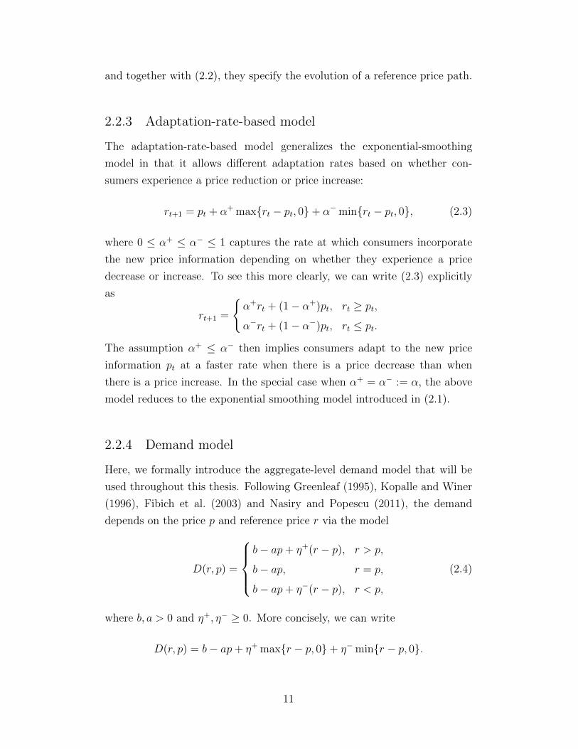
2.2.3 Adaptation-rate-based model

The adaptation-rate-based model generalizes the exponential-smoothing

model in that it allows different adaptation rates based on whether con-

sumers experience a price reduction or price increase:

rt+1 = pt + α+ max{rt − pt, 0}+ α−min{rt − pt, 0}, (2.3)

where 0 ≤ α+ ≤ α− ≤ 1 captures the rate at which consumers incorporate

the new price information depending on whether they experience a price

decrease or increase. To see this more clearly, we can write (2.3) explicitly

as

rt+1 =

{α+rt + (1− α+)pt, rt ≥ pt,

α−rt + (1− α−)pt, rt ≤ pt.

The assumption α+ ≤ α− then implies consumers adapt to the new price

information pt at a faster rate when there is a price decrease than when

there is a price increase. In the special case when α+ = α− := α, the above

model reduces to the exponential smoothing model introduced in (2.1).

2.2.4 Demand model

Here, we formally introduce the aggregate-level demand model that will be

used throughout this thesis. Following Greenleaf (1995), Kopalle and Winer

(1996), Fibich et al. (2003) and Nasiry and Popescu (2011), the demand

depends on the price p and reference price r via the model

D(r, p) =

b− ap+ η+(r − p), r > p,

b− ap, r = p,

b− ap+ η−(r − p), r < p,

(2.4)

where b, a > 0 and η+, η− ≥ 0. More concisely, we can write

D(r, p) = b− ap+ η+ max{r − p, 0}+ η−min{r − p, 0}.

11

Here, D(p, p) = b − ap is the base demand independent of reference prices,

η+(r − p) or η−(r − p) is the additional demand or demand loss induced by

the reference price effect, where r − p is usually referred to as a perceived

surcharge/discount. If r < p, consumers perceive this as a loss, while if

r > p, they perceive it as a gain. Consumers or the aggregate level demands

are classified as loss-averse, loss/gain neutral and gain-seeking depending

on whether η+ < η−, η+ = η− or η+ > η−. The dynamic pricing problems

analyzed in this chapter all focus on either the loss-averse or loss/gain neutral

case. The gain-seeking case is studied in detail in Chapter 3.

The linear form of the demand function is for the purpose of simplifying

the exposition. Most of the results introduced in this thesis can be gener-

alized to nonlinear forms by imposing appropriate assumptions on demand.

Furthermore, the linear form allows us to conveniently estimate the corre-

sponding parameters from real data on historical prices and sales using linear

regression (see Section 2.3).

2.3 Model Comparison

This section complements the literature by empirically comparing the three

memory-based reference price models based on the data in canned tuna cat-

egory. We conduct a detailed analysis using one brand in the data set and

present a summary of the performances of the models for all the brands in

the data set.

2.3.1 Data and method of estimation

We utilize the data set provided by Chevalier et al. (2003) of the canned

tuna product category in the Bayesm Package of the R software. The data

set includes volume of canned tuna sales as well as a measure of display

activity, log price and log wholesale price of seven different brands over 338

weeks.

The data set is extracted and aggregated from the Dominick’s Finer

Foods database maintained by the University of Chicago Booth School of

Business at http://research.chicagobooth.edu/marketing/databases/

dominicks/index.aspx. The original database records comprehensively the

12

http://research.chicagobooth.edu/marketing/databases/dominicks/index.aspx

http://research.chicagobooth.edu/marketing/databases/dominicks/index.aspx

weekly store-level data of each product sold by Dominick’s Finer Foods, a

large supermarket chain in the Chicago area.

Note here that if the initial reference price and α, β, α+/α− in (2.1), (2.2),

(2.3) respectively are known, then reference prices can be generated from the

historical prices and the parameters b, a, η+, η− in the demand function (2.4)

can be estimated using ordinary least squares (OLS). However, α, β, α+/α−

are usually unknown and need to be estimated from the data. There is no

established explicit formula for computing these parameters. Here, we follow

the simple approach employed by Greenleaf (1995). For the exponential

smoothing model, for instance, OLS is performed repeatedly for each value

of α varying in increments of 0.025 from 0 to 1 (excluding 1) and our estimator

α is chosen to be the one that maximizes R2. We exclude α = 1 here because

it will result in perfect collinearity problem and OLS cannot be applied. β,

α+ and α− are computed similarly. For initial reference price, we set it to be

the average price for convenience throughout this section.

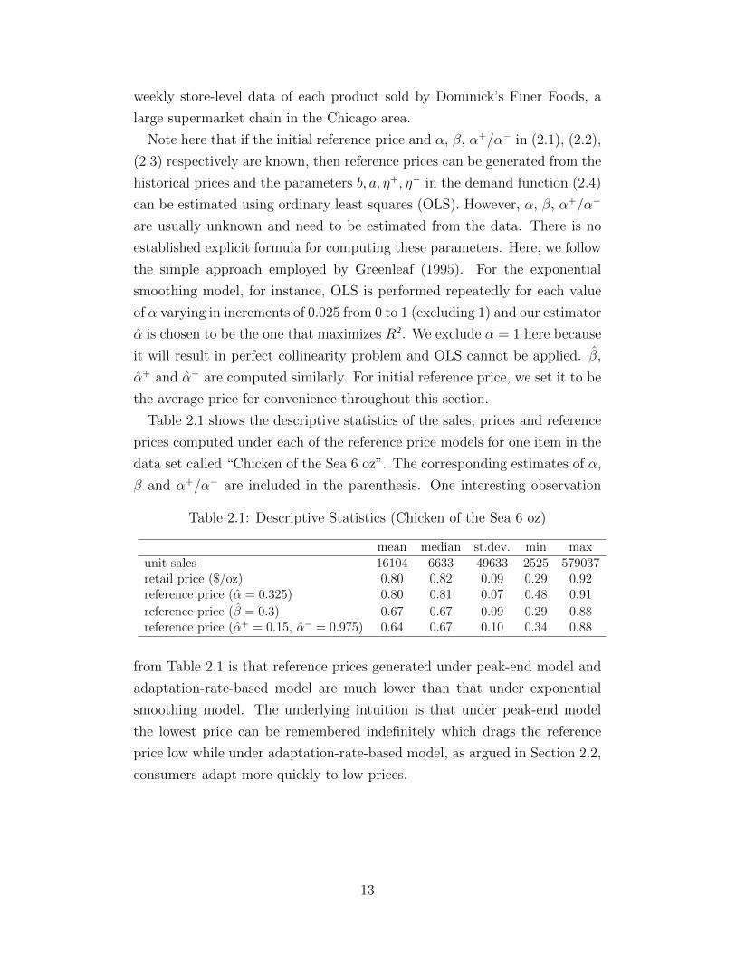
Table 2.1 shows the descriptive statistics of the sales, prices and reference

prices computed under each of the reference price models for one item in the

data set called “Chicken of the Sea 6 oz”. The corresponding estimates of α,

β and α+/α− are included in the parenthesis. One interesting observation

Table 2.1: Descriptive Statistics (Chicken of the Sea 6 oz)

mean median st.dev. min maxunit sales 16104 6633 49633 2525 579037retail price ($/oz) 0.80 0.82 0.09 0.29 0.92reference price (α = 0.325) 0.80 0.81 0.07 0.48 0.91

reference price (β = 0.3) 0.67 0.67 0.09 0.29 0.88reference price (α+ = 0.15, α− = 0.975) 0.64 0.67 0.10 0.34 0.88

from Table 2.1 is that reference prices generated under peak-end model and

adaptation-rate-based model are much lower than that under exponential

smoothing model. The underlying intuition is that under peak-end model

the lowest price can be remembered indefinitely which drags the reference

price low while under adaptation-rate-based model, as argued in Section 2.2,

consumers adapt more quickly to low prices.

13

2.3.2 Comparison results

We first present the regression results for the item “Chicken of the Sea 6

oz” and discuss some of the issues in estimation and comparison. As noted

by Greenleaf (1995), the linear demand model (2.4) suffers from a multi-

collinearity problem. As a result, the standard errors can be huge for some

parameters and the OLS estimate to η− has a wrong sign (see, for example,

the second column in Table 2.2). To tackle this problem, Greenleaf (1995)

uses equity estimator and ridge estimator and obtains the correct signs. Sim-

ilar regularization technique is used in the case study in Chapter 4 to another

data set. However, for the canned tuna category, though ridge regression can

reduce the standard errors, the estimator to η− still has a wrong sign. In-

stead, we look at the restricted model by imposing η− = 0 and we report

the regression results for the full model specified by (2.4), the static model

which ignores reference price effects (η+ = η− = 0) and the restricted model

(η− = 0).

Table 2.2-2.4 summarize the regression results for the three memory-based

reference price models respectively. Two observations that are consistent in

all three models can be made here. First, incorporating reference price effect-

s significantly improves the goodness of fit measured by R2 across all three

models. The exponential smoothing model improves R2 by 90%, the peak-

end model by 138% and the adaptation-rate-based model by 158% respec-

tively. Second, we find the demand for this item to be gain-seeking (η+ > η−)

regardless of which memory-based reference price model one chooses. In ad-

dition, the estimate of η− is statistically insignificant in all three models and

the more parsimonious restricted demand model performs as good as the full

demand model.

Comparing across the three tables, it is clear that the adaptation-rate-

based model performs the best in terms of R2 or adjusted R2 for both the

full demand model and the restricted demand model. It outperforms the

exponential smoothing model by 36%. However, it only outperforms the

peak-end model by 8%. Thus, one needs to be cautious when directly com-

paring the three models in terms of R2 since the adaptation-rate-based model

has one more degree of freedom than the exponential-smoothing model or

the peak-end model. In other words, besides the demand parameters, the

adaption-rate-based model has two additional parameters (α+ and α−) to be

14

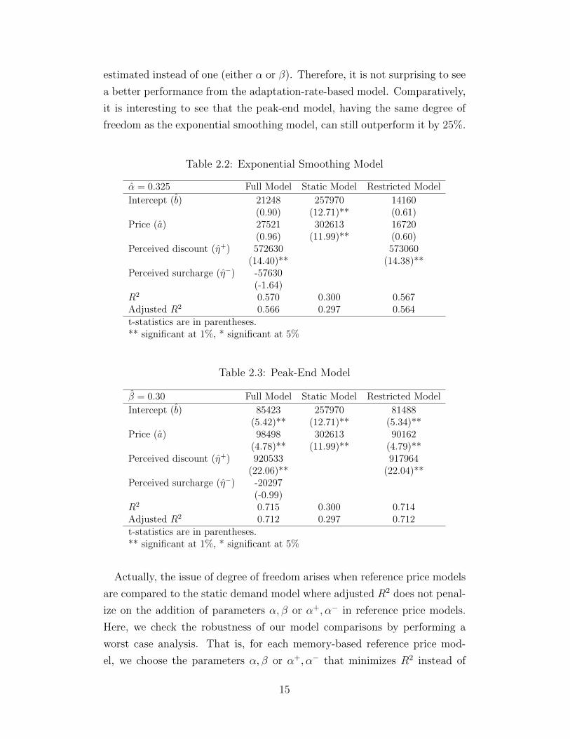
estimated instead of one (either α or β). Therefore, it is not surprising to see

a better performance from the adaptation-rate-based model. Comparatively,

it is interesting to see that the peak-end model, having the same degree of

freedom as the exponential smoothing model, can still outperform it by 25%.

Table 2.2: Exponential Smoothing Model

α = 0.325 Full Model Static Model Restricted Model

Intercept (b) 21248 257970 14160(0.90) (12.71)** (0.61)

Price (a) 27521 302613 16720(0.96) (11.99)** (0.60)

Perceived discount (η+) 572630 573060(14.40)** (14.38)**

Perceived surcharge (η−) -57630(-1.64)

R2 0.570 0.300 0.567Adjusted R2 0.566 0.297 0.564t-statistics are in parentheses.** significant at 1%, * significant at 5%

Table 2.3: Peak-End Model

β = 0.30 Full Model Static Model Restricted Model

Intercept (b) 85423 257970 81488(5.42)** (12.71)** (5.34)**

Price (a) 98498 302613 90162(4.78)** (11.99)** (4.79)**


Perceived surcharge (η−) -20297(-0.99)


Actually, the issue of degree of freedom arises when reference price models

are compared to the static demand model where adjusted R2 does not penal-

ize on the addition of parameters α, β or α+, α− in reference price models.

Here, we check the robustness of our model comparisons by performing a

worst case analysis. That is, for each memory-based reference price mod-

el, we choose the parameters α, β or α+, α− that minimizes R2 instead of

15

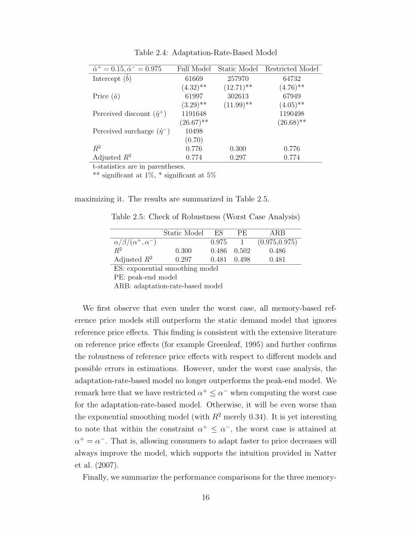
Table 2.4: Adaptation-Rate-Based Model

α+ = 0.15, α− = 0.975 Full Model Static Model Restricted Model

Intercept (b) 61669 257970 64732(4.32)** (12.71)** (4.76)**

Price (a) 61997 302613 67949(3.29)** (11.99)** (4.05)**


Perceived surcharge (η−) 10498(0.70)


maximizing it. The results are summarized in Table 2.5.

Table 2.5: Check of Robustness (Worst Case Analysis)

Static Model ES PE ARBα/β/(α+, α−) 0.975 1 (0.975,0.975)R2 0.300 0.486 0.502 0.486Adjusted R2 0.297 0.481 0.498 0.481ES: exponential smoothing modelPE: peak-end modelARB: adaptation-rate-based model

We first observe that even under the worst case, all memory-based ref-

erence price models still outperform the static demand model that ignores

reference price effects. This finding is consistent with the extensive literature

on reference price effects (for example Greenleaf, 1995) and further confirms

the robustness of reference price effects with respect to different models and

possible errors in estimations. However, under the worst case analysis, the

adaptation-rate-based model no longer outperforms the peak-end model. We

remark here that we have restricted α+ ≤ α− when computing the worst case

for the adaptation-rate-based model. Otherwise, it will be even worse than

the exponential smoothing model (with R2 merely 0.34). It is yet interesting

to note that within the constraint α+ ≤ α−, the worst case is attained at

α+ = α−. That is, allowing consumers to adapt faster to price decreases will

always improve the model, which supports the intuition provided in Natter

et al. (2007).

Finally, we summarize the performance comparisons for the three memory-

16

Table 2.6: Performance Comparisons for All Brands

Static Model ES PE ARBStar Kist 6 oz 0.190 0.359 0.449 0.360Chicken of the Sea 6 oz 0.300 0.570 0.715 0.776Bumble Bee Solid 6.12 oz 0.406 0.490 0.514 0.519Bumble Bee Chunk 6.12 oz 0.259 0.640 0.664 0.650Geisha 6 oz 0.513 0.545 0.545 0.550ES: exponential smoothing modelPE: peak-end modelARB: adaptation-rate-based model

based reference price models for all the brands in the data set in Table 2.6.

We have excluded the two brands with large volume size: “Bumble Bee

Large Cans” and “HH Chunk Lite 6.5 oz” because the estimate for a, the

price sensitivity, has a wrong sign. One can see that generally, the peak-end

and the adaptation-rate-based models perform better than the exponential

smoothing model but the degree of improvements differ case by case. For

the last three brands, the three models perform roughly the same while the

peak-end model has quite an improvement over the exponential smoothing

model for the first two brands. The adaptation-rate-based model, despite

of the increased degree of freedom, only has significant improvement in the

brand “Chicken of the Sea 6 oz”.

2.4 Dynamic Pricing under the Exponential

Smoothing Model

In this section, we present the results on the dynamic pricing problem under

the benchmark model: the exponential smoothing model with loss-averse

demands. This problem has been analyzed by many researchers including

Kopalle et al. (1996), Fibich et al. (2003), Popescu and Wu (2007) and Asva-

nunt (2007). In addition to stating existing results, we offer a new perspective

in proving the steady state results in Popescu and Wu (2007). We utilize the

tools from discrete dynamic system to provide a simple visualization of con-

vergence and such tools enable a clearer comparison to the results to be

developed in Chapter 3.

Given an initial reference price r0, we define the firm’s dynamic pricing

17

problem under the exponential smoothing model as follows:

V (r0) = maxpt∈[0,U ]

∞∑t=0

γtΠ(rt, pt)

s.t. rt+1 = αrt + (1− α)pt, t ≥ 0,

(2.5)

where Π(rt, pt) = ptD(rt, pt) is the one-period profit function and D(·, ·) is

defined in (2.4). Here, we have implicitly assumed that the marginal cost is 0

without loss of generality. We also assume for the remaining of this chapter

that η− ≥ η+. Note that the assumptions η− ≥ η+ and p ≥ 0 allow us to

rewrite the one-period profit as

Π(r, p) = min{Π+(r, p),Π−(r, p)},

where

Π+(r, p) = p[b− ap+ η+(r − p)], (2.6a)

Π−(r, p) = p[b− ap+ η−(r − p)]. (2.6b)

The Bellman equation to problem (2.5) can then be written as

V (r) = maxp∈[0,U ]

{min{Π+(r, p),Π−(r, p)}+ γV (αr + (1− α)p)}, (2.7)

and we use p∗(r) to denote the solution to (2.7). To solve (2.7), we introduce

the following two problems:

V +(r) = maxp∈[0,U ]

Π+(r, p) + γV +(αr + (1− α)p), (2.8a)

V −(r) = maxp∈[0,U ]

Π−(r, p) + γV −(αr + (1− α)p). (2.8b)

The solutions of (2.8a) and (2.8b) are denoted respectively as p+(r) and

p−(r). The following proposition gives a characterization of the solution to

(2.7).

18

Proposition 2.1. There exists 0 ≤ r− ≤ r+ ≤ U such that

p∗(r) =

p−(r), 0 ≤ r ≤ r−,

r, r− ≤ r ≤ r+,

p+(r), r+ ≤ r ≤ U,

and the optimal value function is given by

V (r) =

V −(r), 0 ≤ r ≤ r−,

Π(r, r)

1− γ, r− ≤ r ≤ r+,

V +(r), r+ ≤ r ≤ U.

The proof to Proposition 2.1 can be found both in Popescu and Wu (2007)

and Asvanunt (2007) and is omitted here. One is also referred to Section 2.6,

where we prove similar results for the more general adaptation-rate-based

model. We remark here that Proposition 2.1 does not rely on the linear

form of the demand function and readers are referred to Popescu and Wu

(2007) for the assumptions on demand and profit functions that are necessary

for Proposition 2.1 to hold. With a linear form in (2.4), one can compute

that r− = b(1−γα)2a(1−γα)+(1−γ)η−

and r+ = b(1−γα)2a(1−γα)+(1−γ)η+

. Asvanunt (2007) also

provides explicit expressions for p−(r), p+(r) and V −(r), V +(r).

Given an initial reference price r0 and p∗(r), the sequence of reference

prices {rt} which evolves according to (2.1) is referred to as the reference

price path. A consequence of Proposition 2.1 is the following convergence

result of the reference price path, which essentially says that in the long-run

a constant pricing strategy is optimal.

Proposition 2.2. When r0 < r−, then {rt} is monotonically increasing and

limt→∞ rt = r−, when r0 > r+, then {rt} is monotonically decreasing and

limt→∞ rt = r+. When r− ≤ r0 ≤ r+, then rt = r0 for any t ≥ 0. Any

reference price r ∈ [r−, r+] is then referred to as a steady state.

Again, the mathematical proof for Proposition 2.2 is omitted here. Instead,

we give a graphical visualization of the reference price path in Figure 2.1 to

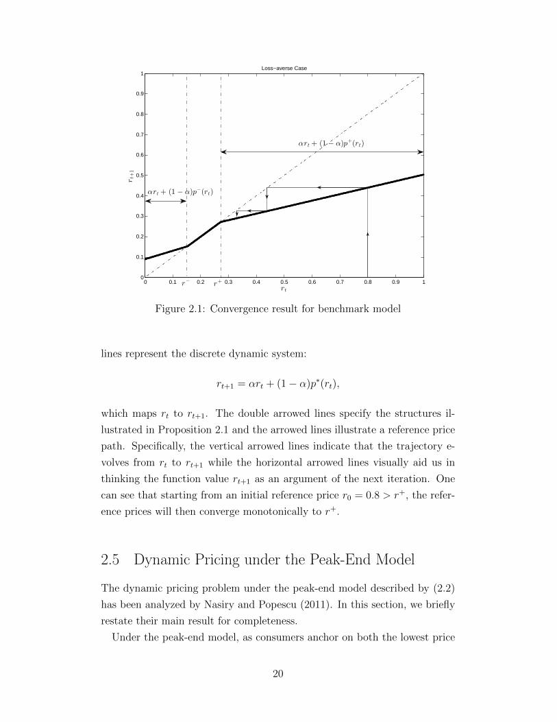
illustrate both Proposition 2.1 and Proposition 2.2. In Figure 2.1, the bold

19

0 0.1 0.2 0.3 0.4 0.5 0.6 0.7 0.8 0.9 10

0.1

0.2

0.3

0.4

0.5

0.6

0.7

0.8

0.9

1

rt

rt+

1

Loss−averse Case

r+r

−

αrt + (1 − α)p+(rt)

αrt + (1 − α)p−(rt)

Figure 2.1: Convergence result for benchmark model

lines represent the discrete dynamic system:

rt+1 = αrt + (1− α)p∗(rt),

which maps rt to rt+1. The double arrowed lines specify the structures il-

lustrated in Proposition 2.1 and the arrowed lines illustrate a reference price

path. Specifically, the vertical arrowed lines indicate that the trajectory e-

volves from rt to rt+1 while the horizontal arrowed lines visually aid us in

thinking the function value rt+1 as an argument of the next iteration. One

can see that starting from an initial reference price r0 = 0.8 > r+, the refer-

ence prices will then converge monotonically to r+.

2.5 Dynamic Pricing under the Peak-End Model

The dynamic pricing problem under the peak-end model described by (2.2)

has been analyzed by Nasiry and Popescu (2011). In this section, we briefly

restate their main result for completeness.

Under the peak-end model, as consumers anchor on both the lowest price

20

as well as the previous period price, two states are needed to describe the

evolution of system. Given the initial state (m0, p0), the firm’s dynamic

pricing problem under the peak-end model is then:

V (m0, p0) = maxpt∈[0,U ]

∞∑t=1

γt−1Π(rt, pt)

s.t. rt+1 = βmt + (1− β)pt, t ≥ 0,

mt+1 = min{mt, pt+1}, t ≥ 0,

(2.9)

and the Bellman equation for problem (2.9) is

V (mt−1, pt−1) = maxpt∈[0,U ]

{min{Π+(rt, pt),Π−(rt, pt)}+ γV (min{mt−1, pt}, pt)},

rt = βmt−1 + (1− β)pt−1.

(2.10)

Let p∗(mt−1, pt−1) denote the optimal pricing strategy that solves (2.10) and

given the initial state (m0, p0), {p∗t} denote the optimal price path given by

p∗t = p∗(mt−1, p∗t−1). Proposition 2.3 summarizes the main result from Nasiry

and Popescu (2011), to which one is referred for detailed analysis and proofs.

Proposition 2.3. Given any initial state (m0, p0), {p∗t} converges monoton-

ically to a steady state price, which depends only on m0.

Again, Proposition 2.3 implies that a constant pricing strategy is optimal

in the long-run. However, Nasiry and Popescu (2011) note that the range

of constant prices that are optimal is wider than that under the exponential

smoothing model and unlike the exponential smoothing model, the optimal

constant prices do not reduce to a single point when consumers are loss/gain

neutral.

2.6 Dynamic Pricing under the

Adaptation-Rate-Based Model

In Section 2.3, we see that the adaptation-rate-based model achieves the best

fit in one of the brand and it is actually used in practice (Natter et al., 2007).

In this section, we complement the literature by analyzing the dynamic pric-

ing problem under the adaptation-rate-based model.

21

Similar to (2.5), the firm’s dynamic pricing problem is

V (r0) = maxpt∈[0,U ]

∞∑t=0

γtΠ(rt, pt)

s.t. rt+1 = pt + α+ max{rt − pt, 0}+ α−min{rt − pt, 0}, t ≥ 0.

(2.11)

Note that we assume α+ ≤ α−, which allows us to rewrite (2.3) as

rt+1 = min{α+rt + (1− α+)pt, α−rt + (1− α−)pt},

and since V (·) is continuous and monotonically increasing, the Bellman e-

quation can be written as

V (r) = maxp∈[0,U ]

{min{Π+(r, p) + γV (α+r + (1− α+)p),

Π−(r, p) + +γV (α−r + (1− α−)p)}},(2.12)

with p∗(r) denoting the optimal solution to (2.11). Similarly, we consider the

following two problems

V +(r) = maxp∈[0,U ]

Π+(r, p) + γV +(α+r + (1− α+)p), (2.13a)

V −(r) = maxp∈[0,U ]

Π−(r, p) + γV −(α−r + (1− α−)p), (2.13b)

with the corresponding solutions denoted as p+(r) and p−(r) respective-

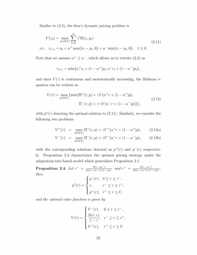
ly. Proposition 2.4 characterizes the optimal pricing strategy under the

adaptation-rate-based model which generalizes Proposition 2.1.

Proposition 2.4. Let r− = b(1−γα−)2a(1−γα−)+(1−γ)η−

and r+ = b(1−γα+)2a(1−γα+)+(1−γ)η+

,

then

p∗(r) =

p−(r), 0 ≤ r ≤ r−,

r, r− ≤ r ≤ r+,

p+(r), r+ ≤ r ≤ U,

and the optimal value function is given by

V (r) =

V −(r), 0 ≤ r ≤ r−,

Π(r, r)

1− γ, r− ≤ r ≤ r+,

V +(r), r+ ≤ r ≤ U.

22

Proof. For 0 ≤ s ≤ 1, we consider the following problem:

V s(rs0) = maxpt∈[0,U ]

∞∑t=0

γtΠs(rst , pt)

s.t. rst+1 = αsrst + (1− αs)pt, t ≥ 0,

(2.14)

where Πs(r, p) = p(b− ap + (sη+ + (1− s)η−)(r − p)) and αs = sα+ + (1−s)α−. Note that this is simply the problem with the exponential smoothing

model (the memory factor is αs) and loss/gain neutral demands (the marginal

reference price effect is sη+ + (1 − s)η−). The superscript “s” on reference

price is to distinguish it from the reference prices generated in problem (2.11).

In the extreme case when s = 0, V s(r) = V −(r) and when s = 1, V s(r) =

V +(r). By Theorem 2 in Popescu and Wu (2007), problem (2.14) admits

a unique steady state rs = b(1−γαs)2a(1−γαs)+(1−γ)(sη++(1−s)η−)

and for any initial

reference price rs0, the reference price path under the optimal pricing strategy

converges monotonically to rs. It is easy to see that r− and r+ are simply

the steady states when s = 0 and s = 1 respectively.

Next, we show that V s(r) ≥ V (r) for any 0 ≤ s ≤ 1. We make two simple

observations here. First, (sη+ +(1−s)η−)(r−p) ≥ min{η+(r−p), η−(r−p)}.Second, αsr+ (1−αs)p ≥ min{α+r+ (1−α+)p, α−r+ (1−α−)p}. The first

observation leads to Πs(r, p) ≥ Π(r, p). For any initial reference price rs0 = r0

and fixed price path {pt}, the second observation implies rst ≥ rt for any t ≥ 0.

Since Πs(r, p) is increasing in r, we have Πs(rst , pt) ≥ Πs(rt, pt) ≥ Π(rt, pt),

which is true for any feasible price path {pt}. Therefore, fixing an optimal

price path {p∗t} for problem (2.11) and letting rs0 = r0, we then have

V s(rs0) ≥∞∑t=0

γtΠs(rst , p∗t ) ≥

∞∑t=0

γtΠ(rt, p∗t ) = V (r0).

In particular, this implies V −(r) ≥ V (r) and V +(r) ≥ V (r).

When r− ≤ r ≤ r+, there exists 0 ≤ s ≤ 1, such that r = rs. As rs is

the steady state for problem (2.14), the pricing path {pt = rs} is optimal for

problem (2.14). On the other hand, it is feasible for problem (2.11) while

resulting an objective value V s(rs). By V s(r) ≥ V (r), {pt = rs} is optimal for

problem (2.11) as well. In other words, p∗(r) = r and V (r) = V s(r) = Π(r,r)1−γ

for r− ≤ r ≤ r+.

When 0 ≤ r ≤ r−, similarly, p−(r) is an optimal solution to (2.13b) and

23

by monotonic convergence to r− it holds p−(r) > r for 0 ≤ r ≤ r−. For

any initial reference price r0 < r−, {p−(rt)} is a feasible solution to problem

(2.11) and by r− ≥ p−(rt) > rt for all t ≥ 0, it will result in an objective value

V −(r0). That is, {p−(rt)} is optimal to problem (2.11), i.e., p∗(r) = p−(r)

and V (r) = V −(r) for 0 ≤ r ≤ r−. The case for r+ ≤ r ≤ U can be proven

in a same way.

One can see from the proof of Proposition 2.4 that Proposition 2.2 can

be directly generalized here. That is, the steady states for the dynam-

ic pricing problem (2.11) are [r−, r+], where r− = b(1−γα−)2a(1−γα−)+(1−γ)η−

and

r+ = b(1−γα+)2a(1−γα+)+(1−γ)η+

. Although the derivation of the analytical results is

similar to the exponential smoothing model, managerial implications under

the adaptation-rate-based model are more in line with that of the peak-end

model. Specifically, our results also imply the range of steady state prices,

i.e., r+ − r−, is wider than that under the exponential smoothing model. In

the special case of loss/gain neutral demands, the optimal constant prices do

not degenerate to a single price point.

0 0.1 0.2 0.3 0.4 0.5 0.6 0.7 0.8 0.9 10

0.1

0.2

0.3

0.4

0.5

0.6

0.7

0.8

0.9

1

α−

Rat

io o

f the

ran

ge o

f ste

ady

stat

es (

%)

η− = 1.5

η− = 2.0

η− = 2.5

η− = 3.0

Figure 2.2: Ratio of steady state ranges

Figure 2.2 illustrates the ratio of the steady state range under the exponen-

tial smoothing model to that under the adaptation-rate-based model, where

24

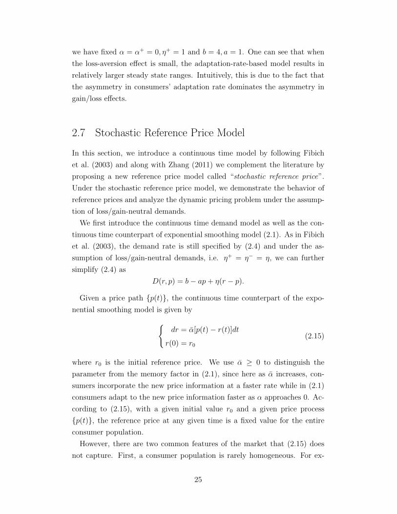
we have fixed α = α+ = 0, η+ = 1 and b = 4, a = 1. One can see that when

the loss-aversion effect is small, the adaptation-rate-based model results in

relatively larger steady state ranges. Intuitively, this is due to the fact that

the asymmetry in consumers’ adaptation rate dominates the asymmetry in

gain/loss effects.

2.7 Stochastic Reference Price Model

In this section, we introduce a continuous time model by following Fibich

et al. (2003) and along with Zhang (2011) we complement the literature by

proposing a new reference price model called “stochastic reference price”.

Under the stochastic reference price model, we demonstrate the behavior of

reference prices and analyze the dynamic pricing problem under the assump-

tion of loss/gain-neutral demands.

We first introduce the continuous time demand model as well as the con-

tinuous time counterpart of exponential smoothing model (2.1). As in Fibich

et al. (2003), the demand rate is still specified by (2.4) and under the as-

sumption of loss/gain-neutral demands, i.e. η+ = η− = η, we can further

simplify (2.4) as

D(r, p) = b− ap+ η(r − p).

Given a price path {p(t)}, the continuous time counterpart of the expo-

nential smoothing model is given by{dr = α[p(t)− r(t)]dt

r(0) = r0

(2.15)

where r0 is the initial reference price. We use α ≥ 0 to distinguish the

parameter from the memory factor in (2.1), since here as α increases, con-

sumers incorporate the new price information at a faster rate while in (2.1)

consumers adapt to the new price information faster as α approaches 0. Ac-

cording to (2.15), with a given initial value r0 and a given price process

{p(t)}, the reference price at any given time is a fixed value for the entire

consumer population.

However, there are two common features of the market that (2.15) does

not capture. First, a consumer population is rarely homogeneous. For ex-

25

ample, brand loyal consumers and brand switchers can make different brand

choice and purchase quantity decisions (Krishnamurthi et al., 1992). Thus,

it is natural to postulate that each consumer should have her own perception

of the prices as well. Second, other exogenous factors like advertisement ac-

tivities and competitors’ prices may influence consumers’ memory processes.

As argued in Section 2.1, consumers’ reference price may also be affected by

contextual effects, i.e. other prices consumers observe at the time of purchase

(Rajendran and Tellis, 1994).

In this section, we try to incorporate heterogeneity as well as exogenous

shocks and describe the more complex behavior of consumers by using a

stochastic differential equation (SDE) (see Øksendal, 2002, for a reference on

the topic of SDE) to model reference price evolution process:

dr(t) = α[p(t)− r(t)]dt+ σ√r(t)dW (t), (2.16)

where W (t) is the standard Wiener process and reference price r(t) is now a

stochastic process.

Note here that for a pre-determined price path {p(t)}, dE[r(t)] = α[p(t)−E[r(t)]]dt. That is, if the firm pre-commits to a price path that is indepen-

dent of the realization of randomness, then the evolution of the expected

reference prices coincide with the deterministic model (2.15) used in Fibich

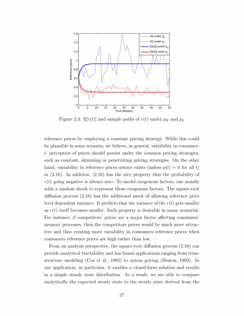
et al. (2003). We illustrate in Figure 2.3 a sample path of (2.16) as well

as E[r(t)] under a constant pricing strategy with two price levels: the high

price pH = 0.92 and the low price pL = 0.29 (the highest and lowest price

in Table 2.1) respectively. In Figure 2.3, we take the initial reference price

r0 = pH+pL2

= 0.605, α = 0.5 and σ = 0.2. One can see that r(t) has a high-

er variance under pH than under pL which reflects the square-root diffusion

term in (2.16).

There are two main considerations in our choice of models. From a mod-

eling perspective, we want a model that can give a good approximation to

the above mentioned two features. To model consumer heterogeneity, incor-

porating randomness is a common practice used in economics and marketing

(see Allenby and Rossi, 1998, for instance). One possible way is to assume α

to be random. However, it is easy to see that if the price is a predetermined

constant, i.e., p(t) = p, for all t ≥ 0, the variance of r(t) will go to zero as

t → ∞. That is, the firm can eliminate such heterogeneity in consumers’

26

0 5 10 15 20 25 30 35 40 45 500

0.2

0.4

0.6

0.8

1

1.2

1.4

1.6

Time (Weeks)

Ref

eren

ce p

rices

r(t) under pH

r(t) under pL

E[r(t)] under pH

E[r(t)] under pL

Figure 2.3: E[r(t)] and sample paths of r(t) under pH and pL

reference prices by employing a constant pricing strategy. While this could

be plausible in some scenario, we believe, in general, variability in consumer-

s’ perception of prices should persist under the common pricing strategies,

such as constant, skimming or penetrating pricing strategies. On the other

hand, variability in reference prices always exists (unless p(t) = 0 for all t)

in (2.16). In addition, (2.16) has the nice property that the probability of

r(t) going negative is always zero. To model exogenous factors, one usually

adds a random shock to represent those exogenous factors. The square-root

diffusion process (2.16) has the additional merit of allowing reference price

level dependent variance. It predicts that the variance of the r(t) gets smaller

as r(t) itself becomes smaller. Such property is desirable in many scenarios.

For instance, if competitors’ prices are a major factor affecting consumers’

memory processes, then the competitors prices would be much more attrac-

tive and thus creating more variability in consumers reference prices when

consumers reference prices are high rather than low.

From an analysis perspective, the square-root diffusion process (2.16) can

provide analytical tractability and has found applications ranging from term-

structure modeling (Cox et al., 1985) to option pricing (Heston, 1993). In

our application, in particular, it enables a closed-form solution and results

in a simple steady state distribution. As a result, we are able to compare

analytically the expected steady state to the steady state derived from the

27

deterministic reference price model.

Under our stochastic reference price model, the firm’s dynamic pricing

problem is

V (r0) = maxp(t)

E[∫ ∞

0

e−γtp(t)D(r(t), p(t))

]dt,

s.t. dr(t) = α[p(t)− r(t)]dt+ σ√r(t)dW (t),

(2.17)

where γ is the discount factor. The corresponding Hamilton-Jacobi-Bellman

(HJB) equation can then be written as

γV (r) = maxp{pD(r, p) + α(p− r)dV (r)

dr+σ2

2rd2V (r)

dr2}. (2.18)

Readers are referred to Miranda and Fackler (2004), for instance, for an

intuitive derivation of the HJB equation (2.18). We denote p∗(r) to be the

optimal solution to (2.18) and r∗(t) to be the reference price path under p∗(r)

which satisfies the SDE

dr∗(t) = α[p∗(r∗(t))− r∗(t)]dt+ σ√r∗(t)dW (t).

Note here that by seeking a state feedback solution p∗(r), we have implicitly

assumed that the firm has the ability to measure or observe the realization

of consumers’ reference price and can set a price accordingly. Similar to the

problems analyzed in the previous sections, we are interested in the long-run

behavior of the optimal prices as well as the resulting reference price path.

Specifically, as t goes to infinity, will r∗(t) converge to a steady state? The

following result gives a complete answer to this question.

Proposition 2.5. The optimal reference price path r∗(t) converges in distri-

bution to the steady state, denoted as R∗s. The density of R∗s is

fR∗s (r) =(2λ/σ2)2λµ/σ2

Γ(2λµ/σ2)r2λµ/σ2−1e−2rλ/σ2

,

where Γ(·) is the gamma function. That is, R∗s follows a gamma distribution

with shape parameter 2λµ/σ2 and rate parameter 2λ/σ2. The constants λ

28

and µ are defined by

λ = α2a+ η − 2αQ

2(a+ η), µ = α

αR + b

2λ(a+ η),

where Q and R are given by

Q =γ

2α2(a+ η) +

2a+ η

2α− a+ η

2α2∆,

R =

[b

α+σ2(a+ η)

α2

]γ −∆

γ + ∆+

[b+

σ2(2a+ η)

2α

]2

γ + ∆,

and ∆ is

∆ =

√γ2 + 2α

2a(γ + α) + γη

η + a.

Proposition 2.5 not only claims the convergence to a steady state, but

also gives an explicit expression for the steady state distribution in terms of

problem parameters. Our result differs from the previous literature in a sense

that the steady state R∗s is a random variable rather than a deterministic

value. This confirms our motivation in modeling consumer heterogeneity:

even under optimal pricing strategy, variability in consumers’ reference prices

still persist.

Figure 2.4 illustrates the steady state distributions under different levels

of α. In Figure 2.4, we have fixed a/b = 0.8, η/b = 0.5, γ = 0.01 and

σ2 = 0.2. One can see that as α grows, the spread of the distribution shrinks.

Intuitively, this is due to the fact that as α grows, the drift term in (2.16) will

have a relatively stronger effect compared to the diffusion term and result in

less variance. In other words, if consumers in the population adapt to the new

price information at a faster rater, then the variability in their perception of

the fair prices can be reduced.

Using Proposition 2.5, we can easily compute the expected steady state

reference price as well as the variance of steady state reference price. Their

explicit expressions are summarized in the following proposition.

Proposition 2.6. Let ∆, µ and λ be the constants defined in Proposition

2.5. The expected steady state reference price r∗s = E[R∗s] is given by

r∗s = µ = r∗D +σ2

2a(γ + α) + γη

[a+ η

α

(γ

2− ∆

2

)+

2a+ η

2

]

29

0 0.5 1 1.5 2 2.5 30

0.5

1

1.5

r

fR

∗ s(r)

α = 0.3α = 0.5α = 0.7α = 0.9

Figure 2.4: Shape of fR∗s (r) under different α

where r∗D is the steady state in the deterministic problem (σ2 = 0):

r∗D =(γ + α)b

2a(γ + α) + γη.

The variance of steady state reference price is given by

var(R∗s) =µ

2λσ2.

We remark here that r∗D is exactly the steady state derived by Fibich et al.

(2003) in the deterministic reference price model. Clearly, when σ = 0,

our model reduces to the deterministic model in Fibich et al. (2003) and r∗s

agrees with their solution. When σ > 0, on the other hand, it is easy to verify

that r∗s > r∗D. That is, the expected steady state reference price is always

higher than the steady state reference price when there is no randomness.

This result is in sharp contrast with the intuition developed in some previous

pricing literature. Recall in Figure 2.3 that a higher price induces a higher

variability in reference price, and consequently higher variability in demands.

Such variability in demands are undesirable in many settings. For example, in

a joint inventory and pricing setting, by comparing the optimal price with the

riskless price (the price obtained from deterministic demands), the optimal

price is always set in a way such that variability in demands is reduced

30

(Petruzzi and Dada, 1999). In our dynamic pricing problem, however, the

firm does not need to worry about the risk of mismatch between supply and

demand and demand variability will not be a concern. On the contrary, it

will bring more opportunities to the firm since higher variability in reference

prices will allow the firm to take advantage of the possible high reference

price level.

0.1 0.2 0.3 0.4 0.5 0.6 0.7 0.8 0.90.59

0.6

0.61

0.62

0.63

0.64

0.65

0.66

0.67

α

Ste

ady

stat

e re

fere

nce

pric

es

r∗s (η/b = 0.2)

r∗D(η/b = 0.2)

r∗s (η/b = 0.5)

r∗D(η/b = 0.5)

r∗s (η/b = 0.8)

r∗D(η/b = 0.8)

Figure 2.5: Comparisons of r∗s and r∗D

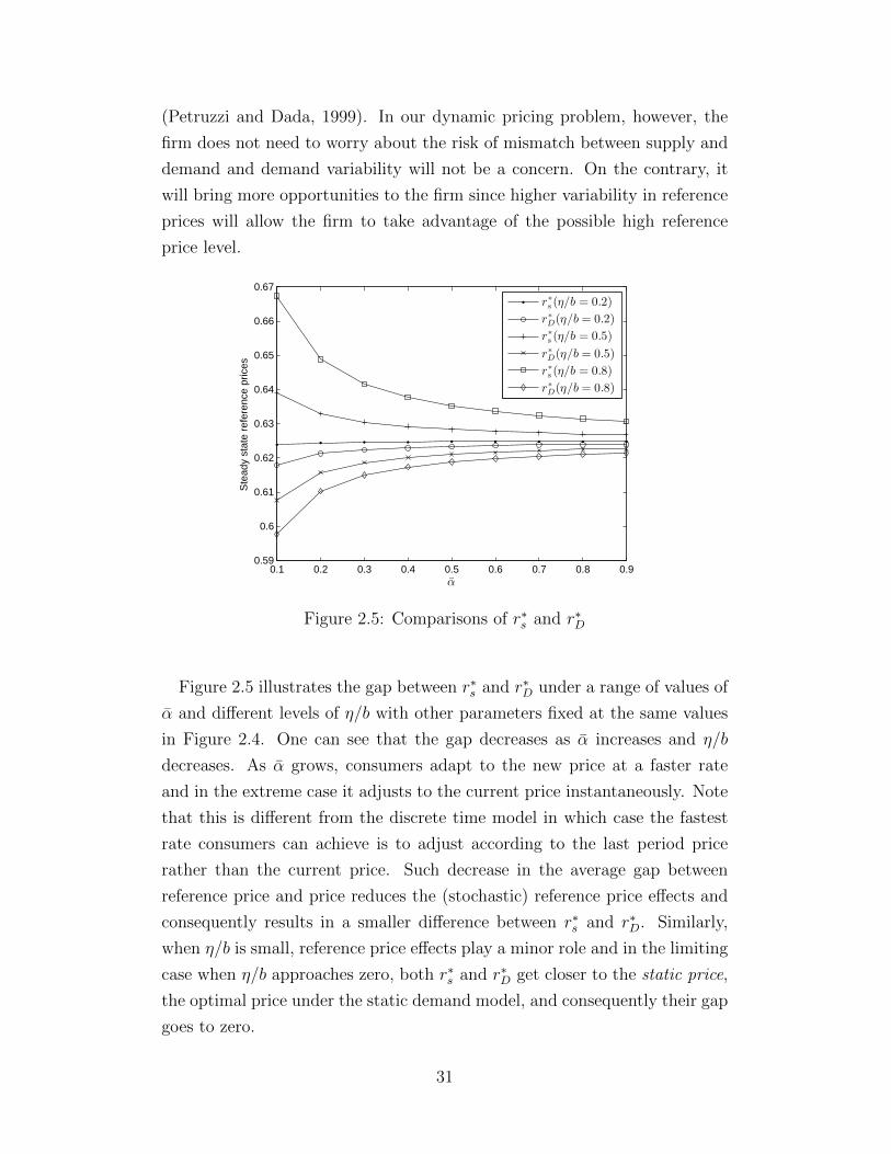
Figure 2.5 illustrates the gap between r∗s and r∗D under a range of values of

α and different levels of η/b with other parameters fixed at the same values

in Figure 2.4. One can see that the gap decreases as α increases and η/b

decreases. As α grows, consumers adapt to the new price at a faster rate

and in the extreme case it adjusts to the current price instantaneously. Note

that this is different from the discrete time model in which case the fastest

rate consumers can achieve is to adjust according to the last period price

rather than the current price. Such decrease in the average gap between

reference price and price reduces the (stochastic) reference price effects and

consequently results in a smaller difference between r∗s and r∗D. Similarly,

when η/b is small, reference price effects play a minor role and in the limiting

case when η/b approaches zero, both r∗s and r∗D get closer to the static price,

the optimal price under the static demand model, and consequently their gap

goes to zero.

31

More interestingly, the expected steady state reference price r∗s and its

deterministic counterpart r∗D can have different behaviors relative to some

problem parameters. When reference price effects are significant (η/b is

large), r∗s is decreasing in α while r∗D is increasing in α. It is easy to see

the monotonicity of r∗D. Since the static price is always higher than r∗D, as α

increases, the model more closely resembles the static demand model and as

a result, r∗D increasingly approaches the static price. The opposite direction

of r∗s is less obvious. One possible explanation is that when α becomes larger,

the benefit of having larger variations in reference price decreases. Similar

explanations apply to the sensitivity of r∗s and r∗D to η/b. As η/b becoming

smaller, the effects of reference price gradually vanish and r∗D increases to

the static price while r∗s decreases to it.

2.8 Conclusion

This chapter summarizes and extends the existing literature in reference

price effects by comparing various reference price models and presenting the

analysis of the dynamic pricing problem with loss/gain neutral or loss-averse

demands under these models.

We empirically compare the widely used exponential smoothing model with

the two recently proposed peak-end model and adaptation-rate-based model.

We find that the peak-end model being as parsimonious as the exponential s-

moothing model, in general, performs the best. However, in one example, the

adaptation-rate-based model still provides a better fit at a cost of increasing

the degree of freedom of model parameters. It would be an interesting future

research direction to further confirm our findings to other product categories

and determine the market conditions under which one model outperforms

another.

Despite the differences in their empirical performances, the managerial im-

plications from the dynamic pricing problems under the three reference price

models are similar. All three models predict that a constant pricing strat-

egy is optimal in the long-run when demands are either loss/gain neutral

or loss-averse. However, based on our analysis of the adaptation-rate-based

model, which is not explored in the previous literature, we find that a range

of constant prices can be optimal even in the case of loss/gain neutral de-

32

mands. This is different from the prediction of the exponential smoothing

model in which case only a single constant price is optimal. We numerically

show that the relative range of steady states compared to the exponential s-

moothing model grows as asymmetry in consumers’ adaption rate dominates

the asymmetry in loss-aversion.

Finally, we extend the literature by introducing a stochastic reference price

model in a continuous time framework. Our motivation in introducing ran-

domness in consumers’ memory processes is to model consumer heterogene-

ity and exogenous factors. We obtain an explicit solution to the steady state

distribution and derive several interesting new insights from analyzing the

dynamic pricing problem under the stochastic reference price effects. Specif-

ically, we find that the expected steady state reference price (price) is higher

than the steady state reference price (price) under a deterministic model

and the larger the variance in consumers’ memory processes, the higher the

steady state reference price (price). In addition, we find that the gap be-

tween the two shrinks as reference price effects diminishes (α increases or

η/b decreases) and they can have opposite sensitivity to the magnitude of

reference price effects.

An interesting future research direction along the line of stochastic refer-

ence price effects would be empirical justification of our models and compar-

isons to other possible ways of modeling consumer heterogeneity or exogenous

factors. Also, we only focus on the case of loss/gain neutral demands, which

enable us to apply tools from stochastic optimal control theory. However,

whether the steady state result can be generalized to loss-averse demands is

still a challenging open question.

33

Chapter 3

Dynamic Pricing Problem with Gain-SeekingReference Price Effect

3.1 Introduction

In Chapter 2, we have introduced the results in several papers (Fibich et al.,

2003; Popescu and Wu, 2007; Nasiry and Popescu, 2011) which all focus on

loss-averse demand model. The conceptual support for loss-aversion follows

from prospect theory (Tversky and Kahneman, 1991) and as a result a widely

beheld belief in the reference price literature postulates that consumers are

loss-averse.

In this chapter, however, we point out that, in practice, it is also pos-

sible for the firm to face gain-seeking demands and the underlying reasons

for this could be either consumers are indeed gain-seeking or the effect of

aggregation. We then study the dynamic pricing problem of a firm facing

gain-seeking demand. We remark here that although the term “loss-seeking”

is used in the previous literature (see, for instance, Popescu and Wu, 2007),

we feel the term “gain-seeking” is more accurate in capturing the fact that

consumers/aggregate demands are more sensitive to gains rather than losses

and note that it has also been adopted in several recent papers (Aflaki and

Popescu, 2013; Kallio and Halme, 2009; Kopalle et al., 2012) as well.

Unlike the common belief that loss-averse behavior is prevalent, it is ad-

mitted in the survey paper by Mazumdar et al. (2005) that “evidence of

loss-aversion is mixed”. In fact, there are empirical evidences that support

gain-seeking behavior at both individual and aggregate level. At an individ-

ual level, two out of five papers reviewed by Mazumdar et al. (2005) that

study the effects of loss-aversion show little or no evidence of loss-aversion.

Specifically, Krishnamurthi et al. (1992) observe that consumers not loyal

to any brand respond more strongly to gains than to losses in all six but

one brand, and Bell and Lattin (2000) suggest through extensive empirical

34

studies across different product categories that loss-aversion may not be a

universal phenomenon in grocery products due to price response heterogene-

ity. More recently, Kopalle et al. (2012) find that for a large number of

households the impact of a gain is greater than that of a loss and on average

the effect of losses is almost negligible compared to that of gains. At an

aggregate level, Greenleaf (1995) shows that the aggregate demand can be

10 times more responsive to gains than losses. Deploying the methodology

of switching regression on the aggregate level data, Raman and Bass (2002)

also encounter gain-seeking behavior in one of their brands.

One also needs to be cautious that loss-aversion at an individual level does

not necessarily imply loss-aversion at an aggregate level. Kallio and Halme

(2009) explicitly define the loss-aversion at an individual level as loss averse

in value and loss-aversion at an aggregate level as loss averse in demand and

give possible conditions under which loss averse in value does not imply loss

averse in demand. One important implication of their conditions in a single

product setting is that when market conditions are harsh (consumers have

overall small probability of purchasing the product, i.e., mainly promotion-

driven consumers), then the market should be more sensitive to gains which

boost the market rather than losses which further make the market more

miserable. Greenleaf (1995) also points out that the presence of gain-seeking

at an aggregate demand level does not necessarily contradict with prospect

theory. Specifically, he argues that the market usually consists of “light”

households who are price-sensitive and have a low probability of purchas-

ing at the regular price, and “heavy” households who have a high purchase

probability at the regular price even when there is a loss. As a result, during

a promotion, when there is a gain, many more light households than heavy

ones are attracted. Consequently, market demand is more sensitive to gains

than losses even though each household may be more sensitive to losses than

gains.

Therefore, one should realize the existence of gain-seeking at an aggregate

level and it can be caused either by gain-seeking behavior at an individual

level (with aggregation not changing the gain-loss asymmetry) or by aggrega-

tion under harsh market conditions. Even if, under certain market conditions,

the gain-seeking model analyzed in this chapter is not fully consistent with

the model aggregating individual level behaviors, it may still be used as a

prescriptive model to provide a plausible tractable approximation.

35

Despite the necessity of analyzing how the firm should respond if gain-

seeking is present in the aggregate level demand, analytical results on the

dynamic pricing problem of a firm in the gain-seeking case are very limited.

To the best of our knowledge, the only result in this case is the non-optimality

of the constant pricing strategy as observed by Kopalle et al. (1996) and

Popescu and Wu (2007). Moreover, Popescu and Wu (2007) postulate that

“High-low pricing, is provably optimal if consumers are focused on gains.”

However, we cannot find any rigorous proof in the literature. Indeed, there

are many practical and interesting open questions left for the dynamic pricing

problem. For example, is high-low pricing, in which only a regular price and

a discount price are employed periodically, indeed optimal in general? If not,

what are the conditions that guarantee its optimality? Furthermore, when

high-low pricing is not optimal, what can we say about the optimal pricing

strategy and the performance of the high-low pricing strategy?

This chapter strives to answer the above questions. Specifically, we find

that even the myopic pricing strategy, where the firm ignores the effect of cur-

rent prices on future revenues and focuses on maximizing short-term revenue,

does not always admit a cyclic high-low price pattern and its long-run behav-

ior can be very complicated. We provide necessary and sufficient conditions

for the existence of a cyclic high-low price pattern in the myopic pricing s-

trategy. In addition, conditions are derived such that the myopic pricing

strategy leads to either a cyclic penetrating pricing strategy in which the re-

sulting reference prices increase within a cycle, or a cyclic skimming pricing

strategy in which the resulting reference prices decrease within a cycle. Our

numerical studies show that high-low pricing is generally not optimal and

the dynamics of the optimal pricing strategy is likely to be significantly more

complex than that resulted from the myopic pricing strategy. Interestingly,

under the assumptions that consumers only remember the most recent price

and the aggregate demand is insensitive to the negative part of the difference

between reference price and price, we prove that the optimal pricing strategy

is a cyclic skimming pricing strategy. In other words, when consumers have

a low reference price, the firm should charge a high price and then gradually

offer deeper and deeper discounts until consumers’ reference price drops low

again and repeat the cycle. The assumptions we made are also found to be

very plausible in our empirical studies. We further provide sufficient condi-

tions for the high-low pricing strategy to be optimal. Our numerical studies

36

suggest that the high-low pricing strategy, when fails to be optimal, can still

achieve over 90% of the optimal profit.

Our work is in sharp contrast to the stream of works in the dynamic pricing

problem when loss-aversion is present at a market level. All these works ar-

rive at the conclusion that a constant pricing strategy is optimal in the long

run. Specifically, Kopalle et al. (1996) observe through numerical studies

that optimal prices converge monotonically and conjecture that a constant

price is optimal in the long run. Fibich et al. (2003) explicitly solve the op-

timal pricing strategy in a continuous time optimal control framework, and

confirm the observation by Kopalle et al. (1996) when demand is piece-wise

linear in price and reference price. Popescu and Wu (2007) extend the result

of Fibich et al. (2003) to general demand functions in a discrete time infinite

horizon setting. Nasiry and Popescu (2011) consider the dynamic pricing

problem with a peak-end based reference price model; they also conclude

the observation by Kopalle et al. (1996). Vast empirical literature, however,

suggests that it is important for practitioners not to take loss-averse assump-

tion as granted. When facing gain-seeking demands, our findings show that

constant pricing strategy can result in as much as 50% loss in profit while

simple cyclic pricing strategies (cyclic skimming or high-low pricing strate-

gies) are optimal or close to optimal in many scenarios. This discrepancy

in results between the loss-averse case and the gain-seeking case is due to

the differences in the underlying structures of the optimization problems. In

essence, under loss-aversion, the single period profit function, though non-

smooth due to the asymmetric responses to losses and gains, is a concave

function of the current price. The gain-seeking demand, on the other hand,

changes the structure of the problem completely. The resulting optimization

problem is neither smooth nor concave.

A few papers have considered dynamic pricing problems in various settings

that also lead to cyclic pricing strategies. Conlisk et al. (1984) assume that

consumers are strategic with two possible valuations and will remain in the

market (possibly forever) until making a purchase. They establish that a

cyclic skimming pricing strategy is optimal. Besbes and Lobel (2015) consider

strategic consumers that are heterogeneous both in valuations and the time

they may spend in the market. They prove that a cyclic pricing strategy is

optimal but a cyclic penetrating or a cyclic skimming pricing strategy may

yield arbitrary poor performance. Ahn et al. (2007) study both production

37

and pricing decisions when consumers have uniformly distributed valuations

and tend to buy the product as soon as the price drops below their valuations.

They show, in a special case where consumers wait at most one period and the

firm has no capacity constraint, that high-low pricing strategy is optimal. Liu

and Cooper (2014) consider a pricing setting similar to Ahn et al. (2007) and

demonstrate that a cyclic skimming pricing strategy is optimal even when

consumers have general valuation distributions and can wait for multiple

periods. We emphasize here some key distinctions of our work from these

papers. In terms of modeling, the argument behind reference price models

is that consumers’ purchase decisions are affected by the prices in the past

rather than anticipated prices in the future. In terms of proofs, we form

a dynamic programming problem and identify the cyclic pricing strategy

by analyzing properties of the value function whereas the above papers all

tackle their problems directly by utilizing the notion of a regeneration point.

Essentially, the driving force that leads to a cyclic pricing strategy in our

model is the gain-seeking behavior of consumers while in these papers is the

waiting behavior of consumers. Another related paper is Geng et al. (2010)

who restrict to high-low pricing strategies and use a different approach by

taking weighted average between the regular price and the discount price

to model reference price. They show that when demand is gain-seeking,

high-low pricing strategy outperforms constant pricing strategy. Our work

following Fibich et al. (2003); Kopalle et al. (1996) and Popescu and Wu

(2007), on the other hand, models the dynamics and intertemporal effects of

reference prices explicitly and settles the conjecture in the existing literature

by showing that high-low pricing strategy may not be optimal.

Our work is also closely related to the on-going research in the one-

dimensional discontinuous map in the dynamic system and chaos community.

Sharkovsky and Chua (1993) examine a certain type of discontinuous maps

that arise in electric circuits. They find that their class of discontinuous maps

has strong temporal chaos and the behavior of trajectories can only be char-

acterized by using probability language. Jain and Banerjee (2003) present a

classification of border-collision bifurcations in discontinuous maps. Depend-

ing on parameters, the resulting dynamics can have various periodic orbits or

chaos. Rajpathak et al. (2012) analyze in detail the stable periodic orbits of

one type of discontinuous maps and explore the possible patterns exhibited

by these orbits. It turns out that the myopic pricing strategy in our work

38

can be reduced to the type of discontinuous maps analyzed in Rajpathak

et al. (2012). However, to the best of our knowledge, the class of discontinu-

ous maps with multiple discontinuous points, into which our optimal pricing

strategy typically falls, has not been considered in the previous literature.

The remainder of this chapter is organized as follows. In Section 3.2, we

remind the readers of the mathematical formulation of our model introduced

in Section 2.2. In Section 3.3, we analyze the dynamics of the myopic pricing

strategy and relate it with the work in discontinuous maps. The structural

results for the optimal pricing strategy are presented in Section 3.4. Section

3.5 presents an empirical study and conducts numerical experiments to test

the performance of simple pricing strategies. Finally, we conclude the chapter

in the last section with some suggestions for future research. The proofs are

all relegated to Appendix B.

3.2 Model

In this section, we restate the exponential smoothing model introduced in

Section 2.2 and introduce the dynamic pricing problem with gain-seeking

demands. Recall that under the exponential smoothing model, the reference

prices evolve according to

rt+1 = αrt + (1− α)pt, t ≥ 0. (3.1)

In the above evolution equation, pt ∈ [0, U ] is the price charged by the firm

at period t, where U is the upper bound on feasible prices. The parameter

α ∈ [0, 1) is called the memory factor or carryover constant (Kalyanaram and

Little, 1994). When α = 1, reference prices remain a constant over the whole

planning horizon and consequently a constant pricing strategy is optimal

irrespective of gain-loss asymmetry. We restrict α < 1 to avoid such a case

that past prices have no impact on demand. As reference prices are generated

from historical prices, it is also reasonable to assume that r0 ∈ [0, U ].

Recall the demand function defined in (2.4). To avoid negative demand,

we further assume that D(0, U) ≥ 0, i.e., U ≤ ba+η−

. Since this chapter

focuses on the gain-seeking case, we have η+ > η− in (2.4).

The firm’s one-period profit is denoted as Π(r, p) = pD(r, p). Here, the

39

marginal cost is assumed to be 0 for simplicity. All our results can be ex-

tended to cases with a non-zero marginal cost. We assume U ≥ b2a

such that

Π(p, p), called the base profit, is not monotone in p ∈ [0, U ]. This assump-

tion allows us to “rule out pathological boundary steady states (Popescu and

Wu, 2007).”, but our analysis can be carried over similarly by distinguish-

ing those boundary steady states when this assumption fails. Note that the

assumptions η+ > η− and p ≥ 0 allow us to rewrite the one-period profit as

Π(r, p) = max{Π+(r, p),Π−(r, p)},

where Π+(r, p) = p[b− ap+ η+(r − p)] and Π−(r, p) = p[b− ap+ η−(r − p)].Contrary to the loss-averse case, the one-period profit function is no longer

a concave function in p.

Given an initial reference price r0, the firm’s long-term profit maximization

problem is then:

V (r0) = maxpt∈[0,U ]

∞∑t=0

γtΠ(rt, pt), (3.2)

where γ ∈ [0, 1) is a discount factor and we interpret 00 = 1. The infinite

horizon problem is of particular interest in the literature since it is often

more tractable than the finite horizon counterpart and provides valuable

insights into the long-run behavior of the optimal pricing strategy, which

in turn may shed light on the development of efficient heuristics for finite

horizon models. It is worth noting here that two assumptions commonly

imposed on optimization problems: differentiability and concavity in the

decision variables, are both absent in the one-period profit function Π(r, p),

which makes the analysis of problem (3.2) quite challenging.

The Bellman equation for problem (3.2) is

V (r) = maxp∈[0,U ]

Π(r, p) + γV (αr + (1− α)p). (3.3)

A pricing strategy p(r) is a function from [0, U ] to [0, U ] that specifies a

feasible solution to (3.3) for a given reference price r. Given any pricing

strategy p(r), the sequence {rt} of reference prices which evolve according

to rt+1 = αrt + (1− α)p(rt), is referred to as the reference price path of the

pricing strategy p(r). We say p(r) has a periodic orbit of period n or is a

cyclic pricing strategy with cycle length n if and only if there exists r0 ∈ [0, U ]

40

such that the reference price path of p(r) satisfies rn = r0 and rt 6= r0 for

all 0 < t < n. Clearly, if rn = r0, then by rt+1 = αrt + (1 − α)p(rt), the

sequence {r0, ..., rn−1} is repeated infinitely over time and this sequence is

referred to as the periodic orbit of p(r). In particular, when n = 1, we say

p(r) admits a steady state r0 and when n = 2, p(r) is a high-low pricing

strategy. If there exists a periodic orbit that has the additional property

that r0 < r1 < ... < rn−1, then we refer p(r) to as a cyclic penetrating

pricing strategy. If, on the other hand, r0 > r1 > ... > rn−1, then we

refer p(r) to as a cyclic skimming pricing strategy. Note that in the special

case when α = 0, r0 < r1 < ... < rn−1 (r0 > r1 > ... > rn−1) if and

only if p(rn−1) < p(r0) < ... < p(rn−2) (p(rn−1) > p(r0) > ... > p(rn−2)),

i.e., the monotonicity of reference prices is equivalent to the monotonicity

of charged prices. However, for α > 0, it is possible to have monotone

reference prices with non-monotone charged prices. Recall that in practice, a

skimming (penetrating) pricing strategy is used to describe pricing strategy

with decreasing (increasing) price path overtime. Here, we use the term

“skimming” (“penetrating”) to reflect the fact that a skimming (penetrating)

pricing strategy is usually designed to capture consumers with decreasing

(increasing) valuations (an analogy of the notion “reference price” in our

model) overtime. Since [0, U ] is compact and the objective function can be

easily shown to be continuous, the optimal pricing strategy that solves (3.3)

exists and is denoted by p∗(r). As mentioned in Section 3.1, Kopalle et al.

(1996) and Popescu and Wu (2007) prove that p∗(r) does not admit a steady

state. That is, for any r ∈ [0, U ], p∗(r) 6= r.

In the following, we will also use the term pattern to describe the existence

of various monotonic structures within a periodic orbit. One is referred to

Rajpathak et al. (2012) for a rigorous definition in the context of discontin-

uous maps. Here, we illustrate the term through a simple example. Con-

sider a periodic orbit with period 4 that consists of four different reference

prices 1, 2, 3, 4. Then, depending on different orderings, the periodic orbit

can demonstrate different patterns or monotonic structures as illustrated in

Figure 3.1. The upper left and lower right panels show the reference price

patterns that are of penetrating and skimming pricing strategy respectively.

However, the upper right panel shows a pattern that has reference prices in-

crease in the first two periods accompanied by a decrease in the third period

while the lower left panel shows a pattern that the reference prices alternate

41

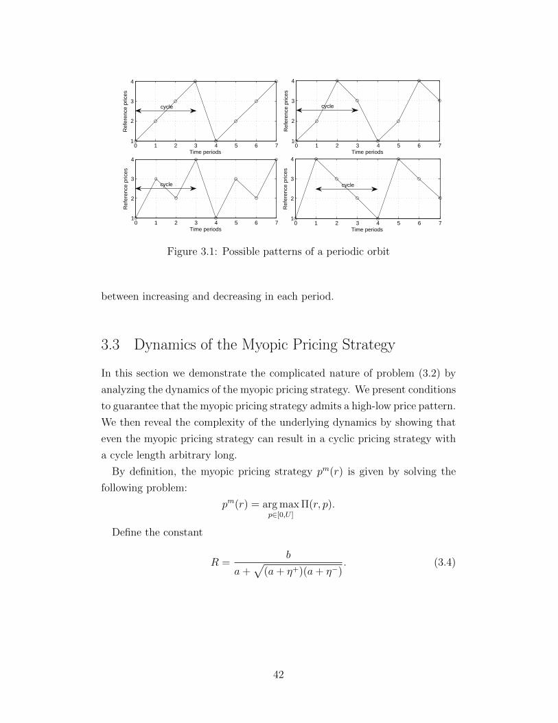
0 1 2 3 4 5 6 71

2

3

4

Time periods

Ref

eren

ce p

rices

0 1 2 3 4 5 6 71

2

3

4

Time periods

Ref

eren

ce p

rices

0 1 2 3 4 5 6 71

2

3

4

Time periods

Ref

eren

ce p

rices

0 1 2 3 4 5 6 71

2

3

4

Time periods

Ref

eren

ce p

rices

cycle cycle

cycle cycle

Figure 3.1: Possible patterns of a periodic orbit

between increasing and decreasing in each period.

3.3 Dynamics of the Myopic Pricing Strategy

In this section we demonstrate the complicated nature of problem (3.2) by

analyzing the dynamics of the myopic pricing strategy. We present conditions

to guarantee that the myopic pricing strategy admits a high-low price pattern.

We then reveal the complexity of the underlying dynamics by showing that

even the myopic pricing strategy can result in a cyclic pricing strategy with

a cycle length arbitrary long.

By definition, the myopic pricing strategy pm(r) is given by solving the

following problem:

pm(r) = arg maxp∈[0,U ]

Π(r, p).

Define the constant

R =b

a+√

(a+ η+)(a+ η−). (3.4)

42

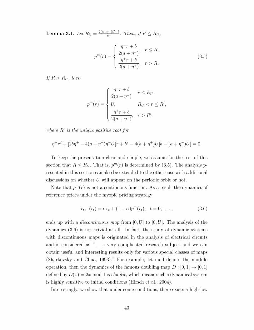
Lemma 3.1. Let RU = 2(a+η−)U−bη−

. Then, if R ≤ RU ,

pm(r) =

η−r + b

2(a+ η−), r ≤ R,

η+r + b

2(a+ η+), r > R.

(3.5)

If R > RU , then

pm(r) =

η−r + b

2(a+ η−), r ≤ RU ,

U, RU < r ≤ R′,

η+r + b

2(a+ η+), r > R′,

where R′ is the unique positive root for

η+r2 + [2bη+ − 4(a+ η+)η−U ]r + b2 − 4(a+ η+)U [b− (a+ η−)U ] = 0.

To keep the presentation clear and simple, we assume for the rest of this

section that R ≤ RU . That is, pm(r) is determined by (3.5). The analysis p-

resented in this section can also be extended to the other case with additional

discussions on whether U will appear on the periodic orbit or not.

Note that pm(r) is not a continuous function. As a result the dynamics of

reference prices under the myopic pricing strategy

rt+1(rt) = αrt + (1− α)pm(rt), t = 0, 1, ..., (3.6)

ends up with a discontinuous map from [0, U ] to [0, U ]. The analysis of the

dynamics (3.6) is not trivial at all. In fact, the study of dynamic systems

with discontinuous maps is originated in the analysis of electrical circuits

and is considered as “... a very complicated research subject and we can

obtain useful and interesting results only for various special classes of maps

(Sharkovsky and Chua, 1993).” For example, let mod denote the modulo

operation, then the dynamics of the famous doubling map D : [0, 1]→ [0, 1]

defined byD(x) = 2x mod 1 is chaotic, which means such a dynamical system

is highly sensitive to initial conditions (Hirsch et al., 2004).

Interestingly, we show that under some conditions, there exists a high-low

43

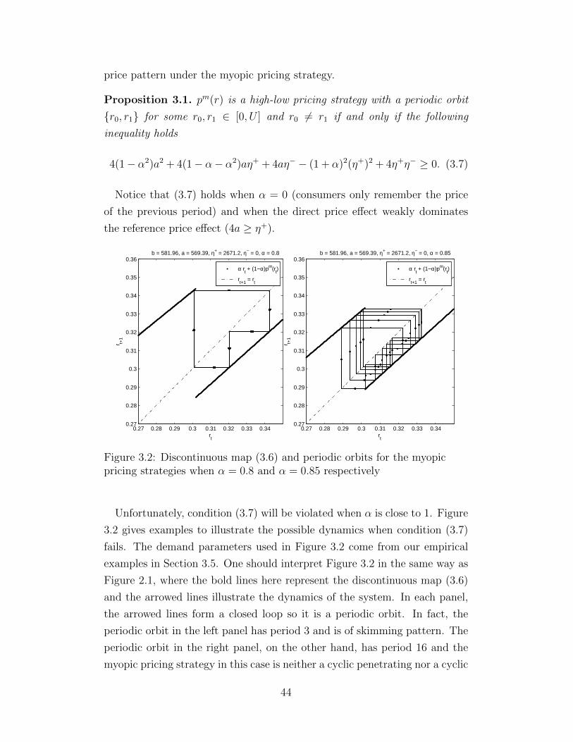
price pattern under the myopic pricing strategy.

Proposition 3.1. pm(r) is a high-low pricing strategy with a periodic orbit

{r0, r1} for some r0, r1 ∈ [0, U ] and r0 6= r1 if and only if the following

inequality holds

4(1− α2)a2 + 4(1− α− α2)aη+ + 4aη− − (1 + α)2(η+)2 + 4η+η− ≥ 0. (3.7)

Notice that (3.7) holds when α = 0 (consumers only remember the price

of the previous period) and when the direct price effect weakly dominates

the reference price effect (4a ≥ η+).

0.27 0.28 0.29 0.3 0.31 0.32 0.33 0.340.27

0.28

0.29

0.3

0.31

0.32

0.33

0.34

0.35

0.36

rt

r t+1

b = 581.96, a = 569.39, η+ = 2671.2, η− = 0, α = 0.8

α rt + (1−α)pm(r

t)

rt+1

= rt

0.27 0.28 0.29 0.3 0.31 0.32 0.33 0.340.27

0.28

0.29

0.3

0.31

0.32

0.33

0.34

0.35

0.36

rt

r t+1

b = 581.96, a = 569.39, η+ = 2671.2, η− = 0, α = 0.85

α rt + (1−α)pm(r

t)

rt+1

= rt

Figure 3.2: Discontinuous map (3.6) and periodic orbits for the myopicpricing strategies when α = 0.8 and α = 0.85 respectively

Unfortunately, condition (3.7) will be violated when α is close to 1. Figure

3.2 gives examples to illustrate the possible dynamics when condition (3.7)

fails. The demand parameters used in Figure 3.2 come from our empirical

examples in Section 3.5. One should interpret Figure 3.2 in the same way as

Figure 2.1, where the bold lines here represent the discontinuous map (3.6)

and the arrowed lines illustrate the dynamics of the system. In each panel,

the arrowed lines form a closed loop so it is a periodic orbit. In fact, the

periodic orbit in the left panel has period 3 and is of skimming pattern. The

periodic orbit in the right panel, on the other hand, has period 16 and the

myopic pricing strategy in this case is neither a cyclic penetrating nor a cyclic

44

skimming pricing strategy. By comparing the two panels, one can see that a

mere increment of 0.05 in α can result in dramatic changes in the dynamics.

As illustrated in Figure 3.1, when the period is greater than or equal

to 4, there could exist other patterns rather than penetrating or skimming

pattern that have the same period. Our numerical experiments illustrate that

both the period and pattern of a periodic orbit can be very sensitive to the

changes in parameters, a phenomenon termed as border collision bifurcation

in the dynamic system and chaos community (Jain and Banerjee, 2003). In

the following, we identify necessary and sufficient conditions for the myopic

pricing strategy to admit a cyclic penetrating pattern and a cyclic skimming

pattern with cycle length n respectively. To simplify the expressions of our

conditions, define constants

µ =a+ η+ −

√a2 + aη+ + aη− + η+η−

η+ − η−,

A = 1 + α− α η−

2(a+ η−), B = 1 + α− α η+

2(a+ η+),

and denote for n ≥ 0 the sum of geometric series∑n

i=0 ki by Skn (for n < 0,

let Skn = 0).

Proposition 3.2. For n ≥ 2, pm(r) is a cyclic penetrating pricing strategy

with cycle length n if and only if the following inequalities hold

An−1

SAn−1

< µ ≤ An−2

An−2B + SAn−2

. (3.8)

On the other hand, pm(r) is a cyclic skimming pricing strategy with cycle

length n if and only if the following inequalities hold

ABn−2 + SBn−3

ABn−2 + SBn−2

< µ ≤SBn−2

SBn−1

. (3.9)

Note that when n = 2, both (3.8) and (3.9) reduce to A1+A

< µ ≤ 11+B

,

which can be simplified to (3.7) by substituting the expressions for A, B and

µ, and by definition, a high-low pricing strategy is both a cyclic penetrating

and a cyclic skimming pricing strategy. For n large enough, there exists other

range of parameters other than (3.8) and (3.9) resulting periodic orbits of

period n that are neither penetrating nor skimming. In fact, corresponding

45

to different parameter regions, there are exactly φ(n) different patterns of

periodic orbits of period n, where φ(·) is the so-called Euler totient function

(Rajpathak et al., 2012).

3.4 Optimal Pricing Strategy

Unlike the myopic pricing strategy, we do not have an explicit solution for

the optimal pricing strategy, which makes the analysis significantly more

challenging. To illustrate the difficulty, we first present a few properties on

the value function and optimal solution.

Since Π(r, p) = max{Π+(r, p),Π−(r, p)}, the Bellman equation can be cor-

respondingly rewritten as

V (r) = maxp∈[0,U ]

{max{Π+(r, p),Π−(r, p)}+ γV (αr + (1− α)p)}. (3.10)

We assume, without loss of generality, that p∗(r) and the optimal solutions

for other optimization problems in this section always take the largest one

among multiple solutions.

Consider the following two problems:

V +(r) = maxp∈[0,U ]

Π+(r, p) + γV (αr + (1− α)p), (3.11a)

V −(r) = maxp∈[0,U ]

Π−(r, p) + γV (αr + (1− α)p). (3.11b)

The solutions of (3.11a) and (3.11b) are denoted respectively as p+(r) and

p−(r). An observation here is that V (r) = max{V +(r), V −(r)} and p∗(r) ∈{p+(r), p−(r)}. We next characterize properties of V ±(r) and p±(r).

Lemma 3.2. Both V +(r) and V −(r) are increasing and convex in r while

p+(r) and p−(r) are increasing in r.

Although problem (3.10) is difficult to analyze due to the term

max{Π+(r, p),Π−(r, p)}, Lemma 3.2 shows that the decomposed problems

(3.11a) and (3.11b) have some desired properties, i.e., monotonic solutions

and optimal objective values. We are interested in how p+(r) and p−(r) re-

late to the optimal pricing strategy p∗(r), and whether it is possible to obtain

simple characterizations for p+(r) and p−(r). For this purpose, we draw in

46

Figure 3.3 the (numerically approximated) optimal pricing strategy for the

example used in the left panel of Figure 3.2 with a discount factor γ = 0.9.

In Figure 3.3, we observe that, similar to the myopic pricing strategy, there

0 0.1 0.2 0.3 0.4 0.5 0.6 0.7 0.8 0.9 1

0.4

0.5

0.6

0.7

0.8

0.9

1

Pric

e

Reference price

b = 581.96, a = 569.39, η+ = 2671.2, η− = 0, α = 0.8, γ = 0.9

Optimal pricep = r

p−(r)

p+(r)

Figure 3.3: Optimal pricing strategy when α = 0.8, η− = 0 and γ = 0.9

exists a point r ∈ [0, U ] such that p∗(r) is given by p−(r) for r ≤ r and

p+(r) for r > r. Unfortunately, though this observation seems to hold in

all our numerical experiments, we do not have a proof for general parameter

configurations. Of course, even if this observation is indeed true, Figure 3.3

suggests that both p+(r) and p−(r) can have numerous discontinuous points,

in contrast to the two linear pieces in the myopic pricing strategy. This

implies that they may not admit any simple characterizations.

In terms of dynamics, we have already demonstrated the dynamics of the

myopic pricing strategy (which has only one discontinuous point and admits

explicit expression) in Section 3.3. Here, we further give a side-by-side com-

parison of the dynamics of the optimal pricing strategies and their periodic

orbits in Figure 3.4 for the examples used in Figure 3.2 with the discount fac-

tor γ = 0.9. The bold lines in Figure 3.4 represent the map αrt+(1−α)p∗(rt)

and as α is close to one in both instances, many discontinuous points observed

in Figure 3.3 become difficult to be distinguished in Figure 3.4 through vi-

sual inspection. When comparing Figure 3.2 and Figure 3.4, it is clear that

the period lengths under optimal pricing strategies can be much larger than

47

these under myopic pricing strategies, which indicates that the dynamics of

the optimal pricing strategy can be much more complicated and the analy-

sis, if possible, is likely to be significantly more challenging than that for the

myopic pricing strategy.

0.45 0.5 0.55 0.60.44

0.46

0.48

0.5

0.52

0.54

0.56

0.58

0.6

rt

r t+1

b = 581.96, a = 569.39, η+ = 2671.2, η− = 0, α = 0.85, γ = 0.9

α r

t + (1−α)p*(r

t)

rt+1

= rt

0.5 0.55 0.6 0.65 0.70.5

0.52

0.54

0.56

0.58

0.6

0.62

0.64

0.66

0.68

0.7

rt

r t+1

b = 581.96, a = 569.39, η+ = 2671.2, η− = 0, α = 0.8, γ = 0.9

α rt + (1−α)p*(r

t)

rt+1

= rt

Figure 3.4: Periodic orbits for the optimal pricing strategies when α = 0.8and α = 0.85 respectively

Thus, for the rest of this section, we focus on a special case satisfying the

following assumption.

Assumption 3.1. Consumers only remember the most recent price (i.e. α =

0) and the demand is insensitive to the perceived surcharge (i.e. η− = 0).

Assumption 3.1 seems restrictive but has very plausible explanations. First

of all, consumers are unlikely to remember many historical prices and form

reference price by averaging them. Several papers, for example, Raman and

Bass (2002); Krishnamurthi et al. (1992); Mayhew and Winer (1992), also

assume that α = 0. It captures the fact that “consumers. . . experience con-

siderable difficulty in recalling accurately even the most recently encountered

prices . . . Thus, it is unlikely that consumers would retrieve from memory and

use prices encountered much beyond the immediate past purchase occasion

(Krishnamurthi et al., 1992).” On the other hand, η− = 0 models the mar-

ket of promotion-driven products, where the demand of product consists of

the base demand b−ap and promotion stimulated demand η+ max{r−p, 0}.

48

This also reflects a harsh market condition under which the firm is very likely

to face a gain-seeking demand (Kallio and Halme, 2009).

Assumption 3.1 also provides good approximation to some practical sce-

narios. Specifically, we provide empirical examples in Section 3.5, in which

by imposing Assumption 3.1 does not result in much loss in the goodness of

fit of the model.

An immediate consequence from Assumption 3.1 is that both V −(r) and

p−(r) are now constant functions. In the sequel, we will use constants p−

and V − to denote the function values of p−(r) and V −(r). V −(r) being a

constant function is critical for the simplification of the problem, as it allows

us to relate p+(r) and p−(r) with p∗(r) in a simple way as demonstrated in

the following lemma.

Lemma 3.3. Under Assumption 3.1, there exists R0 ∈ (0, U) such that if

r ≤ R0, then V (r) = V − and p∗(r) = p− > r. If r > R0, then V (r) = V +(r)

and p∗(r) = p+(r) < r.

Lemma 3.3 gives us a broad picture of what p∗(r) looks like. That is,

when r ≤ R0, p∗(r) is a constant function and is always above r. At the

point R0, there is a “downward jump” from p− > R0 to p+(R0) < R0. When

r > R0, p∗(r) is then monotonically increasing in r. In the sequel, we will

briefly sketch the idea of how to characterize p+(r), which leads to a complete

characterization of the optimal pricing strategy p∗(r).

Let us reconsider problem (3.11a) when r ∈ [R0, U ] and keep in mind that

p+(R0) < R0 and p+(r) is increasing on [R0, U ]. We distinguish between two

cases.

Case 1: For any r ∈ [R0, U ], p+(r) ≤ R0. In this case, V (p+(r)) = V − and

there is no loss of optimality to write (3.11a) as

V +(r) = maxp∈[0,U ]

Π+(r, p) + γV −,

from which we can explicitly solve

p+(r) =η+r + b

2(a+ η+).

49

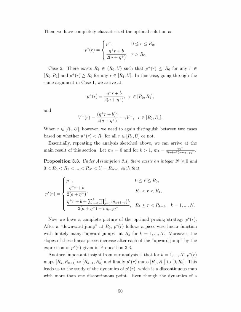
Then, we have completely characterized the optimal solution as

p∗(r) =

p−, 0 ≤ r ≤ R0,

η+r + b

2(a+ η+), r > R0.

Case 2: There exists R1 ∈ (R0, U) such that p+(r) ≤ R0 for any r ∈[R0, R1] and p+(r) ≥ R0 for any r ∈ [R1, U ]. In this case, going through the

same argument in Case 1, we arrive at

p+(r) =η+r + b

2(a+ η+), r ∈ [R0, R1],

and

V +(r) =(η+r + b)2

4(a+ η+)+ γV −, r ∈ [R0, R1].

When r ∈ [R1, U ], however, we need to again distinguish between two cases

based on whether p+(r) < R1 for all r ∈ [R1, U ] or not.

Essentially, repeating the analysis sketched above, we can arrive at the

main result of this section. Let m1 = 0 and for k > 1, mk = γη+

2(a+η+)−mk−1η+.

Proposition 3.3. Under Assumption 3.1, there exists an integer N ≥ 0 and

0 < R0 < R1 < ... < RN < U = RN+1 such that

p∗(r) =

p−, 0 ≤ r ≤ R0,

η+r + b

2(a+ η+), R0 < r < R1,

η+r + b+∑k

i=0(∏i

j=0mk+1−j)b

2(a+ η+)−mk+1η+, Rk ≤ r < Rk+1, k = 1, ..., N.

Now we have a complete picture of the optimal pricing strategy p∗(r).

After a “downward jump” at R0, p∗(r) follows a piece-wise linear function

with finitely many “upward jumps” at Rk for k = 1, ..., N . Moreover, the

slopes of these linear pieces increase after each of the “upward jump” by the

expression of p∗(r) given in Proposition 3.3.

Another important insight from our analysis is that for k = 1, ..., N , p∗(r)

maps [Rk, Rk+1] to [Rk−1, Rk] and finally p∗(r) maps [R0, R1] to [0, R0]. This

leads us to the study of the dynamics of p∗(r), which is a discontinuous map

with more than one discontinuous point. Even though the dynamics of a

50

discontinuous map with only one discontinuous point is already complicated,

the characterization presented in Proposition 3.3 allows us to find simple

dynamics for p∗(r). Denote p∗1(r) = p∗(r) and p∗i (r) = p∗(p∗i−1(r)) for i > 1.

To make the notation clearer, in the following, we alternatively use r∗ to

denote the constant p−.

Proposition 3.4. Let N be the integer in Proposition 3.3. Under Assump-

tion 3.1, there exists an integer n with 2 ≤ n ≤ N + 2, such that p∗n(r∗) = r∗

and for all r0 ∈ [0, U ], the optimal reference price path r∗t converges in at

most N + 2 periods to the unique periodic orbit: {r∗, p∗1(r∗), ..., p∗n−1(r∗)},i.e., there exists 0 ≤ τ ≤ N + 2 such that r∗τ = r∗. Moreover, the periodic

orbit has the property r∗ > p∗1(r∗) > ... > p∗n−1(r∗), i.e., p∗(r) is a cyclic

skimming pricing strategy.

Proposition 3.4 suggests that the following pricing strategy for practition-

ers when the demand they face is gain-seeking and promotion-driven: when

consumers’ initial reference price is low (below R0), the firm should use a

regular price (r∗). Then the firm applies a skimming pricing strategy by

gradually discounting the regular price over time until consumers’ reference

price falls below R0, and repeats such pricing strategy. The intuition behind

is easy to understand. When consumers have a low reference price, as they

are gain-seeking, it will not hurt the firm too much by setting a high price

in order to drag consumers’ reference price to a higher level. After such ma-

nipulation, the firm will benefit greatly by offering discounts since consumers

are sensitive to gains and there will be a boost in demand.

An illustration of the optimal pricing strategy and the periodic orbit is

provided in Figure 3.5. The parameters used for Figure 3.5 are taken from

one of the empirical examples provided in Section 3.5, except γ = 0.1 here.

One can see that, indeed, there are more than one discontinuous point and

in this particular example the periodic orbit has period 3 (n = 3).

Next, we identify conditions on parameters such that a high-low pricing

strategy is optimal. Define the constant K =a+η+−

√(a+η+)2−γ(η+)2

η+and recall

the constant R = b

a+√

(a+η+)(a+η−)= b

a+√a(a+η+)

(here, by Assumption 3.1,

η− = 0), which is the discontinuous point in the myopic pricing strategy,

defined in (3.4).

51

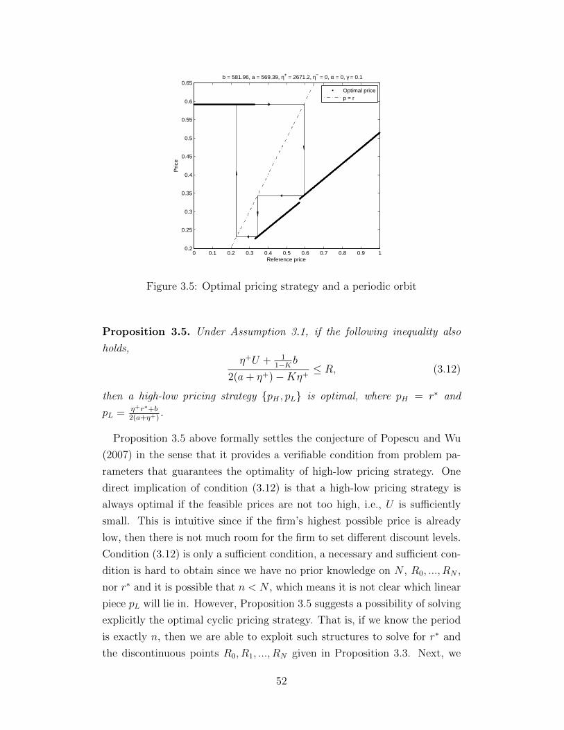
0 0.1 0.2 0.3 0.4 0.5 0.6 0.7 0.8 0.9 10.2

0.25

0.3

0.35

0.4

0.45

0.5

0.55

0.6

0.65

Reference price

Pric

e

b = 581.96, a = 569.39, η+ = 2671.2, η− = 0, α = 0, γ = 0.1

Optimal pricep = r

Figure 3.5: Optimal pricing strategy and a periodic orbit

Proposition 3.5. Under Assumption 3.1, if the following inequality also

holds,η+U + 1

1−K b

2(a+ η+)−Kη+≤ R, (3.12)

then a high-low pricing strategy {pH , pL} is optimal, where pH = r∗ and

pL = η+r∗+b2(a+η+)

.

Proposition 3.5 above formally settles the conjecture of Popescu and Wu

(2007) in the sense that it provides a verifiable condition from problem pa-

rameters that guarantees the optimality of high-low pricing strategy. One

direct implication of condition (3.12) is that a high-low pricing strategy is

always optimal if the feasible prices are not too high, i.e., U is sufficiently

small. This is intuitive since if the firm’s highest possible price is already

low, then there is not much room for the firm to set different discount levels.

Condition (3.12) is only a sufficient condition, a necessary and sufficient con-

dition is hard to obtain since we have no prior knowledge on N , R0, ..., RN ,

nor r∗ and it is possible that n < N , which means it is not clear which linear

piece pL will lie in. However, Proposition 3.5 suggests a possibility of solving

explicitly the optimal cyclic pricing strategy. That is, if we know the period

is exactly n, then we are able to exploit such structures to solve for r∗ and

the discontinuous points R0, R1, ..., RN given in Proposition 3.3. Next, we

52

identify conditions such that the period of the optimal cyclic pricing strategy

is at most n.

Proposition 3.6. Let R0 = R and for k ≥ 1 recursively define Rk to be the

unique solution of the equation

η+r + b+∑k

i=0(∏i

j=0 mk+1−j)b

2(a+ η+)−mk+1η+= Rk−1.

Under Assumption 3.1, if the following inequality holds for some k ≥ 0

η+U + 11−K b

2(a+ η+)−Kη+≤ Rk, (3.13)

then the length of period n must satisfy n ≤ k + 2.

Note that the recursively defined constants Rk provide lower bounds for

the unknown constants Rk given in Proposition 3.3, i.e., Rk ≤ Rk for

k = 0, 1, ..., N (see the proof of Proposition 3.6 in Appendix B). Similar

to Proposition 3.5, one practical implication here is that the cycle length or

the complexity of the pricing strategy depends on the flexibility of pricing,

i.e., the range of feasible prices. When U is small, there is less room for the

firm to apply intricate pricing strategy that will result in a large cycle length.

The advantage of condition (3.13) is that it can be easily verified from the

problem parameters. For instance, from the parameters we used in Figure

3.5 and with U = 1, it is straightforward to compute that

η+U + 11−K b

2(a+ η+)−Kη+= 0.502

and

R0 = 0.302, R1 = 0.493, R2 = 0.949.

Applying Proposition 3.6, we know that the optimal solution has a periodic

orbit with period less than or equal to 4. Indeed, one can see from Figure

3.5 that the optimal solution has a periodic orbit with period 3.

Finally, we present how to solve for r∗ and R0, R1, ..., RN if we know the

period is exactly n. First, it is straightforward to see from our previous

analysis that if the period is n then r∗ ∈ [Rn−2, Rn−1). Next, let V0(r) = V −,

53

V m0 (r) = 0 and recursively for k = 1, ..., N define

Vk(r) = maxp∈[0,U ]

Π+(r, p) + γVk−1(p),

V mk (r) = max

p∈[0,U ]Π+(r, p) + γV m

k−1(p).

Note that the expressions for V mk (r), k = 1, ..., N can be explicitly computed

and it is not difficult to see that

Vk(r) = V mk (r) + γkV0(r) = V m

k (r) + γkV −.

In the proof of Proposition 3.3, given in Appendix B, we have shown that

V (r) = Vn−1(r), r ∈ [Rn−2, Rn−1).

Recall that

r∗ = p− = arg maxp∈[0,U ]

p(b− ap) + γV (p),

V − = maxp∈[0,U ]

p(b− ap) + γV (p).

Thus, without loss of optimality, r∗ and V − can be explicitly solved by

r∗ = arg maxp∈[0,U ]

p(b− ap) + γVn−1(p) = arg maxp∈[0,U ]

p(b− ap) + γV mn−1(p),

V − = maxp∈[0,U ]

p(b− ap) + γVn−1(p) =1

1− γn[r∗(b− ar∗) + γV m

n−1(r∗)].

Once the expression for V − is obtained, we have the explicit expressions

for all Vk(·) for k = 0, ..., N . By continuity of V (·), for k ≥ 0, Rk can be

sequentially computed by solving the equation

Vk(Rk) = Vk+1(Rk),

and finally, N is obtained by N = sup{k : Rk ≤ U}.Combined with Proposition 3.6, if we can find some k ≥ 0 such that (3.13)

holds, then we can repeat the above computations by assuming the period

n = 2, ..., k + 2. As the value function is the unique solution to the Bellman

equation (3.3), the process we suggested is also guaranteed to yield a unique

54

solution. We illustrate the computing process above by continuing with the

example in Figure 3.5. By Proposition 3.6, the period n ≤ 4. As a start, we

assume n = 2, then


p(b− ap) + γV m1 (p) = 0.5890

and consequently we can solve

R0 = 0.3290, R1 = 0.5691.

Notice that r∗ 6∈ [R0, R1) which leads to a contradiction with n = 2.

We proceed to assume n = 3, then


p(b− ap) + γV m2 (p) = 0.5915

and

R0 = 0.3291, R1 = 0.5692, R2 > 1.

Here, r∗ ∈ [R1, R2) is consistent with our assumption that n = 3. Thus, we

have solved explicitly r∗ and R0, R1.

3.5 Numerical Study

In this section, we first provide some empirical examples and try to under-

stand what are the implications of real data for the gain-loss asymmetry as

well as other parameters used in our model. In particular, we show that

Assumption 3.1 generally gives a more parsimonious model while retaining

most of the explanatory power of the full model. We then study the perfor-

mance of several simple pricing strategies as opposed to the optimal pricing

strategy. We further examine the performance of simple cyclic pricing strate-

gies and the robustness of Proposition 3.4 numerically when Assumption 3.1

is violated.

55

3.5.1 Empirical Examples

We utilize the same data set analyzed in Section 2.3. Readers are referred

to Section 2.3 for the description of the data set as well as the method in

estimating memory factor α.

The following table reports the estimates of the key parameters that of

interest, i.e., α, η+ and η− for five brands. The rest two brands, belonging

to larger volume category, are excluded from the analysis since the estimate

for a, the price sensitivity, has a wrong sign. We also report the goodness of

fit measurements, i.e., R2 and adjusted R2, for the comparison between the

full model and the restricted model in which Assumption 3.1 is imposed. All

the standard errors are computed via the bootstrapping procedure described

in Freedman (1984).

Table 3.1: Parameter Estimates and Goodness of Fit

α η+ η− R2 Adjusted R2

Star Kist 6 oz.Full Model 0 268587 -17356 0.360 0.354

(0.064) (34198.15) (24011.89)Restricted Model 0 267124 0 0.359 0.355

Chicken of the Sea 6 oz.Full Model 0.33 573859 -58196 0.570 0.566


Bumble Bee Solid 6.12 oz.Full Model 0.99 15787 -4195 0.496 0.491

(0.008) (5305.44) (4823.14)Restricted Model 0 7646.8 0 0.462 0.459

Bumble Bee Chunk 6.12 oz.Full Model 0.15 343059 -11904 0.640 0.637


Geisha 6 oz.Full Model 0.48 7062.1 574.0 0.545 0.541

(0.15) (1466.40) (1194.65)Restricted Model 0 5402.0 0 0.537 0.534

Standard errors are in parenthesis and are obtained from bootstrapping.

In Table 3.1, for all five brands, η+ is statistically significant and indicates

that the perceived discount term max{rt − pt, 0} has a large impact on the

sales. On the other hand, η− has the wrong sign in all but one brand and

56

is statistically insignificant in all cases. As a result, restricting η− = 0 will

give a more parsimonious model while retaining the explanatory power. By

comparing the full model with the restricted model, we find surprisingly and

uniformly across all five brands, except “Bumble Bee Solid 6.12 oz”, that

restricting α = 0 also has little effect on the goodness of fit of the model.

Our result, in agreement with that by Greenleaf (1995), shows that the

coefficient of the perceived discount is greater than the perceived surcharge.

As we have pointed out in Section 3.1, this result does not necessarily contra-

dict with the prediction made by prospect theory (Tversky and Kahneman,

1991). We consider the demand for the canned tuna in Chicago area was

mainly driven by promotions. In other words, when there is no promotion,

consumers’ reference price tends to be below price and max{rt − pt, 0} = 0.

The only demand left is base demand b−apt. On the other hand, promotion-

s will reduce price below consumers’ reference price and increase the sales

greatly by η+ max{rt − pt, 0}.In summary, our empirical study illustrates that Assumption 3.1 is statis-

tically plausible for some realistic settings and practical applications.

3.5.2 Performance of Simple Pricing Strategies

In this subsection, we first compare the performance of several simple pricing

strategies with that of the optimal pricing strategy based on one of the em-

pirical examples (“Star Kist 6 oz.”) in Section 3.5.1. Note that Assumption

3.1 is satisfied in the “Star Kist 6 oz.” case in Section 3.5.1. To examine

what happens when Assumption 3.1 fails, we first design different parame-

ter configurations that violate Assumption 3.1 and study the performance

of simple cyclic pricing strategies under all these scenarios. Then, we nu-

merically illustrate how the optimal pricing strategies will change when the

assumption η− = 0 is relaxed.

Since the numerical values of the parameter estimates are quite large, for

convenience we divide all the parameters in demand function by 100 without

affecting the optimal solutions. The demand function for the item “Star Kist

6 oz.” is then given by

D(r, p) = 581.96− 569.39p+ 2671.2 max{r − p, 0},

57

and the reference price formulation is

rt+1 = pt.

We set the price range to be [0, 1] which includes the price range of historical

data and the initial reference price to be the average price in the data set,

i.e., r0 = 0.8.

Now we compare the performance of three simple pricing strategies with

the optimal pricing strategy over a horizon of T = 100. For the rest of this

section, we set the discount factor γ = 0.9. The optimal pricing strategy here

is solved by using the algorithm developed in Hu (2012) (one is also referred

to Chapter 4) for the finite horizon problem when Assumption 3.1 holds.

One simple strategy we consider is the constant pricing strategy or Every

Day Low Price (EDLP) mentioned in Fibich et al. (2003), Popescu and Wu

(2007) and Nasiry and Popescu (2011). In this case, the constant pricing

strategy pEDLP amounts to solving

maxp∈[0,1]

100∑t=0

γtp(581.96− 569.39p+ 2671.2 max{rt − p, 0}),

s.t. rt+1 = p, 0 ≤ t ≤ 99, r0 = 0.8.

It is easy to see that the optimal solution is pEDLP = 0.48. Note that similar

to the method by Fibich et al. (2003), here pEDLP depends on r0.

Another simple strategy we consider is the high-low pricing strategy. The

high-low pricing strategy pH and pL amount to solving

maxp1,p2∈[0,1]

100∑t=0

γtpi(581.96− 569.39pi + 2671.2 max{rt − pi, 0}),

s.t. rt+1 = pi, 0 ≤ t ≤ 99, r0 = 0.8,

i = t mod 2, 0 ≤ t ≤ 100.

The above problem turns out to be difficult to solve exactly. Instead, we

discretize the prices and search for the optimal high-low pricing strategies.

The optimal solution is solved as pH = 1 and pL = 0.49.

Finally, we consider the myopic pricing strategy which is explicitly solved

as (3.5).

We plot the relative ratio of the profit obtained up to time t to the optimal

58

0 20 40 60 80 1000.4

0.5

0.6

0.7

0.8

0.9

1

1.1

1.2

1.3

1.4

r0 = 0.8, γ = 0.9

t

Rel

ativ

e pr

ofit

EDLP

Hi−Lo

Myopic

Figure 3.6: Profit comparison of simple pricing strategies

profit up to time t, for 0 ≤ t ≤ T , under the constant, high-low, and myopic

pricing strategies in Figure 3.6. Our result shows that even though in the

first two periods constant and myopic pricing strategies obtain a profit higher

than the optimal pricing strategy, their performances decay quickly. Over

the whole planning horizon, the high-low pricing strategy, which achieves

more than 99% of the optimal profit, is much better than both the constan-

t and myopic pricing strategies. By checking the dynamics of the optimal

pricing strategy for the infinite horizon problem, we find that the optimal

pricing strategy in this particular case is indeed a high-low pricing strategy

and a time horizon of T = 100 is long enough to exhibit the long-run be-

havior. Interestingly, Figure 3.6 shows that even myopic pricing strategy can

outperform the constant pricing strategy.

With the understanding that the high-low pricing strategy performs quite

well in our empirical example, we next examine the performance of the high-

low pricing strategy when Assumption 3.1 is not satisfied. More specifically,

we consider the following demand functions

D(r, p) = 581.96− 569.39p+ 2671.2 max{r − p, 0}+ η−min{r − p, 0},

59

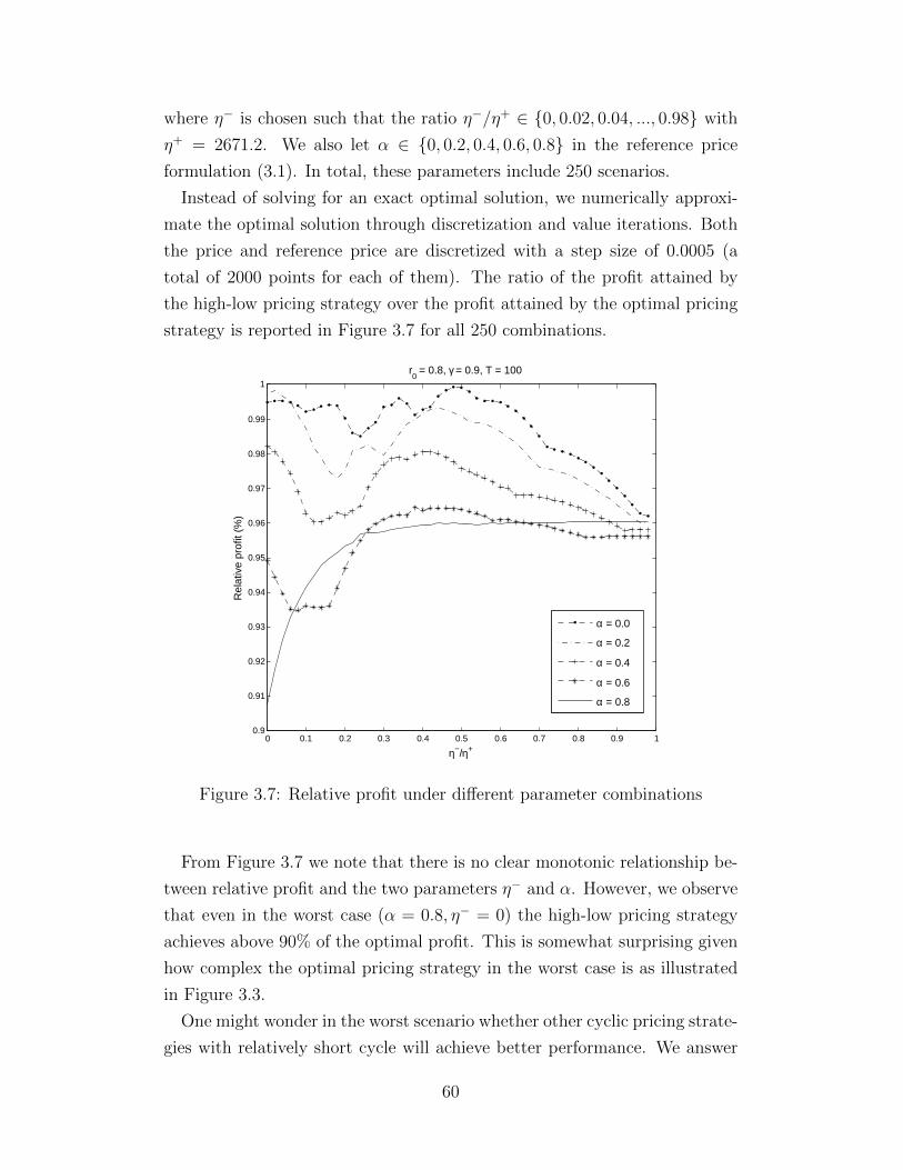
where η− is chosen such that the ratio η−/η+ ∈ {0, 0.02, 0.04, ..., 0.98} with

η+ = 2671.2. We also let α ∈ {0, 0.2, 0.4, 0.6, 0.8} in the reference price

formulation (3.1). In total, these parameters include 250 scenarios.

Instead of solving for an exact optimal solution, we numerically approxi-

mate the optimal solution through discretization and value iterations. Both

the price and reference price are discretized with a step size of 0.0005 (a

total of 2000 points for each of them). The ratio of the profit attained by

the high-low pricing strategy over the profit attained by the optimal pricing

strategy is reported in Figure 3.7 for all 250 combinations.

0 0.1 0.2 0.3 0.4 0.5 0.6 0.7 0.8 0.9 10.9

0.91

0.92

0.93

0.94

0.95

0.96

0.97

0.98

0.99

1

r0 = 0.8, γ = 0.9, T = 100

η−/η+

Rel

ativ

e pr

ofit

(%)

α = 0.0

α = 0.2

α = 0.4

α = 0.6

α = 0.8

Figure 3.7: Relative profit under different parameter combinations

From Figure 3.7 we note that there is no clear monotonic relationship be-

tween relative profit and the two parameters η− and α. However, we observe

that even in the worst case (α = 0.8, η− = 0) the high-low pricing strategy

achieves above 90% of the optimal profit. This is somewhat surprising given

how complex the optimal pricing strategy in the worst case is as illustrated

in Figure 3.3.

One might wonder in the worst scenario whether other cyclic pricing strate-

gies with relatively short cycle will achieve better performance. We answer

60

this question in Table 3.2.

Table 3.2: Performance of Cyclic Pricing Strategies

Cycle Length 1 2 3 4 5Relative Profit 89.87% 90.74% 96.76% 98.34% 98.30%

Note that for this particular parameter configuration, even the constant

pricing strategy (cycle length is 1) can have a decent performance and a

cyclic pricing strategies with cycle length of 3 or 4 can already achieve more

than 95% of the optimal profit. Another interesting fact is that increasing

the length of cycle, though complicating the optimization process, does not

necessarily result in a better performance as indicated in the last two columns

in Table 3.2. This is because, when the optimal pricing strategy is of cycle

length 2, for instance, imposing a constraint that cycle length equals to 3 or

any odd numbers will only make the resulting cyclic pricing strategies more

different from the optimal.

Finally, we check to what extent Proposition 3.4 will still hold if the as-

sumption η− = 0 is relaxed. For this purpose, we fix α = 0 and vary η−

such that the ratio η−/η+ ∈ {0, 0.02, 0.04, ..., 0.98}. When η−/η+ < 0.16, it

is found that high-low pricing strategy is always optimal and the dynamics

proposed in Proposition 3.4 holds true. For conciseness, in Figure 3.8, we on-

ly report the results for the values η−/η+ ∈ {0.16, 0.18, 0.20, 0.22, 0.24, 0.26}.When η−/η+ = 0.16, 0.18, similar to the cases for η−/η+ < 0.16, there is only

one discontinuous point in the optimal pricing strategies and the high-low

pricing strategy is optimal. For η−/η+ = 0.20, 0.22, 0.24, there are multiple

discontinuous points appearing in the optimal pricing strategies, however, the

periodic orbits in these figures indicate that a cyclic skimming pricing strate-

gy with cycle length 3 is still optimal. That is, the conclusion of Proposition

3.4 still holds for η−/η+ ≤ 0.24. However, the last figure shows that anoth-

er 2% increment in the ratio will result in a very different optimal pricing

strategy.

3.6 Conclusion

In this chapter we analyzed a dynamic pricing problem in a market with

gain-seeking consumers. In this model, demand depends on both current

61

0 0.5 10

0.2

0.4

0.6

0.8

1

rt

r t+1

η− = 427.3984

p*(rt)

rt+1 = rt

0 0.5 10

0.2

0.4

0.6

0.8

1

rt

r t+1

η− = 480.8232

p*(rt)

rt+1 = rt

0 0.5 10

0.2

0.4

0.6

0.8

1

rtr t+

1

η− = 534.248

p*(rt)

rt+1 = rt

0 0.5 10

0.2

0.4

0.6

0.8

1

rt

r t+1

η− = 587.6728

p*(rt)

rt+1 = rt

0 0.5 10

0.2

0.4

0.6

0.8

1

rt

r t+1

η− = 641.0976

p*(rt)

rt+1 = rt

0 0.5 10

0.2

0.4

0.6

0.8

1

rt

r t+1

η− = 694.5224

p*(rt)

rt+1 = rt

Figure 3.8: The optimal pricing strategies when α = 0 andη−/η+ ∈ {0.16, 0.18, 0.20, 0.22, 0.24, 0.26}

62

selling price and reference price, where the latter evolves according to an

exponentially smoothing process of past prices.

We showed that even employing the myopic pricing strategy can result in

a very complicated dynamics of reference prices. We identified conditions

that lead to simple pricing dynamics, for example, high-low pricing, cyclic

skimming pricing or cyclic penetrating pricing.

Realizing the complexity of the problem, we restricted ourselves to an em-

pirically validated special case and proved that a cyclic skimming pricing

strategy is optimal over an infinite horizon. We further provided condition-

s on the upper bound of the cycle lengths. Although our characterization

of the optimal pricing strategy built on a piece-wise linear demand model,

both Proposition 3.3 and Proposition 3.4 can be extended to general nonlin-

ear demand functions proposed in Popescu and Wu (2007) by imposing an

assumption similar to Assumption 3.1.

Our work is only a start in exploring the effects of gain-seeking behav-

ior/phenomenon on dynamic pricing problems. It would be very interesting

to both categorize and characterize the possible patterns of the optimal pric-

ing strategy under the general case. As one may see from our analysis of the

special case, the structure of the optimal solution has intimate connections

with the dynamics of the optimal solution. Thus, it is important to under-

stand how the structure and the dynamics of the optimal solution interact

with each other under more general settings.

Finally, it would be interesting to study the impact of gain-seeking ref-

erence price effects on the joint pricing and inventory decisions. Pricing

and inventory integration has received much attentions in the past few years

(see, for example, Chen and Simchi-Levi, 2004a,b, 2006, 2012). Recently,

Chen et al. (2013) incorporated reference price effect into coordinated pric-

ing and inventory models. However, their model focuses only on loss-averse

consumers.

63

Chapter 4

Efficient Algorithms for Dynamic PricingProblem

4.1 Introduction

Part of Chapter 2, Chapter 3 and many of the references therein are devoted

to understanding the qualitative behavior of the optimal pricing strategies

when the firm faces reference price dependent demand and many manageri-

al insights are obtained. However, to our best knowledge, how to compute

the optimal prices accurately and efficiently remains largely unexplored. As

Fibich et al. (2003) point out, “calculations of optimal strategies were limit-

ed to numerical simulations using dynamic programming”. In practice, the

revenue of many firms in retail industry, where a large portion of empirical

evidences on reference price effects are found, can exceed $30 billion per year

(see Talluri and Van Ryzin, 2005). This fact highlights the importance of

even small incremental gains from revenue management. Thus, computing

the optimal prices accurately becomes a critical question. On the other hand,

a firm not only needs to coordinate pricing decisions with other operations

management decisions such as inventory decisions but also makes all those

decisions for over thousands of products. When the more realistic reference

price models are incorporated in such decision support systems, the efficiency

of computing the simplest basic model becomes crucial.

In this chapter, we look into the computational issue of the dynamic pric-

ing problem under the exponential smoothing reference price model. In this

model, a firm sells a product over a finite time horizon and faces possibly

time-varying demands, which depend on not only the price the firm sets in

that period but also all the historical prices the firm set through reference

price effects. Like most of the previous literature, the demand in each pe-

riod is assumed to be deterministic. This assumption is plausible in many

practical settings, in which a firm can predict future demands quite accurate-

64

ly from historical sales data. As we have discussed in Chapter 3, a unique

feature and also a significant challenge in this model is the asymmetry in

reference price effects, i.e., consumers’ perception of gains and losses could

be different. This leads to a non-smooth optimization problem, for which no

standard optimization methods can be applied.

Hu (2012) attempts to address the computational issue in the dynamic

pricing problem with reference price effects in a deterministic joint inventory

and pricing model, which includes the problem analyzed in this chapter as a

subproblem. However, one of the central algorithm in Hu (2012) ignores the

fact that the value function may be non-differentiable, which can cause the

running time of algorithm presented in Hu (2012) to be exponential in the

problem horizon. Indeed, it is still an open question that even for the loss-

averse demands whether the dynamic pricing problem can be solved exactly

in polynomial time or not.

Facing with such challenges, in this chapter we follow the idea in Hu (2012)

to develop an algorithm which we prove to be a polynomial time algorithm

for the loss-averse demands under a certain mild technical condition on the

input parameters. Although our model assumes piecewise linear demand

function, the core part of the algorithm may also be used to other forms

of demand function. In addition to the algorithm itself, a few properties

we found along with the algorithm are potentially applicable to other non-

smooth optimization problems as well. We refer the readers to Hu (2012) for

another polynomial time algorithm that solves a special case of the problem

when demands are gain-seeking and for a heuristic that can be used for any

input parameters. We apply the algorithm in this chapter along with that

developed in Hu (2012) to a practical problem from industry with real data

and demonstrate the efficiency and robustness of the algorithm.

Aside from the stream of literature on dynamic pricing problems with ref-

erence price effects, there are a few recent attempts that incorporate reference

price effects into integrated inventory and pricing models. Gimpl-Heersink

(2008) analyzes a stochastic periodic review finite horizon model in which

demand is a function of both the current price and the reference price with

additive random noise. Chen et al. (2013) study a similar model and intro-

duce a novel transformation technique to convert a non-concave single-period

revenue function to a modified revenue function that is concave. They charac-

terize various structures of optimal solutions. Based on a different mechanism

65

rather than the reference price models, Ahn et al. (2007) develop algorithm-

s for a periodic review finite horizon deterministic model in which demand

depends on past prices. Even though the concentration of this chapter is on

developing algorithms for the pure pricing problem, our algorithms can serve

as a building block in a deterministic joint inventory and pricing problem.

The remainder of this chapter is organized as follows. In Section 4.2 the

mathematical formulation of our model is presented. In Section 4.3, we ana-

lyze the model with loss-averse consumers and develop a strongly polynomial

time algorithm to solve the optimal prices exactly. Our algorithm along with

the algorithms in Hu (2012) are tested on real data in Section 4.4 to solve

a practical industry problem with analysis on the efficiency as well as the

robustness of the algorithms. Finally, we conclude the chapter in the last

section with some suggestions for future research. To maintain a clear pre-

sentation, all technical proofs are presented in Appendix C.

4.2 Model

We assume that the firm sells a product over a finite horizon of T periods.

As in Chapter 3, we restrict ourselves to the exponential smoothing model,

i.e.,

rt+1 = αrt + (1− α)pt, t = 1, 2, · · · , T, (4.1)

where we restrict α < 1 to avoid the case that past prices have no impact on

demand.

Following Chapter 2 and Chapter 3, the demand at period t, with a given

price p and a reference price r, is modeled as

Dt(p, r) = bt − atp+ η+ max{r − p, 0}+ η−min{r − p, 0},

where Dt(p, p) = bt−atp is the base demand independent of reference prices,

η(r − p) is the additional demand or demand loss induced by the reference

price effect. Here, the potential market size bt and the price sensitivity at

are non-negative, but unlike previous chapters, they are allowed to be time-

varying to reflect a dynamic market conditions. In this chapter, we consider

both loss-averse (loss/gain neutral) case and gain-seeking case and make

no assumption on the relative magnitudes of η+, η−. However, since these

66

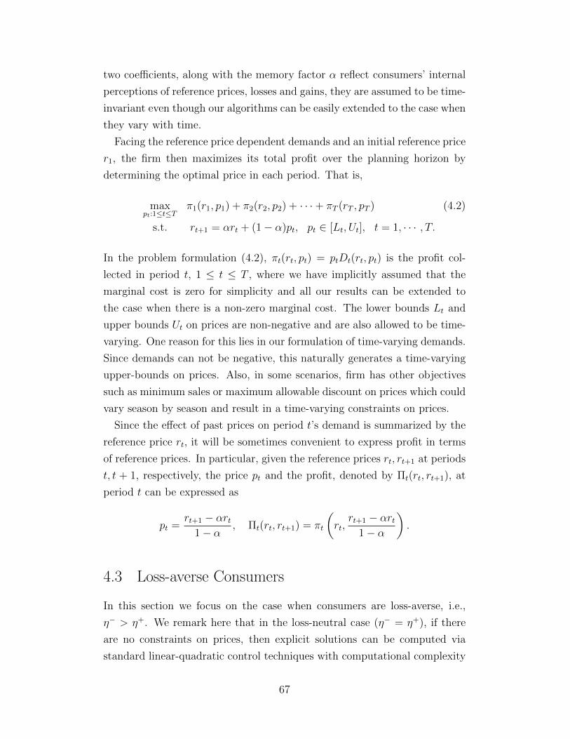
two coefficients, along with the memory factor α reflect consumers’ internal

perceptions of reference prices, losses and gains, they are assumed to be time-

invariant even though our algorithms can be easily extended to the case when

they vary with time.

Facing the reference price dependent demands and an initial reference price

r1, the firm then maximizes its total profit over the planning horizon by

determining the optimal price in each period. That is,

maxpt:1≤t≤T

π1(r1, p1) + π2(r2, p2) + · · ·+ πT (rT , pT ) (4.2)

s.t. rt+1 = αrt + (1− α)pt, pt ∈ [Lt, Ut], t = 1, · · · , T.

In the problem formulation (4.2), πt(rt, pt) = ptDt(rt, pt) is the profit col-

lected in period t, 1 ≤ t ≤ T , where we have implicitly assumed that the

marginal cost is zero for simplicity and all our results can be extended to

the case when there is a non-zero marginal cost. The lower bounds Lt and

upper bounds Ut on prices are non-negative and are also allowed to be time-

varying. One reason for this lies in our formulation of time-varying demands.

Since demands can not be negative, this naturally generates a time-varying

upper-bounds on prices. Also, in some scenarios, firm has other objectives

such as minimum sales or maximum allowable discount on prices which could

vary season by season and result in a time-varying constraints on prices.

Since the effect of past prices on period t’s demand is summarized by the

reference price rt, it will be sometimes convenient to express profit in terms

of reference prices. In particular, given the reference prices rt, rt+1 at periods

t, t + 1, respectively, the price pt and the profit, denoted by Πt(rt, rt+1), at

period t can be expressed as

pt =rt+1 − αrt

1− α, Πt(rt, rt+1) = πt

(rt,

rt+1 − αrt1− α

).

4.3 Loss-averse Consumers

In this section we focus on the case when consumers are loss-averse, i.e.,

η− > η+. We remark here that in the loss-neutral case (η− = η+), if there

are no constraints on prices, then explicit solutions can be computed via

standard linear-quadratic control techniques with computational complexity

67

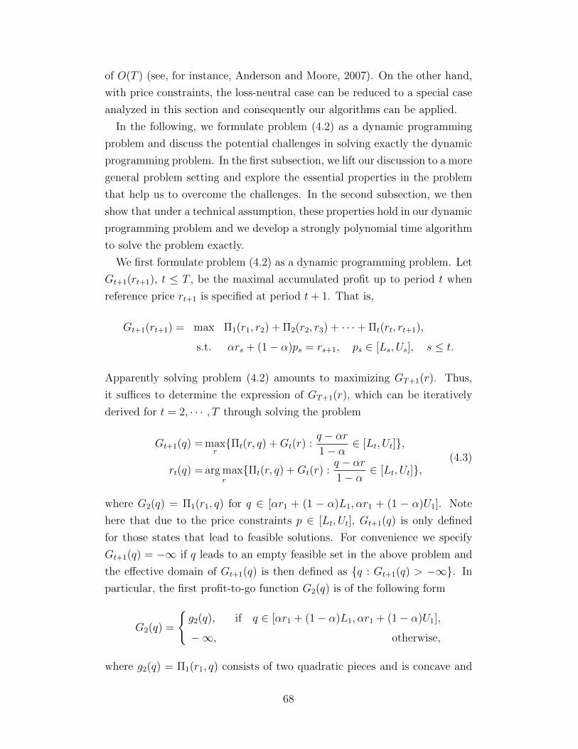
of O(T ) (see, for instance, Anderson and Moore, 2007). On the other hand,

with price constraints, the loss-neutral case can be reduced to a special case

analyzed in this section and consequently our algorithms can be applied.

In the following, we formulate problem (4.2) as a dynamic programming

problem and discuss the potential challenges in solving exactly the dynamic

programming problem. In the first subsection, we lift our discussion to a more

general problem setting and explore the essential properties in the problem

that help us to overcome the challenges. In the second subsection, we then

show that under a technical assumption, these properties hold in our dynamic

programming problem and we develop a strongly polynomial time algorithm

to solve the problem exactly.

We first formulate problem (4.2) as a dynamic programming problem. Let

Gt+1(rt+1), t ≤ T , be the maximal accumulated profit up to period t when

reference price rt+1 is specified at period t+ 1. That is,

Gt+1(rt+1) = max Π1(r1, r2) + Π2(r2, r3) + · · ·+ Πt(rt, rt+1),

s.t. αrs + (1− α)ps = rs+1, ps ∈ [Ls, Us], s ≤ t.

Apparently solving problem (4.2) amounts to maximizing GT+1(r). Thus,

it suffices to determine the expression of GT+1(r), which can be iteratively

derived for t = 2, · · · , T through solving the problem

Gt+1(q) = maxr{Πt(r, q) +Gt(r) :

q − αr1− α

∈ [Lt, Ut]},

rt(q) = arg maxr{Πt(r, q) +Gt(r) :

q − αr1− α

∈ [Lt, Ut]},(4.3)

where G2(q) = Π1(r1, q) for q ∈ [αr1 + (1 − α)L1, αr1 + (1 − α)U1]. Note

here that due to the price constraints p ∈ [Lt, Ut], Gt+1(q) is only defined

for those states that lead to feasible solutions. For convenience we specify

Gt+1(q) = −∞ if q leads to an empty feasible set in the above problem and

the effective domain of Gt+1(q) is then defined as {q : Gt+1(q) > −∞}. In

particular, the first profit-to-go function G2(q) is of the following form

G2(q) =

{g2(q), if q ∈ [αr1 + (1− α)L1, αr1 + (1− α)U1],

−∞, otherwise,

where g2(q) = Π1(r1, q) consists of two quadratic pieces and is concave and

68

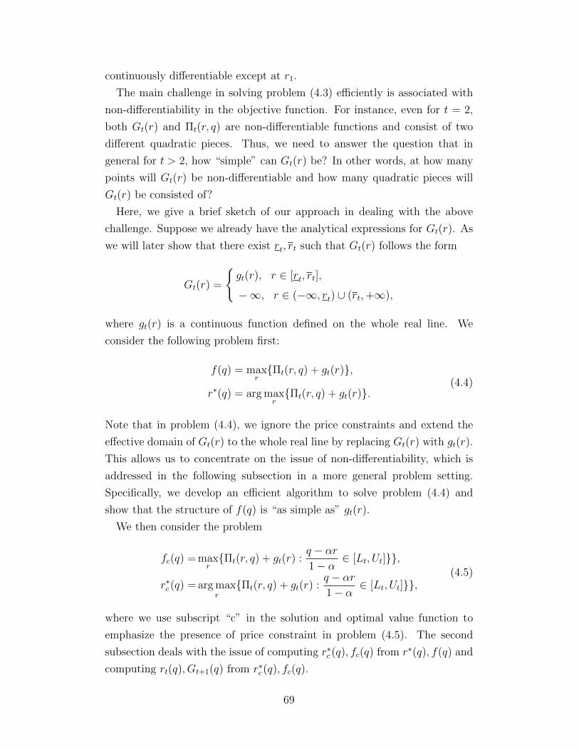
continuously differentiable except at r1.

The main challenge in solving problem (4.3) efficiently is associated with

non-differentiability in the objective function. For instance, even for t = 2,

both Gt(r) and Πt(r, q) are non-differentiable functions and consist of two

different quadratic pieces. Thus, we need to answer the question that in

general for t > 2, how “simple” can Gt(r) be? In other words, at how many

points will Gt(r) be non-differentiable and how many quadratic pieces will

Gt(r) be consisted of?

Here, we give a brief sketch of our approach in dealing with the above

challenge. Suppose we already have the analytical expressions for Gt(r). As

we will later show that there exist rt, rt such that Gt(r) follows the form

Gt(r) =

{gt(r), r ∈ [rt, rt],

−∞, r ∈ (−∞, rt) ∪ (rt,+∞),

where gt(r) is a continuous function defined on the whole real line. We

consider the following problem first:

f(q) = maxr{Πt(r, q) + gt(r)},

r∗(q) = arg maxr{Πt(r, q) + gt(r)}.

(4.4)

Note that in problem (4.4), we ignore the price constraints and extend the

effective domain of Gt(r) to the whole real line by replacing Gt(r) with gt(r).

This allows us to concentrate on the issue of non-differentiability, which is

addressed in the following subsection in a more general problem setting.

Specifically, we develop an efficient algorithm to solve problem (4.4) and

show that the structure of f(q) is “as simple as” gt(r).

We then consider the problem

fc(q) = maxr{Πt(r, q) + gt(r) :

q − αr1− α

∈ [Lt, Ut]}},

r∗c (q) = arg maxr{Πt(r, q) + gt(r) :

q − αr1− α

∈ [Lt, Ut]}},(4.5)

where we use subscript “c” in the solution and optimal value function to

emphasize the presence of price constraint in problem (4.5). The second

subsection deals with the issue of computing r∗c (q), fc(q) from r∗(q), f(q) and

computing rt(q), Gt+1(q) from r∗c (q), fc(q).

69

4.3.1 A General Problem

The purpose of this subsection is two fold. First, we believe the presentation

of the algorithm can be made clean and organized by highlighting only those

properties that are essential for our algorithm. Second, the treatment in a

more general setting naturally makes our algorithm robust to other forms

of demand function. Furthermore, some of the properties we identified are

potentially applicable to other problems as well. The following problem,

which is a generalization of problem (4.4), is considered in this subsection.

f(q) = maxr{Π(r, q) + g(r)},

r∗(q) = arg maxr{Π(r, q) + g(r)}.

(4.6)

We impose the following two assumptions on both the input functions

Π(r, q) and g(r) as well as the output functions f(q) and r∗(q) throughout

this subsection.

Assumption 4.1. (a) Π(r, q) : R2 → R is continuous, strictly supermodular

in (r, q) and strictly concave in r. Furthermore, Π(r, q) has the form

Π(r, q) =

{Π+(r, q), q ≤ r,

Π−(r, q), q ≥ r,

where Π+(r, q) and Π−(r, q) are continuously differentiable functions defined

on R2. We denote π(q) = Π(q, q) = Π+(q, q) = Π−(q, q).

(b) g(r) : R→ R is concave and continuously differentiable except at finite

points r1, ..., rm, with −∞ = r0 < r1 < ... < rm < rm+1 = +∞. More

specifically,

g(r) =

g1(r), r0 ≤ r ≤ r1,

...

gm+1(r), rm ≤ r ≤ rm+1,

where gj(·), 1 ≤ j ≤ m+1 are all continuously differentiable functions defined

on R. We call r1, ..., rm the kink points of g(r).

An immediate consequence from the strict concavity and continuity as-

sumptions in Assumption 4.1 is that r∗(q) is single valued and continuous

(see, for example, Ok, 2007). We further impose the following assumptions

70

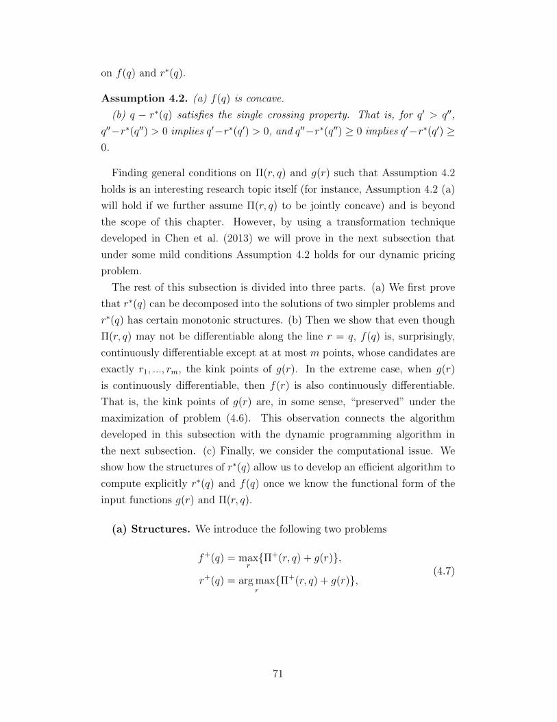
on f(q) and r∗(q).

Assumption 4.2. (a) f(q) is concave.

(b) q − r∗(q) satisfies the single crossing property. That is, for q′ > q′′,

q′′−r∗(q′′) > 0 implies q′−r∗(q′) > 0, and q′′−r∗(q′′) ≥ 0 implies q′−r∗(q′) ≥0.

Finding general conditions on Π(r, q) and g(r) such that Assumption 4.2

holds is an interesting research topic itself (for instance, Assumption 4.2 (a)

will hold if we further assume Π(r, q) to be jointly concave) and is beyond

the scope of this chapter. However, by using a transformation technique

developed in Chen et al. (2013) we will prove in the next subsection that

under some mild conditions Assumption 4.2 holds for our dynamic pricing

problem.

The rest of this subsection is divided into three parts. (a) We first prove

that r∗(q) can be decomposed into the solutions of two simpler problems and

r∗(q) has certain monotonic structures. (b) Then we show that even though

Π(r, q) may not be differentiable along the line r = q, f(q) is, surprisingly,

continuously differentiable except at at most m points, whose candidates are

exactly r1, ..., rm, the kink points of g(r). In the extreme case, when g(r)

is continuously differentiable, then f(r) is also continuously differentiable.

That is, the kink points of g(r) are, in some sense, “preserved” under the

maximization of problem (4.6). This observation connects the algorithm

developed in this subsection with the dynamic programming algorithm in

the next subsection. (c) Finally, we consider the computational issue. We

show how the structures of r∗(q) allow us to develop an efficient algorithm to

compute explicitly r∗(q) and f(q) once we know the functional form of the

input functions g(r) and Π(r, q).

(a) Structures. We introduce the following two problems

f+(q) = maxr{Π+(r, q) + g(r)},

r+(q) = arg maxr{Π+(r, q) + g(r)},

(4.7)

71

and

f−(q) = maxr{Π−(r, q) + g(r)},

r−(q) = arg maxr{Π−(r, q) + g(r)}.

(4.8)

Our first result states that r∗(q) can be decomposed into r+(q), r−(q) in the

following way.

Proposition 4.1. There exist Q ≤ Q, such that

r∗(q) =

r+(q), q < Q,

q, Q ≤ q ≤ Q,

r−(q), q > Q,

and f(q) =

f+(q), q < Q,

π(q) + g(q), Q ≤ q ≤ Q,

f−(q), q > Q.

Next, we closely examine the structure of r+(q) and r−(q).

Lemma 4.1. There exist −∞ = q0 < q1≤ q1 < q

2≤ q2 < ... < q

m≤ qm <

qm+1

= +∞ such that for 1 ≤ j ≤ m, r+(q) = rj on [qj, qj] and r+(q) is

strictly increasing elsewhere.

Lemma 4.1 also holds for r−(q). That is, for 1 ≤ j ≤ m, r−(q) = rj

on [qj, qj] and r−(q) is strictly increasing elsewhere. However, the threshold

values qj

and qj may be different from that for r+(q). Now combining this

observation and Proposition 4.1 we arrive at the following result. With a

slight abuse of notations, we still use qj

and qj to denote the new threshold

values.

Proposition 4.2. There exist −∞ = q0 < q1≤ q1 < q

2≤ q2 < ... < q

m≤

qm < qm+1

= +∞ such that for 1 ≤ j ≤ m, r∗(q) = rj on [qj, qj] and r∗(q)

is strictly increasing elsewhere.

Graphically, as illustrated in Figure 4.1, Proposition 4.2 suggests a ladder

shape of r∗(q). That is, r∗(q) alternates between a strictly increasing piece

and a constant piece with the constant piece corresponding to a kink point of

g(·). Clearly, if we can compute the threshold values and determine the ex-

pressions of the strictly increasing pieces of r∗(q), then the whole expressions

of r∗(q) can be obtained easily. We will address how to determine qj−1 and

qj

as well as compute r∗(q) on (qj−1, qj) in the third part of this subsection.

72

0 0.5 1 1.5 2 2.5 3 3.5 40

0.5

1

1.5

2

2.5

3

3.5

4

q

r∗

(q)

q =Q

r∗(q) = r−(q)

r∗(q) = r+(q)

q = Qq =

q = qL

q

r1

r2

r∗(q) = q

r3

r4

Figure 4.1: Illustration of r∗(q)

(b) Preservation. Now we turn our attention to the optimal value func-

tion f(q). Despite the fact that Π(r, q) may be neither differentiable in r nor

in q, we show that the number of kink points of f(q) are less than or equal

to g(r) and the candidate kink points of f(q) are exactly r1, ..., rm. That is,

f(q) has certain similar properties as g(r), which is desirable in a dynamic

optimization setting.

The preservation of kink points relies critically on the following observa-

tion.

Lemma 4.2. f+(q) is continuously differentiable on (−∞, Q) and f−(q) is

continuously differentiable on (Q,+∞).

We would like to point out that the only assumptions required for Lemma

4.2 to hold (or even extend to the whole domain of q) are the concavity of

f+(q) and f−(q) and the continuous differentiability of Π±(r, q) with respect

to q.

An immediate consequence of Lemma 4.2 is that f(q) is also continuously

differentiable on (−∞, Q) and (Q,+∞). On the other hand, f(q) = π(q) +

g(q), when q ∈ (Q,Q) and the kink points of f(q) are then solely determined

by the kink points of g(q). The following result further claims that f(q) is

differentiable at Q and Q unless Q,Q ∈ {r1, ..., rm}.

73

Proposition 4.3. f(q) has at most m kink points. The possible kink points

are r1, ..., rm.

In the extreme case when m = 0, then f(q) is continuously differentiable

even if the objective function is neither differentiable in the decision vari-

able r nor in the parameter q. In contrast, many envelope theorems that

study the differentiability properties of the value function of a parameterized

optimization problem (see, for example, Milgrom and Segal, 2002; Clausen

and Strub, 2012) assume the objective function to be differentiable in the

parameter.

(c) Computation. To address the issue of computation, we need to

impose the following assumption in the remaining of this subsection on the

functional forms of each continuously differentiable piece of g(r).

Assumption 4.3. For 1 ≤ j ≤ m + 1, gj(r) has the following functional

form on [rj−1, rj]. There exist nj ≥ 1 and rj−1 = r(0)j < r

(1)j < ... < r

(nj−1)j <

r(nj)j = rj such that

gj(r) =

g

(1)j (r), r

(0)j ≤ r ≤ r

(1)j ,

...

g(nj)j (r), r

(nj−1)j ≤ r ≤ r

(nj)j ,

where g(i)j (r), 1 ≤ i ≤ nj, are functions defined on R and have analytical

forms such that the following optimization problems

maxr{Π±(r, q) + g

(i)j (r)},

can be solved in O(1) time.

One example satisfying Assumption 4.3 is the case when Π±(r, q) and

g(i)j (r) are all quadratic functions. For convenience, for 1 ≤ j ≤ m + 1,

we call r(i)j , 1 ≤ i ≤ nj (except r

(nm+1)m+1 = rm+1 = +∞) the breakpoints of g(r)

and denote n =∑m+1

j=1 nj − 1 to be the total number of breakpoints of g(·).Note that the breakpoints include the kink points we defined in Assumption

4.1. The key difference here is that at a breakpoint, the analytical forms

of the function on the two sides of the breakpoint are different. However,

different analytical forms may still result in the left derivative at the break-

74

point having the same value as the right derivative. When the left derivative

does not equal to the right derivative at the breakpoint, we then call this

breakpoint as a kink point.

By Proposition 4.2, on (qj−1, qj), r∗(q) is strictly increasing and rj−1 <

r∗(q) < rj. As a result, there exist qj−1 = q(0)j < q

(1)j < ... < q

(nj−1)j < q

(nj)j =

qj, such that for 1 ≤ i ≤ m, on (q

(i−1)j , q

(i)j ), r

(i−1)j < r∗(q) < r

(i)j . This

suggests that on (q(i−1)j , q

(i)j ),

f(q) = maxr{Π(r, q) + g

(i)j (r)},

r∗(q) = arg maxr{Π(r, q) + g

(i)j (r)}.

Note that this observation also applies to r+(q) and r−(q) on the regions

where they are strictly increasing. Applying Proposition 4.1, by comparing q

with the threshold valuesQ,Q, whether Π(r, q) = Π+(r, q), Π(r, q) = Π−(r, q)

or r∗(q) = q can be determined unambiguously in the above problem. This

leads to the following result to bound the breakpoints of f(q).

Proposition 4.4. f(q) has at most n+m+2 breakpoints. The candidates for

the breakpoints are q(i)j , 1 ≤ j ≤ m + 1, 0 ≤ i ≤ nj (except q

(0)1 = q0 = −∞

and q(nm+1)m+1 = q

m+1= +∞) and Q,Q.

In actual computation, however, the breakpoints are not known before

hand. Algorithm 1 provides a way to both compute the breakpoints and de-

termine the analytical form of the function between the breakpoints. To see

the computational complexity, first note that by Assumption 4.3, the opti-

mization problem inside the loops only needs O(1) time to solve. Consequent-

ly, the expressions for r±(q) can be determined in O(∑m+1

j=1 nj) + O(m) =

O(n + m) time. Finding Q, Q clearly depends on the number of analytical

pieces of r±(q) and takes O(n+m) time. Finally, by Proposition 4.4 there are

at most n+m+ 2 breakpoints, r∗(q) and f(q) can be computed in O(n+m)

time. In summary, the overall computational complexity is O(n+m).

4.3.2 Dynamic Programming Algorithm

In this subsection, we verify that Assumptions 4.1-4.3 hold in our dynamic

pricing problem and we show how to utilize Algorithm 1 as a subroutine in

our dynamic programming algorithm.

75

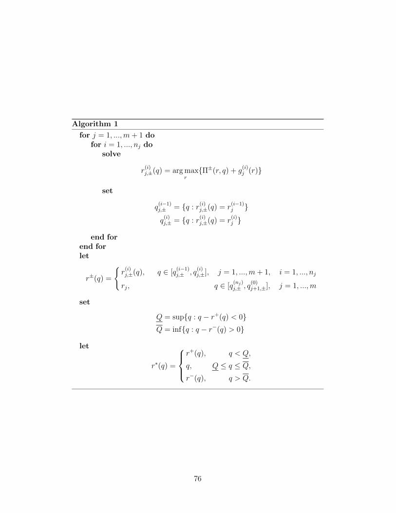
Algorithm 1

for j = 1, ...,m+ 1 dofor i = 1, ..., nj do

solve

r(i)j,±(q) = arg max

r{Π±(r, q) + g

(i)j (r)}

set

q(i−1)j,± = {q : r

(i)j,±(q) = r

(i−1)j }

q(i)j,± = {q : r

(i)j,±(q) = r

(i)j }

end forend forlet

r±(q) =

{r

(i)j,±(q), q ∈ [q

(i−1)j,± , q

(i)j,±], j = 1, ...,m+ 1, i = 1, ..., nj

rj, q ∈ [q(nj)j,± , q

(0)j+1,±], j = 1, ...,m

set

Q = sup{q : q − r+(q) < 0}Q = inf{q : q − r−(q) > 0}

let

r∗(q) =

r+(q), q < Q,

q, Q ≤ q ≤ Q,

r−(q), q > Q.

76

To verify Assumption 4.2, we need the following technical condition on the

problem parameters.

Assumption 4.4.

η− − η+ ≤ 2at − 2αat+1, ∀ 1 ≤ t ≤ T − 1.

Assumption 4.4 holds under the plausible setting when consumers have

short memories (α is small) and the direct price effect dominates the reference

price effect (η+ < η− ≤ at). We will impose Assumption 4.4 throughout this

subsection. However, one should keep in mind that Assumption 4.4 is merely

a sufficient condition to guarantee that Assumption 4.2 holds. As we will

show in Section 4.4 that Assumption 4.2 can be verified in an on-line fashion

as the algorithm implements and may still hold even if Assumption 4.4 fails.

Even though the per-period profit function Πt(r, q) is not jointly concave

in r and q, the following proposition shows iteratively that under Assumption

4.4, the function Gt is strongly concave.

Proposition 4.5. Suppose Assumption 4.4 holds. Then for 2 ≤ t ≤ T + 1,

Gt is strongly concave with concavity constant At = 2αat+η−

2(1−α). That is, Gt(r) =

Gt(r) +Atr2 is also a concave function. Furthermore, there exist rt, rt, such

that Gt(r) follows the form

Gt(r) =

{gt(r), r ∈ [rt, rt],

−∞, r ∈ (−∞, rt) ∪ (rt,+∞),

where gt(r) a continuous function defined on the whole real line.

Before verifying Assumptions 4.1-4.3, we show how one can solve problem

(4.3) from the solutions to problem (4.4). The following lemma helps us

in establishing the connections among problems (4.3), (4.4) and (4.5). Let

p∗c(q) = q−αr∗c (q)1−α .

Lemma 4.3. The solution to problem (4.5): r∗c (q) is single-valued and con-

tinuous in q. Furthermore, both r∗c (q) and p∗c(q) are monotonically increasing

in q.

Now we construct the solutions to problem (4.3) from the solutions to

problem (4.4) in the following two steps.

77

From r∗(q) to r∗c (q): By monotonicity of p∗c(q), when α > 0, we know

there exist qL, qU , qL < qU such that for q < qL, p∗c(q) = Lt and

r∗c (q) = q−(1−α)Lt

α, for qU < q, p∗c(q) = Ut and r∗c (q) = q−(1−α)Ut

α, while

for qL < q < qU , Lt < p∗c(q) < Ut. When α = 0, we can set qL = −∞and qU = +∞. It follows that

r∗c (q) =

q − (1− α)Lt

α, q ∈ (−∞, qL),

r∗(q), q ∈ [qL, qU ],

q − (1− α)Utα

, q ∈ (qU ,+∞),

(4.9)

and

fc(q) =

Πt(

q − (1− α)Ltα

, q) + gt(q − (1− α)Lt

α), q ∈ (−∞, qL),

f(q), q ∈ [qL, qU ],

Πt(q − (1− α)Ut

α, q) + gt(

q − (1− α)Utα

), q ∈ (qU ,+∞).

(4.10)

Finally, when α > 0, qL and qU can be computed through qL = sup{q :

r∗(q) > q−(1−α)Lt

α} and qU = inf{q : r∗(q) < q−(1−α)Ut

α}.

From r∗c (q) to rt(q) : First, note that when α > 0, the price constraint is e-

quivalent to r ∈ [ q−(1−α)Ut

α, q−(1−α)Lt

α]. If [ q−(1−α)Ut

α, q−(1−α)Lt

α]∩ [rt, rt] =

∅, then Gt+1(q) = −∞. That is, the effective domain for Gt+1(q) is

[αrt + (1 − α)Lt, αrt + (1 − α)Ut]. When α = 0, clearly, the effective

domain for Gt+1(q) is simply [Lt, Ut].

Let us restrict our attention to the effective domain of Gt+1(q), i.e.,

q ∈ [αrt + (1− α)Lt, αrt + (1− α)Ut].

If rt ≤ r∗c (q) ≤ rt, then clearly rt(q) = r∗c (q).

If r∗c (q) < rt, since r∗c (q) ∈ [ q−(1−α)Ut

α, q−(1−α)Lt

α] (or (−∞,+∞) if α = 0)

and q is in the effective domain, we must have rt ∈ [ q−(1−α)Ut

α, q−(1−α)Lt

α]

(or (−∞,+∞) if α = 0) as well. Thus, rt is a feasible solution. From

Proposition 4.5, we know that the objective function in problem (4.3)

is concave and consequently we have rt(q) = rt. Similarly, if r∗c (q) > rt,

then rt(q) = rt.

Finally, let qr

= max{sup{q : r∗c (q) < rt}, αrt + (1 − α)Lt} and qr =

78

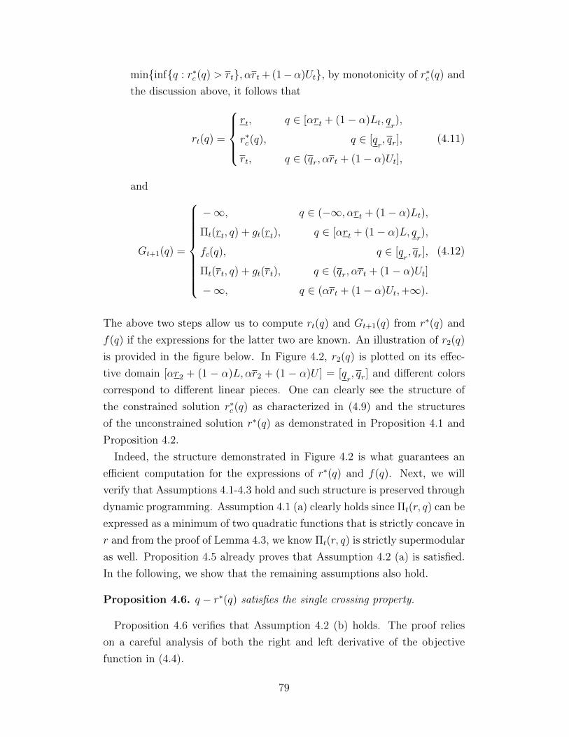
min{inf{q : r∗c (q) > rt}, αrt + (1−α)Ut}, by monotonicity of r∗c (q) and

the discussion above, it follows that

rt(q) =

rt, q ∈ [αrt + (1− α)Lt, qr),

r∗c (q), q ∈ [qr, qr],

rt, q ∈ (qr, αrt + (1− α)Ut],

(4.11)

and

Gt+1(q) =

−∞, q ∈ (−∞, αrt + (1− α)Lt),

Πt(rt, q) + gt(rt), q ∈ [αrt + (1− α)L, qr),

fc(q), q ∈ [qr, qr],

Πt(rt, q) + gt(rt), q ∈ (qr, αrt + (1− α)Ut]

−∞, q ∈ (αrt + (1− α)Ut,+∞).

(4.12)

The above two steps allow us to compute rt(q) and Gt+1(q) from r∗(q) and

f(q) if the expressions for the latter two are known. An illustration of r2(q)

is provided in the figure below. In Figure 4.2, r2(q) is plotted on its effec-

tive domain [αr2 + (1 − α)L, αr2 + (1 − α)U ] = [qr, qr] and different colors

correspond to different linear pieces. One can clearly see the structure of

the constrained solution r∗c (q) as characterized in (4.9) and the structures

of the unconstrained solution r∗(q) as demonstrated in Proposition 4.1 and

Proposition 4.2.

Indeed, the structure demonstrated in Figure 4.2 is what guarantees an

efficient computation for the expressions of r∗(q) and f(q). Next, we will

verify that Assumptions 4.1-4.3 hold and such structure is preserved through

dynamic programming. Assumption 4.1 (a) clearly holds since Πt(r, q) can be

expressed as a minimum of two quadratic functions that is strictly concave in

r and from the proof of Lemma 4.3, we know Πt(r, q) is strictly supermodular

as well. Proposition 4.5 already proves that Assumption 4.2 (a) is satisfied.

In the following, we show that the remaining assumptions also hold.

Proposition 4.6. q − r∗(q) satisfies the single crossing property.

Proposition 4.6 verifies that Assumption 4.2 (b) holds. The proof relies

on a careful analysis of both the right and left derivative of the objective

function in (4.4).

79

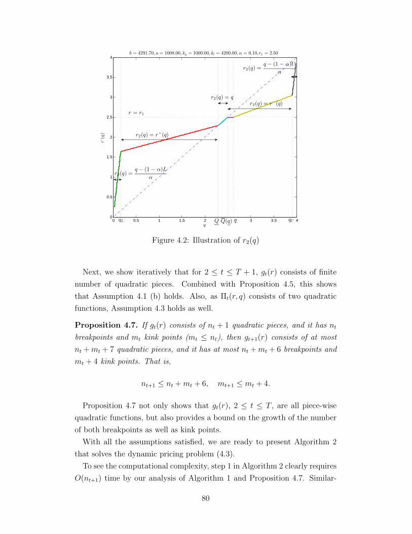
0 0.5 1 1.5 2 3 3.5 40

0.5

1

1.5

2

2.5

3

3.5

4b = 4291.70, a= 1008.00, kg = 1000.00, kl = 4200.00,α = 0.10,r1 = 2.50

q

r∗(q)

r = r1

r2(q) =q − (1 − α)U

α

r2(q) = qr2(q) = r−(q)

r2(q) = r+(q)

r2(q) =q − (1 − α)L

α

qL Q Q(q) q qU

Figure 4.2: Illustration of r2(q)

Next, we show iteratively that for 2 ≤ t ≤ T + 1, gt(r) consists of finite

number of quadratic pieces. Combined with Proposition 4.5, this shows

that Assumption 4.1 (b) holds. Also, as Πt(r, q) consists of two quadratic

functions, Assumption 4.3 holds as well.

Proposition 4.7. If gt(r) consists of nt + 1 quadratic pieces, and it has nt

breakpoints and mt kink points (mt ≤ nt), then gt+1(r) consists of at most

nt +mt + 7 quadratic pieces, and it has at most nt +mt + 6 breakpoints and

mt + 4 kink points. That is,

nt+1 ≤ nt +mt + 6, mt+1 ≤ mt + 4.

Proposition 4.7 not only shows that gt(r), 2 ≤ t ≤ T , are all piece-wise

quadratic functions, but also provides a bound on the growth of the number

of both breakpoints as well as kink points.

With all the assumptions satisfied, we are ready to present Algorithm 2

that solves the dynamic pricing problem (4.3).

To see the computational complexity, step 1 in Algorithm 2 clearly requires

O(nt+1) time by our analysis of Algorithm 1 and Proposition 4.7. Similar-

80

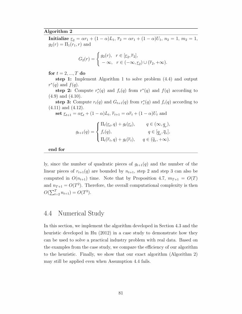
Algorithm 2

Initialize r2 = αr1 + (1 − α)L1, r2 = αr1 + (1 − α)U1, n2 = 1, m2 = 1,g2(r) = Π1(r1, r) and

G2(r) =

{g2(r), r ∈ [r2, r2],

−∞, r ∈ (−∞, r2) ∪ (r2,+∞).

for t = 2, ..., T dostep 1: Implement Algorithm 1 to solve problem (4.4) and output

r∗(q) and f(q).step 2: Compute r∗c (q) and fc(q) from r∗(q) and f(q) according to

(4.9) and (4.10).step 3: Compute rt(q) and Gt+1(q) from r∗c (q) and fc(q) according to

(4.11) and (4.12).set rt+1 = αrt + (1− α)Lt, rt+1 = αrt + (1− α)Ut and

gt+1(q) =

Πt(rt, q) + gt(rt), q ∈ (∞, q

r),

fc(q), q ∈ [qr, qr],

Πt(rt, q) + gt(rt), q ∈ (qr,+∞).

end for

ly, since the number of quadratic pieces of gt+1(q) and the number of the

linear pieces of rt+1(q) are bounded by nt+1, step 2 and step 3 can also be

computed in O(nt+1) time. Note that by Proposition 4.7, mT+1 = O(T )

and nT+1 = O(T 2). Therefore, the overall computational complexity is then

O(∑T

t=2 nt+1) = O(T 3).

4.4 Numerical Study

In this section, we implement the algorithm developed in Section 4.3 and the

heuristic developed in Hu (2012) in a case study to demonstrate how they

can be used to solve a practical industry problem with real data. Based on

the examples from the case study, we compare the efficiency of our algorithm

to the heuristic. Finally, we show that our exact algorithm (Algorithm 2)

may still be applied even when Assumption 4.4 fails.

81

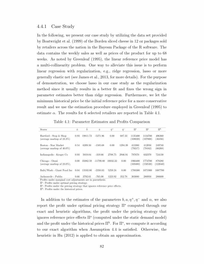
4.4.1 Case Study

In the following, we present our case study by utilizing the data set provided

by Boatwright et al. (1999) of the Borden sliced cheese in 12 oz packages sold

by retailers across the nation in the Bayesm Package of the R software. The

data contains the weekly sales as well as prices of the product for up to 68

weeks. As noted by Greenleaf (1995), the linear reference price model has

a multi-collinearity problem. One way to alleviate this issue is to perform

linear regression with regularization, e.g., ridge regression, lasso or more

generally elastic net (see James et al., 2013, for more details). For the purpose

of demonstration, we choose lasso in our case study as the regularization

method since it usually results in a better fit and fixes the wrong sign in

parameter estimates better than ridge regression. Furthermore, we let the

minimum historical price be the initial reference price for a more conservative

result and we use the estimation procedure employed in Greenleaf (1995) to

estimate α. The results for 6 selected retailers are reported in Table 4.1.

Table 4.1: Parameter Estimates and Profits Comparison

Stores α b a η+ η− Π∗ Πs Πh

Hartford - Stop & Shop 0.93 19811.72 -5271.96 0.00 687.33 1135400 1134700 496360(average markup of 23.3%) (108020) (107800) (46356)

Boston - Star Market 0.54 6209.50 -1585.68 0.00 1294.39 413380 412050 249740(average markup of 40.0%) (79217) (78162) (66268)

Indianapolis - Kroger Co 0.93 5019.04 -319.66 2708.75 2946.91 797670 632370 724130

Chicago - Omni 0.00 35082.59 -11799.80 10032.22 0.00 1966400 1774700 878280(average markup of 23.0%), (169480) (150530) (122640)

Balti/Wash - Giant Food Inc 0.04 13103.80 -2350.83 5259.24 0.00 1788300 1071900 1087700

Jacksonvile - Publix 0.66 3792.61 -765.08 1223.92 352.78 303880 280950 286600Profits under marginal cost adjustments are in parenthesis.Π∗: Profits under optimal pricing strategy.Πs: Profits under the pricing strategy that ignores reference price effects.Πh: Profits under the historical prices.

In addition to the estimates of the parameters b, a, η+, η− and α, we also

report the profit under optimal pricing strategy Π∗ computed through our

exact and heuristic algorithms, the profit under the pricing strategy that

ignores reference price effects Πs (computed under the static demand model)

and the profit under the historical prices Πh. For Π∗, we compute it according

to our exact algorithm when Assumption 4.4 is satisfied. Otherwise, the

heuristic in Hu (2012) is applied to obtain an approximation.

82

From Table 4.1, we can see that demands faced by different retailers can

have significantly different characteristics. The first three retailers face loss-

averse demands while the latter three face gain-seeking demands. Also notice

that the demands for the first and second retailers satisfy Assumption 4.4

while the demands for the fourth retailer satisfy Assumption 3.1.

By comparing the profits, we can see that retailers’ profits can be greatly

improved in many scenarios by using the reference price models rather than

the static demand models. Note that we are only presenting a basic frame-

work in this chapter and many other features such as competitors prices,

seasonal effects, marginal costs, etc., are not taken into consideration since

they are not available in the data set. This could be the primary reason that

in most cases, the optimal pricing strategy results in unbelievable increase in

profits.

In Figure 4.3 and Figure 4.4, we compare the price paths under the optimal

pricing strategy, the pricing strategy that ignores reference price effects (stat-

ic prices) and that of the historical prices for two retailers respectively. Panel

(a) in both figures confirms that ignoring marginal costs can indeed result in

an overly underpriced optimal prices for these two retailers. Unfortunately,

we do not have the data on marginal costs and it is quite possible that some

retailers account for marginal costs when setting up prices while others might

employ a “loss-leader” strategy to drive store traffic. As a compromise, for

those stores that the average optimal prices are overly underpriced compared

to the average historical prices, we test several marginal costs (equivalently

average markup levels) and choose the one that results in a similar average

optimal prices and historical prices. For instance, for the retailer “Boston -

Star Market”, we find that an average markup level of 40% produces close

average prices as well as price paths (see panel (b) in Figure 4.3 for illus-

tration). For the retailer “Indianapolis - Kroger Co”, on the other hand, we

find that average optimal prices are already above average historical prices

and consequently no adjustment is made.

The recomputed profits based on the marginal cost adjustments are re-

ported in the parenthesis in Table 3.1 and the price paths are shown in panel

(b) in Figure 4.3 and Figure 4.4 for the respective retailers in panel (a). For

both retailers, the optimal prices and static prices are now in close range of

the historical prices and the resulting profits are also in a comparable range.

With comparable prices, the underlying reasons in the profits gaps may then

83

be explained intuitively using the existing results in the literature. In the

case of retailer “Boston - Star Market”, since it faces a loss-averse demand,

deep price cuts in the historical prices (see Figure 4.3) can be very costly

(see Section 2.4). On the other hand, the retailer “Chicago - Omni”, is not

exploiting gain-seeking effects in those periods with flat prices (see Figure

4.4) and consequently missing the opportunities to increase its profits (see

Section 3.4).

0 10 20 30 40 50 60 701.8

2

2.2

2.4

2.6

2.8

3

3.2

time

pric

e

optimal pricesstatic pricesactual prices

(a) without marginal cost

0 10 20 30 40 50 60 701.8

2

2.2

2.4

2.6

2.8

3

3.2

time

pric

e


(b) with 40% average markup

Figure 4.3: Comparison of the price paths for retailer: Boston - Star Market

0 10 20 30 40 50 60 701

1.2

1.4

1.6

1.8

2

2.2

2.4

2.6

2.8

time

pric

e


(a) without marginal cost

0 10 20 30 40 50 60 701.6

1.8

2

2.2

2.4

2.6

2.8

3

time

pric

e


(b) with 23% average markup

Figure 4.4: Comparison of the price paths for retailer: Chicago - Omni

Even under marginal cost adjustment, the profit comparisons in Table 3.1

for the store “Hartford - Stop & Shop” can still be deemed as unrealistic,

which requires the attention of additional features. We remark here that, if

84

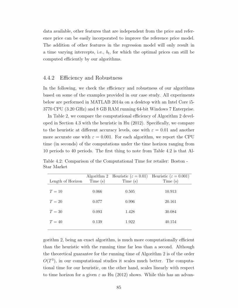
data available, other features that are independent from the price and refer-

ence price can be easily incorporated to improve the reference price model.

The addition of other features in the regression model will only result in

a time varying intercepts, i.e., bt, for which the optimal prices can still be

computed efficiently by our algorithms.

4.4.2 Efficiency and Robustness

In the following, we check the efficiency and robustness of our algorithms

based on some of the examples provided in our case study. All experiments

below are performed in MATLAB 2014a on a desktop with an Intel Core i5-

3770 CPU (3.20 GHz) and 8 GB RAM running 64-bit Windows 7 Enterprise.

In Table 2, we compare the computational efficiency of Algorithm 2 devel-

oped in Section 4.3 with the heuristic in Hu (2012). Specifically, we compare

to the heuristic at different accuracy levels, one with ε = 0.01 and another

more accurate one with ε = 0.001. For each algorithm, we report the CPU

time (in seconds) of the computations under the time horizon ranging from

10 periods to 40 periods. The first thing to note from Table 4.2 is that Al-

Table 4.2: Comparison of the Computational Time for retailer: Boston -Star Market

Algorithm 2 Heuristic (ε = 0.01) Heuristic (ε = 0.001)Length of Horizon Time (s) Time (s) Time (s)

T = 10 0.066 0.505 10.913

T = 20 0.077 0.996 20.161

T = 30 0.093 1.428 30.084

T = 40 0.139 1.922 40.154

gorithm 2, being an exact algorithm, is much more computationally efficient

than the heuristic with the running time far less than a second. Although

the theoretical guarantee for the running time of Algorithm 2 is of the order

O(T 3), in our computational studies it scales much better. The computa-

tional time for our heuristic, on the other hand, scales linearly with respect

to time horizon for a given ε as Hu (2012) shows. While this has an advan-

85

tage in computing long time horizon problems, errors may accumulate over

time and reducing such errors would require relatively significant amount of

computational time.

Next, we show that our exact algorithm can still be applied even if the

technical condition in Assumption 4.4 fails. Indeed, Assumption 4.4 is merely

a sufficient condition to guarantee that Assumption 4.2 holds in our dynamic

pricing problem and in order to present a neat and interpretable condition we

have been quite conservative in the derivation. In actual implementation, it

is not necessary to verify Assumption 4.4 beforehand. Instead, since explicit

expressions are computed during each iteration, one can verify Assumption

4.2 directly in an online fashion. For instance, we have applied Algorithm 2

to the retailer “Indianapolis - Kroger Co” for which Assumption 4.4 fails. We

find that Assumption 4.2 is not violated while implementing the algorithm.

As a result, Proposition 4.7 still holds and the efficiency of the algorithm is

guaranteed. Table 4.3 summarizes the growth of breakpoints of the value

function Gt(q) for the first 20 iterations. As one can see that the growth is

quadratic in t.

Table 4.3: Growth of the number of breakpoints of Gt(q)

t = 2 t = 4 t = 6 t = 8 t = 10 t = 12 t = 14 t = 16 t = 18 t = 20Indiannapolis - Kroger Co 1 9 21 39 68 104 151 211 299 446Boston - Star Market 1 9 17 25 33 41 49 57 65 73

In comparison, the growth of breakpoints of Gt(q) for retailer “Boston -

Star Market”, where Assumption 4.4 holds, is also illustrated in Table 4.3.

Interestingly, the growth is linear instead of quadratic. That is, in addition

of being a simple sufficient condition, the stronger property imposed by As-

sumption 4.4 seems to have the potential of eliminating many breakpoints,

which also explains the efficiency of Algorithm 2 demonstrated in Table 4.2.

4.5 Conclusion

In this chapter we examine the computational side of a dynamic pricing

problem with a memory-based reference price model. In this model, demand

depends on both current selling price and reference price, where the latter

evolves according to an exponentially smoothing process of past prices. We

identify several key structural properties to ensure such non-smooth dynamic

86

optimization problems can be solved exactly in strongly polynomial time. In

the loss-averse case, we characterize the sufficient conditions to guarantee

those structural properties and develop a strongly polynomial time algorithm

to solve for the optimal prices.

To complement our theoretical results, a case study is presented to demon-

strate how our algorithms can be applied in a practical setting. Based on

the examples in the case study, we show that our exact algorithm can be

very efficient and may still be applied even when the technical conditions are

violated.

Our work is only a start in looking at the computational side of the op-

timization models that incorporate reference price effects. We are exploring

several related topics. First, further improvement of the current algorithms

and heuristic is important and interesting. Efficient algorithms become per-

tinent as we incorporate these models into decision support systems which

usually involve many products and other operations decisions.

Secondly, there is a rapidly growing literature on integrated inventory and

pricing models (see Federgruen and Heching, 1999; Chen and Simchi-Levi,

2004a,b; Huh and Janakiraman, 2008; Geunes et al., 2009; Chen and Simchi-

Levi, 2012). Incorporating reference price effects into such models may sig-

nificantly complicate algorithm design. Efficient algorithms in these settings

may then provide even more benefits to the firms facing inventory as well as

pricing decisions.

Finally, we would like to examine the possibility of extending our algo-

rithms to the model with multiple products (see Chapter 5 for a model for-

mulation). Indeed, in settings with multiple products, the state space grows

in dimensions and it is not clear whether the number of quadratic pieces in

the value functions will still be bounded by a polynomial number.

87

Chapter 5

Dynamic Pricing of Multiple Products

5.1 Introduction

So far, we have been focusing solely on the setting in which a monopolist

manages a single product. However, in practice, the demand of a produc-

t can be affected by the prices of other products as well. For example, if

a retailer is selling both Coke and Pepsi, then one would naturally expect

the demand for Coke will be low if the retailer runs a promotion for Pepsi.

Capturing such cross-price effects is a central task in building up a multi-

product model. The multinomial logit model and its variants are commonly

used in the literature to explicitly model the purchase behavior of consumers

when they face multiple substitutable products. As we mentioned in Section

2.1, researchers have managed to incorporate the effects of reference prices

into such models and a lot of empirical studies are conducted (comparative-

ly, as we point out below, empirical studies for linear models are scarce).

However, even single-period multi-product price optimization problems that

ignore reference price effects can be non-trivial and a stream of literature

has been devoted to these problems over the last two decades (see Gallego

and Wang, 2014, and the references therein). Another popular model is the

linear demand models which capture the cross-price effects directly at the

aggregate level and such models are widely used both empirically and ana-

lytically. Yet, empirical studies that incorporate reference price effects into

the multi-product linear demand models are still lacking. Indeed, it would

be a challenge to empirically disentangle the direct cross-price effects with

the indirect ones, which could be caused by the fact that the formation of

reference price is affected by prices of different products.

Nevertheless, a few linear models have been proposed to study reference

price effects in a multi-product setting. Kopalle et al. (1996) propose two

88

such models. Their first model directly generalizes the exponential smooth-

ing model of the single-product setting by adding cross-price effects terms

in the demand function and assuming that consumers have a reference price

for each product which is independent with each other. Their second mod-

el introduces reference brand formulation (see Hardie et al., 1993) which

uses the price of the product consumers purchased last time as a reference

price. Asvanunt (2007), on the other hand, argues that consumers make their

purchasing decision on the store’s overall price level, which is a weighted av-

erage price of different products sold at the store. Consequently, in Asvanunt

(2007), consumers use a uniform reference price when deciding which product

to choose.

In terms of the analysis of dynamic pricing problems, multi-product set-

ting has brought significant challenges and structural results are quite limited

in the literature. Kopalle et al. (1996) show in their exponential smoothing

model that constant pricing strategies are not optimal when demands for each

of the product are gain-seeking while constant pricing strategies outperfor-

m high-low pricing strategies when demands are all loss-averse or loss/gain

neutral. Popescu and Wu (2005) adopt the exponential smoothing model in

Kopalle et al. (1996) and prove that the optimal prices converge to constant

prices for the two products case with both products having loss/gain neutral

demands. They conjecture that the result extend to more than two products

but are unable to prove analytically. Indeed, to the best of our knowledge,

it is not established whether constant pricing strategies are optimal in the

long-run even for loss/gain neutral demands with more than two products.

The main difficulty behind such analysis is the enlargement of state space.

As Popescu and Wu (2005) point out “few general techniques exist for prov-

ing global stability in high dimensions”. As we will see, for loss-averse case,

there is an additional difficulty in the switching behavior of the optimal price

path. In other words, the technique developed in Fibich et al. (2003) (also see

Section 2.4) to separate the solution of the non-smooth dynamic program-

ming problem to the corresponding smooth dynamic programming problems

does not extend to the multi-product setting. The model proposed in As-

vanunt (2007), however, circumvents these difficulties because a single state

variable (store level reference price) is sufficient to describe the system. As a

result, Asvanunt (2007) manages to prove the optimality of constant pricing

strategies in the loss/gain neutral case.

89

This chapter mainly builds upon the exponential smoothing model in a

multi-product setting proposed in Kopalle et al. (1996). We give an explicit

solution to the dynamic pricing problems in a continuous-time framework

with loss/gain neutral demands, which generalizes the solution of Fibich et al.

(2003) in a single-product setting. With the explicit solution, we prove the

conjecture of Popescu and Wu (2005) that for any finite number of products,

the optimal prices converge to a unique steady state. As we have pointed

out earlier, similar techniques to deal with loss-averse demands cannot be

extended to multi-product setting. Instead of seeking optimal solutions, we

propose for two-product case a semi-myopic solution (see Section 5.3.2) that

generalizes the notion of myopic solution and can in some scenarios achieve

optimality. We further develop some novel techniques to show the global

stability of the resulting system.

The remainder of this chapter is organized as follows. In Section 5.2 we

present the mathematical model in a continuous-time framework that ex-

tends the exponential smoothing model in the single-product setting to the

multi-product setting. The dynamic pricing problem is analyzed in Section

5.3. Section 5.4 gives concluding remarks and possible directions for future

research. All technical proofs are relegated to Appendix D.

5.2 Model

We consider a monopolist selling N products and consumers form a reference

price ri for product i, 1 ≤ i ≤ N . Following Kopalle et al. (1996), we assume

that the reference price for each of the product evolves independently and

according to an exponential smoothing process. Similar to (2.15), given the

price pi(t) and the reference price ri(t) for product i at time t, the reference

price evolves according to

dri(t) = α[pi(t)− ri(t)]dt, α > 0. (5.1)

For notational convenience, we denote r = (r1(t), ..., rN(t))>, p =

(p1(t), ..., pN(t))> and r = (dr1(t)dt

, ..., drN (t)dt

)>, then (5.1) can be written more

compactly as

r = α(p− r). (5.2)

90

The demand function for product i is modeled as

Di(t) = bi − aipi(t) +N∑

j=1,j 6=i

θijpj(t)

+ η+i max{ri(t)− pi(t), 0}+ η−i min{ri(t)− pi(t), 0},

where θij models the cross-price effects between products i and j. One s-

tandard assumption here is that∑

j 6=i θij < ai, which ensures the demand of

product i is more sensitive to the change in its own price than to the change

in the prices of all other products (see, for example, Talluri and Van Ryzin,

2005). For ease of exposition, we further assume that θij = θji. Note here

that when θij > 0, products i and j are substitutes while θij < 0 indicates

that they are complements.

The instantaneous profit for the firm is

Π(r,p) =N∑i=1

pi(t)Di(t),

and the corresponding dynamic pricing problem is: given initial reference

prices r0 = (r1(0), ..., rN(0))>, the firm seeks to maximize its long-run profit,

i.e.,

maxp

∫ +∞

0

e−γtΠ(r,p)dt

s.t. r = α(p− r),

(5.3)

where γ is the discount factor.

5.3 Analysis

This section analyzes the dynamic pricing problem (5.3) of multiple products.

For the loss/gain neutral case, we derive an explicit solution, which helps us to

construct a semi-myopic solution for the loss-averse case with two products.

We further prove that the reference price path under the semi-myopic pricing

strategy will converge to a region of steady states.

91

5.3.1 Loss/Gain Neutral Demands

In this subsection, we assume the demands for all the products are loss/gain

neutral. That is, η+i = η−i := ηi, for 1 ≤ i ≤ N . In this case, the instanta-

neous profit can be written in matrix form as

Π(r,p) = p>Rp + r>Kp + b>p, (5.4)

where b = (b1, ..., bN)>,

R =

−(a1 + η1) θ12 . . . θ1N

θ21 −(a2 + η2) . . . θ2N

......

. . ....

θN1 θN2 . . . −(aN + ηN)

and

K =

η1 0 . . . 0

0 η2 . . . 0...

.... . .

...

0 0 . . . ηN

.Before we state our main result, we first examine the properties of the

matrix M := α(α+ γ)I + α(α+ γ2)R−1K, where I is the identity matrix. As

we will see shortly this matrix is critical for our development of the explicit

solution to (5.3).

Lemma 5.1. The matrix M defined by M = α(α+ γ)I + α(α+ γ2)R−1K is

positive definite.

We denote ξ1, ..., ξN (not necessarily all distinct) and v1, ...,vN to be the N

eigenvalues and the corresponding eigenvectors of M with V := (v1, ...,vN).

By Lemma 5.1, we know that ξi > 0 for 1 ≤ i ≤ N and we can define

λi =γ−√γ2+4ξi2

. Finally, we let rs to be the unique solution of the linear

equations

Mrs = −1

2α(α + γ)R−1b. (5.5)

In Proposition 5.1, we give an explicit expression to the solution of the

problem (5.3) using above defined notations .

92

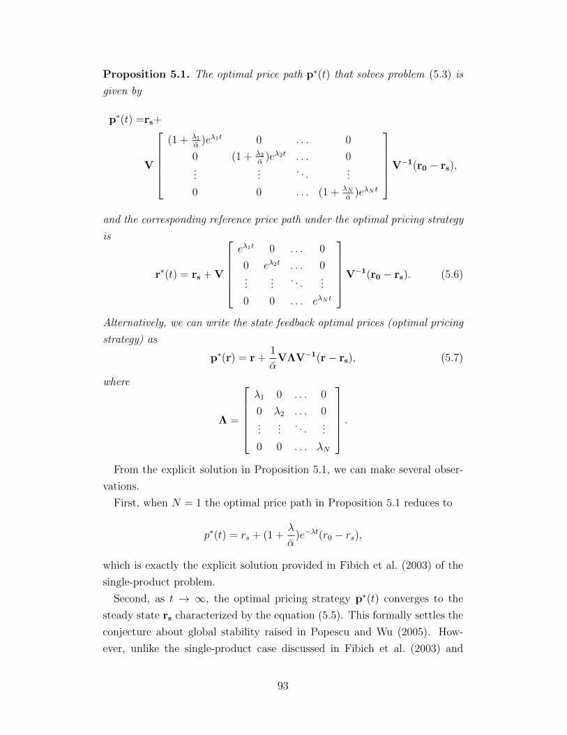
Proposition 5.1. The optimal price path p∗(t) that solves problem (5.3) is

given by

p∗(t) =rs+

V

(1 + λ1

α)eλ1t 0 . . . 0

0 (1 + λ2α

)eλ2t . . . 0...

.... . .

...

0 0 . . . (1 + λNα

)eλN t

V−1(r0 − rs),

and the corresponding reference price path under the optimal pricing strategy

is

r∗(t) = rs + V

eλ1t 0 . . . 0

0 eλ2t . . . 0...

.... . .

...

0 0 . . . eλN t

V−1(r0 − rs). (5.6)

Alternatively, we can write the state feedback optimal prices (optimal pricing

strategy) as

p∗(r) = r +1

αVΛV−1(r− rs), (5.7)

where

Λ =

λ1 0 . . . 0

0 λ2 . . . 0...

.... . .

...

0 0 . . . λN

.From the explicit solution in Proposition 5.1, we can make several obser-

vations.

First, when N = 1 the optimal price path in Proposition 5.1 reduces to

p∗(t) = rs + (1 +λ

α)e−λt(r0 − rs),

which is exactly the explicit solution provided in Fibich et al. (2003) of the

single-product problem.

Second, as t → ∞, the optimal pricing strategy p∗(t) converges to the

steady state rs characterized by the equation (5.5). This formally settles the

conjecture about global stability raised in Popescu and Wu (2005). How-

ever, unlike the single-product case discussed in Fibich et al. (2003) and

93

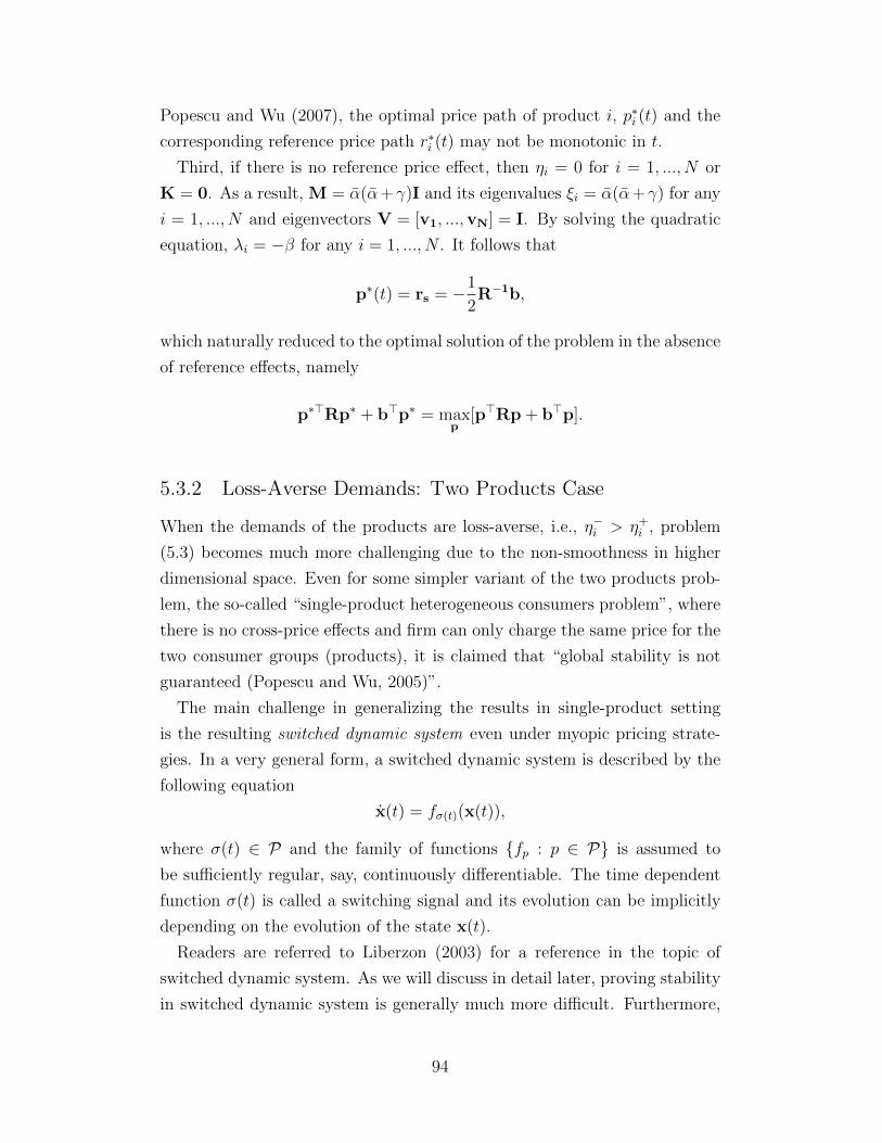
Popescu and Wu (2007), the optimal price path of product i, p∗i (t) and the

corresponding reference price path r∗i (t) may not be monotonic in t.

Third, if there is no reference price effect, then ηi = 0 for i = 1, ..., N or

K = 0. As a result, M = α(α+γ)I and its eigenvalues ξi = α(α+γ) for any

i = 1, ..., N and eigenvectors V = [v1, ...,vN] = I. By solving the quadratic

equation, λi = −β for any i = 1, ..., N . It follows that

p∗(t) = rs = −1

2R−1b,

which naturally reduced to the optimal solution of the problem in the absence

of reference effects, namely

p∗>Rp∗ + b>p∗ = maxp

[p>Rp + b>p].

5.3.2 Loss-Averse Demands: Two Products Case

When the demands of the products are loss-averse, i.e., η−i > η+i , problem

(5.3) becomes much more challenging due to the non-smoothness in higher

dimensional space. Even for some simpler variant of the two products prob-

lem, the so-called “single-product heterogeneous consumers problem”, where

there is no cross-price effects and firm can only charge the same price for the

two consumer groups (products), it is claimed that “global stability is not

guaranteed (Popescu and Wu, 2005)”.

The main challenge in generalizing the results in single-product setting

is the resulting switched dynamic system even under myopic pricing strate-

gies. In a very general form, a switched dynamic system is described by the

following equation

x(t) = fσ(t)(x(t)),

where σ(t) ∈ P and the family of functions {fp : p ∈ P} is assumed to

be sufficiently regular, say, continuously differentiable. The time dependent

function σ(t) is called a switching signal and its evolution can be implicitly

depending on the evolution of the state x(t).

Readers are referred to Liberzon (2003) for a reference in the topic of

switched dynamic system. As we will discuss in detail later, proving stability

in switched dynamic system is generally much more difficult. Furthermore,

94

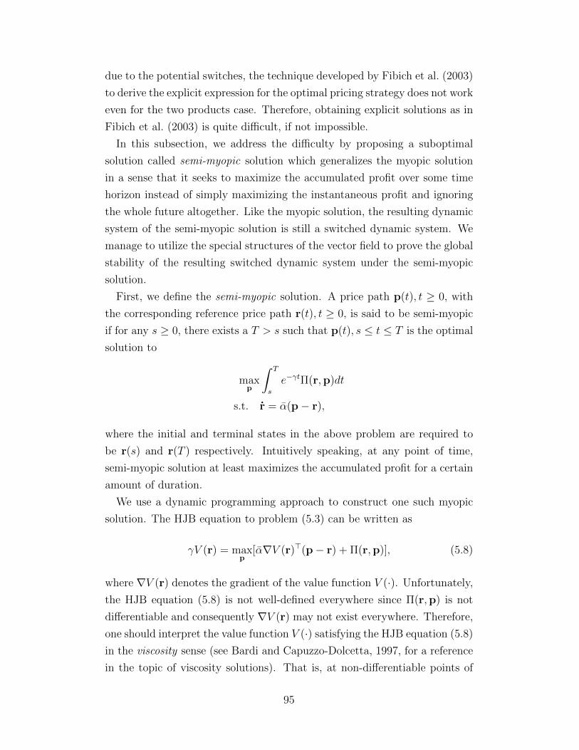
due to the potential switches, the technique developed by Fibich et al. (2003)

to derive the explicit expression for the optimal pricing strategy does not work

even for the two products case. Therefore, obtaining explicit solutions as in

Fibich et al. (2003) is quite difficult, if not impossible.

In this subsection, we address the difficulty by proposing a suboptimal

solution called semi-myopic solution which generalizes the myopic solution

in a sense that it seeks to maximize the accumulated profit over some time

horizon instead of simply maximizing the instantaneous profit and ignoring

the whole future altogether. Like the myopic solution, the resulting dynamic

system of the semi-myopic solution is still a switched dynamic system. We

manage to utilize the special structures of the vector field to prove the global

stability of the resulting switched dynamic system under the semi-myopic

solution.

First, we define the semi-myopic solution. A price path p(t), t ≥ 0, with

the corresponding reference price path r(t), t ≥ 0, is said to be semi-myopic

if for any s ≥ 0, there exists a T > s such that p(t), s ≤ t ≤ T is the optimal

solution to

maxp

∫ T

s

e−γtΠ(r,p)dt

s.t. r = α(p− r),

where the initial and terminal states in the above problem are required to

be r(s) and r(T ) respectively. Intuitively speaking, at any point of time,

semi-myopic solution at least maximizes the accumulated profit for a certain

amount of duration.

We use a dynamic programming approach to construct one such myopic

solution. The HJB equation to problem (5.3) can be written as

γV (r) = maxp

[α∇V (r)>(p− r) + Π(r,p)], (5.8)

where ∇V (r) denotes the gradient of the value function V (·). Unfortunately,

the HJB equation (5.8) is not well-defined everywhere since Π(r,p) is not

differentiable and consequently ∇V (r) may not exist everywhere. Therefore,

one should interpret the value function V (·) satisfying the HJB equation (5.8)

in the viscosity sense (see Bardi and Capuzzo-Dolcetta, 1997, for a reference

in the topic of viscosity solutions). That is, at non-differentiable points of

95

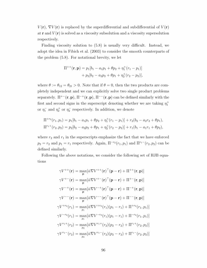
V (r), ∇V (r) is replaced by the superdifferential and subdifferential of V (r)

at r and V (r) is solved as a viscosity subsolution and a viscosity supersolution

respectively.

Finding viscosity solution to (5.8) is usually very difficult. Instead, we

adopt the idea in Fibich et al. (2003) to consider the smooth counterparts of

the problem (5.8). For notational brevity, we let

Π++(r,p) = p1[b1 − a1p1 + θp2 + η+1 (r1 − p1)]

+ p2[b2 − a2p2 + θp1 + η+2 (r2 − p2)],

where θ := θ12 = θ21 > 0. Note that if θ = 0, then the two products are com-

pletely independent and we can explicitly solve two single product problems

separately. Π+−(r,p), Π−+(r,p), Π−−(r,p) can be defined similarly with the

first and second signs in the superscript denoting whether we are taking η+1

or η−1 and η+2 or η−2 respectively. In addition, we denote

Π+r2(r1, p1) = p1[b1 − a1p1 + θp2 + η+1 (r1 − p1)] + r2(b2 − a2r2 + θp1),

Πr1+(r2, p2) = p2[b2 − a2p2 + θp1 + η+2 (r2 − p2)] + r1(b1 − a1r1 + θp2),

where r2 and r1 in the superscripts emphasize the fact that we have enforced

p2 = r2 and p1 = r1 respectively. Again, Π−r2(r1, p1) and Πr1−(r2, p2) can be

defined similarly.

Following the above notations, we consider the following set of HJB equa-

tions

γV ++(r) = maxp

[α∇V ++(r)>(p− r) + Π++(r,p)]

γV +−(r) = maxp

[α∇V +−(r)>(p− r) + Π+−(r,p)]

γV −+(r) = maxp

[α∇V −+(r)>(p− r) + Π−+(r,p)]

γV −−(r) = maxp

[α∇V −−(r)>(p− r) + Π−−(r,p)]

γV +r2(r1) = maxp1

[α∇V +r2(r1)(p1 − r1) + Π+r2(r1, p1)]

γV −r2(r1) = maxp1

[α∇V −r2(r1)(p1 − r1) + Π−r2(r1, p1)]

γV r1+(r2) = maxp2

[α∇V r1+(r2)(p2 − r2) + Πr1+(r2, p2)]

γV r1−(r2) = maxp2

[α∇V r1−(r2)(p2 − r2) + Πr1−(r2, p2)]

96

and denote the solutions to the corresponding HJB equations as p++(r),

p+−(r), p−+(r),p−−(r), p+r21 (r1), p−r21 (r1), pr1+

2 (r2) and pr1−2 (r2) respectively.

Note that all the HJB equations above are well-defined since the instanta-

neous profit functions, say Π++(r,p), are continuously differentiable. Apply-

ing our results in Section 5.3.1, all the solutions admit explicit expressions

and they are linear in states. To construct our semi-myopic solution, we

divide the state space into the following regions:

I++ := {r|p++1 (r)− r1 < 0, p++

2 (r)− r2 < 0}

I+− := {r|p+−1 (r)− r1 < 0, p+−

2 (r)− r2 > 0}

I−+ := {r|p−+1 (r)− r1 > 0, p−+

2 (r)− r2 < 0}

I−− := {r|p−−1 (r)− r1 < 0, p−−2 (r)− r2 < 0}

I+r2 := {r|p++2 (r)− r2 ≥ 0, p+−

2 (r)− r2 ≤ 0, p+r21 (r1)− r1 < 0}

I−r2 := {r|p−+2 (r)− r2 ≥ 0, p−−2 (r)− r2 ≤ 0, p−r21 (r1)− r1 > 0}

Ir1+ := {r|p++1 (r)− r1 ≥ 0, p−+

1 (r)− r1 ≤ 0, pr1+2 (r2)− r2 < 0}

Ir1− := {r|p+−1 (r)− r1 ≥ 0, p−−1 (r)− r1 ≤ 0, pr1−2 (r2)− r2 > 0}

S : the remaining region.

Since all the solutions are linear in states, the above regions are character-

ized by linear inequalities and are therefore polyhedron. With the explicit

solutions, after cumbersome algebraic computations, one can verify that, for

instance, I++ and I+− will not overlap.

We construct the semi-myopic solution by proposing the following pricing

strategy, denoted as pSM(r).

pSM(r) =

p++(r), r ∈ I++,

p+−(r), r ∈ I+−,

p−+(r), r ∈ I−+,

p−−(r), r ∈ I−−,

(p+r21 (r1), r2), r ∈ I+r2 ,

(p−r21 (r1), r2), r ∈ I−r2 ,

(r1, pr1+2 (r2)), r ∈ Ir1+,

(r1, pr1−2 (r2)), r ∈ Ir1−,

r, r ∈ S.

(5.9)

97

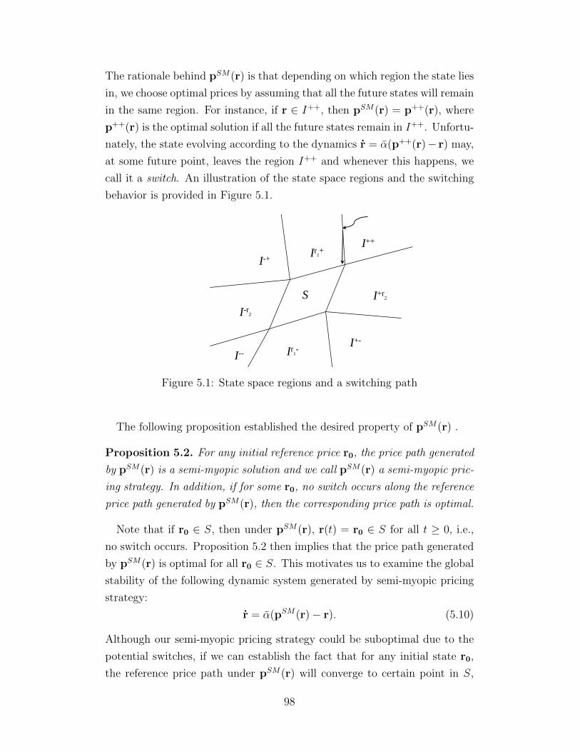
The rationale behind pSM(r) is that depending on which region the state lies

in, we choose optimal prices by assuming that all the future states will remain

in the same region. For instance, if r ∈ I++, then pSM(r) = p++(r), where

p++(r) is the optimal solution if all the future states remain in I++. Unfortu-

nately, the state evolving according to the dynamics r = α(p++(r)− r) may,

at some future point, leaves the region I++ and whenever this happens, we

call it a switch. An illustration of the state space regions and the switching

behavior is provided in Figure 5.1.

SS

SI--

SI++

SI+-

SI+r2

SIr1-

SI-+

SI-r2

SIr1+

Figure 5.1: State space regions and a switching path

The following proposition established the desired property of pSM(r) .

Proposition 5.2. For any initial reference price r0, the price path generated

by pSM(r) is a semi-myopic solution and we call pSM(r) a semi-myopic pric-

ing strategy. In addition, if for some r0, no switch occurs along the reference

price path generated by pSM(r), then the corresponding price path is optimal.

Note that if r0 ∈ S, then under pSM(r), r(t) = r0 ∈ S for all t ≥ 0, i.e.,

no switch occurs. Proposition 5.2 then implies that the price path generated

by pSM(r) is optimal for all r0 ∈ S. This motivates us to examine the global

stability of the following dynamic system generated by semi-myopic pricing

strategy:

r = α(pSM(r)− r). (5.10)

Although our semi-myopic pricing strategy could be suboptimal due to the

potential switches, if we can establish the fact that for any initial state r0,

the reference price path under pSM(r) will converge to certain point in S,

98

then such strategy will, in the long run, bring us to a state where optimality

can be achieved.

Establishing global stability for switched systems is, in general, non-trivial.

While there is a vast amount of literature studying the stability issue of

switched systems (see DeCarlo et al., 2000, for a review), most of the results

extend the classic Lyapunov stability theory by proposing multiple Lyapunov

functions to demonstrate stability. However, even for non-switched systems,

“Lyapunov functions can be hard to come by (p.141 in Stokey et al., 1989)”

and for switched systems, it is pointed out by DeCarlo et al. (2000) that

“despite the variety and significance of the many results on hybrid system

stability, general necessary and sufficient conditions in terms of the structure

of the vector fields have evaded discovery.”

In the following, we utilize the special structures of our problem to prove

the global stability of (5.10). Since we are concerned with the two-product

case, the discussions below will be restricted to two dimensional dynamic

systems, i.e., planar system.

Lemma 5.2. Consider a matrix

A =

[a b

c d

]

with the property that A � 0 and b, c < 0. Let v1 = (v11, v12) and v2 =

(v21, v22) be two eigenvectors of A, then the following must hold

v11v12 > 0, v21v22 < 0.

In other words, the line with one eigenvector as the direction passes through

the first and third quadrants while the line with the other eigenvector as the

direction passes through the second and forth quadrants.

Recall the definition of the matrix M in Lemma 5.1 where it depends on

the parameters ηi, i = 1, ..., N for loss/gain neutral demands. Here, we define

M++ by letting N = 2 and η1 = η+1 , η2 = η+

2 . The matrices M+−,M−+,M−

can be defined in a similar fashion. Note that M++ will have the same

99

eigenvectors as

1

α(α + γ/2)(M++ − αγ

2I)

=1

(a1 + η+1 )(a2 + η+

2 )− θ2

[a1(a2 + η+

2 )− θ2 −θη+2

−θη+1 a2(a1 + η+

1 )− θ2

],

which satisfies the condition in Lemma 5.2. Thus, M++ will have two eigen-

vectors respectively in the first (third) quadrants and the second (forth)

quadrants. The same property can be established for M+−,M−+,M−. Us-

ing the above property of the matrices, we show that if the state path enters

any of the regions I++, I+−, I−+ or I−−, it will converge to a unique steady

state of that region without going out again. We formally state this result

with respect to the region I++ in Lemma 5.3. The results and proofs for the

regions I+−, I−+ and I−− are similar.

Lemma 5.3. Denote ∂I++ to be the boundary of I++. For any r0 ∈ ∂I++

and r(0) ∈ I++, we have r(t) ∈ I++ for any t > 0 and

limt→∞

r(t) = r++s ,

where r++s is the steady state to the system r = α(p++(r)− r).

Using Lemma 5.3, we can then establish the global stability of the system

(5.10).

Proposition 5.3. Starting from any initial state r0, the reference price path

generated according to (5.10) can have at most two switches. As a result,

there exists a T ≥ 0, such that for all t > T , r(t) stays in any one of the

nine regions illustrated in Figure 5.1 and converges to a steady state in S.

We provide in Figure 5.2 a numerical example to illustrate the stability

result in Proposition 5.3. In Figure 5.2, the reference price paths evolving

according to (5.10) are plotted for each initial reference price lying on the

boundaries of the square region. One can see that all reference price paths

converge to the steady states region S in the middle. It is also clear from the

figure that many reference price paths have a sudden change in their evolving

directions which indicates a switching behavior.

100

4 5 6 7 8 9 104

5

6

7

8

9

10

r1

r 2

b1 = 82,b2 = 80,a1 = 16,a2 = 14,η+

1 = 4, η−

1 = 12, η+2 = 1,η−

2 = 11, θ = 10, α = 0.5, γ = 0.2

Figure 5.2: Steady state region and reference price paths

5.4 Conclusion

In this chapter we consider a dynamic pricing problem of multiple products.

If demands for all the products are loss/gain neutral, we can solve the optimal

prices for all the products explicitly. Our solution is a generalization of the

solution in Fibich et al. (2003), which we use to show that in the long run the

optimal prices as well as reference prices converge to a unique steady state.

If the demands are loss-averse, then the dynamic pricing problem for the

multiple products becomes considerably more difficult. Not only the myopic

pricing strategy can result in a switched dynamic system, due to the potential

switching behavior, no existing method can be applied to solve for the optimal

prices. To address these difficulties, we propose a semi-myopic solution,

whose expressions can be explicitly computed. Our semi-myopic solution not

only generalizes the myopic solution, but is also optimal if no switch occurs

along the reference price path generated by the solution. We further prove

that the dynamic system resulted from the semi-myopic solution is globally

stable. The techniques we used in proving stability are potentially useful

101

for establishing the stability property of other switched dynamic systems as

well.

We believe our results in this chapter open up a few future research di-

rections. First of all, as we have pointed out, the semi-myopic solution we

constructed is optimal if no switch occurs along the state path. Can such

regions where no switch occurs be identified (the so-called “positively invari-

ant set”)? Based on this step, one can then further explore what would be

the optimal prices outside of these invariant sets.

It would be useful to both numerically and analytically quantify the opti-

mality gap of our semi-myopic solution. Due to the curse of dimensionality,

solving problem (5.3) numerically becomes a daunting task even for a smal-

l number of products. Deriving computationally efficient upper bounds on

(5.3) will then facilitate performance evaluation.

Finally, a challenging yet interesting direction is to explore the case of

gain-seeking demands and more generally a mixture of gain-seeking as well

as loss-averse demands for multiple products. Although we have established

the complicated behavior of the price dynamics in Chapter 3, whether our an-

alytical results can be carried over to the multi-product settings by imposing

similar assumptions as Assumption 3.1 is still an open question.

102

Chapter 6

Future research

In an effort to capture the relationship between demand and prices more

accurately in a market with repeated purchases and quantify its impact, this

thesis studies reference price models and the resulting dynamic pricing prob-

lems from several perspectives. Chapter 2-4 focuses on a single-product set-

ting. Empirically, we compare different reference price models and examines

the implication of behavioral asymmetry. Analytically, we characterize the

structures of the optimal pricing strategy under the exponential smoothing

reference price models when demands are gain-seeking. Computationally, we

provide efficient algorithms to compute the optimal prices for the exponential

smoothing reference price models.

For tractability, our analytical results and computational algorithms only

consider the exponential smoothing reference price models, while our em-

pirical comparisons suggest that in many cases the peak-end model and the

adaptation-rate-based model can provide a better fit to the data. This open-

s up two interesting research directions. First, we have seen in Chapter 2

that the optimality of constant pricing strategies is quite robust to different

reference price models under loss-averse demands. It is then natural to ask

for gain-seeking demands whether some of the analytical results developed in

Chapter 3 can be extended to the other two reference price models. Second,

developing computationally efficient algorithms for the peak-end model and

the adaptation-rate-based model is practically important since as reported in

Natter et al. (2007), the adaptation-rate-based model is already implemented

in the decision support system of bauMax, an Austrian retailer. Table 6.1

summarizes the existing results and the blank space represent open research

questions.

Chapter 5 represents another direction of extension: dynamic pricing with

multiple products. This is a largely unexplored yet important area and many

open questions remain to be answered. First, several linear demand models

103

Table 6.1: Summary of Results

Structures of optimal pricing strategies Computational algorithmsLoss-averse case Gain-seeking case

ES Popescu and Wu (2007) Chapter 3 Chapter 4PE Nasiry and Popescu (2011)ARB Section 2.6ES: exponential smoothing modelPE: peak-end modelARB: adaptation-rate-based model

for multiple products that incorporate reference price effects have been pro-

posed. An empirical comparison of these models would not only shed light on

how reference prices come into play in a multi-product setting but also give

a guidance on developing analytical results and computational algorithms.

Second, when there is behavioral asymmetry, the resulting dynamic pricing

problem is a high-dimensional non-smooth dynamic programming problem

and is quite challenging. Characterizing the structures of the optimal pricing

strategies and studying the long-run behavior of the prices are crucial for

developing simple heuristics of such complicated problems. Finally, efficient

algorithms and implementations of the algorithms in a practical setting would

be very useful to advance the usage of more realistic models that incorporate

consumers behavior considerations among practitioners.

The topics covered in this thesis is by no means comprehensive. As we

mentioned in Chapter 3 and Chapter 4, the coordination of pricing and in-

ventory decisions is another wide area of research. Due to the increased

complexity, most results in the literature are restricted to exponential s-

moothing model and loss-averse demands. It would be interesting to see how

the results would change if alternative reference price models are employed.

Competition among the firms, is another important factor not discussed in

this thesis. While Fibich et al. (2003) examine the Cournot competition

in a continuous-time framework, analyzing price competitions is limited to

numerical simulations (Kopalle et al., 1996). Analytical results in this area

would provide helpful implications in how reference price effects change the

competitive behaviors among the firms.

104

Appendix A

A.1 Proof of Proposition 2.5

To solve the HJB equation (2.18), we start from solving a finite horizon

problem by following Zhang (2011). That is, let

V (r, t) = maxp(s)

[∫ T

t

e−γtp(s)D(r(s), p(s))ds

]be the value of optimal accumulated profit (profit-to-go function) from time

t to the end of horizon T when the initial reference price is r. Notice that

the value function in our problem (2.17) V (r0) = limT→∞ V (r0, 0).

From standard theory in stochastic optimal control, V (r, t) then satisfies

the HJB equation

γV (r, t)

= maxp

[pD(r, p) +

∂V (r, t)

∂t+ α(p− r)∂V (r, t)

∂r+σ2r

2

∂2V (r, t)

∂r2

] (A.1)

Using first order condition in (A.1) and with a slight abuse of notation, we

can solve p as

p∗(r) =b+ ηr

2(a+ η)+

α

2(a+ η)

∂V (r, t)

∂r.

Substitute the above equation into (A.1), it follows

σ2

2r∂2V

∂r2+∂V

∂t− γV +

α2

4(a+ η)

(∂V

∂r

)2

+

[−αr +

α(b+ ηr)

2(a+ η)

]∂V

∂r

+(b+ ηr)2

4(a+ η)= 0.

105

Introducing a few new notations, this can be written concisely as:

∂V

∂t−γV +Ar

∂2V

∂r2+B

(∂V

∂r

)2

+(p10+p11r)∂V

∂r+p20+p21r+p22r

2 = 0, (A.2)

where

A =σ2

2

B =α2

4(a+ η)

p10 =αb

2(a+ η)

p11 = −α +αη

2(a+ η)

p20 =b2

4(a+ η)

p21 =bη

2(a+ η)

p22 =η2

4(a+ η).

If we assume function V (r, t) has the following form:

V (r, t) = Q(t)r2 +R(t)r +M(t), (A.3)

then we get the following ordinary differential equations (ODEs):

dQ

dt− γQ+ 4BQ2 + 2p11Q+ p22 = 0, (A.4)

dR

dt− γR + 2AQ+ 4BQR + 2p10Q+ p11R + p21 = 0, (A.5)

dM

dt− γM +BR2 + p10R + p20 = 0, (A.6)

with terminal condition Q(T ) = R(T ) = M(T ) = 0.

We first explicitly solve ODE (A.4) by rewriting it as:

dQ

dt= −4B(Q−Q1)(Q−Q2)

106

where Q1 < Q2 are the two distinct roots of the equation:

4BQ2 − (γ − 2p11)Q+ p22 = 0.

Namely:

Q1 =γ − 2p11 −

√(γ − 2p11)2 − 16Bp22

8B,

Q2 =γ − 2p11 +

√(γ − 2p11)2 − 16Bp22

8B.

Therefore:dQ

(Q−Q1)(Q−Q2)= −4Bdt

⇒ dQ

Q1 −Q2

[1

Q−Q1

− 1

Q−Q2

]= −4Bdt

⇒ lnQ−Q1

Q−Q2

= −4B(Q1 −Q2)t+ C

⇒ Q−Q1

Q−Q2

= D · e−4B(Q1−Q2)t, (A.7)

where C and D = eC are constants to be determined. By Q(T ) = 0, we can

solve

D =Q1

Q2

e4B(Q1−Q2)T .

Substitute D back into (A.7), it follows

Q(t) =Q1e

4B(Q1−Q2)T −Q1e4B(Q1−Q2)t

Q1/Q2e4B(Q1−Q2)T − e4B(Q1−Q2)t. (A.8)

With the expressions for Q(t), expressions for R(t) and M(t) can then be

obtained by solving (A.5) and (A.6). Consequently, p∗(r) can be determined

as well. One can easily verify using Theorem 4.1 in chapter VI of Fleming

and Rishel (1982) that p∗(r) solved in this way is indeed optimal and V (r, t)

is given by (A.3).

The solution to (2.18) is then obtained by letting T →∞. Since Q1 < Q2,

we have Q := Q1 = limT→∞Q(t), where by substituting the expressions for

B, p11 and p22

Q =γ

2α2(a+ η) +

2a+ η

2α− a+ η

2α2∆

107

and ∆ is given by:

∆ =

√γ2 + 2α

2a(γ + α) + γη

η + a.

Correspondingly, one can also obtain R := limT→∞R(t) as

R =2p10Q+ p21 + 2AQ

γ − 4BQ− p11

=2α2b+ αb(γ −∆))

α2(γ + ∆)+α(2a+ η) + (a+ η)(γ −∆)

α2(γ + ∆)σ2

=

[b

α+σ2(a+ η)

α2

]γ −∆

γ + ∆+

[b+

σ2(2a+ η)

2α

]2

γ + ∆

.

Similarly, M := limT→∞M(t) can be computed but the expressions for M is

not needed for our following analysis.

Now, we have explicitly solved (2.18), where V (r) = Qr2 + Rr + M and

the optimal pricing strategy is

p∗(r) =b+ ηr

2(a+ η)+α(2Qr +R)

2(a+ η). (A.9)

Substitute (A.9) into the reference price dynamics (2.16), we have the fol-

lowing SDE:

dr∗(t) = α

[2αQ− 2a− η

2(a+ η)r∗(t) +

αR + b

2(a+ η)

]dt+ σ

√r∗(t)dW (t)

:= λ(µ− r∗(t)) + σ√r∗(t)dW (t),

(A.10)

where

λ = α2a+ η − 2αQ

2(a+ η), µ = α

αR + b

2λ(a+ η).

Interestingly, under the optimal pricing strategy, the reference price dy-

namics (A.10) is again a square-root diffusion process. It is easy to show

that λ, µ > 0 and thus the steady state distribution is a gamma distribution

whose shape parameter is 2λµσ2 and rate parameter is 2λ

σ2 (see, for instance,

Cox et al., 1985).

108

A.2 Proof of Proposition 2.6

By Proposition 2.5, R∗s follows a gamma distribution, its mean and variance

can then be computed as

E[R∗s] =2λµ

σ2

σ2

2λ= µ,

var(R∗s) =2λµ

σ2(σ2

2λ)2 =

µ

2λσ2.

Substitute the expressions for Q,R and λ into µ, with cumbersome algebraic

manipulations, one can further obtain

µ =(γ + α)b

2a(γ + α) + γη+

σ2

2a(γ + α) + γη

[a+ η

α

(γ

2− ∆

2

)+

2a+ η

2

].

109

Appendix B

B.1 Proof of Lemma 3.1

Let us first consider the unconstrained problem: maxp Π(r, p). Recall that

Π(r, p) = max{Π+(r, p),Π−(r, p)}

= maxη−≤η≤η+

p(b− ap+ η(r − p)),

where the last equality is due to the linearity of the function p(b−ap+η(r−p))in η.

We can then rewrite maxp Π(r, p) as

maxη−≤η≤η+

maxp−(a+ η)p2 + ηrp+ bp.

Clearly, the inner maximization problem has a unique optimal solution

p(r, η) = ηr+b2(a+η)

with the optimal objective value v(r, η) = (ηr+b)2

4(a+η). Note

further that ∂2v∂r∂η

= ηr(a+η)+a(b+ηr)2(a+η)2

> 0, which indicates that v(r, η) is su-

permodular. Since either η = η+ or η = η−, the supermodularity of v(r, η)

implies the existence of R such that for r ≤ R, v(r, η−) ≥ v(r, η+) and for

r ≥ R, v(r, η+) ≥ v(r, η−). At R, v(r, η−) = v(r, η+) and thus R can be

computed explicitly as R = b

a+√

(a+η+)(a+η−). As a result, the unconstrained

solution is exactly what presents in (3.5).

Observe that when r > R, we have pm(r) = η+r+b2(a+η+)

≤ r. To see this,

suppose pm(r) > r, then

Π(r, pm(r)) = pm(r)(b− apm(r) + η−(r − pm(r)))

> pm(r)(b− apm(r) + η+(r − pm(r))) = v(r, η+),

which contradicts with the fact that Π(r, pm) = v(r, η+) for r > R. Therefore,

110

when r > R, pm(r) can never violate the upper bound U . On the other hand,

by a similar argument for r ≤ R, pm(r) = η−r+b2(a+η−)

≥ r. Moreover, pm(r) is

increasing in r and is equal to U at RU . Thus, if R ≤ RU , then η−r+b2(a+η−)

≤ U

on [0, R] and the unconstrained solution specified above is optimal.

However, if R > RU , then for r ≤ R

v(r, η−) =

(η−r + b)2

4(a+ η−), r ≤ RU ,

− (a+ η−)U2 + η−rU + bU, RU ≤ r ≤ R,

and we need to compare again between v(r, η−) and v(r, η+) on [RU , R]. It is

straightforward to show that R′ is the unique positive solution of v(r, η−) =

v(r, η+) and when r < R′, v(r, η−) > v(r, η+), when r > R′, v(r, η−) <

v(r, η+). Therefore, we arrive at the second form of pm(r).

B.2 Proof of Proposition 3.1

Suppose that a periodic orbit of period 2: {r0, r1} exists, where r0, r1 ∈ [0, U ]

and r0 6= r1. First we observe either r0 ≤ R, r1 > R holds or r0 > R, r1 ≤ R

holds. To see this, suppose that, on the contrary, ri ≤ R for i = 0, 1, then

pm(ri) ≥ ri by the definition of R, which further implies r1−i = αri + (1 −α)pm(ri) ≥ ri. Therefore, r1−i = ri for i = 0, 1, leads to contradiction with

r0 6= r1. Similarly, it is also impossible that ri ≥ R for i = 0, 1. In the

following we assume, without loss of generality, that r0 ≤ R, r1 > R. Then,

r0, r1 satisfy the following equations:

r1 = αr0 + (1− α)η−r0 + b

2(a+ η−),

r0 = αr1 + (1− α)η+r1 + b

2(a+ η+).

Thus, r0, r1 can be explicitly solved as

r0 =[(1 + α)η+ + 2a+ 2η− + 2αa]b

(4a+ 3η− + 2αa+ αη−)η+ + 4αη− + 4αa2 + 4a2 + 2αaη−,

r1 =[(1 + α)η− + 2a+ 2η+ + 2αa]b

(4a+ 3η− + 2αa+ αη−)η+ + 4αη− + 4αa2 + 4a2 + 2αaη−.

111

We have shown that if a periodic orbit of period 2 exists, then it must be

given by the unique solution identified above and has to satisfy r0 ≤ R and

r1 > R. On the other hand, given r0 and r1 specified by above expressions

with r0 ≤ R, r1 > R. Then, by our construction, r1 = αr0 + (1 − α)pm(r0)

and r0 = αr1 + (1 − α)pm(r1), which implies {r0, r1} is a periodic orbit of

period 2. Overall, a periodic orbit of period 2 exists if and only if

[(1 + α)η+ + 2a+ 2η− + 2αa]b

(4a+ 3η− + 2αa+ αη−)η+ + 4αη− + 4αa2 + 4a2 + 2αaη−≤ R,

[(1 + α)η− + 2a+ 2η+ + 2αa]b

(4a+ 3η− + 2αa+ αη−)η+ + 4αη− + 4αa2 + 4a2 + 2αaη−> R.

With cumbersome algebraic manipulations, the above two inequalities can

be simplified to

4(1− α2)a2 + 4(1− α− α2)aη+ + 4aη− − (1 + α)2(η+)2 + 4η+η− ≥ 0,

4(1− α2)a2 + 4(1− α− α2)aη− + 4aη+ − (1 + α)2(η−)2 + 4η+η− > 0.

Observe that the second inequality is naturally satisfied when the first in-

equality is satisfied. Thus, we have arrived at condition (3.7).


By translating R to the origin and scaling η−R+b2(a+η−)

− η+R+b2(a+η+)

to 1, then αr +

(1 − α)pm(r) is equivalent to the following discontinuous map studied in

Rajpathak et al. (2012).

f(r) =

{Ar + µ, r ≤ 0,

Br + µ− 1, r > 0.

Denote {r0, r1, ..., rn−1} be the periodic orbit (if exists) of the above system.

Then it is easy to see that r0 < r1 < ... < rn−1 (r0 > r1 > ... > rn−1) if and

only if r0 < r1 < ... < rn−2 ≤ 0 and rn−1 > 0 (r0 > r1 > ... > rn−2 > 0

and rn−1 ≤ 0 ). If we denote each point rt, 0 ≤ t < n, to be L if rt ≤ 0

and R if rt > 0, then the periodic orbit can be coded as {L,L, ...,L︸︷︷︸n−1

,R}

({R,R, ...,R︸︷︷︸n−1

,L}), which is exactly the so-called prime pattern in Rajpathak

112

et al. (2012). Applying Theorem 1 in Rajpathak et al. (2012), we arrive at

conditions (3.8) and (3.9) that guarantee each type of periodic solution with

period n respectively.


We first prove that V (r) is increasing and convex in r. To see this, define

the following value iteration for i ≥ 0:

Vi+1(r) = maxp∈[0,U ]

Π(r, p) + γVi(αr + (1− α)p),

with V0(r) = 0. We inductively show that Vi(r) is increasing and convex

in r for all i ≥ 0. Clearly, V0(r) trivially has the property. For i > 0,

suppose Vi(r) is increasing and convex in r. Since Π(r, p) is increasing in r,

we immediately have Vi+1(r) is also increasing in r.

To see convexity of Vi+1(r), it is sufficient to show that Π(r, p) is convex

in r. Indeed, recall that Π(r, p) = max{Π+(r, p),Π−(r, p)}, where Π±(r, p) =

p[b−ap+η±(r−p)]. As both Π+(r, p) and Π−(r, p) are convex in r, Π(r, p) is

also convex in r. By Proposition 2.1.15 in Simchi-Levi et al. (2014), Vi+1(r)

is also convex. By Theorem 4.6 in Stokey et al. (1989), limi→∞ Vi(r) = V (r).

Thus, V (r) is both increasing and convex in r.

Since V (r) is increasing and convex in r while both Π+(r, p) and Π−(r, p)

are increasing and convex in r, by applying again Proposition 2.1.15 in

Simchi-Levi et al. (2014) to problems (3.11a) and (3.11b) respectively, we

have V +(r) and V −(r) are also increasing and convex.

On the other hand, as ∂2Π+(r,p)∂r∂p

= η+ > 0 and ∂2Π−(r,p)∂r∂p

= η− > 0, Π+(r, p)

and Π−(r, p) are supermodular in r and p. Moreover, since V (·) is convex,

by Theorem 2.2.6 in Simchi-Levi et al. (2014), V (αr + (1 − α)p) is also

supermodular. As a result, p+(r) and p−(r) are increasing in r.


Clearly, as V −(r) = V − is constant and V +(r) is increasing, there are three

cases. If V +(r) ≥ V − for all r ∈ [0, U ], then R0 = 0. If V +(r) ≤ V − for all

113

r ∈ [0, U ], then R0 = U . If neither of the above cases is true, then we must

have V +(0) < V − and V +(U) > V −. As V +(r) is continuous and increasing,

there must exists 0 < R0 < U , such that if r ≤ R0, then V (r) = V − and

p∗(r) = p− and if r > R0, then V (r) = V +(r) and p∗(r) = p+(r).

Next, we show that whenever p∗(r) = p−, then p∗(r) = p− > r and

whenever p∗(r) = p+(r), then p∗(r) = p+(r) < r. Recall from Section 3.2

that p∗(r) 6= r for any r ∈ [0, U ]. Now suppose p∗(r) = p+(r), but p∗(r) > r,

then V +(r) ≥ V −. However,

V +(r) = Π+(r, p+(r)) + γV (p+(r))

<Π−(r, p+(r)) + γV (p+(r)) ≤ Π−(r, p−) + γV (p−) = V −,

a contradiction. The same claim can be made when p∗(r) = p−.

Finally, if R0 = 0 or R0 = U , then p∗(0) = p+(0) < 0 or p∗(U) = p−(U) >

U , both lead to a contradiction. So we must have 0 < R0 < U .


We first introduce some notations to formalize the idea discussed in Section

3.4. Let V0(r) = V −, then there exists R1 = sup{r ∈ [R0, U ] : p+(r) < R0} ∈(R0, U ] such that for r ∈ (R0, R1), p+(r) = p1(r) = η+r+b

2(a+η+)and

V +(r) = V1(r) = maxp∈[0,U ]

Π+(r, p) + γV0(p) =(η+r + b)2

4(a+ η+)+ γV −.

If R1 = U , then our proposition holds with N = 0.

More generally, for k ≥ 2, if Rk−1 < U , define Rk = sup{r ∈ [R0, U ] :

p+(r) < Rk−1} ∈ (R0, U ]. Note that p+(Rk−1) < Rk−1 by Lemma 3.3 and it

follows Rk > Rk−1. We further define

Vk(r) = maxp∈[0,U ]

Π+(r, p) + γVk−1(p),

pk(r) = arg maxp∈[0,U ]

Π+(r, p) + γVk−1(p).(B.1)

By our construction, on [Rk−1, Rk), Rk−2 ≤ p+(r) < Rk−1. Thus, if V (r) =

V +(r) = Vk−1(r) on [Rk−2, Rk−1), then V (p+(r)) = Vk−1(p+(r)) on [Rk−1, Rk)

and there is no loss of optimality by replacing problem (3.11a) with problem

114

(B.1) above. Therefore, we have inductively shown that V (r) = V +(r) =

Vk(r) and p∗(r) = p+(r) = pk(r) on [Rk−1, Rk).

Next, we inductively show that Vk(r) has the following parametric form:

Vk(r) =1

2Akr

2 +Bkr + Ck,

with Ak ≤ η+. We have already shown the base case for k = 1, with

A1 =(η+)2

2(a+ η+)=η+m2

γ≤ η+,

B1 =η+b

2(a+ η+)=m2b

γ.

With inductive hypothesis,

Vk+1(r) = maxp∈[0,U ]

{Π+(r, p) + γVk(p)}

= maxp∈[0,U ]

{−(a+ η+ − 1

2γAk)p

2 + (b+ η+r + γBk)p+ γCk}.

By Lemma 3.3, pk+1(r) < U . Combined with Ak ≤ η+, we know above

problem is a concave maximization problem with an interior solution. Thus,

the optimal solution can be derived from first order condition:

pk+1(r) =b+ η+r + γBk

2(a+ η+)− γAk.

We can then express

Vk+1(r)

=− (a+ η+ − 1

2γAk)pk+1(r)2 + (b+ η+r + γBk)pk+1(r) + γCk

=(η+)2/2

2(a+ η+)− γAkr2 +

(b+ γBk)η+

2(a+ η+)− γAkr +

(b+ γBk)2/2

2(a+ η+ − γAk)+ γCk.

Thus,

Ak+1 =(η+)2

2(a+ η+)− γAk≤ (η+)2

2(a+ η+)− γη+≤ η+,

Bk+1 =(b+ γBk)η

+

2(a+ η+)− γAk.

115

Combined with the expressions for A1, B1, it is not difficult to see that

Ak =η+

γmk+1,

Bk =1

γ

n∑i=0

i∏j=0

mk+1−jb.

Consequently, we can compute

pk(r) =η+r + b+

∑k−1i=0 (

∏ij=0mk−j)b

2(a+ η+)−mkη+.

If Rk = U , the above analysis has shown that our proposition holds with

N = k − 1.

Finally, we show that the construction of the sequence Rk cannot continue

forever. In other words, there exists N ≥ 0 such that RN+1 > U . We prove

by contradiction. Suppose for any k ≥ 1, Rk ≤ U . Then the following

relation between Rk and Rk+1 must hold for any k ≥ 1: for r ∈ [Rk, Rk+1],

p+(r) ≤ Rk and for r ∈ [Rk+1, U ], p+(r) ≥ Rk. Since Rk is a bounded

increasing sequence, there exists R ≤ U such that

limk→∞

Rk = R.

From the above relation, we conclude that for r ∈ [Rk+1, R], p+(r) ≥ Rk. In

particular, p+(R) ≥ Rk for any k ≥ 1. Taking limits on both sides, we obtain

p+(R) ≥ R,

leading to a contradiction with Lemma 3.3 which states p∗(r) = p+(r) < r

for any r ∈ [R,U ].


From Lemma 3.3, we know that R0 < r∗ ≤ U . Thus, there exists 2 ≤n ≤ N + 2 such that r∗ ∈ [Rn−2, Rn−1]. Let p∗1(r∗) = p+(r∗), then p∗1(r∗) ∈[Rn−3, Rn−2] and p∗1(r∗) < r∗. Inductively, for 1 ≤ i ≤ n − 2 if p∗i (r

∗) ∈[Rn−2−i, Rn−1−i], then let p∗i+1(r∗) = p+(p∗i (r

∗)) and it follows that p∗i+1(r∗) ∈

116

[Rn−3−i, Rn−2−i] if i ≤ n− 3 or p∗i+1(r∗) ∈ [0, R0] if i = n− 2. Furthermore,

it holds p∗i+1(r∗) < p∗i (r∗). Finally, let p∗n(r∗) = p−(p∗n−1(r∗)) = p−. Then

p∗n(r∗) = r∗. We have constructed the periodic orbit {r∗, p∗1(r∗), ..., p∗n−1(r∗)}with the property r∗ > p∗1(r∗) > ... > p∗n−1(r∗).

Next we show that start from any initial reference price r0 ∈ [0, U ], the

optimal reference price path r∗t converges to the periodic orbit in at most

N+2 periods. Clearly, for any r0 ∈ [0, R0], r∗1 = p−(r0) = r∗, and r∗t will then

follow the periodic orbit. For 0 ≤ i ≤ N and any r0 ∈ [Ri, Ri+1], it follows

that r∗1 = p+(r0) ∈ [Ri−1, Ri] if i ≥ 1 or r∗1 = p+(r0) ∈ [0, R0] if i = 0. Again,

inductively, for 1 ≤ t ≤ i it holds that r∗t = p+(r∗t−1) ∈ [Ri−t, Ri−t+1]. Finally,

r∗i+1 ∈ [0, R0] and r∗i+2 = p−(r∗i+1) = r∗ and the reference price path from then

on follows the periodic orbit. In the worst case when r0 ∈ [RN , RN+1], we

know that r∗N+2 = r∗.


The basic idea is to find the condition such that p+(r) ≤ R0 for any r ∈[R0, U ]. If this holds, then for any r0 ∈ [R0, U ] it follows that r∗1 = p+(r0) ∈[0, R0], r∗2 = p−(r∗1) = pH = r∗ and r∗3 = p+(r∗2) = pL, which shows the

existence of the high-low pricing strategy {pH , pL}.However, both R0 and the number of linear pieces as well as the “jumping”

points of p+(r) are unknown. Instead, we strive to find an upper bound: p(r)

on p+(r) and a lower bound R0 on R0 such that condition (3.12) guarantees

p(r) ≤ R0 for all r ∈ [R0, U ], which then implies p+(r) ≤ p(r) ≤ R0 ≤ R0 for

all r ∈ [R0, U ].

First, we claim that the constant K is an upper bound on mk for k ≥ 1.

Clearly, for k = 1, it holds m1 = 0 ≤ K. Suppose for k ≥ 1, we have

mk ≤ K. Then, we want to show that

mk+1 =γη+

2(a+ η+)−mkη+≤ γη+

2(a+ η+)−Kη+≤ K.

The second inequality above is equivalent to:

η+K2 − 2(a+ η+)K + γη+ ≤ 0,

117

and it is straightforward to see that K indeed satisfies the inequality above.

Note that here K < 1. Using the bound on mk and the expression of p∗(r)

in Proposition 3.3, we can then bound p+(r) as

p+(r) ≤ η+r + b+∑∞

i=0Ki+1b

2(a+ η+)−Kη+=

η+r + 11−K b

2(a+ η+)−Kη+= p(r)

Next, we claim that R0 = R = b

a+√a(a+η+)

provides a lower bound for

R0. It is sufficient to show that p∗(r) ≥ pm(r) for any r ∈ [0, R) because if

R > R0, then on (R0, R) we have p∗(r) = p+(r) < r < pm(r), leading to a

contradiction. Indeed, if p∗(r) < pm(r) for some r ∈ (0, R), then as pm(r)

maximizes Π(r, p) and multiple solutions occur only when r = R, we must

have

Π(r, p∗(r)) < Π(r, pm(r)).

Since V (r) is increasing in r, it follows V (p∗(r)) < V (pm(r)), which implies

p∗(r) is not optimal, leading to a contradiction.

Finally, as p(r) is also increasing, condition (3.12) is derived by simply

requiring

p(U) =η+U + 1

1−K b

2(a+ η+)−Kη+≤ R0 = R =

b

a+√a(a+ η+)

,

to ensure p(r) ≤ R for all r ∈ [R0, U ].


The idea is similar to the proof of Proposition 3.5. We claim that Rk ≤ Rk.

The base case for k = 0 is shown in Proposition 3.5. Suppose Rk−1 ≤ Rk−1.

Following the proof of Proposition 3.3, denote

pk+1(r) =η+r + b+

∑ki=0(∏i

j=0mk+1−j)b

2(a+ η+)−mk+1η+.

By our construction, as p+(r) = pk+1(r) on [Rk, Rk+1] and

Rk = sup{r ∈ [R0, U ] : p+(r) = pk+1(r) < Rk−1},

118

while for any r < Rk,

pk+1(r) < Rk−1 ≤ Rk−1.

Thus, Rk ≤ Rk.

Condition (3.13) then implies, p∗2(r∗) ∈ [Ri, Ri+1] for 0 ≤ i ≤ k − 1.

Therefore, by counting the maps from [Ri, Ri+1] to [Ri−1, Ri], it is easy to

see that the length of period is at most k + 2.

119

Appendix C

C.1 Proof of Proposition 4.1

Define Q = sup{q : q − r∗(q) < 0} and Q = inf{q : q − r∗(q) > 0}. By

the single crossing property of q − r∗(q) in Assumption 4.2, we have Q ≤ Q.

Furthermore, when q < Q, q − r∗(q) < 0, when q > Q, q − r∗(q) > 0 and

when Q ≤ q ≤ Q, q − r∗(q) = 0.

As a result, when q < Q,

r∗(q) = arg maxr{Π(r, q) + g(r)}

= arg maxr>q

{Π(r, q) + g(r)}

= arg maxr>q

{Π+(r, q) + g(r)}

= r+(q).

Similarly, when q > Q, it holds r∗(q) = r−(q).

C.2 Proof of Lemma 4.1

First note that the strict supermodularity of Π(r, q) in Assumption 4.1 implies

the strict supermodularity of Π+(r, q). Thus, r+(q) is increasing in q. For

1 ≤ j ≤ m, define qj

= sup{q : r+(q) < rj} and qj = inf{q : r+(q) > rj}.By definition, it is clear that when q

j≤ q ≤ qj, r

+(q) = rj.

For 1 ≤ j ≤ m+ 1 and any qj−1 < q < qj, we then have rj−1 < r+(q) < rj.

Thus, there is no loss of optimality in considering the problem

r+(q) = arg maxr{Π+(r, q) + gj(r)}.

120

Note here that the objective function is now continuously differentiable and

strictly supermodular. There is no constraint imposed on r and consequently,

r+(q) is always an interior solution. By Strict Monotonicity Theorem in

Edlin and Shannon (1998), we then have r+(q) is strictly increasing in q on

qj−1 ≤ q ≤ qj, 1 ≤ j ≤ m+ 1.


Clearly, r∗(q) = q on [Q,Q] and is consequently strictly increasing.

On (−∞, Q], r∗(q) = r+(q) and by Lemma 4.1, r+(q) can only take con-

stant values {rj|rj ≤ Q, 1 ≤ j ≤ m} on the corresponding interval [qj, qj]

and strictly increasing elsewhere.

Similarly, on [Q,+∞), r∗(q) = r−(q) and by Lemma 4.1, r−(q) can only

take constant values {rj|rj ≥ Q, 1 ≤ j ≤ m} on the corresponding interval

[qj, qj] and strictly increasing elsewhere.


By Assumption 4.2 (a), f(q) is concave. Combined with Proposition 4.1,

this implies that f+(q) and f−(q) are concave on (−∞, Q) and (Q,+∞)

respectively.

Now that f+(q) is concave and Π+(r, q) is continuously differentiable. By

Theorem 1 in Milgrom and Segal (2002), f+(q) is differentiable and

df(q)

dq= Π+

q (r+(q), q).

That is, f+(q) is continuously differentiable on (−∞, Q). The same argument

applies to f−(q).


By Proposition 4.1 and Lemma 4.2, we have already proved that f(q) is

continuously differentiable when q < Q and q > Q. Also, note that when Q <

q < Q, f(q) = π(q) + g(q). Since π(q) is continuously differentiable, whether

121

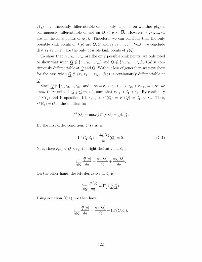
f(q) is continuously differentiable or not only depends on whether g(q) is

continuously differentiable or not on Q < q < Q. However, r1, r2, ..., rm

are all the kink points of g(q). Therefore, we can conclude that the only

possible kink points of f(q) are Q,Q and r1, r2, ..., rm. Next, we conclude

that r1, r2, ..., rm are the only possible kink points of f(q).

To show that r1, r2, ..., rm are the only possible kink points, we only need

to show that when Q /∈ {r1, r2, ..., rm} and Q /∈ {r1, r2, ..., rm}, f(q) is con-

tinuously differentiable at Q and Q. Without loss of generality, we next show

for the case when Q /∈ {r1, r2, ..., rm}, f(q) is continuously differentiable at

Q.

Since Q /∈ {r1, r2, ..., rm} and −∞ = r0 < r1 < ... < rm < rm+1 = +∞, we

know there exists 1 ≤ j ≤ m + 1, such that rj−1 < Q < rj. By continuity

of r∗(q) and Proposition 4.1, rj−1 < r∗(Q) = r+(Q) = Q < rj. Thus,

r+(Q) = Q is the solution to:

f+(Q) = maxr{Π+(r,Q) + gj(r)}.

By the first order condition, Q satisfies

Π+r (Q,Q) +

dgj(r)

dr(Q) = 0. (C.1)

Now, since rj−1 < Q < rj, the right derivative at Q is

limq↓Q

df(q)

dq=dπ(Q)

dq+dgj(Q)

dq.

On the other hand, the left derivative at Q is

limq↑Q

df(q)

dq= Π+

q (Q,Q).

Using equation (C.1), we then have

limq↓Q

df(q)

dq=dπ(Q)

dq− Π+

r (Q,Q).

122

Using total derivative, we then have Π+r (q, q) + Π+

q (q, q) = dπ(q)dq

. That is,

limq↓Q

df(q)

dq= lim

q↑Q

df(q)

dq,

which shows that f(q) is continuously differentiable at Q. The differentiabil-

ity at Q can be proved similarly.


Suppose that Gt(r) is strongly concave with concavity constant At = 2αat+η−

2(1−α).

We will next show first that Gt+1(r) is also strongly concave. The argument

we use also implies the base case G2(r) is strongly concave.

Let Gt(r) = Gt(r) + Atr2 and Bt = 2at+η+

2(1−α), then the Bellman equation

(4.3) can be rewritten as

Gt+1(q) = maxr{Πt(r, q)− Atr2 +Btq

2 + (At+1 −Bt)q2 + Gt(r)}.

By inductive hypothesis, Gt(r) is concave. To prove Gt+1(q) is also concave,

it is sufficient to prove that the objective function is jointly concave in r and

q. We prove this by showing that Πt(r, q)− Atr2 + Btq2 is a jointly concave

function and At+1 −Bt ≤ 0.

Note that Πt(r, q) = min{Π+t (r, q),Π−t (r, q)}, where

Π±t (r, q) = − at + η±

(1− α)2q2+

2αat + (1 + α)η±

(1− α)2qr−α

2at + αη±

(1− α)2r2+

bt1− α

q− btα

1− αr.

From the expression above, we can obtain the Hessian of Π±t (r, q)−Atr2+Btq2

as

1

(1− α)2

[−2(at + η±) + 2(1− α)2Bt 2αat + (1 + α)η±

2αat + (1 + α)η± −2(α2at + αη±)− 2(1− α)2At

].

Substitute the expressions of At and Bt, it can be verified that above matrices

are diagonally dominant and consequently, Π±t (r, q)−Atr2 +Btq2 are jointly

concave. Thus, Πt(r, q)− Atr2 +Btq2 is also jointly concave.

123

To guarantee At+1 −Bt ≤ 0, we need

2αat+1 + η−

2(1− α)≤ 2at + η+

2(1− α),

which is guaranteed by Assumption 4.4.

Finally, note that G2(r) = Π1(r1, r)+B1r2 +(A2−B1)r2. By the fact that

Π1(r1, r) − A1r21 + B1r

2 is jointly concave as shown above, Π1(r1, r) + B1r2

is concave in r. Thus, G2(r) is also concave in r.

To show the second claim, first recall that

G2(r) =

{g2(r), r ∈ [αr1 + (1− α)L1, αr1 + (1− α)U1],

−∞, r ∈ (−∞, αr1 + (1− α)L1) ∪ (αr1 + (1− α)U1,+∞),

which shows that the claim holds for the base case. Now suppose for t ≥ 2,

Gt(r) =

{gt(r), r ∈ [rt, rt],

−∞, r ∈ (−∞, rt) ∪ (rt,+∞).

When α > 0, the price constraint is equivalent as r ∈ [ q−(1−α)Ut

α, q−(1−α)Lt

α].

If [ q−(1−α)Ut

α, q−(1−α)Lt

α]∩ [rt, rt] = ∅, then Gt+1(q) = −∞. That is, we can let

rt+1 = αrt + (1 − α)Lt and rt+1 = αrt + (1 − α)Ut. When α = 0, clearly,

rt+1 = Lt and rt+1 = Ut. In summary, we then have

Gt+1(r) =

{gt+1(r), r ∈ [rt+1, rt+1],

−∞, r ∈ (−∞, rt+1) ∪ (rt+1,+∞).


Since the objective function is strict concave in r and continuous, Maximum

Theorem (Ok, 2007) guarantees that r∗c (q) is single-valued and continuous in

q.

For the second part, it is shown in Chen et al. (2013) that Π(r, q) is super-

modular. Also, note that the constraint set [ q−(1−α)Ut

α, q−(1−α)Lt

α] is ascending

with q. Therefore, by Theorem 2.2.8 in Simchi-Levi et al. (2014), r∗c (q) is in-

creasing in q. To show the monotonicity for p∗c(q), by variable transformation,

124

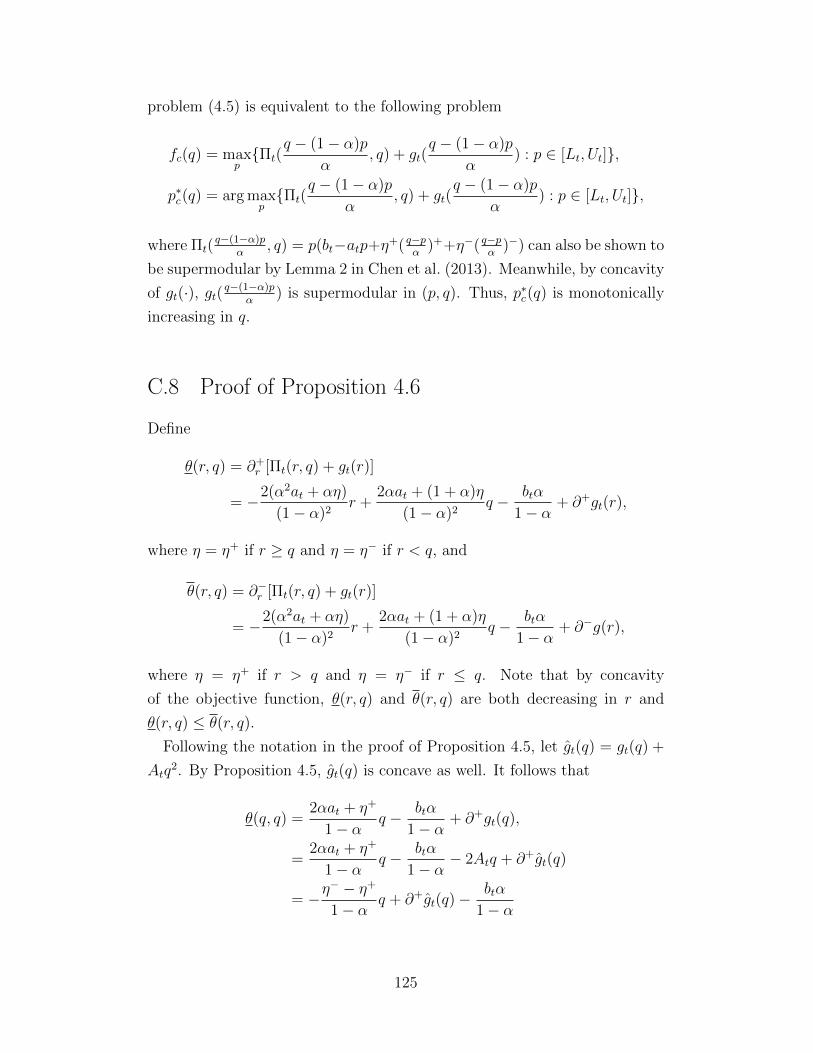
problem (4.5) is equivalent to the following problem

fc(q) = maxp{Πt(

q − (1− α)p

α, q) + gt(

q − (1− α)p

α) : p ∈ [Lt, Ut]},

p∗c(q) = arg maxp{Πt(

q − (1− α)p

α, q) + gt(

q − (1− α)p

α) : p ∈ [Lt, Ut]},

where Πt(q−(1−α)p

α, q) = p(bt−atp+η+( q−p

α)++η−( q−p

α)−) can also be shown to

be supermodular by Lemma 2 in Chen et al. (2013). Meanwhile, by concavity

of gt(·), gt( q−(1−α)pα

) is supermodular in (p, q). Thus, p∗c(q) is monotonically

increasing in q.


Define

θ(r, q) = ∂+r [Πt(r, q) + gt(r)]

= −2(α2at + αη)

(1− α)2r +

2αat + (1 + α)η

(1− α)2q − btα

1− α+ ∂+gt(r),

where η = η+ if r ≥ q and η = η− if r < q, and

θ(r, q) = ∂−r [Πt(r, q) + gt(r)]

= −2(α2at + αη)

(1− α)2r +

2αat + (1 + α)η

(1− α)2q − btα

1− α+ ∂−g(r),

where η = η+ if r > q and η = η− if r ≤ q. Note that by concavity

of the objective function, θ(r, q) and θ(r, q) are both decreasing in r and

θ(r, q) ≤ θ(r, q).

Following the notation in the proof of Proposition 4.5, let gt(q) = gt(q) +

Atq2. By Proposition 4.5, gt(q) is concave as well. It follows that

θ(q, q) =2αat + η+

1− αq − btα

1− α+ ∂+gt(q),

=2αat + η+

1− αq − btα

1− α− 2Atq + ∂+gt(q)

= −η− − η+

1− αq + ∂+gt(q)−

btα

1− α

125

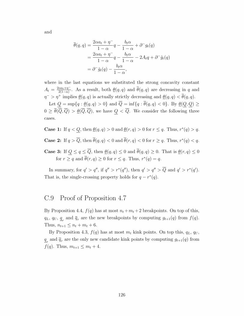
and

θ(q, q) =2αat + η−

1− αq − btα

1− α+ ∂−gt(q)

=2αat + η−

1− αq − btα

1− α− 2Atq + ∂−gt(q)

= ∂−gt(q)−btα

1− α,

where in the last equations we substituted the strong concavity constant

At = 2αat+η−

2(1−α). As a result, both θ(q, q) and θ(q, q) are decreasing in q and

η− > η+ implies θ(q, q) is actually strictly decreasing and θ(q, q) < θ(q, q).

Let Q = sup{q : θ(q, q) > 0} and Q = inf{q : θ(q, q) < 0}. By θ(Q,Q) ≥0 ≥ θ(Q,Q) > θ(Q,Q), we have Q < Q. We consider the following three

cases.

Case 1: If q < Q, then θ(q, q) > 0 and θ(r, q) > 0 for r ≤ q. Thus, r∗(q) > q.

Case 2: If q > Q, then θ(q, q) < 0 and θ(r, q) < 0 for r ≥ q. Thus, r∗(q) < q.

Case 3: If Q ≤ q ≤ Q, then θ(q, q) ≤ 0 and θ(q, q) ≥ 0. That is θ(r, q) ≤ 0

for r ≥ q and θ(r, q) ≥ 0 for r ≤ q. Thus, r∗(q) = q.

In summary, for q′ > q′′, if q′′ > r∗(q′′), then q′ > q′′ > Q and q′ > r∗(q′).

That is, the single-crossing property holds for q − r∗(q).


By Proposition 4.4, f(q) has at most nt+mt+2 breakpoints. On top of this,

qL, qU , qr

and qr are the new breakpoints by computing gt+1(q) from f(q).

Thus, nt+1 ≤ nt +mt + 6.

By Proposition 4.3, f(q) has at most mt kink points. On top this, qL, qU ,

qr

and qr are the only new candidate kink points by computing gt+1(q) from

f(q). Thus, mt+1 ≤ mt + 4.

126

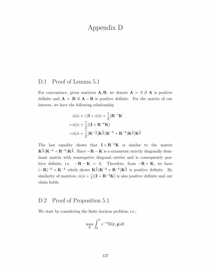
Appendix D

D.1 Proof of Lemma 5.1

For convenience, given matrices A,B, we denote A � 0 if A is positive

definite and A � B if A−B is positive definite. For the matrix of our

interest, we have the following relationship

α(α + γ)I + α(α +γ

2)R−1K

�α(α +γ

2)(I + R−1K)

=α(α +γ

2)K−

12 [K

12 (K−1 + R−1)K

12 ]K

12

The last equality shows that I + R−1K is similar to the matrix

K12 (K−1 + R−1)K

12 . Since −R−K is a symmetric strictly diagonally dom-

inant matrix with nonnegative diagonal entries and is consequently pos-

itive definite, i.e. −R−K � 0. Therefore, from −R � K, we have

(−R)−1 ≺ K−1 which shows K12 (K−1 + R−1)K

12 is positive definite. By

similarity of matrices, α(α + γ2)(I + R−1K) is also positive definite and our

claim holds.

D.2 Proof of Proposition 5.1

We start by considering the finite horizon problem, i.e.,

maxp

∫ T

0

e−γtΠ(r,p)dt.

127

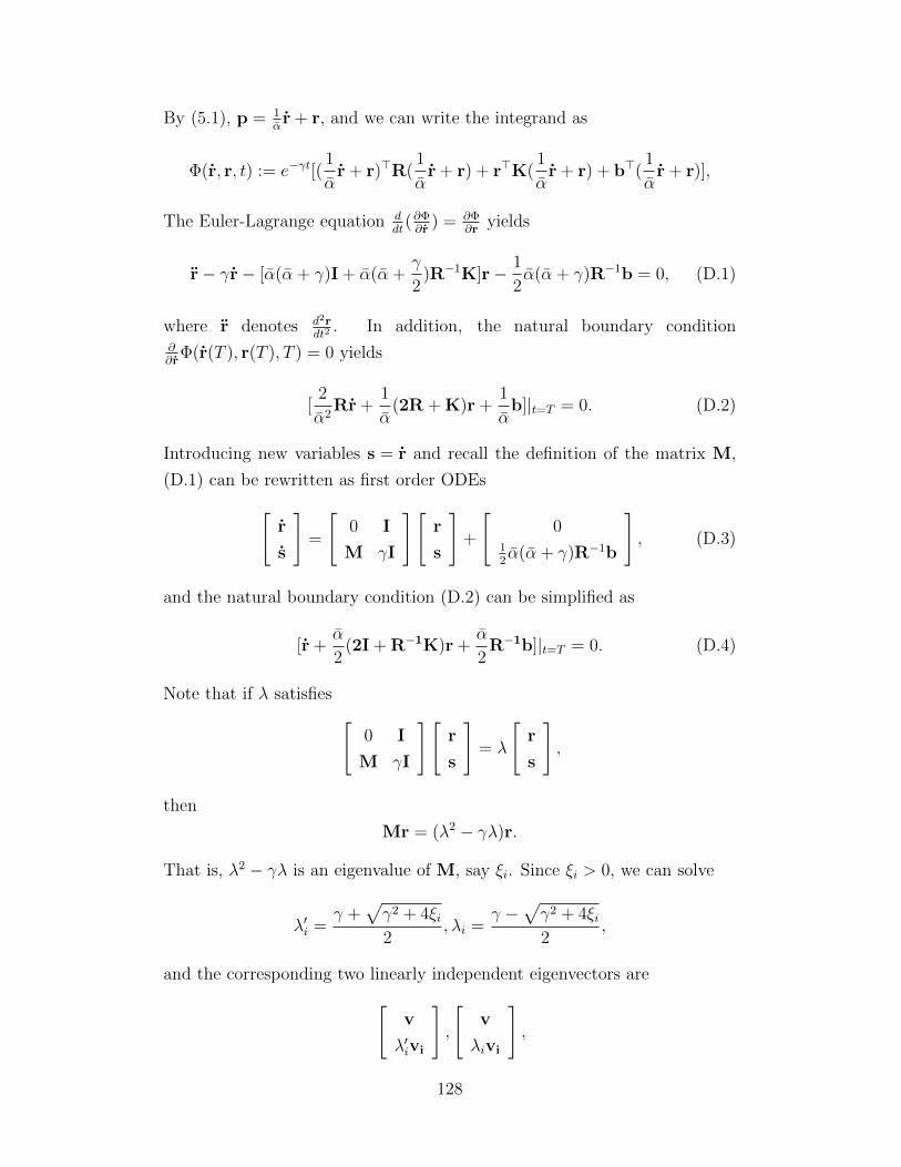
By (5.1), p = 1αr + r, and we can write the integrand as

Φ(r, r, t) := e−γt[(1

αr + r)>R(

1

αr + r) + r>K(

1

αr + r) + b>(

1

αr + r)],

The Euler-Lagrange equation ddt

(∂Φ∂r

) = ∂Φ∂r

yields

r− γr− [α(α + γ)I + α(α +γ

2)R−1K]r− 1

2α(α + γ)R−1b = 0, (D.1)

where r denotes d2rdt2

. In addition, the natural boundary condition∂∂r

Φ(r(T ), r(T ), T ) = 0 yields

[2

α2Rr +

1

α(2R + K)r +

1

αb]|t=T = 0. (D.2)

Introducing new variables s = r and recall the definition of the matrix M,

(D.1) can be rewritten as first order ODEs[r

s

]=

[0 I

M γI

][r

s

]+

[0

12α(α + γ)R−1b

], (D.3)

and the natural boundary condition (D.2) can be simplified as

[r +α

2(2I + R−1K)r +

α

2R−1b]|t=T = 0. (D.4)

Note that if λ satisfies [0 I

M γI

][r

s

]= λ

[r

s

],

then

Mr = (λ2 − γλ)r.

That is, λ2 − γλ is an eigenvalue of M, say ξi. Since ξi > 0, we can solve

λ′i =γ +

√γ2 + 4ξi2

, λi =γ −

√γ2 + 4ξi2

,

and the corresponding two linearly independent eigenvectors are[v

λ′ivi

],

[v

λivi

],

128

where vi is the eigenvector of M corresponding to ξi.

The ODEs (D.3) can then be solved explicitly as[r(t)

s(t)

]=c′1

[v1

λ′1v1

]eλ′1t + c1

[v1

λ1v1

]eλ1t + ...+

c′N

[vN

λ′NvN

]eλ′N t + cN

[vN

λNvN

]eλN t +

[rs

0

] (D.5)

where (rs,0) is a particular solution to the non-homogeneous system and

c′1, c1, ..., c′N , cN are constants to be determined from boundary conditions.

We next show that when T → ∞ the natural boundary condition (D.4)

implies limt→∞

r(t) <∞, which in turn implies c′1 = c′2 = ... = c′N = 0. First, we

note that when t is large enough, the value of ri(t) will be mainly dominated

by c′kvkieλ′kt for some k, where λ′k is the largest eigenvalue and vki is the i-th

component of vk. Similarly, ri(t) will also be dominated by c′kvkiλ′keλ′kt and

consequently has the same sign as ri(t), i.e. ri(t)si(t) ≥ 0. If we left multiply

r(t) on both side of (D.4), then

[r>r +α

2r>(2I + R−1K)r +

α

2R−1br]|t=T = 0.

However, if limt→∞

ri(t) = ∞ for some i, then r>(2I + R−1K)r > r>r → +∞as t → +∞ and will dominate the linear term R−1br. In the mean time

r>r =N∑i=1

ri(t)si(t) ≥ 0 for any t. Thus,

limT→∞

[r>r +β

2r>(2I + R−1K)r +

β

2R−1br]|t=T = +∞,

a contradiction.

Hence, when T →∞, we have derived the solution to (D.1) as

r∗(t) = c1v1eλ1t + ...+ cNvNe

λN t + rs, (D.6)

where c = (c1, ..., cN)> can be solved by

c =V−1(r0 − rs) (D.7)

with the particular solution or the steady state rs being the solution to the

129

equation (5.5). Substitute (D.7) into (D.6), we then arrive at (5.6). The

expressions for the price path and the pricing strategy (5.7) are immediate

consequence of (5.6) and (5.2).

In the remaining, we verify the sufficient conditions for the solution of

Euler-Lagrange equation (D.1) to be the maximizer of (5.3) (see Liberzon,

2011, for a reference on the topic of calculus of variation).

First of all, note that ∂2Φ∂r2

= e−γt 2α2 R is negative definite for any t ≥ 0.

Thus, the strengthened Legendre condition is satisfied.

Second, the Jacobi equation of the variational problem is

x− γx−Mx = 0, (D.8)

which is exactly the homogeneous version of equation (D.1). From our pre-

vious analysis, (D.8) admits a set of N linearly independent solutions

x1 = (eλ′1t − eλ1t)v1, ...,xN = (eλ

′N t − eλN t)vN.

Equivalently, we have

det([

x1 ... xN

]) 6= 0

for any t > 0. Therefore, there is no conjugate point to t = 0 in (0,∞).

Finally, we check the Weierstrass excess function.

E(w, r, r, t) =Φ(w, r, t)− Φ(r, r, t)− (w − r)>∂

∂rΦ(r, r, t)

=e−γt[(1

αw + r)>R(

1

αw + r)− (

1

αr + r)>R(

1

αr + r)

+1

αr>K(w − r) +

1

αb>(w − r)

− 2

α2(w − r)>Rr− 1

α(w − r)>(2R + K)r− 1

α(w − r)>b]

=e−γt1

α2(w − r)>R(w − r) < 0

The last inequality is due to the negative definite property of matrix R.

130


Since we can translate any time point s ≥ 0 back to s = 0, it is sufficient

to show that for any initial reference price r0, there exists T such that the

price path pSM(t), 0 ≤ t ≤ T and reference price path rSM(t), 0 ≤ t ≤ T

generated by pSM(r) maximizes

maxp

∫ T

0

e−γtΠ(r,p)dt

s.t. r = α(p− r),

r(T ) = rSM(T ).

(D.9)

Without loss of generality, we assume r0 ∈ I++. The other cases can be

proved similarly. We let T be the first time rSM(t) exits I++, i.e., the first

time switching occurs. In this case, the objective value of the above problem

under pSM(t), 0 ≤ t ≤ T is∫ T

0

e−γtΠ++(rSM(t),pSM(t))dt,

since rSM(t) ∈ I++ for all 0 ≤ t ≤ T and by definition pSMi (t) − rSMi (t) =

p++i (rSM(t)) − rSMi (t) < 0 for i = 1, 2. Note that on 0 ≤ t ≤ T , pSM(t) =

p++(t), where p++(t), t ≥ 0, denotes the price path generated by p++(r) and

is optimal to the infinite horizon problem

maxp

∫ ∞0

e−γtΠ++(r,p)dt

s.t. r = α(p− r).

(D.10)

We first show that pSM(t), 0 ≤ t ≤ T is optimal to the problem

maxp

∫ T

0

e−γtΠ++(r,p)dt

s.t. r = α(p− r),

r(T ) = rSM(T ).

(D.11)

Suppose p′(t), 0 ≤ t ≤ T and the corresponding reference price path

r′(t), 0 ≤ t ≤ T satisfying r′(T ) = rSM(T ) generate a higher value than∫ T0e−γtΠ++(rSM(t),pSM(t))dt, then we can construct a solution to the infi-

131

nite horizon problem (D.10) as follows:

p(t) =

{p′(t), 0 ≤ t ≤ T,

p++(t), t > T.

It follows that∫ ∞0

e−γtΠ++(r, p)dt =

∫ T

0

e−γtΠ++(r,p′)dt+

∫ ∞T

e−γtΠ++(r,p++)dt

>

∫ T

0

e−γtΠ++(r,p++)dt+

∫ ∞T

e−γtΠ++(r,p++)dt,

where we have suppressed the dependency of reference price path r on the

corresponding price path for brevity. This leads to a contradiction to p++(t)

being optimal to problem (D.10).

Next, we show that pSM(t), 0 ≤ t ≤ T is optimal to the problem (D.9).

Indeed, for any pricing path p(t), it holds∫ T

0

e−γtΠ(r,p)dt ≤∫ T

0

e−γtΠ++(r,p)dt ≤∫ T

0

e−γtΠ++(rSM(t),pSM(t))dt,

where the first inequality is due to the fact that η+i < η−i , i = 1, 2 and the

second inequality is due to the optimality of pSM(t) to (D.11).

If no switch occurs, i.e., rSM(t) ∈ I++ for all t ≥ 0, then letting T = ∞,

the second claim follows from above analysis.


Since the matrix is two dimensional, we can write the eigenvalues and eigen-

vectors explicitly. Namely, let λ1, λ2 be the two eigenvalues, then

λ1 =a+ d

2+ [

(a+ d)2

4− (ad− bc)]

12 ,

λ2 =a+ d

2− [

(a+ d)2

4− (ad− bc)]

12 ,

132

and

v1 =

[λ1 − dc

],

v2 =

[λ2 − dc

].

It follows that

(λ1 − d)(λ2 − d)

=(a− d)2

4− [

(a+ d)2

4− (ad− bc)]

=− bc < 0.

Thus, if λ1 − d < 0, then v11v12 > 0, v21v22 < 0, otherwise swapping the

notations of v1,v2, the result still holds.


Following the convention of our notations, we let Λ++ to be the matrix Λ

defined in Proposition 5.1 when N = 2, η1 = η+1 , η2 = η+

2 and V++ to be

the matrix of eigenvectors of M++. By Proposition 5.1, the dynamics (5.10)

restricted to the region I++ can be explicitly written as

r = V++Λ++(V++)−1(r− r++s ). (D.12)

Clearly, M++ has the same eigenvectors as V++Λ++(V++)−1 and we claim

that one of their eigenvectors, say v = (v1, v2) satisfies v + r++s ∈ I++. Note

that we can always let x = r− r++s to shift the whole system such that the

steady state is the origin. Therefore, to simplify the presentation, we assume

without loss of generality that r++s = 0. In this case, it is equivalent to show

v ∈ I++, where

I++ = {r|p++1 (r)− r1 < 0, p++

2 (r)− r2 < 0}

= {r| 1α

V++Λ++(V++)−1r < 0}.

133

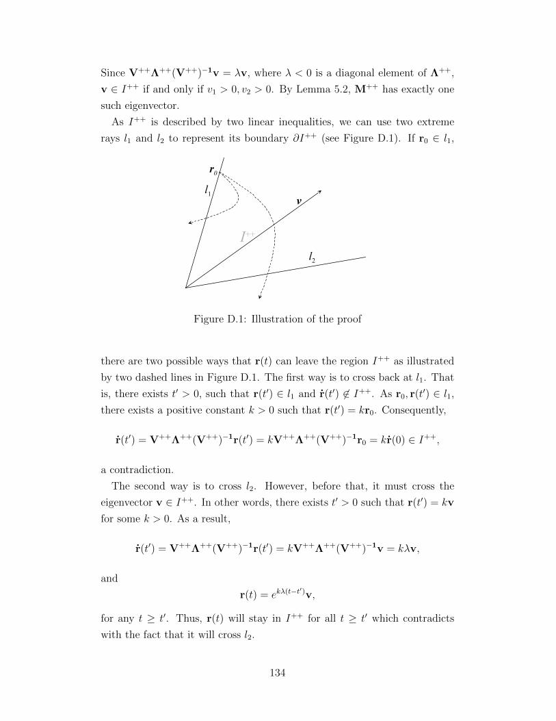
Since V++Λ++(V++)−1v = λv, where λ < 0 is a diagonal element of Λ++,

v ∈ I++ if and only if v1 > 0, v2 > 0. By Lemma 5.2, M++ has exactly one

such eigenvector.

As I++ is described by two linear inequalities, we can use two extreme

rays l1 and l2 to represent its boundary ∂I++ (see Figure D.1). If r0 ∈ l1,

I++

Sl1

Sl2

Sv

Sr0

Figure D.1: Illustration of the proof

there are two possible ways that r(t) can leave the region I++ as illustrated

by two dashed lines in Figure D.1. The first way is to cross back at l1. That

is, there exists t′ > 0, such that r(t′) ∈ l1 and r(t′) 6∈ I++. As r0, r(t′) ∈ l1,

there exists a positive constant k > 0 such that r(t′) = kr0. Consequently,

r(t′) = V++Λ++(V++)−1r(t′) = kV++Λ++(V++)−1r0 = kr(0) ∈ I++,

a contradiction.

The second way is to cross l2. However, before that, it must cross the

eigenvector v ∈ I++. In other words, there exists t′ > 0 such that r(t′) = kv

for some k > 0. As a result,

r(t′) = V++Λ++(V++)−1r(t′) = kV++Λ++(V++)−1v = kλv,

and

r(t) = ekλ(t−t′)v,

for any t ≥ t′. Thus, r(t) will stay in I++ for all t ≥ t′ which contradicts

with the fact that it will cross l2.

134

In summary, as r(t) can neither cross l1 nor l2, it has to stay in I++ for all

t ≥ 0 and follows the dynamics (D.12), which results in limt→∞ r(t) = rs++.


There are three cases. First, if r0 ∈ S, then r(t) = r0 for any t and our claim

holds.

Second, if r0 ∈ I+r2 , I−r2 , Ir1+ or Ir1− (here we suppose r0 ∈ I+r2 without

loss of generality), then either

limt→∞

r(t) = rs+r2 ,

where rs+r2 ∈ S is the steady state to the system r1 = α(p+r2

1 (r1)−r1), r2 = 0,

or there exists t′ such that r(t′) ∈ ∂I++ or r(t′) ∈ ∂I+−. By Lemma 5.3,

when r(t′) ∈ ∂I++ or r(t′) ∈ ∂I+−, it then follows

limt→∞

r(t) = r++s or lim

t→∞r(t) = r+−

s .

Finally, if r0 ∈ I++, I+−, I−+ or I−− (again we assume r0 ∈ I++ without

loss of generality), then either

limt→∞

r(t) = r++s

or there exists t′ such that r(t′) ∈ I+r2 or r(t′) ∈ Ir1+ and we are back to

the second case. Thus, with at most two switches, the reference price path

converges to a steady state in S.

135

References

Aflaki, Sam, Ioana Popescu. 2013. Managing retention in service relation-ships. Management Science 60(2) 415–433.

Ahn, H., M. Gumus, P. Kaminsky. 2007. Pricing and manufacturing deci-sions when demand is a function of prices in multiple periods. OperationsResearch-Baltimore 55(6) 1039–1057.

Allenby, Greg M, Peter E Rossi. 1998. Marketing models of consumer het-erogeneity. Journal of Econometrics 89(1) 57–78.

Anderson, B. D. O., J. B. Moore. 2007. Optimal control: linear quadraticmethods . Courier Corporation.

Asvanunt, A. 2007. Applications of dynamic optimization to strategic pricingand corporate finance. Ph.D. thesis, Columbia University.

Bardi, Martino, Italo Capuzzo-Dolcetta. 1997. Optimal control and viscos-ity solutions of Hamilton-Jacobi-Bellman equations . Springer Science &Business Media.

Bell, D. R., J. M. Lattin. 2000. Looking for loss aversion in scanner paneldata: The confounding effect of price response heterogeneity. MarketingScience 19(2) 185–200.

Besbes, Omar, Ilan Lobel. 2015. Intertemporal price discrimination: Struc-ture and computation of optimal policies. Management Science 61(1)92–110.

Boatwright, P., R. McCulloch, P. Rossi. 1999. Account-level modeling fortrade promotion: An application of a constrained parameter hierarchicalmodel. Journal of the American Statistical Association 94(448) 1063–1073.

Briesch, R.A., L. Krishnamurthi, T. Mazumdar, S.P Raj. 1997. A compar-ative analysis of reference price models. Journal of Consumer Research24(2) 202–214.

Chen, X., P. Hu, S. Shum, Y. Zhang. 2013. Stochastic inventory model withreference price effects. Working Paper .

136

Chen, X., D. Simchi-Levi. 2004a. Coordinating inventory control and pricingstrategies with random demand and fixed ordering cost: The finite horizoncase. Operations Research 52(6) 887–896.

Chen, X., D. Simchi-Levi. 2004b. Coordinating inventory control and pric-ing strategies with random demand and fixed ordering cost: The infinitehorizon case. Mathematics of Operations Research 29(3) 698–723.

Chen, X., D. Simchi-Levi. 2006. Coordinating inventory control and pricingstrategies: The continuous review model. Operations Research Letters34(3) 323–332.

Chen, X., D. Simchi-Levi. 2012. Pricing and inventory management. TheOxford handbook of pricing management. Oxford University Press, Oxford.

Chevalier, J. A., A. K. Kashyap, P. E. Rossi. 2003. Why don’t prices riseduring periods of peak demand? evidence from scanner data. AmericanEconomic Review 93(1) 15–37.

Clausen, A., C. Strub. 2012. Envelope theorems for non-smooth and non-concave optimization. Working Paper .

Conlisk, J., E. Gerstner, J. Sobel. 1984. Cyclic pricing by a durable goodsmonopolist. The Quarterly Journal of Economics 99 489–505.

Cox, John C., Jonathan E. Ingersoll Jr., Stephen A. Ross. 1985. A theory ofthe term structure of interest rates. Econometrica 53 385–407.

DeCarlo, Raymond A, Michael S Branicky, Stefan Pettersson, Bengt Lennart-son. 2000. Perspectives and results on the stability and stabilizability ofhybrid systems. Proceedings of the IEEE 88(7) 1069–1082.

Edlin, A. S., C. Shannon. 1998. Strict monotonicity in comparative statics.Journal of Economic Theory 81(1) 201–219.

Elmaghraby, W., P. Keskinocak. 2003. Dynamic pricing in the presence ofinventory considerations: Research overview, current practices, and futuredirections. Management Science 49 1287–1309.

Federgruen, A., A. Heching. 1999. Combined pricing and inventory controlunder uncertainty. Operations Research 47(3) 454–475.

Fibich, G., A. Gavious, O. Lowengart. 2003. Explicit solutions of op-timization models and differential games with nonsmooth (asymmetric)reference-price effects. Operations Research 51(5) 721–734.

Fleming, W. H., R. W. Rishel. 1982. Deterministic and stochastic optimalcontrol . Springer.

137

Freedman, David. 1984. On bootstrapping two-stage least-squares estimatesin stationary linear models. The Annals of Statistics 12(3) 827–842.

Gallego, Guillermo, Ruxian Wang. 2014. Multiproduct price optimizationand competition under the nested logit model with product-differentiatedprice sensitivities. Operations Research 62(2) 450–461.

Geng, Q., C. Wu, K. Li. 2010. Pricing and promotion frequency in thepresence of reference price effects in supply chains. California Journal ofOperations Management 8(1) 74–82.

Geunes, J., Y. Merzifonluoglu, H. E. Romeijn. 2009. Capacitated procure-ment planning with price-sensitive demand and general concave-revenuefunctions. European Journal of Operational Research 194(2) 390–405.

Gimpl-Heersink, D. I. L. 2008. Joint pricing and inventory control underreference price effects. Ph.D. thesis, Vienna University of Economics andBusiness Administration.

Greenleaf, E.A. 1995. The impact of reference price effects on the profitabilityof price promotions. Marketing Science 14(1) 82–82.

Hardie, B.G.S., E.J. Johnson, P.S. Fader. 1993. Modeling loss aversion andreference dependence effects on brand choice. Marketing Science 12(4)378–394.

Heston, Steven L. 1993. A closed-form solution for options with stochas-tic volatility with applications to bond and currency options. Review offinancial studies 6(2) 327–343.

Hirsch, M. W., S. Smale, R. L. Devaney. 2004. Differential Equations, Dy-namical Systems and An Introduction to Chaos . Elsevier/Academic Press.

Hu, P. 2012. Coordinated pricing and inventory management. Ph.D. thesis,University of Illinois at Urbana-Champaign.

Huh, W. T., G. Janakiraman. 2008. (s, S) optimality in joint inventory-pricing control: An alternate approach. Oper. Res. 56 783–790.

Jain, P., S. Banerjee. 2003. Border-collision bifurcations in one-dimensionaldiscontinuous maps. Int. J. Bifur. Chaos 13 3341–3351.

James, G., D. Witten, T. Hastie, R. Tibshirani. 2013. An Introduction toStatistical Learning with Applications in R. Springer, New York.

Kallio, Markku, Merja Halme. 2009. Redefining loss averse and gain seekingconsumer price behavior based on demand response. Working Paper .

138

Kalyanaram, G., J.D.C. Little. 1994. An empirical analysis of latitude of priceacceptance in consumer package goods. Journal of Consumer Research21(3) 408–418.

Kopalle, P.K., R.S. Winer. 1996. A dynamic model of reference price andexpected quality. Marketing Letters 7(1) 41–52.

Kopalle, Praveen K., P.K. Kannan, Lin Bao Boldt, Neeraj Arora. 2012. Theimpact of household level heterogeneity in reference price effects on optimalretailer pricing policies. Journal of Retailing 88(1) 102–114.

Kopalle, Praveen K., Ambar G. Rao, Jo L. Assuno. 1996. Asymmetric refer-ence price effects and dynamic pricing policies. Marketing Science 15(1)60–85.

Krishnamurthi, L., T. Mazumdar, S. P. Raj. 1992. Asymmetric responseto price in consumer brand choice and purchase quantity decisions. TheJournal of Consumer Research 19(3) 387–400.

Lattin, James M, Randolph E Bucklin. 1989. Reference effects of price andpromotion on brand choice behavior. Journal of Marketing research 299–310.

Liberzon, Daniel. 2003. Switching in systems and control . Springer Science& Business Media.

Liberzon, Daniel. 2011. Calculus of variations and optimal control theory: aconcise introduction. Princeton University Press.

Liu, Y., W. L. Cooper. 2014. Optimal dynamic pricing with patient cus-tomers. Working Paper .

Mayhew, G. E., R. S. Winer. 1992. An empirical analysis of internal andexternal reference prices using scanner data. The Journal of ConsumerResearch 19(1) 62–70.

Mazumdar, T., S. P. Raj, I. Sinha. 2005. Reference price research: Reviewand propositions. Journal of Marketing 69(4) 84–102.

Mazumdar, Tridib, Purushottam Papatla. 1995. Loyalty differences in the useof internal and external reference prices. Marketing Letters 6(2) 111–122.

Milgrom, P., I. Segal. 2002. Envelope theorems for arbitrary choice sets.Econometrica 70(2) 583–601.

Miranda, Mario J, Paul L Fackler. 2004. Applied computational economicsand finance. MIT press.

139

Nasiry, J., I. Popescu. 2011. Dynamic pricing with loss-averse consumers andpeak-end anchoring. Operations Research 59(6) 1361–1368.

Natter, Martin, Thomas Reutterer, Andreas Milde, Alfred Taudes. 2007. Anassortmentwide decision-support system for dynamic pricing and promo-tion planning in diy retailing. Marketing Science 26(4) 576–583.

Ok, E. A. 2007. Real analysis with economic applications , vol. 10. PrincetonUniversity Press.

Øksendal, Bernt. 2002. Stochastic Differential Equations: An Introductionwith Applications . Springer-Verlag New York.

Petruzzi, N.C., M. Dada. 1999. Pricing and the newsvendor problem: Areview with extensions. Oper. Res. 47 183–194.

Popescu, I., Y. Wu. 2007. Dynamic pricing strategies with reference effects.Operations Research 55(3) 413–429.

Popescu, Ioana, Yaozhong Wu. 2005. Dynamic pricing strategies under re-peated interactions. Working paper, INSEAD, Fontainebleau, France .

Rajendran, Kharan N, Gerard J Tellis. 1994. Contextual and temporal com-ponents of reference price. Journal of Marketing 58 22–34.

Rajpathak, B., H. K. Pillai, S. Bandyopadhyay. 2012. Analysis of stableperiodic orbits in the one dimensional linear piecewise-smooth discontinu-ous map. Chaos: An Interdisciplinary Journal of Nonlinear Science 22(3)033126.

Raman, K., F.M. Bass. 2002. A general test of reference price theory in thepresence of threshold effects. Tijdschrift Voor Economie En Management47(2) 205–226.

Sharkovsky, A.N., L.O. Chua. 1993. Chaos in some 1-d discontinuous mapsthat appear in the analysis of electrical circuits. Circuits and SystemsI: Fundamental Theory and Applications, IEEE Transactions on 40(10)722–731.

Simchi-Levi, D., X. Chen, J. Bramel. 2014. The Logic of Logistics: Theory,Algorithms, and Applications for Logistics and Supply Chain Management,Third Edition. Springer.

Stokey, N. L., R. E. Lucas, E. C. Prescott. 1989. Recursive Methods inEconomic Dynamics . Harvard University Press.

Talluri, K. T., G. J. Van Ryzin. 2005. The Theory and Practice of RevenueManagement . Springer Science & Business Media.

140

Tversky, A., D. Kahneman. 1991. Loss aversion in riskless choice: Areference-dependent model. The Quarterly Journal of Economics 106(4)1039.

Weiss, R.M., A.K. Mehrotra. 2001. Online dynamic pricing: Efficiency, equityand the future of e-commerce. Virginia Journal of Law and TechnologyAssociation 6 11–17.

Zhang, Yuhan. 2011. Essays on robust optimization, integrated inventoryand pricing, and reference price effect. Ph.D. thesis, University of Illinoisat Urbana-Champaign.

141

c 2015 zhenyu hu - ideals

Documents