c 2016 reid edward ﬀ - university of florida

DESIGN OF A COMPACT, LIGHTWEIGHT ABSORPTION CHILLER

By

REID EDWARD SHAEFFER

A DISSERTATION PRESENTED TO THE GRADUATE SCHOOLOF THE UNIVERSITY OF FLORIDA IN PARTIAL FULFILLMENT

OF THE REQUIREMENTS FOR THE DEGREE OFDOCTOR OF PHILOSOPHY

UNIVERSITY OF FLORIDA

2016

c⃝ 2016 Reid Edward Shaeffer

To my parents, for their unconditional support and love

ACKNOWLEDGMENTS

I would like to thank my advisor, Dr. Saeed Moghaddam, for his support throughout my

studies. His guidance has taught me many skills that I will undoubtedly use for the rest of my

life.

I thank my committee members; Dr. David Hahn, Dr. Brent Gila, and Dr. Herbert

Ingley for their guidance in my academic career. I would like to thank Dr. Fregly at the for

his counsel; starting with my concerns about graduate school. I would also like to thank Dr.

Angela Lindner for her encouragement from the very beginning.

I cannot continue without mentioning my colleagues; Abdolreza Fazeli, Abhilash Paneri,

Devesh Chugh, Drew Gonsalves, Mehdi Mortazavi, Mike Schmid, Saitej Ravi, and Richard

Rode for their support. They have always been extremely generous and ready to help wherever

possible. It is not every day one comes across a group of friends such as them.

I would like to thank my lifelong friend Louis Searcy. Louis has always been there for me,

no matter the circumstances. He has shown me the potential life holds. It is without question

that I would not be here today without him.

4

TABLE OF CONTENTS

page

ACKNOWLEDGMENTS . . . . . . . . . . . . . . . . . . . . . . . . . . . . . . . . . . . 4

LIST OF TABLES . . . . . . . . . . . . . . . . . . . . . . . . . . . . . . . . . . . . . . 8

LIST OF FIGURES . . . . . . . . . . . . . . . . . . . . . . . . . . . . . . . . . . . . . 9

ABSTRACT . . . . . . . . . . . . . . . . . . . . . . . . . . . . . . . . . . . . . . . . . 14

CHAPTER

1 INTRODUCTION . . . . . . . . . . . . . . . . . . . . . . . . . . . . . . . . . . . 16

2 NUMERICAL METHODS . . . . . . . . . . . . . . . . . . . . . . . . . . . . . . . 20

2.1 Motivation . . . . . . . . . . . . . . . . . . . . . . . . . . . . . . . . . . . . 202.2 Methods . . . . . . . . . . . . . . . . . . . . . . . . . . . . . . . . . . . . . 22

2.2.1 Fluid Property Functions . . . . . . . . . . . . . . . . . . . . . . . . . 262.2.2 Governing Equations . . . . . . . . . . . . . . . . . . . . . . . . . . . 272.2.3 Solver . . . . . . . . . . . . . . . . . . . . . . . . . . . . . . . . . . . 302.2.4 Half Effect . . . . . . . . . . . . . . . . . . . . . . . . . . . . . . . . 312.2.5 User Interface . . . . . . . . . . . . . . . . . . . . . . . . . . . . . . . 332.2.6 Results . . . . . . . . . . . . . . . . . . . . . . . . . . . . . . . . . . 342.2.7 Validation . . . . . . . . . . . . . . . . . . . . . . . . . . . . . . . . . 38

3 EXPERIMENTAL METHODS . . . . . . . . . . . . . . . . . . . . . . . . . . . . . 40

3.1 Motivation . . . . . . . . . . . . . . . . . . . . . . . . . . . . . . . . . . . . 403.2 Concept . . . . . . . . . . . . . . . . . . . . . . . . . . . . . . . . . . . . . 41

3.2.1 Absorption . . . . . . . . . . . . . . . . . . . . . . . . . . . . . . . . 413.2.2 Vacuum Requirements . . . . . . . . . . . . . . . . . . . . . . . . . . 43

3.3 Generation 1 . . . . . . . . . . . . . . . . . . . . . . . . . . . . . . . . . . . 453.3.1 Design . . . . . . . . . . . . . . . . . . . . . . . . . . . . . . . . . . 453.3.2 Fabrication . . . . . . . . . . . . . . . . . . . . . . . . . . . . . . . . 463.3.3 Characteristics . . . . . . . . . . . . . . . . . . . . . . . . . . . . . . 47



3.6 Generation 4 . . . . . . . . . . . . . . . . . . . . . . . . . . . . . . . . . . . 533.6.1 Design . . . . . . . . . . . . . . . . . . . . . . . . . . . . . . . . . . 533.6.2 Fabrication . . . . . . . . . . . . . . . . . . . . . . . . . . . . . . . . 54

5

3.6.3 Characteristics . . . . . . . . . . . . . . . . . . . . . . . . . . . . . . 553.7 Generation 5 . . . . . . . . . . . . . . . . . . . . . . . . . . . . . . . . . . . 55

3.7.1 Design . . . . . . . . . . . . . . . . . . . . . . . . . . . . . . . . . . 553.7.2 Fabrication . . . . . . . . . . . . . . . . . . . . . . . . . . . . . . . . 563.7.3 Characteristics . . . . . . . . . . . . . . . . . . . . . . . . . . . . . . 58

3.8 Generation 6 . . . . . . . . . . . . . . . . . . . . . . . . . . . . . . . . . . . 583.8.1 Design . . . . . . . . . . . . . . . . . . . . . . . . . . . . . . . . . . 58

3.9 Generation 7 . . . . . . . . . . . . . . . . . . . . . . . . . . . . . . . . . . . 59

4 SYSTEM DEVELOPMENT . . . . . . . . . . . . . . . . . . . . . . . . . . . . . . 72

4.1 Environmental Interaction . . . . . . . . . . . . . . . . . . . . . . . . . . . . 724.2 Instrumentation . . . . . . . . . . . . . . . . . . . . . . . . . . . . . . . . . 734.3 Equipment . . . . . . . . . . . . . . . . . . . . . . . . . . . . . . . . . . . . 74

4.3.1 Filter Design and Fabrication . . . . . . . . . . . . . . . . . . . . . . . 744.3.2 Solution Pump . . . . . . . . . . . . . . . . . . . . . . . . . . . . . . 754.3.3 Heating Oil Flow Control . . . . . . . . . . . . . . . . . . . . . . . . . 764.3.4 Heat Exchanger Flow Distribution . . . . . . . . . . . . . . . . . . . . 78

5 PERFORMANCE . . . . . . . . . . . . . . . . . . . . . . . . . . . . . . . . . . . 81

5.1 Experimental and Simulated . . . . . . . . . . . . . . . . . . . . . . . . . . . 815.2 Carnot Efficiency . . . . . . . . . . . . . . . . . . . . . . . . . . . . . . . . . 90

6 COSTS . . . . . . . . . . . . . . . . . . . . . . . . . . . . . . . . . . . . . . . . . 93

7 FUTURE WORK . . . . . . . . . . . . . . . . . . . . . . . . . . . . . . . . . . . 97

7.1 Surface Treatments . . . . . . . . . . . . . . . . . . . . . . . . . . . . . . . 977.2 Desorber Solution Exit Pump . . . . . . . . . . . . . . . . . . . . . . . . . . 1007.3 Membranes . . . . . . . . . . . . . . . . . . . . . . . . . . . . . . . . . . . . 1017.4 Octyl Alcohol . . . . . . . . . . . . . . . . . . . . . . . . . . . . . . . . . . . 102

8 CONCLUSION . . . . . . . . . . . . . . . . . . . . . . . . . . . . . . . . . . . . . 104

APPENDIX . . . . . . . . . . . . . . . . . . . . . . . . . . . . . . . . . . . . . . . . . 106

A.1 Heat Exchanger Material Considerations . . . . . . . . . . . . . . . . . . . . 106A.2 System Component Costs . . . . . . . . . . . . . . . . . . . . . . . . . . . . 110A.3 Half Effect Cycle . . . . . . . . . . . . . . . . . . . . . . . . . . . . . . . . . 111

A.3.1 Governing Equations . . . . . . . . . . . . . . . . . . . . . . . . . . . 113A.3.2 Results . . . . . . . . . . . . . . . . . . . . . . . . . . . . . . . . . . 116

A.4 Governing Equations of Energy and Species of a Falling Film . . . . . . . . . . 116A.4.1 Energy . . . . . . . . . . . . . . . . . . . . . . . . . . . . . . . . . . 116A.4.2 Species . . . . . . . . . . . . . . . . . . . . . . . . . . . . . . . . . . 118

A.5 Circulation Ratio . . . . . . . . . . . . . . . . . . . . . . . . . . . . . . . . . 120A.6 Coefficient of Performance . . . . . . . . . . . . . . . . . . . . . . . . . . . . 121A.7 Sight Glass . . . . . . . . . . . . . . . . . . . . . . . . . . . . . . . . . . . . 122

6

A.7.1 Dynamics . . . . . . . . . . . . . . . . . . . . . . . . . . . . . . . . . 122A.7.2 Thermodynamics . . . . . . . . . . . . . . . . . . . . . . . . . . . . . 126

A.8 Desorber/Condenser Heat Transfer Analysis . . . . . . . . . . . . . . . . . . . 129A.8.1 Desorber Heat Transfer Analysis . . . . . . . . . . . . . . . . . . . . . 129A.8.2 Condenser Heat Transfer Analysis . . . . . . . . . . . . . . . . . . . . 136A.8.3 Condenser Cooling Water Pressure Analysis . . . . . . . . . . . . . . . 141

A.9 Absorber/Evaporator Heat Transfer Analysis . . . . . . . . . . . . . . . . . . 145A.9.1 Absorber Heat Transfer Analysis . . . . . . . . . . . . . . . . . . . . . 145A.9.2 Evaporator Heat Transfer Analysis . . . . . . . . . . . . . . . . . . . . 149

A.10 Offset Strip Fin Heat Transfer Coefficient . . . . . . . . . . . . . . . . . . . . 153

REFERENCES . . . . . . . . . . . . . . . . . . . . . . . . . . . . . . . . . . . . . . . . 158

BIOGRAPHICAL SKETCH . . . . . . . . . . . . . . . . . . . . . . . . . . . . . . . . . 164

7

LIST OF TABLES

Table page

1-1 Key differences between ammonia and lithium bromide systems. . . . . . . . . . . . 18

5-1 Operating Condition 1: Experimental data points. The nodes of the first columncorrespond to the points of Figure 2-2. . . . . . . . . . . . . . . . . . . . . . . . . 84

5-2 Experimental versus simulated performance at Operating Condition 1. . . . . . . . . 84





5-7 Carnot efficiencies for experimental operating conditions. . . . . . . . . . . . . . . . 91

A-1 Heat exchanger material considerations. . . . . . . . . . . . . . . . . . . . . . . . . 106

A-2 Summary of system costs. . . . . . . . . . . . . . . . . . . . . . . . . . . . . . . . 110

8

LIST OF FIGURES

Figure page

1-1 Single effect absorption cycle schematic. . . . . . . . . . . . . . . . . . . . . . . . 16

1-2 Vapor compression cycle versus a basic absorption cycle. . . . . . . . . . . . . . . . 17

2-1 Component control volume. . . . . . . . . . . . . . . . . . . . . . . . . . . . . . . 25

2-2 Single effect cycle broken into a nodal network. . . . . . . . . . . . . . . . . . . . . 26

2-3 Interpolated ionic liquid fluid properties. . . . . . . . . . . . . . . . . . . . . . . . 28

2-4 General single effect absorption cycle Duhring plot. . . . . . . . . . . . . . . . . . . 32

2-5 Convergencece of the software VFAST during simulation. . . . . . . . . . . . . . . 32

2-6 Screenshot of the VFAST user interface. . . . . . . . . . . . . . . . . . . . . . . . 34

2-7 Duhring chart with various absorbents plotted. . . . . . . . . . . . . . . . . . . . . 34

2-8 COP versus desorber exit temperature. . . . . . . . . . . . . . . . . . . . . . . . . 35

2-9 Circulation ratio versus desorber exit temperature. . . . . . . . . . . . . . . . . . . 36

2-10 The quantity f (h4 − h3) versus desorber exit temperature. . . . . . . . . . . . . . 37

2-11 Comparison of simulation results with those in literature. . . . . . . . . . . . . . . . 39

3-1 Ratio of electrical to natural gas rates by state. . . . . . . . . . . . . . . . . . . . . 40

3-2 Typical flow scenario within a commercial system absorber. . . . . . . . . . . . . . 41

3-3 Falling film absorption boundary layers of temperature, velocity, and concentration. . 42

3-4 Effect of non-absorbable gases. . . . . . . . . . . . . . . . . . . . . . . . . . . . . 44

3-5 Falling film concept. . . . . . . . . . . . . . . . . . . . . . . . . . . . . . . . . . . 45

3-6 Symmetric falling film geometry concept. . . . . . . . . . . . . . . . . . . . . . . . 45

3-7 Generation 1 system. . . . . . . . . . . . . . . . . . . . . . . . . . . . . . . . . . 46

3-8 Copper layers joined through soldering. . . . . . . . . . . . . . . . . . . . . . . . . 47

3-9 Copper sample burn through during laser welding. . . . . . . . . . . . . . . . . . . 49

3-10 Copper laser absorption spectrum. . . . . . . . . . . . . . . . . . . . . . . . . . . 49

3-11 Generation 2 heat exchanger. . . . . . . . . . . . . . . . . . . . . . . . . . . . . . 50

3-12 Generation 2 laser welded edge. . . . . . . . . . . . . . . . . . . . . . . . . . . . . 50

9





3-17 Design versus manufactured heat exchanger. . . . . . . . . . . . . . . . . . . . . . 54

3-18 Generation 4 pressure history. . . . . . . . . . . . . . . . . . . . . . . . . . . . . . 55

3-19 Generator 4 desorber thermal communication. . . . . . . . . . . . . . . . . . . . . 56


3-21 Weld failure due to solder contamination. . . . . . . . . . . . . . . . . . . . . . . . 57

3-22 Generation 5 nickel coated fins. . . . . . . . . . . . . . . . . . . . . . . . . . . . . 57


3-24 Generation 6 oil layer fins. . . . . . . . . . . . . . . . . . . . . . . . . . . . . . . . 59

3-25 Pressed sheet profile. . . . . . . . . . . . . . . . . . . . . . . . . . . . . . . . . . 60

3-26 Reduction in thermal communication between Generations 6 and 7. . . . . . . . . . 60

3-27 Typical manifold distribution profile. . . . . . . . . . . . . . . . . . . . . . . . . . 61

3-28 Manifold differential element. . . . . . . . . . . . . . . . . . . . . . . . . . . . . . 62

3-29 Solution distribution manifold. . . . . . . . . . . . . . . . . . . . . . . . . . . . . . 66

3-30 Theoretical versus experimental manifold distribution. . . . . . . . . . . . . . . . . 67

3-31 Theoretical distribution at operating condition. . . . . . . . . . . . . . . . . . . . . 67

3-32 Manifold pressure curve using 55% wt. lithium bromide. . . . . . . . . . . . . . . . 68

3-33 Solder flow profile. . . . . . . . . . . . . . . . . . . . . . . . . . . . . . . . . . . . 69

3-34 Fin bonding quantification. . . . . . . . . . . . . . . . . . . . . . . . . . . . . . . 71

4-1 Diagram of system external connections. . . . . . . . . . . . . . . . . . . . . . . . 72

4-2 Correlating lithium bromide concentration. . . . . . . . . . . . . . . . . . . . . . . 74

4-3 System particulate filter. . . . . . . . . . . . . . . . . . . . . . . . . . . . . . . . . 75

4-4 Filter support and filtration media. . . . . . . . . . . . . . . . . . . . . . . . . . . 75

4-5 Solution pump and charging chamber. . . . . . . . . . . . . . . . . . . . . . . . . 76

10

4-6 Heating oil air entrapment diagram. . . . . . . . . . . . . . . . . . . . . . . . . . . 77

4-7 Heat oil air purge fitting. . . . . . . . . . . . . . . . . . . . . . . . . . . . . . . . 77

4-8 Lateral heating temperature distribution. . . . . . . . . . . . . . . . . . . . . . . . 78

4-9 Custom solution heat exchanger. . . . . . . . . . . . . . . . . . . . . . . . . . . . 78

4-10 Effect of solution heat exchanger effectiveness on COP. . . . . . . . . . . . . . . . 79

4-11 Solution heat exchanger flow distribution. . . . . . . . . . . . . . . . . . . . . . . . 79

4-12 Absorber solution temperatures. . . . . . . . . . . . . . . . . . . . . . . . . . . . . 80

5-1 Assembled system. . . . . . . . . . . . . . . . . . . . . . . . . . . . . . . . . . . . 81

5-2 Assembled system as viewed from the side and rear. . . . . . . . . . . . . . . . . . 82

5-3 System pressure history. . . . . . . . . . . . . . . . . . . . . . . . . . . . . . . . . 82

5-4 Operating Condition 1 Duhring chart. . . . . . . . . . . . . . . . . . . . . . . . . . 83



5-7 Heat exchanger effectiveness. . . . . . . . . . . . . . . . . . . . . . . . . . . . . . 89

5-8 COP versus solution heat exchanger effectiveness. . . . . . . . . . . . . . . . . . . 89

5-9 Reversible absorption cycle plotted on a T − s diagram. . . . . . . . . . . . . . . . 90

5-10 Carnot absorption cycle efficiency for various reservoir temperatures. . . . . . . . . 91

6-1 Desorber materials costs. . . . . . . . . . . . . . . . . . . . . . . . . . . . . . . . 94

6-2 Desorber manufacturing costs. . . . . . . . . . . . . . . . . . . . . . . . . . . . . 94

6-3 Absorber materials costs. . . . . . . . . . . . . . . . . . . . . . . . . . . . . . . . 95

6-4 Absorber manufacturing costs. . . . . . . . . . . . . . . . . . . . . . . . . . . . . 95

6-5 Cost comparison between vapor compression and projected absorption system on acapacity basis. . . . . . . . . . . . . . . . . . . . . . . . . . . . . . . . . . . . . . 96

7-1 Contact angle versus treatment time. . . . . . . . . . . . . . . . . . . . . . . . . . 98

7-2 Fin contact angle before and after treatment. . . . . . . . . . . . . . . . . . . . . . 98

7-3 Treated fin wicking length. . . . . . . . . . . . . . . . . . . . . . . . . . . . . . . 98

7-4 Dropwise and film modes of condensation. . . . . . . . . . . . . . . . . . . . . . . 99

11

7-5 Dropwise and film condensation. . . . . . . . . . . . . . . . . . . . . . . . . . . . 100

7-6 Supplementary desorber exit pump. . . . . . . . . . . . . . . . . . . . . . . . . . . 101

7-7 Improved membrane joining technique. . . . . . . . . . . . . . . . . . . . . . . . . 102

A-1 Crystallized lithium bromide. . . . . . . . . . . . . . . . . . . . . . . . . . . . . . 106

A-2 Typical distribution bar geometry. . . . . . . . . . . . . . . . . . . . . . . . . . . . 106

A-3 Heat exchanger wall thermal circuit. . . . . . . . . . . . . . . . . . . . . . . . . . 107

A-4 Linear polarization resistance setup. . . . . . . . . . . . . . . . . . . . . . . . . . . 109

A-5 Half effect cycle schematic. . . . . . . . . . . . . . . . . . . . . . . . . . . . . . . 111

A-6 Half effect cycle broken into a nodal network. . . . . . . . . . . . . . . . . . . . . . 112

A-7 Typical Duhring plot for a half effect cycle. . . . . . . . . . . . . . . . . . . . . . . 112

A-8 COP versus desorber exit temperature. . . . . . . . . . . . . . . . . . . . . . . . . 116

A-9 Falling film absorption boundary layers of temperature, velocity, and concentration. . 116

A-10 First law of thermodynamics applied to a two-dimensional differential control volume. 117

A-11 Conservation of species applied to a two-dimensional differential control volume. . . 119

A-12 Sight glass system diagram. . . . . . . . . . . . . . . . . . . . . . . . . . . . . . . 123

A-13 Orifice system model. . . . . . . . . . . . . . . . . . . . . . . . . . . . . . . . . . 124

A-14 Sight glass level response to a sine wave input. . . . . . . . . . . . . . . . . . . . . 125

A-15 Sight glass level response to a step input. . . . . . . . . . . . . . . . . . . . . . . . 126

A-16 Generation 7 desorber sight glass. . . . . . . . . . . . . . . . . . . . . . . . . . . . 126

A-17 Bubble formation on fin structure. . . . . . . . . . . . . . . . . . . . . . . . . . . . 127

A-18 Sight glass bubble cavitation. . . . . . . . . . . . . . . . . . . . . . . . . . . . . . 128

A-19 Sight glass process on a T-ν diagram. . . . . . . . . . . . . . . . . . . . . . . . . 129

A-20 Heating oil fin geometry. . . . . . . . . . . . . . . . . . . . . . . . . . . . . . . . . 130

A-21 Fin per inch profile. . . . . . . . . . . . . . . . . . . . . . . . . . . . . . . . . . . 131

A-22 Oil cavity dimensions. . . . . . . . . . . . . . . . . . . . . . . . . . . . . . . . . . 132

A-23 Finned desorption area dimensions. . . . . . . . . . . . . . . . . . . . . . . . . . . 135

A-24 Condenser fin geometry. . . . . . . . . . . . . . . . . . . . . . . . . . . . . . . . . 138

12

A-25 Condenser system head loss curves. . . . . . . . . . . . . . . . . . . . . . . . . . . 142

A-26 Cooling water cover deflection versus pressure. . . . . . . . . . . . . . . . . . . . . 143

A-27 Condenser deflection with bracing. . . . . . . . . . . . . . . . . . . . . . . . . . . 144

A-28 Condenser plate deflection. . . . . . . . . . . . . . . . . . . . . . . . . . . . . . . 144

A-29 Absorber cooling water fins. . . . . . . . . . . . . . . . . . . . . . . . . . . . . . . 145

A-30 Absorber cooling water fin geometry. . . . . . . . . . . . . . . . . . . . . . . . . . 145

A-31 Finned absorption area dimensions. . . . . . . . . . . . . . . . . . . . . . . . . . . 146

A-32 Evaporator fin geometry. . . . . . . . . . . . . . . . . . . . . . . . . . . . . . . . . 149

A-33 Finned evaporation area dimensions. . . . . . . . . . . . . . . . . . . . . . . . . . 150

A-34 Heat transfer test cell. . . . . . . . . . . . . . . . . . . . . . . . . . . . . . . . . . 154

A-35 Laser welded thermocouple. . . . . . . . . . . . . . . . . . . . . . . . . . . . . . . 155

A-36 Laser welded thermocouple calibration. . . . . . . . . . . . . . . . . . . . . . . . . 156

A-37 Experimental heat transfer coefficient measurements for oil. . . . . . . . . . . . . . 156

A-38 Experimental heat transfer coefficient measurements for cooling water. . . . . . . . 157

13

Abstract of Dissertation Presented to the Graduate Schoolof the University of Florida in Partial Fulfillment of theRequirements for the Degree of Doctor of Philosophy

DESIGN OF A COMPACT, LIGHTWEIGHT ABSORPTION CHILLER

By

Reid Edward Shaeffer

December 2016

Chair: Saeed MoghaddamMajor: Mechanical Engineering

In this thesis, an experimental absorption chiller featuring a unique architecture was

developed. Aspects of simulation, concept, fabrication, and experimental testing were

investigated.

Conventional absorption chillers use shell and tube construction for the various heat

exchange components featured in the cycle. A new architecture for absorption chillers is

proposed; one of compact plates offering improvements in heat and mass exchange. Due to

the thermodynamics of the absorption process, a lithium bromide/water chiller operates at

sub-atmospheric pressures. This requires that the entire cycle be a closed system, and the seals

of the components must have hermetic integrity. In order to accomplish this, a never before

seen vacuum chamber manufacturing technique was developed using lasers.

Absorption cycle simulation software was developed to rapidly test the performance of

different working fluids in absorption cycles under different operating conditions. The software

was written with its own custom fluid property database, and is readily capable of having

additional fluids defined. The software is the first of its kind to offer simulation using superior

directly measured fluid properties. Features are included to help users quickly solve a problem

that is notoriously ill conditioned. Simulation was envisioned to work in tandem with the

experimental system; attention was given towards creating simulation software that coupled

with experimental results to gain a deeper understanding of the system.

14

Upon successful completion of heat exchanger fabrication, a complete experimental

absorption system was assembled. After assembly, the whole system was tested to a leak

rate of less than 1 Pascal every 30 years. Experimental data for multiple operating conditions

is shown on Duhring charts and input into the software of Chapter 2 for simulation. The

experimentally measured values show good agreement with those predicted by simulation.

Experimental testing and simulation show that the circulation ratio and solution heat exchanger

effectiveness are key parameters affecting the efficiency of the absorption cycle. The coefficient

of performance (COP) of the experimental system exceeded or was comparable to that of

conventional absorption cycles, while functioning in an extremely compact system format.

15

CHAPTER 1INTRODUCTION

When it rains, it pours. This commonly heard phrase was originally coined by the Morton

Salt Company to advertise a novel table salt. Prior to the addition of an anti-coagulating

agent, table salt would clump together when it rained due to elevated humidity and the

hygroscopic nature of salt. A hygroscopic substance is one which has an attraction to water.

Table salt is an example of a weakly hygroscopic substance, other salts such as lithium bromide

have a greater attraction to water. This property is useful in engineering applications, such as

in absorption refrigeration cycles.

Figure 1-1. Single effect absorption cycle schematic.

Absorption chillers are unique in that they are driven by thermal energy rather than

mechanical work. For example, the ubiquitous vapor compression cycle found in automobiles

16

and homes receives mechanical power in the form of shaft work to a compressor. This work

may be extracted from the crankshaft of an engine, or through an electrically driven motor as

is the case in many homes. Absorption cycles may be thought of as a vapor compression cycle

whose compressor has been replaced by a heat engine. The dashed line of Figure 1-2 shows the

components analogous to the vapor compression cycle’s compressor. Unlike vapor compression,

absorption cycles operate with a binary working fluid instead of a single refrigerant. An

absorption cycle features a refrigerant as well as an absorbent. There are two main absorption

cycle working fluid pairs, ammonia/water and lithium bromide/water. In ammonia/water

systems, ammonia is the refrigerant and water takes the role of the absorbent. In lithium

bromide/water systems, water is the refrigerant and lithium bromide is the absorbent.

+

-Compressor

Motor

Condenser

Evaporator

Expansion

Valve

Condenser

Evaporator

Expansion

Valve

Generator

Absorber

Expansion

Valve

Solution

Pump

Vapor Compression Cycle Absorption Cycle

Heat InHeat

Rejected

Heat

Rejected

Heat

RejectedHeat InHeat In

Figure 1-2. Vapor compression cycle versus a basic absorption cycle.

Ammonia and water was the first absorption working fluid pair devised by Ferdinand

Carre in 1860 [1]. Because ammonia is the refrigerant, it has several unique operating

conditions. The freezing point of ammonia is quite low; ammonia water systems are able

to produce refrigeration temperatures below the freezing point of water. This is not possible

for lithium bromide systems as the evaporator is restricted to the freezing point of water. The

saturation pressure of ammonia corresponding to appropriate evaporator temperatures is above

atmospheric pressures. The evaporator is at the lowest pressure in the system, therefore the

entire cycle is positively pressurized with respect to the ambient. This is advantageous from

17

a manufacturing perspective, as will be discussed later. However, this has serious implications

from an operational standpoint. Ammonia is extremely toxic; if an ammonia system forms

a leak, positive pressure may force ammonia into human proximity. This has proven to

be problematic, with deaths occurring even as recently as this year [2]. The coefficient of

performance (COP, A.6) of ammonia/water systems is also somewhat low compared to that

of lithium bromide cycles. Typical ammonia cycle COP values range from 0.4 − 0.5. Due to

their hazardous operation and lower performance, ammonia/water cycles have sharply declined

in popularity since the introduction of lithium bromide systems in 1940 [1].Table 1-1 serves to

summarize key differences between ammonia and lithium bromide systems.

Table 1-1. Key differences between ammonia and lithium bromide systems.

Absorbent/Refrigerant Toxicity COP Pressures Evaporator Temperatures

Ammonia/water High 0.4-0.5 >Atmospheric <0C

Lithium Bromide/Water Low 0.6-0.8 <Atmospheric >0C

The operation of a basic absorption cycle begins in the desorber; refer to Figure 1-1.

In the desorber, a brine solution of water and lithium bromide is heated by thermal energy

input. The heat causes the solution to boil, evaporating off volatile water. This causes the

solution concentration to increase as water leaves the mixture. The water exits the desorber

as steam vapor, while the concentrated solution flows to the absorber. This process is akin to

concentrating saltwater by distillation.

The steam is condensed in the condenser. The condenser removes heat from the vapor

by a cooling supply, typically water supplied by a cooling tower. Saturated water leaves the

condenser, and is passed through an expansion valve to the low pressure side of the cycle. The

cycle can be considered a two pressure system, components above the pump and expansion

valves are higher pressure, and those below are at a lower pressure. The pressure in the

evaporator must be low enough to boil water at refrigeration temperatures. After the expansion

valve, the water readily boils in the evaporator due to the low pressure and incoming heat. The

18

phase change of the refrigerant consumes heat, creating refrigeration. The refrigerant exits

the evaporator as steam vapor, and is absorbed by the concentrated hygroscopic solution in

the absorber. The absorber must be cooled in order to remove heat of vaporization from the

incoming steam vapor, as well as cool the incoming solution from the desorber.

The aforementioned process is a single effect cycle. In addition to different working fluids,

there are alternate absorption cycle configurations. When stated without clarification, a lithium

bromide/water cycle almost always refers to a single effect configuration. This is the simplest

layout, the configuration shown in Figure 1-1 is a single effect cycle.

Because lithium bromide is a salt, it is highly corrosive and susceptible to crystallization.

Both of these characteristics are detrimental to physical systems. If conditions stray slightly

out of the window of operation, a the lithium bromide system will crystallize ( Fig. A-1) and

cease operation. A crystallization event causes a loss of cooling and requires major overhaul

to correct. This is not acceptable for facilities that depend upon reliable cooling. The issue

of corrosion has been somewhat mitigated through the use of corrosion inhibitors, which

may be toxic and not necessarily effective [3]. The corrosive nature of lithium bromide also

restricts the use of certain materials from system construction. Newly discovered alternative

absorbents, ionic liquids, can be used as a direct replacements and do not exhibit the negative

characteristics of lithium bromide.

19

CHAPTER 2NUMERICAL METHODS

2.1 Motivation

Simulation provides insight into processes taking place in an absorption cycle. This

knowledge is invaluable to the designer as it can be used to design heat exchangers, select

materials and sensors, and specify operating equipment. After fabrication, simulation may be

used to help guide how a system should operate. The work documented here involves both

numerical as well as experimental efforts. Much care was taken to couple these two endeavors.

The experimental system was designed using information taken from simulation studies. In

order to align experimental data with simulation efforts and relay data back into the model,

sensors were deliberately placed in the experimental system.

It is of interest to the engineer to be able to simulate absorption cycles. Simulation allows

designers to predict system heat and mass transfer parameters quickly without the need for

expensive, time consuming experimental work. It is also of interest to test the applicability

of new working fluids before going into the design phase of a system where dimensions and

materials may be required to change in order to accommodate new fluids.

Ionic liquids are a new class of salts that alleviate many problems associated with lithium

bromide absorbents. Ionic liquids are salts that are molten at low temperatures, often being

molten even at room temperature [4]. This feature eliminates the possibility of crystallization

within a cycle using them as the absorbent. In addition, ionic liquids are non-corrosive and

compatible with many metals [5]. This eliminates the need for toxic corrosion inhibitors or

special materials for construction. In addition, most ionic liquids are stable at the temperatures

seen in basic absorption cycles [6].

Ionic liquids are famous for their ability to be modified or “designed” for a particular

task by altering the chemistry of the liquid [7]. There are an immense number of ionic liquid

variations, Sigma-Aldrich notes that there are 1018 theoretically possible combinations, with

300 being commercially available [8]. The working fluid of a system plays a large role in both

20

the performance as well as the window of operation [9]. With such a large number of ionic

liquids, simulation is the only realistic method to investigate the performance of so many ionic

liquids in absorption cycles. This need is the motivation for the presented work on absorption

cycle modeling.

Currently, there is not an absorption modeling software available featuring ionic liquids.

Nor does there exist an absorption modeling software that allows users to define working fluids.

In response, a novel absorption simulation program was created by the author to overcome

these limitations in absorption modeling.

The goal of the simulation software is to be able to rapidly test the performance of new

fluids. The value of this approach may be gleaned from the vast number of potential new ionic

liquid absorbents. The ability to quickly eliminate ineffective working fluid pairs is invaluable

in the search for optimal working fluids. Due to the ability to readily load and test new fluids

for simulation, the software developed was named Variable Fluid Absorption Simulation and

Thermodynamics, or VFAST.

Only 3 publications exist on the topic of ionic liquid/water absorption cycles [10–12]. All 3

of these publications use theoretical models for fluid properties. Preißinger et al. and Dong et

al. [10, 12] use a non-random two-liquid (NRTL) model with activity coefficients. Yokozeki et

al. [11] uses an ideal mixture modified by Gibbs free energy to account for non-ideal behavior.

VFAST is the first simulation that uses superior directly measured fluid properties for increased

accuracy.

The most popular absorption modeling software packages are EES and ABSIM.

Engineering Equation Solver (EES) was created by Klein [13] in the 1970’s. EES is a general

thermal energy analysis software and is capable of absorption cycle modeling due to its fluid

database containing fluid properties of lithium bromide/water and ammonia/water mixtures.

This feature leaves it to up to the user to create his or her own absorption cycle model with

equations. This is a not a task for a general user, creation of an absorption model requires

extensive mathematical and thermodynamic expertise. Although EES is capable of analyzing

21

general absorption problems, it cannot simulate using alternative working fluids. The database

of EES does not include ionic liquids and does not support the addition of user defined fluids.

ABsorption SIMulation (ABSIM) was created at Oak Ridge National Lab in the 1980’s

to model absorption cycles. It has had continued support despite its age, and is reportedly

being updated to run on newer Windows operating systems. ABSIM was written in Fortran

and runs on operating systems up to Windows XP. It was created under the U.S. Department

of Energy (DOE) Absorption Program to test different cycle configurations and working fluids.

A component of the DOE program was the selection of possible working fluids and cycle

candidates [14]. ABSIM’s purpose was to tie these efforts together to allow for simulation of

candidate working fluids in different cycle configurations [15]. ABSIM was ahead of its time;

ionic liquids were just being discovered in the late 70’s [16], coinciding with ABSIM’s creation.

ABSIM’s fluid database was created at a time when the potential for ionic liquids in absorption

was not realized. The fluid database of ABSIM has remained unchanged and does not allow

users to add new fluids such as ionic liquids.

Several other broad-use software packages have been adapted for absorption cycle

modelling as well. Such software is intended for general chemical process analysis. Software

packages such as Aspen Plus have been used in absorption modeling [10, 17]. Again, these

software packages were not intended for absorption modeling nor do they contain fluid property

information for new fluids. In such cases, the user is left to create both absorption cycle models

as well as fluid property models.

2.2 Methods

The idea of simulation is to create a model for a system that will output an accurate

result given an input. All processes must obey the laws of conservation mass and energy. The

conservation of mass states that the time rate of change of mass of a fixed, steady system

must be zero. To explain this mathematically, the time rate of change of mass within a closed

system is written as:

22

dm

dt

∣∣∣i

= 0 (2–1)

dm = 0 (2–2)

∫ 2

1

dm = 0 =∑

m2 −∑

m1 (2–3)

Starting from the definition of the total energy of a substance, changes in kinetic and

potential energy are considered negligible across nodes of cycle components.

E = U +

1

2mv 2 +mgz (2–4)

dE

dt

∣∣∣i

= _Qi − _Wi (2–5)

For a steady system,

dE

dt

∣∣∣i

= 0 (2–6)

dE = dQ − dW (2–7)

∫ 2

1

dE =

∫ 2

1

Q −∫ 2

1

W (2–8)

23

E2 − E1 = 1Q2 − 1W2 (2–9)

Recalling Equation 2–4

U2 − U1 = 1Q2 − 1W2 (2–10)

U2 − U1 = 1Q2 −∫ 2

1

PdV (2–11)

Since the pressure within each control volume is constant,

U2 − U1 = 1Q2 − P

∫ 2

1

dV (2–12)

1Q2 = U2 + PV2 − U1 − PV1 (2–13)

1Q2 = H2 − H1 (2–14)

Using these laws, absorption cycle models were developed. To begin, nodes were placed

at all intersections of the system. A node is defined as the junction between two or more

components, i . Using these nodes as boundaries, control volumes may be defined for each

component in the system as typified in Figure 2-1. Each control volume is subject to the

aforementioned laws. In addition, there must be continuity of governing laws between adjacent

control volumes. Figure 2-2 depicts a schematic of a single effect cycle broken down into

24

1 2

Q

W

Component, iNode Node

Figure 2-1. Component control volume.

a nodal network. Using the idea of individual and coupled control volumes, a model of the

system may be created.

25

Condenser Desorber

Heat

AbsorberEvaporator

Win

Expansion

Pump

1 6

2

3 4

5

7

9

10

Qin/out

= Heatin/out

Q c

Qe

Qa

Qd

Win

= Workin

Valve

ExpansionValve

Exchanger

8

15 16

17 18

13 14

11 12

Figure 2-2. Single effect cycle broken into a nodal network.

2.2.1 Fluid Property Functions

The use of a fluid mixture complicates the analysis further. Once more, fluid property data

is often not available for many mixtures, and even less for ionic liquids. Fortunately, Ficke [18]

provided detailed empirical data points in her dissertation for selection ionic liquids. Ficke’s

publication is recent and state-of-the-art equipment was used to gather data. Her experimental

methods provide reassuring evidence of the accuracy of measurements.

Empirical data from Ficke was programmed into VFAST for manipulation. Ficke recorded

discrete data points, which does not translate into smooth property information. Continuous

fluid properties are required for simulation. The software developed here uses an iterative

process to converge to a solution. The fluid properties are an unknown variable, so the solver

26

must be able to iterate on the fluid properties. The solver uses a modified version of the

Newton-Raphson method to converge. Recalling the requirements of the Newton-Raphson

method, the derivative must exist for the method to succeed. Therefore, the fluid properties

must be continuous to converge.

To fill in the spaces between data points, interpolation was used. The fluid properties

of interest are state points described by pressure, temperature, concentration, and enthalpy.

These 4 parameters constitute 4 dimensions required for interpolation.

h = f (T ,P, x) (2–15)

Interpolation was implemented in VFAST over these 4 dimensions. The interpolation

scheme uses the natural neighbor algorithm for interpolation. The natural neighbor algorithm

has been established as an appropriate scheme for the task [19]. For extrapolation, the nearest

data point was used. This acts to bound the property function in order to keep the solver from

iterating too far outside of the area of empirical data, where errors can be large. A sample

interpolation of an ionic liquid over the four dimensions of interest can be seen in Figure 2-3.

To verify the accuracy of the absorption model, a simulation of established lithium

bromide/water cycles was performed. VFAST uses fluid properties for lithium bromide/water

from the open source fluid database CoolProp [20]. CoolProp created continuous lithium

bromide/water property functions using empirical correlations [21]. In addition to lithium

bromide/water, VFAST has access to the multitude of fluids within CoolProp that may be used

for simulation.

2.2.2 Governing Equations

Referring to the nodes of Figure 2-2, the governing equations for a single effect cycle are:

_m1 = _m4 + _m7 (2–16)

27

Figure 2-3. Fluid properties of the ionic liquid [EMIM][DEP]. Round markers indicate datapoints, while the interpolating surface was generated in VFAST.

_m1x1 = _m4x4 (2–17)

_W = _m1h2 + _m1h1 (2–18)

_m1h2 + _m4h4 = _m1h3 + _m4h5 (2–19)

_Qd + _m1h3 = _m4h4 + _m7h7 (2–20)

h5 = h6 (2–21)

28

_m1h1 + _Qa = _m4h6 + _m7h10 (2–22)

_Qc + _m7h8 = _m7h7 (2–23)

h8 = h9 (2–24)

_Qe + _m7h9 = _m7h10 (2–25)

_W = (Ph − Pl)_m1

ρ1(2–26)

ϵshx =T4 − T5

T4 − T2

(2–27)

_Qe = UAe

(T17 − T10)− (T18 − T9)

ln((T17−T10)(T18−T9)

) (2–28)

_Qc = UAc

(T15 − T8)− (T16 − T7)

ln((T15−T8)(T16−T7)

) (2–29)

_Qd = UAd

(T11 − T4)− (T12 − T7)

ln((T11−T4)(T12−T7)

) (2–30)

29

_Qa = UAa

(T6 − T14)− (T1 − T13)

ln((T6−T14)(T1−T13)

) (2–31)

Ph = f (T8, x8 = 0, quality = 0) (2–32)

Pl = f (T10, x10 = 0, quality = 1) (2–33)

_Qe = _m17cp (T17 − T18) (2–34)

_Qc = _m15cp (T16 − T15) (2–35)

_Qd = _m11cp (T11 − T12) (2–36)

_Qa = _m13cp (T14 − T13) (2–37)

2.2.3 Solver

The simulation software uses an iterative solver, thus initial guesses by the user are

required. The absorption cycle is extremely sensitive to initial guesses for convergence to occur,

often requiring a guess to be accurate within a few tenths of a decimal point. Fortunately,

there are two methods to given insight into what the initial guesses should be. The first

30

method 1) is to deviate from a known solution 2) visualize the cycle on a Duhring plot. When

working with new fluids, method 1) is not an option.

When considering modeling an absorption cycle, one should first plot the cycle on a

Duhring chart (c.f. Figure 2-4). The Duhring chart is to absorption what the T − s diagram

is to vapor compression. The Duhring plot of a binary mixture shows the vapor pressure

versus temperature for various concentrations. The path of the cycle can be visualized on

the chart. The Duhring chart extremely useful, as it provides a quick check to see if a set

of working conditions is possible for a system. An example of a Duhring plot may be seen in

Figure 2-4. After identifying the conditions surrounding the absorption cycle such as heating

supply temperature, cooling supply temperature, and evaporator temperature, the cycle may

be plotted. Using the plotted points as initial guesses, convergence usually occurs readily. A

sample convergence report from a VFAST simulation may be seen in Figure 2-5. It must be

noted that certain points of the cycle do not appear on the Duhring chart. This is because

the Duhring chart is relevant only for points of the cycle which in which the conditions are

saturated. For example, points 2 and 3 are subcooled liquids and do not have meaning when

plotted on a Duhring chart. Superheated fluids are an exception to this rule, such as point 7

where the exit of the desorber is assumed to be pure refrigerant. Points of a pure fluid plotted

to the right of the pure fluid’s curve correspond to superheated vapors.

2.2.4 Half Effect

VFAST is also capable of handling a lesser known cycle that is a variation of the single

effect configuration, a half effect cycle (c.f. Figure A-5). The governing equations used by

VFAST to model a half effect cycle may be found in the the Appendix A.3. A half effect

cycle provides the same function as a single effect, but with much lower quality heat. In

thermodynamics, the quality of heat is a term used to describe the temperature at which heat

is supplied. High quality heat is supplied at high temperature, while low quality heat is supplied

at a low temperature. This feature is extremely advantageous, as low quality heat is generally

less expensive than high quality heat. Often, low quality heat is simply thrown away as the

31

0 20 40 60 80 100 12010

2

101

100

101

102

103

[EMIM][MeSO3]

Temperature (°C)

Pre

ssu

re (

kP

a)

Pure Water

Weak Concentration

% Mass Fraction Absorbent

Strong Concentration

Increasing

Absorbent

Concentration

478

619,10

High

Low

Condenser DesorberAbsorberEvaporator

Figure 2-4. General single effect absorption cycle Duhring plot. The points in the figure aboverefer to Figure 2-2.

Figure 2-5. Convergencece of the software VFAST during simulation.

32

byproduct of industrial activities. Additionally, solar energy energy is a topic of increasing

interest, and will likely play an increasing role in the future [22]. Solar energy is a heat source

that is typically low quality without the use of extensive concentration [22, 23]. Kim et al.

[24] compared several absorption cycles for feasibility in creating an air-cooled solar driven

absorption chiller. Kim et al. concluded that the half-effect cycle was the most likely candidate.

Results of half effect simulations may be found in section A.3 of the Appendix.

2.2.5 User Interface

The user interface of VFAST allows the user to choose from a list of working fluid

pairs. A screenshot of the user interface may be seen in Figure 2-6. Initial guesses for the

unknown parameters must also be provided as VFAST uses an iterative solver. VFAST has

been programmed with example cases for default working fluid pairs, this choice may be made

as a starting point when deviating from known operating conditions of the same fluid. Once

these items are selected, VFAST will iterate until an acceptable error is met, or for a specified

number of iterations. The results of the last iteration are displayed on the cycle figure to the

user for evaluation. In addition, the points are also plotted on a Duhring plot for reference.

The user may also select to output all state point information at each node to an external file

such as an Excel workbook or a comma separated value (CSV) file.

33

Figure 2-6. Screenshot of the VFAST user interface.

2.2.6 Results

Figure 2-7 depicts lithium bromide as well as several different ionic liquids plotted on a

Duhring chart for comparison and visualization of operating temperatures. Recall that the

Duhring chart may be interpreted to estimate external loop temperatures as explained in Figure

2-4.

LiBr

[EMIM][DEP]

[EMIM][TFA]

[EMIM][EtSO4]

Figure 2-7. Duhring chart with various absorbents plotted.

34

In order to properly compare working fluids, all external environmental temperatures acting

upon the cycle were kept identical. Solution heat exchanger effectiveness and cooling capacities

were kept constant as well. Figure 2-8 shows the results of simulation for various desorber exit

temperatures. Variation of desorber exit temperature was chosen as it provides insight into the

capability of a particular working fluid used in an absorption system. Concurrently, the cooling

source and evaporator temperatures were fixed as they are often limited in practical application.

Figure 2-8. COP versus desorber exit temperature, T4.

Notice that the performance of the selected ionic liquids is typically less than that of

lithium bromide. The main reason for this is due to an increased circulation ratio stemming

from decreased refrigerant affinity exhibited by ionic liquids. The circulation ratio, f , makes an

appearance directly in the COP if written in the following form. A derivation of this form of

COP is shown in Appendix section A.6.

f =xstrong

xstrong − xweak(2–38)

35

COP =h10 − h9

h7 − h4 + f (h4 − h3)(2–39)

Where the subscripts refer to Figure 2-2. The circulation ratio versus desorber exit

temperature may be seen in Figure 2-9. As desorber exit temperature increases, the outward

flowing absorbent must reach greater concentrations to maintain the same vapor pressure.

Since the cooling source temperature was fixed, the weak concentration remained constant. As

the strong solution reaches greater concentrations, the circulation ratio f decreases according

to Equation 2–38.

Figure 2-9. Circulation ratio versus desorber exit temperature.

As higher exit temperatures are examined, notice that the circulation ratio of [EMIM][DEP]

crosses below that of [EMIM][TFA] yet the COP of the two absorbents never cross in Figure

2-8. This is because the value of the term (h4 − h3) changes slightly with increasing desorber

exit temperature, acting as compensation. When multiplied by the the circulation as shown in

Figure 2-10, the trend is perfected. Although (h4 − h3) differs slightly between absorbents with

increasing desorber exit temperature, it is still the circulation ratio that plays the dominant

36

role when comparing working fluids. The term h7 − h4 does not vary significantly between

absorbents as desorber exit temperature is increased.

Figure 2-10. The quantity f (h4 − h3) versus desorber exit temperature.

The increased circulation ratio of ionic liquid absorbents is due to decreased affinity for

the refrigerant; water in this case. Holmberg et al. [25] notes that in order to maximize COP,

the difference between saturation temperatures of the refrigerant and absorbent mixture should

be as large as possible for a given pressure. This difference is maximized by an increase in

affinity between the refrigerant and absorbent, which presents itself as an increased saturation

temperature. Othmer [26] concluded the same result, that affinity may be quantified in terms

of the ability of an absorbent to affect the vapor pressure. Othmer came to this conclusion by

observing that a steeper vapor pressure line corresponds to an increased of heat of mixing, a

measure of the degree of affinity of a solute in a solvent. This trend is confirmed here in Figure

2-7. For example, [EMIM][DEP] has the lowest COP, and is also the flattest vapor pressure line

in Figure 2-7 which leads to an increased circulation ratio.

Ionic liquids require high concentrations in order to achieve practical system operating

conditions. Because of their weak affinity towards water, a small decrease in concentration

results in a large change in vapor pressure. Therefore, the difference between the weak and

37

strong solution concentrations is low, leading to an increased circulation ratio, as seen in

Equation 2–38. An optimal ionic liquid will be one that exhibits high affinity for the refrigerant

as confirmed by a steep vapor pressure line when plotted on a Duhring chart.

2.2.7 Validation

The initial testing of VFAST used the text Absorption Chillers and Heat Pumps for

reference [13]. The text describes the operating conditions for an established single effect

lithium bromide system. VFAST was tested with this case, and the output was compared to

the conditions of the text. The output of VFAST had excellent agreement to the text.

In addition, VFAST was compared to a study in literature by Kilic et al. [27]. Figure

2-11 compares values calculated by VFAST to those by Kilic et al. The slight discrepancy

between values is due to two factors. The absorption cycle modelled by Kilic et al. utilizes a

second heat exchanger in the refrigerant line which is not present in the VFAST cycle. This

goal of this approach is to cool the refrigerant upstream of the expansion valve with that

leaving the evaporator. This configuration has been shown to offer little increase in efficiency,

and adds complexity to the cycle. Commercial systems do not include a heat exchanger on

the refrigerant side for this reason. However, because the authors have included it, their

values differ slightly. The second source of discrepancy is due to the choice of fluid property

correlation by the authors. There are several papers correlating thermodynamic properties for

lithium bromide mixtures, and all vary slightly in absolute values. The correlation used in the

fluid library of VFAST differs from the one used by Kilic et al.

38

COP CRTe=8 °C, Tc=40 °C

Te=4 °C, Tc=35 °C

Figure 2-11. Comparison of simulation results with those in literature.

39

CHAPTER 3EXPERIMENTAL METHODS

3.1 Motivation

Across the US, electricity and natural gas rates vary between states (Figure 3-1). In some

states such as Connecticut, electricity rates may be nearly 10 times higher than that of natural

gas [28, 29]. This trend is true for a majority of states, with only a few states paying less than

3 times the electrical rate for natural gas.

Figure 3-1. Ratio of electrical to natural gas rates by state. Adapted data from EIA. (2015).Electric Power Monthly: with data for January 2015. U.S. Energy InformationAdministration, (August) and Natural Gas Prices. (2016).

Many homes rely upon ubiquitous electrically-driven vapor compression air conditioners

without alternative. Absorption refrigeration is an ideal candidate as a competitor. Rather

than use electricity, absorption refrigeration relies upon thermal energy input to drive the

cycle. Natural gas could be burned to provide heat to drive an absorption cycle. Unfortunately,

there is not a residential sized absorption chiller on the market. Commercial absorption chillers

are based upon shell and tube heat exchanger technology, which was never developed with

consumer scales in mind. As a result, commercial absorption systems are massive, measuring

10’s of feet in all dimensions, and having capacities upwards of 100’s of tons. A typical home

requires only 1-5 tons of cooling. Because absorption chillers were based upon established

40

shell and tube heat exchanger designs, they are not optimized for the processes specific to

absorption cycles.

3.2 Concept

3.2.1 Absorption

The absorber is the heart of the absorption process. It is the largest component in the

system. Its design dictates the capacity, affects the coefficient of performance (COP), and

the window of operation. Its large size is due to absorption process kinetics, where water

vapor from the evaporator is absorbed into the concentrated solution from the desorber exit.

The absorption rate of water into a lithium bromide solution is a relatively slow process [30],

requiring a large absorption area to compensate.

Commercial systems employ a falling film over a tube bank in the absorber, shown

schematically in Figure 3-2. Cooling water flows through the inside of the tubes, while

concentrated solution from the desorber falls over the outside of the tubes.

Figure 3-2. Typical flow scenario within a commercial system absorber.

The process of absorption within the cycle is a coupled heat and mass transfer problem.

The coupling is evident in the governing equations of energy (3–1) and species (3–2) applied

to a differential element of falling film. These governing equations are explained in more detail

in section A.4. Absorption is a complex interaction of heat and mass transfer consisting of

three different boundary layers shown in Figure 3-3. To begin, hot solution from the desorber

must be cooled before it can begin to absorb water vapor. As the solution is cooled, its vapor

pressure decreases. This creates a pressure gradient such that Psolution < Pvapor . This gradient

41

causes mass transfer to take place at the interface. The vapor is absorbed, and diffuses into

the film. At the moment of absorption, the heat of vaporization is released by the water vapor

as it is absorbed, as well as a heat of mixing. The simultaneous interplay of these heat and

mass exchanges all affect the absorption rate.

u∂T

∂x= α

∂2T

∂y 2(3–1)

u∂C

∂x= D

∂2C

∂y 2(3–2)

Figure 3-3. Falling film absorption boundary layers of temperature, velocity, and concentration.

It is evident that promoting heat transfer from the solution facilitates absorption. Heat

flux to the wall is related through Equation 3–3. To increase the heat flux, the parameters

kl , δ, (Tsat − Ts) may be looked at. The thermal conductivity of the liquid, kl , cannot be

changed without modifying the fluid.

q′′s =

kl

δ(Tsat − Ts) (3–3)

42

Increasing the temperature difference may be one way of increasing the heat flux, although

this difference is usually fixed the by the environment in which the cycle operates. Another

option may be to maintain a thin solution film during the absorption process. Recall that

one element of the absorption process is condensation. Facilitating condensation will increase

absorption rate. Nusselt showed the effect of film thickness as a resistance to condensation

heat transfer in his classic analysis. Equation 3–3, part of his analysis, shows that condensation

is inversely proportional to film thickness. This is because the film presents a resistance to heat

transfer between vapor and the cooled surface.

The use of a falling film on a planar surface retains the benefits of a falling film, while

eliminating the aforementioned maladies. In summation, a planar falling film prevails over

conventional technology in terms of heat and mass transfer. To illustrate the proposed planar

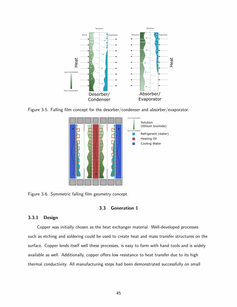
configuration, Figure 3-5 depicts the desorption and absorption processes with heat and mass

flows, while Figure 3-6 illustrates geometrical concepts.

3.2.2 Vacuum Requirements

With the falling film concept in mind, attention was directed towards attempts to realize

designs into physical manifestations. Recall that water is the refrigerant in the cycle, and

it must be boiled at low pressure to produce temperatures usable for refrigeration. Lithium

bromide systems are sensitive to leaks, the presence of non-absorbable gases adversely affects

operation. Non-absorbable gases may become present in the system by either ingress through

leaks or from gases produced internally by corrosion. Non-absorbable gases tend to obscure

absorption by concentrating at the vapor-solution interface as shown in Figure 3-4. This shroud

of non-absorbable gases inversely affects absorption rates.

The low pressure requirement is not exclusive to the refrigerant heat exchangers, the

entire absorption cycle operates at sub-atmospheric pressures. This condition requires that

all components, joints, or penetrations be hermetically sealed. Hermetic seals are among the

most stringent seals produced. The allowable rate of ingress of air into the system is extremely

low, else the thermodynamics of the cycle will become upset. Loss of vacuum is among the

43

g

Figure 3-4. Non-absorbable gases blanket the solution film, hindering absorption.

leading cause of errors in commercial chillers. Ingress of air into a systems leads to decreased

efficiency and capacity, increases the likelihood of crystallization, and accelerates corrosion

rates. Commercial systems are made of carbon steel, which tolerates corrosive lithium bromide

for a reasonable time period so long as there is an absence of oxygen required for corrosion

to take place. If left unchecked, corrosion often necessitates replacement of commercial units.

The lowest pressures experienced by typical systems are in the range of 650− 2300Pa.

A drawback of shell and tube architecture is the low seal integrity of the tubes in the

tube sheets, a problem exacerbated by the sheer number of tubes in a system. Commercial

units use copper or cupronickel for the tubes in the absorber, condenser, and evaporator

[31]. The tubesheet to which these are joined is made of steel for strength. The joint at the

interface of the tubes and tubesheet is created by expanding the tubes into place. During tube

rolling, the tubes are first inserted into the sheet, and are then expanded into place using a

tapered mandrel. Dissimilarities between the two metals, different thermal expansion rates, and

corrosion cause the seals to degrade over time to the point of leaking.

The heat exchangers presented in the following sections were designed to eliminate these

considerations while being an improvement over existing technologies. Consumer scale and

manufacturing cost were also given attention in each design.

44

Heat

Less Concentrated

More Concentrated

Boiling Condensation

Membrane

Heat

Evaporation

Membrane

Absorption

Desorber/

Condenser

Absorber/

Evaporator

Figure 3-5. Falling film concept for the desorber/condenser and absorber/evaporator.

Less Concentrated

More Concentrated

Solution

(lithium bromide)

Heating Oil

Refrigerant (water)

Cooling Water

Figure 3-6. Symmetric falling film geometry concept.

3.3 Generation 1

3.3.1 Design

Copper was initially chosen as the heat exchanger material. Well-developed processes

such as etching and soldering could be used to create heat and mass transfer structures on the

surface. Copper lends itself well these processes, is easy to form with hand tools and is widely

available as well. Additionally, copper offers low resistance to heat transfer due to its high

thermal conductivity. All manufacturing steps had been demonstrated successfully on small

45

scale sample parts. Unfortunately, the success rate was extremely low even for small parts and

difficulty scaled exponentially with increasing part size.

3.3.2 Fabrication

Figure 3-7. Generation 1 system featuring soldered copper heat exchangers. Photo courtesy ofauthor.

The major pitfall of creating thin wall copper heat exchangers lies in the difficulty in

creating hermetic, or vacuum tight, seals at joints. Thin copper sheets were unable to be

joined using temporary seals such as gaskets as they lacked the stiffness required to form such

a seal. Permanent joints such as diffusion bonding, brazing, and soldering were unsuccessful.

The high pressure and temperature used in diffusion bonding caused heat exchangers to

collapse. Brazing was eliminated as the temperatures required exceeded the limit of the internal

components. Soldering was the most appropriate method, and much work was done improving

the technique. Figure 3-7 shows an early assembled system composed of soldered heat

exchangers. Figure 3-8 shows an example of a heat exchanger geometry that was soldered.

46

Figure 3-8. Copper layers joined to brass chambers through soldering. Photo courtesy ofauthor.

3.3.3 Characteristics

Soldering success is highly dependent on geometry and environmental factors such as

cleanliness, temperature, heating, atmosphere, and time. If all parameters are not precisely

controlled, a hermetic seal will not be produced. The geometry of the heat exchanger layers

must be controlled so as to induce capillary wicking of the molten solder into the joints at

elevated temperatures. This geometry must be maintained throughout the heating process

despite inevitable thermal expansion and uneven heating. The copper surfaces must also be

free of oxides and contaminants at the moment the solder begins to flow, or else the copper

surface will not be wetted by solder. Copper begins to oxidize in the presence of oxygen, and is

accelerated at higher temperatures as well.

Other joining techniques were investigated as well. One sample was sent out for diffusion

bonding, and electron beam welding was also considered. During diffusion bonding, the part is

subject to intense heat and pressure. During this process, individual parts are formed into one

by diffusion on the molecular level at the joint interface. Unfortunately, the intense pressure

and heat of the process caused the unit to collapse. Electron beam welding involves applying a

beam of high speed electrons to the joint, welding the two parts into one. This process must

be carried out under vacuum to avoid attenuation of the electrons. Given the relatively large

47

size of the heat exchangers compared to what is typically electron beam welded, parts would

not fit inside commercial electron beam welding vacuum chambers.

3.4 Generation 2

3.4.1 Design

With the techniques developed to create heat and mass transfer enhancing structures on

copper surfaces, it was desirable to continue using copper sheets for the heat exchanger layers.

As was mentioned above, the primary drawback to working with copper was the inability to

create hermetic seals between heat exchanger layers. Seeking out alternative, more precise

joining techniques led to a conversation with a laser welding machine representative. The

company mentioned they would demonstrate the process on several samples. Figure 3-9 shows

a sample featuring a copper to copper seal. The obvious defect highlights an intrinsic property

of copper and laser welding. With the exception of large industrial laser welding equipment,

most laser welders use an Nd:YAG crystal as the medium. Nd:YAG lasers are typically operated

to emit wavelengths in the range of 1064 nm, although other wavelengths are possible

[32, 33]. Copper is highly reflective to light of this wavelength, as shown in the absorption

spectrum of Figure 3-10. This translates to a high load on the laser welding machine itself, as

it must produce powerful laser pulses to input enough energy to the highly reflective copper.

Enough energy must also be applied to overcome the high thermal conductivity of copper

dissipating heat away from the weld zone. Additionally, any impurity in the copper will have a

different absorptivity than the surrounding material. If the laser impacts such an impurity, the

result is an area of high energy absorption leading to a hole such as that of Figure 3-9.

After conversations with a laser welding service provider, it was decided to use a

combination of copper sheets and stainless steel 304. With these materials, the laser spot

diameter could be biased towards the more absorptive stainless steel. Stainless steel is an ideal

material for laser welding. It has good absorption of laser light, and low thermal conductivity

retains heat in the weld zone for a small heat affected zone (HAZ). Biasing the laser towards

48

~1 mm

Figure 3-9. Copper sample burn through during laser welding. Photo courtesy of author.

Figure 3-10. Copper laser absorption spectrum [34].

the stainless steel portion of a joint allows the stainless steel to melt at a higher temperature

and transfer heat to the copper sheet to form a seal.

49

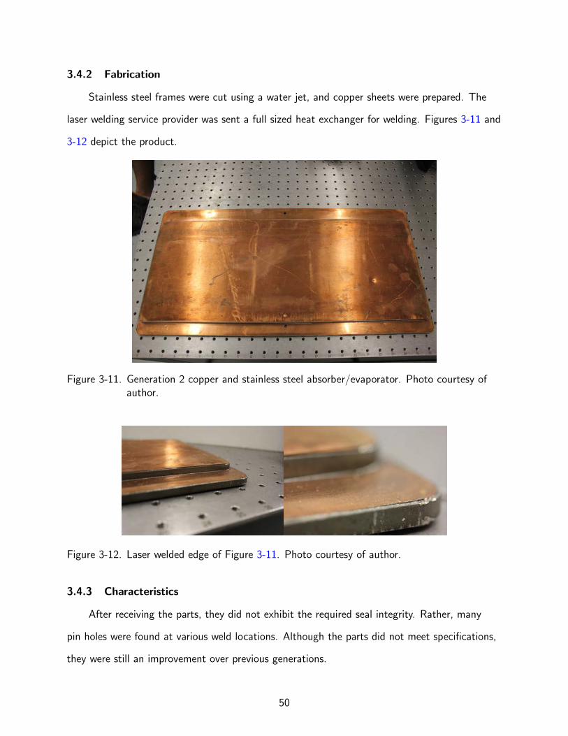
3.4.2 Fabrication

Stainless steel frames were cut using a water jet, and copper sheets were prepared. The

laser welding service provider was sent a full sized heat exchanger for welding. Figures 3-11 and

3-12 depict the product.

Figure 3-11. Generation 2 copper and stainless steel absorber/evaporator. Photo courtesy ofauthor.

Figure 3-12. Laser welded edge of Figure 3-11. Photo courtesy of author.


After receiving the parts, they did not exhibit the required seal integrity. Rather, many

pin holes were found at various weld locations. Although the parts did not meet specifications,

they were still an improvement over previous generations.

50

3.5 Generation 3

3.5.1 Design

After receiving Generation 3 parts back from laser welder that showed optimism, efforts

were turned to further understand the laser welding process. At this time, the company that

laser welded the sample of Figure 3-9 approached me about the possibility of purchasing a

machine. Looking forward, sending parts across the country for custom laser welding services

made looking at purchasing a laser welding machine itself an option. Factoring in the time

needed to become proficient and the cost of the machine, a purchase agreement was reached.

After becoming familiar with the machine, the capabilities and limitations of the process were

readily learned. Particularly promising was the ease of which stainless was laser welded. After

a successful prototype, a decision was made to create an all stainless steel heat exchanger. To

counter the low thermal conductivity of stainless steel, 250 µm thick sheets were specified.

The decision to move from copper to thin stainless sheets meant that structures could no

longer be etched into the surface. Rather, structures made of copper fins were soldered onto

the stainless steel sheets as shown in Figure 3-23. Again, stainless steel frames were cut using a

water jet.

3.5.2 Fabrication

Creation of thin walled vacuum chambers is desired within the vacuum community as

it allows for significantly shorter outgassing times [35]. This concept is relatively new, and

few publications exist on the topic, alluding to the difficulty of creating such a chamber. Of

the publications found, Bennett et al. [36] and Nemanic et al. [37] have created the thinnest

chambers at wall thicknesses of 910 and 600 µm, respectively. Both authors employed tungsten

inert gas (TIG) welding to create the chamber seals. TIG welding is ideal for thin materials due

to its precise arc control. Realizing the potential application for laser welding, the technique

was used for the first time to weld a hermetic heat exchanger. The first small scale prototype

was successful, featuring a wall thickness of just 250 µm, less than half of what was previously

thought to be possible.

51

Figure 3-13. Generation 3 generator/condenser front. Photo courtesy of author.

Figure 3-14. Generation 3 generator/condenser laser welded edge. Photo courtesy of author.


The latest generation of heat exchanger was closer than ever to reaching hermetic

seals. The heat exchanger still leaked, however the rate was lower than any of the previous

generations. Several issues detracted from the success of the part. First, notice the large

number of seams shown in Figures 3-13 and 3-14. The greater the seam length, the greater

the probability of a defect occurring. A reader may suppose that a defect could be repaired

through re-welding. This is normally true, however several defects were caused by solder

contaminating the weld pool. Recall that the fins of the heat exchanger were soldered onto the

surfaces. Any stray traces of solder in the welding area leads to permanent contamination of

52

the weld bead. Solder melts at a temperature much lower than that of stainless steel and tends

to erupt the weld pool, creating porous welds. The solder cannot be adequately cleaned out

of the weld zone. The third problem was with the choice of sheet metal thickness. 250 µm is

difficult to weld even with the precise control of a a laser. Straying the laser out of focus as

little as a few hundred microns can lead to burn through of the stainless steel sheet.

3.6 Generation 4

3.6.1 Design

Taking what had been gleaned from previous experiences about material, geometry, and

surface cleanliness, a new generation of heat exchanger was developed. The small scale sample

part of Generation 3 was hermetic, however the full sized unit was not. The only change was

an increase in the length and number of seams. At this point, it was evident that the number

of seals needed to be reduced in order to make full-sized unit. In order to do so, sheets were

formed to eliminate the need for layers. Knowledge about the capabilities of laser welding

made this design possible. Rather than have the middle cavity create its own layer, a dividing

sheet was simply laser welded inside to create a cavity within the pressed sheet. The latest

generation would incorporate thick, 900 µm formed sheets. Care was taken to prepare the

seams as clean as possible, free of solder.


53

Figure 3-16 shows details on how connections and pressed sheets were laser welded in

Generation 4. Due to the success of Generation 4, these techniques were featured in future

generations.

Figure 3-16. Generation 4 generator/condenser edge. Photo courtesy of author.

Figure 3-17. Design and manufactured Generation 4 generator/condenser. Photo courtesy ofauthor.

3.6.2 Fabrication

The fourth generation of heat exchanger shown in Figures 3-15 and 3-17 marked a

milestone in the project as it successfully featured hermetic seals on all joints, on both sides of

the heat exchanger. This was a huge success, previous generations had only come close to the

required seal integrity. Generation 4 not only was successful, it was repeatable. This success

injected fresh optimism into the project and spurred the creation of an absorber using the same

techniques. Again, an absorber was produced featuring all hermetic seals, both sides. Figure

3-18 shows the pressure history of both sides of the generator/condenser heat exchanger.

54

Figure 3-18. Generation 4 pressure history. During typical operation, the heat exchanger isexpected to experience 7-15 kPa depending on operating conditions.


The compact design of the desorber placed the condenser cooling water layer in close

proximity to the desorber heating oil layer. Unfortunately, the proximity was close enough

to allow substantial thermal communication between the heating oil and cooling water. In a

traditional system, these two external fluid loops are located on either end of a cylindrical heat

exchanger shell to ensure that heat does not pass in between. Thermal connectivity between

the heating supply and the cooling water of the condenser decreases inversely affects the

system COP and capacity. Figure 3-19 depicts the amount of heat transferred between the

layers for a given oil inlet temperature. During the test, 25C water was flowed through the

condenser cooling water layer.

3.7 Generation 5

3.7.1 Design

Generation 5 was the first generation of heat exchanger to feature nickel plated fins as

shown in Figure 3-22. In order to increase corrosion resistance in the desorber, the solution

fins were nickel coated after being brazed to the stainless steel sheet. Nickel is resistant to

55

Figure 3-19. Generator 4 desorber thermal communication between heating and cooling layers.Temperatures note the heating source inlet temperature.

corrosion by lithium bromide, Griess et al. reports low corrosion rates an Oak Ridge National

Laboratory report [38].

3.7.2 Fabrication

Generation 5 marked an attempt to speed up the fabrication process. Each laser welded

heat exchanger has over 50,000 weld beads, which take a significant amount of time to form.

The laser was pulsed at 2.5 Hz, with an overlap of 80% of the laser diameter (700 µm).

Tungsten inert gas (TIG) welding was attempted as an alternative. Of the manual welding

techniques, TIG welding was chosen due to its precision and control.

56


Figure 3-21. Weld failure due to solder contamination. Photo courtesy of author.

Figure 3-22. Generation 5 generator/condenser nickel coated fins. Photo courtesy of author.

57


Unfortunately, TIG welding was unsuccessful due to the increased heat affected zone

(HAZ) compared to that of laser welding. This created problems in areas where fins were

bonded to the backside of the sheet metal, such as the side areas of Figure 3-20. When

welding, the molten weld pool extended through the sheet metal to the solder, which

subsequently melted and contaminated the weld pool and led to cracks such as those in

Figure 3-21.

3.8 Generation 6

3.8.1 Design

Generation 6 was created in parallel with Generation 5 should TIG welding fail. Generation

6 featured all of the advancements of Generation 5 with the exception of nickel coated fins.

The oil fins of Generations 5 and 6 were switched from a wavy type (cf. A-29) to a taller offset

strip fin shown in Figure 3-24. Testing from the previous generation showed low heat transfer

from the oil loop to the system. A further investigation found that wavy fins were susceptible

to blockage from solder wicking into the fin channels during bonding. The previous fins were

also quite short, at only 0.125 in. compared to the new fins at 0.25 in.

Figure 3-23. Generation 6 generator/condenser. Photo courtesy of author.

58

Figure 3-24. Generation 6 generator/condenser oil fins. Photo courtesy of author.

3.9 Generation 7

Generation 7 sought to correct issues learned from testing with Generations 4 and 6 while

retaining the manufacturing techniques learned from previous generations. Several objectives

were laid out to guide the design process. Previous generations has suffered from thermal

communication between heating oil and condenser cooling water, there was no indication

how the solution manifold was performing at off-design conditions, and fin bonding quality of

previous generations had been quantified.

To reduce the amount of heat transfer between the layers, the generator sheets were

pressed deeper than before. The final product was near the limit of industry capability, several

iterations of dies were cut in order to achieve the final part. Tearing and wrinkling of the sheet

metal was problematic for the forming company. Figure 3-25 shows the increase in depth

between the first and second run of pressed sheets.

The problem of thermal communication between layers was effectively dealt with by

increasing the depth of the pressed sheet. Figure 3-26 depicts the decrease in heat transfer

between the heating layer and cooling water layer for the current and previous generation.

59

Figure 3-25. Pressed sheet depth comparison between Generations 6 and 7.

Figure 3-26. Reduction in thermal communication between Generations 6 and 7.

Manifolds play an important role in the success of absorption systems. Typically, the

limiting factor in the capacity of absorption systems is the absorption rate; a phenomena

governed by Fick’s law. Fick’s law says that the rate of absorption is proportional to the

area. The function of a manifold is to distribute absorbent onto the largest area possible for

maximum absorption, enabling cooling capacity. Previous desorber designs had used simple

calculations to model manifold distribution and pressure drop. Desiring more fidelity and

insight into the performance of a manifold, a more in depth analysis was performed. The

60

distribution of fluid is non-uniform down the length of a manifold as shown in Figure 3-27.

This applies only to this type of consecutive manifold, bifurcation style manifolds are exempt

from this assumption as flow naturally distributes in such a manifold. A bifurcation manifold

was not chosen for this application due to their high pressure drop, large size, and difficulty of

manufacturing.

Figure 3-27. Typical manifold distribution profile.

The physical dimensions of the manifold coupled with the fluid kinematic properties

influence how the flow is distributed. A poorly distributed flow as shown in Figure 3-27 occurs

when the pressure drop through the orifices is small relative to the dynamic head in the

manifold. Fraas et al. [39] showed this phenomena between manifolds distributing flow through

heat exchange material.

In order to design a manifold with the desired characteristics, a model or experimental

data is required. Wang [40] investigated this problem with the goal of creating a model to

predict manifold hydrodynamics. The ideas Wang presented in his work were used as aids in

formulating the solution for the case presented here. Beginning with a differential element

within the manifold as shown in Figure 3-28, equations of continuity and the conservation of

momentum may be written.

Continuity

61

x

yux

Px

ux+dx

Px+dx

uy

dx

A

Ay

Figure 3-28. Manifold differential element.

ρuxA− ρux+dxA− ρuyAy = 0 (3–4)

ux+dx = ux +∂ux∂x

dx (3–5)

Combining Equations 3–4 and 3–5

uxA−(ux +

∂ux∂x

dx

)A− uyAy = 0 (3–6)

uxA −uxA − ∂ux∂x

dxA− uyAy = 0 (3–7)

uy = −∂ux∂x

dxA

Ay

(3–8)

let

dx =L

n(3–9)

62

Where L is the length of the manifold, and n is the number of exit ports.

uy = −∂ux∂x

L

n

A

Ay

(3–10)

Momentum

ρu2xA+ PxA−(ux +

∂ux∂x

dx

)2

Aρ−(Px +

∂Px

∂xdx

)A = τwPdx (3–11)

ρu2xA +PxA −ρu2xA − 2ρAux∂ux∂x

dx −PxA − ∂Px

∂xdx A = τwPdx (3–12)

−2ρAux∂ux∂x

− ∂Px

∂xA = τwP (3–13)

τw may be taken from the Darcy-Weisbach equation

P = fL

Dh

ρu2x2

(3–14)

Using the definition of the hydraulic diameter, this is reduced to

τw = f ρu2x8

(3–15)

Flow through orifices is modeled by the following result:

_m =CDAy(

1−(dD

)4)0.5 [2ρ (Px − P0)]0.5 (3–16)

63

Px =

(uy

CD

)2ρ

2

(1−

(d

D

)4)

+ P0 (3–17)

∂Px

∂x=

∂

∂x

[(uy

CD

)2ρ

2

(1−

(d

D

)4)]

+∂P0

∂x(3–18)

Canceling out the last term as the pressure outside the manifold is constant with respect

to length.

∂Px

∂x=

(1

CD

)2ρ

2

(1−

(d

D

)4)

∂u2y∂x

(3–19)

Recalling the result from Equation 3–8

∂Px

∂x=

(1

CD

)2ρ

2

(1−

(d

D

)4)

∂

∂x

[(∂ux∂x

)2(L

n

A

Ay

)2]

(3–20)

∂Px

∂x=

(1

CD

)2ρ

2

(1−

(d

D

)4)(

L

n

A

Ay

)2∂

∂x

[(∂ux∂x

)2]

(3–21)

∂Px

∂x=

(1

CD

)2ρ

2

(1−

(d

D

)4)(

L

n

A

Ay

)2

2∂ux∂x

∂2x

∂x2(3–22)

Going back to the results from Equations 3–13 and 3–15.

−2ρAux∂ux∂x

− ∂Px

∂xA = τwP (3–23)

64

−2ρAux∂ux∂x

− ρ

C 2D

(1−

(d

D

)4)(

L

n

A

Ay

)2∂ux∂x

∂2x

∂x2A = f ρ

u2x8P (3–24)

Dividing by A and ρ,

−2ux∂ux∂x

− 1

C 2D

(1−

(d

D

)4)(

L

n

A

Ay

)2∂ux∂x

∂2x

∂x2= f

u2x2

P

4A(3–25)

−2ux∂ux∂x

− 1

C 2D

(1−

(d

D

)4)(

L

n

A

Ay

)2∂ux∂x

∂2x

∂x2= f

u2x2Dh

(3–26)

For fully developed laminar flow, f = 64Re

[41]

−2ux∂ux∂x

− 1

C 2D

(1−

(d

D

)4)(

L

n

A

Ay

)2∂ux∂x

∂2x

∂x2=

64µ

ρuxDh

ux2

2Dh

(3–27)

−2ux∂ux∂x

− 1

C 2D

(1−

(d

D

)4)(

L

n

A

Ay

)2∂ux∂x

∂2x

∂x2=

32µ

ρD2h

ux (3–28)

∂2x

∂x2+ 2

C 2D(

1−(dD

)4) (nL Ay

A

)2

ux +32µ

ρD2h

C 2D(

1−(dD

)4) (nL Ay

A

)2

ux

(∂ux∂x

)−1

= 0 (3–29)

The manifold discharges to a free space, leaving D to be infinitely large. Therefore,

limD→∞

(1−

(d

D

)4)

→ 1 (3–30)

∂2x

∂x2+ 2C 2

D

(n

L

Ay

A

)2

ux +32µC 2

D

ρD2h

(n

L

Ay

A

)2

ux

(∂ux∂x

)−1

= 0 (3–31)

BC1. u (0) = u

65

BC2. u (L) = 0

The choice of CD = 0.5 was from Johansen [42]. The smaller the port spacing, dx = Ln,

the more accurate the solution will be. A smaller port spacing increases the accuracy of the

Talyor series approximation used for ux+dx . The solution is only applicable for laminar flow

in the manifold body. For the outlets, the flow may be in any regime. The solution is only

applicable to steady, incompressible flows. The solution is only applicable to manifolds with

short runners, those on the order of Lrunner < 2Dorice . For longer runners, the length may

exceed the entrance length and an alternate model for pressure drop through the runners

should be used.

Using this model, the manifold shown in Figure 3-29 was created for experimental testing.

A part drawing of the manifold may be seen in the Appendix, Figure A-2. Made out of

stainless steel and coated with PTFE, the manifold would be durable and corrosion resistant.

The coating serves as a flow control element to keep droplets from coalescing laterally.

Figure 3-29. Solution distribution manifold. A part drawing may be seen in Figure A-2, Photocourtesy of author.

Using water, the manifold showed very good performance compared to the theoretical

lateral distribution predicted by the model, Figure 3-30.

The pressure drop measured across the manifold was also an important consideration.

Knowledge about the pressure drop through the manifold is required in order to select a pump

that can deliver the required flow. The results of modeling compared to experimental values

for different flow rates are shown in Figures 3-31 and 3-32. The red line indicates the design

66

Figure 3-30. Theoretical versus experimental manifold distribution for water. Note the smallvertical scale.

Figure 3-31. Theoretical distribution at operating condition.

67

operating point. The transition from droplet to jet flow out of the nozzles is plotted as well.

No particular regime is preferred, so long as the operating point is not jet flow with sufficient

velocity to allow the flow to depart the falling film structures.

Figure 3-32. Manifold pressure curve using 55% wt. lithium bromide.

The lack of quality bonded fins was a manufacturing problem that had to be addressed.

The technique used on previous generations was developed prior in the lab for joining copper to

copper parts. Plainly speaking, surfaces to be bonded were coated in flux, and pressed together

with a layer of solder ribbon between the parts. One side of the press featured a heating

platen to transfer heat to the parts. When one of the surfaces was switched to stainless steel,

several issues arose with the process. Firstly, stainless steel has a tendency to warp when

heated. This phenomena did not occur with copper, despite the two metals having nearly the

same coefficient of expansion [43]. The reason for this behavior is due to the difference in

thermal conductivity between the materials. Copper has a thermal conductivity ∼ 27X that

of stainless steel. Wherever stainless steel is heated, large temperature gradients are created

translating to stresses and eventually warpage if enough heat is applied. This is detrimental to

the bonding process, both the substrate and the fins should be as flat as possible to achieve

68

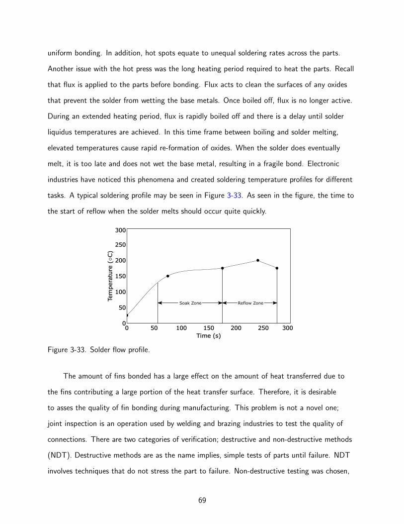
uniform bonding. In addition, hot spots equate to unequal soldering rates across the parts.

Another issue with the hot press was the long heating period required to heat the parts. Recall

that flux is applied to the parts before bonding. Flux acts to clean the surfaces of any oxides

that prevent the solder from wetting the base metals. Once boiled off, flux is no longer active.

During an extended heating period, flux is rapidly boiled off and there is a delay until solder

liquidus temperatures are achieved. In this time frame between boiling and solder melting,

elevated temperatures cause rapid re-formation of oxides. When the solder does eventually

melt, it is too late and does not wet the base metal, resulting in a fragile bond. Electronic

industries have noticed this phenomena and created soldering temperature profiles for different

tasks. A typical soldering profile may be seen in Figure 3-33. As seen in the figure, the time to

the start of reflow when the solder melts should occur quite quickly.

Soak Zone Reflow Zone

Figure 3-33. Solder flow profile.

The amount of fins bonded has a large effect on the amount of heat transferred due to

the fins contributing a large portion of the heat transfer surface. Therefore, it is desirable

to asses the quality of fin bonding during manufacturing. This problem is not a novel one;

joint inspection is an operation used by welding and brazing industries to test the quality of

connections. There are two categories of verification; destructive and non-destructive methods

(NDT). Destructive methods are as the name implies, simple tests of parts until failure. NDT

involves techniques that do not stress the part to failure. Non-destructive testing was chosen,

69

as confidence in the repeatability of the fin bonding process had not been established to the

point making destructive testing meaningful.

Halmshaw presents methods of NDT welded joints in a comprehensive text, [44]. Methods

include: visual, radiographic, ultrasonic, and penetration. Visual methods are not possible, as

the materials are opaque and the joint it obscured by the parts. Radiographic methods take

advantage of absorption of x-rays. Where a void exists, x-ray transmission will be inhibited and

appears as dark areas on the detection image. Ultrasonic methods work on principles similar

to that of x-rays, a void or change in medium alters the amount of sound wave transmission

and appears on the detector as a shift. Penetration methods involve coating the joint with

a penetrating dye, and examining the penetration of the dye into the joint; a technique not

possible due to the geometry of the heat exchanger.

My lab colleague, Saitej Ravi, suggested the use of thermal imaging as a method of

NDT joint examination. Halmshaw did not include this technique, perhaps thermal imaging

equipment was not widely used when the text was written. Chadhuri et al. explored the

possibility of thermal imaging as an NDT technique for a stainless steel to copper brazed joint

[45].

In order to achieve better fin bonding, the hot press method was replaced with a furnace.

A furnace allows for rapid, even heating to minimize oxide formation and warpage. Using this

technique, the fins shown in Figure 3-34 were bonded. To test the quality of the bond as well

as the measurement technique, an IR camera was used to view the fins as they were heated. A

known defect was purposely created in the fins to test the accuracy of the verification method.

70

Steady StateUnsteady Airflow Manufactured

Figure 3-34. Comparison of thermal testing with manufacturing process for a known defect.Photo courtesy of author.

71

CHAPTER 4SYSTEM DEVELOPMENT

4.1 Environmental Interaction

The experimental system interacted with the environment through the external loops

shown in Figure 4-1. Cooling to the condenser and absorber was provided through a

recirculating water chiller by Thermo Scientific. It is important to note that the condenser

and absorber were cooled by the same cooling water source, piped in parallel. Parallel piping

was chosen for system stability. Had the absorber and condenser been piped in series, it

would have restricted the system to a point which may not have been attainable. Although

a recirculating chiller was used here, alternative sources of cooling would be possible. The

evaporator heat input was provided through a recirculating water loop equipped with a heater.

Again, any source of heat input could be used, possibly in the form of a building chilled water

loop. Lastly, heat input to the desorber was provided by a recirculating oil bath by Julabo. The

heating fluid was a high temperature silicone oil. The only consideration for the heating fluid

medium would be that it should evenly distribute heat to the surfaces of the desorber. This

could be in the form of other heat transfer mediums, possibly hot fluid from a solar collector

array.

Figure 4-1. Diagram of external heat transfer loops connected to the system.

72

4.2 Instrumentation

The system was instrumented in order to determine the state points at all nodes shown

in Figure 2-2 for comparison with simulation values. Knowing the state of the fluid at every

point is crucial for performance evaluation and modeling as these points are used modeling. In

order to achieve this, the system was fully instrumented with pressure transducers, flow meters,

and thermocouples at every node in the system. Finding instrumentation that was hermetically

sealed proved to be difficult. Custom thermocouple pipe penetrations had to be designed in

order to measure temperature at various flow locations.

The requirements of the flow meter were particularly stringent. The meters were required

to hold vacuum, have a very low pressure drop, be corrosion resistant, and measure flow

density. The Emerson Micro Motion line of Coriolis flow meter was the only meter found

that met all of these specifications. Coriolis flow meters are extremely accurate and have

high turndown ratios, that is, they are accurate under a wide range of flows. The meters

were able to measure density as well as temperature. This feature was needed in order to

determine the concentration of lithium bromide. Knowing the concentration of lithium bromide

is critical to avoid crystallization that occurs when the solution becomes supersaturated. In

order to correlate density to concentration, the temperature and density of the solution must

be known. Assuming the solvent, water in this case, is incompressible and single phase liquid,

the concentration is a function of temperature and density only.

xLiBr = f (T , ρ) (4–1)

Correlations between temperature, density, and concentration are provided in literature.

Patek et al. provides the most inclusive review of research and goes on to present a unifying

correlation [21]. Using such correlations, the temporal density of a solution flow may be

converted to concentration as seen in Figure 4-2.

73

100ºC

50ºC

75ºC

Increasing

Temperature

Figure 4-2. Density and temperature may be used to correlate the concentration of lithiumbromide.

4.3 Equipment

4.3.1 Filter Design and Fabrication

In addition to theoretical challenges, there are also many operational and practical

hurdles associated with such a system. For example, it is crucial that the ports of the solution

manifolds of the desorber (cf. Figure 3-29) and absorber remain open and free of debris.

Foreign material in the manifolds poses a threat of plugging the ports, causing solution

maldistribution and increasing the pressure drop through the manifold. To ensure that debris

does not enter the heat exchangers, two filters were designed and fabricated for use in the

system. The filters were installed as a part of the closed system, therefore the filter was

required to be hermetic. In order to work as a part of a thermodynamic pressure and gravity

driven system, the filters were also required to have an extremely low pressure drop. Hermetic

filters were available in the market, however they were priced at a minimum of $5000 per filter.

This was unacceptable, two filters would have exceeded the allotted project budget for that

aspect.

A decision was made to create custom filters for use in the system. The filters consisted

of a 43 µm stainless steel mesh supported by a coarse stainless steel screen. Stainless steel

mesh was chosen as the filter media due to its large permeability offering low pressure drop.

Each unit had a filter mesh measuring around 4.5 in. on a side for a total area of 20.25 in.2 .

74

The filter was made by stacking the assembly together while leaving filter media protruding on

the edges. When laser welded, the stainless steel filter media melted into the edge weld bead,

capturing the media. Connections were welded on to complete the filter.

To ensure even distribution of flow across the filter, diverting plates shown in Figure 4-3

were welded on the inside of the inlet to the filters. Uniform flow distribution across the media

shown in Figure 4-4 ensures even caking of debris, and low velocities avoid pushing debris

through the filter.

Figure 4-3. Filter component halves. A diverter plate is installed on piece on the right. Photocourtesy of author.

Filter Support Filter Material

Figure 4-4. Filter support and filtration media. Photo courtesy of author.

4.3.2 Solution Pump

Recall that the entire system must be a closed, hermetic loop.This condition applies to

the pump as well, which must be vacuum sealed. There is a very small market of hermetic

pumps for commercial systems, which are much larger than the system requires here. Only one

75

manufacturer offers an appropriately sized hermetic pump, HNP Mikrosysteme of Germany.

The pump is intended for highly specialized applications requiring ultra precise volumetric doses

and would not be appropriate for the system due to its requirements on inlet flow purity.

In order to overcome this challenge, a hermetic pump was replicated by placing a pump

within a vacuum chamber. A small, inexpensive DC magnetically-driven pump was placed

within a vacuum chamber and its exit piped to an exit feedthrough fitting on the chamber

inner wall. Electrical supply to the pump was provided through a vacuum chamber electrical

feedthrough.

The pump also served a second purpose as a charging chamber. Lithium bromide solution

was inserted into this chamber, and its level was monitored to determine the correct system

charge volume. A photograph of the setup may be seen in Figure 4-5.

Figure 4-5. Dual purpose solution pump and charging chamber. Photo courtesy of author.

4.3.3 Heating Oil Flow Control

In the desorber heating layer, oil flows from top to bottom in order to reduce solution pool

boiling near the exit. Boiling of solution near the exit was found to obscure solution drainage.

Naturally, when filling from the top a bubble will exist in the cavity unless it is removed before

operation. When the design of Figure A-22 was completed, it was uncertain how well the flow

76

would match the ideal case and evenly distribute laterally across the heat exchanger. Initial

testing showed the side opposite the inlet to be much cooler, indicating it was not seeing

hot oil. Consider the effect of a bubble in the cavity as show in Figure 4-6, it will prevent oil

from evenly heating all areas. To facilitate easy purging of the oil layer, a special bleed fitting

(Figure 4-7) was designed and manufactured to attach to the desorber inlet. The fitting allows

a user to open a path for air to escape through a purge valve. Once the air is purged, oil will

begin to trickle out of the purge valve, indicating complete deaeration. After purging, even

temperature distribution was verified with an IRCameras IRC906SLS infrared camera. Figure

4-8 shows the rear of the desorber at reduced temperature steady state testing.

Air

Oil

Inlet

Oil

Exit

Heater

Desorber

Oil Bath

Figure 4-6. Air may be trapped in the heating layer of the desorber as shown here.

Bleeding Port

Oil Inlet

Figure 4-7. Heating oil purge fitting. Photo courtesy of author.

77

Figure 4-8. Even surface oil temperature distribution left to right. Photo courtesy of author.

4.3.4 Heat Exchanger Flow Distribution

The solution heat exchanger has a strong influence on the overall COP of the system.

Figure 4-10 from simulation depicts the trend of COP versus heat exchanger effectiveness.

initially, custom solution heat exchangers were fabricated using the same techniques used to

fabricate the third generation heat exchanger, shown in Figure 4-9. The custom soluation heat

exchangers held vacuum, further supporting conclusions about the full-sized unit of Generation

3. The custom solution heat exchanger held vacuum due to its low number of hermetic seams.

Making a custom solution heat exchangers was a difficult and time consuming process. As

an alternative, an off the shelf brazed plate heat exchanger was found that held vacuum and

offered a larger heat exchange area.

Figure 4-9. Custom solution heat exchanger. Photo courtesy of author.

Brazed plate heat exchangers, also known as compact heat exchangers, offer large heat

transfer areas in a small unit package. They are formed by stacking many alternating plates on

top of each other. Fluid flows in between the layers, alternating between hot and cold flows.

78

Figure 4-10. Effect of solution heat exchanger effectiveness on COP for various operatingconditions. Conditions 1 and 2 refer to experimental data of Chapter 5.

In addition to decreased COP, a poorly performing solution heat exchanger also leads

to a drop in performance and exacerbates crystallization threats. As solution heat exchanger

effectiveness decreases, the hot side exit temperature will increase. Coincidentally, this flow

is the inlet of the absorber. Recall that the solution must be cooled in order for absorption

to take place. As the solution enters the absorber at higher temperatures, absorption rates

decrease accordingly. Reduced absorption rates lead to higher concentrations and eventually

crystallization if left uncorrected.

Inlet

Exit

Inlet

Exitg g

Figure 4-11. Solution heat exchanger flow distribution.

During testing, a lack of heat transfer was noticed in the solution heat exchanger.

A calculation using theoretical Nusselt numbers for the geometry of the flows revealed

79

that only 25% of the plates were active in transferring heat. It is estimated that the flow

approximated the scenario shown in Figure 4-11. Resulting from poor heat transfer, high

inlet temperatures to the absorber were observed as shown in Figure 4-10. In order to correct

the flow distribution problem and wet all of the plates of the heat exchanger, a needle valve

was added downstream to increase the head loss to a height that sufficiently filled the heat

exchanger. Figure 4-12 shows the results of the modification. Notice how the absorber

solution inlet temperature decreased substantially. A plot comparing solution heat exchanger

effectiveness for maldistributed versus corrected heat exchanger operation may be seen in

Figure 5-7.

Maldistribution

Corrected

Figure 4-12. Absorber solution temperatures.

80

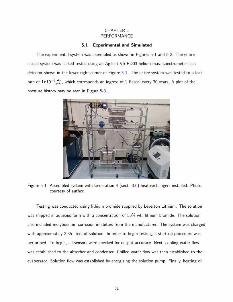
CHAPTER 5PERFORMANCE

5.1 Experimental and Simulated

The experimental system was assembled as shown in Figures 5-1 and 5-2. The entire

closed system was leaked tested using an Agilent VS PD03 helium mass spectrometer leak

detector shown in the lower right corner of Figure 5-1. The entire system was tested to a leak

rate of 1x10−9 Pam3s

, which corresponds an ingress of 1 Pascal every 30 years. A plot of the

pressure history may be seen in Figure 5-3.

Figure 5-1. Assembled system with Generation 4 (sect. 3.6) heat exchangers installed. Photocourtesy of author.

Testing was conducted using lithium bromide supplied by Leverton Lithium. The solution

was shipped in aqueous form with a concentration of 55% wt. lithium bromide. The solution

also included molybdenum corrosion inhibitors from the manufacturer. The system was charged

with approximately 2.35 liters of solution. In order to begin testing, a start-up procedure was

performed. To begin, all sensors were checked for output accuracy. Next, cooling water flow

was established to the absorber and condenser. Chilled water flow was then established to the

evaporator. Solution flow was established by energizing the solution pump. Finally, heating oil

81

Figure 5-2. System side and rear; heat exchangers are installed in both photos. Photo courtesyof author.

Figure 5-3. System pressure history. The decaying pressure is due to the system cooling downafter operation.

82

flow was applied to the generator. The temperature of the heating oil was slowly ramped up to

operating conditions.

System shut-down was the reverse of start-up. First, oil flow to the desorber was stopped.

It was important to keep chilled water circulating in order to vaporized un-absorbed refrigerant

back into solution. Cooling water flow was retained to cool solution incoming to the absorber

to facilitate absorption as was explained in section 3.2.1. Had all external loops been stopped,

the concentrated solution has the possibility to crystallize as it cools down. It is important

to dilute and restore the solution to a safe concentration that will not crystallize at ambient

conditions.

Figures 5-4 - 5-6 depict the results of testing plotted on Duhring charts, while Tables

5-1 - 5-5 contain the state points of the fluid at all nodes of the system numbered in Figure

2-2. Dissimilarities between theoretical and simulated data may be attributed to system heat

loss or slight variations in sensor data. Additionally, the simulation software assumes ideal

operating conditions for the system. Recall that system performance is sensitive to wetting

of the falling film surfaces and solution heat exchanger plates for optimal heat transfer to

take place. During experimentation, these areas may drift slightly out of design conditions,

contributing to alternate system performance values.

0 20 40 60 80 100 12010

2

101

100

101

102

103

Temperature (°C)

Pre

ssure

(kP

a)

Figure 5-4. Operating Condition 1 Duhring chart.

83

Table 5-1. Operating Condition 1: Experimental data points. The nodes of the first column

correspond to the points of Figure 2-2.

Node, i h(kJkg

)m(kg

s

)P (kPa) T (C) x (%wt.LiBr)

1 45.73 0.0109 1.38 24.27 0.43 COP 0.81

2 48.85 0.0109 7.96 25.60 0.43 ϵhx 0.85

3 145.6 0.0109 7.96 65.97 0.43 Qa 1351 W

4 195.2 0.0105 7.96 83.50 0.58 Qc 944 W

5 96.28 0.0105 7.96 33.32 0.58 Qd 1135 W

6 93.31 0.0105 1.38 31.77 0.58 Qe 911 W

7 2606 0.00039 7.96 57.01 - Ua 2442 Wm2K

8 173.4 0.00039 7.96 41.41 - Uc 1307 Wm2K

9 173.4 0.00039 1.38 11.80 - Ud 429.5 Wm2K

10 2522 0.00039 1.38 11.80 - Ue 738.6 Wm2K

Table 5-2. Experimental versus simulated performance at Operating Condition 1.

Case COP

Experimental 0.81

Simulation 0.87

0 20 40 60 80 100 12010

2

101

100

101

102

103

Temperature (°C)

Pre

ssu

re (

kP

a)


84



Node, i h(kJkg

)m(kg

s


1 47.60 0.0077 1.24 25.19 0.45 COP 0.79

2 49.33 0.0077 7.95 25.95 0.45 ϵhx 0.87

3 145.2 0.0077 7.95 67.20 0.45 Qa 1298 W

4 189.8 0.0073 7.95 82.20 0.57 Qc 912.4 W

5 91.34 0.0073 7.95 32.38 0.57 Qd 1124 W

6 94.20 0.0073 1.24 33.86 0.57 Qe 889.1 W

7 2611 0.00038 7.95 59.70 - Ua 2549 Wm2K

8 173.4 0.00038 7.95 41.40 - Uc 1292 Wm2K

9 173.4 0.00038 1.24 10.08 - Ud 380 Wm2K

10 2519 0.00038 1.24 10.08 - Ue 374 Wm2K


Case COP

Experimental 0.79

Simulation 0.86

85

0 20 40 60 80 100 12010

2

101

100

101

102

103

Temperature (°C)

Pre

ssure

(kP

a)




Node, i h(kJkg

)m(kg

s


1 50.36 0.0141 1.55 26.20 0.43 COP 0.76

2 51.14 0.0141 11.85 26.53 0.43 ϵhx 0.832

3 171.9 0.0141 11.85 72.83 0.43 Qa 1994 W

4 210.8 0.0135 11.85 92.16 0.58 Qc 1501 W

5 100.7 0.0135 11.85 36.57 0.58 Qd 1902 W

6 100.1 0.0135 1.55 36.24 0.58 Qe 1452 W

7 2621 0.00063 11.85 65.10 - Ua 2615 Wm2K

8 205.9 0.00063 11.85 49.17 - Uc 1521 Wm2K

9 205.9 0.00063 1.55 13.40 - Ud 435.5 Wm2K

10 2525 0.00063 1.55 13.40 - Ue 836.5 Wm2K

86


Case COP

Experimental 0.76

Simulation 0.85

The main differences between the three operating conditions are in the circulation

ratio, desorber exit temperature, and evaporator temperature. The former two influence the

circulation ratio directly. The circulation ratio is an extremely useful metric for understanding

how an absorption cycle will perform. The circulation ratio is defined as the ratio of the mass

flow rate of the weak solution to that of the refrigerant [13],

f =_m3

_m7

(5–1)

Through manipulation (c.f. A.5) the circulation ratio may be written as a function of the

strong and weak concentrations of the cycle.

f =xstrong

xstrong − xweak(5–2)

To give a physical analogy of the circulation ratio, it is analogous to the efficiency of

a pump. It can be thought of as a ratio of the amount of input going towards pumping

refrigerant versus that consumed by loses. When visualized on a Duhring chart, the circulation

ratio can be abstracted from the “width” of the solution track. A wider track indicates a

greater difference between weak and strong concentrations and thus a lower circulation ratio.

The circulation ratio also makes an appearance directly in the calculation of COP as

seen in Equation 5–3. Appendix section A.6 explains how the COP may be written in this

form. One can immediately see that a low circulation ratio is desired. In equation 5–3, the

term f (h4 − h3) is the sensible heat added to the solution during desorption. This heat must

87

eventually be discarded in the absorber in order to promote absorption as explained in Section

3.2.1.

COP =h10 − h9

h7 − h4 + f (h4 − h3)(5–3)

However, a solution heat exchanger acts to recover this heat. Cycle COP is a strong

function of heat exchanger effectiveness as seen in Figure 4-10. Its effect may be seen

in Equation 5–3. The numerator of can be interpreted as the heat of vaporization of the

refrigerant. The denominator can be interpreted as the sum of sensible heat, (h4 − h3) added

to the solution during desorption, plus the heat of vaporization of the refrigerant (h7 − h4).

One can now directly see the benefits of a low circulation ratio and the addition of a solution

heat exchanger. A solution heat exchanger acts to reduce the difference between the enthalpy

of the two solution flows, h4 − h3. This means that more of the heat input is going towards

vaporizing refrigerant than would be going towards increasing the temperature of the solution.

The effect of heat exchanger effectiveness upon COP may be seen in Figure and 5-8. Notice

how the heat exchanger effectiveness has a strong influence on the COP.

The caveat of using a heat exchanger with a large surface area lies in the problem of

flow distribution. Poor flow distribution in plate heat exchangers can drastically decrease the

effectiveness [46].

88

Figure 5-7. Heat exchanger effectiveness for maldistributed and corrected heat exchangeroperation.

Figure 5-8. COP versus solution heat exchanger effectiveness.

89

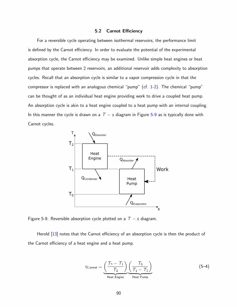
5.2 Carnot Efficiency

For a reversible cycle operating between isothermal reservoirs, the performance limit

is defined by the Carnot efficiency. In order to evaluate the potential of the experimental

absorption cycle, the Carnot efficiency may be examined. Unlike simple heat engines or heat

pumps that operate between 2 reservoirs, an additional reservoir adds complexity to absorption

cycles. Recall that an absorption cycle is similar to a vapor compression cycle in that the

compressor is replaced with an analogous chemical “pump” (cf. 1-2). The chemical “pump”

can be thought of as an individual heat engine providing work to drive a coupled heat pump.

An absorption cycle is akin to a heat engine coupled to a heat pump with an internal coupling.

In this manner the cycle is drawn on a T − s diagram in Figure 5-9 as is typically done with

Carnot cycles.

T

s

Work

T2

T1

T0

Heat

Engine

Heat

Pump

QDesorber

QCondenser

QAbsorber

QEvaporator

Figure 5-9. Reversible absorption cycle plotted on a T − s diagram.

Herold [13] notes that the Carnot efficiency of an absorption cycle is then the product of

the Carnot efficiency of a heat engine and a heat pump.

ηCarnot =

(T2 − T1

T2

)︸︷︷︸

Heat Engine

(T0

T1 − T0

)︸︷︷︸

Heat Pump

(5–4)

90

Unlike typical Carnot cycles, the absorption cycle includes heat exchange with 3 different

temperature reservoirs, T0,T1,T2. The variation of these variables produces an infinite

combination of temperatures over 3 dimensions. A plot of the resulting Carnot efficiency for

ranges of experimentally relevant reservoir temperatures may be seen in Figure 5-10.

T2

T0T1

T2

T0T1

7

2.5

3

3.5

4

4.5

5

5.5

6

6.5

Carnot

Figure 5-10. Carnot absorption cycle efficiency for various reservoir temperatures.

Carnot efficiencies for the experimental conditions described earlier may be seen in Table

5-7.

Table 5-7. Carnot efficiencies for experimental operating conditions.

Operating Condition ηCarnot

1 3.81

2 3.01

3 4.04

Notice that the most efficient cycle occurs when T2 and T0 are maximized and T1 is

minimized. Considering the two parts as separate, a heat engine is most efficient with the

hottest source temperature and the coolest heat refection temperature. A heat pump is most

91

efficient when the cold reservoir temperature is closest to that of the heat rejection reservoir.

These observations are confirmed in Figure 5-10.

92

CHAPTER 6COSTS

In the interest of possible commercialization, a cost analysis is provided. With the

exception of the connections, sensors, and pressed sheets; all pieces used to build heat

exchangers and the complete experimental system were custom made by the author in the

laboratory. The connections used were Swagelok VCR connections selected for their low

leak rates and ability to be opened and closed without wear. The pressed sheets were priced

proportionately to the production run; because the sheets were made in a short-run the costs

were relatively high. To make the pressed sheets, a tooling die was created for forming. The

cost of the die was significant, but represents a one-time cost. Sheet metal forming costs are

extremely sensitive to production volumes due to the significant work in setting up tooling. If

production runs were increased, part cost would drastically decrease. Only 14 pieces of each

type of pressed sheet were made for the desorber and absorber units.

The cost of constituent parts of the generator/condenser unit are shown in Figure

6-1. Major costs include the pressed sheets and fins at $650 and $297 respectively. If the

production run of pressed sheets was expanded, costs are estimated to come down to less

than $20 per sheet. The vast difference between the current and estimated price is due to the

current production run size. Significant setup time drives the current cost of sheets. Fins on

the other hand, are used quite frequently in the laboratory and were ordered on a much larger

production run; 175 fins arrays per order. Given the current production run of fins, it is not

certain that their unit price will decrease drastically with increased production runs. Taking

into account production run discounts on other parts, it is estimated that the cost parts for a

generator-condenser unit could decrease to below the $100 mark.

The costs associated with manufacturing components was also significant, as shown in

Figure 6-2 for the generator/condenser unit. The most expensive processes were laser welding

and brazing. The cost to laser weld a unit came directly from a laser welding service that was

used to create an earlier part, Generation 2.

93

2% 3%

12%

15%

21%

47%

Solution Manifolds

Sheet Metal

Stanless Steel Frames

Connection Fittings

Fins

Pressed Sheets

Total: $1397

Figure 6-1. Desorber materials costs.

44%

46%

5%5%

Brazing

Laser Welding

Drilling

Raw Material Processing

Total: $2975

Figure 6-2. Desorber manufacturing costs.

The same observations on bulk pricing also apply to the absorber as well. Figures 6-1

- 6-4 show an important trend. Although the physical length of the absorber/evaporator is

nearly double that of the desorber/condenser, the cost difference is minimal. In this concept

of heat exchanger cost does not necessarily scale with capacity. This is due to the efforts of

designing the units for ease of manufacturing and scalability. In doing so, the technologies,

materials, manufacturing techniques, and parts are shared between the two units. This

feature allows the heat exchanger to be scaled up physically with no changes in complexity or

manufacturing technique. Only additional materials are required, which are priced according

to bulk discounts and do not contribute significantly to the final cost of the unit. This feature

94

is also advantageous for commercialization as the same facility, equipment, raw material, and

tradesmen may be used to make either the generator/condenser or the absorber/evaporator.

31%

14%31%

5%

14%

3% 2%

Pressed Sheets

Stanless Steel Frames

Fins

Sheet Metal

Connection Fittings

Solution Manifolds

Evaporator Manifolds

Total: $1591

Figure 6-3. Absorber materials costs.

45%

45%

6%4%

Brazing

Laser Welding

Drilling

Raw Material Processing

Total: $3710

Figure 6-4. Absorber manufacturing costs.

As the unit described here was an experimental unit, it of interest to see how the unit

would compare to competing vapor compression equipment on a commercial scale. To estimate

such costs, the materials, equipment, and processes used to build the system were priced

according to large production run rates of approximately 1,000 units per month. A summary of

the individual costs of the system components can be seen in Figure A-2 of the appendix.

As was mentioned above, the cost of the absorption cycle components used here do not

scale one-to-one with capacity. Doubling the capacity does not transmute to double the cost.

On the other hand, vapor compression cycle costs are more sensitive to capacity as shown in

95

Figure 6-5. Figure 6-5 also shows how the estimated cost of the experimental system described

here would scale with capacity on a commercial scale. Notice the intersection of the two lines

at a capacity near 2 tons. Before making the assumption that a vapor compression system is

more economical under this crossover and that an absorption system would be preferred at

higher capacities, recall that energy input costs are not equal between the systems. The reader

is referred back to Figure 3-1 noting that electricity versus natural gas rates vary from state to

state. The most economical system will depend on location as well as capacity.

Figure 6-5. Cost comparison between vapor compression and projected absorption system on acapacity basis.

96

CHAPTER 7FUTURE WORK

7.1 Surface Treatments

Fluid-surface interactions play a large role in the system described above, and are equally

important in other similar areas such as energy and power generation [47]. A common

denominator of these areas is evaporation and condensation. The ability to spread a film

thinly across a surface is desirable to achieve high evaporation heat transfer coefficients. This

is the basic operating principle of falling film evaporators. One such method of creating a

thin film situation in the evaporator may be through the use of a hydrophilic surface. Copper

itself is neutral to slightly hydrophobic with a contact angle of around 90 [48]. In order to be

considered hydrophilic, the contact angle must be less than 90.

Min et al. describes a process to treat copper fins to create hydrophilic conditions at

the surface [49]. The treatment involves submersing the copper surface in a bath of aqueous

sodium hydroxide and potassium persulfate. Depending on the chemical ratios and treatment

time, different results may be obtained. To test the process, a solution was created in an

attempt to yield the lowest contact angle possible. Copper fins used in heat exchanger

fabrication were submerged in solution, and contact angle with water was tested for various

treatment times. Figure 7-1 shows the results of testing, while Figure 7-2 shows the contact

angle before and after treatment.

In addition to hydrophilicity, if the surface could be modified to have capillary a

wicking structure, heat transfer would be further improved. It has been shown that thin

film evaporation can be greatly enhanced through the use of a wicking structure [50]. Creating

microstructures with characteristics lengths needed to produce capillary forces in water on

the physical scale required here does not have an obvious solution. Creating capillary wicking

structures is typically restricted to microfabrication techniques. My colleague Mehdi Mortazavi

noted that sand blasting copper surfaces tended to create chaotic features on the surface that

promoted wicking. To verify this, fins were sand blasted and treated for hydrophilicity using

97

Figure 7-1. Contact angle versus treatment time.

Before Treatment After Treatment (1 hr.)

Figure 7-2. Fin contact angle before and after 1 hr. of treatment. Photo courtesy of author.

the technique described above. The results may be seen in Figure 7-3. To test the wicking

structure, the fin was slowly dipped into a tray of deionized water by mounting the fin to a very

slow motorized stage. The level the fluid rises is the wicking length; values of approximately

0.25 in. were observed. Longer wicking lengths indicated greater capillary forces.

Figure 7-3. Sand blasted and treated fins showing wicking capability. Photo courtesy of author.

98

In other areas, such as the condenser, a hydrophobic surface is preferred. It is well

understood that condensation is inversely related to condensate film thickness, where a film

presents a finite thermal resistance. Eliminating a condensate film can drastically increase heat

transfer coefficients [51], which is known as dropwise condensation (cf. Figure 7-5). Typically,

condensate films are eliminated through various surface treatments. It is not advised to design

a system using heat transfer coefficients obtained from dropwise condensation as the condition

may not be maintainable [52]. However, advancements in coatings may offer solutions to this

problem [53]. Figure 7-5 shows a stainless steel surface which has been treated to become

hydrophobic.

Figure 7-4. Dropwise (left) and film (right) condensation.

99

Figure 7-5. Dropwise and film condensation on a stainless steel tube. The surface shown onthe left has been coated with PTFE, while the right is a lightly polished rawsurface. Photo courtesy of author.

7.2 Desorber Solution Exit Pump

In order to make a system more robust, an additional pump is suggested as shown in

Figure 7-6. The advantage of having a second pumps lies in that the flow entering the absorber

manifold is now mechanically pressurized. This offers multiple advantages in the form of more

stable operation and the ability to make a system more compact. Stability is afforded due

to the maintenance of solution levels in the desorber and absorber. Currently, gravity and

thermodynamic pressure of the desorber are required to move the flow into the absorber. This

presents a limit, suppose a higher flow rate is required at the same thermodynamic conditions.

In contrast, the use of a second pump at the desorber exit allows for such operation, all while

keeping levels within the components constant.

With a secondary pump, body forces are no longer required to move flow from the

desorber to the absorber. The desorber and absorber may now be moved closer together

vertically, or even placed side by side. Taking advantage of the planar form of the heat

exchangers, placing the desorber and absorber side by side would create an ultra-compact

system.

Looking at the practical aspects of this concept, there are points to consider. Most overtly

is that of how to control the secondary pump to maintain constant fluid levels. Figure 7-6

100

shows a possible solution. The head measured in the desorber may be measured to determine

the level of liquid in the heat exchanger which may in turn be used to control the pump at the

discharge. The head may be measured through the difference of two pressure transducers. A

transducer mounted in the head space measures the thermodynamic pressure in the desorber,

while a transducer mounted at the heat exchanger bottom measures thermodynamic and

hydrostatic pressure. The difference of the two readings may be used to calculate the liquid

level in the heat exchanger. This signal may then be manipulated mathematically to dampen

out any wave actions or be adjusted for pump delay.

Desorber

Absorber

Heat Exchanger

Expansion

Valve

Heat

Exchanger

h=constant

h=constant

Pressure

Transducer

+_

Figure 7-6. Supplementary desorber exit pump to maintain fluid levels in the heat exchangers.

7.3 Membranes

The system would benefit from an improved membrane within the heat exchangers. At

the time of fabrication, manufacturing techniques heavily guided membrane selection. A PTFE

coated stainless steel mesh was chosen as it was possible to laser weld the membrane, bonding

101

it securely into place. The pore size and thickness however, were not optimal. Membrane

technology is a rapidly evolving field, and membranes better suited to the application have

been developed. Several PTFE membranes with relatively large pore sizes and high porosity

are available. Unlike the previous membrane, new membranes lack a steel mesh. To give

the membrane strength, the arrangement of Figure 7-7 is recommended. By sandwiching

the membrane between two coarse stainless steel screens, the load is transferred from the

membrane to the screen.

Epoxy

Laser

Weld

Membrane

Support Mesh

Sheet Metal

Figure 7-7. Improved membrane joining technique.

7.4 Octyl Alcohol

Octyl alcohol has the potential to provide large gains in absorption system performance.

Typically, alcohols are thought of as volatile substances; having high vapor pressures much

larger than those allowed in an absorption cycle. However, there are several alcohols that do

not follow this trend. Octyl alcohol and 2-ethy-1-hexanol for example have vapor pressures less

than 100 Pa at room temperature, much lower than those within an absorption cycle. These

alcohols improve absorption cycle performance due to their properties as surfactants, acting

as wetting agents. When applied to an absorption system these alcohols mix with the solution

lowering the surface tension [54–56]. Herold et al. notes that a two-fold increase in absorption

102

mass transfer may be achieved [13]. Higher absorption rates would translate to higher system

capacity.

In terms of desorption, Wu et al. did not see an increase in performance in the desorber

[57]. Wu conducted the experiment using pool boiling, where surface tension is not as

significant. This highlights another advantage of the experimental falling film desorber

developed here. A falling film desorber would exhibit even better performance with the addition

of a surfactant. With a surfactant added, heat and mass transfer would improve with increased

wetting of the falling film surface.

103

CHAPTER 8CONCLUSION

Chapter 1: Introduction: An introduction to absorption cycles is presented and the

principle of operation is described. There are two main working fluid pairs used in absorption

cycles, ammonia/water and lithium bromide/water systems. Due to the hazards and low

performance of ammonia/water systems, their popularity has declined since the introduction of

lithium bromide/water systems.

Chapter 2: Simulation Software Development: Simulation software was created to

rapidly test the performance of different working fluids in absorption cycles under different

operating conditions. The software was written with its own custom fluid property database

using superior directly measured fluid properties for increased accuracy. This is the first

simulation of its kind, previous efforts have used theoretical values for fluid properties. An

explanation of the importance of Duhring charts is given and their relevance to simulation.

The results of simulation show that the working fluid is a large factor in the coefficient of

performance of absorption cycles.

Chapter 3: Development of Compact, Thin Wall, Hermetic Heat Exchangers:

Absorption is a coupled heat and mass transfer process, facilitating heat transfer leads to

an increase in mass transfer. A novel system architecture using falling films offers increased

heat and mass transfer over existing technologies. Due to the sub-atmospheric conditions

fundamental to lithium bromide/water absorption cycles, several generations of heat exchanger

were required to arrive at a functioning prototype.

Chapter 4: System Development: In order to couple experimental efforts with the

simulation software developed in Chapter 2, the system was instrumented to measure the state

points of working fluids within the system. To interact with the absorption cycle, recirculating

chillers and pumped hot oil were used to apply and remove heat from the system. To transport

clean fluid in the system, a hermetic solution pump was created by fitting a pump within a

104

custom vacuum chamber. In order to keep the system internals free of debris, custom filters

were designed and fabricated.

Chapter 5: System Performance: Upon successful completion of heat exchanger

fabrication, a complete experimental absorption system was assembled. After assembly, the

whole system was tested to a leak rate of less than 1 Pascal every 30 years. Experimental

data for multiple operating conditions is shown on Duhring charts and input into the software

of Chapter 2 for simulation. The experimentally measured values show good agreement with

those predicted by simulation. The circulation ratio and solution heat exchanger effectivness

are shown to be key parameters affecting the efficiency of absorption cycles.

Chapter 6: System Costs:The costs associated with building the experimental system

are provided, as well as an estimation for producing units on an commercial scale. It is

shown when system costs are plotted on a capacity basis, an intersection occurs at 2 kW for

absorption and vapor compression systems. Before assuming that one cycle is preferred over

another based on this crossover, one must recall that energy input costs vary between the two

systems.

Chapter 7: Future Work: Chapter 7 outlines recommendations for future component

designs based upon lessons learned from the project. Increasing condensation and evaporation

heat transfer through methods such as surface treatment would increase system performance

or allow for even more compact designs. Reliability and a widened window of operation may

be achieved through the addition of a second pump at the desorber exit. Novel membranes

have the potential to also make the system more robust. Finally, the system was experimentally

operated without any heat transfer additives. The addition of surfactants additives have the

potential to greatly increase system performance.

105

APPENDIX

Figure A-1. Crystallized lithium bromide. Photo courtesy of author.

A

B

C

D

Inlet

Ends Laser

Welded Closed

Figure A-2. Typical distribution bar geometry.

A.1 Heat Exchanger Material Considerations

Table A-1. Heat exchanger material considerations.

Copper Stainless Steel Carbon Steel Brass Aluminum

Cost ($k/ton) 1.8 4.9 3.1 0.5 2.1

Corrosion (MPY) 113 0.0389 518 142 695

Stiffness (GPa) [58] 97 193 207 110 69

Thermal Conductivity (W/mK) [52] 401 14.9 60.5 110 177

Density (kg/m3) [52] 8933 7900 7854 8530 2770

106

The decision to go from copper to stainless steel represents a large change in material

properties. Other materials in between these two extremes were also investigated. Table A-1

shows several key materials and their properties of interest. Stainless steel is twice as stiff, but

only 3% as thermally conductive as copper. Stiffness was important to prevent heat exchangers

from deforming inwards under vacuum. Thermal conductivity plays a role in how the external

environment interacts upon the thermodynamics within the heat exchangers. A low thermal

resistance is desirable for efficiency. The thermal resistance is given by

x

T

Ts,1

Ts,2

Ts,1 Ts,2

L

k

x=L

Figure A-3. Heat exchanger wall conduction thermal resistance.

R ′′ =L

kwall(A–1)

It can be seen that by keeping the wall thickness, L, small the thermal resistance can be

kept low. In fact, conduction through the wall of the vacuum chamber was found through

experimental testing to be a minor parameter affecting the overall thermal resistance. Brass

107

offers a compromise between copper and stainless steel in terms of thermal conductivity.

However the stiffness of brass remains near to that of copper, devaluing it for structural

reasons.

From a practical standpoint, corrosion resistance was an important consideration. As

the system was designed for experimental work, corrosion resistance was paramount. It was

envisioned that the system would be frequently relieved of vacuum, exposing the system to

corrosion facilitating oxygen in the atmosphere. Little information is available in literature on

the compatibility of metals with aqueous lithium bromide. In order to fill in this information

void, a technique known as linear polarization resistance was used to estimate corrosion rates.

Using a Gamry Reference 3000 potentiostat, the technique was applied to several materials.

The manufacturer, Gamry, provides a tutorial on how to conduct a linear polarization sample

test. Linear polarization involves electrochemically applying a potential between a sample

immersed in lithium bromide and an electrode. A photo of the experimental setup may be seen

in Figure A-4. The current response as a function of potential is plotted, and is known as a

polarization resistance plot. The slop of the plot, Ei

can be used to determine the corrosion

current [59]. The corrosion current is directly related to the corrosion rate by the following,

CR (MPY ) =0.13IcorrWsample

ρ(A–2)

Notice the corrosion rates of Table A-1. Corrosion rate is most important for maintaining

hermetic seals of the system. The corrosion rate of copper is low enough that even early

generations of heat exchangers made with copper walls would have lasted for an acceptable

amount of time. Later generations featured copper only in areas of heat transfer in the form

of fins, not for vacuum chamber wall construction. Aluminum is would not be an option for

chamber construction primarily due to its high corrosion rate. In addition, the stiffness and

thermal conductivity of aluminum is less than that of copper.

108

Figure A-4. Linear polarization resistance setup for corrosion testing. Photo courtesy of author.

109

A.2 System Component Costs

Table A-2. Summary of system costs.

Function Part Number Cost

Working Fluids

Lithium bromide Absorbent 2.2 Liter

Hardware

Solution pump DC40H-24110 $7.15

Hermetic case for pump $15.00

System piping (fluid transfer) 10 m $12.54

Expansion valve RF22-5.0 Qty. (2) $10.00

Unit shroud 20 Ga. sheet metal $3.00

Support framework 20 Ga. sheet metal $20.00

Purge pump KNF N84.4ANDC $495.00

Components

Generator/condenser module - $84.44

Absorber/evaporator module - $110.31

Solution heat exchanger - $15.00

Control System

Controller Arduino UNO $8.00

Controller thermocouple input KTA-259T $6.00

Controller display LCD screen $4.58

Control relay G5V-1-DC5, Qty. (2) $1.00

Thermocouples TC-J-NP:T-G-72 Qty. (4) $6.00

Thermocople fittings SS-ML8-ML8-F8 Qty. (4) $5.00

Pressure switch IP10C6N-101KA Qty. (2) $5.00

Total $808

110

A.3 Half Effect Cycle

Figure A-5. Half effect cycle schematic.

111

Condenser High Desorber

Heat

High Absorber Low Desorber

Heat

Low AbsorberEvaporator

Qout

Qout

Qout

Qin

Qin

Qin

Win

Win

Expansion

Pump

Pump

1 6

2

3 4

5

17

7

8

12

11

109

13

14

15

16

Qin/out

= Heatin/out

Win

= Workin

Valve

ExpansionValve

ExpansionValve

Exchanger

Exchanger

Figure A-6. Half effect cycle broken into a nodal network.

0 10 20 30 40 50 60 70 80 90 10010

2

101

100

101

Temperature (°C)

Pre

ssure

(kP

a)

Pure Water

x7,8,9

x 10,11,12

x 1,2,3

x 4,5,6

x = %

Mass

Fracti

on Absorb

ent

1 615,16

4

10

17127

1314

Figure A-7. Typical Duhring plot for a half effect cycle.

112

A.3.1 Governing Equations

_m1 = _m4 + _m13 (A–3)

_m1x1 = _m4x4 (A–4)

_m7 = _m10 + _m13 (A–5)

_m7x7 = _m10x8 (A–6)

Qla = _m4h6 + _m13h16 − _m1h1 (A–7)

Wpl = _m1 (h2 − h1) (A–8)

h6 = h5 (A–9)

_m4 (h4 − h5) = _m1 (h3 − h2) (A–10)

113

Qld = _m4h4 + _m13h17 − _m1h3 (A–11)

Qha = _m10h12 + _m13h17 − _m7h7 (A–12)

Wph = _m7 (h8 − h7) (A–13)

Qhd = _m10h10 + _m13h13 − _m7h9 (A–14)

h12 = h11 (A–15)

_m10 (h10 − h11) = _m7 (h9 − h8) (A–16)

Qc = _m13h13 − _m13h14 (A–17)

h14 = h15 (A–18)

Qe = _m13h16 − _m13h15 (A–19)

114

Ph = f (T14, x14 = 0, quality = 0) (A–20)

Ph = f (T16, x16 = 0, quality = 1) (A–21)

Wpl =_m1

ρ1(Pm − Pl) (A–22)

Wph =_m7

ρ7(Ph − Pm) (A–23)

ϵshxl =(T4 − T5)

(T4 − T2)(A–24)

ϵshxh =(T10 − T11)

(T10 − T8)(A–25)

T1 = T2 (A–26)

T7 = T8 (A–27)

T15 = T16 (A–28)

115

A.3.2 Results

Figure A-8. COP versus desorber exit temperature, T4,10 for various absorbents.

A.4 Governing Equations of Energy and Species of a Falling Film

A.4.1 Energy

Figure A-9. Falling film absorption boundary layers of temperature, velocity, and concentration.

Starting with a control volume in a two-dimensional flow without work,

116

x

y

ue ue+ ( ue) x

qyqy''

qyqy''+ ( )

yqyqy

''

dy

dx

Figure A-10. First law of thermodynamics applied to a two-dimensional differential controlvolume.

(ρue) dy + q′′ydx −

(ρue +

∂ (ρue)

∂xdx

)dy −

(q′′y +

∂(q′′y

)∂y

dy

)dx + q′′′dxdy =

∂ (ρe)

∂tdxdy

(A–29)

As there is no generation or accumulation of energy, and letting q′′y = −k ∂T

∂y

∂ (ρue)

∂x=

∂

∂y

(−k ∂T

∂y

)(A–30)

If the flow is fully developed, incompressible, and of constant thermal conductivity,

ρu∂e

∂x= k

∂2T

∂y 2(A–31)

Neglecting changes in kinetic and potential energy, specific energy e reduces to specific

internal energy, u.

e = u = h − Pν (A–32)

117

∂u

∂x=

∂ (h − Pν)

∂x=

∂h

∂x− ν

∂P

∂x− P

∂ν

∂x(A–33)

Because the falling film is isobaric and incompressible,

∂u

∂x=

∂h

∂x=

cp∂T

∂x(A–34)

If cp is taken to be constant,

∂u

∂x= cp

∂T

∂x(A–35)

Recalling the original equation,

ρcpu∂T

∂x= k

∂2T

∂y 2(A–36)

u∂T

∂x= α

∂2T

∂y 2(A–37)

A.4.2 Species

uCady + N ′′a dx −

(uCa +

∂ (uCa)

∂xdx

)dy −

(N ′′a +

∂ (N ′′a )

∂ydy

)dx = 0 (A–38)

−∂ (uCa)

∂x− ∂ (N ′′

a )

∂y= 0 (A–39)

If the flow is fully developed,

118

x

y

uCauCa+ (uCa)

x

Naqy''

+ ( ) y

dy

dx

Naqy'' Naqy

''

Figure A-11. Conservation of species applied to a two-dimensional differential control volume.

−u∂Ca

∂x− ∂N ′′

a

∂y= 0 (A–40)

Let

N ′′a = −CDab

∂xa∂y

(A–41)

where xa = Ci

Cis the mole fraction of component a, C is the total number of moles per

unit volume of the mixture, and Dab is the diffusion coefficient.

u∂Ca

∂x=

∂

∂y

(CDab

∂xa∂y

)(A–42)

If a is taken to be a dilute species, C will be approximately constant,

∂

∂y

(Dab

∂ (Cxa)

∂y

)=

∂

∂y

(Dab

∂Ca

∂y

)(A–43)

If the diffusion coefficient is taken to be constant as well,

119

u∂Ca

∂x= Dab

∂2Ca

∂y 2(A–44)

Where Ca is the molar concentration of a.

A.5 Circulation Ratio

The circulation ratio is defined as [13]:

f =_m3

_m7

(A–45)

_m3 = _m4 + _m7 (A–46)

_m3x3 = _m4x4 (A–47)

Combining all 3 equations,

_m3 = _m4

x4

x3(A–48)

_m7 = _m4

(x4

x3− 1

)(A–49)

f =_m4

x4x3

_m4

(x4x3− 1) (A–50)

120

f =x4

x4 − x3=

xstrong

xstrong − xweak(A–51)

A.6 Coefficient of Performance

COP =Qe

Qd

(A–52)

The COP may be rewritten as the following using the nodes of Figure 2-2:

COP =_m7 (h10 − h9)

_m7h7 + _m4h4 − _m3h3(A–53)

COP =h10 − h9

h7 +_m4

_m7

h4 − _m3

_m7

h3(A–54)

The circulation ratio is defined as [13]:

f =_m3

_m7

(A–55)

_m4 = _m3 − _m7 (A–56)

COP =h10 − h9

h7 +( _m3− _m7)

_m7

h4 − fh3(A–57)

COP =h10 − h9

h7 − h4 + f (h4 − h3)(A–58)

121

A.7 Sight Glass

A.7.1 Dynamics

The previous sight glass suffered from erroneous, erratic behavior that will be explained in

the next section. The improved design would feature the sight glass integral to the desorber as

shown in Figure A-16. With this geometry, the fluid passages at the top and bottom had to be

small in order to keep the component compact. This created an advantageous situation. The

small fluid passages had the ability to dampen high frequency, small amplitude level changes

due to boiling near the sight glass inlet at the bottom of the heat exchanger. To accomplish

this, the one of the fluid passages, the top port, was drilled using a small diameter tool.

To ensure the sight glass would be able to react on a reasonable time scale for operation,

the simple hydraulic system was modeled using control techniques. Such an analysis provides

estimated response times of the sight glass level for varying dynamic inputs. The input in this

case would be changes of the reservoir fluid level. Equation 3–16 may be used to create a

model for the flow of air through the top sight glass port.

Rearranging and eliminating the ratio of diameters, Equation 3–16 takes the following

form. The ratio of diameters may be eliminated as the orifice expands into an large cavity,

causing D to approach infinity. CD = 0.5 as was the case in the previous analysis due to

similar geometries.

u = CD

√2gH (A–59)

Notice that Equation A–59 is nonlinear due to the square root. A linear model will provide

sufficient insight into the behavior of the system without the need for complex nonlinear

dynamic response analysis techniques. To transform a nonlinear model to a linear one, the

model is linearized about the operating point. In other words, the derivative of the model is

evaluated at the estimated operating point. The model loses accuracy at distances far away

from the operating point. The model here is well suited to this technique; the function (Figure

122

h2

h1

Figure A-12. Sight glass system diagram.

A–60) is relatively linear in the area of interest, and the system is not expected to see point

far from the operating point, Hop. Becuase the operating point is unknown, the model was

linearized at two points representing the operating extremes, such as when the sight glass is

nearly full or empty.

u ≈ ∂u

∂H

∣∣∣Hop

(H) =Cg√

2gHop

(H) = K (H) (A–60)

Writing an expression of continuity for a deforming control volume shown in Figure A-13

∂ V– sg

∂t= Asg

∂hsg∂t

= Aou (A–61)

123

Figure A-13. Orifice system model linearized about the estimated operating point.

An expression is needed to relate the flow of ullage fluid leaving the sight glass tube,

Equation A–59.

∂hsg∂t

= − Ao

Asg

Kh2 +Ao

Asg

Kh1 (A–62)

A state space model may be created from the model,

_x = Ax + Bu (A–63)

y = Cx +Du (A–64)

Ao = 2.8X10−7

Asg = 5.7X10−5

124

d

dt[x ] =

[− Ao

Asg

K

][h2] +

[Ao

Asg

K

][h1] (A–65)

y = [1] [h1] (A–66)

A state space model is able to simulate the response of a system for a given input. During

experimental testing, two types of inputs are likely to occur. The first is a periodic fluctuation

due to boiling of the reservoir fluid. This may be modeled by a periodic sine wave input.

The other scenario would be one in which the levels between the reservoir and sight glass are

different. This may be modeled as step input to the model. The response of the hydraulic

system to these two types of inputs may be seen in Figures A-14 and A-15.

Figure A-14. Sight glass level response to a sine wave input.

Notice how the small orifice of the top port of the sight glass is able to dampen out rapid

changes in level in Figure A-14 yet still provide feedback to the operator that level change is

125

fluctuating. Figure A-15 shows very good system response to a step input. This plot indicates

that if the level is steady after 10 seconds, then the reading is correct.

Figure A-15. Sight glass level response to a step input.

A.7.2 Thermodynamics

Figure A-16. Generation 7 desorber sight glass. Photo courtesy of author.

126

Initial testing showed a liquid level in the desorber sight glass that could not be decreased

despite the desorber exit valve being open. No amount of additional thermodynamic pressure

through heating would discharge the solution from the desorber. Rather, increasing the

temperature of the fluid inside the desorber would raise the level in the sight glass. To get

more insight into the phenomena, the desorber was isolated with valves and heated to create

an isochoric process. The liquid level rose upon heating. This was puzzling, the isochoric

process behaved as if the fluid was expanding! It was hypothesized that the fluid was boiling

in response to heat input, and bubbles were forming and being trapped on the fins on the side

of the liquid pool. This would make the level in the sight glass appear to increase, as bubbles

forming and remaining in the pool would appear as an rise in liquid level. To investigate the

degree of bubble entrapment on the fins, a clear tank was made out of acrylic. The dimensions

of the chamber were chosen to simulate the walls of the desorber when a representative fin

structure was inserted. A resistance heater was placed on the back of the fin structure to

replicate heating oil. The tank was filled with water, and the heater turned on to boil the

liquid. Figure A-17 shows the result.

Figure A-17. Bubble formation on fin structure. Photo courtesy of author.

Some bubbles indeed appeared to be trapped on the surface of the fins. Additionally,

the water level of the tank rose considerably higher in response to heating due to bubble

entrapment in the pool. Both of these observations supported the hypothesis, however they

did not explain why the desorber was unable to drain. Cavitation was also noticed in the sight

127

glass. Figure A-18 is a time lapse showing a bubble collapsing shortly after forming. This

behavior cued an investigation from a more thermodynamic perspective.

Time

Figure A-18. Sight glass bubble cavitation. Photo courtesy of author.

It is important to consider the geometry of the sight glass itself. Notice how it is

separated from the body of the desorber, and loses heat similar to a fin. Because of this, the

thermodynamic state of the fluid in the sight glass is different from that within the desorber. In

order for this type of sight glass to be accurate, the thermodynamic states must be very near.

In the case here, the sight glass was cooler than the desorber bulk fluid. Cavitation occurred

due to thermodynamic instability of the sight glass fluid as it was simultaneously cooled and

heated by the bulk fluid. Figure A-19 depicts the process on a T − ν diagram. The experiment

took place in an isolated desorber, creating a constant volume condition. The bulk fluid initially

at temperature T1 cooled off in the sight glass to T2. Some heat was transferred to the sight

glass fluid by that of the bulk, causing a rise in temperature and cavitation of any adjacent

bubbles.

Most importantly, it is key to observe that the pressure in the sight glass, P2, is lower

than that of P1. This low pressure zone draws an artificial volume of liquid into the sight glass,

indicating a false level reading. For example, suppose 5 mm of level accuracy is desired of

128

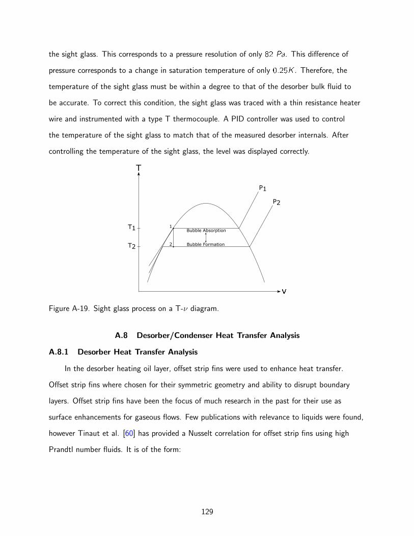
the sight glass. This corresponds to a pressure resolution of only 82 Pa. This difference of

pressure corresponds to a change in saturation temperature of only 0.25K . Therefore, the

temperature of the sight glass must be within a degree to that of the desorber bulk fluid to

be accurate. To correct this condition, the sight glass was traced with a thin resistance heater

wire and instrumented with a type T thermocouple. A PID controller was used to control

the temperature of the sight glass to match that of the measured desorber internals. After

controlling the temperature of the sight glass, the level was displayed correctly.

1

2 Bubble Formation

Bubble AbsorptionT1

T2

T

P1

P2

Figure A-19. Sight glass process on a T-ν diagram.

A.8 Desorber/Condenser Heat Transfer Analysis

A.8.1 Desorber Heat Transfer Analysis

In the desorber heating oil layer, offset strip fins were used to enhance heat transfer.

Offset strip fins where chosen for their symmetric geometry and ability to disrupt boundary

layers. Offset strip fins have been the focus of much research in the past for their use as

surface enhancements for gaseous flows. Few publications with relevance to liquids were found,

however Tinaut et al. [60] has provided a Nusselt correlation for offset strip fins using high

Prandtl number fluids. It is of the form:

129

Nu = 0.0944Re0.647D Pr 1/3 (A–67)

The first step is towards using the correlation is to evaluate the Reynolds number in each

fin channel. The geometry may be seen in Figure A-20

Figure A-20. Heating oil fin geometry.

The geometrical properties of the fins are given as:

• t = 250 µm

• l = 1 in.

15 nsin.

= 0.0666 in. = 1.693x10−3 m

• h = 0.25 in. = 0.00635 m

• w = 0.25 in. = 0.00635 m

• kn = 401 WmK

Dh =4A

P(A–68)

A = (l − 2t) (h − t) (A–69)

130

P = 2 (l − 2t) + 2 (h − t) (A–70)

Dh =4 (l − 2t) (h − t)

2 (l − 2t) + 2 (h − t)(A–71)

Dh =4[1.693x10−3 m − 2 (250 µm)

](0.00635 m − 250 µm)

2 [1.693x10−3 m − 2 (250 µm)] + 2 (0.00635 m − 250 µm)= 0.001995 m (A–72)

Assuming the flow divides evenly into the channels created by the fins,

The number of channels nchannel normal to the flow is given by the fin pitch, F , expressed

in fins per unit length.

FPI

Figure A-21. Fin per inch profile.

wc = 15.97 in. = 0.405 m

Lc = 14.00 in. = 0.3556 m

tc = 0.25 in. = 0.00635 m

nchannel = wc (F ) (A–73)

nchannel = 15.97in.

(15ns

in.

)= 239 (A–74)

131

wc

tc

Lc

Figure A-22. Oil cavity dimensions. Upper cavity wall removed for visual inspection ofinternals. Arrows indicate oil flow pattern.

uchannel =utotalAmanifold

nchannelAchannel

(A–75)

Let the oil flow rate be: _V– = 0.55GPM = 3.469x10−5 m3

s= 0.01348 m

s(0.405 m) (0.00635 m)

uchannel =0.01348 m

s(0.405 m) (0.00635 m)

239 (7.277x10−6 m2)= 0.0199

m

s(A–76)

Note that the velocity within the channels increases as some of the flow area is consumed

by the edges of the fins normal to the flow.

Pr =cpµ

k(A–77)

Pr =1500 J

kgK(8.81× 10−3 Pa · s)0.15 W

mK

= 88.1 (A–78)

132

ReD =ρuchannelDh

µ(A–79)

ReD =960 kg

m3

(0.0199 m

s

)0.001995 m

8.81x10−3 Pa · s= 4.32 (A–80)

Nu = 0.0944 (4.23)0.647 (88.1)1/3 = 1.083 (A–81)

h =Nuk

Dh

(A–82)

h =1.083

(0.15 W

mK

)0.001995m

= 81.43W

m2K(A–83)

The model by Tinaut et al. [60] is conservative, but still shows good agreement with the

experimental data for the fins shown in Figure A-37. Because of this, it will be used for the

heat transfer coefficient. The fin efficiency may now be found:

ηn =tanh (ml)

ml(A–84)

[52] Table 3.5

m =

(2h

knt

)1/2

(A–85)

133

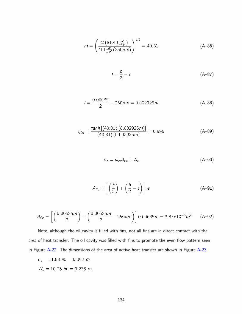
m =

(2(81.43 W

m2K

)401 W

mK(250µm)

)1/2

= 40.31 (A–86)

l =h

2− t (A–87)

l =0.00635

2− 250µm = 0.002925m (A–88)

ηn =tanh [(40.31) (0.002925m)]

(40.31) (0.002925m)= 0.995 (A–89)

At = nnAn + Ab (A–90)

An =

[(h

2

)+

(h

2− t

)]w (A–91)

An =

[(0.00635m

2

)+

(0.00635m

2− 250µm

)]0.00635m = 3.87x10−5m2 (A–92)

Note, although the oil cavity is filled with fins, not all fins are in direct contact with the

area of heat transfer. The oil cavity was filled with fins to promote the even flow pattern seen

in Figure A-22. The dimensions of the area of active heat transfer are shown in Figure A-23.

La = 11.88 in. = 0.302 m

Wa = 10.73 in. = 0.273 m

134

LaWa

Figure A-23. Finned desorption area dimensions.

nn,active =

(11.88 in.15

ns

in.

)(10.73 in.

0.25 in.row

)= 7476 (A–93)

At = 7476(3.87x10−5m2

)+ (0.302m) (0.273m) = 0.372m2 (A–94)

η0 = 1− nnAn

At

(1− ηn) (A–95)

η0 = 1−7476

(3.87x10−5m2

)0.372m2

(1− 0.995) = 0.996 (A–96)

Rt =1

η0hAt

(A–97)

135

1

UA=∑

R =1

η0hoilAt

+L

kA+

1

hdesorptionA(A–98)

hdesorption from Shi et. al. [61].

1

UA=

1

0.996(81.43 W

m2K

)0.372 m2

+9.11× 10−4 m

14.9 WmK

(0.302 m × 0.273 m)+

1

2000 Wm2K

(0.302 m × 0.273 m)

(A–99)

UA = 25W

K(A–100)

A.8.2 Condenser Heat Transfer Analysis

Condensation heat transfer occurs in two modes, film and dropwise [52]. Dropwise

condensation is marked by droplets covering the surface, while film condensation involves the

surface becoming covered in a film of condensed fluid (cf. Figure 7-4). Dropwise condensation

is the more desirable mode of heat transfer. Film condensation creates a resistance to heat

transfer as the film thickness grows, a phenomena that occurs in the direction of gravity.

Unfortunately, dropwise condensation is a condition that cannot be guaranteed. It is highly

dependent on surface factors affecting wettability such as material, cleanliness, and finish.

Therefore, the assumption is made that film condensation will be the only condition.

The design conditions for the condenser are given as:

• P = Psat = 8.543 kPa

• Tsat = 42.76C

• Tw = 25

• ρl = 994.37 kg

m3

• ρv = 0.0587 kg

m3

136

• hfg = 2399.36 kJkg

• µl = 7.35x10−4 Pa · s

• kl = 0.620 WmK

• cp,l = 4.179 kJkgK

Nusselt originally analyzed film condensation and arrived at the following analytical result

for the heat transfer coefficient. Chen showed that the errors associated with this correlation

are less than 3% [52]. All liquid properties are evaluated at the average film temperature.

NuL = 0.943

[ρlg (ρl − ρv) hfgmL

3

µlkl (Tsat − Ts)

]1/4(A–101)

Where hfgm is an improvement provided by Rohsenow [52].

hfgm = hfg + 0.68cp,l (Tsat − Ts) (A–102)

hfgm = 2399.36kJ

kg+ 0.68

(4.179

kJ

kgK

)(42.76C − 25C) = 2449.84

kJ

kgK(A–103)

NuL = 0.943

[994.37 kg

m3

(9.81m

s2

) (994.37 kg

m3 − 0.0587 kg

m3

)2449.84 kJ

kgK(0.00635 m)3

7.35x10−4 Pas(0.620 W

mK

)(42.76 C − 25C)

]1/4= 0.939

(A–104)

hL =NuLkL

L(A–105)

hL =1406.16

(0.620 W

mK

)0.00635 m

= 15244.21W

m2K(A–106)

137

Now, the UA value for a condenser may be calculated.

L

W

Figure A-24. Condenser fin geometry.

L = 0.246m

W = 0.1016m

ηn =tanh (ml)

ml(A–107)

m =

(2h

knt

)1/2

(A–108)

Experimental values for the heat transfer coefficient may be seen in Figure A-38. Using an

average value of 850 Wm2K

,

m =

(2(850 W

m2K

)401 W

mK(250µm)

)1/2

= 130.22 (A–109)

l = h − t (A–110)

138

l = 0.00635m − 250µm = 0.0061m (A–111)

ηn =tanh [(130.22) (0.0061m)]

(130.22) (0.0061m)= 0.831 (A–112)


An = [h + (h − t)]w (A–114)

An = [0.00635m + (0.00635m − 250µm)] 0.00635m = 7.9057x10−5m2 (A–115)

nn = 9.72 in.

(15ns

in.

)(4 in.

0.25 in.row

)= 2320 (A–116)

At = 2320(7.9057x10−5m2

)+ (0.246m) (0.1016m) = 0.208m2 (A–117)

η0 = 1− nnAn

At

(1− ηn) (A–118)

η0 = 1−2320

(7.9057x10−5m2

)0.208m2

(1− 0.831) = 0.851 (A–119)

139

m =

(2h

knt

)1/2

(A–120)

m =

(2(15000 W

m2K

)401 W

mK(250µm)

)1/2

= 547.03 (A–121)

l = h − t (A–122)

l = 0.00635m − 250µm = 0.0061m (A–123)

ηn =tanh [(547.03) (0.0061m)]

(547.03) (0.0061m)= 0.298 (A–124)

η0 = 1− nnAn

At

(1− ηn) (A–125)

η0 = 1−2320

(7.9057x10−5m2

)0.208m2

(1− 0.298) = 0.538 (A–126)

Rt =1

η0hAt

(A–127)

1

UA=

1

hcondensationA+

L

kA+

1

η0hAt

(A–128)

140

1

UA=

1

9152.49 Wm2K

(0.025 m2)+

9.11x10−4 m

14.9 WmK

(0.025 m2)+

1

850 Wm2K

(0.208 m2) 0.851

(A–129)

UA = 74.81W

K(A–130)

A.8.3 Condenser Cooling Water Pressure Analysis

In order to ensure that flow does not short circuit and bypass the cooling water channels,

it is imperative that the cooling water layer does not flex when pressurized. If the plate were

to flex, it would lift off the fin tips and create a head space above the cooling water fins.

Deflection of a plate constrained at the edges makes an appearance in Roark’s Formulas for

Stress and Strain [62] where a solution for the maximum deflection is provided. It is given as:

ymax =αqb4

Et3(A–131)

q = Pressure(Pa)

E = 190GPa [63]

t = 9.11x10−4m

α = from geometry and table of [62]

Where ymax is the deflection at the center of the plate, E is the modulus of elasticity, and

t is the plate thickness. Note that Roark’s solution is only valid for simple geometries; it is not

applicable for the braced plate. The advantage of the braced plate is due to its non-constant

moment of inertia, which Roark’s equation does not support. Finite element analysis (FEA)

was used to estimate the deformation of the braced plate. It is important to verify FEA with

a secondary method; the results from Roark’s method were compared to the FEA analysis of

141

a simple plate to provide a level of validation for the FEA technique. Without validation, the

applicability of the boundary conditions and meshing would be unknown.

In order to calculate the deflection, the pressure expected within the cooling water

layer must be known. This can be found if the pressure drop through the layer is known.

Using the experimental test cell of Figure A-34, the system curve shown in Figure A-25 was

generated. Correlations for pressure drop through offset strip fins have been proposed by

several researchers, Bhowmik et al. [64] presents the most inclusive compilation of offset strip

thermohydrualic research. In addition, a correlation for the pressure drop through such a finned

array is provided in the form:

P =(10Re−0.68

d

) L

Dh

ρu2

2(A–132)

Figure A-25. Condenser system head loss curves.

Using the pressures from Figure A-25, the cover deflection versus pressure was plotted

for a range of expected operating conditions in Figure A-26. It was found that if bracing was

applied in an x-pattern across the face of the plate, the deflection could be reduced by more

142

than 88%. This design was then verified using FEA, Figure A-27 where increasing redness

indicates increasing deformation.

No bra

cing

Bracin

g

Figure A-26. Cooling water cover deflection versus pressure.

The deflection of the plate was measured using a dial indicator with 12.7µ m increments.

The dial was mounted approximately at the center of the condenser, where deflection is

greatest as shown in Figure A-27. Figure A-26 shows excellent agreement between simulated

and experimental values. Any sort of difference between the values may be due to variations in

material property or manufacturing.

143

Figure A-27. Condenser deflection with bracing. Increasing redness indicated increasingdeformation.

Figure A-28. Dial gauge measuring condenser plate deflection. Photo courtesy of author.

144

A.9 Absorber/Evaporator Heat Transfer Analysis

A.9.1 Absorber Heat Transfer Analysis

Figure A-29. Absorber cooling water fins. Photo courtesy of author.

FPI

h

l

t

Figure A-30. Absorber cooling water fin geometry.

The geometrical properties of the fins are given as:

• t = 60 µm

• l = 1F= 1 in.

48 nsin.

= 0.02083 in. = 5.29x10−4 m

• h = 0.125 in. = 0.00635 m

• kn = 401 WmK

Dh =4A

P(A–133)

145

A = (l − 2t) (h − t) (A–134)

P = 2 (l − 2t) + 2 (h − t) (A–135)

Dh =4 (l − 2t) (h − t)

2 (l − 2t) + 2 (h − t)(A–136)

Dh =4[4.09x10−4 m − 2 (60 µm)

] (1.58x10−3 m − 60 µm

)2 [4.09x10−4 m − 2 (60 µm)] + 2 (1.58x10−3 m − 60 µm)

= 6.45x10−3 m (A–137)

Wa

La

Figure A-31. Finned absorption area dimensions.

• La = 23.97 in. = 0.609 m

• wa = 10.11 in. = 0.257 m

nchannel = wa (F ) (A–138)

146

nchannel = 23.97in.

(48ns

in.

)= 1150 (A–139)

Nu = 6.49 [52] (A–140)

h =Nuk

Dh

(A–141)

h =6.49

(0.607 W

mK

)6.45x10−3 m

= 6105W

m2K(A–142)

ηn =tanh (ml)

ml(A–143)

[52] Table 3.5

m =

(2h

knt

)1/2

(A–144)

m =

(2(6105 W

m2K

)401 W

mK(60µm)

)1/2

= 712.4 (A–145)

l =h

2− t (A–146)

147

l =0.00635

2− 60µm = 0.00153 m (A–147)

ηn =tanh [(712.4) (0.00153 m)]

(712.4) (0.00153 m)= 0.731 (A–148)

An =h

2(l) (A–149)

An = 21.53x10−3 m

2(0.257) = 7.85x10−4 m2 (A–150)


At = 1150(7.85x10−4 m2

)+ (0.257m) (0.609m) = 1.059 m2 (A–152)

η0 = 1− nnAn

At

(1− ηn) (A–153)

η0 = 1−1150

(3.87x10−5 m2

)0.372m2

(1− 0.731) = 0.771 (A–154)

Rt =1

η0hAt

(A–155)

148

1

UA=∑

R =1

η0hcoolingwaterAt

+L

kA+

1

habsorptionA(A–156)

1

UA=

1

0.771(6105 W

m2K

)1.059 m2

+9.11× 10−4 m

14.9 WmK

(0.257 m × 0.609 m)+

1

1500 Wm2K

(0.257 m × 0.609 m)

(A–157)

UA = 206W

K(A–158)

A.9.2 Evaporator Heat Transfer Analysis

Figure A-32. Evaporator fin geometry.

• t = 60 µm

• l = 1F= 1 in.

48 nsin.

= 0.02083 in. = 5.29x10−4 m

• h = 0.125 in. = 0.00635 m

• kn = 401 WmK

Dh =4A

P(A–159)

149

A = (l − 2t) (h − t) (A–160)

P = 2 (l − 2t) + 2 (h − t) (A–161)

Dh =4 (l − 2t) (h − t)

2 (l − 2t) + 2 (h − t)(A–162)

Dh =4[4.09x10−4 m − 2 (60 µm)

] (3.18x10−3 m − 60 µm

)2 [4.09x10−4 m − 2 (60 µm)] + 2 (3.18x10−3 m − 60 µm)

= 7.23x10−3 m (A–163)

Hc

Lc

Figure A-33. Finned evaporation area dimensions.

Hc = 5.91 in. = 0.150 m

Lc = 22.0 in. = 0.541 m

nchannel = Lc (F ) (A–164)

150

nchannel = 22.0in.

(48ns

in.

)= 1020 (A–165)

Nu = 6.49 [52] (A–166)

h =Nuk

Dh

(A–167)

h =6.49

(0.607 W

mK

)6.45x10−3 m

= 5448W

m2K(A–168)

ηn =tanh (ml)

ml(A–169)

[52] Table 3.5

m =

(2h

knt

)1/2

(A–170)

m =

(2(5448 W

m2K

)401 W

mK(60µm)

)1/2

= 672.9 (A–171)

l = h − t (A–172)

151

l = 0.00635 m − 60µm = 0.00312 m (A–173)

ηn =tanh [(802.2) (0.00312 m)]

(802.2) (0.00312 m)= 0.462 (A–174)

An = 2h (l) (A–175)

An = 2(3.11x10−3 m

)(0.15 m) = 9.35x10−4 m2 (A–176)


At = 1020(9.35x10−4 m2

)+ (0.15m) (0.541m) = 1.034 m2 (A–178)

η0 = 1− nnAn

At

(1− ηn) (A–179)

η0 = 1−1020

(9.35x10−4 m2

)1.034m2

(1− 0.462) = 0.505 (A–180)

Rt =1

η0hAt

(A–181)

152

1

UA=∑

R =1

η0hchilledwaterAt

+L

kA+

1

hevaporationA(A–182)

1

UA=

1

0.505(5448 W

m2K

)1.034 m2

+9.11× 10−4 m

14.9 WmK

(0.15 m × 0.541 m)+

1

2500 Wm2K

(0.15 m × 0.541 m)

(A–183)

UA = 589W

K(A–184)

A.10 Offset Strip Fin Heat Transfer Coefficient

In order to estimate the fin area required for heat transfer on the working system, the

heat transfer coefficient of the finned structure must be known. Correlations for offset strip

fins have a range of Reynolds numbers in which the correlation is valid. The of Reynolds

numbers the desorber heating oil surfaces are expected to see is outside of the range of

correlations in literature. CFD may be used to estimate the heat transfer coefficient, however

the complex shape would be time consuming and not necesarily accurate. Experimental testing

was chosen to obtain heat transfer coefficient values for fins subjected to heating oil flows. A

representative test cell was fabricated using the same techniques and materials as the actual

system. The test cell may be seen in Figure A-34. Either side of the test cell featured an

electrical resistance heater, allowing the finned base to be heated. Knowing the oil inlet and

exit temperatures as well as the flow rate, the amount of heat transferred to the oil was known.

When calculating the heat transfer coefficient, the following equation was used.

q = η0hAt (Ts − Tm) (A–185)

Where η0 is given by Equation A–118.

153

Figure A-34. Heat transfer test cell.

q = _mcp (Tout − Tin) (A–186)

Combining these two equations plus those for the fin efficiency,

_mcp (Tout − Tin) =

1− nnAn

At

1−tanh

((2hknt

)1/2l

)(

2hknt

)1/2l

hAt (Ts − Tm) (A–187)

On a unit basis, per unit of base area, the bonded fins contribute ≈ 7.2X the surface

area. While this is great for heat transfer, it is a caveat for manufacturing and experimentation.

The heat transfer coefficient is extremely sensitive to area. In addition, it is difficult from a

manufacturing perspective to guarantee every single fin in a large array is bonded. To provide

perspective, the test cell had 1500 fins. Because they make up a large percentage of the the

heat transfer area, an un-bonded fin can greatly disrupt heat transfer measurements. Moreover,

it is not necessarily straightforward to quantify the bond integrity of the fins. To get an idea of

the heat transfer area involved, high speed thermal imaging was used to quantify the bonded

fin area; the technique is described in more detail in Chapter 3.

Other areas of concern are those of surface temperature. Surface temperature measurement

is a difficult task to accomplish. Techniques include infrared, thermochromic liquid crystals

154

[65], and embedded thermocouples. The first two method are not easily applicable to enclosed

heat exchangers, and the latter is difficult with thin sheet metal constructions.

Figure A-35. Thermocouple placed within a 500 µm deep well. Photo courtesy of author.

In critical applications such as nuclear reactors, thermocouples may be laser welded

to metallic structures [66]. Due to the excellent thermal contact, strength, and short

manufacturing time, type T thermocouples were laser welded to the surface of the heat

exchanger as shown in Figure A-35. Biswal et a. showed that type K thermocouples can be

laser welded, however no information about type T thermocouples was available. The Seedbeck

effect should not be affected, however thermocouple accuracy after welding was verified as seen

in Figure A-36.

155

Figure A-36. Heat transfer test cell wall thermocouple calibration.

Figure A-37. Experimental heat transfer coefficient measurements for oil.

156

Figure A-38. Experimental heat transfer coefficient measurements for cooling water through 15FPI offset fins

157

REFERENCES

[1] B. Nagengast, “Air Conditioning and Refrigeration Chronology,” 2006. [Online]. Available:https://www.ashrae.org/filelibrary/doclib/public/200651081623 347.pdf

[2] “1 Dead in Ammonia Leak at Boston Seafood Warehouse,”Boston, mar 2016. [Online]. Available: http://www.cbsnews.com/news/1-dead-in-ammonia-leak-at-boston-seafood-warehouse/

[3] S. V. Oleinik, Y. I. Kuznetsov, and a. R. Vartapetyan, “Corrosion Inhibition of Steel inLithium Bromide Brines,” Protection of Metals, vol. 39, no. 1, pp. 12–18, 2003. [Online].Available: http://dx.doi.org/10.1023/A:1021926721261

[4] P. Wasserscheid and W. Keim, “Ionic Liquids-New ”Solutions” for Transition MetalCatalysis.” Angewandte Chemie (International ed. in English), vol. 39, no. 21, pp.3772–3789, nov 2000. [Online]. Available: http://www.ncbi.nlm.nih.gov/pubmed/11091453

[5] M. Uerdingen, C. Treber, M. Balser, G. Schmitt, and C. Werner, “Corrosion behaviourof ionic liquids,” Green Chemistry, vol. 7, no. 5, p. 321, 2005. [Online]. Available:http://xlink.rsc.org/?DOI=b419320m

[6] M. Seiler, A. Ku, F. Ziegler, and X. Wang, “Sustainable Cooling StrategiesUsing New Chemical System Solutions,” Industrial & Engineering ChemistryResearch, vol. 52, no. 47, pp. 16 519–16 546, 2013. [Online]. Available:http://pubs.acs.org/doi/abs/10.1021/ie401297u

[7] E. D. Bates, R. D. Mayton, I. Ntai, and J. H. Davis, “CO2 capture by a task-specific ionicliquid,” Journal of the American Chemical Society, vol. 124, no. 6, pp. 926–927, 2002.

[8] C. Poole, “Ionic Liquids,” 2007. [Online]. Available: https://www.sigmaaldrich.com/content/dam/sigma-aldrich/docs/Aldrich/Brochure/al chemfile v5 n6.pdf

[9] M. Seiler and M.-C. Schneider, “Ionic liquids: Cooling and heating with heat,” pp. 12–19,2011. [Online]. Available: http://corporate.evonik.com/ layouts/Websites/Internet/DownloadCenterFileHandler.ashx?siteId=bbb7c219-72ac-4866-b79e-9397dc4d070b&fileid=649

[10] M. Preißinger, S. Pollinger, and D. Bruggemann, “Ionic liquid based absorptionchillers for usage of low grade waste heat in industry,” International Journal ofEnergy Research, vol. 37, no. January, pp. 1382–1388, 2013. [Online]. Available:http://dx.doi.org/10.1002/er.2997

[11] a. Yokozeki and M. B. Shiflett, “Water solubility in ionic liquids and application toabsorption cycles,” Industrial and Engineering Chemistry Research, vol. 49, no. 19, pp.9496–9503, 2010. [Online]. Available: http://pubs.acs.org/doi/abs/10.1021/ie1011432

[12] L. Dong, D. Zheng, N. Nie, and Y. Li, “Performance prediction of absorptionrefrigeration cycle based on the measurements of vapor pressure and heat capacity of

158

https://www.ashrae.org/file library/doclib/public/200651081623_347.pdf

http://www.cbsnews.com/news/1-dead-in-ammonia-leak-at-boston-seafood-warehouse/

http://www.cbsnews.com/news/1-dead-in-ammonia-leak-at-boston-seafood-warehouse/

http://dx.doi.org/10.1023/A:1021926721261

http://www.ncbi.nlm.nih.gov/pubmed/11091453

http://xlink.rsc.org/?DOI=b419320m

http://pubs.acs.org/doi/abs/10.1021/ie401297u

https://www.sigmaaldrich.com/content/dam/sigma-aldrich/docs/Aldrich/Brochure/al_chemfile_v5_n6.pdf

https://www.sigmaaldrich.com/content/dam/sigma-aldrich/docs/Aldrich/Brochure/al_chemfile_v5_n6.pdf

http://corporate.evonik.com/_layouts/Websites/Internet/DownloadCenterFileHandler.ashx?siteId=bbb7c219-72ac-4866-b79e-9397dc4d070b&fileid=649



http://dx.doi.org/10.1002/er.2997

http://pubs.acs.org/doi/abs/10.1021/ie1011432

H2O+[DMIM]DMP system,” Applied Energy, vol. 98, pp. 326–332, oct 2012. [Online].Available: http://linkinghub.elsevier.com/retrieve/pii/S0306261912002620

[13] K. E. Herold, R. Radermacher, and S. A. Klein, Absorption Chillers and Heat Pumps.Boca Raton: CRC, 1996.

[14] G. Grossman, “Modular simulation of absorption systems user’s guide and reference,”Oak Ridge National Lab, Tech. Rep. March 1998, 2000. [Online]. Available:http://web.ornl.gov/∼webworks/cpr/rpt/107911 .pdf

[15] G. Grossman and A. Zaltash, “ABSIM - Modular simulation of advanced absorptionsystems,” International Journal of Refrigeration, vol. 24, no. 6, pp. 531–543, 2001.[Online]. Available: http://dx.doi.org/10.1016/S0140-7007(00)00051-7

[16] J. S. Wilkes, J. a. Levisky, R. a. Wilson, and C. L. Hussey, “Dialkylimidazoliumchloroaluminate melts: a new class of room-temperature ionic liquids for electrochemistry,spectroscopy and synthesis,” Inorg. Chem., vol. 21, no. 3, pp. 1263–1264, 1982. [Online].Available: http://pubs.acs.org/doi/abs/10.1021/ic00133a078

[17] E. Ruiz, V. Ferro, J. de Riva, D. Moreno, and J. Palomar, “Evaluation of ionic liquidsas absorbents for ammonia absorption refrigeration cycles using COSMO-based processsimulations,” Applied Energy, vol. 123, pp. 281–291, jun 2014. [Online]. Available:http://linkinghub.elsevier.com/retrieve/pii/S0306261914002062

[18] L. E. Ficke, “Thermodynamic properties of Imidazolium and phosphonium based ionicliquid mixtures with water or carbon dioxide,” Ph.D. dissertation, University of NotreDame, 2010. [Online]. Available: https://curate.nd.edu/concern/etds/dz010p1198p

[19] N. Sukumar, B. Moran, a. Y. Semenov, and V. V. Belikov, “Natural neighbour Galerkinmethods,” International Journal for Numerical Methods in Engineering, vol. 50, no. 1, pp.1–27, 2000.

[20] I. H. Bell, J. Wronski, S. Quoilin, and V. Lemort, “Pure and Pseudo-pure FluidThermophysical Property Evaluation and the Open-Source Thermophysical Property LibraryCoolProp.” Industrial & engineering chemistry research, vol. 53, no. 6, pp. 2498–2508, feb2014.

[21] J. Patek and J. Klomfar, “A computationally effective formulation of the thermodynamicproperties of LiBr-H2O solutions from 273 to 500 K over full composition range,”International Journal of Refrigeration, vol. 29, no. 4, pp. 566–578, 2006. [Online].Available: http://dx.doi.org/10.1016/j.ijrefrig.2005.10.007

[22] R. Amatya, F. Brushett, A. Campanella, G. Kavlak, J. Macko, A. Maurano,J. McNerney, T. Osedach, P. Rodilla, A. Rose, A. Sakti, E. Steinfeld,J. Trancik, and H. Tuller, “The Future of Solar Energy,” MassachusettsInstitute of Technology, Tech. Rep., 2015. [Online]. Available: https://mitei.mit.edu/system/files/MITFutureofSolarEnergyStudy compressed.pdf

159

http://linkinghub.elsevier.com/retrieve/pii/S0306261912002620

http://web.ornl.gov/~webworks/cpr/rpt/107911_.pdf

http://dx.doi.org/10.1016/S0140-7007(00)00051-7

http://pubs.acs.org/doi/abs/10.1021/ic00133a078


https://curate.nd.edu/concern/etds/dz010p1198p

http://dx.doi.org/10.1016/j.ijrefrig.2005.10.007

https://mitei.mit.edu/system/files/MIT Future of Solar Energy Study_compressed.pdf

https://mitei.mit.edu/system/files/MIT Future of Solar Energy Study_compressed.pdf

[23] D. Y. Goswami, F. Kreith, and F. J. Kreider, Prinicples of Solar Engineering, 2nd ed.Taylor and Francis Group, 2000.

[24] D. S. Kim and C. H. M. Machielsen, “Evaluation of Air-Cooled Solar AbsorptionCooling Systems,” in International Sorption Heat Pump Conference, Shanghai,2002, pp. 117–122. [Online]. Available: http://doi.ewi.tudelft.nl/live/binaries/29b66c2b-9a38-4d72-a328-2df33ad064ea/doc/Shanghai02.pdf

[25] P. Holmberg and T. Berntsson, “Alternative working fluids in heat transformers,” inASHRAE Transactions. ASHRAE, 1990, pp. 1582–1589.

[26] D. F. Othmer, “Correlating vapor pressure and latent heat data,” Industrial & EngineeringChemistry, vol. 32, no. 6, p. 841, 1940.

[27] M. Kilic and O. Kaynakli, “Second law-based thermodynamic analysis of water-lithiumbromide absorption refrigeration system,” Energy, vol. 32, no. 8, pp. 1505–1512, 2007.

[28] EIA, “Electric Power Monthly: with data for January 2016,” U.S. Energy InformationAdministration, no. August, 2016.

[29] “Natural Gas Prices,” 2016. [Online]. Available: https://www.eia.gov/dnav/ng/ng pri sum a EPG0 PRS DMcf m.html

[30] S. Bigham, D. Yu, D. Chugh, and S. Moghaddam, “Moving beyond the limits of masstransport in liquid absorbent microfilms through the implementation of surface-inducedvortices,” Energy, vol. 65, pp. 621–630, 2014.

[31] “Absorption Series,” 2001.

[32] D. P’ng and P. Molian, “Q-switch Nd:YAG laser welding of AISI 304 stainless steel foils,”Materials Science and Engineering A, vol. 486, no. 1-2, pp. 680–685, 2008.

[33] T. Y. Fan and Byer, “Modelling and CW operation of a quasi-three-level 946 nm Nd:YAGlaser,” IEEE Journal of Quantum Electronics, vol. 23, no. May, pp. 605–612, 1987.

[34] C. Ruettimann, R. Bartlome, and N. Dury, “Reproducible Copper Welding,” IndustrialLaser Solutions, pp. 24–28, sep 2013.

[35] B. C. Moore, “Thin-walled vacuum chambers of austenitic stainless steel,” Journal ofVacuum Science & Technology A: Vacuum, Surfaces, and Films, vol. 19, no. 1, p. 228,2001. [Online]. Available: http://scitation.aip.org/content/avs/journal/jvsta/19/1/10.1116/1.1333083

[36] J. R. J. Bennett, R. J. Elsey, and R. W. Malton, “Convoluted vacuum tubes for longbaseline interferometric gravitational wave detectors,” Vacuum, vol. 43, no. 1, pp. 531–535,1992.

160

http://doi.ewi.tudelft.nl/live/binaries/29b66c2b-9a38-4d72-a328-2df33ad064ea/doc/Shanghai02.pdf

http://doi.ewi.tudelft.nl/live/binaries/29b66c2b-9a38-4d72-a328-2df33ad064ea/doc/Shanghai02.pdf

https://www.eia.gov/dnav/ng/ng_pri_sum_a_EPG0_PRS_DMcf_m.html

https://www.eia.gov/dnav/ng/ng_pri_sum_a_EPG0_PRS_DMcf_m.html

http://scitation.aip.org/content/avs/journal/jvsta/19/1/10.1116/1.1333083

http://scitation.aip.org/content/avs/journal/jvsta/19/1/10.1116/1.1333083

[37] V. Nemanic and J. Setina, “Experiments with a thin-walled stainless-steel vacuum chamber,”Journal of Vacuum Science & Technology A: Vacuum, Surfaces, and Films, no. May, pp.1789–1793, 2000. [Online]. Available: http://link.aip.org/link/?JVTAD6/18/1789/1

[38] J. Griess, J. DeVan, and H. P. Blanco, “Corrosion of materials in absorption heatingand refrigeration fluids,” Oak Ridge National Laboratory, Tech. Rep., 1985. [Online].Available: http://web.ornl.gov/sci/ees/etsd/btric/eere research reports/thermally activated technologies/absorption/working fluids/ornl tm 9646/ornl tm 9646.pdf

[39] P. Fraas, Arthur, Heat Exchanger Design, 2nd ed. John Wiley & Sons, 1989.

[40] J. Wang, “Theory of flow distribution in manifolds,” Chemical EngineeringJournal, vol. 168, no. 3, pp. 1331–1345, 2011. [Online]. Available:http://dx.doi.org/10.1016/j.cej.2011.02.050

[41] J. P. Pritchard, Fox and McDonald’s introduction to fluid mechanics, 8th ed. John Wiley& Sons, 2011.

[42] F. C. Johansen, “Flow through pipe orifices at low Reynolds numbers,” Proceedings of theRoyal Society of London, vol. 126, no. Series A, pp. 231–245, 1930.

[43] Thermal Properties of Metals, 2002.

[44] R. Halmshaw, Introduction to the Non-Destructive Testing of Welded Joints, 2nd ed.Abington Publishing, 1996. [Online]. Available: http://dx.doi.org/10.1533/9781845698829.frontmatter

[45] P. Chaudhuri, P. Santra, S. Yoele, A. Prakash, D. C. Reddy, L. T. Lachhvani,J. Govindarajan, and Y. C. Saxena, “Non-destructive evaluation of brazed joints betweencooling tube and heat sink by IR thermography and its verification using FE analysis,” NDTand E International, vol. 39, no. 2, pp. 88–95, 2006.

[46] B. P. Rao and S. K. Das, “Effect of flow distribution to the channels on the thermalperformance of the multipass plate heat exchangers,” Heat Transfer Engineering, vol. 25,no. 8, pp. 48–59, 2004. [Online]. Available: http://www.scopus.com/inward/record.url?eid=2-s2.0-10444267259&partnerID=40&md5=440aa8c539c284abfc166ce76f99f146

[47] N. Miljkovic, R. Enright, Y. Nam, K. Lopez, N. Dou, J. Sack, and E. N. Wang,“Jumping-droplet-enhanced condensation on scalable superhydrophobic nanostructuredsurfaces,” Nano Letters, vol. 13, no. 1, pp. 179–187, 2013.

[48] B. T. McDonald and T. Cui, “Superhydrophilic surface modification of copper surfacesby Layer-by-Layer self-assembly and Liquid Phase Deposition of TiO2 thin film,” Journalof Colloid and Interface Science, vol. 354, no. 1, pp. 1–6, 2011. [Online]. Available:http://dx.doi.org/10.1016/j.jcis.2010.09.036

161

http://link.aip.org/link/?JVTAD6/18/1789/1

http://web.ornl.gov/sci/ees/etsd/btric/eere_research_reports/thermally_activated_technologies/absorption/working_fluids/ornl_tm_9646/ornl_tm_9646.pdf



http://dx.doi.org/10.1016/j.cej.2011.02.050

http://dx.doi.org/10.1533/9781845698829.frontmatter

http://dx.doi.org/10.1533/9781845698829.frontmatter

http://www.scopus.com/inward/record.url?eid=2-s2.0-10444267259&partnerID=40&md5=440aa8c539c284abfc166ce76f99f146

http://www.scopus.com/inward/record.url?eid=2-s2.0-10444267259&partnerID=40&md5=440aa8c539c284abfc166ce76f99f146

http://dx.doi.org/10.1016/j.jcis.2010.09.036

[49] J. Min, X. Wu, L. Shen, and F. Gao, “Hydrophilic treatment and performance evaluationof copper finned tube evaporators,” Applied Thermal Engineering, vol. 31, no. 14-15, pp.2936–2942, 2011.

[50] C. Li and G. Petersen, “Evaporation and Boiling in Thin Capillary Wicks,” Transactions ofthe ASME, vol. 128, pp. 1320–1328, 2006.

[51] R. L. Depew, C. A., Reisbig, “Vapor condensation on a horizontal tube using teflon topromote dropwise condensation.” I&EC Process Des. Develop., vol. 3, no. 4, pp. 365–369,1964.

[52] L. T. Bergman, S. A. Lavine, P. F. Incropera, and P. D. Dewitt, Fundamentals of heat andmass transfer, 7th ed. John Wiley & Sons, 2011.

[53] D. J. Preston, D. L. Mafra, N. Miljkovic, J. Kong, and E. N. Wang, “Scalable graphenecoatings for enhanced condensation heat transfer,” Nano Letters, vol. 15, no. 5, pp.2902–2909, 2015.

[54] W. Yao, H. Bjurstom, and F. Settewall, “Surface tension of lithium bromide solutionwith heat-transfer aditives,” Journal of Chemical & Engineering Data, vol. 36, no. 27, pp.96–99, 1991.

[55] K. Ishida and Y. H. Mori, “Surface tension of aqueous lithium bromide solutions containing1-octanol as a ”heat-transfer additive”,” International Communications in Heat and MassTransfer, vol. 23, no. 7, pp. 907–915, 1996.

[56] K. J. Kim and V. P. Janule, “Dynamic surface tension of aqueous lithium bromide with2-ethyl-1-hexanol,” International Communications in Heat and Mass Transfer, vol. 21,no. 6, pp. 839–848, 1994.

[57] W. T. Wu, Y. M. Yang, and J. R. Maa, “Effect of surfactant additive on pool boiling ofconcentrated lithium bromide solution,” International Communications in Heat and MassTransfer, vol. 25, no. 8, pp. 1127–1134, 1998.

[58] D. Callister, William, Materials Science and Engineering, 7th ed. New York: John Wiley& Sons, 2007.

[59] “Basics of Corrosion Measurements.” [Online]. Available: www.princetonappliedresearch.com

[60] F. Tinaut, A. Melgar, and A. R. Ali, “Correlations for heat transfer and flowfriction characteristics of compact plate type heat exchangers,” International journalof Heat and Mass Transfer, vol. 35, no. 7, pp. 1659–1665, 1991. [Online]. Available:http://dx.doi.org/10.1016/0017-9310(92)90136-G

[61] C. Shi, Q. Chen, T.-c. Jen, and W. Yang, “International Journal of Heat and MassTransfer Heat transfer performance of lithium bromide solution in falling film generator,”International Journal of Heat and Mass Transfer, vol. 53, no. 15-16, pp. 3372–3376, 2010.[Online]. Available: http://dx.doi.org/10.1016/j.ijheatmasstransfer.2010.02.051

162

www.princetonappliedresearch.com

www.princetonappliedresearch.com

http://dx.doi.org/10.1016/0017-9310(92)90136-G

http://dx.doi.org/10.1016/j.ijheatmasstransfer.2010.02.051

[62] R. J. Roark, W. C. Young, and R. Plunkett, Formulas for Stress and Strain. McGraw-Hill,1976, vol. 43, no. 3.

[63] F. Beer, E. Johnston, J. DeWolf, and D. Mazurek, Mechanics of Materials, 5th ed. NewYork: McGraw-Hill, 2009.

[64] H. Bhowmik and K.-S. Lee, “Analysis of heat transfer and pressure dropcharacteristics in an offset strip fin heat exchanger,” International Communicationsin Heat and Mass Transfer, vol. 36, no. 3, pp. 259–263, 2009. [Online]. Available:http://dx.doi.org/10.1016/j.icheatmasstransfer.2008.11.001

[65] V. U. Kakade, G. D. Lock, M. Wilson, J. M. Owen, and J. E. Mayhew, “Accurateheat transfer measurements using thermochromic liquid crystal. Part 1: Calibration andcharacteristics of crystals,” International Journal of Heat and Fluid Flow, vol. 30, no. 5, pp.939–949, 2009. [Online]. Available: http://dx.doi.org/10.1016/j.ijheatfluidflow.2009.04.007

[66] R. Biswal, K. Gopal, S. Murugan, S. Venugopal, and T. Jayakumar, “Standardizationof Laser Welding Parameters for Attachment of Thermocouple to Pressurized Capsulefor On-Line Creep Rupture Studies,” Procedia Engineering, vol. 86, pp. 560–566, 2014.[Online]. Available: http://linkinghub.elsevier.com/retrieve/pii/S1877705814020402

163

http://dx.doi.org/10.1016/j.icheatmasstransfer.2008.11.001

http://dx.doi.org/10.1016/j.ijheatfluidflow.2009.04.007


BIOGRAPHICAL SKETCH

Reid E. Shaeffer grew up in the town of Destin along Florida’s Emerald Coast. During

his final years of high school, he began his college career at Northwest Florida State College.

After graduating, he transferred to the University of Florida to study mechanical engineering

where he was one of 3 summa cum laude graduating with a BS in mechanical engineering in

the fall of 2012. He was awarded the University’s prestigious Graduate Student Fellowship to

continue his education. In 2014 he earned his MS in mechanical engineering and completed

Ph.D. studies in December of 2016.

164

c 2016 reid edward ﬀ - university of florida

Documents