c© 2017 Ryan Freedman

LSTM AND EXTENDED DEAD RECKONING AUTOMOBILE ROUTEPREDICTION USING SMARTPHONE SENSORS

BY

RYAN FREEDMAN

THESIS

Submitted in partial fulfillment of the requirementsfor the degree of Master of Science in Computer Science

in the Graduate College of theUniversity of Illinois at Urbana-Champaign, 2017

Urbana, Illinois

Adviser:

Professor Carl A. Gunter

ABSTRACT

We examine the application of two solutions to resolving automobile route

shape using non-GPS sensor information provided by a smart-phone. This is

motivated by the unreliability of GPS sensor information due to the ease of

spoofing of GPS sensor data and areas of low signal. A trace is generated as

output from this algorithm that predicts route taken. The two approaches,

Extended Dead Reckoning and LSTM, are compared for their advantages

and disadvantages.

These concepts are explored by recording nearly one thousand miles of

driving data from Virginia to Indiana to Illinois. The GPS data is used

to train the LSTM neural network along with the thirty non-GPS features

recorded from the smart-phone. The output is a route shape that is used to

determine potential driving route and verify if a route input is correct. This

method is evaluated against our implementation of dead reckoning using the

same data. We find that the machine learning approach allows for precise

route shape prediction with relatively constant accuracy and low sensitivity

to changes in orientation. The extended dead reckoning approach proves to

be substantially more accurate but sensitive to changes in orientation making

the route prediction veer off if the smart-phone is moved mid-route.

In a broader scope, this thesis investigates the application of a recurrent

neural network (RNN) algorithm that is normally used for text-mining appli-

cations to process other types of data, namely sensor data. A more manual

approach, the extended dead reckoning, is used as a comparison for this

application.

ii

To my parents and my sister, for their continual support.

iii

TABLE OF CONTENTS

LIST OF TABLES . . . . . . . . . . . . . . . . . . . . . . . . . . . . . vi

LIST OF FIGURES . . . . . . . . . . . . . . . . . . . . . . . . . . . . vii

LIST OF ABBREVIATIONS . . . . . . . . . . . . . . . . . . . . . . . viii

CHAPTER 1 INTRODUCTION . . . . . . . . . . . . . . . . . . . . 11.1 Problem Statement . . . . . . . . . . . . . . . . . . . . . . . . 11.2 Objective . . . . . . . . . . . . . . . . . . . . . . . . . . . . . 21.3 Contributions . . . . . . . . . . . . . . . . . . . . . . . . . . . 21.4 Thesis Organization . . . . . . . . . . . . . . . . . . . . . . . . 3

CHAPTER 2 BACKGROUND . . . . . . . . . . . . . . . . . . . . . 52.1 Sensors . . . . . . . . . . . . . . . . . . . . . . . . . . . . . . . 52.2 Spoofing . . . . . . . . . . . . . . . . . . . . . . . . . . . . . . 72.3 Recurrent Learning . . . . . . . . . . . . . . . . . . . . . . . . 82.4 Long Short-Term Memory (LSTM) + Forget Gates . . . . . . 82.5 Dead Reckoning . . . . . . . . . . . . . . . . . . . . . . . . . . 92.6 Related Work . . . . . . . . . . . . . . . . . . . . . . . . . . . 9

CHAPTER 3 DATA COLLECTION . . . . . . . . . . . . . . . . . . 123.1 Hardware and Dataset Information . . . . . . . . . . . . . . . 123.2 Setup . . . . . . . . . . . . . . . . . . . . . . . . . . . . . . . . 153.3 Routes . . . . . . . . . . . . . . . . . . . . . . . . . . . . . . . 16

CHAPTER 4 DESIGN AND IMPLEMENTATION . . . . . . . . . . 184.1 Route Shape . . . . . . . . . . . . . . . . . . . . . . . . . . . . 184.2 Route Matching . . . . . . . . . . . . . . . . . . . . . . . . . . 23

CHAPTER 5 RESULTS, EVALUATION, AND DISCUSSION . . . . 255.1 Route Evaluation . . . . . . . . . . . . . . . . . . . . . . . . . 255.2 Comparison Between Methods . . . . . . . . . . . . . . . . . . 33

CHAPTER 6 FUTURE WORK AND CONCLUSION . . . . . . . . 366.1 Future Work . . . . . . . . . . . . . . . . . . . . . . . . . . . . 366.2 Conclusion . . . . . . . . . . . . . . . . . . . . . . . . . . . . . 38

iv

REFERENCES . . . . . . . . . . . . . . . . . . . . . . . . . . . . . . . 39

v

LIST OF TABLES

3.1 Dataset values recorded and precision . . . . . . . . . . . . . . 13

4.1 LSTM Table Summary . . . . . . . . . . . . . . . . . . . . . . 204.2 Acceleration moving from phone coordinates to route co-

ordinates for dead reckoning algorithm. . . . . . . . . . . . . . 22

vi

LIST OF FIGURES

3.1 Orientation of Phone for Indiana to Illinois route. . . . . . . . 143.2 Orientation of Phone for Virginia to Indiana route. . . . . . . 143.3 Phone Mounted for Indiana to Illinois Dataset. . . . . . . . . . 153.4 Phone Mounted for Virginia to Indiana Dataset. . . . . . . . . 163.5 Indianapolis, IN to Urbana, IL GPS Route Driven . . . . . . . 163.6 Leesburg, VA to Indianapolis, IN GPS Route Data . . . . . . 163.7 Leesburg, VA to Indianapolis, IN GPS Route Driven . . . . . 17

4.1 Phone orientation according to gyroscope information. . . . . 21

5.1 LSTM Route Prediction - Training Data. Indiana to Illi-nois Route . . . . . . . . . . . . . . . . . . . . . . . . . . . . . 26

5.2 LSTM Route Prediction - Testing Data. Indiana to IllinoisRoute . . . . . . . . . . . . . . . . . . . . . . . . . . . . . . . 26

5.3 LSTM Route Prediction - Training Data. Virginia to In-diana Route . . . . . . . . . . . . . . . . . . . . . . . . . . . . 27

5.4 LSTM Route Prediction - Testing Data. Virginia to Indi-ana Route . . . . . . . . . . . . . . . . . . . . . . . . . . . . . 28

5.5 EDR Route Matching without Speed Information for a Sta-ble Route Segment . . . . . . . . . . . . . . . . . . . . . . . . 29

5.6 EDR Route Matching without Speed Information for a Sta-ble Route Segment - Zoomed . . . . . . . . . . . . . . . . . . . 30

5.7 Haversine Distance Between Actual Route and EDR Route . . 305.8 EDR Route Matching with Speed Information for a Stable

Route Segment . . . . . . . . . . . . . . . . . . . . . . . . . . 315.9 EDR Route Matching with Speed Information for a Stable

Route Segment - Zoomed . . . . . . . . . . . . . . . . . . . . . 315.10 Haversine Distance Between Actual Route and EDR +

Speed Route . . . . . . . . . . . . . . . . . . . . . . . . . . . . 325.11 EDR Route Matching for a Stable Route Segment - Low

Granularity . . . . . . . . . . . . . . . . . . . . . . . . . . . . 325.12 EDR Route Matching with Speed Information for a Stable

Route Segment - Low Granularity . . . . . . . . . . . . . . . . 33

vii

LIST OF ABBREVIATIONS

GPS Global Positioning System

RNN Recurrent Neural Network

LSTM Long Short-Term Memory + forget gates

OSM OpenStreetMap

MEMS Microelectromechanical Systems

EDR Extended Dead Reckoning

viii

CHAPTER 1

INTRODUCTION

This thesis examines the application of two strategies to resolving automobile

route shape using non-GPS sensor information. Specifically, it examines

how well LSTM and our implementation of accelerometer-gyroscope-based

dead reckoning resolve automobile route shape mid-drive. This section will

address the problem statement, objective, contributions, and an outline for

the remainder of the thesis.

1.1 Problem Statement

Smart phones are a popular alternative choice for use in navigation. There

are many cars without navigation on the road and people who prefer to

use applications, like Waze, for features that are not commonly found in

automobile navigation modules like live traffic alerts and user interaction.

However, GPS on smart-phones frequently requires a cell tower connection

to establish location. This can be an issue in certain areas where towers are

under construction or the communication is frequently interrupted due to

inclement weather or bad service.

Other applications, such as smart phone GPS Trackers, rely on a reliable

GPS signal. However, when an unreliable user is isolated from checks with

this tracker there is motivation to spoof the GPS signal. Spoofing GPS

has been proven to be relatively cheap and achievable[1]. This provides the

method and motivation for a potential vulnerability in these systems. An

alternative routing method that does not require GPS is required.

1

1.2 Objective

The objective of this thesis is to use sensor information provided by a smart

phone in order to estimate routes in the short term. Two approaches are

explored in order to attempt to resolve the issue of unreliable GPS. The ap-

proaches are compared in an effort to present the best solution situationally.

First a machine learning approach is explored. This solution seems par-

ticularly suited to this application because of the nature of recurrent neural

networks being able to recall information from earlier predictions and po-

tentially forget as necessary. The idea is that after a vehicle gets up to and

maintains speed the experience is very similar to that of a stationary car, or

a car maintaining any other speed. So, the solution should be able to recall

and forget changes to current speed and position in the form of acceleration

experienced.

The second approach will be to attempt to establish a baseline as a man-

ual solution. The sensor information in a smart-phone is relatively good for

tracking external influences on the phone in the reference frame of the phone.

The gyroscope gives information about the phones orientation relative to the

direction of gravity and the accelerometer gives information about the accel-

erations experienced by the phone. However, moving this information from

the reference frame of the phone to the reference frame of the vehicle becomes

exceedingly difficult with only the direction of gravity to go on. Normally,

using a compass would be useful in establishing a transformation between

reference frames, however, the magnetic field detector, three hall effect sen-

sors in this case, in a smart phone are environmentally sensitive and require

intermittent calibration. So a method for predicting the transformation to

the world frame will be explored.

1.3 Contributions

The following is a list of the contributions that this thesis makes.

• Implemented route prediction using the LSTM algorithm which takes

non-GPS sensor data as inputs and produces latitude/longitude offsets

as outputs. This is tested against two routes of varying frequency and

lengths with the results presented to demonstrate the viability of this

2

solution to route prediction as an alternative to GPS. The LSTM ap-

proach to route prediction leads to a consistent result when predicting

the route of datasets with high recording frequency. This approach

is found to be robust to movement and changes in orientation of the

device in the short term.

• Implemented an extended dead reckoning route prediction algorithm

which takes non-GPS sensor data, specifically the accelerometer and

gyroscope data, as input and produces velocity and position predictions

as output. This is tested against two routes of varying frequency and

lengths and the results are presented to demonstrate the viability of

this solution to route prediction as an alternative to GPS. The EDR

approach to route prediction leads to a high accuracy result for high

recording frequency but is very sensitive to changes in orientation.

• Recorded a repository of over one thousand miles of driving data at

varying frequencies from Virginia to Indiana and Indiana to Illinois.

Contributed that data to the Illinois Data Bank for publication.

• Compared the two methods of route prediction previously described

for the same routes and discussed the benefits and drawbacks to each

method.

1.4 Thesis Organization

Chapter 2 provides background information necessary to understand the in-

formation and the motivation behind the decisions made in this thesis. Sec-

tion 2.1 details sensor information, specifically those available in the smart

phones that were used and of interest to the EDR algorithm. The second sec-

tion, 2.2, provides an overview for spoofing both GPS and other sensor data.

Section 2.3 goes over recurrent neural networks and their viability for long

term prediction. Section 2.4 goes over LSTM and what advances were neces-

sary to make it maintainable for long durations. Section 2.5 introduces the

dead reckoning concept, common approaches to dead reckoning, and some

applications of dead reckoning. The final section, 2.6, reviews some related

work to this thesis and shows where this thesis drew inspiration from.

3

Chapter 3 provides a description of the data collection methods used. Sec-

tion 3.1 goes over the hardware and sensor information detailing the OS,

version, and model of smart phones used along with other specifications.

Section 3.2 goes over the physical setup used to collect the data such as how

the smart phones were mounted, their relative position in the vehicle, and

the applications used to do data collection. Finally, section 3.3 goes over

the routes that were driven where data was collected and notes about road

conditions at the time of driving.

Chapter 4 covers the design and implementation decisions for the two

route prediction algorithms. Section 4.1 goes through the two algorithm

implementation methods that determine route shape. Section 4.2 describes

the method of route matching used to see whether the sampled routes would

snap to the actual route taken.

Chapter 5 presents the evaluation for the two route evaluation methods.

Section 5.1 goes over the route evaluation for each method showing for both

solutions for both recorded routes. Section 5.2 is a comparison between the

two methods giving the advantages and drawbacks for each.

Chapter 6 is the final chapter which concludes and summarizes the results

of the thesis. Section 6.1 describes some possible future avenues of work that

could be done to either improve upon or expand the work done in this thesis.

Section 6.2 provides a conclusion for the thesis.

4

CHAPTER 2

BACKGROUND

This section contains background information that will assist in understand-

ing the material presented in the rest of the thesis. Smartphone sensors, GPS

spoofing and the mechanisms behind the proposed solution and evaluation

are explored in detail here.

2.1 Sensors

This section will detail information about some of the sensors available to

smart phones and why they are or are not used in the EDR and LSTM

implementations. Specifically, this section will detail what GPS and MEMS

sensors are, why they are or are not reliable for this application.

2.1.1 GPS

A basic understanding of the workings of GPS will help to understand why

spoofing GPS is achievable. GPS uses around 24 satellites that orbit the

planet more than 20 km above the earth’s surface. Each satellite produces

a signal at regular intervals that contains timing and positional information

along with a unique identifier for each satellite. When a GPS receiver obtains

these signals it can use the timing information along with the positional

information to estimate its own position based on the estimated distance to

a minimum of four satellites. [2] [3]

2.1.2 MEMS

Microelectromechanical Systems, or MEMS, sensors are small sensors that

respond to physical input and relay that information directly to the device

5

[4]. In the case of a MEMS accelerometer, for example, there are usually a

set of interlocking plates that output a voltage based on distance from one

another. One set of plates has a free axis of motion attached to a spring, this

allows for measurement of accelerations on the phone in each axis. MEMS

sensors are particularly useful because they are generally considered reliable

and take up little space in the phone.

2.1.3 Accelerometer

The accelerometer is used to measure accelerations that the device experi-

ences. The accelerometer in the devices used here are 3-axis accelerometers

that allow for detection of movement of the phone which is used in numerous

applications. In the case of a MEMS accelerometer the voltage output that

determines acceleration measured [5]. One constant acceleration is gravity.

Depending on the orientation of the phone, this acceleration will be experi-

enced along different axes, as is illustrated in Figure 4.1. The accelerometer,

while delivering the primary information necessary for determining move-

ment and location without GPS, is not sufficient on its own because of the

presence of gravity.

2.1.4 Magnetometer and Hall Effect Sensors

A magnetometer measures magnetic field around a device. Smart phones

typically use Hall-Effect sensors along the x,y, and z axes. Much like the

accelerometer discussed in the previous subsection, the hall sensors output a

voltage that varies based on the magnetic field experienced. Unfortunately,

magnetic field is not location independent and can vary depending on whether

there is current carrying wire or metal plate nearby. Since the smart-phone

is being mounted in a vehicle the likelihood of either is high. In addition,

to determine where north is, the magnetometer needs to be calibrated semi-

frequently. This would cause even more drift than necessary. Establishing a

reference frame not using the Hall Effect sensors will be necessary for dead

reckoning in this context.

6

2.1.5 Gyroscope

A gyroscope is a device that is convenient for tracking and maintaining ori-

entation during rotation and movement. There are a number of different

implementations of gyroscopes but, most commonly, MEMS gyroscopes in-

volve detection of vibration of masses arranged in a cross shape [6]. Like the

accelerometer it has masses that output voltage on a spring but based on

rotation instead of acceleration experienced. Using this information allows

for the determination of linear acceleration within the smart-phone by elimi-

nating acceleration matching the magnitude of gravity based on the “down”

direction.

2.2 Spoofing

In this section, we will cover the various aspects related to spoofing. In

particular, we address the sensors in a smart-phone that are spoofable, how

they have been spoofed, and the ease with which the sensors are spoofed.

2.2.1 GPS Spoofing

The motivation for the development of this thesis partially relies on an under-

standing of GPS Spoofing. Spoofing, generally, refers to imitating something

and passing it off as the real thing. In this case, GPS Spoofing is where a

signal is supplied that has a certain trace that does not match reality.

A common way of spoofing GPS signals is through the use of a GPS signal

generator. There are a number of factors that allow GPS spoofing to occur

with relative ease. One such factor is that civilian GPS is unencrypted,

lacks signal authentication, and has satellite codes widely available to the

public. In addition, satellite signals are generally weak and can be easily

overshadowed by nearer signal generators. Finally, GPS signal generators

can be made for relatively cheap, as little as $300 [1]. Attacks have been

demonstrated that are able to perform denial of service, supply a false signal,

or permanently damage GPS receivers using similar signal generators [7] [8].

An adversary being able to relatively cheaply and easily compromise GPS

data makes the GPS output unreliable in certain situations.

7

2.2.2 MEMS

There are papers that demonstrate attacks against MEMS sensors deny-

ing service[9], and even a paper demonstrating control over the output of a

MEMS accelerometer using acoustic interference[10]. The attacks, however,

are not applicable to the scenarios that motivate this thesis. In order to con-

trol the accelerometer a very high amplitude frequency-specific sound must

be output to the phone in a controlled environment. Even if the attacker

was motivated and put in the position to be able to perform this attack the

ability to measure sound level on the smart-phone would be able to raise an

alert as soon as the attack was started. Although MEMS sensors cannot be

considered completely reliable anymore, in the scenario described in Section

1.1 and 1.2 this method of spoofing would be limited to a detectable denial

of service.

2.3 Recurrent Learning

A neural network allows for input of a set dimension to be mapped to a certain

dimension output. This is good for direct prediction where the inputs have

direct effect on the output and there is no effect from the history of inputs.

However, in the case where a value needs to be output based on previous

values recurrence is necessary. A simple solution to this would be a Simple

Recurrent Neural Network, where instead of one set of inputs generating a

single set of outputs there are loops that allow information from a set number

of previous steps to be used. This works well for applications where history

is of a set length but when history is of variable or indefinite length and the

ability to recall and forget is necessary Simple RNNs do not perform well.

2.4 Long Short-Term Memory (LSTM) + Forget Gates

LSTM is a RNN model that is not affected by the standard RNN issue of not

recalling and learning over larger time steps [11]. However, LSTM has been

shown to fail to learn in very long time series because the internal values of

the LSTM will continue to grow over the course of the series input. However,

forget gates allow the LSTM model to not only recall and learn information

8

over long time series but to forget and reset the internal values as well [12].

The forget gates allows the RNN to periodically reset over time or gradually

fade useless content. The hope is that this gradual fade in and out will be

useful in tracking current speed and direction based on sensor values. In this

thesis, it will be assumed that “LSTM” refers to LSTM + forget gates so as

not to be repetitive.

2.5 Dead Reckoning

Dead reckoning is a form of prediction that allows for determination of po-

sition based on various outputs. The standard protocol has a sensor system

that gives information about object position by providing a velocity, direc-

tion of travel, timestamp, and uncertainty [13]. This is used in a number

of applications including navigation through the use of speed and compass

direction, server prediction in video games based on latency, and pedestrian

movement through detected accelerations and other sensor inputs [14]. Dead

reckoning provides an accurate measure of position when GPS is out but,

over time, its accuracy decreases drifting away from the route. One type of

dead reckoning, inertial navigation, uses sensor output, like accelerometer,

compass, and gyroscope values, to determine location. However, because

of our inability to determine where north is in our application reliably the

method of inertial dead reckoning must be modified to compare against our

LSTM approach.

2.6 Related Work

A large amount of work has been done in route guidance systems that use

sensors to aid navigation and route prediction. Work has also been done with

spoofing prevention and detection. In this section, we go over a sampling of

published work that is related to but distinct from the work done in this

thesis in these two fields.

9

2.6.1 Spoofing Prevention & Detection

Spoofing prevention and detection is a well researched topic with few defini-

tive prevention and detection methods and even fewer that prevent against

all conceivable attacks. There exist countermeasures which use the angle of

signal, signal strength, number of visible satellites, and other signal charac-

teristics [15]. There also exist methods of detecting distortions in correlation

in the receiver that would be caused by spoofing [16]. However, in practice

this produces a large number of false positives due to multipath signals, the

same non-spoofed signal received via reflection or refraction, making this

method of spoofing detection difficult to use effectively [16].

Another recent paper [3] has, seemingly, solved the issue of spoofing pre-

vention and detection from the perspective of the GPS receiver. In the paper,

the authors develop an “Auxiliary Peak Tracker” and “Navigation Message

Inspector”. By assigning multiple channels to peak tracking, monitoring

satellite orbital parameter changes, performing consistency checks, and ex-

amining timing information the authors were able to implement their solution

with only firmware changes and low overhead requirements [3].

These solutions, however, only deal with detecting spoofing by doing detec-

tion on the receiver-side of GPS information. If the adversary has the ability

to supply fabricated GPS information, none of the previous solutions work.

This thesis attempts to deal with a situation in which the GPS information

is considered to be fabricated and create a likely route based on other sensor

information.

2.6.2 Route Prediction & Navigation, Dead Reckoning

There are several forms of navigation and many of them are by no means

new. Dead reckoning, for instance, is hundreds of years old. The issue with

many of these forms of navigation is drift and accuracy, which is highly

improved upon with GPS. However, GPS requiring multiple satellite signals,

not working well indoors, and being easily spoofed ensures that some of these

alternative forms of navigation are not obsolete.

Low bandwidth for mobile communications used to be a large issue for

GPS on mobile devices. Minimizing the number of update messages by up

to 83%, dead reckoning was used to overcome low bandwidth allowance for

10

navigation [13]. In addition, a map-based dead reckoning was proposed that

increased that number to 91% [13]. The map-based protocol takes route net-

work information and performs map-matching based on sensor information.

This reduces the number of updates required and prevents the possibility of

drift because of the use of GPS updates alongside the dead-reckoning method.

The authors detail that this could possibly be improved on by using route

information, such as speed limits, to determine approximate time needed for

updates, which is now available through OSM and other such databases.

In terms of route prediction, dead reckoning is not restricted to vehicle

navigation. Determining pedestrian position cannot rely on map-matching

as pedestrians do not have to stick to defined routes or directions of travel.

Step-based dead reckoning that uses a gyroscope, 3-axis compass, and ac-

celerometer or pedometer has been implemented with variable accuracy from

4 to 52 meters depending on the length of the route, means of step detection,

and how it was held by the user [17]. This step detection through the use

of peak analysis attempts to determine user location without speed informa-

tion. The dead reckoning method of this work inspires the development of

EDR later in this thesis, but with the key distinction of not using a compass

for orientation determination.

Another paper extends dead reckoning to pedestrian position to work with

GPS but, instead of direct calculation of acceleration via peak analysis, a

neural network is used with an accelerometer to predict step length while

indoors [18]. This work used a compass as well to determine orientation,

not necessarily direction of travel, for the user. They found that they had

good accuracy with their method with only a 2% error over a 3500 meter

distance. This work inspires the approach used later in this thesis where a

neural network is used to predict latitude and longitude offsets for a moving

vehicle from sensor information over large distances.

11

CHAPTER 3

DATA COLLECTION

In this section, the data collection methods will be reviewed. The hardware

that was used to obtain the data, the sensors in that hardware, and the

sampling rates for the routes taken are all detailed. The exact setup is

given and it is shown how the recording devices, the two smartphones, were

mounted in the car. Possible flaws in the dataset are also detailed.

3.1 Hardware and Dataset Information

Here the details of what hardware was used and important characteristics of

each dataset are detailed.

3.1.1 Hardware Details

The two datasets were taken with the Samsung Galaxy S6 with Android

Marshmallow 6.0.1 (Indiana to Illinois) and the Samsung Galaxy S4 with

Android Lollipop 5.1.1 (Virginia to Indiana). The only difference in the

sensors available to each phone is that the Samsung Galaxy S6 had a humidity

sensor available, which was not used.

3.1.2 Dataset Details

The Indiana to Illinois dataset was sampled at a rate of 10 Hz whereas the

second, the Virginia to Illinois dataset, was taken at a rate of 1 Hz. The lower

sampling rate was due to having to restart the device early in the trip, which

reset the settings. The Indiana to Illinois dataset was a continuous dataset,

there were no stops for the entire 124 mile journey. A snapshot of the data

collected along with the precision values for each value measured can be seen

12

in Table 3.1. Note that Linear acceleration and gravity are both calculated

from the sensor output of the accelerometer and gyroscope internally. It

should also be noted that each route had the first and last 10% trimmed so

that no interfering data (putting the device into position and taking it out)

would be used.

Value Precision

Accelerometer x/y/z (m/s2) 0.0001

Gravity x/y/z (m/s2) 0.0001

Linear Acceleration x/y/z (m/s2) 0.0001

Gyroscope x/y/z (rad/s) 0.0001

Light (lux) 1

Magnetic Field x/y/z (T ) 0.1

Orientation x/y/z (Azimutho) 0.01

Proximity (in) 3.1/0

Atmospheric Pressure (hPa) 0.01

Sound Level (dB) 0.001

GPS Values x10 Various

Time Since Start (ms) 1

Date 1 ms

Table 3.1: Dataset values recorded and precision

There are some issues with the datasets. Because of the low sampling rate

of the second dataset it’s utility is decreased substantially. Although this

does demonstrate a frequency sensitivity. Taking a sample once per second

makes it very difficult to do anything fine grained. The first dataset was

taken from Indianapolis, Indiana to Urbana, Illinois. This dataset was taken

during heavy rainfall and, because of this, I overestimated the fuel economy

of the vehicle in inclement weather forcing me to halt the trip early in Urbana

before I arrived at my final destination. In addition to this, the GPS card in

the vehicle went bad mid-way through the trip and the phone’s navigation

had to be used instead. This added another pre-processing step, removing

some of the removable data where the smart-phone was being moved, and

was the reason that a secondary smart phone, not the main one, was used

for the second trip. The orientation of the phone over the course of the trip

can be seen in Figure 3.1. There is a noticeable change around minute 55

13

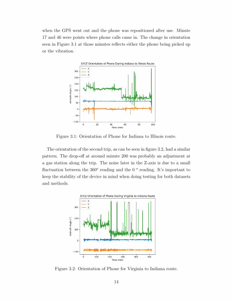
when the GPS went out and the phone was repositioned after use. Minute

17 and 46 were points where phone calls came in. The change in orientation

seen in Figure 3.1 at those minutes reflects either the phone being picked up

or the vibration.

Figure 3.1: Orientation of Phone for Indiana to Illinois route.

The orientation of the second trip, as can be seen in figure 3.2, had a similar

pattern. The drop-off at around minute 200 was probably an adjustment at

a gas station along the trip. The noise later in the Z-axis is due to a small

fluctuation between the 360o reading and the 0 o reading. It’s important to

keep the stability of the device in mind when doing testing for both datasets

and methods.

Figure 3.2: Orientation of Phone for Virginia to Indiana route.

14

3.2 Setup

Figures 3.3 and 3.4 show how the smart phones were mounted in the vehi-

cle. The Indiana to Illinois trip, shown in Figure 3.3, had the smart phone

mounted face down in the front cup-holder, this provided a level of stabil-

ity that was desired so that the phone would move as the car did without

jostling. This also allowed for access to the device in case anything went

wrong. However, since this access was necessary the phone had to be moved

during the trip. This need for movement prompted the use of a second device

during the second recording trial.

Figure 3.3: Phone Mounted for Indiana to Illinois Dataset.

This is a recreation with the other device as no picture was taken on the day of

recording.

The second setup can be seen in Figure 3.4 where the device is mounted

between the seats in the backseat. However, because of the existence of a

metal plate behind the seats the magnetic field recorded is not reliable. The

drawback to this setup is that the passenger cannot check the data recording

to ensure correctness during the driving. This, unfortunately, resulted in an

incorrectly set recording frequency not being corrected at any point during

the ten hour car trip.

15

Figure 3.4: Phone Mounted for Virginia to Indiana Dataset.

3.3 Routes

In Figures 3.5 and 3.6, the two routes recorded are displayed in red. As

can be seen in Figure 3.6 there were some discrepancies in the GPS data.

Whether this was because of bad signal in certain areas, a bad GPS receiver

in the new device, or because the mounted position did not allow for good

reception is not known but this added another step of pre-processing to this

data.

Figure 3.5: Indianapolis, IN to Urbana, IL GPS Route Driven

Figure 3.6: Leesburg, VA to Indianapolis, IN GPS Route Data

16

The removed sections of the route can be seen in red in figure 3.7 and the

actual route in green. This was performed manually as the aberrations were

non-trivial to detect automatically.

Figure 3.7: Leesburg, VA to Indianapolis, IN GPS Route Driven

The green route is the route that was actually taken. The red line is errors in the

data that needed to be processed out before analysis.

17

CHAPTER 4

DESIGN AND IMPLEMENTATION

In this section, the design and implementation of the route shape algorithms

along with the motivation behind the design decisions for those algorithms

will be discussed. The API usage and method of route to map matching will

also be discussed along with the motivation for those decisions.

4.1 Route Shape

Here details of how the two methods of determining route shape were de-

signed and implemented are presented.

4.1.1 LSTM

It was decided that LSTM would be used because of the need for the ma-

chine learning algorithm to recall and forget accelerations. A normal neural

network would not be able to recall a previous state. A Simple RNN would

be able to recall acceleration changes but only in the short term, restricted

by the length of its memory. The LSTM model was the ideal method, being

able to recall and forget as necessary would ideally allow the algorithm to

recall acceleration up to speed and forget it as necessary independent of the

distance from the current iteration.

The Keras Python library was used with Theano as a back-end. The

Theano back-end is more suited to RNNs than TensorFlow so it was used in

this case as was suggested by the Keras documentation. The input values

used can be seen in Table 3.1. The GPS values were omitted as inputs.

The next design decision that had to be made is the number of neurons for

the LSTM layer. Because there are only going to be 3 layers to this neural

network with two outputs it was decided to go with half of the number

18

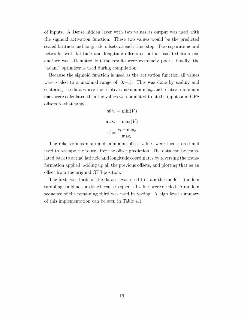
of inputs. A Dense hidden layer with two values as output was used with

the sigmoid activation function. These two values would be the predicted

scaled latitude and longitude offsets at each time-step. Two separate neural

networks with latitude and longitude offsets as output isolated from one

another was attempted but the results were extremely poor. Finally, the

“adam” optimizer is used during compilation.

Because the sigmoid function is used as the activation function all values

were scaled to a maximal range of [0:+1]. This was done by scaling and

centering the data where the relative maximum maxr and relative minimum

minr were calculated then the values were updated to fit the inputs and GPS

offsets to that range.

minr = min(V )

maxr = max(V )

v′i =vi −minrmaxr

The relative maximum and minimum offset values were then stored and

used to reshape the route after the offset prediction. The data can be trans-

lated back to actual latitude and longitude coordinates by reversing the trans-

formation applied, adding up all the previous offsets, and plotting that as an

offset from the original GPS position.

The first two thirds of the dataset was used to train the model. Random

sampling could not be done because sequential values were needed. A random

sequence of the remaining third was used in testing. A high level summary

of this implementation can be seen in Table 4.1.

19

Epochs 70

Timesteps 10

Optimizer adam

Loss Mean Absolute Percentage

Batch Size 1

Shuffle False

Training Set Size 2/3 Dataset

Testing Set Size Up to 1/3 Dataset

LSTM Layer

Neurons 29 or 31

Input Dimension 10 x 31

Dense Layer

Neurons 15

Activation Function Sigmoid

Output Dimension 2

Table 4.1: LSTM Table Summary

4.1.2 Extended Dead Reckoning

The dead reckoning algorithm, normally, would use the velocity vector and

time elapsed to determine route traveled where velocity vector is determined

by using a absolute orientation, usually through a compass, and speed. How-

ever, in the case of a smart phone the magnetic field sensor needs to be in-

termittently calibrated, so another means of determining direction of travel

must be considered. In this case, using the accelerometer and gyroscope to

determine linear acceleration is helpful. The gyroscope allows us to deter-

mine the orientation of the phone and remove the acceleration experienced

due to gravity from the acceleration experienced. Here we represent the

accelerometer output as ~bn, the linear acceleration as ~an, and unit gravity

vector as g.

~an = ~bn − proj(~bn)g

This also gives us some idea about the orientation of the phone. However, it

only tells us the phones alignment to the axis of gravity, it doesn’t reveal all

the information necessary to determine the orientation relative to the vehicle.

20

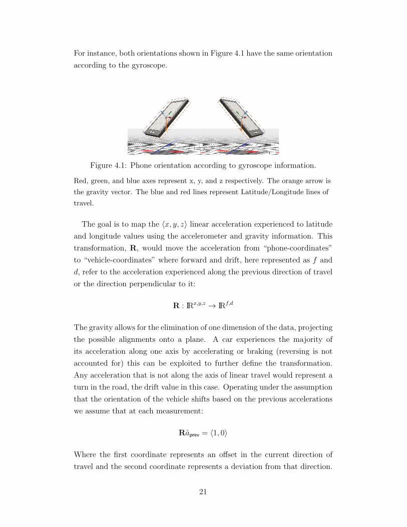
For instance, both orientations shown in Figure 4.1 have the same orientation

according to the gyroscope.

Figure 4.1: Phone orientation according to gyroscope information.

Red, green, and blue axes represent x, y, and z respectively. The orange arrow is

the gravity vector. The blue and red lines represent Latitude/Longitude lines of

travel.

The goal is to map the 〈x, y, z〉 linear acceleration experienced to latitude

and longitude values using the accelerometer and gravity information. This

transformation, R, would move the acceleration from “phone-coordinates”

to “vehicle-coordinates” where forward and drift, here represented as f and

d, refer to the acceleration experienced along the previous direction of travel

or the direction perpendicular to it:

R : IRx,y,z → IRf,d

The gravity allows for the elimination of one dimension of the data, projecting

the possible alignments onto a plane. A car experiences the majority of

its acceleration along one axis by accelerating or braking (reversing is not

accounted for) this can be exploited to further define the transformation.

Any acceleration that is not along the axis of linear travel would represent a

turn in the road, the drift value in this case. Operating under the assumption

that the orientation of the vehicle shifts based on the previous accelerations

we assume that at each measurement:

Raprev = 〈1, 0〉

Where the first coordinate represents an offset in the current direction of

travel and the second coordinate represents a deviation from that direction.

21

For each step we keep track of the previous unit acceleration vector and the

unit orthogonal vector. We calculate the orthogonal vector by taking the

cross product of the previous unit acceleration vector and the previous unit

gravity vector.

aorth = aprev × g

With these vectors being established in the previous timestep we are able

determine our prediction for the acceleration in the frame of the vehicle to

be:

R~a′ = 〈proj(~a′)~aprev , proj(~a′)~aorth〉

Moving from the vehicle frame to the 〈lat, lon〉 space, or “route coordinates”,

is done by cascading the initial direction of travel forward through the time-

steps and using the drift component of acceleration to account for the chang-

ing orientation. Taking v to be the velocity component in route coordinates

we summarize the effective acceleration in table 4.2.

Phone Coordinates Vehicle Coordinates Route Coordinates

IRx,y,z IRf,d IRlat,lon

~a′ R~a′ R~a′ · 〈vprev, vorth〉

Table 4.2: Acceleration moving from phone coordinates to routecoordinates for dead reckoning algorithm.

Multiplying this value by the time elapsed since the last measurement

allows for a sequence of velocity offsets to be calculated. Because modern

vehicles have suspensions that mitigate wear on the driver and the vehicle

a magnification component, m, is used to increase the effective acceleration.

This value would have to be calibrated on a per-vehicle per-orientation basis

but can be done in so few time steps it doesn’t contribute to latency in any

meaningful way.

~v′ = ~vprev + mR~a′ · 〈vprev, vorth〉∆t

The vorth value is determined at the beginning of the loop based on whether

or not the vehicle is in a turn and which direction the vehicle is turning. This

leads to more consistent results than just using a perpendicular value.

vortho =

~v[1]T/||~v[1]T ||, if (~v[1]− ~v[0]) · ~v[1]T ≥ 0

−~v[1]T/||~v[1]T ||, if (~v[1]− ~v[0]) · ~v[1]T < 0(4.1)

22

This check only occurs at the beginning of processing for determining move-

ment between reference frames based on estimated orientation. This velocity

will stay the same relative to the forward unit velocity vector for the duration

of the routing.

These values can then be used to calculate the ∆~x sequence, multiplying

each calculated velocity by the time elapsed.

∆~x′i = ~v′i∆ti

Plotting these offsets gives a route prediction as output. All of this was

done with Python using the NumPy and Math libraries. It can be noted

that this implementation is likely dependent on having acceleration along

the direction of travel when GPS signal is lost. However, this issue can be

combated by back-tracking the route and predicting along known values until

the current time-step is found, either by cascading the R value forward or by

constantly performing these calculations during driving and course-correcting

if a reliable GPS signal is received.

In an attempt to simulate a hardware implementation with the sensor re-

strictions still placed on the algorithm another routing method was generated

alongside this one. Instead of the regular velocity calculation, this second im-

plementation used the speed information, as if it was getting the information

from the vehicle’s speedometer, but used the direction calculations from the

extended dead reckoning algorithm.

~v = speed ∗ (R~a′ · 〈vprev, vorth〉∆t)

||(R~a′ · 〈vprev, vorth〉∆t)||

4.2 Route Matching

There were two main considerations for the map matching algorithm. The

first was to use Open Street Map (OSM) data either using Open Street

Routing Machine (OSRM) or with our own implementation of the Markov

Matching algorithm. The second consideration, which is the one that was

chosen, was to use the Google Maps and Google Places APIs in order to

process this data in batches.

The primary motivator for choosing to use the Google APIs over OSM was

23

primarily for ease of use and the fact that the routes crossed state lines which

was difficult for offline processing using OSM. Using the Google API did not

require any downloaded map information or further work beyond preparing

the route segments in batches of 100 points and stitching the GPS values

back together. OSM and OSRM had the same 100 point restriction and

required map information to be downloaded or specified to certain regions,

which did not work with the extended routes we were using.

The Google Maps API allowed for the usage of a matching algorithm that

put the GPS points onto a route, which is used to determine if the prediction

made is viable. The Google Places API was used in extended testing to find

waypoints alongside OSM data for similar route searches to simulate GPS

spoofing whole routes which will be discussed in Future Work in Section 7.1.

24

CHAPTER 5

RESULTS, EVALUATION, ANDDISCUSSION

In this chapter, the results of the application of the LSTM and EDR are

presented and evaluated. Following the evaluation of the two methods on the

two different granularity datasets there is a discussion on the two methods

and their respective benefits and drawbacks.

5.1 Route Evaluation

Here the results for each method and each route are presented.

5.1.1 LSTM

The first results to go over are from the application of LSTM. The first two-

thirds of the route was used in training, then a relatively unstable route was

used for “hard” testing. Various levels of training were used and tested and it

was determined that the “sweet-spot” for training was 60-75 epochs, which is

consistent with applications to text sentiment analysis examples in the Keras

documentation.

Route 1 - Indiana to Illinois

In figure 5.1, the results of the training on the Indiana to Illinois route, the

route with more frequent measurements, is shown in Figures 5.1 and 5.2.

Although this isn’t necessarily fit perfectly to the route, as can be achieved

with more training, it isn’t overfit to the data. Overfitting leads to poor

results in testing.

25

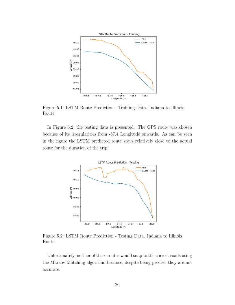
Figure 5.1: LSTM Route Prediction - Training Data. Indiana to IllinoisRoute

In Figure 5.2, the testing data is presented. The GPS route was chosen

because of its irregularities from -87.4 Longitude onwards. As can be seen

in the figure the LSTM predicted route stays relatively close to the actual

route for the duration of the trip.

Figure 5.2: LSTM Route Prediction - Testing Data. Indiana to IllinoisRoute

Unfortunately, neither of these routes would snap to the correct roads using

the Markov Matching algorithm because, despite being precise, they are not

accurate.

26

Route 2 - Virginia to Indiana

Although the first route went well the second route, the Virginia to Indiana

route, did not have results that were nearly as good. This is likely because of

the low frequency, and therefore, low amount of data despite traveling over

a longer distance. The parameters for training on this dataset were main-

tained from the first route. However, re-training had to occur because the

smart-phone was mounted in a different position so the correlation between

the inputs would be different. Unfortunately, the model was not adequate

in predicting the route taken as can be seen in figures 5.3 and 5.4. Even

adjusting the training parameters did nothing to improve the prediction on

this dataset.

Figure 5.3: LSTM Route Prediction - Training Data. Virginia to IndianaRoute

27

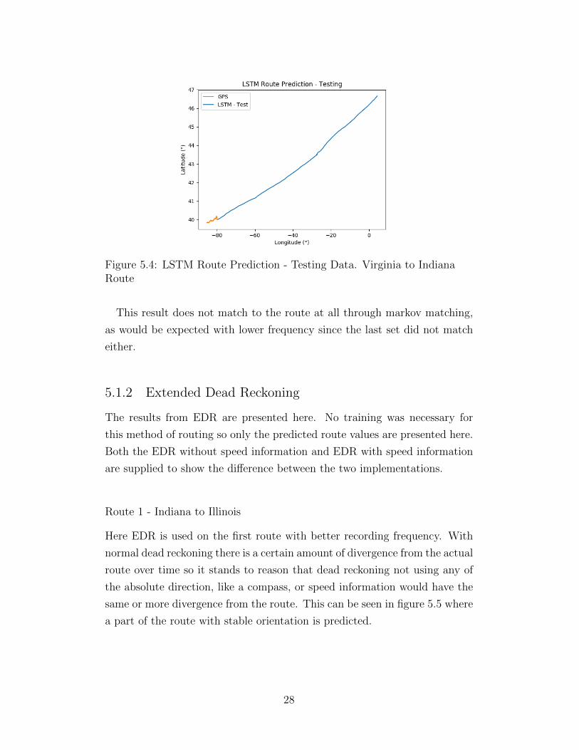
Figure 5.4: LSTM Route Prediction - Testing Data. Virginia to IndianaRoute

This result does not match to the route at all through markov matching,

as would be expected with lower frequency since the last set did not match

either.

5.1.2 Extended Dead Reckoning

The results from EDR are presented here. No training was necessary for

this method of routing so only the predicted route values are presented here.

Both the EDR without speed information and EDR with speed information

are supplied to show the difference between the two implementations.

Route 1 - Indiana to Illinois

Here EDR is used on the first route with better recording frequency. With

normal dead reckoning there is a certain amount of divergence from the actual

route over time so it stands to reason that dead reckoning not using any of

the absolute direction, like a compass, or speed information would have the

same or more divergence from the route. This can be seen in figure 5.5 where

a part of the route with stable orientation is predicted.

28

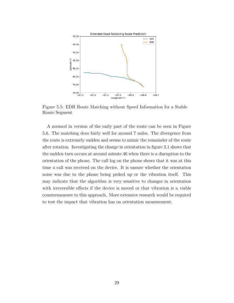
Figure 5.5: EDR Route Matching without Speed Information for a StableRoute Segment

A zoomed in version of the early part of the route can be seen in Figure

5.6. The matching does fairly well for around 7 miles. The divergence from

the route is extremely sudden and seems to mimic the remainder of the route

after rotation. Investigating the change in orientation in figure 3.1 shows that

the sudden turn occurs at around minute 46 when there is a disruption to the

orientation of the phone. The call log on the phone shows that it was at this

time a call was received on the device. It is unsure whether the orientation

noise was due to the phone being picked up or the vibration itself. This

may indicate that the algorithm is very sensitive to changes in orientation

with irreversible effects if the device is moved or that vibration is a viable

countermeasure to this approach. More extensive research would be required

to test the impact that vibration has on orientation measurement.

29

Figure 5.6: EDR Route Matching without Speed Information for a StableRoute Segment - Zoomed

In Figure 5.7, we see this further with a relatively stable haversine distance

between the actual route and the predicted route except at minute 45-46

when there is a sudden shift in route direction leading to steadily increasing

distance when the route is rotated.

Figure 5.7: Haversine Distance Between Actual Route and EDR Route

The same thing that was done without speed information is done with

the speed information for the same stable route segment with similar results.

The first evaluation can be seen in Figure 5.8. This graph looks extremely

similar to Figure 5.5.

30

Figure 5.8: EDR Route Matching with Speed Information for a StableRoute Segment

When we zoom in on the segment we see similar results as before. This

can be seen in figure 5.9. There is a distinct rotation away from the route at

the same point and a slightly more accurate estimation of route length.

Figure 5.9: EDR Route Matching with Speed Information for a StableRoute Segment - Zoomed

The haversine distance deviation also remains similar to before remain-

ing relatively close then departing around minute 45-46 when there is an

orientation noise spike.

31

Figure 5.10: Haversine Distance Between Actual Route and EDR + SpeedRoute

Route 2 - Virginia to Indiana

The same thing was done with the Virginia to Indiana route. However, as

can be seen in the following figures, the EDR method is sensitive to recording

frequency as well and 1 Hz was not nearly enough, even with speed informa-

tion. The first application can be seen for a stable route segment in figure

5.11. Unfortunately, this doesn’t indicate anything other than the fact that

EDR does not work here.

Figure 5.11: EDR Route Matching for a Stable Route Segment - LowGranularity

32

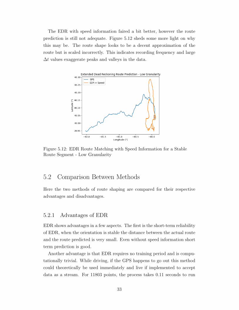
The EDR with speed information faired a bit better, however the route

prediction is still not adequate. Figure 5.12 sheds some more light on why

this may be. The route shape looks to be a decent approximation of the

route but is scaled incorrectly. This indicates recording frequency and large

∆t values exaggerate peaks and valleys in the data.

Figure 5.12: EDR Route Matching with Speed Information for a StableRoute Segment - Low Granularity

5.2 Comparison Between Methods

Here the two methods of route shaping are compared for their respective

advantages and disadvantages.

5.2.1 Advantages of EDR

EDR shows advantages in a few aspects. The first is the short-term reliability

of EDR, when the orientation is stable the distance between the actual route

and the route predicted is very small. Even without speed information short

term prediction is good.

Another advantage is that EDR requires no training period and is compu-

tationally trivial. While driving, if the GPS happens to go out this method

could theoretically be used immediately and live if implemented to accept

data as a stream. For 11803 points, the process takes 0.11 seconds to run

33

fully after paring down to around 5700 points, making average runtime for

a single point around 0.02 ms leaving more than enough time to record at

a much higher frequency than was done here. This is also implemented in

python and not optimized in any way, it may be possible to increase the run-

time of the algorithm further through optimization and reimplementation in

a faster environment.

In addition, this method requires very little memory usage while GPS is

active. It could use as little as the most recent acceleration vector, GPS

position, and orientation prediction. When GPS is out, this would increase

very little as well, as only the most recent changes and one step prior to

the current sensor readings is needed, after the offset is calculated it can be

forgotten.

5.2.2 Disadvantages of EDR

The main disadvantage of EDR is that it is extremely sensitive to changes

in orientation. This can be seen by the drastic change when the phone

was picked up around minute 46 in the first route. The orientation and

accelerations experienced rotate the route and ruin the prediction. As long

as the phone is not moved during route prediction, when the GPS is out, this

should not be an issue, however.

The solution is also sensitive to recording frequency. Any limitations that

exist on recording frequency will impact the accuracy of the algorithm. The

EDR algorithm relies on frequent readings because the ∆t value estimates

those readings to be consistent for the duration of the timestep. However,

with infrequent readings this can overestimate peak values and miss move-

ments in between recordings.

The implementation is a fairly complex estimate and relies on sensor in-

formation to be reliable. As will be discussed in the related work section,

there is some work that demonstrates attacks that question the reliability of

MEMS sensors.

34

5.2.3 Advantages of LSTM

The main advantage of LSTM over the EDR algorithm it that it is more

robust to changes in orientation and acceleration. Using the same route the

LSTM dataset, over the course of the entire route, predicted near the route

shape more consistently than EDR. There is other work that went towards

this thesis, that will be discussed as future work in section 6.1, that could

make use of this route shape to snap the route to a road more effectively

using LSTM rather than EDR because of this consistency.

5.2.4 Disadvantages of LSTM

Like EDR, LSTM is sensitive to recording frequency. However, unlike EDR

this isn’t as easily remedied. Training is a lengthy process that, for 11803

points, took around 16 minutes. Once the model is established, it takes

very little time to predict a route output but if the smart-phone is moved

the model should be re-established. Although, as was seen in the predicted

data, the model applies better to route shaping and is less sensitive than the

EDR solution. If a solution involving continually supplying data to train the

LSTM model existed then this method would be much more viable for route

prediction.

35

CHAPTER 6

FUTURE WORK AND CONCLUSION

In this chapter, future avenues for research are explored. Both route predic-

tion and route matching methods that build on work done outside of this

thesis and work done for this thesis are briefly detailed. The thesis is then

concluded by briefly reiterating the contributions and limitations of this the-

sis.

6.1 Future Work

In this section possible avenues for future work will be explored and detailed.

Other work that was done related to the thesis will also be mentioned in this

section.

6.1.1 Route Prediction

The work on this thesis can be improved on in a couple ways. The respec-

tive advantages and disadvantages of LSTM and EDR seem to line up very

well. While EDR is sensitive to changes in orientation but provides great

accuracy in the short term, LSTM is robust against changes in orientation

but provides better accuracy in the longterm. In addition, EDR can be used

immediately while LSTM requires both time and a large amount of data to

train for effective use. If these two methods were used together then a bet-

ter solution all-around might be achievable. For instance, using EDR in the

short-term and adjusting the direction based on the LSTM route prediction

when orientation change occurs beyond a certain threshold.

Alternatively, if a means of consistently determining the absolute direction

of travel existed, such as north relative to the phone’s orientation, then true

dead reckoning could be used with speed information or the accelerometer

36

data to predict speed changes. This would eliminate the need to worry about

determining turns through accelerations. This method could also potentially

rely on LSTM for general route shape and to counter drift depending on the

accuracy and duration of the trip.

As for route assurance from GPS spoofing, the high accuracy of EDR in

the short term could be used and updated at each iteration to determine

if the GPS output deviates from the sensor prediction. Re-predicting each

timestep based on whether previous GPS values deviated in similarity beyond

an acceptable level. Continual route prediction with LSTM would defend

against large deviations when the phone’s orientation changes whereas during

periods of stable orientation EDR would be able to provide more accurate

output.

6.1.2 Route Matching

More work was done beyond just route prediction that would expand the

usefulness of the LSTM application. That work was done using OSM and

Google Maps/Places for route shape matching. Maps were scanned and sets

of connected subsegments were extracted. These subsegments were roads

that were constituted of waypoints with connected OSMIDs stopping at in-

tersections and deviations of slope by more than 10o. The subsegments that

did not have consistent slope with the values on the route were discarded and

those that remained were sorted through based on speed, timing information,

and how well they matched up to the route shape (using cosine similarity).

If this work was expanded to testing with a more robust implementation it

could provide a reasonable means of route matching which could be used

either as a GPS alternative or as an attack to determine smart-phone user

location.

This means of segment searching could also be used alongside Markov

Matching to provide a similar result with supplied GPS data. This would

allow for the determination of routes with similar shape, sensor output, and

timing information. This could provide a possible means of attack where the

user is supplying an undetectably false trace.

37

6.2 Conclusion

This work demonstrates two feasible implementations of route prediction

given only non-GPS smart phone sensor information and an initial state. In

this thesis, we showed how the LSTM recurrent learning architecture could

be used to predict latitude and longitude offsets with precision even with

the phones orientation changing. We also showed how an extended dead

reckoning algorithm that uses the gyroscope and accelerometer output could

be used to perform route matching with higher accuracy, but also higher

orientation sensitivity. Both of these methods were evaluated on route data

with variable recording frequencies. The accuracy of these predictions is

directly dependent on having high frequency measurements.

This works primary limitation is the low recording frequency of the second

dataset. If the second dataset were recorded at the intended frequency (100

Hz) then the dataset would be substantially more valuable and might provide

more insight to extremely long term prediction with stable orientation. The

future work section explores possible means of application for the methods

proposed.

38

REFERENCES

[1] P. Olson, “Hacking a phone’s gps may havejust got easier,” Aug. 2015. [Online]. Avail-able: https://www.forbes.com/sites/parmyolson/2015/08/07/gps-spoofing-hackers-defcon/

[2] J. SpilkerJr, “Overview of gps operation and design,” Global PositioningSystem: theory and applications, vol. 1, p. 29, 1996.

[3] A. Ranganathan, H. Olafsdottir, and S. Capkun, “Spree: A spoofingresistant gps receiver,” ACM, 2016.

[4] D. K. Shaeffer, “Mems inertial sensors: A tutorial overview.”

[5] P. W. Dwyer, “Mems accelerometer,” U.S. Patent 8 065 915 B2, Nov.29, 2011.

[6] A. Rocchi, “Mems gyroscope for detecting rotational motions about anx-, y-, and/or z-axis,” U.S. Patent 8 789 416 B2, July 29, 2014.

[7] N. O. Tippenhauer, C. Popper, K. B. Rasmussen, and S. Capkun, “Onthe requirements for successful gps spoofing attacks,” ACM, 2011.

[8] L. Heng, J. J. Makela, A. D. Domınguez-Garcıa et al., “Reliable gps-based timing for power systems: A multi-layered multi-receiver archi-tecture,” Inside GNSS, 2014.

[9] Y. Son, H. Shin, and D. Kim, “Rocking drones with intentional soundnoise on gyroscopic sensors,” USENIX, 2015.

[10] T. Trippel, O. Weisse, W. Xu et al., “Walnut: Waging doubt on theintegrity of mems accelerometers with acoustic injection attacks,” IEEE,2017.

[11] S. Hochreiter and J. Schmidhuber, “Long short-term memory,” ACM,1997.

[12] F. A. Gers, J. Schmidhuber, and F. Cummins, “Learning to forget: Con-tinual prediction with lstm,” IDSIA, 6900 Lugano, Switzerland, Tech.Rep. IDSIA-01-99, Jan. 1999.

39

[13] A. Leonhardi, C. Nicu, and K. Rothermel, “A map-based dead reckoningprotocol for updating location information,” 2001.

[14] R. W. Levi and T. Judd, “Dead reckoning navigational system usingaccelerometer to measure foot impacts,” U.S. Patent 5 583 776, Dec. 10,1996.

[15] J. S. Warner and R. G. Johnston, “Gps spoofing countermeasures,”Homeland Security Journal, vol. 25, no. 2, pp. 19–27, 2003.

[16] M. L. Psiaki, B. W. O’hanlon, J. A. Bhatti, D. P. Shepard, T. E.Humphreys et al., “Civilian gps spoofing detection based on dual-receiver correlation of military signals,” Proc. ION GNSS 2011, pp.20–23, 2011.

[17] C. C. HenkMuller, “Personal position measurement using dead reckon-ing,” in Proceedings of the Seventh IEEE International Symposium onWearable Computers (ISWC03), vol. 1530, 2003, pp. 17–00.

[18] S. Beauregard and H. Haas, “Pedestrian dead reckoning: A basis for per-sonal positioning,” in Proceedings of the 3rd Workshop on Positioning,Navigation and Communication, 2006, pp. 27–35.

40