c© 2018 by Venanzio Cichella. All rights reserved.

COOPERATIVE AUTONOMOUS SYSTEMS:MOTION PLANNING AND COORDINATED TRACKING CONTROL

FOR MULTI-VEHICLE MISSIONS

BY

VENANZIO CICHELLA

DISSERTATION

Submitted in partial fulfillment of the requirementsfor the degree of Doctor of Philosophy in Mechanical Engineering

in the Graduate College of theUniversity of Illinois at Urbana-Champaign, 2018

Urbana, Illinois

Doctoral Committee:

Professor Naira Hovakimyan, ChairProfessor Daniel LiberzonProfessor Isaac KaminerProfessor Dusan M. StipanovicProfessor Petros G. Voulgaris

Abstract

In this dissertation a framework for planning and control of cooperative autonomous systems is presented,

which allows a group of Unmanned Vehicle Systems (UxSs) to generate and follow desired trajectories, while

coordinating along them in order to satisfy relative temporal constraints. The described methodology is

based on two key results. First, a centralized optimal motion planning algorithm produces a set of feasi-

ble and flyable trajectories, which guarantee inter-vehicle safety, while satisfying specific temporal mission

requirements, as well as dynamic constraints of the vehicles. Then, a distributed coordinated tracking con-

troller ensures that the vehicles follow the trajectories while coordinating along them in order to arrive at

the final destination at the same time, or with a predefined temporal separation, according to the mission

requirements.

The optimal motion planning problem is formulated as a continuous-time optimal control problem, which

is then approximated by a discrete-time formulation using Bernstein polynomials. Using the convergence

properties of Bernstein polynomial approximation, the thesis provides a rigorous analysis that shows that

the solution to the discrete-time approximation converges to the solution to the continuous-time problem.

The motivation behind this approach lies in the fact that Bernstein polynomials possess favorable geomet-

ric properties that allow for efficient computation of various constraints along the entire trajectory, and

are particularly convenient for generating trajectories for safe operation of multiple vehicles in complex

environments.

The coordinated tracking algorithm relies on the presence of a virtual target tracking controller which

guarantees that the distance between each vehicle and its assigned virtual target running along the desired

trajectory remains bounded throughout the mission. Then, the speed of the virtual target is adjusted in

order to satisfy the temporal constraints and achieve coordination. The coordination problem is formulated

as a consensus problem, with the objective of regulating a suitably defined set of coordination variables to

zero. Conditions are derived under which the consensus algorithm proposed solves the coordination problem

in the presence of faulty communications and switching topologies.

ii

“In that book which is my memory,

On the first page of the chapter that is the day when I first met you,

Appear the words ’Here begins a new life’ ”

Dante Alighieri, Vita Nuova

Dedicated to my wife Caterina

iii

Acknowledgments

Most of all, I would like to express profound gratitude to my adviser, Naira Hovakimyan. You made me feel

at home in Urbana, and taught me more than I could ever give you credit for here. Thank you for always

encouraging my research, providing tremendous support, and allowing me to grow as a researcher. Your guid-

ance, at both professional as well as personal levels, has been invaluable for me and for my future career goals.

I would like to thank the members of my PhD committee, Daniel Liberzon, Isaac Kaminer, Dusan M.

Stipanovic, and Petros G. Voulgaris, who have provided helpful feedback and have been great teachers,

preparing me to get to this place in my academic life. I owe a special word of gratitude to Isaac Kaminer,

who started me in my research journey well before UIUC, and whose ideas, creativity, and knowledge were

crucial to the development of my research work.

The process that led to the completion of my PhD was strongly influenced by the dedicated work of many

other brilliant researchers, to whom I wish to acknowledge my appreciation. These include Vladimir Do-

brokhodov, Antonio Pascoal, Pedro Aguiar, Claire Walton, Anna Trujillo, Roberto Naldi, Lorenzo Marconi,

Alex Kirlik, and Frances Wang.

I would also like to thank my past and present labmates and friends, Bilal, Hanmin, Zhiyuan, Hui, Evgeny,

Ronald, Enric, Jan, Steve, Donglei, Thiago, Arun, Hyung-Jin, Hamid, Kasey, Javier, Gabriel, Alex, Arman,

and Andrew, who made my PhD an enjoyable journey.

Finally, but by no means least, I would like to thank my parents, Patrizia and Paolo, whose unconditional

love and guidance are with me in whatever I pursue; my brother Massimo, for being everything a little

brother should be, and so much more; and my love and best friend Caterina, to whom I would like to

dedicate this thesis: to the chapters of the book that is our life together.

∗ This work was supported in part by NASA, AFOSR and NSF.

iv

Contents

Notation, symbols, and acronyms . . . . . . . . . . . . . . . . . . . . . . . . . . . . . . . . . . vii

Chapter 1 Introduction . . . . . . . . . . . . . . . . . . . . . . . . . . . . . . . . . . . . . . . 11.1 General description . . . . . . . . . . . . . . . . . . . . . . . . . . . . . . . . . . . . . . . . . . 11.2 Motivational scenario: coordinated road search . . . . . . . . . . . . . . . . . . . . . . . . . . 31.3 Literature review and statement of contributions . . . . . . . . . . . . . . . . . . . . . . . . . 5

1.3.1 Optimal motion planning . . . . . . . . . . . . . . . . . . . . . . . . . . . . . . . . . . 51.3.2 Coordinated tracking control . . . . . . . . . . . . . . . . . . . . . . . . . . . . . . . . 8

1.4 Thesis overview . . . . . . . . . . . . . . . . . . . . . . . . . . . . . . . . . . . . . . . . . . . . 9

Chapter 2 General framework and problem formulation . . . . . . . . . . . . . . . . . . . 112.1 General framework . . . . . . . . . . . . . . . . . . . . . . . . . . . . . . . . . . . . . . . . . . 112.2 Problem formulation . . . . . . . . . . . . . . . . . . . . . . . . . . . . . . . . . . . . . . . . . 13

2.2.1 Optimal motion planning . . . . . . . . . . . . . . . . . . . . . . . . . . . . . . . . . . 132.2.2 Coordinated tracking problem . . . . . . . . . . . . . . . . . . . . . . . . . . . . . . . . 16

Chapter 3 Optimal motion planning for differentially flat systems . . . . . . . . . . . . . 233.1 Optimal motion planning as a calculus of variations problem . . . . . . . . . . . . . . . . . . 233.2 Bernstein approximation . . . . . . . . . . . . . . . . . . . . . . . . . . . . . . . . . . . . . . . 253.3 Feasibility and consistency of the approximation . . . . . . . . . . . . . . . . . . . . . . . . . 263.4 Illustrative examples . . . . . . . . . . . . . . . . . . . . . . . . . . . . . . . . . . . . . . . . . 27

Chapter 4 Optimal motion planning . . . . . . . . . . . . . . . . . . . . . . . . . . . . . . . 364.1 Optimal motion planning for a general class of systems . . . . . . . . . . . . . . . . . . . . . . 364.2 Bernstein approximation . . . . . . . . . . . . . . . . . . . . . . . . . . . . . . . . . . . . . . . 374.3 Feasibility and consistency of the approximation . . . . . . . . . . . . . . . . . . . . . . . . . 384.4 Simulation results . . . . . . . . . . . . . . . . . . . . . . . . . . . . . . . . . . . . . . . . . . 39

Chapter 5 Virtual target tracking of multirotor UASs . . . . . . . . . . . . . . . . . . . . 455.1 Problem formulation . . . . . . . . . . . . . . . . . . . . . . . . . . . . . . . . . . . . . . . . . 45

5.1.1 6-DoF model for a multirotor UAS . . . . . . . . . . . . . . . . . . . . . . . . . . . . . 455.1.2 Virtual target tracking error . . . . . . . . . . . . . . . . . . . . . . . . . . . . . . . . . 46

5.2 Virtual target tracking controller . . . . . . . . . . . . . . . . . . . . . . . . . . . . . . . . . . 505.3 Simulation example . . . . . . . . . . . . . . . . . . . . . . . . . . . . . . . . . . . . . . . . . . 52

Chapter 6 Coordination of multiple autonomous vehicles . . . . . . . . . . . . . . . . . . . 616.1 Coordination states and maps . . . . . . . . . . . . . . . . . . . . . . . . . . . . . . . . . . . . 616.2 Coordination control law . . . . . . . . . . . . . . . . . . . . . . . . . . . . . . . . . . . . . . . 636.3 Simulation results . . . . . . . . . . . . . . . . . . . . . . . . . . . . . . . . . . . . . . . . . . 65

6.3.1 Ideal communication - ideal virtual target tracking . . . . . . . . . . . . . . . . . . . . 666.3.2 Range-based communication - ideal virtual target tracking . . . . . . . . . . . . . . . . 676.3.3 Range-based communication - non-ideal virtual target tracking . . . . . . . . . . . . . 67

v

Chapter 7 Flight test results . . . . . . . . . . . . . . . . . . . . . . . . . . . . . . . . . . . . 737.1 System architecture and indoor facility . . . . . . . . . . . . . . . . . . . . . . . . . . . . . . . 737.2 Flight test results . . . . . . . . . . . . . . . . . . . . . . . . . . . . . . . . . . . . . . . . . . . 74

7.2.1 Phase on orbit coordination . . . . . . . . . . . . . . . . . . . . . . . . . . . . . . . . . 747.2.2 Spatial coordination along one axis . . . . . . . . . . . . . . . . . . . . . . . . . . . . . 75

Chapter 8 Conclusions . . . . . . . . . . . . . . . . . . . . . . . . . . . . . . . . . . . . . . . . 818.1 Future work . . . . . . . . . . . . . . . . . . . . . . . . . . . . . . . . . . . . . . . . . . . . . . 82

8.1.1 Optimal motion planning . . . . . . . . . . . . . . . . . . . . . . . . . . . . . . . . . . 828.1.2 Coordinated tracking control . . . . . . . . . . . . . . . . . . . . . . . . . . . . . . . . 838.1.3 Artificial intelligence and optimal decision making . . . . . . . . . . . . . . . . . . . . 838.1.4 Human-UxS interaction . . . . . . . . . . . . . . . . . . . . . . . . . . . . . . . . . . . 84

Appendix A Mathematical background . . . . . . . . . . . . . . . . . . . . . . . . . . . . . . 85A.1 The Hat and Vee Maps . . . . . . . . . . . . . . . . . . . . . . . . . . . . . . . . . . . . . . . 85A.2 Bernstein polynomials . . . . . . . . . . . . . . . . . . . . . . . . . . . . . . . . . . . . . . . . 85

A.2.1 Properties of Bernstein polynomials . . . . . . . . . . . . . . . . . . . . . . . . . . . . 86A.2.2 Bernstein polynomial approximation . . . . . . . . . . . . . . . . . . . . . . . . . . . . 89

Appendix B Proofs and derivations . . . . . . . . . . . . . . . . . . . . . . . . . . . . . . . . 95B.1 Proofs and derivations of Chapter 3 . . . . . . . . . . . . . . . . . . . . . . . . . . . . . . . . 95

B.1.1 Proof of Theorem 1 . . . . . . . . . . . . . . . . . . . . . . . . . . . . . . . . . . . . . 95B.1.2 Proof of Theorem 2 . . . . . . . . . . . . . . . . . . . . . . . . . . . . . . . . . . . . . 96

B.2 Proofs and derivations of Chapter 4 . . . . . . . . . . . . . . . . . . . . . . . . . . . . . . . . 97B.2.1 Proof of Theorem 3 . . . . . . . . . . . . . . . . . . . . . . . . . . . . . . . . . . . . . 97B.2.2 Proof of Theorem 4 . . . . . . . . . . . . . . . . . . . . . . . . . . . . . . . . . . . . . 98

B.3 Proofs and derivations of Chapter 5 . . . . . . . . . . . . . . . . . . . . . . . . . . . . . . . . 101B.3.1 Proof of Lemma 1 . . . . . . . . . . . . . . . . . . . . . . . . . . . . . . . . . . . . . . 101B.3.2 Proof of Lemma 2 . . . . . . . . . . . . . . . . . . . . . . . . . . . . . . . . . . . . . . 102B.3.3 Proof of inequality (B.25) . . . . . . . . . . . . . . . . . . . . . . . . . . . . . . . . . . 105B.3.4 Proof of Lemma 3 . . . . . . . . . . . . . . . . . . . . . . . . . . . . . . . . . . . . . . 105

B.4 Proofs and derivations of Chapter 6 . . . . . . . . . . . . . . . . . . . . . . . . . . . . . . . . 107B.4.1 Proof of Theorem 5 . . . . . . . . . . . . . . . . . . . . . . . . . . . . . . . . . . . . . 107B.4.2 Proof of Corollary 1 . . . . . . . . . . . . . . . . . . . . . . . . . . . . . . . . . . . . . 111

References . . . . . . . . . . . . . . . . . . . . . . . . . . . . . . . . . . . . . . . . . . . . . . . . 112

vi

Notation, symbols, and acronyms

R Field of real numbers.

Z Set of all integers.

Cr Space of functions with r continuous derivatives.

Crd Space of d-vector valued functions with r continuous derivatives.

SO(3) Special orthogonal group of all rotations about the origin of three-dimensional Euclideanspace R

3.

so(3) Set of 3× 3 skew-symmetric matrices over R.

In Identity matrix of size n.

0 Vector of appropriate dimension whose components are all 0.

1 Vector of appropriate dimension whose components are all 1.

F Reference frame.

ωF1/F2 Angular velocity of frame F1 with respect to frame F2.

RF2F1 Rotation matrix from frame F1 to frame F2.

v⊤ Transpose of vector v.

‖v‖ 2-norm of vector v.

‖v‖∞ ∞-norm of vector v.

M⊤ Transpose of matrix M .

det(M) Determinant of matrix M .

tr [M ] Trace of matrix M .

λmax(M) Maximum eigenvalue of matrix M .

λmin(M) Minimum eigenvalue of matrix M .

‖M‖ Induced 2-norm of matrix M .

(·)∧ The hat map. (See Appendix A.1.)

(·)∨ The vee map. (See Appendix A.1.)

End of Lemma, Corollary, and Theorem.

vii

End of Problem.

End of Property.

♠ End of Proof.

♦ End of Remark.

End of Assumption.

♦ End of Example.

DoF Degree of Freedom.

ISS Input-to-State Stable.

PE Persistency of Excitation.

QoS Quality of Service.

UxS Unmanned Vehicle System

UGS Unmanned Ground System

UAS Unmanned Aerial System

USS Unmanned Space System

UMS Unmanned Marine System

NPS Naval Postgraduate School.

UIUC University of Illinois at Urbana-Champaign.

Bold-face, lower-case letters refer to column vectors (e.g. v), while bold-face, capital letters refer to matrices

(e.g. M). In general, the ith component of vector v is denoted by vi, and the (i, j) entry of matrix M is

represented by Mij .

viii

Chapter 1

Introduction

1.1 General description

The field of Unmanned Vehicle Systems (UxSs), including Unmanned Ground Systems (UGSs), Unmanned

Aerial Systems (UASs), Unmanned Space Systems (USS), and Unmanned Marine Systems (UMSs), has gone

through a major transformation in the past two decades. While in the nineties the focus was on developing

large UxSs capable of carrying significant payloads at great distances, significant technological improvements

have shifted academic, industrial, and governmental interest to operations that require multiple small UxSs

functioning in cooperative ways. [1–19]. This stems from the fact that it is far more reliable and cost effective

to deploy groups of heterogeneous UxSs with diverse capabilities and carrying different but complementary

mission-dependent payloads. This yields considerable flexibility in the reconfiguration capabilities as well

as graceful degradation of performance in case of failure of isolated UxS. To enable safe deployment of

groups of UxSs, autonomous vehicles must be capable of performing missions in a cooperative fashion to

achieve common objectives that may be dynamically assigned as the mission unfolds. During these missions,

the vehicles must be able to operate safely and execute coordinated tasks in complex, highly uncertain

environments while maneuvering in close proximity to each other and to obstacles. This poses multiple

challenges inherent to the design, development, and operation of multiple UxSs. Central among them is the

design of motion planning and control strategies for multi-agent systems. Addressing this challenge requires

considerable effort from systems designers and poses a number of extremely interesting theoretical problems.

Over the past few years, there has been a wide range of topics related to motion planning and control

of multiple UxSs that have been addressed in the literature. These topics include: formation control [15,

20–24], collective behaviors and flocking [9–12, 25], synchronization [6–8], multi-agent differential games

[26–28], multi-agent adaptive dynamic programming and reinforcement learning [29–34], cooperative path

and trajectory planning [3, 18, 35–41], coordinated motion control [16, 42–44], and graph theoretic methods

for multi-agent systems [4,5,45–49]. Particularly relevant are the applications of the theory to enable multi-

vehicle missions involving UASs [50–58], UGSs [59–63], USSs [64–66], UMSs [67–74], and heterogeneous

1

UxSs [75–77]. Nevertheless, in spite of the significant body of literature in the field, much work remains to

be done to develop strategies capable of providing the levels of flexibility, performance, and safety required

for the multiple UxSs cooperative missions envisioned in this thesis.

Motivated by these ideas, this thesis addresses the problem of steering a group of UxSs along desired

trajectories while meeting relative temporal constraints. In particular, the cooperative missions considered

require that a motion planning algorithm generates multiple trajectories that are feasible and collision free,

that each vehicle tracks these trajectories, and that the group maintains a desired timing plan to ensure

that all vehicles arrive at their respective final destinations at the same time, or at different times so as to

meet a desired inter-vehicle schedule.

The framework developed in this thesis comprises of (i) a centralized optimal motion planning algorithm

that generates trajectories for multiple UxSs, and (ii) coordination and tracking controllers that enable

the UxSs to follow these trajectories while coordinating with each other, in the presence of partial vehicles

failures and external disturbances. The advantages of this framework compared to solutions such as, for

example, formation control [15,20–24], collective behaviors and flocking [9–12,25], and synchronization [6–8]

are twofold:

• the strategy proposed is more general, and allows a large class of cooperative tasks to be executed. A

compelling example of such tasks is a scenario where a number of UxS are required to maneuver from

initial to desired target positions, with the constraint that they avoid collisions and arrive simultane-

ously at pre-assigned locations. Other illustrative examples fall in the scope of sequential auto-landing,

cooperative ground target search, flocking, synchronization, and formation;

• seamless integration of tracking controllers and coordination algorithms allows to decouple the co-

ordinated tracking control problem into separate ones. This decoupling, in turn, reduces the co-

ordination problem into a simpler consensus problem on suitably defined variables with integrator

dynamics [78–81]. Differently from works on consensus for multi-agent systems [82–87], where the ve-

hicles dynamics are injected into the consensus problem, this simplification allows us to consider more

compelling scenarios such as communication limited environments and rapidly changing topologies,

while retaining rate of convergence guarantees.

Nevertheless, with our approach much effort must be exert in the area of motion planning, in order to develop

algorithms capable of generating trajectories for multiple vehicle missions (near) real-time.

This thesis presents a rigorous formulation of the problems of optimal motion planning and coordinated

tracking control for multi-vehicle missions, and offers solutions to these problem for a general class of UxSs.

2

The thesis proposes a method for motion planning based on numerical approximation of optimal control

problems using Bernstein polynomial approximation. The convergence properties of this method are an-

alyzed, and the efficiency of the resulting motion planning algorithm is studied through several numerical

examples. Furthermore, the thesis presents a coordination control algorithm, and studies its performance in

terms of the Quality of Service (QoS) of the network over which the UxSs communicate, which is affected

by temporary loss of communication links and switching communication topologies. To better motivate the

theoretical developments presented in this dissertation, the next section describes a mission scenario that

warrant the use of a groups of cooperating UxSs.

1.2 Motivational scenario: coordinated road search

One of the applications that motivates the use of multiple cooperative UxSs and poses several challenges to

systems engineers, both from a theoretical and practical standpoint, is autonomous road search. In what

follows we propose an example of road search mission scenario featuring three multirotor UASs. The example

is depicted in Figure 1.1. The mission at hand is triggered by a user who selects an area on an electronic

device displaying a digital map on a touch screen. The global coordinates of the selected region are sent to the

multirotor UASs. An optimization algorithm computes transition paths, which start at the vehicles’ initial

positions, and end at the starting point of the road search mission. Additionally, the optimization algorithm

generates road search paths, which follow the road to allow the vehicles to inspect the selected area. The

transition and road search paths are deconflicted and satisfy the dynamic constraints of the vehicles. Further,

the desired position and speed of each UAS at the end of the transition paths coincides with the position

and speed at the beginning of the road search paths, respectively, to allow for a smooth progression of the

mission. Then, the UASs can execute the cooperative road search mission by following the paths, and at

the same time enforcing the mission’s temporal constraints. Coordination along the transition paths ensures

that the vehicles arrive at the start-points of the road search paths at the same time with desired speed

profiles, and ensures inter-vehicle collision avoidance. Coordination along the road search paths guarantees

overlapping of the fields of view of the three cameras, as emphasized by Figure 1.1a. Finally, it is possible

that the fleet of multirotor UASs must address goals that were not initially planned and appear dynamically

as the mission unfolds. This is the case for UAS 3 in Figure 1.1b, which is required to deviate and inspect

a secondary road. After inspection, the vehicle re-converges to the original road search path synchronizing

with the rest of the fleet. This last part brings to the reader’s attention the benefits of employing cooperative

control algorithms that —like the one presented in this dissertation— do not necessarily lead to swarming

3

(a) Google Maps. 3D view of the cooperative road search scenario.

TAKE OFF

Deviation

TRANSITION

PATHS

ROAD S

EARCH

A

B

UAS 1

UAS 2

UAS 3

(b) Google Maps. 2D projection of the cooperative road search scenario.

Figure 1.1: Cooperative road search using multiple multirotor UASs. The figures illustrate a scenario inwhich cooperation among the UASs is required to accomplish the task at hand. The UASs, starting fromrandom initial positions, follow the transition paths, depicted as solid lines, and arrive at point A. Then,they proceed along the road search paths, represented by solid lines, while coordinating with each other toaccomplish the cooperative road search mission. Cooperation along the road search paths guaranteesnon-zero intersection between the fields of view of the cameras.

4

behaviors.

In the mission scenario described above, the advantages of using a cooperative group of autonomous

vehicles connected by means of a communication network —rather than a single, heavily equipped vehicle—

can be immediately identified. In a cooperative scenario, the team can reconfigure the network in response

to unplanned events as well as changing mission objectives, and optimize strategies for improved target

detection and discrimination. Use of multiple vehicles also improves robustness of the mission execution

against single-point system failures. Furthermore, in a multi-UAS approach, each vehicle of the team may

be required to carry only a reduced number of sensors, making each of the vehicles in the fleet less complex,

thus increasing overall system reliability. This cooperative approach requires, however, the implementation of

robust cooperative control algorithms that will allow the fleet of UASs to maneuver in a coordinated manner

and combine the complementary capabilities of the on-board sensors. In fact, flying in a coordinated fashion

is critical to maximizing the overlap of the fields of view of multiple sensors while reliably maintaining a

desired image resolution.

1.3 Literature review and statement of contributions

The framework adopted builds upon a number of important concepts and techniques that have been the

subject of intensive research. In what follows we briefly review the literature on the most relevant topics

exploited in this thesis, namely motion planning and coordinated tracking control, and outline the main

contributions of this thesis. Additional bibliographic references are included throughout the thesis.

1.3.1 Optimal motion planning

Motion planning plays a key role in enabling autonomous systems accomplish tasks assigned to them safely

and reliably. Over the past decades many approaches to generating trajectories have been proposed. Ex-

amples include bug algorithms, artificial potential functions, roadmap path planners, cell decomposition

methods, and optimal control based trajectory generation. Discussions and details on these methods can be

found in [88–95] and references therein. Each technique has different advantages and disadvantages, and is

best-suited for certain types of problems. Motion planning based on optimal control –i.e. optimal motion

planning– is particularly suitable for applications that require the trajectory to minimize (or maximize) some

cost function while satisfying a complex set of vehicle and problem constraints.

In general, finding a closed-form solution to nonlinear constrained optimal control problems is difficult or

even impossible. Direct methods can be used to approximate optimal control problems to simpler problems,

5

which are easier to solve [96–98]. Direct methods based on discretization, for example, approximate the

states of the dynamic system, or its inputs or both, thus reducing the original problem into a nonlinear

programming problem (NLP) [98], which can then be solved by nonlinear optimization solvers. An im-

portant role in the literature on direct methods based on discretization is played by the work of Polak on

consistency of approximation theory (see [99, Section 3.3]). Borrowing tools from variational analysis, Polak

provides a theoretical framework to assess the convergence properties of discretization schemes for optimal

control problems. Motivated by the consistency of approximation theory, a wide range of methods that use

different discretization schemes have been developed. Few examples include Euler [99], Runge-Kutta [100],

pseudospectral (PS) [101] methods, as well as the method presented in this dissertation.

The pseudospectral optimal control method is one of the most popular direct methods nowadays, and it has

been applied successfully for solving a wide range of optimization problems, e.g. [35,101–106]. Pseudospectral

methods offer several advantages over many other discretization methods, mainly owing to their spectral

(exponential) rate of convergence. For example, consider the Legendre PS optimal control method [101], one

of the most widely used PS methods for motion planning. It is characterized by the following three features:

(i) the continuous functions involved in the optimal control problem, i.e. the states and control inputs, are

approximated at N quadrature nodes, which are determined by the Legendre polynomial; (ii) the integral in

the cost function is approximated by Legendre-Gauss quadrature; (iii) orthogonal collocation (also deemed

as PS method), such as Lagrange interpolation on the Legendre nodes, is used to approximate functions

and their derivatives (dynamics constraints). It was proven that under some assumptions on the solution

to the original optimal control problem, a solution to the discretized optimal control problem exists, and it

converges to the solution of the original problem. One of the features that makes PS methods particularly

attractive is the convergence rate of the polynomial interpolation at the quadrature nodes. In particular,

letting INf(t) be the polynomial interpolation of f(t) at the Legendre nodes in the interval [−1, 1], the

following result holds:

||INf(t)− f(t)||L2 ≤ C

Nm,

where C is a positive variable independent on N , and m is the smoothness of f(t). However, as pointed out

in [107, 108], there is one salient drawback associated with PS methods. When discretizing the trajectories,

the constraints are enforced at the discretization nodes. Unfortunately, satisfaction of constraints cannot be

guaranteed in between the nodes. To avoid violation of the constraints in between the nodes, the order of

approximation (number of nodes) can be increased. However, this leads to larger nonlinear programming

problems, which may become computationally expensive and too inefficient to solve. This problem does not

limit itself to PS methods, but it is common to methods that are based on discretization.

6

This undesirable behaviour becomes obvious, for example, in the multi-vehicle missions considered in this

thesis, where a large number of vehicles have to reach their final destinations by following trajectories that

are spatially (rather than temporally) separated to guarantee inter-vehicle safety. Clearly, with a small

order of approximation, spatial separation between the trajectories will be hardly satisfied. Increasing the

number of nodes will eventually produce spatially separated trajectories, but will also drastically increase

the number of collision avoidance constraints and thus the complexity of the problem (the problem has

n!(n−2)!2!N

2 deconfliction constraints, where n is the number of vehicles, and N is the number of nodes).

This thesis proposes a direct method based on Bernstein approximation of the trajectories. Bernstein

approximants have several nice properties. First, Bernstein basis possesses optimal numerical stability prop-

erties [109, 110], and can handle large order of approximations without suffering from numerical instability

issues. Second, the approximants converge uniformly to the functions that they approximate – and so do

their derivatives [111, Chapter 3]. This, as we will discuss later, is useful to derive convergence properties

of the proposed computational method. Third, due to their favorable geometric properties (see [111, Chap-

ter 5]) Bernstein polynomials afford computationally efficient algorithms for the computation of constraints

such as minimum and maximum velocity, acceleration, minimum distance between paths, etc., for the whole

trajectory, and not only at discretization points (see [112, 113]). Hence, with the proposed approach the

trajectories are guaranteed to be dynamically feasible and collision-free for all times, while retaining the

computational efficiency of methods based on discretization.

Bernstein approximation converges slower than other interpolation or approximation techniques. This

implies that the approach proposed in this thesis is outperformed by, for example, PS methods in terms

of accuracy of approximation of the optimal solution. This is not surprising, since the choice of nodes and

interpolating polynomial in PS methods is dictated by approximation accuracy and convergence speed, while

sacrificing constraints satisfaction in between the nodes. On the other hand, our approach prioritizes safety

and constraint satisfaction, at the expense of a slower convergence rate.

Bernstein polynomials are very useful tools to describe geometric paths, and a growing number of works

in the literature exploit their properties for trajectory generation (see, for example, [114–117]). Using the

notion of consistency of approximation introduced by Polak [99], the present thesis provides a theoretical

foundation for the use of Bernstein polynomials in optimal motion planning. Similar consistency results have

been demonstrated for various discretization schemes, including pseudospectral methods [118,119]. However,

these results are limited to collocation methods [120]. The contribution of the present work is an extension

of these results to a class of non-collocation methods.

7

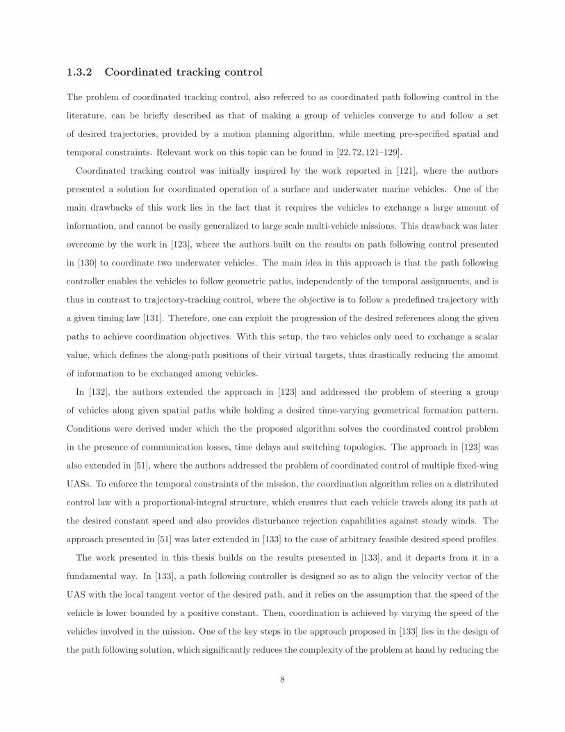
1.3.2 Coordinated tracking control

The problem of coordinated tracking control, also referred to as coordinated path following control in the

literature, can be briefly described as that of making a group of vehicles converge to and follow a set

of desired trajectories, provided by a motion planning algorithm, while meeting pre-specified spatial and

temporal constraints. Relevant work on this topic can be found in [22, 72, 121–129].

Coordinated tracking control was initially inspired by the work reported in [121], where the authors

presented a solution for coordinated operation of a surface and underwater marine vehicles. One of the

main drawbacks of this work lies in the fact that it requires the vehicles to exchange a large amount of

information, and cannot be easily generalized to large scale multi-vehicle missions. This drawback was later

overcome by the work in [123], where the authors built on the results on path following control presented

in [130] to coordinate two underwater vehicles. The main idea in this approach is that the path following

controller enables the vehicles to follow geometric paths, independently of the temporal assignments, and is

thus in contrast to trajectory-tracking control, where the objective is to follow a predefined trajectory with

a given timing law [131]. Therefore, one can exploit the progression of the desired references along the given

paths to achieve coordination objectives. With this setup, the two vehicles only need to exchange a scalar

value, which defines the along-path positions of their virtual targets, thus drastically reducing the amount

of information to be exchanged among vehicles.

In [132], the authors extended the approach in [123] and addressed the problem of steering a group

of vehicles along given spatial paths while holding a desired time-varying geometrical formation pattern.

Conditions were derived under which the the proposed algorithm solves the coordinated control problem

in the presence of communication losses, time delays and switching topologies. The approach in [123] was

also extended in [51], where the authors addressed the problem of coordinated control of multiple fixed-wing

UASs. To enforce the temporal constraints of the mission, the coordination algorithm relies on a distributed

control law with a proportional-integral structure, which ensures that each vehicle travels along its path at

the desired constant speed and also provides disturbance rejection capabilities against steady winds. The

approach presented in [51] was later extended in [133] to the case of arbitrary feasible desired speed profiles.

The work presented in this thesis builds on the results presented in [133], and it departs from it in a

fundamental way. In [133], a path following controller is designed so as to align the velocity vector of the

UAS with the local tangent vector of the desired path, and it relies on the assumption that the speed of the

vehicle is lower bounded by a positive constant. Then, coordination is achieved by varying the speed of the

vehicles involved in the mission. One of the key steps in the approach proposed in [133] lies in the design of

the path following solution, which significantly reduces the complexity of the problem at hand by reducing the

8

coordination dynamics to n simple integrators, where n is the number of UASs. However, while [133] offers

an appealing solution for the cooperative control of fixed-wing UASs, it cannot be employed when dealing

with UxSs that allow the existence of zero velocity vectors (e.g. UASs who can hover, such as multirotors,

or UGSs). This limitation motivated us to reformulate the coordination problem in a different way. The

goal of the work presented in this thesis is to provide a new solution to the coordination problem which

is more general, and can be applied to a broader set of vehicles with different dynamics. In the approach

proposed here, the virtual target (VT) tracking and the coordination control problems are decoupled. At the

VT tracking level, we assume that a control law that enables a UxS to track a virtual target moving along its

assigned path is given. At the coordination level, the synchronization problem is solved by adjusting a new set

of suitably defined coordination variables, thus achieving vehicles’ coordination. It is shown that the solution

to the coordination problem exhibits guaranteed performance in the presence of time-varying communication

networks, that arise due to temporary loss of communication links and switching communication topologies.

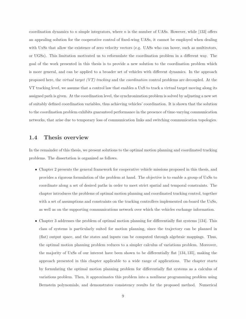
1.4 Thesis overview

In the remainder of this thesis, we present solutions to the optimal motion planning and coordinated tracking

problems. The dissertation is organized as follows.

• Chapter 2 presents the general framework for cooperative vehicle missions proposed in this thesis, and

provides a rigorous formulation of the problem at hand. The objective is to enable a group of UxSs to

coordinate along a set of desired paths in order to meet strict spatial and temporal constraints. The

chapter introduces the problems of optimal motion planning and coordinated tracking control, together

with a set of assumptions and constraints on the tracking controllers implemented on-board the UxSs,

as well as on the supporting communications network over which the vehicles exchange information.

• Chapter 3 addresses the problem of optimal motion planning for differentially flat systems [134]. This

class of systems is particularly suited for motion planning, since the trajectory can be planned in

(flat) output space, and the states and inputs can be computed through algebraic mappings. Thus,

the optimal motion planning problem reduces to a simpler calculus of variations problem. Moreover,

the majority of UxSs of our interest have been shown to be differentially flat [134, 135], making the

approach presented in this chapter applicable to a wide range of applications. The chapter starts

by formulating the optimal motion planning problem for differentially flat systems as a calculus of

variations problem. Then, it approximates this problem into a nonlinear programming problem using

Bernstein polynomials, and demonstrates consistency results for the proposed method. Numerical

9

examples are presented and discussed at the end of the chapter.

• Chapter 4 extends the results presented in Chapter 3 to a more general class of optimal control

problems. Similarly to Chapter 3, this chapter provides an approximation of an optimal control problem

into a nonlinear programming problem using Bernstein polynomials, and it demonstrates consistency

results for this approximation method. Finally, it presents numerical results that demonstrate the

advantages of the proposed approach.

• Chapter 5 presents the development of a control algorithm that solves the VT tracking problem for a

multirotor UAS. An outer-loop VT tracking control law is presented that enables the vehicle, equipped

with an autopilot tracking angular rates and thrust reference commands, to converge to and follow a

desired virtual target. Limits in the performance of the autopilot are considered. The main advantage

of considering angular rates and total thrust as control inputs is that such control strategy can be

employed to a larger set of multirotor craft, independently of the number of propellers and geometric

configurations.

• Chapter 6 addresses the problem of coordinating a group of UxSs. This problem is solved by regulating

a set of suitably defined coordination variables to zero. The chapter defines a set of states that capture

the coordination objective at hand, and proposes control laws that regulate these states. Then, it

derives the performance of the proposed algorithms in the presence of time-varying communication

networks, that arise due to temporary loss of communication links and switching communication

topologies. Finally, simulation results that support the theoretical findings are presented.

• Chapter 7 presents flight test results for two quadrotor UAVs that verify the stability and convergence

properties of the coordination control results presented in Chapter 6. In particular, two scenarios

are proposed in which the quadrotors are required to accomplish simple cooperative tasks, namely

phase on orbit coordination and spatial coordination along one axis. The chapter describes the system

architecture and the indoor facility used to conduct the experiments, and discusses the flight test

results in details.

• Concluding remarks are provided in Chapter 8.

10

Chapter 2

General framework and problem

formulation

2.1 General framework

The integrated framework for cooperative vehicle missions proposed in this thesis uses a hybrid set-up,

where a central unit is responsible for the mission planning and communicates with the vehicles before the

beginning of the mission. Subsequently, decentralized controllers embedded on-board the vehicles ensure that

the mission is accomplished in a safe manner by exchanging information with each other. The framework,

which is depicted in Figure 2.1, can be summarized in three fundamental steps outlined below.

• Motion planning: given a multiple UxS mission, a set of desired trajectories is generated off-line by

an optimal motion planning algorithm for all the vehicles involved in the mission. These trajectories

optimize a cost function, and satisfy initial and final boundary conditions, flyability constraints (e.g.

min/max speed, min/max acceleration, etc.), feasibility constraints (e.g. collision avoidance between

the trajectories, collision avoidance with obstacles), and additional mission-specific constraints.

• VT tracking: the trajectories (which are geometric paths parameterized by time) are re-parameterized

by independent variables (here referred to as virtual times). These re-parameterized trajectories, called

virtual targets henceforth, provide the reference to be tracked by the UxSs. Then, the objective of the

VT tracking controller is to make sure that each UxS follows its assigned virtual target with guaranteed

performance. The VT tracking controller can be designed to handle external disturbance and nonlinear

vehicle dynamics with uncertainties.

• Coordination: The progression of the virtual time of each vehicle is adjusted on-line in order to

ensure that the group of UxSs meets the temporal requirements of the mission, i.e. coordination. This

step relies on the underlying communications network as a means to exchange information among

vehicles, and takes into account tracking errors that incur due to vehicles’ partial failures, external

disturbances, etc. This step allows each vehicle to directly react in a timely fashion to other vehicles

failures and potentially hazardous maneuvers, without having to communicate with a central station.

11

The framework exhibits a multi-loop structure, in which the VT tracking controller stabilizes the position of

the vehicle around a virtual target, while a coordination controller is designed to control the virtual target.

To make these ideas more precise, we notice that the equation of motion of the ith UxS involved in the

cooperative mission can be described by the following system of equations:

Gv,i :

xv,i(t) = fi(xv,i(t),uv,i(t)) , xv,i(0) = xiv,i

pv,i(t) = gi(xv,i(t)) ,

(2.1)

where pv,i(t) is the vehicle’s position, xv,i(t) is the state of the vehicle (which typically includes position,

attitude, velocity), uv,i(t) is the control input (e.g. angular rate, speed, thrust), and fi and gi are vectors of

nonlinear functions describing the nominal behavior of the UxS. The model above is sufficiently general to

capture six-degree-of-freedom (6DoF) dynamics of UxSs. On one hand, a VT tracking controller uv,i(t) can

be designed for system Gv,i in order to provide tracking capabilities, i.e. make the vehicle converge to and

follow a virtual target moving along a desired path, while handling external disturbance and uncertainties

that may affect the nominal behavior given by (2.1). On the other hand, a coordination controller is derived

to control the motion of the virtual target (i.e. the reference to be followed by the VT tracking controller)

in order to achieve coordination, while taking into account VT tracking errors. This multi-loop approach

not only simplifies the design process, but also lends itself to a wide range of applications involving multiple

UxSs with different dynamics.

Vehicle i

Desiredtrajectory

Virtualtarget

VT tracking error

Coord. variables

Ext. VTtracking

CoordinationMotionplanning

Vehicles network

Vehiclekin & dyn

Vehicle states

Cmds

Coordinated tracking control

Figure 2.1: Architecture of the cooperative planning and execution framework adopted.

12

2.2 Problem formulation

2.2.1 Optimal motion planning

Given a set of n UxSs, the problem of optimal motion planning for multi-vehicle missions can be defined as

follows:

Problem 1 Compute a set of n desired trajectories pd,i : [0, tf,i] → Rd, i = 1, . . . , n, that minimize a given

cost function, and satisfy boundary conditions, flyability constraints, feasibility constraints, and pre-defined

mission-specific constraints.

Boundary conditions

In the problem of motion planning for autonomous vehicles, typically the initial and final conditions of the

trajectories, here referred to as boundary conditions, are pre-specified. For example, for the ith vehicle the

following boundary conditions can be enforced:

pd,i(0) = pii , ‖pd,i(0)‖ = vii , pd,i(tf,i) = pf

i , ‖pd,i(tf,i)‖ = vfi , (2.2)

where pii and vii are the initial position and speed, respectively, while pf

i and vfi are the specified quantities

at the final endpoint of the trajectory.

Flyability and feasibility constraints

Flyable trajectories are trajectories that satisfy desired geometric constraints (such as curvature and flight

path angle bounds), and can be tracked by a given vehicle without having it exceed pre-specified bounds on

the vehicle dynamic state and control input (such as speed limits, angular rate bounds, or acceleration limits).

These bounds depend on the UxSs considered, and on their physical limitations. For example, in [81,136] it

has been shown that a multirotor UAS, equipped with an autopilot in charge of tracking angular rate and

total thrust commands, is capable of following trajectories subject to minimum and maximum speed limits,

and maximum acceleration limits. Hence, the flyability constraints of multirotors can be specified as

vmind,i ≤ ‖pd,i(t)‖ ≤ vmax

d,i , ‖pd,i(t)‖ ≤ amaxd,i , (2.3)

where vmind,i ≥ vmin

i , vmaxd,i < vmax

i , and amaxd,i < amax

i , and vmini ≥ 0, vmax

i > 0, and 0 < amaxi ≤ g are the actual

speed and acceleration limits of the multirotor, which can be determined from the maximum available thrust

13

of the rotors, and g is gravity. Note that during the motion planning phase, the more restrictive bounds vmind,i ,

vmaxd,i and amax

d,i are used so as to allow the vehicles to adjust on-line their dynamics, if necessary, in order to

maintain coordination, or to react to unpredicted situations (e.g. pop-up obstacles, external disturbance).

Feasible trajectories are flyable trajectories that avoid collisions with obstacles, and that are spatially

deconflicted in order to avoid inter-vehicle collision, thus ensuring safe simultaneous operation in a common

airspace. Spatial deconfliction between trajectories can be guaranteed through temporal separation (the

vehicles are separated in time) or spatial separation (the spatial paths are separated in space). Letting

pd,i(t), i = 1, . . . , n, be the desired trajectories of the UxSs at time t, temporal separation can be enforced

as follows:

mini,j=1,...,n

i6=j

‖pd,i(t)− pd,j(t)‖2 ≥ E2d , ∀t ∈ [0,max(tf,i, tf,j)], (2.4)

with Ed ≥ E, where E is a minimum separation requirement, which depends, for example, on the dimension

of the UxSs and other safety considerations. Similarly to the flyability constraints, we note that a more con-

servative bound Ed is imposed at the motion planning phase, in order to account for unpredicted situations

(e.g. pop-up obstacles) or tracking errors of the UxSs (due to the presence of external disturbance or partial

failures).

While temporal separation is more computationally efficient, it relies heavily on the performance of a time-

coordination algorithm, which, in turn, depends on the quality and robustness of the communication network

over which the vehicles exchange information with each other. On the other hand, spatial separation can

be employed in situations where the communication network is faulty or jammed, and coordination cannot

be guaranteed. A more in-depth discussion on both strategies can be found in [113,137]. Spatial separation

between the trajectories can be enforced by imposing the following constraints:

mini,j=1,...,n

i6=j

‖pd,i(ti)− pd,j(tj)‖2 ≥ E2d , ∀ti ∈ [0, tf,i] , ∀tj ∈ [0, tf,j ]. (2.5)

Minimum separation between trajectories and obstacles can also be enforced in a similar fashion. Letting

po,k be the position of the kth obstacle, with k = 1, . . . , no, where no is the number of obstacles, in order to

ensure deconfliction with the obstacles the following constraint can be enforced:

mini=1,...,nk=1,...,no

‖pd,i(t)− po,k‖2 ≥ E2d , ∀t ∈ [0, tf,i]. (2.6)

14

Notice that in the above formulation the obstacles are assumed to be static. Moving obstacles can also be

considered in the motion planning phase, as long as their trajectories are known a priori.

Mission-specific constraints

Additional constraints can be imposed on Problem 1, depending on the requirements of the mission consid-

ered. These constraints can be imposed, for example, to require that all vehicles arrive at their respective

final destinations at the same time, or at different times so as to meet a desired inter-vehicle schedule. For

simplicity, and without loss of generality, in this thesis we consider the problem of simultaneous arrival, i.e.

tf,i − tf,j = 0 , i, j = 1, . . . , n , i 6= j , (2.7)

with the understanding that the above constraints can be easily modified, and that the proposed approach

can be employed for a larger set of scenarios.

Optimal motion planning problem

In what follows, we provide a formal definition of Problem 1. Recall that the ith vehicle involved in the

cooperative mission is modelled by the system of equations introduced in Equation (2.1), with state xv,i(t)

and control input uv,i(t). Let xd,i(t) and ud,i(t) be the vectors of desired states and control inputs for

vehicle i. Let xd(t) = [x⊤d,1(t), . . . ,x

⊤d,n(t)]

⊤ ∈ Rnx , and ud(t) = [u⊤

d,1(t), . . . ,u⊤d,n(t)]

⊤ ∈ Rnu . Then,

Problem 1 can be cast into the following optimal control problem with Bolza cost:

Problem 2 Determine xd : [0, tf ] → Rnx and ud : [0, tf ] → R

nu (and possibly tf ) that minimizes

I(xd(t),ud(t)) = E(xd(0),xd(tf )) +

∫ tf

0

F (xd(t),ud(t))dt , (2.8)

subject to

xd(t) = f(xd(t),ud(t)) , ∀t ∈ [0, tf ] (2.9)

e(xd(0),xd(tf )) = 0 , (2.10)

h(xd(t),ud(t)) ≤ 0 , ∀t ∈ [0, tf ] , (2.11)

where E : Rnx × Rnx → R, F : Rnx × R

nu → R, f : Rnx × Rnu → R

nx , e : Rnx × Rnx → R

ne , and

h : Rnx ×Rnu → R

nh are nonlinear functions of their arguments.

15

Remark 1 In Problem 2, the constraint in Equation (2.9) enforces the dynamics of the vehicles considered

in the mission, with f = [f⊤1 , . . . , f⊤

n ]⊤, where fi is introduced in Equation (2.1). Equation (2.10) describes

the boundary conditions and simultaneous time of arrival constraints. The flyability and feasibility constraints

are described by Equation (2.11). The functions E and F in Equation (2.8) are the end point cost and the

running cost of the Bolza-type cost functional, respectively.

♦

Remark 2 The outcome of Problem 2 is a set of optimal states x∗d,i(t) and control inputs u∗

d,i(t), i =

1, . . . , n, which, in turn, provide optimal trajectories p∗d,i(t) computed as

p∗d,i(t) = gi(x

∗d,i(t)) ,

where gi is introduced in Equation (2.1).

♦

2.2.2 Coordinated tracking problem

The coordinated tracking problem is referred to as the problem of enabling a fleet of vehicles to execute

collision-free maneuvers while satisfying temporal specifications, such as simultaneous time of arrival. In the

adopted framework, it is assumed that the UxSs are equipped with a VT tracking algorithm —implemented

on-board the vehicles— responsible for making each vehicle follow a virtual target running along the path

generated by the motion planner. Then, the objective is to design distributed coordination control laws

that adjust the rate of progression of these virtual targets so as to coordinate the entire fleet. One of the

main benefits of this approach lies in the fact that the progression of the virtual targets to be tracked by

the vehicles is adjusted on-line, adapting to external disturbances or vehicles’ tracking errors. Thus, this

approach is more robust than the coordinated trajectory tracking approach, where the coordination task is

solved off-line and the UxSs are simply required to follow the trajectories generated by solving Problem 2.

The coordinated tracking problem is solved in three main steps: the first step consists of implementing a

virtual target moving along the path computed by the motion planning algorithm described earlier. This

objective is achieved by introducing a new parameter, virtual time, denoted here as γi(t), and letting the

virtual target to be tracked by the UxSs be pd,i(γi(t)), where the subscript i refers to the ith UxS involved

in the cooperative mission; the second step consists of making each UxS track the virtual target assigned to

it. This step, referred to as VT tracking, reduces to driving a suitably defined error vector to zero by using

the vehicle’s control inputs; third, to enforce the temporal constraints of the mission, a consensus problem is

16

formulated, in which the objective of the fleet of vehicles is to reach agreement on some distributed variables

of interest that capture the objective of the coordination problem.

Virtual time and virtual target

Given the trajectory pd,i(t) produced by the motion planning algorithm described above, we let the virtual

time γi(t), t ≥ 0, be a temporal variable

γi : R+ → [0, tf ] , for all i = 1 , ... , N , (2.12)

and the virtual target pd,i(γi(t)) be a moving point to be tracked by vehicle i. With this formulation, the

virtual time provides an abstraction of actual (clock) time. It can be stretched or compressed in order to

adjust the progression of the virtual target along the path pd,i(·), so as to achieve pre-specified temporal

requirements, i.e. coordination. If γi(t) ≡ 1, then the progression of the virtual target in time is equal to the

progression of the desired trajectory generated at the motion planning level. More precisely, assume that

γi(t) = 1 , for all t ∈ [0, tf ], with γi(0) = 0. This assumption implies that γi(t) = t for all t. In turn, the

following equality holds

pd,i(γi(t)) = pd,i(t) ,

which, in other words, means that the desired trajectory generated by the motion planner and the virtual

target coincide for all time, and so do their speed and acceleration profiles. On the other hand, γi > 1

(γi < 1) implies a faster (slower) execution of the mission. This statement becomes evident when expressing

the speed and the acceleration of the virtual target in terms of the derivatives of the virtual time:

∥∥∥∥

d

dtpd,i(γi(t))

∥∥∥∥= ‖pd,i(γi(t), γi(t))‖ =

∥∥∥∥

dpd,i(γi(t))

dγi(t)

dγi(t)

dt

∥∥∥∥=

∥∥∥∥

dpd,i(γi(t))

dγi(t)γi(t)

∥∥∥∥, (2.13)

∥∥∥∥

d

dt

(d

dtpd,i(γi(t))

)∥∥∥∥= ‖pd,i(γi(t), γi(t)), γi(t))‖ =

∥∥∥∥

d

dt

(dpd,i(γi(t))

dγi(t)

dγi(t)

dt

)∥∥∥∥

=

∥∥∥∥

d2 pd,i(γi(t))

dγ2i (t)

γ2i (t) +

dpd,i(γi(t))

dγi(t)γi(t)

∥∥∥∥.

(2.14)

Virtual target tracking

Recall that the equations of motion of the UxSs are given by Equation (2.1). Then, the objective of the VT

tracking problem is to design a control law for uv,i(t) such that the VT tracking error

ep,i(t) , pv,i(t)− pd,i(γi(t)) (2.15)

17

converges to a neighborhood of zero. In order for the above problem to be solvable, the dynamics of the

virtual target must not violate the flyability limits of the vehicle. As pointed out in Equations (2.13) and

(2.14), the speed and acceleration of the virtual target, for example, depend not only on the speed and

acceleration profiles of the trajectory pd,i(t) generated by the motion planning algorithm, but also on the

derivatives of the virtual time, γi(t) and γi(t). Therefore, flyability limits on the dynamics of the virtual

time must be enforced to ensure that the virtual target can be followed by the vehicle. Here we assume

that the virtual target can be tracked by the UxS if the trajectories pd,i(t), i = 1, . . . , n satisfy the flyability

constraints imposed by Problem 2, and the derivatives of the virtual time satisfy

γmini ≤ γi(t) ≤ γmax

i , |γi(t)| ≤ γmaxi , (2.16)

for given 0 ≤ γmini < 1, γmax

i > 1 and γmaxi > 0. As discussed later, the dynamics of γi(t) (actually its second

derivative γi(t)) are explicitly controlled and used as an extra degree-of-freedom to achieve coordination.

Therefore, when deriving control laws for γi(t), the saturation bounds in Equation (2.16) must be taken into

consideration.

Remark 3 The limits γmini , γmax

i and γmaxi can be derived from the actual flyability constraints of the vehi-

cle under consideration, and the (more conservative) flyability constraints imposed by the motion planning

algorithm. To clarify this argument, consider the example of a multirotor UAS introduced in Section 2.2.1,

subject to minimum and maximum speed limits vmini and vmax

i , and maximum acceleration limits amaxi ≤ g.

Then, the virtual target assigned to the vehicle must satisfy

vmaxi ≤ ‖pd,i(γi(t), γi(t))‖ =

∥∥∥∥

dpd,i(γi(t))

dγi(t)γi(t)

∥∥∥∥≤ vmax

i , (2.17)

‖pd,i(γi(t), γi(t), γi(t))‖ =

∥∥∥∥

d2 pd,i(γi(t))

dγ2i (t)

γ2i (t) +

dpd,i(γi(t))

dγi(t)γi(t)

∥∥∥∥≤ amax

i ≤ g , (2.18)

where we used Equations (2.13) and (2.14). We notice that the flyability constraints enforced by the motion

planning algorithm (see Equation (2.3)) imply

vmind,i ≤

∥∥∥∥

dpd,i(γi(t))

dγi(t)

∥∥∥∥≤ vmax

d,i ,

∥∥∥∥

d2 pd,i(γi(t))

dγ2i (t)

∥∥∥∥≤ amax

d,i ,

where vmind,i ≥ vmin

i , vmaxd,i < vmax

i , and amaxd,i < amax

i . Therefore, to ensure that the inequalities in (2.17) and

18

(2.18) are satisfied, the dynamics of the virtual time must not exceed the limits in (2.16), with

γmini =

vmini

vmind,i

, γmaxi =

vmaxi

vmaxd,i

, γmaxi =

amaxi − amax

d,i

(vmaxi

vmaxd,i

)2

vmaxd,i

. (2.19)

The equation above also suggests that the constraints imposed on γi(t) and γi(t) can be relaxed by enforcing

more stringent flyability constraints, e.g. larger vmind,i and smaller vmax

d,i and amaxd,i , at the expense of an

increase in computational complexity of the motion planning algorithm.

♦

With this setup, the VT tracking problem can be stated as follows:

Problem 3 Consider n UxSs with equations of motion given by Equation (2.1), and a set of n virtual targets

pd,i(γi(t)), i = 1, . . . , n, assigned to each vehicle, where pd,i(t) are trajectories generated by solving Problem

2, and γi(t) are the virtual times that satisfy the bounds in Equation (2.16). Then, the objective is to design

a VT tracking control law for uv,i(t) such that the VT tracking error defined in Equation (2.15) is uniformly

bounded, i.e. there exists a positive constant c, and for every a ∈ (0, c) there exists ρ = ρ(a) > 0, such that

‖ep(0)‖ ≤ a =⇒ ‖ep(t)‖ ≤ ρ , ∀t ≥ 0 , (2.20)

where ep = [e⊤p,1, . . . , e⊤p,n]

⊤.

The design of control laws for uv,i(t) that solve Problem 3 involves employing nonlinear analysis and/or

robust/adaptive control techniques based upon the knowledge of the nominal model (see Equation (2.1))

which governs the motion of the vehicle under consideration. In [138] and [139], for example, two solutions

are presented to the VT tracking problem for multirotor UASs. In particular, in [139] it is assumed that the

vehicle is equipped with an autopilot capable of tracking angular rates and total thrust commands. Then,

it is shown that the VT tracking controller drives the VT tracking error to a neighborhood of zero even in

the case of nonideal tracking performance of the autopilot. An analogous result is obtained in [138], which

presents a VT tracking control law for AR.Drone UASs equipped with control systems for Euler-angle and

vertical-speed command tracking. Additionally, similar solutions to the VT tracking problem for fixed-wing

UASs and ducted-fan UASs have been proposed in [139] and [140], respectively. Since this thesis deals with

a general class of UxSs, in the remainder of this manuscript we assume that the vehicles involved in the

cooperative missions are equipped with VT tracking controllers that solve Problem 3. Nevertheless, as an

19

example and for the sake of completeness, the development of a VT tracking controller for multirotor UASs

that solves the Problem 3 is reported in Chapter 5.

Coordination among multiple vehicles

This section formulates the coordination problem of a group of n UxSs. Recall that the position of the virtual

target assigned to the ith vehicle at time t is given by pd,i(γi(t)), where pd,i(t) is the trajectory obtained

from the motion planning algorithm, and the parameter γi(t) is the virtual time. The virtual time and its

first time derivative play a crucial role in the coordination problem. In fact, because the desired trajectory

assigned to each vehicle satisfies the simultaneous time of arrival constraint in Equation (2.7), then if

γi(t)− γj(t) = 0 , for all i, j ∈ 1, . . . , n , i 6= j , (2.21)

at time t, all the virtual targets are coordinated. In addition, if

γi(t)− 1 = 0 , for all i ∈ 1, . . . , n , (2.22)

then the virtual targets run along the paths at the desired rate of progression computed by the motion

planning algorithm. Therefore, Equations (2.21) and (2.22) capture the objective of coordination, and a

control law for γi(t) must be formulated to ensure that these equations are satisfied.

To achieve the coordination objective, information must be exchanged among the vehicles over a supporting

communication network. In particular, with the method presented in this thesis, in order to minimize the

amount of information that must be interchanged, the UxSs exchange only its own virtual time variable,

γi(t), with each other. The information flow as well as the constraints imposed by the communication

topology can be modelled using tools from algebraic graph theory. The reader is referred to [141, 142] for

key concepts and details on this topic.

LetL(t) ∈ Rn×n be the Laplacian of the graph Γ(t) over which the UxSs communicate. LetQn ∈ R

(n−1)×n

be a matrix such that Qn1 = 0 and Qn(Qn)⊤ = In−1, with 1 being a vector of appropriate dimension whose

components are all 1.

Remark 4 We notice that a matrix Qk satisfying Qk1 = 0 and Qk(Qk)⊤ = Ik−1 can be found recursively

as follows:

Qk =

√k−1k − 1√

k(k−1)1⊤k−1

0 Qk−1

,

20

with initial condition Q2 = [ 1√2

− 1√2 ]. For simplicity, from now on we let Q , Qn, where n is the number

of vehicles involved in the cooperative mission.

♦

Given the above notation, we can formulate the following assumption:

Assumption 1 The i-th UxS communicates only with a neighbouring set of vehicles, denoted by Ni(t). The

communication between two UxSs is bidirectional with no time delays. The communication network satisfies

the (normalized) persistency of excitation (PE)-like assumption [42]:

1

nT

∫ t+T

t

QL(τ)Q⊤dτ ≥ µIn−1 , (2.23)

where the parameters T > 0 and µ ∈ (0, 1] represent a measure of the level of connectivity of the communi-

cation graph.

Remark 5 Note that µ ∈ (0, 1] follows from the fact that ||QL(τ)Q⊤|| ≤ n [143].

♦

Remark 6 We note that the PE-like condition (2.23) requires the communication graph Γ(t) to be connected

only in an integral sense, not pointwise in time. As a matter of fact, the graph may be disconnected during

some interval of time or may even fail to be connected at all times. In this sense, it is general enough to

capture packet dropouts, loss of communication, and switching topologies.

♦

With the above setup, the coordination problem can now be defined as follows:

Problem 4 (Coordination Problem) Consider n UxSs with equations of motion given by Equation (2.1),

and a set of n trajectories pd,i(t), i = 1, . . . , n generated by solving Problem 2. Assume that the UxSs are

equipped with a VT tracking controller that solves Problem 3, and assume that the vehicles communicate

over a network that satisfies Assumption 1. Then, the objective of coordination is to design feedback control

laws for γi(t) for all vehicles such that:

• there exist a class KL function βcd(·) and a class K function αcd(·) such that, for every pair of vehicles

i and j, i, j ∈ 1, . . . , n, i 6= j, the coordination errors (γi(t)− γj(t)) and (γi(t)− 1) satisfy

|γi(t)− γj(t)| ≤ βcd(||xcd(0)||, t) + αcd

(

sup0≤τ≤t

(||ep(τ)||)

21

|γi(t)− 1| ≤ βcd(||xcd(0)||, t) + αcd

(

sup0≤τ≤t

(||ep(τ)||)

where xcd(0) is a vector that characterizes the initial coordination error of the group of vehicles; and

• the dynamics of the virtual time do not violate the inequalities given by Equation (2.16), i.e.

γmini ≤ γi(t) ≤ γmax

i , |γi(t)| ≤ γmaxi ,

for given 0 ≤ γmini < 1, γmax

i > 1 and γmaxi > 0

22

Chapter 3

Optimal motion planning for

differentially flat systems

This chapter presents a computational framework to efficiently generate feasible and optimal trajectories

for differentially flat autonomous vehicle systems. The optimal motion planning problem defined in Section

2.2.1 is transcribed into a calculus of variations problem using the properties of differential flatness. The

latter is then approximated into a discrete-time problem using Bernstein polynomials. A rigorous analysis

is provided that shows that the solution to the discrete-time approximation converges to the solution to the

continuous time calculus of variations problem. The advantages of the proposed method are investigated

through numerical examples.

3.1 Optimal motion planning as a calculus of variations problem

This section deals with the problem of optimal motion planning, Problem 2, introduced in Section 2.2.1,

for differentially flat systems. For ease of notation, we drop the subscript d from the variables involved in

Problem 2, and restate the problem at hand as follows:

Problem 5 (Problem POC) Determine x(t) : [0, tf ] → Rnx and u(t) : [0, tf ] → R

nu (and possibly tf )

that minimize

I(x(t),u(t)) = E(x(0),x(tf )) +

∫ tf

0

F (x(t),u(t))dt , (3.1)

subject to

x(t) = f(x(t),u(t)) , ∀t ∈ [0, tf ] (3.2)

e(x(0),x(tf )) = 0 , (3.3)

h(x(t),u(t)) ≤ 0 , ∀t ∈ [0, tf ] , (3.4)

where E : Rnx × Rnx → R, F : Rnx × R

nu → R, f : Rnx × Rnu → R

nx , e : Rnx × Rnx → R

ne , and

h : Rnx ×Rnu → R

nh .

23

In this chapter we assume that the system given by Equation (3.2) is differentially flat. Thus, there exists

a flat output y : [0, tf ] → Rny , and nonlinear functions ϕ(·),ϕ1(·), and ϕ2(·), such that

y(t) = ϕ(x(t),u(t), u(t), . . . ,u(s)(t)) ,

and

x(t) = ϕ1(y(t), y(t), . . . ,y(r−1)(t)) ,

u(t) = ϕ2(y(t), y(t), . . . ,y(r)(t)) ,

(3.5)

see [134]. It follows that the optimal control problem, Problem POC, can be transcribed as a calculus of

variations problem, here referred to as Problem PCV. Letting

z(t) = [y(t)⊤, y(t)⊤, . . . ,y(r)(t)⊤]⊤ ∈ R(r+1)ny , (3.6)

Problem PCV can be stated as follows:

Problem 6 (Problem PCV) Determine y(t) (and possibly tf ) that minimizes

I(y(t)) = E(z(0), z(tf )) +

∫ tf

0

F (z(t))dt , (3.7)

subject to

e(z(0), z(tf )) = 0 , (3.8)

h(z(t)) ≤ 0 , ∀t ∈ [0, tf ] , (3.9)

where E(z(0), z(tf )), F (z(t)), e(z(0), z(tf )), and h(z(t)) are obtained by expressing the functions E(x(0),x(tf )),

F (x(t),u(t)), e(x(0),x(tf )), and h(x(t),u(t)) in terms of the flat output using the maps ϕ1(·) and ϕ2(·)

introduced in Equation (3.5), i.e.

E(x(0),x(tf )) = E(ϕ1(y(0), y(0), . . . ,y(r−1)(0)) , ϕ1(y(tf ), y(tf ), . . . ,y

(r−1)(tf )) ) = E(z(0), z(tf )) ,

F (x(t),u(t)) = F (ϕ1(y(t), y(t), . . . ,y(r−1)(t)) , ϕ2(y(t), y(t), . . . ,y

(r)(t)) ) = F (z(t)) ,

e(x(0),x(tf )) = e(ϕ1(y(0), y(0), . . . ,y(r−1)(0)) , ϕ1(y(tf ), y(tf ), . . . ,y

(r−1)(tf )) ) = e(z(0), z(tf )) ,

24

h(x(t),u(t)) = h(ϕ1(y(t), y(t), . . . ,y(r−1)(t)) , ϕ2(y(t), y(t), . . . ,y

(r)(t)) ) = h(z(t)) .

Imposed onto Problem PCV are the following assumptions.

Assumption 2 E, F , e, and h are Lipschitz continuous with respect to their arguments; F ∈ C2.

Assumption 3 An optimal solution y∗(t) to Problem PCV exists and satisfies y∗(t) ∈ Cr+2ny

.

3.2 Bernstein approximation

Let 0 = t0 < t1 < . . . < tN = tf be a set of equidistant time nodes, i.e. tj = jtfN , j = 0, . . . , N . Consider the

following Nth order Bernstein polynomial:

yN (t) =

N∑

j=0

cjbj,N(t) , t ∈ [0, tf ] , (3.10)

where cj , j = 0, . . . , N , are the Bernstein coefficients, and bj,N (t), j = 0, . . . , N , are the Nth order Bernstein

polynomial basis

bj,N (t) =

(N

j

)tj(tf − t)N−j

tNf, t ∈ [0, tf ] ,

and(N

j

)

=N !

j!(N − j)!

(see Appendix A.2). The derivatives of (3.10), namely yN (t), . . . ,y(r)N (t), can be easily computed using the

properties of Bernstein polynomials (see Property 6 or Remark 16 in Appendix A.2.1). Define zN (t) =

[yN (t)⊤, . . . ,y(r)N (t)⊤]⊤ , and c = [c0, . . . , cN ]. Then, Problem PCV can be approximated as follows.

Problem 7 (Problem PCV

N ) Let 0 < δP < 1. Determine c (and possibly tf ) that minimizes

IN (c) = E(zN (0), zN (tN )) + w

N∑

j=0

F (zN (tj)) , (3.11)

25

subject to

||e(zN (0), zN (tN ))|| ≤ N−δP , (3.12)

h(zN (tj)) ≤ N−δP 1 , ∀j = 0, . . . , N , (3.13)

with w =tf

N+1 .

3.3 Feasibility and consistency of the approximation

The outcome of Problem PCVN is a set of optimal Bernstein coefficients c∗ = [c∗0, . . . , c

∗N ], which determine

the optimal Bernstein polynomials (trajectories)

y∗N (t) =

N∑

j=0

c∗jbj,N (t) . (3.14)

In this section we address the following theoretical concerns:

1. the existence of a feasible solution to Problem PCVN ,

2. the convergence of y∗N (t) to the optimal solution of Problem PCV, y∗(t).

The following analysis assumes that the final time in the original optimal control problem is fixed; however,

the results can be easily extended to the case where tf is a decision variable. The main results of this chapter

are summarized in Theorems 1 and 2 below.

Theorem 1 There exists N1 such that for any order of approximation N ≥ N1 Problem PCVN is feasible.

Proof: The proof of Theorem 1 is given in Appendix B.1.1

♠

Theorem 2 Assume that y∗N (t) has a uniform accumulation point, i.e. there exists an infinite subset of

indices V ⊂ Z+ such that

limN∈V

y∗N (t) = y∞(t) .

Assume that y∞(t) ∈ Cr+2ny

. Then, y∞(t) is an optimal solution to Problem PCV.

26

th o

rder

app

rox

Figure 3.1: Graphical description of the consistency result. Using the differential flatness property of UxSs,the optimal motion planning problem, Problem POC, can be rewritten as a calculus of variations problem,Problem PCV. Theorems 1 and 2 state that Problem PCV can be approximated into a nonlinearprogramming problem, Problem PCV

N , the solution of which converges to the solution of Problem PCV.This, in turn, implies that the solution of PCV

N converge to the solution of POC.

Proof: The proof of Theorem 2 is given in Appendix B.1.2

♠

Remark 7 By virtue of the differential flatness property of the systems under consideration, Problem PCV

is equivalent to Problem POC. Therefore, Theorem 2 proves the convergence of the approximate solutions to

optimal solutions of the original control problem, Problem POC. Figure 3.1 provides a graphical interpretation

of the main contribution of this chapter.

♦

Remark 8 The present work focuses on Bernstein polynomial approximation of the trajectories. However,

the results reported in Theorems 1 and 2 and their proofs (see Appendix B.1) apply to any approximation

or interpolation method that satisfies the convergence properties detailed in Lemmas 4, 5 and 6 in Appendix

A.2.2.

♦

3.4 Illustrative examples

This section describes the benefits of the proposed approach through a simulation example. The results are

obtained using MATLAB’s built in fmincon function. The motion of the vehicle considered is governed by

27

100 600 1100-400

0

400

-500 -250 1000

-500

0

500

-1000 0 1000

-500

500

1500

-1000 0 1000

-500

500

1500tf = 98.2s tf = 94s

tf = 63.5stf = 34.6s

Figure 3.2: Motion planning for 1 vehicle: trajectories (solid lines), Bernstein coefficients (diamonds), andobstacles (red circles). Each plot depicts a mission with different initial positions and number of nodes:

y(0) = [100, 60]⊤, N = 5 (top-left); y(0) = [−800, 60]

⊤, N = 5 (top-right); y(0) = [−1500, 60]

⊤, N = 5

(bottom-left); y(0) = [−1500, 60]⊤, N = 50 (bottom-right).

the following differential equations

x1(t) = V (t) cos(x3(t))

x2(t) = V (t) sin(x3(t))

x3(t) = ω(t) ,

(3.15)

with input u(t) = [V (t) , ω(t)]⊤, and flat output y(t) = [x1(t) , x2(t)]⊤. The vehicle is subject to input

constraints Vmin ≤ V (t) ≤ Vmax and −ωmax ≤ ω(t) ≤ ωmax. Additional constraints must be imposed to

avoid collisions with two static obstacles positioned at po,i, i = 1, 2. The objective is to generate a trajectory

that, starting from a given initial position y0, arrives at the desired final destination yf , satisfies the above

constraints, while minimizing the time of arrival. The Bernstein approximation of the flat output y(t) is

defined as

yN (t) =N∑

j=0

cjbj,N (t) = [x1N (t) , x2N (t)]⊤ . (3.16)

The above problem is transcribed as follows: find c = [c0, . . . , cN ] and tf that minimize J =∫ tf0

dt subject

to

V 2min ≤ x2

1N (t) + x22N (t) ≤ V 2

max , (3.17)

−ωmax ≤ x1N (t)x2N (t)− x1N (t)x2N (t)

x21N

(t) + x22N

(t)≤ ωmax , (3.18)

28

||yN (t)− poi || ≥ E , ∀t ∈ [0, tf ] , (3.19)

yN (0) = y0 , yN (tf ) = yf . (3.20)

It can be verified that the expression for the square of the speed in Equation (3.17) is a Bernstein polynomial,

and the angular rate in Equation (3.18) is a rational Bernstein polynomial [111]. The properties of Bernstein

polynomials given in Appendix A.2.1 carry over rational Bernstein polynomials [113]. Thus, the continuous-

time expressions in Equations (3.17), (3.18), and (3.19) can be computed by means of the minimum distance

algorithm (see Property 8 in Appendix A.2.1), and the above problem can be solved as a finite dimensional

problem. Finally, the constraints in Equation (3.20) can be enforced directly on the first and last Bernstein

coefficients, since c0 = yN (0) and cN = yN (tf ) (Property 1 in Appendix A.2.1 —end-point values).

Figure 3.2 illustrates the results of the proposed approach with Vmin = 15m/s, Vmax = 32m/s, ωmax =

0.3rad/s, E = 50m, and yf = [1200 , 0]⊤ and for three different initial positions. The objective of this

numerical example is to demonstrate that the collision avoidance constraints, for example, are satisfied

independently of the length of the trajectory, for fixed (small) order of approximation, N = 5. If a more

accurate approximation to the optimal solution is required, the number of nodes can be increased (see

bottom-left and right plots in Figure 3.2). This is one aspect of the present approach that differs from other

discretization methods, such as pseudospectral methods. When using pseudospectral methods, collision

avoidance can be guaranteed only at the collocation points [114]. As the length of the path increases, for

example, the order of approximation must grow to guarantee separation with the obstacles.

In the next scenario, the same time-optimal motion planning problem for one vehicle depicted in the

top-left plot of Figure 3.2 is augmented with four additional vehicles. Each vehicle is required to satisfy

the constraints given by Equations (3.17), (3.18), and (3.19), plus temporal separation between each pair of

trajectories for inter-vehicle safety, i.e.

||yiN (t)− yjN (t)|| ≥ E , (3.21)

∀i, j = 1, . . . , 5, i 6= j ∀t ∈ [0, tf ], where yiN (t) is the Bernstein approximant of the flat output of vehicle i

computed as in Equation (3.16). Similarly to the previous example, the above constraints can be efficiently

computed using the minimum distance algorithm, and inter-vehicle safety can be guaranteed for the entire

trajectories for any order of approximation. Figure 3.3 shows the results of the proposed method with

N = 5. The 2D trajectories are depicted in Figure 3.3a. Figures 3.3b and 3.3c depict the speed and angular

rates, respectively, which remain within the lower and upper limits. The temporal separation between the

29

trajectories is shown in Figure 3.4. The optimal time of arrival is tf ≈ 55.01s.

The advantages of the proposed method become even more evident when spatial separation constraints,

i.e.

||yiN (ti)− yjN (tj)|| ≥ E , (3.22)

∀i, j = 1, . . . , 5, i 6= j ∀ti, tj ∈ [0, tf ], must be enforced instead of temporal separation. Notice that with

the above constraints, the trajectories are required to be separated by E for all times and cannot intersect.

If one had to enforce (3.22) using pseudospectral methods, separation should be enforced between each

node of each trajectory, resulting in 10N2 spatial separation constraints. It is clear that an increase of the

number of nodes for safety could jeopardize the computational appeal of the method. On the other hand,

when using the method proposed in this chapter, not only spatial separation can be guaranteed with low

orders of approximation, but also, to obtain more accurate approximations, the order of approximation can

be scaled up without drastically increasing the complexity of the NLP, i.e. the number of constraints is

independent of N . Figure 3.5 depicts the results obtained by enforcing the spatial separation constraints

instead of the less conservative temporal separation constraints. In Figure 3.5a the order of approximation

is set to N = 5, while N = 40 in Figure 3.5b. The optimal time of arrivals are tf ≈ 55.62s and tf ≈ 53.73s,

respectively. Finally, Figures 3.6 and 3.7 illustrate the spatial separation between the trajectories when

temporal separation and spatial separation, respectively, are enforced. In particular, Figure 3.6 depicts the

spatial separation of the trajectories introduced in Figure 3.3a. It can be clearly noticed that the spatial

separation between the pairs of trajectories exceeds the lower limit E = 50m, even though the trajectories

are temporally separated (Figure 3.4). On the other hand, the spatial separation between the trajectories

depicted in Figure 3.5a always satisfies the minimum spatial separation requirement, as demonstrated by

Figure 3.7.

30

-500 0 500 1000X [m]

-800

-600

-400

-200

0

200

400

Y [m

]

UxS 1

UxS 2

UxS 3

UxS 4

UxS 5

(a) 2D Plot. N = 5, tf ≈ 55.01s.

0 10 20 30 40 50 60time [s]

15

20

25

30

35

spee

d [m

/s]

(b) Vehicles’ speed.

0 10 20 30 40 50 60time [s]

-0.2

-0.1

0

0.1

0.2

0.3

ang

rate

[rad

/s]

(c) Vehicles’ angular rate.

Figure 3.3: Motion planning for 5 vehicles. Temporal Separation.

31

0 10 20 30 40 50 60time [s]

0

100

200

300

400

500

600

700

dist

ance

[m]

(a) Distance between UxSs 1 and 2.

0 10 20 30 40 50 60time [s]

0

50

100

150

200

250

300

350

400

dist

ance

[m]

(b) Distance between UxSs 1 and 3.

0 10 20 30 40 50 60time [s]

0

100

200

300

400

500

600

dist

ance

[m]

(c) Distance between UxSs 1 and 4.

0 10 20 30 40 50 60time [s]

0

100

200

300

400

500

600

700

800

dist

ance

[m]

(d) Distance between UxSs 1 and 5.

0 10 20 30 40 50 60time [s]

0

50

100

150

200

250

300

350

400

dist

ance

[m]

(e) Distance between UxSs 2 and 3.

0 10 20 30 40 50 60time [s]

0

100

200

300

400

500

600

dist

ance

[m]

(f) Distance between UxSs 2 and 4.

0 10 20 30 40 50 60time [s]

0

100

200

300

400

500

600

700

800

dist

ance

[m]

(g) Distance between UxSs 2 and 5.

0 10 20 30 40 50 60time [s]

0

100

200

300

400

500

600

dist

ance

[m]

(h) Distance between UxSs 3 and 4.

0 10 20 30 40 50 60time [s]

0

50

100

150

200

250

300

350

400

dist

ance

[m]

(i) Distance between UxSs 3 and 5.

0 10 20 30 40 50 60time [s]

0

100

200

300

400

500

600

dist

ance

[m]

(j) Distance between UxSs 4 and 5.

Figure 3.4: Temporal separation between the UxSs (referred to the mission depicted in Figure 3.3a)

32

-500 0 500 1000X [m]

-600

-400

-200

0

200

400

Y [m

]

(a) 2D Plot. N = 5, tf ≈ 55.62s.

-500 0 500 1000X [m]

-500

0

500

Y [m

]

(b) 2D Plot. N = 40, tf ≈ 53.73s.

Figure 3.5: Motion planning for 5 vehicles. Spatial separation.

33

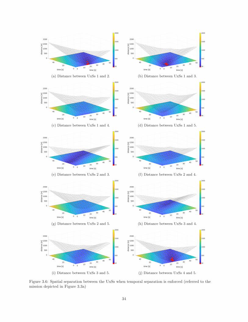
0

500

40

1000

50

dist

ance

[m]

40

1500

time [s] time [s]

3020

2000

20100 0

50

500

1000

1500

2000

(a) Distance between UxSs 1 and 2.

0

500

40

1000

50

dist

ance

[m]

40

1500

time [s] time [s]

3020

2000

20100 0

50

500

1000

1500

2000

(b) Distance between UxSs 1 and 3.

0

500

40

1000

50

dist

ance

[m]

40

1500

time [s] time [s]

3020

2000

20100 0

50

500

1000

1500

2000

(c) Distance between UxSs 1 and 4.

0

500

40

1000

50

dist

ance

[m]

40

1500

time [s] time [s]

3020

2000

20100 0

50

500

1000

1500

2000

(d) Distance between UxSs 1 and 5.

0

500

40

1000

50

dist

ance

[m]

40

1500

time [s] time [s]

3020

2000

20100 0

50

500

1000

1500

2000

(e) Distance between UxSs 2 and 3.

0

500

40

1000

50

dist

ance

[m]

40

1500

time [s] time [s]

3020

2000

20100 0

50

500

1000

1500

2000

(f) Distance between UxSs 2 and 4.

0

500

40

1000

50

dist

ance

[m]

40

1500

time [s] time [s]

3020

2000

20100 0

50

500

1000

1500

2000

(g) Distance between UxSs 2 and 5.

0

500

40

1000

50

dist

ance

[m]

40

1500

time [s] time [s]

3020

2000

20100 0

50

500

1000

1500

2000

(h) Distance between UxSs 3 and 4.

0

500

40

1000

50

dist

ance

[m]

40

1500

time [s] time [s]

3020

2000

20100 0

50

500

1000

1500

2000

(i) Distance between UxSs 3 and 5.

0

500

40

1000

50

dist

ance

[m]

40

1500

time [s] time [s]

3020

2000

20100 0

50

500

1000

1500

2000

(j) Distance between UxSs 4 and 5.

Figure 3.6: Spatial separation between the UxSs when temporal separation is enforced (referred to themission depicted in Figure 3.3a)

34

5040

30

time [s]20

1000

20time [s]

40

2000

1500

1000

500

0

dist

ance

[m]

50

500

1000

1500

2000

(a) Distance between UxSs 1 and 2.

5040

30

time [s]20

1000

20time [s]

40

2000

1500

1000

500

0

dist

ance

[m]

50

500

1000

1500

2000

(b) Distance between UxSs 1 and 3.

5040

30

time [s]20

1000

20time [s]

40

2000

1500

1000

500

0

dist

ance

[m]

50

500

1000

1500

2000

(c) Distance between UxSs 1 and 4.

5040

30

time [s]20

1000

20time [s]

40

2000

1500

1000

500

0

dist

ance

[m]

50

500

1000

1500

2000

(d) Distance between UxSs 1 and 5.

5040

30

time [s]20

1000

20time [s]

40

2000

1500

1000

500

0

dist

ance

[m]

50

500

1000

1500

2000

(e) Distance between UxSs 2 and 3.

5040

30

time [s]20

1000

20time [s]

40

2000

1500

1000

500

0

dist

ance

[m]

50

500

1000

1500

2000

(f) Distance between UxSs 2 and 4.

5040

30

time [s]20

1000

20time [s]

40

2000

1500

1000

500

0

dist

ance

[m]

50

500

1000

1500

2000

(g) Distance between UxSs 2 and 5.

5040

30

time [s]20

1000

20time [s]

40

2000

1500

1000

500

0

dist

ance

[m]

50

500

1000

1500

2000

(h) Distance between UxSs 3 and 4.

5040

30

time [s]20

1000

20time [s]

40

2000

1500

1000

500

0

dist

ance

[m]

50

500

1000

1500

2000

(i) Distance between UxSs 3 and 5.

0

500

40

1000

50

dist

ance

[m]

40

1500

time [s] time [s]

3020

2000

20100 0

50

500

1000

1500

2000

(j) Distance between UxSs 4 and 5.

Figure 3.7: Spatial separation between the UxSs when spatial separation is enforced (referred to themission depicted in Figure 3.5a)

35

Chapter 4

Optimal motion planning

This chapter extends the results presented in Chapter 3 to a more general class of optimal motion plan-

ning problems. In particular, while in Chapter 3 it was assumed that the UxSs under consideration are

differentially flat, in the present chapter we consider UxSs governed by general nonlinear dynamics. In

this case, the optimal motion planning problem is captured by a general optimal control problem of Bolza

type. Similarly to Chapter 3, this chapter provides an approximation of the optimal control problem into

a nonlinear programming problem using Bernstein polynomials, and it demonstrates consistency results for

this approximation method. Finally, it presents numerical results that demonstrate the advantages of the

proposed approach.

4.1 Optimal motion planning for a general class of systems

This chapter deals with the optimal motion planning problem introduced in Section 2.2.1, Problem POC.

For the reader’s convenience, the problem at hand is reported below.

Problem 8 (Problem POC) Determine x : [0, tf ] → Rnx and u : [0, tf ] → R

nu (and possibly tf ) that

minimize

I(x(t),u(t)) = E(x(0),x(tf )) +

∫ tf

0

F (x(t),u(t))dt (4.1)

subject to

x = f(x(t),u(t)) , ∀t ∈ [0, tf ], (4.2)

e(x(0),x(tf )) = 0 , (4.3)

h(x(t),u(t)) ≤ 0 , ∀t ∈ [0, tf ] , (4.4)

where E : Rnx × Rnx → R, F : Rnx × R

nu → R are the terminal and running costs, respectively, f :

Rnx ×R

nu → Rnx is the system dynamics, e : Rnx ×R

nx → Rne is the vector of boundary conditions, and

h : Rnx ×Rnu → R

nh is the vector of state and input constraints.

36

Notice that for ease of notation we dropped the subscript ‘d’ from the variables involved in the above

problem.

Imposed onto Problem POC are the following assumptions:

Assumption 4 E, F , f , e, and h are Lipschitz continuous with respect to their arguments. F (·) ∈ C2.

Assumption 5 Optimal state x∗(t) and control u∗(t) to Problem POC exist and satisfy x∗(t) ∈ C2nx

and

u∗(t) ∈ C2nu

.

Notice that the above problem definition is general enough to support several applications, including

trajectory planning for multiple vehicles with dynamics given by Equation (4.2), which is the focus of this

chapter.

4.2 Bernstein approximation

The purpose of this section is to formulate a discretized version of Problem POC, here referred to as Problem

POCN , where N denotes the order of approximation. In order to accomplish this, we must approximate the

components that make up Problem POC, which are the input and the state, the cost function, the system

dynamics, and the equality and inequality constraints.

Similarly to Chapter 3, we start by considering the following Nth order Bernstein polynomials:

xN(t) =

N∑

j=0

cj,xbj,N(t) , uN (t) =

N∑

j=0

cj,ubj,N (t), (4.5)

with xN : [0, tf ] → Rnx , uN : [0, tf ] → R

nu , cj,x ∈ Rnx and cj,u ∈ R

nu . Let cx ∈ Rnx×(N+1) and

cu ∈ Rnu×(N+1) be defined as

cx = [c0,x , . . . , cN,x], cu = [c0,u , . . . , cN,u].

The derivative of xN (t) is computed as follows

xN (t) =

N∑

j=0

(N∑

i=0

ci,xDij

)

bj,N(t) ,

37

where Dij is the (i, j) entry of the differentiation matrix D ∈ R(N+1)×(N+1), which can be computed using

the properties of Bernstein polynomials (see Properties 4 and 6, and Remark 16 in Appendix A.2.1). Let

0 = t0 < t1 < . . . < tN = tf be a set of equidistant time nodes, i.e. tj = jtfN , j = 0, . . . , N . Then, Problem

POCN can be stated as follows.

Problem 9 (Problem POC

N ) Let 0 < δP < 1. Determine cx and cu (and possibly tf ) that minimize

IN (cx, cu) = E(xN (0),xN(tN )) + w

N∑

j=0

F (xN (tj),uN (tj)) , (4.6)

subject to

‖xN(tj)− f(xN (tj),uN (tj))‖ ≤ N−δP , (4.7)

∀j = 0, . . . , N ,

e(xN (0),xN (tN )) = 0 , (4.8)

h(xN (tj),uN (tj)) ≤ N−δP 1 , ∀j = 0, . . . , N . (4.9)

with w =tf

N+1 .

4.3 Feasibility and consistency of the approximation

The outcome of Problem POCN is a set of optimal Bernstein coefficients c∗x and c∗u which determine the

Bernstein polynomials x∗N (t) and u∗

N (t), i.e.

x∗N(t) =

N∑

j=0

c∗j,xbj,N(t) , u∗N(t) =

N∑

j=0

c∗j,ubj,N (t) . (4.10)

Similarly to Chapter 3, we now address the following theoretical concerns:

1. the existence of a feasible solution to Problem POCN ,

2. the convergence of the optimal solution of Problem POCN to the optimal solution of Problem POC.

For the sake of simplicity the following analysis assumes that the variable tf in Problem POC is fixed;

however, the results and the proofs can be easily extended to the case where tf is a decision variable. The

main results of this chapter are summarized in Theorems 3 and 4 below.

38

Theorem 3 There exists N1 such that for any order of approximation N ≥ N1 Problem POCN is feasible.

Proof: The proof of Theorem 3 is given in Appendix B.2.1.

♠

Theorem 4 Let c∗x, c∗u be an optimal solutions to Problem POC

N , and x∗N (t),u∗

N (t) be the Bernstein polyno-

mials given by (4.10). Assume x∗N (t),u∗

N (t) has a uniform accumulation point, i.e. there exists an infinite

subset of indices V ∈ Z+ such that

limN∈V

(x∗N (t),u∗

N (t)) = (x∞(t),u∞(t)) ,

and assume that x∞(t) and u∞(t) are continuous on [0, tf ]. Then, (x∞(t),u∞(t)) is an optimal solution to

Problem POC.

Proof: The proof of Theorem 4 is given in Appendix B.2.2.

♠

Remark 9 Notice that the above results extend the results of Chapter 3 to a more general class of systems

with nonlinear dynamics. In fact, the proofs of Theorems 3 and 4 follow similar steps as the proofs of

Theorems 1 and 2. However, the dynamics constraint in Problem PCVN (see Equation (4.7)), which is absent

in the problem formulation of Chapter 3, poses additional technical challenges to demonstrate the consistency

results stated above. These challenges are addressed in Appendix A.2.

♦

4.4 Simulation results

This section discusses the benefits of the proposed approach in solving the optimal trajectory generation

problem through two simulation scenarios. The results are obtained using MATLAB’s built in fmincon

function.

In the first scenario, the 2D trajectory generation problem for a single vehicle is considered. The vehicle,

modelled as a single integrator, is required to navigate from the initial position x0 = [−500,−900]m to the

final destination xf = [1500,−600]m while minimizing the time of arrival. The algorithm must ensure a

minimum separation of E = 50m with three obstacles positioned at po,1 = [0−800]⊤m, po,2 = [450−750]⊤m,

39

and po,3 = [850 − 730]⊤m. Finally, the norm of the input must remain within minimum and maximum

saturation limits umin = 15m/s and umax = 32m/s. This problem can be formally stated as follows:

Determine x(t),u(t) and tf that minimize

I(x(t),u(t)) =

∫ tf

0

dt

subject to

x(t) = u(t) , ∀t ∈ [0, tf ],

x(0) = x0 , x(tf ) = xf ,

||x(t)− po,i|| ≥ E , ∀t ∈ [0, tf ], i = 1, 2, 3 ,

umin ≤ ||u(t)|| ≤ umax , ∀t ∈ [0, tf ].

The discretization method proposed in this chapter is compared to the Legendre PS method based on

Lagrange interpolation at Legendre-Gauss-Lobatto nodes (for implementation details the reader is referred

to [144]). The results are enclosed in Figure 4.1. The top-left, top-center, and bottom-left figures show the

trajectories obtained using the PS method with orders of approximation 5, 20, and 100, respectively. The PS

method enforces the constraints only at the discretization nodes, and not in between them. By increasing the

number of nodes, the distance between the entire trajectory and the obstacles increases towards the desired

value E = 50m. However, as demonstrated by the top-right figure, which depicts the distance between

the trajectories and the obstacles for the three order of approximations indicated above, the minimum

separation constraint is never satisfied. On the other hand, the bottom-center figure shows that with the

proposed method, even by choosing a small number of nodes (N=5 in this example), the collision avoidance

constraint can be computed for the entire curve using, for example, the algorithm in [112], and is thus

guaranteed along the whole trajectory. The bottom-right figure supports this claim by showing that the

distance between the trajectory and the obstacles is always greater than the required value.

The possibility of choosing low order of approximations while guaranteeing constraint satisfaction is the

strength of our approach, which prioritizes safety and feasibility of the trajectories over optimality. The

advantage of our method becomes more evident in multiple vehicles missions, where the trajectories assigned

to the vehicles must be spatially or temporally separated. Recall that spatial separation is guaranteed if

the minimum distance between any two points on two paths is greater than or equal to a minimum spatial

40

X [m]-500 0 500 1000 1500

Y [m

]

-1500

-1000

-500

0

PS method - 5th order

X [m]-500 0 500 1000 1500

Y [m

]

-1500

-1000

-500

0

PS method - 20th order

X [m]-500 0 500 1000 1500

Y [m

]

-1500

-1000

-500

0

PS method - 100th order

X [m]-500 0 500 1000 1500

Y [m

]

-1500

-1000

-500

0

Bernestein method - 5th order

time [s]0 10 20 30 40 50 60

Y [m

]

20

40

60

80

100

120

140PS method - Distance

N=5N=20N=100

time [s]0 10 20 30 40 50 60

Y [m

]

20

40

60

80

100

120

140Bernstein method - Distance

Figure 4.1: Legendre PS vs Bernstein approximation method: collision avoidance with multiple obstacles.

clearance, i.e.

‖pi(ti)− pj(tj)‖ ≥ E , ∀ti, tj ∈ [0, tf ] , ∀i, j = 1, . . . , n , i 6= j. (4.11)

Temporal separation, on the other hand, is achieved if for any time t the minimum distance between two

vehicles is greater than or equal to the minimum spatial clearance, i.e.

‖pi(t)− pj(t)‖ ≥ E , ∀t ∈ [0, tf ], ∀i, j = 1, . . . , n , i 6= j. (4.12)

Consider a mission scenario in which n vehicles, starting from their initial positions, have to follow spatially

separated trajectories to reach predefined final destinations. By adopting the PS method described above,

spatial separation would have to be enforced by imposing separation constraints between every node of every

trajectory. Thus, the problem would have(n2

)N2 separation constraints, where N is the number of nodes and

(n2

)is the binomial coefficient. An increased number of nodes (dictated, perhaps, by reasons similar to the

ones discussed in the first simulation scenario of this section), would increase the complexity in the searching

for the optimal solution, making the PS approach practically infeasible for these types of applications. On

the other hand, with our approach constraint satisfaction is achieved independently on the number of nodes.

This is discussed in the next simulation scenario described below.

Figure 4.2 illustrates the results of a multiple vehicles mission in which n = 11 vehicles, starting from their

41

initial positions, have to reach a ‘V’ shaped formation while minimizing the time of arrival. The Bernstein

approximation method is employed with order of approximation N = 8. The dynamics of the ith vehicle

are governed by the following differential equations

x1,i(t) = Vi(t) cos(x3,i(t))

x2,i(t) = Vi(t) sin(x3,i(t))

x3,i(t) = ωi(t) ,

(4.13)

with input ui(t) = [Vi(t) , ωi(t)]⊤, and state xi(t) = [x1,i(t) , x2,i(t) , x3,i(t)]

⊤. The input constraints are as

follows:

Vmin ≤ Vi(t) ≤ Vmax , (4.14)

−ωmax ≤ ωi(t) ≤ ωmax , (4.15)

with Vmin = 15m/s, Vmax = 32m/s, and ωmax = 0.3rad/s. Finally, temporal separation constraints are

imposed between each pair of trajectories, i.e.

||pi(t)− pj(t)|| ≥ E , (4.16)

∀i, j = 1, . . . , 11, i 6= j ∀t ∈ [0, tf ], where E = 50m, and pi(t) = [x1,i(t) , x2,i(t)]⊤.

The constraints in Equations (4.14), (4.15), and (4.16) are computed using the minimum distance algo-

rithm introduced in Appendix A.2.1, Property 8. Figures 4.3 and 4.4 show the time history of the speeds and

angular rates, respectively, demonstrating that the input saturation constraints are satisfied for all times.

At last, the same simulation is repeated, but the temporal separation constraint given by Equation (4.16)

is replaced by the (more stringent) spatial separation requirement

||pi(tk)− pj(tp)|| ≥ E , (4.17)

∀i, j = 1, . . . , 11, i 6= j ∀tk, tp ∈ [0, tf ]. Figure 4.5 depicts the 2D trajectories. Figures 4.6 and 4.7 illustrate

the speed and angular rate commands, respectively.

42

X [m]-500 0 500 1000 1500 2000 2500

Y [m

]

-500

0

500

1000

1500

2000

Figure 4.2: Multiple vehicles mission - temporal separation: 2D paths.

time [s]0 10 20 30 40 50 60 70 80 90

spee

d [m

/s]

15

20

25

30

35

Figure 4.3: Multiple vehicles mission - temporal separation: speed profiles.

time [s]0 10 20 30 40 50 60 70 80 90

ang

rate

[rad

/s]

-0.1

-0.05

0

0.05

0.1

0.15

0.2

0.25

0.3

Figure 4.4: Multiple vehicles mission - temporal separation: angular rates.

43

X [m]-500 0 500 1000 1500 2000 2500

Y [m

]

-500

0

500

1000

1500

2000

Figure 4.5: Multiple vehicles mission - spatial separation: 2D paths.

time [s]0 10 20 30 40 50 60 70 80 90

spee

d [m

/s]

15

20

25

30

35

Figure 4.6: Multiple vehicles mission - spatial separation: speed profiles.

time [s]0 10 20 30 40 50 60 70 80 90

ang

rate

[rad

/s]

-0.2

-0.1

0

0.1

0.2

0.3

Figure 4.7: Multiple vehicles mission - spatial separation: angular rates.

44

Chapter 5

Virtual target tracking of multirotor

UASs

This chapter describes an outer-loop 3D VT tracking control algorithm for multirotor UASs. The control

law derived enables a multirotor equipped with an autopilot capable of tracking angular-rate and thrust

reference commands to converge to and follow a virtual target. The method that we propose employs key

concepts and techniques introduced in [145] for trajectory tracking of a quadrotor where the total thrust

force and the moment vector generated by the four rotors act as control inputs. Since most multirotors

today come equipped with an autopilot capable of tracking total thrust and angular-rate commands, the

objective of this chapter is to develop a VT tracking control algorithm that exploits this feature by using the

autopilot commands as control inputs. A rigorous stability analysis is performed to assess the convergence

properties of this algorithm for the cases of ideal and non-ideal tracking performance of the autopilot. The

main advantage of this approach is the fact that it can be easily used with a variety of commercially available

multirotors.

5.1 Problem formulation

This section formulates the problem of VT tracking for a multirotor UAS, that is the main topic of the

present chapter. We first present the equations of motion of a multirotor UAS. This is followed by the

definition of a set of VT tracking error variables and the formulation of the VT tracking problem at hand.

5.1.1 6-DoF model for a multirotor UAS

Let I denote an inertial frame e1, e2, e3 and B the body frame b1, b2, b3 attached to the center of

gravity of the multirotor. It is assumed that the vehicle is equipped with an inner-loop autopilot that controls

the UAS moments and uses the angular rates and total thrust as command inputs [136, 138]. Furthermore,

it is assumed that atmospheric forces are negligible [146,147]. Then, the six degree of freedom model for the

45

multirotor UAS kinematics and dynamics is given by

Gv =

p = v ,

mv = T b3 −mge3 ,

R = R(ω)∧ ,

(5.1)

where p and v are the position and velocity of the vehicle’s center of mass in the inertial frame with respect

to the basis e1, e2, e3, m is the vehicle’s mass, T is the total thrust of the propellers, R = RIB is the

rotation matrix from the body frame to the inertial frame, ω = ωB/IB = [p, q, r] is the vector of the

angular rates of the vehicle with respect to I, resolved in B, and (·)∧ denotes the hat map (see Appendix

A.1). The multirotor UAS system is depicted in Figure 5.2a.

5.1.2 Virtual target tracking error

Recall from Section 2.2.2 that pd,i(γi(t)) is the virtual target to be tracked by the ith multirotor UAS

involved in the cooperative mission, where γi(t) is the virtual time defined as

γi : R+ → [0, tf ] . (5.2)

For ease of notation, and since this chapter deals with the VT tracking problem for a single vehicle, in the

remainder of this chapter we drop the subscript i from the variables of interest. Moreover, for the purpose

of brevity, we omit the time-dependency.

We start by defining the position error vector ep ∈ R3 as

ep = pd(γ)− p , (5.3)

and the velocity error vector ev ∈ R3 as

ev = pd(γ)− p . (5.4)

Following [145] we now introduce an auxiliary frame D, which is used (i) to shape the approach to the

path as a function of the error components ep and ev, and (ii) to impose a desired orientation on the vehicle.

Let the rotation matrix from the frame D to the inertial frame I be

Rc := RID = [b1D , b2D , b3D] ,

46

where

b3D =(kp + sp)ep + (kv + sv)ev +mge3 +mpd(γ)

‖(kp + sp)ep + (kv + sv)ev +mge3 +mpd(γ)‖, (5.5)

for some kp, kv > 1, and

sp =

sign(e⊤p e3) , if ‖kpep + kvev +mge3 +mpd(γ)‖ = 0

0 otherwise

,

sv =

sign(e⊤v e3) , if ‖kpep + kvev +mge3 +mpd(γ)‖ = 0

0 otherwise

.

The vector b3D defines the desired orientation of the b3-axis of the multirotor required in order to converge

to the desired position pd(γ) and velocity pd(γ). As an example, Figure 5.1 illustrates the case where

the displacement between the UAS position and the virtual target is along the e1 axis; then, the desired

orientation of the multirotor’s b3-axis is b3D = [b3D1 , 0 , b3D3], i.e. the horizontal component of the b3D

axis along the e2 direction is zero, and the UAS moves solely along the e1 axis, thus reaching the virtual

target. Figure 5.1 also shows how different approaches to the path can be obtained by tuning the control

gain kp (for the sake of simplicity in the illustration the value of the control gain kv is set to 0). The vector

b1D describes the desired orientation of the multirotor’s b1 axis, and it can be arbitrarily chosen as long as

it is orthonormal to b3D. Consequently, b2D is chosen to be orthonormal to b1D and b3D.

Remark 10 Given the vector b3D defined in (5.5), let b⋆1D

be a vector that describes the desired orientation

of b1, but that is not orthonormal to b3D. Assume that b⋆1D

is not parallel to b3D. Then, b1D and b2D

can be found as follows [145]:

b2D =b3D × b⋆

1D

||b3D × b⋆1D

||, b1D = b2D × b3D .

Figure 5.2 depicts the geometry of the problem at hand.

♦

Lemma 1 From the definition of sp and sv, the denominator of b3D is always greater than 0 . Therefore

the vectors b1D, b2D, and b3D are always well defined.

Proof: The proof of Lemma 1 is given in Appendix B.3.1.

47

Desired Path

Virtual Target

Desired Path

Virtual Target

Desired Path

Virtual Target

Figure 5.1: Approach to the path.

Next we introduce a set of variables that will be used later to formulate the VT tracking problem. In

particular, let R be the rotation matrix from B to D, that is

R = RDB = R⊤

c R .

Then

˙R = R(ω)∧ ,

where

ω = ωB/DB =

p

q

r

− R⊤ωD/ID , (5.6)

and ωD/ID can be computed as follows:

(ωD/ID)∧ = R⊤c Rc .

Note that, if R = I3, then the frame B coincides with the desired frame D. Furthermore, consider the

following real-valued function on SO(3)

Ψ(R) =1

2tr(I3 − R) , (5.7)

and its time derivative

Ψ(R) = −1

2tr(R(ω)∧).

48

Desired Path

Virtual Target

(a) Actual orientation of the vehicle

Desired Path

Virtual Target

(b) Desired orientation to approach the path

Figure 5.2: Geometry of the problem.

Finally, let

eR =1

2(R − R⊤)∨ , (5.8)

where (·)∨ denotes the vee map (see Appendix A.1). Using Equation (A.1) in Appendix A.1 we obtain:

Ψ(R) = eR · ω . (5.9)

Therefore, the dynamics of the VT tracking errors can be summarized by the following system of equations:

ep = ev

mev = mpd(γ)− T b3 +mge3

Ψ(R) = eR · ω ,

(5.10)

and the VT tracking error vector xpf (t) can be formally defined as

xpf = [e⊤p , e⊤v , e⊤R]⊤ .

Notice that in the region Ψ(R) < 1, if xpf = 0, then the VT tracking position error, the VT tracking velocity

error, and the VT tracking attitude error are equal to zero, i.e.

ep = 0 , ev = 0 , Ψ(R) = 0 .

Using the above notation, we now define the VT tracking problem for a multirotor UAS.

Problem 10 Consider a multirotor UAS and a virtual target pd(γ(t)), where pd(t) is the trajectory gener-

ated by solving the optimal motion planning problem, Problem 2, and γ(t) is the virtual time. Assume that

49

the dynamics of the virtual time satisfy the bounds given in Equation (2.16), with γmini , γmax

i and γmaxi given

by Equation (2.19). The objective is to design feedback control laws for the total thrust T (t), roll rate p(t),

pitch rate q(t), and yaw rate r(t) such that the generalized VT tracking error vector xpf = [e⊤p , e⊤v , Ψ(R)]⊤,

with the dynamics described in (5.10), converges to a neighborhood of the origin.

Remark 11 Notice that the VT tracking problem definition above adapts the definition in Section 2.2.2,

Problem 3, to the VT tracking problem for multirotor UASs.

♦

With this setup, we can now design control laws that solve the VT tracking control problem as defined

above.

5.2 Virtual target tracking controller

First, let the total thrust command be governed by

Tc = ((kp + sp)ep + (kv + sv)ev +mge3 +mpd(γ))⊤b3 . (5.11)

In addition, let the angular rate commands be given by

pc

qc

rc

= R⊤ωD/ID − kReR , (5.12)

for some kR > 0.

Then, the Lemma below states one of the main results of this chapter:

Lemma 2 Let the total thrust Tc(t) and the angular rate commands [pc(t) , qc(t) , rc(t)] be governed by

(5.11) and (5.12). Assume ideal performance for the existing inner-loop autopilot (i.e. T (t) = Tc(t) and

[p(t) , q(t) , r(t)] = [pc(t) , qc(t) , rc(t)] ∀t ≥ 0). Then, there exist kp , kv , kR such that the error vector

xpf = [e⊤p , e⊤v , e⊤R]⊤ (5.13)

50

converges exponentially to zero with rate of convergence

λpf <c1(1− c2)

m, (5.14)

in the corresponding domain of attraction

Ωpf ,

(ep , R) |Ψ(R) ≤ c2 , ||ep|| ≤ epmax

, (5.15)

for some c1, epmax > 0 and c2 < 1/2. In other words, the error vector xpf satisfies

‖xpf (t)‖ ≤ kpf ‖xpf (0)‖e−λpf t ,

where

kpf :=

√

λmax(W2)

λmin(W1), (5.16)

and

W1 =

kp

2 − c12 0

− c12

m2 0

0 0 1

, W2 =

kp

2 − c12 0

− c12

m2 0

0 0 11−c2

. (5.17)

♦

Proof: The proof of Lemma 2 is given in Appendix B.3.2.

Note that we modified the controller used in [145] in two important ways. First, we reparametrized it as

VT tracking controller and second we modified it to use angular rates and thrust as control inputs to be

tracked by an existing inner-loop autopilot. In turn, this compels us to consider the underlying performance

limitations due to the constraints of the inner-loop controller. Thus, as our last step, we consider the case

of non perfect tracking performance of the autopilot, which is the main result of this chapter.

Lemma 3 Let the total thrust Tc(t) and the angular rate commands [pc(t) , qc(t) , rc(t)] be governed by

(5.11) and (5.12). Let the inner-loop autopilot satisfy the following performance bounds

|pc(t)− p(t)| ≤ γp , |qc(t)− q(t)| ≤ γq , |rc(t)− r(t)| ≤ γr , |Tc(t)− T (t)| ≤ γT ,

where T (t) , p(t) , q(t), and r(t) are the actual total thrust and angular rates, and let γω =√

γ2p + γ2

q + γ2r .

51

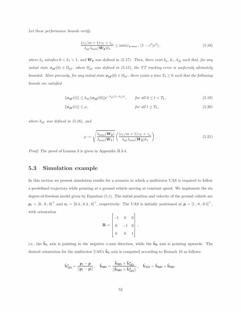
Let these performance bounds verify

(c1/m+ 1)γT + γωλpf λmin(W2)δλ

≤ min(epmax , (1− c2)c2) , (5.18)

where δλ satisfies 0 < δλ < 1, and W2 was defined in (5.17). Then, there exist kp , kv , kR such that, for any

initial state xpf (0) ∈ Ωpf , where Ωpf was defined in (5.15), the VT tracking error is uniformly ultimately

bounded. More precisely, for any initial state xpf (0) ∈ Ωpf , there exists a time Tb ≥ 0 such that the following

bounds are satisfied

‖xpf (t)‖ ≤ kpf ‖xpf (0)‖e−λpf (1−δλ)t , for all 0 ≤ t < Tb , (5.19)

‖xpf (t)‖ ≤ ρ , for all t ≥ Tb , (5.20)

where kpf was defined in (5.16), and

ρ :=

√

λmax(W2)

λmin(W1)

((c1/m+ 1)γT + γωλpf λmin(W2)δλ

)

. (5.21)

Proof: The proof of Lemma 3 is given in Appendix B.3.4.

5.3 Simulation example

In this section we present simulation results for a scenario in which a multirotor UAS is required to follow

a predefined trajectory while pointing at a ground vehicle moving at constant speed. We implement the six

degree-of-freedom model given by Equation (5.1). The initial position and velocity of the ground vehicle are

pt = [0 , 0 , 0]⊤ and vt = [0.4 , 0.4 , 0]⊤, respectively. The UAS is initially positioned at p = [1 , 0 , 0.5]⊤,

with orientation

R =

−1 0 0

0 −1 0

0 0 1

,

i.e., the b1 axis is pointing in the negative x-axis direction, while the b3 axis is pointing upwards. The

desired orientation for the multirotor UAS’s b1-axis is computed according to Remark 10 as follows:

b⋆1D

=pt − p

||pt − p|| , b2D =b3D × b⋆

1D

||b3D × b⋆1D

||, b1D = b2D × b3D .

52

Figure 5.3 includes the simulation results. In particular, Figures 5.3a and 5.3b illustrate the 2D and 3D

plots of the actual and desired trajectories of the UAS, as well as the ground vehicle’s trajectory, while

Figures 5.3c and 5.3d show the speed and acceleration profiles, respectively. The execution of the mission

at three different time steps is depicted in Figure 5.4, which illustrates the desired (red) and actual (blue)

trajectories of the UAS. The multirotor’s body frame B (positioned on the vehicle’s center of gravity) and

the desired frame D (positioned on the desired path) are also depicted in the same figure, with the b1

and b1D axes always pointing towards the ground vehicle. Figure 5.5 highlights the performance of the VT

tracking algorithm. In particular, it is shown that the VT tracking errors converge to a neighborhood of

zero at t ≈ 8 s. The VT tracking control efforts, namely angular rates and total thrust, are also depicted in

the same figure.

For the sake of providing a more realistic simulation scenario, we repeat the above experiment, and

implement a simple inner-loop autopilot for angular rate and total thrust commands tracking. Additionally,

measurement noise and transmission delays have been added. The 2D and 3D plots of the actual and

desired trajectories are illustrated in Figures 5.6a and 5.6b, respectively, while Figures 5.6c and 5.6d depict

the actual and desired speed and acceleration profiles. Figure 5.7 depicts the performance of the mission at

three different times. The performance of the VT tracking controller is illustrated in Figure 5.8. Figure 5.8a

shows the VT tracking error, converging to a neighborhood of zero slower with respect to the previous case

(see Figure 5.5a). Finally, the VT tracking commands and actual angular rates and total thrust of the

vehicle are shown in Figures 5.8b–5.8e.

Finally, Figure 5.9 presents an additional simulation scenario in which the multirotor UAS is asked to

perform more aggressive maneuvers by “drawing” the phrase path following in the air. The overall mission

is executed in 260 s. However, for the sake of clarity, Figures 5.9c, 5.9d, and 5.9e show the VT tracking

error in the first 20 s of the mission. The desired path is produced by connecting four Bernstein polynomials

approximants using a total of 400 points.

In the simulation scenarios described in this section, the control gains have been selected as follows:

kp = 3 , kv = 3 , kR = 5 .

53

x [m]0 5 10

y [m

]

0

2

4

6

8

10

(a) 2D Path

(b) 3D Path

time [s]0 5 10 15 20

spee

d [m

/s]

-5

0

5

(c) Speed profile

time [s]0 5 10 15 20

acce

lera

tion

[m/s

2 ]

-5

0

5

(d) Acceleration profile

Figure 5.3: 3D VT tracking: simulation scenario.

54

-50

y [m]

51015-5

05

10

x [m]

15

5

0

z [m

]

x [m]-5 0 5 10 15

y [m

]

0

5

10

-50

y [m]

51015-5

05

10

x [m]

15

5

0

z [m

]

x [m]-5 0 5 10 15

y [m

]

0

5

10

-50

y [m]

51015-5

05

10

x [m]

15

5

0

z [m

]

x [m]-5 0 5 10 15

y [m

]

0

5

10

t = 0.0 s

t = 3.5 s

t = 15.0 s

Figure 5.4: 3D VT tracking of a multirotor UAS.

55

time [s]0 2 4 6 8 10 12 14 16 18 20

Pat

h fo

llow

ing

erro

rs

0

0.5

1

1.5

2

2.5

3epevΨ(R)

(a) VT tracking error

time [s]0 5 10 15 20

p[1/s]

-0.2

0

0.2

0.4

0.6

(b) Angular rate, p(t).

time [s]0 5 10 15 20

q[1/s]

-1

-0.5

0

0.5

(c) Angular rate, q(t).

time [s]0 5 10 15 20

r[1/s]

-0.4

-0.2

0

0.2

0.4

(d) Angular rate, r(t).

time [s]0 5 10 15 20

T[K

g∗m/s2]

18

20

22

24

(e) Total thrust, T (t).

Figure 5.5: VT tracking errors commands.

56

x [m]-2 0 2 4 6 8 10 12

y [m

]

0

2

4

6

8

10

(a) 2D Path

(b) 3D Path

time [s]0 5 10 15 20

spee

d [m

/s]

-4

-2

0

2

4

6

(c) Speed profile

time [s]0 5 10 15 20

acce

lera

tion

[m/s

]

0

5

10

(d) Acceleration profile

Figure 5.6: 3D VT tracking: simulation scenario.

57

-50

y [m]

51015-5

05

10

x [m]

15

5

0

z [m

]

x [m]-5 0 5 10 15

y [m

]

0

5

10

-50

y [m]

51015-5

05

10

x [m]

150

5

z [m

]

x [m]-5 0 5 10 15

y [m

]

0

5

10

-50

y [m]

51015-5

05

10

x [m]

15

5

0

z [m

]

x [m]-5 0 5 10 15

y [m

]

0

5

10

t = 0.0 s

t = 3.5 s

t = 15.0 s

Figure 5.7: 3D VT tracking of a multirotor UAS.

58

time [s]0 2 4 6 8 10 12 14 16 18 20

Pat

h fo

llow

ing

erro

rs

0

0.5

1

1.5

2

2.5

3epevΨ(R)

(a) VT tracking error

time [s]0 5 10 15 20

pc,p

[1/s]

-0.5

0

0.5

1ppc

(b) Angular rate, p(t)

time [s]0 5 10 15 20

q c,q

[1/s]

-1.5

-1

-0.5

0

0.5

1qqc

(c) Angular rate, q(t)

time [s]0 5 10 15 20

r c,r

[1/s]

-1

-0.5

0

0.5

1

1.5rrc

(d) Angular rate, r(t)

time [s]0 5 10 15 20

Tc,T

[Kg∗m/s

2]

0

5

10

15

20

25TTc

(e) Total thrust, T (t)

Figure 5.8: VT tracking commands.

59

y [m]

8

6

4

210

5x [m]

01

1.52

z [m

]

desired pathquadrotor

(a) 3D Path

x [m]0 5 10

y [m

]

2

4

6

8

(b) 2D Path

time [s]0 10 20 30

e p

0

1

2

(c) VT tracking error, ep(t)

time [s]0 10 20 30

e v

0

0.5

1

1.5

(d) VT tracking error, ev(t)

time [s]0 10 20 30

ΨR

0

0.005

0.01

(e) VT tracking error, ΨR(t)

Figure 5.9: Drone drawing a Bezier curve.

60

Chapter 6

Coordination of multiple autonomous

vehicles

This chapter addresses the problem of coordinating a group of UxSs. As described in previous chapters,

the cooperative missions considered require that each vehicle follow a feasible collision-free path, and that

all vehicles arrive at their respective final destinations at the same time, or at different times but meeting

a desired inter-vehicle schedule. In this chapter we assume that the UxSs under consideration are equipped

with VT tracking controllers, which enable the vehicles to track a set of feasible virtual targets. Then, the

coordination problem is solved by controlling the rate of progression of the virtual targets along given desired

trajectories. We tackle the problem of coordination control with time-varying communications networks

using a Lyapunov-based approach and derive performance bounds as a function of the quality of service of

the communications network. Furthermore, we study the degradation in performance that arises when the

VT tracking controller exhibits bounded tracking errors.

6.1 Coordination states and maps

Recall from Section 2.2.2 that the desired position assigned to the ith vehicle at time t is given by pd,i(γi(t)),

where pd,i(t) is the trajectory produced by the motion planning algorithm, and the parameter γi(t) is the

virtual time. We notice that, if γi(t) = 1, the desired speed profile to which the vehicle is required to

fly is equal to the speed profile given by the trajectory generation algorithm (i.e. γi(t) = 1 implies that

the mission is executed at the desired pace). On the other hand, γi(t) > 1 (γi(t) < 1) implies a faster

(slower) execution of the mission. The virtual time and its first time derivative play a crucial role in the

coordination problem. In fact, given that the paths produced by the trajectory generation algorithm satisfy

the simultaneous time-of-arrival requirement (see Equation (2.7)), we say that if

γi(t)− γj(t) = 0 , ∀i, j ∈ 1, . . . , n , i 6= j , (6.1)

61

then, at time t, all the vehicles are coordinated. Moreover, as already discussed in Section 2.2.2, if

γi − 1 = 0 , ∀i ∈ 1, . . . , n , (6.2)

then the desired speed at which the vehicles are required to converge is equal to the desired speed profile

established at the motion planning level. Thus, Equations (6.1) and (6.2) capture the objective of coor-

dination, and require that a control law for γi must be formulated to ensure that the objective will be

achieved.

Remark 12 We notice that if the desired trajectories pd,i(t) produced by the motion planning algorithm

satisfy the temporal separation requirement, i.e.

‖pd,i(t)− pd,j(t)‖ ≥ Ed , ∀t ∈ [0, tf] , i, j = 1, . . . , n, i 6= j

(see Section 2.2.1), and if the vehicles are equipped with VT tracking algorithms that solve Problem 3 in

Section 2.2.2, then satisfaction of Equations (6.1) and (6.2) ensures inter-vehicle collision avoidance.

♦

Now, let γ(t) = [γ1(t), . . . , γn(t)]⊤, and define the coordination error vectors as

ζ1(t) = Qγ(t) ∈ Rn−1 , (6.3)

ζ2(t) = γ(t)− 1 ∈ Rn . (6.4)

Recall from Section 2.2.2 that the n − 1 × n matrix Q satisfies Q1 = 0; it follows that if ζ1(t) = 0,

then γi − γj = 0, ∀i, j ∈ 1, . . . , n. Furthermore, convergence of ζ2(t) to zero implies that the individual

parameterizing variables γi(t) evolve at the desired rate 1.

Using the above notation, the coordination problem in Section 2.2.2, Problem 4, can be restated as follows:

Problem 11 Consider a set of n UxSs. Assume that the ith UxS, with i ∈ 1, . . . , n, is equipped with (i) a

motion planning algorithm that solves Problem 2, Section 2.2.1, and (ii) a VT tracking controller that solves

Problem 3, Section 2.2.2. Then, the objective of coordination is to design feedback control laws for γi(t) for

all vehicles such that the coordination vector defined as

xcd = [ζ⊤1 , ζ⊤

2 ]⊤ ,

converges to a neighborhood of zero, and such that the dynamics of the virtual times satisfy Equation (2.16).

62

6.2 Coordination control law

To solve the coordination problem, we let the evolution of γi(t) be driven by the following control law:

γi = −b(γi − 1)− a∑

j∈Ni

(γi − γj)− αi(xpf ,i) ,

γi(0) = 0 , γi(0) = 1 ,

where a and b are positive coordination control gains, while αi(ep,i) is defined as

αi(ep,i) =pd,i(γi)

⊤ep,i

‖pd,i(γi)‖+ δ,

with δ being a positive design parameter. The dynamics of γ(t) can be written in compact form as

γ = −bζ2 − aLγ − α(ep) , γ(0) = 0n, γ(0) = 1 , (6.5)

where

ep = [e⊤p,1, . . . , e⊤p,n]

⊤ ∈ R9n ,

α(ep) = [α1(ep,1), . . . , αn(ep,n)]⊤ ∈ R

n .

The following result is obtained:

Theorem 5 Consider a set of n UxSs. Assume that the ith UxS, with i ∈ 1, . . . , n, is equipped with (i)

a motion planning algorithm that solves Problem 2 (see Section 2.2.1), and (ii) a VT tracking controller

that solves Problem 3 (see Section 2.2.2). Assume that the communication network over which the UxSs

communicate satisfies Assumption 1 given in Section 2.2.2. Let the coordination error vector xcd(t) at time

t = 0 and the VT tracking performance bound ρ introduced in Problem 3, Equation 2.20, satisfy

max (||xTC(0)||, ρ) ≤ min

(1− γmin

(κ1 + κ2),γmax − 1

(κ1 + κ2),

γmax

(2bκ1 + 2bκ2 + 1),

)

, (6.6)

for some κ1, κ2 > 0, with γmin = maxi=1,...,n γmini , γmax = mini=1,...,n γ

maxi , and γmax = mini=1,...,n γ

maxi .

Finally, let γ be governed by the control law given by Equation (6.5). Then, there exist control gains a, b,

63

and δ such that the coordination error is uniformly bounded. In particular, the coordination error satisfies

||xcd(t)|| ≤ κ1||xcd(0)||e−λcdt + κ2 supt≥0

(||ep(t)||) , (6.7)

with guaranteed rate of convergence

λcd ,a

b

nµδλT (1 + a

bnT )2, 0 < δλ < 1 . (6.8)

Furthermore, the dynamics of the virtual times γi(t) and γi(t) satisfy the bounds given by Equation (2.16).

Proof: The proof of Theorem 5 is given in Appendix B.4.1.

♠

Remark 13 Notice that the maximum convergence rate λcd is obtained when the control gains a and b

satisfy

a

b=

1

nT. (6.9)

Substituting (6.9) in (6.8), one obtains

maxa,b>0

(λcd) =µδλ4T 2

,

i.e. the rate of convergence depends on the quality of the network only.

♦

Corollary 1 Suppose that each UxSs is equipped with an ideal VT tracking controller such that the VT

tracking error converges exponentially fast to zero (e.g. the VT tracking algorithm designed in Chapter

5 is exponentially stable under ideal performance of the inner-loop autopilot, see Lemma 2). Then, the

coordination error converges exponentially fast to zero as follows:

||xcd(t)|| ≤ κ1||xcd(0)||e−λcd t + κ2||ep(0)||e−λpf +λcd

2t , (6.10)

for some κ1, κ2 > 0.

Proof: The proof of Corollary 1 is given in Appendix B.4.2.

♠

64

Remark 14 Notice that the coordination control law introduced in (6.5) depends also on the VT tracking

error. By virtue of the VT tracking dependent term (i.e. α(ep)), if for example one vehicle is away from

the desired position (||ep|| 6= 0 ), its assigned virtual target speeds up or slows down in order to reduce the

VT tracking error; then, as a direct consequence, also the other vehicles involved in the cooperative mission

adjust their speed to maintain coordination. This point will become clear in Section 6.3, where the simulation

results are presented.

♦

Remark 15 The formulation of the coordination problem described above assumes only relative temporal

constraints in the execution of a given mission. Absolute temporal constraints, such as specifications in the

desired final time of the mission, are not considered. Nevertheless, such constraints can be easily incorporated

in the problem formulation, and enforced by judiciously modifying the coordination control laws presented in

this chapter.

♦

6.3 Simulation results

In this section we present simulation results for the scenario introduced in Figure 6.1, where eight quadrotor

UASs, initially positioned along the perimeter of a 40m× 40m square area, have to exchange their positions

and arrive at their final destinations at the same time. Before the mission starts, a set of trajectories are

generated which ensure temporal deconfliction (E = 1m) of the UASs, i.e.

minj,k=1,...,8

j 6=k

‖pd,j(t)− pd,k(t)‖2 ≥ E2 , for all t ∈ [0, tf ] .

Figure 6.1 depicts the 2D projection of these trajectories.

In the remainder of this section, we analyze and validate the theoretical findings through three different

simulations. In the first simulation we consider the case of ideal all-to-all communication between the vehicles,

and assume that the UASs’ states coincide with their desired positions, velocities, and orientations for all

time, i.e. ||ep(t)|| = 0 , ∀t ≥ 0. In the second simulation, a similar experiment is performed, but considering

non-ideal communication. In the third simulation, we introduce VT tracking errors by implementing the

VT tracking controller introduced in Chapter 5 with a simple inner-loop autopilot for angular rate and total

65

-10 0 10 20 30x [m]

-20

-10

0

10

20

y [m

]

UAS1UAS2UAS3UAS4UAS5UAS6UAS7UAS8

FC6

FC7

IC7

FC1

IC5

IC4

FC8 IC3 IC2FC4

IC1

FC2

IC8FC5FC3

IC6

Figure 6.1: Simulation results with eight quadrotor UASs - desired (solid lines) and UASs (dashed lines)trajectories.

thrust commands tracking. In all the experiments, the control gains are chosen to be

a = 1.5 , b = 3.6 , δ = 3 .

To illustrate the convergence properties of the solution, the virtual times are initialized as follows:

γ1(0) = 2 , γ4(0) = 3 , γ6(0) = 1 , γ8(0) = 1.5 , γ2(0) = γ3(0) = γ5(0) = γ7(0) = 0 .

6.3.1 Ideal communication - ideal virtual target tracking

In this simulation, all the vehicles communicate with each other all the time, i.e. lii(t) = 7 , lij(t) =

−1 , ∀t ≥ 0 , ∀i, j ∈ 1 , . . . , 8 , i 6= j, where lij(t)′s are the entries of the Laplacian matrix L(t).

Moroever, we let ||ep(t)|| = 0 , ∀t ≥ 0, i.e. the VT tracking algorithm exhibits ideal performance.

At time t = 0 the vehicles start navigating the room and follow the predefined trajectories until they reach

their final destination, at time t ≈ 8.8s. In Figure 6.1, the solid lines indicate the trajectories of each UAS,

while ICi and FCi indicate, respectively, initial and final position of UASi.

In Figure 6.3 the coordination variables are illustrated. At the beginning of the mission vehicles 1, 4, 6

and 8 speed up, while vehicles 2, 3, 5 and 7 slow down (see Figure 6.3b and 6.3c) until, at time t ≈ 2s,

coordination is achieved. Figure 6.3a shows convergence of the virtual times to the same increasing value.

66

time [s]1 2 3 4 5 6 7 8 9

Est

imat

e of

Qof

S

0

0.2

0.4

0.6

0.8

1

Figure 6.2: Estimate of Quality of Service.

6.3.2 Range-based communication - ideal virtual target tracking

The same experiment is repeated, but in this case we let UASi and UASj communicate with each other at

time t ≥ 0 only if ||pi(t)− pj(t)|| ≤ 20m .

Figure 6.2 depicts an estimate of the Quality of Service of the network computed as

µ(t) = λmin

(1

n

1

T

∫ t

t−T

QL(τ)Q⊤dτ

)

, t ≥ T ,

(see Assumption 1 in Section 2.2.2) with n = 8 and T = 1s. As can be seen from the figure, the estimate of

the Quality of Service is greater at t ≈ 4− 5s, when the vehicles are positioned near the center of the area,

thus all closer to each other. On the other hand, such a value is smaller at the beginning and the end of the

mission, when the vehicles communicate only with few neighbours. Figure 6.4 depicts the performance of

the coordination algorithm. It can be noted that the coordination variables converge to the desired values

at time t ≈ 4s slower than the case with ideal-communication.

6.3.3 Range-based communication - non-ideal virtual target tracking

In this last experiment, to illustrate impact of the non-zero VT tracking error, we implemented the VT

tracking controller described in Chapter 5 together with a simple inner loop autopilot to track angular

rates and total thrust commands. According to the result obtained in Lemma 3, the VT tracking error is

ultimately bounded, and the coordination error satisfies (6.7). The communication topology is the one used

67

in the previous experiment.

The vehicles start, at t = 0, with an initial displacement from the desired positions, and track the desired

paths. In Figure 6.1 the dashed lines indicate the actual trajectories of the UASs. Figure 6.5 shows the time

history of the coordination variables. Figure 6.6 depicts the time history of the norm of the coordination

error state ||xcd(t)|| (green line), and compares it with the two cases described above (blue and red lines).

As expected, the coordination error converges to a neighborhood of the origin, and remains bounded.

Finally, Figure 6.7 shows the minimum distance between the vehicles throughout the mission, which is

mini,j

||pi(t)− pj(t)|| , (6.11)

in three different cases: (i) blue line - ideal VT tracking performance; (ii) green line - the VT tracking error is

introduced, and the coordination control law given in (6.5) is employed; (iii) red line - the VT tracking error

is introduced, and the coordination law employed does not depend on the VT tracking error (i.e. Equation

(6.5) without the third term αpf (ep)). While in case (i) temporal separation is guaranteed at the trajectory

generation level, when the UASs are away from the desired position, the coordination algorithm must take

into account the VT tracking error in order to ensure that the actual UASs’ positions are separated. As it

was pointed out in Remark 14, the third term in Equation (6.5) enables the UASs to maintain coordination

even in the presence of VT tracking errors, which in turn implies that a minimum separation between the

vehicles is guaranteed. As it can be seen from Figure 6.5b and 6.5c, since UAS8 is initially displaced by

a considerable distance from its desired position, when the mission starts the virtual time associated with

UAS8 (i.e. γ8) decelerates significantly (γ8 < 1 and γ8 < 0) by virtue of αpf (ep), to allow the vehicle to

approach the desired point faster. As a consequence, also γ1 decelerates to coordinate with γ8, thus allowing

the actual vehicles to synchronize with each other along the paths and maintain a desired separation. In

absence of the term αpf (ep), the virtual times associated with the vehicles would keep coordinating with

each other without accounting for the actual position of the UASs, thus leading to potential collisions (red

line in Figure 6.7).

68

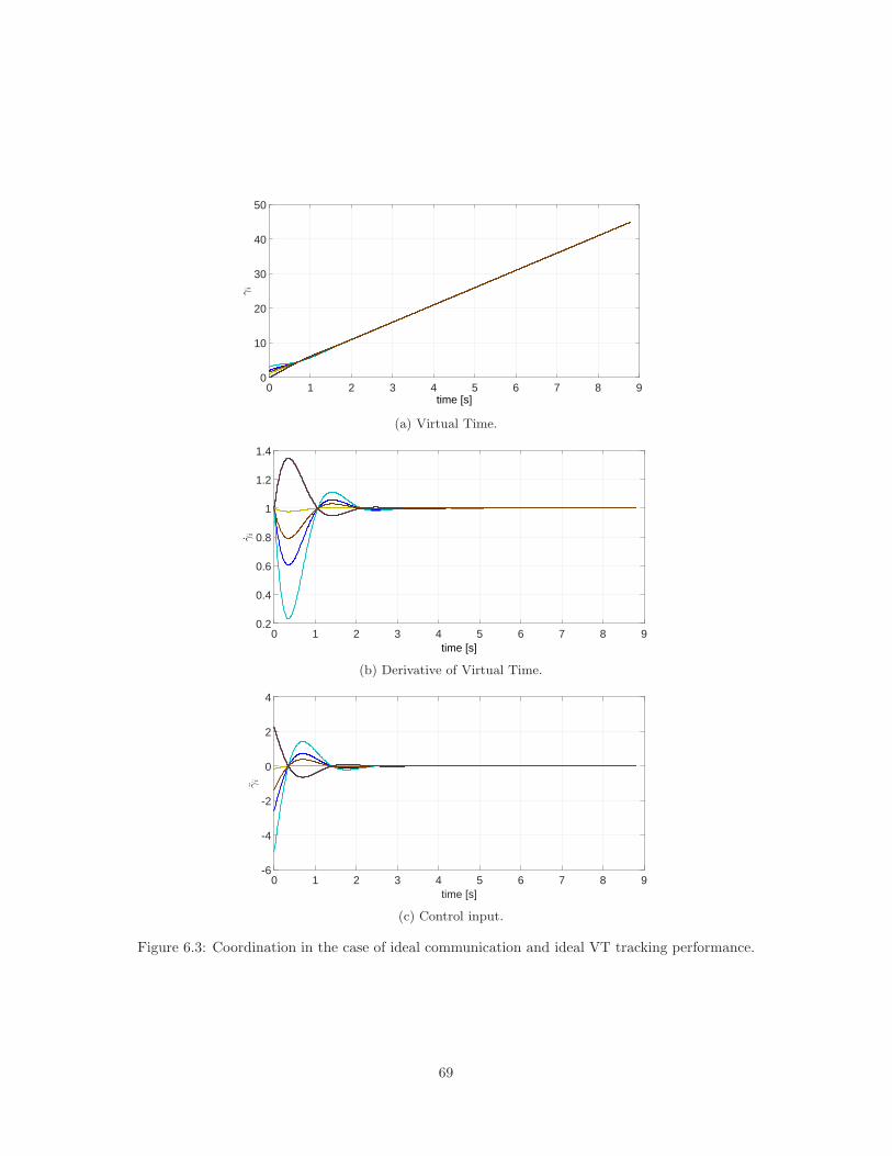
time [s]0 1 2 3 4 5 6 7 8 9

γi

0

10

20

30

40

50

(a) Virtual Time.

time [s]0 1 2 3 4 5 6 7 8 9

γi

0.2

0.4

0.6

0.8

1

1.2

1.4

(b) Derivative of Virtual Time.

time [s]0 1 2 3 4 5 6 7 8 9

γi

-6

-4

-2

0

2

4

(c) Control input.

Figure 6.3: Coordination in the case of ideal communication and ideal VT tracking performance.

69

time [s]0 1 2 3 4 5 6 7 8 9

γi

0

10

20

30

40

50

(a) Virtual Time.

time [s]0 1 2 3 4 5 6 7 8 9

γi

0.6

0.7

0.8

0.9

1

1.1

1.2

1.3

(b) Derivative of Virtual Time.

time [s]0 1 2 3 4 5 6 7 8 9

γi

-2

-1.5

-1

-0.5

0

0.5

1

1.5

(c) Control input.

Figure 6.4: Coordination in the case of range-based communication and ideal VT tracking performance.

70

time [s]0 1 2 3 4 5 6 7 8 9

γi

0

10

20

30

40

50

(a) Virtual Time.

time [s]0 1 2 3 4 5 6 7 8 9

γi

0.4

0.6

0.8

1

1.2

1.4

(b) Derivative of Virtual Time.

time [s]0 1 2 3 4 5 6 7 8 9

γi

-2.5

-2

-1.5

-1

-0.5

0

0.5

1

(c) Control input.

Figure 6.5: Coordination in the case of range-based communication and non-ideal VT trackingperformance.

71

0 1 2 3 4 5 6 7 8 9time [s]

0

1

2

3

4 Ideal Comm - Ideal trackingNon-ideal Comm - Ideal trackingNon-ideal Comm - Non-ideal tracking

Figure 6.6: Coordination error vector.

0 1 2 3 4 5 6 7 8 9time [s]

0

5

10

15

20

25

Tem

pora

l sep

arat

ion

[m]

Ideal trackingNon-ideal tracking - w/o tracking error dependencyNon-ideal tracking - with tracking error dependency

UAS1 & UAS8

Figure 6.7: Temporal separation between vehicles.

72

Chapter 7

Flight test results

This chapter presents the results of flight tests with two quadrotor UASs aimed at verifying experimentally

the stability and convergence properties associated with the coordination controller presented in Chapter 6.

We consider two operational scenarios in which the quadrotors are required to execute simple cooperative

tasks. Namely, phase on orbit coordination and spatial coordination along one axis. The reader is referred

to [148], where videos of additional experiments can be found. In what follows, we first describe the system

architecture and the indoor facility used to conduct the experiments, after which we discuss the flight test

results in detail.

7.1 System architecture and indoor facility

The flight tests presented in this chapter were performed at the Center for Autonomous Vehicle Research

(CAVR), Naval Postgraduate School, Monterey, CA [149] (see Figure 7.1). The facility is equipped with

eight VICON T-160 cameras [150] connected into one network to provide precise synthetic geopositioning

with resolution in the order of 1mm in the volume of 30 × 30 × 20ft1. The motion capture system data

are transmitted to MATLAB\Simulink, running on a Linux OS (ground station). The update rate of the

position, velocity, and attitude signals from VICON is available at the frequency of up to 200Hz. The

quadrotor UASs employed in these flight tests are the Parrot AR.Drones [151] depicted in Figure 7.2. This

platform, commercially available to the general public, is equipped with a sonar height sensor, an Inertial

Measurement Unit (IMU) capable of collecting linear acceleration, angular velocity and orientation of the

UAS, two cameras (one pointing forward, and the other one facing downwards), and an on-board computer

running proprietary software (see Figure 7.2a). The software includes an inner-loop stabilizer which uses the

sonar sensor and IMU data in order to track roll, pitch, yaw rate, and vertical speed commands. Therefore,

the VT tracking problem discussed in Chapter 5 needs to be reformulated for this particular platform, and

a VT tracking algorithm needs to be derived. The VT tracking controller employed in these flight tests

1The facility includes sixteen cameras at the time of this writing, providing geopositioning data in the volume of 40×40×30ft.

73

uses the aforementioned commands as control inputs. A thorough description of the VT tracking algorithm

is given in [138]. The VT tracking controller and the coordination algorithm are implemented on the host

machine (i.e. the MATLAB\Simulink code implemented on the ground station). The host machine sends

the VT tracking commands to the AR.Drones via a wireless ad-hoc connection with an update rate of up to

50Hz. The coordination variables are exchanged among the UASs at a data transfer rate of 100Hz (imposed

via Simulink). A schematic of the indoor facility and the system architecture is illustrated in Figure 7.1a.

7.2 Flight test results

This section describes two flight test scenarios that validate the efficacy of the coordination algorithm

described in Chapter 6. The control law introduced in Equation (6.5) is implemented, with control gains

selected as follows:

a = 3 , b = 5 , δ = 5 .

In the first scenario, i.e. phase on orbit coordination, two AR.Drones are required to fly along a circular

planar path while maintaining a desired time-varying phase shift. In the second scenario, namely spatial

coordination along one axis, the UASs are prescribed to follow paths of different lengths while adjusting

their speeds in order to maintain coordination along one direction. In what follows, we discuss the results

in details.

7.2.1 Phase on orbit coordination

In this scenario two quadrotor UASs are required to follow a circular reference of radius 2m. Figure 7.3

shows the desired orbit and the actual trajectories of the two quadrotors. Since the two UASs are tasked

to follow the same orbit, a phase-on-orbit separation is required between the two vehicles to avoid collision.

This separation is specified on-line from the ground station, and it varies according to mission requirements.

The UASs are initially required to keep a 180-deg phase separation (face-to-face); at approximately t = 94 s,

the required phase separation switches to 90 deg; the two quadrotors keep this configuration for about 14 s,

when the required phase separation switches back to 180 deg; finally, in the last part of the experiment,

the UASs are required to keep a phase separation of 270 deg. The scenario at hand is depicted in Figure

7.4, which shows the execution of the mission at six different times. A video of the flight test can be found

at http://naira.mechse.illinois.edu/quadrotor-uavs/. The desired phase-on-orbit separation, along

with the actual phase separation between the two UASs, is shown in Figure 7.5. Finally, Figure 7.6 shows

the convergence of γ1 and γ2 to the desired rate 1, as well as the convergence of the coordination errors to

74

Vicon Flying arena

UAVs

Ground

station

30 ft

30 ft

20 ft

UAV e

quip

men

t

Common Operational Environment

UAVs

position

velocity

attitude

Path-following

commands

(a) Schematic of the indoor facility. (b) CAVR, Naval Postgraduate School.

Figure 7.1: Indoor facility.

Front view

camera

Down facing

camera

Height sensor

On-board CPU

(a) AR.Drone quadrotor. (b) AR.Drone quadrotor with shell.

Figure 7.2: Quadrotor UAS employed in the flight test experiments.

a neighborhood of zero. From these figures it can be noticed that when the desired phase shift changes, the

coordination variables slightly deviate from their equilibria, and then converge again after a small transient

by virtue of the time-coordination controller.

7.2.2 Spatial coordination along one axis

In this scenario, the AR.Drones are tasked to follow two paths of different lengths, and coordinate along one

direction. In particular, UAS1 is required to follow a straight line of length 5m along the y-axis, while UAS2

has to follow a semicircle of radius 2.5m. Figure 7.7 depicts the desired and actual paths of UAS1 and UAS2.

While the mission unfolds, the UASs adjust their speed profiles in order to always face at each other, i.e.

coordinate along the y-axis. Figure 7.8 shows the execution of the mission at hand at four different times,

verifying the efficacy of the coordination algorithm. The speed profiles are illustrated in Figure 7.9. It can

be noticed that the speed of UAS2 is always greater than the one of UAS1, since the desired path assigned

to the second quadrotor is longer than the one assigned to the first vehicle. Finally, Figure 7.10 depicts

the time history of the coordination variables, which remain within a neighborhood of their equilibria as

expected.

75

04

0.5

2 4

1

z [m

]

2

1.5

y [m]

0

x [m]

0

2

-2 -2-4 -4

UAS1

UAS2

Desired orbit

Figure 7.3: Phase on orbit coordination; 3D Paths.

76

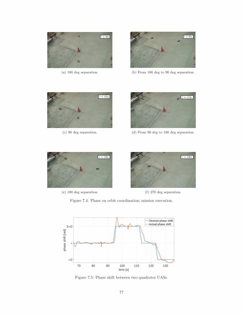
(a) 180 deg separation. (b) From 180 deg to 90 deg separation.

(c) 90 deg separation. (d) From 90 deg to 180 deg separation.

(e) 180 deg separation. (f) 270 deg separation.

Figure 7.4: Phase on orbit coordination; mission execution.

time [s]70 80 90 100 110 120 130

phas

e sh

ift [r

ad]

π/2

π

3π/2

Desired phase shiftActual phase shift

Figure 7.5: Phase shift between two quadrotor UASs.

77

time [s]70 80 90 100 110 120 130

γ1−

γ2[s*]

-0.1

0

0.1

time [s]70 80 90 100 110 120 130

γ1,γ

2[s*/

s]

0.9

1

1.1γ1

γ2

Figure 7.6: Phase on orbit coordination; errors.

78

-4

-2

y [m]

00

4

2 2

x [m]

0

-24-4

1

z [m

]

2

UAS1

Virtual Target 1UAS

2

Virtual Target 2

Figure 7.7: Spatial coordination along one axis; 3D Paths.

(a) (b)

(c) (d)

Figure 7.8: Spatial coordination along one axis; mission execution.

79

time [s]155 160 165 170 175

spee

d pr

ofile

s [m

/s]

-0.2

0

0.2

0.4

0.6

Figure 7.9: Speed profiles of the quadrotor UASs.

time [s]155 160 165 170 175

γ1−

γ2[s*]

-0.1

0

0.1

time [s]155 160 165 170 175

γ1,γ

2[s*/

s]

0.9

1

1.1γ1

γ2

Figure 7.10: Spatial coordination along one axis; errors.

80

Chapter 8

Conclusions

In this thesis a general framework for control of cooperative autonomous systems has been presented, which

allows a group of Unmanned Vehicle Systems (UxSs) to follow desired trajectories while coordinating along

them in order to satisfy relative temporal constraints. The described methodology is based on three key steps.

Initially, as a result of an optimal motion planning algorithm, each vehicle is assigned a desired trajectory.

The desired trajectory satisfies specific mission requirements, boundary conditions, flyability constraints,

and feasibility constraints, while minimizing a given cost function. Secondly, virtual target (VT) tracking

algorithms implemented on-board the UxSs enable the vehicles to follow their assigned virtual targets running

along the desired trajectories. Finally, distributed coordination algorithms adjust the progression of the

virtual targets along the desired trajectories to ensure that the vehicles coordinate in order to arrive at

the final destination at the same time, or with a predefined temporal separation, according to the mission

requirements.

The methodology derived integrates various concepts and tools from a broad spectrum of disciplines,

including nonlinear analysis and control, graph theory, optimal control, and numerical analysis, and yields

a streamlined design procedure for the control of cooperative autonomous systems. The approach presented

applies to teams of heterogeneous systems and departs considerably from well known algorithms used to

obtain swarming behaviour, which is unsuitable for most of the mission scenarios envisioned in this thesis.

To solve the optimal motion planning problem, this thesis proposed a numerical method able to efficiently

generate feasible and safe trajectories for multiple UxSs. The method is based on direct approximation of a

continuous-time optimal control problem into a discrete-time formulation using Bernstein polynomial approx-

imation. These polynomials have favorable geometric properties which allow to efficiently compute minimum

distance between curves, saturation constraints, etc., along the entire trajectory. Thus, the proposed ap-

proach is particularly convenient for generating trajectories for safe operation of multiple autonomous vehicles

in complex environments. Furthermore, Bernstein polynomials possess convergence properties which were

used in this thesis to derive convergence results of the discrete solution to the solution of the continuous-time

problem.

81

The coordination problem was formulated as a consensus problem, with the objective of regulating a

suitably defined set of coordination variables to zero. Using results from nonlinear systems and graph theory,

conditions were derived under which the consensus algorithm proposed solves the coordination problem in

the presence of switching communications topologies and communication dropouts. Lower bounds were also

derived on the performance of the algorithm as a function of the quality of service (QoS) of the supporting

communications network, which in the context of this thesis represents a measure of the level of connectivity

of the communications graph. It is relevant to emphasize that the coordination result is independent on the

dynamics of the vehicles considered, and on the solution to the VT tracking problem adopted, as long as the

VT tracking algorithm satisfies ultimate boundedness properties. Nevertheless, for the sake of completeness,

a VT tracking algorithm for multirotor UASs was proposed.

In order to bridge the gap between theory and practice, this thesis included the results of flight tests

with multiple multirotor UASs executing cooperative missions. The results illustrated the efficacy of the

algorithms proposed. They also demonstrated the validity of the general theoretical framework adopted for

control of cooperative autonomous systems in realistic applications as well as the feasibility of the onboard

implementation of the algorithms derived.

8.1 Future work

The research developments carried out in this thesis hold promise for the use of UxSs in real world environ-

ments. Nevertheless, there is ample room for improvement and intensive research efforts are warranted in a

number of topics. A few representative examples are outlined below.

8.1.1 Optimal motion planning

The optimal motion planning algorithm presented in this dissertation requires execution in a centralized

fashion. However, for large scale multiple UxSs missions, a centralized motion planning approach has several

drawbacks, and a decentralized motion planning architecture is desired or even necessary. Future research

will formulate the decentralized optimal motion planning problem as a distributed constrained optimal

control problem. Particular emphasis should be placed on the development of a computational framework,

based on Bernstein polynomials, and communication protocols that (i) minimize the exchange of information

among the UxSs, and (ii) guarantee robustness against partial communication failures and variations of the

network topology. Future developments must also account for the presence of uncertainties in the motion

planning problem. The framework proposed in this thesis considers multiple vehicles cooperative missions in

82

deterministic environments, in which the optimal motion planning problem can be formulated as an optimal

control problem. However, there may be situations in which it is necessary to solve a more general optimal

motion planning problem that cannot be cast into Problem 2, Section 2.2.1. To this end, immediate future

research on the approximation method proposed in Chapters 3 and 4 should address generalized stochastic

optimal control problems.

8.1.2 Coordinated tracking control

The coordination control problem addressed in Chapter 6 focuses on cooperative missions that require

satisfaction of relative temporal specifications. Future developments will address a broader range of missions

in which additional absolute temporal requirements are enforced, e.g. arrival within a prescribed time range,

or time-varying desired rate of progression of the mission that can be specified on-line by an operator. This

extended coordination problem can be addressed by appropriately reformulating the consensus problem

introduced in Chapter 2 as a collective tracking problem, or by explicitly controlling the desired rate of change

of the coordination states. Additional relevant avenues of research include the derivation of stability and

performance guarantees for the proposed coordination algorithm in the presence of quantized information

exchange, directed communication graphs, and time-varying switching topologies that do not satisfy the

persistency of excitation requirement given in Assumption 1, Section 2.2.2.

8.1.3 Artificial intelligence and optimal decision making

One of the biggest challenges for the integration of autonomous vehicles in real-world environments is the

inability of UxSs to autonomously make decisions and take actions in uncertain and unpredicted circum-

stances. It is therefore important to develop solutions that will allow empowering the UxSs as highly

trained systems capable of handling complex problems under high level of uncertainty. To this end, new

breakthroughs will be required at the intersection of artificial intelligence and control theory. Of particular

interest is the design of an artificial intelligence based software platform that enables multiple UxS decision

making based on a smart management of: commanded tasks, UxS own resources, external resources available

(other UxSs/sensors or humans), general action constraints, and behavioral rules. The research approach

should leverage efforts in deep learning, numerical and variational analysis, and robust and adaptive control

in order to provide the autonomous systems with both learning from big data and qualitative model-based

decision-making capabilities.

83

8.1.4 Human-UxS interaction

The interaction between humans and robots (HRI) has been an active area of research during the last few

decades [152–154]. In social robotics, HRI has been shown to be a possibility at a social level [155], and

robots have been successfully designed in order to take into account humans’ perception and comfort level

(by, for example, perceiving humans’ emotions from their facial expressions, and also conveying emotions

by animating a robotic face [156]). Although these results are key for efficient cooperation between humans

and robots, it is not possible to use them in the context of UxSs, which are designed from functional point of

view and do not have a humanoid aspect. On the other hand, UxSs offer a novel robotic platform thanks to a

number of benefits, such as size, agility, payload capacity, flying capabilities, to mention a few. Future work

in the broad area of autonomous systems should address the problem of designing UxSs that are perceived

as safe by humans. This will pose formidable challenges from human factor, psychology, social science, and

engineering perspectives, and will yield new concepts and tools for the design of systems that will enable

effective human-UxS interaction. Particular emphasis is to be placed on the derivation of models of human

perception as a function of UxSs motion features. The achievement of this goal will not only contribute

to the conceptual understanding of human perception of technology and autonomous systems, but will also

promote the use of this knowledge for safe operation of UxSs in a human populated environment, thereby

extending and combining research from both HRI and autonomous systems.

84

Appendix A

Mathematical background

A.1 The Hat and Vee Maps

The hat map (·)∧ : R3 → so(3) is defined as

(x)∧ =

0 −x3 x2

x3 0 −x1

−x2 x1 0

for x = [x1, x2, x3]⊤ ∈ R

3. The inverse of the hat map is referred to as the vee map (·)∨ : so(3) → R3. A

property of the hat and vee maps used in this book is given below:

tr [M(x)∧] = −x ·(M −M⊤

)∨, (A.1)

which holds for any x ∈ R3, and M ∈ R

3×3. We refer to [145] for further details on the hat and vee maps.

A.2 Bernstein polynomials

The Bernstein basis polynomials of degree N are defined as

bj,N (t) =

(N

j

)

ζj(1 − ζ)N−j , ζ ∈ [0, 1] ,

for j = 0, . . . , N , with(N

j

)

=N !

j!(N − j)!.

They were originally introduced by the mathematician Sergei Natanovich Bernstein in 1912 to facilitate a

constructive proof of the Weierstrass approximation theorem [157]. An Nth order Bernstein polynomial

85

pN : [0, 1] → R is a linear combination of N + 1 Bernstein basis polynomials of order N , i.e.

pN (ζ) =

N∑

j=0

cjbj,N (ζ) , ζ ∈ [0, 1] ,

where cj ∈ R, j = 0, . . . , N , are referred to as Bernstein coefficients (also known as control points). For

the sake of generality, and with a slight abuse of terminology, in this thesis we extend the definition of a

Bernstein polynomial given above to a polynomial pN : [t0, tf ] → Rd that is expressed in the following form

pN(t) =

N∑

j=0

cjbj,N (t) , (A.2)

defined over the domain t ∈ [t0, tf ], with cj ∈ Rd, and

bj,N(t) =

(N

j

)(t− t0)

j(tf − t)N−j

(tf − t0)N.

Bernstein polynomials were popularized by Pierre Bezier in the early 1960s as useful tools for geometric design

(Bezier used Bernstein polynomials to design the shape of the cars at the Renault company in France), and

are now widely used in computer graphics, animations and type fonts such as postscript fonts and true type

fonts. For this reason, the Bernstein polynomial introduced in Equation (A.2) is often referred to as a Bezier

curve, especially when used to describe a spatial curve.

Bernstein polynomials possess favorable geometric and numerical properties and computational proce-

dures, which can be exploited in many application domains, including motion planning. In what follows, we

provide a review of the properties that are used throughout this thesis. For an extensive review on Bernstein

polynomials and their properties the reader is referred to [111].

A.2.1 Properties of Bernstein polynomials

Property 1 (End point values) The Bernstein polynomial given by Equation (A.2) satisfies pN(t0) = c0

and pN (tf ) = cN . Moreover, the tangent of a Bernstein polynomial at the initial and final points lies on

the vectors c1 − c0 and cN − cN−1, respectively. A graphical depiction of this property is provided by Figure

A.1a, which shows a 2D spatial curve defined by a 5th order Bernstein polynomial.

Property 2 (Convex hull) A Bernstein polynomial is completely contained in the convex hull of its Bern-

stein coefficients (see Figure A.1b).

86

Property 3 (de Casteljau Algorithm) The de Casteljau algorithm is an efficient and numerically stable

recursive method to evaluate a Bernstein polynomial at any given point. The de Casteljau algorithm is also

used to split a Bernstein polynomial into two independent ones. Given an N th order Bernstein polynomial

pN : [t0, tf ] → Rd, and a scalar tdiv ∈ [t0, tf ], the Bernstein polynomial at tdiv can be computed using the

following recursive relation

c(0)i = ci , i = 0, . . . , N

c(j)i = c

(j−1)i

tf − tdivtf − t0

+ c(j−1)i+1

tdiv − t0tf − t0

, i = 0, . . . , N − j , j = 1, . . . , N .

Then, the Bernstein polynomial evaluated at tdiv is given by

pN (tdiv) = c(N)0 .

Moreover, the Bernstein polynomial can be subdivided at tdiv into two N th order Bernstein polynomials with

Bernstein coefficients

c(0)0 , c

(1)0 , . . . , c

(N)0 , and c

(N)0 , c

(N−1)1 , . . . , c

(0)N .

Figure A.1c depicts a 2D curve defined by an 5th order Bernstein polynomial (with Bernstein coefficients

described by blue circles). The curve is subdivided into two 5th order Bernstein polynomials, each with

Bernstein coefficients described by black and red circles.

Property 4 (Degree Elevation) The N th order Bernstein polynomial pN (t) given by Equation (A.2)

can be rewritten as a Bernstein polynomial of order N + r, for all r ∈ Z+, with Bernstein coefficients

c(r)0 , . . . , c

(r)N+r given by

c(r)j =

min(N,j)∑

i=max(0,j−r)

(r

j−1

)(Ni

)

(N+rj

) ci , j = 0, . . . , N + r.

Property 5 (Product) The product of an M th order and an N th order Bernstein polynomials with Bern-

stein coefficients a0, . . . ,aM and b0, . . . , bN is an (M + N)th order Bernstein polynomial with Bernstein

coefficients

cj =

min(M,j)∑

k=max(0,j−N)

(Mk

)(N

j−k

)

(M+N

j

) akbj−k , j = 0, . . . ,M +N.

87

Property 6 (Derivative of a Bernstein polynomial) Consider the Bernstein polynomial given by Equa-

tion (A.2). Its r-th derivative w.r.t t is a Bernstein polynomial of order N − r, which can be easily computed

as follows:

p(r)N (t) =

N−r∑

j=0

bj,N−r(t)∆rNcj , (A.3)

where ∆rN is the weighted forward difference operator

∆rNcj =

N !

(N − r)!(tf − t0)r∆rcj , (A.4)

and ∆r is the forward difference operator w.r.t j, i.e.

∆rcj = ∆r−1cj+1 −∆r−1cj .

Remark 16 By combining Properties 4 and 6 the derivative of a N th order Bernstein polynomial can be

also expressed as a N th order Bernstein polynomial

♦

Property 7 (Integral of a Bernstein polynomial:) The definite integral of the Bernstein polynomial

pN (t) given by Equation (A.2) can be computed as follows:

∫ tf

t0

pN (t)dt =(tf − t0)

N + 1

N∑

j=0

cj . (A.5)

Property 8 (Minimum distance) The minimum distance between two Bernstein polynomials fN (t) and

gN (t), with t ∈ [t0, tf ], namely

minta,tb∈[t0,tf ]

||fN (ta)− gN (tb)|| , argminta,tb∈[t0,tf ]

||fN (ta)− gN (tb)|| . (A.6)

can be efficiently computed by exploiting Properties 2 (convex hull) and 3 (de Casteljau algorithm), in com-

bination with the Gilbert-Johnson-Keerthi (GJK) distance algorithm [158]. The latter is widely used in

computer graphics and video games to compute the minimum distance between convex shapes. In [112] the

authors propose an iterative procedure that uses the above tools to compute (A.6) within a desired tolerance.

88

This procedure is extremely useful for motion planning applications to efficiently compute the spatial clear-

ance between two paths, or between a path and an obstacle. For example, the minimum distance between

the 2D Bernstein polynomial and the point depicted in Figure A.1d is computed in less than 5 ms using an

implementation in MATLAB, while the minimum distance between the 3D Bernstein polynomials depicted

in Figure A.1e is computed in less than 30 ms. The same procedure can also be employed to compute the

extrema (maximum and minimum) of a Bernstein polynomial [113].

A.2.2 Bernstein polynomial approximation

Bernstein polynomials can be used to approximate functions. Consider a vector valued function p : [t0, tf ] →

Rd. The Nth order Bernstein polynomial approximation of p(t) is a Bernstein polynomial pN(t) computed

as in (A.2) with cj = p(tj), tj =(

t0 + jtf−t0N

)

, and j = 0, . . . , N . Namely,

pN(t) =

N∑

j=0

cjbj,N (t) , cj = p

(

t0 + jtf − t0N

)

. (A.7)

The following results hold for Bernstein polynomial approximations.

Lemma 4 Let p(t) ∈ C2d. Then, the Bernstein polynomial approximation given by Equation (A.7) satisfies

‖pN(t)− p(t)‖ ≤ A

N,

for all t ∈ [t0, tf ], where A is independent of N .

Proof: We start noticing that the following equality holds:

(t− t0)(tf − t)

Nbj,N(t) =

(

t0 + jtf − t0N

− t

)

bj,N (t) .

89

Let p(t) = [p1(t), . . . , pd(t)]. Consider the ith scalar function of p(t), i.e. pi(t), and its Bernstein polynomial

approximation pN,i(t). Then, one can derive the generalized Stancu’s remainder formula as follows:

pN,i(t)− pi(t) =N∑

j=0

bj,N (t)

(

pi

(

t0 + jtf − t0N

)

− pi(t)

)

=

N∑

j=0

bj,N (t)

[

t0 + jtf − t0N

, t; pi

](

t0 + jtf − t0N

− t

)

=(t− t0)(tf − t)

N

N∑

j=0

bj,N (t)

[

t0 + jtf − t0N

, t; pi

]

=(t− t0)(tf − t)

(tf − t0)

N∑

j=0

[

t0 + jtf − t0N

, t; pi

]

(bj−1,N−1(t)− bj,N−1(t))

=(t− t0)(tf − t)

(tf − t0)

N−1∑

j=0

([

t0 + jtf − t0N

, t; pi

]

−[

t0 + (j + 1)tf − t0N

, t; pi

])

bj,N−1(t)

=(t− t0)(tf − t)

N

N−1∑

j=0

[

t0 + jtf − t0N

, t0 + (j + 1)tf − t0N

, t; pi

]

bj,N−1(t) ,

(A.8)

where [x0, . . . , xk; pi] denotes the k-th order divided difference of pi(t) at the points x0, . . . , xk. Thus, the

following result holds:

|pN,i(t)− pi(t)| ≤(t− t0)(tf − t)

2Nmax

t∈[t0 , tf ]|pi(t)| ,

which proves Lemma 4 with

A =d(t− t0)(tf − t)

2max

t∈[t0,tf ], i=1,...,d|pi(t)|.

♠

Lemma 5 Let pN (t) be the Bernstein polynomial approximation of the vector valued function p(t) ∈ Cr+2d

for some r ∈ Z+. Let p(r)(t) denote the rth derivative of p(t). The following bound holds:

||p(r)N (t)− p(r)(t)|| ≤ B

N,

where B is independent of N .

Proof: This proof generalizes the proof given in [159, Section 3], where a result similar to the one presented

in Lemma 5 with p : [0, 1] → R, p ∈ Cr+2 is demonstrated.

90

Let p(t) = [p1(t), . . . , pd(t)], and consider the scalar valued function pi(t) and its Bernstein polynomial

approximation pN,i(t). Let us define the following operator [159]:

Bn,s,mpi(t) =

n−s∑

j=0

t0 + jtf − t0N

, . . . , t0 + (j + s)tf − t0N

, t, . . . , t︸ ︷︷ ︸

m

; pi

bj,n−s . (A.9)

Then, Equation (A.8) can be rewritten as follows:

pN,i(t)− pi(t) =(t− t0)(tf − t)

NBN,1,1pi(t) .

Differentiation of the above equation using the Leibniz rule gives

p(r)N,i(t)− p

(r)i (t) =

r∑

k=0

(r

k

)dk

dtk

((t− t0)(tf − t)

N

)

B(r−k)N,1,1 pi(t)

=(t− t0)(tf − t)

NB

(r)N,1,1pi(t) +

r(tf − 2t+ t0)

NB

(r−1)N,1,1 pi(t)−

r(r − 1)

NB

(r−2)N,1,1 pi(t) .

(A.10)

Now we investigate the derivatives of BN,1,1pi(t). By using the following relationship [160, Chapter 2]

dr

dtr

[

t0 + jtf − t0N

, t0 + (j + 1)tf − t0N

, t; pi

]

= r!

t0 + jtf − t0N

, t0 + (j + 1)tf − t0N

, t, . . . , t︸ ︷︷ ︸

r+1

; pi

,

differentiation of Equation (A.9) with s = m = 1 gives

(BN,1,1pi)(r)(t)

=

N−1∑

j=0

r∑

k=0

(r

k

)

(r − k)!

t0 + j

tf − t0N

, t0 + (j + 1)tf − t0N

, t, . . . , t︸ ︷︷ ︸

r−k+1

; pi

b

(k)j,N−1(t)

= r!

r∑

k=0

(N − 1) · · · (N − k)

k!(tf − t0)k

N−k−1∑

j=0

∆k

t0 + j

tf − t0N

, t0 + (j + 1)tf − t0N

, t, . . . , t︸ ︷︷ ︸

r−k+1

; pi

× bj,N−k−1(t) .

(A.11)

91

Notice that

∆

[

t0 + jtf − t0N

, t0 + (j + 1)tf − t0N

, t, . . . , t; pi

]

=

[

t0 + (j + 1)tf − t0N

, t0 + (j + 2)tf − t0N

, t, . . . , t; pi

]

−[

t0 + (j + 1)tf − t0N

, t0 + (j + 2)tf − t0N

, t, . . . , t; pi

]

=2(tf − t0)

N

[

t0 + jtf − t0N

, t0 + (j + 1)tf − t0N

, t0 + (j + 2)tf − t0N

, t, . . . , t; pi

]

,

(A.12)

and continuing to apply ∆ implies

∆k

[

t0 + jtf − t0N

, t0 + (j + 1)tf − t0N

, t, . . . , t; pi

]

=(k + 1)!(tf − t0)

k

Nk

[

t0 + jtf − t0N

, . . . , t0 + (j + k + 1)tf − t0N

, t, . . . , t; pi

]

.

Substituting the last result into Equation (A.11) and replacing k by k − 1 gives

(BN,1,1pi)(r)(t) = r!

r+1∑

k=1

k(N − 1) · · · (N − k + 1)

Nk−1

×N−k−1∑

j=0

t0 + j

tf − t0N

, . . . , t0 + (j + k)tf − t0N

, t, . . . , t︸ ︷︷ ︸

r−k+2

; pi

bj,N−k(t)

= r!

r+1∑

k=1

k(N − 1) · · · (N − k + 1)

Nk−1BN,k,r−k+2 .

From the previous equation we can conclude the following

||(BN,1,1pi)(r)(t)|| ≤ r!

r+1∑

i=1

k||p(r+2)

i ||(r + 2)!

≤ ||p(r+2)i ||2

. (A.13)

Recalling Equation (A.10), we get

|p(r)N,i(t)− p(r)i (t)| ≤ 1

2N

(

(t− t0)(tf − t)||p(r+2)i (t)||+ r|tf − 2t+ t0|||p(r+1)

i (t)||+ r(r − 1)||p(r)i (t)||)

.

Then, Lemma 5 follows with

B =d

2max

t∈[t0,tf ], i=1,...,n

(

(t− t0)(tf − t)||p(r+2)i ||+ r|tf − 2t+ t0|||p(r+1)

i ||+ r(r − 1)||p(r)i ||)

.

92

♠

Lemma 6 Let pN (t) be the Bernstein polynomial approximation of a vector valued function p(t) ∈ C2d. The

following bound holds∥∥∥∥

∫ tf

t0

p(t)dt−∫ tf

t0

pN (t)dt

∥∥∥∥≤ C

N.

where C is independent of N .

Proof: We note that

∥∥∥∥

∫ tf

t0

p(t)dt−∫ tf

t0

pN (t)dt

∥∥∥∥≤∫ tf

t0

||p(t)− pN (t)||dt ≤ d

2Nmax

t∈[t0,tf ], i=1,...,d|pi(t)|

∫ tf

t0

(t− t0)(tf − t)dt ,

where we used Lemma 4. Then, Lemma 6 follows by noticing that∫ tft0(t− t0)(tf − t)dt =

(tf−t0)3

6 .

♠

Remark 17 By using Property 7 with cj given by Equation (A.7), Lemma 6 can be rewritten as follows:

∥∥∥∥∥∥

∫ tf

t0

p(t)dt− (tf − t0)

N + 1

N∑

j=0

p

(

t0 + jtf − t0N

)∥∥∥∥∥∥

≤ C

N.

where C is independent of N .

♦

93

-2 0 2 4 6X [m]

-1

0

1

2

3

4

5

6

7

8

Y [m

]

(a) End point values property.

-2 0 2 4 6X [m]

-1

0

1

2

3

4

5

6

7

8

Y [m

]

(b) Convex hull property.

-2 0 2 4 6X [m]

-1

0

1

2

3

4

5

6

7

8

Y [m

]

(c) de Casteljau algorithm.

-2 0 2 4 6X [m]

-1

0

1

2

3

4

5

6

7

8

Y [m

]

(d) Minimum distance to a point.

20151050-5-10

0

100

30

20

10

0

40

200

Z [m

]Y

[m]

fN (t)

gN (t)

d

(e) Distance between two 3D Bernstein polynomials

Figure A.1: 2D and 3D spatial curves defined by Bernstein polynomials, i.e. Bezier curves.

94

Appendix B

Proofs and derivations

B.1 Proofs and derivations of Chapter 3

B.1.1 Proof of Theorem 1

To prove Theorem 1 it suffices to show that there exists c = [c0, . . . , cN ] that satisfies the constraints of

Problem PCVN , namely Equations (3.12) and (3.13). Let y(t) ∈ Cr+2

nybe a feasible solution to Problem PCV,

which exists by assumption (see Assumption 3 in Section 3.1), and define cj = y(tj), tj = jtfN , j = 0, . . . , N .

Then, let

yN (t) =

N∑

j=0

cjbj,N(t) .

From Lemmas 4 and 5 in Appendix A.2.2, and Assumption 3 in Section 3.1 it follows that

||zN (t)− z(t)|| ≤ C

N,

where z(t) = [y(t)⊤, . . . ,y(r)(t)⊤]⊤, and zN (t) = [yN (t)⊤, . . . ,y(r)N (t)⊤]⊤, for some C independent of N .

Now consider the inequality constraint given by (3.13). We have

h(zN (tj)) ≤ h(z(tj)) + ||h(zN (tj))− h(z(tj))|| ≤ LhC

N,

where Lh is the Lipschitz constant of h(·) (see Assumption 2 in Section 3.1). Thus, using the properties

of exponential growth, there exists N1 such that for all N ≥ N1 the inequality in (3.13) holds. Following

a similar argument it can be shown that the equality constraint given by Equation (3.12) is also satisfied,

thus proving Theorem 1.

♠

95

B.1.2 Proof of Theorem 2

This proof is divided into three steps: (1) we show that y∞(t) is a feasible solution to Problem PCV ; (2) we

prove that

limN∈V

IN (c∗) = I(y∞(t)) ; (B.1)

(3) finally, we show that I(y∞(t)) = I(y∗(t)) .

Step (1): We need to show that y∞(t) satisfies the constraints of Problem PCV , namely Equations (3.8)

and (3.9). We start by demonstrating that Equation (3.9) holds, and we do so in a proof by contradiction.

Assume that y∞(t) does not satisfy (3.9). Then, there exists t′ ∈ [0, tf ] such that

h(z∞(t′)) > 0 . (B.2)

Since the nodes tkNk=0 are dense in [0, tf ], for any infinite set V there exists a sequence of indices kNN∈V

such that

limN∈V

||z∗N (t′)− z∗

N (tkN)|| = 0 .

Then, we have

h(z∞(t′)) ≤ limN∈V

||h(z∗N (t′))− h(z∗

N (tkN))||

+ limN∈V

h(z∗N (tkN

))

≤ limN∈V

Lh||z∗N (t′)− z∗

N (tkN)||+ lim

N∈VN−δP = 0 ,

where we used the fact that z∗N (tkN

) satisfies the constraints in (3.13), and h(·) is Lipschitz. This contradicts

(B.2), and in doing so proves that y∞(t) satisfies the inequality constraint in (3.9). By using an identical

argument it can be shown that y∞(t) satisfies also the equality constraint in (3.8).

Step (2): We need to show that the following equalities hold

E(z∞(0), z∞(tf )) = limN∈V

E(z∗N (0), z∗

N (tN )) ,

∫ tf

0

F (z∞(t))dt = limN∈V

wN∑

j=0

F (z∗N (tj)) .

The first relationship above follows easily from z∞(0) = limN∈V z∗N (0) and z∞(tf ) = limN∈V z∗

N (tN ). To

prove the second equality, we notice that from Lemma 6 in Appendix A.2.2 (see also Remark 17 in the same

96

appendix) we have∫ tf

0

F (z∞(t))dt = limN∈V

w

N∑

j=0

F (z∞(tj)) ,

with w =tf

N+1 , which combined with the following result

limN∈V

w

N∑

j=0

F (z∞(tj)) = limN∈V

w

N∑

j=0

F (z∗N (tj)) ,

proves Equation (B.1).

Step (3): Finally, we need to demonstrate that I(y∞(t)) = I(y∗(t)) . First, define

yN (t) =

N∑

j=0

cjbj,N(t) ,

with cj = y∗(tj), j = 0, . . . , N , tj = jtfN . Similarly to the proof of Theorem 1, one can show that c is a

feasible solution of Problem PCVN . Furthermore, Lemma 6 in Appendix A.2.2 and an argument similar to

the one presented in Step (2) of this proof yield

I(y∗(t)) = limN∈V

IN (c) . (B.3)

Recall that c∗ is an optimal solution of Problem PCVN . Then, we can write

I(y∗(t)) ≤ I(y∞(t)) = limN∈V

IN (c∗) ≤ limN∈V

IN (c) .

The combination of the above expression with Equation (B.3) completes the proof of Theorem 2.

B.2 Proofs and derivations of Chapter 4

B.2.1 Proof of Theorem 3

Let x(t) and u(t) be a feasible solution to Problem POC, which exists by Assumption 5 in Section 4.1. The

goal is to show that there exist cx and cu such that the Bernstein polynomials given by

xN(t) =N∑

j=0

cj,xbj,N(t) , uN(t) =N∑

j=0

cj,ubj,N (t) .

97

satisfy the constraints in (4.7), (4.8), and (4.9). To this end, let us define ck,x = x(tk) and ck,u = u(tk),

∀k ∈ 1, . . . , N. Using Lemmas 4 and 5 in Appendix A.2.2 we have

||xN (t)− x(t)|| ≤ Cx

N, ||uN(t)− u(t)|| ≤ Cu

N,

||xN (t)− x(t)|| ≤ C1

N,

(B.4)

for all t ∈ [0, tf ], where Cx, Cu, C1 are independent of N . To prove that the dynamic constraint is satisfied,

we add and subtract the term x(tk)−f(x(tk),u(tk)) from the left hand side of Equation (4.7), which yields

||xN (tk)− f(xN (tk),uN (tk))|| ≤ ||xN (tk)− x(tk)||

+ ||f(xN (tk),uN (tk))− f(x(tk),u(tk))||

+ ||x(tk)− f(x(tk),u(tk))|| .

The third term in the right hand side of the inequality above is zero (see Equation (4.2)). Moreover, using

Equation (B.4) and the fact that f is Lipschitz (see Assumption 4), we get

||xN (tk)− f(xN (tk),uN (tk))|| ≤1

N(C1 + Lf (Cx + Cu)) ,

where Lf is the Lipschitz constant of f . Using the properties of exponential growth, for any 0 < δP < 1

there exists N1 such that ∀N ≥ N1 we have

(C1 + Lf (Cx + Cu))N−1 ≤ N−δP ,

which proves that the constraint in Equation (4.7) is satisfied.

The constraint in Equation (4.9) follows easily from the proof of Theorem 1, and by noticing that h is

Lipschitz. Finally, using the end point values property of Bernstein polynomials (see Property 1 in Appendix

A.2.1) we have xN(0) = c0,x and xN (tf ) = cN,x, which by definition implies that e(xN (0),xN(tN )) =

e(x(0),x(tf )) = 0, thus proving Equation (4.8). This completes the proof of Theorem

Remark 18 chp4.thm:existence.

♠

B.2.2 Proof of Theorem 4

Similarly to the proof of Theorem 2, this proof is divided in three steps.

98

(1) we prove that (x∞(t),u∞(t)) is a feasible solution to Problem POC;

(2) we show that

limN∈V

IN (c∗x, c∗u) = I(x∞(t),u∞(t)) ;

(3) we prove that (x∞(t),u∞(t)) is an optimal solution to Problem POC, i.e.

I(x∞(t),u∞(t)) = I(x∗(t),u∗(t)) .

Step (1): First, we show that (x∞(t),u∞(t)) satisfies the dynamic constraint of Problem POC, that is

x∞(t)− f(x∞(t),u∞(t)) = 0 .

We show this by contradiction. Assume that the above equality does not hold. Then, there exists t′ such that

||x∞(t′)− f(x∞(t′),u∞(t′))|| > 0 . (B.5)

Since the time nodes tj =jtfN , j = 0, . . . , N , are dense in [0, tf ], and x∞(t), x∞(t), and u∞(t) are continuous

functions by assumption, for some k = 0, . . . , N the left hand side of the above inequality satisfies

||x∞(t′)− f(x∞(t′),u∞(t′))|| = limN∈V

||x∗N (tk)− f(x∗

N (tk),u∗N (tk))||.

However, the dynamic constraint in Problem POCN is

||x∗N(tk)− f(x∗

N (tk),u∗N(tk))|| ≤ N−δP , 0 < δP < 1,

which implies

limN∈V

||x∗N (tk)− f(x∗

N (tk),u∗N (tk))|| = lim

N∈VN−δP = 0.

The above result contradicts Equation (B.5), and in doing so proves that (x∞(t),u∞(t)) satisfies the dynamic

constraint in Equation (4.2). The equality and inequality constraints in (4.8) and (4.9) follow easily by a

similar argument (see also the proof of Theorem 2).

Step (2): In this part we need to prove the following:

limN∈V

(

E(x∗

N(0),x∗

N(tN)) + w

N∑

j=0

F (x∗

N(tj),u∗

N (tj))

)

= E(x∞(0),x∞(tf )) +

∫ tf

0

F (x∞(t),u∞(t))dt . (B.6)

99

Let us focus on the integral terms in the equation above. Notice that from Lemma 6 in Appendix A.2.2 (see

also Remark 17 in the same appendix) and the fact that F ∈ C2 (see Assumption 4) we get

∫ tf

0

F (x∞(t),u∞(t))dt = limN∈V

N∑

j=0

wF (x∞(tj),u∞(tj)) = lim

N∈V

N∑

j=0

wF (x∗N (tj),u

∗N (tj)) .

Similarly, using the Lipschitz assumption on E, one can conclude that

limN∈V

E(x∗N (0),x∗

N(tN )) = E(x∞(0),x∞(tf )) ,

which, in turn, demonstrates Equation (B.6).

Step (3): Finally, it remains to be shown that

I(x∞(t),u∞(t)) = I(x∗(t),u∗(t)) .

Let us define ck,x = x∗(tk) and ck,u = u∗(tk), ∀k ∈ 1, . . . , N. Then, following an argument similar to the

one in the proof of Theorem 3, one can show that there exists N1 such that for any N ≥ N1 the pair (cx, cu)

is a feasible solution to Problem POCN . Moreover, Lemma 6 in Appendix A.2.2 and an argument similar to

Step (2) yield

limN∈V

IN (cx, cu) = I(x∗(t),u∗(t)) . (B.7)

Recall that, by definition, c∗x and c∗u are optimal solutions to Problem POCN , which implies that

I(x∗(t),u∗(t)) ≤ I(x∞(t),u∞(t)) = limN∈V

IN (c∗x, c∗u) ≤ lim

N∈VIN (cx, cu) . (B.8)

The last inequality, combined with (B.7), gives

I(x∗(t),u∗(t)) = I(x∞(t),u∞(t)) ,

which completes the proof of Theorem 4.

♠

100

B.3 Proofs and derivations of Chapter 5

B.3.1 Proof of Lemma 1

Consider the vector b3D, defined as follows:

b3D =(kp + sp)ep + (kv + sv)ev +mge3 +mpd(γ)

||(kp + sp)ep + (kv + sv)ev +mge3 +mpd(γ)||, (B.9)

where kp, kv > 1, and

sp =

sign(e⊤p e3) , if ||kpep + kvev +mge3 +mpd(γ)|| = 0

0 otherwise

,

sv =

sign(e⊤v e3) , if ||kpep + kvev +mge3 +mpd(γ)|| = 0

0 otherwise

.

The vector in (B.9) is not defined if

(kp + sp)ep + (kv + sv)ev +mge3 +mpd(γ) = 0 . (B.10)

Therefore, we need to show that Equation (B.10) is never verified. Let us write the previous vector equation

as three different scalar equations as follows:

((kp + sp)ep + (kv + sv)ev +mpd(γ))⊤e1 = 0

((kp + sp)ep + (kv + sv)ev +mpd(γ))⊤e2 = 0

((kp + sp)ep + (kv + sv)ev +mge3 +mpd(γ))⊤e3 = 0 .

(B.11)

From the definition of sp and sv, the last equation above can be written as follows, depending on the value

of ||kpep + kvev +mge3 +mpd(γ)||:

|e⊤p e3|+ |e⊤v e3| = 0, if ||kpep + kvev +mge3 +mpd(γ)|| = 0

(kpep + kvev +mge3 +mpd(γ))⊤e3 = 0, if ||kpep + kvev +mge3 +mpd(γ)|| 6= 0 .

Since we assumed that ||pd(γ)|| < g (see Equation (2.18)), the first condition above is never verified. More-

over, we notice that the second condition cannot hold without violating either the first or second equation in

101

(B.11), which completes the proof.

B.3.2 Proof of Lemma 2

We start noticing that in Ωc the following bounds hold:

Ψ(R) ≤ c2 <1

2, (B.12)

||eR||2 ≤ Ψ(R) ≤ 1

1− c2||eR||2 , (B.13)

||ep|| ≤ epmax . (B.14)

Then, we note that if (B.12) is verified, the following inequality holds:

||eR|| ≤ c2 . (B.15)

Let us choose the following Lyapunov candidate function:

V =kp2||ep||2 +

m

2||ev||2 +Ψ(R) + c1e

⊤p ev , (B.16)

where c1, kp,m > 0 were defined in Chapter 5. The bound in (B.13) allows us to write the Lyapunov

candidate function as follow:

x⊤pfW1xpf ≤ V (xpf ) ≤ x⊤

pf W2xpf , (B.17)

where xpf = [e⊤p , e⊤v , e⊤R]⊤, and

W1 =

kp

2 − c12 0

− c12

m2 0

0 0 1

, W2 =

kp

2 − c12 0

− c12

m2 0

0 0 11−c2

.

The derivative of the Lyapunov function follows:

V = kpe⊤p ep +me⊤v ev + e⊤

Rω + c1e

⊤v ep + c1e

⊤p ev . (B.18)

Next, consider

mev = mpd(γ) +mge3 − T b3 . (B.19)

102

Adding and subtracting the term T b3D

b3D

⊤b3

we get:

mev =mpd(γ) +mge3 −T b3D

b3D

⊤b3

− T

b3D

⊤b3

(

(b3D

⊤b3)b3 − b3D

)

. (B.20)

Let X = T

b3D

⊤b3

(

(b3D

⊤b3)b3 − b3D

)

. Notice that X is bounded as follows [145]:

||X|| < ((kp + sp)||ep||+ (kv + sv)||ev||+ 2mg)||eR|| . (B.21)

Let also

A = − ((kp + sp)ep + (kv + sv)ev +mge3 +mpd(γ)) .

Then, from the definition of b3D and T in (5.5) and (5.11), we note that T = −A⊤b3 , b3D = − A||A|| and

−A = ||A||b3D. Therefore, we get

T b3D

b3D

⊤b3

=(−A⊤b3)b3D

b3D

⊤b3

= ||A||b3D = −A.

Then, equation (B.20) becomes:

mev = −(kp + sp)ep − (kv + sv)ev −X , (B.22)

which allows us to rewrite the derivative of the Lyapunov function as follows:

V =(kpe

⊤x ev + e⊤v (−(kp + sp)ep − (kv + sv)ev −X) +

1

2e⊤Rω + c1e

⊤v ev

+c1me⊤p (−(kp + sp)ep − (kv + sv)ev −X)

)

.

Substituting the control law for the angular rate introduced in (5.12), straightforward computations lead to

V ≤(

−c1(kp + sp)

m||ep||2 − (kv + sv − c1)||ev||2 − kR||eR||2

+

(c1(kv + sv)

m+ sp

)

||ep||||ev|| +||X||(c1m||ep||+ ||ev||

))

.

103

Finally, the bounds in (B.15) and (B.21) give

V ≤− c1(kp − 1)

m(1 − c2)||ep||2 − ((kv − 1)(1− c2)− c1)||ev||2

− kR||eR||2 +(c1(kv + 1)

m(1 + c2) + 1

)

||ep||||ev||

+ ((kp + 1)epmax + 2mg)||eR||||ev||+ 2gc1||eR||||ep||

=− x⊤pfQxpf ,

(B.23)

with Q being defined as follows:

Q =

c1(kp−1)m (1− c2) − 1

2

[c1(kv+1)

m (1 + c2) + 1]

−gc1

− 12

[c1(kv+1)

m (1 + c2) + 1]

(kv − 1)(1− c2)− c1 −kp+12 epmax −mg

−gc1 −kp+12 epmax −mg kR

. (B.24)

By properly choosing kp, kv, and kR, one can show that the following inequality holds

Q− 2λpfW2 ≥ 0 , (B.25)

where λpf and W2 were defined in (5.14) and (5.17) respectively, and the matrix Q is defined in (B.24)

A proof of the existence of kp, kv, and kR that satisfy inequality (B.25) is given in Appendix B.3.3.

We can therefore upper bound the derivative of the Lyapunov function as follows:

V (t) ≤ −2λpf V (t) .

Using the Comparison Lemma, the following result holds:

V (t) ≤ V (0)e−2λpf t ,

which implies that the following inequality

||xpf (t)|| ≤√

λmax(W2)

λmin(W1)||xpf (0)||e−λpf t (B.26)

is verified for any t ≥ 0, which completes the proof.

104

B.3.3 Proof of inequality (B.25)

We need to prove that the following inequality holds:

Q− 2λpfW2 =

c1(kp − 1)

m(1 − c2)

− λpf kp

− c1(kv + 1)

2m(1 + c2)

− 1

2− λpf c1

−gc1

− c1(kv + 1)

2m(1 + c2)

− 1

2− λpf c1

(kv − 1)(1− c2)

− c1 − λpfm−kp+1

2 epmax −mg

−gc1 −kp+12 epmax −mg kR − 2

λpf

1−c2

≥ 0 . (B.27)

We notice that since λpf < c1(1 − c2)/m, by letting kv > 1 +c1+λpf m

1−c2 , there exists some kp such that the

upper left 2×2 corner of (Q−2λpfW2) is positive definite. Finally, since the only element of Q−2λpfW2 that

depends on kR is its (3, 3) entry, then it can be shown that there is some kR such that det(Q−2λpfW2) > 0.

B.3.4 Proof of Lemma 3

Start by considering the Lyapunov function in (B.16), with time derivative given by

V = kpe⊤p ep +me⊤v ev + e⊤

Rω + c1e

⊤v ep + c1e

⊤p ev . (B.28)

At this point, we notice that

e⊤Rω = e⊤

R

p

q

r

− R⊤ωD/ID

= e⊤R

p− pc

q − qc

r − rc

+

pc

qc

rc

− R⊤ωD/ID

. (B.29)

Letting pc, qc, rc be governed by the control law given in (5.12), the previous equation becomes:

e⊤Rω = e⊤

R

p− pc

q − qc

r − rc

− 2kReR

.

105

Similarly, consider the term

mev = mpd(γ) +mge3 − T b3 + Tcb3 − Tcb3

= mpd(γ) +mge3 − Tcb3 − (T − Tc)b3

= −(kp + sp)ep − (kv + sv)ev −X − (T − Tc)b3 .

(B.30)

Substituting (B.29) and (B.30) in (B.28), and after some algebraic manipulations similar to the ones outlined

in Appendices B.3.2 and B.3.3, we get:

V ≤ −2λpf V + γω||eR||+ γT (||ev||+c1m||ep||) ,

which can be rewritten as

V ≤ −2λpf (1− δλ)V

− 2λpf δλ

(kp2||ep||2 +

m

2||ev||2 +

1

1− c2||eR||2 + c1e

⊤p ev

)

+ γω||eR||+ γT

(

||ev||+c1m||ep||

)

,

where δλ satisfies 0 < δλ < 1. If follows that, for all xpf satisfying

−2λpf δλ

(kp2||ep||2 +

m

2||ev||2 +

1

1− c2||eR||2 + c1e

⊤p ev

)

+ γω||eR||+ γT

(

||ev||+c1m||ep||

)

≤ 0 , (B.31)

the derivative of the Lyapunov function is lower bounded as follows

V ≤ −2λpf (1− δλ)V .

We notice that inequality (B.31) can be rewritten as

2λpf δλ

(kp2||ep||

(

||ep|| −γT c1

kpλpf δλ

)

+m

2||ev||

(

||ev|| −γT

mλpf δλ

)

+||eR||(

1

1− c2||eR|| −

γω2λpf δλ

)

+ c1e⊤p ev

)

≥ 0 ,

which is satisfied outside the closed set D defined by

D :=

(xpf ∈ R9 | ‖ep‖ ≤ γT c1

kxλpf δλ, ‖ev‖ ≤ γT

mλpf δλ, ‖eR‖ ≤ γω(1− c2)

2λpf δλ

,

106

which is contained inside the compact set

Ωb :=

(xpf ∈ R9 | ‖xpf ‖ ≤ (c1/m+ 1)γT + γω

λpf λmin(W2)δλ

.

Then, the design constraints for the performance bounds γω and γT given in (5.18) imply that the set Ωb is

contained in Ωpf . Finally, using a proof similar to that of [161, Theorem 4.18], it can be shown that for any

initial state xpf (0) ∈ Ωpf , there is a time Tb ≥ 0 such that the following bounds are satisfied

||xpf (t)|| ≤ kpf ||xpf (0)||e−λpf (1−δλ)t , for all 0 ≤ t < Tb ,

||xpf (t)|| ≤ ρ , for all t ≥ Tb ,

with

kpf ,

√

λmax(W2)

λmin(W1),

and

ρ ,

√

λmax(W2)

λmin(W1)

((c1/m+ 1)γT + γωλpf λmin(W2)δλ

)

,

which completes the proof.

B.4 Proofs and derivations of Chapter 6

B.4.1 Proof of Theorem 5

Consider the following system

φ(t) = −a

bLφ(t) , (B.32)

where the matrix L(t) = QL(t)Q⊤ satisfies the (PE)-like condition in Assumption 1, Section 2.2.2. Then,

using the result reported in [162, Lemma 5], we conclude that the system in (B.32) is GUES (globally

uniformly exponentially stable), and that the following bound holds:

||φ(t)|| ≤ kλ||φ(0)||e−γλt ,

with kλ = 1 and γλ ≥ λcd = ab

nµT (1+ a

bnT )2 . This, together with [162, Lemma 1] or a similar argument as

the one in [161, Theorem 4.14], implies that there exists a continuously differentiable, symmetric, positive

107

definite matrix P (t) that satisfies the inequalities

0 < c1I ,c32n

I ≤ P (t) ≤ c42γλ

I , c2I

P − a

bLP − a

bPL ≤ −c3I .

(B.33)

Next, introducing the vector

χ(t) = bζ1(t) +Qζ2(t) ,

the auxiliary coordination state can be defined as xTC = [χ⊤, ζ⊤2]⊤, with dynamics

χ = −ab Lχ+ a

bQLζ2 −Qαpf (ep)

ζ2 = −(bI − abL)ζ2 − a

bLQ⊤χ − αpf (ep) .

(B.34)

Consider the following Lyapunov candidate function

V = χ⊤Pχ +β1

2||ζ2||2 = x⊤

TCWxTC , (B.35)

where β1 > 0, P was introduced above, and

W =

P 0

0 β1

2 I

.

Using (B.34), ,the time-derivative of (B.35) can be computed to yield

V = χ⊤P(

−a

bLχ +

a

bQLζ2 −Qαpf

)

+(

−a

bχ⊤L+

a

bζ⊤2LQ⊤ − α⊤

pf Q⊤)

Pχ

+ χ⊤Pχ+ β1ζ⊤2

(

−(

bI − a

bL)

ζ2 − a

bLQ⊤χ − αpf

)

,

which leads to

V ≤χ⊤(

P − a

bPL− a

bLP

)

χ− β1ζ⊤2

(

bI − a

bL)

ζ2

+ 2a

bn||P ||||χ||||ζ2||+ 2||P ||||χ||||αpf ||

+ β1a

bn||ζ2||||χ||+ β1||ζ2||||αpf || ,

108

where we used the fact that ||L|| ≤ n. Using (B.33), and after straightforward computations, we obtain:

V ≤− c3||χ||2 − β1

(

b− a

bn)

||ζ2||2 +(

2a

bnc2 + β1

a

bn)

||ζ2||||χ||+

+ 2 (2c2||χ||+ β1||ζ2||)vmax

vmin + δ||ep|| ,

where vmax = maxivi,max , vmin = minivi,min.

Finally, using c2 = c42γλ

, letting c4 = c3, and choosing δ > vmax − vmin, we get

V ≤− c3||χ||2 − β1

(

b− a

bn)

||ζ2||2 +(a

b

nc3

λcd

+ β1a

bn

)

||ζ2||||χ||+

+ 2

(c3

λcd

+ β1

)

||xTC ||||ep|| ,

that can be written in matrix form as

V ≤ −x⊤TCMxTC + 2

(c3

λcd

+ β1

)

||xTC ||||ep|| ,

with

M =

c3 −(abnc3λcd

+ β1abn)

−(

abnc3λcd

+ β1abn)

β1

(b− a

bn)

.

Now, for any δλ satisfying 0 < δλ < 1, define λcd , δλλcd . Then, by choosing b large enough, the following

matrix inequality holds:

M − 2λcdW ≥

c3 − c3λcd

λcd−(

abnc3¯λcd

+ β1abn)

−(

abnc3¯λcd

+ β1abn)

β1

(b− a

bn)− β1λcd

≥ 0 . (B.36)

Thus, the derivative of the Lyapunov function is bounded as follows

V ≤ −2λcdV + 2

(c3

λcd

+ β1

)

||xTC ||||ep|| .

Using [161, Lemma 4.6], one can conclude that the system (B.34) is input to state stable, with input ep, and

the following bound holds:

||xTC(t)|| ≤√

max (c2, β1/2)

min (c1, β1/2)||xTC(0)||e−λcdt +

√

max (c2, β1/2)

min (c1, β1/2)

c3λcd

+ β1

λcd min (c1, β1/2)supt≥0

(||ep(t)||) . (B.37)

109

Finally, from the definition

xTC , Sxcd , S =

bIn−1 Q

0 In

,

we can conclude that

||xcd(t)|| ≤ κ1||xcd(0)||e−λcdt + κ2 supt≥0

(||ep(t)||) , (B.38)

with

κ1 = ||S−1||√

max (c2, β1/2)

min (c1, β1/2)||S|| , (B.39)

and

κ2 = ||S−1||√

max (c2, β1/2)

min (c1, β1/2)

c3λcd

+ β1

λcd min (c1, β1/2). (B.40)

As a last step to complete the proof, we need to demonstrate that γi and γi ∀i ∈ 1 . . . , n satisfy the bounds

given in (2.16). To this end, notice that

γi ≤ b||ζ2||+ an||ζ1||+ ||ep|| .

For simplicity, let b > an. Using the bound in (B.38), and recalling the bound on the path-following error

given in Lemma 3, the above inequality reduces to

γi ≤ (2bκ1 + 2bκ2 + 1)max (||xcd (0)||, ρ) .

Moreover, using the fact that

||ζ2(t)|| ≤ κ1||xcd(0)||e−λcd t + κ2 supt≥0

(||ep(t)||) ,

one can show

γi ≤ 1 + (κ1 + κ2)max (||xcd(0)||, ρ) ,

γi ≥ 1− (κ1 + κ2)max (||xcd(0)||, ρ) .

Finally, since by assumption inequality (6.6) holds, then (2.16) is satisfied, and one can show that the

bound in (B.38) holds ∀t ≥ 0.

110

B.4.2 Proof of Corollary 1

Assume that the given VT tracking algorithm satisfies

||ep(t)|| ≤ kpf ||ep(0)||e−λpf t . (B.41)

Now, rewrite inequality (B.38) as follows:

||xcd(t)|| ≤ κ1||xcd (s)||e−λcd(t−s) + κ2 sups≤τ≤t

(||ep(τ)||) , (B.42)

where t ≥ s ≥ 0. Apply (B.42) with s = t/2 to obtain

||xcd (t)|| ≤ κ1||xcd(t/2)||e−λcd(t/2) + κ2 supt/2≤τ≤t

(||ep(τ)||) . (B.43)

Apply (B.42) with s = 0 and t replaced by t/2 to obtain the estimate of xcd(t/2) as

||xcd(t/2)|| ≤ κ1||xcd(0)||e−λcd (t/2) + κ2 sup0≤τ≤t/2

(||ep(τ)||) . (B.44)

Combining (B.43) and (B.44) we get

||xcd (t)|| ≤ κ1e−λcdt/2

(

κ1||xcd(0)||e−λcd t/2 + κ2 sup0≤τ≤t/2

(||ep(τ)||))

+ κ2 supt/2≤τ≤t

(||ep(τ)||) . (B.45)

Notice that using (B.41) we can write

sup0≤τ≤t/2

(||ep(τ)||) ≤ kpf ||ep(0)|| ,

supt/2≤τ≤t

(||ep(τ)||) ≤ kpf ||ep(0)||e−λpf t/2

Therefore, combining (B.45) with the previous two inequalities, and letting

κ1 , κ21 , κ2 , (1 + κ1)κ2kpf , (B.46)

we get

||xcd(t)|| ≤ κ1||xcd(0)||e−λcd t + κ2||ep(0)||e−λpf +λcd

2t ,

thus proving Corollary 1.

111

References

[1] F. L. Lewis, H. Zhang, K. Hengster-Movric, and A. Das, Cooperative Control of Multi-Agent Systems:Optimal and Adaptive Design Approaches. London. UK: Springer, 2014.

[2] D. Stevenson, M.Wheeler, M. E. Campbell, W. W.Whitacre, R. T. Rysdyk, and R.Wise, “Cooperativetracking flight test,” in AIAA Guidance, Navigation and Control Conference, Hilton Head, SC, August2007, AIAA-2007-6756.

[3] Y. Kuwata and J. P. How, “Cooperative distributed robust trajectory optimization using recedinghorizon MILP,” IEEE Transactions on Control System Technology, vol. 19, no. 2, pp. 423–431, March2011.

[4] M. Mesbahi, “On state-dependent dynamic graphs and their controllability properties,” IEEE Trans-actions on Automatic Control, vol. 50, no. 3, pp. 387–392, March 2005.

[5] M. Cao, D. A. Spielman, and A. S. Morse, “A lower bound on convergence of a distributed networkconsensus algorithm,” in IEEE Conference on Decision and Control, Seville, Spain, December 2005,pp. 2356–2361.

[6] Q.-C. Pham and J.-J. Slotine, “Stable concurrent synchronization in dynamic system networks,” NeuralNetworks, vol. 20, no. 1, pp. 62–77, January 2007.

[7] A. Pikovsky, M. Rosenblum, and J. Kurths, Synchronization: A Universal Concept in NonlinearSciences. Cambridge, UK: Cambridge University Press, 2001.

[8] R. Sepulchre, D. Paley, and N. Leonard, Collective Motion and Oscillator Synchronization, ser. LectureNotes in Control and Information Sciences. Springer-Verlag Berlin, 2005, vol. 309, pp. 189–206.

[9] V. D. Blondel, J. M. Hendrickx, A. Olshevsky, and J. N. Tsitsiklis, “Convergence in multiagent co-ordination, consensus, and flocking,” in IEEE Conference on Decision and Control, Seville, Spain,December 2005, pp. 2996–3000.

[10] A. Jadbabaie, J. Lin, and A. S. Morse, “Coordination of groups of mobile autonomous agents usingnearest neighbor rules,” IEEE Transactions on Automatic Control, vol. 48, no. 6, pp. 988–1001, June2003.

[11] Z. Qu, Cooperative Control of Dynamical Systems: Applications to Autonomous Vehicles. London,UK: Springer-Verlag London, 2009.

[12] J. Shamma, Ed., Cooperative Control of Distributed Multi-Agent Systems. Chichester, UK: JohnWiley & Sons, 2007.

[13] Z. Lin, B. A. Francis, and M. Maggiore, “State agreement for continuous-time coupled nonlinearsystems,” SIAM Journal on Control and Optimization, vol. 46, no. 1, pp. 288–307, 2007.

[14] W. B. Dunbar and R. M. Murray, “Distributed receding horizon control for multi-vehicle formationstabilization,” Automatica, vol. 42, no. 4, pp. 549–558, April 2006.

112

[15] F. Liao, R. Teo, J. L. Wang, X. Dong, F. Lin, and K. Peng, “Distributed formation and reconfigurationcontrol of vtol UAVs,” IEEE Transactions on Control Systems Technology, vol. 25, no. 1, pp. 270–277,2017.

[16] J. H. van Schuppen and T. Villa, Coordination control of distributed systems. Springer, 2015.

[17] K. P. Bollino and L. R. Lewis, “Collision-free multi-UAV optimal path planning and cooperativecontrol for tactical applications,” in AIAA Guidance, Navigation and Control Conference, Honolulu,HI, August 2008, AIAA 2008-7134.

[18] N. Mathew, S. L. Smith, and S. L. Waslander, “Optimal path planning in cooperative heterogeneousmulti-robot delivery systems,” in Algorithmic Foundations of Robotics XI. Springer, 2015, pp. 407–423.

[19] A. Tsourdos, B. A. White, and M. Shanmugavel, Cooperative Path Planning of Unmanned AerialVehicles. Chichester, UK: John Wiley & Sons, 2010.

[20] G. Antonelli, F. Arrichiello, F. Caccavale, and A. Marino, “Decentralized time-varying formationcontrol for multi-robot systems,” The International Journal of Robotics Research, vol. 33, no. 7, pp.1029–1043, 2014.

[21] W. B. Dunbar and R. M. Murray, “Distributed receding horizon control for multi-vehicle formationstabilization,” Automatica, vol. 42, no. 4, pp. 549–558, April 2006.

[22] M. Egerstedt and X. Hu, “Formation constrained multi-agent control,” IEEE Transactions on Roboticsand Automation, vol. 17, no. 6, pp. 947–951, December 2001.

[23] J. A. Fax and R. M. Murray, “Information flow and cooperative control of vehicle formations,” IEEETransactions on Automatic Control, vol. 49, no. 9, pp. 1465–1476, September 2004.

[24] R. Olfati Saber, W. B. Dunbar, and R. M. Murray, “Cooperative control of multi-vehicle systemsusing cost graphs and optimization,” in American Control Conference, Denver, CO, June 2003, pp.2217–2222.

[25] R. Olfati Saber, “Flocking for multi-agent dynamic systems: Algorithms and theory,” IEEE Transac-tions on Automatic Control, vol. 51, no. 3, pp. 401–420, March 2006.

[26] E. Semsar-Kazerooni and K. Khorasani, “Multi-agent team cooperation: A game theory approach,”Automatica, vol. 45, no. 10, pp. 2205–2213, 2009.

[27] D. M. Stipanovic, A. Melikyan, and N. Hovakimyan, “Some sufficient conditions for multi-playerpursuit-evasion games with continuous and discrete observations,” in Advances in Dynamic Gamesand Their Applications. Springer, 2009, pp. 1–13.

[28] T. Mylvaganam, M. Sassano, and A. Astolfi, “A constructive differential game approach to collisionavoidance in multi-agent systems,” in American Control Conference (ACC), 2014. IEEE, 2014, pp.311–316.

[29] J. Hu, M. P. Wellman et al., “Multiagent reinforcement learning: theoretical framework and an algo-rithm.” in ICML, vol. 98. Citeseer, 1998, pp. 242–250.

[30] M. L. Littman, “Markov games as a framework for multi-agent reinforcement learning,” in MachineLearning Proceedings 1994. Elsevier, 1994, pp. 157–163.

[31] H. Zhang, J. Zhang, G.-H. Yang, and Y. Luo, “Leader-based optimal coordination control for theconsensus problem of multiagent differential games via fuzzy adaptive dynamic programming,” IEEETransactions on Fuzzy Systems, vol. 23, no. 1, pp. 152–163, 2015.

113

[32] K. G. Vamvoudakis, F. L. Lewis, and G. R. Hudas, “Multi-agent differential graphical games: Onlineadaptive learning solution for synchronization with optimality,” Automatica, vol. 48, no. 8, pp. 1598–1611, 2012.

[33] J. Foerster, I. A. Assael, N. de Freitas, and S. Whiteson, “Learning to communicate with deep multi-agent reinforcement learning,” in Advances in Neural Information Processing Systems, 2016, pp. 2137–2145.

[34] J. Z. Leibo, V. Zambaldi, M. Lanctot, J. Marecki, and T. Graepel, “Multi-agent reinforcement learningin sequential social dilemmas,” in Proceedings of the 16th Conference on Autonomous Agents andMultiAgent Systems. International Foundation for Autonomous Agents and Multiagent Systems,2017, pp. 464–473.

[35] K. Bollino and L. R. Lewis, “Collision-free multi-UAV optimal path planning and cooperative controlfor tactical applications,” in AIAA Guidance, Navigation and Control Conference and Exhibit, 2008,p. 7134.

[36] T. W. McLain and R. W. Beard, “Coordination variables, coordination functions, and cooperativetiming missions,” Journal of Guidance, Control, and Dynamics, vol. 28, no. 1, pp. 150–161, 2005.

[37] J. Ousingsawat and M. E. Campbell, “Optimal cooperative reconnaissance using multiple vehicles,”AIAA Journal of Guidance, Control, and Dynamics, vol. 30, no. 1, pp. 122–132, 2007.

[38] E. Scholte and M. E. Campbell, “Robust nonlinear model predictive control with partial state infor-mation,” IEEE Transactions on Control Systems Technology, vol. 16, no. 4, pp. 636–651, 2008.

[39] T. Schouwenaars, J. How, and E. Feron, “Decentralized cooperative trajectory planning of multipleaircraft with hard safety guarantees,” in AIAA Guidance, Navigation, and Control Conference andExhibit, 2004, p. 5141.

[40] A. Tsourdos, B. White, and M. Shanmugavel, Cooperative path planning of unmanned aerial vehicles.John Wiley & Sons, 2010, vol. 32.

[41] Y. Zhang, J. Yang, S. Chen, and J. Chen, “Decentralized cooperative trajectory planning for multi-ple UAVs in dynamic and uncertain environments,” in 2015 IEEE 7th International Conference onIntelligent Computing and Information Systems (ICICIS). IEEE, 2015, pp. 377–382.

[42] M. Arcak, “Passivity as a design tool for group coordination,” IEEE Transactions on AutomaticControl, vol. 52, no. 8, pp. 1380–1390, 2007.

[43] T. Keviczky, F. Borrelli, K. Fregene, D. Godbole, and G. J. Balas, “Decentralized receding horizoncontrol and coordination of autonomous vehicle formations,” IEEE Transactions on Control SystemsTechnology, vol. 16, no. 1, pp. 19–33, 2008.

[44] W. Ren and Y. Cao, Distributed coordination of multi-agent networks: emergent problems, models,and issues. Springer Science & Business Media, 2010.

[45] L. Moreau, “Stability of multiagent systems with time-dependent communication links,” IEEE Trans-actions on Automatic Control, vol. 50, no. 2, pp. 169–182, 2005.

[46] R. Olfati-Saber and R. M. Murray, “Consensus problems in networks of agents with switching topologyand time-delays,” IEEE Transactions on Automatic Control, vol. 49, no. 9, pp. 1520–1533, 2004.

[47] D. J. Stilwell, E. M. Bollt, and D. G. Roberson, “Sufficient conditions for fast switching synchronizationin time-varying network topologies,” SIAM Journal on Applied Dynamical Systems, vol. 5, no. 1, pp.140–156, 2006.

[48] M. Fiedler, “Algebraic connectivity of graphs,” Czechoslovak mathematical journal, vol. 23, no. 2, pp.298–305, 1973.

114

[49] Y. Kim and M. Mesbahi, “On maximizing the second smallest eigenvalue of a state-dependent graphlaplacian,” IEEE Transactions on Automatic Control, vol. 51, no. 1, pp. 116–120, 2006.

[50] R. W. Beard, T. W. McLain, D. B. Nelson, D. Kingston, and D. Johanson, “Decentralized cooperativeaerial surveillance using fixed-wing miniature UAVs,” Proceedings of the IEEE, vol. 94, no. 7, pp.1306–1324, July 2006.

[51] I. Kaminer, O. A. Yakimenko, A. M. Pascoal, and R. Ghabcheloo, “Path generation, path followingand coordinated control for time-critical missions of multiple UAVs,” in American Control Conference,Mineapolis, MN, June 2006, pp. 4906–4913.

[52] K. Nonami, F. Kendoul, S. Suzuki, W. Wang, and D. Nakazawa, Autonomous Flying Robots: Un-manned Aerial Vehicles and Micro Aerial Vehicles. Tokyo, Japan: Springer Tokyo, 2010.

[53] T. Shima and S. Rasmussen, Eds., UAV Cooperative Decision and Control: Challenges and PracticalApproaches, ser. Advances in Design and Control. Philadelphia, PA: Society for Industrial and AppliedMathematics, 2009.

[54] Y. D. Song, Y. Li, and X. H. Liao, “Orthogonal transformation based robust adaptive close formationcontrol of multi-UAVs,” in American Control Conference, vol. 5, Portland, OR, June 2005, pp. 2983–2988.

[55] D. M. Stipanovic, G. Inalhan, R. Teo, and C. J. Tomlin, “Decentralized overlapping control of aformation of unmanned aerial vehicles,” Automatica, vol. 40, no. 8, pp. 1285–1296, August 2004.

[56] R. Ritz, M. W. Muller, M. Hehn, and R. D’Andrea, “Cooperative quadrocopter ball throwing andcatching,” in Intelligent Robots and Systems (IROS), 2012 IEEE/RSJ International Conference on.IEEE, 2012, pp. 4972–4978.

[57] D. Mellinger, M. Shomin, N. Michael, and V. Kumar, “Cooperative grasping and transport usingmultiple quadrotors,” in Distributed autonomous robotic systems. Springer, 2013, pp. 545–558.

[58] K. P. Valavanis and G. J. Vachtsevanos, Eds., Handbook of Unmanned Aerial Vehicles. Dordrecht,The Netherlands: Springer Dordrecht, 2015.

[59] R. Ghabcheloo, A. M. Pascoal, C. Silvestre, and I. Kaminer, “Coordinated path following controlof multiple wheeled robots using linearization techniques,” International Journal of Systems Science,vol. 37, no. 6, pp. 399–414, May 2006.

[60] W. Ren and N. Sorensen, “Distributed coordination architecture for multi-robot formation control,”Robotics and Autonomous Systems, vol. 56, no. 6, pp. 324–333, April 2008.

[61] A. Stubbs, V. Vladimerou, A. T. Fulford, D. King, J. Strick, and G. E. Dullerud, “Multivehicle systemscontrol over networks,” IEEE Control Systems Magazine, vol. 26, no. 3, pp. 56–69, June 2006.

[62] X. Lan and M. Schwager, “Rapidly exploring random cycles: Persistent estimation of spatiotemporalfields with multiple sensing robots,” IEEE Transactions on Robotics, vol. 32, no. 5, pp. 1230–1244,2016.

[63] R. Doriya, K. M. Srivastava, and P. Buwe, “An architecture for detection of land mines usingswarm robots,” in Emerging Research in Computing, Information, Communication and Applications.Springer, 2016, pp. 311–323.

[64] R. W. Beard, J. Lawton, and F. Y. Hadaegh, “A coordination architecture for spacecraft formationcontrol,” IEEE Transactions on Control System Technology, vol. 9, no. 6, pp. 777–790, November 2001.

[65] M. Mesbahi and F. Y. Hadaegh, “Formation flying control of multiple spacecraft via graphs, matrixinequalities, and switching,” AIAA Journal of Guidance, Control and Dynamics, vol. 24, no. 2, pp.369–377, March–April 2001.

115

[66] W. Ren, “Formation keeping and attitude alignment for multiple spacecraft through local interactions,”AIAA Journal of Guidance, Control and Dynamics, vol. 30, no. 2, pp. 633–638, March–April 2007.

[67] A. Matos, A. Martins, A. Dias, B. Ferreira, J. M. Almeida, H. Ferreira, G. Amaral, A. Figueiredo,R. Almeida, and F. Silva, “Multiple robot operations for maritime search and rescue in eurathlon 2015competition,” in OCEANS 2016-Shanghai. IEEE, 2016, pp. 1–7.

[68] C. Hu, L. Fu, and Y. Yang, “Cooperative navigation and control for surface-underwater autonomousmarine vehicles,” in Technology, Networking, Electronic and Automation Control Conference (ITNEC),2017 IEEE 2nd Information. IEEE, 2017, pp. 589–592.

[69] F. Arrichiello, S. Chiaverini, and T. I. Fossen, “Formation control of marine surface vessels using thenull-space-based behavioral control,” in Group Coordination and Cooperative Control, ser. LectureNotes in Control and Information Sciences, K. Y. Pettersen, J. T. Gravdahl, and H. Nijmeijer, Eds.Springer-Verlag Berlin Heidelberg, 2006, vol. 336, pp. 1–19.

[70] M. Breivik, V. E. Hovstein, and T. I. Fossen, “Ship formation control: A guided leader-followerapproach,” in IFAC World Congress, Seoul, South Korea, July 2008.

[71] T. I. Fossen, Marine Control Systems: Guidance, Navigation and Control of Ships, Rigs and Under-water Vehicles. Trondheim, Norway: Marine Cybernetics, 2002.

[72] I.-A. F. Ihle, “Coordinated control of marine craft,” Ph.D. dissertation, Norwegian University of Scienceand Technology, Trondheim, Norway, September 2006.

[73] A. Marino, G. Antonelli, A. P. Aguiar, A. Pascoal, and S. Chiaverini, “A decentralized strategy formultirobot sampling/patrolling: Theory and experiments,” IEEE Transactions on Control SystemsTechnology, vol. 23, no. 1, pp. 313–322, 2015.

[74] J. M. Soares, A. P. Aguiar, A. M. Pascoal, and A. Martinoli, “Design and implementation of a range-based formation controller for marine robots,” in ROBOT2013: First Iberian Robotics Conference.Springer, 2014, pp. 55–67.

[75] T. Petrovic, T. Haus, B. Arbanas, M. Orsag, and S. Bogdan, “Can UAV and UGV be best buddies?towards heterogeneous aerial-ground cooperative robot system for complex aerial manipulation tasks,”in Informatics in Control, Automation and Robotics (ICINCO), 2015 12th International Conferenceon, vol. 1. IEEE, 2015, pp. 238–245.

[76] X. Xiao, J. Dufek, T. Woodbury, and R. Murphy, “UAV assisted USV visual navigation for marinemass casualty incident response,” in 2017 IEEE/RSJ International Conference on Intelligent Robotsand Systems (IROS). IEEE, 2017, pp. 6105–6110.

[77] D. Doroftei, A. Matos, E. Silva, V. Lobo, R. Wagemans, and G. De Cubber, “Operational validationof robots for risky environments,” in 8th IARP Workshop on Robotics for Risky Environments, 2015.

[78] E. Xargay, V. Dobrokhodov, I. Kaminer, A. M. Pascoal, N. Hovakimyan, and C. Cao, “Time-criticalcooperative control of multiple autonomous vehicles: Robust distributed strategies for path-followingcontrol and time-coordination over dynamic communications networks,” IEEE Control Systems Mag-azine, vol. 32, no. 5, pp. 49–73, October 2012.

[79] V. Cichella, I. Kaminer, V. Dobrokhodov, E. Xargay, R. Choe, N. Hovakimyan, A. P. Aguiar, andM. A. Pascoal, “Cooperative Path-Following of Multiple Multirotors over Time-Varying Networks,”IEEE Transactions on Automation Science and Engineering, vol. 12, no. 3, pp. 945–957, July 2015.

[80] V. Cichella, R. Choe, S. B. Mehdi, E. Xargay, N. Hovakimyan, V. Dobrokhodov, I. Kaminer, M. A.Pascoal, and A. P. Aguiar, “Safe coordinated maneuvering of teams of multirotor unmanned aerialvehicles: A cooperative control framework for multivehicle, time-critical missions,” IEEE ControlSystems Magazine, vol. 36, no. 4, pp. 59–82, 2016.

116

[81] I. Kaminer, M. A. Pascoal, E. Xargay, N. Hovakimyan, V. Cichella, and V. Dobrokhodov, Time-CriticalCooperative Control of Autonomous Air Vehicles. Elsevier, 2017.

[82] R. Olfati Saber, J. A. Fax, and R. M. Murray, “Consensus and cooperation in networked multi-agentsystems,” Proceedings of the IEEE, vol. 95, no. 1, pp. 215–233, January 2007.

[83] W. Ren, R. W. Beard, and E. M. Atkins, “A survey of consensus problems in multi-agent coordination,”in American Control Conference, 2005. Proceedings of the 2005. IEEE, 2005, pp. 1859–1864.

[84] A. Nedic, A. Ozdaglar, and P. A. Parrilo, “Constrained consensus and optimization in multi-agentnetworks,” IEEE Transactions on Automatic Control, vol. 55, no. 4, pp. 922–938, 2010.

[85] Y. Cao, W. Ren, F. Chen, and G. Zong, “Finite-time consensus of multi-agent networks with inherentnonlinear dynamics under an undirected interaction graph,” in American Control Conference (ACC),2011. IEEE, 2011, pp. 4020–4025.

[86] N. Chopra and M. W. Spong, “On exponential synchronization of kuramoto oscillators,” IEEE Trans-actions on Automatic Control, vol. 54, no. 2, pp. 353–357, 2009.

[87] D. V. Dimarogonas and K. J. Kyriakopoulos, “On the rendezvous problem for multiple nonholonomicagents,” IEEE Transactions on Automatic Control, vol. 52, no. 5, pp. 916–922, 2007.

[88] J. Ng and T. Braunl, “Performance comparison of bug navigation algorithms,” Journal of Intelligent& Robotic Systems, vol. 50, no. 1, pp. 73–84, 2007.

[89] O. Khatib, “Real-time obstacle avoidance for manipulators and mobile robots,” in Autonomous robotvehicles. Springer, 1986, pp. 396–404.

[90] R. Siegwart, I. R. Nourbakhsh, and D. Scaramuzza, Introduction to autonomous mobile robots. MITpress, 2011.

[91] H. M. Choset, Principles of robot motion: theory, algorithms, and implementation. MIT press, 2005.

[92] J.-C. Latombe, Robot motion planning. Springer Science & Business Media, 2012, vol. 124.

[93] J. T. Betts, “Survey of numerical methods for trajectory optimization,” Journal of Guidance, Control,and Dynamics, vol. 21, no. 2, pp. 193–207, 1998.

[94] O. Von Stryk and R. Bulirsch, “Direct and indirect methods for trajectory optimization,” Annals ofoperations research, vol. 37, no. 1, pp. 357–373, 1992.

[95] S. M. LaValle, Planning algorithms. Cambridge university press, 2006.

[96] A. V. Rao, “A survey of numerical methods for optimal control,” Advances in the Astronautical Sci-ences, vol. 135, no. 1, pp. 497–528, 2009.

[97] B. A. Conway, “A survey of methods available for the numerical optimization of continuous dynamicsystems,” Journal of Optimization Theory and Applications, vol. 152, no. 2, pp. 271–306, 2012.

[98] J. T. Betts, Practical methods for optimal control and estimation using nonlinear programming. SIAM,2010.

[99] E. Polak, “Optimization: Algorithms and consistent approximations,” 1997, Springer Verlage Publi-cations.

[100] A. Schwartz and E. Polak, “Consistent approximations for optimal control problems based on runge–kutta integration,” SIAM Journal on Control and Optimization, vol. 34, no. 4, pp. 1235–1269, 1996.

[101] I. M. Ross and M. Karpenko, “A review of pseudospectral optimal control: From theory to flight,”Annual Reviews in Control, vol. 36, no. 2, pp. 182–197, 2012.

117

[102] F. Fahroo and I. M. Ross, “On discrete-time optimality conditions for pseudospectral methods,” inAIAA/AAS Astrodynamics Specialist Conference and Exhibit, 2006, p. 6304.

[103] K. Bollino, L. R. Lewis, P. Sekhavat, and I. M. Ross, “Pseudospectral optimal control: a clear road forautonomous intelligent path planning,” in AIAA Infotech@ Aerospace 2007 Conference and Exhibit,2007, p. 2831.

[104] Q. Gong, R. Lewis, and M. Ross, “Pseudospectral motion planning for autonomous vehicles,” AIAAJournal of Guidance, Control, and Dynamics, vol. 32, no. 3, pp. 1039–1045, 2009.

[105] N. S. Bedrossian, S. Bhatt, W. Kang, and I. M. Ross, “Zero-propellant maneuver guidance,” IEEEControl Systems, vol. 29, no. 5, 2009.

[106] N. Bedrossian, S. Bhatt, M. Lammers, L. Nguyen, and Y. Zhang, “First ever flight demonstration ofzero propellant maneuver (tm) attitute control concept,” in AIAA Guidance, Navigation and ControlConference and Exhibit, 2007, p. 6734.

[107] Y. Chen, M. Cutler, and J. P. How, “Decoupled multiagent path planning via incremental sequentialconvex programming,” in 2015 IEEE International Conference on Robotics and Automation (ICRA).IEEE, 2015, pp. 5954–5961.

[108] F. Augugliaro, A. P. Schoellig, and R. D’Andrea, “Generation of collision-free trajectories for a quadro-copter fleet: A sequential convex programming approach,” in Intelligent Robots and Systems (IROS),2012 IEEE/RSJ International Conference on. IEEE, 2012, pp. 1917–1922.

[109] G. Farin, Curves and surfaces for computer-aided geometric design: a practical guide. Elsevier, 2014.

[110] R. Farouki and T. Goodman, “On the optimal stability of the Bernstein basis,” Mathematics ofComputation of the American Mathematical Society, vol. 65, no. 216, pp. 1553–1566, 1996.

[111] R. T. Farouki, “The Bernstein polynomial basis: a centennial retrospective,” Computer Aided Geo-metric Design, vol. 29, no. 6, pp. 379–419, 2012.

[112] J.-W. Chang, Y.-K. Choi, M.-S. Kim, and W. Wang, “Computation of the minimum distance betweentwo Bezier curves/surfaces,” Computers & Graphics, vol. 35, no. 3, pp. 677–684, 2011.

[113] R. Choe, “Distributed cooperative trajectory generation for multiple autonomous vehicles us-ing pythagorean hodograph Bezier curves,” Ph.D. dissertation, University of Illinois at Urbana-Champaign, 2017.

[114] R. Choe, J. Puig-Navarro, V. Cichella, E. Xargay, and N. Hovakimyan, “Cooperative trajectory gen-eration using Pythagorean Hodograph Bezier curves,” AIAA Journal of Guidance, Control, and Dy-namics, pp. 1–20, 2016.

[115] L. Yang, D. Song, J. Xiao, J. Han, L. Yang, and Y. Cao, “Generation of dynamically feasible andcollision free trajectory by applying six-order Bezier curve and local optimal reshaping,” in 2015IEEE/RSJ International Conference on Intelligent Robots and Systems (IROS). IEEE, 2015, pp.643–648.

[116] O. K. Sahingoz, “Generation of Bezier curve-based flyable trajectories for multi-UAV systems withparallel genetic algorithm,” Journal of Intelligent & Robotic Systems, vol. 74, no. 1-2, p. 499, 2014.

[117] B. Park, Y.-C. Lee, and W. Y. Han, “Trajectory generation method using Bezier spiral curves for high-speed on-road autonomous vehicles,” in Automation Science and Engineering (CASE), 2014 IEEEInternational Conference on. IEEE, 2014, pp. 927–932.

[118] Q. Gong, W. Kang, and I. M. Ross, “A pseudospectral method for the optimal control of constrainedfeedback linearizable systems,” IEEE Transactions on Automatic Control, vol. 51, no. 7, pp. 1115–1129,2006.

118

[119] Q. Gong, I. M. Ross, W. Kang, and F. Fahroo, “Connections between the covector mapping theoremand convergence of pseudospectral methods for optimal control,” Computational Optimization andApplications, vol. 41, no. 3, pp. 307–335, 2008.

[120] Q. Gong, I. M. Ross, and F. Fahroo, “Spectral and pseudospectral optimal control over arbitrarygrids,” Journal of Optimization Theory and Applications, vol. 169, no. 3, pp. 759–783, 2016.

[121] P. Encarnacao and A. M. Pascoal, “Combined trajectory tracking and path following: An applicationto the coordinated control of autonomous marine craft,” in IEEE Conference on Decision and Control,Orlando, FL, December 2001, pp. 964–969.

[122] R. Skjetne, S. Moi, and T. I. Fossen, “Nonlinear formation control of marine craft,” in IEEE Conferenceon Decision and Control, vol. 2, Las Vegas, NV, December 2002, pp. 1699–1704.

[123] L. Lapierre, D. Soetanto, and A. M. Pascoal, “Coordinated motion control of marine robots,” in IFACConference on Manoeuvering and Control of Marine Craft, Girona, Spain, September 2003.

[124] R. Skjetne, I.-A. F. Ihle, and T. I. Fossen, “Formation control by synchronizing multiple maneuver-ing systems,” in IFAC Conference on Manoeuvering and Control of Marine Craft, Girona, Spain,September 2003.

[125] A. P. Aguiar and A. M. Pascoal, “Coordinated path-following control for nonlinear systems with logic-based communication,” in IEEE Conference on Decision and Control, New Orleans, LA, December2007, pp. 1473–1479.

[126] Y. Xu and J. P. Hespanha, “Communication logic design and analysis for networked control systems,”in Current Trends in Nonlinear Systems and Control, ser. Systems and Control: Foundations & Ap-plications, L. Menini, L. Zaccarian, and C. T. Abdallah, Eds. Cambridge, MA: Birkhauser Boston,2006, pp. 495–514.

[127] J. K. Yook, D. M. Tilbury, and N. R. Soparkar, “Trading computation and bandwidth: Reducingcommunication in distributed control systems using state estimators,” IEEE Transactions on ControlSystem Technology, vol. 10, no. 4, pp. 503–518, July 2002.

[128] E. Kyrkjebø and K. Y. Pettersen, “Ship replenishment using synchronization control,” in IFAC Con-ference on Manoeuvering and Control of Marine Craft, Girona, Spain, September 2003.

[129] E. Kyrkjebø, M. Wondergem, K. Y. Pettersen, and H. Nijmeijer, “Experimental results on synchroniza-tion control of ship rendezvous operations,” in IFAC Conference on Control Applications in MarineSystems, Ancona, Italy, July 2004, pp. 453–458.

[130] D. Soetanto, L. Lapierre, and A. M. Pascoal, “Adaptive, non-singular path-following control of dynamicwheeled robots,” in International Conference on Advanced Robotics, Coimbra, Portugal, June–July2003, pp. 1387–1392.

[131] A. P. Aguiar, J. P. Hespanha, and P. V. Kokotovic, “Performance limitations in reference tracking andpath following for nonlinear systems,” Automatica, vol. 44, no. 3, pp. 598–610, March 2008.

[132] R. Ghabcheloo, A. P. Aguiar, A. M. Pascoal, C. Silvestre, I. Kaminer, and J. P. Hespanha, “Coordi-nated path-following in the presence of communication losses and delays,” SIAM Journal on Controland Optimization, vol. 48, no. 1, pp. 234–265, 2009.

[133] E. Xargay, I. Kaminer, M. A. Pascoal, N. Hovakimyan, V. Dobrokhodov, V. Cichella, A. P. Aguiar,and R. Ghabcheloo, “Time-critical cooperative path following of multiple unmanned aerial vehiclesover time-varying networks,” AIAA Journal of Guidance, Control, and Dynamics, vol. 36, no. 2, pp.499–516, 2013.

[134] M. Fliess, J. Levine, P. Martin, and P. Rouchon, “Flatness and defect of non-linear systems: introduc-tory theory and examples,” International journal of control, vol. 61, no. 6, pp. 1327–1361, 1995.

119

[135] M. J. Van Nieuwstadt and R. M. Murray, “Real-time trajectory generation for differentially flat sys-tems,” International Journal of Robust and Nonlinear Control, vol. 8, no. 11, pp. 995–1020, 1998.

[136] V. Cichella, R. Choe, S. B. Mehdi, E. Xargay, N. Hovakimyan, I. Kaminer, and V. Dobrokhodov,“A 3D path-following approach for a multirotor UAV on SO(3),” in IFAC Research, Education andDevelopment of Unmanned Aerial Systems, vol. 2, no. 1, 2013, pp. 13–18.

[137] R. Choe, J. Puig-Navarro, V. Cichella, E. Xargay, and N. Hovakimyan, “Trajectory generation usingspatial Pythagorean Hodograph Bezier curves,” in AIAA Guidance, Navigation and Control Confer-ence, Kissimmee, FL, January 2015.

[138] V. Cichella, I. Kaminer, E. Xargay, V. Dobrokhodov, N. Hovakimyan, M. A. Pascoal, and A. P. Aguiar,“A Lyapunov-based approach for time-coordinated 3D path-following of multiple quadrotors,” in 201251st IEEE Conference on Decision and Control (CDC). IEEE, 2012, pp. 1776–1781.

[139] V. Cichella, R. Naldi, V. Dobrokhodov, I. Kaminer, and L. Marconi, “On 3D path following control ofa ducted-fan UAV on SO(3),” in 2011 50th IEEE Conference on Decision and Control (CDC). IEEE,2011, pp. 3578–3583.

[140] V. Cichella, E. Xargay, V. Dobrokhodov, I. Kaminer, A. M. Pascoal, and N. Hovakimyan, “Geometric3D path-following control for a fixed-wing UAV on SO(3),” in AIAA Guidance, Navigation and ControlConference, Portland, OR, January 2011.

[141] N. Biggs, Algebraic Graph Theory. New York, NY: Cambridge University Press, 1993.

[142] R. Diestel, Graph Theory 3rd. ed. Springer-Verlag, Heidelberg - New York, 2005.

[143] C. Godsil and G. Royle, Algebraic graph theory. Springer New York, 2001, vol. 207.

[144] Q. Gong, W. Kang, N. S. Bedrossian, F. Fahroo, P. Sekhavat, and K. Bollino, “Pseudospectral optimalcontrol for military and industrial applications,” in Decision and Control, 2007 46th IEEE Conferenceon. IEEE, 2007, pp. 4128–4142.

[145] T. Lee, M. Leok, and N. H. McClamroch, “Control of complex maneuvers for a quadrotor UAV usinggeometric methods on SE(3),” 2011, available online: arXiv:1003.2005v4.

[146] P. Castillo, R. Lozano, and A. Dzul, “Stabilization of a mini rotorcraft with four rotors,” IEEE controlsystems magazine, vol. 25, no. 6, pp. 45–55, 2005.

[147] A. Tayebi and S. McGilvray, “Attitude stabilization of a VTOL quadrotor aircraft,” IEEE Transactionson control systems technology, vol. 14, no. 3, pp. 562–571, 2006.

[148] Advanced Controls Research Laboratory at the University of Illinois at Urbana Champaign, “Quadro-tor UAVs,” http://naira.mechse.illinois.edu/quadrotor-UAVs/, Online; accessed April 15, 2018.

[149] Naval Postgraduate School, Monterey, CA, “Center for Autonomous Vehicle Research,” http://my.nps.edu/web/cavr, Online; accessed April 15, 2018.

[150] Motion Capture System from Vicon, https://www.vicon.com/, Online; accessed April 15, 2018.

[151] AR.Drone Parrot, http://ardrone.parrot.com, Online; accessed April 15, 2018.

[152] T. Fong, I. Nourbakhsh, and K. Dautenhahn, “A survey of socially interactive robots,” Robotics andautonomous systems, vol. 42, no. 3, pp. 143–166, 2003.

[153] M. A. Goodrich and A. C. Schultz, “Human-robot interaction: a survey,” Foundations and Trends inHuman-Computer Interaction, vol. 1, no. 3, pp. 203–275, 2007.

[154] P. A. Lasota, T. Fong, J. A. Shah et al., “A survey of methods for safe human-robot interaction,”Foundations and Trends R© in Robotics, vol. 5, no. 4, pp. 261–349, 2017.

120

[155] T. Fong, I. Nourbakhsh, and K. Dautenhahn, “A survey of socially interactive robots,”Robotics and Autonomous Systems, vol. 42, pp. 143 – 166, 2003. [Online]. Available:http://www.sciencedirect.com/science/article/pii/S092188900200372X

[156] C. Breazeal, “Emotion and Sociable Humanoid Robots,” International Journal of Human-Computer Studies, vol. 59, no. 1-2, pp. 119–155, July 2003. [Online]. Available: http://dx.doi.org/10.1016/S1071-5819(03)00018-1

[157] S. N. Bernstein, “Demonstration du theoreme de Weierstrass fondee sur le calcul des probabilites(demonstration of a theorem of Weierstrass based on the calculus of probabilities),” Communicationsde la Societe Mathematique de Kharkov, vol. 13, no. 1, pp. 1–2, 1912.

[158] E. G. Gilbert, D. W. Johnson, and S. S. Keerthi, “A fast procedure for computing the distance betweencomplex objects in three-dimensional space,” IEEE Journal on Robotics and Automation, vol. 4, no. 2,pp. 193–203, 1988.

[159] M. S. Floater, “On the convergence of derivatives of Bernstein approximation,” Journal of Approxi-mation Theory, vol. 134, no. 1, pp. 130–135, 2005.

[160] S. D. Conte and C. W. D. Boor, Elementary numerical analysis: an algorithmic approach. McGraw-Hill Higher Education, 1980.

[161] H. K. Khalil, Nonlinear Systems. Englewood Cliffs, NJ: Prentice Hall, 2002.

[162] A. Lorıa and E. Panteley, “Uniform exponential stability of linear time-varying systems: Revisited,”Systems & Control Letters, vol. 47, no. 1, pp. 13–24, September 2002.

121