c© 2020 Hantian Ding

MACHINE LEARNING FOR BIOLOGICAL NETWORKS

BY

HANTIAN DING

THESIS

Submitted in partial fulfillment of the requirementsfor the degree of Master of Science in Computer Science

in the Graduate College of theUniversity of Illinois at Urbana-Champaign, 2020

Urbana, Illinois

Adviser:

Assistant Professor Jian Peng

ABSTRACT

Genetic studies often involve huge number of covariants that interact with each other, in

the form of expressions or mutations. It is crucial to mine important covariants associated

with different diseases for better clinical treatment. Traditional statistical methods have

been successful in testing single covariants, but are limited when studying the joint effect

of multiple related genes. Hence, incorporating biological interaction networks becomes

a promising approach for genetic association study. On the other hand, the advance of

graph learning algorithms has made it possible to build data-driven models for large graph

problems. These methods generally fall into two categories: 1) random walk and 2) deep

graph neural net. We study how to leverage information from biological networks under

these frameworks to solve genetic association problems on large scale. Towards this end,

we have applied graph neural network to cancer prognostic prediction. We also develop a

network diffusion method for variant association study for Parkinson’s disease. Our results

demonstrate the power of graph learning algorithms in biological domain.

ii

To my parents, for their love and support.

iii

ACKNOWLEDGMENTS

I would like to deliver my sincere thanks to my advisor Assistant Professor Jian Peng. Prof.

Peng is not only a glorious researcher in the field of bioinformatics and machine learning,

but also a supportive advisor throughout my Master’s years. It’s my greatest honor to work

as one of Prof. Peng’s students.

Data resources:

The results shown here are part based upon data generated by the The Cancer Genome

Atlas Program (TCGA) Research Network: https://www.cancer.gov/tcga.

Data biospecimens used in the analyses presented in this article were obtained from the

Parkinson’s Progression Markers Initiative (PPMI) (www.ppmi-info.org/specimens). As

such, the investigators within PPMI contributed to the design and implementation of PPMI

and/or provided data and collected biospecimens, but did not participate in the analysis or

writing of this report. For up-to- date information on the study, visit www.ppmi-info.org.

PPMI - a public-private partnership - is funded by The Michael J. Fox Foundation for

Parkinson’s Research and funding partners, including [list the full names of all PPMI funding

partners found at www.ppmi-info.org/fundingpartners].

iv

TABLE OF CONTENTS

CHAPTER 1 OVERVIEW . . . . . . . . . . . . . . . . . . . . . . . . . . . . . . . . 11.1 Machine Learning in Computational Biology . . . . . . . . . . . . . . . . . . 11.2 Biological Interaction Networks . . . . . . . . . . . . . . . . . . . . . . . . . 21.3 Machine Learning on Graphs . . . . . . . . . . . . . . . . . . . . . . . . . . . 2

CHAPTER 2 CANCER PROGNOSIS PREDICTION . . . . . . . . . . . . . . . . . 42.1 Introduction . . . . . . . . . . . . . . . . . . . . . . . . . . . . . . . . . . . . 42.2 Survival Analysis in Cancer Genomics . . . . . . . . . . . . . . . . . . . . . . 42.3 Graph Neural Networks . . . . . . . . . . . . . . . . . . . . . . . . . . . . . 72.4 Message Passing Neural Network . . . . . . . . . . . . . . . . . . . . . . . . 122.5 Spectral Graph Neural Network . . . . . . . . . . . . . . . . . . . . . . . . . 132.6 Experiment . . . . . . . . . . . . . . . . . . . . . . . . . . . . . . . . . . . . 142.7 Conclusion . . . . . . . . . . . . . . . . . . . . . . . . . . . . . . . . . . . . . 16

CHAPTER 3 GENETIC ASSOCIATION STUDY FOR PARKINSON’S DISEASE 183.1 Introduction . . . . . . . . . . . . . . . . . . . . . . . . . . . . . . . . . . . . 183.2 Related Work . . . . . . . . . . . . . . . . . . . . . . . . . . . . . . . . . . . 193.3 Problem Definition . . . . . . . . . . . . . . . . . . . . . . . . . . . . . . . . 193.4 Method . . . . . . . . . . . . . . . . . . . . . . . . . . . . . . . . . . . . . . 203.5 Experiment . . . . . . . . . . . . . . . . . . . . . . . . . . . . . . . . . . . . 223.6 Conclusion . . . . . . . . . . . . . . . . . . . . . . . . . . . . . . . . . . . . . 26

REFERENCES . . . . . . . . . . . . . . . . . . . . . . . . . . . . . . . . . . . . . . . 28

v

CHAPTER 1: OVERVIEW

1.1 MACHINE LEARNING IN COMPUTATIONAL BIOLOGY

Computational biology is the science of using biological data to develop algorithms or

models in order to understand biological systems and relationships. While biologists conduct

in vivo and in vitro experiments for scientific discoveries, they are facing a large search space

of bio-molecule structures, gene sequences, mutations, and many others. On the other hand,

these experiments can be prohibitively expensive such that exhaustive search in wet lab is

unaffordable. To alleviate this issue, computational biologists design algorithms and models

to analyze biological data obtained from wet lab. Their in silico work not only reveals the

underlying biological relationships from data, but also guides in vivo and in vitro experiments

by proposing high-quality hypotheses, reducing the search space by a significant amount.

In the past, computational biologists have largely focused on designing combinatorial

and statistical methods that work on a relatively small amount of data. With the recent

development of Next-Generation Sequencing (NGS), massive amount of data is now available

for study. It is crucial to design new methods that are both computationally and statistically

efficient for analyzing data on a large scale. Machine learning, which has achieved huge

success in domains such as vision, natural language processing and social network mining,

has become increasingly popular in bioinformatics.

However, new challenges arise for using machine learning techniques in computational

biology. First, biological data are typically in a large feature space, which can be genes,

proteins or molecule structures, with a relatively small amount of samples. A large portion

of machine learning algorithms, including deep learning, are data hungry, meaning that they

may fail when the number of features far exceeds the number of data points. It is occasionally

possible to do feature selection by expert knowledge, but in most cases people have no idea

which part of the features are important for the problem. Essentially, we need to design

algorithms that can automatically handle a large feature space and find useful features.

Secondly, biological data have different structures in the form of matrices, sequences and

graphs. Even in a single task there may be different data structures involved. For example,

a protein interaction network may be constructed from the matrix data of patient muta-

tion profiles. How to incorporate the heterogeneous data structures in machine learning

algorithms becomes another critical issue in algorithm design.

In summary, machine learning has become increasingly popular in computational biology.

Nevertheless, to leverage its power, we need to carefully design algorithms and models that

1

overcome the aforementioned challenges. In this thesis, we will focus on handling one specific

type of data, namely the biological interaction network.

1.2 BIOLOGICAL INTERACTION NETWORKS

Biological networks are summarized information networks constructed from multiple sources

of data. The data source could be from experiments, literature or databases. Protein in-

teraction networks and gene interaction networks are two common examples, and they can

translate to each other in the way that genes encode proteins. In a protein interaction net-

work, each node corresponds to a unique protein. Each edge denotes interaction between two

proteins. Sometimes a weight is assigned to the edge, indicating the strength of interaction

or correlation.

Biological interaction networks serve as databases in graph structure, encoding human

knowledge about genes and proteins. So far they have been used for case study and feature

selection. However, we hope to design a systematic way to incorporate the network as part

of the machine learning algorithm to solve problems that involve modeling protein/gene

interactions. To this end, we turn to machine learning on graphs, a subfield of machine

learning that specifically deals with graph-type data.

1.3 MACHINE LEARNING ON GRAPHS

Graphs are ubiquitous structures in computer science. Typical examples include social

networks, academic citation graphs, knowledge graphs, and biochemical molecule structures.

Graphs model the interaction between vertices. In contrast to learning over the classical

matrix data, where each data point is assumed to be independent, learning over graph is

able to capture the relationship among each pair of nodes, as well as the holistic graph

topology.

Learning methods over graphs mainly fall into two categories: 1) random walk-based

methods, which is more traditional and has been widely used, 2) deep graph neural network,

which appears recently and achieves great performance on large scale problems. Random

walk models the diffusion of a probability matrix through the graph. Information is prop-

agated towards neighboring nodes to reflect the graph structure. One famous example is

Google’s PageRank, which propagates node importance to rank all websites.

Deep graph neural networks takes the philosophy of both random walk and graph convo-

lution. Each node is represented by a low dimensional vector. Every time the node vector

2

is updated by neighborhood aggregation, which propagates the information from its neigh-

boring node vectors. Optionally, the node vectors can be further aggregated to obtain a

graph-level representation for classifiying the whole graph.

In our study, we use random walk and graph neural network for two different problems

respectively. We first apply graph neural network to cancer prognostic prognosis, where we

use gene expressions over the interaction network to predict patient survival. We also devise

a random walk-based method for neural degenerative disease stratification. We will describe

these two studies in Chapter 2 and 3.

3

CHAPTER 2: CANCER PROGNOSIS PREDICTION

2.1 INTRODUCTION

We study the biological problem of cancer prognosis prediction, which falls into the larger

category of survival analysis. Given certain features of a cancer patient, such as information

about gene expression and somatic mutation, the task is to predict the patient’s survival time.

Several machine learning frameworks have been developed for prognosis prediction, including

Cox-proportional hazards regression (Cox-PH)[1], Cox-boost[2], Cox-nnet[3], and random

survival forest[4]. However, none of these models is able to incorporate prior biological

knowledge that would be helpful to prognosis prediction. In particular, the protein-protein

interaction networks (PPI networks) carry rich relational information about genes. It is

promising to make improvement on prognosis prediction by incorporating PPI networks into

the classical learning frameworks for survival analysis.

We start by reviewing both the classical statistical model for prognostic prediction, and the

recently developed graph learning techniques that are potentially applicable to our problem.

Then we will describe our adapted method, followed by experiment results and analysis. In

section 2.2 we will establish a general Cox-PH framework for survival analysis and introduce

existing methods on the framework. In section 2.3 we review graph learning techniques and

discuss about applicability of these methods to our problem. We conducted experiments on

a real world cancer dataset with two different types of graph neural networks, of which the

details are described in section 2.4 and 2.5. To adjust the existing graph neural network

architecture to our problem, we design two novel loss functions based on the classical partial

log likelihood, which increase memory efficiency and allow training over arbitrarily large

population scale. Experiment results are presented and analyzed in section 2.6. We compare

our methods against baselines and discuss why they succeed or fail.

2.2 SURVIVAL ANALYSIS IN CANCER GENOMICS

In this section we introduce the Cox-PH model and its extensions [1].

2.2.1 Cox proportional hazards regression

Let T be the random variable indicating the survival time of the patient. The hazard

function h(t) is the (probability) density of death at time t conditioned on survival until

4

time t or later. Formally,

h(t) = lim∆t→0

Pr(t ≤ T < t+ ∆t)

∆t · Pr(T > t)(2.1)

One can think of the hazard function as measuring the likelihood of death right after time

t given the patient is still alive at time t.

Since we care about the survival of multiple patients, h(t) should be different across

patients. Let xi be the feature vector of patient i, in general h(t|xi) is a function of both t

and xi, i.e. h(t|xi) = f(t, xi).

The Cox proportional hazards regression models h(t|xi) as

h(t|xi) = h0(t)eθi (2.2)

θi = x>i β. (2.3)

Here, h0(t) is the baseline hazard at time t, corresponding to the hazard when xi = 0. β is

the parameter estimating the importance of each feature in xi. Notice that β is independent

of time. Hence the cox model separates the dependence on t and xi apart from each other.

Specifically, the hazard ratio defined as h(t|xi)/h0(t) is time invariant.

Typically the data for survival contains both the feature vector xi and the survival time

ti for each patient. A patient record is censored if death does not occur during the time of

observation. In this case, we do not know the survival time of the patient. We only know it

is longer than the observation duration. Let C(i) be the indicator of a record being censored

or not. C(i) = 1 if record i is uncensored, and C(i) = 0 if censored.

The probability of the event (or death) occurring at time ti with patient i is

li(β) =h(ti|xi)∑

j:tj≥ti h(ti|xj)=

h0(ti)eθi∑

j:tj≥ti h0(ti)eθj=

eθi∑j:tj≥ti e

θj(2.4)

which is independent of h0(t).

The objective function used in Cox-PH is the partial log-likelihood over all observed events,

assuming independence between the events.

PL(β) = log∏

i:C(i)=1

li(β) =∑

i:C(i)=1

(θi − log∑j:tj≥ti

eθj) (2.5)

It is called ”partial” because each li is conditioned on observing exactly one death at time

ti. Following the maximum likelihood estimation, we can maximize the partial log-likelihood

5

to estimate the parameter β.

As a final remark, the objective PL(β) is essentially a multi-class cross entropy loss with

softmax over the logits θ’s. On the other hand, θ is a linear function of the input x. Hence,

Cox-PH is essentially a logistic regression model. Cox-boost modifies Cox-PH by applying

”gradient boosting” in training [2]. This is a standard way of using boosting to improve

logistic regression model, which we do not discuss in detail.

2.2.2 Cox-nnet

In Cox-PH, the logits θi is linear in the input xi, which implies that different features

contribute to the hazard ratio independently. This naive assumption is not desirable as

co-occurrence of two specific features may result in a much larger impact on survival, for

example, expression of two functionally related genes. Cox-PH can be too simple to model

complicated patterns on gene level. Cox-nnet replaces the linear predictor with a multi-layer

perceptron (MLP) of 1 hidden layer. [3] Specifically, they compute θi as

θi = G(Wxi + b)>β (2.6)

Here W is the transforming matrix from input to hidden layer, b is the bias on hidden

layer, and G is the non-linear activation function applied coordinate-wise. In their paper,

the tanh function is used for G. Similarly, Cox-nnet maximize the partial log-likelihood to

estimate parameters W , b, β.

Although Cox-nnet is advantageous in model capacity compared with Cox-PH, overfitting

becomes a big problem as the artificial neural network, or MLP, introduces too many pa-

rameters. Let m be the input dimension (the number of input features), n be the number

of patients in the dataset. Usually, n ≈ 103 ∼ 104. Following the authors’ design, they

set the hidden layer size to be the square root of the input size. Thus the total number of

parameters in Cox-nnet is O(m3/2). Typically m ≈ 104, which results in millions of param-

eters. Hence, we expect that modifying the network structure by reducing the number of

parameters would substantially improve the performance.

Besides that, the Cox-nnet is incapable of incorporating prior biological knowledge on

genes. Since the size of survival dataset is usually small, incorporating knowledge from

outside resources can potentially benefit the performance as a type of data augmentation.

6

2.3 GRAPH NEURAL NETWORKS

In this section, we review several graph neural networks that are potentially useful to

prognosis prediction. Before that, we first look at how to reformulate the Cox model to

include a graph neural network.

2.3.1 General framework

We consider the protein-protein interaction (PPI) network as our outside knowledge. The

PPI network represents the relationship between proteins, and equivalently between genes.

To incorporate this graph structure into the prediction model, we can modify the network

structure that outputs θi. In general, we define an attributed graph (G,X), whereG = (V,E)

is the unweighted PPI network whose nodes are genes, and the k−th row of matrix, denoted

by xk, is the feature vector on gene k. Suppose we have information on N genes and there are

D features for each gene, then X ∈ RN×D. We compute θ through a graph neural network

(GNN).

θ = (GNN(G,X))>β (2.7)

Notice that G is fixed across patients since we use the same PPI network for all patients.

This is typically represented as an adjacency matrix A ∈ RN×N . The output θ only depends

the input feature X which is distinct for each patient. Compared with the vectorized input

used in Cox-PH and Cox-nnet, here we reorganize the same input into a matrix.

In the rest of this section, we will explore the possibility of the ”GNN” by reviewing the

recently developed graph neural networks. The general idea of graph neural network is to

treat the input graph as a computation graph. At each time step, the node state is updated

by aggregating information from its neighbors. Figure 2.1 shows the information flow in

neighborhood aggregation. 1

We simplify the message passing framework suggested in [6] to divide a graph neural

network into two phases: a message passing phase and a readout phase. The message

passing phase runs for T steps. At each step t, the hidden state htv of each node v is updated

by the message from neighbors:

ht+1v = ft(h

tv, {(htw, evw) : w ∈ N(v)}) (2.8)

The readout phase compute an output vector using the final hidden states:

1Picture modified from [5]

7

s = R({hTv |v ∈ G}) (2.9)

evw is the edge between v and w. Since we do not have edge attributes, this can be

omitted. N(v) denotes the neighbors of v in G. Usually 1-neighbor is used for N(v), but

one can define multi-hop neighbors. ft is the updating rule at time t, which can be different

across time. R is the readout function. ft and R need to be learned from data. The initial

hidden state is set to be the input feature on v. (i.e. h0v = xv).

It is worth pointing out that instead of iterating over all nodes in the graph, sometimes all

the hidden states at one time step are written as a matrix H t such that each row represents

the hidden state of one node. This formulation results in easy implementation with sparse

matrix multiplication in some cases.

Figure 2.1: neighborhood aggregation in graph neural network

2.3.2 Graph convolutional network

The graph convolutional network [7] updates the hidden states by the following layer-wise

propagation rule:

H(l+1) = σ(D−12 AD−

12H(l)W (l)) (2.10)

Here A = A+ IN is the adjacency matrix with self connections. IN is the identity matrix.

D is the diagonal matrix such that Dii =∑

j Aij. W(l) is the trainable weight matrix. σ(·)

is the nonlinear activation function such as ReLU. In the original paper the final aggregation

for readout is unnecessary because the method is tested with node classification. For our

purpose, we may use sum, mean or a fully connected layer on concatenation of hidden states

for the readout function R.

8

One problem with this method is that it treats the node v and its neighbors equally. It is

more desirable that the centroid can be distinguished from the neighbors.

2.3.3 GraphSAGE

GraphSAGE [5] adopts the following forward propagation rule:

htN(v) = AGGt({ht−1u : u ∈ N(v)}) (2.11)

htv = σ(W t(ht−1v , htN(v))) (2.12)

htv = htv/||htv|| (2.13)

σ(·) is the non-linear activation function. W t is the weight matrix. (ht−1v , htN(v)) is the

concatenation of the two vectors. AGGt is the aggregation function. The authors provide

three options for the aggregation function, including mean aggregator, LSTM aggregator

and (max) pooling aggregator.

GraphSAGE also uses sampling to reduce the computational complexity. Instead of enu-

merating all the neighbors of a node, it randomly sample a fixed number of neighbors to

form N(v) at each iteration.

2.3.4 Gated graph neural network

The gated graph neural network (GG-NN) [8] works for graphs with different types of

edges. In the message passing phase, it computes

at+1v =

∑w∈N(v)

Aevwhtw (2.14)

ht+1v = GRU(htv, a

t+1v ), (2.15)

where Aevw is a learned matrix that is shared across edges of the same type, and GRU

is the Gated Recurrent Unit. Parameters in GRU are shared across time steps and across

nodes. Horizontally (one time step over the whole graph), GG-NN performs convolution over

the graph. Vertically (one node over all time steps), GG-NN is a recurrent neural network

receiving inputs from neighbors over the time.

Finally, the graph level output is defined as

9

s = tanh(∑v∈V

σ(i(hTv , xv))� tanh(j(hTv , xv)))

(2.16)

where σ is the logistic sigmoid function, � is coordinate-wise multiplication, i(·), j(·) are

neural networks. The σ(i(hTv , xv)) part serves as an attention mechanism to decide which

node more relevant to the graph level task.

2.3.5 Graph attention network

Graph attention network (GAT) [9] introduces attention mechanism to decide the impor-

tance level among all the neighbors. Compared with the graph convolutional network in

section 2.3.2 which uses the normalized adjacency matrix to determine weights of neigh-

boring nodes, GAT directly computes the weight using self attention on the hidden states.

Given the centroid v, for w ∈ N(v), the attention coefficient is computed as

etvw = LeakyReLU(⟨at,W thtv||W thtw

⟩) (2.17)

and normalized by softmax over all the neighbors:

αtvw = softmaxw(etvw) =exp(etvw)∑

u∈N(v) exp(etvu). (2.18)

Here 〈, 〉 denotes inner product. || denotes concatenation of vectors. at and W t are

parameters for step t. The next hidden state is then computed using the attention coefficient

and a non-linear activation σ:

ht+1v = σ(

∑w∈N(v)

αtvwWthtw). (2.19)

To stabilize self attention learning, the authors also propose to use multiple attention

channels. That is to compute K different ht+1v with independent parameters and concatenate

them together.

Similar to GG-NN in section 2.3.4, GAT controls the rate of update in neighborhood

aggregation. The difference is that GG-NN applies the same update rate for all the neighbors,

while GAT computes update rate for individual neighboring node by self attention.

10

2.3.6 Hierarchical differentiable pooling

Most graph neural networks, such as those mentioned above, are mostly designed for

node level classification/embedding. Although these methods can be used for graph-level

prediction, they generally take an naive approach in the readout phase, such as mean or

average of node vectors. [10] introduces a hierarchical graph network that is specific for

graph level prediction. The intuition is that we can shrink the graph step by step and finally

the original graph is concentrated onto one node, which represents the whole graph. See

figure 2.2 for an illustration. 2

Figure 2.2: Hierarchically contract the graph to a single node

To contract the graph G into a smaller one G′, they model G and G′ together as a match-

ing graph and learn the node embeddings and adjacency matrix of G′ from G. Two separate

graph neural networks are run on G to obtain an embedding matrix and an assignment

matrix. Embedding matrix contains the node embeddings of vertices in G, while the assign-

ment matrix measures the edge weight between vertices in G and vertices in G′. These edges

”softly assign” vertices in G to vertices in G′. The adjacency matrix and node embeddings

of G′ are calculated based on this soft assignment. Such contraction may repeat for several

steps such that the final contracted graph contains only one node.

The method is highly flexible in the way that the graph neural network used to compute

the embedding matrix and assignment matrix can be any one mentioned before in this

section. More importantly, the graph level representation is obtained through a hierarchy of

graphs rather than a naive sum over nodes. However, this methods is computationally more

expensive since it uses two graph neural networks at each contraction step and typically 3-5

steps are needed for large graphs.

2.3.7 Challenges for GNN-based survival prediction

Although graph neural network is a promising approach to overcome the weakness of ex-

isting methods under the Cox model, there remain two challenges. First, there are around

2Picture from [10]

11

20,000 human genes which constitute a large interaction graph. With the high computa-

tional complexity of graph neural network, evaluating the partial log-likelihood can be very

expensive as it requires running over the whole batch. Secondly, data for cancer patients

cannot cover all the genes as covered in a PPI network. We either need to filling the missing

information on part of the genes or prune the graph to fit the survival data. Effectiveness

for both approaches heavily rely on expert knowledge about the relative importance of each

gene. It is important to develop a learning algorithm that is both computationally and

statistically efficient for cancer progonostic prediction.

2.4 MESSAGE PASSING NEURAL NETWORK

2.4.1 Model architecture

As described in the previous section, most GNN architectures fall into the general frame-

work of message passing neural network. Hence, we propose our model with a message

passing phase followed by a readout phase.

Message passing phase

Let hk(u) be the hidden representation of node u at layer k. We use unweighted graph

with a cutting threshold of 0.4 for edge weights, excluding self connection.

ak(u) =∑

v∈N (u)

µ(hk(v)) (2.20)

hk+1(u) = ν([ak(u), hk(u)]) (2.21)

Here [·, ·] denotes concatenation of two vectors. µ, ν are two-layer ReLU networks (linear,

ReLU, linear, ReLU), µ : Rdk 7→ Rdk , ν : R2dk 7→ Rdk+1 . Both of them have hidden dimension

4. A batch norm layer with dk+1 channels is added before the final ReLU of ν.

Readout phase

We use K layers described above. To make the final prediction, we use the DeepSet

architecture.

θ = f(∑u∈V

g(hK(u))) (2.22)

Here f and g are two-layer ReLU networks like µ and ν. Here θ serves as the hazard ratio

in the cox regression. We minimize the partial log likelihood to train the model.

12

Details

We set h0(u) = x(u) to be the input feature, which in our case is the RNA expression

value and standardized RNA expression value. We use two GCN layers as described in the

message passing phase. The hidden dimension dk = 32 for all layers. Hidden dimensions of

f and g are d1/2k and d

1/4k respectively. Output dimension of g is d

1/2k . The final output θ is

treated as the log relative hazard (the same θ as in section 1.2.1).

2.4.2 Loss function

The original partial log likelihood described in section 1.2.1 requires knowing the θ’s from

all patients, which means we need to train the model in full batch. Considering the scale

of the interaction graph (∼ 20,000) and the number of patients (∼ 1,000), the memory cost

would be infeasible. Hence we propose two memory efficient adaptation of the partial log

likelihood loss.

Minibatch partial log likelihood. We compute the partial log likelihood over B, a

minibatch of individuals, instead of the whole population.

PL(β,B) = log∏

i∈B:C(i)=1

li(β) =∑

i∈B:C(i)=1

(θi − log∑

j∈B:tj≥ti

eθj) (2.23)

This is reduced to the original partial log likelihood formula if B is set to be the whole

population.

Pairwise contrastive loss. Since the survival regression is essentially a partial ranking

problem, we can use the pairwise ranking loss. In each iteration, we take two individuals i

and j that are comparable in the cox model, say i lives longer than j. Then

Li,j(β) = max{0, θi − θj + δ} (2.24)

Here δ is the constant offset for hinge loss.

The proposed loss functions can be computed over a small minibatch and thus reduce the

memory cost. Empirically we find they do not make big difference in terms of accuracy, so

we only report the result with minibatch partial likelihood.

2.5 SPECTRAL GRAPH NEURAL NETWORK

Unlike the recent message passing architectures that aggregates local information for pre-

diction, spectral graph neural networks utilize spectral transformation that can be compu-

13

tationally more efficient for cases where the graph topology is fixed for all inputs. We adapt

the architecture from [11] which proposed a fast localized spectral filter. This method has

been shown effective for breast cancer type classification [12].

Let G = (V,E) be the interaction graph with node set V and edge set E. Let xp ∈ Rn be

the graph signal (or gene expression) of patient p over the n nodes (or genes). L = D−A is

the graph Laplacian, where A is the weighted adjacency matrix and D is the degree matrix.

The graph convolution of signal x is defined as follows. Let L = UΛU> be an eigen

decomposition of L, and λ1, . . . , λn be the eigen values. The graph Fourier transform is

defined as x = U>x and the inverse graph Fourier transform is defined as x = Ux. Then the

graph convolution operator ∗G is defined as

x ∗G y = U((U>x)� (U>y)) (2.25)

= U((U>y)� (U>x)) (2.26)

= Uy(Λ)(U>x) (2.27)

where � is the element-wise product, and y(Λ) = diag[y(λ1), . . . , y(λn)].

The Chebyshev polynomial Tk(x) is recursively defined as

Tk(x) = 2xTk−1(x)− Tk−2(x), (2.28)

with T0 = 1, T1 = x. The final graph convolution filter can be approximated as

x ∗G yθ′ =K−1∑k=0

θ′kTk(L)(x), (2.29)

where L = 2L/λmax − In. The final result is obtained by an average pooling layer.

Since the spectral graph convolution method requires less memory, it is affordable to run

a full batch training. Thus we keep to the original partial log likelihood as our loss function.

2.6 EXPERIMENT

2.6.1 Data

The RNA expression data of breast cancer patients are downloaded from The Cancer

Genome Atlas Program (TCGA-BRCA). We use STRING protein-protein interaction net-

work [13] as the gene interaction network. Genes with missing values in expression data are

14

removed and gene entrez ID from expression data are further mapped to STRING protein

ID. Table 1.1 shows the number of overlap genes from above data. Finally, we get 12032

genes on the interaction network with expression data

TCGA TCGA(no NaN) map STRING ppiTCGA 18321 16821 16742TCGA(no NaN) 12659 12048 12032map 18593 18543STRING ppi 19354

Table 2.1: Number of overlap genes

2.6.2 Result

We report the 5-fold cross validation result of C-Index on test set. For each split, we use

15% of training data for validation purpose. Results are compared against two baselines:

the linear Cox-PH model and multi-layer perceptron Cox model (Cox-MLP)[3]. In the table

below, ”Message passing” stands for message passing graph neural network, and ”Spectral”

stands for the spectral convolution neural network. For both proposed methods, we do early

stopping according to the C-Index on validation set which is evaluated every 10 epochs. We

use Adam optimizer for all models with learning rate 10−4.

C-indexCox-PH 59.7Cox-MLP 62.5Message passing 57.4Spectral 66.3

Table 2.2: Performance comparison

2.6.3 Discussion

The performance of message passing is worse than the two baselines. We suspect the reason

is that message passing neural networks requires rich topological information during training,

but in our experiment, the underlying interaction graph is an invariant across samples, which

significantly limited the power of such kind of models. In general, graph neural networks are

used in both transductive and inductive scenarios. The survival prediction problem should

be considered as inductive learning. However, typically inductive learning on graphs requires

15

a number of graphs that differ in graph topology. In our case, the graph topology is fixed,

and only node attributes change across training samples. Interestingly, when the STRING

PPI graph is replaced with a random graph, we get almost the same result, which indicates

that graph structure is poorly utilized.

On the other hand, the spectral graph convolution network performs the best among

all the models. This confirms us that information from biological interaction network is

useful for prognostic prediction in breast cancer, as compared to Cox-MLP and Cox-PH

which do not receive such information during training and inference. The success of spectral

method over message passing methods also demonstrate the importance of the model being

topologically invariant to input graphs, which improves not only the performance, but also

the computational efficiency as the topological information can be pre-computed.

2.7 CONCLUSION

We present the statistical model for survival prediction and identify the underlying ma-

chine learning problem. Although message passing-based graph neural networks seems a

promising approach to overcome the weakness of the classical Cox model, the empirical re-

sult is not satisfactory. On the other hand, spectral-based graph neural network achieves

strong performance over baselines, demonstrating the power of biological network in cancer

prognostic prediction. It is promising to explore other graph neural network architectures

for better performance in the future. It is also interesting to develop an algorithm to identify

important pathways over the interaction network that are unique to a disease.

From the machine learning perspective, though various message passing style graph neural

networks have achieved great success in tasks on social networks, academic graphs and

molecular structures, they may fail in other scenarios, as shown in our experiment. Diversity

in graph topology is critical for effectively training graph neural networks. On the other hand,

spectral based graph learning which is less popular these days turns out to be more effective

and more efficient for problems with fixed topology. Apart from our prognostic prediction

problem with genetic interaction network, there are other graph learning problems with fixed

graph topology such as predicting weather change or population growth across regions. It

would be valuable to study the computational methods applied in these domains and adapt

to cancer genomic problems.

Although this study has only focused on prognostic prediction of the breast cancer, the

philosophy could potentially be extended to many other prediction problems with gene

expressions or mutations. Biological interaction networks can always provided additional

16

information about correlations between genetic covariants. We also suspect that using a

problem-specific network, rather than the general purpose network as in our experiment,

would potentially benefit the performance. For example, an interaction network constructed

from brain cells may be a better fit for predicting neurodegenerative diseases.

17

CHAPTER 3: GENETIC ASSOCIATION STUDY FOR PARKINSON’SDISEASE

3.1 INTRODUCTION

The advent of next generation sequencing (NGS) has facilitated the discovery of genetic

mutations in human diseases. In contrast to traditional SNP-array approach, NGS is most

effective in detecting rare genetics variants or structural genome changes. These genetic mu-

tations are likely to be associated with nervous system disorders, in particular the Parkinson’s

disease. The decreasing cost of NGS has provided an abundant resources of data on genetic

variants on the scale of whole exome sequencing (WES) or even whole genome sequencing

(WGS). However, we are facing the challenge of detecting significance of these rare variants

from the large scale data. Traditional statistical methods fail in this case largely due to the

sparsity of signals of rare variants.

It is crucial to devise novel methods with sufficient statistical power to reveal the effect of

rare variants on neurogenic diseases. Towards this end, several rare variant association tests

have been proposed. See [14] for a comprehensive survey over these methods. However, these

methods generally aggregate variant by contiguous chunks of loci over the genome, or simply

by genes, which potentially limits its power as they only consider rather simple patterns of

variant combinations. In the meanwhile, with the extreme sparsity of the data, it is likely

that some effective variants are missing (not revealed in experiments) due to limited sample

size. Hence, it is important to recover them during the analysis.

In this project, we leverage information from biological gene networks to assist the analysis

of rare variants. We adopt a technique called network diffusion to propagate gene-level

signals over the interaction graph to get a more comprehensive picture of overall mutation

profile of individual patients. By introducing biological networks, we are allowed to extend

aggregation patterns from aggregation within genes to across genes. The gene network also

makes it possible to determine the effect of genetic mutations that are not experimentally

measured. Our assumption is that variant impact comes from not only single genes but also

network harbors. In this way, we are able to recover important harbors by locality over the

gene network.

It is worth mentioning that the clinical data are used for evaluation only. Our method

is based on unsupervised clustering which requires no labels. The feature obtained from

random walk over the interaction graph allows us to cluster the patient profiles into groups

and we empirically find that these groups are highly correlated to disease phenotypes.

18

3.2 RELATED WORK

In complement to GenomeWide Association Study (GWAS) for common variants, gene

or region based tests for rare variant association study have been recently proposed, most

of which use the idea of aggregating single variants with weak signals into larger group of

better statistical significance. One important class of these tests are termed as burden tests.

They collapse information for various genetic variants into a single score and test it against

a given trait. The cohort allelic sums test (CAST) ([15]) assumes equal weight for variants

in the same group and variants all have deleterious effects. However, these assumptions

are too strong in real cases. The Sequence Kernel Association Test (SKAT) ([16]), uses

a variance-component approach to estimate both positive and negative effects. Moreover,

SKAT models SNP-SNP interactions by adaptively assigning weight to each variant. SKAT.

Although SKAT outperforms burden tests when a large fraction of the variants in a region

are noncausal or the effects of causal variants are in different directions, it is inferior in

simpler cases when most variants are causal with the same direction of effects. SKAT-O

([17]) combines these two approaches to optimize the performance.

On the other hand, network diffusion has been widely adopted in association studies. Net-

work based stratification (NBS) has successfully applied network diffusion to type tumors by

propagating somatic mutation information over tumor-specific interaction networks.([18],[19])

While neurogenic diseases typically exhibit more complex patterns than cancers, we expect

the power of network diffusion can help in our case.

3.3 PROBLEM DEFINITION

Let M ∈ Rn×p be the patient-by-gene profile. The value Mij encodes the SNP information

of gene j in patient i, which can be either a binary value, or a normalized count. In the binary

case, Mij = 1 if there is at least one variant in the gene region, and Mij = 0 otherwise. In case

of count, we normalize the number of SNPs over the gene region by background mutations.

We also introduce a gene interaction network G = (V,E), whose vertices are all human

genes and edges are interactions. We always treat G as a weighted graph. If the network is

originally unweighted, we assign 0/1 weights to edges. The interaction network is shared for

all patients.

We formulate the problem as an unsupervised clustering. Our goal is to cluster all the

patients by their mutation profiles. To evaluate the resulting clusters, we use information

from clinical diagnosis of progression of Parkinson’s disease. Specifically, we look at the

19

UPDRS score (Unified Parkinson Disease Rating Scale). The UPDRS score is computed

by rating on various Parkinson-related symptoms. For each patient, UPDRS is measured

multiple times over the years to reflect the progression of disease. In our study, we discretize

the timeline by a bin size of 10 months and take the average of UPDRS scores in the same

bin. Consequently, for each cluster of patients we can draw a curve of average UPDRS versus

time, which serves as the phenotype. An effective clustering algorithm should separate apart

curves from different clusters. In case of binary clustering, the result should correspond to

a high risk group and a low risk group.

3.4 METHOD

In this section, we describe our network-based stratification method. As described in the

previous section, our input data is a patient-by-gene mutation profile M , and an interaction

network G = (V,E).

To outline, our method consists of three main steps. First, since the network G may

be constructed for general purpose and not for our problem specifically, we need to find a

proper subnetwork with some prior domain knowledge (Section 4.1). By doing this we also

reduce the computational burden. The next step is to run random walk with restart over

the subgraph to get smoothed patient profiles (Section 4.2). Finally, we do clustering over

the result from network diffusion (Section 4.3).

3.4.1 Network Filtering

We first filter the network G by a pre-determined gene set S, which comes from (1)

important genes related to Parkinson’s disease found by previous studies, and (2) genes

corresponding to non-zero columns of our data matrix M (i.e. at least one patient has

a mutation on this gene). Although the original network G is usually well connected, its

subgraph directly from S may be fragmented. There are three criterions for choosing the

subgraph G:

1. G should be connected, for the sake of random walk in the next step.

2. G should contain as many genes from S as possible.

3. G should contain as few genes outside S as possible.

20

For these three purposes, we first partition the induced subgraph of G from S into con-

nected components. We take the largest component c1 as the base and grow c1 by adding

other components. If another component ci can be connected to c1 via a single vertex v, we

attach ci and v to the existing subgraph. Otherwise, distance between ci and c1 would be

larger than 1, and we simply drop ci. Details of network filtering is in Algorithm 1.

Algorithm 3.1: Network filtering

Input: Network G = (V,E), Node Set S

GS = G.subgraph(S);

c1, c2, . . . , ck = ConnectedComponent(GS);

Let c1 be the largest connected component.;

N = c1 for i← 2 to k do

if there is v ∈ V such that c1 and ci are connected through v then

Add ci to N;

Add v to N;

end

end

return G.subgraph(N)

3.4.2 Random Walk with Restart

We perform random walk with restart over the subnetwork obtained from the previous

step. Let A be the adjacency matrix of the subnetwork. The transition probability matrix

B is defined by normalizing edge weights by out degrees.

Bij =Aij∑j Aij

(3.1)

Let F0 = M be the initial state, Ft be the state at time t, and α be the restart probability.

At each iteration, we update Ft according to the following:

Ft+1 = (1− α)FtB + αF0 (3.2)

We iteratively update the state until the convergence criterion ||Ft+1 − Ft||F ≤ ε is met.

Here || · ||F is Frobenius norm, and ε is set to 10−6.

21

3.4.3 Clustering

The output F from random walk is an n×q matrix, where q equals the number of vertices

in the subnetwork. We reduce the dimension using singular value decomposition (SVD).

Formally,

F = USV > (3.3)

M = UdS1/2d (3.4)

Ud, Sd denote the first d columns of U , S respectively. We use d = 50 and take M as the

truncated patient profile. We further compute a cosine distance matrix D of rows in Md.

Dij = 1− cos(Mi,,Mj,) (3.5)

KMeans++ clustering is applied to matrix D to generate the final clusters.

3.5 EXPERIMENT

We evaluate our method on datasets from Parkinson’s Progression Markers Initiative

(PPMI). We extract Single nucleotide variants (SNVs) from both whole exome sequencing

data and target gene sequencing data. In this project, we only focus on nonsynonymous

exonic variants, which result in amino acid change in corresponding proteins. There totally

402 patients diagnosed with Parkinson’s disease from WES dataset, and 430 from target gene

sequencing dataset. Variant information in VCF format is converted to one patient-by-gene

matrix with binary values. The STRING protein-protein interaction network [13] is used

for random walk propagation. We run our algorithm on the mutation matrix and plot the

UPDRS curves of resulting clusters.

On both datasets our method can clearly separate the two curves apart, indicating that

the population is stratified into two groups with different risks. As expected, the whole

exome sequencing data gives a more comprehensive picture than the target gene sequencing

data that only covers a few hundred of genes. This also demonstrates the importance of

studying Parkinson’s disease on a whole-genome level to discover a larger set of relevant

genes.

22

Figure 3.1: Target gene sequencing (binary)

Figure 3.2: Whole exome sequencing (binary)

3.5.1 Counting-based Variant Matrix

Instead of using binary indicators, we also tried normalized counting matrix as the input to

network diffusion. For each patient and each gene, we divide the number of nonsynonymous

exonic variants by the number of background variants on the same gene. Background types

include intronic, regulatory, and synonymous exonic variants, which we believe has less

impact on the disease. Below we present the results.

As one can see, using normalized count does not improve the result. We suspect this is

due to the type of variants in use. It is likely that even a single nonsynonymous variant

can result in malfunction of the whole protein, and thus the number of variants is not super

important.

23

Figure 3.3: Target gene sequencing (count)

Figure 3.4: Whole exome sequencing (count)

3.5.2 Rare Variant Filtering

We also considered using rare variants only in whole exome sequencing dataset. For this

purpose, we filtered all nonsynonymous variants by Non-Finish European minor MAF in

ExAC ([20]) and CADD score ([21]). Specifically, we retain variants with NFE MAF < 0.02,

and CADD score > 10. The results are shown below (with binary mutations).

The result shows that common variants may still play an important role in Parkinson’s

disease, as the performance significantly decreases without them. It would be interesting to

study common variants and rare variants separately and then combine the results, which

will be done in further experiments.

24

Figure 3.5: Rare variants only in whole exome sequencing

3.5.3 Splicing and regulatory effects

In addition to exonic mutations, we turn to variants with splicing and regulatory effects.

The whole genome study (WES) dataset is downloaded from PPMI website. Variants are

annotated by the Ensembl Variant Effect Predictor (Ensembl VEP) [22] and ANNOVAR

[23] for downstream effects. We collected variants with splicing effects and variants with

regulatory effects respectively. Results are shown in Figure 2.6 and Figure 2.7.

Figure 3.6: Variants with splicing effects

In contrast to the exonic variants, the splicing and regulatory variants show little discrim-

inative power for disease phenotypes. Although it is believed that regulatory variants play

an important role in neurodegenerative diseases, we may need to devise new algorithms to

explore their effects.

25

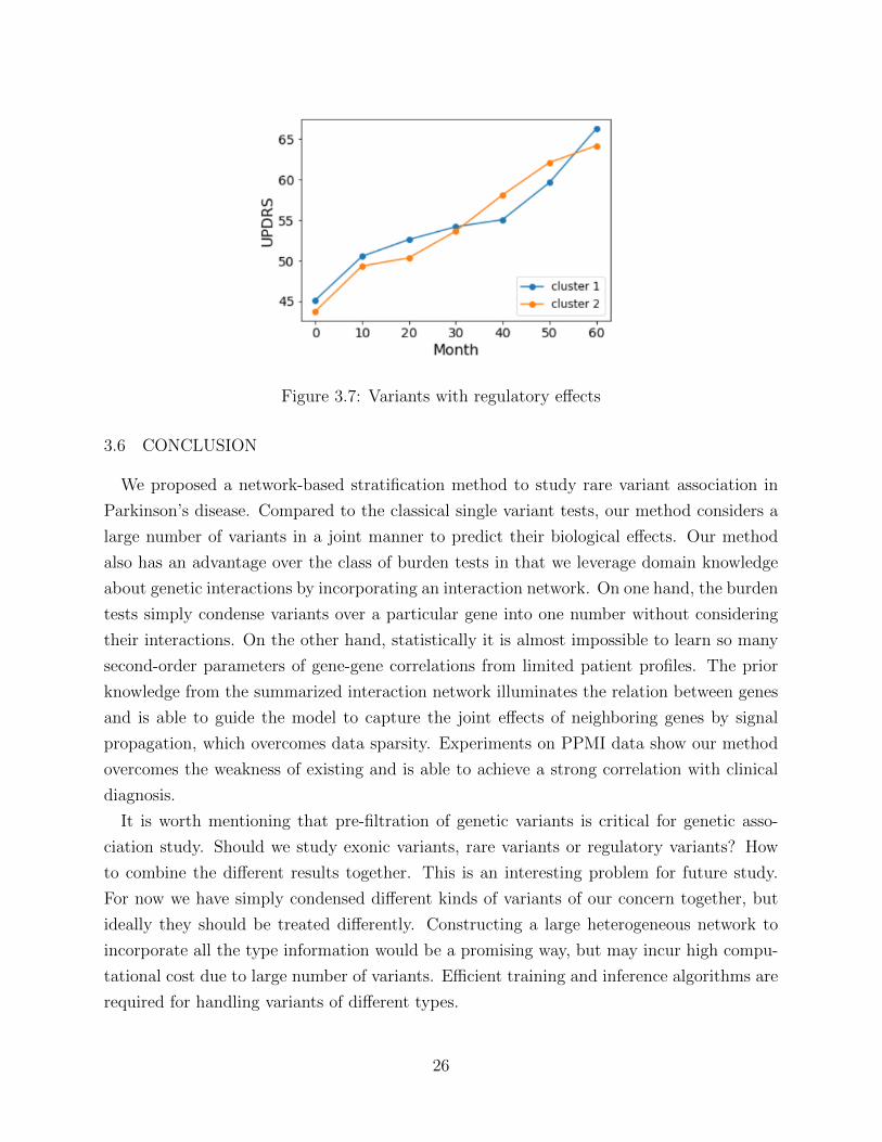
Figure 3.7: Variants with regulatory effects

3.6 CONCLUSION

We proposed a network-based stratification method to study rare variant association in

Parkinson’s disease. Compared to the classical single variant tests, our method considers a

large number of variants in a joint manner to predict their biological effects. Our method

also has an advantage over the class of burden tests in that we leverage domain knowledge

about genetic interactions by incorporating an interaction network. On one hand, the burden

tests simply condense variants over a particular gene into one number without considering

their interactions. On the other hand, statistically it is almost impossible to learn so many

second-order parameters of gene-gene correlations from limited patient profiles. The prior

knowledge from the summarized interaction network illuminates the relation between genes

and is able to guide the model to capture the joint effects of neighboring genes by signal

propagation, which overcomes data sparsity. Experiments on PPMI data show our method

overcomes the weakness of existing and is able to achieve a strong correlation with clinical

diagnosis.

It is worth mentioning that pre-filtration of genetic variants is critical for genetic asso-

ciation study. Should we study exonic variants, rare variants or regulatory variants? How

to combine the different results together. This is an interesting problem for future study.

For now we have simply condensed different kinds of variants of our concern together, but

ideally they should be treated differently. Constructing a large heterogeneous network to

incorporate all the type information would be a promising way, but may incur high compu-

tational cost due to large number of variants. Efficient training and inference algorithms are

required for handling variants of different types.

26

We also hope to extend the NBS framework to supervised settings and perform pathway

detection to discover important genes for Parkinson’s disease that are previously unknown.

There have been works on plant genome-wide association studies using multiple linear re-

gressions. See [24] and [25]. Nevertheless, human genomics is more complicated than plants.

It is important to study how to deal with the correlations between large number of variants

of different types.

27

REFERENCES

[1] T. M. Therneau and P. M. Grambsch, Modeling survival data: extending the Cox model.Springer Science & Business Media, 2013.

[2] H. Binder, “Coxboost: Cox models by likelihood based boosting for a single survivalendpoint or competing risks,” R package version, vol. 1, 2013.

[3] T. Ching, X. Zhu, and L. X. Garmire, “Cox-nnet: An artificial neural network methodfor prognosis prediction of high-throughput omics data,” PLoS computational biology,vol. 14, no. 4, p. e1006076, 2018.

[4] H. Ishwaran, U. B. Kogalur, E. H. Blackstone, M. S. Lauer et al., “Random survivalforests,” The annals of applied statistics, vol. 2, no. 3, pp. 841–860, 2008.

[5] W. Hamilton, Z. Ying, and J. Leskovec, “Inductive representation learning on largegraphs,” in Advances in Neural Information Processing Systems, 2017, pp. 1024–1034.

[6] J. Gilmer, S. S. Schoenholz, P. F. Riley, O. Vinyals, and G. E. Dahl, “Neural messagepassing for quantum chemistry,” arXiv preprint arXiv:1704.01212, 2017.

[7] T. N. Kipf and M. Welling, “Semi-supervised classification with graph convolutionalnetworks,” arXiv preprint arXiv:1609.02907, 2016.

[8] Y. Li, D. Tarlow, M. Brockschmidt, and R. Zemel, “Gated graph sequence neuralnetworks,” arXiv preprint arXiv:1511.05493, 2015.

[9] P. Velickovic, G. Cucurull, A. Casanova, A. Romero, P. Lio, and Y. Bengio, “Graphattention networks,” arXiv preprint arXiv:1710.10903, vol. 1, no. 2, 2017.

[10] Z. Ying, J. You, C. Morris, X. Ren, W. Hamilton, and J. Leskovec, “Hierarchical graphrepresentation learning with differentiable pooling,” in Advances in Neural InformationProcessing Systems, 2018, pp. 4801–4811.

[11] M. Defferrard, X. Bresson, and P. Vandergheynst, “Convolutional neural net-works on graphs with fast localized spectral filtering,” in Advances in NeuralInformation Processing Systems 29: Annual Conference on Neural InformationProcessing Systems 2016, December 5-10, 2016, Barcelona, Spain, D. D. Lee,M. Sugiyama, U. von Luxburg, I. Guyon, and R. Garnett, Eds., 2016. [Online].Available: http://papers.nips.cc/paper/6081-convolutional-neural-networks-on-graphs-with-fast-localized-spectral-filtering pp. 3837–3845.

[12] S. Rhee, S. Seo, and S. Kim, “Hybrid approach of relation network and localized graphconvolutional filtering for breast cancer subtype classification,” in Proceedings of theTwenty-Seventh International Joint Conference on Artificial Intelligence, IJCAI 2018,July 13-19, 2018, Stockholm, Sweden, J. Lang, Ed. ijcai.org, 2018. [Online]. Available:https://doi.org/10.24963/ijcai.2018/490 pp. 3527–3534.

28

[13] D. Szklarczyk, A. Franceschini, S. Wyder, K. Forslund, D. Heller, J. Huerta-Cepas,M. Simonovic, A. Roth, A. Santos, K. P. Tsafou et al., “String v10: protein–proteininteraction networks, integrated over the tree of life,” Nucleic acids research, vol. 43,no. D1, pp. D447–D452, 2014.

[14] S. Lee, G. R. Abecasis, M. Boehnke, and X. Lin, “Rare-variant association analysis:study designs and statistical tests,” The American Journal of Human Genetics, vol. 95,no. 1, pp. 5–23, 2014.

[15] S. Morgenthaler and W. G. Thilly, “A strategy to discover genes that carry multi-allelicor mono-allelic risk for common diseases: a cohort allelic sums test (cast),” MutationResearch/Fundamental and Molecular Mechanisms of Mutagenesis, vol. 615, no. 1-2,pp. 28–56, 2007.

[16] M. C. Wu, S. Lee, T. Cai, Y. Li, M. Boehnke, and X. Lin, “Rare-variant associationtesting for sequencing data with the sequence kernel association test,” The AmericanJournal of Human Genetics, vol. 89, no. 1, pp. 82–93, 2011.

[17] S. Lee, M. J. Emond, M. J. Bamshad, K. C. Barnes, M. J. Rieder, D. A. Nickerson,E. L. P. Team, D. C. Christiani, M. M. Wurfel, X. Lin et al., “Optimal unified approachfor rare-variant association testing with application to small-sample case-control whole-exome sequencing studies,” The American Journal of Human Genetics, vol. 91, no. 2,pp. 224–237, 2012.

[18] M. Hofree, J. P. Shen, H. Carter, A. Gross, and T. Ideker, “Network-based stratificationof tumor mutations,” Nature methods, vol. 10, no. 11, p. 1108, 2013.

[19] S. Wang, J. Ma, W. Zhang, J. P. Shen, J. Huang, J. Peng, and T. Ideker, “Typingtumors using pathways selected by somatic evolution,” Nature communications, vol. 9,no. 1, p. 4159, 2018.

[20] K. J. Karczewski, L. C. Francioli, G. Tiao, B. B. Cummings, J. Alfoldi, Q. Wang, R. L.Collins, K. M. Laricchia, A. Ganna, D. P. Birnbaum et al., “Variation across 141,456human exomes and genomes reveals the spectrum of loss-of-function intolerance acrosshuman protein-coding genes,” BioRxiv, p. 531210, 2019.

[21] P. Rentzsch, D. Witten, G. M. Cooper, J. Shendure, and M. Kircher, “Cadd: predictingthe deleteriousness of variants throughout the human genome,” Nucleic acids research,vol. 47, no. D1, pp. D886–D894, 2018.

[22] W. McLaren, L. Gil, S. E. Hunt, H. S. Riat, G. R. Ritchie, A. Thormann, P. Flicek,and F. Cunningham, “The ensembl variant effect predictor,” Genome biology, vol. 17,no. 1, p. 122, 2016.

[23] K. Wang, M. Li, and H. Hakonarson, “Annovar: functional annotation of genetic vari-ants from high-throughput sequencing data,” Nucleic acids research, vol. 38, no. 16, pp.e164–e164, 2010.

29

[24] X. Zhou and M. Stephens, “Efficient multivariate linear mixed model algorithms forgenome-wide association studies,” Nature methods, vol. 11, no. 4, p. 407, 2014.

[25] N. A. Furlotte and E. Eskin, “Efficient multiple-trait association and estimation ofgenetic correlation using the matrix-variate linear mixed model,” Genetics, vol. 200,no. 1, pp. 59–68, 2015.

30