c alibration and v erification of s …streamnologies.com/support/pdfs/calibration.pdfc alibration...

1 Singhofen & Associates, Inc. 6961 University Blvd., Winter Park, FL 32792 . E-mail: [email protected]

CALIBRATION AND VERIFICATIONOF STORMWATER MODELS

By Peter J. Singhofen, P.E.1

ABSTRACT: Although calibration and verification have long been recognized as importantconsiderations in the use and application of stormwater models, the process can be quite complexand daunting, involving a seemingly infinite number of combinations and permutations ofparameters that directly affect the behavior of a model. The process is further complicated asattempts are made to evaluate the effectiveness of altering certain parameters. For example, if arunoff curve number is increased such that a simulated peak stage more closely matches arecorded high water mark, does that necessarily imply that the model is predicting reality moreclosely? The purpose of this paper is to examine the sensitivity of several modeling parametersduring the calibration process and how changes to those parameters affect stage hydrographs. TheIntegral Square Error (ISE) is used as a tool to evaluate the effectiveness of model alterations onthe entire stage hydrograph rather than simply evaluating peak stages or peak flow rates. Anurbanized watershed (the Central Drainage Ditch Basin) located within the corporate limits of theCity of Tallahassee is used as an example. An approximate 10-year 24-hour storm that occurred inMarch 1994 is used for calibration purposes. Three other significant storms that also occurred in1994 are used for verification purposes.

INTRODUCTION

The calibration of a stormwater model typicallyinvolves comparing simulated stages, flows and/orvolumes of water with observed data for a recent andsignificant storm event. Depending on the outcome ofthe comparison, certain model parameters are adjustedsuch that the predicted values more closely matchhistorical values until a "best fit" is achieved. Theprocess is typically iterative and each subsequentadjustment depends on the outcome of the previousiteration. It can be a tedious, complicated and oftenfrustrating ordeal especially when the historical data areinadequate or of poor quality. The process is furthercomplicated as the modeling professional attempts tointerpret and evaluate the effectiveness of eachcombination and permutation.

Once a final set of modeling parameters has beenselected (i.e., the model has been calibrated), it isimportant to examine the ability of the model to predictother storm events with the same degree of reliability asthe calibrated model. This is accomplished bysimulating two or three other historical storm eventsthat occurred in the same watershed prior to significantalterations in the basin such as major land use changesor drainage improvements. Preferably, the verificationstorms should vary from the calibration storm in bothmagnitude and duration, but they should be longenough and large enough to impact all points in thewatershed under consideration. For example, if it has

been determined that the travel time in a particularwatershed from the most extreme point to its outlet is 3hours, then perhaps storms of 3-hour duration or greatershould be considered for verification purposes.Engineering judgement must be used in the selection ofcalibration and verification storms.

Stormwater models, especially hydrodynamicmodels, are quite complex and typically involvethousands of individual data elements and hundreds ofjudgement calls by the modeling professional. Each ofthese can and often are questioned. Whether justified ornot, if the model has not been demonstrated to predictactual occurrences with some degree of reliability, itwill be subject to criticism and difficult to defend.Therefore, the importance of calibration and subsequentverification cannot be overstated.

Successful calibration requires two key elements.First, an accurate and reliable historical record of bothrainfall and stream data (stage and/or flow data) for thestudy area must be available. Continuous recorders arepreferred although high water marks will suffice ifother records are unavailable. Second, accurate inputdata for the model including land use and drainageinfrastructure consistent with the time period to be usedfor calibration and verification purposes must becompiled. It makes little sense to use a storm event thatoccurred in 1960 for calibration of a model preparedbased on conditions in 2001.

-2-

Calibration and Verification of Stormwater Models by Peter J. Singhofen, P.E.Florida Association of Stormwater Utilities 2001 Annual Conference, June 20-22, 2001

The purpose of this paper is to examine thesensitivity of several modeling parameters during thecalibration process and how changes to thoseparameters affect stage hydrographs. These parametersinclude the peak rate factor (K'), runoff curve numbers,and roughness coefficients along the channels. TheIntegral Square Error (ISE) is used as a tool to evaluatethe effectiveness of model alterations on the entire stagehydrograph rather than simply evaluating peak stages orpeak flow rates. A 6-square mile urbanized watershed(the Central Drainage Ditch Basin) located within thecorporate limits of the City of Tallahassee is used as anexample. Five continuous rain gage recorders (5-minuteintervals) are located within this basin as well as fourcontinuous stream gage recorders (also 5-minuteintervals).

HISTORICAL DATA

The City of Tallahassee, Leon County and theNorthwest Florida Water Management District enteredinto a tri-party agreement several years ago to jointlyfund and monitor a comprehensive network of rain andstream gages. This monitoring program is intended tocollect dry weather and storm event discharge data atmajor outfall locations in Leon County and the City ofTallahassee and is in partial fulfillment of requirementsset forth by the USEPA National Pollutant DischargeElimination System (NPDES). Continuous records ofprecipitation and stages are maintained to aid inestimating flows, volumes and annual pollutant loads.The data is also used to update hydologic and floodingconditions as growth and development occurs. The tri-party agreement encompasses a total of 31 recordingstations including 16 stream gages that monitor stageand velocity, 3 stream gages that monitor only stage,and 12 rainfall gages. The FY2000 cost for maintainingthese 31 stations was $71,286 and equally shared by theCity of Tallahassee and Leon County. An equivalentamount of "inkind" services was provided by theNorthwest Florida Water Management District.

In addition to the stations described above, the Cityof Tallahassee maintains 6 other rain gages and 4-10stream gages. The actual number of stream gages at anypoint in time varies. They are installed and/or removeddepending on specific capital improvement projects.Approximately 25% of a technician's time is dedicatedto maintaining these stations.

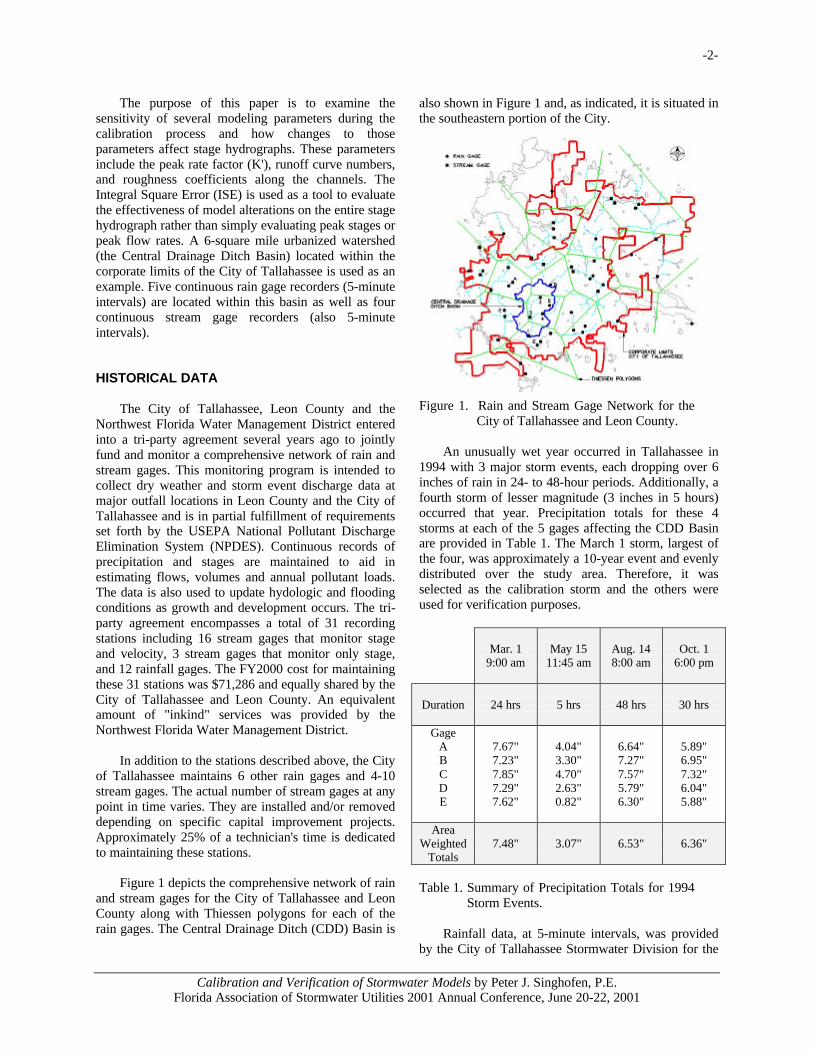
Figure 1 depicts the comprehensive network of rainand stream gages for the City of Tallahassee and LeonCounty along with Thiessen polygons for each of therain gages. The Central Drainage Ditch (CDD) Basin is

also shown in Figure 1 and, as indicated, it is situated inthe southeastern portion of the City.

Figure 1. Rain and Stream Gage Network for theCity of Tallahassee and Leon County.

An unusually wet year occurred in Tallahassee in1994 with 3 major storm events, each dropping over 6inches of rain in 24- to 48-hour periods. Additionally, afourth storm of lesser magnitude (3 inches in 5 hours)occurred that year. Precipitation totals for these 4storms at each of the 5 gages affecting the CDD Basinare provided in Table 1. The March 1 storm, largest ofthe four, was approximately a 10-year event and evenlydistributed over the study area. Therefore, it wasselected as the calibration storm and the others wereused for verification purposes.

Mar. 19:00 am

May 1511:45 am

Aug. 148:00 am

Oct. 16:00 pm

Duration 24 hrs 5 hrs 48 hrs 30 hrs

GageABCDE

7.67"7.23"7.85"7.29"7.62"

4.04"3.30"4.70"2.63"0.82"

6.64"7.27"7.57"5.79"6.30"

5.89"6.95"7.32"6.04"5.88"

AreaWeighted

Totals7.48" 3.07" 6.53" 6.36"

Table 1. Summary of Precipitation Totals for 1994Storm Events.

Rainfall data, at 5-minute intervals, was providedby the City of Tallahassee Stormwater Division for the

-3-


4 storms and 5 rain gages listed in Table 1. As shown inFigure 2, individual Thiessen polygons for each raingage cover only a portion of the CDD Basin. In aneffort to more accurately account for the non-uniformdistribution of rainfall in the study area, rainfall data forindividual sub-basins was assigned based on theThiessen polygon encompassing the sub-basin. Table 2provides a breakdown of the total area served by eachof the 5 rain gages in or near the CDD Basin.

Figure 1. Thiessen Polygons and Stream GageLocations in the CDD Basin.

RainGage

Area(ac)

% ofTotal

ABCDE

573.3 590.4 650.61,416.8 504.7

15.3415.8017.4237.9313.51

Totals 3,735.8 100.00

Table 2. Areas Served by Rain Gages.

In addition to the 5 rain gages, 4 stream gagesdesignated 1, 2, 3 and 4 are located in the CDD Basin(refer to Figure 2). Three of these are located along theCDD and the fourth is on a tributary to the CDD. Gages1, 2 and 3 are located at the lower end, near themidpoint and at the upper end of the CDD, respectively.These 3 gages were used for calibration purposes while

gage 4 was used as a boundary condition for the model.Flow records were obtained from the City ofTallahassee Stormwater Division for gage 4 andspecified as inflow hydrographs for the stormwatermodel.

STORMWATER MODEL

A comprehensive hydrologic and hydrauliccomputer model was prepared for the CDD Basin tosimulate the rainfall-runoff process. Specifically, theInterconnected Channel and Pond Routing Model(ICPR v2.20) was used for all stormwater modelingpurposes. This model has been accepted by the FederalEmergency Management Agency (FEMA) for use onflood plain investigations associated with floodinsurance applications and it is widely used throughoutFlorida and the United States. ICPR is distributed byStreamline Technologies, Inc. Information can be foundat www.streamnologies.com.

The Soil Conservation Service (SCS) unithydrograph method was used for all sub-basins in theCDD system. This method requires drainage areas, SCScurve numbers, and times of concentration for eachsub-basin. Additionally, estimates of directly connectedimpervious areas (DCIA's) were included in thehydrologic analysis. A total of 80 individual sub-basinswere delineated from 1”=200’ scale aerial topographicmaps (2-foot contour intervals) provided by the City ofTallahassee. These boundaries were refined based onfield inspections, a literature review and discussionswith city staff. Existing land use was determined fromaerial photographs taken within a few years of thecalibration and verification storms. Soils informationwas obtained from the Leon County Soil Surveyprepared by the USDA Soil Conservation Service (nowthe Natural Resource Conservation Service).

Table 3 includes each of the land use typesencountered in the study area along with their assumedpercentage of directly connected impervious areas(DCIA) and the runoff curve number for the remainingnon-DCIA based on normal antecedent moistureconditions. Since one of the calibration parameters isthe runoff curve number for non-dcia's, adjustments tocurve numbers based on antecedent moisture conditionsare provided in Table 4.

The CDD system was discretized into 93 nodes and147 links. Nodes are discrete locations within thewatershed used to define inflow points, boundaryconditions, storage areas, changes in channel slope orgeometry, or any other points of interest. Runoffhydrographs are loaded at individual nodes in the

-4-


system and ICPR computes water surface elevations ateach node in the model. Links are used to connectnodes together and include pipes, channels, weirs, dropstructures, bridges, dam breaches, and rating curves.ICPR calculates flows for each link based on watersurface elevations at its connecting nodes. Hydraulicdata requirements for the ICPR model include twogeneral types: (1) node data (e.g., location, pond storageor channel overbank storage, initial stages, boundaryconditions, etc.); and, (2) link data (e.g., pipe geometry,channel cross-section, weir invert information, etc.).

Two types of boundary conditions are used for theCDD model. The first is a stage-time relationship at thedownstream-most node in the model located belowstream gage #1. Stage-time relationships for each of the4 historical storms were provided by the City ofTallahassee Stormwater Division. The second boundarycondition is a time-discharge relationship located at theupper end of the eastern tributary to the CDD nearstream gage #2. Discharge hydrographs based onhistorical gaging data at this location for the 4 stormswere also provided by the City of TallahasseeStormwater Division.

Extensive field surveys of the CDD were obtainedin the summer and fall of 1997. These included detailedstructure geometry for 9 bridges and associatedroadway profiles, and cross section data forapproximately 17 channel locations. The top-of-bank,toe of slope, channel flow line, water surface elevation,and any other pertinent topographic breaks werecollected for each cross section. Construction levelsurveys were also performed for approximately 3,700feet of the CDD.

CALIBRATION PARAMETERS

As previously stated, three primary parameterswere varied during the calibration process of the CDDmodel: (1) the peak rate factor (K'); (2) curve numbers;and, (3) channel roughness characteristics. The peakrate factor is used in conjunction with the unithydrograph method to alter the shape and timing of thedischarge hydrograph for individual drainage sub-basins. As the peak rate factor increases, the rising andfalling legs of the runoff hydrograph become steeperand the peak rate of runoff increases, in effect, reducingstorage in the sub-basin. As the peak rate factordecreases, peak flow rates decrease and the volume ofrunoff is attenuated or pushed farther out in time, thusincreasing storage in the sub-basin. Adjusting the peak

rate factor alters the overall shape of the dischargehydrograph and when combined with other sub-basinhydrographs, can affect timing and peak flow rates indrainage conveyance systems such as the CDD. Peakrate factors of 256, 323 and 484 were evaluated.

ICPR assumes an initial abstraction of 0.1" overdirectly connected impervious areas (DCIA's) and then100% of the rainfall (beyond 0.1") falling on the DCIAappears as runoff. Consequently, use of DCIA's in theCDD model accounts for runoff almost immediatelyafter rainfall commences. This technique is appropriatefor highly urbanized areas similar to the CDD Basin.

Land UseNumber Land Use

Description

%IMP

%DCIA

Curve Number for Non-DCIA1

A B C D110 SF Res. (1/2-1 ac) 25 15 44.9 64.7 76.4 81.8

120 SF Res. (1/4 ac) 38 22 47.9 66.6 77.6 82.7

130 SF Res. (<=1/6 ac) 60 38 54.3 70.6 80.2 84.7

133 Multi-Family 71 57 47.3 66.2 77.4 82.5

140 Comm. (<30% open) 85 68 49.0 67.3 78.1 83.1

147 Comm. (>30% open) 70 57 47.3 66.2 77.4 82.5

150 Industrial 70 57 47.3 66.2 77.4 82.5

170 Institutional 85 68 49.0 67.3 78.1 83.1

182 Golf Course 25 25 53.2 69.9 79.8 84.3

183 Race Tracks 0 0 49.0 69.0 79.0 84.0

185 Parks and Zoos 0 0 49.0 69.0 79.0 84.0

186 Recreational 0 0 49.0 69.0 79.0 84.0

190 Open Land 0 0 39.6 59.4 70.4 76.3

211 Improved Pasture 0 0 49.0 69.0 79.0 84.0

320 Rangeland (shrub) 0 0 35.0 56.0 70.0 77.0

400 Wooded 0 0 27.9 50.0 63.8 70.4

500 Ponds w/ Berms 95 0 98.0 98.0 98.0 98.0

620 Wetland Forest 95 0 98.0 98.0 98.0 98.0

640 Wetland Marsh 95 0 98.0 98.0 98.0 98.0

812 Railroads 63 50 37.5 55.9 68.3 74.3

814 Roads w/ C&G 100 0 96.4 96.4 96.4 96.4

816 Canals 60 60 47.5 66.6 77.6 82.7

830 Utilities 0 0 49.0 69.0 79.0 84.01 CN's based on AMC II

Table 3. DCIA and SCS Curve Numbers for Non-DCIA by Land Use

-5-


Sub-basin runoff curve numbers in ICPR representall areas that are not DCIA. Curve numbers can varyfrom 0 to 100, with a curve number of 0 producing norunoff and a curve number of 100 producing 100%runoff. However, the relationship between curvenumber and runoff is non-linear and depends on theamount of rainfall among other factors. The curvenumbers for non-DCIA's in the CDD Basin were variedduring the calibration process discussed in this paper.Three sets of curve numbers were evaluated: (1) CN'sbased on AMC II (normal conditions); (2) CN's basedon AMC I (dry conditions); and, (3) CN's based on theaverage of normal and dry conditions AMC (I+II)/2.

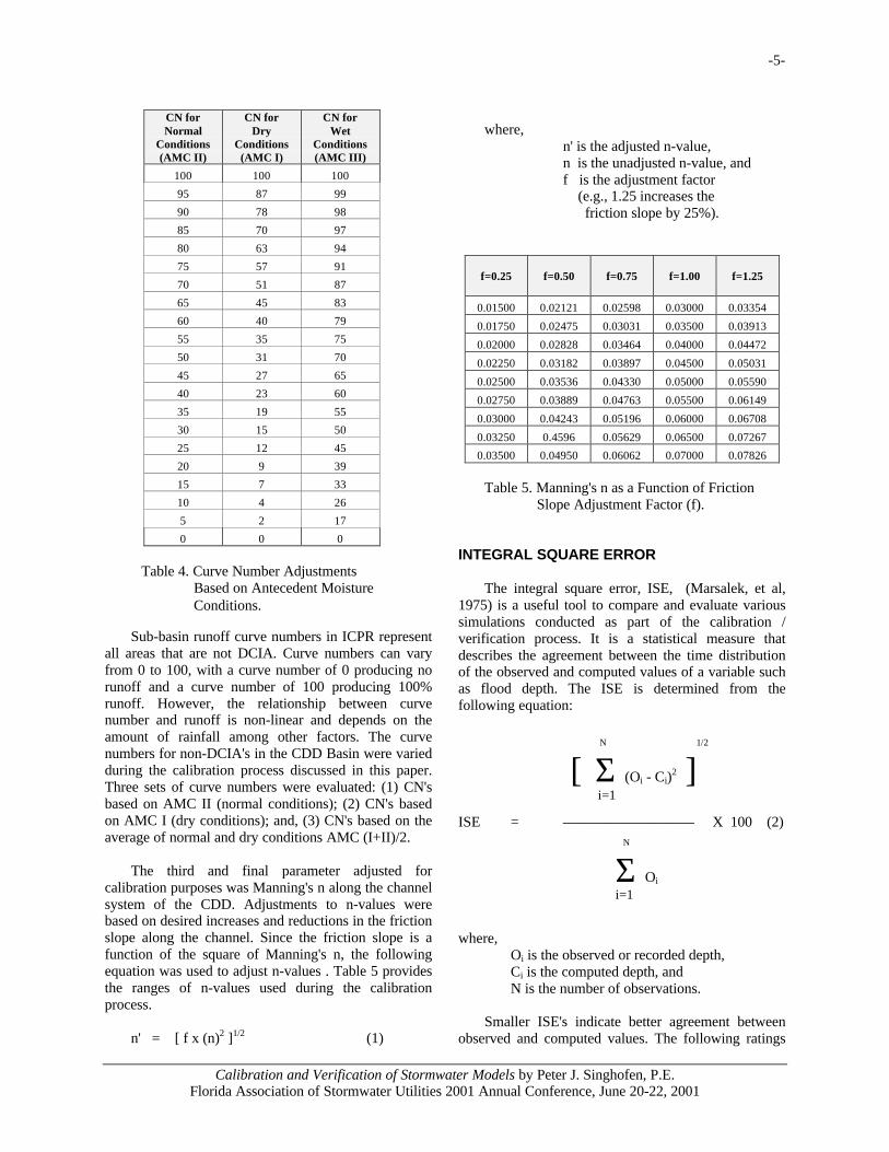
The third and final parameter adjusted forcalibration purposes was Manning's n along the channelsystem of the CDD. Adjustments to n-values werebased on desired increases and reductions in the frictionslope along the channel. Since the friction slope is afunction of the square of Manning's n, the followingequation was used to adjust n-values . Table 5 providesthe ranges of n-values used during the calibrationprocess.

n' = [ f x (n)2 ]1/2 (1)

where,n' is the adjusted n-value,n is the unadjusted n-value, andf is the adjustment factor (e.g., 1.25 increases the friction slope by 25%).

f=0.25 f=0.50 f=0.75 f=1.00 f=1.25

0.01500 0.02121 0.02598 0.03000 0.03354

0.01750 0.02475 0.03031 0.03500 0.03913

0.02000 0.02828 0.03464 0.04000 0.04472

0.02250 0.03182 0.03897 0.04500 0.05031

0.02500 0.03536 0.04330 0.05000 0.05590

0.02750 0.03889 0.04763 0.05500 0.06149

0.03000 0.04243 0.05196 0.06000 0.06708

0.03250 0.4596 0.05629 0.06500 0.07267

0.03500 0.04950 0.06062 0.07000 0.07826

Table 5. Manning's n as a Function of FrictionSlope Adjustment Factor (f).

INTEGRAL SQUARE ERROR

The integral square error, ISE, (Marsalek, et al,1975) is a useful tool to compare and evaluate varioussimulations conducted as part of the calibration /verification process. It is a statistical measure thatdescribes the agreement between the time distributionof the observed and computed values of a variable suchas flood depth. The ISE is determined from thefollowing equation:

N 1/2

[ Σ (Oi - Ci)2 ]

i=1

ISE = ————————— X 100 (2) N

Σ Oi i=1

where,Oi is the observed or recorded depth,Ci is the computed depth, andN is the number of observations.

Smaller ISE's indicate better agreement betweenobserved and computed values. The following ratings

CN forNormal

Conditions(AMC II)

CN forDry

Conditions(AMC I)

CN forWet

Conditions(AMC III)

100 100 100

95 87 99

90 78 98

85 70 97

80 63 94

75 57 91

70 51 87

65 45 83

60 40 79

55 35 75

50 31 70

45 27 65

40 23 60

35 19 55

30 15 50

25 12 45

20 9 39

15 7 33

10 4 26

5 2 17

0 0 0

Table 4. Curve Number AdjustmentsBased on Antecedent MoistureConditions.

-6-


have been recommended by Sarma, Delleur and Rao(1969):

0.0% ≤ ISE ≤ 3.0% excellent 3.0% ≤ ISE ≤ 6.0% very good 6.0% ≤ ISE ≤ 10.0% good10.0% ≤ ISE ≤ 25.0% fair25.0% ≤ ISE poor

The ISE was computed for each of the 3 gagesused for calibration purposes and for each set ofparameters that were evaluated.

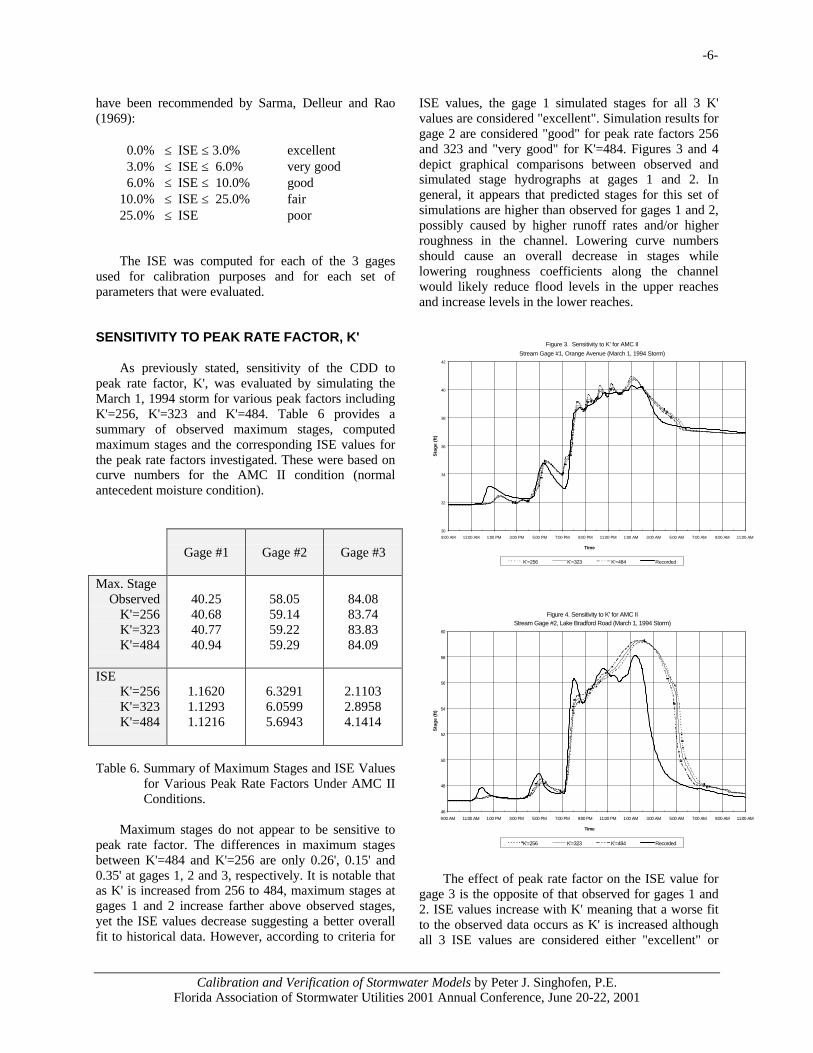
SENSITIVITY TO PEAK RATE FACTOR, K'

As previously stated, sensitivity of the CDD topeak rate factor, K', was evaluated by simulating theMarch 1, 1994 storm for various peak factors includingK'=256, K'=323 and K'=484. Table 6 provides asummary of observed maximum stages, computedmaximum stages and the corresponding ISE values forthe peak rate factors investigated. These were based oncurve numbers for the AMC II condition (normalantecedent moisture condition).

Gage #1 Gage #2 Gage #3

Max. StageObserved

K'=256K'=323K'=484

40.2540.6840.7740.94

58.0559.1459.2259.29

84.0883.7483.8384.09

ISEK'=256K'=323K'=484

1.16201.12931.1216

6.32916.05995.6943

2.11032.89584.1414

Table 6. Summary of Maximum Stages and ISE Valuesfor Various Peak Rate Factors Under AMC IIConditions.

Maximum stages do not appear to be sensitive topeak rate factor. The differences in maximum stagesbetween K'=484 and K'=256 are only 0.26', 0.15' and0.35' at gages 1, 2 and 3, respectively. It is notable thatas K' is increased from 256 to 484, maximum stages atgages 1 and 2 increase farther above observed stages,yet the ISE values decrease suggesting a better overallfit to historical data. However, according to criteria for

ISE values, the gage 1 simulated stages for all 3 K'values are considered "excellent". Simulation results forgage 2 are considered "good" for peak rate factors 256and 323 and "very good" for K'=484. Figures 3 and 4depict graphical comparisons between observed andsimulated stage hydrographs at gages 1 and 2. Ingeneral, it appears that predicted stages for this set ofsimulations are higher than observed for gages 1 and 2,possibly caused by higher runoff rates and/or higherroughness in the channel. Lowering curve numbersshould cause an overall decrease in stages whilelowering roughness coefficients along the channelwould likely reduce flood levels in the upper reachesand increase levels in the lower reaches.

The effect of peak rate factor on the ISE value forgage 3 is the opposite of that observed for gages 1 and2. ISE values increase with K' meaning that a worse fitto the observed data occurs as K' is increased althoughall 3 ISE values are considered either "excellent" or

Figure 3. Sensitivity to K' for AMC II

Stream Gage #1, Orange Avenue (March 1, 1994 Storm)

30

32

34

36

38

40

42

9:00 AM 11:00 AM 1:00 PM 3:00 PM 5:00 PM 7:00 PM 9:00 PM 11:00 PM 1:00 AM 3:00 AM 5:00 AM 7:00 AM 9:00 AM 11:00 AM

Time

Sta

ge

(ft)

K'=256 K'=323 K'=484 Recorded

Figure 4. Sensitivity to K' for AMC IIStream Gage #2, Lake Bradford Road (March 1, 1994 Storm)

46

48

50

52

54

56

58

60


Time

Sta

ge

(ft)

K'=256 K'=323 K'=484 Recorded

-7-


"very good". Examination of the stage hydrographs forgage 3 (see Figure 5) indicate a phase shift ofapproximately 1 hour between the simulated andobserved hydrographs. Since gage 3 is located in a largedetention pond at the headwaters of the CDD andrecieves runoff from a single drainage sub-basin, it ispossible in ICPR to "shift" the inflow hydrograph by anhour. Doing so for K'=484 reduces the ISE from 4.1414to 1.6338 significantly improving the fit. However, thepossibility of data error must be considered. It isconceivable that the reported rainfall data for thisparticular basin was shifted by an hour possibly due to apower outage. Rather than introduce a time shift at thispoint in the calibration process, the writer believes itwould be more appropriate to examine this area againafter the validation simulations are completed.

SENSITIVITY TO RUNOFF CURVE NUMBERS

As indicated in the previous section, predictedstages along the CDD generally appear higher thanobserved levels for the 3 peak rate factors examined.K'=484 seems to produce the best overall fit along theCDD according to ISE values although peak stages aremore than 1 foot higher than observed maximums atgage 2. Therefore, it seems appropriate to reduce therunoff volume (i.e., reduce runoff curve numbers) andhold the peak rate factor to K'=484. In an effort tomethodically reduce the runoff curve numbers, Table 4was used as a guide. In addition to the AMC IIconditions evaluated in the previous section, AMC Iand AMC (I+II)/2 were added to the calibration set.

Table 7 provides a summary of the results of thisanalysis. Maximum stages at each of the 3 gages havenow been "bracketed" meaning there are sets ofcalibration parameters that predict maximum stages

above and below the observed peak flood levels. This isimportant because it narrows the search for anacceptable set of modeling parameters. Likewise, theISE values are considered "very good" to "excellent" inall cases. Based on the 3 scenarios evaluated, the AMC(I+II)/2 with a K'=484 appears to be the "best fit"overall because in addition to the more than acceptableISE values, simulated peak stages for the 3 gages arewithin 6 inches of observed levels. This places thecomputed maximum depths at all 3 gages less than 4%different from observed maximum depths.


Max. StageObserved

AMC IAMC (I+II)/2

AMC II

40.2540.1340.5140.94

58.0557.2558.4959.29

84.0883.5483.8184.09

ISEAMC I

AMC (I+II)/2AMC II

1.11791.02401.1216

4.62965.32215.6943

4.51084.08084.1414

Table 7. Summary of Maximum Stages and ISE Valuesfor Various AMC's with K'=484.

The model appears to be more sensitive to curvenumbers than peak rate factor, especially at gage 2.Gage 2 is located approximately midway along theCDD and upstream of a major highway crossing withlarge box culverts. There are numerous otherimpediments to flow immediately downstream of thegage including two 30-inch aerial sewer crossings, arailroad crossing, a roadway bridge crossing andsandwiched between all of these is a confluence with amajor tributary system to the east. All of these combineto create complex hydraulic and tailwater influences ongage 2.

Figures 6 and 7 depict observed and simulatedstage hydrographs at gages 1 and 2. Visually, AMC(I+II)/2 appears to fit better at gage 1 and this issupported by the lower ISE value. Although AMC(I+II)/2 fits better for gage 2 on the rising leg and alongthe peaks, it tends to lag the observed hydrograph onthe recession limb. Figure 8 shows the observed andsimulated stage hydrographs for gage 3.

Figure 5. Sensitivity to K' for AMC IIStream Gage #3, Frenchtown Pond (March 1, 1994 Storm)

75

76

77

78

79

80

81

82

83

84

85


Time

Sta

ge

(ft)

K'=256 K'=323 K'=484 Recorded

-8-


Figure 7. Sensitivity to AMC for K'=484Stream Gage #2, Lake Bradford Road (March 1, 1994 Storm)

46

48

50

52

54

56

58

60


Time

Sta

ge

(ft)

AMC I AMC (I+II)/2 AMC II Recorded

Figure 8. Sensitivity to AMC for K'=484Stream Gage #3, Frenchtown Pond (March 1, 1994 Storm)

75

76

77

78

79

80

81

82

83

84

85


Time

Sta

ge

(ft)


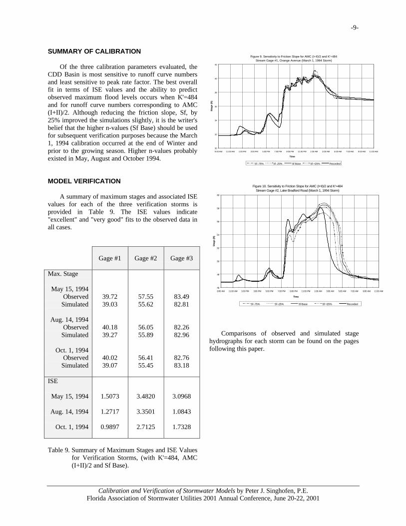
SENSITIVITY TO FRICTION SLOPE

As indicated in Table 8, altering the friction slope,Sf, has no impact on gage 3 because it is locatedupstream in a detention beyond the influence of thesechanges. Maximum flood levels at gage 1 vary onlyslightly, increasing as the friction slope is decreasedand decreasing as the friction slope is increased. Thisseems to be opposite of what one might expect, but itmust be remembered that this gage is located at thedownstream end of the CDD. By decreasing the frictionslope (i.e., reducing Manning's n) water is moved moreefficiently from the upper portion of the basin to thelower portion, thereby increasing flow stagesdownstream.

The impact at gage 2 is a little more significantthan gage 1, but relatively minor overall. Increasing thefriction by 25% above the base values causes only a0.29' difference in maximum stages or about a 2.6%difference in flood depths. Reducing the friction slopeby 25% lowers the maximum water level by 0.33' or2.9%.

Examination of the ISE values indicate an"excellent" fit for gage 1 and "very good" fits for gages2 and 3 in all cases. Stage hydrographs for gages 1 and2 are depicted in Figures 9 and 10, respectively. Figure10 includes a scenario for reduction of the friction slopeby 75%. Although this is a little drastic, it indicates thatmaximum stages are pulled down too far at gage 2 andthat stormwater is probably moved too efficientlydownstream.


Max. StageObserved

Sf -25%Sf Base

Sf +25%

40.2540.7140.5140.43

58.0558.1658.4958.78

84.0883.8183.8183.81

ISESf -25%Sf Base

Sf +25%

1.01801.02401.0481

4.90415.32215.5868

4.08084.08084.0808

Table 8. Summary of Maximum Stages and ISE Valuesfor Various Adjustments to the Friction Slope,Sf, with K'=484 and AMC (I+II)/2.

Figure 6. Sensitivity to AMC for K'=484Stream Gage #1, Orange Avenue (March 1, 1994 Storm)

30

32

34

36

38

40

42


Time

Sta

ge

(ft)


-9-


Figure 9. Sensitivity to Friction Slope for AMC (I+II)/2 and K'=484Stream Gage #1, Orange Avenue (March 1, 1994 Storm)

30

32

34

36

38

40

42


Time

Sta

ge

(ft)

Sf -75% Sf -25% Sf Base Sf +25% Recorded

Figure 10. Sensitivity to Friction Slope for AMC (I+II)/2 and K'=484Stream Gage #2, Lake Bradford Road (March 1, 1994 Storm)

46

48

50

52

54

56

58

60


Time

Sta

ge

(ft)

Sf -75% Sf -25% Sf Base Sf +25% Recorded

SUMMARY OF CALIBRATION

Of the three calibration parameters evaluated, theCDD Basin is most sensitive to runoff curve numbersand least sensitive to peak rate factor. The best overallfit in terms of ISE values and the ability to predictobserved maximum flood levels occurs when K'=484and for runoff curve numbers corresponding to AMC(I+II)/2. Although reducing the friction slope, Sf, by25% improved the simulations slightly, it is the writer'sbelief that the higher n-values (Sf Base) should be usedfor subsequent verification purposes because the March1, 1994 calibration occurred at the end of Winter andprior to the growing season. Higher n-values probablyexisted in May, August and October 1994.

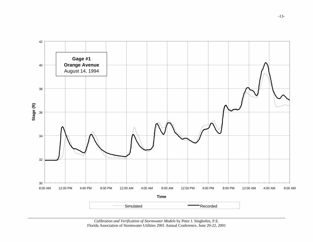
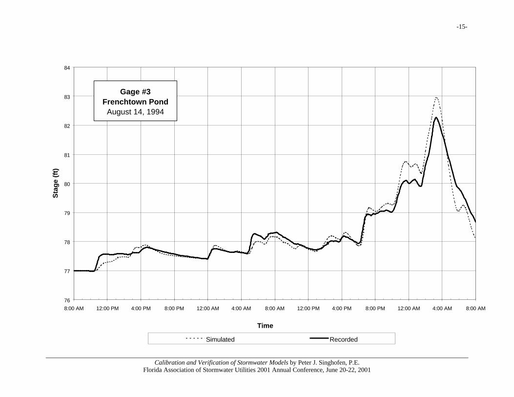
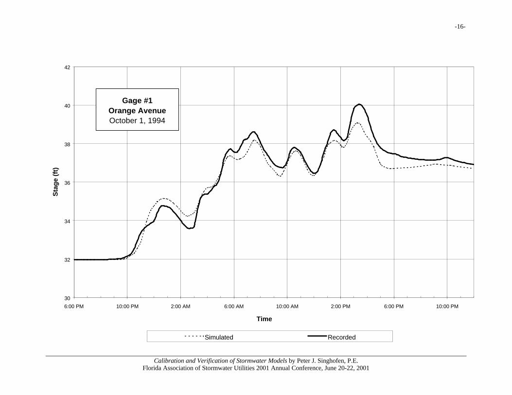
MODEL VERIFICATION

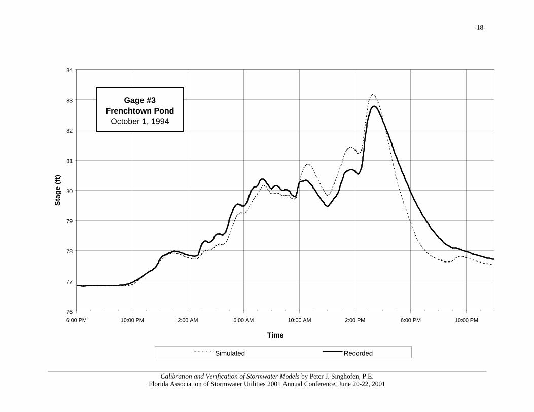
A summary of maximum stages and associated ISEvalues for each of the three verification storms isprovided in Table 9. The ISE values indicate"excellent" and "very good" fits to the observed data inall cases.


Max. Stage

May 15, 1994Observed

Simulated

Aug. 14, 1994Observed

Simulated

Oct. 1, 1994Observed

Simulated

39.7239.03

40.1839.27

40.0239.07

57.5555.62

56.0555.89

56.4155.45

83.4982.81

82.2682.96

82.7683.18

ISE

May 15, 1994

Aug. 14, 1994

Oct. 1, 1994

1.5073

1.2717

0.9897

3.4820

3.3501

2.7125

3.0968

1.0843

1.7328

Table 9. Summary of Maximum Stages and ISE Valuesfor Verification Storms, (with K'=484, AMC(I+II)/2 and Sf Base).

Comparisons of observed and simulated stagehydrographs for each storm can be found on the pagesfollowing this paper.

1 Singhofen & Associates, Inc. 6961 University Blvd., Winter Park, FL 32792 . E-mail: [email protected]

30

32

34

36

38

40

42

11:45 AM 12:45 PM 1:45 PM 2:45 PM 3:45 PM 4:45 PM 5:45 PM 6:45 PM 7:45 PM 8:45 PM 9:45 PM

Time

Sta

ge

(ft)

Simulated Recorded

Gage #1, Orange Avenue

May 15, 1994

-11-


45

47

49

51

53

55

57

59


Time

Sta

ge

(ft)

Simulated Recorded

Gage #2, Lake Bradford Road

May 15, 1994

-12-


75

76

77

78

79

80

81

82

83

84

85


Time

Sta

ge

(ft)

Simulated Recorded

Gage #3,Frenchtown Pond

May 15, 1994

-13-


30

32

34

36

38

40

42

8:00 AM 12:00 PM 4:00 PM 8:00 PM 12:00 AM 4:00 AM 8:00 AM 12:00 PM 4:00 PM 8:00 PM 12:00 AM 4:00 AM 8:00 AM

Time

Sta

ge

(ft)

Simulated Recorded

Gage #1Orange AvenueAugust 14, 1994

-14-


45

47

49

51

53

55

57

8:00 AM 12:00 PM 4:00 PM 8:00 PM 11:59 PM 3:59 AM 7:59 AM 11:59 AM 3:59 PM 7:59 PM 11:59 PM 3:59 AM 7:59 AM

Time

Sta

ge

(ft)

Simulated Recorded

Gage #2Lake Bradford Road

August 14, 1994

-15-


76

77

78

79

80

81

82

83

84

8:00 AM 12:00 PM 4:00 PM 8:00 PM 12:00 AM 4:00 AM 8:00 AM 12:00 PM 4:00 PM 8:00 PM 12:00 AM 4:00 AM 8:00 AM

Time

Sta

ge

(ft)

Simulated Recorded

Gage #3Frenchtown Pond

August 14, 1994

-16-


30

32

34

36

38

40

42

6:00 PM 10:00 PM 2:00 AM 6:00 AM 10:00 AM 2:00 PM 6:00 PM 10:00 PM

Time

Sta

ge

(ft)

Simulated Recorded

Gage #1Orange AvenueOctober 1, 1994

-17-


45

47

49

51

53

55

57


Time

Sta

ge

(ft)

Simulated Recorded

Gage #2Lake Bradford Road

October 1, 1994

-18-


76

77

78

79

80

81

82

83

84


Time

Sta

ge

(ft)

Simulated Recorded

Gage #3Frenchtown Pond

October 1, 1994

c alibration and v erification of s …streamnologies.com/support/pdfs/calibration.pdfc alibration...

Documents