c copyright 2011 haibing lu all rights reserved
TRANSCRIPT

c© Copyright 2011
Haibing Lu
All Rights Reserved

BOOLEAN MATRIX DECOMPOSITION AND EXTENSIONWITH APPLICATIONS
byHaibing Lu
A dissertation submitted to theGraduate school-Newark
Rutgers, The State University of New Jerseyin partial fulfillment of the requirements
for the degree ofDoctor of Philosophy
Graduate Program in ManagementInformation Technology Major
Written under the direction ofDr. Vijayalakshmi Atluri
Dr. Jaideep Vaidyaand approved by
Newark, New JerseyOctober 2011

DISSERTATION ABSTRACT
BOOLEAN MATRIX DECOMPOSITION AND EXTENSIONWITH APPLICATIONS
By Haibing Lu
Dissertation Directors: Dr. Vijayalakshmi Atluri and Dr. Jaideep Vaidya
Boolean matrix decomposition (BMD) refers to decomposing of an input Boolean
matrix into a product of two Boolean matrices, where the firstmatrix represents a
set of meaningful concepts, and the second describes how theobserved data can
be expressed as combinations of those concepts. As opposed to standard matrix
factorization, BMD focuses on Boolean data and employs Boolean matrix prod-
uct instead of standard matrix product. The key advantage ofBMD is that BMD
solutions provide much more interpretability, which enable BMD to have wide
applications in multiple domains, including role mining, text mining, discrete pat-
tern mining, and many others.
There are three main challenges in the research of BMD. First, real applica-
tions carry varying expectations and constraints on BMD solutions, which make
the task of searching for a good BMD solution nontrivial. Second, BMD by itself
has the issue of insufficiency in modeling some real data semantics, as only the set
union operation is employed in combination. Third, BMD variants are generally
ii

NP-hard in nature, which makes practitioners reluctant to apply the BMD model
to large scale data analysis.
All of the three challenges are addressed in this dissertation. First, a unified
framework, which is based on integer linear programming, ispresented to encom-
pass all BMD variants. Such a framework allows us to directlyadopt fruitful re-
search results in the optimization field to solve our own problems. It also provides
researchers across different domains with a new perspective to view their prob-
lems and enables them to share their research results. Second, a novel extended
Boolean matrix decomposition (EBMD) model is proposed. It allows describing
an observed record as an inclusion of some concepts with an exclusion of some
other concepts. Thus EBMD is effective to meet the needs of modeling some
complex data semantics. Third, rank-one BMD is studied. Rank-one BMD is to
decompose a Boolean matrix into the product of two Boolean vectors, which can
be interpreted as a dominant pattern vector and a presence vector. By recursively
applying rank-one BMD, a Boolean matrix is partitioned intoclusters and dis-
crete patterns of the observed data are thus discovered. Rank-one BMD can serve
many functions of regular BMD, while rank-one BMD is relatively easy to solve
compared to regular BMD. In addition, efficient 2-approximation algorithms are
found for some special cases of rank-one BMD.
iii

PREFACE
Dissertation Committee Members• Dr. Nabil Adam, Rutgers University
• Dr. Vijayalakshmi Atluri, Rutgers University
• Dr. Pierangela Samarati, University of Milan
• Dr. Jaideep Vaidya, Rutgers University
• Dr. Hui Xiong, Rutgers University
iv

ACKNOWLEDGEMENTS
The writing of a dissertation for me is more like reading my autobiography. All
memories in the past five years are surfacing. Looking back atmy work, I am
deeply grateful for all helps and supports I have received throughout the course of
my doctorate study.
I would like to express my deepest gratitude to my esteemed advisors, Dr.
Vijay Atluri and Dr. Jaideep Vaidya. Without their expert guidance and help, this
dissertation would not have been possible and I would not have gone so far in
academic research.
My thanks go out to Dr. Nabil Adam, Dr. Hui Xiong, and Dr. Pierangela
Samarati for their perceptive comments on improving my dissertation work.
I also wish to thank all my friends and student-colleagues atRutgers Business
School for enriching my life and giving me joy.
Finally, I want to thank my wife and my parents who have alwayssupported
me and stood by me with their patience and encouragement. I will pay you for the
rest of my life.
Thank you all!
v

TABLE OF CONTENTS
ABSTRACT . . . . . . . . . . . . . . . . . . . . . . . . . . . . . . . . . . . . . . . . . . .. . . . . . . . . . . . . . . ii
PREFACE . . . . . . . . . . . . . . . . . . . . . . . . . . . . . . . . . . . . . . . . . . . .. . . . . . . . . . . . . . . . iv
ACKNOWLEDGEMENTS. . . . . . . . . . . . . . . . . . . . . . . . . . . . . . . . . . .. . . . . . . . . . v
CHAPTER 1. INTRODUCTION . . . . . . . . . . . . . . . . . . . . . . . . . . . . . .. . . . . . . . 1
1.1 Problem Statement . . . . . . . . . . . . . . . . . . . . . . . . . . . . . . . .. . . . . . . . . . . . 7
1.2 Research Challenges . . . . . . . . . . . . . . . . . . . . . . . . . . . . . .. . . . . . . . . . . . 11
1.3 Contributions . . . . . . . . . . . . . . . . . . . . . . . . . . . . . . . . . . .. . . . . . . . . . . . . . 13
1.4 Outline of the Dissertation . . . . . . . . . . . . . . . . . . . . . . . .. . . . . . . . . . . . . . 13
CHAPTER 2. RELATED WORK . . . . . . . . . . . . . . . . . . . . . . . . . . . . . . .. . . . . . 14
2.1 Role Engineering . . . . . . . . . . . . . . . . . . . . . . . . . . . . . . . . .. . . . . . . . . . . . 14
2.2 Text Mining . . . . . . . . . . . . . . . . . . . . . . . . . . . . . . . . . . . . . .. . . . . . . . . . . . 15
2.3 Ordinary Matrix Factorization . . . . . . . . . . . . . . . . . . . . .. . . . . . . . . . . . . . 16
2.4 Nonnegative Matrix Factorization . . . . . . . . . . . . . . . . . .. . . . . . . . . . . . . 17
2.5 Boolean Matrix Factorization . . . . . . . . . . . . . . . . . . . . . .. . . . . . . . . . . . . 17
2.6 Probabilistic Matrix Factorization . . . . . . . . . . . . . . . .. . . . . . . . . . . . . . . 18
CHAPTER 3. BACKGROUND . . . . . . . . . . . . . . . . . . . . . . . . . . . . . . . .. . . . . . . 20
3.1 Access Control . . . . . . . . . . . . . . . . . . . . . . . . . . . . . . . . . . .. . . . . . . . . . . . 20
3.2 Computational Complexity . . . . . . . . . . . . . . . . . . . . . . . . .. . . . . . . . . . . . 23
3.3 Approximation Algorithm . . . . . . . . . . . . . . . . . . . . . . . . . .. . . . . . . . . . . . 25
3.4 Mathematical Programming . . . . . . . . . . . . . . . . . . . . . . . . .. . . . . . . . . . . 27
3.5 Heuristics . . . . . . . . . . . . . . . . . . . . . . . . . . . . . . . . . . . . . .. . . . . . . . . . . . . . 29
vi

CHAPTER 4. BOOLEAN MATRIX DECOMPOSITION. . . . . . . . . . . . . . . .30
4.1 BMD Variants with Applications . . . . . . . . . . . . . . . . . . . . .. . . . . . . . . . . 30
4.1.1 Basic BMD . . . . . . . . . . . . . . . . . . . . . . . . . . . . . . . . . . . . . .. . . . . . 30
4.1.2 Cost BMD . . . . . . . . . . . . . . . . . . . . . . . . . . . . . . . . . . . . . . .. . . . . . 35
4.1.3 Approximate BMD and Its Variants . . . . . . . . . . . . . . . . . .. . . . . . 36
4.1.4 Partial BMD . . . . . . . . . . . . . . . . . . . . . . . . . . . . . . . . . . . .. . . . . . . 38
4.2 Theoretical Study . . . . . . . . . . . . . . . . . . . . . . . . . . . . . . . .. . . . . . . . . . . . . 38
4.3 Mathematical Programming Formulation . . . . . . . . . . . . . .. . . . . . . . . . . 41
4.3.1 Partial BMD . . . . . . . . . . . . . . . . . . . . . . . . . . . . . . . . . . . .. . . . . . . 42
4.3.2 Basic BMD . . . . . . . . . . . . . . . . . . . . . . . . . . . . . . . . . . . . . .. . . . . . 44
4.3.3 Approximate BMD . . . . . . . . . . . . . . . . . . . . . . . . . . . . . . . .. . . . . . 46
4.3.4 Cost BMD . . . . . . . . . . . . . . . . . . . . . . . . . . . . . . . . . . . . . . .. . . . . . 46
4.3.5 Discussion . . . . . . . . . . . . . . . . . . . . . . . . . . . . . . . . . . . .. . . . . . . . . 47
4.4 Algorithm Design for BMD Variants . . . . . . . . . . . . . . . . . . .. . . . . . . . . . 48
4.4.1 Candidate Role Set Generating . . . . . . . . . . . . . . . . . . . .. . . . . . . . 48
4.4.2 Partial BMD . . . . . . . . . . . . . . . . . . . . . . . . . . . . . . . . . . . .. . . . . . . 50
4.4.3 Basic BMD . . . . . . . . . . . . . . . . . . . . . . . . . . . . . . . . . . . . . .. . . . . . 52
4.4.4 Approximate BMD . . . . . . . . . . . . . . . . . . . . . . . . . . . . . . . .. . . . . . 54
4.4.5 Cost BMD . . . . . . . . . . . . . . . . . . . . . . . . . . . . . . . . . . . . . . .. . . . . . 54
4.5 Experimental Study . . . . . . . . . . . . . . . . . . . . . . . . . . . . . . .. . . . . . . . . . . . 55
4.5.1 Synthetic Data . . . . . . . . . . . . . . . . . . . . . . . . . . . . . . . . .. . . . . . . . . 56
4.5.2 Real Data . . . . . . . . . . . . . . . . . . . . . . . . . . . . . . . . . . . . . .. . . . . . . . 61
CHAPTER 5. EXTENDED BOOLEAN MATRIX DECOMPOSITION . . . 65
5.1 Motivation of EBMD . . . . . . . . . . . . . . . . . . . . . . . . . . . . . . . .. . . . . . . . . . 66
5.2 Extended Boolean Matrix Decomposition . . . . . . . . . . . . . .. . . . . . . . . . . 72
5.3 Semantic Role Mining Problem . . . . . . . . . . . . . . . . . . . . . . .. . . . . . . . . . 76
5.4 Theoretical Study . . . . . . . . . . . . . . . . . . . . . . . . . . . . . . . .. . . . . . . . . . . . . 80
5.5 Mathematical Programming Formulation . . . . . . . . . . . . . .. . . . . . . . . . . 88
5.6 Algorithm Design . . . . . . . . . . . . . . . . . . . . . . . . . . . . . . . . .. . . . . . . . . . . . 93
5.6.1 Partial SRM I . . . . . . . . . . . . . . . . . . . . . . . . . . . . . . . . . . .. . . . . . . 93
5.6.2 Conservative Partial SRM I . . . . . . . . . . . . . . . . . . . . . . .. . . . . . . 95
vii

5.6.3 Partial SRM II . . . . . . . . . . . . . . . . . . . . . . . . . . . . . . . . . .. . . . . . . . 96
5.6.4 Conservative Partial SRM II . . . . . . . . . . . . . . . . . . . . . .. . . . . . . . 99
5.7 Experimental Study . . . . . . . . . . . . . . . . . . . . . . . . . . . . . . .. . . . . . . . . . . . 99
5.7.1 Synthetic Data . . . . . . . . . . . . . . . . . . . . . . . . . . . . . . . . .. . . . . . . . . 100
5.7.2 Real Data . . . . . . . . . . . . . . . . . . . . . . . . . . . . . . . . . . . . . .. . . . . . . . 103
CHAPTER 6. RANK-ONE BOOLEAN MATRIX DECOMPOSITION . . . 106
6.1 Motivation of Weighted Rank-One BMD . . . . . . . . . . . . . . . . .. . . . . . . . 107
6.2 Weighted Rank-One Binary Matrix Approximation . . . . . . .. . . . . . . . . . 110
6.3 Relation with Other Existing Problems . . . . . . . . . . . . . . .. . . . . . . . . . . . 113
6.4 Mathematical Programming Formulation . . . . . . . . . . . . . .. . . . . . . . . . . 117
6.4.1 Unconstrained Quadratic Binary Programming . . . . . . .. . . . . . . 117
6.4.2 Integer Linear Programming . . . . . . . . . . . . . . . . . . . . . .. . . . . . . . 118
6.4.3 Linear Programming Relaxation . . . . . . . . . . . . . . . . . . .. . . . . . . . 119
6.5 Computational Complexity and Approximation Algorithm. . . . . . . . . . . 122
6.5.1 Computational Complexity . . . . . . . . . . . . . . . . . . . . . . .. . . . . . . . 122
6.5.2 Approximation Algorithm . . . . . . . . . . . . . . . . . . . . . . . .. . . . . . . . 123
6.6 Adaptive Tabu Search Heuristic . . . . . . . . . . . . . . . . . . . . .. . . . . . . . . . . . 126
6.6.1 Constructive Phase . . . . . . . . . . . . . . . . . . . . . . . . . . . . .. . . . . . . . . 129
6.6.2 Destructive Phase . . . . . . . . . . . . . . . . . . . . . . . . . . . . . .. . . . . . . . . 130
6.6.3 Transitive Phase . . . . . . . . . . . . . . . . . . . . . . . . . . . . . . .. . . . . . . . . 131
6.7 Experiments . . . . . . . . . . . . . . . . . . . . . . . . . . . . . . . . . . . . .. . . . . . . . . . . . 132
CHAPTER 7. CONCLUSION AND FUTURE WORK . . . . . . . . . . . . . . . . . . 139
REFERENCES. . . . . . . . . . . . . . . . . . . . . . . . . . . . . . . . . . . . . . . . .. . . . . . . . . . . . . . . 141
viii

1
CHAPTER 1
INTRODUCTION
Many kinds of real data sets can be represented by Boolean matrices, such as
market basket data, document data, Web click-stream data and user-to-permission
assignment data in an organization. For instance, market basket data contains cus-
tomer transaction records, where each record can be represented as a Boolean vec-
tor where each element indicates whether or not the corresponding item/product is
purchased. A document can be described by a Boolean vector where each element
indicates whether or not a corresponding word/term is present.
Interestingly, many important data analysis tasks on Boolean data can be
transformed as Boolean matrix decomposition (BMD) problems. BMD is to de-
compose a Boolean matrixAm×n into two matricesXm×k andCk×n, such that
A = X⊗
C. In which,⊗
is called Boolean matrix product and significantly
different from the ordinary matrix product.⊗
is built on the logical arithmetic
operations,∨ and∧. If A = X⊗
C, we have
aij =k
∨
l=1
(Xit ∧ Ctj) . (1.1)
An input Boolean matrixAm×n can be viewed asm data records withn at-
tributes{1, 2, ..., n}. Theith row vector corresponds to an attribute subsetAi such

2
thatAi contains the attributej if Aij = 1.
Ck×n can be viewed as as a collection ofk concepts, where each concept is a
subset of attributes{1, 2, ..., n}. Concepti consists of attributej if Cij = 1.
Xm×k can be interpreted as a combination matrix, showing how eachobserved
data record is represented as a union of a subset of concepts.
Then a BMD solutionA = X ⊗ C can be interpreted as follows:
Ai =⋃
xij=1
Cj, ∀j . (1.2)
Such interpretability enables BMD to model many real data semantics, which
cannot be found in an ordinary matrix factorization.
Take the role mining problem (RMP) as an example. RMP comes from the im-
plementation of Role-based access control (RBAC). RBAC is awidely accepted
access control model, which greatly simplifies administration by assigning each
user a few roles instead of a large number of individual permissions, where a role
is a subset of permissions. To take the advantages of RBAC, organizations need
to define a good set of roles, and then assign them to users appropriately, the work
of which is called role engineering. To automate the processof role engineering,
Vaidya et al. [62] propose to mine roles from existing user-to-permission assign-
ment data, which is the origin of RMP. Look at the example of user-to-permission
assignment data represented by a bipartite graph as shown inFigure 1.1. With
m permissions andn users, that bipartite graph can be represented by a Boolean
matrix Am×n, whereaij = 1 if the ith permission is assigned to thejth user,

3
U1
U2
U3
U4
U5
U6
P1
P2
P3
Users
(Documents,
Permissions
(Terms,
A
Figure 1.1. Bipartite Graph
otherwise 0. As we know, a role is nothing, but a subset of permissions. The
basic objective of RMP is to find a set of roles and user-to-role assignments, such
that every user has exactly the same permissions as what theyhad. To meet that
requirement, the union of permissions contained by roles assigned to each user
has to be the permission set that was assigned to that user. A feasible solution
for the example of Figure 1.1 is as shown in Figure 1.2. In which, permission-
to-role assignments and user-to-role assignments return two Boolean matricesC
andX. Hence, that graph is corresponding to a BMD solution asA = X⊗
C.
As we can see, role mining is essentially to finding a BMD solution with exist-
ing user-to-permission assignments as the input Boolean matrix. Besides RBAC,
BMD can be applied to many other domains. For example, if the bipartite graph of
Figure 1.1 is representing document-to-term data, the third layer of the tripartite
graph of Figure 1.2 gives a set of topics extracted from existing document-to-term
data . If the bipartite graph of Figure 1.1 describes a marketbasket data set, a
BMD solution implied from Figure 1.2 generates a set of product itemsets, which

4
might be beneficial for supermarkets to design promotion strategies. There are
prevalent applications of BMD in many domains involving Boolean data analysis
tasks. However, there are three prominent problems existing in the research field
of BMD as follows.
U1
U2
U3
U4
U5
U6
P1
P2
P3
Users
(Documents,
Permissions
(Terms,
R1
R2
Roles
(Topics,
Itemsets
X C
Figure 1.2. Tripartite Graph
1. Lack of a General Framework.
Most Boolean data analysis tasks cannot be simply modeled asfinding
a feasible BMD solution. Usually specific objectives and constraints are
attached. For example, to maximize the benefits of adopting the RBAC
scheme, one possible way is to find a minimum set of roles. In the lan-
guage of BMD, it is to find a feasible BMD solution, such thatC is of the
least rows. While, to minimize the RBAC administrative work, one needs
to find a set of roles, which brings the least assignments. In other words,
the decomposed matrices of the input user-to-permission assignment ma-

5
trix contain the least 1’s cells. Besides various objectives, some constraints
may be applied. For example, each user is limited to have up tok roles, or
no pair of roles overlap more thant permissions. As we can see, even the
role ming problem alone generates many variants of BMD. However, there
are many other research problems that can be modeled throughBMD, such
as document summarization in text mining, tiling databases, market basket
data analysis, Boolean data compressing, feature selection, dimensionality
reduction, etc. We observe that despite in different domains, many prob-
lems are equivalent from the perspective of BMD. For instance, the basic
RMP problem in role mining [60] and the minimum tiling problem in tiling
databases [19] are the same. Unfortunately, these problemsused to be stud-
ied in their own disciplinary. So to fully exploit the benefits of BMD and
help people recognize its importance, we need a general framework, which
enables to classify, model, and solve problems from different domains. So
people across different domains can share their intelligence and collaborate
closely.
2. Insufficiency of BMD in Modeling Real Data Semantics.
The reason why BMD has broad applications is that its decomposition so-
lutions provide such interpretabilites that each observedBoolean record is
expressed as a union of a subset of concepts. A BMD solution not only
identifies concepts, but also shows how to reconstruct observed data from
those concepts. However, we notice that the Boolean matrix product only
considers the union operation. In other words, a successfulBMD gives a set
of concepts and shows how every column of the input data can beexpressed

6
as a union of some subset of those concepts. This way of modeling incom-
pletely represents some real data semantics. Essentially,it ignores a critical
component – the set difference operation: a column can be expressed as the
combination of union of certain concepts as well as the exclusion of other
topics.
To explain this explicitly, we look at a simple text mining example. One of
main research topics in text mining is given a large number ofdocuments
to generate a few topics to summarize them, where each document can be
represented by a Boolean matrixAm×n with aij = 1 if the ith document con-
tains thejth term, otherwise 0. Then a rowAi is corresponding to a subset
of terms. Suppose a presidential speech covers all topics except ”EDUCA-
TION”. With BMD, to describe that speech, we have to list all mentioned
topics. However, if we create a topic called ”ALL-TOPICS”, that speech
can simply be expressed asALL − TOPICS\EDUCATION . Another
advantage of introducing the set difference operation is that we may be able
to use fewer topics to describe the same documents. To take these advan-
tages, we need to extend the conventional BMD model and come up with a
more general model, which can represent both the set union operation and
the set difference operation.
3. Inability of Rank-One BMD to Impose Personal Preferences.
Mining discrete patterns in binary data is important for many data analysis
tasks, such as data sampling, compression, and clustering.An example is
that replacing individual records with their patterns would greatly reduce
data size and simplify subsequent data analysis tasks. As a straightforward

7
approach, rank-one binary matrix decomposition has been actively studied
recently for mining discrete patterns from binary data. It factorizes a binary
matrix into the multiplication of one binary pattern vectorand one binary
presence vector, while minimizing mismatching entries. However, this ap-
proach suffers from two serious problems. First, if all records are replaced
with their respective patterns, the noise could make as muchas 50% in the
resulting approximate data. This is because the approach simply assumes
that a pattern is present in a record as long as their matchingentries are more
than their mismatching entries. Second, two error types, 1-becoming-0 and
0-becoming-1, are treated evenly, while in many application domains they
are discriminated.
1.1 Problem Statement
The objective of this dissertation is to investigate methodologies to facilitate cer-
tain types of Boolean data analysis tasks, which can be viewed as variants of
matrix decomposition. Specifically, we will address the following three research
issues.
1. Boolean Matrix Decomposition.
As Boolean matrix decomposition provides solutions of goodinterpretabil-
ities, it has attracted increasing attention recently. However, as it is a rela-
tively new topic, it has not received enough attention, despite its great po-
tentiality of being applied to many research domains. The subsequence is
that the BMD model is not well studied, and its importance andpotential
8
applications are not recognized. To improve this fact, we will address the
following sub-problems:
• reviewing important research problems that can be modeled through
BMD, and identify their corresponding BMD variants, some typical
problems of which will be collected for further extensive study;
• building a unified framework to encompass all BMD variants;
• studying computational complexity of those identified typical BMD
variants;
• designing effective and efficient algorithms for those important BMD
variants.
2. Extended Boolean Matrix Decomposition.
Although BMD has lot of potential applications, it lacks a critical compo-
nent in combination, the set difference operation. It makesBMD not suffi-
cient to model certain semantics. To address it, we propose anew notion,
extended Boolean matrix decomposition, which allows each observed data
record to be expressed as an inclusion of a subset of conceptswith an ex-
clusion of another subset of concepts. The introduction of the set difference
operation will not only correct the deficiency of BMD in modeling, but also
enable us to describe observed Boolean data with fewer concepts in a more
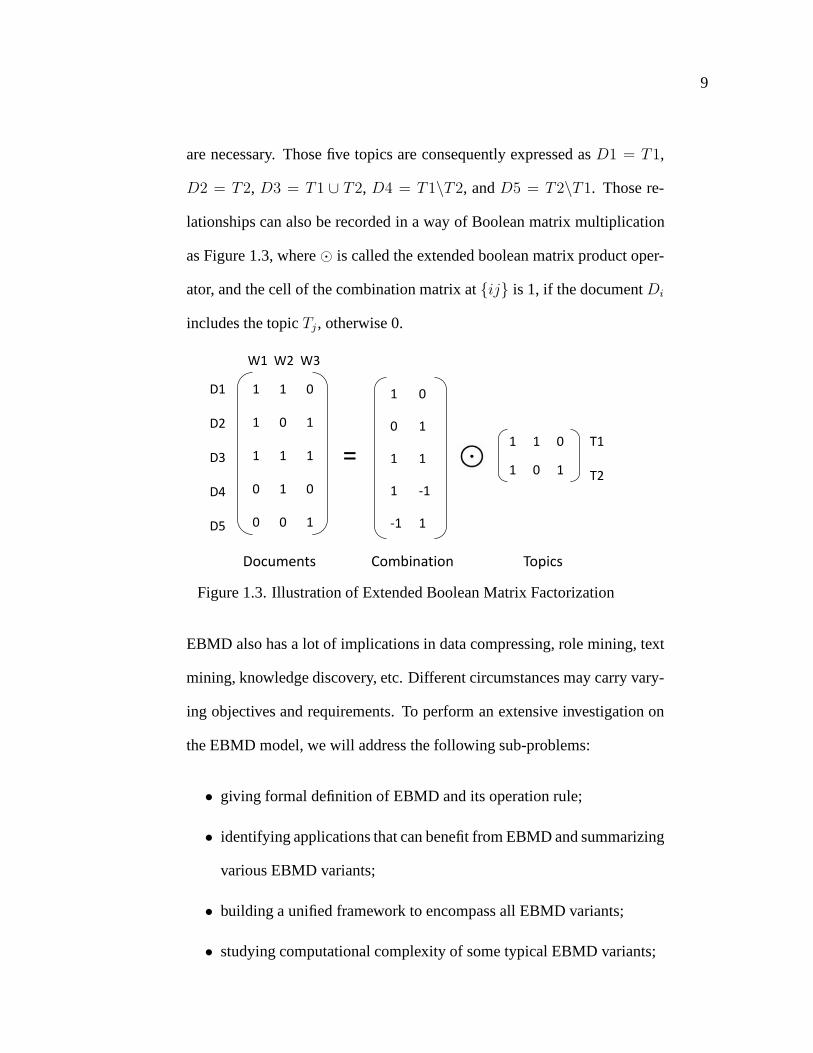
succinct way. For example, suppose a document-to-term dataset is given
as the matrix on the left side of Equation 1.3. With BMD, the least number
of topics needed to describe those five documents is 3. However, by intro-
ducing the set difference operation, only two topics as shown in Figure 1.3
9
are necessary. Those five topics are consequently expressedasD1 = T1,
D2 = T2, D3 = T1 ∪ T2, D4 = T1\T2, andD5 = T2\T1. Those re-
lationships can also be recorded in a way of Boolean matrix multiplication
as Figure 1.3, where⊙ is called the extended boolean matrix product oper-
ator, and the cell of the combination matrix at{ij} is 1, if the documentDi
includes the topicTj , otherwise 0.
1 1 0
1 0 1
1 1 1
0 1 0
0 0 1
1 0
0 1
1 1
1 -1
-1 1
1 1 0
1 0 1=
D1
D2
D3
D4
D5
W1 W2 W3
T1
T2
Documents TopicsCombination
Figure 1.3. Illustration of Extended Boolean Matrix Factorization
EBMD also has a lot of implications in data compressing, rolemining, text
mining, knowledge discovery, etc. Different circumstances may carry vary-
ing objectives and requirements. To perform an extensive investigation on
the EBMD model, we will address the following sub-problems:
• giving formal definition of EBMD and its operation rule;
• identifying applications that can benefit from EBMD and summarizing
various EBMD variants;
• building a unified framework to encompass all EBMD variants;
• studying computational complexity of some typical EBMD variants;

10
• designing good algorithms for those EBMD variants.
3. Weighted Rank-One Boolean Matrix Decomposition.
Example 1.1 Given a matrixA, a rank-one approximation is computed as
follows:
A =
1 0 1 1 01 1 1 1 10 0 1 0 01 1 1 1 0
≈
1101
(
1 1 1 1 0)
= XY T . (1.3)
Rank-one BMD is a special variant of BMD. It is to decompose a Boolean
matrix, where each row is an observed record, into the product of two
Boolean vectors as illustrated in Equation 1.3. The decomposed Boolean
row vector(1, 1, 1, 1, 0) can be viewed as a dominant pattern of the ob-
served data and the Boolean column vector(1, 1, 0, 1)T , called a presence
vector, shows which observed records belong to this dominant pattern. By
its component values, the presence vector divides observeddata records into
two parts. By recursively applying rank-one BMD on every part, observed
Boolean vectors can be divided into indivisible clusters. Dominant patterns
for those clusters constitute discrete patterns of original data.
However, users are not able to impose their personal preferences on error
type distribution of discovered patterns and the number of patterns. Look
at the same example. What if one expects to discover more discrete pat-
terns to improve the accuracy of patterns in approximating observed data?
What if one wants to discover a set of patterns which can describe observed

11
data without introducing any 1-becoming-0 errors, becausethere are only a
few 1’s cells in the original data? To address these two issue, we propose
weighted rank-one BMD, which is at the basis of conventionalBMD to in-
troduce different weights on 0-becoming-1 errors and 1-becoming-0 errors.
To determine wether a data record belongs to a discrete pattern, three pieces
of information need to be considered: (i) components of 1 in both the pat-
tern and the data record, (ii) components which are 1 in the pattern and 0 in
the data record; and (iii) components which are 0 in the pattern and 1 in the
data record. By applying different weights to the three parts, instead of the
same value as in conventional rank-one binary matrix approximation, users
can effectively control the level of accuracy in the final approximate matrix
and impose their preferences on the distribution of error types. Thus We
call the problem weighted rank-one BMD.
1.2 Research Challenges
BMD is a relatively new research topic, but has received muchattention recently
from many research fields because of its good adaptability toreal semantics. How-
ever, there are three main challenges remaining.
First, there lacks a general framework covering all BMD variants. It makes
literature work not beneficial for solving other similar problems with only minor
modifications. One of main reasons might be that people across different research
fields have not seen their problems from the perspective of BMD. Actually, if they
do, they would realize that their problems have much commonality. Hence, the
first problem this dissertation deals with is to review all problems, which can be

12
modeled through BMD, and categorizes them into five main groups. To exploit
the commonality of those problems, we will formulate them through mathematical
programming. Once done that, for new problems with minor modifications from
any of formulated problems, we simply change correspondingconstraints or the
objective function.
The second challenge is that the conventional BMD model doesnot consider
the set difference operation, which makes it not be able to model the exclusion
relationship, and limits the interpretabilities of decomposition solution. To ad-
dress it, we propose EBMD, which allows both the set union operation and the
set difference operation. Though it has broad applications, people may not realize
it. Thus we will discuss all possible applications of EBMD and categorize them
into groups as well. Furthermore, to exploit the commonality of those problems,
we formulate them through integer programming (IP), which allows us to take
advantages of available IP software packages and algorithms. As EBMD is a new
notion, the computational complexity of its variants has never been studied. We
will look at them also int this dissertation. Additionally,efficient heuristics will
be designed for each EBMD variant.
The third challenge is that all problems to be studied are combinatorial prob-
lems in nature, which are usually hard to solve. The main application domains of
our research are data mining and information security. Research problems occur-
ring in those two domains usually involve large scale data, which requires us to
give effective and efficient algorithms for the formulated combinational problems.

13
1.3 Contributions
There are four main contributions in this dissertation. First, the BMD problem is
extensively investigated. Important BMD variants, which have pragmatic implica-
tions in reality, and their relations are identified and studied. Second, we propose
the EBMD model, which addresses the inability of the BMD model to describe
the set difference relationship. The proposed EBMD model also has the ability
to discover some underlying data semantics along with the data mining process.
Third, the weighted rank-one BMD model is proposed. It allows users to effec-
tively impose their preferences on the number of mined discrete patterns and the
error type distribution of resultant approximate data. Fourth, for each proposed
problem, the computational complexity result is given, integer programming for-
mulation is provided, and effective and efficient solutions, such as approximation
algorithms and heuristics, are presented.
1.4 Outline of the Dissertation
The organization of the rest paper is as follows. Chapter 2 reviews the literature
work related to Boolean matrix applications. Chapter 3 gives some background
knowledge on computational complexity, mathematical programming, approxi-
mation algorithms, and heuristics. Chapters 4-6 study Boolean matrix decompo-
sition, extended Boolean matrix decomposition, and weighted rank-one Boolean
matrix decomposition respectively. Chapter 7 concludes our dissertation

14
CHAPTER 2
RELATED WORK
2.1 Role Engineering
Role engineering arises from implementing the RBAC system.RBAC is an ac-
cess control system that users are assigned to roles insteadto permissions. As
the number of required roles is usually much less than the number of permis-
sions, RBAC has the advantage of administrative efficiency over the conventional
permission-based access control. Due to its advantage, many organizations want
to transfer from their old access control systems to the RBACsystem. To re-
alize the full potential of RBAC, one must first define a complete and correct
set of roles. According to a study by NIST, this task has been identified as the
costliest component in realizing RBAC. The concept of role engineering was first
presented by Coyne [11]. It refers to the systematic work fordetermining roles.
Conceptually, there are two types of approaches towards role engineering. They
are top-down and bottom-up. Top-down is by analyzing business processes to de-
duce roles [1, 2, 11]. However, all those approaches share one common weakness
that it ignores existing user-to-permission assignments and calls for the cooper-
ation among various authorities from different disciplines. The bottom-up ap-
proach generates roles purely from the existing user-to-permission assignments.
It allows the automation of role generation without knowingthe semantics of busi-

15
ness. Kuhlmann, Shohat, and Schmipf [47] present a bottom-up approach using
clustering technique similar to the well known k-means clustering. Schlegelmilch
and Steffens [58] have proposed an agglomerative clustering based role mining
approach, known as ORCA. More recently, Vaidya et al. [62] proposed an ap-
proach based on subset enumeration, called RoleMiner. Thisapproach not only
eases the task of role engineering, but also helps in providing the security ad-
ministrators an insight into user-to-role assignments. However, it does require
an expert review of the results to choose which of the discovered roles are most
advantageous to implement. To find the optimal role set matching the interesting-
ness measures , Vaidya et al. [60] took a step forward to propose the role mining
problem. Lu et al. [42] further connect the role mining problem with the Boolean
matrix decomposition problem.
2.2 Text Mining
Text mining, roughly equivalent to text analytic, refers generally to the process of
deriving high-quality information from text. High-quality information is typically
derived through the deriving of patterns and trends throughmeans such as statis-
tical pattern learning. Text mining usually involves the process of structuring the
input text, deriving patterns within the structured data, and finally evaluation and
interpretation of the output. High quality in text mining usually refers to some
combination of relevance, novelty, and interestingness. Typical text mining tasks
include text categorization, text clustering, concept/entity extraction, production
of granular taxonomies, sentiment analysis, document summarization, and entity
relation modeling (i.e., learning relations between namedentities) [30]. For in-

16
stance, data summarization is becoming an very important research topic, because
with the widespread of internet technology we are facing thedramatically increas-
ing amount of document data. Its basic task is to categorize alarge amount of
documents into some topics, where each topic could simply bea subset of words
or a representative document. A good summarization scheme not only reduces
data storage space, but also facilitates the task of information retrieval [5].
2.3 Ordinary Matrix Factorization
Ordinary matrix decomposition is a well-studied problem that has been the focus
of significant research. Indeed, one of the earliest motivations of matrix decom-
position came from the problem of solving linear equations.It is known that if a
matrixA can be decomposed into the product of a lower triangular matrix L and
a upper triangular matrixU , solving the systemsL(UX) = b andUX = L−1U
is much easier thanAX = b [13]. In recent years, a big motivation for matrix
decomposition is for data analysis and data processing. Oneof best known meth-
ods is perhaps the Singular Value Decomposition,X = U∑
V , whereU andV
are orthogonal real-valued matrices containing the left and right singular vectors
of A, and∑
is a diagonal matrix containing the singular values ofA [13]. One
classic application of this method is to get the optimal rank-k factorization ofA
by setting all but the topk singular values in∑
to 0. In this sense, matrix de-
composition can be used for compressing data. The underlying reason is that if
we findAm×n = Xm×k · Ck×n andk is much less thanm andn, storingX andC
instead ofA will save great space [29].

17
2.4 Nonnegative Matrix Factorization
While the SVD is optimal in terms of the Frobenius norm, recently, people have
realized that it does not have sufficient interpretability.To address this problem,
multiple new methods were proposed, like Probabilistic Latent Semantic Index-
ing [27], Latent Dirichlet Allocation [9] and Nonnegative Matrix Factorization
(NMF) [31]. NMF is also an old problem that has been extensively studied in [55].
In NMF, the added restriction is that all the matrices shouldbe non-negative. This
can help cluster data, find centroids and even describe the probabilistic relation-
ships between individual points and centroids. Ding et al. [15] show the equiva-
lence of NMF, spectral clustering andK-means clustering. The work of Lee and
Seung [38, 39] also helped bring much attention from machinelearning and data
mining research communities to NMF.
2.5 Boolean Matrix Factorization
Since many real applications involve Boolean data, such as document-to-term
data, web click-stream data (users vs websites), DNA microarray expression pro-
files and protein-protein complex interaction network [63], Boolean data have ob-
tained a special and important space in the domain of data analysis [40]. It is
natural to represent Boolean data by Boolean matrices, which are a special case of
non-negative matrices. Many research problems involved inBoolean data analy-
sis can be reduced to Boolean matrix factorization. Geerts et al. [19] propose the
tiling databases problem which aims to find a set of tiles to cover a 0-1 database.
Since a tile can be represented by a Boolean vector, the tiling databases problem
is reduced to finding a factorization ofA = C⊗
X by limiting each column of

18
C to be a subset of one column ofA, because each tile can only cover cells of
1. Miettinen et al. [52] considerC as a discrete basis ofA, from whichA can
be reconstructed. GivenA, how to find a good basis is their core problem. This
work is further developed by Miettinen [48] whereC is limited to be the subset of
columns ofA. This limitation gives increased interpretability since each column
of C can be seen as a centroid ofA from the perspective of clustering. [48] also
allows the factorizationC⊗
X to cover cells containing zeros inA as long as
the amount of error is within a tolerable threshold. Haibinget al. [42] looks at
the Boolean matrix factorization problem in the context of role based access con-
trol (RBAC). The first and most difficult step of implementingRBAC is mining
roles given the user-permission assignment. By representing the user-permission
assignment, the user-role assignment and the mined role setby Boolean matrices
A, C andX, we haveA = C⊗
A. Therefore, the role mining problem is to find
a Boolean matrix factorization ofA.
2.6 Probabilistic Matrix Factorization
Probabilistic matrix factorization is viewing the input matrix from the statistic per-
spective. The most famous work might be principle componentanalysis (PCA)
[3]. It transforms a number of possibly correlated variables into a smaller number
of uncorrelated variables called principal components. PCA involves the calcula-
tion of the eigenvalue decomposition of a data covariance matrix or singular value
decomposition of a data matrix. Some work were proposed to use matrix factor-
ization to model user rating profiles for collaborative filtering [45,46]. Their core
idea is to find a good factorization of the input matrix to reconstruct the missing

19
cells in the input data. In [8, 14, 27], they use the concept ofmatrix factorization
to find latent factors by which to index documents. It can be applied in clustering
as well. Some work even tried clustering two attributes of the input data simul-
taneously, by factoring a matrix into the product of three matrices [17, 44, 51].

20
CHAPTER 3
BACKGROUND
3.1 Access Control
In computer system security, role-based access control (RBAC) is an approach to
restricting system access to authorized users. Due to its advantages in administra-
tive efficiency and flexibility, it has been used by the majority of enterprisers and
is a newer alternative approach to mandatory access control(MAC) and discre-
tionary access control (DAC).
Sandu R. et al. [57] is one of the most cited papers in the field of RBAC.
It definedRBAC0, the basic model,RBAC1 which introduces role hierarchies,
RBAC2 which introduces constraints at the basis ofRBAC0, andRBAC3 which
includes both role hierarchies and constrains. Their detailed descriptions are given
as follows.
Definition 3.1 (RBAC0)
• U, R, P and S (users, roles, permissions and sessions, respectively);
• PA ⊆ P ×R, a many-to-many permian-to-role assignment relation;
• UA ⊆ U × R, a many-to-many user-to-role assignment relation;

21
• user :S → U , a function mapping each sessionsi to the single user user(si)
(constant for the session’s lifetime);
• roles : S → 2R, a function mapping each sessionsi to a set of roes
roles(si) ⊆ {r|(user(si), r) ∈ UA} (which can change with time) and
sessionsi has the permissionsUr ∈ roles(si){p|(p, r) ∈ PA}.
The base model consists of everything except role hierarchies and constraints.
Definition 3.2 TheRBAC1 model has the following components:
• U, R, P, S, PA, UA, and user are unchanged fromRBAC0;
• RH ⊆ P × R is a partial order onR called the role hierarchy or role
dominance relation, also written as≥; and;
• roles : S → 2n is modified fromRBAC0 to requireroles(si) ⊆ {r|(∃r′ ≥
r)[(usr(si), r′) ∈ UA} (which can change with time) and sessionsi has the
permissions∪r∈roles(si){p|(∃r′′ ≤ r)[(p, r′′) ∈ PA]}.
Definition 3.3 RBAC2 is unchanged fromRBAC0 except for requiring that there
be constraints to determine the acceptability of various components ofRBAC0.
Only acceptable values will be permitted.
Common access control constraints include mutually exclusive roles, cardi-
nality, and prerequisite roles.
Mutually exclusive roles.The most common RBAC constraint could be mu-
tually exclusive roles. The same user can be assigned to at most one role in a

22
mutually exclusive set. This supports separation of duties, which is further en-
sured by a mutual exclusion constraint on permission assignments.
Cardinality. Another user assignment constraint is a maximum number of
members in a role. Only one person can fill the role of department chair; Simi-
larly, the number of roles an individual user can belong to could also be limited.
These are cardinality constraints, which can be correspondingly applied to permis-
sion assignments to control the distribution of powerful permissions. Minimum
cardinality constraint, on the other hand, may be difficult to implement. For exam-
ple, if a role requires a minimum number of members, it would be difficult for the
system to know if one of the members disappeared and to respond appropriately.
Prerequisite roles.The concept of prerequisite roles is based on competency
and appropriateness, whereby a user can be assigned to roleA only if the user
already is assigned to roleB. For example, only users who are already assigned to
the project role can be assigned to the testing role in that project. The prerequisite
(project) role is junior to the new (test) role. In practice,prerequisites between
incomparable roles are less likely to occur.
Other Constraints Constraints also apply to sessions and other user and role
functions associated with a session. A user may belong to tworoles but cannot
be active in both at the same time. Other session constraintslimit the number of
sessions a user can have active at the same time. Correspondingly, the number of
sessions to which a permission is assigned can be limited.
Definition 3.4 RBAC3 provides both role hierarchies and constraints as it com-
binesRBAC1 andRBAC2.

23
3.2 Computational Complexity
Computational complexity measures how difficult it is to solve a problem. In
this dissertation, we are dealing with many discrete optimization problems. To
gain an insight into the difficulty of those problems, performing computational
complexity analysis is necessary. The book [18] provides a perfect guide to the
computational complexity theory.
Definition 3.5 P, also known as PTIME or DTIME, is one of the most fundamen-
tal complexity classes. It contains all decision problems which can be solved by a
deterministic Turing machine using a polynomial amount of computation time, or
polynomial time.
People commonly think that P is the class of computational problems which are
”efficiently solvable” or ”tractable”. In practice, some problems not known to be
in P have practical solutions, and some that are in P do not. But this is a useful
rule of thumb.
Definition 3.6 NP is the set of decision problems where the ”yes”-instance can
be recognized in polynomial time by a non-deterministic Turing machine.
Intuitively, NP is the set of all decision problems for whichthe instances where
the answer is ”yes” have efficiently verifiable proofs of the fact that the answer is
indeed ”yes”. The complexity class P is contained in NP, but NP contains many
important problems, the hardest of which are called NP-complete problems, for
which no polynomial-time algorithms are known.
24
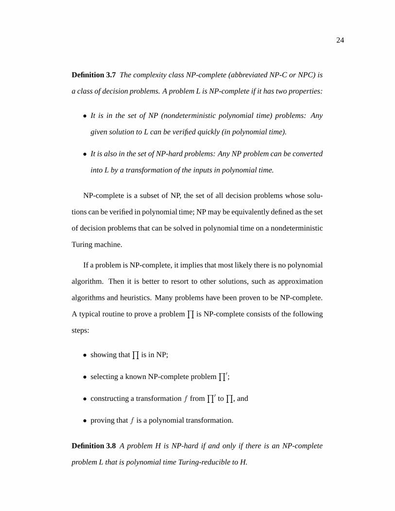
Definition 3.7 The complexity class NP-complete (abbreviated NP-C or NPC)is
a class of decision problems. A problem L is NP-complete if ithas two properties:
• It is in the set of NP (nondeterministic polynomial time) problems: Any
given solution to L can be verified quickly (in polynomial time).
• It is also in the set of NP-hard problems: Any NP problem can beconverted
into L by a transformation of the inputs in polynomial time.
NP-complete is a subset of NP, the set of all decision problems whose solu-
tions can be verified in polynomial time; NP may be equivalently defined as the set
of decision problems that can be solved in polynomial time ona nondeterministic
Turing machine.
If a problem is NP-complete, it implies that most likely there is no polynomial
algorithm. Then it is better to resort to other solutions, such as approximation
algorithms and heuristics. Many problems have been proven to be NP-complete.
A typical routine to prove a problem∏
is NP-complete consists of the following
steps:
• showing that∏
is in NP;
• selecting a known NP-complete problem∏′;
• constructing a transformationf from∏′ to
∏
, and
• proving thatf is a polynomial transformation.
Definition 3.8 A problem H is NP-hard if and only if there is an NP-complete
problem L that is polynomial time Turing-reducible to H.

25
Informally, NP-hard means ”at least as hard as the hardest problems in NP”.
NP-hard problems may be of any type: decision problems, search problems, or
optimization problems.
3.3 Approximation Algorithm
In computer science and operations research, approximation algorithms are algo-
rithms used to find approximate solutions to optimization problems. Approxima-
tion algorithms are often associated with NP-hard problems; since it is unlikely
that there can ever be efficient polynomial-time exact algorithms solving NP-hard
problems, one settles for polynomial time sub-optimal solutions. Unlike heuris-
tics, which usually only find reasonably good solutions reasonably fast, one wants
provable solution quality and provable run time bounds. Ideally, the approxima-
tion is optimal up to a small constant factor. Approximationalgorithms are in-
creasingly being used for problems where exact polynomial-time algorithms are
known but are too expensive due to the input size.
Before giving the formal definition of approximation algorithm, we define
combinatorial optimization problem. A combinatorial optimization problem∏
is either a minimization problem or a maximization problem and consists of the
following three parts:
• a setDQ of instances;
• for each instanceI ∈ DQ, a finite setSQ(I) of candidate solutions forI;
and
• a functionmQ that assigns to each instanceI ∈ DQ and each candidate

26
solutionσ ∈ SQ(I) a positive rational numbermQ(I, σ), called the solution
value forσ.
If∏
is a minimization (problem) problem, then an optimal solution for an
instanceI ∈ Dprod is a candidate solutionσ∗ ∈ SQ(I) such that, for allσ ∈
SQ(I), mQ(I, σ∗) ≤ mQ(I, σ) (mQ(I, σ∗) ≥ mQ(I, σ)).
Definition 3.9 An algorithmA is a ρ-approximation algorithm of the optimiza-
tion problem∏
if the valuef(x) of the approximation solutionA(x) to any in-
stancex of∏
, is not more than a factorρ times the value,OPT , of an optimum
solution.{
OPT ≤ f(x) ≤ ρOPT, ifρ > 1
ρOPT ≤ f(x) ≤ OPT, ifρ < 1.(3.1)
Definition 3.10 A family of approximation algorithms for a problemP, {Aǫ}ǫ, is
called a polynomial approximation scheme or PAS, if algorithmAǫ is a (1 + ǫ)-
approximation algorithm and its running time is polynomialin the size of the input
for a fixedǫ.
Definition 3.11 A family of approximation algorithms for a problemP, {Aǫ}ǫ,
is called a fully polynomial approximation scheme or FPAS, if algorithmAǫ is a
(1 + ǫ)-approximation algorithm and its running time is polynomial in the size of
the input and1/ǫ.
When a FPAS is a family of randomized algorithms, it will be called fully
polynomial randomized approximation scheme or FPRAS.

27
3.4 Mathematical Programming
Mathematical programming or optimization refers to choosing the best element
from some set of available alternatives.
In the simplest case, this means solving problems in which one seeks to mini-
mize or maximize a real function by systematically choosingthe values of real or
integer variables from within an allowed set. This formulation, using a scalar, real-
valued objective function, is probably the simplest example; the generalization of
optimization theory and techniques to other formulations comprises a large area
of applied mathematics. More generally, it means finding ”best available” values
of some objective function given a defined domain, includinga variety of different
types of objective functions and different types of domains.
Linear programming (LP), is a special type of convex programming, studies
the case in which the objective function is linear and the setof constraints is speci-
fied using only linear equalities and inequalities. Such a set is called a polyhedron
or a polytope if it is bounded. Linear programs can be expressed in the following
form.
maximize(minimize) cT x (3.2)
subject to Ax ≤ b (3.3)
There are several good algorithms for linear program. The simplex algo-
rithm [12], developed by George Dantzig in 1947, solves LP problems by con-
structing a feasible solution at a vertex of the polytope andthen walking along

28
a path on the edges of the polytope to vertices with non-decreasing values of
the objective function until an optimum is reached. In practice, the simplex al-
gorithm is quite efficient and can be guaranteed to find the global optimum if
certain precautions against cycling are taken. However, the simplex algorithm
has poor worst-case behavior. Leonid Khachiyan in 1979 introduced the ellip-
soid method [12], the first worst-case polynomial-time algorithm for linear pro-
gramming. Khachiyan’s algorithm was of landmark importance for establishing
the polynomial-time solvability of linear programs. It also inspired new lines of
research in linear programming with the development of interior point methods,
which can be implemented as a practical tool. In contrast to the simplex algorithm,
which finds the optimal solution by progressing along pointson the boundary of
a polytopal set, interior point methods move through the interior of the feasible
region.
Integer programming studies linear programs in which some or all variables
are constrained to take on integer values. This is not convex, and in general much
more difficult than regular linear programming. Integer programming problems
are in many practical situations (those with bounded variables) NP-hard. 0-1 in-
teger programming or binary integer programming (BIP) is the special case of
integer programming where variables are required to be 0 or 1. This problem is
also classified as NP-hard, and in fact the decision version was one of Karp’s 21
NP-complete problems. Advanced algorithms for solving integer linear programs
include: cutting-plane method, branch and bound, branch and cut, and branch and
price.

29
3.5 Heuristics
In computer science, heuristic designates a computationalmethod that optimizes
a problem by iteratively trying to improve a candidate solution with regard to
a given measure of quality. Heuristics make few or no assumptions about the
problem being optimized and can search very large spaces of candidate solutions.
However, heuristics do not guarantee an optimal solution isever found. Many
heuristics implement some form of stochastic optimization.
Heuristics are used for combinatorial optimization in which an optimal solu-
tion is sought over a discrete search space. Popular heuristics for combinatorial
problems include simulated annealing by Kirkpatrick et al.[33], genetic algo-
rithms by Holland et al. [28], ant colony optimization by Dorigo,[9] and tabu
search by Glover [20].

30
CHAPTER 4
BOOLEAN MATRIX DECOMPOSITION
4.1 BMD Variants with Applications
4.1.1 Basic BMD
The basic BMD problem is to decompose an input Boolean matrixinto two Boolean
matrices with the minimum size. In other words, it is to find the most succinct
representation of a Boolean matrix in the form of Boolean matrix decomposition.
According to the rule of BMD, a Boolean matrix with the size ofm× n can only
be decomposed into two Boolean matrices with the sizes ofm× k andk × n. So
to minimize the size of decomposed matrices is to minimizek, which gives the
definition of the basic BMD problem as the following.
Problem 4.1 ( Basic BMD) Given a matrixA ∈ {0, 1}m×n, find matricesX ∈
{0, 1}m×k andC ∈ {0, 1}k×n, such thatA = X⊗
C andk is minimized.
The basic BMD problem has pragmatic implications in many application do-
mains, including role mining, tiling databases, graph theory and set theory. Many
problems in those application domains can be formulated as the basic BMD prob-
lem with appropriate transformations. In the following, wewill introduce some
of them.

31
u1
u2
u3
u4
u5
u6
p1
p2
p3
Users
( Document, Transaction Record)Permissions
(Term, Product)
A
Figure 4.1. Bipartite Graph
1 1 00 1 11 1 11 1 11 1 11 1 1
=
1 00 11 11 11 11 1
⊗
(
1 1 00 1 1
)
. (4.1)
Role Mining. The basic BMD problem can find its important application in
role mining. As introduced in Chapter 2, the role mining problem arises from the
implementation of a role-based access control system. It isto discover a good role
set from user-to-permission assignments existing in an organization and assign
these roles to users appropriately such that each user gets the same permissions as
original. Role-based access control is usually administratively efficient compared
to the traditional permission-based access control, especially for large-scale sys-
tems. It is due to the fact that the number of required roles isusually much less
than the number of permissions.
The basic RMP problem, the fundamental role mining variant,attempts to find
a minimum set of roles, which would maximize the benefits of RBAC. This prob-

32
u1
u2
u3
u4
u5
u6
R1
R2
p1
p2
p3
Users
(Document, Transaction Record)Permissions
(Term, Product)
Role
(Topic, Itemset)
B C
Figure 4.2. Tripartite Graph
lem is a basic BMD problem. Look at Figure 6.1a, an illustrative example of user-
to-permission assignments. An edge means that its associated user is assigned its
associated permission. Such user-to-permission assignments can be completely
recorded by the Boolean matrix on the left to the equal sigh inEquation (4.1),
where each row corresponds to a user, each column corresponds to a permission,
and the value of 1 represents its corresponding user has its corresponding permis-
sion; otherwise, not. Similarly, the role mining solution as shown in Figure 5.5a
can be mapped to the two Boolean matrices on the right to the equal sign in Equa-
tion (4.1). The first Boolean matrix on the right to the equal sign gives the same
role assignments as shown in Figure 5.5a and the second Boolean matrix denotes
two roles. So the basic RMP problem is equivalent to decomposing the Boolean
matrix Am× representing the user-to-permission assignments into twoBoolean
matricesXm×k andCk×n, while minimizingk.
Market Basket Analysis. The basic BMD problem can be applied on market
basket analysis as well. Market basket data contains the transactions on product

33
items, and is one of the main data types studied in the data mining research field.
Market basket data are considered containing much information on customer be-
haviors and product values. The underlying patterns on market basket data are
crucial to designing good commercializing strategies.
Market basket data can be represented in the form of a Booleanmatrix with
the cell at the position of{ij} indicating whether or not the transactioni includes
the itemj. It can also be expressed as a bipartite graph as illustratedin Figure
6.1a, where nodes on the left side are transactions, nodes onthe right side are
items, and an edge means the transaction includes the item.
An important market basket data analysis task is to determine what items typ-
ically appear together, e.g., which items customers typically buy together in a
database of supermarket transactions. This in turn gives insight into questions
such as how to group them in store layout or product packages,how to market
these products more effectively, or which items to offer on sale to increase the
sale of other items.
Conventional solutions for determining such itemsets is based on the metric
of support. The support of an itemset X is the ratio of transactions in which an
itemset appears to the total number of transactions. Given asupport threshold
value, any itemset with a greater support value is considered to be frequent and
selected.
However, this way suffers from some limitations. For a large-scale database
a low support threshold would generate overwhelming itemsets, which are not of
practical use for data owners. It is true that a high support threshold would reduce

34
selected itemsets significantly. However, such selected itemsets do not guarantee
to cover the whole database or to describe all customer behaviors. In fact, in
reality some itemsets might be less frequent, but quite important. A good itemset
group is then expected to completely cover the whole database.
The basic BMD can be effectively utilized to resolve the itemset overwhelm-
ing issue. Instead of discovering frequent itemsets, we discover minimal itemsets
to cover the whole transaction database. Such a solution canalso be depicted
by a tripartite graph as shown in 5.5a. The nodes in the middledenote itemsets.
Edges between itemsets and items show the components of eachitemset, while
edges between transactions and itemsets gives the description for each transaction
as a union of some itemsets. A tripartite graph is corresponding to two Boolean
matrices. Hence, the task of minimizing the number of itemsets to describe a
transaction database is a basic BMD problem.
Topic Identification
With the fast development of internet and database technologies, a huge amount
of text data are generated and collected everyday, which creates needs for auto-
mated analysis. Given a collection of documents, a basic problem is: what topics
are frequently discussed in the collection? Its answer would assist human un-
derstanding of the essence within documents and help in archiving and retrieving
documents.
Given a collection of documents, a set of key words can be discovered. Each
document then can be structured as a subset of keywords, which further can be rep-
resented as a Boolean row vector with each dimension corresponding to a keyword

35
and each component value indicating whether or not the keyword is included. As
a result, a collection of documents can be represented as a Boolean matrix. It can
be depicted as a bipartite graph as shown in Figure 4.5a as well.
The topic identification problem can be performed as follows: Discover mini-
mal topics, each of which is a subset of keywords, to describethe given collection
of documents. The solution would give a limited number of topics, which is a
complete description of the whole collection of documents.
Such a topic identification problem is a basic BMD problem. Again, look at
Figure 5.5a. The relation between documents, topics, and keywords is depicted as
a tripartite graph, which decomposes the Boolean matrix of the document collec-
tion into two Boolean matrices.
4.1.2 Cost BMD
The cost BMD problem is to find a BMD solution minimizing the complexity
of decomposition solution, which is the number of 1’s cells in the decomposed
matrices, instead of the number of roles.
Problem 4.2 (Cost BMD) Given a Boolean matrixA ∈ m× n, find Boolean
matricesX ∈ {m×k} andC ∈ {k×n}, such thatA = X⊗
C and||X||1+||C||1
is minimized.
Cost BMD has an important application in role mining. The edge-RMP prob-
lem [60] is searching for the role set corresponding to the minimum administrative
cost, which is quantified by the total number of 1’s cells in the role-to-permission

36
assignment matrixC and the user-to-role assignment matrixX, as the manage-
ment information system makes assignments only based on 1’scells.
Cost BMD can also be applied in Boolean data compression. AsA = X⊗
C,
storingA can be replaced by storingX andC, if the total size ofX andC is much
smaller than the size ofA. To store a sparse Boolean matrix, only positions of 1’s
cells need to be maintained. Therefore, the size of a Booleanmatrix is the number
of its 1’s cells. The problem of searching for the best compressing strategy for
sparse matrices becomes a cost BMD problem.
4.1.3 Approximate BMD and Its Variants
The approximate BMD problem is to find a BMD solution without the restriction
of exactness and is described as follows.
Problem 4.3 (Approximate BMD) Given a Boolean matrixA ∈ m× n and a
threshold valueδ, find Boolean matricesX ∈ {m × k} andC ∈ {k × n}, such
that ||A−X⊗
C||1 ≤ δ andk is minimized.
An important motivation of approximate BMD is that in many cases a large
number of concepts are required to exactly describe the observed Boolean data,
while only a few concepts are necessary if a certain amount ofinexactness is
allowed. For those cases, if the exactness issue is not fatal, people tend to reduce
the number of necessary concepts by introducing a limited amount of errors.
This model can be well applied to the text mining scenario, asfor a large
document-word data set, restricting each document be represented exactly by an

37
union of a subset of topics tends to cause the over-fitting problem. Hence it is bet-
ter to allow some level of inexactness. It will facilitate the subsequent information
retrieval task as well since less topics make indexing work easier. Approximate
BMD can also be used to model the approximate RMP problem [62], which is a
variant of basic RMP.
However, certain applications may have specific requirements on the charac-
teristics of errors. It leads to two variants, 1-0 error freeBMD and 0-1 error BMD,
defined as follows.
Problem 4.4 (1-0 Error Free BMD) Given a Boolean matrixA ∈ m× n and a
threshold valueδ, find Boolean matricesX ∈ {m × k} andC ∈ {k × n}, such
that∑
ij |aij − (X ⊗ C)ij| is minimized and(X ⊗ C)ij = 1 if aij = 1.
Problem 4.5 (0-1 Error Free BMD) Given a Boolean matrixA ∈ m× n and a
threshold valueδ, find Boolean matricesC ∈ {m × k} andX ∈ {k × n}, such
that∑
ij |aij − (X ⊗ C)ij| is minimized and(X ⊗ C)ij = 0 if aij = 0.
For a sparse Boolean matrix with very few 1’s cells, 1-0 errors would cause
much information loss in the resultant Boolean matrix reconstructed from its ap-
proximate BMD solution. Hence, it is preferred to avoid 1-0 errors when decom-
posing sparse Boolean matrices, which gives rise to 1-0 error free BMD.
In the setting of role-based access control, 0-1 errors meanover-assignments.
Over-assignments would cause serious security and safety problems because users
may misuse permissions that are not supposed to be granted tothem. Under-
38
assignments, which are 1-0 errors, are relatively more tolerable. Therefore, it is
preferred to have 0-1 error free in the approximate RMP setting.
4.1.4 Partial BMD
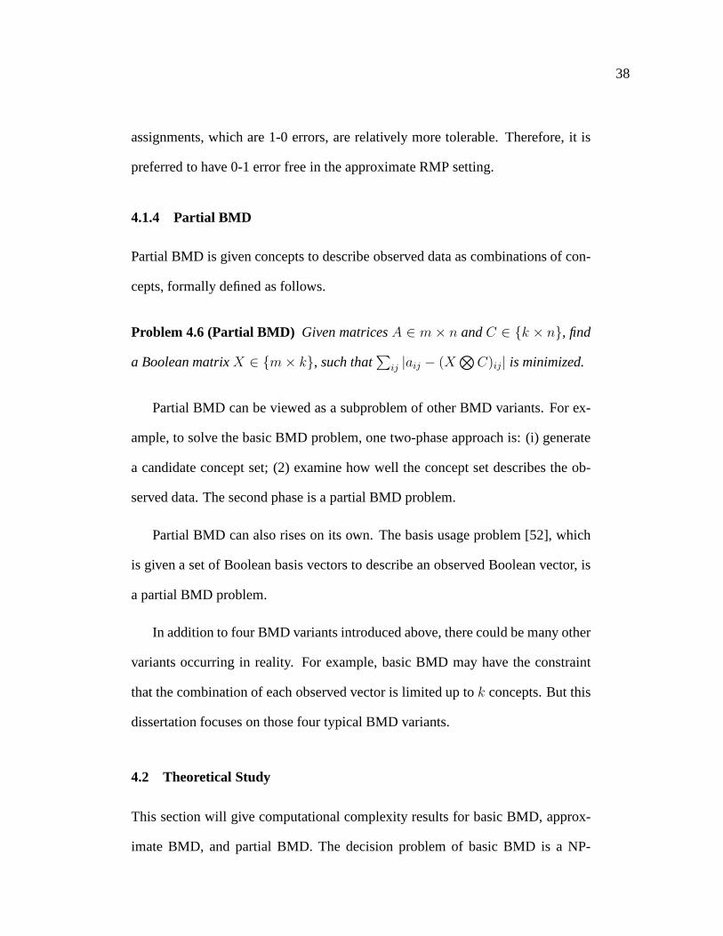
Partial BMD is given concepts to describe observed data as combinations of con-
cepts, formally defined as follows.
Problem 4.6 (Partial BMD) Given matricesA ∈ m× n andC ∈ {k × n}, find
a Boolean matrixX ∈ {m× k}, such that∑
ij |aij − (X⊗
C)ij| is minimized.
Partial BMD can be viewed as a subproblem of other BMD variants. For ex-
ample, to solve the basic BMD problem, one two-phase approach is: (i) generate
a candidate concept set; (2) examine how well the concept setdescribes the ob-
served data. The second phase is a partial BMD problem.
Partial BMD can also rises on its own. The basis usage problem[52], which
is given a set of Boolean basis vectors to describe an observed Boolean vector, is
a partial BMD problem.
In addition to four BMD variants introduced above, there could be many other
variants occurring in reality. For example, basic BMD may have the constraint
that the combination of each observed vector is limited up tok concepts. But this
dissertation focuses on those four typical BMD variants.
4.2 Theoretical Study
This section will give computational complexity results for basic BMD, approx-
imate BMD, and partial BMD. The decision problem of basic BMDis a NP-

39
complete problem, which can be proven by a reduction to the set basis problem
known to be NP-compete.
Definition 4.1 (Set Basis Problem)INSTANCE: A finite setU , a family S =
{S1, ..., SN} of subsets ofU and a positive integerk. QUESTION: Does there
exist a set basis of size at mostk for S?
Theorem 4.1 The decision problem of basic BMD is NP-complete.
Proof. The decision problem of basic BMD can be phrased as follows. IN-
STANCE: A Boolean matrixA and a positive integerk. QUESTION: Does there
exist a BMD solutionXm×k andCk×n of A?
For any set basis instance, we can find a basic BMD instance, which is true
if and only if the set basis instance is true. For a set basis instance{U ,S, k},
we create a vector sCce with dimensions of|U|, which denotes the number of
elements in|U|, and each dimension corresponding to an element in{U}. We also
construct row vectors{A1, ..., AN}, such thatAi(j) = 1 if Si contains elementj.
So far, we have created a basic BMD instance{A, k}. It is not difficult to see that
the constructed instance is true if and only if the set basis instance is true.�
Basic BMD essentially is a special case of approximate BMD with the error
threshold of 0. Hence, the decision problem of approximate BMD is NP-complete
as well.
The decision problem of partial BMD is also NP-complete, which can be
proven by a reduction to a known NP-complete problem,±PSC [49] described
as follows.

40
Problem 4.7 (±PSC ) INSTANCE: Two disjoint setsP and N of positive and
negative elements, respectively, a collectionS of subsets ofP⋃
N , and a pos-
itive integert. QUESTION: Does there exist a subcollectionC ∈ S, such that
|P\(∪C|) + |N ∩ (∪C|) ≤ t.
Theorem 4.2 The decision problem of partial BMD is NP-complete.
Proof. The decision problem of partial BMD can be phrased as follows. IN-
STANCE: two Boolean matricesAm×n andCk×n, and a positive numbert. QUES-
TION: Does there exist a Boolean matrixX such that∑
ij |aij − (X ⊗C)ij| ≤ t.
Given an instance of the decision problem of partial BMD, it is not difficult to
check if it is true. So the decision problem of partial BMD belongs to NP.
For any±PSC instance{P, N,S, t}, we can construct a decision partial BMD
instance as follows, which is true if and only if the±PSC instance is true. We
let A to a 1 × (|P | + |N |) Boolean vector, with the first|P | components being
1 and the others being 0. In addition, for the1 × (|P | + |N |) vector sCce, we
let the firstP dimensions correspond to positive elements inP respectively and
the lastN dimensions correspond to negative elements inN respectively. For
each element subsetsi in S, we create a Boolean row vectorCi of C such that:
if si contains some element, the component ofCi which corresponds to that Cr-
ticular element is 1; otherwise 0. The constructed decisionpartial BMD instance
{A1×(|P |+|N |), C|S|×(|P |+|N |), t} is equivalent to the±PSC instance.�

41
4.3 Mathematical Programming Formulation
BMD variants share much commonality. For example, the only difference be-
tween basic BMD and cost BMD is in the objective functions. The difference
between approximate BMD and basic BMD is that approximate BMD allows in-
exactness. A natural arising thought is that if we can build aunified framework
for all BMD variants, we then do not need to deal with each problem individu-
ally. Additionally when new BMD variants appear, system engineers do not need
to start from scratch and can take advantage of algorithms that have been devel-
oped for existing BMD variants. As all BMD variants are essentially optimization
problems, we propose to formulate them through integer linear programming.
There are many benefits by connecting BMD variants with integer linear pro-
gramming. First, optimization has been studied for more than half century. There
are quite a few good exact optimization algorithms, even forinteger linear pro-
gramming, such as branch-and-bound [37]. In addition, successful optimization
software Packages are easily obtainable, such as Matlab andthe Neos server1.
Even though those BMD variants are proven to be hard to solve,small or medium
size problems can still be solved through traditional optimization techniques. In
addition to exact algorithms, approximation algorithms may be developed through
LP-based techniques, such as dual-fitting [41], randomizedrounding [23], and
primal-dual schema [36]. The linear programming frameworkwe will propose in
fact can not only incorporate BMD variants, but also problems in other application
domains, such as tiling database problems [19] and discretebasis problems [50].
1http://www-neos.mcs.anl.gov/

42
For ease of explaining, in this section, we will discuss BMD variants in the role
mining context, where a BMD solution{X, C} of user-to-permission assignments
A gives rolesC and user-to-role assignmentsX.
4.3.1 Partial BMD
In the context of role mining, partial BMD is given user-to-permission assign-
mentsA and rolesC to assign roles appropriately to users such that the resultant
user-to-permission assignment errors∑
ij |aij − (X ⊗ C)ij| is minimized. Then
the partial BMD problem can be roughly represented as follows:
minimize ||A−X ⊗ C||1.
To formulate it as an explicit integer linear programming problem, we first
formulateX ⊗ C = 0 and then relax it by tolerating errors.
To do so, we letCi denote rolei andAi denote permissions assigned to user
i. A −X ⊗ C = 0 means every user’s permission set should be represented as a
union of some candidate roles. This can be phrased asAi =⋃
t∈siCt, wheresi
denotes the role subset assigned to useri. {si} can convert to a Boolean matrixX
such thatXit = 1 if role t belongs tosi, otherwiseXit = 0.
The constraint essentially says that if some user has a particular permission, at
least one role having that permission has to be assigned to that user. In turn, if that
user does not have some permission, none of the roles having that permission can
be assigned to it. SoX ⊗ C = A can be transformed to the following equation
set.{
∑qt=1 XitCtj ≥ 1, if Aij = 1
∑qt=1 XitCtj = 0, if Aij = 0
(4.2)

43
To formulate inexactness, we introduce a non-negative slack variable{Vij} to
each constraint and have the following modified constraints.
{∑q
t=1 XitCtj + Vij ≥ 1, if Aij = 1∑q
t=1 XitCtj − Vij = 0, if Aij = 0(4.3)
For Aij = 1,∑q
t=1 XitCtj + Vij ≥ 1 allows∑q
t=1 XitCtj to be 0. ForAij = 0,∑q
t=1 XitCtj−Vij = 0 allows∑q
t=1 XitCtj to be greater than 1. In other words, if
Vij > 0, the constraint enforcing whetherAij = 1 or Aij = 0 is not satisfied. The
objective function||A−X ⊗ C||1 is then the count of unsatisfied constraints for
A = X ⊗ C. To formulate the objective function, we need to count the positive
variables{Vij}. To do so, we introduce another Boolean variable set{Uit} and
enforce the following constraints:
{
MUij ≥ Vij
Uij ≤ Vij.
In which, the bigM is a large constant greater thanq. The above two inequalities
ensure that ifVij ≥ 1, Uij = 1 and if Vij = 0, Uij = 0. Thus, the count of
positive{Vij} is∑
ij Uij . Therefore, the integer linear programming formulation
for partial BMD is as the following
minimize∑
ij
Uij
∑qt=1 XitRtj + Vij ≥ 1, if UCij = 1
∑qt=1 XitRtj − Vij = 0, if UCij = 0
MUij − Vij ≥ 0, ∀i, j
Uij ≤ Vij, ∀i, j
Xit, Uij ∈ {0, 1}, Vij ≥ 0
.
(4.4)

44
4.3.2 Basic BMD
With the integer linear program formulation for partial BMD, it is easy to for-
mulate other BMD variants. Consider basic BMD. In the role mining setting,
it means given user-to-permission assignmentsAm×n to find user-to-role assign-
mentsXm×k and permission-to-role assignmentsCk×n. It can be succinctly put
as an optimization problem as follows:
minimize k
s.t. Xm×k ⊗ Ck×n = Am×n.
For simplicity, we break up the basic BMD into two subproblems: (i) find a
candidate role set{R1, R2, ..., Rq}; (ii) locate a minimum candidate role subset to
form A.
A role is nothing, but a permission subset. Givenn permissions, there are2n
possible roles. But most of them can be easily eliminated. For example, if none
of users had both permissionsi andj, any permission subset containing both per-
missionsi and j can never be a candidate role. We will explicitly discuss the
generation of candidate roles when we conduct experimentalstudy on BMD vari-
ants later. Here assume we have already had a candidate role set{R1, R2, ..., Rq}.
Then consider the second subproblem, which is similar to partial BMD.
Every user’s permission set should be able to be representedas a union of
some candidate roles. This can be phrased as the following:Ai =⋃
t∈siRt,
wheresi denotes the candidate role subset assigned to useri andAi denotes the
permission subset assigned to useri. {si} can convert to a Boolean matrixX such
thatXit = 1 if candidate rolet belongs tosi, otherwiseXit = 0. As bothX andR

45
are Boolean matrices, their relation can be represented by the following Boolean
matrix multiplication,Xn×q ⊗ Rq×m = An×n, whereR andA are given andX
is unknown. AsXit indicates whetherRj is assigned to useri, so if ∀t Xit = 0,
it means thatRt is never employed. So the basic BMD is essentially to minimize
the number of non-zero columns inX.
Same as the partial BMD, the constraintX ⊗ R = A can be enforced by
{∑q
t=1 XitRtj ≥ 1, if Aij = 1∑q
t=1 XitRtj = 0, if Aij = 0. (4.5)
Now we need to count the number of non-zero columns inX. To do so, we
introduce a set of Boolean slack variables{d1, ..., dq}, wheredt = 1 indicates
role t is present, otherwise not. Then|Roles| =∑q
t=1 dt. Sincedt indicates the
presence of a role,dt should only be 1 when at least one user is assigned rolet.
Thus,dt = 1 when at least one of{X1t, ..., Xmt} is 1. We can formulate this by
adding in the constraints{dt ≥ Xit, ∀i, t}.
Finally, putting every thing together, the basic BMD is formulated as the fol-
lowing
minimize∑
t
dt
∑qt=1 XitRtj ≥ 1, if Aij = 1
∑qt=1 XitRtj = 0, if Aij = 0
dt ≥ Xij, ∀i, j
dt, Xij ∈ {0, 1}
.
(4.6)

46
4.3.3 Approximate BMD
In the role mining setting, approximate BMD problem means tominimize the
number of required roles within a tolerable amount of errors. In Equation 4.4,
the error amount is formulated as∑
ij Uij . In Equation 4.6, the number of roles
is formulated as∑
t dt. By combining these two equation systems together, we
easily obtain the formulation for the approximate BMD problem as Equation 4.7.
minimize∑
t
dt
∑qt=1 XitRtj + Vij ≥ 1, if Aij = 1
∑qt=1 XitRtj − Vij = 0, if Aij = 0
MUij − Vij ≥ 0, ∀i, j
Uij ≤ Vij , ∀i, j
dt ≥ Xit, ∀i, t∑
i
∑
j Uij ≤ δ
dj, Xit, Uij ∈ {0, 1}, Vij ≥ 0
.
(4.7)
In which,∑n
i=1
∑mj=1 Uij ≤ δ ensures the total deviating cells less thanδ and the
objective function∑q
t=1 dt is the number of mined roles.
4.3.4 Cost BMD
Different from basic BMD, cost BMD is to minimize the administrative cost. As
a RBAC system only needs to maintain explicit user-to-role assignments and ex-
plicit role-to-permission assignments, the administrative cost is hence evaluated
by positive cells in the decomposed matricesX andC. By employing the same
notations in the integer linear program formulation for thebasic BMD as in Equa-
tion 4.6, the administrative cost can be formulated as the following
||X||1 + ||C||1 =∑
i
∑
t
Xit +∑
t
(dt
∑
j
Rtj). (4.8)

47
∑
i
∑
t Xit is the count of positive cells inX and∑
t(dt
∑
j Rtj) counts positive
cells in selected candidate roles, which is||C||1. Thus, the integer linear program
formulation for cost BMD can be obtained by replacing the objective function in
Equation 4.6 with the formula in Equation 4.8.
4.3.5 Discussion
From the integer linear program formulating processes for those role mining vari-
ants, we observe that once one role mining variant is successfully formulated, it
is easy to formulate other variants. This fact illustrates the benefit of building a
unified integer linear program framework of the role mining problem. Such an
integer linear program framework is broad and flexible to incorporate new vari-
ants, which may appear in practice. For instance, a role mining engineer may
not want to see 0-becoming-1 errors in an approximate BMD solution, because
0-becoming-1 errors mean that a user obtains unauthorized permissions, which
may harm the system security severely. To reflect this concern in the integer lin-
ear program formulation , we could simply replace the constraint for Aij = 0 of∑q
t=1 XitRtj − Vij = 0 in Equation 4.7 by∑q
t=1 XitRtj = 0. Consider another
instance that all roles are expected to be highly repetitively used. To realize this
expectation, we could add a constraint that∑
i Xit ≥ LB, where∑
i Xit is the
number of users granted rolet andLB is a specified frequency lower bound. So
every picked role is employed more thanLB times.

48
4.4 Algorithm Design for BMD Variants
The integer linear program formulation for the partial BMD takesmn variables
and for other BMD variants takes aboutmq variables, wherem is the number of
users,n is the number of permissions, andq is the number of candidate roles. The
state-of-art integer linear program software Packages candeal with up to millions
variables. So for problems of sizes withm andq greater than 1000, we have to
resort to efficient heuristics. In this section, we will propose efficient heuristics
for BMD variants. They are easy to implement and run fast. Their effectiveness
will be validated in the next section. Like the above integerlinear program for-
mulations that require candidate roles to be given, our heuristics need candidate
concepts generated beforehand as well. So before presenting our heuristics, we
will first discuss ways of generating candidate concepts. For ease of explaining,
we will still discuss it in the role mining setting.
4.4.1 Candidate Role Set Generating
We present three ways of generating candidate roles. All of them were somehow
mentioned in other peoples’ work before either in the role mining context or in
the discrete basis context.
Intersection. We call the first methodIntersection, which is proposed by
Vaidya et. in [62]. This method includes every unique user’spermission set as
a candidate role. In addition the intersections of every twouser permission sets
are included as candidate roles as well. This method is basedon two observa-
tions. First in order to make a permission subset be a role, itmust be employed
and assigned to some user. In other words, a candidate role must be a subset of

49
some user’s permission set. The other observation is that tomake a RBAC system
succinct and efficient, roles should be repetitively employed. So a role is desired
to be assigned to multiple users. Hence, a candidate role is expected to be the
intersection of two or multiple user’s permission sets. Givenm users, candidate
roles generated by theIntersectionmethod iso(m2).
Association. This method is to exploit the correlations between the columns
of existing user-to-permission assignmentsA by employing the association rule
mining concept in [52]. It was presented as a part of theASSOalgorithm proposed
for the discrete basis problem. The concrete generation process is as follows. Sup-
pose user-to-permission assignmentsAm×n are given. LetA(:, i) denote theith
column. Thenn candidate roles will be generated, represented by a Booleanma-
trix Cn×n. In which,Cij = 1 if 〈A(:, i), A(:, j)〉\〈A(:, i), A(:, i)〉 ≥ τ ; otherwise
0. The operator〈., .〉 is the vector inner product operation, andτ is a predeter-
mined threshold controlling the level of correlation.
Itself. This method is to simply treat unique user’s permission setsfrom A
as candidate roles. It was studied in [48], but in the scenario of the discrete basis
problem. The problem is to find a discrete basis for an input Boolean matrix, such
that the discrete basis is a subset of columns (or rows) of theinput Boolean matrix.
In the role mining context, if employing this method to generate candidate roles,
it is assumed that for every role there must be one user who is granted this role
and only this role.

50
4.4.2 Partial BMD
As we mentioned earlier, partial BMD is equivalent to the basis usage problem.
A heuristic called Loc& IterX was proposed for the basis usage problem in [48].
Here we propose two more effective heuristics, one greedy approach and one sim-
ulated annealing approach.
Without loss of generality, we assume that there is only one user. HenceA is
a1× n row vector. A role setCr×n is given. partial BMD becomes to find a role
subset, such that the union of permissions contained in those roles is closest toA.
Greedy. A greedy algorithm is any algorithm that makes the locally optimal
choice at each stage with the hope of finding the global optimum. It has many
successful applications, such as the traveling salesman problem and the knapsack
problem. Our greedy approach consists of a preliminary step. It is to assign all
roles inC which aresubordinateto A to the user. A roleC1 is considered to be
subordinate to a roleC2 if all permissions contained byC1 belong toC2. After
that, iteratively pick one remaining role which can reduce the reconstruction error
by the most and assign it to the user, till the reconstructionerror cannot be reduced
any more.
Simulated Annealing Simulated annealing is a generic probabilistic heuris-
tic for the global optimization problem. It locates a good approximation to the
global optimum of a given function in a large search space. Different from greedy
heuristics, simulated annealing is a generalization of a Markov Chain Monte Carlo
method, which has a solid theoretical foundation. We present a simulated anneal-
ing heuristic for the partial BMD problem as the following. First, we let(0, ..., 0)

51
Algorithm 4.1 Greedy Algorithm for Partial BMD
Input: A1×n andCr×n
Output: X1×r
1: X1×r ← (0, ..., 0);2: for i← 1 : r do3: if Ci ⊆ A then4: X[i] = 1;5: end if6: end for7: loop8: Ci=the best remaining role,j=the largest improvement;9: if j > 0 then
10: X[i] = 1;11: else12: break13: end if14: end loop
be the starting state ofX1×r. Then at each stage, randomly select its neighboring
value by randomly picking one element ofX and flipping its value from 0 to 1 or
from 1 to 0. If the newX better reconstructsA, the next state is the newX. If
not, with a certain probability less than 1, the next state isthe newX . In other
words, with certain probability, it remains its original state. This property reduces
the chance of being stuck at a local optimum. The procedure described above
allows a solution state to move to another solution state andhence produces a
Markov Chain. Denote thenth state bex and the randomly selected neighboring
value bey. If the next state isy with probability min{1, exp{λV (x)/N(x)}exp{λV (y)/N(y)}
}] or it
remainsx, whereλ is a constant,V (t) is the reconstruction error with the solution
t, andN(t) is the number of neighboring values oft. Such a Markov Chain has
a limiting probability of 1 for arriving at optimal minimization solutions when
λ → ∞ [56]. But it has been found to be more useful or efficient to allow the

52
Algorithm 4.2 Simulated Annealing Algorithm for Partial BMD
Input: A1×n andCr×n
Output: X1×r
1: X, x← (0, ..., 0); n← 1;2: while n ≤ limit & V (X) > 0 do3: y= a random neighboring value ofx;4: if V (y) < V (X) then5: X ← y;6: end if7: x = y with probability
min{1, exp{log(1+n)V (x)}exp{Clog(1+n)V (y)}
};8: n← n + 1;9: end while
value ofλ to change with time. Simulated annealing is a popular variation of
the preceding. Here, we adopt the formula proposed by Besag et al. [54] and let
the transition probability bemin{1, exp{λnV (x)/N(x)}exp{λnV (y)/N(y)}
} whereλn = log(1 + n). In
our case,N(x) andN(y) are equivalent and are canceled out in the formula. As
computing time is limited, we terminate the algorithm aftera certain number of it-
erations regardless of whether or not the global optimum is reached. Our complete
simulated annealing algorithm is described as in Algorithm4.2.
4.4.3 Basic BMD
The heuristic proposed for the basic BMD also runs in a greedyfashion. Look at
the integer linear program formulation for the basic BMD as Equation 4.6. There
are two main types of constraints, one for{Aij = 1} and the other for{Aij = 0}.
In order to satisfy the constraint set{∑q
t=1 XitRtj = 0, if Ait = 0}, if Rjt = 1,
Xit must be equal to 0. Therefore, many variablesXit can be determined directly
in this way. Then the constraint set{∑q
t=1 XitRtj = 0, if Ait = 0} is all satisfied.
Next consider{∑q
t=1 XitRtj ≥ 1, if Ait = 1}. To satisfy it, if the particular

53
cellsRt1j , Rt2,j, ...Rtk ,j are 1, one of the associated cellsXit1 , Xit2, ...Xitk has to
be 1.
Now, consider the objective functionmin∑q
t=1 dt. Asdt is determined by the
constraintdt ≥ Xit. Hence once one of the cells{Xit, ∀t} is 1, dt is forced to
be 1. In other words, no matter how many variables in{Xit, ∀t} take the value
of 1, the objective function value is always increased by 1. Our greedy algorithm
utilizes this property. At each step, choose a candidate role Rt such that by set-
ting {Xit, ∀t}, except those predetermined, be 1, the most remaining constraints
{∑q
t=1 XitRtj = 1, if Aij = 1} are satisfied. We call the count of such satisfied
remaining constraints the basic-key.
Definition 4.2 (Basic-Key) For each column of the variable matrix{Xit}, the
count of the constraints{∑q
t=1 XijRtj = 1, if Aij = 1} being satisfied by letting
the cells of such a variable column be 1 except the cells predetermined, is called
its basic-key.
If there are multiple columns with the same greatest basic-key, we simply
choose the column with the least index. Once a column is chosen, it means that
the associated candidate role is chosen and the associateddt is set to be 1. Then
delete the satisfied constraints and perform the same procedure repetitively till all
the constraints are satisfied. The full procedure of this greedy algorithm is given
in Algorithm 4.3.

54
Algorithm 4.3 Greedy Algorithm for Basic BMD
Input: Unique user-to-permission assignmentsAm×n and candidate roles{R1, ..., Rq}.
Output: X andC1: C = ∅;2: Investigate the constraints{
∑qt=1 XitRtj = 0} in Equation 4.6 and determine
some ofXit to be 0;3: Select the candidate roleRt with the greatest basic-key value and include it
in C.4: Let undetermined values in{Xit} be 1 and deleter hence satisfied constraints
in {∑q
t=1 XitRtj > 1};5: Go back to step 3 till all constraints of{
∑qt=1 XitRtj = 0} and
{∑q
t=1 XitRtj > 0} are satisfied.6: Set the remaining variables inX to be 0.7: X is the subset of rows inX corresponding to selected roles inC.
4.4.4 Approximate BMD
From the integer linear program formulation perspective, approximate BMD seems
much more complicated than basic BMD. However an efficient greedy heuris-
tic for the approximate BMD can be easily developed by modifying the greedy
heuristic for the basic BMD. As theδ-approximate BMD toleratesδ amount of
errors, we can terminate Algorithm 4.3 early once the remaining uncovered 1’s
cells are less thanδ.
4.4.5 Cost BMD
Cost BMD is to minimize the administrative cost||X||1+||C||1, while basic BMD
only aims to minimize the number of roles. So a basic BMD optimal solution is
not necessarily a cost BMD solution. Cost BMD was studied in [61], where a
greedy heuristic was proposed. To distinguish it, we call itEdge-Key. Here we
propose a new heuristic, calledTwo-Stage.

55
Cost BMD objective consists of two parts||X||1 and ||C||1. Intuitively less
number of roles leads to a less value of||C||. In this sense, an optimal solution of
basic BMD can be a not-bad solution for cost BMD. Our greedy heuristic for basic
BMD is able to produce a goodC. However,X produced by the greedy heuristic
is just a byproduct and not in its optimal form. We can start a second phase
and reduce user-role assignments by reassigning obtained roles ofC to each user.
It is essentially another basic BMD problem that assigning the minimum roles
from C to exactly cover all permissions for a user. So here we can adopt our
greedy heuristic again. It is a common fact that if a role contains permissions not
originally possessed by a user, the role can never be assigned to the user. With
this rational, we can simplify the second-phase task by filtering out unlikely roles
from C in advance. The complete algorithm is as described in Algorithm 4.4.
Algorithm 4.4 Two-Stage Algorithm for Edge-BMD
Input: user-to-permission assignmentsAm×n and candidate roles{R1, ..., Rq}.Output: ||X||1 + ||C||1
1: Run Algorithm 4.3 with{R1, ..., Rq} to obtainC.2: for eachAi do3: Remove roles that contain permissions not belonging toAi from C.4: Run Algorithm 4.3 with remaining roles inC to obtainXi.5: end for
4.5 Experimental Study
In this section, we conduct extensive numerical experiments on both synthetic
data sets and real data sets to evaluate the performance of our heuristics.
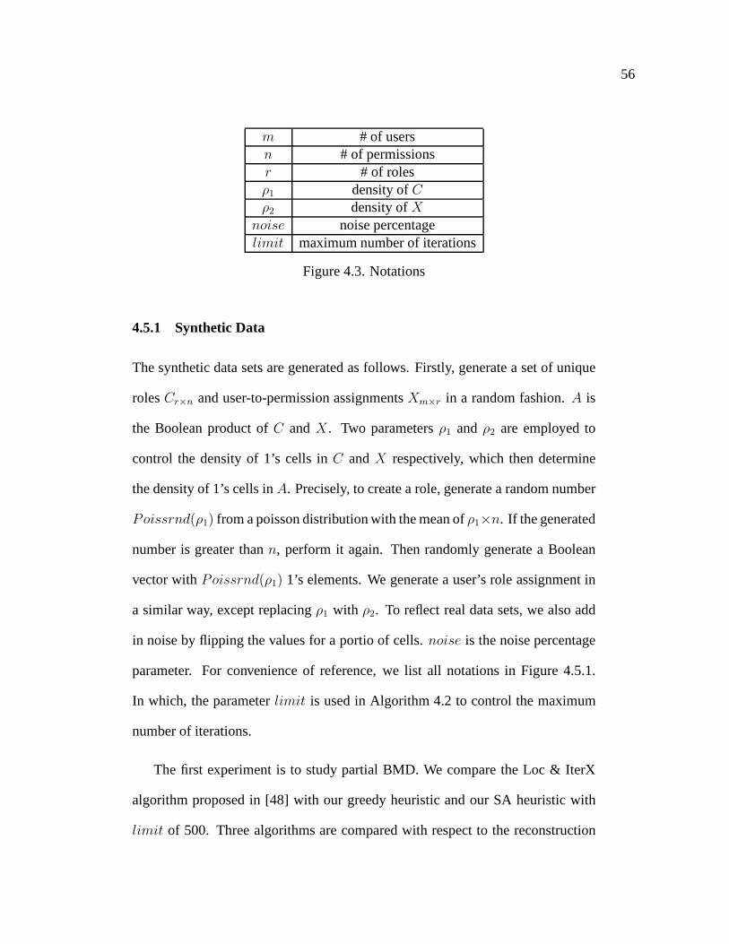
56
m # of usersn # of permissionsr # of rolesρ1 density ofCρ2 density ofX
noise noise percentagelimit maximum number of iterations
Figure 4.3. Notations
4.5.1 Synthetic Data
The synthetic data sets are generated as follows. Firstly, generate a set of unique
rolesCr×n and user-to-permission assignmentsXm×r in a random fashion.A is
the Boolean product ofC andX. Two parametersρ1 andρ2 are employed to
control the density of 1’s cells inC andX respectively, which then determine
the density of 1’s cells inA. Precisely, to create a role, generate a random number
Poissrnd(ρ1) from a poisson distribution with the mean ofρ1×n. If the generated
number is greater thann, perform it again. Then randomly generate a Boolean
vector withPoissrnd(ρ1) 1’s elements. We generate a user’s role assignment in
a similar way, except replacingρ1 with ρ2. To reflect real data sets, we also add
in noise by flipping the values for a portio of cells.noise is the noise percentage
parameter. For convenience of reference, we list all notations in Figure 4.5.1.
In which, the parameterlimit is used in Algorithm 4.2 to control the maximum
number of iterations.
The first experiment is to study partial BMD. We compare the Loc & IterX
algorithm proposed in [48] with our greedy heuristic and ourSA heuristic with
limit of 500. Three algorithms are compared with respect to the reconstruction

57
0 0.05 0.1 0.15 0.20
0.2
0.4
0.6
0.8
Noise Percentage
Rec
onst
ruct
ion
Err
or R
atio
GreedyLoc & IterXSimulated Annealing
(a) ρ1=0.3,ρ2=0.3,m=50,n=50,r=10,limit=500
0 500 1000 15000.25
0.3
0.35
0.4
0.45
Maximum Number of Iterations
Rec
onst
ruct
ion
Err
or R
atio
GreedySimulated Annealing
(b) ρ1=0.3, ρ2=0.3, m=1, n=50,r=30,noise=0.2
0 500 1000 15000
0.05
0.1
0.15
0.2
0.25
Maximum Number of Iterations
Com
putin
g T
ime
(sec
onds
)
GreedySimulated Annealing
(c) ρ1=0.3, ρ2=0.3, m=1, n=50,r=30,noise=0.2
Figure 4.4. Experimental Results on Partial BMD
error ratio, which is defined asErrorRatio = ||A−A′||1/||A||1, whereA′ denotes
the reconstructedA.
The concrete experimental design is as follows. (i) Generate a number of data
sets{X, C, A} with m = 50, n = 50, ρ1 = 0.3, ρ2 = 0.3 andnoise varying from
0 to 0.2; (ii) Run the Loc & IterX, the greedy algorithm, and the SA algorithm
with limit of 500 respectively to obtainX andA′ givenC andA. The experiment
result is illustrated as shown in Figure 4.4a. It shows the greedy algorithm and the
SA algorithm are significantly better than the Loc & IterX algorithm. The other
observation is that the performances of the greedy heuristic and the SA heuristic
are comparable.
Different from the greedy heuristic, which returns a local optimum in most
cases, a SA heuristic can with probability one reach a globaloptimum with enough

58
computing time; in other words unlimited number of iterations. However, the
meaning of existence for a heuristic is that it can get a good solution in an accept-
able time. So we conduct another experiment to investigate how our SA heuristic
performs as opposed tolimit. We generate 100 sets of{X, C, A} with ρ1=0.3,
ρ2=0.3, m=1, n=50, r=30, andnoise=0.2. limit varies from 50 to 2500. Run
both the greedy heuristic and the SA heuristic against them.Figure 4.4b shows
that the SA heuristic has better performance than the greedyheuristic whenlimit
is greater than 500. It also shows at the beginning small increase inlimit can im-
prove the performance by a lot for the SA heuristic. However,whenlimit reaches
certain point, the improvement becomes much less significant. It somehow shows
that the greedy heuristic has relatively satisfactory performance. Figure 4.4c plots
computing times for both methods. The computing time for theSA heuristic in-
creases linearly withlimit. However, to achieve the same performance as the
greedy heuristic, the SA heuristic takes more time. So we conclude that the SA
heuristic is recommended for small-size problems while thegreedy heuristic is
suitable for large-size problems.
Next we study our greedy heuristic for basic BMD. The heuristic is closely
dependent on candidate roles. Three ways of generating candidate roles were in-
troduced:Itself, Intersection, andAssociation. As Associationhas a parameter of
association thresholdτ , for a fair comparison, we consider two cases,τ = 0.9 and
τ = 0.7. We generate{A} with ρ1=0.3, ρ2=0.3, m=50, n=50, r=10, noise=0.
Then run Algorithm 4.3 with each candidate role set respectively to findX and
C. The results are illustrated as shown in Figure 4.5a. BothIntersectionandItself
are able to reconstructA completely, butAssociation. With respect to the error

59
reducing speed,Associationis inferior to two other approaches. OverallIntersec-
tion has the best performance, while the performance ofAssociationis far from
satisfactory. So ignoringAssociation, we then further studyItself and Intersec-
tion with respect to computing time. Figure 4.5b shows thatIntersectiontakes
much more time thanItself. The underlying reason is thatIntersectionproduces
o(m2) candidate roles as opposed too(n) candidate roles produced byItself. We
conclude that for small size problemsIntersectionis preferred whileItself is rec-
ommended for large size problems.
Our greedy heuristic for approximate BMD is same as that for basic BMD,
except that it terminates early. So the previous experimental results are valid for
studying approximate BMD. Figure 4.5c plots reconstruction error ratio values
with respect to required number of roles. If a small amount oferrors are allowed,
A can be successfully reconstructed with much less number of roles. For example,
Itself needs only 10 roles to cover more than 80 percent of existing permissions,
while 20 extra roles are needed to cover the remaining permissions. Somehow
it can be interpreted that roles returned by approximate BMDare more ”funda-
mental”. It suggests that if a bottom-up role engineering approach is only used to
identify promising roles to assist a top-down engineering approach, approximate
BMD is more efficient. Figure 4.5d shows the relation betweendata density and
the number of required roles for full coverage. As the data density is indirectly
determined byρ1 andρ2. The experiment is to letρ1 andρ2 have the same value
and vary them together from 0.1 to 0.6. In Figure 4.5d, both lines suggest that
for denser data sets more roles are required. In other words,our greedy heuristic
performs better for sparse data sets, while real access control data sets are usually

60
0 10 20 300
0.2
0.4
0.6
0.8
1
Number of Roles
Err
or R
atio
ItselfAssociation, τ=0.9Association, τ=0.7Intersection
(a) ρ1,ρ2=0.3, m,n=50, r=10,noise=0
0 0.5 10
5
10
Error RatioC
ompu
ting
Tim
e (s
econ
ds)
ItselfIntersection
(b) ρ1,ρ2=0.3,m=1, n=50,r=30,noise=0.2
5 10 15 20 250
0.2
0.4
0.6
0.8
1
Number of Roles
Err
or R
atio
ItselfIntersection
(c) ρ1,ρ2=0.3, m,n=50, r=10,noise=0
0 0.2 0.4 0.6 0.810
15
20
25
30
35
ρ1 and ρ
2
Num
ber
of R
equi
red
Rol
es
ItselfIntersection
(d) m,n=50,r=10,noise=0
40 60 80 10010
20
30
40
50
60
m and n
Num
ber
of R
equi
red
Rol
es
ItselfIntersection
(e)ρ1,ρ2=0.3,r=10,noise=0
Figure 4.5. Experimental Results on Basic BMD and Approximate BMD

61
very sparse. We then study the relation between data size andour greedy heuristic
performance. We letm andn be same and vary them from 40 to 100. Figure 4.5e
illustrates that our heuristic performs good for medium andsmall sizes.
Next we evaluate theTwo-Stagealgorithm proposed for edge BMD by com-
paring it with theEdge-Keyalgorithm proposed in [61]. For convenience, we
let default parameters for generatingA be {m = 50, n = 50, ρ1 = 0.3, ρ2 =
0.3, noise = 0}. We then variate one parameter each time, generate a set ofAs,
and runTwo-StageandEdge-Keyrespectively on them. As both algorithms re-
quire input candidate roles, we consider bothItself andIntersection. Hence, we
actually compare four approaches:(Two-Stage, Itself), (Two-Stage, Intersection),
(Edge-Key, Itself),and (Edge-Key, Intersection). Experimental results are illus-
trated as shown in Figure 4.6. All four graphs suggest thatTwo-Stageis better
thanEdge-Key.
4.5.2 Real Data
We run our greedy heuristics on real data sets collected by Ene et al. [16]. They
areemea, healthcare, domino, firewall 1, andfirewall 2.
The first experiment is to study the basic BMD. We run Algorithm 4.3 against
each data set with candidate roles generated byItself andIntersectionrespectively.
Numbers of roles required for full coverage are recorded in Figure 4.7. The num-
ber of required roles is much less than the number of permissions for each case.
It successfully demonstrates the power of RBAC and also the effectiveness of our
heuristic on discovering roles. Another observation is that the performance ofIn-
tersectionis not always better thanItself when working with our greedy heuristic.

62
0.2 0.4 0.6
500
1000
1500
2000
ρ1 and ρ
2
Edg
e V
alue
Edge−Key, Itself,Two−Stage, ItselfEdge−Key, IntersectionTwo−Stage, Intersection
5 10 15 20 25 300
1000
2000
3000
r
Edg
e V
alue
Edge−Key, Itself,Two−Stage, ItselfEdge−Key, IntersectionTwo−Stage, Intersection
0.1 0.2 0.31200
1300
1400
1500
1600
1700
noise
Edg
e V
alue
Edge−Key, Itself,Two−Stage, ItselfEdge−Key, IntersectionTwo−Stage, Intersection
40 60 80 100 120
500
1000
1500
2000
m and n
Edg
e V
alue
Edge−Key, Itself,Two−Stage, ItselfEdge−Key, IntersectionTwo−Stage, Intersection
Figure 4.6. Reconstructed Error Ratio w.r.t. Percentage ofRequired Roles ForReal Data Sets
In theory, withIntersectionthe optimal solution of a basic BMD is better than that
with Itself, as the feasible solution space is expanded. However, if thealgorithm
runs in a greedy manner, it is not always true.
The second experiment is to study theδ-approximate BMD. We run Algorithm
4.3 and record remaining errors when a new role is identified.Figure 4.8 plots
reconstruction error ratios with respect to number of required roles. The first
observation is that all lines drop fast at the beginning. It suggests that a few roles
are usually able to reduce error ratio to a very low level. Roles early identified can
hence be interpreted as ”more valuable”. Another observations is that much more
roles are required to cover the remaining few 1’s at the end. It suggests hat if a role
mining approach is used as a tool to assist a top-down role engineering approach,
δ-approximate BMD might be sufficient. The other important observation is that

63
Data Set Users Permissions ||A||1 Itself# of Roles Edge Value
Edge-Key Two-Stageemea 35 3,046 7,220 34 7,281 7,246healthcare 46 46 1,486 16 624 478domino 79 231 730 20 810 727firewall 1 365 709 31,951 71 5,475 4,937firewall 2 325 590 36,428 10 1,796 1,456
Data Set Users Permissions ||A||1 Intersection# of Roles Edge Value
Edge-Key Two-Stageemea 35 3,046 7,220 43 9,078 9,014healthcare 46 46 1,486 14 553 412domino 79 231 730 21 814 827firewall 1 365 709 31,951 65 4,508 4,034firewall 2 325 590 36,428 10 1,796 1,456
Figure 4.7. Number of Roles and Edge Value for Full Coverage for Real Data Sets
Intersectiondose not always perform better thanItself in our greedy heuristic. In
fact, if only considering early mined roles, their performances are comparable.
The third experiment is to study the edge BMD. We run(Two-Stage, Itself),
(Two-Stage, Intersection), (Edge-Key, Itself),and(Edge-Key, Intersection)respec-
tively against each data set. Their edge values are recordedin Figure 4.7. Our
Two-Stagealgorithm performs better than theEdge-Keyalgorithm for nearly all
cases except for thedomino data set withIntersection. The experimental results
demonstrate the advantage of RBAC over the traditional access control system
once again, as the edge-value (administration cost) is muchless than||A||1 for
any case.

64
0 20 400
0.2
0.4
0.6
0.8
1
Number of Roles
Err
or R
atio
Emea
ItselfIntersection
0 5 10 15
0.2
0.4
0.6
0.8
1
Number of Roles
Err
or R
atio
Healthcare
ItselfIntersection
0 10 200
0.2
0.4
0.6
0.8
1
Number of RolesE
rror
Rat
io
Domino
ItselfIntersection
0 20 40 600
0.2
0.4
0.6
0.8
1
Number of Roles
Err
or R
atio
Fire1
ItselfIntersection
0 5 100
0.2
0.4
0.6
0.8
1
Number of Roles
Err
or R
atio
Fire2
ItselfIntersection
Figure 4.8. Reconstructed Error Ratio w.r.t. Number of Required Roles For RealData Sets

65
CHAPTER 5
EXTENDED BOOLEAN MATRIX DECOMPOSITION
Boolean matrix decomposition is to decompose a Boolean matrix into the product
of two Boolean matrices, where the first matrix represents a set of meaningful
concepts, and the second describes how the observed data canbe expressed as
combinations of those concepts. The combination is only in terms of the set union.
In other words, a successful Boolean matrix decomposition gives a set of concepts
and shows how every column of the input data can be expressed as a union of some
subset of those concepts.
However, this way of modeling only incompletely representsreal data seman-
tics. Essentially, it ignores a critical component – the setdifference operation: a
column can be expressed as the combination of union of certain concepts as well
as the exclusion of other concepts. This has two significant benefits. First, the
total number of concepts required to describe the data may itself be reduced. Sec-
ond, a more succinct summarization may be found for every column. In this paper,
we propose the extended Boolean matrix decomposition (EBMD) problem, which
aims to factor boolean matrices using both the set union and set difference opera-
tions. We study several variants of the problem, show that they are NP-hard, and
propose efficient heuristics to solve them. Extensive experimental results demon-
strate the power of EBMD.

66
To better explain EBMD, we will study it in the context of rolemining in the
following.
5.1 Motivation of EBMD
Role-based access control (RBAC) has proven to be a very successful model for
access control. Its flexibility and cost-efficiency have resulted in it being widely
adopted by current commercial systems. Indeed, it has been the model of choice
for migration in the case of enterprises still employing traditional access control
schemes. However, for such enterprises, the first and indeedthe most crucial step
is to design a good set of roles and assign them appropriatelyto each user. This
process of designing roles is called role engineering [11].While top-down tech-
niques have been proposed for role engineering, for large-scale enterprises with
more than thousands of users and permissions, bottom-up role extraction, called
role mining, which mines roles purely from existing user-permission assignments
without considering their semantic meanings, has become quite popular.
Semantics likeexceptionsandseparation of duty constraint(SoD) are indis-
pensable parts of RBAC,critical to model real-world cases.While SoD constraints
are restrictions on users and roles to capture policy semantics, allowing the se-
mantics related to exceptions are needed for a more succincttranslation of access
control policies to the actual specification. However, existing solutions for role
mining such as BMD are not able to capture or reflect semantics, specifically the
exceptions and separation of duty constraints. We will explicitly explain both
below.
Exceptions: Exceptions are inherent to any real world access control policy that

67
uses some notion of abstraction in the authorization. Sincethe focus of this paper
is on role mining, we consider the role based access control policy. Suppose the
RBAC policy states that any user with role “manager” is allowed to access the
file “project A”. However assume there exists an exception tothis policy stating
that all users except John (who can play the role of the manager) is not allowed
to access “project A” due to certain conflict of interest requirements. Such excep-
tions are quite common to real world policies. Under a typical RBAC policy this
is supported through a negative authorization as it does notmake sense to create
a new role specifically to John alone. It is important to realize that supporting
negative authorizations sometimes may result in conflicting authorizations (in this
case due to permission inheritance through role hierarchy). These can be han-
dled by implementing conflict resolution policies (in this example, negatives take
precedence). Assume other users assigned to “manager” are Alice, Bob, Cathy,
Dave and Eve, and the permission to access “project A” isp, the corresponding
user-to-permission assignments of this example would be asshown in figure 5.1.
Traditional role mining approaches attempt to mine roles that have the same per-
mission sets. In this case, two roles will be mined, first comprising of Alice, Bob,
Cathy, Dave and Eve, and the second with John alone. Our proposed role min-
ing approach in this paper attempts to capture the underlying semantics of such
exceptions and eliminates mining of such incorrect role sets. Note that similar
exceptions can be found with other abstractions of authorizations. An example of
such a policy would be “John is allowed to access all project reports except the
report of project A”. Our approach can elegantly handle exceptions of these kinds
as well.

68
user pAlice 1Bob 1
Cathy 1Dave 1Eve 1John -1
Figure 5.1. User-to-permission assignments of the exampleabove
Separation of Duty Constraints: SoD constraints are an integral part of RBAC,
as stated in the definition ofRBAC2 [57]. These help to limit exploitation of priv-
ileges and limit fraud. Consider the following toy example.Assume the follow-
ing four permissions of a company: “Purchasing”, “Auditing”, “Marketing” and
“Sales”. A person can assume multiple permissions. Supposethat the same per-
son is in charge of purchasing and sales. Hence these two permissions are grouped
together as a role, which can be represented by a Boolean vector as{1, 0, 0, 1}T .
To prevent fraud, the company has a policy stating that a person cannot assume
both “Purchasing” and “Auditing” permissions. Simply representing a role as a
Boolean vector cannot reflect this constraint. Even though the “auditing” permis-
sion is not included in{1, 0, 0, 1}T , a person who has been assigned this role, can
obtain the “Auditing” permission by acquiring other roles,which is perfectly valid
in the BMD model. We however, would like to recognize such constraints as part
of the mining process itself.
To address this ineffectiveness of the BMD model in capturing semantics, we
propose introducingnegative permissionsor negative user-role assignment, which
can cleverly resolve both of the above issues.
As distinct from regular permissions, negative permissions mean that once

69
a permission is assigned to a user negatively, this user can never exercise that
permission. Thus, negative permissions have higher priority than positive permis-
sions. Indeed, if the user is already assigned the permission positively through
another role or even through the hierarchy, this assignmentis automatically re-
voked. If the user is assigned the permission positively in the future, it still does
not become effective. Thus, negative permissions yield a great power and can
effectively model both SoD constraints and exceptions.
SoD constraints can be modeled through introducing negative permissions
in roles. Consider again the “Purchasing” and “Auditing” example. To enforce
the SoD constraint on them, for any role containing one of them, we add the
negative permission of the other. Hence, the role of{1, 0, 0, 1}T is changed to
{1,−1, 0, 1}T , where the cell of -1 denotes the negative “Auditing” permission.
As a result any employee assuming that role can never have the“Auditing” per-
mission, unless the role assignment is revoked. We denote such roles, allowing
negative permissions, assemantic roles.
Exceptions can be modeled through introducing negative user-role assign-
ments. Negative user-role assignments mean that if a role isassigned to a user,
the user cannot have access to any permission of that role. The negative user-role
assignment is superior to the positive (or regular) user-role assignment. Revisiting
the “Manager” example of John. To forbid him from accessing “project A”, we
only need to assign the “manager” role negatively to him. We call such user-role
assignments, which include both positive and negative assignments, assemantic
user-role assignments.
Indeed, negative authorizations are integral part of many access control sys-
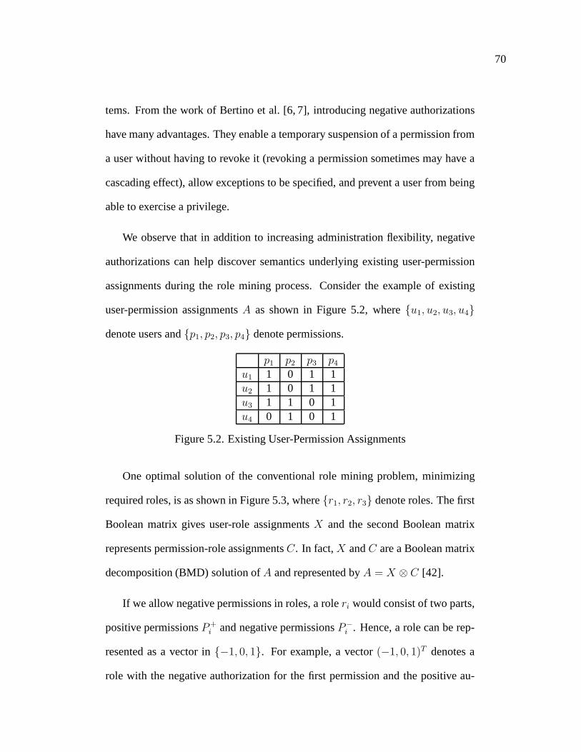
70
tems. From the work of Bertino et al. [6, 7], introducing negative authorizations
have many advantages. They enable a temporary suspension ofa permission from
a user without having to revoke it (revoking a permission sometimes may have a
cascading effect), allow exceptions to be specified, and prevent a user from being
able to exercise a privilege.
We observe that in addition to increasing administration flexibility, negative
authorizations can help discover semantics underlying existing user-permission
assignments during the role mining process. Consider the example of existing
user-permission assignmentsA as shown in Figure 5.2, where{u1, u2, u3, u4}
denote users and{p1, p2, p3, p4} denote permissions.
p1 p2 p3 p4
u1 1 0 1 1u2 1 0 1 1u3 1 1 0 1u4 0 1 0 1
Figure 5.2. Existing User-Permission Assignments
One optimal solution of the conventional role mining problem, minimizing
required roles, is as shown in Figure 5.3, where{r1, r2, r3} denote roles. The first
Boolean matrix gives user-role assignmentsX and the second Boolean matrix
represents permission-role assignmentsC. In fact,X andC are a Boolean matrix
decomposition (BMD) solution ofA and represented byA = X ⊗ C [42].
If we allow negative permissions in roles, a roleri would consist of two parts,
positive permissionsP+i and negative permissionsP−
i . Hence, a role can be rep-
resented as a vector in{−1, 0, 1}. For example, a vector(−1, 0, 1)T denotes a
role with the negative authorization for the first permission and the positive au-

71
r1 r2 r3
u1 1 0 1u2 1 0 1u3 1 1 0u4 0 1 0
(a) X
p1 p2 p3 p4
r1 1 0 0 1r2 0 1 0 1r3 0 0 1 0
(b) C
Figure 5.3. Conventional Role Mining
thorization for the third permission. Assigningri to a user means that the user
can never have any permission ofP−i unlessri is revoked and the user can have a
permission ofP+i if he is not assigned any role consisting of its negation.
Now let us do the same thing as the conventional role mining problem, mini-
mizing the number of required roles. The only difference is that negative permis-
sions are allowed this time. As we expect it to discover underlying data semantics,
we call it thesemantic role mining problem. For the same user-permission assign-
ments as above, the resultant optimal solution is as shown inFigure 5.4.
r1 r2
u1 1 0u2 1 0u3 1 1u4 0 1
(a) X
p1 p2 p3 p4
r1 1 0 1 1r2 0 1 -1 1
(b) C
Figure 5.4. Semantic Role Mining with Negative Permission
The first impression on the result is that with negative authorization for per-
missions we need only two roles to reconstruct the same existing user-permission
assignments. Further by taking a close look, you can find moreinformation.
First, r2 : {0, 1,−1, 1} shows that ifr2 is assigned to a user, he can never has

72
the privilege ofp3. It implies thatp3 might be exclusive fromp2 andp4. Sec-
ond, r1 : {1, 0, 1, 1} shows thatp2 andp4 can be existent in one role. It leaves
one plausible explanation that there is a separation of dutyconstraint onp2 and
p3. So the real semantic might be there are indeed only two rolesin the sys-
tem,r1 : {1, 0, 1, 1} andr2 : {0, 1, 0, 1}. The reason thatu3 does not getp3 even
thought he is assignedr2, is the separation of duty constraint onp2 andp3. How-
ever, the conventional role mining approach is not able to discover such semantics.
Compared to the result in Figure 5.3, the result in Figure 5.4seems more plausible.
This toy example demonstrates the ability of negative authorization on dis-
covering underlying semantics. To perform semantic role mining, we propose in-
troducing a new approach, extended Boolean matrix decomposition (EBMD). As
its name tells, EBMD extends from BMD. It allows -1 in one of the decomposed
matrices. Thus, EBMD is to decompose one Boolean matrix intoone Boolean
matrix and one matrix in{−1, 0, 1}.
From the technical perspective, semantic role mining is like finding a good
EBMD solution of the Boolean matrix corresponding to given user-permission
assignments. However, it is more complicated than that. Theparticular role min-
ing context has to be incorporated in the matrix decomposition process.
5.2 Extended Boolean Matrix Decomposition
In this section, we will introduce a novel matrix decomposition method EBMD,
which addresses the ineffectiveness of BMD in its ability ofcapturing real data
semantics. To help better understand the function of EBMD, let us recall BMD
first.

73
BMD is essentially to discover a set of discrete concepts anduse them to de-
scribe each observed Boolean record as a union of some discrete concepts. The
key advantage of BMD is to provide much interpretability to decomposition solu-
tions. To illustrate it, look at the example of Equation 5.2.
a1 a2 a3 a4d1 : 1 1 0 1d2 : 0 1 1 0d3 : 1 0 0 1d4 : 1 1 1 1
=
1 0 00 1 00 0 11 1 0
⊗
a1 a2 a3 a4c1 : 1 1 0 1c2 : 0 1 1 0c3 : 1 0 0 1
.
(5.1)
The matrix on the left is the observed records. In which, 1 means that the
record consists of the attribute. For example,d1 = {a1, a2, a4}. The matrix
on the right is the discovered concepts, each of which is a subset of attributes.
For example,c1 = {a1, a2, a4}. The combination matrix tells how observed
records can be described as a union of some discovered concepts. For example,
d4 = c1 ∪ c2.
BMD does provide much interpretability to matrix decomposition solutions.
However, it is only able to represent the set union operation. In reality, some data
semantics requires the representation of the set difference operation as well. For
example, in the access control setting, a role could be negatively assigned to a
user, such that any permissions belonging to the role can never be assigned to the
user.
To enable BMD to capture the set difference operation, we introduce a new
concept EBMD, which allows -1 in the combination matrix and uses it to represent
the set difference operation.

74
Consider the same above example. By introducing -1 in the combination
matrix, we obtain a new decomposition solution as below, where⊙ denotes the
EBMD multiplication operator.
a1 a2 a3 a4d1 : 1 1 0 1d2 : 0 1 1 0d3 : 1 0 0 1d4 : 1 1 1 1
=
1 00 11 −11 1
⊙
a1 a2 a3 a4c1 : 1 1 0 1c2 : 0 1 1 0
.
(5.2)
Notice that with the introduction of the set difference operation only two con-
cepts are needed to represent the same observed data. The combination matrix
shows that:d1 = c1, d2 = c2, d3 = c1 \ c2, andd4 = c1 ∪ c2.
As illustrated, EBMD is to describe a set of observed recordswith a small set
of concepts, such that each record can be represented as inclusion of one subset
of concepts with exclusion of another subset of concepts. Ifa record includes
one concept, that record should contain all elements of thatconcept; if a record
excludes one concept, that record should not contain any element of that record.
As is natural in set operations, exclusion overrides inclusion. In other words, if
a record excludes one concept, any element in that concept isnot included in the
reconstructed record, even if it is present in any other concept that is included in
that record.
The essential task of EBMD is to find a set of concepts and the way of re-
constructing the input Boolean matrix with those concepts.Similar to BMD, a
concept is represented by a Boolean vector. In BMD, the combinations are repre-
sented by a Boolean matrix, where an element of 1 for a record denotes that the

75
corresponding concept is included, otherwise not. To reflect the set difference op-
eration, we introduce elements of -1. So an EBMD solution of aBoolean matrix
Am×n is in a form of{Xm×k, Ck×n}, where the concept matrixC is a Boolean
matrix and the combination matrixX is in {−1, 0, 1} wherexij = 1 denotes the
jth record includes theith concept andxij = −1 denotes thejth record excludes
the ith concept. In contrast to BMD, we denote EBMD asA = X ⊙ C. The
following is the formal set-theoretic EMBD definition:
Definition 5.1 (EBMD) {X ∈ {−1, 0, 1}, C ∈ {0, 1}} is called an EBMD solu-
tion ofA ∈ {0, 1}, denoted byA = X ⊙ C, if Ai = ∪xij=1Cj \ ∪xij=−1Cj, where
Ai denotes the item subset corresponding to elements of 1 in thejth row ofA and
Cj denotes similarly.
Although the definition of EBMD is intuitive, the⊙ operator cannot be di-
rectly executed as the⊗ operator of BMD. So we give the following definition of
the⊙ operator based on logic arithmetic.
Definition 5.2 (⊙ operator) The⊙ operator operates over a matrixXm×k ∈
{−1, 0, 1}m×k and a matrixCk×n ∈ {0, 1}k×n . If Am×n = Xn×k ⊙ Ck×n, we
have
aij=1 if (∃t1) (xi,t1 = 1 AND ct1,j = 1)
AND (¬∃ t2) (xi,t2 = 1 AND ct2,j = −1)
aij=0 if (¬∃ t1) (xi,t1 = 1 AND ct1,j = 1)
OR (∃ t2) (xi,t2 = 1 AND ct2,j = −1)
wherei ∈ [1, m] andj ∈ [1, n]
Note that the⊙ and⊗ operators are equivalent when all entries inX are
binary.

76
The EBMD operator is commutative as described as follows.
Property 5.1 (Commutativity) (Xm×k ⊙ Ck×n)T = CT
k×n ⊙ CTm×k.
The commutativity implies that ifA = C ⊙ X whereC ∈ {−1, 0, 1} and
X ∈ {0, 1}, we haveAT = XT ⊙CT as well. So EBMD essentially decomposes
one Boolean matrix into one Boolean matrix and one matrix in{−1, 0, 1}, while
the order of them does not matter.
Look at Figure 5.4, in which the negative element appears in the second de-
composed matrix. To interpret such an EBMD solution, we can consider its in-
verse as the follows. It gives us another perspective to lookat negative permission
authorizations in a role. Each ”role”ri can be viewed a set of users. Each per-
missionpi corresponds to a set of users who are assigned the permission. The
EBMD result as shown in Figure 5.3 gives thatp1 = r1, p2 = r2, p3 = r1 \ r2, and
p4 = r1 ∪ r2.
u1 u2 u3 u4p1 : 1 1 0 1p2 : 0 1 1 0p3 : 1 0 0 1p4 : 1 1 1 1
=
r1 r2
p1 1 0p2 0 1p3 1 −1p4 1 1
⊙
u1 u2 u3 u4r1 : 1 1 0 1r2 : 0 1 1 0
.
(5.3)
5.3 Semantic Role Mining Problem
We have illustrated how negative authorizations can help identify underlying data
semantics and discover a succinct role-based access control system. Negative
authorizations can be negative permissions in a role or negative role assignments.
However, it does not make sense to have both in a system as it would be difficult
77
to interpret a negative assignment of a role, which includesa negative permission.
So in the access control setting, we limit negative authorization to be only one
kind, either negative role assignments or negative permissions.
Roles and role assignments with negative authorizations are called semantic
roles and semantic user-role assignments respectively. They are defined as fol-
lows.
Definition 5.3 (Semantic Role)A semantic roleri is a role consisting of positive
permissionsP+i and negative permissionsP−
i .
Definition 5.4 (Semantic Role Assignment)A semantic role assignmentci con-
sists of positive role assignmentsR+i and negative role assignmentsR−
i .
A permission can be assigned to a user both positively and negatively. To
resolve such a conflict, we require that a negative permission assignment always
overrides a positive permission assignment. In other words, if a permissionpi is
negatively assigned to a user, the user can never have that permission, unless the
negative assignment of the permissionpi is revoked.
The goal of role mining is to discover a good set of roles. The goodness of a
set of roles is usually evaluated by the number of roles. As illustrated before, with
negative authorizations, less roles would be needed and some underlying data se-
mantics such as SoD and exception constraints could also be revealed. Therefore,
we introduce the semantic role mining problem as follows.
Problem 5.1 (Semantic Role Mining (SRM))Given existing user-permission as-
signmentsA, discover a RBAC system with the minimum number of rolesC (or

78
semantic roles) and identify the corresponding user-role assignmentsX (or se-
mantic role assignments).
SRM is essentially to find an EBMD solutionX andC of the Boolean matrix
of A. One ofX andC is a Boolean matrix and the other is a matrix in{−1, 0, 1}.
Mathematically, SRM can be formulated as an optimization problem as follows.
minimize k
s.t. Am×n = Xm×k ⊙ Ck×n.
It is not easy to find such an optimal EBMD solution. We observethat the
SRM problem can be broke down into two subproblems: identifyone decom-
posed matrix and then determine the other decomposed matrix. Based on this
observation, we propose an alternating approach to solve the SRM problem. For
ease of explanation, we describe it in the language of EMBD. The sketch of this
alternating approach is depicted as in Algorithm 5.3
Algorithm 5.5 Sketch of An Alternating Approach for EBMD
1: Input: A ∈ {0, 1}m×n
2: Output:C ∈ {−1, 0, 1}m×k andX ∈ {0, 1}k×n
3: Define an initial value ofX andC;4: while The current EBMD solution can be improveddo5: GivenX, improveC;6: GivenC, improveX;7: end while
Two subproblems arise from this alternating approach. We call them partial
SRM I and partial SRM II.
Problem 5.2 (Partial SRM I) Given original user-permission assignmentsA and

79
regular rolesC (or regular user-role assignmentsX), find semantic user-role as-
signmentsX (or semantic rolesC), such that||A−X ⊙ C||1 is minimized.
The partial SRM II can also arise on its own. One possible scenario is that reg-
ular roles are given, the system administrator wants to assign fewer roles to each
user by employing both positive role assignments and negative role assignments.
Problem 5.3 (Partial SRM II) Given original user-permission assignmentA and
semantic rolesC (or semantic user-role assignmentsX), find regular user-role
assignmentX (or regularC) , such that||A−X ⊙ C||1 is minimized.
The partial SRM I problem can arise on its own in a scenario as the follow-
ing. Recall that semantic roles can be deployed to enforce some SoD polices by
introducing negative permissions in roles. Suppose that SoD polices have been
enforced and the reflective semantic roles are given. Now we need to assign those
roles appropriately to users to match their existing user-permission assignments.
This is a partial SRM I problem.
In the language of EBMD, partial SRM problems are essentially given a Boolean
matrix and a part of its EBMD solution to find the other part.
Notice that for partial SRM problems, we allow errors instead of requiring
exact matching. The rationale is that the role mining phase essentially aims to
identifying roles, not finalizing roles. By allowing reconstruction errors, we can
obtain a broad picture of role sets. The other important reason is that the in-
put user-permission assignments themselves may contain errors. Exact matching
would cause results to be over-fitting.

80
There are two types of errors, 1 becoming 0 and 0 becoming 1. However, not
both are favored in the role mining context. When facing 1 becoming 0 errors, a
user can always call help desk to request missing permissions. While, 0 becoming
1 errors can directly harm system safety. Hence the conservative way is to avoid
0 becoming 1 errors in the first place. Therefore, we introduce two variants.
Problem 5.4 (Conservative Partial SRM I) Given original user-permission as-
signmentA and regular rolesC (or regular user-role assignmentsX), find se-
mantic user-role assignmentX (or semantic rolesC), such that||A − X ⊙ C||1
is minimized and(X ⊙ C)ij = 0 if Aij = 0.
Problem 5.5 (Conservative Partial SRM II) Given original user-permission as-
signmentA and semantic rolesC (or semantic user-role assignmentsX), find reg-
ular user-role assignmentX (or regularC) , such that||A−X⊙C||1 is minimized
and(X ⊙ C)ij = 0 if Aij = 0.
5.4 Theoretical Study
This section studies complexity of presented SRM (EBMD) variants. We start
by looking at the partial SRM I problem. Its decision versionproblem is NP-
complete, which can be proven by a reduction to a known NP-complete problem,
the decision BU problem [48].
Problem 5.6 (Decision BU)Given binary matricesAm×n andCk×n, and a non-
negative integert, is there a binary matrixXm×k such that||A−X ⊗ C||1 ≤ t?

81
Theorem 5.1 The decision partial SRM I problem is NP-complete.
Proof.The decision partial SRM I problem obviously belongs to NP. The decision
partial SRM I problem can be polynomially reduced to the decision BU problem.
A decision BU instance is a triplet{A′m×n, C ′
k×n, t′}, wheret′ is a positive integer.
We construct a decision partial SRM II problem instance{A, C, t}, whereA is a
m × (n + 2t) binary matrix where the first2t columns containing all 1’s and the
remainingm columns areA′, andC is ak× (n+2t) binary matrix where the first
2t columns contain all 1’s and the remainingn columns areC ′. If the solution
X for that decision EBU instance consists of cells of -1,||A−X ⊗ C||1 must be
greater thant. ThereforeX can only be in{0, 1}. WhenX is limited to be in
{0, 1}, the⊙ operator is equivalent to the⊗ operator. Therefore, the decision BU
instance is true if and only if the constructed decision EBU instance is true.�
Let us now look at the conservative partial SRM I problem. It is a NP-hard
problem as well. For ease of understanding, we would to like to study it in the
setting of the red-blue set cover problem (RBSC) [10].
Problem 5.7 (RBSC ) Given a finite set of red elementsR and a finite set of blue
elementsB and a familyS = {S1, ..., Sn} ∈ 2R∪B, find a subfamilyC ∈ S which
covers all blue elements, but which covers the minimum possible number of red
elements.
The conservative partial SRM I problem can be viewed as a special variant of
the RBSC problem as follows.

82
Problem 5.8 (Decision Extended RBSC I)Given disjoint setsR and B of red
and blue elements, a collectionS = {S1, ..., Sn} ∈ 2R∪B, and a nonnegative
numbert, are there two subcollectionsC1, C2 ⊆ S such that⋃
C1\⋃
C2 covers
more thant blue elements, while no red elements are covered?
Theorem 5.2 The decision extended RBSC I problem is NP-complete.
Proof. Given a solution of the decision extended RBSC I problem, it is easy to
determine wether it is true or not. Hence the decision extended RBSC problem
belongs to NP. Then we will prove that it can be reduced to a known NP-complete
problem, the decision RBSC problem. For any instance of the decision RBSC
problem{R, B,S, t}, we create a corresponding decision extended RBSC I in-
stance{R′, B′,S ′, t′}, such that:
• for each blue elementbi in B, create a corresponding red elementr′i and
include it inR′. Hence,|B| = |R′|;
• For each red elementri in R, create a corresponding blue elementb′i and
include it inB′.
• In addition, we createk more blue elements,
{b′|R|+1, ..., b′|R|+k}, wherek ≫ |R|+ |B|.
• For eachsi ∈ S, creates′i, such that for eachbi in si, include the corre-
spondingr′i in s′i and for eachri in si, include the correspondingb′i in s′i.
Includes′i in S ′

83
• Create a subset ofs′|S|+1, such that it contains all blue and red elements. In
other words,
s′|S|+1 = R ∪ B ∪ {b′|R|+1, ..., b′|R|+k}.
• Let S ′ = {s′1, ..., s′|S|} ∪ s|S|+1.
• Let t’=t.
Illustration to the instance construction. Suppose the decision RBSC instance
is {{b1, b2, r1}, {b1, r1, r2}, {b2, b3, r2}} and t = 1. The constructed extended
RBSC II instance is{{r′1, r′2, b
′1}, {r
′1, b
′1, b
′2},
{r′2, r′3, b
′2}, {r
′1, r
′2, b
′1, b
′2, b
′3, b
′4, b
′5, b
′6, b
′7, b
′8}}.
Becauses′|S|+1 containsk new blue elements, which do not belong to any
subset, andk ≫ |R| + |B|, the optimal solution should be thats′|S|+1 excluding
a subcollection of{s′1, ..., s′|S|}, such that the subcollection covers the minimum
blue elements while covers all red elements. As the blue and red elements inS ′ are
corresponding to the red and blue elements inS respectively, the decision RBSC
instance is true, if and only if the constructed decision extended RBSC II instance
is true. As decision extended RBSC II belongs to NP, it is NP-complete.�
The above proof naturally leads to the following conclusion.
Theorem 5.3 The decision conservative partial SRM I is NP-complete.
We now look at the partial SRM II problem. Its decision problem can be
proven by a reduction the decision BU problem as well.
Theorem 5.4 The problem of decision partial SRM II is NP-complete.
84
Proof. Given user-role assignmentsUA, it is easy to determine whether||UPA−
UA⊗PA||1 ≤ t is satisfied or not. The determination can be done in a polynomial
time. So the problem of decision partial SRM II belongs to NP.Next we will build
a mapping from the decision BU problem to the decision partial SRM II problem.
For every instance of the decision BU problem,{A, X, t}, we can create a cor-
responding instance of the problem of decision partial SRM II, {UPA, PA, t},
such thatUPA = A andPA = X. Because there is no cell with the value of -1
in PA and the partial SRM II problem requiresUA to be all positive assignments,
we haveUA⊙ PA = UA ⊗ PA. So the instance of{A, X, t} is true if and only
if the instance of{UPA, PA, t} is true. Hence, the problem of decision partial
SRM II is NP-complete.�
Then we study the conservative partial SRM II problem. Before we give the
NP-complete proof, we introduce one known NP-complete problems, Positive-
Negative Partial Set Cover (±PSC) [48].
Problem 5.9 (±PSC ) Given disjoint setsP andN of positive and negative ele-
ments, respectively and a collectionS of subsets ofP⋃
N , find a subcollection
C ∈ S minimizing|P\(∪C|) + |N ∩ (∪C|).
The±PSC problem is extended from the RBSC problem. If we replace pos-
itive and negative elements with blue and red elements respectively, the±PSC
problem becomes to find a subfamilyC ∈ S which minimizes the sum of uncov-
ered blue elements and covered red elements. Hence, the onlydifference between

85
RBSC and±PSC is that the RBSC problem requires all blue elements to be cov-
ered.
To prove the decision version of conservative partial SRM IUis complete, we
will relate it to a special case of±PSC, where the number of positive elements is
same as the number of negative elements. We simply call it equal±PSC.
Problem 5.10 (Equal±PSC ) Given disjoint setsP andN of positive and neg-
ative elements respectively, where|P | = |N |, and a collectionS of subsets of
P⋃
N , find a subcollectionC ∈ S minimizing|P\(∪C)|+ |N ∩ (∪C)|.
Theorem 5.5 The decision equal±PSC problem is NP-complete.
Proof. Equal±PSC is a special case of±PSC. Obviously, it belongs to NP.
Next, we will show that for every instance of decision±PSC, we can find a cor-
responding decision equal±PSC instance. Given a decision±PSC instance as
{P, N,S, t}, we create a corresponding equal±PSC instance{P ′, N ′,S ′, t′} such
that:
• if |P | < |N |
⊲ Introduce|N | − |P | new positive elements,
{p′|P |+1, ..., p′|N |}. Let P ′ = P ∪ {p′|P |+1, ..., p
′|N |}
⊲ Let N ′ = N .
⊲ For every subsetsi ∈ S, create a subsets′i such thats′i = si ∪
{p′|P |+1, ..., p′|N |} and include it inS ′. SoS ′ = {s′1, ..., s
′|S|}.

86
⊲ t′ = t.
• else if|P | > |N |
⊲ Introduce|P | − |N | new negative elements,
{n′|N |+1, ..., n
′|P |}. Let N ′ = N ∪ {n′
|N |+1, ..., n′|P |}
⊲ Let P ′ = P .
⊲ For every subsetsi ∈ S, create a subsets′i such thats′i = si ∪
{n′|N |+1, ..., n
′|P |} and include it inS ′. SoS ′ = {s′1, ..., s
′|S|}.
⊲ t′ = t + (|N | − |P |).
• else
⊲ P ′ = P ; N ′ = N ; S ′ = S; t′ = t.
Consider the case of|P | < |N |. If the±PSC instance,{P, N,S, t}, is true,
there exists a subcollectionC ∈ S such that|P\(∪C)| + |N ∩ (∪C)| < t. We
can find a subcollectionC′ ∈ S ′ corresponding toC ∈ S. As {p′|P |+1, ..., p′|N |}
belong to any subset inC′, we have|P ′\(∪C′)|=|P\(∪C)|. It is obvious true that
|N ′ ∩ (∪C′)| = |N ∩ (∪C)|. So we have|P ′\(∪C′)| + |N ′ ∩ (∪C′)| < t. In the
other way,if the decision equal±PSC instance is true, the±PSC instance must be
true.
For |P | > |N |, as new negative elements{n′|N |+1, ..., n
′|P |} are added for
each subset, we have|N ′ ∩ (∪C′)| = |N ∩ (∪C) + (|N | − |P |)|. It is true that
{p′|P |+1, ..., p′|N |} = {p|P |+1, ..., p|N |}. Hence, we have|P\(∪C)|+ |N ∩ (∪C)| =
|P\(∪C)|+ |N ∩ (∪C)|+ (|N | − |P |). Therefore, the decision±PSC instance is
true if and only if the equal±PSC instance is true.

87
For the case of|P | = |N |, both instances are equivalent.�
Next we will prove the decision version of conservative partial SRM I is NP-
complete by relating it to the decision equal±PSC problem.
Theorem 5.6 The problem of decision conservative partial SRM II is NP-complete.
Proof. A decision conservative partial SRM II instance is a triplet{UPA, PA, t}.
Given a solutionUA, it is easy to check whether||UPA − UA ⊙ PA||1 ≤ t is
true or not. So the decision conservative partial SRM II problem belongs to NP.
Next, we will reduce it to the known NP-complete problem, decision equal±PSC.
For any decision±PSC instance{P, N,S, t}, we create a corresponding decision
conservative partial SRM II instance{UPA, PA, t′}, such that:
• Let |Permissions| = |P | (or |N |) and each permission correspond to an
element.
• For each subsetsi of S, create a role, which corresponds to a row inPA,
such that:
⊲ if si containsnj , PA(i, j) = −1.
⊲ if si containspj and excludesnj , PA(i, j) = 1.
⊲ if sj has neitherpj, nornj, PA(i, j) = 0.
• Let UPA be a single row with all elements being 1.
• Let t’=t.
88
Illustration to the instance construction: Suppose a RBSC instance is as
{{p1, p2, n1}, {p2, n2}, {p1, n2}}, with only two blue elements and two red ele-
ments. The corresponding instance of conservative partialSRM I is : UPA =
(1, 1) andPA =
-1 00 -11 -1
.
Recall the definition of semantic roles that if a user is assigned to a role with
negative permissioni, he can never have that permission, even though he is as-
signed to other roles with positive permissioni. The above mapping actually cor-
respond positive elementpi to positive permissioni, negative elementni to nega-
tive permissioni, andUPA to all positive elements. Further as we need to cover
UPA, which contains all permissions, there will never be 0-1 errors. Hence, we
do not even need to consider it for such constructed instances. Suppose a subset
of roles are selected, which givesUA. The total number of permissions assigned
to the user is:
#(covered positive permissions)−#(covered negative permissions)
Hence, the difference betweenUPA and real assignment is
|Permissions| − (#(covered positive permissions)− #(covered negative permissions))= |Permissions| − #(covered positive permissions) + #(covered negative permissions)= #(uncovered positive permissions) + #(covered negative permissions)= P\(∪C| + |N ∩ (∪C|.
It shows that the equal±PSC instance is true if and only if the constructed
partial SRM I instance is true.�
5.5 Mathematical Programming Formulation
We introduced SRM, partial SRM I and II, and their 0-1 error free and 1-0 error
free variants. Although they are NP-hard, standard mathematical programming

89
software packages can still solve small or even medium scaleproblems. In this
section, we will provide mixed integer program formulationfor all presented SRM
(EBMD) variants.
We start by looking at SRM, which is given observed binary data to find a
EBMD solution with the minimum size. For ease of explanation, let us assume
the case of regular roles and semantic user-to-role assignments. The problem
becomes to find a EBMD decomposition{Xm×k, Ck×n} of Am×n, whereC is
a matrix in{0, 1} andX is a matrix in{−1, 0, 1}. The EBMD solution space is
huge. To further ease the problem, we assume a set of candidate rolesC are given.
The problem then becomes to finding a minimum candidate role set to describe
the observed dataA.

90
min∑
k∈K
yk (5.4)
s.t
∑
k∈Ks.t.aij=1
x+ikckj ≥ 1, ∀i ∈M, j ∈ N (5.5)
∑
k∈Ks.t.aij=1
x−ikckj = 0, ∀i ∈M, j ∈ N (5.6)
∑
k∈Ks.t.aij=0
x+ikckj ≤ tijB, ∀i ∈M, j ∈ N (5.7)
∑
k∈Ks.t.aij=0
x−ikckj ≥ 1− (1− tij)M, ∀i ∈M, j ∈ N (5.8)
x+ik + x−
ik ≤ 1, ∀k, j (5.9)
yk ≥ x+ik, ∀k ∈ K, i ∈M (5.10)
yk ≥ x−ik, ∀k ∈ K, i ∈M (5.11)
tij ∈ {0, 1}, ∀i ∈M, j ∈ N (5.12)
x+ik, x
−ik ∈ {0, 1}, ∀k ∈ K, i ∈M (5.13)
The formulated mixed integer program is as Equations (5.4-5.13). Descrip-
tions about the mixed linear program are given as follows:
• ckj is binary and given.ckj = 1 means the candidate rolek contains the
permissionj; otherwise not.
• x+ik andx−
ik are binary variables to to be determined.x+ik = 1 means the
candidate rolek is positively assigned to the useri; otherwise not. x−ik
means the candidate rolek is negatively assigned to the useri; otherwise
not.

91
• Equation 5.5 ensures that whenaij = 1, at least one candidate role which
contains the permissionj is positively assigned to the useri.
• Equation 5.6 ensures that whenaij = 1, no candidate role which contains
the permissionj is negatively assigned to the useri.
• tij is a binary auxiliary variable andB is a large enough constant. Equa-
tions 5.7 and 5.8 ensure that whenaij = 0, either no role containing the
permissionj is positively assigned to the useri, or some role containing the
permissionj is negatively assigned to the useri.
• Equation 5.9 ensures that a role is assigned positively or negatively.
• yk is a binary variable. When it is 1, the rolek is employed; otherwise
not. Equations 5.10 and 5.11 ensures that if some rolek has been employed
regardless of in a positive way or in a negatively way,yk is 1.
• The objective function∑
k yk is to minimize the number of selected roles.
Partial SRM I is givenA andC to findX minimizing∑
ij |aij− (A⊙C)ij |. It
is very similar to the SRM problem with candidate roles beinggiven. The mixed
integer program formulation for partial SRM I is as Equations (5.14 - 5.25), which
is quite similar to the above formulation for SRM I. Descriptions on differences
are given as follows:
• In Equations (5.15 - 5.18), auxiliary non-negative variablesu+ij andu−ij
are utilized to allow inexactness. If one ofu+ij andu−ij is positive, there
is an assignment error of the permissionj to the userj. It could be over-
assignment or under-assignment.

92
• vij is a binary variable, indicating whether there is an assignment error ataij .
Equation 5.22 ensures that if there is an assignment error ofthe permission
j to the userj, vij = 1.
• For the descriptions of the rest constraints, refer to the preceding descrip-
tions of the mixed integer formulation of SRM.
min∑
i∈M
vij (5.14)
s.t.
∑
k∈Ks.t.aij=1
x+ikckj + u+
ij ≥ 1, ∀i ∈M, j ∈ N (5.15)
∑
k∈Ks.t.aij=1
x−ikckj − u−
ij = 0, ∀i ∈M, j ∈ N (5.16)
∑
k∈Ks.t.aij=0
x+ikckj − u+
ij ≤ tijB, ∀i ∈M, j ∈ N (5.17)
∑
k∈Ks.t.aij=0
x−ikckj + u−
ij ≥ 1− (1− tij)M, ∀i ∈M, j ∈ N (5.18)
x+ik + x−
ik ≤ 1, ∀k, j (5.19)
yk ≥ x+ik, ∀k ∈ K, i ∈M (5.20)
yk ≥ x−ik, ∀k ∈ K, i ∈M (5.21)
u+ij + u−
ij ≤ vijB, ∀i ∈M, j ∈ N (5.22)
tij ∈ {0, 1}, ∀i ∈M, j ∈ N (5.23)
x+ik, x
−ik ∈ {0, 1}, ∀k ∈ K, i ∈M (5.24)
u+ij, u
−ij ≥ 0, ∀i ∈M, j ∈ N (5.25)
(5.26)

93
SRM II is givenA andX to find C. The mixed integer program formulation
for SRM II is the same as Equations (5.14 - 5.25). But note thatX, a matrix in
{−1, 0, 1}, is represented by two Boolean matrixX+ andX−. If the useri is
assigned to the rolej positively,x+ij = 1. If it is a negative assignment,x−
ij = 1.
5.6 Algorithm Design
5.6.1 Partial SRM I
In the language of EBMD, the partial SRM I problem is given a Boolean matrixA
and a concept matrixC to find the combination matrixX ∈ {−1, 0, 1} such that
||A−X ⊙ C||1 is minimized. As||A−X ⊙ C||1 =∑
i ||Ai −Xi ⊙C||1, where
Ai andXi denote theith row of A andX respectively, a partial SRM I problem
can be divided into a set of subproblems with each row ofA as an input Boolean
matrix. So without loss of generality, we considerA to be a Boolean row vector.
As a result of that, the partial SRM I problem can be describedas a variant of the
RBSC problem as follows.
Consider the following partial SRM I problem, where the variables{x1, x2, x3}
need to be determined.
(
1 1 0 1)
=(
x1 x2 x3
)
⊙
1 0 0 10 1 1 00 0 1 0
. (5.27)
Let each column correspond to a distinct element, where the columns at which
the elements of the input Boolean vector are 1, correspond toblue elements and
the remaining rows correspond to red elements. Then, the first, second and fourth
columns correspond to blue elements{b1, b2, b3} respectively and the third column
corresponds to the red element{r1}, as illustrated in Figure 5.5a. Consequently,

94
( 1 1 0 1 )
2 31 1
(a) Columns Mapped to Ele-ments
1 3 12 1
(b) Concepts Mapped to Baskets
Figure 5.5. Mapping Illustration I
the given concept matrixC can be mapped a collectionC of subsets of red-blue
elements{B∪R}, whereB andR denote the blue element set and the red element
set respectively, such that{{b1, b3}, {b2, r1},{r1}}, as illustrated in Figure 5.5b.
Hence, the partial SRM I problem becomes:
• Given a collectionC of subsets of red-blue elements{B ∪ R}, find two
subcollectionsC1 andC2 such that(∪C1)\(∪C2) maximizes
#(covered blue elements) −#(covered red elements).
Denote baskets from left to right in Figure 5.5b to bec1, c2, and c3 respec-
tively. It is not difficult to see that the optimal solution is(c1 ∪ c2)\c3. Therefore
{x1, x2, x3} = (1, 1,−1).
As proven in the previous section, the decision partial SRM Iproblem is NP-
complete in general. So we propose an efficient and effectivegreedy heuristic.
We first divide the given subset collectionC into three groups{CB, CR, CB,R},
whereCB includes subsets containing blue elements only,CR consists of red ele-
ments only and the subsets inCB,R have both red and blue elements. Obviously,
includingCB in C1 andCR in C2 dose not introduce any covering error. SinceCR
has been included inC2, assigning any subset ofC2, in which all contained red
elements belong toCR, to C1 does not introduce covering error either. Next, we

95
need to assign the remaining subsets ofCB,R to eitherC1 or C2. We will do it in an
iterative fashion. At each step we select a subsetc from the remainingCB,R and
put it in C1. The selection criteria is based on the following function:
f1 =#(Newly Covered Blue)
#(Newly Covered Red). (5.28)
The numerator part in the criteria function denotes the number of newly cov-
ered blue elements by includingc, while the denominator part denotes the number
of newly covered red elements. We iteratively select the subset with the great-
est criteria value till all blue elements are covered in the hope that the least red
elements would be included in the final solution. The complete algorithm is as
described in Algorithm 5.6.
Algorithm 5.6 Partial SRM I
Input: A collectionC of subsets of{B ∪ R}.Output: Two subcollectionsC1 andC2.
1: Divide C into {CB, CR, CB,R}2: IncludeCB in C1, andCR in C2;3: UpdateCB,R by deleting elements contained inCB andCR;4: SetB′ = ∪CB,R ∩B andR′ = ∅;5: while The objective value can be further improved.do6: Select the subsetc ∈ CB,R with the largestf1 value and include it inC1;7: UpdateB′ asB′\(c ∩B), andR′ asR′ ∪ (c ∩ R).8: end while
5.6.2 Conservative Partial SRM I
The conservative partial SRM I problem requires no 0 becoming 1 errors. In the
red-blue set cover problem setting, it can be described as follows:
• Given a collectionC of subsets of red-blue elements{B ∪R}, find two sub-
collectionsC1 andC2 such that(∪C1)\(∪C2) maximizes#(covered blue elements),

96
while no red elements are covered.
Its decision problem has been proven to be NP-complete. Similar to the partial
SRM I problem, we propose a greedy heuristic for its conservative version as
described in Algorithm 5.7. Notice that the first two steps are the same as that
for the partial SRM I problem. After the first two steps, only subsets inC{B, R}
remain. For each remaining subsetc, if its contained elements are already included
in C2, we include it inC1, as it will not introduce any red element in the final
solution.
Algorithm 5.7 Conservative Partial SRM I
Input: A collectionC of subsets of{B ∪ R}.Output: Two subcollectionsC1 andC2.
1: Divide C into {CB, CR, CB,R}2: IncludeCB in C1 andCR in C23: for eachc ∈ CB,R do4: if c ∩R ∈ CR then5: Includec in C1.6: end if7: end for
5.6.3 Partial SRM II
The partial SRM II problem is given a Boolean matrixA and a combination matrix
X in {−1, 0, 1}, to find a concept matrixC, such that||A−X⊙C||1 is minimized.
As the⊙ operator has the commutative property, the objective function can be
rewritten as||AT − CT ⊙XT ||1, which basically changes the order ofC andX.
So we can viewX as the concept matrix, while concepts may contain negative
elements. As||AT −CT ⊙XT ||1 =∑
i(||ATi − (CT )i⊙XT ||1), then the original
problem can be divided into a set of subproblems with each rowof AT as the input

97
data. Therefore without loss of generalization, we consider AT as a Boolean row
vector.
(
1 1 0 1)
=(
x1 x2 x3
)
⊙
1 0 0 −10 1 −1 01 0 1 1
. (5.29)
For ease of explaining our algorithm later, we firstly look atan example as
shown in Equation 5.29. The row vector on the left and the matrix on the right
are the input data.{x1, x2, x3} are Boolean variables to be determined. This
partial SRM II problem can be also viewed as a variant of the red-blue set cover
problem. First, we map columns to red-blue elements. The mapping policy is the
same as what we did for the partial SRM I problem. The mapping result is as
shown in Figure 5.6a. Now we will map each row vector in the concept matrix on
the right side of Equation 5.29 to a basket of red-blue elements. Notice that each
row vector may contain three different component values{-1,0, 1}. The value of
1 corresponds to the set union operation, while the the valueof -1 corresponds to
the set different operation. To reflect that, we map each row vector to a special
red-blue element basket in the form ofc+\c−, where bothc+ andc+ are red-blue
element subsets. Based on this mapping rule, the row vectorsin the example
of Equation 5.29 are mapped to baskets as illustrated in Figure 5.6b, where the
symbol of\ denotes the set difference operator. The partial SRM II problem can
be described as follows:
• Given a basket set of{{c+1 \c
−1 }, ..., {c
+k \c
−k }}, where{c+
i , c−i } are red-blue
element subsets, select a basket subsetS such that(∪i∈Sc+i )\(∪i∈Sc−i ) max-
imizes#(covered blue elements)−#(covered red elements).

98
( 1 1 0 1 )
2 31 1
(a) Columns Mapped to Ele-ments
1 3
1
2 1 1 3
(b) Concepts Mapped to Baskets
Figure 5.6. Mapping Illustration II
For the example of Figure 5.6b, it is not difficult to see that the optimal solu-
tion is to select the second and third baskets. The result covers all blue elements
without introducing a red elements. However, the partial SRM II problem in gen-
eral has been proven to be NP-hard in the previous section. Sowe propose a
greedy heuristic. Its basic idea is to iteratively select the best remaining basket
based on some selection criteria. We observe that four casesmay occur when
including a basket into the solution: (1) new blue elements being covered; (2)
new red elements being covered; (3) new blue elements being excluded; (4) new
red elements being excluded. Obviously the first and the fourth cases are desired
while the other two cases are disliked. So our selection criteria is based on the
function in Equation 5.30 and the greedy heuristic is described in Algorithm 5.8.
f2 =#(Newly Covered Blue) + #(Newly Excluded Red)
#(Newly Covered Red) + #(Newly Excluded Blue). (5.30)
Algorithm 5.8 Partial SRM II
Input: A red-blue element basket set of{{c+1 \c
−1 }, ..., {c
+k \c
−k }}.
Output: A red-blue element basket subsetS .1: Iteratively include the basket with the greatestf1 value intoS till the objective
value cannot be improved.
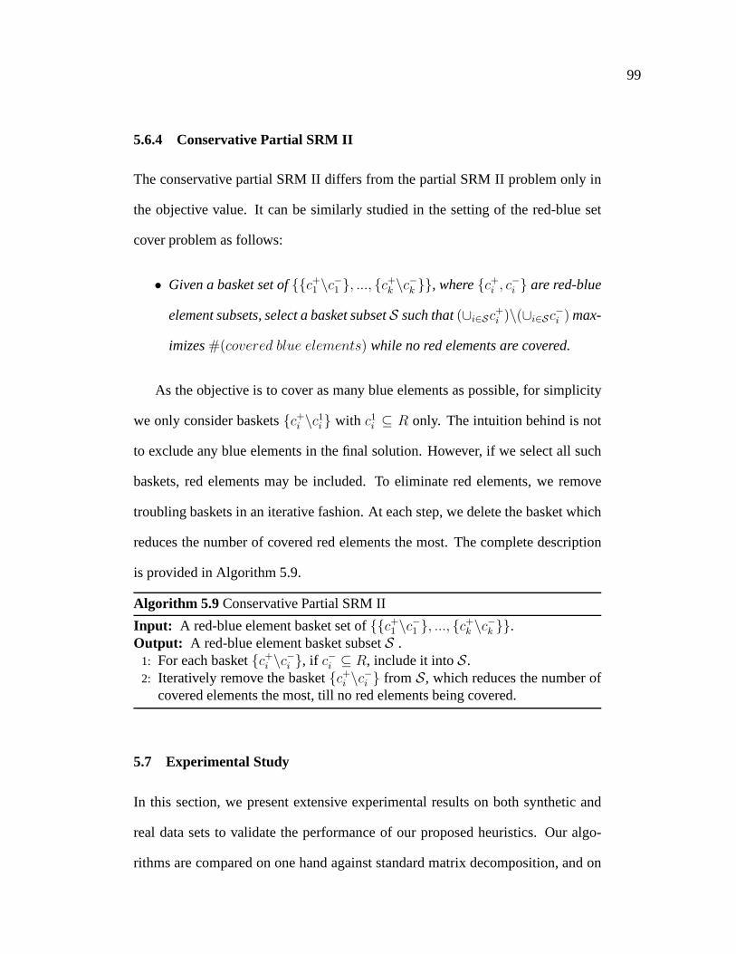
99
5.6.4 Conservative Partial SRM II
The conservative partial SRM II differs from the partial SRMII problem only in
the objective value. It can be similarly studied in the setting of the red-blue set
cover problem as follows:
• Given a basket set of{{c+1 \c
−1 }, ..., {c
+k \c
−k }}, where{c+
i , c−i } are red-blue
element subsets, select a basket subsetS such that(∪i∈Sc+i )\(∪i∈Sc−i ) max-
imizes#(covered blue elements) while no red elements are covered.
As the objective is to cover as many blue elements as possible, for simplicity
we only consider baskets{c+i \c
1i } with c1
i ⊆ R only. The intuition behind is not
to exclude any blue elements in the final solution. However, if we select all such
baskets, red elements may be included. To eliminate red elements, we remove
troubling baskets in an iterative fashion. At each step, we delete the basket which
reduces the number of covered red elements the most. The complete description
is provided in Algorithm 5.9.
Algorithm 5.9 Conservative Partial SRM II
Input: A red-blue element basket set of{{c+1 \c
−1 }, ..., {c
+k \c
−k }}.
Output: A red-blue element basket subsetS .1: For each basket{c+
i \c−i }, if c−i ⊆ R, include it intoS.
2: Iteratively remove the basket{c+i \c
−i } from S, which reduces the number of
covered elements the most, till no red elements being covered.
5.7 Experimental Study
In this section, we present extensive experimental resultson both synthetic and
real data sets to validate the performance of our proposed heuristics. Our algo-
rithms are compared on one hand against standard matrix decomposition, and on

100
the other hand against conventional Boolean matrix decomposition. The algo-
rithm computing standard matrix decomposition isSV D, which is a benchmark
for computing standard matrix decomposition. As SVD returns results of real val-
ues, to be fair, we round them to be binary by setting all values less than 0.5 to
0, and all other values to 1. Hence, this algorithm is called SVD 0/1. The algo-
rithm computing conventional Boolean matrix decomposition is the Loc& IterX
algorithm proposed in [48], which has been experimentally proven to have better
performance than other Boolean matrix decomposition algorithms.
5.7.1 Synthetic Data
We study the behavior of the heuristics with respect to the decomposition size and
noise.
The synthetic data is generated as follows. First, generatek Boolean vectors
randomly as basis, each of which has 50 elements and about 1/3elements are
1. Second, use basis vectors to generate other100 − k vectors. The detailed
procedures are : (i) randomly selectingk/3 basis vectors; (ii) randomly assigning
half selected basis vectors toC1 and the other half toC2; (iii) computing∪C1\∪C2
as a generated vector. The size of such a generated matrix is50× 100. After that,
add noise to the matrix by randomly flipping the values of a given fraction of the
data.
To compare reconstruction error, we use two kinds of measure. The first is
ER1 = ||A − A′||1/size(A), whereA is the input matrix andA′ is the recon-
structed matrix. The second isER2 = ||A − A′||1/||A||1. ER1 reflects how
much fraction of the data is not correctly reconstructed.ER2 is to compare the

101
amount of reconstruction error against the total number of 1’s cells. The reason
of employingER2 is that if the input Boolean matrix is sparse, a low value of
ER1 does not demonstrate the input matrix is correctly reconstructed, as simply
returning a matrix of zeros would have a low value ofER1.
The first experiment is to test the effect of sizek with respect to reconstruction
error. We varyk from 4 to 20 and for each size we generate 5 matrices. Reported
results are mean values over these five matrices. For algorithms of Loc&IterX,
EBMD and 0-1 error free EBMD we use basis vectors asC.
5 10 15 200
0.2
0.4
0.6
0.8
1
k
ER
1
EBMD0−1 Error Free EBMDLoc & IterXSVD 0/1
Figure 5.7. Reconstruction Error Ratio withER1 w.r.t. k
5 10 15 200
0.1
0.2
k
ER
2
EBMD0−1 Error Free EBMDLoc & IterXSVD 0/1
Figure 5.8. Reconstruction Error Ratio withER1 w.r.t. k
The experimental results are as shown in Figures 5.7 and 5.8.As we can see,
the reconstruction error ratios of all three EBMD approaches are lower than those
of Loc&IterX and close to those of SVD 0/1. WithER1, the reconstruction error

102
ratios of EBMD approaches are as low as 0.05 on average. WithER2, they are
still as low as 0.2 on average.
The second experiment is to test the effect of noise with respect to reconstruc-
tion error. We vary noise ratio from 0 to 0.5. The experimental results are as
shown in Figures 5.9 and 5.10. The reconstruction error ratios of EBMD and 1-0
error free EBMD are still lower than those of Loc&IterX and close to SVD 0/1.
However, the reconstruction error ratios of 0-1 error free EBMD are much higher
than other approaches even though the amount of noise is little.
0 0.1 0.2 0.3 0.40
0.1
0.2
0.3
0.4
0.5
Noise Ratio
ER
1
EBMD0−1 Error Free EBMDLoc & IterXSVD 0/1
Figure 5.9. Factorization Cost w.r.t. Reconstruction Error Ratio for SyntheticData
0 0.1 0.2 0.3 0.40
0.5
1
1.5
2
2.5
Noise Ratio
ER
2
EBMD0−1 Error Free EBMDLoc & IterXSVD 0/1
Figure 5.10. Factorization Cost w.r.t. Reconstruction Error Ratio for SyntheticData

103
5.7.2 Real Data
One of our main contributions that we claim is that our heuristic algorithm can
decompose a Boolean matrix with much less reconstruction error than the con-
ventional Boolean matrix decomposition method. In this section, we demonstrate
that the claim holds for real data as well.
Four real data sets are used. The News data set is a subset of 20Newsgroups
dataset1. We select the first 400 messages and the top frequent 100 words in them,
and replace the counts with 1 or 0. Then, we obtain a100 × 400 matrix, which
happens to have no repetitive columns. Votes dataset2 contains plenary votes of
Finnish Parliament. Same as [48], we only consider those MPsthat served an
entire term. During 1999-2001, there were 773 plenary votesand 196 MPs served
the entire term. As an MP can cast four different types of votes (yea, Nay, Abstain,
and Absent), two different dataset are actually used: VotesYes sets Yeas as 1s and
all other votes are 0s, while VotesNo sets Nays as 1’s and all other votes as 0’s.
The Query data set is a user/clicked URL binary matrix, extracted from a large-
scale query log. The query log data include two important attributes, UserID (the
identity query issuer), and ClickedURL (the URL eventuallyclicked by that user
in that single query). We have first selected the top 40 frequent clicked URLs
from the query log with 1,889,761 queries in total and removed all the queries
that are not related to those 40 Clicked URLs (we thus obtain 196,218 queries
with 40 clicked URLs). Consequently, we have generated another dimension of
the matrix by choosing the top 1000 users who have executed most queries in this
1http://people.csail.mit.edu/jrennie/20Newsgroups/2http://www.fsd.uta.fi/english/data/cagalogue/FSD2117/meF2117e.html

104
Data k EBMD 0-1 EBMD Loc& IterX SVD 0/1News 5 0.2575 0.3966 0.2811 0.2085
10 0.2350 0.3791 0.2633 0.175015 0.2200 0.3647 0.2397 0.1457
VotesNo 5 0.0777 0.1921 0.0830 0.064210 0.0704 0.1860 0.0763 0.049615 0.0684 0.1755 0.0722 0.0398
VotesYes 5 0.1531 0.6491 0.1613 0.077910 0.1334 0.6421 0.1459 0.092915 0.1244 0.6320 0.1336 0.0775
Query 5 0.1162 0.1220 0.1168 0.089210 0.0921 0.0974 0.1071 0.053615 0.0710 0.0812 0.1451 0.0301
Table 5.1. Reconstruction Error Ratios withER1 for real datasets
small group of query log. The result is a binary matrix with the dimension of
40*1000. After deleting repetitive columns, finally we havea matrix of40× 200.
The experimental results are shown in Tables 5.1 and 5.2. We can see that the
heuristic of EBMD decomposes real datasets with less reconstruction errors than
Loc&IterX and close to SVD 0/1, while decomposition solutions provided by the
heuristics for 0-1 EBMD have higher reconstruction error ratios.

105
Data k EBMD 0-1 EBMD Loc& IterX SVD 0/1News 5 0.6154 0.9477 0.6718 0.4982
10 0.5616 0.9058 0.6293 0.418115 0.5258 0.8714 0.5728 0.3482
VotesNo 5 0.3829 0.9464 0.4091 0.316110 0.3471 0.9164 0.3761 0.244515 0.3368 0.8647 0.3557 0.1963
VotesYes 5 0.2311 0.9799 0.2435 0.117610 0.2014 0.9692 0.2203 0.140315 0.1878 0.9540 0.2017 0.1170
Query 5 0.6961 0.7305 0.6992 0.534010 0.5516 0.5831 0.6415 0.321115 0.4251 0.4865 0.4925 0.1804
Table 5.2. Reconstruction Error Ratios withER2 for real datasets

106
CHAPTER 6
RANK-ONE BOOLEAN MATRIX DECOMPOSITION
Rank-one Boolean matrix decomposition is a special BMD case, where the de-
composed matrices are limited to Boolean vectors. Mathematically speaking, it
is to decompose a Boolean matrixAm×n into the product ofXm×1 ⊗ C1×n. One
important application of BMD is to mine discrete patterns inbinary data, which
is important for many data analysis tasks, such as data sampling, compression,
and clustering. An example is that replacing individual records with their patterns
would greatly reduce data size and simplify subsequent dataanalysis tasks. As
a straightforward approach, rank-one binary matrix approximation has been ac-
tively studied recently for mining discrete patterns from binary data. It factorizes
a binary matrix into the multiplication of one binary pattern vector and one binary
presence vector, while minimizing mismatching entries.
However, this approach suffers from two serious problems. First, if all records
are replaced with their respective patterns, the noise could make as much as 50%
in the resulting approximate data. This is because the approach simply assumes
that a pattern is present in a record as long as their matchingentries are more
than their mismatching entries. Second, two error types, 1-becoming-0 and 0-
becoming-1, are treated evenly, while in many application domains they are dis-
criminated. To address the two issues, we propose weighted rank-one binary ma-
107
trix approximation. It enables the tradeoff between the accuracy and succinctness
in approximate data and allows users to impose their personal preferences on the
importance of different error types.
In this section, we will study weighted rank-one BMD. Its decision problem
will be proved to be NP-complete. To solve it, several different mathematical pro-
gramming formulations are provided, from which 2-approximation algorithms are
derived for some special cases. An adaptive tabu search heuristic is presented for
solving the general problem, and our experimental study shows the effectiveness
of the heuristic.
6.1 Motivation of Weighted Rank-One BMD
With the fast development of computer and internet technologies and the de-
creased cost of data storage devices, a large volume of data are generated and
gathered every day. Many datasets have discrete attributes, such as those gener-
ated from information retrieval, bio-informatics, and market transactions. Much
attention has been focused on efficient techniques for analyzing large and high
dimensional datasets. Common tasks for analyzing high dimensional data in-
clude extracting correlations between data items, classification, and clustering
data items and finding condensed representations. The analysis of large-scale
datasets commonly has to deal with the curse of dimensionality. A useful ap-
proach is to compress datasets while preserving important underlying patterns.
Conventional matrix factorization techniques can effectively and efficiently com-
press datasets with continuous attributes. For example, singular value decompo-
sition (SVD) can efficiently reduce a given matrix into a low-rank matrix while

108
minimizing the Frobenius norm of the difference. However, result interpretation
is difficult for datasets with discrete attributes.
Existing techniques for mining discrete patterns from binary data include PROX-
IMUS [34], which can serve the purpose of data compression aswell. The idea is
to decomposes a given binary matrix into a pattern vector anda presence vector,
which are restricted to be binary, such that the multiplication of two decomposed
vectors has the least mismatching entries with the originalbinary matrix. It is
also calledrank-one binary matrix approximation. Given the presence vector, the
matrix is partitioned into two parts. The part with the presence of the pattern is
grouped together. By recursively applying the same process, all row vectors are
clustered and their respective patterns are identified. Thetask of analyzing the
original binary matrix can be switched on those mined patterns, which have much
smaller size. This technique has received increased attention recently [35, 59].
For example, Shen et al. [59] even provide an efficient 2-approximation algorithm
for rank-one binary matrix approximation recursively conducted in a process of
PROXIMUS.
Rank-one binary matrix approximation is to solveminX,Y ||A − XY T ||F ,
whereX andY are binary vectors and called presence vector and pattern vec-
tor respectively. Based on entry values ofX, rows ofA can be divided into two
parts. The part associated with entries with the value of 1 inX are considered
having patternY . By recursively applying rank-one binary matrix approximation,
a collection of discrete patterns are mined, which can be utilized to approximate
the original data and cluster row vectors.

109
Example 6.1 Given a matrixA, a rank-one approximation is computed as fol-
lows:
A =
1 0 1 1 01 1 1 1 10 0 1 0 01 1 1 1 0
≈
1101
(
1 1 1 1 0)
= XY T . (6.1)
The discrete pattern mining approach based on rank-one approximation is
straightforward and not difficult to implement. However, itsuffers from two seri-
ous issues.
The first issue is that according to the objective functionminX,Y ||A−XY T ||F ,
a row vectorAi:, denoting theith row of A, is considered having patternY as
long as their matching components are greater than mismatching components. In
other words, the mismatching ratio could be nearly as much asfifty percent. As
a result, the final collection of mined discreet patterns cannot serve as a good
approximation to the original data matrix and all subsequent data analysis results
would be questionable. To illustrate it, we give Example 6.2. Clearly rank-one
binary matrix approximation is not able to divide row vectors of the binary matrix
on the left side of Equation (3). As a result, rank-one binarymatrix approximation
is only able to identify one discrete pattern, while there are two obvious discrete
patterns in the original data. Furthermore, the mined pattern {1, 1, 1, 1, 0} can
hardly represent row vector{0, 1, 1, 1, 1}, as their matching entries are only one
more than mismatching entries.
Example 6.2 The rank-one binary matrix approximation for a binary matrix with

110
two obvious patterns is computed as below:
1 1 1 1 01 1 1 1 01 1 1 1 00 1 1 1 10 1 1 1 1
≈
11111
(
1 1 1 1 0)
. (6.2)
The second issue with rank-one binary matrix approximationis that it does not
support discrimination on 1-becoming-0 errors and 0-becoming-1 errors, which
however is requested by many applications. To illustrate it, we give Example 3.
With (1, 1, 1, 1, 0) as the pattern to approximate all row vectors, it introducesone
0-becoming-1 error to the first row vector and one 1-becoming-0 error to the third
row vector. For the role mining problem arising from implementing role-based
access control [42], the value of 1 in a binary matrix represents a permission
assignment. Analyzing an approximate user-to-permissionmatrix with many 0-
becoming-1 errors would generate roles with surplus permissions, which seriously
affect system security and safety. In this application, 0-becoming-1 errors should
be forbidden.
Example 6.3 Consider the following rank-one approximation:
1 1 1 1 11 1 1 1 01 1 1 0 0
≈
111
(
1 1 1 1 0)
. (6.3)
6.2 Weighted Rank-One Binary Matrix Approximation
Desired features of a discrete pattern mining technique should include allowing
the trade-off between the approximation accuracy and the simplicity of mined

111
patterns, and enabling users to impose their preferences onthe error type distri-
bution. We achieve them by proposing a new measure on the significance of a
pattern in a row vector and a new definition of pattern presence. They are defined
as below.
Definition 6.1 (Pattern Significance) The significance of a patternY ∈ {0, 1}1×n
in an objectA ∈ {0, 1}1×n denoted byS(Y, A), is measured by
S(Y, A) = max{0, f11(Y, A)− w1f10(Y, A)− w2f01(Y, A)}
wherefij(Y, A) is the number of attributes which arei in Y and j in A, andw1
andw2 are positive weight parameters.
Definition 6.2 (Pattern Presence) If S(Y, A) > 0, the patternY ∈ {0, 1}1×n is
considered present in the objectA ∈ {0, 1}1×n.
Weight parametersw1 andw2 have two purposes. First, the sum value ofw1
andw2 can be utilized to control the level of error tolerance, in other words ap-
proximation accuracy. The greater sum value leads to less error tolerance, hence
higher accuracy in approximation. The ratio betweenw1 andw2 reflects the pref-
erences on two error types. The greater weight means being more disliked.
The essential goal of rank-one binary matrix approximationis to discover a
pattern with the most significance in the data matrix. We callsuch a patterndom-
inant discrete pattern. Weighted rank-one binary matrix approximationis to take
penalty weights into account at the basis of conventional rank-one matrix approx-
imation. Whenw1 = 1 andw2 = 1, the weighted problem is the same as the

112
conventional problem. Given a patternY , it is easy to determine presence vector
X even with the presence of penalty weights. So instead of looking for the pair of
X andY at the same time, we consider weighted rank-one binary matrix approx-
imation as the dominant discrete pattern mining problem defined as following.
Definition 6.3 (Dominant Discrete Pattern Mining) Givenm objects consisting
ofn binary attributes represented by a matrixA ∈ {0, 1}m×n, find a dominant pat-
ternY ∈ {0, 1}1×n, such that its total values of pattern significance∑
i S(Y, Ai:)
are maximized, whereAi: denotes theith row vector ofA.
Two following examples are illustrated to show how weightedrank-one binary
matrix approximation can effectively address the two issues with rank-one binary
matrix approximation.
Example 6.4 Reconsider the binary matrix in Example 6.2. By lettingw1 = w2 =
2, its weighted rank-one binary matrix approximation, wherethe vector on the
right side is the dominant discrete pattern, is as below:
1 1 1 1 01 1 1 1 01 1 1 1 00 1 1 1 10 1 1 1 1
≈
11100
(
1 1 1 1 0)
. (6.4)
In the above example, by doubly penalizing errors, row vectors are successfully
divided and{1, 1, 1, 1, 0} is indeed a true pattern for rows associated with the
presence vector. By applying weighted rank-one binary matrix approximation to
the other part, pattern{0, 1, 1, 1, 1} is also successfully revealed.

113
Example 6.5 Look at the binary matrix in Example 6.3. By lettingw1 = 1 and
w2 = 3, its weighted rank-one binary matrix approximation is as below:
1 1 1 1 11 1 1 1 01 1 1 0 0
≈
111
(
1 1 1 0 0)
. (6.5)
It is free of 1-becoming-0 errors.
Due to the binary data type, each row can be represented as a subset ofn
attributes. Such a representation provides a convenient way to describe some
relationships between two binary row vectors which we will utilize later. They
are defined as following.
Definition 6.4 (Superset, Strict Superset, Subset, and Strict Subset) For two bi-
naryn-dimensional row vectorsX andY , if Yi = 1, ∀Xi = 1 , Y is a superset of
X andX is a subset ofY . If Y is superset ofX and there existsi such thatYi = 1
andXi = 0, Y is a strict superset ofX, whileX is a strict subset ofY .
6.3 Relation with Other Existing Problems
The dominant discrete pattern mining problem can be relatedto many research
problems that have been studied in the literature. Those problems can be viewed
as either its special case or its variant.
Definition 6.5 (Maximum Edge Biclique Problem[53]) Given a bipartite graph
G = (V1∪V2, E) and a positive integerK, doesG contain a biclique with at least
k edges?

114
A bicilique is a kind of bipartite graph where every vertex ofthe first set is con-
nected to every vertex of the second set. The maximum edge biclique problem
defined as above is a special case of the dominant discrete pattern mining problem
whenw1 is 0 andw2 is greater than the maximal number of 1’s entries in a row of
A, denoted bymaxi||Ai:||1. With w1 being 0,f10(Y, Ai:) is not counted in the pat-
tern significance formula ofS(Y, Ai:). With w2 being greater thanmaxi||Ai:||1,
a patternY can never be present in a row vectorAi:, which is an exact subset of
Ai:. Therefore the dominant discrete pattern mining problem with w1 = 0 and
w2 ≥ maxi||Ai:||1 is to find a patternY which covers the most 1’s entries in row
vectors ofA, which are supersets ofY . Any binary matrixAm×n can be expressed
as an equivalent bipartite graphG = (V1 ∪ V2, E), whereV1 hasm vertices corre-
sponding to all rows ,V2 hasn vertices corresponding to all attributes, and there
is an edge connecting verticesV1(i) andV2(j) if Ai,j = 1. As a 1’s entry inA cor-
responds to an edge in its equivalent bipartite graph, a dominant discrete pattern
with w1 = 0 andw2 ≥ maxi||Ai:||1 induces a maximum edge biclique.
For illustration, consider the binary matrix in Equation (6.1) as an example.
It can be expressed as the bipartite graph in Figure 6.1a. Itsdominant discrete
pattern withw1 = 0 andw2 greater thann is given as in Equation (6.6) and its
induced biclique is as shown in Figure6.1b.
1 0 1 1 01 1 1 1 10 0 1 0 01 1 1 1 0
≈
0101
×(
1 1 1 1 0)
. (6.6)
Definition 6.6 (Maximum Tile [19]) Given a databaseD as a binary matrix
Am×n, find the tile with the largest area inD, where a tile corresponds to a row

115
(a) (b)
Figure 6.1. A Bipartite Graph and Its maximum Edge Biclique
index subsetR and a column index setC, such thatA(i, j) = 1, ∀i ∈ R, j ∈ C .
The maximum tile problem defined as above is essentially to find the largest
tile full of 1’s entries in a binary matrix, allowing the manipulation on the order
of rows and columns. It is equivalent to the maximum edge clique problem, and
hence equivalent to the dominant discrete pattern problem with w1 = 0 andw2 ≥
maxi||Ai:||1.
Consider the binary matrix on the left side of Equation (6.6)as a tiling database.
The largest tile induced by the dominant discrete pattern isas shown in Equation
(6.7).
1 0 1 1 0
1 1 1 1 1
0 0 1 0 0
1 1 1 1 0
(6.7)
Definition 6.7 (Maximum Edge Weight Biclique Problem[43]) Given a bipar-
tite graph{V1 ∪ V2, E} and weights{wij} associated with edges{(V1(i), V2(j))}
respectively, find a bicliqueC, where the sum of the edge weights is maximum.

116
The dominant discrete pattern problem withw1 andw2 being equal can be
mapped to a special case of the maximum edge weight biclique problem. The
maximum edge weight biclique problem is to find a biclique with the maximum
weight from a complete bipartite graph. As we have illustrated, any binary matrix
Am×n can be expressed as a bipartite graphG(V1 ∪ V2, E). We can further ex-
pand it as a weighted complete bipartite graph. First complete all missing edges
to make it as a complete graph. Then assign a weight of 1 to all edges in the
original bipartite graph and a negative weight of−w1 to the newly added edges.
A dominant discrete pattern in the original binary matrix would correspond to a
maximum weight biclique in the constructed weighted complete bipartite graph.
For illustration, reconsider the binary matrix in Equation(6.1). Its correspond-
ing maximum edge weight biclique problem instance is as shown in Figure 6.2,
where dashed lines are original edges with the weight of 1 andthick lines are
added edges with the weight of−w1.
Figure 6.2. Edge-Weighted Complete Bipartite Graph

117
6.4 Mathematical Programming Formulation
The main result of this section is to present mathematical programming formula-
tions for the dominant discrete pattern mining problem. In particular, we give an
unconstrained quadratic binary programming formulation,an integer linear pro-
gramming formulation, and a relaxed linear programming formulation, which for
the case ofw1 = w2 = 1 induces a 2-approximate algorithm.
6.4.1 Unconstrained Quadratic Binary Programming
The dominant discrete pattern mining problem is to find the patternY maximizing
the global pattern significance∑
i S(Y, Ai:) for a given binary matrixA. Its cor-
responding presence vectorX can be obtained easily after the dominant discrete
patternY is found. But in the quadratic binary programming formulation given as
below, we treat presence vectorX as variables along with pattern vectorY .
∑
i S(Y, Ai:)
=∑
i max{0, f11(Y, Ai:)− w1f10(Y, Ai:)− w2f01(Y, Ai:)}
=∑
i Xi(f11(Y, Ai:)− w1f10(Y, Ai:)− w2f01(Y, Ai:))
=∑
i Xi(∑
j AijYj − w1
∑
j(1− Aij)Yj
−w2
∑
j Aij(1− Yj))
=∑
ij(Aij + w1Aij + w2Aij − w1)XiYj −∑
ij w2AijXi
= XT UY −XT V~1
(6.8)
whereU is defined asUij = Aij + w1Aij + w2Aij − w1, Vij is defined asw2Aij ,
and~1 denotes the all-ones vector.
The explanation of the above equation deduction process is as follows: (i) The

118
first induction step is obvious; (ii) The second induction step is by the fact that if
f11(Y, Ai:)−w1f10(Y, Ai:)−w2f01(Y, Ai:) ≤ 0, Xi = 0; (iii) In the third induction
step,f11(Y, Ai:) counting the number of attributes whereY andAi: both are 1 is
measured by∑
j AijYj, andf10(Y, Ai:) andf01(Y, Ai:) are by(1 − Aij)Yj and
Aij(1 − Yj) respectively; (iv) The last induction step arranges the whole formula
as matrix multiplications.
Therefore the dominant discrete pattern mining problem canbe simplified
as an unconstrained binary quadratic programming problem as max{XT UY −
XT V~1|X ∈ {0, 1}m, Y ∈ {0, 1}n}. A binary matrix is closely related to a bipar-
tite graph. It is also a useful approach for problems involved with a bipartite graph
to be formulated as an unconstrained quadratic binary programming problem [4].
6.4.2 Integer Linear Programming
The unconstrained quadratic binary programming formulation can be linearized as
an integer linear programming problem by introducing auxiliary binary variables
{Zij} as below.
max∑
ij
UijZij −∑
ij
VijXi
s.t.
−Xi − Yj + 2Zij ≤ 0 ∀i, j
Xi + Yj − Zij ≤ 1 ∀i, j
Xi, Yj, Zij ∈ {0, 1}
.
(6.9)
The linearization is done by replacingXiYj with Zij . As the value ofXiYj can
only be either 0 or 1, soZij is binary. Constraints−Xi − Yj + 2Zij ≤ 0 and
Xi + Yj − Zij ≤ 1 guarantee: (i)Zij = 1 when bothXi andYj are 1; (ii)Zij = 0
when one ofXi andYj is 0.
The linearization skill of replacingXiYj with a binary variableZij is also em-
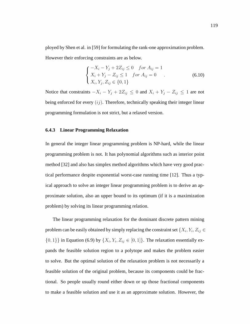
119
ployed by Shen et al. in [59] for formulating the rank-one approximation problem.
However their enforcing constraints are as below.
−Xi − Yj + 2Zij ≤ 0 for Aij = 1
Xi + Yj − Zij ≤ 1 for Aij = 0
Xi, Yj, Zij ∈ {0, 1}
. (6.10)
Notice that constraints−Xi − Yj + 2Zij ≤ 0 andXi + Yj − Zij ≤ 1 are not
being enforced for every(ij). Therefore, technically speaking their integer linear
programming formulation is not strict, but a relaxed version.
6.4.3 Linear Programming Relaxation
In general the integer linear programming problem is NP-hard, while the linear
programming problem is not. It has polynomial algorithms such as interior point
method [32] and also has simplex method algorithms which have very good prac-
tical performance despite exponential worst-case runningtime [12]. Thus a typ-
ical approach to solve an integer linear programming problem is to derive an ap-
proximate solution, also an upper bound to its optimum (if itis a maximization
problem) by solving its linear programming relation.
The linear programming relaxation for the dominant discrete pattern mining
problem can be easily obtained by simply replacing the constraint set{Xi, Yi, Zij ∈
{0, 1}} in Equation (6.9) by{Xi, Yi, Zij ∈ [0, 1]}. The relaxation essentially ex-
pands the feasible solution region to a polytope and makes the problem easier
to solve. But the optimal solution of the relaxation problemis not necessarily a
feasible solution of the original problem, because its components could be frac-
tional. So people usually round either down or up those fractional components
to make a feasible solution and use it as an approximate solution. However, the

120
approximation ratio is not guaranteed.
As we mentioned earlier, the integer programming formulation for the rank-
one approximation problem provided by Shen et al. in [59] is not a strict for-
mulation, but a relaxed version. However, such a relaxed integer programming
formulation surprisingly leads to a 2-approximation algorithm via simplex meth-
ods. We may directly apply their approach to our problem. Accordingly a new
linear programming relaxation for Equation (6.11) is givenas below.
max∑
ij
UijZij −∑
ij
VijXi
s.t.
−Xi − Yj + 2Zij ≤ 0 for Aij = 1
Xi + Yj − Zij ≤ 1 for Aij = 0
Xi, Yj, Zij ∈ [0, 1]
.
(6.11)
Theorem 6.1 The optimal solution of Equation (6.11) via simplex algorithms is
integral, in other words a feasible solution of Equation (6.9).
Proof. As Equation (6.11) has the same constraints as the linear programming re-
laxation problem studied in [59], the same result holds thatthe coefficient matrix
of the inequality constraint set is a totally unimodular matrix. A totally unimod-
ular matrix is a matrix for which the determinant of every square non-singular
submatrix is 1 or -1. All parameters on the right side of inequalities are also in-
tegral. Two properties lead to that the optimal solution of Equation (6.11) via
a simplex algorithm is integral. The reason is as following.A simplex method
is searching from one basic feasible solution to another basic feasible solution
till the optimum is reached. Suppose the constraint set has astandard form as
{AX = b, X ≥ 0}, to which any linear constraint set can be transformed. A

121
basic feasible solution is corresponding to a partition{XB, XN} of variablesX
and accordingly the constraint set can be reformed asBXB + NXN = b. By
lettingXN = 0, XB = B−1b. If B−1b > 0, {B−1b, 0} is a basic feasible solution.
According to the Cramer’s rule [22], theith competent ofXB is det(B′)det(B)
, where
det(B) denotes the determinant ofB, B′ is B except itsith column is replaced
by b. Because in Equation (6.11) the coefficient matrix of the constraint set is
totally unimodular, the determinant of every square non-singular submatrix is 1 or
-1. Hence the denominator ofdet(B′)det(B)
is 1 or -1. Since all parameters in Equation
(6.11) is integral, the nominator ofdet(B′)det(B)
is also integral. Thus every component
of any basic feasible solution of Equation (6.11) via a simplex algorithm is inte-
gral, and the optimal solution of the relaxation problem is afeasible solution of
its original problem.
Our proof is built on the basis of the proof given by Shen et al.[59]. But in
addition to pointing out the existence of two sufficient conditions that a totally
unimodular coefficient matrix and all integral parameters,we provide a deep in-
sight on why those two conditions make all basic feasible solutions via a simplex
algorithm integral.
Unfortunately, one cannot prove that the optimal solution of Equation (6.11) is
2-approximate to the optimal solution of Equation (6.9). Weconjecture that they
are at least very close. More importantly the optimal solution of Equation (6.11)
is a feasible solution of Equation (6.9). The problem of finding a feasible solution
of a system of inequalities in integers in general is NP-complete. Many good
heuristics for complex combinatorial optimization problems are starting from a
feasible solution and then iteratively improving the current solution by certain

122
rules. A good starting feasible solution such as the optimalsolution of Equation
(6.11) could save much computing time.
6.5 Computational Complexity and Approximation Algorithm
The main result of this section is to prove that the decision problem of dominant
discrete pattern mining is NP-complete and present 2-approximation algorithms
to some special cases of the dominant discrete pattern mining problem.
6.5.1 Computational Complexity
We prove NP-completeness of the decision problem of dominant discrete pattern
mining by a reduction from the decision maximum edge biclique problem.
Lemma 6.1 The decision maximum edge biclique problem is NP-complete [53].
Theorem 6.2 The decision problem of dominant discrete pattern mining isNP-
complete.
Proof. The decision problem of dominant discrete pattern mining isgiven a bi-
nary matrixAm×n and a valueδ to determine if there is a patternY such that∑
j S(Ai:, Y ) ≥ δ. Given a dominant discrete patternY , it is easy to determine
whether the instance is true. Thus the decision problem of dominant discrete pat-
tern mining belongs to NP. In the previous section, we showedthat the dominant
discrete pattern mining problem is a generalization of the maximum edge biclique
problem, the decision version of which is NP-complete. Therefore, the decision
problem of dominant discrete pattern mining is NP-complete.

123
6.5.2 Approximation Algorithm
We will study three special cases of the dominant discrete pattern mining prob-
lem and present approximation algorithms for them. Before doing that, we first
introduce a result.
Lemma 6.2 Any integer linear programming problem withn variables subject
to m linear constraints with at most two variables per inequality, and with all
variables bounded between 0 andU , has a 2-approximation algorithm which runs
in polynomial timeO(mnU2log(Un2m)) [26].
Hochaum et al. in [26] present a 2-approximation algorithm for integer linear
programs with at most two variables per inequality. We briefly introduce this
algorithm here. It transforms the integer program into a monotone integer system
first 1, computes an optimal solution for it, and then modifies the result via some
simple rule to obtain a feasible solution to the original problem, which is also a
2-approximate solution.
Case 1:w1 = 1 andw2 ≥ T whereT is the maximal number of entries with
the value of 1 in a row ofA.
As we have shown in the preceding section, the dominant discrete pattern min-
ing problem withw1 = 1 andw2 ≥ T is equivalent to the maximum edge biclique
problem. Hochbaun in [25] gives a linear programming formulation for the edge
weighted biclique problem which is to delete from a bipartite graph{V1, V2, E},
1For the definition of a monotone integer system, refer to the paper [24].

124
a minimum weight collection of edges so that the remaining edges induce a com-
plete bipartite graph. By slight modifications, we obtain a linear programming
formulation for our special case as below.
max∑
Aij=1
Zij
s.t.
2Zij − (Xi + Yj) ≤ 0, for Aij = 1
Xi + Yj ≤ 1, for Aij = 0
Xi, Yj, Zij ∈ {0, 1}
.
(6.12)
Becausew2 ≥ T , XY T cannot cover 1’s entries inA. In other wordsXiYj = 0
if Aij = 0, which is guaranteed by the constraint set{Xi +Yj ≤ 1, for Aij = 0}.
The objective function∑
Aij=1 Zij counts(i, j) such that bothAij andZij are 1.
Zij can be 1 if and only if bothXi andYj are 1, which is guaranteed by the first
constraint set{2Zij − (Xi + Yj) ≤ 0, for Aij = 1}.
The constraint of2Zij − (Xi + Yj) ≤ 0 can be spit into two equivalent con-
straintsZij−Xi ≤ 0 andZij−Yj ≤ 0. The similar skill is also used in [25]. Then
Equation (6.12) can be put in the form with at most two variables per inequality
as below.
max∑
Aij=1
Zij
s.t.
Zij −Xi ≤ 0, for Aij = 1
Zij − Yj ≤ 0, for Aij = 1
Xi + Yj ≤ 1, for Aij = 0
Xi, Yj, Zij ∈ {0, 1}
.
(6.13)
It naturally leads to the following theorem.
Theorem 6.3 The dominant discrete pattern mining problem withw1 = 1 and

125
w2 ≥ T is 2-approximable.
Case 2:w1 ≥ T whereT is the maximal number of entries with the value of 1
in a row ofA.
w1 ≥ T enforces that a patternY can only be present in its subset. In the pre-
ceding section, we have shown that the dominant discrete pattern mining problem
with w1 ≥ T is equivalent to finding a maximum weight biclique from a com-
plete weighted bipartite graph. In which, the weight for theedges corresponding
to entries with the value of 1 inA is 1 and the weight for the other edges is−w1.
It is a special case of the edge weighted biclique problem studied in [25]. Again
by modifying the linear programming formulation for the edge weighted biclique
problem provided in [25], we obtain a linear programming formulation for our
problem as below.
max∑
Aij=1
Zij −∑
Aij=0
w2Zij
s.t.
Zij −Xi ≤ 0
Zij − Yj ≤ 0
Xi, Yj, Zij ∈ {0, 1}
.
(6.14)
Equation (6.14) is similar to Equation (6.13), except that:(i) the constraint set
of Xi+Yj ≤ 1, for Aij = 0 is deleted because it is not necessary, and the weights
of {Zij} are replaced with 1 and−w2 accordingly. Every inequality constraint of
Equation (6.14) has only two variables. Obviously the approximation algorithm
presented in [26] applies to it. We state it as below.
Theorem 6.4 The dominant discrete pattern mining problem withw1 ≥ T is 2-
approximable.

126
Case 3:w1 = 1 andw2 = 1.
The dominant discrete pattern mining problem withw1 = 1 andw2 = 1 is
equivalent to the rank-one approximation problem. A 2-approximation algorithm
via linear programming relaxation is proposed by Shen et al.in [59]. For simplic-
ity, we skip its details.
6.6 Adaptive Tabu Search Heuristic
A tabu search heuristic is presented for the dominant discrete pattern mining prob-
lem. For large-scale problems running time for mathematical programming is al-
ways an issue. A 2-approximation algorithm sometimes cannot produce satisfac-
tory results in practice. The dominant discrete pattern mining problem essentially
is a combinatorial optimization problem. For such type of problem heuristics
usually bring good practical performance. An iterative heuristic is employed for
the rank-one approximation problem by both [59] and [34]. Its basic idea is that
starting from a feasible solution of patternY and presence vectorX, alternatively
fixing one of them and then searching for the best solution of the counterpart till
both are stable. The only difference between [59] and [34] isthat in [59] instead
of a random starting solution the starting feasible solution is the optimal solution
of Equation (6.11), which is 2-approximate to the optimal solution of the origi-
nal problem. Their iterative heuristic can be viewed as a greedy heuristic, which
greedily picks a neighboring solution at each iteration. One drawback with greedy
heuristics is that it is easy to reach local optimums, and once reaching it the solu-
tion cannot be improved any more.
To address the local optimum issue, we present an adaptive tabu search heuris-

127
tic. Tabu search is a mathematical optimization method. It essentially belongs to
the class of local search techniques as well. But it enhancesthe performance of
a local search method by using memory structures. When a potential solution
has been determined, it is marked as ”taboo” so that the algorithm does not visit
that possibility repeatedly. In Section 6.4, we have shown that the dominant dis-
crete pattern mining problem can be formulated as an unconstrained quadratic bi-
nary program. In literature, tabu search has been successfully employed to solve
quadratic binary programming problems [21]. This is another reason why we
choose tabu search.
The dominant discrete pattern mining problem is given a binary matrix A to
maximize∑
i S(Ai:, Y ). It is easy to computeS(Ai:, Y ) onceY is determined.
The adaptive tabu search approach taken here is a modification of the adaptive
memory tabu search presented in [21]. The basic procedure ofour algorithm
is as following. It starts with an initial solution ofY and then goes through a
series of alternative constructive phases and destructivephases. In the constructive
phases, progressively set 0 components ofY to 1, while in the destructive phase,
progressively set 1 components ofY to 0. At each iteration, one component ofY
is chosen and its value is flipped.
A greedy rule would be choosing the component by changing which improves
the objective function the most. However, to avoid visitingsome solutions re-
peatedly, frequency and recency information is utilized. Frequency information
is aboutcritical solutionsencountered to date. A critical solution is the solution
at which the next move (either add 1 or drop 1) causes the objective function to
decrease. Such an event is called acritical event. Recency information is aboutk

128
span number of further steps after a critical eventspan∗ maximum value ofspanDir direction on changing the value ofspanpr penalty weight from the recency tabu listpf penalty weight from the frequency tabu list
IterCount count of total iterationsIterCount∗ maximum value ofIterCountIterSpan count of iterations at the current value ofspan
t scale parameter on the maximum value ofIterSpan
Table 6.1. Parameter Descriptions
Algorithm 6.10 Tabu Search Algorithm
Input: A, IterCount∗, pr, pf , span∗, t;Output: X, Y ;
1: Y =0, Ybest=0, IterCount=0, span=1, Dir=increase, Count=0,IterSpan=0;
2: while IterCount < IterCount∗ do3: Conduct the constructive phase;4: Conduct the transitive phase;5: Conduct the destructive phase;6: Conduct the transitive phase;7: end while
critical solutions recently visited. Two pieces of information are stored in two tabu
lists respectively. A greedy approach would stop at a critical event. But the tabu
search heuristic taken here would keep moving. The number offurther moving
steps is based onstrategic oscillation. Such a scheme would enable the solution
to step out some local optimums. The amplitude of oscillation, in other words
the number of further moving steps, is determined by a parameter, span. The
span parameter is fixed for a certain number of iterations andthen changed in a
systematic fashion. To manage the value ofspan, an additional transitive phase is
added between each constructive phase and each destructivephase. So technically
speaking the adaptive tabu search approach consists of three phases.

129
The general structure of the tabu search approach is as outlined in Algorithm
6.10. Parameter descriptions are provided in Table 6.1. Variablespan determines
the further steps that can be made after encountering a critical solution.span∗ is
an input parameter, limiting the maximum value ofspan. The value ofDir indi-
cates the direction of changing the value ofspan, either increasing or decreasing.
pr andpf are penalty weights on information derived from recency andfrequency
tabu lists respectively. Its usage will be elaborated later. VariableIterCount
counts the total iterations to date.IterCount∗ is an input parameter limiting the
maximum value ofIterCount and hence the algorithm runtime.IterSpan counts
iterations that have been made at the current value ofspan. t is an input scale pa-
rameter on the maximum value ofIterSpan. We explain it explicitly later. The
termination condition of Algorithm 6.10 is the total numberof iterations less than
IterCount∗. It could be replaced with a termination condition on the runtime. In
each loop, three phases are traversed in order.
6.6.1 Constructive Phase
In the constructive phase, we progressively pick a 0 component of Y and flip
it to 1. The intuitive component-picking policy is to choosethe component by
flipping which contributes the largest net increase to the objective function value∑
i S(Ai:, Y ). But we want to avoid repeatedly visiting some solutions. Tothis
end, two tabu lists are utilized to influence the search process. The recency tabu
list is a vector denoted byVr, which is the sum of the most recentk critical solu-
tions. At each critical event, it is updated as below:Vr = Vr + Y (current) −
Y (current − k), whereY (current) denotes the current critical solution and

130
Y (current− k) denotes the critical solution encountered beforek critical events.
The frequency tabu list is the sum of all critical solutions encountered so far. At
each critical event, it is updated as below:Vf = Vf + Y (current). To avoid re-
peatedly visiting some critical solutions, we give certainpenalty on a 0 component
which was 1 in recent critical solutions or was 1 frequently in the past critical so-
lutions. So the final evaluation on a 1 component at thejth position is determined
by the following measure:
f1(j) =∑
i S(Ai:, Y + ej)−∑
i S(Ai:, Y )−pr ∗ Vr(j)− pf ∗ Vf (j)
. (6.15)
In above,ej is a unit vector with thejth entry of 1,pr andpf are penalty weights,
andVr(j) andVf(j) are thejth entry ofVr andVf respectively.
The details of the constructive phase are as described in Algorithm 6.11. It
consists of two parts. The first part is to iteratively flip thecomponent which
maximizes the evaluation formula of Equation (6.15). The second part is to make
span more iterations after a critical event occurs.
6.6.2 Destructive Phase
In the destructive phase, we progressively pick a 1 component in Y and change it
to 0. The evaluation measure for component picking is as below. It is similar to
Equation (6.15) except that we add penalty terms.
f2(j) =∑
i S(Ai:, Y − ej)−∑
i S(Ai:, Y )+pr ∗ Vr(j) + pf ∗ Vf (j)
. (6.16)
The details of the destructive phase is as shown in Algorithm6.12. It is same
as Algorithm 6.11 except that the component picking rule is changed.

131
Algorithm 6.11 Constructive Phase
1: while |Y | < n do2: Find j′ maximizingf1(j) subject toY (j) = 0;3: if f1(j
′) > 0 then4: Y = Y + ej ;5: IterCount = IterCount + 1;6: UpdateYbest if necessary;7: end if8: end while9: while CountSpan ≤ span and|Y | > 0 do
10: j′ = argmaxY (j)=1(f2(j));11: if f1(j
′) ≤ 0 then12: UpdateVr andVf ;13: end if14: Y = Y + ej;15: CountSpan = CountSpan + 1;16: IterCount = IterCount + 1;17: UpdateYbest if necessary;18: end while19: CountSpan = 0;
6.6.3 Transitive Phase
If span is an unchanged constant, the constitutive phase and the destructive phase
constitute a complete tabu search algorithm. A largespan would enlarge the
search space at the expense of increasing runtime. But with asmall span the
algorithm might not be able to find a satisfactory solution. To address the issue,
adaptive tabu search adjusts the value ofspan in a systematic fashion. We fix
the value ofspan for a certain number of iterations and then increase it by 1.
Keep doing this untilspan reachesspan∗, the maximum value predefined. After
that, we gradually decrease the value ofspan by 1. Therefore, the value ofspan
will transverse back and forth between 1 andspan∗. The complete procedure of
transitive phase is as described in Algorithm 6.13.

132
Algorithm 6.12 Destructive Phase
1: while |Y | > 0 do2: Find j′ maximizingf2(j) subject toY (j) = 1.3: if f2(j
′) > 0 then4: Y = Y − ej ;5: IterCount = IterCount + 1;6: UpdateYbest if necessary;7: end if8: end while9: while CountSpan ≤ span and|Y | > 0 do
10: j′ = argmaxY (j)=1(f2(j));11: if f2(j
′) ≤ 0 then12: UpdateVr andVf ;13: end if14: Y = Y − ej ;15: CountSpan = CountSpan + 1;16: IterCount = IterCount + 1;17: UpdateYbest if necessary;18: end while19: CountSpan = 0;
6.7 Experiments
In this section, we illustrate the properties of weighted rank-one binary matrix
approximation by implementing it on synthetic data. The synthetic data are cre-
ated as following: (i) Generate eight random binary row vectors, such that each
vector is of size1 × 50 and has exactly50 ∗ ρ components of 1, whereρ is the
parameter determining data sparseness and within[0, 1]; (ii) Generate 200, 200,
150, 150, 100, 100, 50, and 50 copies respectively for each ofthe eight vectors,
and put them together to constitute a binary matrix with size1000 × 50. There-
fore the resultant binary matrix contains eight discrete patterns;(iii) Flip the value
for each cell in the binary matrix with probabilityρ ∗ ξ, whereξ is the parameter
determining noise ratio and is within[0, 1].

133
Algorithm 6.13 Transitive Phase
1: if Dir = increase then2: if span > span∗ then3: span = span∗;4: Dir = decrease;5: IterSpan = 0;6: else7: if IterSpan > t ∗ span then8: span = span + 1;9: IterSpan = 0;
10: end if11: end if12: else13: if span = 0 then14: span = 1;15: Dir = increase;16: IterSpan = 0;17: else18: if IterSpan > t ∗ span then19: span = span− 1;20: IterSpan = 0;21: end if22: end if23: end if
We first study the performance of the adaptive tabu search heuristic with re-
spect to its speed of convergence. Parameter settings for the adaptive tabu search
heuristic are as:pr = 1, pf = IterCount50
, span∗ = 3, IterCount∗ = 500, and
t = 3. We run it on two synthetic binary matrices with generating parameter
values as{ρ = 0.3, ξ = 0.2} and{ρ = 0.3, ξ = 0} respectively. The experi-
mental results are as shown in Figures 6.3a and 6.3b. In Figure 6.3a, it shows that
the adaptive tabu search heuristic only takes about 15 iterations to reach a discrete
pattern with significance value of 200. The pattern is the global optimum solution,
because according to the data generating process with the noise parameterξ = 0
the dominant discrete pattern covers 200 row vectors. In Figure 6.3b, it shows

134
0 500 1000 15000
0.05
0.1
0.15
0.2
0.25
Maximum Number of Iterations
Com
putin
g T
ime
(sec
onds
)
GreedySimulated Annealing
(a)ρ = 0.3, ξ = 0
0 500 1000 15000.25
0.3
0.35
0.4
0.45
Maximum Number of Iterations
Rec
onst
ruct
ion
Err
or R
atio
GreedySimulated Annealing
(b) ρ = 0.3, ξ = 0.2
Figure 6.3. Speed of Convergence
that the adaptive tabu search heuristic only takes about 15 iterations to reach a
pattern with significance value of about 220. As no efficient way to check if the
found pattern is dominant, but according to the data generating process, it should
be nearly dominant at least. Both graphs verify the high convergence rate of our
adaptive tabu search heuristic.
We then evaluate the performance of the adaptive tabu searchheuristic by
comparing it to the alternating iterative approach proposed in [34] with respect to
approximation ratio. The approximation ratio measure is defined asf11−f10−f01
||A||1
wheref11 is the number of matching entries with the value of 1,f10 is the num-
ber of 1-becoming-0 errors,f01 is the number of 0-becoming-1 errors, and||A||1
is the number of 1 entries in the original data. For a fair comparison, we let
penalty weighesw1 andw2 for weighted rank-one binary matrix approximation
be 1. Specific parameter setting for the adaptive tabu searchheuristic is:pr = 1,
pf = IterCount50
, span∗ = 3, IterCount∗ = 500, and t = 3. Regardingpf ,
IterCount50
means that the frequency tabu list has more and more impact when the
algorithm proceeds.
We compare our algorithm with the alternating iterative approach on various

135
0 10 20 300
0.2
0.4
0.6
0.8
1
Number of Roles
Err
or R
atio
ItselfAssociation, τ=0.9Association, τ=0.7Intersection
(a) Varying Density
0 0.5 10
5
10
Error Ratio
Com
putin
g T
ime
(sec
onds
)
ItselfIntersection
(b) Varying Noise
Figure 6.4. Comparison w.r.t Approximation Ratio on Synthetic Data
datasets. We first generate data by fixing the noise ratioξ to be 0.2 and vary-
ing the density parameter valueρ from 0.1 to 0.5. As both algorithms require an
initial solution. To be favorable to the alternating iterative approach, we employ
the Partition andNeighborprocedures designed for the alternating iterative ap-
proach proposed in [34] to generate initial solutions. The experimental results are
as shown in Figures 6.4a. The observation is that the tabu search heuristic per-
formances significantly better than the alternating iterative approach in any case.
According to the data-generating process, the dominant discrete pattern should
cover about 20 percent of the whole binary matrix. So the maximum approxima-
tion ratio is around 0.2. Experimental results show that theadaptive tabu search
heuristic produces nearly optimal solutions, while the performance of the alter-
nating iterative approach is unsatisfactory. We then generate data by fixing the
density parameter valueρ to be 0.3 and varying noise from 0 to 0.4. The results is
as shown in Figure 6.4b. They again confirm the conclusion that the adaptive tabu
search heuristic has significantly better performance.
Next we investigate the impact of penalty weights on the quality and proper-
ties of mined patterns. Two measures could be employed to evaluate the quality

136
of mined patterns. The first measure is the number of patterns. The objective of
rank-one matrix approximation is to reduce the size of original data by replac-
ing individual records with their corresponding patterns.So less patterns means
more succinct approximate data. The second measure is approximation ratio. It
is always desirable to retain the original data informationin the approximate data,
because severely contaminated data would hardly produce any convincing data
analysis result.
Again we run our adaptive tabu search heuristic on syntheticdata with the
same data-generating process as before. First, we letw1 = w2 and increase their
values gradually. We run our pattern mining algorithm on various data with dif-
ferent data-generating parameter settings. The experimental results are as shown
in Figures 6.5a-6.5d. In these four graphs, the same observation is that by increas-
ing penalty weights approximation ratio increases consistently. However, with
conventional rank-one binary matrix factorization, approximation ratio is not ad-
justable. When penalty weights are increased to 4, the approximation ratio can be
improved to be nearly 1, while the required number of patterns is still significantly
less than the number of original records.
We then fix one of penalty weights and vary the other to investigate the impact
of penalty weights on error type distribution. First, we fixw2 to be 1 and then
vary w1 from 1 to 4. The experimental result is as shown in Figure 6.5e. It
is clearly observed that type I error rate decreases consistently with increasing
w1. Whenw1 = 4, the type I error rate is as low as 0.1. We then fixw1 and
vary w2. The experimental result is as shown in Figure 6.5f. The samefact is
observed. It supports the second main advantage of weightedrank-one binary

137
matrix factorization. By adjusting the value ofw1 andw2, users can easily reflect
their preferences on error type distribution.

138
5 10 15 20 250
0.2
0.4
0.6
0.8
1
Number of Roles
Err
or R
atio
ItselfIntersection
(a)ρ = 0.3, ξ = 0.2, w1 = w2
0 0.2 0.4 0.6 0.810
15
20
25
30
35
ρ1 and ρ
2
Num
ber
of R
equi
red
Rol
es
ItselfIntersection
(b) ρ = 0.1, ξ = 0.2, w1 = w2
40 60 80 10010
20
30
40
50
60
m and n
Num
ber
of R
equi
red
Rol
es
ItselfIntersection
(c) ρ = 0.3, ξ = 0, w1 = w2
0 50 100 150 2000.86
0.88
0.9
0.92
0.94
0.96
0.98
1
m
Adm
inis
trat
ive
Cos
t Com
paris
on
(d) ρ = 0.1, ξ = 0, w1 = w2
0 0.05 0.1 0.15 0.20
0.2
0.4
0.6
0.8
Noise Percentage
Rec
onst
ruct
ion
Err
or R
atio
GreedyLoc & IterXSimulated Annealing
(e)ρ = 0.3, ξ = 0, w2 = 1
0 0.05 0.1 0.15 0.20
0.1
0.2
0.3
0.4
0.5
Noise Percentage
ER
1
GreedyLoc & IterXSimulated Annealing
(f) ρ = 0.1, ξ = 0, w1 = 1
Figure 6.5. Impact of Penalty Weights on Approximation Ratio, Number of Pat-terns, and Error Type Distribution

139
CHAPTER 7
CONCLUSION AND FUTURE WORK
This dissertation studies BMD, extended BMD and weighted rank-one BMD.
BMD has many applications including text mining, role mining, clustering, and
information retrieval. Important BMD variants are extensively investigated and a
general integer programming framework for studying BMD variants is provided.
Extended BMD improves the conventional BMD model by including the set dif-
ference operation, which not only makes the decomposition solution more inter-
pretable, but also decomposes an input Boolean matrix in a more succinct way.
Weighted rank-one BMD provides a flexible approach to mine discrete patterns
from binary records. It allows users to effectively impose their preferences on
the approximation level of mined discrete patterns and the error type distribution
in the approximation. For each presented Boolean matrix decomposition vari-
ant, computational complexity is performed, integer programming formulation is
given, and alternative approaches such as approximation algorithms and heuristics
are provided. Extensive experiments on synthetic and real data sets are conducted
to evaluate the performance of our proposed algorithms.
There are still a lot of future work remaining. We will name a few here. First,
there are some other interesting applications of BMD that have not been inves-
tigated. For example, BMD can be applied to social network analysis, because

140
social network data can be represented as a Boolean matrix and a BMD solution
identifies cliques among the data. Another application is overlapping clustering
which is important in many domains such as DNA microarray analysis . A BMD
solution divides observed Boolean records into clusters, while a record can be-
long to multiple clusters. Second, in reality data often change over time. So the
real observed data could be a three-dimensional Boolean matrix. There is no any
existing approach that can effectively discover patterns from three-dimensional
Boolean matrix. In the future, we plan to look at those interesting remaining
problems.

REFERENCES
[1] A. K ERN, M. KUHLMANN , A. S., AND MOFFETT, J. Observations on the
role lifecyle in the context of enterprise security managemen. In7th ACM
Symposium on Access Control Models and Technologies(June 2002).
[2] A. SCHAAD , J. M., AND JACOB, J. The role-based access control system
of a european bank: A case study and discussion. InACM Symposisum on
Access Control Models and Technologies(May 2001).
[3] A NDERSON, T. W. An Introduction to Multivariate Statistical Analysis (Wi-
ley Series in Probability and Statistics) (Hardcover). Wiley-Interscience.
[4] B. ALIDAEE , F. GLOVER, G. K. H. W. Solving the maximum edge weight
clique problem via unconstrained quadratic programming.Eur. J. Oper. Res.
181, 2 (2007), 592–597.
[5] BERRY, M. W. Survey of Text Mining. Springer-Verlag New York, Inc.,
Secaucus, NJ, USA, 2003.
[6] BERTINO, E., SAMARATI , P., AND JAJODIA, S. Authorizations in rela-
tional database management systems. InCCS ’93: Proceedings of the 1st
ACM conference on Computer and communications security(New York, NY,
USA, 1993), ACM, pp. 130–139.
141

142
[7] BERTINO, E., SAMARATI , P.,AND JAJODIA, S. An extended authorization
model for relational databases.IEEE Trans. on Knowl. and Data Eng. 9, 1
(1997), 85–101.
[8] B INGHAM , E., MANNILA , H., AND SEPPANEN, J. K. Topics in 0-1 data.
In Proceedings of the Eighth ACM SIGKDD International Conference on
Knowledge Discovery and Data Mining (KDD-2002)(Edmonton, Alberta,
Canada, July 2002), D. Hand, D. Keim, and R. Ng, Eds., pp. 450–455.
[9] BLEI , D. M., NG, A. Y., JORDAN, M. I., AND LAFFERTY, J. Latent
dirichlet allocation.Journal of Machine Learning Research 3(2003), 2003.
[10] CARR, R. D., DODDI, S., KONJEVOD, G., AND MARATHE, M. On the
red-blue set cover problem. InSODA ’00: Proceedings of the eleventh
annual ACM-SIAM symposium on Discrete algorithms(Philadelphia, PA,
USA, 2000), Society for Industrial and Applied Mathematics, pp. 345–353.
[11] COYNE, E. J. Role engineering. InRBAC ’95: Proceedings of the first
ACM Workshop on Role-based access control(New York, NY, USA, 1996),
ACM, p. 4.
[12] DANTZIG , G. Linear Programming and Extensions. Princeton University
Press, 1998.
[13] DAVID , B. I., AND N., T. L. Numerical Linear Algebra. Philadelphia:
Society for Industrial and Applied Mathematics, 1997.
[14] DEERWESTER, S., DUMAIS, S. T., FURNAS, G. W., LANDAUER, T. K.,
AND HARSHMAN, R. Indexing by latent semantic analysis.Journal of the
143
American Society for Information Science 41(1990), 391–407.
[15] DING, C., HE, X., AND SIMON , H. D. On the equivalence of nonnegative
matrix factorization and spectral clustering. InProc. SIAM Data Mining
Conf (2005), pp. 606–610.
[16] ENE, A., HORNE, W., MILOSAVLJEVIC, N., RAO, P., SCHREIBER, R.,
AND TARJAN, R. E. Fast exact and heuristic methods for role minimization
problems. InSACMAT ’08: Proceedings of the 13th ACM symposium on
Access control models and technologies(New York, NY, USA, 2008), ACM,
pp. 1–10.
[17] FRANK , M., BASIN, D., AND BUHMANN , J. M. A class of probabilistic
models for role engineering. InCCS ’08: Proceedings of the 15th ACM con-
ference on Computer and communications security(New York, NY, USA,
2008), ACM, pp. 299–310.
[18] GAREY, M. R., AND JOHNSON, D. S. Computers and Intractability: A
Guide to the Theory of NP-Completeness. W. H. Freeman & Co., New York,
NY, USA, 1979.
[19] GEERTS, F., GOETHALS, B., AND M IELIKAINEN , T. Tiling databases. In
Discovery Science(2004), Springer, pp. 278–289.
[20] GLOVER, F. Tabu search ł part i.ORSA Journal on Computing 1, 3 (1989),
190–206.
[21] GLOVER, F., KOCHENBERGER, G. A., AND ALIDAEE , B. Adaptive mem-
ory tabu search for binary quadratic programs.Management Science 44, 3

144
(1998), 336–345.
[22] GOLUB, G., AND LOAN, C. V. Matrix Computations. The Johns Hopkins
Universtiy Press, Baltimore, MD, USA, 3rd edition, 1996.
[23] HOCHBAUM, D. Approximation algorithms for the set covering and vertex
cover problems.SIAM Journal on Computing(1955), 2:83–97.
[24] HOCHBAUM, D. S. Simple and fast algorithms for linear and integer pro-
grams with two variables per inequality.SIAM J. Comput. 23, 6 (1994),
1179–1192.
[25] HOCHBAUM, D. S. Approximating clique and biclique problems.J. Algo-
rithms 29(1998), 174–200.
[26] HOCHBAUM, D. S., MEGIDDO, N., NAOR, J., AND TAMIR , A. Tight
bounds and 2-approximation algorithms for integer programs with two vari-
ables per inequality.Mathematical Programming 62(1992), 69–83.
[27] HOFMANN, T. Probabilistic latent semantic indexing. InProceedings of
the 22nd annual international conference on Research and development in
information retrieval (SIGIR)(New York, NY, USA, 1999), ACM, pp. 50–
57.
[28] HOLLAND , J. Adaptation in Natural and Artificial Systems. University of
Michigan Press, 1975.
[29] HORN, R. A., AND JOHNSON, C. R. Matrix Analysis. 1997.

145
[30] HWEE TAN , A. Text mining: The state of the art and the challenges. InIn
Proceedings of the PAKDD 1999 Workshop on Knowledge Disocovery from
Advanced Databases(1999), pp. 65–70.
[31] HYV ONEN, S., MIETTINEN, P., AND TERZI, E. Interpretable nonnegative
matrix decompositions. InKDD (2008), pp. 345–353.
[32] KARMARKAR , N. A new polynomial-time algorithm for linear program-
ming. In STOC ’84: Proceedings of the sixteenth annual ACM symposium
on Theory of computing(New York, NY, USA, 1984), ACM, pp. 302–311.
[33] K IRKPATRICK, S., GELATT JR., C., AND VECCHI, M. Optimization by
simulated annealing.Science 220, 4598 (1983), 671C680.
[34] KOYUTURK, M., AND GRAMA , A. Proximus: a framework for analyzing
very high dimensional discrete-attributed datasets. InKDD ’03: Proceed-
ings of the ninth ACM SIGKDD international conference on Knowledge dis-
covery and data mining(New York, NY, USA, 2003), ACM, pp. 147–156.
[35] KOYUTURK, M., GRAMA , A., AND RAMAKRISHNAN , N. Compression,
clustering, and pattern discovery in very high-dimensional discrete-attribute
data sets.IEEE Trans. on Knowl. and Data Eng. 17, 4 (2005), 447–461.
[36] KUHN, K. The hungarian method for the assgnment problem.Navel Re-
search Logistics Quarterly(1955), 2:83–97.
[37] LAND , A. H., AND DOIG, A. G. An automatic method of solving discrete
programming problems.Econometrica 28, 3, 497–520.

146
[38] LEE, D. D., AND SEUNG, H. S. Learning the parts of objects by non-
negative matrix factorization.Nature 401, 6755 (October 1999), 788–791.
[39] LEE, D. D., AND SEUNG, H. S. Algorithms for non-negative matrix fac-
torization. InNIPS(2000), pp. 556–562.
[40] L I , T. A general model for clustering binary data. InProceedings of the
eleventh ACM SIGKDD international conference on Knowledgediscovery
in data mining(2005), pp. 188–197.
[41] LOVASZ, L. On the ratio of optimal integral and fractional covers.Discrete
Mathematics(1975), 13:383–390.
[42] LU, H., VAIDYA , J.,AND ATLURI , V. Optimal boolean matrix decomposi-
tion: Application to role engineering.IEEE 24th International Conference
on Data Engineering(2008), 297–306.
[43] M. DAWANDE , P. K., AND TAYUR, S. On the biclique problem in bipartite
graphs. GSIA working paper 1996-04, Carnegie-Mellon University, 1997.
[44] MADEIRA , S., AND OLIVEIRA , A. Biclustering algorithms for biolog-
ical data analysis: a survey.Computational Biology and Bioinformatics,
IEEE/ACM Transactions on 1, 1 (Jan.-March 2004), 24–45.
[45] MARLIN , B. Modeling user rating profiles for collaborative filtering. In In
NIPS*17(2003), MIT Press.
[46] MARLIN , B., AND ZEMEL, R. S. The multiple multiplicative factor model
for collaborative filtering. InIn Proceedings of the 21st International Con-
ference on Machine learning(2004), p. 2004.
147
[47] MARTIN KUHLMANN , D. S., AND SCHIMPF, G. Role mining - revealing
business roles for security administration using data mining technology. In
SACMAT ’03: Proceedings of the eighth ACM symposium on Access control
models and technologies(New York, NY, USA, 2003), ACM, pp. 179–186.
[48] M IETTINEN, P. The boolean column and column-row matrix decomposi-
tions. Data Min. Knowl. Discov. 17, 1 (2008), 39–56.
[49] M IETTINEN, P. On the positive–negative partial set cover problem.Inf.
Process. Lett. 108, 4 (2008), 219–221.
[50] M IETTINEN, P., MIELIKAINEN , T., GIONIS, A., DAS, G., AND MAN-
NILA ., H. The discrete basis problem. InKnowledge Discovery in
Databases: PKDD 2006 C 10th European Conference on Principles and
Practice of Knowledge Discovery in Databases(2006), Springer, pp. 335–
346.
[51] M ISHRA, N., RON, D., AND SWAMINATHAN , R. On finding large con-
junctive clusters. InIn Computational Learning Theory(2003), Springer,
pp. 448–462.
[52] PAULI , M., TANELI , M., ARISTIDES, G., GAUTAM , D., AND HEIKKI ,
M. The discrete basis problem.IEEE Transactions on Knowledge and Data
Engineering 20, 10 (2008), 1348–1362.
[53] PEETERS, R. The maximum edge biclique problem is np-complete.Dis-
crete Appl. Math. 131, 3 (2003), 651–654.

148
[54] PETER, J. B., GREEN, P., HIGDON, D., AND MENGERSEN, K. Bayesian
computation and stochastic systems, 1995.
[55] PRELIC, A., BLEULER, S., ZIMMERMANN , P., WILLE , A., BUHLMANN ,
P., GRUISSEM, W., HENNIG, L., THIELE, L., AND ZITZLER, E. A sys-
tematic comparison and evaluation of biclustering methodsfor gene expres-
sion data.Bioinformatics 22, 9 (May 2006), 1122–1129.
[56] ROSS, S. M. Simulation, Third Edition (Statistical Modeling and Decision
Science) (Hardcover). Academic Press, 2002.
[57] SANDHU , R. S., COYNE, E. J., FEINSTEIN, H. L., AND YOUMAN , C. E.
Role-based access control models.IEEE Computer 29, 2 (1996), 38–47.
[58] SCHLEGELMILCH, J.,AND STEFFENS, U. Role mining with orca. InSAC-
MAT ’05: Proceedings of the tenth ACM symposium on Access control mod-
els and technologies(New York, NY, USA, 2005), ACM, pp. 168–176.
[59] SHEN, B.-H., JI , S.,AND YE, J. Mining discrete patterns via binary matrix
factorization. InKDD ’09: Proceedings of the 15th ACM SIGKDD interna-
tional conference on Knowledge discovery and data mining(New York, NY,
USA, 2009), ACM, pp. 757–766.
[60] VAIDYA , J., ATLURI , V., AND GUO, Q. The role mining problem: finding
a minimal descriptive set of roles. InSACMAT(2007), pp. 175–184.
[61] VAIDYA , J., ATLURI , V., GUO, Q., AND LU, H. Edge-rmp: Minimizing
administrative assignments for role-based access control. J. Comput. Secur.
17, 2 (2009), 211–235.

149
[62] VAIDYA , J., ATLURI , V., AND WARNER, J. Roleminer: mining roles using
subset enumeration. InThe 13th ACM conference on Computer and commu-
nications security(2006), pp. 144–153.
[63] ZHANG, Z., LI , T., DING, C., AND ZHANG, X. Binary matrix factorization
with applications. InProceedings of the 2007 Seventh IEEE International
Conference on Data Mining(2007), pp. 391–400.
150
VITA
Haibing Lu
1981 Born at Dafeng, Jiangsu, China.1998-2002 B.S., Information and Computing Science, Xi’an Jiaotong University, China.2002-2005 M.S., Computing Mathematics, Xi’an Jiaotong University, China.2005-2006 Full-Time Research Assistant, School of Information Systems, Singapore
Management University, Singapore.2006-2010 Graduate Assistantship, Rutgers Business School.2007-2009 Rutgers Business School Dean Award - Ph.D. Competition.2008 Rutgers Business School CIMIC Award (one per school).2010-2011 Dissertation Fellowship, Rutgers Business School.2011 Ph.D. in Management (IT Major), Rutgers University.
Publications
2006 H. Lu, Y. Li, and X. Wu. Disclosure Risk in Dynamic Two-Dimensional Con-tingency Tables. ICISS 2006.H. Lu, Y. Li, and X. Wu. Disclosure Analysis for Two-Way Contingency Ta-bles. PSD 2006.Y. Li, H. Lu, and R. Deng. Practical Inference Control for Data Cubes. S&P2006.
2008 H. Lu and Y. Li. Practical Inference Control for Data Cubes. IEEE Transactionon Dependable and Secure Computing, 5(2): 87-98.Y. Li and H. Lu. Disclosure Analysis and Control in Statistical Databases.ESORICS 2008.H. Lu, X. He, J. Vaidya, and N. Adam. Secure Construction of ContingencyTables from Distributed Data. DBSec 2008.H. Lu, J. Vaidya, and V. Atluri. Optimal Boolean Matrix Decomposition: Ap-plication to Role Engineering. ICDE 2008.
2009 J. Vaidya, V. Atluri, Q. Guo, and H. Lu. Role Engineeringfor MinimizingAdministrative Assignment. Journal of Computer Security,17 (2): 211-235.H. Lu, Y. Li, V. Atluri, and J. Vaidya. An Efficient Online Auditing Approachto Limit Private Data Disclosure. EDBT 2009.H. Lu, J. Vaidya, V. Atluri, and Yuan Hong. Extended Boolean Matrix Decom-position. ICDM 2009.
2010 X. He, H. Lu, J. Vaidya and V. Atluri. Secure Construction of ContingencyTables from Distributed Data. Journal of Computer Security.J. Vaidya, V. Atluri, Q. Guo, and H. Lu. Role Mining in the Presence of Noise.DBSec 2010.
2011 H. Lu, J. Vaidya, V. Atluri, H. Shin and L. Jiang. Weighted Rank-One BinaryMatrix Factorization. SDM 2011.Y. Hong, J. Vaidya and H. Lu. Efficient Distributed Linear Programming withLimited Disclosure. DBSec 2011.E. Uzun, V. Atluri, H. Lu and J. Vaidya. An Optimization Modelfor the Ex-tended Role Mining Problem. DBSec 2011.H. Lu and S. Huang. Clustering Panel Data. SDM Workshop on Marketing2011.