c copyright 2014 eder marinho sousa · a blended finite element method for multi-fluid plasma...
TRANSCRIPT

c©Copyright 2014
Eder Marinho Sousa


A Blended Finite Element Method for Multi-Fluid Plasma Modeling
Eder Marinho Sousa
A dissertationsubmitted in partial fulfillment of the
requirements for the degree of
Doctor of Philosophy
University of Washington
2014
Reading Committee:
Dr. Uri Shumlak, Chair
Dr. Settivoine You
Dr. Richard Milroy
Program Authorized to Offer Degree:Aeronautics and Astronautics


University of Washington
Abstract
A Blended Finite Element Method for Multi-Fluid Plasma Modeling
Eder Marinho Sousa
Chair of the Supervisory Committee:
Professor and Acting Chair Dr. Uri Shumlak
Aeronautics and Astronautics Department
In a multi-fluid plasma model electrons and ions are represented as separate fluids that
interact through collisions and electromagnetic fields. The model encapsulates physics that
spans a vast range of temporal and spatial scales, which renders the model stiff and conse-
quently difficult to solve numerically. To address the large range of time scales, a blended
continuous and discontinuous Galerkin method is proposed, where ions are modeled using
an explicit Runge-Kutta discontinuous Galerkin method while the electrons and electromag-
netic fields are modeled using an implicit continuous Galerkin method. This approach is able
to capture large-gradient ion physics like shock formation, while resolving high-frequency
electron dynamics in a computationally efficient manner. The convergence properties of the
method are analyzed and the method is tested on an electromagnetic shock problem. The
numerical method produces results comparable with current state-of-the-art finite volume
and discontinuous Galerkin methods, while decreasing the computational time for cases
where realistic ion-to-electron mass ratios are used, and realistic speed-of-light to thermal
speed ratios are needed. The method is used to study Inertial Confinement Fusion (ICF)
fuel species separation where multi-fluid effects are relevant, and the high pressure gradient
experienced by the ions causes them to shock, separate, and generate large electric fields.
In addition, it is shown that single-fluid plasma codes can overestimate the neutron yield in
ICF. For validation purposes, simulation results are compared with experimental data. A
meaningful comparison requires the quantification of uncertainties in simulations. The un-


certainties in the method are quantified using the multi-level Monte Carlo (MMC) method.
The method reduces the computational cost over the standard Monte Carlo method by us-
ing multiple levels of discretization to calculate the statistical information of a given model.
The MMC method is applied to the Geospace Environment Modeling (GEM) magnetic
reconnection challenge problem, in which a reconnected flux is calculated for a given set
of initial conditions. A reconnection flux variation envelope is provided, which provides
a more rigorous approach to comparing simulation results to from different plasma mod-
els. In addition, unbounded domains necessary to allow material and fields to leave the
computational domain are modeled using a combined lacuna-based open boundary condi-
tions (LOBC) and perfectly matched layers (PML). This combined method is applied to
the electromagnetic wave-pulse, and is shown to considerably reduce reflections from the
boundaries. Combining this work addresses some the challenges of high-fidelity modeling
of plasmas, and demonstrates the utility of novel numerical techniques that allow for simu-
lation of experimentally-relevant physics over a large range of scales.


TABLE OF CONTENTS
Page
List of Figures . . . . . . . . . . . . . . . . . . . . . . . . . . . . . . . . . . . . . . . . iv
List of Tables . . . . . . . . . . . . . . . . . . . . . . . . . . . . . . . . . . . . . . . . . ix
Chapter 1: Introduction . . . . . . . . . . . . . . . . . . . . . . . . . . . . . . . . . 1
1.1 The Multi-Fluid Plasma Model . . . . . . . . . . . . . . . . . . . . . . . . . . 2
1.2 The Blended Finite Element Method . . . . . . . . . . . . . . . . . . . . . . . 3
1.3 Inertial Confinement Fusion Fuel Species Separation . . . . . . . . . . . . . . 4
1.4 Uncertainty Quantification using the Multi-level Monte Carlo Method . . . . 5
1.5 Lacuna-based Open Boundary Conditions . . . . . . . . . . . . . . . . . . . . 6
1.6 Objective . . . . . . . . . . . . . . . . . . . . . . . . . . . . . . . . . . . . . . 6
Chapter 2: The Multi-Fluid Plasma Model . . . . . . . . . . . . . . . . . . . . . . 8
2.1 Introduction . . . . . . . . . . . . . . . . . . . . . . . . . . . . . . . . . . . . . 8
2.2 Derivation of the multi-fluid plasma model equations . . . . . . . . . . . . . . 9
2.3 Maxwell’s equations . . . . . . . . . . . . . . . . . . . . . . . . . . . . . . . . 12
2.4 Normalized multi-fluid equations . . . . . . . . . . . . . . . . . . . . . . . . . 14
2.5 Ideal Multi-Fluid Plasma Model . . . . . . . . . . . . . . . . . . . . . . . . . 16
2.6 Numerical properties of the Multi-Fluid Plasma Model . . . . . . . . . . . . . 17
2.7 Summary . . . . . . . . . . . . . . . . . . . . . . . . . . . . . . . . . . . . . . 17
Chapter 3: A Blended Finite Element Method . . . . . . . . . . . . . . . . . . . . 19
3.1 Prior and foundational work . . . . . . . . . . . . . . . . . . . . . . . . . . . . 19
3.2 Description of the Numerical Method . . . . . . . . . . . . . . . . . . . . . . . 22
3.3 Continuous Galerkin Finite Element Method . . . . . . . . . . . . . . . . . . 22
3.4 Discontinuous Galerkin Method . . . . . . . . . . . . . . . . . . . . . . . . . . 26
3.5 Implicit Theta-method Time Integration . . . . . . . . . . . . . . . . . . . . . 28
3.6 Explicit Runge-Kutta Time Integration . . . . . . . . . . . . . . . . . . . . . 29
3.7 Continuous and Discontinuous Galerkin Couple Through Source Terms . . . . 29
i

3.8 General Implementation Details . . . . . . . . . . . . . . . . . . . . . . . . . . 31
3.9 Summary . . . . . . . . . . . . . . . . . . . . . . . . . . . . . . . . . . . . . . 35
Chapter 4: Validation and Verification of the Blended Finite Element Method . . 36
4.1 1-D Advection Equation: Convergence Studies . . . . . . . . . . . . . . . . . 36
4.2 Two-Fluid Plasma Soliton in 1-D: Accuracy and Timing Studies . . . . . . . 38
4.3 The Electromagnetic Plasma Shock Problem . . . . . . . . . . . . . . . . . . 41
4.4 Summary . . . . . . . . . . . . . . . . . . . . . . . . . . . . . . . . . . . . . . 49
Chapter 5: Inertial Confinement Fusion Fuel Species Separation . . . . . . . . . . 51
5.1 Introduction . . . . . . . . . . . . . . . . . . . . . . . . . . . . . . . . . . . . . 51
5.2 Planar Geometry Results . . . . . . . . . . . . . . . . . . . . . . . . . . . . . 53
5.3 Spherical Geometry Results . . . . . . . . . . . . . . . . . . . . . . . . . . . . 56
5.4 Summary . . . . . . . . . . . . . . . . . . . . . . . . . . . . . . . . . . . . . . 65
Chapter 6: Uncertainty Quantification of the GEM Challenge Magnetic Recon-nection Problem Using the Multilevel Monte Carlo Method . . . . . . 67
6.1 Prior and Foundational Work . . . . . . . . . . . . . . . . . . . . . . . . . . . 67
6.2 Plasma Models for Uncertainty Quantification Study . . . . . . . . . . . . . . 69
6.3 Standard Monte Carlo Method . . . . . . . . . . . . . . . . . . . . . . . . . . 71
6.4 Multilevel Monte Carlo Method . . . . . . . . . . . . . . . . . . . . . . . . . . 72
6.5 Numerical Results . . . . . . . . . . . . . . . . . . . . . . . . . . . . . . . . . 75
6.6 Discussion . . . . . . . . . . . . . . . . . . . . . . . . . . . . . . . . . . . . . . 81
6.7 Summary . . . . . . . . . . . . . . . . . . . . . . . . . . . . . . . . . . . . . . 84
Chapter 7: Open Boundary Conditions . . . . . . . . . . . . . . . . . . . . . . . . 85
7.1 Prior and Foundational Work . . . . . . . . . . . . . . . . . . . . . . . . . . . 85
7.2 The Lacuna-based Open Boundary Condition (LOBC) . . . . . . . . . . . . . 87
7.3 Application of the LOBCs to Maxwell Equations . . . . . . . . . . . . . . . . 90
7.4 Combined Application of PMLs and LOBCs to Maxwell’s Equations . . . . . 94
7.5 Summary . . . . . . . . . . . . . . . . . . . . . . . . . . . . . . . . . . . . . . 95
Chapter 8: Conclusion . . . . . . . . . . . . . . . . . . . . . . . . . . . . . . . . . . 98
8.1 Suggested Future Work . . . . . . . . . . . . . . . . . . . . . . . . . . . . . . 100
Bibliography . . . . . . . . . . . . . . . . . . . . . . . . . . . . . . . . . . . . . . . . . 101
ii
Appendix A: Probabilistic Collocation Method . . . . . . . . . . . . . . . . . . . . . 113
Appendix B: WARPX Description . . . . . . . . . . . . . . . . . . . . . . . . . . . . 115
Appendix C: Species Separation Input File . . . . . . . . . . . . . . . . . . . . . . . 117
iii
LIST OF FIGURES
Figure Number Page
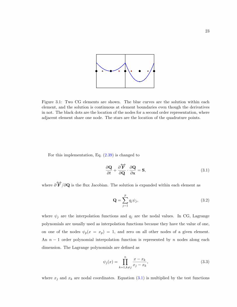
3.1 Two CG elements are shown. The blue curves are the solution within eachelement, and the solution is continuous at element boundaries even thoughthe derivatives in not. The black dots are the location of the nodes for asecond order representation, where adjacent element share one node. Thestars are the location of the quadrature points. . . . . . . . . . . . . . . . . . 23
3.2 Two DG elements are shown. The blue curves are the solution within each el-ement, and the solution is discontinuous at element boundaries. The stars arethe location of the quadrature points. Note that the location of quadraturepoints for the DG method coincide with the ones of the CG method. . . . . . 26
4.1 Log-log plot of the L2-norm as a function of ∆x for the linear advectionproblem using a fixed time step of ∆t = 0.00125 and spatial orders 3, 4, and5 for the CG and the DG schemes. The κ value for the artificial dissipation is10−7. The linear portion of each line has a slope that corresponds to the orderof accuracy of the numerical method. Both methods converge as expected. . . 37
4.2 Log-log plot of the L2-norm as a function of ∆x for the linear advectionproblem using a fixed CFL = 1 and spatial orders 2, 3, and 4 for the CG andthe DG schemes. The κ value for the artificial dissipation is 10−7. All of thelines have a slope of two corresponding to the temporal order of accuracy ofboth the CG and DG section of the BFEM method. . . . . . . . . . . . . . . 38
4.3 Ion density fluctuations propagate from the center of the domain towards theboundaries. The DG and BFEM solutions using 512 second-order elementsare compared to a converged finite volume solution of 5,000 cells at t = 40.Both methods resolve the oscillations of the problem, but there is some phaseerrors associated with the BFEM. . . . . . . . . . . . . . . . . . . . . . . . . . 40
4.4 L2-norm of error the DG and the BFEM over time. The DG method errornorm is lower than the BFEM one, but the error is only about 1.5% of theconverged solution. . . . . . . . . . . . . . . . . . . . . . . . . . . . . . . . . . 41
4.5 L2-norm of error the DG and the BFEM over time for a case where mi/me =1. The DG and BFEM L2-norms are the same because both simulations havethe same time-step and the electron plasma frequency is resolved. . . . . . . . 42
iv

4.6 The features of the electromagnetic plasma shock are a fast rarefaction wave(FR), a slow compound wave (SC), a contact discontinuity (CD), a slow shock(SS), and another fast rarefaction wave (FR). The solution also shows fastelectromagnetic waves that propagate faster than MHD waves[1]. . . . . . . . 43
4.7 The total mass density is plotted for the electromagnetic plasma shock prob-lem at t = 0.05τc. The main features of the problem are captured by allthree methods, but the BFEM does not resolve the EM waves properly, whichmaybe due to the artificial dissipation in the method. . . . . . . . . . . . . . 45
4.8 The total mass density is plotted for the electromagnetic plasma shock prob-lem at t = 0.05τc. The results were obtained using different ∆t. ∆tmaxcorresponds to the maximum value allowed for an explicit methods and forthis problem ∆t = 42.9∆tmax is the maximum value allowed by the semi-implicit BFEM, where the ion dynamics restricts the time-step. . . . . . . . . 46
4.9 Mass density plot comparing two cases where the electron fluid artificial dissi-pation, κe, is decreased by a factor of 10, with the DG method. The solutionfor the lower artificial dissipation captures the wave-like behavior better. Thecompound wave spikes up in amplitude, and the right rarefaction wave is notvisible. . . . . . . . . . . . . . . . . . . . . . . . . . . . . . . . . . . . . . . . . 48
4.10 Mass density solution comparing two BFEM cases where the electromagneticfields artificial dissipation is decreased by a factor of 10. The reduced dis-sipation solution agrees better with DG solution, reinforcing the point thatthe wave-like behavior arises from the interaction of the electron fluid withthe electromagnetic fields. . . . . . . . . . . . . . . . . . . . . . . . . . . . . . 48
5.1 Density plots at t = 150ps, for two ion species for δi = 1.2, c/vo = 3, 065and Kni = 0.8. Z is the ionization level and µ is the ratio of the ion massto a proton mass. Plot (b) shows the decrease in separation with an increasein the ionization level. Plot (c) is the case more relevant for ICF, and itshows that there is less separation compared to (a) and (b). In plot (d)Kni = 0.008 showing that for high collisionality the solution converges to asingle fluid averaged atom for a µ = 6. . . . . . . . . . . . . . . . . . . . . . . 55
5.2 Plot for a spherical imploding DT plasma for c/vo = 1120, δ = 5.37× 10⁻³,Kni = 1.07× 10⁻², Kne = 8.3× 10⁻³, and f = 0.06. Shown are the numberdensity, temperature and radial electric field at t = 1.375 ns. As the compres-sion evolves and the fluids approach the center the density and temperatureincrease. The charge separation between the ions and the electron generateradial electric fields which peak at regions of large density and temperaturegradients. . . . . . . . . . . . . . . . . . . . . . . . . . . . . . . . . . . . . . . 57
v
5.3 Relative difference between the deuterium and the tritium number densitiesas a function of radius and time. Regions where the deuterium percentageis larger are in red, and blue where the tritium is larger. The deuteriumseparates from the tritium from the beginning and the separation increasesas time progresses. A 0.35 ns interval separates the deuterium and the tritiumshocks reaching the center. . . . . . . . . . . . . . . . . . . . . . . . . . . . . 58
5.4 (a) Plots the normalized maximum values of the deuterium pressure gradi-ent, electric, and frictional forces for the time interval before the deuteriumreaches the center of the capsule. The pressure gradient and the electricforce cause the separation and are orders of magnitude larger than the fric-tional force which resists the separation. (b) For the same time interval thelargest value of the mean free path and the corresponding Knudsen numberare plotted. This shows that for the majority of the time Kn < 10−2, so afluid description of the plasma is valid. (c) and (d) show the Kndd and Knttrespectively, and as these fluid approach the center of the imploding capsule,the deuterium-deuterium and tritium-tritium collisions decrease. . . . . . . . 60
5.5 Comparison of the variables used when calculating the neutron yield for thethree-fluid and two-fluid cases. Comparison of the ratio of the density productndnt in the three-fluid simulation with the square of the density of the two-fluid simulation. The density product for the two-fluid case is larger then thethree-fluid case where the ions have separated, therefore the first term in theyield calculation is larger for the two-fluid simulation. . . . . . . . . . . . . . 63
5.6 Temperature and DT reactivity at r = 0 for the three-fluid and two-fluidsimulations are plotted over time. In the three-fluid simulation ions reachthe center earlier causing an increase in the temperature and the reactivitya few nanoseconds before the two-fluid ions reach the center. Although thetemperature is initially larger for the three-fluid case, after the two-fluid casereaches the center its temperature remains steadily higher. . . . . . . . . . . . 64
5.7 Maximum electric field plotted over time. The two-fluid case produces alarger peak electric field than the three-fluid simulation by a factor of two.However, gigavolt per meter electric fields produce forces that are still toosmall compared to the plasma pressures in the problem. . . . . . . . . . . . . 65
6.1 L2−norm error for the mean and variance as a function of computational timeusing the quasi-neutral ion cyclotron wave test problem. With cs =
√1.4,
ωc = 10.0, Bz = 1.0, mi = 1.0 and q = 10.0 and initial values of ρ = 1.0and p = 1.0. The rates of convergence for the mean using the MC and MMCmethods are similar. The rate of convergence for the variance using the MMCmethod is faster than the MC method. . . . . . . . . . . . . . . . . . . . . . . 76
vi

6.2 Mean (top) and variance (bottom) of the reconnected flux for varying ion-to-electron mass ratio ranging from 25 to 100, for the MMC, MC, and PCmethods. . . . . . . . . . . . . . . . . . . . . . . . . . . . . . . . . . . . . . . 79
6.3 Mean (top) and variance (bottom) of the reconnected flux for varying speedof light to Alfven speed ratio ranging from 10 to 20, for the MMC, standardMC, and PC method. . . . . . . . . . . . . . . . . . . . . . . . . . . . . . . . 80
6.4 Mean (top) and variance (bottom) of the reconnected flux for varying am-plitude of the magnetic flux perturbation ranging from [0.085, 0.115], for theMMC, standard MC, and PC method. . . . . . . . . . . . . . . . . . . . . . . 81
6.5 Ion density and magnetic field vectors showing the formation of a secondsmaller magnetic island at the center and as a result the reconnected flux inthese cases is slightly higher because there are no asymmetries in the gridand during the solution the smaller island will remain at the center of thegrid. However if some numerical asymmetry develops the island will move tothe right or the left. ωcit = 38 and mi/me = 25. . . . . . . . . . . . . . . . . . 82
6.6 Reconnected flux plotted versus time for different plasma models used inthe GEM challenge paper [2] compared to two-fluid model. The error barsrepresent the uncertainty due to the sensitivity in the c/vA as measured usingthe MMC method in Fig. 6.3. The Two-fluid region of certainty encompassthe full particle case and most of the hybrid reconnected flux, while the Hall-MHD case is almost completely outside the region of confidence. . . . . . . . 83
7.1 Lacuna are still regions present in wave-like solutions on odd-dimension spaces. 86
7.2 The transition function µ(x) varies from zero in the interior domain to onein the exterior domain and is Co and C1 continuous. . . . . . . . . . . . . . . 88
7.3 A cylindrical pulse propagates through free space, plot of the log |Bz|. Theblack dashed lines show the limit of the interior domain and the purple dashedlines delimit the auxiliary domain. The top and right side boundary condi-tions are conducting walls. There are no reflections from the boundaries. . . . 91
7.4 Plot of log |Bz| at t = 1.168. In the ZNG there are considerably large reflec-tions from the boundaries while the LOBC the reflections extremely small,in the other of 10−16. . . . . . . . . . . . . . . . . . . . . . . . . . . . . . . . . 92
7.5 The logarithm of maximum value of the magnetic field magnitude is plottedversus the elapsed simulation time. The ZNG method produces reflectionwhen the pulse reaches the boundaries while the LOBC does not. . . . . . . . 93
7.6 A combined PML-LOBC is applied to the left boundary while a PML-onlyBC is used to the right boundary. The region in gray is the exterior domainof the LOBC, and both region in magenta represent the PMLs. The domainof interest is in blue with the initialization in orange. Top and bottom BCsare reflecting walls. . . . . . . . . . . . . . . . . . . . . . . . . . . . . . . . . . 95
vii
7.7 Plot of log |Hz|. Top and bottom boundary conditions are reflecting. Theright BC is a simple PML and the left BC are a mixed PML and Lacuna.(a) Shows that the PML has become unstable in the right boundary, whileat the left boundary the reintegration of the auxiliary domain has reset thePML, removing the instability. (b) The PML instability has contaminatedthe computational domain on the right boundary, while the left boundarystill behaves as intended with no reflections nor instabilities. . . . . . . . . . . 96
B.1 Structure of a WARPX input file for any PDE type. . . . . . . . . . . . . . . 116
viii

LIST OF TABLES
Table Number Page
4.1 Total computing time elapsed and time savings for a simulations using afully DG method, compared to one using the BFEM for different values ofelectron-to-ion mass ratio and the speed-of-light to the ion sound speed. . . . 39
4.2 Characteristic speeds and frequencies for the electromagnetic shock problem. 47
5.1 Parameter used in Eq. (5.6) for the calculation of the DT reactivity as afunction of the ions temperature[3]. . . . . . . . . . . . . . . . . . . . . . . . . 61
ix

ACKNOWLEDGMENTS
I wish to express sincere appreciation to the Aeronautics and Astronautics Department
staff and faculty, and especially to my committee chair, and advisor Professor Uri Shumlak,
for both financial and moral support. His guidance during the course of my graduate career
has been indispensable, from helping me choose classes, to homework help, and even his
help suggesting my name for my current position. I would like to thank my colleagues in
the computational plasma dynamics lab, Robert Lilly, Noah Reddell, Sean Miller, Peter
Norgaard, and Andrew Ho for the numerous and fruitful discussions, and for all the help
they have given me through the years. A special thanks to Genia Vogman for the numerous
suggestions, discussions, and thorough reviews of papers and this dissertation. I am grateful
for the constant support and encouragement from my family and friends, which have made
the long night and short vacations tolerable, and encouraged me to continue when there
seemed to be no light at the end of the tunnel. A special thanks to my employers at the
Air Force Research Lab for all the support completing this dissertation. To all my deep and
sincere THANK YOU!
x
DEDICATION
to my dear mother Fatima, father Zeca, aunt Marina, and Step-father Stephen.
xi

1
Chapter 1
INTRODUCTION
Plasma is the fourth state of matter, and is characterized as a quasi-neutral gas of
charged and neutral particles that exhibit collective behavior[4]. About 99% of matter in
the universe is in the state of plasma; stars, interstellar nebulae, accretion discs, solar wind,
etc. Here on Earth lightning and auroras are examples of natural occurrences of plasma,
while plasma displays in most living rooms in America and fluorescent light bulbs, present
in almost every home, are examples of artificially produced plasmas.
Plasma can be described as a “soup” of positively charge ions and negatively charged
electrons. These charged particles generate electric fields, which then produce forces on the
ions and electrons. In addition, collisions between the different plasma constituents cause
momentum and energy to propagate from one to another until the plasma comes to an
equilibrium state. Due to the mass difference between the electrons and ions, plasmas have
disparate time and spatial scales. The electron dynamics occurs on fast time scales, while
ions are relatively slow to respond.
Human produced plasmas are essential parts of ion thrusters[5], Z-pinches[6], tokamaks[7],
stellarators[8], and others. The operation of these devices require aa extensive understand-
ing of plasma behavior under different conditions. In the past fifty years, the development
of the field of plasma physics has been guided in part by the goal of achieving an efficient
means of producing nuclear fusion energy. The National Ignition Facility (NIF), for example,
aims to address the challenges associated with inertial confinement fusion[9]. While efficient
inertial fusion energy production is still a ways away, NIF has increased our understanding
of hydrodynamic instabilities[10], mix[11], laser plasma interactions[12], kinetic effects[13],
new plasma diagnostics[14], and presented new computational challenges. In the south of
France, the International Thermonuclear Experimental Reactor (ITER)[15], a tokamak, is
currently being built with the same goal of nuclear fusion energy production. Numerous
2
challenges and obstacles need to be addressed before first plasma is produced and numerous
more will arise after. Simulations will continue to play an instrumental role in extending our
understanding of plasma physics and will be vital to addressing the challenges of developing
a viable fusion source. Experiments are extremely costly, which makes modeling crucial to
aid our understanding of the physics.
1.1 The Multi-Fluid Plasma Model
In an attempt to better predict the behavior of plasmas, different computer models have been
developed over the years. The most complete plasma model is an N-body problem where
electrons, ions, and neutrals interact through the Lorentz forces and binary collisions. This
N-body plasma model is extremely accurate and can model plasmas under any conditions,
however, the model is extremely complex due to the large number of particles needed to
represent a plasma, and the computational resources it requires.
Kinetic models perform an ensemble average of particle velocities to create a velocity
distribution function, which describes the probability that a particle has a certain velocity
at a given location in the plasma. This model is able to capture all the temporal and spatial
scales of the plasma. However, the probability distribution function is dependent on three
position and three velocity independent variables, which makes this model six-dimensional
and computationally unattractive.
The kinetic description of a plasma can be reduced from six dimensions to three dimen-
sions, provided that the particles that constitute the plasma are sufficiently collisional. The
resulting model is the fluid model, in which each particle species is a fluid with an associated
mass, momentum, and energy density[16]. The fluid model is not as general as the kinetic
model in that it assumes that each species is in local thermodynamic equilibrium, though
different species need not have the same thermodynamic equilibrium (e.g. ions can have a
different temperature than electrons). Despite the simplifying assumption, the multi-fluid
description of a plasma retains much of the physics relevant to and measured in fusion
experiments.
The most widely used plasma description, the ideal magnetohydrodynamic[17] (MHD)
model, represents plasma as a single fluid. This model is obtained from the multi-fluid
3
plasma model by neglecting the electron inertia (me → 0), and by eliminating high frequency
short-wavelength phenomena (εo → 0). Ideal MHD is valid in high collisionality and low
resistivity regimes. MHD is a good model to describe large scale instabilities in devices
such as Z-pinches, spheromak, and tokamak. However, when the characteristic spatial and
temporal scales are small, multi-fluid effects become relevant[18], in which case the MHD
description is not adequate. The multi-fluid plasma model captures non-neutral effects,
which produce local electric fields, and models electron plasma waves and Debye shielding
effects. The multi-fluid plasma model has a more expansive region of applicability, which
might include high resistivity, large Larmor radius, or lower collisionality plasma regimes.
Due to its reduced dimensionality compared to kinetic models, and its generalized physics
compared to MHD, the multi-fluid model is selected as the optimal platform for investigating
fusion-relevant plasma physics. Chapter 2 describes the detailed derivation of the multi-fluid
model.
1.2 The Blended Finite Element Method
A two-fluid plasma model has been implemented using a high-resolution wave propagation
finite volume method in Ref. [19]. The two-fluid plasma model is a special case of the
multi-fluid plasma model where there is only one ion fluid and the electron fluid. Finite
volume methods maintain the conservation properties of the model, and are able to resolve
discontinuities with high accuracy. However, the wave propagation method has challenges
capturing the high frequency oscillations of the plasma, causing phase error[20]. These
oscillations are physical, not numerical, which can be difficult to resolve numerically.
In Ref. [21] the discontinuous Galerkin (DG) method is applied to the two-fluid plasma
model. Like the finite volume method the DG method also retains the conservation prop-
erties of the two-fluid plasma model, and can capture shocks accurately. In addition, the
DG method can produce high order spatial resolution, and can resolve high frequency os-
cillations without producing phase errors. The challenge of this method comes from the
time integration, as the spatial order of accuracy is increased the time-step becomes very
restrictive[22]. In Ref. [23], DG method is expanded to implicit time integration in an
attempt to relax the time-stepping restrictions.However, due to sharp gradients and discon-
4
tinuities the nonlinear Jacobian matrix, needed for the implicit time integration, to become
ill-conditioned and the solution often did not converge.
In most plasma applications, ions are often the only fluid that shocks, the electron and
electromagnetic fields often do not. When the electrons and fields are modeled using a
continuous Galerkin (CG) finite element method, the time integration can be done implic-
itly and the solution converges because CG methods are well behaved for implicit time
integration[24]. The ion and neutral fluids can be represented using an explicit discontinu-
ous Galerkin method. This method where the ion/neutral are advanced explicitly using a
DG and the electrons and electromagnetic field are evolved implicitly using a CG method
is referred to as a blended finite element method (BFEM) henceforth (Sec. 3).
The BFEM has multiple advantages for the multi-fluid plasma model (MFPM). The
fast moving electrons are modeled implicitly and do not dictate restrictive time-steps, as
they have the smallest mass and can move at higher speeds than the ions and neutrals.
Another advantage is that, the DG and CG are both finite element methods, and as such,
they provide high order spatial resolution of the plasma.
1.3 Inertial Confinement Fusion Fuel Species Separation
In Inertial Confinement Fusion (ICF) the plasma is under extremely large pressure and
densities, and small spatial and temporal scales dominate the physics. Under these condi-
tions, multi-fluid plasma effects are relevant and cannot be ignored. The temporal scales of
interest are associated with the ion dynamics, but the electrons play an important role, e.g.
charge separation and electric field, and heat conduction. Therefore, the MHD model in
not well suited for ICF plasmas. The multi-fluid plasma model provides a more generalized
description of fuel separation in ICF capsules, and in conjunction with BFEM provides a
computationally efficient means of simulating the associated physics.
The more generalized physics encapsulated by the multi-fluid model can help shed light
on the cause of the overestimated neutron production observed in ICF experiments. After
the deuterium-tritium (DT) filled capsule has been compressed to fusion conditions, one
of the diagnostics used to analyze the burn history is the neutron yield. Recent yield
measurements conducted at the OMEGA facility have shown that the measured yield is

5
about 50% less than the expected[25]. It is believed that this discrepancy is due to the DT
fuel separation caused by the generation of large electric fields, on the order of GV/m.
ICF simulations are done using radiation-hydrodynamic codes that assume a single
charge-neutral average-mass DT fluid[10]. This model is incapable of producing fuel sep-
aration. Additionally the charge-neutral assumption does not allow for charge separation
effects that cause local electric fields. The MFPM does not have these assumption, which
makes it an ideal candidate for this problem. In Chapter 5 the MFPM using the BFEM is
used to study the effects of ICF fuel separation on the neutron yield.
1.4 Uncertainty Quantification using the Multi-level Monte Carlo Method
To verify computer simulations, numerical results have to be compared to experimental
data. For a rigorous comparison, it is important to account for the numerous sources
of uncertainty in simulations, which include: assumptions made in the derivation of the
model, accuracy of numerical methods, boundary condition implementation, initial condi-
tion implementations, numerical constants, etc. Treating all the parameters as stochastic
is computationally expensive, which points to the necessity to develop different sensitivity
analysis methods to rank the importance of the random inputs and their interactions[26].
The standard most well know method to quantify uncertainty is the Monte Carlo
method[27], but this method is slow to converge and requires a large number of simulations.
The Multilevel Monte Carlo (MMC) method, developed in Ref. [26] for use in computa-
tional finance, on the other hand converges much faster. The MMC method reduces the
computational complexity through the use of a multilevel approach that combines results
obtained using different levels of discretization.
The MMC method uses a geometric sequence of time-steps similar to the multi-grid
method and has proven to be efficient and reliable in achieving the desired accuracy. This
permits establishment of regions of confidence in simulations which can subsequently be
compared to experimental results. The MMC method shows promising results when it
comes to accuracy and computational cost[28]. See Chapter 6 for the implementation.
6
1.5 Lacuna-based Open Boundary Conditions
Simulating open boundary conditions has always been challenging. Nonetheless, numerous
problems from aerodynamics, to plasmas, to astrophysics, require the numerical approxima-
tion of far fields. Whenever open boundary domains are truncated to a finite computational
domain, special care is needed when implementing boundary conditions, otherwise waves
propagating outwards are reflected into the computational domain creating non-physical
conditions.
In Chapter 7, the lacuna-based open boundary conditions[29] (LOBC) is implemented.
Lacuna is a region in space that, after being disturbed by a traveling wave, has returned to
its original condition and any change to a traveling wave does not affect its lacuna. This
method is combined the perfectly matched layer[30] (PML) method to solve the problem of
PMLs becoming unstable for long running simulations[31]. Combining both methods allow
for the LOBC to be more efficient and less computationally expensive.
1.6 Objective
The objective of this dissertation is to develop a multi-fluid plasma framework that can
be applied to problems where there are plasmas composed of multiple ion and neutral
species, and the electron dynamics are relevant. The framework is applicable in problems
where there is high collisionality within each species, and there is local thermodynamical
equilibrium.
A blended finite element method is developed to numerically represent the multi-fluid
plasma model. The BFEM is conservative, high order accurate, can resolve shock and high
frequency oscillations, and eliminates the most stringent time-step limitations imposed by
explicit methods.
The BFEM is applied to the ICF capsule fuel species separation problem, in which
multi-fluid effects are relevant and which is of extreme importance to ICF research. To
allow for rigorous comparison between simulation and experiments, an uncertainty quan-
tification analysis is developed and demonstrated to work on the well-studied problem of
magnetic reconnection. Boundary conditions, such as those relevant in ICF, that involve
7
the propagation of signals out of the simulated domain require special treatment. A means
of handling such boundaries is developed so as to avoid spurious unphysical reflections of
signals. Together the described numerical methods and techniques extend the present ca-
pabilities of fluid plasma simulations, and the scope of physics that can be captured with
fluid models.

8
Chapter 2
THE MULTI-FLUID PLASMA MODEL
2.1 Introduction
Developments in plasma physics have been propelled by the necessity to better understand
phenomena relevant to the study stellar structures, effects of the solar wind on the earth’s
magnetosphere, fusion energy research, space propulsion, etc. over the years. As such,
numerous plasma models have been developed.
Kinetic models represent the velocity probability distribution function in phase space,
and time, f(x,v, t). The evolution of the distribution function is described by the Boltzmann
equation,∂fs∂t
+ v · ∂fs∂x
+qsms
(E + v ×B) · ∂fs∂v
=
(∂fs∂t
)coll
. (2.1)
Each of the plasma constituents is represented by a distribution function. The model is six-
dimensional as the position and velocity space dimensions are independent, which makes
it computationally expensive. As a consequence, kinetic models are limited to narrow
distributions, small spacial dimensions, and short time scales. In addition, velocity space
extends to infinity, making the implementation of boundary conditions challenging.
Particle-in-Cell (PIC) models describe the plasma as electrons and ions particles re-
sponding to the electromagnetic forces and collisions. To reduce the complexity of the
problem, instead of evolving individual particles, super-particles are used, which represent
many particles, but have the same mass-to-charge ratio as individual ones. The problem
with these super-particles is that they can produce statistical errors caused by relatively
fewer particles than in actual plasmas. In addition, the model is six-dimensional, making it
computationally expensive as well.
In Ref. [1] a two-fluid plasma model is presented, which reduces the six-dimensional
kinetic model to three dimensions. This reduction is achieved by taking the first three
9
velocity moments of the Boltzmann equation for all the plasma species. The moments
describe the evolution of the bulk properties of the plasma: density, momentum, and energy.
The pressure is assumed to be isotropic and the heat flux tensor is zero. The model is derived
by assuming local thermodynamic equilibrium within each fluid, but not between different
fluids.
The magnetohydrodynamics (MHD) model[17], the most widely used plasma model, is
derived from the two-fluid plasma model by neglecting the electron momentum and assuming
the speed of light is much larger than any speeds in the system (infinite speed of light). As
a consequence of neglecting the electron inertia, the electron momentum equation reduces
to the generalized Ohm’s law and the kinetic energy of the electrons is zero. In addition,
the infinite speed of light assumption ignores all the high frequency electromagnetic waves,
and sets the vacuum permitivity to zero. This means that the displacement current term of
Ampere’s law is zero, and from Poisson’s equation this assumption implies that the electron
and ion number density must always be equal (quasi-neutral plasma). The MHD model
is often further simplified to an ideal MHD model, which limits its applicability to high
collisionality, small Larmor radius, and low resistivity regimes. The two-fluid model is a
generalization of the MHD model, which makes it applicable to a broader range of plasma
regimes.
For the applications of interest in this dissertation, an expansion of the two-fluid plasma
model to a multi-fluid plasma model is done to describe plasmas where more than one ion
or neutral species are present. The multi-fluid can be applied to a wider range of plasma
regimes than MHD and is less computationally expensive than kinetic or PIC models making
it a good compromise between computational cost and plasma regimes.
2.2 Derivation of the multi-fluid plasma model equations
The multi-fluid plasma model includes a description for the evolution of multiple species:
ions, neutrals, and electrons[16]. Each species mass, momentum, and energy is evolved
separately. Multiple species add multi-scale effects to the model. The electron dynamics
occur at fast time scales while the ion and neutral dynamics happens at much slower time-
scales. The disparate scales are often a manifestation of the mass ratio of the species

10
and their interaction with the electromagnetic fields. This interaction produces waves that
propagate in the plasma at different speeds, and some propagation occurring at faster than
MHD waves[1].
Evaluating the velocity moments of Eq. (2.1) result in the multi-fluid plasma model,
where, the zeroth moment produces the conservation of mass, the first moment the con-
servation of momentum and the third moment the conservation of energy. The process of
obtaining the equations is described in details in Refs. [32] and [33]. The right-hand-side of
the Boltzmann equation accounts for the species collisions. Collisions can be grouped into
scattering and reacting collisions such as ionization, recombination and charge exchange,
however, here only scattering collision will be considered, the plasma is assumed to be fully
ionized.
The zeroth velocity moment provides a statement for conservation of mass,
∂ρs∂t
+∇ · (ρsus) = 0, (2.2)
where the subscript s denotes the species, ρs is the density, us is the velocity. The first
moment is conservation of momentum,
∂ρsus∂t
+∇ ·(ρsusus + ps
←→I)
=ρsqsms
(E + us ×B) +∑r
Rrs −∇ ·←→Π s, (2.3)
and the second moment is the conservation of energy,
∂εs∂t
+∇ · ((εs + ps)us) =
(ρsqsms
E +∑r
Rrs
)· us +
←→Π s : ∇us −∇ · qs +
∑r
Qrs. (2.4)
E and B are the electric and magnetic fields, m is the mass, qs is the charge, ps is the
pressure, and εs is the total energy given as
εs =ps
γ − 1+
1
2ρs|us|2. (2.5)
The term Rrs accounts for the momentum transfer between species s and r. In momentum
transfer between the ions and the electrons, the more massive ions lose less momentum
11
than the electrons. In other words, this term accounts for the electrical resistive force, and
Rrs · us is Ohmic heating. The momentum term is obtained from Ref. [34] as,
Rrs = −νsρs(αov‖ + v⊥) (2.6)
where νs is the collision frequency and v = ur − us, αo = 0.51 for Z = 1 and αo = 0.44 for
Z = 2. The subscripts ‖ and ⊥ denote the directions parallel and perpendicular to magnetic
field. The electron-ion, νe, and ion-ion, νi, collision frequencies are given as
νe =4√
2πe4Z2ni log Λ
3√meT
3/2e
, (2.7)
νi =4√πe4Z4ni log Λ
3√miT
3/2i
, (2.8)
where Z is the ionization level, e is the electron charge, and log Λ is the Coulomb logarithm.
The viscous stress tensor,←→Π s, corresponds to a random-walk diffusion of momentum.
Ion viscosity is greater than the electron viscosity by a factor of mi/me[34], which implies
that the viscosity of a plasma is primarily governed by the ions. There is dissipation of
energy in the form of heat due to viscosity, which is accounted for by the viscous heating
term←→Π s : ∇us. The viscous stress tensor, in the absence of strong magnetic fields, is
defined as←→Π s = −ηs
←→Ws (2.9)
where ηs is the species viscosity and defined for electrons and ions as
ηe = 0.73pe/νe ηi = 0.96pi/νi, (2.10)
and←→Ws = ∇αusβ +∇βusα −
2
3δαβ∇ · us. (2.11)
The first two terms on the right-hand-side of the equation above, are the transposes of each
other, velocity gradients. The δαβ ensures that the divergence of the velocity is applied only
for the diagonal components of the velocity gradient tensor.
12
In Eq. (2.4), Qrs is the thermal equilibration term between species, which drives the
plasma to reach an equilibrium temperature for all species in the absence of other transport
terms. The thermal equilibration is evaluated differently for ions and electrons
Qie = Q∆ =3ρeνemi
(Te − Ti), (2.12)
Qei = −Rie · (ue − ui)−Q∆, (2.13)
Qii′ =3ρiνimi′
(Ti − Ti′), (2.14)
where e represents the electrons, i is any ion, i′ is a different ion species. The temperature
is Ts = ps/ns, and ns is the number density.
The heat flux, qs in Eq. (2.4), represents the diffusion of energy associated with the
random motion of particles. In magnetized plasmas the heat flux parallel and perpendicular
to the magnetic field are different. In the direction parallel to the field, the electron thermal
conductivity is greater than the ion thermal conductivity by a factor of√mi/me at similar
temperatures[34]. But in perpendicular direction the reverse is true by the same factor.
However, in cases where there are steep temperature gradients, and the ratio of the ion
and electron average mean free path λi,e to the scale length of the temperature gradient
LT = T/|∇T | is not small, e.g. λi,e/LT ≥ 10−2 the heat flow should be replaced by the free
streaming heat flux [35, 36], given as
qs = fm−1/2s nsT
3/2s t (2.15)
where t = ∇T/|∇T | is a unit vector in the direction of the temperature gradient, and f is
the flux limiter usually determined by comparing results to experimental measurements. A
value of f = 0.03 is usually used[35].
2.3 Maxwell’s equations
The electromagnetic fields, E and B, are solved with Maxwell’s equations
∂B
∂t+∇×E = 0, (2.16)
13
1
c2
∂E
∂t−∇×B = −µo
∑s
qsms
ρsus, (2.17)
εo∇ ·E =∑s
qsms
ρs, (2.18)
∇ ·B = 0, (2.19)
where εo is the permittivity of free space, µo is the permeability of free space and c =
1/√εoµo is the speed of light.
Maxwell’s equations are overdetermined. There are six unknowns and eight equations.
Analytically the two divergence equation, Gauss’ law and the divergence of the magnetic
field, are satisfied over time as long the initial conditions satisfy them, but numerically there
are round-off errors that violate these divergence constraints. To address this problem,
Maxwell’s equations are cast in purely hyperbolic form as described in Ref. [37],
∂B
∂t+∇×E + γ∇Ψ = 0, (2.20)
1
c2
∂E
∂t−∇×B + χ∇Φ = −µo
∑s
qsms
ρsus, (2.21)
1
χ
∂Φ
∂t+∇ ·E =
∑s
qsms
ρs, (2.22)
1
γc2∂Ψ
∂t+∇ ·B = 0. (2.23)
Error correction potentials Ψ and Φ are introduced for the divergence of B and E respec-
tively. In this model, the errors are propagated out of the computational domain at speeds
equal or larger than the speed of light, c. The error propagation speed is set by the error
correction coefficients γ and χ. The larger the value of coefficients the larger the error prop-
agation speed is, i.e., the errors are propagated out of the computational domain faster.
However, large error propagation speeds require more restrictive explicit time steps, as the
error propagation speed become the fastest traveling waves in the system. Therefore, in
most problems, a value of one is sufficient to enforce the divergence constraints.

14
2.4 Normalized multi-fluid equations
The multi-fluid plasma equation can be cast in non-dimensional form. There are numerical
and physical advantages to casting model in this form. Physically non-dimensionalization
has the advantage that all systems, independent of size, that have the same non-dimensional
parameters will behave in the same way. Numerically non-dimensionalization, can make a
system less stiff, and easier to converge to a solution.
For the normalization used here, a characteristic mass density, velocity, and length scale
(ρ0, u0, L) are introduced, and the normalized values are defined as ρs ≡ ρs/ρ0, us ≡ us/u0,
and x ≡ x/L. Substituting these normalizations into Eq. (2.2) gives
[ρ0
τ
] ∂ρs∂t
+[ρ0u0
L
]∇ · (ρsus) = 0.
Setting the characteristic time (τ) to τ ≡ t/t = L/u0, the terms in the square brackets
cancel, and the normalized continuity equation simplifies to
∂ρs∂t
+∇ · (ρsus) = 0, (2.24)
where the tildes have been dropped for clarity.
The momentum equation, Eq. (2.3), is also normalized using the same characteristic
values and additional ones for pressure, electric and magnetic fields (p0, E0, B0). Each
species charge is normalized by the electron charge, which introduces the ionization level
Zs = qs/e. The momentum equation becomes
[ρ0u0
τ
] ∂ (ρsus)
∂t+
[ρu2
0
L
]∇ · (ρsusus) +
[p0
L
]∇ps =
[en0E0]ZsnsE + [en0u0B0]Zsnsus × B+∑r
[ρ0u0νs]ρs(αov‖ + v⊥)− ∇ ·([η0u0
L2
]←→Ws
), (2.25)
and n0 = ρ0/m0. The terms in square brackets on the left-hand side cancel if the char-
acteristic pressure is set to p0 = m0n0u20. However, the terms in square brackets on the
15
right-hand side do not cancel. The normalized characteristic ion skin depth is defined as
δ ≡ δiL
=c
ωpi=
√ε0m0c2
e2n0L2. (2.26)
which is then used to set the characteristic electric field, E0 =(m0c
2)/(eLδ2
), the subscript
0 denotes the plasma species that is being used as reference for the normalization. The
normalized, characteristic Larmor radius is defined as
rL ≡rL0
L=
u0
ωciL=m0u0
eLB0, (2.27)
which then sets the characteristic magnetic field, B0 = (m0u0) / (eLrL). The Knudsen
number is
Kns = λmfps /L, (2.28)
where λmfps = u0/νs is the mean-free-path of species s, and the Reynolds number is defined
as Res = ρ0u0Lηs
. The Knudsen and Reynolds numbers are related by
Kn =1
Re. (2.29)
The normalized momentum equation simplifies to
∂ (ρsus)
∂t+∇ · (ρsusus) +∇ps =
1
δ2
c2
u20
ZsnsE +1
rLZsnsus ×B+∑
r
1
Knsρs(αov‖ + v⊥)−∇ ·
(Kns←→Ws
). (2.30)
The tildes have again been dropped for clarity.
Following the same procedure, the energy Eq. (2.4) is normalized and becomes,
∂εs∂t
+∇ · ((εs + ps) us) =1
δ2
c2
u20
Zsnsuα ·E +∑r
1
Knsρs(αov‖ + v⊥) · us
−Kns←→Ws : ∇us −∇ · qs +
1
Kns
∑r
Qrs, (2.31)
16
Maxwell’s equation also need to be normalized using the same non-dimensional param-
eters. The normalized Gauss’s law is
∇ ·E =∑s
Zsns, (2.32)
the divergence of magnetic field remains the same
∇ ·B = 0 (2.33)
Faraday’s law is,∂B
∂t+rLδ2
c2
u20
∇×E = 0, (2.34)
and Ampere’s law becomes,
∂E
∂t− δ2
rL∇×B = −
∑s
Zsnsus. (2.35)
2.5 Ideal Multi-Fluid Plasma Model
An ideal form of the multi-fluid plasma equations can be obtained when the viscosity and
the heat flux are zero and there is no interspecies collisions. This assumption simplifies the
calculations and reduces the computational cost because the anisotropic pressure tensor Πs
is not calculated. The balance laws for the multi-fluid plasma model (dimensional) are given
by
∂ρs∂t
+∇ · (ρsus) = 0, (2.36)
∂ρsus∂t
+∇ · (ρsusus + psI) =ρsqsms
(E + us ×B), (2.37)
∂εs∂t
+∇ · ((εs + ps)us) =ρsqsms
us ·E, (2.38)
Maxwell’s equations are expressed as Eqs. (2.16)-(2.19).

17
2.6 Numerical properties of the Multi-Fluid Plasma Model
The multi-fluid plasma equations are inhomogeneous with hyperbolic homogeneous part,
meaning that the system flux Jacobian has real eigenvalues and a complete set of eigenvec-
tors. Hyperbolic equation systems can be cast in balance form as
∂Q
∂t+∇ ·
←→F = S, (2.39)
where q is the vector of conserved variables,←→F is the flux tensor and S is the source term.
The eigenvalues of the flux Jacobian (∂←→F /∂Q) are the characteristic speeds of the
multi-fluid equation system, the fluids speed of sound,
cse =
√γpeρe
, csi =
√γpiρi
(2.40)
and the speed of light, c. The subscript i in equation Eq. (2.40) represents all the ion species.
In addition, the eigenvalues of the source Jacobian (∂S/∂Q) are all purely imaginary[20]
and the first three being 0,±iωp, where ωp is the plasma frequency,
ωps =
√nsq2
s
εoms. (2.41)
Imaginary eigenvalues of the source Jacobian make the sources dispersive. This dispersion
is physical not numerical, and is due to the presence of a wide range of plasma waves
that result from the interaction of the charged fluids with the electromagnetic fields. The
presence of physical dispersion restrict the type of numerical methods that can be used
to properly capture such dispersion and not introduce numerical dispersion nor numerical
dissipation that might dampen such oscillations.
2.7 Summary
The multi-fluid plasma model is presented as a generalization of the MHD model, and ap-
plicable to a broad range of plasma regimes. The model is less computationally expensive
than PIC and kinetic codes, while retaining the relevant physics for most engineering ap-

18
plications and experiments. Collisional terms are given by the Braginskii closures and the
system of equations are normalized so that all collisional terms depend on the same non-
dimensional parameter, the Knudsen number. The electric field is scaled by the ion skin
depth and the magnetic fields by the Larmor radius, and the field evolution is done using
Maxwell’s equations. The model has disparate time scales that need to be resolved in order
to properly describe the physics of a problem.

19
Chapter 3
A BLENDED FINITE ELEMENT METHOD
3.1 Prior and foundational work
The choice of numerical methods that can be used in the solution of a partial differential
equation (PDE) is dictated by the PDE’s type. The multi-fluid plasma equations, described
in Chapter 2, form an inhomogeneous equation system with homogeneous hyperbolic part,
which can be put in balance law form given by Eq. (2.39). A balance law PDE is said to
have hyperbolic homogeneous part if the flux Jacobian, ∂←→F /∂Q, has real eigenvalues and
a complete set of distinct eigenvectors. Balance laws can be solved using the finite volume
wave propagation method described in Ref. [38]. This numerical method is second-order
accurate, it provides good resolution of shocks even when the initial conditions are smooth,
and is conservative.
The wave propagation method has been successfully applied to fluid mechanics[39],
elasticity[40], Tsunami modeling[41], etc. In Ref. [42] the method is successfully applied to
the magnetic reconnection problem using a two-fluid plasma model, where the reconnected
flux calculated as comparable to the results of the GEM challenge magnetic reconnection[2].
The wave propagation method cannot incorporate the source term directly into the cal-
culation of the fluxes and requires source splitting techniques. This produces phase er-
rors when the characteristic frequency is high compared to the frequency of information
propagation[20].
Continuous Galerkin (CG) finite element methods have also been used for solving plasma
models. In the CG method the variables are represented within each element using poly-
nomial basis functions where the order of the polynomials determine the spatial order of
accuracy of the method. In Ref. [24] a reduced quintic triangular finite element method for
MHD is presented. The method enforces continuity of the solution and its first derivative.
In Ref. [43] a CG method for the extended MHD model is implemented in the NIMROD
20
code. The code is restricted to periodic configurations, and is a conforming representation
composed of 2D finite elements in the poloidal plane and finite Fourier series in the toroidal
direction. NIMROD has been used extensively in plasma simulations in Refs. [44, 45, 46, 47].
CG methods tend to be dispersive and often require some artificial dissipation to damp
high frequency oscillations. The MHD model, with low speed flows, there are dissipation
terms that ensure smoothness. The multi-fluid plasma model on the other hand is dispersive,
and has no physical source of dissipation, therefore for the implementation discussed in this
dissertation (Sec. 3.3), artificial dissipation is used to dampen high frequency oscillations.
The MHD model has a large range of timescales which makes implicit time integration
desirable for most simulations. In Ref. [48] an implicit method is applied using a CG method.
And in Ref. [49] the hyperbolic MHD model is converted into parabolic equations in order to
make them more amenable to multigrid methods and physics-based preconditioning. This in
turn makes the Jacobian-free implicit time integration diagonally dominant and convergence
is attained using few iterations. CG methods are well suited to use implicit time integration
methods and are used in this dissertation (Sec. 3.5) for the multi-fluid plasma model to
relax the disparate time constrains imposed by an explicit method.
A method that combines the advantages of both finite volume methods (good shock
capturing and conservation properties) and CG methods (high order accuracy and flux/-
source coupling) is the Discontinuous Galerkin (DG) finite element method. The method
was introduced by Ref. [50] for the study of two-dimensional neutron transport. Like in
CG, the DG solution is represented by a set of polynomial basis functions in each element
but there is no continuity enforcement at the element boundaries.
The DG method was expanded to solve non-linear equations in Ref. [51] where they use
total variation diminishing (TVD) Runge-Kutta time integration, and the Navier-Stokes
equations[52] for unstructured grids and linear, quadratic, and cubic elements[53, 54, 55].
In plasma simulations the DG method has been used to model ideal MHD in Refs. [56]
and [57], and in kinetic modeling for the Vlasov-Poisson equation system in Ref [58]. An
extensive study of the DG method applied to the two-fluid plasma model and the challenges
of the dispersive source term can be found in Ref. [20]. It was shown there that, the DG
method was able to capture high frequency oscillations accurately at higher order discretiza-
21
tions without producing phase error, while accurately representing the relevant physics. The
major benefit of the DG method is that it is remarkably robust in the presence of rapid
oscillations while simultaneously capturing discontinuity fronts. One of the disadvantages
of the DG method is that, with a polynomial basis function of degree p, the explicit time-
step is limited by the CFL condition as CFL≤ 1/(2p− 1)[22]. This CFL restriction can be
extremely costly for problems that require high resolution.
An ideal numerical method for multi-fluid plasma model would be one that: is capable
of capturing shocks, has high order accuracy, resolves fast oscillations, and does not impose
strict time-step limitations, e.g. an implicit DG method. In Ref. [23] an implicit time
integration for the complete two-fluid plasma model discretized using DG was attempted;
however, the non-linear Newton solver would not always converge. This was due to the fact
that in regions of sharp gradients the use of limiters is required, and that made the Jacobian
for the non-linear solver ill-conditioned.
A blended finite element method (BFEM) is presented to achieve the goals described in
the previous paragraph. In the blended finite element method the electron fluid and the
electromagnetic fields are represented using a CG method while all ions and neutral fluids
are represented using a DG method. This ensures that the method is higher order accurate
(depending on the basis functions used), and is able to resolve fast oscillations (flux and
sources are coupled). Regarding shock capturing, for most plasma of interest the electron
fluid and the electromagnetic fields are smooth throughout the domain, and in most cases
do not have sharp gradient or discontinuities making their representation with a CG method
appropriate. Shocks occur in ion and neutral fluids and are captured with the DG method.
Smooth solution in the electron fluid and electromagnetic fields means that there is no
need to use limiters, which makes them excellent candidates for implicit time integration.
The time-stepping is dictated by the characteristic speeds of the multi-fluid plasma model,
which are the species acoustic speeds and the speed of light. In addition, the characteristic
frequencies (plasma and cyclotron) need to be resolved to capture the full physics of the
multi-fluid model. Evolving the electron fluid and electromagnetic fields implicitly removes
the strictest time-step limitation, namely those due to the speed of light, the electron
acoustic speed, and the electron plasma and cyclotron frequencies. In this dissertation a
22
Crank-Nicholson[59] implicit time integration is used.
The ion and neutral fluids do shock and require limiters, which is where implicit DG
time integration has the most challenges, so these fluids are evolved explicitly using Runge-
Kutta time integration (Sec. 3.6). Therefore, we can achieve the goals of capturing shocks
where it is needed, higher order spatial accuracy everywhere, and have relaxed the time-step
restrictions considerably by removing the most stringent limitations.
3.2 Description of the Numerical Method
In the new BFEM method the ion and neutral fluids are modeled using a DG method with
an explicit Runge-Kutta time integration method, while a CG method with implicit time
integration is used for the electron and the electromagnetic fields. Since the fast moving
electrons and the fields do not shock, limiters are not needed and the Jacobian for a Newton
solver is not ill-conditioned. This allows for bigger time steps compared to a fully explicit
method. Often the electron dynamics or the speed of light impose the most restrictive time
step constraints for explicit methods. The DG method for the ions and neutrals is evolved
explicitly, nonetheless, the time steps are less stringent than an entirely explicit method.
3.3 Continuous Galerkin Finite Element Method
In the continuous Galerkin[60] (CG) finite element method the variables are expanded as a
series of polynomial shape functions (also known as interpolation functions) over the volume
of each element, Ω. The order of the polynomials define the spatial order of accuracy of
the numerical method, and how fast the numerical solution converges to the exact solution
as the element size decreases. If the element size is defined as h and the polynomial order
is p the error in the solution is of order O(hp+1), e.g., for linear elements p = 1 and the
convergence rate is of order O(h2), therefore, halving the element size decreases the error
in the solution by a factor of four.
In nodal CG C0 continuity is enforced where adjacent elements have the same nodal
values but the derivatives are not continuous at element boundaries, as depicted in Fig. 3.1.
23
Figure 3.1: Two CG elements are shown. The blue curves are the solution within eachelement, and the solution is continuous at element boundaries even though the derivativesin not. The black dots are the location of the nodes for a second order representation, whereadjacent element share one node. The stars are the location of the quadrature points.
For this implementation, Eq. (2.39) is changed to
∂Q
∂t+∂←→F
∂Q· ∂Q
∂x= S, (3.1)
where ∂←→F /∂Q is the flux Jacobian. The solution is expanded within each element as
Q =
p∑j=1
qjψj , (3.2)
where ψj are the interpolation functions and qj are the nodal values. In CG, Lagrange
polynomials are usually used as interpolation functions because they have the value of one,
on one of the nodes ψp(x = xp) = 1, and zero on all other nodes of a given element.
An n − 1 order polynomial interpolation function is represented by n nodes along each
dimension. The Lagrange polynomials are defined as
ψj(x) =
n∏k=1,k 6=j
x− xkxj − xk
, (3.3)
where xj and xk are nodal coordinates. Equation (3.1) is multiplied by the test functions
24
and integrated over each element volume
∫Ωdxvj
∂Q
∂t+
∫Ωdxvj
∂←→F
∂Q· ∂Q
∂x=
∫ΩdxvjS. (3.4)
In a Galerkin method the test and interpolation functions are the same, vj = ψj , therefore
the governing equation becomes
∫Ωdxψj
∂
∂t
n∑p=1
ψjqp +
∫Ωdx∂←→F
∂Qψj
∂
∂x
n∑p=0
ψpqp =
∫ΩdxψjS. (3.5)
Since the nodal values qp do not vary in space they can be brought outside the integral
∂qp∂t
∫Ωdxψjψp + qp
∫Ωdx∂←→F
∂Qψj∂ψp∂x
=
∫ΩdxψjS. (3.6)
The first integral is the element mass matrix,
←→MΩ =
∫Ωdxψjψp. (3.7)
The spatially dependent terms can be moved to the right-hand-side,
←→MΩ
qn+1p − qnp
∆t= −
∫Ωdx∂←→F
∂Qψj∂ψp∂x
qp +
∫ΩdxψjS. (3.8)
and evaluated using Gauss-Legendre quadrature rules.
The CG method introduces no dissipation, and in regions of sharp gradient it is prone
to high frequency oscillations (Gibbs phenomenon). These oscillations can be dampened by
adding some artificial numerical dissipation. A second derivative of the conserved variables
is added to Eq. (2.39),∂Q
∂t+∇ ·
←→F = S + κ∇2Q∗, (3.9)
where the scalar κ is added to scale the numerical dissipation and minimize the impact it
may have on the physics of the problem. The vector Q∗ indicates that the modeled variable
components being dissipated may be a subset of the conserved ones.

25
Multiplying the dissipation term by the basis functions, integrating over the element
volume, and expanding Q∗ with basis functions, the following is attained
κ∇2Q∗ ⇒∫
Ωdxvκ∇2Q∗ ⇒ −κq∗p
∫Ωdx∂ψj∂x
∂ψp∂x
+ κ
(ψj∂ψp∂x
q∗p
)∂Ω
. (3.10)
The last term in Eq. (3.10) is a surface term and in the CG method that is a physical
boundary term, which accounts for boundary conditions, in particular the natural/Neumann
boundary conditions.
Let the artificial dissipation matrix be defined as,
←→D Ω = −κ
∫Ω
∂ψj∂x
∂ψp∂x
dx, (3.11)
and the source vector as
fΩ =
∫ΩψjSdx, (3.12)
and moving all the spatially dependent terms to the right-hand-side, the evolution equation
can be written as
←→MΩ
qn+1p − qnp
∆t= −qp
∫Ωdx∂←→F
∂qψj∂ψp∂x
+ fΩ +←→D Ωq∗p + κ
(ψj∂ψp∂x
q∗p
)∂Ω
= R(qnp ). (3.13)
In the CG method, all the unknowns (nodal values) must be solved simultaneously, therefore
the element equations are assembled into global mass (←→M) and dissipation (
←→D ) matrices.
The integral term in Eq. (3.13) and the source vector (fΩ) also need to be assembled into a
global vectors. The link between the local matrices and the global ones is done through a
connectivity matrix whose coefficient bij is the global node number corresponding node j of
element i[60]. In continuous Galerkin nodes are shared between elements, which means that
some node numbers will appear in multiple rows of the connectivity matrix. For example,
the element mass matrix entries (M ekl) are added to the global matrix according to
Mmn =
E∑e=1
N∑k=1
N∑l=1
M ekl, (3.14)

26
and m = bek, n = bel. The total number of elements is E and the number of nodes per
element is N .
3.4 Discontinuous Galerkin Method
The discontinuous Galerkin (DG) method implemented here follows closely the implemen-
tation done in Refs. [23, 21]. The main difference between the DG and CG methods is the
way the solution is treated between elements. While in CG the solution at element bound-
aries is required to be continuous, for the DG method the solution can be discontinuous.
In addition, the CG method is a nodal finite element method while the DG method is a
modal. The advantage of using modal for DG is that the implementation of limiters is easily
done[23], while nodal CG can enforce continuity between elements because boundary nodes
are shared between them.
The conserved variables are expanded as piecewise continuous polynomial of degree p
within each element, as shown in Fig. 3.2.
Figure 3.2: Two DG elements are shown. The blue curves are the solution within eachelement, and the solution is discontinuous at element boundaries. The stars are the locationof the quadrature points. Note that the location of quadrature points for the DG methodcoincide with the ones of the CG method.
The order of the polynomials determine the spatial order of accuracy of the method
as explained in the previous section. The conserved variables Q from Eq. (2.39) are then
expressed as linear combinations of shape functions vp and expansion coefficients, qp, in

27
each element
Q =n∑p=1
qpvp. (3.15)
Legendre polynomials up to order n − 1 are used as test functions because they form an
orthogonal basis, ∫Ωvp(x)vm(x)dx = ∆V Cpδpm (3.16)
where ∆V is the volume of the element Ω, Cp = 1/(2p + 1) are normalized constants, and
δpm is the Kronecker delta.
The balance laws equations in Eq. (2.39) are multiplied by the basis functions, vp, and
integrated over each element volume
∂
∂t
∫ΩvmQdV +
∫Ωvm∇ · FdV =
∫Ω
SvmdV. (3.17)
Integration by parts is applied to the second term, and the above equation becomes
∫Ωvm
∂Q
∂tdV +
∮∂ΩvmF · dA−
∫Ω
F · ∇vmdV =
∫ΩvmSdV. (3.18)
When the conserved variables are expanded using Eq. (3.15), and the orthogonality of the
basis functions are taken into account the first term of the above equation simplifies to
∫Ωvm
∂Q
∂tdV =
∂
∂t
∫ΩvpvmqpdV = ∆V Cp
∂qp∂t
. (3.19)
The second term in Eq. (3.18) is a surface integral that accounts for the fluxes across each
element boundary. The calculation of this numerical flux is done using Lax-Frederich flux
expression, however other flux calculations can be used. Lax-Friedrich fluxes are given as
F =1
2(F+
i − F−i+1)− 1
2|λ|(Q+
i −Q−i+1), (3.20)
where |λ| is the maximum characteristic speed (eigenvalue of the flux Jacobian) of the
average conserved values of elements i and i + 1, and superscripts + and − represent the
values at the upper and lower boundaries of an element, respectively. The integrals over the
28
volume of the elements, Ω, of Eq. (3.18) are evaluated using Gauss-Legendre quadrature
rules. The temporally and spatially dependent terms can be separated
dqpdt
= L(qp) =1
∆V
∫ΩvSdV − 1
∆V
∮∂ΩvF · dA +
1
∆V
∫Ω
F · ∇vdV, (3.21)
where L(qp) is the operator containing all the spatially dependent terms and the equation
becomes an ordinary differential equation (ODE)
dqpdt
= L(qp). (3.22)
3.5 Implicit Theta-method Time Integration
The time integration for the CG method is done using the θ-method. The formulation of
the θ-method for Eq. (3.13) is then given as
←→M
qn+1 − qn
∆t= (1− θ)R(qn) + θR(qn+1). (3.23)
Choosing θ = 1 the method is equivalent to the implicit backward Euler, and θ = 0 is the
explicit forward Euler but both methods are only first order accurate. When θ = 0.5 it
corresponds to the Crank-Nicholson method[59] which is an implicit method and second-
order accurate.
A Newton method is used to solve for qn+1. The Newton method is used for finding
successively better approximations to the roots of a real-valued function g(x + dx) = 0
(residual function),
g(x+ ∆x) = g(x) + g′(x)∆x+ ... = 0. (3.24)
The residual function for the implicit finite element method is given as
G(qn) =
←→M
∆t(qn+1 − qn)− (1− θ)R(qn)− θR(qn+1) = 0. (3.25)
The Jacobian is←→J (qn) =
∂G(qn)
∂qn=
←→M
∆t− (1− θ)∂R(qn)
∂qn(3.26)

29
and the equation being solved is given as
←→J (qn)∆q = −G(qn), (3.27)
qn+1 = qn + ∆q. (3.28)
3.6 Explicit Runge-Kutta Time Integration
Second-order total variation bounded (TVB) Runge-Kutta[51] time integration is used for
DG method,
q1p = qnp + ∆tL(qnp ), (3.29)
qn+1p =
1
2q1p +
1
2qnp +
1
2∆tL(q1
p). (3.30)
The Courant-Frederich-Levy (CFL) stability condition of the DG method requires that
CFL = c∆t/∆x ≈ 1/(2p − 1), where p is the order of the basis function. Due to the
time-step restrictions that are imposed by the explicit RKDG and the presence of high and
low frequency oscillations in the two-fluid plasma model and implicit time-stepping scheme
is appealing.
3.7 Continuous and Discontinuous Galerkin Couple Through Source Terms
Both the CG and a DG methods provide good coupling between the sources and the fluxes
since neither is a split method. Therefore, the DG and CG representations only couple
through the treatment of the source terms. The balance law equations for the ions and
neutrals (qn = 0) are given as
∂Qi∂t︷ ︸︸ ︷
∂
∂t
ρi
ρiui
εi
+
∇·Fi(Qi)︷ ︸︸ ︷∂
∂x
ρiui
(ρiuiui + pi←→I )
(εi + pi)ui
=
Si(Qi,Qem)︷ ︸︸ ︷0
ρiqimi
(E + ui ×B)
ρiqimi
ui ·E
. (3.31)
where the em subscript denotes the electromagnetic fields variables.
For the evolution of the electron fluid and the electromagnetic fields, the divergence of
30
the flux term in the balance law is replaced by the product of the flux Jacobian and the
spatial gradient of the conserved variables. The evolution equation for the electron fluid is
then expressed as
∂Qe∂t︷ ︸︸ ︷
∂
∂t
ρe
ρeue
εe
+∂←→F
∂Q·
∂Qe∂x︷ ︸︸ ︷
∂
∂x
ρe
ρeue
εe
=
S(Qe,Qem)︷ ︸︸ ︷0
ρeqeme
(E + ue ×B)
ρeqeme
ue ·E
, (3.32)
where the flux Jacobian can be expressed in terms of electron fluid variables, and
∂←→F e
∂Q=
0 1 0 0 0
−u2 + (γ−1)2 (u2 + v2 + w2) (γ + 3)u −(γ − 1)v −(γ − 1)w γ − 1
−uv v u 0 0
−uw w 0 u 0
− (e+p)uρ + u
2 (u2 + v2 + w3) e+pρ − u
2 −(γ − 1)uv −γuw γu
,
(3.33)
where ue = ux+vy+wz and the e subscript has been omitted for clarity. The field evolution
equations in one-dimension are
∂Qem∂t︷ ︸︸ ︷
∂
∂t
Ex
Ey
Ez
Bx
By
Bz
+
∂←→F em
∂Qem︷ ︸︸ ︷
0 0 0 0 0 0
0 0 0 0 0 c2
0 0 0 0 −c2 0
0 0 0 0 0 0
0 0 −1 0 0 0
0 1 0 0 0 0
∂Qem∂x︷ ︸︸ ︷
· ∂∂x
Ex
Ey
Ez
Bx
By
Bz
=
Sem(Qe,Qi)︷ ︸︸ ︷
− 1
εo
∑s
qsms
ρs
us
vs
ws
0
0
0
. (3.34)
The Maxwell equation flux Jacobian is different for each direction. The coupling between
the CG and DG is done through the source terms, where integrals are evaluated using the
same Gauss-Legendre quadrature rules for all fluid.

31
3.8 General Implementation Details
The BFEM method is implemented in the Washington Approximate Riemann Plasma Solver
(WARPX), described in appendix (B), which is a partial differential equations solver, fo-
cused mainly on hyperbolic equations, but can handle any equation systems.
3.8.1 Continuous Galerkin Matrix Assembling
The implementation is done using the Portable Extension Toolkit for Scientific Computation[61]
(PETSc) and the Scalable Nonlinear Equations Solvers (SNES) are used for the implicit
time advance. PETSc has the capability of managing all the data communication between
different processors and can build massively parallel matrices.
The use of matrices is needed for the implementation of the CG discretization and the
implicit time integration described by Eq. (3.25). The element mass matrix is the same for
every element since the implementation is done on a structured grid. The evaluation of the
element mass matrix integral, Eq. (3.7), is done using Gauss-Legendre quadrature rules
for (unsigned i =0; i< nodesPerElem ; ++i ) // row
for (unsigned j =0; j< nodesPerElem ; ++j ) // column
for (unsigned g l =0; gl< quad−>numQuadPoint ( ) ; ++g l ) // quadrature
Me[ i ] [ j ] += quad−>w( g l )∗ quad−>l a g p o l ( i , g l )
∗ quad−>l a g p o l ( j , g l )∗ Je ;
where lagpol is the Lagrange polynomials evaluated at the quadrature locations, w is the
weights and Je is the determinant of the Jacobian of transformation. After the element
matrix has been evaluated, the global mass matrix,←→M, can be built in PETSc using the
following commands
MatCreate (comm. getMpiComm() ,&MassM ) ;
MatSetSizes (MassM, numUnknowns , numUnknowns , totNumUnknowns , totNumUnknowns ) ;
MatSetType (MassM,MATMPIAIJ) ;
MatSetFromOptions (MassM ) ;
MatMPIAIJSetPreallocation (MassM, nr ,PETSC NULL, n r o f f ,PETSC NULL) ;
32
where numUnknowns is the number of unknowns in a given processor, which corresponds
to the number of nodes multiplied by the number of conserved variables at each. And
totNumUnknowns is the total number of unknowns for the entire problem. The number of
non-zeros for each row is set by the parameter nr. The element to global matrix mapping
is done according to Eq. (3.14),
for (unsigned k=0; k< nodesPerElem ; ++k )
m = quad−>c o n n e c t i v i t y ( e , k)+ npad ;
for (unsigned l = 0 ; l < nodesPerElem ; ++l )
n = quad−>c o n n e c t i v i t y ( e , l )+ npad ;
for (unsigned j = 0 ; j< meqn ; ++j )
MatSetValue ( mass , m∗ meqn+j ,
n∗ meqn+j , Me[ k ] [ l ] , ADD VALUES) ;
where meqn is the number of component or conserved variable at each node. The element
dissipation matrix, Eq. (3.11), is built similarly
De [ i ] [ j ] += quad−>w( g l )∗ quad−>d lagpo l ( i , g l )∗ quad−>d lagpo l ( j , g l )∗1 . / Je ;
where dlagpol is the derivative of the Lagrangian polynomials evaluated at the quadrature
point.
3.8.2 PETSc Matrix-Free Methods for Implicit Time Integration
Implicit time integration requires the evaluation of the Jacobian matrix, but this can be done
without formally building a matrix by instead evaluating the matrix-vector multiplication
as←→J (Qn)a =
∂G(Qn)
∂Qna =
G(qn + h+ a)−G(qn)
h(3.35)
where h is a small value computed internally by PETSc and G is the residual function
given by Eq. (3.25). A matrix coloring[62] is needed to efficiently evaluate the matrix-vector
33
product. The matrix coloring is done as following
unsigned value = blockS ize− meqn ;
for ( int i =0; i< numElem ; ++i )
int imin = ( i==0 ) ? 0 : ( i −1)∗ value ;
int imax = ( i== numElem−1 ) ? numUnknowns : i ∗ value+b lo ckS i z e+value −1;
for ( int k=0; k<b lo ckS i z e ; ++k )
int j r = i ∗ value + k ;
// s e t non−zero e lements to 1.0
for ( int j c = imin ; j c < imax ; ++j c )
MatSetValue ( co lo r , j r , jc , 1 . 0 , INSERT VALUES ) ;
where numElem is the total number of elements and blockSize = meqn×(numberofnodesperelement).
Once the matrix color has been populated, a coloring object is create
MatGetColoring ( jacobian , MATCOLORINGSL, &i s c o l o r i n g ) ;
the a finite different coloring is created using
MatFDColoringCreate ( jacobian , i s c o l o r i n g , &matFDColoring ) ;
and the function evaluation G for the finite different approximation is done using
MatFDColoringSetFunction ( matFDColoring ,
( PetscErrorCode (∗ ) ( void ) ) WxFemPetscSnesSolver : : evaluateFunct ion ,
( void ∗) c l s ) ;
finally set Jacobian evaluation function as
SNESSetJacobian ( so lve r , jacobian , jacobian ,
SNESDefaultComputeJacobianColor , matFDColoring ) ;
the non-linear problem is solved by invoking the command
34
SNESSolve ( so lve r , PETSC NULL, so lVec to r ) ;
where solver is the nonlinear solver object and solV ector is the solution vector.
3.8.3 Continuous Galerkin Boundary Conditions
The boundary conditions are implemented using the penalty method which guarantees that
the matrices remain symmetric. For an←→A u = F, a boundary on node zero u0 = g0 would
be implemented by
←→A 00 ⇒
←→A 00 + α (3.36)
F0 ⇒ F0 + αg0. (3.37)
where α is a large value added to the diagonal of the matrix and the right-hand-side vector.
For this implementation the penalty method is applied to the mass,←→M Eq. (3.7), and the
dissipation ,←→D Eq. (3.11), matrices.
3.8.4 Discontinuous Galerkin Boundary Conditions
For the DG portion of the BFEM, the boundary conditions are imposed through ghost
cells, where Dirichlet and Neumann boundary conditions can be imposed. Note that this
boundary values are applied to the expansion coefficients which depend on the polynomial
order being used. For example, to implement Dirichlet value of zero, the coefficients of all
even basis functions are set to the negative of the adjacent domain cell, and the coefficients
of all odd basis functions in the ghost cells remain the same as the adjacent domain cell.
3.8.5 Discontinuous Galerkin Limiters
The DG method uses limiters around sharp gradients and discontinuities. Limiters can be
applied to either the conserved or the characteristic variables depending on the limiter. The
implementation of limiters was done by Srinivasan in Ref. [23].

35
3.9 Summary
A new numerical method, blended finite element method (BFEM), has been introduced
for the multi-fluid plasma model. A continuous Galerkin finite element method is used
to discretize the electron fluid and the electromagnetic fields, and a discontinuous Galerkin
finite element method for the all ion and neutral fluids. The method is higher order accurate
in space and second order in time. The electron fluid and the electromagnetic fields time
evolution is computed implicitly, which reduces the most stringent time limitation of the
multi-fluid plasma model. The shock capturing propertied of the discontinuous Galerkin
method are ideal at resolving the discontinuities of the ion and neutral fluids, which are
the fluids that do shock. The result is a method that is robust, accurate, and can resolve
physical aspects of the plasma without introducing numerical noise.
36
Chapter 4
VALIDATION AND VERIFICATION OF THE BLENDED FINITEELEMENT METHOD
4.1 1-D Advection Equation: Convergence Studies
In Ref. [23] the linear advection equation was used to study the spatial and temporal conver-
gence of the solution versus the polynomial order used in a discontinuous Galerkin method.
The problem is the simplest of hyperbolic equations, does not have any source terms, and
is linear, which restricts the accuracy of the solution solely to the numerical method. The
one-dimensional linear advection equation is given as
∂Q
∂t+∂Q
∂x= 0. (4.1)
The pulse is initialized to a Gaussian given as Q(x, 0) = e−10(x−2)2 on a domain size of
x ∈ [0, 10]. The pulse is propagated from x = 2 to x = 8 (a total time interval of ∆T = 6)
and compared to the analytical solution given as Q(x) = e−10(x−8)2 . The error in the
numerical solution is calculated by evaluating the L2-norm as
||∆Q||2 =
√√√√ 1
n
n∑i=1
(Q−Qi)2. (4.2)
where Q is the analytical solution and Qi is the numerical solution. The subscript i repre-
sents the summation is done over the quadrature points for the DG method and the nodal
values for the CG case, and n is the total number of nodes or quadrature points.
Figure 4.1 shows the L2-norm for the advected pulse using a fixed ∆t = 0.00125 with
different polynomial interpolation functions for the DG and the CG methods. The fixed time
steps isolates the convergence effect to the spatial order. The plot shows that, for equivalent
order polynomial interpolation functions, the CG and DG methods converges at the same

37
Figure 4.1: Log-log plot of the L2-norm as a function of ∆x for the linear advection problemusing a fixed time step of ∆t = 0.00125 and spatial orders 3, 4, and 5 for the CG and theDG schemes. The κ value for the artificial dissipation is 10−7. The linear portion of eachline has a slope that corresponds to the order of accuracy of the numerical method. Bothmethods converge as expected.
rate, i.e. the linear portion of the curve have the same slope. The CG scheme L2-norm
plateaus around 10−5, which is due to the artificial dissipation. The artificial dissipation
decreases the peak of the Gaussian every time-step and over the interval ∆T = 6 the peak
for all cases has decreased by the same amount.
Figure 4.2 shows the calculated L2-norm for the advection problem using a fixed CFL
number of CFL = 1.0. For each spatial order, the time-step is given as ∆t = CFL∆x.
This isolates the rate of convergence to the temporal order of accuracy of the time-stepping
method. For the CG a θ-method is used with θ = 0.5, which is the Crank-Nicholson
method that is second-order accurate, and for the DG a second-order TVB Runge-Kutta
time integration is used, which is also second-order accurate. The slope of the lines for
both method is two, i.e. for every decade decrease in ∆x there are two decades decrease
in the L2-norm. Therefore, the desired temporal converge is attained by the time-stepping
methods.

38
Figure 4.2: Log-log plot of the L2-norm as a function of ∆x for the linear advection problemusing a fixed CFL = 1 and spatial orders 2, 3, and 4 for the CG and the DG schemes. The κvalue for the artificial dissipation is 10−7. All of the lines have a slope of two correspondingto the temporal order of accuracy of both the CG and DG section of the BFEM method.
4.2 Two-Fluid Plasma Soliton in 1-D: Accuracy and Timing Studies
A one-dimensional soliton propagation[63] is modeled using the multi-fluid plasma model.
This problem is used to study the accuracy and compare the computational cost of the
BFEM and the DG method. This problem is chosen because it describes a multi-fluid
plasma composed of one electron and one ion-fluid, and is one the simplest problems that
can be solved using the BFEM. In addition, the solution of the problem is smooth, which
permits the use of small values of artificial dissipation for BFEM, eliminating the inaccura-
cies associated with the artificial dissipation, as seen in the previous section.
The problem in this section solves the ideal multi-fluid plasma model described in
Sec. 2.5. The initialized for the z-component of the magnetic field is Bz = 1.0, the temper-
ature (T = p/n, where n is the number density n = ρ/m) is Te = Ti = 0.01, ui = ue = 0,
q = 1, and ne = ni = 1.0 + e−10(x−6)2 on a domain x ∈ [0, 12]. The ratio of specific heats is
γ = 2. The simulation uses 512 second-order elements for DG and BFEM.
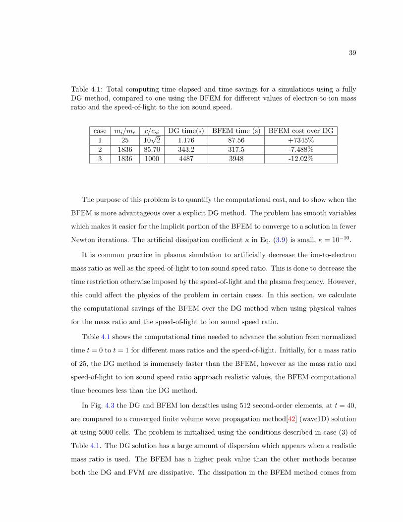
39
Table 4.1: Total computing time elapsed and time savings for a simulations using a fullyDG method, compared to one using the BFEM for different values of electron-to-ion massratio and the speed-of-light to the ion sound speed.
case mi/me c/csi DG time(s) BFEM time (s) BFEM cost over DG
1 25 10√
2 1.176 87.56 +7345%
2 1836 85.70 343.2 317.5 -7.488%
3 1836 1000 4487 3948 -12.02%
The purpose of this problem is to quantify the computational cost, and to show when the
BFEM is more advantageous over a explicit DG method. The problem has smooth variables
which makes it easier for the implicit portion of the BFEM to converge to a solution in fewer
Newton iterations. The artificial dissipation coefficient κ in Eq. (3.9) is small, κ = 10−10.
It is common practice in plasma simulation to artificially decrease the ion-to-electron
mass ratio as well as the speed-of-light to ion sound speed ratio. This is done to decrease the
time restriction otherwise imposed by the speed-of-light and the plasma frequency. However,
this could affect the physics of the problem in certain cases. In this section, we calculate
the computational savings of the BFEM over the DG method when using physical values
for the mass ratio and the speed-of-light to ion sound speed ratio.
Table 4.1 shows the computational time needed to advance the solution from normalized
time t = 0 to t = 1 for different mass ratios and the speed-of-light. Initially, for a mass ratio
of 25, the DG method is immensely faster than the BFEM, however as the mass ratio and
speed-of-light to ion sound speed ratio approach realistic values, the BFEM computational
time becomes less than the DG method.
In Fig. 4.3 the DG and BFEM ion densities using 512 second-order elements, at t = 40,
are compared to a converged finite volume wave propagation method[42] (wave1D) solution
at using 5000 cells. The problem is initialized using the conditions described in case (3) of
Table 4.1. The DG solution has a large amount of dispersion which appears when a realistic
mass ratio is used. The BFEM has a higher peak value than the other methods because
both the DG and FVM are dissipative. The dissipation in the BFEM method comes from

40
(a) (b)
Figure 4.3: Ion density fluctuations propagate from the center of the domain towards theboundaries. The DG and BFEM solutions using 512 second-order elements are comparedto a converged finite volume solution of 5,000 cells at t = 40. Both methods resolve theoscillations of the problem, but there is some phase errors associated with the BFEM.
the artificial dissipation term, Eq. (3.9), but for smooth solutions, the value of κ can be
small, κ = 10−10.
Figure 4.4 plots the evolution over time of the L2-norm of the relative error for the DG
and BFEM. The error is defined as
error =ρki − ρciρci
(4.3)
where ρci is the mass density for the converged solution and ρki represents the solution given
by the DG or BFEM. The error is evaluated at each quadrature point (DG) or the nodal
values (BFEM). The DG error L2-norm is lower than the BFEM one, but the error is
only on the order of about ∼ 1.5% of the converged solution using a resolution of one-
tenth. Therefore, it is an acceptable error for the computational saving attained. The
source of the error is the fact that DG and converged solution are obtained using a explicit
time integration which resolves the electron plasma frequency, while the BFEM does not
resolve the electron plasma frequency. Figure 4.5 compares the L2-norm for a case where the
electron-to-ion mass ratio is one, and for that case the error for both methods is comparable
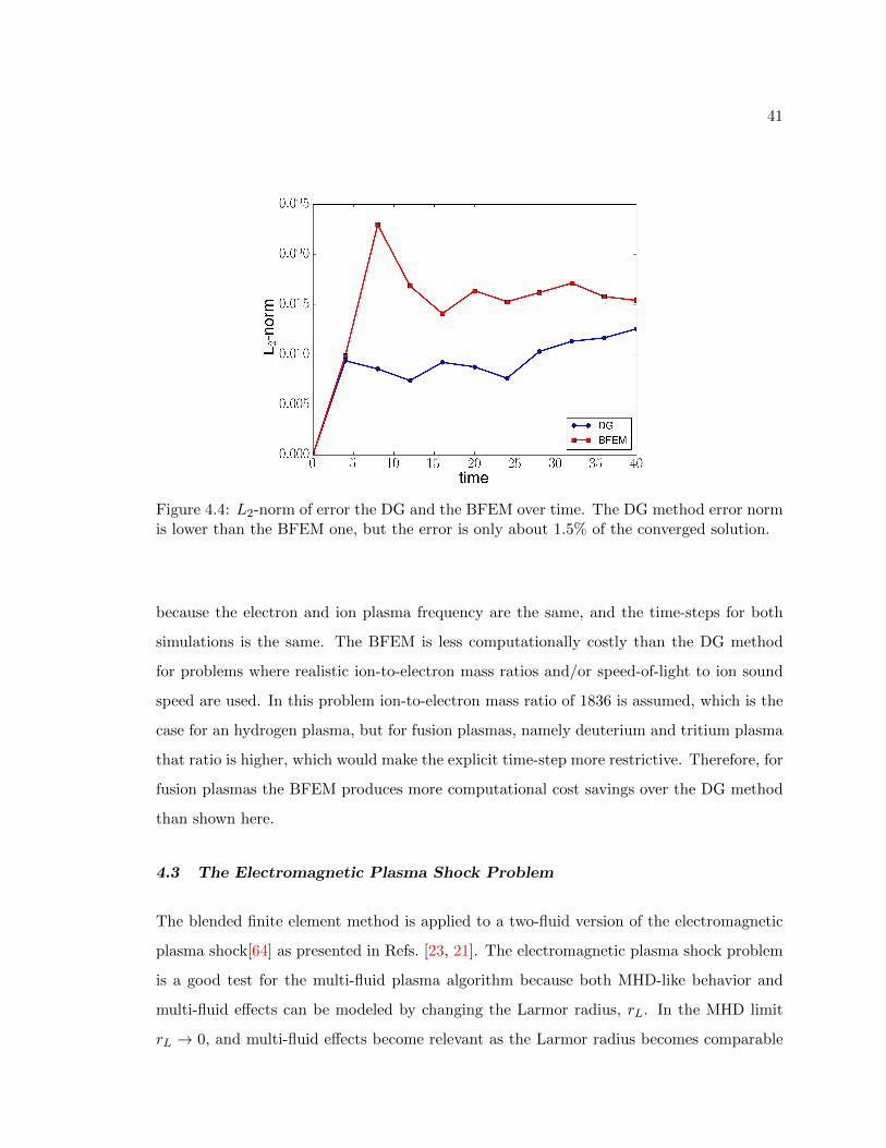
41
Figure 4.4: L2-norm of error the DG and the BFEM over time. The DG method error normis lower than the BFEM one, but the error is only about 1.5% of the converged solution.
because the electron and ion plasma frequency are the same, and the time-steps for both
simulations is the same. The BFEM is less computationally costly than the DG method
for problems where realistic ion-to-electron mass ratios and/or speed-of-light to ion sound
speed are used. In this problem ion-to-electron mass ratio of 1836 is assumed, which is the
case for an hydrogen plasma, but for fusion plasmas, namely deuterium and tritium plasma
that ratio is higher, which would make the explicit time-step more restrictive. Therefore, for
fusion plasmas the BFEM produces more computational cost savings over the DG method
than shown here.
4.3 The Electromagnetic Plasma Shock Problem
The blended finite element method is applied to a two-fluid version of the electromagnetic
plasma shock[64] as presented in Refs. [23, 21]. The electromagnetic plasma shock problem
is a good test for the multi-fluid plasma algorithm because both MHD-like behavior and
multi-fluid effects can be modeled by changing the Larmor radius, rL. In the MHD limit
rL → 0, and multi-fluid effects become relevant as the Larmor radius becomes comparable

42
Figure 4.5: L2-norm of error the DG and the BFEM over time for a case where mi/me = 1.The DG and BFEM L2-norms are the same because both simulations have the same time-step and the electron plasma frequency is resolved.
to the scale length of the problem. For Larmor radius comparable to the domain size, the
electron fluid couples to the magnetic field and the solution contains wave-like structures
that propagate faster than MHD waves, and can be seen in Fig. 4.6.
The electromagnetic plasma shock is an initial boundary value problem with a discon-
tinuity in the variables such that half of the domain is at one state and the other half is at
another state. For the test case presented here, mi/me = 1836. The problem is described
in detail in [1]. The solution features are shown in Fig. 4.6. From left to right they are, a
fast rarefaction wave (FR), a slow compound wave (SC), a contact discontinuity (CD), a
slow shock (SS), and another fast rarefaction wave (FR).

43
Figure 4.6: The features of the electromagnetic plasma shock are a fast rarefaction wave(FR), a slow compound wave (SC), a contact discontinuity (CD), a slow shock (SS), andanother fast rarefaction wave (FR). The solution also shows fast electromagnetic waves thatpropagate faster than MHD waves[1].

44
The two-fluid equivalent initial conditions for the electromagnetic plasma shock are
ne
ue
ve
we
pe
ni
ui
vi
wi
pi
Bx
By
Bz
Ex
Ey
Ez
left
=
1.0
0
0
0
0.5× 10⁻⁴
1.0
0
0
0
0.5× 10⁻⁴
0.75× 10⁻²
1.0× 10⁻²
0
0
0
0
, and
ne
ue
ve
we
pe
ni
ui
vi
wi
pi
Bx
By
Bz
Ex
Ey
Ez
right
=
0.125
0
0
0
0.05× 10⁻⁴
0.125
0
0
0
0.05× 10⁻⁴
0.75× 10⁻²
−1.0× 10⁻²
0
0
0
0
. (4.4)
The parameters used for the problem are obtained from Ref. [1], and are c/u0 = 110, δ = 1,
rL = 0.73, γe = γi = 53 and the ion-to-electron mass ratio is mi/me = 1836. A grid
resolution of 512 second order elements is used. Time is normalized as τc =1000rLc
.
The blended finite element method is compared to a discontinuous Galerkin (DG)
implementation[21] and to a wave propagation method finite volume (FV) methods[42].
Figure 4.7 shows the mass density profile for all three methods and there is good agreement
between all of them. The BFEM smoothed the oscillations in the problem, which is due to
the artificial dissipation and is discussed in more detail in Sec. 4.3.2.

45
Figure 4.7: The total mass density is plotted for the electromagnetic plasma shock problemat t = 0.05τc. The main features of the problem are captured by all three methods, but theBFEM does not resolve the EM waves properly, which maybe due to the artificial dissipationin the method.

46
Figure 4.8: The total mass density is plotted for the electromagnetic plasma shock problemat t = 0.05τc. The results were obtained using different ∆t. ∆tmax corresponds to themaximum value allowed for an explicit methods and for this problem ∆t = 42.9∆tmax isthe maximum value allowed by the semi-implicit BFEM, where the ion dynamics restrictsthe time-step.
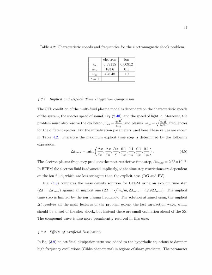
47
Table 4.2: Characteristic speeds and frequencies for the electromagnetic shock problem.
electron ion
cs 0.39115 0.00912
ωcs 183.6 0.1
ωps 428.48 10
c = 1
4.3.1 Implicit and Explicit Time Integration Comparison
The CFL condition of the multi-fluid plasma model is dependent on the characteristic speeds
of the system, the species speed of sound, Eq. (2.40), and the speed of light, c. Moreover, the
problem must also resolve the cyclotron, ωcs =qsB
ms, and plasma, ωps =
√nsq2sεoms
, frequencies
for the different species. For the initialization parameters used here, these values are shown
in Table 4.2. Therefore the maximum explicit time step is determined by the following
expression,
∆tmax = min
(∆x
cse,∆x
csi,∆x
c,
0.1
ωce,0.1
ωci,
0.1
ωpe,
0.1
ωpi
). (4.5)
The electron plasma frequency produces the most restrictive time-step, ∆tmax = 2.33×10⁻⁴.
In BFEM the electron fluid is advanced implicitly, so the time step restrictions are dependent
on the ion fluid, which are less stringent than the explicit case (DG and FV).
Fig. (4.8) compares the mass density solution for BFEM using an explicit time step
(∆t = ∆tmax) against an implicit one (∆t =√mi/me∆tmax = 42.9∆tmax). The implicit
time step is limited by the ion plasma frequency. The solution attained using the implicit
∆t resolves all the main features of the problem except the fast rarefaction wave, which
should be ahead of the slow shock, but instead there are small oscillation ahead of the SS.
The compound wave is also more prominently resolved in this case.
4.3.2 Effects of Artificial Dissipation
In Eq. (3.9) an artificial dissipation term was added to the hyperbolic equations to dampen
high frequency oscillations (Gibbs phenomena) in regions of sharp gradients. The parameter

48
Figure 4.9: Mass density plot comparing two cases where the electron fluid artificial dissi-pation, κe, is decreased by a factor of 10, with the DG method. The solution for the lowerartificial dissipation captures the wave-like behavior better. The compound wave spikes upin amplitude, and the right rarefaction wave is not visible.
Figure 4.10: Mass density solution comparing two BFEM cases where the electromagneticfields artificial dissipation is decreased by a factor of 10. The reduced dissipation solutionagrees better with DG solution, reinforcing the point that the wave-like behavior arises fromthe interaction of the electron fluid with the electromagnetic fields.

49
κ was introduced to scale the amount of artificial dissipation on the physics of the problem.
There are no guidelines on how to pick a value for κ. If it is too small the solution will
have high amplitude node-to-node oscillations that grow over time, making the solution of
the nonlinear Newton solver more stiff and hard to converge. On the other hand, if κ is
too big the solution will smooth out all the relevant features of the problem producing an
inaccurate result.
In the BFEM the artificial dissipation is applied only to the electron fluid variables and
the electromagnetic field equations. It is possible to apply different values of κ for the two
equation system separately.
In Fig. 4.9 the effects of the artificial dissipation on the electron fluid equations is studied.
There, it can be seen that reducing the value of κ from 10−6 to 10−7 makes the compound
wave more distinct and the oscillations due to charge separation and fast waves are more
visible. However, the solution is out of phase with the DG result and the second FR wave
is not resolved. Small oscillation appear superimposed onto the larger wavelength fast
electromagnetic waves.
Decreasing the artificial dissipation in Maxwell’s equations resolves the oscillations due to
species separation and the phase shift is less visible in the solution in Fig. 4.10. In addition,
in this case the fast rarefaction wave is resolved properly. In this case there is remarkable
agreement between the BFEM and the DG solutions. In conclusion, the artificial dissipation
plays an important role in the accuracy of the BFEM. It might be prudent to investigate
better forms of calculating the parameter κ or different forms of artificial dissipation.
4.4 Summary
The DG and CG schemes converge according to the theoretically predicted values. The order
of the accuracy of the scheme depends on the polynomial order of the interpolation function
chosen. Both time-stepping methods are second-order accurate in time. The BFEM is less
computationally expensive when realistic values of the ion-to-electron mass and speed of
light to ion sounds speed ratios are used. For problems where the electron dynamics can
be ignored the results produced by the BFEM are comparable to the DG method. The
artificial dissipation can affect the results considerably, therefore it needs to be tuned in

50
order to resolve physical oscillations in the problem while damping numerical dispersion.
51
Chapter 5
INERTIAL CONFINEMENT FUSION FUEL SPECIES SEPARATION
5.1 Introduction
In inertial confinement fusion (ICF) experiments a spherical capsule is compressed to high
densities and pressures using a laser driver. The capsule is filled with deuterium and tritium
ice (DT-ice). Fusion is achieved when the plasma has reached ion temperatures greater than
10 keV and an areal density greater than 0.3 g/cm2[65].
One of the products of the fusion reaction is neutrons. Neutron energies are measured to
identify what fusion reactions are occurring, and to quantify the reaction rates by counting
the number of neutrons produced per unit time. In Ref. [25] the authors measured the
neutron yield of an ICF pellet using direct drive at the OMEGA facility and found that the
DT reaction yield was lower than expected, which was in line with the results in Ref. [66]
where the neutron yield was 50% lower than expected. They attributed this yield reduction
to fuel stratification caused by baro-diffusion[67] (pressure gradient-driven diffusion), which
leads to the separation of the deuterium and the tritium during the implosion. Thermo-
diffusion[68] and electro-diffusion[69] have also been suggested to cause ICF fuel separation.
After large electric fields were inferred during ICF capsule implosions, it was proposed in
Ref. [65] that the presence of these fields could produce significant amount of baro-diffusion
in ICF capsules implosions. The baro-diffusion is localized to regions of sharp gradients
and electric fields have formed[67]. The baro-diffusion argument is that, in a DT plasma,
the deuterium will experience a larger acceleration than the tritium because of its larger
charge-to-mass ratio. The deuterons will move closer to the region where the electric field
is large, and in the process shield the tritons from experiencing the same field intensity.
The deuterium shielding of the electric field has the effect of compounding the two species
separation.
Three main candidates have been proposed for the origin of the electric field in the ICF

52
pellets[65]. The first candidate is electron pressure gradient caused by the acceleration at
the pusher-fuel interface and also by ionization gradients. The second candidate is simple
charge separation caused by the fact that electrons have a lower mass and accelerate ahead of
the ions generating electric fields. And the third candidate is concentration driven diffusion
of the electrons ahead of the ion shock creating an electric field. Of these three mechanisms,
only the third one predicts field values the same order of magnitude as the inferred values
from experimental results[25].
Challenges in theoretically predicting this electric field and observing the deuterium-
tritium separation can be attributed to the fact that ICF capsule implosions are generally
modeled using radiation-hydrodynamic (rad-hydro) codes which are single fluid, mass aver-
aged, and charge neutral[10]. Rad-hydro codes are adequate when modeling hydrodynamic
instabilities that develop in ICF capsules; however, species separation is inherently a multi-
fluid effect and generation of local electromagnetic fields precludes the use of the MHD
model[17] because it assumes charge neutrality.
ICF fuel species separation have been modeled using a hybrid-PIC code in Ref. [70],
where the authors analyzed the effects that the charge-to-mass ratio had on ion separation.
For the ICF relevant case, DT plasmas, the separation was less than the cases with ionization
of two and an ion mass ratio of ten. In spherical geometry the authors found that the yield
was highly dependent on the choice of heat flux limiter for the free streaming heat flux
model used[36]. However, there was no comparison of the multi-fluid results with a single
fluid averaged atom to study if the current ICF codes are correctly predicting the neutron
yield.
Ion Vlasov-Fokker-Planck(VFP) simulations were performed recently in Ref. [71] where
the authors compared the results of a two-ion species simulation with one of a single ion
species simulation. They found that the temperature and density at the stagnation phase
of the ICF implosion for the two-ion species were higher than the one predicted by a av-
erage atom radiation hydrodynamic code. In addition, the yield rate, number of neutrons
produced per unit time, for the two-ion fluid was higher that the single-ion simulation.
However, the authors do not make any references to electric field, in the simulations or
what causes the separation.
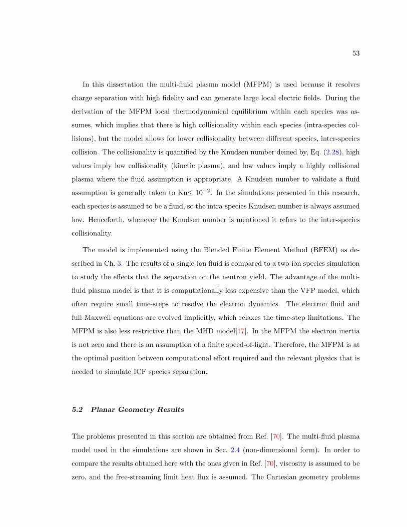
53
In this dissertation the multi-fluid plasma model (MFPM) is used because it resolves
charge separation with high fidelity and can generate large local electric fields. During the
derivation of the MFPM local thermodynamical equilibrium within each species was as-
sumes, which implies that there is high collisionality within each species (intra-species col-
lisions), but the model allows for lower collisionality between different species, inter-species
collision. The collisionality is quantified by the Knudsen number deined by, Eq. (2.28), high
values imply low collisionality (kinetic plasma), and low values imply a highly collisional
plasma where the fluid assumption is appropriate. A Knudsen number to validate a fluid
assumption is generally taken to Kn≤ 10−2. In the simulations presented in this research,
each species is assumed to be a fluid, so the intra-species Knudsen number is always assumed
low. Henceforth, whenever the Knudsen number is mentioned it refers to the inter-species
collisionality.
The model is implemented using the Blended Finite Element Method (BFEM) as de-
scribed in Ch. 3. The results of a single-ion fluid is compared to a two-ion species simulation
to study the effects that the separation on the neutron yield. The advantage of the multi-
fluid plasma model is that it is computationally less expensive than the VFP model, which
often require small time-steps to resolve the electron dynamics. The electron fluid and
full Maxwell equations are evolved implicitly, which relaxes the time-step limitations. The
MFPM is also less restrictive than the MHD model[17]. In the MFPM the electron inertia
is not zero and there is an assumption of a finite speed-of-light. Therefore, the MFPM is at
the optimal position between computational effort required and the relevant physics that is
needed to simulate ICF species separation.
5.2 Planar Geometry Results
The problems presented in this section are obtained from Ref. [70]. The multi-fluid plasma
model used in the simulations are shown in Sec. 2.4 (non-dimensional form). In order to
compare the results obtained here with the ones given in Ref. [70], viscosity is assumed to be
zero, and the free-streaming limit heat flux is assumed. The Cartesian geometry problems

54
are initialized as x < 0 µm :
∑i
ni = 4× 1019 cm−3; T = 100 eV
x > 0 µm :∑i
ni = 1× 1019 cm−3; T = 10 eV
(5.1)
where the subscript i denotes all the ion species. The plasma is initially assumed to be
charge neutral everywhere, ne =∑i
Zini, and the heat flux is zero. The Knudsen number
is calculated using the ion thermal speed and the ion-ion collision frequency, Kni = 0.8. The
only non-ideal terms considered are the momentum transfer and the thermal equilibration
terms, the heat flux is set to zero as well as the viscosity. The computational domain is x∈
[-30 µm, 30 µm], and zero normal gradient boundary condition are applied at x=-30 µm
and x=30 µm.
The goal is to analyze how ions of different mass and ionization levels separate if ini-
tialized to the same conditions. Fig. 5.1 shows the density profile of a multi-fluid plasma in
Cartesian geometry. The plasma has three constituents, two-ion species and electrons. It
can be seen that the separation between the ion species is dependent on the charge-to-mass
ratio, µ = mi/mp, where mi is an ion mass and mp is the proton mass. An increase in
the ionization level, Z = q/e, from Fig. 5.1(a) to 5.1(b) decreases the species separation.
This points to the role that electric fields have in the separation for this particular case.
The increase in the ionization level causes the force generated by the electric field to double
and leads to a larger acceleration of the heavier fluid. From Fig. 5.1(a) to 5.1(c) a de-
crease in the mass difference between the two ions causes the species separation to decrease.
When the heavier fluid’s mass is decreased, two effects are observed: its speed-of-sound
increases, making the shock front propagate faster; and its acceleration due to the electric
field increases.
High collisionality drives the two ion species to a common equilibrium state. In Fig. 5.1(d)
a high collisionality multi-fluid plasma simulation is compared to a single-fluid averaged
mass plasma under the same conditions. The single-fluid approximation is valid only if
there is high collisionality between the species. However, during the capsule implosion

55
(a) (b)
(c)(d)
Figure 5.1: Density plots at t = 150ps, for two ion species for δi = 1.2, c/vo = 3, 065 andKni = 0.8. Z is the ionization level and µ is the ratio of the ion mass to a proton mass.Plot (b) shows the decrease in separation with an increase in the ionization level. Plot (c)is the case more relevant for ICF, and it shows that there is less separation compared to (a)and (b). In plot (d) Kni = 0.008 showing that for high collisionality the solution convergesto a single fluid averaged atom for a µ = 6.
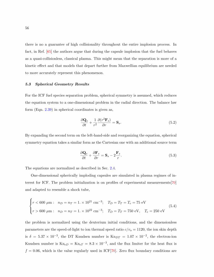
56
there is no a guarantee of high collisionality throughout the entire implosion process. In
fact, in Ref. [65] the authors argue that during the capsule implosion that the fuel behaves
as a quasi-collisionless, classical plasma. This might mean that the separation is more of a
kinetic effect and that models that depart further from Maxwellian equilibrium are needed
to more accurately represent this phenomenon.
5.3 Spherical Geometry Results
For the ICF fuel species separation problem, spherical symmetry is assumed, which reduces
the equation system to a one-dimensional problem in the radial direction. The balance law
form (Eqn. 2.39) in spherical coordinates is given as,
∂Qs
∂t+
1
r2
∂(r2Fs)
∂r= Ss. (5.2)
By expanding the second term on the left-hand-side and reorganizing the equation, spherical
symmetry equation takes a similar form as the Cartesian one with an additional source term
∂Qs
∂t+∂Fs
∂r= Ss − 2
Fs
r. (5.3)
The equations are normalized as described in Sec. 2.4.
One-dimensional spherically imploding capsules are simulated in plasma regimes of in-
terest for ICF. The problem initialization is on profiles of experimental measurements[70]
and adapted to resemble a shock tube,
r < 600 µm : nD = nT = 1.× 1021 cm−3; TD = TT = Te = 75 eV
r > 600 µm : nD = nT = 1.× 1022 cm−3; TD = TT = 750 eV, Te = 250 eV
(5.4)
the problem is normalized using the deuterium initial conditions, and the dimensionless
parameters are the speed-of-light to ion thermal speed ratio c/vo = 1120, the ion skin depth
is δ = 5.37 × 10⁻³, the DT Knudsen number is KnDT = 1.07 × 10⁻², the electron-ion
Knudsen number is KneD = KneT = 8.3 × 10⁻³, and the flux limiter for the heat flux is
f = 0.06, which is the value regularly used in ICF[70]. Zero flux boundary conditions are

57
Figure 5.2: Plot for a spherical imploding DT plasma for c/vo = 1120, δ = 5.37 × 10⁻³,Kni = 1.07 × 10⁻², Kne = 8.3 × 10⁻³, and f = 0.06. Shown are the number density,temperature and radial electric field at t = 1.375 ns. As the compression evolves and thefluids approach the center the density and temperature increase. The charge separationbetween the ions and the electron generate radial electric fields which peak at regions oflarge density and temperature gradients.
used at r = 0 µm and zero normal gradient boundary conditions are used at r = 800 µm.
Figure 5.2 shows profiles of the number density, temperature and electric field at t =
1.375 ns. There is clearly a separation of the deuterium and the tritium, and electric fields
in the order of GV/m form and peak in regions where the density and temperature gradients
are large. Fig. 5.3 shows the relative difference in number density between the deuterium
and the tritium. The separation occurs from the beginning of the simulation and increases
over time, and by the time the deuterium shock front reaches the center of the of the
capsule, it is ∼ 170 µm ahead of the tritium shock front. The time delay between when
the deuterium shock reaches r = 0 to when the tritium one does is ∼ 0.35 ns. The peak
deuterium concentration occurs slightly off center (region in gray in Fig. 5.3) as the reflected

58
Figure 5.3: Relative difference between the deuterium and the tritium number densities asa function of radius and time. Regions where the deuterium percentage is larger are in red,and blue where the tritium is larger. The deuterium separates from the tritium from thebeginning and the separation increases as time progresses. A 0.35 ns interval separates thedeuterium and the tritium shocks reaching the center.

59
portion interacts with a fraction that is moving towards the center. After both species have
reached the center (t ∼ 1.7 ns) there is a depletion of the deuterium from the center, shown
in the figure in blue.
Fields on the order of Gigavolts per meter (GV/m) develop. In Refs. [65, 67], the authors
suggested that at the beginning of the simulation, the electric field produces an equivalent
force on both ion species. The deuterium, which has a smaller mass, experiences a bigger
acceleration, and moves to shield the tritium from the electric field thereby reducing its
accelerations. To verify if the electric fields are actually the cause of the separation, the
maximum value of the different forces present in the system are a plotted as a function
of time in Fig. 5.4(a). There are three forces acting on each ion, the pressure gradient
(dp/dr) that separates them, the frictional force (Rdt) that opposes the separation, and the
electric force that, in this case, also contributes to the separation of the two ion species.
The frictional force is six orders of magnitude smaller than the pressure gradient which
dominates through the entire implosion. The force produced by the electric field is about an
order of magnitude larger than the frictional force, which acts to increase the ion separation.
Therefore, even though the electric fields are in the order of GV/m, the force they produce
are small in comparison to the pressure gradient. Therefore the electric fields are not the
main cause of the species separation. If the frictional force is small, then the DT Knudsen
number is large, which brings into question whether a fluid model is appropriate to represent
the physics in this problem. Figure 5.4(b)shows the value of the deuterium-tritium Knudsen
number as a function of space and time. Recall that Kn 10−2 is where fluid description
of the plasma is valid. The plot shows that a fluid description is valid for almost the entire
duration of the implosion, until t ∼ 1 ns, where the Knudsen number starts increasing
due to the rapid increase in the deuterium temperature, Kndt ∼ T 2d /nt. In regions of
large deuterium temperature and low tritium number density Kndt is large, and the plasma
becomes kinetic and fluid description breaks down. Figures. 5.4(c) and (d) show the Kndd
and Kntt as a function of space and time, respectively, and as deuterium and tritium fluids
approach the center, kinetic physics start to dominate.
The three-fluid (deuterium-tritium-electron) simulation, used above, is compared to a
two-fluid fluid one, composed of a DT-ion fluid with an averaged DT-mass and an electron
60
(a) (b)
(c) (d)
Figure 5.4: (a) Plots the normalized maximum values of the deuterium pressure gradient,electric, and frictional forces for the time interval before the deuterium reaches the centerof the capsule. The pressure gradient and the electric force cause the separation and areorders of magnitude larger than the frictional force which resists the separation. (b) For thesame time interval the largest value of the mean free path and the corresponding Knudsennumber are plotted. This shows that for the majority of the time Kn < 10−2, so a fluiddescription of the plasma is valid. (c) and (d) show the Kndd and Kntt respectively, andas these fluid approach the center of the imploding capsule, the deuterium-deuterium andtritium-tritium collisions decrease.

61
Table 5.1: Parameter used in Eq. (5.6) for the calculation of the DT reactivity as a functionof the ions temperature[3].
Reaction Fit Units T +D → n+4 He
C0 keV1/3 6.6610
C1 × 1016 cm3/s 643.41
C2 × 103 keV−1 15.136
C3 × 103 keV−1 75.189
C4 × 103 keV−2 4.6064
C5 × 103 keV−2 13.500
C6 × 103 keV−3 -0.10675
C7 × 103 keV−3 0.01366
T range keV 0.2-100
Error <0.25%
fluid. Current ICF HYDRA simulations[10] are done using averaged mass models. It is
suspected that species separation affects the DT fusion reaction rate considerably, and may
be the cause of the unexpectedly low neutron yield. A measurement of how much the
DT-fusion reaction has occurred is done by measuring the neutron yield given as
Y =
∫ ∫nDnT 〈σν〉DTdV dt (5.5)
where the DT reactivity, 〈σν〉DT , can be fitted using the expression[3]
〈σν〉DT = C1ζ−5/6ξ2 exp
(−3ζ1/3ξ
)(5.6)
where
ζ = 1− C2T + C4T2 + C6T
3
1 + C3T + C5T 2 + C7T 3, (5.7)
and
ξ = C0/T1/3. (5.8)
The values of the constants C0 − C7 are given in Table (5.1). In the three-fluid simulation
the averaged temperature is calculated as T = (pD + pT )/(nD + nT ).

62
Comparing the three-fluid and two-fluid yields over a 2 ns interval we obtain that
Y3f/Y2f = 0.3362. In the three-fluid case, there is separation of the deuterium from the
tritium, and as a consequence, the yield is only about one third that of the two-fluid prob-
lem. Figure 5.5 compares the product of the number density for both cases and the ratio
of the reactivities are plotted. The figure shows three shocks reaching the center and be-
ing reflected. The first shock corresponds to the 3-fluid case when the deuterium reaches
the center. The second shock corresponds to the 2-fluid case when the averaged mass ion
reaches the center. The third one is when the tritium from the 3-fluid case reaches the
center. If a horizontal line, at a fixed radius, is drawn, and nDnT is measured, the value for
the two-fluid simulation is higher, therefore the yield calculation for the two-fluid should be
bigger than the three-fluid simulation.
Figure 5.6 shows the temperature and reactivity at the center of the capsule plotted as
a function of time. The deuterium reaches the center earlier than ion fluid in the two-fluid
simulation. At this time in the simulation, the temperature of the two-fluid simulations at r
= 0 is still low and the ion reaches the capsule center ∼ 0.175 ns after the deuterium. After
another ∼ 0.175 ns, the tritium fluid from the three-fluid simulation reaches the capsule
center and the mass averaged temperature of the three-fluid simulation dips below the two-
fluid ion temperature. For the remainder of the simulations the three-fluid ion temperature
remains below the two-fluid temperature. Figure 5.6 also shows why initially the ratio of
the two reactivities is 15 orders of magnitude, that is because the deuterium reaches the
center first. Note that the two-fluid plasma reaches the center exactly in between the time
the deuterium and the tritium for the three-fluid plasma, as expected for a mass averaged
fluid.
The electric fields have their peak value at the shock fronts. In Fig. 5.7 the maximum
electric field is plotted over time. The peak field for the two-fluid plasma is on the order
a 160 GV/m while the three-fluid has double peaks corresponding to when the deuterium
and tritium reach the center, and is about ∼ 80 GV/m. These values of the electric field
are of the same order of magnitude as those inferred and simulated in Ref. [65].
63
Figure 5.5: Comparison of the variables used when calculating the neutron yield for thethree-fluid and two-fluid cases. Comparison of the ratio of the density product ndnt inthe three-fluid simulation with the square of the density of the two-fluid simulation. Thedensity product for the two-fluid case is larger then the three-fluid case where the ionshave separated, therefore the first term in the yield calculation is larger for the two-fluidsimulation.
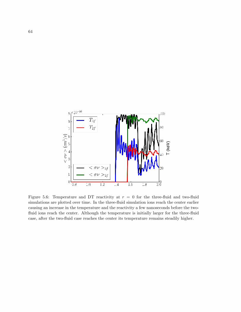
64
Figure 5.6: Temperature and DT reactivity at r = 0 for the three-fluid and two-fluidsimulations are plotted over time. In the three-fluid simulation ions reach the center earliercausing an increase in the temperature and the reactivity a few nanoseconds before the two-fluid ions reach the center. Although the temperature is initially larger for the three-fluidcase, after the two-fluid case reaches the center its temperature remains steadily higher.

65
Figure 5.7: Maximum electric field plotted over time. The two-fluid case produces a largerpeak electric field than the three-fluid simulation by a factor of two. However, gigavolt permeter electric fields produce forces that are still too small compared to the plasma pressuresin the problem.
5.4 Summary
The Inertial Confinement Fusion (ICF) fuel species separation problem has been exten-
sively analyzed using the multi-fluid plasma model and the blended finite element method.
Most ICF capsule implosion simulations assume that there is high collisionality between the
deuterium and tritium, therefore, they use radiation-hydrodynamic simulations to study
separation. It is shown that the single fluid, average mass atom assumption is not accurate
because the collisionality between the deuterium and the tritium is low, and in a Knudsen
number regime where there is a transition from a fluid to a kinetic plasma. Low collisional-
ity between the ion species is not capable of producing fictional forces that are large enough
to overcome the pressure gradients experienced by the plasma. Electric field on the order of
Gigavolts per meter are generated, however the forces they produce is small in comparison
to the pressure gradients, which are the main cause of separation. The separation of the
ICF fuel causes the fusion reaction rate to decrease to about one third of the yield pro-

66
duced by radiation-hydrodynamic conditions, which are in line with the 50% reduction that
experimental results have shown.
67
Chapter 6
UNCERTAINTY QUANTIFICATION OF THE GEM CHALLENGEMAGNETIC RECONNECTION PROBLEM USING THE
MULTILEVEL MONTE CARLO METHOD
6.1 Prior and Foundational Work
Uncertainty quantification (UQ) of plasma simulations are extremely important because,
in most cases, they are compared to experimental results in an attempt to validate the
simulations and explain the relevant physics of an experiment. Just like experimental data
have a region of certainty in the measured data (error bars), uncertainty quantification can
be used to produce the same effect on computationally generated results.
There are numerous sources of uncertainty in many plasma models, including the Two-
Fluid Plasma Model (TFPM). This uncertainties range from individual parameters uncer-
tainty, to boundary or initial conditions, transport coefficients among others. Often times
the exact value of a parameter is not know, only a range of values. Treating all the input
values as stochastic ic computationally expensive. Therefore, different sensitivity analy-
sis methods have been developed to rank the importance of the random inputs and their
interactions.
The Multilevel Monte Carlo (MMC) method was developed by Giles[26] for use in com-
putational finance for the solution of stochastic differential equations. Giles proved that
computational complexity could be reduced through the use of a multilevel approach that
combines results obtained using different levels of discretization while reducing the variance.
The MMC method uses a geometric sequence of time-steps similar to the multi-grid method
and has proven to be efficient and reliable in achieving the desired accuracy.
This permits establishment of regions of confidence in simulations which can subse-
quently be compared to experimental results. The MM method shows promising results
when it come to accuracy and computational cost.
The MMC method was extended from stochastic ODEs to elliptic PDEs in problems with
68
random coefficients arising in ground water flow[28]. In the case of the PDEs the geometric
series is applied to the spatial discretization instead of the temporal although both may
be related through the CFL stability condition. There is a dramatic reduction in cost
associated with the MMC method over the standard Monte Carlo (MC) method. Most of
the uncertainty can be captured on a coarse spatial discretization, thereby reducing the need
for numerous simulations on the finer and more computationally expensive discretizations.
Another method used in this study is the Probabilistic Collocation (PC) method. The
PC method was first introduced by Tatang and McRae [72], and recently Xiu and Hesthaven
[73] have used Lagrange polynomial interpolation to construct high-order stochastic colloca-
tion methods. The properties of PC method were extensively studied in the past ten years.
The errors of integrating or interpolating functions with Sobolev regularity were analyzed for
Smolyak constructions based on one-dimensional nested Clenshaw-Curtis rules[74, 75, 76].
The degree of exactness of the Smolyak quadrature using Clenshaw-Curtis and Gaussian
one-dimensional rules was investigated in Ref. [75]. The efficiency of Clenshaw-Curtis-based
sparse grid stochastic collocation was demonstrated in comparison to other stochastic meth-
ods on an elliptic problem[73]. In 2003, Gerstner and Griebel [77] introduced the dimension-
adaptive tensor product quadrature method. Sparse grid collocation schemes were applied
to solving stochastic natural convection problems[78]. An adaptive hierarchical sparse grid
collocation algorithm has been developed[79, 80].
Reference [81] describes a Multi-Element Probabilistic Collocation Method (ME-PCM)
that was developed to study the sensitivity of the TFPM model. The ME-PCM based sen-
sitivity analysis method is efficient and can achieve fast convergence compared to standard
MC based sensitivity analysis methods for cases with 20 – 100 random parameters.
In the research reported here, the MMC, MC, and PC methods will be applied to the
GEM challenge magnetic reconnection[2] problem for sensitivity and uncertainty quantifi-
cation study. Magnetic reconnection is a physical process that occurs in plasma by which
the magnetic field lines tear and reconnect and in the process convert magnetic energy into
kinetic energy. This phenomenon is present in virtually every plasma, whether in laboratory
fusion research experiments, stars solar flares, or even in the Earth’s magnetosphere.
Reference [2] presents multiple plasma models that are used in an effort to understand

69
the process on magnetic reconnection in better detail. Ideal MHD the magnetic field lines
are frozen into and move with the plasma; however for magnetic reconnection to occur,
the frozen-in flow constraint must be broken and this can only be done if there is some
resistivity or two-fluid effects.
In a fluid description the frozen-in constraint is broken and the magnetic topology is
allowed to change when the scale sizes in the system approach the electron skin depth
δe = c/ωpe, where c is the speed of light and ωpe is the electron plasma frequency. Therefore,
changing the electron mass or the speed of light affects this scale size[82].
The plasma model used here is the two-fluid model which models the electrons and
ions as separate fluids and couples both fluids through the Maxwell’s equations[37]. The
numerical scheme used is the wave propagation method[38]. It is a class of Godunov meth-
ods, which rely on the solution of a Riemann problem at each cell interface while allowing
for discontinuities at these interfaces. Second order accuracy is achieved by applying flux
limiters.
The main objective of this work is to evaluate the benefits of the MMC method and
quantify the uncertainty in the GEM challenge problem due to the choice of ion-to-electron
mass ratio, speed of light to Alfven speed ratio, and the magnetic flux perturbation that
determines the dominant mode in reconnection, on the reconnected flux evolution.
6.2 Plasma Models for Uncertainty Quantification Study
In this work, two different plasma models are employed to quantify the uncertainty and
compare three UQ methods (MC, MMC and PC). The first plasma model is the quasi-
neutral ion cyclotron waves model. The problem models a quasi-neutral ion cyclotron wave,
a dispersive wave, in an uniform plasma in a magnetic field that is constant in space and
time. Like the two-fluid plasma model, the quasi-neutral ion cyclotron waves has imaginary

70
eigenvalues of the source Jacobian. The equation system being solved is given as
∂ρ
∂t+ ρ
du
dx= 0, (6.1)
ρ
(∂u
∂t+ u
∂u
∂x
)+∂p
∂x= nqu×B = ρωcu× b, (6.2)
∂ε
∂t+
d
dx((ε+ p)u) = 0, (6.3)
where ρ is the mass density, u is the velocity, p is the pressure, B is the magnetic field, b is
the unit vector in the direction of B, ωc =q|B|m
is the ion cyclotron frequency, and
ε =p
γ − 1+
1
2ρu2 (6.4)
is the total energy density, where γ is the ratio of specific heats.
A benefit of using this problem is that the exact solution of the velocity field is known
and given by
u(x, t) = −N∑n=0
uo12n+ 1
sin(knx+ ωnt), (6.5)
when the fluid is initially perturbed with the random velocity (to simulate uncertainty),
u1(x) = uo1(ξ)N∑n=0
i
2n+ 1eiknx, (6.6)
where uo1(ξ) is the random velocity, ξ is a random variable with uniform distribution, U [10−10
to 10−4], kn = 2π(2n+1) is the wave number, ωn = ±√k2nc
2s + ω2
c is the dispersion relation,
and cs =√γp/ρ is the speed of sound. This problem is computationally inexpensive.
The second plasma model is the collisionless TFPM[83, 16, 84] which is derived by taking
moments of the Boltzmann equation and regarding the electron and ion species as separate
fluids. The resulting equation system for the TFPM is used to evolve the fluid variables and
Maxwell’s equations advance the electric and magnetic fields. The fluids and fields variables
couple through the source terms.
There are several sources of uncertainty in the two-fluid plasma model. Often times
modelers change the ion-to-electron mass ratio or the speed of light to Alfven speed ratio to

71
speed up the computation. This study aims to quantify the uncertainty of varying the ion-to-
electron mass ratio, speed of light to Alfven speed ratio, and the magnetic flux perturbation
that determines the dominant mode of the reconnection, have on the reconnected flux of the
the GEM magnetic reconnection challenge. In particular, we assumemi/me = ξ1, where ξ1 is
a random variable with uniform distribution U [25, 100], vA/c = ξ2, ξ2 is a random variable
with uniform distribution, U [10, 20], vA = B/√µoρ and the magnetic flux perturbation,
ψ = ξ3ψp. Here ξ3 is a random variable with uniform distribution, U [0.085, 0.115].
The other model used is the ideal multi-fluid plasma model described in Sec. 2.5. The
source terms in Maxwell’s equations couple the fluid variables to the electromagnetic fields
and the Lorentz forces act as body forces on the electrons and ions. These source terms
introduce physical dispersion in the two-fluid model which comes from the fact the flux
Jacobian of the system has imaginary eigenvalues and therefore the waves in the system are
undamped[84].
Contrary to the MHD model, the two-fluid plasma model includes the Hall and diamagnetic-
drift terms, assumes a finite speed of light, and a finite electron mass. These assumptions
allow for the description of displacement current effects and high-frequency oscillations.
Both models are solved using the high-resolution wave propagation (a finite volume)
method. The solution method belongs to the class of Godunov solvers, which rely on the
solution of Riemann problems described in Refs. [83, 19, 38] and can be applied to balance
laws of the form Eq. (2.39). A Riemann problem is solved at each cell interface and the
solution is, in general, discontinuous. Second order accuracy can be achieved by performing
a linear reconstruction of the waves needed to compute the numerical fluxes at the cell
interfaces[19].
6.3 Standard Monte Carlo Method
In statistics, aggregate mathematical measures are created to characterize data, these rules
are referred to as estimators. Common estimators are the mean value and the variance of

72
the data set. In the standard MC method the mean estimator is given as
E[PMCm,N ] =
1
N
N∑i=1
P im, (6.7)
where N is the number of samples and P im is a measured quantity of each sample i obtained
using m spatial grid points. The value of P im obtained using m grid points approaches the
exact solution, P , as the number of grid points increases and the mean square error (MSE),
e2, can be represented as
e2MC = V[PMC
m,N ] + (E[Pm]− E[P ])2. (6.8)
The first term represents the sampling error and is given by
V[PMCm,N ] =
1
N − 1
N∑i=1
(P im − E[PMCm,N ])2, (6.9)
which is the variance. The second term of Eq. (6.8) represents the discretization error. To
achieve an MSE less than ε2, both terms are chosen to be less ε2/2. Reducing the first term
is achieved by having a large number of samples, N ∼ O(ε−2). The second term is reduced
by increasing the number of grid points (increased resolution), m ∼ O(ε−1/α) where α is
the discretization convergence rate[28].
6.4 Multilevel Monte Carlo Method
For most numerical simulations, either large sample size or high discretization are computa-
tional expensive. Therefore, novel methods that reduce the numerical error while achieving
“reasonable” discretization and sample size are desired. In this case the MMC method is
chosen to quantify the uncertainty in the two-fluid plasma model.
When there is uncertainty in a quantity or constant being used in a numerical simulation
it is common to use a MC method to study the effects of this uncertainty in the solution of
the problem. This is done by running a large number of simulations each using a randomly
selected value of set quantity within the uncertainty interval. All the simulations are exe-
73
cuted using the same discretization. For the MMC method for each random quantity two
simulations are done at different discretization.
The MMC estimator is defined as
PMMCm =
L∑l=0
Yl, (6.10)
where
Yl =1
Nl
Nl∑i=1
(P iml− P iml−1
), (6.11)
The MMC mean estimator is
E[PMMCm ] =
L∑l=0
E[Yl], (6.12)
where P im−1= 0. In this case, because there are different discretization levels, l, the spacial
resolution becomes, ml, to denote the number of grid points at level l. Also, the sample size
(N) from Eq. (6.7) is now level dependent (Nl) and does not need to be the same for every
level. Yl is estimated independently for each level l and the multilevel variance estimator is
V[PMMCm ] =
L∑l=0
V[Yl]. (6.13)
Following Eq. (6.8) the error in the MMC method is expressed as
e2MMC =
L∑l=0
V[Yl] + (E[Pml− P ])2, (6.14)
where
V[Yl] =1
NlV (Pml
− Pml−1). (6.15)
The multilevel variance V[Yl] = N−1l V (Pml
− Pml−1) → 0 as l → ∞ and if the variance is
decreasing, a lesser number of sample data will be needed, consequently Nl → 1 as l→∞.
The cost at the coarsest level is fixed for all levels of accuracy. Achieving an overall MSE of
ε with MMC method is easier than the standard MC method. The MMC method is used
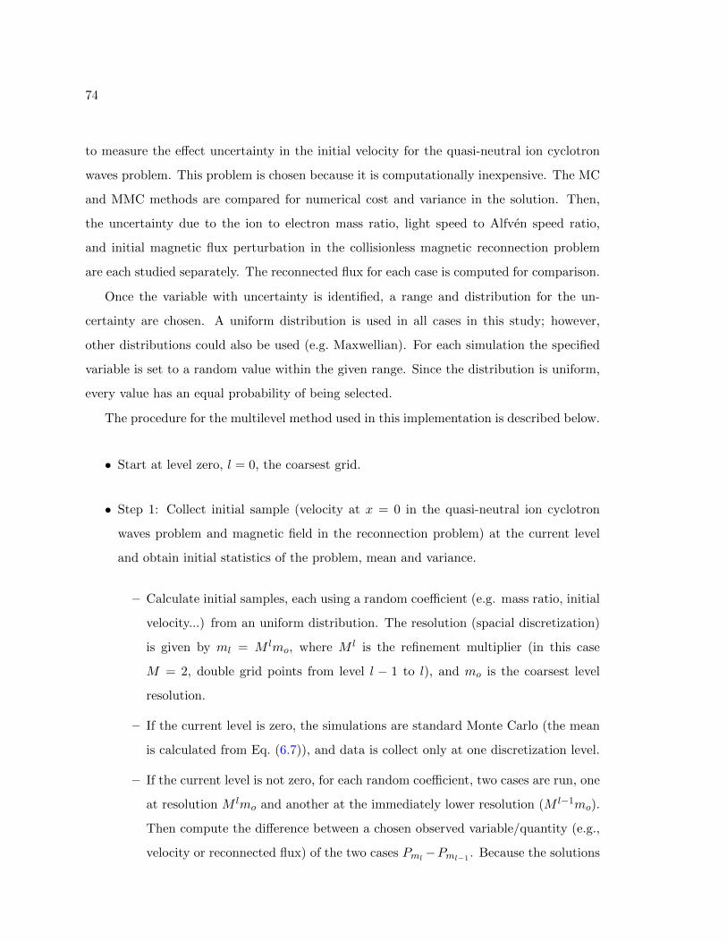
74
to measure the effect uncertainty in the initial velocity for the quasi-neutral ion cyclotron
waves problem. This problem is chosen because it is computationally inexpensive. The MC
and MMC methods are compared for numerical cost and variance in the solution. Then,
the uncertainty due to the ion to electron mass ratio, light speed to Alfven speed ratio,
and initial magnetic flux perturbation in the collisionless magnetic reconnection problem
are each studied separately. The reconnected flux for each case is computed for comparison.
Once the variable with uncertainty is identified, a range and distribution for the un-
certainty are chosen. A uniform distribution is used in all cases in this study; however,
other distributions could also be used (e.g. Maxwellian). For each simulation the specified
variable is set to a random value within the given range. Since the distribution is uniform,
every value has an equal probability of being selected.
The procedure for the multilevel method used in this implementation is described below.
• Start at level zero, l = 0, the coarsest grid.
• Step 1: Collect initial sample (velocity at x = 0 in the quasi-neutral ion cyclotron
waves problem and magnetic field in the reconnection problem) at the current level
and obtain initial statistics of the problem, mean and variance.
– Calculate initial samples, each using a random coefficient (e.g. mass ratio, initial
velocity...) from an uniform distribution. The resolution (spacial discretization)
is given by ml = M lmo, where M l is the refinement multiplier (in this case
M = 2, double grid points from level l − 1 to l), and mo is the coarsest level
resolution.
– If the current level is zero, the simulations are standard Monte Carlo (the mean
is calculated from Eq. (6.7)), and data is collect only at one discretization level.
– If the current level is not zero, for each random coefficient, two cases are run, one
at resolution M lmo and another at the immediately lower resolution (M l−1mo).
Then compute the difference between a chosen observed variable/quantity (e.g.,
velocity or reconnected flux) of the two cases Pml−Pml−1
. Because the solutions

75
are at different resolutions, the intermediate values at the coarse grid are the
average of the values of the two closest grid-points.
– The multilevel estimator of the mean of the solution is given by Eq. (6.12) and
is calculated from data collected at two different discretization levels.
• Step 2: Estimate the variance using the initial sample. The unbiased variance of each
level is given by Eq. (6.15). Not to be confused with the overall method variance given
in Eq. (6.13).
• Step 3: Calculate the optimal sample size for all levels up to the current one. The
optimal number, Nl required to reduce the variance Vl to less than 12ε
2 is given from
Ref. [26] as
Nl = 2ε−2√Vlml
(l∑
k=0
√Vk/mk
). (6.16)
• Step 4: Collect additional sample at each level as needed for the new Nl. Run addi-
tional cases if Nl is bigger than the initial number of the sample.
• Step 5: Check for convergence. If l ≥ 1, and max(M−1|PMMC
L−1 |, |PMMCL |
)<
1√2
(M−
1)ε then the error is less than 1√2ε and the solution has converged.
• Step 6: If the solution has not converged, increment level to l + 1 and repeat from
step 1.
Another uncertainty quantification method, probabilistic collocation, is described in the
Appendix.
6.5 Numerical Results
The quasilinear ion cyclotron wave problem is used to examine the performance of the
MMC method in computing the expected values of the velocity. This model is nonlinear
and less computationally expensive than the full two-fluid model. It is a one-dimensional
(1D) problem, with periodic boundary conditions and the velocity field is initialized to the

76
Figure 6.1: L2 − norm error for the mean and variance as a function of computationaltime using the quasi-neutral ion cyclotron wave test problem. With cs =
√1.4, ωc = 10.0,
Bz = 1.0, mi = 1.0 and q = 10.0 and initial values of ρ = 1.0 and p = 1.0. The ratesof convergence for the mean using the MC and MMC methods are similar. The rate ofconvergence for the variance using the MMC method is faster than the MC method.
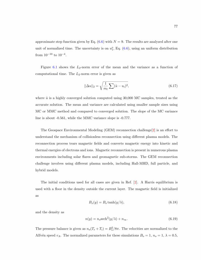
77
approximate step function given by Eq. (6.6) with N = 9. The results are analyzed after one
unit of normalized time. The uncertainty is on uo1, Eq. (6.6), using an uniform distribution
from 10−10 to 10−4.
Figure 6.1 shows the L2-norm error of the mean and the variance as a function of
computational time. The L2-norm error is given as
||∆u||2 =
√1
ml
∑(u− ui)2, (6.17)
where u is a highly converged solution computed using 30,000 MC samples, treated as the
accurate solution. The mean and variance are calculated using smaller sample sizes using
MC or MMC method and compared to converged solution. The slope of the MC variance
line is about -0.561, while the MMC variance slope is -0.777.
The Geospace Environmental Modeling (GEM) reconnection challenge[2] is an effort to
understand the mechanism of collisionless reconnection using different plasma models. The
reconnection process tears magnetic fields and converts magnetic energy into kinetic and
thermal energies of electrons and ions. Magnetic reconnection is present in numerous plasma
environments including solar flares and geomagnetic sub-storms. The GEM reconnection
challenge involves using different plasma models, including Hall-MHD, full particle, and
hybrid models.
The initial conditions used for all cases are given in Ref. [2]. A Harris equilibrium is
used with a floor in the density outside the current layer. The magnetic field is initialized
as
Bx(y) = Bo tanh(y/λ), (6.18)
and the density as
n(y) = nosech2(y/λ) + n∞. (6.19)
The pressure balance is given as no(Te + Ti) = B2o/8π. The velocities are normalized to the
Alfven speed vA. The normalized parameters for these simulations Bo = 1, no = 1, λ = 0.5,

78
n∞/no = 0.2, Te/Ti = 0.2. An initial perturbation in the magnetic flux is given as
ψ(x, y) = ψo cos(2πx/Lx) cos(πy/Ly), (6.20)
and the magnetic field perturbation is given as B = z × ∇ψ and ψo = ξ3 which is the
third source of uncertainty that is investigated in this research. When the uncertainties of
mi/me and c/vA are being studied, ξ3 is set to 0.1. The unit scale length is the ion-skin
depth (c/ωpi) and the unit time scale is the inverse ion cyclotron frequency (ω−1ci ). The
computational domain is Lx = 8π and Ly = 4π and the final time is 400/ωci. The problem
has periodic boundary conditions in the x-direction and conducting boundary conditions in
the y-direction. To compare results, the reconnected flux, φ, is computed using,
φ(t) =1
2Lx
∫ Lx/2
−Lx/2|By(x, y = 0, t)|dx. (6.21)
The two-fluid plasma method used in these simulations are in good agreement with the
benchmarked results published in the GEM challenge paper [2] and can be seen in Ref. [19].
For magnetic reconnection to occur and magnetic fields to tear and reconnect, the mag-
netic field lines can not be frozen into the plasma and must move with the plasma. In a
fluid description of plasmas the frozen-in constraint is broken and the magnetic topology is
allowed to change when the length scales in the problem approach the electron skin depth
δe = c/ωpe , where c is the speed of light and ωpe is the electron plasma frequency. In this
study the effects of varying the speed of light and the electron mass are analyzed. Changing
these quantities change the electron skin depth, which in turn could affect the reconnected
flux.
In a hydrogen plasma the ion-to-electron mass ratio is 1836. However, running simu-
lations at this mass ratio presents a challenge. The two-fluid plasma model has disparate
timescales, i.e., ω−1cs and ω−1
ps need to be resolved, where
ωcs =qs|B|ms
, ωps =
√nsq2
s
εoms(6.22)

79
Figure 6.2: Mean (top) and variance (bottom) of the reconnected flux for varying ion-to-electron mass ratio ranging from 25 to 100, for the MMC, MC, and PC methods.
are the cyclotron frequency and the plasma frequency for each species, respectively. Decreas-
ing the ion-to-electron mass ratio relaxes the time step restrictions and allows simulations
to be completed in less time. A small artificial mass ratio of mi/me = 25 is used in the
GEM challenge paper to reduce the stiffness and speedup the computation.
Figure 6.2 shows the mean and variance reconnected flux for simulations by varying the
mass ratio mi/me ∈ [25, 100] and the results of the MMC method is compared to the MC
and PC methods results. The MMC simulations are completed using two levels with 32
simulations at a coarse grid (256×128) and 16 at a twice finer grid. The PC method has 33
simulations and the MC has 56, all at 512× 256 resolution. The results for this case show
that all three methods produce approximately the same mean and variance, σ2.
For the MMC method the variance is computed using
σ2[Pl] = E[P 2l ]− E2[Pl] (6.23)
where
E[P 2l ] = E[P 2
o ] +
L∑l=1
E[P 2l − P 2
l−1] (6.24)

80
Figure 6.3: Mean (top) and variance (bottom) of the reconnected flux for varying speedof light to Alfven speed ratio ranging from 10 to 20, for the MMC, standard MC, and PCmethod.
instead of the multilevel estimator given by Eq. (6.13).
The second variable of the skin depth that is analyzed is the speed of light, c. In the
two-fluid plasma model, explicitly advancing the equations in time is limited by the highest
frequency or the fastest velocity in the system. The speed of light is often the fastest
speed in the system and hence usually generates the most restrictive time step constraint.
Relaxing this restriction can be achieved by reducing the value of c. As mentioned before,
all the velocities in the GEM challenge paper are normalized to the Alfven speed and in all
simulations εo = µo = 1.
Figure 6.3 shows the mean and variance when the ratio of the speed of light to the
Alfven speed is varied from c/vA ∈ [10, 20] for the three different methods, MMC (2 levels,
32 samples at level 0 and 16 at level 1), MC (56 samples), and PC method (33 samples),
at the resolution of 512 × 256 (for the MMC this is the resolution of level 1, finest grid
resolution).
The GEM reconnection challenge Harris equilibrium is perturbed by a sinusoidal flux
with an amplitude ψo as described by Eq. (6.20). Depending on the amplitude of this
perturbation the reconnection is either delayed or sped up, therefore, the reconnected flux

81
Figure 6.4: Mean (top) and variance (bottom) of the reconnected flux for varying amplitudeof the magnetic flux perturbation ranging from [0.085, 0.115], for the MMC, standard MC,and PC method.
should be highly sensitive to variations in this parameter. Figure 6.4 shows the mean and
variance of the reconnected flux when ψo ∈ [0.085, 0.115] of the background magnetic field
amplitude.
6.6 Discussion
The MMC, MC, and PC methods are applied to the GEM magnetic reconnection problem
to study the sensitivity of the reconnected flux to uncertainties in ion-to-electron mass ratio,
speed of light to Alfven speed ratio, and the magnitude of the initial magnetic flux pertur-
bation. The goal is to determine which of the methods is more computational inexpensive
and reduces the variance more rapidly as the sample size is increased.
Initially the performance of the different methods is studied using the quasilinear ion
cyclotron wave problem since it is computationally inexpensive. Figure 6.1 shows that the
error decreases as the computational cost increases. However, the error in the MMC variance
is lower than the MC method, and the variance decreases much faster for the MMC method.
Therefore the MMC method gives a better result with less computation effort.
Figure 6.2 shows the results for the mass ratio study. Here the variance is relatively low

82
Figure 6.5: Ion density and magnetic field vectors showing the formation of a second smallermagnetic island at the center and as a result the reconnected flux in these cases is slightlyhigher because there are no asymmetries in the grid and during the solution the smallerisland will remain at the center of the grid. However if some numerical asymmetry developsthe island will move to the right or the left. ωcit = 38 and mi/me = 25.
except between ωcit = 25 – 35, therefore the reconnected flux is relatively independent of
the mass ratio. A possible explanation for the higher variance between ωcit = 25 – 35 is
that for certain cases an intermediate, smaller magnetic island forms at the center of the
domain as seen in Fig. 6.5. This smaller island eventually merges with the bigger island.
Figure 6.3 demonstrates good agreement of the mean and the variance between the
different methods showing the small sensitivity of the problem to changes in the speed
of light to Alfven speed ratio. Like the mass ratio case, the variance also spikes around
ωcit = 23.0 for the same reason as explained for the mass ratio.
The variance of the MC method is observed to be stochastically higher than the variance
of the MMC and PC methods, as seen in Fig. 6.4. The MMC mean follows closely the MC
mean. The cost of the MMC is much lower than the MC. The MMC method has 36
simulations at 256 × 128 resolution and only 6 simulations at 512 × 256 which resulted in
a total of 4075 CPU-hours while the MC has 46 simulations at 512× 256 resolution and a
total of 6496 CPU-hours. Therefore, there is a total computational time saving of about one
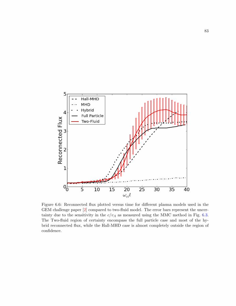
83
Figure 6.6: Reconnected flux plotted versus time for different plasma models used in theGEM challenge paper [2] compared to two-fluid model. The error bars represent the uncer-tainty due to the sensitivity in the c/vA as measured using the MMC method in Fig. 6.3.The Two-fluid region of certainty encompass the full particle case and most of the hy-brid reconnected flux, while the Hall-MHD case is almost completely outside the region ofconfidence.
84
third (37.3%) of the MMC method over the standard MC method and a smaller variance.
The PC method has a total CPU time of 4660 CPU-hours (33 simulations at 512 × 128
resolution) which is 14.4% more computationally expensive as the MMC.
Figure 6.6 compares the reconnected flux computed by the different plasma models given
in Ref. [2] and the reconnected flux computed by the two-fluid plasma model. The MHD and
Hall-MHD models assume the speed of light is infinite while the hybrid, full particle, and
two-fluid models assume a finite value. In the two-fluid case the standard deviation is plotted
as the error bars to see the influence of varying the speed of light on the reconnected flux.
Our results seem to be somewhere between the hybrid and the Hall-MHD models. The
two-fluid plasma model results compare favorably with the full particle, Hall-MHD, and
hybrid models. MHD has insufficient physics to capture collisionless reconnection.
6.7 Summary
A less costly method of obtaining the mean and variance of a numerical simulation with
uncertainty in parameters is presented. The cost reduction comes from the fact that a
large number of simulations are done at a coarse resolution which captures the variance of
the uncertainty, and few simulations are done at a fine resolution which resolves the mean
accurately. Coarse resolution simulations are computationally inexpensive, while the finer
ones are more expensive but only a few are needed. Less costly computation of the region
of validity of simulation results allow for the comparison of numerical and computational
values more accurately and for better computer models validation.

85
Chapter 7
OPEN BOUNDARY CONDITIONS
7.1 Prior and Foundational Work
One method that has been used to simulate open boundary conditions is the Perfectly
Matched Layers (PML)[30]. In the PML method an absorbing layer is added at the domain
boundary, which absorbs and dissipates incoming waves while reducing reflections. This is
done by first matching the impedance of the computation domain and the absorbing layer
to eliminate reflections and achieve 100% transmission of the incoming waves. Once the
waves have been transmitted to the layer, they are dampened, i.e. the PML acts as a lossy
medium. This method has been developed extensively for electromagnetics problems in the
frequency [85] and time domain [86]. The method is successful at eliminating refection.
However, PML’s become unstable when integrated over long time intervals and exacerbate
the problem of accumulation of error in long-term numerical simulations[87].
Another method used for hyperbolic partial differential equation systems with sharp aft
fronts is the lacuna-based open boundary conditions (LOBC)[29]. Lacuna is a region in
space that, after being disturbed by a traveling wave, has returned to its original condition.
The basic idea is that, any finite size domain will fall within the lacuna of any traveling
wave if enough time has been elapsed. Therefore, any change to a traveling wave will not
affect its lacuna which contains the computational domain of interest.
The advantage of the lacuna method is that it allows for stable long-term integration of
the equations driven by continuously operating sources without accumulation of numerical
error. The method is also non-local in space and time, and can be applied to any geometry
domain. The implementation of this method requires the creation of an auxiliary grid/do-
main that overlaps with computational grid of interest at the boundary that is open. Any
incoming waves to this boundary are transmitted to the auxiliary grid, which in turn pro-
vides the required closure (boundary condition) for the computational domain. Once the
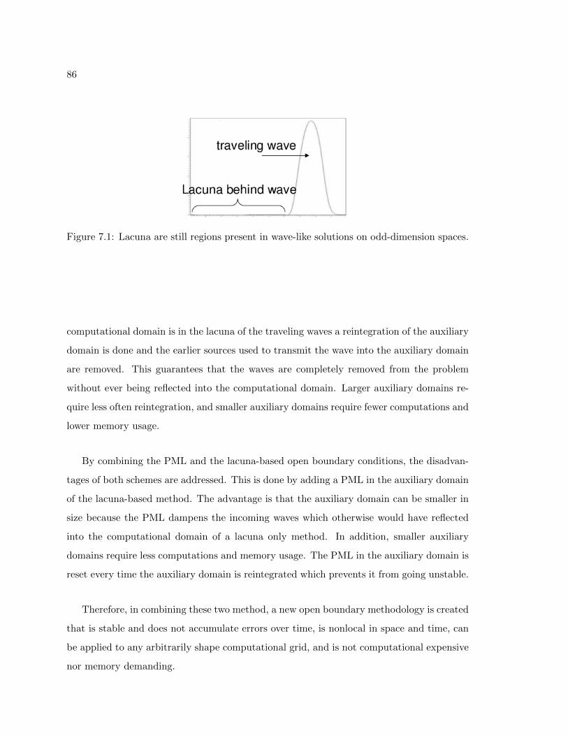
86
Figure 7.1: Lacuna are still regions present in wave-like solutions on odd-dimension spaces.
computational domain is in the lacuna of the traveling waves a reintegration of the auxiliary
domain is done and the earlier sources used to transmit the wave into the auxiliary domain
are removed. This guarantees that the waves are completely removed from the problem
without ever being reflected into the computational domain. Larger auxiliary domains re-
quire less often reintegration, and smaller auxiliary domains require fewer computations and
lower memory usage.
By combining the PML and the lacuna-based open boundary conditions, the disadvan-
tages of both schemes are addressed. This is done by adding a PML in the auxiliary domain
of the lacuna-based method. The advantage is that the auxiliary domain can be smaller in
size because the PML dampens the incoming waves which otherwise would have reflected
into the computational domain of a lacuna only method. In addition, smaller auxiliary
domains require less computations and memory usage. The PML in the auxiliary domain is
reset every time the auxiliary domain is reintegrated which prevents it from going unstable.
Therefore, in combining these two method, a new open boundary methodology is created
that is stable and does not accumulate errors over time, is nonlocal in space and time, can
be applied to any arbitrarily shape computational grid, and is not computational expensive
nor memory demanding.
87
7.2 The Lacuna-based Open Boundary Condition (LOBC)
For the implementation of the LOBCs, the original infinite-domain problem is split into
an interior and an auxiliary sub-domains. The interior problem becomes the bounded
computational region of interest, whereas the auxiliary problem models an infinite domain.
The two problems are dependent on each other. The sources for the auxiliary problem
depend on the interior solution, and the solution of the auxiliary problem provides the
required boundary conditions for the interior one[29].
This still leaves the auxiliary problem defined in an infinite domain. There, any changes
applied to a propagating wave will not affect its lacuna (the interior domain). Therefore, a
reintegration of the solution can be done in which “sufficiently” earlier sources of the wave
is removed.
The interior problem is evolved using hyperbolic equations in balance law form, given
by Eq. (2.39), and the auxiliary domain is evolved using,
∂w
∂t+∇ · F(w) = S(w) + Ω(Q). (7.1)
The auxiliary source term Ω(Q), in Eq. (7.1), couples the interior solution to the auxiliary
one. This source is solely dependent on values in a transition region; the location where
the two domains overlap. To calculate this source, an auxiliary function, µ(x), is needed to
guarantee that the two problems match at the boundary between the interior and exterior
domain, while making the transition smooth, as shown in Fig. (7.2). This function is
µ(x) = 1 in the exterior domain and µ(x) = 0 in the interior domain except the transition
region, where µ(x) varies from zero to one smoothly and be C1 continuous everywhere. The
interior variable Q and the auxiliary variable w are related through µ(x) as w = µ(x)Q.
Solving Eq. (7.1) for the time derivative, substituting w = µ(x)Q, and noting that µ is
only a function of position, the following relation is obtained
µ∂Q
∂t= −∇ · F(µQ) + S(µQ) + Ω(Q), (7.2)

88
Figure 7.2: The transition function µ(x) varies from zero in the interior domain to one inthe exterior domain and is Co and C1 continuous.
substituting Eq. (2.39) into Eq. (7.2) leads to an expression of the auxiliary source
Ω(Q) = ∇ · F (µQ)− S(µQ)− µ∇ · F (Q) + µS(Q). (7.3)
For homogeneous problems where fluxes and sources that are linear functions of q, the
calculation of the auxiliary source can be reduced to Ω(Q) = F · ∇µ.
Another important step of this method is referred to as the temporal re-integration of
the auxiliary sources described in Ref. [88]. Waves in the auxiliary domain, can themselves
be reflected from the exterior boundaries which can eventually re-enter the interior domain.
To avoid this, a reintegration of the auxiliary sources is performed at constant time intervals,
and earlier contributions to the auxiliary sources are removed. Since the interior domain
is in the lacuna of such contributions any removal of auxiliary source does not affect the
interior solution.
To better understand this process consider the following. Suppose that at t = t0 and
step n = 0 the source Ω0 is generated and at every subsequent time step, n, the equivalent
source Ωn is generated. After the simulation has been elapsed for t = TN the source ΩN

89
has been generated. At this point it can be deemed that sufficient time has passed and
the computational (interior) domain is in the lacuna of the wavelet that the sources from
n = 0...nr (nr < N) are no longer affect the interior solution. Therefore, the re-integration
of the auxiliary domain can be done following Eq. (7.1) to attain the new solution at t = TN
w|tN =
∫ TN
tnr
∂w
∂tdt = w|tnr
+N∑
i=nr
∫ TN
tnr
(−∇ · F(w) + S(w) + Ωi) dt. (7.4)
Equation (7.4) gives the auxiliary solution from the beginning of the simulation to the
current time. All the sources from timesteps n = 0...nr − 1 are ignored and only the
sources from n = nr...N are used, that means w|tnr= 0. Only the source contributions
from n = nr...N are retained. If each source contribution can be viewed as being a discrete
value, Ωi, integrating each contribution from time t = tn to t = tN gives the current solution
due to the earlier source. Therefore, if all the contributions from all the discrete values of the
source from n = nr to n = N are added up, the solution w|tN at t = tN is obtained without
the earlier sources. This reintegration guarantees that no waves re-enter the interior domain
after they have completely exited it. It is not practical to do the reintegration every time
step. The maximum time that the wavelet can propagate without re-entering the interior
domain is denoted as the reintegration time (Tmaxri ); this value depends on the size of the
exterior domain, dext, and the fastest traveling speed in the system, c
Tmaxri =2dextc
. (7.5)
The implementation is as follows,
1. Integrate Eq. (2.39) and get Q in the interior domain;
2. Calculate the auxiliary source using Q and Eq. (7.3);
3. Integrate Eq. (7.1) using the auxiliary source and obtain w;
4. Use the new w to apply the boundary conditions to Q;
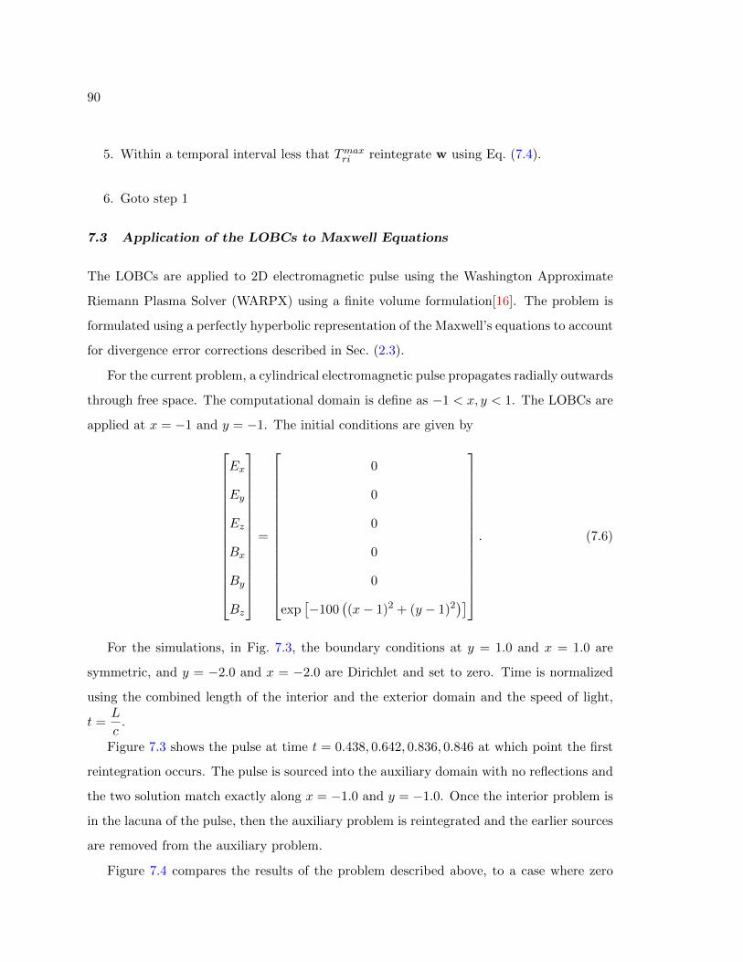
90
5. Within a temporal interval less that Tmaxri reintegrate w using Eq. (7.4).
6. Goto step 1
7.3 Application of the LOBCs to Maxwell Equations
The LOBCs are applied to 2D electromagnetic pulse using the Washington Approximate
Riemann Plasma Solver (WARPX) using a finite volume formulation[16]. The problem is
formulated using a perfectly hyperbolic representation of the Maxwell’s equations to account
for divergence error corrections described in Sec. (2.3).
For the current problem, a cylindrical electromagnetic pulse propagates radially outwards
through free space. The computational domain is define as −1 < x, y < 1. The LOBCs are
applied at x = −1 and y = −1. The initial conditions are given by
Ex
Ey
Ez
Bx
By
Bz
=
0
0
0
0
0
exp[−100
((x− 1)2 + (y − 1)2
)]
. (7.6)
For the simulations, in Fig. 7.3, the boundary conditions at y = 1.0 and x = 1.0 are
symmetric, and y = −2.0 and x = −2.0 are Dirichlet and set to zero. Time is normalized
using the combined length of the interior and the exterior domain and the speed of light,
t =L
c.
Figure 7.3 shows the pulse at time t = 0.438, 0.642, 0.836, 0.846 at which point the first
reintegration occurs. The pulse is sourced into the auxiliary domain with no reflections and
the two solution match exactly along x = −1.0 and y = −1.0. Once the interior problem is
in the lacuna of the pulse, then the auxiliary problem is reintegrated and the earlier sources
are removed from the auxiliary problem.
Figure 7.4 compares the results of the problem described above, to a case where zero
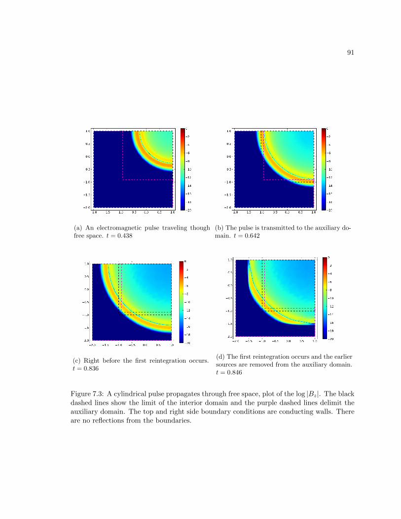
91
(a) An electromagnetic pulse traveling thoughfree space. t = 0.438
(b) The pulse is transmitted to the auxiliary do-main. t = 0.642
(c) Right before the first reintegration occurs.t = 0.836
(d) The first reintegration occurs and the earliersources are removed from the auxiliary domain.t = 0.846
Figure 7.3: A cylindrical pulse propagates through free space, plot of the log |Bz|. The blackdashed lines show the limit of the interior domain and the purple dashed lines delimit theauxiliary domain. The top and right side boundary conditions are conducting walls. Thereare no reflections from the boundaries.
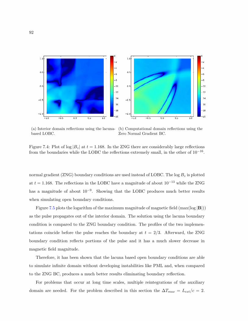
92
(a) Interior domain reflections using the lacuna-based LOBC.
(b) Computational domain reflections using theZero Normal Gradient BC.
Figure 7.4: Plot of log |Bz| at t = 1.168. In the ZNG there are considerably large reflectionsfrom the boundaries while the LOBC the reflections extremely small, in the other of 10−16.
normal gradient (ZNG) boundary conditions are used instead of LOBC. The logBz is plotted
at t = 1.168. The reflections in the LOBC have a magnitude of about 10−13 while the ZNG
has a magnitude of about 10−9. Showing that the LOBC produces much better results
when simulating open boundary conditions.
Figure 7.5 plots the logarithm of the maximum magnitude of magnetic field (max(log |B|))
as the pulse propagates out of the interior domain. The solution using the lacuna boundary
condition is compared to the ZNG boundary condition. The profiles of the two implemen-
tations coincide before the pulse reaches the boundary at t = 2/3. Afterward, the ZNG
boundary condition reflects portions of the pulse and it has a much slower decrease in
magnetic field magnitude.
Therefore, it has been shown that the lacuna based open boundary conditions are able
to simulate infinite domain without developing instabilities like PML and, when compared
to the ZNG BC, produces a much better results eliminating boundary reflection.
For problems that occur at long time scales, multiple reintegrations of the auxiliary
domain are needed. For the problem described in this section the ∆Tmax = Lext/c = 2.

93
Figure 7.5: The logarithm of maximum value of the magnetic field magnitude is plottedversus the elapsed simulation time. The ZNG method produces reflection when the pulsereaches the boundaries while the LOBC does not.
94
For smaller exterior domains the reintegration has to occur more frequent, and for larger
ones more memory is need to store the auxiliary sources. Therefore, there is a compromise
between the frequency of reintegration and exterior domain size used. One way to eliminate
this dependence is described in the next section.
7.4 Combined Application of PMLs and LOBCs to Maxwell’s Equations
Adding PML at the outer boundary of the auxiliary domain of a LOBC implementation, is
done to solve two problems: to reduce the frequency of reintegration of the LOBC, and by
doing so resetting the PML to prevent it from going unstable.
For the current implementation an unspilt PML is used for the 2D Maxwell’s equations.
The PML is applied in the x-direction boundaries. The PML implemented here is the
physically motivated PML [31]
∂Ex∂t
=∂Hz
∂y+ σ(Ex − P ) (7.7)
∂Ey∂t
= −∂Hz
∂x− σEy (7.8)
∂Hz
∂t=
∂Ex∂y− ∂Ex
∂y− σHz (7.9)
∂P
∂t= σ(Ex − P ). (7.10)
where P is nonzero only in the PML. The wave dampening is controlled by the variable
σ(x) = (x− a)3/d3, d the PML thickness, and a is the location of the PML boundary.
The goal is to compare the performance of a PML only application (on the right) versus
a combined PML-LOBC one (on the left), as illustrated in Fig. 7.6: the regions in magenta
are the extend of the PMLs and the region in gray is the exterior domain of the POBC.
The problem is initialized according to Ref. [87] on a computational domain (x, y)| − 50 ≤
x ≤ 110,−50 ≤ y ≤ 50 d = 10, and ∆x = ∆y = 1, and the fields are initialized as
Hz(x, y, t = 0) =
cos8
(π√x2+y2
2ro
)if√x2 + y2 ≤ ro,
0 if√x2 + y2 > ro.
(7.11)
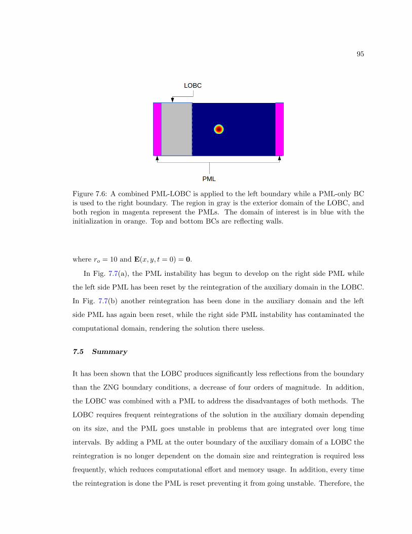
95
Figure 7.6: A combined PML-LOBC is applied to the left boundary while a PML-only BCis used to the right boundary. The region in gray is the exterior domain of the LOBC, andboth region in magenta represent the PMLs. The domain of interest is in blue with theinitialization in orange. Top and bottom BCs are reflecting walls.
where ro = 10 and E(x, y, t = 0) = 0.
In Fig. 7.7(a), the PML instability has begun to develop on the right side PML while
the left side PML has been reset by the reintegration of the auxiliary domain in the LOBC.
In Fig. 7.7(b) another reintegration has been done in the auxiliary domain and the left
side PML has again been reset, while the right side PML instability has contaminated the
computational domain, rendering the solution there useless.
7.5 Summary
It has been shown that the LOBC produces significantly less reflections from the boundary
than the ZNG boundary conditions, a decrease of four orders of magnitude. In addition,
the LOBC was combined with a PML to address the disadvantages of both methods. The
LOBC requires frequent reintegrations of the solution in the auxiliary domain depending
on its size, and the PML goes unstable in problems that are integrated over long time
intervals. By adding a PML at the outer boundary of the auxiliary domain of a LOBC the
reintegration is no longer dependent on the domain size and reintegration is required less
frequently, which reduces computational effort and memory usage. In addition, every time
the reintegration is done the PML is reset preventing it from going unstable. Therefore, the

96
(a) t = 200L/c
(b) t = 425L/c
Figure 7.7: Plot of log |Hz|. Top and bottom boundary conditions are reflecting. The rightBC is a simple PML and the left BC are a mixed PML and Lacuna. (a) Shows that the PMLhas become unstable in the right boundary, while at the left boundary the reintegration ofthe auxiliary domain has reset the PML, removing the instability. (b) The PML instabilityhas contaminated the computational domain on the right boundary, while the left boundarystill behaves as intended with no reflections nor instabilities.
97
combined PML and LOBC method can be applied to any geometry domain, is non-local
in space and time, considerably reduces reflection from the boundaries, and can be used in
long running problems at moderate computational effort and reduced memory usage.

98
Chapter 8
CONCLUSION
The multi-fluid plasma model (MFPM) has been presented. The MFPM is a generaliza-
tion of the MHD model that retains the electron dynamics and a finite speed of light. The
model is derived from the kinetic description of a plasma by assuming local thermodynam-
ical equilibrium within each of the species.
Multiscale effects are present in the MFPM, which is a manifestation of the large mass
difference between the electron and ion species. In order to properly model the physics of
the MFPM, an efficient numerical method have to be developed, the blended finite element
method (BFEM). The BFEM uses a discontinuous Galerkin representation for the ion and
neutral fluids with an explicit time integration. The electrons and electromagnetic fields are
discretized using a continuous Galerkin representation, and the time integrated is done using
an implicit method. The method is high order accurate and highly efficient. Verification
of the BFEM is done using simple test problems as well as for more complex multi-fluid
problems.
The BFEM is applied to the problem of inertial confinement fusion (ICF) fuel species
separation. The problem initialization is based on experimental results from OMEGA, but
simplified to a shock-tube-like problem. Deuterium-tritium separation and its effect on
neutron yield is investigated. The results show that there is considerable separation of the
deuterium from the tritium and that the separation is dominated by the pressure gradient.
Electric fields in the order of Gigavolts per meter develop, but the forces they produce are
small in comparison to the pressure gradients. Inter-species collisionality decreases as the
plasma approaches the center of the capsule, and the Knudsen number increase indicating
a transition from a fluid to a kinetic description of the plasma. In addition, the separation
causes the neutron yield to be reduced compared to a mass-average fluid simulation. The
neutron yield measured are on the same order of magnitude as experimental results.
99
Uncertainty quantification techniques are applied to the well-studied problem of mag-
netic reconnection. Studies of the sensitivity of the reconnected flux to uncertainties in ion-
to-electron mass ratio, speed of light to Alfven speed ratio, and the magnitude of the initial
magnetic flux perturbation are done. Three uncertainty quantification methods are com-
pared for accuracy and computational cost. The Multi-level Monte Carlo (MMC) method
performs better than the other methods and can capture the true mean and variance of the
problems at relatively low computational cost. Therefore, the MMC method can be easy
used to compare computational results with experimental data accurately, and at low cost.
Lacuna-based open boundary conditions (LOBC) are implemented in conjunction with
the perfectly matched layer (PML) method to address the problem of numerical reflection
when simulating open boundary conditions. The combined method of using the LOBC with
PMLs at its boundaries address the shortcomings of both methods. The LOBC reintegration
can be done less frequently, and the PML instabilities can be prevent from contaminating the
computational domain. When the reintegration occurs, the PML is reset. The results show
that this approach is successful in eliminating reflections, and is computationally efficient.
In summary, a novel numerical method, the blended finite element method, is intro-
duced and demonstrated to effectively and efficiently model plasmas using the multi-fluid
representation. The method is applied to standard benchmarks, and experimental con-
figurations involving ICF conditions in an effort to answer some relevant questions in the
field. The effects of uncertainty in simulations is quantified efficiently, accurately, and at
low computational cost. And, in anticipation of further developments in this area of re-
search, methods of treating open boundary conditions are investigated, and a new approach
is presented. Together, the combined numerical methods and techniques offer a means of
extending the capabilities of plasma physics simulations. In particular, they offer a high-
fidelity and computationally efficient means of treating ICF-relevant physics, and provide a
means of capturing multi-fluid effects in a way that is consistent, conservative, high-order
accurate, and computationally viable.

100
8.1 Suggested Future Work
The inclusion of ionization and recombinations models to the multi-fluid plasma model is
a natural next step, which would make the model more complete and extended it to a
wider range of plasma conditions, for example ion-thrusters, plasma assisted combustion,
or plasma actuators.
Future work for the BFEM include the study of better artificial dissipation models or
other methods to dampen the high frequency oscillations associated with sharp gradients
and discontinuities. In addition, the BFEM can easily be extended to higher dimensionality
by calculating fluxes in the additional dimensions for DG representation and by calculating
the flux Jacobian in the other directions for the CG portion.
For the ICF species separation problem, future work would include adding fusion reaction
that occur in DT-plasma which would allow for the modeling of neutrons species at different
energies and additional ions products of the fusion reactions. Accounting for reaction can
then be used to measure the amount of the deuterium and tritium that fuses. In addition,
better DT-reactivity models are need, which are dependent on separate deuterium and
tritium temperatures instead of an averaged one. Fluid models that allow for departure
from Maxwellian distributions (higher moment models) are desirable for regions where the
Knudsen number is large which encompasses some regimes in inertial confinement fusion.

101
BIBLIOGRAPHY
[1] U. Shumlak and J. Loverich. Approximate riemann solver for the two-fluid plasma
model. Journal of Computational Physics, 187:620–638, 2003.
[2] J. Birn, J. F. Drake, M. A. Shay, B. N. Rogers, R. E. Denton, M. Hesse,
M. Kuznetsova, Z. W. Ma, A. Bhattacharjee, A. Otto, and P. L. Pritchett. Geospace
environmental modeling (gem) magnetic reconnection challenge. J. Geo. Res.,
106(A3):3715–3719, March 2001.
[3] S. Atzeni and J. Meyer ter Vehn. Inertial Fusion. Number 125 in International Series
of Monographs on Physics. Oxford University Press.
[4] F. F. Chen. Introduction to plasma physcis and controlled fusion, volume 1. Plenum
Press.
[5] Hui Liu, Boying Wu, Daren Yu, Yong Cao, and Ping Duan. Particle-in-cell simulation
of a hall thruster. Journal of Physics D: Applied Physics, 43(16):165202, 2010.
[6] M G Haines. A review of the dense z -pinch. Plasma Physics and Controlled Fusion,
53(9):093001, 2011.
[7] S.P. Hirshman and D.J. Sigmar. Neoclassical transport of impurities in tokamak
plasmas. Nuclear Fusion, 21(9):1079, 1981.
[8] P Helander, C D Beidler, T M Bird, M Drevlak, Y Feng, R Hatzky, F Jenko, R Kleiber,
J H E Proll, Yu Turkin, and P Xanthopoulos. Stellarator and tokamak plasmas: a
comparison. Plasma Physics and Controlled Fusion, 54(12):124009, 2012.
[9] John D. Lindl, Peter Amendt, Richard L. Berger, S. Gail Glendinning, Siegfried H.
Glenzer, Steven W. Haan, Robert L. Kauffman, Otto L. Landen, and Laurence J.
Suter1. The physics basis for ignition using indirect-drive targets on the national
ignition facility. Physics of Plasmas, 11:339, 2004.
102
[10] M. M. Marinak, G. D. Kerbel, N. A. Gentile, O. Jones, D. Munro, S. Pollaine, T. R.
Dittrich, and S. W. Haan. Three-dimensional HYDRA simulations of national ignition
facility targets. Physics of Plasmas, 8(5), 2001.
[11] S. P. Regan, R. Epstein, B. A. Hammel, L. J. Suter, J. Ralph, H. Scott, M. A. Barrios,
D. K. Bradley, D. A. Callahan, C. Cerjan, G. W. Collins, S. N. Dixit, T. Doeppner,
M. J. Edwards, D. R. Farley, S. Glenn, S. H. Glenzer, I. E. Golovkin, S. W. Haan,
A. Hamza, D. G. Hicks, N. Izumi, J. D. Kilkenny, J. L. Kline, G. A. Kyrala, O. L.
Landen, T. Ma, J. J. MacFarlane, R. C. Mancini, R. L. McCrory, N. B. Meezan,
D. D. Meyerhofer, A. Nikroo, K. J. Peterson, T. C. Sangster, P. Springer, and R. P. J.
Town. Hot-spot mix in ignition-scale implosions on the NIF. Physics of Plasmas,
19(5), 2012.
[12] B. J. MacGowan, B. B. Afeyan, C. A. Back, R. L. Berger, G. Bonnaud, M. Casanova,
B. I. Cohen, D. E. Desenne, D. F. DuBois, A. G. Dulieu, K. G. Estabrook, J. C.
Fernandez, S. H. Glenzer, D. E. Hinkel, T. B. Kaiser, D. H. Kalantar, R. L. Kauffman,
R. K. Kirkwood, W. L. Kruer, A. B. Langdon, B. F. Lasinski, D. S. Montgomery, J. D.
Moody, D. H. Munro, L. V. Powers, H. A. Rose, C. Rousseaux, R. E. Turner, B. H.
Wilde, S. C. Wilks, and E. A. Williams. Laser-plasma interactions in ignitionscale
hohlraum plasmas. Physics of Plasmas, 3(5), 1996.
[13] S. Atzeni, A. Schiavi, F. Califano, F. Cattani, F. Cornolti, D. Del Sarto, T.V. Liseyk-
ina, A. Macchi, and F. Pegoraro. Fluid and kinetic simulation of inertial confinement
fusion plasmas. Computer Physics Communications, 169(1-3):153 – 159, 2005.
[14] V. Yu. Glebov, D. D. Meyerhofer, T. C. Sangster, C. Stoeckl, S. Roberts, C. A.
Barrera, J. R. Celeste, C. J. Cerjan, L. S. Dauffy, D. C. Eder, R. L. Griffith, S. W.
Haan, B. A. Hammel, S. P. Hatchett, N. Izumi, J. R. Kimbrough, J. A. Koch, O. L.
Landen, R. A. Lerche, B. J. MacGowan, M. J. Moran, E. W. Ng, T. W. Phillips,
P. M. Song, R. Tommasini, B. K. Young, S. E. Caldwell, G. P. Grim, S. C. Evans,
J. M. Mack, T. J. Sedillo, M. D. Wilke, D. C. Wilson, C. S. Young, D. Casey, J. A.
Frenje, C. K. Li, R. D. Petrasso, F. H. Sguin, J. L. Bourgade, L. Disdier, M. Houry,

103
I. Lantuejoul, O. Landoas, G. A. Chandler, G. W. Cooper, R. J. Leeper, R. E. Olson,
C. L. Ruiz, M. A. Sweeney, S. P. Padalino, C. Horsfield, and B. A. Davis. Development
of nuclear diagnostics for the national ignition facility (invited). Review of Scientific
Instruments, 77(10), 2006.
[15] R.J. Hawryluk, D.J. Campbell, G. Janeschitz, P.R. Thomas, R. Albanese, R. Am-
brosino, C. Bachmann, L. Baylor, M. Becoulet, I. Benfatto, J. Bialek, A. Boozer,
A. Brooks, R. Budny, T. Casper, M. Cavinato, J.-J. Cordier, V. Chuyanov, E. Doyle,
T. Evans, G. Federici, M. Fenstermacher, H. Fujieda, K. G’al, A. Garofalo, L. Garzotti,
D. Gates, Y. Gribov, P. Heitzenroeder, T.C. Hender, N. Holtkamp, D. Humphreys,
I. Hutchinson, K. Ioki, J. Johner, G. Johnson, Y. Kamada, A. Kavin, C. Kessel,
R. Khayrutdinov, G. Kramer, A. Kukushkin, K. Lackner, I. Landman, P. Lang,
Y. Liang, J. Linke, B. Lipschultz, A. Loarte, G.D. Loesser, C. Lowry, T. Luce,
V. Lukash, S. Maruyama, M. Mattei, J. Menard, M. Merola, A. Mineev, N. Mitchell,
E. Nardon, R. Nazikian, B. Nelson, C. Neumeyer, J.-K. Park, R. Pearce, R.A. Pitts,
A. Polevoi, A. Portone, M. Okabayashi, P.H. Rebut, V. Riccardo, J. Roth, S. Sabbagh,
G. Saibene, G. Sannazzaro, M. Schaffer, M. Shimada, A. Sen, A. Sips, C.H. Skinner,
P. Snyder, R. Stambaugh, E. Strait, M. Sugihara, E. Tsitrone, J. Urano, M. Valovic,
M. Wade, J. Wesley, R. White, D.G. Whyte, S. Wu, M. Wykes, and L. Zakharov.
Principal physics developments evaluated in the iter design review. Nuclear Fusion,
49(6):065012, 2009.
[16] U. Shumlak, R. Lilly, N. Reddell, E. Sousa, and B. Srinivasan. Advanced physics
calculations using a multi-fluid plasma model. Computer Physics Communications,
182(9):1767 – 1770, 2011.
[17] J. P. Freidberg. Ideal magnetohydrodynamic theory of magnetic fusion systems. Rev.
Mod. Phys, 54(801), 1982.
[18] Ammar Hakim. High-resolution Wave Propagation Schemer for Two-Fluid Plasma
Simulations. PhD thesis, University of Washington, 2006.
[19] A. Hakim, J. Loverich, and U. Shumlak. A high resolution wave propagation scheme
104
for ideal two-fluid plasma equations. Journal of Computational Physics, 219:418–442,
2006.
[20] B. Srinivasan, A. Hakim, and U. Shumlak. Numerical methods for two-fluid dispersive
fast mhd phenomena. Commun. Comput. Phys., 10(1):183–215, 2011.
[21] J. Loverich, A. Hakim, and U. Shumlak. A discontinuous galerkin method for ideal
two-fluid plasma equations. Commun. Comput. Phys., 9(240), 2011.
[22] B. Cockburn and C. W. Shu. Runge-Kutta discontinuous Galerkin methods for
convection-dominated problems. Journal of Scientific Computing, 16(3):173–261,
2001.
[23] B. Srinivasan. Numerical Methods for 3-dimensional Magnetic Confinement Config-
urations using Two-Fluid Plasma Equations. PhD thesis, University of Washington,
2010.
[24] S. C. Jardin. A triangular finite element with first-derivative continuity applied to
fusion mhd applications. Journal of Computational Physics, 200(1):133–152, 2004.
[25] D. T. Casey, J. A. Frenje, M. Gatu Johnson, M. J. E. Manuel, H. G. Rinderknecht,
N. Sinenian, F. H. Seguin, C. K. Li, R. D. Petrasso, P. B. Radha, J. A. Delettrez,
V. Yu Glebov, D. D. Meyerhofer, T. C. Sangster, D. P. McNabb, P. A. Amendt, R. N.
Boyd, J. R. Rygg, H. W. Herrmann, Y. H. Kim, and A. D. Bacher. Evidence for
Stratification of Deuterium-Tritium Fuel in Inertial Confinement Fusion Implosions.
Physical Review Letters, 108(075002), 2012.
[26] M. B. Giles. Multilevel monte carlo path simulation. Operations Research, 56(3):981–
986, 2008.
[27] George Kuczera and Eric Parent. Monte carlo assessment of parameter uncertainty
in conceptual catchment models: the metropolis algorithm. Journal of Hydrology,
211(1-4):69 – 85, 1998.

105
[28] K. A. Cliffe, M. B. Giles, R. Scheichl, and A. L. Teckentrup. Multilevel monte carlo
methods and applications to elliptic pdes with random coefficients. 2011.
[29] S. V. Tsynkov. On the application of lacunae-based methods to maxwell’s equations.
J. Comput. Phys., (199):126–149, 2004.
[30] J. P. Berenger. A perfectly matched layer for the absorption on electromagnetic waves.
Journal of Computational Physics, 114:185–200, 1994.
[31] S. Abarbanel, D. Gottlieb, and J. S. Hesthaven. Long time behavior of the perfectly
matched layer equations in computational electromagnetics. Journal of Scientific
Computing, 17:405–422, 2002.
[32] U. Shumlak, R. Lilly, N. Reddell, E. Sousa, and B. Srinivasan. Advanced Physics
Calculations using a Multi-Fluid Plasma Model. Computer Physics Communications,
18:1767–1770, 2011.
[33] E.T. Meier and U. Shumlak. A general nonlinear fluid model for reacting plasma-
neutral mixtures. Physics of Plasmas, 19(072508), 2012.
[34] S.L. Braginskii. Transport processes in plasma. In Achad M. A. Leontovich, editor,
Reviews of Plasma Physics, pages 205–311. Consultants Bureau, 1965.
[35] H. Yemin and H. Xiwei. The properties and structure of a plasma non-neutral shock.
Physics of Plasmas, 10(7), 2003.
[36] D. R. Gray and J. D. Kilkenny. The measurement of ion acoustic turbulence and
reduced thermal conductivity caused by a large temperature gradient in a laser heated
plasma. Plasma Physics, 22:81–111, 1980.
[37] R. Schneider C. D. Munz, P. Omnes, E. Sonnendruer, and U. Voss. Divergence
correction techniques for maxwell solvers based n a hyperbolic model. Journal of
Computational Physics, 161:484–511, 2000.
[38] R. J. LeVeque. Finite Volume Methods for Hyperbolic Problems. Cambridge University
Press, 1st edition, 2002.

106
[39] R. J. LeVeque and D. L. George. High-resolution finite volume methods for the shallow
water equations with bathymetry and dry states. In C. Synolakis P. L-F. Liu, H. Yeh,
editor, Advanced Numerical Models for Simulationg Tsunami Waves and Runup, pages
43–73, 2007.
[40] R. J. LeVeque. Finite volume methods for nonlinear elasticity in heterogeneous media.
Int. J. Numer. Meth. Fluids, (93-104), 2002.
[41] R. J. LeVeque. Tsunami modeling. to appear in the Princeton Companion to Applied
Mathematics (N. J. Higham, Editor).
[42] A. Hakim and U. Shumlak. High resolution wave propagation scheme for ideal two-
fluid plasma equations. Journal of Computational Physics, 219(1):418–442, 2006.
[43] C.R. Sovinec, A.H. Glasser, T.A. Gianakon, D.C. Barnes, R.A. Nebel, S.E. Kruger,
D.D. Schnack, S.J. Plimpton, A. Tarditi, and M.S. Chu. Nonlinear magnetohydrody-
namics simulation using high-order finite elements. Journal of Computational Physics,
195(1):355 – 386, 2004.
[44] N.A. Murphy, A.K. Young, C. Shen, J. Lin, and L. Ni. The plasmoid instability during
asymmetric inflow magnetic reconnection. Physics of Plasmas, 20(6), 2013.
[45] V. A. Izzo. Impurity mixing and radiation asymmetry in massive gas injection simu-
lations of diii-d. Physics of Plasmas, 20(5), 2013.
[46] John Slough and Richard Milroy. High flux frc facility for stability and confinement
studies. Journal of Fusion Energy, 29(6):567–570, 2010.
[47] Angus I.D. Macnab and Simon Woodruff. Extended mhd simulations of the com-
pression and stability of spheromaks for current drive. Journal of Fusion Energy,
28(2):183–186, 2009.
[48] S.C. Jardin, J. Breslau, and N. Ferraro. A high-order implicit finite element method for
integrating the two-fluid magnetohydrodynamic equations in two dimensions. Journal
of Computational Physics, 226(2):2146 – 2174, 2007.

107
[49] L. Chacon, D.A. Knoll, and J.M. Finn. An implicit, nonlinear reduced resistive MHD
solver. Journal of Computational Physics, 178(1):15 – 36, 2002.
[50] H. W. Reed and T. R. Hill. Triangular mesh methods for the neutron transport
equation. Los Alamos Scientific Laboratory Report LA-UR-73-479, 1973.
[51] B. Cockburn and C. W. Shu. Tvb runge-kutta local projection discontinous galerkin fi-
nite element for conservation laws ii-general framework. Math. Comput., 52(186):411–
435, 1989.
[52] F. Bassi and S. Rebay. A high-order accurate discontinuous finite element method
for the numerical solution of the compressible navierstokes equations. Journal of
Computational Physics, 131:267–279, 1997.
[53] F. Bassi, L. Botti, A. Colombo, and S. Rebay. Agglomeration based discontinuous
galerkin discretization of the euler and navierstokes equations. Computers and Fluids,
61(0):77 – 85, 2012.
[54] E. Ferrer and R.H.J. Willden. A high order discontinuous galerkin finite element
solver for the incompressible navierstokes equations. Computers and Fluids, 46(1):224
– 230, 2011.
[55] Philipp Birken, Gregor Gassner, and Mark. Preconditioning for modal discontinuous
galerkin methods for unsteady 3d navierstokes equations. Journal of Computational
Physics, 240(0):20 – 35, 2013.
[56] Fengyan Li, Liwei Xu, and Sergey Yakovlev. Central discontinuous galerkin methods
for ideal MHD equations with the exactly divergence-free magnetic field. Journal
of Computational Physics, 230(12):4828 – 4847, 2011.
[57] V. Wheatley, H. Kumar, and P. Huguenot. On the role of riemann solvers in dis-
continuous galerkin methods for magnetohydrodynamics. Journal of Computational
Physics, 229(3):660 – 680, 2010.
108
[58] James A. Rossmanith and David C. Seal. A positivity-preserving high-order semi-
lagrangian discontinuous galerkin scheme for the vlasovpoisson equations. Journal of
Computational Physics, 230(16):6203 – 6232, 2011.
[59] J. Crank and P. Nicholson. A Partial Method for Numerical Evaluation of Solutions
of Partial Differential Equations of the Heat-Conduction Type. Advances in Compu-
tational Mathemathics, 6:207–226, 1996.
[60] J. N. Reddy. An Introduction to the Finite Element Method. McGraw-Hill, 3rd edition.
[61] Satish Balay, Shrirang Abhyankar, Mark F. Adams, Jed Brown, Peter Brune, Kris
Buschelman, Victor Eijkhout, William D. Gropp, Dinesh Kaushik, Matthew G. Kne-
pley, Lois Curfman McInnes, Karl Rupp, Barry F. Smith, and Hong Zhang. PETSc
users manual. Technical Report ANL-95/11 - Revision 3.5, Argonne National Labo-
ratory, 2014.
[62] Assefaw Hadish Gebremedhin, Fredrik Manne, and Alex Pothen. What color is your
jacobian? graph coloring for computing derivatives. SIAM Rev., 47(4):629–705, April
2005.
[63] S. Baboolal. Finite-difference modeling of solitons induced by a density hump in a
plasma multi-fluid. Mathematics and Computers in Simulation, 55:309–316, 2001.
[64] M. Brio and C. C. Wu. An upwind differencing scheme for the equations of ideal
magnetohydrodynamics. Journal of Computational Physics, 75:400–422, 1988.
[65] P. A. Amendt, J. L. Milovich, S. C. Wilks, C. K. Li, R. D. Petrasso, and F. H.
Seguin. Electric Field and Ionization-Gradient Effects on Inertial-Confinement-Fusion
Implosions. Plasma Phys. Control. Fusion, 51(124048), 2009.
[66] H. W. Herrmann, J. R. Langenbrunner, J. M. Mack, J. H. Cooley, D. C. Wilson,
S. C. Evans, T. J. Sedillo, G. A. Kyrala, S. E. Caldwell, C. S. Young, A. Nobile,
J. Wermer, S. Paglieri, A. M. McEvoy, Y. Kim, S. H. Batha, C. J. Horsfield, D. Drew,
W. Garbett, M. Rubery, V. Yu. Glebov, S. Roberts, and J. A. Frenje. Anomalous

109
yield reduction in direct-drive deuterium/tritium implosions due to h3e additiona).
Physics of Plasmas, 16(5), 2009.
[67] P. Amendt, S. C. Wilks, C. Bellei, C. K. Li, and R. D. Petrasso. The Potential
Role of Electric Fields and Plasma Barodiffusion on the Inertial Confinement Fusion
Database. Physics of Plasma, 18(056308), 2011.
[68] G. Kagan and X. Z. Tang. Thermo-diffusion in inertially confined plasmas.
arXiv:1310.8227v1 [physics.plasm-ph].
[69] G. Kagan and X. Z. Tang. Electro-diffusion in a plasma with two ion species. Physics
of Plasmas, 19(082709), 2012.
[70] C. Bellei, P. A. Amendt, S. C. Wilks, M. G. Haines, D. T. Casey, C. K. Li, R. Petrasso,
and D. R. Welch. Species separation in inertial confinement fusion fuels. Physics of
Plasmas, 20(012701), 2013.
[71] A. Inglebert, B. Canaud, and O. Larroche. Species separation and modification
of neutron diagnostics in inertial-confinement fusion. EPL (Europhysics Letters),
107(6):65003, 2014.
[72] M. Tatang and G. McRae. Direct treatment of uncertainty in models of reaction and
transport. Technical report, MIT Tech. Rep., 1994.
[73] D. Xiu and J. S. Hesthaven. High order collocation methods for differential equations
with random inputs. SIAM J. Sci. Comput., 27(3):1118–1139, 2005.
[74] E. Novak and K. Ritter. High dimensional integration of smooth funcions over cubes.
Numer. Math., 75:79–97, 1996.
[75] E. Novak and K. Ritter. Simple cubature formulas with high polynomial exactness.
Constr. Approx., 15:499–522, 1999.
[76] V. Barthelmann, E. Novak, and K. Ritter. High dimensional polynomial interpolation
on sparse grids. Adv. Comput. Math., 12:273–288, 2000.
110
[77] T. Gerstner and M. Griebel. Dimension-adaptive tensor-product quadrature. Com-
puting, 71(1):65–87, 2003.
[78] B. Ganapathysubramanian and N. Zabaras. Sparse grid collocation schemes for
stochastic natural convection problems. J. Comput. Phys., 225(1):652–685, 2007.
[79] M. Griebel. Adaptive sparse grid multilevel methods for elliptic pdes based on finite
differences. Computing, 61(2):151–180, 1998.
[80] X. Ma and N. Zabaras. An adaptive hierarchical sparse grid collocation algorithm for
the solution of stochastic differential equations. J. Comput. Phys., 228(8):3084–3113,
2009.
[81] G. Lin and G. E. Karniadakis. Sensitivity analysis and stochastic simulations of non-
equilibrium plasma flow. Int. J. Numer. Meth. Engng, (80):738–766, March 2009.
[82] M. A. Shay, J. F. Drake, B. N. Rogers, and R. E. Denton. Alvenic collisionless
magnetic reconnection and the hall term. J. Geo. Res., 106(A3):3759–3772, March
2001.
[83] U. Shumlak and J. Loverich. Approximate Riemann solver for the two-fluid plasma
model. J. Comput. Phys., 187:620–638, 2003.
[84] B. Srinivasan, A. Hakim, and U. Shumlak. Numerical methods for two-fluid dispersive
fast MHD phenomena. Comm. Comput. Phys., 9, 2011.
[85] W. Shin and S. Fan. Choice of the perfectly matched layer boundary condition for
frequency-domain maxwells equations solvers. Journal of Computational Physics,
231:3406–3431, 2012.
[86] S. D. Gedney. A anisotropic perfectly matched layer-absorbing for the truncation of
FDTD lattices. IEEE transaction on antennas and propagation, 44(12), 1996.
[87] S. Abarbanel, H. Qasimov, and S. Tsynkov. Long-time performance of unsplit PMLs
with explicit second order schemes. Journal of Scientific Computing, 41:1–12, 2009.
111
[88] E. T. Meier, A. H. Glasser, V. S. Lukin, and U. Shumlak. Modeling open boundaries
in dissipative mhd simulation. Journal of Computational Physics, (231):2963–2976,
2012.
[89] C.K. Birdsall and A.B Langdon. Plasma Physics via Computer Simulation. CRC
Press.
[90] S. W. Haan. Weakly nonlinear hydrodynamic instabilities in inertial fusion. Physics
of Fluids B: Plasma Physics (1989-1993), 3(8):2349–2355, 1991.
[91] Li Wang and Dimitri Mavriplis. Implicit solution of the unsteady euler equations for
high-order accurate discontinuous galerkin discretizations. AIAA, (0109), 2006.
[92] M. Yamada, Y. Ren, H. Ji, J. Breslau, S. Gerhardt, R. Kulsrud, and A. Kuritsyn. Ex-
perimental study of two-fluid effects on magnetic reconnection in a laboratory plasma
with variable collisionality. Phys. of Plasmas, 13(052119), 2006.
[93] A. Otto. Geospace environment modeling (gem) magnetic reconnection challenge:
MHD and Hall MHD - constant and current dependent resitivity models. J. Geo.
Res., 106:3751–3757, 2001.
[94] J. D. Anderson. Computational Fluid Dynamics, The Basics with Applications.
McGraw-Hill, 1995.
[95] G. A. Sod. Survey of several finite difference methods for systems of nonlinear hyper-
bolic conservation laws. Journal of Computational Physics, 26(4), 1978.
[96] C. Bellei, P. A. Amendt, S. C. Wilks, M. G. Haines, and D. T. Casey et al. Species
separation in inertial confinement fusion fuels. Phys. Plasma, 20(012701), 2013.
[97] A. Hakim, J. Loverich, and U. Shumlak. A high resolution wave propagation scheme
for ideal two-fluid plasma equations. Journal of Computational Physics, 219:418–442,
2006.
[98] S. Smolyak. Quadrature and interpolation formulas for tensor products of certain
classes of functions. Soviet Math. Dokl., 4:240–243, 1963.
112
[99] G. Lin and A. M. Tartakovsky. Numerical studies of three-dimensional stochastic
Darcy’s equation and stochastic advection-diffusion-dispersion equation. J. Sci. Com-
put., 43(1):92–117, 2010.
[100] G. Lin and A. M. Tartakovsky. An efficient, high-order probabilistic collocation
method on sparse grids for three-dimensional flow and solute transport in randomly
heterogeneous porous media. Advances in Water Resources, 32(5):712–722, 2009.
[101] R. Cools. Monomial cubature rules since ‘stroud’: A compilation. J. Comput. Appl.
Math., 48:309–326, 1993.
[102] R. Cools. Monomial cubature rules since ‘stroud’: A compilation - part 2. J. Comput.
Appl. Math., 112:21–27, 1999.
[103] A. Barth, C. Schwab, and N. Zollinger. Multilevel monte carlo finite element method
for elliptic pde’s with stochastic coefficients. Technical report, Swiss Federal Institute
of Technology Zurich, June 2010. Research Report No. 2010-18.
[104] W. G. Vincenti and C. H. Kruger. Introduction to Physical Gas Dynamics. Krieger
Publishing Company, 2002.

113
Appendix A
PROBABILISTIC COLLOCATION METHOD
We compare the efficiency of the MMC method with other uncertainty quantification
methods. In particular, we compare MMC with MC and PC methods. The general proce-
dure for the PC method is similar to that of the MC method, except that different sampling
points and corresponding weights are selected. The procedure consists of three main steps:
1. Generate Nc collocation points in a complete probability space, (Ω,A,P) based on a
quadrature formula based on the distribution of the random parameters (see details
in Refs. [101, 102]), where Ω is the event space, A ∈ 2Ω the σ-algebra, and P the
probability measure;
2. Solve a deterministic problem at each collocation point;
3. Estimate the solution statistics using the corresponding quadrature rule;
E[P (x, t)] =
∫ΓP (x, t, ξ)ρ(ξ)dξ
≈Nc∑k=1
P (x, t, ξk)ρ(ξk)wk, (A.1)
V [P ](x, t) =
∫Γ(P (x, t, ξ)− E[u])2ρ(ξ)dξ
≈Nc∑k=1
P 2(x, t, ξk)ρ(ξ)wk − E[v]2, (A.2)
where x,t and ξ are the spatial coordinate vector, time and random variable. ρ(ξ) is the
probabilistic distribution function (PDF) of random variable ξ, Nc is the number of quadra-
ture points, ξk is the set of quadrature points, and wk is the corresponding set of
114
weights, which are the combination of quadrature weights in each random dimension. In
the second step of the PC method approach, as for the MC method, any existing determin-
istic code can be used. Extensive reviews on the construction of quadrature formulas may
be found in Refs. [101, 102]. In this work, the Smolyak formula [98] is used to construct the
collocation point set, which is a linear combination of tensor product formulas and has a
significantly smaller number of points than the full tensor product set. Recently, high order
stochastic collocation methods [73, 100, 99] has been developed based on sparse grids using
the Smolyak formula [98]. Such sparse grids do not depend as strongly on the dimensionality
of the random space and as such are more suitable for applications with high-dimensional
random inputs. Detailed descriptions on building the collocation point set can be found in
Refs. [73, 100, 99].

115
Appendix B
WARPX DESCRIPTION
The simulations in the dissertation were performed using the Washington Approximate
Riemann Plasma Solver (WARPX). The code is partial differential equation (PDE) solver,
mainly for equations in balance law form as in Eq. (2.39). Fig. (B.1) describes the structure
of an input file which can be applied to any PDE system.
Parallelization in done using the Message Passing Interface (MPI) which makes WARPX
high performance, scalable, and portable. The Hierarchical Data Format version five
(HDF5) library to output the data I/O, which can be done in parallel as well as in se-
ries. The output files can have multiple datasets, multidimensional arrays. The Portable
Extensible Toolkit for Scientific Computation[61] (PETSc) function can also be called from
WARPX. PETSc is PDE equation solver suite that allows for the solution of linear and
nonlinear equations and has its own time integrators. PETSc uses MPI and is massively
parallel, and has been execute in hundred of thousand of CPUs and GPUs.
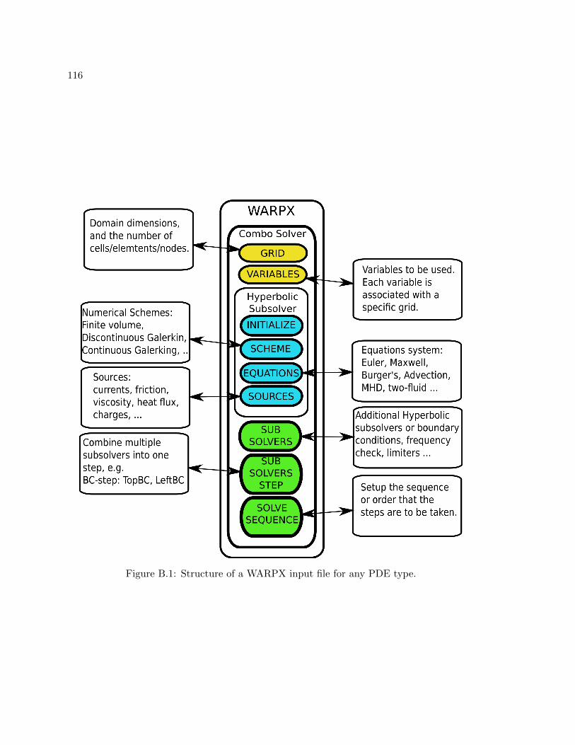
116
Figure B.1: Structure of a WARPX input file for any PDE type.

117
Appendix C
SPECIES SEPARATION INPUT FILE
<warpx>
Simulat ion = ssbr iowu
Verbos i ty = debug
<ssbriowu>
Type = WxSolver
Kind = comboSolver
Time = [ 0 . 0 , 0 . 0 013 ]
Out = 500
Dt = 1.5 e−07
<DGgrid>
Type = WxGridBox
Lower = [ 0 . 0 ]
Upper = [ 0 . 0 0 1 ]
Ce l l s = [ 1 2 8 ]
</DGgrid>
<FEMgrid>
Type = WxGridBox
Lower = [ 0 . 0 ]
Upper = [ 0 . 0 0 1 ]
Ce l l s = [ 2 5 7 ]
</FEMgrid>
<qemold>
Type = WxVariable
Kind = parArray
OnGrid = FEMgrid
NumComponents = 13
GhostCel l s = [ 2 , 2 ]
</qemold>
<qemmid>
Type = WxVariable
Kind = parArray
OnGrid = FEMgrid
NumComponents = 13
GhostCel l s = [ 2 , 2 ]
</qemmid>
<qemnew>
Type = WxVariable
Kind = parArray
OnGrid = FEMgrid
NumComponents = 13
GhostCel l s = [ 2 , 2 ]
</qemnew>
<qionold>
Type = WxVariable
Kind = parArray
OnGrid = DGgrid
NumComponents = 20
GhostCel l s = [ 2 , 2 ]
</qionold>
<dqion>
Type = WxVariable
Kind = parArray
OnGrid = DGgrid
NumComponents = 20
GhostCel l s = [ 2 , 2 ]
</dqion>
<dqion1>
Type = WxVariable
Kind = parArray
OnGrid = DGgrid
NumComponents = 20
GhostCel l s = [ 2 , 2 ]
</dqion1>
<qion1>
Type = WxVariable
Kind = parArray
OnGrid = DGgrid
NumComponents = 20
GhostCel l s = [ 2 , 2 ]
</qion1>
<qionnew>
Type = WxVariable
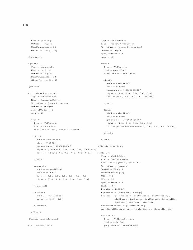
118
Kind = parArray
OnGrid = DGgrid
NumComponents = 20
GhostCel l s = [ 2 , 2 ]
</qionnew>
<gtAux>
Type = WxVariable
Kind = parArray
OnGrid = DGgrid
NumComponents = 12
GhostCel l s = [ 2 , 2 ]
</gtAux>
<i n i t i a l c ond e l c max>
Type = WxSubSolver
Kind = femArraySetter
WriteVars = [ qemold , qemnew ]
OnGrid = FEMgrid
spat i a lOrde r = 2
meqn = 13
<func>
Type = WxFunction
Kind = comboFunc
func t i on s = [ e l c , maxwell , errPot ]
<e l c>
Kind = eulerShock
s l o c = 0.00075
gas gamma = 1.66666666667
r i gh t = [0 . 000544 , 0 . 0 , 0 . 0 , 0 . 0 , 0 . 033333 ]
l e f t = [ 5 . 4 466 e−05, 0 . 0 , 0 . 0 , 0 . 0 , 0 . 0 1 ]
</e l c>
<maxwell>
Kind = maxwellShock
s l o c = 0.00075
l e f t = [ 0 . 0 , 0 . 0 , 0 . 0 , 0 . 0 , 0 . 0 , 0 . 0 ]
r i g h t = [ 0 . 0 , 0 . 0 , 0 . 0 , 0 . 0 , 0 . 0 , 0 . 0 ]
</maxwell>
<errPot>
Kind = constVecFunc
va lues = [ 0 . 0 , 0 . 0 ]
</errPot>
</func>
</ i n i t i a l c ond e l c max>
< i n i t i a l c o nd i o n >
Type = WxSubSolver
Kind = funcDGArraySetter
WriteVars = [ qionold , qionnew ]
OnGrid = DGgrid
spat i a lOrde r = 2
meqn = 10
<func>
Type = WxFunction
Kind = comboFunc
func t i on s = [ ion2 , ion3 ]
<ion2>
Kind = eulerShock
s l o c = 0.00075
gas gamma = 1.66666666667
r i gh t = [ 1 . 0 , 0 . 0 , 0 . 0 , 0 . 0 , 0 . 5 ]
l e f t = [ 0 . 1 , 0 . 0 , 0 . 0 , 0 . 0 , 0 . 0 0 5 ]
</ion2>
<ion3>
Kind = eulerShock
s l o c = 0.00075
gas gamma = 1.66666666667
r i gh t = [ 1 . 5 , 0 . 0 , 0 . 0 , 0 . 0 , 0 . 5 ]
l e f t = [0 .15000000000000002 , 0 . 0 , 0 . 0 , 0 . 0 , 0 . 0 0 5 ]
</ion3>
</func>
</ i n i t i a l c o nd i o n >
<calcem>
Type = WxSubSolver
Kind = fem1dImpl i c i t
ReadVars = [ qemold , q iono ld ]
WriteVars = [ qemnew ]
OnGrid = FEMgrid
auxEqnNums = [ 1 0 ]
Cf l = 0 .5
Cflm = 0.5
spat i a lOrde r = 2
theta = 0 .5
Penalty = 10000.0
Equations = [ eu l e rE lc , maxEqn ]
Sources = [ e lcCurrents , ionCurrents , ionCurrents3 ,
elcCharge , ionCharge , ionCharge3 , l o r entzE l c ,
SplEuler , elecDeut , e l e cT r i t ]
GradientSources = [ e lecHeatFlux ]
A r t i f i c i a l D i s s i p a t i o n = [ Eu l e rd i s s i p , Maxwel ld i s s ip ]
<eu l e rE lc>
Type = WxHyperbolicEqn
Kind = eulerEqn
gas gamma = 1.66666666667

119
minPressure = 0.005
</eu le rE lc>
<maxEqn>
Type = WxHyperbolicEqn
Kind = phMaxwellEqn
c0 = 1 .0
gamma = 0.0
ch i = 0 .0
normal ized = true
c0tov0 = 1120.0
Larmor = 1 .0
sk in depth = 0.00537
</maxEqn>
<e lcCurrents>
Type = WxHyperbolicSrc
Kind = cur r en t s
InpRange = [ 1 , 2 , 3 ]
OutRange = [ 5 , 6 , 7 ]
mass = 0.000272331154684
charge = −1.0
ep s i l on0 = 1 .0
</e lcCurrents>
<ionCurrents>
Type = WxHyperbolicSrc
Kind = extCurrents
AuxInpRange = [ 1 , 2 , 3 ]
OutRange = [ 5 , 6 , 7 ]
charge = 1 .0
mass = 1 .0
ep s i l on0 = 1 .0
</ionCurrents>
<ionCurrents3>
Type = WxHyperbolicSrc
Kind = extCurrents
AuxInpRange = [ 6 , 7 , 8 ]
OutRange = [ 5 , 6 , 7 ]
charge = 1 .0
mass = 1 .5
ep s i l on0 = 1 .0
</ionCurrents3>
<elcCharge>
Type = WxHyperbolicSrc
Kind = normCharges
InpRange = [ 0 ]
OutRange = [ 1 1 ]
mass = 0.000272331154684
ch i = 0 .0
c0tov0 = 1120.0
Larmor = 1 .0
sk in depth = 0.00537
Z alpha = −1.0
</elcCharge>
<ionCharge>
Type = WxHyperbolicSrc
Kind = normExtCharges
AuxInpRange = [ 0 ]
OutRange = [ 1 1 ]
mass = 1 .0
ch i = 0 .0
c0tov0 = 1120.0
Larmor = 1 .0
sk in depth = 0.00537
Z alpha = 1 .0
</ionCharge>
<ionCharge3>
Type = WxHyperbolicSrc
Kind = normExtCharges
AuxInpRange = [ 5 ]
OutRange = [ 1 1 ]
mass = 1 .5
ch i = 0 .0
c0tov0 = 1120.0
Larmor = 1 .0
sk in depth = 0.00537
Z alpha = 1 .0
</ionCharge3>
<l o r entzE l c>
Type = WxHyperbolicSrc
Kind = normLorentzForces
InpRange = [ 0 , 1 , 2 , 3 , 5 , 6 , 7 , 8 , 9 , 10 ]
OutRange = [ 1 , 2 , 3 , 4 ]
mass = 0.000272331154684
Z alpha = −1.0
CtoV0 rat io = 1120.0
Larmor = 1 .0
Skin depth = 0.00537
</lo r entzE l c>
<Eu l e rd i s s i p>
Type = WxHyperbolicSrc
Kind = eu l e rA r t i fD i s s
InpRange = [ 0 , 1 , 2 , 3 , 4 ]
OutRange = [ 0 , 1 , 2 , 3 , 4 ]
d i s s i p a t i o n = 5e−05
gas gamma = 1.66666666667
</Eu l e rd i s s i p>
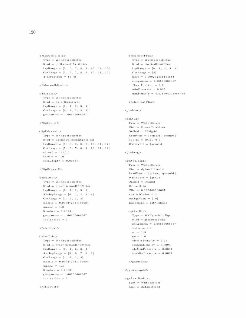
120
<Maxwel ld iss ip>
Type = WxHyperbolicSrc
Kind = phMaxwel lArt i fDiss
InpRange = [ 5 , 6 , 7 , 8 , 9 , 10 , 11 , 12 ]
OutRange = [ 5 , 6 , 7 , 8 , 9 , 10 , 11 , 12 ]
d i s s i p a t i o n = 1e−05
</Maxwel ld iss ip>
<SplEuler>
Type = WxHyperbolicSrc
Kind = eu l e r Sph e r i c a l
InpRange = [ 0 , 1 , 2 , 3 , 4 ]
OutRange = [ 0 , 1 , 2 , 3 , 4 ]
gas gamma = 1.66666666667
</SplEuler>
<SplMaxwell>
Type = WxHyperbolicSrc
Kind = phMaxwellNormSpherical
InpRange = [ 5 , 6 , 7 , 8 , 9 , 10 , 11 , 12 ]
OutRange = [ 5 , 6 , 7 , 8 , 9 , 10 , 11 , 12 ]
c0tov0 = 1120.0
Larmor = 1 .0
sk in depth = 0.00537
</SplMaxwell>
<elecDeut>
Type = WxHyperbolicSrc
Kind = bragFrictionBFEMelec
InpRange = [ 0 , 1 , 2 , 3 , 4 ]
AuxInpRange = [ 0 , 1 , 2 , 3 , 4 ]
OutRange = [ 1 , 2 , 3 , 4 ]
mass e = 0.000272331154684
mass i = 1 .0
Knudsen = 0.0083
gas gamma = 1.66666666667
i o n i z a t i o n = 1
</elecDeut>
<e l e cTr i t>
Type = WxHyperbolicSrc
Kind = bragFrictionBFEMelec
InpRange = [ 0 , 1 , 2 , 3 , 4 ]
AuxInpRange = [ 5 , 6 , 7 , 8 , 9 ]
OutRange = [ 1 , 2 , 3 , 4 ]
mass e = 0.000272331154684
mass i = 1 .5
Knudsen = 0.0083
gas gamma = 1.66666666667
i o n i z a t i o n = 1
</e l e cTr i t>
<elecHeatFlux>
Type = WxHyperbolicSrc
Kind = l imitedHeatFlux
InpRange = [ 0 , 1 , 2 , 3 , 4 ]
OutRange = [ 4 ]
mass = 0.000272331154684
gas gamma = 1.66666666667
f l u x l im i t e r = 0 .2
minPressure = 0.005
minDensity = 4.41176470588 e−06
</elecHeatFlux>
</calcem>
<calAvg>
Type = WxSubSolver
Kind = linearCombiner
OnGrid = FEMgrid
ReadVars = [ qemold , qemnew ]
c o e f f s = [ 0 . 5 , 0 . 5 ]
WriteVars = [ qemmid ]
</calAvg>
<gtAux qold>
Type = WxSubSolver
Kind = dgAuxSolver1d
ReadVars = [ gtAux , q iono ld ]
WriteVars = [ gtAux ]
OnGrid = DGgrid
Cf l = 0.15
Cflm = 0.166666666667
spat i a lOrde r = 2
auxEqnNums = [ 1 0 ]
Equations = [ gtAuxEqn ]
<gtAuxEqn>
Type = WxHyperbolicEqn
Kind = gradDensTemp
gas gamma = 1.66666666667
bo l t z = 1 .0
mi = 1 .5
me = 1.0
elcMinDensity = 0.01
ionMinDensity = 0.0093
e lcMinPressure = 0.0031
ionMinPressure = 0.0031
</gtAuxEqn>
</gtAux qold>
<gtAux l imit>
Type = WxSubSolver
Kind = dgLimiter1d
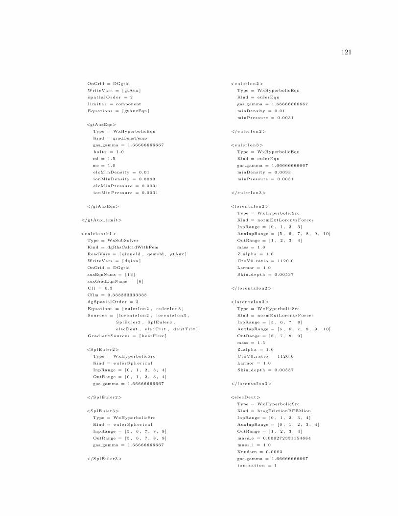
121
OnGrid = DGgrid
WriteVars = [ gtAux ]
spa t i a lOrde r = 2
l im i t e r = component
Equations = [ gtAuxEqn ]
<gtAuxEqn>
Type = WxHyperbolicEqn
Kind = gradDensTemp
gas gamma = 1.66666666667
bo l t z = 1 .0
mi = 1 .5
me = 1.0
elcMinDensity = 0.01
ionMinDensity = 0.0093
e lcMinPressure = 0.0031
ionMinPressure = 0.0031
</gtAuxEqn>
</gtAux l imit>
<ca l c i onrk1>
Type = WxSubSolver
Kind = dgRhsCalc1dWithFem
ReadVars = [ qionold , qemold , gtAux ]
WriteVars = [ dqion ]
OnGrid = DGgrid
auxEqnNums = [ 1 3 ]
auxGradEqnNums = [ 6 ]
Cf l = 0 .3
Cflm = 0.333333333333
dgSpat ia lOrder = 2
Equations = [ eu le r Ion2 , eu l e r I on3 ]
Sources = [ lo rentz Ion2 , l o r entz Ion3 ,
SplEuler2 , SplEuler3 ,
elecDeut , e l e cTr i t , deutTr i t ]
GradientSources = [ heatFlux ]
<SplEuler2>
Type = WxHyperbolicSrc
Kind = eu l e r Sph e r i c a l
InpRange = [ 0 , 1 , 2 , 3 , 4 ]
OutRange = [ 0 , 1 , 2 , 3 , 4 ]
gas gamma = 1.66666666667
</SplEuler2>
<SplEuler3>
Type = WxHyperbolicSrc
Kind = eu l e r Sph e r i c a l
InpRange = [ 5 , 6 , 7 , 8 , 9 ]
OutRange = [ 5 , 6 , 7 , 8 , 9 ]
gas gamma = 1.66666666667
</SplEuler3>
<eu le r Ion2>
Type = WxHyperbolicEqn
Kind = eulerEqn
gas gamma = 1.66666666667
minDensity = 0.01
minPressure = 0.0031
</eu le r Ion2>
<eu le r Ion3>
Type = WxHyperbolicEqn
Kind = eulerEqn
gas gamma = 1.66666666667
minDensity = 0.0093
minPressure = 0.0031
</eu le r Ion3>
<l o r entz Ion2>
Type = WxHyperbolicSrc
Kind = normExtLorentzForces
InpRange = [ 0 , 1 , 2 , 3 ]
AuxInpRange = [ 5 , 6 , 7 , 8 , 9 , 10 ]
OutRange = [ 1 , 2 , 3 , 4 ]
mass = 1 .0
Z alpha = 1 .0
CtoV0 rat io = 1120.0
Larmor = 1 .0
Skin depth = 0.00537
</lo rentz Ion2>
<l o r entz Ion3>
Type = WxHyperbolicSrc
Kind = normExtLorentzForces
InpRange = [ 5 , 6 , 7 , 8 ]
AuxInpRange = [ 5 , 6 , 7 , 8 , 9 , 10 ]
OutRange = [ 6 , 7 , 8 , 9 ]
mass = 1 .5
Z alpha = 1 .0
CtoV0 rat io = 1120.0
Larmor = 1 .0
Skin depth = 0.00537
</lo rentz Ion3>
<elecDeut>
Type = WxHyperbolicSrc
Kind = bragFrictionBFEMion
InpRange = [ 0 , 1 , 2 , 3 , 4 ]
AuxInpRange = [ 0 , 1 , 2 , 3 , 4 ]
OutRange = [ 1 , 2 , 3 , 4 ]
mass e = 0.000272331154684
mass i = 1 .0
Knudsen = 0.0083
gas gamma = 1.66666666667
i o n i z a t i o n = 1

122
</elecDeut>
<e l e cTr i t>
Type = WxHyperbolicSrc
Kind = bragFrictionBFEMion
InpRange = [ 5 , 6 , 7 , 8 , 9 ]
AuxInpRange = [ 0 , 1 , 2 , 3 , 4 ]
OutRange = [ 6 , 7 , 8 , 9 ]
mass e = 0.000272331154684
mass i = 1 .5
Knudsen = 0.0083
gas gamma = 1.66666666667
i o n i z a t i o n = 1
</e l e cTr i t>
<deutTrit>
Type = WxHyperbolicSrc
Kind = bragFrictionBFEMionIon
InpRange = [ 0 , 1 , 2 , 3 , 4 , 5 , 6 , 7 , 8 , 9 ]
OutRange = [ 1 , 2 , 3 , 4 , 6 , 7 , 8 , 9 ]
mass ip = 1 .5
mass i = 1 .0
Knudsen = 0.0107
gas gamma = 1.66666666667
i o n i z a t i o n = 1
</deutTrit>
<heatFlux>
Type = WxHyperbolicSrc
Kind = dgLimitedHeatFlux
AuxInpRange = [ 0 , 3 ]
OutRange = [ 4 , 9 ]
mass i = 1 .5
mass e = 1 .0
f l u x l im i t e r = 0 .2
</heatFlux>
</ca l c i onrk1>
<rk 1 ion>
Type = WxSubSolver
Kind = linearCombiner
OnGrid = DGgrid
ReadVars = [ qionold , dqion ]
c o e f f s = [ 1 . 0 , 1 . 0 ]
WriteVars = [ qion1 ]
</rk 1 ion>
<gtAux q1>
Type = WxSubSolver
Kind = dgAuxSolver1d
ReadVars = [ gtAux , qion1 ]
WriteVars = [ gtAux ]
OnGrid = DGgrid
Cf l = 0.15
Cflm = 0.166666666667
spat i a lOrde r = 2
auxEqnNums = [ 1 0 ]
Equations = [ gtAuxEqn ]
<gtAuxEqn>
Type = WxHyperbolicEqn
Kind = gradDensTemp
gas gamma = 1.66666666667
bo l t z = 1 .0
mi = 1 .5
me = 1.0
elcMinDensity = 0.01
ionMinDensity = 0.0093
e lcMinPressure = 0.0031
ionMinPressure = 0.0031
</gtAuxEqn>
</gtAux q1>
<ca l c i onrk2>
Type = WxSubSolver
Kind = dgRhsCalc1dWithFem
ReadVars = [ qion1 , qemnew , gtAux ]
WriteVars = [ dqion1 ]
OnGrid = DGgrid
auxEqnNums = [ 1 3 ]
auxGradEqnNums = [ 6 ]
Cf l = 0 .3
Cflm = 0.333333333333
dgSpat ia lOrder = 2
Equations = [ eu le r Ion2 , eu l e r I on3 ]
Sources = [ lo rentz Ion2 , l o r entz Ion3 , SplEuler2 ,
SplEuler3 , elecDeut , e l e cTr i t , deutTr i t ]
GradientSources = [ heatFlux ]
<SplEuler2>
Type = WxHyperbolicSrc
Kind = eu l e r Sph e r i c a l
InpRange = [ 0 , 1 , 2 , 3 , 4 ]
OutRange = [ 0 , 1 , 2 , 3 , 4 ]
gas gamma = 1.66666666667
</SplEuler2>
<SplEuler3>
Type = WxHyperbolicSrc
Kind = eu l e r Sph e r i c a l
InpRange = [ 5 , 6 , 7 , 8 , 9 ]
OutRange = [ 5 , 6 , 7 , 8 , 9 ]
gas gamma = 1.66666666667
</SplEuler3>
123
<eu le r Ion2>
Type = WxHyperbolicEqn
Kind = eulerEqn
gas gamma = 1.66666666667
minDensity = 0.01
minPressure = 0.0031
</eu le r Ion2>
<eu le r Ion3>
Type = WxHyperbolicEqn
Kind = eulerEqn
gas gamma = 1.66666666667
minDensity = 0.0093
minPressure = 0.0031
</eu le r Ion3>
<l o r entz Ion2>
Type = WxHyperbolicSrc
Kind = normExtLorentzForces
InpRange = [ 0 , 1 , 2 , 3 ]
AuxInpRange = [ 5 , 6 , 7 , 8 , 9 , 10 ]
OutRange = [ 1 , 2 , 3 , 4 ]
mass = 1 .0
Z alpha = 1 .0
CtoV0 rat io = 1120.0
Larmor = 1 .0
Skin depth = 0.00537
</lo rentz Ion2>
<l o r entz Ion3>
Type = WxHyperbolicSrc
Kind = normExtLorentzForces
InpRange = [ 5 , 6 , 7 , 8 ]
AuxInpRange = [ 5 , 6 , 7 , 8 , 9 , 10 ]
OutRange = [ 6 , 7 , 8 , 9 ]
mass = 1 .5
Z alpha = 1 .0
CtoV0 rat io = 1120.0
Larmor = 1 .0
Skin depth = 0.00537
</lo rentz Ion3>
<elecDeut>
Type = WxHyperbolicSrc
Kind = bragFrictionBFEMion
InpRange = [ 0 , 1 , 2 , 3 , 4 ]
AuxInpRange = [ 0 , 1 , 2 , 3 , 4 ]
OutRange = [ 1 , 2 , 3 , 4 ]
mass e = 0.000272331154684
mass i = 1 .0
Knudsen = 0.0083
gas gamma = 1.66666666667
i o n i z a t i o n = 1
</elecDeut>
<e l e cTr i t>
Type = WxHyperbolicSrc
Kind = bragFrictionBFEMion
InpRange = [ 5 , 6 , 7 , 8 , 9 ]
AuxInpRange = [ 0 , 1 , 2 , 3 , 4 ]
OutRange = [ 6 , 7 , 8 , 9 ]
mass e = 0.000272331154684
mass i = 1 .5
Knudsen = 0.0083
gas gamma = 1.66666666667
i o n i z a t i o n = 1
</e l e cTr i t>
<deutTrit>
Type = WxHyperbolicSrc
Kind = bragFrictionBFEMionIon
InpRange = [ 0 , 1 , 2 , 3 , 4 , 5 , 6 , 7 , 8 , 9 ]
OutRange = [ 1 , 2 , 3 , 4 , 6 , 7 , 8 , 9 ]
mass ip = 1 .5
mass i = 1 .0
Knudsen = 0.0107
gas gamma = 1.66666666667
i o n i z a t i o n = 1
</deutTrit>
<heatFlux>
Type = WxHyperbolicSrc
Kind = dgLimitedHeatFlux
AuxInpRange = [ 0 , 3 ]
OutRange = [ 4 , 9 ]
mass i = 1 .5
mass e = 1 .0
f l u x l im i t e r = 0 .2
</heatFlux>
</ca l c i onrk2>
<rk 2 ion>
Type = WxSubSolver
Kind = linearCombiner
OnGrid = DGgrid
ReadVars = [ qionold , qion1 , dqion1 ]
c o e f f s = [ 0 . 5 , 0 . 5 , 0 . 5 ]
WriteVars = [ qionnew ]
</rk 2 ion>
<qnew l imi t ion>
Type = WxSubSolver
Kind = dgLimiter1d

124
OnGrid = DGgrid
WriteVars = [ qionnew ]
spat i a lOrde r = 2
l im i t e r = component
Equations = [ eu ler2 , eu l e r 3 ]
<eu ler2>
Type = WxHyperbolicEqn
Kind = eulerLaxEqn
gas gamma = 1.66666666667
minDensity = 0.01
minPressure = 0.0031
</eu ler2>
<eu ler3>
Type = WxHyperbolicEqn
Kind = eulerLaxEqn
gas gamma = 1.66666666667
minDensity = 0.0093
minPressure = 0.0031
</eu ler3>
</qnew l imi t ion>
<q1 l im i t i on>
Type = WxSubSolver
Kind = dgLimiter1d
OnGrid = DGgrid
WriteVars = [ qion1 ]
spa t i a lOrde r = 2
l im i t e r = component
Equations = [ eu ler2 , eu l e r 3 ]
<eu ler2>
Type = WxHyperbolicEqn
Kind = eulerLaxEqn
gas gamma = 1.66666666667
minDensity = 0.01
minPressure = 0.0031
</eu ler2>
<eu ler3>
Type = WxHyperbolicEqn
Kind = eulerLaxEqn
gas gamma = 1.66666666667
minDensity = 0.0093
minPressure = 0.0031
</eu ler3>
</q1 l im i t i on>
<l e f tBC ion>
Type = WxSubSolver
Kind = bcSphericalDGions
OnGrid = DGgrid
WriteVars = [ q iono ld ]
d i r e c t i o n = 0
edge = lower
</le f tBC ion>
<l e f tBCq1 ion>
Type = WxSubSolver
Kind = bcSphericalDGions
OnGrid = DGgrid
WriteVars = [ qion1 ]
d i r e c t i o n = 0
edge = lower
</le f tBCq1 ion>
<leftBCqnew ion>
Type = WxSubSolver
Kind = bcSphericalDGions
OnGrid = DGgrid
WriteVars = [ qionnew ]
d i r e c t i o n = 0
edge = lower
</leftBCqnew ion>
<r ightBC ion>
Type = WxSubSolver
Kind = bcCopy
OnGrid = DGgrid
WriteVars = [ q iono ld ]
d i r e c t i o n = 0
edge = upper
</rightBC ion>
<r ightBCq1 ion>
Type = WxSubSolver
Kind = bcCopy
OnGrid = DGgrid
WriteVars = [ qion1 ]
d i r e c t i o n = 0
edge = upper
</rightBCq1 ion>
<rightBCqnew ion>
Type = WxSubSolver
Kind = bcCopy
OnGrid = DGgrid
WriteVars = [ qionnew ]
d i r e c t i o n = 0
edge = upper
</rightBCqnew ion>
125
<leftBCq1 em>
Type = WxSubSolver
Kind = Spher i ca lCenter
OnGrid = FEMgrid
WriteVars = [ qemmid ]
d i r e c t i o n = 0
edge = lower
</leftBCq1 em>
<leftBCq1 em>
Type = WxSubSolver
Kind = bcCopy
OnGrid = FEMgrid
WriteVars = [ qemmid ]
d i r e c t i o n = 0
edge = lower
</leftBCq1 em>
<rightBCq1 em>
Type = WxSubSolver
Kind = bcCopy
OnGrid = FEMgrid
WriteVars = [ qemmid ]
d i r e c t i o n = 0
edge = upper
</rightBCq1 em>
<leftBC gtAux>
Type = WxSubSolver
Kind = bcCopy
OnGrid = DGgrid
WriteVars = [ gtAux ]
d i r e c t i o n = 0
edge = lower
</leftBC gtAux>
<rightBC gtAux>
Type = WxSubSolver
Kind = bcCopy
OnGrid = DGgrid
WriteVars = [ gtAux ]
d i r e c t i o n = 0
edge = upper
</rightBC gtAux>
<leftBCqnew em>
Type = WxSubSolver
Kind = Spher i ca lCenter
OnGrid = FEMgrid
WriteVars = [ qemnew ]
d i r e c t i o n = 0
edge = lower
</leftBCqnew em>
<leftBCqnew em>
Type = WxSubSolver
Kind = bcCopy
OnGrid = FEMgrid
WriteVars = [ qemnew ]
d i r e c t i o n = 0
edge = lower
</leftBCqnew em>
<rightBCqnew em>
Type = WxSubSolver
Kind = bcCopy
OnGrid = FEMgrid
WriteVars = [ qemnew ]
d i r e c t i o n = 0
edge = upper
</rightBCqnew em>
<leftBCqold em>
Type = WxSubSolver
Kind = Spher i ca lCenter
OnGrid = FEMgrid
WriteVars = [ qemold ]
d i r e c t i o n = 0
edge = lower
</leftBCqold em>
<rightBCqold em>
Type = WxSubSolver
Kind = bcCopy
OnGrid = FEMgrid
WriteVars = [ qemold ]
d i r e c t i o n = 0
edge = upper
</rightBCqold em>
<copier em>
Type = WxSubSolver
Kind = linearCombiner
OnGrid = FEMgrid
ReadVars = [ qemnew ]
c o e f f s = [ 1 . 0 ]
WriteVars = [ qemold ]
</copier em>
<cop i e r i on>
Type = WxSubSolver
Kind = linearCombiner

126
OnGrid = DGgrid
ReadVars = [ qionnew ]
c o e f f s = [ 1 . 0 ]
WriteVars = [ q iono ld ]
</cop i e r i on>
<chk f req>
Type = WxSubSolver
Kind = checkFreqTimeStepMixedFemDg
charge = 1 .0
ionmass = 1 .0
e lcmass = 0.000272331154684
ep s i l on0 = 1e−07
spat i a lOrde r = 2
OnGrid = FEMgrid
ReadVars = [ qemold , q iono ld ]
</chk f req>
<nancheckem>
Type = WxSubSolver
Kind = isNANCheck
OnGrid = FEMgrid
ReadVars = [ qemnew ]
</nancheckem>
<nancheckq1>
Type = WxSubSolver
Kind = isNANCheck
OnGrid = DGgrid
ReadVars = [ dqion ]
</nancheckq1>
<isNANq1>
Type = WxSubSolverStep
SubSolvers = [ nancheckq1 ]
DtFrac = 1 .0
</isNANq1>
<isNANqem>
Type = WxSubSolverStep
SubSolvers = [ nancheckem ]
DtFrac = 1 .0
</isNANqem>
<i n i tArrays>
Type = WxSubSolverStep
SubSolvers = [ i n i t i a l c ond e l c max ,
i n i t i a l c o n d i o n ]
DtFrac = 1 .0
</in i tArrays>
<gradT stage1>
Type = WxSubSolverStep
SubSolvers = [ gtAux qold , gtAux l imit ]
SyncVars = [ gtAux ]
DtFrac = 1 .0
</gradT stage1>
<ionRK1>
Type = WxSubSolverStep
SubSolvers = [ ca l c i onrk1 , rk 1 ion , q 1 l im i t i o n ]
DtFrac = 1 .0
</ionRK1>
<emRK1>
Type = WxSubSolverStep
SubSolvers = [ calcem , calAvg ]
DtFrac = 1 .0
</emRK1>
<gradT stage2>
Type = WxSubSolverStep
SubSolvers = [ gtAux q1 , gtAux l imit ]
SyncVars = [ gtAux ]
DtFrac = 1 .0
</gradT stage2>
<ionRK2>
Type = WxSubSolverStep
SubSolvers = [ ca l c i onrk2 , rk 2 ion , qnew l im i t i on ]
DtFrac = 1 .0
</ionRK2>
<emRK2>
Type = WxSubSolverStep
SubSolvers = [ calcemrk2 , rk 2 em ]
DtFrac = 1 .0
</emRK2>
<applyBC ion>
Type = WxSubSolverStep
SubSolvers = [ le f tBC ion , r ightBC ion ]
DtFrac = 1 .0
</applyBC ion>
<applyBCq1 ion>
Type = WxSubSolverStep
SubSolvers = [ le f tBCq1 ion , r ightBCq1 ion ]
DtFrac = 1 .0
127
</applyBCq1 ion>
<applyBCq1 em>
Type = WxSubSolverStep
SubSolvers = [ leftBCq1 em , rightBCq1 em ]
DtFrac = 1 .0
</applyBCq1 em>
<applyBCqnew ion>
Type = WxSubSolverStep
SubSolvers = [ leftBCqnew ion , rightBCqnew ion ]
DtFrac = 1 .0
</applyBCqnew ion>
<applyBCqnew em>
Type = WxSubSolverStep
SubSolvers = [ leftBCqnew em , rightBCqnew em ,
leftBCqold em , rightBCqold em ]
DtFrac = 1 .0
</applyBCqnew em>
<applyBCgt>
Type = WxSubSolverStep
SubSolvers = [ leftBC gtAux , rightBC gtAux ]
DtFrac = 1 .0
</applyBCgt>
<copy>
Type = WxSubSolverStep
SubSolvers = [ copier em , c op i e r i o n ]
SyncVars = [ qemold , q iono ld ]
DtFrac = 1 .0
</copy>
<chkFreqDt>
Type = WxSubSolverStep
SubSolvers = [ chk f r eq ]
DtFrac = 1 .0
</chkFreqDt>
<SolverSequence>
Type = WxSolverSequence
StartOnly = [ in i tArrays , applyBC ion , applyBCq1 em ]
PerStep = [ chkFreqDt , gradT stage1 , applyBCgt , emRK1,
applyBCqnew em , ionRK1 , applyBCq1 ion ,
gradT stage2 , applyBCgt , ionRK2 ,
applyBCqnew ion , copy ]
</SolverSequence>
</ssbriowu>
</warpx>
128
VITA
Eder grew up in the Mindelo, Cabo Verde island in the west coast of Africa before
moving to Boston in 2001. He earned his B.S. and Masters degree in Aerospace engineering
at Embry-Riddle Aeronautical University in Daytona Beach, FL and PhD in Aerospace
and Energetics at the University of Washington in Seattle, WA. He currently works as an
ERC, Inc contractor for the Air Force Research Lab at Edwards Air Force Base. While in
graduate school he played volleyball way too much, basketball not enough, and canoed just
about the right amount at UW’s WAC.