c©Copyright 2018

Maryclare Griffin

Model-Based Penalized Regression

Maryclare Griffin

A dissertationsubmitted in partial fulfillment of the

requirements for the degree of

Doctor of Philosophy

University of Washington

2018

Reading Committee:

Peter Hoff, Chair

Daniela Witten

Mathias Drton

Program Authorized to Offer Degree:Statistics

University of Washington

Abstract

Model-Based Penalized Regression

Maryclare Griffin

Chair of the Supervisory Committee:Professor Peter Hoff

Duke University, Department of Statistical Science

This thesis contains three chapters that consider penalized regression from a model-based

perspective, interpreting penalties as assumed prior distributions for unknown regression co-

efficients. In the first chapter, we show that treating an `1 penalty as a prior can facilitate

the choice of tuning parameters when standard methods for choosing the tuning parameters

are not available, and when it is necessary to choose multiple tuning parameters simulta-

neously. In the second chapter, we consider a possible drawback of treating penalties as

models, specifically possible misspecification. We introduce an easy-to-compute moment-

based misspecification test for the Laplace prior, argue that the risk of misspecification calls

for consideration of a larger class of `q penalties and corresponding prior distributions, and

define easy-to-compute moment-based unknown prior parameters that yield improved es-

timation of the unknown regression coefficients in simulations. In the third chapter, we

introduce structured shrinkage priors for dependent regression coefficients which generalize

popular independent shrinkage priors. These can be useful in various applied settings where

many regression coefficients are not only expected to be nearly or exactly equal to zero, but

also structured.

TABLE OF CONTENTS

Page

List of Figures . . . . . . . . . . . . . . . . . . . . . . . . . . . . . . . . . . . . . . . iv

Chapter 1: Introduction . . . . . . . . . . . . . . . . . . . . . . . . . . . . . . . . 1

Chapter 2: Lasso ANOVA Decompositions for Matrix and Tensor Data . . . . . . 6

2.1 Introduction . . . . . . . . . . . . . . . . . . . . . . . . . . . . . . . . . . . . 6

2.2 LANOVA Nuisance Parameter Estimation . . . . . . . . . . . . . . . . . . . 9

2.3 Mean Estimation, Interpretation, Model Checking and Robustness . . . . . . 12

2.4 Extensions . . . . . . . . . . . . . . . . . . . . . . . . . . . . . . . . . . . . . 19

2.5 Numerical Examples . . . . . . . . . . . . . . . . . . . . . . . . . . . . . . . 21

2.6 Discussion . . . . . . . . . . . . . . . . . . . . . . . . . . . . . . . . . . . . . 27

Chapter 3: Testing Sparsity-Inducing Penalties . . . . . . . . . . . . . . . . . . . . 30

3.1 Introduction . . . . . . . . . . . . . . . . . . . . . . . . . . . . . . . . . . . . 30

3.2 Testing the Laplace Prior . . . . . . . . . . . . . . . . . . . . . . . . . . . . . 33

3.3 Adaptive Estimation of β . . . . . . . . . . . . . . . . . . . . . . . . . . . . 39

3.4 Relationship to Estimating Sparse β . . . . . . . . . . . . . . . . . . . . . . 44

3.5 Applications . . . . . . . . . . . . . . . . . . . . . . . . . . . . . . . . . . . . 47

3.6 Discussion . . . . . . . . . . . . . . . . . . . . . . . . . . . . . . . . . . . . . 49

Chapter 4: Structured Shrinkage Priors . . . . . . . . . . . . . . . . . . . . . . . . 52

4.1 Introduction . . . . . . . . . . . . . . . . . . . . . . . . . . . . . . . . . . . . 52

4.2 Three Structured Shrinkage Priors and Their Properties . . . . . . . . . . . 59

4.3 Computation Under Structured Shrinkage Priors . . . . . . . . . . . . . . . . 67

4.4 Variance Component Estimation . . . . . . . . . . . . . . . . . . . . . . . . . 73

4.5 Application . . . . . . . . . . . . . . . . . . . . . . . . . . . . . . . . . . . . 75

4.6 Discussion . . . . . . . . . . . . . . . . . . . . . . . . . . . . . . . . . . . . . 78

i

Chapter 5: Conclusions and Future Work . . . . . . . . . . . . . . . . . . . . . . . 89

Appendix A: Supplement to “Lasso ANOVA Decompositions for Matrix and TensorData” . . . . . . . . . . . . . . . . . . . . . . . . . . . . . . . . . . . . 103

A.1 Uniqueness of M , A and C . . . . . . . . . . . . . . . . . . . . . . . . . . . 103

A.2 Equivalence of ANOVA Decomposition of Y and M . . . . . . . . . . . . . 104

A.3 Proof of Proposition 2.2.1 . . . . . . . . . . . . . . . . . . . . . . . . . . . . 104

A.4 Proof of Proposition 2.2.2 . . . . . . . . . . . . . . . . . . . . . . . . . . . . 109

A.5 Derivation of Asymptotic Variance of σ2c . . . . . . . . . . . . . . . . . . . . 112

A.6 Derivation of Asymptotic Variance of λc . . . . . . . . . . . . . . . . . . . . 124

A.7 Derivation of Asymptotic Joint Distribution of σ2c and σ2

z . . . . . . . . . . . 124

A.8 Proof of Proposition 2.3.1 . . . . . . . . . . . . . . . . . . . . . . . . . . . . 125

A.9 Proof of Proposition 2.3.2 . . . . . . . . . . . . . . . . . . . . . . . . . . . . 125

A.10 Proof of Proposition 2.3.3 . . . . . . . . . . . . . . . . . . . . . . . . . . . . 126

A.11 Proof of Proposition 2.3.4 . . . . . . . . . . . . . . . . . . . . . . . . . . . . 127

A.12 Negative Variance Parameter Estimates . . . . . . . . . . . . . . . . . . . . . 128

A.13 Block Coordinate Descent for LANOVA Penalization for Matrices with Lower-Order Mean Parameters Penalized . . . . . . . . . . . . . . . . . . . . . . . . 129

A.14 Proof of Proposition 2.4.1 . . . . . . . . . . . . . . . . . . . . . . . . . . . . 129

A.15 Proof of Proposition 2.4.2 . . . . . . . . . . . . . . . . . . . . . . . . . . . . 137

A.16 Notes on Extending Propositions 2.3.1-2.3.3 to Tensor Data . . . . . . . . . 141

A.17 Block Coordinate Descent for LANOVA Penalization for Three-Way TensorData . . . . . . . . . . . . . . . . . . . . . . . . . . . . . . . . . . . . . . . . 144

A.18 Lower-Order Mean Parameter Variance Estimators for Three-Way Tensors . 144

Appendix B: Supplement to “Testing Sparsity-Inducing Penalties” . . . . . . . . . . 146

B.1 Proof of Propositions 3.2.1 and 3.2.2 . . . . . . . . . . . . . . . . . . . . . . 146

B.2 Bias of ψ (βδ) . . . . . . . . . . . . . . . . . . . . . . . . . . . . . . . . . . . 147

B.3 Coordinate Descent Algorithm/Mode Thresholding Function . . . . . . . . . 148

B.4 Full Conditional Distributions for Gibbs Sampling . . . . . . . . . . . . . . 150

B.5 Estimates of τ 2, σ2 and q for EP Distributed β . . . . . . . . . . . . . . . . 151

B.6 Estimates of τ 2, σ2 and q for Spike-and-Slab Distributed β . . . . . . . . . 152

Appendix C: Supplement to “Structured Shrinkage Priors” . . . . . . . . . . . . . . 153

ii

C.1 Univariate Marginal Distributions . . . . . . . . . . . . . . . . . . . . . . . . 153

C.2 Proofs of Propositions 2.1 and 2.3 . . . . . . . . . . . . . . . . . . . . . . . . 153

C.3 Expectation of sj when s2j ∼ gamma(c, c) . . . . . . . . . . . . . . . . . . . . 155

C.4 Maximum correlation for bivariate β under SNG prior . . . . . . . . . . . . 156

C.5 Kurtosis of βj Under an Unstructured SNG Prior . . . . . . . . . . . . . . . 156

C.6 Expectation of s under a unit variance stable prior . . . . . . . . . . . . . . 156

C.7 Maximum correlation for bivariate β under SPB prior . . . . . . . . . . . . . 157

C.8 Proofs of Propositions 2.2 and 2.4 . . . . . . . . . . . . . . . . . . . . . . . . 157

C.9 Alternative Approaches to Posterior Computation . . . . . . . . . . . . . . . 159

C.10 Univarate Slice Sampling . . . . . . . . . . . . . . . . . . . . . . . . . . . . . 161

C.11 Simulation from Full Conditional Distribution for δj . . . . . . . . . . . . . . 161

C.12 Simulation from Full Conditional Distribution for ρ . . . . . . . . . . . . . . 161

C.13 Prior Conditional Distribution of s2j |δj and sj|δj under SPB Prior . . . . . . 162

C.14 Prior Conditional Distribution of sj under SNG Prior . . . . . . . . . . . . . 163

iii

LIST OF FIGURES

Figure Number Page

2.1 Asymptotic relative efficiency V[σ2c ]/V[σ2

c ] of the MMLE σ2c versus our moment-

based estimator σ2c as a function of the true variances σ2

c and σ2z . . . . . . . . 12

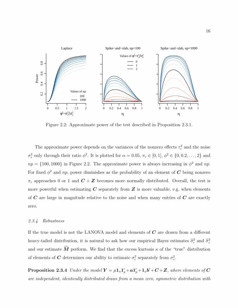
2.2 Approximate power of the test described in Proposition 2.3.1. . . . . . . . . 16

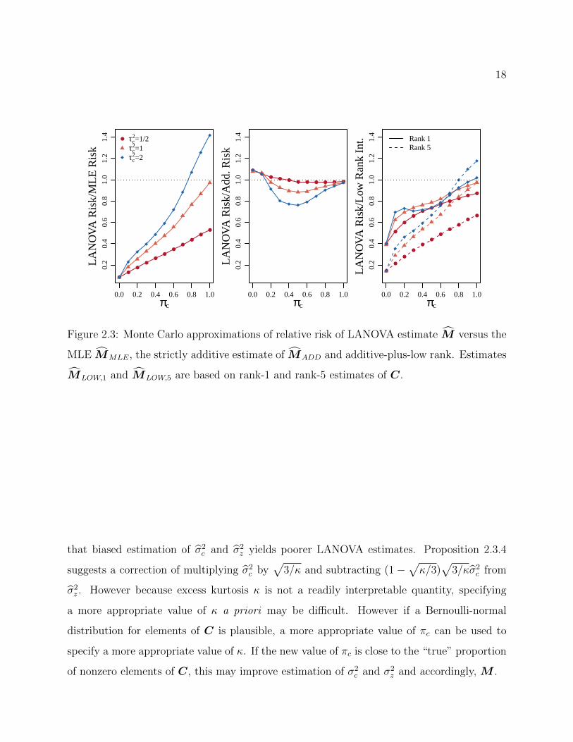
2.3 Monte Carlo approximations of relative risk of LANOVA estimate M versusthe MLE MMLE, the strictly additive estimate of MADD and additive-plus-low rank. Estimates MLOW,1 and MLOW,5 are based on rank-1 and rank-5estimates of C. . . . . . . . . . . . . . . . . . . . . . . . . . . . . . . . . . . 18

2.4 Elements of the 356 × 43 matrix C. The first panel shows the entire matrixC with rows (genes) and columns (tumors) sorted in decreasing order of the

row and column sparsity rates. The second panel zooms in on the rows of C(genes) marked in the first panel, which correspond to the fifty rows (genes)with the lowest sparsity rates. Colors correspond to positive (red) versus

negative (blue) values of C and darkness corresponds to magnitude. . . . . 23

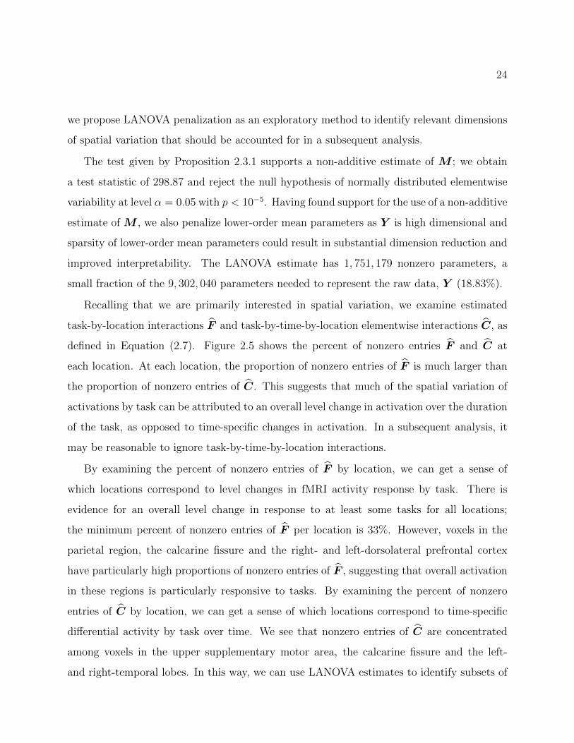
2.5 Percent of nonzero entries of F and C by location, where F and C estimateF and C as defined in Equation (2.7). Entries of F index task-by-locationinteraction terms and entries of C index task-by-time-by-location elementwiseinteraction terms. Darker colors indicate higher percentages. . . . . . . . . . 25

2.6 Entries of C. Red (blue) points indicate positive (negative) nonzero entries

of C and darker colors correspond to larger magnitudes. . . . . . . . . . . . 26

3.1 The first panel shows exponential power densities for fixed variance τ 2 = 1and varying values of the shape parameter q. The second panel shows themode thresholding function for σ2 = τ 2 = 1 and the values of q considered inthe first panel. The third panel shows the relationship between the kurtosisof the exponential power distribution and the shape parameter, q. . . . . . . 34

3.2 Power and Type-I error of level-0.05 tests for data simulated from model (3.1)with exponential power distributed β and σ2 = τ 2 = 1. A horizontal dashedgray line is given at 0.05. . . . . . . . . . . . . . . . . . . . . . . . . . . . . . 38

3.3 Adaptive estimation procedure versus Laplace prior performance for data sim-ulated from model (3.1) with exponential power distributed β and σ2 = τ 2 = 1. 43

iv

3.4 Power of level-0.05 tests for data simulated from a linear regression modelwith standard normal errors and Bernoulli-normal regression coefficients withsparsity rate 1 − π and unit variance. A horizontal dashed gray line is givenat 0.05. . . . . . . . . . . . . . . . . . . . . . . . . . . . . . . . . . . . . . . . 45

3.5 Adaptive estimation procedure versus Laplace prior performance for datasimulated from a linear regression model with standard normal errors andBernoulli-normal regression coefficients with sparsity rate 1−π and unit vari-ance. . . . . . . . . . . . . . . . . . . . . . . . . . . . . . . . . . . . . . . . . 46

3.6 Posterior modes, means and selected marginal distributions under exponentialpower (EP) priors and Laplace (L) priors of β for diabetes and glucose datasets. 50

4.1 Panel (a) reprinted from Bruneel (2018) shows a subject using the P300 speller.Panel (b) shows the locations of EEG sensors on the skull reprinted and mod-ified from Sharma (2013), with sensors included in our analysis highlighted inred. Arrows indicate the order of the channels appear in the data. . . . . . . 53

4.2 A subset of single-subject P300 speller data. Lines represents trials, i.e. rowsxi. Trials are plotted separately by whether or not the target letter was beingshown during the trial. . . . . . . . . . . . . . . . . . . . . . . . . . . . . . . 54

4.3 The first panel shows the values of a 208 × 8 ridge estimate BR for a sin-gle subject based on n = 140 trials which minimizes h (y|X,β,φ) + 1

2β′β.

The second panel shows a histogram of elements of BR plotted against anormal density with the same mean and variance as elements of BR. Thethird panel plots pairs of elements of BR that correspond to consecutive timepoints (bR,ij, bR,(i+1)j) against a gray dashed 45 line. The last panel shows

correlations of elements of BR across channels. . . . . . . . . . . . . . . . . . 81

4.4 Relationships between structured product normal (SPN), structured normal-gamma (SNG) and structured power/bridge (SPB) shrinkage priors and inde-pendent, identically distributed (IID) Laplace and multivariate normal priors. 82

4.5 Log-likelihood contours for β ∈ R2 with unit marginal prior variance andmarginal prior correlation ρ = 0.5. . . . . . . . . . . . . . . . . . . . . . . . . 82

4.6 Maximum marginal prior correlation ρ for β ∈ R2 as a function of kurtosis. . 83

4.7 Copula estimates for β ∈ R2 with unit marginal prior variances and marginalprior correlation ρ = 0.5. . . . . . . . . . . . . . . . . . . . . . . . . . . . . . 83

4.8 Univariate conditional prior distributions pβ1|β2 (β1|β2, ρ,θ) for β ∈ R2 withunit marginal prior variances, marginal prior correlation ρ ∈ 0, 0.5 andβ2 ∈ 0, 2. . . . . . . . . . . . . . . . . . . . . . . . . . . . . . . . . . . . . 84

v

4.9 Approximate mode-thresholding functions computed according to (4.1) forβ ∈ R2 with unit marginal prior variances, marginal prior correlation ρ = 0.5,noise variance φ2 = 0.1, βOLS,2 ∈ −0.5, 0, 0.5, 1 and βOLS,1 ∈ (0, 1). . . . . . 84

4.10 Normal LA-within-EM estimates of variances and correlations of Σ2. . . . . 85

4.11 Approximate posterior medians of empirical Bayes estimates of B under in-dependent and corresponding structured priors. . . . . . . . . . . . . . . . . 86

4.12 ROC curves for held out test data using empirical Bayes approximate posteriormedians of the fitted values. . . . . . . . . . . . . . . . . . . . . . . . . . . . 87

4.13 Approximate posterior medians of fully Bayes estimates of B. . . . . . . . . 88

4.14 ROC curves for held out test data using fully Bayes approximate posteriormedians of fitted values. . . . . . . . . . . . . . . . . . . . . . . . . . . . . . 88

B.1 Performance of estimators of τ 2, σ2 and q for exponential power distributedβ. True values printed in red. . . . . . . . . . . . . . . . . . . . . . . . . . . 151

B.2 Performance of estimators of τ 2, σ2 and κ+ 3 for Bernoulli-normal spike-and-slab distributed β. True values printed in red. . . . . . . . . . . . . . . . . . 152

vi

ACKNOWLEDGMENTS

To Peter, for teaching me to be creative in my research. Thank you for giving me the

freedom to explore my various ideas, both good and bad, and for believing that I might

eventually have some good ones. I am very grateful to you for pointing me to the problems

that led to this thesis and for paying for me to move to Duke so I could continue to drop

into your office with questions and work through problems on the whiteboard.

To my committee members. Thank you to Mathias for encouraging me to apply to the

University of Washington to study statistics and for giving me advice on most of the major

career decisions I’ve made since 2012, Daniela for teaching a phenomenal course on how to

be an academic statistician and for offering pep talks as I navigated the publishing process

and Betz for introducing me to the fascinating world of statistical methods for infectious

disease research and for continuing to be supportive even when my research interests took

me in another direction.

To my collaborators on my first statistical publication. Thank you to Elena for inviting

me to participate in a research project before I even arrived on campus and guiding it to

completion, Krista for having been and continuing to be a consistently wonderful mentor

and Mark for frequently providing positive feedback and encouraging guidance.

To the many fantastic teachers I have had over the years. Thank you to Mrs. Donaghue

for teaching advanced math classes in middle school, Mr. Garr for introducing me to some

of my favorite authors, Mrs. Petti and Mrs. McFarland for making me a better writer, Mrs.

Leonard for going above and beyond as math teacher and Professor Heckman for valuing my

work as a research assistant and continuing to encourage me long afterwards.

To my fiance, for supporting me, especially when I decided it would be best for me to

vii

move across the country to finish this degree. Thank you for picking up the phone every

time I would call, coming to visit Durham for weeks at a time and not breaking up with me

when I spontaneously adopted a second troubled dog.

To my loving and perfectly weird family. To my dad for raising me to believe I could do

anything, my mom for teaching me to be curious and inventive, my sister Norah for keeping

me humble by mocking me mercilessly, Grandma Griffin for her care and praise, Grandma

Carney for her wit and energy and Grandpa Carney for his kindness and generosity.

To my friends, in no particular order! To Kelly for always being an eager partner in crime,

James and Evelyn for always knowing where to go dancing, Kamala for working beside me

all through college, Cecilia for being an exceptional letter writer, Jack, Ricky and Robby for

making analysis more bearable, Andy for being my most reliable ally in the battle for base R

graphics, Lily for introducing me to my favorite pens, Cathy, Paul, Evan, Becky and Bobby

for listening to me panic about math tests between dives, Rebecca for collaborating with me

on a spreadsheet of inspiring lady statisticians, Karsten for dragging me up Mailbox Peak,

Kyle for educating me on the merits of Taco Bell, Alden for putting up with Baxter in the

office and on several alpine lake hikes, Sam for being the best co-GSR, Jessica for keeping

me up to date on internet slang, Theresa, Leigh, Laina and Bailey for giving me advice and

being great role models, Hannah, Corinne and Nilanjana for letting me give them advice

and becoming good friends, Matt, Ashley and Angelica for making Durham feel like home,

Felipe, Mauricio, Andee, Carrie and Victor for always making time for lunch, Mike, Liz,

Lindsay, Jake, Abbas, Steph, Jody and Phil for letting me have a desk in your social office.

To future young statisticians. I read several theses as I prepared to write my own. In

the event that you come across mine, I’d like you to know that I never felt like writing

this material came naturally. Everything presented here was nearly thrown away on several

occasions and I often wanted to quit. The first time I started to feel confident in and proud

of my work was only several months ago, and I still only feel that way part of the time.

viii

DEDICATION

To my dogs. To Baxter, for being by my side from the beginning, and to Hope, for trying

to make me into a morning person.

ix

1

Chapter 1

INTRODUCTION

The material in this thesis deals with penalized regression and its Bayesian counterpart,

regression under a prior on the regression coefficients. The relationship between penalized

regression and Bayesian regression has long been recognized (Tibshirani, 1996). Let y be an

observed n×1 response, let X be an observed n×p matrix of covariates and let β be a p×1

vector of unknown regression coefficients. In the linear regression setting, Lasso penalized

regression solves

minimizeβ||y −Xβ||22 + λ ||β||1

.

This is equivalent to computing the posterior mode of β under the model

y|X,β ∼ normal(Xβ, σ2In

), βj ∼ Laplace

(0, 2σ2/λ

),

where In is an n × n identity matrix and σ2 > 0 and λ > 0 are scale parameters. More

generally, let h (y|X,β,φ) be an objective function depending on nuisance parameters φ

that relates the unknown regression coefficients β and covariates X to the observed response

y, and let f (β|θ) be a penalty function that depends on tuning parameters θ. Any penalized

regression estimate obtained by solving

minimizeβ h (y|X,β,y,φ) + f (β|θ)

corresponds to the posterior mode of β under the model

py|β (y|X,β,φ) ∝ exp −h (y|X,β,y,φ) , pβ (β|θ) ∝ exp −f (β|θ) ,

where φ and θ can be interpreted as distributional parameters for the distributions of the

data and the coefficients.

2

Despite the fact that this correspondence between penalties and priors is well established,

the penalized regression and Bayesian literatures remain fairly divided. Within the penalized

regression literature, penalties are rarely treated as implying a specific model for the data and

regression coefficients. Rather, the penalty is interpreted as a tool for producing estimates

of regression coefficients with certain desirable properties, e.g. sparsity, and nuisance and

tuning parameters tend to be chosen to optimize predictive performance. This approach can

be advantageous in that it is relatively simple to implement, outperforms many alternatives

in terms of prediction and scales well to accommodate massive data. Within the Bayesian

literature, researchers either take an empirical Bayes approach, estimating φ and θ from the

marginal likelihood of the data, or a fully Bayes approach, assuming prior distributions for

φ and θ. Fully Bayes approaches are more popular, because they can be used to account

for uncertainty in the estimation of φ and θ and because estimating φ and θ the marginal

likelihood of the data as a function of φ and θ can be prohibitively computationally de-

manding under many common penalized regression models. Letting pφ (φ) and pθ (θ) refer

to the prior densities of φ and θ, this yields the model

py|β (y|X,β) ∝∫ ∞−∞

exp −h (y|X,β,y,φ) pφ (φ) dφ,

pβ (β|θ) ∝∫ ∞−∞

exp −f (β|θ) pθ (θ) dθ.

Under this model, the posterior mode can be more computationally challenging to compute

because the correspondingly penalty is a function of an intractable integral. Accordingly,

researchers in the Bayesian literature tend to use posterior means or medians as estimators

of β, which are easier to compute but do not have the same desirable properties of the

posterior mode for fixed values of φ and θ, e.g. elementwise sparsity. Even when φ and θ

are treated as fixed and empirical Bayes approaches are used, the Bayesian literature still

tends to discourage use of the posterior mode as an estimator of β and encourage use of the

posterior mean or median instead (Park and Casella, 2008; Hans, 2009). This is motivated

by decision-theoretic concerns, as the posterior mean and median are known to minimize

squared and absolute error loss, respectively. However it still results in estimators of β that

3

may not have the same desirable properties as the posterior mode, e.g. sparsity.

To our knowledge relatively little research has occupied the middle ground, i.e. has inter-

preted penalties as priors without assuming prior distributions for unknown distributional

parameters or discarding the posterior mode as a viable estimator. Doing so affords us

the ability to estimate tuning parameters/unknown distributional parameters, which can be

difficult to specify when they are numerous, data are limited or inference on the unknown

regression parameters as opposed to prediction is the primary goal. Furthermore, treating

the use of a penalty as equivalent to assuming a specific prior distribution allows us to draw

on a vast decision theory literature that can be used to justify the use of various posterior

summaries as estimators depending on the inferential goals of a specific problem (Bernardo

and Smith, 2000; Hans, 2009). This thesis helps to fill this gap in the literature. Although

we will use Bayesian terminology throughout this thesis, the ideas discussed here are not

strictly Bayesian in scope. Rather, they relate to the long literature on smoothing and

mixed models, in which regression coefficients are modeled to encourage various desirable

properties, distributional parameters are estimated from the marginal likelihood of the data,

and posterior summaries are used as estimators (Wand, 2003).

The first chapter in this thesis, “Lasso ANOVA Decompositions for Matrix and Tensor

Data,” focuses on the use of Lasso penalized ANOVA for matrices and higher order arrays.

In the matrix case, we consider Lasso penalized linear regression for y = vec (Y ), where

Y is a p1 × p2 matrix and X =[

1p1p2 1p2 ⊗ Ip1 Ip2 ⊗ 1p1 Ip1p2

], where 1p1p2 is a

p1p2 × 1 vector of ones. The unknown regression coefficients, β, can be decomposed into a

grand mean, row, column and element-wise components β =[µ a′ b′ vec (C)′

]′, where

only elements of C are subjected to a Lasso penalty. This problem poses the following

challenge: every element of Y corresponds to a unique element of C, so cross validation

is actually infeasible. We tackle this problem by treating the Lasso penalty as a Laplace

prior and recognizing that differences in normal and Laplace tail behavior, as measured by

kurtosis, allow for the construction of moment-based estimators of the noise variance and

Lasso tuning parameter. In the process, we explore how treating the Lasso penalty as a

4

prior is uniquely vulnerable to model misspecification, specifically of the prior distribution

of the regression coefficients. We observe evidence that suggests a Laplace prior will tend

to underpenalize the unknown regression coefficients when the empirical distribution of the

unobserved true regression coefficients is heavier than Laplace tailed and will overpenalize

the unknown regression coefficients when the empirical distribution of the unobserved true

regression coefficients is lighter than Laplace tailed.

Motivated by the issue of prior specification, the second chapter in this thesis “Testing

Sparsity-Inducing Penalties,” explores the choice of prior for more general linear regression

problems. We introduce a moment-based test of whether or not the tail behavior of ordinary

least squares or ridge estimates of the unknown regression coefficients is consistent with what

would be observed if the true unobserved regression coefficients were Laplace distributed, as

well as moment-based estimators of the prior parameters of a broader class of priors which

corresponds to `q penalties. We demonstrate that implementing such a test and adaptively

specifying the prior in the event of rejection can improve estimation of the regression co-

efficients, resolving the over- and underpenalization problems associated with treating the

Lasso penalty as a Laplace prior distribution.

The third chapter in this thesis, “Structured Shrinkage Priors,” considers an additional

kind of misspecification. In the first two chapters, we considered independent prior distri-

butions for the regression coefficients, which correspond to separable penalties which can

be decomposed. These priors do not encourage structure among the regression coefficients.

However, in many high dimensional regression settings the regression coefficients may have

some known structure a priori, e.g. the regression coefficients may be ordered in space

or correspond to a vectorized matrix or tensor of regression coefficients. Accordingly, in

this last chapter we develop structured shrinkage priors that generalize multivariate normal,

Laplace, exponential power and normal-gamma priors. These priors allow for the regres-

sion coefficients to be correlated a priori without sacrificing sparsity and shrinkage. The

primary challenges in working with these structured shrinkage priors are computational, as

the corresponding penalty is an intractable p-dimensional integral and the full conditional

5

distributions that are needed to simulate from the full conditional distribution of the regres-

sion coefficients are not necessarily standard distributions. We overcome these issues using a

flexible elliptical slice sampling procedure, and demonstrate that these priors can be used to

introduce structure while preserving sparsity of the corresponding penalized estimate given

by the posterior mode.

6

Chapter 2

LASSO ANOVA DECOMPOSITIONS FOR MATRIX ANDTENSOR DATA

2.1 Introduction

Researchers are often interested in estimating the entries of an unknown n× p mean matrix

M given a single noisy realization, Y = M + Z, where the entries of Z are assumed to

be independent, identically distributed mean zero normal random variables with unknown

variance σ2z . Consider a noisy matrix Y of gene expression measurements for p different genes

and n tumors. Researchers may be interested in which tumors have unique gene expression

profiles and which genes are differentially expressed across different tumors.

This is challenging because no replicates are observed; each unknown mij corresponds to

a single observation yij. As a result, the maximum likelihood estimate Y has high variability.

Accordingly, simplifying assumptions that reduce the dimensionality of M are often made.

Many such assumptions relate to a two-way ANOVA decomposition of M :

M = µ1n1′p + a1′p + 1nb

′ +C, (2.1)

where µ is an unknown grand mean, a is an n × 1 vector of unknown row effects, b is a

p × 1 vector of unknown column effects, C is a matrix of elementwise “interaction” effects

and 1n and 1p are n× 1 and p× 1 vectors of ones, respectively. In the absence of replicates,

implicitly assuming C = 0 is common. This reduces the number of freely varying unknown

parameters, from np to n+ p, but is also unlikely to be appropriate in practice.

In the settings we consider, it is likely that at least some elements of C are nonzero,

e.g. some tumor-gene combinations or treatment pairs in a factorial design may have large

interaction effects that are not explained by a strictly additive model. If M is approximately

7

additive in the sense that large deviations from additivity are rare, then C is sparse and

estimation of M may be improved by penalizing elements of C:

minimizeµ,a,b,C

1

2σ2z

∣∣∣∣vecY −

(µ1n1

′p + a1′p + 1nb

′ +C)∣∣∣∣2

2+ λc ||vec (C)||1

. (2.2)

The `1 penalty induces sparsity among the estimated entries of C, and solving this penalized

regression problem yields unique estimates of M and C. Elements of C can be interpreted

as interactions insofar as they indicate deviation from a strictly additive model.

This is a departure from the literature, in which assumptions on the rank of C are

often made. Some set µ = 0, a = 0 and b = 0 and assume C is low rank (Fazel, 2002;

Hoff, 2007; Candes et al., 2013; Josse and Sardy, 2016), while others treat µ, a and b as

unknown, apply the standard ANOVA zero-sum constraints for identifiability, 1′na = 1′pb = 0

and C ′1n = 0 and C1p = 0, and assume that C is low rank (Gollob, 1968; Johnson and

Graybill, 1972; Mandel, 1971; Goodman and Haberman, 1990). We refer to the latter as an

additive-plus-low-rank model for M . Assuming that C is low rank implies that elements of

C are multiplicative in row and column factors, i.e. if C is rank R then cij =∑R

r=1 λrur,ivr,j.

Although useful in many settings, assuming low rank C has two main limitations. First,

in the presence of unknown noise variance, σ2z , existing methods for choosing the rank can be

computationally expensive for large matrices (Hoff, 2007), require strong assumptions such

as known σ2z (Candes et al., 2013), or rely on approximations to account for unknown σ2

z

that may not always perform well in practice (Josse and Sardy, 2016). Second, even when

the rank can be chosen well, these methods conflate the presence of elementwise effects of

scientific interest with the presence of multiplicative effects. While this may be plausible in

many settings, it is easy to imagine scenarios in which a low rank C may fail to capture

elementwise effects of scientific interest. For instance, if Y were an n× n square matrix and

all cii were large while all cij, i 6= j were equal to zero, a rank n estimate of C would be

needed.

That said, solving Equation (2.2) requires specification of λc and σ2z . One approach

might be to recognize that we can rewrite Equation (2.2) to depend on a single parameter

8

η = λcσ2z and specify η using cross-validation. However, cross-validation is not appropriate

for this problem. Consider a subset Y 1 of Y with at least two elements from each row and

column of Y and let Y 2 denote the remaining entries. For a fixed value of η, we can obtain

estimates of µ, a, b, and elements C1 of C corresponding to Y 1. However, computing out-of-

sample predictions for Y 2 requires estimates of the elements C2 of C corresponding to Y 2.

Cross-validation cannot be performed without making additional assumptions that relate the

values of µ, a, b and C1 to C2. Another approach involves viewing the `1 penalty on C as a

Laplace prior distribution, in which case λc and σ2z can be interpreted as nuisance parameters.

However, obtaining empirical Bayes estimates of λc and σ2z via maximum marginal likelihood

may be prohibitively computationally demanding (Figueiredo, 2003; Park and Casella, 2008).

In this chapter we present moment-based empirical Bayes estimators of the nuisance

parameters λc and σ2z that are easy to compute, consistent and independent of assumptions

made regarding a and b. Moment-based estimators can be sensitive to outliers, however we

consider settings in which n or p are very large and moments can be estimated well. As our

approach to estimating λc and σ2z uses the Laplace prior interpretation of the `1 penalty, we

refer to estimation of M via optimization of Equation (2.2) using these nuisance parameter

estimators as LANOVA penalization, and we refer to the estimate M as the LANOVA

estimate.

The chapter proceeds as follows: In Section 2.2, we introduce moment-based estimators

for λc and σ2z , show that they are consistent as either the number of rows or columns of

Y goes to infinity and show that their efficiency is comparable to that of asymptotically

efficient marginal maximum likelihood estimators (MMLEs). In Section 2.3, we discuss es-

timation of M via Equation (2.2) given estimates of λc and σ2z and introduce a test of

whether or not elements of C are heavy-tailed, which allows us to avoid LANOVA penal-

ization in settings where it is especially inappropriate. We also investigate the performance

of LANOVA estimates of M relative to strictly additive estimates, strictly non-additive

estimates and additive-plus-low-rank estimates and examine robustness to misspecification

of the distribution of elements of C. In Section 2.4, we extend LANOVA penalization to

9

include penalization of lower-order mean parameters a and b and also to apply to the case

where Y is a K-way tensor. In Section 2.5, we apply LANOVA penalization to a matrix of

gene expression measurements, a three-way tensor of fMRI data and a three-way tensor of

wheat infection data. In Section 2.6 we discuss extensions, specifically multilinear regression

models and opportunities that arise in the presence of replicates.

2.2 LANOVA Nuisance Parameter Estimation

Consider the following statistical model for deviations of Y from a strictly additive model:

Y = µ1n1′p + a1′p + 1nb

′ +C +Z (2.3)

C = cij ∼ i.i.d. Laplace(0, λ−1

c

), Z = zij ∼ i.i.d. N

(0, σ2

z

).

The posterior mode of µ, a, b and C under this Laplace prior for C and flat priors for

µ, a and b corresponds to the solution of the LANOVA penalization problem given by

Equation (2.2).

We construct estimators of λc and σ2z as follows. Letting Hk = Ik − 1k1k/k be the

k× k centering matrix, we define R = HnY Hp. R depends on C and Z alone, specifically

R = Hn (C +Z)Hp. We construct estimators of λc and σ2z from R by leveraging the

difference between Laplace and normal tail behavior as measured by fourth order moments.

The fourth order central moment of any random variable x with mean µx and variance σ2x

can be expressed as E[(x− µx)4] = (κ+ 3)σ4

x, where κ is interpreted as the excess kurtosis

of the distribution of x relative to a normal distribution. A normally distributed variable has

excess kurtosis equal to 0, whereas a Laplace distributed random variable has excess kurtosis

equal to 3. It follows that the second and fourth order central moments of elements of C+Z

are E[(cij + zij)

2] = σ2c + σ2

z and E[(cij + zij)

4] = 3σ4c + 3 (σ2

c + σ2z)

2, respectively, where

σ2c = 2/λ2

c is the variance of a Laplace(λ−1c ) random variable. Given values of E

[(cij + zij)

2]and E

[(cij + zij)

4], we see that σ2c and σ2

z , and accordingly λc, can easily be recovered.

We do not observe C + Z directly, but we can use the second and fourth order sam-

ple moments of R, an estimate of C + Z, given by r(2) = 1np

∑ni=1

∑pj=1 r

2ij and r(4) =

10

1np

∑ni=1

∑pj=1 r

4ij, respectively, to separately estimate σ2

c and σ2z . These estimators are:

σ4c =

n3p3

(n− 1) (n2 − 3n+ 3) (p− 1) (p2 − 3p+ 3)

r(4)/3−

(r(2))2

(2.4)

σ2c =√σ4c , σ2

z =

np

(n− 1) (p− 1)

r(2) − σ2

c .

An estimator of λc is then given by λc =√

2/σ2c .

The estimator σ4c is biased. It is possible to obtain an unbiased estimator for σ4

c , however

the unbiased estimator will not be consistent as n → ∞ with p fixed or p → ∞ with n

fixed. Because these estimators depend on higher-order terms which can be very sensitive to

outliers, it is desirable to have consistency as either the number of rows or columns grows.

Accordingly, we prefer the biased estimator and examine its bias in the following proposition.

Proposition 2.2.1 Under the model given by Equation (2.3),

E[σ4c

]− σ4

c =−

n3p3

(n− 1) (n2 − 3n+ 3) (p− 1) (p2 − 3p+ 3)

[3 (n− 1)2 (p− 1)2

n3p3

σ4c+

2 (n− 1) (p− 1)

n2p2

(σ2c + σ2

z

)2].

A proof of this proposition and all other results presented in this chapter are given in an

appendix. The bias is always negative and accordingly, yields overpenalization of C. When

both n and p are small, σ4c tends to underestimate σ4

c . Recalling that σ4c is inversely related

to λc, this reflects a tendency to overpenalize and accordingly overshrink elements of C when

both n and p are small. This is not undesirable, in that it reflects a tendency to prefer the

simple additive model when few data are available. We also observe that the bias depends

not only on both σ2c and σ2

z . Holding n, p and σ2c fixed, we will overestimate λc more when

σ2z is larger. Again, this is not undesirable, in that it reflects a tendency to prefer the simple

additive model when the data are very noisy. Last, we see that the bias is O (1/np), i.e. the

bias approaches zero as either the number of rows or the number of columns increases. The

large sample behavior of our estimators of the nuisance parameters is similar.

11

Proposition 2.2.2 Under the model given by Equation (2.3), σ4c

p→ σ4c , σ2

c

p→ σ2c , λc

p→ λc

and σ2z

p→ σ2z as n→∞ with p fixed, p→∞ with n fixed, or n, p→∞.

Although these nuisance parameter estimators are easy to compute and consistent as n→

∞ or p → ∞, they are not maximum likelihood estimators and may not be asymptotically

efficient even as n → ∞ and p → ∞. Accordingly, we compare the asymptotic efficiency

of our estimator σ2c to that of the corresponding asymptotically efficient marginal maximum

likelihood estimator (MMLE) denoted by σ2c as n and p→∞. As noted in the Introduction,

obtaining σ2c is computationally demanding because maximizing the marginal likelihood of

the data requires a Gibbs-within-EM algorithm that is slow to converge (Park and Casella,

2008). Fortunately, computing the asymptotic variance of σ2c is simpler than computing σ2

c

itself. The asymptotic variance of σ2c is given by the Cramer-Rao lower bound for σ2

c , which

can be computed numerically from the density of the sum of Laplace and normally distributed

variables (Nadarajah, 2006; Dıaz-Frances and Montoya, 2008). The asymptotic variance of

σ2c is straightforward to compute as

√np (σ4

c − σ4c ) converges in distribution to a moment

estimator of σ4c . We note that the asymptotic variance of λc is similarly straightforward to

compute; both asymptotic variances are given in the appendix. Letting V [σ2c ] and V [σ2

c ]

refer to the variances of the estimators σ2c and σ2

c , we plot the asymptotic relative efficiency

V [σ2c ] /V [σ2

c ] over values of σ2c , σ

2z ∈ [0, 1] in Figure 2.1. Note that the relative efficiency of

σ2c compared to σ2

c also reflects the relative efficiency of our estimators λc and σ2z compared

to the MMLEs λc and σ2c , respectively, because both are simple functions of σ2

c .

When σ2c is small relative to σ2

z , the MMLE σ2c tends to be slightly more efficient. When

σ2c is large relative to σ2

z , σ2c tends to be much more efficient. However, in such cases the

interactions will not be heavily penalized and LANOVA penalization will not tend to yield

a simplified, nearly additive estimate of M . Put another way, Figure 2.1 indicates that λc

and σ2z will be nearly as efficient as the corresponding MMLEs when LANOVA penalization

is useful for producing a simplified, nearly additive estimate of M with sparse interactions.

We also note that because they are moment-based, our estimators may be more robust to

12

Asymptotic Relative Efficiency of σ~c2 versus σc

2

σc2

σ z2

0.2 0.3 0.4

0.5

0.6

0.7

0

.8

0.9

0.0 0.2 0.4 0.6 0.8 1.0

0.0

0.2

0.4

0.6

0.8

1.0

Figure 2.1: Asymptotic relative efficiency V[σ2c ]/V[σ2

c ] of the MMLE σ2c versus our moment-

based estimator σ2c as a function of the true variances σ2

c and σ2z .

misspecification of the distribution of elements of C and Z than the MMLEs.

2.3 Mean Estimation, Interpretation, Model Checking and Robustness

2.3.1 Mean Estimation

In practice, our nuisance parameter estimators are not guaranteed to be nonnegative and

two special cases can arise. When σ4c < 0, we set σ2

c = 0 and C = 0 and set M = MADD,

where MADD = (In −Hn)Y (Ip −Hp) is the strictly additive estimate. When σ2z < 0, we

reset σ2z = 0 and set M = MMLE, where MMLE = Y is the strictly non-additive estimate.

Neither special case prohibits estimation of M .

We assess how often these special cases arise via a small simulation study. Setting σ2z = 1,

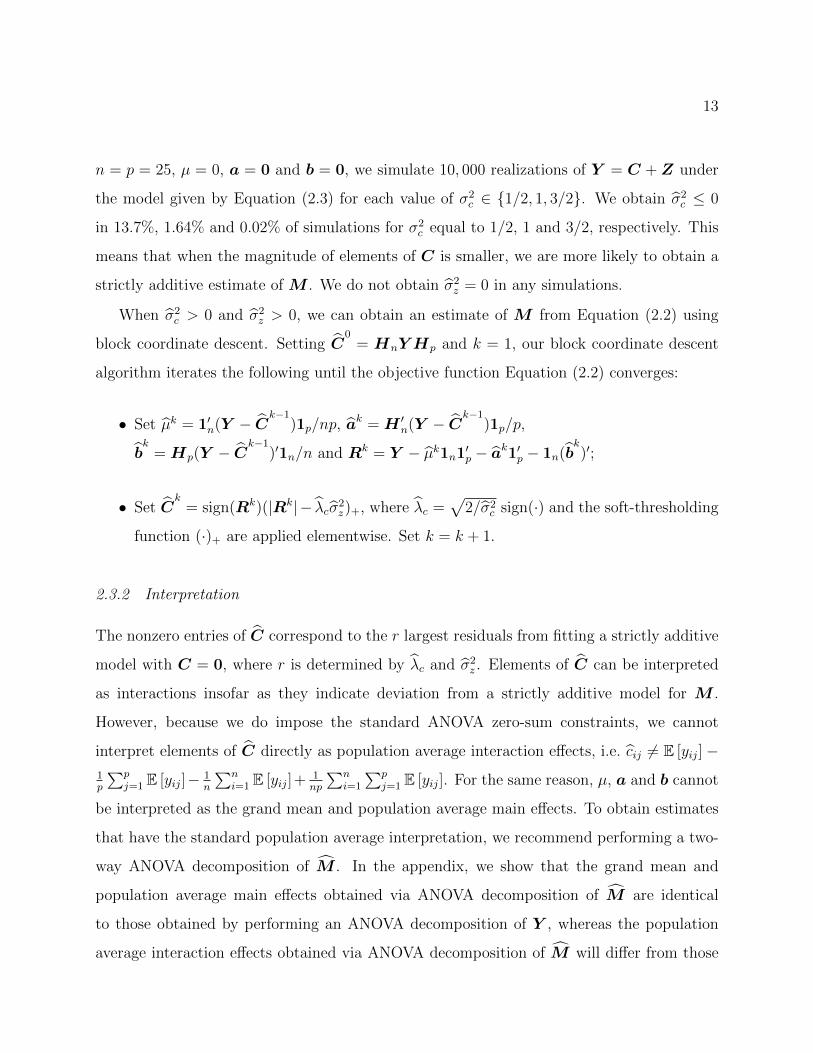
13

n = p = 25, µ = 0, a = 0 and b = 0, we simulate 10, 000 realizations of Y = C +Z under

the model given by Equation (2.3) for each value of σ2c ∈ 1/2, 1, 3/2. We obtain σ2

c ≤ 0

in 13.7%, 1.64% and 0.02% of simulations for σ2c equal to 1/2, 1 and 3/2, respectively. This

means that when the magnitude of elements of C is smaller, we are more likely to obtain a

strictly additive estimate of M . We do not obtain σ2z = 0 in any simulations.

When σ2c > 0 and σ2

z > 0, we can obtain an estimate of M from Equation (2.2) using

block coordinate descent. Setting C0

= HnY Hp and k = 1, our block coordinate descent

algorithm iterates the following until the objective function Equation (2.2) converges:

• Set µk = 1′n(Y − Ck−1

)1p/np, ak = H ′n(Y − C

k−1)1p/p,

bk

= Hp(Y − Ck−1

)′1n/n and Rk = Y − µk1n1′p − ak1′p − 1n(b

k)′;

• Set Ck

= sign(Rk)(|Rk|− λcσ2z)+, where λc =

√2/σ2

c sign(·) and the soft-thresholding

function (·)+ are applied elementwise. Set k = k + 1.

2.3.2 Interpretation

The nonzero entries of C correspond to the r largest residuals from fitting a strictly additive

model with C = 0, where r is determined by λc and σ2z . Elements of C can be interpreted

as interactions insofar as they indicate deviation from a strictly additive model for M .

However, because we do impose the standard ANOVA zero-sum constraints, we cannot

interpret elements of C directly as population average interaction effects, i.e. cij 6= E [yij]−1p

∑pj=1 E [yij]− 1

n

∑ni=1 E [yij]+

1np

∑ni=1

∑pj=1 E [yij]. For the same reason, µ, a and b cannot

be interpreted as the grand mean and population average main effects. To obtain estimates

that have the standard population average interpretation, we recommend performing a two-

way ANOVA decomposition of M . In the appendix, we show that the grand mean and

population average main effects obtained via ANOVA decomposition of M are identical

to those obtained by performing an ANOVA decomposition of Y , whereas the population

average interaction effects obtained via ANOVA decomposition of M will differ from those

14

obtained via ANOVA decomposition of Y and may include many entries that are nearly

equal to zero.

2.3.3 Testing

LANOVA penalization assumes the distribution of entries of C have tail behavior consistent

with a Laplace distribution. It is natural to ask if this assumption is appropriate but it is

difficult to test it, because C and Z enter into the observed data through their sum C +Z.

Accordingly, we suggest a test of the more general assumption that elements of C are heavy-

tailed. This allows us to rule out LANOVA penalization when it is especially inappropriate,

i.e. when the data suggest elements of C are normal tailed. When the distribution of

elements of C is heavy-tailed, the distribution of elements of C+Z will also be heavy-tailed

and will have strictly positive excess kurtosis. In contrast, when elements of C are either all

zero or have a distribution with normal tails, elements of C+Z have excess kurtosis equal to

exactly zero. We construct a test of the null hypothesis H0: cij + zij ∼ i.i.d. N (0, σ2c + σ2

z),

which encompasses the cases in which C = 0 or elements of C are normally distributed.

Conveniently, the test statistic is a simple function of σ2c , and σ2

z and can be computed at

little additional computational cost. We can also think of this as a test of deconvolvability

of C +Z or whether or not the variances σ2c and σ2

z can be separately identified, where the

null hypothesis is that deconvolution of C + Z is not possible and the variances σ2c and σ2

z

cannot be separately identified.

Proposition 2.3.1 For Y = µ1n1′p+a1′p+1nb

′+C+Z, as n and p→∞ an asymptotically

level-α test of H0: cij + zij ∼ i.i.d. N (0, σ2c + σ2

z) is obtained by rejecting H0 when

√np

σ4c√

83

(σ2c + σ2

z)2

> z1−α,

where z1−α denotes the 1− α quantile of the standard normal distribution.

This test gives us power against the alternative where elements C are heavy-tailed and

LANOVA penalization may be appropriate.

15

Because this is an approximate test, we assess its level in finite samples in a small simu-

lation study. Setting σ2z = 1, n = p, µ = 0, a = 0 and b = 0, we simulate 10, 000 realizations

of Y = C + Z under H0 for each value of n ∈ 25, 100 and σ2c ∈ 1/2, 1, 3/2. When

n = p = 25, the test rejects at a slightly higher rate than the nominal level. It rejects in

7.98%, 7.65% and 8.66% of simulations for σ2c equal to 1/2, 1 and 3/2, respectively. When

n = p = 100, the test nearly achieves the desired level. It rejects in 6.13%, 5.60% and 6.00% of

simulations for σ2c equal to 1/2, 1 and 3/2, respectively. We compute the approximate power

of this test under two heavy-tailed distributions for elements of C: the Laplace distribution

assumed for LANOVA penalization and a Bernoulli-normal spike-and-slab distribution.

Proposition 2.3.2 Assume that elements of C are independent, identically distributed mean

zero Laplace random variables with variance σ2c and let φ2 = σ2

c/σ2z . Then as n and p→∞,

the asymptotic power of the test given by Proposition 2.3.1 is:

1− Φ

z1−α −√

3np8

(φ2

φ2+1

)2

√1 +

68φ8+36φ6+9φ4

(1+φ2)4

.

The power depends on the variances σ2c and σ2

z only through their ratio φ2. It is plotted for

for α = 0.05, φ2 ∈ [0, 2] and np = 100, 200, . . . , 1000 in Figure 2.2. The power of the test is

increasing in φ2 and increasing more quickly when np is larger and more data are available.

Now we consider the power for Bernoulli-normal spike-and-slab distributed elements of

C.

Proposition 2.3.3 Assume that elements of C are independent, identically distributed Bernoulli-

normal random variables. An element of C is exactly equal to zero with probability 1 − πc,

and normally distributed with mean zero and variance τ 2c otherwise. Letting φ2 = τ 2

c /σ2z , as

n and p→∞, the asymptotic power of the test given by Proposition 2.3.1 is:

1− Φ

z1−α − πc (1− πc)√

3np8

(φ2

πcφ2+1

)2

√1 + πc (1− πc)

(20π2

c−28πc+35)φ8+16(5−πc)φ6+72φ4

8(πcφ2+1)4

.

16P

ower

φ2=σc2 σz

2

Laplace

0.2

0.4

0.6

0.8

0 0.5 1 1.5 2

Values of np

2001000

πc

Spike−and−slab, np=100

Values of φ2=τc2 σz

2

012

0 0.2 0.4 0.6 0.8 1

πc

Spike−and−slab, np=1000

0 0.2 0.4 0.6 0.8 1

Figure 2.2: Approximate power of the test described in Proposition 2.3.1.

The approximate power depends on the variances of the nonzero effects τ 2c and the noise

σ2z only through their ratio φ2. It is plotted for α = 0.05, πc ∈ [0, 1], φ2 ∈ 0, 0.2, . . . , 2 and

np = 100, 1000 in Figure 2.2. The approximate power is always increasing in φ2 and np.

For fixed φ2 and np, power diminishes as the probability of an element of C being nonzero

πc approaches 0 or 1 and C + Z becomes more normally distributed. Overall, the test is

more powerful when estimating C separately from Z is more valuable, e.g. when elements

of C are large in magnitude relative to the noise and when many entries of C are exactly

zero.

2.3.4 Robustness

If the true model is not the LANOVA model and elements of C are drawn from a different

heavy-tailed distribution, it is natural to ask how our empirical Bayes estimates σ2c and σ2

z

and our estimate M perform. We find that the excess kurtosis κ of the “true” distribution

of elements of C determines our ability to estimate σ2c separately from σ2

z .

Proposition 2.3.4 Under the model Y = µ1n1′p+a1′p+1nb

′+C+Z, where elements of C

are independent, identically distributed draws from a mean zero, symmetric distribution with

17

variance σ2c , excess kurtosis κ and finite eighth moment and elements of Z are normally

distributed with mean zero and variance σ2z , we have that σ2

c

p→√κ/3σ2

c and σ2z

p→ σ2z +(

1−√κ/3)σ2c as n→∞ with p fixed, p→∞ with n fixed, or n and p→∞.

Proposition 2.3.4 indicates that we underestimate σ2c when elements of C are lighter-

than-Laplace tailed and we overestimate σ2c when elements of C are heavier-than-Laplace

tailed. To see how this affects estimation of M , we consider Bernoulli-normal spike-and-

slab distributed elements of C and compare the risk of the LANOVA estimate M to the

risk of the maximum likelihood estimate MMLE, the risk of the strictly additive estimate

MADD and the risk of additive-plus-low rank estimates of M denoted by MLOW,1 and

MLOW,5 which assume rank-1 and rank-5 C, respectively. Additive-plus-low-rank estimates

are computed according to Johnson and Graybill (1972). We compute Monte Carlo estimates

of the risks setting n = p = 25, µ = 0, a = 0, b = 0 and σ2z = 1 and varying τ 2

c = 1/2, 1, 2

and πc = 0, 0.1, . . . , 0.9, 1. For each value of τ 2c , the variance of nonzero elements of C,

and πc, the probability any element of C is nonzero, the Monte Carlo estimate is based on

500 simulated Y . As M is a function of µ, a, b and C, the performance M reflects the

performance of µ, a, b and C indirectly.

The results indicate generally favorable performance of the LANOVA estimate M for

Bernoulli-normal C. Recalling that MADD is strictly additive and MMLE is strictly non-

additive, the LANOVA estimate M outperforms MADD when πc is larger and M has fewer

additive elements and outperforms MMLE when πc is smaller and M has more additive

elements. The LANOVA estimate M outperforms additive-plus-low-rank estimates MLOW,1

and MLOW,5 when πc is smaller and more elements of C are exactly equal to zero. The

LANOVA estimate M performs worse than MADD and MMLE when πc ≈ 0 or πc ≈ 1 and

M is nearly strictly additive and nearly strictly non-additive, respectively.

Recalling Proposition 2.3.4, note that the LANOVA estimate M performs best relative to

MADD when πc ≈ 0.5. When πc = 0.5, the excess kurtosis of the Bernoulli-normal spike-and-

slab distribution κ = 3 (1− πc) /πc matches that of the Laplace distribution. This suggests

18

0.0 0.2 0.4 0.6 0.8 1.0

0.2

0.4

0.6

0.8

1.0

1.2

1.4

LAN

OVA

Ris

k/M

LE R

isk

πc

τc2=1/2

τc2=1

τc2=2

0.0 0.2 0.4 0.6 0.8 1.0

0.2

0.4

0.6

0.8

1.0

1.2

1.4

LAN

OVA

Ris

k/A

dd. R

isk

πc

0.0 0.2 0.4 0.6 0.8 1.0

0.2

0.4

0.6

0.8

1.0

1.2

1.4

LAN

OVA

Ris

k/Lo

w R

ank

Int.

πc

Rank 1Rank 5

Figure 2.3: Monte Carlo approximations of relative risk of LANOVA estimate M versus the

MLE MMLE, the strictly additive estimate of MADD and additive-plus-low rank. Estimates

MLOW,1 and MLOW,5 are based on rank-1 and rank-5 estimates of C.

that biased estimation of σ2c and σ2

z yields poorer LANOVA estimates. Proposition 2.3.4

suggests a correction of multiplying σ2c by

√3/κ and subtracting (1−

√κ/3)

√3/κσ2

c from

σ2z . However because excess kurtosis κ is not a readily interpretable quantity, specifying

a more appropriate value of κ a priori may be difficult. However if a Bernoulli-normal

distribution for elements of C is plausible, a more appropriate value of πc can be used to

specify a more appropriate value of κ. If the new value of πc is close to the “true” proportion

of nonzero elements of C, this may improve estimation of σ2c and σ2

z and accordingly, M .

19

2.4 Extensions

2.4.1 Penalizing Lower-Order Parameters

When Y has many rows or columns, it may be reasonable to believe that many elements of

a or b are exactly zero. A natural extension of Equation (2.2) is given by

minimizeµ,a,b,C1

2σ2z

||vec (Y −M )||22 + λa ||a||1 + λb ||b||1 + λc ||vec (C)||1 , (2.5)

where we still have M = 1n1′pµ + a1′p + 1nb

′ +C. Again, using the posterior mode inter-

pretation of Equation (2.5), we can estimate σ2a and σ2

b from the observed data, Y :

σ2a =

1

n− 1

n∑i=1

a2i −

n

(n− 1) (p− 1)r(2), σ2

b =1

p− 1

p∑j=1

b2j −

p

(n− 1) (p− 1)r(2).

where a = HnY 1p/p and b = HpY′1n/n are OLS estimates for a and b. The estimators

λa =√

2/σ2a and λb =

√2/σ2

b can be shown to be consistent for λa and λb as n → ∞ and

p→∞, respectively. Because λc and σ2z do not depend on of a and b, our estimators for λc

and σ2z are unchanged. A block coordinate descent algorithm for solving Equation (2.5) is

given in the appendix. With respect to interpretation, population average row and column

main effects can be obtained via ANOVA decomposition of M .

2.4.2 Tensor Data

LANOVA penalization can be extended to a p1 × p2 × · · · × pK K-mode tensor Y . We

consider:

vec (Y ) = Wβ + vec (C) + vec (Z) (2.6)

C = ci1...iK ∼ i.i.d. Laplace(0, λ−1

c

), Z = zi1...iK ∼ i.i.d. N

(0, σ2

z

),

where vec (Y ) is the∏K

k=1 pk vectorization of the K-mode tensor Y with “lower” indices

moving “faster” and W and β are the design matrix and unknown mean parameters cor-

responding to a K-way ANOVA decomposition treating the K modes of Y as factors. The

20

matrix W = [W 1, . . . ,W 2K−1] is obtained by concatenating the 2K − 1 unique matrices of

the formW l = (W l,1 ⊗ · · · ⊗W l,K), where eachW l,k is equal to either Ipk or 1pk , excluding

the identity matrix, IpK⊗· · ·⊗Ip1 . As in the matrix case, approaches that assume a low rank

C are common (van Eeuwijk and Kroonenberg, 1998; Gerard and Hoff, 2017). We penalize

elements of the highest order mean term C for which no replicates are observed. In the

three-way tensor case, the first part of Equation (2.6) refers to the following decomposition:

yijk = µ+ ai + bj + dk + eij + fik + gjk + cijk + zijk. (2.7)

Estimates of σ2z and λc are constructed from vec (R) = (HK ⊗ · · · ⊗H1) vec (Y ), where

Hk = Ipk − 1pk1pk/pk is the pk × pk centering matrix and ‘⊗’ is the Kronecker product. As

in the matrix case, vec (R) is independent of the lower-order unknown mean parameters β,

i.e. vec (R) = (HK ⊗ · · · ⊗H1) vec (C +Z). Our estimates of σ2z and λc are still functions

of the second and fourth sample moments of R: r(2) = 1p

∑pi=1 r

2i and r(4) = 1

p

∑pi=1 r

4i , where

p =∏K

k=1 pk. We extend our empirical Bayes estimators as follows:

σ4c =

K∏k=1

p3k

(pk − 1) (p2k − 3pk + 3)

r(4)/3−

(r(2))2

(2.8)

σ2c =√σ4c , σ2

z =

(K∏k=1

pkpk − 1

)r(2) − σ2

c ,

where λc =√

2/σ2c . As in the matrix case, we can compute the bias of σ4

c .

Proposition 2.4.1 Under the model given by Equation (2.6),

E[σ4c

]− σ4

c =−

K∏k=1

p3k

(pk − 1) (p2k − 3pk + 3)

[3

K∏k=1

(pk − 1)2

p3k

σ4c+(

2K∏k=1

pk − 1

p2k

)(σ2c + σ2

z

)2

].

Interpretation of this result is analogous to the matrix case. We tend to prefer the simpler

model with vec (C) = 0 over a more complicated model with nonzero elements of vec (C)

when few data are available or when the data are very noisy. Additionally, E [σ4c ] − σ4

c =

21

O (1/p), i.e. the bias of σ4c diminishes as the number of levels of any mode increases. We also

assess the large-sample performance of our empirical Bayes estimators in the K-way tensor

case.

Proposition 2.4.2 Under the model given by Equation (2.6), σ4c

p→ σ4c , σ2

c

p→ σ2c , λc

p→ λc

and σ2z

p→ σ2z as pk′ →∞ with pk, k 6= k′, fixed or p1, . . . , pK →∞.

A block coordinate descent algorithm for estimating the unknown mean parameters is

given in the appendix. Results for testing the appropriateness of assuming heavy-tailed C

and robustness carry over to K-way tensors. K-way tensor analogues to Propositions 2.3.1-

2.3.4, where we replace np with p and assume all p1, . . . , pK → ∞, are shown to hold in

the appendix. Lastly we can also extend LANOVA penalization for tensor data to penal-

ize lower-order mean parameters. Because tensor-variate Y include even more lower-order

mean parameters, penalizing lower-order parameters is especially useful. We give nuisance

parameter estimators for penalizing lower-order parameters in the three-way case in the

appendix.

2.5 Numerical Examples

Brain Tumor Data: We consider a 356 × 43 matrix of gene expression measurements

for 356 genes and 43 brain tumors. The 43 brain tumors include 24 glioblastomas and 19

oligodendroglial tumors, which include 5 astrocytomas, 8 oligodendrogliomas and 6 mixed

oligoastrocytomas. This data is contained in the denoiseR package for R (Josse et al.,

2016), and it has been used to identify genes associated with glioblastomas versus oligo-

dendroglial tumors (Bredel et al., 2005; de Tayrac et al., 2009). We focus on comparison

to de Tayrac et al. (2009), who used a variation of principal components analysis of Y to

identify differentially expressed genes and groups of tumors which is similar to using an

additive-plus-low-rank estimate of M . Unlike pairwise test-based methods which require

prespecified tumor groupings, LANOVA penalization and additive-plus-low-rank estimates

can be used to examine differential expression both within and across types of brain tumors.

22

Differential expression within types of brain tumors in particular is of recent interest (Bleeker

et al., 2012).

We apply LANOVA penalization with penalized interaction effects and unpenalized main

effects. The test given by Proposition 2.3.1 supports a non-additive estimate ofM ; we obtain

a test statistic of 18.45 and reject the null hypothesis of normally distributed elementwise

variability at level α = 0.05 with p < 10−5. We estimate that 11, 188 elements of C (73%)

are exactly equal to zero, i.e. most genes are not differentially expressed. Figure 2.4 shows

C and a subset containing fifty genes with the lowest gene-by-tumor sparsity rates.

The results of LANOVA penalization are consistent with those of de Tayrac et al. (2009).

We observe that 49% and 56% of the elements of C involving the genes ASPA and PDPN

are nonzero. Examination of M indicates overexpression of these genes among glioblastomas

relative to oligodendroglial tumors, as observed in de Tayrac et al. (2009).

LANOVA penalization yields additional results that are consistent with the wider liter-

ature. The gene DLL3 has the highest rate of gene-by-tumor interactions at 74% and tends

to be underexpressed in glioblastomas. This is consistent with findings of overexpression of

DLL3 in brain tumors with better prognoses (Bleeker et al., 2012). The KLRC genes KLRC1,

KLRC2 and KLRC3.1 all have very high rates of gene-by-tumor interactions at 72%, 70%

and 60%. Ducray et al. (2008) has found evidence for differential KLRC expression across

glioma subtypes. LANOVA penalization also indicates that several brain tumors have unique

gene expression profiles. Glioblastomas 3, 4 and 30 have rates of nonzero gene-by-tumor in-

teractions exceeding 50% and similar gene expression profiles. Specifically, we observe over-

expression of FCGR2B and HMOX1 and underexpression of RTN3 for gliomastomas 3, 4

and 30. Overexpression of FCGR2B or HMOX1 is associated with poorer prognosis (Zhang

et al., 2016; Ghosh et al., 2016), and RTN3 is differentially expressed across subgroups of

glioblastoma that differ with respect to prognosis (Cosset et al., 2017). This suggests that

glioblastomas 3, 4 and 30 may correspond to an especially aggressive subtype.

23

Gen

e

Tumor

GB

M31

GB

M29

GB

M23

GB

M22

AO

A6

sGB

M1

GB

M24

AO

A2

GB

M26

GS

1JP

A3

GB

M11

GB

M25 O

2G

BM

15 O5

AO

2A

O1

GB

M1

GB

M6

sGB

M3

GB

M28

AO

A1

JPA

2A

OA

3A

O3

GB

M16

GS

2A

A3

AO

A4

GN

N1

GB

M27

GB

M21

GB

M5

LGG

1A

OA

7G

BM

9O

4O

3O

1G

BM

30G

BM

4G

BM

3

GB

M31

GB

M29

GB

M23

GB

M22

AO

A6

sGB

M1

GB

M24

AO

A2

GB

M26

GS

1JP

A3

GB

M11

GB

M25 O

2G

BM

15 O5

AO

2A

O1

GB

M1

GB

M6

sGB

M3

GB

M28

AO

A1

JPA

2A

OA

3A

O3

GB

M16

GS

2A

A3

AO

A4

GN

N1

GB

M27

GB

M21

GB

M5

LGG

1A

OA

7G

BM

9O

4O

3O

1G

BM

30G

BM

4G

BM

3

COL1A2SNRPN

PLA2G2AFBXO2

SERPINI1GAS1

EPB49NPTX1

TNFRSF12AASPA

LGALS3RAB27BSTXBP1

L3MBTL4RAB30

BGNLOC541471

FAM84BVEGF

FBXL16AA029415

FGF13L1CAMMASP1EDNRBPDE2A

ADMAA906888

SOX4MGC26694

ABCC3CKMT1A

VSNL1ESM1SYT7PDPNCA12

COL3A1EPHB1SNCG

MICAL2TIMP1

COL1A1KLRC3.1

CHI3L2KLRC2

IMAGE.33267KLRC1H78560

DLL3

Tumor

Figure 2.4: Elements of the 356 × 43 matrix C. The first panel shows the entire matrix C

with rows (genes) and columns (tumors) sorted in decreasing order of the row and column

sparsity rates. The second panel zooms in on the rows of C (genes) marked in the first panel,

which correspond to the fifty rows (genes) with the lowest sparsity rates. Colors correspond

to positive (red) versus negative (blue) values of C and darkness corresponds to magnitude.

fMRI Data: Second, we consider a tensor of fMRI data which appeared in Mitchell et al.

(2004). During each of 36 tasks, fMRI activations were measured at 55 time points and 4, 698

locations (voxels). Accordingly, the data can be represented as a 36× 55× 4, 698 three-way

tensor. Because the data are so high dimensional, many methods of analysis are prohibitively

computationally burdensome. Accordingly, parcellation approaches that reduce the spatial

resolution of fMRI data by grouping voxels into spatially contiguous groups are common,

however, the choice of a specific parcellation can be difficult (Thirion et al., 2014). Instead,

24

we propose LANOVA penalization as an exploratory method to identify relevant dimensions

of spatial variation that should be accounted for in a subsequent analysis.

The test given by Proposition 2.3.1 supports a non-additive estimate of M ; we obtain

a test statistic of 298.87 and reject the null hypothesis of normally distributed elementwise

variability at level α = 0.05 with p < 10−5. Having found support for the use of a non-additive

estimate of M , we also penalize lower-order mean parameters as Y is high dimensional and

sparsity of lower-order mean parameters could result in substantial dimension reduction and

improved interpretability. The LANOVA estimate has 1, 751, 179 nonzero parameters, a

small fraction of the 9, 302, 040 parameters needed to represent the raw data, Y (18.83%).

Recalling that we are primarily interested in spatial variation, we examine estimated

task-by-location interactions F and task-by-time-by-location elementwise interactions C, as

defined in Equation (2.7). Figure 2.5 shows the percent of nonzero entries F and C at

each location. At each location, the proportion of nonzero entries of F is much larger than

the proportion of nonzero entries of C. This suggests that much of the spatial variation of

activations by task can be attributed to an overall level change in activation over the duration

of the task, as opposed to time-specific changes in activation. In a subsequent analysis, it

may be reasonable to ignore task-by-time-by-location interactions.

By examining the percent of nonzero entries of F by location, we can get a sense of

which locations correspond to level changes in fMRI activity response by task. There is

evidence for an overall level change in response to at least some tasks for all locations;

the minimum percent of nonzero entries of F per location is 33%. However, voxels in the

parietal region, the calcarine fissure and the right- and left-dorsolateral prefrontal cortex

have particularly high proportions of nonzero entries of F , suggesting that overall activation

in these regions is particularly responsive to tasks. By examining the percent of nonzero

entries of C by location, we can get a sense of which locations correspond to time-specific

differential activity by task over time. We see that nonzero entries of C are concentrated

among voxels in the upper supplementary motor area, the calcarine fissure and the left-

and right-temporal lobes. In this way, we can use LANOVA estimates to identify subsets of

25

FC

Figure 2.5: Percent of nonzero entries of F and C by location, where F and C estimate F

and C as defined in Equation (2.7). Entries of F index task-by-location interaction terms

and entries of C index task-by-time-by-location elementwise interaction terms. Darker colors

indicate higher percentages.

relevant voxels that should be included in a subsequent analysis.

Fusarium Data: Last, we consider the problem of checking for nonzero three-way inter-

actions in experimental data without replicates. The data is a 20 × 7 × 4 three-way tensor

containing severity of disease incidence ratings for 20 varieties of wheat infected with 7 strains

of Fusarium head blight over 4 years, from 1990-1993, that appeared in van Eeuwijk and

Kroonenberg (1998). There is scientific reason to believe that several nonzero three-way

variety-by-strain-by-year interactions are present. van Eeuwijk and Kroonenberg (1998) ex-

amined these interactions using a rank-1 tensor model for C using a single multiplicative

component for C with cijk = αiγjδk, however as noted in the Introduction if the true inter-

actions are sparse a low rank model may not be sufficient even if few nonzero interactions

are present.

As in van Eeuwijk and Kroonenberg (1998), we transform the severity ratings to the logit

scale before estimating LANOVA parameters. The test given by Proposition 2.3.1 supports

a non-additive estimate of M ; we obtain a test statistic of 3.99 and reject the null hypothesis

26

of normally distributed elementwise variability at level α = 0.05 with p = 3.34 × 10−5. We

obtain 87 nonzero entries of C (16%).

1990

7F

12H

13H

14H

15H

16G

17G

Blight Strains

N1N2N3N4N5

F11F12F13F14F15G16G17G18G19G20H21H22H23H24H25

Whe

at V

arie

ties

1991

7F

12H

13H

14H

15H

16G

17G

Blight Strains

1992

7F

12H

13H

14H

15H

16G

17G

Blight Strains

1993

7F

12H

13H

14H

15H

16G

17G

Blight Strains

Figure 2.6: Entries of C. Red (blue) points indicate positive (negative) nonzero entries of

C and darker colors correspond to larger magnitudes.

Figure 2.6 shows nonzero elements of C, with dashed lines separating groups of wheat

and blight by country of origin: Hungary (H), Germany (G), France (F) or the Netherlands

(N). We can interpret elements of C as evidence for variety-by-year-by-strain interactions

that cannot be expressed as additive in variety-by-year, year-by-strain and variety-by-strain

effects. Like van Eeuwijk and Kroonenberg (1998), we observe large three-way interactions

in 1992, during which there was a disturbance in the storage of blight strains. Specifically,

we observe interactions involving Dutch variety 2, the only variety with no infections at all

in 1992, and interactions between Hungarian varieties 21 and 23 and foreign blight strains,

which despite the storage disturbance were still able to cause infection in these two Hungarian

varieties alone. We also observe evidence for “real” three way interactions for varieties

exposed to Hungarian strain 12 in 1991 and French varieties exposed to Hungarian strains

27

in 1993 as well as other interactions. We do not have enough information about the data

to assess whether or not these estimated interactions are related to features of the study or

known patterns in the behavior of certain varieties and strains, however they suggest further

investigation of these varieties and strains may be warranted.

2.6 Discussion

This chapter demonstrates the use the common Lasso penalty and the corresponding Laplace

prior distribution for estimating elementwise effects of scientific interest in the absence of

replicates. Our procedure, LANOVA penalization, can also be interpreted as assessing ev-

idence for nonadditivity. We show that our nuisance parameter estimators are consistent,

explore their behavior when assumptions are violated and demonstrate that the correspond-

ing mean parameter estimates tend to perform favorably relative to strictly additive, strictly

non-additive and additive-plus-low-rank estimates when elements of C are Bernoulli-normal

distributed. We emphasize that LANOVA penalization is computationally simple. The nui-

sance parameter estimators are easy to compute for arbitrarily large matrices, and estimates

of M can be computed using a fast block coordinate descent algorithm that exploits the

structure of the problem. We also extend LANOVA penalization to penalize lower-order

mean parameters and apply to tensors. Finally, we show that LANOVA estimates can be

used to examine gene-by-tumor interactions using microarray data, to perform exploratory

analysis of spatial variation in activation response to tasks over time in high dimensional

fMRI data and to assess evidence for “real” elementwise interaction effects in experimental

data. To conclude, we discuss several limitations and extensions.

One limitation is that we assume heavy-tailed elementwise variation is of scientific inter-

est and should be incorporated into the mean M , whereas normally distributed elementwise

variation is spurious noise Z. If the noise is heavy-tailed, it may erroneously be incorpo-

rated into the estimate of C. Similar issues arise with low rank models for C, insofar as

systematic correlated noise can erroneously be incorporated into the estimate of C. In gen-

eral, any method that aims to separate elementwise variation into components that are of

28

scientific interest and spurious noise requires strong assumptions that must be considered in

the context of the problem. Another limitation is that the results of the simulation study

assessing the performance of the LANOVA estimate M do not necessarily suggest favorable

performance of the LANOVA estimate in all settings. First, we only consider Bernoulli-

normal elements of C where each element cij is exactly equal to 0 with probability 1 − πcand normally distributed with mean zero and variance τ 2

c otherwise. Although we expect the

LANOVA estimate to perform well when elements of C are heavy tailed, we do not expect

the LANOVA estimate to perform well when elements of C are light-tailed. Second, this

scenario considers C with independent, identically distributed elements. In some settings,

it may be reasonable to expect dependence across elements of C and additive-plus-low-rank

estimates may perform better.

The methods presented in this chapter could be extended in several ways. Although we

use our estimators of λc and σ2z in posterior mode estimation, the same estimators could

also be used to simulate from the posterior distribution using a Gibbs sampler. The output

of a Gibbs sampler could be used to construct credible intervals for elements of M , which

would be one way of addressing uncertainty. We may also want to account for additional

uncertainty induced by estimating λc and σ2z . To address this, a fully Bayesian approach with

prior distributions set for λc and σ2z could be taken at the cost of losing a sparse estimate of

C. Our empirical Bayes nuisance parameter estimators could be used to set parameters of

prior distributions for λc or σ2z . Last, LANOVA penalization for matrices is a specific case

of the more general bilinear regression model, where we assume Y = AW +BX +C +Z,

given known W and X. The same logic used in this chapter could be extended to this

context and a more general multilinear context for tensor Y .

Finally, our intuition combined with the results of Section 2.3 suggests that the Laplace

distributional assumptions used in this chapter are likely to be violated in many settings.

Whereas the strength of the Laplace distributional assumption for elements of C can be

justified by the need to make some assumptions in the absence of replicate measurements,

it cannot be similarly justified for lower-order mean parameters. This leads us to one last

29

extension: improved distribution specification for unknown mean parameters in the presence

of replicate measurements. In future work, we will consider scenarios where we have enough

data to estimate the variances of unknown mean parameters and noise from second order

moments alone and can use fourth order moments to test the appropriateness of a specific

distribution for unknown mean parameters or choose a better one.

30

Chapter 3

TESTING SPARSITY-INDUCING PENALTIES

3.1 Introduction

Lasso estimators are ubiquitous in linear regression due to their desirable properties and

computational feasibility, as they can be used to produce sparse estimates of regression coef-

ficients without sacrificing convexity of the estimation problem (Tibshirani, 2011). The lasso

estimator solves minimizeβ ||y −Xβ||22 + λ ||β||1, where y is an n × 1 vector of responses,

X is an n × p design matrix and the value λ > 0 determines the relative importance of

the penalty ||β||1 compared to the model fit ||y −Xβ||22 in estimating β. It has long been

recognized that the lasso estimator corresponds to the posterior mode when y = Xβ + z

and elements of z and β are independent normal and Laplace random variables, respectively

(Tibshirani, 1996; Figueiredo, 2003). The Laplace prior interpretation is popular in part

because sampling from the full posterior distribution using a Gibbs sampler is computa-

tionally feasible (Park and Casella, 2008). This allows computation of alternative posterior

summaries, e.g. the posterior mean, median and quantiles, which can be used to obtain

point and interval estimates of β. Furthermore, the prior interpretation of a penalty yields

decision theoretic justifications for using the corresponding penalized estimate or alternative

posterior summaries to estimate β (Hans, 2009).

However, many researchers have found that the lasso estimator may perform suboptimally

compared to other penalized estimators if the true value of β is highly sparse or not sparse

at all (Fan and Li, 2001; Leeb and Potscher, 2008). Analogously, posterior summaries under

a Laplace prior have been found to be suboptimal compared to posterior summaries under

other priors, depending on the empirical distribution of true values of the elements of β

(Griffin and Brown, 2010; Carvalho et al., 2010; Castillo et al., 2015; Bhattacharya et al.,

31

2015; van der Pas et al., 2017). As a result, although a lasso estimator or a Laplace prior

may be a reasonable default choice in high-dimensional problems due to its blend of desirable

properties and computational feasibility, it would be useful to have a data-driven means to

assess its appropriateness, and choose a more appropriate prior or penalty if suggested by

the data.

One approach is to embed the lasso estimator in a larger class of penalized estimators

and determine if the lasso estimator is a reasonable choice within this class. Consider the

class of `q penalized estimators, which solve minimizeβ ||y −Xβ||22 +λ ||β||qq for some q > 0,

where ||β||qq =∑p

j=1 |βj|q. This includes the ridge estimator given by q = 2, which has long

been known to have desirable shrinkage properties (Hoerl and Kennard, 1970). The `q class

includes the class of bridge estimators described by Frank and Friedman (1993) and accord-

ingly, penalties that can outperform `1 penalties when the true value of β is highly sparse, at

the cost of losing convexity of the estimation problem (Huang et al., 2008; Mazumder et al.,

2011; Marjanovic and Solo, 2014). Approaches to evaluating the appropriateness of q = 1

from this perspective might include cross validation, generalized cross validation or unbiased

risk estimate minimization over values of λ and q simultaneously. However, these procedures

can be challenging to perform over a two dimensional grid. Another approach is to assume

the more flexible class of exponential power prior distributions which includes the Laplace

prior as a special case (Subbotin, 1923; Box and Tiao, 1973):

y = Xβ + z, β1, . . . , βpi.i.d.∼ EP (τ, q) , z ∼ N

(0, σ2In

), (3.1)

where EP is the exponential power distribution with unknown shape parameter q > 0 and

τ 2 and σ2 are the unknown variances of the regression coefficients β and error z. The corre-

sponding posterior mode of β is an `q-penalized estimate with λ = τ−q(Γ(3/q)Γ(1/q)

)q/2. Posterior

simulation under an exponential power prior can be more computationally demanding, how-

ever the corresponding posterior summaries may outperform those based on Laplace priors

for highly sparse or non-sparse β. Fully Bayesian inference could proceed by assuming priors

for the error variance σ2, λ and q at the expense of losing a possibly sparse and compu-

32

tationally tractable posterior mode (Polson et al., 2014). Accordingly, we could evaluate

the appropriateness of a Laplace prior by computing a Bayes factor. However, specifying

reasonable priors for λ and q that yield a proper posterior distribution is difficult in practice

(Fabrizi and Trivisano, 2010; Salazar et al., 2012).

Alternatively, a likelihood ratio or score test of the null hypothesis H : q = 1 against

the alternative hypothesis, K : q 6= 1 under the model given by (3.1) could be constructed.

However, constructing a likelihood ratio test would require prohibitively computationally

demanding maximum likelihood estimation of τ 2, σ2 and q under the alternative. Both

likelihood ratio and score tests would also require derivation of the distribution of the test

statistic under the null, which is challenging due to marginal dependence of y induced by

assuming a prior distribution for β. Importantly, all of these approaches except the con-

struction of a score test share the disadvantage of requiring penalized estimation or posterior

simulation for q 6= 1 be performed regardless of whether or not q = 1 is deemed appropriate,

which negates any computational advantages offered by assuming q = 1.

In this chapter we consider the Laplace and exponential power prior interpretations of

the lasso and `q penalties. We propose fast and easy-to-implement procedures for testing

the appropriateness of a Laplace prior (q = 1) and estimating q in the event of rejection. In

Section 3.2 we describe our testing procedure, which rejects the Laplace prior if an estimate

of the kurtosis of the elements of β exceeds a particular threshold. The threshold is chosen

so that the test rejects with probability approximately equal to α, on average across datasets

and Laplace-distributed coefficient vectors β. We evaluate the performance of the approx-

imation and the power of the testing procedure numerically via simulation. In Section 3.3

we introduce moment-based empirical Bayes estimates of q and the variances σ2 and τ 2 of

the error and the regression coefficients. We also propose a two-stage adaptive procedure

for estimating β. If the testing procedure fails to reject the null, the adaptive estimation

procedure defaults to an estimate computed under a Laplace prior. Otherwise, we estimate β

under an exponential power prior using an estimated value of q. We show via simulation that

the adaptive estimation procedure outperforms estimators based on a Laplace prior when

33

elements of β have an exponential power distribution with q 6= 1 and performs similarly to

estimators based on a Laplace prior when elements of β have a Laplace distribution. In Sec-

tion 3.4, we demonstrate that the adaptive procedure also improves estimation of sparse β

when elements of β have a spike-and-slab distribution. In Section 3.5, we apply the testing

and estimation procedures to several datasets commonly used in the penalized regression

literature. A discussion follows in Section 3.6.

3.2 Testing the Laplace Prior

Our approach to testing the appropriateness of the Laplace prior treats the Laplace prior

as a special case of the larger class of exponential power distributions (Subbotin, 1923; Box

and Tiao, 1973). This class includes the normal and Laplace distributions. The exponential

power density is given by

p(βj|τ 2, q

)=( q

2τ

)√ Γ (3/q)

Γ (1/q)3 exp

−(

Γ (3/q)

Γ (1/q)

)q/2 ∣∣∣∣βjτ∣∣∣∣q, (3.2)

where q > 0 is an unknown shape parameter and τ 2 is the variance. The first panel of

Figure 3.1 plots exponential power densities for different values of q with the variance fixed

at τ 2 = 1. Because the exponential power distributions have simple distribution functions

with easy to compute moments and can accommodate a wide range of tail behaviors, they

quickly became popular as alternative error distributions (Subbotin, 1923; Diananda, 1949;

Box, 1953; Box and Tiao, 1973).

When an exponential power prior is assumed for β, we can understand how the choice

of q provides flexible penalization by examining the mode thresholding function. The mode

thresholding function relates the OLS estimate for a simplified problem with a single stan-

dardized covariate to the posterior mode of β. Let x be a standardized n×1 covariate vector

with ||x||22 = 1, let β be a scalar and let βols = x>y. The mode thresholding function is

given by:

arg minβ1

2σ2

(βols − β

)2

+

(Γ (3/q)

Γ (1/q)

)q/2 ∣∣∣∣βτ∣∣∣∣q .

34

This function is not generally available in closed form but can be computed numerically, even

when q < 1 and the mode thresholding problem is non-convex (Marjanovic and Solo, 2014).

The second panel of Figure 3.1 shows the mode thresholding function for σ2 = τ 2 = 1.

−2 −1 0 1 2

0.0

0.4

0.8

1.2

βj

p(β j

|q,τ2

=1)

Value of q

0.511.524

0 1 2 3 4 5

01

23

45

βOLS

Pos

terio

r M

ode

of β

q

κ+

3

0.5 1.5 2.5 3.5

1.8

510

1520

25

q=1 (Laplace)q=2 (Normal)

Figure 3.1: The first panel shows exponential power densities for fixed variance τ 2 = 1 and

varying values of the shape parameter q. The second panel shows the mode thresholding

function for σ2 = τ 2 = 1 and the values of q considered in the first panel. The third panel

shows the relationship between the kurtosis of the exponential power distribution and the

shape parameter, q.

Within the class of exponential power priors, the relationship between the shape param-

eter q and kurtosis E[β4j

]/E[β2j

]2is one-to-one and given by:

κ+ 3 = Γ (5/q) Γ (1/q) /Γ (3/q)2 , (3.3)

where κ refers to the excess kurtosis relative to a normal distribution. We plot kurtosis as a

function of q in the third panel of Figure 3.1. Accordingly, if β were observed we could naively

construct a test statistic based on the empirical kurtosis of the elements of β. We define the

test statistic ψ(β) = m4 (β) /m2 (β)2, where m2 (β) = 1p

∑pj=1 β

2p and m4 (β) = 1

p

∑pj=1 β

4p

are the second and fourth empirical moments of β. The test statistic ψ(β) is the empirical

kurtosis of the elements of the vector β. An exact level-α test of H could be performed by

comparing the test statistic to the α/2 and 1−α/2 quantiles of the distribution of ψ(β) under

35

the null. Because the distribution of ψ(β) under an exponential power prior depends only

on q and not τ 2, we can obtain Monte Carlo estimates of the α/2 and 1−α/2 quantiles ψα/2

and ψ1−α/2 by simulating entries of β∗ from any Laplace distribution and and computing

ψ (β∗). As this test is available only when β is observed, we refer to this as the oracle test.

In practice, β is not observed. However when n > p and X>X is full rank, the OLS

estimator βols =(X>X

)−1X>y is available. As a surrogate for ψ(β), we can use ψ(βols) as

a test statistic. If n >> p, then βols ≈ β conditional on β. It follows that ψ(βols

)d≈ ψ(β)

when treating β as random.

Proposition 3.2.1 Under normality of the errors z as assumed in (3.1),

E[(ψ(βols)− ψ(β))2|β

]≤ 16σ2

(m6(β)

m2(β)4

)tr((X>X)−1)/p+ o

(σ2tr((X>X)−1)/p

)(3.4)

where m6 (β) = 1p

∑pj=1 β

6j .

Details are provided in the appendix. Accordingly, when tr((X>X)−1)/p is small an ap-

proximate level-α test of H is obtained by rejecting H when ψ(βols

)/∈(ψα/2, ψ1−α/2

).

Although the behavior of the OLS estimator is well understood, we introduce some addi-

tional notation to help explain when tr((X>X))−1 is likely to be small for large n. Let V be

a diagonal matrix with diagonal elements√

diag(X>X

)and C be the “correlation” matrix

corresponding to X>X, such that X>X = V CV . Let ηj refer to eigenvalues of C. The

eigenvalues ηj indicate the overall collinearity of X. When columns of X are orthogonal,

η1 = · · · = ηp = 1, whereas when X is highly collinear the smallest values of ηj may be very

close or exactly equal to 0. Applying Theorem 3.4 of Styan (1973) we can write

tr((X>X)−1)/p ≤ maxj

(1

||xj||22

)maxj

(1

η2j

).

We can see that as long as ||xj||22 are large, which will tend to be the case when n is large,

and eigenvalues of ηj are not very small, i.e. X is not too highly collinear, tr((X>X)−1)/p

will be small enough to justify using ψ(βols) as a surrogate for ψ(β).

36

However, penalized regression is often considered when n < p or X is highly collinear.

When n < p, the OLS estimator is not unique and so neither is ψ(βols). When n ≥ p

but X is highly collinear, i.e. some columns of X are strongly correlated with others and

tr((X>X)−1)/p may not be small even for large values of n. When columns of X have been

centered and standardized to have norm n according to standard practice, we can easily see

that the quantity tr((X>X)−1)/p = 1np

∑pj=1

1ηj

will “blow up” if any values of ηj are very

close to or exactly equal to zero and quantiles of ψ(β) will poorly approximate quantiles of

ψ(βols).

Fortunately, we can construct a modified test using a ridge estimate of β, βδ = V −1(C+

δ2Ip)−1V −1X>y, where δ ≥ 0 is a nonnegative constant. Ridge estimators reduce variance

at the cost of yielding a biased estimate of β, E[βδ|β] = V −1 (C + δ2Ip)−1CV β. However

letting βδ = E[βδ|β], the distribution of ψ (βδ) under an exponential power prior still only

depends on q and not τ 2. Accordingly, if βδ were observed we could perform an exact level-α

test of H by comparing ψ (βδ) to Monte Carlo estimates of the α/2 and 1 − α/2 quantiles

ψδ,α/2 and ψδ,1−α/2 obtained by simulating β∗ from any Laplace distribution and computing

ψ(β∗δ = ψ(V −1 (C + δ2Ip)

−1CV β∗) . In practice, we can use ψ(βδ) as a surrogate for

ψ (βδ) to obtain an approximate level-α test.

Proposition 3.2.2 Let Σδ = V −1 (C + δ2Ip)−1C (C + δ2Ip)

−1V −1. Under normality of

the errors z as assumed in the model given by (3.1),

E[(ψ(βδ)− ψ(βδ))

2|β]≤ 16σ2

(m6 (βδ)

m2(βδ)4

)tr (Σδ) /p+ o

(σ2tr (Σδ) /p

), (3.5)

where mk (βδ) = 1p

∑pj=1 β

kj .

Details are provided in the appendix. It follows that when tr (Σδ) /p is small, an approximate

level-α test of H is obtained by rejecting H when ψ(βδ) /∈(ψδ,α/2, ψδ,1−α/2

).

As the performance of this test depends on tr (Σδ) /p, it depends not only on X but also

on δ2. Again applying Theorem 3.4 of Styan (1973), we can write

tr (Σδ) /p ≤ maxj

(1

||xj||22

)maxj

(ηj

(ηj + δ2)2

).

37

The first term depends only on the design matrix, X. As long as ||xj||22 are large, which again

is likely to be the case for large n, the first term will be small. The second term depends on δ2

through the eigenvalue ratiosηj

(ηj+δ2)2. Heuristically, the eigenvalue ratios are decreasing in δ2

and setting δ2 to be very large would ensure that tr (Σδ) /p is very close to 0 and that ψ(βδ)

performs well as a surrogate for ψ(βδ). However, increasing δ2 also reduces the power of the

test as it forces the ridge estimate closer to the zero vector. To ensure that the eigenvalue

ratios do not “blow up” while retaining as much power as possible we recommend setting

δ2 = (1−minimizejηj)+, where η1, . . . , ηp are the eigenvalues of C. When the columns of

X are standardized to have norm n, tr (Σδ) /p = 1np

∑pi=1

ηj

(δ2+ηj)2 . Accordingly with δ2 set

to δ2 = (1−minimizejηj)+, we can at least ensure that tr (Σδ) /p ≤ 1n.

The tests based on ψ(βols) and ψ(βδ) have several good features. First, the approx-

imate distributions of the test statistics ψ(βols) and ψ(βδ) do not depend on the values

of the unknown parameters τ 2 or σ2, and so their approximate null distributions may be

simulated easily. Second, both test statistics are easy and quick-to-compute even for very

high dimensional data. Third, both test statistics are invariant to rescaling of y or X by a

constant.

We examine the performance of the tests with a simulation study. We simulate parameters

and data according to the model (3.1). When simulating data and parameters, we set

σ2 = τ 2 = 1 and consider p ∈ 25, 50, 75, 100, n ∈ 50, 100, 200 and q ∈ 0.1, . . . , 2.

Because the OLS and ridge test statistics are invariant to rescaling of y by a constant, the

simulation results depend only on τ 2/σ2, and in this case reflect the performance of the tests

when τ 2 = σ2. For each combination of p, n and q, we simulate 1, 000 values of X and β,

drawing entries of X independently from the standard normal distribution. When n > p,

we use the OLS test statistic ψ(βols). When n ≤ p, we use the ridge test statistic ψ(βδ).

Figure 3.2 shows the power of the level-0.05 tests, i.e. the proportion of simulated datasets

for which we reject H at level-0.05 as a function of q and n. When q = 1, this gives the level

of the test. The last panel shows the power of the oracle test based on ψ(β).

The simulation results shown in Figure 3.2 indicate that the tests will perform well relative

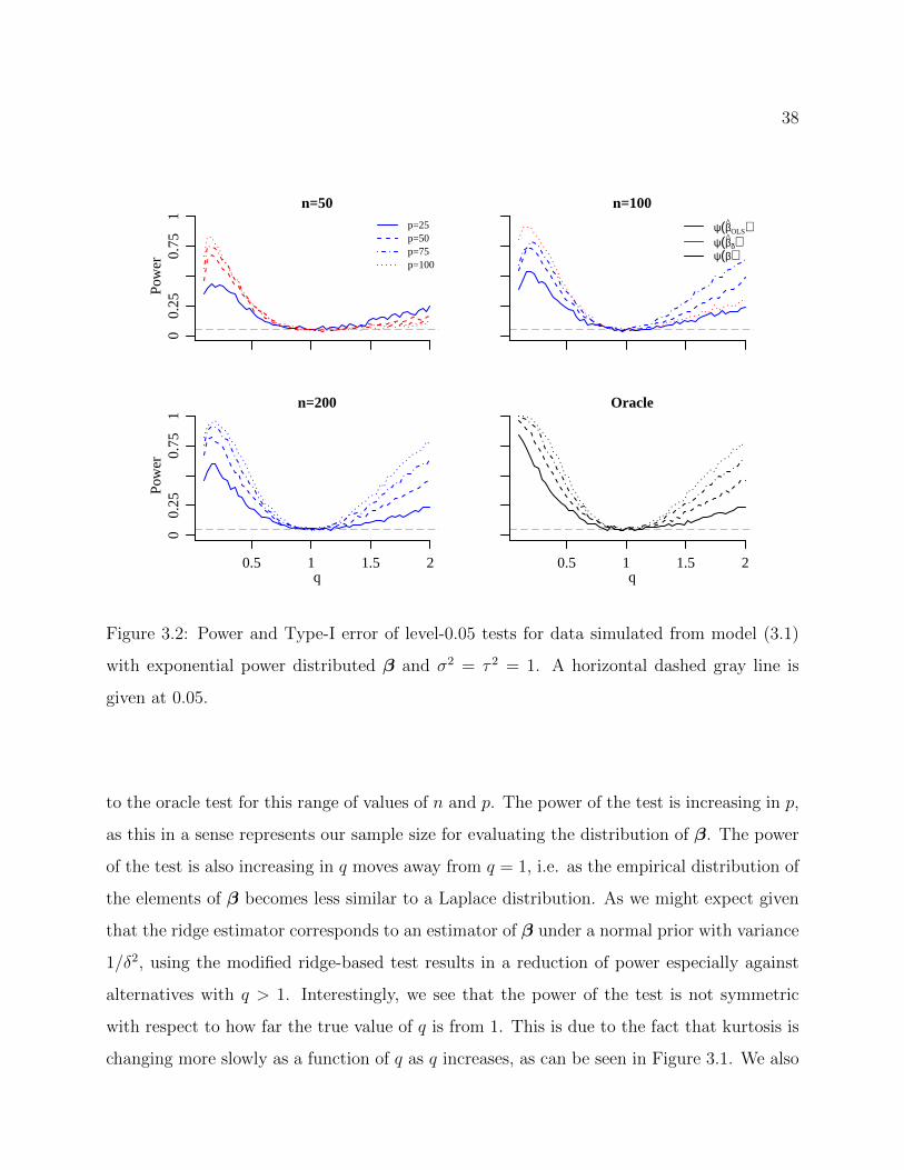
38

n=50

Pow

er0

0.25

0.75

1

p=25p=50p=75p=100

n=100

ψ(βOLS)ψ(βδ)ψ(β)

n=200

q

Pow

er0

0.25

0.75

1

0.5 1 1.5 2

Oracle

q0.5 1 1.5 2

Figure 3.2: Power and Type-I error of level-0.05 tests for data simulated from model (3.1)

with exponential power distributed β and σ2 = τ 2 = 1. A horizontal dashed gray line is

given at 0.05.

to the oracle test for this range of values of n and p. The power of the test is increasing in p,

as this in a sense represents our sample size for evaluating the distribution of β. The power

of the test is also increasing in q moves away from q = 1, i.e. as the empirical distribution of

the elements of β becomes less similar to a Laplace distribution. As we might expect given

that the ridge estimator corresponds to an estimator of β under a normal prior with variance

1/δ2, using the modified ridge-based test results in a reduction of power especially against

alternatives with q > 1. Interestingly, we see that the power of the test is not symmetric

with respect to how far the true value of q is from 1. This is due to the fact that kurtosis is

changing more slowly as a function of q as q increases, as can be seen in Figure 3.1. We also

39

observe a dip in power for very small values of q when ψ(βols) or ψ(βδ) are used. This can

be explained by examining the bias of m2(βols) which appears in the denominator of ψ(βols)

E[m2(βols)

]= m2(β) + σ2tr((X>X)−1)/p.

When q is very small and p is less than or equal to 100, most elements of β will be very close

to zero with high probability. For instance, when q = 0.1 and τ 2 = 1, Pr(|βj| ≥ 0.1) ≈ 0.08.

When most elements of β are very close to 0, m2 (β) will be small and m2(βols) will be

dominated by the error incurred by estimating β. The behavior of ψ(βδ) at small values of

q can be explained analogously.

3.3 Adaptive Estimation of β

Rejection of the null hypothesis implies that the empirical distribution of the unobserved

entries of β does not resemble a Laplace distribution. This suggests a two-stage adaptive

procedure for estimating β that first tests the appropriateness of the Laplace prior and

estimates β under a Laplace prior if the test accepts and estimates β under an exponential

power prior otherwise. This procedure requires estimates of τ 2 and σ2 if the test accepts and

τ 2, σ2 and q if the test rejects, as well as procedures for computing the posterior mode or

simulating from the posterior distribution of β under an exponential power prior. We do not

specify which posterior summary should be used to estimate β in general. It is well known

that different posterior summaries minimize different loss functions (Hans, 2009), and we

view the choice of posterior summary as problem-specific.

We consider empirical Bayes estimation of q, τ 2 and σ2. Estimating these parameters

by maximizing the marginal likelihood of the data∫p (y|X,β, σ2) p (β|τ 2, q) dβ is difficult

because the integral is not available in closed form for arbitrary values of q. The problem

is not amenable to a Gibbs-within-EM algorithm for maximizing over σ2, τ 2 and q jointly

and Gibbs-within-EM algorithms to obtain maximum marginal likelihood estimates of τ 2

and σ2 for fixed q are computationally intensive and tend to be slow to converge (Roy and

Chakraborty, 2016). As a result, we consider easy and quick to compute moment-based

40

empirical Bayes estimators of σ2, τ 2 and q. As moment estimators, they are more robust

to misspecification of the prior and residual distributions than likelihood-based alternatives.

Conveniently, the estimators for τ 2 and σ2 do not depend on q. This yields simple and

interpretable comparisons of estimates of β computed under Laplace versus exponential

power priors.

3.3.1 Estimation of q

The test statistics ψ(βols) and ψ(βδ) can be used to estimate q. In the previous section,

we demonstrated that an approximate test of H could be obtained by using ψ(βols) as a

surrogate for ψ(β) when tr((X>X)−1)/p is small. Recall that the quantity ψ(β) is the

empirical kurtosis of β and is defined as a function of the second and fourth empirical

moments of β, m2(β) and m4(β) . As m2(β)p→ E[β2

j ] and m4(β)p→ E[β4

j ] as p → ∞, it

follows from the continuous mapping theorem that ψ(β)p→ κ+ 3 as p→∞, where κ+ 3 is

the kurtosis of the distribution of elements of β. Accordingly, we can use ψ(βols) directly as

an estimator of the kurtosis κ+ 3 when tr((X>X)−1) is small and p is large.

When the ridge-based test statistic ψ(βδ) is used, estimation of κ is less straightfor-

ward. Even if m2(βδ)p→ E[m2(βδ)] and m4(βδ)

p→ E[m4(βδ)] as p → ∞, the con-

tinuous mapping theorem implies ψ(βδ)p→ (γ (κ+ 3) + ω) /α2 as p → ∞, where α =

tr(X>XD2X>X)/p, γ =∑p

j=1

∑pk=1(DX>X)4

jk/p, ω = 3((∑p

j=1(X>XD2X>X)2jj)/p−

γ) and D = V −1 (C + δ2Ip)−1V −1. This suggests the follow bias correction

κ+ 3 =

(α2

γ

)(ψ(βδ)−

ω

α2

). (3.6)

Additional details are provided in the appendix.

Given an estimate of κ + 3, we estimate q from (3.3), κ + 3 = Γ (5/q) Γ (1/q) /Γ (3/q)2

using Newton’s method.

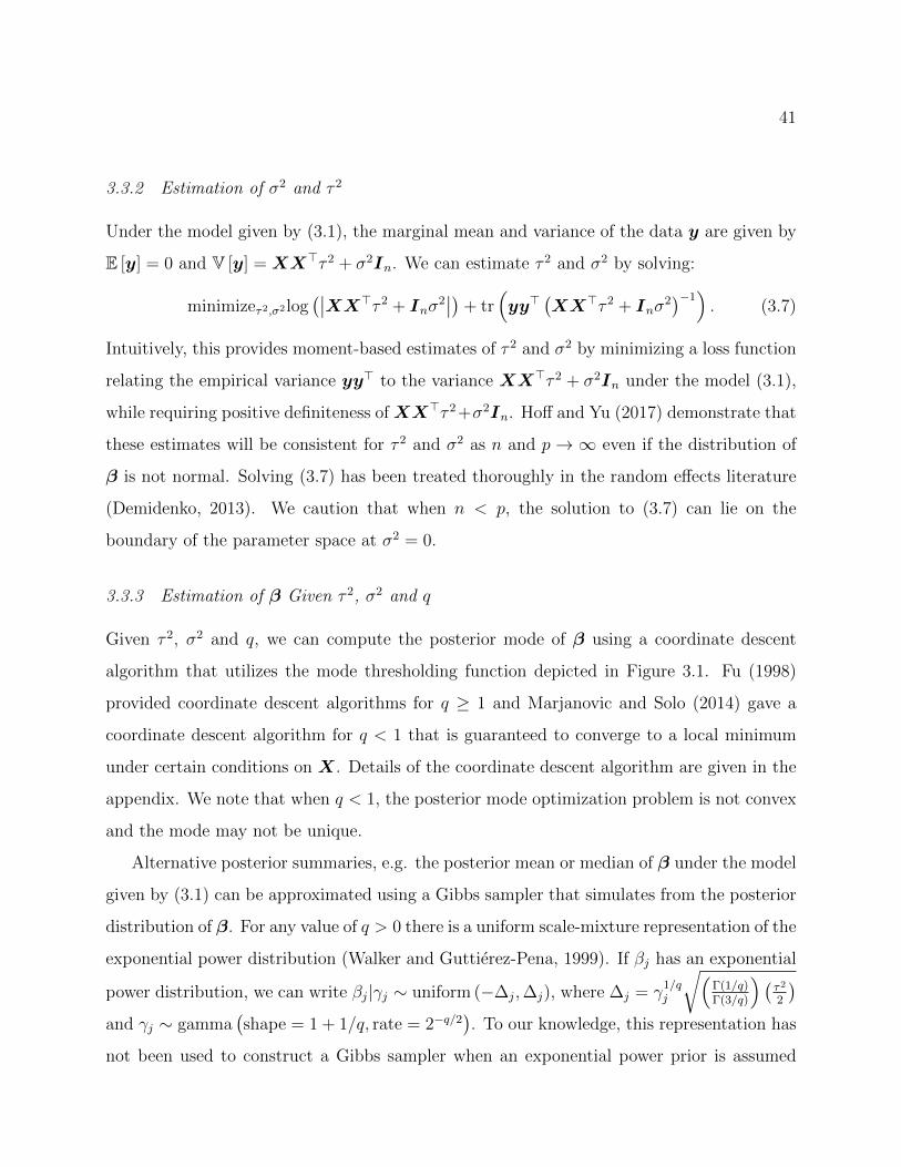
41

3.3.2 Estimation of σ2 and τ 2

Under the model given by (3.1), the marginal mean and variance of the data y are given by

E [y] = 0 and V [y] = XX>τ 2 + σ2In. We can estimate τ 2 and σ2 by solving:

minimizeτ2,σ2 log(∣∣XX>τ 2 + Inσ

2∣∣)+ tr

(yy>

(XX>τ 2 + Inσ

2)−1). (3.7)

Intuitively, this provides moment-based estimates of τ 2 and σ2 by minimizing a loss function

relating the empirical variance yy> to the variance XX>τ 2 + σ2In under the model (3.1),

while requiring positive definiteness ofXX>τ 2 +σ2In. Hoff and Yu (2017) demonstrate that

these estimates will be consistent for τ 2 and σ2 as n and p → ∞ even if the distribution of

β is not normal. Solving (3.7) has been treated thoroughly in the random effects literature

(Demidenko, 2013). We caution that when n < p, the solution to (3.7) can lie on the

boundary of the parameter space at σ2 = 0.

3.3.3 Estimation of β Given τ 2, σ2 and q

Given τ 2, σ2 and q, we can compute the posterior mode of β using a coordinate descent

algorithm that utilizes the mode thresholding function depicted in Figure 3.1. Fu (1998)

provided coordinate descent algorithms for q ≥ 1 and Marjanovic and Solo (2014) gave a

coordinate descent algorithm for q < 1 that is guaranteed to converge to a local minimum

under certain conditions on X. Details of the coordinate descent algorithm are given in the

appendix. We note that when q < 1, the posterior mode optimization problem is not convex

and the mode may not be unique.

Alternative posterior summaries, e.g. the posterior mean or median of β under the model

given by (3.1) can be approximated using a Gibbs sampler that simulates from the posterior

distribution of β. For any value of q > 0 there is a uniform scale-mixture representation of the

exponential power distribution (Walker and Guttierez-Pena, 1999). If βj has an exponential

power distribution, we can write βj|γj ∼ uniform (−∆j,∆j), where ∆j = γ1/qj

√(Γ(1/q)Γ(3/q)

) (τ2

2

)and γj ∼ gamma

(shape = 1 + 1/q, rate = 2−q/2

). To our knowledge, this representation has

not been used to construct a Gibbs sampler when an exponential power prior is assumed

42

for regression coefficients corresponding to an arbitrary design matrix X. Using this repre-

sentation, the full conditional distribution for β given γ is a truncated multivariate normal

distribution and the full conditional distributions for elements of γ given β are independent

translated exponential distributions. Full conditional distributions are given in the appendix.

3.3.4 Simulation Results

We assess the performance of the adaptive procedure via simulation. We simulate data

from (3.1) with τ 2 = σ2 = 1, p = 100, n ∈ 100, 200 and q ∈ 0.25, 1, 4 and entries

of X drawn from a standard normal distribution. For each pair of values of n and q, we

simulate 100 values of y from (3.1). When n > p, we use 100 different design matrices,

X, whereas when n ≤ p we fix the design matrix X so that some matrix calculations

involving X can be precomputed. As noted previously, when n ≤ p the solution to the

variance component estimation problem (3.7) can lie on the boundary of the parameter

space at σ2 = 0. For the purposes of this simulation study, we require simulated datasets

yield σ2 = 0. We use posterior means of β in the adaptive estimation procedure as opposed

to other posterior summaries because the posterior mean minimizes posterior squared error

loss and accordingly allows for straightforward performance comparisons (Hans, 2009). We

approximate posterior means from 10, 500 simulations from the posterior distribution using

the Gibbs sampler described in Section 3.3.3, discarding the first 500 iterations as burn-in.

In general, the sampler mixes better with larger q and n. The smallest effective sample sizes

for n = 100 and n = 200 are 53 and 222, respectively.

For n = 100, we reject the null hypothesis that q = 1 at level α = 0.05 in 100%, 1% and

62% of the simulations when q = 0.25, q = 1 and q = 4. Analogously, when n = 200 we reject

the null hypothesis that q = 1 at level α = 0.05 in 93%, 5% and 100% of simulations when

q = 0.25, q = 1 and q = 4. These rejection rates are roughly as expected given the results

of the simulation study of the testing procedure given that we only perform 100 simulations

for each value of n and q. Figure 3.3 shows mean squared error (MSE) for estimating β

using the adaptive procedure plotted against the mean squared error for estimating β under

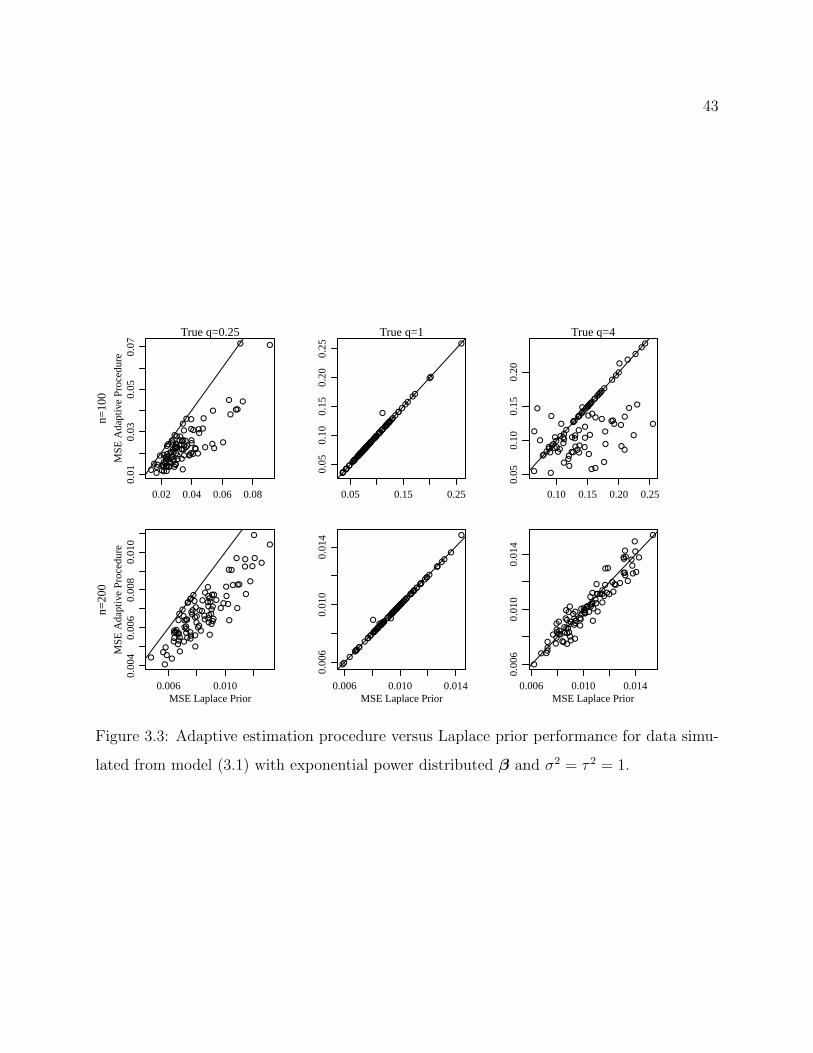
43

0.02 0.04 0.06 0.08

0.01

0.03

0.05

0.07

MS

E A

dapt

ive

Pro

cedu

re

n=10

0

True q=0.25

0.05 0.15 0.25

0.05

0.10

0.15

0.20

0.25

True q=1

0.10 0.15 0.20 0.25

0.05

0.10

0.15

0.20

True q=4

0.006 0.010

0.00

40.

006

0.00

80.

010

MSE Laplace Prior

MS

E A

dapt

ive

Pro

cedu

re

n=20

0

0.006 0.010 0.014

0.00

60.

010

0.01

4

MSE Laplace Prior

0.006 0.010 0.014

0.00

60.

010

0.01

4

MSE Laplace Prior

Figure 3.3: Adaptive estimation procedure versus Laplace prior performance for data simu-

lated from model (3.1) with exponential power distributed β and σ2 = τ 2 = 1.

44

a Laplace prior. Histograms of estimates of σ2, τ 2 and q are given in the appendix.

We see that the adaptive procedure yields substantial improvements when the true value

of q is small, almost no loss when the true value of q is in fact equal to 1 and some small

improvements and little loss when the true value of q is large. Smaller improvements when

the true value of q is large are likely due to the fact that the estimates of q are more

variable when q is larger. We note that incorporating testing into the adaptive procedure

is important to these performance results. Recall that both tests of H based on ψ(βols)

and ψ(βδ) have low power when p is relatively small, i.e. when little information about

the features of the distribution of β is observed. Accordingly, incorporating testing into

the estimation procedure protects us against losses in performance that could result from

imprecise estimation of q.

3.4 Relationship to Estimating Sparse β

The lasso penalty/Laplace prior is often used when β is believed to be sparse, i.e. many

elements of β are believed to be equal to exactly zero. Accordingly, we repeat the testing

and estimation simulation studies performed in the previous sections for Bernoulli-normal

spike-and-slab distributed β where βj is exactly equal to zero with probability 1 − π and

drawn from a N (0, τ 2/π) distribution otherwise. This parametrization ensures that elements

of β have variance τ 2. The kurtosis of this distribution is given by κ + 3 = 3/π and when

π = 0.5, the kurtosis of this distribution matches that of a Laplace distribution. We repeat

the testing simulation study in Section 3.2 for a range of values of π instead of q and show

the results in Figure 3.4.

As expected, our tests tend not to reject H : q = 1 when the kurtosis of the spike-and-slab

distribution is similar to the kurtosis of the Laplace prior at π = 0.5. Importantly, our tests

reject a Laplace prior when π is small and β is very sparse. This suggests that the adaptive

procedure for estimating β might yield performance improvements even when elements of

β do not have an exponential power distribution. We repeat the estimation simulations

described in Section 3.3.4 for π ∈ 0.1, 0.5, 0.9 and show the results in Figure 3.5. Again,

45

n=50

Pow

er0

0.5

1

p=25p=50p=75p=100

n=100

ψ(βOLS)ψ(βδ)ψ(β)

n=200

π

Pow

er0

0.5

1

0.2 0.4 0.6 0.8

Oracle

π0.2 0.4 0.6 0.8

Figure 3.4: Power of level-0.05 tests for data simulated from a linear regression model with

standard normal errors and Bernoulli-normal regression coefficients with sparsity rate 1− π

and unit variance. A horizontal dashed gray line is given at 0.05.

histograms of estimates of σ2, τ 2 and q are given in the appendix. Before discussing the results

of the simulations, we note that as we might expect based on the previous simulations the

sampler mixes better with larger values of π and n. The smallest effective sample sizes for

n = 100 and n = 200 are 70 and 253, respectively.

With spike-and-slab distributed β, the adaptive procedure still outperforms estimates

based on the Laplace prior in the majority of simulations. We see substantial performance

gains from the adaptive procedure when π = 0.1 for both n = 100 and n = 200. Again, we

observe some losses in performance when π = 0.9, i.e. when the kurtosis is relatively low

and estimates of q are more variable. Again, we emphasize that incorporating the test into

the adaptive procedure does play an important role in its performance. When π = 0.9 and

results of a test of H are ignored, the mean squared error for estimating β using q = q exceeds

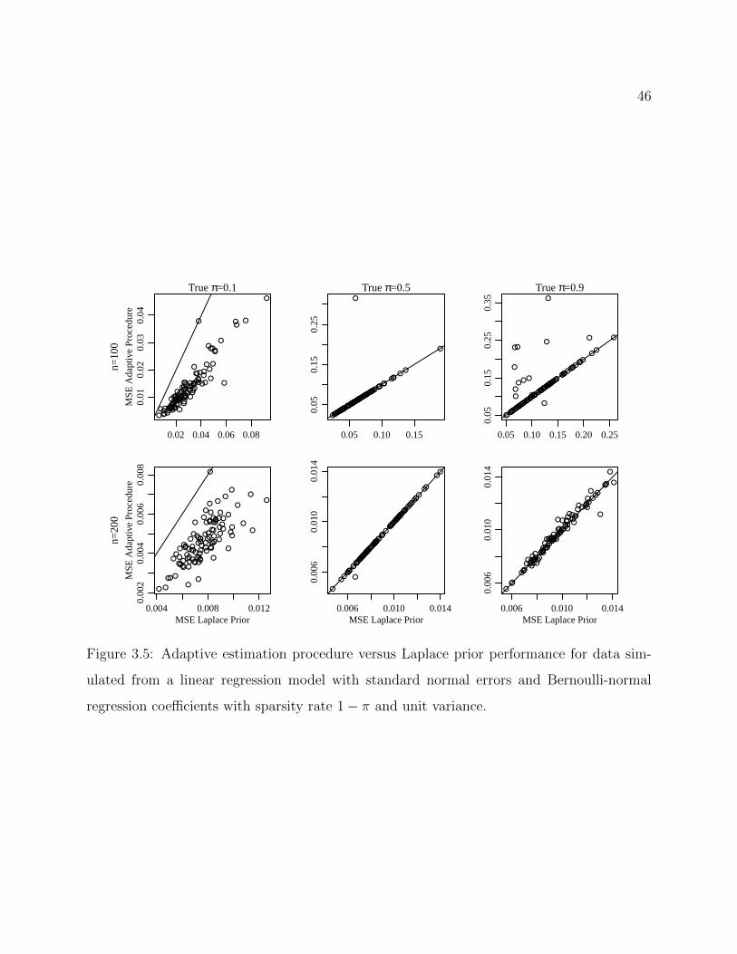
46

0.02 0.04 0.06 0.08

0.01

0.02

0.03

0.04

MS

E A

dapt

ive

Pro

cedu

re

n=10

0

True π=0.1

0.05 0.10 0.15

0.05

0.15

0.25

True π=0.5

0.05 0.10 0.15 0.20 0.25

0.05

0.15

0.25

0.35

True π=0.9

0.004 0.008 0.012

0.00

20.

004

0.00

60.

008

MSE Laplace Prior

MS

E A

dapt

ive

Pro

cedu

re

n=20

0

0.006 0.010 0.014

0.00

60.

010

0.01

4

MSE Laplace Prior

0.006 0.010 0.014

0.00

60.

010

0.01

4

MSE Laplace Prior

Figure 3.5: Adaptive estimation procedure versus Laplace prior performance for data sim-

ulated from a linear regression model with standard normal errors and Bernoulli-normal

regression coefficients with sparsity rate 1− π and unit variance.

47

the mean squared error using a Laplace prior in 56% and 67% of simulations when n = 100

and n = 200, respectively. When the exponential power prior is only used when a test of H

rejects and a Laplace prior is used otherwise, this drops to 12% and 34%, respectively.

3.5 Applications

We apply the methods described in this chapter to four datasets that have appeared pre-

viously in the penalized regression literature: the diabetes data, the Boston housing data,

motif data and glucose data (Efron et al., 2004; Park and Casella, 2008; Polson et al., 2014;

Buhlmann and van de Geer, 2011; Priami and Morine, 2015). The diabetes data featured in

Efron et al. (2004), Park and Casella (2008) and Polson et al. (2014) contains a quantitative

measure of diabetes progression for n = 442 patients y and ten covariates: age, sex, body

mass index, average blood pressure and six blood serum measurements. A design matrix X

is obtained from the ten original covariates,(

102

)pairwise interactions and 9 quadratic terms

yielding p = 64. In the Boston housing data (Polson et al., 2014), the response vector y is

the median house price for n = 506 Boston census tracts and the design matrix is made up

of 13 measurements of census tract characteristics and all(

132

)squared terms and pairwise

interactions, yielding p = 104. The motif data featured in Buhlmann and van de Geer (2011)

contains measurements of protein binding intensity y at n = 287 regions of the DNA se-

quence and p = 195 covariates X made up of measurements of motif abundance for p motifs

at each region. The glucose data from Priami and Morine (2015) contains measurements of

blood glucose concentration y for n = 68 subjects belonging to several families with com-

plete data on p = 72 covariates, which include various metabolite measurements along with

several health indicators. We subtract an overall mean and family-specific group means off

of the response and the design matrix containing the 72 covariates to be used for regression.

For all four data sets, we centered and standardized the response y and the columns of the

design matrix X by subtracting off their means and dividing by their standard deviations.

We use the ridge-based test for all four data sets because either n < p or the design matrix is

highly collinear andX>X has condition number less than 10−5. As in the simulations shown

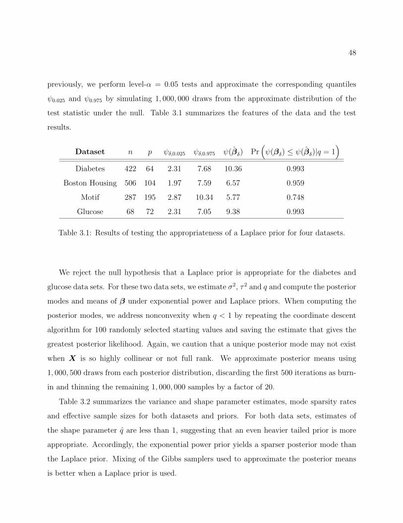
48

previously, we perform level-α = 0.05 tests and approximate the corresponding quantiles

ψ0.025 and ψ0.975 by simulating 1, 000, 000 draws from the approximate distribution of the

test statistic under the null. Table 3.1 summarizes the features of the data and the test

results.

Dataset n p ψδ,0.025 ψδ,0.975 ψ(βδ) Pr(ψ(βδ) ≤ ψ(βδ)|q = 1

)Diabetes 422 64 2.31 7.68 10.36 0.993

Boston Housing 506 104 1.97 7.59 6.57 0.959

Motif 287 195 2.87 10.34 5.77 0.748

Glucose 68 72 2.31 7.05 9.38 0.993

Table 3.1: Results of testing the appropriateness of a Laplace prior for four datasets.

We reject the null hypothesis that a Laplace prior is appropriate for the diabetes and

glucose data sets. For these two data sets, we estimate σ2, τ 2 and q and compute the posterior

modes and means of β under exponential power and Laplace priors. When computing the

posterior modes, we address nonconvexity when q < 1 by repeating the coordinate descent

algorithm for 100 randomly selected starting values and saving the estimate that gives the

greatest posterior likelihood. Again, we caution that a unique posterior mode may not exist

when X is so highly collinear or not full rank. We approximate posterior means using

1, 000, 500 draws from each posterior distribution, discarding the first 500 iterations as burn-

in and thinning the remaining 1, 000, 000 samples by a factor of 20.

Table 3.2 summarizes the variance and shape parameter estimates, mode sparsity rates

and effective sample sizes for both datasets and priors. For both data sets, estimates of

the shape parameter q are less than 1, suggesting that an even heavier tailed prior is more

appropriate. Accordingly, the exponential power prior yields a sparser posterior mode than

the Laplace prior. Mixing of the Gibbs samplers used to approximate the posterior means

is better when a Laplace prior is used.

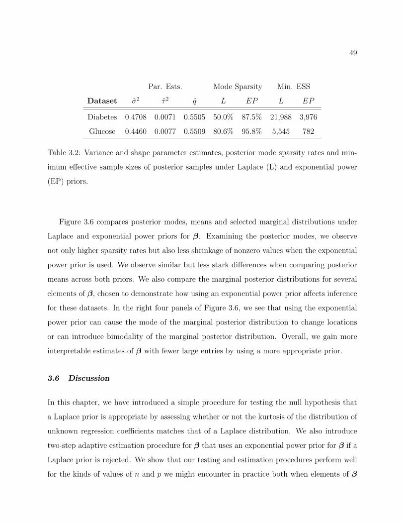
49

Par. Ests. Mode Sparsity Min. ESS

Dataset σ2 τ 2 q L EP L EP

Diabetes 0.4708 0.0071 0.5505 50.0% 87.5% 21,988 3,976

Glucose 0.4460 0.0077 0.5509 80.6% 95.8% 5,545 782

Table 3.2: Variance and shape parameter estimates, posterior mode sparsity rates and min-

imum effective sample sizes of posterior samples under Laplace (L) and exponential power

(EP) priors.

Figure 3.6 compares posterior modes, means and selected marginal distributions under

Laplace and exponential power priors for β. Examining the posterior modes, we observe

not only higher sparsity rates but also less shrinkage of nonzero values when the exponential

power prior is used. We observe similar but less stark differences when comparing posterior

means across both priors. We also compare the marginal posterior distributions for several

elements of β, chosen to demonstrate how using an exponential power prior affects inference

for these datasets. In the right four panels of Figure 3.6, we see that using the exponential

power prior can cause the mode of the marginal posterior distribution to change locations

or can introduce bimodality of the marginal posterior distribution. Overall, we gain more

interpretable estimates of β with fewer large entries by using a more appropriate prior.

3.6 Discussion

In this chapter, we have introduced a simple procedure for testing the null hypothesis that

a Laplace prior is appropriate by assessing whether or not the kurtosis of the distribution of

unknown regression coefficients matches that of a Laplace distribution. We also introduce

two-step adaptive estimation procedure for β that uses an exponential power prior for β if a

Laplace prior is rejected. We show that our testing and estimation procedures perform well

for the kinds of values of n and p we might encounter in practice both when elements of β

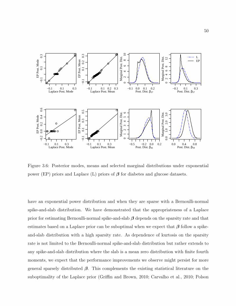
50

−0.1 0.1 0.3

−0.

10.

10.

3

Laplace Post. Mode

EP

Pos

t. M

ode

−0.1 0.1 0.2 0.3

−0.

10.

10.

20.

3

Laplace Post. Mean

EP

Pos

t. M

ean

−0.1 0.0 0.1 0.2

02

46

810

Post. Dist. β37

Mar

gina

l Pos

t. D

ist.

−0.1 0.1 0.3

02

46

812

Post. Dist. β57

Mar

gina

l Pos

t. D

ist.

LEP

−0.1 0.1 0.3

−0.

20.

00.

20.

40.

6

Laplace Post. Mode

EP

Pos

t. M

ode

−0.1 0.1 0.3

−0.

10.

10.

30.

5

Laplace Post. Mean

EP

Pos

t. M

ean

−0.5 −0.2 0.0 0.2

01

23

45

6

Post. Dist. β41

Mar

gina

l Pos

t. D

ist.

0.0 0.4 0.8

0.0

1.0

2.0

3.0

Post. Dist. β59

Mar

gina

l Pos

t. D

ist.

Figure 3.6: Posterior modes, means and selected marginal distributions under exponential

power (EP) priors and Laplace (L) priors of β for diabetes and glucose datasets.

have an exponential power distribution and when they are sparse with a Bernoulli-normal

spike-and-slab distribution. We have demonstrated that the appropriateness of a Laplace

prior for estimating Bernoulli-normal spike-and-slab β depends on the sparsity rate and that

estimates based on a Laplace prior can be suboptimal when we expect that β follow a spike-

and-slab distribution with a high sparsity rate. As dependence of kurtosis on the sparsity

rate is not limited to the Bernoulli-normal spike-and-slab distribution but rather extends to

any spike-and-slab distribution where the slab is a mean zero distribution with finite fourth

moments, we expect that the performance improvements we observe might persist for more

general sparsely distributed β. This complements the existing statistical literature on the

suboptimality of the Laplace prior (Griffin and Brown, 2010; Carvalho et al., 2010; Polson

51

et al., 2014; Bhattacharya et al., 2015).

This chapter focuses specifically on misspecification of the Laplace prior for the regression

coefficients in a linear model with normal errors. Because the derivation of the approximate

level-α test follows from the existence of a consistent estimator of β or a known linear function

of β, the methods described in this chapter can be extended to include linear models with

elliptically contoured errors and generalized linear models. The methods described in this

chapter could also be extended to include the construction of a confidence interval either for

the kurtosis of the distribution of the elements of β or the exponential power shape parameter

q. Furthermore, the methods can be generalized to test the null hypothesis that elements of

β have an exponential power distribution with q = q > 0 or to test a null hypothesis that

elements of β have a different symmetric, mean zero distribution as long as this different

distribution can be characterized by its kurtosis and is easy to simulate from, e.g. the normal-

gamma distribution given by Griffin and Brown (2010) or the Dirichlet-Laplace distribution

given by Bhattacharya et al. (2015).

Throughout this chapter we have conflated heavy tails (high kurtosis) with peakedness of

the density of β. However, it is not generally true that “peakedness” must increase with tail

weight (Westfall, 2014). This is important because sparsity of the posterior mode specifically

arises from the “peakedness” of the prior on β. Accordingly, three parameter distributions

like the generalized t-distribution given by Choy and Chan (2008) that allow kurtosis and

“peakedness” to vary separately may be useful alternative priors for β.

52

Chapter 4

STRUCTURED SHRINKAGE PRIORS

4.1 Introduction

Consider the problem of estimating regression coefficients for a generalized linear model,

where we observe an n × 1 vector of responses y and an n × p matrix of regressors X and

are interested in estimating a p × 1 vector of regression coefficients β which are related to

y via a known link function E [y] = g (Xβ) and a probabilistic model for y given E [y] and

unknown distributional parameters φ. Letting exp −h (y|X,β,φ) refer to the likelihood

of the data y given Xβ and φ, maximum likelihood estimates of β given φ are obtained by

minimizing h (y|X,β,φ) over β. This is a standard, well known problem (McCullagh and

Nelder, 1989). However, when the the data is high dimensional, i.e. number of covariates

p is large, especially relative to the number of responses n, inference and prediction can

be challenging. Standard maximum likelihood estimates of β may have prohibitively large

variance or fail to be unique. In such high dimensional settings, a common approach is to

assume a prior distribution for β. For instance, a mean-zero multivariate normal prior with

covariance matrix Σ, β ∼ normal (0,Σ) might be chosen to encourage a structured estimate

of β, or a mean-zero independent Laplace prior with variance σ2, βji.i.d.∼ Laplace

(0, σ/

√2),

might be chosen to encourage a sparse or nearly sparse estimate of β depending on which

posterior summary is used to estimate β. Using the posterior mode to estimate β corresponds

to penalized estimation of β.

In this paper, we consider problems where the covariate vectors xi, and accordingly the

regression coefficients β, can be interpreted as a vectorized K-mode matrix or tensor with

dimensions p1 × . . . pK . As such, β = vec (B) is structured. Because such problems are

often very high dimensional with large p =∏K

k=1 pk relative to n, we focus specifically on

53

(a) (b)

Figure 4.1: Panel (a) reprinted from Bruneel (2018) shows a subject using the P300 speller.

Panel (b) shows the locations of EEG sensors on the skull reprinted and modified from

Sharma (2013), with sensors included in our analysis highlighted in red. Arrows indicate the

order of the channels appear in the data.

settings where we also expect B to be sparse or nearly sparse. We motivate this with a

problem that arises in the development of brain-computer interfaces. Brain-computer inter-

faces (BCIs) are used to detect changes in subjects’ cognitive state from contemporaneous

electroencephalography (EEG) measurements, which can be collected non-invasively at high

temporal resolution (Makeig et al., 2012; Wolpaw and Wolpaw, 2012). We consider the P300

speller, a specific BCI device which is designed to detect when a subject is viewing a specified

target letter, as depicted in use in Figure 4.1a. We consider a subset of data collected from

fourteen subjects using a P300 speller and a gGAMMA.sys EEG device Forney et al. (2013).

For an individual subject, we observe 240 indicators yi for whether or not the subject was

viewing a specified target letter during trial i and xi is a vectorized 208× 8 matrix of EEG

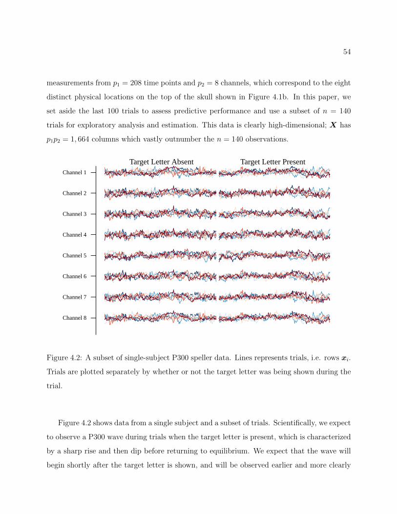
54

measurements from p1 = 208 time points and p2 = 8 channels, which correspond to the eight

distinct physical locations on the top of the skull shown in Figure 4.1b. In this paper, we

set aside the last 100 trials to assess predictive performance and use a subset of n = 140

trials for exploratory analysis and estimation. This data is clearly high-dimensional; X has

p1p2 = 1, 664 columns which vastly outnumber the n = 140 observations.

Channel 8

Channel 7

Channel 6

Channel 5

Channel 4

Channel 3

Channel 2

Channel 1

Target Letter Absent Target Letter Present

Figure 4.2: A subset of single-subject P300 speller data. Lines represents trials, i.e. rows xi.

Trials are plotted separately by whether or not the target letter was being shown during the

trial.

Figure 4.2 shows data from a single subject and a subset of trials. Scientifically, we expect

to observe a P300 wave during trials when the target letter is present, which is characterized

by a sharp rise and then dip before returning to equilibrium. We expect that the wave will

begin shortly after the target letter is shown, and will be observed earlier and more clearly

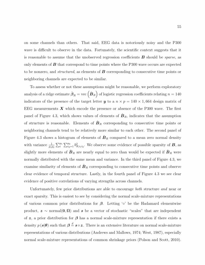
55

on some channels than others. That said, EEG data is notoriously noisy and the P300

wave is difficult to observe in the data. Fortunately, the scientific context suggests that it

is reasonable to assume that the unobserved regression coefficients B should be sparse, as

only elements of B that correspond to time points where the P300 wave occurs are expected

to be nonzero, and structured, as elements of B corresponding to consecutive time points or

neighboring channels are expected to be similar.

To assess whether or not these assumptions might be reasonable, we perform exploratory

analysis of a ridge estimate βR = vec(BR

)of logistic regression coefficients relating n = 140

indicators of the presence of the target letter y to a n × p = 140 × 1, 664 design matrix of

EEG measurements X which encode the presence or absence of the P300 wave. The first

panel of Figure 4.3, which shows values of elements of BR, indicates that the assumption

of structure is reasonable. Elements of BR corresponding to consecutive time points or

neighboring channels tend to be relatively more similar to each other. The second panel of

Figure 4.3 shows a histogram of elements of BR compared to a mean zero normal density

with variance 1p1p2

∑p1i

∑p2i2=1 b

2R,i1i2

. We observe some evidence of possible sparsity of B, as

slightly more elements of BR are nearly equal to zero than would be expected if BR were

normally distributed with the same mean and variance. In the third panel of Figure 4.3, we

examine similarity of elements of BR corresponding to consecutive time points and observe

clear evidence of temporal structure. Lastly, in the fourth panel of Figure 4.3 we see clear

evidence of positive correlations of varying strengths across channels.

Unfortunately, few prior distributions are able to encourage both structure and near or

exact sparsity. This is easiest to see by considering the normal scale-mixture representations

of various common prior distributions for β. Letting ‘’ be the Hadamard elementwise

product, z ∼ normal(0,Ω) and s be a vector of stochastic “scales” that are independent

of z, a prior distribution for β has a normal scale-mixture representation if there exists a

density p (s|θ) such that βd= s z. There is an extensive literature on normal scale-mixture

representations of various distributions (Andrews and Mallows, 1974; West, 1987), especially

normal scale-mixture representations of common shrinkage priors (Polson and Scott, 2010).

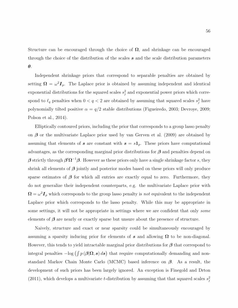
56

Structure can be encouraged through the choice of Ω, and shrinkage can be encouraged

through the choice of the distribution of the scales s and the scale distribution parameters

θ.

Independent shrinkage priors that correspond to separable penalties are obtained by

setting Ω = ω2Ip. The Laplace prior is obtained by assuming independent and identical

exponential distributions for the squared scales s2j and exponential power priors which corre-

spond to `q penalties when 0 < q < 2 are obtained by assuming that squared scales s2j have

polynomially tilted positive α = q/2 stable distributions (Figueiredo, 2003; Devroye, 2009;

Polson et al., 2014).

Elliptically contoured priors, including the prior that corresponds to a group lasso penalty

on β or the multivariate Laplace prior used by van Gerven et al. (2009) are obtained by

assuming that elements of s are constant with s = s1p. These priors have computational

advantages, as the corresponding marginal prior distributions for β and penalties depend on

β strictly through β′Ω−1β. However as these priors only have a single shrinkage factor s, they

shrink all elements of β jointly and posterior modes based on these priors will only produce

sparse estimates of β for which all entries are exactly equal to zero. Furthermore, they

do not generalize their independent counterparts, e.g. the multivariate Laplace prior with

Ω = ω2Ip which corresponds to the group lasso penalty is not equivalent to the independent

Laplace prior which corresponds to the lasso penalty. While this may be appropriate in

some settings, it will not be appropriate in settings where we are confident that only some

elements of β are nearly or exactly sparse but unsure about the presence of structure.

Naively, structure and exact or near sparsity could be simultaneously encouraged by

assuming a sparsity inducing prior for elements of s and allowing Ω to be non-diagonal.

However, this tends to yield intractable marginal prior distributions for β that correspond to

integral penalties −log(∫

p (β|Ω, s) ds)

that require computationally demanding and non-

standard Markov Chain Monte Carlo (MCMC) based inference on β. As a result, the

development of such priors has been largely ignored. An exception is Finegold and Drton

(2011), which develops a multivariate t-distribution by assuming that that squared scales s2j

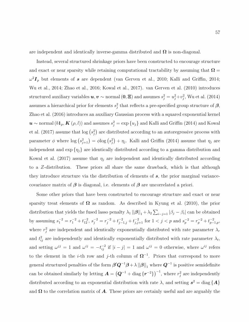
57

are independent and identically inverse-gamma distributed and Ω is non-diagonal.

Instead, several structured shrinkage priors have been constructed to encourage structure

and exact or near sparsity while retaining computational tractability by assuming that Ω =

ω2Ip but elements of s are dependent (van Gerven et al., 2010; Kalli and Griffin, 2014;

Wu et al., 2014; Zhao et al., 2016; Kowal et al., 2017). van Gerven et al. (2010) introduces

structured auxiliary variables u,v ∼ normal (0,Ξ) and assumes s2j = u2

j+v2j , Wu et al. (2014)

assumes a hierarchical prior for elements s2j that reflects a pre-specified group structure of β,

Zhao et al. (2016) introduces an auxiliary Gaussian process with a squared exponential kernel

u ∼ normal (b1p,K (ρ, l)) and assumes s2j = exp uj and Kalli and Griffin (2014) and Kowal

et al. (2017) assume that log(s2j

)are distributed according to an autoregressive process with

parameter φ where log(s2j+1

)= φlog

(s2j

)+ ηj. Kalli and Griffin (2014) assume that ηj are

independent and exp ηj are identically distributed according to a gamma distribution and

Kowal et al. (2017) assume that ηj are independent and identically distributed according

to a Z-distribution. These priors all share the same drawback, which is that although

they introduce structure via the distribution of elements of s, the prior marginal variance-

covariance matrix of β is diagonal, i.e. elements of β are uncorrelated a priori.

Some other priors that have been constructed to encourage structure and exact or near

sparsity treat elements of Ω as random. As described in Kyung et al. (2010), the prior

distribution that yields the fused lasso penalty λ1 ||β||1 +λ2

∑i−j=1 |βj − βi| can be obtained

by assuming s−21 = r−2

1 + t−212 , s−2

j = r−2j + t−2

j−1,j + t−2j,j+1 for 1 < j < p and s−2

p = r−2p + t−2

p−1,p,

where r2j are independent and identically exponentially distributed with rate parameter λr

and t2ij are independently and identically exponentially distributed with rate parameter λt,

and setting ωjj = 1 and ωij = −t−2ij if |i− j| = 1 and ωij = 0 otherwise, where ωij refers

to the element in the i-th row and j-th column of Ω−1. Priors that correspond to more

general structured penalties of the form β′Q−1β+λ ||β||1 where Q−1 is positive semidefinite

can be obtained similarly by letting A =(Q−1 + diag r−2

)−1, where r2

j are independently

distributed according to an exponential distribution with rate λ, and setting s2 = diag A

and Ω to the correlation matrix of A. These priors are certainly useful and are arguably the

58

most reasonable set of existing priors for encouraging structure and near or exact sparsity.

However, priors like the prior corresponding to the fused lasso penalty become much more

difficult to work with when the structure is not pre-specified, i.e. orderings or groupings of

elements of β are not known a priori, and can suffer from computational inefficiencies as the

number of latent variables increases with the complexity of the structure of β if posterior

summaries other than the posterior mode are of interest or maximum marginal likelihood

estimates of the unknown prior distribution parameters are to be obtained. Furthermore,

the unknown parameters for priors corresponding to the more general structured penalty or

more structured generalizations of the fused lasso penalty can be difficult to set or estimate

as they become higher dimensional, especially because they do not relate straightforwardly

to prior moments of β. One last class of relevant priors are the structured normal-gamma

priors introduced in Griffin and Brown (2012b) and Griffin and Brown (2012a), which are

obtained by introducing structure via a p×p matrix C and setting sj = cjjrj and(Ω1/2

)ij

=

cijrj/ (ciiri), where r2j are independent and identically gamma distributed. Like the priors

previously discussed, estimation or specification of C can be challenging. Furthermore, many

of the desirable properties of this prior are specific to the gamma distribution assumption

for r2j .

Ideally, we would like to work with a class of structured shrinkage priors that (i) can

encourage general forms of structure by allowing for correlations across elements of β a

priori, (ii) can encourage near or exact sparsity of elements of β, (iii) yield computationally

tractable posterior mode and posterior distribution simulation problems and (iv) span the

range of common structured and sparsity inducing priors by generalizing the multivariate

normal prior as well as the independent Laplace prior. We construct such a class of priors

by revisiting the naive approach where we assume βd= s z and non-diagonal Ω. These

priors are easy to interpret from a data generating perspective and have easy-to-compute

moments, specifically Σ = V [β] = E [ss′] Ω. We demonstrate that elliptical slice sampling

can be used to overcome the computational issues that have previously made use of such prior

distributions challenging, regardless of the distribution assumed for elements of s (Murray

59

et al., 2010). In Section 4.2, we introduce three novel priors, the structured normal product

(SPN), structured normal-gamma (SNG) and structured power/bridge (SPB) shrinkage prior

distributions for penalized regression. The SPN and SNG priors generalize the normal-

gamma prior described in Caron and Doucet (2008) and Griffin and Brown (2010), and the

SPB prior generalizes the power/bridge prior (Frank and Friedman, 1993; Polson et al., 2014).

Figure 4.4 shows how the novel structured shrinkage priors we introduce relate to Laplace

and normal prior distributions. We discuss the properties of these priors in Section 4.2. In

Section 4.3, we describe posterior inference as it pertains to performing Gibbs-within-EM

estimation of posterior modes and simulating from the full posterior distribution. Because

problems that benefit from prior distributions that encourage both structure and exact or

near sparsity are often very high dimensional, i.e. have large n or p =∏K

k=1 pk, we show

how elliptical slice sampling can be used to avoid large matrix crossproducts and inversions

for arbitrary log likelihoods h (y|X,β,φ). In Section 4.4, we consider the unknown variance

components and discuss maximum marginal likelihood empirical Bayes estimation, moment-

based empirical Bayes estimation and fully Bayes inference. In Section 4.5, we apply the

shrinkage priors considered to the P300 speller data depicted in Figures 4.2 and 4.3.

4.2 Three Structured Shrinkage Priors and Their Properties

4.2.1 Prior Distributions

Structured Product Normal (SPN) Prior: The structured product normal (SPN)

prior is obtained by assuming that s ∼ normal(0,Ψ). Originally discussed as a sparsity

inducing penalty in Hoff (2016), the SPN prior is uniquely computationally simple to work

with as the full conditional distributions of z and s are both multivariate normal distribu-

tions. The SPN prior is also appealing intuitively as it allows elements of s to be correlated

a priori, in contrast to the SNG and SPB priors which assume elements of s are independent.

Incidentally, the SPN prior generalizes a special case of the independent normal gamma prior

(Griffin and Brown, 2010). When Ψ,Ω ∝ Ip, the SPN prior corresponds to the independent

60

normal-gamma prior with s2j ∼ gamma(shape = 1/2, rate = 1/2).

The SPN prior has 2p+ p (p− 1) unknown variance parameters, of which p+ p (p− 1) /2

are separately identified. Letting CΩ and CΨ be the correlation matrices corresponding to

Ω and Ψ, we can write Ω = diag√ωCΩdiag

√ω

and Ψ = diag√ψCΨdiag

√ψ

.

We can rewrite the SPN prior for β as

βd=(√

ω ψ) (z/√ω) (s/√ψ),

where√

and / are applied elementwise. We can see that the variances ω and ψ are not

separately identified from the data, because the first term only depends on the variances

through their product, and the distributions of the second two terms depend only on CΩ

andCΨ. Off-diagonal elements ofCΩ andCΨ are identified from the data, as they determine

fourth-order cross moments of elements of β. Recalling that we have defined Σ = ΩΨ and

letting CΣ be the correlation matrix corresponding to Σ, we have

E[β2jβ

2k

]σjjσkk

= 1 + 2c2Ω,jk + 2c2

Ψ,jk + 4c2Σ,jk j 6= k

E[β2jβkβl

]σjj√σkkσll

= cΣ,kl + 4cΣ,jkcΣ,jl + 2cΩ,klcΨ,jkcΨ,jl + 2cΨ,klcΩ,jkcΩ,jl j 6= k, j 6= l, k 6= l.

We can see that these fourth-order cross moments depend on the values of both cΩ,jk and

cΨ,jk, in addition to their product cΣ,jk. As such, both unknown parameters are separately

identifiable. However, whether or not the individual values of cΩ,jk and cΨ,jk correspond to

correlations of elements of z or s is not known, as we can write:

βd=(√

ω ψ)(C

1/2Ψ C

−1/2Ω z/

√ω)(C

1/2Ω C

−1/2Ψ s/

√ψ).

To reduce the number of freely varying parameters and to facilitate identifiability of CΩ and

CΨ from second order moments of β alone, we define a special case of the SPN prior which

requires that |cΩ,ij| = |cΨ,ij|. We refer to this as the symmetric SPN (sSPN) prior.

Structured Normal-Gamma (SNG) Prior: The structured normal-gamma (SNG) prior

is a structured generalization of the normal-gamma prior of Griffin and Brown (2010) ob-

tained by assuming that s2j are independent gamma random variables. Because the scales

61

of each s2j are not separately identifiable from the variances of elements of z, we assume

s2j ∼ gamma(shape = c, rate = c) such that E

[s2j

]= 1 without loss of generality, where c

is treated as fixed and known. When Ω ∝ Ip and c = 1, the normal-gamma prior reduces

to an independent Laplace prior. Accordingly, we can think of the special case of the SNG

prior when c = 1 and arbitrary Ω as a novel multivariate Laplace prior.

Structured Power/Bridge (SPB) Prior: The structured power/bridge (SPB) prior

generalizes the bridge or exponential power prior discussed in Polson et al. (2014). This prior

is obtained by assuming that s2j are independently distributed according to a polynomially

tilted positive α-stable distribution with index of stability α = q/2, where q is treated as

fixed and known (Devroye, 2009; Polson et al., 2014). Again, the scales of each s2j are not

separately identifiable from the variances of elements of z, we parametrize the polynomially

tilted positive α-stable distribution to ensure that E[s2j

]= 1. When q = 1, the SPB prior

also generalizes the independent Laplace prior and accordingly, coincides with the SNG prior

when c = 1.

4.2.2 Properties

Joint Marginal Prior Distributions

Under the SPN, SNG and SPB priors, the marginal prior distributions pβ (β|Ω,θ) correspond

to intractable integrals∫pβ (β|s,Ω) p (s|θ) ds. As a result, it is challenging to study the

properties of these prior distributions and the penalties functions they correspond to directly.

Fortunately, we can simulate from the marginal prior distributions easily. We simulate

from four SNG priors with c ∈ 0.3, 0.5, 1, 10, the sSPN prior, four SPB priors with q =

0.65, 0.78, 1, 1.75 and an SPN prior with unit variances and ρΩ = ρ0.1 and ρ0.9Ψ . We note

that values of c and q are chosen to correspond to equal tail weight as measured by kurtosis,

e.g. the SNG prior with c = 0.3 has the same kurtosis as the SPB prior with q = 0.65 and

the SNG prior with c = 0.5 has the same kurtosis as the SPB prior with q = 0.78.

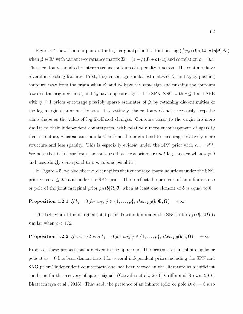
62

Figure 4.5 shows contour plots of the log marginal prior distributions log(∫

pβ (β|s,Ω) p (s|θ) ds)

when β ∈ R2 with variance-covariance matrix Σ = (1− ρ) I2+ρ121′2 and correlation ρ = 0.5.

These contours can also be interpreted as contours of a penalty function. The contours have

several interesting features. First, they encourage similar estimates of β1 and β2 by pushing

contours away from the origin when β1 and β2 have the same sign and pushing the contours

towards the origin when β1 and β2 have opposite signs. The SPN, SNG with c ≤ 1 and SPB

with q ≤ 1 priors encourage possibly sparse estimates of β by retaining discontinuities of

the log marginal prior on the axes. Interestingly, the contours do not necessarily keep the

same shape as the value of log-likelihood changes. Contours closer to the origin are more

similar to their independent counterparts, with relatively more encouragement of sparsity

than structure, whereas contours farther from the origin tend to encourage relatively more

structure and less sparsity. This is especially evident under the SPN prior with ρω = ρ0.1.

We note that it is clear from the contours that these priors are not log-concave when ρ 6= 0

and accordingly correspond to non-convex penalties.

In Figure 4.5, we also observe clear spikes that encourage sparse solutions under the SNG

prior when c ≤ 0.5 and under the SPN prior. These reflect the presence of an infinite spike

or pole of the joint marginal prior pβ (b|Ω,θ) when at least one element of b is equal to 0.

Proposition 4.2.1 If bj = 0 for any j ∈ 1, . . . , p, then pβ(b|Ψ,Ω) = +∞.

The behavior of the marginal joint prior distribution under the SNG prior pβ(β|c,Ω) is

similar when c < 1/2.

Proposition 4.2.2 If c < 1/2 and bj = 0 for any j ∈ 1, . . . , p, then pβ(b|c,Ω) = +∞.

Proofs of these propositions are given in the appendix. The presence of an infinite spike or

pole at bj = 0 has been demonstrated for several independent priors including the SPN and

SNG priors’ independent counterparts and has been viewed in the literature as a sufficient

condition for the recovery of sparse signals (Carvalho et al., 2010; Griffin and Brown, 2010;

Bhattacharya et al., 2015). That said, the presence of an infinite spike or pole at bj = 0 also

63

makes the already challenging problem of computing the posterior mode intractable, as the

log marginal prior is not only nonconvex but also has infinitely many modes.

Range of Σ

The SPN, SNG and SPB priors differ in the amount of structure that they can be used to

characterize because the marginal variance Σ = E[ss′]Ω must be positive semidefinite. The

behavior of E[ss′] determines the amount of structure a prior can characterize. Under the

SPN prior, Ψ can be chosen freely and accordingly E[ss′] can take on any value. Because it

is possible to find at least one pair of positive semidefinite covariance matrices Ω and Ψ that

satisfy Σ = Ω Ψ (Styan, 1973), the SPN prior can be used to characterize any structure

that can be represented by a positive semidefinite matrix Σ.

The sSPN prior is less flexible. Although it is challenging to describe the specific prop-

erties of covariance matrices Σ for which Ω and Ψ satisfying |ωij| = |ψij| are positive

semidefinite, it is straightforward to find a positive semidefinite matrix Σ for which Ω or Ψ

satisfying |ωij| = |ψij| are not positive definite.

The SNG and SPB priors are also limited to characterizing a restricted range of struc-

ture. Diagonal elements of E[ss′] are equal to 1, whereas off-diagonal elements are equal to

E[sj]2 < E[s2

j ] = 1. Thus, E[ss′] shrinks off-diagonal elements of Ω, reducing dependence.

Similar behavior was observed for alternative multivariate t-distributions in Finegold and

Drton (2011). When β ∈ R2, we can explicitly calculate the maximum marginal prior cor-

relation ρ under the SNG and SPB priors as a function of c or q. Under the SNG prior,

the maximum correlation is equal to c−1(Γ(c + 1/2)/Γ(c))2 and under the SPB prior, the

maximum correlation is equal to (π/2)(Γ(2/q)/√

Γ(1/q)Γ(3/q))2. When q = c = 1 and both

priors are equivalent, the maximum correlation is equal to π/4 ≈ 0.79.

We plot the maximum correlation as a function of kurtosis under both priors in Figure 4.6.

We observe greater reductions in the maximum correlation when the tails are heavier, and

under the SNG prior relative to a SPB prior with equal kurtosis. The restricted range of Σ

under the SNG and SPB priors is similar to the restricted range of the variance-covariance

64

matrix of the alternative multivariate t-distribution introduced in Finegold and Drton (2011).

Intuitively, the restricted range of Σ relates to the conflict that arises between the properties

of the marginal density pβ (β|Ω,θ) needed to preserve elementwise near or exact sparsity,

specifically concentration of the density along the axes, and the properties of the marginal

density needed to encourage structure, specifically concentration of the density along a line

when p = 2.

Copulas

We can visualize the dependence structures induced by all three priors by estimating the

copulas for β ∈ R2 with unit marginal variances and correlation ρ = 0.5. Figure 4.7 com-

pares estimates of the copulas of the same SPN, SNG and SPB priors considered previously.

All estimates by simulating 1, 000, 000 values from the corresponding prior, transforming

simulated values of β1 and β2 into percentiles u1 and u2, and computing a kernel bivariate

density estimate of the percentiles.

The behavior of the SPN copula depends on how ρ is factored into ρΩ and ρΨ. Under

the sSPN prior with ρΩ = ρΨ, the sSNG copula indicates that when elements of β are

positively correlated, the sSPN prior concentrates around values of β that are jointly very

small or exactly equal to zero and around values of β that have the same sign and are very

large in magnitude. When we set ρΩ = ρ0.1 and ρΨ = ρ0.9, the SPN prior concentrates

more strongly around values of β that are jointly very small or exactly equal to zero and

around values of β that that have the same sign and are very large in magnitude. This

parametrization of the SPN prior also concentrates slightly less around values of β along

the axes, where one element is very small or exactly zero and the other is not. Last, this

parametrization of the SPN prior concentrates more around values of β that are opposite

in sign but similar in magnitude. Arguably, this could be considered undesirable behavior

and reflects the strangeness of a data generating process that assumes β is made up of one

strongly correlated component and one very weakly correlated component, both of which

can take any value on R. Such a prior model for β is unlikely to make sense in many real

65

applications.

The behavior of the SNG and SPB copulas is generally similar when the kurtosis is held

constant under both priors, and depends on how similar the prior is to multivariate normal

distribution. Both display increasingly strong orthant dependence as the priors become less

normal with heavier tails, i.e. as c or q → 0. This means that as c or q → 0, the priors

concentrate more strongly around values of β that have the same sign. Compared to the

SPN priors, the SNG and SPB priors also concentrate more around the axes where at a single

element of β is close to or exactly equal to zero. The SNG prior displays especially strong

orthant dependence and appears to converge to a uniform distribution over the positive and

negative orthants as c→ 0, which likely results from the presence of an infinite spike or pole

of the marginal prior density when any element of β is equal to zero under the SNG prior.

Like the concentration of the SPN prior with ρΩ = ρ0.1 around values of β that have opposite

signs but similar magnitudes, convergence of the SNG prior to a uniform distribution on the

positive and negative orthants as c → 0 may be undesirable behavior and may not make

sense in many real applications. The softer contours of the SPB prior likely correspond to

more plausible models for β in many settings.

Univariate Marginal Prior Distributions

For all three priors, the univariate marginal distributions of elements of β belong to the

same family as the unstructured independent priors that they generalize. We show this in

the appendix, although it is straightforward to see from the stochastic representations of the

priors.

We also show that under the SPN and SNG priors with c ≤ 1/2, the univariate marginal

prior distributions an infinite spike or pole of the joint marginal prior pβ (b|Ω,θ) when at

least one element of b is equal to 0.

Proposition 4.2.3 For any j ∈ 1, . . . , p, pβj(0|Ψ,Ω) = +∞.

Likewise, the marginal distribution of a single element of βj has a pole at 0 under the

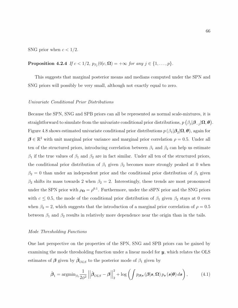
66

SNG prior when c < 1/2.

Proposition 4.2.4 If c < 1/2, pβj(0|c,Ω) = +∞ for any j ∈ 1, . . . , p.

This suggests that marginal posterior means and medians computed under the SPN and

SNG priors will possibly be very small, although not exactly equal to zero.

Univariate Conditional Prior Distributions

Because the SPN, SNG and SPB priors can all be represented as normal scale-mixtures, it is

straightforward to simulate from the univariate conditional prior distributions, p(βj|β−j|Ω,θ

).

Figure 4.8 shows estimated univariate conditional prior distributions p (β1|β2|Ω,θ), again for

β ∈ R2 with unit marginal prior variance and marginal prior correlation ρ = 0.5. Under all

ten of the structured priors, introducing correlation between β1 and β2 can help us estimate

β1 if the true values of β1 and β2 are in fact similar. Under all ten of the structured priors,

the conditional prior distribution of β1 given β2 becomes more strongly peaked at 0 when

β2 = 0 than under an independent prior and the conditional prior distribution of β1 given

β2 shifts its mass towards 2 when β2 = 2. Interestingly, these trends are most pronounced

under the SPN prior with ρΩ = ρ0.1. Furthermore, under the sSPN prior and the SNG priors

with c ≤ 0.5, the mode of the conditional prior distribution of β1 given β2 stays at 0 even

when β2 = 2, which suggests that the introduction of a marginal prior correlation of ρ = 0.5

between β1 and β2 results in relatively more dependence near the origin than in the tails.

Mode Thresholding Functions

One last perspective on the properties of the SPN, SNG and SPB priors can be gained by

examining the mode thresholding function under a linear model for y, which relates the OLS

estimates of β given by βOLS to the posterior mode of β1 given by

β1 = argminβ11

2φ2

∣∣∣∣∣∣βOLS − β∣∣∣∣∣∣22

+ log

(∫pβ|s (β|s,Ω) ps (s|θ) ds

), (4.1)

67

for fixed values of the noise variance φ2, prior parameters Ω and θ and β. The mode-

thresholding function is not available in closed form but can be approximated using a Gibbs-

within-EM described in the following section.

Figure 4.9 shows approximate mode-thresholding functions for β ∈ R2 with unit marginal

prior variances, marginal prior correlation ρ = 0.5, noise variance φ2 = 0.1, βOLS,2 ∈

−0.5, 0, 0.5, 1 and βOLS,1 ∈ (0, 1), computed from 1, 001, 000 Gibbs sampler iterations,

with the first 1, 000 samples discarded as burn-in. Examination of the mode-thresholding

functions confirms that the SPN prior, SNG prior with c ≤ 1 and SPB prior with c ≤ 1 can

yield possible sparse posterior mode estimates of β, and that the introduction of structure

encourages or discourages sparse estimates β1 depending not only on the observed value of

βOLS,1 but also the observed value of βOLS,2. There are a few interesting trends that re-

late to previously identified properties of the SPN, SNG and SPB priors. We observe that

both SPN priors shrink β1 towards 0 more aggressively when βOLS,2 = −0.5 than when

βOLS,2 = 0, which reflects the tendency of the SPN priors to encourage not only estimates of

β with similar signs but also similar magnitudes. For all four sparsity inducing priors, the

value of βOLS,2 appears to affect the estimate β1 more when βOLS,1 is smaller, which reflects

the general tendency of all of the Laplace- and heavier-than-Laplace tailed priors to display

relatively stronger dependence at the origin than in the tails.

4.3 Computation Under Structured Shrinkage Priors

The posterior mode of β maximizes the integral∫p (y|X,β,φ) p (β|Ω, s) p (s|θ) ds over β.

As noted previously, we can also think of the posterior mode as a penalized estimate of

β, where the penalty is given by −log(∫

p (β|Ω, s) p (s|θ) ds). This integral is generally

intractable when Ω is not diagonal, but can be maximized using an MCMC within Expecta-

tion Maximization (EM) algorithm (Dempster et al., 1977). Given an initial value β(0), this

algorithm proceeds by iterating the following until∣∣∣∣∣∣β(i+1) − β(i)

∣∣∣∣∣∣22

converges:

• using MCMC to simulate M draws s(1), . . . , s(M) from the full conditional distribution

68

of s given β(i) and θ, set E[(

1s

) (1s

)′ |β(i),θ]

= 1M

∑Mj=1

(1s(j)

) (1s(j)

)′;

• set β(i+1) = argminβh (y|X,β,φ) + 12β′(Ω−1 E

[(1s

) (1s

)′ |β(i),θ])β.

Alternative posterior summaries can be obtained by simulating M values β(1), . . . ,β(M)

from the joint posterior distribution of (β, s) given y, X, φ and θ given an initial value

β(0) by iteratively simulating s(j) from the full conditional distribution of s given β(j−1) and

θ and simulating β(j) from the full conditional distribution of β given y, X, s(j) and φ.

The posterior mean of β can be obtained by computing the sample mean 1M

∑Mj=1 β

(j), and

alternative posterior summaries can be obtained by computing the corresponding sample

quantities for β(1), . . . ,β(M).

We rely on elliptical slice sampling to simulate from both full conditional distributions

(Murray et al., 2010). Elliptical slice sampling can be used in cases where a density for a mul-

tivariate random variable pz (z) can be factored into a normal component and a remainder

as follows

pz (z) ∝z exp

−1

2(z −m)′ V −1 (z −m)

f (z,η) , (4.2)

where m and V are known and f (η, z) is a known arbitrary function of z and some known

quantity η. Elliptical slice sampling leverages the fact that zd= z1sin (ζ) + z2cos (ζ) +m

when z ∼ normal (m,V ) and z1, z2 ∼ normal (0,V ), regardless of what distribution is

assumed for ζ. It follows that simulating z according to (4.2) is equivalent to simulating

(ζ,z1, z2) from according to

pz1,z2,ζ (z1, z2, ζ) ∝z1,z2,ζexp

−1

2

(z′1V

−1z1 + z2V−1z2

)(4.3)

× fz (z1sin (ζ) + z2cos (ζ) +m,η) ,

where ζ ∈ [0, 2π] and setting z = z1sin (ζ) + z2cos (ζ) +m. Importantly, simulating from

(4.3) can be performed in two straightforward steps. Given initial values ζ(0) and z(0), we

iteratively:

69

• simulate ε(i) ∼ normal (0,V ) and set z(i)1 and z

(i)2

(z

(i)1 z

(i)2

)=(z(i−1) −m ε(i)

) sin(ζ(i−1)

)cos(ζ(i−1)

)cos(ζ(i−1)

)−sin

(ζ(i−1)

) ,

i.e. by rotating ε(i) and z(i−1) −m;

• simulate ζ(i) given z(i)1 and z

(i)1 .

Naively, we can think of elliptical slice sampling as iteratively proposing new simulated values

of z centered at m, not unlike random-walk Metropolis-Hastings, but replacing the choice

of acceptance or rejection with rotation. This is computationally convenient, as it reduces

the very difficult problem of simulating z from a nonstandard multivariate distribution to

the much simpler problem of simulating a multivariate normal vector and a scalar from a

nonstandard univariate distribution on a bounded support, which can be achieved quickly

and efficiently using univariate slice sampling as described in the appendix (Neal, 2003).

Furthermore, computational benefits may arise even when (4.2) is a standard distribution if

z is high dimensional and V is structured in some way that facilitates simulation, e.g. V is

diagonal, block-diagonal or separable.

4.3.1 Simulating from the Full Conditional Distribution of β

For computational reasons, we simulate from pβ|s,y (β|s,X,y,β,Ω,φ) by performing a

change of variables to u = Ω−1/2diag s−1 β and simulating from pu|y,X

(u|X,y,φ

)where

X = Xdiag sΩ1/2 and then setting β = diag sΩ1/2u. The full conditional distribution

of u given the data and other unknown parameters is proportional to

exp−h(y|X,v,φ

)exp

−1

2u′u

.

As written, elliptical slice sampling can be used to simulate from the full conditional dis-

tribution. However, it may mix slowly if the posterior mean of u is not close to the prior

mean 0 and if the posterior variance is not close to Ip. To improve mixing, we pre- and

70

post-multiply by the kernel of a multivariate normal density with mean u and variance V ,

where neither u nor V depend on u,

exp

−1

2(u− u)′ V

−1(u− u)

︸ ︷︷ ︸

(∗)

(4.4)

× exp

−h(y|X,u,φ

)− 1

2

(u′u+ (u− u)′ V

−1(u− u)

)︸ ︷︷ ︸

(∗∗)

,

and use the normal kernel (∗) as the normal component for elliptical slice sampling and (∗∗)

as the remainder. We can improve mixing by choosing u and V to approximate the mean

and variance of the full conditional distribution of u. A natural choice for approximating

the the mean and variance of the full conditional distribution is the Laplace approximation,

where the mean is the mode of pu|s,y,X

(u|y, X,φ

),

u = argminuh(y|X,u,φ

)+

1

2u′u,

and the variance as a function of u is

V (u) =

(∂2

∂u∂u′h(y|X, u,φ

)+ Ip

)−1

.

The mean can be computed easily for many common choices of h(y|X,u,φ

), e.g. via

coordinate descent, even when p is very large. However when p is very large, as will be

the case in many scenarios where structured shrinkage priors are useful, the matrix inversion

required to compute V (u) may not be possible. Furthermore, when X is poorly conditioned

and p is large, coordinate descent may converge prohibitively slowly. Fortunately, we only

require that u and V do not depend past values of u. As a result, we can address feasibility

problems that arise in high dimensions by using an approximate posterior mode u, e.g.

from a handful of iterations of coordinate descent initialized at the previous value of u,

and by using a diagonal approximation of V . We find that the computationally simple

approximation V = Ip works well, because(∂2

∂u∂u′h(y|X, u,φ

)+ Ip

)−1

= Ip −(Ip +

∂2

∂u∂u′h(y|X, u,φ

))−1∂2

∂u∂u′h(y|X, u,φ

)

71

and accordingly diagV (u)

≤ 1p. Using this approach, we can simulate from the full con-

ditional distribution pβ|s,y (β|s,X,y,β,Ω,φ) quickly using a handful of matrix operations

that scale well when n and p are large, especially when rows of X can be represented as

arrays and Ω is separable with components that correspond to variability along dimensions

of X.

4.3.2 Simulating from the Full Conditional Distribution of s

Given a prior psj (sj|θ), the full conditional distribution of s can be written as proportional

to

exp

−1

2

p∑j=1

s−2j β2

jωjj

︸ ︷︷ ︸

(∗)

(p∏j=1

(s−2j

) 12−1

)︸ ︷︷ ︸

(∗∗)

(4.5)

×

(p∏j=1

s−2j psj (sj|θ) exp

−1

2

∑j′ 6=j

s−1j s−1

j′ βjβj′ωjj′

),

where ωij refer to the element in the i-th row and j-th column of Ω−1 The choices psj (sj|θ)

that yield the SPN, SNG and SPB models do not yield standard distributions that are easy

to simulate from when Ω is not a diagonal matrix. However, after performing a change of

variables we can use elliptical slice sampling to simulate from the full conditional distribution

of s for arbitrary priors on s. The procedure varies depending on whether elements sj are

defined on R, as is the case under the SPN prior, or R++ = (0,+∞), as is the case under

the SNG and SPB priors.

Elements sj Defined on R

When elements sj are defined on R, we note that the term (∗) in (4.5) is the kernel of the

product of p mean zero normal densities in s−1j . Accordingly, we perform the change of

variables sj = r−1j , yielding

exp

−1

2

p∑j=1

r2jβ

2jω

jj

(p∏j=1

(rj)12−1

)(p∏j=1

psj(r−1j |θ

)exp

−1

2

∑j′ 6=j

rjrj′βjβj′ωjj′

).

72

It follows that simulating from the full conditional distribution of s is equivalent to simulating

from the full conditional distribution of r and setting sj = 1/rj. Because the first term is

the kernel of a multivariate normal density in r, elliptical slice sampling can again be used.

Elements sj Defined on R++

When elements sj are defined on R++, we note that the product of the terms (∗) and (∗∗)

in (4.5) is the kernel of the product of p scaled chi-square density in s−2j with one degree of

freedom. Accordingly, we perform the change of variables s−2j = tj, yielding

exp

−1

2

p∑j=1

tjβ2jω

jj

(p∏j=1

t12−1

j

)(p∏j=1

t− 1

2j psj

(t− 1

2j |θ

)exp

−1

2

∑j′ 6=j

√tjtj′βjβj′ω

jj′

).

As a scaled chi-square random variable with one degree of freedom, tjd= r2

j where rji.i.d.∼

normal(0, 1/

(β2jω

jj))

. It follows that simulating from the full conditional distribution of s

is equivalent to simulating from the full conditional distribution of r,

exp

−1

2

p∑j=1

r2jβ

2jω

jj

(p∏j=1

|rj|−1 psj(|rj|−1 |θ

)exp

−1

2

∑j′ 6=j

|rjrj′| βjβj′ωjj′

),

and setting sj = 1/rj. Because the first term is the kernel of a multivariate normal density

in r, elliptical slice sampling can be used.

Simulating from the Full Conditional of δ Under the SPB Prior

In the case of the SPB prior, an additional computational challenge arises because the poly-

nomially tilted positive α-stable density psj (sj|θ) is not available in closed form. Fortunately,

a polynomially tilted positive α-stable density that can be represented as a rate mixture of

generalized gamma random variables (Devroye, 2009):

s2jd=

Γ(

12α

)ξ

1−αα

j

2Γ(

32α

) , ξji.i.d.∼ gamma

(shape =

1 + α

2α, rate = f (δj|α)

)and

pδj (δj|α) ∝ f (δj|α)α−12α ,

73

where f (δj|α) = sin (αδj)α

1−α sin ((1− α) δj) /sin (δj)1

1−α and δj ∈ (0, π). As a result, it is

also necessary to simulate from the full conditional of δ, which is given by

p (δj|ξj, q) ∝ f (δj|α) exp −f (δj|α) ξj .

This is not a standard density, however it is straightforward to simulate from it using uni-

variate slice sampling techniques because δj ∈ (0, π). Details on the derivation of this full

conditional distribution and the implementation of the univariate slice sampling step are

provided in the appendix.

4.4 Variance Component Estimation

4.4.1 Maximum Marginal Likelihood

In the previous section, we presented a general approach for simulating from the posterior

distribution of β under the SPN, SNG and SPB priors. As a result, we can perform maximum

marginal likelihood estimation (MMLE) of the unknown variance components Ω and, in the

case of the SPN prior, Ψ, using an Gibbs-within-EM algorithm. This is easiest to approach

by writing the likelihood as an integral over s and z, where β = s z. We have:∫exp −h (y|X, s z,φ)

(1√

2π |Ω|exp

−1

2z′Ω−1z

)p (s|θ) dzds.

Given an initial value Ω(0), Gibbs-within-EM estimates of Ω can be obtained by iterating

the following until∣∣∣∣∣∣Ω(i+1) −Ω(i)

∣∣∣∣∣∣F

converges:

• using MCMC to simulate M draws(z(1), s(1)

), . . . ,

(z(M), s(M)

)from the joint posterior

distribution of (z, s) given Ω(i), φ and θ, set E[zz′|Ω(i),X,y,φ,θ

]= 1

M

∑Mj=1 z

(j)(z(j))′

;

• set Ω(i+1) = argminΩ>0log (|Ω|) + 12tr(Ω−1E

[zz′|Ω(i),X,y,φ,θ

]).

In practice, we will rarely assume Ω is unstructured, as doing so requires estimating p +

p (p− 1) /2 unknown parameters from a single observation of a p × 1 vector. Instead, we

74

will parametrize Ω as a function of lower-dimensional parameters, e.g. as a function of a

single autoregressive parameter ρ or as a function of several separable covariance matrices

Ω = ΩK ⊗ · · · ⊗ Ω1 which correspond to variation along different modes of the matrix or

tensor of regression coefficients B. However, the general approach to maximum marginal

likelihood estimation of Ω remains the same, with minimzation over Ω in the second step

replaced by minimization over the lower-dimensional components.

4.4.2 Method of Moments

In practice, maximum marginal likelihood estimation of variance components can converge

prohibitively slowly (Roy and Chakraborty, 2016). Furthermore, it requires repeated simula-

tion from the posterior distribution of β for different values of the unknown parameters φ, Ω

and in the case of the SPN prior Ψ, which can be prohibitively computationally demanding

when the data are high dimensional. Fortunately, method of moments type estimates of the

unknown variance components can be obtained under the SNG and SPB priors for fixed c

and q respectively, and under the SPN prior when the symmetric formulation is used. As

noted in the Introduction, the prior moments are easy to compute under all three priors

E [β] = E [s] E [z] and Σ = E [ss′] E [zz′] .

Furthermore, under the sSPN, SNG and SPB priors, the unknown parameters are determined

by second order moments of β. When y is linearly related to Xβ, a positive semidefinite

estimate of Σ can be obtained using methods from Perry (2017). When a generalized linear

model with a nonlinear relationship between Xβ and y is used, we are not able to take such

a simple approach. However, the ease of computing prior moments under the SPN, SNG

and SPB priors suggests that an estimate of Σ could be computed approximately either

under a multivariate normal prior for β using maximum marginal likelihood or using an

EM algorithm with a Laplace approximation to perform the expectation step. Henceforth,

we refer to the former as normal Gibbs-within-EM estimates and the latter as normal LA-

within-EM estimates.

75

Under the sSPN prior, estimates of Ω and Ψ can be obtained from an estimate Σ by

projecting

√∣∣∣Σ∣∣∣ and sign

Σ√∣∣∣Σ∣∣∣ onto the positive semi-definite cone, where

√·, |·| and

sign · are applied elementwise. Under the SNG and SPB priors, an estimate of Ω can

be obtained from an estimate Σ by projecting Σ/((

1− E [sj]2) Ip + E [sj]

2 1p1′p

)onto the

positive semi-definite cone, where ‘/’ is applied elementwise, E [sj]2 = c−1(Γ(c+ 1/2)/Γ(c))2

under the SNG prior and E [sj]2 = (π/2)(Γ(2/q)/

√Γ(1/q)Γ(3/q))2 under the SPB prior.

4.4.3 Fully Bayes Inference

Alternatively, fully Bayes inference with prior distributions over unknown prior parameters

could be performed. For all three priors, a conjugate inverse-Wishart prior for Ω is a natural

choice. For the SPN prior, a conjugate inverse-Wishart prior for Ψ is likewise a natural

choice.

4.5 Application

We assume Σ is separable, i.e. Σ = Σ2 ⊗ Σ1, where Σ2 is a 8 × 8 covariance matrix

that characterizes the relationships of regression coefficients B across channels and Σ1 is a

208 × 208 covariance matrix that characterizes the relationship of regression coefficients B

over time. Because we only observe a single realization of B, we assume that Σ1 is has an

autoregressive structure of order one. Because the scales of Σ1 and Σ2 are not separately

identifiable, we assume that Σ1 can be written as a function of a single autoregressive pa-

rameter ρ with σ1,ij = ρ|i−j| without loss of generality. We include an intercept γ in the

linear model and assume an improper uniform prior γ ∼ uniform (−∞,∞). We perform

empirical Bayes inference, with fixed ρ and Σ2 estimated from the data, as well as fully

Bayes inference with prior distributions assumed for Ω and, in the case of the SPN prior,

Ψ. We note that autoregressive structure is preserved when the elementwise product of two

autoregressive matrices is computed, i.e. if Ω1 and Ψ1 have autoregressive structure of order

one with parameters ρΩ and ρΨ, then Σ1 has autoregressive structure of order one with

parameter ρ = ρΩρΨ. In contrast, autoregressive and separable structures are not preserved

76

by multiplying an exchangeable matrix, E [ss′], and an autoregressive or separable matrix.

4.5.1 Empirical Bayes Estimation

Empirical Bayes results are based on estimates of ρ and Σ2 obtained under using the normal

LA-within-EM approach described in Section 4.4.2. We make this decision because maximum

marginal likelihood estimation is challenging for such high dimensional data, in this case

with p = 1, 644. The empirical Bayes estimates suggest strong autocorrelation of elements

of B over time with ρ = 0.43. Figure 4.10 shows the estimated variances and correlations

of Σ2, which likewise suggests heterogeneity of B magnitudes across channels and strong

positive and negative correlations across channels. We compare estimates of β obtained under

structured shrinkage priors to estimates of β obtained under the corresponding independent

priors, with ρ = 0 and Σ2 = σIp2 . We estimate σ = 4.18 × 10−4 using the same LA-

within-EM approach. In this setting, we found that the Polya-Gamma latent variable of

Polson et al. (2013) approach outperformed elliptical slice sampling for simulating from

pβ|s,y (β|s,X,y,φ,Ω) in terms of speed and effective sample size. Accordingly, the results

presented were computed using Polya-Gamma latent variables.

The Gibbs samplers based on independent priors appear to mix relatively well, with

a minimum effective sample size for γ and β of 1, 211 based on 5, 000 samples from the

posterior. The Gibbs samplers based on structured priors mix much less well, with minimum

expected sample sizes of 3, 367 under a multivariate normal prior, 5, 000 under the SPN prior,

196.49, 2, 739.58, 16.34 and 60.45 under the SNG priors with c = 0.3, c = 0.5, c = 1 and

c = 10, respectively, and 5000.00, 3, 901.81, 5, 000.00 and 25.89 under the SPB prior with

q = 0.65, q = 0.78, q = 1 and q = 1.75, respectively. Poor mixing is especially evident when

comparing posterior medians under the SNG prior with c = 1 and the SPB prior with q = 1,

which should be identical.

Figure 4.11 shows posterior medians for B under independent and corresponding struc-

tured priors. Unsurprisingly given that we estimate a smaller overall variance under an

independent prior, we observe that entries of B are shrink more aggressively under the in-

77

dependent prior. We also observe little structure under the independent priors. Under the

structured priors, we observe clear and strong structure of B over time and across chan-

nels under all of the structured priors. The posterior medians under the structured priors

are easier to interpret, as they indicate that the behavior of EEG measurements at several

distinct time points on a subset of channels is relevant to prediction.

Figure 4.12 shows ROC curves for using the posterior median fitted values to classify 100

held out trials for a subset of priors. Although not shown here, we note that in all cases

the structured shrinkage priors outperform their independent counterparts. We observe that

for this data, several of the structured shrinkage priors slightly outperform the multivariate

SNO (multivariate normal) prior, indicating that there can be classification benefits from

using a more complex structured shrinkage prior.

4.5.2 Fully Bayes Estimation

Fully Bayes results are based on assuming Ω−12 ∼ Wishart (10, I8), ρΩ ∼ uniform (−1, 1)

and, when using the SPN prior, Ψ−12 ∼Wishart (10, I8), ρΨ ∼ uniform (−1, 1).

Regarding simulation from pβ|s,y (β|s,X,y,Ω,ψ), we find that elliptical slice sampling

is more stable than the Polya-Gamma latent variable approach in this case, although neither

performs well for data on this scale Polson et al. (2013). We compute u using a single cycle of

block coordinate descent each iteration starting from the previous value of u, with elements

of β split into approximately 67 groups of 25 elements per group. We use a weak convergence

threshold of 1qk

∣∣∣∣∣∣β(i+1)k − β(i)

k

∣∣∣∣∣∣1< 10−2 for each coordinate descent iteration, where k indexes

the block, qk is the number of elements in block k and i indexes Newton-Raphson iterations

within each block and we permit a maximum of 100 Newton-Raphson iterations per cycle

for each block of elements of β. We assume V = Ip. We simulate from the full conditional

distributions of ρΩ and ρΨ using univariate slice sampling as described in the appendix.

Unsurprisingly given the choices of priors for Ω2 and Ψ centered at Ip2 and the priors

for ρΩ and ρΨ centered at 0, we estimate larger overall variances and less structure than in

the empirical Bayes setting. Posterior medians of the overall variances range from 0.20 to

78

0.62 and posterior medians of the marginal autoregressive parameter ρ rangr from −0.005

to 0.008.

Figure 4.13 shows posterior median estimates of elements of B under a multivariate

normal prior (SNO) and nine choices of structured shrinkage priors.They are less structured

than the empirical Bayes posterior medians, however they nonetheless show some evidence

of similarity across channels and over time. The Gibbs samplers do not mix well, with

minimum effective sample sizes for γ, β and elements of Σ of of 1.44 under a multivariate

normal prior, 3.31 under the SPN prior, 3, 1.32, 1.33 and 1.07 under the SNG priors with

c = 0.3, c = 0.5, c = 1 and c = 10, respectively, and 2.14, 1.34, 1.65 and 3.27 under the SPB

prior with q = 0.65, q = 0.78, q = 1 and q = 1.75, respectively, based on 51, 000 samples

from the posterior. Poor mixing is especially evident form the lack of correspondence between

posterior medians under the SNG and SPB priors with c = 1 and q = 1, which are identical

priors, and under the SNO prior and SNG priors with c = 10 and q = 1.75, which are very

similar priors. Despite the poor mixing, we note that the posterior medians under the SNG

priors conform to our prior expectations insofar as they all display similar structure but

increasing shrinkage of individual elements of β as c→ 0.

Figure 4.14 shows ROC curves for using the posterior median fitted values to classify 100

held out trials for a subset of priors. We observe that for this data, the SNO (multivariate

normal) prior tends to perform best, suggesting that the fully Bayes implementation of the

structured shrinkage priors does not improve performance. This could be due to poor mixing

under the SPN and SNG priors, poor choice of priors on Ω, Ψ, ρΩ and ρΨ, or too poor fit

of the more complex structured shrinkage priors for this data.

4.6 Discussion

We introduce three novel structured shrinkage priors for regression coefficients in generalized

linear models, the SPN, SNG and SPB priors. We carefully explore and compare properties

of these prior distributions and show that they can encourage both shrinkage and near or ex-

act sparsity and structure, which can be difficult to simultaneously model using existing prior

79

distributions. We provide a parsimonious and general approach to posterior mode estimation

and full posterior distribution simulation based on univariate and elliptical slice sampling

that not only allows for straightforward simulation of elements of s from nonstandard full

conditional distributions but also is tailored to especially high dimensional problems where

n or p are large, as it avoids large matrix inversions and crossproducts in the simulation from

the full conditional distribution of β. Last, we consider the problem of estimating logistic

regression coefficients in a P300 speller prediction problem, in which we are interested in

relating indicators of whether or not a subject is viewing a specific target letter y to a mul-

tivariate time series of contemporaneous EEG measurements. We demonstrate how all three

prior distributions can improve interpretability of estimated logistic regression coefficients

and out of sample prediction relative to multivariate normal or independent priors.

This material has several additional applications. Throughout, we have focused on the

development of structured shrinkage prior distributions for regression coefficients in gener-

alized linear models, however the same distributions could be used to model correlated and

heavy-tailed errors as in Finegold and Drton (2011), as alternatives to Gaussian process mod-

els or to construct shrinkage priors for other quantities, e.g. covariance matrices (Daniels

and Pourahmadi, 2002). Also, the key insight that allows us to construct a tractable Gibbs

sampler for simulating from ps|β (s|β,θ) under the SPN, SNG and SPB priors can be to

perform posterior inference under other novel structured generalizations of any shrinkage

priors that have normal scale-mixture representations. This includes the popular horseshoe

prior, as well as others (Polson and Scott, 2010; Bhattacharya et al., 2015). This follows

from the fact that a change of variables facilitates the use of elliptical slice sampling for sim-

ulating from the full conditional distribution ps|β (s|β,θ) for arbitrary priors ps (s|θ). Last,

when X is full rank the material presented in this paper could be used to develop novel

g-priors by setting Ω ∝ (X ′X)−1

(Zellner, 1986). Such priors might be useful for addressing

problems that arise when the Laplace prior or lasso penalty are used when columns of X

are correlated.

One limitation of this work is that the approach we develop for simulating from pr|β (r|β,θ)

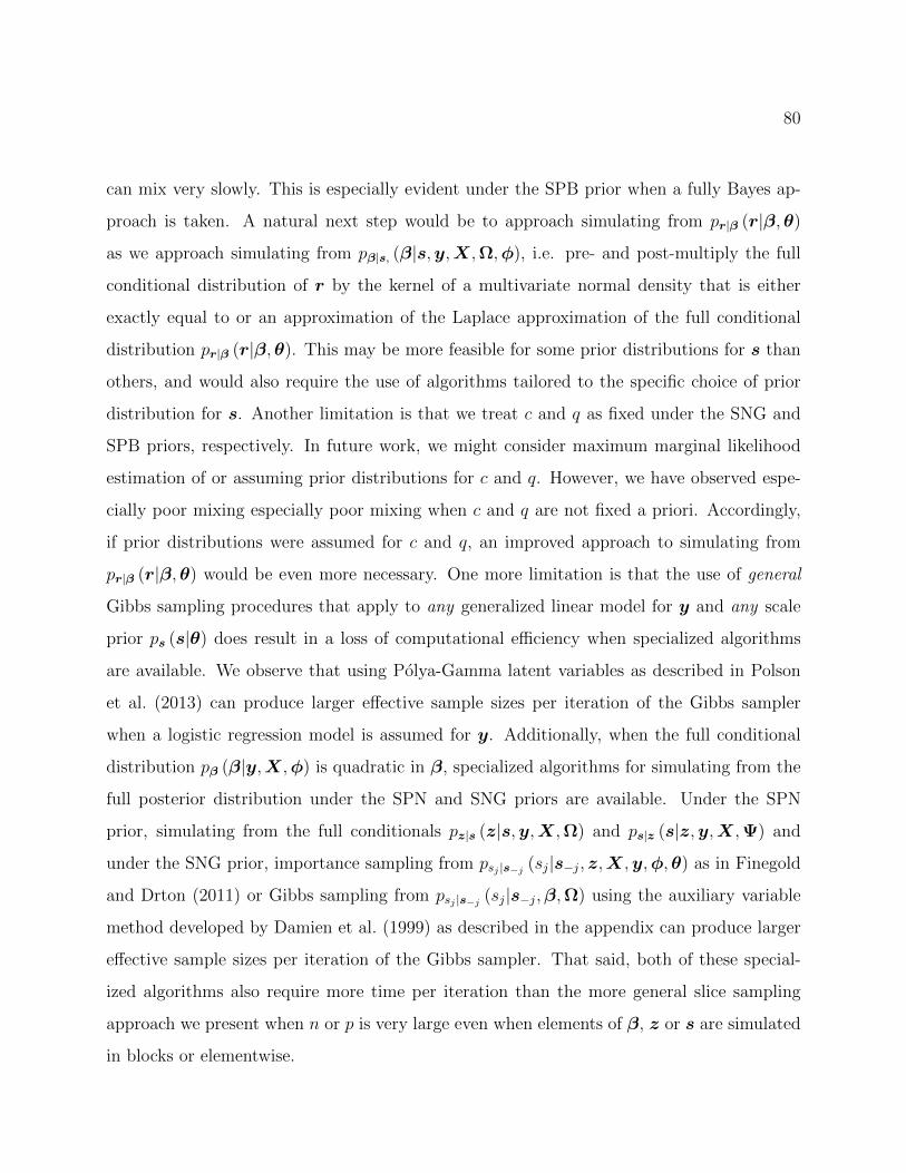
80

can mix very slowly. This is especially evident under the SPB prior when a fully Bayes ap-

proach is taken. A natural next step would be to approach simulating from pr|β (r|β,θ)

as we approach simulating from pβ|s, (β|s,y,X,Ω,φ), i.e. pre- and post-multiply the full

conditional distribution of r by the kernel of a multivariate normal density that is either

exactly equal to or an approximation of the Laplace approximation of the full conditional

distribution pr|β (r|β,θ). This may be more feasible for some prior distributions for s than

others, and would also require the use of algorithms tailored to the specific choice of prior

distribution for s. Another limitation is that we treat c and q as fixed under the SNG and

SPB priors, respectively. In future work, we might consider maximum marginal likelihood

estimation of or assuming prior distributions for c and q. However, we have observed espe-

cially poor mixing especially poor mixing when c and q are not fixed a priori. Accordingly,

if prior distributions were assumed for c and q, an improved approach to simulating from

pr|β (r|β,θ) would be even more necessary. One more limitation is that the use of general

Gibbs sampling procedures that apply to any generalized linear model for y and any scale

prior ps (s|θ) does result in a loss of computational efficiency when specialized algorithms

are available. We observe that using Polya-Gamma latent variables as described in Polson

et al. (2013) can produce larger effective sample sizes per iteration of the Gibbs sampler

when a logistic regression model is assumed for y. Additionally, when the full conditional

distribution pβ (β|y,X,φ) is quadratic in β, specialized algorithms for simulating from the

full posterior distribution under the SPN and SNG priors are available. Under the SPN

prior, simulating from the full conditionals pz|s (z|s,y,X,Ω) and ps|z (s|z,y,X,Ψ) and

under the SNG prior, importance sampling from psj |s−j (sj|s−j, z,X,y,φ,θ) as in Finegold

and Drton (2011) or Gibbs sampling from psj |s−j (sj|s−j,β,Ω) using the auxiliary variable

method developed by Damien et al. (1999) as described in the appendix can produce larger

effective sample sizes per iteration of the Gibbs sampler. That said, both of these special-

ized algorithms also require more time per iteration than the more general slice sampling

approach we present when n or p is very large even when elements of β, z or s are simulated

in blocks or elementwise.

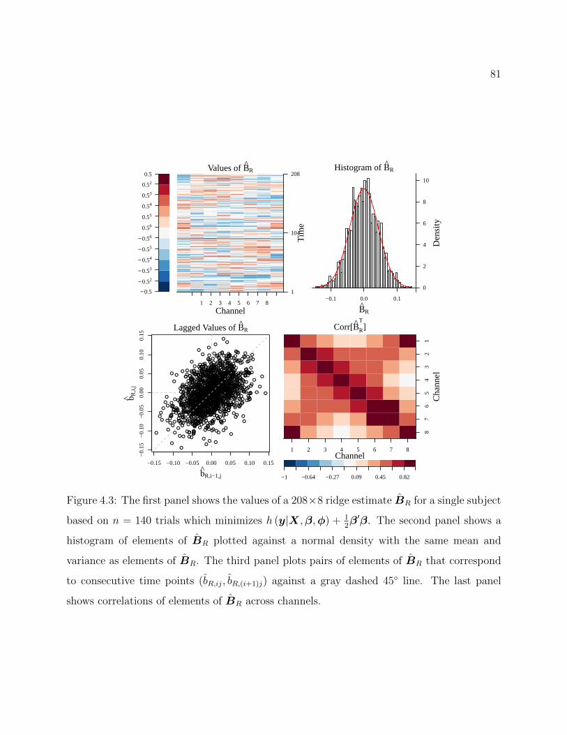
81

− 0.5

− 0.52

− 0.53

− 0.54

− 0.55

− 0.56

0.56

0.55

0.54

0.53

0.52

0.5

1

104

208

Tim

e1 2 3 4 5 6 7 8

Channel

Values of BR

0

2

4

6

8

10

Den

sity

−0.1 0.0 0.1

BR

Histogram of BR

−0.15 −0.10 −0.05 0.00 0.05 0.10 0.15

−0.

15−

0.10

−0.

050.

000.

050.

100.

15

Lagged Values of BR

b R,i,

j

bR,i−1,j

Corr[BR

T]

87

65

43

21

1 2 3 4 5 6 7 8

Cha

nnel

Channel

−1 −0.64 −0.27 0.09 0.45 0.82

Figure 4.3: The first panel shows the values of a 208×8 ridge estimate BR for a single subject

based on n = 140 trials which minimizes h (y|X,β,φ) + 12β′β. The second panel shows a

histogram of elements of BR plotted against a normal density with the same mean and

variance as elements of BR. The third panel plots pairs of elements of BR that correspond

to consecutive time points (bR,ij, bR,(i+1)j) against a gray dashed 45 line. The last panel

shows correlations of elements of BR across channels.

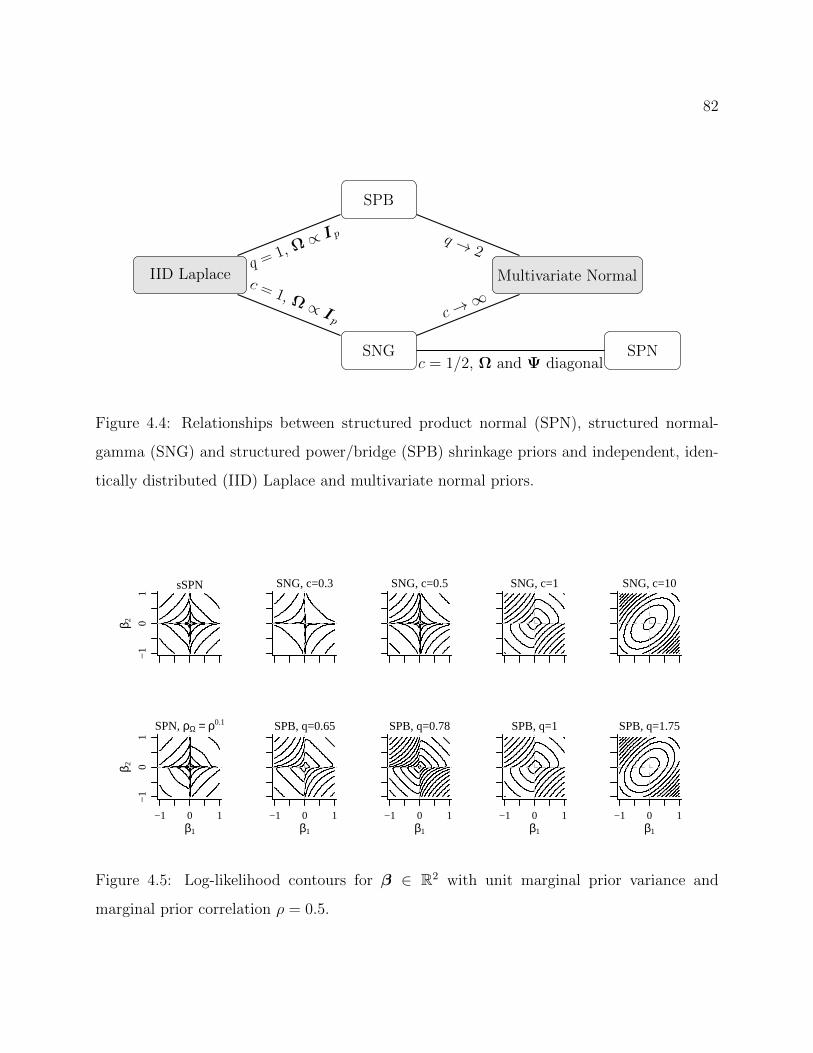
82

IID Laplace Multivariate Normal

SNG

SPB

SPN

c→∞

q → 2

c = 1/2, Ω and Ψ diagonal

c = 1, Ω ∝ Ip

q = 1, Ω ∝I p

Figure 4.4: Relationships between structured product normal (SPN), structured normal-

gamma (SNG) and structured power/bridge (SPB) shrinkage priors and independent, iden-

tically distributed (IID) Laplace and multivariate normal priors.

sSPN

−1

01

β 2

SNG, c=0.3 SNG, c=0.5 SNG, c=1 SNG, c=10

SPN, ρΩ = ρ0.1

−1 0 1β1

−1

01

β 2

SPB, q=0.65

−1 0 1β1

SPB, q=0.78

−1 0 1β1

SPB, q=1

−1 0 1β1

SPB, q=1.75

−1 0 1β1

Figure 4.5: Log-likelihood contours for β ∈ R2 with unit marginal prior variance and

marginal prior correlation ρ = 0.5.

83

10 20 30 40 50 60

0.0

0.4

0.8

Kurtosis

Max

. Cor

rela

tion ρ

SNGSPB

Figure 4.6: Maximum marginal prior correlation ρ for β ∈ R2 as a function of kurtosis.

sSPN

00.

51

u 2

SNG, c=0.3 SNG, c=0.5 SNG, c=1 SNG, c=10

SPN, ρΩ = ρ0.1

0 0.5 1u1

00.

51

u 2

SPB, q=0.65

0 0.5 1u1

SPB, q=0.78

0 0.5 1u1

SPB, q=1

0 0.5 1u1

SPB, q=1.75

0 0.5 1u1

Figure 4.7: Copula estimates for β ∈ R2 with unit marginal prior variances and marginal

prior correlation ρ = 0.5.

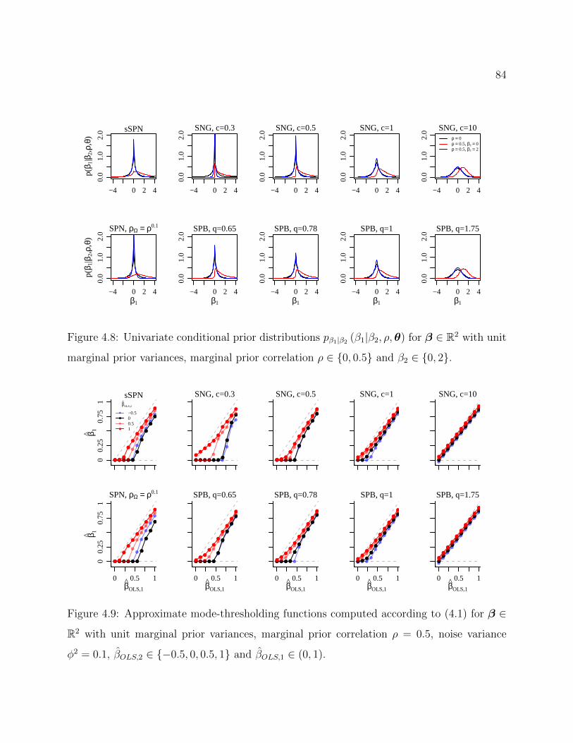
84

−4 0 2 4

0.0

1.0

2.0 sSPN

p(β 1

|β2,

ρ,θ)

−4 0 2 40.

01.

02.

0 SNG, c=0.3

−4 0 2 4

0.0

1.0

2.0 SNG, c=0.5

−4 0 2 4

0.0

1.0

2.0 SNG, c=1

−4 0 2 4

0.0

1.0

2.0 SNG, c=10

ρ = 0ρ = 0.5, β2 = 0ρ = 0.5, β2 = 2

−4 0 2 4

0.0

1.0

2.0 SPN, ρΩ = ρ0.1

p(β 1

|β2,

ρ,θ)

β1

−4 0 2 4

0.0

1.0

2.0 SPB, q=0.65

β1

−4 0 2 4

0.0

1.0

2.0 SPB, q=0.78

β1

−4 0 2 4

0.0

1.0

2.0 SPB, q=1

β1

−4 0 2 4

0.0

1.0

2.0 SPB, q=1.75

β1

Figure 4.8: Univariate conditional prior distributions pβ1|β2 (β1|β2, ρ,θ) for β ∈ R2 with unit

marginal prior variances, marginal prior correlation ρ ∈ 0, 0.5 and β2 ∈ 0, 2.

sSPN

00.

250.

751

β 1

βOLS,2

−0.500.51

SNG, c=0.3

SNG, c=0.5

SNG, c=1

SNG, c=10

SPN, ρΩ = ρ0.1

0 0.5 1βOLS,1

00.

250.

751

β 1

SPB, q=0.65

0 0.5 1βOLS,1

SPB, q=0.78

0 0.5 1βOLS,1

SPB, q=1

0 0.5 1βOLS,1

SPB, q=1.75

0 0.5 1βOLS,1

Figure 4.9: Approximate mode-thresholding functions computed according to (4.1) for β ∈

R2 with unit marginal prior variances, marginal prior correlation ρ = 0.5, noise variance

φ2 = 0.1, βOLS,2 ∈ −0.5, 0, 0.5, 1 and βOLS,1 ∈ (0, 1).

85

diag(Σ2)

0.001

87

65

43

21

Cha

nnel

σjj

Corr[Σ2]

87

65

43

21

1 2 3 4 5 6 7 8

Cha

nnel

Channel

−1

−0.82

−0.64

−0.45

−0.27

−0.09

0.09

0.27

0.45

0.64

0.82

1

Figure 4.10: Normal LA-within-EM estimates of variances and correlations of Σ2.

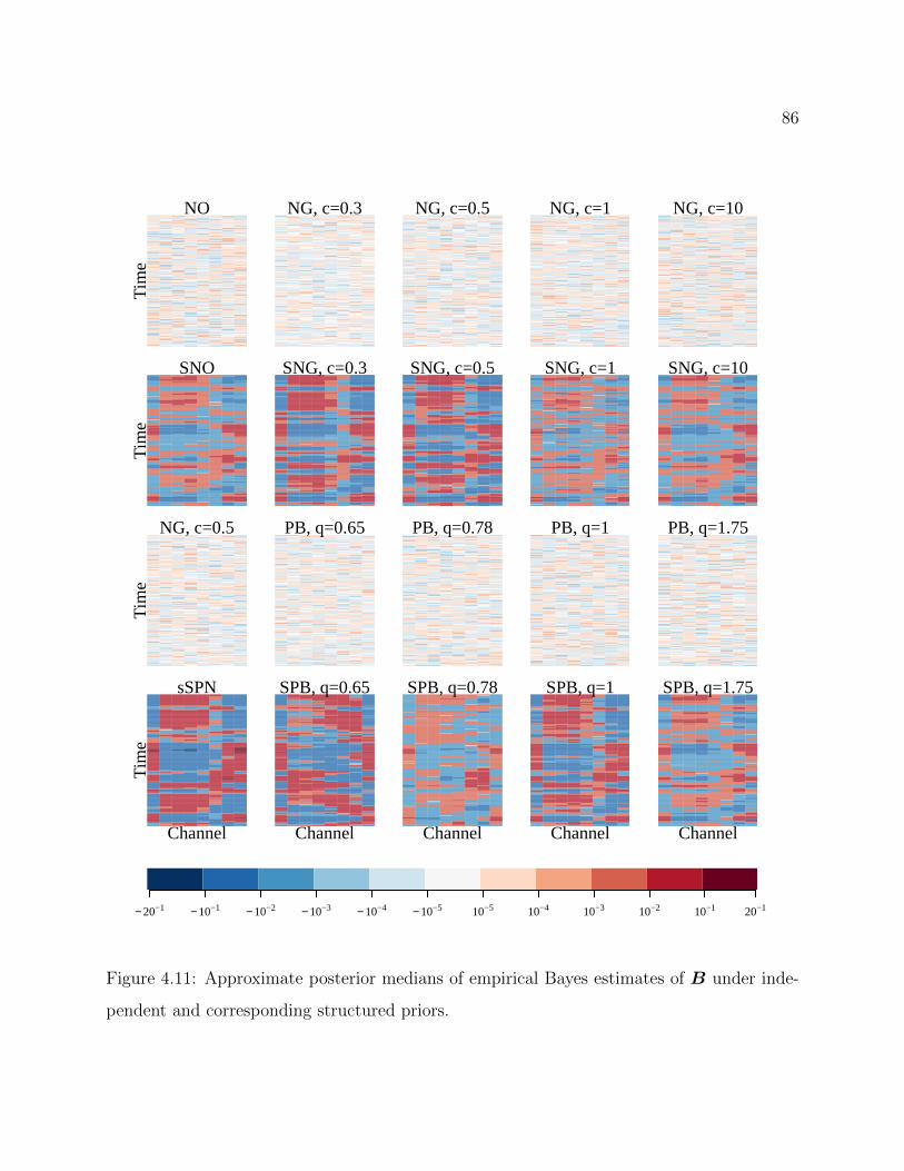
86

NO

Tim

e

NG, c=0.3 NG, c=0.5 NG, c=1 NG, c=10

SNO

Tim

e

SNG, c=0.3 SNG, c=0.5 SNG, c=1 SNG, c=10

NG, c=0.5

Tim

e

PB, q=0.65 PB, q=0.78 PB, q=1 PB, q=1.75

sSPN

Tim

e

Channel

SPB, q=0.65

Channel

SPB, q=0.78

Channel

SPB, q=1

Channel

SPB, q=1.75

Channel

− 20−1 − 10−1 − 10−2 − 10−3 − 10−4 − 10−5 10−5 10−4 10−3 10−2 10−1 20−1

Figure 4.11: Approximate posterior medians of empirical Bayes estimates of B under inde-

pendent and corresponding structured priors.

87

0.0 0.2 0.4 0.6 0.8 1.0

0.0

0.2

0.4

0.6

0.8

1.0

FPR

TP

R

SNOSPB, q=0.78SNG, c=1SNG, c=10

Figure 4.12: ROC curves for held out test data using empirical Bayes approximate posterior

medians of the fitted values.

88

SNO

Tim

e

SNG, c=0.3 SNG, c=0.5 SNG, c=1 SNG, c=10

sSPN

Tim

e

Channel

SPB, q=0.65

Channel

SPB, q=0.78

Channel

SPB, q=1

Channel

SPB, q=1.75

Channel

−2.648 −0.5 −0.25 −0.1 −0.01 −0.001 0.001 0.01 0.1 0.25 0.5 2.648

Figure 4.13: Approximate posterior medians of fully Bayes estimates of B.

0.0 0.2 0.4 0.6 0.8 1.0

0.0

ROC Curves Based on Posterior Medians

FPR

TP

R

SNOSPNSNG, c=0.3SNG, c=0.5SNG, c=1SNG, c=10

Figure 4.14: ROC curves for held out test data using fully Bayes approximate posterior

medians of fitted values.

89

Chapter 5

CONCLUSIONS AND FUTURE WORK

This thesis has considered advantages and disadvantages of interpreting penalized re-

gression problems from a model-based perspective. We show that treating penalties as

priors facilitates estimation of unknown prior or tuning parameters in settings where other

approaches either fail or are impractical, enables joint estimation of many unknown prior

parameters simultaneously, and aids in the construction of novel, interpretable priors with

desirable properties. We also show that treating penalties as priors without carefully con-

sidering whether or not a certain prior is appropriate can be perilous. We encourage the use

of broader classes of priors to protect against poor prior specification.

In the first two chapters, we consider problems that require estimation of a one-to-three

dimensional vector of unknown likelihood and prior distribution parameters for which the

maximum marginal likelihood estimates are not computationally feasible to obtain. We are

are able to develop moment-based approaches to these problems that are easy and quick to

compute. However, such moment-based approaches are likely less efficient than likelihood-

based approaches as well as challenging to extend to settings where the response y is related

nonlinearly to β, e.g. where generalized linear models for y are used or where β = vec (B)

is the vectorization of a matrix for which a rank shrinkage prior is assumed. Doss (2010)

provides an MCMC assisted approach to the approximation of intractable likelihood surfaces

that could be applied to obtain maximum marginal likelihood estimates of the unknown like-

lihood and prior distribution parameters. Regarding the second chapter, “Testing Sparsity-

Inducing Penalties,” maximum marginal likelihood estimation of the unknown likelihood and

prior distribution parameters could be used to construct a likelihood ratio test of the null

hypothesis that a Laplace prior for regression coefficients β is appropriate if the distribution

90

of the likelihood test statistic under the null could be derived.

Material in the second chapter, “Testing Sparsity-Inducing Penalties,” suggests the de-

velopment of pathwise coordinate descent algorithms for `q penalties. Previous work has

found that pathwise coordinate descent algorithms can be useful for solving penalized re-

gression problems under other penalties that span `0 to `1 penalties, but has also argued

that the family of `q penalties are not amenable to pathwise coordinate descent algorithms

(Mazumder et al., 2011). Observations we make in “Testing Sparsity-Inducing Penalties”

suggest that the properties that Mazumder et al. (2011) argued make `q penalties ill suited

to pathwise coordinate descent are not inherent to `q penalties but rather are a consequence

of the standard parametrization used in the optimization literature, λ ||β||qq. As a result, we

may conduct a small additional project that shows how the parametrization of the `q penalty

used in ‘Testing Sparsity-Inducing Penalties” 2(

Γ(3/q)Γ(1/q)τ2

)q/2||β||qq can be used to construct

pathwise coordinate descent algorithms for fast computation of `q penalized estimates and

entire regularization surfaces.

The third chapter, “Structured Shrinkage Priors,” suggests several avenues for future

work. Because a change of variables facilitates the use of elliptical slice sampling for sim-

ulating from the full conditional distribution ps|β (s|β,θ) for arbitrary priors ps (s|θ), one

natural extension might be to consider the construction of novel correlated priors for s that

generalize the independent normal and polynomially tilted priors used to generate SNG and

SPB priors. The main challenge would be in defining density functions for s that correspond

to integrable multivariate distributions with reasonable properties. The slice sampling ap-

proach we take for simulating from the full conditional distribution ps|β,θ (s|β,θ) could be

used even more generally to simulate from full conditional distributions of correlation ma-

trices and elements on the Stiefel or Grassman manifolds in a generic way. Consider the

problem of simulating from a probability distribution over p× p correlation matrices C with

density pC (C), which might arise in data fusion type problems where p × p sample covari-

ance matrices S1, . . . ,Sn are observed, each of which measures relationships between the

same p units measured using different devices or at different times. We might want to model

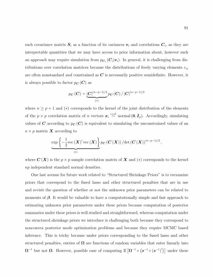
91

each covariance matrix Si as a function of its variances vi and correlations Ci, as they are

interpretable quantities that we may have access to prior information about, however such

an approach may require simulation from pCi (Ci|vi). In general, it is challenging from dis-

tributions over correlation matrices because the distributions of freely varying elements cij

are often nonstandard and constrained as C is necessarily positive semidefinite. However, it

is always possible to factor pC (C) as

pC (C) = |C|(n−p−1)/2︸ ︷︷ ︸(∗)

pC (C) / |C|(n−p−1)/2

where n ≥ p + 1 and (∗) corresponds to the kernel of the joint distribution of the elements

of the p × p correlation matrix of n vectors xii.i.d.∼ normal (0, Ip). Accordingly, simulating

values of C according to pC (C) is equivalent to simulating the unconstrained values of an

n× p matrix X according to

exp

−1

2vec (X)′ vec (X)

︸ ︷︷ ︸

(∗)

pC (C (X)) /det (C (X))(n−p−1)/2 ,

where C (X) is the p× p sample correlation matrix of X and (∗) corresponds to the kernel

np independent standard normal densities.

One last avenue for future work related to “Structured Shrinkage Priors” is to reexamine

priors that correspond to the fused lasso and other structured penalties that are in use

and revisit the question of whether or not the unknown prior parameters can be related to

moments of β. It would be valuable to have a computationally simple and fast approach to

estimating unknown prior parameters under these priors because computation of posterior

summaries under these priors is well studied and straightforward, whereas computation under

the structured shrinkage priors we introduce is challenging both because they correspond to

nonconvex posterior mode optimization problems and because they require MCMC based

inference. This is tricky because under priors corresponding to the fused lasso and other

structured penalties, entries of Ω are functions of random variables that enter linearly into

Ω−1 but not Ω. However, possible ease of computing E[Ω−1

(s−1 (s−1)

′)]under these

92

priors suggests that we might be able to overcome this difficulty and relate moments of β to

the unknown prior parameters.

93

BIBLIOGRAPHY

Andrews, D. F. and C. L. Mallows (1974). Scale Mixtures of Normal Distributions. Journal

of the Royal Statistical Society. Series B 36 (1), 99–102.

Bernardo, J. and A. F. M. Smith (2000). Bayesian Theory. Chichester: Wiley.

Bhattacharya, A., D. Pati, N. S. Pillai, and D. B. Dunson (2015). Dirichlet Laplace Priors for

Optimal Shrinkage. Journal of the American Statistical Association 110 (512), 1479–1490.

Bleeker, F. E., R. J. Molenaar, and S. Leenstra (2012). Recent advances in the molecular

understanding of glioblastoma. Journal of Neuro-Oncology 108 (1), 11–27.

Box, G. E. P. (1953). A Note on Regions for Tests of Kurtosis. Biometrika 40 (3/4), 465–468.

Box, G. E. P. and G. C. Tiao (1973). Bayesian Assessment of Assumptions. In Bayesian

Inference in Statistical Analysis, Chapter 3, pp. 149–202. Reading, MA: Addison-Wesley

Pub. Co.

Bredel, M., C. Bredel, D. Juric, G. R. Harsh, H. Vogel, L. D. Recht, and B. I. Sikic (2005).

Functional Network Analysis Reveals Extended Gliomagenesis Pathway Maps and Three

Novel MYC-Interacting Genes in Human Gliomas. Cancer Research 65 (19), 8679–8689.

Bruneel, B. (2018). DE DUIKERKLOK EN DE P300-SPELLER.

Buhlmann, P. and S. van de Geer (2011). Statistics for High-Dimensional Data: Methods,

Theory and Applications. Heidelberg: Springer.

Candes, E. J., C. A. Sing-Long, and J. D. Trzasko (2013). Unbiased Risk Estimates for

Singular Value Thresholding and Spectral Estimators. IEEE Transactions on Signal Pro-

cessing 61 (19), 4643–4657.

94

Caron, F. and A. Doucet (2008). Sparse Bayesian Nonparametric Regression. International

Conference on Machine Learning , 88–95.

Carvalho, C. M., N. G. Polson, and J. G. Scott (2010). The horseshoe estimator for sparse

signals. Biometrika 97 (2), 465–480.

Castillo, I., J. Schmidt-Hieber, and A. W. Van Der Vaart (2015). Bayesian linear regression

with sparse priors. Annals of Statistics 43 (5), 1986–2018.

Choy, S. T. B. and J. S. K. Chan (2008). Scale Mixtures Distributions in Statistical Mod-

elling. Australian and New Zealand Journal of Statistics 50 (2), 135–146.

Cosset, E., S. Ilmjarv, V. Dutoit, K. Elliott, T. von Schalscha, M. F. Camargo, A. Reiss,

T. Moroishi, L. Seguin, G. Gomez, J. S. Moo, O. Preynat-Seauve, K. H. Krause, H. Chnei-

weiss, J. N. Sarkaria, K. L. Guan, P. Y. Dietrich, S. M. Weis, P. S. Mischel, and D. A.

Cheresh (2017). Glut3 Addiction Is a Druggable Vulnerability for a Molecularly Defined

Subpopulation of Glioblastoma. Cancer Cell 32, 856–868.

Damien, P., J. Wakefield, and S. Walker (1999). Gibbs Sampling for Bayesian Non-Conjugate

and Hierarchical Models by Using Auxiliary Variables. Journal of the Royal Statistical

Society. Series B (Statistical Methodology) 61 (2), 331–344.

Daniels, M. J. and M. Pourahmadi (2002). Bayesian analysis of covariance matrices and

dynamic models for longitudinal data. Biometrika 89 (3), 553–566.

de Tayrac, M., S. Le, M. Aubry, J. Mosser, and F. Husson (2009). Simultaneous analysis of

distinct Omics data sets with integration of biological knowledge: Multiple Factor Analysis

approach. BMC Genomics 10 (1), 32.

Demidenko, E. (2013). Mixed Models: Theory and Applications with R (Second ed.). Hobo-

ken, New Jersey: John Wiley and Sons, Inc.

95

Dempster, A. P., N. M. Laird, and D. B. Rubin (1977). Maximum likelihood from incomplete

data via the EM algorithm. Journal of the Royal Statistical Society. Series B 39 (1), 1–38.

Devroye, L. (2009). Random variate generation for exponentially and polynomially tilted

stable distributions. ACM Transactions on Modeling and Computer Simulation 19 (4),

1–20.

Diananda, P. H. (1949). Note on some properties of maximum likelihood estimates. Mathe-

matical Proceedings of the Cambridge Philosophical Society 45 (04), 536–544.

Dıaz-Frances, E. and J. A. Montoya (2008). Correction to On the linear combination of

normal and Laplace random variables, by Nadarajah, S., Computational Statistics, 2006,

21, 6371. Computational Statistics 23 (4), 661–666.

Doss, H. (2010). Estimation of Large Families of Bayes Factors from Markov Chain Output.

Statistica Sinica 20, 537–560.

Ducray, F., A. Idbaih, A. de Reynies, I. Bieche, J. Thillet, K. Mokhtari, S. Lair, Y. Marie,

S. Paris, M. Vidaud, K. Hoang-Xuan, O. Delattre, J. Y. Delattre, and M. Sanson (2008).

Anaplastic oligodendrogliomas with 1p19q codeletion have a proneural gene expression

profile. Molecular Cancer 7, 1–17.

Efron, B., T. Hastie, I. Johnstone, and R. Tibshirani (2004). Least Angle Regression. The

Annals of Statistics 32 (2), 407–499.

Fabrizi, E. and C. Trivisano (2010). Robust linear mixed models for Small Area Estimation.

Journal of Statistical Planning and Inference 140 (2), 433–443.

Fan, J. and R. Li (2001). Variable Selection via Nonconcave Penalized Likelihood and its

Oracle Properties. Journal of the American Statistical Association 96 (456), 1348–1360.

Fazel, M. (2002). Matrix Rank Minimization with Applications. Ph. d. thesis, Stanford

University.

96

Figueiredo, M. A. T. (2003). Adaptive Sparseness for Supervised Learning. IEEE Transac-

tions on Pattern Analysis and Machine Intelligence 25 (9), 1150–1159.

Finegold, M. and M. Drton (2011). Robust graphical modeling of gene networks using

classical and alternative t-distributions. Annals of Applied Statistics 5 (2 A), 1057–1080.

Forney, E., C. Anderson, P. Davies, W. Gavin, B. Taylor, and M. Roll (2013). A Comparison

of EEG Systems for Use in P300 Spellers by Users With Motor Impairments in Real-World

Environments. Proceedings of the Fifth International Brain-Computer Interface Meeting .

Frank, I. E. and J. H. Friedman (1993). A Statistical View of Some Chemometrics Regression

Tools. Technometrics 35 (2), 109.

Fu, W. J. (1998). Penalized Regressions: The Bridge Versus the Lasso. Journal of Compu-

tational and Graphical Statistics 7 (3), 397–416.

Gerard, D. and P. Hoff (2017). Adaptive Higher-order Spectral Estimators. Electronic

Journal of Statistics 11 (2), 3703–3737.

Ghosh, D., I. V. Ulasov, L. Chen, L. E. Harkins, K. Wallenborg, P. Hothi, S. Rostad,

L. Hood, and C. S. Cobbs (2016). TGFb-Responsive HMOX1 Expression Is Associated

with Stemness and Invasion in Glioblastoma Multiforme. Stem Cells 34 (9), 2276–2289.

Gollob, H. F. (1968). A statistical model which combines features of factor analytic and

analysis of variance techniques. Psychometrika 33 (1), 73–115.

Goodman, L. A. and S. J. Haberman (1990). The Analysis of Nonadditivity in Two-Way

Analysis of Variance. Journal of the American Statistical Association 85 (409), 139–145.

Griffin, J. E. and P. J. Brown (2010). Inference with normal-gamma prior distributions in

regression problems. Bayesian Analysis 5 (1), 171–188.

Griffin, J. E. and P. J. Brown (2012a). Competing Sparsity: A hierarchical prior for sparse

regression with grouped effects.

97

Griffin, J. E. and P. J. Brown (2012b). Structuring shrinkage: some correlated priors for

regression. Biometrika 99 (2), 481–487.

Hans, C. (2009). Bayesian lasso regression. Biometrika 96 (4), 835–845.

Hoerl, A. E. and R. W. Kennard (1970). Ridge Regression: Biased Estimation for Nonorthog-

onal Problems. Technometrics 12 (1), 55.

Hoff, P. D. (2007). Model averaging and dimension selection for the singular value decom-

position. Journal of the American Statistical Association 102 (478), 674–685.

Hoff, P. D. (2016). Equivariant and Scale-Free Tucker Decomposition Models. Bayesian

Analysis 11 (3), 627–648.

Hoff, P. D. and C. Yu (2017). Exact adaptive confidence intervals for linear regression

coefficients. arXiv: 1705.08331v2 .

Huang, J., J. L. Horowitz, and S. Ma (2008). Asymptotic Properties of Bridge Estimators

in Sparse High-Dimensional Regression Models. The Annals of Statistics 36 (2), 587–613.

Johnson, D. E. and F. A. Graybill (1972). An Analysis of a Two-Way Model with Interaction

and No Replication. Journal of the American Statistical Association 67 (340), 862–868.

Josse, J. and S. Sardy (2016). Adaptive shrinkage of singular values. Statistics and Comput-

ing 26 (3), 715–724.

Josse, J., S. Sardy, and S. Wager (2016). denoiseR: A Package for Low Rank Matrix Esti-

mation. R package version 1.0.

Kalli, M. and Griffin (2014). Time-varying sparsity in dynamic regression models. Journal

of Econometrics 178, 779–793.

Konig, R. H., H. Neudecker, and T. Wansbeek (1992). Unbiased Estimation of Fourth-Order

Matrix Moments. Linear Algebra and Its Applications 160, 163–174.

98

Kowal, D. R., D. S. Matteson, and D. Ruppert (2017). Dynamic Shrinkage Processes.

Kyung, M., J. Gill, M. Ghosh, and G. Casella (2010). Penalized Regression, Standard Errors,

and Bayesian Lassos. Bayesian Analysis 5 (2), 369–412.

Leeb, H. and B. M. Potscher (2008). Sparse estimators and the oracle property, or the return

of Hodges’ estimator. Journal of Econometrics 142 (1), 201–211.

Makeig, S., C. Kothe, T. Mullen, N. Bigdely-Shamlo, Z. Zhang, and K. Kreutz-Delgado

(2012). Evolving Signal Processing for Brain Computer Interfaces. Proceedings of the

IEEE 100 (Special Centennial Issue), 1567–1584.

Mandel, J. (1971). A New Analysis of Variance Model for Non-Additive Data. Technomet-

rics 13 (1), 1–18.

Marjanovic, G. and V. Solo (2014). lq Sparsity Penalized Linear Regression with Cyclic

Descent. IEEE Transactions on Signal Processing 62 (6), 1464–1475.

Mazumder, R., J. H. Friedman, and T. Hastie (2011). SparseNet: Coordinate Descent With

Nonconvex Penalties. Journal of the American Statistical Association 106 (495), 1125–

1138.

McCullagh, P. and J. A. Nelder (1989). Generalized Linear Models (2nd ed.). London:

Chapman & Hall.

Mitchell, T. M., R. Hutchinson, R. S. Niculescu, and X. Wang (2004). Learning to Decode

Cognitive States from Brain Images. Machine Learning 57 (January), 145–175.

Murray, I., R. P. Adams, and D. J. C. Mackay (2010). Elliptical slice sampling. Journal of

Machine Learning Research: WC&P 9, 541–548.

Nadarajah, S. (2006). On the linear combination of normal and Laplace random variables.

Computational Statistics 21 (1), 63–71.

99

Neal, R. M. (2003). Slice Sampling. Annals of Statistics 31 (3), 758–767.

Park, T. and G. Casella (2008). The Bayesian Lasso. Journal of the American Statistical

Association 103 (482), 681–686.

Perry, P. O. (2017). Fast moment-based estimation for hierarchical models. Journal of the

Royal Statistical Society. Series B 79 (1), 267–291.

Polson, N. G. and J. G. Scott (2010). Shrink Globally, Act Locally: Bayesian Sparsity and

Regularization. In J. M. Bernardo, M. J. Bayarri, J. O. Berger, A. P. Dawid, D. Heckerman,

A. F. M. Smith, and M. West (Eds.), Bayesian Statistics 9, pp. 501–538. Oxford University

Press.

Polson, N. G., J. G. Scott, and J. Windle (2013). Bayesian inference for logistic models using

Polya-Gamma latent variables. Journal of the American Statistical Association 108 (504),

1339–1349.

Polson, N. G., J. G. Scott, and J. Windle (2014). The Bayesian bridge. Journal of the Royal

Statistical Society. Series B: Statistical Methodology 76 (4), 713–733.

Priami, C. and M. J. Morine (2015). Analysis of Biological Systems. London: Imperial

College Press.

Robert, C. P. (1995). Simulation of truncated normal variables. Statistics and Computing 5,

121–125.

Rodriguez-Yam, G., R. A. Davis, and L. L. Scharf (2004). Efficient Gibbs Sampling of

Truncated Multivariate Normal with Application to Constrained Linear Regression.

Roy, V. and S. Chakraborty (2016). Selection of Tuning Parameters, Solution Paths and

Standard Errors for Bayesian Lassos. Bayesian Analysis TBA(TBA), 1–26.

100

Salazar, E., M. A. R. Ferreira, and H. S. Migon (2012). Objective Bayesian analysis for

exponential power regression models. Sankhya: The Indian Journal of Statistics, Series

B 74 (1), 107–125.

Sharma, N. (2013). Single-Trial P300 Classification with LDA and Neural Networks. Ph. D.

thesis, Colorado State University.

Styan, P. H. (1973). Hadamard Products and Multivariate Statistical Analysis. Linear

Algebra and Its Applications 6, 217–240.

Subbotin, M. T. (1923). On the Law of Frequency of Error. Matematicheskii Sbornik 31 (2),

296–301.

Thirion, B., G. Varoquaux, E. Dohmatob, and J. B. Poline (2014). Which fMRI clustering

gives good brain parcellations? Frontiers in Neuroscience 8 (8 JUL), 1–13.

Tibshirani, R. (1996). Regression Shrinkage and Selection via the Lasso. Journal of the

Royal Statistical Society: Series B (Statistical Methodology) 58 (1), 267–288.

Tibshirani, R. (2011). Regression Shrinkage and Selection Via the Lasso: a retrospective.

Journal of the Royal Statistical Society. Series B: Statistical Methodology 73 (3), 273–282.

Tibshirani, R. J. (2013). The lasso problem and uniqueness. Electronic Journal of Statis-

tics 7 (1), 1456–1490.

van der Pas, S., B. Szabo, and A. W. van der Vaart (2017). Adaptive posterior contraction

rates for the horseshoe. Electronic Journal of Statistics 11 (2).

Van der Vaart, A. W. (2000). Asymptotic Statistics. Cambridge University Press.

van Eeuwijk, F. A. and P. M. Kroonenberg (1998). Multiplicative Models for Interaction in

Three-Way ANOVA, with Applications to Plant Breeding. Biometrics 54 (4), 1315–1333.

101

van Gerven, M., B. Cseke, R. Oostenveld, and T. Heskes (2009). Bayesian Source Local-

ization with the Multivariate Laplace Prior. Advances in Neural Information Processing

Systems 22, 1–9.

van Gerven, M. A. J., B. Cseke, F. P. de Lange, and T. Heskes (2010). Efficient Bayesian

multivariate fMRI analysis using a sparsifying spatio-temporal prior. Neuroimage 50,

150–161.

Walker, S. G. and E. Guttierez-Pena (1999). Robustifying Bayesian Procedures. Bayesian

Statistics 6, 685–710.

Wand, M. P. (2003). Smoothing and mixed models. Computational Statistics 18 (2), 223–249.

West, M. (1987). On Scale Mixtures of Normal Distributions. Biometrika 74 (3), 646–648.

Westfall, P. H. (2014). Kurtosis as Peakedness, 1905 - 2014. R.I.P. The American Statisti-

cian 68 (3), 191–195.

Wolpaw, J. and E. W. Wolpaw (2012). Brain-Computer Interfaces: Principles and Practice.

USA: Oxford University Press.

Wu, A., M. Park, O. Koyejo, and J. W. Pillow (2014). Sparse Bayesian structure learning

with dependent relevance determination prior. Advances in Neural Information Processing

Systems , 1628–1636.

Zellner, A. (1986). On Assessing Prior Distributions and Bayesian Regression Analysis with

g Prior Distributions. In P. K. Goel and Z. A. (Eds.), Bayesian Inference and Decision

Techniques: Essays in Honor of Bruno de Finetti, pp. 233–243. New York: Elsevier.

Zhang, C., J. Li, H. Wang, and S. Wei Song (2016). Identification of a five B cell-associated

gene prognostic and predictive signature for advanced glioma patients harboring immuno-

suppressive subtype preference. Oncotarget 7 (45), 73971–73983.

102

Zhao, S., C. Gao, S. Mukherjee, and Engel (2016). Bayesian group factor analysis with

structured sparsity. Journal of Machine Learning Research 17, 1–47.

103

Appendix A

SUPPLEMENT TO “LASSO ANOVA DECOMPOSITIONS FORMATRIX AND TENSOR DATA”

A.1 Uniqueness of M , A and C

As this is a standard lasso regression problem, uniqueness of M is well known (Tibshirani,

2013). Suppose we have two unique solutions for A: A and A, where A 6= A. Then it must

be the case that A = A+α1′p + 1nβ′, where α 6= 0 and/or β 6= 0, i.e. α1′p + 1nβ

′ 6= 0. Let

C and C be the corresponding solutions for C. By uniqueness of M , we have:

A+ C = A+ C = M .

It follows that C = M − A and C = M − A. Substituting our expression for A in terms

of A into C yields C = M − A−α1′p − 1nβ′. Then:∣∣∣∣∣∣vec

(C)∣∣∣∣∣∣

1=∣∣∣∣∣∣vec

(M − A−α1′p − 1nβ

′)∣∣∣∣∣∣

1

≤∣∣∣∣∣∣vec

(M − A

)∣∣∣∣∣∣1

+∣∣∣∣vec

(α1′p + 1nβ

′)∣∣∣∣1

=∣∣∣∣∣∣vec

(C)∣∣∣∣∣∣

1+∣∣∣∣vec

(α1′p + 1nβ

′)∣∣∣∣1.

It follows that∣∣∣∣∣∣vec

(C)∣∣∣∣∣∣

1<∣∣∣∣∣∣vec

(C)∣∣∣∣∣∣

1and

1

2σ2z

∣∣∣∣∣∣vec(Y − M

)∣∣∣∣∣∣22

+ λc

∣∣∣∣∣∣vec(C)∣∣∣∣∣∣

1<

1

2σ2z

∣∣∣∣∣∣vec(Y − M

)∣∣∣∣∣∣22

+ λc

∣∣∣∣∣∣vec(C)∣∣∣∣∣∣

1.

This contradicts our claim that the A and C solve the penalized regression problem. It

follows that A is unique and as C is uniquely determined by M and A, it follows that C is

unique as well.

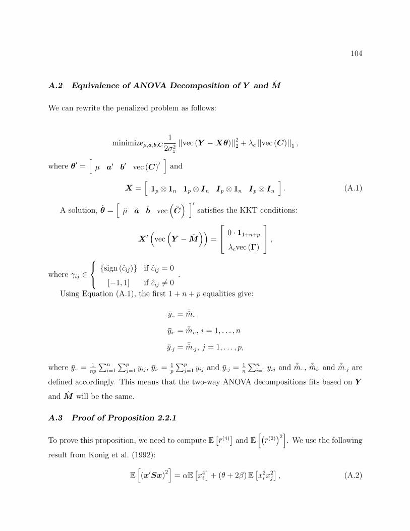
104

A.2 Equivalence of ANOVA Decomposition of Y and M

We can rewrite the penalized problem as follows:

minimizeµ,a,b,C1

2σ2z

||vec (Y −Xθ)||22 + λc ||vec (C)||1 ,

where θ′ =[µ a′ b′ vec (C)′

]and

X =[

1p ⊗ 1n 1p ⊗ In Ip ⊗ 1n Ip ⊗ In]. (A.1)

A solution, θ =[µ a b vec

(C) ]′

satisfies the KKT conditions:

X ′(

vec(Y − M

))=

0 · 11+n+p

λcvec (Γ)

,where γij ∈

sign (cij) if cij = 0

[−1, 1] if cij 6= 0.

Using Equation (A.1), the first 1 + n+ p equalities give:

y·· = ¯m··

yi· = ¯mi·, i = 1, . . . , n

y·j = ¯m·j, j = 1, . . . , p,

where y·· = 1np

∑ni=1

∑pj=1 yij, yi· = 1

p

∑pj=1 yij and y·j = 1

n

∑ni=1 yij and ¯m··, ¯mi· and ¯m·j are

defined accordingly. This means that the two-way ANOVA decompositions fits based on Y

and M will be the same.

A.3 Proof of Proposition 2.2.1

To prove this proposition, we need to compute E[r(4)]

and E[(r(2))2]. We use the following

result from Konig et al. (1992):

E[(x′Sx)

2]

= αE[x4i

]+ (θ + 2β)E

[x2ix

2j

], (A.2)

105

for a mean zero random vector x of independent elements and symmetric fixed matrix S,

where α =∑

i s2ii, θ =

∑i 6=j siisjj and β =

∑i 6=j s

2ij.

First, we rewrite E[(r(2))2]

to resemble Equation (A.2):

(r(2))2

=1

n2p2

(vec (C +Z)′ (Hp ⊗Hn) (vec (C +Z))

)2.

We compute α, θ and β below:

α = (np)

((n− 1) (p− 1)

np

)2

=(n− 1)2 (p− 1)2

np

θ = np (np− 1)

((n− 1) (p− 1)

np

)2

=(np− 1) (n− 1)2 (p− 1)2

np

β = np (p− 1)

(n− 1

np

)2

+ n (n− 1) p

(p− 1

np

)2

+ n (n− 1) p (p− 1)

(1

np

)2

=(n− 1)2 (p− 1) + (n− 1) (p− 1)2 + (n− 1) (p− 1)

np

Recalling κ is defined such that E[c4ij

]= (κ+ 3)σ4

c and plugging these expressions for

α, β and θ into Equation (A.2) yields:

E[(r(2))2]

=(n− 1)2 (p− 1)2

n3p3

(κσ4

c + 3(σ2c + σ2

z

)2)

+ (A.3)

(np− 1) (n− 1)2 (p− 1)2

n3p3

(σ2c + σ2

z

)2+

2

((n− 1)2 (p− 1) + (n− 1) (p− 1)2 + (n− 1) (p− 1)

n3p3

)(σ2c + σ2

z

)2

=κ

((n− 1)2 (p− 1)2

n3p3

)σ4c +

((n− 1) (p− 1)

np

)2 (σ2c + σ2

z

)2+

2

((n− 1) (p− 1)

n2p2

)(σ2c + σ2

z

)2.

Now we compute r(4). Letting Ekk be an np× np matrix with the k-th diagonal element

equal to 1 and all other elements equal to 0. We can rewrite r(4) so each term in resembles

106

Equation (A.2):

r(4) =1

np

np∑k=1

(vec (R)′Ekkvec (R)

)2

=1

np

np∑k=1

(vec (C +Z)′ (Hp ⊗Hn)Ekk (Hp ⊗Hn) vec (C +Z)

)2.

The matrices (Hp ⊗Hn)Ekk (Hp ⊗Hn) take the place of S in Equation (A.2).

From Equation (A.2), we have to compute the sum of squared diagonal elements, denoted

by αk, the sum of pairwise products of distinct diagonal elements, denoted by θk, and the

sum of squared off-diagonal elements, denoted by βk, for each of these matrices. Before going

further, we show that θk = βk. Letting ek is an np× 1 vector with the k-th element equal to

1 and all other elements equal to 0,

αk + βk = tr ((Hp ⊗Hn)Ekk (Hp ⊗Hn) (Hp ⊗Hn)Ekk (Hp ⊗Hn))

= tr ((Hp ⊗Hn) eke′k (Hp ⊗Hn) eke

′k)

= (e′k (Hp ⊗Hn) ek)2

=

((n− 1) (p− 1)

np

)2

,

αk + θk = tr ((Hp ⊗Hn)Ekk (Hp ⊗Hn)⊗ (Hp ⊗Hn)Ekk (Hp ⊗Hn))

= tr ((Hp ⊗Hn)Ekk (Hp ⊗Hn))2

= tr ((Hp ⊗Hn) eke′k)

2

= (e′k (Hp ⊗Hn) ek)2

=

((n− 1) (p− 1)

np

)2

.

It follows that βk = θk.

This means we only need to compute the sum of squared diagonal elements and the sum

of pairwise products of distinct diagonal elements of (Hp ⊗Hn)Ekk (Hp ⊗Hn).

Each matrix, (Hp ⊗Hn)Ekk (Hp ⊗Hn), is constructed by multiplying the k-th column

and the k-th row of (Hp ⊗Hn). By symmetry of (Hp ⊗Hn), this is the same as multiplying

107

the k-th column, denoted by (Hp ⊗Hn)k, by its transpose,

(Hp ⊗Hn)Ekk (Hp ⊗Hn) = (Hp ⊗Hn)k (Hp ⊗Hn)′k .

Regardless of k, each column (Hp ⊗Hn)k has the following elements:

• One element equal to (n−1)(p−1)np

;

• (p− 1) elements equal to − (n−1)np

;

• (n− 1) elements equal to − (p−1)np

• (n− 1) (p− 1) elements equal to 1np

.

The diagonal elements of (Hp ⊗Hn)Ekk (Hp ⊗Hn) will be given by the squared el-

ements of (Hp ⊗Hn)k. Note that the only feature of the diagonal elements of

(Hp ⊗Hn)Ekk (Hp ⊗Hn) that depends on k is the order of these elements. Accordingly,

the sum of squared diagonal elements, αk, and the sum of pairwise products of distinct

108

diagonal elements, θk, will not depend on k. Dropping the subscript, we compute α and θ:

α =

((n− 1) (p− 1)

np

)4

+ (p− 1)

(n− 1

np

)4

+ (n− 1)

(p− 1

np

)4

+ (n− 1) (p− 1)

(1

np

)4

=(n− 1) (p− 1)

n4p4

((n− 1)3 (p− 1)3 + (n− 1)3 + (p− 1)3 + 1

)=

(n− 1) (n2 − 3n+ 3) (p− 1) (p2 − 3p+ 3)

n4p4

θ = (p− 1)

((n− 1)4 (p− 1)2

n4p4

)+ (n− 1)

((n− 1)2 (p− 1)4

n4p4

)+ (n− 1) (p− 1)

((n− 1)2 (p− 1)2

n4p4

)+

(p− 1) (p− 2)

((n− 1)4

n4p4

)+ (n− 1) (p− 1)

((n− 1)2 (p− 1)2

n4p4

)+ (n− 1) (p− 1)2

((n− 1)2

n4p4

)+

(n− 1) (n− 2)

((p− 1)4

n4p4

)+ (n− 1)2 (p− 1)

((p− 1)2

n4p4

)+

(n− 1) (p− 1) ((n− 1) (p− 1)− 1)

(1

n4p4

)=

1

n4p4

((p− 1)3 (n− 1)4 + (p− 1)4 (n− 1)3 + (p− 1)3 (n− 1)3

+ (p− 1)3 (n− 1)4 + (p− 1) (p− 2) (n− 1)4 + (p− 1)3 (n− 1)3 + (p− 1)2 (n− 1)3 +

(p− 1)4 (n− 1)3 + (p− 1)3 (n− 1)3 + (n− 1) (n− 2) (p− 1)4 + (p− 1)3 (n− 1)2 +

(n− 1)3 (p− 1)3 + (n− 1)3 (p− 1)2 + (n− 1)2 (p− 1)3 + (n− 1) (p− 1) ((n− 1) (p− 1)− 1))

=1

n4p4

(2 (p− 1)3 (n− 1)4 + 2 (p− 1)4 (n− 1)3 + 4 (p− 1)3 (n− 1)3 +

(p− 1) (p− 2) (n− 1)4 + 2 (p− 1)2 (n− 1)3 + (n− 1) (n− 2) (p− 1)4 + 2 (p− 1)3 (n− 1)2 +

(n− 1) (p− 1) ((n− 1) (p− 1)− 1))

=(n− 1) (p− 1) (2np2 + 2n2p− 3p2 − 3n2 − 8np+ 9p+ 9n− 9)

n3p3

=

((n− 1) (p− 1)

np

)2

− (n− 1) (n2 − 3n+ 3) (p− 1) (p2 − 3p+ 3)

n3p3.

109

Plugging these expressions into Equation (A.2) yields:

E[r(4)]

=κ

((n− 1) (n2 − 3n+ 3) (p− 1) (p2 − 3p+ 3)

n3p3

)σ4c+ (A.4)

3

((n− 1) (p− 1)

np

)2 (σ2c + σ2

z

)2.

Plugging in the excess kurtosis, κ = 3, of Laplace distributed cij, Proposition 2.2.1 follows

straightforwardly from the definition of σ4c and Equations (A.3) and (A.4).

A.4 Proof of Proposition 2.2.2

We start by showing consistency of our empirical Bayes estimators as p → ∞ with n fixed.

The proof of consistency of our empirical Bayes estimators as n→∞ with p fixed is analo-

gous.

Recalling that our empirical Bayes estimators are functions of r(2) and r(4), we start by

proving that r(2) p→(n−1n

)(σ2

c + σ2z) as p→∞ for fixed n. First, we compute E

[r(2)].

E[r(2)]

=1

npE[vec (R)′ vec (R)

](A.5)

=1

npE[vec (C +Z)′ (Hp ⊗Hn) vec (C +Z)

]=

1

npE[vec (C +Z)′ (Hp ⊗Hn) vec (C +Z)

]=

1

nptr((Hp ⊗Hn)E

[vec (C +Z) vec (C +Z)′

])=

1

nptr (Hp ⊗Hn)

(σ2c + σ2

z

)=

(n− 1) (p− 1)

np

(σ2c + σ2

z

).

For fixed n, as p→∞, E[r(2)]

= O (1)(n−1n

)(σ2

c + σ2z).

We can compute V[r(2)]

explicitly using Equation (A.3).

V[r(2)]

= κ

((n− 1)2 (p− 1)2

n3p3

)σ4c + 2

((n− 1) (p− 1)

n2p2

)(σ2c + σ2

z

)2. (A.6)

110

For fixed n, as p → ∞, V[r(2)]

= O(

1p

). It follows that r(2) p→

(n−1n

)(σ2

c + σ2z) as

p→∞ for fixed n.

Now we show r(4) p→ κ

((n−1)(n2−3n+3)

n3

)σ4c + 3

(n−1n

)2(σ2

c + σ2z)

2as p→∞ for fixed n.

From Equation (A.4), we have E[r(4)]

=

(O (1)κ

(n−1)(n2−3n+3)n3

)σ4c +

O (1) 3(n−1n

)2(σ2

c + σ2z)

2as p → ∞ for fixed n. Now we evaluate the order of V

[r(4)],

starting by evaluating the order of E[(r(4))2]. For convenience, we let xij = cij +zij and use

the following way of writing elements of R: rij = xij − xi·− x·j + x··, where xi· =1p

∑pj=1 xij,

x·j = 1n

∑ni=1 xij and x·· =

1np

∑ni=1

∑pj=1 xij.

E[(r(4))2]

=E

( 1

np

n∑i=1

p∑j=1

r2ij

)2

=1

n2p2E

[n∑i=1

p∑j=1

r8ij +

n∑i′=1

∑j′=p,i′j′ 6=ij

r4ijr

4i′j′

]

=1

n2p2E

[n∑i=1

p∑j=1

(xij − x·j +Op

(1√p

))8]

+

1

n2p2E

[n∑i=1

p∑j=1

n∑i′ 6=i

(xij − x·j +Op

(1√p

))4(xi′j′ − x·j′ +Op

(1√p

))4]

+

1

n2p2E

[n∑i=1

p∑j=1

n∑i′=1

∑j′ 6=j

(xij − x·j +Op

(1√p

))4(xi′j′ − x·j′ +Op

(1√p

))4]

=1

npE[x8

11

]+O

(1

p

)+

1

n2p2

n∑i=1

p∑j=1

n∑i′=1

E[(xij − x·j)4 (xi′j − x·j)4]+O

(1√p

)+

1

n2p2

n∑i=1

p∑j=1

n∑i′=1

∑j′ 6=j

E[(xij − x·j)4]E [(xi′j′ − x·j′)4]+O

(1

p2

)=

1

pE[(x11 − x·1)4 (x21 − x·1)4]︸ ︷︷ ︸

∗

+

(p− 1

p

)E[(x11 − x·1)4]E [(x12 − x·2)4]+O

(1√p

)

=

(p− 1

p

)E[(x11 − x·1)4]2 +O

(1√p

).

111

The term marked by ∗ is constant for fixed n, it is a degree eight polynomial of n

independent elements of X, with coefficients that depend on n alone.

Now we need to compute the remaining unknown term,

E[(x11 − x·1)4] = E

(n− 1

nx11 −

1

n

n∑i=2

xi1

)4

=

(n− 1

n

)4

E[x4

11

]+ 6

(n− 1

n

)2

E[x2

11

]E

( 1

n

n∑i=2

xi1

)2+ E

( 1

n

n∑i=2

xi1

)4

=

(n− 1

n

)4

E[x4

11

]+

6 (n− 1)3

n4E[x2

11

]2+n− 1

n4E[x4

11

]+

3 (n− 1) (n− 2)

n4E[x2

11

]2=

(n− 1)((n− 1)3 + 1

)n4

E[x4

11

]+

(n− 1)(6 (n− 1)2 + 3 (n− 2)

)n4

E[x2

11

]2=

(n− 1) (n2 − 3n+ 3)

n3E[x4

11

]+

3 (n− 1) (2n− 3)

n3E[x2

11

]2= κ

(n− 1) (n2 − 3n+ 3)

n3σ4c + 3

(n− 1

n

)2 (σ2c + σ2

z

)2.

Combining this with our expression for E[(r(4))2], we have V

[(r(4))2]

= O(

1√p

)as

p → ∞ for fixed n. It follows that r(4) p→ κ

((n−1)(n2−3n+3)

n3

)σ4c + 3

(n−1n

)2(σ2

c + σ2z)

2as

p→∞ for fixed n.

Plugging in the excess kurtosis, κ = 3, of Laplace distributed cij, combining r(4) p→

3

((n−1)(n2−3n+3)

n3

)σ4c +3

(n−1n

)2(σ2

c + σ2z)

2as p→∞ for fixed n with r(2) p→

(n−1n

)(σ2

c + σ2z)

as p → ∞ for fixed n, and applying the continuous mapping theorem yields σ4c

p→ σ4c ,

σ2c

p→ σ2c , λc

p→ λc and σ2z

p→ σ2z as p→∞ for fixed n.

Now we show consistency of our empirical Bayes estimators as n, p → ∞. It follows

directly from Equations (A.5) and (A.6) that r(2) p→ σ2c + σ2

z as n, p → ∞. Regarding r(4),

we again let xij = cij + zij and use the following decomposition:

rij = xij − xi· − x·j + x··.

For convenience, we also let n = π1q, p = π2q, where 0 < π1 < 1 and 0 < π2 < 1 are fixed

and π1 + π2 = 1. Then the scenario n, p→∞ is equivalent to q →∞. We have:

112

r(4) =1

π1π2q2

π1q∑i=1

π2q∑j=1

(xij − xi· − x·j + x··)4 (A.7)

=1

π1π2q2

π1q∑i=1

π2q∑j=1

(xij +Op

(1√q

))4

=1

π1π2q2

π1q∑i=1

π2q∑j=1

x4ij + x3

ijOp

(1√q

)+ x2

ijOp

(1

q

)+ xijOp

(1√q3

)+Op

(1

q2

)= x(4) −

(κσ4

c + 3(σ2c + σ2

z

)2)

︸ ︷︷ ︸Op( 1

q )

+(κσ4

c + 3(σ2c + σ2

z

)2)

+Op

(1

q

)

=κσ4c + 3

(σ2c + σ2

z

)2+Op

(1

q

).

It follows that r(4) p→ κσ4c + 3 (σ2

c + σ2z)

2as q →∞, i.e. as n, p→∞.

Plugging in the excess kurtosis, κ = 3, of Laplace distributed cij, combining r(4) p→

3σ4c +3 (σ2

c + σ2z)

2as n, p→∞ with r(2) p→ σ2

c +σ2z as n, p→∞ and applying the continuous

mapping theorem yields σ4c

p→ σ4c , σ

2c

p→ σ2c , λc

p→ λc and σ2z

p→ σ2z as n, p→∞.

A.5 Derivation of Asymptotic Variance of σ2c

Letting xij = cij + zij, we will use the following decomposition:

rij = xij − xi· − x·j + x··.

Without loss of generality, we let n = π1q, p = π2q, where 0 < π1 < 1 and 0 < π2 < 1

are fixed and π1 + π2 = 1. Then the scenario n, p→∞ is equivalent to q →∞.

For r(2) we have:

113

r(2) =1

π1π2q2

π1q∑i=1

π2q∑j=1

(xij − xi· − x·j + x··)2

=1

π1π2q2

π1q∑i=1

π2q∑j=1

(xij − xi· − x·j +Op

(1

q

))2

=1

π1π2q2

π1q∑i=1

π2q∑j=1

(xij − xi· − x·j)2 + (xij − xi· − x·j)Op

(1

q

)+Op

(1

q2

)

=1

π1π2q2

π1q∑i=1

π2q∑j=1

(xij − xi· − x·j)2 +Op

(1

q2

)

=1

π1π2q2

π1q∑i=1

π2q∑j=1

x2ij + x2

i· + x2·j − 2xijxi· − 2xijx·j + 2xi·x·j +Op

(1

q2

)

We find the order of most of the terms below:

1

π1π2q2

π1q∑i=1

π2q∑j=1

xijxi· =

(1

π1π2q2

π1q∑i=1

π2q∑j=1

xij

)Op

(1√q

)

= Op

(1√q3

)1

π1π2q2

π1q∑i=1

π2q∑j=1

xijx·j = Op

(1√q3

)1

π1π2q2

π1q∑i=1

π2q∑j=1

xi·x·j =

(1

π1q

π1q∑i=1

xi·

)(1

π2q

π2q∑j=1

x·j

)

= x2··

= Op

(1

q2

).

Plugging these expressions into the equation for r(2) gives:

r(2) =x(2) +1

π1q

π1q∑i=1

x2i· +

1

π2q

π2q∑j=1

x2·j +Op

(1√q3

).

114

Now we compute the means and find the orders of the variances of the middle two terms,

starting with 1π1q

∑π1qi=1 x

2i·.

E

[1

π1q

π1q∑i=1

x2i·

]= E

[x2i·]

=1

π22q

2E

( π2q∑j=1

xij

)2

=1

π22q

2

(π2qE

[x2ij

])=

E[x2ij

]π2q

.

Note that 1π1q

∑π1qi=1 x

2i· is a mean over independent variables, x2

i·. Accordingly,

V[

1π1q

∑π1qi=1 x

2i·

]= 1

π1qV [x2

i·]. Now we find the order of V [x2i·]:

V[x2i·]

= E[x4i·]− E

[x2i·]2

=1

π42q

4E

( π2q∑j=1

xij

)4+O

(1

q2

)

=1

π42q

4

(π2qE

[x4ij

]+ 3π2q (π2q − 1)E

[x2ij

]2)+O

(1

q2

)= O

(1

q2

).

Then V[

1π1q

∑π1qi=1 x

2i·

]= O

(1q3

)and 1

π1q

∑π1qi=1 x

2i· −

E[x2ij]π2q

= Op

(1√q3

). The same logic yields

1π2q

∑π2qj=1 x

2·j −

E[x2ij]π1q

= Op

(1√q3

). Plugging this into the equation for r(2) gives:

r(2) =x(2) +E[x2ij

]π1q

+E[x2ij

]π2q

+Op

(1√q3

)

=x(2) +E[x2ij

]π1π2q

+Op

(1√q3

)

For r(4) we have:

115

r(4) =1

π1π2q2

π1q∑i=1

π2q∑j=1

(xij − xi· − x·j + x··)4

=1

π1π2q2

π1q∑i=1

π2q∑j=1

(xij − xi· − x·j +Op

(1

q

))4

=1

π1π2q2

π1q∑i=1

π2q∑j=1

(xij − xi· − x·j)4 + (xij − xi· − x·j)3Op

(1

q

)+

(xij − xi· − x·j)2Op

(1

q2

)+ (xij − xi· − x·j)Op

(1

q3

)+Op

(1

q4

)=

1

π1π2q2

π1q∑i=1

π2q∑j=1

(xij − xi· − x·j)4 +Op

(1

q2

)+Op

(1

q2

)+Op

(1

q4

)+Op

(1

q4

)

=1

π1π2q2

π1q∑i=1

π2q∑j=1

(xij − xi· − x·j)4 +Op

(1

q2

)

=1

π1π2q2

π1q∑i=1

π2q∑j=1

x4ij + x4

i· + x4·j + 4x3

ijxi· + 4xijx3i· + 4x3

ijx·j + 4xijx3·j + 4x3

i·x·j + 4xi·x3·j+

6x2ijx

2i· + 6x2

ijx2·j + 6x2

i·x2·j + 12x2

ijxi·x·j + 12xijx2i·x·j + 12xijxi·x

2·j +Op

(1

q2

)

116

As with r(2), we can find the order of most of these terms:

1

π1π2q2

π1q∑i=1

π2q∑j=1

x4i· = Op

(1

q2

)1

π1π2q2

π1q∑i=1

π2q∑j=1

x4·j = Op

(1

q2

)1

π1π2q2

π1q∑i=1

π2q∑j=1

x3ijxi· =

1

π1π2q2

π1q∑i=1

π2q∑j=1

x3ijOp

(1√q

)= Op

(1√q3

)1

π1π2q2

π1q∑i=1

π2q∑j=1

x3ijx·j = Op

(1√q3

)1

π1π2q2

π1q∑i=1

π2q∑j=1

xijx3i· =

1

π1π2q2

π1q∑i=1

π2q∑j=1

xijOp

(1√q3

)= Op

(1√q5

)1

π1π2q2

π1q∑i=1

π2q∑j=1

xijx3·j = Op

(1√q5

)1

π1π2q2

π1q∑i=1

π2q∑j=1

xi·x3·j = Op

(1√q

)Op

(1√q3

)= Op

(1

q2

)1

π1π2q2

π1q∑i=1

π2q∑j=1

x3i·x·j = Op

(1

q2

)1

π1π2q2

π1q∑i=1

π2q∑j=1

x2i·x

2·j = Op

(1

q

)Op

(1

q

)= Op

(1

q2

)1

π1π2q2

π1q∑i=1

π2q∑j=1

xijx2i·x·j = Op

(1

q

)Op

(1

q

)Op

(1√q

)= Op

(1√q5

)1

π1π2q2

π1q∑i=1

π2q∑j=1

xijxi·x2·j = Op

(1√q5

).

Plugging these expressions into the equation for r(2) gives:

r(4) =x(4) +6

π1π2q2

π1q∑i=1

π2q∑j=1

x2ijx

2i· +

6

π1π2q2

π1q∑i=1

π2q∑j=1

x2ijx

2·j +

12

π1π2q2

π1q∑i=1

π2q∑j=1

x2ijxi·x·j +Op

(1√q3

).

Now we compute the means and find the orders of the variances of the remaining terms,

starting with 1π1π2q2

∑π1qi=1

∑π2qj=1 x

2ijx

2i·:

117

E

[1

π1π2q2

π1q∑i=1

π2q∑j=1

x2ijx

2i·

]=

1

π1q

π1q∑i=1

E

[x2i·

(1

π2q

π2q∑j=1

x2ij

)]

=1

π1q

π1q∑i=1

E

( 1

π2q

π2q∑j=1

xij

)2(1

π2q

π2q∑j=1

x2ij

)=

1

π1q

π1q∑i=1

1

π32q

3E

( π2q∑j=1

xij

)2( π2q∑j=1

x2ij

)=

1

π1q

π1q∑i=1

(1

π32q

3

(π2qE

[x4ij

]+ π2q (π2q − 1)E

[x2ij

]2))

=E[x4ij

]+ (π2q − 1)E

[x2ij

]2π2

2q2

=O

(1

q2

)+

E[x2ij

]2π2q

.

Note that this term is the mean of π1q independent, identically distributed terms, so to

find order of its variance we just need to find the order of the variance of a single one of the

terms.

V

[x2i·

(1

π2q

π2q∑j=1

x2ij

)]= E

(x2i·

(1

π2q

π2q∑j=1

x2ij

))2− E

[x2i·

(1

π2q

π2q∑j=1

x2ij

)]2

=1

π62q

6E

( π2q∑j=1

xij

)4( π2q∑j=1

x2ij

)2+O

(1

q2

)=

1

π62q

6

(π2qE

[x8ij

]+ π2q (π2q − 1)E

[x4ij

]2+ 2π2q (π2q − 1)E

[x6ij

]E[x2ij

]+

2π2q (π2q − 1) (π2q − 2)E[x4ij

]E[x2ij

]2+ 6π2q (π2q − 1)E

[x6ij

]E[x2ij

]+

12π2q (π2q − 1)E[x4ij

]E[x4ij

]+ 12π2q (π2q − 1) (π2q − 2) (π2q − 3)E

[x2ij

]4)+

O

(1

q2

)= O

(1

q2

).

118

It follows that V[

1π1π2q2

∑π1qi=1

∑π2qj=1 x

2ijx

2i·

]= O

(1q3

)and

1

π1π2q2

π1q∑i=1

π2q∑j=1

x2ijx

2i· − E

[1

π1π2q2

π1q∑i=1

π2q∑j=1

x2ijx

2i·

]= Op

(1√q3

).

By the same logic, E[

1π1π2q2

∑π1qi=1

∑π2qj=1 x

2ijx

2·j

]= O

(1q2

)+

E[x2ij]2

π1qand

1

π1π2q2

π1q∑i=1

π2q∑j=1

x2ijx

2·j − E

[1

π1π2q2

π1q∑i=1

π2q∑j=1

x2ijx

2·j

]= Op

(1√q3

).

Now we just have to compute the mean and order of the variance of one last term,

1π1π2q2

∑π1qi=1

∑π2qj=1 x

2ijxi·x·j.

E

[1

π1π2q2

π1q∑i=1

π2q∑j=1

x2ijxi·x·j

]=

(1

π21π

22q

4

) π1q∑i=1

π2q∑j=1

E

[x2ij

(π2q∑j′=1

xij′

)(π1q∑i′=1

xi′j

)]

=π1π2q

2E[x4ij

]π2

1π22q

4=

E[x4ij

]π1π2q2

= O

(1

q2

).

Because this term cannot be written as an average over independent, identically dis-

tributed random variables, computing the variance in this case is a little bit trickier. We

have

119

V

[1

π1π2q2

π1q∑i=1

π2q∑j=1

x2ijxi·x·j

]=

1

π21π

22q

4

(π1q∑i=1

π2q∑j=1

V[x2ijxi·x·j

]+ 2

π1q∑i=1

π2q∑j=1

π2q∑j′=1,j′ 6=j

Cov[x2ijxi·x·j, x

2ij′xi·x·j′

]+

2

π1q∑i=1

π2q∑j=1

π1q∑i′=1,i′ 6=i

Cov[x2ijxi·x·j, x

2i′jxi′·x·j

]+

2

π1q∑i=1

π2q∑j=1

π1q∑i′=1,i′ 6=i

π2q∑j′=1,j′ 6=j

Cov[x2ijxi·x·j, x

2i′j′xi′·x·j′

])

=1

π21π

22q

4

(π1π2q

2V[x2ijxi·x·j

]+ 2π1π2q

2 (π2q − 1) Cov[x2ijxi·x·j, x

2ij′xi·x·j′

]+

2π1π2q2 (π2q − 1) Cov

[x2ijxi·x·j, x

2i′jxi′·x·j

]+

2π1π2q2(π1π2q

2 − π1q − π2q + 1)

Cov[x2ijxi·x·j, x

2i′j′xi′·x·j′

])=

1

π1π2q2V[x2ijxi·x·j

]+

2 (π2q − 1)

π1π2q2Cov

[x2ijxi·x·j, x

2ij′xi·x·j′

]+

2 (π2q − 1)

π1π2q2Cov

[x2ijxi·x·j, x

2i′jxi′·x·j

]+

2 (π1π2q2 − π1q − π2q + 1)

π1π2q2Cov

[x2ijxi·x·j, x

2i′j′xi′·x·j′

]=O

(1

q2

)V[x2ijxi·x·j

]+O

(1

q

)Cov

[x2ijxi·x·j, x

2ij′xi·x·j′

]+

O

(1

q

)Cov

[x2ijxi·x·j, x

2i′jxi′·x·j

]+O (1) Cov

[x2ijxi·x·j, x

2i′j′xi′·x·j′

].

Examining the first term we have:

V[x2ijxi·x·j

]= E

[x4ijx

2i·x

2·j]− E

[x2ijxi·x·j

]2=

(1

π21π

22q

4

)E

x4ij

(π2q∑j′=1

xij′

)2( π1q∑i′=1

xi′j

)2+O

(1

q4

)

=

(E[x8ij

]+ π1q (π2q − 1)E

[x4ij

]E[x2ij

]2π2

1π22q

4

)+O

(1

q4

)= O

(1

q2

).

120

Then examining the second term we have:

Cov[x2ijxi·x·j, x

2ij′xi·x·j′

]=E

[x2ijx

2ij′x

2i·x·jx·j′

]− E

[x2ijxi·x·j

]2=

1

π21π

22q

4E

x2ijx

2ij′

(π2q∑j′′

xij′′

)2( π1q∑i′=1

xi′j

)(π1q∑i′′=1

xi′′j

)+O

(1

q4

)

=2E[x4ijx

4ij′

]π2

1π22q

4+O

(1

q4

)= O

(1

q4

).

The same logic yields Cov[x2ijxi·x·j, x

2ij′xi·x·j′

]= O

(1q4

).

Then examining the last term yields:

Cov[x2ijxi·x·j, x

2i′j′xi′·x·j′

]= E

[x2ijx

2i′j′xi·xi′·x·jx·j′

]− E [xijxi·x·j]

2

= E[x2ijxi·x·j

]E[x2i′j′xi′·x·j′

]− E [xijxi·x·j]

2 = 0.

Putting the pieces together, we get:

V

[1

π1π2q2

π1q∑i=1

π2q∑j=1

x2ijxi·x·j

]=O

(1

q2

)O

(1

q2

)+O

(1

q

)O

(1

q4

)+O

(1

q

)O

(1

q4

)= O

(1

q4

).

It follows that

1

π1π2q2

π1q∑i=1

π2q∑j=1

x2ijxi·x·j − E

[1

π1π2q2

π1q∑i=1

π2q∑j=1

x2ijxi·x·j

]= Op

(1

q2

).

121

Substituting these expressions into our last equation for r(4), we get:

r(4) =x(4) + 6

(1

π1π2q2

π1q∑i=1

π2q∑j=1

x2ijx

2i· − E

[1

π1π2q2

π1q∑i=1

π2q∑j=1

x2ijx

2i·

])+ E

[1

π1π2q2

π1q∑i=1

π2q∑j=1

x2ijx

2i·

]+

6

(1

π1π2q2

π1q∑i=1

π2q∑j=1

x2ijx

2·j − E

[1

π1π2q2

π1q∑i=1

π2q∑j=1

x2ijx

2·j

])+ 6E

[1

π1π2q2

π1q∑i=1

π2q∑j=1

x2ijx

2·j

]+

12

(1

π1π2q2

π1q∑i=1

π2q∑j=1

x2ijxi·x·j − E

[1

π1π2q2

π1q∑i=1

π2q∑j=1

x2ijxi·x·j

])+ 12E

[1

π1π2q2

π1q∑i=1

π2q∑j=1

x2ijxi·x·j

]+

Op

(1√q3

)

=x(4) +Op

(1√q3

)+O

(1

q2

)+

6E[x2ij

]2π1q

+

Op

(1√q3

)+O

(1

q2

)+

6E[x2ij

]2π2q

+Op

(1

q2

)+O

(1

q2

)+Op

(1√q3

)

=x(4) +6E[x2ij

]2π1π2q

+O

(1

q2

)+Op

(1√q3

).

122

Now we plug these expressions for r(2) and r(4) into our equation for σ4c :

σ4c =O (1)

(r(4)/3−

(r(2))2)

=O (1)

x(4)/3 +2E[x2ij

]2π1π2q

+O

(1

q2

)+Op

(1√q3

)−

(x(2) +

E[x2ij

]π1π2q

+Op

(1√q3

))2

=O (1)

(x(4)/3−

(x(2))2

+2E[x2ij

]2π1π2q

+O

(1

q2

)+Op

(1√q3

)−

(E[x2ij

]π1π2q

)2

︸ ︷︷ ︸O(

1q2

)+Op

(1

q3

)+Op

(1√q3

)+Op

(1√q5

)− 2

(x(2))(E

[x2ij

]π1π2q

)

=O (1)

x(4)/3−(x(2))2

+2E[x2ij

]2π1π2q

− 2(x(2) − E

[x2ij

])︸ ︷︷ ︸Op( 1

q )

(E[x2ij

]π1π2q

)︸ ︷︷ ︸

O( 1q )

−2

(E[x2ij

]2π1π2q

)+

O

(1

q2

)+Op

(1√q3

))

= O (1)

(x(4)/3−

(x(2))2

+O

(1

q2

)+Op

(1√q3

)).

Recalling that κ is defined such that E[x4ij

]/3− E

[x2ij

]2= κσ4/3, we have

√π1π2q2

(σ4c − κσ4

c/3) d→

√π1π2q2

(x(4)/3−

(x2)2 − κσ4

c/3)

as q →∞.

But what is the distribution of the right hand side? As x(2) and x(4) are sample moments

of independent, identically distributed random variables xij, we know that as q →∞:

√π1π2q2

x(2) − E[x2ij

]x(4) − E

[x4ij

] d→ N

0,

V[x2ij

]Cov

[x2ij, x

4ij

]Cov

[x2ij, x

4ij

]V[x4ij

] .

123

Let f (y, z) = z/3− y2 and note that f(E[x2ij

],E[x4ij

])= κσ4

c/3 and

∇f(E[x2ij

],E[x4ij

])=

−2E[x2ij

]1/3

.

Applying the delta method yields:

√π1π2q2

(x(4)/3−

(x(2))2 − κσ4

c/3)

d→ (A.8)

N(

0, 4E[x2ij

]2 V [x2ij

]− 4E

[x2ij

]Cov

[x2ij, x

4ij

]/3 + V

[x4ij

]/9)

as q →∞.

Up to this point, we have just used the assumption that xij = cij + zij, where zij is

normal and both cij and zij are independent, identically distributed from symmetric, mean

zero distributions. This will be convenient later, when we need to find the asymptotic

distribution of σ4c assuming (a) cij are normally distributed and/or exactly equal to zero and

(b) assuming cij are drawn from a Bernoulli-normal spike-and-slab prior. However here, we

are interested in finding the asymptotic variance of σ4c assuming cij are Laplace distributed

with variance σ2c . In this case, we have:

E[x2ij

]= σ2

c + σ2z

E[x4ij

]= 3σ4

c + 3(σ2c + σ2

z

)2

V[x2ij

]= 5σ4

c + 4σ2cσ

2z + 2σ4

z

Cov[x2ij, x

4ij

]= 6(14σ6

c + 13σ4cσ

2z + 6σ2

cσ4z + 2σ6

z)

V[x4ij

]= 12(207σ8

c + 204σ6cσ

2z + 99σ4

cσ4z + 32σ2

cσ6 + 8σ8

z).

Substituting these in to our expression for the asymptotic variance of σ4c and simplifying

yields and substituting n and p back in for π1q and π2q, we have

√np(σ4c − σ4

c

) d→ N(0, 8(69σ8

c + 42σ6cσ

2z + 15σ4

cσ4 + 4σ2

cσ6z + σ8

z)/3)

(A.9)

as n, p→∞.

124

A.6 Derivation of Asymptotic Variance of λc

We can obtain the asymptotic variance of λc =√

2/(σ4c )

1/4 from the asymptotic distribution

of σ2c via the delta method. The asymptotic variance of λc is given by:(

−√2

4σ5c

)2(8

3

)(69σ8

c + 42σ6cσ

2z + 15σ4

cσ4 + 4σ2

cσ6z + σ8

z

)/np =

(1

3σ2c

)(69 + 42ψ2 + 15ψ4 + 4ψ6 + ψ8

)/np,

where φ2 = σ2z/σ

2c .

A.7 Derivation of Asymptotic Joint Distribution of σ2c and σ2

z

Again, we let xij = cij + zij. Using the derivation given in Section 5, we have:

√np

r2

r4−

σ2c + σ2

z

3σ4c + 3 (σ2

c + σ2z)

d→ √np

x2

x4−

σ2c + σ2

z

3σ4c + 3 (σ2

c + σ2z)

as n, p→∞.

Applying the delta method and letting ψ2 = σ2z/σ

2c yields:

√np

σ2c

σ2z

−

σ2c

σ2z

d→ N

(0,σ4c

3Σ

),

where

σ11 = 2(69 + 42ψ2 + 15ψ4 + 4ψ6 + ψ8

)σ12 = −

(111 + 72ψ2 + 30ψ4 + 8ψ6 + 2ψ8

)σ22 = 99 + 72ψ2 + 36ψ4 + 8ψ6 + 2ψ8.

Note that Σ only depends on ψ2, the ratio of σ2z to σ2

c .

Letting z =√

3npσ4c

σ2c

σ2z

−

σ2c

σ2z

and noting that zd→ N (0,Σ) as n, p→∞,

1− Pr

σ2c

σ2z

≥ 0

= 1− Pr

z ≥ − 1

σ2c

σ2c

σ2z

= 1− Pr

z ≥ −√3np

1

ψ2

.

This probability depends only on the dimensions n and p and the ratio of the variances ψ.

125

A.8 Proof of Proposition 2.3.1

The proof of Proposition 2.3.1 follows directly from the derivation of the asymptotic distri-

bution of σ4c given in the previous section. To prove Proposition 2.3.1, we need to find the

asymptotic distribution of σ4c under the null hypothesis, H0: cij + zij ∼ i.i.d. N (0, σ2

c + σ2z).

Under this null hypothesis, cij + zijd= cij + zij, where cij is Laplace distributed with 0 and

zij is normally distributed with variance σ2c + σ2

z . Applying equation (A.9), yields:

√npσ4

cd→ N

(0, 8

(σ2c + σ2

z

)4/3)

as n, p→∞.

However when we are testing the null hypothesis, σ2c + σ2

z is unknown. Fortunately,

(σ2c + σ2

z)4

=((

np(n−1)(p−1)

)r(2))4 p→ σ2

c + σ2z as n, p→∞.

It follows directly from Equations (A.5) and (A.6) that σ2c + σ2

z

p→ σ2c + σ2

z as n, p→∞,

and by the continuous mapping theorem (σ2c + σ2

z)4 p→ (σ2

c + σ2z)

4as n, p→∞. Accordingly,

√np

σ4c√

83

(σ2c + σ2

z)2

d→ N (0, 1)

as n, p→∞ and under H0, Pr

(√np

(σ4c√

83

(σ2c+σ2

z)2

)> z1−α

)→ α as n, p→∞.

A.9 Proof of Proposition 2.3.2

Combining Equation (A.9) and consistency of σ2c + σ2

z for σ2c + σ2

z as n, p→∞ that follows

from Equations (A.5) and (A.6), we have:

√np

σ4c√

83

(σ2c + σ2

z)2− σ4

c√83

(σ2c + σ2

z)2

d→ N

(0,

69σ8c + 42σ6

cσ2z + 15σ4

cσ4 + 4σ2

cσ6z + σ8

z

(σ4c + σ2

z)4

).

126

We can simplify the mean and variance and write them as a function of φ2 = σ2c/σ

2z :

σ4c√

83

(σ2c + σ2

z)2

=

√3

8

(φ4

(φ2 + 1)2

)69σ8

c + 42σ6cσ

2z + 15σ4

cσ4 + 4σ2

cσ6z + σ8

z

(σ4c + σ2

z)4 =

68σ8c + 36σ6

cσ2z + 9σ4

cσ4 + (σ2

c + σ2c )

4

(σ4c + σ2

z)4

= 1 +68σ8

c + 36σ6cσ

2z + 9σ4

cσ4

(σ4c + σ2

z)4

= 1 +68φ8 + 36φ6 + 9φ4

(φ4 + 1)4 .

It follows that:

Pr

√np σ4

c√83

(σ2c + σ2

z)2

> z1−α

→ 1− Φ

z1−α −√

3np8

(φ4

(φ2+1)2

)√

1 + 68φ8+36φ6+9φ4

(φ4+1)4

as n, p→∞.

A.10 Proof of Proposition 2.3.3

To prove Proposition 2.3.3, we first need to compute the unknown quantities that appear in

Equation (A.8):

E[x2ij

]=πcτ

2c + σ2

z

E[x4ij

]=3(πcτ

4c + 2πcτ

2c σ

2z + σ4

z

)E[x6ij

]=E

[c6ij

]+ 15E

[c4ij

]E[z2ij

]+ 15E

[c2ij

]E[z4ij

]+ E

[z6ij

]=15

(πcτ

6c + 3πcτ

4c σ

2z + 3πcτ

2c σ

4z + σ6

z

)E[x8ij

]=E

[c8ij

]+ 28E

[c6ij

]E[z2ij

]+ 70E

[c4ij

]E[z4ij

]+ 28E

[c2ij

]E[z6ij

]+ E

[z8ij

]=105

(πcτ

8c + 4πcτ

6c σ

2z + 6πcτ

4c σ

4z + 4πcτ

2c σ

6z + σ8

z

)V[x2ij

]= (3− πc) πcτ 4

c + 4πcτ2c σ

2z + 2σ2

z

Cov[x2ij, x

4ij

]=12σ6

z + 36πcσ4zτ

2c + 42πcσ

2zτ

4c − 6π2

cσ2zτ

4c + 15πcτ

6c − 3π2

cτ6c

V[x4ij

]=96σ8

z + 384πcσ6zτ

2c + 612πcσ

4zτ

4c − 36π2

cσ4zτ

4c + 420πcσ

2zτ

6c − 36π2

cσ2zτ

6c + 105πcτ

8c − 9π2

cτ8.

127

Equation (A.8) yields the following variance:

1

3

(8σ8

z + 32πcσ6zτ

2c + 24 (3− πc) πcσ4

zτ4c + 16πc

(5− 6πc + 3π2

c

)σ2zτ

6c + πc

(35− 63πc + 48π2

c − 12π3c

)τ 8c

).

This can be simplified slightly to:

1

3

(8(πcτ

2c + σ2

c

)4+ πc (1− πc)

(72τ 4

c σ4z + 16 (5− πc) τ 6

c σ2z + (35− 28πc + 20) τ 8

c

))Now combining this with consistency of σ2

c + σ2z for σ2

c +σ2z = πcτ

2c +σ2

z as n, p→∞ that

follows directly from from Equations (A.5) and (A.6), we have:

√np

σ4c√

83

(σ2c + σ2

z)2− πc (1− πc) τ 4

c√83

(πcτ 2c + σ2

z)2

d→

N

(0, 1 +

πc (1− πc) (72τ 4c σ

4z + 16 (5− πc) τ 6

c σ2z + (35− 28πc + 20) τ 8

c )

8 (πcτ 2c + σ2

z)4

).

We can simplify the mean and variance and write them as a function of φ2 = τ 2c /σ

2z :

πc (1− πc) τ 4c√

83

(πcτ 2c + σ2

z)2

=πc (1− πc)φ4√

83

(πcφ2 + 1)2

1 +πc (1− πc) (72τ 4

c σ4z + 16 (5− πc) τ 6

c σ2z + (35− 28πc + 20) τ 8

c )

8 (πcτ 2c + σ2

z)4 =

1 +πc (1− πc) (72φ4 + 16 (5− πc)φ6 + (35− 28πc + 20)φ8)

8 (πcφ2 + 1)4

It follows that:

Pr

√np σ4

c√83

(σ2c + σ2

z)2

> z1−α

→ 1− Φ

z1−α −√

3np8

πc(1−πc)φ4

(πcφ2+1)2√1 + πc(1−πc)(72φ4+16(5−πc)φ6+(35−28πc+20π2

c )φ8)

8(πcφ2+1)4

as n, p→∞.

A.11 Proof of Proposition 2.3.4

First, we consider the case where p→∞ with n fixed. The case where p→∞ with n fixed

is analogous. In the proof of Proposition 2.2.2, we show that r(2) p→(n−1n

)(σ2

c + σ2z) and

128

r(4) p→ κ

((n−1)(n2−3n+3)

n3

)σ4c + 3

(n−1n

)2(σ2

c + σ2z)

2as p → ∞ with n fixed. Applying the

continous mapping theorem yields σ2c

p→√κ/3σ2

c and σ2z

p→ σ2z +

(1−

√κ/3)σ2z as p→∞

with n fixed.

Now we consider the case where n, p → ∞. In the proof of Proposition 2.2.2, we show

that r(2) p→ σ2c + σ2

z and r(4) p→ κσ4c + 3 (σ2

c + σ2z)

2as n, p → ∞. Applying the continous

mapping theorem yields σ2c

p→√κ/3σ2

c and σ2z

p→ σ2z +

(1−

√κ/3)σ2z as n, p→∞.

A.12 Negative Variance Parameter Estimates

% σ2z ≤ 0

τ 2c

πc0 0.1 0.2 0.3 0.4 0.5 0.6 0.7 0.8 0.9 1

0.5 0.00 0.00 0.00 0.00 0.00 0.00 0.00 0.00 0.00 0.00 0.00

1 0.00 0.00 0.00 0.00 0.00 0.00 0.00 0.00 0.00 0.00 0.00

1.5 0.00 0.00 0.20 0.00 0.00 0.00 0.00 0.00 0.00 0.00 0.00

% σ2c ≤ 0

τ 2c

πc0 0.1 0.2 0.3 0.4 0.5 0.6 0.7 0.8 0.9 1

0.5 56.40 47.40 40.20 33.60 35.40 37.00 36.40 45.00 44.60 48.60 52.20

1 56.60 29.00 20.80 12.80 13.00 13.40 15.60 28.20 29.80 40.80 55.80

1.5 52.60 12.00 4.20 2.80 3.60 4.80 6.60 10.40 22.20 35.20 55.60

Table A.1: Rates of negative estimates of σ2c and σ2

z across simulations.

Table A.1 shows the rates of negative estimates of σ2c and σ2

z across simulations using

Bernoulli-normal spike-and-slab distributed elements of C, setting n = p = 25, µ = 0, a = 0,

b = 0 and σ2z = 1 and varying τ 2

c = 1/2, 1, 3/2 and πc = 0, 0.1, . . . , 0.9, 1. For each pair

129

of values of τ 2c and πc 500 values of Y are simulated.

A.13 Block Coordinate Descent for LANOVA Penalization for Matrices withLower-Order Mean Parameters Penalized

We can use block coordinate descent to obtain estimates of the unknown mean parameters

by iterating the following procedure until the objective function

1

2σ2z

||vec (Y −M )||22 + λa ||a||1 + λb ||b||1 + λc ||vec (C)||1

converges, starting with a(0) = HnY 1p/p, b(0)

= HpY′1n/n and C

(0)= HnY Hp and

k = 1:

• Set µ(k) = 1′n

(Y − a(k−1)1′p − 1n

(b

(k−1))′− C

(k−1))

1p/ (np);

• Set R(k)a = Y − µ(k)1n1

′p − 1n

(b

(k−1))′− C

(k−1)and set

a(k) = sign(HnR

(k)a 1p/p

)(∣∣∣HnR(k)a 1p/p

∣∣∣− λaσ2z/p)

+;

• Set R(k)b = Y − µ(k)1n1

′p − a

(k)1′p − C(k−1)

and set

b(k)

= sign

(Hp

(R

(k)b

)′1n/n

)(∣∣∣HnR(k)a 1p/p

∣∣∣− λbσ2z/n)

+;

• Set R(k)c = Y −µ(k)1n1

′p−a

(k)1′p−1nb(k)

and set C(k)

= sign(R(k)c

)(∣∣∣R(k)c

∣∣∣− λcσ2z

)+

.

A.14 Proof of Proposition 2.4.1

We prove Proposition 2.4.1 by computing E[(r(2))2]

and E[r(4)]. Starting with E

[(r(2))2],

we again use the result of Konig et al. (1992) given by Equation (A.2), which yields:

E[(r(2))2]

=E[(

vec (C +Z)′H(K)vec (C +Z))2]

(A.10)

=αK

(κσ4

c + 3(σ2c + σ2

z

)2)

+ (θK + 2βK)(σ2c + σ2

z

)2,

130

where αK =∑p

j=1

(h

(K)jj

)2

, βK =∑p

j=1

∑pl=1,l 6=j h

(K)jj h

(K)ll and θK =∑p

j=1

∑pl=1,l 6=j

(h

(K)jl

)2

and κ is the excess kurtosis for the distribution of the elements of

C, which in this case where elements of C are assumed to be Laplace distributed is κ = 3.

From the definition of H(K) it is straightforward to see that all of the diagonal elements

of H(K) are identical and equal to∏K

k=1pk−1pk

. Therefore, it is straightforward to compute

αK and θK .

αK =K∏k=1

pK

(pK − 1

pK

)2

=K∏k=1

(pk − 1)2

pk

θK =K∏k=1

pk

(K∏k=1

pk − 1

)K∏k=1

(pk − 1

pk

)2

=

(K∏k=1

pk − 1

)K∏k=1

(pk − 1)2

pk

=K∏k=1

(pk − 1)2 −K∏k=1

(pk − 1)2

pk

Computing βK is a little bit trickier, however we can rewrite H(K) = HK ⊗H(K−1) and

obtain a formula for βK as a function of αK−1 and βK−1:

βK =pK (pK − 1)

(1

p2K

)(αK−1 + βK−1) + pK

(pK − 1

pK

)2

βK−1

=

(pK − 1

pK

)(αK−1 + βK−1) +

(pK − 1)2

pKβK−1

=

(pK − 1

pK

)αK−1 + (pK − 1) βK−1

To eliminate βK−1 from this expression, we note that αK + βK = tr(H(K)H(K)

)=

131

tr(H(K)

)=

(∏Kk=1 pk

)(∏Kk=1

pk−1pk

)=

∏Kk=1 (pk − 1). Adding and subtracting

(pK − 1)αK−1 yields:

βK =

(pK − 1

pK− (pK − 1)

)αK−1 + (pK − 1) (αK−1 + βK−1)

=

(pK − 1

pK− (pK − 1)

)αK−1 + (pK − 1)

K−1∏k=1

(pk − 1)

=

(2pK − 1− p2

K

pK

)K−1∏k=1

(pk − 1)2

pk+

K∏k=1

(pk − 1)

=−K∏k=1

(pk − 1)2

pk︸ ︷︷ ︸αK

+K∏k=1

(pk − 1) .

Plugging these terms in to Equation (A.10) yields:

E[(r(2))2]

=K∏k=1

(pk − 1)2

pk

(κσ4

c + 3(σ2c + σ2

z

)2)

+ (A.11)(K∏k=1

(pk − 1)2 −K∏k=1

(pk − 1)2

pk+

2

(−

K∏k=1

(pk − 1)2

pk+

K∏k=1

(pk − 1)

))(σ2c + σ2

z

)2

=K∏k=1

(pk − 1)2

pkκσ4

c +

(K∏k=1

(pk − 1)2 +K∏k=1

2 (pk − 1)

)(σ2c + σ2

z

)2.

Now we need to compute E[r(4)]. We start by rewriting the expression,

E[r(4)]

=1∏K

k=1 pk

K∑k=1

pk∑ik=1

(vec (R)Q(i1,...,iK)vec (R)

)2

=1∏K

k=1 pk

p1∑i1=1

· · ·pK∑iK=1

(vec (C +Z)′H(K)Q(i1,...,iK)H(K)vec (C +Z)

)2

where Q(i1...iK) =(eiKe

′iK

)⊗ · · · ⊗

(ei1e

′i1

), where eik is a pk × 1 vector with entry ik equal

to 1 and all other entries equal to zero.

132

Again, we can use Equation (A.2):

E[r(4)]

=1∏K

k=1 pk

p1∑i1

· · ·pK∑iK=1

∏Kk=1 pk∑j=1

(H(K)Q(i1,...,iK)H(K)

)2

jj

(κσ4

c + 3(σ2c + σ2

z

)2)

+

∏Kk=1 pk∑j=1

∏Kk=1 pk∑

l=1,l 6=j

((H(K)Q(i1,...,iK)H(K)

)jj

(H(K)Q(i1,...,iK)H(K)

)ll

+

2(H(K)Q(i1,...,iK)H(K)

)2

jl

)(σ2c + σ2

z

)2).

First, to simplify the problem, we show that

∏Kk=1 pk∑j=1

∏Kk=1 pk∑

l=1,l 6=j

(H(K)Q(i1,...,iK)H(K)

)jj

(H(K)Q(i1,...,iK)H(K)

)ll

=

∏Kk=1 pk∑j=1

∏Kk=1 pk∑

l=1,l 6=j

(H(K)Q(i1,...,iK)H(K)

)2

jl.

First, we compute the following:

∏Kk=1 pk∑j=1

(H(K)Q(i1,...,iK)H(K)

)2

jj+

∏Kk=1 pk∑j=1

∏Kk=1 pk∑

l=1,l 6=j

(H(K)Q(i1,...,iK)H(K)

)jj

(H(K)Q(i1,...,iK)H(K)

)ll

=

tr((H(K)Q(i1,...,iK)H(K)

)⊗(H(K)Q(i1,...,iK)H(K)

))=

tr(H(K)Q(i1,...,iK)H(K)

)2

=

tr(Q(i1,...,iK)H(K)

)2

=

K∏k=1

tr(eike

′ik

(Ipk − 1pk1

′pk/pk))2

=

K∏k=1

tr((e′ik − 1′pk/pk

)eik)2

=

K∏k=1

(pk − 1

pk

)2

.

133

Now we compute:

∏Kk=1 pk∑j=1

(H(K)Q(i1,...,iK)H(K)

)2

jj+

∏Kk=1 pk∑j=1

∏Kk=1 pk∑

l=1,l 6=j

(H(K)Q(i1,...,iK)H(K)

)2

jl=

tr(H(K)Q(i1,...,iK)H(K)H(K)Q(i1,...,iK)H(K)

)=

tr(H(K)Q(i1,...,iK)H(K)Q(i1,...,iK)

)=

K∏k=1

tr((Ipk − 1pk1

′pk/pk)eike

′ik

(Ipk − 1pk1

′pk/pk)eike

′ik

)=

K∏k=1

tr(e′ik (eik − 1pk/pk)

(e′ik − 1′pk/pk

)eik)

=

K∏k=1

(pk − 1

pk

)2

.

It follows that

∏Kk=1 pk∑j=1

∏Kk=1 pk∑

l=1,l 6=j

(H(K)Q(i1,...,iK)H(K)

)jj

(H(K)Q(i1,...,iK)H(K)

)ll

=

∏Kk=1 pk∑j=1

∏Kk=1 pk∑

l=1,l 6=j

(H(K)Q(i1,...,iK)H(K)

)2

jl.

Now, to determine if∑∏K

k=1 pkj=1

(H(K)Q(i1,...,iK)H(K)

)2

jjand∑∏K

k=1 pkj=1

∑∏Kk=1 pk

l=1,l 6=j

(H(K)Q(i1,...,iK)H(K)

)2

jldepend on the values of i1, . . . , iK , we ex-

amine the structure of each H(K)Q(i1,...,iK)H(K).

H(K)Q(i1,...,iK)H(K) = (HK ⊗ · · · ⊗H1)((eiKe

′iK

)⊗ · · · ⊗

(ei1e

′i1

))(HK ⊗ · · · ⊗H1)

=(HKeiKe

′iKHK

)⊗ · · · ⊗

(H1ei1e

′i1H1

).

Each matrix Hkeike′ikHk is formed by multiplying the ik-th elements of each row of Hk

by the ik-th elements of each column of Hk, yielding a matrix with:

• one diagonal element equal to(pk−1pk

)2

;

• pk − 1 diagonal elements equal to 1p2k

;

134

• 2 (pk − 1) off-diagonal elements equal to −(pk−1p2k

);

• pk (pk − 1)− 2 (pk − 1) elements equal to 1p2k

.

Accordingly, the specific ik used to construct the matrix Hkeike′ikHk determines the

relative locations of the diagonal elements and the relative locations of the off-diagonal

elements, but not the composition and values of the off-diagonal elements and diagonal

elements. As a result, the sum of squared diagonal elements, the sum of pairwise product of

different diagonal elements and the sum of squared off-diagonal elements for each submatrix

will will not depend on the specific eik used to construct the matrix.

Likewise, because the diagonal elements of H(K)Q(i1,...,iK)H(K) are given by the prod-

ucts of diagonal elements of the components, Hkeike′ikHk, and the off-diagonal elements of

H(K)Q(i1,...,iK)H(K) are given by the products of diagonal and off-diagonal or off-diagonal

alone elements of the components, Hkeike′ikHk, the sum of squared diagonal elements and

the sum of squared off diagonal elements ofH(K)Q(i1,...,iK)H(K) will not depend on the values

of i1, . . . , iK .

Defining S(K) = H(K)Q(i1,...,iK)H(K) and setting αK =∑p

j=1

(s

(K)jj

)2

, θK =∑pj=1

∑pl=1,l 6=j s

(K)jj sll and βK =

∑pj=1

∑pl=1,k 6=j

(s

(K)jl

)2

, applying Equation (4.1) from Konig

et al. (1992) yields: For reasons discussed below, we drop the (i1, . . . , iK) superscript on S

because the sums of squared entries of S and sums of products of diagonal entries of S that

we are interested in computing do not depend on them and it simplifies notation. We explain

why this is the case later on.

Now we simplify the notation. Let S(K) = H(K)Q(i1,...,iK)H(K), dropping the i1, . . . , iK

indices because the functions of S(K) we are interested in do not depend on them. Define

αK =∑∏K

k=1 pkj=1

(s

(K)ll

)2

and βK =∑∏K

k=1 pkj=1

∑∏Kk=1 pk

l=1,l 6=j

(s

(K)jl

)2

. Note that we can simplify our

expression for E[r(4)]

from earlier as follows:

E[r(4)]

=αK

(κσ4

c + 3(σ2c + σ2

z

)2)

+ 3βK(σ2c + σ2

z

)2. (A.12)

135

To help us compute αK and βK , we can expand and rewrite S(K) as follows to obtain a

recursive formula for S(K) given S(K−1), which will :

S(K) = (HK ⊗ · · · ⊗H1)((eiKe

′iK

)⊗ · · · ⊗

(ei1e

′i1

))(HK ⊗ · · · ⊗H1)

=(HKei1e

′i1HK

)⊗(

(HK−1 ⊗ . . .H1)((eiK−1

e′iK−1

)⊗ · · · ⊗

(ei1e

′i1

))(HK−1 ⊗ . . .H1)

)=(HKei1e

′i1HK

)⊗ S(K−1).

We can compute αK recursively from this formula; the sum of sqaured diagonal elements

of S(K) will equal the sum of each diagonal element of HKei1e′i1HK squared multiplied by

the sum of squared diagonal elements of S(K−1), αK−1:

αK =

((pK − 1)4

p4K

+(pK − 1)

p4K

)αK−1

=(pK − 1)

p4K

(p3K − 3p2

K + 3pK)αK−1

=(pK − 1)

p3K

(p2K − 3pK + 3

)αK−1

=K∏k=1

(pk − 1) (p2k − 3pk + 3)

p3k

Now we can compute βK in a similar way. The sum of squared off-diagonal elements of

S(K) will be given by the sum of each diagonal element of HKei1e′i1HK squared multiplied

by the sum of squared off diagonal elements of S(K−1), βK−1, plus the sum of each off-

diagonal element of HKei1e′i1HK squared multiplied by the sum of squared elements of

S(K−1), αK−1 + βK−1.

136

βK =

((pK − 1

pK

)4

+(pK − 1)

p4K

)βK−1+(

2 (pK − 1)3

p4K

+pK (pK − 1)− 2 (pK − 1)

p4K

)(αK−1 + βK−1)

=

(pK − 1

p4K

)((pK − 1)3 + 1 + 2 (pK − 1)2 + pK − 2

)βK−1+(

pK − 1

p4K

)(2 (pK − 1)2 + pK − 2

)αK−1

=

(pK − 1

p4K

)(p3K − 3p2

K + 3pK + 1 + 2p2K − 4pK + 2 + pK − 2

)βK−1+(

pK − 1

p4K

)(2p2

K − 4pK + 2 + pK − 2)αK−1

=

(pK − 1

p3K

)((p2K − pK

)(αK−1 + βK−1) +

(−p2

K + 3pK − 3)αK−1

)Noting that αK−1 + βK−1 = tr

(S(K−1)S(K−1)

), which we computed earlier as equal to∏K−1

k=1

(pk−1pk

)2

, we can eliminate βK−1 from this expression, yielding:

βK =

(pK − 1

pK

)2 K−1∏k=1

(pk − 1

pk

)2

− αK

=K∏k=1

(pk − 1

pk

)2

− αK

=K∏k=1

(pk − 1

pk

)2

−K∏k=1

(pk − 1) (p2k − 3pk + 3)

p3k

.

Substituting these quantities into Equation (A.12) yields:

E[r(4)]

=K∏k=1

(pk − 1) (p2k − 3pk + 3)

p3k

(κσ4

c

)+

K∏k=1

(pk − 1

pk

)2

3(σ2c + σ2

z

)2. (A.13)

Proposition 2.4.1 follows directly from Equations (A.11) and (A.13) and plugging in

κ = 3.

137

A.15 Proof of Proposition 2.4.2

First, we consider the scenario where a single pk′ → ∞, with all other pk, k 6= k′ held

fixed. Without loss of generality, we consider pK →∞ and assume pk, k < K, fixed. First,

we show consistency of r(2), which involves first computing E[r(2)]

and then showing that

V[r(2)]

= O(

1pK

).

We compute E[r(2)]

as follows, where Hk = Ipk−1pk1′pk/pk and H(K) = HK⊗· · ·⊗H1:

E[r(2)]

=1∏K

k=1 pkE[vec (Y )′H(K)vec (Y )

](A.14)

=1∏K

k=1 pkE[vec (C +Z)′H(K)vec (C +Z)

]=

1∏Kk=1 pk

tr(H(K)

) (σ2c + σ2

z

)=

K∏k=1

(pk − 1

pk

)(σ2c + σ2

z

).

Now we turn to computing V[r(2)], which we write as:

V[r(2)]

= E[(r(2))2]− E

[r(2)]2

(A.15)

=1∏K

k=1 p2k

E[(

vec (C +Z)′H(K)vec (C +Z))2]−

K∏k=1

(pk − 1

pk

)2 (σ2c + σ2

z

)2.

Substituting the expression for E[(r(2))2]

given by Equation (A.11) into the expression

for the variance of r(2) yields:

V[r(2)]

=K∏k=1

(pk − 1)2

p3k

κσ4c +

K∏k=1

2 (pk − 1)

p2k

(σ2c + σ2

z

)2

=O

(1

pK

).

As a result, r(2) p→∏K−1

k=1

(pk−1pk

)(σ2

c + σ2z) as pK → ∞ and pk, k < K fixed. More

generally, for fixed k′, r(2) p→∏K

k=1,k 6=k′

(pk−1pk

)(σ2

c + σ2z) as pk′ →∞ and pk, k 6= k′ fixed.

Now we show consistency of r(4), which involves using the expression for E[r(2)]

given

by Equation (A.13) and showing that V[r(4)]

= O(

1pK

). First, we drop the (K) superscript

138

from H(K) and let p =∏K

k=1 pk for simplicity. We decompose H : H = F − 1pKG, where

F = IpK ⊗HK−1⊗ · · · ⊗H1 and G =(1pK1′pK

)⊗HK−1⊗ · · · ⊗H1. Accordingly, we have

vec (R) =(F − 1

pkG)

vec (Y ).

Let f j and gj refer to the j-th rows of F and G, accordingly. Then the j-th element

of vec (R), rj = f ′jvec (Y ) − g′jvec (Y ) /pK . The operation g′jvec (Y ) /pK takes means of

elements of Y over the K-th mode, so g′jvec (Y ) /pK = Op

(1√pK

). Then:

V[r(4)]

=V

[1

p

p∑j=1

r4j

](A.16)

= E

(1

p

p∑j=1

(f ′jvec (Y ) +Op

(1√pK

))4)2−(E[1

p

p∑j=1

r4j

])2

Expanding the first term, we have:

E

(1

p

p∑j=1

(f ′jvec (Y ) +Op

(1√pK

))4)2 =

1

p2

p∑j=1

E

[(f ′jvec (Y ) +Op

(1√pK

))8]

+

1

p2

p∑j=1

p∑j′=1,j′ 6=j

E

[(f ′jvec (Y ) +Op

(1√pK

))4(f ′j′vec (Y ) +Op

(1√pK

))4].

Now let’s consider the structure of each f j, recalling that F = IpK ⊗HK−1 ⊗ · · · ⊗H1.

Each f j has p entries, but only∏K−1

k=1 pk entries are nonzero. If vec (Y )j belongs to the ij-th

level of the K-th mode of Y , the nonzero entries correspond to elements of vec (Y ) that also

belong to the ij-th level of the K-th mode of Y . This means that each product, f ′jvec (Y ),

includes only the∏K−1

k=1 pk entries of vec (Y ) that belong to the ij-th level of the K-th mode

of Y .

Because the number of elements of Y in each f ′jvec (Y ), the entries of any f j, and the

eighth moment of each element of Y are finite and do not depend at all on pK and are fixed

when p1, . . . , pK−1 are fixed, each E[(f ′jvec (Y )

)a]for a = 1, . . . , 8 are finite and fixed for

139

fixed p1, . . . , pK−1. As a result, E[(f ′jvec (Y )

)a]Op

(1√pK

)= Op

(1√pK

). Additionally, by

exchangeability of the elements of Y and structure of the matrix F (each row of F contains

the same elements in a different order), E[(f ′jvec (Y )

)a]= E

[(f ′1vec (Y ))

a]for all j and

1p2

∑pj=1 E

[(f ′jvec (Y )

)8]

= 1pE[(f ′1vec (Y ))

8]

= O(

1p1

). Then we can simplify the first

term as follows:

E

(1

p

p∑j=1

(f ′jvec (Y ) +Op

(1√pK

))4)2 =

1

p2

p∑j=1

p∑j′=1,j′ 6=j

E[(f ′jvec (Y )

)4 (f ′j′vec (Y )

)4]

+Op

(1√pK

).

Now, we consider how the f ′jvec (Y ) and f ′j′vec (Y ) relate when j 6= j′, specifically with

respect to which elements of Y are contained in each and if there is any overlap. We define

ij as the level of the K-th mode that the element vec (Y )j belongs to. For a fixed j, let Jjdenote the set of

∏K−1k=1 pk− 1 indices that correspond to other entries of Y belonging to the

ij-th level of the K-th mode of Y , besides vec (Y )j. Then if j′ /∈ Jj, f ′j′vec (Y ) does not

contain any of the same elements of Y as f ′jvec (Y ), so we can write:

E

(1

p

p∑j=1

(f ′jvec (Y ) +Op

(1√pK

))4)2 =

1

p2

p∑j=1

∑j′∈Jj

E[(f ′jvec (Y )

)4 (f ′j′vec (Y )

)4]

+1

p2

p∑j=1

∑j′ /∈Jj

E[(f ′jvec (Y )

)4]E[(f ′j′vec (Y )

)4]

+

Op

(1√pK

)=

1

p2

p∑j=1

∑j′∈Jj

E[(f ′jvec (Y )

)4 (f ′j′vec (Y )

)4]

+(pK − 1)

∏K−1k=1 pk

pE[(f ′1vec (Y ))

4]2

+Op

(1√pK

)1

p2

p∑j=1

∑j′∈Jj

E[(f ′jvec (Y )

)4 (f ′j′vec (Y )

)4]

+ E[(f ′1vec (Y ))

4]2

+Op

(1√pK

)

Note that by the same arguments, we can expand the second term of Equation (A.16)

140

similarly: (E

[1

p

p∑j=1

r4j

])2

= (E [f ′1vec (Y )])2

+O

(1

pK

).

Then we have

V[r(4)]

=1

p2

p∑j=1

∑j′∈Jj

E[(f ′jvec (Y )

)4 (f ′j′vec (Y )

)4]

+Op

(1√pK

).

The last step is to address the first term in the above expression. Recall that for fixed

j,(f ′j′vec (Y )

)4for j′ ∈ Jj contains the same

∏K−1k=1 pk elements of Y as

(f ′jvec (Y )

)4,

with coefficients that do not depend on pK . Therefore,(f ′jvec (Y )

)4 (f ′j′vec (Y )

)4is

a polynomial in∏K−1

k=1 pk elements of Y which does not depend on pK at all, there-

fore E[(f ′jvec (Y )

)4 (f ′j′vec (Y )

)4]

is fixed and finite. It may not be the case that

E[(f ′jvec (Y )

)4 (f ′j′vec (Y )

)4]

is equal for any j,j′ ∈ Jj, but a maximum, which

again does not depend on pK and is fixed for fixed p1, . . . , pK−1 exists. Let C =

minimizej,j′∈JjE[(f ′jvec (Y )

)4 (f ′j′vec (Y )

)4]. Then

1

p2

p∑j=1

∑j′∈Jj

E[(f ′jvec (Y )

)4 (f ′j′vec (Y )

)4]≤p(∏K−1

k=1 pk − 1)

p2C

=

(1

pK+

1

p

)C = O

(1

pK

).

Accordingly, V[r(4)]

= Op

(1√pK

). Then

r(4) p→K−1∏k=1

(pk − 1) (p2k − 3pk + 3)

p3k

(κσ4

c

)+

K−1∏k=1

(pk − 1

pk

)2

3(σ2c + σ2

z

)2

as pK →∞ when pk, k < K fixed.

Combining this result with r(2) p→∏K−1

k=1

(pk−1pk

)(σ2

c + σ2z) as pK → ∞ when pk, k < K

fixed, plugging in κ = 3 and applying the continuous mapping theorem yields σ4c

p→ σ4c ,

σ2c

p→ σ2c , λc

p→ λc and σ2z

p→ σ2z .

141

Now we consider the scenario where p1, . . . , pK → ∞. It follows directly from Equa-

tions (A.14) and (A.15) that r(2) p→ σ2c + σ2

z as p1, . . . , pK → ∞. Next, we need to examine

r(4). For convenience, we also let pk = πkq, where 0 < πk < 1 are fixed and∑K

k=1 πk = 1.

We also let π =∏K

k=1 πk Then the scenario p1, . . . , pK → ∞ is equivalent to q → ∞. We

again let xi1...iK = ci1...iK + zi1...iK . In this case, we do not give an explicit decomposition

of elements of R into elements of X, rather we note that each element of R is a sum of

the corresponding element of X and averages over terms of X that belong to at least one

of the same modes. The averages with the largest variances are given by averages over the

levels of just one mode, e.g. x·i2...iK = 1π1q

∑π1qi1=1 xi1...iK = Op

(1√q

). Using the same logic as

Equation (A.7) we can write:

r(4) =1

πqK

K∑k=1

πkq∑ik=1

(xi1...iK +Op

(1√q

))4

= x(4) +Op

(1

q

)= κσ4

c + 3(σ2c + σ2

z

)2.

It follows that r(4) p→ κσ4c + 3 (σ2

c + σ2z)

2as q →∞, i.e. as p1, . . . , pK →∞.

Plugging in the excess kurtosis, κ = 3, of Laplace distributed cij, combining r(4) p→

3σ4c + 3 (σ2

c + σ2z)

2as p1, . . . , pK →∞ with r(2) p→ σ2

c + σ2z as p1, . . . , pK →∞ and applying

the continuous mapping theorem yields σ4c

p→ σ4c , σ

2c

p→ σ2c , λc

p→ λc and σ2z

p→ σ2z as

p1, . . . , pK →∞.

A.16 Notes on Extending Propositions 2.3.1-2.3.3 to Tensor Data

Extending Propositions 2.3.1-2.3.3 to tensor data amounts to showing

√p(σ4c − κσ4

c/3) d→ √p

(x(4)/3−

(x(2))− κσ4

c/3),

where xi1...iK = ci1...iK + zi1...iK , as p1, . . . , pK →∞. We do not go into great detail showing

this as we did in the matrix case because all the same logic used to prove r(2) d→ x(2) and

r(4) d→ x(4) as n, p→∞ in the matrix case can be applied.

142

For convenience, we also let pk = πkq, where 0 < πk < 1 are fixed and∑K

k=1 πk = 1. We

also let π =∏K

k=1 πk Then the scenario p1, . . . , pK → ∞ is equivalent to q → ∞. As in the

previous proof, we do not give an explicit decomposition of elements of R into elements of

X, rather we note that each element of R is a sum of the corresponding element of X and

averages over terms of X that belong to at least one of the same modes. The averages with

the largest variances are given by averages over the levels of just one mode, e.g. x·i2...iK =

1π1q

∑π1qi1=1 xi1...iK = Op

(1√q

), and the averages with the second largest variances are given by

averages over the levels of two modes, e.g. x··i3...iK = 1π1π2q2

∑π1qi1=1

∑π2qi2=1 xi1i2...iK = Op

(1q

).

For ease of notation, we’ll write the average of elements of X over level ik of the k-th mode

as x−ik . We can write:

ri1...iK = xi1...iK −K∑k=1

x−ik +Op

(1

q

).

For r(2) we have:

r(2) =1

πqK

K∑k=1

πkq∑ik=1

(xi1...iK −

K∑k=1

x−ik +Op

(1

q

))2

=1

πqK

K∑k=1

πkq∑ik=1

(xi1...iK −

K∑k=1

x−ik

)2

+

(xi1...iK −

K∑k=1

x−ik

)Op

(1

q

)+Op

(1

q2

)

=1

πqK

K∑k=1

πkq∑ik=1

(xi1...iK −

K∑k=1

x−ik

)2

+Op

(1

q2

)

=1

πqK

K∑k=1

πkq∑ik=1

x2i1...iK

+K∑k=1

x2−ik − 2

K∑k=1

xi1...iK x−ik + 2K∑k=1

K∑k′=1,k′ 6=k

x−ik x−i′k +Op

(1

q2

)

=x(2) +E[x2i1...iK

]πq

+Op

(1√q3

),

where the last line follows from using the same logic as the matrix case.

143

For r(4) we have:

r(4) =1

πqK

K∑k=1

πkq∑ik=1

(xi1...iK −

K∑k=1

x−ik +Op

(1

q

))4

=1

πqK

K∑k=1

πkq∑ik=1

(xi1...iK −

K∑k=1

x−ik

)4

+

(xi1...iK −

K∑k=1

x−ik

)3

Op

(1

q

)+

(xi1...iK −

K∑k=1

x−ik

)2

Op

(1

q2

)+

(xi1...iK −

K∑k=1

x−ik

)Op

(1

q3

)+Op

(1

q4

)

=1

πqK

K∑k=1

πkq∑ik=1

(xi1...iK −

K∑k=1

x−ik

)4

+Op

(1

q2

)

=1

πqK

K∑k=1

πkq∑ik=1

x2i1...iK

+K∑k=1

x2−ik − 2

K∑k=1

xi1...iK x−ik + 2K∑k=1

K∑k′=1,k′ 6=k

x−ik x−i′k +Op

(1

q2

)

=x(4) +6E[x2i1...iK

]πq

+O

(1

q2

)+Op

(1√q3

),

where again the last line follows from using the same logic as the matrix case.

Now we plug these expressions for r(2) and r(4) into our equation for σ4c :

σ4c =O (1)

(r(4)/3−

(r(2))2)

= O (1)

(x(4)/3−

(x(2))2

+O

(1

q2

)+Op

(1√q3

)).

Recalling that κ is defined such that E[x4ij

]/3− E

[x2ij

]2= κσ4/3, we have

√πqK

(σ4c − κσ4

c/3) d→

√πqK

(x(4)/3−

(x2)2 − κσ4

c/3)

as q →∞, i.e.

√p(σ4c − κσ4

c/3) d→ √p

(x(4)/3−

(x2)2 − κσ4

c/3).

as p1, . . . , pK →∞.

144

A.17 Block Coordinate Descent for LANOVA Penalization for Three-WayTensor Data

We can use block coordinate descent to obtain estimates of the unknown mean parameters

as by iterating the following procedure until the objective function,

1

2σ2c

||vec (Y )−Xβ − vec (C)||22 + λc ||vec (C)||1

converges, starting with vec(C

(0))

= (HpK ⊗ · · · ⊗Hp1) vec (Y ) and k = 1:

• Set β(k)

= argminβ

∣∣∣∣∣∣vec (Y )− vec(C

(k−1))−Wβ

∣∣∣∣∣∣22;

• Set vec(C

(k))

= sign(

vec (Y )−Wβ(k))(∣∣∣vec (Y )−Xβ

(k)∣∣∣− λcσ2

z

)+

.

The step of setting β(k)

is simpler than it appears, because as we have observed in the

matrix case, the unpenalized regression problem is the equivalent to fitting a K-way ANOVA

decomposition to Y − C(k−1)

.

A.18 Lower-Order Mean Parameter Variance Estimators for Three-Way Ten-sors

First we define the following unpenalized OLS estimates:

a = (1p3/p3 ⊗ 1p2/p2 ⊗Hp1) vec (Y )

b = (1p3/p3 ⊗Hp2 ⊗ 1p1/p1) vec (Y )

d = (Hp3 ⊗ 1p2/p2 ⊗ 1p1/p1) vec (Y )

vec(E)

= (1p3/p3 ⊗Hp2 ⊗Hp1) vec (Y )

vec(F)

= (Hp3 ⊗ 1p2/p2 ⊗Hp1) vec (Y )

vec(G)

= (Hp3 ⊗Hp2 ⊗ 1p1/p1) vec (Y ) .

145

Now we define the following estimators of lower order-mean parameter variances:

σ2a =

p1

p1 − 1

(¯a(2) − 1

p2 − 1¯e(2) − 1

p3 − 1¯f (2) +

1

(p2 − 1) (p3 − 1)¯r(2)

)σ2b =

p2

p2 − 1

(¯b(2) − 1

p1 − 1¯e(2) − 1

p3 − 1¯g(2) +

1

(p1 − 1) (p3 − 1)¯r(2)

)σ2d =

p3

p3 − 1

(¯d(2) − 1

p1 − 1¯f (2) − 1

p2 − 1¯g(2) +

1

(p1 − 1) (p2 − 1)¯r(2)

)σ2e =

p1p2

(p1 − 1) (p2 − 1)

(¯e(2) − 1

p3 − 1¯r(2)

)σ2f =

p1p3

(p1 − 1) (p3 − 1)

(¯f (2) − 1

p2 − 1¯r(2)

)σ2g =

p2p3

(p2 − 1) (p3 − 1)

(¯g(2) − 1

p1 − 1¯r(2)

).

where ¯a(2) = 1n

∑ni=1 a

2i ,

¯d(2) = 1np2

∑ni=1

∑p2j=1 d

2ij and ¯b(2), ¯c(2), ¯e(2) and ¯f (2) are defined

accordingly and σ2a estimates σ2

a = 2/λ2a, σ

2b , σ

2c , σ

2d, σ

2e and σ2

f . These estimators are unbiased

and consistent under certain asymptotic scenarios; all of the estimators are consistent as

p1, . . . , pK →∞, however only σ2a, σ

2e and σ2

f are consistent as p1 →∞ with p2, p3 fixed.

146

Appendix B

SUPPLEMENT TO “TESTING SPARSITY-INDUCINGPENALTIES”

B.1 Proof of Propositions 3.2.1 and 3.2.2

Proposition 3.2.1 is a special case of Proposition 3.2.2 with δ2 = 0. Accordingly, a proof of

3.2.2 suffices for both.

Let βδ = V −1(C + δ2Ip)−1V −1X>y, where δ ≥ 0 is a nonzero constant, where V is a

diagonal matrix with diagonal elements√

diag(X>X

)and C is a “correlation” matrix cor-

responding to X>X, such that X>X = V CV . Define βδ = V −1 (C + δ2Ip)−1CV β and

Σδ = V −1 (C + δ2Ip)−1C (C + δ2Ip)

−1V −1. Under normality of the errors z as assumed

in the model given by

y = Xβ + z, β1, . . . , βpi.i.d.∼ EP (τ, q) , z ∼ N

(0, σ2In

)(B.1)

where EP is the exponential power distribution with unknown shape parameter q, τ 2 and σ2

are the unknown variances of the regression coefficients β and noise z, βδ|β ∼ N (βδ, σ2Σδ).

Following Van der Vaart (2000), the approximate distribution of ψ(βδ

)conditional on

β, can be obtained via a Taylor expansion/the delta method:

ψ(βδ

)=ψ (βδ) +∇ψ (βδ)

′(βδ − βδ

)+ r

(βδ,βδ

), (B.2)

where elements of ∇ψ (βδ) are given by

∂

∂βj

1p

∑pj′=1 β

4j(

1p

∑pj′=1 β

2j

)2 =4

p

β3j

(1p

∑pj′=1 β

2j

)− βj

(1p

∑pj′=1 β

4j

)(

1p

∑pj′=1 β

2j

)3

and r

(βδ − βδ

)is a remainder term that depends on βδ − βδ and higher-order derivatives

of the function ψ (·) evaluated at βδ. Because higher order derivatives of the function ψ (·)

147

will all involve the constant 1p

multiplied by a function of βδ and p and and βδ − βδ,

r(βδ,βδ

)=op

(1

p

∣∣∣∣∣∣βδ − βδ∣∣∣∣∣∣2

)= op

(σ2tr(Σδ)/p

)Returning to (B.2) and letting β3

δ refer to βδ with elements raised to the third power

E[(ψ(βδ)− ψ(βδ))2|β] =

16σ2

p2m2 (βδ)6

(m2 (βδ)

2 β3>δ Σδβ

3δ −m4 (βδ)

2 β>δ Σδβδ)

+

o(σ2tr (Σδ) /p

).

Letting m6 (βδ) = 1p

∑pj=1 β

6δ,j, it follows that

E[(ψ(βδ)− ψ(βδ))2|β] ≤ 16σ2

p2m2(βδ)4(β3>

δ Σδβ3δ) + o

(σ2tr (Σδ)

)≤ 16σ2

(m6 (βδ)

m2 (βδ)4

)tr (Σδ) /p+ o

(σ2tr (Σδ) /p

).

B.2 Bias of ψ (βδ)

A first order approximation of the distribution of ψ (βδ) is given by:

ψ (βδ) =m4 (βδ) /m2 (βδ)2 ≈ E [m4 (βδ)] /E [m2 (βδ)]

2 +

∇f (E [m2 (βδ)] ,E [m4 (βδ)])′m,

where m =

m2 (βδ)− E [m2 (βδ)]

m4 (βδ)− E [m4 (βδ)]

and f (m2 (βδ) ,m4 (βδ)) = m4 (βδ) /m2 (βδ)2. We

can see that when m2(βδ)p→ E[m2(βδ)] and m4(βδ)

p→ E[m4(βδ)], applying the continuous

mapping theorem yields that approximate the mean of ψ(βδ) will be E [m4 (βδ)] /E [m2 (βδ)]2.

We can compute E[m2(βδ)] and E[m4(βδ)] as follows:

E [m2 (βδ)] =1

pE[tr(β>δ βδ

)]=

1

pE[tr(V C

(C + δ2Ip

)−1V −1V −1

(C + δ2Ip

)−1CV ββ>

)]=τ 2

ptr(V C

(C + δ2Ip

)−1V −1V −1

(C + δ2Ip

)−1CV

)=τ 2

ptr(X>XD2X>X

),

148

where D = V −1 (C + δ2Ip)−1V −1.

Letting A = DX>X with rows aj,

E [m4 (βδ)] =1

p

p∑j=1

E[(a>j β

)4]

=1

p

p∑j=1

p∑k=1

a4jkE

[β4j

]+ 3

p∑k 6=k

a2jka

2jk′E

[β2j

]2=τ 4

p

p∑j=1

p∑k=1

a4jk (κ+ 3) + 3

p∑k 6=k

a2jka

2jk′

Then letting α = tr(X>XD2X>X)/p, γ =∑p

j=1

∑pk=1(DX>X)4

jk/p and

ω = 3((∑p

j=1(X>XD2X>X)2jj)/p− γ) we have

E [m4 (βδ)] /E [m2 (βδ)]2 =p (γ (κ+ 3) + ω) /α2.

B.3 Coordinate Descent Algorithm/Mode Thresholding Function

Let xj refer to the j-th column of X, X−j refer to the matrix X with the j-th column

removed and β−j refer to the vector β with the j-th element removed. The solution to the

problem

minimizeβ ||y −Xβ||22 + λ ||β||qq

can be computed by iteratively solving

minimizeβjx>j xjβ

2j − 2βjx

′j

(y −X−jβ−j

)+ λ |βj|q

for j = 1, . . . , p until convergence of the objective function is obtained.

This requires repeatedly solving the following (which corresponds to the mode threshold-

ing problem when z = βols)

minimizeβ1

2(β − z)2 + λ |β|q .

149

When q ≤ 1, the solution is computed using the method described in Marjanovic and

Solo (2014). When q > 1, the solution is computed as follows. Like in Marjanovic and Solo

(2014), we assume that the optimal value of γ will have the same sign as z. This allows us

to reduce the original problem to the simpler problem:

minimizeγ>01

2(γ − |z|)2 + λγq. (B.3)

The optimal γ solves:

γ + λqγq−1 = |z| .

γ + λqγq−1 is monotonically increasing for γ > 0. There are various ways to solve this

problem, we did so γ using bisection. Because γ + λqγq−1 ≥ 0 and γ + λqγq−1 ≥ γ for all

γ ≥ 0, we can be sure that the optimal value of γ is in the interval [0, |z|]. Taking l(0) = 0,

u(0) = |z| and γ(0) = l(0) +(u(0) − l(0)

)/2 and setting k = 0, the bisection algorithm is as

follows:

• Set z(k) = γ(k) + λq(γ(k))q−1

.

• Compare z(k) to |z|.

– If z(k) = |z|, take l(k+1) = u(k+1) = γ(k).

– If z(k) > |z|, keep l(k+1) = l(k) and set u(k+1) = γ(k).

– If z(k) < |z|, keep u(k+1) = u(k) and set l(k+1) = γ(k).

• Set γ(k+1) = l(k+1) +(u(k+1) − l(k+1)

)/2.

• If u(k+1) = l(k+1) set the optimal value of β to sign (z) γ(k+1).

• If u(k+1) 6= l(k+1), repeat these steps.

150

B.4 Full Conditional Distributions for Gibbs Sampling

The full conditional distribution of β given γ is given by:

p (β|X,y,γ) ∝β exp

− 1

2σ2(β′X ′Xβ + 2β′X ′y)

1−∆<β<∆,

where ∆j =(√

Γ(1/q)Γ(3/q)

)(τγ

1/qj√2

). This is a truncated multivariate normal distribution. To

draw samples from p (β|X,y,γ), we use the method described in Rodriguez-Yam et al.

(2004) apply a change of variables to transform the problem of sampling from a p-variate

truncated multivariate normal distribution to p univariate truncated normal distributions.

We sample from each univariate truncated normal distribution using Robert (1995). Al-

though this is not the most modern approach, it was the most stable method we considered.

For convenience, define ηj =(√

Γ(3/q)Γ(1/q)

)(√2|β|jτ

). Then the full conditional distribution

for each γj is given by:

p (γj|βj) ∝γj exp−2−

q2γj

1ηqj<γj

.

This is a translated exponential distribution, from which sampling is straightforward.

151

B.5 Estimates of τ 2, σ2 and q for EP Distributed β

Figure B.1 shows histograms of the estimates of τ 2, σ2 and q corresponding to the simulations

considered in Figure 3 of the main text.

0.25 1 4

0.0

1.0

2.0

3.0

q

n=10

0

Estimates of σ2

0.25 1 4

01

23

4

q

τ2

Estimates of τ2

0.25 1 4

05

1015

2025

30

q

q

Estimates of q

0.25 1 4

0.8

1.0

1.2

1.4

q

n=20

0

0.25 1 4

02

46

8

q

τ2

0.25 1 4

05

1015

2025

30

q

q

Figure B.1: Performance of estimators of τ 2, σ2 and q for exponential power distributed β.

True values printed in red.

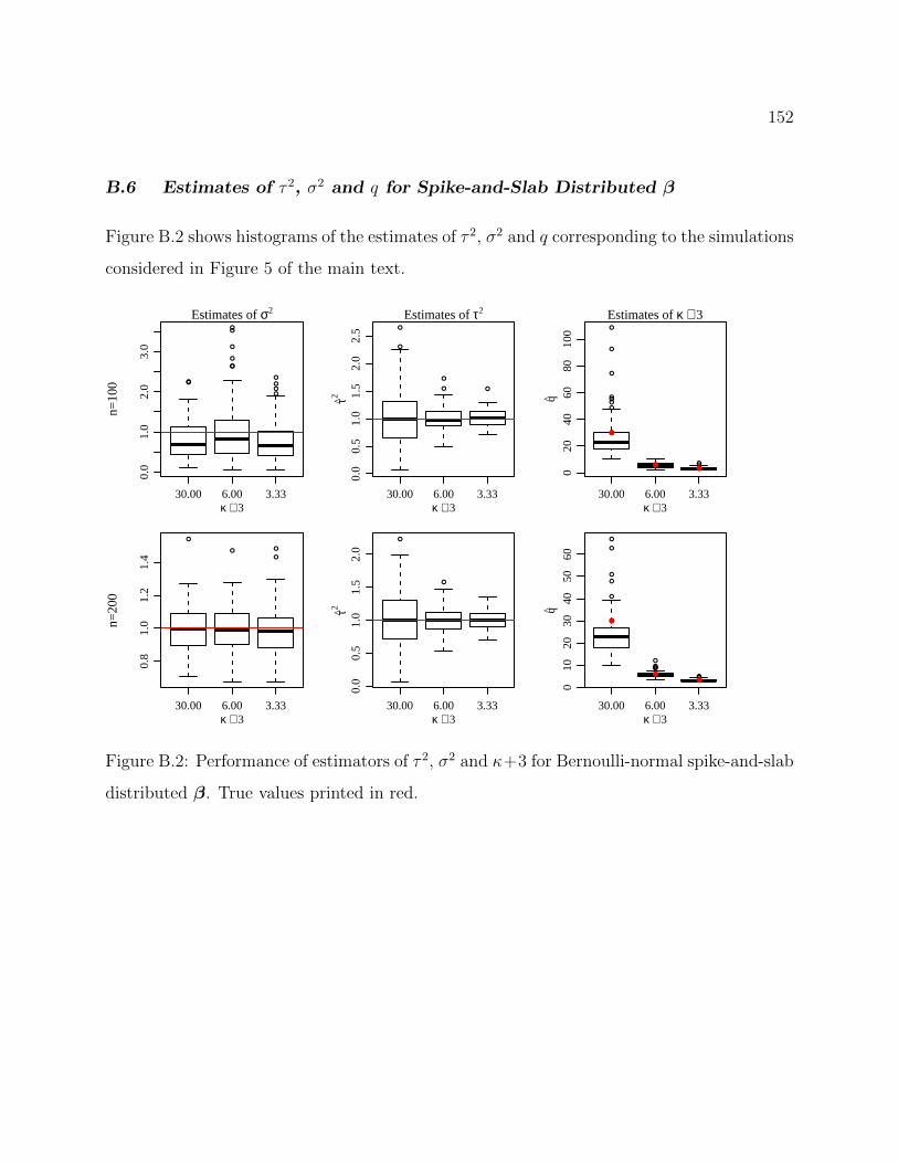
152

B.6 Estimates of τ 2, σ2 and q for Spike-and-Slab Distributed β

Figure B.2 shows histograms of the estimates of τ 2, σ2 and q corresponding to the simulations

considered in Figure 5 of the main text.

30.00 6.00 3.33

0.0

1.0

2.0

3.0

κ + 3

n=10

0

Estimates of σ2

30.00 6.00 3.33

0.0

0.5

1.0

1.5

2.0

2.5

κ + 3

τ2

Estimates of τ2

30.00 6.00 3.33

020

4060

8010

0

κ + 3

q

Estimates of κ + 3

30.00 6.00 3.33

0.8

1.0

1.2

1.4

κ + 3

n=20

0

30.00 6.00 3.33

0.0

0.5

1.0

1.5

2.0

κ + 3

τ2

30.00 6.00 3.33

010

2030

4050

60

κ + 3

q

Figure B.2: Performance of estimators of τ 2, σ2 and κ+3 for Bernoulli-normal spike-and-slab

distributed β. True values printed in red.

153

Appendix C

SUPPLEMENT TO “STRUCTURED SHRINKAGE PRIORS”

C.1 Univariate Marginal Distributions

Intuitively, it is clear from the stochastic representation that the marginal distributions are

the same as the corresponding univariate shrinkage prior. We can show this directly as

follows. The joint marginal prior distribution of β is

pβ (β) =

∫p (s) p (β/s)

(p∏j=1

1

|sj|

)ds1 . . . dsp

Then pβ1 (β1) is given by

pβ1 (β1) =

∫p (β1/s1) p

(β−1/s−1|β1/s1

)( p∏j=1

p (sj)

|sj|

)ds1 . . . dspdβ2 . . . dβp

=

∫p (β1/s1) p (s1) / |s1|

(∫p(β−1/s−1|β1/s1

)( p∏j=2

p (sj)

|sj|

)ds2 . . . dspdβ2 . . . dβp

)︸ ︷︷ ︸

(∗)

ds1.

The term (∗) is equal to∫p(β−1|β1/s1

)dβ2 . . . dβp. This is the integral of a density, and

accordingly (∗) = 1 and pβ1 =∫p (β1/s1) p (s1) / |s1| ds1.

C.2 Proofs of Propositions 2.1 and 2.3

First, we prove the following lemma:

Lemma C.2.1 For α > 0 and γ ∈ R,∫∞−∞

1|s|exp−α(s2 − γs)ds = +∞.

First let’s consider this integral when γ > 0:∫ ∞−∞

1

|s|exp

−α(s2 − γs

)ds =

∫ 0

−∞−1

sexp −αss−γ ds+∫ γ

0

1

sexp −αss−γ ds+

∫ ∞γ

1

sexp −αss−γ ds.

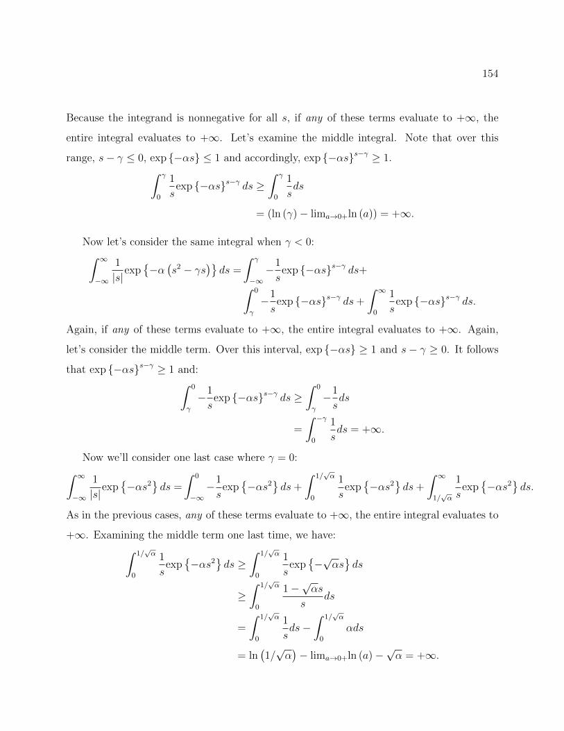
154

Because the integrand is nonnegative for all s, if any of these terms evaluate to +∞, the

entire integral evaluates to +∞. Let’s examine the middle integral. Note that over this

range, s− γ ≤ 0, exp −αs ≤ 1 and accordingly, exp −αss−γ ≥ 1.∫ γ

0

1

sexp −αss−γ ds ≥

∫ γ

0

1

sds

= (ln (γ)− lima→0+ln (a)) = +∞.

Now let’s consider the same integral when γ < 0:∫ ∞−∞

1

|s|exp

−α(s2 − γs

)ds =

∫ γ

−∞−1

sexp −αss−γ ds+∫ 0

γ

−1

sexp −αss−γ ds+

∫ ∞0

1

sexp −αss−γ ds.

Again, if any of these terms evaluate to +∞, the entire integral evaluates to +∞. Again,

let’s consider the middle term. Over this interval, exp −αs ≥ 1 and s− γ ≥ 0. It follows

that exp −αss−γ ≥ 1 and:∫ 0

γ

−1

sexp −αss−γ ds ≥

∫ 0

γ

−1

sds

=

∫ −γ0

1

sds = +∞.

Now we’ll consider one last case where γ = 0:∫ ∞−∞

1

|s|exp

−αs2

ds =

∫ 0

−∞−1

sexp

−αs2

ds+

∫ 1/√α

0

1

sexp

−αs2

ds+

∫ ∞1/√α

1

sexp

−αs2

ds.

As in the previous cases, any of these terms evaluate to +∞, the entire integral evaluates to

+∞. Examining the middle term one last time, we have:∫ 1/√α

0

1

sexp

−αs2

ds ≥

∫ 1/√α

0

1

sexp

−√αsds

≥∫ 1/

√α

0

1−√αs

sds

=

∫ 1/√α

0

1

sds−

∫ 1/√α

0

αds

= ln(1/√α)− lima→0+ln (a)−

√α = +∞.

155

Proof of Proposition 2.1: Now we can evaluate the marginal density pβ(b|Ω,Ψ) when

bj = 0 for some j ∈ 1, . . . , p. Without loss of generality, set β1 = 0. Letting b−1 and s−1

refer to the vectors b and s each with the first element removed, (Ω−1)−1,−1 be the matrix

Ω−1 with the first row and column removed, (Ψ−1)−1,−1 be the matrix Ψ−1 with the first row

and column removed and (Ψ−1)−1,1 be the first column of Ψ−1 excluding the first element.

For b = (0, b−1),

pβ ((0, b−1) |Ψ,Ω) ∝∫

1∏pi=1 |si|

exp

−1

2

(b′diag 1/sΩ−1diag 1/s b+ s′Ψ−1s

)ds

=

∫1∏p

2=1 |si|exp

−1

2

(b′−1diag 1/s−1

(Ω−1

)−1,−1 diag 1/s−1 b−1 + s

′−1(Ψ−1

)−1,−1 s−1

)∫ ∞−∞

1

|s1|exp

−1

2

(s21(Ψ−1

)11− 2s1

(Ψ−1

)′−1,1 s−1

)ds1︸ ︷︷ ︸

(∗)

ds−1.

Applying Lemma C.2.1, the term denoted by (∗) evaluates to +∞ for every value of s−1.

Proof of Proposition 2.3: Proposition 2.3 follows from Proposition 2.1 and

Lemma C.2.1. Again, letting β1 = 0, for β = (0,β−1),

pβ1 (0|Ψ,Ω) ∝∫

1∏pi=1 |si|

exp

−1

2

(β′diag 1/sΩ−1diag 1/sβ + s′Ψ−1s

)dsdβ−1

=

∫1∏p

2=1 |si|exp

−1

2

(β′−1diag 1/s−1

(Ω−1

)−1,−1 diag 1/s−1β−1 + s

′−1(Ψ−1

)−1,−1 s−1

)∫ ∞−∞

1

|s1|exp

−1

2

(s21(Ψ−1

)11− 2s1

(Ψ−1

)′−1,1 s−1

)ds1︸ ︷︷ ︸

(∗)

ds−1dβ−1.

Again, (∗) evaluates to +∞ for any value of s−1 and does not depend at all on β−1.

C.3 Expectation of sj when s2j ∼ gamma(c, c)

When s2j ∼ gamma(c, c), we have:∫ ∞

0

sjcc

Γ (c)

(s2j

)c−1exp

−cs2

j

ds2

j =cc

Γ (c)

∫ ∞0

(s2j

)c+1/2−1exp

−cs2

j

ds2

j

=

(ccΓ (c+ 1/2)

cc+1/2Γ (c)

)= c−1/2 (Γ (c+ 1/2) /Γ (c))

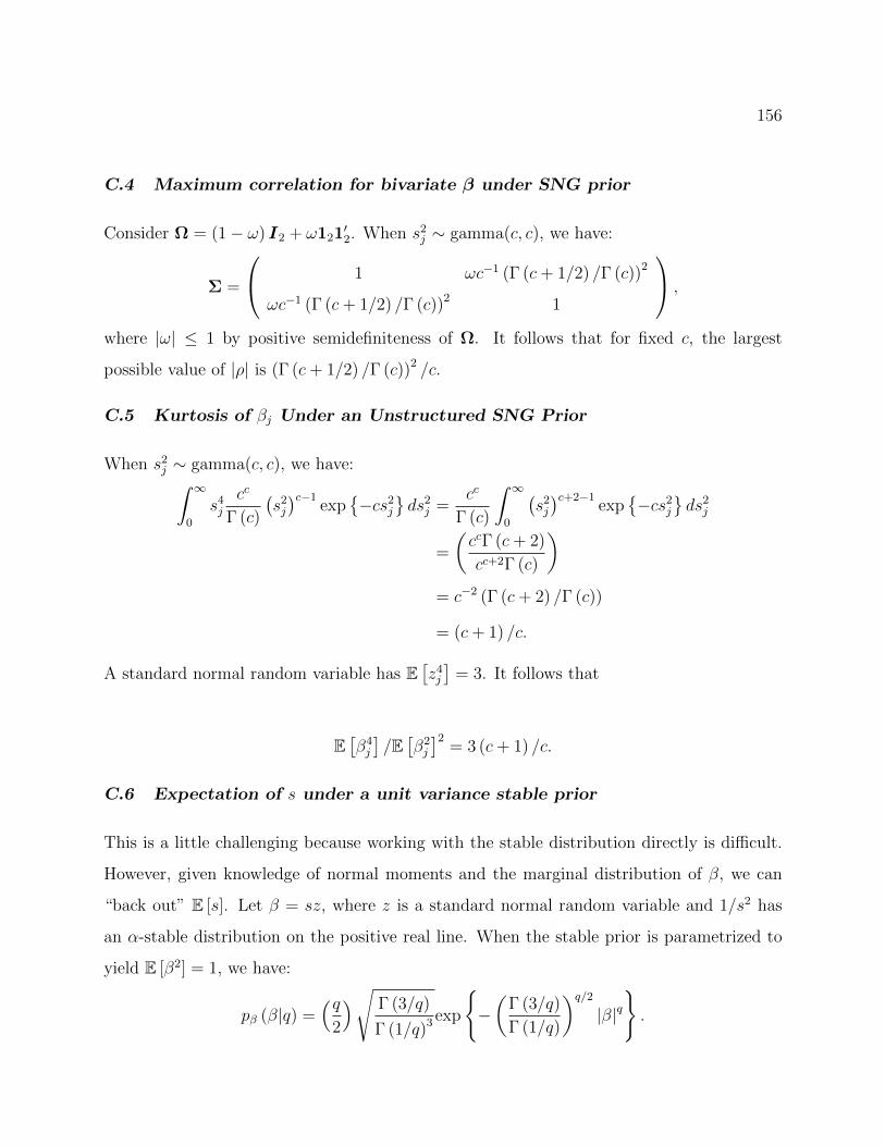
156

C.4 Maximum correlation for bivariate β under SNG prior

Consider Ω = (1− ω) I2 + ω121′2. When s2

j ∼ gamma(c, c), we have:

Σ =

1 ωc−1 (Γ (c+ 1/2) /Γ (c))2

ωc−1 (Γ (c+ 1/2) /Γ (c))2 1

,

where |ω| ≤ 1 by positive semidefiniteness of Ω. It follows that for fixed c, the largest

possible value of |ρ| is (Γ (c+ 1/2) /Γ (c))2 /c.

C.5 Kurtosis of βj Under an Unstructured SNG Prior

When s2j ∼ gamma(c, c), we have:∫ ∞

0

s4j

cc

Γ (c)

(s2j

)c−1exp

−cs2

j

ds2

j =cc

Γ (c)

∫ ∞0

(s2j

)c+2−1exp

−cs2

j

ds2

j

=

(ccΓ (c+ 2)

cc+2Γ (c)

)= c−2 (Γ (c+ 2) /Γ (c))

= (c+ 1) /c.

A standard normal random variable has E[z4j

]= 3. It follows that

E[β4j

]/E[β2j

]2= 3 (c+ 1) /c.

C.6 Expectation of s under a unit variance stable prior

This is a little challenging because working with the stable distribution directly is difficult.

However, given knowledge of normal moments and the marginal distribution of β, we can

“back out” E [s]. Let β = sz, where z is a standard normal random variable and 1/s2 has

an α-stable distribution on the positive real line. When the stable prior is parametrized to

yield E [β2] = 1, we have:

pβ (β|q) =(q

2

)√ Γ (3/q)

Γ (1/q)3 exp

−(

Γ (3/q)

Γ (1/q)

)q/2|β|q.

157

Now, to determine E [s], note that E [|β|] = E [s]E [|z|]. We have

E [|β|] = 2

∫ ∞0

βpβ (β|q) dβ

= q

√Γ (3/q)

Γ (1/q)3

∫ ∞0

βexp

−(

Γ (3/q)

Γ (1/q)

)q/2βq

dβ

=

(√Γ (3/q)

Γ (1/q)3

)(Γ (2/q) Γ (1/q)

Γ (3/q)

)=

Γ (2/q)√Γ (1/q) Γ (3/q)

.

According to Wikipedia, E [|z|] =√

2/π. It follows that

E [s] =

√π

2

(Γ (2/q)√

Γ (1/q) Γ (3/q)

).

C.7 Maximum correlation for bivariate β under SPB prior

Consider Ω = (1− ω) I2 + ω121′2. We have:

Σ =

1 ω(π2

)( Γ(2/q)√Γ(1/q)Γ(3/q)

)2

ω(π2

)(Γ(2/q)√

Γ(1/q)Γ(3/q)

)2

1

,

where |ω| ≤ 1 by positive semidefiniteness of Ω. It follows that for fixed q, the largest

possible value of |ρ| is(π2

)( Γ(2/q)√Γ(1/q)Γ(3/q)

)2

.

C.8 Proofs of Propositions 2.2 and 2.4

First, we prove the following lemma:

Lemma C.8.1 For 0 < c < 1/2,∫∞

0(s2)c−1/2−1exp −cs2 ds2 = +∞.

We can break the integral into two nonnegative components, as follows:∫ ∞0

(s2)c−1/2−1exp−cs2

ds2 =

∫ 1/c

0

(s2)c−1/2−1exp−cs2

ds2 +

∫ ∞1/c

(s2)c−1/2−1exp−cs2

ds2.

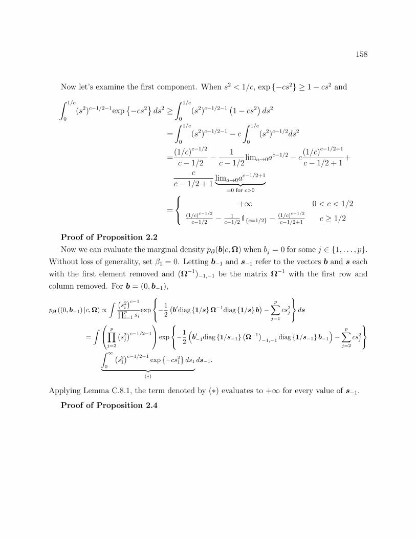
158

Now let’s examine the first component. When s2 < 1/c, exp −cs2 ≥ 1− cs2 and∫ 1/c

0

(s2)c−1/2−1exp−cs2

ds2 ≥

∫ 1/c

0

(s2)c−1/2−1(1− cs2

)ds2

=

∫ 1/c

0

(s2)c−1/2−1 − c∫ 1/c

0

(s2)c−1/2ds2

=(1/c)c−1/2

c− 1/2− 1

c− 1/2lima→0a

c−1/2 − c(1/c)c−1/2+1

c− 1/2 + 1+

c

c− 1/2 + 1lima→0a

c−1/2+1︸ ︷︷ ︸=0 for c>0

=

+∞ 0 < c < 1/2

(1/c)c−1/2

c−1/2− 1

c−1/21c=1/2 − (1/c)c−1/2

c−1/2+1c ≥ 1/2

Proof of Proposition 2.2

Now we can evaluate the marginal density pβ(b|c,Ω) when bj = 0 for some j ∈ 1, . . . , p.Without loss of generality, set β1 = 0. Letting b−1 and s−1 refer to the vectors b and s each

with the first element removed and (Ω−1)−1,−1 be the matrix Ω−1 with the first row and

column removed. For b = (0, b−1),

pβ ((0, b−1) |c,Ω) ∝∫ (

s2i)c−1∏pi=1 si

exp

−1

2

(b′diag 1/sΩ−1diag 1/s b

)−

p∑j=1

cs2j

ds

=

∫ p∏j=2

(s2j)c−1/2−1 exp

−1

2

(b′−1diag 1/s−1

(Ω−1

)−1,−1 diag 1/s−1 b−1

)−

p∑j=2

cs2j

∫ ∞0

(s21)c−1/2−1

exp−cs21

ds1︸ ︷︷ ︸

(∗)

ds−1.

Applying Lemma C.8.1, the term denoted by (∗) evaluates to +∞ for every value of s−1.

Proof of Proposition 2.4

159

Proposition 2.4 follows from Proposition 2.2 and Lemma C.8.1. For β = (0,β−1),

pβ1(0|c,Ω) ∝

∫ (s2i)c−1∏pi=1 si

exp

−1

2

(β′diag 1/sΩ−1diag 1/sβ

)−

p∑j=1

cs2j

dsdβ−1

=

∫ p∏j=2

(s2j)c−1/2−1 exp

−1

2

(β′−1diag 1/s−1

(Ω−1

)−1,−1 diag 1/s−1β−1

)−

p∑j=2

cs2j

∫ ∞0

(s21)c−1/2−1

exp−cs21

ds1︸ ︷︷ ︸

(∗)

ds−1dβ−1.

Again, (∗) evaluates to +∞ for any value of s−1 and does not depend at all on β−1.

C.9 Alternative Approaches to Posterior Computation

Gibbs sampling is very straightforward when the SPN prior is used, as the full conditional

distributions ps|z(s|z,y,X,Ψ, σ2) and pz|s(z|s,y,X,Ω, σ2) are multivariate normal distri-

butions. Exact full conditional distributions are given in the appendix.

Posterior inference for the SNG and SPB priors is more challenging than posterior infer-

ence for the SPN prior, as there is not an obvious stochastic representation of β that yields

tractable full conditional distributions for elements of s. Under the SNG and SPB priors

we have β|s ∼ normal(0, diagsΩdiags), so the full conditional distribution of β is a

multivariate normal distribution. Letting psj (sj|θ) refer to the prior density of s under an

SPB or SNG prior and letting θ refer to the corresponding prior parameter, c or q, the full

conditional distribution of s is

ps (s|β,Ω, θ) ∝ exp

−1

2

p∑j=1

p∑j′=1,j′ 6=j

βjβj′

ωjj′sjsj′

︸ ︷︷ ︸

(∗)

p∏j=1

(psj (sj|θ)

sj

)exp

−1

2

(1

s2j

(β2j

ωjj

))︸ ︷︷ ︸

(∗∗)

,

where ωjj is the entry in the i-th row and j-th column of of Ω−1. This is not a standard

distribution under either the SNG or SPB priors, either for the entire vector s or for each

element of sj conditional on the remaining elements s−j. However, the term (∗) is a simple

function of elements of s that is monotonic for in each sj conditional on the remaining

160

elements s−j, and the term (∗∗) is a product of p densities that are straightforward to

simulate from. Under the SNG prior, (∗∗) is a product of p generalized inverse gaussian

densities and under the SPB prior, (∗∗) is a product of p exponentially tilted positive α-

stable densities. Accordingly, the auxiliary variable method introduced by Damien et al.

(1999) can be used. We define a new variable u > 0, such that

ps2,u(s2, u|β,Ω, θ

)∝ 1

u<exp

− 1

2

∑pj=1

∑p

j′=1,j′ 6=j

βjβj′

ωjj′sjsj′

p∏j=1

(psj (sj|θ)

sj

)exp

−1

2

(1

s2j

(β2j

ωjj

)).

We can simulate from the full conditional distribution p (s|β,Ω, c) by drawing a value of u

at the current value of s from a uniform distribution on (0, exp−12

∑pj=1

∑pj′=1,j′ 6=j

βjβj′

ωjj′sjsj′)

and then drawing each value of sj at the current value of u and remaining values s−j from a

truncated generalized inverse Gaussian distribution or exponentially tilted positive α-stable

distribution that satisfies the constraint u < exp−12

∑pj=1

∑pj′=1,j′ 6=j

βjβj′

ωjj′sjsj′. Importantly,

this constraint can be rewritten as a bound on each sj at the current value of u and remaining

values s2−j as follows:

sj

(log (u) +

1

2

p∑j′=1,j′ 6=j

p∑j′′=1,j′′ 6=j,j′

βj′βj′′

ωj′j′′sj′sj′′

)︸ ︷︷ ︸

aj

< −1

2

p∑j′=1,j′ 6=j

βjβj′

ωjj′sj′︸ ︷︷ ︸dj

.

The constraint on sj is sj < dj/aj if aj > 0 and sj > dj/aj otherwise. The ability to

obtain explicit constraints on each sj is advantageous because it can yield efficiency gains

if a fast method for simulating from a left- or right-truncated generalized inverse Gaussian

distribution or exponentially tilted positive α-stable distribution is available. We are able to

construct such a method for simulating from truncated generalized inverse Gaussian distribu-

tions and describe it in the appendix. Sampling from truncated exponentially tilted positive

α-stable distributions is more challenging, as the positive α-stable density does not have a

closed form. For this paper, we take the naive approach of simulating from a truncated

exponentially tilted positive α-stable distribution until the constraint is satisfied.

161

C.10 Univarate Slice Sampling

In several places in this paper, we use a univariate slice sampling algorithm described in

Neal (2003) to simulate values of a random variable x ∈ [a, b] with density proportional to

exp g (x). Given a previous value x, we can simulate a new value x′ from a full conditional

using univariate slice sampling as follows:

1. Draw e ∼ exp (1).

2. Draw d ∼ uniform (a, b).

• If g (x)− e ≤ g (d), set x′ = d.

• If g (x)− e > g (d):

(a) If d < x, set a = d, else if d ≥ x set b = d.

(b) Return to 3.

C.11 Simulation from Full Conditional Distribution for δj

When using the SPB prior, we have s2j

d= Γ (1/ (2α)) ξ

1−αα

j / (2Γ (3/ (2α))), where ξj ∼

gamma ((1 + α) / (2α) , f (δj|α)) and pδj (δj|α) ∝ f (δj|α)α−12α on (0, π). Suppose s2

j is fixed.

Then ξj =(2Γ (3/ (2α)) s2

j/Γ (1/ (2α))) α

1−α . Then we can write the full conditional distribu-

tion of δj as

p (δj|ξj, q) ∝f (δj|α)1+α2α exp −f (δj|α) ξj f (δj|α)

α−12α

=f (δj|α) exp −f (δj|α) ξj .

Apply the univariate slice sampling algorithm described in Section C.10 using g (x) =

log (f (x|α))− f (x|α) ξj and initial values a = 0 and b = π.

C.12 Simulation from Full Conditional Distribution for ρ

In the real data application, I consider the setting where B and S are p1 × p2 matrices and

β = vec (B/S) has covariance matrix V [β/s] = Ω2 ⊗Ω1, where Ω1 is depends on a single

162

autoregressive parameter, ρ, with ω1,ij = ρ|i−j|. The full conditional distribution of ρ is:

pρ (ρ|−) ∝ |Ω1|−p22 exp

−1

2tr(Ω−1

1 (B/S) Ω−12 (B/S)

)=(1− ρ2

)− (p1−1)p22 exp

−1

2tr(Ω−1

1 (B/S) Ω−12 (B/S)

)πρ (ρ) ,

where elements of Ω−11 are given by

ω111 = ωpp1 =

(1− ρ2

)−1

ωjj1 =(1− ρ2

)−1 (1 + ρ2

)j 6= 1, j 6= p

ωjk1 = −ρ(1− ρ2

)−1 |j − k| = 1

and πρ (ρ) is the density of an assumed prior distribution for ρ. We assume a uniform prior

on (−1, 1), i.e. beta (1, 1) prior for (ρ+ 1) /2.

C.13 Prior Conditional Distribution of s2j |δj and sj|δj under SPB Prior

When using the SPB prior, we have s2j

d= Γ (1/ (2α)) ξ

1−αα

j / (2Γ (3/ (2α))), where ξj ∼

gamma ((1 + α) / (2α) , f (δj|α)) and pδj (δj|α) ∝ f (δj|α)α−12α on (0, π). We want to com-

pute the prior conditional distribution πs2j(s2j |δj, α

)for use in the elliptical slice sampler for

s. We have:

s2jd=Γ (1/ (2α)) ξ

1−αα

j / (2Γ (3/ (2α)))

=(

(Γ (1/ (2α)) / (2Γ (3/ (2α))))α

1−α ξj

) 1−αα

d=ξ

1−αα

j , ξj ∼ gamma

1 + α

2α,

(2Γ(

32α

)Γ(

12α

) ) α1−α

f (δj|α)

We can find the density of s2j via change of variables. We have

ξj =(s2j

) α1−α , dξj =

(α

1− α

)(s2j

) α1−α−1

ds2j .

163

Then the prior conditional distribution is

πs2j(s2j |δj, α

)∝((s2j

) α1−α) 1+α

2α−1 (

s2j

) α1−α−1

exp

−(

2Γ(

32α

)s2j

Γ(

12α

) ) α1−α

f (δj|α)

=(s2j

) 1+α2(1−α)−1

exp

−(

2Γ(

32α

)s2j

Γ(

12α

) ) α1−α

f (δj|α)

.

In practice, we end up working with sj, so once more

πsj (sj|δj, α) ∝s1+α1−α−1

j exp

−(

2Γ(

32α

)s2j

Γ(

12α

) ) α1−α

f (δj|α)

.

C.14 Prior Conditional Distribution of sj under SNG Prior

Under the SNG prior, we have

πs2j(s2j |c)∝(s2j

)c−1exp

−s2

jc.

In practice, we end up working with sj, which has the density

πsj (sj|c) ∝ (sj)2c−1 exp

−s2

jc.

164

VITA

<Insert information about myself here.>