c copyright by manki cho august, 2014

c©Copyright by

Manki Cho

August, 2014

STEKLOV EIGENPROBLEMS AND APPROXIMATIONS

OF HARMONIC FUNCTIONS

A Dissertation

Presented to

the Faculty of the Department of Mathematics

University of Houston

In Partial Fulfillment

of the Requirements for the Degree

Doctor of Philosophy

By

Manki Cho

August, 2014



Manki Cho

Approved:

Dr. Giles Auchmuty (Committee Chair)Department of Mathematics, University of Houston

Committee Members:

Dr. Tsorng-Whay PanDepartment of Mathematics, University of Houston

Dr. Daniel OnofreiDepartment of Mathematics, University of Houston

Dr. Ralph William MetcalfeDepartment of Mechanical Engineering


Dean, College of Natural Sciences and Mathematics


ii

Acknowledgements

I would like to sincerely thank my Ph.D. thesis advisor, Dr. Giles Auchmuty,

for his never-ending encouragement, support, inspiration, and patience. Dr. Giles

Auchmuty has taught me everything that I know about partial differential equations

and he helped me to be a better mathematician. I feel extremely honored to do my

research under his guidance. Moreover, I acknowledge him for his concerns about my

family. I would never forget his care about my family.

I would also like to express my gratitude to my committee members, Dr. Tsorng-

Whay Pan, Dr. Daniel Onofrei, and Dr. Ralph Metcalfe for spending their times to

read my thesis carefully and for the valuable comments and suggestions. I am also

very thankful to all the academic and administrative members in the Department of

Mathematics at the University of Houston. In particular, I would like to thank Dr.

Shanyu Ji for his support and care during my graduate years. I would like to thank

all my fellow graduate students for sharing and spending their times with me.

I dedicate the thesis to my parents and family. My parents, Sungoh Cho and

Myoeung Kim and my younger brother, Youngki Cho have always loved, encouraged,

and supported me. There is no word that I could describe my love to my lovely wife,

Mikyoung Park. Without her, this work could never have been done. Special thanks

go to my adorable babies, Yena Cho and Mason Yongjae Cho for their love and smiles.

iii



An Abstract of a Dissertation

Presented to

the Faculty of the Department of Mathematics


In Partial Fulfillment

of the Requirements for the Degree

Doctor of Philosophy

By

Manki Cho

August, 2014

iv

Abstract

In this work, we provide explicit formulae for harmonic Steklov eigenvalues and

associated Steklov eigenfunctions by solving a Steklov eigenproblem on bounded rect-

angles in R2. This allows the description of all the Steklov eigenvalues and their

corresponding Steklov eigenfunctions.

The harmonic Steklov eigenfunctions provide orthogonal sets in H1(Ω) and com-

plete orthonormal bases of L2(∂Ω, dσ). This enables us to study Steklov eigenfunc-

tion expansions of harmonic functions. Comparing against the expansion in terms

of Neumann eigenfunctions, the Steklov expansions usually converge faster than the

Neumann expansions. Results are described by relative errors of finite terms of each

expansion with respect to the L2, L∞, and gradient norms.

Solutions of Laplace’s equation subject to inhomogeneous Dirichlet, Neumann,

Robin, or other boundary data are approximated by Steklov expansions. These rep-

resentations involve boundary conditions and explicit spectral approximations are

found.

In the end, we provide the general formulae for u(0, 0) where harmonic functions

u(x, y) are solutions of boundary value problems on a rectangle. These harmonic

functions are determined precisely in terms of their respective boundary data.

v

Contents

Abstract v

1 Introduction 1

2 Assumptions, Definitions, and Notations 4

3 Harmonic Steklov Eigenvalues and Eigenfunctions 7

3.1 Analytic Solutions of the Steklov Eigenproblem . . . . . . . . . . . . 7

3.2 Families of Steklov Eigenfunctions . . . . . . . . . . . . . . . . . . . . 9

3.3 The Determining Equations . . . . . . . . . . . . . . . . . . . . . . . 16

3.4 A Special Solution . . . . . . . . . . . . . . . . . . . . . . . . . . . . 20

3.5 The Ordering of Eigenfunctions and Eigenvalues . . . . . . . . . . . . 21

3.6 Normalized Steklov Eigenfunctions . . . . . . . . . . . . . . . . . . . 25

4 Spectral Representations for Harmonic Functions 32

4.1 The Steklov Expansion . . . . . . . . . . . . . . . . . . . . . . . . . . 32

4.2 Relative Errors for the Steklov Expansion . . . . . . . . . . . . . . . 35

5 Solutions of Boundary Value Problems on Ω 47

5.1 The Harmonic Dirichlet Problem . . . . . . . . . . . . . . . . . . . . 47

vi

5.2 The Harmonic Neumann Problem . . . . . . . . . . . . . . . . . . . . 56

5.3 The Harmonic Robin Problem . . . . . . . . . . . . . . . . . . . . . . 60

5.4 The Generalized Boundary Data . . . . . . . . . . . . . . . . . . . . . 67

6 An Application of the Steklov Expansion 69

6.1 The Mean Value Property . . . . . . . . . . . . . . . . . . . . . . . . 69

6.2 The Correction Term . . . . . . . . . . . . . . . . . . . . . . . . . . . 74

6.3 Several Examples . . . . . . . . . . . . . . . . . . . . . . . . . . . . . 76

Bibliography 82

vii

Chapter 1

Introduction

In this thesis, we mainly study harmonic functions that are solutions of Laplace’s

equation on bounded regions in R2. Combined with boundary data which may be of

Dirichlet, Neumann, or Robin type, there are many questions how harmonic functions

can be determined by their respective boundary conditions. Eigenvalue analyses

have been studied to provide spectral representations. In Section 9 and 10 of [1],

applications and some results of Steklov eigenproblems for prototypical second order

elliptic partial differential operators on the regions in R2 were described. For these

eigenproblems, the existence of an infinite and discrete spectrum is demonstrated.

We begin in Chapter 3 with a Steklov eigenproblem on bounded rectangle Ω =

[−L,L]× [−Lh, Lh] for non zero constants L and h. The first positive eigenvalue and

a corresponding eigenfunction of this problem may be found by variational principles.

The description is developed in Section 3 of [1] and a different variational principle

is described in Chapter 3 of [6]. Separation of variables of (x, y) ∈ R2 will be used

to provide explicit formulae for all Steklov eigenvalues and corresponding Steklov

eigenfunctions. Determining equations will be derived from the boundary condition

1

CHAPTER 1. INTRODUCTION

and their solutions are involved in Steklov eigenvalues and eigenfunctions.

Families of Steklov eigenfunctions are described and classified by their boundary

functions. The maximal orthonormal set in L2(∂Ω, dσ) will be constructed by the

boundary values of Steklov eigenfunctions. Also Steklov eigenfunctions provide an

orthogonal basis of the space of all harmonic functions on Ω with respect to a special

inner product. These results lead to orthogonal series expansion, in terms of the

Steklov eigenfunctions, for harmonic functions. The approximations depend only on

the boundary values. This series converges strongly in H1(Ω) with respect to the

∂-inner product.

In Chapter 4 the Neumann eigenproblem is introduced and eigenfunctions of this

problem will be normalized with respect to L2(Ω). The Steklov expansion will be

compared against the Neumann expansion, defined by the set of Neumann eigenfunc-

tions, for harmonic functions. Numerical experiments support that the M-th partial

sum of the Setklov expansion converges faster than the Neumann one.

These results will be used to describe Steklov spectral representation of solutions of

Laplace’s equation with non homogeneous boundary conditions. Dirichlet, Neumann

and Robin type boundary conditions are considered and generalized in Chapter 5.

Results about completeness of these representations rely on that the set of Steklov

eigenfunctions may provide an orthonormal basis of L2(∂Ω, dσ) and also an orthogonal

basis of the space of harmonic functions on Ω.

An approximated solution defined by the finite partial sum of series expansion

will be used to describe the unique solution of boundary valued problems. For each

problem, numerical experiments will be implemented and support the description

of solutions in Ω. Harmonic functions which have complicated boundary functions

are considered and experiments implies that only a few terms are required to obtain

2

CHAPTER 1. INTRODUCTION

pointwise approximations of the solutions.

In Chapter 6 we study correction terms for the mean value property of harmonic

functions. This yields approximations of u(0, 0) in a certain boundary value problem.

Finally we show that the Steklov expansion provides other general formulae for u(0, 0)

where u(x, y) are solutions of Laplace’s equation with non zero boundary conditions.

3

Chapter 2

Assumptions, Definitions, and

Notations

In this dissertation, a region Ω is a rectangle in R2. The closure of a region is denoted

Ω and its boundary is ∂Ω := Ω \ Ω. We shall assume that Ω is bounded in R2 and

∂Ω is compact and Lipschitz.

Here dσ will represent Hausdorff one-dimensional measure of arc-length and ν is

the outward unit normal at points of ∂Ω. All functions in this work will take value

in [−∞,∞].

Let p ∈ [1,∞] then the real Lebesgue spaces Lp(Ω) and Lp(∂Ω, dσ) are defined

in the standard manner with their usual p-norm denoted by ||u||p and ||u||p,∂Ω, re-

spectively. In addition, for the case when p = 2, L2(Ω) and L2(∂Ω) are real Hilbert

spaces with respect to their respective inner products

< u, v >2,Ω:=

∫Ω

u(x)v(x) dx and < u, v >2,∂Ω:=∫−∂Ωuv dσ (2.1)

4

CHAPTER 2. ASSUMPTIONS, DEFINITIONS, AND NOTATIONS

Here∫−∂Ωuv dσ = | 1

∂Ω|∫∂Ωuv dσ where |∂Ω| is the perimeter of the boundary. Denote

the mean value of a function u on the boundary by u :=∫−∂Ωu dσ.

W 1,p(Ω) denotes the standard Sobolev space of functions on Ω that are in Lp(Ω)

and whose weak derivatives D1u and D2u are in L2(Ω). It is a real Banach space

under the standard W 1,p-norm

||u||W 1,p(Ω) := (

∫Ω

|u|p + |∇u|pdx)1p (2.2)

where ∇u is the gradient of the function u.

We mainly use the space H1(Ω) that is the usual real Sobolev space of functions

on Ω corresponding to W 1,2(Ω). It is a real Hilbert space under the standard H1-inner

product

[u, v]1 =

∫Ω

[u(x) · v(x) +∇u(x) · ∇v(x)]dx (2.3)

and the associated norm is denoted by ||u||1,2.

The trace of a continuous function on Ω to the boundary ∂Ω is its restriction to ∂Ω.

The trace map of H1(Ω) to a class of functions on ∂Ω is the linear extension of the map

restricting Lipschitz continuous functions on Ω to ∂Ω. The region Ω is said to satisfy

a compact trace theorem provided that the trace mapping Γ : H1(Ω) → L2(∂Ω, dσ)

is compact(see Chapter 2 of [17]). Sometimes u will be used in place of Γu when

considering the trace of a function on ∂Ω. These results are for general u. When

u ∈ W 1,1(Ω), the trace of u on ∂Ω is well-defined. Also it is a Lebesgue integrable

function with respect to σ, more details may be found in Section 4.2 of [16].

Evans and Gariepy (see p133, Theorem 1 of [16]) show that Γ is continuous, and

Grisvard (see Theorem 1.5.1.10 of [11]) proves an inequality that implies this compact

trace result. Also, DiBenedetto (see Chapter ix, Section 18 of [8]) provides result of

5

CHAPTER 2. ASSUMPTIONS, DEFINITIONS, AND NOTATIONS

this type.

The region Ω considered in this work satisfies the compact trace theorem.

Instead of (2.3), we will mainly use the ∂-inner product

[u, v]∂ :=

∫Ω

∇u · ∇v dx+∫−∂Ωuv dσ (2.4)

The corresponding norm is denoted by ||u||∂. From Corollary 6.2 of [1], this norm is

equivalent to the standard norm of H1(Ω). And this is part of Theorem 21A of [21].

A function u ∈ H1(Ω) is said to be harmonic on Ω if it satisfies

∫Ω

∇u · ∇v dx = 0 for all v ∈ C1c (Ω) (2.5)

where C1c (Ω) is the set of all C1-functions on Ω with compact support in Ω.

H(Ω) is defined to be the space of all harmonic functions on Ω. Then the usual

Sobolev space H10 (Ω) is the closure of C1

c (Ω) in H1(Ω)-norm. It is easy to see that

H(Ω) is ∂-orthogonal to H10 (Ω) also H1(Ω) may be expressed as

H1(Ω) = H10 (Ω)⊕∂ H(Ω) (2.6)

Here ⊕∂ represents a ∂-orthogonal decomposition. Zeidler provides the discussion

about this result in Section 22.4 of [21].

In this work, we will use the letter e to specify a power-of-ten scale factor. All

boundary and area integrals in thesis are computed approximately on Matlab(see [12])

by using adaptive Simpson’s method(see Chapter 6 of [7]) with a tolerance, e−6.

6

Chapter 3

Harmonic Steklov Eigenvalues and

Eigenfunctions

3.1 Analytic Solutions of the Steklov Eigenprob-

lem

Let Ω be the two-dimensional rectangle [−L,L]×[−Lh, Lh] in the xy-plane for positive

constants L and h. Here h is called the aspect ratio. Denote the boundary segments

by Γ1 for y = −Lh, Γ2 for x = L, Γ3 for y = Lh, and Γ4 for x = −L (see Figure

(3.1)).

Consider the problem of finding non trivial functions s(x, y) ∈ H1(Ω) and the real

values δ that satisfy

∆s = 0 in Ω (3.1)

Dνs = δs on ∂Ω (3.2)

7

3.1 ANALYTIC SOLUTIONS OF THE STEKLOV EIGENPROBLEM

x axis

y axis

Γ2

Γ3

Γ4

Γ1

Figure 3.1: The boundary segments of Ω

Here ∆ is the Laplacian and Dνs is the unit outward normal derivative of s on the

boundary. A non-zero function s(x, y) ∈ H1(Ω) is said to be a harmonic Steklov

eigenfunction on Ω corresponding to the harmonic Steklov eigenvalue δ.

The weak form of (3.1)-(3.2) is to find (δ, s) in R×H1(Ω) satisfying

∫Ω

∇s · ∇v dx = δ

∫∂Ω

sv dσ for all v ∈ H1(Ω) (3.3)

This harmonic Steklov eigenproblem has been studied for a long time, particularly

as it has been treated for the sloshing of a perfect fluid in a tank(see Fox and Kutter

[10] or McIver [18]).

δ0 = 0 is the least Steklov eigenvalue of this problem corresponding to the eigen-

function s0(x, y) ≡ 1 on Ω. This eigenvalue is simple. By setting s = v in (3.3)

we see that all other Steklov eigenvalues are positive. An efficient computational

approach to obtaining the Steklov eigenvalues and eigenfunctions via a generalized

eigenvalue formulation is developed in [14]. Here we shall find all strictly positive

8

3.2 FAMILIES OF STEKLOV EIGENFUNCTIONS

Steklov eigenvalues and associated Steklov eigenfunctions.

Assume that

s(x, y) = V (x)W (y) (3.4)

Substituting (3.4) into (3.1) yields

V ′′W + VW ′′ = 0 on Ω (3.5)

Or dividing by VW

−V′′

V=W ′′

W= b (3.6)

Here b is a constant and we obtain two ordinary differential equations for V (x) and

W (y)

V ′′ = −bV and W ′′ = bW on Ω (3.7)

There are four classes of eigenfunctions for constants θ1, θ2, and b := ±ν2 given by

(I). s(x, y) = sin(νx+ θ1) sinh(νy + θ2)

(II). s(x, y) = sinh(νx+ θ1) sin(νy + θ2)

(III). s(x, y) = cos(νx+ θ1) cosh(νy + θ2)

(IV). s(x, y) = cosh(νx+ θ1) cos(νy + θ2)

3.2 Families of Steklov Eigenfunctions

For each family of eigenfunctions, there are respective conditions on ν for the solutions

to obey the boundary conditions. Consider s(x, y) = sin(νx + θ1) sinh(νy + θ2).

Without loss of generality, we can assume ν ≥ 0. If ν = 0 then s(x, y) =constant and

9


δ = 0.

For these families of eigenfunctions, the boundary condition at x = −L is that

−∂s∂x

(−L, y) = δs(L, y) (3.8)

This becomes, for the family (I) of eigenfunctions

−ν cos(−νL+ θ1) sinh(νy + θ2) = δ sin(−νL+ θ1) sinh(νy + θ2) (3.9)

Then we obtain an equation for the Steklov eigenvalues,

δ = −ν cot(−νL+ θ1). (3.10)

And the boundary condition at x = L is that,

∂s

∂x(L, y) = δs(L, y) (3.11)

This provides a different equation for δ,

δ = ν cot(νL+ θ1) (3.12)

Combining (3.10) and (3.12) yields

ν[cot(−νL+ θ1) + cot(νL+ θ1)] = 0 (3.13)

10


Since ν > 0, cot(−νL+ θ1) + cot(νL+ θ1) = 0 or

cos(−νL+ θ1)

sin(−νL+ θ1)+

cos(νL+ θ1)

sin(νL+ θ1)= 0 (3.14)

It is equivalent to

cos(−νL+ θ1) sin(νL+ θ1) + cos(νL+ θ1) sin(−νL+ θ1) = 0 (3.15)

This implies sin(2θ1) = 0, hence θ1 = kπ2

, for k ∈ 0, 1, 2, . . . . Substitute it, then

sk(x, y) = sin(νx+kπ

2) sinh(νy + θ2) (3.16)

δk = ν cot(νL+kπ

2) (3.17)

If k is even then sin(νx+ kπ2

) = ± sin(νx). If k is odd then sin(νx+ kπ2

) = ∓ cos(νx).

Now, we shall consider the boundary conditions on Γ1 and Γ3. The boundary condi-

tion at y = −Lh,

−∂s∂y

(x,−Lh) = δs(x,−Lh) (3.18)

implies that

−ν sin(νx+kπ

2) cosh(−νLh+ θ2) = δ sin(νx+

kπ

2) sinh(−νLh+ θ2) (3.19)

Equation (3.19) becomes

δ = −ν coth(−νLh+ θ2) (3.20)

11


Similarly, the boundary condition on Γ3,

∂s

∂y(x, Lh) = δs(x, Lh) (3.21)

yields that

δ = ν coth(νLh+ θ2) (3.22)

We combine (3.20) and (3.22) to have

ν[coth(−νLh+ θ2) + coth(νLh+ θ2)] = 0 (3.23)

When ν 6= 0, then

cosh(−νLh+ θ2)

sinh(−νLh+ θ2)+

cosh(νLh+ θ2)

sinh(νLh+ θ2)= 0 (3.24)

Then we see that sinh(2θ2) = 0, so θ2 = 0. Finally, we arrive at

sk(x, y) = sin(νx) sinh(νy) if k is even (3.25)

or sk(x, y) = cos(νx) sinh(νy) if k is odd (3.26)

δ = ν coth(νLh) (3.27)

On the other hand, so far we found two different equations of ν for δ, (3.17) and

(3.27). Combining them provides ν = 0 or else

coth(νLh)− cot(νL+kπ

2) = 0 (3.28)

If k is even, then coth(νLh)−cot(νL) = 0. If k is odd, then coth(νLh)+tan(νL) = 0.

12


This will be called the determining equation. The left hand side of this equation

is denoted by D(ν). Here we shall provide formulae of all Steklov eigenvalue and

corresponding Steklov eigenfunctions together with the determining equations. We

list the followings eigenfunctions s(I)(x, y), eigenvalues δ(I)k , and ν

(I)k with D

(I)k (ν)

corresponding to k (mod 2) for the first family (I).

When k ≡ 0 (mod 2), s(I)2k (x, y) = sin(ν

(I)k x) sinh(ν

(I)k y)

δ(I)2k = ν

(I)k cot(ν

(I)k L)

ν(I)k is the k-th solution of D

(I)0 (ν) = 0

with D(I)0 (ν) := coth(νLh)− cot(νL)

When k ≡ 1 (mod 2), s(I)2k+1(x, y) = cos(ν

(I)k x) sinh(ν

(I)k y)

δ(I)2k+1 = −ν(I)

k tan(ν(I)k L)

ν(I)k is the k-th solution of D

(I)1 (ν) = 0

with D(I)1 (ν) := coth(νLh) + tan(νL)

For the second group of Steklov eigenfunctions, we may list eigenfunctions s(II)(x, y),

eigenvalues δ(II)k , and ν

(II)k with D

(II)k (ν), derived in the same way as for group (I).

When k ≡ 0 (mod 2), s(II)2k (x, y) = sinh(ν

(II)k x) sin(ν

(II)k y)

δ(II)2k = ν

(II)k cot(ν

(II)k Lh)

ν(II)k is the k-th solution of D

(II)0 (ν) = 0

with D(II)0 (ν) := coth(νL)− cot(νLh)

13


When k ≡ 1 (mod 2), s(II)2k+1(x, y) = sinh(ν

(II)k x) cos(ν

(II)k y)

δ(II)2k+1 = −ν(II)

k tan(ν(II)k Lh)

ν(II)k is the k-th solution of D

(II)1 (ν) = 0

with D(II)1 (ν) := coth(νL) + tan(νLh)

Next we apply the boundary conditions to Steklov eigenfunction groups (III) and

(IV). Consider the group (III), s(x, y) = cos(νx + θ1) cosh(νy + θ2). The boundary

condition on Γ1, (3.8) yields

ν sin(−νL+ θ1) cosh(νy + θ2) = δ cos(−νL+ θ1) cosh(νy + θ2) (3.29)

which becomes

δ = ν tan(−νL+ θ1) (3.30)

Applying (3.11) implies

−ν sin(νL+ θ1) cosh(νy + θ2) = δ cos(νL+ θ1) cosh(νy + θ2) (3.31)

It follows

δ = −ν tan(νL+ θ1) (3.32)

Then, from (3.30) and (3.32) we obtain an equation of ν

ν[tan(−νL+ θ1) + tan(νL+ θ1)] = 0 (3.33)

14


Hence we see that sin(2θ1) = 0. Again θ1 = kπ2

, for k ∈ 0, 1, 2, . . . as described in

previous two families of Steklov eigenfunctions.

Next we move on to the boundary conditions of y. If we apply (3.18) to sk(x, y) =

cos(νx+ kπ2

) cosh(νy), then we arrive at

−ν cos(νx+kπ

2) sinh(−νLh+ θ2) = δ cos(νx+

kπ

2) cosh(−νLh+ θ2) (3.34)

Then we obtain

δ = −ν tanh(−νLh+ θ2) (3.35)

The boundary condition at y = Lh, (3.21) yields

ν cos(νx+kπ

2) sinh(νLh+ θ2) = δ cos(νx+

kπ

2) cosh(νLh+ θ2) (3.36)

This becomes

δ = ν tanh(νLh+ θ2) (3.37)

Then θ2 may be found from combining (3.35) and (3.37)

ν tanh(−νLh+ θ2) + ν tanh(νLh+ θ2) = ν sinh(2θ2) = 0 (3.38)

It follows θ2 = 0. Here we shall list eigenfunctions s(III)(x, y), eigenvalues δ(III)k , and

ν(III)k with D

(III)k (ν) corresponding to k (mod 2) for the family (III).

When k ≡ 0 (mod 2), s(III)2k (x, y) = cos(ν

(III)k x) cosh(ν

(III)k y)

δ(III)2k = −ν(III)

k tan(ν(III)k L)

ν(III)k is the k-th solution of D

(III)0 (ν) = 0

15

3.3 THE DETERMINING EQUATIONS

with D(III)0 (ν) := tanh(νLh) + tan(νL)

When k ≡ 1 (mod 2), s(III)2k+1(x, y) = − sin(ν

(III)k x) cosh(ν

(III)k y)

δ(III)2k+1 = ν

(III)k cot(ν

(III)k L)

ν(III)k is the k-th solution of D

(III)1 (ν) = 0

with D(III)1 (ν) := tanh(νLh)− cot(νL)

The followings are the family (IV).

When k ≡ 0 (mod 2), s(IV )2k (x, y) = cosh(ν

(IV )k x) cos(ν

(IV )k y)

δ(IV )2k = −ν(IV )

k tan(ν(IV )k Lh)

ν(IV )k is the k-th solution of D

(IV )0 (ν) = 0

with D(IV )0 (ν) := tanh(νL) + tan(νLh)

When k ≡ 1 (mod 2), s(IV )2k+1(x, y) = − cosh(ν

(IV )k x) sin(ν

(IV )k y)

δ(IV )2k+1 = ν

(IV )k cot(ν

(IV )k Lh)

ν(IV )k is the k-th solution of D

(IV )1 (ν) = 0

with D(IV )1 (ν) := tanh(νL)− cot(νLh)

3.3 The Description of Steklov Eigenfunctions and

Determining Equations

In this work, the Steklov eigenfunctions of the forms sin(νx) sinh(νy) and cos(νx) sinh(νy)

are denoted by the ssh and csh Steklov eigenfunctions, respectively. Similarly Steklov

16


eigenfunctions which have the forms sin(νx) cosh(νy) and cos(νx) cosh(νy) will be

named by the sch and cch Steklov eigenfunctions, respectively. We use this naming

tradition for the rest of other eigenfunctions. The chs, chc, shs, and shc Steklov eigen-

functions represent respective eigenfunctions which of the forms cosh(νx) sin(νy),

cosh(νx) cos(νy), sinh(νx) sin(νy), and sinh(νx) cos(νy).

The Steklov eigenfunctions described in the previous chapter have continuous

traces on the boundary. Table (3.1) shows that which Steklov eigenfunctions are even

and odd about the center on each side.

Steklov eigenfunction on Γ2 and Γ4 on Γ1 and Γ3

ssh and shs odd in x odd in ycch and chc even in x even in ysch and shc odd in x even in ychs and csh even in x odd in y

Table 3.1: The symmetry of each Steklov eigenfunction on the boundary

Now, we shall describe the determining equations. Consider z = coth(w) and

z = tanh(w). For positive w, these two functions have a horizontal asymptote

z=1. Then after a few solutions of the equations D(I)0 (ν) = 0 and D

(III)1 (ν) = 0,

they have same solutions. This also holds for D(I)1 (ν) = 0 and D

(III)0 (ν) = 0,

D(II)0 (ν) = 0 and D

(IV )1 (ν) = 0, D

(II)1 (ν) = 0 and D

(IV )o (ν) = 0. In addition, for

the case when h=1, D(I)0 (ν) = D

(II)0 (ν), D

(I)1 (ν) = D

(II)1 (ν), D

(III)0 (ν) = D

(IV )0 (ν),

and D(III)1 (ν) = D

(IV )1 (ν). Here we provide Figures (3.2)-(3.5) which show solutions

of each determining equation for the case when L = h = 1.

We implement the fixed-point iteration method(see Section 6.1.4 of [7]) on Matlab

with a tolerance, 2.2204e−16. We observe that ν2 on Figure (3.2) and ν3 on Figure

(3.5) are same when they are evaluated to 4 decimal places. Also ν2 and ν3 on Figures

17


(3.3) and (3.4) are same, respectively.

0 pi/2L pi/L 2pi/3L 2pi/L 5pi/2L 3pi/L

−6

−4

−2

0

2

4

6

ν

z

z=coth(ν L)z=cot(ν L)

ν1

ν2

Figure 3.2: Solutions of D(I)0 (ν) = 0 or D

(II)0 (ν) = 0. ν1 = 3.9266 and ν2 = 7.0686.


−6

−4

−2

0

2

4

6

ν

z

z=coth(ν L)z=−tan(ν L)

ν1 ν

2ν

3

Figure 3.3: Solutions of D(I)1 (ν) = 0 or D

(II)1 (ν) = 0. ν1 = 2.347, ν2 = 5.4978, and

ν3 = 8.6394.

18



−6

−4

−2

0

2

4

6

ν

z

z=tanh(ν L)z=−tan(ν L)

ν1 ν

2ν

3

Figure 3.4: Solutions of D(III)0 (ν) = 0 or D

(IV )0 (ν) = 0. ν1 = 2.365, ν2 = 5.4978, and

ν3 = 8.6394.


−6

−4

−2

0

2

4

6

ν

z

z=tanh(ν L)z=cot(ν L)

ν1

ν2

ν3

Figure 3.5: Solutions of D(III)1 (ν) = 0 or D

(IV )1 (ν) = 0. ν1 = 0.93755, ν2 = 3.9274,

and ν3 = 7.0686.

19

3.4 A SPECIAL SOLUTION

3.4 A Special Steklov Eigenvalue and a Correspond-

ing Steklov Eigenfunction

In this section, we look for a special Steklov eigenvalue and a corresponding eigen-

function quite different from four families described in the preceding section. These

may be found if we start with letting b = ν = 0 on (3.6). Then we have two ordinary

equations, V ′′ = 0 and W ′′ = 0 on Ω. It means that s(x, y) = (Ax+B)(Cy +D) for

constants A,B,C, and D. In order to find those constants, we apply the boundary

condition. (3.8) yields

−A(Cy +D) = δ(−AL+B)(Cy +D) (3.39)

Or,

A(1− δL) + δB = 0 (3.40)

Since all strictly positive eigenvalues are concerned, δL = 1 and B = 0. Same results

may obtained from (3.11). For C and D, from (3.18) or (3.21) we have

−(Ax)C = δ(Ax)(−CLh+D) (3.41)

Then δLh = 1 and D = 0. It implies that when h=1, additional Steklov eigenvalue,

δ = 1L

with the associated Steklov eigenfunction, s(x, y) = xy will be obtained and

this eigenvalue is simple. This functions is linear on each segment of the boundary.

20

3.5 THE ORDERING OF EIGENFUNCTIONS AND EIGENVALUES

3.5 The Ordering of Eigenfunctions and Eigenval-

ues

We shall index the first n Steklov eigenvalues so that 0 = δ0 < δ1 ≤ δ2 ≤ · · · ≤ δn−1.

Theorem 7.2 of [1] yields that each Steklov eigenvalue δi has finite multiplicity and

δi → ∞ as i → ∞. Let si be a Steklov eigenfunction corresponding to δi for 0 ≤

i ≤ n− 1. The following is a list of first 13 Steklov eigenfunctions after s0(x, y) ≡ 1

with corresponding νi and Steklov eigenvalues δi when L = h = 1. They came from

Sections 3.2 and 3.3.

s1(x, y) = − sin(0.93755x) cosh(0.93755y), ν1 = 0.93755, δ1 = 0.68825

s2(x, y) = − cosh(0.93755x) sin(0.93755y), ν2 = 0.93755, δ2 = 0.68825

s3(x, y) = xy, ν3 = 0, δ3 = 1.0000

s4(x, y) = cos(2.365x) cosh(2.365y), ν4 = 2.365, δ4 = 2.3236

s5(x, y) = cosh(2.365x) cos(2.365y), ν5 = 2.365, δ5 = 2.3236

s6(x, y) = cos(2.347x) sinh(2.347y), ν6 = 2.347, δ6 = 2.3904

s7(x, y) = sinh(2.347x) cos(2.347y), ν7 = 2.347, δ7 = 2.3904

s8(x, y) = − sin(3.9274x) cosh(3.9274y), ν8 = 3.9274, δ8 = 3.9243

s9(x, y) = − cosh(3.9274x) sin(3.9274y), ν9 = 3.9274, δ9 = 3.9243

s10(x, y) = sin(3.9266x) sinh(3.9266y), ν10 = 3.9266, δ10 = 3.9297

s11(x, y) = sinh(3.9266x) sin(3.9266y), ν11 = 3.9266, δ11 = 3.9297

s12(x, y) = cos(5.4978x) cosh(5.4978y), ν12 = 5.4978, δ12 = 5.4976

s13(x, y) = cosh(5.4978x) cos(5.4978y), ν13 = 5.4978, δ13 = 5.4976

21


We observe that in this order, δ0 and δ3 are simple and the other Steklov eigen-

values are double, respectively. The next eigenvalues in this case are in Table (3.2).

j 14 15 16 17 18 19 20 21δj 5.4976 5.4976 7.0686 7.0686 7.0686 7.0686 8.6394 8.6394

j 22 23 24 25 26 27 28 29δj 8.6394 8.6394 10.21 10.21 10.21 10.2 11.781 11.781

j 30 31 32 33 34 35 36 37δj 11.781 11.781 13.352 13.352 13.352 13.352 14.922 14.922

Table 3.2: Steklov eigenvalues

Table (3.2) shows that after 13th eigenvalue, these eigenvalues appear to have

multiplicity 4 when evaluated to 4 decimal places. In Table (3.3), we see that when

h=0.9, Steklov eigenvalues δi have multiplicity 2 for i ≥ 16 and when h=0.8 and

h=0.5, δi have multiplicity 2 for i ≥ 14, respectively.

Let 50 eigenvalues be 0 = δ0 < δ1 < δ2 < · · · < δj < · · · < δ49. In Figure (3.6),

we see that Steklov eigenvalues are increasing linearly against j with respective slopes

39.542(h=1), 42.177(h=0.9), 44.471(h=0.8), and 53.454(h=0.5).

22


h=0.9 h=0.8 h=0.5δ0 0 0 0δ1 0.67143 0.65105 0.55531δ2 0.78189 0.8991 1.5271δ3 1.0579 1.1361 1.6294δ4 2.3046 2.2749 2.0522δ5 2.4417 2.4467 2.7811δ6 2.5964 2.9325 3.7967δ7 2.6403 2.9582 4.0672δ8 3.9118 3.9142 4.7117δ9 3.9328 3.9397 4.7131δ10 4.3621 4.9083 5.4572δ11 4.3645 4.9092 5.5391δ12 5.4974 5.4963 7.0575δ13 5.4984 5.4993 7.0799δ14 6.1087 6.8724 7.8542δ15 6.1088 6.8724 7.8542δ16 7.0688 7.0687 8.6468δ17 7.0688 7.0687 8.6468δ18 7.8544 8.6399 10.211δ19 7.8544 8.6399 10.211δ20 8.6401 8.8363 10.997δ21 8.6401 8.8363 10.997δ22 9.6004 10.211 11.782δ23 9.6004 10.211 11.782δ24 10.212 10.801 13.354δ25 10.212 10.801 13.354

Table 3.3: First 26 Steklov eigenvalues for h=0.9, 0.8, and 0.5 when L=1

23


0 10 20 30 40 500

5

10

15

20

25

30

35

40

45

50

j

δ j

h=1h=0.9h=0.8h=0.5

Figure 3.6: Distinct eigenvalues against j

24

3.6 NORMALIZED STEKLOV EIGENFUNCTIONS

3.6 Normalized Steklov Eigenfunctions

The Steklov eigenfunctions si ∈ H1(Ω) described in the previous section have con-

tinuous traces on the boundary ∂Ω. We define the boundary normalized Steklov

eigenfunctions to have∫−∂Ωsi(x, y)2 dσ = 1, i.e.,

si(x, y) := ||si||−12,∂Ωsi(x, y) for (x, y) ∈ Ω, and i ≥ 0 (3.42)

They also satisfy∫−∂Ωsisj dσ = 0 when i 6= j. We notice that s0 ≡ 1 so that for i > 0,∫

−∂Ωsidσ =< si, 1 >2,∂Ω=< si, s0 >2,∂Ω= 0, i.e., the mean value of si on the boundary

is zero. Theorem 4.1 of [2] says that S := si : i ≥ 0 is a maximal orthonormal set

in L2(∂Ω, dσ) and a maximal orthogonal set in H1(Ω). Again, we let L = h = 1.

Consider si, 1 ≤ i ≤ 13. The following table gives their amplitudes ,maximum and

minimum values on the boundary, and values at each of corners.

amplitude max min s(−1,−1) s(1,−1) s(1, 1) s(−1, 1)s1 2.8284 1.4142 -1.4142 1.4142 -1.4142 -1.4142 1.4142s2 2.82842 1.4142 -1.4142 1.4142 1.4142 -1.4142 -1.4142s3 3.4642 1.7321 -1.7321 1.7321 -1.7321 1.7321 -1.7321

s4, s5 3.3967 1.9825 -1.4142 -1.4142 -1.4142 -1.4142 -1.4142s6 4.0371 2.0185 -1.4142 1.4142 1.4142 -1.4142 -1.4142s7 4.0371 2.0185 1.4142 1.4142 -1.4142 -1.4142 1.4142s8 3.9984 1.9992 -1.9992 -1.4142 1.4142 1.4142 -1.4142s9 3.9984 1.9992 -1.9992 -1.4142 -1.4142 1.4142 1.4142

s10, s11 4.0015 2.0007 -2.0007 -1.4142 1.4142 -1.4142 1.4142s12, s13 4 2 -2 1.4142 1.4142 1.4142 1.4142

Table 3.4: Normalized Steklov eigenfunctions

Table (3.4) shows that at each corner, for 1 ≤ i ≤ 13, si has a same absolute value,

1.4142 except for s3. Figures (3.7)-(3.10) graph the normalized Steklov eigenfunctions

25


on each side. We compare si for i ∈ [1, 3, 4, 6, 8, 10, 12] to see how they are oscillate

on each side. Same result will be observed for i ∈ [2, 5, 7, 9, 11, 13]. On each graph,

except for s4 some eigenfunctions are multiplied by −1 so that all eigenfunctions

have same value at x = −1 or y = −1. Figures (3.11)-(3.13) represent respective

contour plots of successive Steklov eigenfunctions si, 1 ≤ i ≤ 13 and show that the

eigenfunctions are very “flat” in the interior of the rectangle.

26


−1 −0.5 0 0.5 1−2

−1.5

−1

−0.5

0

0.5

1

1.5

2

x

Normalized Steklov eigenfunctions on Γ1

s i(x,−

1)

−s1−s3s4−s6s8s10−s12

Figure 3.7: Normalized Steklov eigenfunctions si on Γ1 for i ∈ [1, 3, 4, 6, 8, 10, 12]

−1 −0.5 0 0.5 1−2

−1.5

−1

−0.5

0

0.5

1

1.5

2

y


s i(1,y

)

s1s3s4−s6−s8−s10−s12


27


−1 −0.5 0 0.5 1−2

−1.5

−1

−0.5

0

0.5

1

1.5

2

x


s i(x,1)

−s1s3s4s6s8−s10−s12


−1 −0.5 0 0.5 1−2

−1.5

−1

−0.5

0

0.5

1

1.5

2

y


s i(−

1,y)

−s1−s3s4−s6s8s10−s12

Figure 3.10: Nomalized Steklov eigenfunctions si on Γ4 for i ∈ [1, 3, 4, 6, 8, 10, 12]

28


x

y

s1(x, y)

−1 −0.5 0 0.5 1−1

−0.8

−0.6

−0.4

−0.2

0

0.2

0.4

0.6

0.8

1

−1

−0.5

0

0.5

1

x

y

s2(x, y)

−1 −0.5 0 0.5 1−1

−0.8

−0.6

−0.4

−0.2

0

0.2

0.4

0.6

0.8

1

−1

−0.5

0

0.5

1

x

y

s3(x, y)

−1 −0.5 0 0.5 1−1

−0.8

−0.6

−0.4

−0.2

0

0.2

0.4

0.6

0.8

1

−1.5

−1

−0.5

0

0.5

1

1.5

x

y

s4(x, y)

−1 −0.5 0 0.5 1−1

−0.8

−0.6

−0.4

−0.2

0

0.2

0.4

0.6

0.8

1

−1

−0.5

0

0.5

1

1.5

Figure 3.11: Contour plots of Steklov eigenfunctions s1(Left top), s2(Right top),s3(Left bottom), and s4(Right bottom).

29


x

y

s5(x, y)

−1 −0.5 0 0.5 1−1

−0.8

−0.6

−0.4

−0.2

0

0.2

0.4

0.6

0.8

1

−1

−0.5

0

0.5

1

1.5

x

y

s6(x, y)

−1 −0.5 0 0.5 1−1

−0.8

−0.6

−0.4

−0.2

0

0.2

0.4

0.6

0.8

1

−2

−1.5

−1

−0.5

0

0.5

1

1.5

2

x

y

s7(x, y)

−1 −0.5 0 0.5 1−1

−0.8

−0.6

−0.4

−0.2

0

0.2

0.4

0.6

0.8

1

−2

−1.5

−1

−0.5

0

0.5

1

1.5

2

x

y

s8(x, y)

−1 −0.5 0 0.5 1−1

−0.8

−0.6

−0.4

−0.2

0

0.2

0.4

0.6

0.8

1

−1.5

−1

−0.5

0

0.5

1

1.5

Figure 3.12: Contour plots of Steklov eigenfunctions s5(Left top), s6(Right top),s7(Left bottom), and s8(Right bottom).

30


x

y

s9(x, y)

−1 −0.5 0 0.5 1−1

−0.8

−0.6

−0.4

−0.2

0

0.2

0.4

0.6

0.8

1

−1.5

−1

−0.5

0

0.5

1

1.5

x

y

s10(x, y)

−1 −0.5 0 0.5 1−1

−0.8

−0.6

−0.4

−0.2

0

0.2

0.4

0.6

0.8

1

−1.5

−1

−0.5

0

0.5

1

1.5

x

y

s11(x, y)

−1 −0.5 0 0.5 1−1

−0.8

−0.6

−0.4

−0.2

0

0.2

0.4

0.6

0.8

1

−1.5

−1

−0.5

0

0.5

1

1.5

x

y

s12(x, y)

−1 −0.5 0 0.5 1−1

−0.8

−0.6

−0.4

−0.2

0

0.2

0.4

0.6

0.8

1

−1.5

−1

−0.5

0

0.5

1

1.5

x

y

s13(x, y)

−1 −0.5 0 0.5 1−1

−0.8

−0.6

−0.4

−0.2

0

0.2

0.4

0.6

0.8

1

−1.5

−1

−0.5

0

0.5

1

1.5

Figure 3.13: Contour plots of Steklov eigenfunctions s9(Left top), s10(Right top),s11(Left middle), s12(Right middle), and s13(Left bottom).

31

Chapter 4

Spectral Representations for

Harmonic Functions

4.1 The Steklov and Neumann Expansions of Har-

monic Functions

The Neumann eigenproblem is that of finding non-trivial solutions of the problem

−∆n = ρn in Ω (4.1)

Dνn = 0 on ∂Ω (4.2)

where Ω = [−L,L]× [−Lh, Lh]. The weak form of (4.1)-(4.2) is to find the real values

ρ such that there is a non-zero solution n in H1(Ω) of

∫Ω

∇n · ∇v dx = ρ

∫Ω

nv dx for all v ∈ H1(Ω) (4.3)

32

4.1 THE STEKLOV EXPANSION

The function n(x, y) will be called the Neumann eigenfunction corresponding to the

Neumann eigenvalue ρ.

The explicit formulae of solutions of this problem are well known(see Chapter

4 of [20]). The Neumann eigenvalues are ρjk = ( jπ2L

)2 + ( kπ2Lh

)2 for j, k ≥ 0 and

corresponding Neumann eigenfunctions are njk(x, y) = cos( jπ2L

(x + L)) cos( kπ2Lh

(y +

Lh)) for j, k ≥ 0. Let the first i Neumann eigenvalues be 0 = ρ0 ≤ ρ1 ≤ ρ2 ≤

. . . ≤ ρi−1 and n0, n1, . . . , ni−1 be a corresponding set of orthonormal eigenfunctions

in L2(Ω) with respect to the inner product defined in Chapter 2. Then the set

N := ni : i ≥ 0 is a maximal orthonormal set in L2(Ω) and an orthogonal subset

of H1(Ω)(see Section 11.3 of [20]).

Let fM :=M∑i=0

cini(x, y), M ≥ 1 with ci :=< f, ni(x, y) >2,Ω be the M-th partial

sum of the Neumann expansion of f. Then we see that

||fM ||21,2 =M∑i=0

[

∫Ω

ci2|∇ni|2 dx+

∫Ω

ci2n2

i dx] (4.4)

=M∑i=0

(ci2ρi + ci

2) (4.5)

=M∑i=0

ci2(ρi + 1) (4.6)

The second equality holds from (4.3). This implies that a function f is in H1(Ω) if

and only if

limM→∞

M∑i=0

ci2(ρi + 1) <∞ (4.7)

When f ∈ H1(Ω) then the sequence fM converges to f in H1(Ω). These results

may be summarized as follows.

Theorem 4.1. Assume Ω, ∂Ω, ρi, ni, and ci are defined as above. Then a function f

33

4.1 THE STEKLOV EXPANSION

is in H1(Ω) if and only if f satisfies (4.7). In this case, the sequence fM converges

strongly in the H1-norm.

An expression of form

f(x, y) := limM→∞

M∑i=0

cisi(x, y) with ci :=< f, si >2,∂Ω (4.8)

will be called the Steklov expansion of f. Let fM(x, y) :=M∑i=0

cisi(x, y), M ≥ 1 be the

M-th partial sum of the Steklov expansion of f. Then

||fM ||2∂ =M∑i=0

[

∫Ω

c2i |∇si|2 dx+

∫−∂Ωc2i si

2 dσ] (4.9)

=M∑i=0

(c2i |∂Ω|δi + c2

i ) (4.10)

=M∑i=0

c2i (|∂Ω|δi + 1) (4.11)

The second equality holds from (3.3). This shows that (4.8) represents an H1-

harmonic function if and only if

limM→∞

M∑i=0

c2i (|∂Ω|δi + 1) <∞ (4.12)

When f ∈ H1(Ω) then the sequence fM converges to f in H1(Ω). Above results


Theorem 4.2. Assume Ω, ∂Ω, δi, and si are defined in Chapter 3 and ci is defined

as above. Then a harmonic function f is in H1(Ω) if and only if f satisfies (4.12). In

this case, the sequence fM converges strongly in the the ∂-norm on H1(Ω).

34

4.2 RELATIVE ERRORS FOR THE STEKLOV EXPANSION

This is a special case of Corollary 9.5 of [1].

4.2 Relative Errors for the Steklov Expansion

As described in the preceding section, a H1(Ω) function f has representations in series

involving either the Steklov and Neumann eigenfunctions. Here we will compare

these expansions where f is a harmonic function. We consider the M-th Steklov

approximation of f, namely, fM and the M-th Neumann approximation of f, namely,

fM as defined in the previous section. Then Theorem 4.2 implies that limM→∞

||f −

fM || = 0 where the norm is either || · ||2 or ||∇ · ||2. However, when it comes to the

Neumann expansion of a harmonic function on Ω, we suspect the convergence is very

slow.

Now we perform numerical experiments to compare the Steklov expansion of f

against the Neumann expansion of f. Let L=1, then Ω = [−1, 1] × [−h, h]. Corre-

sponding to h=1, 0.8, and 0.5, results of relative errors of two expansions of harmonic

functions with respect to ||·||2, ||·||∞, and ||∇·||2 against M are plotted and numerical

results will be presented in tables, respectively. We suspect that the graph of each

relative error with respect to three norms is the decay like CM−α for constants C

and α > 0. This α will be called the decay power.

35


1. f1(x, y) := x2 − y2

(i) Case: h=1

10 20 30 40 50 60 70 80 90 1000

0.05

0.1

0.15

0.2

0.25

0.3

M

Re

la

tiv

e e

rro

r

Steklov expansionNeumann expansion

10 20 30 40 50 60 70 80 90 1000

0.05

0.1

0.15

0.2

0.25

0.3

0.35

M

Re

la

tiv

e e

rro

r


10 20 30 40 50 60 70 80 90 1000

0.1

0.2

0.3

0.4

0.5

0.6

MR

ela

tiv

e e

rro

r


Figure 4.1: Relative errors of the M-th Steklov and Neumann approximations of f in|| · ||2(left), || · ||∞(middle), and ||∇ · ||2(right) against M.

Relative error in || · ||2 Relative error in || · ||∞ Relative error in ||∇ · ||2M Steklov Neumann Steklov Neumann Steklov Neumann8 0.13246 0.27579 0.23642 0.35997 0.32974 0.6261616 0.046567 0.21723 0.13259 0.31893 0.1911 0.5622148 0.0064485 0.083119 0.047911 0.15577 0.070161 0.41538100 0.0016837 0.057443 0.024455 0.12126 0.03588 0.3668

α 1.7204 0.75587 0.95734 0.54293 0.88426 0.26002

Table 4.1: Relative errors of two approximations in three different norms correspond-ing to M=8, 16, 48, and 100 and decay power α of each approximation

36


(ii) Case: h=0.8

10 20 30 40 50 60 70 80 90 1000

0.05

0.1

0.15

0.2

0.25

0.3

M

Re

la

tiv

e e

rro

r


10 20 30 40 50 60 70 80 90 1000

0.05

0.1

0.15

0.2

0.25

0.3

0.35

M

Re

la

tiv

e e

rro

r


10 20 30 40 50 60 70 80 90 1000

0.1

0.2

0.3

0.4

0.5

0.6

M

Re

la

tiv

e e

rro

r



Relative error in || · ||2 Relative error in || · ||∞ Relative error in ||∇ · ||2Steklov Neumann Steklov Neumann Steklov Neumann

M=8 0.12637 0.26119 0.19731 0.32448 0.33178 0.62616M=16 0.044385 0.17742 0.11016 0.22484 0.19229 0.54718M=48 0.0069735 0.062451 0.04218 0.11577 0.076082 0.38649M=100 0.0014391 0.054402 0.019058 0.1099 0.034504 0.36681

α 1.7677 0.76712 0.99223 0.54002 0.90438 0.26367

Table 4.2: Relative errors of two approximations in three different norms correspond-ing to M=8, 16, 48, and 100 and decay power α of each expansion

37


(iii) Case: h=0.5

10 20 30 40 50 60 70 80 90 1000

0.02

0.04

0.06

0.08

0.1

0.12

0.14

0.16

M

Re

la

tiv

e e

rro

r


10 20 30 40 50 60 70 80 90 1000

0.05

0.1

0.15

0.2

0.25

M

Re

la

tiv

e e

rro

r


10 20 30 40 50 60 70 80 90 1000

0.1

0.2

0.3

0.4

0.5

0.6

M

Re

la

tiv

e e

rro

r




M=8 0.11485 0.17014 0.16753 0.24472 0.37291 0.6167M=16 0.045657 0.11431 0.095438 0.18471 0.23943 0.52008M=48 0.0040452 0.050171 0.026844 0.10409 0.070197 0.39453M=100 0.0010539 0.044561 0.01368 0.097589 0.035432 0.36681

α 1.8098 0.63042 1.0303 0.43145 0.91334 0.22467


38


2. f2(x, y) := x3 − 3xy2

(i) Case: h=1

10 20 30 40 50 60 70 80 90 1000

0.05

0.1

0.15

0.2

0.25

0.3

M

Re

la

tiv

e e

rro

r


10 20 30 40 50 60 70 80 90 1000

0.05

0.1

0.15

0.2

0.25

0.3

0.35

0.4

0.45

M

Re

la

tiv

e e

rro

r


10 20 30 40 50 60 70 80 90 1000

0.1

0.2

0.3

0.4

0.5

0.6

0.7

MR

ela

tiv

e e

rro

r




M=8 0.23532 0.33646 0.24566 0.45541 0.42959 0.66188M=16 0.066016 0.2628 0.11606 0.33227 0.22477 0.61056M=48 0.0076111 0.115 0.037666 0.22457 0.075806 0.43917M=100 0.0017546 0.097556 0.018021 0.16661 0.036421 0.39435

α 1.81324 0.62013 1.06807 0.44281 0.93594 0.25825


39


(ii) Case: h=0.8

10 20 30 40 50 60 70 80 90 1000

0.05

0.1

0.15

0.2

0.25

0.3

0.35

0.4

0.45

M

Re

la

tiv

e e

rro

r


10 20 30 40 50 60 70 80 90 1000

0.1

0.2

0.3

0.4

0.5

M

Re

la

tiv

e e

rro

r


10 20 30 40 50 60 70 80 90 1000

0.1

0.2

0.3

0.4

0.5

0.6

0.7

M

Re

la

tiv

e e

rro

r




M=8 0.39048 0.48713 0.4583 0.56504 0.53293 0.72995M=16 0.10549 0.30736 0.21235 0.42937 0.27599 0.64628M=48 0.010813 0.10186 0.064758 0.21921 0.090487 0.44097M=100 0.0025008 0.071259 0.030952 0.16696 0.043425 0.39065

α 1.1755 0.77663 1.10134 0.52389 0.90627 0.27284


40


(iii) Case: h=0.5

10 20 30 40 50 60 70 80 90 1000

0.05

0.1

0.15

0.2

0.25

0.3

0.35

M

Re

la

tiv

e e

rro

r


10 20 30 40 50 60 70 80 90 1000

0.05

0.1

0.15

0.2

0.25

0.3

0.35

0.4

M

Re

la

tiv

e e

rro

r


10 20 30 40 50 60 70 80 90 1000

0.1

0.2

0.3

0.4

0.5

0.6

0.7

M

Re

la

tiv

e e

rro

r


Figure 4.6: Relative errors of the Steklov expansion and the Neumann expansion off in || · ||2(left), || · ||∞(middle), and ||∇ · ||2(right) against M.


M=8 0.2273 0.36485 0.31918 0.41866 0.50235 0.75813M=16 0.089806 0.19556 0.15327 0.24876 0.31473 0.61087M=48 0.010614 0.094018 0.048661 0.14528 0.10553 0.47617M=100 0.0025661 0.075623 0.023901 0.12782 0.050653 0.42735

α 1.7141 0.70509 1.0068 0.53112 0.87572 0.24712


41


3. f3(x, y) := ex cos(y)

(i) Case: h=1

10 20 30 40 50 60 70 80 90 1000

0.01

0.02

0.03

0.04

0.05

0.06

0.07

0.08

0.09

M

Re

la

tiv

e e

rro

r


10 20 30 40 50 60 70 80 90 1000

0.02

0.04

0.06

0.08

0.1

0.12

0.14

0.16

0.18

M

Re

la

tiv

e e

rro

r


10 20 30 40 50 60 70 80 90 1000

0.1

0.2

0.3

0.4

0.5

MR

ela

tiv

e e

rro

r




M=8 0.031515 0.090918 0.087062 0.18943 0.17451 0.56524M=16 0.0085158 0.036242 0.039163 0.099367 0.089113 0.31523M=48 9.7296e−4 0.032847 0.012568 0.042084 0.029905 0.28779M=100 2.2543e−4 0.031514 0.0060059 0.036215 0.014364 0.26985

α 1.8378 0.5337 1.0545 0.52328 0.93684 0.21941


42


(ii) Case: h=0.8

10 20 30 40 50 60 70 80 90 1000

0.01

0.02

0.03

0.04

0.05

0.06

0.07

M

Re

la

tiv

e e

rro

r


10 20 30 40 50 60 70 80 90 1000

0.02

0.04

0.06

0.08

0.1

0.12

0.14

0.16

M

Re

la

tiv

e e

rro

r


10 20 30 40 50 60 70 80 90 1000

0.1

0.2

0.3

0.4

0.5

M

Re

la

tiv

e e

rro

r




M=8 0.043536 0.078954 0.090734 0.16864 0.31844 0.58594M=16 0.012631 0.044691 0.046694 0.1064 0.17249 0.47203M=48 0.0015617 0.015963 0.016238 0.050817 0.061894 0.33343M=100 3.4074e−4 0.012471 0.0075501 0.044924 0.028865 0.30627

α 1.8241 0.69704 1.0483 0.49437 0.92487 0.23541


43


(iii) Case: h=0.5

10 20 30 40 50 60 70 80 90 1000

0.005

0.01

0.015

0.02

0.025

0.03

0.035

0.04

0.045

0.05

M

Re

la

tiv

e e

rro

r


10 20 30 40 50 60 70 80 90 1000

0.02

0.04

0.06

0.08

0.1

0.12

M

Re

la

tiv

e e

rro

r


10 20 30 40 50 60 70 80 90 1000

0.05

0.1

0.15

0.2

0.25

0.3

0.35

0.4

0.45

0.5

M

Re

la

tiv

e e

rro

r




M=8 0.029402 0.060554 0.08137 0.14831 0.31304 0.53662M=16 0.010927 0.026931 0.041328 0.07982 0.18936 0.40797M=48 0.0011222 0.012298 0.012354 0.045946 0.059625 0.3139M=100 2.8045e−4 0.011414 0.0061766 0.043488 0.029283 0.30064

α 1.8241 0.69698 1.0483 0.4943 0.91009 0.23537


44


In our experiments, we analyze relative errors of two different expansions of three

harmonic functions, x2 − y2, x3 − 3xy2, and ex cos(y), respectively. The results are

plotted in Figures (4.1)-(4.9). Each figure has the x-axis and the y-axis which repre-

sent the number of terms in expansions and relative error, respectively. These results

clearly show that the Neumann expansion converges very slowly whereas the Steklov

expansion can quickly reconstruct a function. In three different norms, fewer terms

are necessary for the Steklov expansion to converge compared to the Neumann ex-

pansion. Figures also show good L2-convergence while the convergence in other two

norms is less favorable.

Similar conclusions can be drawn from Tables (4.1)-(4.9), which report each rel-

ative error corresponding to M=8, 16, 48, and 100 and each decay power in three

different norms. The decay power allows us to estimate the rate of convergence for

each approximation.

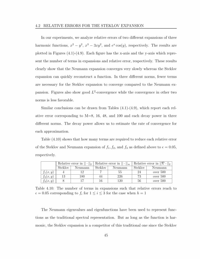
Table (4.10) shows that how many terms are required to reduce each relative error

of the Steklov and Neumann expansion of f1, f2, and f3 as defined above to ε = 0.05,

respectively.


f1(x, y) 4 12 7 55 24 over 500f2(x, y) 13 180 44 226 73 over 500f3(x, y) 8 17 16 120 56 over 500

Table 4.10: The number of terms in expansions such that relative errors reach toε = 0.05 corresponding to fi for 1 ≤ i ≤ 3 for the case when h = 1

The Neumann eigenvalues and eigenfunctions have been used to represent func-

tions as the traditional spectral representation. But as long as the function is har-

monic, the Steklov expansion is a competitor of this traditional one since the Steklov

45


expansion does not suffer from the number of eigenfunction terms to converge to a

fixed accuracy. Hence, the Steklov spectral expansion is a promising alternative for

representing harmonic functions.

46

Chapter 5

Solutions of Boundary Value

Problems on Ω

5.1 The Harmonic Dirichlet Problem

We consider a function u ∈ H1(Ω) satisfies

∆u = 0 in Ω (5.1)

u = η on ∂Ω (5.2)

This is often known as the Harmonic Dirichlet (HD) problem. There are various

different theories for solving the HD problem on Ω. See the comprehensive survey by

Benilan in Chapter 2 of [9] and also the lectures of Kenig [13].

The description of trace spaces using Steklov eigenfunctions is developed in [2] and

its application to Dirichlet problems for harmonic functions is described in Chapter 6

of [4]. Our interest is in finding solutions of this problem when η is continuous on the

47

5.1 THE HARMONIC DIRICHLET PROBLEM

boundary. When η is not continuous on the boundary, especially not in H12 (∂Ω)(see

Chapter 4 and 6 of [5]), the generalized harmonic Dirichlet problem that arises in the

theory of thin films is described in Chapter 5 of [3].

Here we assume that η = Γu ∈ L2(∂Ω, dσ) and Ω = [−L,L] × [−Lh, Lh]. We

consider approximations of the solution of the HD problem on Ω in terms of the

harmonic Steklov eigenfunctions.

Theorem 4.2 implies that the solution of the HD problem may be represented by

u(x, y) =∞∑i=0

ηisi(x, y) for (x, y) ∈ Ω with ηi :=< η, si >2,∂Ω (5.3)

and we expect the partial sums uM(x, y) =M∑i=0

ηisi(x, y) for (x, y) ∈ Ω to be good

approximations of the solution. Clearly, each partial sum is harmonic and has a

continuous trace η on the boundary. As observed in the previous chapter, the finite

sum of the Steklov expansion of u can approximate the solution of the HD problem

under a small error. Define the Steklov approximation of u to be the M-th partial sum

of this expansion and denoted by uM . When the solution is obtained approximately

by uM , there could be a couple of advantages of using the Steklov expansion for the

HD problem. As described in the preceding chapter, uM can quickly reconstruct

the solution of the HD problem. The fact that the number of Steklov eigenfunction

expected to use is small yields that computational costs may be saved when the

Steklov expansion method is implemented on Matlab.

Moreover, the Steklov expansion only requires evaluating boundary integrals.

Once boundary normalized Steklov eigenfunctions are known, as described in Sec-

tion 3.6, the set of the eigenfunctions spans L2(∂Ω, dσ). The boundary condition of

48


the HD problem is well approximated by the Steklov expansion. Here we provide

numerical experiments and reveal these advantages.

Assume η is continuous and bounded on ∂Ω and we will look at functions that are

even or odd about the center of each side. The HD problem on Ω = [−1, 1]× [−1, 1]

is solved by using the Steklov expansion method. We do not know the exact solution

of the problem, but we perform experiments for uM corresponding to M=8, 16, 48,

and 100. Figures and contour sets of uM in Ω are provided.

49


1.

η1(x, y) =

1− x2 on Γ1 and Γ3

1− y2 on Γ2 and Γ4

This η1(x, y) is a piecewise function that is even about the center on each side,

non negative on ∂Ω, and η1 = 23> 0. Figure (5.1) shows graphs of uM(x, y) in

Ω and next Figure (5.2) represents contour lines of uM(x, y) corresponding to

M=8, 16, 48, and 100, respectively.

−1−0.5

00.5

1

−1

−0.5

0

0.5

10

0.2

0.4

0.6

0.8

1

x

The 8−th Steklov approximation

y

u8(x

,y)

−1−0.5

00.5

1

−1

−0.5

0

0.5

10

0.2

0.4

0.6

0.8

1

x


y

u16

(x,y

)

−1−0.5

00.5

1

−1

−0.5

0

0.5

10

0.2

0.4

0.6

0.8

1

x


y

u48

(x,y

)

−1−0.5

00.5

1

−1

−0.5

0

0.5

10

0.2

0.4

0.6

0.8

1

x


y

u10

0(x,y

)

Figure 5.1: The M-th Steklov approximations of the HD Problem on [−1, 1]× [−1, 1]for η = η1 corresponding to M=8(Left top), 16(Right top), 48(Left bottom), and100(Right bottom).

50


x

yThe 8−th Steklov approximation

−1 −0.5 0 0.5 1−1

−0.8

−0.6

−0.4

−0.2

0

0.2

0.4

0.6

0.8

1

0.1

0.2

0.3

0.4

0.5

0.6

0.7

0.8

0.9

1

x

y


−1 −0.5 0 0.5 1−1

−0.8

−0.6

−0.4

−0.2

0

0.2

0.4

0.6

0.8

1

0.1

0.2

0.3

0.4

0.5

0.6

0.7

0.8

0.9

x

y


−1 −0.5 0 0.5 1−1

−0.8

−0.6

−0.4

−0.2

0

0.2

0.4

0.6

0.8

1

0.1

0.2

0.3

0.4

0.5

0.6

0.7

0.8

0.9

x

y


−1 −0.5 0 0.5 1−1

−0.8

−0.6

−0.4

−0.2

0

0.2

0.4

0.6

0.8

1

0.1

0.2

0.3

0.4

0.5

0.6

0.7

0.8

0.9

Figure 5.2: Contour plots of the M-th Steklov approximations of the HD Problem on[−1, 1] × [−1, 1] for η = η1 corresponding to M=8(Left top), 16(Right top), 48(Leftbottom), and 100(Right bottom).

We observe that for each M, uM(x, y) is symmetric about both x-axis and y-

axis, non negative on ∂Ω and uM = 23. In Figure (5.2), we see that if (x, y)

is the center of Ω, then uM is quite flat. We point out that there is no sig-

nificant difference between uM(x, y) against M for (x, y) ∈ Ω for M ≥ 16 and

max(x,y)∈∂Ω

|η1(x, y)−u100(x, y)| = 8.5826e−4. Hence a solution u of the HD problem

on Ω = [−1, 1]× [−1, 1] where η = η1 from the maximum principles(see Section

8.3 of [19]) obeys |u(x, y)− u100(x, y)| ≤ 8.5826e−4 for all (x, y) ∈ Ω.

51


2.

η2(x, y) =

1− x3 on Γ1

1 + y3 on Γ2

1 + x3 on Γ3

1− y3 on Γ4

This η2(x, y) is a continuous function that is odd about the center on each side,

non negative, and η2 = 1 > 0.

−1−0.5

00.5

1

−1

−0.5

0

0.5

10

0.5

1

1.5

2

x


y

u8(x

,y)

−1−0.5

00.5

1

−1

−0.5

0

0.5

10

0.5

1

1.5

2

x


y

u16

(x,y

)

−1−0.5

00.5

1

−1

−0.5

0

0.5

10

0.5

1

1.5

2

x


y

u48

(x,y

)

−1−0.5

00.5

1

−1

−0.5

0

0.5

10

0.5

1

1.5

2

x


y

u10

0(x,y

)


52


x


−1 −0.5 0 0.5 1−1

−0.8

−0.6

−0.4

−0.2

0

0.2

0.4

0.6

0.8

1

0.4

0.6

0.8

1

1.2

1.4

1.6

x

y


−1 −0.5 0 0.5 1−1

−0.8

−0.6

−0.4

−0.2

0

0.2

0.4

0.6

0.8

1

0.2

0.4

0.6

0.8

1

1.2

1.4

1.6

1.8

x

y


−1 −0.5 0 0.5 1−1

−0.8

−0.6

−0.4

−0.2

0

0.2

0.4

0.6

0.8

1

0.2

0.4

0.6

0.8

1

1.2

1.4

1.6

1.8

x

y


−1 −0.5 0 0.5 1−1

−0.8

−0.6

−0.4

−0.2

0

0.2

0.4

0.6

0.8

1

0.2

0.4

0.6

0.8

1

1.2

1.4

1.6

1.8


Figure (5.3) shows that on each side u8 is linearly piecewise while η2 is cubic on

each side. So the 8-th partial sum, u8 is not a very good approximation to the

solution of the HD problem on Ω = [−1, 1] × [−1, 1] for η = η2. However, we

see that each uM is a cubic function that is odd about the center on each side

similar to η2 and uM = 1 for M=16, 48, and 100. Especially, max(x,y)∈∂Ω

|η2(x, y)−

u100(x, y)| = 0.0023938. Hence we can say that a solution u of this problem

obeys |u(x, y)− u100(x, y)| ≤ 0.0023938 for all (x, y) ∈ Ω.

53


3.

η3(x, y) =

cos(4πx) on Γ1 and Γ3

cos(2πy) on Γ2 and Γ4

This η3(x, y) is a piecewise function that is even about zero on each side and

η3 = 0. Compared against η1, this function involves more oscillations on each

side. Especially, there are lots of oscillations on Γ1 and Γ3.

−1−0.5

00.5

1

−1

−0.5

0

0.5

1

−1

−0.5

0

0.5

1

x


y

u8(x

,y)

−1−0.5

00.5

1

−1

−0.5

0

0.5

1

−1

−0.5

0

0.5

1

x


y

u16

(x,y

)

−1−0.5

00.5

1

−1

−0.5

0

0.5

1

−1

−0.5

0

0.5

1

x


y

u48

(x,y

)

−1−0.5

00.5

1

−1

−0.5

0

0.5

1

−1

−0.5

0

0.5

1

x


y

u10

0(x,y

)


54


x


−1 −0.5 0 0.5 1−1

−0.8

−0.6

−0.4

−0.2

0

0.2

0.4

0.6

0.8

1

−0.1

−0.08

−0.06

−0.04

−0.02

0

0.02

0.04

0.06

0.08

0.1

x

y


−1 −0.5 0 0.5 1−1

−0.8

−0.6

−0.4

−0.2

0

0.2

0.4

0.6

0.8

1

−0.8

−0.6

−0.4

−0.2

0

0.2

0.4

0.6

0.8

x

y


−1 −0.5 0 0.5 1−1

−0.8

−0.6

−0.4

−0.2

0

0.2

0.4

0.6

0.8

1

−1

−0.8

−0.6

−0.4

−0.2

0

0.2

0.4

0.6

0.8

1

x

y


−1 −0.5 0 0.5 1−1

−0.8

−0.6

−0.4

−0.2

0

0.2

0.4

0.6

0.8

1

−1

−0.8

−0.6

−0.4

−0.2

0

0.2

0.4

0.6

0.8

1


Figure (5.6) shows that for each M, uM is symmetric about both x-axis and

y-axis and around the center, it is flat. In Figure (5.5), we see that nice approxi-

mation uM are not obtained for M ≤ 16 since there are fewer oscillations on each

side than in η3. However, u48 is oscillating as much as η3 and u48 = 6.2153e−14.

We point out that max(x,y)∈∂Ω

|η3(x, y)−u100(x, y)| = 0.0042578. Hence the Steklov

expansion method gives a good approximation of a solution of the HD Problem

on Ω = [−1, 1]× [−1, 1] for η = η3 .

55

5.2 THE HARMONIC NEUMANN PROBLEM

5.2 The Harmonic Neumann Problem

In this section ,we want to approximate solutions u ∈ H1∂(Ω) of

∆u = 0 in Ω (5.4)

Dνu = η on ∂Ω (5.5)

Here η ∈ L2(∂Ω, dσ). This problem will be called the Harmonic Neumann (HN)

problem. The weak form of (5.4)-(5.5) is to find a function u in H1(Ω) satisfying

∫Ω

∇n · ∇v dx = δ

∫∂Ω

nv dσ for all v ∈ H1(Ω) (5.6)

Since S = si : i ≥ 0 is a orthogonal basis of H(Ω), we can represent a solution of

this problem by u(x, y) =∞∑i=0

cisi(x, y) on Ω for non zero constant ci, i ≥ 0. Then the

boundary condition is that

Dνu(x, y) =∞∑i=0

cjDν si(x, y) (5.7)

=∞∑i=0

ciδisi(x, y) (5.8)

The second equality holds from (3.2). One has

η(x, y) =∞∑i=0

< η, si >2,∂Ω si(x, y) for (x, y) ∈ ∂Ω (5.9)

Comparing with (5.8) yields that ciδi =< η, si >2,∂Ω. Equivalently

ci =< η, si >2,∂Ω

δifor i > 0 (5.10)

56


Put v(x) ≡ 1 on Ω and substitute on (5.6), then a necessary condition for the HN

problem to have a solution is that

∫−∂Ωη dσ = 0 (5.11)

It implies that c0 = 0. In this case, Theorem 9.3 of [1] says that this problem has a

unique solution. Then the unique solution of the HN problem has the representation

u(x, y) =∞∑i=1

< η, si >2,∂Ω

δisi(x, y) for (x, y) ∈ Ω (5.12)

We recall η3 from the preceding section. Since η3 = 0, there exists a unique solution of

the HN problem on Ω for η = η3. We provide similar numerical results of the Steklov

approximations of a solution of the HN problem on Ω = [−1, 1]× [−1, 1] where η = η3

as performed in the previous section.

57


η3(x, y) =



−1−0.5

00.5

1

−1

−0.5

0

0.5

1

−0.2

−0.1

0

0.1

0.2

x


y

u8(x

,y)

−1−0.5

00.5

1

−1

−0.5

0

0.5

1

−0.2

−0.1

0

0.1

0.2

x


y

u16

(x,y

)

−1−0.5

00.5

1

−1

−0.5

0

0.5

1

−0.2

−0.1

0

0.1

0.2

x


y

u48

(x,y

)

−1−0.5

00.5

1

−1

−0.5

0

0.5

1

−0.2

−0.1

0

0.1

0.2

x


y

u10

0(x,y

)

Figure 5.7: The M-th Steklov approximations of the HN Problem on [−1, 1]× [−1, 1]for η = η3 corresponding to M=8(Left top), 16(Right top), 48(Left bottom), and100(Right bottom).

58


x

y


−1 −0.5 0 0.5 1−1

−0.8

−0.6

−0.4

−0.2

0

0.2

0.4

0.6

0.8

1

−0.04

−0.03

−0.02

−0.01

0

0.01

0.02

0.03

0.04

0.05

x

y


−1 −0.5 0 0.5 1−1

−0.8

−0.6

−0.4

−0.2

0

0.2

0.4

0.6

0.8

1

−0.15

−0.1

−0.05

0

0.05

0.1

0.15

x

y


−1 −0.5 0 0.5 1−1

−0.8

−0.6

−0.4

−0.2

0

0.2

0.4

0.6

0.8

1

−0.15

−0.1

−0.05

0

0.05

0.1

0.15

0.2

x

y


−1 −0.5 0 0.5 1−1

−0.8

−0.6

−0.4

−0.2

0

0.2

0.4

0.6

0.8

1

−0.15

−0.1

−0.05

0

0.05

0.1

0.15

0.2

Figure 5.8: Contour plots of the M-th Steklov approximations of the HN Problem on[−1, 1] × [−1, 1] for η = η3 corresponding to M=8(Left top), 16(Right top), 48(Leftbottom), and 100(Right bottom).

59

5.3 THE HARMONIC ROBIN PROBLEM

5.3 The Harmonic Robin Problem

In this section, we consider a function u ∈ H1(Ω) satisfies

∆u = 0 in Ω (5.13)

Dνu+ u = η on ∂Ω (5.14)

Here η ∈ L2(∂Ω, dσ). This problem will be called the Harmonic Robin (HR) problem.

As described in the preceding section, in order to approximate a solution of this

problem we start with u(x, y) =∞∑i=0

cisi(x, y) on Ω for non zero constant ci, i ≥ 0.

Then the boundary condition becomes

Dνu(x, y) + u(x, y) =∞∑i=0

ciDν si(x, y) +∞∑i=0

cisi(x, y)

=∞∑i=0

ciδisi(x, y) +∞∑i=0

cisi(x, y)

=∞∑i=0

ci(δi + 1)si(x, y)

Comparing with (5.9) yields that

ci =< η, si >2,∂Ω

δi + 1for i ≥ 0 (5.15)

Hence we can represent the solution of the HR problem by

u(x, y) =∞∑i=0

< η, si >2,∂Ω

δi + 1si(x, y) for (x, y) ∈ Ω (5.16)

Again we recall η1, η1, and η3 from Section 5.1. We perform numerical experiments

60


of the Steklov approximations of a solution of the HR problem on Ω = [−1, 1]×[−1, 1].

1.

η1(x, y) =

1− x2 on Γ1 and Γ3

1− y2 on Γ2 and Γ4

−1−0.5

00.5

1

−1

−0.5

0

0.5

1

0.5

0.55

0.6

0.65

0.7

0.75

x


y

u8(x

,y)

−1−0.5

00.5

1

−1

−0.5

0

0.5

1

0.5

0.55

0.6

0.65

0.7

0.75

x


y

u16

(x,y

)

−1−0.5

00.5

1

−1

−0.5

0

0.5

1

0.5

0.55

0.6

0.65

0.7

0.75

x


y

u48

(x,y

)

−1−0.5

00.5

1

−1

−0.5

0

0.5

1

0.5

0.55

0.6

0.65

0.7

0.75

x


y

u10

0(x,y

)

Figure 5.9: The M-th Steklov approximations of the HR Problem on [−1, 1]× [−1, 1]for η = η1 corresponding to M=8(Left top), 16(Right top), 48(Left bottom), and100(Right bottom).

61


x

y


−1 −0.5 0 0.5 1−1

−0.8

−0.6

−0.4

−0.2

0

0.2

0.4

0.6

0.8

1

0.5

0.55

0.6

0.65

0.7

0.75

x

y


−1 −0.5 0 0.5 1−1

−0.8

−0.6

−0.4

−0.2

0

0.2

0.4

0.6

0.8

1

0.5

0.55

0.6

0.65

0.7

0.75

x

y


−1 −0.5 0 0.5 1−1

−0.8

−0.6

−0.4

−0.2

0

0.2

0.4

0.6

0.8

1

0.5

0.55

0.6

0.65

0.7

0.75

x

y


−1 −0.5 0 0.5 1−1

−0.8

−0.6

−0.4

−0.2

0

0.2

0.4

0.6

0.8

1

0.5

0.55

0.6

0.65

0.7

0.75

Figure 5.10: Contour lines of the M-th Steklov approximations of the HR Problem on[−1, 1] × [−1, 1] for η = η1 corresponding to M=8(Left top), 16(Right top), 48(Leftbottom), and 100(Right bottom).

62


2.

η2(x, y) =

1− x3 on Γ1

1 + y3 on Γ2

1 + x3 on Γ3

1− y3 on Γ4

−1−0.5

00.5

1

−1

−0.5

0

0.5

10.6

0.8

1

1.2

1.4

x


y

u8(x

,y)

−1−0.5

00.5

1

−1

−0.5

0

0.5

10.6

0.8

1

1.2

1.4

x


y

u16

(x,y

)

−1−0.5

00.5

1

−1

−0.5

0

0.5

10.6

0.8

1

1.2

1.4

x


y

u48

(x,y

)

−1−0.5

00.5

1

−1

−0.5

0

0.5

10.6

0.8

1

1.2

1.4

x


y

u10

0(x,y

)


63


x

y


−1 −0.5 0 0.5 1−1

−0.8

−0.6

−0.4

−0.2

0

0.2

0.4

0.6

0.8

1

0.7

0.8

0.9

1

1.1

1.2

1.3

x

y


−1 −0.5 0 0.5 1−1

−0.8

−0.6

−0.4

−0.2

0

0.2

0.4

0.6

0.8

1

0.7

0.8

0.9

1

1.1

1.2

1.3

x

y


−1 −0.5 0 0.5 1−1

−0.8

−0.6

−0.4

−0.2

0

0.2

0.4

0.6

0.8

1

0.7

0.8

0.9

1

1.1

1.2

1.3

x

y


−1 −0.5 0 0.5 1−1

−0.8

−0.6

−0.4

−0.2

0

0.2

0.4

0.6

0.8

1

0.7

0.8

0.9

1

1.1

1.2

1.3


64


3.

η3(x, y) =



−1−0.5

00.5

1

−1

−0.5

0

0.5

1

−0.15

−0.1

−0.05

0

0.05

0.1

0.15

x


y

u8(x

,y)

−1−0.5

00.5

1

−1

−0.5

0

0.5

1

−0.15

−0.1

−0.05

0

0.05

0.1

0.15

x


y

u16

(x,y

)

−1−0.5

00.5

1

−1

−0.5

0

0.5

1

−0.15

−0.1

−0.05

0

0.05

0.1

0.15

x


y

u48

(x,y

)

−1−0.5

00.5

1

−1

−0.5

0

0.5

1

−0.15

−0.1

−0.05

0

0.05

0.1

0.15

x


y

u10

0(x,y

)


65


x

y


−1 −0.5 0 0.5 1−1

−0.8

−0.6

−0.4

−0.2

0

0.2

0.4

0.6

0.8

1

−0.03

−0.02

−0.01

0

0.01

0.02

0.03

0.04

x

y


−1 −0.5 0 0.5 1−1

−0.8

−0.6

−0.4

−0.2

0

0.2

0.4

0.6

0.8

1

−0.1

−0.05

0

0.05

0.1

0.15

x

y


−1 −0.5 0 0.5 1−1

−0.8

−0.6

−0.4

−0.2

0

0.2

0.4

0.6

0.8

1

−0.1

−0.05

0

0.05

0.1

0.15

x

y


−1 −0.5 0 0.5 1−1

−0.8

−0.6

−0.4

−0.2

0

0.2

0.4

0.6

0.8

1

−0.1

−0.05

0

0.05

0.1

0.15


66

5.4 THE GENERALIZED BOUNDARY DATA

5.4 The Generalized Boundary Data

In this section, we generalize the boundary conditions. Consider finding a solution

u ∈ H1(Ω) satisfies that for t ∈ [0, 1),

∆u = 0 in Ω (5.17)

(1− t)Dνu+ tu = η on ∂Ω (5.18)

Here η ∈ L2(∂Ω, dσ). Taking t = 0 in (5.18) provides the Neumann boundary condi-

tion. The Dirichlet problem can be treated as the limit t→ 1− of the above problem.

For 0 < t < 1, we again represent a solution of this problem by u(x, y) =∞∑i=0

cisi(x, y) on Ω for non zero constant ci, i ≥ 0. Then the boundary condition

yields that

(1− t)Dνu(x, y) + tu(x, y) = (1− t)∞∑i=0

ciDν si(x, y) + t∞∑i=0

cisi(x, y)

= (1− t)∞∑i=0

ciδisi(x, y) + t∞∑i=0

cisi(x, y)

=∞∑i=0

((1− t)δi + t)cisi(x, y)

Then (5.9) implies that

ci =< η, sj >2,∂Ω

(1− t)δj + tfor i ≥ 0 (5.19)

Theorem 9.2 of [1] says that this problem has a unique solution. Hence the unique

67

5.4 THE GENERALIZED BOUNDARY DATA

solution u of (5.17)-(5.17) has the Steklov series representation

u(x, y) =∞∑i=0

< η, sj >2,∂Ω

(1− t)δj + tsi(x, y) for (x, y) ∈ Ω (5.20)

for 0 < t < 1.

68

Chapter 6

An Application of the Steklov

Expansion

6.1 The Mean Value Property

We develop and describe an application of the Steklov expansion of harmonic func-

tions. The Steklov expansion method, to approximate a solution of the certain prob-

lem, enables to describe a solution on ∂Ω, but also in Ω. In numerical results in

the preceding chapter, we saw that the Steklov approximation is flat around the cen-

ter. We shall investigate to describe solutions of boundary value problems in Ω more

precisely.

The mean value property provides a way to estimate the value of solutions at the

center of Ω. Let u be a harmonic function in a disk D and continuous in its closure

D. Then the mean value property states that the value of u at the center of D equals

the average of u on its circumference(see Section 2.2 of [15]). Note that the mean

value property holds where Ω is a disk. Since in this work, Ω is a rectangle, the mean

69

6.1 THE MEAN VALUE PROPERTY

value property does not always hold.

Now consider the HD problem on Ω = [−1, 1] × [−1, 1]. We want to find the

general formula for u(0, 0) where u is the unique solution of this problem. (5.3) yields

that

u(0, 0) =∞∑i=0

< η, si >2,∂Ω si(0, 0) (6.1)

=< η, s0 >2,∂Ω s0(0, 0) +∞∑i=1

< η, si >2,∂Ω si(0, 0) (6.2)

= η +∞∑i=1

< η, si >2,∂Ω si(0, 0) (6.3)

= η +∑k∈K

< η, sk >2,∂Ω sk(0, 0) (6.4)

Here sk : k ∈ K is the subset of S such that sk(0, 0) 6= 0 for k ≥ 1. These results


Theorem 6.1. Assume Ω, ∂Ω, S, δi, and si are defined in Chapter 3 and the set K

is defined as above. Also assume that u is a harmonic function on Ω with u = η on

∂Ω. Then u(0, 0) is given by (6.4).

In particular the ”correction term” to the mean value theorem is C :=∑k∈K

<

η, sk >2,∂Ω sk(0, 0). This is the difference between u(0, 0) and the mean value of u on

∂Ω.

Here we shall describe the set K in (6.4). Since sin(0) = sinh(0) = 0, si(0, 0) = 0

for most i. Only the cch and chc Steklov eigenfunctions are non-zero at the center.

So K is the set of orders of cch and chc Steklov eigenfunctions and given by

K = 4, 5, 12, 13, 20, 21, 28, 29, 36, 37, 44, 45, 54, 55, ... (6.5)

70


We list sk for 4 ≤ k ≤ 95 .

s4 = 0.36926 cos(2.365x) cosh(2.365y)

s5 = 0.36926 cosh(2.365x) cos(2.365y)

s12 = 0.016382 cos(5.4978x) cosh(5.4978y)

s13 = 0.016382 cosh(5.4978x) cos(5.4978y)

s20 = 7.0799e−4 cos(8.6394x) cosh(8.6394y)

s21 = 7.0799e−4 cosh(8.6394x) cos(8.6394y)

s28 = 3.0595e−5 cos(11.781x) cosh(11.781y)

s29 = 3.0595e−5 cosh(11.781x) cos(11.781y)

s36 = 1.3221e−6 cos(14.923x) cosh(14.923y)

s37 = 1.3221e−6 cosh(14.923x) cos(14.923y)

s44 = 5.7134e−8 cos(18.064x) cosh(18.064y)

s45 = 5.7134e−8 cosh(18.064x)) cos(18.064y)

s54 = 2.469e−9 cos(21.206x) cosh(21.206y)

s55 = 2.469e−9 cosh(21.206x) cos(21.206y)

s62 = 1.0669e−10 cos(24.347x) cosh(24.347y)

s63 = 1.0669e−10 cosh(24.347x) cos(24.347y)

s70 = 4.6107e−12 cos(27.489x) cosh(27.489y)

s71 = 4.6107e−12 cosh(27.489x) cos(27.489y)

s78 = 1.9925e−13 cos(30.631x) cosh(30.631y)

s79 = 1.9925e−13 cosh(30.631x) cos(30.631y)

71


s86 = 8.6102e−15 cos(33.772x) cosh(33.772y)

s87 = 8.6102e−15 cosh(33.772x) cos(33.772y)

s94 = 3.7208e−16 cos(36.914x) cosh(36.914y)

s95 = 3.7208e−16 cosh(36.914x) cos(36.914y)

We note that max(x,y)∈∂Ω

sk = 1.9826 for k=4 and 5, max(x,y)∈∂Ω

sk = 2 for 12 ≤ k ≤ 95

when evaluated to 4 decimal places.

k 4 5 12 13 20 21sk(0, 0) 0.36926 0.36926 0.016382 0.016382 7.0799e−4 7.0799e−4

k 28 29 36 37 44 45sk(0, 0) 3.0595e−5 3.0595e−5 1.3221e−6 1.3221e−6 5.7134e−8 5.7134e−8

k 54 55 62 63 70 71sk(0, 0) 2.469e−9 2.469e−9 1.0669e−10 1.0669e−10 4.6107e−12 4.6107e−12

k 78 79 86 87 94 95sk(0, 0) 1.9925e−13 1.9925e−13 8.6102e−15 8.6102e−15 3.7208e−16 3.7208e−16

Table 6.1: sk(0, 0)

In Table (6.1), we report sk(0, 0) for 4 ≤ k ≤ 95 and it corresponds to ||sk||−12,∂Ω

where sk is the Steklov eigenfunction defined in Section 3.5. For 4 ≤ k ≤ 95, sk(0, 0)

is decreasing and getting closer to 0 against k.

Now we are concerned with how these values are decreasing. Let kr be the r-th

element of the set K. In other words, r represents an index of k in the set K. Here we

suspect that the graph of skr(0, 0) against r is the exponential decay like e−ar for non

zero constant a. Then

log(|skr+2(0, 0)− skr(0, 0)|) = log(|e−a(r+2) − e−ar|) (6.6)

72

6.2 THE CORRECTION TERM

6.2 The Correction Term

Let Kr = ki| 1 ≤ i ≤ r. Define CD(r) :=∑k∈Kr

< η, sk >2,∂Ω sk(0, 0) to be the

r-th correction term of u(0, 0) where u is a solution of the HD problem with η = Γu.

In this section, we shall describe this correction term. Completeness of the Steklov

expansion of the solution of the HD problem ensures that limr→∞

CD(r) = u(0, 0) − η.

We are concerned with the number of the Steklov eigenfunctions in the correct term

required to converge to a certain accuracy.

We recall u1(x, y) = x2 − y2, u2(x, y) = x3 − 3xy2, and u3(x, y) = ex cos(y) from

Section 4.2. Let ηi = Γui for 1 ≤ i ≤ 3. These functions are H1-harmonic functions

on Ω and their traces are continuous on the boundary. We know that η1 = η2 = 0 and

η3 = 0.96671. Also we notice that u1(0, 0) = u2(0, 0) = 0 and u3(0, 0) = 1. Denote

the r-th the correction term of ui(0, 0) by CDi(r) for 1 ≤ i ≤ 3. Then we suspect that

when i = 1 and i = 2, CDi(r)→ 0 as r →∞ and when i = 3, CD3(r)→ 0.03329 as

r →∞.

We notice that when η is odd about the center on each side of the boundary then

< η, sk >2,∂Ω= 0 for all k ∈ K. It implies that < η2, sk >2,∂Ω= 0 for all k ∈ K so

that CD2(r) = 0 for all r. In this case, there is no difference between u2(0, 0) and its

mean value on the boundary. Here we can see how much the Steklov expansion of

harmonic functions is efficient.

Numerical experiments of approximations of u1(0, 0) are reported in Table (6.2)

and it shows that the 21th correction term of u1(0, 0) gives a nice approximation of

u1(0, 0).

For u3, we evaluate (u3(0, 0)−u3)−CD3(r) to see how it decreases to zero. Table

(6.3) shows that the 21th correction term of u3(0, 0) can be a good approximation of

74

6.2 THE CORRECTION TERM

r 7 9 11 13CD1(r) 6.2349e−7 −1.6793e−8 4.9523e−10 −1.5529e−11

r 15 17 19 21CD1(r) 5.0908e−13 −1.7258e−14 6.0066e−16 −2.1352e−17

Table 6.2: The r-th correction term of u1

u3(0, 0)−u3. We again suspect that the graph of the r-th correction term against r is

r 7 9 11 13(u3(0, 0)− u3)− CD3(r) −3.0348e−7 8.1522e−9 −2.4008e−10 7.5188e−12

r 15 17 19 21(u3(0, 0)− u3)− CD3(r) 1.3451e−13 −1.2321e−14 7.2873e−16 2.3984e−18

Table 6.3: The difference between CD3(r) and (u3(0, 0)− u3)

the exponential decay as described in the previous chapter. Then we consider the liner

graph of log(|CDi(r + 2)− CDi(r)|) against r to estimate of the rate of convergence

for the approximations as a function of r. In Figure (6.2), we can observe how fast

each correction term converges by using only 24 cch and chc Steklov eigenfunctions.

These results show that only a few terms in the Steklov expansion are necessary to

obtain good approximations of the value of the solution of the HD problem at the

center of Ω.

75

6.3 SEVERAL EXAMPLES

7 9 11 13 15 17 19 21−40

−35

−30

−25

−20

−15

−10

r

log

(|C

D(r

+2

)−C

D(r

)|)

u

1

u3

Figure 6.2: The linear decay of log(|CD1(r + 2) − CD1(r)|) and log(|CD3(r + 2) −CD3(r)|) with their approximated slopes, -1.7206 and -1.721, respectively.

6.3 Several Examples

In this section, we develop the formulae of u(0, 0) where u(x, y) are solutions of

Laplace’s equation subject to certain boundary condition on Ω. We consider the

problem of finding non trivial solutions in H1(Ω) that satisfy

∆u = 0 in Ω (6.9)

Dνu+ bu = η on ∂Ω (6.10)

76


where b is a constant. Here η ∈ L2(∂Ω, dσ). Then (6.10) will be treated as the

Neumann boundary condition when b=0 or the Robin boundary condition when

b=1.

When b 6= 0, from the analysis of the previous chapter the unique solution of this

problem has the Steklov series representation

u(x, y) =∞∑i=0

< η, si >2,∂Ω

b+ δisi(x, y) for (x, y) ∈ Ω (6.11)

Then the explicit formula of u(0, 0) is given by

u(0, 0) =η

b+

∑k∈K

< η, sk >2,∂Ω

b+ δksk(0, 0) (6.12)

Here the set K is defined in (6.5).

When b = 0 and η = 0, (5.12) yields that

u(0, 0) =∑k∈K

< η, sk >2,∂Ω

δksk(0, 0) (6.13)

Define CN(r) :=∑k∈Kr

<η,sk>2,∂Ω

δksk(0, 0) to be the r-th correction term of u(0, 0)

where u is a solution of the HN problem. Also we define CR(r) :=∑k∈Kr

<η,sk>2,∂Ω

1+δksk(0, 0)

to be the r-th correction term of u(0, 0) where u is a solution of the HR problem.

Now we have the machinery to perform numerical experiments which show that

the value of solutions at the center can be nicely approximated by our formulae.

Let Ω = [−1, 1] × [−1, 1]. Denote the solution of the HD, HN, and HR problem

on Ω by uD, uN , and uR, respectively. We recall η1, η2, and η3 from Section 5.1. We

note that η1 = 23, η2 = 1, and η3 = 0.

77


Since η2 is odd about the center on each side of the boundary, then < η2, sk >2,∂Ω=

0 for all k ∈ K. Then uD(0, 0) = uR(0, 0) = η2 = 1. In other words, the value of each

solution at the center of Ω is exactly obtained by the mean value of each solution on

the boundary.

Next we let η = η1. In this case, there is no solution of the HN problem since

η1 6= 0. We evaluate the r-th correction terms of uD(0, 0) and uR(0, 0), respectively.

Table (6.4) reports absolute values of the difference between the r-th and the (r+2)-th

correction terms corresponding to uD(0, 0) and uR(0, 0), respectively. These results

show that uD(0, 0) ≈ η1 + CD(23) = 0.66667 + 0.15459 = 0.82126 and uR(0, 0) ≈

η1 + CR(23) = 0.66667 + 0.046594 = 0.71326. In Figure (6.3), we observe how fast

each correction term converges within r=23 and the bounded error of each correction

term is quite small.

r 7 9 11 13|CD(r + 2)− CD(r)| 3.1164e−7 8.3923e−9 2.476e−10 7.7686e−12

r 15 17 19 21|CD(r + 2)− CD(r)| 2.5481e−13 8.6429e−15 3.0095e−16 1.0703e−17

r 7 9 11 13|CR(r + 2)− CR(r)| 2.4258e−8 5.246e−10 1.2932e−11 3.4848e−13

r 15 17 19 21|CR(r + 2)− CR(r)| 1.0017e−14 3.0237e−16 9.4852e−18 3.0691e−19

Table 6.4: Absolute values of the difference of the r-th and the (r+2)-th correctionterms for η = η1 corresponding to uD(0, 0) and uR(0, 0), respectively

Now we let η = η3. We perform similar experiments and results are given in

Table (6.5) and Figure (6.4). Figure (6.4) shows that each correction term converges

quickly. Then uD(0, 0) ≈ CD(23) = −0.030398, uN(0, 0) ≈ CN(23) = −0.015236,

and uR(0, 0) ≈ CR(23) = −0.010421.

Here we emphasize that only a few Steklov eigenfunctions are required to approx-

78


r 7 9 11 13|CD(r + 2)− CD(r)| 1.5451e−6 3.7155e−8 9.8596e−10 2.8002e−11

r 15 17 19 21|CD(r + 2)− CD(r)| 8.3568e−13 2.5923e−14 8.2967e−16 2.7253e−17

r 7 9 11 13|CN(r + 2)− CN(r)| 1.3405e−7 2.5171e−9 5.5001e−11 1.3285e−12

r 15 17 19 21|CN(r + 2)− CN(r)| 3.4498e−14 9.4718e−16 2.7193e−17 8.0983e−19

r 7 9 11 13|CR(r + 2)− CR(r)| 1.234e−7 2.3577e−9 5.2098e−11 1.2684e−12

r 15 17 19 21|CR(r + 2)− CR(r)| 3.3131e−14 9.1381e−16 2.633e−17 7.8647e−19

Table 6.5: Absolute values of the difference of the r-th and the (r+2)-th correctionterm for η = η3 corresponding to uD(0, 0), uN(0, 0), and uR(0, 0), respectively

imate the value of solutions at the center of Ω with a high accuracy. Moreover, when

η is odd about the center on each side of the boundary, then uD(0, 0), uN(0, 0)(if

η = 0), and uR(0, 0) are exactly computed and the values equal η.

79

Bibliography

[1] G. Auchmuty. Steklov eigenproblems and the representation of solutions of elliptic bound-

ary value problems. Numer. Funct. Anal. Optim. 25 (2004), 321-348.

[2] G. Auchmuty. Spectral characterizations of the trace spaces Hs(∂Ω). SIAM J. Math.

Anal. 38 (2006), 894-905.

[3] G. Auchmuty and P. Kloucek Generalized harmonic functions and the dewetting of thins

films. Appl. Math. Optim. 55 (2007), 145-161.

[4] G. Auchmuty Reproducing kernels for Hilbert spaces of real harmonic functions. SIAM

J. Math. Anal.41 (2009), 1994-2009.

[5] R. A. Adams and J. J. F. Fournier. Sobolev Spaces. Second Edition. Elsevier/Academic

Press, Amsterdam (2003).

[6] C. Bandle. Isoperimetric Inequalities and Applications. Pitman, London (1980).

[7] G. Dahlquist and A. Bjorck. Numerical Methods in Scientific Computing: Volume I.

Society for Industrial and Applied Mathematics, PI (2008).

[8] E. DiBenedetto. Real Analysis. Birkhauser, Boston (2001).

[9] R. Dautray and J-L. Lions. Mathematical Analysis and Numerical Methods for Science

and Technology. Vol. 1. Springer-Verlag, Berlin (1990).

82

BIBLIOGRAPHY

[10] D. W. Fox and J. R. Kuttler. Sloshing Frequencies Z. Angew. Math. Phys. 34 (1983),

668-696.

[11] P. Grisvard. Elliptic Problems in Nonsmooth Domains. Pitman, Boston (1985).

[12] W. Gander. and W. Gautschi. Adaptive Quadrature Revisited. BIT. Vol. 40 (2000),

84-101

[13] C. Kenig. Harmonic Analysis Techniques for Second Order Elliptic Boundary Value

Problems. CBMS Reg. Conf. Ser. Math. 83. AMS, Providence, RI (1994).

[14] P. Kloucek, D. C. Sorensen and J. L. Wightman The approximation and computation

of a basis of the trace space H12 . J. Sci. Comput. Volume 32, Issue 1, (2007), 73-108.

[15] L.C. Evans. Partial Differential Equations. Second edition. American Mathematical

Society, Providence, RI (2010).

[16] L.C. Evans and R.F. Gariepy. Measure Theory and Fine Properties of Functions. CRC

Press, Boca Raton, FL (1992).

[17] J. Necas. Direct Methods in the Theory of Elliptic Equations. Springer-Verlag, New

York (2012).

[18] P. McIver. Sloshing frequencies for cylindrical and spherical containers filled to an

arbitrary depth. Journal of Fluid Mechanics. 201, 243-257.

[19] R. C. McOwen. Partial Differential Equations: Methods and Applications. Second Edi-

tion. Pearson Education Inc., New Jersey (2003).

[20] W. A. Strauss. Partial Differential Equations: An Introduction. Second Edition. John

Wiley and Sons Inc., New York (2008).

[21] E. Zeidler. Nonlinear Functional Analysis and Its Applications: IIA. Springer-Verlag,

New York (1985).

83

c copyright by manki cho august, 2014

Documents