CREDIT CONSTRAINTS AND

FIRM PRODUCTIVITY: EVIDENCE FROM ITALY

Francesco Manaresi Nicola Pierri

Working paper no. 137

January 2017

Credit Constraints and Firm Productivity:

Evidence from Italy

Francesco Manaresi∗ Nicola Pierri§

First Version: September 2015This Version: January 2017

Abstract

This paper studies the impact of credit constraints on manufactur-

ers’ production. We exploit a matched firm-bank panel data covering

all Italian companies over the period 1998-2012 to derive a measure of

supply-side shock to firm specific credit constraints, and study how it af-

fects input accumulation and value added productivity. We show that an

expansion in the credit supply faced by a firm increases both input accu-

mulation (size effect) and its ability to generate value added for a given

level of inputs (productivity effect). Results are robust to various pro-

ductivity estimation techniques, and to an alternative measure of credit

supply shock that uses the 2007-2008 interbank market freeze to control

for assortative matching between firms and banks. We discuss different

potential channels for the estimated effect and explore their empirical

implications.

1 Introduction

To grow and thrive firms need reliable access to external funding. A

growing literature studies how credit market frictions affect the al-

location of resources among firms with heterogeneous productivity.

These frictions, such as credit constraints, may prevent the market

∗Bank of Italy, Structural Economic Department.§Stanford University.

We thank Nick Bloom, Tim Bresnahan, Matteo Bugamelli, Francesca Carta, Matt Gentzkow,Andrea Linarello, Francesca Lotti, Davide Malacrino, Luigi Pistaferri, Joshua Rauh, PietroTebaldi and all partecipants to Stanford IO workshop, Stanford applied economics seminarand Second Bay Area Labor and Public conference for their insightful comments; all errorsand mistakes remain our sole responsibility. Corresponding author: Francesco Manaresi,francesco.manaresi@bancaditalia.it.

to equate the marginal product of capital among all firms (Hsieh and

Klenow 2009). The inefficient allocation of capital is found to play a

significant role in explaining productivity differentials across coun-

tries (e.g. Restuccia and Rogerson 2008, Bartelsman et al. 2013).

Financial frictions may hamper input allocation mostly by deter-

ring entry and technology adoption (Midrigan and Xu 2014). while

among incumbent firms and for given technology their role is mit-

igated by self-financing (Moll 2014). So far, most of this literature

has assumed firm’s productivity not to be directly affected by credit

frictions.1 Yet, better access to external funding may also improve

firm’s efficiency of production. Indeed, credit constraints may de-

ter technological upgrade, induce factor hoarding, and limit export

orientation of firms (Gine and Yang 2009, Meza and Quintin 2007,

Paravisini et al. 2014), and here are vast evidence of the impact of

these factors on productivity growth2 .

In this paper we empirically assess whether there is a direct ef-

fect of idiosyncratic, time-varying shocks to credit constraints on

firm productivity growth. To identify firm-level measures of credit

shocks, we consider two different methods. First, we exploit infor-

mation on credit granted by all banks to all Italian incorporated

firms over the period 1998-2012 and, following Amiti and Wein-

stein (forthcoming), we decompose the growth rate of credit of each

bank-firm pair in firm-year and bank-year fixed effects. We then ag-

gregate the bank-year fixed effects at the firm level, using previous-

year credit shares as weights, to obtain a proxy of firm-specific credit

supply shifters that may relax or tight credit constraints. Second,

we focus on the Great Recession (period 2007-2010) and use the

identification strategy of Cingano et al. (2016): we exploit banks’

pre-crisis differential exposure to the interbank market collapse as

a credit supply shock, which is averaged at the firm using pre-crisis

credit shares as weights.

1The work by Caggese (2016), contemporaneous to our research, is a notable exception.2See, for instance, Acemoglu et al. 2006 and De Loecker 2011

1

We match these idiosyncratic shocks with balance-sheet informa-

tion for a large sample of around 16K Italian manufacturing firms

observed over the period 1998-2012. Consistently with previous lit-

erature (e.g. Greenstone et al. 2015, Chodorow-Reich 2014), we

find that credit supply affects the size of firms: input accumulation

(notably, investments) increase when credit constraints get slacker.

We document that the impact on output is significantly larger

than the one on input accumulation, suggesting that it may go be-

yond the size of activity. We investigate more in depth this finding

by estimating value-added total factor productivity (Ackelberg et al.

2015; Wooldridge 2009) using a wide array of functional forms for

firm’s production, and employing different proxy variables. We also

consider a simpler approach by imposing Cobb-Douglas production

function and constant return to scale and then either estimating the

elasticity to labor using cost share or assuming its value equal to two

thirds. Using any of these measures of TFP, we identify a positive

productivity effect of expansionary credit shocks. Thus, relaxing of

credit constraints do not only allow firms to expand its input en-

dowment, but also increase the ability to generate value added for a

given amount of inputs. The effect is found to be particularly rele-

vant for smaller firms (as defined by firm’s capital), and it is present

both before and during the financial crisis. Our baseline empirical

model controls for firm- and year-specific unobserved heterogeneity,

as well as lagged measures of firm size (as measured by capital and

value added), liquidity, and cashflow, and results are found to be re-

markably robust to model specification.3 The effect on TFP growth

is found to persist for at least 2 years and does not revert overtime,

resulting in a permanent differential in productivity levels among

firms.

We cannot estimate production function including the constraints

3Similar (but smaller) results are found when considering net revenues (rather than valueadded) as relevant measure of output and when including non-manufacturing firms in thesample. These additional results are available upon request.

2

directly, since we do not observe their exact value but only some

plausibly exogenous shifter. Therefore, to address the issues raised

by DeLocker (2013), which apply to our setting, we show that, at

least in the value added case, any reasonable values for the pa-

rameters implies a positive productivity effect of credit availabil-

ity. Furthermore, the elasticities estimated by ignoring the role of

credit constraints are still consistent under the null, therefore all

hypothesis-testing exercises are statistically valid. Because of the

same measurement problem, we can only infer the magnitude of the

productivity effect in an approximate and heuristic way.

We provide preliminary empirical evidence on some potential

channels. We find that credit shocks affect the probability that the

firm engages in R&D (Aghion et al. 2012) and exports (Paravisini

et al. 2014, De Loecker 2011), while we fail to identify a significant

impact on ICT adoption. However, a more in-depth investigation of

the mechanisms is left to future research.

The productivity effect of credit shocks has implications for sev-

eral recent topics in economic research. First, it may help explain

part of the large differences in firm productivity, measured within

narrowly defined sectors, that have been consistently found by eco-

nomic scholars (Syverson 2011). While several potential causes have

been identified in the literature (such as management practices,

R&D activities, IT adoption, incentive payments, or learning-by-

doing),4 the roots of this heterogeneity may be partly traced back

to unequal access to external funds.

Second, our work is related to the growing literature which exploit

borrowers-lenders matches information to study real effects of finan-

cial shocks, such as Chodorow-Reich (2014), Jimenez et al (2012),

Paravisini et al (2014), Iyer et al (2014), Schnabl (2012). Some re-

cent developments have relied on the same Italian data we employ

4See, for instance, Doraszelski and Jaumandreu (2013), Bloom et al (2012), Lazear (2000),and Benkard (2000).

3

in this work: Cingano et al (2016), Bonaccorsi di Patti and Sette

(2015), Buono and Formai (2016), Bottero, Lenzu and Mezzanotti

(2015). All these papers have focused on identifying the effect on

input accumulation (what we call “size effect”). We contribute to

this literature by considering the impact on the whole production

function. This allows us to pinpoint the additional productivity ef-

fect of financial shocks to the real economy.

Another strand of the literature studied real effects of financial

shocks using a macroeconomic perspective (e.g, Jorda et al (2012)

and Reinhart and Rogoff (2009)). In particular, our finding is an

important complement to the works relating the consequences of

allocation of resources to aggregate productivity, such as Hsieh and

Klenow (2009), Midrigan and Xu (2014), Moll (2014), and Gopinath

et al. (2015), who focus on southern European countries.

Since the credit constraints are a specific form of financing con-

straints, this paper is closely related to the corporate finance liter-

ature which analyze the effects of financial frictions on investment,

such as Fazzari et al (1988) and Rauh (2006). Finally, our work

is related to the theoretical and empirical treatment of innovation

dependence on financing frictions: see Caggese (2016) and Garcia-

Macia (2015) for recent examples.

Our focus on Italy is not only driven by the extremely rich data

available for this country, which is crucial for our empirical strat-

egy. Indeed, studying firms’ productivity in Italy is of paramount

importance since the country has been experiencing a long-lasting

productivity slump (Accetturo et al. 2013). Credit constraints may

be particularly relevant in explaining this trend, as Italian firms are

extremely reliant on banks’ external funds. 5

5Italian firms have higher leverage than their US (or other European countries) counter-parts and also a larger share of bank debt over total financial liabilities. Elaboration of theauthors on the survey of lenders carried by ECB show that Italian firms have on average 43.8%leverage versus 26.6% for US counterpart, and that more than 60% of their debt is comingfrom banks.

4

The remainder of the paper is structured as follows. Section 2 de-

scribes the data used in the analysis, while Section 3 introduces the

general framework guiding empirical exercise. Section 4 describes

the general measure of credit supply shifters. Section 5 reports and

comments the results on the productivity effect of credit constraints.

Section 6 presents the complementary identification strategy exploit-

ing the interbank market collapse as a credit supply shifter. Section

7 reports several robustness exercises. Section 8 investigates persis-

tence, heterogeneity and possible mechanisms behind the effect we

document. Section 9 concludes.

2 Data

One key contribution of this paper is to bring together two litera-

tures: the one that studies the economic activity of the firm within

the theoretical framework of a production function, and the empiri-

cal finance literature that studies the effects of credit supply shocks.

Production function estimate rely on detailed firm balance-sheet in-

formation, while sound identifications of credit supply shocks are

currently based on firm-bank matched data. We are able to link

these two types of data together to perform our empirical exercise.

2.1 Firm balance-sheets: the CADS dataset

The Company Accounts Data System (CADS) is a proprietary database

administered by CERVEDGroup Ltd. for credit risk evaluation. It

collects detailed balance-sheet and income statement information on

a large sample of non-financial incorporated firms since 1982. It is

used by banks for credit decisions and, hence, the data are carefully

controlled.

We focus on firms active in manufacturing sectors.6 Firms in

CADS account for a large share of total value added of Italian in-

6Results available from the authors upon request show that the main results hold whenusing a larger sample including non-manufacturing sectors.

5

corporated manufacturing firms. The sample, however, is not ran-

domly drawn, since a firm is observed only if it has ever borrowed

from at least one bank.

From CADS we select balance-sheet data from 1998 to 20127 to

obtain the main variables we use in our production function esti-

mation. Firm’s level of overall capital in each year is estimated

from information on book-value of capital, investments, divestments,

and depreciation using the perpetual-inventory method 8. Operative

value added, expenditure in services and expenditure in row mate-

rials (and intermediates) are taken from profit-and-loss statements

and deflated using sector-level deflators from national accounts. La-

bor is measured by the wage bill, deflated using CPI.9 We also in-

clude additional firm characteristics, such as cash-flow and liquidity,

that will be used as firm-level controls.

The table below reports descriptive statistics of these variables.

Yearly value added for the mean firm is around e6 mln, whlie its

distribution is right-skewed: the median firm’s value added being

around 1/4 of the mean. A similar positive difference between

mean and median values can be observed also for production in-

puts (columns 2 to 5). Mean and median of the main variables are

extremely similar once log transformation is applied, as shown by

table 10 in the appendix.

7We also use balance-sheet information from 1996 and 1997 to compute lags and growthrates of the variables of interests.

8Capital series are built by Lenzu and Manaresi (2016), using sector-specific investmentdeflators and depreciation rates.

9In a robustness test we use headcount, which is available for only part of the sample, asmeasure of labor input and results do not vary dramatically.

6

Tab

le1:

Des

crip

tive

Sta

tist

ics:

level

san

dra

tios

(1)

(2)

(3)

(4)

(5)

(6)

(7)

(8)

Val

ue

Cap

ital

Wag

eE

xp

end

itu

reE

xp

end

itu

reV

alu

eA

dd

edL

iqu

idit

yC

ash

Flo

wA

dd

edB

ill

for

Mate

rials

for

Ser

vic

esov

erC

ap

ital

Ove

rC

ap

ital

Ove

rC

ap

ital

mea

n59

8178

0627

6114921

6018

170%

0.3

4%

0.3

2%

med

ian

2205

2741

1050

4545

2104

88%

0.0

7%

0.1

6%

sd24

871

2308

912

219

111626

31627

3.7

2.0

01

.006

N22

2629

2226

2922

2629

203903

222608

222629

222629

222629

Yea

rs19

98-2

012.

Val

ues

are

in(d

eflate

d)

thou

san

ds

of

2010

euro

sfo

rco

lum

ns

(1)

-(5

).

7

2.2 Firm-bank matched data: the Italian Credit Register

The Italian Credit Register (CR), owned by the Bank of Italy, col-

lects from all intermediaries operating in Italy (banks, other finan-

cial intermediaries providing credit, special purpose vehicles) indi-

vidual data on borrowers with exposures above 75,000 euros towards

a single intermediary. Exposures include both debt and guarantees.

A borrower with debt of, say, 20,000 euros towards a bank appears

in the CR if she also provides guarantees worth at least 55,000 eu-

ros to another individual borrowing from the same bank.10 The

CR contains data on the outstanding bank debt of each borrower,

distinguished into loans backed by account receivables, term loans,

and revolving credit lines. The CR also contains information about

the granting institution and the unique tax identification number

of the borrower. Banks routinely use the CR as a tool to monitor

borrowers, which ensures a high quality of the data. We select credit

relationships between all banks and all Italian incorporated firms in

each year from 1998 to 2012 (we use 1997 data to compute growth

rates).

We consider total quantity of outstanding credit granted at the

end of each year. We do not differentiate between different kind

of credit (for instance credit line versus loans), because the choice

of which type of credit to increase/decrease is ultimately the result

of strategic bargaining between banks and firms. We also focus on

credit granted rather than on credit used, as the latter is more likely

affected by credit demand.

Table 12 in the appendix, provides descriptive statistics of the

CR dataset. On average, we have information for 468,984 firms

and 1,008 banks per year. Each firm has a relationship with 2.8

banks (around 45% of firms have a credit relationship with just one

bank), while the average number of relationships each bank has is

10The 75,000 euros threshold has been lowered to 30,000 euros since January 2009; in arobustness exercise we show our analysis is not affected by the change in threshold.

8

1,321. Finally, the average credit granted in each relationship is

e529 thousands.11

3 General Framework

Consider a firm i operating in sector s at time t. The firm combines

capital Ki,t and labor Li,t to generate value added V Ai,t (i.e., output

value net of variable costs12) according to the function:

V Ai,t = Ωi,tFs(Ki,t, Li,t) (1)

where F s(·) is a sector specific production function, and Ωi,t is

firm’s idiosyncratic Hicks-neutral productivity. Let all the firms in

the sector be facing same prices, so that we can express inputs in

terms of their expenditures.

Firm’s choices are subject to two dynamic constraints:

Ki,t = Ki,t−1(1− δs) + Ii,t (2)

and

Ki,t ≤ Ki,t−1 · Λi,t (3)

The first equation is the law of motion of capital, for which we

allow depreciation δs to be sector-specific, and where Ii,t are expen-

ditures in investments goods, such as machinery or buildings.

The second equation is a simple representation of credit con-

straints, where Λi,t measures the firm-specific strength of such fric-

tion, and Λi,t →∞ corresponds to the case of perfect access to capi-

tal markets. The constraint may also be interpreted as a financially-

originated capital adjustment cost. Notice that equation (3) is iso-

morphic to other representations linking capital acquisition to finan-

11We focus on banks, rather than banking groups, as relationship lending is usually basedat the bank-level. Results using data aggregated at the banking group level, available uponrequest by the author, are nonetheless qualitatively and quantitatively very similar.

12Gross of labor cost.

9

cial variables, such as the one used by Midrigan and Xu (2014), and

Moll (2014).13

Heterogeneity in Λi,t, both in the cross-section of firms and over

time, may reflect several factors, such as financial markets’ and

firms’ characteristics. For instance, a large literature documents

that firms have lower credit constraints in more competitive finan-

cial markets (e.g., Kerr and Nanda (2009); Bertrand, Schoar, and

Thesmar (2007)). Furthermore, more profitable firms might have

slacker capital constraints (i.e., higher Λ) because lenders are able

to identify them. Finally, firms can endogenously reduce their con-

straint by accumulating liquid assets.14

We study how an exogenous shock to Λi,t affects firm’s value

added V Ai,t. From (1), with an abuse of notation15 and omitting

subscripts for simplicity, we get:

∂V A

∂Λ= Ω

(∂F

∂K· ∂K∂Λ

+∂F

∂L· ∂L∂Λ

)+∂Ω

∂Λ· F (4)

where K and L are the constrained optimal quantities. The first

polynomial, in parentheses, is the size effect : the impact of credit

constraints on input accumulation. The last derivative ∂Ω/∂Λ rep-

resents the productivity effect : an impact on the ability to produce

value added, conditional on the level of inputs. In Section ??, we

provide evidence of the effect of credit shocks to input accumulation

(∂K/∂Λ and ∂L/∂Λ). As previously discussed, several papers have

estimated the impact of a shock to credit constraints on inputs: for

instance, Gan (2009), Amiti and Weinstein (2013), and Cingano et

al. (2016) focus on ∂K∂Λ

, finding a positive effect; while Chodorow-

13For instance, Moll (2014) writes Ki,t ≤ ΛAi,t where A is the net asset position of theentrepreneur. Since we are allowing the constraint to be firm-specific and time varying, we

can define ai,t =Ai,t

Ki,tand write Ki,t ≤ Ki,t−1 · Λi,t with Λi,t = Λ · ai,t−1. Notice that we

consider the net worth of the company rather than the one of the entrepreneur.14Although we do not explicitly model companies’ possibility to “save out constraints” (as

in Moll 2014), we control for liquidity and cash flow in our empirical specifications.15We use derivative sign to indicate both changes in equilibrium quantities due to external

shocks to the constraints and elasticities of the production function with respect to inputs.

10

Reich (2014), Bentolilla et al. (2014), and Greenstone et al. (2015)

identify ∂L∂Λ

> 0. Under the null-hypothesis, these impacts are the

only channels through which value added can be affected

Our central research question is, thus, testing the null-hypothesis:

H0 :∂Ω

∂Λ= 0 (5)

Under H1, aside from the size effect, credit constraints have a

significant productivity effect.

To empirically test this hypothesis, we start from equations (1)

and (3); switching to logarithms we get:

ωi,t = vai,t − f s(ki,t, li,t) (6)

λi,t ≥ ∆ki,t (7)

We posit a linear relationship between the logarithmic transfor-

mation of idiosyncratic productivity and constraint:

ωi,t = ψt + ψi + αλi,t + ηi,t (8)

where ψ’s represent fixed effects, while ηi,t is the part of idiosyn-

cratic productivity not affected by financial friction. We can now

perform a two-sided test:

H0 : α = 0 H1 : α 6= 0

While theoretically very simple, there are several reasons for

which the empirical implementation of this test represents a though

challenge. First, neither productivity nor credit constraints can be

directly observed by the econometrician. Productivity estimation

entails a plethora of identification issues, as highlighted by the large

literature devoted to this task (e.g., Ackerberg er al. 2007). Proxies

of λi,t have been historically based on balance-sheets variables, such

as firm’s cash-holdings. Yet, the validity of such proxies has been

11

effectively questioned (Kaplan and Zingales 1997).

Even if the researcher could observe both λi,t and ωi,t, we would

need to assume some form of independence between the error in

equation (8) and the credit constraint to test H0 using a simple

correlation. This might be an extremely undesirable assumption.

For instance, better firms might be considered safer borrowers and,

therefore, face slacker financial constraints; also, aggregate or sector-

specific shocks may affect both productivity and their access to cap-

ital markets. Some of these contextual confounding factors may be

controlled for using fixed effects or observable covariates, yet poten-

tial biases in estimating α may hardly be ruled out.

In the next sections, we detail how we tackle each of these issues.

In particular, we apply several state-of-the-art methodologies to es-

timate sector-specific production functions and obtain firm-specific

productivity levels. Then, we describe our proxy for shifts in cap-

ital constraints (λi,t), and we discuss the assumptions under which

it can be considered exogenous with respect to productivity. Lastly,

we exploit some specific events affecting banks ability to finance

their borrowers to provide an alternative testing strategy.

4 Credit Supply Shifter

In order to derive a shifter of credit constraints which is both firm-

specific and independent with respect to shocks to its demand and

productivity growth, we focus on bank credit. We leverage on the

information provided by Italian Credit Register which collects infor-

mation on the total amount of lending provided by all Italians bank

to firms (see Section 2). Let Ci,b,t be total outstanding credit granted

by bank b to firm i at time t, and ∆ci,b,t its growth rate (as prox-

ied by the delta-log difference). Inasmuch each firm borrows from

at least 2 banks, we can follow Amiti and Weinstein (forthcoming)

and decompose this growth rate into firm-specific and bank-specific

12

shocks:

∆ci,b,t = φb,t + χi,t + ξi,b,t (9)

We interpret φb,t as approximation for bank-specific changes in

credit supply between year t and t − 1. We aggregate these bank-

specific shocks at the firm-level to obtain a firm-specific shifter of

financial constraints:

si,t =B∑b=1

wi,b,t−1φb,t (10)

where wi,b,t−1 = Ci,b,t−1/∑

bCi,b,t−1 is previous-period16 share of to-

tal credit to firm i coming from bank b.17 In our sample, this shifter

of financial constraints has mean equal to 0.0019, median 0.0091,

and standard deviation 0.0379.

Several remarks can be made here. First, notice that, while φb,t

can be estimated solely from firms with multiple lending relation-

ships, si,t can be attributed also to firms who borrow from just one

bank. Second, for si,t to be a relevant proxy of changes in finan-

cial constraints, firms must not to be able to fully substitute the

negative supply shock from one bank with credit from other banks.

There is large evidence that this substitutability is far from per-

fect (Khwaja and Mian (2008), Chodorow-Reich (2014), Jimenez

et al. (2012)). Usually this imperfect substitutability is explained

by asymmetric information, that can be mitigated by relationship

lending (see Sette and Gobbi (2015) for Italian evidence). Indeed,

banks acquire privileged information on its clients and borrowers,

decreasing the amount of asymmetry. Moreover, the opportunity of

future credit fosters incentives to repay, mitigating concerns related

to limited commitment.

16We adopt a simple and transparent definition of firm-bank connection: firm i is connectedto bank b iff Ci,b,t > 0.

17Alternatively, one may compute the unweighted average of bank-specific shocks. Base-line results using this definition, available upon request, do not differ both qualitatively andquantitatively.

13

Second, identification of φb,t is based on an addictive assumption

on the structure of demand and supply. This assumption, while

largely made by the empirical literature on financial shocks, does

not come without loss of generality. For it to be valid, it must be

that banks share the same information set about all borrowers they

are connected to, and evaluate similarly these information.18 Third,

firm-bank matched preferences must be either constant over time or

uncorrelated with credit supply shocks. For instance, let Xit be a

firm characteristics, such as book value of asset and Xbt be a bank

characteristics, such as leverage in previous period. Then, if banks

with higher leverage contract their credit during period t but do so

less for firms with high book value, then we would need to write:

∆ci,b,t = β1Xit + β2Xbt + β3XbtXit + ξi,b,t

and the additive assumption would fail.

4.1 Testing the Credit-Supply Shifter

To test whether our measure of credit supply shifter is effective, we

perform some simple assessment exercises.

Assume si,t identifies a shift in credit constraints. Then, we may

posit the following relation:

∆λi,t = θ0 + θ1si,t + εi,t (11)

with θ1 > 0. Recalling inequality (7), we write

∆ki,t ≤ λi,t ⇒∆2ki,t ≤ ∆λi,t = θ0 + θ1si,t + εi,t

In the case of firms for which the constraint is binding both in t

18Most of “hard” information available to a connected bank is conveyed by the CreditRegister and firm balance-sheet; i.e., the same data we exploit.

14

and t− 1, we have:

∆2ki,t = θ0 + θ1si,t + εi,t (12)

where ∆2ki,t is the change in net investment flows. Because we

cannot directly observe the subset of constrained firms in the sample,

we are not able to pin down θ1 empirically. Rather, under simple

monotonicity assumption, we may estimate the sign of the effect.

Furthermore, if the shifter moves firm specific credit supply, there

must be an effect on the amount of credit received. To test this

additional hypothesis, we may run

∆ci,t = θc0 + θc1si,t + εci,t (13)

where ∆ci,t is the change in (log) credit granted between year

t− 1 and t. Importantly, ci,t includes the total amount of outstand-

ing credit to the firm, not only the credit provided by lenders with

pre-existing connection. Thus, the estimate of θc1 can be informa-

tive about the presence of sizable substitution effects (Jimenez et

al. 2014).

Empirically, we exploit the panel dimension of our dataset, by

including firm and year fixed-effects.19 The former controls for firm

characteristics that are constant overtime, the latter for business cy-

cle factors. We also include a set of (lagged) controls: a third degree

polynomial in capital (to control for size), ratios of VA to capital (as

a proxy of firm’s profitability), and two measures of internal finance:

liquidity to capital and cash-flow to capital ratios.20

Results are presented in table (2) below: we estimate a positive

and statistically significant (at any confidence level) effect of the

shifter on credit growth and acceleration in capital accumulation:

this finding confirms the intuition that positive supply shocks cap-

tured by the shifter are associated with constraints getting slacker,

19That is, θ0 = θt + θi and θc0 = θct + θci .20In estimating (12) and (13), we include also firms having a single lending relationship.

15

namely θ1 > 0. An increase in credit supply is translated one to

one to actual credit: it might indicates that substitution between

banks is not meaningfully affecting the estimate of supply shocks.

A one standard deviation increase in the shifter is associated with

an increase in ∆2ki,t of around 0.3%, which is about half of the size

of its median and less than 1% of its standard deviation. The inclu-

sion of controls does not change coefficient on credit and amplifies

coefficients on capital accumulation.

Table 2: Credit supply shifter on credit granted and capital accumulation

(1) (2) (3) (4)VARIABLES ∆ci,t ∆ci,t ∆2ki,t ∆2ki,t

si,t 1.045*** 1.038*** 0.0768*** 0.102***(0.0417) (0.0416) (0.0334) (0.0317)

Ki,t−2 -0.546*** 0.129***(0.0619) (0.0346)

K2i,t−2 0.130*** -0.0360***

(0.0309) (0.0102)

K3i,t−2 -0.00773*** 0.00230***

(0.00237) (0.000796)

vai.t−2

ki,t−20.00168* -0.0216***

(0.000881) (0.00332)

liqudityi.t−2

ki,t−2-0.0638 -2.627***

(0.210) (0.470)

cashflowi.t−2

ki,t−21.555*** -2.509**

(0.536) (1.206)

Firm FEs Y Y Y YYear FEs Y Y Y Y

Observations 207823 207823 207823 207823R2 0.193 0.195 0.168 0.192

Robust standard errors in parentheses

*** p<0.01, ** p<0.05, * p<0.1

16

5 Effect of Shocks to Credit Supply

5.1 Value Added and its Input

We move now to investigate the effect of credit shock to inputs

and output. We consider the credit-supply shifter as an exogenous

shocks of credit conditions and we use it as a regressor. It is funda-

mental to notice that we are not instrumenting credit level or growth

with the shifter: we are interested in understanding the effect of a

specific friction on firms’ behavior and outcome, not of the credit

itself, which is an equilibrium quantity.

The dependent variable of interest is the log growth rate in value

added and its inputs: capital and labor. As before, each observation

represents one Italian manufacturing firm (belonging to CADS) for

one year between 1998 and 2012 (panel). Estimation are performed

using only within-firm variation (firm FEs). We also include year

FEs and a set of (lagged) controls: third degree polynomial in cap-

ital (measure of size), ratios of VA to capital, liquidity to capital,

and cash-flow to capital.

Results, which are presented in table 3 below, shows that the

credit shifter has a positive and statistically significant effect on the

growth rate of value added and capital, but a much smaller (and not

distinguishable from zero) effect on labor expenditure. Firms fac-

ing slacker credit constraints increase their investment and produce

more value added. We can use the result from table 2 to interpret

the magnitude of the effects: the same positive supply-shock that is

needed to increase credit granted by 1% cause an increase in capital

of around 0.07% to 0.09% and an increase in value added of about

0.16%.

The punchline of table 3 is that the output responds to expan-

sion (or contraction) in credit supply more strongly that inputs.

This statistical finding is the cornerstone of our analysis. For in-

17

stance, let us consider the columns denoted by odd numbers. The

sum of the elasticity of capital and labor to the shifter is about 0.1,

less than the elasticity of the value added. If we were to impose a

Cobb-Douglas structure on this data, these estimates would imply

that even if the production function parameters were both equal to

one (which would imply an unreal 200% return to scale), then the

effect of credit shifter on value added could not be explained with

its effect on inputs alone.

Table 3: Credit supply shifter on Value Added and its input

(1) (2) (3) (4) (5) (6)VARIABLES ∆ki,t ∆ki,t ∆li,t ∆li,t ∆vai,t ∆vai,t

si,t 0.0902*** 0.0714*** 0.00812 0.00167 0.164*** 0.157***(0.0196) (0.0186) (0.0157) (0.0156) (0.0273) (0.0272)

Ki,t−2 -1.013*** -0.288*** -0.288***(0.0669) (0.0224) (0.0350)

K2i,t−2 0.272*** 0.0933*** 0.115***

(0.0409) (0.0112) (0.0136)

K3i,t−2 -0.0177*** -0.00618*** -0.00766***

(0.00310) (0.000847) (0.00109)

vai.t−2

ki,t−2-1.62e-07 -2.05e-06*** -4.74e-06***

(3.19e-07) (2.76e-07) (6.60e-07)

liqudityi.t−2

ki,t−21.831*** 0.379** 0.923***

(0.286) (0.163) (0.213)

cashflowi.t−2

ki,t−28.019*** 0.748*** -2.795***

(0.532) (0.187) (0.303)

Firm FEs Y Y Y Y Y YYear FEs Y Y Y Y Y Y

Observations 222629 222629 222629 222629 222629 222629R2 0.323 0.357 0.318 0.322 0.234 0.237

Robust standard errors in parentheses

*** p<0.01, ** p<0.05, * p<0.1

This finding is extremely important, because it reassure us that

18

effect of the shifter on productivity is totally driven by data and

not by the specific procedure used to estimate production function,

which are usually very demanding in terms of assumption required

to deliver consistent estimates. To be more clear, let us consider

again the Cobb-Douglas case:

vai,t = βkki,t + βlli,t + ωi,t ⇒

∆vai,t = βk∆ki,t + βl∆li,t + ∆ωi,t

Using again the derivative sign, with an abuse of notation, we

write

∂∆va

∂∆λ= βk · ∂∆k

∂∆λ+ βl · ∂∆l

∂∆λ+∂∆ω

∂∆λ

∂∆ω

∂∆λ=∂∆va

∂∆λ− βk · ∂∆k

∂∆λ− βl · ∂∆l

∂∆λ

given that, for each variable X

∂∆X

∂∆λ=∂∆X

∂s· 1

θ1

we can write

∂∆ω

∂∆λ=

1

θ1

(∂∆va

∂s− βk · ∂∆k

∂s− βl · ∂∆l

∂s

)plugging estimate from table 3

∂∆ω

∂∆λ=

1

θ1

(0.164− βk · 0.0902− βl · 0.00812

)with θ1 > 0 it implies that:

βk · 0.0902 + βl · 0.00812 < 0.164⇒ ∂∆ω

∂∆λ= α > 0

which holds for any plausible values of βk and βl.

Furthermore, the effect of credit on value added are not mediated

19

by other intermediate inputs, as shown by table A.1 in the appendix.

5.2 Productivity Estimate

Firms combine capital and labor to generate value added. We adopt

a Hicks-neutral definition of productivity, and assume that output

elasticities to input are sector-specific. Labor and capital are cho-

sen after the company observes its specific value of productivity and

constraints.

vai,t = ωi,t + f s(ki,t, li,t) (14)

To obtain ωi,t as in equation (6), we start by estimating sector-

specific (log)production functions f s(ki,t, li,t) using various different

assumptions. For this purpose, we follow Ackelberg et al (2006,

ACF hereafter), and Wooldrige (2009), who build on the seminal

works of Olley and Pakes (1996) and Levinsohn and Petrin (2003).

We consider either a Cobb-Douglas or a trans-log functional form

for f(·).21 We use multiple proxy variables for estimation: expendi-

ture in materials, expenditure in services and, in some specifications,

capital growth rate. We allow labor (together with capital) to have

dynamic implications, an essential feature of a production function

in countries, like Italy, where labor market frictions are severe. We

allow capital acquired in period t to contribute to production imme-

diately (a conservative assumption for our purposes), yet results are

robust to impose that Kt affects production at t + 1 only. We use

third order polynomials to approximate conditional expectations:

this allows us to perform the estimate using a two-equations GMM

(Wooldridge 2009).

21Cobb-Douglas and trans-log functions can be considered first- and second-order Taylorexpansions of any smooth functional form.

20

We do not observe firm-level input and output prices, conse-

quently we have to rely on sector-level deflators. Thus, our measure

of productivity is revenue-based, rather than quantity-based (Fos-

ter et al. 2008). This distinction may be relevant if, say, changes

in credit constraints affect firm mark-up (e.g., because they are less

able to invest in brand recognition and trade-mark registration, or

to exert effort in seeking new profitable opportunities).

We also consider simpler specifications by imposing Cobb-Douglas

and constant returns to scale. The elasticity of output to labor is

estimated by the median labor share (cost of labor over value added)

at sector level,22 or it is assumed equal to some default value (0.75,

0.67, or 0.6). This (admittedly very simplistic) set of estimates are

useful to show that results are not driven by specific estimation tech-

niques.23

Traditional production function estimation methods that rely on

proxy variables require the assumption that productivity evolves

exogenously. In our setting, we must assume that the past level

of credit constraints λi,t−1 does not affect current productivity ωi,t,

conditional on ωi,t−1,24 which should not be assumed away in case

the we detect an effect of contemporaneous λi,t on ωi,t. Firms choices

which affect productivity dynamics can be explicitly modeled if ob-

served (as in Doraszelski and Jaumandreu (2013)). DeLocker (2013),

studying learning-by-exporting, concludes that estimation of pro-

duction function without considering the joint decisions of produc-

ing, investing and exporting might lead to bias estimate of the ef-

fect of entering a new market on productivity. We recognize the

issue is present in our setting. Since we do not observe directly

the firm-specific credit constraints (but only some exogenous shifter

of them), we cannot estimate an endogenous productivity model,

22Which deliver consistent estimate for fl under the assumption of fully adjustable inputs.23We also propose few measures of productivity based on net revenues rather than value

added, estimated either following ACF or by cost shares for flexible inputs (labor, services andmaterials). Results, available upon request, are qualitatively similar but smaller in magnitude.

24That is, Pr[ωi,t = v|ωi,t−1, λi,t−1] = Pr[ωi,t = v|ωi,t−1].

21

including λi,t itself. Therefore, we respond to the critique in a dif-

ferent way. Firstly, we notice that the the parameters estimated are

still consistent under the null that productivity is unaffected by the

credit shocks.25 Therefore, we can still perform a valid test of this

null,26 (as long as standard errors are corrected for the multistage

procedure), while the magnitudes should be interpreted with ex-

treme caution.27 Furthermore, the results in previous section show

that, at least in the simplest case (value added production function,

Cobb-Douglas in labor and capital) any reasonable values for the

elasticities leads us to the conclusion that credit constraints affect

productivity. That is, as long as we are unwilling to allow for ex-

tremely high returns-to-scale (i.e. close to 200%) of the value added

function, then the effect on output of a change in credit constraints

is too strong to be rationalized by the effect on the observed inputs

alone; therefore, we conclude that, in any reasonable production

function framework, productivity must be responding to credit sup-

ply.

5.3 Effects on Productivity

The estimation procedures described in the previous section pro-

vides sector-specific elasticity of value added to inputs. With them,

we calculate productivity as a residual:

ωi,t = vai,t − βkki,t − βlli,t

and similarly for trans-log specification.

25As long as we can still use expenses in services and materials to proxy for unobservedproductivity (inversion of the error). Notice that, according to the estimates presented inthe previous section, slacker credit constraints accelerate capital accumulation, while keepingflexible inputs unchanged.

26Similarly, De Locker (2013) laments lack of power for the test, not wrong size.27In particular, following De Locker(2013) intuition, we conjecture we might be underes-

timating the effect of credit constraints on productivity growth. In fact, slacker constraints(similarly to export in De Locker’s paper) are related to larger investment and higher produc-tivity growth, and its omission bias upward the capital coefficient and, consequently, downwardthe coefficient of λi,t on productivity residual.

22

Combining equations 8 and 11 we can write the log growth in

productivity as a function of the shifter:

∆ωi,t = ψt + γsi,t + ηi,t (15)

where

• γ = α · θ1

• ηi,t = ∆ηi,t + αεi,t

• ψt = ∆ψt + θ0α which represents time (or other) fixed effects

The error term ηi,t collects firm specific characteristics which af-

fect the growth rate of productivity (∆ηi,t) or can improves firm

ability to collect external funds (εi,t). If the procedure employed to

separate firm and bank fixed effects on credit growth is valid, then

the shifter captures only supply side variability and is uncorrelated

with firm specific characteristics contained in ηi,t28. Consequently,

we can estimate γ by OLS. Since the analysis in previous sections

suggest that the shifter has a positive effect on making the con-

straints slacker (i.e. θ1 > 0), then we can test the null hypothesis

H0 α = 0 (or α ≤ 0) by testing γ = 0 (or γ ≤ 0).

Therefore, to investigate the effect of credit shocks on productiv-

ity, we perform OLS on the model:

∆ωi,t = ψt + ψi + γsi,t + ηi,t (16)

where si,t is our supply credit shifter and ψt, ψi are year and firm

fixed effects. Each observation is an Italian manufacturing firm for

one year, from 1998 to 2012. Results are presented in table 4 below.

We repeat the exercise for seven different series of ωi,t, each com-

puted with a different methodology: columns from (1) to (4) use

parameters estimated with ACF methods, as previously explained,

28For more discussion on the potential source of correlation between ∆ηi,t and si,t, such asassortative matching, see section about instrumental variables approach

23

using either Cobb-Douglas or Trans-Log functional form and differ-

ent set of proxies. Columns (5)-(7) use “Solow residual” as depen-

dent variables, imposing different elasticity of value added to capital.

The estimated effects of credit supply expansion on productiv-

ity growth is positive and statistically significant. A one standard

deviation increase in the shifter leads to about half of percentage

point increase in productivity, which is equivalent to about 1.4% of

its standard deviation. Using the results in table 2 we can interpret

the magnitude in an alternative way: the same supply shocks which

is needed to increase total granted credit by 1% increases produc-

tivity by around one tenth of a percentage point. It is interesting to

notice that the results are very similar across different series of pro-

ductivity estimates. Moreover, results are almost unchanged if we

include the usual set of lagged controls (third degree polynomial in

capital, value to capital, liquidity to capital and cash flow to capital

ratios) as shown in table A.1 in the appendix.

6 The Interbank Market Collapse as a Credit

Supply Shock in Italy

The credit supply shifter si,t has the value of being general, in that

it can be attributed to all firms (both multiple and single-borrowers)

and measured in all years for which there is bank-firm data on credit

granted. Yet, as discussed in Section 4, this generality comes at the

expenses of several assumptions which allow the shifter to be or-

thogonal to credit demand.

An alternative strategy is to look for a specific “natural exper-

iment” in which credit supply shifts are arguably exogenous with

respect to firm demand. The interbank market represents a critical

source of funding for banks: it allows them to readily fill liquidity

needs of different maturities through secured and unsecured con-

24

Table 4: Effects of Credit shifter on Productivity growth(1) (2) (3) (4) (5) (6) (7)

VARIABLES ∆ωi,t ∆ωi,t ∆ωi,t ∆ωi,t ∆ωi,t ∆ωi,t ∆ωi,t

si,t 0.116*** 0.131*** 0.141*** 0.159*** 0.135*** 0.129*** 0.123***(0.0292) (0.0261) (0.0259) (0.0279) (0.0243) (0.0246) (0.0250)

Firm FEs Y Y Y Y Y Y YYear FEs Y Y Y Y Y Y Y

Prod. Function T-L C-D T-L T-L C-D (CRS) C-D (CRS) C-D (CRS)

Estimation of ωi,t ACF ACF ACF ACF Assumed Assumed Assumedβk = .25 βk = .33 βk = .40

Proxy vars mat, serv mat, serv mat mat, serv, ∆ki,t

Observations 222629 222629 222629 222629 222629 222629 222629R2 0.164 0.177 0.184 0.167 0.184 0.188 0.191

Robust standard errors in parentheses

*** p<0.01, ** p<0.05, * p<0.1

tracts. Total gross interbank funding represented over 13.3% of

total assets of Italian banks at the end of 2006. Market transac-

tions begun shrinking in July 2007, when fears about the spread of

toxic assets in banks’ balance-sheets made the evaluation of coun-

terparty risk extremely difficult (Brunnermeier 2009); the situation

worsened further after Lehman’s default in September 2008. As a

consequence, total transactions among banks fell significantly. In

Italy, in particular, they plummeted from 24bn. Euros in 2006 to

4.8bn. at the end of 2009. At the same time, the cost of raising funds

in the interbank market rose sharply: the Euribor-Eurepo spread,

which was practically zero until August 2007, reached over 50 basis

points for all maturities in the subsequent year; it then increased by

5 times after the Lehman crisis, and remained well above 20 basis

points in the following years.

Some recent papers have exploited the collapse of the interbank

market as a source of exogenous shock to credit supply. They found

25

that bank pre-crisis exposure to the interbank shock, as measured

by the ratio between interbank liabilities and assets, was a signif-

icant predictor of a drop in credit granted during the crisis (Iyer

et al. 2014), and that this drop had a significant negative effect

on firm’s capital accumulation (Cingano et al. 2016). They also

report several empirical tests showing that bank pre-crisis exposure

was not correlated with its borrowers’ characteristics, such as in-

vestment opportunities and firm growth potential, thus making this

variable particularly suitable to instrument the impact of credit sup-

ply on firm’s outcomes.

We focus on the period 2007-2009. Our measure of firm exposure

to the credit supply tightening is the average 2006 interbank expo-

sure of Italian banks at the firm level, using firm’s specific credit

shares in 2006 as weights. Because firm exposure is time-invariant,

we cross-sectional observations over the three years window. We

add year times sector times province FEs. Formally, for each firm i

active in industry s and province p over the years t ∈ [2007, 2009],

we estimate the model:

∆DVi,p,s,t = σ0 + σ1INTBKi,2006 + ψp,s,t + εi,p,s,t (17)

where the dependent variable is either firm inputs and output, or

various measures of productivity.

In Table 5, we provide results of the impact of interbank shock

on input accumulation and output growth. Similarly to the results

using the general credit supply shifter, the impact on value added

is stronger than the one on inputs. Also, among the two inputs

considered, the main effect is found on capital accumulation, while

the one on employment is not statistically different from zero.

Table 6 display the estimated impact of the interbank shock on

productivity, using several different estimates of Hicks-neutral effi-

ciency: as in the previous Section, we consider different production

functions (Trans-Log, Cobb-Douglas, and Cobb-Douglas with con-

26

Table 5: Effect of Interbank Shock on Value Added, Capital, and EmploymentYearly Growth Rates (Years 2007-2009)

(1) (2) (3)Dependent Variable ∆vai,t ∆ki,t ∆li,t

¯INTBKi,2006 -0.144*** -0.063* -0.027(0.049) (0.039) (0.033)

Year×Province Y Y Y×Sector FEs Y Y Y

Observations 38058 38058 38058

stant returns-to-scale) and different proxy variables for identification

(only materials; materials and services; materials, services, and the

lagged growth rate of capital).

Results show that a 1 percentage point increase in average pre-crisis

interbank-to-assets ratio is associated with a yearly drop in produc-

tivity growth ranging from -0.1 to -0.2 percentage points. All in

all, the results are remarkably similar to those obtained using the

general supply shifter.

27

Tab

le6:

Eff

ect

ofIn

terb

an

kS

hock

on

Pro

du

ctiv

ity

Gro

wth

(Yea

rs2007-2

009)

(1)

(2)

(3)

(4)

(5)

(6)

(7)

¯INTBK

i,2006

-0.1

98**

-0.1

28**

-0.1

35***

-0.1

10

-0.1

12**

-0.1

10**

-0.1

08**

(0.0

802)

(0.0

526)

(0.0

514)

(0.0

709)

(0.0

485)

(0.0

493)

(0.0

502)

Pro

d.

Fu

nct

ion

T-L

C-D

T-L

T-L

C-D

(CR

S)

C-D

(CR

S)

C-D

(CR

S)

Est

imat

ion

ofωi,t

AC

FA

CF

AC

FA

CF

Ass

um

edA

ssu

med

Ass

um

edβk

=.2

5βk

=.3

3βk

=.4

0P

roxy

vars

mat

,se

rvm

at,

serv

mat

mat,

serv

,∆ki,t

Yea

r×P

rovin

ceY

YY

YY

YY

×S

ecto

rF

Es

Ob

serv

atio

ns

3805

838

058

38058

38058

38058

38058

38058

R2

(2S

LS

)0.

104

0.106

0.1

12

0.1

54

0.1

14

0.1

19

0.1

23

Rob

ust

stan

dard

erro

rsin

pare

nth

eses

***

p<

0.0

1,

**

p<

0.0

5,

*p<

0.1

28

7 Robustness

We perform a series of additional robustness test to strengthen our

results. Results are, in most cases, not sensitive to the use of differ-

ent productivity series.

7.1 Granular Borrowers

The presence of “granular” firms can be a concern for the exclusion

restriction of si,t from equation 15: companies big enough to con-

stitute a large share of the portfolio of loans of a bank can directly

affect the financial health of such financial institution. Therefore,

we repeat our baseline estimates by applying a strict selection rule:

we drop any firm which at any point in time receive credit from

any bank for an amount above 1% of the total credit granted by

that same financial institution. Results are presented in table A.1

which shows that parameters are extremely similar to the version in-

cluding the whole sample, both in size that in statistical significance.

7.2 Fixed Effects Structure

In the main specification we employ firm fixed effects to control for

firm heterogeneity that might be correlated with both credit shocks

and productivity growth. To check that this choice is not entirely

driving the results, we repeat the estimation procedure with a vari-

ety of FEs structures. Results are presented in table 18, which em-

ploys residual from Cobb-Douglas production function29. Column

(1) includes only year FEs, while column (2) add province FEs. Col-

umn (3) includes, beside firm FEs, a year times sector times province

FEs: it is supposed to capture business cycle specific to industries

and geographic areas. Column (4) is the baseline estimate. Any

structure delivers the same result about the positive and significa-

29Estimation is performed following ACF procedure, and using services and materials ex-penditure as proxy variables.

29

tive effect of the credit shifter on productivity growth. However,

the size of the coefficient is affected by the estimator: in particular,

using only within firm variance to estimate the parameters increases

the coefficients.

7.3 Lending to Clients, Lending to Supplier

Another important possible source of endogeneity is the direct ef-

fect of banks’ credit shocks on firms’ demand. For instance, if there

is positive correlation between clients’ and suppliers’ lenders, then

when any bank contracts its supply of credit, it affects a borrower

both through the cuts to its credit and by the diminished amount

of credit given to its client.

Why should clients and suppliers to borrow from the same lender?

Bank might focus in supplying a particular value chain for two main

reasons: first, because of geographical and sector specialization,

which our fixed effects (province and 2-digit industry) might be too

coarse to capture. Secondly, there might be economy of scope in ac-

quiring information about firms operating in strong interconnection.

To investigate whether the causal effect we have been underlying

acts through firms improved ability to produce and sell their product

(value added productivity) rather than from direct effect of credit

shocks on companies demand, we perform a simple heterogeneity

exercise: we investigate how the effect of the credit shocks vary

between firms with different export orientation. In fact, when firms

sell abroad, is much less likely that they might borrow from the

same banks than their clients. More generally, these firms are less

likely to be exposed to local demand shocks. We calculate the share

of export over revenueexporti,tyi,t

and we interact it with the credit supply shifter, estimating the

model:

30

∆ωi,t = ψt+ψi+γ0si,t+γ1exporti,t−2

yi,t−2

+γ2si,t ·exporti,t−2

yi,t−2

+ηi,t (18)

the parameter γ2 is informative on how the shocks has different

effects according to firms export propensity. We use lagged values

for export propensity to avoid additional endogeneity issues. Results

are presented in tables 19 and 20, in the appendix, where productiv-

ity is estimated, respectively, assuming Cobb-Douglas or Trans-Log

production function. Columns (4) to (6) in each table repeat the

exercise by using a dummy variable equal to one if firm i generated

more than half of its revenue abroad.

We cannot reject the null that γ2 = 0 in any specification: results

indicates that firms more export-intensive are not differently affected

by the credit supply shock. Therefore, we can reasonably reject the

concern that the effect of credit shifter on firms capacity to generate

value added comes from a direct effect on firms’ clients capacity to

finance purchases of intermediate inputs.

8 Heterogeneity, Persistence and Possible Mech-

anisms

After showing that supply-side shocks to credit constraints affect

productivity we ask whether the effect is mainly driven by expansion

or contractions. Is productivity harmed when constraints get tighter

or does productivity benefit when they become slacker? For this

reason we estimate the model:

∆ωi,t = ψt + ψi + γsi,t + γnegsi,t · 1[si,t < 0] + ηi,t (19)

Moreover, we want to know whether the effect we detect is mainly

or solely driven by the financial and economic crisis of the late 2000’s.

We, consequently estimate:

31

∆ωi,t = ψt + ψi + γsi,t + γpre2007si,t · 1[t < 2007] + ηi,t (20)

Finally, we ask whether small and large firms are affected in dif-

ferent manner by the supply-side credit shocks. We divide firms by

quartile according to lagged capital, then we run:

∆ωi,t = ψt+ψi+γsi,t+γinteractionsi,t·1[kt−2 ∈ Q4,t−2]+γQ41[kt−2 ∈ Q4,t−2]+ηi,t

(21)

where Q4,t−2 is the upper quartile of firms’ capital distribution in

year t− 2.

Table 7 below uses residuals from Cobb-Douglas to measure pro-

ductivity and show that the effect is symmetric around zeros: tight-

ening of credit constraints have no larger effects than expansion nor

vice-versa. We also find that the effect is not statistically different

before 2007 than from 2007 on: it was present before the credit

crunch and the following financial crisis.30 As for the role of size,

we find that the effect of credit supply shocks is significantly lower

for firms in the upper quartile of the capital distribution.31 This

might be due either to bigger firms having better ability to substi-

tute away from lenders contracting credit supply or to banks being

more reluctant to cut loans and credit lines to larger borrowers.

Then, we investigate heterogeneity between different industries:

we repeated the estimation procedure sector by sector. Four in-

dustries seems to be the main driver of the positive effect of credit

supply on productivity: production of vehicles (car excluded), pro-

duction of electrical appliance (and non electrical home appliance),

production of metal manufactures, and textile production.32

Finally, we investigate the persistence of the effect on productiv-

30The test is also showing that the change in threshold to be registered in the CreditRegister, which happened in 2009 (from 75k to 35k), is not affecting our results.

31The effect on this subsample is actually not different from zero, as we show in a separateregression whose results are available upon request.

32Results available upon request.

32

Table 7: Heterogeneity (C-D)

(1) (2) (3)VARIABLES ∆ωi,t ∆ωi,t ∆ωi,t

si,t 0.109*** 0.115*** 0.178***(0.0384) (0.0395) (0.0337)

si,t · 1[si,t < 0] 0.0414(0.0806)

si,t · 1[ki,t−2 ∈ Qt] -0.111**(0.0473)

1[ki,t−2 ∈ Qt−2] -0.00257(0.00239)

si,t · 1[t < 2007] 0.0396(0.0450)

Year FEs Y Y Y

Firm FEs Y Y Y

Observations 222629 222629 222629R2 0.177 0.177 0.177

Robust standard errors in parentheses

*** p<0.01, ** p<0.05, * p<0.1

ity by running OLS on the models:

∆ωi,t = ψt + ψi +3∑

τ=0

si,t−τγτ + ηi,t (22)

and

ωi,t = ψt + ψi +3∑

τ=0

si,t−τγτ + ηi,t (23)

Tables 21 and 22 in the appendix contain the resulting estimates.

The former table uses residual from Cobb-Doubglas33 estimate of

production function, while the latter is based on Trans-Log estima-

tion34. We include also lagged values of the dependent variable in

33Materials and Services as proxies34Materials, Services and ∆ki,t as proxies

33

columns (2) and (4) of each table. Two patterns clearly arises from

the data. First, the effect on productivity growth is not permanent:

the effects of the shifters show a partial ‘rebound’ (negative coef-

ficient at past lags - columns 1 and 2). This result is consistent

with firms being able to “save out of credit constraints” over time

(Moll 2014). Second, the increase in productivity is persistent: the

coefficient on productivity levels (log) is positive and significant for

several lags (columns 3 and 4). Moreover, the ‘rebound’ noticed on

growth rate is not of the same size of the contemporaneous effect.

8.1 Possible Channels

We look for empirical evidence about the possible mechanisms link-

ing credit frictions and productivity. In particular, we are able to

test three different, non-alternative, channels: ITC adoption, R&D

expenditures, and export orientation. Notice that these are only

three of many potential mechanisms: for instance, it may be that

slacker credit constraints allow for timely quality upgrading of new

products in the face of new market opportunities, or they help firm

in building consumer confidence through marketing and advertise-

ments, or improving the quality of the workforce. We leave testing

other potential channels to future research.

Information on ITC adoption is available from INVIND, a survey

conducted by Bank of Italy on services and manufacturing compa-

nies, for the years 1999-2001.35 We consider two variables: the

number of PC per employee and the number of PC per 1,000 euros

of capital. We estimate the baseline model either on the whole IN-

VIND sample, or excluding the top-quartile firms by size (because

we have found that very large firms are much less hit by credit

shocks). Table 8 presents results from the resulting four specifica-

tions. The shifter seems positively correlated with the two measures

of ITC adoption, but the impact is not statistically different from

35Speed of adoption of ITC technology caused large difference in productivity between USand European companies, as shown by Bloom et al (2012).

34

Table 8: Credit Supply shifter on ITC adoption and utilization rate

(1) (2) (3) (4)

VARIABLES log(

PCsemployees

)log(

PCsemployees

)log(PCsK

)log(PCsK

)si,t 0.117 0.302 0.257 0.513

(0.149) (0.282) (0.220) (0.379)

Year FEFirm FEObs 6541 1969 6232 2193Sample All Exclude top 25% All Exclude top 25%R2 0.935 0.932 0.939 0.921

Clustered standard errors in parenthesesFirm and year FE are included*** p<0.01, ** p<0.05, * p<0.1

zero (possibly because of the small sample size).

Moreover, we find a positive and significant effect of supply-side

shocks on self-declared capital utilization, which might indicate that

factors’ hoarding plays a role as amplification mechanism.36

INVIND survey is also used to identify firms who engage in ex-

port and in R&D expenditures. We consider dichotomic variables

for the extensive margin of both activities. For what regards R&D

expenditures, we have two different variables: one which solely elic-

its R&D is available only for three waves of INVIND, the other is

available over the period 2001-2013, yet includes both R&D and

marketing. Results presented in Table 9 show that there is a posi-

tive and significant effect of the credit shifter on the propensity to

perform R&D activities and to engage in export.

36However, expenditure on flexible inputs do not respond to credit shocks and, consequently,we might not give too much weight on this self-declared measure of factor utilization.

35

Table 9: Credit Supply shifter on ITC adoption and utilization rate

(1) (2) (3)VARIABLES Expti,t R&Di,t RD&Etali,t

si,t 0.152* 0.238* -0.064(0.085) (0.128) (0.105)

Year FEFirm FEObs 13,249 5,991 15,177

Clustered standard errors in parentheses*** p<0.01, ** p<0.05, * p<0.1

9 Conclusions

The evidence presented in this paper indicates that credit con-

straints do not only limit the amount of inputs that each firm can

acquire ceteris paribus, but also harm their ability to generate value

added for a given amount of inputs. Equivalently, this empirical

investigation shows that a share of the heterogeneity measured in

firms productivity is caused by heterogeneity in access to external

funding.

We exploit information about bank-firms credit relations to cre-

ate a supply-side shifter of credit constraints, following the intuition

of the “lending channel”: firms connected to banks which contract

(expand) the supply of credit experience a tightening (loosening) of

their credit constraints. We show that this shifter does not only

affect firms acquisition of capital, but also its value added produc-

tivity, as estimated by standard techniques. We perform several

robustness exercises, to show that our findings are not driven by

correlation between lenders and borrowers’ performance. In partic-

ular, we enrich our analysis with two different instrumental vari-

able approaches taken from the previous literature (dependence of

lenders from Interbank mkt and merger and acquisition episodes),

to control for assortative matching or other possible source of en-

36

dogeneity. The instrumented estimates of the effect of supply-side

shocks on productivity are still positive and statistically significant.

Moreover, they are substantially larger than their OLS counterpart.

We interpret this finding as evidence that, if any endogeneity issues

is biasing our baseline estimates, this is dampening our coefficients.

We study heterogeneity and persistence of the effect we detect.

We show that the effect is symmetric around zero: it is not driven

solely by contraction. The effect is present with the magnitude be-

fore the credit crunch and the following economic crisis. Moreover,

we show that firms in the upper quartile of size distribution are un-

affected by the credit supply contraction. Finally, we show that the

effect of a credit shock on productivity is persistent but not perma-

nent.

The paper shows that it is not only the quantity of capital ac-

quired that matter, but also the power to implement opportune

investment at the right time (to exploit new opportunities) and the

freedom to choose the best productive structure without concern

from possible lack of external funds.

37

10 References

1. Accetturo A., A. Bassanetti, M. Bugamelli, I. Faiella, P. Fi-

naldi Russo, D. Franco, S. Giacomelli, and M. Omiccioli (2013)

“The Italian industrial system between globalization and cri-

sis”, Bank of Italy Occasional Papers no. 193.

2. Acemoglu D., P. Aghion, and F. Zilibotti (2006), “Distance

to Frontier, Selection, and Economic Growth”, Journal of the

European Economic Association, 4(1), 37-74.

3. Ackerberg, D.A., C. Lanier Benkard, S. Berry, and A. Pakes

(2007) “Econometric Tools for Analyzing Market Outcomes”,

in “Handbook of Econometrics”.

4. Aghion P., P. Askenazy, N. Berman, G. Cette, and L. Eymard

(2012), Credit Constraints and the Cyclicality of R&D Invest-

ment: Evidence from France, Journal of the European Eco-

nomic Association, 10(5), 1001-1024.

5. Amiti M. and D.E. Weinstein (forthcoming) “How Much do

Idiosyncratic Bank Shocks Affect Investment? Evidence from

Matched Bank-Firm Data”, Journal of Political Economy

6. Amiti M. and D.E. Weinstein (2011) “Exports and Financial

Shocks” Quarterly Journal of Economics, 126(4), 1841-1877.

7. Bartelsman E., J. Haltiwanger, and S. Scarpetta (2013) “Cross-

Country Differences in Productivity: The Role of Allocation

and Selection” American Economic Review, 103(1), 305-334.

8. Bentolila S., M., Jansen, G. Jimenez, and S. Ruano (2015)

“When Credit Dries Up: Job Losses in the Great Recession”,

CEMFI Working Paper no. 1310.

9. Benkard C. Lanier (2000) “Learning and Forgetting: The Dy-

namics of Aircraft Production”, American Economic Review,

90(4), 1034-1054.

38

10. Bloom N., R. Sadun, and J. Van Reenen (2012) “Americans Do

IT Better: US Multinationals and the Productivity Miracle”,

American Economic Review, 102(1), 167-201.

11. Bottero M., S. Lenzu and, F. Mezzanotti (2015) ”Sovereing

Debt Exposure and the Bank Lending Channel: Impact on

Credit Supply and the Real Economy”, Bank of Italy Working

Paper no. 1032.

12. Buono I. and Formai (2016) “The Heterogenenous Response of

Domestic Sales and Exports to Bank Credit Shocks”, Bank of

Italy Working Paper no. 1066..

13. Caggese A. (2016) “Financing Constraints, Radical versus In-

cremental Innovation, and Aggregate Productivity”, CREI Work-

ing Paper no. 865.

14. Chodorow-Reich G. (2014)“The Employment Effects of Credit

Market Disruptions: Firm-level Evidence from the 2008-09 Fi-

nancial Crisis” Quarterly Journal of Economics, 129(2014), 1-

59.

15. Cingano F., F. Manaresi, and E. Sette (2016) “Does credit

crunch investments down? New evidence on the real effects of

the bank-lending channel”, Review of Financial Studies, 29(10),

2737-2773.

16. Doraszelski and Jaumandreu (2013), “R&D and productiv-

ity: Estimating endogenous productivity”, Review of Economic

Studies, 80(4), 1338-1383.

17. De Loecker J. (2011), “Product Differentiation, Multi-Product

Firms and Estimating the Impact of Trade Liberalization on

Productivity”, Econometrica, 79(5), 1407-1451.

18. De Loecker J. (2013),“Detecting Learning by Exporting” Amer-

ican Economic Journal: Microeconomics, 5(3), 1-21.

RAND Journal of Economics, 44(2), 249-274.

39

19. Fazzari S.M., G. Hubbard, and B.C. Petersen (1988) “Financ-

ing Constraints and Corporate Investment” Brooking Papers

on Economic Activity.

20. Foster L., J. Haltiwanger, and C. Syverson (2008) “Realloca-

tion, Firm Turnover, and Efficiency: Selection on Productivity

or Profitability” American Economic Review, 98(1), 394-425.

21. Garcia-Macia D. (2015) “The Financing of Ideas and the Great

Deviation”, mimeo

22. Gine X. and D. Yang (2009), “Insurance, Credit, and Tech-

nology Adoption: Field Experimental Evidence from Malawi”

Journal of Development Economics, 8(1), 1-11.

23. Gopinath G., S. Kalemli-Ozcan, L. Karabarbounis, and C.

Villegas-Sanchez (2015) “Capital Allocation and Productivity

in South Europe”, NBER Working Paper no. 21453.

24. Hsieh C.T. and P.J. Klenow (2009) “Misallocation and Manu-

facturing TFP in China and India”, Quarterly Journal of Eco-

nomics, 124(4), 1403-1448.

25. Iyer, Lopes, Peydro and Schoar (2014), “Interbank Liquid-

ity Crunch and the Firm Credit Crunch: Evidence from the

2007–2009 Crisis”, Review of Financial Studies

26. Khwaja A.I. and A. Mian (2008) “Tracing The Impact of Bank

Liquidity Shocks ”, American Economic Review, 98(4), 1413-

1442.

27. Jimenez, Ongena, Peydro and Saurina (2012) “Credit Sup-

ply and Monetary Policy: Identifying the Bank Balance-Sheet

Channel with Loan Applications” American Economic Review

28. Jorda, Schularick and Taylor (2012) “When Credit Bites Back:

Leverage, Business Cycles, and Crises”, Federal Reserve Bank

of San Francisco.

40

29. Meza F. and E. Quintin (2007), Factor Utilization and the

Real Impact of Financial Crises, the B.E. Journal of Macroe-

conomics, 7(1).

30. Midrigan and Xu (2013) “ Finance and Misallocation: Evidence

from Plant-Level Data”, American Economic Review

31. Moll (2014) “Productivity Losses from Financial Frictions: Can

Self-financing Undo Capital Misallocation?”, American Eco-

nomic Review

32. Lazear E.P. (2000) “Performance Pay and Productivity”, Amer-

ican Economic Review, 90(5), 1346-1361.

33. Levinsohn and Petrin (2003) “Estimating Production Func-

tions Using Inputs to Control for Unobservables”, Review of

Economic Studies

34. Lenzu, S. and F. Manaresi (2017) “Credit Over the Cycles”,

mimeo.

35. Olley and Pakes (1996) “Dynamics of Productivity in the Telecom-

munications Equipment Industry”, Econometrica

36. Paravisini, Rappoport, P. Schnabl, and D. Wolfenzon (2014)

“Dissecting the Effect of Credit Supply on Trade: Evidence

from Matched Credit-Export Data”, Review of Economic Stud-

ies, 82(1), 333-359.

37. Rauh J. (2006) “Investment and Financing Constraints: Evi-

dence from the Funding of Corporate Pension Plans”, Journal

of Finance, 61(1), 33-71.

38. Reinhart and Rogoff (2009) “The Aftermath of Financial Crises

”, American Economic Review

39. Schnabl P. (2012) “The International Transmission of Bank

Liquidity Shocks: Evidence from an Emerging Market”, Jour-

nal of Finance, 67(3), 897-932.

41

40. Syverson C. (2011) “What Determines Productivity?” Journal

of Economic Literature, 49(2), 326-365.

41. Wooldridge J. (2009) “On estimating firm-level production func-

tions using proxy variables to control for unobservables”, Eco-

nomic Letters

42

Table 10: Descriptive Statistics: logs

(1) (2) (3) (4) (5)Value Capital Wage Expenditure ExpenditureAdded Bill for Materials for Services

mean 7.7 7.8 2.3 8.4 7.6median 7.7 7.9 2.3 8.4 7.6sd 1.3 1.5 1.3 1.5 1.2

N 222629 222629 222629 203790 222608Years 1998-2012. Values are in logs of thousands of 2010 euros

Figure 1: Distribution of Credit Supply Shifter

05

10

15

s_i,t

−.3 −.2 −.1 0 .1Bank Shock − DLog style − var acceoy

Histogram of Credit Supply Shifter

A Appendix

A.1 Results of Productivity Estimation

Table 13 below presents the mean of the parameter estimates, where

averages are taken weighting each sector by number of firms. Using

a Cobb-Douglas production function, we estimate slightly declining

returns-to-scale, with labor elasticity of value added at 0.66, and

capital elasticity at around 0.28.

43

Table 11: Descriptive Statistics: delta logs

(1) (2) (3) (4)∆vai,t ∆ki,t ∆li,t ∆2ki,t

mean -.005 .015 .069 -.027median .015 .016 -.002 -.006sd .363 .201 .237 .335

N 222629 222629 222629 222629Years 1998-2012. Values are in logs of thousands of 2010 euros

Table 12: Credit Register - Descriptive Statistics

Year No. of Banks No. of % Firms with Mean Granted No. of Firms No. ofper Firm Firms Multiple Banks Credit per Bank Banks

1998 2.9 860 57% 398 860 10531999 3.0 920 57% 427 920 10472000 2.9 997 57% 462 997 10132001 3.1 1132 60% 461 1132 10032002 3.0 1178 58% 503 1177 9922003 2.8 1176 56% 535 1176 9942004 2.8 1224 55% 558 1224 9852005 2.8 1269 55% 588 1269 9922006 2.7 1308 55% 640 1307 10082007 2.8 1366 55% 655 1366 10252008 2.9 1442 57% 638 1442 10212009 2.7 1717 57% 546 1717 10222010 2.8 1806 59% 504 1806 10082011 2.7 1714 56% 528 1714 9822012 2.8 1708 59% 490 1708 977Average

Credit Granted is in thousands of euros.

44

Table 13: Averages of estimated elasticity of VA to inputs

Functional Form Proxy Vars. βl βk βll βkk βlk

Cobb-Douglas Material & Services .660 .277(.147) (.149)

Trans-log Material & Services .637 .181 .040 .023 -.056(.519) (.361) (.054) (.025) (.059)

Trans-log Material, Services & ∆ki,t .664 .149 .044 .026 -.063(.502) (.278) (.039) (.021) (.045)

Figure 2 shows the trend in productivity over time. We plot

the average (log) residual of value-added across firms (normalized

at their 1998 level) estimated using 4 different techniques: the three

whose average parameters are reported in Table 13 and the Solow

residual calculated with βksolow = .33.

As the figure shows, that Italian manufacturing system did not

improve its value added productivity over the last two decades.

Large oscillations during the recent financial crisis may signal that

residuals are strongly affected by demand conditions. Furthermore,

it is interesting to notice that series deriving from estimated coef-

ficients are much similar than the one obtained from Solow residu-

als.This may signal that simplistic estimate of productivity may be

hampered by severe biases, pointing to the importance of using a

more structural approach.

45

.7.8

.91

1.1

Re

sid

ua

ls:

log

Va

lue

Ad

de

d

1995 2000 2005 2010 2015anno

Cobb−Douglas, mat&serv Trans−Log, mat & serv

Trans−Log: mat, serv & D.lnk Solow Residual, beta_k=.33

Year−level means, normalized to 1998 value.

Dynamics of productivity

Figure 2: Average productivity - 1998-2008

46

Table 14: Credit supply shifter on inputs

(1) (2) (3) (4)VARIABLES ∆mati,t ∆servi,t ∆ki,t ∆li,t

si,t 0.0188 -0.0319 0.0902*** 0.00812(0.0260) (0.0216) (0.0196) (0.0157)

Firm FEs Y Y Y YYear FEs Y Y Y Y

Observations 199043 222598 222629 222629R2 0.319 0.269 0.323 0.318∆mati,t and ∆servi,t refers to logs of expenditure for materials and services

Robust standard errors in parentheses

*** p<0.01, ** p<0.05, * p<0.1

47

Tab

le15

:E

ffec

tsof

Cre

dit

shif

ter

on

Pro

du

ctiv

ity

gro

wth

wit

hco

ntr

ols

(1)

(2)

(3)

(4)

(5)

(6)

(7)

VA

RIA

BL

ES

∆ωi,t

∆ωi,t

∆ωi,t

∆ωi,t

∆ωi,t

∆ωi,t

∆ωi,t

s i,t

0.11

7***

0.13

5***

0.1

43***

0.1

57***

0.1

40***

0.1

36***

0.1

32***

(0.0

291)

(0.0

260)

(0.0

258)

(0.0

279)

(0.0

242)

(0.0

245)

(0.0

248)

Ki,t−

20.

119*

**0.

0657**

0.0

976***

-0.0

00573

0.0

928***

0.1

43***

0.1

94***

(0.0

313)

(0.0

283)

(0.0

280)

(0.0

258)

(0.0

233)

(0.0

252)

(0.0

273)

K2 i,t−

2-0

.030

0***

-0.0

175*

-0.0

222**

0.0

0516

-0.0

253***

-0.0

387***

-0.0

522***

(0.0

0964)

(0.0

0931)

(0.0

0863)

(0.0

0768)

(0.0

0804)

(0.0

0957)

(0.0

113)

K3 i,t−

20.

0019

0***

0.00

102

0.0

0134**

-0.0

00442

0.0

0171***

0.0

0258***

0.0

0345***

(0.0

00689)

(0.0

00697)

(0.0

00631)

(0.0

00562)

(0.0

00591)

(0.0

00707)

(0.0

00837)

vai.t

−2

ki,t

−2

0.00

426*

**0.

00127*

0.0

0421***

0.0

0610***

0.0

0173**

0.0

00105

-0.0

0127

(0.0

00786)

(0.0

00763)

(0.0

00757)

(0.0

00902)

(0.0

00757)

(0.0

00802)

(0.0

00866)

liqi.t

−2

ki,t

−2

0.11

90.

00788

0.1

17

0.2

34

0.1

19

0.0

772

0.0

314

(0.2

10)

(0.2

21)

(0.2

07)

(0.2

06)

(0.2

13)

(0.2

23)

(0.2

34)

cashflow

i.t

−2

ki,t

−2

-5.7

91**

*-6

.100***

-5.9

84***

-6.1

37***

-6.2

46***

-6.2

64***

-6.3

05***

(0.4

89)

(0.5

04)

(0.4

81)

(0.4

90)

(0.4

88)

(0.5

09)

(0.5

34)

Fir

mF

Es

YY

YY

YY

YY

ear

FE

sY

YY

YY

YY

Pro

d.

Fu

nct

ion

T-L

C-D

T-L

T-L

C-D

(CR

S)

C-D

(CR

S)

C-D

(CR

S)

Est

imat

ion

ofωi,t

AC

FA

CF

AC

FA

CF

Ass

um

edA

ssu

med

Ass

um

edβk

=.2

5βk

=.3

3βk

=.4

0P

roxy

vars

mat

,se

rvm

at,

serv

mat

mat,

serv

,∆ki,t

Ob

serv

atio

ns

2226

2922

2629

222629

222629

222629

222629

222629

R2

0.16

50.

180

0.1

86

0.1

69

0.1

88

0.1

93

0.1

97

Rob

ust

stan

dard

erro

rsin

pare

nth

eses

***

p<

0.0

1,

**

p<

0.0

5,

*p<

0.1

48

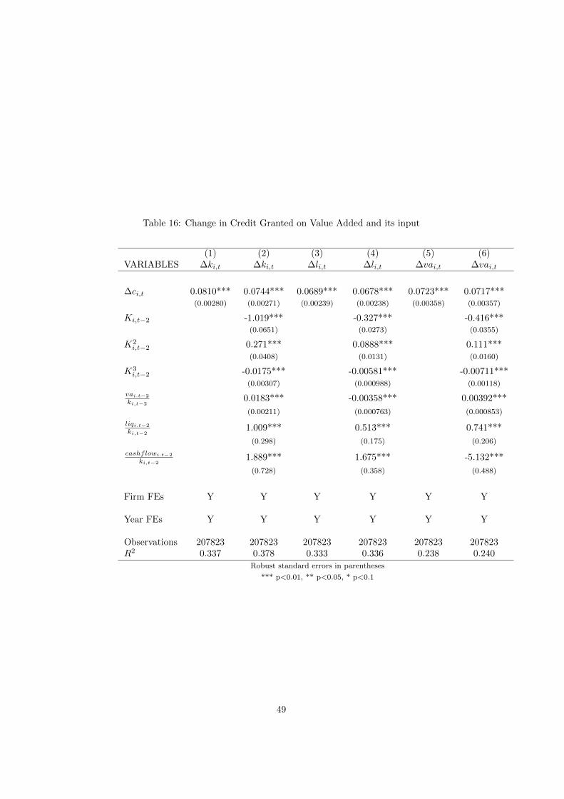
Table 16: Change in Credit Granted on Value Added and its input

(1) (2) (3) (4) (5) (6)VARIABLES ∆ki,t ∆ki,t ∆li,t ∆li,t ∆vai,t ∆vai,t

∆ci,t 0.0810*** 0.0744*** 0.0689*** 0.0678*** 0.0723*** 0.0717***(0.00280) (0.00271) (0.00239) (0.00238) (0.00358) (0.00357)

Ki,t−2 -1.019*** -0.327*** -0.416***(0.0651) (0.0273) (0.0355)

K2i,t−2 0.271*** 0.0888*** 0.111***

(0.0408) (0.0131) (0.0160)

K3i,t−2 -0.0175*** -0.00581*** -0.00711***

(0.00307) (0.000988) (0.00118)

vai.t−2

ki,t−20.0183*** -0.00358*** 0.00392***

(0.00211) (0.000763) (0.000853)

liqi.t−2

ki,t−21.009*** 0.513*** 0.741***

(0.298) (0.175) (0.206)

cashflowi.t−2

ki,t−21.889*** 1.675*** -5.132***

(0.728) (0.358) (0.488)

Firm FEs Y Y Y Y Y Y

Year FEs Y Y Y Y Y Y

Observations 207823 207823 207823 207823 207823 207823R2 0.337 0.378 0.333 0.336 0.238 0.240

Robust standard errors in parentheses

*** p<0.01, ** p<0.05, * p<0.1

49

Table 17: Effects of Credit shifter on Productivity growth, 1% threshold(1) (2) (3) (4) (5) (6) (7)

VARIABLES ∆ωi,t ∆ωi,t ∆ωi,t ∆ωi,t ∆ωi,t ∆ωi,t ∆ωi,t

si,t 0.101** 0.144*** 0.156*** 0.119*** 0.149*** 0.143*** 0.137***(0.0442) (0.0290) (0.0288) (0.0388) (0.0271) (0.0275) (0.0279)

Firm FEs Y Y Y Y Y Y YYear FEs Y Y Y Y Y Y Y

Prod. Function T-L C-D T-L T-L C-D (CRS) C-D (CRS) C-D (CRS)

Estimation of ωi,t ACF ACF ACF ACF Assumed Assumed Assumedβk = .25 βk = .33 βk = .40

Proxy vars mat, serv mat, serv mat mat, serv, ∆ki,t

Observations 179098 179098 179098 179098 179098 179098 179098R2 0.138 0.194 0.200 0.145 0.201 0.205 0.208

Robust standard errors in parentheses

*** p<0.01, ** p<0.05, * p<0.1

50

Table 18: Credit supply shifter on Productivity, different FEs Structures

(1) (2) (3) (4)VARIABLES ∆ωi,t ∆ωi,t ∆ωi,t ∆ωi,t

si,t 0.0403** 0.0637*** 0.0976*** 0.131***(0.0174) (0.0179) (0.0290) (0.0261)

Year FEs Y Y Y Y

Firm FEs Y Y

Province FEs Y Y

Year×Province Y×Sector

Observations 222629 222629 222629 222629R2 0.027 0.033 0.310 0.177

Robust standard errors in parentheses

*** p<0.01, ** p<0.05, * p<0.1

51

Tab

le19:

Sh

are

of

exp

ort

reve

nu

e(C

-D)

(1)

(2)

(3)

(4)

(5)

(6)

VA

RIA

BL

ES

∆ωi,t

∆ωi,t

∆ωi,t

∆ωi,t

∆ωi,t

∆ωi,t

s i,t

0.13

4***

1.68

32.3

10**

0.1

32***

1.1

59*

2.3

79**

(0.0

288)

(1.1

32)

(0.9

57)

(0.0

283)

(0.6

83)

(0.9

65)

export i

,t−

2

yi,t

−2

-0.0

0596

*-0

.0591

0.0

0749

(0.0

0347)

(0.0

848)

(0.0

104)

s i,t·e

xport i

,t−

2

yi,t

−2

-0.0

252

-7.6

36

4.6

13

(0.0

675)

(11.5

3)

(8.0

11)

1[e

xport i

,t−

2

yi,t

−2

>.5

]-0

.00483

-0.0

0199

0.0

0619

(0.0

0313)

(0.0

0448)

(0.0

0615)

1[e

xport i

,t−

2

yi,t

−2

>.5

]·s i

,t-0

.00662

0.9

15

1.7

84

(0.0

626)

(1.5

90)

(4.9

74)

Est

imat

ion

OL

S2S

LS

2S

LS

OL

S2S

LS

2S

LS

Inst

rum

ents

M&A

i,[t−2;t]

¯INTBK

i,2006

M&A

i,[t−2;t]

¯INTBK

i,2006

Yea

rF

Es

YY

YY

YY

Fir

mF

Es

YY

YY

Yea

r×P

rovin

ceY

Y×

Sec

tor

FE

s

Ob

serv

atio

ns

2226

2222

2622

38057

222622

222622

38057

R2

0.17

70.

133

-0.0

44

0.1

77

0.1

68

-0.0

20

Rob

ust

stan

dard

erro

rsin

pare

nth

eses

***

p<

0.0

1,

**

p<

0.0

5,

*p<

0.1

52

Tab

le20:

Sh

are

of

exp

ort

reve

nue

(T-L

)

(1)

(2)

(3)

(4)

(5)

(6)

VA

RIA

BL

ES

∆ωi,t

∆ωi,t

∆ωi,t

∆ωi,t

∆ωi,t

∆ωi,t

s i,t

0.12

8***

1.46

62.1

32*

0.1

45***

2.1

61**

2.3

99*

(0.0

380)

(1.5

49)

(1.2

47)

(0.0

373)

(0.9

27)

(1.2

67)

export i

,t−

2

yi,t

−2

-0.0

0994

**0.

0495

-0.0

0803

(0.0

0491)

(0.1

16)

(0.0

126)

s i,t·e

xport i

,t−

2

yi,t

−2

-0.0

271

7.31

73.0

38

(0.0

947)

(15.7

3)

(8.8

14)

1[e

xport i

,t−

2

yi,t

−2

>.5

]-0

.00801*

-0.0

110*

0.0

00363

(0.0

0448)

(0.0

0638)

(0.0

0786)

1[e

xport i

,t−

2

yi,t

−2

>.5

]·s i

,t-0

.136

-2.9

50

-1.2

36

(0.0

923)

(2.2

88)

(5.9

24)

Est

imat

ion

OL

S2S

LS

2S

LS

OL

S2S

LS

2S

LS

Inst

rum

ents

M&A

i,[t−2;t]

¯INTBK

i,2006

M&A

i,[t−2;t]

¯INTBK

i,2006

Yea

rF

Es

YY

YY

YY

Fir

mF

Es

YY

YY

Yea

r×P

rovin

ceY

Y×

Sec

tor

FE

s

Ob

serv

atio

ns

2226

2222

2622

38057

222622

222622

38057

R2

0.13

50.

090

0.0

00

0.1

35

0.1

21

0.0

11

Rob

ust

stan

dard

erro

rsin

pare

nth

eses

***

p<

0.0

1,

**

p<

0.0

5,

*p<

0.1

53

Table 21: Persistence (C-D)

(1) (2) (3) (4)VARIABLES ∆ωi,t ∆ωi,t ωi,t ωi,t

si,t 0.164*** 0.205*** 0.192*** 0.190***(0.0322) (0.0328) (0.0355) (0.0303)

si,t−1 -0.0196 0.0585* 0.161*** 0.0830***(0.0334) (0.0324) (0.0330) (0.0297)

si,t−2 -0.0929*** -0.0721** 0.0693** -0.0189(0.0349) (0.0334) (0.0323) (0.0300)

si,t−3 0.0305 -0.000333 0.119*** 0.0653**(0.0320) (0.0320) (0.0338) (0.0290)

∆ωi,t−1 -0.421***(0.00762)

∆ωi,t−2 -0.232***(0.00574)

∆ωi,t−3 -0.140***(0.00512)

ωi,t−1 0.421***(0.00781)

ωi,t−2 0.0710***(0.00654)

ωi,t−3 -0.00260(0.00511)

Year FEs Y Y Y Y

Firm FEs Y Y Y Y

Observations 170367 151852 170367 166292R2 0.199 0.302 0.875 0.897

Robust standard errors in parentheses

*** p<0.01, ** p<0.05, * p<0.1

54

Table 22: Persistence (T-L)

(1) (2) (3) (4)VARIABLES ∆ωi,t ∆ωi,t ωi,t ωi,t

si,t 0.154*** 0.228*** 0.312*** 0.231***(0.0431) (0.0456) (0.0524) (0.0416)

si,t−1 -0.00163 0.0602 0.245*** 0.106***(0.0445) (0.0448) (0.0476) (0.0402)

si,t−2 -0.0778* -0.0677 0.0964** -0.00312(0.0460) (0.0456) (0.0470) (0.0406)

si,t−3 -0.00265 -0.0227 0.122** 0.0448(0.0422) (0.0440) (0.0493) (0.0391)

∆ωi,t−1 -0.343***(0.00858)

∆ωi,t−2 -0.203***(0.00714)

∆ωi,t−3 -0.130***(0.00665)

ωi,t−1 0.501***(0.00885)

ωi,t−2 0.0537***(0.00746)

ωi,t−3 -0.0205***(0.00676)

Year FEs Y Y Y Y

Firm FEs Y Y Y Y

Observations 170367 151852 170367 166292R2 0.152 0.239 0.943 0.957

Robust standard errors in parentheses

*** p<0.01, ** p<0.05, * p<0.1

55