c o .& y - nasa
TRANSCRIPT
cC O .& Y
SOLAR FLARE PARTICLE PROPAGATION — COMPARISON OF
A NEW ANALYTIC SOLUTION WITH SPACECRAFT
MEASUREMENTS
Thesis by
John Edward Lupton
CALIFORNIA INSTITUTE OF TECHNOLOGY

SOLAR FLARE PARTICLE PROPAGATION — COMPARISON OF
A NEW ANALYTIC SOLUTION WITH SPACECRAFT
MEASUREMENTS
Thesis by
John Edward Lupton

ii
ACKNOWLEDGMENT
This thesis is to a great extent the result of the guidance of my
faculty sponsor, Professor Edward C. Stone. I am grateful for his sug-
gestions and encouragement, and especially for his ability to find time
for me within his busy schedule.
My thanks go to Dr. Stephen S. Murray, whose thesis was the pre-
decessor of the work presented here, and whose advice concerning many
of the particulars of the OGO-6 experiment was indispensable. Steve
was responsible for the calibration of the instrument response to
protons, and many of his data analysis programs were borrowed directly
for this work.
I would also like to acknowledge Professor Rochus E. Vogt, who is
co-investigator on the OGO-6 experiment. Dr. Vogt's support, both
moral and technical, is appreciated.\
My theoretical efforts were greatly aided by discussions with
Caltech Professors J. R. Jokipii, Jon Mathews and Don Cohen, and by
talks with Dr. L. A. Fisk of GSFC and Miriam A. Forman of the State
University of New York. I also greatly appreciate discussions with Dr.
John Fanselow, and with my fellow graduate students Lawrence Evans, Tom
Garrard, Alan Cummings, and James Brown.
Special thanks go to my undergraduate helpers Paul Sand, who •
carried out many of the necessary computer calculations, and Don Gunter,
whose constant barrage of questions led to the clarification of many
problems.

ill
Caltech's Solar and Gnlactic Cosmic Ray Experiment aboard OGO-6
was the result of the joint efforts of the personnel of the Space
Radiation Laboratory, the Central Engineering Services, the Analog
Technology Corporation, TRW Systems, Inc., and the OGO Project Office
of the National Aeronautics and Space Administration. Among the
Caltech staff, William E. Althouse must be mentioned as that indis-
pensable person who really understands the OGO-6 experiment elec-
tronics. Thanks also to Ellen Aguilar and Florence Pickett for their
help with the data handling and analysis.
Valuable support for my graduate work at Caltech was provided by
an N.D.E.A. Fellowship and a NASA Traineeship. The research work
presented here .was supported in part by the National Aeronautics and
Space Administration under Contract No. NAS5-9312 and Grant Nos.
NGR-05-002-160 and NGL-05-002-007.
I am especially grateful to my wife Kathy, whose nimble fingers
at the keyboard of the Selectric transformed my scribblings into the
pages which follow.

iv
ABSTRACT
A new analytic solution has been obtained to the complete
Fokker-Planck equation for solar flare particle propagation including
the effects of convection, energy-change, corotation, and diffusion
2with K = constant and Kg « r . It is assumed that the particles are
injected impulsively at a single point in space, and that a boundary
exists beyond which the particles are free to escape. Several solar
flare particle events have been observed with the Caltech Solar and
Galactic Cosmic Ray Experiment aboard OGO-6. Detailed comparisons of
the predictions of the new solution with these observations of
1-70 MeV protons show that the model adequately describes both the
rise and decay times, indicating that < = constant is a better des-
cription of conditions inside 1 AU than is < « r. With an outer
boundary at 2.7 AU, a solar wind velocity of 400 km/sec, and a
20 2radial diffusion coefficient < - 2-8 x 10 cm /sec, the model gives
reasonable fits to the time-profile of 1-10 MeV protons from "classi-
cal" flare-associated events. It is not necessary to invoke a
scatter-free region near the sun in order to reproduce the fast rise
times observed for directly-connected events. The new solution also
yields a time-evolution for the vector anisotropy which agrees well
with previously reported observations.
In addition, the new solution predicts that, during the decay
phase, a typical convex spectral feature initially at energy T will
move to lower energies at an exponential rate given by T =K.LNK.
T expC-t/T.,.....--,). Assuming adiabatic deceleration and a boundary atO 1S.J.1N1S.
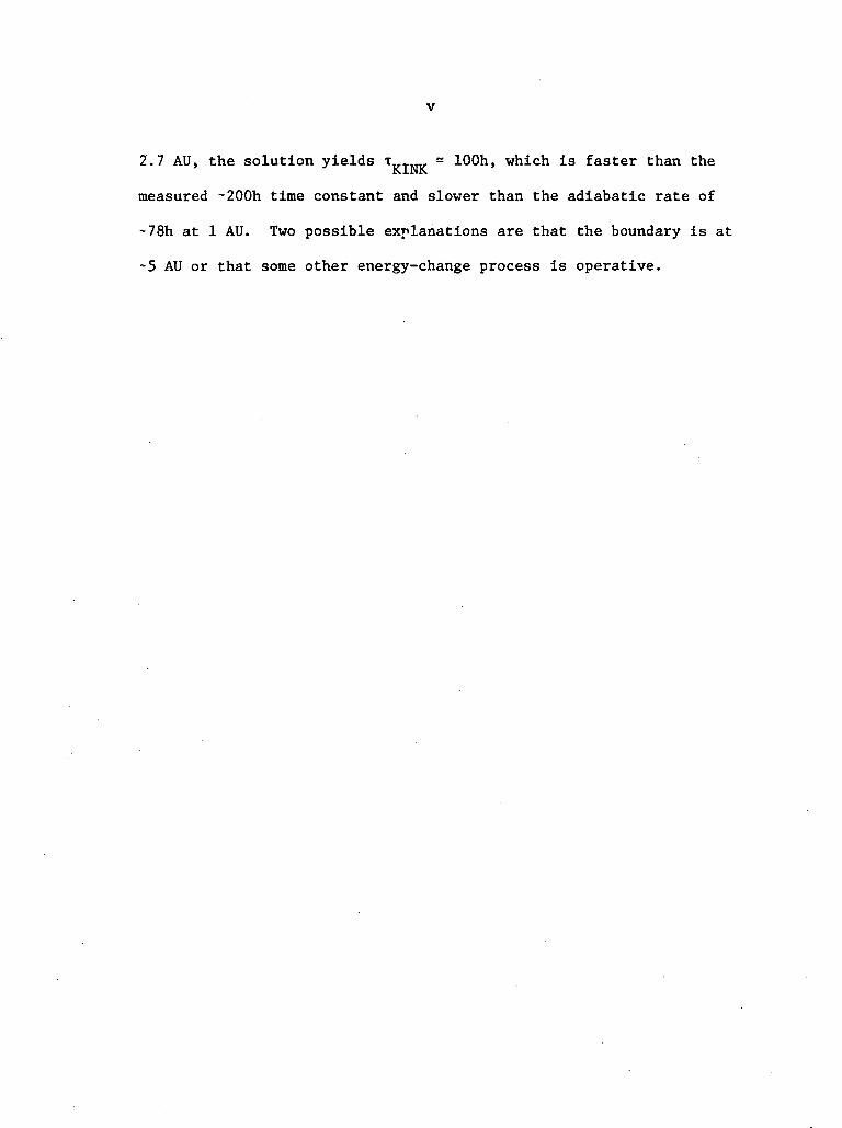
2.7 AU, the solution yields T = lOOh, which is faster than theKJ.NK
measured ~200h time constant and slower than the adiabatic rate of
~78h at 1 AU. Two possible explanations are that the boundary is at
~5 AU or that some other energy-change process is operative.

vi
TABLE OF CONTENTS
PART TITLE PAGE
I. INTRODUCTION 1
II. INSTRUMENT 4
A. General Description 4
B. The AE-Range Telescope 6
1. Physical Description 6
2. Detectors 9
3. Anti-coincidence Shield 11
4. Electronics 11
5. Electronics Calibration 15
C. Spacecraft 17
1. The Satellite Orbit 17
2. Invariant Latitude and Magnetic Local Time 18
III. DATA ANALYSIS 22
A. Proton Response of the AE-Range Telescope 22
1. Accelerator Calibration 22
2. Proton Energy-loss Calculation 23
3. Pulse Height Data Reduction 25
B. Bulk Data Processing 37
1. Tape Merging 38
2. Polar Rate Averages 38
3. Orbit Plots 40
4. Calculation of Proton Flux 45

vii
PART TITLE PAGE
IV. OBSERVATIONS 47
A. Event Identification 48
B. OGO-6 Flare Observations 50
V. DISCUSSION 65
A. Introduction 65
B. Background 70
1. The Interplanetary Medium 70
2. The Fokker-Planck Equation and Particle 72
Diffusion
3. Solar Flare Particle Events 78
C. Solving the Fokker-Planck Equation for Solar 80
Flare Particle Injection
1. Some Boundary Conditions and Simplifying 80
Assumptions
2. Separation of Variables ' 82
3. The Azimuthal Dependence 83
4. The Energy Dependence 85
5. The Radial Dependence 87
D. The New Solution 89
1. Derivation 89
2. Behavior of the Solution 91

viii
PART TJTLF. PAGE
V. DISCUSSION (cont.)
E. Fits to Data Assuming Pure Adiabatic Deceleration 100
1. Method of Fitting Actual Data 100
2. Forman's Solution 102
3. Fits using the New Solution 104
4. Evaluation 108
F. Vector Particle Anisotropy 113
1. Definition 113
2. Observations 114
3. Anisotropy Predicted by the New Solution 115
G. The Energy-Change Effect 120
1. Statement of the Problem 120
2. Observations 121
3. Energy-Change Predicted by the New Solution 124
4. Conclusions Concerning the Energy-Change 136
Process
VI. CONCLUSION 141
Appendix A - OGO-6 Monthly Summary Plots for June 1969 144
through February 1970
Appendix B - Solution for the Azimuthal Dependence 157
ix
PART TITLE PAGE
Appendix C - Derivation of the New Solution to the 159
Radial Equation
1. Derivation of the Solution 159
2. The Orthogonality Relation for Regular 162
Coulomb Wave Functions
3. Evaluating the Orthogonality Integral 163
Appendix D - Notes on Calculating the New Solution 165
References 168

LIST OF FIGURES
NUMBER TITLE PAGE
II-l Cross-section of AE-Range Telescope 7
II-2 AE-Range Telescope Electronics Block Diagram 13
II-3 Typical OGO-6 Orbital Trajectories in Geocentric 19
Coordinates
II-4 Typical OGO-6 Orbital Trajectories in A-MLT 21
Coordinates
III-l Calculated Average Energy Loss in Various Range 24
Telescope Detectors vs. Incident Energy
III-2 Dl vs. D2 Proton Response 27
III-3 D2 vs. D3 Proton Response 29
III-4 Actual Dl vs. D2 Pulse Height Data 31
III-5 Actual D2 vs. D3 Pulse Height Data 33
III-6 Flow Chart of Range Telescope Data Processing 39
III-7 Computer-Generated Rate Plot 42
III-8 Computer-Generated Orbit Plot 44
III-9 Computer-Generated Plot of Proton Flux vs. 46
Incident Energy
IV-la Time Histories of Four Selected Solar Flare 53 - 56
-lb Particle Events
-Ic
-Id
NUMBER
xi
TITLE PAGE
IV-2a Samples of Proton Differential Energy Spectrum 60 - 63
-2b During Decay Phase of Four Selected Flare
-2c Events
-2d
V-l Diffusion Coefficient K vs. Proton Kinetic Energy 76
V-2 New Radial Solution R(r,t) vs. Radial Distance r 92
for Various Times After Particle Injection
V-3 New Radial Solution R(r,t) vs. time t Observed at 93
Different Distances.
V-4 Dependence of the Decay Time Constant !:_.„-, on < , 95Lite. r
V, L, and C.
V-5 Radial Distribution of Particles at Late Times vs. 97
r for Various Ratios V/K .
V-6 Particle Current S, and its Components S and S 99V ft
vs. r for three values of < .
V-7 Fits to 2 November 1969 Event Using Forman's 103
Solution with L = 2.3 AU.
V-8 Fits to 7 June 1969 Event Using New Solution • 105
with L = 2.7 AU
V-9 Fits to 2 November 1969 Event Using New Solution 106
with L = 2.7 AU
V-10 Fits to 31 January 1970 Event Using New Solution 107
with L = 2.7 AU.

xii
NUMBER TITLE PAGE/
V-ll Best-fit Values of K vs. Proton Energy for 109
All Three Events
V-12 Diffusive and Convective Components of Aniso- 118
tropy Predicted by New Solution vs. Time
V-13 Vector Diagram of Time- Evolution of Anisotropy 119
V-14 Time-Dependence of Intersection Energy During 123
Decay Phase of 7 June 1969 and 31 January
1970 Events
V-15 Time-Evolution of Convex Spectrum Generated by 127
Superposition of Power Laws
V-16 Dependence of Calculated T,..T „, on Spectral Shape 131
V-17 Dependence of T,,TlkTt.. on V, L, and K . 132J\J.r)Jx r
V-18 Dependence of T-,TXTI. on T., and L. 133KIWIS. &
V-19 Time- Evolution of the Curvature in the Kink 135
V-20 Fits to 7 June 1969 Event with New Solution 137
Matching Observed Energy-Change Rate
V-21 Fits to 31 January 1970 Event with New Solution 138
Matching Observed Energy-Change Rate
A- la OGO-6 Data Summary Plots for June 1969 to 148 - 156
-Ib February 1970
-Ic
-Id
-le
xiii
NUMBER TITLE PAGE
A-lf OGO-6 Data Summary Plots for June 1969 to 148 - 156
-lg February 1970 (continued)
-Ih
-li
D-l Computer Routines Used to Calculate the 166
New Solution
xiv
LIST OF TABLES
NUMBER TITLE PAGE
II-1 OGO-6 Experiment F-20 Particle Telescopes 5
H-2 - AE-Range Telescope Stack 8
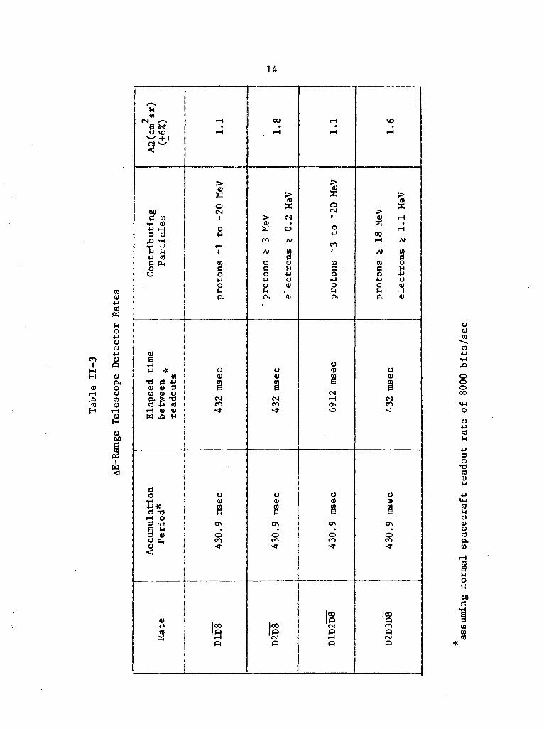
II-3 AE-Range Telescope Detector Rates 14
II-4 Ground-based Commands for AE-Range Telescope 16
III-l AE-Range Telescope Proton Pulse Height Bins 35
IV-1 Flare-associated Events Observed on OGO-6 51
Between June 1969 and February 1970
IV-2 Summary of Four Selected Flare Events 57
V-l Some Analytic Solutions to Fokker-Planck 69
Equations for Solar Flare Particle
Propagation
V-2 Power Law Superposition of a Density Spectrum 126
with a Convex Kink
I. INTRODUCTION
The study of solar cosmic rays includes several separate areas of
interest: the means by which solar particles are accelerated and in-
jected into interplanetary space, the transport and storage of these
particles in the solar system, and the problem of particle access to
the magnetosphere. The subject of this dissertation, the propagation
of solar flare protons, is part of the second of these topics. In
particular, near-earth observations of solar flare proton fluxes will
be used to develop a more complete representation of the physical
processes governing energetic particle transport.
The basic principles underlying the propagation of cosmic rays
in the solar system are at the present time fairly well established .
The picture of the interplanetary medium with a spiral magnetic field
imbedded in an outward-flowing solar wind plasma has won general accept-
(2)ance , and the first observational verification of the diffusion-
approximation to cosmic ray motion was made by Meyer, Parker, and
(3)Simpson in 1956 ' More recently, Parker added terms for particle con-
vection and energy-change in the solar wind to the equation for particle
(4)diffusion . This Fokker-Planck equation is now widely-used as a
description of particle transport in the solar system. In addition, a
relationship between the observed fluctuations in the magnetic field
and the magnitude of the diffusion tensor has been developed by
Jokipii ' ' and others ' , and has provided an independent means of
estimating the rate of particle diffusion.
Many solutions to the Fokker-Planck equation have been developed
in an effort to explain the particle fluxes observed subsequent to
solar flare injection. The models proposed have become more and more
refined, and analytic solutions now exist which include impulsive
injection, anisotropic diffusion (due to the presence of the average
magnetic field), convection, and energy-change > > > >
Despite these developments, none of these solutions have successfully
explained all of the observed features of solar flare events. Several
important questions remain unanswered: the exact nature of the
diffusion tensor and especially its dependence on radial distance and
particle energy; the method of particle injection and the possibility
of storage near the sun; the possible existence of a scatter-free
region extending outward some distance from the sun; the way in which
the particles become distributed in solar longitude; and whether or
not an outer boundary to the diffusing region exists beyond which part-
icles are free to escape.
The work presented here is a continuation of the process of compar-
ing theoretical solutions with spacecraft observations. Several solar
flare particle events have been observed with the Caltech Solar and
Galactic Cosmic Ray Experiment aboard NASA's OGO-6 spacecraft. In
addition, a new analytic solution has been obtained to the complete
Fokker-Planck equation including the effects of convection, energy-
change, solar rotation, and anisotropic diffusion using a radial
diffusion coefficient independent of distance. The predictions of
this new solution have been compared with the observed time-profile of

1-70 MeV protons, with previous measurements by McCracken et al.
of the anisotropy in the particle flux, and also with OGO-6 observa-
tions of the time-evolution of a feature in the proton energy spectrum.
These comparisons show that the model is capable of explaining both the
rise and decay phases of "classical" solar flare proton events, and
allow one to draw definite conclusions concerning the diffusion tensor,
the free-escape boundary, the possibility of a near-sun scatter-free
region, and the nature of the energy-change effect.
II. INSTRUMENT
A. General Description
Experiment F-20 aboard NASA's OGO-6 spacecraft is a solar and
galactic cosmic ray experiment consisting of 3 separate charged-particle
telescopes which share a common electronics package. The device was
designed and constructed at Caltech. A complete description of the
experiment with particular emphasis on the electronics has been published
previously
Although this dissertation is concerned only with the data from the
AE-Range Telescope portion of the F-20 experiment, some description of
the other parts of the instrument are included here for completeness.
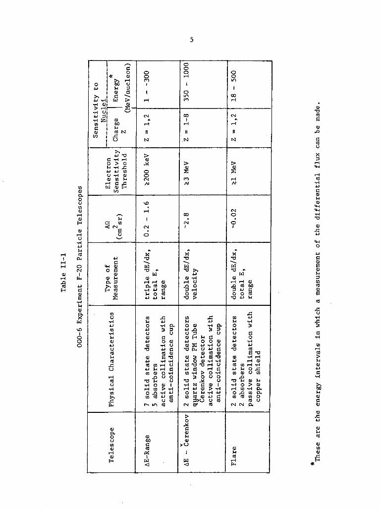
The separate charged particle measurements made by the three tele-
scopes are described in Table II-l. By combining measurements of energy
loss rate, total energy, range, and velocity, the instrument can separ-
ate charges up to Z = 8 and can make accurate measurements of particle
incident kinetic energy in the following ranges:
electrons: 200 keV to ~100 MeV
protons and alphas: -1 MeV/nucleon - 1 GeV/nucleon
lithium-oxygen nuclei: 350 MeV/nucleon - 1 GeV/nucleon.
The incident energy upper limit can be extended by using the geomagnetic
field as a particle spectrometer.
Since the experiment uses only 72 bits out of the total 1152 bit
OGO-6 main commutator data sequence, cosmic ray data from only one of
the three telescopes can be accumulated during each sequence. The elec-
tronics package includes a logic and priority subsystem that determines
•§
H
COCOaoaCOCOrHCOH
COrHO
•H4-1rlCO
OCM
rl
4-1CICU
B-uvd
o4J
4J -H•H CO> ^jr-l•H O4J 3•H £5
COccu
!
T
i
C
U(
C(1
c0
•x coP»-» rHoO Orl 3CO Cc ^-
W >.<y&
CO009-1CO NI
43. O
4J *rj(3 -H rHO > OM -H 43U 4J COCJ -H COCO CO V<-1 C 433 CO H
CO
x-^(-1
S COC CM
BCJ
4-1
H COD B
cu0 rl3, 3>-, CD-1 CO
CU
COOiH4JCO•H
CU4-1CJCO
Cfl
6r- \cflo
•HCO
fH
cua,oo10cucuH
ooCO}
1rH
CMA
rH
II
(S3
cu
ooCMA!
rH
I
CM•
O
•t
-a"P?rr) •>
WCO
rH rH CUPu Cfl 00
•H 4J Ct-t O CO4-1 4-1 rt
CO 43»H 4->O -HP.4J S3CJ CJCO C4-1 O CUCU -HO
T3 4J C2 cu
4J TH -HCfl CO rH CJ4-1 rl rH CCO CU O iH
4D CJ OT3 rl CJ•rl O CU 1
O 43 -H 4JCO Cfl 4J C
U cflr» m cfl
cu00cCO
<-y*
1
ooorH
1
OinCO
coI
rH
II
.N
^>(U2
COA*
OO•
^
X*-o
^*^J ^»4-1
CO -HrH 0
O CO-a >
CO 43rl 4JO CO -HO.4-1 43 S 3O3 CJCO H rl C4-1 O O CUCU S 4J -rl CJ
T3 PL, CJ 4-1 C3CU cfl CU
cu S 4-> B *o4J O Q) iH -Hcfl T3 -O rH 04J 13 rH CCO -rl > O -rl
S 0 0 OT3 4«J CJ•H N C CU 1
O M M -H 4-1CO Cfl Q) 4-1 (3
3>cj o cflCN a* cfl
oca)}-lCO
>o1u
ooLO
1oorH
CMf<
i-H
IIN
^>OJsrHAI
CMO
•
O
x"
H*Q *t
WCO
rH rH CO43 Cfl 003 w fiO O cO
T3 4-1 rl
43CO 4-1i-t iHo s4JCJ Ccu o^J 1 i
CU 4J*O cfl
B *^3Q) -H i-H4J i-H 0)Cfl CO rH -H4J rl O 43CO CU CJ CO
oT3 rl 0) rl•H O > Q)
o 43 ca a.co co co o
Cfl CJCM CM O,
CO^1cfl
rH
cu•acoBcu41
CCOU
i-H
cfl•H4JCcuS-icu
>4H
<4H
•H•acu
43
ccu0)MCOCfl
cfl
CJ•H
"s
COrH
CO
cu4JC
rlCUCCU
CO434-1
COhCO
COCOcu
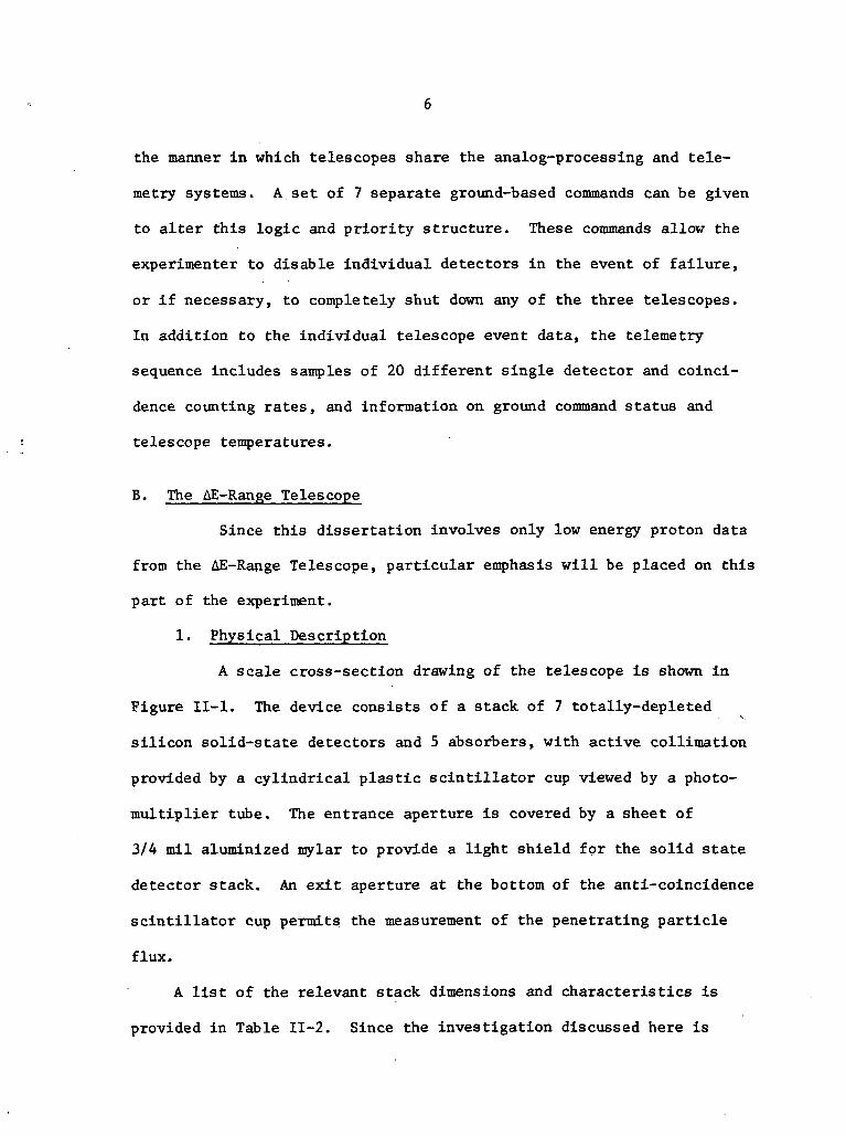
the manner in which telescopes share the analog-processing and tele-
metry systems. A set of 7 separate ground-based commands can be given
to alter this logic and priority structure. These commands allow the
experimenter to disable individual detectors in the event of failure,
or if necessary, to completely shut down any of the three telescopes.
In addition to the individual telescope event data, the telemetry
sequence includes samples of 20 different single detector and coinci-
dence counting rates, and information on ground command status and
telescope temperatures.
B. The AE-Range Telescope
Since this dissertation involves only low energy proton data
from the AE-Range Telescope, particular emphasis will be placed on this
part of the experiment.
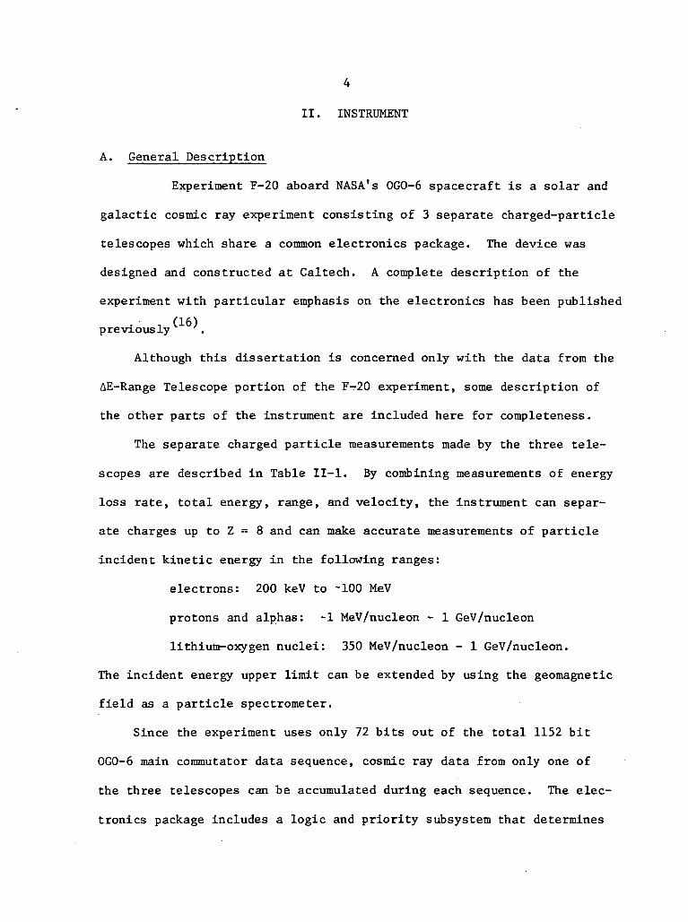
1. Physical Description
A scale cross-section drawing of the telescope is shown in
Figure II-l. The device consists of a stack of 7 totally-depleted
silicon solid-state detectors and 5 absorbers, with active collimation
provided by a cylindrical plastic scintillator cup viewed by a photo-
multiplier tube. The entrance aperture is covered by a sheet of
3/4 mil aluminized mylar to provide a light shield for the solid state
detector stack. An exit aperture at the bottom of the anti-coincidence
scintillator cup permits the measurement of the penetrating particle
flux.
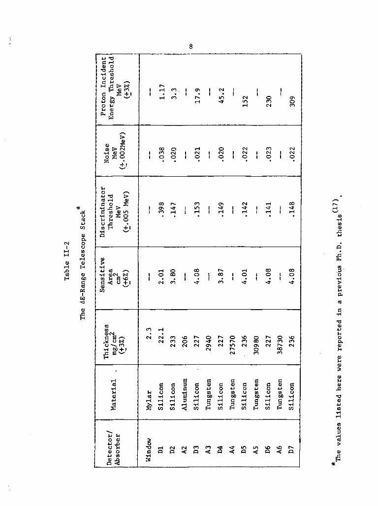
A list of the relevant stack dimensions and characteristics is
provided in Table II-2. Since the investigation discussed here is

Aii (CIVT-SR)DI-2 1.13D2-3 1.62D2-4 1.38D2-5 0.82D2-6 0.48D2-7 0.26
RANGE (G-CIVr2)A2 AL 0.21A3 W 2.9A4 W 27.6A5 W 31.0A6 W 38.7
PM
RCA 4439
0cm
Figure II-l: Scale cross-section drawing of the AE-Range Telescope.The Afl values have -6% uncertainty due-to the uncertainty in the sizeof the detector sensitive areas. The absorber thickness values areaccurate to ±3%. The values listed here were reported in a previousPh.D. thesis (17).
CMI
(U
Ort4-1cooia.ouco<u
00
i<a
4-) *"OC i-l0) O
•H CO0 0>Cj W /"^M .d > fr«
H 0) enc a -f iS §3 ~O Mrl 01p| Cj
w
0>oi SCO > CM
•H 01 Oo S o55 i1
MO ^"N4-i -a >«) rH 0)C o S•d fi >B to o» m•H Q) S Orl M O0 Jeto H ,+,1
O
01
•H4J cd *"s•H CUCM 6-SCO rl B VOC <! 0 +101 ^co
COCOCUCM
S S,O*•* o &*so *•». eni-l «> + !
fi
rHOS•H
i
O 014-> ^DU rl0) O4J CO
1 i-H en I <^ | CM 1 |1 • • 1 • 1 • 1 1
I-H en r m CMrH «* U~l
rH
00 O rH O CM1 en CM 1 CM 1 CM 1 CM |1 O O 1 O 1 O 1 O |
oo r en CT^ CM1 o\ -» i m i st i «* i1 en rH 1 rH | rH | i-H |
• • • • •
i-H O 00 Is* i-H1 O 00 | O 1 00 1 O I1 1 1 1 1
CM en <r en -*
en rH• •c M C M e n v o i ^ O f - O v o o
c M c n o e M « i t c M r - » e n o oc M c M C M < y > e M i n c M a \
CM r^ oCM en
S C C CC C 3 ( J O ) C O ) C O IO O C O 4 J O 4 J O 4 J
r l U U l H U C O O . C O U c OC 8 - H - H B - H M i H 0 0 - H 0 01 - l r H r H 3 r H C r H C r H ( 3> , i H - H r H - H 3 - H 3 - H 3S c o c o < j J c o H c o H c o H
§• O i - H c M C M e n e n « a : - s t ' i n mC P Q < Q < Q < Q <•H
11
O CTien oCM en
en CMCM I CMO 1 O
i-H CO<• i <rrH | rH• •
oo ooO 1 O
1^^ %^
^^ ^^ ^DCM en enCM r- CM
ooen
CC 0) C0 4J 0O CO 0iH 00 -HrH C rH•H 3 iHCO H CO
vo vo r*^Q ^j p.
CO•HCO0)
3o
•5!01rl
cdc•H
a>
OOu
01M01S
a>4JCO
cocu
10)$
concerned with protons below 150 MeV indicent energy, only detectors
Dl through D4 will be discussed in detail. Particle energy-loss can
be measured in detectors Dl, D2, and D3 using three separate pulse-
height analyzers, while triggers in detectors D4 through D7 are used
to indicate particle range. When the experiment is in the normal
operating command mode, either a D1D8 or a D2D3D8 trigger will
initiate pulse-height analysis. The D8 anti- coincidence shield not
only provides collimation for the telescope, but also rejects undesir-
able interaction and shower-type events which scatter particles into
the scintillator. For protons below 45 MeV incident energy, a triple
energy-loss measurement is recorded in Dl, D2, and D3. When any of
the "range detectors" D4 through D7 are triggered, this range informa-
tion replaces the Dl pulse height in the readout sequence.
Because of its high -400 keV discriminator threshold and small
depletion depth, detector Dl has less than 1% electron detection
(18efficiency for any incident electron energy ' . The problem of
separating low energy electrons from nuclei is thus easily solved
even for particles which stop in Dl.
2. Detectors
The seven solid-state detectors used in the range stack are
all totally-depleted silicon surface-barrier type devices manufactured
especially for Caltech by ORTEC (Oak Ridge Technical Enterprises Corp.),
The notation D1D8 is used to indicate a Dl trigger in the absence of aD8 trigger. D8 is thus in "anti-coincidence." In the same way, D2D3D8means a D2-D3 coincidence in combination with a D8 anti-coincidence.

10
With the exception of Dl, they have a nominal 1000ym depletion depth
2and 4.0 cm sensitive area. Surface-barrier detectors were used because
they have low noise and high reliability in a variety of environments,
and because they have high resistance to radiation damage from energetic
particles. In the case of Dl and D2, surface barriers were particularly
desirable because they can be manufactured with very thin dead regions
which allows an accurate measurement of particle total energy.
The detectors used in the experiment flight unit were carefully
selected on the basis of thickness, sensitive area, bias voltage needed
for total depletion, noise at full bias, and performance in a thermal-
vacuum environment. Since such devices cannot withstand any physical
contact from micrometers, fingers, etc., all physical measurements were
made in a "remote" fashion using energetic particles. The sensitive
area and total thickness were determined by irradiating each detector
with a well-collimated monoenergetic electron beam from a magnetic
3-ray spectrometer. More exact thickness measurements were made for Dl,
D2 and D3 when the completed flight unit was exposed to 1 - 23 MeV
protons from Caltech's Tandem Van de Graaff accelerator. Determinations
of dead layer thickness and proper operating bias voltage were made by
212exposing each detector surface to ThB(Pb ) alpha particles. The most
important test consisted of a two-week thermal-vacuum exposure for each
detector at full bias voltage. During the two weeks the detector noise
and leakage current were recorded frequently; an environment of <10
torr and +40°C was maintained.

11
Each detector in the operating experiment has a pulse-height dis-
criminator threshold associated with it that has been carefully adjust-
ed to reject detector noise but include all appropriate particle pulses
(see Table II-2). This threshold, which is clearly a function of both
detector thickness and noise level, was set (for all detectors except
Dl) so that 99% of all minimum-ionizing particles cause a trigger.
3. Anti-coincidence Shield
The anti-coincidence cup consists of a cylinder of NE 102
plastic scintillator material viewed by a RCA 4439 photomultiplier
137tube. The PM tube was tested using a Cs source in combination with
a Jfel crystal to determine the optimum operating bias voltage. The
discriminator was set using ground level muons incident on the assembled
D8 scintillator so that at least 99% of these minimum ionizing particles
cause a D8 trigger. Although this D8 threshold corresponds to only
~400 keV energy loss in the scintillator, the presence of an aluminum
housing which surrounds the scintillator raises the D8 incident energy
threshold to -9 MeV for protons and 0.6 MeV for electrons. Thus the
anti-coincidence cup acts as a mechanical collimator at low energies.
4. Electronics
The electronics package, which has been described in detail
elsewhere , consists of the following separate subsystems:
1) AE-Range telescope electronicsV
2) Cerenkov telescope electronics
3) Flare telescope electronics
12
4) Analog signal processor
5) Coincidence and priority logic
6) Rate accumulators
7) Data storage, formatting, readout, and spacecraft interface
8) Power supply
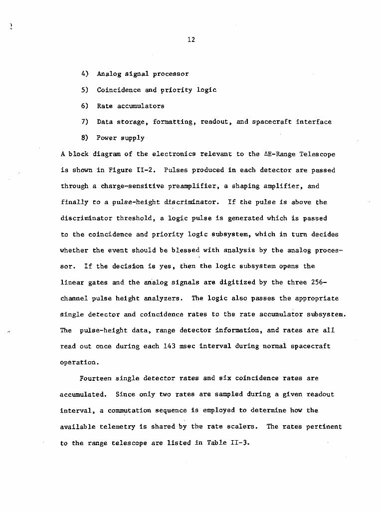
A block diagram of the electronics relevant to the AE-Range Telescope
is shown in Figure II-2. Pulses produced in each detector are passed
through a charge-sensitive preamplifier, a shaping amplifier, and
finally to a pulse-height discriminator. If the pulse is above the
discriminator threshold, a logic pulse is generated which is passed
to the coincidence and priority logic subsystem, which in turn decides
whether the event should be blessed with analysis by the analog proces-
sor. If the decision is yes, then the logic subsystem opens the
linear gates and the analog signals are digitized by the three 256-
channel pulse height analyzers. The logic also passes the appropriate
single detector and coincidence rates to the rate accumulator subsystem.
The pulse-height data, range detector information, and rates are all
read out once during each 143 msec interval during normal spacecraft
operation.
Fourteen single detector rates and six coincidence rates are
accumulated. Since only two rates are sampled during a given readout
interval, a commutation sequence is employed to determine how the
available telemetry is shared by the rate sealers. The rates pertinent
to the range telescope are listed in Table II-3.

13
00
•HQ
oo
cooco
o<uMw(Ua.ooCD(UiHa>H
(U00
CMI
0)>-lcm•H
COIH
0)rH
•aH
05CU
O4JO<u4Ja)pCUIXOO(00)
rH0)H
0)00Iw
1
COCM t-e *«
CJ VO
60C co
•H CU4J rH3 0,0 -H•H 4J
4J COC P-,OO
•H4-> *
COT3 C 4-1(U CU 3CO CU O£X 3 *T3tO 4-i CO
rH CU CUW ,£> M
O•H4-»*
cO *OrH O3 -H
3 CUCJ P-lo
CU
topt$
rH•
rH
0
O4-1
rH
COeo4-1O
(X
ucu
CMCO
* -
ucuCO6o\coCO
looorHQ
oo•
rH
1
> CM
S co
CO A)
A) COC
CO O
O 4-)I i u
O 0)^4 f— |
o. cu
ucu£3
CO* -
ucug
o\CDco
000CMo
rH•
rH
0CM
O4-1
CO1
mfio4-1o|
IX
ucucoI
CMrHCTivO
UCU
°?QCO
ooQ
0rHQ
vO•
rH
CU
> ^
£ rH
corH A»
At COcco oC rJO 4J4-1 CJO CUVI rH(X CU
ucu
CMCO•*^
CJcug
CTi
OCO
looo
'COQCMO
Ocuco
15
As mentioned previously, all three telescopes compete for the use
of the analog-processor and telemetry. During normal command-mode
operation, the Flare telescope has highest priority, while the Range
Vand Cerenkov telescopes compete on an equal basis at a lower priority
level. Thus the Flare telescope, which is a miniature version of the
Range telescope with passive instead of active collimation, begins to
dominate the analysis as the particle flux reaches the saturationV
levels for the Range and Cerenkov telescopes. This priority system can
be altered easily by means of the seven separate ground commands avail-
able. Table II-4 lists the ground based command combinations which are
pertinent to the operation of the Range telescope, and shows how these
commands affect the logic and priority structure.
5. Electronics Calibration
The basic principle behind the use of solid-state detectors
is that the charge pulse produced at the detector terminals is propor-
tional to the energy deposited in the active detector volume by the
charged particle. In order to convert digital pulse height data into
particle energy loss information, one must know the values of the
thresholds of all the PHA channels in units of MeV of particle energy
loss.
The calibration of the pulse-height analyzers was carried out as
a two-step process. First the voltage pulses from a Berkeley Tail
Pulse Generator were applied across a separate test capacitor at the
input of each charge-sensitive preamplifier. By varying the height of
this voltage test pulse and observing the pulse height analyzer output,

16
COi-H
•sH
>
4JcCU
gO
CJ
i
oO TO•H CO00 COO 0
»J 0M
00 fn
•H 00V4 OCO t-Hoo cd00 ti
•H <!
E-i V4O
t)eM 6
a cd
S55
s ^ll0 3
<UT3
rH
H
£4
O&
j«enOCM
^JO
ISrHO
Hicoa)PH
6
co
r^CJ
COrH•rlCd
>4H
£j
IM•rl
aco•HO
looteQCNft
CO
jQ
ceco•H
rHQ
3
coi— f•rled
CMO
m•H
rjCO
•HO
ISenQrlO
looorHQ
CUrHrQcdg
enQ
inCJ
M0
CO CrH O•H iHed 4J
M-l COC i-H
S S i4-1 S
MH o o•H CU O
rH CdC COcu cd> l-l 4J•rl O e«O IH T3
loooCMP
rl0
looorHQ
CUrH,£>cdg
CM
vOCJ
CO•rlCOfr*»
cd§COf^CO0000•H
4J
looQen
°^^rH
O
leoaenQ
1
mCJ
*oi
4-13
J=CO
(UcxooCOCU
rHcu4-1
CO00Ccd
OS
1
1
ovOCJ
vo mCJ CJm -*O CJ

17
the threshold value of each analyzer channel was determined in units
of pulser mV. In a similar way the discriminator threshold in pulser
mV was determined for each detector.
The second step involved the conversion of pulser mV to energy
loss in keV, which is equivalent to determining the value of the indi-
vidual test capacitors. This was achieved by irradiating each detector
with ThB alpha particles (with energies of 6.045, 6.083, and 8.776 MeV),
and comparing these particle-produced pulses with those of the test
pulser. The PHA and discriminator thresholds were thus determined
to an accuracy <jl% for temperatures between -5 C and +40°C. Typical
analyzer channel widths are -50 keV, yielding a saturation value of
~13 MeV for each of the 256-channel analyzers.
Tests of the logic and priority structure, command modes, and
rate sealers were also made using the ground support equipment. A more
detailed description of all the electronics test procedures has been
given in a previous Ph.D. thesis .
C. Spacecraft
1. The Satellite Orbit
The OGO-6 spacecraft is the last in a series of Orbiting
Geophysical Observatories flown by NASA. It was launched on June 5,
1969 into a polar orbit described by the following parameters:
perigee 397 km
apogee 1098 km
inclination 82°
period 99.8 minutes
18
Caltech's experiment F-20, which is one of 26 independent experiments
.aboard the satellite, is mounted on the -Z door so that the telescope
entrance apertures always face away from the earth.
The satellite orbit can be pictured as nearly fixed in space with
the earth rotating beneath. The earth's rotational axis is tilted 8°
out of the plane of the spacecraft orbit, so that the satellite never
reaches a QiOgiapltLc. latitude greater than 82° N or S. When the
satellite crosses the geographic equator from south to north, this is
taken conventionally as the beginning of a new revolution. Each of the
"14 revolutions per day are numbered consecutively throughout the life
of the satellite.
Since low energy cosmic ray particles have access to the earth's
magnetosphere only in the vicinity of the north and south magnetic
poles , the location of the satellite orbit in the polar regions is
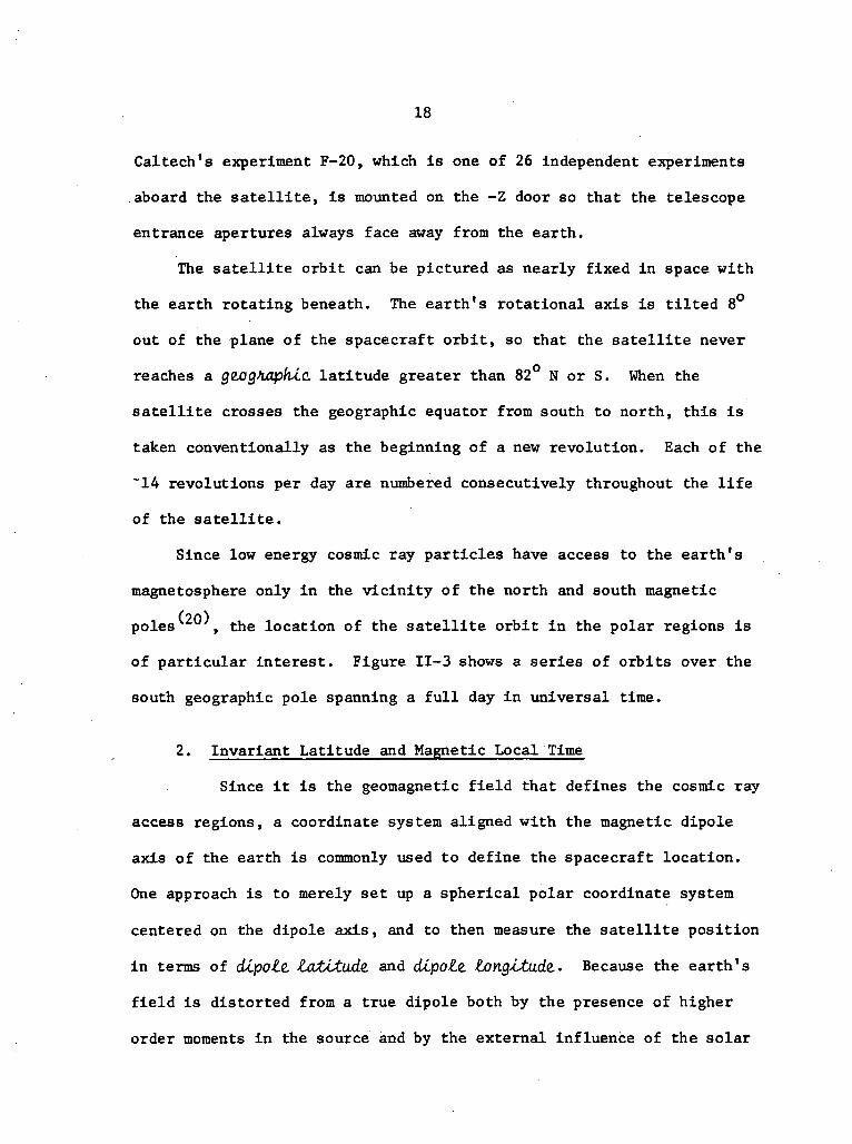
of particular interest. Figure II-3 shows a series of orbits over the
south geographic pole spanning a full day in universal time.
2. Invariant Latitude and Magnetic Local Time
Since it is the geomagnetic field that defines the cosmic ray
access regions, a coordinate system aligned with the magnetic dipole
axis of the earth is commonly used to define the spacecraft location.
One approach is to merely set up a spherical polar coordinate system
centered on the dipole axis, and to then measure the satellite position
in terms of diipoZe. tatitu.de. and dipo£e. tong<itu.de.. Because the earth's
field is distorted from a true dipole both by the presence of higher
order moments in the source and by the external influence of the solar
19
±180°
-90°-
SOUTHGEOGRAPHIC
•+90°
GEOGRAPHIC LONGITUDE
Figure II-3: Typical orbital trajectories for OGO-6 across the southpole in geocentric coordinates. The south invariant pole is the pointat which A - 90°.

20
wind, a non-spherical coordinate system using 4.nvaSitant taut/utdde. A» and/o -I 99}
magnetic. tocaJt time, MLT, has been found to be more appropriate ' .
These quantities are defined as follows:
| dipole longitude! /dipole longitudeMLT = I of spacecraft inI - Iof earth-sun line) + 12 hours
\ hours / \ in hours
(dipole latitude adjusted for \distortions of the geomagnetic 1field from a true dipole /
The value of the invariant latitude A for a deformed geomagnetic line
of force is defined to be the same as the dipole latitude of the equi-
valent undistorted "dipole" line of force. Note that any distortion of
the field lines in the azimuthal direction is neglected by the MLT
parameter. When the spacecraft is in the magnetic meridian plane that
contains the earth-sun line, it is at MLT = 1200 hours.
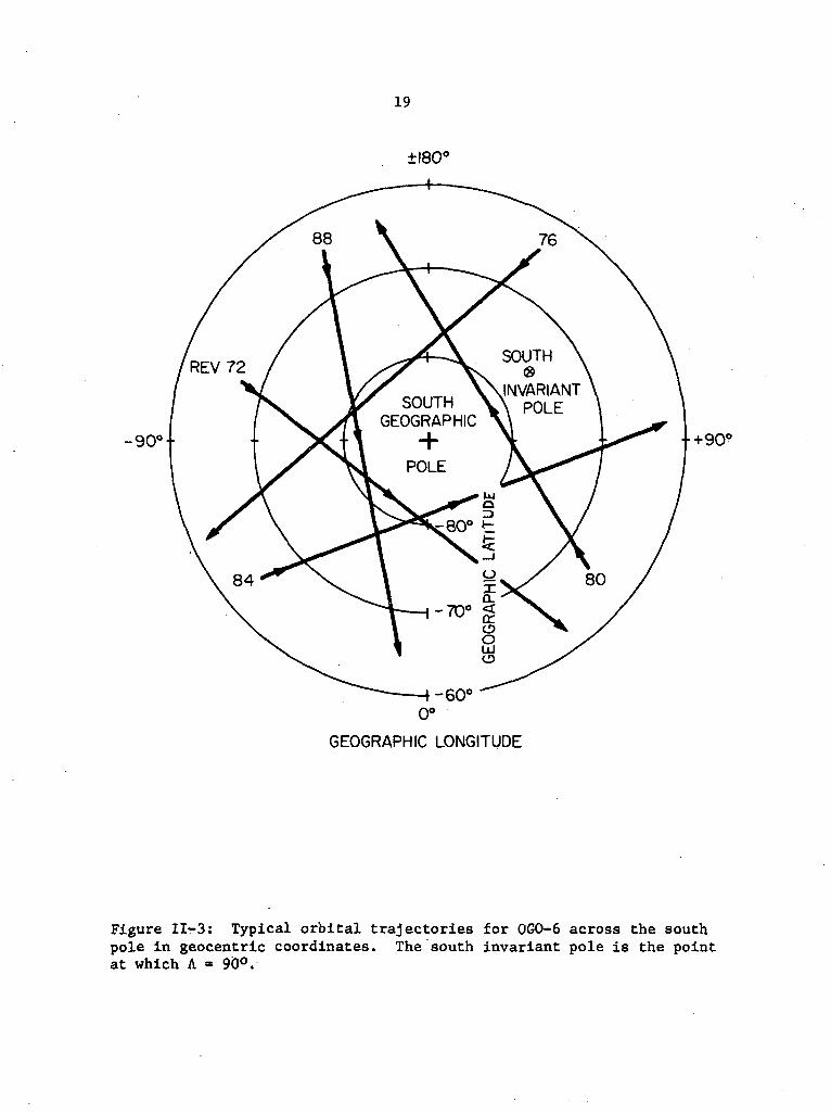
Figure II-4 shows the orbits of the previous figure plotted in
the A - MLT coordinate frame. Since the rotational and magnetic poles
differ in latitude by -11.5°, the orbit covers most values of A during
a 24-hour period. Note that the din.Z.o£ion in which the spacecraft
crosses the A - MLT plane is roughly constant with time. This cover-
age region rotates slowly at the rate of -1.8 /day, and the spacecraft
thus covers the entire A - MLT plane once every 100 days.
21
1200
1800 BOH 0600
-60°00002400
MAGNETIC LOCAL TIME
Figure,11-4: Typical orbital trajectories for OGO=-6-access the southpole in A-MLT coordinates. The dashed-line indicates where interpola-tion was necessary to determine the trajectory.

22
III. DATA ANALYSIS
This section describes the manner in which the raw data
produced by the F-20 Experiment are converted to useful information
about the intensity and composition of the cosmic ray particles in
the vicinity of the OGO-6 spacecraft.
A. Proton Response of the AE-Range Telescope
Using the results of the electronics calibration of the
analog-processors, one can convert a digital pulse height into a value
for the particle energy-loss in the detector depletion region. Given
a double or triple energy-loss measurement for a single particle event,
the problem remains to determine the particle charge Z and incident
kinetic energy E. The following is a discussion of how this problem
is solved for Dl through D4 proton events in the Range Telescope.
1. Accelerator Calibration
A straightforward way to determine the response of a cosmic
ray telescope to low energy protons is to simply expose the device to
a monoenergetic proton beam and observe the response directly. Such
an experiment has in fact been performed on the assembled F-20 flight
unit using Caltech's Tandem Van de Graaff accelerator. Although the
primary proton beam of the Caltech accelerator is limited to 12 MeV
10 3 12energy, 23 MeV protons can be produced by means of the B (He ,p) C
reaction. A magnetic spectrometer was used to select the desired beam
energy and also to limit the energy spread to AE/E = 1%. The Ground
23
Support Equipment was used to simulate the experiment-spacecraft inter-
face and to write the digital data on magnetic tape.
After some analysis, the incident proton energies needed to pene-
trate to the top of Dl, D2, A2, D3, and A3 (see Figure II-l) were
determined precisely. This information, in combination with the range-
(23)energy tables for protons in mylar, silicon, aluminum, and tungsten ,
yielded an accurate thickness measurement for the Mylar window and for
detectors Dl, D2, and D3. Analysis of the pulse-height data from the
accelerator runs also determined the most-probable pulse height com-
binations in Dl, D2, and D3 for various incident proton energies. A
detailed description of the Tandem Van de Graaff calibration has been
given by S . Murray .
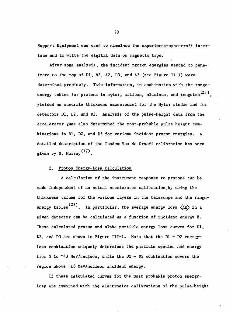
2. Proton Energy-Loss Calculation
A calculation of the instrument response to protons can be
made independent of an actual accelerator calibration by using the
thickness values for the various layers in the telescope and the range-
energy tables . In particular, the average energy loss < \E in a
given detector can be calculated as a function of incident energy E.
These calculated proton and alpha particle energy loss curves for Dl,
D2, and D3 are shown in Figure III-l. Note that the Dl - D2 energy-
loss combination uniquely determines the particle species and energy
from 3 to ~40 MeV/nucleon, while the D2 - D3 combination covers the
region above -IS MeV/nucleon incident energy.
If these calculated curves for the most probable proton energy-
loss are combined with the electronics calibrations of the pulse-height

24
100
>o>
ALd<V
10
10-I
protonsalphas
PHASaturationLevel
I 10 I02 I03
INCIDENT ENERGY (MeV/nucleon)
Figure III-l: Calculated average energy loss <AE> in various RangeTelescope .-detectors as a function of incident kinetic energy. Thecalculation is based on the Janni range-energy .tables.
25
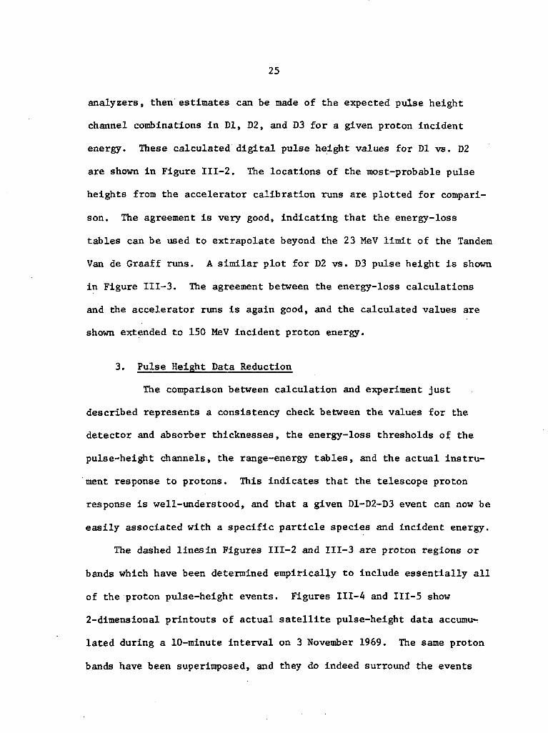
analyzers, then estimates can be made of the expected pulse height
channel combinations in Dl, D2, and D3 for a given proton incident
energy. These calculated digital pulse height values for Dl vs. D2
are shown in Figure III-2. The locations of the most-probable pulse
heights from the accelerator calibration runs are plotted for compari-
son. The agreement is very good, indicating that the energy-loss
tables can be used to extrapolate beyond the 23 MeV limit of the Tandem
Van de Graaff runs. A similar plot for D2 vs. D3 pulse height is shown
in Figure III-3. The agreement between the energy-loss calculations
and the accelerator runs is again good, and the calculated values are
shown extended to 150 MeV incident proton energy.
3. Pulse Height Data Reduction
The comparison between calculation and experiment just
described represents a consistency check between the values for the
detector and absorber thicknesses, the energy-loss thresholds of the
pulse-height channels, the range-energy tables, and the actual instru-
ment response to protons. This indicates that the telescope proton
response is well-understood, and that a given D1-D2-D3 event can now be
easily associated with a specific particle species and incident energy.
The dashed linesin Figures III-2 and III-3 are proton regions or
bands which have been determined empirically to include essentially all
of the proton pulse-height events. Figures III-4 and III-5 show
2-dimensional printouts of actual satellite pulse-height data accumu-
lated during a 10-minute interval on 3 November 1969. The same proton
bands have been superimposed, and they do indeed surround the events
26
Figure III-2
Proton response plotted on the 2-dimensional Dl vs. D2 pulse-
height plane. The numbers denote incident proton kinetic energy
in MeV. The crosses are the most-probable D1-D2 pulse-height
pairs derived from the results of the Tandem Van de Graaff accel-
erator calibration. The dots are the results of the average
energy-loss calculation based on the Janni range-energy tables
and on the best estimates for the Range Telescope detector and
absorber thicknesses. The dashed line defines a proton "band"
which includes essentially all valid proton events.

27
LJ
Xoh-XoUJX
UJC/)
COQ
13NNVHO JLH9I3H 3Sind 10

28
Figure III-3
Proton response plotted on the 2-dimensional D2 vs. D3 pulse-
height plane. The numbers denote incident proton kinetic
energy in MeV. The crosses are the most-probable D2-D3 pulse
height pairs derived from the results of the Tandem Van de
Graaff accelerator calibration. The dots are the results of
the average energy-loss calculation based on the Janni range-
energy tables and on the best estimates for the Range Tele-
scope detector and absorber thicknesses. The dashed line
defines a proton "band" which includes essentially all valid
proton events.

o«•CM
OOCM
oCM
LJ2zr
oh-X
LUCO
IDQ_
§2
o<M
oooGO
o(0
H3NNVHO 1H9I3H 3S"]f\d 20
30
Figure III-4
The Dl vs. D2 pulse height array observed during a polar
pass on 3 November 1969. The numbers indicate the total
number of events which occurred with a particular D1-D2
pulse height combination. The PHA channel numbers are
pseudo-logarithmic (256 actual channels have been com-
pressed into 60). The boundary of the proton band and the
calculated locus for o-partides have been superimposed.
The exact nature of the pulse-height scales and event
number code is explained in reference 17.
31
^
* •
jI-1f1111
11
Sinin
-
•4
-
J
/
ri1
•4
*S
'-
CM *4US«t
-
/
A
gs
//-
••
-
»
-•j/
/
"
AH-
"*
$3
Aim
Al
^
-
"
N-
^(M
•«
*4—
H
"•
SR «m^
x
—
o
R
•*
•4
IM
IM«n
4M
r-
IM
M
CM
p4
tM
Ft
•V
*
9
•
'•
,
.
|
•
•
'
;
;.
•
*•
9
•
"*
>4
n
N
•4
!
r"<rm
m
m
CM
fM
-
Al
14
"*
\* f*
* mD mA
H
J.
IM
ss
~ —
rJ-
Al
AI r-m 4(A -4
Al
J
^
--
M Al
^^
•4
^
fAl
«~
:„
j
•4 *4
**
*fl
*M
Im
1-4 in
m am o«in <n
mIM
I
"•
^ X
as
•***••,.-
•
CO
u
ca
J•
.
*
••
•
'
.
.
•
i
8
v ^
*
IA
^
*
(A
tfl
r
—
9>•4
"
^
J
^
Al
m
I:•« O
a o>U Al
•H
J
**
X X
rJ^Al
CM Al
ff> 00
CO P.
am
<-*
O *4
•41
-
*^
•4 »4
« tn
-
*4»4
0
m
• mm-4
•4
»4
•4
* m
^
*«P. <D
"«.«„
^
1•4
-
—
f* •«
*
*
<•
<nM
^
(H
0 O>
-rIM -»
AI tnAI m
•O Al
•4 *
-4 CM
Al
1
•"
*"
9 r-
N•4
tM
«
f*>
-
•»
-
Al
**
•4
•4
m
1
•4
IM
•4 ^4
4 Al
v4
—
^ f*
\
IM
•4
]-
-
"
0.-
^8i
n
*!n
IM
•^ Om
^•4
•4 inIM
4
n
n
n
•M
1*1
0
M
•4
A|
-t
)
««rp« m
IM
Al
O
32
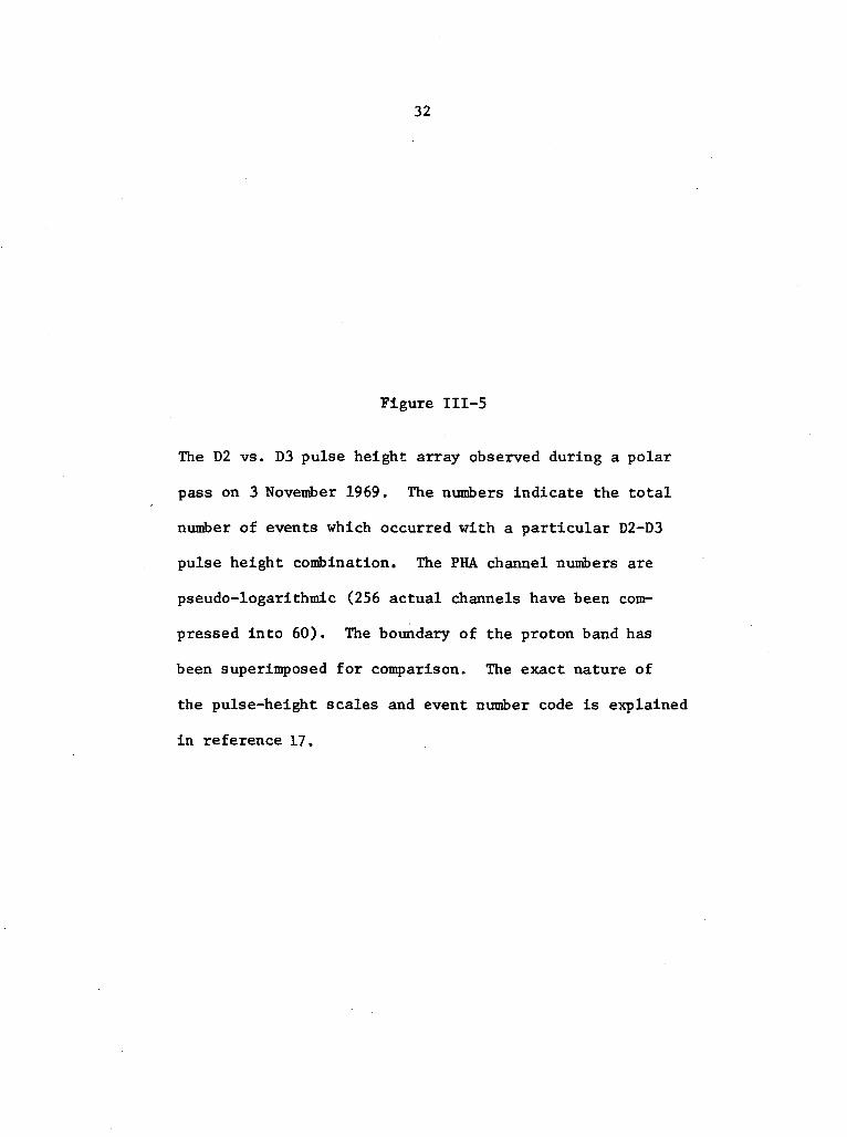
Figure III-5
The D2 vs. D3 pulse height array observed during a polar
pass on 3 November 1969. The numbers indicate the total
number of events which occurred with a particular D2-D3
pulse height combination. The PHA channel numbers are
pseudo-logarithmic (256 actual channels have been com-
pressed into 60). The boundary of the proton band has
been superimposed for comparison. The exact nature of
the pulse-height scales and event number code is explained
in reference 17.
33
3•
1
3flvt
2
Q
so
J-:
1
1ou.o
oa.a
K Q O" «^ 7 A m
O ILO
m m i*t
« *
o m *»»»

34
of interest. The events which are not within the boundaries of these
bands are either electrons, alphas, or in a few cases, protons which
have deposited anomalously small amounts of energy in at least one
of the detectors.
Using the relation between pulse-height response and incident
energy displayed in Figures III-2 and III-3, these bands were divided
into bins which correspond to different proton incident energy
intervals. Specifically, the D1-D2-D3 pulse height "space" was divided
into 37 proton incident energy bins by slicing the proton bands along
calculated lines of constant incident energy (see Table III-l). At
incident energies below -3 MeV, protons stop in Dl and no 2-dimensional
pulse-height information is available to cleanly separate protons from
other charged particles. Since Dl is insensitive to electrons, the
only threatening contaminants to the Dl proton analysis are low energy
alpha particles. This alpha contamination can easily be estimated
and can usually be neglected. Thus, below 3-MeV, the proton analysis
consists of a one-to-one map between groups of Dl pulse-height channels
and proton incident energy intervals.
The physics of the data reduction is contained in the proton pulse-
height bins and the incident energy intervals assigned to them. Given
such a set of bins, the rest of the analysis consists of deciding
whether each pulse-height event lies in the proton band, and if so, in
which bin. The proton differential flux dJ/dE can then be determined
as follows:

35
TABLE III-l
Proton Pulse-Height Analysis Bins for the
AE-Range Telescope
Bin No. Incident Energy Type of Analysis
1
2
3
4
5
6
7
8
9
10
11
12
13
14
15
16
17
18
rain
1.17
1.27
1.37
1.49
1.61
1.73
1.87
2.00
2.14
2.28
2.42
2.56
2.70
2.85
2.99
3.14
3.30
3.60
Emax
1.27
1.37
1.49
1.61
1.73
1.87
2.00 Dl Singles
2.14 AQ - 1.13 cm2sr + 6%
2.28
2.42
2.56
2.70
2.85
2.99
3.14
3.30Dl - D2
3.60Afi =1.13 cm sr + 6%
4.00

36
TABLE III-l (Cont.)
Bin No. Incident Energy Type of Analysis
19
20
21
22
23
24
25
26
27
28
29
30
31
32
37
33
34
35
36
min
4.00
4.50
5.00
6.00
7.00
9.00
15.00
20.00
30.00
20.00
17.90
20.00
25.00
35.00
20.00
45.00
70.00
100.00
45.00
Emax
4.50
5.00
6.00
7.00 oi - D2 cont.
9.00 Aft = 1.13 cm2sr + 6%
15.00
20.00
30.00
45.00
25.00
20.00
25.00D2 - D3 — no D4
35.00Afl = 1.59 cm2sr + 6%
45.00
45.00
70.00
100.00 D2D3 with D4
150.00 Afi = 1.2 cm2sr + 6%
150.00

37
EMIN., EMAX. = incident energy limits to pulse-height bin i
S. = number of pulse-height events in bin i in given timeinterval
N = normalizer between pulse-height data and actual particlerates
- (DIPS counting rate in counts/sec)
(total no. of D1D8 pulse-height events)
2An. = geometrical factor in cm sr assigned to bin i
dji 2 -1—-=r = proton differential flux at bin i in (cm sec sr MeV)during time interval
SIN
An± (EMAXj[ -
The normalizer N must be used instead of the actual accumulation time
because there are frequently many more valid events than can be analyzed
and readout.
B. Bulk Data Processing
The OGO-6 spacecraft has orbited the earth in a fully-opera-
tional state for 15 months (from 5 June 1969 to 29 August 1970). During
this period, the satellite completed 6500 orbits, and Caltech's experi-
ment F-20 accumulated approximately 2 x 10 bits of digital cosmic ray
data. With such a huge data set, it is virtually impossible to
completely process all of the data in a reasonable amount of time.
Consequently, a quick-processing scheme has been devised which allows

38
one to scan the data and select time periods of particular interest for
more detailed analysis. The overall data processing plan for the
Range Telescope is described in Figure III-6.
1. Tape Merging
The raw spacecraft data are received from Goddard Space Flight
Center in the form of Attitude-Orbit Tapes, which describe the satel-
lite location and orientation at 1-minute intervals, and Experimenter
Tapes, which contain the decommutated data from Caltech's Experiment
F-20. The first step in the data reduction process is to combine the
cosmic ray data with the relevant attitude-orbit information and write
the result on a single "merged" tape via a program named MERGE (see
Figure III-6). These merged tapes are the basic input for all subse-
quent steps in the data analysis.
2. Polar Rate Averages
Since the work discussed in this thesis is concerned with the
intensity of <in£eAp£an&ttUiy cosmic rays, the data of interest can be
accumulated only in the polar regions (see Section II-C). Although the
question of particle access to the magnetosphere is a very complicated
(24)and still unsolved problem , there does exist a given region in
A-MLT space at each pole where the flux is independent of spatial posi-
tion and identical to the interplanetary flux in the vicinity of the
earth . This region is roughly defined by |A| > 72° , even though
the exact boundary location depends on MLT, particle rigidity, and on
the configuration of the geomagnetic and interplanetary fields.

39
1o.S
g|
1
s
si55u g£.»o «Kl
V,1
Si«&
£X
g•5*5i«_ o>o o
«* ^
0 x
w
*o^ "*" o— *«>aS*° lSK Q. .« wS g
= i w.E> SU-J £*•£
oo>0
u_ o.
tL.
~"li
IsS M
0> &o
s
S » 2^0 > ?0£3 *2_l^^s15I5&fel*
•
co
t- E £E ""5^1 32 o><? CLg1 Ss!£ dl ft
i
cfl4J
i *1 T3
O.O
/• - o
«5 <nv >,~- SS» «5 5 " — ° E"• a = Ta, .•=».£ .S .OWE «5 6 2 8 *
Ti
5
ifs i
-i o S"=Si{!- si
tnUl1—
Qh.
1
c >. _ _ co«>'x g1""" S. • " *"
0= § *§. 0^ t r5{
"22 ^ *^rf ni
""^S"0 i *• Sv *-v
£ i «•* « e r- J OJoo - - r 2J'S tt I ^C
?sf5&f
S
5 5^i
i
C MI
ll'ef! 1" 5
O1 ' rH
CK
cuVi
00

The program P0LRAT is used to process the merged tapes and sample
the cosmic ray data automatically whenever |A| > 72°. The appropriate
range telescope coincidence and single detector counting rates are
averaged over these polar "cuts" and the results are punched on cards.
A routine called FLXPLT is then used to plot these individual polar
rate averages vs. time. Figure III-7 is an example of a typical com-
puter-generated "rate plot" which enables one to decide whether the data
should be subjected to more intensive (and more expensive) analysis.
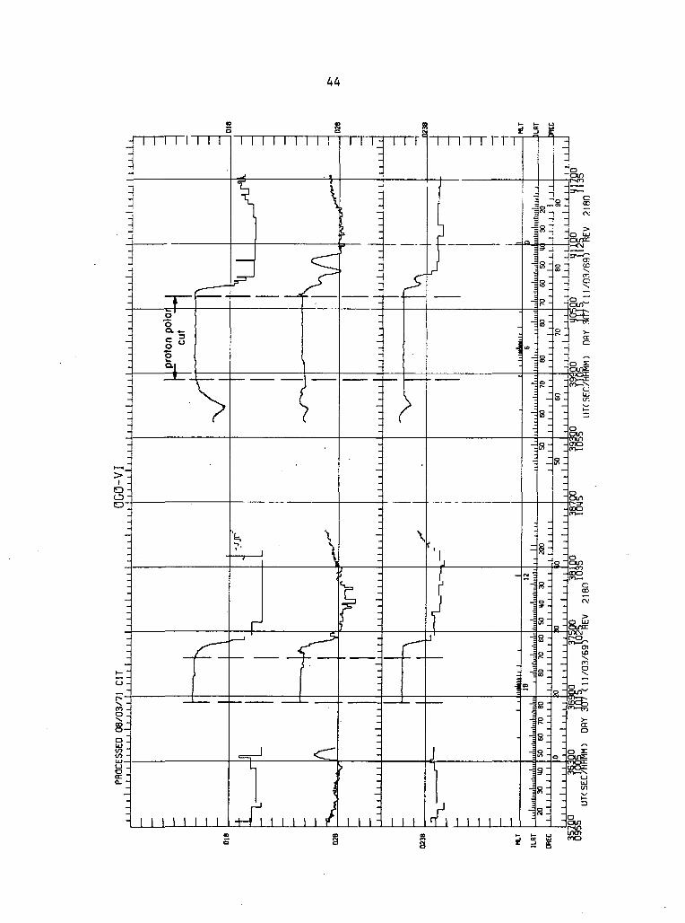
3. Orbit Plots
In order to analyze the data in a given time period in more
detail, the proton polar access regions must be defined more precisely.
A program named RATES is used to generate continuous plots of the key
detector counting rates as a function of time for each satellite orbit.
Such an "orbit plot" (see Figure III-8) makes the proton polar access
regions obvious and allows one to easily hand-pick time "cuts" for
further analysis. The dashed lines on Figure III-8 indicate the proton
polar cuts chosen for this particular orbit.
The orbit plot shown in Figure III-8 is in fact a streamlined
version which includes only the most important Range Telescope coinci-
dence rates. The write-up for the RATES program describes how more
complete orbit plots including some of the pulse-height data and all of
the 20 experiment counting rates can be generated.
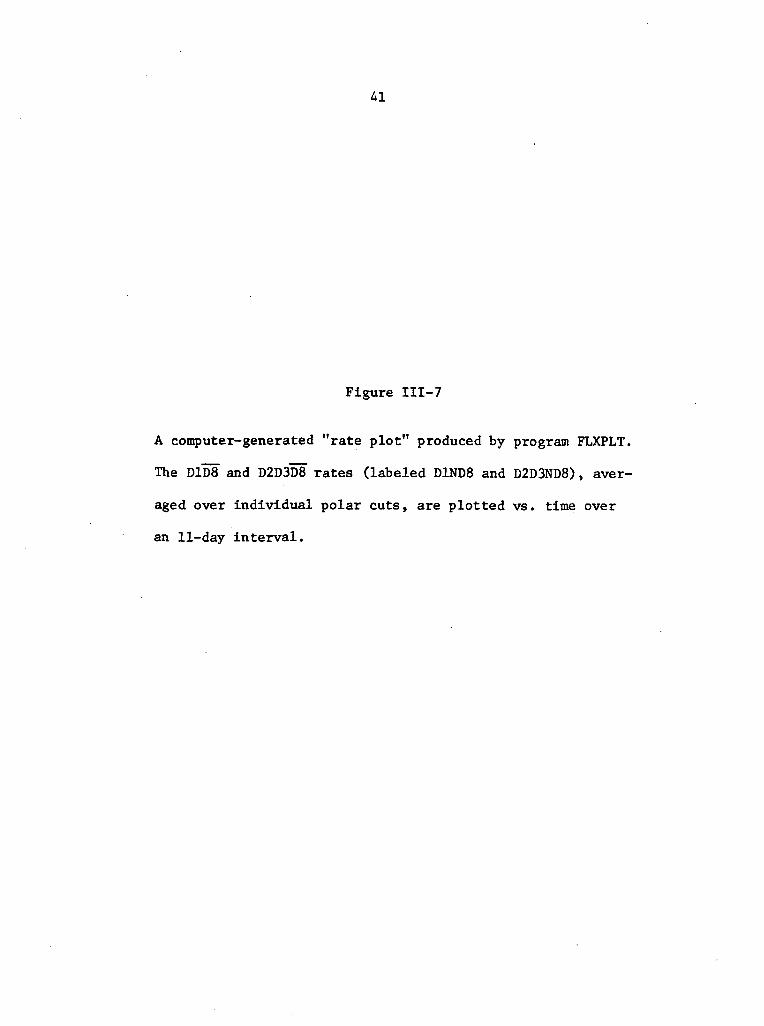
Figure III-7
A computer-generated "rate plot" produced by program FLXPLT.
The D1D8 and D2D3D8~ rates (labeled D1ND8 and D2D3ND8), aver-
aged over individual polar cuts, are plotted vs. time over
an 11-day interval.

42
Illl 1 1 lll I 1M
2J
* Ȥ
= <
% T»» *
M n =55 E
ll
X g i
*
§3 ir?I
tt =
J i l l I I
. *I M 1 1 1 III 1 1 1 1
S3xrru ao/ou 'soiibb 'S3ibia
<vPt

43
Figure III-8
A computer-generated "orbit plot" produced by the program
RATES. The D1D8, D2D8, and D2D3D8 coincidence rates (labeled
D18, D28, and D238) are plotted continuously vs. time for one
full spacecraft orbit. Magnetic Local Time and Invariant
Latitude are also included. The proton access regions are
clearly evident, and the hand-picked cuts have been marked
with dashed lines. Each tickmark along the Y-axis represents
one decade in counting rate. Changes in the D2D8 counting rate
during the proton polar cuts are due to electrons.
45
4. Calculation of Proton Flux
The time cuts chosen from the orbit plots are used as inputs
to the programs MT0TALE and/or MTW0D which process the pulse-height data
on the merged tapes during the time intervals specified. (See Figure
III-6.) Printed output of the 2-dimensional pulse-height analyzer
arrays can be produced (Figures 111-4 and III-5 are examples). The
proton differential fluxes in each of the 37 bins are calculated and
punched on cards. These cards are in turn used as an input to FLXPLT,
which produces plots of the flux time-profiles analogous to the rate
profiles of Figure III-7. Alternatively, the flux bins can be plotted
together for each polar cut to form an instantaneous proton differential
energy spectrum as in Figure III-9.
This completes the description of how the instrument and spacecraft
function, and in particular how the Range Telescope responds to the low
energy cosmic ray protons which are the topic of this dissertation. A
brief account has been given of the manner in which the tremendous bulk
of satellite data is scanned, sampled, and converted to useful informa-
tion, the information desired is of course the interplanetary proton
flux as a function of energy and time.

46
10 3,- I I I I I I I 11 I I I I I I I I! I I I I I I |-I1 'REV 21805 -
10 2
- i*- \UJz:ocen 10 ioUJto
10
I I I I I I III
FBOM ll:0«:00 OflY 307 -
TO 11:17:30 onr 307 -
i*i—*—i
T
I I I 1 111, i i i i i 11110° 10' 10 *
ENERGY (MEV)10
Figure III-9: A computer-generated plcrt.of the flux calculated for eachof the 37 pulse-height bins vs. incident energy for a single polar pass.The plot thus represents an instantaneous sample of the proton differen-tial energy spectrum.

47
IV. OBSERVATIONS
Solar cosmic ray phenomena as observed near the earth can be
(25)divided into the following four distinct types :
a) Flare-associated events — associated with optical flares,
x-ray and microwave emission. Electrons and nucleons observed at the
earth generally display a rapid (<2 day) intensity increase followed by
a slower decay phase.
b) Recurrent events — particle increases which sometimes appear
on the next rotation* after a flare-associated event. These events dis-
play roughly the same time history as the original flare and apparently
originate from the same active region.
c) Energetic particles associated with an active center —
increases which display no velocity dispersion and are not associated
with solar flare activity. They are thought to be particles emitted
continuously from an active region but confined to a given region of
interplanetary space. The time-profile of the event, which persists
from 3-14 days, is thus produced by the "co-rotation" of this region
past the earth. These events display steep proton energy spectra and
are often anti-correlated with the MeV electron intensity.
d) Energetic storm particle events — large intensity increases of
low energy protons and electrons associated with (and believed to be
accelerated by) strong interplanetary shock waves.
*The surface of the sun revolves at a rate which depends on solar lati-tude (the period is -27 days at the equator).
48
This dissertation is concerned only with flare-associated events,
and specifically with the means by which these flare particles, which
are assumed to be injected impulsively on the sun at the location of
the optical flare, propagate through interplanetary space to the earth.
The details of the actual flare event on the solar surface are of inter-
est here only when they affect the subsequent particle propagation and
the intensity observations at the earth. This section discusses the
method by which flare-associated events are identified, and summarizes
the OGO-6 proton intensity observations of four such events which are
discussed in Section V.
A. Event Identification
The typical solar flare proton behavior in the vicinity of
the earth can be described as a rapid rise in intensity, followed by a
smooth turnover and an approximately exponential decay phase with
T = 5 - 3 0 hours '. However, such "typical" flare time-profiles
are rarely observed, and in many cases it is difficult to separate flare
events from the other three types of solar phenomena. In order to yield
useful clues about the nature of particle propagation in interplanetary
space, the following information must be determined about an individual
flare event:
a) The event identification must be unambiguous — that is, it
must be possible to associate the intensity observations at earth on a
one-to-one basis with a &j.ngte. optical flare event on the sun. The
particle injection time (+ a few hours) and the point of injection on
the sun (in solar latitude and longitude) can easily be determined once

49
the optical counterpart of the cosmic ray event has been identified.
Multiple flare events, which occur frequently, are deemed unsuitable
for more detailed analysis.
b) It must be determined that no co-rotating features (i.e.,
recurrent events or active center events) or interplanetary magnetic
field boundaries have rotated by the earth during the flare observation
period. Such occurrences complicate the situation immensely and make
detailed analysis very difficult.
c) The average value of the solar wind velocity in the vicinity
of the earth must be determined. This is a parameter which affects the
particle propagation and thus is needed for complete analysis of the
event.
The method by which particle events can be accurately identified
is provided by the solar geophysical data published by ESSA (now
(27 28 )NOAA) ' . The emission of Type IV radio bursts and hard x-rays are
generally accepted as indicators of solar particle acceleration and
( 26 29)injection ' . Although an intense optical flare is not necessarily
a good candidate for a particle event, Type IV radio and/or x-ray
emission simultaneous with an optical flare of reasonable size (impor-
tance 21) preceding the particle increase by only a few hours is taken
to be a good event identification. Co-rotating features, magnetic field
boundary crossings, and shock wave events can usually be identified and
eliminated because they are often associated with disturbances of the
geomagnetic field (sudden commencements and sudden impulses) and with
sudden large changes in the solar wind plasma velocity.

50
B. QGO-6 Solar Flare Observations
For the period from 7 June 1969 to 11 February 1970, the
Caltech Solar and Galactic Cosmic Ray Experiment aboard OGO-6 operated
normally and recorded 250 days of nearly uninterrupted cosmic ray data.
On February 11, 1970, the C4 ground command was given because of a
noisy Dl detector , making subsequent Range Telescope data nearly
useless for the purposes of this detailed investigation. These 9 months
of data, which were carefully scanned for solar flare events, are sum-
marized in Appendix A. Table IV-1 lists the 12 flare-associated events
of significant magnitude that occurred during this period. Of these 12,
only 7 could be clearly associated with an optical flare, and 3 of
these'were either multiple events or were complicate'd by magnetic dis-
turbances .
Figure IV-1 shows the intensity vs. time profile at several
energies for each of the four remaining events. Each intensity point
represents an individual polar pass analyzed in the manner described in
Section III. The ESSA data for optical flares, x-ray flares, Type-IV
radio emission, sudden commencements, sudden impulses, and solar wind
velocity have been included. Table IV-2 summarizes the optical identi-
fication which has been assumed for each of these events.
The 7 June 69 event suffers from some ambiguity as to optical
flare identification, although this produces only an uncertainty as to
the exact injection time. The precursor to this event, which is quite
evident in Figure IV-l-a, may be due to the earlier flare at 0018 -
0130 UT on the same day. The decay phase of this event has been studied
in some detail elsewhere^17'3 .

51
TABLE IV-1
OG0.6
Approximate UT ofDate Particle increaseDate
± 4 hours
OpticalFlare
Identification
7 June 69
25 Sept
27 Sept
14 Oct
2 Nov
24 Nov
18 Dec
19 Dec
30 Dec
28 Jan 70
29 Jan
31 Jan
1700
1100
2200
0000 - 0800
1000
1200
1800
2400
2400
1600
1200
2000
yes
yes
yes
7
yes
yes
no
no
yes
1
no
yes
Comment
OK
Multiple Flare
Magnetic Storm
Possible Multiple
Flare
OK - Magnetic Stormbeginning on Nov. /
Multiple Flare
No Identification
No Identification
OK
Multiple Flares
OK

52
Figure IV-1
Time histories of four selected solar flare particle events.
The following quantities are plotted vs. universal time:
Polar averages of the proton differential flux as ob-served by experiment F-20 aboard OGO-6 for variousincident energy bins.
Optical Flares of significant magnitude — the impor-tance is included.
X-ray Flares — observations from Explorers 33 and 35
at 2 - 12&.
Type-IV Radio Emission — reported as "Solar RadioSpectral Observations" by ESSA.
Sudden Commencements and Sudden Impulses — disturbancesof the geomagnetic field often related to fluctuatingconditions in interplanetary space.
Solar Wind Velocity — near-earth observations on Vela3 and 5, and less relevant observations from Pioneer VIand VII. The Pioneer spacecraft are typically separatedfrom the earth by -100° in heliocentric longitude.
With the exception of the proton intensity, all of the data
er it
(28)
(27)were taken from the ESSA Bulletins , and further information can
be found in the descriptive text provided by ESSA
Graph a — The 7 June 1969 Event
Graph b — The 2 November 1969 Event
Graph c — The 30 December 1969 Event
Graph d — The 31 January 1970 Event

53
I05
I04
j_^
| I03
o 2
CM
Eo
— 10XID
Li_ 1-r?^-0
O )n-irr I0
lO'3
Optical Flares
X-ray FlaresType-I2 RadioSudden Comm.Sudden Impulses
0 600
> a> 500
§ E^ •* 400
cr3 300oin
1 1 1 1 1 1 1
7 JUNE 1969 EVENT• 1.17-1.27 MeV» 2.99 -3. 14 MeV
%! tl%*flL. * 7.0 -9.0 MeV
t f*^*\***'\t
,.»V \*^£/S * *%, ••
ty / *' *~^ ** ****&v$^r— • I** * * ifto * *^ —
^ ^^/^» "^v A
I 1 1 1 1 1 1B Z.N 2B 3B - 3B 2Bll!iN 1 1 H I
1 1 3 1
1 ^ 1
1 1
1 II 1
*<&* ° ^ela
_ a A a Pioneer 3ZI _* A Pioneer 3ZE
A A
^ A— TT
0 0 0 OQ o
0
0 00° 0 0
1 1 , 1 1 1 1 1 1 1 1 1 . 1 !
00 12 00 12 00 12 00 12 00 12 00 12 00 12 00 12 007 8 9 10 II 12 13 14
UNIVERSAL TIME-JUNE 1969
Figure IV-l-a

54
IU
I03
| I02
</>
8 I0
N
Eo
— 1X
_/ii -|
Z0g to'2
,o-3
.o4
Optical FlaresX-ray FlaresType-IZ RadioSudden Comm.Sudden Impulses
£ 600—8-J 500£ o>$^ >400
5 •*rr 300
2
i i i i i i
" -;?*X : :— • J^, *^fr ••
.V'V •*+,* '
;«. x V- j£ ^ ***» *
^L ^**A ***
^\ **9^^ ^"""^ , ^T-^^
8»* '« * ^^^f **!,*» > l^^* • I• , ,«/« "V^* t
pff ' ** • 1
1 ^"v,", i.^.."•a-
x mi K • KX1 1 1 1 1 1
38 38 2N 2N 26 2N 38B 8 1 1 ! H I
1 1 1 1
* 2 NOV 1969 EVENT&7»"* ^ • 1. 17-1. 27 MeV
* • 7.0 -9.0 MeV* "20 -45 MeV\ » 45 -150 MeV
•
^ V.W .*^ • *mJ
% * •«^*c«-• A
** A**
* *i*-. r^^^ivx?i.:-.: ^. .
i i i i1NI
B 1 1 1 D III 1 II ' B1 1 II
II 1 11 1
_ o Vela
o Pioneer 3ZI» Pioneer 3ZE
"
0 0 •
a *
1 , 1 , 1 . 1 . 1 . 1
I III I0)0
Oo
o -° a
° oA
4 «-
0
-
1 1 1 . 1 , 1 ,
00 12 00 12 00 12 00 12 00 12 00 12 00 12 00 12 00 12 00 12 00 12 002 3 4 5 6 7 8 9 I O I I I 2
UNIVERSAL TIME-NOVEMBER 1969
Figure IV-l-b
55
IO4
IO3
<flo 10o>V)
CSJ
Xr>
cr0.
io 2
id4
Optical Flares
X-ray FlaresType-EZ RadioSudden Comm.Sudden Impulses
>- 600
500O3UJ>O •< 400
„ 300-
OV)
30 DEC 1969 EVENT• 1.17-1.27 MeV» 7.0-9.0 MeV
T •* *...t
" '
IB
Pioneer 3HPioneer 331 f
_aaa aa
1 1 1 1
00 12 00 12 00 12 00 12 00 12 00 12 00 12 002 9 3 0 3 1 I 2 3 4UNIVERSAL TIME-DEC 1969-JAN 1970
Figure IV-l-c

56
IU
I03
> -o2
coo 100)to
CM
o 1
X
-I IOH
o5 10-'rrQ.
lO'3
ID'4
Optical Flares
X-ray FlaresType-EZ RadioSudden .Comrn.Sudden Impulses
^ 600H
O 500
LU 0
Q<400
•z. E^ 300IT
1 1 1 1 i 1 1
31 JAN 1970 EVENT• 1. 17-1. 27 MeV
% . * 7.0-9.0 MeV• #*• • • 20.0 -45.0 MeV
Ti vvA A •
** "jy
• ^ * ^ * *N i«
*!.•;•. lj*^•*lf- /r.
L.' ^*' "''•*"j-,X. *• .• 1-..{ I _• T ---r...}• • •
I I I 1 > • • 1 • M 12B
II II
II
1
o Velao Pioneer 21
o ooo _. „„o a Pioneer 3ZII
o oo ooo oo
00°
o
1 , 1 , 1 , 1 , 1 , 1 , 1 ,CO 00 12 00 12 00 12 00 12 00 12 00 12 00 12 00 12 00
3 1 I 2 3 4 5 6 7
UNIVERSAL TIME-JANUARY & FEBRUARY 1970
Figure IV-l-d
57
CMI
M
SPQ
CO•Hco
cfl
•acuoCU
cuenco4Je
cucfl
rHfn
CU43
is3
CO
CU +-> "O+-<: c >>
•H 4J Ot) S -H CUcu u coS M O ~^=3 CO rH 6CO rH (U JJS,CO 0 >
•< CO
14-1O
H CU CP rH 0
O «H'O -H 4Jat 4J oS M CU3 cfl -nco CM (3CO M
M1cup*>. 0H -H
«4-l Cfl0 OS
^cfl
I coX 0)<4-4 CflO rH
FKH!=>
^ H
*(U COVi 0)Cfl 4-1
rH Vl Cfl
^/ssrH \ O TJCfl CO VlCJ O
•H O
PiO
cuu
MOP.
„ M
0)4JCflQ
OlO
+1
oo* "
ooCMO
+1
O0OOo
ONmON0
1COmo
ooorH
1
C"
O OCO CMr-. ooo oI I
O VOCO OvO OO0 0
mrHCO
m*^u
KCM
VO
CU
0OrHrH
1OCOONo
mCMCO
oo
ooorH
•H
om
oo•H
OO
+1
OO
oSo+1oCOm
ONmSm•3-ONo
oco
IONCOcr.o
m
O
COCOONrH
COoON
OOOCM
ooON
mrHCOI
m00
vOrH
tVOCOm
inrH
r*omrH
mCOm
Om
CMCMCOI
CMvO
PQCO
ONvO
I
<N
PQCM
ONvO
U
*->rHCO
f^CMN.
enciH4-10)iHrH3
PQ
COCOVIcu
434-1
gO
U-l
*
T>COeCOcO
O•rl4-1COO
•HM-l•H4-1(3CU
•H
rH 43co aU CU
•H 4J4-1 rHP. <0o o0) l4-<
43 O4J
c•> -H
CO MC -H•H Nl4J<U TJ
rH O3 M
PQ CO35
CO >»CO 43W
(3CU CU
4-1 CO
13•H CO
434J P.Cfl CO
•H VlX 00<a o
4-14-1 OO 43C P.
T) M•H CO*O ^H
oCO CO^Jcfl 6TJ O
^1CU i«-l
^1CO MrH O*W ,C
4-1rH 3
CO cflU
•H CU*-> 43P.4JO
^jCU 43
43
rHCU 4J0 0C cu
,_J ^J•n *CO -H
•f- "O
1O
rHCU
^TD(3
£
Mcfl
rHOCO
(Uf!
4-1
CT I
4-1a•HCO
ti(UUC3 •
CO<U -H
43 CO
rHm cfl
° 9COCU 4J•t-1 C
§ 3•H rr4J 0)to coCU 43
30) CO
43 CUcfl 43t3 4-JOCO <4-(cfl Ocu
^*cu coVlcfl C
cucu cu
£ sCU 4-14-1 OCO (3*
•HrH CU
V-ico cur4 £6or4 CO
cu o1-1
cu v-i43 0)4-1
cu••&S3 43O 4-1
434-1 »
5 4^"-r- -H•i— CJ
58
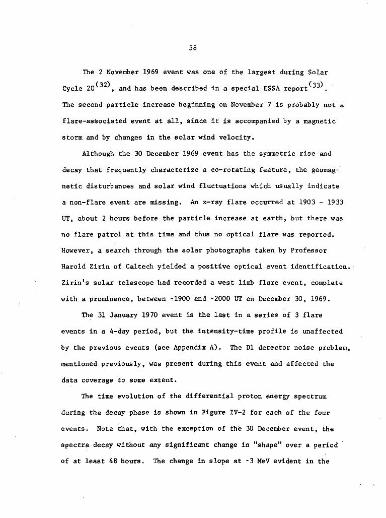
The 2 November 1969 event was one of the largest during Solar
(32) (w)Cycle 20 , and has been described in a special ESSA report J.
The second particle increase beginning on November 7 is probably not a
flare-associated event at all, since it is accompanied by a magnetic
storm and by changes in the solar wind velocity.
Although the 30 December 1969 event has the symmetric rise and
decay that frequently characterize a co-rotating feature, the geomag-
netic disturbances and solar wind fluctuations which usually indicate
a non-flare event are missing. An x-ray flare occurred at 1903 - 1933
UT, about 2 hours before the particle increase at earth, but there was
no flare patrol at this time and thus no optical flare was reported.
However, a search through the solar photographs taken by Professor
Harold Zirin of Caltech yielded a positive optical event identification.
Zirin's solar telescope had recorded a west limb flare event, complete
with a prominence, between -1900 and -2000 UT on December 30, 1969.
The 31 January 1970 event is the last in a series of 3 flare
events in a 4-day period, but the intensity-time profile is unaffected
by the previous events (see Appendix A). The Dl detector noise problem,
mentioned previously, was present during this event and affected the
data coverage to some extent.
The time evolution of the differential proton energy spectrum
during the decay phase is shown in Figure IV-2 for each of the four
events. Note that, with the exception of the 30 December event, the
spectra decay without any significant change in "shape" over a period
of at least 48 hours. The change in slope at -3 MeV evident in the

59
Figure IV-2
Samples of the proton differential energy spectrum during the
decay phase of four selected solar flare particle events. The
observations were made by Caltech's Solar and Galactic Cosmic
Ray Experiment aboard OGO-6 and thus represent the near-earth
particle flux. In each case, two spectra separated in time
are included to demonstrate the time evolution of the proton
flux. With the exception of the 30 Dec 1969 event, the spectra
decay without significant change in shape over a 2-day period.
Graph a — The 7 June 1969 Event
Graph b — The 2 November 1969 Event
Graph c — The 30 December 1969 Event
Graph d — The 31 January 1970 Event

60
IU
IO2
>5 10
0o>
CVJ
O |
XZ>
u_
§,o-Q:
io2
io3
_ i i i i i i i i i i i 1 1 1 1 1 1 1
- \ 7 JUNE 1969 EVENT- "B
v • REV 79 N• * REV 108 N
-* %
*« *
- , *- Si: * ^
^ OH
* i I •T I
— — • i ^ i —^ • T *
i hH hH
i : ; , i10
INCIDENT ENERGY (MeV)100
Figure IV-2-a
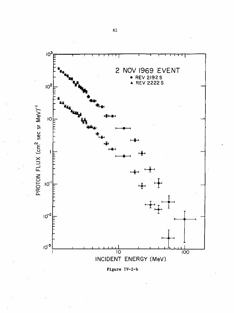
61
I0
10
10C/5
O0)
(\J
^^ I
XZ>
§ 10"cro_
10"
10"
***
T
2 NOV 1969 EVENT• REV 2I92SA REV 2222 S
HH
i—< >
I I I I
10INCIDENT ENERGY (MeV)
Figure IV-2-b
100
62
ICT 1
10
o>
XID
LJL
irQ_
ft
**
r
ft
30 DEC 1969 EVENT• REV 3031 S* REV 3047S
*
^ JH
io-3
lO'4 1 I
10 100
INCIDENT ENERGY (MeV)
Figure IV-2-c

63
10*
10\
wi
oo>UJ
XID
OcrQ_
10
to 2
lO'3
I0 4
i
31 JAN 1970 EVENT• REV 3502N* REV 3530N
i—*—i
T I—< >—*H M
10INCIDENT ENERGY (MeV)
100
Figure IV-2-d

64
7 June 69 and 31 January 70 spectra are of particular interest because
they allow one to determine whether any energy-change processes are
(31)occurring as part of the solar particle transport .
In summary, the analysis of about 9 months of OGO-6 cosmic ray
data has yielded four solar flare proton events which are uncompli-
cated and which can be easily associated with an optical flare on the
sun. The relevant information about these events consists of the
time and position of particle injection at the sun, the interplanetary
conditions at the time (such as the solar wind velocity), and the
proton intensity vs. time profile for various incident energy bins as
observed at earth. This information, which is the result of standard
analysis procedures, holds some clues to the physics of the propaga-
tion of solar flare particles and to the nature of interplanetary
space. These clues are the subject of the next section.
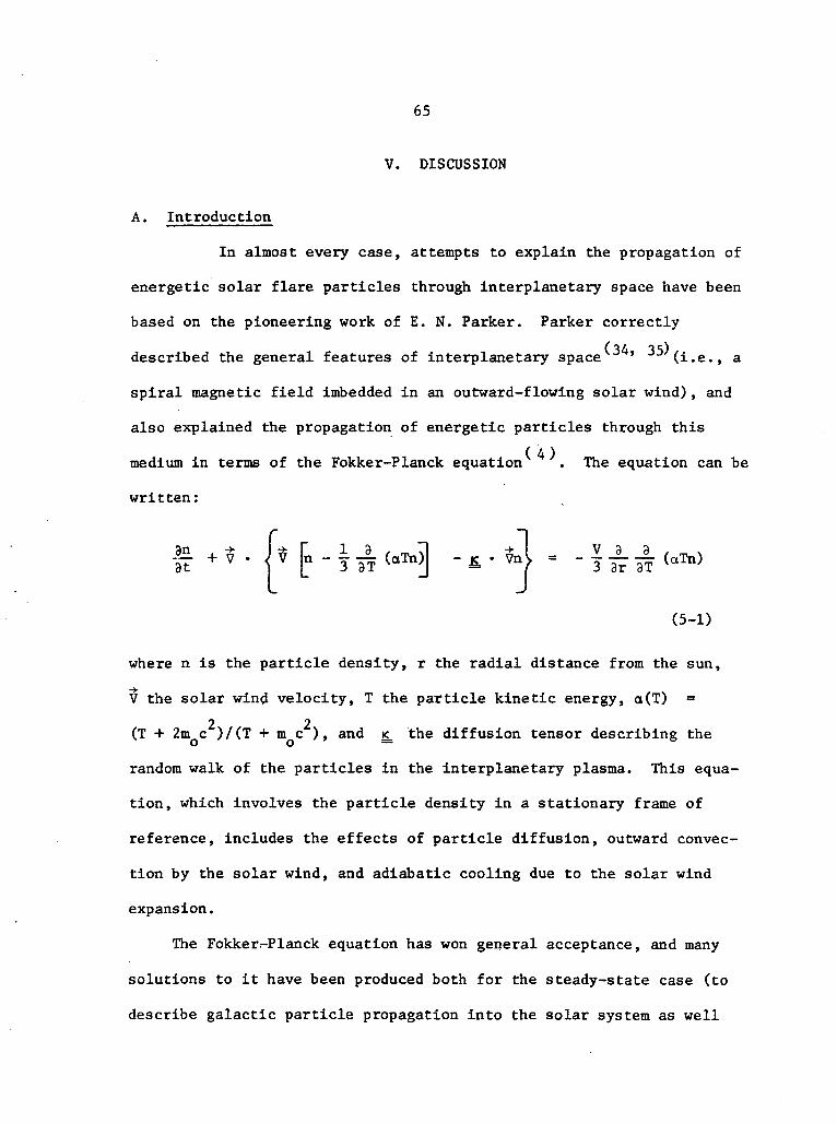
65
V. DISCUSSION
A. Introduction
In almost every case, attempts to explain the propagation of
energetic solar flare particles through interplanetary space have been
based on the pioneering work of E. N. Parker. Parker correctly
described the general features of interplanetary space ' 5 (i.e., a
spiral magnetic field imbedded in an outward-flowing solar wind), and
also explained the propagation of energetic particles through this
medium in terms of the Fokker-Planck equation . The equation can be
written:
(5-1)
where n is the particle density, r the radial distance from the sun,
V the solar wind velocity, T the particle kinetic energy, a(T) =
2 2(T + 2m c )/(T + m c ), and <_ the diffusion tensor describing the
random walk of the particles in the interplanetary plasma. This equa-
tion, which involves the particle density in a stationary frame of
reference, includes the effects of particle diffusion, outward convec-
tion by the solar wind, and adiabatic cooling due to the solar wind
expansion.
The Fokker.-Planck equation has won general acceptance, and many
solutions to it have been produced both for the steady-state case (to
describe galactic particle propagation into the solar system as well

66
/n
as steady-state solar emission), and for the time-dependent case '
10,11,12,13,14,36,37) ,(to describe solar flare cosmic ray injection and
transport). Because the equation is difficult to solve, every success-
ful analytic solution has associated with it a set of simplifying assump-
tions and boundary conditions which make the equation soluble but at the
same time critically affect the behavior of the solution. Current
discussions about the theory of solar flare particle events are thus
more often concerned with the validity of the assumptions used to
produce a given solution, than with the physics contained in the differ-
ential equation itself.
The following is a partial list of unsolved problems concerning the
theory of solar flare particle events:
1) The Diffusion Tensor — Although it is generally assumed
that <_ can be separated into components K|( and K^ parallel and
perpendicular to the spiral interplanetary field , very little
is known about the dependence of g. on distance from the sun and on
particle energy, especially at low energies. The most widely-used
estimates of the dependence of < on particle energy T and radial
distance r have been based on measurements of the power spectrum of
the fluctuations in the interplanetary field between 1 and
1.5 AnU.8.9.38.39
2) Azimuthal Propagation — Spacecraft observations of a
longitudinal gradient in the solar flare particle density persist-
ing for many days have been reported ' ' ' and indicate
that, in at least some cases, very little perpendicular particle

67
diffusion occurs in interplanetary space. The idea has thus
developed that K± « KH and that flare particles are distributed
in solar longitude early in the event by some transport process
occurring near the sun, rather than by diffusion "across" the field
(42)lines in interplanetary space . However, this idea has not
been developed to the point where it can explain the observed
dependence of intensity rise time on parent flare position
3) An Outer Boundary to the Diffusing Region — In order to
explain the often-observed exponential decay of flare events , a
perfectly-absorbing outer boundary to the diffusing region at
( 3 10 12 )r = L has been introduced in some models ' ' . The position
and even the existence of this boundary remain points of contro-
versy(l3).
4) Scatter-free Propagation Near the Sun ~ The general
question of the boundary conditions in existence near the sun is
(43)still unanswered. In particular, it has been suggested that
the rapid arrival and subsequent slow decay of the particles
observed at earth can be explained in terms of a "scatter-free"
region extending from the sun outward to some distance r < 1 AU.
5) The Energy-Change Process — Recently the first experi-
mental evidence for the adiabatic cooling effect (predicted by the
(31)Fokker-Planck equation) was reported , and the notion that a
particle acceleration process may be competing with this adiabatic
(44)deceleration was also introduced . This "energy-change problem,"
46 47which has received a good deal of attention lately l > ' ' , is
still unsolved.

68
6) Particle Anisotropy — The anisotropy in the flux of
~10 MeV protons has been observed to change magnitude and direc-
tion during a flare event » > » » .A completely success-
ful solar flare model must explain these anisotropy observations
in at least a qualitative fashion.
The most important solar flare models that have been developed to
date are summarized in Table V-l. The ADB solution of Burlaga
appears to explain the behavior of £100 MeV protons fairly well.
However, no onaJLyt>ic. solution exists which can fit both, the rise and
decay observations for low energy protons (-1-10 MeV) while including
the effects of convection and energy-change which have been demonstrated
to be significant at low energies ' .
In the discussion which follows, a new analytic solution will be
developed which includes a boundary to the diffusing region at r = L,
*assumes instantaneous particle injection at one point, uses K = constant,
and includes the effects of convection and energy-change. It will be
demonstrated that this solution agrees well with near-earth observa-
tions of low energy solar flare protons using reasonable values of <
and L without the assumption of a scatter-free region near the sun.
The predictions of the model will also be compared with the existing
data concerning energy-change processes.
The new solution presented is really concerned with the Mldiat
transport of solar cosmic rays, which can be separated from the problem
K is identical to <„ if one assumes a radial magnetic field.
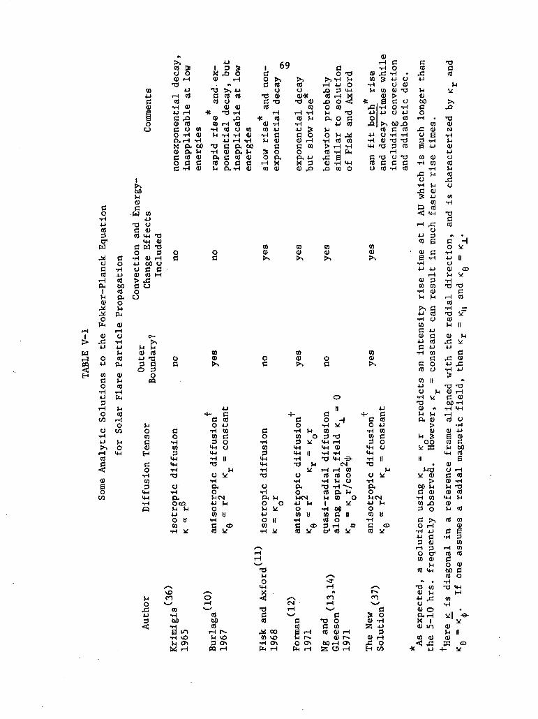
Pd
co•H4JCfl3crW
Upjcfl
rHP-IiVlcu
£&
r^OPU
CU
4-1
O4-1
COCo•H4J3
rH0
CJ•H4J
^rHcfl
^cuS0
c0•H4JCO00COP.0Vi
p_l
cui-HCJ•H4-1VlCO
01VlCO
Fn
ViCO
rHO
CO
Vio
co4-1CCU
B
Ou
1ps00Vlcue
W CO4-1
T3 CJC cuCfl M-l "O
MH CUC W -O0 3iH CU rH4J 00 CJU C CCU CO M
c uoU
c—
^Vl VlCU CO4J T33 C0 3
O
VloCOeCUH
CO•HCO3
M-lM-l•HQ
VlO
4J3
*
£*CJ 0CU rH
TJ4-1
rH COCO
•H CU4J rHC f>CU CflC cjO tHCUrHX P.CU P.C CO0 CC -H
0c
oc
co•Hco3
MHM-l•H*O
CJ•HP,OcaVl Vl4JO 8CO
y—svOcn
N_X
CO•H00•HB lA
•H vOvi ON^» ^J
u1 3 SX ,0 5CU rH
M
TJ >> 4JC CO cflCO U
<n <u* -0 rH
CU ,£>CO rH Cfl
0) iH CO CJCU Vl -H iH•rl 4-1 rH00 T3 C P.Vl -H CU P.cu a. c roc co o cCU Vl P.iH
oe
COcu,
4JH- C
C COO 4J
•H COCO C3 0
M-l OMH•H IIT)
VlCJ ^•HP,OViCN4J VlOco a•HC CDcfl i£
y~xorHN»y
cfl00CO
rH f .Vl vO3 ON
1 690 >, >>J3 cfl
CJ13 euC -octf
rH* Cfl
0) -rlCO CO 4-1CU -rl C
•H Vl CUoo av i Socu op.C rH XCU CO CU
COcuJ>^
0c
ao•HCO3
MHMH•H""C3
U•HPu VIO OVl U4-10 IICO, - * ^/
/»-\
rHrHS.X
-aMo
MHX
-dfj(0
y 00m \o
•H 0%PU rH
COOcu*
13 CUCO
rH lHCO Vi•H4J £c oCU rHe cooP. 4JX 3cu .a
COCU
^^
COcu
^_
co
•H VlCO O3 Sj^
MHMH ||•HTJ Vl
U
PuoVICN4J MoCO «•HC3 CDcfl V
yM^
<NrH>«/
c6 rHVi r^O ONPu rH
CO 13
t*.TH VlrH 4-1 O,0 3 MHCfl rH X
J3 O <O COVl 13ex o c
4J CflViO V4 X
•H cfl CO> rH -HCfl TH fej= eCU -rl MH
43 CO O
COCU
^
Oc
oII
cO -f•H VCO3 -a
MH CU•H -H*rj MH ~ -
CNrH rH CO
CO CO O•H Vl 0X> -H ~~-cfl ft ViM CO O1 V
•H 09CO C DCO O3 rH Sa> co u
s~\*&rH
M
COrHN*
C•o oC coCO CU i-H
<U r-OOrH ON
S3 O rH
CUCOiHVl
•KJ24-10.n4-1•HMH
CcflCJ
COcu^t
CO<ur**»
4-CO•Hco3
MHMH•H•0
U•HP.O
0)rH C•H 0.C -H -S 4-1 O
U CUcn cu -acu >8 C cj•H O iH4-1 U 4J
cfl>> 00^3cfl C cflO -H -HCU -O T3-a 3 co
rH
T3 O T3C C CCO -H cfl
4JCcfl4-1COCooII
VlV
VICN4-1OCO•HCCO
^r~c*1v_
cu^<uH
Vl
B
CDv/
\
iyCo•H4-13rHO
CO
CCO
,C4-1
Vl0100corH .
COj= cuo S3 -HB 4J
co cu•H CO
•rH.C Via•H Vlj; <uS 4J
COp CO•< M-l
rH ^=CJ
4-1 3co 6
• <u cB -H•H4-1 4-1
i-H01 3CO CO
•H 01Vi Vi
^> C4-1 CO•H CJCOC 4Jcu c4-1 CflC 4-1•H M
GC 0CO O
co n4-1CJ Vl•H Mf*O0) «-Vi ViP. 01
CUVl £00
V PC
II•
Vn3V 0)
00 Vin cu•H CO
CO ,03 0
C >i0 rH
•H 4-14J C3 CU
rH 3O CTCO 01
ViCO M-l
•> •T3 CO01 ^
UQ) OP. rH
01 mco cu< ji
* 4J -
T3
CO
VlV
>^^sT301N•HVi014JocflVlcflAO
CO•H
tfCCO
M •
c HO i£•H4J IIOCU CDVl V•H'O TJ
CrH CO
CO•H ^*O iCOVi II
0) ViX V4J
C,C CU4J ,C•H 4J
^ *»T3 T3CU rHC CU00 iH
•H MHrH
CO CJ•H
01 4-1S 0)cfl CVl 00
M-l COB
cuCJ rHa cfl01 -Hvi -a01 cfl
MH VlCUVi cfl
CO COcu
C 6•H 3
COrH CO
CO cflco cu00 Ccfl 0iHTJ MH
I-HCO•H
[1 *O-
^01vi nCU
— u

70
of a.Z4J/nu£haJt propagation. Evidently this "perpendicular" particle
transport cannot be explained with only the simple interplanetary
diffusion process used in the discussion which follows. Nevertheless,
a brief description of this "longitudinal distribution" problem will be
given, even though the real answer must be left to those with access to
multiple spacecraft measurements.
The predictions of the model will also be compared with observa-
tions of the vector particle anisotropy at 1 AU. It will be shown that
the new solution is capable of explaining most of the features of
these anisotropy measurements.
B. Background
A short description will now be given of the present state of
knowledge concerning the interplanetary medium, the manner in which
solar cosmic rays propagate through this medium, and the sorts of
particle observations that result from solar-flare type injection.
1. The Interplanetary Medium
Unlike the problems of particle propagation, the features of
interplanetary space are now fairly well understood, particularly in
the vicinity of the earth. Several coherent summaries of the charac-
teristics of the interplanetary medium as related to solar cosmic rays
, , . (1,26,29)have been given
Interplanetary space consists primarily of a highly conductive but
nearly electrically neutral plasma which is an extension of the solar
corona and is moving radially outward in all directions. This "solar
71
wind," which "blows" at a velocity of 300 - 500 km/sec at 1 AU,
dominates the interplanetary medium out to at least 5 AU and probably
to 20 - 100 AU. The plasma, which is composed of roughly equal numbers
of protons and electrons, has a temperature of ~2 x 10 °K at the
4 5corona. Near the earth, the plasma has cooled to ~10 to 10 °K ando
has a density of ~3 - 10 protons /cm .
Imbedded in the plasma is a magnetic field which originates in
the solar photosphere. This B-field is rigidly coupled to the plasma
due to the high conductivity, and consequently the field lines are
drawn outward by the force of the solar wind. Because the photosphere,
where the solar field originates, rotates with a period of -27 days (at
the equator), the interplanetary field is rotated into a spiral.
Assuming a constant solar wind velocity V, the average field is well
approximated by an Archimedian spiral ^
V«> - A )
flsin 6
where (r,6,<J>) are spherical polar coordinates centered at the sun and
f2 = 2.7 x 10 radians/sec is the angular velocity of solar rotation.
The ambient field thus makes an angle i|j(r) = tan" (fir/V) with respect
to the radius vector. For V = 400 km/sec and r = 1 AU, \i> = 48 .
_2The field intensity falls off roughly as r due to the solar wind
expansion, and has a value of -5 x 10~ gauss at 1 AU.
Superimposed on this large-scale field are small-scale fluctua-
tions in the field direction and intensity which produce deviations
from the average configuration. These irregularities act as scattering

72
centers for the energetic particles and lead to the notion of cosmic
ray "diffusion." In addition, the solar wind plasma is permeated with
various "transient phenomena" — discontinuities, shock waves, and
hydromagnetic waves — which contribute to the fluctuations in the
medium.
Measurements of the average direction of the magnetic field vector
over many solar rotations have shown that the ecliptic plane is divided
into fairly stable "sectors" of alternating field direction^ . These
sectors, which require several days each to rotate past the earth,
appear to be correlated with geomagnetic storm activity. The sector
boundaries may very well act as barriers to energetic particle propaga-
tion.
The solar wind interacts in a complex way with the quasi-dipole
geomagnetic field, creating a bow shock and magnetosphere. The
boundary between the geomagnetic and interplanetary fields is a separate
branch of geophysics in itself, and is of importance here only as it
affects the OGO-6 particle observations (see Section III-B).
2. The Fokker-Planck Equation and Particle Diffusion
The details of cosmic ray transport depend on both the large
scale and small scale features of the interplanetary field. If the
small scale fluctuations were not present, the energetic particles would
be confined to gyrate about individual field lines like beads sliding
along wires. However, the field irregularities or "kinks" act as
resonant scattering centers whenever the scale-length of the irregular-
ity is of the same order as the particle gyro-radius. The scattered

73
particles thus random walk in both pitch angle and position, and the
propagation can be approximated by a diffusion tensor £. In a reference
frame with the z-axis along the average field direction,
\
tf ic 0Kd KJL °
0 O K
(5-3)
,,
where K,, characterizes the particle diffusion along the field lines,
<L across the field lines, and <, includes the effects of curvature and
gradient drifts . The diffusion is anisotropic because of the
average magnetic field structure present.
The picture is further complicated because the scattering centers
are imbedded in the moving solar wind plasma. Since the field irregular-
ities are convected outward by the solar wind, there is a net outward
particle transport or convection separate from the particle diffusion
process. In addition, the solar wind is continually expanding to fill
interplanetary space (V • V / 0), and the field irregularities are
thus on the average moving away from each other. This expansion
produces an adiabatic cooling or deceleration of the cosmic rays at the
(4 )ratev
^ = - | o(T) T tf • v") (5-4)
There is some question as to whether this is the only important energy-
(31 44)change process at work in interplanetary space '

74
All of these particle propagation effects can be combined into a
single differential equation for the time rate of change of the particle
density:
•22. - V • (£ • Vn) - V - (rtf) + . 1 [|Y (a(T)Tn)l (5-5)
The right-hand side of this form for the Fokker-Planck equation
includes terms for particle diffusion, convection, and adiabatic decel-
eration. This equation gives an adequate description of energetic
particle transport as long as the pitch angle scattering can be charac-
terized by a diffusion tensor. The Fokker-Planck equation is not valid
whenever a large pitch angle anisotropy is present, and other
( 52 530approaches must be used '
Although the validity of the Fokker-Planck equation is generally
accepted, the exact nature of the diffusion tensor K_ is still undefined,
largely because of the lack of adequate space-probe observations. The
only real agreement seems to be that the antisymmetric terms can in most
cases be ignored (K = 0) and that <n and KJ_ probably depend on both
particle energy T and heliocentric distance r.
Jokipii has shown that the diffusion coefficient </T) can be
related to the power spectrum of the fluctuations in the magnetic field.
Using Mariner IV magnetic field observations, Jokipii ' ' , and
(38)Jokipii and Coleman have obtained the following values for K.. at
r = 1 AU as a function of particle rigidity R (in GV) and velocity
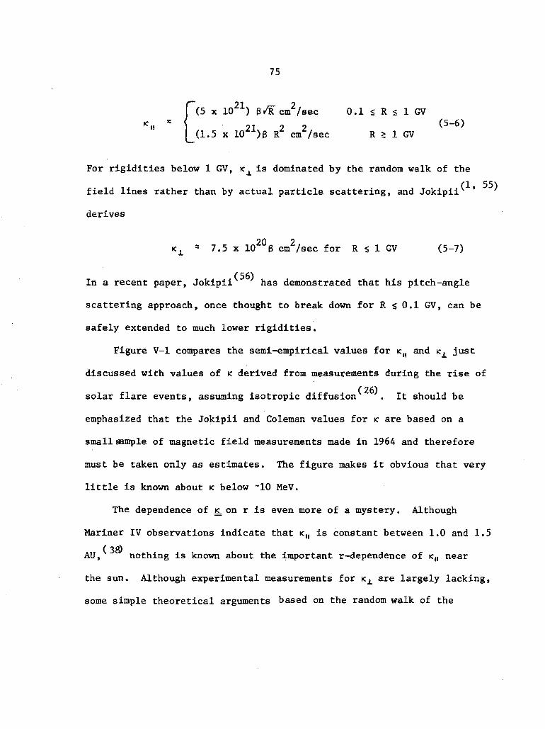
75
(5 x 10²¹) evil cm2/sec 0.1 s R < 1 GV21 2 2 (5-6)
(1.5 x 10 )g R cm /sec R > 1 GV
For rigidities below 1 GV, <A is dominated by the random walk of the
field lines rather than by actual particle scattering, and Jokipii '
derives
ort oKA s 7.5 x 10 3 cm /sec for R < 1 GV (5-7)
In a recent paper, Jokipii has demonstrated that his pitch-angle
scattering approach, once thought to break down for R $ 0.1 GV, can be
safely extended to much lower rigidities.
Figure V-l compares the semi-empirical values for <„ and K^ just
discussed with values of K derived from measurements during the rise off og)
solar flare events, assuming isotropic diffusion . It should be
emphasized that the Jokipii and Coleman values for ic are based on a
small sample of magnetic field measurements made in 1964 and therefore
must be taken only as estimates. The figure makes it obvious that very
little is known about < below -10 MeV.
The dependence of £ on r is even more of a mystery. Although
Mariner IV observations indicate that K(I is constant between 1.0 and 1.5
( 38)AU, nothing is known about the important r-dependence of <„ near
the sun. Although experimental measurements for KX are largely lacking,
some simple theoretical arguments based on the random walk of the
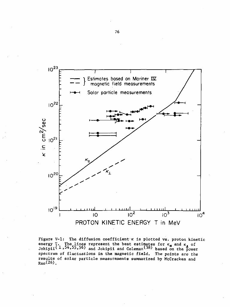
1023
1022
o
CVJ
1021
c
*
1020
1019
76
Estimates based on Mariner EZmagnetic field measurements
Solar particle measurements
/c
L.I
10 10
PROTON KINETIC ENERGY T in MeV
Figure V-l: The diffusion coefficient K is plotted vs. proton kineticenergy T. The lines represent the best estimates for KH and <, ofJokipii< 1,54,55,56) and j0kipii and Coleman^
38) based on the powerspectrum of fluctuations in the magnetic field. The points are theresults of solar particle measurements summarized by McCracken andRao<26).

77
ofield lines, indicate that K^ should vary as r . In addition, the
2assumption of an r dependence for xc, makes the equation easily solu-
ble. As mentioned previously, it is possible that the azimuthal parti-
cle transport is dominated by a separate near-sun diffusion region and
that perpendicular diffusion in interplanetary space is relatively un-
important.
Since the Fokker-Planck equation can be solved much more easily if
any of the terms can be neglected, it is of interest to calculate the
relative magnitudes of the various terms. Using the value of < at
1 MeV from Figure V-l, a solar wind velocity V = 400 km/sec, and assum-
ing that the scale length £ for changes in the density is about 1 AU,
the diffusive term becoaes:
19 23 \ ~ <n (6 x 10 cm /sec) ,_ ,n-7 -lvVn) ~ —=• = n ~ 5- * n(3 x 10 sec )
£ (1.5 x 10XJ cm)
For comparison, the convection term is roughly
+ * . Vn (4 x 107 cm/sec) ,, ,--6 -1.V • nV = — = n -* rrr = n(3 x 10 sec )1 (1.5 x 10 cm)
This crude calculation indicates that "solar wind" effects are very
important when the diffusion coefficient is small. It is thus a
violation of the basic physics of the Fokker-Planck equation to ignore
the terms for convection and adiabatic deceleration at low proton
energies.
78
3. Solar Flare Particle Events
McCracken and Rao have classified solar flare particle
events as either p/LOmpt, occurring within hours of the parent flare ,
or de</ed, occurring ^ 24 hours after the parent flare or even without
an obvious optical flare association. In fact, it is no longer
believed that flare particles are always injected impulsively at the
(29)sun — proton precursors have been observed, and many flare parti-
cle events have been explained in terms of particle storage and/or
continual production at the sun. Nevertheless, a large fraction of the
so-called "prompt" events appear to be consistent with impulsive injec-
tion and can be clearly associated with a parent optical flare. The
four event observations presented in Section IV fall into this group,
and it is this class of particle events which is the subject of this
dissertation.
Solar flare particle events have been observed at 1 AU for many
years, and as a result, the behavior of the "typical" event has been
/25 26 29^fairly well defined ' ' . The following are a few of the commonly
observed characteristics of prompt solar flare events which any solar
flare model must attempt to explain:
a) The intensity vs. time profile for most prompt events is
characterized by a rapid increase to maximum intensity followed
by a decay phase which at late times is approximately exponential.
The time-to-maximum T is typically 5-35 hours , and the exponen-
tial decay time constant T = 8 - 27 hours.
b) The shape of the profile, especially during the rise,
79
depends strongly on the distance in heliocentric longitude between
the flare and the foot of the line of force connected to the
observer. (The foot of the line of force passing through the earth
is typically at 60 W solar longitude). T is greater for east-
limb events because the longitudinal separation <|> is greater
(compare the 7 June 69 event of Figure IV-2 with the events of
2 Nov 69 and 31 Jan 70). Burlaga has shown that T variesm
roughly as <f> . McCracken has pointed out that particles from
west-limb flares are more frequently detected than those from
east-limb events, even though the parent optical flares occur in
the east and west with equal probability.
c) A well-defined velocity dispersion is seen, especially
for west-limb events. As expected, the high energy or faster
particles arrive first.
d) The low energy (~1 MeV) protons last longer (decay more
slowly) and exhibit more intensity variation than the higher
energy protons.
e) The typical vector anisotropy observation is character-
ized by a strong anisotropy from -45°W early in the event which
later decreases to a smaller equilibrium value directed from ~45°E
at late times . McCracken reports that the anisotropy
measured using neutron monitor data is strongest for west limb
events.
This completes the discussion of what is known about solar flare
particle propagation through interplanetary space and should set the

80
stage for the following attempt to describe this propagation.
C. Solving the Fokker-Planck Equation for Solar Flare Particle Injec-
tion
1. Some Boundary Conditions and Simplifying Assumptions
The following is a list of assumptions, conventions and
boundary conditions which will be applied to the Fokker-Planck equation:
a) The particle density n depends only on spatial position
(r, 6, <j>), time t, and particle kinetic energy T.
b) All parameters except for the particle density n are
assumed to be independent of energy T. One can set a(T) = 2 for
protons below -100 MeV.
c) The solar wind velocity V is radial and independent of
(r, 9, <{>) and t.
d) No attempt is made to describe transient phenomena such
as solar wind fluctuations, shock waves, and hydromagnetic waves.
e) The particles are impulsively injected at r = r at times
t = 0. Specifically,
6(r - r )n(r, 9, <f>, t = 0) - ^- f (0, 4.) (5-8)
r
f) It is required that the density n remain finite as r -> 0.
g) A perfectly absorbing boundary exists at r = L such that
n(L, 6, <j>, t) = 0.
h) The diffusion tensor will be taken to be diagonal in a
frame of reference (r, 6, <j>) aligned with the radial direction.

81
2Specifically, < will be defined by < = K . = K-r and= e <l> iK = < = constant, both independent of energy T.
These assumptions are intended to facilitate a solution to the
equation without compromising any of the important physics involved.
The most serious simplifications are that g_ is independent of energy T
and aligned with the radial direction. It will be shown that the
energy-dependence can be approximated by breaking the energy domain
into separate intervals within which < is independent of T, as long as
the intervals are large with respect to the ~30% energy-change which
(31)has been observed to occur during a typical -3 day decay period .
Some additional comment should be made about the assumed diagonal
form for the diffusion tensor:
/Kr
0
\ o
0
Ke
0
0
0
K
\
/
This is not identical to the assumption of a radial magnetic field.
However, the simplest and most widely-used interpretation of this
assumption is to equate it with the neglect of the spiral field. Then
< = K , KQ = K, = K., and one must make an additional distinctionr n e <j> j.
between actual radial distances in interplanetary space and the radius
variable r, which now represents a path length measured along a spiral
field line. This interpretation, which sacrifices surprisingly little
of the physics involved, will be adopted in this discussion until a
treatment of the anisotropy is attempted.

82
The boundary condition at the sun would seem to be more appropri-
ately described by either a perfectly absorbing or perfectly reflecting
boundary at r = r (instead of at the origin). However, a recent papers
by Englade indicates that the type of solar boundary condition
assumed has little effect on the time profile observed at 1 All. Evi-
dently more appropriate inner boundary conditions serve only to make the
solution less manageable.
The existence of an outer absorbing boundary is not an accepted
point. Several authors have developed solutions using an infinite
(13)diffusing region (see Table V-l) . In particular, Ng and Gleeson
claim that an "approximately" exponential decay can be produced assum-3
ing K = < (1 + r ) . However, their K function appears to be just
another way of smoothly introducing a region of free escape where
K •> °° and n -> 0. The fact remains that observations of exponential
decays are the rule rather than the exception, and a free escape bound-
ary produces such a decay.
The r-dependence for K is a very important assumption, as will be
demonstrated later in the discussion.
2. Separation of Variables
We are now in a position to attack the Fokker-Planck equation
using the technique of separation of variables. Assuming a radial mag-
2netic field, a diffusion tensor defined by K (r) and <Q(r) = <,r bothr Q J.
independent of T, and V independent of spatial position, one can re-
write equation (5-5) in spherical polar coordinates as:
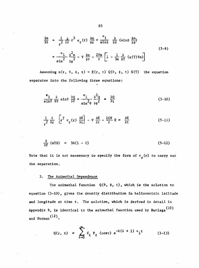
83
12 - -I- _2_ r2 r <V} -52- + l _
3t ~ r2 9r r Vr; 3r sine 90 90
OKl 9 n „ 9n 2Vn 1 9
—T~2 - v 17 -sin 9<{i
(5-9)
Assuming n(r, 6, 4», t) = R(r, t) Q(6, <}>, t) S(T) the equation
separates into the following three equations:
*i _L ,lnfl 12 + <]- 1^2-12
sine 38 Sin 99 . 2a ..2 " 3tsin 9 9<p
1 3 [2 ( , 3Rl „ 3R 2CV 0 3R-9? Lr Kr(r) id - V 3 ? - — R= 9F
- (oTS) = 3S(1 - C) (5-12)
Note that it is not necessary to specify the form of < (r) to carry out
the separation.
3. The Azimuthal Dependence
The azimuthal function Q(9, 4>, t) , which is the solution to
equation (5-10) , gives the density distribution in heliocentric latitude
and longitude at time t. The solution, which is derived in detail in
Appendix B, is identical to the azimuthal function used by Burlaga
and Forman
Q(Y, t) = - C P (C03^ e~ l (5-13)
84
where cosy = cos9 cos6 + sin9 sin9Q cos(4> - 4> ) (5-14)
(0, <(>) = point of observation
(9 , d> ) = center of azimuthal distributiono o
The C0 are chosen so that Q(y, t=0) matches f(9, <£) , the assumed injec-X*
tion profile at the sun. For 6-f unction injection aty = 0, we have
C = 2£ + 1 and00
2. (24 +Q(Y, t) = . (24 + l) PS (cosy)£=0
Burlaga ; has described the behavior of this Q(y, t) function in
f,ome detail.(CQ)
Feit Jy has shown that for a source uniform over an emission cone
of half -angle y '
P9 ^ <COSY0) - po+i (cosy )
C = -^ - 2 - — - — (5-16)
1 - cosyo
Presumably any symmetric f(6, (J>) can be generated using the proper
coefficients C0 .JO
If we choose our coordinate system coincident with the accepted
solar spherical coordinates, then our observation point at earth corres
ponds to e = y , <J> = -^r . The angle <j>, which is 58° for r = 1 AU and
V = 400 km/sec, indicates that the earth is typically connected by the
spiral field to a point at ~58°W solar longitude on the sun. We can
thus define a new separation angle y' which is a function of time t and

(5-17)
85
includes both corotation and the spiral angle:
cosy' = sine cos(<j> (t) - <J>)o o
= cosX cos($ —— + fit)o o V
where X = TT - 0 = solar latitude of optical flareo 2 o r
<f> (t) = $ + fit = the actual time-dependent solar longitude
of flare location
and $ = solar longitude of optical flare at t = 0
(*o > 0 for W longitude)
It should be mentioned here that the above formulation of the per-
pendicular transport process is probably far too simple to accurately
describe the actual situation. Multiple spacecraft observations of
particle fluxes and anisotropies indicate that rapid near-sun diffusion
and/or particle injection over a large solar surface area should be
invoked ' ' ' . Despite this evidence, the simple point-injec-
tion and 2-dimensional interplanetary diffusion process described by
equation 5-15 will be employed in the discussion which follows. The
shortcomings of this simple Q(y,t) function, which will be discussed
carefully, do not in any way affect the validity of the new solution
for tiadL&t particle transport.
4. The Energy Dependence
Equation 5-12 for S(T) can be reduced to the following form:
a(T)T II - 13 - 3C - a(T) + T |£| S (5-18)
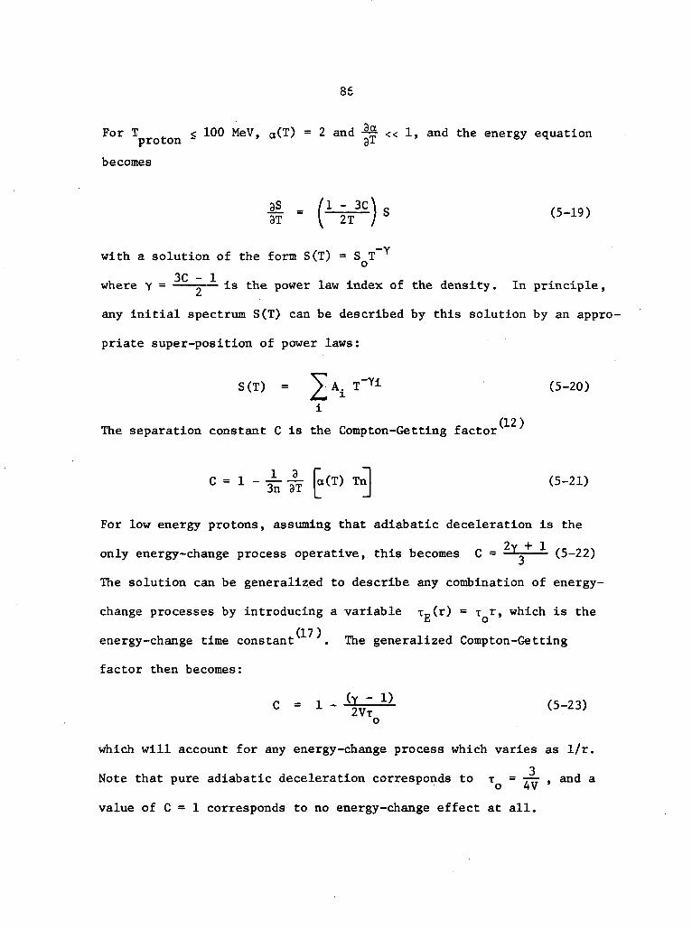
86
For T < 100 MeV, a(T) = 2 and -^ « 1, and the energy equation
becomes
with a solution of the form S(T) = S T~Y
3C - 1where y = 5— *s t'ie Power aw index of the density. In principle,
any initial spectrum S(T) can be described by this solution by an appro-
priate super-position of power laws:
S(T) - Ai T~ (5-20)
i(12)The separation constant C is the Compton-Getting factor
C = 1 - - -^ o(T) Tnn]For low energy protons, assuming that adiabatic deceleration is the
2v + 1only energy-change process operative, this becomes C = Tv— (5-22)
The solution can be generalized to describe any combination of energy-
change processes by introducing a variable (r) = T r, which is then o
energy-change time constant . The generalized Compton-Getting
factor then becomes:
C = 1 - (jgv" 1} (5-23)o
which will account for any energy-change process which varies as 1/r.
3Note that pure adiabatic deceleration corresponds to T = TTT » and a
value of C = 1 corresponds to no energy-change effect at all.

87
5. The Radial Dependence
Most of the features of a solar flare event observed at 1 AU
are due to the "radial" transport involving convection, energy-change,
and diffusion parallel to the field lines. For this reason, much effort
has been devoted to solving the radial equation (equation 5-11). Even
if the perpendicular diffusion is neglected (K- = 0), the equation
describing the radial propagation remains unchanged.
Burlaga , has solved the radial equation by neglecting the
terms for convection and energy-change, including a perfectly absorbing
boundary at r = L, and assuming K (r) = K. His differential equation
becomes
A. + liK = IJS. (5_24)9r2 r 9r K 8t
24)
He derives the following eigenvalue expansion for the radial dependence:
where the constant A is an arbitrary normalization determined by the
number of particles injected. His overall solution which includes the
azimuthal distribution, is
n(r, 6, <f>, t) =R(r,t) Q(0, <fr, t) (5-26)
Burlaga's solution produces a rapid rise and an exponential .decay and
thus adequately describes the time profile of high energy (T £ 100 MeV)
protons observed at earth. However, this solution is inapplicable to
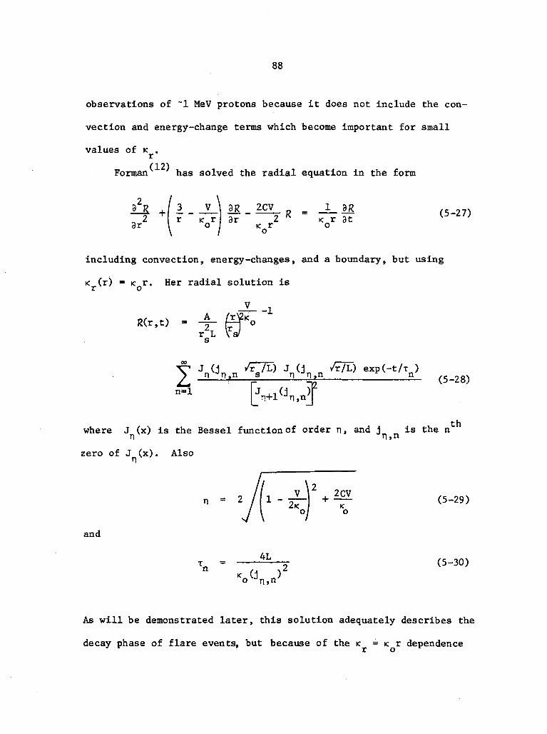
88
observations of ~1 MeV protons because it does not include the con-
vection and energy-change terms which become important for small
values of K .
(12)Forman has solved the radial equation in the form
L M ^ (5_27)( }2 r k r r a r 2 * KT r_ *• II. N. 1. I OL *• Is *•9r I o <_r o
including convection, energy-changes, and a boundary, but using
K (r) = K r. Her radial solution isr o
r L \a/
(5-28)i if
n=l
where J (x) is the Bessel function of order n, and j is the nn n>nzero of J (x). Also
V \2 . 2CV" ' 2/r-2J- +±r <5-2»o/ o
and
T = -y (5-30)
As will be demonstrated later, this solution adequately describes the
decay phase of flare events, but because of the < = < r dependence

89
chosen, predicts a rise time which is slower than the 5-10 hours
observed.
D. The New Solution
1. Derivation
It is apparent that a solution to the radial equation
(equation 5-11) similar to Forman's but using K (r) = constant might
yield desirable results. The equation becomes
A solution has in fact been found using the boundary conditions and
assumptions listed in Section V-C-1. The details of the derivation
are given in Appendix C.
(37)The new solution, which was recently reported , can be written
as the following eigenvalue expansion:
|_V(r - rs)/2ic|
(5-32)
expR(r,t) -A r rs
, rs) Fo(g/2 n, n r) -t/Te
—.. Nn=l n
where F (n,p) is the regular Coulomb wave function . The a are
the eigenvalues defined by the outer boundary condition
F (B/2./5" ,/T L) - 0 . (5-33)o n n

90
The other parameters are defined as follows;
3 = v(2c - I)/K
C = Compton-Getting Factor
= 1 + (Y - D/2VT
rn = 4</(4<2a + V2)
(5-34)
(5-35)
(5-36)
Nn "dx
X
2
/3F \o
9p
2$
"^n
/ 3F \o
3pi
l**\ oan
/ JX=L
here FQ(n,p)
arbitrary normalization
(5-37)
This expansion converges rapidly for t > 5 hours, C$4, and
20 2K > 10 cm /sec. The details of calculating the radial solution are
discussed in Appendix D.
In the limit as V -»- 0, we have g -*• 0, F (Q/2-/U , v/cTx) ->• sin(nrrx/L),
2 2 2 LT ->• L /n TT XT, N -»• j- and the solution reduces smoothly to Burlaga's
solution (equation 5-25) as expected.
The complete solution including the energy-dependence can now be
written as:
n(r,e,4>,t,T) = Q(e,*,t)T~Yi
which consists of a sum over different radial functions R.(r,t) each

91
corresponding to a different Compton-Getting factor
C. = 1 + (Y± - D/2VT . Equation 5-38 is thus the response to impul-
sive injection of the form
«(r - r )S(T) (5-39)
r-Tiwith S(T) = Z- A± T 'i . (5-40)
2. Behavior Of the Solution
The radial dependence R(r,t), defined by equation 5-32,
defines most of the features of the particle time profile. Figure V-2
shows the distribution of particles as a function of radial distance r
at various times using reasonable values of the parameters. The peak
in the particle distribution, which is initially near the sun due to the
<5-function injection, moves outward until the effect of the absorbing
boundary is felt and eventually assumes a stable "shape" at late
times.
The time-profiles R(r,t) vs. t observed at different radial
distances r are shown in Figure V-3. As expected, the time-to-maximum
T depends on the radial position of the observer because the maximumm
intensity occurs roughly when the peak in the radial distribution
(Figure V-2) moves past the observation point. Note that the T
observed at 1 AU is < 20 hours. At late times, the intensity decays
exponentially with a time constant T™,, roughly independent of radial
position. A glance at equation 5-32 makes it clear that only the first
eigenvalue (n=l) survives and that the decay phase is described by the
92
100
10
ooin
10"
10-2
10,-3
t = 5 hours
/cr = 5 x I020 cm2/sec
V = 400 km/sec
C = 1.0
L = 2.3 AU
rs = .0047 AU
0 0.4 0.8 1.2 1.6r in AU
2.0 2.4
Figure V-2: The new radial solution R(r,t), defined by equation 5-32,is plotted vs. radial distance.r for various times after particle in-jection. Typical values of the parameters were chosen and are indicat-ed on the graph. Note that the distribution, which is initially peakednear the sun due to the 6-function injection, reaches a stable config-uration at late times.
93
100
10
juooin
.av.o
I- 10
Id2
10
OQ O /
*> = 5*10 cm/secV = 400 km/secC = I.OL=2.3AUrs = .0047AU
r = I.OAU
I 120 40 60 80
TIME tin hours100 120 140
Figure V-3: The intensity R(r,t) predicted by the new solution isplotted vs. time for various observation distances r. Note thatalthough the time-to-maximum depends on radial distance, the time-profileeventually reduces to an exponential decay independent of observer posi-tion. The values of the parameters, which are the same as in FigureV-2, are listed on the figure.

94
following equation:
exp(Vr/2K )FR(r,t)
r
Thus if one is concerned only with the exponential decay phase of an
event, the predictions of the new model can be summarized by the single
quantity T = T- , which is independent of position and time andUKL/ J.
depends only on the boundary location L, the solar wind speed V, the
diffusion coefficient K , and the energy-change parameter C.
Figure V-4 shows how TnT,-, varies with K , L, V, and C. ForJJ£!t(_* IT
small values of K , T..,,., becomes essentially independent of < becauser iJtiVj r
the particle transport outward to the boundary is dominated by convec-
tion and energy-change processes. For large values of K , the solar
wind effects become unimportant, and the decay time constant approaches
Burlaga's (K ) dependence.
Increasing the solar wind speed hastens the decay, as expected
(Figure V-4a) , because the contribution of both convection and energy-
change to the decay rate is increased. In the limit V -*• 0, !•_„,„L)c,0
becomes identical to Burlaga's expression (see equation 5-25).
Changing the boundary position L has a marked effect on the decay
rate, as shown in Figure V-4b. The decay in the particle intensity is
largely produced by the outward transport of the particles to the
boundary, where they "escape." A more distant boundary means that the
processes of diffusion and convection cannot 3 iiver particles to the
boundary at the same rate, and Tn.,_ must increase accordingly. AljCi\j
close look at the behavior of the complete solution shows that at short

95oo e> o
<U iH4J (0•U OO P.
CO (0•H -O
O O
3 Q)rH 43O 4J01
4-1S O<ua toa)4) 2
JS rH4J (0
>>fi mo
0)4J
•aa)
to>
,0 a)
o> 3W CO
H 4J CO•H (X
4-1 UC O O )CO rH 004-1 cu c0) > COC J2O T3 OU C I
0) |S 00
• H M O )4-1 CO C
rH Q)
CO 0) <U
<U 0) 4J"O .C
4-1 M-lrH O
CO M-l•H O CO4J <UC W 3Q) Q) rHa 3 coO rH >CX COX! > 4J(U C
ca ai0) 3 M
X O <UH iH M-i
CO -H
> cfl CJ
Q) Jj *Oh ° S3 u-< cO00
•H M •>fH V rJ
96
times, when the particles have not yet reached the boundary, the
profile is independent of L.
The Compton-Getting factor C characterizes the extent to which the
random walk of the particles in energy-space affects the decay. While
a value of C = 1 corresponds to ignoring the energy-change effects
completely, a typical value of C = 3 means that at L= 1 AU the intensi-
ty is decaying, due to the energy-change process, at a rate that can
be estimated from equation 5-5:
\
T-n
ENERGY-CHANGE On/8t)
r
2CV= 17 hours (5-42)
This is of the same order as the actual decay time constant and indi-
cates that the contribution of C to the decay rate is significant —
a conclusion which is substantiated by Figure V-4c.
The relative distribution of particles f(r) in radial distance r
at late times is given by
f (r) - exp |vr/2icj r'1 vU/2/ai ^ r] (5-43)
and depends only on L, C, and the ratio V/K. This function is shown in
Figure V-5 for various typical values of this ratio. The boundary
condition f(L) =0 is quite evident. Again, for V/K ->• 0, f(r)
reduces to Burlaga's sin(mrr/L)/r which is peaked at the origin. As
V/K is increased, the peak in the distribution becomes more pronounced
and moves outward due to the increased convective force. The depen-
dence of the position of this peak on V/K has been discussed by
Forman

97
= 2.3AUC= 1.0V= 400 km/sec
2.4
Figure V-5: The radial distribution of particles at late times isplotted vs. r for various values of the ratio V/K .
98
The transport process occurring at any position r is best
described by the particle current S, which is simply the vector parti-
cle flux.
<f = Cvii - £ • $i (5-44)
For the radial B-field assumption used so far in this discussion, jf is
radial and can be treated as a scalar composed of two terms
and
Sv - CVR (5-45)
-K 8R/8r (5-46)L
which are the convective and diffusive components of the total particle
current. Note the azimuthal part of the solution Q(Y»t) has been
neglected, and that Sy is proportional to the radial solution R(r,t),
while S is proportional to the slope 3R/3r.
Figure V-6, which shows the decay-phase values of S, S , and S
as a function of r, makes it clear which transport process is most
important at any given radial distance. At the outer boundary, the net
particle flux is outward and is due entirely to diffusion. Because the
typical particle distribution at late-times is peaked at r > 1 AU (see
Figure V-5), the gradient over much of the distance is positive and the
diffusive current S in this region is directed inward. This inwardK °
diffusion, which impedes the process of particle escape, exactly
balances with outward convective current at the origin to produce
S(r=0) =0.

99
AUV=400 km/secC = I.
1.6 2.0 2.4rin AU
Figure V-6: The particle current S at late times as well as theconvective and diffusive components, Sy and SK, are plotted vs. rfor three values of K . The shaded area emphasizes the regionwhere the diffusive current SK is inward.
100
The decay time constant T = n/(an/gt) is a measure of the
total "stored" particle population relative to the rate at which
particles reach the boundary and escape. Figure V-4 shows that a broad
20 2maximum in TnT?P vs. < occurs typically for < ~ 2 x 10 cm /sec.
This maximum in T , which has been discussed by Forman , can be
understood qualitatively as the certain combination of parameters which
produces the lowest loss rate per unit stored particle.
E. Fits to Data Assuming Pure Adiabatic Deceleration
1. Method of Fitting Actual Data
Attempts were made to fit the flare event time-profiles des-
cribed in Section IV using the solution of Forman and the new solution.
In each case, the following assumptions and parameter values were
employed:
a) It was assumed that adiabatic deceleration due to the
solar wind expansion was the only energy-change process operative.
The Compton-Getting factor C was thus defined in terms of the power
law index y of the particle density as C = (2y + l)/3 (see Section
V-C-4).
b) Observations of the intensity within different energy bins
were treated separately. The density was assumed to be a power law
within each incident energy bin, and a separate value of C was thus
assigned to each energy interval by evaluating y(T) = d(ln n)/d(lnT)
at the center of the interval. The fact that the spectra of
Figure IV-2 are stable with time indicates that the "mixing"

101
between various energy bins is not very pronounced, and that the
description of each bin by means of an independent solution to the
differential equation is reasonable. In the same way, the energy
(31)change rate reported by Murray et al. indicates that the
"typical" particle does not lose enough energy to move from one bin
to another during the typical observation period.
c) The spiral character of the interplanetary field was par-
tially taken into account by assuming that the observations at
earth correspond to r = 1.15 AU, which is the path length along
the spiral field for V = 400 km/sec. The spiral field and the
corotation effect were also included by using the azimuthal
function Q(y',t) defined by equations 5-15 and 5-17. The depen-
dence of the longitude of the directly-connected field line on
the solar wind velocity V was included as well. The solar angular
velocity was defined as ft = 2.69 x 10 radians/sec, the value at
the solar equator.
d) The particles were assumed to be injected as a 6-function
in r, 6, and <J>. Thus the cone half-angle was y = 0 in all cases.
The coordinates (X ,$ ) and time of injection for each event were
defined precisely in terms of the parent flare identification
summarized in Table IV-2. The radial position of injection was
assumed to be the surface of the sun r = 0.0047 AU.s
e) The solar wind velocity was set to the best estimate
based on the ESSA data (see Section IV).

102
f) Thus the only (J'le.e parameters for each fit were the
diffusion coefficients K and K., the boundary position L, and ther 0
arbitrary normalization A. An initial choice of L = 2.3 AU was made
based on the fits made by Burlaga .
Because of the complicated nature of the flare profiles, a least-
squares fitting technique could not be easily used. Instead, a simple
but tedious optimization with respect to K , KD and A was made by eyer 0
for each profile.
2. Forman's Solution
An attempted fit to the 2 November 69 event profile using
Forman's solution (equation 5-28) with < (r) = K r is shown in Figure
V-7. With L = 2.3 AU, her solution duplicates the decay profile using
reasonable values of K and < (evaluated at 1 AU), but cannot match the' 8
rapid rise observed. Forman has attributed the long rise time predicted
by her solution to the simple boundary condition assumed at the origin
(12)and to the < « r dependence used . As will be demonstrated next,
the r-dependence assumed for K inside 1 AU has a drastic effect on the
time-to-maximum, for an obvious reason: early in the event the particles
are peaked near the sun, the propagation is due almost entirely to
diffusion, and the rate of particle transport is thus very sensitive to
the near-sun value of K . Concerning the boundary condition at the sun,
Englade has recently used Burlaga1s ADB model to study the effect of
(co)different boundary conditions at r = r ° . He reports that the type
O
of boundary condition assumed has surprisingly little effect on the
profile observed at 1 AU.
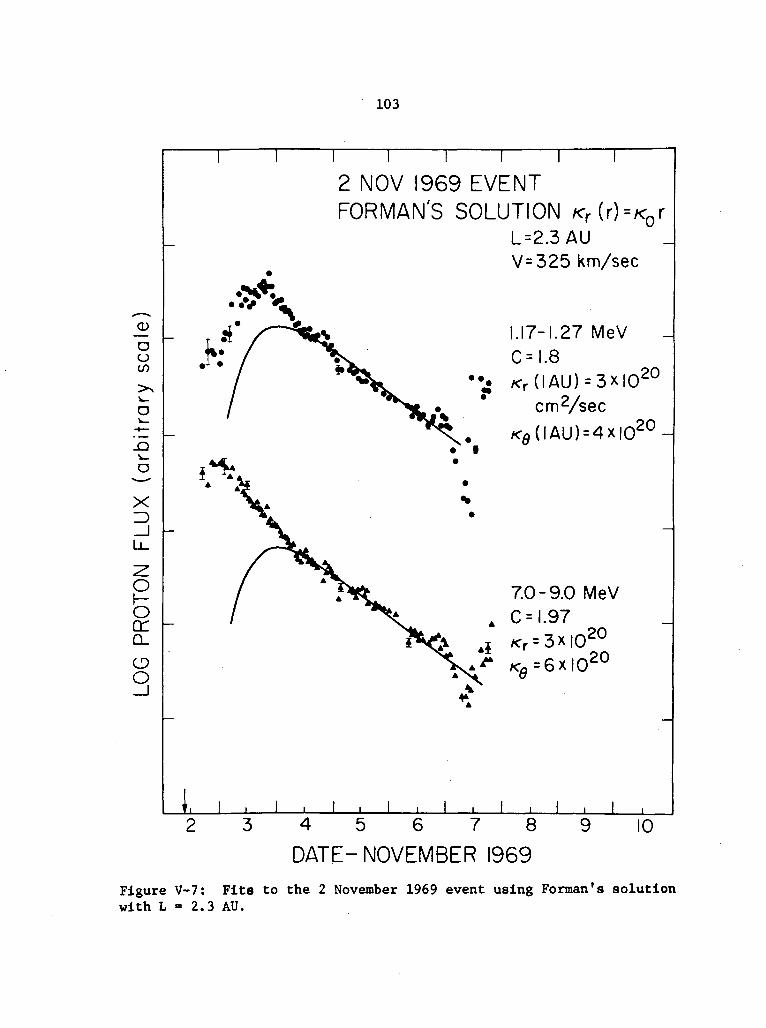
103
O0CO
O
X
O
Ocro_
O
I I I I I I2 NOV 1969 EVENTFORMAN'S SOLUTION /c r(r)=/cQr
L=2.3AUV=325 km/sec
1.17-1.27 MeVC=l.8
*202/sc m s e c
N20
7.0-9.0 MeVC = l.97K =3x|Q20
^v ,^20
I2 3 4 5 6 7 8 9
DATE-NOVEMBER 196910
Figure V-7: Fits to the 2 November 1969 event using Fonnan's solutionwith L = 2.3 AU.
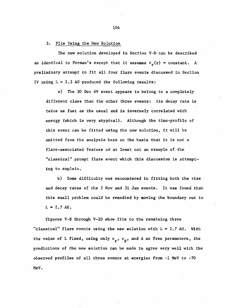
104
3. Fits Using the New Solution
The new solution developed in Section V-D can be described
as identical to Forman's except that it assumes <r(r) = constant. A
preliminary attempt to fit all four flare events discussed in Section
IV using L = 2.3 AU produced the following results:
a) The 30 Dec 69 event appears to belong to a completely
different class than the other three events: its decay rate is
twice as fast as the usual and is inversely correlated with
energy (which is very atypical). Although the time-profile of
this event can be fitted using the new solution, it will be
omitted from the analysis here on the basis that it is not a
flare-associated feature or at least not an example of the
"classical" prompt flare event which this discussion is attempt-
ing to explain.
b) Some difficulty was encountered in fitting both the rise
and decay rates of the 2 Nov and 31 Jan events. It was found that
this small problem could be remedied by moving the boundary out to
L = 2.7 AU.
Figures V-8 through V-10 show fits to the remaining three
"classical" flare events using the new solution with L = 2.7 AU. With
the value of L fixed, using only K , < , and A as free parameters, ther o
predictions of the new solution can be made to agree very well with the
observed profiles of all three events at energies from ~1 MeV to -70
MeV.
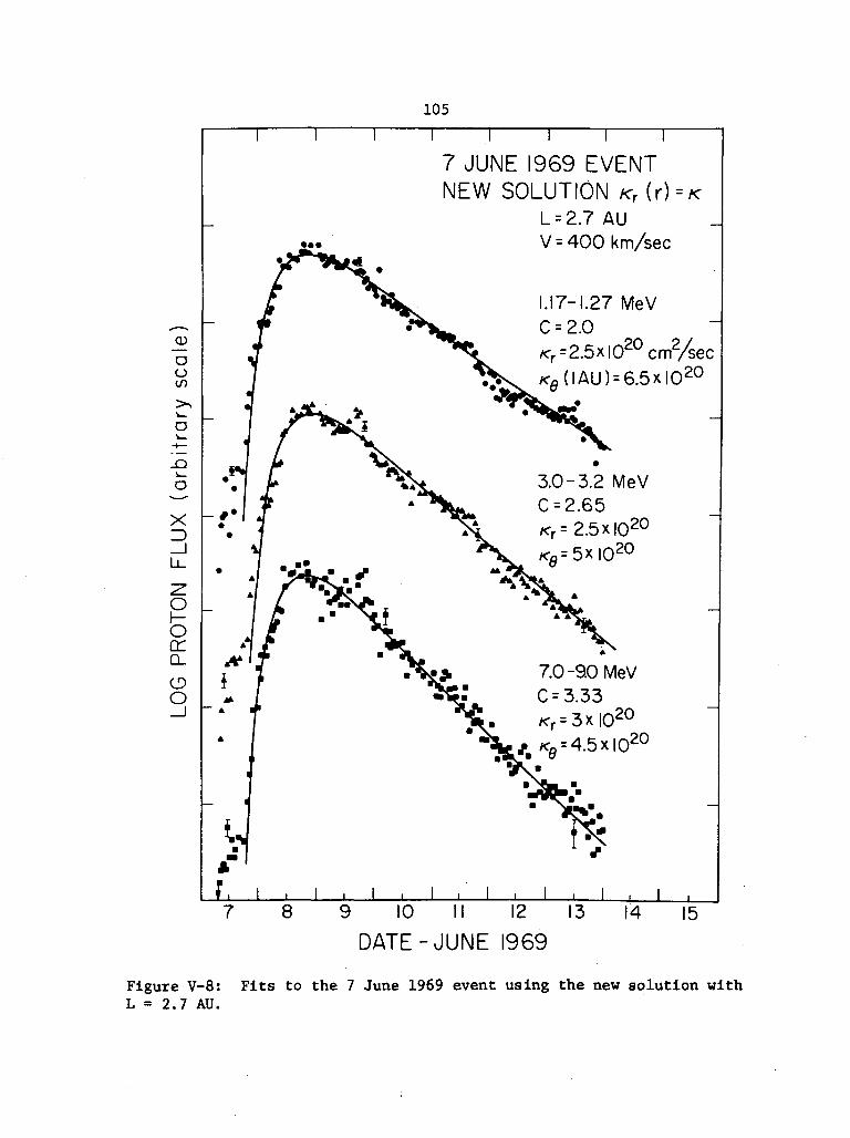
105
7 JUNE 1969 EVENTNEW SOLUTION /c r(r)
= 2.7 AUV = 400 km/sec
5xl020cm2/sec= 6.5xl020
7.0-9.0MeV= 3.33
9 10 II 12 13
DATE-JUNE 1969
Figure V-8: Fits to the 7 June 1969 event using the new solution withL = 2.7 AU.
106
oo
o
15
XID_lU_
-z.O
cro_
o
2 NOV 1969 EVENTNEW SOLUTION /c r(r)= K
L = 2.7 AUV = 325 km/sec
•* 1.17-1.27 MeV
V, c = l-8•
./cr=2.3xl020cm2/se3
" 7.0 - 9.0 MeV* C = 1.97
2021
KT= 5x 10KQ =I.OX|0
l5-20MeVC =2.43KT = 7 x I020
45-70 MeVC =3.0Kr = 8 x 10²⁰
.21* iUI I I
4 5 6 7 8 9DATE - NOVEMBER 1969
10
Figure V-9: Fits to the 2 November 1969 event using the new solutionwith L = 2.7 AU.

107
ooto
D
D
X=>
oocrQ_
O
~ ~ i i i i r ~
31 JAN 1970 EVENTNEW SOLUTION /c r(r)=/c
L = 2.7 AUV=400 km/sec
17-1.27 MeV2.05_ .^20 2/= 3x10 cm /sec
( IAU) = l.2xl021
9.0 MeV.50
= 7*I020
= l.8x|Q21
- 20 MeV2.38
:r = 8x|020
:0=l.8x|021
31 2 3 4 5 6
DATE-JAN & FEB 1970
8
Figure V-10: Fits to the 31 January 1970 event using the new solutionwith L = 2.7 AU.
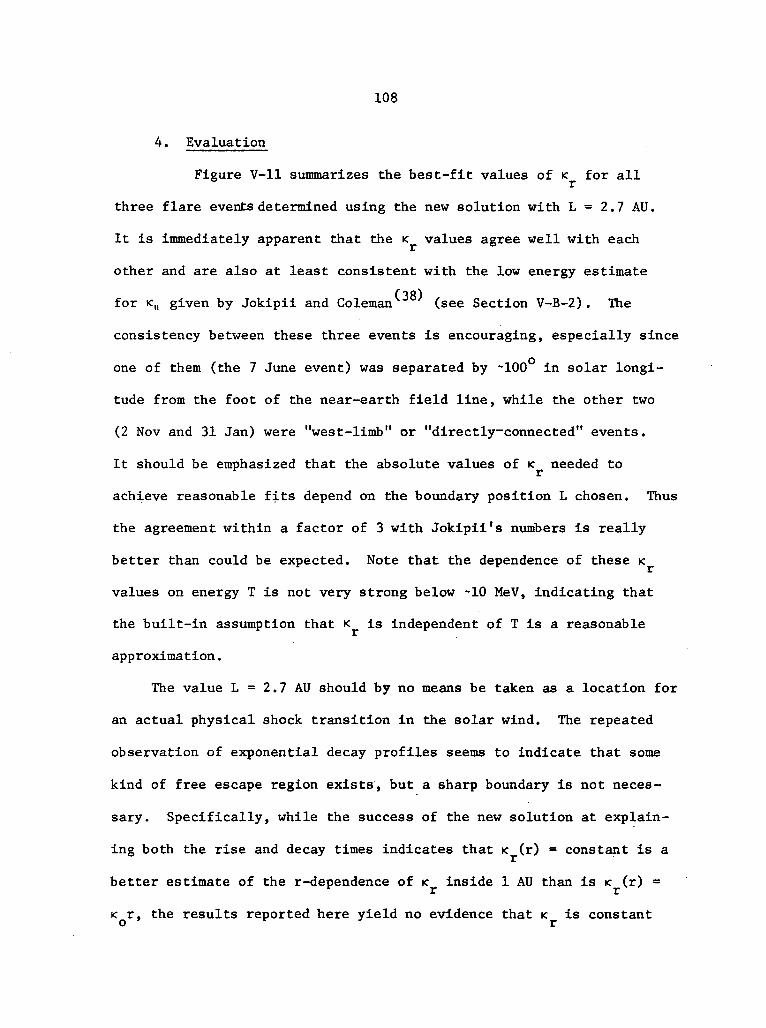
108
4. Evaluation
Figure V-ll summarizes the best-fit values of K for all
three flare events determined using the new solution with L = 2.7 AU.
It is immediately apparent that the ic values agree well with each
other and are also at least consistent with the low energy estimate
(18)for <„ given by Jokipii and Coleman (see Section V-B-2). The
consistency between these three events is encouraging, especially since
one of them (the 7 June event) was separated by ~100 in solar longi-
tude from the foot of the near-earth field line, while the other two
(2 Nov and 31 Jan) were "west-limb" or "directly-connected" events.
It should be emphasized that the absolute values of < needed to
achieve reasonable fits depend on the boundary position L chosen. Thus
the agreement within a factor of 3 with Jokipii's numbers is really
better than could be expected. Note that the dependence of these K
values on energy T is not very strong below -10 MeV, indicating that
the built-in assumption that K is independent of T is a reasonable
approximation.
The value L = 2.7 AU should by no means be taken as a location for
an actual physical shock transition in the solar wind. The repeated
observation of exponential decay profiles seems to indicate that some
kind of free escape region exists, but a sharp boundary is not neces-
sary. Specifically, while the success of the new solution at explain-
ing both the rise and decay times indicates that < (r) = constant is a
better estimate of the r-dependence of ic inside 1 AU than is K (r) =
< r, the results reported here yield no evidence that K is constant

109
1022
O
CJ
§io21
1020
FITS TO DATA L = 2.7 AU
• 7 JUNE 69 EVENT
* 2 NOV 69 EVENT
o 31 JAN 70 EVENT
Estimate ofJokipii and Coleman
10PROTON KINETIC ENERGY T in MeV
100
Figure V-ll: The best-fit values of <r are plotted vs. proton energy Tfor all three flare events. The values were determined using the newsolution with L = 2.7 AU. The estimate of Jokipii and Coleman based onMariner IV field measurements is included for comparison (see SectionV-B-2).
110
beyond 1 AU. Thus the physical significance of L = 2.7 AU depends
on whether K = constant is a good estimate of actual conditions
between 1 AU and the boundary.
It is interesting to note that the best-fit values of < (1 AU)
obtained using Forman's solution are nearly identical to those ob-
tained using K (r) = constant (compare Figures V-7 and V-9). One
would expect that the decay rate at late times would depend on the
average value of K beyond 1 AU, since the majority of the particles
are stored in this region. However, Forman's solution yields identi-
cal decay times with a < (r) that is everywhere beyond 1 AU greater
than the K of the new solution. The decay rate is thus not very
sensitive to the r-dependence of < , probably because the particle
transport at low energies is dominated by convection at late times.
In contrast to the radial particle propagation described by the
new solution, the azimuthal diffusion does not appear to be explained
very well by the simple model used. Although the actual data have
been fitted quite well (even for the 7 June event for which perpendi-
cular diffusion is important), the best-fit values of < are not con-0
sistent from flare to flare and disagree with the estimates based on
Mariner IV observations. Worst of all, the K value is in almost every6
case larger than the corresponding K , which is in disagreement with
the observations of McCracken et al. as well as with the calcula-
tions of Jokipii^ .
McCracken et al. have presented the picture that the particles
spread rapidly in longitude near the sun, and at the same time begin to
Ill
move outward along the field lines. Later in the event, when the near-
sun diffusion region has been depleted, the particles assume an azi-
muthal distribution in interplanetary space which has a shape defined
by the specifics of the near-sun propagation, but which is smoothed
out very slowly because < is small in interplanetary space.
This explanation, which seems to be a reasonable one, is completely
different than the simple point-injection and 2-dimensional diffusion
used here. It was found, however, that the solution for the directly-
connected events was relatively insensitive to the value of < , simply6
because the azimuthal part of the solution doesn't play a very import-
ant role in determining the profile. The large values of K deter-6
mined for the events of 2 Nov and 31 Jan can thus be taken as indications
that the azimuthal part of the solution can (and should) really be
ignored completely whenever the parent flare is close to the line-of-
force passing through the earth.
However, for the 7 June 1969 event, the longitudinal solution
cannot be neglected. Nor can the rise profile for this event be
explained away as the effect of a rigid azimuthal distribution corotat-
ing by the earth: the gradient in longitude needed to explain the rise
is much steeper than that observed by McCracken et al. In fact,
the effect of corotation on the event profile observed at earth seems
to be small, contrary to the claim of McCracken et al. that the
decay rate observed should depend critically on whether the earth is
corotating toward or away from the peak of the longitudinal distribu-
tion. Based on McCracken's observations of the longitudinal

112
gradient dn/d0 a n/40 , one finds that corotation will super-
impose a ±5 hour effect on a typical decay constant of T _„ = 20 hours.DiiC
Also, in our admittedly small sample of flare data, no correlation of
decay time with corotation direction is evident — in fact the measured
decay times are remarkably similar for east and west limb events
(compare 7 June with 2 Nov and 31 Jan).
It seems that the slow rise of the June event must be due to the
finite evolution time of the near-sun longitudinal distribution. It is
then not such a surprise that our simple Q(0,<j>,t) function produces a
profile which, when combined with the radial dependence R(r,t), matches
the actual data quite well: although our azimuthal solution was
intended to describe a 2-dimensional diffusion process in interplanetary
space, it can just as well describe a similar random walk within a
narrow region near the sun. The values of Kfl determined by fitting the
7 June event can thus be taken as an indication of the rate of near-
sun propagation, rather than as a measure of K near the earth.
Finally, the results of the fitting procedure are consistent with
the assumption that adiabatic deceleration is the only energy-change
process operative. However, this question can only be answered by
comparing the predictions of the new model directly with experimental
evidence for the energy-change effect, such as that reported by Murray
(31)et al. This energy-change problem will be discussed in a later
section.

113
F. Vector Particle AnisoCropy
Measurements of the solar flare proton flux in interplanetary
space have shown that this flux is not completely isotropic, and that
the anisotropy is most pronounced early in a flare event ' . It
is of interest to compare these observations with the predictions of
the new solution.
1. Definition
We first define the following quantities:
/particle flux directed from a ]j(9,4>)dfi = \given solid angle increment dft/
B(M)dB . i
/contribution to the density from\\a solid angle increment dQ J
w = particle velocity
When the particle flux j(9,<)>) is nearly isotropic, it can be written
as
(5-47)
where £ is the particle anisotropy.
The omnidirectional flux is then simply
(5-48)
and the net flux through a surface is identical to the particle current
S discussed in Section V-D-2:

114
s = fdn j (e ,< ( ) ) cose = fdn IQ(I + scose) cose(5-49)
The average density n, which is the quantity predicted by the solution,
can be written as
- 4lTl
n = / dfi n(9,<f>) = - - (5-50)J w
Finally, the vectoi anisotropy £ can be defined in terms of the densi-
ty n and the previously discussed particle current S:
->• "}<? "? -> ig = «. = £ (CV - i K_ • Vn) (5-51)
nw w n =
The magnitude of the anisotropy can easily be related to the maximum
and minimum values of j(9,<J>) measured with a cosmic ray telescope:
III - (5-52)Jmax Jmin
2. Observations
No anisotropy measurements can be made from the OGO-6 space-
craft, because its orbit lies within the magnetosphere . We must
therefore rely on measurements such as the Pioneer observations report
ed by McCracken et al. ' . For 7-20 MeV protons at ~1 AU, they
observe a large 25-50% anisotropy early in a solar event which is
directed roughly along the field (from -45 W) . This strong initial
anisotropy then changes in magnitude and direction so that at late
times it has a strength of about 5-10% directed approximately

115
perpendicular to the field (from -45 E) . The details of their aniso-
tropy observations vary greatly from event-to-event, but the general
features just described are nearly always present.
3. Anisotropy Predicted by the New Solution
At this point, the following conclusions have been drawn con-
cerning the new solution and its ability to predict the features of
solar flare events:
a) By taking the magnetic field as radial, and thus equating
ic = K and < = < = < > reasonable fits to the 1-20 MeV protonr 8 <f>
data have been achieved using L = 2.3 - 2.7 AU, C = 1.5 - 3.5,
20 21 2and K = 2 x 10 to 1 x 10 cm /sec (all reasonable values) .
b) The azimuthal diffusion is probably only significant in
a small region near the sun, and as suggested by the observations
of McCracken et al. , K « K in interplanetary space. Exceptb r
when the near-sun longitudinal diffusion process affects the event
rise profile (as in the case of the 7 June 69 event) , the azimuthal
part of the solution is best ignored completely (K. = K, = 0).D <p
Ng and Gleeson 3>*-tt) have used another interpretation of the
assumption that the diffusion tensor is diagonal in a frame aligned
with the radial direction. Instead of neglecting the spiral nature of
the field, they have completely neglected all perpendicular diffusion
(K , = 0) and azimuthal gradients and have taken K (r) = K r =•*• r on _1
K; (r)cos ij) where fy = tan fir/V is the spiral angle. Thus their rather
2special form of K(| (r) = K r/cos ty is simply the r-dependence needed to
produce K (r) = K r.

116
The nature of this assumption by Ng and Gleeson can be seen more
clearly by writing the diffusion tensor in a reference frame aligned
with the B-field,
(5-53)
/«„ oo K
n r\
0 \
0
\°and then transforming it into a frame aligned with the radial direc-
tion
0 \
\ o
(5-54)
where c = cosijj and s = sin\|». Even if one sets < = 0, the tensor is
still non-diagonal due to diffusion in $ caused by < . Ng and Gleeson
2have neglected all the elements of the tensor except < = K = K cos ^
and have thus used purely radial diffusion to describe diffusion along
the spiral field.
This interpretation, which is only an approximation of the actual
situation, can easily be applied to the solution developed in this
2dissertation. The r-dependence for K becomes <„ (r) = K/COS ij/, and the
gradient Vn = cosi(;(3n/9r) . Then we can write separate expressions for
the diffusive and conve.ctive parts of the vector anisotropy:
3 is %V *K. OK .—^— cosii -— e,,w R Y 3r B w cosiji 3r
(5-55)

117
V
where R(r,t) is the radial part of the solution, e., is the unit vectoro
/\
directed outward along the spiral field, and e is the radial unitA A
vector. The vectors e and e meet at an angle ty - 48 at 1 AU, and
the resultant £ has a direction which depends on the relative magni-
tudes |SV| and (sj.
The calculated magnitudes of £ and £ as a function of time are
shown in Figure V-12 for several values of K . Note that £v is
independent of time, while £ decreases in magnitude and eventually
reaches an equilibrium value which is negative for typical values of
< .r
The vector combination of these separate components is shown in
Figure V-13, which depicts the evolution of \ in one-day steps. A
typical observation borrowed from McCracken et al. is shown for
comparison. The parameter values chosen are typical for -10 MeV
protons, and the agreement with the observations of McCracken et al.
is quite good: C decreases in magnitude and changes direction from the
west to the east. The strength of the anisotropy predicted at late
times is ~3-8% (depending on the values of V, K , and C chosen), a
value which is in good agreement with the McCracken observations.
Figures V-5 and V-6 make it obvious why the anisotropy observed
at 1 AU is directed from the east at late times. The typical equili-
brium particle distribution has a peak situated beyond 1 AU. The
diffusive anisotropy at 1 AU is thus directed inward along the field,

118
I l l I I I
oo>(f)\v
_ c ^13 b — , >< rf ^
0 < 2f> 0 Q o oco sj- co — ' —n n n M n_l > 0 - g I
o o 1> S> i1- ><
WEr % 1-
CM '
o 1II
t~ 1y 1
> <^\^ 1s
11IJ^•^2^"^.•^^^^
1 1 1
oO)
O"\^CM
, Eo
o1 CM
I f )v_»>
0-~l 0"x| ^mi ^
I ^1
1 11 11 1I
//1 /
1 /1 1I//
/I ./ / .* -/ / ^^- /•y n:
I ! i1 1!i i i
CD sfr CO O OO <3- CDi i *
oosj-
0oro
O0CO
OO~~
O
% ui u'nv o'i = -02AdOdlOSINV 3AISnddlO
ccfl
COV-r-t
IjJ*
>">Wf^t
0 4JV4 Cfl
t! -12O 4-1CO
•H CU
rt Wto o
cus
J24J .
U-l S^O
14-1co o4JC COcu cuS 3Or-lftcO(0 e >
^; o toJ 3O £ 0(— > -H
-1- -H X4•M tO
.E Si>> V4
^- Coo u-ioLL! ^ g^- "2s> C -H^ CO 4J
1— cu .> CO•H >W ^3 t)
14-4 CU>4-l 4J•H 4J-a o
,—4QJ CX
vC
4-1 CUM
1 1 j fj\HH *Wo
C »CO O S^CU -H
13 4J 14-13 3 04-1 rH
•H o -aC M C00 toco 50 cu cu
c a<U vH
jn cu 4-1H J2w m•• :* °
CN ,0 4J•H c
1 T3 CU> CU T3
*-> CCU U CUM -H Q.3 -a cu00 0) 73•H vj ePK CX .H

119
o<utn
CVJ
oOCVJ
oII
O
aU> <U
rH !CO O> (0h - uCO O U4-1 . OC CM S
CO U•a -a
OCOco o
a.a)
P.o on ooCO II•HC >cO
COffl
o
o <:4JO CO(0 .> CN
co iiJ3
cfl <J>** ^ ^O3 VJ CT.' CU rH
CO
O i-l
O•H4-1
rHO
CU
k
cu00 CC O
•H -Hco PM
CO
4J
<UC
COo
•H(X>N'-4J CO
CO 00C
CO -H
>0)
o u-is VCO COH C O00 O rHCO tH•H 4J ||•a o
•H Ct-i 13 CO CU
co§4JOn(X
>CU
o0)
exCU H
OCMM I
<: 4J T3C ^a> to o
CO COrH
^
<U1
CU T3 .^ C rH3 CO00 II•H *-Nfe CO Vi

120
and produces an eastward anisotropy when combined with the outward
radial convective current. At early times, the large density grad-
ient produces a strong outward diffusive anisotropy directed along
the field. This is exactly the description used by McCracken et al.
to explain the features of their anisotropy observations.
G. The Energy-Change Effect
1. Statement of the Problem
Recently, Murray et al. reported a direct observation of the
(31)energy-change effect during the 7 June 1969 solar flare event
Their observation consisted of mapping the time-evolution of a "kink"
or "knee" in the proton differential energy spectrum. They found that
this kink moved to lower energies at a rate characterized by an expon-
ential time constant T = 210 + 10 hours, a result which appears toK.J.NK —
be at variance with the energy-change rate at 1 AU predicted assuming
only adiabatic deceleration. They interpreted this as an indication
that an acceleration process may be competing with the adiabatic dec-
eleration and thus producing a slower energy-change rate.
In a companion paper, Jokipii suggested that solar flare particles
could be energized via second-order Fermi acceleration by hydromagnetic
(44)waves travelling in the interplanetary medium . He presents an
estimate of the strength of the effect, and concludes that this Fermi
acceleration may well be fast enough to offset a sizable fraction of
the adiabatic deceleration.
121
Subsequent discussions of this problem have pointed out that the
decay rate in energy of a spectral feature depends not only on whether
or not a competing acceleration process is present, but also on the
spatial distribution of particles with respect to the
observer (45'46>47'48>61). Based on an earlier solution by Forman(62),
which ignored diffusion and radial gradients, Murray et al. compared
the adiabatic time constant at 7 AU given by T(l AU) = 3r/4V =
78 hours (for V = 400 km/sec), with the measured TT,__, = 210 hours.
KINK
This approach is not generally correct when solar particles are diffus-
ing over a large region of interplanetary space. The time constant
•L,(r) « r characterizes the instantaneous energy-loss rate experienced
by a particle at position r in a frame moving with the solar wind.
Thus, especially during the decay phase, a typical solar flare particle
undergoes a random walk in position and thereby samples many different
rates of energy- loss. One might then expect the energy-change rate to
be described by the TE(T) at the position where the "average" particle
spends its time, rather than by the TTT(I AU) at the position of the
observer. This simple characterization will be investigated more
rigorously.
2. Observations
Thus far two "well-behaved" flare events have been observed
aboard OGO-6 which have a clearly-defined kink in their decay-phase
spectra at ~3 MeV: the events of 7 June 1969 and 31 Jan 1970 (see
Figure IV-2). The following procedure, similar to that employed by
(01)Murray et al. , has been used to investigate the energy vs. time
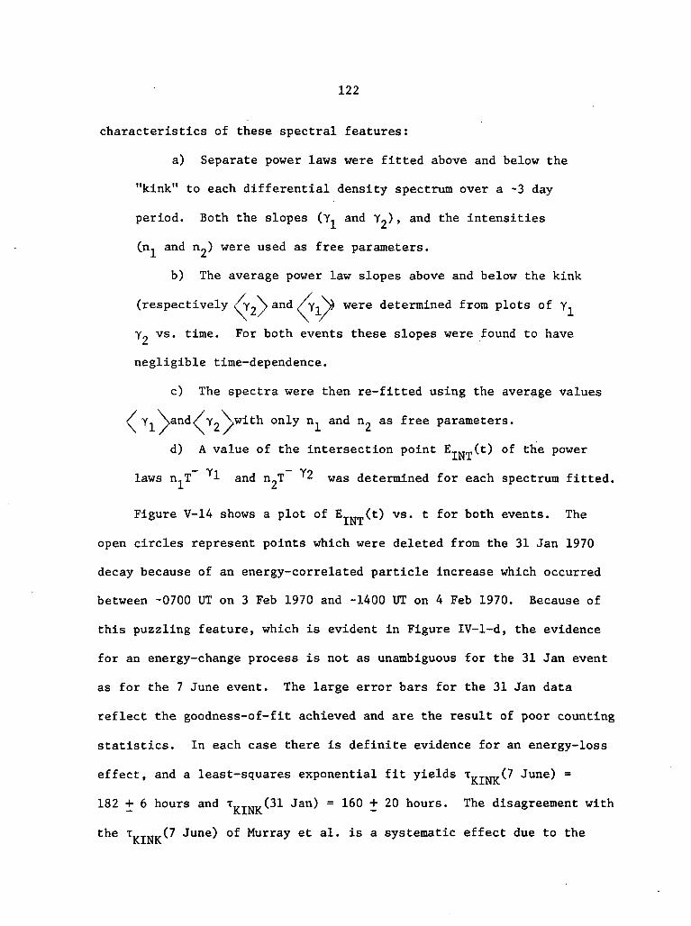
122
characteristics of these spectral features:
a) Separate power laws were fitted above and below the
"kink" to each differential density spectrum over a ~3 day
period. Both the slopes (Y, and Y2) . and the intensities
(n, and n«) were used as free parameters.
b) The average power law slopes above and below the kink
(respectively O'o"' anc* /Yi were determined from plots of Y -,
Y~ vs. time. For both events these slopes were found to have
negligible time-dependence.
c) The spectra were then re-fitted using the average values
Y-, \and/Y2 \with only n.. and n_ as free parameters.
d) A value of the intersection point E (t) of the power
laws n-T 1 and n«T 2 was determined for each spectrum fitted.
Figure V-14 shows a plot of E (t) vs. t for both events. The
open circles represent points which were deleted from the 31 Jan 1970
decay because of an energy-correlated particle increase which occurred
between -0700 UT on 3 Feb 1970 and -1400 UT on 4 Feb 1970. Because of
this puzzling feature, which is evident in Figure IV-l-d, the evidence
for an energy-change process is not as unambiguous for the 31 Jan event
as for the 7 June event. The large error bars for the 31 Jan data
reflect the goodness-of-fit achieved and are the result of poor counting
statistics. In each case there is definite evidence for an energy-loss
effect, and a least-squares exponential fit yields TVT.TO.(7 June) =JxJLrJJx
182 + 6 hours and TVTHt_(31 Jan) = 160 + 20 hours. The disagreement with— K.1NK. —
the T T T (7 June) of Murray et al. is a systematic effect due to the
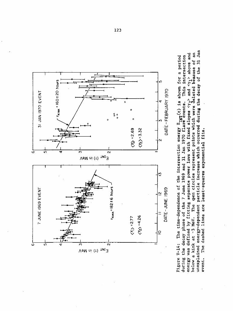
123
ro
A3|/\l
CJ
V \S
O(C >
trQDUJ
rO LL.I
LU
OJ
m
I
LJ>LU
0}
LU
00
/\ <£x xV \s
ro OJ
ro
CDIDcnUJz-3
I
<Q
4J C M 01C cd 41 H
GO0)
01 01 >a co ?>-. o)
I 00 0)
o >w cdO) 0)
A91AI
H C 60 > O. 4->3 -H M O X C00 V4 01 i-H 01 0)•H 3 C 0) C >Pn TJ 0) ,0 3 Q)
124
specific choice made for /y, Nand YoN anc* t*ie difference of -28 + 12
hours can be taken as an indication of this systematic uncertainty.
The fact that the power law asymptotes y, and y» as well as the
"kink" are stable with time is an important observation in itself: it
indicates that the energy "smearing" caused by the particle random
walk in position is not so great as to erase a spectral feature within
the ~3 day period needed to define the energy decay rate.
3. Energy-Change Predicted by the New Solution
Although considerable discussion has been waged concerning the
energy-change process for solar flare particles, no prediction has yet
been made using any model which can be compared directly to the avail- .
able energy-decay observations of a convex-shaped spectral feature.
Palmer and Urch and Gleeson have carried out calculations con-
cerning the way in which an energy "spike" propagates. Gleeson and
Ng , on the other hand, have applied their recent flare propagation
solution directly to the observations of Murray et al. They make
the simple geometrical calculation that a concave, power law kink
(steeper at lower energies) defined by
n(T) = niT~Yl + n2T~
Y2 (5-57)
will move to lower energies at a rate defined by
TKINK* T2)
where T, is the decay constant associated with slope y1 , etc.
125
Unfortunately, energy spikes and concave spectral kinks are rarely
observed, and it is not immediately obvious how the evolution of such
features can be related to the existing observations of a convex kink.
For this reason, an attempt has been undertaken to predict the evolu-
tion of a convex kink using the new solution. The method is straight-
forward (see equation 5-38) but difficult to implement. At late times,
the new solution predicts that a pure power law spectrum defined by
slope Y will decay exponentially at Tnvri. Any initial spectrum S(T)JJUL
that can be written as a superposition of power laws
S(T) = A1T"Yi (5-59)
can then be propagated in time .by
n(T,t) = A±T"Yi e~t/Ti (5-60)
where the one-to-one correspondence between each Y. and T, involves
the calculation of the first Coulomb wave function eigenvalue and
depends on T L, V, and < . With some difficulty, a set of A.'s£j r i
and Y.'s have been found which, when superimposed, produce a convex
density spectrum S(T) with power law asymptotes of Y, = 2 and YO = ^
above and below 3 MeV. These coefficients as well as a representative
set of T. values are listed in Table V-2.i
Figure V-15 shows the S(T) spectrum thus generated and also the
way it evolves over a 200 hour period using typical values of the para-
meters. Several results are evident:
a) The S(T) generated is a good approximation to the observed

126
TABLE V-2
Power Law Superposition, of a Density Spectrum
with a Convex Kink
assuming L = 2.3 AUV = 400 km/sec< = 3 x 10²⁰ Cm
2/sec
i
1
2
3
4
5
6
7
8
9
10
11
12
13
14
15
16
1.75
2.00
2.25
2.50
2.75
3.00
3.25
3.50
3.75
4.00
4.25
4.50
4.75
5.00
5.25
5.50
Ai-3cm
3.8133
-29.128
0.3227
561.42
-1767.9
1495.4
909.92
-954.86
-0.4838
-872.78
711.74
177.88
-115.51
-2.9039
-58.594
26.527
TE(1 AU)
/*• —
Ci= ^f
1.50
1.67
1.83
2.00
2.17
2.33
2.50
2.67
2.83
3.00
3.17
3.33
3.50
3.67
3.83
4.00
=78 hours
fl Tt
hrs
31.88
29.43
27.38
25.62
24.10
22.77
21.59
20.54
19.60
18.75
17.98
17.28
16.63
16.03
15.48
14.97

127
Figure V-15
An initial spectrum with a convex kink at ~3 MeV and power
law asymptotes of YI = 2 and y? = 4 is shown. This spectrum
S(T) = y A T i was generated by superimposing 16 separate
power laws. The time-evolution of this input spectrum was
calculated by assigning (via the new solution) a separate
decay time constant T^ to each power law element of S(T).
For the parameter values chosen, the spectral shape is reas-
onably stable over an ~8 day period, and the "kink" moves
exponentially to lower energies at a rate characterized by
!..,...„, = 106 hours. The power law slope y(T) of the spectraK.J.JNK.
are shown to emphasize the kink movement and to illustrate
the slight rounding effect which occurs.
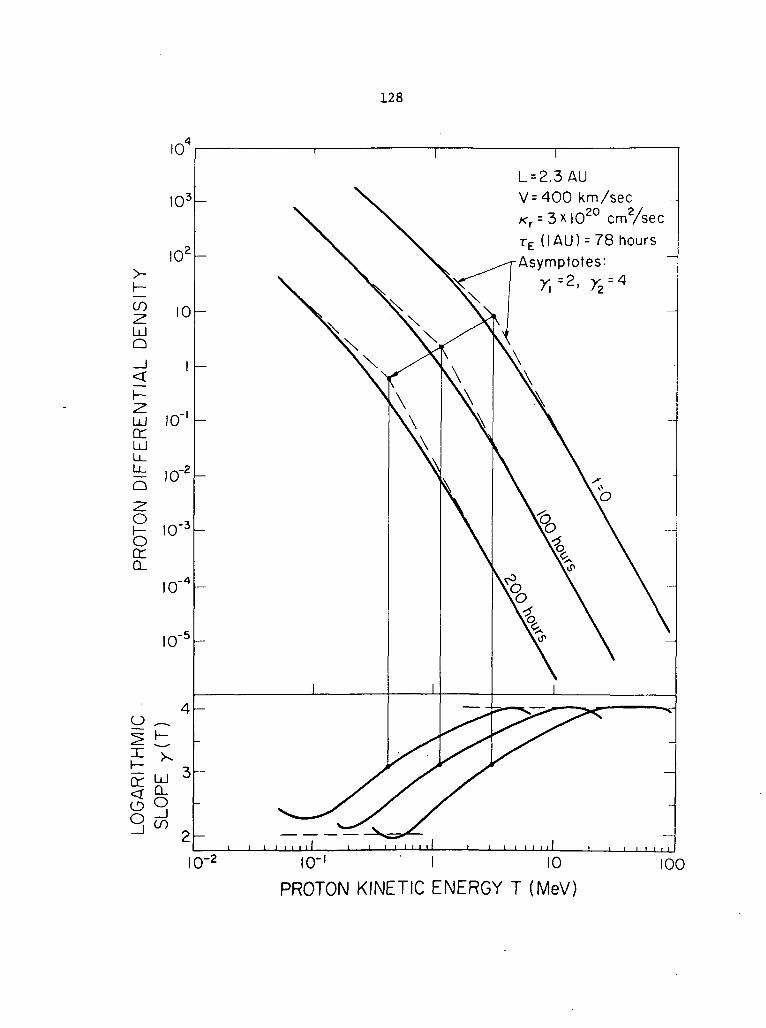
128
AUV=400 km/sec
cmVsecrE ( IAU) = 78 hoursAsymptotes:
IOH I 10
PROTON KINETIC ENERGY T (MeV)
100

129
spectra for 7 June 69 and 31 Jan 70.
b) The spectrum decays both in density and energy but retains
retains its shape over a long (~8 day) period.
c) There is some "rounding" of the kink — a result expected
due to the particle random walk.
d) The kink decays at t , = 106 + 4 hours for this choiceK.J.Nlx ~"
of parameters — a value still in disagreement with the observa-
tions.
The assumption that < is independent of energy T (built into the
new solution) must be discussed carefully when making predictions con-
cerning the energy-change process. A strong dependence of < on T
would affect the time-evolution of the spectrum and make the model
inapplicable. The < energy dependence is in fact relatively weak:
the best-fit values of « for a given solar flare vary by only about a
factor of 2 in the interval from 1 to 10 MeV (see Figure V-ll) . As
will be shown in Figure V-17, the dependence of TV-™,, on K is alsor
weak, another indication that an energy-independent K is a reasonable
approximation .
The application of the formula of Gleeson and Ng using the asymp-
totes Y-i = 2 and Y2 = ^ yields a similar result:
= (29.43h)(18.75h)(4-2) = 1Q3 hours
*iWR (29.43h - 18.75h)
Thus , even though this convex spectrum cannot be written as the super-
position of two power laws (as in equation 5-57), the rate of kink

130
movement can be predicted by considering the independent evolution of
the power law asymptotes using equation 5-58.
A glance at Figure V-5 shows that for V = 400 km/sec and
20 2K = 3 x 10 cm /sec, the particle distribution is peaked at r = 1.4 AU
and thus the "average" particle should lose energy at T (1.4 AU) -
109 hours, in agreement with the inore exact analysis just completed.
Further investigation has shown that the value of f , is rel-IxLrllx
atively insensitive to the choice of the asymptotes Y-i an^ Yo« The
complete power law superposition technique was used to generate a dif-
ferent convex spectrum with asymptotes of 2.6 and 4.2, a more accurate
approximation to the 7 June 1969 spectrum. This kink was found to
propagate at the same rate as the kink defined by Y, = 2 and Y~ = 4.
In addition, the simple formula (equation 5-58) was used to investigate
the dependence of TK-rNK on Y, and Y2 = Y, + AY in more detail. Figure
V-16 shows that TKINK varies by only -10% over the entire range of
reasonable values for the power law slope. One would then conclude that
any spectrum, as long as it contains no very sharp features, will decay
in energy at rate close to (T ) independent of shape.
The dependence of T on V, L, K and T is explored in FiguresK.J.WJS. r £i
V-17 and V-18 using both the simple formula and the power law super-
position. The agreement between these two methods of calculating TK.J.NK.
is almost exact. Increasing the distance to the boundary L decreases
the energy-loss rate because the particles on the average spend their
time further from the sun and thus experience a larger T (r) . Increas-
ing the solar wind velocity also increases the distance to the peak in

131
o>
rOcJn
o 00
I 1
ro
c\j
mo
oo
m
sjnoij ui
(3CO
C0COcuCU
(— Io
oCOr-lyao
14-4
CUrH0,SCO
0)434-1
43*
TJ0)4JCO
3O
rHCOO
COCO
!*555M*St
H
M-lO
cuoCCU*^C*0)Cu0)•oCU
43H
• •
rH1
CU
360•HP«4
13
CJCOo01
H
;JL.<3
+rH
J>-
II
CM>-
•o(3<0
rH
CO0)4-1O4JP.
^COCO
S
COrH
CU
0(X
cu434J
VM0
CO•H4JOC
M-l
CO
COCO
gO
43CO
CO•rl
00z
T)CUCO3
cu0.cfl
CO
rHCO
4-JOCUexCO
CU434-J
04J
cu•H4-1•HCOCCUCOC
•rH
^,— (CU
•H4-1CO1r^
CU
CO•H
^£zS
r-<
M-l0
CU3
rHCO
^
CU434-1
4-1CO
434-1
CO•H
CO•HCO

300
200-
100
o 0
— 300
200
100
0
132
V = 400 km/sec
(IAD) - 78 hours
• power lowsuperpositionmethod
l I I t i l l i I
1020 10211022
in cm2/sec
Figure V-17: The dependence of TKINK on V, L and Kr is shown using
both the simple formula and the complete power law superpositionmethod.
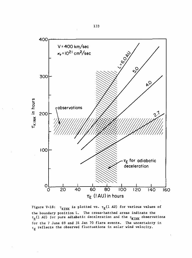
133
400
300
CO
o-C
•- 200
100
0
V = 400 km/sec
*r=l021 cmVsec
TE for adiabaticdeceleration
20 40 60 80 100TE (I AU) in hours
120 140 160
Figure V-18: T,,THI, is plotted vs. Tp.(l AU) for various values ofKINK. "the boundary position L. The cross-hatched areas indicate the
AU) for pure adiabatic deceleration and the observations
for the 7 June 69 and 31 Jan 70 flare events. The uncertainty inT reflects the observed fluctuations in solar wind velocity.
134
the particle distribution, but this effect is overshadowed by the
direct dependence of T (r) on V — an increase in V thus also increases
the energy-loss rate because the solar wind expansion is everywhere
occurring more rapidly. The dependence on K is surprisingly weak, and
is no doubt due to the variation of the particle distribution with the
ratio V/K (see Figure V-5).
Figure V-18 shows the linear dependence of !„......,.. on T_(l AU) for
various boundary positions L. The observed T , values for 7 June 69KINK.
and 31 Jan 70 are included for reference. This figure makes it clear
that in order to duplicate the measured T x of 160 - 190 hours oneKJ.RIK.
must either a) move the boundary out to L = 4-5 AU while retaining pure
adiabatic deceleration T^Cl AU) = 78 hours, or b) keep the boundary atJu
the usual 2.3-2.7 AU but assume a weaker energy-change process charac-
terized by T (1 AU) - 110 - 140 hours. The observations could alsoLJ
be matched with the new solution by using V = 250 km/sec, but this is
in direct conflict with the -400 km/sec value measured in interplanet-
ary space at the time.
In addition to the kink movement, it is evident from Figure V-15
that the kink in the power law superposition spectrum becomes slightly
more rounded as it evolves. A quantitative expression of this "kink
rounding" is given in Figure V-19, which plots the curvature
dy(T)/dlnT evaluated at y = 3.0 as a function of time. The smearing
effect, which is an expected result of the particle diffusion process,
is unambiguous but small: the curvature changes by less than 10% over
a 200 hour interval for this particular spectrum. Presumably a sharper

135
qronx
LUcr
1crZ>o
L = 2.3 AUV = 400 km/sec
Kr = 3xl020cm2/secTE (IAU) = 78hrs
0 50 100 150 200TIME in hours
250
Figure V-19: The quantity dy(T)/dlnT evaluated at y = 3.0 via thepower law superposition method is plotted vs. time. This quantityis a measure of the curvature or sharpness of the kink in the spec-trum, and it is apparent that a finite but small (~10%) smearingeffect occurs over the 200 hour time interval shown.

136
spectral feature would be initially smeared more rapidly. Unfortunate-
ly, this rounding is an order of magnitude too small to be measured by
the OGO-6 experiment during a typical 3-4 day observation period. The
fact that the analytic solution predicts a small finite rounding for
this particular spectrum suggests that experimental verification could
be made by comparing more accurately determined solar flare proton spec-
tra with the evolution of better power law approximations.
4. Conclusions Concerning the Energy-Change Process
One would like to be able to decide either for or against the
existence of a competing acceleration process, but the investigation
thus far shows that the lower rate of kink movement observed can be
produced equally well by a larger boundary distance or by an energy-
change process roughly half as strong as the adiabatic process. A
final attempt was made to settle the issue by re-fitting the event
intensity vs. time profiles using parameters which produce a TV ofK.JLNK.
160 - 190 hours.
Figures V-20 and V-21 compare fits to the 7 June and 31 Jan events
at 1.17 - 1.27 MeV using a) a larger boundary and b) a weaker energy-
change process. For the directly-connected 31 Jan 70 event only the
radial part of the solution was used (per the discussion in Section
V-E-4). Unfortunately the fits are equally good for the two cases, and
no conclusion can be drawn.
It is clear that moving the boundary out to L = 4-5 AU merely
changes the peak in the particle distribution out to r = 2.3 AU, so that

137
OOCO
Oi_
'J5i_JD
X
OI-ocrCL
O
7 JUNE 1969 EVENT.17-1.27 MeV
NEW SOLUTION /c r ( r ) = KV = 400 km/sec
L = 5.0 AUrr.(IAU) = 78 hrsC = 2.0KT = 4.5 x I02lcm%ec
L = 2.7 AU(IAU) = 1 40 hrs
r- 1.0 x I0
II 12 13
JUNE 1969
Figure V-20: Fits to the 7 June 1969 event at 1.17 - 1.27 MeV usingthe new solution. The observed T,,.,™ = 182 hours was matched by twodifferent methods: by a) moving the Boundary out to L = 5.0 AU andb) decreasing the strength of the energy change process toT£(l AU) = 140 hours.
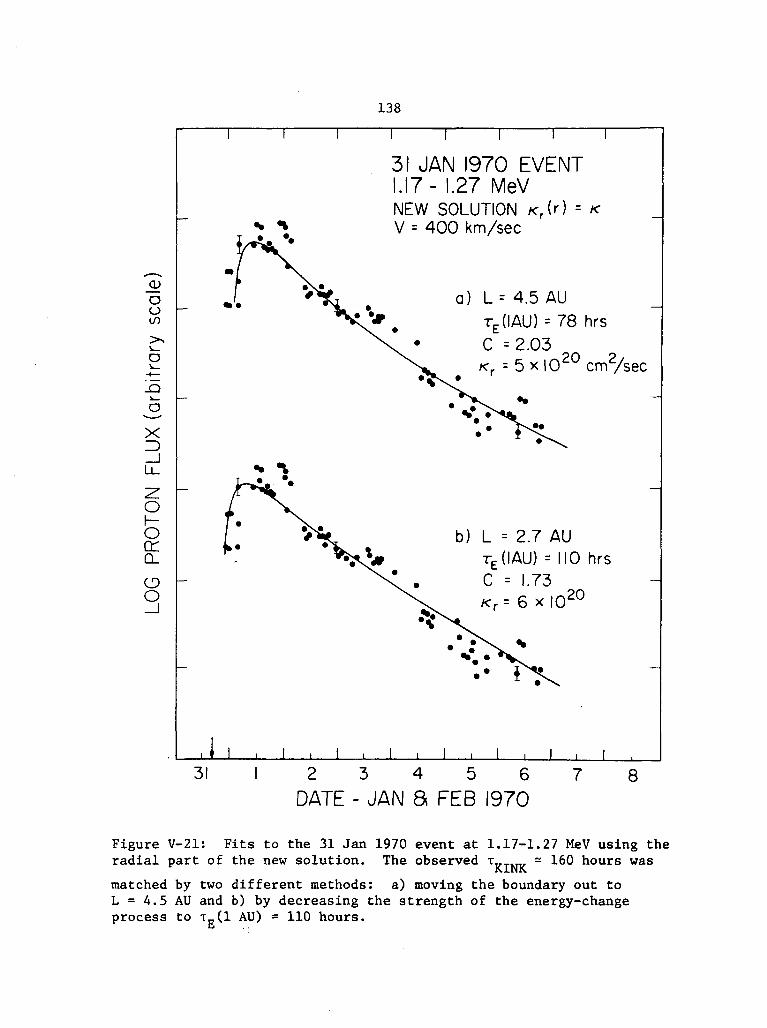
138
OOCO
Xz>_JU_
LO\-ocro_
o
31 JAN 1970 EVENT1.17- 1.27 MeVNEW SOLUTION /c r ( r ) = KV = 400 km/sec
L= 4.5 AU(IAU) = 78 hrs
cm /sec
b) L = 2.7 AUTE(IAU) = 110 hrsC =
20
31 2 3 4 5 6DATE - JAN 8 FEB 1970
8
Figure V-21: Fits to the 31 Jan 1970 event at 1.17-1.27 MeV using theradial part of the new solution. The observed T = 160 hours was
K.JLNKmatched by two different methods: a) moving the boundary out toL = 4.5 AU and b) by decreasing the strength of the energy-changeprocess to T,,(l AU) = 110 hours.
139
T (2.3 AU) matches the observed f , - 180 hours. Since any means of£j KJLriK.
peaking the distribution at 2.3 AU will produce essentially the same
energy-change effect, a third method for reproducing the observed
energy-change rate can be evoked by employing a K (r) which depends on
distance r (beyond 1 AU) in such a way that the particles are peaked
much closer to the boundary. Although this approach is not within
the assumptions of the new solution, it can be understood qualitatively
in terms of the discussion present earlier in Section V-D-2. It can
easily be seen that a K (r) which decreases beyond 1 AU will cause the
particle distribution to be peaked at a larger radial distance. This
effect can be explained by noticing that a smaller < increases the
ratio V/K on the average and thus pushes the peak outward (see
Figure V-5). It is interesting that this third method requires a form
for K (r) which has the opposite radial dependence to the frequently-
used < (r) which increases with distance.
It is apparent that this energy-change question cannot easily be
answered with observations at 1 AU. One would like either to follow
the energy vs. time history of a single particle or alternatively to
at least determine the spatial distribution of particles so that the
energy loss rate T (r) of the "average" particle is known. Gleeson
(45)and Palmer have suggested (but not carried out) a rather difficult
experiment which would afford a direct measurement of the energy-loss
rate: they propose the simultaneous observation from two spacecraft
situated on the same heliocentric radial line of a "pulse" of nearly
140
monoenergetic particles such as might be convected outward during a
flare event.

141
VI. CONCLUSION
The new solution presented here consists of resolving the differ-
ential equation for the radial part of the particle propagation, using
ic (r) = constant, and including the effects of convection and energy-
change known to be important at low energies. This new radial solution,
when combined with the azimuthal solution used by Burlaga and
(12)Forman , is capable of accurately reproducing both the rise and
decay of the "classical" prompt solar flare proton event observed at
1 AU using reasonable values of the parameters.
The principal limitations of the new solution are that it assumes
a diffusion tensor which is independent of energy and diagonal in a
reference frame aligned with the radial direction (rather than with
the B-field). Within these limitations, the comparison of the predic-
tions of the new solution with actual data leads to the following
conclusions concerning solar flare particle propagation in the inter-
planetary medium:
a) The Diffusion Tensor — The success of the new solution
in fitting both the rise and decay of flare events indicates that
K (r) = constant is a better approximation to the actual condi-
tions inside the 1 AU than is K (r) « r. It is not necessary to
invoke a scatter-free region near the sun in order to reproduce
the fast rise time observed for directly-connected flare events.
The K values derived from fits to actual data have a weak energy

142
dependence and agree reasonably well with the estimates for <
based on Mariner IV magnetic field measurements.
b) The Azimuthal Propagation — The simple point-injection
and 2-dimensional longitudinal diffusion adopted here does not
seem to be an accurate description of the actual processes at
work. Although it appears that the azimuthal solution can be
neglected for directly-connected events, some kind of longitudinal
propagation must be invoked to explain the slow rise times of
east limb events. Even though this propagation may occur near the
sun, the 2-dimensional interplanetary diffusion adopted in this
discussion is capable of explaining at least qualitatively the
slow rise profiles of these east limb flares.
c) Free-Escape Boundary — The success of the new solution
in fitting the decay phases of flare events indicates that the
assumption of a free-escape boundary at some 2 - 5 AU is at least
a reasonable approximation to the actual interplanetary conditions.
For example a sharp boundary may not exist, but there might instead
be a finite region of rapidly increasing diffusion coefficient.
d) Anisotropy — Despite the limitations of the solution with
respect to the actual spiral nature of the interplanetary field, it
is possible to understand essentially all of the features of the
observed vector anisotropy in terms of the solution. In fact, even
the absolute value of the residual anisotropy predicted agrees well
with the 5 - 10% observed.
143
e) The Energy-Change Process — By superimposing power law
spectra, it was possible to reproduce a spectrum with a convex
kink and to verify, via the new solution, that such a feature will
move to lower energies as has been observed. The existing energy-
change observations can be explained in the light of the new
solution in at least three different ways: 1) by means of a
boundary at ~2.7 AU and an energy-change process weaker than pure
adiabatic deceleration, 2) by pure adiabatic deceleration and a
boundary at 4-5 AU, or 3) by a somewhat different solution with a
boundary at ~2.7 AU and a form for K (r) which decreases beyond
1 AU. The resolution of this question must await more sophisti-
cated spacecraft measurements.

144
Appendix A
OGO-6 Monthly Summary Plots for June 1969
through February 1970
Figure A-l consists of computer-generated plots which summar-
ize the OGO-6 range telescope polar counting rates (see Section II) as
(27 28 well as certain geophysical data from the ESSA Bulletins ' . The
nine months of June 1969 through February 1970 are covered. Full credit
(63 )for these summary plots must go to L. C. Evans , for developing the
necessary computer coding, and to T. L. Garrard for generating the
OGO-6 plots shown here.
For each month the following information, starting at the top, is
plotted vs. time:
1) The average polar D1D8 counting rate in cts/sec (labelled Dl)
is plotted logarithmically. This rate is nearly insensitive to
electrons but responds to nuclei from ~1.2 to -20 MeV/nucleon.
2) The average polar D2D8 counting rate in cts/sec (labelled D2)
is plotted logarithmically. This rate responds to electrons
£ 200 keV and to nuclei ^^3 MeV/nucleon.
3) The average polar D1D2D8 counting rate in cts/sec (labelled
D1D2) is plotted logarithmically. This rate responds to nuclei
from ~3 to ~20 MeV/nucleon.
4) The average polar D2D3D8 counting rate in cts/sec (labelled
D2D3) is plotted logarithmically. This rate responds to electrons
> 1 MeV and nuclei £ 19 MeV/nucleon.
145
5) The >10 MeV solar proton fluxes measured by the Solar Proton
Monitoring Experiment aboard Explorer 41. This cosmic ray tele-
(28}scope which is described briefly in the ESSA descriptive text ,
also has some electron sensitivity. The large rate excursions
repeated at -4.3 day intervals are due to the periodic passage of
the satellite through the earth's radiation belts. These excur-
sions have been largely suppressed by the plotting program.
6) Normalized hourly average counting rates for 2 neutron moni-
tors: Alert (upper line) and Deep River.
7) The standardized K-index of geomagnetic activity from twelve
observations are averaged to obtain K . The quasi-logarithmic K
scale ranges from 0(quiet) to 9 (very disturbed). The legend for
the plots is identical to that adopted by ESSA.
8) Geomagnetic storm sudden commencements (labelled SC) are
indicated by solid triangles if confirmed and by open triangles if
unconfirmed.
9) Magnetogram sudden impulses (labelled SI) are indicated by
solid diamonds if confirmed and open diamonds if unconfirmed.
10) Optical solar flares (labelled SOLAR FLARE) of importance
greater than 2F observed by the world-wide system of solar obser-
vatories are indicated by a small vertical line plotted at the
beginning time of the flare. The importance (2N, 3B, etc.) is
included. Periods of no flare patrol are indicated by horizontal
lines of appropriate length.
11) 2 - 12A solar x-ray flares (labelled X RAY) with a peak flux

146
at least 4 times the ambient value are indicated by a vertical
line. These data were collected by experiments aboard Explorers
33 and 35.
12) Occurrences of type^-IV radio emission (labelled TP IV RADIO)
are indicated by vertical lines. This radiation is normally asso-
ciated with the acceleration of solar flare electrons.
The gaps in the OGO-6 data after November 1969 are in most cases
due to incomplete processing rather than actual data coverage problems.

147
Figure A-l
OGO-6 Data Summary Plots
A description of these plots is given in the text of
Appendix A:
Graph a
Graph b
Graph c
Graph d
Graph e
Graph f
Graph g
Graph h
Graph i
June 1969
July 1969
August 1969
September 1969
October 1969
November 1969
December 1969
January 1970
February 1970

148
~x
1 „/•• "'"V... A'—'—'—
00
NI I2F
2 2B N
I I I I I33 22EB NB
I I•2 ' 2B 8
1 ' 2 ' 3 'M PS '6 '7JUNE 19G9
* 9 I 10 ' li ' 12 ' 13 ' 1U I 15 ' 16 ' 17 ' 16 ' 19 I 20 ' 21 ' 22 ' 23 ' 2U T25 ' 26 ' 27 ' 28 ' 29 I 30
Figure A-l-a

149
r~ - r - - r
»„-- »r~
r
VAT •*? .'-.,
!
r—
,.,o'L
i 'JJ.'.V.VJJ-,
10r
-I 1 . 1 1 1 1 , 1 1 1 1 , =1 , , 1 . , , , 1 r-
f- «tf6'<W!L*W ^nf-a/tV*..* tV^/j^V^N ttA^\jffi V *•<. *>f^y^f .,,'»,».f.i.'-.»>; ^Mf^ff^M^f
ofc^-^T- f- • ^"•^• -r-^^r-/
IllL-VM.! -! ^^ ^Jml^im^^UfmkA ^jMllkW
«o
1 1 1 1 1
1 '2 '3 'M IS '6 '7 '8 '9 I 10' 11 ' 12' 13' 11 I 15' 16' 17' 18' 191 20' 21 ' 22' 23' 21 I 25' 26' 27 ' 28' 29 I 30 ' 3]JULY 1969
Figure A-l-b
150
f310
-1 T
-i 1 1 1 1 1 1 1—1 1 1—[-
T: 1 1 T, 1 r
Ci *xtr,' ^/oi»A •ff^~f
-] T; i i r-^-] 1 1 i , 1 r
K~*R **J. -^WW * iKT-^m i, '*****»*• f^ »i.***ys»s»V; "CJffi^ftfftc- ~«-(,v«.>o»i
-e=P=- ^^- 00F^ps
- *^—h °r\S (v^ \^~
»0 0
X WT
If IV
1 1 1 1 ! 1 1
1 '2 '3 ' <l 15 '6 '7 '8 '9 I 10 ' II ' 12 ' 13 ' IV I 15 ' 16 ' 17 ' IB ' 19 I 20 ' 21 ' 22 ' 23 ' 2V I 25 ' 26 ' 27 ' 28 ' 29 I 30 ' 31RUG 1969
Figure A-l-c
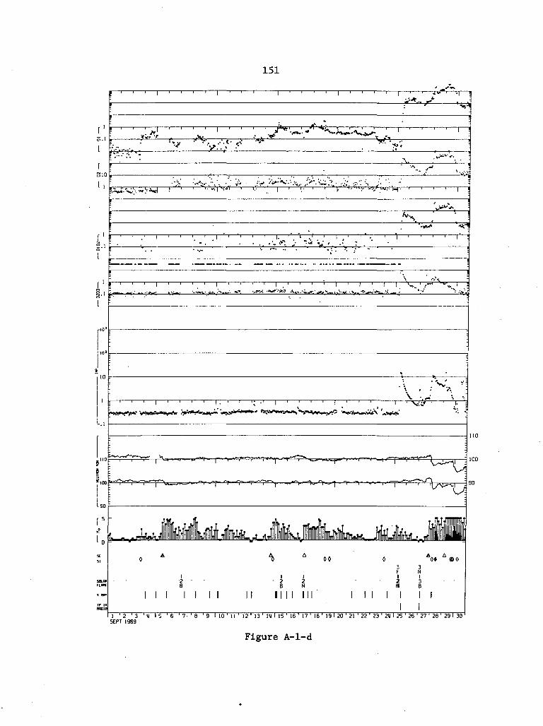
151
if*.. _..*
5.1
h
r2.1
&t i
10
"fff *./•*•* ?& •<+*f+*Mi\ '..XT*.'
1
o«
i i 1 1 i i i1 '2 '3 '11 IS '6 '7- '8 '9 I 10 ' 11 ' 12' 13' 1<I I IS1 16' 17 ' 18' 191 20' 21 'K ' 23' 2V I 25' 26' 27 ' 28' 291 30
SEPT 1969
Figure A-l-d

152
>f..:-:- •...:'.' '\S«. . . - . ' . . : . . .:•..
il-J i • 'i f j 1 f; f '"" i" A.| "**" i'" •'• i .'-V j -'• «ii.!' :j£, •. iVy. i 1 x
r
I I2 2N N
_
I', r3"T"3"1 n I 5 1~G~" 7 '8 '9 I 10' 11 ' 12' 13' 1M I 15' 16 ' 17' 18' 191 20' 21 ' 22' 23 r 2M T25 S 1? ^28 ' ?9 I'.m ' JlOL7 !9G9
100
Figure A-l-e

153
-I 1 1 1 ^»-l.*.*l" f—r
! ' 1~
[ 'S.i ».VA**«V<*** ,.a".» .VJi *'"*'*"••.*.•• -**.'C.V .»--.* .1»^ *•*
10
' ' ' V - 'V . - • '••!:.'
110
100
<= 90
I§¥ioo
« « 000p
I I I I I I I I I2 2 2 2 2 2 2 - 2 2B B N B B B N N N
HID Ill l II UNI II MM I II1
1 '2 '3 ' M IS '6 '7 '8 '9 I 10 ' 11 ' 12 ' 13 ' 14 I 15' 16' 17 ' 18 ' 191 20 ' 21 ' 22' 23' 21 I 25 ' 26 ' 27 ' 28 ' 29 I 30NOV 1963
Figure A-l-f

154
•\'J ~X f*v-
:-'h-
10
\VTfVrwk.
100-Kv-T
lUjfliM ift.y.jJl T
0 0 0
DEC 1969T ' 1 I 5"' 6 '7 '8 '9 I 10 ' 11 ' 12 ' 13 ' 11 I 15 ' 16 ' 17 ' 18 ' 19 I 20 ' 21' 22 ' 23 ' 24 I 25 ' 26 ' 27 ' 28 ' 29Tlo r31
Figure A-l-g

155
oo
-2 22N BN
1 '2 '3 '14 15 '6 '7 'B '9 I 10 ' 11 ' 12 ' 13 ' 14 I 15 ' 16 ' 17 ' 18JflN 1970
19 I 20 ' 21 ' 22 ' 23 ' 24 I 25 ' 26 ' 27 ' 28 ' 29 I 30 ' 31
Figure A-l-h
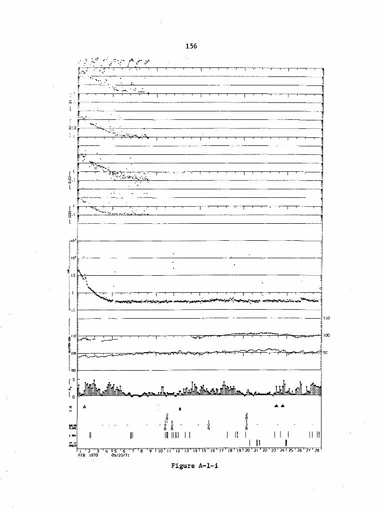
156
r_n
10
10
00
90
-1 1 1—
L
2 2B B
1 '2 '3 ' it IS '6 '7 '8 '9 I 10 ' 11 ' 12 ' 13 ' 1U I 15' 16 ' 17 ' 18' 19 I 20 ' 21'22' 23 ' 21 I 25 ' 26 ' 27 ' 28FEB 1970 09/23/71
Figure A-l-i
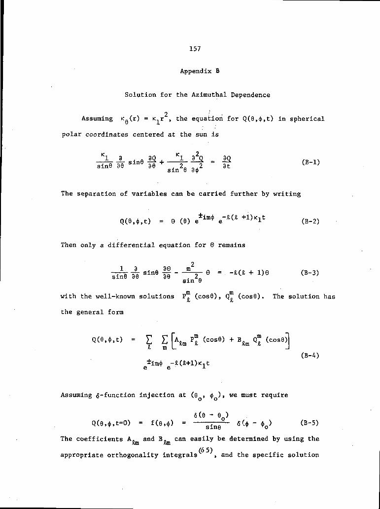
157
Appendix B
Solution for the Azimuthal Dependence
2 ''Assuming Ke(r)
= K-,* > the equation for Q(6,<|>,t) in spherical
polar coordinates centered at the sun is
Kl 3 . A 9Q . <1 92Q 80 ,_ 1N
^9 30 sln6 36 + — 27 -2 = 3T &-Vsin 6 dtp
The separation of variables can be carried further by writing
Q(e.*,t) = 0 (8) e±im* e-£(i +1)Klfc (B-2)
Then only a differential equation for 0 remains
lin? W Sin6 f - -T 9 -.-K£+l>e CB-3)sin 6
with the well-known solutions P0 (cos6), Q. (cos9). The solution hasAt J6
the general form
QCe,*,t) - £ E km Pj (cose) + B^m Qm (cose)]
£ m L J(B-4)
e
Assuming ^-function injection at (0 , <j> ) , we must require
6(9 - 8 )Q(e,<(),t=0) = f(e,<j>) = - — 6(4 ~ <|>0) (B-5)
The coefficients A, and Bn can easily be determined by using theJem xm
appropriate orthogonality integrals , and the specific solution

158
becomes:
(B-6)
where y = cos6 and y = cos6 . The addition theorem for spherical
harmonics can now be applied
iT y (& - m> • p* /u\ Pm
+ x ^ a + m), F£ ty; mS=£
CB-7)
Y is the angle between (9,9) and (9 ,<j> ) given by
COSY = cos9 cos9 + sin9 sin9 cos(9 - 9 )° (B-8)
Our solution for 2-dimensional diffusion thus reduces to the 1-dimen-
sional solution
CB-9)
Evidently the 2-dimensional random walk in 9 and <f> is completely
equivalent to a 1-dimensional diffusion problem because the gradient
VQ is directed radially outward from (9 , <J> ) . This will be the case
as long as the injection profile f(9,<j>) is symmetric about the point
(0 , (j> ) and K (r) = < (r) .o o O 9
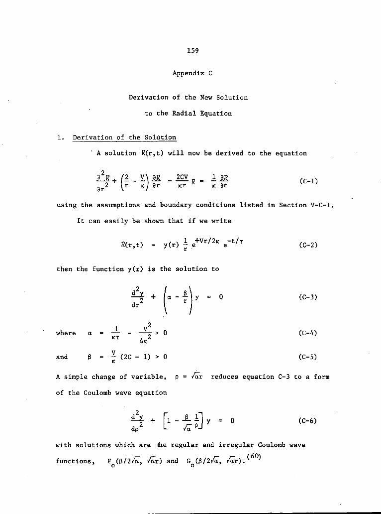
159
Appendix C
Derivation of the New Solution
to the Radial Equation
1. Derivation of the Solution
' A solution R(r,t) will now be derived to the equation
o8R 2CV 1 9R"37 ~ Tr~ R = 7 "3T (C~1)
using the assumptions and boundary conditions listed in Section V-C-1,
It can easily be shown that if we write
RCr.t) = y(r) i e+Vr/2K e-t/T (C-2)
then the function y(r) is the solution to
' B\. , a - * 1 y - 0 (C-3)dr
1 V2where a = — - —r- > 0 (C-4)
and 3 = - (2C - 1) > 0 (C-5)
A simple change of variable, p = /Tr reduces equation C-3 to a form
of the Coulomb wave equation
9 • i ••• _ « i * ~ w (C-6)dpZ
with solutions which are the regular and irregular Coulomb wave
functions, F (3/2t/cT, >/ar) and G (3/2/T,(60)
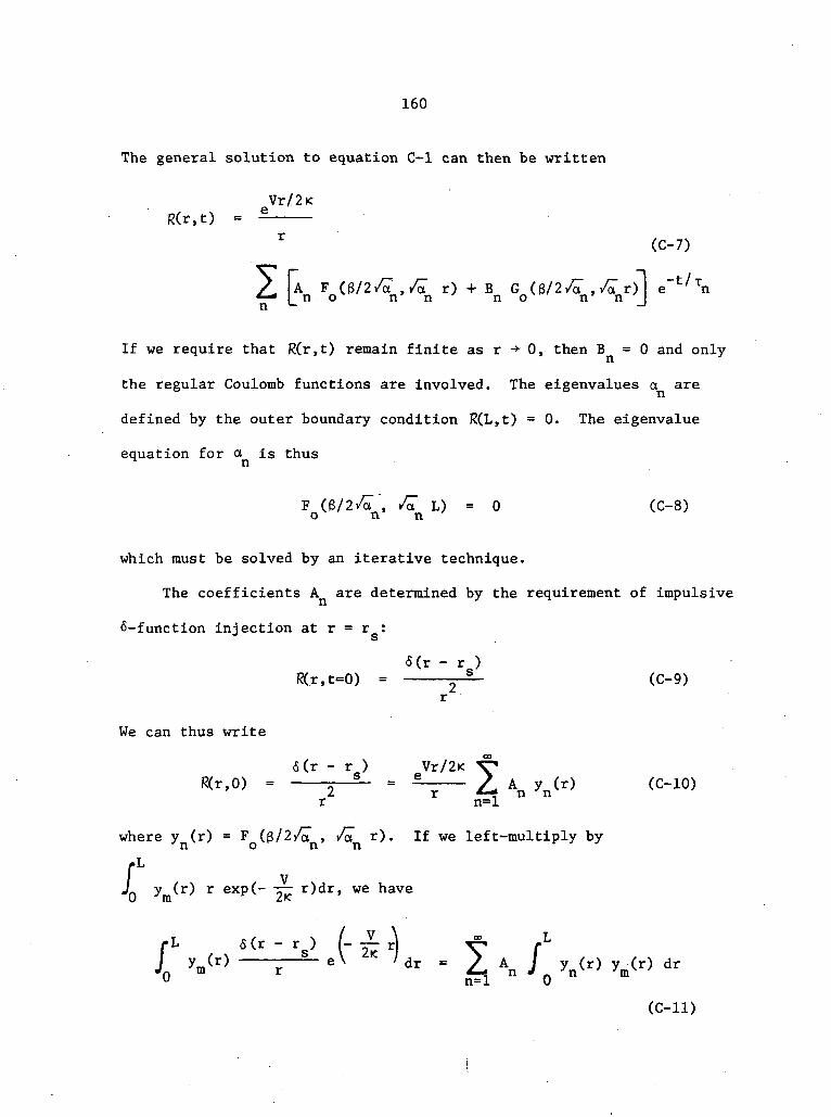
160
The general solution to equation C-l can then be written
Vr/2KR(r,t) = $ -
r (C-7)
JAn .*-
, r) 't/T
If we require that R(r,t) remain finite as r •> 0, then B = 0 and only
the regular Coulomb functions are involved. The eigenvalues a are
defined by the outer boundary condition R(L,t) = 0. The eigenvalue
equation for a is thus
F (8/2/T, /T L) = 0 (C-8)o n n
which must be solved by an iterative technique.
The coefficients A are determined by the requirement of impulsive
S-function injection at r = r :
<S(r - r )RCr.t-0) = -S- (C-9)
r
We can thus write
6(r - r ) Vr/2</r/2< 7BCr.O) = 2— - = ~r L A- 7n(r) (C-10)
r n=l
where y (r) = F (&/2/a , t/a r). If we left-multiply by
r exp(- -r— r)dr, we have
L. . ~ • ~ s' \ "Jtf ~\ "\. I
y (r) y (r) dr0 " L n^l " * 0 n m
(C-ll)
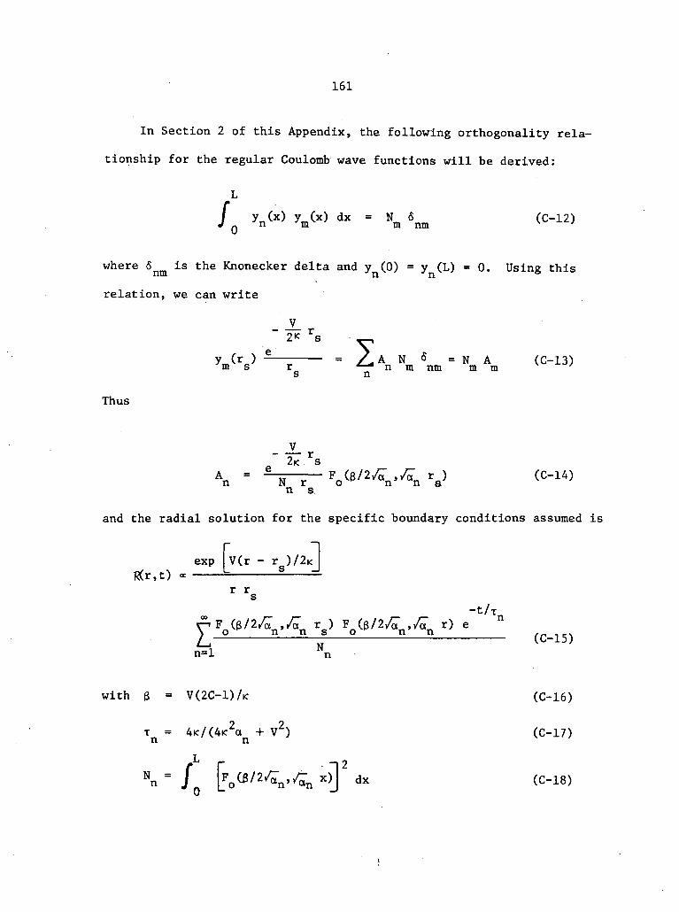
161
In Section 2 of this Appendix, the following orthogonality rela-
tionship for the regular Coulomb wave functions will be derived:
Jj
/v,,60 y Cx) dx = N
n n m m CC-12)
where 6nm is the Knonecker delta and y (0) = y (L) = 0. Using this
relation, we can write
JL2< rs
s n
Thus
An * ITT F
n s
and the radial solution for the specific boundary conditions assumed is
expR(r,t) «
. -c/<,r) e
—i Nn-1 n
with g = V(2C-1)/K (C-16)
4ic/(4K2an + V2) (C-17)
N n = /
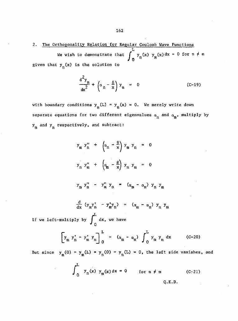
162
2. The Orthogonality Relation for Regular Coulomb Wave FunctionsL
dx = 0 for n mWe wish to demonstrate that f y (x) y Cx)j n m
given that y (x) is the solution to
dV
with boundary conditions y (L) = y (x) = 0. We merely write down
separate equations for two different eigenvalues a and a , multiply by
y and y respectively, and subtract:
ym yn + (an - f) ym yn
yn y^ + L -
= 0
y,, ym = °
" "- y" y = (a - a )'m Jn vum uny
= (am ' an) yn
If we left-multiply by / dx, we have0
f dx,J 0
r -^L rLv y ' - y ' y = (a -a) I y y dx (C-20)JJm •'n 7m /nj Q m ny J 'm 7n
But since y (0) = y (L) = y CO) = y (L) = 0, the left side vanishes, andm m n n
rLJ yn(x) ymCx)dx = 0 for n ^ m (« Q 11 in
Q.E.D.

163
3. Evaluating the Orthogonality Integral
Equation C-21 can be generalized as
dx ' N 6Y. n iii n mn
The problem remains to evaluate the normalization integral N . Using
equation C-21, one can write this as the following limit:
(_ymyn * ymynJ 0N = limit " V - a (C~23)
a -> a m nm n
applying 1'Hopitals Rule, we have
Nnm - a =a
m n
= [ya(Vx) y'(an'
0
L (C-24)
where y(an>x) = Yn(x) and ya(an»x) = J^ y(a,x)
However, y(a ,0) = y(a ,L) = y (a ,0) = 0
and
ot=an
Nn = yaCan'L) y'(an'L) (C~25)
In terms of the Coulomb wave functions, this becomes

164
Nn 4a o 3nn
9F
(C-26)
x=L
where FQ(TI,P) = FQ andn 3p
Equation C-26 is not a simple evaluation of N , but it greatly facili-
tates the calculation because time-consuming numerical integration can
be avoided.
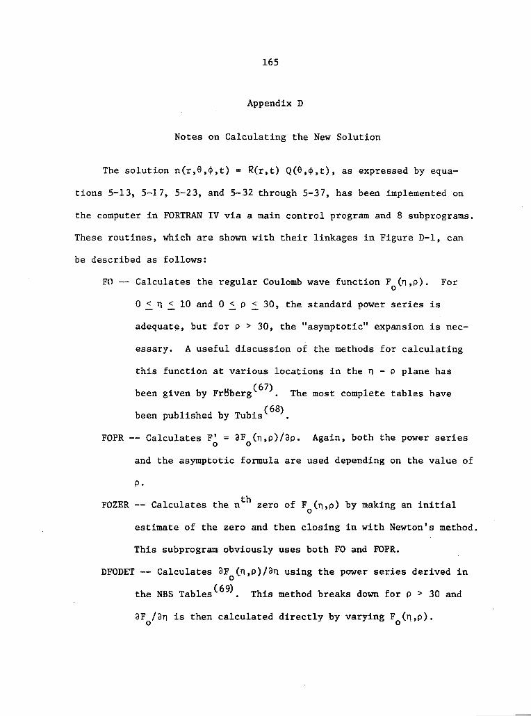
165
Appendix D
Notes on Calculating the New Solution
The solution n(r,6,<J>,t) = R(r,t) Q(6,4>,t), as expressed by equa-
tions 5-13, 5-17, 5-23, and 5-32 through 5-37, has been implemented on
the computer in FORTRAN IV via a main control program and 8 subprograms.
These routines, which are shown with their linkages in Figure D-l, can
be described as follows:
FO — Calculates the regular Coulomb wave function F (n,p). For
0 <_ n £ 10 and 0 <^ p <^ 30, the standard power series is
adequate, but for p > 30, the "asymptotic" expansion is nec-
essary. A useful discussion of the methods for calculating
this function at various locations in the n - P plane has
been given by FrBberg . The most complete tables have
( f>R\been published by Tubis .
FOPR — Calculates F' = 3F (n,p)/3p. Again, both the power series
and the asymptotic formula are used depending on the value of
P.
FOZER — Calculates the n zero of F (n,p) by making an initial
estimate of the zero and then closing in with Newton's method.
This subprogram obviously uses both FO and FOPR.
DFODET — Calculates 3F (n,p)/3n using the power series derived in
the NBS Tables . This method breaks down for p > 30 and
3F /3n is then calculated directly by varying F (n,p).

166
CO4JO
4-1c•H
I
PiPuOFn
Csl
H
§
gO
T
CD COc
0)0) 4-1
jG OJ
" gcu ^4-1 CO(0 CX
T-(
3 4JO 3
•H fXCO 4-1O 3
OO4J TD >
0) OCO 4-» T-l3 3 4J
O- OCO C 0)0) -H WC•H cu aS g ^O 13M 0)
• CH C -HCU O MH4J -H CU3 4J 13O. 3g i-H 0)O O M
O CO CO
bO•H
co
iMCO
« VCO
3CX

167
LUPT0N — Calculates the new radial solution R(r,t) using the subprog-
rams FO, FOPR, FOZER and DFODET. Using the input parameters V,
r, r , L, K, t and NMAX, LUPT0N carries out the following opera-s
tions:
a) Defines 3 = V(2C-1)/K
b) Calculates the eigenvalues a(n) for n = 1, NMAX using FOZER.
c) Calculates the value of the normalization integral N for
n=l, NMAX (see Appendix C) without any numerical integration using
FOPR and DFODET.
d) Sums the eigenvalue series (Equation 5-32) and finds R(r,t).
P — Evaluates the Legendre polynomial P.(y) using a recursion relation.Jo
L0NGTD — Calculates the azimuthal solution Q(y,t) via subprogram P for
injection uniform over a cone of half-angle y •
MAIN — The main control program. Converts Q(y>t) into the function
Q(y',t) including field spiral and corotation. Then MAIN either
prints n(r,y',t) or plots n vs. t using MtiDPLT.
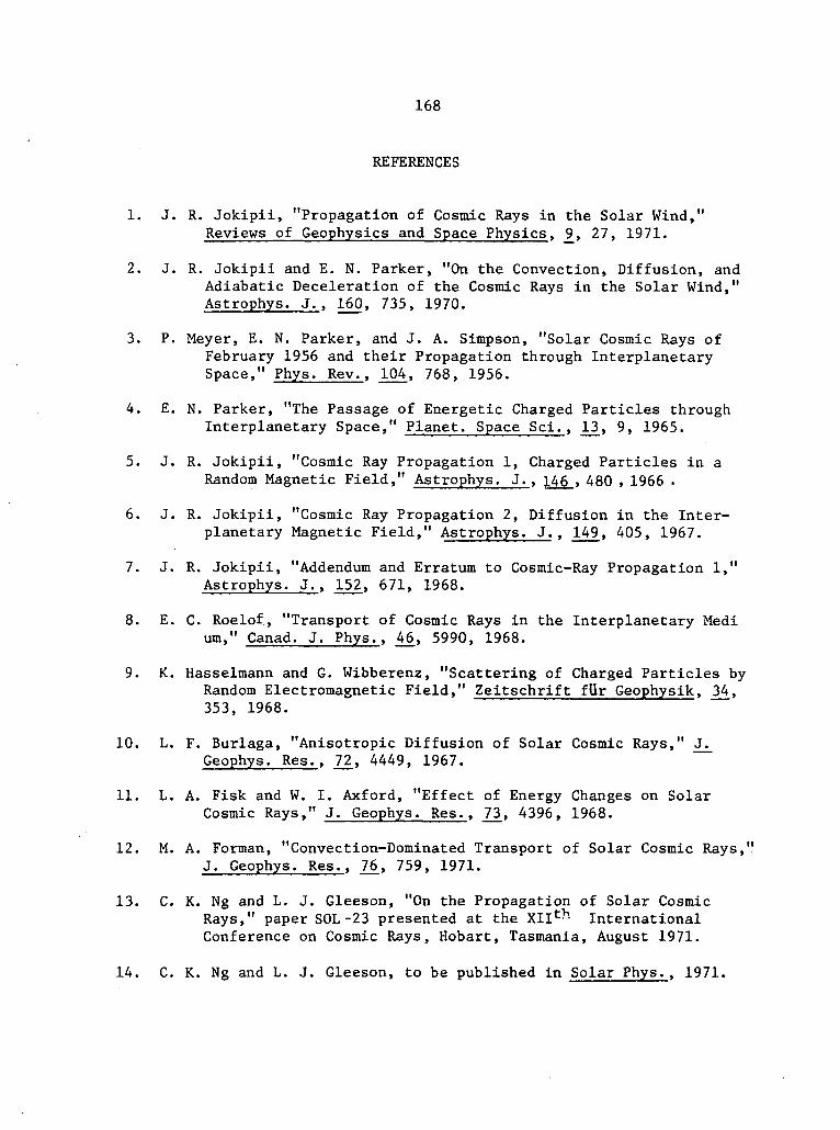
168
REFERENCES
1. J. R. Jokipii, "Propagation of Cosmic Rays in the Solar Wind,"Reviews of Geophysics and Space Physics, _9, 27, 1971.
2. J. R. Jokipii and E. N. Parker, "On the Convection, Diffusion, andAdiabatic Deceleration of the Cosmic Rays in the Solar Wind,"Astrophys. J., 160, 735, 1970.
3. P. Meyer, E. N. Parker, and J. A. Simpson, "Solar Cosmic Rays ofFebruary 1956 and their Propagation through InterplanetarySpace," Phys. Rev., 104, 768, 1956.
4. E. N. Parker, "The Passage of Energetic Charged Particles throughInterplanetary Space," Planet. Space Sci. , 13, 9, 1965.
5. J. R. Jokipii, "Cosmic Ray Propagation 1, Charged Particles in aRandom Magnetic Field," Astrophys. J., 146_, 480 , 1966 .
6. J. R. Jokipii, "Cosmic Ray Propagation 2, Diffusion in the Inter-planetary Magnetic Field," Astrophys. J., 149, 405, 1967.
7. J. R. Jokipii, "Addendum and Erratum to Cosmic-Ray Propagation 1,"Astrophys. J., 152, 671, 1968.
8. E. C. Roelof, "Transport of Cosmic Rays in the Interplanetary Mediurn," Canad. J. Phys.. 46_, 5990, 1968.
9. K. Hasselmann and G. Wibberenz, "Scattering of Charged Particles byRandom Electromagnetic Field," Zeitschrift fUr Geophysik, 34,353, 1968.
10. L. F. Burlaga, "Anisotropic Diffusion of Solar Cosmic Rays," J.Geophys. Res.. 72, 4449, 1967.
11. L. A. Fisk and W. I. Axford, "Effect of Energy Changes on SolarCosmic Rays," J. Geophys. Res., 73, 4396, 1968.
12. M. A. Forman, "Convection-Dominated Transport of Solar Cosmic Rays,"J. Geophys. Res., 76>, 759, 1971.
13. C. K. Ng and L. J. Gleeson, "On the Propagation of Solar CosmicRays," paper SOL-23 presented at the XIIth InternationalConference on Cosmic Rays, Hobart, Tasmania, August 1971.
14. C. K. Ng and L. J. Gleeson, to be published in Solar Phys., 1971.
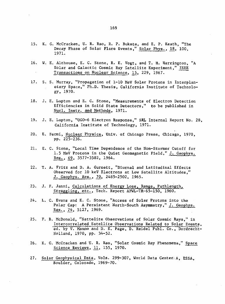
169
15. K. G. McCracken, U. R. Rao, R. P. Bukata, and E. P. Keath, "TheDecay Phase of Solar Flare Events," Solar Phys., 18, 100,1971.
16. W. E. Althouse, E. C. Stone, R. E. Vogt, and T. H. Harrington, "ASolar and Galactic Cosmic Ray Satellite Experiment," IEEETransactions on Nuclear Science. 15, 229, 1967.
17. S. S. Murray, "Propagation of 1-10 MeV Solar Protons in Interplan-etary Space," Ph.D. Thesis, California Institute of Technolo-gy, 1970.
18. J. E. Lupton and E. C. Stone, "Measurements of Electron DetectionEfficiencies in Solid State Detectors," to be published inNucl. Instr. and Methods, 1971.
19. J. E. Lupton, "OGO-6 Electron Response," SRL Internal Report No. 28,California Institute of Technology, 1971.
20. E. Fermi, Nuclear Physics, Univ. of Chicago Press, Chicago, 1970,pp. 225-236.
21. E. C. Stone, "Local Time Dependence of the Non-Stormer Cutoff for1.5 MeV Protons in the Quiet Geomagnetic Field," J. Geophys.Res., 6J3, 3577-3582, 1964.
22. T. A. Fritz and D. A. Gurnett, "Diurnal and Latitudinal EffectsObserved for 10 keV Electrons at Low Satellite Altitudes,"J. Geophys. Res.. W, 2485-2502, 1965.
23. J. F. Janni, Calculations of Energy Loss, Range, Path-length,Straggling, etc., Tech. Report AFWL-TR-65-150, 1960.
24. L. C. Evans and E. C. Stone, "Access of Solar Protons into thePolar Cap: A Persistent North-South Asymmetry," J. Geophys.Res., _74, 5127, 1969.
25. F. B. McDonald, "Sattelite Observations of Solar Cosmic Rays," inIntercorrelated Satellite Observations Related to Solar Events,ed. by V. Manno and D. E. Page, D. Reidel Publ. Co., Dordrecht-Holland, 1970, pp. 34-52.
26. K. G. McCracken and U. R. Rao, "Solar Cosmic Ray Phenomena," SpaceScience Reviews, 11, 155, 1970.
27. Solar Geophysical Data, Vols. 299-307, World Data Center. A, ESSA,Boulder, Colorado, 1969-70.

170
28. Solar Geophysical Data. IER-FB-294 (Supplement), "DescriptiveText," World Data Center A, ESSA, Boulder, Colorado, Febr.1969.
29. L. D. Kavanagh, Jr., A. W. Schardt, and E. C. Roelof, "Solar Windand Solar Energetic Particles: Properties and Interactions,"Reviews of Geophys. and Space Phys., Vol. 8, No. 2, 389,1970.
30. It was later discovered by the author that the Dl noise was correl-ated with the spacecraft exposure to sunlight and that thefailure was probably caused by a broken Range Telescope mylarwindow.
31. S. S. Murray, E. C. Stone, and R. E. Vogt, "Interplanetary Deceler-ation of Solar Cosmic Rays," Phys. Rev. Letters, 26, 663,1971.
32. A. J. Masley and P. R. Salterblom, "Solar Cosmic Ray ObservationsDuring the September and November 1969 Events," paper SOL-33presented at the XIItn International Conference on CosmicRays, Hobart, Tasmania, August 1971.
33. Report UAG-13, "Data on the Solar Proton Event of Noberaber 2, 1969through the Geomagnetic Storm of November 8-10, 1969," com-piled by D. B. Bucknaw and J. V. Lincoln, World Data Center A,NOAA, Boulder Colorado, 1971.
34. E. N. Parker, "Dynamics of the Interplanetary Gas and MagneticField," As trophys. J., 128, 664, 1958.
35. E. N. Parker, "Cosmic Ray Modulation by the Solar Wind," Phys. Rev.,110, 1445, 1958.
36. S. M. Krimigis, "Interplanetary Diffusion Model for the Time Behav-ior of Intensity in a Solar Cosmic Ray Event," J. Geophys.Res.. 2943, 1965.
37. J. E. Lupton and E. C. Stone, "Transport of Solar Flare Protons —Comparison of a New Analytical Model with Spacecraft Measure-ments," paper SOL-22 presented at the XIIth InternationalConference on Cosmic Rays, Hobart, Tasmania, August 1971.
38. J. R. Jokipii and P. J. Coleman, Jr., "Cosmic Ray Diffusion Tensorand Its Variation Observed with Mariner 4," J. Geophys. Res. ,73, 5495, 1968.
39. J. R. Jokipii and E. N. Parker, "Cosmic Ray Life and the StochasticNature of the Galactic Magnetic Fluid," Astrophys. J.. 155, 799,1969.

171
40. E. P. Keath, R. P. Bukata, K. G. McCracken, and U. R. Rao, "TheAnomalous Distribution in Heliocentric Longitude of SolarInjected Cosmic Radiation," Solar Phys.. 18, 503, 1971.
41. R. P. Bukata, U. R. Rao, K. G. McCracken, and E. P. Keath, "Obser-vation of Particle Fluxes over Extended Solar Longitudesduring the Solar Flare Event of March 31 to April 10, 1969,"paper SOL-27 presented at the XIIth International Conferenceon Cosmic Rays, Hobart, Tasmania, Aug. 1971.
42. R. P. Lin, S. W. Kahler, and E. C. Roelof, "Solar Flare Injectionand Propagation of Low-Energy Protons and Electrons in theEvent of 7-9 July, 1966," Solar Phys., 4_, 338, 1967.
43. J. Kunstmann and G. Webberenz, "The Structure of InterplanetarySpace During the March 24, 1966 Solar Event," paper SOL-16presented at the XIIth International Conference on CosmicRays, Hobart, Tasmania, Aug. 1971.
44. J. R. Jokipii, "Deceleration and Acceleration of Cosmic Rays inthe Solar Wind," Phys. Rev. Letters, 26, 666, 1971.
45. L. J. Gleeson and I. D. Palmer, "On the Direct Observation ofCosmic-Ray Energy Losses," Astroph. and Sp. Sci., 12, 123,1971.
46. I. D. Palmer, "Cosmic Ray Energy Losses at 1 AU during SolarProton Events," paper SOL-25 presented at the XIIth Inter-national Conference on Cosmic Rays, Hobart, Tasmania, August,1971.
47. I. H. Urch and L. J. Gleeson, "Energy Changes of Solar Cosmic RayParticles," paper SOL-24 presented at the XIIth InternationalConference on Cosmic Rays, Hobart, Tasmania, August, 1971.
48. M. A. Forman, "Convection-Dominated Transport of Solar Cosmic Rays,"paper SOL-26 presented at the XIIth International Conferenceon Cosmic Rays, Hobart, Tasmania, August, 1971.
49. K. G. McCracken, U. R. Rao, and R. P. Bukata, "Cosmic-Ray Propaga-tion Processes, 1, A Study of the Cosmic-Ray Flare Effect,"J. Geophys. Res., 72, 4293, 1967.
50. U. R. Rao, K. G. McCracken, F. R. Allum, R. A. R. Palmeira, W. C.Bartley, and I. Palmer, "Anisotropy Characteristics of LowEnergy Cosmic Ray Population of Solar Origin," paper SOL-29presented at the XIIth International Conference on CosmicRays, Hobart, Tasmania, August, 1971.

172
51. J. M. Wllcox and N. F. Ness, "Quasi-stationary Corotating Structurein the Interplanetary Medium," J. Geophys. Res., 70, 5793,1965.
52. W. I. Axford, "Anisotropic Diffusion of Solar Cosmic Rays," Planet.Space Sci., 13, 1301, 1965.
53. L. F. Burlaga, "Anisotropic Solar Cosmic Ray Propagation in an In-homogeneous Medium," presented at the XIt'1 International Con-ference on Cosmic Rays, Budapest, Hungary, August, 1969.
54. J. R. Jokipii, "Modulation of Low Rigidity Cosmic Rays and thePower Law Spectrum of the Interplanetary Magnetic Field in1962 and 1965," Canadian J. Phys. , 46., 5950, 1968.
55. J. R. Jokipii, personal communication, 1971.
56. J. R. Jokipii, "Fokker-Planck Equations for Charged ParticleTransport in Random Fields," preprint, California Instituteof Technology, 1971.
57. K. G. McCracken, "Anisotropies in Cosmic Radiation of Solar Origin,"in Solar Proton Manual, NASA Tech. Report R-169, ed. by F. B.McDonald, pp. 57-88, 1963.
58. R. C. Englade, "Effects of the Solar Boundary Condition on Flare-Particle Propagation," J. Geophys. Res., 76, 6190, 1971.
59. J. Feit, "Confinement of Solar Flare Cosmic Rays to Sections of theCorotating Solar Magnetic Field," J. Geophys. Res., 74, 5579,1969.
60. M. Abramowitz and I. A. Stegun, Handbook of Mathematical Functions,Dover, New York, 1964, p. 538.
61. L. J. Gleeson and C. K. Ng, "Energy Changes of Cosmic Rays -in Inter-planetary Space," preprint, Monash University, Australia,1971.
62. M. A. Forman, "The Equilibrium Anisotropy in the Flux of 10 MeVSolar Flare Particles and Their Convection in the Solar Wind,"J. Geophys. Res., 75, 3147, 1970.
63. L. C. Evans, "OGO-4 Data Coverage Plots," SRL Internal Report No.25, California Institute of Technology, 1971.
64. T. L. Garrard, "OGO-6 Monthly Summary Plots," SRL Internal ReportNo. 27, California Institute of Technology, 1971.

173
65. J. Mathews and R. L. Walker, Mathematical Methods of Physics,W. A. Benjamin, Inc., New York, 1965, pp. 162-171.
66. J. D. Jackson, Classical Electrodynamics, John Wiley and Sons,New York, 1963, pp. 67-69.
67. C. E. FrBberg, "Numerical Treatment of Coulomb Wave Functions,"Rev. Mod. Phys., 27, 399, 1955.
68. A. Tubis, Tables of Non-Relativistic Coulomb Wave Functions, La-2150, Los Alamos Scient. Lab., Los Alamos, N. Hex., 1958.
69. National Bureau of Standards, Tables of Coulomb Wave Functions,Vol. I, Applied Math. Series 17, U. S. Govt. Printing Office,Wash., D. C., 1952.