chapterlloydhutchison.weebly.com/uploads/5/6/6/0/56603395/... · web viewdata analysis chapter 3...

Further Mathematics 2016Core: DATA ANALYSISChapter 3 – INTRODUCTION TO REGRESSION

Extract from Study Design Key knowledge

correlation coefficient, r, its interpretation, the issue of correlation and cause and effect least squares line and its use in modelling linear associations data transformation and its purpose

Key skills construct scatterplots and use them to identify and describe associations between two numerical

variables calculate the correlation coefficient, r, and interpret it in the context of the data answer statistical questions that require a knowledge of the associations between pairs of

variables determine the equation of the least squares line giving the coefficients correct to a required

number of decimal places or significant figures as specified distinguish between correlation and causation use the least squares line of best fit to model and analyse the linear association between two

numerical variables and interpret the model in the context of the association being modelled calculate the coefficient of determination, r2, and interpret in the context of the association being

modelled and use the model to make predictions, being aware of the problem of extrapolation construct a residual analysis to test the assumption of linearity and, in the case of clear non-

linearity, transform the data to achieve linearity and repeat the modelling process using the transformed data

Chapter Sections Questions to be completed3.2 Response/dependent and explanatory/independent variables 2, 4, 8, 9, 10, 11, 123.3 Scatterplots 4, 5, 6, 93.4 Pearson’s product-moment correlation coefficient 2, 11, 12, 143.5 Calculating r and the coefficient of determination 1, 3, 5, 6, 8, 10, 163.6 Fitting a straight line – least squares regression 7, 8, 10, 11, 14, 153.7 Interpretation, interpolation and extrapolation 1, 3, 5, 10, 15, 173.8 Residual analysis 1, 3, 7, 11, 13, 143.9 Transforming to linearity 1, 3, 6, 8, 10, 14, 15

More resources available athttp://pcsfurthermaths.weebly.com

http://pcsfurthermaths.weebly.com/

Table of ContentsExtract from Study Design.........................................................................................................................................1

Key knowledge......................................................................................................................................................1Key skills................................................................................................................................................................1

3.2 Response (dependent) and explanatory (independent) variables...........................................3Worked Example 1:..............................................................................................................................................3

3.3 Scatterplots.................................................................................................................................................. 4Fitting straight lines to bivariate data........................................................................................................................4

Worked Example 2:..............................................................................................................................................5Worked Example 3:..............................................................................................................................................6

3.4 Pearson’s Product - Moment Correlation Coefficient (r)...............................................................8Worked Example 4:..............................................................................................................................................9

3.5 Calculating r & the Coefficient of Determination (r2).....................................................................9Pearson’s product-moment correlation coefficient (r)..........................................................................................9

Worked Example 5:............................................................................................................................................10Correlation and causation.......................................................................................................................................12non-causal explanations..........................................................................................................................................13The coefficient of determination r2.........................................................................................................................13

Worked Example 6:............................................................................................................................................14

3.6 Fitting a straight line - least-squares regression...........................................................................14The calculation of the equation of a least-squares regression line is simple using a CAS calculator.......................15

Worked Example 7:............................................................................................................................................15Calculating the least-squares regression line by hand........................................................................................16

Worked Example 8:.............................................................................................................................................17

3.7 Interpretation, Interpolation and Extrapolation..........................................................................17Interpreting slope and intercept (b and a)...........................................................................................................17

Worked Example 9:.............................................................................................................................................18Interpolation............................................................................................................................................................18

Worked Example 10:...........................................................................................................................................18Extrapolation...........................................................................................................................................................19

Worked Example 11:...........................................................................................................................................19Reliability of Results................................................................................................................................................20

3.8 Residual analysis..................................................................................................................................... 20Residual Plot............................................................................................................................................................21

Worked Example 12:..........................................................................................................................................22Worked Example 13:..........................................................................................................................................25

3.9 Transforming to Linearity.................................................................................................................... 26Transformations are needed when the scatterplot is not linear..............................................................................26Choosing the correct transformations.....................................................................................................................26

Quadratic Transformations.................................................................................................................................26Logarithmic and Reciprocal Transformations......................................................................................................27Worked Example 15:..........................................................................................................................................28

Using the transformed line for predictions..............................................................................................................29Worked Example 16:..........................................................................................................................................29PAST EXAM QUESTION (Exam 2 - 2011)...........................................................................................................30PAST EXAM QUESTION (Exam 2 - 2012)...........................................................................................................31

of 32

3.2 Response (dependent) and explanatory (independent) variables

A set of data involving two variables where one affects the other is called bivariate data. If the values of one variable “respond” to the values of another variable, then the former variable is referred to as the response (dependent) variable. So an explanatory (independent) variable is a factor that influences the response (dependent) variable.

When a relationship between two sets of variables is being examined, it is important to know which one of the two variables responds to the other. Most often we can make a judgement about this, although sometimes it may not be possible. For example in the case where a study compared the heights of company employees against their annual salaries. In this case, it is not appropriate to designate one variable as explanatory and one as response.

In the case where the ages of company employees are compared with their annual salaries, you might reasonably expect that the annual salary of an employee would depend on the person’s age since ages would associate with years of experience. In this case, the age of the employee is the explanatory variable and the salary of the employee is the response variable.

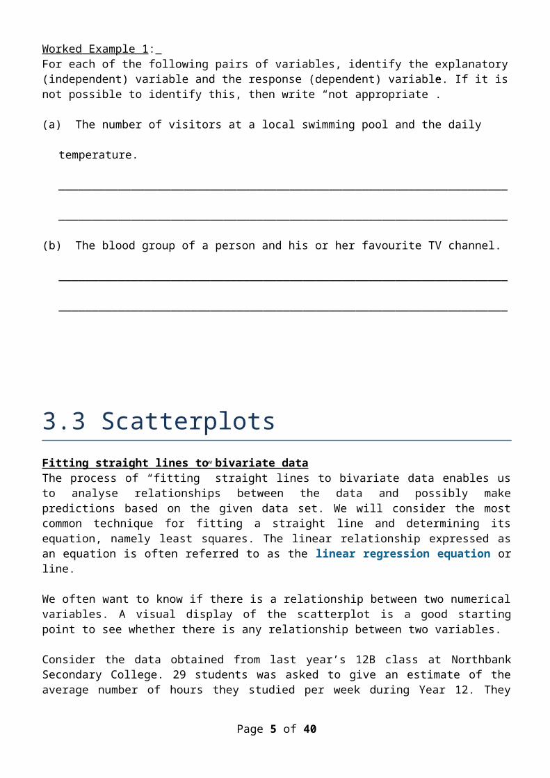
Worked Example 1 : For each of the following pairs of variables, identify the explanatory (independent) variable and the response (dependent) variable. If it is not possible to identify this, then write “not appropriate”.

(a) The number of visitors at a local swimming pool and the daily temperature.

_________________________________________________________________________________

_________________________________________________________________________________

(b) The blood group of a person and his or her favourite TV channel.

_________________________________________________________________________________

_________________________________________________________________________________

of 32

3.3 ScatterplotsFitting straight lines to bivariate data The process of “fitting” straight lines to bivariate data enables us to analyse relationships between the data and possibly make predictions based on the given data set. We will consider the most common technique for fitting a straight line and determining its equation, namely least squares. The linear relationship expressed as an equation is often referred to as the linear regression equation or line.

We often want to know if there is a relationship between two numerical variables. A visual display of the scatterplot is a good starting point to see whether there is any relationship between two variables.

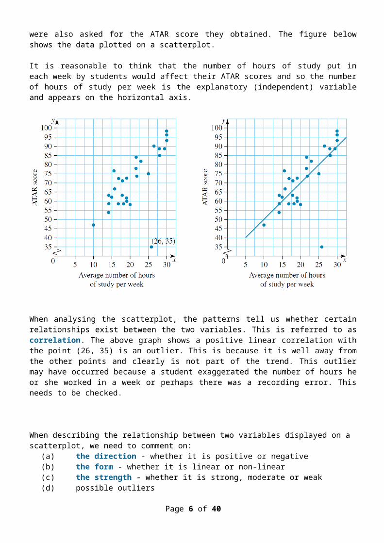
Consider the data obtained from last year’s 12B class at Northbank Secondary College. 29 students was asked to give an estimate of the average number of hours they studied per week during Year 12. They were also asked for the ATAR score they obtained. The figure below shows the data plotted on a scatterplot.

It is reasonable to think that the number of hours of study put in each week by students would affect their ATAR scores and so the number of hours of study per week is the explanatory (independent) variable and appears on the horizontal axis.

When analysing the scatterplot, the patterns tell us whether certain relationships exist between the two variables. This is referred to as correlation. The above graph shows a positive linear correlation with the point (26, 35) is an outlier. This is because it is well away from the other points and clearly is not part of the trend. This outlier may have occurred because a student exaggerated the number of hours he or she worked in a week or perhaps there was a recording error. This needs to be checked.

of 32

When describing the relationship between two variables displayed on a scatterplot, we need to comment on:

(a) the direction - whether it is positive or negative(b) the form - whether it is linear or non-linear(c) the strength - whether it is strong, moderate or weak(d) possible outliers

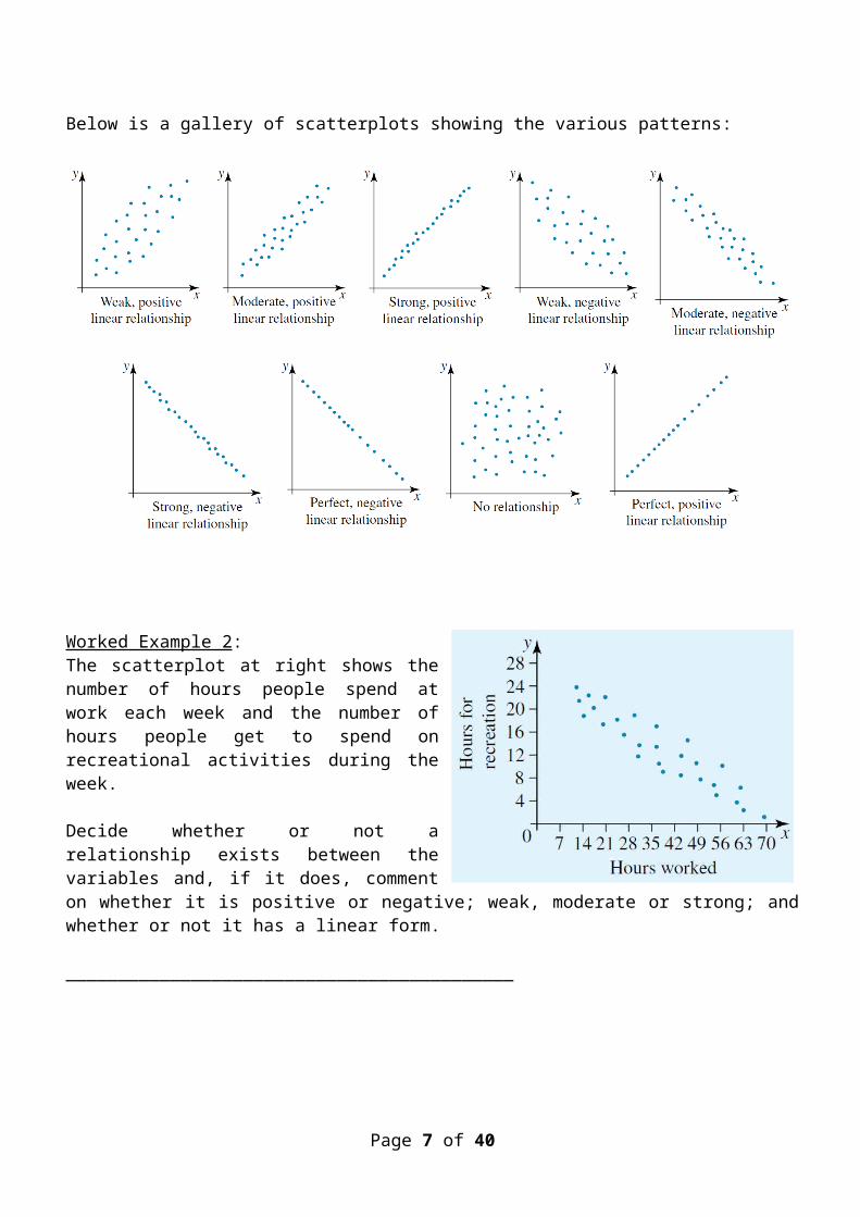
Below is a gallery of scatterplots showing the various patterns:

Worked Example 2 :The scatterplot at right shows the number of hours people spend at work each week and the number of hours people get to spend on recreational activities during the week.

Decide whether or not a relationship exists between the variables and, if it does, comment on whether it is positive or negative; weak, moderate or strong; and whether or not it has a linear form.

___________________________________________

of 32

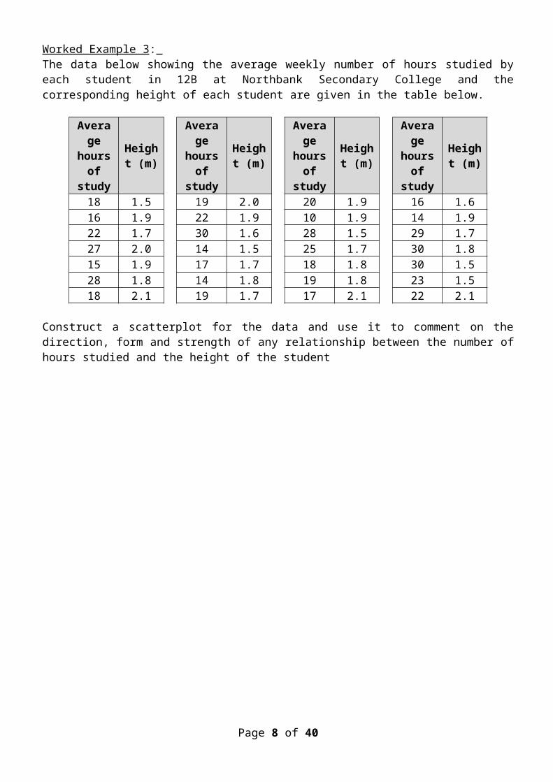
Worked Example 3 : The data below showing the average weekly number of hours studied by each student in 12B at Northbank Secondary College and the corresponding height of each student are given in the table below.

Average hours of

study

Height (m)

Average hours of

study

Height (m)

Average hours of study

Height (m)

Average hours of

study

Height (m)

18 1.5 19 2.0 20 1.9 16 1.616 1.9 22 1.9 10 1.9 14 1.922 1.7 30 1.6 28 1.5 29 1.727 2.0 14 1.5 25 1.7 30 1.815 1.9 17 1.7 18 1.8 30 1.528 1.8 14 1.8 19 1.8 23 1.518 2.1 19 1.7 17 2.1 22 2.1

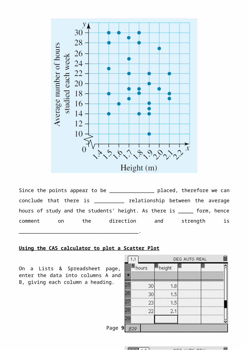
Construct a scatterplot for the data and use it to comment on the direction, form and strength of any relationship between the number of hours studied and the height of the student

Since the points appear to be _______________ placed, therefore we can conclude that there is

__________ relationship between the average hours of study and the students’ height. As there is

of 32

_____ form, hence comment on the direction and strength is

________________________________________.

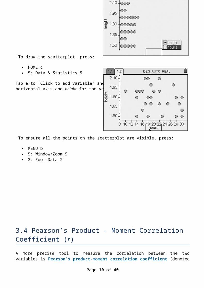
Using the CAS calculator to plot a Scatter Plot

On a Lists & Spreadsheet page, enter the data into columns A and B, giving each column a heading.

To draw the scatterplot, press:

HOME c 5: Data & Statistics 5

Tab e to ‘Click to add variable’ and then choose hours for the horizontal axis and height for the vertical axis.

To ensure all the points on the scatterplot are visible, press:

MENU b 5: Window/Zoom 5 2: Zoom-Data 2

of 32

3.4 Pearson’s Product - Moment Correlation Coefficient (r)

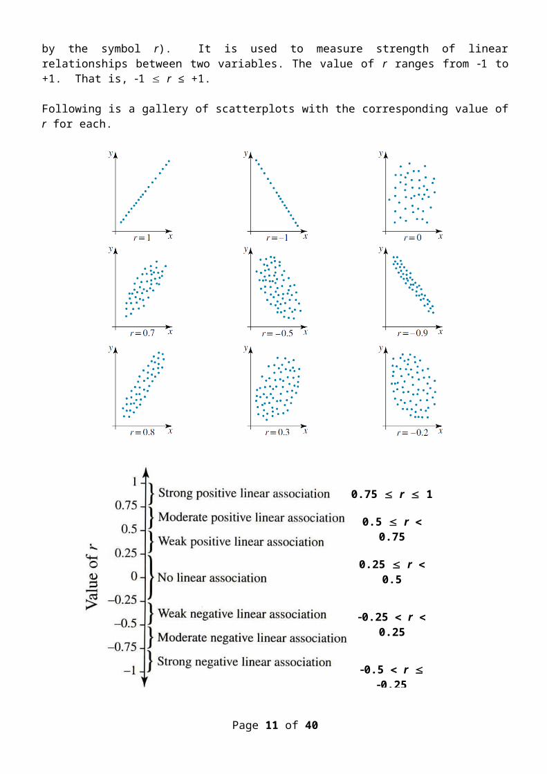
A more precise tool to measure the correlation between the two variables is Pearson’s product-moment correlation coefficient (denoted by the symbol r). It is used to measure strength of linear relationships between two variables. The value of r ranges from 1 to +1. That is, 1 r ≤ +1.

Following is a gallery of scatterplots with the corresponding value of r for each.

of 32

Worked Example 4 :For each of the following:

(i) Estimate the value of Pearson’s product-moment correlation coefficient (r) from the scatterplot.(ii) Use this to comment on the strength and direction of the relationship between the two

variables.

3.5 Calculating r & the Coefficient of Determination (r2)

Pearson’s product-moment correlation coefficient ( r )

The formula for calculating Pearson’s correlation coefficient r is as follows:

of 32

0.75 r 1

0.5 r 0.75

0.25 r 0.5

0.25 r 0.25

0.5 r 0.25

0.75 r 0.5

1 r 0.75

However, the calculation of r is often done using CAS calculator.

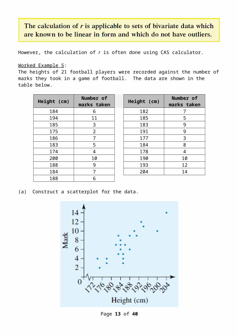
Worked Example 5 :The heights of 21 football players were recorded against the number of marks they took in a game of football. The data are shown in the table below.

Height (cm) Number of marks taken Height (cm) Number of marks

taken184 6 182 7194 11 185 5185 3 183 9175 2 191 9186 7 177 3183 5 184 8174 4 178 4200 10 190 10188 9 193 12184 7 204 14188 6

(a) Construct a scatterplot for the data.

of 32

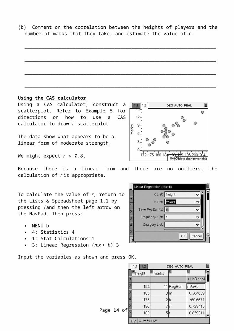
(b) Comment on the correlation between the heights of players and the number of marks that they take, and estimate the value of r.

__________________________________________________________________________________

__________________________________________________________________________________

__________________________________________________________________________________

__________________________________________________________________________________

Using the CAS calculatorUsing a CAS calculator, construct a scatterplot. Refer to Example 5 for directions on how to use a CAS calculator to draw a scatterplot.

The data show what appears to be a linear form of moderate strength.

We might expect r 0.8.

Because there is a linear form and there are no outliers, the calculation of r is appropriate.

To calculate the value of r, return to the Lists & Spreadsheet page 1.1 by pressing /and then the left arrow on the NavPad. Then press:

MENU b 4: Statistics 4 1: Stat Calculations 1

of 32

3: Linear Regression (mx + b) 3

Input the variables as shown and press OK.

Scrolling down shows r = 0.859311.

(c) Calculate r and use it to comment on the relationship between the heights of players and the number of marks they take in a game.

Since the value of r = _______________, it indicates that there is a _______________

_______________ ____________ relationship between the height of the player and the number

of marks taken in a game.

Correlation and causation

In Worked example 5 we saw that r = 0.86. While we are entitled to say that there is a strong association between the height of a footballer and the number of marks he takes, we cannot assert that the height of a footballer causes him to take a lot of marks. Being tall might assist in taking marks, but there will be many other factors which come into play; for example, skill level, accuracy of passes from teammates, abilities of the opposing team, and so on.

So, while establishing a high degree of correlation between two variables may be interesting and can often flag the need for further, more detailed investigation, it in no way gives us any basis to comment on whether or not one variable causes particular values in another variable.

As we have looked at earlier in this topic, correlation is a statistic measure that defines the size and direction of the relationship between two variables. Causation states that one event is the result of the occurrence of the other event (or variable). This is also referred to as cause and effect, where one event is the cause and this makes another event happen, this being the effect.

An example of a cause and effect relationship could be an alarm going off (cause - happens first) and a person waking up (effect - happens later). It is also important to realise that a high correlation does not imply causation. For example, a person smoking could have a high correlation with alcoholism but it is not necessarily the cause of it, thus they are different.

of 32

One way to test for causality is experimentally, where a control study is the most effective. This involves splitting the sample or population data and making one a control group (e.g. one group gets a placebo and the other get some form of medication). Another way is via an observational study which also compares against a control variable, but the researcher has no control over the experiment (e.g. smokers and non-smokers who develop lung cancer). They have no control over whether they develop lung cancer or not.

non-causal explanations

Although we may observe a strong correlation between two variables, this does not necessarily mean that an association exists. In some cases the correlation between two variables can be explained by a common response variable which provides the association. For example, a study may show that there is a strong correlation between house sizes and the life expectancy of home owners. While a bigger house will not directly lead to a longer life expectancy, a common response variable, the income of the house owner, provides a direct link to both variables and is more likely to be the underlying cause for the observed correlation.

In other cases there may be hidden, confounding reasons for an observed correlation between two variables. For example, a lack of exercise may provide a strong correlation to heart failure, but other hidden variables such as nutrition and lifestyle might have a stronger influence.

Finally, an association between two variables may be purely down to coincidence. For example, a strong correlation (r = 0.99) between the consumption of margarine and the divorce rate in the American state of Maine. Can we conclude that eating margarine causes people in Maine to divorce? The larger a data set is, the less chance there is that coincidence will have an impact. When looking at correlation and causation be sure to consider all of the possible explanations before jumping to conclusions. In professional research, many similar tests are often carried out to try to identify the exact cause for a shown correlation between two variables.The coefficient of determination r 2

The coefficient of determination is determined by squaring the Pearson’s product moment correlation coefficient that is r2.

The value of the coefficient of determination (r2) ranges between 0 and 1, that is 0 r2 1. It tells us the proportion of variation in one variable which can be explained by the variation in the other variable.

When asked to interpret the coefficient of determination value, r2, we must first determine the effect (dependent) variable and the cause (independent) variable then use the following statement below precisely

r 2 value as percentage (%) of the variation in the y -axis/effect/response/dependent variable can be explained by the variation in the x -axis/cause/explanatory/independent variable .

of 32

Worked Example 6 : A set of data giving the number of police traffic patrols on duty and the number of fatalities for the region was recorded and a correlation coefficient of r = 0.8 was found. Calculate the coefficient of determination and interpret its value.

(a) If this is a causal relationship state the most likely variable to be the cause and which to be the effect.

Cause (explanatory/independent) Variable ______________________________________________

Effect (response/dependent) variable ___________________________________________________

(b) Calculate the coefficient of determination and interpret its value.

Coefficient of determination, r2 = ____________ = ____________

Write the Coefficient of determination as a percentage (%) __________________________________

Interpret the meaning of the coefficient of determination value.

________ of the variation in ____________________________________________ can be explained

by the variation in the _______________________________________________________________

3.6 Fitting a straight line — least-squares regression

A method for finding the equation of a straight line which is fitted to data is known as the method of least-squares regression. It is used when data show a linear relationship and have no obvious outliers.

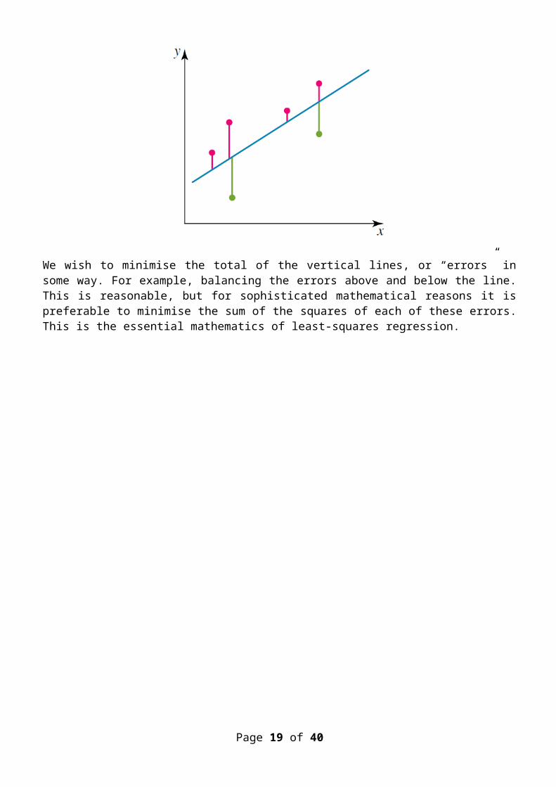
To understand the underlying theory behind least-squares, consider the regression line shown.

of 32

We wish to minimise the total of the vertical lines, or “errors” in some way. For example, balancing the errors above and below the line. This is reasonable, but for sophisticated mathematical reasons it is preferable to minimise the sum of the squares of each of these errors. This is the essential mathematics of least-squares regression.

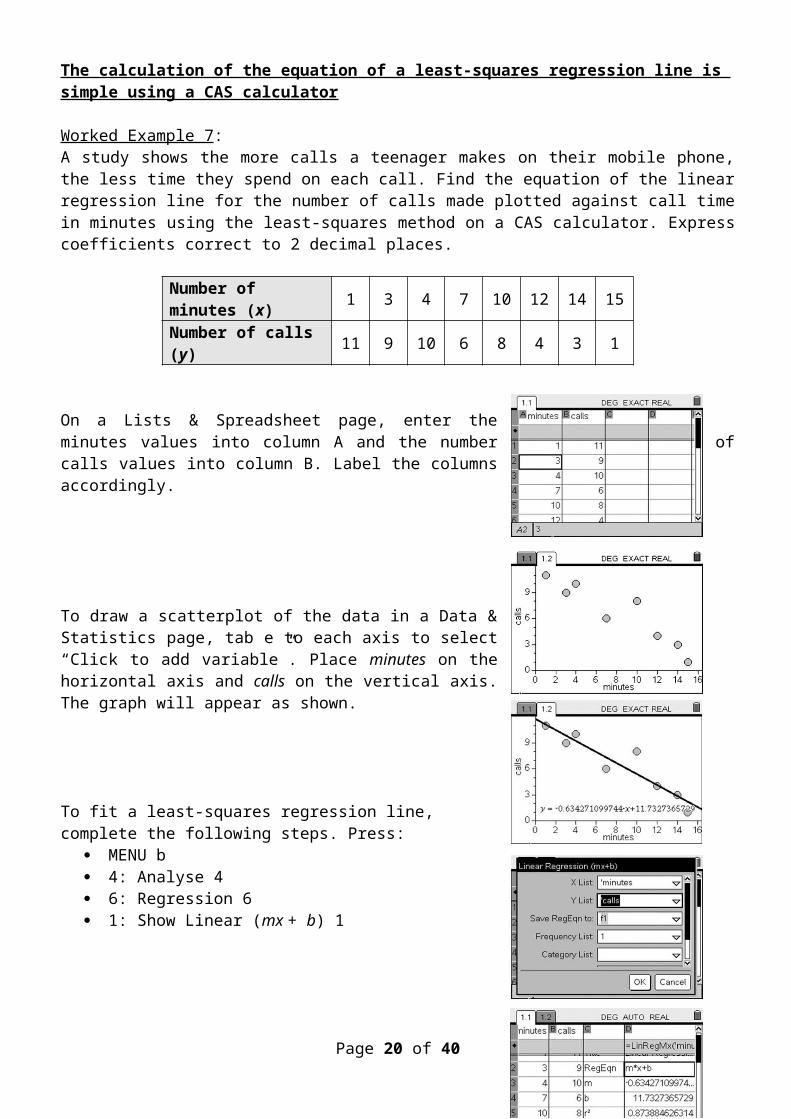
The calculation of the equation of a least-squares regression line is simple using a CAS calculator

Worked Example 7 :A study shows the more calls a teenager makes on their mobile phone, the less time they spend on each call. Find the equation of the linear regression line for the number of calls made plotted against call time in minutes using the least-squares method on a CAS calculator. Express coefficients correct to 2 decimal places.

Number of minutes (x) 1 3 4 7 10 12 14 15

of 32

Number of calls (y) 11 9 10 6 8 4 3 1

On a Lists & Spreadsheet page, enter the minutes values into column A and the number of calls values into column B. Label the columns accordingly.

To draw a scatterplot of the data in a Data & Statistics page, tab e to each axis to select “Click to add variable”. Place minutes on the horizontal axis and calls on the vertical axis. The graph will appear as shown.

To fit a least-squares regression line, complete the following steps. Press:

MENU b 4: Analyse 4 6: Regression 6 1: Show Linear (mx + b) 1

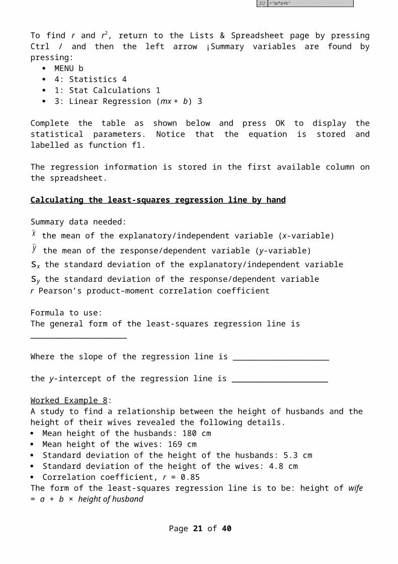
To find r and r2, return to the Lists & Spreadsheet page by pressing Ctrl / and then the left arrow ¡Summary variables are found by pressing:

MENU b 4: Statistics 4 1: Stat Calculations 1 3: Linear Regression (mx + b) 3

Complete the table as shown below and press OK to display the statistical parameters. Notice that the equation is stored and labelled as function f1.

The regression information is stored in the first available column on the spreadsheet.

Calculating the least-squares regression line by hand

Summary data needed:x the mean of the explanatory/independent variable (x-variable)y the mean of the response/dependent variable (y-variable)sx the standard deviation of the explanatory/independent variablesy the standard deviation of the response/dependent variabler Pearson’s product–moment correlation coefficient

of 32

Formula to use:The general form of the least-squares regression line is ____________________

Where the slope of the regression line is ____________________

the y-intercept of the regression line is ____________________

Worked Example 8 :A study to find a relationship between the height of husbands and the height of their wives revealed the following details. Mean height of the husbands: 180 cm Mean height of the wives: 169 cm Standard deviation of the height of the husbands: 5.3 cm Standard deviation of the height of the wives: 4.8 cm Correlation coefficient, r = 0.85The form of the least-squares regression line is to be: height of wife = a + b × height of husband

(a) Which variable is the response/dependent variable? _____________________________________

(b) Calculate the value of b for the regression line (correct to 2 significant figures).

(c) Calculate the value of a for the regression line (correct to 2 significant figures).

(d) Use the equation of the regression line to predict the height of a wife whose husband is 195 cm tall (correct to the nearest cm).

3.7 Interpretation, Interpolation and Extrapolation

Interpreting slope and intercept ( b and a ) The slope (b) indicates the change in the response variable as the explanatory/independence variable change by one unit. In another word, it is the rate of change which the data are increasing or decreasing.

The y-intercept indicates the value of the response variable when the explanatory variable equal to zero, that is at the start when x = 0.

of 32

Worked Example 9 :In the study of the growth of a species of bacterium, it is assumed that the growth is linear. However, it is very expensive to measure the number of bacteria in a sample. Given the data listed below, find:

Day of experiment 1 4 5 9 11

Number of bacteria 500 1000 1100 2100 2500

(a) the equation describing the relationship between the two variables in the form y = a + bx______________________________________________________________________________

______________________________________________________________________________

______________________________________________________________________________

______________________________________________________________________________

______________________________________________________________________________

(b) the rate at which bacteria are growing______________________________________________________________________________

______________________________________________________________________________

______________________________________________________________________________

______________________________________________________________________________

______________________________________________________________________________

(c) the number of bacteria at the start of the experiment.______________________________________________________________________________

______________________________________________________________________________

______________________________________________________________________________

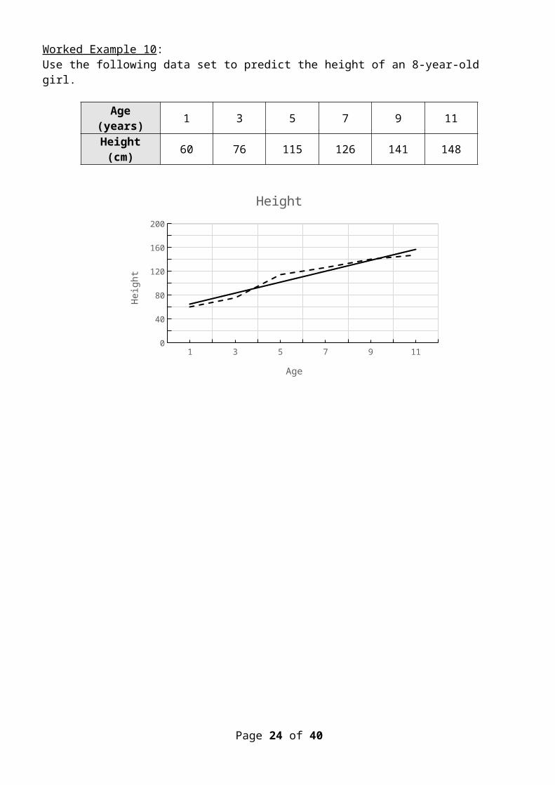
Interpolation Interpolation is the use of the equation of the regression line to predict values within the range of data in a set. That is the values that are in between the values that are already in the data set. If the data are highly linear (r near +1 or – 1) then we can be confident that our interpolated value is quite accurate. If the data are not highly linear (r near 0) then our confidence is reduced.

Worked Example 10 :Use the following data set to predict the height of an 8-year-old girl.

Age (years) 1 3 5 7 9 11

Height (cm) 60 76 115 126 141 148

of 32

1 3 5 7 9 110

20406080

100120140160180200

Height

Age

Heig

ht

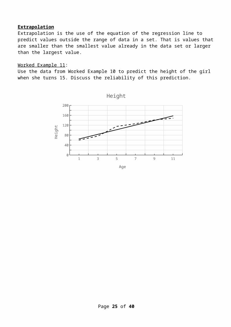
Extrapolation Extrapolation is the use of the equation of the regression line to predict values outside the range of data in a set. That is values that are smaller than the smallest value already in the data set or larger than the largest value.

Worked Example 11 :Use the data from Worked Example 10 to predict the height of the girl when she turns 15. Discuss the reliability of this prediction.

of 32

1 3 5 7 9 110

20406080

100120140160180200

Height

Age

Heig

ht

Reliability of Results Results predicted from the trend/regression line of a scatterplot can be considered reliable only if: a reasonably large number of points were used to draw the scatterplot, a reasonably strong correlation was shown to exist between the variables. The stronger the

correlation, the greater the confidence in the prediction. the predictions were made using interpolation and not extrapolation. Extrapolated results can never

be considered to be reliable because when extrapolation is used we are assuming that the trend line continues unchanged.

3.8 Residual analysisThere are situations where the mere fitting of a regression line to some data is not enough to convince us that the data set is truly linear. Even if the correlation is close to +1 or – 1 it still may not be convincing enough. The next stage is to analyse the residuals, or deviations, of each data point from the straight line.

of 32

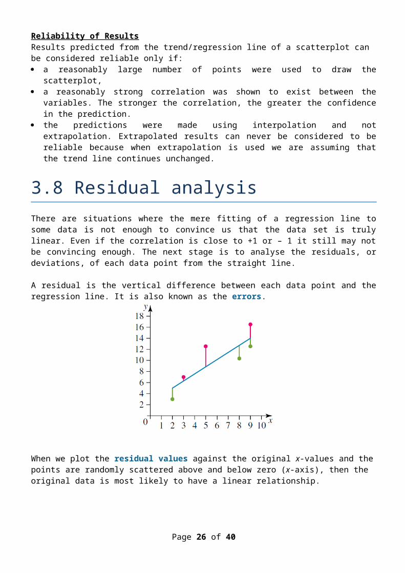
A residual is the vertical difference between each data point and the regression line. It is also known as the errors.

When we plot the residual values against the original x-values and the points are randomly scattered above and below zero (x-axis), then the original data is most likely to have a linear relationship.

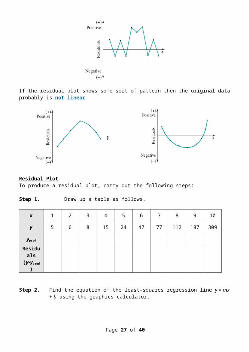
If the residual plot shows some sort of pattern then the original data probably is not linear.

Residual Plot To produce a residual plot, carry out the following steps:

Step 1. Draw up a table as follows.

x 1 2 3 4 5 6 7 8 9 10

of 32

y 5 6 8 15 24 47 77 112 187 309

ypred

Residuals(yypred)

Step 2. Find the equation of the least-squares regression line y = mx + b using the graphics calculator.

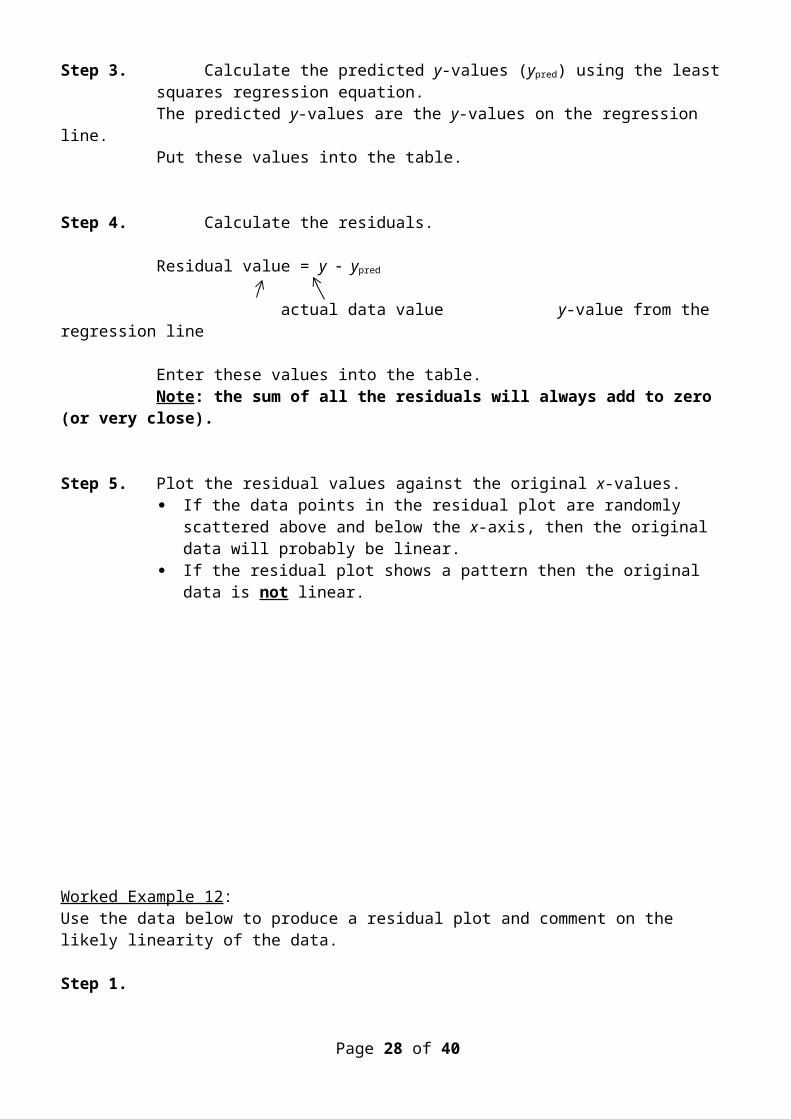
Step 3. Calculate the predicted y-values (ypred) using the least squares regression equation. The predicted y-values are the y-values on the regression line.Put these values into the table.

Step 4. Calculate the residuals.

Residual value = y ypred

actual data value y-value from the regression line

Enter these values into the table.Note: the sum of all the residuals will always add to zero (or very close).

Step 5. Plot the residual values against the original x-values. If the data points in the residual plot are randomly scattered above and below the x-

axis, then the original data will probably be linear. If the residual plot shows a pattern then the original data is not linear.

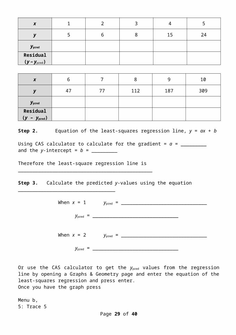
Worked Example 12 :Use the data below to produce a residual plot and comment on the likely linearity of the data.

Step 1.

x 1 2 3 4 5

of 32

y 5 6 8 15 24

ypred

Residual(y – ypred)

x 6 7 8 9 10

y 47 77 112 187 309

ypred

Residual(y – ypred)

Step 2. Equation of the least-squares regression line, y = ax + b

Using CAS calculator to calculate for the gradient = a = _________ and the y-intercept = b = _________

Therefore the least-square regression line is _______________________________________________

Step 3. Calculate the predicted y-values using the equation __________________________________

When x = 1 ypred = ______________________________

ypred = ______________________________

When x = 2 ypred = ______________________________

ypred = ______________________________

Or use the CAS calculator to get the ypred values from the regression line by opening a Graphs & Geometry page and enter the equation of the least-squares regression and press enter.Once you have the graph press

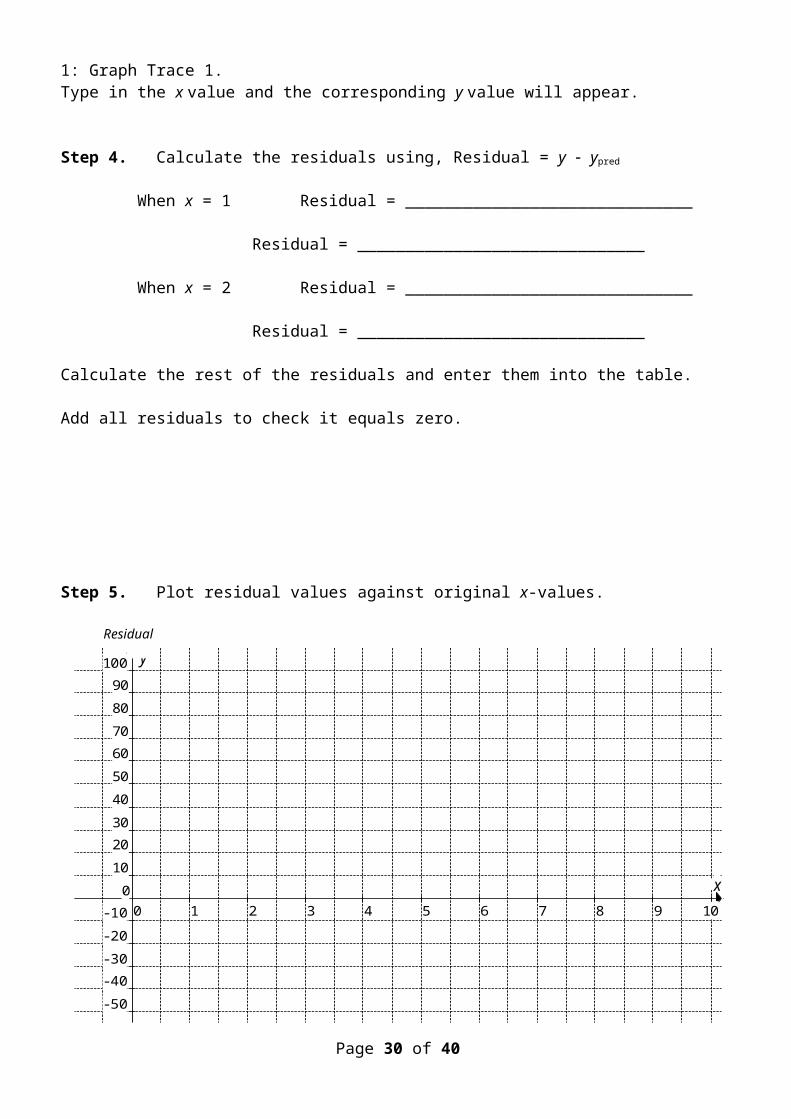
Menu b, 5: Trace 5 1: Graph Trace 1. Type in the x value and the corresponding y value will appear.

Step 4. Calculate the residuals using, Residual = y ypred

When x = 1 Residual = ______________________________

Residual = ______________________________

When x = 2 Residual = ______________________________

of 32

Residual = ______________________________

Calculate the rest of the residuals and enter them into the table.

Add all residuals to check it equals zero.

Step 5. Plot residual values against original x-values.

x

y

0 1 2 3 4 5 6 7 8 9 10

-50-40-30-20-10

0102030405060708090

100

The residual plot shows ______________________________________________________________

__________________________________________________________________________________

__________________________________________________________________________________

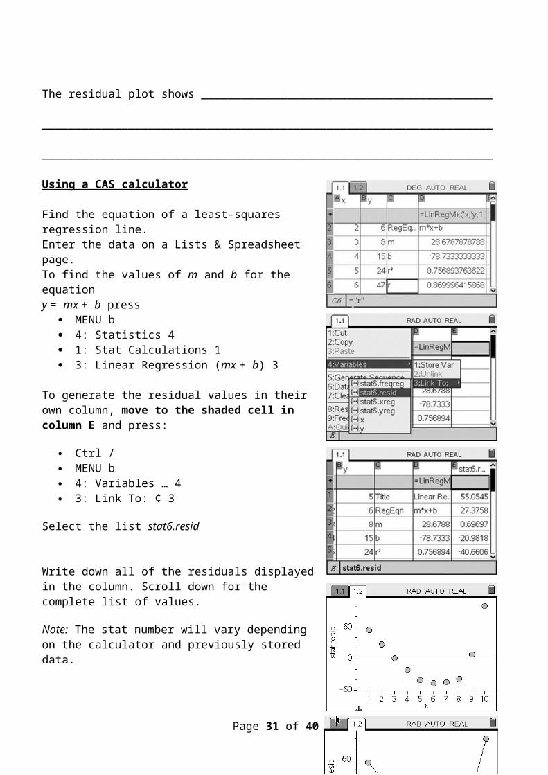
Using a CAS calculator

Find the equation of a least-squares regression line.Enter the data on a Lists & Spreadsheet page.To find the values of m and b for the equation y = mx + b press

MENU b of 32

Residual

4: Statistics 4 1: Stat Calculations 1 3: Linear Regression (mx + b) 3

To generate the residual values in their own column, move to the shaded cell in column E and press:

Ctrl / MENU b 4: Variables … 4 3: Link To: ¢ 3

Select the list stat6.resid

Write down all of the residuals displayed in the column. Scroll down for the complete list of values.

Note: The stat number will vary depending on the calculator and previously stored data.

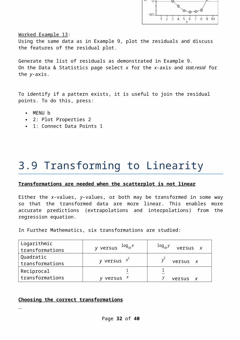
Worked Example 13 :Using the same data as in Example 9, plot the residuals and discuss the features of the residual plot.

Generate the list of residuals as demonstrated in Example 9.On the Data & Statistics page select x for the x-axis and stat.resid for the y-axis.

To identify if a pattern exists, it is useful to join the residual points. To do this, press:

MENU b 2: Plot Properties 2 1: Connect Data Points 1

3.9 Transforming to LinearityTransformations are needed when the scatterplot is not linear

Either the x-values, y-values, or both may be transformed in some way so that the transformed data are more linear. This enables more accurate predictions (extrapolations and interpolations) from the regression equation.

In Further Mathematics, six transformations are studied:

Logarithmic transformations y versus log10 x log10 y versus x of 32

Quadratic transformations y versus x2 y2 versus x

Reciprocal transformationsy versus

1x

1y versus x

Choosing the correct transformations Quadratic Transformations

_________________________________ ______________________________

__________________________________________________ _____________________________________________

Logarithmic and Reciprocal Transformations

_________________________________ ______________________________

_________________________________ ______________________________

of 32

_________________________________ ______________________________

_________________________________ ______________________________

There are at least two possible transformations for any given non-linear scatterplot, the decision as to which is the best comes from the r value. The transformation with the better r value, that is closest to +1 or 1, should be considered as the most appropriate.

To transform to linearity1. Plot the original data then apply the least squares regression line. Do a residual plot to examine if a

pattern suggests the data are non-linear.2. Examine the high values of x and/or y and decide if the data need to be compressed or stretched to

make them linear.3. Transform the data by either:

(a) compressing x- or y-values using the reciprocal ( or ) or logarithmic (log10 x or log10 y ) functions(b) stretching x- or y-values using the square function (x2 or y2).

4. Plot the transformed data and its least squares regression line. Examine the residuals or correlation coefficient r to see if it is a better fit.

5. Repeat steps 2 to 4 for all appropriate transformations.

Worked Example 15 :Logarithmic transformation.Apply a logarithmic transformation to the following data which represent a patient’s heart rate as a function of time. The regression line has been determined as:Heart rate 6.97 × Time after operation 93.2, with r 0.895Time after operation (h) x 1 2 3 4 5 6 7 8Heart rate (beats/min) y 100 80 65 55 50 51 48 46.

of 32 View the residual plot.Change the y-axis to stat.resid

Open a Data & Statistics page.Place time on the x- axis and heart rate on the y-axis.Show the regression line Menu b

Open a Lists & Spreadsheet page. Label the columns and enter the data.

The transformed equation is_____________________________________________________________

is better than the original equation since the value of r improved from 0.895 to____________________Using the transformed line for predictions

When predicting remember to use the transformed equation.

Worked Example 16 : Reciprocal transformation

(a) Using a CAS calculator, apply a reciprocal ( 1

x ) transformation to the following data

(b) Use the transformed regression equation to predict the number of students wearing a jumper when the temperature is 12oC

Temperature (°C) x 5 10 15 20 25 30 35

Number of students in a class wearing jumpers y 18 10 6 5 3 2 2

of 32

View the residual plot.Change the y-axis to stat.resid

Open a Data & Statistics page.Place time on the x- axis and heart rate on the y-axis.Show the regression line Menu b

Open a Lists & Spreadsheet page. Label the columns and enter the data.

PAST EXAM QUESTION (Exam 2 - 2011)

of 32

PAST EXAM QUESTION (Exam 2 - 2012)

of 32

chapterlloydhutchison.weebly.com/uploads/5/6/6/0/56603395/... · web viewdata analysis chapter 3...

Documents