c04.qxd 5/10/02 5:18 pm page 97 rk ul 6 rk ul...
TRANSCRIPT
97
4Continuous RandomVariables and Probability Distributions
CHAPTER OUTLINE
LEARNING OBJECTIVES
After careful study of this chapter you should be able to do the following:1. Determine probabilities from probability density functions.2. Determine probabilities from cumulative distribution functions and cumulative distribution func-
tions from probability density functions, and the reverse.3. Calculate means and variances for continuous random variables.4. Understand the assumptions for each of the continuous probability distributions presented.5. Select an appropriate continuous probability distribution to calculate probabilities in specific
applications.6. Calculate probabilities, determine means and variances for each of the continuous probability
distributions presented.7. Standardize normal random variables.
4-1 CONTINUOUS RANDOMVARIABLES
4-2 PROBABILITY DISTRIBUTIONSAND PROBABILITY DENSITYFUNCTIONS
4-3 CUMULATIVE DISTRIBUTIONFUNCTIONS
4-4 MEAN AND VARIANCE OF ACONTINUOUS RANDOM VARIABLE
4-5 CONTINUOUS UNIFORM DISTRIBUTION
4-6 NORMAL DISTRIBUTION
4-7 NORMAL APPROXIMATION TOTHE BINOMIAL AND POISSONDISTRIBUTIONS
4-8 CONTINUITY CORRECTION TOIMPROVE THE APPROXIMATION (CD ONLY)
4-9 EXPONENTIAL DISTRIBUTION
4-10 ERLANG AND GAMMA DISTRIBUTIONS
4-10.1 Erlang Distribution
4-10.2 Gamma Distribution
4-11 WEIBULL DISTRIBUTION
4-12 LOGNORMAL DISTRIBUTION
c04.qxd 5/10/02 5:18 PM Page 97 RK UL 6 RK UL 6:Desktop Folder:TEMP WORK:MONTGOMERY:REVISES UPLO D CH 1 14 FIN L:Quark Files:
98 CHAPTER 4 CONTINUOUS RANDOM VARIABLES AND PROBABILITY DISTRIBUTIONS
8. Use the table for the cumulative distribution function of a standard normal distribution to calcu-late probabilities.
9. Approximate probabilities for some binomial and Poisson distributions.
CD MATERIAL10. Use continuity corrections to improve the normal approximation to those binomial and Poisson
distributions.
Answers for most odd numbered exercises are at the end of the book. Answers to exercises whosenumbers are surrounded by a box can be accessed in the e-Text by clicking on the box. Completeworked solutions to certain exercises are also available in the e-Text. These are indicated in theAnswers to Selected Exercises section by a box around the exercise number. Exercises are alsoavailable for some of the text sections that appear on CD only. These exercises may be found withinthe e-Text immediately following the section they accompany.
4-1 CONTINUOUS RANDOM VARIABLES
Previously, we discussed the measurement of the current in a thin copper wire. We noted thatthe results might differ slightly in day-to-day replications because of small variations in vari-ables that are not controlled in our experiment—changes in ambient temperatures, small im-purities in the chemical composition of the wire, current source drifts, and so forth.
Another example is the selection of one part from a day’s production and very accuratelymeasuring a dimensional length. In practice, there can be small variations in the actualmeasured lengths due to many causes, such as vibrations, temperature fluctuations, operatordifferences, calibrations, cutting tool wear, bearing wear, and raw material changes. Even themeasurement procedure can produce variations in the final results.
In these types of experiments, the measurement of interest—current in a copper wire ex-periment, length of a machined part—can be represented by a random variable. It is reason-able to model the range of possible values of the random variable by an interval (finite orinfinite) of real numbers. For example, for the length of a machined part, our model enablesthe measurement from the experiment to result in any value within an interval of real numbers.Because the range is any value in an interval, the model provides for any precision in lengthmeasurements. However, because the number of possible values of the random variable X isuncountably infinite, X has a distinctly different distribution from the discrete random vari-ables studied previously. The range of X includes all values in an interval of real numbers; thatis, the range of X can be thought of as a continuum.
A number of continuous distributions frequently arise in applications. These distributionsare described, and example computations of probabilities, means, and variances are providedin the remaining sections of this chapter.
4-2 PROBABILITY DISTRIBUTIONS AND PROBABILITYDENSITY FUNCTIONS
Density functions are commonly used in engineering to describe physical systems. For exam-ple, consider the density of a loading on a long, thin beam as shown in Fig. 4-1. For any pointx along the beam, the density can be described by a function (in grams/cm). Intervals withlarge loadings correspond to large values for the function. The total loading between points aand b is determined as the integral of the density function from a to b. This integral is the area
c04.qxd 5/10/02 5:18 PM Page 98 RK UL 6 RK UL 6:Desktop Folder:TEMP WORK:MONTGOMERY:REVISES UPLO D CH 1 14 FIN L:Quark Files:

4-2 PROBABILITY DISTRIBUTIONS AND PROBABILITY DENSITY FUNCTIONS 99
under the density function over this interval, and it can be loosely interpreted as the sum of allthe loadings over this interval.
Similarly, a probability density function f(x) can be used to describe the probability dis-tribution of a continuous random variable X. If an interval is likely to contain a value for X,its probability is large and it corresponds to large values for f(x). The probability that X is be-tween a and b is determined as the integral of f(x) from a to b. See Fig. 4-2.
For a continuous random variable X, a probability density function is a functionsuch that
(1)
(2)
(3) area under from a to b
for any a and b (4-1)
f 1x2P1a � X � b2 � �b
a f 1x2 dx �
��
��
f 1x2 dx � 1
f 1x2 � 0
Definition
Load
ing
x
P(a < X < b)
a b x
f (x)
Figure 4-1 Densityfunction of a loading on along, thin beam.
Figure 4-2 Probability determined from the areaunder f(x).
A probability density function provides a simple description of the probabilities associ-ated with a random variable. As long as f(x) is nonnegative and
so that the probabilities are properly restricted. A probability densityfunction is zero for x values that cannot occur and it is assumed to be zero wherever it is notspecifically defined.
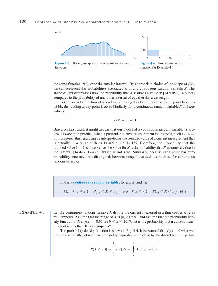
A histogram is an approximation to a probability density function. See Fig. 4-3. For eachinterval of the histogram, the area of the bar equals the relative frequency (proportion) of themeasurements in the interval. The relative frequency is an estimate of the probability that ameasurement falls in the interval. Similarly, the area under f(x) over any interval equals thetrue probability that a measurement falls in the interval.
The important point is that f(x) is used to calculate an area that represents the prob-ability that X assumes a value in [a, b]. For the current measurement example, the proba-bility that X results in [14 mA, 15 mA] is the integral of the probability density function ofX over this interval. The probability that X results in [14.5 mA, 14.6 mA] is the integral of
0 � P1a � X � b2 � 1��
�� f 1x2 dx � 1,
c04.qxd 5/10/02 5:18 PM Page 99 RK UL 6 RK UL 6:Desktop Folder:TEMP WORK:MONTGOMERY:REVISES UPLO D CH 1 14 FIN L:Quark Files:
100 CHAPTER 4 CONTINUOUS RANDOM VARIABLES AND PROBABILITY DISTRIBUTIONS
the same function, f(x), over the smaller interval. By appropriate choice of the shape of f(x),we can represent the probabilities associated with any continuous random variable X. Theshape of f(x) determines how the probability that X assumes a value in [14.5 mA, 14.6 mA]compares to the probability of any other interval of equal or different length.
For the density function of a loading on a long thin beam, because every point has zerowidth, the loading at any point is zero. Similarly, for a continuous random variable X and anyvalue x.
Based on this result, it might appear that our model of a continuous random variable is use-less. However, in practice, when a particular current measurement is observed, such as 14.47milliamperes, this result can be interpreted as the rounded value of a current measurement thatis actually in a range such as Therefore, the probability that therounded value 14.47 is observed as the value for X is the probability that X assumes a value inthe interval [14.465, 14.475], which is not zero. Similarly, because each point has zeroprobability, one need not distinguish between inequalities such as � or � for continuousrandom variables.
14.465 � x � 14.475.
P1X � x2 � 0
If X is a continuous random variable, for any and
(4-2)P1x1 � X � x22 � P1x1 � X � x22 � P1x1 � X � x22 � P1x1 � X � x22x2,x1
EXAMPLE 4-1 Let the continuous random variable X denote the current measured in a thin copper wire inmilliamperes. Assume that the range of X is [0, 20 mA], and assume that the probability den-sity function of X is for What is the probability that a current meas-urement is less than 10 milliamperes?
The probability density function is shown in Fig. 4-4. It is assumed that whereverit is not specifically defined. The probability requested is indicated by the shaded area in Fig. 4-4.
P1X � 102 � �10
0 f 1x2 dx � �
10
0
0.05 dx � 0.5
f 1x2 � 0
0 � x � 20.f 1x2 � 0.05
Figure 4-4 Probability densityfunction for Example 4-1.
0 10 20 x
0.05
f (x)
Figure 4-3 Histogram approximates a probability densityfunction.
x
f (x)
c04.qxd 5/10/02 5:19 PM Page 100 RK UL 6 RK UL 6:Desktop Folder:TEMP WORK:MONTGOMERY:REVISES UPLO D CH 1 14 FIN L:Quark Files:
4-2 PROBABILITY DISTRIBUTIONS AND PROBABILITY DENSITY FUNCTIONS 101
As another example,
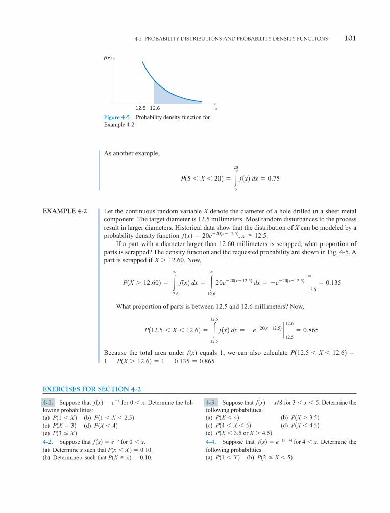
EXAMPLE 4-2 Let the continuous random variable X denote the diameter of a hole drilled in a sheet metalcomponent. The target diameter is 12.5 millimeters. Most random disturbances to the processresult in larger diameters. Historical data show that the distribution of X can be modeled by aprobability density function
If a part with a diameter larger than 12.60 millimeters is scrapped, what proportion ofparts is scrapped? The density function and the requested probability are shown in Fig. 4-5. Apart is scrapped if Now,
What proportion of parts is between 12.5 and 12.6 millimeters? Now,
Because the total area under f(x) equals 1, we can also calculate
EXERCISES FOR SECTION 4-2
1 � P1X � 12.62 � 1 � 0.135 � 0.865.P112.5 � X � 12.62 �
P112.5 � X � 12.62 � �12.6
12.5 f 1x2 dx � �e�201x�12.52 ` 12.6
12.5� 0.865
P1X � 12.602 � ��
12.6 f 1x2 dx � �
�
12.6
20e�201x�12.52 dx � �e�201x�12.52 ` �12.6
� 0.135
X � 12.60.
f 1x2 � 20e�201x�12.52, x � 12.5.
P15 � X � 202 � �20
5 f 1x2 dx � 0.75
Figure 4-5 Probability density function forExample 4-2.
12.5
f (x)
x12.6
4-1. Suppose that for Determine the fol-lowing probabilities:(a) (b)(c) (d)(e)
4-2. Suppose that for (a) Determine x such that (b) Determine x such that P1X � x2 � 0.10.
P1x � X 2 � 0.10.0 � x.f 1x2 � e�x
P13 � X 2P1X � 42P1X � 32P11 � X � 2.52P11 � X 2
0 � x.f 1x2 � e�x 4-3. Suppose that for Determine thefollowing probabilities:(a) (b)(c) (d)(e)
4-4. Suppose that Determine thefollowing probabilities:(a) (b) P12 � X � 52P11 � X 2
f 1x2 � e�1x�42 for 4 � x.
P1X � 3.5 or X � 4.52P1X � 4.52P14 � X � 52P1X � 3.52P1X � 423 � x � 5.f 1x2 � x8
c04.qxd 5/10/02 5:19 PM Page 101 RK UL 6 RK UL 6:Desktop Folder:TEMP WORK:MONTGOMERY:REVISES UPLO D CH 1 14 FIN L:Quark Files:
Extending the definition of f(x) to the entire real line enables us to define the cumulative dis-tribution function for all real numbers. The following example illustrates the definition.
EXAMPLE 4-3 For the copper current measurement in Example 4-1, the cumulative distribution function ofthe random variable X consists of three expressions. If Therefore,
F1x2 � 0, for x � 0
x � 0, f 1x2 � 0.
102 CHAPTER 4 CONTINUOUS RANDOM VARIABLES AND PROBABILITY DISTRIBUTIONS
4-3 CUMULATIVE DISTRIBUTION FUNCTIONS
An alternative method to describe the distribution of a discrete random variable can also beused for continuous random variables.
The cumulative distribution function of a continuous random variable X is
(4-3)
for �� � x � �.
F1x2 � P1X � x2 � �x
�� f 1u2 du
Definition
(c) (d)(e) Determine x such that P(X � x) � 0.90.
4-5. Suppose that for Determinethe following probabilities:(a) (b)(c) (d)(e)(f) Determine x such that
4-6. The probability density function of the time to failureof an electronic component in a copier (in hours) is f(x) �
for Determine the probability that
(a) A component lasts more than 3000 hours before failure.(b) A component fails in the interval from 1000 to 2000 hours.(c) A component fails before 1000 hours.(d) Determine the number of hours at which 10% of all com-
ponents have failed.
4-7. The probability density function of the net weight inpounds of a packaged chemical herbicide is for
pounds.(a) Determine the probability that a package weighs more
than 50 pounds.
49.75 � x � 50.25f 1x2 � 2.0
x � 0.e�x1000
1000
P1x � X 2 � 0.05.P1X � 0 or X � �0.52
P1X � �22P1�0.5 � X � 0.52P10.5 � X 2P10 � X 2
�1 � x � 1.f 1x2 � 1.5x2
P18 � X � 122P15 � X 2 (b) How much chemical is contained in 90% of all packages?
4-8. The probability density function of the length of ahinge for fastening a door is for millimeters. Determine the following:(a)(b)(c) If the specifications for this process are from 74.7
to 75.3 millimeters, what proportion of hinges meetsspecifications?
4-9. The probability density function of the length of ametal rod is for 2.3 � x � 2.8 meters.(a) If the specifications for this process are from 2.25 to 2.75
meters, what proportion of the bars fail to meet the speci-fications?
(b) Assume that the probability density function is for an interval of length 0.5 meters. Over what valueshould the density be centered to achieve the greatest pro-portion of bars within specifications?
4-10. If X is a continuous random variable, argue that P(x1 �X � x2) � P(x1 � X � x2) � P(x1 � X � x2) � P(x1 � X � x2).
f 1x2 � 2
f 1x2 � 2
P1X � 74.8 or X � 75.22P1X � 74.82
74.6 � x � 75.4f 1x2 � 1.25
c04.qxd 5/10/02 5:19 PM Page 102 RK UL 6 RK UL 6:Desktop Folder:TEMP WORK:MONTGOMERY:REVISES UPLO D CH 1 14 FIN L:Quark Files:
4-3 CUMULATIVE DISTRIBUTION FUNCTIONS 103
and
Finally,
Therefore,
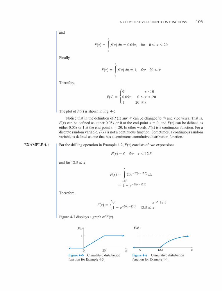
The plot of F(x) is shown in Fig. 4-6.
Notice that in the definition of F(x) any can be changed to and vice versa. That is,F(x) can be defined as either 0.05x or 0 at the end-point and F(x) can be defined aseither 0.05x or 1 at the end-point In other words, F(x) is a continuous function. For adiscrete random variable, F(x) is not a continuous function. Sometimes, a continuous randomvariable is defined as one that has a continuous cumulative distribution function.
EXAMPLE 4-4 For the drilling operation in Example 4-2, F(x) consists of two expressions.
for
and for
Therefore,
Figure 4-7 displays a graph of F(x).
F1x2 � e0 x � 12.5
1 � e�201x�12.52 12.5 � x
� 1 � e�201x�12.52
F1x2 � �x
12.5
20e�201u�12.52 du
12.5 � x
x � 12.5F1x2 � 0
x � 20.x � 0,
��
F1x2 � •0 x � 0
0.05x 0 � x � 20
1 20 � x
F1x2 � �x
0 f 1u2 du � 1, for 20 � x
F1x2 � �x
0 f 1u2 du � 0.05x, for 0 � x � 20
Figure 4-6 Cumulative distributionfunction for Example 4-3.
20
1
x0
F(x)
Figure 4-7 Cumulative distributionfunction for Example 4-4.
12.5
1
x0
F(x)
c04.qxd 5/10/02 5:19 PM Page 103 RK UL 6 RK UL 6:Desktop Folder:TEMP WORK:MONTGOMERY:REVISES UPLO D CH 1 14 FIN L:Quark Files:
104 CHAPTER 4 CONTINUOUS RANDOM VARIABLES AND PROBABILITY DISTRIBUTIONS
The probability density function of a continuous random variable can be determined fromthe cumulative distribution function by differentiating. Recall that the fundamental theorem ofcalculus states that
Then, given F(x)
as long as the derivative exists.
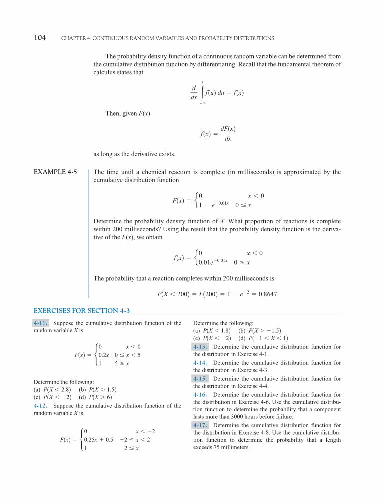
EXAMPLE 4-5 The time until a chemical reaction is complete (in milliseconds) is approximated by thecumulative distribution function
Determine the probability density function of X. What proportion of reactions is completewithin 200 milliseconds? Using the result that the probability density function is the deriva-tive of the F(x), we obtain
The probability that a reaction completes within 200 milliseconds is
EXERCISES FOR SECTION 4-3
P1X � 2002 � F12002 � 1 � e�2 � 0.8647.
f 1x2 � e0 x � 0
0.01e�0.01x 0 � x
F1x2 � e0 x � 0
1 � e�0.01x 0 � x
f 1x2 �dF1x2
dx
d
dx �
x
��
f 1u2 du � f 1x2
4-11. Suppose the cumulative distribution function of therandom variable X is
Determine the following:(a) (b)(c) (d)
4-12. Suppose the cumulative distribution function of therandom variable X is
F1x2 � •0 x � �2
0.25x � 0.5 �2 � x � 2
1 2 � x
P1X � 62P1X � �22P1X � 1.52P1X � 2.82
F1x2 � •0 x � 0
0.2x 0 � x � 5
1 5 � x
Determine the following:(a) (b)(c) (d)
4-13. Determine the cumulative distribution function forthe distribution in Exercise 4-1.
4-14. Determine the cumulative distribution function forthe distribution in Exercise 4-3.
4-15. Determine the cumulative distribution function forthe distribution in Exercise 4-4.
4-16. Determine the cumulative distribution function forthe distribution in Exercise 4-6. Use the cumulative distribu-tion function to determine the probability that a componentlasts more than 3000 hours before failure.
4-17. Determine the cumulative distribution function forthe distribution in Exercise 4-8. Use the cumulative distribu-tion function to determine the probability that a lengthexceeds 75 millimeters.
P1�1 � X � 12P1X � �22P1X � �1.52P1X � 1.82
c04.qxd 5/13/02 11:16 M Page 104 RK UL 6 RK UL 6:Desktop Folder:TEMP WORK:MONTGOMERY:REVISES UPLO D CH 1 14 FIN L:Quark Files:
4-4 MEAN AND VARIANCE OF A CONTINUOUSRANDOM VARIABLE
The mean and variance of a continuous random variable are defined similarly to a discreterandom variable. Integration replaces summation in the definitions. If a probability densityfunction is viewed as a loading on a beam as in Fig. 4-1, the mean is the balance point.
4-4 MEAN AND VARIANCE OF A CONTINUOUS RANDOM VARIABLE 105
Determine the probability density function for each of the fol-lowing cumulative distribution functions.
4-18.4-19.
4-20.
4-21. The gap width is an important property of a magneticrecording head. In coded units, if the width is a continuous ran-dom variable over the range from 0 � x � 2 with f(x) � 0.5x,determine the cumulative distribution function of the gap width.
F1x2 � µ0 x � �2
0.25x � 0.5 �2 � x � 1
0.5x � 0.25 1 � x � 1.5
1 1.5 � x
F1x2 � µ0 x � 0
0.2x 0 � x � 4
0.04x � 0.64 4 � x � 9
1 9 � x
F1x2 � 1 � e�2x x � 0
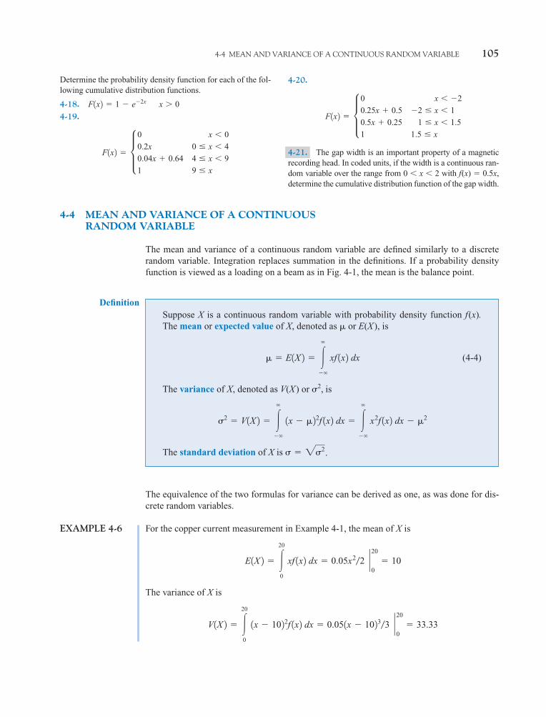
Suppose X is a continuous random variable with probability density function f(x).The mean or expected value of X, denoted as or E(X), is
(4-4)
The variance of X, denoted as V(X) or is
The standard deviation of X is . � 22
2 � V1X 2 � ��
��
1x � 22f 1x2 dx � ��
��
x2f 1x2 dx � 2
2,
� E1X 2 � ��
��
xf 1x2 dx
Definition
The equivalence of the two formulas for variance can be derived as one, as was done for dis-crete random variables.
EXAMPLE 4-6 For the copper current measurement in Example 4-1, the mean of X is
The variance of X is
V1X 2 � �20
0
1x � 1022f 1x2 dx � 0.051x � 1023�3 ` 20
0� 33.33
E1X 2 � �20
0
xf 1x2 dx � 0.05x2�2 ` 20
0� 10
c04.qxd 5/13/02 11:16 M Page 105 RK UL 6 RK UL 6:Desktop Folder:TEMP WORK:MONTGOMERY:REVISES UPLO D CH 1 14 FIN L:Quark Files:

106 CHAPTER 4 CONTINUOUS RANDOM VARIABLES AND PROBABILITY DISTRIBUTIONS
EXAMPLE 4-7 In Example 4-1, X is the current measured in milliamperes. What is the expected value of thesquared current? Now, Therefore,
In the previous example, the expected value of X 2 does not equal E(X) squared. However, inthe special case that for any constants a and b, Thiscan be shown from the properties of integrals.
EXAMPLE 4-8 For the drilling operation in Example 4-2, the mean of X is
Integration by parts can be used to show that
The variance of X is
Although more difficult, integration by parts can be used two times to show that V(X) � 0.0025.
EXERCISES FOR SECTION 4-4
V1X 2 � ��
12.5
1x � 12.5522f 1x2 dx
E1X 2 � �xe�201x�12.52 � e�201x�12.5220
` �12.5
� 12.5 � 0.05 � 12.55
E1X 2 � ��
12.5
xf 1x2 dx � ��
12.5
x 20e�201x�12.52 dx
E 3h1X 2 4 � aE1X 2 � b.h1X 2 � aX � b
E 3h1X 2 4 � ��
��
x2f 1x2 dx � �20
0
0.05x2 dx � 0.05 x3
3 ` 20
0� 133.33
h1X 2 � X 2.
If X is a continuous random variable with probability density function f(x),
(4-5)E 3h1X 2 4 � ��
��
h1x2 f 1x2 dx
Expected Valueof a Function of
a ContinuousRandomVariable
4-22. Suppose for Determine themean and variance of X.
4-23. Suppose for Determine themean and variance of X.
4-24. Suppose for Determinethe mean and variance of X.
�1 � x � 1.f 1x2 � 1.5x2
0 � x � 4.f 1x2 � 0.125x
0 � x � 4.f 1x2 � 0.25 4-25. Suppose that for Determinethe mean and variance for x.
4-26. Determine the mean and variance of the weight ofpackages in Exercise 4.7.
4-27. The thickness of a conductive coating in micrometershas a density function of 600x�2 for 100 m � x � 120 m.
3 � x � 5.f 1x2 � x�8
The expected value of a function h(X ) of a continuous random variable is defined similarly toa function of a discrete random variable.
c04.qxd 5/13/02 11:16 M Page 106 RK UL 6 RK UL 6:Desktop Folder:TEMP WORK:MONTGOMERY:REVISES UPLO D CH 1 14 FIN L:Quark Files:
4-5 CONTINUOUS UNIFORM DISTRIBUTION
The simplest continuous distribution is analogous to its discrete counterpart.
4-5 CONTINUOUS UNIFORM DISTRIBUTION 107
A continuous random variable X with probability density function
(4-6)
is a continuous uniform random variable.
f 1x2 � 1 1b � a2, a � x � b
Definition
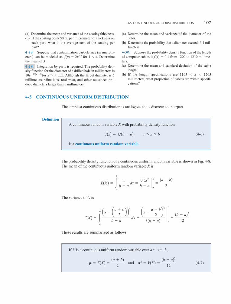
The probability density function of a continuous uniform random variable is shown in Fig. 4-8.The mean of the continuous uniform random variable X is
The variance of X is
These results are summarized as follows.
V1X 2 � �
b
a
ax � aa b
2bb2
b � a dx �
ax �a b
2b3
31b � a2 †b
a�1b � a22
12
E1X 2 � �
b
a
x
b � a dx �
0.5x2
b � a ` b
a�1a b2
2
(a) Determine the mean and variance of the coating thickness.(b) If the coating costs $0.50 per micrometer of thickness on
each part, what is the average cost of the coating perpart?
4-28. Suppose that contamination particle size (in microm-eters) can be modeled as for Determinethe mean of X.
4-29. Integration by parts is required. The probability den-sity function for the diameter of a drilled hole in millimeters is
for mm. Although the target diameter is 5millimeters, vibrations, tool wear, and other nuisances pro-duce diameters larger than 5 millimeters.
x � 510e�101x�52
1 � x.f 1x2 � 2x�3
(a) Determine the mean and variance of the diameter of theholes.
(b) Determine the probability that a diameter exceeds 5.1 mil-limeters.
4-30. Suppose the probability density function of the lengthof computer cables is f(x) � 0.1 from 1200 to 1210 millime-ters.(a) Determine the mean and standard deviation of the cable
length.(b) If the length specifications are 1195 � x � 1205
millimeters, what proportion of cables are within specifi-cations?
If X is a continuous uniform random variable over a � x � b,
(4-7)� � E1X 2 �1a b2
2 and �2 � V1X 2 �
1b � a2212
c04.qxd 5/10/02 5:19 PM Page 107 RK UL 6 RK UL 6:Desktop Folder:TEMP WORK:MONTGOMERY:REVISES UPLO D CH 1 14 FIN L:Quark Files:
108 CHAPTER 4 CONTINUOUS RANDOM VARIABLES AND PROBABILITY DISTRIBUTIONS
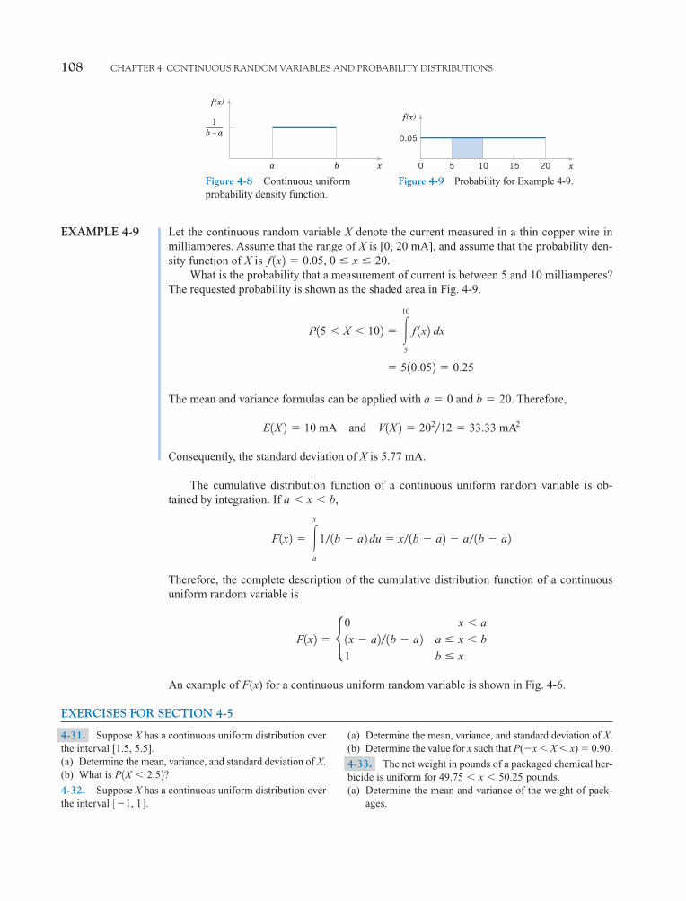
EXAMPLE 4-9 Let the continuous random variable X denote the current measured in a thin copper wire inmilliamperes. Assume that the range of X is [0, 20 mA], and assume that the probability den-sity function of X is
What is the probability that a measurement of current is between 5 and 10 milliamperes?The requested probability is shown as the shaded area in Fig. 4-9.
The mean and variance formulas can be applied with and Therefore,
Consequently, the standard deviation of X is 5.77 mA.
The cumulative distribution function of a continuous uniform random variable is ob-tained by integration. If
Therefore, the complete description of the cumulative distribution function of a continuousuniform random variable is
An example of F(x) for a continuous uniform random variable is shown in Fig. 4-6.
EXERCISES FOR SECTION 4-5
F1x2 � •0 x � a
1x � a2 1b � a2 a � x � b
1 b � x
F1x2 � �x
a
1 1b � a2 du � x 1b � a2 � a 1b � a2
a � x � b,
E1X 2 � 10 mA and V1X 2 � 20212 � 33.33 mA2
b � 20.a � 0
� 510.052 � 0.25
P15 � X � 102 � �10
5 f 1x2 dx
f 1x2 � 0.05, 0 � x � 20.
Figure 4-9 Probability for Example 4-9.
x
f(x)
0 5 10 15 20
0.05
Figure 4-8 Continuous uniformprobability density function.
a
1b – a
x
f(x)
b
4-31. Suppose X has a continuous uniform distribution overthe interval [1.5, 5.5].(a) Determine the mean, variance, and standard deviation of X.(b) What is ?
4-32. Suppose X has a continuous uniform distribution overthe interval 3�1, 1 4 .
P1X � 2.52
(a) Determine the mean, variance, and standard deviation of X.(b) Determine the value for x such that P(�x � X � x) � 0.90.
4-33. The net weight in pounds of a packaged chemical her-bicide is uniform for pounds.(a) Determine the mean and variance of the weight of pack-
ages.
49.75 � x � 50.25
c04.qxd 5/10/02 5:19 PM Page 108 RK UL 6 RK UL 6:Desktop Folder:TEMP WORK:MONTGOMERY:REVISES UPLO D CH 1 14 FIN L:Quark Files:
4-6 NORMAL DISTRIBUTION 109
4-6 NORMAL DISTRIBUTION
Undoubtedly, the most widely used model for the distribution of a random variable is a normaldistribution. Whenever a random experiment is replicated, the random variable that equals theaverage (or total) result over the replicates tends to have a normal distribution as the number ofreplicates becomes large. De Moivre presented this fundamental result, known as the centrallimit theorem, in 1733. Unfortunately, his work was lost for some time, and Gauss independ-ently developed a normal distribution nearly 100 years later. Although De Moivre was latercredited with the derivation, a normal distribution is also referred to as a Gaussian distribution.
When do we average (or total) results? Almost always. For example, an automotive engi-neer may plan a study to average pull-off force measurements from several connectors. If weassume that each measurement results from a replicate of a random experiment, the normaldistribution can be used to make approximate conclusions about this average. These conclu-sions are the primary topics in the subsequent chapters of this book.
Furthermore, sometimes the central limit theorem is less obvious. For example, assume thatthe deviation (or error) in the length of a machined part is the sum of a large number of in-finitesimal effects, such as temperature and humidity drifts, vibrations, cutting angle variations,cutting tool wear, bearing wear, rotational speed variations, mounting and fixturing variations,variations in numerous raw material characteristics, and variation in levels of contamination. Ifthe component errors are independent and equally likely to be positive or negative, the total errorcan be shown to have an approximate normal distribution. Furthermore, the normal distributionarises in the study of numerous basic physical phenomena. For example, the physicist Maxwelldeveloped a normal distribution from simple assumptions regarding the velocities of molecules.
The theoretical basis of a normal distribution is mentioned to justify the somewhat com-plex form of the probability density function. Our objective now is to calculate probabilitiesfor a normal random variable. The central limit theorem will be stated more carefully later.
(b) Determine the cumulative distribution function of theweight of packages.
(c) Determine
4-34. The thickness of a flange on an aircraft component isuniformly distributed between 0.95 and 1.05 millimeters.(a) Determine the cumulative distribution function of flange
thickness.(b) Determine the proportion of flanges that exceeds 1.02
millimeters.(c) What thickness is exceeded by 90% of the flanges?(d) Determine the mean and variance of flange thickness.
4-35. Suppose the time it takes a data collection operator tofill out an electronic form for a database is uniformly between1.5 and 2.2 minutes.(a) What is the mean and variance of the time it takes an op-
erator to fill out the form?(b) What is the probability that it will take less than two min-
utes to fill out the form?(c) Determine the cumulative distribution function of the time
it takes to fill out the form.
4-36. The probability density function of the time it takes ahematology cell counter to complete a test on a blood sampleis seconds.f 1x2 � 0.2 for 50 � x � 75
P1X � 50.12.(a) What percentage of tests require more than 70 seconds to
complete.(b) What percentage of tests require less than one minute to
complete.(c) Determine the mean and variance of the time to complete
a test on a sample.
4-37. The thickness of photoresist applied to wafers insemiconductor manufacturing at a particular location on thewafer is uniformly distributed between 0.2050 and 0.2150micrometers.(a) Determine the cumulative distribution function of pho-
toresist thickness.(b) Determine the proportion of wafers that exceeds 0.2125
micrometers in photoresist thickness.(c) What thickness is exceeded by 10% of the wafers?(d) Determine the mean and variance of photoresist thickness.
4-38. The probability density function of the time requiredto complete an assembly operation is for
seconds.(a) Determine the proportion of assemblies that requires more
than 35 seconds to complete.(b) What time is exceeded by 90% of the assemblies?(c) Determine the mean and variance of time of assembly.
30 � x � 40f 1x2 � 0.1
c04.qxd 5/10/02 5:19 PM Page 109 RK UL 6 RK UL 6:Desktop Folder:TEMP WORK:MONTGOMERY:REVISES UPLO D CH 1 14 FIN L:Quark Files:
110 CHAPTER 4 CONTINUOUS RANDOM VARIABLES AND PROBABILITY DISTRIBUTIONS
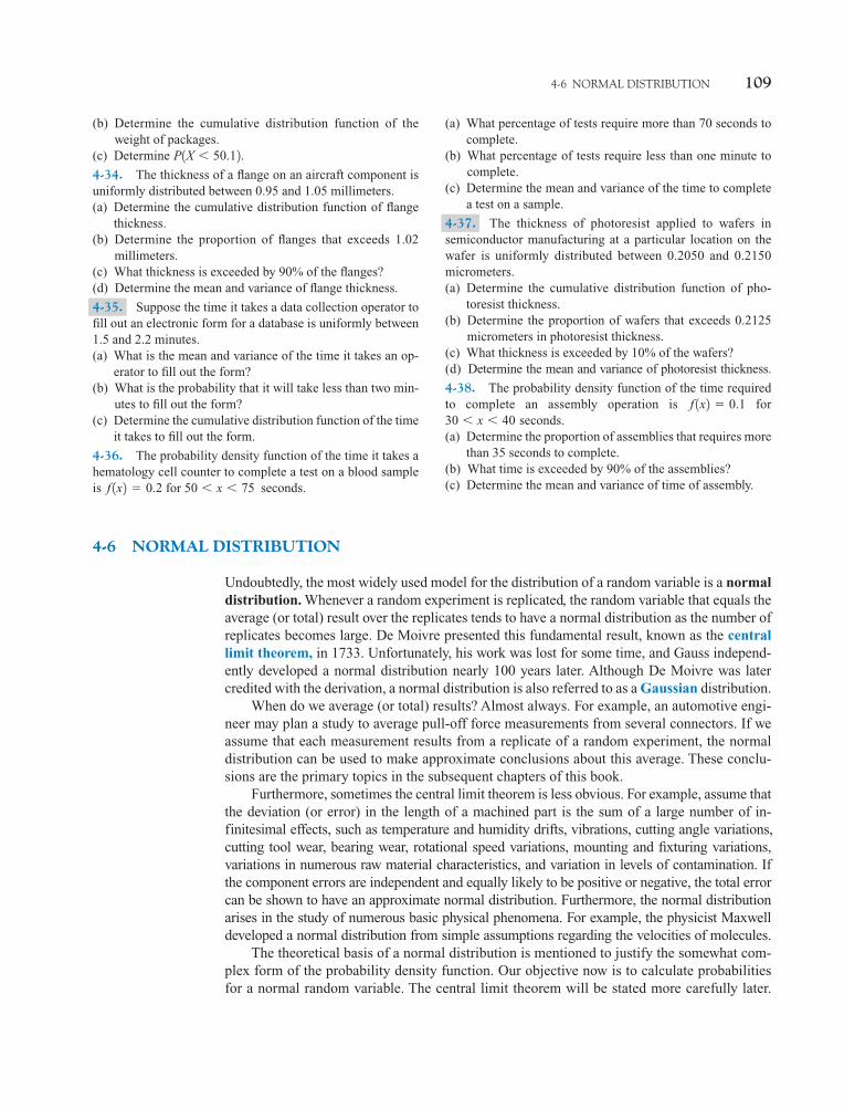
Figure 4-10 Normal probability density functions forselected values of the parameters and �2.�
A random variable X with probability density function
(4-8)
is a normal random variable with parameters �, where and � � 0.Also,
(4-9)
and the notation is used to denote the distribution. The mean and varianceof X are shown to equal � and respectively, at the end of this Section 5-6.�2,
N1�, �22
E1X 2 � � and V1X2 � �2
�� � � � �,
f 1x2 �112�
e
�1x��22
2�2 �� � x � �
Definition
� = 5 x� = 15
σ2 = 1
σ2 = 4
σ2 = 1f (x)
Random variables with different means and variances can be modeled by normal proba-bility density functions with appropriate choices of the center and width of the curve. Thevalue of determines the center of the probability density function and the value of
determines the width. Figure 4-10 illustrates several normal probability densityfunctions with selected values of � and �2. Each has the characteristic symmetric bell-shapedcurve, but the centers and dispersions differ. The following definition provides the formula fornormal probability density functions.
V1X 2 � �2E1X 2 � �
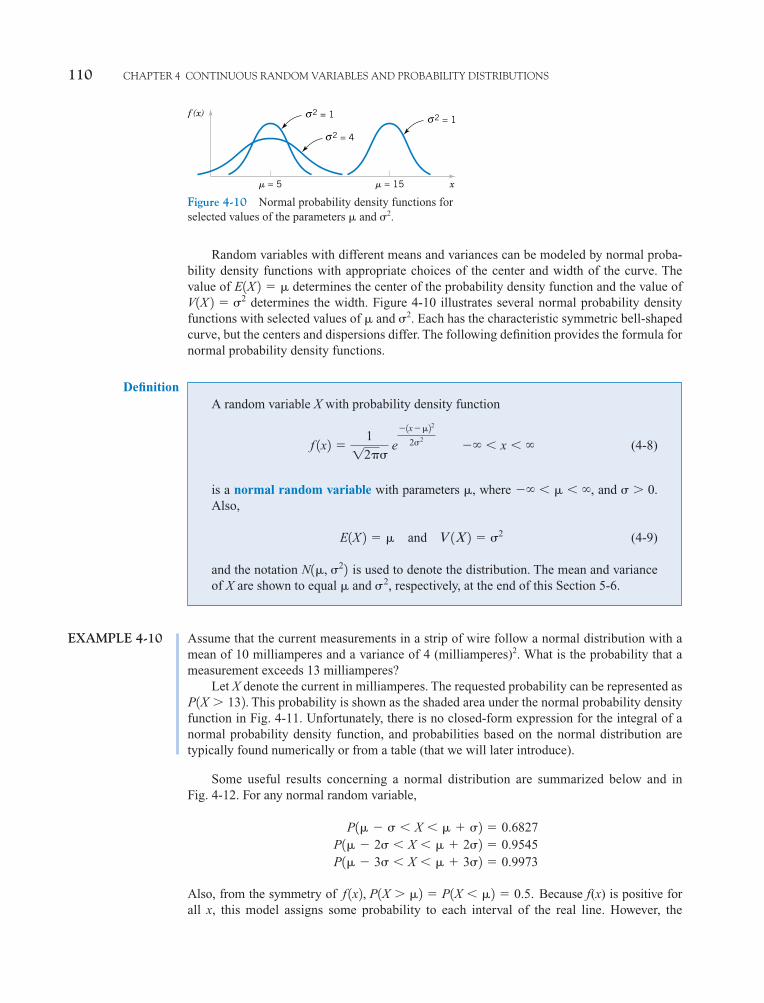
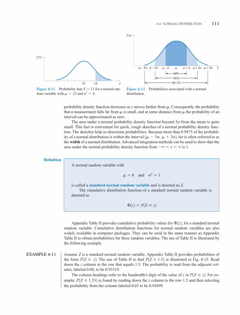
EXAMPLE 4-10 Assume that the current measurements in a strip of wire follow a normal distribution with amean of 10 milliamperes and a variance of 4 (milliamperes)2. What is the probability that ameasurement exceeds 13 milliamperes?
Let X denote the current in milliamperes. The requested probability can be represented asThis probability is shown as the shaded area under the normal probability density
function in Fig. 4-11. Unfortunately, there is no closed-form expression for the integral of anormal probability density function, and probabilities based on the normal distribution aretypically found numerically or from a table (that we will later introduce).
Some useful results concerning a normal distribution are summarized below and inFig. 4-12. For any normal random variable,
Also, from the symmetry of Because f(x) is positive forall x, this model assigns some probability to each interval of the real line. However, the
f 1x2, P1X � �2 � P1X � �2 � 0.5.
P1� � 3� � X � � 3�2 � 0.9973 P1� � 2� � X � � 2�2 � 0.9545
P1� � � � X � � �2 � 0.6827
P1X � 132.
c04.qxd 5/13/02 11:17 M Page 110 RK UL 6 RK UL 6:Desktop Folder:TEMP WORK:MONTGOMERY:REVISES UPLO D CH 1 14 FIN L:Quark Files:
4-6 NORMAL DISTRIBUTION 111
probability density function decreases as x moves farther from �. Consequently, the probabilitythat a measurement falls far from � is small, and at some distance from � the probability of aninterval can be approximated as zero.
The area under a normal probability density function beyond 3� from the mean is quitesmall. This fact is convenient for quick, rough sketches of a normal probability density func-tion. The sketches help us determine probabilities. Because more than 0.9973 of the probabil-ity of a normal distribution is within the interval , 6� is often referred to asthe width of a normal distribution. Advanced integration methods can be used to show that thearea under the normal probability density function from is 1.�� � x � �
1� � 3�, � 3�2
Figure 4-11 Probability that X � 13 for a normal ran-dom variable with and �2 � 4.� � 10
10 x13
f (x)
Figure 4-12 Probabilities associated with a normaldistribution.
– 3 x� � – 2µ � – � � � +� � + 2� � + 3� �
68%
95%
99.7%
f (x)
A normal random variable with
is called a standard normal random variable and is denoted as Z.The cumulative distribution function of a standard normal random variable is
denoted as
�1z2 � P1Z � z2
� � 0 and �2 � 1
Definition
Appendix Table II provides cumulative probability values for , for a standard normalrandom variable. Cumulative distribution functions for normal random variables are alsowidely available in computer packages. They can be used in the same manner as AppendixTable II to obtain probabilities for these random variables. The use of Table II is illustrated bythe following example.
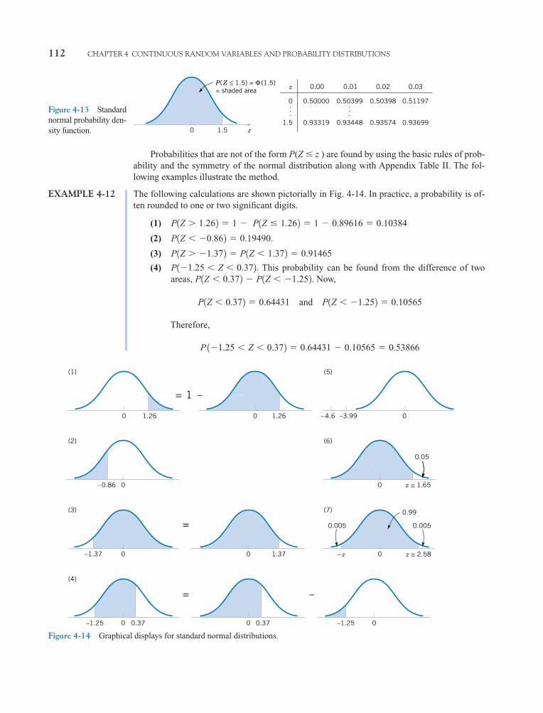
EXAMPLE 4-11 Assume Z is a standard normal random variable. Appendix Table II provides probabilities ofthe form The use of Table II to find is illustrated in Fig. 4-13. Readdown the z column to the row that equals 1.5. The probability is read from the adjacent col-umn, labeled 0.00, to be 0.93319.
The column headings refer to the hundredth’s digit of the value of z in For ex-ample, is found by reading down the z column to the row 1.5 and then selectingthe probability from the column labeled 0.03 to be 0.93699.
P1Z � 1.532P1Z � z2.
P1Z � 1.52P1Z � z2.
�1z2
c04.qxd 5/10/02 5:19 PM Page 111 RK UL 6 RK UL 6:Desktop Folder:TEMP WORK:MONTGOMERY:REVISES UPLO D CH 1 14 FIN L:Quark Files:
112 CHAPTER 4 CONTINUOUS RANDOM VARIABLES AND PROBABILITY DISTRIBUTIONS
Probabilities that are not of the form P(Z � z ) are found by using the basic rules of prob-ability and the symmetry of the normal distribution along with Appendix Table II. The fol-lowing examples illustrate the method.
EXAMPLE 4-12 The following calculations are shown pictorially in Fig. 4-14. In practice, a probability is of-ten rounded to one or two significant digits.
(1)
(2)
(3)
(4) . This probability can be found from the difference of twoareas, . Now,
Therefore,
P 1�1.25 � Z � 0.372 � 0.64431 � 0.10565 � 0.53866
P1Z � 0.372 � 0.64431 and P1Z � �1.252 � 0.10565
P1Z � 0.372 � P1Z � �1.252P1�1.25 � Z � 0.372P1Z � �1.372 � P1Z � 1.372 � 0.91465
P1Z � �0.862 � 0.19490.
P1Z � 1.262 � 1 � P1Z � 1.262 � 1 � 0.89616 � 0.10384
(1) (5)
0 –3.99
(2)
0 0
(3) (7)
0 0 0
0 0 0
1.26 0 1.26
–0.86
0.05
z ≅ 1.65
z ≅ 2.58
0.0050.005
– z
0.99
–1.37
=
1.37
=
0.37–1.25 –1.250.37
–
= –
(4)
–4.6 0
(6)
1
Figure 4-14 Graphical displays for standard normal distributions.
Figure 4-13 Standardnormal probability den-sity function. z0
= shaded areaP(Z ≤ 1.5) = Φ (1.5)
1.5
0.00 0.01 0.02
0
1.5
z
0.93319
. .
.
. .
.
0.93448 0.93574
0.50000 0.50399 0.50398
0.03
0.93699
0.51197
c04.qxd 5/10/02 5:19 PM Page 112 RK UL 6 RK UL 6:Desktop Folder:TEMP WORK:MONTGOMERY:REVISES UPLO D CH 1 14 FIN L:Quark Files:
(5) cannot be found exactly from Appendix Table II. However, the lastentry in the table can be used to find that . Because
is nearly zero.
(6) Find the value z such that This probability expression can be writ-ten as . Now, Table II is used in reverse. We search through theprobabilities to find the value that corresponds to 0.95. The solution is illustrated inFig. 4-14. We do not find 0.95 exactly; the nearest value is 0.95053, correspondingto z = 1.65.
(7) Find the value of z such that . Because of the symmetry ofthe normal distribution, if the area of the shaded region in Fig. 4-14(7) is to equal0.99, the area in each tail of the distribution must equal 0.005. Therefore, the valuefor z corresponds to a probability of 0.995 in Table II. The nearest probability inTable II is 0.99506, when z = 2.58.
The preceding examples show how to calculate probabilities for standard normal randomvariables. To use the same approach for an arbitrary normal random variable would require aseparate table for every possible pair of values for � and �. Fortunately, all normal probabilitydistributions are related algebraically, and Appendix Table II can be used to find the probabili-ties associated with an arbitrary normal random variable by first using a simple transformation.
P1�z � Z � z2 � 0.99
P1Z � z2 � 0.95P1Z � z2 � 0.05.
P1Z � �4.62 � P1Z � �3.992, P1Z � �4.62P1Z � �3.992 � 0.00003P1Z � �4.62
4-6 NORMAL DISTRIBUTION 113
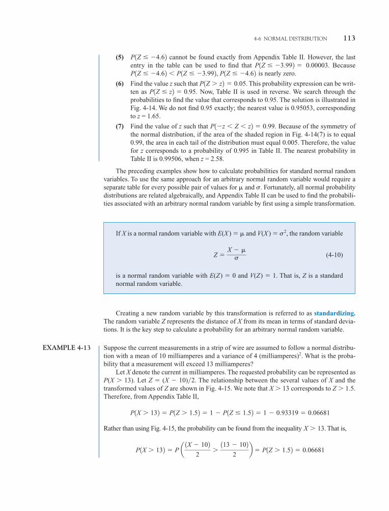
If X is a normal random variable with E(X ) � � and V(X ) � �2, the random variable
(4-10)
is a normal random variable with E(Z) � 0 and V(Z) � 1. That is, Z is a standardnormal random variable.
Z �X � �
�
Creating a new random variable by this transformation is referred to as standardizing.The random variable Z represents the distance of X from its mean in terms of standard devia-tions. It is the key step to calculate a probability for an arbitrary normal random variable.
EXAMPLE 4-13 Suppose the current measurements in a strip of wire are assumed to follow a normal distribu-tion with a mean of 10 milliamperes and a variance of 4 (milliamperes)2. What is the proba-bility that a measurement will exceed 13 milliamperes?
Let X denote the current in milliamperes. The requested probability can be represented asP(X � 13). Let Z � (X � 10)�2. The relationship between the several values of X and thetransformed values of Z are shown in Fig. 4-15. We note that X � 13 corresponds to Z � 1.5.Therefore, from Appendix Table II,
Rather than using Fig. 4-15, the probability can be found from the inequality That is,
P1X � 132 � P a 1X � 1022
�113 � 102
2b � P1Z � 1.52 � 0.06681
X � 13.
P1X � 132 � P1Z � 1.52 � 1 � P1Z � 1.52 � 1 � 0.93319 � 0.06681
c04.qxd 5/13/02 11:18 M Page 113 RK UL 6 RK UL 6:Desktop Folder:TEMP WORK:MONTGOMERY:REVISES UPLO D CH 1 14 FIN L:Quark Files:

114 CHAPTER 4 CONTINUOUS RANDOM VARIABLES AND PROBABILITY DISTRIBUTIONS
Figure 4-15 Standardizing a normal random variable.
4 x7 9 10 13 16
–3 z–1.5 –0.5 0 1.5 3
11
0.5
0 1.5
Distribution of Z =X – µ
σ
Distribution of X
10 13 x
z
Suppose X is a normal random variable with mean � and variance �2. Then,
(4-11)
where Z is a standard normal random variable, and is the z-valueobtained by standardizing X.
The probability is obtained by entering Appendix Table II with .z � 1x � �2�z �1x � �2
�
P 1X � x2 � P aX � �� �
x � �� b � P1Z � z2
EXAMPLE 4-14 Continuing the previous example, what is the probability that a current measurement is be-tween 9 and 11 milliamperes? From Fig. 4-15, or by proceeding algebraically, we have
Determine the value for which the probability that a current measurement is belowthis value is 0.98. The requested value is shown graphically in Fig. 4-16. We need the value ofx such that P(X � x) � 0.98. By standardizing, this probability expression can be written as
Appendix Table II is used to find the z-value such that P(Z � z) � 0.98. The nearest proba-bility from Table II results in
P1Z � 2.052 � 0.97982
� 0.98� P1Z � 1x � 10222
P1X � x2 � P1 1X � 1022 � 1x � 10222
� 0.69146 � 0.30854 � 0.38292 � P1�0.5 � Z � 0.52 � P1Z � 0.52 � P1Z � �0.52
P19 � X � 112 � P1 19 � 1022 � 1X � 1022 � 111 � 10222
In the preceding example, the value 13 is transformed to 1.5 by standardizing, and 1.5 isoften referred to as the z-value associated with a probability. The following summarizes thecalculation of probabilities derived from normal random variables.
c04.qxd 5/10/02 5:19 PM Page 114 RK UL 6 RK UL 6:Desktop Folder:TEMP WORK:MONTGOMERY:REVISES UPLO D CH 1 14 FIN L:Quark Files:
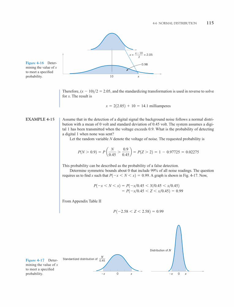
Therefore, (x � 10)�2 � 2.05, and the standardizing transformation is used in reverse to solvefor x. The result is
EXAMPLE 4-15 Assume that in the detection of a digital signal the background noise follows a normal distri-bution with a mean of 0 volt and standard deviation of 0.45 volt. The system assumes a digi-tal 1 has been transmitted when the voltage exceeds 0.9. What is the probability of detectinga digital 1 when none was sent?
Let the random variable N denote the voltage of noise. The requested probability is
This probability can be described as the probability of a false detection.Determine symmetric bounds about 0 that include 99% of all noise readings. The question
requires us to find x such that . A graph is shown in Fig. 4-17. Now,
From Appendix Table II
P 1�2.58 � Z � 2.582 � 0.99
� P1�x0.45 � Z � x0.452 � 0.99 P1�x � N � x2 � P1�x0.45 � N0.45 � x0.452
P1�x � N � x2 � 0.99
P1N � 0.92 � P a N
0.45�
0.90.45b � P1Z � 22 � 1 � 0.97725 � 0.02275
x � 212.052 10 � 14.1 milliamperes
4-6 NORMAL DISTRIBUTION 115
10 x
z = = 2.05x – 10
2
0.98Figure 4-16 Deter-mining the value of xto meet a specifiedprobability.
Standardized distribution ofN
0.45
z– z 0 0 x– x
Distribution of N
Figure 4-17 Deter-mining the value of xto meet a specifiedprobability.
c04.qxd 5/10/02 5:19 PM Page 115 RK UL 6 RK UL 6:Desktop Folder:TEMP WORK:MONTGOMERY:REVISES UPLO D CH 1 14 FIN L:Quark Files:
116 CHAPTER 4 CONTINUOUS RANDOM VARIABLES AND PROBABILITY DISTRIBUTIONS
Therefore,
and
Suppose a digital 1 is represented as a shift in the mean of the noise distribution to 1.8volts. What is the probability that a digital 1 is not detected? Let the random variable S denotethe voltage when a digital 1 is transmitted. Then,
This probability can be interpreted as the probability of a missed signal.
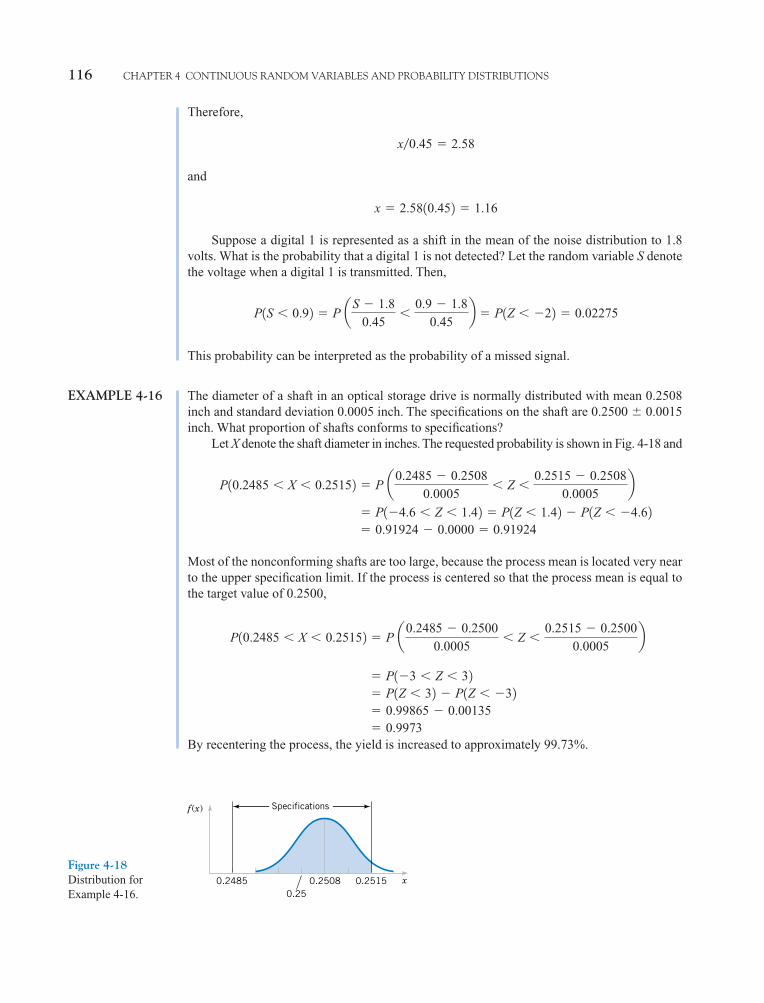
EXAMPLE 4-16 The diameter of a shaft in an optical storage drive is normally distributed with mean 0.2508inch and standard deviation 0.0005 inch. The specifications on the shaft are 0.2500 � 0.0015inch. What proportion of shafts conforms to specifications?
Let X denote the shaft diameter in inches. The requested probability is shown in Fig. 4-18 and
Most of the nonconforming shafts are too large, because the process mean is located very nearto the upper specification limit. If the process is centered so that the process mean is equal tothe target value of 0.2500,
By recentering the process, the yield is increased to approximately 99.73%.� 0.9973� 0.99865 � 0.00135� P1Z � 32 � P1Z � �32� P1�3 � Z � 32
P10.2485 � X � 0.25152 � P a0.2485 � 0.25000.0005
� Z �0.2515 � 0.2500
0.0005b
� 0.91924 � 0.0000 � 0.91924� P1�4.6 � Z � 1.42 � P1Z � 1.42 � P1Z � �4.62
P10.2485 � X � 0.25152 � P a0.2485 � 0.25080.0005
� Z �0.2515 � 0.2508
0.0005b
P1S � 0.92 � P aS � 1.80.45
�0.9 � 1.8
0.45b � P1Z � �22 � 0.02275
x � 2.5810.452 � 1.16
x0.45 � 2.58
0.2515
f (x)
0.25080.25
0.2485 x
Specifications
Figure 4-18Distribution forExample 4-16.
c04.qxd 5/10/02 5:19 PM Page 116 RK UL 6 RK UL 6:Desktop Folder:TEMP WORK:MONTGOMERY:REVISES UPLO D CH 1 14 FIN L:Quark Files:
4-6 NORMAL DISTRIBUTION 117
Mean and Variance of the Normal Distribution (CD Only)
EXERCISES FOR SECTION 4-6
4-39. Use Appendix Table II to determine the followingprobabilities for the standard normal random variable Z:(a) P(Z � 1.32) (b) P(Z � 3.0)(c) P(Z � 1.45) (d) P(Z � �2.15)(e) P(�2.34 � Z � 1.76)
4-40. Use Appendix Table II to determine the followingprobabilities for the standard normal random variable Z:(a) P(�1 � Z � 1) (b) P(�2 � Z � 2)(c) P(�3 � Z � 3) (d) P(Z � 3)(e) P(0 � Z � 1)
4-41. Assume Z has a standard normal distribution. UseAppendix Table II to determine the value for z that solves eachof the following:(a) P( Z � z) � 0.9 (b) P(Z � z) � 0.5(c) P( Z � z) � 0.1 (d) P(Z � z) � 0.9(e) P(�1.24 � Z � z) � 0.8
4-42. Assume Z has a standard normal distribution. UseAppendix Table II to determine the value for z that solves eachof the following:(a) P(�z � Z � z) � 0.95 (b) P(�z � Z � z) � 0.99(c) P(�z � Z � z) � 0.68 (d) P(�z � Z � z) � 0.9973
4-43. Assume X is normally distributed with a mean of 10and a standard deviation of 2. Determine the following:(a) P(X � 13) (b) P(X � 9)(c) P(6 � X � 14) (d) P(2 � X � 4)(e) P(�2 � X � 8)
4-44. Assume X is normally distributed with a mean of 10and a standard deviation of 2. Determine the value for x thatsolves each of the following:(a) P(X � x) � 0.5(b) P(X � x) � 0.95(c) P(x � X � 10) � 0.2(d) P(�x � X � 10 � x) � 0.95(e) P(�x � X � 10 � x) � 0.99
4-45. Assume X is normally distributed with a mean of 5and a standard deviation of 4. Determine the following:(a) P(X � 11) (b) P(X � 0)(c) P(3 � X � 7) (d) P(�2 � X � 9)(e) P(2 � X � 8)
4-46. Assume X is normally distributed with a mean of 5and a standard deviation of 4. Determine the value for x thatsolves each of the following:(a) P(X � x) � 0.5 (b) P(X � x) � 0.95(c) P(x � X � 9) � 0.2 (d) P(3 � X � x) � 0.95(e) P(�x � X � x) � 0.99
4-47. The compressive strength of samples of cement canbe modeled by a normal distribution with a mean of 6000 kilo-grams per square centimeter and a standard deviation of 100kilograms per square centimeter.
(a) What is the probability that a sample’s strength is less than6250 Kg/cm2?
(b) What is the probability that a sample’s strength is between5800 and 5900 Kg/cm2?
(c) What strength is exceeded by 95% of the samples?
4-48. The tensile strength of paper is modeled by a normaldistribution with a mean of 35 pounds per square inch and astandard deviation of 2 pounds per square inch.(a) What is the probability that the strength of a sample is less
than 40 lb/in2?(b) If the specifications require the tensile strength to
exceed 30 lb/in2, what proportion of the samples isscrapped?
4-49. The line width of for semiconductor manufacturing isassumed to be normally distributed with a mean of 0.5 mi-crometer and a standard deviation of 0.05 micrometer.(a) What is the probability that a line width is greater than
0.62 micrometer?(b) What is the probability that a line width is between 0.47
and 0.63 micrometer?(c) The line width of 90% of samples is below what value?
4-50. The fill volume of an automated filling machine usedfor filling cans of carbonated beverage is normally distributedwith a mean of 12.4 fluid ounces and a standard deviation of0.1 fluid ounce.(a) What is the probability a fill volume is less than 12 fluid
ounces?(b) If all cans less than 12.1 or greater than 12.6 ounces are
scrapped, what proportion of cans is scrapped?(c) Determine specifications that are symmetric about the
mean that include 99% of all cans.
4-51. The time it takes a cell to divide (called mitosis) isnormally distributed with an average time of one hour and astandard deviation of 5 minutes.(a) What is the probability that a cell divides in less than
45 minutes?(b) What is the probability that it takes a cell more than
65 minutes to divide?(c) What is the time that it takes approximately 99% of all
cells to complete mitosis?
4-52. In the previous exercise, suppose that the mean of thefilling operation can be adjusted easily, but the standard devi-ation remains at 0.1 ounce.(a) At what value should the mean be set so that 99.9% of all
cans exceed 12 ounces?(b) At what value should the mean be set so that 99.9% of all
cans exceed 12 ounces if the standard deviation can be re-duced to 0.05 fluid ounce?
c04.qxd 5/10/02 5:19 PM Page 117 RK UL 6 RK UL 6:Desktop Folder:TEMP WORK:MONTGOMERY:REVISES UPLO D CH 1 14 FIN L:Quark Files:
118 CHAPTER 4 CONTINUOUS RANDOM VARIABLES AND PROBABILITY DISTRIBUTIONS
4-53. The reaction time of a driver to visual stimulus is nor-mally distributed with a mean of 0.4 seconds and a standarddeviation of 0.05 seconds.(a) What is the probability that a reaction requires more than
0.5 seconds?(b) What is the probability that a reaction requires between
0.4 and 0.5 seconds?(c) What is the reaction time that is exceeded 90% of the
time?
4-54. The speed of a file transfer from a server on campus toa personal computer at a student’s home on a weekdayevening is normally distributed with a mean of 60 kilobits persecond and a standard deviation of 4 kilobits per second.(a) What is the probability that the file will transfer at a speed
of 70 kilobits per second or more?(b) What is the probability that the file will transfer at a speed
of less than 58 kilobits per second?(c) If the file is 1 megabyte, what is the average time it will
take to transfer the file? (Assume eight bits per byte.)
4-55. The length of an injection-molded plastic case thatholds magnetic tape is normally distributed with a length of90.2 millimeters and a standard deviation of 0.1 millimeter.(a) What is the probability that a part is longer than 90.3 mil-
limeters or shorter than 89.7 millimeters?(b) What should the process mean be set at to obtain the great-
est number of parts between 89.7 and 90.3 millimeters?(c) If parts that are not between 89.7 and 90.3 millimeters are
scrapped, what is the yield for the process mean that youselected in part (b)?
4-56. In the previous exercise assume that the process iscentered so that the mean is 90 millimeters and the standarddeviation is 0.1 millimeter. Suppose that 10 cases are meas-ured, and they are assumed to be independent.(a) What is the probability that all 10 cases are between 89.7
and 90.3 millimeters?(b) What is the expected number of the 10 cases that are be-
tween 89.7 and 90.3 millimeters?
4-57. The sick-leave time of employees in a firm in a monthis normally distributed with a mean of 100 hours and a stan-dard deviation of 20 hours.(a) What is the probability that the sick-leave time for next
month will be between 50 and 80 hours?(b) How much time should be budgeted for sick leave if the
budgeted amount should be exceeded with a probabilityof only 10%?
4-58. The life of a semiconductor laser at a constant poweris normally distributed with a mean of 7000 hours and a stan-dard deviation of 600 hours.(a) What is the probability that a laser fails before 5000
hours?(b) What is the life in hours that 95% of the lasers exceed?(c) If three lasers are used in a product and they are assumed
to fail independently, what is the probability that all threeare still operating after 7000 hours?
4-59. The diameter of the dot produced by a printer is nor-mally distributed with a mean diameter of 0.002 inch and astandard deviation of 0.0004 inch.(a) What is the probability that the diameter of a dot exceeds
0.0026 inch?(b) What is the probability that a diameter is between 0.0014
and 0.0026 inch?(c) What standard deviation of diameters is needed so that the
probability in part (b) is 0.995?
4-60. The weight of a sophisticated running shoe is nor-mally distributed with a mean of 12 ounces and a standard de-viation of 0.5 ounce.(a) What is the probability that a shoe weighs more than 13
ounces?(b) What must the standard deviation of weight be in order for
the company to state that 99.9% of its shoes are less than13 ounces?
(c) If the standard deviation remains at 0.5 ounce, what mustthe mean weight be in order for the company to state that99.9% of its shoes are less than 13 ounces?
4-7 NORMAL APPROXIMATION TO THE BINOMIALAND POISSON DISTRIBUTIONS
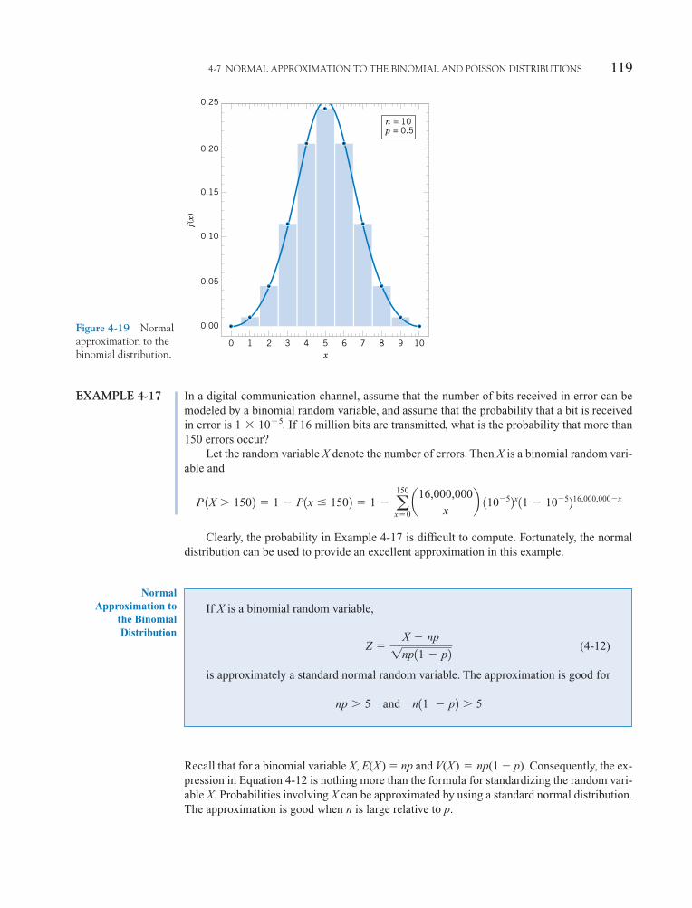
We began our section on the normal distribution with the central limit theorem and the nor-mal distribution as an approximation to a random variable with a large number of trials.Consequently, it should not be a surprise to learn that the normal distribution can be usedto approximate binomial probabilities for cases in which n is large. The following exampleillustrates that for many physical systems the binomial model is appropriate with an ex-tremely large value for n. In these cases, it is difficult to calculate probabilities by using thebinomial distribution. Fortunately, the normal approximation is most effective in thesecases. An illustration is provided in Fig. 4-19. The area of each bar equals the binomialprobability of x. Notice that the area of bars can be approximated by areas under the nor-mal density function.
c04.qxd 5/10/02 5:19 PM Page 118 RK UL 6 RK UL 6:Desktop Folder:TEMP WORK:MONTGOMERY:REVISES UPLO D CH 1 14 FIN L:Quark Files:
4-7 NORMAL APPROXIMATION TO THE BINOMIAL AND POISSON DISTRIBUTIONS 119
EXAMPLE 4-17 In a digital communication channel, assume that the number of bits received in error can bemodeled by a binomial random variable, and assume that the probability that a bit is receivedin error is . If 16 million bits are transmitted, what is the probability that more than150 errors occur?
Let the random variable X denote the number of errors. Then X is a binomial random vari-able and
Clearly, the probability in Example 4-17 is difficult to compute. Fortunately, the normaldistribution can be used to provide an excellent approximation in this example.
P 1X � 1502 � 1 � P1x � 1502 � 1 � a150
x�0a16,000,000
xb 110�52x11 � 10�5216,000,000�x
1 � 10�5
Figure 4-19 Normalapproximation to thebinomial distribution.
0 1 2 3 4 5 6 7 8 9 10
0.00
0.05
0.10
0.20
0.25
x
f(x)
n = 10
0.15
p = 0.5
If X is a binomial random variable,
(4-12)
is approximately a standard normal random variable. The approximation is good for
np � 5 and n11 � p2 � 5
Z �X � np1np11 � p2
NormalApproximation to
the BinomialDistribution
Recall that for a binomial variable X, E(X) � np and V(X) � np(1 � p). Consequently, the ex-pression in Equation 4-12 is nothing more than the formula for standardizing the random vari-able X. Probabilities involving X can be approximated by using a standard normal distribution.The approximation is good when n is large relative to p.
c04.qxd 5/10/02 5:19 PM Page 119 RK UL 6 RK UL 6:Desktop Folder:TEMP WORK:MONTGOMERY:REVISES UPLO D CH 1 14 FIN L:Quark Files:
120 CHAPTER 4 CONTINUOUS RANDOM VARIABLES AND PROBABILITY DISTRIBUTIONS
EXAMPLE 4-18 The digital communication problem in the previous example is solved as follows:
Because and n(1 � p) is much larger, the approximationis expected to work well in this case.
EXAMPLE 4-19 Again consider the transmission of bits in Example 4-18. To judge how well the normalapproximation works, assume only n � 50 bits are to be transmitted and that the probabilityof an error is p � 0.1. The exact probability that 2 or less errors occur is
Based on the normal approximation
Even for a sample as small as 50 bits, the normal approximation is reasonable.
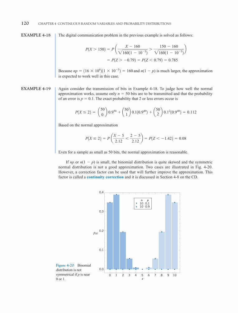
If np or n(1 � p) is small, the binomial distribution is quite skewed and the symmetricnormal distribution is not a good approximation. Two cases are illustrated in Fig. 4-20.However, a correction factor can be used that will further improve the approximation. Thisfactor is called a continuity correction and it is discussed in Section 4-8 on the CD.
P1X � 22 � P aX � 52.12
�2 � 52.12
b � P1Z � �1.422 � 0.08
P1X � 22 � a500b 0.950 a50
1b 0.110.9492 a50
2 b 0.1210.9482 � 0.112
np � 116 � 1062 11 � 10�52 � 160
� P1Z � �0.792 � P1Z � 0.792 � 0.785
P1X � 1502 � P a X � 160216011 � 10�52 �150 � 160216011 � 10�52 b
Figure 4-20 Binomialdistribution is notsymmetrical if p is near0 or 1.
0 1 2 3 4 5 6 7 8 9 10
0.0
0.1
0.3
0.4
x
f(x)0.2
n p10 0.110 0.9
c04.qxd 5/10/02 5:19 PM Page 120 RK UL 6 RK UL 6:Desktop Folder:TEMP WORK:MONTGOMERY:REVISES UPLO D CH 1 14 FIN L:Quark Files:
4-7 NORMAL APPROXIMATION TO THE BIOMIAL AND POISSON DISTRIBUTIONS 121
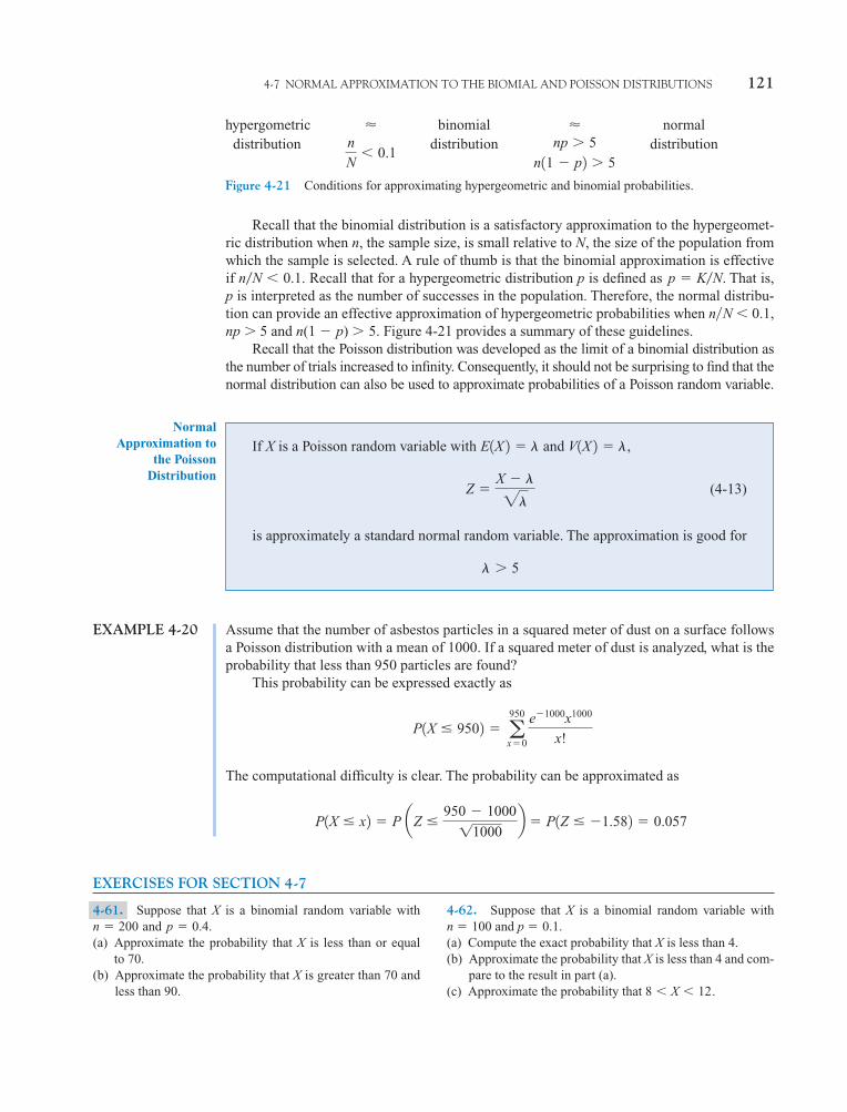
Recall that the binomial distribution is a satisfactory approximation to the hypergeomet-ric distribution when n, the sample size, is small relative to N, the size of the population fromwhich the sample is selected. A rule of thumb is that the binomial approximation is effectiveif . Recall that for a hypergeometric distribution p is defined as That is,p is interpreted as the number of successes in the population. Therefore, the normal distribu-tion can provide an effective approximation of hypergeometric probabilities when n�N � 0.1,np � 5 and n(1 � p) � 5. Figure 4-21 provides a summary of these guidelines.
Recall that the Poisson distribution was developed as the limit of a binomial distribution asthe number of trials increased to infinity. Consequently, it should not be surprising to find that thenormal distribution can also be used to approximate probabilities of a Poisson random variable.
p � KN.nN � 0.1
If X is a Poisson random variable with and
(4-13)
is approximately a standard normal random variable. The approximation is good for
� � 5
Z �X � �2�
V1X 2 � �,E1X 2 � �
NormalApproximation to
the PoissonDistribution
hypergometric � binomial � normal distribution distribution distributionnp � 5n
N� 0.1
Figure 4-21 Conditions for approximating hypergeometric and binomial probabilities.
n11 � p2 � 5
EXAMPLE 4-20 Assume that the number of asbestos particles in a squared meter of dust on a surface followsa Poisson distribution with a mean of 1000. If a squared meter of dust is analyzed, what is theprobability that less than 950 particles are found?
This probability can be expressed exactly as
The computational difficulty is clear. The probability can be approximated as
EXERCISES FOR SECTION 4-7
P1X � x2 � P aZ �950 � 100011000
b � P1Z � �1.582 � 0.057
P1X � 9502 � a950
x�0
e�1000x1000
x!
4-61. Suppose that X is a binomial random variable withand
(a) Approximate the probability that X is less than or equalto 70.
(b) Approximate the probability that X is greater than 70 andless than 90.
p � 0.4.n � 2004-62. Suppose that X is a binomial random variable withn � 100 and p � 0.1.(a) Compute the exact probability that X is less than 4.(b) Approximate the probability that X is less than 4 and com-
pare to the result in part (a).(c) Approximate the probability that .8 � X � 12
c04.qxd 5/10/02 5:19 PM Page 121 RK UL 6 RK UL 6:Desktop Folder:TEMP WORK:MONTGOMERY:REVISES UPLO D CH 1 14 FIN L:Quark Files:
122 CHAPTER 4 CONTINUOUS RANDOM VARIABLES AND PROBABILITY DISTRIBUTIONS
4-63. The manufacturing of semiconductor chips produces2% defective chips. Assume the chips are independent andthat a lot contains 1000 chips.(a) Approximate the probability that more than 25 chips are
defective.(b) Approximate the probability that between 20 and 30 chips
are defective.
4-64. A supplier ships a lot of 1000 electrical connectors. Asample of 25 is selected at random, without replacement.Assume the lot contains 100 defective connectors.(a) Using a binomial approximation, what is the probability
that there are no defective connectors in the sample?(b) Use the normal approximation to answer the result in part
(a). Is the approximation satisfactory?(c) Redo parts (a) and (b) assuming the lot size is 500. Is the nor-
mal approximation to the probability that there are no defec-tive connectors in the sample satisfactory in this case?
4-65. An electronic office product contains 5000 elec-tronic components. Assume that the probability that eachcomponent operates without failure during the useful life ofthe product is 0.999, and assume that the components failindependently. Approximate the probability that 10 or moreof the original 5000 components fail during the useful life ofthe product.
4-66. Suppose that the number of asbestos particles in a sam-ple of 1 squared centimeter of dust is a Poisson random variablewith a mean of 1000. What is the probability that 10 squared cen-timeters of dust contains more than 10,000 particles?
4-67. A corporate Web site contains errors on 50 of 1000pages. If 100 pages are sampled randomly, without replace-
ment, approximate the probability that at least 1 of the pagesin error are in the sample.
4-68. Hits to a high-volume Web site are assumed to followa Poisson distribution with a mean of 10,000 per day.Approximate each of the following:(a) The probability of more than 20,000 hits in a day(b) The probability of less than 9900 hits in a day(c) The value such that the probability that the number of hits
in a day exceed the value is 0.01
4-69. Continuation of Exercise 4-68.(a) Approximate the expected number of days in a year (365
days) that exceed 10,200 hits.(b) Approximate the probability that over a year (365 days)
more than 15 days each have more than 10,200 hits.
4-70. The percentage of people exposed to a bacteria whobecome ill is 20%. Assume that people are independent. Assumethat 1000 people are exposed to the bacteria. Approximate eachof the following:(a) The probability that more than 225 become ill(b) The probability that between 175 and 225 become ill(c) The value such that the probability that the number of peo-
ple that become ill exceeds the value is 0.01
4-71. A high-volume printer produces minor print-qualityerrors on a test pattern of 1000 pages of text according to aPoisson distribution with a mean of 0.4 per page.(a) Why are the number of errors on each page independent
random variables?(b) What is the mean number of pages with errors (one or more)?(c) Approximate the probability that more than 350 pages
contain errors (one or more).
4-8 CONTINUITY CORRECTION TO IMPROVETHE APPROXIMATION (CD ONLY)
4-9 EXPONENTIAL DISTRIBUTION
The discussion of the Poisson distribution defined a random variable to be the number offlaws along a length of copper wire. The distance between flaws is another random variablethat is often of interest. Let the random variable X denote the length from any starting point onthe wire until a flaw is detected.
As you might expect, the distribution of X can be obtained from knowledge of thedistribution of the number of flaws. The key to the relationship is the following concept. Thedistance to the first flaw exceeds 3 millimeters if and only if there are no flaws within a lengthof 3 millimeters—simple, but sufficient for an analysis of the distribution of X.
In general, let the random variable N denote the number of flaws in x millimeters of wire.If the mean number of flaws is per millimeter, N has a Poisson distribution with mean .We assume that the wire is longer than the value of x. Now,
P1X � x2 � P1N � 02 �e��x1�x20
0!� e��x
�x�
c04.qxd 5/10/02 5:19 PM Page 122 RK UL 6 RK UL 6:Desktop Folder:TEMP WORK:MONTGOMERY:REVISES UPLO D CH 1 14 FIN L:Quark Files:
4-9 EXPONENTIAL DISTRIBUTION 123
Therefore,
is the cumulative distribution function of X. By differentiating F(x), the probability densityfunction of X is calculated to be
The derivation of the distribution of X depends only on the assumption that the flaws inthe wire follow a Poisson process. Also, the starting point for measuring X doesn’t matterbecause the probability of the number of flaws in an interval of a Poisson process dependsonly on the length of the interval, not on the location. For any Poisson process, the followinggeneral result applies.
f 1x2 � �e��x, x � 0
F1x2 � P1X � x2 � 1 � e��x, x � 0
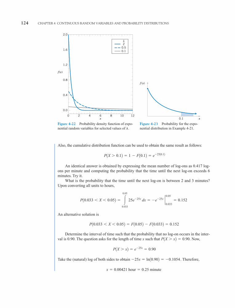
The exponential distribution obtains its name from the exponential function in the proba-bility density function. Plots of the exponential distribution for selected values of are shownin Fig. 4-22. For any value of , the exponential distribution is quite skewed. The followingresults are easily obtained and are left as an exercise.
��
The random variable X that equals the distance between successive counts of aPoisson process with mean is an exponential random variable with parame-ter The probability density function of X is
(4-14)f 1x2 � �e��x for 0 � x � �
�.� � 0
Definition
If the random variable X has an exponential distribution with parameter ,
(4-15)� � E1X 2 �1� and �2 � V1X 2 �
1
�2
�
It is important to use consistent units in the calculation of probabilities, means, and variancesinvolving exponential random variables. The following example illustrates unit conversions.
EXAMPLE 4-21 In a large corporate computer network, user log-ons to the system can be modeled as a Pois-son process with a mean of 25 log-ons per hour. What is the probability that there are no log-ons in an interval of 6 minutes?
Let X denote the time in hours from the start of the interval until the first log-on. Then, Xhas an exponential distribution with log-ons per hour. We are interested in the proba-bility that X exceeds 6 minutes. Because is given in log-ons per hour, we express all timeunits in hours. That is, 6 minutes � 0.1 hour. The probability requested is shown as the shadedarea under the probability density function in Fig. 4-23. Therefore,
P1X � 0.12 � �
�
0.1
25e�25x dx � e�2510.12 � 0.082
�� � 25
c04.qxd 5/10/02 5:19 PM Page 123 RK UL 6 RK UL 6:Desktop Folder:TEMP WORK:MONTGOMERY:REVISES UPLO D CH 1 14 FIN L:Quark Files:
124 CHAPTER 4 CONTINUOUS RANDOM VARIABLES AND PROBABILITY DISTRIBUTIONS
Also, the cumulative distribution function can be used to obtain the same result as follows:
An identical answer is obtained by expressing the mean number of log-ons as 0.417 log-ons per minute and computing the probability that the time until the next log-on exceeds 6minutes. Try it.
What is the probability that the time until the next log-on is between 2 and 3 minutes?Upon converting all units to hours,
An alternative solution is
Determine the interval of time such that the probability that no log-on occurs in the inter-val is 0.90. The question asks for the length of time x such that . Now,
Take the (natural) log of both sides to obtain . Therefore,
x � 0.00421 hour � 0.25 minute
�25x � ln10.902 � �0.1054
P1X � x2 � e�25x � 0.90
P1X � x2 � 0.90
P10.033 � X � 0.052 � F10.052 � F10.0332 � 0.152
P10.033 � X � 0.052 � �0.05
0.033 25e�25x dx � �e�25x ` 0.05
0.033� 0.152
P1X � 0.12 � 1 � F10.12 � e�2510.12
0
0.0
0.4
0.8
1.2
1.6
2.0
2 4 6 8 10 12x
f (x)
20.50.1
λ
Figure 4-22 Probability density function of expo-nential random variables for selected values of .�
0.1 x
f (x)
Figure 4-23 Probability for the expo-nential distribution in Example 4-21.
c04.qxd 5/10/02 5:20 PM Page 124 RK UL 6 RK UL 6:Desktop Folder:TEMP WORK:MONTGOMERY:REVISES UPLO D CH 1 14 FIN L:Quark Files:

4-9 EXPONENTIAL DISTRIBUTION 125
Furthermore, the mean time until the next log-on is
The standard deviation of the time until the next log-on is
In the previous example, the probability that there are no log-ons in a 6-minute interval is0.082 regardless of the starting time of the interval. A Poisson process assumes that events oc-cur uniformly throughout the interval of observation; that is, there is no clustering of events.If the log-ons are well modeled by a Poisson process, the probability that the first log-on afternoon occurs after 12:06 P.M. is the same as the probability that the first log-on after 3:00 P.M.occurs after 3:06 P.M. And if someone logs on at 2:22 P.M., the probability the next log-onoccurs after 2:28 P.M. is still 0.082.
Our starting point for observing the system does not matter. However, if there arehigh-use periods during the day, such as right after 8:00 A.M., followed by a period of lowuse, a Poisson process is not an appropriate model for log-ons and the distribution is notappropriate for computing probabilities. It might be reasonable to model each of the high-and low-use periods by a separate Poisson process, employing a larger value for duringthe high-use periods and a smaller value otherwise. Then, an exponential distribution withthe corresponding value of can be used to calculate log-on probabilities for the high- andlow-use periods.
Lack of Memory PropertyAn even more interesting property of an exponential random variable is concerned with con-ditional probabilities.
EXAMPLE 4-22 Let X denote the time between detections of a particle with a geiger counter and assume thatX has an exponential distribution with minutes. The probability that we detect a par-ticle within 30 seconds of starting the counter is
In this calculation, all units are converted to minutes. Now, suppose we turn on the geigercounter and wait 3 minutes without detecting a particle. What is the probability that a particleis detected in the next 30 seconds?
Because we have already been waiting for 3 minutes, we feel that we are “due.’’ Thatis, the probability of a detection in the next 30 seconds should be greater than 0.3. However,for an exponential distribution, this is not true. The requested probability can be expressedas the conditional probability that From the definition of conditionalprobability,
where
P13 � X � 3.52 � F13.52 � F132 � 31 � e�3.51.4 4 � 31 � e�31.4 4 � 0.0035
P1X � 3.5 ƒ X � 32 � P13 � X � 3.52P1X � 32
P1X � 3.5 ƒ X � 32.
P1X � 0.5 minute2 � F10.52 � 1 � e�0.51.4 � 0.30
� � 1.4
�
�
� � 125 hours � 2.4 minutes
� � 125 � 0.04 hour � 2.4 minutes
c04.qxd 5/10/02 5:20 PM Page 125 RK UL 6 RK UL 6:Desktop Folder:TEMP WORK:MONTGOMERY:REVISES UPLO D CH 1 14 FIN L:Quark Files:
126 CHAPTER 4 CONTINUOUS RANDOM VARIABLES AND PROBABILITY DISTRIBUTIONS
and
Therefore,
After waiting for 3 minutes without a detection, the probability of a detection in the next 30seconds is the same as the probability of a detection in the 30 seconds immediately after start-ing the counter. The fact that you have waited 3 minutes without a detection does not changethe probability of a detection in the next 30 seconds.
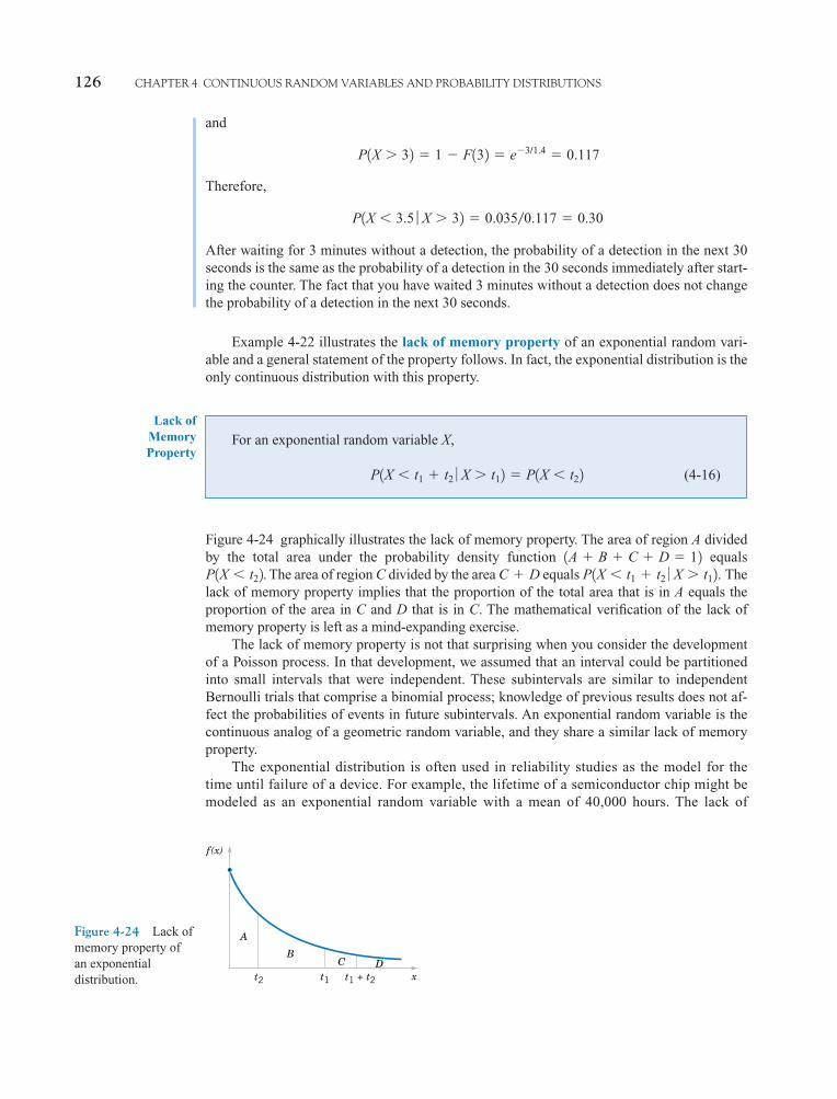
Example 4-22 illustrates the lack of memory property of an exponential random vari-able and a general statement of the property follows. In fact, the exponential distribution is theonly continuous distribution with this property.
P1X � 3.5 ƒ X � 32 � 0.0350.117 � 0.30
P1X � 32 � 1 � F132 � e�3/1.4 � 0.117
For an exponential random variable X,
(4-16)P1X � t1 t2 0 X � t12 � P1X � t22
Lack ofMemoryProperty
Figure 4-24 graphically illustrates the lack of memory property. The area of region A dividedby the total area under the probability density function equals
. The area of region C divided by the area equals Thelack of memory property implies that the proportion of the total area that is in A equals theproportion of the area in C and D that is in C. The mathematical verification of the lack ofmemory property is left as a mind-expanding exercise.
The lack of memory property is not that surprising when you consider the developmentof a Poisson process. In that development, we assumed that an interval could be partitionedinto small intervals that were independent. These subintervals are similar to independentBernoulli trials that comprise a binomial process; knowledge of previous results does not af-fect the probabilities of events in future subintervals. An exponential random variable is thecontinuous analog of a geometric random variable, and they share a similar lack of memoryproperty.
The exponential distribution is often used in reliability studies as the model for thetime until failure of a device. For example, the lifetime of a semiconductor chip might bemodeled as an exponential random variable with a mean of 40,000 hours. The lack of
P1X � t1 t2 0 X � t12.C DP1X � t221A B C D � 12
Figure 4-24 Lack ofmemory property ofan exponentialdistribution. t2 x
C DB
A
t1 t1 + t2
f (x)
c04.qxd 5/10/02 5:20 PM Page 126 RK UL 6 RK UL 6:Desktop Folder:TEMP WORK:MONTGOMERY:REVISES UPLO D CH 1 14 FIN L:Quark Files:
4-9 EXPONENTIAL DISTRIBUTION 127
memory property of the exponential distribution implies that the device does not wear out.That is, regardless of how long the device has been operating, the probability of a failurein the next 1000 hours is the same as the probability of a failure in the first 1000 hours ofoperation. The lifetime L of a device with failures caused by random shocks might be ap-propriately modeled as an exponential random variable. However, the lifetime L of adevice that suffers slow mechanical wear, such as bearing wear, is better modeled by a dis-tribution such that increases with t. Distributions such as the Weibulldistribution are often used, in practice, to model the failure time of this type of device. TheWeibull distribution is presented in a later section.
EXERCISES FOR SECTION 4-9
P1L � t �t 0 L � t2
4-72. Suppose X has an exponential distribution with � � 2.Determine the following:(a) (b)(c) (d)
(e) Find the value of x such that
4-73. Suppose X has an exponential distribution with meanequal to 10. Determine the following:(a)(b)(c)
(d) Find the value of x such that
4-74. Suppose the counts recorded by a geiger counter followa Poisson process with an average of two counts per minute.(a) What is the probability that there are no counts in a 30-
second interval?(b) What is the probability that the first count occurs in less
than 10 seconds?(c) What is the probability that the first count occurs between
1 and 2 minutes after start-up?
4-75. Suppose that the log-ons to a computer network fol-low a Poisson process with an average of 3 counts per minute.(a) What is the mean time between counts?(b) What is the standard deviation of the time between counts?(c) Determine x such that the probability that at least one
count occurs before time x minutes is 0.95.
4-76. The time to failure (in hours) for a laser in a cytome-try machine is modeled by an exponential distribution with
(a) What is the probability that the laser will last at least20,000 hours?
(b) What is the probability that the laser will last at most30,000 hours?
(c) What is the probability that the laser will last between20,000 and 30,000 hours?
4-77. The time between calls to a plumbing supply businessis exponentially distributed with a mean time between calls of15 minutes.(a) What is the probability that there are no calls within a 30-
minute interval?
� � 0.00004.
P1X � x2 � 0.95.
P1X � 302P1X � 202P1X � 102
P1X � x2 � 0.05.
P11 � X � 22P1X � 12P1X � 22P1X � 02
(b) What is the probability that at least one call arrives withina 10-minute interval?
(c) What is the probability that the first call arrives within 5and 10 minutes after opening?
(d) Determine the length of an interval of time such that theprobability of at least one call in the interval is 0.90.
4-78. The life of automobile voltage regulators has an expo-nential distribution with a mean life of six years. You purchasean automobile that is six years old, with a working voltageregulator, and plan to own it for six years.(a) What is the probability that the voltage regulator fails dur-
ing your ownership?(b) If your regulator fails after you own the automobile three
years and it is replaced, what is the mean time until thenext failure?
4-79. The time to failure (in hours) of fans in a personal com-puter can be modeled by an exponential distribution with
(a) What proportion of the fans will last at least 10,000 hours?(b) What proportion of the fans will last at most 7000 hours?
4-80. The time between the arrival of electronic messages atyour computer is exponentially distributed with a mean of twohours.(a) What is the probability that you do not receive a message
during a two-hour period?(b) If you have not had a message in the last four hours, what
is the probability that you do not receive a message in thenext two hours?
(c) What is the expected time between your fifth and sixthmessages?
4-81. The time between arrivals of taxis at a busy intersec-tion is exponentially distributed with a mean of 10 minutes.(a) What is the probability that you wait longer than one hour
for a taxi?(b) Suppose you have already been waiting for one hour for a
taxi, what is the probability that one arrives within thenext 10 minutes?
4-82. Continuation of Exercise 4-81.(a) Determine x such that the probability that you wait more
than x minutes is 0.10.
� � 0.0003.
c04.qxd 5/10/02 5:20 PM Page 127 RK UL 6 RK UL 6:Desktop Folder:TEMP WORK:MONTGOMERY:REVISES UPLO D CH 1 14 FIN L:Quark Files:
128 CHAPTER 4 CONTINUOUS RANDOM VARIABLES AND PROBABILITY DISTRIBUTIONS
(b) Determine x such that the probability that you wait lessthan x minutes is 0.90.
(c) Determine x such that the probability that you wait lessthan x minutes is 0.50.
4-83. The distance between major cracks in a highway fol-lows an exponential distribution with a mean of 5 miles.(a) What is the probability that there are no major cracks in a
10-mile stretch of the highway?(b) What is the probability that there are two major cracks in
a 10-mile stretch of the highway?(c) What is the standard deviation of the distance between
major cracks?
4-84. Continuation of Exercise 4-83.(a) What is the probability that the first major crack occurs
between 12 and 15 miles of the start of inspection?(b) What is the probability that there are no major cracks in
two separate 5-mile stretches of the highway?(c) Given that there are no cracks in the first 5 miles in-
spected, what is the probability that there are no majorcracks in the next 10 miles inspected?
4-85. The lifetime of a mechanical assembly in a vibrationtest is exponentially distributed with a mean of 400 hours.(a) What is the probability that an assembly on test fails in
less than 100 hours?(b) What is the probability that an assembly operates for more
than 500 hours before failure?(c) If an assembly has been on test for 400 hours without a fail-
ure, what is the probability of a failure in the next 100 hours?
4-86. Continuation of Exercise 4-85.(a) If 10 assemblies are tested, what is the probability that at
least one fails in less than 100 hours? Assume that the as-semblies fail independently.
(b) If 10 assemblies are tested, what is the probability that allhave failed by 800 hours? Assume the assemblies failindependently.
4-87. When a bus service reduces fares, a particular tripfrom New York City to Albany, New York, is very popular.A small bus can carry four passengers. The time between callsfor tickets is exponentially distributed with a mean of 30 min-utes. Assume that each call orders one ticket. What is the prob-ability that the bus is filled in less than 3 hours from the timeof the fare reduction?
4-88. The time between arrivals of small aircraft at a countyairport is exponentially distributed with a mean of one hour.What is the probability that more than three aircraft arrivewithin an hour?
4-89. Continuation of Exercise 4-88.(a) If 30 separate one-hour intervals are chosen, what is the
probability that no interval contains more than three arrivals?(b) Determine the length of an interval of time (in hours) such
that the probability that no arrivals occur during the inter-val is 0.10.
4-90. The time between calls to a corporate office is expo-nentially distributed with a mean of 10 minutes.(a) What is the probability that there are more than three calls
in one-half hour?(b) What is the probability that there are no calls within one-
half hour?(c) Determine x such that the probability that there are no
calls within x hours is 0.01.
4-91. Continuation of Exercise 4-90.(a) What is the probability that there are no calls within a two-
hour interval?(b) If four nonoverlapping one-half hour intervals are se-
lected, what is the probability that none of these intervalscontains any call?
(c) Explain the relationship between the results in part (a)and (b).
4-92. If the random variable X has an exponential distribu-tion with mean , determine the following:(a) (b)
(c)(d) How do the results depend on ?
4-93. Assume that the flaws along a magnetic tape follow aPoisson distribution with a mean of 0.2 flaw per meter. Let Xdenote the distance between two successive flaws.(a) What is the mean of X ?(b) What is the probability that there are no flaws in 10 con-
secutive meters of tape?(c) Does your answer to part (b) change if the 10 meters are
not consecutive?(d) How many meters of tape need to be inspected so that the
probability that at least one flaw is found is 90%?
4-94. Continuation of Exercise 4-93. (More diff icult ques-tions.)(a) What is the probability that the first time the distance be-
tween two flaws exceeds 8 meters is at the fifth flaw?(b) What is the mean number of flaws before a distance be-
tween two flaws exceeds 8 meters?
4-95. Derive the formula for the mean and variance of anexponential random variable.
�P1X � 3�2
P1X � 2�2P1X � �2 �
4-10 ERLANG AND GAMMA DISTRIBUTIONS
4-10.1 Erlang Distribution
An exponential random variable describes the length until the first count is obtained in aPoisson process. A generalization of the exponential distribution is the length until r counts
c04.qxd 5/10/02 5:20 PM Page 128 RK UL 6 RK UL 6:Desktop Folder:TEMP WORK:MONTGOMERY:REVISES UPLO D CH 1 14 FIN L:Quark Files:
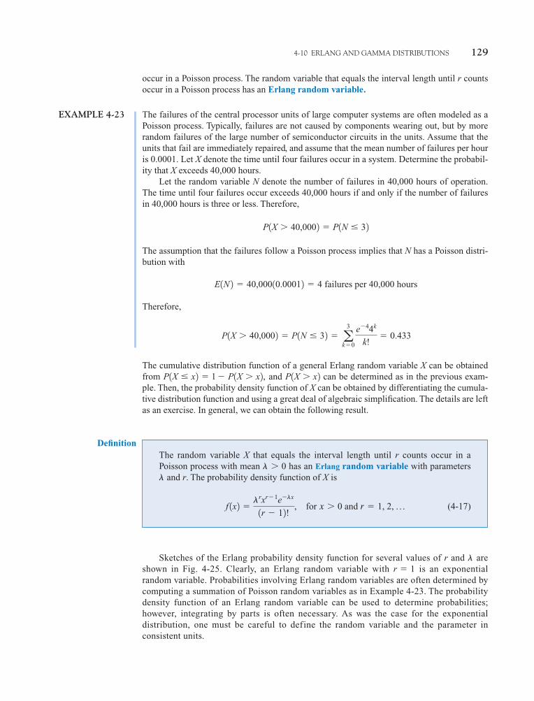
4-10 ERLANG AND GAMMA DISTRIBUTIONS 129
occur in a Poisson process. The random variable that equals the interval length until r countsoccur in a Poisson process has an Erlang random variable.
EXAMPLE 4-23 The failures of the central processor units of large computer systems are often modeled as aPoisson process. Typically, failures are not caused by components wearing out, but by morerandom failures of the large number of semiconductor circuits in the units. Assume that theunits that fail are immediately repaired, and assume that the mean number of failures per houris 0.0001. Let X denote the time until four failures occur in a system. Determine the probabil-ity that X exceeds 40,000 hours.
Let the random variable N denote the number of failures in 40,000 hours of operation.The time until four failures occur exceeds 40,000 hours if and only if the number of failuresin 40,000 hours is three or less. Therefore,
The assumption that the failures follow a Poisson process implies that N has a Poisson distri-bution with
Therefore,
The cumulative distribution function of a general Erlang random variable X can be obtainedfrom and can be determined as in the previous exam-ple. Then, the probability density function of X can be obtained by differentiating the cumula-tive distribution function and using a great deal of algebraic simplification. The details are leftas an exercise. In general, we can obtain the following result.
P1X � x2P1X � x2 � 1 � P1X � x2,
P1X � 40,0002 � P1N � 32 � a3
k�0
e�44k
k!� 0.433
E1N 2 � 40,00010.00012 � 4 failures per 40,000 hours
P1X � 40,0002 � P1N � 32
The random variable X that equals the interval length until r counts occur in aPoisson process with mean has an Erlang random variable with parameters
and r. The probability density function of X is
(4-17)f 1x2 ��rxr�1e��x
1r � 12!, for x � 0 and r � 1, 2, p
�� � 0
Definition
Sketches of the Erlang probability density function for several values of r and areshown in Fig. 4-25. Clearly, an Erlang random variable with is an exponentialrandom variable. Probabilities involving Erlang random variables are often determined bycomputing a summation of Poisson random variables as in Example 4-23. The probabilitydensity function of an Erlang random variable can be used to determine probabilities;however, integrating by parts is often necessary. As was the case for the exponentialdistribution, one must be careful to define the random variable and the parameter inconsistent units.
r � 1�
c04.qxd 5/13/02 11:19 M Page 129 RK UL 6 RK UL 6:Desktop Folder:TEMP WORK:MONTGOMERY:REVISES UPLO D CH 1 14 FIN L:Quark Files:
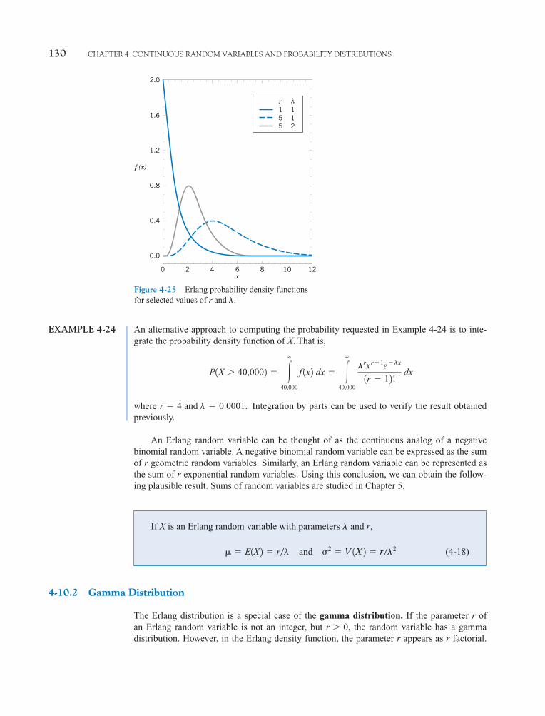
130 CHAPTER 4 CONTINUOUS RANDOM VARIABLES AND PROBABILITY DISTRIBUTIONS
EXAMPLE 4-24 An alternative approach to computing the probability requested in Example 4-24 is to inte-grate the probability density function of X. That is,
where Integration by parts can be used to verify the result obtainedpreviously.
An Erlang random variable can be thought of as the continuous analog of a negativebinomial random variable. A negative binomial random variable can be expressed as the sumof r geometric random variables. Similarly, an Erlang random variable can be represented asthe sum of r exponential random variables. Using this conclusion, we can obtain the follow-ing plausible result. Sums of random variables are studied in Chapter 5.
r � 4 and � � 0.0001.
P1X � 40,0002 � ��
40,000 f 1x2 dx � �
�
40,000
�rxr�1e��x
1r � 12! dx
0
0.0
0.4
0.8
1.2
1.6
2.0
2 4 6 8 10 12x
f (x)
155
112
λr
Figure 4-25 Erlang probability density functionsfor selected values of r and .�
If X is an Erlang random variable with parameters and r,
(4-18)� � E1X 2 � r�� and �2 � V1X2 � r��2
�
4-10.2 Gamma Distribution
The Erlang distribution is a special case of the gamma distribution. If the parameter r ofan Erlang random variable is not an integer, but , the random variable has a gammadistribution. However, in the Erlang density function, the parameter r appears as r factorial.
r � 0
c04.qxd 6/23/02 7:38 PM Page 130 RK UL 6 RK UL 6:Desktop Folder:
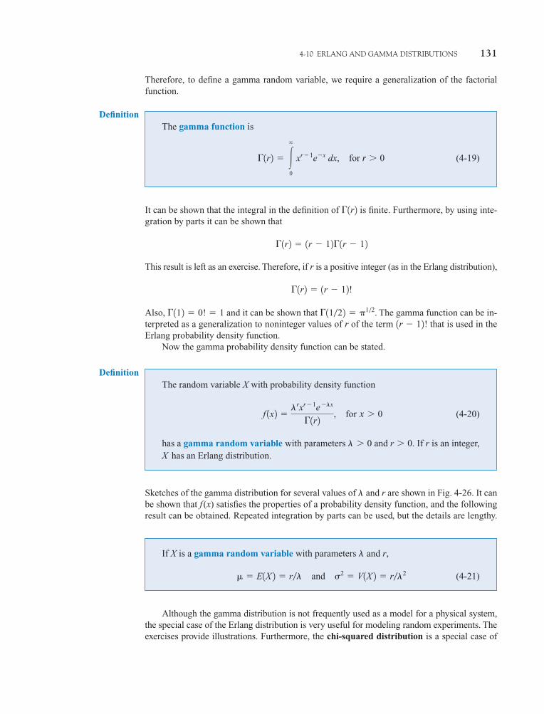
4-10 ERLANG AND GAMMA DISTRIBUTIONS 131
It can be shown that the integral in the definition of is finite. Furthermore, by using inte-gration by parts it can be shown that
This result is left as an exercise. Therefore, if r is a positive integer (as in the Erlang distribution),
Also, and it can be shown that . The gamma function can be in-terpreted as a generalization to noninteger values of r of the term that is used in theErlang probability density function.
Now the gamma probability density function can be stated.
1r � 12!�1122 � 12�112 � 0! � 1
�1r2 � 1r � 12!
�1r2 � 1r � 12�1r � 12
�1r2
Sketches of the gamma distribution for several values of and r are shown in Fig. 4-26. It canbe shown that f(x) satisfies the properties of a probability density function, and the followingresult can be obtained. Repeated integration by parts can be used, but the details are lengthy.
�
Although the gamma distribution is not frequently used as a model for a physical system,the special case of the Erlang distribution is very useful for modeling random experiments. Theexercises provide illustrations. Furthermore, the chi-squared distribution is a special case of
The gamma function is
(4-19)�1r2 � ��
0 xr�1e�x dx, for r � 0
Definition
The random variable X with probability density function
(4-20)
has a gamma random variable with parameters . If r is an integer,X has an Erlang distribution.
� � 0 and r � 0
f 1x2 ��rxr�1e
��x
�1r2 , for x � 0
Definition
If X is a gamma random variable with parameters and r,
(4-21)� � E1X 2 � r� and �2 � V1X 2 � r�2
�
Therefore, to define a gamma random variable, we require a generalization of the factorialfunction.
c04.qxd 5/10/02 5:20 PM Page 131 RK UL 6 RK UL 6:Desktop Folder:TEMP WORK:MONTGOMERY:REVISES UPLO D CH 1 14 FIN L:Quark Files:
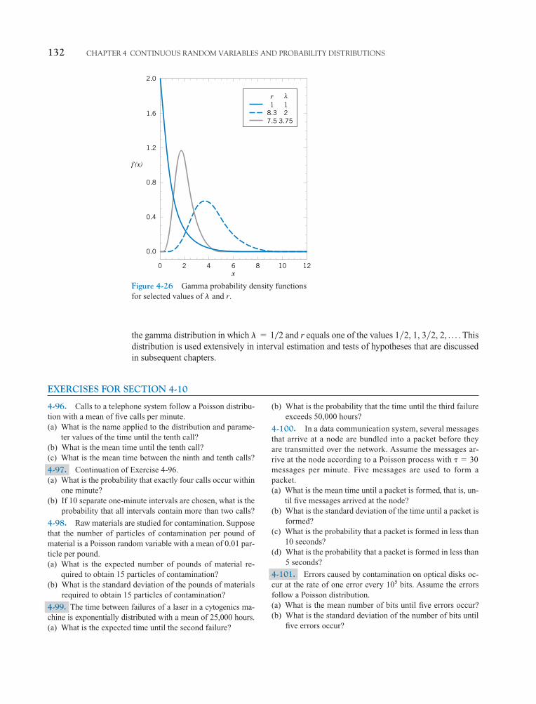
132 CHAPTER 4 CONTINUOUS RANDOM VARIABLES AND PROBABILITY DISTRIBUTIONS
the gamma distribution in which and r equals one of the values 1�2, 1, 3�2, 2, p . Thisdistribution is used extensively in interval estimation and tests of hypotheses that are discussedin subsequent chapters.
EXERCISES FOR SECTION 4-10
� � 12
Figure 4-26 Gamma probability density functionsfor selected values of and r.�
0
0.0
0.4
0.8
1.2
1.6
2.0
2 4 6 8 10 12x
18.37.5
12
3.75
λr
f (x)
4-96. Calls to a telephone system follow a Poisson distribu-tion with a mean of five calls per minute.(a) What is the name applied to the distribution and parame-
ter values of the time until the tenth call?(b) What is the mean time until the tenth call?(c) What is the mean time between the ninth and tenth calls?
4-97. Continuation of Exercise 4-96.(a) What is the probability that exactly four calls occur within
one minute?(b) If 10 separate one-minute intervals are chosen, what is the
probability that all intervals contain more than two calls?
4-98. Raw materials are studied for contamination. Supposethat the number of particles of contamination per pound ofmaterial is a Poisson random variable with a mean of 0.01 par-ticle per pound.(a) What is the expected number of pounds of material re-
quired to obtain 15 particles of contamination?(b) What is the standard deviation of the pounds of materials
required to obtain 15 particles of contamination?
4-99. The time between failures of a laser in a cytogenics ma-chine is exponentially distributed with a mean of 25,000 hours.(a) What is the expected time until the second failure?
(b) What is the probability that the time until the third failureexceeds 50,000 hours?
4-100. In a data communication system, several messagesthat arrive at a node are bundled into a packet before theyare transmitted over the network. Assume the messages ar-rive at the node according to a Poisson process with messages per minute. Five messages are used to form apacket.(a) What is the mean time until a packet is formed, that is, un-
til five messages arrived at the node?(b) What is the standard deviation of the time until a packet is
formed?(c) What is the probability that a packet is formed in less than
10 seconds?(d) What is the probability that a packet is formed in less than
5 seconds?
4-101. Errors caused by contamination on optical disks oc-cur at the rate of one error every bits. Assume the errorsfollow a Poisson distribution.(a) What is the mean number of bits until five errors occur?(b) What is the standard deviation of the number of bits until
five errors occur?
105
� � 30
c04.qxd 5/10/02 5:20 PM Page 132 RK UL 6 RK UL 6:Desktop Folder:TEMP WORK:MONTGOMERY:REVISES UPLO D CH 1 14 FIN L:Quark Files:
4-11 WEIBULL DISTRIBUTION 133
(c) The error-correcting code might be ineffective if there arethree or more errors within bits. What is the probabil-ity of this event?
4-102. Calls to the help line of a large computer distributorfollow a Possion distribution with a mean of 20 calls per minute.(a) What is the mean time until the one-hundredth call?(b) What is the mean time between call numbers 50 and 80?(c) What is the probability that three or more calls occur
within 15 seconds?
4-103. The time between arrivals of customers at an auto-matic teller machine is an exponential random variable with amean of 5 minutes.(a) What is the probability that more than three customers
arrive in 10 minutes?(b) What is the probability that the time until the fifth cus-
tomer arrives is less than 15 minutes?
1054-104. The time between process problems in a manufac-turing line is exponentially distributed with a mean of 30 days.(a) What is the expected time until the fourth problem?(b) What is the probability that the time until the fourth prob-
lem exceeds 120 days?
4-105. Use the properties of the gamma function to evaluatethe following:(a) (b)(c)
4-106. Use integration by parts to show that
4-107. Show that the gamma density function in-tegrates to 1.
4-108. Use the result for the gamma distribution to determinethe mean and variance of a chi-square distribution with r � 7�2.
f 1x, �, r2�1r � 12.
�1r2 � 1r � 12�19�22
�15�22�162
4-11 WEIBULL DISTRIBUTION
As mentioned previously, the Weibull distribution is often used to model the time until failureof many different physical systems. The parameters in the distribution provide a great deal offlexibility to model systems in which the number of failures increases with time (bearingwear), decreases with time (some semiconductors), or remains constant with time (failurescaused by external shocks to the system).
The flexibility of the Weibull distribution is illustrated by the graphs of selected probabilitydensity functions in Fig. 4-27. By inspecting the probability density function, it is seen thatwhen , the Weibull distribution is identical to the exponential distribution.
The cumulative distribution function is often used to compute probabilities. The follow-ing result can be obtained.
� � 1
The random variable X with probability density function
(4-22)
is a Weibull random variable with scale parameter and shape parameter � � 0.� � 0
f 1x2 ��
� ax
�b��1
exp c�ax
�b� d , for x � 0
Definition
If X has a Weibull distribution with parameters and , then the cumulative distri-bution function of X is
(4-23)F1x2 � 1 � e�ax
�b�
��
c04.qxd 5/13/02 11:19 M Page 133 RK UL 6 RK UL 6:Desktop Folder:TEMP WORK:MONTGOMERY:REVISES UPLO D CH 1 14 FIN L:Quark Files:
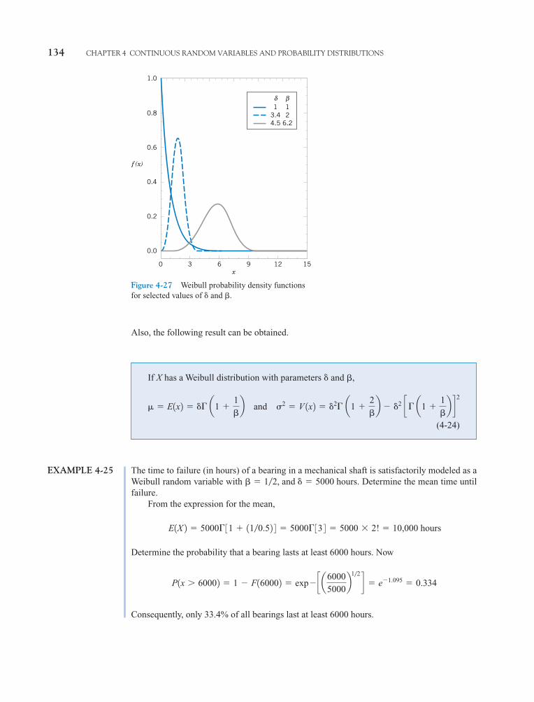
Also, the following result can be obtained.
134 CHAPTER 4 CONTINUOUS RANDOM VARIABLES AND PROBABILITY DISTRIBUTIONS
If X has a Weibull distribution with parameters and ,
(4-24)
� E1x2 � �� a1 1�b and �2 � V 1x2 � �2�
a1 2�b � �2 c�
a1 1�b d 2
��
EXAMPLE 4-25 The time to failure (in hours) of a bearing in a mechanical shaft is satisfactorily modeled as aWeibull random variable with Determine the mean time untilfailure.
From the expression for the mean,
Determine the probability that a bearing lasts at least 6000 hours. Now
Consequently, only 33.4% of all bearings last at least 6000 hours.
P1x � 60002 � 1 � F160002 � exp� c a60005000
b1�2 d � e�1.095 � 0.334
E1X 2 � 5000� 31 11�0.52 4 � 5000� 33 4 � 5000 � 2! � 10,000 hours
� � 1�2, and � � 5000 hours.
Figure 4-27 Weibull probability density functionsfor selected values of and .��
0
0.0
0.2
0.4
0.6
0.8
1.0
3 6 9 12 15x
f (x)
13.44.5
12
6.2
βδ
c04.qxd 5/13/02 11:19 M Page 134 RK UL 6 RK UL 6:Desktop Folder:TEMP WORK:MONTGOMERY:REVISES UPLO D CH 1 14 FIN L:Quark Files:
4-12 LOGNORMAL DISTRIBUTION 135
4-109. Suppose that X has a Weibull distribution withand hours. Determine the mean and vari-
ance of X.
4-110. Suppose that X has a Weibull distribution and hours. Determine the following:(a) (b)
4-111. Assume that the life of a roller bearing follows aWeibull distribution with parameters and hours.(a) Determine the probability that a bearing lasts at least 8000
hours.(b) Determine the mean time until failure of a bearing.(c) If 10 bearings are in use and failures occur independently,
what is the probability that all 10 bearings last at least8000 hours?
4-112. The life (in hours) of a computer processing unit(CPU) is modeled by a Weibull distribution with parameters
and hours.(a) Determine the mean life of the CPU.(b) Determine the variance of the life of the CPU.(c) What is the probability that the CPU fails before 500
hours?
� � 900� � 3
� � 10,000� � 2
P1X � 50002P1X � 10,0002� � 100
� � 0.2
� � 100� � 0.24-113. Assume the life of a packaged magnetic disk exposedto corrosive gases has a Weibull distribution with andthe mean life is 600 hours.(a) Determine the probability that a packaged disk lasts at
least 500 hours.(b) Determine the probability that a packaged disk fails be-
fore 400 hours.
4-114. The life of a recirculating pump follows a Weibulldistribution with parameters , and hours.(a) Determine the mean life of a pump.(b) Determine the variance of the life of a pump.(c) What is the probability that a pump will last longer than its
mean?
4-115. The life (in hours) of a magnetic resonance imagin-ing machine (MRI) is modeled by a Weibull distribution withparameters and hours.(a) Determine the mean life of the MRI.(b) Determine the variance of the life of the MRI.(c) What is the probability that the MRI fails before 250 hours?
4-116. If X is a Weibull random variable with � � 1, and� � 1000, what is another name for the distribution of X andwhat is the mean of X ?
� � 500� � 2
� � 700� � 2
� � 0.5
4-12 LOGNORMAL DISTRIBUTION
Variables in a system sometimes follow an exponential relationship as . If theexponent is a random variable, say is a random variable and the distribu-tion of X is of interest. An important special case occurs when W has a normal distribution.In that case, the distribution of X is called a lognormal distribution. The name followsfrom the transformation ln . That is, the natural logarithm of X is normally dis-tributed.
Probabilities for X are obtained from the transformation to W, but we need to recognizethat the range of X is . Suppose that W is normally distributed with mean and variance
; then the cumulative distribution function for X is
for , where Z is a standard normal random variable. Therefore, Appendix Table II can beused to determine the probability. Also,
The probability density function of X can be obtained from the derivative of F(x).This derivative is applied to the last term in the expression for F(x), the integral of the stan-dard normal density function. Furthermore, from the probability density function, themean and variance of X can be derived. The details are omitted, but a summary of resultsfollows.
F1x2 � 0, for x � 0.x � 0
� P cZ �ln 1x2 � �
� d � � c ln 1x2 � �� d
F1x2 � P 3X � x 4 � P 3exp1W 2 � x 4 � P 3W � ln 1x2 4�2
�10, �2
1X 2 � W
W, X � exp 1W 2 x � exp1w2
EXERCISES FOR SECTION 4-11
c04.qxd 5/10/02 5:20 PM Page 135 RK UL 6 RK UL 6:Desktop Folder:TEMP WORK:MONTGOMERY:REVISES UPLO D CH 1 14 FIN L:Quark Files:
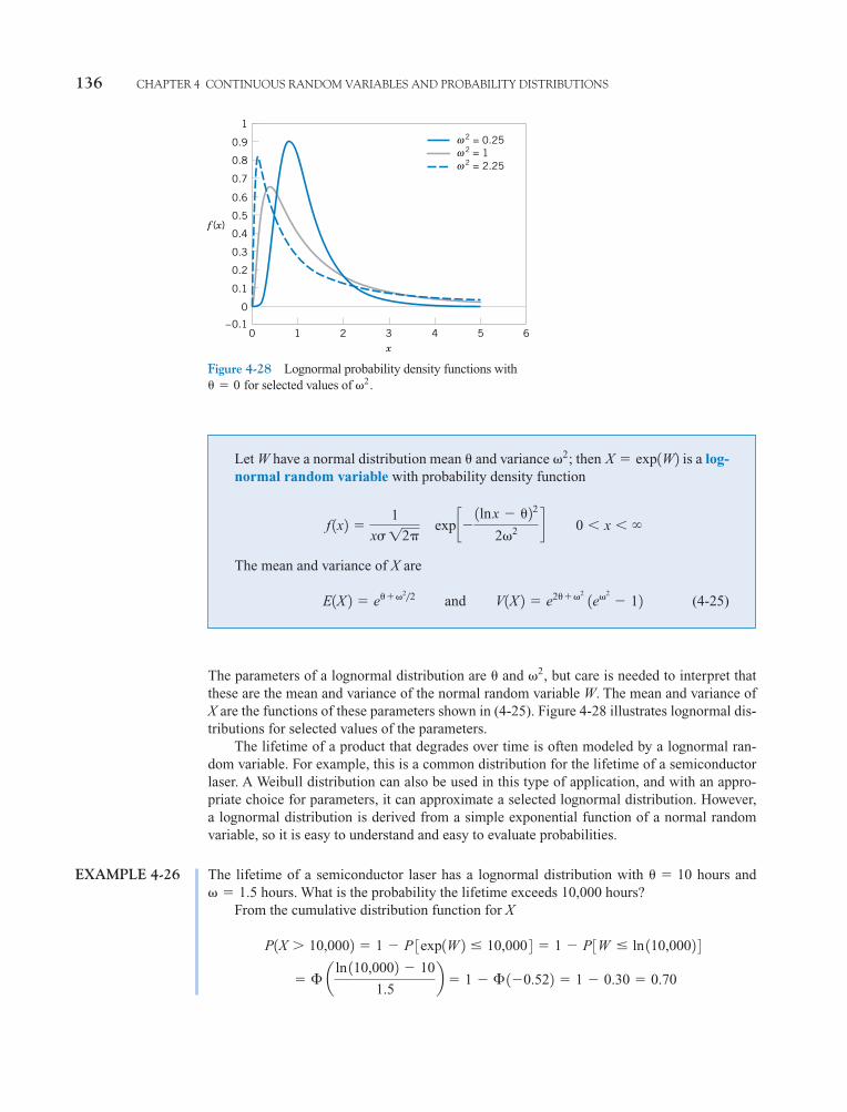
136 CHAPTER 4 CONTINUOUS RANDOM VARIABLES AND PROBABILITY DISTRIBUTIONS
The parameters of a lognormal distribution are and , but care is needed to interpret thatthese are the mean and variance of the normal random variable W. The mean and variance ofX are the functions of these parameters shown in (4-25). Figure 4-28 illustrates lognormal dis-tributions for selected values of the parameters.
The lifetime of a product that degrades over time is often modeled by a lognormal ran-dom variable. For example, this is a common distribution for the lifetime of a semiconductorlaser. A Weibull distribution can also be used in this type of application, and with an appro-priate choice for parameters, it can approximate a selected lognormal distribution. However,a lognormal distribution is derived from a simple exponential function of a normal randomvariable, so it is easy to understand and easy to evaluate probabilities.
EXAMPLE 4-26 The lifetime of a semiconductor laser has a lognormal distribution with hours andhours. What is the probability the lifetime exceeds 10,000 hours?
From the cumulative distribution function for X
� � a ln 110,0002 � 10
1.5b � 1 � � 1�0.522 � 1 � 0.30 � 0.70
P1X � 10,0002 � 1 � P 3exp 1W 2 � 10,000 4 � 1 � P 3W � ln 110,0002 4
� � 1.5� � 10
�2�
Let W have a normal distribution mean and variance ; then is a log-normal random variable with probability density function
The mean and variance of X are
(4-25)E1X 2 � e��22 and V1X 2 � e2��2
1e�2
� 12
f 1x2 �1
x� 12 exp c� 1ln x � �22
2�2 d 0 � x � �
X � exp1W2�2�
–0.1
0
0.1
0.2
0.3
0.4
0.5
0.6
0.7
0.8
0.9
1
0 1 2 3 4 5 6
f (x)
x
2 = 0.252 = 12 = 2.25ω
ωω
Figure 4-28 Lognormal probability density functions withfor selected values of .�2� � 0
c04.qxd 5/10/02 5:20 PM Page 136 RK UL 6 RK UL 6:Desktop Folder:TEMP WORK:MONTGOMERY:REVISES UPLO D CH 1 14 FIN L:Quark Files:
4-12 LOGNORMAL DISTRIBUTION 137
What lifetime is exceeded by 99% of lasers? The question is to determine x such that. Therefore,
From Appendix Table II, when . Therefore,
Determine the mean and standard deviation of lifetime. Now,
so the standard deviation of X is 197,661.5 hours. Notice that the standard deviation of life-time is large relative to the mean.
EXERCISES FOR SECTION 4-12
V1X 2 � e2��21e�2
� 12 � exp 120 2.252 3exp 12.252 � 1 4 � 39,070,059,886.6
E1X 2 � e��22 � exp 110 1.1252 � 67,846.3
ln 1x2 � 10
1.5� �2.33 and x � exp 16.5052 � 668.48 hours.
z � �2.33 1 � �1z2 � 0.99
P1X � x2 � P 3exp 1W 2 � x 4 � P 3W � ln 1x2 4 � 1 � � a ln 1x2 � 10
1.5b � 0.99
P1X � x2 � 0.99
4-117. Suppose that X has a lognormal distribution withparameters and . Determine the following:(a)(b) The value for x such that (c) The mean and variance of X
4-118. Suppose that X has a lognormal distribution withparameters and . Determine the following:(a)(b) The value for x such that (c) The mean and variance of X
4-119. Suppose that X has a lognormal distribution with pa-rameters and . Determine the following:(a)(b) The conditional probability that given that
(c) What does the difference between the probabilities inparts (a) and (b) imply about lifetimes of lognormal ran-dom variables?
4-120. The length of time (in seconds) that a user views apage on a Web site before moving to another page is a lognor-mal random variable with parameters and .(a) What is the probability that a page is viewed for more than
10 seconds?(b) What is the length of time that 50% of users view the page?(c) What is the mean and standard deviation of the time until
a user moves from the page?
4-121. Suppose that X has a lognormal distribution and thatthe mean and variance of X are 100 and 85,000, respectively.
�2 � 1� � 0.5
X � 1000X � 1500
P1X � 5002�2 � 4� � 2
P1X � x2 � 0.1P1500 � X � 10002
�2 � 9� � �2
P1X � x2 � 0.95P1X � 13,3002
�2 � 9� � 5Determine the parameters and of the lognormal distribu-tion. (Hint: define and and write twoequations in terms of x and y.)
4-122. The lifetime of a semiconductor laser has a log-normal distribution, and it is known that the mean and stan-dard deviation of lifetime are 10,000 and 20,000, respec-tively.(a) Calculate the parameters of the lognormal distribution(b) Determine the probability that a lifetime exceeds 10,000
hours(c) Determine the lifetime that is exceeded by 90% of lasers
4-123. Derive the probability density function of a lognor-mal random variable from the derivative of the cumulativedistribution function.
Supplemental Exercises
4-124. Suppose that for Determine the following:(a)(b)
(c)
4-125. Continuation of Exercise 4-124. Determine thecumulative distribution function of the random variable.
4-126. Continuation of Exercise 4-124. Determine themean and variance of the random variable.
P12.5 � X � 3.52P1X � 32P1X � 2.52
2 � x � 4.f 1x2 � 0.5x � 1
y � exp 1�22x � exp 1�2 �2�
c04.qxd 5/10/02 5:20 PM Page 137 RK UL 6 RK UL 6:Desktop Folder:TEMP WORK:MONTGOMERY:REVISES UPLO D CH 1 14 FIN L:Quark Files:
138 CHAPTER 4 CONTINUOUS RANDOM VARIABLES AND PROBABILITY DISTRIBUTIONS
4-127. The time between calls is exponentially distributedwith a mean time between calls of 10 minutes.(a) What is the probability that the time until the first call is
less than 5 minutes?(b) What is the probability that the time until the first call is
between 5 and 15 minutes?(c) Determine the length of an interval of time such that the
probability of at least one call in the interval is 0.90.
4-128. Continuation of Exercise 4-127.(a) If there has not been a call in 10 minutes, what is the proba-
bility that the time until the next call is less than 5 minutes?(b) What is the probability that there are no calls in the inter-
vals from 10:00 to 10:05, from 11:30 to 11:35, and from2:00 to 2:05?
4-129. Continuation of Exercise 4-127.(a) What is the probability that the time until the third call is
greater than 30 minutes?(b) What is the mean time until the fifth call?
4-130. The CPU of a personal computer has a lifetime thatis exponentially distributed with a mean lifetime of six years.You have owned this CPU for three years. What is the proba-bility that the CPU fails in the next three years?
4-131. Continuation of Exercise 4-130. Assume that yourcorporation has owned 10 CPUs for three years, and assumethat the CPUs fail independently. What is the probability thatat least one fails within the next three years?
4-132. Suppose that X has a lognormal distribution withparameters and . Determine the following:(a)(b) The value for x such that (c) The mean and variance of X
4-133. Suppose that X has a lognormal distribution and thatthe mean and variance of X are 50 and 4000, respectively.Determine the following:
(a) The parameters and of the lognormal distribution(b) The probability that X is less than 150
4-134. Asbestos fibers in a dust sample are identified by anelectron microscope after sample preparation. Suppose thatthe number of fibers is a Poisson random variable and themean number of fibers per squared centimeter of surface dustis 100. A sample of 800 square centimeters of dust is analyzed.Assume a particular grid cell under the microscope represents1/160,000 of the sample.(a) What is the probability that at least one fiber is visible in
the grid cell?(b) What is the mean of the number of grid cells that need to
be viewed to observe 10 that contain fibers?(c) What is the standard deviation of the number of grid cells
that need to be viewed to observe 10 that contain fibers?
4-135. Without an automated irrigation system, the heightof plants two weeks after germination is normally distributedwith a mean of 2.5 centimeters and a standard deviation of 0.5centimeters.
�2�
P1X � x2 � 0.05P110 � X � 502
�2 � 4� � 0
(a) What is the probability that a plant’s height is greater than2.25 centimeters?
(b) What is the probability that a plant’s height is between 2.0and 3.0 centimeters?
(c) What height is exceeded by 90% of the plants?
4-136. Continuation of Exercise 4-135. With an automatedirrigation system, a plant grows to a height of 3.5 centimeterstwo weeks after germination.(a) What is the probability of obtaining a plant of this height or
greater from the distribution of heights in Exercise 4-135.(b) Do you think the automated irrigation system increases
the plant height at two weeks after germination?
4-137. The thickness of a laminated covering for a woodsurface is normally distributed with a mean of 5 millimetersand a standard deviation of 0.2 millimeter.(a) What is the probability that a covering thickness is greater
than 5.5 millimeters?(b) If the specifications require the thickness to be between
4.5 and 5.5 millimeters, what proportion of coverings donot meet specifications?
(c) The covering thickness of 95% of samples is below whatvalue?
4-138. The diameter of the dot produced by a printer is nor-mally distributed with a mean diameter of 0.002 inch.Suppose that the specifications require the dot diameter to bebetween 0.0014 and 0.0026 inch. If the probability that a dotmeets specifications is to be 0.9973, what standard deviationis needed?
4-139. Continuation of Exercise 4-138. Assume that the stan-dard deviation of the size of a dot is 0.0004 inch. If the proba-bility that a dot meets specifications is to be 0.9973, what spec-ifications are needed? Assume that the specifications are to bechosen symmetrically around the mean of 0.002.
4-140. The life of a semiconductor laser at a constant poweris normally distributed with a mean of 7000 hours and a stan-dard deviation of 600 hours.(a) What is the probability that a laser fails before 5,800
hours?(b) What is the life in hours that 90% of the lasers exceed?
4-141. Continuation of Exercise 4-140. What should themean life equal in order for 99% of the lasers to exceed 10,000hours before failure?
4-142. Continuation of Exercise 4-140. A product containsthree lasers, and the product fails if any of the lasers fails.Assume the lasers fail independently. What should the meanlife equal in order for 99% of the products to exceed 10,000hours before failure?
4-143. Continuation of Exercise 140. Rework parts (a) and(b). Assume that the lifetime is an exponential random vari-able with the same mean.
4-144. Continuation of Exercise 4-140. Rework parts (a)and (b). Assume that the lifetime is a lognormal random vari-able with the same mean and standard deviation.
c04.qxd 5/10/02 5:20 PM Page 138 RK UL 6 RK UL 6:Desktop Folder:TEMP WORK:MONTGOMERY:REVISES UPLO D CH 1 14 FIN L:Quark Files:
4-12 LOGNORMAL DISTRIBUTION 139
4-145. A square inch of carpeting contains 50 carpet fibers.The probability of a damaged fiber is 0.0001. Assume thedamaged fibers occur independently.(a) Approximate the probability of one or more damaged
fibers in 1 square yard of carpeting.(b) Approximate the probability of four or more damaged
fibers in 1 square yard of carpeting.
4-146. An airline makes 200 reservations for a flight thatholds 185 passengers. The probability that a passenger arrives
for the flight is 0.9 and the passengers are assumed to be inde-pendent.(a) Approximate the probability that all the passengers that
arrive can be seated.(b) Approximate the probability that there are empty seats.(c) Approximate the number of reservations that the airline
should make so that the probability that everyone who ar-rives can be seated is 0.95. [Hint: Successively try valuesfor the number of reservations.]
4-147. The steps in this exercise lead to the probabil-ity density function of an Erlang random variable X withparameters and
(a) Use the Poisson distribution to express .(b) Use the result from part (a) to determine the cumu-
lative distribution function of X.(c) Differentiate the cumulative distribution function in
part (b) and simplify to obtain the probability den-sity function of X.
4-148. A bearing assembly contains 10 bearings. Thebearing diameters are assumed to be independent andnormally distributed with a mean of 1.5 millimeters anda standard deviation of 0.025 millimeter. What is theprobability that the maximum diameter bearing in theassembly exceeds 1.6 millimeters?
4-149. Let the random variable X denote a measure-ment from a manufactured product. Suppose the targetvalue for the measurement is m. For example, X coulddenote a dimensional length, and the target might be 10millimeters. The quality loss of the process producingthe product is defined to be the expected value of
, where k is a constant that relates a devia-tion from target to a loss measured in dollars.(a) Suppose X is a continuous random variable with
and . What is the quality lossof the process?
(b) Suppose X is a continuous random variable withand . What is the quality loss
of the process?
4-150. The lifetime of an electronic amplifier is mod-eled as an exponential random variable. If 10% of the
amplifiers have a mean of 20,000 hours and the remain-ing amplifiers have a mean of 50,000 hours, what pro-portion of the amplifiers fail before 60,000 hours?
4-151. Lack of Memory Property. Show that foran exponential random variable X,
4-152. A process is said to be of six-sigma quality ifthe process mean is at least six standard deviations fromthe nearest specification. Assume a normally distributedmeasurement.(a) If a process mean is centered between the upper and
lower specifications at a distance of six standard de-viations from each, what is the probability that aproduct does not meet specifications? Using theresult that 0.000001 equals one part per million,express the answer in parts per million.
(b) Because it is difficult to maintain a process meancentered between the specifications, the probabilityof a product not meeting specifications is often cal-culated after assuming the process shifts. If theprocess mean positioned as in part (a) shifts upwardby 1.5 standard deviations, what is the probabilitythat a product does not meet specifications? Expressthe answer in parts per million.
(c) Rework part (a). Assume that the process mean isat a distance of three standard deviations.
(d) Rework part (b). Assume that the process mean is ata distance of three standard deviations and thenshifts upward by 1.5 standard deviations.
(e) Compare the results in parts (b) and (d) and comment.
X � t12 � P1X � t22P1X � t1 t2 0
V1X2 � �2E1X2 � �
V1X2 � �2E1X2 � m
$k1X � m22
P1X � x2r � 1, 2, p .
r, f 1x2 � �rxr�1e��x 1r � 12!, x � 0,�
MIND-EXPANDING EXERCISES
c04.qxd 5/10/02 5:20 PM Page 139 RK UL 6 RK UL 6:Desktop Folder:TEMP WORK:MONTGOMERY:REVISES UPLO D CH 1 14 FIN L:Quark Files:

140 CHAPTER 4 CONTINUOUS RANDOM VARIABLES AND PROBABILITY DISTRIBUTIONS
In the E-book, click on anyterm or concept below togo to that subject.
Chi-squared distribution
Continuous uniformdistribution
Cumulative probabilitydistribution function-continuous randomvariable
Erlang distributionExponential distribution
Gamma distributionLack of memory
property-continuousrandom variable
Lognormal distribution
Mean-continuousrandom variable
Mean-function of acontinuous randomvariable
Normal approximation tobinomial and Poissonprobabilities
Normal distributionProbability density
functionProbability distribution-
continuous randomvariable
Standard deviation-continuous randomvariable
Standard normaldistribution
StandardizingVariance-continuous
random variableWeibull distribution
CD MATERIALContinuity correction
IMPORTANT TERMS AND CONCEPTS
c04.qxd 5/10/02 5:20 PM Page 140 RK UL 6 RK UL 6:Desktop Folder:TEMP WORK:MONTGOMERY:REVISES UPLO D CH 1 14 FIN L:Quark Files:
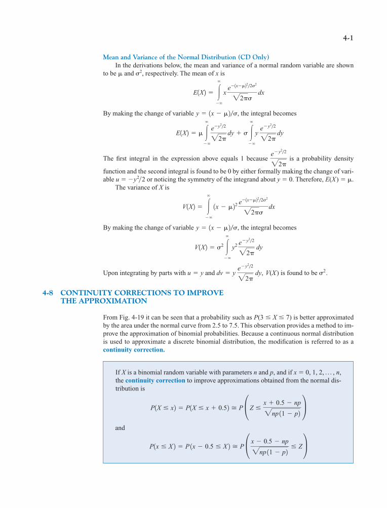
4-1
Mean and Variance of the Normal Distribution (CD Only)In the derivations below, the mean and variance of a normal random variable are shown
to be � and �2, respectively. The mean of x is
By making the change of variable , the integral becomes
The first integral in the expression above equals 1 because is a probability density
function and the second integral is found to be 0 by either formally making the change of vari-able u � �y2�2 or noticing the symmetry of the integrand about y � 0. Therefore, E(X) � �.
The variance of X is
By making the change of variable , the integral becomes
Upon integrating by parts with and V(X) is found to be .
4-8 CONTINUITY CORRECTIONS TO IMPROVETHE APPROXIMATION
From Fig. 4-19 it can be seen that a probability such as P(3 � X � 7) is better approximatedby the area under the normal curve from 2.5 to 7.5. This observation provides a method to im-prove the approximation of binomial probabilities. Because a continuous normal distributionis used to approximate a discrete binomial distribution, the modification is referred to as acontinuity correction.
�2dv � y e�y2�222�
dy,u � y
V1X2 � �2 �
� y2
e�y2�222�
dy
y � 1x � �2��V1X2 � �
� 1x � �22
e�1x��22�2�222�� dx
e�y2�222�
E1X2 � � �
�
e�y2�222� dy � �
�
y e�y2�222�
dy
y � 1x � �2��E1X2 � �
�
x e�1x��22�2�222��
dx
If X is a binomial random variable with parameters n and p, and if x � 0, 1, 2, p , n,the continuity correction to improve approximations obtained from the normal dis-tribution is
and
P1x � X 2 � P 1x � 0.5 � X 2 � P ° x � 0.5 � np2np 11 � p2 � Z¢
P1X � x2 � P1X � x 0.52 � P °Z �x 0.5 � np2np 11 � p2 ¢
PQ220 6234F.CD(04) 5/13/02 11:55 M Page 1 RK UL 6 RK UL 6:Desktop Folder:TEMP WORK:MONTGOMERY:REVISES UPLO D CH 1 14 FIN L:Quark
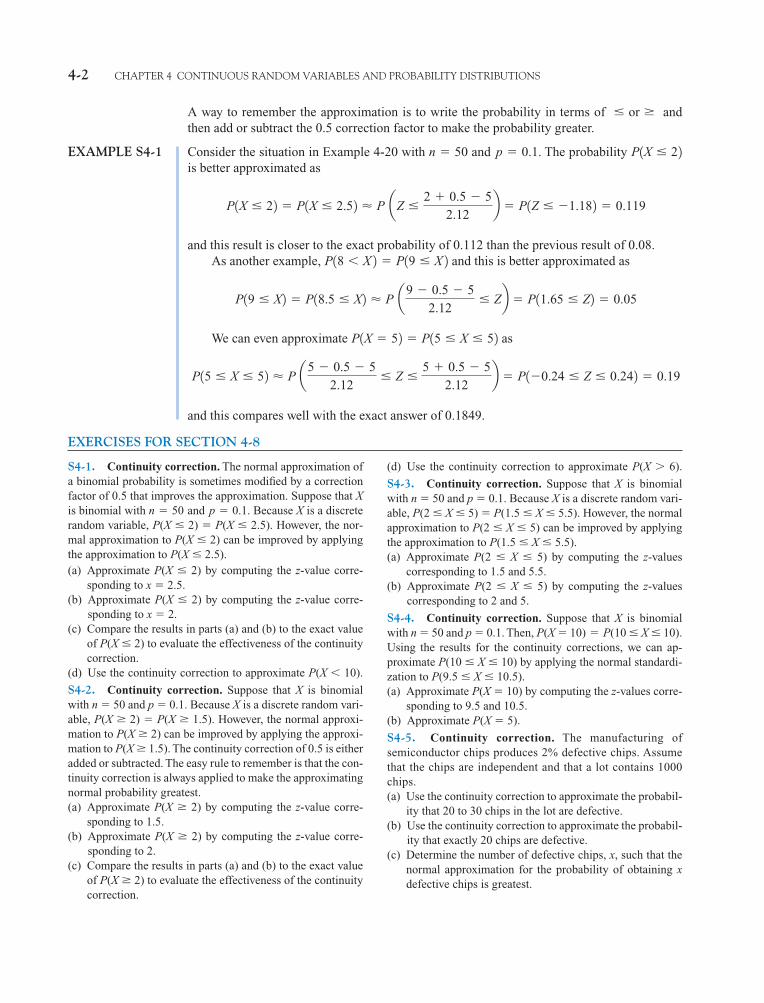
4-2 CHAPTER 4 CONTINUOUS RANDOM VARIABLES AND PROBABILITY DISTRIBUTIONS
A way to remember the approximation is to write the probability in terms of andthen add or subtract the 0.5 correction factor to make the probability greater.
EXAMPLE S4-1 Consider the situation in Example 4-20 with and . The probability is better approximated as
and this result is closer to the exact probability of 0.112 than the previous result of 0.08.As another example, and this is better approximated as
We can even approximate as
and this compares well with the exact answer of 0.1849.
EXERCISES FOR SECTION 4-8
P15 � X � 52 � P a5 � 0.5 � 52.12
� Z �5 0.5 � 5
2.12b � P1�0.24 � Z � 0.242 � 0.19
P1X � 52 � P15 � X � 52P19 � X2 � P18.5 � X2 � P a9 � 0.5 � 5
2.12� Zb � P11.65 � Z2 � 0.05
P18 � X 2 � P19 � X 2
P1X � 22 � P1X � 2.52 � P aZ �2 0.5 � 5
2.12b � P1Z � �1.182 � 0.119
P1X � 22p � 0.1n � 50
� or �
S4-1. Continuity correction. The normal approximation ofa binomial probability is sometimes modified by a correctionfactor of 0.5 that improves the approximation. Suppose that Xis binomial with and . Because X is a discreterandom variable, P(X � 2) � P(X � 2.5). However, the nor-mal approximation to P(X � 2) can be improved by applyingthe approximation to P(X � 2.5).(a) Approximate P(X � 2) by computing the z-value corre-
sponding to x � 2.5.(b) Approximate P(X � 2) by computing the z-value corre-
sponding to x � 2.(c) Compare the results in parts (a) and (b) to the exact value
of P(X � 2) to evaluate the effectiveness of the continuitycorrection.
(d) Use the continuity correction to approximate P(X � 10).
S4-2. Continuity correction. Suppose that X is binomialwith n � 50 and p � 0.1. Because X is a discrete random vari-able, P(X � 2) � P(X � 1.5). However, the normal approxi-mation to P(X � 2) can be improved by applying the approxi-mation to P(X � 1.5). The continuity correction of 0.5 is eitheradded or subtracted. The easy rule to remember is that the con-tinuity correction is always applied to make the approximatingnormal probability greatest.(a) Approximate P(X � 2) by computing the z-value corre-
sponding to 1.5.(b) Approximate P(X � 2) by computing the z-value corre-
sponding to 2.(c) Compare the results in parts (a) and (b) to the exact value
of P(X � 2) to evaluate the effectiveness of the continuitycorrection.
p � 0.1n � 50
(d) Use the continuity correction to approximate P(X 6).
S4-3. Continuity correction. Suppose that X is binomialwith n � 50 and p � 0.1. Because X is a discrete random vari-able, P(2 � X � 5) � P(1.5 � X � 5.5). However, the normalapproximation to P(2 � X � 5) can be improved by applyingthe approximation to P(1.5 � X � 5.5).(a) Approximate P(2 � X � 5) by computing the z-values
corresponding to 1.5 and 5.5.(b) Approximate P(2 � X � 5) by computing the z-values
corresponding to 2 and 5.
S4-4. Continuity correction. Suppose that X is binomialwith n � 50 and p � 0.1. Then, P(X � 10) � P(10 � X � 10).Using the results for the continuity corrections, we can ap-proximate P(10 � X � 10) by applying the normal standardi-zation to P(9.5 � X � 10.5).(a) Approximate P(X � 10) by computing the z-values corre-
sponding to 9.5 and 10.5.(b) Approximate P(X � 5).
S4-5. Continuity correction. The manufacturing ofsemiconductor chips produces 2% defective chips. Assumethat the chips are independent and that a lot contains 1000chips.(a) Use the continuity correction to approximate the probabil-
ity that 20 to 30 chips in the lot are defective.(b) Use the continuity correction to approximate the probabil-
ity that exactly 20 chips are defective.(c) Determine the number of defective chips, x, such that the
normal approximation for the probability of obtaining xdefective chips is greatest.
PQ220 6234F.CD(04) 5/13/02 11:55 M Page 2 RK UL 6 RK UL 6:Desktop Folder:TEMP WORK:MONTGOMERY:REVISES UPLO D CH 1 14 FIN L:Quark