c6-text - jica
TRANSCRIPT


Chapter 6 Test Borehole
6 - 37
6.2 Pumping Test
6.2.1 Outline of the Test
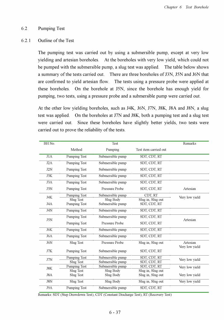
The pumping test was carried out by using a submersible pump, except at very low
yielding and artesian boreholes. At the boreholes with very low yield, which could not
be pumped with the submersible pump, a slug test was applied. The table below shows
a summary of the tests carried out. There are three boreholes of J3N, J5N and J6N that
are confirmed to yield artesian flow. The tests using a pressure probe were applied at
these boreholes. On the borehole at J5N, since the borehole has enough yield for
pumping, two tests, using a pressure probe and a submersible pump were carried out.
At the other low yielding boreholes, such as J4K, J6N, J7N, J8K, J8A and J8N, a slug
test was applied. On the boreholes at J7N and J8K, both a pumping test and a slug test
were carried out. Since these boreholes have slightly better yields, two tests were
carried out to prove the reliability of the tests.
BH No. Test Remarks
Method Pumping Test item carried out
J1A Pumping Test Submersible pump SDT, CDT, RT
J2A Pumping Test Submersible pump SDT, CDT, RT
J2N Pumping Test Submersible pump SDT, CDT, RT
J3K Pumping Test Submersible pump SDT, CDT, RT
J3A Pumping Test Submersible pump SDT, CDT, RT
J3N Pumping Test Pressure Probe SDT, CDT, RT Artesian
Pumping Test Submersible pump CDT, RT J4K
Slug Test Slug Body Slug in, Slug out Very low yield
J4A Pumping Test Submersible pump SDT, CDT, RT
J4N Pumping Test Submersible pump SDT, CDT, RT
Pumping Test Submersible pump SDT, CDT, RT J5N
Pumping Test Pressure Probe SDT, CDT, RT Artesian
J6K Pumping Test Submersible pump SDT, CDT, RT
J6A Pumping Test Submersible pump SDT, CDT, RT
J6N Slug Test Pressure Probe Slug in, Slug out Artesian Very low yield
J7K Pumping Test Submersible pump SDT, CDT, RT
Pumping Test Submersible pump SDT, CDT, RT J7N
Slug Test Submersible pump SDT, CDT, RT Very low yield
Pumping Test Submersible pump SDT, CDT, RT J8K
Slug Test Slug Body Slug in, Slug out Very low yield
J8A Slug Test Slug Body Slug in, Slug out Very low yield
J8N Slug Test Slug Body Slug in, Slug out Very low yield
J9A Pumping Test Submersible pump SDT, CDT, RT
Remarks: SDT (Step Drawdown Test), CDT (Constant Discharge Test), RT (Recovery Test)

Chapter 6 Test Borehole
6 - 38
6.2.2 Measurement
1) Tests Carried Out
The following phases were applied to the pumping tests:
Phase 1: Provisional test
A short provisional test was normally done before the commencement of the pumping test. The purpose of the test was to measure the approximate pumping rate and to decide on the number of steps necessary for the step drawdown test, and to adjust the valve-opening rate to achieve the prescribed pumping rate. The discharge and the duration of each test and the number of steps were determined by the results of the provisional test.
Phase 2: Step drawdown test
Normally at least five steps (sometimes more or less) were performed with each step measuring 120 minutes or occasionally shorter in duration.
Phase 3: Constant discharge test
The test was done in most cases 72 hours or occasionally longer or shorter in duration. The test was performed as soon as the water in the borehole had recovered to its static water level after completion of the step drawdown test.
Phase 4: Time recovery test
The test commenced immediately on completion of the constant discharge test and continued until the water level returned to its static water level or occasionally over a shorter period.
2) Method of Measurement
The original static water level in the borehole was always measured before any test pumping commenced. Throughout the duration of each test, the water level in the borehole was measured and recorded following the observation time schedule listed below:

Chapter 6 Test Borehole
6 - 39
Time from start of pumping or pumping
rate increase (minutes) Time interval between observations (minutes)
0 - 5 0.5 5 - 10 1 10 - 20 2 20 - 30 3 30 - 60 5 60 - 120 10 120 - 240 20 240 - 360 40 360 - 720 60 720 - 2880 120
2880 and longer 240
The flow of all water pumped from the borehole during the pumping test was measured by an approved method using mainly a triangular weir. Discharge rates were recorded during the pumping test at intervals corresponding to those for water level measurements.
Existing boreholes were used for observation boreholes during the test pumping, if they were located near the test borehole and were suitable for that purpose. In addition, where the sites, two or three test boreholes were drilled, namely J-2, J-3, J-4, J-6, J-7 and J-8, boreholes other than test borehole were also used as observation boreholes during the test pumping. The way of water level measurement in the observation boreholes was similar as that of the test borehole.
6.2.3 Method of Analysis
1) Aquifer Constants
The aquifer constants necessary for the hydrogeological evaluation are transmissibility, storage coefficient and permeability. These aquifer constants were analyzed by using the results of constant discharge and recovery tests. The methods used for analysis of the aquifer constants are shown in below.
i) The Theis Method
Theis (1935) solved the non-equilibrium flow equations in radial coordinates. For the specific definition of u given, the integral is known as the well function W(u), and can be represented by an infinite Taylor series. Using this function, the equation becomes:

Chapter 6 Test Borehole
6 - 40
( )uWT
Qs
π4=
A log/log scale plot of the relationship W(u) along the y-axis versus 1/u along the x-axis is commonly called the Theis curve. The field measurements are similarly plotted on a log-log plot with t along the x-axis and s along the y-axis. The data analysis is done by matching the observed data to the type curve.
ii) The Cooper & Jacob Method
This solution is valid for greater time and smaller separation distance from the pumping well (smaller u values, i.e. u<0.01 ). The resulting equation is:
sQ
T∆
=π43.2
2025.2
rTt
S =
where s is drawdown, Q is the well discharge rate, t is time, r is the radial distance, and S and T are the storativity and transmissivity respectively.
The above equation plots as a straight line on semi-logarithmic plot if the limiting conditions are met. Thus, straight-line plots of drawdown versus time can be produced after sufficient time has elapsed. In pumping tests with multiple observation wells, the closer wells will meet the conditions before the more distant ones. Time is plotted along the logarithmic x-axis and drawdown is plotted along the linear y-axis.
iii) Theis and Jacob Recovery Test Method
The recovery / rebound of the water level in a pumping well can also be used to estimate aquifer transmissivity. Analysis of the recovery can be used to confirm data values obtained using the pumping test data, or it may be the only data available in the case where only a production well is available. In cases where observation well data are not available and it is necessary to estimate aquifer properties with only a production well, water level data during the pumping test cannot be used because they are subject to well losses which cause the drawdown in the well to be significantly greater than the drawdown in the aquifer just outside the well. This can be overcome by measuring the recovery of the water level in the well after the pump has been shut down.
According to Theis (1935), the residual drawdown after pumping has ceased is:

Chapter 6 Test Borehole
6 - 41
( ) ( )'4
' uWuWT
Qs −=
π
where,
TtSr
u4
2
=
'4'
'2
TtSr
u =
and, Q is the constant discharge rate, T is the transmissivity, r is the distance to the observation well, s' is the residual drawdown, S and S' are the storativity values during pumping and recovery respectively, and t and t' are the time elapsed since the start and ending of pumping respectively.
iv) Hantush Method
Most confined aquifers are not totally isolated from sources of vertical recharge. Less permeable layers, either above or below the aquifer, can leak water into the aquifer under pumping conditions.
The Hantush and Jacob (1955) solution to the above equation is given by:
=
Lr
uWT
QS ,
4π
TSr
uπ4
2
=
A log/log plot of the relationship W(u,r/L) along the y-axis versus 1/u along the x-axis is used as the type curve as with the Theis method. The field measurements are plotted as t or t/r2 along the x-axis and s along the y-axis. The data analysis is done by curve matching..

Chapter 6 Test Borehole
6 - 42
v) Bouwer-Rice Slug Test Method
The Bouwer and Rice (1976) slug test analysis method is designed to more accurately estimate the hydraulic conductivity of the aquifer material by better accounting for the piezometer geometry . In a slug/bail test, a solid "slug" is lowered into/removed from the piezometer instantaneously raising/lowering the water level in the piezometer. The Bouwer and Rice (1976) equation for hydraulic conductivity is:
( )
=
t
cont
hh
tl
LRRr
K 02
ln2
/ln
where, r = piezometer radius R = radius measured from center of well to undisturbed aquifer material Rcont = contributing radial distance over which the difference in head, h0, is dissipated in the aquifer L = the length of the screen h0 = head in well at t0 = 0 ht = head in well at t > t0
Since the contributing radius of aquifer is seldom known a priori, Bouwer and Rice developed some empirical curves to account for this radius by three coefficients (A,B,C) which are all functions of the ratio of L/R. Coefficients A and B are used for partially penetrating wells whereas coefficient C is used only for fully penetrating wells.
The data are plotted with time on a logarithmic x-axis and ht/ho on a linear y-axis.
2) Borehole Hydraulics
i) Well Efficiency
Well efficiency is given by the following formula;
Well Efficiency (%) Ew=BQ /(BQ +CQ2)
Where
B = aquifer loss
C = well loss
Q = discharge rate (l/s)

Chapter 6 Test Borehole
6 - 43
ii) Radius of Influence
The Radius of Influence is given by the following formula after the Theis Equation;
Radius of Influence (m) R=(4Ttu/S)0.5
s=(Q/4πT)W(u)
Where Q =Discharge rate (m3/h)
T =Transmissivity (m2/h)
s =drawdown(m)(0.001)
S =Effective porosity (0.3)
W(u) =Well function of Theis
t =Time of pumping operation (h)
6.2.4 Borehole Hydraulics
Borehole hydraulics were evaluated by the results of the step drawdown test data. These include well efficiency, aquifer boundary type and area of influence. At the low yielding boreholes of J4K, J6N, J8A and J8N, however, no step drawdown test was performed.
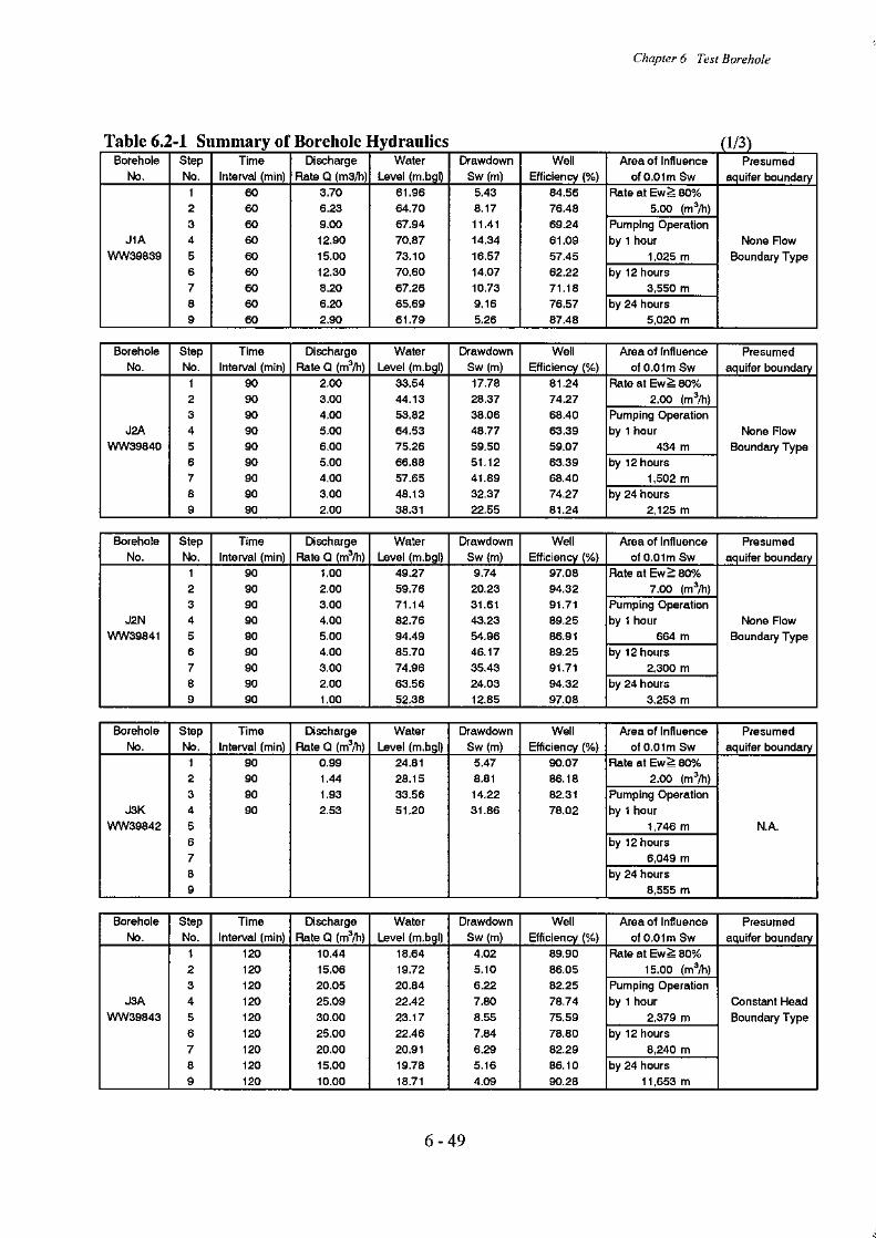
The evaluation sheets for all boreholes are listed in Appendix A-2, and a summary of results are shown in Table 6.2-1.
1) Well Efficiency
Well efficiency calculated by aquifer loss and well loss, was analyzed using the Jacob method for step drawdown test data. Aquifer parameters used for the calculation of well efficiency were obtained from the evaluation results of the constant discharge test. The well efficiencies at the range of flow rates used during the step drawdown test was calculated.
2) Aquifer Boundary Type
In the most of the step drawdown tests, reverse tests were conducted to evaluate the aquifer boundary. Two types of aquifer boundary, namely a “non-flow boundary type” and a “constant head boundary type” could be presumed by the relation between the discharge rate and the drawdown of both forward and reverse tests. None flow boundary types are defined as “the aquifer has a none flow boundary or a barrier, due to 1) a geological structure such as fault, buried valley, etc., 2) an impermeable barrier, 3) the formation of a conspicuous permeability”. Constant head boundary types are
Chapter 6 Test Borehole
6 - 44
defined as “the aquifer is characterized as 1) a relatively high permeability, 2) a relatively high storage, 3) associated with recharge by surface water and 4) receives induced recharge from the upper formation”.
3) Area of Influence
The area of influence at the rates of well efficiency within the following ranges were calculated: 1) less than 50%, 2) 50% to 70%, 3) 70% to 80% and 4) more than 80%. The area of influence is estimated, under the condition that the influenced drawdown is 0.01m within the pumping time from one hour to 8,760 hours.
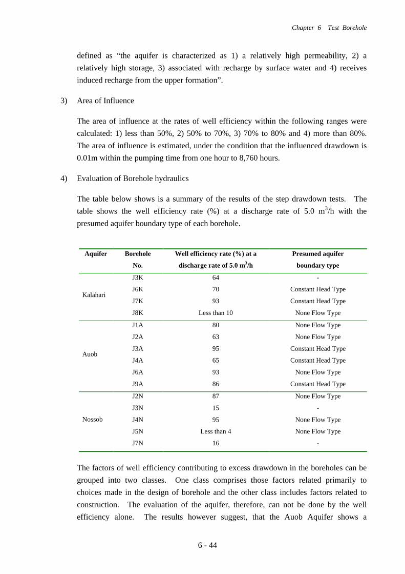
4) Evaluation of Borehole hydraulics
The table below shows is a summary of the results of the step drawdown tests. The table shows the well efficiency rate (%) at a discharge rate of 5.0 m3/h with the presumed aquifer boundary type of each borehole.
Aquifer Borehole
No.
Well efficiency rate (%) at a
discharge rate of 5.0 m3/h
Presumed aquifer
boundary type
J3K 64 -
J6K 70 Constant Head Type
J7K 93 Constant Head Type Kalahari
J8K Less than 10 None Flow Type
J1A 80 None Flow Type
J2A 63 None Flow Type
J3A 95 Constant Head Type
J4A 65 Constant Head Type
J6A 93 None Flow Type
Auob
J9A 86 Constant Head Type
J2N 87 None Flow Type
J3N 15 -
J4N 95 None Flow Type
J5N Less than 4 None Flow Type
Nossob
J7N 16 -
The factors of well efficiency contributing to excess drawdown in the boreholes can be grouped into two classes. One class comprises those factors related primarily to choices made in the design of borehole and the other class includes factors related to construction. The evaluation of the aquifer, therefore, can not be done by the well efficiency alone. The results however suggest, that the Auob Aquifer shows a
Chapter 6 Test Borehole
6 - 45
relatively high well efficiency overall. On the other hand, the boreholes with extremely low well efficiency are concentrated in the Nossob Aquifer and one in the Kalahari Aquifer. The boreholes drilled into the Nossob Aquifer are also very low yielding.
Most of the boreholes within the Kalahari and Auob are characterized by a “constant head type” aquifer boundary, whereas all Nossob boreholes are “none flow type aquifer boundary”. The results suggest that the Nossob Aquifer is characterized as extremely low permeability and an extremely low recharged.
6.2.5 Aquifer Constants
Aquifer constants necessary for the hydrogeological evaluation are transmissibility, storage coefficient and permeability. These aquifer constants were analyzed by using the results of constant discharge and recovery tests.
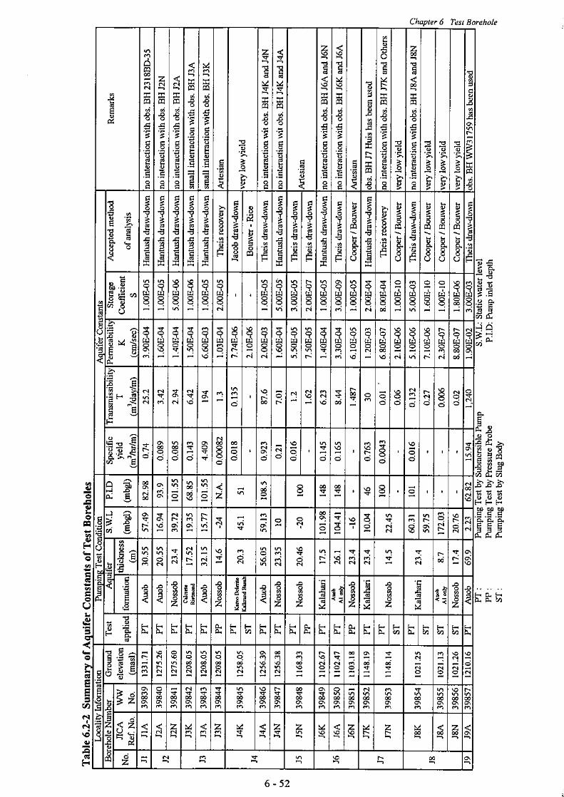
The evaluation sheets of aquifer constants for all boreholes are listed in Appendix A-2. A summary of results are shown in Table 6.2-2.
1) Specific Yield
The quantity of water that a unit volume of unconfined aquifer gives up by gravity is called its specific yield. Specific yield was calculated by the drawdown and pumping rate at the constant discharge test.
2) Transmissibility
Transmissibility is the rate at which water is transmitted through a unit width of an aquifer under a unit hydraulic gradient. The value is given in cubic meters per day through a vertical section of an aquifer one meter wide and extending through the full saturated height of an aquifer under a hydraulic gradient of 1. Both of the constant discharge and recovery tests were used for the analysis.
3) Permeability
Permeability is the property or capacity of an aquifer to transmitting a fluid. It is a measure of the relative ease of fluid flow under unequal pressure. Both the constant discharge and recovery tests were used for the analysis.
Chapter 6 Test Borehole
6 - 46
4) Storage Coefficient
The storage coefficient is the volume of water that an aquifer releases from or takes into storage per unit surface area of the aquifer per unit change in head. In this project, however, no observation borehole were drilled. Both the constant discharge test and recovery tests were used for the analysis. The presented value of the storage coefficient in this report is therefore an estimated value.
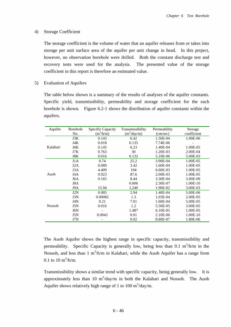
5) Evaluation of Aquifers
The table below shown is a summary of the results of analyses of the aquifer constants. Specific yield, transmissibility, permeability and storage coefficient for the each borehole is shown. Figure 6.2-1 shows the distribution of aquifer constants within the aquifers.
Aquifer Borehole No.
Specific Capacity (m3/h/m)
Transmissibility (m3/day/m)
Permeability (cm/sec)
Storage coefficient
J3K 0.143 6.42 1.50E-04 1.00E-06 J4K 0.018 0.135 7.74E-06 - J6K 0.145 6.23 1.40E-04 1.00E-05 J7K 0.763 30 1.20E-03 2.00E-04
Kalahari
J8K 0.016 0.132 5.10E-06 5.00E-03 J1A 0.74 25.2 3.90E-04 1.00E-05 J2A 0.089 3.42 1.60E-04 1.00E-05 J3A 4.409 194 6.60E-03 1.00E-05 J4A 0.923 87.6 2.00E-03 1.00E-05 J6A 0.165 8.44 3.30E-04 3.00E-09 J8A 0.006 2.30E-07 1.00E-10
Auob
J9A 15.94 1,240 1.90E-02 3.00E-03 J2N 0.085 2.94 1.40E-04 5.00E-06 J3N 0.00082 1.3 1.03E-04 2.00E-05 J4N 0.21 7.01 1.60E-04 5.00E-05 J5N 0.016 1.2 5.50E-05 3.00E-05 J6N - 1.487 6.10E-05 1.00E-05 J5N 0.0043 0.01 2.10E-06 1.00E-10
Nossob
J7N - 0.02 8.80E-07 1.80E-06
The Auob Aquifer shows the highest range in specific capacity, transmissibility and permeability. Specific Capacity is generally low, being less than 0.1 m3/h/m in the Nossob, and less than 1 m3/h/m in Kalahari, while the Auob Aquifer has a range from 0.1 to 10 m3/h/m.
Transmissibility shows a similar trend with specific capacity, being generally low. It is approximately less than 10 m3/day/m in both the Kalahari and Nossob. The Auob Aquifer shows relatively high range of 1 to 100 m3/day/m.

Chapter 6 Test Borehole
6 - 47
Permeability of the Nossob and Kalahari Aquifers also low. It is generally less than 1×10⁻⁴ cm/sec in Nossob, and less than 1×10⁻⁴ cm/sec for the Kalahari. The Auob Aquifer shows a range from 1×10⁻⁴ cm/sec to1×10-2 cm/sec. As illustrated by the
following figure, the permeability calculated in the Nossob and Kalahari can be categorized as a low-permeable silt to clay. A range of 1×10⁻⁴ cm/sec to1×10-2
cm/sec of Auob Aquifer is categorized as a low to high permeable silt to sand.
Interrelationship between permeability and grain size. (After Linsely et al. 1958)
Considering such a permeability range and a relatively high transmissibility and specific capacity, it is suggested that the Auob Aquifer represents the promising aquifer in the area. The Kalahari Aquifer has locally alow potential, and the, Nossob Aquifer is generally a non-productive aquifer from an aquifer constant point of view.
6.2.6 Interaction Between the Aquifers
During the measurement of water levels within the production borehole, if other drilled boreholes or existing boreholes were near the production borehole, water levels in these boreholes were done in a similar way. Such was the case at locations J-2, J-3, J-4, J-6, J-7 and J-8. Only at location of J-3 was a small interaction between the Kalahari and Auob Aquifers observed.
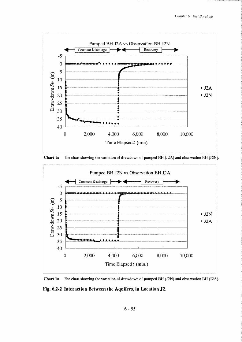
1) Location J-2 (See Fig. 6.2-2)
A total of two boreholes, J2A and J2N, were drilled at this location. No interaction between the aquifers was observed.
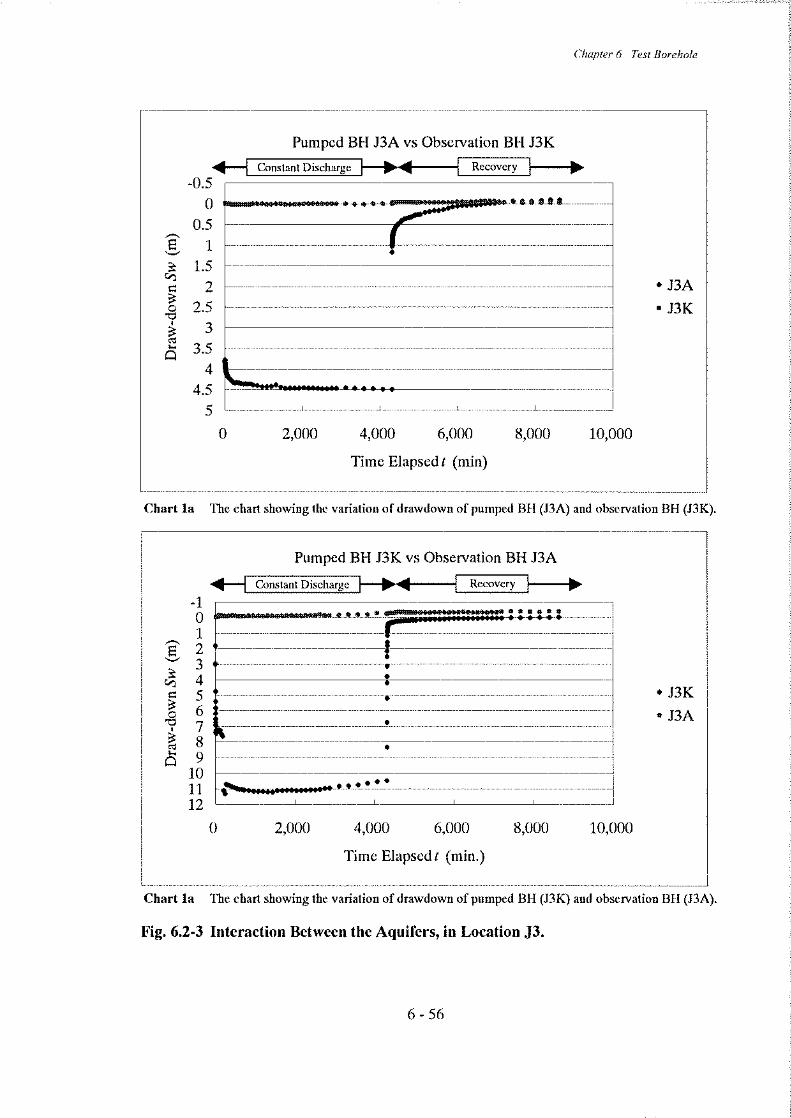
2) Location J-3 (See Fig. 6.2-3)
A total of two boreholes, J3A and J3K, were drilled at this location. A small interaction between the Kalahari and Auob Aquifers was observed. A remarkable variation of drawdown was observed prior to the commencement of the recovery test.
k (cm/sec)
Soil Clay Silt Sand Gravel
Permiability Unpermeable Low-Permeable High-Permeable Very High-Permeable
1 10 210-8 10-6 10-4 10-2
Chapter 6 Test Borehole
6 - 48
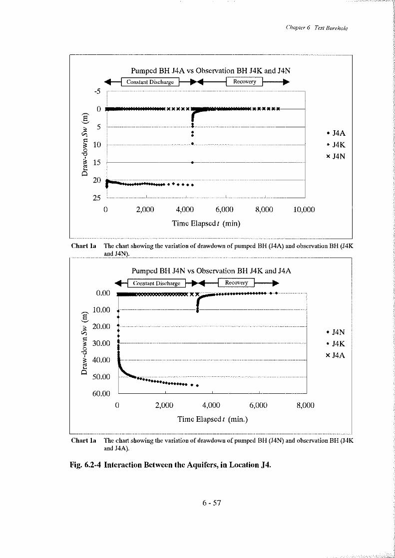
3) Location J-4 (See Fig. 6.2-4)
A total of three boreholes, J4K, J4A and J4N, were drilled at this location. No interaction between the aquifers was observed.
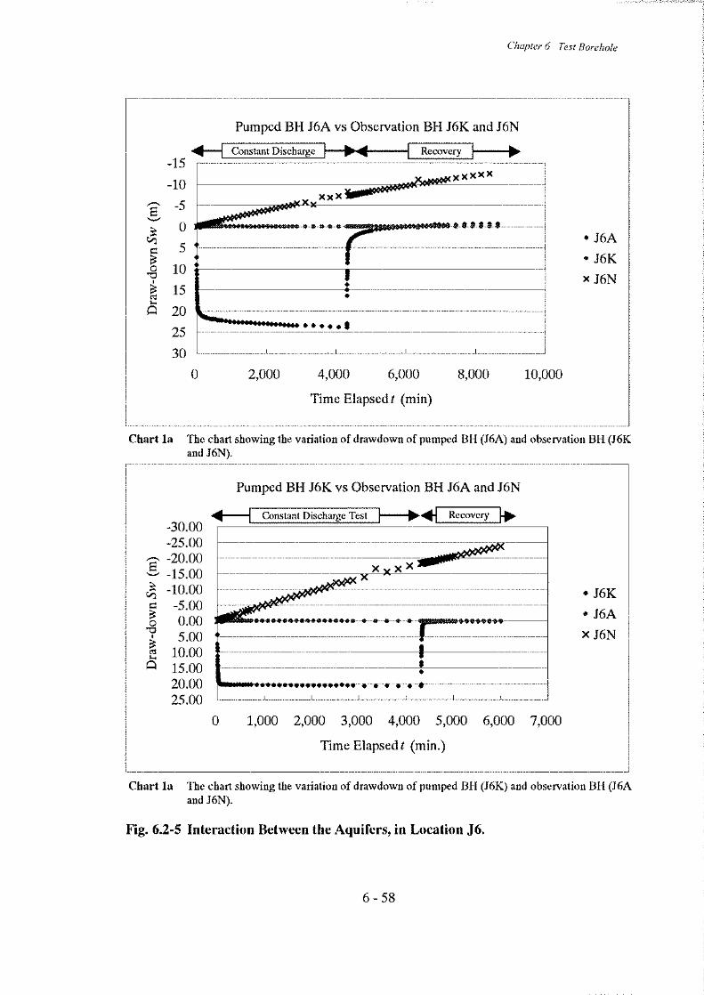
4) Location J-6 (See Fig. 6.2-5)
A total of three boreholes, J6K, J6A and J6N, were drilled at this location. No interaction between the aquifers was observed.
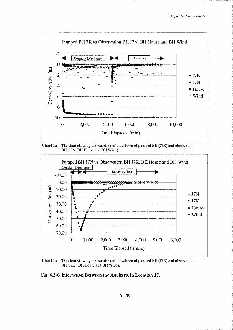
5) Location J-7 (See Fig. 6.2-6)
A total of two boreholes, J7K and J7N, were drilled at this location. Two farmer’s boreholes named House and Wind pump were was used as observation boreholes. In these boreholes, a variation of drawdown was observed during pumping of J7K borehole. No interaction, however between the Kalahari and Nossob Aquifers was observed.
6) Location J-8 (See Fig. 6.2-7)
A total of three boreholes, J8K, J8A and J8N, were drilled at this location. No interaction between the aquifers was observed.
6.2.7 Pumping Test Analysis of Existing Boreholes
During the series of survey, the pumping test data of the existing boreholes were collected to analysis the aquifer constants. The available data, however, is very limited, only six analyzable data was found. Table 6.2-3 shows the result of analysis. The borehole number of WW24604 at Garton has 3 result. This is not three boreholes, three different pumping test was done in the same borehole.


Chapter 6 Test Borehole
6 - 61
6.3 Installation of Water Level Recorder
6.3.1 Recorders, Installed
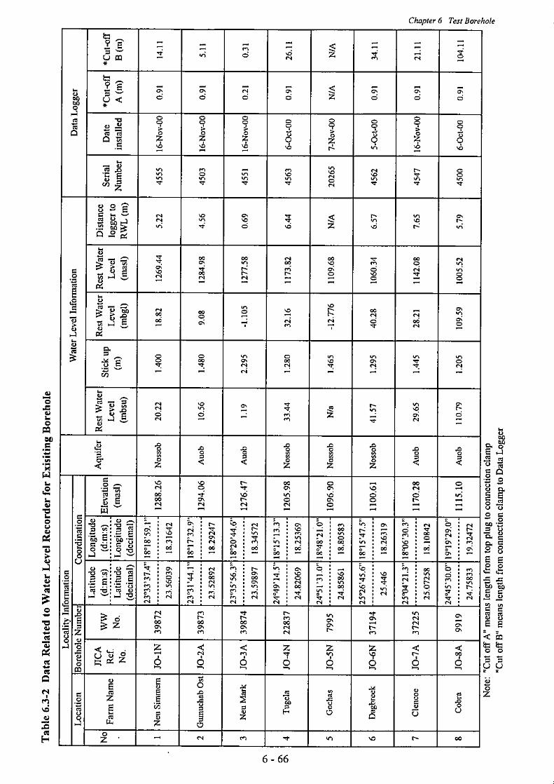
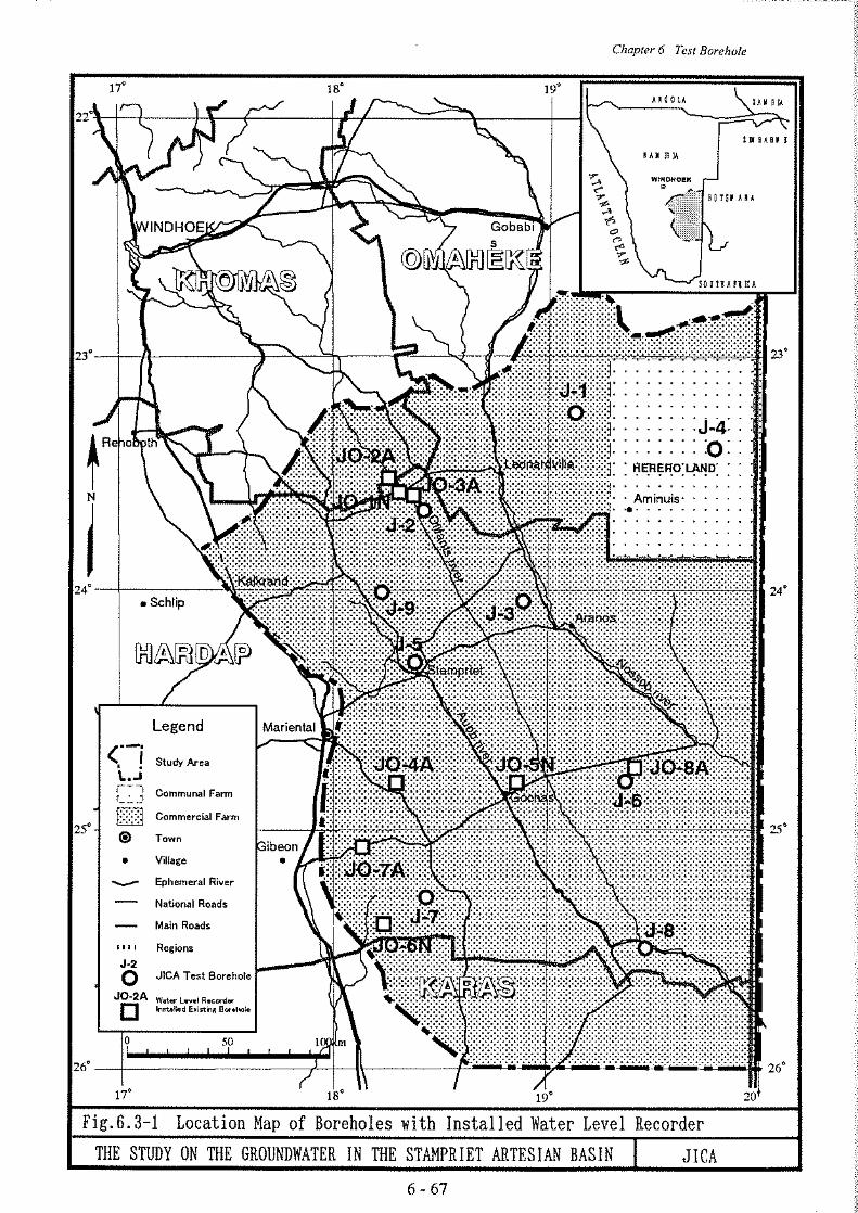
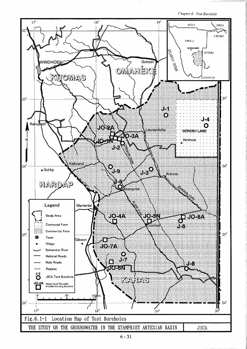
Water level recorders were installed in all of 19 JICA test boreholes as well as on eight existing boreholes. The existing boreholes were selected based on discussions with DWA. The location of these boreholes are shown on Fig.6.3-1. Two types of recorders namely, the floater type and pressure probe type were installed. The pressure probe was fitted to only for four artesian boreholes ie. J3N, J5N, J6N and JO-5N(an existing borehole).
All information in connection with water levels and data-loggers for the JICA boreholes is summarized in Table 6.3-1 and in Table 6.3-2 as for existing boreholes.
In the columns of “Data Logger”, information of the data-logger installed is described. “Serial Number” shows the identification of each data logger. “Date Installed” corresponds to the first date on which water level monitoring commenced. “Cut-off A” and “Cut-off B” shows the length of cable from plug to clamp, and from clamp to data probe respectively. Only the float type recorder has such information.
6.3.2 Specification of Water Level Recorder
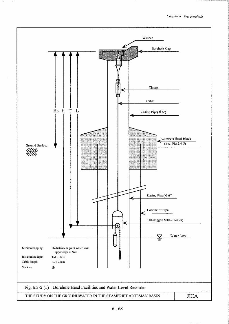
(1) Float Type (See Fig. 6.3-2 (1) and 6.3-2(2))
The main specification features are summarized as follows:
- memory: 32KByte for at least 32x484 = 15,488 measuring values (without time marks)
- communication: via M-Bus with communication interface at RS232 with 2400Baud
: increase read data by up to 4800 Baud values - clock: real time clock ±15ppm - operating temperature: -20 to +70℃ (exception: glaciation) - power supply conditions: average tempereature <25℃
: max. pluses 500/day : measuring cycle times ≧15min
: max. interface operation 5min/month - operating life: 15 years - expected runtime: 20 years
The float type recorder consists mainly of a plug, cable, clamp, data logger, ball chain, floater and weight. The data logger connects the plug by clamp and cable.
Chapter 6 Test Borehole
6 - 62
As described above, the manufacturer guarantees the battery life for 15 years. Therefore, the data logger must be sent to the manufacturer to change the battery.
The memory capacity of the data logger is only 15,488 measuring values. The time interval for data recording was set every 1 hour for monitoring purposes. If data capturing is carried out once a year, the number of data becomes 8,760 measuring values. The data logger can be left for about 1.5 years, with out down-loading the data.
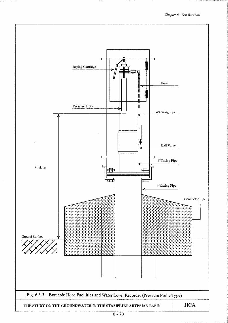
(2) Pressure Probe Type (See Fig. 6.3-3)
The main specification features are summarized as follows;
- memory: 32KByte for at least 32x484 = 15,488 measuring values - communication: via M-Bus with communication interface at RS232
with 2400baud : increase to 4800 baud by read out possible
- clock: real time clock ±15ppm - operating temperature: -20 to +70℃ (exception: freezing) - battery life time: average tempereature <25℃ : measuring cycle times ≧15min
: with max. 5min interface operation per month : >10 years guaranteed
The pressure probe type recorder consists mainly of a plug, cable and data logger with pressure sensor. The data logger connects to the plug by the cable only.
As described above, the manufacturer guarantees 10 years for battery life, whereafter the data logger must be sent to the manufacturer to change the battery.
The memory capacity of the data logger is only 15,488 measuring values. The time interval for data recording was set at every 1 hour for monitoring purposes. If data capturing is carried out once a year, number of measuring values becomes 8,760. The data logger can be left for about 1.5 years, without down-loading the data.
6.3.3 Technical Transfer on Operation and Maintenance of the Recorder
Technical transfer to the DWA officials relating to the operation and maintenance of the recorder was carried out during November 2000. The items transferred and confirmed are summarized as follows:
i) Reading actual value of water level and total memorized number in the data logger ii) Checking the function of data logger by laptop computer
Chapter 6 Test Borehole
6 - 63
iii) Data capturing by laptop computer
6.3.4 Recommendation on Operation and Maintenance
As mentioned above, on both types of recorder, the maximum number of the data that can be memorized is only 15,488 measuring values. If this number is exceeded, new data will overwrite the old automatically. In order to avoid such losses, it is recommended that data capturing should be executed at least once a year. The borehole head facility consists of not only of the recorder, but also of other devices is installed to maintain the proper function of the recorder. Inspection of these devicesis also required. From this point of view, it is considered that a visit to the boreholes for data capturing at least once a year is appropriate.
A washer was fixed between the nut and fixing device in the cap in order to prevent the recorder falling down. It must however, be handled with care, water sampling or pumping, and the recorder must be held securely.
When the settings of data-logger are going to be changed, such as interval time, the memory of the data-logger will be initialised automatically. To avoid data losses in the logger, memorized data should first be saved before such settings are changed.