cable broadband network architecture and capacity planning

Cable Broadband Network Architecture and Capacity Planning: ‘Working Fill Factor’

An exposition of cable technology considerations pertaining to the ‘Working Fill Factor’, in the matter of wholesale high-speed access under the Canadian Radio-Television and Telecommunications Commission (CRTC) Third Party Internet Access (TPIA) service.

January 2017

CableLabs Cable Network Architecture & Capacity Planning: ‘Working Fill Factor’

ii

About CableLabs Founded in 1988, CableLabs is the Innovation and R&D Lab for the global cable industry. With a strong focus on innovation, CableLabs develops technologies and specifications for the secure delivery of broadband Internet access, video, voice, and next generation services. It also provides testing, certification facilities and technical leadership for the industry. CableLabs’ mission is to enable cable operators to be the providers of choice to their customers. CableLabs currently has 55 members across four continents.

About This Report With this report, CableLabs articulates the technological and operational factors involved in cable broadband network capacity planning. Within the CRTC’s Phase II Costing framework for regulated wholesale broadband access, we focus on the Working Fill Factor (WFF). We do not provide company-specific WFF estimates, but rather articulate reasonable ranges based on common cable technology, network, and operating principles. The methods that operators use for capacity planning are well established, and their efficacy is evident in broadband performance measurement efforts. The concepts expressed in this report reflect practices used by cable operators across North America.


iii

Contents

1 Introduction 1

2 Cable Broadband Network Architecture 2

3 Working Fill Factors and Cable Networks 53.1 A Model of Cable Network Utilization 83.2 Working Fill Factors 23

4 Working Fill Factors in Practice 33

5 Conclusion 36

Appendix 37


1

1 Introduction [1] CableLabs’ largest Canadian member companies are required by the CRTC to provide third-party wholesale access to their Internet broadband facilities. The wholesale rates for this third-party Internet access (TPIA) service are determined on a cost recovery basis by the CRTC, according to a specific approach, known as Phase II costing. Under Phase II costing, cost-based rates for telecommunication services are determined based on prospective incremental costs.1 The determination of these rates relies on a number of inputs from regulated facilities-based Internet Service Providers, including information pertaining to broadband network utilization and capacity planning, known as the Working Fill Factor (WFF). [2] This report articulates the capacity planning considerations used by cable operators across North America. We do not address all aspects of Phase II costing, nor do we provide company-specific information. Rather, we highlight technical and operational factors in cable broadband networking that are relevant to the WFF element of the CRTC’s Phase II costing for TPIA services. We accomplish this by articulating a model of the cable network WFF and through empirical data. [3] As detailed in this report, capacity planning on cable broadband networks is influenced by factors including target utilization levels during peak periods, variability in traffic across network segments serving different numbers of end-users, the time required to augment capacity, traffic growth anticipated during that period, and a number of other considerations. We observe that the cumulative effect of

1See ILEC Regulatory Economic Studies Manual, Section 1.2.1.


2

these considerations leads to WFFs in the range of 25% to 45% for service groups and 15% to 45% for nodes.

2 Cable Broadband Network Architecture [4] Cable networks deliver Internet access through a shared architecture that is distinct from DSL or fiber to the premise (FTTP) networks. An overview of cable architecture is, therefore, essential for developing the WFFs of cable networks and understanding how they differ from WFFs pertaining to networks of other technologies. [5] Cable broadband networks utilize statistical multiplexing to share a fixed amount of network capacity across a group of users. The network’s architecture is a hybrid of fiber and coaxial cable, utilizing frequency division duplexing to divide upstream and downstream transmissions. [6] Approximately 750 MHz to 1 GHz of spectrum is typically available on cable networks to be shared across all services, including television, broadband, and voice.2 Upstream traffic uses the lower portion of the frequency duplex cable system, between 5 MHz and 42 MHz usually, and downstream traffic uses the remaining upper portion of the available frequencies. The precise amounts of upstream, downstream, and total spectrum available may vary by network, but the values noted here are typical for North American systems. [7] The amount of spectrum on the cable system dedicated to broadband depends, in part, on the requirements of the other

2 While the 750 MHz – 1 GHz may be a typical range, there are systems that operate at lower levels of spectrum (e.g., down to 450 MHz).


3

services, particularly television. Cable networks have historically been segmented into 6 MHz-wide channels, reflecting the channel bandwidth for over-the-air broadcast television. The bandwidth used for video services on today’s networks is a function of the amount of content carried, the transmission technology (e.g., digital or analog), compression rates, delivery architectures (e.g., broadcast or multicast), and other factors. As operators invest to enable greater efficiency in video delivery, 6 MHz channels on the cable system can be “reclaimed” for broadband services. Spectrum is scarce on a cable network and investment is designed to expand or better utilize it. [8] Cable broadband technology, known as Data Over Cable Service Interface Specification or DOCSIS® technology, is specified by CableLabs on behalf of the global cable industry. DOCSIS technology addresses both the physical layer and media access control (MAC) layer of cable broadband services. DOCSIS technology was initially specified in 1997; several revisions to the specification have been made over time to enable higher-performing services. Today, DOCSIS 3.0 technology is the most widely deployed cable broadband technology. [9] With DOCSIS 3.0 technology, each 6 MHz channel can provide approximately 32 to 38 Megabits per second (Mbps) of useable bandwidth at a modulation rate of 256-QAM. As more channels are dedicated to broadband service, they can be aggregated to enable high-speed services. The term “capacity” will be used henceforth to represent the total amount of shared bandwidth available for broadband service.

[10] DOCSIS 3.1 is the latest iteration of DOCSIS technology. It provides larger channel sizes (up to 192 MHz) and higher modulation rates (up to 4096-QAM), allowing cable operators to further increase


4

their broadband speeds and capacity. Our analysis of utilization and WFFs is applicable to both current DOCSIS 3.0 and forthcoming DOCSIS 3.1 deployments, since similar capacity planning and utilization concepts apply to both technologies. [11] The capacity described above is shared among many users (collectively referred to as a service group). In a typical cable network, fiber optics connect the headend to a neighborhood hub, and then to an optical node. Coaxial cable then extends beyond the node to the end customers, of which there are generally between 50 and 500 households. Beyond the node, the coaxial network may utilize amplifiers to extend the range of the signal. These 50 to 500 households on the node share the capacity provided by DOCSIS technology. This architecture is depicted below in Figure 1.3

Figure 1: Cable Network Architecture

[12] The MAC protocols of DOCSIS technology, which allocate capacity across users on a node, enable the cable broadband network

3Source: Wikimedia Commons


5

to be shared. Within DOCSIS technology, communications are managed by the cable modem termination system (CMTS), which is located in the headend or hub site. The CMTS arbitrates the communications of all cable modems connected to it; there is no direct communication between modems. Individual modem transmissions are managed by a contention mechanism where requests are made to the CMTS, which then queues, prioritizes, and authorizes transmissions. In so doing, the CMTS ensures that available capacity is apportioned across all users on the node in the appropriate fashion. [13] While we use the term CMTS throughout the document, we recognize that operators are also deploying Converged Cable Access Platform (CCAP) equipment to provide broadband services. Within this document, the term “CMTS” includes both CMTS equipment and the CMTS functionality within CCAP equipment.

3 Working Fill Factors and Cable Networks [14] This section presents a model of a typical cable broadband access network and derives expressions that describe its WFF. A WFF can be described as the average operational utilization level of the entire access network at steady-state. Under Phase II costing, cost-based rates for telecommunication services, such as TPIA service, are based on a company’s specific prospective incremental costs causal to providing the service. [15] The provision of TPIA services requires the use of shared facilities. The requirement for a company to add more capacity is advanced due to the additional data traffic demand associated with customers using some of the shared facilities’ capacity. This is referred


6

to as the cost of advancement. The following model highlights several factors explaining why the amount of advanced capacity required by a shared facility exceeds the current level of demand. [16] The approach generally used in Phase II costing to establish this cost of advancement is the capacity cost method. Under the capacity cost method, an estimate of the average utilization (i.e., the WFF) is applied to the total cost of the shared facility to recognize the non-service producing cost of the shared facility.4 The following equation expresses this relationship:

𝑈𝑛𝑖𝑡𝐶𝑜𝑠𝑡𝑜𝑓𝑆ℎ𝑎𝑟𝑒𝑑𝐹𝑎𝑐𝑖𝑙𝑖𝑡𝑦 = 𝑇𝑜𝑡𝑎𝑙𝐶𝑜𝑠𝑡𝑜𝑓𝑆ℎ𝑎𝑟𝑒𝑑𝐹𝑎𝑐𝑖𝑙𝑖𝑡𝑦

(𝐶𝑎𝑝𝑎𝑐𝑖𝑡𝑦𝑜𝑓𝑆ℎ𝑎𝑟𝑒𝑑𝐹𝑎𝑐𝑖𝑙𝑖𝑡𝑦 ∗ 𝑊𝐹𝐹)

[17] The context of a non-service producing cost is different in cable networks, relative to other types of telecommunications networks such as DSL. In DSL networks, non-service producing costs are typically ports that do not have an active subscriber currently assigned. For purposes of a WFF, DSL networks are binary: subscribed lines are service-producing, while non-subscribed lines are not. [18] Because of their shared architecture, cable networks do not have this binary mapping between subscribers and costs. In a cable network, non-service producing costs reflect capacity that is unused at the moment of measurement. This capacity will be used at some point, though, by the subscribers that share it. As discussed later in this section, this usage can come from variability in household traffic

4 See Telecom Decision CRTC 2013-76, paragraph 9.


7

or from growth in household demand over time.5 Neither of these cases depend on a new subscriber being added to convert these costs into service producing costs as on a DSL network. [19] A cable network’s WFF will vary between measurements over time, but remains reflective of the underlying system’s steady-state for two primary reasons. First, the variation in its measurement is driven by the highly variable nature of household demand. Since the network’s WFF measurement reflects the data traffic of thousands of households, though, its WFF is more stable and with lower variation than what is observed at the household-level. Second, the network is composed of many pieces that experience investment at different times, but all of which experience growth in subscriber demand. When a network’s WFF is measured at two different times, the individual service groups or nodes may have different utilization levels, but the overall mix of utilization states would be similar, if we assume regular investment by the operator. [20] The model presented below describes how a cable access network's shared architecture affects WFF calculations, and why this network characteristic produces WFF values that are lower than the historical WFF values of legacy telecommunications networks. [21] To supplement and support the following theoretical model, we obtained a sample of DOCSIS data traffic measurements from a Canadian operator in 1-second intervals to illustrate the important network characteristics that are foundational to the model. This sample includes per-second usage measurements from 56 service

5Note that we use the terms “subscriber” and “household” interchangeably throughout this document. A household is serviced by a single cable modem and is treated as a single subscriber by a cable operator.


8

groups, all located in the same market, from November 13-19, 2016. Throughout the model description, we reference and highlight relevant insights from this sample as appropriate. A complete description of the sample and the figures that are referenced are contained in an Appendix at the end of the document. We consider this sample and the features we highlight to be representative of typical data traffic on cable access networks in North America, but not an authoritative view of all cable networks due to the idiosyncrasies of each network.

3.1 A Model of Cable Network Utilization [22] Cable broadband access networks are composed of four important pieces: households, optical nodes, service groups, and cable modem termination systems. We begin by discussing the role of time in our model, and then provide descriptions of each network component in turn. Time in This Model [23] In the following equations, unless noted otherwise, time 𝑡 represents both the specific time (e.g., date and time) and duration of measurement of a network statistic. Typical data traffic measurements are performed over an integration time period, usually 15 minutes, so the two aspects of this timing are naturally the same. For example, if Operator A is measuring Node 1’s downstream traffic in 15-minute periods, a data row might look like what is presented in Table 1. The “Time Stamp” column tells us that time 𝑡 is 8:15 PM to 8:30 PM on January 1, 2017, and the “Downstream Bits” column says Node 1 transferred a total of 445,875,425 downstream bits over this 15-minute period. When variation in household demand is discussed later, we are referring to the stochastic nature of how heavy or light


9

household demand is for much smaller periods (e.g., milliseconds to seconds) within this 15-minute window. This level of observation might be described as “instantaneous” to emphasize smaller time periods trying to capture brief instances of maximum utilization.

Table 1: Example Data Row of Household Demand

Time Stamp Node Downstream Bits 2017-01-01 20:15:00 1 445875425

Households [24] Households are the end users of the network. A group of roughly 50 to 500 households are typically serviced by an individual optical node. The cable modems used in this particular group of homes share the same capacity, listen to the same network events and act only on the events that are meant for that modem. The households connected to a single node are indexed by 𝑖. A household's demand at time 𝑡 is usually measured in bits or bytes and denoted by ℎ;(𝑡). Household demand ℎ;(𝑡) is characterized by its highly variable and stochastic nature. The aggregate demand across all households on node 𝑛 at time 𝑡 is

𝐻=(𝑡) = ℎ;(𝑡).?

;@A

Nodes and Service Groups [25] Households are grouped by individual nodes on the network, and nodes are then grouped into service groups. Modern cable access networks may have a one-to-one mapping between nodes and service groups, where there is no distinction between the two. However, there are instances of a many-to-one mapping between nodes and service groups, due to specific cable access network topologies used to connect households. There are various configurations of how


10

downstream and upstream service groups can be related on the network. As a result, the interdependence between them can mean that growth in either the downstream or upstream portions can prompt investment. [26] A service group has capacity of 𝐶, which is generally fixed for the purposes of our model and changes infrequently (on the order of years). When there is a one-to-one mapping between a node and a service group, the single node has access to all of 𝐶, but when there are multiple nodes in a service group, each of the nodes must collectively share 𝐶 among the connected households. Service groups are able to share capacity with many households because of statistical multiplexing. That is, the probability of multiple households simultaneously requesting enough data to consume 100% of 𝐶 is low enough that sharing capacity across the group is feasible. [27] A cable network has a total of 𝐽 service groups, individually indexed by 𝑗, and each service group 𝑗 has 𝑁E total nodes indexed by 𝑛. Service group 𝑗's utilization at time 𝑡 is calculated as

𝑢E(𝑡) = 𝐻=(𝑡)GH

=@A𝐶E(𝑡).

[28] Operators typically observe only an aggregation of service group 𝑗’s total usage at time 𝑡, and not an individual node's usage (𝐻=(𝑡)). Of course, this is only an issue when there are multiple nodes in a service group. It follows that a service group's utilization 𝑢E(𝑡) is highly variable because it is a function of household demand ℎ;(𝑡). [29] In Figure 6 of the Appendix, we illustrate how measuring service group utilization 𝑢E(𝑡) in 15-minute intervals is related to per-second (i.e., “instantaneous”) variation of household demand ℎ;(𝑡) over the interval. We observe that as 𝑢E(𝑡) increases, the variability and


11

distribution of per-second utilization increases, too. For 15-minute periods that averaged 10-12% utilization6, the 5th percentile of per-second utilization is 5% and the 95th percentile is 18%, a spread of 13 percentage points. 15-minute periods with average utilization of 50-52% have a 5th percentile of 32% and a 95th percentile of 75%, a 43 percentage point spread. As we move to higher average utilization states, the 5th and 95th percentiles both increase, as does the difference between them. These ranges of per-second utilization illustrate why calculating average utilization over longer periods can hide the substantial variation in “instantaneous” utilization and why the investment practices described later are appropriate on a cable network’s shared architecture. CMTS [30] Cable modem termination systems (CMTS) are the next level of aggregation in a cable access network and where service groups are collected and managed by the operator. The main purpose of a CMTS is to convert backbone network traffic into a suitable format for delivery to households (by way of service groups and nodes). Another role of a CMTS is to provide routing and switching for individual service groups. While a CMTS contains a set of service groups, the individual service groups do not compete for CMTS capacity in the same way a household does within a service group. The CMTS connection to the operator's backbone network is rarely a binding constraint, so we assume there is sufficient capacity to meet the concurrent demand across service groups at any time 𝑡. As such,

6 When calculating 𝑢E(𝑡), only total household demand over the 15-minutes are observed. The interval’s average is then calculated by dividing this total by total capacity 𝐶E(𝑡), which provides a measure of utilization that assumes the traffic occurred uniformly over the interval.


12

CMTS utilization is calculated as an aggregation of the individual service groups.7 [31] Figure 7 of the Appendix shows the relationship between 15-minute CMTS-level aggregations of service group utilization and the variability of 15-minute average utilization for service groups in the aggregation. These CMTS-level aggregations, more generally, give context for how network-wide calculations are related to underlying service group variation over the same measurement intervals. When average CMTS utilization over 15-minutes is 10%, the 5th percentile 15-minute service group average is ~0% and the 95th percentile is ~25%. For 15-minute periods where CMTS utilization averaged 20%, the 5th percentile of service group averages is ~5% and the 95th percentile is ~40%. Similar to Figure 6 in the Appendix, we observe a wider range of service group utilization as CMTS utilization increases. Variation on a Cable Network [32] Variation in the utilization of a cable access network is created by individual households independently deciding when to use the Internet at any point in time. Household network requests are differentiated by frequency, intensity, and duration. There are a variety of factors that explain a household's preferences of making network requests. Examples of such factors are the household's Internet service tier, number of people in the household, number and type of

7 One could also measure the utilization of the CMTS’ connection to the operator’s backbone network, but since this connection is rarely a binding constraint and not as common as aggregating across service groups, we do not focus on this specific calculation. The connection to the backbone network receives investment over time to handle growth in household demand. Similar to other parts of the network that are covered in more detail later in this document, this investment typically occurs in a manner that would produce a low WFF.


13

Internet-connected devices, age, income, and individual preferences for different online activities. [33] There are two relevant characteristics of this variation with respect to network investment and operation. First, households are not synchronized when they submit network requests. Correlation in household requests may exist for such events as the Super Bowl or Netflix releasing a new season of a popular show, but households are ultimately independent agents. [34] Second, household network requests are heterogeneous in nature and a function of a household's preferences. Some households are light email users, while others are heavy over-the-top video viewers. Depending on the requested content’s type and the speed of the household's Internet service tier, network requests can utilize a portion of the service group's capacity for different durations and intensities. For example, the same 1 gigabyte file downloaded by two different households, one with a 1 Gbps connection and the other with a 50 Mbps connection, will burden capacity differently.8 [35] The variation of household demand describes how the intensity of network requests fluctuates from one “instantaneous” moment to the next. Any level of aggregation (e.g., 𝐻 𝑡 or 𝑢(𝑡)) will lose information on these “instantaneous” moments of household demand. Since network requests are asynchronous, one interval could be light and the next heavy, something cable network operators must be mindful of when planning capacity investments.

8 Note that speeds set for different Internet service tiers are configuration decisions made by the operator and not reflective of network limitations. Their usage here is to illustrate how a subscriber’s speed tier can influence the nature of their traffic.


14

[36] The variation in “instantaneous” household demand is what Figure 6 in the Appendix illustrates by showing the relationship between 15-minute service group average utilization and the per-second utilization within the same measurement interval. Recall from earlier that the range of per-second utilization can exceed a 40 percentage point spread. [37] Variation in “instantaneous” household demand is also reflected in Figure 7 of the Appendix, when considered jointly with Figure 6. Consider the earlier example from Figure 7, where we stated that for network-wide 15-minute averages of 20%, the 95th percentile service group average utilization is 40%. From Figure 6, we would expect that a service group with 15-minute average utilization of 40-42% would have a 95th percentile per-second utilization level of 60%. This connection between the two figures illustrates earlier statements that measuring average utilization in 15-minute intervals hides substantial variation that occurs at an “instantaneous” level, and that these “instantaneous” bursts can be much larger than the average utilization may suggest. Measuring Utilization on the Network [38] As described in the “Nodes and Service Groups” section, service group 𝑗's utilization 𝑢E(𝑡) is measured at time 𝑡 by taking household demand and dividing by 𝐶E. These utilization measurements are then aggregated at the CMTS and network-wide levels. Since 𝑢E(𝑡) is a function of household demand 𝐻=(𝑡), the variation in household demand covered in the previous section affects these utilization calculations the same way. While 𝑢E(𝑡) would be measured ideally at a high resolution, it is practically collected over intervals ranging from 5 to 15 minutes for long-term storage and to make it easier to communicate and interpret.


15

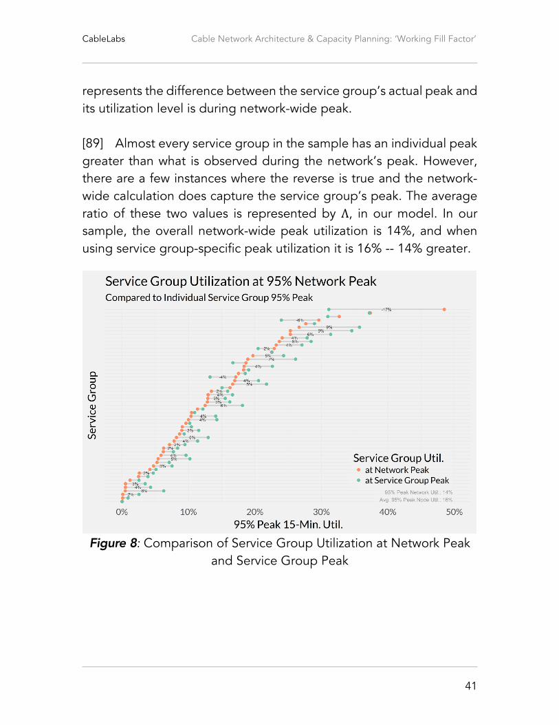
[39] As service group utilization is aggregated to the CMTS and network-wide levels, the variability in utilization measurements decreases, further smoothing the highly variable nature of household demand.9 That is, if we observed 15-minute intervals over time, we would expect there to be less variability in a CMTS' average utilization (across all of its service groups) than in an individual service group's average utilization (across all of its households). Since service groups and households are connected directly, the service group represents the smallest cluster of households on the network, and where we expect variation to be the greatest. A CMTS contains many service groups, so its average utilization includes many more subscribers (total number of households across all of its service groups) and the variability in its average utilization will be smaller. For the same reason, variation in network-wide utilization (across all of its CMTS) would be smaller than at the CMTS or service group level. [40] The differing x-axis ranges in Figures 6 and 7 illustrate how variation in utilization decreases at higher levels of network aggregation. There is no data filtering applied to these figures, so the range of values on the x-axes are reflective of the actual distributions 9 This result follows from probability theory’s law of large numbers, which states that as a sample size increases its average will converge, in probability, to the expected average. A common example of this result is flipping a fair coin many times. For a given number of flips, we would expect there to be 50% heads and 50% tails. For a small number of flips, we may observe a ratio that differs from our expectation, but the law of large numbers states that as the number of flips increases the observed ratio should converge to the expected 50-50 split. In the context of a cable network, this means that since network-wide calculations are over a much larger sample of households, we expect there to be less variation in its observed average and what we would expect before measurement. Similarly, since service groups and nodes are composed of fewer households, we would expect there to be a larger difference, on average, between the observed and expected averages.


16

in our sample. In Figure 6, where we aggregate utilization to the service group level, the x-axis stretches from 0% to 80% and has a standard deviation of 5.8, but in Figure 7, where we aggregate information to the network-wide level (a higher level of network aggregation than a service group), the x-axis spans from only 0% to 30% and has a lower standard deviation of 4.5. As such, our observed distribution of network-wide utilization has a smaller range and less variance than the distribution of service group utilization, as theorized earlier by the law of large numbers. Capacity Investments in Cable Networks [41] Adding capacity to a service group is done by either increasing its amount of spectrum or segmenting its households into smaller groups. Investment is unique to a specific operator, influenced by internal strategies, dependent on network configuration, and can be impacted by previous investment decisions, but there are some generally accepted practices for network augmentation that are covered below. [42] In some cases, operators may be able to allot additional spectrum within a service group to broadband. Examples of such cases that would free spectrum for reallocation include an increase in usage of switched digital video or a transition of television signals from analog to digital. This reallocation of spectrum would apply to an entire region of the network and the additional capacity would be added to each service group, regardless of the service group’s need. This type of broadband capacity augmentation is less regular, as it generally requires multi-year planning and investment. [43] A more common and regular approach to creating capacity for a service group is to segment its households into smaller groups,


17

reducing “competition” for DOCSIS network capacity between households. This usually involves the creation of new service groups and/or nodes to serve these smaller groups of households. Two examples of how an operator might accomplish this are provided below:

• Example 1: Consider a service group of capacity 𝐶E that includes two nodes. If an operator wants to increases capacity for these households, they may create an additional service group and move the two nodes to a one-to-one configuration. Now, both of the new service groups have capacity of 𝐶E and the households connected to each (which is smaller in number than the two combined) are able to share their service group's capacity of 𝐶E. The following, which is summarized in Figure 2 below, is an example of such a change: Assume that Service Group J includes Nodes 1 and 2 and has capacity of 500 Mbps.10 Node 1 connects 225 households and Node 2 connects 250 households for a total of 475 households sharing Service Group J’s 500 Mbps. Operator A now creates Service Group K with capacity 500 Mbps11 and configures the network so that Service Group J connects only to Node 1 and Service Group K connects only to Node 2. After this change, Node 1’s 225 households are sharing Service Group J’s 500 Mbps and Node 2’s 250 households are sharing Service Group K’s 500 Mbps.

10The use of 500 Mbps as a capacity value is strictly for illustrative purposes and is not meant to reflect any specific operator’s capacity allocation to a service group.11 We assume that Service Group K would have the same capacity as Service Group J because it is common for cable operators to plan for the same channel allocation to all service groups. This enables uniform offerings, reduces operational complexity, and aligns with CMTS provisioning conventions.


18

Figure 2: Diagram of New Service Group Investment Example

• Example 2: Consider a service group that has a one-to-one

mapping to a node. Here, an operator may decide to perform a “node split”, where they create a service group and a new node is physically installed in the field. After installation, half of the original node's households are moved to the new node and service group. Similar to the previous example, there are now two smaller groups of households that are able to share a service group's capacity 𝐶. An example of this is the following: Assume that Service Group J is connected to Node 1 and Node 1 has 450 households. Service Group J has capacity of 500 Mbps. Operator A now creates Service Group K with capacity 500 Mbps and physically installs Node 2 out in the field. As a part of the change, Service Group K and


19

Node 2 are connected and 225 of Node 1’s households are moved to Node 2. After this change, the remaining 225 households on Node 1 share all of Service Group J’s 500 Mbps and the 225 households moved to Node 2 share all of Service Group K’s 500 Mbps. This example is illustrated below in Figure 3.

Figure 3: Diagram of Node Split Investment Example

[44] The two examples above also highlight how the costs of segmenting households into smaller groups can vary by investment type. In the first example, moving a node to a new service group may only involve access to the CMTS. However, the second option of performing a node split requires municipal permits, access to utility poles (that may be owned by competing firms), digging up the


20

ground, laying new fiber, and installing new network equipment in the field, in addition to accessing the CMTS. Depending on the location of this new equipment, labor costs and construction lead times may both be considerable. [45] Since capacity is typically added in large chunks, and not in small increments, when households are split into smaller groups, operators must be mindful of both variation in household demand and the expected growth of demand over time. Household demand has grown historically in an exponential fashion with growth of 45% to 55% year-over-year common. The expected duration of a capacity investment to meet both current and future demand is another aspect of this model's timing we revisit in a later section, when discussing WFFs. If an operator plans for a certain investment in a service group to last a year and growth is greater than expected, it can be costly for an operator to resolve this problem quickly, before the next round of investment was planned. Operators are generally aggressive in adding capacity, which reduces the likelihood of unforeseen events negatively impacting the network and service quality. They prefer instead to err on the side of ensuring adequate capacity is provided to meet customer traffic demand. [46] Network investment in the form of service group splits also brings uncertainty in the amount of capacity that will be created. Above in the first example, since individual node utilization is unknown, because measurement occurs at the service group, the operator may create the new service group and find that many of the heavy usage households are still on the same node and the additional capacity created did not significantly reduce utilization for that node -- this likely initiates another costly round of investment sooner than expected. If the operator is unable to perform the same type of investment as before (i.e., moving to a one-to-one configuration), they


21

will have to use another form of network augmentation such as a node split, which could carry much higher costs for the aforementioned reasons. [47] Operators closely track and forecast service group utilization over time to inform investment planning. Because of variation in household demand, there are instantaneous moments within the 15-minute intervals that exceed the interval's average utilization and could even totally consume the service group’s capacity 𝐶. At higher average utilization levels, this variation increases the likelihood that network performance degrades. Household demand is variable enough that these high-utilization events can occur at average utilization levels around 50%-60%, lower than what might be expected. This is shown in Figure 6 of the Appendix, as discussed earlier in the “Nodes and Service Groups” section. [48] As such, capacity investment focuses heavily on what is typically called “peak demand.” Peak demand is usually calculated as the 95th percentile utilization level for a sample of 15-minute measurements, typically spanning weeks to months. For example, if Operator A has a sample of 100 15-minute observations of network-wide average utilization (across all CMTS), peak demand is the 5th largest value in the sample. Internet usage follows a diurnal pattern of lightest usage during the middle of the night and heaviest usage in the late evening. Demands on network infrastructure are collectively greatest during these late evening hours, where average service group utilization is typically at its highest level for the day and household variation is most impactful on the network's state. It is during these evening hours that the network usually experiences peak demand. A peak demand calculation of an individual service group helps inform operators of when investment is needed by signaling how heavily it is being utilized during its busy hour.


22

[49] An important consideration when calculating peak demand is that the network’s peak demand does not necessarily capture an individual service group’s peak demand. The difference between the two is that the network’s calculation would be from a sample of many service groups and the latter calculation is for just a specific service group. There is no guarantee that the 95th percentile measurement of an individual service group is in the 95th percentile measurement period of the network (i.e., the timing of each service group’s peak demand is not synchronized, even for service groups in the same time zone). If the 95th percentiles of each service group are considered together, network peak demand would be greater than basing it on the network’s average utilization (i.e., the notion of “peak demand” that occurs typically during late evening hours). [50] The relationship between a service group’s peak demand and the network’s peak demand is summarized in Figure 8 of the Appendix. For virtually all service groups in our sample, the service group’s individual 95th percentile 15-minute average utilization level is greater than what the service group’s average utilization is during the network’s 95th percentile 15-minute average. This means the timing of the service groups’ peaks are not aligned. We do observe, however, a few instances where the network’s 95th percentile did capture a service group’s 95th percentile. If we use all of the individual service group 95th percentiles to calculate network-wide utilization, we find this value is 14% greater than the network’s 95th percentile. That is, the network-wide 95th percentile average utilization level understates the service group peak utilization levels by 14%. [51] Because of the highly variable nature of household demand and its exponential growth over time, operators are sensitive to estimation errors of how much capacity is needed. There is a mixed investment strategy of proactive and reactive measures by operators to handle


23

peak demand. Proactive investment adds capacity that will be needed to meet peak demand over a period of time, while reactive changes occur when growth is much faster on a service group than anticipated. The exact combination of these two types of investment is unique to each operator and situation.

3.2 Working Fill Factors [52] We interpret a network’s WFF to be the average operational utilization level of a specific entity (e.g., service groups or nodes) over the entire access network at steady-state. WFFs are reflective of operator objectives for providing consistent levels of provisioned service to subscribers. It follows that a network’s WFF will be different if based on service groups or nodes. Since service groups are composed of individual nodes and a node’s utilization cannot be greater than a service group’s, we would expect a WFF based on service group data to be greater than or equal to a WFF based on node data.12 The equivalency case would occur when every service group on the network is mapped one-to-one to a node. [53] Since a WFF is a network-wide utilization calculation, its interpretation and derivation must consider all aspects of the cable network outlined in Section 3.1. Specifically, a WFF must consider the relationship between the following pieces of information:

12We note in paragraph [28] that operators may not be able to observe per node utilization when there is a many-to-one mapping between nodes and service groups. This does not prevent an operator from calculating a node-based WFF value. Since a WFF is an average, all that is needed is to divide the total number of bytes (or bits) passed over a period of time (i.e., the numerator for calculating an average) by the number of nodes on the network (i.e., the denominator for calculating an average).


24

• There is a maximum threshold utilization level that should not be exceeded to ensure optimal network performance. This utilization level is similar for all service groups on the network and typically a benchmark for the service groups’ peak demand (e.g., 95th percentile average utilization level).

• Household demand is variable and reflected by service groups and CMTS differently.

• Network investment is regular over time by an operator (e.g., it is easier to budget investment and manage a workforce that has a smooth workload over the year), but not continuous for a specific service group. Capacity is added commonly to the network in large quantities for a group of households by segmenting them into smaller groups.

• Operators must plan for large amounts of growth in household demand between investment cycles to address growth trends. Operators try to create enough advanced capacity that the aforementioned maximum threshold utilization level where network performance degrades is not reached. More generally, the time planned for by the operator depends on the expected growth in household demand, the expected frequency of network investment, and the types of network augmentation to be performed. However, as modern cable access networks move towards smaller service group and node sizes, forecasting usage becomes harder and the error around these predictions becomes larger. This follows from an individual household’s demand being highly variable. When there are fewer households grouped together, the difference between expected usage and actual usage will be larger, on average, because the sample size is smaller and the law of large numbers is less applicable. In addition, as the number of


25

service groups grows, investment and capacity upgrade cycles become longer, increasing uncertainty in demand growth between cycles as a function of time.

• There are other costs and aspects of network investment that create friction in investment choices. Network construction tasks are usually grouped together because of factors such as municipal permits and cost efficiencies. The purchase or configuration requirements of network equipment (e.g., CMTS equipment) may group resources (e.g., upstream and downstream capacity) in manner that inhibits the optimization of investment in each resource independently. It follows that since service group and node investment is lumpy (i.e., capacity is added in relatively large amounts at irregular intervals) in part due to these frictions, an operator may decide to be aggressive in upgrading certain nodes, if they may not have access again in the short-run.

Deriving a Network’s Expected WFF [54] This section develops intuition on how a network’s expected WFF can be modeled. The following derivation is for an “expected” WFF because the network’s actual WFF is unknown until measured. We begin at the service group level by discussing what the expected utilization is at a point in time, and then move to a network-wide aggregation of these service group expectations. We conclude by relating this network-wide aggregation to the network’s expected WFF. [55] For a service group, there are three important factors that determine its expected utilization at time 𝑡.


26

• The service group’s maximum target threshold utilization level, set by the operator

• The timing and nature of investment in the service group by the operator

• Cost frictions the operator faces when making investment Each of these factors, and the relationship between them, is covered below. [56] Let service group 𝑗's maximum target threshold utilization level be denoted as 𝑈E(𝜎E), where 𝜎E is variation in household demand. 𝑈E(𝜎E) is a utilization level that applies to the 15-minute average utilization periods (i.e., average utilization at time 𝑡), and 𝜎E is likely a standard deviation or Markov chain of “instantaneous” household demand over the same period. Average utilization for service group 𝑗 that reaches or exceeds 𝑈E(𝜎E) makes it likely that network performance is slightly degraded for the connected households to service group 𝑗. [57] 𝑈E is a function of 𝜎E because variation in household demand is fundamental to how high or low 𝑈E should be set. If there is large variance in “instantaneous” household demand (a large 𝜎E), then 𝑈E will need to be lower. When average utilization is too high, large bursts of household demand could exceed service group 𝑗’s capacity of 𝐶E, something an operator does not want. An extreme example would be to imagine how variation would affect an average utilization level of 95%. For even a small standard deviation around a mean of 95%, complete consumption of 𝐶E would be easily achieved. In practice, 𝑈E(𝜎E) is usually between 70% and 80%, depending on the operator.


27

[58] Recall that Figure 6 in the Appendix relates 15-minute average utilization to per-second variation in utilization, which is the exact dynamic described above between the set maximum threshold utilization level 𝑈E and household demand variation 𝜎E. In Figure 6, we observe for 15-minute average utilization periods over 65%, the 95th percentile per-second utilization exceeds 90%, approaching full consumption of the service group’s capacity. Validating that these high utilization levels are not desirable from the operator’s perspective, the number of these high-utilization observations in the data is far lower than the number of observations at lower utilization levels. [59] Operators make capacity investments in service groups by choosing some form of investment and estimating an expected duration of time the investment should be able to accommodate growth in peak demand before additional investment is needed. We represent the set of investment types an operator can choose from (e.g., a node split, adding channels to broadband) by ℱ and the specific type chosen by the operator to be 𝑠. Next, let 𝜏(𝑡) represent the expected percentage of the advanced capacity created by investment choice 𝑠 is to be available at time 𝑡. This entire investment process is denoted as 𝐼{N∈ℱ,Q R }

E . [60] To illustrate the mechanics of this investment process 𝐼{N∈ℱ,Q R }

E , we use the “node split” example (i.e., Example 2) from the earlier “Capacity Investments in Cable Networks” section. Recall, in this example, we are moving from a single service group-to-node pairing, and evenly splitting the households on this node across a new service group and node that are created by the investment. In the above mathematical notation, 𝑠 = "𝑛𝑜𝑑𝑒𝑠𝑝𝑙𝑖𝑡" and 𝜏(𝑡) is defined over the interval 50%, 100% . The 50% lower bound of this 𝜏 interval is right


28

after investment is completed, and the 100% upper bound represents the end of the planned investment cycle. [61] There is a close connection between 𝑠 and 𝜏(𝑡) because the type of investment chosen by the operator will determine what gains to capacity are expected. Depending on the investment choice 𝑠 ∈ ℱ, the lower and upper bounds of 𝜏(𝑡)may be different to reflect the operator's intentions of investment. For example, consider a modification to the “node split” example referenced above where the operator is planning for 50% growth over a 3-year window. This growth rate suggests peak demand will increase to be around 3.4 times the current level, and the single service group-to-node pairing will need to be split four ways, not two. This means the 𝜏 𝑡 intervals would be defined over 25%, 100% , not 50%, 100% as above in the two-way split example. [62] Finally, let other cost frictions related to network investment be represented by 𝑀. These frictions in the operator's investment strategies can arise from getting municipal permits, labor cost efficiencies, purchase or configuration requirements of network equipment, etc. [63] Putting the above together in one functional form, we define service group 𝑗's expected maximum utilization level (EMUL) at time 𝑡 to be

𝐸𝑀𝑈𝐿E|R = 𝑈E 𝜎E ∙ 𝐼{N∈ℱ,Q(R)}E ∙ 1 − 𝑀 ,

where 𝑈E 𝜎E is the node's threshold maximum utilization level, 𝐼{N∈ℱ,Q(R)}E is the node's position along the advanced capacity cycle at

time 𝑡, and (1 − 𝑀) are cost frictions related to investment.


29

[64] A couple of key points about this 𝐸𝑀𝑈𝐿E|R equation. First, the above equation is an expectation because utilization at time 𝑡 is unknown until household demand 𝐻(𝑡) is observed. Second, since 𝑈E 𝜎E sets the upper threshold of what a service group's average utilization should be, an 𝐸𝑀𝑈𝐿E|R is an expectation of what the maximum utilization level service group 𝑗 would be when observed at time 𝑡. When utilization of service group 𝑗 is observed at time 𝑡 it will most likely be below the 𝐸𝑀𝑈𝐿E|R estimate, as a result (i.e., there is a small probability the observation would be at its maximum). The intuition of there being a difference between a service group’s expected maximum utilization, as defined by the 𝐸𝑀𝑈𝐿E|R equation, and its actual utilization level when network-wide peak demand is measured is what motivates the inclusion of the Λ parameter below. [65] Table 2 below uses the same "node split” example to show how the variables in the 𝐸𝑀𝑈𝐿E|R equation are related for the original service group in the example. Notice that 𝐶E is constant over all time periods (i.e., columns in the table) and the effective capacity gain is coming from fewer households sharing this capacity. 𝑈E 𝜎E remains constant for the purposes of this example, but the operator’s expectation of 𝜎E may be changing as the service group size decreases (as discussed in paragraph [1]). 𝑀 is constant, reflecting that operator expectations are not generally changing with regard to these factors. The movement in 𝐸𝑀𝑈𝐿E|R is being driven by changes in 𝐼{N∈ℱ,Q(R)}

E by the network investment.13

13In our example, traffic demand is divided equally, but this is rarely the case in practice given variations in household demand and the constraints of network topology. The term 𝑀 in our EMUL equation can include accounting for less than equal splitting of demand when nodes are split.


30

Table 2: Example EMUL Calculation for a Service Group Variable t-2 t-1 t t+1 t+2

𝐶E 500 Mbps 500 Mbps 500 Mbps 500 Mbps 500 Mbps Num of HH 450 HH 450 HH 225 HH 225 HH 225 HH

𝑈E 𝜎E 75% 75% 75% 75% 75% 𝐼{N∈ℱ,Q(R)}E 90% 91% 50% 51% 52%

𝑀 5% 5% 5% 5% 5% 𝐸𝑀𝑈𝐿E|R 64% 65% 36% 36% 37%

[66] At time 𝑡 the 36% 𝐸𝑀𝑈𝐿E|R value is an estimate of what the most extreme average utilization value would be when measured. As mentioned above, it is most likely that the service group’s average utilization will be below this estimate, when the network-wide peak demand is calculated. This can be seen in Table 2 by recognizing how conservative 𝐸𝑀𝑈𝐿E|R is when investment occurs. Notice at time 𝑡 − 1 the service group was at 91% along the previous investment cycle’s advanced capacity, not 100%. However, at time 𝑡, the 50% factor is applied with the assumption that usage during the previous cycle reached 100% of the advanced capacity (where average utilization would be close to 𝑈E 𝜎E ). This has two implications. First, an operator is likely to be aggressive with investment to provide a high-degree of network performance across a service group. Second, it reflects the notion that a service group’s observed average utilization during network-wide peak demand is likely below this 36% estimate. [67] We estimate a network's WFF at time 𝑡 to be a weighted average of the individual service group EMUL's

𝑊𝐹𝐹R = (1 − Λ) ∙1𝐽 𝐸𝑀𝑈𝐿E|R

a

E@A

.

[68] Recall that 𝐸𝑀𝑈𝐿E|R is an expected maximum utilization for service group 𝑗 at time 𝑡. As discussed above, when the network’s


31

peak utilization is calculated, not many of the service groups (if any) will be at these exact levels (as discussed in paragraphs [49] and [50]). As a maximum, 𝐸𝑀𝑈𝐿E|R represents a relatively rare event on the network, albeit an important one for investment. A simple average of the expected maximum utilization levels of all service group at time 𝑡 would overstate what the actual WFF will be when measured. [69] Λ adjusts for the difference of how an 𝐸𝑀𝑈𝐿E|R is defined (as an expected maximum for a service group) and what would actually be measured by the operator (a network-wide aggregated value with lower variability). If all service groups experienced peak demand at the same time Λ would be equal to 1, but since this is not the case, Λ is defined over the interval [0, 1]. The average difference between a service group’s expected maximum and observed level at network peak could be estimated from a long enough time series (e.g., weeks to months, since there can be profound one-off network events) of service group utilization. [70] In the earlier “Capacity Investments in Cable Networks” section, we discussed how Figure 8 in the Appendix illustrates how the 95th percentile average utilization level of an individual service group does not usually align with the network-wide 95th percentile average utilization level. Figure 8 is relevant here because it depicts the same relationship described above in motivating the Λ parameter of our model. As the model pertains to Figure 8, our 𝐸𝑀𝑈𝐿E|R equation is modeling the service group specific peaks, and the 𝑊𝐹𝐹R equation is describing the network’s measured peak utilization. From our sample, we estimate a 14% larger utilization level for the network when based on individual service group peaks and not the network’s 95th percentile average utilization level. Said another way, the network 95th percentile peak underestimates the sum of 95th percentile peaks of the individual nodes by 14%. As mentioned earlier, since our sample is


32

only representative of modern cable access networks, this 14% value should not be considered an universal point estimate applicable to all cable networks. [71] This model is flexible enough to allow for 𝐸𝑀𝑈𝐿E|R to be calculated using service group, node, or CMTS data. As the context of the calculations changes, the variables in the model (e.g., 𝑈E 𝜎E and Λ) would need to be updated accordingly. All of the discussion on the variability in household demand, growth rates in peak demand, how variation in average utilization decreases at higher levels of aggregation is still applicable, the context just changes. An Example WFF Calculation [72] Consider a cable access network composed of 1 CMTS and 3 service groups. Assume two of the service groups, 𝑗 ∈ 1, 2 , are the result of a recent node split (i.e., the exact same type of investment considered in Table 2 for consistency) intended to create double the capacity during peak demand. The third service group, 𝑗 = 3, is about to be augmented and at the end of its investment cycle. Assume the operator of this network has a target maximum utilization threshold of 75% and other cost frictions related to investment of 5%. Finally, assume for the purposes of this example that this network has a Λ =30%. That is, the individual service group peaks are about 30% greater, on average, than during the network’s peak. [73] Since service groups 𝑗 ∈ 1, 2 are the result of a recent node split, we will set 𝐼E to 50%. This is the same calculation made in Table 2 at time 𝑡.

𝐸𝑀𝑈𝐿A,e|R = 𝑈E 𝜎E ∙ 𝐼 N∈ℱ,Q RE ∙ 1 − 𝑀 = 75% ∙ 50% ∙ 1 − 5%

= 36%


33

[74] For service group 𝑗 = 3 we set 𝐼E to 100% since it is at the end of its investment cycle and about to be augmented.

𝐸𝑀𝑈𝐿h|R = 𝑈E 𝜎E ∙ 𝐼 N∈ℱ,Q RE ∙ 1 − 𝑀 = 75% ∙ 100% ∙ 1 − 5%

= 71% [75] The estimated WFF of this network is

𝑊𝐹𝐹 = 1 − Λ ∙1𝐽 𝐸𝑀𝑈𝐿E|R =

a

E@A

1 − 30% ∙13 𝐸𝑀𝑈𝐿E|R =

h

E@A

33%

4 Working Fill Factors in Practice [76] While the model outlined in Section 3 is representative of cable access networks across North America, there are idiosyncratic characteristics of each operator’s network, and the localities to which they provide service, that affect each network’s WFF. Some of the reasons cable access networks may have different WFFs are:

• Bandwidth demand of different subscriber populations may be more or less variable than others. As a result, the target maximum utilization threshold 𝑈E would be updated to reflect those conditions.

• Different operators may have different investment strategies. In general, an operator's strategy will depend on the frequency of investment, estimated growth in household demand (including accommodation for uncertainty in this estimate), and the target amount of advanced capacity from the investment.

• When building an expectation of 𝐼{N∈ℱ,Q(R)}E , recognizing that

while operators have investment strategies, the most efficient


34

investment option for a service group will depend on its specific configuration and location on the network.

• Cost frictions (𝑀) related to network investment might be unique to individual operators. These operator-specific factors could be the location of their networks and the politics, weather, and seasonality of these areas, economies of scale, or any other unique feature of an operator that affects how they plan to invest.

[77] The confluence of these factors leads us to expect WFFs in the range of 25% to 45% when based on service group data and within the range of 15% to 45% when based on nodes. [78] The efficacy of the capacity and investment strategies we outline for cable networks is reflected in how well cable networks rank in performance studies. In Figure 4, we present the CRTC’s measurements of how well different Canadian operators are at providing real-world download speeds that meet the advertised speeds. During off-peak hours, all cable operators meet, and usually exceed, their advertised download speeds. The same result qualitatively holds when measured during peak hours. [79] Figure 5 reports a similar view of realized downstream speeds from the FCC’s latest 2016 Measuring Broadband America report. Similar to Figure 4, cable networks provide speeds in line with advertised the majority of the time. All operators’ actual median speed is at least 95% of the advertised rate over 70% of the time. Actual speeds are less than 80% of the advertised rates less than 10% of the time. In both Figures 4 and 5, we observe cable operators providing service that consistently matches or exceeds advertised rates. Moreover, these cable networks are performing either comparable to


35

or better than other network technologies. These observations support the network management practices outlined in this paper.

Figure 4: Download Speed as a Percentage of Advertised Speed

(Figure from CRTC) 14

Figure 5: Comparison of Median Download Speed and Advertised

Speed (Figure from FCC) 15

14 This figure is from page 14 of the electronic copy of the CRTC’s “SamKnows Analysis of Broadband Performance in Canada March & April 2016”, dated September 1, 2016. 15 This figure is from page 18 of the FCC’s “2016 Measuring Broadband America Fixed Broadband Report.”


36

5 Conclusion [80] We have articulated in this report the capacity planning and technology considerations on cable broadband networks. Through construction of a model, we have explored how a range of factors influences network utilization, including target utilization levels during peak periods, variability in traffic across network segments serving different numbers of end-users, the time required to augment capacity and traffic growth anticipated during that period, among other considerations. In addition, through empirical observation of utilization on a representative network, explored in detail in the Appendix, we observe these factors in action. [81] The considerations presented here are crucial for arriving at Working Fill Factors for cable operators under CRTC Phase II costing for TPIA services. However, we do not endeavor to calculate specific WFFs for each cable operator subject to TPIA, as specific values will vary depending on the network circumstances and investment strategies of each operator. Nevertheless, these capacity planning and technology considerations are common across all North American operators. The efficacy of these technologies and practices is apparent in the high level of service provided to broadband customers.


37

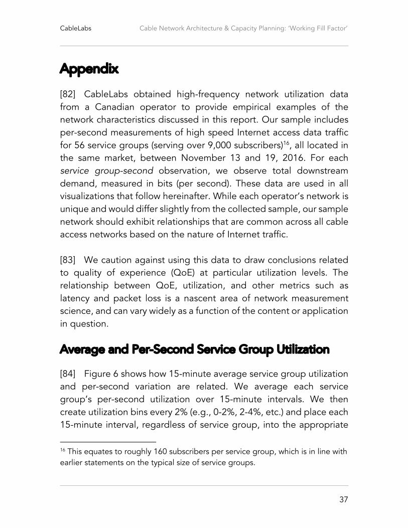
Appendix [82] CableLabs obtained high-frequency network utilization data from a Canadian operator to provide empirical examples of the network characteristics discussed in this report. Our sample includes per-second measurements of high speed Internet access data traffic for 56 service groups (serving over 9,000 subscribers)16, all located in the same market, between November 13 and 19, 2016. For each service group-second observation, we observe total downstream demand, measured in bits (per second). These data are used in all visualizations that follow hereinafter. While each operator’s network is unique and would differ slightly from the collected sample, our sample network should exhibit relationships that are common across all cable access networks based on the nature of Internet traffic. [83] We caution against using this data to draw conclusions related to quality of experience (QoE) at particular utilization levels. The relationship between QoE, utilization, and other metrics such as latency and packet loss is a nascent area of network measurement science, and can vary widely as a function of the content or application in question.

Average and Per-Second Service Group Utilization [84] Figure 6 shows how 15-minute average service group utilization and per-second variation are related. We average each service group’s per-second utilization over 15-minute intervals. We then create utilization bins every 2% (e.g., 0-2%, 2-4%, etc.) and place each 15-minute interval, regardless of service group, into the appropriate

16 This equates to roughly 160 subscribers per service group, which is in line with earlier statements on the typical size of service groups.


38

bin based on its average utilization value. For each utilization bin, we calculate distributional statistics (e.g., 5th percentile, median, etc.) on its per-second observations and construct the box plots in the figure. [85] As 15-minute average utilization increases, the per-second utilization distribution shifts upward and has increased variation, until the service group starts to become saturated for a portion of the 15-minute period. For example, 15-minute samples with utilizations of 40%-42% have a 95th percentile per-second utilization of 60% and a 75th percentile per-second utilization of 48%. Although 15-minute intervals with average utilization exceeding 60% are rare in our sample, we do observe per-second instances where a service group’s capacity is totally saturated.

Figure 6: 15-Minute Average Service Group Utilization and Per-

Second Variation

95%

75%

50%

25%

Mean

5%

Per-Sec Util.

n=15-min intervals


39

Network-Wide and Service Group Utilization [86] Figure 7 below illustrates how 15-minute network-wide utilization and variability of service group utilization from the same period. We calculate network-wide utilization for each 15-minute period by averaging across 15-minute service group average utilizations. Similar to the methodology of Figure 6, we create utilization bins every 1% and group each 15-minute network-wide average into the appropriate bin. For each utilization bin, we calculate summary statistics of the observed 15-minute service group averages to construct the box plots in Figure 7. [87] As network-wide utilization increases, we observe more variance in the service group utilizations, but since the 5th percentile is relatively constant for all utilization bins, there is little evidence of the underlying distribution shifting upward like in Figure 6. The ranges of service group utilization can be larger than what the network-wide average may suggest. For network-wide utilization of 20%, service group utilization falls between 2% and 42%. Put differently, this upper bound of 42% is 100% larger than the average and the lower bound of 2% is one tenth the average. Recall Figure 6 describes the relationship between 15-minute service group averages and per-second variation in utilization, which adds richer context for the values in each box plot of Figure 7. For the 42% upper bound in this example, Figure 6 states we expect per-second utilization bursts on the service group to reach 60%. Similarly, when the network reaches 25-30%, the rightmost box plots in Figure 7, some service groups have average utilization above 60%, which from Figure 6 suggests they have periods where per-second utilization is over 80%.


40

Figure 7: 15-Minute Average Network Utilization and Service Group

Variation

Network Peak and Service Group Peak Utilization [88] Figure 8 depicts the relationship between what a service group’s utilization is during the network’s and its own peak utilization. A service group’s 95th percentile utilization level is represented by a green dot in the figure and calculated using the same method from Figure 6. We calculate network-wide peak utilization by summing across service groups for each 15-minute interval and identifying the 95th percentile utilization level (i.e., the 34the greatest 15-minute period). A service group’s utilization level during the network-wide peak period is denoted by an orange dot in the figure. The distance between the green and orange dots of a service group in Figure 8

95%

75%

50%

25%

Mean

5%

Svc. Group15-Min Util.

n=15-min intervals


41

represents the difference between the service group’s actual peak and its utilization level is during network-wide peak. [89] Almost every service group in the sample has an individual peak greater than what is observed during the network’s peak. However, there are a few instances where the reverse is true and the network-wide calculation does capture the service group’s peak. The average ratio of these two values is represented by Λ, in our model. In our sample, the overall network-wide peak utilization is 14%, and when using service group-specific peak utilization it is 16% -- 14% greater.

Figure 8: Comparison of Service Group Utilization at Network Peak

and Service Group Peak

cable broadband network architecture and capacity planning

Documents