cad5 surfaces

7/29/2019 CAD5 Surfaces

http://slidepdf.com/reader/full/cad5-surfaces 1/22

Chapter 5 - Surfaces

CHAPTER 5

SURFACES

5.1 Introduction

Wire frame models are unable to represent complex surfaces of objects like car, ship,

airplane wing, castings etc. A surface model can be used to represent the surface profile

of these objects. Also, surface model can be used for calculating mass properties,interference between parts, generating cross-sectioned views, generating finite element

mesh, and generating NC tool paths for continuous path machining. Additionally, surface

model can be used to fit experimental data, discretized solutions of differential equations,

construction of pressure surface, construction of stress distribution etc.

Surface creation on a CAD system usually requires wire frame entities: lines, curves,

points, etc. All analytical and synthetic curves can be used to generate surfaces.In order to visualize surfaces on a graphic display, a mesh, say m x n in size is usually

displayed; the mesh size is controlled by the user. Most CAD systems provide options toset the mesh size.

A surface of an object is more complete and less ambiguous representation than its wireframe model; it is an extension of a wire frame model with additional information.

A wire frame model can be extracted from a surface model by deleting all surface entities

(not the wireframe entities – point, lines, or curves!). Databases of surface models arecentralized and associative, manipulation of surface entities in one view is automatically

reflected in the other views. Surface models can be shaded and represented with hidden

lines.




5.2 Types of Surfaces

5.2.1 Plane SurfaceThis is the simplest surface, requires 3 non-coincidental points to define an infinite plane.

The plane surface can be used to generate cross sectional views by intersecting a surface

or solidmodel with it.

5.2.2 Ruled (lofted) SurfaceThis is a linear surface. It interpolates linearly between two boundary curves that definethe surface. Boundary curves can be any wire frame entity. The surface is ideal to

represent surfaces that do not have any twists or kinks.

Boundary Curve

5.2.3 Surface of RevolutionThis is an axisymmetric surface that can model axisymmetric objects. It is generated by

rotating a planar wire frame entity in space about the axis of symmetry of a given angle.

Curve axis of

symmetry

Lecture notes © by R. B. Agarwal Computer Aided Design in Mechanical Engineering 5-2




5.2.4 Tabulated SurfaceThis is a surface generated by translating a planar curve a given distance along a

specified direction. The plane of the curve is perpendicular to the axis of the generated

cylinder.

Cylindrical Surface

Curve

5.2.5 Bi-linear SurfaceThis 3-D surface is generated by interpolation of 4 endpoints. Bi-linear surfaces are very

useful in finite element analysis. A mechanical structure is discretized into elements,

which are generated by interpolating 4 node points to form a 2-D solid element.

P2 P3

P1 P4

5.2.6 Coons PatchCoons patch or surface is generated by the interpolation of 4 edge curves as shown.

Edge 2

Edge1 Edge 3

Edge 4





5.2.7 Bezier SurfaceThis is a synthetic surface similar to the Bezier curve and is obtained by transformation

of a Bezier curve. It permits twists and kinks in the surface. The surface does not pass

through all the data points.

5.2.8 B-Spline SurfaceThis is a synthetic surface and does not pass through all data points. The surface is

capable of giving very smooth contours, and can be reshaped with local controls.

Mathematical derivation of the B-spline surface is beyond the scope of this course. Onlylimited mathematical consideration will be given here.

Computer generated surfaces play a very important part in manufacturing of engineering

products. A surface generated by a CAD program provides a very accurate and smoothsurface, which can be generated by NC machines without any room for misinterpretation.

Therefore, in manufacturing, computer generated surfaces are preferred. Since surfacesare mathematical models, we can quickly find the centroid, surface area, etc. Another advantage of CAD surfaces is that they can be easily modified.





5.3 Interpolated Surfaces – Bilinear Surface

A bilinear surface is obtained by linear interpolation between four points, which may or

may not lie in the same plane. The four points appear as vertices or corner points and the

parameter values u and v create lines at various intervals to provide the surface visibility,shown in the figure. The parameters u and v are defined as

0 ≤ u ≤ 1, and 0 ≤ v ≤ 1

P (1,1) P (1,0)

P(0,0)

P(1,0)P(0,1)

P(1,1)

u Bilinear Patch

P (0,1)

v

P (0,0)

The interpolated parametric equation of a bilinear surface is given as:

P (u,v) = (1-u) (1-v) P(0,0) + u (1-v) P(1,0) + (1-u) P(0,1) + u v P(1,1)

In matrix form, it can be written as

P(u,v) = [(1-u)(1-v) u(1-v) (1-u)v uv]

Node points in FEA

Application of Bilinear Surfaces

Bilinear patches are extensively used in 2-D finite element analysis (FEA). In FEA, an

engineering structure is defined by several bilinear surfaces (elements), which are created

by joining points on the structure’s geometry, called nodes. The nodes are connected toother nodes to create quadrilateral surfaces. Points not lying on the nodes are calculated

by interpolation. Thus, the entire structure is completely defined by the nodes and the

bilinear surfaces.

Drawbacks of Bilinear Surfaces

Bilinear surfaces have a very limited use, mainly, for FEA. Since only 4 points can beused in the interpolation, the smoothness of the generated surface is limited. Additionally,

there is no flexibility to control shapes of the surface, unlike the sweeped surfaces.





5.4 Interpolated Surfaces – Coons Patch

A linear interpolation between four bounded curves is used to generate a Coons surface,

also called as Coons patch. The method is credited to S. Coons who developed thisconcept for generating a surface.

Linear interpolation between the boundary curves P(0,v), P(u,0), P(1,v) , and P(u,1) givesthe equation

Q(u,v) = (1-v) P(u,0) + u P(1,v) + v P(u,1) + (1-u) P(0,v)

P(1,v) P (1,1)

P (1,0)

P(u,1) u

P(u,0) Coons Patch

P (0,1) v P (0,0)

P(0,v)

The above equation gives wrong values at the corners (u,v = 0 and 1). For example,

substituting the values of u and v we get,

Q(0,0) = P(0,0) + P(0,0) = 2P(0,0)

Q(1,0) = 2P(1,0), etc.

Which are obviously wrong values. Therefore, The coons patch is created by

modification of the interpolation equation, where the corners are subtracted. Themodified interpolation equation is given as,

P(u,v) = (1-v) P(u,0) + u P(1,v) – v P(u,1) + (1-u) P(0,v) – (1-u) (1-v) P(0,0) – u (1-v) x P(1,0) - (1-u) v P(0,1) – u v P(1,1).

For computational purposes, it is more convenient to write this equation as,





P(u,0)

P(1,v)

P(u,1)P(0,v)

-P(0,0)

-P(1,0)

P(u,0)

-P(0,1)

-P(1,1)

P(u,1)

P(0,v)

P(1,v)

0

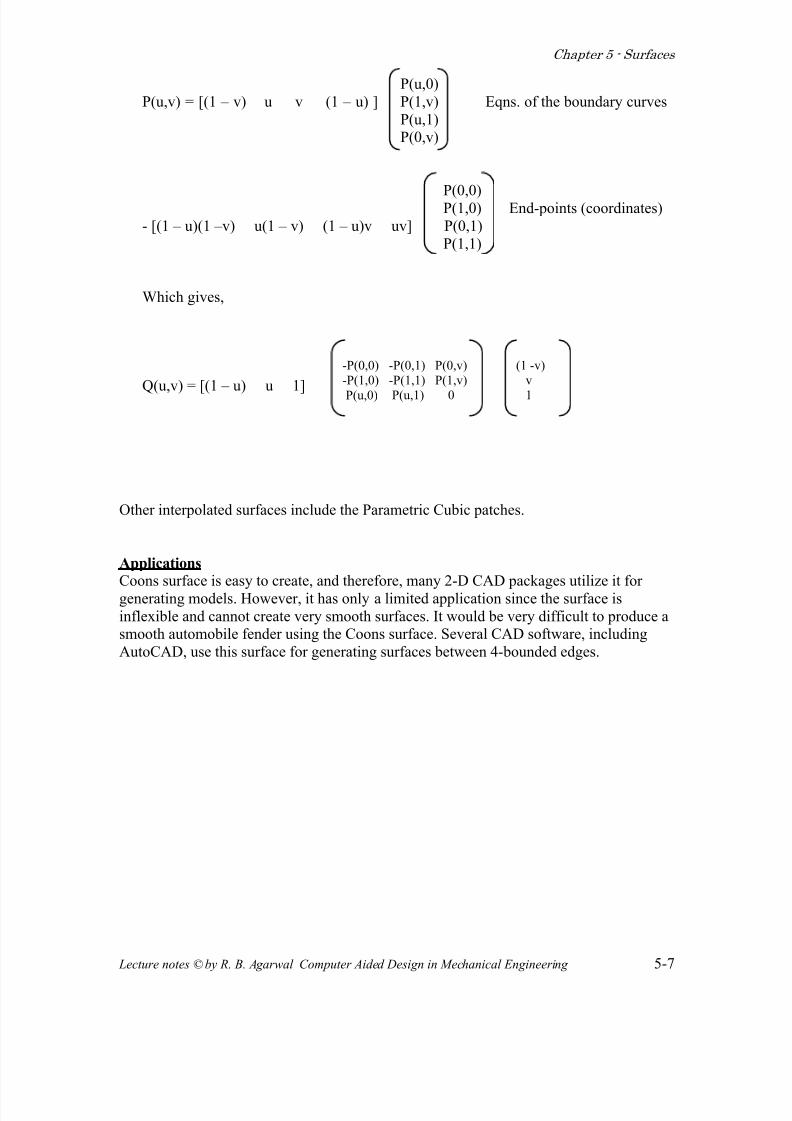
P(u,v) = [(1 – v) u v (1 – u) ] Eqns. of the boundary curves

P(0,0)P(1,0) End-points (coordinates)

- [(1 – u)(1 –v) u(1 – v) (1 – u)v uv] P(0,1)

P(1,1)

Which gives,

(1 -v)

v

1Q(u,v) = [(1 – u) u 1]

Other interpolated surfaces include the Parametric Cubic patches.

Applications

Coons surface is easy to create, and therefore, many 2-D CAD packages utilize it for

generating models. However, it has only a limited application since the surface is

inflexible and cannot create very smooth surfaces. It would be very difficult to produce asmooth automobile fender using the Coons surface. Several CAD software, including

AutoCAD, use this surface for generating surfaces between 4-bounded edges.





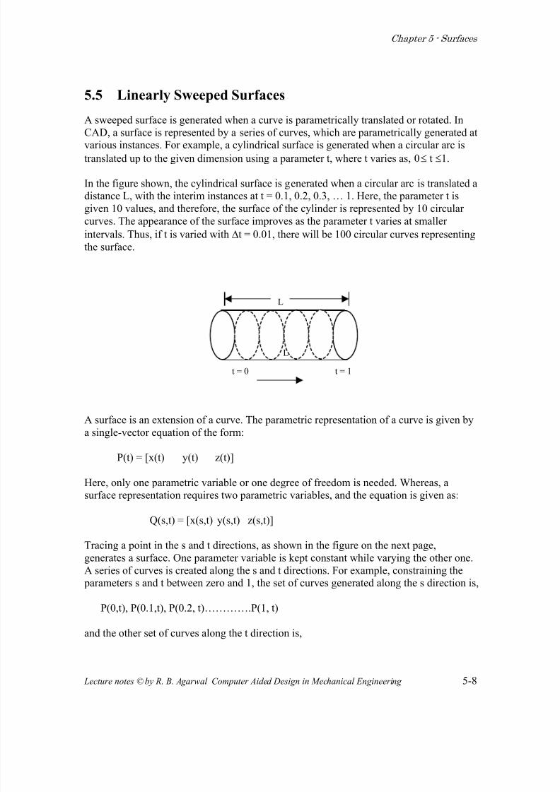
5.5 Linearly Sweeped Surfaces

A sweeped surface is generated when a curve is parametrically translated or rotated. In

CAD, a surface is represented by a series of curves, which are parametrically generated atvarious instances. For example, a cylindrical surface is generated when a circular arc is

translated up to the given dimension using a parameter t, where t varies as, 0 ≤ t ≤1.

In the figure shown, the cylindrical surface is generated when a circular arc is translated adistance L, with the interim instances at t = 0.1, 0.2, 0.3, … 1. Here, the parameter t is

given 10 values, and therefore, the surface of the cylinder is represented by 10 circular

curves. The appearance of the surface improves as the parameter t varies at smaller

intervals. Thus, if t is varied with ∆t = 0.01, there will be 100 circular curves representing

the surface.

L

t = 0 t = 1

L

A surface is an extension of a curve. The parametric representation of a curve is given bya single-vector equation of the form:

P(t) = [x(t) y(t) z(t)]

Here, only one parametric variable or one degree of freedom is needed. Whereas, asurface representation requires two parametric variables, and the equation is given as:

Q(s,t) = [x(s,t) y(s,t) z(s,t)]

Tracing a point in the s and t directions, as shown in the figure on the next page,

generates a surface. One parameter variable is kept constant while varying the other one.A series of curves is created along the s and t directions. For example, constraining the parameters s and t between zero and 1, the set of curves generated along the s direction is,

P(0,t), P(0.1,t), P(0.2, t)………….P(1, t)

and the other set of curves along the t direction is,





P(s,0), P(s,0.1),…P(S, 0.9), P(s,1).

P (s,1)

P(0,t)

t P (1,t)

s

P (s,0)

Thus, creation of a surface requires creation of the multiple curves that constitute it. This

concept can be applied to both, the surface that has an analytical formulation (conicsections) and to a free-form surface (Bezier, B-spline).





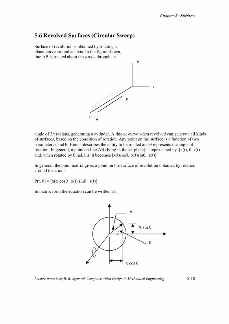
5.6 Revolved Surfaces (Circular Sweep)

Surface of revolution is obtained by rotating a

plane-curve around an axis. In the figure shown,

line AB is rotated about the z-axis through any

B

A

x

z

angle of 2π radians, generating a cylinder. A line or curve when revolved can generate all kinds

of surfaces, based on the condition of rotation. Any point on the surface is a function of two

parameters t and θ. Here, t describes the entity to be rotated and θ represents the angle of

rotation. In general, a point on line AB (lying in the xz-plane) is represented by [x(t), 0, z(t)]

and, when rotated by θ radians, it becomes [x(t)cosθ, x(t)sinθ, z(t)].

In general, the point matrix gives a point on the surface of revolution obtained by rotation

around the z-axis,

P(t, θ) = [x(t) cosθ x(t) sinθ z(t)]

In matrix form the equation can be written as,

x

X sin θ

θ

x cos θ





cosθ sinθ 0 00 1 0 0

P (t, θ) = [x(t) 0 z(t) 1] 0 0 1 00 0 0 1

Note: The above rotation matrix is equivalent to the rotational transformation matrix

studied earlier, which is,

cosθ sinθ 0 0 cosθ sinθ 0 00 1 0 0 - sinθ cosθ 0 0

0 0 1 0 = 0 0 1 0

0 0 0 1 0 0 0 1

Thus, the generated surface is a rotational transformation of a line (or curve), except θ is

not constant, but has values, 0 ≤ θ ≤ 2π.

Example

Generate the conical surface obtained by rotation of the line segment AB around the z-

axis with,

A = ( 1,0,1) and B = ( 7,0,7).

Solution

Line AB can be represented in parametric form as:

P (t) = [x(t) y(t) z(t)], and the parametric equation of a line is,

P (t) = A + (B-A) t

based on this equation, the coordinates of a of point on the line are given as,

x(t) = 1 + (7-1) t = 1+ 6t,

y(t) = 0





z(t) = 1 + (7-1) t = 1 + 6t

The equation of the surface as given above is,

P(t, θ) = [x(t) cosθ x(t)sinθ z(t)] or

= [(1+6t) cosθ (1+6t) sinθ (1+6t)] - equation of the surface

Any point on the surface can be located by substituting t and θ values in the above

equation, e.g.: at t = 0.4 and θ = π/2 radians

P(0.4, π/2) = [1+6(.4)cos (π/2) 1+ 6(.4) sin (π/2) 1 + 6(.4) ]

= [0 3.4 3.4], which is the point on the surface at (.4, π/2)

Example

Generate a Torus by rotating a circle of radius r and the center at (a,0,0) about the z-axis.

Solution

Rotating a circle contained in the x z plane around the z-axis can generate a torus. The

center of the circle has coordinates (a,0,0) and equation of the circle in parametric form is

given as;

P (φ) = [(a + r cosφ, 0, r sinφ]

The torus is represented by,

Q(φ, θ) = {[(a + r cosφ) cosθ], [(a + rcosφ) sinθ], rsinφ} – equation of the torus

In this case, the parameters are φ and θ.





5.7 Circular Sweep of a Synthetic Curve

Equation of a synthetic curve (free-form curve), as derived earlier, is given as,

P (t) = [t] [M] [V]

The surface of revolution is then given by,

Q (t, θ) = [t] [M] [V] [Tr] θ

= [Q(t)][Tr]θ

Where, Q(t, θ ) is the equation of the curve, and [Tr]θ

is the rotation matrix about the z-axis.

Note: To rotate the curve about the axis, we will have to use the translation and rotationmatrices.

Example:

A cubic Bezier curve is defined by the control points: P1 (1,0,2), P2 (3,0,4), P3 (2,0,6),

P4 (5,0,7). Find the surface of revolution obtained by revolving the curve about the z-axis

and calculate the point on the surface at t = 0.5, θ = π/4 rad.

Solution

The cubic Bezier curve is given by the equation,

P (t) = [t][m][v]-1 3 -3 1 v0

3 -6 3 0 v1

= [t3

t2

t 1] -3 3 0 0 v2 1 0 0 0 v3

Substituting the coordinates of the points, we get

-1 3 -3 1 1 0 2 13 -6 3 0 3 0 4 1

P (t) = [t3

t2

t 1] -3 3 0 0 2 0 6 1

1 0 0 0 5 0 7 1





The surface of revolution is:

-1 3 -3 1 1 0 2 1 cosθ sinθ 0 03 -6 3 0 3 0 4 1 0 0 0 0

Q (t, θ) = [t3

t2

t 1] -3 3 0 0 2 0 6 1 0 0 1 0 0 ≤ θ ≤ 2πn1 0 0 0 5 0 7 1 0 0 0 1

0 ≤ n ≤ 1

For t = 0.5 and θ = π/4, the surface equation is,

-1 3 -3 1 1 0 2 1 cos(π/4) sin(π/4) 0 03 -6 3 0 3 0 4 1 0 0 0 0

Q (t, θ) = [(.5)3

(.5)2

(.5) 1] -3 3 0 0 2 0 6 1 0 0 1 01 0 0 0 5 0 7 1 0 0 0 1

= [1.86 1.86 4.86 1]





5.8 Creating a Surface by Parametric Sweeping

In the examples given above, sweeping a curve parametrically generated the surfaces. In

parametric sweeping procedure, a surface is generated through the movement of a line or

a curve along or around a defined path. The curve is sweeped as the sweep parameter is

varied from the values of 0 to 1, creating several instances of the curve along the sweep path. In general, the equation of the surface can be given as,

Q (t, s) = P (t) T (s)

Where, P (t) is the parametric equation of a curve and T(s) is the sweep transformation based on the shape of the path. The sweep transformation can consist of translation,

scaling, rotation or a combined transformation. If the path is a straight line, the points

along the path on the line can be represented by,

x(s) = as

y(s) = bsz(s) = cs

and T (s) is given as,

1 0 0 0

0 1 0 0

T(s) = 0 0 1 0as bs cs 1

Where, a, b, c are coordinate values, and 0 ≤ s ≤ 1

This is equivalent to a three-dimensional translation of a curve with several traces

generated along the path, controlled by how the parameter s is varied.

Example

Consider the Bezier curve defined by the control points P1 = (0,5,0), P2 = (3,4,0), P3 =

(2,0,0), and P4 = (5,0,0). Translate the curve five units along the z-axis to generate a

swept surface.

Solution

Q (t,s) = [P(t)] [Tt], substituting the numbers, we get,

-1 3 -3 1 0 5 0 1 1 0 0 0

3 -6 3 0 3 4 0 1 0 1 0 0Q (t, s) = [t

3t2

t 1] -3 3 0 0 2 0 0 1 0 0 1 0

1 0 0 0 5 0 0 1 0 0 5s 1

Substituting the value of s and solving the matrices can calculate any point on the surface.





5.9 Creating a Surface by Sweeping a polygon

Any polygon can be sweeped around a given path to generate a surface. The equation of

the surface is given as,

Q(s, t) = [P]{T(s)]

Where, [P] is the point matrix, and T(s) is the transformation matrix.

Example:

Sweep (rotate) the triangle A(2,2), B(5,7), C(-2,-5) around x-axis and generate the

surface

solution:

Q(s,t) = [P] [T(s)]

2 2 0 1 1 0 0 0

= 5 7 0 1 0 cos2πn sin2πn 0

-2 -5 0 1 0 - sin2πn cos2πn 00 0 0 1

Note: The value of n locates various positions on the swept surface.





5.10 Creating a Parametric Cubic Patch

Parametric cubic patch or surface is generated by four boundary curves; the curves are

parametric cubic polynomials. The equation of a parametric cubic curve was defined

earlier as:

2 -2 1 1 P(0)-3 3 -2 -1 P(1)

= [t3

t2

t 1] 0 0 1 0 P’(0)1 0 0 0 P’(1)

Constant matrix for n = 3 geometry matrix

Where P(0) = Coordinates of the first point at t = 0

P(1) = coordinates of the last point at t = 1

P’(0) = values of the slopes in x, y, z directions at t = 0

P’(1) = values of the slopes in x, y, z directions at t = 1

Analogous to a cubic curve, a parametric cubic surface can be defined by 16 points:

- 4 points for coordinates of the corner points

- 8 points for slopes in the s & t directions

- 4 points for twist vectors (second derivatives)

Using a procedure similar to the one carried out in the derivation of the cubic curve, wecan derive the geometric coefficient matrix for the surface, which is given as,

P(0,0) P(0,1) Pt(0,0) Pt(0,1)P(1,0) P(1,1) Pt(1,0) Pt(1,1)

[G]H = Ps(0,0) Ps(0,1) Pst (0,0) Pst(0,1)

Ps(1,0) Ps(1,1) Pst(1,0) Pst (1,1)

Which can be broken into 4 groups as,

Position of corner points, Derivatives w.r.t. t of corner points

Derivatives w.r.t s at corner points, Cross derivatives at corner points





Twist vectors, not shown here, are the partial derivatives: dPs/dt & dPt/ds. These vectors

control the internal shape of the surface.

With the geometric coefficient matrix defined, the equation of the surface can be written

as,

P(s.t) = [s] [M]H [G]H [MH]T

[t]T

Where: [s] = [s3

s2

s 1][M]H = [Constant matrix for n = 3 ]

[MH]T

= Transpose of [M]H

[G]H = Geometry matrix as defined by the 16 points, and

t3

[t]T

= t2

t1

Example:

Given: A parametric cubic surface is defined by its Cartesian components as follows:

3 0 1 1 t3

1 0 0 1 t2

x(s,t) = [s3 s2 s 1] 2 1 1 1 t

0 2 -1 0 1

1 1 1 1 t3

1 0 0 0 t2

y(s,t) = [s3

s2

s 1] 2 3 0 0 t1 2 0 2 1

0 1 2 3 t3

1 0 2 0 t2

z(s,t) = [s3

s2

s 1] 3 1 2 1 t

1 0 1 1 1





Obtain the normal vector at the point where s = ½, t = ½

Solution:

P(s,t) = [S] [M]H [G]H [MH]T

[t]T

= [x(s,t), y(s,t), z(s,t)]

X(s,t) = [s] [A]x [t]T

Where [A]x = [M]H [G]H [MH]T

The normal vector n is given by

n = Psx Pt

where Ps = ∂P/ds & Pt = ∂P/dt

3 0 1 1 t3

1 0 0 1 t2

x(s,t) = [s3

s2

s 1] 2 1 1 1 t

0 2 -1 0 1

3 0 1 1 t3

1 0 0 1 t2

xs(s,t) = [3s2

2s 1 0] 2 1 1 1 t

0 2 -1 0 1

3 0 1 1 3t2

1 0 0 1 2t

xt(s,t) = [s

3s

2s 1] 2 1 1 1 1

0 2 -1 0 0

at s = 0.5 & t = 0.5





xs(s,t) = 4.5313

xt(s,t) = 3.3438

similarly, we can evaluate ys(s,t), yt(s,t), zs(s,t) and zt(s,t)

ys (s,t) = 2.5313

yt (s,t) = 5.5313

zs (s,t) = 6.9375

zt (s,t) = 5.4375

And, Ps(s,t) = [4.5313, 2.5313, 6.9375]Pt(s,t) = [3.3438, 5.5313, 5.4375]

i j k

n = Ps(0.5,0.5) x Pt(0.5,0.5) = 4.5313 2.5313 6.9375

3.3438 5.5313 5.4375

= -24.61 i - 1.4413j + 16.59 k





Bi,n(s) & B j,m(t) are the Bernstein blending functions in the s and t directions.

In matrix form, the Bezier surface can be represented by,

Q(s,t) = [S] [M]B [V]B [([M)

T

]B

[t]

T

For a cubic surface this equation reduces to:

-1 3 -3 1 v0,0 v0,1 v0,2 v0,3

-3 -6 3 0 v1,0 v1,1 v1,2 v1,3 Q(s,t) = [s

3s

2s 1] 3 3 0 0 v2,0 v2,1 v2,2 v2,3 x

1 0 0 0 v3,0 v3,1 v3,2 v3,3

1 3 -3 1 t3

3 -6 3 0 t2

-3 3 0 0 t

1 0 0 0 1

Note that, to represent a cubic Bezier surface, 16 control points must be specified, and

several Bezier surfaces can be combined to create a complex surface.

cad5 surfaces

Documents