CAHIER DE RECHERCHE No

WORKING PAPER No.

Retirement and Savings Institute

SDG-1335

9

Designing Disability Insurance Reforms:

Tightening Eligibility Rules or Reducing Benefits?∗

Andreas Haller, University of Zurich and IZA

Stefan Staubli, University of Calgary and NBER

Josef Zweimüller, University of Zurich and CEPR

August 2020

Abstract

We study the welfare e�ects of disability insurance (DI) and derive social-optimality conditions for the

two main DI policy parameters: (i) DI eligibility rules and (ii) DI bene�ts. Causal evidence from two DI

reforms in Austria generate �scal multipliers (total over mechanical cost reductions) of 2.0-2.5 for stricter

DI eligibility rules and of 1.3-1.4 for lower DI bene�ts. Stricter DI eligibility rules generate lower income

losses (earnings + transfers), particularly at the lower end of the income distribution. Our analysis suggests

that the welfare cost of rolling back the Austrian DI program is lower through tightening eligibility rules

than through lowering bene�ts. Applying our framework to the US DI system suggests that both loosening

eligibility rules, and increasing bene�ts, would be welfare increasing.

Keywords: Disability insurance, screening, bene�ts, policy reform

JEL Codes: H53; H55; J14; J21; J65.

∗Address: Andreas Haller, University of Zurich, CH-8000 Zürich, Switzerland; email andreas.haller@uzh.ch. Stefan Staubli,University of Calgary, Calgary, AB T2N 1N4, Canada; email sstaubli@ucalgary.ca. Staubli is also a�litated with CEPR andIZA. Josef Zweimüller, University of Zurich, CH-8000 Zurich, Switzerland; email josef.zweimueller@econ.uzh.ch. Zweimüller is alsoa�liated with CESifo and IZA. We thank Tabea Bucher-Koenen, Raj Chetty, Richard Disney, Thomas Hoe, Lucija Muehlenbachs,Timothy Moore, Matthew Notowidigdo, Luigi Pistaferri, Philippe Ruh, Florian Scheuer, Johannes Spinnewijn, Alexander Strand,ConnyWunsch and seminar participants at Erasmus University Rotterdam, University of Amsterdam, University of Bonn, Universityof Manitoba, University of Melbourne, Universitat Pompeu Fabra, University of Salzburg, University of Zurich, CEPR LabourEconomics Symposium, CEPR Public Economics Symposium, CEPR/NBER Aging/Health workshop, NBER Summer Institute,workshop on �Family, Aging, Social Insurance� in Bergen, and the VfS Population Economics meeting in Basel for helpful comments.This research was supported by the U.S. Social Security Administration through grant #1DRC12000002-04 to the National Bureauof Economic Research as part of the SSA Disability Research Consortium. The �ndings and conclusions expressed are solely thoseof the author and do not represent the views of SSA, any agency of the Federal Government, or the NBER. All remaining errorsare our own.

1 Introduction

The number of disability insurance (DI) recipients has risen rapidly over the past decades in most OECD

countries despite generally improving health, higher material living standards, and less physically demanding

working conditions.1 The increasing �nancial burden of DI programs for taxpayers has led many governments to

implement DI reforms aiming explicitly at reducing the DI program in�ow and DI expenditures. While restrictive

DI reforms reduce the �scal burden for taxpayers, they also impose utility losses on individuals su�ering from

a disability. The welfare consequences ultimately depend on how DI reforms address this incentive-insurance

trade-o�.

In this paper, we pursue the �su�cient-statistics� approach of policy evaluation to shed light on the welfare

e�ects of DI reforms; an approach that has been extensively applied to optimal unemployment insurance (UI).

DI programs di�er from UI programs in two key dimensions. DI receipt is typically permanent, implying

that a key behavioral margin are DI applications driving program in�ow, and the assessment of DI eligibility

requires a medical test, implying that DI reforms need to address the incentive-insurance trade-o� of two policy

instruments: DI eligibility rules and DI bene�ts.2 Indeed, proponents of rolling back the DI program argue

that DI bene�ts are not only too generous but also too easy to obtain. Our paper is the �rst to analyze in a

comprehensive way the welfare e�ects of both DI policy instruments using su�cient statistics.

Our analysis comes in three steps. First, we set up a general theoretical framework to study how DI a�ects

individuals' choices. We derive social-optimality formulas that characterize the incentive-insurance trade-o� in

DI under general economic environments. The incentive costs � both for DI eligibility rules and DI bene�ts � can

be expressed in terms of a �scal multiplier. The �scal multiplier measures the total cost savings of a DI reform

relative to the �mechanical� �scal e�ect, the �scal cost savings in the absence of any behavioral responses. The

�scal multiplier is a key benchmark for welfare analysis: A DI reform is welfare enhancing if the �scal multiplier

is larger than the associated insurance losses. Put di�erently, a DI reform generating a �scal multiplier of x is

welfare enhancing if one dollar in the hands of a marginal DI recipient has a lower social value than x dollars

in public funds.

In the second step of our analysis, we provide a causal analysis of two DI reforms that were implemented

in Austria in 2003 and 2013. The 2003 reform implemented changes to the pension formula reducing DI

1In the US, 2.6 percent of individuals in the age group of 20 to 64 were receiving DI bene�ts in 1992, but by 2012 this fractionhad risen to 5.3 percent. Many European countries have also experienced signi�cant growth of their DI programs, particularlyScandinavian countries. In 2015, public spending on disabilility insurance (�incapacity�) programs amounted to an OECD-averageof 1.9% of GDP, with substantial variation across countries: 1.3% in the US, 1.7% in France, 1.9% in the UK, 2.1% in Austria andGermany, and more than 4% in Sweden, Norway and Denmark (OECD, 2020).

2In contrast, UI receipt is typcially temporary and assessing UI eligibility is straightforward. Moreover, the relevant behavioralmargin in UI (job-search e�ort) a�ects the program out�ow, which is primarily driven by the generosity of a single policy instrument:the UI bene�t level. Baily (1978) has pioneered the theoretical analysis of optimal UI and Chetty (2006) has developed the su�cient-statistics approach in the UI context. More recent applications of the su�cient statistic approach for optimal UI include Shimerand Werning (2007), Chetty (2008), Kroft (2008), Schmieder et al. (2012), Landais (2015), Kroft and Notowidigdo (2016), Landaiset al. (2018) and Kolsrud et al. (2018). See the article by Chetty and Finkelstein (2013) for a detailed discussion of this literature.

1

bene�t levels substantially for some individuals but less so for others. The quasi-experimental variation in

DI bene�ts over time and across individuals allows us to identify the causal e�ect of DI bene�ts. The 2013

reform implemented stricter DI eligibility rules by increasing the �relaxed screening age� (RSA), the age at

which vocational factors in the DI determination process increase DI award rates substantially. Because of

a staggered increase in the RSA, we can compare �adjacent� cohorts to identify the causal e�ect of stricter

DI eligibility rules. Using population data from the Austrian social security register (ASSD) merged with the

universe of DI applications (provided by the Austrian Ministry of Social A�airs, BMASK), we �nd that stricter

DI eligibility rules and lower DI bene�ts in the Austrian DI reforms generated behavioral responses, which

lowered DI program costs substantially.3

The third step of our analysis explores the welfare e�ects of the Austrian DI reforms. To estimate the �scal

multiplier, we can draw on our reduced-form estimate of the total �scal e�ect (the numerator), but we still

have to estimate the mechanical �scal cost savings in the absence of behavioral responses (the denominator).

In the case of lower DI bene�ts, the mechanical �scal e�ect of a one-percent reduction in DI bene�ts is simply

one percent of the pre-reform mean of DI expenditures, which yields a �scal multiplier between 1.3 and 1.4.

Estimating the mechanical �scal e�ect of stricter DI eligibility rules is less straightforward, because we need to

know who is an always applicant (who does not abstain from applying even under stricter DI eligibility rules).

Unfortunately, we cannot observe in the data who is an always applicant and who is a marginal applicant (who

abstains from applying under stricter eligibility rules).4 We argue (and provide supportive evidence) that the

mechanical �scal e�ect can be inferred from the re-application behavior of previously rejected DI applicants.

Based on this strategy, we estimate a �scal multiplier between 2.0 and 2.5.

Taken together, the relative size of �scal multipliers suggests that stricter DI eligibility rules are more e�ective

than lower DI bene�ts in reducing program expenditures. But to assess the relative welfare e�ects, we also need

to compare the insurance losses of the two policy instruments. While we lack the necessary data (on health,

wealth, and consumption) to estimate the insurance losses directly, we �nd that income losses (earnings plus

transfers) associated with stricter DI eligibility rules are smaller than those associated with lower DI bene�ts,

particularly in the lowest quintile of the income distribution. Through the lens of our theoretical framework,

this pattern suggests lower insurance losses of stricter DI eligibility rules compared to lower DI bene�ts. Hence,

3The linked social security and DI applications data provide us with a �unique� data set in the sense that we observe not only allDI applications but also all workers (applicants and non-applicants) covered in the ASSD (about 80% of the Austrian population).Observing applicants and non-applicnts allow us to study in detail individuals' DI application behavior. Staubli (2011) studiesthe labor market e�ects of an earlier increase in the RSA in 1996, but he has no application data and cannot study applicationbehavior, which is important in the present context, since individuals' application behavior is a key driver of the welfare e�ects ofDI reforms.

4If always applicants and marginal applicants had identical (observed and unobserved) characteristics, the mechanical �scal e�ectof stricter DI eligibility rules could be estimated simply by applying lower DI award rates to the average pre-reform DI applicant.We conduct a complier analysis (Imbens and Rubin 1997; Abadie 2003) which shows that always applicants and marginal applicantsdi�er signi�cantly with respect to a number of observed characteristics. Hence, approximating the mechanical e�ect (the �scal costsavings of always applicants) by the cost savings of average applicants (a mixture of always applicants and marginal applicants) ismisleading.

2

to roll-back the Austrian DI program, our results conclude that the welfare cost of stricter eligibility rules would

be smaller than that of bene�t cuts.5

While we think our paper makes progress using the su�cient-statistics approach for optimal DI, we need

to keep in mind the limitations of this approach. First, the welfare implications are drawn from reduced-form

estimates, which apply only �locally� to the particular Austrian context. However, our analysis is of more general

interest, since many DI programs feature eligibility rules similar to Austria that are based on vocational factors

such as age or work history. For example, in the US DI system applicants older than age 55 are evaluated

based on more lenient eligibility standards than applicants between ages 50 and 55, who are subject to more

lenient standards than applicants below age 50.6 Di�erent from what we �nd for Austria, Chen and van der

Klaauw (2008) and Deshpande et al. (forthcoming) do not �nd sorting of applications around these age cuto�s,

suggesting no behavioral response and a �scal multiplier of DI eligibility rules of 1.7 Previous US estimates

on the behavioral responses to changes in DI bene�t levels result in a �scal multiplier very similar to the one

we estimate for Austria. For example, Low and Pistaferri (2015) estimate an elasticity of DI applications with

respect to bene�t levels of 0.62. Together with a DI award rate of 0.67 (French and Song, 2014), this elasticity

suggests a �scal multiplier of lower DI bene�ts of 1.3-1.4 for the US.

A second limitation of the su�cient-statistics approach is that it applies only to marginal (in�nitesimally

small) policy changes, while in reality we are interested in non-marginal policy changes (Kleven, forthcoming).

We address this issue by deriving social optimality conditions for non-marginal DI policy changes and show

that our analysis of the �scal multiplier, a core concept of our framework, is also valid with non-marginal policy

changes. We further show, for non-marginal policy changes, how income losses (along the income distribution)

can be used to bound insurance losses and how these bounds are useful for ranking the two DI policy instruments.

A third limitation of the su�cient-statistics approach is that, without restrictions on preferences and the

economic environment, one typically ends up with a large number of elasticities to be estimated. Our concept

of the �scal multiplier (with its focus on overall program costs) is useful, because it permits welfare analysis

without making speci�c restrictions to reduce the number of elasticities. In this respect, our framework is similar

to Lee et al. (forthcoming) and Hendren and Sprung-Keyser (2020).8

5While our analysis cannot put a number on the absolute insurance losses, a tentative analysis (based on CRRA preferencesand hand-to-mouth consumers) suggests that insurance losses and �scal gains of lower DI bene�ts are of similar size (i.e. DIbene�ts are optimal), while insurance losses fall short of �scal gains of tighter DI eligibility rules (i.e. tightening eligibility rules iswelfare-enhancing).

6There are consideration of revising the US vocational factors. In 2012 the Congressional Budget O�ce proposed to increasethe age cuto�s of the relaxed eligibility rules (Mann et al., 2014).

7Appendix Figure D.25 contrasts the US application behavior to the Austrian application behavior. In Austria, there is a largespike in DI applications exactly at the RSA. In the US, there is no spike in DI applications at the age cuto�s but a discontinuousjump in award rates.

8Lee et al. (forthcoming) estimate the �scal externality of UI bene�t reforms. The �scal externality is the behavioral �scale�ect relative to the mechanical �scal e�ect. Hence, what we refer to as the �scal multiplier is 1+�scal externality. Hendren andSprung-Keyser (2020) use the concept of the Marginal Value of Public Funds (�MVPF�) to evaluate 133 historical policy changes inthe US. The MVPF is the willingness to pay for a policy divided by the net cost to the government. In our application, the MVPFcorresponds to the insurance value divided by the �scal multiplier. We separate the two e�ects. In the case of DI, determiningthe insurance value is not straightforward (and to some degree a judgment call), while the �scal multiplier can be estimated with

3

An interesting aspect of our approach relates more speci�cally to the impact of DI eligibility rules. One

might have thought that a welfare analysis of tighter DI rules requires pinning down type-I and type-II errors

(false rejections and false acceptances). However, we show that it su�ces to estimate the mechanical �scal

e�ect, which is an advantage, because it substantially reduces the data requirements and the complexity of the

analysis. The disadvantage is that we cannot address the accuracy of the screening process � an important open

question in DI research. Instead, a more structural approach, such as the one of Low and Pistaferri (2015), is

able to directly estimate the type-I and type-II errors. Benitez-Silva et al. (2004) and Low and Pistaferri (2019)

provide further evidence on the classi�cation errors of the DI screening process.

This paper contributes to an active literature on the labor market and welfare e�ects of disability insurance

programs (for reviews, see Bound and Burkhauser, 1999; Low and Pistaferri, forthcoming). Our paper comple-

ments the strand of literature that evaluates the incentive-insurance trade-o� in DI programs using structural

models. Most closely related are the US studies of Bound et al. (2004) and Low and Pistaferri (2015). Bound

et al. (2004) simulate the bene�ts and costs of changes in disability bene�t levels and �nd that the implicit price

of providing an additional dollar of income to DI recipients � what we call the �scal multiplier of DI bene�ts �

is 1.5, very similar to our estimate. Low and Pistaferri (2015) assess DI eligibility criteria and DI bene�t levels

in the US and conclude that social welfare could be raised by loosening eligibility criteria and raising bene�ts.

We reach the same conclusion by applying our framework to existing US estimates.

Bound et al. (2010) specify a structural model to study the interplay between health and labor force partic-

ipation. They �nd that removing the DI program entirely would have little e�ect on individuals in good health

but would hurt individuals in bad health. Autor et al. (2019) use a judge leniency instrumental variable design

and a structural model to estimate the consumption and welfare e�ects of DI in Norway. They show that DI

increases household income and consumption for singles but not for married individuals. Their results point,

like ours, to the importance of bene�t substitution.

Our paper also contributes to the theoretical literature on optimal disability insurance. We extend the

model of Diamond and Sheshinski (1995) by expressing the social optimality conditions of DI eligibility rules

and DI bene�t levels as a function of su�cient statistics, which we can estimate empirically using program

evaluation methods. We also generalize their setup to a dynamic environment with rich heterogeneity across

agents. Also related are the US studies of Meyer and Mok (2019) and Deshpande et al. (forthcoming) who apply

the Bailey-Chetty formula for optimal UI bene�ts to DI and estimate the e�ect of receiving DI on consumption

and �nancial outcomes. Similarly, Ball and Low (2014) estimate the e�ect of DI on consumption in the UK

to infer the insurance value of DI bene�ts. We go beyond these papers by studying the welfare e�ects of DI

eligibility rules and comparing them to the welfare e�ects of DI bene�ts. Understanding the e�ects of eligibility

reduced-form methods.

4

rules is important as the discussion about DI reforms focuses on whether individuals are truly eligible for DI

bene�ts.

Our paper also relates to the strand of literature that estimates the impact of DI on applications, DI take-up,

and labor supply using reduced-form methods without considering welfare e�ects.9 Autor and Duggan (2003)

�nd that relaxed eligibility rules and increases in the DI replacement rates explain the stark growth of DI rolls

in the US and lead to a lower unemployment rate.10 Parsons (1991) and Gruber and Kubik (1997) exploit

variation in DI rejection rates across US states over time and �nd that an increase rejection rates reduces DI

applications and increases labor force participation. We �nd similar evidence for self-screening in response to

stricter eligibility rules, i.e. a decline in applications, and also show that stricter eligibility rules target healthier

individuals via our complier analysis.11 Our paper also relates to studies that explore the e�ects of DI bene�t

levels for application behavior and labor supply (Gruber, 2000; Campolieti, 2004; Mullen and Staubli, 2016).

We build on these papers by estimating the e�ects of DI bene�ts on bene�t substitution and �scal costs, which

are key for assessing the welfare e�ects of lower DI bene�ts.

The paper is organized as follows. The next section presents a model of disability insurance and formulas

for optimal disability eligibility and bene�ts. Section 3 describes the data and institutional background in

Austria. Sections 4 and 5 present the empirical results on stricter DI eligibility rules and lower DI bene�t levels,

respectively. Section 6 estimates the �scal multipliers of these two policy instruments and discusses how our

estimates can be used for welfare evaluation. Section 7 applies our framework to the US disability system.

Section 8 concludes.

2 Theoretical Framework

In this section, we explore how the two main DI policy parameters � the strictness of DI eligibility rules and

the level of DI bene�ts � a�ect social welfare, as well as labor supply and application behavior of potential DI

claimants.12 Section 2.1 starts with the static framework of Diamond and Sheshinski (1995) and Section 2.2

9Another important strand of the literature studies the impact of DI receipt on labor force participation by comparing acceptedand rejected DI applicants (Bound, 1989; von Wachter et al., 2011), by exploting variation in eligibility rules (Chen and van derKlaauw, 2008), and by exploiting the random assignment of DI applicants to examiners and administrative law judges (Maestaset al., 2013; French and Song, 2014). We do not directly contribute to this literature, but changes in labor force participation arere�ected in our program cost estimates. We also do not study out�ow from DI (Campolieti and Riddell, 2012, Borghans et al.,2014, Moore, 2015) or earnings of DI recipients (Kostol and Mogstad, 2014, Gelber et al., 2017, Ruh and Staubli, 2019 and Kostøland Myhre, 2020), but these responses enter the �scal multiplier as well.

10Autor and Duggan (2006) discuss potential DI reforms to counteract the cost explosion of the DI program in the US. Theypoint out that there are three ways to reduce the size of DI programs: (i) tightening the screening process (eligibility rules), (ii)reducing the incentives to seek bene�ts (lower DI bene�ts) and (iii) encouraging faster exit. Our framework sheds light on thewelfare e�ects of options (i) and (ii).

11de Jong et al. (2011) and Godard et al. (2019) �nd that another aspect of the application process, more intense screening ofapplicants, also reduces DI applications and improves targeting to more deserving applicants. In contrast, Deshpande and Li (2019)show that higher application costs have adverse targeting e�ects by inducing individuals who would have quali�ed for DI to nolonger apply.

12By increasing the �strictness of disability eligibility rules� we mean any policy making it more di�cult that a DI application� with a given degree of disability � gets accepted. This is what Low and Pistaferri (2015) and Diamond and Sheshinski (1995)call, respectively, �strictness of screening� and �disability standard�. The terms disability rules, disability standard, and disability

5

extends the analysis to a dynamic setting.

2.1 A Static Model of Optimal DI

Setup. Consider an agent living for two periods. In the �rst period, she works, earns a wage w, pays a

lump-sum tax τ (which �nances the DI program) and enjoys utility u(w − τ). There are no savings nor any

other choices in the �rst period.13 In the second period, the agent su�ers a disability shock θ, modelled as a

random draw from a continuous distribution F (θ). If θ is small (= the disability not very severe), the agent

continues working and enjoys second-period utility u(w)−θ. If θ is su�ciently large (= the disability severe), the

agent applies for DI bene�ts. A DI application causes disutility ψ, capturing the extensive medical checks, the

bureaucratic hassle, etc. associated with the DI assessment process. The �xed application cost ψ is important in

the present context as it ensures that DI application choices depend on the eligibility rules of the DI system.14

With probability p(θ) the application is accepted, where p′(θ) > 0.15 When the application is accepted, the

agent withdraws from work, claims DI bene�ts b and gets second-period utility v(b)−ψ. When the application

is rejected, the applicant either resumes work and gets second-period utility u(w)−θ−ψ; or claims social welfare

z < b and gets second-period utility v(z)− ψ. (No disutility or uncertainty are associated with claiming social

welfare.) Appendix Figure A.1 illustrates the sequence of events and agent's choices in the second period.

DI Applications and Labor Supply. Let us now look at the DI application choice and the labor supply

decision. An individual prefers working over claiming social welfare bene�ts if her disability is θ < θR ≡

u(w) − v(z) > 0, i.e. if the utility of claiming social welfare falls short of the utility of working. Hence, θR

denotes the �marginal social welfare claimant�. Consider an agent whose disability is not extremely severe,

θ < θR. (This implies she goes back to work in case her DI application gets rejected.) Her application

choice compares the utility when staying employed, u(w) − θ, to the expected utility when applying for DI,

p (θ) v(b) + [1− p (θ)] (u(w)− θ)−ψ. The �marginal applicant,� the agent who is indi�erent between �ling a DI

application and remaining employed, has disability

θA = u(w)− v(b) +ψ

p(θA). (1)

It follows that agents with disability θ ≥ θA apply for DI, while agents with disability θ < θA remain employed.

Figure 1, Panel (a) characterizes the outcome of agents' DI application choices. It draws the probability of

screening are used interchangeably. The formal de�nition of strictness is discussed in detail in section 2.1.13The setup follows Chetty (2006) who reconsiders Baily's (1978) formula of optimal unemployment insurance (UI). The stylized

two-period framework - tax payments but no DI application choices in the �rst period, while no tax payments but DI applicationchoices in the second period - simpli�es the formula without changing the substance of the argument.

14Here we deviate from Diamond and Sheshinski (1995) who do not consider application costs. Recent empirical studies supportthe idea that application costs are important drivers of DI applications, e.g. Deshpande and Li (2019) and Godard et al. (2019).

15Below, we will analyze a situation where the government has control over the p(θ)-function. By adopting stricter eligibilityrules, the p(θ)-function shifts down, so that p takes a lower value for any given θ (and vice versa).

6

DI award p(θ) against θ and indicates the disability cuto�-levels θA and θR. Agents with a disability θ ≥ θA

apply for DI; if rejected, those with disability θ ∈[θA, θR

)return to work, while those with θ ≥ θR go on social

welfare.

Equation (1), and its graphical representation in Figure 1, applies when θA < θR, i.e. a marginal applicant

returns to work in case her DI application is rejected. We discuss in Appendix A.1 the formal conditions under

which θA < θR holds. Note that this is not a critical assumption and we do not impose it in the general model.

Moreover, it is worth emphasizing that this is a natural assumption in the present context. With θA < θR the

model predicts that DI policy parameters a�ect labor supply decisions. Distortionary labor supply e�ects of DI

programs are supported by a large body of empirical evidence.16

DI Policy Instruments. We now assess the welfare e�ects of two policy instruments that characterize any

DI system: the level of DI bene�ts and the strictness of DI eligibility rules. While the role of DI bene�ts b

is straightforward and poses no major conceptual problems, the role of DI eligibility rules θ∗ needs further

discussion. The inherent problem of the DI assessment process is that the true disability θ is the agent's private

information. For this reason, a DI applicant has to undergo a disability assessment process, which delivers an

estimate of her disability to the government. Formally, the government observes s = θ+ e(θ), where s is a noisy

signal, θ is the applicant's true disability and e(θ) is the noise.17 The strictness of DI eligibility rules � the

policy parameter under direct control of the government � can be captured by a critical value of s, call it θ∗,

such that a DI application with s ≥ θ∗ is accepted, while an application with s < θ∗ is rejected. The acceptance

probability can then be written as p(θ; θ∗).18 In what follows, we consider the case where the government can

change θ∗ but takes the signal as given. This is the context of our empirical analysis below, which exploits

quasi-experimental variation in the �relaxed screening age� (RSA) at which DI eligibility rules become more

lenient. In our notation, the strictness of DI eligibility equals θ∗ = θH before the RSA and falls to θL < θH after

the RSA. An increase in the RSA from age R to some higher age R + ∆, implies that, during the age window

[R,R+ ∆], the treated cohort is subject to the strict DI eligibility standard θH , while the control cohort is

subject to the lenient standard θL. If cohorts are otherwise similar (in productivity, health, preferences, etc.),

a plausible assumption for �adjacent� cohorts, comparing treated to control cohorts identi�es the causal e�ect

16A number of papers provide direct evidence on the work behavior of rejected DI applicants. These �ndings are perfectlyconsistent with the predictions of the model with θA < θR. Bound (1989); von Wachter et al. (2011); Maestas et al. (2013); Frenchand Song (2014) use rejected DI applicants as a control group for accepted applicants to study the impact of DI on labor supply.For instance,von Wachter et al. (2011) report that, in 69.6% of rejected DI applicants aged 30-44 in the US report positive yearlyearnings two years after the DI application and 57.4% report earnings higher than three months of full-time employment at theminimum wage in 2000. The corresponding numbers are 52.6% and 42.7% for rejected DI applicants aged 45-64. In the Norwegianstudy by Kostol and Mogstad (2014), about 30 percent of rejected DI applicants aged 18-49 are participating on the labor market.

17The variance of the noise is likely to vary with the severity of the disability as very severe and perhaps also very weak disabilitiesare more easy to assess than intermediate cases.

18In the following we assume that the DI assessment process is informative, i.e. we assume ∂p(θ; θ∗)/∂θ ≥ 0. This implies thatin an applicant pool with a more severe disability a smaller fraction of DI assessments fall short of an arbitrary cuto� θ∗ and willensure that on average the award probability is increasing in the severity of the disability.

7

of an increase in θ∗ on the outcomes of interest.19

Welfare E�ects of DI Reforms. We follow the literature assuming society's objective can be represented

by a utilitarian social welfare function. Assuming a population of mass unity and abstracting from discounting,

the social welfare function is given by

W (θ∗, b) = u(w − τ) +´ θA

0(u(w)− θ)dF (θ) +

´ θRθA

(1− p(θ; θ∗))(u(w)− θ)dF (θ)+

+´∞θAp(θ; θ∗)v(b)dF (θ) +

´∞θR

(1− p(θ; θ∗))v(z)dF (θ)−´∞θAψdF (θ).

(2)

The right-hand-side terms sum up the welfare levels of the various agents: �rst-period workers, all of whom are

working and paying taxes (�rst term on the right-hand-side); the working healthy (second term), the rejected DI

applicants resuming work (third term); the DI recipients (fourth term); and the social-welfare recipients (�fth

term). The last term takes account of the aggregate welfare losses associated with DI application costs. When

designing the optimal DI program, the government needs to take into account agents' behavioral responses

to changes in DI policy parameters. Furthermore, the social planner is constrained by a balanced-budget

requirement: DI and social welfare bene�t payments have to be covered by the taxes raised in the �rst period,

τ = b

∞

θA

p(θ; θ∗)dF (θ) + z

∞

θR

(1− p(θ; θ∗))dF (θ). (3)

In what follows, we discuss the welfare e�ects of DI reforms. We �rst look at the e�ects of implementing more

stringent DI eligibility rules, before we turn to the e�ects of reducing DI bene�ts. The discussion is framed

in terms of implementing a more restrictive DI system, because most policy debates center around reducing

the �nancial burden of the DI program. Of course, analogous arguments hold for reforms that increase the

generosity of the DI system.

Stricter DI Eligibility Rules: Marginal Increase in θ∗. The utilitarian government sets DI eligibility

rules θ∗ to maximize social welfare W , taking into account the balanced-budget requirement and agents' DI

application responses. In Appendix A.1, we show that the welfare e�ect of increasing θ∗ is

19The government could, in principle, take measures other than varying θ∗ to manipulate the DI award probability p(θ; θ∗). Forinstance, the goal of a DI reform could be to increase the precision of DI screening, to avoid type-I and type-II errors (= falseacceptances and false rejections) of an imperfectly functioning DI assessment system. This could be done through more extensivemedical checks, better equipment, monitoring of DI applicants, etc.. Such measures would reduce the variance of the noise e(θ).However, unlike changing θ∗, changing the precision of the signal requires resources and welfare calculations need to take intoaccount society's willingness to pay for improved DI screening. While such policies are clearly relevant in practice, we do notanalyze their welfare implications here, mainly because we cannot address them empirically with our data. However, we considerthis a potentially interesting direction for future research. Low and Pistaferri (2015) and Low and Pistaferri (2019) make progressin this direction by estimating type-I and type-II errors in the US award process.

8

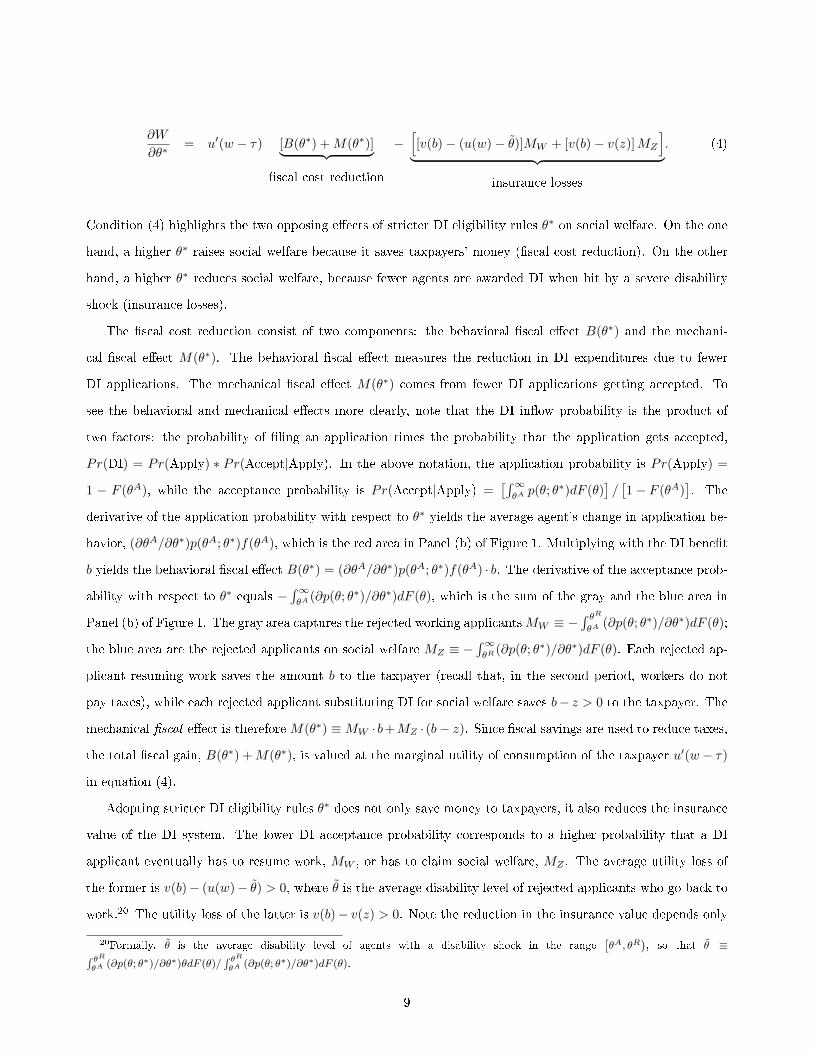
∂W

∂θ∗= u′(w − τ) [B(θ∗) +M(θ∗)]︸ ︷︷ ︸

�scal cost reduction

−[[v(b)− (u(w)− θ)]MW + [v(b)− v(z)]MZ

]︸ ︷︷ ︸

insurance losses

. (4)

Condition (4) highlights the two opposing e�ects of stricter DI eligibility rules θ∗ on social welfare. On the one

hand, a higher θ∗ raises social welfare because it saves taxpayers' money (�scal cost reduction). On the other

hand, a higher θ∗ reduces social welfare, because fewer agents are awarded DI when hit by a severe disability

shock (insurance losses).

The �scal cost reduction consist of two components: the behavioral �scal e�ect B(θ∗) and the mechani-

cal �scal e�ect M(θ∗). The behavioral �scal e�ect measures the reduction in DI expenditures due to fewer

DI applications. The mechanical �scal e�ect M(θ∗) comes from fewer DI applications getting accepted. To

see the behavioral and mechanical e�ects more clearly, note that the DI in�ow probability is the product of

two factors: the probability of �ling an application times the probability that the application gets accepted,

Pr(DI) = Pr(Apply) ∗ Pr(Accept|Apply). In the above notation, the application probability is Pr(Apply) =

1 − F (θA), while the acceptance probability is Pr(Accept|Apply) =[´∞θAp(θ; θ∗)dF (θ)

]/[1− F (θA)

]. The

derivative of the application probability with respect to θ∗ yields the average agent's change in application be-

havior, (∂θA/∂θ∗)p(θA; θ∗)f(θA), which is the red area in Panel (b) of Figure 1. Multiplying with the DI bene�t

b yields the behavioral �scal e�ect B(θ∗) = (∂θA/∂θ∗)p(θA; θ∗)f(θA) · b. The derivative of the acceptance prob-

ability with respect to θ∗ equals −´∞θA

(∂p(θ; θ∗)/∂θ∗)dF (θ), which is the sum of the gray and the blue area in

Panel (b) of Figure 1. The gray area captures the rejected working applicantsMW ≡ −´ θRθA

(∂p(θ; θ∗)/∂θ∗)dF (θ);

the blue area are the rejected applicants on social welfare MZ ≡ −´∞θR

(∂p(θ; θ∗)/∂θ∗)dF (θ). Each rejected ap-

plicant resuming work saves the amount b to the taxpayer (recall that, in the second period, workers do not

pay taxes), while each rejected applicant substituting DI for social welfare saves b− z > 0 to the taxpayer. The

mechanical �scal e�ect is therefore M(θ∗) ≡MW · b+MZ · (b− z). Since �scal savings are used to reduce taxes,

the total �scal gain, B(θ∗) +M(θ∗), is valued at the marginal utility of consumption of the taxpayer u′(w− τ)

in equation (4).

Adopting stricter DI eligibility rules θ∗ does not only save money to taxpayers, it also reduces the insurance

value of the DI system. The lower DI acceptance probability corresponds to a higher probability that a DI

applicant eventually has to resume work, MW , or has to claim social welfare, MZ . The average utility loss of

the former is v(b)− (u(w)− θ) > 0, where θ is the average disability level of rejected applicants who go back to

work.20 The utility loss of the latter is v(b)− v(z) > 0. Note the reduction in the insurance value depends only

20Formally, θ is the average disability level of agents with a disability shock in the range[θA, θR

), so that θ ≡´ θR

θA (∂p(θ; θ∗)/∂θ∗)θdF (θ)/´ θRθA (∂p(θ; θ∗)/∂θ∗)dF (θ).

9

Figure 1: Illustration of Static Model and E�ects of Stricter Eligibility Rules

(a) Illustration of Model (b) E�ects of Stricter Eligibility Rules

Notes: Panel (a) illustrates the basic setup. Individuals are characterized by disability level θ and can choose whether to work, apply toDI or leave the labor force and consume social welfare bene�ts. The award process to DI is noisy and individuals are awarded DI withprobability p(θ). We assume that p(θ) is weakly increasing in θ. This captures that (i) it is di�cult to assess the true disability level of anindividual and (ii) the assessment contains nonetheless some valuable information on the true disability level. The marginal DI applicant

is denoted by θA and individuals with θ ≥ θA apply to DI. The marginal welfare bene�ts type is denoted by θR and individuals withθ ≥ θR will go on welfare bene�ts if they are rejected. Panel (b) illustrates the e�ects of stricter eligibility criteria. Stricter criteriashift down the award probability curve. The area between the two award probability curves is the mechanical e�ect. A fraction of themechanically rejected applicants returns to work (gray area). The other fraction substitutes DI bene�ts with welfare bene�ts (blue area).Stricter eligibility criteria also shift the marginal applicant to the right. The change in the marginal applicant times the award probabilityof the marginal applicant is the behavioral e�ect (red area).

on the mechanical e�ect but not on the behavioral e�ect. This is a direct implication of the Envelope theorem.21

Intuitively, only marginal applicants react to a marginal change in the strictness of eligibility rules. Marginal

applicants are indi�erent between applying and not applying. Hence, if a marginal increase in θ∗ induces them

not to �le an application, their welfare is not directly a�ected. However, fewer applications reduce the �nancial

burden of the DI system, thus they generate a positive �scal e�ect that bene�ts taxpayers.

The optimal strictness of eligibility rules θ∗ balances the trade-o� between insurance loss and �scal gain,

where (4) is set to zero. For later use, we rewrite this condition as

∂W

∂θ∗R 0 ⇐⇒ 1 +

B(θ∗)

M(θ∗)R

LW + LZu′(w − τ)M(θ∗)

, (5)

where LW ≡ [v(b) − (u(w) − θ)]MW > 0 and LZ ≡ [v(b)− v(z)]MZ > 0 are the aggregate utility losses suf-

fered by the additionally rejected applicants resuming work (LW ) and claiming social welfare (LZ), respectively.

The two sides of the inequality have an intuitive interpretation. The left-hand-side is the �scal multiplier,

1 + B(θ∗)/M(θ∗), and measures the reduction in the �nancial burden for the taxpayer per mechanically saved

dollar (= hypothetical �scal gain when application behavior remains unchanged). The right-hand-side is the

21While the decision to apply is discrete the envelope theorem applies because we have a marginal change in the policy parameterθ∗. In Appendix A.1 we show this formally and also discuss how the welfare evaluation changes in case of a discrete (non-marginal)change of θ∗.

10

corresponding reduction of the insurance value in monetary units. Dividing by the marginal utility of con-

sumption of the taxpayer u′(w− τ)M(θ∗) yields the insurance loss (in monetary terms) per mechanically saved

dollar.

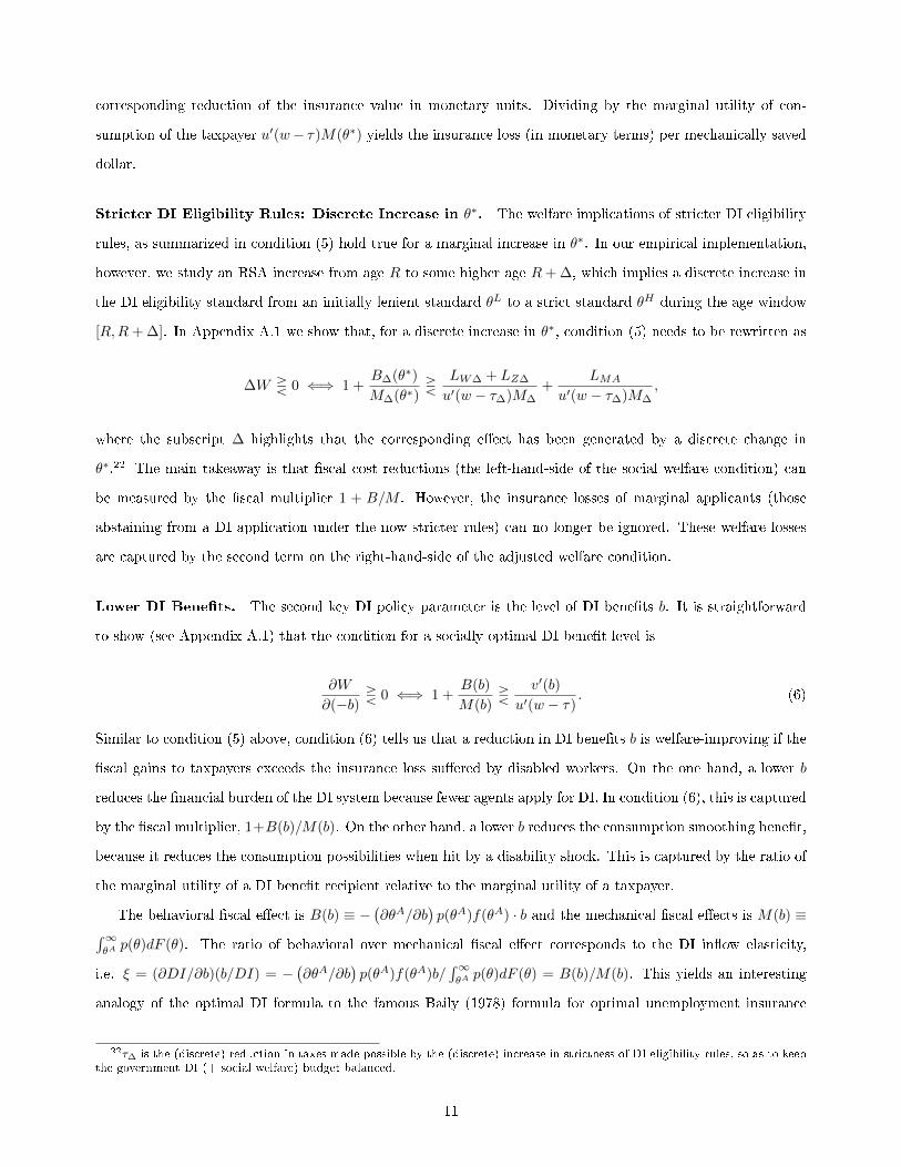
Stricter DI Eligibility Rules: Discrete Increase in θ∗. The welfare implications of stricter DI eligibility

rules, as summarized in condition (5) hold true for a marginal increase in θ∗. In our empirical implementation,

however, we study an RSA increase from age R to some higher age R+ ∆, which implies a discrete increase in

the DI eligibility standard from an initially lenient standard θL to a strict standard θH during the age window

[R,R+ ∆]. In Appendix A.1 we show that, for a discrete increase in θ∗, condition (5) needs to be rewritten as

∆W R 0 ⇐⇒ 1 +B∆(θ∗)

M∆(θ∗)R

LW∆ + LZ∆

u′(w − τ∆)M∆+

LMA

u′(w − τ∆)M∆,

where the subscript ∆ highlights that the corresponding e�ect has been generated by a discrete change in

θ∗.22 The main takeaway is that �scal cost reductions (the left-hand-side of the social welfare condition) can

be measured by the �scal multiplier 1 + B/M . However, the insurance losses of marginal applicants (those

abstaining from a DI application under the now stricter rules) can no longer be ignored. These welfare losses

are captured by the second term on the right-hand-side of the adjusted welfare condition.

Lower DI Bene�ts. The second key DI policy parameter is the level of DI bene�ts b. It is straightforward

to show (see Appendix A.1) that the condition for a socially optimal DI bene�t level is

∂W

∂(−b)R 0 ⇐⇒ 1 +

B(b)

M(b)R

v′(b)

u′(w − τ). (6)

Similar to condition (5) above, condition (6) tells us that a reduction in DI bene�ts b is welfare-improving if the

�scal gains to taxpayers exceeds the insurance loss su�ered by disabled workers. On the one hand, a lower b

reduces the �nancial burden of the DI system because fewer agents apply for DI. In condition (6), this is captured

by the �scal multiplier, 1+B(b)/M(b). On the other hand, a lower b reduces the consumption smoothing bene�t,

because it reduces the consumption possibilities when hit by a disability shock. This is captured by the ratio of

the marginal utility of a DI bene�t recipient relative to the marginal utility of a taxpayer.

The behavioral �scal e�ect is B(b) ≡ −(∂θA/∂b

)p(θA)f(θA) · b and the mechanical �scal e�ects is M(b) ≡

´∞θAp(θ)dF (θ). The ratio of behavioral over mechanical �scal e�ect corresponds to the DI in�ow elasticity,

i.e. ξ = (∂DI/∂b)(b/DI) = −(∂θA/∂b

)p(θA)f(θA)b/

´∞θAp(θ)dF (θ) = B(b)/M(b). This yields an interesting

analogy of the optimal DI formula to the famous Baily (1978) formula for optimal unemployment insurance

22τ∆ is the (discrete) reduction in taxes made possible by the (discrete) increase in strictness of DI eligibility rules, so as to keepthe government DI (+ social welfare) budget balanced.

11

(UI). Both in the case of UI and in the case of DI, the condition for the socially optimal bene�t level can be

written as 1 + η = v′(b)/u′(w− τ). In the Baily (1978) model of optimal UI, η is the elasticity of unemployment

duration with respect to the UI bene�t level; in the above model of optimal DI, η = ξ, the elasticity of the DI

in�ow with respect to the DI bene�t level. In other words, the relevant moral-hazard margin in the case of DI

is the program in�ow, while the relevant margin in the case of UI is the program out�ow.23

So far, we have derived conditions for social optimality for each single DI policy parameter, holding the

other policy parameter �xed. A natural question is how a DI reform should optimally combine these two policy

parameters. More precisely: how strongly � and in which direction � should DI eligibility rules θ∗ be changed per

unit change of DI bene�ts b? In Appendix A.1 we discuss how the formulas for optimal bene�ts and eligibility

rules are informative for the optimal policy mix.

2.2 The General Model

The above model highlights the basic trade-o�s of DI policy reforms but misses two ingredients that are

crucial in designing and evaluating DI reforms: heterogeneity across individuals and intertemporal choices. In

the model of section 2.1, agents di�er only in θ and all actions happen within one period. In what follows, we

allow for multiple sources of heterogeneity (such as wages and other factors) and we extend the model to multiple

periods. This latter extension allows us to capture the intertemporal nature of the DI application choice. In the

context of our empirical analysis below � which exploits an RSA increase from R to some higher age R +4 �

it is obvious, that the question �When should I apply?� becomes crucial. To address the DI application timing

in a meaningful way, a dynamic framework is needed.

Agents' Choices and Social Welfare. Assume that the agent's time horizon consists of T periods, in-

dexed by t = 0, . . . , T − 1. Denote by θi,t the disability shock, by χi,t a vector of other shocks (such as

wages/productivity and other factors) in�uencing the DI application choice, and by Ai,t the level of �nancial

assets available at the beginning of period t. Once the state vector Xi,t = (θi,t, Ai,t, χi,t) is revealed, agent i

decides whether to apply for DI, and if rejected, whether to resume work or claim social welfare. The appli-

cation and work decisions are based on knowledge of Xi,t and expectations about future realizations of Xi,t+s,

s = t + 1, . . . , T − 1. Simultaneously with the DI application choice, the agent decides how much to consume

and save in period t.24 The decisions in period t determine Ai,t+1 and, together with realizations θi,t+1 and

χi,t+1, form the state vector Xt+1, on the basis of which the agent makes her t+ 1 choices, and so on.

23The implicit assumption here is that DI generosity does neither a�ect the intensive margin of labor supply (DI recipients donot work on the labor market) nor the out�ow from DI (DI is an absorbing state, no DI spell ever terminates to a regular job orany other destination).

24The within-period sequence of work and DI-application choices is just like the one of the static model, captured in Figure A.1.However, the general model also admits the possibility that θA ≥ θR, so that equation (A.1) is violated. This might occur foragents with low wage realization and low DI acceptance probabilities.

12

The utilitarian government can freely choose DI policy parameters P = (θ∗0 , . . . , θ∗T−1; b0, . . . , bT−1) and seeks

to maximize the objective

maxP

W (P ) =

ˆi

Vi(P )di+ λ(G(P )− G

), (7)

where W (P ) denotes social welfare under policy P ; Vi(P ) is the (expected) indirect lifetime utility of agent

i (who responds optimally to policy P ), λ is the Lagrange multiplier on the government's budget constraint,

G(P ) is the net �scal revenue, and G is an exogenous revenue constraint. G(P ) is given by

G(P ) =

ˆi

E

[T−1∑t=0

(1 + rt)−t

(Wi,t · τi,t −Di,t · bi,t − Zi,t · zi,t)

]di, (8)

where (Di,t,Wi,t, Zi,t) denote the probabilities that in period t agent i is on DI, at work or on social welfare.

In Appendix A.2 we show that agent i's indirect (expected) lifetime utility can be written as

Vi(P ) = maxE

[T−1∑t=0

βt(v(cDi,t) ·Di,t + v(cZi,t) · Zi,t +

(u(cWi,t)− θi,t

)·Wi,t − Λi,t · ψ

)](9)

+E

[T−1∑t=0

βtµDi,t((1 + rt)Ai,t + bi,t − cDi,t −Ai,t+1

)Di,t

]

+E

[T−1∑t=0

βtµWi,t((1 + rt)Ai,t + wi,t − τi,t − cWi,t −Ai,t+1

)Wi,t

]

+E

[T−1∑t=0

βtµZi,t((1 + rt)Ai,t + zi,t − cZi,t −Ai,t+1

)Zi,t

],

where the �rst line summarizes agent i′s period utilities, with (cDi,t, cWi,t , c

Zi,t) as the consumption levels in the

various states, and Λi,t as the DI application indicator. The remaining lines are agent i's budget constraints

associated with being on DI (second line), at work (third line), and on social welfare (fourth line). The corre-

sponding Lagrangian multipliers are denoted by (µDi,t, µWi,t , µ

Zi,t) .

Stricter DI Eligibility Rules. We now explore the welfare e�ects of marginally changing the strictness of

DI eligibility rules θ∗s , while leaving all other elements of the DI policy vector P = (θ∗0 , . . . , θ∗T−1; b0, . . . , bT−1)

unchanged. Notice that this thought experiment is equivalent to an RSA increase, the policy change we exploit

below to empirically estimate the e�ect of stricter DI eligibility rules. An RSA policy implies that θ∗t takes high

values up until age R− 1 and falls to lower values from age R onward. If the relaxed screening age is increased

from age R = s to R = s+1, this is equivalent to an increase in θ∗s but unchanged values of θ∗t 6=s.25 In Appendix

25Notice further that our analysis in the text studies the welfare e�ects of a marginal increase θ∗s while an RSA policy typicallyimplies a discrete change in θ∗t at the RSA. Assume that θ

∗t = θH for ages t = 0, . . . , R−1 and θ∗t = θL < θH for ages t = R, . . . , T−1.

Then an increase in the RSA from R = s to R = s + 1 is associated with a discrete change in θ∗s equal to 4θ∗s = θH − θL. Wediscuss the welfare e�ects of a discrete change in θ∗ in Appendix A.1 for the static model and in Appendix A.2 for the general

13

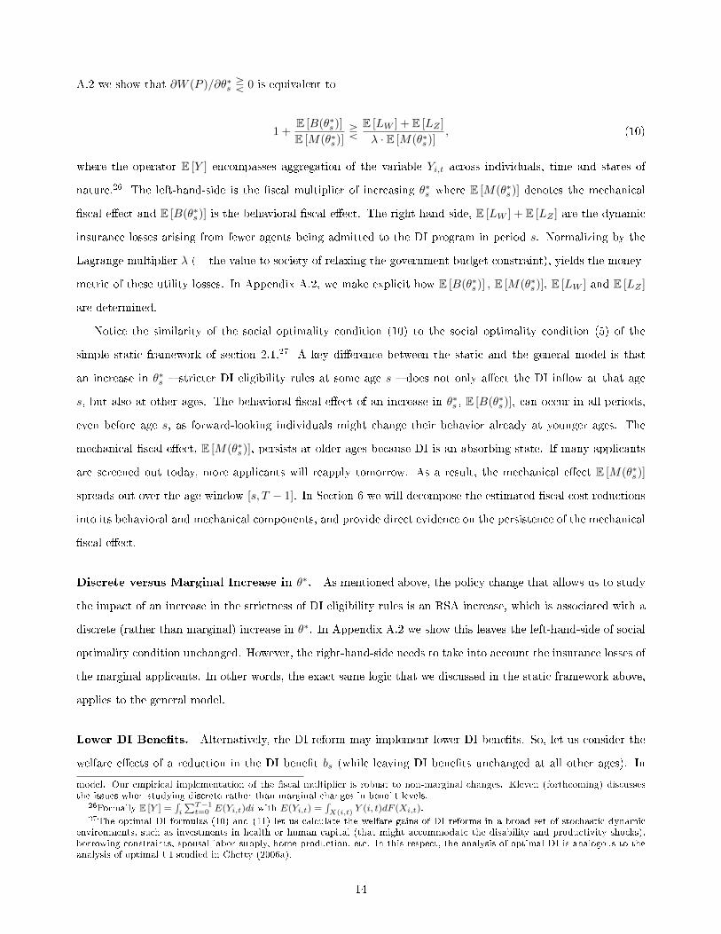
A.2 we show that ∂W (P )/∂θ∗s R 0 is equivalent to

1 +E [B(θ∗s)]

E [M(θ∗s)]R

E [LW ] + E [LZ ]

λ · E [M(θ∗s)], (10)

where the operator E [Y ] encompasses aggregation of the variable Yi,t across individuals, time and states of

nature.26 The left-hand-side is the �scal multiplier of increasing θ∗s where E [M(θ∗s)] denotes the mechanical

�scal e�ect and E [B(θ∗s)] is the behavioral �scal e�ect. The right-hand side, E [LW ] + E [LZ ] are the dynamic

insurance losses arising from fewer agents being admitted to the DI program in period s. Normalizing by the

Lagrange multiplier λ (= the value to society of relaxing the government budget constraint), yields the money-

metric of these utility losses. In Appendix A.2, we make explicit how E [B(θ∗s)] , E [M(θ∗s)], E [LW ] and E [LZ ]

are determined.

Notice the similarity of the social optimality condition (10) to the social optimality condition (5) of the

simple static framework of section 2.1.27 A key di�erence between the static and the general model is that

an increase in θ∗s � stricter DI eligibility rules at some age s � does not only a�ect the DI in�ow at that age

s, but also at other ages. The behavioral �scal e�ect of an increase in θ∗s , E [B(θ∗s)], can occur in all periods,

even before age s, as forward-looking individuals might change their behavior already at younger ages. The

mechanical �scal e�ect, E [M(θ∗s)], persists at older ages because DI is an absorbing state. If many applicants

are screened out today, more applicants will reapply tomorrow. As a result, the mechanical e�ect E [M(θ∗s)]

spreads out over the age window [s, T − 1]. In Section 6 we will decompose the estimated �scal cost reductions

into its behavioral and mechanical components, and provide direct evidence on the persistence of the mechanical

�scal e�ect.

Discrete versus Marginal Increase in θ∗. As mentioned above, the policy change that allows us to study

the impact of an increase in the strictness of DI eligibility rules is an RSA increase, which is associated with a

discrete (rather than marginal) increase in θ∗. In Appendix A.2 we show this leaves the left-hand-side of social

optimality condition unchanged. However, the right-hand-side needs to take into account the insurance losses of

the marginal applicants. In other words, the exact same logic that we discussed in the static framework above,

applies to the general model.

Lower DI Bene�ts. Alternatively, the DI reform may implement lower DI bene�ts. So, let us consider the

welfare e�ects of a reduction in the DI bene�t bs (while leaving DI bene�ts unchanged at all other ages). In

model. Our empirical implementation of the �scal multiplier is robust to non-marginal changes. Kleven (forthcoming) discussesthe issues when studying discrete rather than marginal changes in bene�t levels.

26Formally E [Y ] =´i

∑T−1t=0 E(Yi,t)di with E(Yi,t) =

´X(i,t) Y (i, t)dF (Xi,t).

27The optimal DI formulas (10) and (11) let us calculate the welfare gains of DI reforms in a broad set of stochastic dynamicenvironments, such as investments in health or human capital (that might accommodate the disability and productivity shocks),borrowing constraints, spousal labor supply, home production, etc. In this respect, the analysis of optimal DI is analogous to theanalysis of optimal UI studied in Chetty (2006a).

14

Appendix A.2 we show that that condition −∂W (P )/∂(bs) R 0 is equivalent to

1 +E [B(bs)]

E [M(bs)]R

E[v′(cD)

]λ · E [M(bs)]

, (11)

where E [B(bs)] and E [M(bs)] are the behavioral and mechanical �scal e�ects of a marginal reduction of bs.

Again, this looks very similar to the static model. Just like before, behavioral responses to a reduction of bs

occur in all periods. Mechanical responses occur at age s only (because we consider lower bene�ts paid out at

age s but unchanged bene�ts at all other ages).

3 Institutional Background and Data

3.1 Institutional Background

Like in many developed countries, Austria has three transfer programs that provide income replacement

for economic or health reasons: disability insurance (DI), sickness insurance (SI), and unemployment insurance

(UI). The DI program is �nanced by a payroll tax on earned income and provides partial earnings replacement

to workers below the full retirement age with at least 5 insurance years within the last 10 years.28DI applicants

must submit their application to the local DI o�ce. Employees at the DI o�ce �rst check whether the applicant

meets the formal requirements for DI receipt. Importantly, and di�erent from the U.S, DI applicants are not

required to stop working. Then a team of disability examiners and physicians assesses the severity of the medical

impairment and the applicant's residual earnings capacity. An impairment is considered to be severe if it lasts

at least six months and limits the applicant's mental or physical ability to engage in substantial gainful activity.

DI Eligibility Rules. The assessment of the applicant's residual earnings capacity depends on work experi-

ence and whether his or her age is below or above a relaxed screening age (RSA) threshold, currently set at age

60. Applicants below the RSA are awarded DI bene�ts if the earnings capacity has been reduced to less 50%

of the earnings capacity of a healthy person in any reasonable occupation the individual could be expected to

carry out.29 Applicants above the RSA (who have worked for at least 10 years within the last 15 years) need

to have an earnings capacity of less than 50% in a similar occupation.30 The RSA was 57 until the end of 2012

and was increased in three one-year steps to age 60 by 2017. We exploit the variation in the RSA to identify

28Insurance years include both contribution years (periods of employment, including sick leave and maternity leave) and non-contribution years (periods of unemployment, military service, or secondary education). The required insurance years increase byone month for every two months above age 50 up to a maximum of 15 insurance years.The insurance years requirement does notapply if the disability is job-related; for each occupation there exists an explicit list of qualifying impairments.

29Eligibility standards are less strict for semi-skilled and skilled applicants below the RSA threshold, whose set of reasonableoccupations is more limited. To be classi�ed as semi-skilled or skilled, an applicant must have worked in a semi-skilled or skilledoccupation for 7.5 years or more in the most recent 15 years.

30Access to disability insurance is also relaxed in other countries at older ages, including Australia, Canada, Denmark, Swedenuntil 1997 (Karlström et al., 2008), and the United States (Chen and van der Klaauw, 2008).

15

the labor market e�ects of stricter DI eligibility rules (section 4). Once bene�ts are awarded, DI bene�ciaries

receive monthly payments until their return to work, medical recovery or death. DI bene�ts can be granted for

a temporary period, but less than 4 percent of claimants ever leave the DI rolls.

DI Bene�ts. DI bene�ts are subject to income and payroll taxation and replace approximately 70 percent of

pre-disability net earnings up to a maximum of about e4,500 per month. The level of DI bene�ts is calculated

by multiplying a pension coe�cient, which varies by age and insurance years, with an assessment basis, which

is the average indexed capped earnings over a given period of time (e.g., the best 16 years in 2004 at the

beginning of our study period). Younger applicants with limited work experience qualify for a special increment

to supplement their bene�ts. DI bene�ciaries may continue work, but those earning more than an exempt

threshold lose up to 50 percent of their bene�ts.31 A pension reform in 2004 gradually decreased the bene�t

levels for most workers, providing exogenous variation we use to identify the labor market e�ects of changes in

bene�t levels (section 5).

SI and UI Bene�ts. In case of a temporary illness, employers continue to pay 100% of earnings for up to

12 weeks. Once the right to full bene�ts paid by the employer has expired, individuals may claim SI bene�ts

which are taxed and replace approximately 65% of the last net wage up to the same maximum that applies to

DI bene�ts. SI bene�t duration is 52 (26) weeks for individuals who have worked at least (less than) 6 months

in the previous 12 months. UI bene�ts replace 55 percent of the previous wage subject to a minimum and

maximum. The maximum UI bene�t duration 39 weeks of regular UI bene�ts for workers below 50 and 52

weeks for workers above 50 (provided they have paid UI contributions for at least 9 years in the last 15 years).

Job losers who exhaust the regular UI bene�ts can apply for unemployment assistance. These means-tested

transfers last for an inde�nite period and are about 70 percent of regular UI bene�ts.

3.2 Data

We merge data from two administrative registers. First, the Austrian Social Security Database (ASSD)

contains detailed longitudinal information for the universe of workers in Austria between 1972 and 2018. The

ASSD records all employment, unemployment, disability, sick leave, and retirement spells as well as a limited set

of background characteristics (gender, month and year of birth, blue- or white-collar status). Spells before 1972

are available for individuals who have claimed a public pension by the end of 2008. The ASSD also contains

some �rm-speci�c information: geographic region, industry a�liation, and �rm identi�ers that allow us to link

both individuals and �rms. See Zweimüller et al. (2009) for a detailed description of the data. Second, we

31Ruh and Staubli, 2019 show that this policy induces DI bene�ciaries to keep their earnings below the exempt threshold inorder to retain bene�ts.

16

use data on all DI applications, which cover the period 2004 to 2017 and contain detailed information on the

date of the application, the date of the decision, the decision itself (i.e. reject or accept), the reported medical

impairment of the applicant, and the stage of the application (i.e. �rst application, re-application, or appeal).

Starting from the population data set, we impose three restrictions. First, we exclude women because their

eligibility age for an old age pension gradually increased from age 56 to age 60 during our observation window,

making it di�cult to disentangle the e�ect of DI reforms from the e�ect of increasing the retirement age.32

Second, we exclude self-employed and civil service workers, because they are covered by a di�erent pension

system than private-sector workers. Third, we exclude observations in which individuals are over age 62, at

which point many become eligible for an old age pension. Our sample covers more than three quarters of all

active labor market participants in Austria. Since we observe complete work histories, we can precisely calculate

how much DI bene�ts individuals would get at any point in time and whether individuals have su�cient work

experience to apply for DI bene�ts under the relaxed eligibility criteria above the RSA.

Table B.1 in Appendix B shows summary statistics for the sample we use to study the e�ects of stricter

DI eligibility rules. To capture changes in labor market behavior around the RSA, we limit the sample to men

between age 54 and age 62 with at least 10 employment years in the past 15 years (measured at age 56). These

men are considered eligible for relaxed DI eligibility, while men with less than 10 employment years in the past

15 years are considered ineligible.33 We will use the sample of ineligibles for placebo tests. Since our empirical

strategy exploits increases in the RSA from 57 to 58 and from 58 to 59, we distinguish between three cohorts

of men: RSA 57, RSA 58, and RSA 59 who qualify for relaxed DI eligibility at age 57, age 58, and age 59,

respectively. We observe individuals on a quarterly basis.

Our �rst set of outcome variables focus on DI application behavior. DI application ever is an indicator

for whether an individual has ever applied for DI bene�ts. DI application yearly is an indicator for whether

an individual has applied for DI bene�ts at a particular age. We also distinguish yearly applications by the

underlying health impairment (mental disorders, musculoskeletal disorders, and other disorders) and whether

the applications is a re-application, meaning that the applicant has applied for DI before. Our second set of

outcome variables focus on labor market outcomes. DI bene�t receipt is an indicator for whether an individual

is receiving DI bene�ts, employment is indicator for whether an individual is employed, and other bene�t receipt

is an indicator for whether the individual is receiving UI or SI bene�ts.34 In the empirical analysis, we also

calculate the bene�t and earnings streams associated with each labor market status, allowing us to study the

32Staubli and Zweimüller (2013) show that this increase had sizeable employment and unemployment e�ects.33Note that only individuals who worked in a similar occupation for 10 of the last 15 years are eligible for relaxed DI eligibility,

while our de�nition is based on whether somebody has worked in any occupation for 10 years of the last 15 years because we canonly observe industry a�liation and not occupation. This implies that the eligible sample will include some individuals who arein fact not eligible for relaxed screening, but this number is likely small because what constitutes a similar occupation is de�nedbroadly.

34DI spells are back-dated in the ASSD to the date the claim was �led, so an individual who applied for DI bene�ts late inthe calendar year and was awarded bene�ts in the next calendar year is observed to claim bene�ts in the calendar year when theapplication was �led.

17

�scal e�ects of stricter DI eligibility rules.

Table B.2 in Appendix B shows summary statistics for the sample, we use to study the e�ects of changes

in DI bene�t levels. Following Mullen and Staubli (2016), we de�ne a reference date, January 1, and obtain

all information to compute potential DI bene�ts and other relevant individuals characteristics as of this date

for each year an individual is not receiving DI bene�ts. We estimate the e�ects separately for the age groups

30-56 and 57-60, which is also the age group of interest when studying the e�ects of stricter DI eligibility rules.

Our main outcome variables of interest are indicators for whether, within a year, individuals apply for DI (DI

application), are awarded DI bene�ts (DI in�ow), exit employment (employment out�ow), or stop receiving UI

or SI bene�ts (other bene�t out�ow).

4 The E�ect of Tighter DI Eligibility Rules

4.1 The 2013 DI Reform

In April 2012, the Austrian government announced the 2. Stability Act (2. Stabilitätsgesetz), which became

e�ective on January 1, 2013. The Act had two objectives: reduce expenditures in the public pension systems

and foster employment among older workers. The only change to the DI program was a stepwise increase in the

RSA threshold from age 57 to age 60. Up until December 2012 the RSA was age 57. The RSA was increased

to age 58 in January 2013, followed by further increases to age 59 in January 2015 and age 60 in January 2017.

Individuals who had not worked in a similar occupation for 10 years in the last 15 years were not a�ected by

the increases as they were not eligible for relaxed DI eligiblity rules. We focus on the increases in the RSA to

58 and 59, because the available data preclude the analysis of the increase in the RSA to 60.

The RSA increases create variation in the tightness of DI eligibility rules at certain ages across birth cohorts.

For example, the RSA is 58 for men who turn 57 between December 2012 and November 2013 (those born

after November 1955 and before December 1956).35 We label this birth cohort the RSA-58 cohort. Conversely,

the RSA is 57 for men born before December 1955 and we label this cohort the RSA-57 cohort. Men in the

RSA-58 cohort, compared to men in the RSA-57 cohort, face stricter disability screening at age 57. The RSA

is 59 for men born after November 1956 and we label this cohort the RSA-59 cohort. Men in the RSA-59

cohort, compared to men in the RSA-57 cohort, face stricter DI eligibility rules at ages 57 and 58. Figure B.5

in Appendix B illustrates the step-wise increase graphically.

Figure B.6 in Appendix B provides descriptive evidence on the labor market e�ects of the RSA increases.

Trends in labor market outcomes across birth cohorts are remarkably similar until age 57 � the relaxed screening

age for the RSA-57 cohort. At this age, the DI recipient rate rises sharply in the RSA-57 cohort. The percent

35Applications are assessed using the rules in the month after �ling. Therefore, if someone turns 57 in December 2012 andapplies to DI his application is evaluated in January 2013, when the new RSA of 58 applies.

18

of DI applicants also increases, suggesting that individuals are aware of the RSA and time their DI application

to this age. Conversely, the percent of men who are employed or receive other bene�ts drops at age 57, pointing

to the role of DI as a substitute for UI or SI. We observe similar breaks in trends when the RSA-58 and RSA-

59 cohorts reach their RSA. Interestingly, cohorts with a higher RSA never catch up to cohorts with a lower

RSA. To capture these persistence (and also potential anticipation) e�ects, our empirical strategy is designed

to identify the entire age pro�le of the RSA increase.

4.2 Estimation Strategy

We exploit the exogenous variation in the RSA threshold across birth cohorts in a di�erence-in-di�erences

design. Control (= older) birth cohorts are eligible to the more lenient DI eligibility rules already at age 57

(RSA=57), while treated (= younger) birth cohorts are eligible only at age 58 or age 59 (RSA=58 or 59) . Thus,

we can identify the e�ect of stricter DI eligibility rules by comparing the age pro�les of younger and older birth

cohorts. This comparison can be implemented by estimating regressions of the following type:

yict = α+ θa + πc + λt +

61∑k=54\56

βkI[age = k] +X ′ictδ + εict, (12)

where i denotes individual, c denotes birth cohort, and t denotes year-quarter; yict is the outcome variable of

interest (such as an indicator for receiving DI bene�ts), θa are dummies for age in years to control for age-speci�c

levels in the outcome variable, πc are dummies for year-month of birth to capture time-constant di�erences across

birth cohorts, λt are dummies for year and quarter to capture common time shocks and seasonal e�ects, and

Xict represent individual or region speci�c characteristics to control for any observable di�erences that might

confound the analysis.36 We cluster standard errors at the year-month of birth.

The key variables of interest are the indicators I[age = k], which are equal to one if an individual's age is

equal to k, where k runs from 54 to 61 using k = 56 as the reference age. Each βk-coe�cient measures the

average causal e�ect of an RSA increase at age k. To obtain the average e�ect of an RSA increase over a wider

age interval, we can simply take the average of di�erent βk-coe�cients. For example,∑61k=57 βk/5 measures the

average change in the outcome variable at each age in the age interval 57 to 61.

We estimate the e�ects of the RSA-58 and RSA-59 change separately, using always the RSA-57 cohort as

the control group. This way we can directly compare the e�ects of a one-year and a two-year RSA increase.

Another reason to estimate the e�ects separately is that, compared to the RSA-58 cohort, men in the RSA-59

cohort have more time to adjust to the reform. They just turned 55 years old when the reform was announced,

while men in the RSA-58 cohort were almost 57 years old. Having more time to adjust increases the scope for

36The �xed e�ects θa, πc, and λt are not collinear, because each age-in-year and year-quarter cell contains cohorts with di�erentyear-month of birth.

19

anticipation e�ect: changes in behavior even before age 57.

The identi�cation assumption is that, absent the increase in the RSA, the change in yict at a certain age

would have been comparable between treated birth cohorts (RSA=58 or 59) and control cohorts (RSA=57).

A potential concern is that age-speci�c trends in the outcome variable could change across birth cohorts for

reasons unrelated to the RSA increases. The estimated βk-coe�cients for k < 57 provide placebo checks for

spurious trends. They should not be statistically signi�cant if the identi�cation assumption holds, although

they could also pick up anticipation e�ects. As an additional placebo check, we estimate equation (12) for men

who never become eligible for to the lenient DI eligibility rules because they have worked less than 10 years in

the past 15 years. They should not respond to the changes in the RSA.

4.3 Empirical Results

Figure 2 shows the estimated βk-coe�cients from equation (12) for the RSA-58 and the RSA-59 increases for

four key outcomes: DI bene�t receipt, DI application ever, employment, and other bene�ts. The shaded area

denotes the 95 percent con�dence interval. In all graphs, we see that the estimates before age 57, the pre-reform

RSA, are close to zero and statistically insigni�cant, providing evidence that the estimates are not confounded

by di�erential trends across birth cohorts.

As panel (a) shows, because of the RSA increases, fewer men receive DI bene�ts between ages 57 and age

61. DI recipiency rates drop by about 4 percentage points at age 57. For the RSA-58 cohort, DI recipiency

rate remains lower after age 57, even though DI eligibility rules have become more lenient. For the RSA-59

cohort, the DI recipiency rate declines further at age 58 and is still lower at age 59 when this cohort quali�es

for relaxed DI eligibility rules. If applying for DI imposes utility costs, we would expect that fewer people

apply when eligibility criteria are strict. Indeed, panel (b) shows that DI application rates for the RSA-58 and

RSA-59 cohorts drop at all ages above 56.37 Panels (c) and (d) show that stricter DI eligibility rules increase

employment and other bene�t receipt above age 56.38 The expansion in employment persists until the last age

we can observe in the data, and is about twice as large for the RSA-59 cohort compared to the RSA-58 cohort.

While the rise in other bene�t receipt is temporary for the RSA-58 cohort, it persists up to the last age for the

RSA-59 cohort.

It is interesting to look at the timing and dynamics of the estimates in Figure 2. First, we �nd no evidence

for anticipation e�ects, which is less surprising for the RSA-58 cohort, because they learned about the reform

37Appendix Figure B.11 decomposes DI application ever by impairment type. It shows that fewer individuals apply withmusculoskeletal and other impairments, but the same number of individuals apply with mental impairments.

38Appendix Figure B.12 shows that the expansion in employment is primarily driven by individuals who are already employedand who stay employed longer, rather than by individuals who are on other bene� receipt and who start working when the RSAincreases. Similarly, Appendix Figure B.13 shows that the increase in other bene�t receipt is primarily driven by individuals who arealready reciving other bene�ts and now receive other bene�ts longer until they reach the new RSA, at which point many transitionto the DI program.

20

Figure 2: E�ects of RSA on Labor Market States and DI Application Ever by Age

(a) DI Bene�t ReceiptRSA 58 RSA 59

-6-4

-20

2Pe

rcen

t

54 55 56 57 58 59 60 61Age

-6-4

-20

2Pe

rcen

t

54 55 56 57 58 59 60Age

(b) DI Application EverRSA 58 RSA 59

-4-2

02

4Pe

rcen

t

54 55 56 57 58 59 60Age

-4-2

02

4Pe

rcen

t

54 55 56 57 58 59Age

(c) EmploymentRSA 58 RSA 59

-20

24

6Pe

rcen

t

54 55 56 57 58 59 60 61Age

-20

24

6Pe

rcen

t

54 55 56 57 58 59 60Age

(d) Other Bene�t ReceiptRSA 58 RSA 59

-20

24

6Pe

rcen

t

54 55 56 57 58 59 60 61Age

-20

24

6Pe

rcen

t

54 55 56 57 58 59 60Age

Notes: The �gure shows the estimated βk-coe�cients from the econometric speci�cation in (12) for the RSA-58 and RSA-59 increases usingthe sample of eligible men. The shaded area denotes the 95 percent con�dence interval.

21

just a couple months before turning 57. The RSA-59 cohort knew about the reform two years before turning

57 and had time to adjust, but all estimates before age 57 are close to zero and insigni�cant. Second, the DI

application rate falls at age 57, implying that individuals are aware of the RSA and adjust their behavior. If the

estimated e�ects were purely mechanical, applications at age 57 should not react. Third, the estimated e�ects

are highly persistent and show up at ages beyond the RSA. This is consistent with persistent mechanical e�ects

as discussed in section 2.2 above. The strength of mechanical and behavioral e�ects is of crucial importance as

their relative size determines the e�ect of tightening DI eligibility rules on social welfare. We discuss welfare

e�ects in Section 6, where we propose an empirical strategy to directly estimate the mechanical e�ect, allowing

us to split up the total e�ect of the interesting outcomes into its behavioral and mechanical component.

In Figure B.7 in Appendix B, we plot the estimated βk-coe�cients from equation (12) for men with too

little work experience to be eligible for the lenient DI eligibility rules. For this �placebo� groups, we �nd that

DI bene�t receipt, DI application ever, employment and other bene�t receipt do not di�er signi�cantly across

birth cohorts, even after age 56. This provides strong support that our main estimates are not confounded by

di�erential trends across birth cohorts.

A useful way to summarize the e�ects of tighter DI eligibility rules is by taking the average of the βk-

coe�cients after age 56 (since point estimates are insigni�cant before age 57). We report these estimates in

Table 1, distinguishing between men who are and those who are not eligible for relaxed DI eligibility rules. The

estimates capture the average e�ect between age 57 and age 61 for the RSA-58 increase and between age 57 and

age 60 for the RSA-59 increase.39 The exception are DI application ever, which we observe for one year less.

Concerning the labor market e�ects (Panel A), we �nd that the share of men in the RSA-58 cohort receiving

DI bene�ts declines by 2.54 percentage points, or about 14 percent relative to the mean above the RSA. Men in

the RSA-58 cohort are also less likely to apply for DI, but the decline is only half as large as the decline in DI

bene�t receipt. Most men who do not qualify for DI anymore continue to work: the average employment rate

increases by 1.85 percentage points. But bene�t substitution is also important: other bene�t receipt increases

by 0.94 percentage points. The labor market e�ects for the RSA-59 cohort are qualitatively similar but about

twice as large compared to the RSA-58 cohort. On the other hand, men not eligible to the RSA (the placebo

group) barely change their labor market behavior. The DI recipiency rate declines for non-eligible men in the

RSA-59 cohort, but the reduction is about �ve times smaller relative to eligible men and likely re�ects that

some non-eligible men qualify for relaxed DI eligibility as they get older.

Panel B reports the �scal e�ect of the RSA increases, which are crucial for assessing the welfare e�ects of

stricter DI eligibility rules. We focus on four outcomes: DI bene�ts, tax revenue, other bene�ts, and the total

39While the e�ects are still visible at age 61 for RSA 58 and age 60 for RSA 59, these e�ects should disappear at age 62 whenmost men in Austria retire (see Figure B.8 in the Appendix). We can estimate the e�ect of RSA 58 and RSA 59 up to age 62if we assume that the RSA increases have the same e�ect until age 62 as at the last age, we currently observe in the data. Thisassumption is reasonable because the e�ects stabilize after age 58 as Figure 2 shows. Appendix Table B.3 shows the correspondingaverage e�ects up to age 62. They are statistically indistinguishable from the estimates in Table 1.

22

Table 1: Average E�ect of Stricter DI Eligibility Rules

Eligible Non-eligible (placebo)

RSA 58 RSA 59 RSA 58 RSA 59

Estimate Mean Estimate Mean Estimate Mean Estimate Mean

A. Labor market e�ects (%)

DI bene�t receipt -2.54??? 18.56 -4.82??? 17.3 -0.40 38.17 -0.91?? 37.52

(0.44) (0.41) (0.38) (0.39)

DI application ever -1.19??? 21.81 -2.67??? 20.29 -0.16 38.61 -0.1 37.89

(0.34) (0.32) (0.32) (0.34)

Employment 1.85??? 68.36 3.01??? 71.59 0.32 14.34 0.2 14.73

(0.39) (0.39) (0.3) (0.33)

Other bene�t receipt 0.94??? 7.55 2.26??? 7.30 -0.01 19.8 0.49 20.08

(0.25) (0.27) (0.38) (0.39)

B. Fiscal e�ects (Euro)

DI bene�ts -884??? 6756 -1727??? 6245 -115 11012 -395??? 10721

(A) (161) (150) (120) (113)

Tax revenue 263??? 11185 407??? 11625 16 1582 -10 1608

(B) (56) (59) (33) (35)

Other bene�ts 172??? 1217 448??? 1182 -5 2233 89 2277

(C) (46) (57) (55) (62)

Total �scal e�ect -976??? -3213 -1686??? -4199 -135 11663 -297??? 11389

(A-B+C) (185) (176) (115) (113)

No. Observations 2,444,975 2,176,311 916,207 806,100

Notes: The table reports the average e�ect of the RSA for the ages above age 56. The estimates are constructed by taking the average ofthe βk-coe�cients from equation (12) for k ≥ 57. The eligible-sample comprises men who, at age 56, have worked for at least 10 years inthe last 15 years. The non-eligible-sample comprises men who, at age 56, have worked less than 10 years in the last 15 years. Mean denotesthe mean above the RSA for the RSA-57 cohort. Fiscal e�ects are reported in 2018 Euro. Standard errors clustered at the year-month ofbirth level are reported in parentheses. Levels of signi�cance: ?1%, ??5%, and ???1%.

�scal e�ect, which is the sum of bene�ts received minus taxes paid. We calculate the outcomes on an individual

basis, multiplying at each age the number of days an individual spends in a given labor market state times the

daily bene�t received or taxes paid in that state. We then estimate equation (12) for each outcome separately

and average the βk-coe�cients above age 56. Appendix Figure B.14 plots the estimated βk-coe�cients. They

are close to zero and statistically insigni�cant before age 57 and statistically di�erent from zero after age 56.

Tighter DI eligibility rules (RSA=58 or 59) lessen spending on DI bene�ts and raise tax revenues from

increased work activity, but they also raise spending on other bene�ts because of bene�t substitution. The

reduction in DI bene�ts in the RSA-58 cohort is 884 Euro per individual and year, which in absolute value is

about three times larger than the increase in tax revenue (263 euro) and �ve times larger than the increase in

other bene�ts (172 euro). Overall, total �scal costs at each age above 56 declines by 976 Euro per individual

and year. The estimates for eligible men in the RSA-59 cohort are about twice as large compared to the

RSA-58 cohort. The estimates for men who are not eligible for an RSA (placebo group) are small and mostly

insigni�cant.

23

5 Impact of Bene�t Generosity

The ideal experiment to analyze the impact of a change DI bene�ts would be to randomize the level of DI

bene�ts across individuals. We emulate this ideal experiment with a quasi-experimental research design that

exploits variation in DI bene�ts from a large pension reform. Our approach follows Mullen and Staubli (2016)

who estimate the elasticity of DI claiming with respect to bene�t generosity using variation in DI bene�ts in

Austria from several reforms between 1987 and 2010. We di�er from their study in two aspects. First, we update

their estimates for a more recent time period (2004 to 2017). This period is characterized by lower replacement

rates and stricter disability screening compared to the 1980s and 1990s, which could a�ect the responsiveness

of DI claiming and applications to bene�t levels. Second, we study the e�ect of bene�t generosity on a novel

set of outcomes, including employment, other bene�t receipt, and �scal costs, which are key for assessing the

welfare e�ects of a change in bene�t generosity.

5.1 The 2003 Pension Reform

In January 2004, the Austrian government implemented several changes to the calculation of DI bene�ts

as part of a larger reform (Pensionsreform 2003). These changes reduced the potential bene�t level for most

individuals, although individuals with limited work history experienced an increase in the potential bene�t

level. Before the reform, they would qualify for a special supplement to their bene�ts if they were below age

56. The reform gradually increased the age limit for the special supplement to age 60 between 2004 and 2010.

Over the same time, the reform phased in a reduction in the pension coe�cient and an increase in the penalty

for claiming bene�ts before the normal retirement age (age 65 for men and age 60 for women).40 The reform

also gradually increased the length of the assessment basis from 16 years to 40 years by 2028. The large scale

reduction in bene�ts was heavily criticized by the public. In response to the backlash, the Austrian government

passed legislation in 2005, limiting the maximum bene�t reduction to �ve percent of the projected pre-reform

bene�ts. The maximum bene�t reduction was then increased by 0.25 percent each year; in 2017 it was equal to

8.25 percent of pre-reform bene�ts.

Figure B.9 in Appendix B illustrates the e�ect of the reform by showing the distribution of changes in

potential DI bene�ts between 2004 and 2017. We plot separate �gures for men ages 30 to 56 and men ages

57 to 60, which is the age group we focus on when studying stricter eligibility criteria. The reform produced

potential winners and losers. About 90 percent of 57-60 year old men experienced a loss in potential DI bene�ts

of up to 10 percent. The remaining 10 percent gained from the increase in age limit for the special increment

40Before the reform each insurance year increased the pension coe�cient by 2 percentage points, while each year of claimingbefore the normal retirement age reduced the pension coe�cient by 3 percentage points (capped at a maximum of 10.5 percentagepoints or 15 percent of the pre-penalty pension coe�cient, whichever is lower). The reform gradually reduced the pension coe�cientadjustment for each insurance year from 2 to 1.78 percentage points between 2004 and 2009 and changed the penalty for each yearof early claiming to 4.2 percent of the pension coe�cient (capped at 15 percent of the full pension).

24

and experienced a rise in potential DI bene�ts. The share of losers and winners are similar among 30-56 year

old men, although the losses are more unevenly distributed. About 40 percent experienced a loss in potential

DI bene�ts of at least 5 percent, while 20 percent experienced almost no loss.

5.2 Estimation Strategy

We exploit the variation in DI bene�t levels stemming from the 2003 pension reform to estimate the causal

impact of changes in bene�t levels on labor market and �scal outcomes. We are interested in estimating the

following regression:

yit = α+X ′itβ + γbit(Zit) + λt + εit, (13)

where i denotes individual, t denotes year, yit is the outcome variable of interest such as applying for DI,

Xit is a vector of demographic and labor market characteristics, bt(Zit) are log potential DI bene�ts which are

a function of labor market characteristics Zit ∈ Xit (age, insurance years, and the assessment basis), λt are year

�xed e�ects, and εit are any unobserved factors a�ecting the outcome such as taste for work. The parameter of

interest is γ, which measures the average e�ect of a change in bene�t levels on the outcome variable.

As Mullen and Staubli (2016) discuss, if b is a linear function of Zit, we cannot separately identify γ and β

because no variation is left in b after controlling for Zit. If γ is a non-linear function of Zit, we can identify γ

as long as su�cient residual variation is left in b after controlling for Zit.41 A drawback of this identi�cation

strategy is that it relies heavily on functional form, creating bias in γ if the direct e�ect Zit of yit is incorrectly

speci�ed (Bound, 1989). This problem can be solved by exploiting the 2003 reform, because it creates variation

in b that is independent from Zit. Intuitively, with the policy reform we observe individuals with similar Zit

but di�erent potential bene�ts b. This approach is akin to a di�erence-in-di�erences estimation strategy, where

identi�cation is obtained by relating individuals' di�erential response to their di�erential change in bene�t levels

stemming from the policy reform.

Mullen and Staubli (2016) show that the policy-induced variation in b can be isolated by including the

individual-speci�c (log) hypothetical bene�ts under each policy regime as additional controls in equation (13).42

Because of the phased-in nature of the 2003 policy reform, we have 14 di�erent hypothetical bene�ts for each

year from 2004 to 2017:

41For example, if we control for Zit in a very �exible way by including polynomials or other transformations of Zit,γ may notbe identi�ed because potential bene�ts are collinear with Zit.

42This approach has also been used by Fevang et al. (2017) to estimate the e�ect of temporary disability insurance bene�ts onthe duration of temporary disability insurance spells using policy variation in Norway and by Nielsen et al. (2010) to estimate theresponse of college enrollment to changes in student aid using a Danish reform.

25

yit = α+X ′itβ + γbit(Zit) +

2017∑r=2005

δrbr(Zit) + λt + εit, (14)

where br(Zit) denotes hypothetical DI bene�ts under the policy regime r. By controlling for hypothetical DI

bene�ts, we ensure that actual potential bene�ts are uncorrelated with any unobservable factors a�ecting the

outcome variable, so that γ identi�es the causal e�ect of DI bene�ts. We assess the quality of our prediction of

hypothetical DI bene�ts under di�erent policy regimes by comparing predicted DI bene�ts to actual DI bene�ts

for the subsample of bene�ciaries who received bene�ts in 2004 or who began receiving bene�ts after 2004.

Appendix Figure B.15 plots mean matched DI bene�ts against mean predicted DI bene�ts. Actual bene�ts

track our predicted bene�ts very closely. We cluster standard errors at the year-month of birth.

The identi�cation assumption necessary for consistency of our estimates is the standard common trends

assumption, which in this case requires that absent the 2003 reform the outcome variable would have evolved

similarly across groups with di�erential change in bene�t levels. To test the appropriateness of our identi�cation

strategy, we estimate 1,000 placebo regressions in which we randomly assign individuals within each cell de�ned

by year, insurance-year decile, and assessment decile potential bene�ts br(Zit) from a di�erent year. If our

empirical strategy isolates the policy-induced variation in DI bene�ts, then we expect the placebo estimates to

be clustered around zero.

5.3 Empirical Results

Table 2 summarizes our main results with Panel A providing estimates of equation (14) for labor market

outcomes and Panel B providing analogous estimates for �scal outcomes, which serve as inputs for the �scal

multiplier. We �nd that a point percent increase in DI bene�ts increase the propensity to apply for DI bene�ts

by 0.171 percentage points for the age group 57-60 and by 0.014 percentage points for the age group 30-56.

These estimates correspond to a 0.64 percent and 0.84 percent increase in the application level. We also observe

DI in�ow increases by 0.093 percentage points for the age group 57-60 and by 0.003 percentage points for the

age group 30-56. Taken together, these estimates imply an award rate of 54 percent (=0.093/0.171) for the

marginal applicant in the age group 57-60, and a lower award rate of 21 percent for a marginal applicant in the

age group 30-56. The higher award rate for 57-60 year old individuals highlights the signi�cant relaxation in

eligibility criteria above the RSA. An increase in bene�t levels has no e�ect on employment but signi�cantly

increases out�ow from other bene�ts, suggesting that marginal enrollees were receiving other bene�ts before

being awarded DI bene�ts.

Concerning the �scal e�ects, we observe that one percent increase in DI bene�ts expands spending on DI

bene�ts and lowers tax revenue, but also lessens spending on other bene�ts because of bene�t substitution. The

increase in annual DI spending for a one percent increase in bene�ts amounts to 36.95 Euro for a 57-60 year

26

Table 2: Average E�ect of Bene�t Generosity

Ages 57-60 Ages 30-56

Estimate Mean Estimate Mean

A. Labor market e�ects (%)

DI application ever 0.171??? 26.71 0.014??? 1.66

(0.019) (0.003)

DI in�ow 0.093??? 18.68 0.003??? 1.22

(0.015) (0.001)

Employment out�ow -0.004 71.43 <0.001 89.24

(0.011) (0.001)

Other bene�t out�ow 0.097??? 9.89 0.003??? 9.54

(0.012) (0.001)

B. Fiscal e�ects (Euro)

DI bene�ts 36.95??? 4,516 2.26??? 324

(A) (3.16) (0.26)

Payroll taxes -2.37??? 9,915 -0.19??? 10,322

(B) (1.12) (0.07)

Other bene�ts -20.62??? 1,944 -1.27??? 1,630

(C) (2.33) (0.24)

Behavioral �scal e�ect 18.69??? -3,455 1.18??? -8,368

(D=A-B+C) (3.14) (0.18)

Observations 1,453,448 15,968,003

Notes: The table reports estimates for γ from the econometric speci�cation in (14). Fiscal e�ects are reported in annual 2018 Euro. Mean

denotes the mean in levels for the year 2004. Standard errors clustered at the year-month of birth level are reported in parentheses. Levelsof signi�cance: ?1%, ??5%, and ???1%.

old individual and to 2.26 Euro for a 30-56 year old individual. About half of the additional DI spending is

compensated with lower spending on other bene�ts, while the loss in tax revenue is quantitatively small. Overall,

we �nd that the behavioral responses to a one percent increase in DI bene�ts raise annual �scal spending by

18.69 Euro per 57-60 year individual and by 1.18 Euro per 30-56 year old individual.

Appendix Figure B.10 presents the results of our placebo regressions. The �gure plots the empirical cumu-

lative distribution of the 1,000 placebo estimates together with the true estimate for each outcome in Panel A

of Table 2. The �gures con�rm that true increases in bene�t generosity lead to unusually large increases in DI

in�ow, DI applications, and other bene�t out�ow (but have no e�ect on employment out�ow). In contrast, the

placebo increases in bene�t generosity lead to estimates that are close to zero.

6 Estimating the Fiscal Multiplier of DI Reforms

The main purpose of this section is to estimate �scal multipliers of DI policy reforms. There are two main

reasons why this is of primary interest. First, �scal multipliers provide us with an important benchmark for

welfare analysis: A DI reform generating a �scal multiplier of, say, 2 is welfare enhancing, if taking away one

dollar from DI recipients yields an insurance loss of less than two dollars, or, put di�erently, if one dollar in the

27

hands of a marginal DI recipient has a lower social value as two dollars in the hands of the government.43 Fiscal

multipliers of stricter DI eligibility rules and lower DI bene�ts provide us with estimates of the left-hand-side

of the social optimality conditions (10) and (11). Because we cannot estimate the right-hand-side of these

conditions � due to lack of data on the dynamics of consumption, assets and health � we can only provide

speculative estimates for the involved insurance losses.44 The second reason for the crucial importance of �scal

multipliers is that they allow us to compare the e�ectiveness of alternative DI policy instruments. For instance,

if stricter DI eligibility rules generate a �scal multiplier substantially larger than the multiplier of reducing DI

bene�ts, then a DI reform a�ecting the same group of agents should implement stricter DI eligibility rules.

In what follows, we �rst estimate the �scal multiplier generated by the Austrian DI reforms, separately for

tightening DI eligibility rules and reducing DI bene�ts. We then compare the e�ectiveness of the two DI policy

instruments, taking account of who is mainly a�ected by them. We also provide a tentative assessment of the

welfare e�ects of DI policies in the US, using previous empirical estimates of the impact on the DI in�ow of

(age discontinuities in) the DI eligibility criteria and of DI bene�t changes.

6.1 The Fiscal Multiplier of Stricter DI Eligibility Rules

In the notation of our theoretical model, an increase in the RSA from age R to age R + 1 corresponds to

stricter DI eligibility rules during the age window [R,R+ 1], which leads to total �scal cost savings E [4G(θ∗R)].45

In Section 4 we have explored the e�ects of increasing the RSA and came up with an estimate of total �scal cost

savings. However, this does not yet allow us to put a number on the �scal multiplier. To be able to do that,

we need to decompose the total �scal cost savings into its behavioral and mechanical components, E[B(θ∗R)]

and E[M(θ∗R)]. This decomposition poses a challenge to the researcher, because these two quantities cannot be

directly estimated from the data. The problem is that we cannot directly observe who is a marginal applicant

and who is an always applicant. However, this information is essential since the behavioral e�ect is driven by

marginal applicants and the mechanical e�ect is driven by always applicants.

To make progress, we proceed in two steps. First, we characterize marginal and always applicants using

the complier analysis method for di�erence-in-di�erences settings (Imbens and Rubin, 1997; Abadie, 2003;

De Chaisemartin and D'Haultfoeuille, 2018; Jäger et al., 2019). The complier analysis shows that marginal

and always applicants are di�erent on a number of characteristics. Hence, decomposing the total �scal e�ects

43�Taking away one dollar from DI recipients� here means �taking mechanically away one dollar�, i.e. not taking into accountpossible behavioral responses. This corresponds to the thought experiment underlying the optimal DI policy formulas (10) and (11)which are normalized by mechanically saved dollars.

44For instance, insurance losses can be calculated, if one is willing assume that DI recipients (i) are hand-to-mouth consumersand (ii) have identical CRRA preferences. Such a procedure is often implemented when data for a direct estimation of insurancelosses are not available. In Appendix D we show that, under those assumptions, we can calculate upper and lower bounds of theinsurance losses resulting from stricter DI eligibility rules. We also show that insurance losses from reduced DI bene�t generositycan be calculated in a straightforward way. Notice that the assumption of hand-to-mouth consumers assumes away self-insurance.Hence, these tentative estimates should be considered an upper bound of the true insurance losses.

45In the above empirical analysis, we studied the increase in the RSA from age 57 to both age 58 and age 59. Of course, theexact same logic applies if the RSA is increased by two years rather than only one year.

28

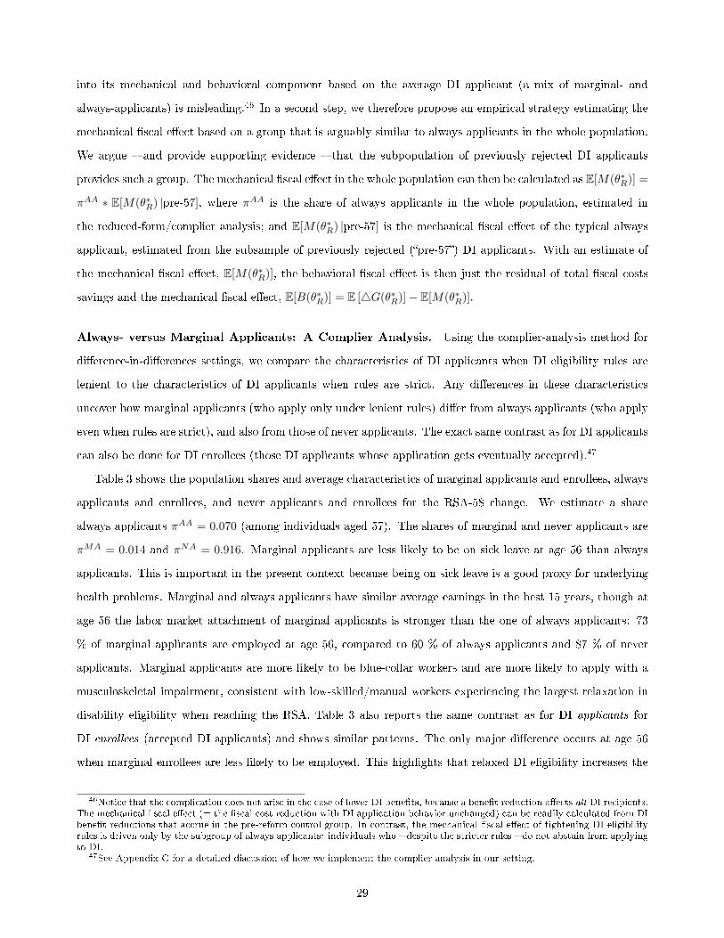
into its mechanical and behavioral component based on the average DI applicant (a mix of marginal- and

always-applicants) is misleading.46 In a second step, we therefore propose an empirical strategy estimating the

mechanical �scal e�ect based on a group that is arguably similar to always applicants in the whole population.

We argue � and provide supporting evidence � that the subpopulation of previously rejected DI applicants

provides such a group. The mechanical �scal e�ect in the whole population can then be calculated as E[M(θ∗R)] =

πAA ∗ E[M(θ∗R) |pre-57], where πAA is the share of always applicants in the whole population, estimated in

the reduced-form/complier analysis; and E[M(θ∗R) |pre-57] is the mechanical �scal e�ect of the typical always

applicant, estimated from the subsample of previously rejected (�pre-57�) DI applicants. With an estimate of

the mechanical �scal e�ect, E[M(θ∗R)], the behavioral �scal e�ect is then just the residual of total �scal costs

savings and the mechanical �scal e�ect, E[B(θ∗R)] = E [4G(θ∗R)]− E[M(θ∗R)].

Always- versus Marginal Applicants: A Complier Analysis. Using the complier-analysis method for

di�erence-in-di�erences settings, we compare the characteristics of DI applicants when DI eligibility rules are

lenient to the characteristics of DI applicants when rules are strict. Any di�erences in these characteristics

uncover how marginal applicants (who apply only under lenient rules) di�er from always applicants (who apply

even when rules are strict), and also from those of never applicants. The exact same contrast as for DI applicants

can also be done for DI enrollees (those DI applicants whose application gets eventually accepted).47

Table 3 shows the population shares and average characteristics of marginal applicants and enrollees, always

applicants and enrollees, and never applicants and enrollees for the RSA-58 change. We estimate a share

always applicants πAA = 0.070 (among individuals aged 57). The shares of marginal and never applicants are

πMA = 0.014 and πNA = 0.916. Marginal applicants are less likely to be on sick leave at age 56 than always

applicants. This is important in the present context because being on sick leave is a good proxy for underlying

health problems. Marginal and always applicants have similar average earnings in the best 15 years, though at

age 56 the labor market attachment of marginal applicants is stronger than the one of always applicants: 73

% of marginal applicants are employed at age 56, compared to 60 % of always applicants and 87 % of never

applicants. Marginal applicants are more likely to be blue-collar workers and are more likely to apply with a

musculoskeletal impairment, consistent with low-skilled/manual workers experiencing the largest relaxation in

disability eligibility when reaching the RSA. Table 3 also reports the same contrast as for DI applicants for

DI enrollees (accepted DI applicants) and shows similar patterns. The only major di�erence occurs at age 56

when marginal enrollees are less likely to be employed. This highlights that relaxed DI eligibility increases the

46Notice that the complication does not arise in the case of lower DI bene�ts, because a bene�t reduction a�ects all DI recipients.The mechanical �scal e�ect (= the �scal cost reduction with DI application behavior unchanged) can be readily calculated from DIbene�t reductions that accrue in the pre-reform control group. In contrast, the mechanical �scal e�ect of tightening DI eligibilityrules is driven only by the subgroup of always applicants: individuals who � despite the stricter rules � do not abstain from applyingto DI.

47See Appendix C for a detailed discussion of how we implement the complier analysis in our setting.

29

probability of a DI award for applicants who are in better health but have poor labor market prospects.48

Pre-57 Applicants: Representative for Always Applicants? We argue that the mechanical �scal e�ect

can be estimated from the subpopulation of individuals who �led a DI application during ages 50-56. In what

follows, we refer to this subpopulation as pre-57 applicants.49 This raises the question whether pre-57 applicants

� who re-apply at age 57 � are indeed representative for the always applicants of the whole population. Notice

�rst that pre-57 applicants qualify as always applicants in the sense that they have applied under the strict DI

eligibility rules (which apply to applications below the RSA). Using pre-57 applicants as our study group, we

can perform the exact same evaluation exercise that we performed in Section 4 on the whole population. Just

like the whole population, pre-57 applicants can be divided into a treated group (subject to RSA=58) and a

control group (RSA=57), and the comparison of the two groups is informative on the causal impact of the RSA

increase on pre-57 applicants. Clearly, any e�ect that emerges at age 57 (or later) can only be identi�ed from

agents who have not yet entered DI before they turned 57, i.e. individuals whose previous DI application got

rejected, and who re-apply at age 57.50

The comparison of treated and control groups among pre-57 applicants delivers an unbiased estimate for the

mechanical �scal e�ect for the always applicants in the whole population, if the distribution of health shocks (and

other relevant characteristics) among pre-57 applicants is identical to the distribution of these characteristics

among always-applicants in the whole population. While this identifying assumption is per se fundamentally

untestable, we provide several pieces of evidence consistent with that assumption.

First, we look at the (re-)application behavior of pre-57 applicants in the treated and control groups: (i)

before age 57, (ii) at age 57, and (iii) after age 57. Before age 57, the two groups are subject to the same (strict)

DI eligibility rules and we would therefore not expect any (mechanical) di�erence among them.51 At age 57, the

treated group is subject to strict eligibility rules (RSA=58), while the control group is already subject to the

lenient rules (RSA=57). However, if the application behavior of pre-57 applicants is indeed representative for a

group of always-applicants, a change in the strictness of DI eligibility rules should not change their application

behavior. After age 57, however, we expect re-applications to be di�erent between treated and control groups.

As discussed in Section 2.2, the mechanical e�ect persists at older age, because DI is an absorbing state. If

many applicants are screened out today, more applicants will reapply tomorrow. As a result, the mechanical

48The analogous results for the RSA-59 change resemble qualitatively the results for the RSA-58 change. This is shown inAppendix Table C.5.

49Appendix Table D.6 shows summary statistics for the pre-57 applicant sample.50When the study group is the whole population (as in Section 4), individuals contributing to the identi�cation of an RSA-e�ect

at age 57 (or later) are those who did not yet apply for DI; and those who have previously applied but whose application gotrejected. In contrast, the subpopulation of pre-57 applicants, individuals contributing to identi�cation comprise, by construction,only of previously rejected DI applicants.

51In priniciple, pre-57 applicants in the treated group could change their application behavior before age 57 � anticipating thattheir RSA will be larger than the one of the control groups and hence apply more frequently than the control group. If we see suchbehavioral e�ects, this would invalidate our assumption that pre-57 applicants are a study group that consists of always applicantsonly.

30

Table 3: Applicant and enrollee characteristics, RSA 58

Marginal (M) Always (A) Di�erence Never (N) Di�erence

M-A M-N

A. Applicants

Share in population 0.014??? 0.070??? -0.056??? 0.916??? -0.902???

(0.001) (0.011) (0.002) (0.001) (0.002)

Sick Leave at age 56 (%) 1.00 9.63??? -8.63??? 1.03??? -0.03

(1.87) (0.30) (2.11) (0.02) (1.87)

Unemployed at age 56 (%) 21.02??? 26.02??? -5.00 4.91??? 16.11???

(3.38) (0.59) (3.89) (0.04) (3.38)

Employed at age 56 (%) 72.94??? 60.29??? 12.65??? 86.57∗∗∗ -13.64???

(3.85) (0.65) (4.39) (0.07) (3.85)

Avg. annual earnings best 15 years (Euro) 41,183??? 40,894??? 289 46,074??? -4,891???

(791) (146) (918) (27) (792)

Blue-collar (%) 93.26??? 81.35??? 11.91??? 55.29??? 37.98???

(3.59) (0.63) (4.12) (0.12) (3.60)

Musculoskeletal impairment (%) 59.52??? 43.89??? 15.63???

(4.57) (0.77) (5.23)

Mental impairment (%) 15.27??? 14.28??? 0.99

(3.44) (0.64) (4.02)

Other impairment (%) 25.21∗∗∗ 41.83∗∗∗ -16.62∗∗∗

(4.66) (0.77) (5.33)

B. Enrollees

Share in population 0.038??? 0.017??? 0.022??? 0.945??? -0.907???

(0.001) (0.001) (0.001) (0.001) (0.001)

Sick Leave at age 56 (%) 10.78??? 15.9??? -5.18??? 1.01??? 9.77???

(0.40) (0.63) (0.92) (0.01) (0.40)

Unemployed at age 56 (%) 36.13??? 23.05??? 13.07??? 5.13??? 31.00???

(0.71) (0.88) (1.39) (0.04) (0.71)

Employed at age 56 (%) 49.41??? 57.37??? -7.96??? 86.44??? -37.03???

(0.74) (0.99) (1.54) (0.07) (0.74)

Avg. annual earnings best 15 years (Euro) 40,639??? 41,433??? -794? 45,919??? -5,280???

(177) (321) (467) (25) (179)

Blue-collar (%) 88.12??? 77.20??? 10.91??? 56.07??? 32.04???

(0.81) (1.40) (2.07) (0.11) (0.81)

Musculoskeletal impairment (%) 56.40??? 28.83??? 27.57???

(0.98) (1.43) (2.17)

Mental impairment (%) 6.96??? 23.46??? -16.50???

(0.78) (1.47) (2.14)

Other impairment (%) 35.43??? 46.26??? -10.83???

(1.02) (1.69) (2.53)

Notes: The table reports the population shares and average characteristics of marginal applicants and enrollees, always applicants andenrollees, and never applicants and enrollees for the RSA-58 increase. We derive these estimates using the complier analysis for di�erence-in-di�erences settings described in Appendix C. Earnings are reported in 2018 Euro. Levels of signi�cance: ?1%, ??5%, and ???1%.

31

Figure 3: E�ect of RSA on DI Application Yearly and DI In�ow by Age for Pre-57 Applicants

(a) DI Application YearlyRSA 58 RSA 59

-10

-50

510

1520

25Pe

rcen

t

54 55 56 57 58 59 60Age

-10

-50

510

1520

25Pe

rcen

t

54 55 56 57 58 59Age

(b) DI In�owRSA 58 RSA 59

-20

-15

-10

-50

510

15Pe

rcen

t

54 55 56 57 58 59 60 61Age

-20

-15

-10

-50

510

15Pe

rcen

t

54 55 56 57 58 59 60Age

Notes: The �gure shows the estimated βk-coe�cients from the econometric speci�cation in (12) for the RSA-58 and RSA-59 increases usingthe sample of pre-57 applicants. Pre-57 applicants comprise individuals who have applied for DI between age 50 and age 56. The shadedarea denotes the 95 percent con�dence interval.

e�ect E [M(θ∗R)] needs to include �scal cost savings accruing after age R = 57.

Figure 3 plots the coe�cients of the same di�-in-di� strategy as in Section 4 among the subpopulation of

pre-57 applicants, with panels (a) and (b) focusing on DI application yearly and DI in�ow, respectively. The

di�erences in DI application yearly and DI in�ow between treated and control groups line up almost perfectly

with those expected from always applicants, both for treated cohorts with RSA=58 (left �gure) and RSA=59

(right �gure). Before age 57, there are no di�erences between treated and control groups. At age 57 � when

DI application yearly of the treated (but not those of controls) are evaluated under strict DI eligibility rules �

there is no (or only a weak) di�erences in DI application yearly but a large downward spike in DI in�ow. This

is exactly what one would expect among always applicants: no di�erences in applications but more rejected

applications among the treated. After age 57, we see a signi�cant increase both in DI application yearly and in

DI in�ow among the treated cohorts.52

While the DI application behavior of pre-57 applicants is very similar to what one would expect from a

group of always applicants, this does necessarily mean that the mechanical �scal e�ect estimated from the

52Similar to Section 4, DI application and DI in�ow rates are measured in percent of the entire pre-57 subpopulation (rather ashazard rates, where we would condition the application- and in�ow-rates at age t on the subpopulation not yet on on DI at aget− 1).

32

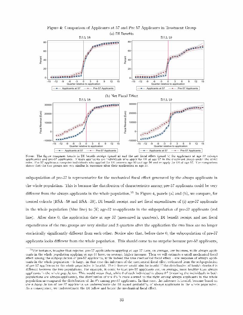
Figure 4: Comparison of Applicants at 57 and Pre-57 Applicants in Treatment Group

(a) DI Bene�tsRSA 58 RSA 59

0

20

40

60

80Pe

rcen

t

-15 -12 -9 -6 -3 0 3 6 9 12 15Quarter relative to application

Applicants at 57 Pre-57 Applicants

0

20

40

60

80

Perc

ent

-15 -12 -9 -6 -3 0 3 6 9 12 15Quarter relative to application

Applicants at 57 Pre-57 Applicants

(b) Net Fiscal E�ectRSA 58 RSA 59

-10000

0

10000

20000

30000

Fisc

al R

even

ue (E

uro)

-15 -12 -9 -6 -3 0 3 6 9 12 15Quarter relative to application

Applicants at 57 Pre-57 Applicants

-10000

0

10000

20000

30000

Fisc

al R

even

ue (E

uro)

-15 -12 -9 -6 -3 0 3 6 9 12 15Quarter relative to application

Applicants at 57 Pre-57 Applicants

Notes: The �gure compares trends in DI bene�t receipt (panel a) and the net �scal e�ect (panel b) for applicants at age 57 (alwaysapplicants) and pre-57 applicants. Always applicants are individuals who apply for DI at age 57 in the treatment group under the strictrules. Pre-57 applicants comprise individuals who applied for DI between age 50 and age 56 and re-apply for DI at age 57. The comparisonshows that the two groups are very similar in outcomes after their application at age 57.

subpopulation of pre-57 is representative for the mechanical �scal e�ect generated by the always applicants in

the whole population. This is because the distribution of characteristics among pre-57 applicants could be very

di�erent from the always applicants in the whole population.53 In Figure 4, panels (a) and (b), we compare, for

treated cohorts (RSA=58 and RSA=59), DI bene�t receipt and net �scal expenditures of (i) age-57 applicants

in the whole population (blue line) to (ii) age-57 re-applicants in the subpopulation of pre-57 applicants (red

line). After date 0, the application date at age 57 (measured in quarters), DI bene�t receipt and net �scal

expenditures of the two groups are very similar and 3 quarters after the application the two lines are no longer

statistically signi�cantly di�erent from each other. Notice also that, before date 0, the subpopulation of pre-57

applicants looks di�erent from the whole population. This should come to no surprise because pre-57 applicants,

53For instance, imagine that rejected pre-57 applicants re-appyling at age 57 have, on average, low incomes, while always appli-cants in the whole population applying at age 57 have, on average, higher incomes. Then we will estimate a small mechanical �scale�ect among the subpopulation of pre-57 applicants, while indeed the true mechanical �scal e�ect � the response of always appli-cants in the whole population � is large. In that case the inference of the mechanical �scal e�ect estimated from the subpopulationof pre-57 applicants to the whole population is invalid. The inference would also be invalid if the distribution of health shocks θ isdi�erent between the two populations. For example, it could be that pre-57 applicants are, on average, more healthy than alwaysapplicants in the whole population. This would mean that, while θ of each individual is above θA (meaning the individuals in bothpopulations are always-applicants), the distribution of the θ's is more skewed to the right among always applicants in the wholepopulation as compared the distribution of the θ's among pre-57 applicants. In that case, the inference is invalid, because based onthe subpopulation of pre-57 applicants we underestimate the DI award probability of always applicants in the whole population.As a consequence, we underestimate the DI in�ow and hence the mechanical �scal e�ect.

33

by construction, already �led a DI application before date 0, while age-57 applicants in the whole population did

not necessarily. Figure 4 supports our identifying assumption that pre-57 applicants are indeed representative

for always applicants in the whole population.54

Estimating the Fiscal Multiplier. We perform the same di�-in-di� evaluation analysis among pre-57 ap-

plicants that we performed in Section 4 among the whole population. Figure 5 plots the di�-in-di� estimates by

age for labor market outcomes and the net �scal e�ect. Figure 5 provides empirical evidence on the persistence

of the mechanical e�ect (as theoretically discussed in Section 2.2). For the RSA-58 cohort, DI bene�t receipt

signi�cantly drops at age 57 and then steadily catches up and is at age 59/60 back to the level of the cohort

with lenient DI eligibility at age 57. Interestingly, always applicants have a small employment e�ect at age 57

that vanishes afterwards, the bene�t substitution e�ect is large. This implies that the permanent changes in

employment and disability receipt in the population in Figure 2 must be driven by behavioral changes and are

not due to a persistent mechanical e�ect. We see similar patterns for the RSA-59 cohort, where the mechanical

e�ect persists for two years and then starts to disappear, as one would expect.

We are now ready to decompose the total �scal cost savings into its mechanical and behavioral component and

calculate the �scal multiplier of tightening DI eligibility rules. Table 4 presents the decomposition of the �scal

e�ect into behavioral and mechanical �scal e�ect. A one year increase in the RSA generates a net �scal e�ect

for always applicants of E [∆G(θ∗R)|pre-57] = 5, 585Euro.55 If our identifying assumption is satis�ed, we have

E [∆G(θ∗R)|pre-57] = E [M(θ∗R)|pre-57] = E [M(θ∗R)] /πAA, where the �rst equality says that the total �scal e�ect

of pre-57 applicants is purely mechanical and the second equality says that pre-57 applicants are representative

for always applicants in the whole population.56 The mechanical �scal e�ect in the whole population can then

be calculated as E [M(θ∗R)] = 5, 585Euro∗0.070 = 391Euro where πAA = 0.070 is the share of always applicants

from Table 3. The behavioral �scal e�ect is calculated as the di�erence between the �scal cost e�ect from

Table 1 and the mechanical �scal e�ect, E [B(θ∗R)] = 976− 391 = 585Euro. This decomposition implies a �scal

multiplier of 2.50. For the RSA increase from 57 to 59 we �nd a multiplier of 2.05 as displayed in Table 4.

The multiplier has to be compared to the insurance value to assess the welfare e�ect of the reform. The

insurance value measures the social value of one dollar in the hands of DI applicants who are mechanically

screened out under the stricter DI eligibility rules. Hence, increasing the RSA by one year (two years) is welfare

54In Appendix Figures D.17-D.18 we explore the respresentativeness of pre-57 further. In Figure D.17 we show that pre-57applicants award rates and application behavior (at and after age 57) that are very similar the those of all applicants at age 57.Appendix Figure D.18 shows that pre-57 and applicants at age 57 are also comparable in terms of employment and other bene�treceipt after their age-57 application.

55Notice that E [∆G|pre-57] is de�ned as the net �scal savings among pre-57 applicants who reapply at age 57. To obtain this e�ectwe proceed as follows. We �rst estimate the net �scal e�ect among all individuals belonging to the subpopulation of pre-57 applicants,irrespective of whether they �led a re-application at age 57. This yields an estimate of E [∆G|pre-57] ∗ Pr(re-apply at 57) =1, 167Euro. We then need to rescale by the probability that a pre-57 applicant reapplies at age 57, P (reapply at 57) = 0.209 toobtain E [∆G|pre-57] = 5, 585Euro.

56Notice that, by de�nition, the mechanical �scal e�ect E[M(θ∗R)

]comprises the total (mechanical) cost savings per individual

in the whole population, i.e. unconditional on a DI application, while E [∆G|pre-57] conditions on an application at age 57.

34

Figure 5: Mechanical E�ect of RSA on Labor Market States and Net Fiscal Revenue by Age

(a) DI Bene�t ReceiptRSA 58 RSA 59

-25

-20

-15

-10

-50

5Pe

rcen

t

54 55 56 57 58 59 60 61Age

-25

-20

-15

-10

-50

5Pe

rcen

t

54 55 56 57 58 59 60Age

(b) Other Bene�t ReceiptRSA 58 RSA 59

-10

-50

510

1520

Perc

ent

54 55 56 57 58 59 60 61Age

-10

-50

510

1520

Perc

ent

54 55 56 57 58 59 60Age

(c) EmploymentRSA 58 RSA 59

-10

-50

510

1520

Perc

ent

54 55 56 57 58 59 60 61Age

-10

-50

510

1520

Perc

ent

54 55 56 57 58 59 60Age

(d) Net Fiscal E�ectRSA 58 RSA 59

-500

0-4

000

-300

0-2

000

-100

00

1000

Euro

54 55 56 57 58 59 60 61Age

-500

0-4

000

-300

0-2

000

-100

00

1000

Euro

54 55 56 57 58 59 60Age

Notes: The �gure shows the estimated βk-coe�cients from the econometric speci�cation in (12) for the RSA-58 and RSA-59 increases usingthe sample of always applicants. Always applicants comprise individuals who have applied for DI between age 54 and age 56. The shadedarea denotes the 95 percent con�dence interval.

35

Table 4: Fiscal Multiplier for Eligibility Rules and Bene�t Generosity

Eligibility Rules Bene�t Generosity

RSA 58 RSA 59 Ages 57-60 Ages 30-56

Estimate % Estimate % Estimate % Estimate %

Total �scal e�ect 976 1,686 63.85 4.42

Mechanical �scal e�ect (M) 391 40% 823 49% 45.16 71% 3.24 73%

Behavioral �scal e�ect (B) 585 60% 863 51% 18.69 29% 1.18 27%

Fiscal multiplier (1+B/M) 2.50 2.05 1.41 1.36

Notes: Table presents estimates of the �scal multiplier for stricter eligibility rules and more generous DI bene�ts. The �scal multiplier ofstricter eligibility is constructed as follows. The total �scal e�ect is taken from Table 1 (with opposite sign). The mechanical �scal e�ect isestimated using the sample of pre 57 applicants and then re-scaled by the population share of always applicants (see text for details). Thebehavioral �scal e�ect is the total �scal e�ect minus the mechanical �scal e�ect.The �scal multiplier of bene�t generosity is constructed as follows. The behavioral �scal e�ect is taken from Table 2. The mechanical �scale�ect captures a 1%-increase in DI bene�ts for all DI bene�ciaries in 2004. It is obtained by multiplying the mean DI bene�ts in Table 2with 0.01. The total �scal e�ect is the sum of the mechanical and behavioral �scal e�ects.

increasing if 1 dollar in the hands of a�ected DI recipients has a social value of less than 2.50 dollars (2.05

dollars). The �scal multiplier therefore is the evaluation benchmark for the insurance value. Due to lack of

data on consumption and assets, we cannot directly estimate the insurance losses, the right-hand-side of the

social optimality condition (10). Nevertheless, we also discuss in Appendix D.2 how we can put a number on

the insurance value by assuming hand-to-mouth consumers with identical CRRA preferences. We �nd that

increasing the RSA by one (two) years is welfare improving if risk aversion is below 2.8 (2.2).57

6.2 The Fiscal Multiplier of Lower DI Bene�ts

While estimating the �scal multiplier of stricter DI eligibility rules is complicated, estimating the �scal

multiplier of the second important DI policy instrument, DI bene�ts, is rather straightforward. In section 5,

we have directly estimated E [B(bs)], the behavioral �scal e�ect of a DI bene�t reduction. According to our

estimates in Table 2, the behavioral �scal e�ect is 18.69 Euros per year for a 1% DI bene�t cut during ages

57-60 (and 1.18 Euros per year for a 1% DI bene�t cut during ages 30-56). To determine the �scal multiplier, we

additionally need the mechanical �scal e�ect, E [M(bs)] � which is simply one percent of the pre-reform mean

of DI bene�t expenditures. From Table 2, panel B column 2, a DI bene�t cut for the 57-60 year old population

yields a mechanical �scal e�ect of 0.01 · 4, 516 = 45.16 Euro per year (and 0.01 · 324 = 3.24 Euro per year for a

DI bene�t cut during ages 30-56, see column 4). The total �scal e�ect � the sum of behavioral and mechanical

�scal e�ects � is then 63.85 Euro (bene�t cut during ages 57-60) and 4.42 Euro per year (ages 30-56). The �scal

multipliers of reducing DI bene�ts is 1.41 for a DI bene�t cut during the age group 57-60 (and 1.36 for the age

group 30-56). Table 4 summarizes our results.

To assess the overall welfare consequences of a DI bene�t cut, the �scal multiplier needs to be compared to

the associated insurance losses. As mentioned above, we lack the necessary data to perform a comprehensive

57To the extent that DI recipients are self-insured through own savings, the insurance loss of a DI reform is smaller. The criticallevel of risk aversion above which makes a DI reform welfare-reducing is then correspondingly higher.

36

welfare analysis.58 Nevertheless, the �scal multiplier provides us with an interesting benchmark: Cutting DI

bene�ts by 1 % is welfare increasing if 1 dollar in the hands of DI recipients has a social value of less than 1.41

dollars.

6.3 Tightening DI Eligibility Rules or Reducing DI Bene�ts?

Using our results from Austrian DI reforms, we �nally explore the relative performance of the two DI policy

instruments in terms of economic welfare. The above analysis has shown that the �scal multiplier of stricter DI

eligibility rules is signi�cantly larger than the �scal multiplier of reducing DI bene�ts. A mechanical one-dollar

reduction of the DI budget reduces the overall expenditures 1.8 times (= 2.50/1.41) more strongly when the

reduction is due to stricter DI eligibility rules (RSA increase to age 58) rather than due to lower DI bene�ts.

Put di�erently, if the insurance losses associated with stricter DI eligibility rules and lower DI bene�ts were

equally large, policy makers should tighten eligibility rather than cutting bene�ts.59

Clearly, insurance losses of the two policy instruments are not identical. Comparing the right-hand-sides of

the social optimality conditions (10) and (11) shows that stricter DI eligibility rules a�ect only the additionally

screened-out DI applicants, while lower DI bene�ts a�ect all DI recipients alike. While we lack the necessary

data (on consumption, wealth and health conditions) to put a number on the absolute value of the insurance

losses, we can make progress comparing the insurance losses associated with the two DI policy instruments.

We proceed in two steps. We �rst use our theoretical framework developed in section 2.2 to derive a condition

comparing the insurance loss of tighter DI rules with the loss of lower DI bene�ts. Then we implement this

condition empirically and show that the insurance loss associated with tighter DI eligibility rules is, in all

likelihood, smaller than the insurance loss associated with lower DI bene�ts.

In Appendix D.5, we show that a su�cient condition for the insurance loss of stricter DI eligibility rules

being smaller than the insurance loss of lower DI bene�ts is

E

T−1∑t=0

βt ·v′i(c

Di,t)

λ·∆Di,t (bi,t − zi,t)

E [M∆(θ∗s)]︸ ︷︷ ︸upper bound income loss

≤ E

T−1∑t=0

βt ·v′i(c

Di,t)

λ·

Di,t

(bHi,t − bLi,t

)E [M∆(b)]︸ ︷︷ ︸

lower bound income loss

. (15)

The left-hand-side of condition (15) is an upper bound of the insurance loss associated with tighter DI eligibility

58Just like in the case of stricter DI eligibility rules, we quantify the possible insurance losses associated with DI bene�t cutunder the assumption of hand-to-mouth consumers with identical CRRA preferences. This yields a critical value of relative riskaversion of 1.1 (for a DI bene�t cut during ages 57-60), above which the reduction of DI bene�ts was actually welfare-reducing. Weshow this in Appendix D.3.

59This holds if insurance losses are smaller than the �scal gains for both policy instruments, i.e. it is optimal to cut the generosityof the DI program. If, instead, the insurance loss was larger than the �scal multiplier (for both instruments), a DI reform shouldimplement higher DI bene�ts rather than relaxed DI eligibility rules (given the insurance gains are equal) � the lower multiplier ofDI bene�ts means that increasing bene�ts is less costly to taxpayers. We focus here on the relative performance of the two policyinstruments if a policy maker wants to cut DI program costs.

37

rules which comes from additionally rejected DI applicants (indicated by ∆Di,t = 1).60 The right-hand-side of

the condition shows a lower bound of the insurance loss associated with cutting DI bene�ts. This insurance

loss equals the utility loss of DI recipients (indicated by Di,t = 1) all of whom are a�ected by lower DI bene�ts.

Notice that condition (15) splits the insurance loss into a (bounded) income loss and a welfare weight, v′(cDi,t)/λ.

An obvious advantage is that income losses can be estimated directly from the data. Clearly, comparing income

losses of the average individual is of limited interest, because the two DI policy instruments a�ect di�erent

individuals (who have di�erent welfare weights that we cannot estimate). However, we can make progress

by looking at income losses of individuals at di�erent positions in the earnings distribution. If income losses

associated with tighter DI eligibility rules were falling short of those associated with lower DI bene�ts at all

income levels � roughly speaking, at all levels of cD � then the above condition would be satis�ed. In that case,

we would conclude that tightening DI eligibility rules does not only generate a larger �scal multiplier but also

a smaller insurance loss than cutting DI bene�ts.

The second (empirical) step is to implement condition (15). For the left-hand-side of (15) we estimate the

bounds on income losses, separately for each income quintile, using the empirical model (12) and individuals'

income (= labor earnings net of payroll taxes + DI bene�ts + UI bene�ts + SI bene�ts) as a dependent variable.

We �x the income quintile of an individual at age 55 and convert the estimated treatment-coe�cients into an

average yearly income loss during ages 57-61. For rejected DI applicants resuming work we implement the

bound on income loss (bi,t− zi,t) by replacing their labor earnings with their potential social welfare bene�ts.61

For the right-hand-side of (15) we can directly calculate the reduction in DI bene�ts (bHi,t− bLi,t) of DI recipients.

Following condition (15), we normalize the absolute income losses by the mechanical �scal e�ect of the respective

DI policy instrument from Table 4. This �normalized� income loss measures, separately for each quintile, the

average (bounded) income reduction associated with a 1 Euro mechanical reduction in �scal spending of the

respective policy instrument.62

Figure 6 shows the normalized (bounded) income losses by income quintiles. In the lowest income quintile,

stricter DI eligibility rules (blue lines in Figure 6) generate signi�cantly lower income losses than lower DI

bene�ts (red line in Figure 6), while the opposite is true for the third quintile. In contrast, the income losses

are almost identical for the second, fourth and �fth quintile. In terms of magnitudes, the income-loss di�erence

is high in the lowest income quintile � tighter DI rules generate normalized income losses that are about 1.50

Euros lower than the income losses generated by lower DI bene�ts. The income-loss di�erence is smaller in the

middle of the income distribution � normalized income losses are 0.20-0.40 Euro higher with tighter DI rules

60The left-hand-side calculates the hypothetical insurance loss if all rejected DI applicants get social welfare bene�ts. In fact,many rejected DI applicants go back to work earning a higher income (but su�ering from impaired health). The condition takesadvantage of the fact that, for rejected DI applicants resuming work, we have v(zi,t) < u(wi,t)− θ. Using v(zi,t) as a lower boundfor the utility of this group leads to the above condition.

61We construct the potential social welfare bene�ts as a weighted mix of UI and SI bene�ts (weighted by the relative share ofUI and SI bene�ts recipients). This leads to an average replacement rate of 59 percent of previous earnings.

62Figures D.22 and D.23 show the income losses by income source (including labor earnings).

38

Figure 6: Bounds of Normalized Income Loss: Eligibility Rules vs. Bene�t Generosity

01

23

4N

orm

aliz

ed in

com

e lo

ss (E

uro)

1 2 3 4 5Income quintile

RSA 58 RSA 59 Generosity

Notes: The �gure implements the relative comparison of the insurance losses of stricter eligibility rules and reduced DI bene�ts fromcondition (15). The Figure plots the bounds on the normalized income losses in each income quintile for the RSA increases and a reductionin bene�t generosity. In the lowest income quintile, stricter DI eligibility rules (blue lines) generate signi�cantly lower income losses thanlower DI bene�ts (red line), while the opposite is true for the third quintile. The income losses are almost identical for the second, fourthand �fth quintile. In terms of magnitudes, the income-loss di�erence is high in the lowest income quintile � tighter DI rules generatenormalized income losses that are about 1.50 Euros lower than the income losses generated by lower DI bene�ts. The income-loss di�erenceis smaller in the middle of the income distribution � normalized income losses are 0.40 Euro higher with tighter DI rules compared withlower DI bene�ts. Roughly speaking, the insurance loss of stricter eligibility rules is smaller than the insurance loss of reduced DI bene�ts(=condition (15) holds) if a 40 cents reduction in income in the third income quintile does not generate a higher utility loss than a 1.50Euro reduction in income in the lowest income quintile.

compared with lower DI bene�ts. Roughly speaking, condition (15) holds if a 40 cents reduction in income

in the third income quintile does not generate a higher utility loss than a 1.50 Euro reduction in income in

the lowest income quintile.63 Naturally, we would expect the welfare weight of the lowest income quintile to

be larger than the welfare weight of the third income quintile. We therefore conclude that the insurance loss

associated with stricter DI eligibility is smaller than the insurance loss associated with reducing DI bene�ts.

In sum, our analysis of the Austrian DI reforms lead to the conclusion that �scal multiplier of stricter DI

eligibility rules are substantially larger than �scal multipliers of cutting DI bene�ts. Moreover, we �nd that

the overall insurance loss of tighter DI eligibility rules is, in all likelihood, smaller than the average insurance

loss resulting from lower DI bene�ts. In the Austrian context, our estimates suggest that the welfare cost of

tightening DI eligibility is smaller than that of cutting DI bene�ts. The next section applies our framework to

the US context, which has similar age speci�c eligibility criteria as the Austrian RSA.

7 Application to the US Disability System

The US DI eligibility criteria are also subject to vocational factors similar to the RSA in Austria. This

medical-vocational grid introduces sharp discontinuities in initial award rates by age. Chen and van der Klaauw

(2008) use these discontinuities to estimate the labor supply e�ects of DI bene�t receipt. We use their estimates

for our framework to discuss the welfare e�ects of abolishing/shifting these age cuto�s in the US. In contrast

63Of course, this statement holds only approximately, since there is heterogeneity within the income quintiles.

39

to Austria the US age cuto�s do not seem to a�ect application behavior. There is no strategic bunching of

applications at these ages as shown by Figure 6 in Chen and van der Klaauw (2008). Chen and van der Klaauw

(2008) argue that the rules are not well-known among DI applicants and therefore there is no systematic sorting

around the age cuto�s in the US. Appendix Figure D.25 contrasts the US application behavior to the Austrian

application behavior and reveals that the Austrian rules are well known as there is large spike of applications

exactly at the RSA. In contrast the US evidence suggests no behavioral response with respect to the age-

dependent eligibility criteria (E [B(θ∗US)] = 0) and a �scal multiplier of unity in the US context. Therefore,

tighter DI eligibility rules at these age cuto�s in the US are welfare reducing � provided that one dollar in the

hands of DI recipients has a social value of at least one dollar. Notice that this is almost certainly the case (to

the extent that DI applicants are, on average, more deserving than the whole population).

There is no direct reduced-form estimate of the �scal multiplier of DI bene�t generosity in the US. In the

simple static model from section 2.1 the bene�t take-up elasticity ξ is a su�cient statistic (the �scal multiplier

is simply 1 + ξ). Bound and Burkhauser (1999) provide a literature review and report take-up elasticities in the

range of 0.3-0.4. Low and Pistaferri (2015)'s structural model implies an application bene�t elasticity of 0.62.

Multiplied with the average award rate of 0.67 from French and Song (2014) this implies a take-up elasticity

of ξ = 0.41. Hence, the US evidence would imply a �scal multiplier of 1.3-1.4. With this back of the envelope

calculation we �nd a very similar �scal multiplier in the US as in Austria. The DI replacement rates in the

US are lower than in Austria and hence the insurance value in the US should be higher than in Austria. This

implies that bene�ts in the US might to be too low. Bound et al. 2004 study the welfare e�ects of more generous

DI bene�ts in the US in a structural model. Interestingly, they estimate a �scal multiplier of 1.5 for DI bene�t

generosity, which is similar in magnitude as our back of the envelope calculation based on elasticities only.64

It is worth noting that our �ndings are closely in line with the conclusions of Low and Pistaferri (2015) who

�nd that US DI reforms � which increase DI bene�ts and/or relax DI eligibility rules � are welfare improving.

Low and Pistaferri (2015) reach this conclusion after setting up and estimating a structural life-cycle model.

This is quite di�erent from our methodology which is based on the su�cient-statistics approach and focuses on

the local e�ect after age 55-60. Despite these methodological di�erences, conducting similar policy experiments

lead to very similar conclusions.

8 Conclusion

In this paper, we provide a framework to analyze the welfare e�ects of stricter DI eligibility criteria versus

lower DI bene�ts by developing su�cient-statistics formulas. We show that the �scal multiplier is crucial for

64Bound et al. 2004 estimate the average implicit price of providing an additional dollar of income to recipients in the presenceof moral hazard. This is the same concept as we refer to as the ��scal multiplier�.

40

evaluation of the e�ectiveness of DI policies and estimate �scal multipliers of stricter DI eligibility rules and

lower DI bene�ts in the context of Austria.

To estimate the e�ects of stricter DI eligibility rules, we exploit variation in DI eligibility strictness that

is generated by a policy reform. Prior to 2013 DI eligibility standards were signi�cantly relaxed for workers

above age 57 relative to those below age 57. A 2013 pension reform increased the relaxed screening age (RSA)

threshold from age 57 to age 58, followed by further increases to age 59 in 2015 and age 60 in 2017. These

step-wise increases generate quasi-experimental variation in the strictness of DI eligibility at a certain age by

date of birth. To examine the impacts of changes in DI bene�t levels, we exploit a large pension reform that

reduced potential bene�t levels for most individuals, although pension levels increased for some individuals with

limited work experience.

We �nd that stricter eligibility creates �scal multipliers of 2-2.5 and reducing bene�t generosity has �scal

multipliers of 1.3-1.4. This implies that by tightening eligibility criteria the policy maker can induce larger

behavioral changes and generate greater cost reductions compared to reducing DI bene�ts. Hence, on the cost

side stricter eligibility criteria are more e�ective. Reducing bene�t generosity is only preferable to stricter

eligibility criteria if the insurance loss of reducing bene�ts was more than 1.1 dollars smaller than the insurance

loss of stricter eligibility criteria. Our analysis of income losses along the income distribution suggests that the

insurance loss of lower DI bene�ts is larger than the insurance loss of tighter eligibility rules.

41

References

Abadie, Alberto. 2003. �Semiparametric Instrumental Variable Estimation of Treatment Response Models.�Journal of Econometrics, 113 (2): 231�263.

Autor, David, Andreas Kostøl, Magne Mogstad, and Bradley Setzler. 2019. �Disability Bene�ts,Consumption Insurance, and Household Labor Supply.� American Economic Review, 109 (7): 2613�54.

Autor, David H. and Mark G. Duggan. 2003. �The Rise in the Disability Rolls and the Decline in Unem-ployment.� Quarterly Journal of Economics, 118 (1): 157�206.

Autor, David H. and Mark G. Duggan. 2006. �The Growth in the Social Security Disability Rolls: AFiscal Crisis Unfolding.� Journal of Economic Perspectives, 20 (3): 71�96.

Baily, Martin Neil. 1978. �Some Aspects of Optimal Unemployment Insurance.� Journal of Public Economics,10 (3): 379�402.

Ball, Ste�an and Hamish Low. 2014. �Do Self-insurance and Disability Insurance Prevent ConsumptionLoss on Disability?� Economica, 81 (323): 468�490.

Benitez-Silva, Hugo, Moshe Buchinsky, and John Rust. 2004. �How Large are the Classi�cation Errors inthe Social Security Disability Award Process?� Working Paper 10219, National Bureau of Economic Research.

Borghans, Lex, Anne C. Gielen, and Erzo F.P. Luttmer. 2014. �Social Support Substitution and theEarnings Rebound: Evidence from a Regression Discontinuity in Disability Insurance Reform.� AmericanEconomic Journal: Economic Policy, 6 (4): 34�70.

Bound, John. 1989. �The Health and Earnings of Rejected Disability Insurance Applicants.� American Eco-nomic Review, 79 (3): 482�503.

Bound, John and Richard V. Burkhauser. 1999. �Economic Analysis of Transfer Programs Targeted onPeople with Disabilities.� In Handbook of Labor Economics, volume 3, chapter 51, Elsevier, pp. 3417�3528.

Bound, John, Julie Berry Cullen, Austin Nichols, and Lucie Schmidt. 2004. �The Welfare Implicationsof Increasing Disability Insurance Bene�t Generosity.� Journal of Public Economics, 88 (12): 2487�2514.

Bound, John, Todd Stinebrickner, and Timothy Waidmann. 2010. �Health, Economic Resources andthe Work Decisions of Older Men.� Journal of Econometrics, 156 (1): 106�129.

Campolieti, Michele. 2004. �Disability Insurance Bene�ts and Labor Supply: Some Additional Evidence.�Journal of Labor Economics, 22 (4): 863�889.

Campolieti, Michele and Chris Riddell. 2012. �Disability Policy and the Labor Market: Evidence from aNatural Experiment in Canada, 1998�2006.� Journal of Public Economics, 96 (3-4): 306�16.

Chen, Susan andWilbert van der Klaauw. 2008. �The Work Disincentive E�ects of the Disability InsuranceProgram in the 1990s.� Journal of Econometrics, 142 (2): 757�784.

Chetty, Raj. 2006a. �A General Formula for the Optimal Level of Social Insurance.� Journal of Public Eco-nomics, 90 (10-11): 1879�1901.

Chetty, Raj. 2006b. �A New Method of Estimating Risk Aversion.� American Economic Review, 96 (5):1821�1834.

Chetty, Raj. 2008. �Moral Hazard versus Liquidity and Optimal Unemployment Insurance.� Journal of PoliticalEconomy, 116 (2): 173�234.

Chetty, Raj and Amy Finkelstein. 2013. �Social Insurance: Connecting Theory to Data.� In Alan J.Auerbach, Raj Chetty, Martin Feldstein, and Emmanuel Saez, eds., Handbook of Public Economics: Volume5, chapter 3, Elsevier, pp. 111�193.

Clausen, Andrew and Carlo Strub. 2020. �Reverse Calculus and Nested Optimization.� Journal of EconomicTheory, 187 : 105019.

De Chaisemartin, Clément and Xavier D'Haultfoeuille. 2018. �Fuzzy Di�erences-in-Di�erences.� TheReview of Economic Studies, 85 (2): 999�1028.

de Jong, Philip, Maarten Lindeboom, and Bas van der Klaauw. 2011. �Screening Disability InsuranceApplications.� Journal of the European Economic Association, 9 (1): 106�129.

Deshpande, Manasi, Tal Gross, and Yalun Su. forthcoming. �Disability and Distress: The E�ect ofDisability Programs on Financial Outcomes.� American Economic Journal: Applied Economics.

Deshpande, Manasi and Yue Li. 2019. �Who Is Screened Out? Application Costs and the Targeting ofDisability Programs.� American Economic Journal: Economic Policy, 11 (4): 213�48.

Diamond, Peter A. and Eytan Sheshinski. 1995. �Economic Aspects of Optimal Disability Bene�ts.�Journal of Public Economics, 57 (1): 1�23.

42

Fevang, Elisabeth, Inés Hardoy, and Knut Røed. 2017. �Temporary Disability Insurance and EconomicDisincentives.� The Economic Journal, 127 (603): 1410�1432.

French, Eric and Jae Song. 2014. �The E�ect of Disability Insurance Receipt on Labor Supply.� AmericanEconomic Journal: Economic Policy, 6 (2): 291�337.

Gelber, Alexander, Timothy J. Moore, and Alexander Strand. 2017. �The E�ect of Disability InsurancePayments on Bene�ciaries' Earnings.� American Economic Journal: Economic Policy, 9 (3): 229�61.

Godard, M.C.M., P.W.C. Koning, and M. Lindeboom. 2019. �Targeting Disability Insurance Applica-tions with Screening.� WorkingPaper 036/V, Tinbergen Institute.

Gruber, Jonathan. 2000. �Disability Insurance Bene�ts and Labor Supply.� Journal of Political Economy,108 (6): 1162�1183.

Gruber, Jonathan and Je�rey D. Kubik. 1997. �Disability Insurance Rejection Rates and the Labor Supplyof Older Workers.� Journal of Public Economics, 64 : 1�23.

Hendren, Nathaniel and Ben Sprung-Keyser. 2020. �A Uni�ed Welfare Analysis of Government Policies.�Quarterly Journal of Economics, 135 (3): 1209�1318.

Imbens, Guido W. and Donald B. Rubin. 1997. �Estimating Outcome Distributions for Compliers inInstrumental Variables Models.� The Review of Economic Studies, 64 (4): 555�574.

Jäger, Simon, Benjamin Schoefer, and Josef Zweimüller. 2019. �Marginal Jobs and Job Surplus: A Testof the E�ciency of Separations.� NBER Working Paper No. 25492.

Karlström, Anders, Må rten Palme, and Ingemar Svensson. 2008. �The Employment E�ect of StricterRules for Eligibility for DI: Evidence from a Natural Experiment in Sweden.� Journal of Public Economics,92 (10-11): 2071�2082.

Kleven, Henrik J. forthcoming. �Su�cient Statistics Revisited.� Annual Review of Economics.Kolsrud, Jonas, Camille Landais, Peter Nilsson, and Johannes Spinnewijn. 2018. �The OptimalTiming of Unemployment Bene�ts: Theory and Evidence from Sweden.� American Economic Review, 108 (4-5): 985�1033.

Kostøl, Andreas and Andreas Myhre. 2020. �Labor Supply Responses to Learning the Tax and Bene�tSchedule.� Working Paper.

Kostol, Andreas R. and Magne Mogstad. 2014. �How Financial Incentives Induce Disability InsuranceRecipients to Return to Work.� American Economic Review, 104 (2): 624�55.

Kroft, Kory. 2008. �Takeup, Social Multipliers and Optimal Social Insurance.� Journal of Public Economics,92 (3-4): 722�737.

Kroft, Kory and Matthew J. Notowidigdo. 2016. �Should Unemployment Insurance Vary with the Un-employment Rate? Theory and Evidence.� Review of Economic Studies, 83 (3): 1092�1124.

Landais, Camille. 2015. �Assessing the Welfare E�ects of Unemployment Bene�ts Using the Regression KinkDesign.� American Economic Journal: Economic Policy, 7 (4): 243�78.

Landais, Camille, Pascal Michaillat, and Emmanuel Saez. 2018. �A Macroeconomic Approach to OptimalUnemployment Insurance: Theory.� American Economic Journal: Economic Policy, 10 (2): 152�81.

Lee, David S., Pauline Leung, Christopher J. O'Leary, Zhuan Pei, and Simon Quach. forthcoming.�Are Su�cient Statistics Necessary? Nonparametric Measurement of Deadweight Loss in UnemploymentInsurance.� Journal of Labor Economics.

Low, Hamish and Luigi Pistaferri. 2015. �Disability Insurance and the Dynamics of the Incentive InsuranceTrade-O�.� American Economic Review, 105 (10): 2986�3029.

Low, Hamish and Luigi Pistaferri. 2019. �Disability Insurance: Error Rates and Gender Di�erences.� NBERWorking Paper No. 26513.

Low, Hamish and Luigi Pistaferri. forthcoming. �Disability Insurance: Theoretical Trade-O�s and EmpiricalEvidence.� Fiscal Studies.

Maestas, Nicole, Kathleen J. Mullen, and Alexander Strand. 2013. �Does Disability Insurance ReceiptDiscourage Work? Using Examiner Assignment to Estimate Causal E�ects of SSDI Receipt.� AmericanEconomic Review, 103 (5): 1797�1829.

Mann, David R, David C Stapleton, and Jeanette de Richemond. 2014. �Vocational Factors in theSocial Security Disability Determination Process: A Literature Review.� Technical report, Mathematica PolicyResearch.

Meyer, Bruce D. and Wallace K.C. Mok. 2019. �Disability, Earnings, Income and Consumption.� Journalof Public Economics, 171 : 51�69.

43

Moore, Timothy J. 2015. �The Employment E�ect of Terminating Disability Bene�ts.� Journal of PublicEconomics, 124 : 30�43.

Mullen, Kathleen J. and Stefan Staubli. 2016. �Disability Bene�t Generosity and Labor Force Withdrawl.�Journal of Public Economics, 143 : 49�63.

Nielsen, Helena Skyt, Torben Sorensen, and Christopher Taber. 2010. �Estimating the E�ect of StudentAid on College Enrollment: Evidence from a Government Grant Policy Reform.� American Economic Journal:Economic Policy, 2 : 185�212.

OECD. 2020. �Public Spending on Incapacity (Indicator).� Technical report.Parsons, Donald O. 1991. �Self-Screening in Targeted Public Transfer Programs.� Journal of Political Econ-omy, 99 (4): 859�876.

Ruh, Philippe and Stefan Staubli. 2019. �Financial Incentives and Earnings of Disability Insurance Recip-ients: Evidence from a Notch Design.� American Economic Journal: Economic Policy, 11 (2): 269�300.

Schmieder, Johannes F., Till von Wachter, and Stefan Bender. 2012. �The E�ects of Extended Un-employment Insurance Over the Business Cycle: Evidence from Regression Discontinuity Estimates Over 20Years.� Quarterly Journal of Economics, 127 (2): 701�752.

Shimer, Robert and Iván Werning. 2007. �Reservation Wages and Unemployment Insurance.� QuarterlyJournal of Economics, 122 (3): 1145�1185.

Staubli, Stefan. 2011. �The Impact of Stricter Criteria for Disability Insurance on Labor Force Participation.�Journal of Public Economics, 95 (9-10): 1223�1235.

Staubli, Stefan and Josef Zweimüller. 2013. �Does Raising the Early Retirement Age Increase Employmentof Older Workers?� Journal of Public Economics, 108 : 17�32.

Strand, Alexander. 2016. �E�ects of Tightening the Medical-Vocational Grid: Comments on Haller, Staubliand Zweimüller.� In Disability Research Consortium Annual Conference, Washington DC, August 2016.

von Wachter, Till, Jae Song, and Joyce Manchester. 2011. �Trends in Employment and Earnings ofAllowed and Rejected Applicants to the Social Security Disability Insurance Program.� American EconomicReview, 101 (7): 3308�3329.

Zweimüller, Josef, Rudolf Winter-Ebmer, Rafael Lalive, Andreas Kuhn, Jean-Philipe Wuellrich,

Oliver Ruf, and Simon Büchi. 2009. �Austrian Social Security Database.� Working Paper University ofZurich, 401 : 1�80.

44

Online Appendix (Not for Publication)

A Theory

A.1 Static Model

Condition Under Which θA < θR Holds. The discussion of the model in the main text � and the decision

sequence in Figure A.1 � assume that θA < θR. This means that the social welfare program is a safety net to

which an agent only applies after a DI application is rejected. Here we derive the condition under which this

holds true.

The utility of claiming social welfare falls short of the utility of working if the agent's disability is θ < θR ≡

u(w)− v(z) > 0. Hence, θR is the �marginal social welfare claimant�. If θ ≥ θR the agent prefers social welfare

over working and vice versa. An agent with θ ≥ θR applies to DI if v(z) < p (θ) v(b) + [1− p (θ)] v(z)− ψ (the

utility on social welfare falls short of the expected utility of applying to DI). If this latter condition holds for

θ = θR, it also holds for θ > θR, because p′(θ) > 0 and b > z. Thus, no agent will claim social welfare bene�ts

unless a previous DI application has been rejected, if

ψ < p(θR) [(v(b)− v(z)] . (A.1)

The condition is intuitive: if the DI program is generous (low ψ, high p(θ) and high b) and/or the social welfare

program restrictive (low z), an agent with a severe disability �rst tries to get on DI, and claims social welfare

only if her DI application gets denied. In the basic model, we assume condition (A.1) is satis�ed.

Condition (A.1) also implies θA < θR, i.e. a marginal applicant returns to work in case her DI application is

rejected. To see this, assume to the contrary, that θA ≥ θR. Then the marginal applicant is indi�erent between

applying for DI and claiming social welfare, p(θA)]v(b) + [1− p(θA)]v(z)− ψ = v(z) or ψ = p(θA) [v(b)− v(z)],

where θA is the corresponding threshold disability. However, this latter equality � together with p(θA) ≥ p(θR)

� implies that condition (A.1) is violated. In other words, while this alternative scenario is possible in principle,

it is ruled out under the maintained parameter constellation. The intuition is similar as before: if the DI system

is generous and/or social welfare restrictive, the rejected marginal applicant goes back to employment.

45

Figure A.1: DI Application Model: Decision Tree

Note: The �gure shows the decision tree of the second period in the static model. If the disability level θ is small, the agent continuesworking and enjoys utility u(w)− θ. If the disability is severe an agent applies to DI and is accepted with probability p(θ). Second periodutility is v(b) − ψin case of acceptance into DI. If the agent's application is rejected, she needs to decide whether to return to work (withutility u(w)− θ − ψ) or consume other social welfare bene�ts (with utility v(z)− ψ).

Welfare E�ect Strictness of DI Eligibility Rules. Starting from (2) the welfare e�ect of changing θ∗ is

given by

∂W

∂θ∗= −u′(w − τ)

∂τ

∂θ∗+

∞

θA

∂p(θ; θ∗)

∂θ∗v(b)dF (θ)−

θRˆ

θA

∂p(θ; θ∗)

∂θ∗(u(w)− θ)dF (θ) (A.2)

−∞

θR

∂p(θ; θ∗)

∂θ∗v(z)dF (θ) +

∂θA

∂θ∗p(θA)f(θA)

(u(w)− v(b) +

ψ

p(θA)− θA

)︸ ︷︷ ︸

=0 by de�nition of θA in eq. (1)

where

∂τ

∂θ∗=

∞

θA

∂p(θ; θ∗)

∂θ∗bdF (θ)− b∂θ

A

∂θ∗p(θA)f(θA)−

∞

θR

∂p(θ; θ∗)

∂θ∗zdF (θ) (A.3)

following from the planner's budget constraint. De�ning B(θ∗) ≡ b(∂θA/∂θ∗

)p(θA)f(θA), MW ≡

−´ θRθA

(∂p(θ; θ∗)/∂θ∗) dF (θ), MZ ≡ −´∞θR

(∂p(θ; θ∗)/∂θ∗) dF (θ) andM(θ∗) ≡MW b+MZ(b−z), we can rewrite

−∂τ/∂θ∗ = B(θ∗) + M(θ∗). Plugging these terms into the above equation for ∂W/∂θ∗ yields condition (4) in

the main text.

Welfare E�ect Strictness of DI Eligibility Rules: Non-marginal Change. Condition (4) in the main

text holds for a marginal change in θ∗. Here we consider the welfare e�ect of a discrete change. Suppose strictness

46

of eligibility rules increase from θL to θH > θL. This implies that the award probability falls p(θ; θH) < p(θ; θL)

and fewer individuals apply θAH > θAL (θAL denotes the marginal applicant with the lenient criteria θL and θAH

denotes the marginal applicant with the high standard θH). Note θR is still independent of the eligibility rules.

Figure A.2 illustrates the e�ects of a non-marginal change in strictness of eligibility rules. If rules become

stricter, the award probability curve shifts down from p(θ; θL) to p(θ; θH). As a response fewer individuals

apply. Individuals with θ < θAH no longer apply under the stricter rules. Individuals with θ ∈[θAL , θ

AH

]are therefore �marginal applicants� as they only apply under the lenient rules. The share of these marginal

applicants is πMA = F (θAH) − F (θAL ). The behavioral e�ect is the area under the old award curve of these

marginal applicants. Individuals with a disability level above θAH continue to apply. These are always applicants

and their share is πAA = 1 − F (θAH). The di�erence between the old and new award curve for these always

applicants corresponds to the mechanical e�ect. Some of these mechanically screened out individuals return to

work (gray area) and some substitute to welfare bene�ts (blue area). Hence, we have the same e�ects as in the

marginal case, but these e�ects are slightly di�erently de�ned.

Figure A.2: Illustration Non-Marginal Change

Note: This �gure illustrates the e�ects of a non-marginal change in strictness of DI eligibility rules.

Let WH and WL denote welfare in the two regimes. Welfare in the two regimes S ∈ {H,L} is

WS = u(w − τ) +´ θAS

0(u(w)− θ)dF (θ) +

´ θRθAS

(1− p(θ; θS))(u(w)− θ)dF (θ)+

+´∞θASp(θ; θS)v(b)dF (θ) +

´∞θR

(1− p(θ; θS))v(z)dF (θ)−´∞θASψdF (θ).

(A.4)

47

The welfare e�ect of this discrete change ∆W ≡WH −WL is given by

∆W = u(w − τH)− u(w − τL) (A.5)

−θRˆ

θAH

[p(θ; θL)− p(θ; θH)

][v(b)− (u(w)− θ)] dF (θ)−

∞

θR

[p(θ; θL)− p(θ; θH)

][v(b)− v(z)] dF (θ)

−θAHˆ

θAL

p(θ; θL) [v(b)− (u(w)− θ)]− ψdF (θ).

The �rst line of (A.5) captures the gain for the taxpayer (the �scal cost reduction), the second line is the loss in

insurance value for the always applicants (mechanically screened out). The third line is the insurance loss that

marginal applicants experience and is the key di�erence to the marginal case. The Envelope theorem does not

apply for a non-marginal change in θ∗ and behavioral responses have a �rst order welfare e�ect. Note that for the

limiting case of a marginal change θH → θL we have θAH → θAL and´ θAHθAL

p(θ; θL) [v(b)− (u(w)− θ)]−ψdF (θ)→

p(θAL ; θL)[v(b)− (u(w)− θAL )

]− ψ = 0 by the de�nition of the marginal applicant θAL .

Using the government budget constraint we can rewrite the �scal e�ect again as the behavioral �scal e�ect

B∆ plus the mechanical �scal e�ect M∆:

τL − τH = b ·θAHˆ

θAL

p(θ; θL)dF (θ)

︸ ︷︷ ︸≡B∆

(A.6)

= +b ·θRˆ

θAH

[p(θ; θL)− p(θ; θH)

]dF (θ)− (b− z) ·

∞

θR

[p(θ; θL)− p(θ; θH)

]dF (θ)

︸ ︷︷ ︸.

≡M∆

Moreover, we can write the welfare e�ect associated with the �scal e�ect as u(w − τH) − u(w − τL) =

λ(τL − τH

)= λ (B∆ +M∆), where λ = u′(w − τ∆) with τ∆ such that this equality holds.65 We can then

rearrange (A.5) to ∆W R 0⇔

1 +B∆

M∆R

LW∆ + LZ∆

u′(w − τ∆)M∆+

LMA

u′(w − τ∆)M∆(A.7)

where

LW∆ ≡θRˆ

θAH

[p(θ; θL)− p(θ; θH)

][v(b)− (u(w)− θ)] dF (θ), (A.8)

65Later on in the general model λ will denote the multiplier of the government budget constraint and therefore measures thesocial value of public funds.

48

LZ∆ ≡∞

θR

[p(θ; θL)− p(θ; θH)

][v(b)− v(z)] dF (θ) (A.9)

and

LMA ≡θAHˆ

θAL

p(θ; θL) [v(b)− (u(w)− θ)]− ψdF (θ). (A.10)

In summary, the �scal multiplier is still key for evaluating welfare e�ects. Moreover, we show later on that our

empirical method to estimate the multiplier is robust to non-marginal changes; and that the insurance value is

the discrete analog of the marginal change with the additional term LMA.

Welfare E�ect DI Bene�t Level. Starting from equation (2) we get

∂W

∂b= −u′(w − τ)

∂τ

∂b+

∞

θA

p(θ; θ∗)v′(b)dF (θ) (A.11)

+∂θA

∂θ∗p(θA)f(θA)

(u(w)− v(b) +

ψ

p(θA)− θA

)︸ ︷︷ ︸

=0 by de�nition of θA

where ∂τ/∂b = −b(∂θA/∂b)p(θA)f(θA)

)+´∞θAp(θ; θ∗)dF (θ) = B(b) +M(b) is the change in taxes necessary to

fund a DI system with a marginally higher DI bene�t b. (6) then immediately follows from (A.11).

Optimal Policy Mix. So far, we have derived conditions for social optimality for each single DI policy

parameter, holding the other policy parameter �xed. However, a natural question is how a DI reform should

optimally combine these two policy parameters. More precisely: how strongly � and in which direction � should

DI eligibility rules θ∗ be changed per unit change of DI bene�ts b?

The slope of the gradient answers this question of the optimal policy mix. Figure A.3 illustrates the idea

of the optimal policy mix. It depicts the current policy (θ∗0 , b0). The dotted curve indicates the combinations

of (θ∗, b) that generate the same level of social welfare. Consider the e�ect of a DI reform starting from the

pre-reform DI policy is (θ∗0 , b0). The vertical (horizontal) arrow shows how θ∗ (resp. b) needs to be changed

to increase welfare. In Figure A.3 the vertical arrow points up and the horizontal arrow points to the left,

indicating that a welfare-enhancing DI reform implement lower bene�ts and stricter eligibility rules.66 The

length of the arrows correspond to the e�ciency gains associated with the respective policy instrument. In

Figure A.3 the horizontal arrow is short, while the vertical arrow is long, suggesting that the DI reform should

strongly increase θ∗ per unit reduction of b. The slope of the gradient � the arrow pointing to the northwest �

66Alternatively, if the horizontal arrow points to the right and the vertical arrow points up, the existing DI system is toorestrictive in both dimensions and a welfare reform increasing DI bene�ts and implementing more lenient DI eligibility rules iswelfare improving. Of course, all other permutations are possible.

49

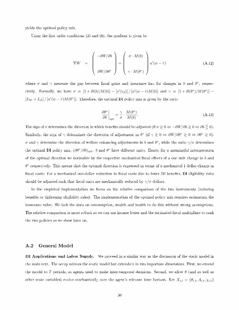
yields the optimal policy mix.

Using the �rst order conditions (5) and (6), the gradient is given by

∇W =

−∂W/∂b

∂W/∂θ∗

=

σ ·M(b)

γ ·M(θ∗)

u′(w − τ) (A.12)

where σ and γ measure the gap between �scal gains and insurance loss for changes in b and θ∗, respec-

tively. Formally, we have σ ≡ [1 +B(b)/M(b)] − [v′(cd)] / [u′(w − τ)M(b)] and γ ≡ [1 +B(θ∗)/M(θ∗)] −

[LW + LZ ] / [u′(w − τ)M(θ∗)]. Therefore, the optimal DI policy mix is given by the ratio

∂θ∗

∂b

∣∣∣∣opt

=γ

σ· M(θ∗)

M(b). (A.13)

The sign of σ determines the direction in which bene�ts should be adjusted (if σ ≷ 0⇔ −∂W/∂b ≷ 0⇔ ∂b Q 0).

Similarly, the sign of γ determines the direction of adjustment in θ∗ (if γ ≷ 0 ⇔ ∂W/∂θ∗ ≷ 0 ⇔ ∂θ∗ ≷ 0).

σ and γ determine the direction of welfare-enhancing adjustments in b and θ∗, while the ratio γ/σ determines

the optimal DI policy mix, (∂θ∗/∂b)opt. b and θ∗ have di�erent units. Hence, for a meaningful interpretation

of the optimal direction we normalize by the respective mechanical �scal e�ects of a one unit change in b and

θ∗ respectively. This means that the optimal direction is expressed in terms of a mechanical 1 dollar change in

�scal costs: For a mechanical one-dollar reduction in �scal costs due to lower DI bene�ts, DI eligibility rules

should be adjusted such that �scal costs are mechanically reduced by γ/σ dollars.

In the empirical implementation we focus on the relative comparison of the two instruments (reducing

bene�ts or tightening eligibility rules). The implementation of the optimal policy mix requires estimating the

insurance value. We lack the data on consumption, wealth and health to do this without strong assumptions.

The relative comparison is more robust as we can use income losses and the estimated �scal multipliers to rank

the two policies as we show later on.

A.2 General Model

DI Applications and Labor Supply. We proceed in a similar way as the discussion of the static model in

the main text. The setup mirrors the static model but extends it in two important dimensions. First, we extend

the model to T periods, so agents need to make inter-temporal decisions. Second, we allow θ (and as well as

other state variables) evolve stochastically over the agent's relevant time horizon. Let Xi,t = {θi,t, Ai,t, χi,t}

50

Figure A.3: Optimal Policy Mix � Gradient of Welfare Function

Notes: The �gure illustrates the idea of the optimal policy mix. It shows the gradient in case DI eligibility should be stricter and bene�tsshould be less generous. The dashed line is the indi�erence curve of the welfare function of the current bene�t level and strictness of DIeligibility. The gradient of the welfare function is orthogonal to the indi�erence curve and points in the direction of greatest increase of thefunction.

denote the vector of state variables where θi,t denotes agent i's disability level in period t, Ai,t denotes the asset

level and χi,t is a vector of other state variables (which allows for heterogeneity across agents such as di�erences

in wages etc.). The state vector Xi,t summarizes all the information relevant for agent i's choices in period t.

The laws of motion of assets in the disability, employment and welfare bene�t state are

Ai,t+1 = (1 + rt)Ai,t + bi,t(Xi,t)− cDi,t(Xi,t) (A.14)

Ai,t+1 = (1 + rt)Ai,t + wi,t(Xi,t)− τi,t(Xi,t)− cEi,t(Xi,t) (A.15)

Ai,t+1 = (1 + rt)Ai,t + zi,t(Xi,t)− cZi,t(Xi,t). (A.16)

bi,t(Xi,t) denotes DI bene�ts of individual i in period t and can depend on the agent's state Xi,t. Analogously,

wi,t(Xi,t) denotes labor income, τi,t(Xi,t) are taxes and zi,t(Xi,t) denotes social welfare bene�ts. Agents make

state contingent plans on how much to consume in each labor market state{cDi,t(Xi,t), c

Wi,t(Xi,t), c

Zi,t(Xi,t)

},

whether they apply to DI bene�ts αi,t(Xi,t) ∈ {0, 1} and, if not, on DI whether they work or claim social

welfare bene�ts ωi,t(Xi,t) ∈ {0, 1}.

The within-period sequence of events and choices is identical to the static model in Section 2.1. At the

beginning of the period, the shocks θi,t and χi,t are revealed. Having learned Xi,t, she decides whether to �le a

DI application and, if accepted, becomes a DI bene�ciary for the rest of her life.67 If her application is rejected,

she either resumes work or claims social welfare, whatever yields higher utility.

67The assumption that DI is an absorbing state, is supported by the empirically observed negligibly low out�ow rates, particularlyamong older workers.

51

Denote by Di,t,Wi,t and Zi,t, respectively, the probability that, in period t, agent i is a DI bene�t recipient,

an employed worker, or a social welfare recipient. These probabilities are given by

Di,t = 1−

[t∏

k=0

(1− αi,k(Xi,k) · p (θi,k, θ∗k))

](A.17)

Wi,t = ωi,t(Xi,t)

[t∏

k=0

(1− αi,k(Xi,k) · p (θi,k, θ∗k))

](A.18)

Zi,t = (1− ωi,t(Xi,t))

[t∏

k=0

(1− αi,k(Xi,k) · p (θi,k, θ∗k))

]. (A.19)

The probability agent i transitions to DI in period k is αi,k(Xi,k) · p (θi,k, θ∗k). Hence, the probability that an

agent is not yet on DI in period t is[∏t

k=0 (1− αi,k(Xi,k) · p (θi,k, θ∗k))]. From this pool, ωi,t(Xi,t) of the non

DI individuals work and 1 − ωi,t(Xi,t) are on social welfare bene�ts.68 We assume that the �rst application

bears a �x cost ψ and follow-up applications are costless. Λi,t = αi,t(Xi,t)∏t−1k=0 (1− αi,k(Xi,k)) ∈ 0, 1 indicates

whether agent i applies for the �rst time in period t. The other state variables, disutility of work θi,t and χi,t,

follow stochastic processes that can, in principle, depend on agents' choices. The expectation operator E [·]

below captures the evolution of the state variables and encompasses aggregation across individuals and time.69

The agent's problem is then given by

Vi(P ) = maxE

[T−1∑t=0

βt(v(cDi,t) ·Di,t + v(cZi,t) · Zi,t +

(u(cWi,t)− θi,t

)·Wi,t − Λi,t · ψ

)](A.20)

+E

[T−1∑t=0

βtµDi,t((1 + rt)Ai,t + bi,t − cDi,t −Ai,t+1

)Di,t

]

+E

[T−1∑t=0

βtµWi,t((1 + rt)Ai,t + wi,t − τi,t − cWi,t −Ai,t+1

)Wi,t

]

+E

[T−1∑t=0

βtµZi,t((1 + rt)Ai,t + zi,t − cZi,t −Ai,t+1

)Zi,t

].

Welfare E�ect of DI Reforms. We proceed in the same way as we did in the static framework. We �rst

set up the utilitarian planner's problem and study the impact of more stringent DI eligibility rules. The social

planner maximizes social welfare by choosing the strictness of DI eligibility θ∗s and DI bene�t function bs in

each period s. We denote this disability policy by P = {θ∗s , bs}T−1s=0 . The planner therefore solves

68We assume that social welfare, unlike DI, is not an absorbing state. This implies that an agent who has not yet entered DI is�at risk� of being employed or being on social welfare in period k.

69The operator E [Y ] aggregates the variable Y over states of nature and across individuals, i.e. E [Y ] =´ ´

Y (Xi,t)dF (Xi,t)diwhere F (·) is the distribution of state variables X(i, t). Notice that this is a �exible formulation: the only restriction we impose

on this distribution of state variables is that it does not directly depend on the planner's policy instruments P = {θ∗t , bt}T−1t=0 . The

evolution of X(i, t), however, can depend on agent i′s choices which themselves depend on the policy instruments P . We use theoperator E [Yi,t] =

´Y (Xi,t)dF (Xi,t) to denote the expectation w.r.t. state variables for a given individual.

52

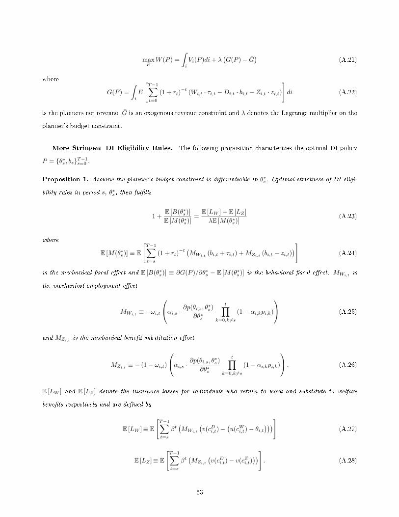
maxP

W (P ) =

ˆi

Vi(P )di+ λ(G(P )− G

)(A.21)

where

G(P ) =

ˆi

E

[T−1∑t=0

(1 + rt)−t

(Wi,t · τi,t −Di,t · bi,t − Zi,t · zi,t)

]di (A.22)

is the planners net revenue, G is an exogenous revenue constraint and λ denotes the Lagrange multiplier on the

planner's budget constraint.

More Stringent DI Eligibility Rules. The following proposition characterizes the optimal DI policy

P = {θ∗s , bs}T−1s=0 .

Proposition 1. Assume the planner's budget constraint is di�erentiable in θ∗s . Optimal strictness of DI eligi-

bility rules in period s, θ∗s , then ful�lls

1 +E [B(θ∗s)]

E [M(θ∗s)]=

E [LW ] + E [LZ ]

λE [M(θ∗s)](A.23)

where

E [M(θ∗s)] ≡ E

[T−1∑t=s

(1 + rt)−t (

MWi,t(bi,t + τi,t) +MZi,t (bi,t − zi,t)

)](A.24)

is the mechanical �scal e�ect and E [B(θ∗s)] ≡ ∂G(P )/∂θ∗s − E [M(θ∗s)] is the behavioral �scal e�ect. MWi,tis

the mechanical employment e�ect

MWi,t ≡ −ωi,t

αi,s · ∂p(θi,s, θ∗s)

∂θ∗s

t∏k=0,k 6=s

(1− αi,kpi,k)

(A.25)

and MZi,t is the mechanical bene�t substitution e�ect

MZi,t ≡ − (1− ωi,t)

αi,s · ∂p(θi,s, θ∗s)

∂θ∗s

t∏k=0,k 6=s

(1− αi,kpi,k)

. (A.26)

E [LW ] and E [LZ ] denote the insurance losses for individuals who return to work and substitute to welfare

bene�ts respectively and are de�ned by

E [LW ]≡ E

[T−1∑t=s

βt(MWi,t

(v(cDi,t)−

(u(cWi,t)− θi,t

)))](A.27)

E [LZ ]≡ E

[T−1∑t=s

βt(MZi,t

(v(cDi,t)− v(cZi,t)

))]. (A.28)

53

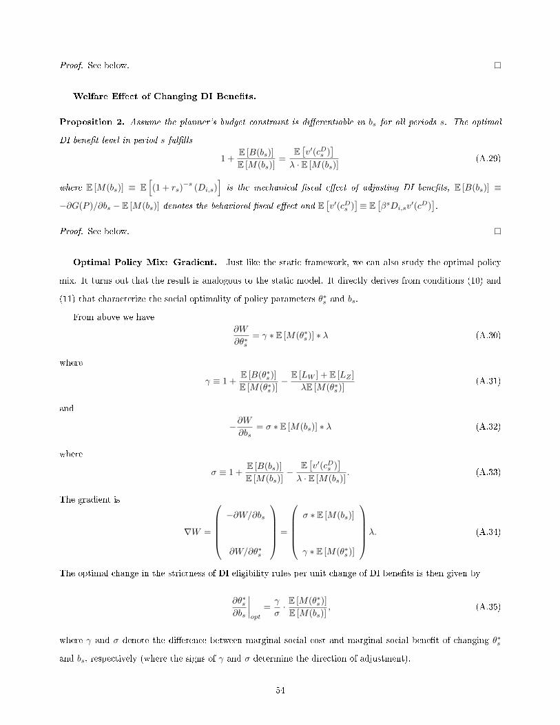
Proof. See below.

Welfare E�ect of Changing DI Bene�ts.

Proposition 2. Assume the planner's budget constraint is di�erentiable in bs for all periods s. The optimal

DI bene�t level in period s ful�lls

1 +E [B(bs)]

E [M(bs)]=

E[v′(cDs )

]λ · E [M(bs)]

(A.29)

where E [M(bs)] ≡ E[(1 + rs)

−s(Di,s)

]is the mechanical �scal e�ect of adjusting DI bene�ts, E [B(bs)] ≡

−∂G(P )/∂bs − E [M(bs)] denotes the behavioral �scal e�ect and E[v′(cDs )

]≡ E

[βsDi,sv

′(cD)].

Proof. See below.

Optimal Policy Mix: Gradient. Just like the static framework, we can also study the optimal policy

mix. It turns out that the result is analogous to the static model. It directly derives from conditions (10) and

(11) that characterize the social optimality of policy parameters θ∗s and bs.

From above we have

∂W

∂θ∗s= γ ∗ E [M(θ∗s)] ∗ λ (A.30)

where

γ ≡ 1 +E [B(θ∗s)]

E [M(θ∗s)]− E [LW ] + E [LZ ]

λE [M(θ∗s)](A.31)

and

−∂W∂bs

= σ ∗ E [M(bs)] ∗ λ (A.32)

where

σ ≡ 1 +E [B(bs)]

E [M(bs)]−

E[v′(cDs )

]λ · E [M(bs)]

. (A.33)

The gradient is

∇W =

−∂W/∂bs

∂W/∂θ∗s

=

σ ∗ E [M(bs)]

γ ∗ E [M(θ∗s)]

λ. (A.34)

The optimal change in the strictness of DI eligibility rules per unit change of DI bene�ts is then given by

∂θ∗s∂bs

∣∣∣∣opt

=γ

σ· E [M(θ∗s)]

E [M(bs)], (A.35)

where γ and σ denote the di�erence between marginal social cost and marginal social bene�t of changing θ∗s

and bs, respectively (where the signs of γ and σ determine the direction of adjustment).

54

Comparing Static and Dynamic Models. Observe the similarity between the dynamic, general solution

and the one of the static model. In the static model, we had

∂W

∂θ∗R 0 ⇐⇒ 1 +

B(θ∗)

M(θ∗)R

[v(b)− (u(w)− θ)]MW + [v(b)− v(z)]MZ

u′(w − τ)M(θ∗)

and in the dynamic model we have

∂W

∂θ∗sR 0 ⇐⇒ 1 +

E [B(θ∗s)]

E [M(θ∗s)]R

E[∑T−1

t=s βt((vi(c

Di,t)−

(ui(c

Wi,t)− θi,t

))MWi,t +

(vi(c

Di,t)− vi(cZi,t)

)MZi,t

)]λE [M(θ∗s)]

.

Proofs.

Proof. Proposition 1

The proof is a direct application of the Envelope Theorem. To derive conditions (A.23) and (A.29) we apply

the di�erentiable sandwich lemma from Clausen and Strub (2020). Clausen and Strub (2020) establish that if

a function F (c) is sandwiched at some point c between two di�erentiable functions (upper and lower support

functions U(c) and L(c)), then this function F is di�erentiable at this point c. Moreover, the derivative of

the sandwiched function F equals the derivative of the upper and lower support functions at this point, i.e.

F ′(c) = U ′(c) = L′(c). Figure A.4 illustrates this idea nicely. The proof here therefore identi�es di�erentiable

upper and lower support functions of the welfare function W (P ).

Figure A.4: Illustration Di�erentiable Sandwich Lemma

Notes: This Figure illustrates the di�erentiable sandwich lemma of Clausen and Strub (2020), which is the key argument in theproof of Proposition 1 and 2.Source:Clausen and Strub (2020).

Let P denote the optimal policy, i.e. the P = {θ∗s , bs}T−1s=0 that maximizes welfare. By de�nition W (P ) ≥

W (P )∀P and therefore the constant function U(P ) = W (P ) is a natural upper support function. We have

U ′(P ) = 0.

55

For the lower support function we use the idea of the �lazy� decision maker who does not take into account

agents' behavioral responses to the policy change. Let Vi(P ) denote the agent's indirect utility if she sticks to

her behavior that is optimal for policy P even when the policy is changed to another P . That is, for all potential

policies P the agent does not adjust her behavior. Therefore, Vi(P ) ≤ Vi(P ). As a lower support function we

then take L(P ) =´Vi(P )di+λ

(G(P )− G

). The derivative of this lower support function with respect to θ∗s is

∂L(P )

∂θ∗s= E

T−1∑t=s

βt

αi,s · ∂p(θi,s, θ∗s)

∂θ∗s

t∏k=0,k 6=s

(1− αi,kpi,k)

{v(cDi,t)− v(cZi,t) · (1− ωi,t) . . .

. . . −(u(cWi,t)− θi,t

)· ωi,t

}]+ λ

∂G(P )

∂θ∗s. (A.36)

We can decompose the total �scal e�ect ∂G(P )/∂θ∗s into the mechanical and behavioral �scal e�ect. The

mechanical e�ect is

E [M(θ∗s)] = −E

T−1∑t=s

(1 + rt)−t

αi,s · ∂p(θi,s, θ∗s)

∂θ∗s

t∏k=0,k 6=s

(1− αi,kpi,k)

(bi,t + τi,t · ωi,t − zi,t · (1− ωi,t))

and we de�ne the behavioral �scal e�ect as the residual E [B(θ∗s)] = ∂G(P )/∂θ∗s−E [M(θ∗s)].70 The di�erentiable

sandwich lemma then implies that ∂W (P )/∂θ∗s = ∂L(P )/∂θ∗s = ∂U(P )/∂θ∗s = 0 at the optimal policy. It is

then straightforward to rearrange (A.36) to (A.23).

Proof. Proposition 2.

We apply the same logic to the optimal DI bene�t policy as in the previous proof. We have

∂L(P )

∂bs= E

[βsµDi,s

]+ λ

∂G(P )

∂bs. (A.37)

The agent's �rst order condition implies E[βsµDi,sDi,s

]= E

[βsv′(cDi,s)Di,s

]. De�ne the mechanical �scal e�ect

as E [M(bs)] = E[(1 + rs)

−s(Di,s)

]and the behavioral �scal e�ect is again de�ned as the di�erence between

total �scal e�ect and mechanical �scal e�ect E [B(bs)] = −∂G(P )/∂bs−E [M(bs)]. We again have ∂W (P )/∂bs =

∂L(P )/∂bs = ∂U(P )/∂bs = 0. It is then straightforward to rearrange (A.37) to obtain (A.29).

Welfare E�ect Stricter Eligibility Rules: Non-marginal Change. Analogous to the discussion in

the static model, consider a discrete change in eligibility rules in period s from θLs to θHs > θLs . To re-

semble our empirical setup, assume that strictness of DI eligibility is high, θ∗ = θH , until age s and le-

nient afterwards. This is denoted by policy PL = (θH0 , . . . , θHs−1, θ

Ls , θ

Ls+1, θ

∗T−1; b0, . . . , bT−1). The reform

we study empirically increased the age of relaxed screening from s to s + 1. This corresponds to policy

70The behavioral �scal e�ect contains the �scal e�ect of all changes in behavior by agents. For instance, changes in DI applicationbehavior.

56

PH = (θH0 , . . . , θHs−1, θ

Hs , θ

Ls+1, θ

∗T−1; b0, . . . , bT−1). Let aHi,t denote the application decision of individual i in

period t if the policy is PH and aLi,t denote the application decision under policy PL. The discrete welfare e�ect

is

∆W = W (PH)−W (PL) (A.38)

=

ˆi

Vi(PH)− Vi(PL)di+ λ

(G(PH)−G(PL)

)assuming that λ is the same under both policies. We can again decompose the �scal e�ect G(PH)−G(PL) into

the mechanical and behavioral �scal e�ect. The mechanical �scal e�ect is given by

E [M∆(θ∗s)] ≡ E

[T−1∑t=s

(1 + rt)−t (

M∆Wi,t(bi,t + τi,t) +M∆Zi,t (bi,t − zi,t)

)](A.39)

where M∆Wi,tis the mechanical employment e�ect

M∆Wi,t≡ ωi,t

αHi,s · [pLi,s − pHi,s] t∏k=0,k 6=s

(1− αHi,kpi,k

) (A.40)

and M∆Zi,t is the mechanical bene�t substitution e�ect

M∆Zi,t ≡ (1− ωi,t)

αHi,s · [pLi,s − pHi,s] t∏k=0,k 6=s

(1− αHi,kpi,k

) . (A.41)

The mechanical �scal e�ect is, as in the static model, driven by always applicants, αHi,s = 1 (those who apply

under the strict rules at age s), and the change in their award probability[pLi,s − pHi,s

]. The share of always

applicants at age s is given by πAA = E[αHi,s ·

∏s−1k=0

(1− αHi,kpi,k

)].71 We de�ne the behavioral �scal e�ect as

the residual E [B∆(θ∗s)] ≡(G(PH)−G(PL)

)− E [M∆(θ∗s)]. The behavioral �scal e�ect is driven by changes in

the application behavior and potential other changes in behavior (which might a�ect the whole state distribution

F (Xi,t)). Writing out the behavioral �scal e�ect is cumbersome because many margins can change. Empirically,

we follow the same strategy by estimating the total �scal e�ect and the mechanical �scal e�ect and then calculate

the behavioral �scal e�ect as the residual.

Similarly, we can write the insurance loss as

ˆi

Vi(PH)− Vi(PL)di = E [L∆W ] + E [L∆Z ] + E [LMA] (A.42)

71The share of marginal applicants is πMA = E[[αLi,s − αHi,s

]·∏s−1k=0

(1− αHi,kpi,k

)].

57

where

E [L∆W ]≡ E

[T−1∑t=s

βt(M∆Wi,t

(vi(c

Di,t)−

(ui(c

Wi,t)− θi,t

)))](A.43)

E [L∆Z ]≡ E

[T−1∑t=s

βt(M∆Zi,t

(vi(c

Di,t)− vi(cZi,t)

))](A.44)

and E [LMA] ≡´iVi(P

H) − Vi(PL)di − E [L∆W ] − E [L∆Z ] > 0 is the utility loss associated with behavioral

changes. The welfare e�ect of a discrete change is therefore ∆W R 0⇔ if

1 +E [B∆(θ∗s)]

E [M∆(θ∗s)]R

E [L∆W ] + E [L∆Z ]

λE [M∆(θ∗s)]+

E [LMA]

λE [M∆(θ∗s)]. (A.45)

58

B Empirical Analysis: Additional Tables and Figures

B.1 Summary Statistics Samples

Table B.1: Summary Statistics, RSA Sample

RSA 57 RSA 58 RSA 59

DI application ever (%) 17.23 14.83 11.84

DI application yearly (%) 4.66 3.96 3.54

w/ mental disorders 0.65 0.63 0.60

w/ musculoskeletal system 2.24 1.78 1.51

w/ other disorders (%) 1.78 1.56 1.44

Re-application yearly (%) 1.46 1.41 1.28

DI bene�t receipt (%) 12.94 10.01 7.01

Employment ( %) 75.54 77.69 81.60

Other bene�t receipt (%) 7.51 7.85 7.92

Avg. annual earnings best 15 years (Euro) 41,148 42,193 43,007

(10,743) (10,933) (10,956)

Insurance years by age 50 28.72 29.29 29.44

(7.02) (6.97) (6.78)

Employment years by age 50 13.87 13.93 13.95

(2.01) (1.99) (1.99)

Was ever on sick leave by age 50 (%) 33.27 32.02 31.15

Blue-collar (%) 57.61 56.51 56.28

No. Observations 1,557,723 887,252 809,342

No. Individuals 49,418 28,144 29,245

Notes: The table reports summary statistics for men between age 54 and age 62. The RSA-57 cohort comprises men born between December1953 and November 1955, the RSA-58 cohort comprises men born between December 1955 and November 1956, and the RSA-59 cohortcomprises men born between December 1956 and November 1957. Earnings are reported in 2018 Euro. Sample standard deviations forcontinuous variables are reported in parentheses.

B.2 Stricter DI Eligibility Rules: The 2013 Reform

Figure B.5 illustrates the step-wise increase in the RSA from age 57 to age 60 graphically. The RSA increased

from age 57 to age 58 on January 1, 2013, followed by further increases to age 59 on January 1, 2015 and to

age 60 on January 1, 2017. All changes were announced in November 2012.

Figure B.6 provides descriptive evidence on the labor market e�ects of the RSA increases. We plot, by

birth cohort, the percentage of males aged 54-61 receiving DI bene�ts, having ever applied for DI, working, and

receiving other bene�ts. For each variable, trends across birth cohorts are remarkably similar until age 57 �

the relaxed screening age for the RSA-57 cohort. At this age, the DI recipient rate rises sharply in the RSA-57

cohort. The percentage males having ever applied for DI also increases, suggesting that many are aware of the

59

Table B.2: Summary Statistics, Bene�t-Generosity Sample

Age Groups

57-60 30-56

DI application (%) 6.10 0.78

w/ mental disorders 0.47 0.11

w/ musculoskeletal system 2.02 0.16

w/ other disorders 3.61 0.52

DI in�ow (%) 4.06 0.35

Employment outlfow (%) 1.55 0.06

Other bene�t out�ow (%) 2.51 0.29

Age (years) 57.35 42.39

(6.98) (3.37)

Insurance years 36.98 22.61

(8.16) (8.44)

Last annual earnings (Euro) 41,405 39,511

(18,038) (17,196)

Avg. annual earnings, best 15 years (Euro) 38,855 42,481

(12,512) (12,680)

Blue-collar (%) 49.25 50.68

No. Observations 1,453,448 15,968,003

No. Individuals 491,426 1,801,685Notes: The table reports summary statistics for 30-56 year old men and 57-60 year old men using data for the years 2004 to 2017. Earningsare reported in 2018 Euro. Sample standard deviations for continuous variables are reported in parentheses.

Figure B.5: The 2013 Reform: Increase in the RSA

5758

5960

Age

1/2011 1/2013 1/2015 1/2017Calendar time

Notes: The �gure displays the step-wise increase in the relaxed screening age (RSA) for DI bene�ts from age 57 to age 60, as mandated bythe 2012 2nd Stability Act. Source: Austrian federal law (Bundesgesetzblatt) no. 35/2012.

RSA and time their DI application to this age. Conversely, the percentage males of the RSA-57 cohort who are

employed or receive other bene�ts drops at age 57, pointing to the role of DI as a substitute for UI or SI.

We observe similar breaks in trends when the RSA-58 and RSA-59 cohorts reach their RSA, but interestingly

cohorts with a higher RSA never catch up to cohorts with a lower RSA. For example, the DI recipiency rate

rises sharply at age 58 for the RSA-58 cohort, but it never reaches the level of the RSA-57 cohort. A one year

increase in the RSA changes labor market dynamics not only at the age where disability eligibility becomes

60

Figure B.6: Labor Market States and DI Applications Ever, by Age and RSA

(a) DI Bene�t Receipt

010

2030

Perc

ent

54 55 56 57 58 59 60 61Age

RSA 57 RSA 58 RSA 59

(b) DI Application Ever

010

2030

Perc

ent

54 55 56 57 58 59 60 61Age

RSA 57 RSA 58 RSA 59

(c) Employment

6070

8090

Perc

ent

54 55 56 57 58 59 60 61Age

RSA 57 RSA 58 RSA 59

(d) Other Bene�t Receipt

010

2030

Perc

ent

54 55 56 57 58 59 60 61Age

RSA 57 RSA 58 RSA 59

Notes: The �gure shows trends in DI bene�t receipt, DI application ever (measuring whether somebody has ever applied for DI), employment,and other bene�t receipt by age for the di�erent RSA cohorts.

stricter, but also at higher ages. Our empirical strategy is designed to separately identify the e�ect of the RSA

at the ages where eligibility becomes stricter as well as at higher ages where eligibility is relaxed.

RSA E�ect Among Non-eligible Males. In Figure B.7, we plot the estimated βk-coe�cients from equation

(12) for men with too little work experience to be eligible for DI under relaxed eligibility rules. We �nd that DI

bene�t receipt, DI application ever, employment and other bene�t receipt do not di�er signi�cantly across birth

cohorts, even after age 56, providing strong support for the absence of di�erential trends across birth cohorts.

61

Figure B.7: E�ects of RSA on DI Bene�t Receipt and DI Applications by Age, Non-eligibles

(a) DI Bene�t ReceiptRSA 58 RSA 59

-4-2

02

4Pe

rcen

t

54 55 56 57 58 59 60 61Age

-4-2

02

4Pe

rcen

t

54 55 56 57 58 59 60Age

(b) DI Application EverRSA 58 RSA 59

-4-2

02

4Pe

rcen

t

54 55 56 57 58 59 60Age

-4-2

02

4Pe

rcen

t

54 55 56 57 58 59Age

(c) EmploymentRSA 58 RSA 59

-4-2

02

4Pe

rcen

t

54 55 56 57 58 59 60 61Age

-4-2

02

4Pe

rcen

t

54 55 56 57 58 59 60Age

(d) Other Bene�t ReceiptRSA 58 RSA 59

-4-2

02

4Pe

rcen

t

54 55 56 57 58 59 60 61Age

-4-2

02

4Pe

rcen

t

54 55 56 57 58 59 60Age

Notes: The �gure shows the estimated βk-coe�cients from the econometric speci�cation in (12) for the RSA 58 and RSA 59 increases usingthe sample of non-eligible men. The shaded area denotes the 95 percent con�dence interval.

62

Tracking RSA E�ects up to Age 62. The empirical results suggest that the RSA increases have long-term

e�ect up to the last age, we can observe treated cohorts in the data (age 61 for the RSA-58 cohort and age 60

for the RSA-59 cohort). A natural question is whether these e�ects would continue even beyond the last age, we

currently observe in the data? A simple way to shed light on this question is by looking at an older cohort, men

born in 1954, whom we can track until age 63. We would expect that the e�ects of the RSA increases disappear

at age 62. At this age most men in Austria retire, because they become eligible for retirement bene�ts. Indeed,

if we plot age trends in labor market outcomes and DI application ever for men born in 1954 (Figure B.8), at

age 62 we observe sharp drops in the precent of men receiving DI bene�ts, being employed, or receiving other

bene�ts.

Figure B.8: Trends by Age for Eligible Men Born in 1954

(a) DI Bene�t Receipt

05

1015

2025

Perc

ent

54 55 56 57 58 59 60 61 62 63Age

(b) DI Application Ever

510

1520

2530

Perc

ent

54 55 56 57 58 59 60 61 62 63Age

(c) Employment

2040

6080

100

Perc

ent

54 55 56 57 58 59 60 61 62 63Age

(d) Other Bene�t Receipt

24

68

10Pe

rcen

t

54 55 56 57 58 59 60 61 62 63Age

Notes: The �gure shows trends in DI bene�t receipt, DI application ever (measuring whether somebody has ever applied for DI), employment,and other bene�t receipt by age for men born 1954 who we can track until age 63.

We can estimate the e�ect of the RSA increases up to age 62 if we assume that the βk-coe�cient estimates

in equation (12) are unchanged between the last age, we currently observe in the data, and age 62. This

assumption is reasonable because, as Figure B.14 shows, the e�ects stabilize after age 58. Table B.3 reports the

correpsonding average e�ects between age 57 and age 61, that is∑61k=57 βk/5. For the RSA-58 cohort, we can

63

Table B.3: Average E�ect Above RSA up to Age 62, Men

Eligible Non-eligible

2013 2015 2013 2015

Estimate Mean Estimate Mean Estimate Mean Estimate Mean

A. Labor market e�ects (%)

DI bene�t receipt -2.54??? 18.56 -4.94??? 17.3 -0.4 38.17 -0.96?? 37.52

(0.44) (0.43) (0.38) (0.42)

DI application ever -1.17??? 21.81 -2.86??? 20.29 -0.15 38.61 0.05 37.89

(0.36) (0.36) (0.34) (0.42)

Employment 1.85??? 68.36 3.18??? 71.59 0.32 14.34 0.19 14.73

(0.39) (0.43) (0.3) (0.35)

Other bene�t receipt 0.94??? 7.55 2.20??? 7.3 -0.01 19.8 0.5 20.08

(0.25) (0.30) (0.38) (0.42)

B. Fiscal e�ects (euro)

DI bene�ts -884??? 6756 -1793??? 6245 -115 11012 -445??? 10721

(A) (161) (159) (120) (123)

Tax revenue 263??? 11185 427??? 11625 16 1582 -16 1608

(B) (56) (65) (33) (38)

Other bene�ts 172??? 1217 451??? 1182 -5 2233 92 2277

(C) (46) (63) (55) (67)

Total �scal e�ect -976??? -3213 -1769??? -4199 -135 11663 -338??? 11389

(A-B+C) (185) (186) (115) (123)

No. Observations 2,444,975 2,176,311 916,207 806,100

Notes: The tabe reports the average e�ect of the RSA for the ages between above age 56 and below age 62. The estimates are constructedby taking the average of the βk-coe�cients from equation (12) for k ≥ 57. The eligible-sample comprises men who, at age 56, have workedfor at least 10 years in the last 15 years. The non-eligible-sample comprises men who, at age 56, have worked less than 10 years in thelast 15 years. Mean denotes the mean above the RSA for the RSA-57 cohort. Fiscal e�ects are reported in 2018 Euro. Standard errorsclustered at the year-month of birth level are reported in parentheses. Levels of signi�cance: ?1%, ??5%, and ???1%.

observe labor market outcomes up to age 61. Thus, the only estimate that changes compared to Table 1 is the

estimate on DI application ever, which we observe only until age 60. We �nd that the application rate declines

by 1.17 percentage points on average, which is almost identical to the estimate in Table 1 (-1.19 percentage

points). We �nd equally small di�erences when comparing the estimates for the RSA-59 cohort.

B.3 Lower DI Bene�ts: The 2003 Reform

Figure B.9 illustrates the e�ect of the 2003 reform by showing the distribution of changes in potential DI

bene�ts between 2004 and 2017.

64

Figure B.9: Cumulative Distribution Functions of %-change in DI Bene�ts

(a) Ages 57-60

0.2

.4.6

.81

Pr(x

<=

X)

-10 -5 0 5 10 15Percent difference in DI pension

(b) Ages 30-56

0.2

.4.6

.81

Pr(x

<=

X)

-10 -5 0 5 10 15Percent difference in DI pension

Notes: The �gure shows the cumulative distribution in the percent change in DI bene�ts between 2004 and 2017 for men between ages57-60 (panel a) and men between ages 30-56 (panel b).

Placebo Estimates Bene�t Generosity. To test the appropriateness of our strategy to identify the e�ect

of DI bene�ts, we estimate 1,000 placebo regressions, in which we randomly assign individuals within each

cell de�ned by year, insurance-year decile, and assessment decile potential bene�ts br(Zit) from a di�erent year.

Appendix Figure B.10 plots the empirical cumulative distribution of the placebo estimates together with the true

estimate for each outcome in Panel A of Table 2. The �gures con�rm that true increases in bene�t generosity

lead to unusually large increases in DI in�ow, DI applications, and other bene�t out�ow, but have no e�ect on

employment out�ow.

65

Figure B.10: Distribution of Placebo Estimates

(a) DI In�owAges 57-60 Ages 30-56

0.1

.2.3

.4.5

.6.7

.8.9

1Em

piric

al C

DF

-.06 -.04 -.02 0 .02 .04 .06 .08Estimated placebo coefficient (γ)

0.1

.2.3

.4.5

.6.7

.8.9

1Em

piric

al C

DF

-.005 -.004 -.003 -.002 -.001 0 .001 .002 .003 .004 .005Estimated placebo coefficient (γ)

(b) DI ApplicationsAges 57-60 Ages 30-56

0.1

.2.3

.4.5

.6.7

.8.9

1Em

piric

al C

DF

-.06 -.03 0 .03 .06 .09 .12 .15Estimated placebo coefficient (γ)

0.1

.2.3

.4.5

.6.7

.8.9

1Em

piric

al C

DF

-.012 -.009 -.006 -.003 0 .003 .006 .009 .012 .015Estimated placebo coefficient (γ)

(c) Employment Out�owAges 57-60 Ages 30-56

0.1

.2.3

.4.5

.6.7

.8.9

1Em

piric

al C

DF

-.025 -.02 -.015 -.01 -.005 0 .005 .01 .015 .02 .025Estimated placebo coefficient (γ)

0.1

.2.3

.4.5

.6.7

.8.9

1Em

piric

al C

DF

-.0018 -.0012 -.0006 0 .0006 .0012 .0018Estimated placebo coefficient (γ)

(d) Other Bene�t Out�owAges 57-60 Ages 30-56

0.1

.2.3

.4.5

.6.7

.8.9

1Em

piric

al C

DF

-.04 -.02 0 .02 .04 .06 .08Estimated placebo coefficient (γ)

0.1

.2.3

.4.5

.6.7

.8.9

1Em

piric

al C

DF

-.004 -.003 -.002 -.001 0 .001 .002 .003 .004 .005Estimated placebo coefficient (γ)

Notes: The �gure plots the empirical distribution of placebo e�ects for labor market outcomes estimated. The CDF is constructed from 1,000estimates of γ from estimation equation (14) when we randomly assign individuals within each call de�ned by year, insurance-year decile,and assessment-basis decile potential bene�ts bit from a di�erent year. The vertical line shows the treatment e�ect estimate responded inTable.

66

B.4 DI Application E�ects by Medical Impairment

Our main results indicate that stricter DI eligibility rules and lower DI bene�ts reduce the propensity to

apply for DI bene�ts. Here we examine the application e�ect on the type of impairments with which individuals

apply, separately for each DI policy instrument. Figure B.11 plots the estimated βk-coe�cients from equation

(12) for increases in the RSA to 58 and 59. As outcome variables we use whether individuals have ever applied

with a mental impariment, a musculoskeletal impairment, or an other impairment. The shaded area denotes the

95 percent con�dence interval. The estimates suggest that an increase in the RSA reduces mainly applications

with musculoskeletal and other impairments, while applications with mental impairments do not change.

Figure B.11: RSA E�ects by Application Impairment

(a) RSA 58Mental Impairment Musculoskeletal System Other Impairment

-2-1

01

2P

erce

nt

54 55 56 57 58 59 60Age

-2-1

01

2P

erce

nt

54 55 56 57 58 59 60Age

-2-1

01

2P

erce

nt54 55 56 57 58 59 60

Age

(b) RSA 59

Mental Impairment Musculoskeletal System Other Impairment

-2-1

01

2P

erce

nt

54 55 56 57 58 59Age

-2-1

01

2P

erce

nt

54 55 56 57 58 59Age

-2-1

01

2P

erce

nt

54 55 56 57 58 59Age

Notes: The �gure shows the estimated βk-coe�cients from the econometric speci�cation in (12) for the RSA 58 and RSA 59 increases usingthe sample of eligible men. The shaded area denotes the 95 percent con�dence interval.

Table B.4 shows how changes in bene�t generosity a�ect the type of impairment with which individuals

apply for DI. Similar to stricter DI eligibility rules, we �nd no signi�cant e�ect on the number of applications

with a mental impairment, but signifcant increase in the number of applications with a musculoskeletal or any

other impairment. The absence of an e�ect on applications with a mental impairment is interesting, because a

mental illness is often considered a di�cult-to-verify disorder (see, e.g., Autor and Duggan, 2006) and one would

expect it to be responsive to changes in DI policy, but our �ndings do not provide support for this intuition.

67

B.5 The E�ect of DI Reforms on Labor Market Transitions

Our estimates show that stricter DI eligibility rules increases employment and other bene�t receipt among

treated cohorts. The increases can result either from changes in the in�ow into employment or other bene�t

receipt, or changes in the persistences in employment or other bene�t receipt. To shed light on the importance

of these two e�ects, Figures B.12 and B.13 plots the estimated βk-coe�cients from equation (12) using as

outcome variable transitions from and persistence in employment and other bene�t receipt.

Figure B.12: RSA E�ects on Transitions from Employment

(a) RSA 58To DI To Employment To Other Bene�ts

-20

24

6P

erce

nt

54 55 56 57 58 59 60 61Age

-20

24

6P

erce

nt

54 55 56 57 58 59 60 61Age

-20

24

6P

erce

nt

54 55 56 57 58 59 60 61Age

(b) RSA 59To DI To Employment To Other Bene�ts

-20

24

6P

erce

nt

54 55 56 57 58 59 60Age

-20

24

6P

erce

nt

54 55 56 57 58 59 60Age

-20

24

6P

erce

nt

54 55 56 57 58 59 60Age

Notes: The �gure shows the estimated βk-coe�cients from the econometric speci�cation in (12) for the RSA-58 and RSA-59 increases usingthe sample of eligible men. The shaded area denotes the 95 percent con�dence interval.

The �rst colum of �gure B.12 shows a drop in transitions from employment to DI at the ages where DI

eligibility rules become stricter but not at other ages. The middle column shows that stricter DI eligibility

rules induce indivdiuals who already employed to stay employed longer. The last column shows an increase in

ransitions from employment to other bene�t receipt, but the magnitude of the e�ect is only about half as big

as the increase in employment persistence. Similarly, the �rst colum of �gure B.13 shows a drop in transitions

from other bene�ts to DI at the ages where DI eligibility rules become stricter, but we also see an increase in

transitions into DI as soon as a cohort reaches its RSA, suggesting that some individuals receive other bene�ts

longer until they reach the new RSA. Consistent with this idea, the third column of B.13 shows a sharp

68

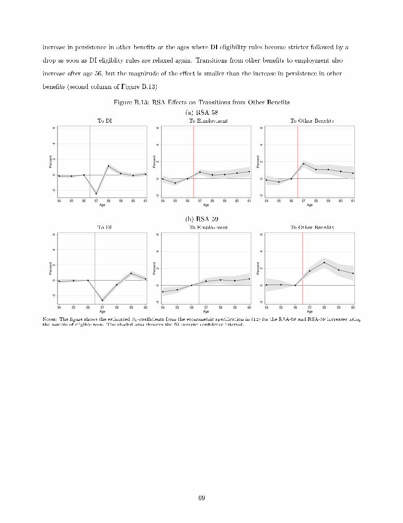
increase in persistence in other bene�ts at the ages where DI eligibility rules become stricter followed by a

drop as soon as DI eligiblity rules are relaxed again. Transitions from other bene�ts to employment also

increase after age 56, but the magnitude of the e�ect is smaller than the increase in persistence in other

bene�ts (second column of Figure B.13)

Figure B.13: RSA E�ects on Transitions from Other Bene�ts

(a) RSA 58To DI To Employment To Other Bene�ts

-20

24

6P

erce

nt

54 55 56 57 58 59 60 61Age

-20

24

6P

erce

nt

54 55 56 57 58 59 60 61Age

-20

24

6P

erce

nt

54 55 56 57 58 59 60 61Age

(b) RSA 59To DI To Employment To Other Bene�ts

-20

24

6P

erce

nt

54 55 56 57 58 59 60Age

-20

24

6P

erce

nt

54 55 56 57 58 59 60Age

-20

24

6P

erce

nt

54 55 56 57 58 59 60Age

Notes: The �gure shows the estimated βk-coe�cients from the econometric speci�cation in (12) for the RSA-58 and RSA-59 increases usingthe sample of eligible men. The shaded area denotes the 95 percent con�dence interval.

69

B.6 Fiscal E�ects

Figure B.14: Fiscal E�ects of RSA by Age

(a) DI Bene�tsRSA 58 RSA 59

-120

0-8

00-4

000

400

Euro

54 55 56 57 58 59 60 61Age

-300

0-2

400

-180

0-1

200

-600

060

0Eu

ro

54 55 56 57 58 59 60Age

(b) Tax RevenueRSA 58 RSA 59

-400

-200

020

040

060

0Eu

ro

54 55 56 57 58 59 60 61Age

-400

040

080

012

00Eu

ro

54 55 56 57 58 59 60Age

(c) Other Bene�tsRSA 58 RSA 59

-400

-200

020

040

060

0Eu

ro

54 55 56 57 58 59 60 61Age

-400

040

080

012

00Eu

ro

54 55 56 57 58 59 60Age

(d) Total Fiscal E�ectRSA 58 RSA 59

-240

0-1

800

-120

0-6

000

600

Euro

54 55 56 57 58 59 60 61Age

-240

0-1

800

-120

0-6

000

600

Euro

54 55 56 57 58 59 60Age

Notes: The �gure shows the estimated βk-coe�cients from the econometric speci�cation in (12) for the RSA-58 and RSA-59 increases usingthe sample of eligible men. The shaded area denotes the 95 percent con�dence interval.

70

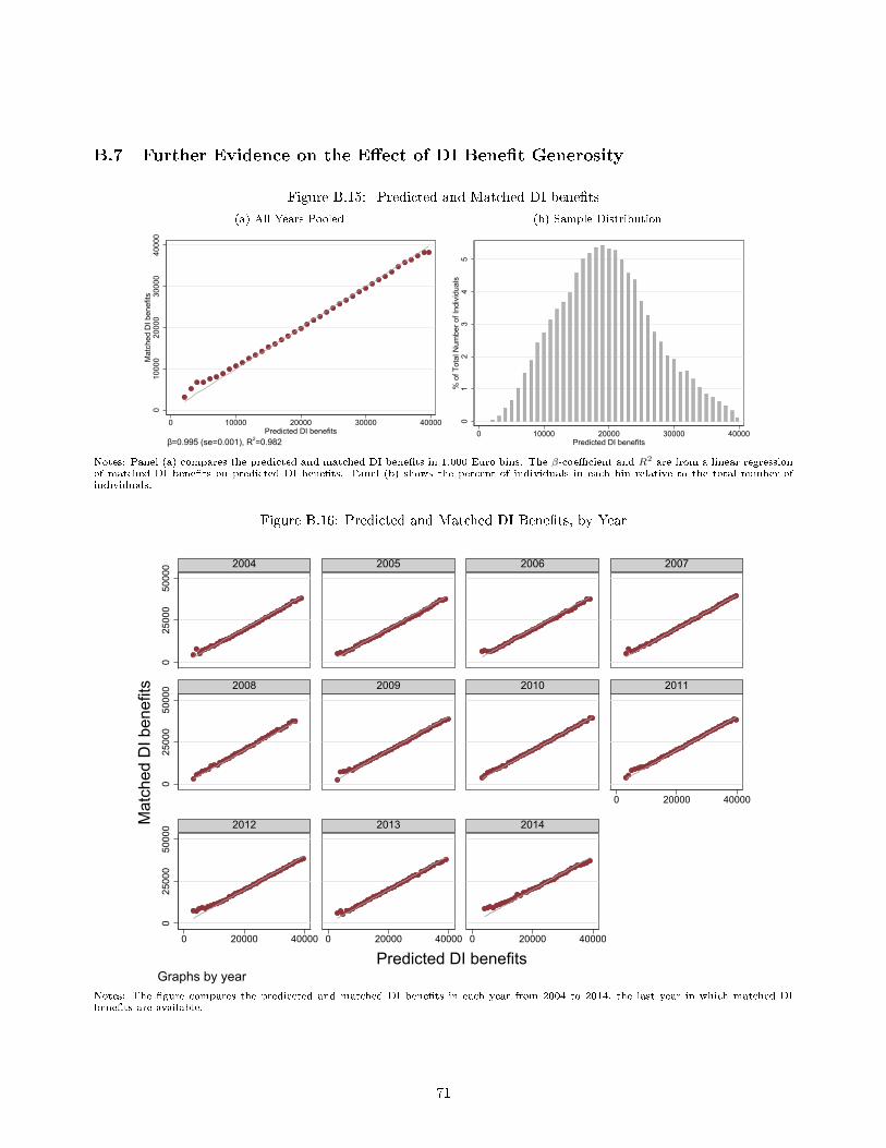
B.7 Further Evidence on the E�ect of DI Bene�t Generosity

Figure B.15: Predicted and Matched DI bene�ts

(a) All Years Pooled

010

000

2000

030

000

4000

0M

atch

ed D

I ben

efits

0 10000 20000 30000 40000Predicted DI benefits

β=0.995 (se=0.001), R2=0.982

(b) Sample Distribution

01

23

45

% o

f Tot

al N

umbe

r of I

ndiv

idua

ls

0 10000 20000 30000 40000Predicted DI benefits

Notes: Panel (a) compares the predicted and matched DI bene�ts in 1,000 Euro bins. The β-coe�cient and R2 are from a linear regressionof matched DI bene�ts on predicted DI bene�ts. Panel (b) shows the percent of individuals in each bin relative to the total number ofindividuals.

Figure B.16: Predicted and Matched DI Bene�ts, by Year

025

000

5000

00

2500

050

000

025

000

5000

0

0 20000 40000

0 20000 40000 0 20000 40000 0 20000 40000

2004 2005 2006 2007

2008 2009 2010 2011

2012 2013 2014Mat

ched

DI b

enef

its

Predicted DI benefitsGraphs by year

Notes: The �gure compares the prediected and matched DI bene�ts in each year from 2004 to 2014, the last year in which matched DIbene�ts are available.

71

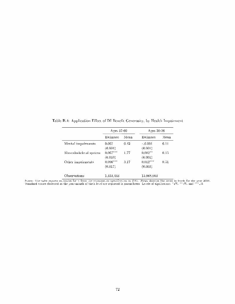
Table B.4: Application E�ect of DI Bene�t Generosity, by Health Impairment

Ages 57-60 Ages 30-56

Estimate Mean Estimate Mean

Mental impairments 0.007 0.42 <0.001 0.11

(0.004) (0.001)

Musculoskeletal system 0.067??? 1.77 0.002?? 0.15

(0.010) (0.001)

Other impairments 0.096??? 3.17 0.012??? 0.51

(0.017) (0.003)

Observations 1,453,448 15,968,003

Notes: The tabe reports estimates for γ from the econometric speci�cation in (14). Mean denotes the mean in levels for the year 2004.Standard errors clustered at the year-month of birth level are reported in parentheses. Levels of signi�cance: ?1%, ??5%, and ???1%.

72

C Characterizing Compliers

C.1 Framework for Complier Analysis

In this section, we describe the complier analysis for di�erence-in-di�erences settings, as outlined in

De Chaisemartin and D'Haultfoeuille (2018); Jäger et al. (2019), to study the characteristics of marginal,

always, and never applicants. (We follow the same steps to study the characterististcs of marginal, always, and

never enrollees.) For the RSA-58 change, we focus on the ages 56 and 57 and compare the RSA-58 cohort to the

RSA-57 cohort. The RSA-57 cohort faces relaxed DI eligibility standards at age 57, while eligibility standards

for the RSA-58 cohort are strict at both ages. For the RSA-59 increase, we focus on the ages 55 to 58 and

compare the RSA-59 cohort to the RSA-57 cohort. The RSA-57 cohort faces relaxed DI eligibility standards at

age 57 and age 58, while eligibility standards for the RSA-59 cohort are strict at any age between 55 and 58.

We denote by a the age window. It can take two values: a = A57 is the age window above 56 and a = B57

is the age window below 57. We denote by c the cohort; c = T is the RSA-57 cohort (the treatment cohort)

and c = C is the RSA-58 cohort (the control cohort). For the RSA-59 change, c = C denotes the RSA-59

cohort. We have a binary instrument Z, equal to one if DI eligibility is relaxed and zero otherwise, that is Z = 1

for (T,A57) and Z = 0 for (T,B57), (C,A57), and (C,B57). AP is an indicator whether an individual applies

for DI bene�ts. Following the potential outcomes framework, AP can take two potential values: AP0 is the

potential value of AP for Z = 0 and AP1 is the potential value of AP for Z = 1. We can now distinguish three

groups of applicants: always applicants (AP0 = AP1 = 1), never applicants (AP0 = AP1 = 0), and marginal

applicants who only apply when DI eligibility standards are relaxed (AP0 = 0 and AP1 = 1). We de�ne the

di�erent groups of enrollees in the same way basend on an indicator DI, which is one if an individual is awarded

DI bene�ts and zero otherwise. DI0 and DI1denote the potential values of DI for Z = 0 and Z = 1.

Estimating the expected value of a characteristic X for never applicants is straightforward. All individuals in

(T,A57) who do not apply for DI are never applicants if we assume AP1−AP0 ≥ 0, the standard monotonicity

assumption in the instrumental variables literature.72 We can estimate the conditional value of a never applicant

characteristic E(X|AP1 = 0, T, A57) by the corresponding sample mean 1NnaT,A57

∑iε(T,A57)Xi· I(APi = 0),where

i is individual and NnaT,A57 is the number of people in (T,A57) who do not apply for DI and I(APi = 0) is

equal to one if an individual has not applied for DI and zero otherwise. We use the same logic to estimate the

expected value of a characteristic for a never enrollee.

Estimating the expected value of a characteristic for marginal and always applicants is more challenging

and requires additional assumptions (Jäger et al., 2019). The key insight is that the expected value of a

characteristic X for all applicants in (T,A57) is a weighted average of the expected value for marginal and

72The monotonicity assumption rules out defying applicants who would apply when DI eligibility rules are strict but not whenDI eligibility rules are relaxed.

73

always applicants, where the weights represent the share of marginal applicants and always applicants among

all applicants. We can re-arrange the weighted average to get an expression for the expected value of a marginal

applicant characteristic:

E(X|AP0 = 0, AP1 = 1, T, A57) =πma + πaa

πma· E(X|AP1 = 1, T, A57)− πaa

πma· E(X|AP0 = 1, T, A57) (C.46)

where πma = NmaT,A57/NT,A57 and πaa = Naa

T,A57/NT,A57 are the shares of marginal and always applicants in

(T,A57).

We can estimate each term of the right-hand side of equation (C.46) empirically. We estimate the shares of

each group of applicants with the following regression:

APiac = α+ βa + γc + δ Zac + εiac, (C.47)

where βa is a �xed e�ect for the age window a = A57 and γc is a �xed e�ect for the cohort c = T . If Z is

independent from AP and application trends in the absence of relaxed DI eligibility are parallel across cohorts,

then πaa = α + β + γ is the share of always applicants, πma = δ is the share of marginal applicants, and

πna = 1 − πaa − πma is the share of never applicants (De Chaisemartin and D'Haultfoeuille (2018); Jäger

et al. (2019)).73 We estimate the share of always enrollees (πae), marginal enrollees (πme) and never enrollees

(πne) in the same way, but simply use DI as the dependent variable in equation (C.47). We estimate the

conditional value of an applicant characteristic E(X|AP1 = 1, T, A57) by the corresponding sample mean

(1/NaT,A57) ·

∑iε(T,A57)Xi· I(APi = 1),where Na

T,A57 is the number of applicants in (T,A57) and I(APi = 1) is

one if an individual has applied for DI.

Calculating E(X|AP0 = 1, AP1 = 1, T, A57) is more di�cult, because we never get to see whether applicants

in (T,A57) would have applied if eligibility standards were strict, that is we never observe the potential outcome

AP0. But because of monotonicity we know that individuals who apply when eligibility standards are strict also

apply when eligibility standards are relaxed, allowing us to write E(X|AP0 = 1, AP1 = 1, T, A57) = E(X|AP0 =

1, T, A57). If trends in X are parallel across cohorts under strict eligibility standards and Z is independent from

AP and X, we can estimate E(X|AP0 = 1, T, A57) using the change in applications for cohort C, E(X|AP0 =

1, T, A57) = E(X|AP0 = 1, T, B57) + E(X|AP0 = 1, C,A57) − E(X|AP0 = 1, C,B57). We can estimate

each element on the right-hand side by the corresponding sample mean: (1/NaT,B57) ·

∑iε(T,B57)Xi· I(APi =

1) + (1/NaC,A57) ·

∑iε(C,A57)Xi· I(APi = 1)− (1/Na

C,B57) ·∑iε(C,B57)Xi· I(APi = 1).

73Formaly, the independence assumption is equal to AP0, AP1 ⊥ Z | a, c and the parallel trend assumption is equal toE(AP0|A57, T )-E(AP0|B57, T ) = E(AP0|A57, C)− E(AP0|B57, C).

74

C.2 Complier Analysis for the RSA-59 Increase

Table C.5 shows the population shares and average characteristics of marginal applicants and enrollees, always

applicants and enrollees, and never applicants and enrollees for the RSA-59 change. The di�erences between

the various groups of applicants and enrollees mirror the patterns for the RSA-58 change (Table 3). Marginal

applicants and enrollees, compared to always applicants and enrollees, are in better health (proxied by sick

leave absence at age 56), are more likely to be employed at age 56, are more likely to work in blue-collar jobs

and are more likely to apply with a musculoskeletal impairment. Overall, these di�erences provide evidence

consistent with marginal applicants and enrollees having a higher work capacity than always applicants and

enrollees (but a lower work capacity than never applicants and enrollees).

75

Table C.5: Characteristics of DI Applicants and DI Recipients, RSA 59

Marginal (M) Always (A) Di�erence Never (N) Di�erence

M-A M-NA. Applicants

Share in population (%) 0.033??? 0.102??? -0.069??? 0.866??? -0.833???

(0.001) (0.001) (0.002) (0.001) (0.002)

Sick Leave at age 56 (%) -0.88 8.38??? -9.26??? 0.92??? -1.80??

(0.74) (0.20) (0.91) (0.01) (0.74)

Unemployed at age 56 (%) 10.65??? 25.53??? -14.88??? 4.26??? 6.40???

(1.57) (0.43) (1.96) (0.03) (1.57)

Employed at age 56 (%) 84.83??? 62.80??? 22.03??? 87.15??? -2.31

(1.94) (0.52) (2.40) (0.06) (1.94)

Avg. annual earnings (euro) 41,392??? 41,054??? 339 46,347??? -4,955???

(365) (109) (465) (20) (367)

Blue-collar (%) 85.87??? 80.34??? 5.53??? 53.89??? 31.98???

(1.63) (0.48) (2.07) (0.09) (1.63)

Musculoskeletal (%) 74.93??? 36.37??? 38.57???

(2.29) (0.53) (2.70)

Mental (%) 4.55??? 17.83??? -13.27???

(1.67) (0.48) (2.10)

Other (%) 20.51??? 45.80??? -25.29???

(2.15) (0.57) (2.65)

B.Enrollees

Share in population (%) 8.00??? 3.82??? 4.19??? 88.18??? -80.17???

(0.10) (0.08) (0.16) (0.05) (0.13)

Sick Leave at age 56 (%) 6.40??? 9.90??? -3.50??? 0.83??? 5.58???

(0.19) (0.28) (0.44) (0.01) (0.19)

Unemployed at age 56 (%) 23.20??? 16.92??? 6.28??? 4.68??? 18.52???

(0.32) (0.44) (0.69) (0.03) (0.32)

Employed at age 56 (%) 70.05??? 64.31??? 5.74??? 86.79??? -16.74???

(0.41) (0.69) (1.03) (0.05) (0.41)

Avg. annual earnings (euro) 40,852??? 42,207??? -1,355??? 46,231??? -5,379???

(94) (149) (229) (19) (94)

Blue-collar (%) 87.69??? 72.73??? 14.96??? 54.24??? 33.45???

(0.44) (0.66) (1.02) (0.08) (0.44)

Musculoskeletal (%) 57.28??? 24.91??? 32.37???

(0.54) (0.64) (1.03)

Mental (%) 7.43??? 25.18??? -17.76???

(0.42) (0.68) (1.02)

Other (%) 30.57??? 55.02??? -24.45???

(0.54) (0.77) (1.19)Notes: The tabe reports the population shares and average characteristics of marginal applicants and enrollees, always applicants andenrollees, and never applicants and enrollees for the RSA-59 increase. Earnings are reported in 2018 Euro. Levels of signi�cance: ?1%,??5%, and ???1%.

76

D Fiscal Multipliers

D.1 Comparing Pre-57 Applicants to Always Applicants in the Treatment Group

Table D.6 presents summary statistics for the pre-57 applicants sample, which we use to estimate the

mechanical e�ect of stricter eligibility rules. Around 50 percent of the pre-57 applicants are already on DI

by age 57. Around 40 percent of the remaining individuals reapply at age 57. 60 to 77 percent of all pre-57

applicants are on DI bene�ts by age 60. In total we have around 6000 pre-57 applicants in the control group

(RSA 57) and around 3000 individuals in each of the two treatment groups (RSA 58 and RSA 59). In terms of

labor market characteristics before age 57 the treatment and control groups are very comparable.

Table D.6: Summary Statistics, Pre-57 Applicants

RSA 57 RSA 58 RSA 59

On DI by age 57 (%) 50.89 49.36 47.63

Died by age 57 (%) 2.44 3.12 2.72

Apply at age 57 (%) 21.27 18.13 13.81

w/ mental disorders 2.69 2.85 2.46

w/ musculoskeletal system 11.49 8.78 6.55

w/ other disorders (%) 7.20 6.60 4.86

Apply ever after age 57 (%) 33.70 38.26 32.72

DI bene�t receipt at age 60 (%) 77.36 69.67 65.09Employment at age 60 ( %) 7.39 10.53 13.33

Other bene�t receipt at age 60 (%) 9.55 13.68 15.79

Avg. annual earnings best 15 years (Euro) 37,926 38,808 39,245

(9,037) (9,316) (8,823)

Insurance years by age 50 29.11 29.59 29.94

(7.07) (6.97) (6.49)

Employment years by age 50 13.60 13.67 13.69

(1.99) (1.94) (1.93)

Was ever on sick leave by age 50 (%) 58.70 56.97 57.41

Blue-collar (%) 57.61 56.51 56.28

No. Observations 192,591 100,490 84,299

No. Individuals 6,282 3,304 3,128

Notes: The table reports summary statistics for men between age 54 and age 62 who have applied for DI during ages 50-56 (pre-57applicants). The RSA-57 cohort comprises men born between December 1953 and November 1955, the RSA-58 cohort comprises men bornbetween December 1955 and November 1956, and the RSA-59 cohort comprises men born between December 1956 and November 1957.Earnings are reported in 2018 Euro. Sample standard deviations for continuous variables are reported in parentheses.

The DI applicants at age 57 in the whole population consist of (i) DI applicants who �le an application for the

�rst time and (ii) DI re-applicants whose pre-57 application got rejected (= those in the subpopulation of pre-57

applicants whose previous DI application was rejected and who re-apply at age 57). Hence, our comparison

of pre-57 applicants who re-apply at age 57 to applicants at age 57 in the whole population boils down to

comparing group (ii) to the sum of groups (i) and (ii). The share of pre-57 applicants among all applicants at

age 57 in the RSA-58 sample is 35 percent, the share of group of pre-57 applicants in the RSA-59 sample is 37

77

percent. Hence, around one third of all applicants at age 57 already �led an application before age 57 and two

thirds are �rst-time applicants.

Figure 4, Panel (a) in the main text shows that these two groups have very similar DI bene�t receipt rates.

Figure D.17 decomposes DI bene�t receipt further into application rates and award rates and shows that the

two groups are almost identical in these dimensions as well. The very similar award rates indicate that the

pre-57 applicants seem to be representative for applicants at age 57.

Figure D.17: Applicants at 57 versus Pre-57 Applicants, Treated Cohorts Only

(a) DI Application RateRSA 58 RSA 59

0

20

40

60

80

100

Perc

ent

-15 -12 -9 -6 -3 0 3 6 9 12 15Quarter relative to application

Applicants at 57 Pre-57 Applicants

0

20

40

60

80

100

Perc

ent

-15 -12 -9 -6 -3 0 3 6 9 12 15Quarter relative to application

Applicants at 57 Pre-57 Applicants

(b) DI Award RateRSA 58 RSA 59

-100

-50

0

50

100

150

Perc

ent

-15 -12 -9 -6 -3 0 3 6 9 12 15Quarter relative to application

Applicants at 57 Pre-57 Applicants

-50

0

50

100

150

200

Perc

ent

-15 -12 -9 -6 -3 0 3 6 9 12 15Quarter relative to application

Applicants at 57 Pre-57 Applicants

Notes: The �gure compares trends in DI application rates (panel a) and the DI award rates (panel b) for applicants at age 57 (alwaysapplicants) and pre-57 applicants in the treatment groups. Always applicants are individuals who apply for for DI at age 57. Pre-57applicants comprise individuals who applied for DI between age 50 and age 56 and re-apply for DI at age 57. The comparison shows thatthe two groups are very similar in outcomes after their application at age 57.

Figure D.18 compares the two groups with respect to employment, other bene�t receipt, social security

contributions and other bene�t payments. The two groups show a similar pattern after their application at 57

but they are not identical. Applicants at age 57 have slightly higher employment and a lower chance to receive

other welfare bene�ts than pre-57 applicants. This arises because �rst time applicants at age 57 have a higher

employment probability than pre-57 applicants. The di�erences are, however, not large.

78

Figure D.18: Pre-57 Applicants versus Age-57 Applicants

(a) EmploymentRSA 58 RSA 59

0

20

40

60

80Pe

rcen

t

-15 -12 -9 -6 -3 0 3 6 9 12 15Quarter relative to application

Applicants at 57 Pre-57 Applicants

0

20

40

60

80

Perc

ent

-15 -12 -9 -6 -3 0 3 6 9 12 15Quarter relative to application

Applicants at 57 Pre-57 Applicants

(b) Other Bene�t ReceiptRSA 58 RSA 59

0

20

40

60

80

Perc

ent

-15 -12 -9 -6 -3 0 3 6 9 12 15Quarter relative to application

Applicants at 57 Pre-57 Applicants

0

20

40

60

80

Perc

ent

-15 -12 -9 -6 -3 0 3 6 9 12 15Quarter relative to application

Applicants at 57 Pre-57 Applicants

(c) Tax RevenuesRSA 58 RSA 59

0

5000

10000

15000

Euro

-15 -12 -9 -6 -3 0 3 6 9 12 15Quarter relative to application

Applicants at 57 Pre-57 Applicants

0

5000

10000

15000

Euro

-15 -12 -9 -6 -3 0 3 6 9 12 15Quarter relative to application

Applicants at 57 Pre-57 Applicants

(d) Other Bene�t PaymentsRSA 58 RSA 59

0

2000

4000

6000

8000

10000

Euro

-15 -12 -9 -6 -3 0 3 6 9 12 15Quarter relative to application

Applicants at 57 Pre-57 Applicants

0

20

40

60

80

Perc

ent

-15 -12 -9 -6 -3 0 3 6 9 12 15Quarter relative to application

Applicants at 57 Pre-57 Applicants

79

D.2 Insurance Loss of Stricter DI Eligibility Rules

Implementing the insurance value (the rhs of (10)) is associated with several challenges. In contrast to

the su�cient statistics literature on UI, the utility loss is expressed in di�erences in utility levels rather than

in marginal utilities. Moreover, the insurance value also depends on the abstract quantity θ. We tackle this

challenges by deriving bounds of the insurance value that do not depend on the unobserved disability level θ.

Furthermore, we assume utility is state-independent and CRRA, i.e. v(c) = u(c) = c1−γ−11−γ , and that we have

hand-to-mouth consumers.74 In the following we discuss the derivation of the bounds and the implications of

our assumptions. For this de�ne the insurance value as

∆V ≡ 1

λE [M(θ∗s)]E

[T−1∑t=s

βt(MWi,t

(v(cDi,t)−

(u(cWi,t)− θi,t

))+MZi,t

(v(cDi,t)− v(cZi,t)

))](D.48)

In the following we derive lower and upper bounds on this insurance value ∆V .

Upper Bound Insurance Value. The social welfare bene�ts act as safety net. An agent cannot do worse

than being on social welfare bene�ts in all periods. The insurance loss can therefore not be larger than

∆V ≤ 1

λE [M(θ∗s)]E

[T−1∑t=s

βt(MWi,t

+MZi,t

) (v(cDi,t)− v(cZi,t)

)]. (D.49)

This bound assumes that individuals who are screened out are all on social welfare bene�ts. Individuals who

decide to work at some points can only do better than being on social welfare bene�ts in all periods and hence

experience a lower insurance loss than assumed by this bound.

Lower Bound Insurance Value. Since MWi,t

(v(cDi,t)−

(u(cWi,t)− θi,t

))≥ 0 we have

∆V ≥ 1

λE [M(θ∗s)]E

[T−1∑t=s

βt(MZi,t

(v(cDi,t)− v(cZi,t)

))]. (D.50)

This lower bound simply assumes that individuals who are screened out and then return to work have no loss

in insurance value, i.e. they are indi�erent between working and receiving DI bene�ts.

Implementation. To implement (D.49) we make four assumptions. First, we measure the insurance loss

relative to an increase in resources during an employment spell (λ = E[∑T−1

t=0 βtu′(cWi,t)]where cWi,t is the

consumption level of working individuals). This is the standard to measure the insurance value in the UI

literature. Second, we assume utility is state-independent and CRRA, i.e. v(c) = u(c) = c1−γ−11−γ . Third, we

assume individuals are hand-to-mouth and set consumption equal to current income (cDi,t = bi,t, cZi,t = zi,t, c

Wi,t =

74We only observe transfers and incomes in our data and cannot measure consumption.

80

wi,t − τi,t). We assume this because we cannot observe consumption in our data. This assumption provides an

upper bound on the insurance value. If individuals can self-insure through savings the insurance loss is smaller

than if they were hand-to-mouth and simply consumed their income. Hence, in our implementation we tend to

overestimate the insurance loss. Fourth, we assume no discounting β = (1 + r) = 1. All e�ects are within a 5

years horizon and hence discounting does not play a major role.

With these assumptions we have

∆V ≤ 1

E[∑T−1

t=0 u′(wi,t − τi,t)]E [M(θ∗s)]

E

[T−1∑t=s

(MWi,t

+MZi,t

) 1

1− γ((bi,t)

1−γ − (zi,t)1−γ)] (D.51)

and

∆V ≥ 1

E[∑T−1

t=0 u′(wi,t − τi,t)]E [M(θ∗s)]

E

[T−1∑t=s

MZi,t

1

1− γ((bi,t)

1−γ − (zi,t)1−γ)] . (D.52)

We calculate E[∑T−1

t=0 u′(wi,t − τi,t)]from the data for a given value of risk aversion. We then estimate the

mechanical �scal e�ect E [M(θ∗s)] in Section 6. E[∑T−1

t=s

(MWi,t

+MZi,t

)1

1−γ((bi,t)

1−γ − (zi,t)1−γ)] in (D.51)

only depends on the mechanical e�ect. We therefore use the same pre-57 applicants strategy as in the main

text to estimate the mechanical �scal e�ect. Here we just apply this strategy to a di�erent outcome. For each

individual we create a variable qi,t which is equal to the DI bene�ts bi,t if this individual is on DI bene�ts

and equal to the individuals (hypothetical) social welfare bene�ts zi,t if this individual is not on DI bene�ts.

This ensures that an individual who returns to work experiences a utility loss as if she was on social welfare

bene�ts. We then calculate for a given risk aversion γ the utility vi,t = 11−γ (qi,t)

1−γ and run our DiD strategy

on this outcome variable vi,t. Analogously to the mechanical �scal e�ect this identi�es the mechanical utility

loss E[∑T−1

t=s

(MWi,t

+MZi,t

)1

1−γ((bi,t)

1−γ − (zi,t)1−γ)].

To estimate E[∑T−1

t=s MZi,t1

1−γ((bi,t)

1−γ − (zi,t)1−γ)] in (D.52) we create a variable li,t which is equal

to the actual DI bene�t bi,t if this individual is on DI, and equal to the hypothetical DI bene�t bi,t if the

individual is employed (= the DI bene�t the individual would receive in case of a DI reward); and li,t is equal

to the individual social welfare bene�ts zi,t if this individual is on social welfare bene�ts. This ensures that

an individual experiences no utility loss if she returns to work after being screened out (i.e. there is only a

insurance loss if MZi,t = 1). We then calculate for a given risk aversion γ the utility ui,t = 11−γ (li,t)

1−γ and run

our DiD strategy on this outcome variable ui,t.

Using this approach we estimate the upper and lower bound of the insurance loss for di�erent values of

risk aversion and plot the two bounds in Figure D.19. We �nd that shifting the RSA by one year is welfare-

improving if risk aversion γ < 2.8 and it is welfare-reducing if γ > 3.1. Increasing the RSA by two years is

81

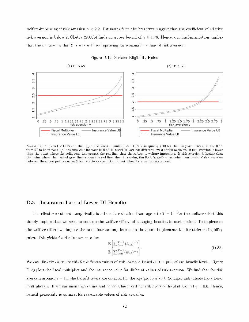
welfare-improving if risk aversion γ < 2.2. Estimates from the literature suggest that the coe�cient of relative

risk aversion is below 2, Chetty (2006b) �nds an upper bound of γ ≤ 1.78. Hence, our implementation implies

that the increase in the RSA was welfare-improving for reasonable values of risk aversion.

Figure D.19: Stricter Eligibility Rules

(a) RSA 58

11.

52

2.5

33.

54

0 .25 .5 .75 1 1.251.51.75 2 2.252.52.75 3 3.253.5risk aversion γ

Fiscal Multiplier Insurance Value UBInsurance Value LB

(b) RSA 59

11.

52

2.5

33.

54

0 .25 .5 .75 1 1.25 1.5 1.75 2 2.25 2.5 2.75 3risk aversion γ

Fiscal Multiplier Insurance Value UBInsurance Value LB

Notes: Figure plots the LHS and the upper and lower bounds of the RHS of inequality (10) for the one year increase in the RSAfrom 57 to 58 in panel (a) and two year increase in RSA in panel (b) against di�erent levels of risk aversion. If risk aversion is lowerthan the point where the solid gray line crosses the red line, then the reform is welfare improving. If risk aversion is higher thanthe point where the dashed gray line crosses the red line, then increasing the RSA is welfare reducing. For levels of risk aversionbetween these two points our su�cient statistics condition do not allow for a welfare statement.

D.3 Insurance Loss of Lower DI Bene�ts

The e�ect we estimate empirically is a bene�t reduction from age s to T − 1. For the welfare e�ect this

simply implies that we need to sum up the welfare e�ects of changing bene�ts in each period. To implement

the welfare e�ects we impose the same four assumptions as in the above implementation for stricter eligibility

rules. This yields for the insurance value

E[∑T−1

t=s (bi,s)−γ]

E[∑T−1

t=0 (wi,t)−γ] . (D.53)

We can directly calculate this for di�erent values of risk aversion based on the pre-reform bene�t levels. Figure

D.20 plots the �scal multiplier and the insurance value for di�erent values of risk aversion. We �nd that for risk

aversion around γ = 1.1 the bene�t levels are optimal for the age group 57-60. Younger individuals have lower

multipliers with similar insurance values and hence a lower critical risk aversion level of around γ = 0.6. Hence,

bene�t generosity is optimal for reasonable values of risk aversion.

82

Figure D.20: Welfare E�ects Bene�t Generosity, Men

(a) Ages 57-601

23

45

0 .25 .5 .75 1 1.25 1.5 1.75 2 2.25 2.5 2.75 3Risk aversion γ

Fiscal Multiplier Insurance Value

(b) Ages 30-56

11.

52

2.5

33.

54

0 .25 .5 .75 1 1.25 1.5 1.75 2 2.25 2.5 2.75 3Risk aversion γ

Fiscal Multiplier Insurance Value

Notes: Figure plots the LHS and RHS of inequality (11) for men aged 57-60 in panel (a) and 30-56 in panel (b) against di�erentlevels of risk aversion. If risk aversion is higher than the point where the gray line crosses the red line, then it is welfare improvingto increase bene�t generosity. If risk aversion is lower than this point, it is welfare improving to reduce bene�t generosity.

D.4 Optimal Policy Mix

For the gradient we can use the implementation from above to express γ and σ from equation (A.35) as a

function of risk aversion. For γ we use the upper and lower bounds and therefore get a range of optimal directions

for a given level of risk aversion. The optimal direction γσ measures the direction in units of mechanical cost

reductions. Intuitively, the gradient says that for a one dollar mechanical reduction in �scal costs due to

lower bene�ts, eligibility rules should be stricter such that γσ dollars are saved mechanically. Figure D.21 plots

the gradient for di�erent values of risk aversion. Panel (a) plots the optimal combination of changing bene�t

generosity and eligibility rules at age 57. For risk aversion below 1.15 bene�ts should be reduced and eligibility

rules should be stricter. For instance with risk aversion of 0.5 the optimal combination reduces spending through

stricter eligibility rules by 4 dollars for a one dollar reduction in spending due to lower bene�ts. Hence, at this

level of risk aversion DI eligibility is optimally tightened more than bene�ts. For levels of risk aversion above

2.8, bene�ts should be increased and eligibility rules should be less strict. In this region it is more e�ective to

increase bene�ts than making eligibility less strict (optimal direction of around dθ∗

db ≈0.1-0.2). For risk aversion

between 1.15 and 2.8 eligibility criteria should be tightened but bene�ts more generous. Panel (b) plots the

optimal direction for the adjustment of eligibility between 57 and 59. This gradient looks qualitatively similar

to the gradient in Panel (a).

83

Figure D.21: Optimal Policy Mix: Gradient

(a) RSA 58

reduce benefits increase benefits

stricter eligibility less strict

-20

-15

-10

-50

510

1520

0 .25 .5 .75 1 1.25 1.5 1.75 2 2.25 2.5 2.75 3 3.25 3.5risk aversion γ

(b) RSA 59

reduce benefits increase benefits

stricter eligibility less strict

-20

-15

-10

-50

510

1520

0 .25 .5 .75 1 1.25 1.5 1.75 2 2.25 2.5 2.75 3 3.25 3.5risk aversion γ

Notes: Figure plots the optimal combination of changing bene�t generosity and eligibility, i.e. the direction γσfrom equation (A.35).

The red lines indicate the critical risk aversion values for optimal DI bene�ts and eligibility rules.

D.5 Relation between Insurance Loss and Income Loss

Stricter DI Eligibility Rules. Analogously to the discussion in Appendix A.2 consider a discrete change in

eligibility rules in period s from θLs to θHs > θLs . We can write the insurance loss of stricter eligibility rules as

∆Vθ∗ ≡ˆi

Vi(θLs )− Vi(θHs )di (D.54)

≤ E

[T−1∑t=0

βt(∆DW

i,t

(vi(c

Di,t)−

{u(cWi,t)− θi,t

})+ ∆DZ

i,t

(vi(c

Di,t)− vi(cZi,t)

))](D.55)

−E

[T−1∑t=0

βt∆Λi,t · ψ

].

Expression (D.55) captures the insurance loss due to changes in the labor market status. ∆DWi,t and ∆DZ

i,t

denote the change in labor market status of individual i in period t from disability to employment and from

disability to other welfare bene�ts, respectively. This change in disability status can arise because individual i is

rejected (mechanical e�ect) or no longer applies (behavioral e�ect). ∆Λi,t ·ψ denotes the reduction in application

costs of individual i due to changing her application decision in period t. Other behavioral changes, such as

adaption of consumption and savings decision in anticipation of the stricter eligibility rules, would reduce the

insurance loss. Therefore, (D.55) is an inequality. Note that for a marginal change in θ∗s behavioral changes

would not have a �rst order welfare e�ect due to the envelope theorem. Then ∆DWi,t and ∆DZ

i,t would only

account for the mechanical changes. In this sense, our relative comparison of the insurance losses is robust to

non-marginal changes as ∆DWi,t and ∆DZ

i,t also capture changes in DI levels due to changes in behavior.

84

We now further bound the insurance loss ∆Vθ∗ and relate it to the income loss. We have

∆Vθ∗ ≤ E

[T−1∑t=0

βt(∆DW

i,t

(vi(c

Di,t)−

{u(cWi,t)− θi,t

})+ ∆DZ

i,t

(vi(c

Di,t)− vi(cZi,t)

))](D.56)

≤ E

[T−1∑t=0

βt∆Di,t

(vi(c

Di,t)− vi(cZi,t)

)](D.57)

≈ E

[T−1∑t=0

βt∆Di,tv′i(c

Di,t)(cDi,t − cZi,t

)](D.58)

≤ E

[T−1∑t=0

βt∆Di,tv′i(c

Di,t) (bi,t − zi,t)

](D.59)

where (D.56) simply drops the reduction in application costs, ∆Λi,t · ψ ≥ 0, in (D.55). (D.57) uses that other

welfare bene�ts act as a safety net, i.e. individuals who choose to work cannot be worse of than on other welfare

bene�ts, and we de�ne ∆Di,t ≡ ∆DWi,t + ∆DZ

i,t. (D.58) follows from a �rst order Taylor approximation and

(D.59) uses that the consumption drop cannot be larger than the income drop (savings dampen the income

loss).

Therefore, we have an upper bound on the insurance loss given by

∆Vθ∗

λE [M∆(θ∗s)]≤ E

T−1∑t=0

βtv′i(c

Di,t)

λ︸ ︷︷ ︸"welfare weight"

∆Di,t (bi,t − zi,t)E [M∆(θ∗s)]︸ ︷︷ ︸

bound normalized income loss

. (D.60)

In Figure 6 we estimate the bounds of the normalized income loss by income quintile. The income quintiles can

be thought of as an approximation of the welfare weight in the above inequality.

Lower DI Bene�ts . Similarly to the above discussion consider a discrete change in DI bene�ts bHi,t to

bLi,t < bHi,t. We have

∆Vb ≡ˆi

Vi(bH)− Vi(bL)di (D.61)

≥ E

[T−1∑t=0

βtDi,tv′i(c

Di,t)(bHi,t − bLi,t

)]. (D.62)

Inequality (D.62) holds because changes in behavior lead to additional utility losses for non-marginal changes

in DI bene�ts. As a lower bound for the insurance loss of reducing bene�ts we have

85

∆VbλE [M∆(b)]

≥ E

T−1∑t=0

βtv′i(c

Di,t)

λ︸ ︷︷ ︸"welfare weight"

Di,t

(bHi,t − bLi,t

)E [M∆(b)]︸ ︷︷ ︸

bound normalized income loss

. (D.63)

Comparing Insurance Loss of DI Eligibility Rules and DI Bene�ts. From (D.60) and (D.63) follows

that the insurance loss of stricter eligibility rules is smaller than the insurance loss of reduced bene�ts if

E

[T−1∑t=0

βtv′i(c

Di,t)

λ

∆Di,t (bi,t − zi,t)E [M∆(θ∗s)]

]≤ E

[T−1∑t=0

βtv′i(c

Di,t)

λ

Di,t

(bHi,t − bLi,t

)E [M∆(b)]

](D.64)

holds. Figure 6 implements this inequality empirically by estimating the bounds of the income losses by income

quintiles and we discuss the implications in the main text.

Income Losses of DI Eligibility Rules and DI Bene�ts. As an additional interesting exercise we also

look at the (unbounded) income losses of the two policy instruments taking labor earnings into account for

stricter eligibility and behavioral changes (like lower DI take-up) for the reduction in DI bene�ts. Figure D.22

displays the results of this exercise by income sources for the RSA-58 and RSA-59 increases. Panel (a) shows

that mostly individuals in the lower three income quintiles are a�ected by stricter eligibility rules. For the

RSA-58 increase, the lowest three quintiles loose on average around 1000 Euros in DI bene�ts between age 57

and 61. The DI bene�t loss is similarly distributed for the two year increase to RSA 59 with an approximately

twice as large magnitude. This loss in DI bene�ts is to some degree o�set with higher labor income (Panel (b))

and more income from other bene�ts (Panel (c)). Panel (d) presents the net e�ect on total income. The higher

income quintiles can o�set their DI income loss to a large degree with higher labor income. Only the lowest

quintile experiences a substantial loss. We do the same exercise for lower DI bene�ts in D.23. We �nd that for

the income losses associated with lower DI bene�ts are more pronounced at the lower quintiles. These losses are

only weakly compensated by other transfers, while labor earnings are not a�ected. There are also some losses

due to lower DI income in the second and third income quintile though these losses are substantially smaller,

while other income sources are largely una�ected by the the DI bene�t cut.

In Figure D.24 we present the normalized income losses in each income quintile for the RSA increases and

bene�t generosity from the unbounded income losses from Figures D.22 and D.23.75 Figure D.24 shows that for

the (unbounded) income losses the conclusion is even clearer as for the bounded income losses. The normalized

income loss of bene�t generosity is for all quintiles larger than that of stricter eligibility rules (the red line is

above the blue line, except for the third quintile where the losses are very similar).

If the objective function of the planner would not take disutility of work into account, i.e. θi,t would not

75The normalized income loss is simply the the total income loss by quintile in Panel (d) in Figures D.22 and D.23 divided bythe respective mechanical �scal e�ect from Table 4.

86

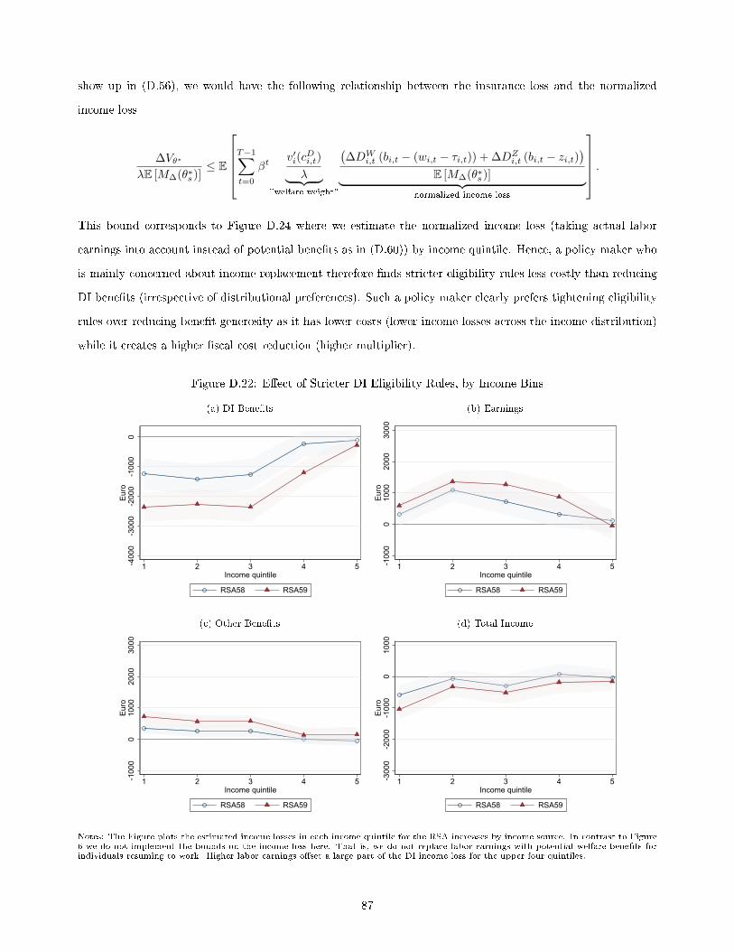
show up in (D.56), we would have the following relationship between the insurance loss and the normalized

income loss

∆Vθ∗

λE [M∆(θ∗s)]≤ E

T−1∑t=0

βtv′i(c

Di,t)

λ︸ ︷︷ ︸"welfare weight"

(∆DW

i,t (bi,t − (wi,t − τi,t)) + ∆DZi,t (bi,t − zi,t)

)E [M∆(θ∗s)]︸ ︷︷ ︸

normalized income loss

.

This bound corresponds to Figure D.24 where we estimate the normalized income loss (taking actual labor

earnings into account instead of potential bene�ts as in (D.60)) by income quintile. Hence, a policy maker who

is mainly concerned about income replacement therefore �nds stricter eligibility rules less costly than reducing

DI bene�ts (irrespective of distributional preferences). Such a policy maker clearly prefers tightening eligibility

rules over reducing bene�t generosity as it has lower costs (lower income losses across the income distribution)

while it creates a higher �scal cost reduction (higher multiplier).

Figure D.22: E�ect of Stricter DI Eligibility Rules, by Income Bins

(a) DI Bene�ts

-400

0-3

000

-200

0-1

000

0Eu

ro

1 2 3 4 5Income quintile

RSA58 RSA59

(b) Earnings

-100

00

1000

2000

3000

Euro

1 2 3 4 5Income quintile

RSA58 RSA59

(c) Other Bene�ts

-100

00

1000

2000

3000

Euro

1 2 3 4 5Income quintile

RSA58 RSA59

(d) Total Income

-300

0-2

000

-100

00

1000

Euro

1 2 3 4 5Income quintile

RSA58 RSA59

Notes: The Figure plots the estimated income losses in each income quintile for the RSA increases by income source. In contrast to Figure6 we do not implement the bounds on the income loss here. That is, we do not replace labor earnings with potential welfare bene�ts forindividuals resuming to work. Higher labor earnings o�set a large part of the DI income loss for the upper four quintiles.

87

Figure D.23: E�ect of bene�t generosity by income bins

(a) DI Bene�ts

040

8012

016

0Eu

ro

1 2 3 4 5Income quintile

(b) Earnings

-80

-40

040

80Eu

ro

1 2 3 4 5Income quintile

(c) Other Bene�ts

-80

-40

040

80Eu

ro

1 2 3 4 5Income quintile

(d) Total Income

040

8012

016

0Eu

ro

1 2 3 4 5Income quintile

Notes: The Figure plots the estimated income losses in each income quintile for reduced bene�t generosity by income source. In contrastto Figure 6 we do not implement the bounds on the income loss here. That means we also consider changes in behavior, like reduced DItake-up, that trigger changes in income.

Figure D.24: Normalized Income Loss Eligibility Rules vs. Bene�t Generosity

01

23

4N

orm

aliz

ed in

com

e lo

ss (

Eur

o)

1 2 3 4 5Income quintile

RSA 58 RSA 59 GenerosityNotes: The �gure plots the normalized income losses in each income quintile for the RSA increases and a reduction in bene�t generosity.Income quintiles are measured at age 55. The normalized income loss is simply the total income loss by quintile in Panel (d) in FiguresD.22 and D.23 divided by the respective mechanical �scal e�ect from Table 4. The normalized income loss measures the quintile's incomereduction for a 1 Euro mechanical reduction in �scal spending.

88

D.6 Austria versus US: DI Applications and DI In�ow by Age

Figure D.25: Application and Award Rate by Age: US vs. Austria

(a) Application RateUS Austria

0.5

11.

52

2.5

3Pe

rcen

t

52 53 54 55 56 57 58 59 60Age

0.5

11.

52

2.5

3Pe

rcen

t

52 53 54 55 56 57 58 59 60Age

(b) Allowance RateUS Austria

020

4060

80Pe

rcen

t

45 46 47 48 49 50 51 52 53 54 55 56 57 58 59 60Age

MedicalMedical-Vocational

020

4060

80Pe

rcen

t

52 53 54 55 56 57 58 59 60Age

Notes: Panel (a) contrasts the US application behavior to the Austrian application behavior around the age cuto�s of relaxed eligibilityrules. In Austria there is large spike of DI applications exactly at the RSA. In the US, there is no strategic bunching of DI applications atthe age cuto�s. Panel (b) shows that in both countries there is a discontinuous jump in award rates at the age cuto�s.Source: The US Figures are based on Strand (2016).

89