calculating and aggregating direct trust and …...calculating and aggregating direct trust and...
TRANSCRIPT

Calculating and Aggregating Direct
Trust and Reputation in Organic
Computing Systems
Dissertation
zur Erlangung des akademischen Grades eines
Doktor der Naturwissenschaften
der Fakultat fur Angewandte Informatik der Universitat Augsburg
eingereicht von
Dipl.-Inf. Rolf Kiefhaber

Erstgutachter: Prof. Dr. rer. nat. Theo Ungerer
Zweitgutachter: Prof. Dr. rer. nat. Jorg Hahner
Tag der mundlichen Prufung: 6.2.2014

Abstract
The growing complexity of current computer systems requires a high amount of admin-
istration, which poses an increasingly challenging task for manual administration. The
Autonomic and Organic Computing Initiatives have introduced so called self-x proper-
ties, including self-configuration, self-optimization, self-healing, and self-protection, to
allow administration to become autonomous. Although research in this area revealed
promising results, it expects all participants to further the system goal, i.e, their benev-
olence is assumed. In open systems, where arbitrary participants can join the systems,
this benevolence assumption must be dropped, since such a participant may act mali-
ciously and try to exploit the system. This introduces a not yet considered uncertainty,
which needs to be addressed.
In human society, trust relations are used to lower the uncertainty of transactions with
unknown interaction partners. Trust is based on past experiences with someone, as well
as recommendations of trusted third parties. In this work trust metrics for direct trust,
reputation, confidence, and an aggregation of them are presented. While the presented
metrics were primarily designed to improve the self-x properties of OC systems they can
also be used by applications in Multi-Agent-Systems to evaluate the behavior of other
agents. Direct trust is calculated by the Delayed-Ack metric, that assesses the reliability
of nodes in Organic Computing systems. The other metrics are general enough to be
used with all kinds of contexts and facets to cover any kind of trust requirements of
a system, as long as corresponding direct trust values exist. These metrics include
reputation (Neighbor-Trust), confidence, and an aggregation of them.
Evaluations based on an Automated Design Space Exploration are conducted to find the
best configurations for each metric, especially to identify the importance of direct trust,
reputation, and confidence for the total trust value. They illustrate, that reputation, i.e.,
the recommendations of others, is an important aspect to evaluate the trustworthiness
of an interaction partner. In addition, it is shown that a gradual change of priority
from reputation to direct trust is preferable instead of a sudden switch when enough
confidence in the correctness of ones own experiences is accumulated. All evaluations
focus on systems with volatile behavior, i.e., system participants change their behavior
over time. In such a system, the ability to adapt fast to behavior changes has turned
out to be the most important parameter.


Kurzfassung
Die steigende Komplexitat aktueller Systeme benotigt einen hohen Grad an Adminis-
tration, was eine wachsende Herausforderung fur die manuelle Administration darstellt.
Die Autonomic- und Organic-Computing Initiativen haben so genannte Selbst-x Eigen-
schaften vorgestellt, unter anderem Selbst-Konfiguration, Selbst-Optimierung, Selbst-
Heilung sowie Selbst-Schutz, die eine autonome Administration erlauben. Obwohl die
Forschung in diesem Gebiet erfolgversprechende Ergebnisse geliefert hat, wird von allen
Teilnehmern erwartet, dass sie das Systemziel vorantreiben, d.h., ihr Wohlwollen wird
vorausgesetzt. In offenen Systemen, in denen beliebige Teilnehmer dem System beitreten
konnen, muss diese Wohlverhaltensannahme fallen gelassen werden, da solche Teilnehmer
bosartig handeln und versuchen konnen, das System auszunutzen.
In einer menschlichen Gesellschaft werden Vertrauensbeziehungen dazu benutzt, die Un-
sicherheit von Transaktionen mit unbekannten Interaktionspartnern zu mindern. Ver-
trauen basiert auf den bisherigen Erfahrungen mit Jemandem und auf Empfehlun-
gen von Dritten. In dieser Arbeit werden Trust-Metriken fur direkten Trust, Repu-
tation, Konfidenz und deren Aggregation vorgestellt. Obwohl die vorgestellten Metriken
hauptsachlich dafur entworfen wurden, die Selbst-x Eigenschaften von Organic-Compu-
ting Systemen zu verbessern, konnen sie ebenso von Applikationen in Multi-Agenten-
Systemen benutzt werden, um das Verhalten anderer Agenten einschatzen zu konnen.
Direkter Trust wird durch die Delayed-Ack Metrik berechnet, welche die Zuverlassigkeit
von Knoten in Organic-Computing Systemen einschatzt. Die anderen Metriken sind
allgemein genug gehalten, um in jedem Kontext und jeder Facette benutzt werden zu
konnen, in dem ein System operiert, solange ein Trust-Wert fur direkten Trust existiert.
Diese Metriken beinhalten Reputation (Neighbor-Trust), Konfidenz und die Aggregation
dieser.
Es werden Evaluationen basierend auf einer automatischen Design Space Exploration
durchgefuhrt, um die beste Konfiguration fur jede Metrik zu finden, um dabei speziell
die Wichtigkeit von direktem Trust, Reputation und Konfidenz auf den gesamten Trust-
Wert zu identifizieren. Sie veranschaulichen, dass Reputation, d.h. die Vorschlage Drit-
ter, ein wichtiger Aspekt ist, um die Vertrauenswurdigkeit eines Interaktionspartners
einschatzen zu konnen. Zusatzlich zeigen sie, dass ein gradueller Wechsel von Repu-
tation zu eigenen Erfahrungen einem plotzlichen Wechsel vorzuziehen ist, wenn genug
Zuversicht auf die Korrektheit der eigenen Erfahrungen vorhanden ist. Alle Auswertun-
gen befassen sich mit Systemen mit unbestandigem Verhalten, d.h. Systemteilnehmer
andern ihr Verhalten uber die Zeit. In solch einem System hat sich herausgestellt, dass

die Fahigkeit, sich schnell an Verhaltensanderungen anpassen zu konnen, der wichtigste
Faktor ist.
6

Danksagung
Ich danke Prof. Dr. Theo Ungerer fur seine Betreuung fur diese Dissertation, insbeson-
dere hat er mich immer auf Kurs gehalten. Ich danke ebenso meinem Zweitgutachter
Prof. Dr. Jorg Hahner fur seine Unterstutzung und schnelle Erstellung des Gutachtens,
damit ich meine Prufung zeitnah abschließen konnte.
Ich danke allen Kollegen, mit denen ich im Laufe des OC-Trust Projektes zusamme-
narbeiten konnte. Diese hat immer fantastisch geklappt und gab mir die Moglichkeit,
verschiedene Sichtweisen zu meinem Thema kennenzulernen. Speziell danke ich meinen
Kollegen Julia Schmitt, Ralf Jahr, Bernhard Fechner und Michael Roth fur ihre Un-
terstutzung, anregenden Diskussionen und Zusammenarbeit.
Schließlich danke ich noch meinen Eltern sowie meinem guten Freund Steffen Borgwardt,
die mich die Jahre voll unterstutzt haben und ohne die ich diese Arbeit nicht hatte
beenden konnen.
7


Contents
1. Introduction 13
2. Organic Computing and Trust Definitions 17
2.1. Organic Computing . . . . . . . . . . . . . . . . . . . . . . . . . . . . . . 17
2.1.1. Self-Configuration . . . . . . . . . . . . . . . . . . . . . . . . . . . 18
2.1.2. Self-Optimization . . . . . . . . . . . . . . . . . . . . . . . . . . . 19
2.1.3. Self-Healing . . . . . . . . . . . . . . . . . . . . . . . . . . . . . . 19
2.1.4. Self-Protection . . . . . . . . . . . . . . . . . . . . . . . . . . . . 19
2.1.5. Organic Computing Systems . . . . . . . . . . . . . . . . . . . . . 20
2.2. Definition of Trust . . . . . . . . . . . . . . . . . . . . . . . . . . . . . . 21
2.3. Application Scenarios . . . . . . . . . . . . . . . . . . . . . . . . . . . . . 24
2.4. Trust Metrics in Literature . . . . . . . . . . . . . . . . . . . . . . . . . . 26
3. Trust Metrics 29
3.1. Direct Trust . . . . . . . . . . . . . . . . . . . . . . . . . . . . . . . . . . 30
3.1.1. Delayed-Ack Algorithm . . . . . . . . . . . . . . . . . . . . . . . . 30
3.1.2. Evaluation . . . . . . . . . . . . . . . . . . . . . . . . . . . . . . . 34
3.2. Reputation . . . . . . . . . . . . . . . . . . . . . . . . . . . . . . . . . . 36
3.2.1. Neighbor-Trust Algorithm . . . . . . . . . . . . . . . . . . . . . . 37
3.2.2. Evaluation . . . . . . . . . . . . . . . . . . . . . . . . . . . . . . . 39
3.3. Confidence . . . . . . . . . . . . . . . . . . . . . . . . . . . . . . . . . . . 43
3.3.1. Number of Experiences . . . . . . . . . . . . . . . . . . . . . . . . 44
3.3.2. Age of Experiences . . . . . . . . . . . . . . . . . . . . . . . . . . 45
3.3.3. Variance of Experiences . . . . . . . . . . . . . . . . . . . . . . . 46
3.3.4. Evaluation . . . . . . . . . . . . . . . . . . . . . . . . . . . . . . . 48
3.4. Aggregating Direct Trust and Reputation . . . . . . . . . . . . . . . . . . 52
4. Evaluating the Effects of all Trust Metric Parts 55
4.1. Automated Design Space Exploration . . . . . . . . . . . . . . . . . . . . 56
4.2. Abstract Evaluation Scenario . . . . . . . . . . . . . . . . . . . . . . . . 58
4.3. Scenario with Some Behavior Changes . . . . . . . . . . . . . . . . . . . 60
4.3.1. Continuous Experience Ratings . . . . . . . . . . . . . . . . . . . 60
9
Contents
4.3.2. Binary Experience Ratings . . . . . . . . . . . . . . . . . . . . . . 66
4.4. Scenario with Few Behavior Changes . . . . . . . . . . . . . . . . . . . . 71
4.4.1. Continuous Experience Ratings . . . . . . . . . . . . . . . . . . . 71
4.4.2. Binary Experience Ratings . . . . . . . . . . . . . . . . . . . . . . 76
4.5. Scenario with Frequent Behavior Changes . . . . . . . . . . . . . . . . . 80
4.5.1. Continuous Experience Ratings . . . . . . . . . . . . . . . . . . . 80
4.5.2. Binary Experience Ratings . . . . . . . . . . . . . . . . . . . . . . 84
5. Trust-Enabling Middleware (TEM) 87
5.1. Architecture . . . . . . . . . . . . . . . . . . . . . . . . . . . . . . . . . . 88
5.2. Organic Manager . . . . . . . . . . . . . . . . . . . . . . . . . . . . . . . 92
5.3. The Trust Metric Infrastructure . . . . . . . . . . . . . . . . . . . . . . . 93
5.4. Confidence . . . . . . . . . . . . . . . . . . . . . . . . . . . . . . . . . . . 100
6. Conclusion 103
A. Proof to calculate maximal variance 107
List of Figures 111
Bibliography 115
10

List of Abbreviations
ADSE Automated Design Space Exploration
AVPP Autonomous Virtual Power Plant
CPU Central Processing Unit
DFG Deutsche Forschungsgemeinschaft (German Research Foundation)
DT Direct Trust
DTC Direct Trust and Confidence
DTCR Direct Trust, Confidence and Reputation
EU European Union
FADSE Framework for Automated Design Space Exploration
ID Identifier
JVM Java Virtual Machine
MAS Multi-Agent System
NSGAII Nondominated Sorting Genetic Algorithm II
P2P Peer-to-Peer
RAND Random
SMPSO Speed-constrained Multi-objective Particle Swarm Optimization
TC Trusted Community
TCP Transmission Control Protocol
TEM Trust-Enabling Middleware
TEMAS Trust-Enabled Multi-Agent System
TMI Trust Metric Infrastructure
UDP User Datagram Protocol
UUID Universally Unique Identifier
11


1. Introduction
Modern systems consist of a growing number of interacting parts, whose interactions in-
crease in complexity as well. This leads to challenges for their design and administration.
A lot of work has to be done at design time to enable the systems to handle all possible
situations they need to operate in. Organic Computing (OC) [44] identified the growing
complexity as a critical problem and introduced mechanisms for a possible solution. The
primary goal of OC is to move decisions from design time to runtime. By giving the
system control over its own configuration, an OC system is able to autonomously adapt
to at design time unforeseen situations. To achieve this, OC introduced so called self-
x properties, i.e., self-configuration, self-optimization, self-healing and self-protection.
To implement these properties the systems constantly observe themselves and initi-
ate autonomous reconfigurations when necessary (Observer/Controller paradigm). By
enabling autonomous reconfigurations, OC systems are able to react to disturbances
without the immediate intervention of a user.
So far, OC systems assume the benevolence of every involved interaction partner to ob-
tain a more robust system using these self-x properties. In open heterogeneous systems,
like in cloud [43] or grid [17] computing, this benevolence assumption can no longer hold.
In such systems, participants can enter and leave the systems at will. In addition, not
every participant is interested in an altruistic cooperation to further the system goal.
Some participants might try to exploit the systems or even try to attack and disrupt it.
This introduces a new level of uncertainty and risk to the systems, when the participants
might have malicious interaction partners.
Human societies cope with uncertain interaction partners, and the possible risks when
working with them, by using trust. Trust is a subjective concept, that considers past
actions of another person to gauge its upcoming behavior. Trust has shown to be an
enabling ability for human societies. With it, one can assess the possible risk that might
occur with that interaction. By transferring the concept of trust into OC systems,
the described uncertainties and risks can be assessed as well by monitoring and and
evaluating the behavior of the system participants. Using this information the self-x
properties of OC systems are able to consider the behavior of its participants, even in
case of behavior changes, and are therefore able to maintain a more robust configuration
in the face of unreliable components. This enables a reliable system out of unreliable
13

1. Introduction
components.
In this work I present trust metrics for direct trust, reputation, confidence and an ag-
gregation of them. While the presented metrics were primarily designed to improve the
self-x properties of OC systems they can also be used by applications in Multi-Agent-
Systems (MAS) [60][61] to assess the behavior of other agents. On the one hand, the
metrics focus to improve the self-x properties on middleware level, i.e., without knowl-
edge about the applications running on the middleware, but on the other hand they
are designed to be as general as possible where possible. The presented metric for di-
rect trust (Delayed-Ack) focuses on the reliability of nodes in a Multi-Agent-System
(MAS) to provide information for suitable targets when assigning or relocating services
or agents. The reputation, confidence and aggregation metrics are designed to work with
every kind of direct trust value and can therefore be used to process direct trust values
of agents as well as nodes.
Chapter 2 describes the OC systems considered in this work, explains the self-x properties
in more detail and gives an overview over existing OC systems. After that, the concept of
trust is described and defined, giving a more in depth description of the facets considered
in this work, followed by a description of the context sensitive and subjective nature of
trust. Current trust metrics and frameworks are discussed at the end of the chapter.
Chapter 3 presents the trust metrics for direct trust, reputation, confidence and ag-
gregation with some small evaluations for each metric showing its effectiveness. The
Delayed-Ack metric calculates the reliability of nodes, providing direct trust values.
The reputation is calculated by the Neighbor-Trust algorithm, which is able to identify
lying nodes and only considers trustworthy recommendations. Confidence as a means to
assess the accuracy of ones own direct trust value serves as basis to weight direct trust
and reputation to a total trust value. Figure 1.1 depicts the relation of the different
trust aspects, i.e., direct trust, reputation, and confidence to get a total trust value.
Chapter 4 presents an evaluation based on Automated Design Space Exploration (ADSE).
The trust metrics introduced in Chapter 3 are evaluated in a MAS with changing agent
behavior. There are two main research questions investigated in this chapter:
1. To identify the effect and importance of the different aspects of trust, including
direct trust, reputation, and confidence on a total trust value, i.e., in what situation
only some of them are used to make the decision, with which possible partner to
interact with.
2. Finding the turning point between reputation (the opinion of others) and direct
trust (ones own opinion), when direct trust dominates reputation. The main re-
search question is, if that point can be denominated or if a more fuzzy approach
is required.
14

Reputation
Delayed-Ack Neighbor-Trust
Direct Trust
Confidence
Total Trust
+
Ag
gre
gatio
n
Figure 1.1.: Aggregating direct trust with confidence and reputation to a total trust valueincluding the corresponding metrics described in this work.
These points are investigated in a pure computational system with no human involve-
ment.
Chapter 5 presents the Trust-Enabling Middleware (TEM) that was developed to provide
agents and other applications a platform to exploit the trust metrics described in this
work. It allows applications to use their own direct trust metrics with the reputation,
and confidence metrics by well defined interfaces. They are general enough to support
calculations on agent level, i.e., trust about other agents independent on which nodes
they were one, and middleware level, i.e., trust about other nodes. This makes the TEM
a suitable platform for trust-enhanced self-properties.
Finally, Chapter 6 concludes this dissertation by discussing the results of the evaluations
and presents future work.
15

2. Organic Computing and Trust
Definitions
2.1. Organic Computing
Organic Computing describes a class of systems, where adaptions of the systems are
moved from design time to runtime. An OC system self-configures, self-optimizes, self-
heals and self-protects autonomously to minimize the need of interventions by an ad-
ministrator. These properties are called the self-x properties. The self-x properties were
first discussed by Horn in the Autonomic Computing Manifest [24] at IBM, introducing
the field of Autonomic Computing. Kephart [31] refined the work of Horn, describing
the self-x properties in more detail. Autonomic Computing was founded to manage the
increasing complexity of modern systems, especially data centers, by introducing self-x
properties to these systems.
Organic Computing [44] expanded these ideas to a broader class of systems. Organic
Computing aims to enhance complex systems, e.g, middleware systems [58] or traffic
light systems [48], with the aforementioned self-x properties. In particular, the effect of
emergence is important in the context of Organic Computing. Emergence is a global
system property that is a result from the local behavior of its participants. A typical
example for an emerging property is the ability of ants to find the shortest path to a
food source just by following and emitting pheromones [15]. Every ant decides whether
to follow the pheromone trace set by other ants or explore new ways, while emitting
pheromones itself. Adding pheromones to an already existing pheromone track intensifies
it and increases the chance of other ants to follow this track. The pheromones dilute
over time, which results in the shortest path to accumulate higher pheromone levels than
longer paths. While only using local rules the ant system in total is able to find the
shortest path to a food source without a global entity, which makes this an emergent
ability.
The fundamental idea of OC systems is the transfer of decisions from design time to run-
time. This allows OC systems to adapt autonomously to a higher variety of situations,
because not every situation has to be considered when designing the system. OC sys-
tems constantly observe themselves and the environment they are in, identify situations
17

2. Organic Computing and Trust Definitions
when they enter an unacceptable state and reconfigure themselves to regain an accept-
able state. This ability is called the Observer/Controller paradigm [44]. A variant of
the Observer-Controller paradigm is the MAPE (M onitor, Analyze, P lan, and Execute)
cycle [31] introduced in Autonomic Computing. A system constantly monitors the sys-
tem state. The collected data are then analyzed to identify unwanted system states. In
case one such state occurs, a plan is created to move the system back into an acceptable
state, which is then executed.
The OC systems considered in this work are grid systems [17]. A grid system consists of
several heterogeneous parts, called nodes, that can communicate with each other. Each
node is capable to run several services that provide the functionality of the grid. Some
examples of grid systems are described in Section 2.3. A node is typically a single PC that
runs a middleware which abstracts the transport layer, which allows the services to send
messages to other nodes without the need to know, if the nodes communicate with UDP
or TCP. The middleware used in this work is the Trust-Enabling Middleware (TEM) [1],
which is described in more detail in Chapter 5. Nodes are heterogeneous, because they
have different amounts of resources, e.g., CPU power and memory, and services require
different amounts of these resources. These systems are also open, i.e., participants can
enter and leave the system at any time. The services on the grid can also be agents,
forming a Multi-Agent-System (MAS) [60][61]. An agent can act autonomously, while
a service only reacts to incoming requests. Agents are able to collaborate and form
communities to improve the system. Figure 2.1 displays a sample network with three
TEM nodes and some services on these nodes.
ServiceService
ServiceService
TEM
TEM TEM TEMFigure 2.1.: A sample network using the TEM.
The following sections (2.1.1 - 2.1.4) will look at the four self-x properties more closely.
2.1.1. Self-Configuration
A normal system has a configuration defined at design time and starts using this con-
figuration. If such a configuration has to be changed a human typically adjusts the
configuration and applies it to the system. A self-configuring system is able to build an
initial configuration as well as detect and identify situations requiring a reconfiguration
18

2.1. Organic Computing
and executing it autonomously. In our grid system, a service has to be assigned or re-
located to an appropriate node. The distribution of the services on the nodes form the
configuration of the grid. If a new service or node enters the system, a reconfiguration
has to be conducted. An appropriate node has to be identified and the service then
relocated to it. When a new node enters the system, it may be more appropriate for
services than the nodes they are allocated to. This leads to the next self-x property,
self-optimization, which chooses the best configuration for a given optimization goal.
2.1.2. Self-Optimization
Self-optimization enables a system to autonomously reach a optimized state, which can
vary per application, without the need of a user. A typical optimization for a distributed
system is load balancing. Services are distributed in such a way that all nodes are
equally loaded. Current self-organization algorithms do either expect their nodes to be
reliable or consider only an inevitable decrease of a node’s reliability, e.g, a failure due
to hardware degregation. In an open system, the reliability of the nodes can fluctuate,
i.e., the reliability can increase again. This is the case, when an unstable connection to
a node stabilizes again. To create a reliable system out of such unreliable components,
the self-organization algorithms need additional information by constantly monitoring
the behavior of the nodes in the system. Trust values do provide this information, see
Section 2.2.
2.1.3. Self-Healing
A self-healing system is able to react to partial failures, i.e., the failure of a node. It is
able to detect such a failure and reorganize itself to compensate it. In a grid, a node
may fail and the system is then able to restart all of its services on other nodes. A self-
healing algorithm is therefore a reactive algorithm to identify an unwanted or unstable
system state and initiate actions to move the system into a stable state again. Taking the
trustworthiness of node into account, i.e., its reliability, it is possible to predict upcoming
failures when the reliability of a node is dropping, adding a proactive component. In
addition, when restarting services from a failed node, these services can be started on a
trustworthy node. Otherwise that service might be in need to be restarted again, when
the new node itself is unreliable and therefore likely to fail as well.
2.1.4. Self-Protection
A self-protecting system is able to identify attacks on its infrastructure and uses proac-
tive steps to reduce or prevent the impact of such attacks. Since trust evaluates nodes
19

2. Organic Computing and Trust Definitions
as appropriate interaction partners, an attack on the trust metrics, which result in mis-
leading trust values, can impair the robustness of the system. A trust system therefore
has to implement a self-protection mechanism to increase its robustness against such
attacks.
2.1.5. Organic Computing Systems
This section presents relevant systems from the field of Organic Computing.
The Artificial Hormone System (AHS) [58] is a middleware inspired by the human hor-
mone system. It distributes tasks on heterogeneous processing elements, e.g., on a pro-
cessor grid. It uses artificial hormones to find the best suitable processing element (PE)
for a given task, including eager value, suppressor, and accelerator hormones. Eager val-
ues initially determine the suitability of a PE for a specific task, which is then modified
by suppressors that reduce and accelerators that increase its suitability. The application
of suppressors and accelerators depends on several factors, e.g, if a group of tasks should
be executed in close proximity (accelerators for close PEs, suppressors for far PEs) or if a
PE is already loaded with other tasks (suppressors for this PE). Through the hormones
the AHS implements self-configuration, self-optimization, and self-healing. Compared
to this work, the AHS requires all PEs to be trustworthy to achieve these abilities, i.e.,
all PEs equally have to work towards the system goal. Otherwise, misleading hormones
could be created, potentially destabilizing the system.
Organic Traffic Control [48] adds adaptive behavior to the traffic control of urban road
networks. So far, traffic lights are programmed with a fixed-time signal plan that are
based on expected and typical traffic. These preset plans can not cope with unforeseen
situations, though, including traffic jams or road works. By giving the traffic lights
the ability to communicate and observe the current traffic flow, the signal plans can be
adjusted with the goal to reduce the number of total stops each vehicle has to take.
Additionally, recommendations can be given to the vehicles to choose another path,
when an incident, e.g., a traffic jam, has occurred. The approach uses a reinforced
learning system (XCS) [59] to adapt to unknown situations at runtime. To achieve these
improvements, each participant has to cooperate, especially the recommendations for
alternative routes in case of an incident, is based on an assumption of benevolence. If
not, malicious recommendations could actually create a traffic jam, which would result
in the opposite effect than what was originally intended.
CARISMA [47] is a middleware for embedded distributed systems. It is able to distribute
tasks and react to failing nodes or new nodes entering the system. Some of these tasks
have real-time constraints [7]. A task with a real-time constraint must finish its work
within a specified time span or its result is worthless or may even cause a catastrophic
20

2.2. Definition of Trust
result, e.g, an airbag in a car that did not trigger in time. CARISMA introduces so
called capabilities, which provide a general description of the abilities of a node and
its resources. To support the real-time requirements, CARSIMA expects to run on
specialized hardware that provides these real-time capabilities. Here, the collaboration
of each node is essential, otherwise a node lying about its capabilities would result in
failed deadlines of real-time tasks.
The Self-Organizing Smart Camera System [22][28] consists of a number of cameras
with computation power. They communicate and work together to autonomously track
persons or groups of persons. They are able to maintain their tracking abilities in
case of partial communication failures and can even compensate for cameras that have
failed. Due to the processing power of each camera, the required calculations are done
distributively, negating a single point of failure. However, the system relies on the
correctness of the calculations done by the cameras. If a camera deliberately returns
false but plausible results, the information from the system would be compromised, e.g.,
falsifying statistics or loosing track of a person. This benevolence assumption hinders
the approach to be applied in an open system that uses arbitrary but available cameras
from unknown sources, when no own cameras are available.
The Organic Middleware OCµ [50] distributes services on a distributed system with
the goal to load balance the nodes in the system. It was enhanced with an automated
planner [55] to combine the separated self-x properties into an integrated approach.
However, in an open system with arbitrary nodes, not every node is equally suited
for a service, even if it provides the required resources. Nodes might be unreliable or
have malicious intent. The Trust-Enabling Middleware (TEM) presented in this work
improves OCµ by integrating the trust metrics. OCµ and TEM are described in more
detail in Chapter 5.
2.2. Definition of Trust
As was described in Section 2.1.5, current OC systems assume the benevolence of all par-
ticipants. Only when every part of the system tries to further the system goal, emergent
properties occur. In an open and heterogeneous system, that benevolence assumption
must be dropped. In such a system, malicious participants have to be considered, which
adds uncertainties and risks. By observing the behavior of the participants, malicious
ones can be identified. Trust enables cooperation, when uncertainty and risks exist and
is therefore an adequate tool to rate the behavior of an interaction partner and adjust
decisions accordingly [54].
By observing the trustworthiness of interaction partners the self-x properties of OC
systems can be improved. Services, that are more important, e.g., that are essential for
21

2. Organic Computing and Trust Definitions
the system, can be assigned to more trustworthy nodes, therefore reducing the chance of
their failure. This increases the availability of these services, which increases the overall
robustness of the system, since a failure of the important services would have a much
higher impact than failing of normal services.
Trust was investigated in several works, Marsh [41] made a thorough review of the
literature to trust on philosophy, sociology and psychology and described a first approach
to transfer trust into computational systems. Since then more research was conducted
to model trust for computational systems, e.g., the FIRE [25] trust framework. An
overview of newer trust frameworks is presented in Section 2.4.
Trust is context sensitive, multifaceted and subjective. It is context specific, since trust
in an interaction partner does not include for all possible interactions, e.g., Alice may
trust Bob to drive her safely per car, but not to fly her safely per plane. So Bob is
trustworthy in the context as a car driver, but not in the context of a pilot. In an
OC system, where a node can have several different services, which may each provide a
different capability, the trust value has to be distinguished for each service of a node. In
addition, an arbitrary context can be specified for each service.
Trust consists of several facets, the following of which were defined by the DFG Research
Group 1085 OC-Trust [57]:
Functional correctness: The quality of a system to adhere to its functional specifica-
tion under the condition that no unexpected disturbances occur in the system’s
environment.
Safety: The quality of a system to be free of the possibility to enter a state or to create
an output that may impose harm to its users, the system itself or parts of it, or to
its environment.
Security: The absence of possibilities to defect the system in ways that disclose private
information, change or delete data without authorization, or to unlawfully assume
the authority to act on behalf of others in the system.
Reliability: The quality of a system to remain available even under disturbances or
partial failure for a specified period of time as measured quantitatively by means
of guaranteed availability, mean-time between failures, or stochastically defined
performance guarantees.
Credibility: The belief in the ability and willingness of a cooperation partner to par-
ticipate in an interaction in a desirable manner. Also, the ability of a system to
communicate with a user consistently and transparently.
Usability: The quality of a system to provide an interface to the user that can be used ef-
ficiently, effectively and satisfactorily that in particular incorporates consideration
of user control, transparency and privacy.
22

2.2. Definition of Trust
Trust can either be calculated by a global trust metric or by local trust metrics. An
example for a global trust metric would be the eBay reputation metric1, where all par-
ticipants write their experiences in a centralized repository and also request trust values
from that repository. A local trust metric calculates a trust value locally on each par-
ticipant of the trust net, without a global entity. Therefore these trust values can vary
between different participants, making them subjective.
Apart from being context specific and having different facets, trust consists of two as-
pects: Direct trust and Reputation.
Direct trust describes the personal experiences one gathers about another, based on
interactions with that interaction partner.
Reputation on the other hand describes the experiences of third parties, recommenda-
tions based on the information gathered from others, who had direct experiences
themselves.
Direct trust is typically preferred over reputation, since using ones own experiences
instills more confidence than using the opinions of others. But at times, e.g., when not
enough or outdated experiences exist, reputation can be used to complement the own
lack of information. Figure 1.1 illustrates how direct trust, reputation and confidence
are aggregated to a total trust value. The metrics used for direct trust (Delayed-Ack)
and reputation (Neighbor-Trust) are described in Section 3.1 and Section 3.2.
Most trust metrics in this work are generally applicable to all facets. Reputation, con-
fidence and the aggregation work with direct trust values, i.e., they work if a direct
trust value can be calculated. The reliability of a node indicates its qualification to
host important services. A node with a low reliability has a higher chance of failure
and is therefore not suitable for important services. The Delayed-Ack algorithm (see
Section 3.1) was developed to gauge the reliability of a node. Reliability trust values
are best suited for trust-enhanced self-x properties. The credibility rates the ability of
a service to deliver what it promised. When working with a service, a specific perfor-
mance is expected from that interaction, e.g., based on the interface description or a
Quality of Service promise. An interaction that fulfills that promise increases the cred-
ibility of a service, and problems with the interaction lowers it. This information is
crucial for applications to decide which service to interact with. The decision whether
a service provided a satisfactory interaction, can only be done by the application. The
applications developed in the OC-Trust project use trust of the facet credibility. Besides
Delayed-Ack to calculate reliability on middleware level, algorithms to gather reputation
(Section 3.2), confidence (Section 3.3) and an aggregation of these values (Section 3.4)
are presented in this work. They are suitable to be used with any kind of direct trust of
every facet. Overall these facets are based on the behavior of interaction partners and
1http://pages.ebay.com/help/feedback/scores-reputation.html
23
2. Organic Computing and Trust Definitions
have to be calculated at runtime.
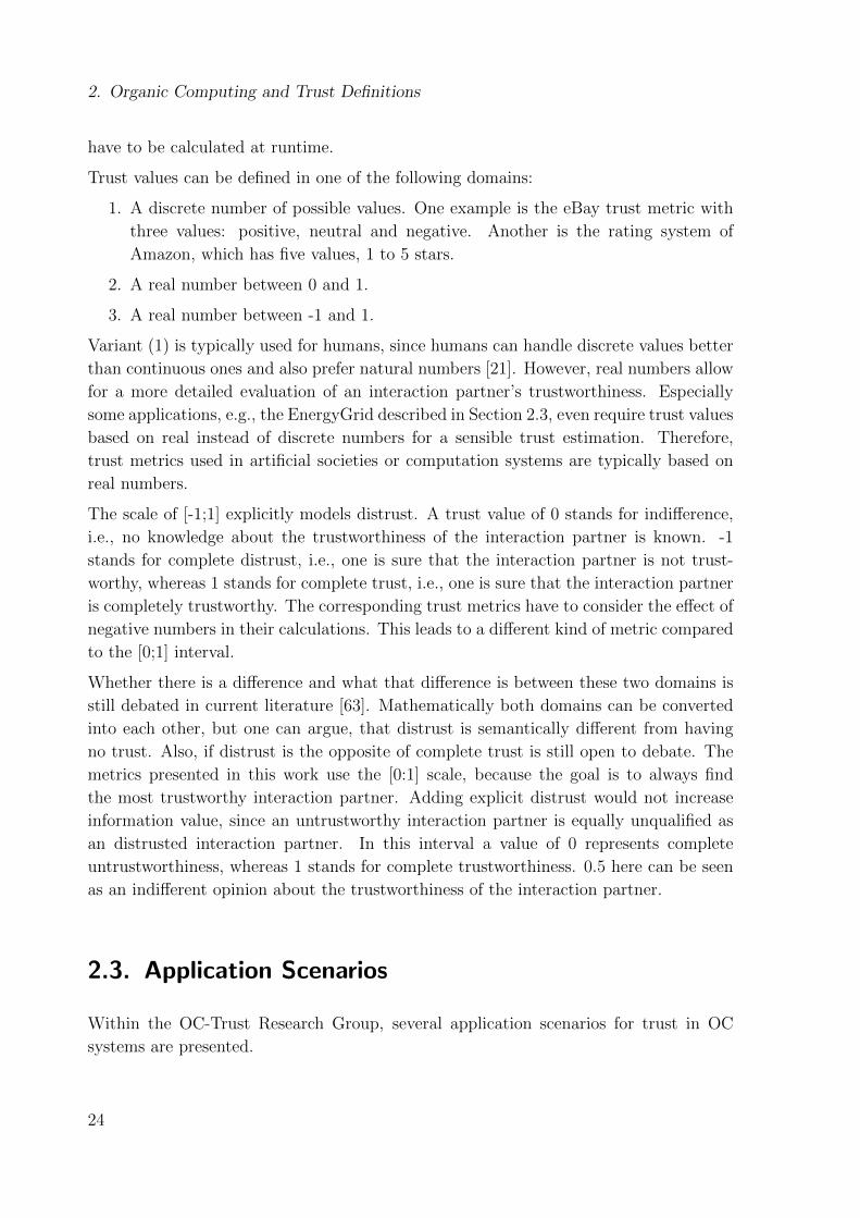
Trust values can be defined in one of the following domains:
1. A discrete number of possible values. One example is the eBay trust metric with
three values: positive, neutral and negative. Another is the rating system of
Amazon, which has five values, 1 to 5 stars.
2. A real number between 0 and 1.
3. A real number between -1 and 1.
Variant (1) is typically used for humans, since humans can handle discrete values better
than continuous ones and also prefer natural numbers [21]. However, real numbers allow
for a more detailed evaluation of an interaction partner’s trustworthiness. Especially
some applications, e.g., the EnergyGrid described in Section 2.3, even require trust values
based on real instead of discrete numbers for a sensible trust estimation. Therefore,
trust metrics used in artificial societies or computation systems are typically based on
real numbers.
The scale of [-1;1] explicitly models distrust. A trust value of 0 stands for indifference,
i.e., no knowledge about the trustworthiness of the interaction partner is known. -1
stands for complete distrust, i.e., one is sure that the interaction partner is not trust-
worthy, whereas 1 stands for complete trust, i.e., one is sure that the interaction partner
is completely trustworthy. The corresponding trust metrics have to consider the effect of
negative numbers in their calculations. This leads to a different kind of metric compared
to the [0;1] interval.
Whether there is a difference and what that difference is between these two domains is
still debated in current literature [63]. Mathematically both domains can be converted
into each other, but one can argue, that distrust is semantically different from having
no trust. Also, if distrust is the opposite of complete trust is still open to debate. The
metrics presented in this work use the [0:1] scale, because the goal is to always find
the most trustworthy interaction partner. Adding explicit distrust would not increase
information value, since an untrustworthy interaction partner is equally unqualified as
an distrusted interaction partner. In this interval a value of 0 represents complete
untrustworthiness, whereas 1 stands for complete trustworthiness. 0.5 here can be seen
as an indifferent opinion about the trustworthiness of the interaction partner.
2.3. Application Scenarios
Within the OC-Trust Research Group, several application scenarios for trust in OC
systems are presented.
24

2.3. Application Scenarios
Our current energy grid is supplied by an increasing number of different power plants,
which have either a deterministic or stochastic energy production. Deterministic power
plants can adjust their energy production, e.g., coal or atomic power plants. The en-
ergy production of stochastic power plants is not controllable, it is dependent on the
environment, e.g., solar power plants produce energy in relation to the current level of
solar radiation, or wind power plants depend on the strength of the wind. In recent
years, the amount of stochastic power plants has increased, particularly since they do
not consume fossil fuel. The European Union published its goal to further regenerative
energy sources 2 which will increase the amount of stochastic power plants by an even
greater amount in the near future.
This poses a significant challenge for the future structure of the energy grid. It is based
on the fact, that the same amount of energy is produced and consumed. With an increase
of stochastic power plants, the regulation of the energy grid to maintain this equilibrium
will be increasingly difficult, exceeding the possibility of the manual regulation of today.
For an automatic regulation, the power production of the stochastic power plants needs
to be predicted, e.g, by using the weather forecast, so that the deterministic power
plants can be regulated as needed. By integrating trust, the trustworthiness of the
predictions can be measured. This allows a self-organizing system of Autonomous Virtual
Power Plants (AVPPs) [56] that group together small power plants with accurate and
non accurate power predictions. Grouping trustworthy and untrustworthy power plants
together to an AVPP prevents the possibility of a cumulative divergence of the energy
production of several untrustworthy power plants at once that might prevent a timely
reaction. AVPPs also reduce the complexity to calculate plans for the deterministic
power plants to balance the variable output of the stochastic power plants, since these
plans need only be calculated per AVPP instead of the entire energy grid. Trust is
therefore a way to cope with the upcoming uncertainties of the future energy grid, when
a high number of power plants are of a stochastic nature.
Another example of an application that profits from the inclusion of trust is an open
computing grid. Such a grid provides high parallel computation power for applications
that profit from it, e.g., face recognition [6] or ray tracing [19]. However, not every
member of the grid is equally interested and able to perform computational tasks for
other members. For example, some members might want to exploit the grid by only
sending and rejecting every task from others, so called FreeRiders [4]. By introducing
trust, the members can identify those malicious nodes and form Trusted Communities
(TCs) [37]. The members of a TC know each other to be trustworthy, which reduces
the risk for each member to receive unsatisfactory work. By continuous observation of
the behavior of the members of a trusted community, members can be excluded if their
behavior changes. The other way is also possible, a so far untrustworthy participant can
2http://ec.europa.eu/clima/policies/package/
25
2. Organic Computing and Trust Definitions
regain its trustworthiness and rejoin a trusted community, if it acts accordingly. This
reduces the need to distribute redundant tasks to cope for untrustworthy nodes in the
computing grid, increasing its throughput.
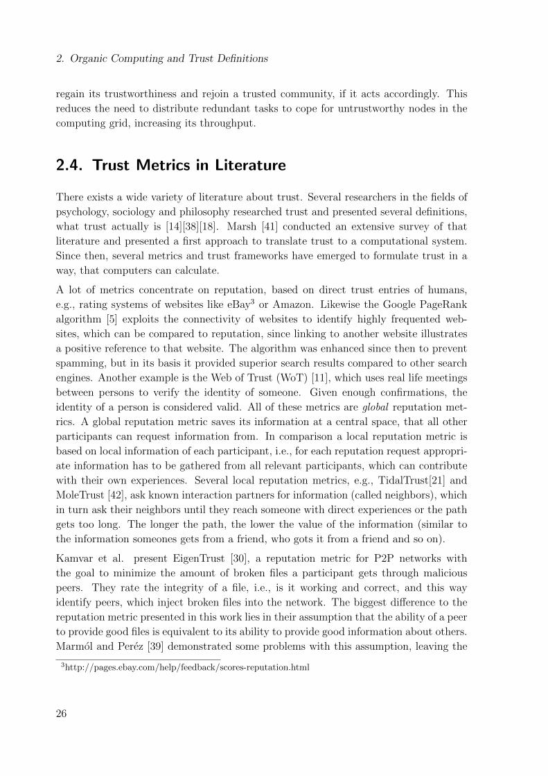
2.4. Trust Metrics in Literature
There exists a wide variety of literature about trust. Several researchers in the fields of
psychology, sociology and philosophy researched trust and presented several definitions,
what trust actually is [14][38][18]. Marsh [41] conducted an extensive survey of that
literature and presented a first approach to translate trust to a computational system.
Since then, several metrics and trust frameworks have emerged to formulate trust in a
way, that computers can calculate.
A lot of metrics concentrate on reputation, based on direct trust entries of humans,
e.g., rating systems of websites like eBay3 or Amazon. Likewise the Google PageRank
algorithm [5] exploits the connectivity of websites to identify highly frequented web-
sites, which can be compared to reputation, since linking to another website illustrates
a positive reference to that website. The algorithm was enhanced since then to prevent
spamming, but in its basis it provided superior search results compared to other search
engines. Another example is the Web of Trust (WoT) [11], which uses real life meetings
between persons to verify the identity of someone. Given enough confirmations, the
identity of a person is considered valid. All of these metrics are global reputation met-
rics. A global reputation metric saves its information at a central space, that all other
participants can request information from. In comparison a local reputation metric is
based on local information of each participant, i.e., for each reputation request appropri-
ate information has to be gathered from all relevant participants, which can contribute
with their own experiences. Several local reputation metrics, e.g., TidalTrust[21] and
MoleTrust [42], ask known interaction partners for information (called neighbors), which
in turn ask their neighbors until they reach someone with direct experiences or the path
gets too long. The longer the path, the lower the value of the information (similar to
the information someones gets from a friend, who gots it from a friend and so on).
Kamvar et al. present EigenTrust [30], a reputation metric for P2P networks with
the goal to minimize the amount of broken files a participant gets through malicious
peers. They rate the integrity of a file, i.e., is it working and correct, and this way
identify peers, which inject broken files into the network. The biggest difference to the
reputation metric presented in this work lies in their assumption that the ability of a peer
to provide good files is equivalent to its ability to provide good information about others.
Marmol and Perez [39] demonstrated some problems with this assumption, leaving the
3http://pages.ebay.com/help/feedback/scores-reputation.html
26

2.4. Trust Metrics in Literature
metric vulnerable for certain kinds of attacks. The Neighbor-Trust metric in this work
explicitly separates these two. They also assume that trust is transitive, which is not
necessarily true. The question whether trust should be assumed to be transitive or not
is an ongoing debate [12][21].
SPORAS [62] is yet another reputation metric. Its focus is to prevent entities to leave
and rejoin the network to reset possible bad reputation values. Compared to Neighbor-
Trust, SPORAS does not assign different values for the reputation value provided by
another entity and the trustworthiness of that entity to give accurate reputation data.
The trustworthiness is calculated from its reputation value. Neighbor-Trust differentiates
between these values by defining separate weights; Marmol and Perez [39] have shown
the importance to do this.
FIRE [26] is a trust framework combining direct trust and reputation (called witness
reputation in FIRE). In addition, it adds the trust parts of certified trust and role-
based trust. Certified trust describes past experiences others had with an agent, who
can present it as reference of his past interactions. Role-based trust stands for generic
behavior of agents within a role and the underlying rules are handcrafted by users. The
four parts are then aggregated with a weighted mean, whereas the weights are adjusted
by a user depending on the current system. In comparison, the metrics described in this
work do not require user hand-crafted parts like the role-based trust of FIRE and are
therefore able to run in a fully automated environment.
ReGreT [51][52] is a trust framework providing similar metrics for direct trust, rep-
utation, and aggregation to the metrics described in this work. Some differences yet
exist. The age of experiences is part of the direct trust calculation whereas the trust
metrics described in this work consider the age, number and variance as part of the
confidence. ReGreT describes a similar metric, which is called the reliability of the trust
value instead of confidence. Additionally, the formulas for the confidence metrics used
in this work are parametrized. Similarly, the reputation metric can be parametrized
to define the threshold, when one’s own experiences are close enough to the reputation
data given by a neighbor (called a witness in ReGreT). Also instead of directly using
the confidence for the aggregation of direct trust and reputation a weight is calculated
by a parameterizable function using the confidence. One of the major differences though
lies in the evaluation. While ReGreT works in a scenario with fixed agent behavior the
evaluation in this work investigates systems with varying agent behavior, where a very
trustworthy agent can change to the direct opposite. Several such changes per scenario
are considered. Bernard et al. [3], e.g., describe a system with such adaptive agents.
27

3. Trust Metrics
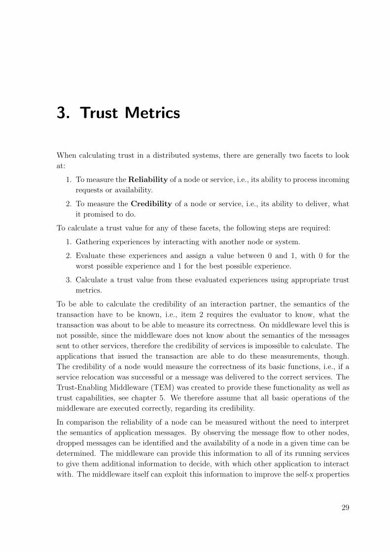
When calculating trust in a distributed systems, there are generally two facets to look
at:
1. To measure theReliability of a node or service, i.e., its ability to process incoming
requests or availability.
2. To measure the Credibility of a node or service, i.e., its ability to deliver, what
it promised to do.
To calculate a trust value for any of these facets, the following steps are required:
1. Gathering experiences by interacting with another node or system.
2. Evaluate these experiences and assign a value between 0 and 1, with 0 for the
worst possible experience and 1 for the best possible experience.
3. Calculate a trust value from these evaluated experiences using appropriate trust
metrics.
To be able to calculate the credibility of an interaction partner, the semantics of the
transaction have to be known, i.e., item 2 requires the evaluator to know, what the
transaction was about to be able to measure its correctness. On middleware level this is
not possible, since the middleware does not know about the semantics of the messages
sent to other services, therefore the credibility of services is impossible to calculate. The
applications that issued the transaction are able to do these measurements, though.
The credibility of a node would measure the correctness of its basic functions, i.e., if a
service relocation was successful or a message was delivered to the correct services. The
Trust-Enabling Middleware (TEM) was created to provide these functionality as well as
trust capabilities, see chapter 5. We therefore assume that all basic operations of the
middleware are executed correctly, regarding its credibility.
In comparison the reliability of a node can be measured without the need to interpret
the semantics of application messages. By observing the message flow to other nodes,
dropped messages can be identified and the availability of a node in a given time can be
determined. The middleware can provide this information to all of its running services
to give them additional information to decide, with which other application to interact
with. The middleware itself can exploit this information to improve the self-x properties
29

3. Trust Metrics
to create a more robust service distribution and react on changes in the environment that
reduces the reliability of a node. Section 3.1 presents the Delayed-Ack algorithm [35][36]
that identifies lost messages and calculates a direct trust value from it.
Section 3.2 presents the Neighbor-Trust metric [33], a metric to calculate reputation
that is able to identify lying nodes and adjust its reputation calculation to only include
trustworthy nodes. Section 3.3 shows, how the accuracy of the calculated direct trust can
be measured by determining the confidence in these trust values [32]. Finally section 3.4
presents a metric to calculate a total trust value out of direct trust and reputation
using confidence to weight both parts for the total value [34]. All of these metrics do
not require the Delayed-Ack algorithm as direct trust metric, but work with any type
of direct trust metric and every facet. This allows the applications running on the
middleware to exploit these metrics based on their own direct trust metrics, leading to
a generic approach for calculating trust in a distributed system. The implementation of
these metrics into the TEM are described in chapter 5.
3.1. Direct Trust
The reliability of a node is an important basis for all interactions executed on the system.
If a node is not reliable, i.e., it cannot be reached due to a high rate of lost messages,
the applications on it can be as good as they will, their calculations are unable to reach
their interaction partner or only with a lot of delay due to error corrections. For the
self-x properties the reliability has also to be considered to assign those services that are
essential for the structural integrity of the system only to highly reliable nodes. It also
allows for a more robust failure detection, where the chance of all observers of a node
failing simultaneously is minimized. Due to these reasons the Delayed-Ack algorithm
was developed to measure the reliability of a node by observing the message flow between
nodes and identifying lost messages.
3.1.1. Delayed-Ack Algorithm
The Delayed-Ack algorithm observes the message flow on middleware level. This espe-
cially means that no knowledge from the underlying transport layer need to be consid-
ered. While TCP has error corrections, message loss can be expected by using UDP.
Loosing a message can have two reasons:
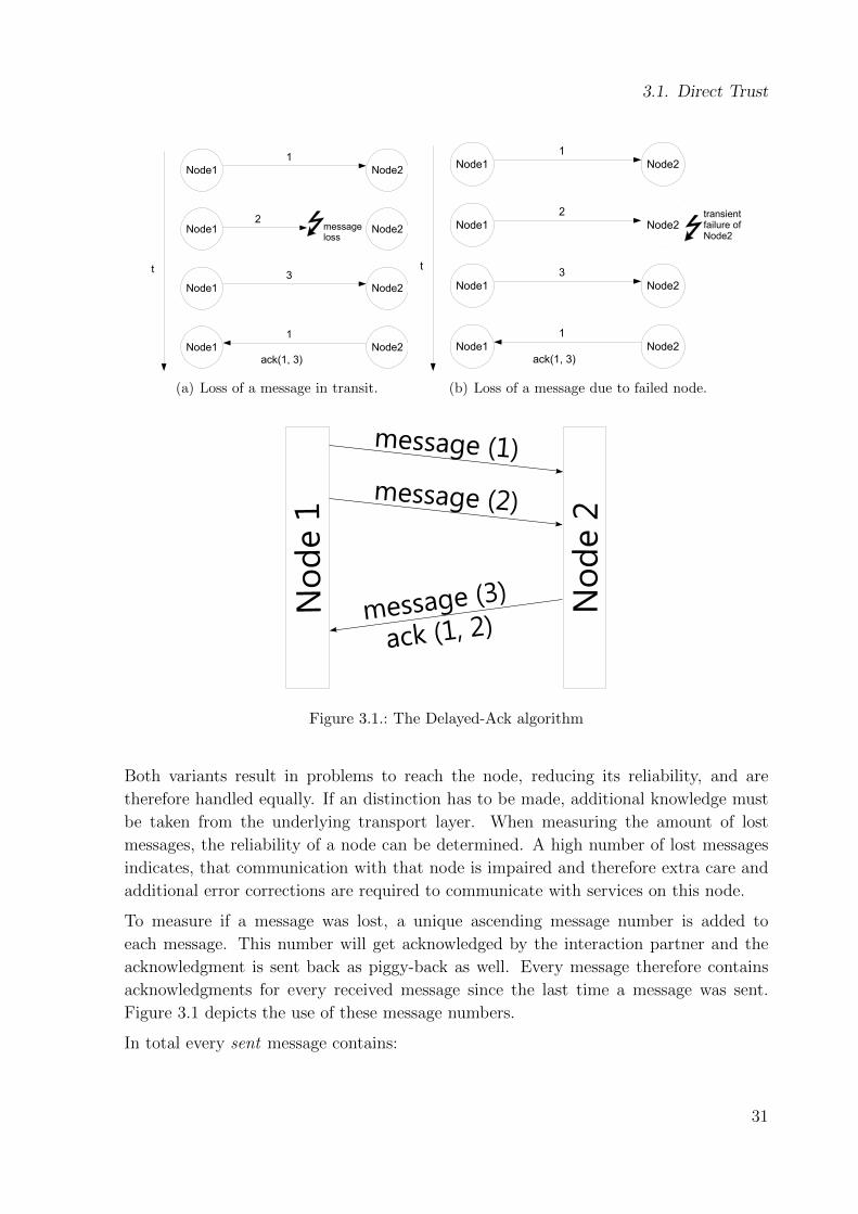
� The message is lost on its way to the node, see Figure 3.1(a) or
� the message is lost because the target node has failed, see Figure 3.1(b).
30
3.1. Direct Trust
Node1 Node21
Node1 Node22
Node1 Node21
ack(1, 3)
Node1 Node23
messageloss
t
(a) Loss of a message in transit.
����� �����
�
����� �����
�
����� �����
�
��������
����� �����
�
������������������������
�
(b) Loss of a message due to failed node.
Figure 3.1.: The Delayed-Ack algorithm
Both variants result in problems to reach the node, reducing its reliability, and are
therefore handled equally. If an distinction has to be made, additional knowledge must
be taken from the underlying transport layer. When measuring the amount of lost
messages, the reliability of a node can be determined. A high number of lost messages
indicates, that communication with that node is impaired and therefore extra care and
additional error corrections are required to communicate with services on this node.
To measure if a message was lost, a unique ascending message number is added to
each message. This number will get acknowledged by the interaction partner and the
acknowledgment is sent back as piggy-back as well. Every message therefore contains
acknowledgments for every received message since the last time a message was sent.
Figure 3.1 depicts the use of these message numbers.
In total every sent message contains:
31

3. Trust Metrics
� A unique ascending message number
� A list of acknowledgments, acknowledging all messages received since the last time
a message was sent.
The received acknowledgments are then compared to the list of sent message numbers.
In case of message numbers that are not acknowledged, so called gaps, the message is
considered lost, resulting in a negative experience (0). Acknowledged message numbers
result in a positive experience (1). If messages do not get acknowledged after a set
amount of time, a negative experience (0) is saved. This allows for an increase in
negative experiences over time, after a node failed and stopped sending message, and
therefore is not generating any more gaps. If an acknowledgment is received after the
message was already set as not received, the experience is retroactively changed to a
positive value (1).
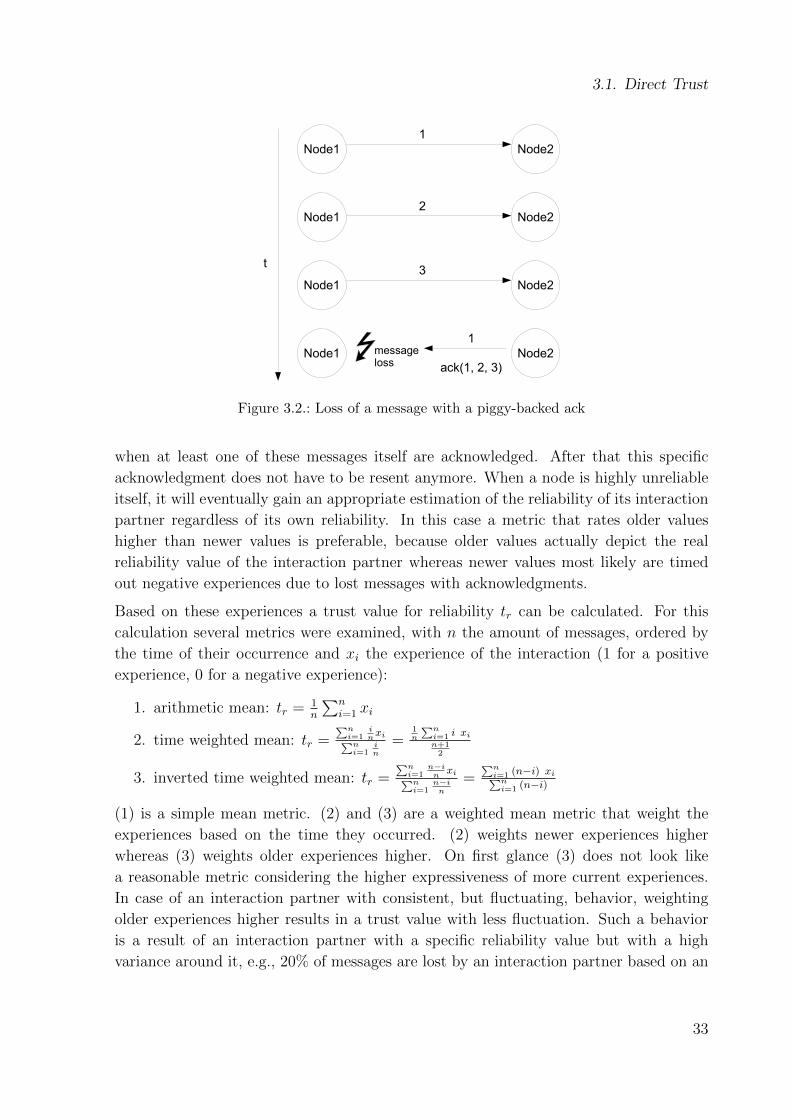
A potential problem with the Delayed-Ack algorithm occurs, when a node rates the
reliability of a communication partner but is unreliable itself. Let node1 be the unreliable
node and node2 its interaction partner, then the following case can occur:
1. Node1 sends some messages to node2.
2. Node2 receives the messages and responds later, adding the acknowledgments for
the received messages.
3. Node1 on the other hand now looses the messages sent by node2 with the added
acknowledgment due to a transient failure of node1.
4. Node1 will now rate node2’s reliability down because it believes node2 to have
lost the original messages while node1 lost the message with the acknowledgment
instead.
Figure 3.2 depicts the loss of a message, which would acknowledge three messages sent
by node1.
In this case a node unjustifiable rates down the reliability of interaction partners because
of its own bad reliability. Evaluations have shown that the calculated trust value tn for
node n in this case results in
tn = t(self) · t(real)n
where t(self) denotes the reliability value of the node, which is rating the node n, and
t(real)n denotes the trust value of the node n, if the observing node would be completely
reliable and not loose some messages itself.
To counter this effect the Delayed-Ack algorithm[35] was improved to the Enhanced
Delayed-Ack [36] algorithm. The basic idea is to resend acknowledgments until it is
certain at least one message with this acknowledgment is received. This is archived
32
3.1. Direct Trust
Node1 Node21
Node1 Node2
Node1 Node21
ack(1, 2, 3)
Node1 Node23
messageloss
t
2
Figure 3.2.: Loss of a message with a piggy-backed ack
when at least one of these messages itself are acknowledged. After that this specific
acknowledgment does not have to be resent anymore. When a node is highly unreliable
itself, it will eventually gain an appropriate estimation of the reliability of its interaction
partner regardless of its own reliability. In this case a metric that rates older values
higher than newer values is preferable, because older values actually depict the real
reliability value of the interaction partner whereas newer values most likely are timed
out negative experiences due to lost messages with acknowledgments.
Based on these experiences a trust value for reliability tr can be calculated. For this
calculation several metrics were examined, with n the amount of messages, ordered by
the time of their occurrence and xi the experience of the interaction (1 for a positive
experience, 0 for a negative experience):
1. arithmetic mean: tr =1n
ni=1 xi
2. time weighted mean: tr =n
i=1inxin
i=1in
=1n
ni=1 i xin+12
3. inverted time weighted mean: tr =n
i=1n−in
xini=1
n−in
=n
i=1 (n−i) xini=1 (n−i)
(1) is a simple mean metric. (2) and (3) are a weighted mean metric that weight the
experiences based on the time they occurred. (2) weights newer experiences higher
whereas (3) weights older experiences higher. On first glance (3) does not look like
a reasonable metric considering the higher expressiveness of more current experiences.
In case of an interaction partner with consistent, but fluctuating, behavior, weighting
older experiences higher results in a trust value with less fluctuation. Such a behavior
is a result of an interaction partner with a specific reliability value but with a high
variance around it, e.g., 20% of messages are lost by an interaction partner based on an
33
3. Trust Metrics
observation of lost (0.0) and received (1.0) messages. A mean value will average these
losses to a reliability value of 0.8 (loss of 20% messages), but new experiences of 1.0 or
0.0 will create a high fluctuation around the mean value especially if current experiences
are weighted high. This effect is diminished by rating old experiences higher.
3.1.2. Evaluation
To evaluate the Delayed-Ack algorithm it is analyzed with respect to its convergence
speed towards a fixed real trust value. Every node has a specific fixed trust value p.
Such a node will react to messages with a probability of (1-p). So if the node’s real
fixed trust value is 0.9, 10% of the messages are lost and therefore not acknowledged. In
the evaluation the sought reliability value of that node is therefore 0.9. The evaluation
analyzes the amount of interactions needed for the algorithms to converge on the real
trust values as well as how much impact bad reliability of an observer has on its observing
capabilities.
To accomplish this, a network of 30 nodes is used with the following configuration:
� Ten nodes with 100% reliability,
� ten nodes with 90% reliability, and
� ten nodes with 50% reliability.
A node with a reliability value of less than 100% only receives messages with the given
percentage, be it because of transient node failures or actual message loss. A node picks
two random nodes as communication partners at every time step and sends a message
to them. The corresponding nodes reply with 75% probability. This should picture a
real world system where applications send requests to other applications on other nodes
but not always expect a reply, e.g., when a simple information message is sent. The
chosen percentages stand for perfect nodes (100%), slightly unreliable nodes (90%), as
well as very unreliable nodes (50%) and should represent typical nodes within a network.
Ten nodes of every type were chosen to get a variety of results due to the randomness
of the message loss probabilities and averaged results. The very low reliability of the
nodes, especially a 50% message loss, were chosen to demonstrate the robustness of the
algorithm in systems with very unreliable components.
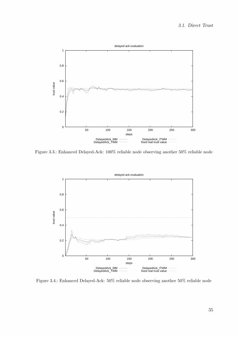
Figure 3.3 shows the average result of all nodes with 100% probability observing the
nodes with 50% probability. After some interactions the observed trust value stabilizes
around the real trust value. The Delayed-Ack algorithm gauged the trust of other nodes
successfully.
On the other hand if the observing node itself is unreliable it gets a biased view on other
nodes, demonstrated by Figure 3.4. This scenario is similar to the aforementioned, but
34
3.1. Direct Trust
0
0.2
0.4
0.6
0.8
1
50 100 150 200 250 300
trus
t val
ue
steps
delayed ack evaluation
DelayedAck_MMDelayedAck_TWM
DelayedAck_ITWMfixed real trust value
Figure 3.3.: Enhanced Delayed-Ack: 100% reliable node observing another 50% reliable node
0
0.2
0.4
0.6
0.8
1
50 100 150 200 250 300
trus
t val
ue
steps
delayed ack evaluation
DelayedAck_MMDelayedAck_TWM
DelayedAck_ITWMfixed real trust value
Figure 3.4.: Enhanced Delayed-Ack: 50% reliable node observing another 50% reliable node
35

3. Trust Metrics
0
0.2
0.4
0.6
0.8
1
50 100 150 200 250 300
trus
t val
ue
steps
enhanced delayed ack evaluation
EnhancedDelayedAck_MMEnhancedDelayedAck_TWM
EnhancedDelayedAck_ITWMfixed real trust value
Figure 3.5.: Enhanced Delayed-Ack: 50% reliable node observing another 50% reliable node
this time the observing node has a 50% reliability instead of 100%. As can be seen,
the observed trust value stabilizes but at a far lower value than the real trust value.
This happens due to additional message losses caused by the observing node. Not only
are message lost that were sent to the interaction partner but also the messages coming
from this interaction partner, probably containing acknowledgments of actually received
messages. Losing these messages and therefore rightly sent acknowledgments marks
these message incorrectly as not received. In total the observed trust value is close to
0.25, which is the product of the reliability of both nodes.
In contrast Figure 3.5 shows the same situation, nodes with 50% reliability observing
nodes with 50% reliability, with the use of the Enhanced Delayed-Ack algorithm. Com-
pared to Delayed-Ack the observing node gets a quite correct impression of the observed
node, regardless of its own unreliable state.
3.2. Reputation
While direct trust gives a good estimation of an interaction partner’s behavior, it is
not always available. Especially when a new node enters the system, it does not know
anything about the system yet. Additionally it’s behavior itself is not known to any node
in the network. The network on the one hand has no choice but to build experiences
with the new participating node by conduction transactions with it. The new node on
36

3.2. Reputation
a
b
c
wab
tac
tbc
Figure 3.6.: Nodes in the reputation graph
the other hand can exploit the knowledge of the nodes in the network, that already
accumulated experiences with each other until it has enough own experiences itself.
These indirect experiences from third parties are called reputation.
3.2.1. Neighbor-Trust Algorithm
To measure reputation the Neighbor-Trust Algorithm [33] is introduced. It is based on
metric 2 presented by Satzger et al. [53], which gathers the direct trust information of
all neighbors of the target node. Neighbors in this context describes all nodes that have
direct trust information about the interaction partner. Satzger et al. calculated a mean
value of the direct trust values of the neighbors. The Neighbor-Trust Algorithm enhances
the metric to a weighted mean, where the weights are adjusted over time to consider
only neighbors that had similar experiences than oneself, thereby introducing a learning
component. Figure 3.6 shows a short example of a network and the neighborhood
relationships.
Alice (a) wants to get information about Carol (c), so she asks Bob (b) about his opinion
about Carol. wab is the trust Alice gives the information Bob provides respectively the
weight she gives his information and tbc is the direct trust value Bob has about Carol.
Later Alice might have a direct experience with Carol, displayed by tac. To get an
accurate value, Alice will ask more entities than just Bob. She will ask all neighbors
(i ∈ neighbors(c)) of Carol.
The reputation rab, i.e., the reputation a gathered about b by collecting information
about b from its neighbors (i ∈ neighbors(c)), is calculated with the following formula:
37

3. Trust Metrics
01
+θ
-θ
tactbc
tac-τ tac+τtac-τ* tac+τ*
Figure 3.7.: Characteristics of the weight adjustment function of the neighbor-trust reputationmetric
rac =
i∈neighbors(c) wai · tic
i∈neighbors(c) wai
The learning component is the weight wai. This weight will be adjusted over time,
depending how similar the trust values from the neighbors correlate with the node’s own
experience. If an experience is close enough to the information given by a neighbor, its
weight will be increased and further information will be rated higher. Then again, if the
discrepancy is too high the weight will be reduced and therefore further information of
this neighbor will be rated down. This creates a group of neighbors that had similar
experiences than the asking node. Golbeck [20] showed with a movie review platform
enhanced with a social network, that getting reviews from users preferring similar movies
yielded better information than getting the global mean. Not only does the Neighbor-
Trust Algorithm provide this functionality, but it also excludes nodes that provide false
information purposely.
Figure 3.7 shows the characteristics of the weight adjustment function:
w will only be adjusted within a maximal adjustment θ, thus preventing a too excessive
change of w through a single transaction. Furthermore, two thresholds are defined:
� τ : Up to this threshold the experiences of the neighbor and one’s own are close
enough to increase the weight to this neighbor. More precisely the obtained trust
value from the neighbor tbc lies within the own direct trust value tac ± τ .
� τ ∗: Up to τ ∗ but beyond τ the difference between the received trust value of the
neighbor tbc and one’s own trust value tab is too high, therefore w is decreased.
Beyond that w is reduced fully by θ.
In total the formula for the Neighbor-Trust metric is as follows:
38

3.2. Reputation
wn+1ab = wn
ab
+(
τ−|tnac−tnbc|τ
) · θ, if 0 ≤ |tnac − tnbc| ≤ τ
−(|tnac−tnbc|−τ
τ∗−τ) · θ, if τ < |tnac − tnbc| ≤ τ ∗
−θ, otherwise
3.2.2. Evaluation
To evaluate the Neighbor-Trust metric a network of 10 nodes with different percentages
of lying (malicious) nodes was used. The relatively small number 10 was chosen to
identify specific effects that are presented further down. Simulations with more nodes
yielded similar results. A node is malicious if it returns a reputation value that does
not match its actual experiences, i.e., it is lying about other nodes. In the case of
this simulation the malicious nodes always return a reputation value of 0, regardless of
previous experiences. By doing this, they try to denunciate all other nodes to push their
own reputation value compared to the others. The malicious nodes themselves return
always wrong results if interacted with. The simulation was conducted in timesteps. In
every timestep every node chose an interaction partner based on their reputation values,
whereas the node with the highest reputation value was chosen. In case of a draw, one
of the nodes with the highest reputation rating was chosen randomly. Especially at the
start of the evaluation, when no reputation value is known yet, a random node is chosen
for the first interaction. Apart from the first interaction, a value has to be defined for
nodes, which were not interacted with yet and therefore no information about them
exist so far. An arbitrary starting value has to be assigned to such a node to be able to
compare it to the others. The simulation will show the effect for different initial values.
To show the results, the nodes were categorized in two types: honest and malicious
nodes. For each time step the average reputation value of the honest nodes about the
two types are displayed as well as the weight the honest nodes have about both types.
The weight represents the honesty the corresponding nodes have about relaying their
direct experiences.
Figure 3.8 displays the results for a network with 30% malicious nodes. Mainly two
things can be seen here. In the start, the honest nodes get wrong reputation data
about other honest nodes due to the false information of the malicious nodes. Over
time the malicious nodes are identified as such, which can be seen by the decreasing
weight the honest nodes have about the malicious nodes. Simultaneously the reputation
of the honest nodes increases as the weight of the malicious nodes drops. After about
20 interactions all malicious nodes are identified as such and have their weights set to 0.
Therefore their reputation data is removed from the calculation and does not influence
it anymore.
39

3. Trust Metrics
0
0,2
0,4
0,6
0,8
1
1 6 11 16 21 26 31
rep
uta
tio
n
time step
reputation: honest about honest reputations: honest about malicious
weights: honest about honest weights: honest about malicious
Figure 3.8.: Reputation in a network with 30% malicious nodes
Apart from that the weight of honest nodes about the other honest nodes starts and
ends at 1: Telling the truth, their weight never gets reduced. The same happens with
the reputation data of the honest nodes about the malicious nodes. Since they never lie,
they always rely their bad experiences about the malicious nodes.
In Figure 3.9 the amount of malicious nodes was increased to 50%. The results are
similar to 30%. Even increasing the amount of malicious nodes to 70%, as can be seen
in Figure 3.10, results in a stable system. This demonstrates the robustness of the
Neighbor-Trust metric, as it returns meaningful results, even if the amount of malicious
nodes exceeds 50% of the total nodes.
In the three scenarios above the threshold for unknown nodes was set to 0, i.e., if no
reputation data was available for a node a start value of 0 was assumed. This can be
seen as a pessimistic approach [40]. In Figure 3.11 the threshold was changed to 0.5,
i.e., a node with no reputation data starts with 0.5. Similar to the above scenarios the
honest nodes identified the malicious nodes resulting in a final reputation value of 1 for
other honest nodes.
Compared to the other scenarios the average weight value stabilizes on a value above
0. Since this value is an average value, not all weights of honest nodes about malicious
nodes are set to 0. In this case a switch to another interaction partner occurred after
its reputation dropped below 0.5, the threshold for an unknown node. In the end the
malicious nodes and the honest nodes interacted with a different set of nodes. From the
point of view of an honest node, some of its final interaction partners never interacted
40

3.2. Reputation
0
0,2
0,4
0,6
0,8
1
1 6 11 16 21 26 31
rep
uta
tio
n
time step
reputations: honest about honest reputations: good about malicious
weights: honest about honest weights: honest about malicious
Figure 3.9.: Reputation in a network with 50% malicious nodes
0
0,2
0,4
0,6
0,8
1
1 6 11 16 21 26 31
rep
uta
tio
n
time step
reputation: honest about honest reputation: honest about malicious
weights: honest about honest weights: honest about malicious
Figure 3.10.: Reputation in a network with 70% malicious nodes
41

3. Trust Metrics
0
0,2
0,4
0,6
0,8
1
1 6 11 16 21 26 31
rep
uta
tio
n
time step
reputations: honest about honest reputations: honest about malicious
weights: honest about honest weights: honest about malicious
Figure 3.11.: Reputation in a network with 50% malicious nodes and threshold 0.5
with some malicious nodes, therefore no results are returned from reputation requests
from these nodes. This is especially true, since the evaluation used the TEM middleware
that handles reputation requests internally based on the saved data of the services.
Services can only save the results of their experiences into the middleware. If no results
were saved, the middleware does not return any value, thus preventing a malicious service
to, e.g, return 0 to every reputation request. By not receiving any reputation data from
some malicious nodes no more comparisons to its own experiences can be observed, hence
the weight value stays above 0. Therefore the average weight stays above 0.
Figure 3.12 shows an interesting effect of a single isolated node in a network with 50%
malicious nodes. By chance all honest nodes interacted with a single node, in this
case node7. This resulted in no experiences gathered with the isolated node shown in
Figure 3.12. Therefore the reputation data about the honest node stayed at the starting
threshold, in this case 0. The weight of the malicious nodes about the isolated node is
dropping, since the malicious nodes actually did interact with the isolated node. But
compared to the honest nodes, they always save a bad experience into the middleware,
although the isolated node returns positive results. The comparison between the two
values and the calculation of the weight is done within the middleware, which leads to the
decrease of the weight. Therefore using the TEM middleware increases the robustness
against malicious services. The weight stabilizes at a value > 0 due to similar results as
with Figure 3.11.
42

3.3. Confidence
0
0,2
0,4
0,6
0,8
1
1 6 11 16 21 26 31
rep
uta
tio
n
time step
reputation: malicious about this node reputation: honest about this node
weights honest about this node weights malicious about this node
Figure 3.12.: an isolated node with 50% malicious nodes
3.3. Confidence
Direct trust itself already gives a good estimation of the observable behavior of a com-
munication partner. But this estimation might not be very reliable itself, e.g., only a
few values might not be enough to gauge the true behavior of an interaction partner, as
can be seen in the evaluation of the Delayed-Ack algorithm. Therefore an estimation of
the reliability of the trust value, the confidence, is introduced [32]. This work was done
in cooperation with Gerrit Anders and Florian Siefert, University of Augsburg. The
confidence consists of three parts:
1. The number of experiences cn: A low number of experiences might not be enough
to gauge the behavior correctly, as can be seen in the Delayed-Ack evaluation.
2. The age of experiences ca: Older entries might not reflect the true behavior of an
interaction partner anymore, especially when the behavior can change.
3. The variance of the experiences cv: A high variance in the observed behavior indi-
cates a higher uncertainty for future interactions, especially a rise in the variance
might stand for a change in the behavior of the interaction partner.
The metric of every part is based on the same function, depicted in Figure 3.13:
43
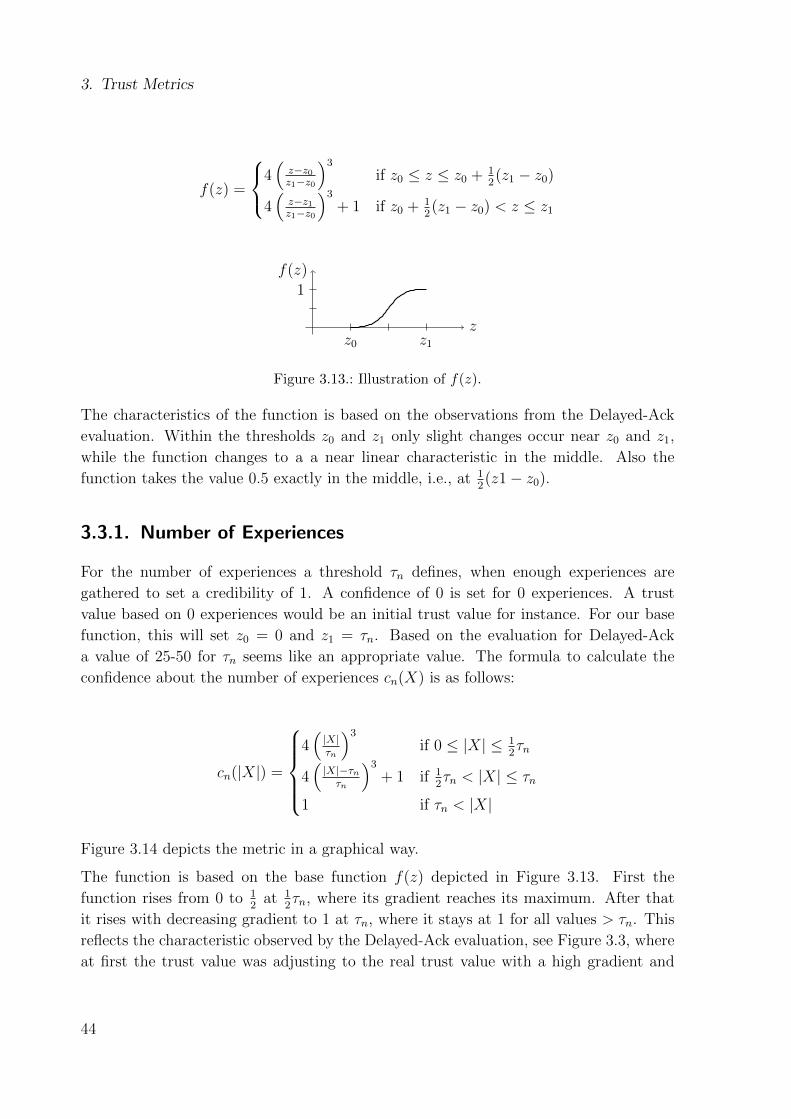
3. Trust Metrics
f(z) =
4
z−z0z1−z0
3
if z0 ≤ z ≤ z0 +12(z1 − z0)
4
z−z1z1−z0
3
+ 1 if z0 +12(z1 − z0) < z ≤ z1
z
f(z)
1
z0 z1
Figure 3.13.: Illustration of f(z).
The characteristics of the function is based on the observations from the Delayed-Ack
evaluation. Within the thresholds z0 and z1 only slight changes occur near z0 and z1,
while the function changes to a a near linear characteristic in the middle. Also the
function takes the value 0.5 exactly in the middle, i.e., at 12(z1− z0).
3.3.1. Number of Experiences
For the number of experiences a threshold τn defines, when enough experiences are
gathered to set a credibility of 1. A confidence of 0 is set for 0 experiences. A trust
value based on 0 experiences would be an initial trust value for instance. For our base
function, this will set z0 = 0 and z1 = τn. Based on the evaluation for Delayed-Ack
a value of 25-50 for τn seems like an appropriate value. The formula to calculate the
confidence about the number of experiences cn(X) is as follows:
cn(|X|) =
4
|X|τn
3
if 0 ≤ |X| ≤ 12τn
4
|X|−τnτn
3
+ 1 if 12τn < |X| ≤ τn
1 if τn < |X|
Figure 3.14 depicts the metric in a graphical way.
The function is based on the base function f(z) depicted in Figure 3.13. First the
function rises from 0 to 12at 1
2τn, where its gradient reaches its maximum. After that
it rises with decreasing gradient to 1 at τn, where it stays at 1 for all values > τn. This
reflects the characteristic observed by the Delayed-Ack evaluation, see Figure 3.3, where
at first the trust value was adjusting to the real trust value with a high gradient and
44

3.3. Confidence
|X|
cn(|X|)1
12τn τn
Figure 3.14.: Illustration of cn(|X|).
stabilized with decreasing gradient at the actual trust value. Similarly a small change
near the edges (0 or τn) changes the confidence only a bit, while in the middle at 12τn a
change in the number of experiences has the highest influence on the confidence. The
other parts of the confidence use functions with a similar characteristic.
3.3.2. Age of Experiences
For the age of experiences, two thresholds are introduced: z0 = τr on the one hand
defines the time frame, up until experiences count as up to date, therefore resulting into
a confidence value of 1. z1 = τo on the other hand denotes the point in time, from when
experiences are considered as completely out of date, resulting in a confidence value of
0. In between those two thresholds the confidence level drops according to the basic
confidence function. In total the formula for the confidence for the age of experiences is
as follows:
r(ax) =
1 if 0 ≤ ax < τr
−4
a−τrτo−τr
3
+ 1 if τr ≤ ax ≤ τr +12(τo − τr)
−4
a−τoτo−τr
3
if τr +12(τo − τr) < ax ≤ τo
0 if τo < ax
Figure 3.15 depicts the formula in a graphical way.
ax
r(ax)
1
τr τo
Figure 3.15.: Illustration of r(a).
45

3. Trust Metrics
This formula will rate every single experience by its age. The confidence is 1 until the
first threshold τr is reached, which marks the point, when the experience starts to get
old. After that the confidence falls with increasing gradient to 12at 1
2(τo − τr). Then it
falls with reducing gradient to 0 at τo, where it stays at for all ratings > τo indicating
that the experience is fully outdated.
After every experience was rated, the total confidence is calculated by calculating the
mean from the single confidence values:
ca(X) =
x∈X r(ax)
|X|
3.3.3. Variance of Experiences
The variance can be used as an indication for a behavioral change, especially if the age
of experiences can not be used, e.g., a change occurs during consecutive interactions.
An increase in the variance, and therefore a drop in the confidence of the variance,
indicates such a behavior change, since returning results will differ from the results up
to this point. After some time the confidence will stabilize again. At this point the new
trust value has adjusted and represents the new behavior. The formula to calculate the
variance confidence Cv(X) is as follows:
cv(vX) =
−4
vXν
3+ 1 if 0 ≤ vX ≤ 1
2ν
−4vX−ν
ν
3if 1
2ν < vX ≤ ν
where v describes the highest possible variance, when the confidence reaches 0. In this
case v = 0.25, which is the maximal confidence for a mean value of 0.5. For the proof
for this claim see appendix A. Figure 3.16 depicts the formula in a graphical way.
vX
cv(vX)
1
12ν ν
Figure 3.16.: Illustration of cv(X).
A confidence of 1 equals 0 variance, i.e., all results are identical, while a confidence of 0
marks maximal variance. The maximal confidence is dependent on the mean value, e.g.,
the maximal confidence for a mean value of 0.5 is 0.25 whereas the maximal confidence
46

3.3. Confidence
for a mean value of 0.4 is 0.24. Because v of the confidence formula is chosen statically
to be 0.25, only a distribution around the mean value 0.5 can actually reach confidence
0, all others will have a minimum confidence greater than 0. The closer the mean value
is to 0 or 1, the closer is also the minimum confidence for the variance. If v is not chosen
to be 0.25, but to be the maximum variance for the according mean value (the trust
value here) unintentional effects can be observed. A variance of 0.1 would translate to
another confidence value for a maximal variance of 0.25 than for a maximal variance of
0.24 since the function characteristics are slightly compressed. One would expect the
same confidence value of identical variance values. Instead the total maximum of 0.25
is always chosen as v and the minimum confidence is instead changed, the function is
cut off at the lower end.
v
µ12
0.25
1
Figure 3.17.: maximal variance v
Figure 3.17 demonstrates the behavior of the maximal variance v compared to mean
values µ. The maximum is, as mentioned above, at v = 0.25 for µ = 0.5. The character-
istics are similar to the other two functions. The confidence is 1 for a variance of 0 and
falls with increasing gradient to 12at 1
2v. After that it drops with a decreasing gradient
to 0 at v. Since the variance is between 0 and v, the maximal variance, this marks also
the domain of the variance confidence.
All three parts of the confidence metric are aggregated to a total confidence value c with
configurable weights:
c =wncn(|X|) + waca(X) + wvcv(vX)
wn + wa + wv
where wn is the weight for the number of experiences, wa the weight for the age of
experiences and wv the weight for the variance of experiences. Each application is able
to adjust the weights according to their requirements. By default all parts are weighted
equally, i.e., wn = wa = wv = 1.
47

3. Trust Metrics
3.3.4. Evaluation
To evaluate the effectiveness of the confidence metrics, a network consisting of 100 agents
was created. Another dedicated agent chooses in every timestep, with which of the 100
possible agents it wants to interact with. Each agent i has a mean benefit bi. The 100
agents were created using 4 different types:
� Type 1: bi ∈ [0.85, 0.95] (30 agents)
� Type 2: bi ∈ [0.55, 0.65] (40 agents)
� Type 3: bi ∈ [0.4, 0.5] (20 agents)
� Type 4: bi ∈ [0.2, 0.3] (10 agents)
In addition, the agents have a variance of vi in their behavior. The agents of each
type have vi = 0.1 (40%), vi = 0.05 (30%) and vi = 0.025 (40%). The benefit of an
interaction with such an agent is created by using a beta distribution with their mean
bi and variance vi. In addition a sliding time window was used, only taken into account
the last 30 interactions to calculate the trust value and the corresponding confidence
values.
As a first evaluation the dedicated agent interacted 100 times in a row with a single
agent i with the following characteristics:
� The Agent i was of Type 2 with bi ≈ 0.6 and vi = 0.1.
� Agent i changed its behavior to Type 4 with bi ≈ 0.2 and vi = 0.1 after 60
timesteps.
� The confidence formulas were parametrized with τr = 30, τo = 40 and τn = 25.
The interaction with this agent is conducted in 3 steps:
1. An interaction per timestep for 30 timesteps.
2. Type change from Type 2 to 4 at timestep 30, but no further interactions for
another 30 timesteps.
3. Again one interaction per timestep for 40 timesteps, up to a total of 100 timesteps.
Figure 3.18 displays the evaluation and the three steps.
In part 1, up until timestep 30, the dedicated agent interacts once per timestep with
agent i. The trust value evens out on the mean benefit bi of the agent i. The confidence
of the number of experiences (cn) increases up to its threshold τn, where it stays at
1. This covers the time the trust value needs to even out and correctly represents the
mean benefit this agent facilitates. Since there are experiences in every timestep, the
confidence about the age of experiences stays at 1. The confidence of the variance
stabilizes at around 0.75. This value is below 1, because the benefit of the agent varies
48

3.3. Confidence
interaction partnerchanges behavior no interactions resuming interactions
Figure 3.18.: Confidence values of a single agent
per transaction, as can be seen in the value vi.
In part 2, after the behavior change and interactions stop, the trust stays at its old
value, since no more interaction indicate its change. However, the experience age and
the corresponding confidence value drops. At timestep 60, 20 out of the 30 gathered
experiences have fully expired and therefore have a confidence rating of 0 regarding
their age. The 10 newest, which are still 30-40 timesteps old, have decreasing values
of confidence. In total this brings the confidence down to about 0.2. The variance
confidence is stable, since only the data from timestep 1-30 are still available and they
do not change after the additional 30 timesteps have passed.
In part 3, interactions with the agent i are resumed and continued for another 40
timesteps with one interaction per timestep. With interactions that return values ac-
cording to the new benefit gain, the trust value drops until it reaches the expected value,
where it stabilizes. Since new interactions are conducted the age confidence increases
until it reaches 1 again. The interesting part is the variance confidence. Since the new
interaction results now differ from the old values the variance increases and therefore the
corresponding confidence drops. After more of the new interaction results are gathered,
the system adapts to the new behavior and as the trust value reaches its real value the
variance confidence stabilizes at its new value, indicating the trust value is accurate
again.
After initially investigating the different parts of the confidence metric, the designated
agent now chooses 1 agent out of all 100 in every timestep to interact with. The selection
metrics are based on a roulette-wheel metric. A roulette-wheel metric assigns all choices
49
3. Trust Metrics
a possibility value and chooses randomly, where choices with a higher value have a higher
chance to be selected. In total 4 selection metrics were used:
� selRdm: An agent was chosen randomly using a uniform distribution, setting a
baseline for comparison.
� selTrust : The designated agent calculated the trust values for all agents and se-
lected an interaction partner by a roulette-wheel selection method.
� selTrustConf : The designated agent additionally assessed its confidence in these
trust values and used the product of trust and confidence in combination with a
roulette-wheel selection method.
� selTrust2Conf : This method determined an interaction partner in two stages.
First, a set of 10 agents was selected by using the selTrust method. Subsequently,
the designated agent selected its interaction partner by using the selTrustConf
selection method.
The evaluation goes for 8000 timesteps with 2 behavior changes at timestep 2000 and
4000:
� Type 1: 6/4/2 agents changed to Type 2/3/41.
� Type 2: 6/6/2 agents changed to Type 1/3/4.
� Type 3: 4/6/1 agents changed to Type 1/2/4.
� Type 4: 2/2/1 agents changed to Type 1/2/3.
All agents are initiated with a trust value by conducting exactly 1 interaction, before the
evaluation itself is started. Due to the higher amount of possible interaction partners, a
long time span might occur between 2 interactions with a single agent, therefore the age
confidence metric got parametrized differently, i.e., with τr = 2000 and τo = 3000. The
total confidence was calculated with wn = wa = wv =13, giving all 3 parts equal weight
for the total confidence value. The results are averaged from 200 evaluation runs.
Figure 3.19 displays the average gain in benefit of the designated agent of the last 50
interactions per time step. The random selection metric selRdm has the lowest gain of
benefit but is stable throughout the evaluation. Using trust alone (selTrust) already
increases the gain in benefit by approximately 9.54% compared to selRdm at time step
8000. At timestep 2000 and 6000, when the behavior chances, a drop in the gain of benefit
can be observed. This is to be expected, since agents with former good benefit are chosen
although they now act a lot worse. The system acknowledges this change though and
stabilizes again. Regardless, selTrust never drops below selRdm, even shorty after the
changes. Adding confidence to trust with the simple method of selTrustConf increases
1Type 1: 6/4/2 agents changed to Type 2/3/4 means: 6 agents of type 1 changed to type 2, 4 agentsof type 1 changed to type 3 and 2 agents of type 1 changed to type 4.
50

3.3. Confidence
Figure 3.19.: Average gain in benefit
Figure 3.20.: Average difference between expected and real gain in benefit
the benefit gain, but not significantly, whereas the more complex metric selTrust2Conf
does strongly increase the benefit gain, by 17.84% compared to selRdm.
Figure 3.20 displays a slightly different sight on the evaluation. Here the difference
between the expected benefit and actual benefit is depicted. The lower the difference, the
better. selRmd is displayed here as comparison, but the data was not used for selection
purposes. Similar to the benefit gain, selRdm is the worst metric and selTrust2Conf the
best.
51
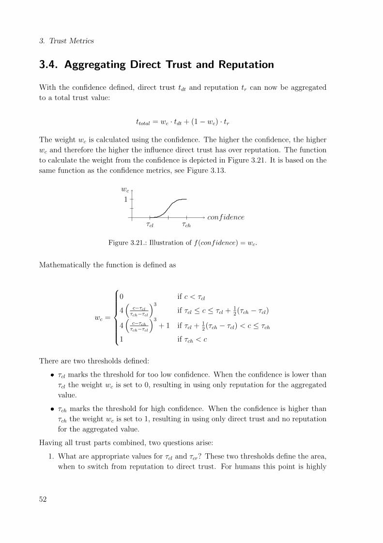
3. Trust Metrics
3.4. Aggregating Direct Trust and Reputation
With the confidence defined, direct trust tdt and reputation tr can now be aggregated
to a total trust value:
ttotal = wc · tdt + (1− wc) · tr
The weight wc is calculated using the confidence. The higher the confidence, the higher
wc and therefore the higher the influence direct trust has over reputation. The function
to calculate the weight from the confidence is depicted in Figure 3.21. It is based on the
same function as the confidence metrics, see Figure 3.13.
confidence
wc
1
τcl τch
Figure 3.21.: Illustration of f(confidence) = wc.
Mathematically the function is defined as
wc =
0 if c < τcl
4
c−τclτch−τcl
3
if τcl ≤ c ≤ τcl +12(τch − τcl)
4
c−τchτch−τcl
3
+ 1 if τcl +12(τch − τcl) < c ≤ τch
1 if τch < c
There are two thresholds defined:
� τcl marks the threshold for too low confidence. When the confidence is lower than
τcl the weight wc is set to 0, resulting in using only reputation for the aggregated
value.
� τch marks the threshold for high confidence. When the confidence is higher than
τch the weight wc is set to 1, resulting in using only direct trust and no reputation
for the aggregated value.
Having all trust parts combined, two questions arise:
1. What are appropriate values for τcl and τcr? These two thresholds define the area,
when to switch from reputation to direct trust. For humans this point is highly
52

3.4. Aggregating Direct Trust and Reputation
subjective and therefore a quantification of it proves difficult.
2. How do the parameters of the different metrics influence the result and which parts
(direct trust, reputation, confidence and aggregation) of the metrics are favorable
for future decisions.
The metrics for confidence, reputation, and aggregation define a total of 12 different pa-
rameters. The direct trust metric itself is not parametrized, since it is either application
specific (when rating application interaction) or surveyed by the Delayed-Ack algorithm
for node reliability, which is not parametrizable. Table 3.1 summarizes the different
parameters defined in the trust metrics.
Table 3.1.: Parameters to configure the metrics direct trust with confidence (DTC, top only)and direct trust with confidence and reputation (DTCR, top and bottom part);also the history length needs to be defined for all metrics.
wn {0, 1, . . . 10000} weight for the number confidencewa {0, 1, . . . 10000} weight for the age confidencewv {0, 1, . . . 10000} weight for the variance confidenceτn {0, 1, . . . 50} threshold for the number confidenceτr {0, 1, . . . 8000} recent experiences threshold for the age confidenceτo {0, 1, . . . 8000} outdated experiences threshold for the age confidencers {0.1, 0.2, . . . 1} initial weight for the reputationθ {0.00, 0.01, . . . 1} maximal weight adjustment per experience for the reputationτ {0.01, 0.02, . . . 1} threshold for positive weight adjustment for the reputationτ ∗ {0.01, 0.02, . . . 1} threshold for the negative weight adjustment for the reputationτch {0.00, 0.01, . . . 1} high confidence threshold for the aggregation weightτcl {0.00, 0.01, . . . 1} low confidence threshold for the aggregation weight
All these parameters span a total design space of ≈ 3.36∗1032 possible configurations. Acomplete investigation of such a large design space is not feasible, therefore an Automated
Design Space Exploration (ADSE) utilizing heuristic search algorithms, e.g., particle
swarm optimization or genetic algorithms, is performed. A definition of ADSE and the
algorithms used are presented in Chapter 4, which contains the scenario to evaluate these
metrics. Through ADSE the other research question to identify appropriate values for
τcl τcr is also feasible. First results of the evaluation were published in [34]. Chapter 4
presents the basis scenario but expands it with further evaluations.
53

4. Evaluating the Effects of all Trust
Metric Parts
This chapter describes the scenarios to evaluate the aggregation metric, i.e., the combi-
nation of direct trust and reputation using the confidence to calculate the weight between
the two. It is similar to the scenario for the confidence, with the following enhancements:
� The parameter space of the different metrics is traversed by an Automated Design
Space Exploration to identify the best parameters as well as the influence these
parameters have on each other.
� Besides direct trust and direct trust with confidence, the aggregation of direct
trust and reputation with the help of the confidence is evaluated and compared to
the other two metrics as well as random.
In addition, the difference between trust calculations based on continuous and binary
experience ratings is investigated. On the one hand the Delayed-Ack algorithm for
reliability rates message transitions either with 0 (not received) or 1 (received). On
the other hand the algorithms for credibility applied by the other research groups of
the OC-Trust project rate their experiences with continuous values [3][2]. Furthermore
the influence of behavior changes, especially the amount of their occurrences, for both
experience ratings (binary and continuous) are examined.
Section 4.1 describes the automated design space exploration (ADSE) used to investigate
the effects, that different amounts of behavior changes and different kinds of experience
ratings might have. Section 4.2 presents the evaluation environment, in which all eval-
uations are conducted. Then the results for different behavior change amounts are
presented, each for continuous and dual experience ratings. The fist scenario, described
in Section 4.3 features 8 behavior changes that increase in occurrence before the system
stabilizes again. In a second scenario, described in Section 4.4, only 2 behavior changes,
far apart, are examined. Finally, in Section 4.5, a volatile system with 160 behavior
changes is examined.
55

4. Evaluating the Effects of all Trust Metric Parts
4.1. Automated Design Space Exploration
The general idea of an Automatic Design Space Exploration (ADSE) is to find good
values for parameters with heuristic (e.g. genetic) algorithms automatically; this is
especially useful when a mathematical solution is not easy to reach. The core algorithm
defines values for all parameters; such a set of values is called configuration and represents
a point in the multi-dimensional design space or parameter space. The quality of a
configuration is measured by a single or multiple performance indicators called objectives.
Typically, there are a lot more parameters than objectives.
Alternative methods to find good configurations are manual exploration and exhaustive
search. In a manual exploration an engineer manually tries to find good configurations
(“educated search”). Although this method can provide results very quickly there is a
high risk of stopping in a local optimum, hence the best global solution is not found. In
an exhaustive search all possible configurations are evaluated. Hence it is guaranteed to
find the global optimum. Nevertheless, the price for evaluating all possible configurations
is high; for large design spaces this method is simply not applicable.
An ADSE, especially if run with widely accepted good quality algorithms, can both
dramatically reduce the number of necessary evaluations and reduce the risk of finding
local optima as well.
The dominance relationship defines an order for configurations. A configuration i dom-
inates another configuration j if all values of the objectives for i are better or the same
and for at least one definitely better than those of j. The true Pareto front is defined as
the optimal set consisting of all non-dominated individuals. It is approximated during
the ADSE by the set of known non-dominated individuals, which is called approximated
Pareto front.
Different exploration runs can be compared with the hypervolume, also called hyperarea.
It is the region between the so-called hypervolume reference point and the approximation
of the Pareto front. The higher the hypervolume is, the better is the found approximation
of the Pareto front.
The Framework for Automatic Design Space Exploration (FADSE) provides a way to
reduce development effort for fast and reliable explorations with standard algorithms. It
was originally presented by Horia Calborean to find optimal configurations of processor
architectures [9][10] and was later enhanced for robustness and to accelerate explorations
by parallel evaluations [8]. It is now able to optimize both hardware and code optimiza-
tion parameters [27], e.g., FADSE is implemented completely in Java and available as
open source1.
1Homepage of FADSE: http://code.google.com/p/fadse/
56
4.1. Automated Design Space Exploration
The main advantages of FADSE are that it provides (a) best-practice standard algo-
rithms, which are modified for (b) parallel evaluation of the individuals of a generation
and (c) accelerated with a database to avoid re-evaluation of an already known individ-
ual. Also, FADSE features (d) mechanisms to improve robustness of the evaluation, i.e.,
it can automatically recover from errors in the evaluation of an individual, deal with
infeasible individuals, and stores checkpoint files after every generation allowing a late
resume of an exploration.
ADSE applies genetic and particle swarm algorithms to heuristically search the design
space for an optimal enough solution. Commonly these algorithms do not find the global
optimum, but typically find a local optimum that is quite close to the global optimum.
Genetic Algorithms [23] try to mimic evolution. Each configuration is defined as a
vector and called an individual, where each element of the vector represents one
parameter. A generation contains a set number of individuals, e.g., 100. Each
individual of a generation is rated by a fitness function. After each individual
was rated, a new generation is created by building offspring using crossover and
mutation of selected individuals. Crossover takes two individuals and combines
one part of the first individual’s configuration with another part of the second
individuals’s configuration. Mutation randomly changes some part of an individ-
ual. After that some individuals of the original generation are replaced with the
newly generated individuals. Then the algorithm starts again with the new gener-
ation until a defined number of generations are processed. The initial generation
is created randomly. How to conduct crossover, mutation, and what individuals
to replace on a new generation depends on the algorithm used. In this work the
NSGAII [13] genetic algorithm was used for FADSE.
Particle Swarm Algorithms [46] take natural swarms, like fish schools or swarm of
birds, as basis. A number of individuals are randomly created. Similar to genetic
algorithms, each individual represents a configuration. Each individual (consisting
of n different parameters) moves through the design space with an n-dimensional
velocity vector. This vector is composed of three components: (1) its old velocity
vector, (2) the difference between its current and its best known position and (3)
the difference between its current position and the best known position of the entire
swarm. These three parts are weighted to create the final velocity vector and can
be parametrized, e.g., a high weight for (1) would focus on exploring the design
space. In addition (2) and (3) include random modifiers to add some individualism
to each particle. In this work the particle swarm algorithm SMPSO [45] was used
for the evaluation.
Since the particle swarm algorithm SMPSO provided better results than NSGAII all
evaluations were conducted using SMPSO instead of NSGAII.
57
4. Evaluating the Effects of all Trust Metric Parts
4.2. Abstract Evaluation Scenario
The evaluation is based on agents of a Multi-Agent System (MAS), which want to inter-
act with each other to further their personal goals. The MAS consists of 10 evaluation
agents that decide each time step with which of 100 possible agents to interact with.
These agents reply to an interaction request with either a continuous value between 0
and 1 (first evaluation type) or with a binary value of 0 or 1 (second evaluation type).
These replies represent the quality of the interaction, with 0 being the worst and 1 being
the best possible outcome. This result is the benefit an agent gets from this interaction
and is a quality measure for the selection of the transaction partner. The agent can
either be a service, which rates the credibility of another service or a node, which rates
the reliability of another node.
In a real life system the entity that initiated the interaction needs a way to evaluate
the quality of an interaction to be able to rate it. The Delayed-Ack algorithm rates
interactions with either 0 or 1, 1 being a received message, 0 for a message that was
lost. The credibility algorithms of the other OC-Trust groups rate their experiences with
values between 0 and 1. Both cases are evaluated for each scenario). In the simulation,
we assume each agent performs predictably. This means that, on average, an interaction
with an agent leads to the same result, although with some variation. This is archived
by using a beta distribution [29] with a specific mean value µ and a variance. A beta
distribution additionally provides the possibility to simulate other distribution functions
to simulate alternative behavior, e.g. mean distribution with α = 1 and β = 1 to simulate
completely random behavior. For binary experience values, a random number (r) from
the beta distribution is rounded to either 0 (µ < r) or 1 (µ ≥ r).
An exemplary agent could be one for face recognition. Based on the hardware it is
running on and the quality of the algorithm, its results should be on the same level of
quality. Nevertheless there can be variations depending on the quality of the picture it
has to work with.
To simulate different agent qualities, four types of agents are defined with different mean
values µ for the benefit that can be gained from interacting with one of them:
� Type 1: µ ∈ [0.85, 0.95], 30 agents
� Type 2: µ ∈ [0.55, 0.65], 40 agents
� Type 3: µ ∈ [0.4, 0.5], 20 agents
� Type 4: µ ∈ [0.2, 0.3], 10 agents
Additionally, the agents of each type are initialized with different variances σ2 for their
mean benefits:
58

4.2. Abstract Evaluation Scenario
� high variance of σ2 = 0.15, 40% of agents within each type group
� medium variance of σ2 = 0.1, 30% of agents within each type group
� low variance of σ2 = 0.05, 30% of agents within each type group
Over time, the agents can change their behavior. In real life, this could, e.g., be triggered
by environment factors like a reduction of available computing capacity by a user, which
would increase response time of an agent and therefore the quality of the outcome. To
model the switches in agents’ behaviors the following changes are performed2:
� Type 1: 6/4/2 agents change to type 2/3/4.
� Type 2: 6/6/2 agents change to type 1/3/4.
� Type 3: 4/6/1 agents change to type 1/2/4.
� Type 4: 2/2/1 agents change to type 1/2/3.
An evaluation is performed for 8000 time steps, where each evaluation agent chooses one
agent to interact with and performs a single interaction. In total, 50 such evaluations
were per scenario and averaged. Only the results of the first evaluation agent are observed
to ease comparability and because the other nine of ten evaluation agents are needed
only for their reputation values. In case of direct trust as selection metric, calculating
the average result of all ten agents would influence the overall result negatively because
a kind of reputation would also be considered.
Each time step the evaluation agents have to decide, with whom of the 100 agents to
interact with. The metric used for that decision is called the selection metric. In total,
four selection metrics are used.
All metrics beside the random metric are based on roulette wheel selection, similar to
the evaluation of the confidence metric, see Section 3.3. For this, all possible candidates
are placed on a metaphoric roulette wheel, whereas a higher factor for a candidate means
a bigger fraction of the wheel. Then a random number is taken to choose the candidate.
A candidate with a higher trust value has a higher chance to be picked than someone
with a lower trust value. By using this base metric we give the evaluation agents the
chance to still explore possible other agents to interact with while still having a high
chance to exploit already known good agents.
� Random (RAND): A random selection metric is used as baseline. This metric
picks one of the 100 agents randomly in each time step.
� Direct trust (DT): In this selection metric, only direct trust is used as selection
metric. Trust is calculated by a normal mean metric. The trust values are used
2Type 1: 6/4/2 to type 2/3/4 means that 6 agents of type 1 switch their behavior to type 2, 4 of type1 switch to type 3, and 2 of type 1 switch to type 4, and vice versa.
59

4. Evaluating the Effects of all Trust Metric Parts
for the roulette wheel metric.
� Direct trust and confidence (DTC): In this metric we add confidence as se-
lection parameter. For that we use a two step approach, similar to the confidence
evaluation:
1. Calculate the direct trust values for all agents and choose 10 different agents
by using the roulette wheel metric.
2. Calculate confidence for these 10 agents, multiply it with trust value and use
the result for a second round of roulette wheel.
Such a two step approach always yields better results than executing step 2 alone.
This effect can be seen in [32].
� Direct trust, confidence, and reputation (DTCR): In this metric reputation
is additionally considered. The metric is similar to trust and confidence, as that a
two step roulette wheel metric is used again. Step 1 is identical as before, whereas
step 2 uses the trust aggregation metric described in Section 3.4. As reputation
data, the direct trust data of the other nine evaluation agents are taken.
4.3. Scenario with Some Behavior Changes
In the first scenario, a total of 8 behavior changes are conducted. They are triggered
after 1000 time steps and again after 1000, 200, 500, 200, 100, 2000, and 2000 time steps.
The last 1000 time steps do not have any more behavior changes. This mimics a system,
that is stable for a time, then starts to fluctuate in its behavior until it stabilizes again.
Evaluations with continuous as well as binary experience values are run to investigate
the influence and difference of these two different ratings.
4.3.1. Continuous Experience Ratings
In this section, experiences are rated with continuous values, i.e., values between 0 and 1.
The following results show the total cumulative benefit compared to the history length
for every selection metric. The points displayed in the graphs are all configurations
evaluated by SMPSO in all exploration runs. Because of the optimization goals the
number of generated and evaluated configurations is more dense in the top-left corner
and not equally distributed.
Selection metric random (RAND) with benefit 5018 is taken as baseline.
The selection metric direct trust (DT), see Figure 4.1, is not influenced by parameters
besides the history length. Hence its results do not show any variance. It can be seen that
60

4.3. Scenario with Some Behavior Changes
with lower history length better results are achieved, whereas using only the most recent
experience (history length is 1) results in the worst observed benefit. A history length
of 2 is the most profitable setting in the evaluated scenario. Only a few experiences as
history give the system the chance to adapt quickly to changes. In comparison, if the
history length is a high value, then the history can also contain many already out-dated
experiences. They do not reflect the current behavior of the agent anymore, and hence
have a negative impact on the trust value. When the agent is not changing its behavior,
i.e., is in a stable state, the last few experiences are enough to model its upcoming
behavior accurately, too.
Figure 4.2 depicts the results for selection metric direct trust and confidence (DTC).
The resulting benefit is higher compared to direct trust (DT) only but features a high
variance; especially with low history length very low benefits can be observed. The trend
of a higher benefit with lower history length is still visible. The top values are at history
length 2-3. While giving generally better results than with only direct trust (DT), the
high variance of the results shows that adding confidence might result in worse benefit
compared to only direct trust (DT) if the parameters are set unwisely.
The results for selection metric direct trust, confidence, and reputation (DTCR)
are displayed in Figure 4.3. By adding reputation, the best results for every history
length are comparable to the results of selection metric DTC. The trend of lower history
length leading to better benefits is unchanged. The important difference to metric DTC
is the variance of the data and the benefit obtained with unluckily chosen parameter
values. The variance is much smaller than without reputation. Also there are no low
runaway values, which leads to much more stable results.
Concluding, the evaluation shows that with all three aspects, i.e., direct trust, confidence,
and reputation, much better and more robust results can be achieved. In addition, we
did not observe any configuration3 with metric DT, DTC, or DTCR, that showed lower
benefit than metric random (RAND)4. The impact of the history length on the benefit
seems surprising because the best results were achieved not with a high number of past
experiences but with only a few of them.5 However, a low history length gives the system
a chance to swiftly adapt to changing agent behavior.
The observed minimum and maximum values for all selection metrics are shown, in
comparison to RAND as baseline, in Figure 4.4. The history length was set to 2. In
order to get the displayed observed worst benefits, SMPSO was configured to minimize
3In total, about 40,000 configurations were evaluated.4Nevertheless, it is not impossible but extremely unlikely that always the best theoretical agent isselected by chance and hence better results can also be achieved non-deterministically with metricrandom (see infinite monkey theorem).
5The dominant points are found in all three Figures for history lengths 1, 2, and 3. Because of this, atypical Pareto front cannot be observed; it consists only of these three configurations.
61
4. Evaluating the Effects of all Trust Metric Parts
benefit, hence looking for the worst configuration. As mentioned before, with direct trust
(DT) a higher benefit than random is archived. Adding confidence (DTC), the benefit
can be increased but with the possibility of getting worse benefit if parameters are
chosen unwisely. Nonetheless, the worst result for direct trust with confidence (DTC) is
still better than with random (RAND). By adding reputation (DTCR), the worst found
result is significantly better; it is even better than the best result of direct trust (DT)
alone. Reputation seems to reduce the effects of bad parameter settings and leads to
good results, even in the worst case.
Figure 4.1, 4.2, and 4.3 show that the history length is generally the dominating factor
for the benefit. Figure 4.2 shows as well, that even with a history length of 2, the
cumulative benefit can be quite low for selection metric DTC, if the other parameters
are chosen unluckily.
To get an idea about how to set the different parameters in order to have a very good
benefit with high probability the configurations were classified into two groups. The
best 10% of all configurations are classified as very good and are the group that should
be isolated from all the other configurations. With statistical analysis and a decision
tree calculated automatically with the algorithm C4.5 [49] the following was observed:
� Amount confidence: The threshold of the amount confidence τn must not be
higher than the history length, therefore there is not much choice how to configure
it with such low history length values. The weight for this part of the confidence
was generally set quite high in the DTC metric. In the DTCR metric the weight
was set relatively uniformly over the domain range.
� Age confidence: In the DTC metric, the thresholds were set far apart, i.e., a
lower value for τr and a higher value for τo, creating a larger gray zone. In contrast,
the thresholds did not show any trend in the DTCR metric. For the weight, no
trend was discernible for the DTC or the DTCR metric.
� Variance confidence: The weight for the variance metric tended to be at a lower
value for the DTC metric, while showing no trend in the DTCR metric.
� Reputation metric: The τ threshold tended towards a low value, while the τ ∗
value spanned a higher range. This means a narrow range for the reputation weight
to increase, with a wider range for it to decrease. An agent thus expected a high
similarity to increase the weight and was fast to reduce the weight. The maximum
adjustment θ for the reputation just showed a value of 0.8 or lower, but was
uniformly distributed within that interval. The initial weight rs was distributed
over the entire domain with a slight preference in the value range of > 0.5.
� Aggregation metric: When looking at the thresholds for the aggregation method
a strong trend to always consider reputation can be seen. Nearly all of the values
62

4.3. Scenario with Some Behavior Changes
for τch were set near confidence 1. This means that the area when taking no
reputation into account was practically non existent. On the other hand, the low
threshold τcl was set relatively low, which also resulted in a nearly nonexistent area
for using direct trust only. In total, the transition from reputation only to direct
trust only seems to be fluent.
To summarize, the history length appears to be the dominating factor. An explanation
would be, that by using a low amount of experiences, the system can adjust quickly
to changes, while some experiences are also enough, when the behavior of an agent
is consistent over time. Another interesting result is the combination of direct trust
and reputation. Both of them are important to use with a fluent transition between
them. Reputation strongly helps to counteract possibly wrong decisions, which explains
the missing trends for the confidence parameters: Due to the corrective ability of the
reputation, the parameters for the confidence are less influential. In human society,
both direct trust and reputation are applied for decision making and our evaluation has
shown, that this also applies for computational agent societies.
0 5 10 15 20 25 30 35 40 45 505100
5300
5500
5700
5900
6100
History Length
Be
ne
fit
Figure 4.1.: Benefit versus history length for selection metric direct trust (DT) using continuousexperience ratings (8 behavior changes)
63
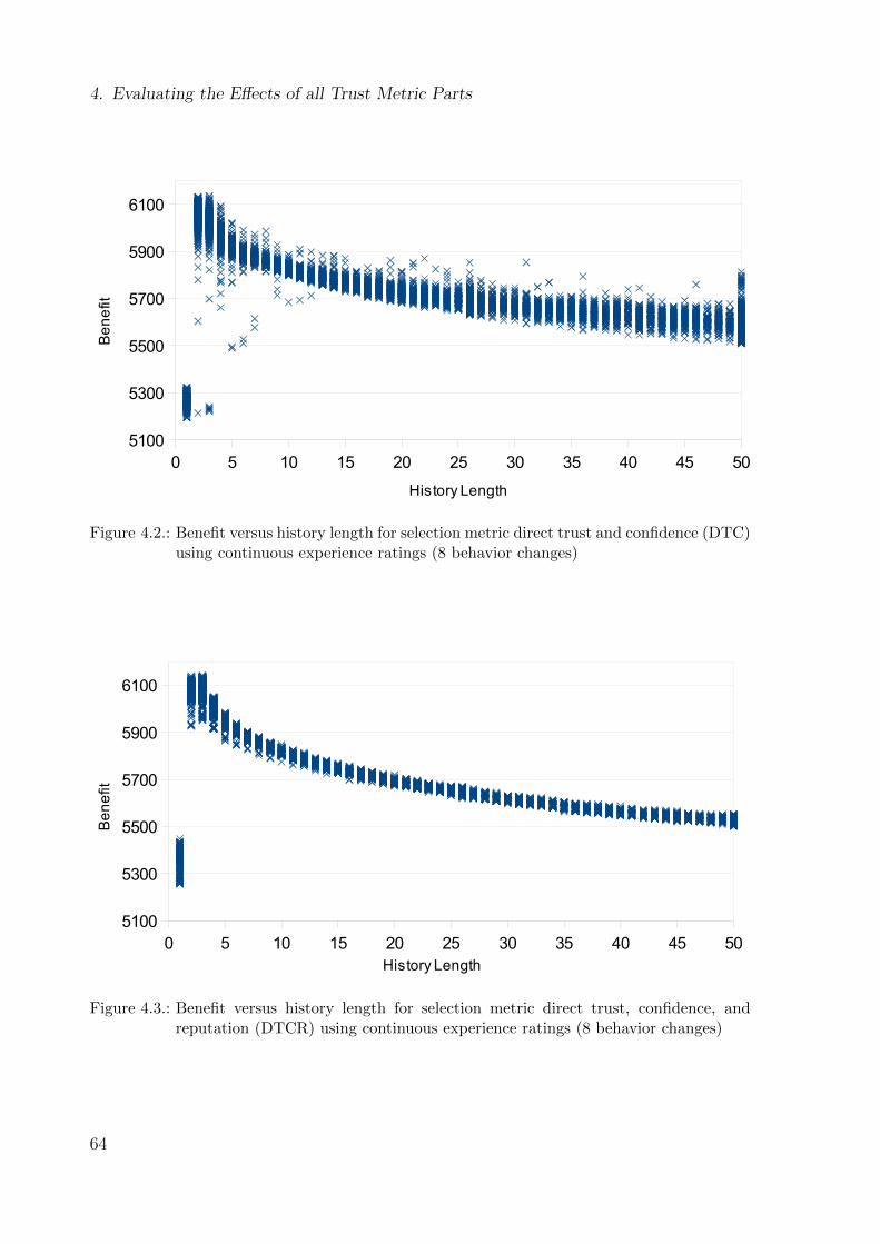
4. Evaluating the Effects of all Trust Metric Parts
0 5 10 15 20 25 30 35 40 45 505100
5300
5500
5700
5900
6100
History Length
Be
ne
fit
Figure 4.2.: Benefit versus history length for selection metric direct trust and confidence (DTC)using continuous experience ratings (8 behavior changes)
0 5 10 15 20 25 30 35 40 45 505100
5300
5500
5700
5900
6100
History Length
Be
ne
fit
Figure 4.3.: Benefit versus history length for selection metric direct trust, confidence, andreputation (DTCR) using continuous experience ratings (8 behavior changes)
64

4.3. Scenario with Some Behavior Changes
DT DTC DTCR4600
4800
5000
5200
5400
5600
5800
6000
6200
6400
5724
5162
5912
5724
6136 6145MIN MAX
Benefit
RAND
Figure 4.4.: Best and worst observed results for each selection metric in comparison with ran-dom (RAND) for history length 2 when using continuous experience ratings (8behavior changes)
65

4. Evaluating the Effects of all Trust Metric Parts
4.3.2. Binary Experience Ratings
The aforementioned evaluation was based on experience ratings between 0 and 1. Such
an assumption can be made if the direct trust values are credibility values, e.g., when
evaluating the amount of correctly tagged faces on a picture using a face recognition
algorithm. In such a case, a single misclassified face does not result in an experience
rating of 0, but a value between 0 and 1. In other cases, i.e., with the Delayed-Ack
algorithm, the direct trust values can only be set to either 0 or 1.
To investigate the differences between using binary experience values and continuous
ones, a similar experiment was conducted. There the agent behavior is based on a beta
distribution with a target mean value and a variation. The agent configuration is the
same as for the first experiment, but the continuous values from the beta distribution
are rounded in the following way: If the number drawn from the beta distribution is
smaller than the mean value, it is rounded down to 0. Otherwise it is rounded up to 1.
Again an automated design space exploration (ADSE) was executed to find the best con-
figuration for the direct trust (DT), direct trust and confidence (DTC) as well as direct
trust, confidence and reputation (DTCR) metrics regarding the parameters described in
table 3.1.
Figure 4.5 shows the results for the DT selection metric. Since nearly all by ADSE
investigated parameters described in Table 3.1 are for confidence, reputation and aggre-
gation, the only free parameter is the history length. Similar to continuous experience
values a lower history length is favorable to gain a high benefit.
Figure 4.6 shows the results for the DTC selection metric. The results show a similar
trend towards lower history length for higher benefit. The vast majority of good results is
observed with low history length with only singular exceptions at higher history length.
As with the first experiment, a variation of benefits for each history length can be
observed, demonstrating the effect of unwisely chosen parameters. The few points with
very good benefit at high history are found due to a specific characteristic of the heuristic
algorithms. These algorithms tend to over adjust parameters, i.e., they find parameters
that are optimized for one specific case the algorithm is run on and that are not useful
in any other situation. These single values can therefore be ignored.
Figure 4.7 lastly shows the result when combining direct trust, confidence and rep-
utation (DTCR). The same trend of lower history length for greater benefit persists
here as well. As with the first experiment, the reputation reduces the variation of benefits
at each history length.
A first difference to observe is the absence of low benefit results for small history length,
even on the DT and DTC metrics. To turn to this effect, another ADSE was conducted,
but this time with a fixed history length of 2. Figure 4.8 shows the results of the
66

4.3. Scenario with Some Behavior Changes
experiment, depicting the minimal and maximal cumulative benefit per metric. As
reference, the benefit of the random (RAND) metric (4871), which picks an agent
randomly in every time step, is depicted as well.
Here a major difference to the first experiment is seen. The best and worst results for
all metrics are about the same. They only vary insignificantly. When looking at the
values that were chosen for the parameters of Table 3.1, wv (the weight of the confidence
metric) tended towards high values, hence the variance is an important aspect. As was
shown in Appendix A, a variance value based on {0,1}-values is always maximal, so
therefore one would expect the variance to not be important. The answer to that also
explains the difference to the continuous experiment. Based on binary experience values
and a history length of 2, only three possible trust values tdirect exist (based on the
experience ratings r):
� tdirect = 0 if r = (0, 0)
� tdirect = 0.5 if r = (1, 0) or r = (0, 1)
� tdirect = 1 if r = (1, 1)
Also, only two possible variations for an experience exist, either 0 or 1. So when choosing
a random agent, the chance to get a 1 is calculated based on the mean value of each
agent. Considering the agent types described in the first section and using a mean
distribution to choose the actual mean value for a specific agent the mean value of each
interval is used to estimate the result of random:
� Type 1 has a mean value of 0.8, providing 30 agents.
� Type 2 has a mean value of 0.6, providing 40 agents.
� Type 3 has a mean value of 0.45, providing 20 agents.
� Type 4 has a mean value of 0.25, providing 10 agents.
The mean value also is the chance to get a 1 from an agent, so the chance per timestep
to get a 1 when picking randomly is 0.8∗30+0.6∗40+0.45∗20+0.25∗10 = 0.595. The
experiment ran for 8000 timestep so the expected average result of the random selection
metric is 8000 ∗ 0.595 = 4760. The observed result of 4871 was only about 2.3% off. A
small deviation was to be expected, since the variance of each agent was not considered
to simplify the calculation of the expected result.
Considering only the last two experiences, an adequate prediction can be done for the
next transaction. The closer the mean value is to the extremes of 0 and 1, the better
the prediction, since a longer chain of zeros and ones is required to obtain that mean
value, e.g., mean value 0.9 = 9∗1+1∗010
. The goal is to find agents with a high mean value
and avoid agents with a low mean value, so this prediction is especially well-suited.
This also explains why a high weight was chosen for the confidence variance. If a trust
67

4. Evaluating the Effects of all Trust Metric Parts
value of 0 or 1 was calculated, the variance confidence is 1 (variance of 0). Since all
considered experiences had the same rating, one can expect the next experience to be
the same. The only other value, 0.5, results in a confidence variance of 0 (variance
maximal). In this case the prediction of the next experience has the highest uncertainty
so it is the best to ask others, i.e., include reputation.
A noticeable difference to the experiment with continuous experience ratings is on the one
hand the much higher cumulative benefit at low history length and a lower cumulative
benefit at higher history length. Since an experience can only be good (rated as 1) or
bad (rated as 0), a mean value can be misleading. An exception are the mean values
of 0 and 1 as was explained above. All other values just mark uncertainty about the
interaction partner and how good the next interaction will be. The evaluation has shown
that adding several grades of uncertainty does not add more information, especially since
they also increase the time until a change of behavior is identified. When the diversity
of uncertainty gets too high, i.e., too many mean values between 0 and 1, the cumulative
benefit even drops below the achieved benefit of the continuous experiment.
Having a binary rating system for experience increased the total benefit and is therefore
preferred to a continuous rating system, but how experiences can be rated is application
specific. The Delayed-Ack Algorithm logically rates messages binary (received or not
received) while the Energy Grid rates a prediction of power production. The further the
prediction is off from the actual production, the worse the prediction which is naturally
a continuous rating.
68

4.3. Scenario with Some Behavior Changes
0 5 10 15 20 25 30 35 40 45 505100
5300
5500
5700
5900
6100
6300
6500
6700
6900
7100
History Length
Ben
efit
Figure 4.5.: Benefit versus history length for selection metric direct trust (DT) using binaryexperience ratings (8 behavior changes)
Figure 4.6.: Benefit versus history length for selection metric direct trust and confidence (DTC)using binary experience ratings (8 behavior changes)
69
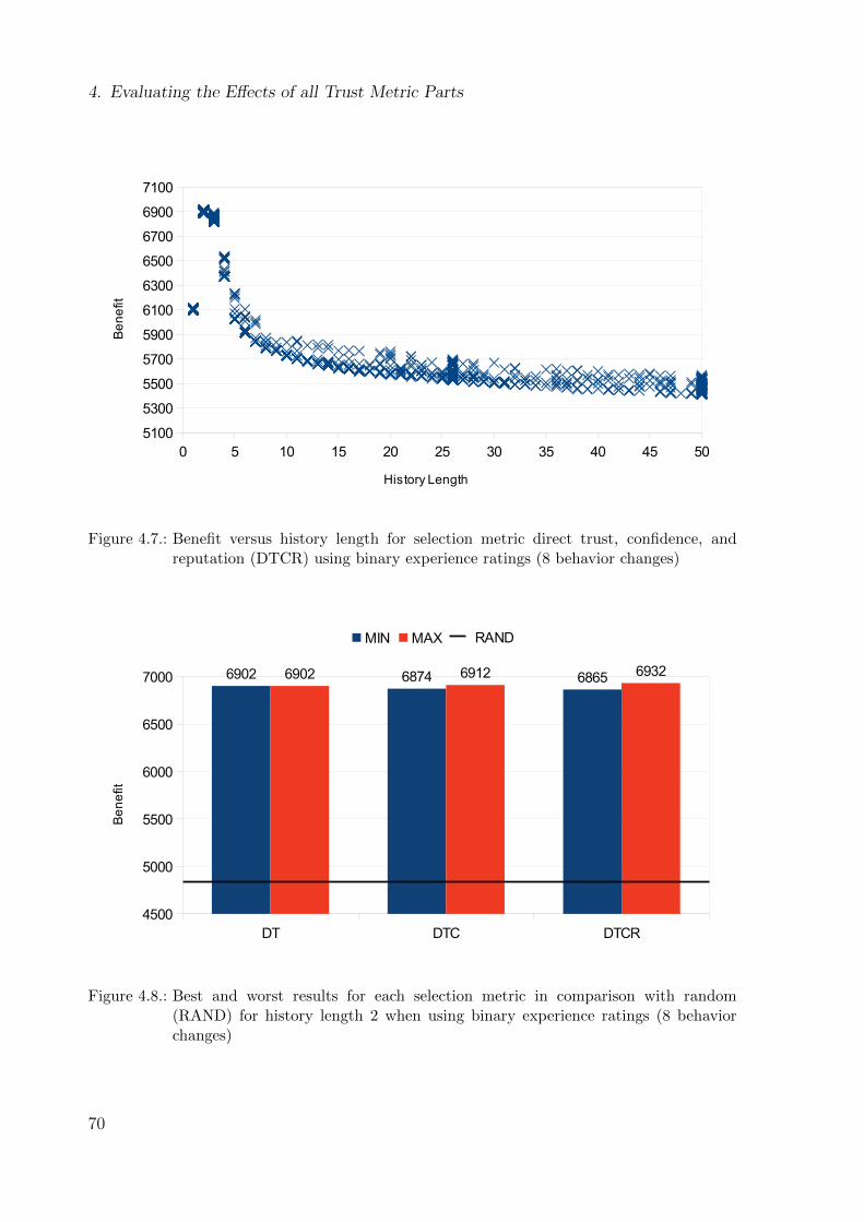
4. Evaluating the Effects of all Trust Metric Parts
0 5 10 15 20 25 30 35 40 45 505100
5300
5500
5700
5900
6100
6300
6500
6700
6900
7100
History Length
Be
ne
fit
Figure 4.7.: Benefit versus history length for selection metric direct trust, confidence, andreputation (DTCR) using binary experience ratings (8 behavior changes)
Figure 4.8.: Best and worst results for each selection metric in comparison with random(RAND) for history length 2 when using binary experience ratings (8 behaviorchanges)
70

4.4. Scenario with Few Behavior Changes
4.4. Scenario with Few Behavior Changes
In this section the amount of behavior changes is reduced, yet not completely removed.
Behavior changes are conducted after 2000 and then again after another 4000 time
steps. The last 2000 time steps contain no more behavior changes. In total, only 2
behavior changes are done within this scenario. Again both continuous as well as binary
experience ratings are investigated.
4.4.1. Continuous Experience Ratings
First the results for continuous experience ratings are presented. As before every expe-
rience is rated with a value between 0 and 1.
Figure 4.9 depicts the results if only direct trust (DT) is used to decide the next inter-
action partner. The characteristics of the curve is similar to the preceding experiment.
A lower history length is preferable to a higher history length. The difference to before
is, that a history length of 3 results in about the same, if not slightly higher, cumulative
benefit as a history length of 2.
Figure 4.10 depicts the cumulative benefit for different history lengths when using direct
trust with confidence (DTC) to select the next interaction partner. The results for
this metric are widely different than the other experiments so far. Compared to them, the
history length is not the dominating factor, instead a high variance of good cumulative
benefit values can be observed up to history length 30. Since the behavior of each agent
is stable most of the time, a fast adjustment is not essential here, leaving the history
length with strongly reduced influence on the total result. Instead, the configuration of
the other parameters is more important to obtain a good cumulative benefit.
Figure 4.11 depicts the results when using all three parts of the trust metric, i.e., direct
trust, confidence, and reputation (DTCR). Here the history length is again the
dominating factor. Similar to using only direct trust, but contrary to the experiments
with 8 behavior changes, the highest cumulative benefit is achieved with history length
3 and not with 2.
Since a history length of 3 seems to create better results than a history length of 2, the
best and worst possible configurations for both history length 2 and 3 are investigated.
The baseline selection metric random (RAND) achieved a cumulative benefit of 4871.
Figure 4.12 shows the best and worst cumulative benefit that were found by ADSE for
history length 2. The results are similar to the experiment with 8 behavior changes. That
is adding confidence (DTC) or reputation (DTCR) can result in a better cumulative
benefit than direct trust (DT) alone. But the DTC metric also allows for a worse
cumulative benefit, if an unwisely set of parameters are chosen, while adding reputation
71

4. Evaluating the Effects of all Trust Metric Parts
with the DTCR metric evens out bad parameter configurations with the lowest found
result being higher than with direct trust alone. The best found result for DTC and
DTCR are similar.
Increasing the history length to 3 yields interesting results, see Figure 4.13. For one,
the cumulative benefit is generally higher with all metrics, which is to be expected when
looking at the experiments with variable history length. The most notable difference
though is the strong increase of the best possible value for direct trust, increasing it even
beyond the best possible value for the DTCR metric.
A statistical analysis showed some interesting effects:
� Number Confidence: Due to the low number of considered past experiences,
i.e., low history length, the number confidence had very little influence. Its weight
to the total confidence value showed no trend in the analysis.
� Age Confidence: An experience was aging fast, i.e., dropping below 1 for its
actuality rating, in both metrics (τr tended to low values). The threshold, when
to consider it out of date (τo) showed no real trend, but was in the higher half of
the domain for the DTCR metric. Its weight showed no trend in the DTC metric
and was low in the DTCR metric.
� Variance confidence: While the weight of the variance metric showed no trend
in the DTC metric, it tended to higher values in the DTCR metric.
� Reputation metric: Here an interesting effect occurred. Both thresholds tended
to high values, with τ ∗ set near the maximum of the domain. This means that
even a considerable deviation from a recommendation to ones own experience is
still considered good enough for a positive adjustment of the participant that gave
the recommendation.
� Aggregation metric: The parameters for the aggregation metric were chosen
to mostly use reputation only: τcl tended high with τch near the maximum of the
domain. The result was a system that is similar to web reputation systems, e.g,
the ebay reputation metric. They often take decisions based on the experience
of others. Since the system is in a mostly stable state, i.e., nearly no behavior
changes, a combination of the knowledge of others was an acceptable basis to
choose the next interaction partner.
72

4.4. Scenario with Few Behavior Changes
0 5 10 15 20 25 30 35 40 45 505100
5300
5500
5700
5900
6100
6300
6500
6700
history length
be
ne
fit
Figure 4.9.: Benefit versus history length for selection metric direct trust (DT) using continuousexperience ratings (only 2 behavior changes)
Figure 4.10.: Benefit versus history length for selection metric direct trust and confidence(DTC) using continuous experience ratings (only 2 behavior changes)
73

4. Evaluating the Effects of all Trust Metric Parts
0 5 10 15 20 25 30 35 40 45 505100
5300
5500
5700
5900
6100
6300
6500
6700
history length
be
ne
fit
Figure 4.11.: Benefit versus history length for selection metric direct trust, confidence, andreputation (DTCR) using continuous experience ratings (only 2 behavior changes)
Figure 4.12.: Best and worst observed results for each selection metric in comparison withrandom (RAND) for history length 2 when using continuous experience ratings(only 2 behavior changes)
74

4.4. Scenario with Few Behavior Changes
DT DTC DTCR4500
5000
5500
6000
5719
5180
6032
5719
63726244
MIN MAX
Benefit
RAND
Figure 4.13.: Best and worst observed results for each selection metric in comparison withrandom (RAND) for history length 3 when using continuous experience ratings(only 2 behavior changes)
75

4. Evaluating the Effects of all Trust Metric Parts
4.4.2. Binary Experience Ratings
As comparison, this experiment uses binary experience values, i.e., experiences are rated
as either 0 or 1. Otherwise the experiment is identical to the continuous variant with
only a total of 2 behavior changes.
Figure 4.14 depicts the result for the direct trust (DT) selection metric. Here the
history length is again the dominating factor, with a maximum cumulative benefit at
history length 2.
Figure 4.15 depicts the results when adding confidence to direct trust (DTC) when
selecting a suitable interaction partner. Similar to the continuous experiment, the re-
sults show some high benefit values at higher history length, but with less variance.
Nonetheless lower history length is preferable, since no low results were observed while
having the highest result at low histoy length.
Adding reputation to direct trust and confidence (DTCR), see Figure 4.16, re-
duces the variance of the results. Here the impact of a low history length is again
prevalent. The best results are again observed with history length 2.
Since a history length of 2 seems to be the best choice, all selection metrics were ex-
amined with a fixed history length of 2. The results are depicted in Figure 4.17. Ran-
dom (RAND) was again used as baseline with an achieved cumulated benefit of 4886.
The results are similar to the experiment with binary experience values and 8 behavior
changes. The minimum and maximum achieved cumulative benefit values are similar.
In addition, not much can be gained by adding confidence and reputation.
As comparison with the continuous results, Figure 4.18 depicts the best and worst found
parameter set for a fixed history length of 3 instead of 2. The best found parameter
set for the DTC metric is slightly higher with a history length of 2, showing a similar
trend as the continuous case. But typical for the experiments with binary experiment
ratings, the minimal and maximal found benefit values differ only slightly. Additionally,
the benefit values found with the DTCR metric are better with history length 2 than
with 3. So in total, history length 2 is preferable in the binary case.
76
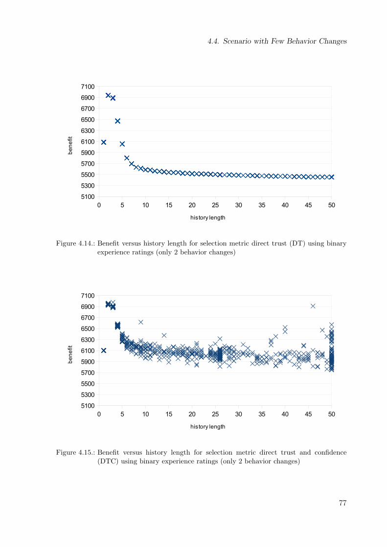
4.4. Scenario with Few Behavior Changes
0 5 10 15 20 25 30 35 40 45 505100
5300
5500
5700
5900
6100
6300
6500
6700
6900
7100
history length
be
ne
fit
Figure 4.14.: Benefit versus history length for selection metric direct trust (DT) using binaryexperience ratings (only 2 behavior changes)
Figure 4.15.: Benefit versus history length for selection metric direct trust and confidence(DTC) using binary experience ratings (only 2 behavior changes)
77
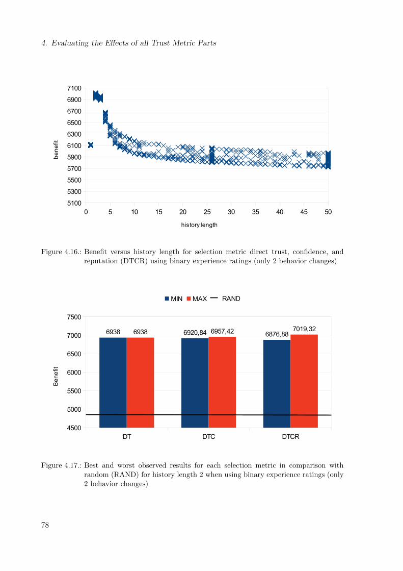
4. Evaluating the Effects of all Trust Metric Parts
0 5 10 15 20 25 30 35 40 45 505100
5300
5500
5700
5900
6100
6300
6500
6700
6900
7100
history length
be
ne
fit
Figure 4.16.: Benefit versus history length for selection metric direct trust, confidence, andreputation (DTCR) using binary experience ratings (only 2 behavior changes)
Figure 4.17.: Best and worst observed results for each selection metric in comparison withrandom (RAND) for history length 2 when using binary experience ratings (only2 behavior changes)
78

4.4. Scenario with Few Behavior Changes
DT DTC DTCR4500
5000
5500
6000
6500
7000
7500
6891 6869 68636891 6976 6967
MIN MAX
Benefit
RAND
Figure 4.18.: Best and worst observed results for each selection metric in comparison withrandom (RAND) for history length 3 when using binary experience ratings (only2 behavior changes)
79
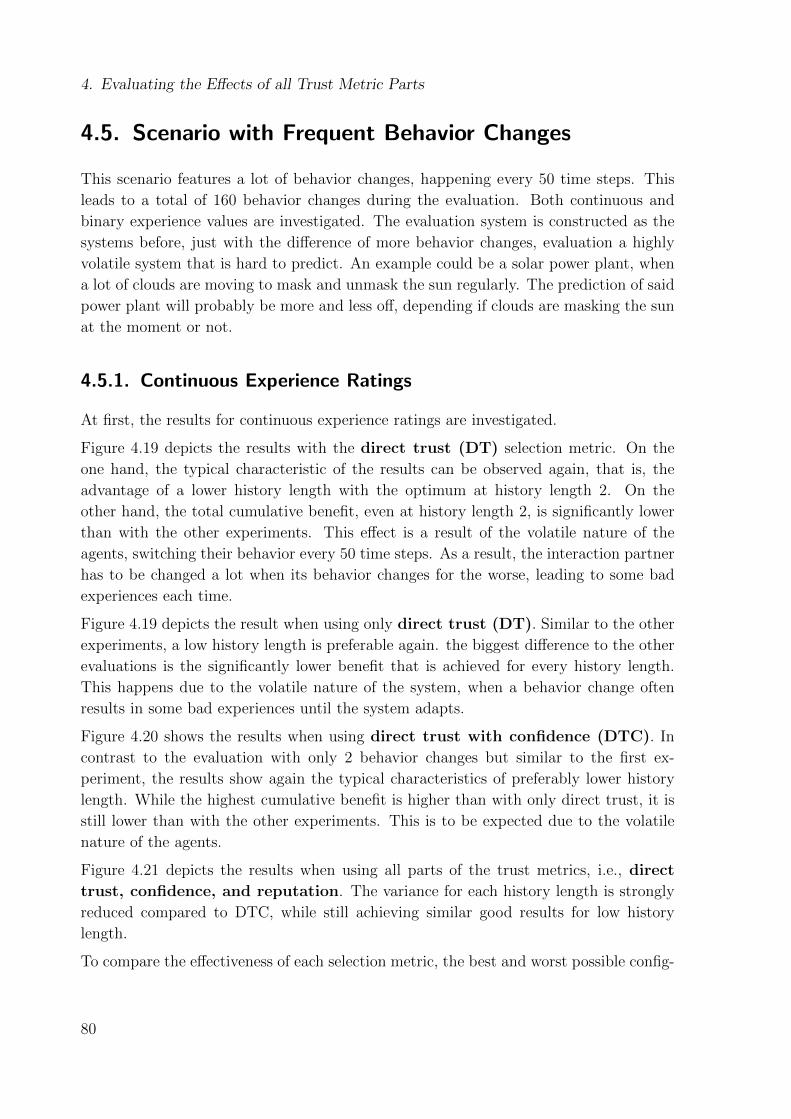
4. Evaluating the Effects of all Trust Metric Parts
4.5. Scenario with Frequent Behavior Changes
This scenario features a lot of behavior changes, happening every 50 time steps. This
leads to a total of 160 behavior changes during the evaluation. Both continuous and
binary experience values are investigated. The evaluation system is constructed as the
systems before, just with the difference of more behavior changes, evaluation a highly
volatile system that is hard to predict. An example could be a solar power plant, when
a lot of clouds are moving to mask and unmask the sun regularly. The prediction of said
power plant will probably be more and less off, depending if clouds are masking the sun
at the moment or not.
4.5.1. Continuous Experience Ratings
At first, the results for continuous experience ratings are investigated.
Figure 4.19 depicts the results with the direct trust (DT) selection metric. On the
one hand, the typical characteristic of the results can be observed again, that is, the
advantage of a lower history length with the optimum at history length 2. On the
other hand, the total cumulative benefit, even at history length 2, is significantly lower
than with the other experiments. This effect is a result of the volatile nature of the
agents, switching their behavior every 50 time steps. As a result, the interaction partner
has to be changed a lot when its behavior changes for the worse, leading to some bad
experiences each time.
Figure 4.19 depicts the result when using only direct trust (DT). Similar to the other
experiments, a low history length is preferable again. the biggest difference to the other
evaluations is the significantly lower benefit that is achieved for every history length.
This happens due to the volatile nature of the system, when a behavior change often
results in some bad experiences until the system adapts.
Figure 4.20 shows the results when using direct trust with confidence (DTC). In
contrast to the evaluation with only 2 behavior changes but similar to the first ex-
periment, the results show again the typical characteristics of preferably lower history
length. While the highest cumulative benefit is higher than with only direct trust, it is
still lower than with the other experiments. This is to be expected due to the volatile
nature of the agents.
Figure 4.21 depicts the results when using all parts of the trust metrics, i.e., direct
trust, confidence, and reputation. The variance for each history length is strongly
reduced compared to DTC, while still achieving similar good results for low history
length.
To compare the effectiveness of each selection metric, the best and worst possible config-
80
4.5. Scenario with Frequent Behavior Changes
uration for history length 2 was searched for. Similar to the other experiments, history
length 2 provided the highest cumulative benefit. Figure 4.22 depicts the best and worst
found benefit values for each selection metric. Random (RAND) as baseline achieved
a cumulative benefit of 4997. All metrics are significantly better than random selection.
It also shows that the DTC metric provided better results than the DT metric. If the
other 12 parameters are chosen unwisely, the result is as lows as with the DT metric.
Adding reputation increases the minimal found cumulative benefit, while retaining the
good results of DTC.
Some parameters showed definite trends on a statistical analysis:
� Number Confidence: Due to the low history length, the amount confidence
naturally featured a low value for wn, i.e., the confidence reached 1 very fast.
For DTC, it was weighted very highly for the total confidence, while the opposite
happened for DTCR.
� Age Confidence: Both the DTC and DTCR metric favored a parameter choice
to swiftly let the actuality rating of an experience drop below the maximum (low
τr) but with a significant time until they are marked as outdated (middle to high
τo). For DTC the amount confidence was rated very low for the total confidence
while the DTCR metric preferred a low to middle weight.
� Variance confidence: The variance confidence showed no trend for both DTC
and DTCR.
� Reputation metric: The reputation metric was parametrized to feature a very
small area for a positive match (low τ threshold) but with a high area until the rec-
ommendation is adjusted negatively (high τ ∗). The maximal adjustment was also
set very high, so a false recommendation was punished strongly. This reinforces
the observed effect, that fast change to behavior is important in such a volatile
system.
� Aggregation metric: For the aggregation the thresholds for the confidence were
chosen wide apart, creating a big range, where the total trust value is shifted from
reputation to direct trust. It was preferable to nearly always include both parts in
the total trust value.
81

4. Evaluating the Effects of all Trust Metric Parts
0 5 10 15 20 25 30 35 40 45 505200
5300
5400
5500
5600
5700
5800
5900
6000
6100
6200
history length
be
ne
fit
Figure 4.19.: Benefit versus history length for selection metric direct trust (DT) using contin-uous experience ratings (behavior changes every 50 time steps)
Figure 4.20.: Benefit versus history length for selection metric direct trust and confidence(DTC) using continuous experience ratings (behavior changes every 50 time steps)
82

4.5. Scenario with Frequent Behavior Changes
0 5 10 15 20 25 30 35 40 45 505200
5300
5400
5500
5600
5700
5800
5900
6000
6100
6200
history length
be
ne
fit
Figure 4.21.: Benefit versus history length for selection metric direct trust, confidence, andreputation (DTCR) using continuous experience ratings (behavior changes every50 time steps)
Figure 4.22.: Best and worst observed results for each selection metric in comparison withrandom (RAND) for history length 2 when using continuous experience ratings(behavior changes every 50 time steps)
83

4. Evaluating the Effects of all Trust Metric Parts
4.5.2. Binary Experience Ratings
The last experiment was run with binary experience ratings but still 160 behavior
changes.
Figure 4.23 depicts the results for the direct trust (DT) selection metric. The positive
effect of low history length can be clearly seen, with the maximum at history length 2 yet
again. The best parameter set found results in a cumulative benefit that is higher than
with continuous experience ratings. But it is also lower than the achieved cumulative
benefits of the other experiments with binary experience ratings. It is therefore consistent
with the continuous experiment that showed similar results, i.e., the volatile nature of
the agents lowers the achievable benefit. One big difference to all other experiments can
be observed, though: The achieved cumulative benefit for history length 1 is quite high
and one of the better points. Since the system is highly volatile of its behavior, a fast
adjustment to change is required, which also explains the strong increase in benefit when
getting to the lower history length values. Due to the high necessity of a fast behavior
change adjustment and the fact, that an experience can only be of two types (good or
bad), a history length of one provided acceptable results. Nonetheless, a meaningful,
i.e., non trivial, mean value is still preferable for the best result.
Figure 4.24 shows the results for the direct trust with confidence (DTC) selection
metric. Similar to the other experiments, a low history length is preferable. The ob-
tained benefit values show some variation on higher history length depending on the
chosen values for the other 12 parameters. Also, similar to the DT metric, the achieved
cumulative benefit for history length 1 is quite high and does show no deviation. The
missing deviation can be explained, since most metrics are based on some kind of mean
value, which can not deviate based on only one single value.
Figure 4.25 shows the results, if all trust metric parts, i.e., direct trust, confidence
and reputation (DTCR), are used in conjunction. It shows the typical characteristics
of preferable low history length while negating the variation of DTC. Yet again, the result
for history length 1 is quite high.
To conclude, Figure 4.26 shows a direct comparison of each selection metric (DT, DTC,
and DTCR) for history length 2, which has proven to be the optimal value, overshadow-
ing the other 12 parameters. For each selection metric the minimal and maximal found
benefit are displayed, as well as the benefit obtained by random (RAND) selection
(4872). All minimal and maximal values are close to each other while being significantly
better than random selection, which is consistent with the other binary experiments.
The generally lower benefit values are due to the volatile system with 160 behavior
changes. Therefore several more bad interactions each time the system needs to adapt
are experienced, leading to a generally lower total result.
84

4.5. Scenario with Frequent Behavior Changes
0 5 10 15 20 25 30 35 40 45 504500
4700
4900
5100
5300
5500
5700
5900
6100
6300
6500
history length
be
ne
fit
Figure 4.23.: Benefit versus history length for selection metric direct trust (DT) using binaryexperience ratings (behavior changes every 50 time steps)
Figure 4.24.: Benefit versus history length for selection metric direct trust and confidence(DTC) using binary experience ratings (behavior changes every 50 time steps)
85

4. Evaluating the Effects of all Trust Metric Parts
0 5 10 15 20 25 30 35 40 45 504500
4700
4900
5100
5300
5500
5700
5900
6100
6300
6500
history length
be
ne
fit
Figure 4.25.: Benefit versus history length for selection metric direct trust, confidence, andreputation (DTCR) using binary experience ratings (behavior changes every 50time steps)
Figure 4.26.: Best and worst observed results for each selection metric in comparison with ran-dom (RAND) for history length 2 when using binary experience ratings (behaviorchanges every 50 time steps)
86
5. Trust-Enabling Middleware (TEM)
To make the trust metrics described in Chapter 3 available for a wide variety of ap-
plications the Trust-Enabling Middleware (TEM) [1] was designed. The goal of
the TEM is to provide a prototypical implementation of an distributed organic system
that provides the aforementioned trust metrics. Each instance of the TEM middleware
represents a logical node in a distributed system, which can be a grid system or a Multi-
Agent-System (MAS). The TEM was enhanced with MAS concepts in the OC-Trust
research group to the Trust-Enabled Multi-Agent-System (TEMAS) [1].
The TEM as basis of the TEMAS serves as basis for all kinds of applications, which can
be registered and run on the TEM. These services define the functionality available. In
turn, the TEM provides the following capabilities for every service:
� Sending and receiving messages with logical node IDs. The middleware executes
the actual message sending on lower level.
� Monitoring of the message flow. Each service can register monitors in the TEM,
which are able to monitor all incoming (from a node to services) and outgoing
(from services to other nodes) messages.
� Piggybacking additional information on application messages. With the aforemen-
tioned monitors additional data can be added to application messages, e.g., which
is used by the Delayed-Ack algorithm (see Section 3.1) to identify whether the
messages were received.
� Saving experiences and calculating direct trust and reputation. The TEM provides
all the metrics described in Chapter 3, which in turn can be utilized by the services.
The architecture of the so called trust metric infrastructure is described in
Section 5.3.
Each service can be in one of three states, depicted by Figure 5.1.
� Unregistered: Such a service is just instantiated but not yet registered on a node.
It can neither receive messages nor generally participate in the system in any way.
� Inactive: The service is registered on a node. A message queue is created and all
messages for the service are stored in it. They are not sent to the service until it
is active.
87

5. Trust-Enabling Middleware (TEM)
unregistered inactive active
unregister
(destroy)
startregister(init)
stop
Figure 5.1.: Life-cycle of a service
� Active: The service is now fully functional and can communicate and receive
messages normally.
5.1. Architecture
The TEM is a multi-tier middleware system depicted in Figure 5.2. It is based on OCµ
[50], a middleware for Organic Computing Systems. In OCµ the left part is the System
under Observation and Control (SuOC) that is monitored and controlled by the Organic
Manager [50][55]. TEM adds trust capabilities to OCµ by adding the TrustService as a
core service for the trust calculations and will adjust the self-x properties of OCµ by using
the collected trust values. Compared to typical self-x property algorithms, especially for
self-configuration that only consider load information, trust is an opinion about someone
else. This implies that trust information can not be gathered from a node directly,
unlike load information, but have to be calculated by others. This significant difference
requires new approaches for the self-x properties and are not simple adjustments for
already existing algorithms.
A TEM node represents a logical node in a network, usually a PC. The Middleware, the
left part of Figure 5.2, consists of three layers:
� TransportConnector: This layer handles the communication between nodes.
All implementations have to implement the TransportConnector interface, ab-
stracting the actual transport layer from the applications. The TEM provides a
LocalTransportConnector, which handles the transport of messages within the
same JVM and therefore enables several logical nodes to run on a single PC. An-
other important TransportConncector is the JXTATransportConnector, which
88
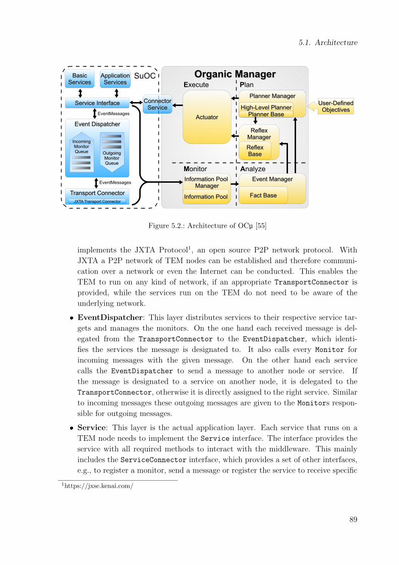
5.1. Architecture
BasicBasicServicesServices
ApplicationApplicationServicesServices
Transport ConnectorTransport ConnectorJXTA Transport Connector
Organic ManagerOrganic Manager
User-DefinedUser-DefinedObjectivesObjectives
ReflexReflexManagerManager
ReflexReflexBaseBase
Planner ManagerPlanner Manager
High-Level PlannerHigh-Level PlannerPlanner BasePlanner BaseActuatorActuator
Information Pool Information Pool ManagerManager
Information PoolInformation Pool
Event ManagerEvent Manager
Fact BaseFact Base
Service InterfaceService Interface
EventMessages
Event DispatcherEvent Dispatcher
OutgoingOutgoingMonitorMonitorQueueQueue
IncomingIncomingMonitorMonitorQueueQueue
EventMessages
SuOC
Monitor Analyze
PlanExecute
ConnectorConnectorServiceService
Figure 5.2.: Architecture of OCµ [55]
implements the JXTA Protocol1, an open source P2P network protocol. With
JXTA a P2P network of TEM nodes can be established and therefore communi-
cation over a network or even the Internet can be conducted. This enables the
TEM to run on any kind of network, if an appropriate TransportConnector is
provided, while the services run on the TEM do not need to be aware of the
underlying network.
� EventDispatcher: This layer distributes services to their respective service tar-
gets and manages the monitors. On the one hand each received message is del-
egated from the TransportConnector to the EventDispatcher, which identi-
fies the services the message is designated to. It also calls every Monitor for
incoming messages with the given message. On the other hand each service
calls the EventDispatcher to send a message to another node or service. If
the message is designated to a service on another node, it is delegated to the
TransportConnector, otherwise it is directly assigned to the right service. Similar
to incoming messages these outgoing messages are given to the Monitors respon-
sible for outgoing messages.
� Service: This layer is the actual application layer. Each service that runs on a
TEM node needs to implement the Service interface. The interface provides the
service with all required methods to interact with the middleware. This mainly
includes the ServiceConnector interface, which provides a set of other interfaces,
e.g., to register a monitor, send a message or register the service to receive specific
1https://jxse.kenai.com/
89
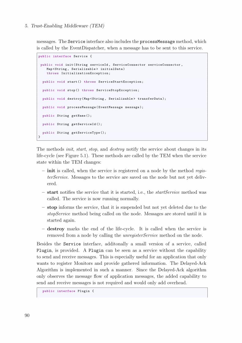
5. Trust-Enabling Middleware (TEM)
messages. The Service interface also includes the processMessagemethod, which
is called by the EventDispatcher, when a message has to be sent to this service.
public interface Service {
public void init(String serviceId , ServiceConnector serviceConnector ,
Map <String , Serializable > initialData)
throws InitializationException;
public void start() throws ServiceStartException;
public void stop() throws ServiceStopException;
public void destroy(Map <String , Serializable > transferData );
public void processMessage(EventMessage message );
public String getName ();
public String getServiceId ();
public String getServiceType ();
}
The methods init, start, stop, and destroy notify the service about changes in its
life-cycle (see Figure 5.1). These methods are called by the TEM when the service
state within the TEM changes:
– init is called, when the service is registered on a node by the method regis-
terService. Messages to the service are saved on the node but not yet deliv-
ered.
– start notifies the service that it is started, i.e., the startService method was
called. The service is now running normally.
– stop informs the service, that it is suspended but not yet deleted due to the
stopService method being called on the node. Messages are stored until it is
started again.
– destroy marks the end of the life-cycle. It is called when the service is
removed from a node by calling the unregisterService method on the node.
Besides the Service interface, additonally a small version of a service, called
Plugin, is provided. A Plugin can be seen as a service without the capability
to send and receive messages. This is especially useful for an application that only
wants to register Monitors and provide gathered information. The Delayed-Ack
Algorithm is implemented in such a manner. Since the Delayed-Ack algorithm
only observes the message flow of application messages, the added capability to
send and receive messages is not required and would only add overhead.
public interface Plugin {
90
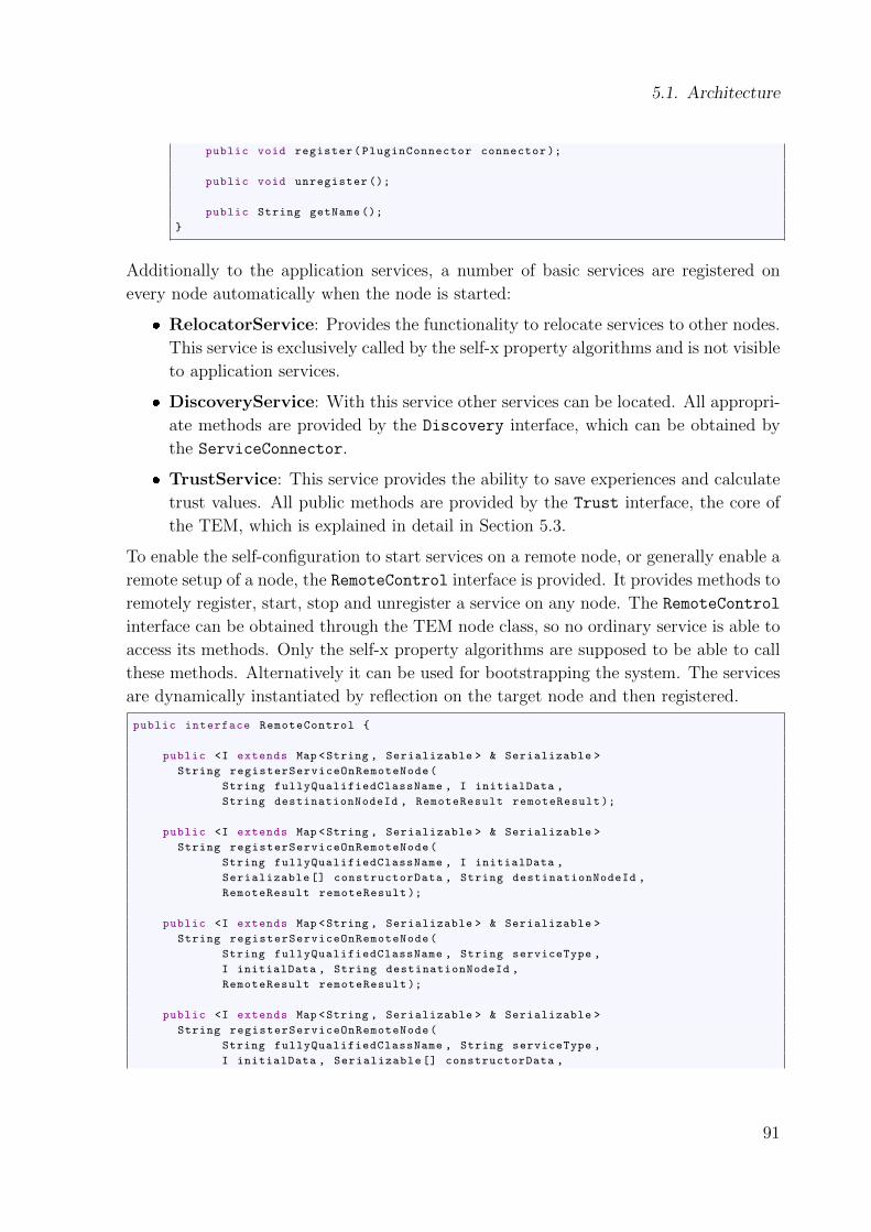
5.1. Architecture
public void register(PluginConnector connector );
public void unregister ();
public String getName ();
}
Additionally to the application services, a number of basic services are registered on
every node automatically when the node is started:
� RelocatorService: Provides the functionality to relocate services to other nodes.
This service is exclusively called by the self-x property algorithms and is not visible
to application services.
� DiscoveryService: With this service other services can be located. All appropri-
ate methods are provided by the Discovery interface, which can be obtained by
the ServiceConnector.
� TrustService: This service provides the ability to save experiences and calculate
trust values. All public methods are provided by the Trust interface, the core of
the TEM, which is explained in detail in Section 5.3.
To enable the self-configuration to start services on a remote node, or generally enable a
remote setup of a node, the RemoteControl interface is provided. It provides methods to
remotely register, start, stop and unregister a service on any node. The RemoteControl
interface can be obtained through the TEM node class, so no ordinary service is able to
access its methods. Only the self-x property algorithms are supposed to be able to call
these methods. Alternatively it can be used for bootstrapping the system. The services
are dynamically instantiated by reflection on the target node and then registered.
public interface RemoteControl {
public <I extends Map <String , Serializable > & Serializable >
String registerServiceOnRemoteNode(
String fullyQualifiedClassName , I initialData ,
String destinationNodeId , RemoteResult remoteResult );
public <I extends Map <String , Serializable > & Serializable >
String registerServiceOnRemoteNode(
String fullyQualifiedClassName , I initialData ,
Serializable [] constructorData , String destinationNodeId ,
RemoteResult remoteResult );
public <I extends Map <String , Serializable > & Serializable >
String registerServiceOnRemoteNode(
String fullyQualifiedClassName , String serviceType ,
I initialData , String destinationNodeId ,
RemoteResult remoteResult );
public <I extends Map <String , Serializable > & Serializable >
String registerServiceOnRemoteNode(
String fullyQualifiedClassName , String serviceType ,
I initialData , Serializable [] constructorData ,
91
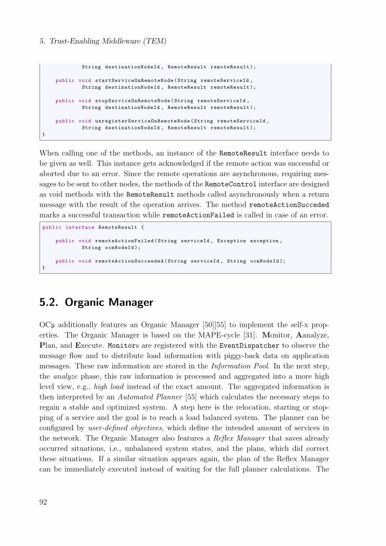
5. Trust-Enabling Middleware (TEM)
String destinationNodeId , RemoteResult remoteResult );
public void startServiceOnRemoteNode(String remoteServiceId ,
String destinationNodeId , RemoteResult remoteResult );
public void stopServiceOnRemoteNode(String remoteServiceId ,
String destinationNodeId , RemoteResult remoteResult );
public void unregisterServiceOnRemoteNode(String remoteServiceId ,
String destinationNodeId , RemoteResult remoteResult );
}
When calling one of the methods, an instance of the RemoteResult interface needs to
be given as well. This instance gets acknowledged if the remote action was successful or
aborted due to an error. Since the remote operations are asynchronous, requiring mes-
sages to be sent to other nodes, the methods of the RemoteControl interface are designed
as void methods with the RemoteResult methods called asynchronously when a return
message with the result of the operation arrives. The method remoteActionSucceded
marks a successful transaction while remoteActionFailed is called in case of an error.
public interface RemoteResult {
public void remoteActionFailed(String serviceId , Exception exception ,
String ocmNodeId );
public void remoteActionSucceeded(String serviceId , String ocmNodeId );
}
5.2. Organic Manager
OCµ additionally features an Organic Manager [50][55] to implement the self-x prop-
erties. The Organic Manager is based on the MAPE-cycle [31]: Monitor, Aanalyze,
Plan, and Execute. Monitors are registered with the EventDispatcher to observe the
message flow and to distribute load information with piggy-back data on application
messages. These raw information are stored in the Information Pool. In the next step,
the analyze phase, this raw information is processed and aggregated into a more high
level view, e.g., high load instead of the exact amount. The aggregated information is
then interpreted by an Automated Planner [55] which calculates the necessary steps to
regain a stable and optimized system. A step here is the relocation, starting or stop-
ping of a service and the goal is to reach a load balanced system. The planner can be
configured by user-defined objectives, which define the intended amount of services in
the network. The Organic Manager also features a Reflex Manager that saves already
occurred situations, i.e., unbalanced system states, and the plans, which did correct
these situations. If a similar situation appears again, the plan of the Reflex Manager
can be immediately executed instead of waiting for the full planner calculations. The
92

5.3. The Trust Metric Infrastructure
actual execution of each step is performed by the Actuator. The Actuator has a direct
connection to OCµ and is therefore able to send messages to other nodes to realize the
service relocations, starts and stops.
The main aspect of the Organic Manager is the automated planner. A planner finds
a series of steps to reach a designated goal, in case of OCµ a distributed load of the
nodes. The steps to reach that goal can either be the relocation, starting or stopping
of a service. The start or stop steps are required, because users can define objectives,
like at least 10 services of a specific type have to run in the system. The planner makes
sure to start the appropriate amount of services. It also relocates the services to balance
the load. While the planner does indeed find suitable solutions for the objectives, its
scalability is a problem. A planer searches through the entire planning space, which is
constructed as a tree with all possible paths. The nodes of said tree are the steps the
system can take. In general the runtime of the planner increases exponentially with the
size of the problem. To counter this problem, the Reflex Manager was introduced that
caches already calculated plans for further use if a similar situation occurs again.
With the introduction of trust, a planner is not suitable anymore due to its runtime.
Trust values are expected to change constantly during the runtime of a system, which
would result in repeated misses of the Reflex Manager and therefore constant recalcu-
lation of new plans. This also means, that a change in a trust value of a node would
trigger the planner again, leading to constant replanning, a high consumption of runtime
and long reaction times. For such an ever-changing property like trust a planner is not
a suitable tool. Therefore the TEM takes a different approach with integrated basic
services for the self-x properties.
5.3. The Trust Metric Infrastructure
The trust metric infrastructure (TMI) consists of all interfaces and classes for the trust
calculation, Figure 5.5 at the end of this chapter gives an overview of the involved classes.
The TEMAS technical report [1] presents an in depth description of the entire system.
This chapter will focus on the general structure of the TMI. The Trust interface is the
entry point for all services to the TMI and provides all required methods for trust calcu-
lations. Emphasis was put to support any kind of trust calculation from applications as
well as the middleware. Especially the different viewpoints of the middleware and MAS
(Multi-Agent-Systems) are supported.
� Middleware view: The self-x properties need trust values about a node, and its
reliability to host important services.
� MAS view: Multi-Agent-Systems calculate trust values about other agents and
93

5. Trust-Enabling Middleware (TEM)
abstract from the node they are running on. Therefore their experiences and trust
values are about specific agents and normally do not include node information.
To calculate trust the services save so called RawData into the TEM. These RawData
represent the experiences the services had with their interaction partners. These expe-
riences already contain an evaluation of these interactions, i.e., a value between 0 and
1 with 0 representing the worst and 1 the best possible outcome. When a direct trust
calculation is initialized, a Transformer transforms them into TransformedData, e.g.,
applying a sliding time window. Then an Interpreter calculates TrustData out of the
TransformedData. This process is depicted in Figure 5.3.
RawData
TransformedData
TrustData
Transformer
Interpreter
Figure 5.3.: Trust calculation process
RawData represents all experiences gathered with an interaction partner. The type of
these experiences are application specific. The Delayed-Ack algorithm, e.g., uses
an additional list that contains ACKs of messages that were set to not received
due to a timeout, which defines a waiting time for ACKs of sent messages. After
the timeout has elapsed, a message is considered as lost. These late ACKs need
to be verified as ACKs for real messages to prevent manipulation of the reliability
value, otherwise a malicious node could send random message numbers as ACKs
and those would be considered real without cross checking if those numbers were
actually sent. After setting a number to not received in the database it is removed
from memory to prevent a memory leak. The RawData are saved per
� source service, that made the experience,
� target service, with whom the experiences was made,
� target node, which hosted the service the interaction was conducted with,
� facet, and
� context
The ID of a service consists of two parts:
1. The type of the service, usually the fully qualified class name. This default
94
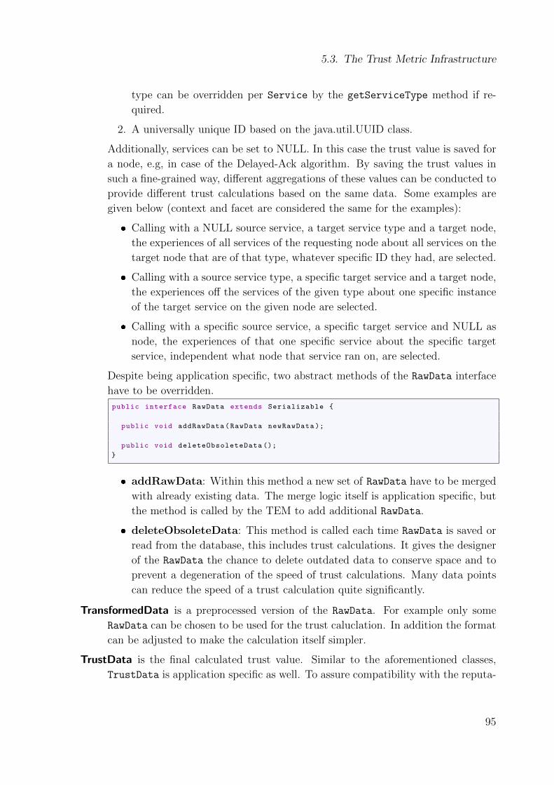
5.3. The Trust Metric Infrastructure
type can be overridden per Service by the getServiceType method if re-
quired.
2. A universally unique ID based on the java.util.UUID class.
Additionally, services can be set to NULL. In this case the trust value is saved for
a node, e.g, in case of the Delayed-Ack algorithm. By saving the trust values in
such a fine-grained way, different aggregations of these values can be conducted to
provide different trust calculations based on the same data. Some examples are
given below (context and facet are considered the same for the examples):
� Calling with a NULL source service, a target service type and a target node,
the experiences of all services of the requesting node about all services on the
target node that are of that type, whatever specific ID they had, are selected.
� Calling with a source service type, a specific target service and a target node,
the experiences off the services of the given type about one specific instance
of the target service on the given node are selected.
� Calling with a specific source service, a specific target service and NULL as
node, the experiences of that one specific service about the specific target
service, independent what node that service ran on, are selected.
Despite being application specific, two abstract methods of the RawData interface
have to be overridden.
public interface RawData extends Serializable {
public void addRawData(RawData newRawData );
public void deleteObsoleteData ();
}
� addRawData: Within this method a new set of RawData have to be merged
with already existing data. The merge logic itself is application specific, but
the method is called by the TEM to add additional RawData.
� deleteObsoleteData: This method is called each time RawData is saved or
read from the database, this includes trust calculations. It gives the designer
of the RawData the chance to delete outdated data to conserve space and to
prevent a degeneration of the speed of trust calculations. Many data points
can reduce the speed of a trust calculation quite significantly.
TransformedData is a preprocessed version of the RawData. For example only some
RawData can be chosen to be used for the trust caluclation. In addition the format
can be adjusted to make the calculation itself simpler.
TrustData is the final calculated trust value. Similar to the aforementioned classes,
TrustData is application specific as well. To assure compatibility with the reputa-
95
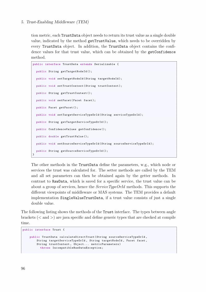
5. Trust-Enabling Middleware (TEM)
tion metric, each TrustData object needs to return its trust value as a single double
value, indicated by the method getTrustValue, which needs to be overridden by
every TrustData object. In addition, the TrustData object contains the confi-
dence values for that trust value, which can be obtained by the getConfidence
method.
public interface TrustData extends Serializable {
public String getTargetNodeId ();
public void setTargetNodeId(String targetNodeId );
public void setTrustContext(String trustContext );
public String getTrustContext ();
public void setFacet(Facet facet );
public Facet getFacet ();
public void setTargetServiceTypeOrId(String serviceTypeOrId );
public String getTargetServiceTypeOrId ();
public ConfidenceValues getConfidence ();
public double getTrustValue ();
public void setSourceServiceTypeOrId(String sourceServiceTypeOrId );
public String getSourceServiceTypeOrId ();
}
The other methods in the TrustData define the parameters, w.g., which node or
services the trust was calculated for. The setter methods are called by the TEM
and all set parameters can then be obtained again by the getter methods. In
contrast to RawData, which is saved for a specific service, the trust value can be
about a group of services, hence the ServiceTypeOrId methods. This supports the
different viewpoints of middleware or MAS systems. The TEM provides a default
implementation SingleValueTrustData, if a trust value consists of just a single
double value.
The following listing shows the methods of the Trust interface. The types between angle
brackets (< and >) are java specific and define generic types that are checked at compile
time.
public interface Trust {
public TrustData calculateDirectTrust(String sourceServiceTypeOrId ,
String targetServiceTypeOrId , String targetNodeId , Facet facet ,
String trustContext , Object ... metricParameters)
throws IncompatibleRawDataException;
96

5.3. The Trust Metric Infrastructure
public <R extends RawData , T extends TransformedData ,
U extends TrustData > U calculateDirectTrust(
String sourceServiceTypeOrId , String targetServiceTypeOrId ,
String targetNodeId , Facet facet , String trustContext ,
Transformer <R, T> transformer , Interpreter <T, U> interpreter ,
ConfidenceMetric confidenceMetric , Object ... metricParameters)
throws IncompatibleRawDataException;
public void calculateReputation(String sourceServiceTypeOrId ,
String targetServiceTypeOrId , String targetNodeId , Facet facet ,
String trustContext , long timeout ,
ReputationResultListener resultListener );
public void addRawData(String sourceNodeId , String sourceServiceId ,
String targetNodeId , String targetServiceId , Facet facet ,
String trustContext , RawData rawData)
throws IncompatibleRawDataException;
public List <RawData > getRawData(String sourceNodeId ,
String sourceServiceTypeOrId , String targetNodeId ,
String targetServiceTypeOrId , Facet facet , String trustContext );
public <R extends RawData , T extends TransformedData ,
U extends TrustData > void setTrustMetric(
String serviceType , Facet facet , String trustContext ,
Transformer <R, T> transformer , Interpreter <T, U> interpreter );
public <R extends RawData , T extends TransformedData ,
U extends TrustData > void setTrustMetric(
String serviceType , Facet facet , String trustContext ,
Transformer <R, T> transformer , Interpreter <T, U> interpreter ,
ConfidenceMetric confidenceMetric );
public Metric <? extends RawData , ? extends TransformedData ,
? extends TrustData > getTrustMetric(
String serviceType , Facet facet , String trustContext );
}
setTrustMetric: Sets a default metric to use for direct trust calculations. The metric
consists of a Transformer and an Interpreter, where the output type of the
Transformer needs to match the input type of the Interpreter, as well as the
confidence metric. The metric is set for the service type, facet and context. The
service type is defined by the getServiceType method of the Service interface.
Typically the fully qualified class name of the Service class is returned, but more
sophisticated types are also possible. By using the service type, every specific
instance of a Service uses the same Transformer and Interpreter.
calculateDirectTrust: This method enables the calculation of a direct trust value for
the services or the middleware. It comes in two versions: One additionally expects
the corresponding Transformerand Interpreter to use for the calculation, the
other tries to take the default ones set by the setTrustMetric method. Both
methods expect the following arguments:
� sourceServiceTypeOrId: This parameter defines, which of the service’s
97
5. Trust-Enabling Middleware (TEM)
data, that made the experiences, should be used for the trust calculation.
This can either be a specific instance of a service (e.g., a specific hash service),
a service type (e.g. a hash service), or NULL, if the experiences of all services
run on his node should be considered.
� targetServiceTypeOrId: This defines the service, about whom the trust
should be calculated. Either the calculation is about a specific service in-
stance, a service type or, if NULL, about the node itself.
� targetNodeId: This specifies the node ID of which the trust is calculated.
Either this specifies the node the service or service type is on, or is set to
NULL. In this case a trust value of a service aggregated over all the nodes it
was on is calculated.
� facet: The trust facet to use for the calculation. The RawData have to be
saved for this facet. Most of the time, applications use the facet credibility.
The Delayed-Ack algorithm uses the facet reliability.
� context: The context the trust is calculated in. Most of the time, the context
is NULL, since using the service in addition to the node is good enough. The
Delayed-Ack algorithm uses a specific context, since his experiences are on
node level, hence the services are NULL, and need to be distinguished from
the other experiences that might be saved on node level.
Giving less precise or none information on some of the aforementioned parameters
results in different aggregation levels for the trust calculation. On the one hand a
call with a specific targetServiceId and sourceServiceId as well as a NULL nodeId
calculates the trust based on the experience of a specific service, but independent
on what node that service was on in its lifetime, which is a typical call in a
Multi-Agent-System. On the other hand, a NULL for targetServiceTypeOrId, a
targetServiceType and a specific nodeId provides the trust value of a service type
on a node based on the experiences of every service on the requester node. Such
a request would give an estimation, how appropriate a node was so far for a
service type. By providing such a flexible request interface, every system view is
supported.
calculateReputation: With this method, a service can obtain reputation data of other
services or nodes. The calculateReputation method can be called in a similar
flexible way as the calculateDirectTrust methods. The method sends messages
to the node the trust value is requested of, who sends it to all its neighbors,
i.e., all nodes that interacted with the target node and therefore are expected to
have direct trust information. The TEM applies a Monitor to save all nodes that
were interacted with by observing outgoing messages and saving the IDs of the
target nodes. Then the direct trust value is calculated and returned to the original
98

5.3. The Trust Metric Infrastructure
node. These values are then used as input data for the Neighbor-Trust algorithm
described in Section 3.2.
Compared to calculating direct trust, this is an asynchronous method. This means
that the method can not wait until all results are returned, because, from the sight
of the calling node, the total number of results is not known, as well as the maximal
time such a request needs. Therefore the caller of the method has to provide
a timeout and an object, an implementation of the ReputationResultListener
interface, that can receive the result of the reputation calculation after the timeout
has elapsed.
public interface ReputationResultListener {
public void calculatedReputation
(SingleValueTrustData reputationData );
}
Figure 5.4 depicts the message flow of the method.
node1 node2
neighbor1
neighbor2
1: request
2: relay
2: relay
3: response
3: response
Figure 5.4.: Message flow on a reputation request
addRawData: Adds new RawData to the TEM. The data is saved to the identifiers
sourceService, targetService, targetNode, facet and context. If some RawData object
already exists for these identifiers, the addRawData method is called with the new
object and both experiences are merged. The merged object is then saved.
getRawData: Returns the RawData object for the identifiers described above.
An overview of the classes and interfaces used for trust calculations in the TEM, also
called the trust metric infrastructure (TMI), can be seen in Figure 5.5
99
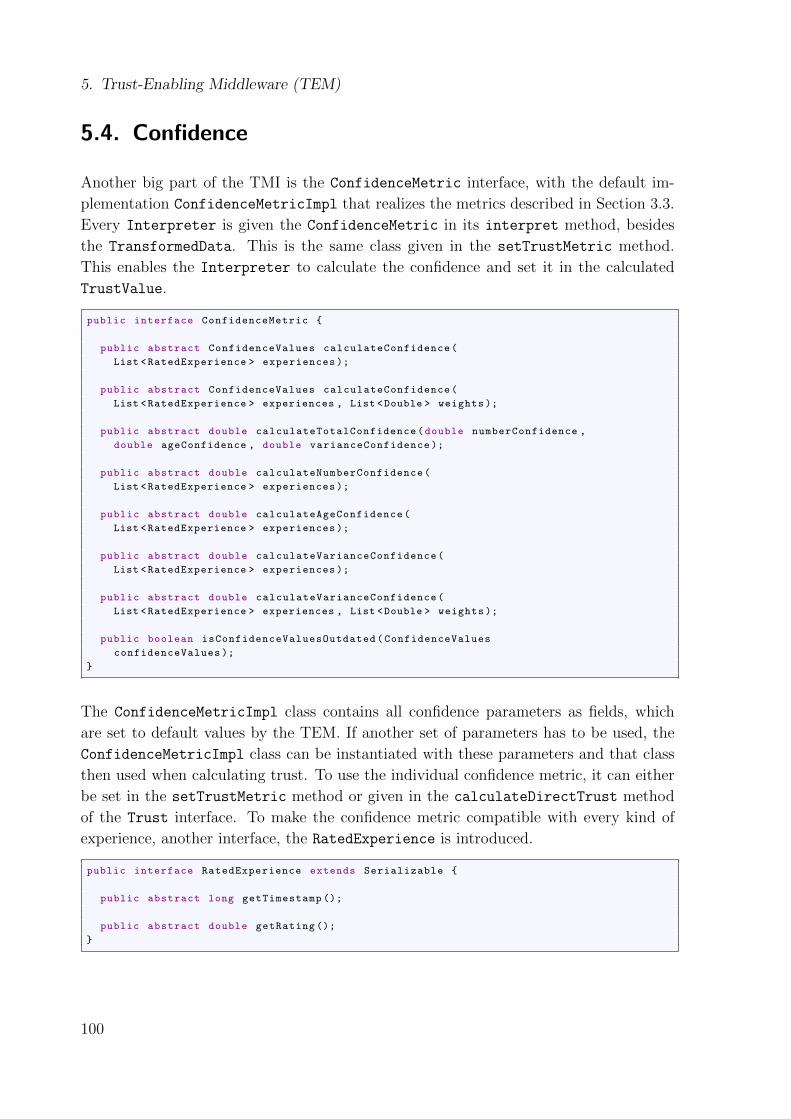
5. Trust-Enabling Middleware (TEM)
5.4. Confidence
Another big part of the TMI is the ConfidenceMetric interface, with the default im-
plementation ConfidenceMetricImpl that realizes the metrics described in Section 3.3.
Every Interpreter is given the ConfidenceMetric in its interpret method, besides
the TransformedData. This is the same class given in the setTrustMetric method.
This enables the Interpreter to calculate the confidence and set it in the calculated
TrustValue.
public interface ConfidenceMetric {
public abstract ConfidenceValues calculateConfidence(
List <RatedExperience > experiences );
public abstract ConfidenceValues calculateConfidence(
List <RatedExperience > experiences , List <Double > weights );
public abstract double calculateTotalConfidence(double numberConfidence ,
double ageConfidence , double varianceConfidence );
public abstract double calculateNumberConfidence(
List <RatedExperience > experiences );
public abstract double calculateAgeConfidence(
List <RatedExperience > experiences );
public abstract double calculateVarianceConfidence(
List <RatedExperience > experiences );
public abstract double calculateVarianceConfidence(
List <RatedExperience > experiences , List <Double > weights );
public boolean isConfidenceValuesOutdated(ConfidenceValues
confidenceValues );
}
The ConfidenceMetricImpl class contains all confidence parameters as fields, which
are set to default values by the TEM. If another set of parameters has to be used, the
ConfidenceMetricImpl class can be instantiated with these parameters and that class
then used when calculating trust. To use the individual confidence metric, it can either
be set in the setTrustMetric method or given in the calculateDirectTrust method
of the Trust interface. To make the confidence metric compatible with every kind of
experience, another interface, the RatedExperience is introduced.
public interface RatedExperience extends Serializable {
public abstract long getTimestamp ();
public abstract double getRating ();
}
100

5.4. Confidence
The interface needs to be implemented either by all experiences saved in RawData or
generated by the Transformer. It tells the confidence metric, when the experience
happened (getTimestamp) and rates each experience with a number between 0 and 1
(getRating). This information is sufficient for the confidence calculation and abstracts
the actual raw data that was used to calculate the trust value, making it useable for any
kind of data.
101

5. Trust-Enabling Middleware (TEM)
Re
pu
tati
on
Re
su
ltL
iste
ne
r
Tru
stS
erv
ice
Me
tric
Co
nfi
de
nc
eM
etr
ic
Sin
gle
Va
lue
Tru
stD
ata
Inte
rpre
ter
Co
nfi
de
nc
eM
etr
icIm
pl
Tra
ns
form
er
Ra
ted
Ex
pe
rie
nc
e
Co
nfi
de
nc
eV
alu
es
«e
nu
me
ratio
n»
Fa
ce
t
Ab
str
ac
tTru
stD
ata
Tra
ns
form
ed
Da
taR
aw
Da
taT
rus
tDa
ta
Tru
st
ho
lds in
da
tab
ase
*
0..
1
1
0..
1
0..
11
«u
se
»
sa
ve
s
*0..
1
exp
ects
1
1..
*
«u
se
»
cre
ate
s
*1
1
0..
1
exp
ects
1
1..
*
cre
ate
s
1
1..
*
cre
ate
s
11..
*
«u
se
»
«u
se
»
Figure 5.5.: Reduced class diagram of the trust metric infrastructure
102

6. Conclusion
In this work a framework to calculate trust in Organic Computing Systems was intro-
duced. The framework consists of metrics to calculate direct trust, confidence, reputa-
tion, as well as a metric to combine these three parts. In this thesis, trust encompasses
several facets, e.g., reliability and credibility, and can be applied to different contexts.
Therefore, most trust metrics were designed to support several kinds of systems, e.g, a
computing grid or energy grid. The direct trust metric Delayed-Ack gathers reliability
information of other nodes on middleware level, while the other parts, i.e., confidence,
reputation, and the aggregation of all, work for all trust facets, as long as a direct trust
metric is supplied. However, the metrics were mainly designed to improve the self-x
properties of Organic Computing Systems. In particular, this means that trust was
applied to a pure computational system without human participants.
In addition to the trust framework, the Trust-Enabling Middleware (TEM) was designed,
which allows services, that are hosted on nodes running the middleware, to exploit
the presented trust metrics. Services can also add their own trust metrics for direct
trust through a well defined interface. The TEM was developed in Java to be platform
independent, allowing it to even run on mobile devices supporting Java like Android
smartphones. The trust metrics, especially the Delayed-Ack algorithm to asses the
reliability of other nodes, are fully implemented. Together with the monitoring system
to observe the message flow and to add piggy-back information on application messages,
the TEM is ready to host trust-enhanced self-x algorithms.
Additionally, the importance of each part of the trust framework, i.e., direct trust,
confidence, and reputation has been evaluated, to gain the most benefit of a system. For
this, Automated Design Space Exploration (ADSE) with the help of a particle swarm
algorithm was applied. The use of ADSE was required due to the dimension of the
design space of ≈ 3.36 ∗ 1032 possible parameter settings. The most important aspect
of the evaluation was the change in behavior of the participants, when the benefit from
interacting with a participant changes for the worse and the system has to adapt. Beside
the impact of each trust metric, the turning point when switching from reputation to
direct trust when making the decision with whom to interact, was investigated. If there
is a specific point, when to change from reputation to direct trust. Or if there is a gray
zone, where both parts are important but the weight shifts slowly towards direct trust.
103

6. Conclusion
In experiments, one characteristic stood out: One parameter, the history length, dom-
inated the other twelve. The history length defines the amount of past experiences,
which are considered when calculating the trust values, be it direct trust or reputation.
Intuitively, one would expect to consider several experiences to get a good assessment of
someones’ behavior, yet a history length of two proved to be the best choice. By using
only the last two experiences, the system can adjust much faster to changing behavior,
while still maintaining a good enough estimation of the targets’ current behavior. With
the DTC metric, the influence of the other parameters was the strongest, reputation
(DTCR metric) mitigated most of the variance. This behavior could be observed in
nearly all scenarios, the DTC (direct trust and confidence) metric with only two behav-
ior changes being the only exception, where the other parameters where more important
than the history length. An explanation for this might be, that in a highly stable system,
where all participants stay true to their behavior nearly all of the time, the interaction
partners rarely need to adapt. Adding reputation reinstated the dominance of the his-
tory length again, though. And even with only eight behavior changes, the history length
is again dominant in all scenarios.
This leads to the conclusion, that exploiting the stable state of a system weights less than
a fast adaption to change. The opposite is only true if the time between changes, i.e., the
time of stability, is sufficiently long. So in a system showing high behavior fluctuation,
fast adaption is most important. A history length of two seems to be sufficient for
computational systems. In comparison, humans feel subjectively better if they can
resort to a larger amount of past experiences, regardless if that many experiences are
rationally required to asses the trustworthiness of an interaction partner.
Another prevalent effect in each scenario was a higher achieved cumulative benefit when
experience ratings were based on binary instead of continuous values, i.e., only 0 (bad
experience) or 1 (good experience) compared to values between 0 and 1. Intuitively,
this seems unexpected, since a continuous rating allows for a more precise estimation.
But combined with a preferable low history length, there are only three possible trust
values based on binary experience ratings: 0, 0.5, and 1. A trust value of 0 or 1 is
based on identical experiences (all 0 or all 1) and a strong indication that the next
experience will be the same, especially if the actual behavior of the interaction partner
is close to the extremes of 0 and 1. Since the goal of the interactions is to make as many
good experiences as possible, i.e., experiences rated with 1, a streak of good experiences
provides a good estimation about the future. At the same time, a short history length,
in this case two, gives the opportunity to adapt fast to a behavior change; see above.
It seems that a binary basis for experience ratings is preferable to continuous ratings.
However, the rating function depends on the underlying application. The Delayed-
Ack algorithm is suitable to be binary rated (0 for a lost message, 1 for a received
message). Other applications can only sensibly use continuous ratings, e.g., the energy
104

grid application. Here, the experience rating represents the divergence between a power
prediction and the actual power production of a power plant. This divergence requires
a continuous scale by nature.
Regarding the turning point between direct trust and reputation, the evaluations have
shown that a single point between these two can not be defined. Essentially the opposite
was the case. Reputation was still considered with high confidence, as well as direct trust
with low confidence. This means that both reputation and direct trust are considered
when assessing the trustworthiness of an interaction partner, with a steady shift from
reputation to direct trust when the confidence in one’s own experiences increases. This is
similar to how humans utilize trust. Preferences differ from person to person, and there
are extremes on both ends; but humans are still influenced by the recommendations
of others although they had their own experiences so far. This shows that computer
systems can profit from the inclusion of trust like humans.
A next step to research are the effects of a low history length. If the observed effect car-
ries over to other scenarios, or if a transfer to user trust is possible. An answer to these
questions could increase the insight of the trust concept. Within the field of Organic
Computing, the presented trust metrics are now ready to be integrated into the self-x
properties, including self-configuration, self-optimization, and self-healing. The consid-
eration of trust allows a differentiation of service importance, moving more important
services to more reliable nodes and, therefore, increasing the robustness of the system.
A degeneration of reliability of a node over time enables the self-configuration to predict
an impending node failure, which allows the application of preemptive measures, e.g.,
moving services from an endangered node, before it actually crashes.
Another important aspect is the robustness of the trust metrics themselves. When
integrated into the self-x properties, the robustness of the trust metrics is most important
and a manipulation by an attack can jeopardize the stability of the system. Marmol
and Perez [39] describe attacks on trust metrics and an evaluation of the metrics against
these attacks would be a logical next step.
105

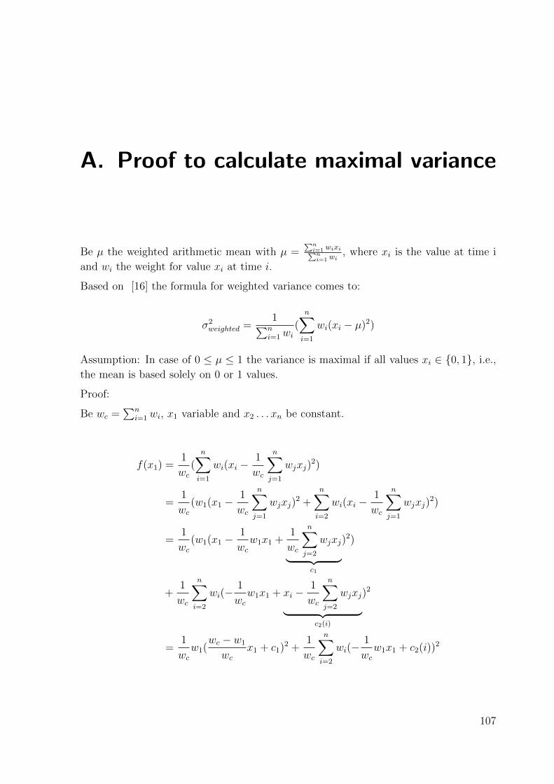
A. Proof to calculate maximal variance
Be µ the weighted arithmetic mean with µ =n
i=1 wixini=1 wi
, where xi is the value at time i
and wi the weight for value xi at time i.
Based on [16] the formula for weighted variance comes to:
σ2weighted =
1ni=1wi
(n
i=1
wi(xi − µ)2)
Assumption: In case of 0 ≤ µ ≤ 1 the variance is maximal if all values xi ∈ {0, 1}, i.e.,the mean is based solely on 0 or 1 values.
Proof:
Be wc =n
i=1wi, x1 variable and x2 . . . xn be constant.
f(x1) =1
wc
(n
i=1
wi(xi −1
wc
nj=1
wjxj)2)
=1
wc
(w1(x1 −1
wc
nj=1
wjxj)2 +
ni=2
wi(xi −1
wc
nj=1
wjxj)2)
=1
wc
(w1(x1 −1
wc
w1x1 +1
wc
nj=2
wjxj c1
)2)
+1
wc
ni=2
wi(−1
wc
w1x1 + xi −1
wc
nj=2
wjxj c2(i)
)2
=1
wc
w1(wc − w1
wc
x1 + c1)2 +
1
wc
ni=2
wi(−1
wc
w1x1 + c2(i))2
107

A. Proof to calculate maximal variance
1. Deviation:
f ′(x1) =1
wc
w12(wc − w1
wc
x1 + c1)wc − w1
wc
+1
wc
ni=2
wi2(−1
wc
w1x1 + c2(i))(−1
wc
w1)
=1
wc
w12(wc − w1)
2
w2c
x1 +1
wc
w12wc − w1
wc
c1 c3
+1
wc
ni=2
wi2(−w1
wc
)2x1 + wi2(−w1
wc
)c2(i)
=2w1(wc − w1)
2
w3c
x1 + c3 +1
wc
(wc − w1)2w2
1
w2c
x1 +1
wc
ni=2
wi2(−w1
wc
)c2(i) c4
=2w1(wc − w1)
2
w3c
x1 +2w2
1(wc − w1)
w3c
x1 + c3 + c4 c5
=2w1(wc − w1)((wc − w1) + w1)
w3c
x1 + c5
=2w1(wc − w1)
w2c
x1 + c5
2. Deviation:
f ′′(x1) =2w1
w2c
(wc − w1)
The 2nd deviation is > 0 for n > 1 and weights > 0. In case of n = 1 the sum of all
weights wc consists of only the first weight w1, therefore wc = w1, which results in 0 for
the second deviation. The same is true for weights equal to 0. Otherwise the second
deviation is always greater 0, regardless of the values of xi, resulting in an increasing
gradient of the original function. The maximum of the function is therefore at the limits
of the domain, in this case 0 or 1. Without loss of generality this conclusion applies to
all xi. Therefore the variance with all xi ∈ {0, 1} is maximal.
If all xi ∈ {0, 1} the weighted mean algorithm can be written as:
108

µmaxv =
{i∈X|xi=1}wixi +
{i∈X|xi=0}wixin
i=1wi
=
{i∈X|xi=1}win
i=1wi
=⇒ µmaxv
ni=1
wi =
{i∈X|xi=1}
wi
Also:
{i∈X|xi=0}
wi =n
i=1
wi −
{i∈X|xi=1}
wi
The weighted confidence formula has a similar special case for xi ∈ {0, 1}:
σ2 =1n
i=1wi
(
{i∈X|xi=1}
wi(1− µ)2 +
{i∈X|xi=0}
wi(0− µ)2)
=1n
i=1wi
(µn
i=1
wi(1− µ)2 + (n
i=1
wi − µn
i=1
wi)(0− µ)2))
= µ(1− µ)2 + (1− µ)(0− µ)2
= µ(1− 2µ+ µ2) + (1− µ)µ2
= µ− 2µ2 + µ3 + µ2 − µ3
= µ− µ2
In total the formula for the maximal variance is, with or without weights:
σ2 = µ− µ2
When all weights are set to 1, the weighted variance is equivalent to the normal variance,
therefore this formula holds true for normal variance as well.
109

List of Figures
1.1. Aggregating direct trust with confidence and reputation to a total trust
value including the corresponding metrics described in this work. . . . . . 15
2.1. A sample network using the TEM. . . . . . . . . . . . . . . . . . . . . . 18
3.1. The Delayed-Ack algorithm . . . . . . . . . . . . . . . . . . . . . . . . . 31
3.2. Loss of a message with a piggy-backed ack . . . . . . . . . . . . . . . . . 33
3.3. Enhanced Delayed-Ack: 100% reliable node observing another 50% reli-
able node . . . . . . . . . . . . . . . . . . . . . . . . . . . . . . . . . . . 35
3.4. Enhanced Delayed-Ack: 50% reliable node observing another 50% reliable
node . . . . . . . . . . . . . . . . . . . . . . . . . . . . . . . . . . . . . . 35
3.5. Enhanced Delayed-Ack: 50% reliable node observing another 50% reliable
node . . . . . . . . . . . . . . . . . . . . . . . . . . . . . . . . . . . . . . 36
3.6. Nodes in the reputation graph . . . . . . . . . . . . . . . . . . . . . . . . 37
3.7. Characteristics of the weight adjustment function of the neighbor-trust
reputation metric . . . . . . . . . . . . . . . . . . . . . . . . . . . . . . . 38
3.8. Reputation in a network with 30% malicious nodes . . . . . . . . . . . . 40
3.9. Reputation in a network with 50% malicious nodes . . . . . . . . . . . . 41
3.10. Reputation in a network with 70% malicious nodes . . . . . . . . . . . . 41
3.11. Reputation in a network with 50% malicious nodes and threshold 0.5 . . 42
3.12. an isolated node with 50% malicious nodes . . . . . . . . . . . . . . . . . 43
3.13. Illustration of f(z). . . . . . . . . . . . . . . . . . . . . . . . . . . . . . . 44
3.14. Illustration of cn(|X|). . . . . . . . . . . . . . . . . . . . . . . . . . . . . 45
3.15. Illustration of r(a). . . . . . . . . . . . . . . . . . . . . . . . . . . . . . . 45
3.16. Illustration of cv(X). . . . . . . . . . . . . . . . . . . . . . . . . . . . . . 46
3.17. maximal variance v . . . . . . . . . . . . . . . . . . . . . . . . . . . . . . 47
3.18. Confidence values of a single agent . . . . . . . . . . . . . . . . . . . . . 49
3.19. Average gain in benefit . . . . . . . . . . . . . . . . . . . . . . . . . . . . 51
3.20. Average difference between expected and real gain in benefit . . . . . . . 51
3.21. Illustration of f(confidence) = wc. . . . . . . . . . . . . . . . . . . . . . 52
4.1. Benefit versus history length for selection metric direct trust (DT) using
continuous experience ratings (8 behavior changes) . . . . . . . . . . . . 63
111

List of Figures
4.2. Benefit versus history length for selection metric direct trust and confi-
dence (DTC) using continuous experience ratings (8 behavior changes) . 64
4.3. Benefit versus history length for selection metric direct trust, confidence,
and reputation (DTCR) using continuous experience ratings (8 behavior
changes) . . . . . . . . . . . . . . . . . . . . . . . . . . . . . . . . . . . . 64
4.4. Best and worst observed results for each selection metric in comparison
with random (RAND) for history length 2 when using continuous expe-
rience ratings (8 behavior changes) . . . . . . . . . . . . . . . . . . . . . 65
4.5. Benefit versus history length for selection metric direct trust (DT) using
binary experience ratings (8 behavior changes) . . . . . . . . . . . . . . . 69
4.6. Benefit versus history length for selection metric direct trust and confi-
dence (DTC) using binary experience ratings (8 behavior changes) . . . . 69
4.7. Benefit versus history length for selection metric direct trust, confidence,
and reputation (DTCR) using binary experience ratings (8 behavior changes) 70
4.8. Best and worst results for each selection metric in comparison with ran-
dom (RAND) for history length 2 when using binary experience ratings
(8 behavior changes) . . . . . . . . . . . . . . . . . . . . . . . . . . . . . 70
4.9. Benefit versus history length for selection metric direct trust (DT) using
continuous experience ratings (only 2 behavior changes) . . . . . . . . . . 73
4.10. Benefit versus history length for selection metric direct trust and confi-
dence (DTC) using continuous experience ratings (only 2 behavior changes) 73
4.11. Benefit versus history length for selection metric direct trust, confidence,
and reputation (DTCR) using continuous experience ratings (only 2 be-
havior changes) . . . . . . . . . . . . . . . . . . . . . . . . . . . . . . . . 74
4.12. Best and worst observed results for each selection metric in comparison
with random (RAND) for history length 2 when using continuous expe-
rience ratings (only 2 behavior changes) . . . . . . . . . . . . . . . . . . . 74
4.13. Best and worst observed results for each selection metric in comparison
with random (RAND) for history length 3 when using continuous expe-
rience ratings (only 2 behavior changes) . . . . . . . . . . . . . . . . . . . 75
4.14. Benefit versus history length for selection metric direct trust (DT) using
binary experience ratings (only 2 behavior changes) . . . . . . . . . . . . 77
4.15. Benefit versus history length for selection metric direct trust and confi-
dence (DTC) using binary experience ratings (only 2 behavior changes) . 77
4.16. Benefit versus history length for selection metric direct trust, confidence,
and reputation (DTCR) using binary experience ratings (only 2 behavior
changes) . . . . . . . . . . . . . . . . . . . . . . . . . . . . . . . . . . . . 78
4.17. Best and worst observed results for each selection metric in comparison
with random (RAND) for history length 2 when using binary experience
ratings (only 2 behavior changes) . . . . . . . . . . . . . . . . . . . . . . 78
112

List of Figures
4.18. Best and worst observed results for each selection metric in comparison
with random (RAND) for history length 3 when using binary experience
ratings (only 2 behavior changes) . . . . . . . . . . . . . . . . . . . . . . 79
4.19. Benefit versus history length for selection metric direct trust (DT) using
continuous experience ratings (behavior changes every 50 time steps) . . 82
4.20. Benefit versus history length for selection metric direct trust and confi-
dence (DTC) using continuous experience ratings (behavior changes every
50 time steps) . . . . . . . . . . . . . . . . . . . . . . . . . . . . . . . . . 82
4.21. Benefit versus history length for selection metric direct trust, confidence,
and reputation (DTCR) using continuous experience ratings (behavior
changes every 50 time steps) . . . . . . . . . . . . . . . . . . . . . . . . . 83
4.22. Best and worst observed results for each selection metric in comparison
with random (RAND) for history length 2 when using continuous expe-
rience ratings (behavior changes every 50 time steps) . . . . . . . . . . . 83
4.23. Benefit versus history length for selection metric direct trust (DT) using
binary experience ratings (behavior changes every 50 time steps) . . . . . 85
4.24. Benefit versus history length for selection metric direct trust and confi-
dence (DTC) using binary experience ratings (behavior changes every 50
time steps) . . . . . . . . . . . . . . . . . . . . . . . . . . . . . . . . . . . 85
4.25. Benefit versus history length for selection metric direct trust, confidence,
and reputation (DTCR) using binary experience ratings (behavior changes
every 50 time steps) . . . . . . . . . . . . . . . . . . . . . . . . . . . . . 86
4.26. Best and worst observed results for each selection metric in comparison
with random (RAND) for history length 2 when using binary experience
ratings (behavior changes every 50 time steps) . . . . . . . . . . . . . . . 86
5.1. Life-cycle of a service . . . . . . . . . . . . . . . . . . . . . . . . . . . . . 88
5.2. Architecture of OCµ [55] . . . . . . . . . . . . . . . . . . . . . . . . . . . 89
5.3. Trust calculation process . . . . . . . . . . . . . . . . . . . . . . . . . . . 94
5.4. Message flow on a reputation request . . . . . . . . . . . . . . . . . . . . 99
5.5. Reduced class diagram of the trust metric infrastructure . . . . . . . . . 102
113


Bibliography
[1] G. Anders, F. Siefert, N. Msadek, R. Kiefhaber, O. Kosak, W. Reif, and T. Ungerer.
TEMAS – A Trust-Enabling Multi-Agent System for Open Environments. Technical
Report 2013-04, Universitat Augsburg, April 2013.
[2] G. Anders, F. Siefert, J.-P. Steghofer, and W. Reif. Trust-Based Scenarios – Pre-
dicting Future Agent Behavior in Open Self-Organizing Systems. In Proc. of the
7th International Workshop on Self-Organizing Systems (IWSOS 2013), May 2013.
[3] Y. Bernard, L. Klejnowski, E. Cakar, J. Hahner, and C. Muller-Schloer. Efficiency
and Robustness Using Trusted Communities in a Trusted Desktop Grid. In Self-
Adaptive and Self-Organizing Systems Workshops (SASOW), 2011 Fifth IEEE Con-
ference on, pages 21–26, October 2011.
[4] Y. Bernard, L. Klejnowski, J. Hahner, and C. Muller-Schloer. Towards Trust in
Desktop Grid Systems. In 10th IEEE/ACM International Conference on Cluster,
Cloud and Grid Computing (CCGrid), 2010, pages 637–642, May 2010.
[5] S. Brin and L. Page. The anatomy of a large-scale hypertextual web search engine.
In COMPUTER NETWORKS AND ISDN SYSTEMS, pages 107–117. Elsevier
Science Publishers B. V., 1998.
[6] R. Brunelli. Template Matching Techniques in Computer Vision: Theory and Prac-
tice. Wiley Publishing, 2009.
[7] G. C. Buttazzo. Hard Real-time Computing Systems: Predictable Scheduling Al-
gorithms And Applications (Real-Time Systems Series). Springer-Verlag TELOS,
Santa Clara, CA, USA, 2004.
[8] H. Calborean. Multi-Objective Optimization of Advanced Computer Architectures
using Domain-Knowledge. PhD thesis, Lucian Blaga University of Sibiu, Romania,
2011 (PhD Supervisor: Prof. Lucian Vintan, PhD), Sibiu, Romania, 2011.
[9] H. Calborean and L. Vintan. An automatic design space exploration framework for
multicore architecture optimizations. In Roedunet International Conference (RoE-
duNet), 2010 9th, pages 202–207, Sibiu, Romania, June 2010.
[10] H. Calborean and L. Vintan. Framework for Automatic Design Space Exploration
of Computer Systems. Acta Universitatis Cibiniensis Technical Series, May 2011.
115

Bibliography
[11] G. Caronni. Walking the web of trust. In 9th IEEE International Workshops
on Enabling Technologies: Infrastructure for Collaborative Enterprises (WETICE
2000), 4-16 June 2000, Gaithersburg, MD, USA, pages 153–158, 2000.
[12] B. Christianson and W. S. Harbison. Why isn’t trust transitive? In Proceedings
of the International Workshop on Security Protocols, pages 171–176, London, UK,
UK, 1997. Springer-Verlag.
[13] K. Deb, A. Pratap, S. Agarwal, and T. Meyarivan. A fast and elitist multiobjective
genetic algorithm: NSGA-II. Evolutionary Computation, IEEE Transactions on,
6(2):182–197, 2002.
[14] M. Deutsch. Cooperation and trust. some theoretical notes. In M. R. Jones, editor,
Nebraska Symposium on Motivation. McGraw-Hill Publishing, 1962.
[15] M. Dorigo, V. Maniezzo, and A. Colorni. Ant system: optimization by a colony of
cooperating agents. IEEE Transactions on Systems, Man, and Cybernetics, Part
B: Cybernetics, 26(1):29–41, 1996.
[16] T. Finch. Incremental calculation of weighted mean and variance. University of
Cambridge, 2009.
[17] I. Foster, C. Kesselman, and S. Tuecke. The anatomy of the grid: Enabling scalable
virtual organizations. Int. J. High Perform. Comput. Appl., 15(3):200–222, Aug.
2001.
[18] D. Gambetta. Can We Trust Trust?, chapter 13, pages 213–237. Basil Blackwell,
1990.
[19] A. Glassner. An Introduction to Ray Tracing. Academic Press. Academic Press,
1989.
[20] J. Golbeck and J. Hendler. FilmTrust: movie recommendations using trust in web-
based social networks. In 3rd IEEE Consumer Communications and Networking
Conference (CCNC 2006), volume 1, pages 282–286, 2006.
[21] J. A. Golbeck. Computing and applying trust in web-based social networks. PhD
thesis, University of Maryland, College Park, MD, USA, 2005.
[22] M. Hoffmann, M. Wittke, J. Hahner, and C. Muller-Schloer. Spatial partitioning in
self-organizing smart camera systems. J. Sel. Topics Signal Processing, 2(4):480–
492, 2008.
[23] J. H. Holland. Adaptation in natural and artificial systems. MIT Press, Cambridge,
MA, USA, 1992.
[24] P. Horn. Autonomic Computing: IBMs Perspective on the State of Information
Technology also known as ”‘IBM’s Autonomic Computing Manifesto”’. IBM Cor-
116

Bibliography
poration, pages 1–39, 2001.
[25] T. Huynh, N. R. Jennings, and N. Shadbolt. An integrated trust and reputation
model for open multi-agent systems. Journal of Autonomous Agents and Multi-
Agent Systems, 13(2):119–154, 2006.
[26] T. D. Huynh, N. R. Jennings, and N. R. Shadbolt. Fire: An integrated trust and
reputation model for open multi-agent systems. In R. L. de Mantaras and L. Saitta,
editors, Proceedings of the 16th Eureopean Conference on Artificial Intelligence,
ECAI’2004, including Prestigious Applicants of Intelligent Systems, PAIS 2004,
Valencia, Spain, August 22-27, 2004, pages 18–22. IOS Press, 2004.
[27] R. Jahr, H. Calborean, L. Vintan, and T. Ungerer. Finding near-perfect parameters
for hardware and code optimizations with automatic multi-objective design space
explorations. Concurrency and Computation: Practice and Experience, page n/a,
2012.
[28] U. Janen, H. Spiegelberg, L. Sommer, S. von Mammen, J. Brehm, and J. Hahner.
Object tracking as job-scheduling problem. In Proceedings of 7th ACM/IEEE In-
ternational Conference on Distributed Smart Cameras (ICDSC 2013), 2013.
[29] N. Johnson, S. Kotz, and N. Balakrishnan. Continuous univariate distributions.
Distributions in statistics. Wiley, 2. edition, 1995.
[30] S. D. Kamvar, M. T. Schlosser, and H. Garcia-Molina. The Eigentrust algorithm for
reputation management in P2P networks. In Proceedings of the 12th international
conference on World Wide Web, WWW ’03, pages 640–651, New York, NY, USA,
2003. ACM.
[31] J. O. Kephart and D. M. Chess. The vision of autonomic computing. IEEE Com-
puter, 36(1):41–50, 2003.
[32] R. Kiefhaber, G. Anders, F. Siefert, T. Ungerer, and W. Reif. Confidence as a
means to assess the accuracy of trust values. In G. Min, Y. Wu, L. C. Liu, X. Jin,
S. A. Jarvis, and A. Y. Al-Dubai, editors, Proceedings of the 11th IEEE Inter-
national Conference on Trust, Security and Privacy in Computing and Commu-
nications (TrustCom 2012), Liverpool, United Kingdom, June 25-27, 2012, pages
690–697, 2012.
[33] R. Kiefhaber, S. Hammer, B. Savs, J. Schmitt, M. Roth, F. Kluge, E. Andre, and
T. Ungerer. The neighbor-trust metric to measure reputation in organic computing
systems. In Fifth IEEE Conference on Self-Adaptive and Self-Organizing Systems
Workshops (SASO 2011), pages 41 – 46, october 2011.
[34] R. Kiefhaber, R. Jahr, N. Msadek, and T. Ungerer. Ranking of Direct Trust,
Confidence, and Reputation in an Abstract System with Unreliable Components. In
117

Bibliography
Proceedings of the 10th IEEE International Conference on Autonomic and Trusted
Computing (ATC 2013), Vietri sul Mare, Italy, December 18-20, 2013, 2013.
[35] R. Kiefhaber, B. Satzger, J. Schmitt, M. Roth, and T. Ungerer. The delayed ack
method to measure trust in organic computing systems. In Fourth IEEE Interna-
tional Conference on Self-Adaptive and Self-Organizing Systems Workshop (SASO
2010), pages 184 –189, september 2010.
[36] R. Kiefhaber, B. Satzger, J. Schmitt, M. Roth, and T. Ungerer. Trust measurement
methods in organic computing systems by direct observation. In IEEE/IFIP 8th
International Conference on Embedded and Ubiquitous Computing (EUC 2010),
pages 105 –111, december 2010.
[37] L. Klejnowski, Y. Bernard, G. Anders, C. Muller-Schloer, and W. Reif. Trusted
community - a trust-based multi-agent organisation for open systems. In J. Filipe
and A. L. N. Fred, editors, ICAART (1), pages 312–317. SciTePress, 2013.
[38] N. Luhmann. Trust and Power. John Wiley and Sons Ltd., 1979.
[39] F. G. Marmol and G. M. Perez. Security threats scenarios in trust and reputation
models for distributed systems. Computers & Security, 28(7):545–556, 2009.
[40] S. Marsh. Optimism and pessimism in trust. In In Proceedings of the Ibero-American
Conference on Artificial Intelligence (IBERAMIA 94). McGraw-Hill Publishing,
1994.
[41] S. P. Marsh. Formalising Trust as a Computational Concept. PhD thesis, University
of Stirling, April 1994.
[42] P. Massa and P. Avesani. Trust metrics on controversial users: balancing between
tyranny of the majority and echo chambers. International Journal on Semantic
Web and Information Systems, 2007.
[43] P. Mell and T. Grance. The nist definition of cloud computing. Technical Report
800-145, National Institute of Standards and Technology (NIST), Gaithersburg,
MD, September 2011.
[44] C. Muller-Schloer. Organic computing: on the feasibility of controlled emergence.
In A. Orailoglu, P. H. Chou, P. Eles, and A. Jantsch, editors, Proceedings of the
2nd IEEE/ACM/IFIP International Conference on Hardware/Software Codesign
and System Synthesis, CODES+ISSS 2004, Stockholm, Sweden, September 8-10,
2004, pages 2–5. ACM, 2004.
[45] A. Nebro, J. Durillo, J. Garcıa-Nieto, C. A. Coello, F. Luna, and E. Alba. SMPSO:
A new pso-based metaheuristic for multi-objective optimization. In Proceedings of
the IEEE Symposium Series on Computational Intelligence, pages 66–73, 2009.
[46] N. Nedjah and L. de Macedo Mourelle, editors. Swarm Intelligent Systems, vol-
118

Bibliography
ume 26 of Studies in Computational Intelligence. Springer, 2006.
[47] M. Nickschas and U. Brinkschulte. CARISMA - A Service-Oriented, Real-Time
Organic Middleware Architecture. Journal of Software, 4(7):654–663, 2009.
[48] H. Prothmann, S. Tomforde, J. Branke, J. Hahner, C. Muller-Schloer, and
H. Schmeck. Organic traffic control. In C. Muller-Schloer, H. Schmeck, and T. Un-
gerer, editors, Organic Computing – A Paradigm Shift for Complex Systems, vol-
ume 1 of Autonomic Systems, pages 431–446. Springer Basel, 2011.
[49] J. R. Quinlan. C4.5: Programs for Machine Learning (Morgan Kaufmann Series
in Machine Learning). Morgan Kaufmann, 1st edition, January 1993.
[50] M. Roth, J. Schmitt, R. Kiefhaber, F. Kluge, and T. Ungerer. Organic computing
middleware for ubiquitous environments. In C. Muller-Schloer, H. Schmeck, and
T. Ungerer, editors, Organic Computing – A Paradigm Shift for Complex Systems,
volume 1 of Autonomic Systems, pages 339–351. Springer Basel, 2011.
[51] J. Sabater and C. Sierra. Social ReGreT, a reputation model based on social rela-
tions. SIGecom Exch., 3(1):44–56, Dec. 2001.
[52] J. Sabater Mir. Trust and reputation for agent societies. PhD thesis, Universitat
Autonoma de Barcelona, 2002.
[53] B. Satzger, F. Mutschelknaus, F. Bagci, F. Kluge, and T. Ungerer. Towards trust-
worthy self-optimization for distributed systems. In S. Lee and P. Narasimhan,
editors, Software Technologies for Embedded and Ubiquitous Systems, volume 5860
of Lecture Notes in Computer Science, pages 58–68. Springer Berlin / Heidelberg,
2009.
[54] M. Schillo, P. Funk, and M. Rovatsos. Using trust for detecting deceitful agents in
artificial societies. Applied Artificial Intelligence, 14(8):825–848, 2000.
[55] J. Schmitt. Zweistufige, Planer-basierte Organic Computing Middleware. PhD the-
sis, University of Augsburg, 2013.
[56] J.-P. Steghofer, G. Anders, F. Siefert, and W. Reif. A system of systems approach
to the evolutionary transformation of power management systems. In Proceedings of
INFORMATIK 2013 – Workshop on “Smart Grids”, Lecture Notes in Informatics.
Bonner Kollen Verlag, 2013.
[57] J.-P. Steghofer, R. Kiefhaber, K. Leichtenstern, Y. Bernard, L. Klejnowski, W. Reif,
T. Ungerer, E. Andre, J. Hahner, and C. Muller-Schloer. Trustworthy organic
computing systems: Challenges and perspectives. In B. Xie, J. Branke, S. Sadjadi,
D. Zhang, and X. Zhou, editors, Autonomic and Trusted Computing, volume 6407
of Lecture Notes in Computer Science, pages 62–76. Springer Berlin / Heidelberg,
2010.
119
Bibliography
[58] A. von Renteln, U. Brinkschulte, and M. Pacher. The artificial hormone system -
an organic middleware for self-organising real-time task allocation. In C. Muller-
Schloer, H. Schmeck, and T. Ungerer, editors, Organic Computing – A Paradigm
Shift for Complex Systems, pages 369–384. Springer, 2011.
[59] S. W. Wilson. Classifier fitness based on accuracy. Evol. Comput., 3(2):149–175,
June 1995.
[60] M. J. Wooldridge and N. R. Jennings. Intelligent agents: Theory and practice. The
Knowledge Engineering Review, 10(2):115–152, 1995.
[61] M. Woolridge and M. J. Wooldridge. Introduction to Multiagent Systems. John
Wiley & Sons, Inc., New York, NY, USA, 2001.
[62] G. Zacharia. Trust management through reputation mechanisms. Applied Artificial
Intelligence, 14:881–907, 2000.
[63] C.-N. Ziegler and G. Lausen. Propagation models for trust and distrust in social
networks. Information Systems Frontiers, 7(4-5):337–358, Dec. 2005.
120