calculating anisotropic physical properties from texture data … · calculating anisotropic...

Calculating anisotropic physical properties from texture data using

the MTEX open-source package

DAVID MAINPRICE1*, RALF HIELSCHER2 & HELMUT SCHAEBEN3

1Geosciences Montpellier UMR CNRS 5243, Universite Montpellier 2,

34095 Montpellier Cedex 05, France2Fakultat fur Mathematik, Technische Universitat Chemnitz, 09126 Chemnitz, Germany3Mathematische Geologie und Geoinformatik, Institut fur Geophysik und Geoinformatik,

Technische Universitat Freiberg, 09596 Freiberg, Germany

*Corresponding author (e-mail: [email protected])

Abstract: This paper presents the background for the calculation of physical properties of anaggregate from constituent crystal properties and the texture of the aggregate in a coherentmanner. Emphasis is placed on the important tensor properties of 2nd and 4th rank with appli-cations in rock deformation, structural geology, geodynamics and geophysics. We cover textureinformation that comes from pole figure diffraction and single orientation measurements (electronbackscattered diffraction or EBSD, electron channelling pattern, Laue pattern, optical microscopeuniversal-stage). In particular, we provide explicit formulae for the calculation of the averagedtensor from individual orientations or from an orientation distribution function (ODF). For thelatter we consider numerical integration and an approach based on the expansion into sphericalharmonics. This paper also serves as a reference paper for the mathematical tensor capabilitiesof the texture analysis software MTEX, which is a comprehensive, freely available MatLabtoolbox that covers a wide range of problems in quantitative texture analysis, for example, ODFmodelling, pole figure to ODF inversion, EBSD data analysis and grain detection. MTEX offersa programming interface which allows the processing of involved research problems as wellas highly customizable visualization capabilities; MTEX is therefore ideal for presentations,publications and teaching demonstrations.

The estimation of physical properties of crystallineaggregates from the properties of the componentcrystals has been subject of extensive literaturesince the classical work of Voigt (1928) and Reuss(1929). Such an approach is only feasible if thebulk properties of the crystals dominate the physicalproperty of the aggregate and the effects of grain-boundary interfaces can be ignored. For example,the methods discussed here cannot be applied tothe electrical properties of water-saturated rock,where the role of interfacial conduction is likely tobe important. Many properties of interest to earthand materials scientists can be evaluated from theknowledge of the single-crystal tensors and theorientation distribution function (ODF) of crystalsin an aggregate, for example, thermal diffusivity,thermal expansion, diamagnetism and elastic wavevelocities.

The majority of rock-forming minerals havestrongly anisotropic physical properties and manyrocks also have strong crystal preferred orientations(CPOs, or textures as they are called in materialsscience; these terms are used interchangeably in

this paper as no possible confusion can result inpresent context) that can be described conciselyin a quantitative manner by the orientationdistribution function ODF. The combination ofstrong CPOs and anisotropic single-crystal pro-perties results in a three-dimensional variation inrock properties. Petrophysical measurements areusually made under hydrostatic pressure and oftenat high temperatures to simulate conditions in theEarth, where presumably the micro-cracks presentat ambient conditions are closed. The necessity towork at high pressure and temperature conditionslimits the number of orientations that can bemeasured. Typically, three orthogonal directionsare measured parallel to structural features, suchas the lineation and foliation normal defined bygrain shape. The evaluation of physical propertiesfrom CPO allows the determination of propertiesover the complete orientation sphere of the speci-men reference frame.

This paper is designed as a reference paperfor earth and material scientists who want to usethe texture analysis software MTEX to compute

From: Prior, D. J., Rutter, E. H. & Tatham, D. J. (eds) Deformation Mechanisms, Rheology and Tectonics:Microstructures, Mechanics and Anisotropy. Geological Society, London, Special Publications, 360, 175–192.DOI: 10.1144/SP360.10# The Geological Society of London 2011. Publishing disclaimer: www.geolsoc.org.uk/pub_ethics

http://www.geolsoc.org.uk/pub_ethics

physical tensor properties of aggregates fromconstituent crystal properties and the texture ofthe aggregate. MTEX is a comprehensive, freelyavailable MatLab toolbox that covers a wide rangeof problems in quantitative texture analysis, forexample: ODF modelling, pole figure to ODF inver-sion, electron backscatter diffraction (EBSD) dataanalysis and grain detection. The MTEX toolboxcan be downloaded from http://mtex.googlecode.com. Unlike many other texture analysis software,it offers a programming interface which allows forthe efficient processing of complex research pro-blems in the form of scripts (M-files). The MatLabenvironment provides a wide variety of high-qualitygraphics file formats to aid publication and displayof the results. In addition the MTEX toolbox willwork identically on Microsoft Windows, AppleMac OSX and Linux platforms in 32 and 64 bitmodes with a simple installation procedure.

In MTEX texture analysis information such asODFs, EBSD data and pole figures are representedby variables of different types. For example, inorder to define a unimodal ODF with half-width108, preferred orientation 108, 208, 308 Eulerangles and cubic crystal symmetry, the command

myODF = unimodalODF(orientation(’Euler’,10*degree, 20*degree,30*degree),... symmetry (’cubic’), ’halfwidth’,10*degree)

is issued which generates a variable myODF of typeODF, displayed as

myODF = ODFspecimen symmetry: tricliniccrystal symmetry : cubic

Radially symmetric portion:kernel: de la Vallee Poussin, hw = 10center: (10, 20, 30)weight: 1

We will use this style of displaying input and outputto make the syntax of MTEX as clear as possible.Note that there is also an exhaustive interactivedocumentation included in MTEX, which explainsthe syntax of each command in detail.

The outline of the paper is as follows. In the firstsection the basics of tensors mathematics and crystalgeometry are briefly described and presented interms of MTEX commands. In the second sectionthese basics are discussed for some classicalsecond-order tensors and the elasticity tensors.In particular, we give a comprehensive overviewabout elastic properties that can be computeddirectly from the elastic stiffness tensor. All calcu-lations are accompanied by the correspondingMTEX commands. In the third section we areconcerned with the calculation of average mattertensors from their single-crystal counterparts and

the texture of the aggregate. Here we consider tex-tures given by individual orientation measurements,which lead to the well-known Voigt, Reuss and Hillaverages, as well as textures given by ODFs, whichlead to formulae involving integrals over the orien-tation space. We can compute these integrals inseveral ways: either we use known quadraturerule, or we compute the expansion of the rotatedtensor into generalized spherical harmonics andapply Parseval’s theorem. Explicit formulae forthe expansion of a tensor into generalized sphericalharmonics and a proof that the order of the tensordefines the maximum order of this expansion isincluded in the Appendix.

Tensor mathematics and crystal geometry

In what follows we give the necessary backgroundto undertake physical property calculation forsingle crystals, without the full mathematical devel-opments that can be found elsewhere (e.g. Nye1985). We will restrict ourselves to linear physicalproperties, which are properties that can bedescribed by a linear relationship between causeand effect such as stress and strain for linearelasticity.

Tensors

Mathematically, a tensor T of rank r is a r-linearmapping which can be represented by anr-dimensional matrix Ti1,i2,...,ir . A rank zero tensoris simply a scalar value, a rank-one tensor Ti is avector and a rank-two tensor Tij has the form of amatrix. Linearity means that the tensor applied to rvectors x1, . . . , xr [ R3, defines a mapping

(x1, . . . , xr) −�∑3

i1=1

∑3

i2=1

· · ·∑3

ir=1

Ti1 ,..., irx1

i1· · · xr

ir

which is linear in each of the arguments x1, . . . , xr .Physically, tensors are used to describe linear inter-actions between physical properties. In the simplestcase, scalar properties are modelled by rankzero tensor whereas vector fields (i.e. direction-dependent properties) are modelled by rank-onetensors. An example for a second-rank tensor isthe thermal conductivity tensor kij which describesthe linear relationship between the negative temp-erature gradient −gradT = −(∂T

∂x1, ∂T∂x2

, ∂T∂x3

), that is afirst-order tensor, and the heat flux q = (q1, q2, q3)per unit area which is also a first-order tensor. Thelinear relationship is given by the equality

qi = −∑3

j=1

kij

∂T

∂xj

, i = 1, . . . , 3,

D. MAINPRICE ET AL.176

and can be seen as a matrix vector product of thethermal conductivity tensor kij interpreted as amatrix and the negative temperature gradient inter-preted as a vector. In the present example the nega-tive temperature gradient is called applied tensorand the heat flux is called induced tensor.

In the general case, we define a rank r tensorTi1,...,ir inductively as the linear relationshipbetween two physical properties which are mod-elled by a rank s tensor A j1, j2, ..., js and a rank ttensor Bk1,k2,...,kt

, such that the equation r = t + s issatisfied. The rank of a tensor is therefore given bythe rank of the induced tensor plus the rank of theapplied tensor. The linear dependency between theapplied tensor A and the induced tensor B is givenby the tensor product

Bk1,...,kt=

∑3

j1=1

∑3

j1=1

· · ·∑3

js=1

Tk1 ,k2 ,..., kt , j1,..., jsA j1,..., js

= Tk1,k2,..., kt , j1,..., js A j1 ,..., js .

In the right-hand side of the last equationwe used the Einstein summation convention andomitted the sum sign for every two equal indexes;this will be default in all further formulae.

In MTEX a tensor is represented by a variable oftype tensor. In order to create such a variable, ther-dimensional matrix has to be specified. As anexample we consider the 2nd rank stress tensorsij, which can be defined by

M = [[1.45 0.00 0.19];...[0.00 2.11 0.00];...[0.19 0.00 1.79]];

sigma = tensor (M, ’name’, ’stress’,’unit’, ’MPa’);

sigma = stress tensor (size: 3 3)rank: 2unit: MPa

1.45 0.00 0.190.00 2.11 0.000.19 0.00 1.79

Furthermore, we defined the normal�n = (1, 0, 0) to plane by

n = vector3d (1,0,0)n = vector3d (size: 1 1)

x y z1 0 0

According to Cauchy’s stress principle, thestress vector T�n associated with the plane normal �nis then computed by

T�nj = sij �ni .

In MTEX this equation may be written as

T = EinsteinSum (sigma, [-1 1], n, -1,’unit’, ’MPa’)

T = tensor (size: 3)unit: MParank: 1

1.4500.19

Note that the 21 in the arguments of the com-mand EinsteinSum indicates the dimen-sion which has to be summed up and the 1 inthe argument indicates that the second dimensionof s becomes the first dimension of T. Usingthe stress vector T�n, the scalar magnitudes ofthe normal stress sN and the shear stress sS aregiven as

sN = T�ni �ni = sij �ni �nj and sS =

��T�n

i T�ni − s2

N

√.

In MTEX the corresponding calculation reads as

sigmaN = double (EinsteinSum (T, -1, n,-1))

sigmaS = sqrt (double(EinsteinSum (T, -1,T, -1))2 sigma N^2)

sigmaN = 1.4500sigmaS = 0.1900

The crystal reference frame

Tensors can be classified into two types: mattertensors describing physical properties such aselectrical or thermal conductivity, magnetic per-meability, etc. of a crystalline specimen, and fieldtensors describing applied forces such as stress,strain or a electric field to a specimen. Furthermore,it is important to distinguish between single-crystaltensors describing constituent crystal propertiesand tensors describing averaged macroscopic prop-erties of a polycrystalline specimen. While the refer-ence frame for the latter is the specimen coordinatesystem, the reference frame for single-crystaltensor properties is unambiguously connected tothe crystal coordinate system. The reference framesand their conventions are explained below. We willrestrict ourselves to tensors of single or polycrystalsdefined in a Cartesian reference frame comprising

the three unit vectors �XT , �YT , �ZT . The use of anorthogonal reference frame for single crystalsavoids the complications of the metric associatedwith the crystal unit cell axes. In any case, almostall modern measurements of physical propertytensors are reported using Cartesian referenceframes.

ANISOTROPIC PHYSICAL PROPERTIES 177

We next discuss how the single-crystal tensorreference frame is defined using the crystal coordi-nate system. In the general case of triclinic crystalsymmetry, the crystal coordinate system is specifiedby its axis lengths a, b, c and inter-axial angles a, b,g resulting in a non-Euclidean coordinate system�a, �b, �c for the general case. In order to align the

Euclidean tensor reference frame �XT , �YT , �ZT inthe crystal coordinate system, several conventionsare in use. The most common conventions are sum-marized in Table 1.

In MTEX the alignment of the crystal referenceframe is defined together with the symmetry groupand the crystal coordinate system. All this infor-mation is stored in a variable of type symmetry.For example by

cs_tensor = symmetry(’triclinic’ [5.29],9.18, 9.42],...[90.4, 98.9, 90.1]* degree, ’X||a*’,’Z||c’, ’mineral’, ’Talc’);

cs_tensor = symmetry(size: 1)

mineral : Talc

symmetry : triclinic (2 1)a, b, c : 5.3, 9.2, 9.4alpha, beta, gamma : 90.4, 98.9, 90.1reference frame : X||a*, Z||c

we store in the variable cs_tensor the geometryof Talc which has triclinic crystal symmetry, axislengths 5.29, 9.18, 9.42, inter-axial angles 90.48,98.98, 90.18 and the convention for a Cartesianright-handed tensor reference frame �X||�a∗, �Z||�c;

we therefore have �Y = �Z × �X for the alignment ofthe crystal reference frame. In order to define acrystal constituent property tensor with respect tothis crystal reference frame, we append the variablecs_tensor to its definition, that is,

M = [[219.83 59.66 -4.82 -0.82 -33.87-1.04];...[59.66 216.38 -3.67 1.79 -16.51-0.62];...[-4.82 -3.67 48.89 4.12 -15.52-3.59];...[-0.82 1.79 4.12 26.54 -3.60-6.41];...[-33.87 -16.51 -15.52 -3.60 22.85-1.67];...[-1.04 -0.62 -3.59 -6.41 -1.6778.29]];

C = tensor(M, ’name’, ’elastic stiffness,’unit’, ’GPa’, cs_tensor)

C = elastic stiffness tensor(size : 3 3 3 3)unit: GParank: 4

mineral: Talc (triclinic, X||a*, Z||c)

tensor in Voigt matrix representation219.83 59.66 -4.82 -0.82 -33.87 -1.0459.66 216.38 -3.67 1.79 -16.51 -0.62-4.82 -3.67 48.89 4.12 -15.52 -3.59-0.82 1.79 4.12 26.54 -3.60 -6.41

-33.87 -16.51 -15.52 -3.60 22.85 -1.67-1.04 -0.62 -3.59 -6.41 -1.67 78.29

defines the elastic stiffness tensor in GPa of Talc.This example will be discussed in greater detail inthe section ‘Elasticity tensors’.

Crystal orientations

Let �Xc, �Yc, �Zc be a Euclidean crystal coordi-nate system assigned to a specific crystal and let�Xs, �Ys, �Zs be a specimen coordinate system. Inpolycrystalline materials, the two coordinatesystems generally do not coincide. Their relativealignment describes the orientation of the crystalwithin the specimen. More specifically, the orien-tation of a crystal is defined as the (active) rotationg that rotates the specimen coordinate system intocoincidence with the crystal coordinate system.From another point of view, the rotation g can bedescribed as the basis transformation from thecrystal coordinate system to the specimen coordi-nate system. Let �h = (h1, h2, h3) be the coordinatesof a specific direction with respect to the crys-tal coordinate system. Then �r = (r1, r2, r3) = g�hare the coordinates of the same direction withrespect to the specimen coordinate system.

Crystal orientations are typically defined byEuler angles, either by specifying rotations with

Table 1. Alignment of the crystal reference framefor the tensors of physical properties of crystals. Thenotation �a, �b, �c, �m corresponds to crystallographicdirections in the direct lattice space, whereas thenotation �a∗ , �b∗ , �c∗ denotes the correspondingdirections in the reciprocal lattice space, which areparallel to the normal to the plane written as ⊥a for�a∗, etc. Note that there are at least two possiblereference choices for all symmetries exceptorthorhombic, tetragonal and cubic

Crystal symmetries �XT �YT �ZT

Orthorhombic,tetragonal, cubic

�a �b �c

Trigonal, hexagonal �a �m �c�m −�a �c

Monoclinic �a∗ �b �c�a �b �c∗

Triclinic �a∗ �ZT × �XT �c�a �ZT × �XT �c∗�YT × �ZT �b

∗�c

�YT × �ZT �b �c∗


angles f1, F, f2 about the axes Zs, Xs, Zs (Bungeconvention) or with angles a, b, g about the axesZs, Ys, Zs (Matthies convention). Both conventions,and also some others, are supported in MTEX. Inorder to define an orientation in MTEX we start byfixing the crystal reference frame �Xc, �Yc, �Zc usedfor the definition of the orientation,

cs_orientation = symmetry(’triclinic’[5.29], 9.18, 9.42],...[90.4, 98.9, 90.1]* degree, ’X||a*’,’Z||c’, ’mineral’, ’Talc’);

cs_orientation = crystal symmetry(size: 1)

mineral : talcsymmetry : triclinic (-1)a, b, c : 5.3, 9.2, 9.4alpha, beta, gamma: 90.4, 98.9, 90.1reference frame : X||a, Z||c*

Now an orientation can be defined as a variable oftype orientation, it is common practice to use theletter g to denote an orientation, derived from theGerman word Gefuge used by Sander (1911).

g = orientation (’Euler’, 10*degree,20*degree, 5*degree, ’Bunge’,cs_orientation)

g = orientation (size : 1 1)mineral : talccrystal symmetry : triclinic, X||a,

Z||c*specimen symmetry: triclinic

Bunge Euler angles in degreephi1 Phi phi210 20 5

Note that for the definition of an orientation thecrystal reference frame is crucial. The definitionof the variable of type orientation thereforeincludes a variable of type symmetry, storing therelevant information. This applies in particular ifthe orientation data (i.e. Euler angles) are importedfrom third-party measurement systems such asEBSD and associated software with their ownspecific conventions for �Xc, �Yc, �Zc, which shouldbe defined when using the MTEX import wizard.

In order to demonstrate the coordinate transformbetween the crystal and the specimen coordinatesystem, we choose a crystal direction in the recipro-cal lattice �h = h �a∗ +kb∗ + ℓc∗ (pole to a plane) bydefining a variable of type Miller:

h = Miller (1, 1, 0, cs_orientation, ’hkl’)h = Miller (size: 1 1)

mineral : talc (triclinic, X||a,Z||c*)

h 1k 1l 0

and express it in terms of the specimen coordinatesystem for a specific orientation g ¼ (108, 208, 58)

r = g * hr = vector3d (size: 1 1),

x y z0.714153 0.62047 0.324041

The resulting variable is of type vector3d reflect-ing that the new coordinate system is the specimencoordinate system. Note that in order that the coor-dinate transformation rule makes sense physically,the corresponding crystal reference frames usedfor the definition of the orientation and the crystaldirection by Miller indices must coincide. Alterna-tively, a crystal direction �u = u�a + v�b + w�c indirect space can be specified:

u = Miller (1, 1, 0, cs_orientation, ’uvw’)h = Miller (size: 1 1), uvw

mineral: talc (triclinic, X||a,Z||c*)

u 1v 1w 0

and expressed in terms of the specimen coordinatesystem

r = g * ur = vector3d (size: 1 1),

x y z0.266258 0.912596 0.310283

This obviously gives a different direction, sincedirect and reciprocal space do not coincide for tricli-nic crystal symmetry.

The relationship between the single-crystal

physical property and Euler angle reference

frames

Let us consider a rank r tensor Ti1,...,ir describingsome physical property of a crystal with respectto a well-defined crystal reference frame�XT , �YT , �ZT . We are often interested in expressingthe tensor with respect to another, differentEuclidean reference frame �X, �Y , �Z, which might be

(1) a crystallographically equivalent crystal refer-ence frame,

(2) a different convention for aligning the Eucli-dean reference frame to the crystal coordinatesystem or

(3) a specimen coordinate system.

Let us first consider a vector �h that has the represen-tation

�h = hT1�XT + hT

2�YT + hT

3�XT


with respect to the tensor reference frame

�XT , �YT , �ZT , and the representation

�h = h1�X + h2

�Y + h3�X

with respect to the other reference frame �X, �Y , �Z.Then the coordinates hT

1 , hT2 , hT

3 and h1, h2, h3

satisfy the transformation rule

h1

h2

h3

⎛⎝

⎞⎠ =

�X · �XT �X · �YT �X · �ZT

�Y · �XT �Y · �YT �Y · �ZT

�Z · �XT �Z · �YT �Z · �ZT

⎛⎝

⎞⎠

︸︷︷︸=:R

hT1

hT2

hT3

⎛⎝

⎞⎠,

(1)

that is, the matrix R performs the coordinate trans-formation from the tensor reference frame�XT , �YT , �ZT to the other reference frame �X, �Y , �Z.The matrix R can also be interpreted as the rotationmatrix that rotates the second reference frameinto coincidence with the tensor reference frame.Considering hT

j to be a rank-one tensor, the trans-formation rule becomes

hi = hTj Rij.

This formula generalizes to arbitrary tensors. LetTT

i1 ,...,irbe the coefficients of a rank r tensor with

respect to the crystal reference frame XT, YT, ZT

and let Ti1,...,ir be the coefficients with respectto another reference frame X, Y , Z. Then thelinear orthogonal transformation law for Cartesiantensors states that

Ti1,...,ir = TTj1 ,..., jr

Ri1 j1 · · ·Rirjr. (2)

Let us now examine the three cases for a newreference frame as mentioned at the beginning ofthis section. In the case of a crystallographicallyequivalent reference frame, the coordinate trans-form R is a symmetry element of the crystal andthe tensor remains invariant with respect to thiscoordinate transformation, that is T i1,...,ir = Ti1 ,...,ir .

In the case that the other reference frame �X, �Y , �Zfollows a different convention in aligning to thecrystal coordinate system, the transformed tensorT i1 ,...,ir is generally different to the original tensor.In MTEX this change of reference frame is carriedout by the command set. Let us consider theelastic stiffness tensor Cijkl of talc (as definedabove) as:

C = elastic stiffness tensor (size: 3 3 3 3)unit: GParank: 4

mineral: talc (triclinic, X||a*, Z||c)

219.83 59.66 -4.82 -0.82 -33.87 -1.0459.66 216.38 -3.67 1.79 -16.51 -0.62-4.82 -3.67 48.89 4.12 -15.52 -3.59-0.82 1.79 4.12 26.54 -3.60 -6.41-33.87 -16.51 -15.52 -3.60 22.85 -1.67-1.04 -0.62 -3.59 -6.41 -1.67 78.29

and let us consider the reference frame cs_orienta-tion as defined in the previous section

cs_orientation = symmetry(Size : 1)mineral : talcsymmetry : triclinic (-1)a, b, c : 5.29, 9.18, 9.42alpha, beta, gamma: 90.4, 98.9, 90.1reference frame : X||a, Z||c*

Then the elastic stiffness tensor Cijkl of talc withrespect to the reference frame cs_orientationis computed by setting cs_orientation as thenew reference frame, that is

C_orientation = set(C, ’CS’,cs_orientation)

C_orientation = elastic stiffness tensor(size: 3 3 3 3)

unit: GParank: 4

mineral: talc (triclinic, X||a, Z||c*)

tensor in Voigt matrix representation231.82 63.19 -5.76 0.76 -4.31 -0.5963.19 216.31 -7.23 2.85 -5.99 -0.86-5.76 -7.23 38.92 2.23 -16.69 -4.30.76 2.85 2.23 25.8 -4.24 1.86-4.31 -5.99 -16.69 -4.24 21.9 -0.14-0.59 -0.86 -4.3 1.86 -0.14 79.02

Finally, we consider the case that the second refer-ence frame is not aligned to the crystal coordinatesystem but to the specimen coordinate system.According to the previous section, the coordinatetransform then defines the orientation g of thecrystal and equation (2) tells us how the tensor hasto be rotated according to the crystal orientation.In this case we will write

Ti1,...,ir = TTj1,..., jr

(g)

= TTj1,..., jr

Ri1 j1 (g) · · · Rirjr (g), (3)

to express the dependency of the resulting tensorfrom the orientation g. Here Rirjr

(g) is the rotationmatrix defined by the orientation g. In orderto apply equation (3), it is of major importancethat the tensor reference frame and the crystal refer-ence frame used for describing the orientationcoincide. If they do not coincide, the tensor has tobe transformed to the same crystal reference frameused for describing the orientation. When working


with tensors and orientation data it is thereforealways necessary to know the tensor referenceframe and the crystal reference frame used fordescribing the orientation. In practical applicationsthis is not always a simple task, as this informationis sometimes hidden by the commercial EBSDsystems.

If the corresponding reference frames are speci-fied in the definition of the tensor as well as in thedefinition of the orientation, MTEX automaticallychecks for coincidence and performs the necessarycoordinate transforms if they do not coincide.Eventually, the rotated tensor for an orientationg ¼ (108, 208, 58) is computed by the commandrotate:

C_rotated = rotate (C,g)C_rotated = elastic_stifness tensor(size: 3 3 3 3)unit: GParank: 4

tensor in Voigt matrix representation228.79 56.05 1.92 19.99 -13.82 6.8556.05 176.08 11.69 50.32 -7.62 4.421.92 11.69 43.27 5.28 -19.48 2.3319.99 50.32 5.28 43.41 -1.74 0.24-13.82 -7.62 -19.48 -1.74 29.35 17.346.85 4.42 2.33 0.24 17.34 73.4

Note, that the resulting tensor does not contain anyinformation on the original mineral or referenceframe; this is because the single-crystal tensor isnow with respect to the specimen coordinatesystem and can be averaged with any other elasticstiffness tensor from any other crystal of any com-position and orientation.

Single-crystal anisotropic properties

We now present some classical properties of singlecrystals that can be described by tensors (cf. Nye1985).

Second-rank tensors

A typical second-rank tensor describes the relation-ship between an applied vector field and an inducedvector field, such that the induced effect is equal tothe tensor property multiplied by the applied vector.Examples of such a tensor are

† the electrical conductivity tensor, where theapplied electric field induces a field of currentdensity,

† the dielectric susceptibility tensor, where theapplied electric field intensity induces electricpolarization,

† the magnetic susceptibility tensor, where theapplied magnetic field induces the intensity ofmagnetization,

† the magnetic permeability tensor, where theapplied magnetic field induces magneticinduction,

† the thermal conductivity tensor, where the appliednegative temperature gradient induces heat flux.

As a typical example for a second-rank tensor weconsider the thermal conductivity tensor k,

k =k11 k12 k13

k21 k22 k23

k31 k32 k33

⎛⎝

⎞⎠

=

− ∂x1

∂Tq1 − ∂x2

∂Tq1 − ∂x2

∂Tq1

− ∂x1

∂Tq2 − ∂x2

∂Tq2 − ∂x2

∂Tq2

− ∂x1

∂Tq3 − ∂x2

∂Tq3 − ∂x2

∂Tq3

⎛⎜⎜⎜⎜⎜⎝

⎞⎟⎟⎟⎟⎟⎠

which relates the negative temperature gradient−gradT = −(∂T/∂x1, ∂T/∂x2, ∂T/∂x3) to the heatflux q = (q1, q2, q3) per unit area by

qi = −∑3

j=1

kij

∂T

∂xj

= −kij

∂T

∂xj

. (4)

In the present example the applied vector is thenegative temperature gradient and the inducedvector is the heat flux. Furthermore, we see thatthe relating vector is built up as a matrix wherethe applied vector is the denominator of the rowsand the induced vector is the numerator ofcolumns. We see that the tensor entries kij describethe heat flux qi in direction Xi given a thermal gradi-ent ∂T/∂xj in direction Xj.

As an example we consider the thermal conduc-tivity of monoclinic orthoclase (Hofer & Schilling2002). We start by defining the tensor referenceframe and the tensor coefficients in W m21 K21.

cs-tensor = symmetry(’monoclinic’,[8.561, 12.996, 7.192] ,...[90, 116.01, 90]*degree, ’mineral’,’orthoclase’,’Y||b’,’Z||c’);

M = [[1.45 0.00 0.19];...[0.00 2.11 0.00];...[0.19 0.00 1.79]];

Now the thermal conductivity tensor k isdefined by

k = tensor (M, ’name’, ’thermal_conductivity’, unit’, ’W_1/m_1/K’,cs_tensor)

k = thermal conductivity tensor (size: 3 3)unit : W 1/m 1/Krank : 2mineral: orthoclase (monoclinic,

X||a*, Y||b, Z||c)


1.45 0 0.190 2.11 00.19 0 1.79

Using the thermal conductivity tensor k we cancompute the thermal flux q in W m22 for a tempera-ture gradient in K m21:

gradT = Miller(1,1,0, cs_tensor, ’uvw’)gradT = Miller (size: 1 1), uvw

mineral: orthoclase (monoclinic,X||a*, Y||b, Z||c)

u 1v 1w 0

by equation (4). In MTEX, this becomes

q = EinsteinSum(k, [1 -1],gradT, -1,’name’, ’thermal_flux’, ’unit’, ’W_1/m^2’)

q = thermal flux tensor (size: 3)unit : W 1/m^2rank : 1mineral: orthoclase (monoclinic,

X||a*, Y||b, Z||c)0.6721.7606-0.3392

Note that the 21 in the arguments of the commandEinsteinSum indicates the dimension which hasto be summed up and the 1 in the argument indicatesthat the first dimension of k becomes the first dimen-sion of q; see equation (4).

A second-order tensor kij can be visualized byplotting its magnitude R(�x) in a given direction �x,

R(�x) = kij �xi �xj .

In MTEX the magnitude in a given direction �xcan be computed via

x = Miller (1,0,0, cs_tensor, ’uvw’);R = EinsteinSum (k, [-1 -2],x,- 1,x,- 2)R = tensor (size:)

rank : 0mineral: orthoclase (monoclinic,

X||a*, Y||b, Z||c)

1.3656

Again, the negative arguments 21 and 22 indicatewhich dimensions have to be multiplied andsummed up. Alternatively, we can use thecommand magnitude,

R = directionalMagnitude (k, x)

Since in MTEX the directional magnitude is thedefault output of the plot command, the code

plot(k)colorbar

plots the directional magnitude of k with respect toany direction �x as shown in Figure 1. Note that, bydefault, the X axis is plotted in the north direction,the Y axis is plotted in the west direction and the Zaxis is at the centre of the plot. This default alignmentcan be changed by the commands plotx2north,plotx2east, plotx2south, plotx2west.

When the tensor k is rotated the directional mag-nitude rotates accordingly. This can be checked inMTEX by

g = orientation(’Euler’,10*degree,20*degree,30*degree,cs_tensor);

k_rot = rotate(k,g);Plot(k_rot)

min:1.37

max:2.1

Z

Y

X

1.4

1.5

1.6

1.7

1.8

1.9

2

2.1

min:1.37

max:2.1

1.4

1.5

1.6

1.7

1.8

1.9

2

2.1

Fig. 1. The thermal conductivity k of orthoclase visualized by its directionally varying magnitude for left: the tensor instandard orientation and right: the rotated tensor.


The resulting ploat is shown in Figure 1.Furthermore, from the directional magnitude we

observe that the thermal conductivity tensor k issymmetric, that is, kij = k ji. This implies that thethermal conductivity is an axial or non-polar prop-erty, which means that the magnitude of heat flowis the same in positive or negative crystallographicdirections.

We want to emphasize that there are alsosecond-rank tensors which do not describe therelationship between an applied vector field and aninduced vector field but relate, for instance, azero-rank tensor to a second-rank tensor. Thethermal expansion tensor a, defined

aij =∂1ij

∂T,

is an example of such a tensor which relates a smallapplied temperature change ∂T (a scalar orzero-rank tensor) to the induced strain tensor 1ij (asecond-rank tensor). The corresponding coefficientof volume thermal expansion becomes

1

V

∂V

∂T= aii.

This relationship holds true only for smallchanges in temperature. For larger changes in temp-erature, higher-order terms have to be considered(see Fei 1995 for data on minerals). This alsoapplies to other tensors.

Elasticity tensors

We will now present fourth-rank tensors, but restrictourselves to the elastic tensors. Let sij be thesecond-rank stress tensor and let 1kl be thesecond-rank infinitesimal strain tensor. Thenthe fourth-rank elastic stiffness tensor Cijkl describesthe stress sij induced by the strain 1kl, defined

sij = Cijkl1kl, (5)

which is known as Hooke’s law for linear elasticity.Alternatively, the fourth-order elastic compliancetensor Sijkl describes the strain 1kl induced by thestress sij, defined

1kl = Sijklsij.

The above definitions may also be written as

Cijkl =∂sij

∂1kl

and Sijkl =∂1kl

∂sij

.

In the case of static equilibrium for the stresstensor and infinitesimal deformation for the strain

tensor, both tensors are symmetric, that is,sij = s ji and 1ij = 1 ji. For the elastic stiffnesstensor, this implies the symmetry

Cijkl = Cijlk = C jikl = C jilk

reducing the number of independent entries of thetensor from 34¼ 81 to 36. Since the elastic stiffnessCijkl is related to the internal energy U of a body by

Cijkl =∂

∂1kl

∂U

∂1ij

( ),

assuming constant entropy, we obtain by theSchwarz integrability condition that allows theinterchanging of the order of partial derivatives ofa function:

Cijkl =∂

∂1kl

∂U

∂1ij

( )= ∂2U

∂1ij∂1kl

( )= ∂2U

∂1kl∂1ij

( )= Cklij.

Hence,

Cijkl = Cklij

which further reduces the number of independententries from 36 to 21 (e.g. Mainprice 2007). These21 independent entries may be efficiently rep-resented in the form of a symmetric 6 × 6 matrixCmn, m, n = 1, . . . , 6 as introduced by Voigt(1928). The entries Cmn of this matrix representationequal the tensor entries Cijkl whenever m and n cor-respond to ij and kl according to:

m or n 1 2 3 4 5 6

ij or kl 11 22 33 23, 32 13, 31 12, 21

The Voigt notation is used for published compila-tions of elastic tensors (e.g. Bass 1995; Isaak 2001).

In a similar manner, a Voigt representationSmn is defined for the elastic compliance tensorSijkl. However, there are additional factors whenconverting between the Voigt Smn matrix represen-tation and the tensor representation Sijkl. Moreprecisely, for ij, kl, m, n which correspond toeach other according to the above table, we havethe identities:

Sijkl

= P · Smn,

P = 1, if both m, n = 1, 2, 3

P = 12, if either m or n are 4, 5, 6

P = 14, if both m, n = 4, 5, 6

⎧⎪⎨⎪⎩

⎫⎪⎬⎪⎭


Using the Voigt matrix representation of theelastic stiffness tensor (equation (5)) may bewritten as

s11

s22

s33

s23

s13

s12

⎛⎜⎜⎜⎜⎜⎜⎝

⎞⎟⎟⎟⎟⎟⎟⎠ =

C11 C12 C13 C14 C15 C16

C21 C22 C23 C24 C25 C26

C31 C32 C33 C34 C35 C36

C41 C42 C43 C44 C45 C46

C51 C52 C53 C54 C55 C56

C61 C62 C63 C64 C65 C66

⎛⎜⎜⎜⎜⎜⎜⎝

⎞⎟⎟⎟⎟⎟⎟⎠

×

111

122

133

2123

2113

2112

⎛⎜⎜⎜⎜⎜⎜⎝

⎞⎟⎟⎟⎟⎟⎟⎠.

The matrix representation of Hooke’s law allowsfor a straightforward interpretation of the tensorcoefficients Cij. For example the tensor coefficientC11 describes the dependency between normalstress s11 in direction X and axial strain 111 in thesame direction. The coefficient C14 describes thedependency between normal stress s11 in directionX and shear strain 2123 = 2132 in direction Y inthe plane normal to Z. The dependency betweennormal stress s11 and axial strains 111, 122 and 133

along X, Y and Z is described by C11, C12 and C13,whereas the dependencies between the normalstress s11 and shear strains 2123, 2113 and 2112 aredescribed by C14, C15 and C16. These effects aremost important in low-symmetry crystals, such astriclinic and monoclinic crystals, where there are alarge number of non-zero coefficients.

In MTEX the elasticity tensors may be specifieddirectly in Voigt notation as we have already seen inthe ‘Tensor mathematics and crystal geometry’section. Alternatively, tensors may also be importedfrom ASCII files using a graphical interface calledimport wizard in MTEX.

Let C be the elastic stiffness tensor for talc inGPa as defined in ‘The crystal reference frame’section.

C = elastic_stiffness tensor(size: 3 3 3 3)unit : GParank : 4mineral: talc (triclinic, X||a*, Z||c)

tensor in Voigt matrix representation219.83 59.66 -4.82 -0.82 -33.87 -1.0459.66 -216.38 -3.67 1.79 -16.51 -0.62-4.82 -3.67 48.89 4.12 -15.52 -3.59-0.82 1.79 4.12 26.54 -3.6 -6.41-33.87 -16.51 -15.52 -3.6 22.85 -1.67-1.04 -0.62 -3.59 -6.41 -1.67 78.29

The elastic compliance S in GPa21 can then becomputed by inverting the tensor C.

S = inv(C)S = elastic compliance tensor

(size: 3 3 3 3)unit : 1/GParank : 4mineral: talc (triclinic, X||a*,

Z||c)

tensor in Voigt matrix (×1023)representation

6.91 -0.83 4.71 0.74 6.56 0.35-0.83 5.14 1.41 -0.04 1.72 0.084.71 1.41 30.31 -0.13 14.35 1.030.74 -0.04 -0.13 9.94 2.12 0.866.56 1.72 14.35 2.12 21.71 1.020.35 0.08 1.03 0.86 1.02 3.31

Elastic properties

The fourth-order elastic stiffness tensor Cijkl andfourth-order elastic compliance tensor Sijkl are thestarting point for the calculation of a number ofelastic anisotropicphysical properties, which include

† Young’s modulus,† shear modulus,† Poisson’s ratio,† linear compressibility,† compressional and shear elastic wave velocities,† wavefront velocities,† mean sound velocities,† Debye temperature,

and, of course, their isotropic equivalents. In thefollowing we provide a short overview of theseproperties.

Scalar volume compressibility. First we consider thescalar volume compressibility b. Using the fact thatthe change of volume is given in terms of the straintensor 1ij by

∂V

V= 1ii,

we determine, for hydrostatic or isotropic pressure(which is given by the stress tensor skl = −Pdkl),that the change of volume is given by

∂V

V= −PSiikk.

The volume compressibility is therefore

b = − ∂V

V

1

P= Siikk.

Linear compressibility. The linear compressibilityb(x) of a crystal is the strain, that is the relativechange in length ∂l/l, for a specific crystallographic


direction x when the crystal is subjected to a unitchange in hydrostatic pressure −Pdkl. From

∂l

l= 1ijxixj = −PSiikkxixj

we conclude

b(x) = − ∂l

l

1

P= Sijkkxixj.

Young’s modulus. Young’s modulus E is the ratio ofthe axial (longitudinal) stress to the lateral (trans-verse) strain in a tensile or compressive test. Aswe have seen earlier when discussing the elasticstiffness tensor, this type of uniaxial stress isaccompanied by lateral and shear strains as well asthe axial strain. Young’s modulus in direction x isgiven by

E(x) = (Sijklxixjxkxl)−1.

Shear modulus. Unlike Young’s modulus, the shearmodulus G in an anisotropic medium is definedusing two directions: the shear plane h and theshear direction u. For example, if the shear stresss12 results in the shear strain 2112 then the corre-sponding shear modulus is G = s12/2112. FromHooke’s law we have

112 = S1212s12 + S1221s21,

and hence G = (4S1212)−1. The shear modulus for anarbitrary, but orthogonal, shear plane h and sheardirection u is given by

G(h, u) = (4Sijklhiujhkul)−1.

Poisson ratio. The anisotropic Poisson ratio isdefined by the elastic strain in two orthogonal direc-tions: the longitudinal (or axial) direction x and thetransverse (or lateral) direction y. The lateral strainis defined by −1ijyiyj along y and the longitudinalstrain by 1ijxixj along x. The anisotropic Poissonratio n(x, y) is given as the ratio of lateral to longi-tudinal strain (Sirotin & Shakolskaya 1982) as

n(x, y) = − 1ijyiyj

1klxkxl

= − Sijklxixjykyl

Smnopxmxnxoxp

.

The anisotropic Poisson ratio has recently beenreported for talc (Mainprice et al. 2008) and hasbeen found to be negative for many directions atlow pressure.

Wave velocities. The Christoffel equation, first pub-lished by Christoffel (1877), can be used to calculateelastic wave velocities and the polarizations in ananisotropic elastic medium from the elastic stiffnesstensor Cijkl or, more straightforward, from the Chris-toffel tensor Tik which is, for a unit propagationdirection �n, defined by

Tik(�n) = Cijkl �nj �nl .

Since the elastic tensors are symmetric, we have

Tik(�n) = Cijklnjnl = C jikl �nj �nl = Cijlk �nj �nl

= Cklij �nj �nl = Tki(�n),

and hence the Christoffel tensor T(�n) is symmetric.The Christoffel tensor is also invariant upon thechange of sign of the propagation direction, as theelastic tensor is not sensitive to the presence orabsence of a centre of crystal symmetry (being acentro-symmetric physical property).

Because the elastic strain energy 1/2Cijkl 1ij1kl

of a stable crystal is always positive and real (e.g.Nye 1985), the eigenvalues l1, l1 and l3 of theChristoffel tensor Tik(�n) are real and positive.They are related to the wave velocities Vp, Vs1 andVs2 of the plane P-, S1- and S2-waves propagatingin the direction �n by the formulae

Vp =��l1

r

√, Vs1 =

��l2

r

√, Vs2 =

��l3

r

√,

where r denotes the material density. The threeeigenvectors of the Christoffel tensor are the polar-ization directions, also called vibration, particlemovement or displacement vectors, of the threewaves. As the Christoffel tensor is symmetric, thethree polarization directions are mutually perpen-dicular. In the most general case there are no par-ticular angular relationships between polarizationdirections p and the propagation direction �n.However, the P-wave polarization direction is typi-cally nearly parallel and the two S-waves polariz-ations are nearly perpendicular to the propagationdirection. They are termed quasi-P or quasi-Swaves. The S-wave velocities may be identifiedunambiguously by their relative velocity Vs1 . Vs2.

All the elastic properties mentioned in thissection have direct expressions in MTEX:

beta = volumeCompressibility (C)beta = linearCompressibility (C,x)

E = YoungsModulus (C,x)G = shearModulus (C,h,u)

nu = PoissonRatio (C,x,y)T = ChristoffelTensor (C,n)


Note that all these commands take the compli-ance tensor C as basis for the calculations. For thecalculation of the wave velocities the commandvelocity

[vp, vs1, vs2, pp, ps1, ps2] = velocity(C,x ,rho)

allows for the computation of the wave velocitiesand the corresponding polarization directions.

Visualization

In order to visualize the above quantities, MTEXoffers a simple, yet flexible, syntax. Let us demon-strate it using the Talc example of the previoussection. In order to plot the linear compressibilityb(�x) or Young’s Modulus E(�x) as a function of thedirection �x, we use the commands

plot (C, ’PlotType’,’linearCompressibility’)

plot (C, ’PlotType’, ’YoungsModulus’)

The resulting plots are shown in Figure 2.Next we want to visualize the wave velocities

and the polarization directions. Let us start withthe P-wave velocity in km s21 which is plotted by

rho = 2.78276;plot (C, ’PlotType’, ’velocity’, ’vp’,

’density’, rho)

Note that we had to pass the density rho in g cm23 tothe plot command. We now want to plot the P-wavepolarization directions on top, so use the commands

hold on and hold off to prevent MTEX from clearingthe output window:

hold onplot(C, ’PlotType’, ’velocity’, ’pp’,

’density’, rho);hold off

The result is shown in Figure 3. Instead ofonly specifying the variables to plot, we can alsoperform simple calculations. From the commands

plot (C, ’PlotType’, ’velocity’,’200*(vs1-vs2)./(vs1+vs2)’,’density’, rho);

hold onplot (C, ’PlotType’, ’velocity’, ’ps1’,


the S-wave anisotropy in percent is plotted togetherwith the polarization directions of the fastest S-waveps1. Another example illustrating the flexibility ofthe system is the following plot of the velocityratio Vp/Vs1 together with the direction of theS1-wave polarizations.

plot (C, ’PlotType’, ’velocity’,’vp./vs1’, ’density’, rho);

hold onplot (C, ’PlotType’, ’velocity’,’ps1’,


Anisotropic properties of polyphase

aggregates

In this section we are concerned with the problemof calculating average physical properties of

min:−0.0025

max:0.05

Z

Y

X

0

0.005

0.01

0.015

0.02

0.025

0.03

0.035

0.04

0.045

min:17

max:213

Z

Y

X

20

40

60

80

100

120

140

160

180

200

Fig. 2. Left: the linear compressibility in GPa21 and right: Young’s modulus in GPa for talc.


polyphase aggregates. To this end, two ingredientsare required for each phase p:

(1) the property tensor Tpi1,...,ir

describing the phys-ical behaviour of a single crystal in the refer-ence orientation,

(2) the orientation density function (ODF) f p(g)describing the volume portion DV/V ofcrystals having orientation g or a representa-tive set of individual orientations gm,m = 1, . . . , M (e.g. measured by EBSD).

As an example we consider an aggregate composedof two minerals (glaucophane and epidote) usingdata from a blueschist from the Ile de Groix,France. The corresponding crystal reference framesare defined by

cs_glaucophane = symmetry (’2/m’,[9.5334, 17.7347, 5.3008],[90.00,103.597, 90.00] * degree, ’mineral’,’glaucophane’);

cs_epidote = symmetry (’2/m’, [8.8877,5.6275, 10.1517],[90.00, 115.383,90.00] * degree, ’mineral’,’epidote’);

For glaucophane the elastic stiffness was measuredby Bezacier et al. (2010) who provided the tensor

C_glaucophane = tensor (size: 3 3 3 3)rank : 4

mineral: glaucophane (2/m, X||a*,Y||b, Z||c)

tensor in Voigt matrix representation122.28 45.69 37.24 0 2.35 045.69 231.5 74.91 0 -4.78 037.24 74.91 254.57 0 -23.74 00 0 0 79.67 0 8.892.35 -4.78 -23.74 0 52.82 00 0 0 8.89 0 51.24

For epidote, the elastic stiffness was measuredby Aleksandrov et al. (1974):

C_epidote = tensor (size: 3 3 3 3)rank : 4mineral: epidote (2/m, X||a*, Y||b,

Z||c)

tensor in Voigt matrixrepresentation

211.5 65.6 43.2 0 -6.5 065.6 239 43.6 0 -10.4 043.2 43.6 202.1 0 -20 00 0 0 39.1 0 -2.3-6.5 -10.4 -20 0 43.4 00 0 0 -2.3 0 79.5

Computing the average tensor from

individual orientations

We start with the case that we have individual orien-tation data gm, m ¼ 1, . . ., M, that is, from EBSD orU-stage measurements, and volume fractionsVm, m ¼ 1, . . ., M. The best-known averaging tech-niques for obtaining estimates of the effective prop-erties of aggregates are those developed for elasticconstants by Voigt (1887, 1928) and Reuss (1929).The Voigt average is defined by assuming that theinduced tensor (in broadest sense, includingvectors) field is everywhere homogeneous or con-stant, that is, the induced tensor at every positionis set equal to the macroscopic induced tensor ofthe specimen. In the classical example of elasticity,the strain field is considered constant. The Voigtaverage is sometimes called the ‘series’ averageby analogy with Ohm’s law for electrical circuits.

The Voigt average specimen effective tensorkTlVoigt

is defined by the volume average of the indi-vidual tensors T(gc

m) with crystal orientations gcm and

volume fractions Vm:

kTlVoigt =∑M

m=1

VmT(gcm).

min:3.94

max:9.1 4

4.5

5

5.5

6

6.5

7

7.5

8

8.5

9(a) (b) (c)

P-wave velocity

min:0.2

max:86

10

20

30

40

50

60

70

80

S-wave anisotropy

min:1

max:1.7

1.1

1.2

1.3

1.4

1.5

1.6

1.7

Vp/Vs1 ratio

Fig. 3. Wave velocities of a Talc crystal plotted on seismic colour maps: (a) P-wave velocity together with the P-wavepolarization direction; (b) S-wave anisotropy in percent together with the S1-wave polarization direction; and(c) the ratio of Vp/Vs1 velocities together with the S1-wave polarization direction.


Contrarily, the Reuss average is defined byassuming that the applied tensor field is everywhereconstant, that is, the applied tensor at every positionis set equal to the macroscopic applied tensor of thespecimen. In the classical example of elasticity, thestress field is considered constant. The Reussaverage is sometimes called the ‘parallel’ average.The specimen effective tensor kTlReuss

is definedby the volume ensemble average of the inverses ofthe individual tensors T−1(gc

m):

kTlReuss =∑M

m=1

VmT−1(gcm)

[ ]−1

.

The experimentally measured tensor of aggre-gates is generally between the Voigt and Reussaverage bounds as the applied and induced tensorfields distributions are expected to be betweenuniform induced (Voigt bound) and uniformapplied (Reuss bound) field limits. Hill (1952)observed that the arithmetic mean of the Voigt andReuss bounds

kTlHill = 12(kTlVoigt + kTlReuss

),

sometimes called the Hill or Voigt–Reuss–Hill(VRH) average, is often close to experimentalvalues for the elastic fourth-order tensor. Althoughthe VRH average has no theoretical justification, itis widely used in earth and materials sciences.

In the example outlined above of an aggregateconsisting of glaucophane and epidote, we consideran EBSD dataset measured by Bezacier et al.(2010). In MTEX such individual orientation dataare represented by a variable of type EBSD whichis generated from an ASCII file containing the indi-vidual orientation measurements by the command:

ebsd = loadEBSD (’FileName’,{cs_glaucophane, cs_epidote})

ebsd = EBSD (Groix_A50_5_stitched. ctf)

properties: bands, bc, bs, error, madphase orientations mineral symmetry

crystal reference frame1 055504 glaucophane 2/m X||a*,

Y||b, Z||c2 63694 epidote 2/m X||a*, Y||b,

Z||c

It should be noted that for both minerals the crystalreference frames have to be specified in thecommand loadEBSD.

The Voigt, Reuss and Hill average tensors cannow be computed for each phase separately by thecommand calcTensor:

[TVoigt, TReuss, THill] = calcTensor(ebsd, C_epidote, ’phase’, 2)

C_Voigt = tensor (size: 3 3 3 3)rank: 4

tensor in Voigt matrix representation215 55.39 66.15 -0.42 3.02 -4.6955.39 179.04 59.12 1.04 -1.06 0.0666.15 59.12 202.05 0.94 1.16 -0.77-0.42 1.04 0.94 60.67 -0.86 -0.553.02 -1.06 1.16 -0.86 71.77 -0.65-4.69 0.06 -0.77 -0.55 -0.65 57.81

C_Reuss = tensor (size: 3 3 3 3)rank: 4

tensor in Voigt matrix representation201.17 56.48 65.94 -0.28 3.21 -4.6856.48 163.39 61.49 1.23 -1.58 -0.1365.94 61.49 189.67 1.29 0.75 -0.64-0.28 1.23 1.29 52.85 -0.99 -0.383.21 -1.58 0.75 -099 65.28 -0.6-4.68 -0.13 -0.64 -0.38 -0.6 50.6

C_Hill = tensor (size: 3 3 3 3)rank: 4

tensor in Voigt matrix representation208.09 55.93 66.05 -0.35 3.11 -4.6955.93 171.22 60.31 1.13 -1.32 -0.0466.05 60.31 195.86 1.11 0.96 -0.71-0.35 1.13 1.11 56.76 -0.93 -0.463.11 -1.32 0.96 -0.93 68.52 -0.62-4.69 -0.04 -0.71 -0.46 -0.62 54.21

If no phase is specified and all the tensors for allphases are specified, the command

[TVoigt, TReuss, THill] = calcTensor(ebsd, C_glaucophane, C_epidote)

computes the average over all phases. These calcu-lations have been validated using the CarewareFORTRAN code (Mainprice 1990). We emphasizethat MTEX automatically checks for the agreementof the EBSD and tensor reference frames for allphases. In case different conventions have beenused, MTEX automatically transforms the EBSDdata into the convention of the tensors.

Computing the average tensor from an ODF

Next we consider the case that the texture is givenby an ODF f. The ODF may originate from texturemodelling (Bachmann et al. 2010), pole figureinversion (Hielscher & Schaeben 2008) or densityestimation from EBSD data (Hielscher et al.2010). All these diverse sources may be handledby MTEX.

Given an ODF f, the Voigt average kTlVoigtof a

tensor T is defined by the integral

kTlVoigt =∫

SO(3)

T(g)f (g)dg (6)


whereas the Reuss average kTlReussis defined as

kTlReuss =∫

SO(3)

T−1(g)f (g)dg

[ ]−1

. (7)

Equations (6) and (7) can be computed in twodifferent ways. First, we can use a quadrature rule:for a set of orientations gm and weights vm, theVoigt average is approximated by

kTlVoigt ≈∑M

m=1

T(gm)vmf (gm).

Clearly, the accuracy of the approximationdepends on the number of nodes gm and the smooth-ness of the ODF. An alternative approach tocompute the average tensor, avoiding this depen-dency, uses the expansion of the rotated tensorinto generalized spherical harmonics, Dℓ

kk′ (g). LetTi1,...,ir be a tensor of rank r. It is well known (cf.Kneer 1965; Bunge 1968; Ganster & Geiss 1985;Humbert & Diz 1991; Mainprice & Humbert1994; Morris 2006) that the rotated tensorTi1,...,ir (g) has an expansion into generalized spheri-cal harmonics up to order r,

Ti1 ,...,ir(g) =

∑r

ℓ=0

∑ℓk,k′=−ℓ

T i1,...,ir (l, k, k′)Dℓkk′ (g). (8)

The explicit calculations of the coefficientsT i1,...,ir (l, k, k′) are given in the Appendix. Assumethat the ODF has an expansion into generalizedspherical harmonics of the form

f (g) =∑r

ℓ=0

∑ℓk,k′=−ℓ

f (l, k, k′)Dℓkk′ (g).

The average tensor with respect to this ODF canthen be computed by the formula

1

8p2

∫SO(3)

Ti1,...,ir (g)f (g)

= 1

8p2

∫SO(3)

Ti1,...,ir (g) f (g)dg

=∑r

ℓ=0

1

2ℓ+ 1

∑ℓk,k′=−ℓ

T i1 ,...,ir (l, k, k′)f (l, k, k′).

By default MTEX uses the Fourier approach,which is much faster than using numerical inte-gration (quadrature rule) which requires a discreti-zation of the ODF. Numerical integration isapplied only in the cases when MTEX cannot

determine the Fourier coefficients of the ODF inan efficient manner. At the present time, only theBingham distributed ODFs pose this problem. Allthe necessary calculations are done automatically,including the correction for different crystal refer-ence frames.

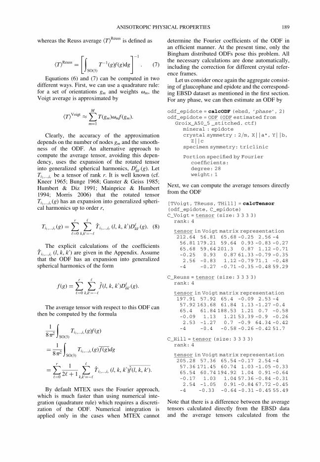
Let us consider once again the aggregate consist-ing of glaucophane and epidote and the correspond-ing EBSD dataset as mentioned in the first section.For any phase, we can then estimate an ODF by

odf_epidote = calcODF (ebsd, ’phase’, 2)odf_epidote = ODF (ODF estimated from

Groix_A50_5 _stitched. ctf)mineral : epidotecrystal symmetry : 2/m, X||a*, Y||b,

Z||cspecimen symmetry: triclinic

Portion specified by Fouriercoefficients:degree: 28weight: 1

Next, we can compute the average tensors directlyfrom the ODF

[TVoigt, TReuss, THill] = calcTensor(odf_epidote, C_epidote)C_Voigt = tensor (size: 3 3 3 3)

rank: 4

tensor in Voigt matrix representation212.64 56.81 65.68 -0.25 2.56 -456.81 179.21 59.64 0.93 -0.83 -0.2765.68 59.64 201.3 0.87 1.12 -0.71-0.25 0.93 0.87 61.33 -0.79 -0.352.56 -0.83 1.12 -0.79 71.1 -0.48-4 -0.27 -0.71 -0.35 -0.48 59.29

C_Reuss = tensor (size: 3 3 3 3)rank: 4


C_Hill = tensor (size: 3 3 3 3)rank: 4


Note that there is a difference between the averagetensors calculated directly from the EBSD dataand the average tensors calculated from the


estimated ODF. These differences result from thesmoothing effect of the kernel density estimation(cf. van den Boogaart 2001). The magnitude of thedifference depends on the actual choice of thekernel. It is smaller for sharper kernels, or more pre-cisely for kernels with leading Fourier coefficientsclose to1. An example for a family of well-suitedkernels can be found in Hielscher (2010).

Conclusions

An extensive set of functions have been developedand validated for the calculation of anisotropiccrystal physical properties using Cartesian tensorsfor the MTEX open-source MatLab toolbox. Thefunctions can be applied to tensors of single orpolycrystalline materials. The average tensors ofpolycrystalline and multi-phase aggregates usingthe Voigt, Reuss and Hill methods have beenimplemented using three methods: (a) the weightedsummation for individual orientation data (e.g.EBSD); (b) the weighted integral of the ODF; and(c) using the Fourier coefficients of the ODF.Special attention has been paid to the crystallo-graphic reference frame used for orientation data(e.g. Euler angles) and Cartesian tensors, as thesereference frames are often different in low-symmetry crystals and dependent on the provenanceof the orientation and tensor data. The suite ofMTEX functions can be used to construct project-specific MatLab M-files and to process orientationdata of any type in a coherent workflow from thetexture analysis to the anisotropic physical proper-ties. A wide range of graphical tools provides publi-cation quality output in a number of formats.The construction of M-files for specific problemsprovides a problem-solving method for teachingelementary to advanced texture analysis andanisotropic physical properties. The open-sourcenature of this project (http://mtex.googlecode.com)allows researchers to access all the details of theircalculations, check intermediate results and furtherthe project by adding new functions on Linux,Mac OSX or Windows platforms.

The authors gratefully acknowledge that this contributionresults from scientific cooperation on the research project‘Texture and Physical Properties of Rocks’ which wasfunded by the French-German program EGIDE-PROCOPE. This bilateral program is sponsored by theGerman Academic Exchange Service (DAAD) with finan-cial funds from the federal ministry of education andresearch (BMBF) and the French ministry of foreignaffairs. We would like to dedicate this work to the lateM. Casey (Leeds) who had written his own highly efficientFORTRAN code to perform pole figure inversion for low-symmetry minerals using the spherical harmonicsapproach of Bunge (Casey 1981). The program sourcecode was freely distributed by Martin to all interested

scientists since about 1979, well before today’s open-source movement. Martin requested in July 2007 thatDM made his own FORTRAN code open-source; inresponse to that request we have extended MTEX toinclude physical properties in MatLab, a programminglanguage more accessible to young scientists and currentteaching practices. Finally, the authors would liketo thank the editors D. J. Prior, E. H. Rutter and D. J.Tatham for the considerable work in compiling thisspecial volume dedicated to Martin Casey, their kind con-sideration in accepting our late submission and theirdetailed comments, which improved the manuscript.

Appendix: Fourier coefficients of the

rotated tensor

In this section we are concerned with the Fouriercoefficients of tensors, since they are requiredin equation (8). Previous work on this problem canbe found in Jones (1985). Here we presentexplicit formulae for the Fourier coefficientsTm1,...,mr

(J, L, K) in terms of the tensor coefficientsTm1 ,...,mr

(g). In particular, we show that the order ofthe Fourier expansion is bound by the rank ofthe tensor.

Let us first consider the case of a rank-one tensorTm. Given an orientation g [ SO(3), the rotatedtensor may be expressed as

Tm(g) = TnRmn(g)

where Rij(g) is the rotation matrix corresponding tothe orientation g. Since the entries of the rotationmatrix R(g) are related to the generalized sphericalharmonics D1

ℓk(g) by

Rmn(g) = D1ℓkUmℓUnk,

U =

1�2

√ i 0 − 1�2

√ i

− 1�2

√ i 0 1�2

√ i

0 i 0

⎛⎜⎝

⎞⎟⎠,

we obtain

Tm(g) = TnD1ℓkUmℓUnk.

The Fourier coefficients Tm (1, ℓ, k) of Tm(g) aretherefore given by

Tm (1, ℓ, k) = TnUmℓUnk.

Next we switch to the case of a rank-two tensorTm1m2

(g). In this case we obtain

Tm1m2(g)

= Tn1n2Rm1n2

(g)Rm2n2(g)

= Tn1n2D1

ℓ1k1(g)Um1ℓ1

Un1k1D1

ℓ2k2(g)Um2ℓ2

Un2k2.


With the Clebsch Gordan coefficientsk j1m1 j2m2|JMl (cf. Varshalovich et al. 1988), wehave

Dj1ℓ1k1

(g)Dj2

ℓ2k2(g)

=∑j1+j2

J=0

k j1ℓ1 j2ℓ2|JLlk j1k1 j2k2|JKlDJLK(g)

(9)

and hence

Tm1m2(g) =

∑2

J=0

Tn1n2Um1ℓ1

Un1k1Um2ℓ2

Un2k2

k1ℓ11ℓ2|JLlk1k11k2|JKlDJLK(g).

Finally, for the Fourier coefficients of Tmm′ , weobtain

Tm1m2(J, L, K) =Tn1n2

Um1ℓ1Un1k1

Um2ℓ2Un2k2

k1ℓ11ℓ2|JLlk1k11k2|JKl.

For a third-rank tensor we have

Tm1m2m3(g) = Tn1n2n3

Rm1n1(g)Rm2n2

(g)Rm3n3(g)

= Tn1n2n3D1

ℓ1k1Um1ℓ1

Un1k1D1

ℓ2k2

Um2ℓ2Un1k2

D1ℓ3k3

Um3ℓ3Un1k3

.

Using equation (9) we obtain

Tm1m2m3(g)

= Tn1n2n3D1

ℓ1k1Um1ℓ1

Un1k1D1

ℓ2k2Um2ℓ2

Un1k2D1

ℓ3k3

Um3ℓ3Un1k3

=∑2

J1=0

Tn1n2n3Um1ℓ1

Un1k1Um2ℓ2

Un1k2Um3ℓ3

Un1k3

k1ℓ11ℓ2|J1L1lk1k11k2|J1K1lDJ1

L1K1(g)D1

ℓ3k3

=∑2

J1=0

∑J1+1

J2=0

Tn1n2n3Um1ℓ1

Un1k1Um2ℓ2

Un1k2Um3ℓ3

Un1k3

k1ℓ11ℓ2|J1L1lk1k11k2|J1K1l

kJ1L11ℓ3|J2L2lkJ1K11k3|J2K2lDJ2

L2K2(g).

The coefficients of Tm1m2m3are therefore given

by

Tm1m2m3(J2, L2, K2)

=∑2

J1=J2−1

Tn1n2n3Um1ℓ1

Un1k1Um2ℓ2

Un1k2Um3ℓ3

Un1k3

k1ℓ11ℓ2|J1L1lk1k11k2|J1K1lkJ1L11ℓ3|J2L2lkJ1K11k3|J2K2l.

Finally, we consider the case of a fourth-ranktensor Tm1 ,m2 ,m3 ,m4

. Here we have

Tm1 ,m2 ,m3 ,m4

= Tn1,n2,n3 ,n4D1

m1 ,n1D1

m2,n2D1

m3,n3D1

m4 ,n4

= Tn1,n2,n3 ,n4

∑2

J1=0

∑2

J2=0

k1m11m2|J1M1lk1n11n2|J1N1l

DJ1

M1,N1k1m31m4|J2M2lk1n31n4|J2N2lDJ2

M2,N2

= Tn1,n2,n3 ,n4

∑4

J0=0

∑2

J1=0

∑2

J2=0

k1m11m2|J1M1l

k1n11n2|J1N1lk1m31m4|J2M2lk1n31n4|J2N2l

kJ1M1J2M2|J0M0lkJ1N1J2N2|J0N0lDJ0

M0 ,N0

and hence

Tm1 ,m2 ,m3 ,m4(J0, M0, N0)

=∑2

J1=0

∑2

J2=0

k1m11m2|J1M1lk1n11n2|J1N1l

k1m31m4|J2M2lk1n31n4|J2N2lkJ1M1J2M2|J0M0lkJ1N1J2N2|J0N0l.

References

Aleksandrov, K. S., Alchikov, U. V., Belikov, B. P.,Zaslavskii, B. I. & Krupnyi, A. I. 1974. Velocitiesof elastic waves in minerals at atmospheric pressureand increasing precision of elastic constants by meansof EVM (in Russian). Izvestiya of the Academy of theSciences of the USSR, Geologic Series, 10, 15–24.

Bachmann, F., Hielscher, H., Jupp, P. E., Pantleon,W., Schaeben, H. & Wegert, E. 2010. Inferentialstatistics of electron backscatter diffraction datafrom within individual crystalline grains. Journal ofApplied Crystallography, 43, 1338–1355.

Bass, J. D. 1995. Elastic properties of minerals, melts, andglasses. In: Ahrens, T. J. (ed.) Handbook of PhysicalConstants. American Geophysical Union, SpecialPublication, 45–63.

Bezacier, L., Reynard, B., Bass, J. D., Wang, J. &Mainprice, D. 2010. Elasticity of glaucophane andseismic properties of high-pressure low-temperatureoceanic rocks in subduction zones. Tectonophysics,494, 201–210.

Bunge, H.-J. 1968. Uber die elastischen konstantenkubischer materialien mit beliebiger textur. Kristallund Technik, 3, 431–438.

Casey, M. 1981. Numerical analysis of x-ray texture data:an implementation in FORTRAN allowing triclinic oraxial specimen symmetry and most crystal symmetries.Tectonophysics, 78, 51–64.

Christoffel, E. B. 1877. Uber die Fortpflanzung vanStossen durch elastische feste Korper. Annali di Mate-matica pura ed applicata, Serie II, 8, 193–243.


Fei, Y. 1995. Thermal expansion. In: Ahrens, T. J. (ed.)Minerals Physics and Crystallography: A Handbookof Physical Constants. American Geophysical Union,Washington, DC, 29–44.

Ganster, J. & Geiss, D. 1985. Polycrystalline simpleaverage of mechanical properties in thegeneral (triclinic) case. Physica Status Solidi (B),132, 395–407.

Hielscher, R. 2010. Kernel density estimation on therotation group, Preprint, Fakultat fur Mathematik, TUChemnitz. http://www.tu-chemnitz.de/mathematik/preprint/2010/PREPRINT_07.php.

Hielscher, R. & Schaeben, H. 2008. A novel pole figureinversion method: specification of the MTEXalgorithm. Journal of Applied Crystallography, 41,1024–1037, doi: 10.1107/S0021889808030112.

Hielscher, R., Schaeben, H. & Siemes, H. 2010. Orien-tation distribution within a single hematite crystal.Mathematical Geosciences, 42, 359–375.

Hill, R. 1952. The elastic behaviour of a crystalline aggre-gate. Proceedings of the Physical Society A, 65,349–354.

Hofer, M. & Schilling, F. R. 2002. Heat transfer inquartz, orthoclase, and sanidine. Physics and Chem-istry of Minerals, 29, 571–584.

Humbert, M. & Diz, J. 1991. Some practical featuresfor calculating the polycrystalline elastic propertiesfrom texture. Journal of Applied Crystallography, 24,978–981.

Isaak, D. G. 2001. Elastic properties of minerals andplanetary objects. In: Levy, M., Bass, H. & Stern,R. (eds) Handbook of Elastic Properties of Solids,Liquids, and Gases, Volume III: Elastic Properties ofSolids: Biological and Organic Materials, Earth andMarine Sciences. Academic Press, New York,325–376.

Jones, M. N. 1985. Spherical Harmonics and Tensorsfor Classical Field Theory. Research Studies Press,Letchworth, England. 230.

Kneer, G. 1965. Uber die berechnung der elastizitatsmo-duln vielkristalliner aggregate mit texture. PhysicaStatus Solidi, 9, 825–838.

Mainprice, D. 1990. An efficient FORTRAN program tocalculate seismic anisotropy from the lattice preferred

orientation of minerals. Computers & Geosciences, 16,385–393.

Mainprice, D. 2007. Seismic anisotropy of the deepEarth from a mineral and rock physics perspective.In: Schubert, G. (ed.) Treatise in Geophysics.Elsevier, Oxford, 2, 437–492.

Mainprice, D. & Humbert, M. 1994. Methods ofcalculating petrophysical properties from lattice pre-ferred orientation data. Surveys in Geophysics, 15,575–592.

Mainprice, D., Le Page, Y., Rodgers, J. & Jouanna, P.2008. Ab initio elastic properties of talc from 0 to12 GPa: interpretation of seismic velocities at mantlepressures and prediction of auxetic behaviour at lowpressure. Earth and Planetary Science Letters, 274,327–338, doi: 10.1016/j.epsl.2008.07.047.

Morris, P. R. 2006. Polycrystalline elastic constants fortriclinic crystal and physical symmetry. Journal ofApplied Crystallography, 39, 502–508.

Nye, J. F. 1985. Physical Properties of Crystals: TheirRepresentation by Tensors and Matrices. 2nd edn.,Oxford University Press, England.

Reuss, A. 1929. Berechnung der Fließrenze vonMischkristallen auf Grund der Plastizitatsbedingungfur Einkristalle. Zeitschrift fur angewandte Physik,9, 49–58.

Sander, B. 1911. Uber Zusammenhange zwischenTeilbewegung und Gefuge in Gesteinen. TschermaksMineralogische und Petrographische Mitteilungen,30, 381–384.

Sirotin, Yu. I. & Shakolskaya, M. P. 1982. Fundamen-tals of Crystal Physics. Mir, Moscow, 654.

van den Boogaart, K. G. 2001. Statistics for individualcrystallographic orientation measurements. PhDThesis, Shaker, Freiburg University of Mining &Technology.

Varshalovich, D. A., Moskalev, A. N. & Khersonskii,V. K. 1988. Quantum Theory of Angular Momentum.World Scientific Publishing Co., Singapore.

Voigt, W. 1887. Theoretische studien uber die elastizitats-verhaltnisse. Abhandlungen der Akademie der Wis-senschaften in Gottingen, 34, 48–55.

Voigt, W. 1928. Lehrbuch der Kristallphysik. Teubner-Verlag, Leipzig.




calculating anisotropic physical properties from texture data … · calculating anisotropic...

Documents