Calculating landscape surface area from digital elevation models

Jeff S. Jenness

Abstract There are many reasons to want to know the true surface area of the landscape, especially in landscape analysis and studies of wildlife habitat. Surface area provides a better esti- mate of the land area available to an animal than planimetric area, and the ratio of this surface area to planimetric area provides a useful measure of topographic roughness of the landscape. This paper describes a straightforward method of calculating surface-area grids directly from digital elevation models (DEMs), by generating 8 3-dimensional trian- gles connecting each cell centerpoint with the centerpoints of the 8 surrounding cells, then calculating and summing the area of the portions of each triangle that lay within the cell boundary. This method tended to be slightly less accurate than using Triangulated Irregular Networks (TINS) to generate surface-area statistics, especially when trying to analyze areas enclosed by vector-based polygons (i.e., management units or study areas) when there were few cells within the polygon. Accuracy and precision increased rapid- ly with increasing cell counts, however, and the calculated surface-area value was con- sistently close to the TIN-based area value at cell counts above 250. Raster-based analy- ses offer several advantages that are difficult or impossible to achieve with TINS, includ- ing neighborhood analysis, faster processing speed, and more consistent output. Useful derivative products such as surface-ratio grids are simple to calculate from surface-area grids. Finally, raster-formatted digital elevation data are widely and often freely available, whereas TINS must generally be generated by the user.

Key words elevation, landscape, surface area, surface ratio, terrain ruggedness, TIN, topographic roughness, rugosity, triangulated irregular network

Landscape area is almost always presented in terms of planimetric area, as if a square kilometer in a mountainous area represents the same amount of land area as a square kilometer in the plains. Predictions of home ranges for wildlife species generally use planimetric area even when describ- ing mountain goats (Oreamnos americanus) and pumas (Felis concolor). But if a species' behavior and population dynamics are functions of available resources, and if those resources are spatially limit- ed, I suggest assessing resources using surface area of the landscape.

Surface area also is a basis for a useful measure of landscape topographic roughness. The surface-area ratio of any particular region on the landscape can

be calculated by dividing the surface area of that region by the planimetric area. For example, Bowden et al. (2003) found that ratio estimators of Mexican spotted owl (Strix occidentalis lucida) population size were more precise using a version of this surface-area ratio than with planimetric area.

Many wildlife species are identified with topo- graphic attributes, including the topographic roughness or ruggedness of the landscape. For example, Wakelyn (1 987) found greater numbers of Rocky Mountain bighorn sheep (Ovis canadensis canadensis) in mountain ranges with higher meas- ures of topographic relief, and Gionfriddo and Krausman (1986) found that desert bighorn sheep (0. c. mexicana) generally were found at or near

Author's address: United States Department of Agriculture Forest Service, Rocky Mountain Research Station, 2500 S. Pine Knoll Drive, Flagstaii, AZ 86001, USA; e-mail: jeffj@jennessent.com.

I-- - -- - - - - - - -- 830 Wildltfe Society Rtilletin 2004.32(3):829-839

the tops of steep slopes and close to steep, rocky escape terrain. Warrick and Cypher (1998) found that kit foxes (Vu@es nzucrotis ~ n u t i w ) near Bakersfield. California were strongly associated with low topographic ruggedness, and Wiggers and Beasorn (1986) found that Texas white-tailed deer (Ochcoileus ui~;qiuici.n~~s fexunz~s) appeared to prefer areas with lcss topographic ruggedness than desert mule deer (0. her-mionzls crooki).

A variety of methods exist in the literature for measuring terrain irregularity. Hobson (1972) described some early computational methods for estimating surface area and discussed the concept of surface-area ratios. Beasom (1983) described a method for estimating land surface ruggedness based on the intersections of sample points and con- tour lines on a contour map, and Jenness (2000) described a similar method based on measuring the density of contour lines in an area. Mandelbrot (1983:29,112- 1 IS) described the concept of a "frac- tal dimension" in which the dimension of an irregu- lar surhce lies between 2 (representing a flat plain) and 3 (representing a surface that goes through every point within ;I volume). Calculating this frac- tal dimension can be very challenging computation- ally, and Polidori et al. (1991), Lam and De Cola ( I 993), and Lorimer el al. (1 994) discussed a variety of methods for estimating the fractal dimension for a landscape, An estimate of surface area also could be derived from slope and aspect within a cell (Berry 2002), although Hodgson (1 995) demonstrated how most slope-aspect algorithms generate values reflect- ing an area 1.6-2 times the size of the actual cell. Surface-area values derived with this method would therefore be unduly influenced by adjacent cells.

In this paper I demonstrate a straightforward method for calculating the surface area of land- scapes from digital elevation models (DEMs), which are widely and hcely available within the IJnited States and are becoming increasingly available throughout the rest of the world Uet Propulsion Laboratory 2003, Gesch el al. 2002, United States Geo1ogic;ll Survey [USGSl 2002). I compared sur- face-area values produced by this method with val- ues produced with triangulated irregular networks (TINS), which are .$-dimensional vector representa- tions of a landscape created by connecting the DEM elevation values into a continuous surface. Unlike DEMs, theseTINs are continuous vector sur- faces and therefore can be precisely measured and clipped. I also discuss aclvantages and tlisadvan- tages of this method in comparison to usingTINs.

Methods Throughout this paper I refer to "grids." and in

this case a grid is a specific type of geographic data used by ArcInfo and Arcview. '4 grid essentially is a raster image in which each pixel is referred to as a "cell" and has a particular value associated with it. For USGS DEMs. the cell value reflects the elevation in meters of the central point in that cell.

The method described here derives surhce areas for a cell using elevation information from that cell plus the 8 adjacent cells. For example, given a sample elevation grid, this method would calculate the surface area for the cell with eleva- tion value " 165" based on the elevation values of that cell plus the 8 surrounding cells (Figure I ) . That central cell and its surrounding cells are pic- tured in 3-dimensional space as a set of adjacent columns, each rising as high as its specified eleva- tion value (Figure 26).

The 3-dimensional centerpoints of each of these 9 cells are used to calculate the Euclidian distance between the focal cell's centcrpoint and the cen- terpoints of each of the 8 surrounding cells. I use the term "surface length'' to highlight he 3-dimen- sional character of this line; this is not the plani- metric (horizontal) distance between cell center- points. Next. calculate the surface lengths of the lines that connect each of the 8 surrounding cells with the ones adjacent to it to get the lengths of the sides of the 8 triangles projected in .$dimensional space that all meet at the centerpoint of the central cell (Figure 3h).

These surface lengths are calculated using the Pythagorean theorem. Thus, for any 2 cell center-

r i g ~ ~ r e I . ';mall L)~g~tal E le~~ l t i on rbtodel (DFM! with rlev,ltion values nver1,iid on each cell. Use CI "rnov~ng window" approach to calculate the surface x e a for each cell bawd on the elevation from 1ha1 cell pluh the elevation v,ilues for the f l surrounding cells.

- - - - - - - - - . Calculating surface area Jenness 831

Figure 2 . Using the elevation values from Figure I, cells A-l represent cells necessary to calculate the surlnce area for the central cell (a). The cells can be visualizecl as a set of acliacent colunlns each rising to their respective elevation values (I)).

points P and Q:

where

cr=planimetric (horizontal) distance from P to Q, b=difference in elevation between P and Q. c=surfhce distance from P to Q.

Distance "b" is easy to calculate because it is sim- ply the absolute difference between the 2 cell ele- vation values. Distance "a" is even easier for the cells directly to the north, east, south, and west. bccause it is simply the length of the side of the cells (L). For cells in diagonal directions, use the Pythagorean theorem again to c:~lculate that dis-

7

tance "a" = d2L2. Conducting these calculations for the central cell

plus the 8 adjacent cells produces the lengths for the sides of the 8 triangles connecting the center of the central cell to the centers of the 8 adjacent cells. However, this leads to :I minor complication because these triangles extend past the cell bound- ary and therefore represent an area larger than the cell. The triangles nwst be trimmed to the cell

Figure 3. C;IICLIIJ~~ 3-dimensional lengths I)etwern the center of the central cell to the centers of the s ~ ~ r r o ~ ~ n t l i n g cclls, and the lengths belween ~d jacent surroi~nding cells, to gct thc edge lengths for the tri;lnglei I-VIII Is). These triangles form 'I con- tlnuous surface over the 9 cells (b!.

boundaries (Figure 4) by dividing all the length val- ues by 2. This action is justified based on the Side- Angle-Side similarity criterion for similar triangles (Euclid 1956:204), which states that "If two trian- gles haw one angle equal to one angle and the sides about the equal angles proportional, the tri- angles will be equiangular and will have those angles equal which the corresponcling sides sub- tend." Each original triangle is "similar" to its corre- sponding clipped triangle because the 2 sides extending from the center cell in the original trian- gle are exactly twice as long as the respective sides in the clipped triangle. and the angles defined by these 2 sides are the same in each triangle. Therefore, the third side of the clipped triangle must be exactly hall' as long as the corresponding side of the original triangle.

Now when the lengths of the .3 sides are used to calculate the area of the triangle, the 3 sides will represent only the portion of thc triangle that lies within the cell boundaries. For example, using the elevation DEM from Figure 1 , and assuming that

Fig~ire 4. Surfnre area within the cell should only reflect the areas oi triilnglcs i-viii [a), so trim the triangles to [he cell I,o~~ndnries i b ~ by dividing all the triangle siclc lengths Ily 2.

cells are 100 m on a side and that elevation values are also in meters, begin by calculating the 16 tri- angle edge lengths for the 8 3-dimensional triangles radiating out from the central cell E (Figures 2a, 3n). Divide these surhce lengths in half to get the sides for triangles i-viii in Figure 4 (Table I), and use those lengths to determine the surface areas for each triangle (Table 2). The area of a triangle given the lengths of sides a. 6, and c (Abramowitz and Stegun 1772) is calculated as:

where

Finally, sum the 8 triangle area values to get final surface-area value for the cell (10,280.48 mL in this example). This is 280 mL more than planinletric area of the cell ( 100 n1 x 100 m= 10.000 mL).

Table 1. Elevation values for the 9 cells in Figure 2'7 ,Ire used to generate 16 surface lengths for the edges o i the 8 triangles in Figc~re 'la. Thesc surface lengths are divided in half to get the edges for the 8 triangles in Figure 42.

Surtace

Triangle Planimetric Elevation Surface length (mi edge lencth (m) difference im! lencth im! 2

Testirzg I tested the accuracy of this method by generat-

ing a surface-area grid in which the cell value for each cell reflected the surfiice area within that cell. I then calculated total surface area within several sets of polygons randomly distributed across the landscape. I initially calculatccl polygonal surface areas using the methods described in this paper and then coinpared those with surface-area values calculated viaTINs. As 3D vector representations of the landscape, theseTINs provide a true continuous surface based on the DEM elevation values. They provide a good baseline t o compare against

Table 2. Calculations o i true surface area for triangles i-viii (Figure 4aj based on the 1 h edge lengths from Table 1 . - - - - ~

Triangle Triangle Edges Edge lengths (nil area im2)

- .-

I E h An, BE 71.81, 50.99, 50.06 1,276.22 - - - II BE, BC, EC 50.06, 30.56, 70.89 1,265.48 . . . 1 1 1 i\9 DE, EX 50.12, 50.80, 71.81 1,272.95 - - .- iv EC, CF, EF 70.89, 50.25, 50.99 1,280.88

v 6?j 30.80, 50.16, 70.89 1,273.94 ---

vi EF, FI, El 50.99, 51.31, 73.91 1,306.88 - - - vii EG, EH, GH 70.89, 50.06. 50.76 1,265.48

. . . --- ~ H I EH, I:[, HI .i0.06, 73.91. 53.49 1,338.64

-- - - . - . . . - - - --- - Calculating surface area 4 Jenness 833

because they can be pre- cisely clipped to polygon boundaries and measured.

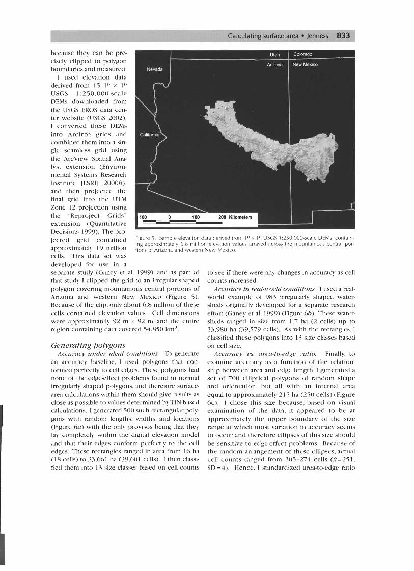
I used elevation data derived from 25 lo x 1" USGS 1 :250,000-scale DEMs downloaded from the USGS EROS data cen- ter website (USGS 2002). I converted these DEMs into ArcInfo grids and combined them into a sin- gle seamless grid using the ArcView Spatial Ana- lyst extension (Environ- mental Systems Research Institute [ESRI] 20000), and then projected the final grid into the LJTM Zone 12 projection using the "Reproject Grids" extension (Quantitative Decisions 1999). The pro- jected grid containetl F i g ~ ~ r c .;. b m p l e elevation data derived troni I " x l o USLS 1 :250,000-scale DEMs, contain

ing approximately 6.8 million elevation values arrayed across the mountainous central por nlillion tion, of Arizona antl western New Mexico.

cells. This data set was developed for use in a separate study (Caney et al. I999), and as part of that study I clipped the grid to an irregular-shaped polygon covering mountainous central portions of Arizona and western New ~Mexico (Figure 5 ) . Because of the clip, only about 6.8 million of these cells contained elevation values. Cell dimensions were approximately 92 m x 92 m, and the entire region containing data covered 54,850 km2.

Generating Polygons Accu~aqy u~zder ided conu'itions. To generate

an accuracy baseline. I used polygons that con- formed perfectly to cell edges. These polygons had none of the edge-effect problems found in normal irregularly shaped polygons, and therefore surface- area calculations within them should give results as close as possible to values determined byTIN-based calculations. I generated 500 such rectanguhr poly- gons with random lengths. widths, and locations (Figure Ga) with the only provisos being that they lay completely within the digital elevation model and that their edges conform perfectly to the cell edges. These rectangles ranged in area from 10 ha (18 cells) to 33,601 ha (39,001 cells). I then classi- fied them into 13 size classes based on cell counts

to see if there were any changes in accuracy as cell counts increased.

Accztrwcy in real-zix)rld cotzditions. I used a real- world example of 983 irregularly shaped water- sheds originally developed for a separate research effort (Ganey et al. 1999) (Figure 6b). These water- sheds ranged in size from 1.7 ha (2 cells) up to 33,980 ha (39,579 cells). As with the rectangles, I classified these polygons into 13 size classes based on cell size.

Accul-LI~J us, ai-ea-to-edge mtio. Finally, to examine accuracy as a function of the relation- ship between area antl edge length, I generated a set of 700 elliptical polygons of random shape and orientation, but all with an internal area equal to approximately 21 5 ha (250 cells) (Figure bc). I chose this size because, based on visual examination of the data, it appeared to be at :ipproximately the upper boundary of the size range at which most variation in accuracy seems to occul; and therefore ellipses of this size should be sensitive to edge-effect problems. Because of the random arrangement of these ellipses, actual cell counts ranged from 205-274 cells (3=251, SD = 4). Hence, I standardized area-to-edge ratio

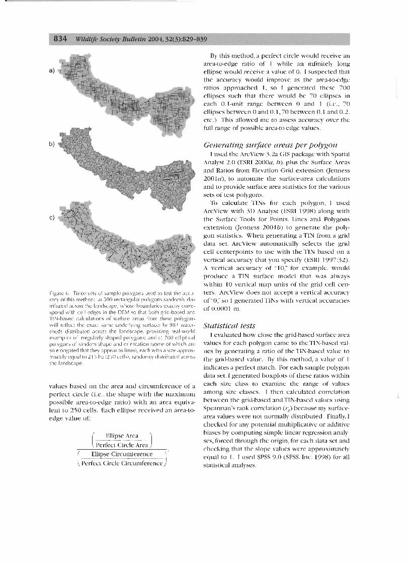
Figure 6. Three sets of sample polygons used to test the KCLI-

racy of this niethod: '11 500 rectangular polygons ranrlornlv dis- tributed across the landscape, whosc boundaries exactly corre- spond with cell edges in the DCM so that both grid-based ~ n d TIN-based calcirlations of surface areas from these polygons wil l retlect !he exact same underlying surface; bi 983 water- sheds distributed across the landscape, providing real-world examples o i irregularly shaped polygons; and c) 700 elliptical polygons of random shape and orientation (some of which are so elongated that they appear as lines!, each with a size approx- imately equal to 2 15 ha (250 cellsi, randomly clistrib~~ted across the landscape.

values based on the area and circumference of' a perfect circle (i.e., the shape with the maximum possible area-to-edge ratio) with an area equiva- lent to 250 cells. Each ellipse received an area-to- edge value of:

Ellipse Area

[Perfect Circle Area

i Ellipse Circumference

Perfect Circle Circumference

By this method, a perfect circle would receive an area-to-edge ratio of 1 while an infinitely long ellipse would receive a value of 0. I suspectecl that the accuracy would improve as the area-to-edge ratios approached 1, so I generated these 700 ellipses such that there would be 70 ellipses in each 0.1-unit range between 0 and 1 (i.e., 70 ellipses between 0 and 0.1,70 between 0.1 and 0.2, etc.). This allowed me to assess accuracy over the h l l range of possible area-to-edge values.

Generating surface areas per polygon I used the ArcView 3.2a GIS package with Spatial

Analyst 2.0 (ESRI 2000a, b). plus the Surface Areas and Ratios from Elevation Grid extension uenness 2001n), to automate the surface-area calculations and to provide surface area statistics for the various sets of' test polygons.

To calculate TINs for each polygon, I used ArcView with 3D Analyst (ESRI 1998) along with the Surface Tools for Points. Lines and Polygons extension Uenness 2001b) to generate the poly- gon statistics. When generating ;I TIN from a grid data set, ArcView automatically selects the grid cell centerpoints to use with the TIN based on a vertical accuracy that you specify (ESRI 1997:32). A vertical accuracy of "10," for example, would produce a TIN surface model that was always within 10 vertical map units of the grid cell cen- ters. ArcView does not accept a vertical accuracy of "0," so I generated TINs with vertical accuracies of 0.0001 m.

Statistical tests I evaluated how close the grid-based surface-area

values for each polygon came to the TIN-based val- ues by generating a ratio of the TIN-based value to the grid-based value. By this method, a value of 1 indicates a perfect match. For each sample polygon data set, I generated boxplots of these ratios within each size class to examine the range of values among size classes. I then calculated correlation between the grid-based and TIN-based values using Spearman's rank correlation (rs) because my surface- area values were not normally distributed. Finally, I checked for any potential multiplicative or additive biases by computing simple linear regression analy- ses, forced through the origin, for each data set and checking that the slope values were approxitnately equal to 1 . I used SPSS 9.0 (SPSS. Inc. 1998) for all statistical analyses.

Results The ratios of TIN-based

to grid-bascd surface-area values for the 500 rectan- gles tended to be very close to 1 in all size class- es (Figure 7) , with slightly more variation at the lower s i x classes. The TIN-based values tended to be slightly but consis- tently higher than the grid-based values at cell counts >2,500, with mean 8

0.99975 N.19 19 16 15 52 68 59 35 75 56 34 27 25 ratio valucs ranging from 1 .000007 - I . 0000 18.

250 750 2.500 7,500 15,000 25,000 40,000

Regression through the 500 1,000 5,000 10,000 20,000 30,000

origin produced a slope Number of cells in rectangle (SE < Figure 7. Hoxplots representing the ratio of TIN- lmed surtace area over grid-bawd surface

0.0001, 95% CI = 1.000- area, for the 500 randomly distributed rectangles irom Figure 6a. The edges o i these rectan-

1.000). T ~ ~ ~ T I N - - , ~ ~ ~ ~ sur- gles perfectly correspond with the edges of the underlying g r d cells. Horizontal bars within boxes represent the median, the tops and bottoms o i the boxes represent the 75th and 25th

face areas and the grid- quant~les, and the whiskers represent the range excluding outliers and extremes. Outlicrs (vai- based surface areas were ues >1.5 box lengths from box) are displayed with the symbol "o" ;and extremes ivalues >3

highly (rs > box lengths irom the box i are displdyecl with the symbol *'*".

0.999). The ratios among the 983 watersheds also tended to come close to 1 in all size classes (Figure gons was lower than with the larger polygons (rs= 8). Again, the greatest variability was at the smallest 0.825). Regression through the origin produced a size class (cell count<250). TIN-based c:llculations slope value of 0.999 (SE = 0.001, 95% CI = again were highly correlated with grid-based calcu- 0.998- 1.001.). lations (I:, > 0.999). Re- gression through the ori- gin produced a slope value of 1.000 (SE < 0.0001, 95% CI = 1.000- 1 .000).

The set of 700 standard- % ized ellipses showed a general trend toward increasing accuracy and O

precision as the area-to- edge ratios approached 1. with the mnge of values in each class becoming pro- ? gressively narrower (Fig- f 0,9 ure 9). The median value was close to 1 in all 250 750 2,500 7,500 15,000 25,000 40.000

cases, but the correlation 500 1,000 5,000 10,000 20,000 30,000 between TIN-based and Number of cells in watershed grid-based calculations among these smaller poly- rigure 8. Boxplots representing the ratio of TIN-based surface .lrea over grd-hasecl surface

area, for the 983 watershed, from Figure 66.

Standardized ratio of area over edge Figure 9. Boxplots representing the ratio of TIN-l~ased surface area over grid-hasrd surface area, for the 700 standardized ellipses from Figure 6c-. These ellipses have a constant internal area but random shapes, orientations, and locations. They are classified according Lo their standardired ,ires-to-edar ratio, where 0 reflects a n infinitely stretched ellipse and i reflects a

Discussion Raster data sets such as DEMs and surface-area

grids are inherently less accurate and precise than vector data sets such as TINS and polygons. The most accurate measure of the surface area within a polygon should include all the area within the poly- gon and no niore. Except in unusual circum- stances, raster data sets do not meet this criterion because cells in a raster data set do not sit perfect- ly within polygon boundaries. Cells typically over- lap the polygon edges, and GIS packages generally consider cells to be "inside" a polygon only if the cell center lies inside that polygon. Therefore? raster representations o f polygons have a stair- stepped appearance. incorporating some areas out- side the polygon and missing some areas inside. Cells lying directly on the border always lie partly inside and partly outside a polygon. but they are always classified as being entirely inside or outside the polygon. Therefore, the accuracy of a surface- area measurement within a polygon is affected by what proportion of the cells lie along the polygon edge. This proportion typically decreases as the number of cells increases. so accuracy should also increase as the number of cells increases.

Although cell-based calculations are inherently less precise and accurate than vector-based calcula-

on the order of about

tions, this method still came extremely close to duplicating results from TIN-based surface-area calculations. Accuracy and precision increased as the number of cells increased. Under ideal conditions in which the test polygon edges corre- sponded exactly to the cell edges, this method produced nearly identical surface-area calculations. The regression slope val- ues and extremely low standard error values demonstrated that there was no apparent bias in this method. Surface-area values computed using this method did tend to be slightly lower than those con~puted withTIN- based methods, but only 0.1-0.2 mvlla, suggesting

that this method did well at duplicating TIN-based values for grid cells that do not lie on polygon boundaries.

Under conditions more analogous to real-world situations, this method produced variable accura- cies when there were <250 cells in a particular polygon and good-to-excellent accuracy at cell counts >250. At higher cell counts, the grid-based values were almost identical toTIN-based values.

The analysis of the 983 watersheds showed con- siderably more variability when the polygons con- tained <250 grid cells (Figure 8): which is reason- able considering the inherent imprecision in grirl- based processes. Polygons containing relatively few grid cells would be most affected by errors caused by grid cells lying on the polygon boundary. The proportion of interior cells to edge cells increased as overall cell counts increased, causing niore of the total polygon surface area to be derived from the highly accurate interior cell values. This trend was also illustrated in the calculations involv- ing the 700 standardized ellipses, in which variabil- ity steadily decreased as area-to-edge ratios approached I . The range of values in the 0.0-0.1 class was 4 times as large as the range in the 0.5-0.6 class and 7 times the range in the 0.9- I .O class

(Figure 9). The ellipses with area-to-edge ratios clos- er to 1 had proportionally fewer edge cells, and therefore more of the surface-area calc~~lations were based on accurate interior cell values.

Advantages and disadvantages qf t/Xs method over using TINS

Given that the testing and comparisons present- ed in this paper assume that TIN-based calculations are thc most accurate, it is natural to wonder why we should not just useTINs. TINs offer many atlvan- tages over raster data sets for many aspects of sur- face analysis. As vector objects. they are not affect- ed by the edge-effect problems that are unavoidable with raster-based methods and are considerably more reliable antl accurate over areas with relative- ly low cell counts Wang and Lo 1999). They gen- erally take up much less space on the hard drive than raster data, and they are often more aestheti- cally pleasing to display (~Mahdi et al. 1998). However, the methods described in this paper offer advantages that are difficult or impossible to achieve with TINs.

Surface-ureu mtio griefs. Surface-area grids may easily be standardized into surface-area ratio grids by dividing the surface-area value for each cell by the planimetric area within that cell. Thcse surface- area ratio gricls are useful as a measure of topo- graphic roughness or ruggedness over an area and conceivably could be used :is friction or cost gricls for analysis of movement (such grids would steer the predicted direction of movement based on the topographic roughness of a cell). Because thesc ratio grids are in raster format, they also lend them- selves to neighborhood-based statistics as described below.

Neighbothod nndysis. In many cases we are not interested in values of individual cells but rather the values in a region around those cells. This is especially common when we are interested in phenomena over multiple spatial scales. For example, neighborhood analysis can be applied to surface-area grids to produce grids representing the sum, maximum, minimum, mean, or standard devia- tion of surface areas within neighborhoods of increasing size surrounding each cell. These neigh- borhoods can take on a variety of shapes, including squares, doughnuts, wedges, and irregular shapes (ESRI 1996: 103). Neighborhood analysis is simple with raster data but very difficult withTINs.

Fustc.1- proc~wing speed. Given comparable res- olutions, TINS take longer to generate and work

with than raster data sets. A process that takes min- utes or seconds with a raster data set may take sev- eral hours with a TIN.

,Ifow consistml and coinpamblt. outbut. TINs often are generated according to a specified accu- racy tolerance in which the surface must come within a specific vertical distance of each elevation point, meaning that aTIN surface rarely goes exact- ly through all the base elevation points on the land- scape. This also means that 2 TINS may have been generated with different tolerances, and therefore surface statistics derived from those TINs may not be comparable. This is especially problematic when the TINs are derived using whatever default accuracy is suggested by the software, which gen- erally varies from analysis to analysis based on the range of elevation values in the DElM. The method described in this paper, however, will always pro- duce a surface-area grid that takes full advantage of all the elevation points in the DEM. Surfwe-area sta- tistics derived from any region may then be justifi- ably compared with any other region.

Data is readi@ avuila6le. Digital elevation mod- els, at least within the United States, are widely available and often ti-eely downloadable off the Internet (Gesch et al. 2002,USGS 2002). Worldwide data from the 2000 Shuttle Radar Topography Mission is steadily becoming available (Jet Propulsion Laboratory 2003). TINs, however. are rarely available (the author has never seen them available on the Internet) and therefore must be generated by the user.

Mow accurutc. proportiom of' available resources. By weighting resource maps with under- lying surface-area values, land managers and researchers can generate more accurate extents and proportions of resources within a particular region. This is especially true if any of the resources are especially associated with particularly steep or flat areas.

The method described in this paper provides a straightforward antl accurate way to generate sur- face-area values directly from a OEM. People who use this method will h c e accuracy and precision errors when they calculate surface areas within vector-based polygons simply because of problems inherent in extracting data from raster-based sources (like grids and DEMs) and applying them to precisely defined vector objects (like management units and study areas). However, accuracy and pre- cision problems diminish rapidly as cell counts increase and become negligible for most purposes

at cell counts >250. The calculations involved, while most effectively computed in a GIS package, also could easily be clone in :t spreadsheet. For users of ESRI's ArcView 3.x softwarc with Spatial Amalyst, the author offers a frce extension that automates the process and directly produces sur- face-area and surface-ratio grids from grid-formatted DEMs. This extension may be downloaded from the author's website at http://www.jennessent.conl/ arcview/surface-areas,htm or from the ESRI Arcscripts site at http://arcscripts.esri.com/ tletails.asp?dbid=l1697.

Acknowledgments. I thank J. Aguilar-~Manjarrez, L. 1. Engelman, J. L. Ganey, L. M. Johnson, R. King. D. Whitaker, G. White, and :~n anonymous reviewer for their va1u:tble assistance with reviewing early drafts of this mnnuscript.

Literature cited hwaiowrr7, kl . . , \s~) I.A. S ~ ; I ! V 1072. H:lndhook of mathemat-

ical functions with formulas, grr~plls and mathematical t:tbles. 1)over Publications. New York, New York. IJSA.

I%~\h041. S. L. 1 9 8 3 . A tecllniquc fnr assessing lend surface ruggeclness. Journal of Wildlife ~Managcment 47: 1 163-1 166.

HIXRY. J. K 2002. lise surSace area for realistic calculations. Geoworld 1 i(9): 20-21

Ro\vr)~,s. I). C.. G. <:. Wl~rrr:,A. H. FRASKI.IN. .\XI) J. L. Ghslil: 2005. Estimating popu1:ltion size with correlated sampling unit estimates. Journal o f Wilcllife management 67: 1- 10.

ESVIUO>~II'SIAI SYSIIMS RI~WAIKII I s s ~ r r i w . 1996. Llsing the Arcview spatixl analyst: adwinced spatial analysis using rrtster :tnd vector data. Environmental Systems Research Institute, Redlands. Californi;~. USA.

E,\~II{O.\~IP.>,I;\I. SYS~EW R~:sl;\ac.il I s s r ~ n n:. 1997. Ilsing Arcview 3D :~n;~lyst: .?it) surface creation. visualization, and ;~nalysis. Environmental Syztcms Research Institute. Redlancls. (21lih)rnia. IISA.

E w I R ~ N . \ ~ ~ s I ; \ I . S Y S T ~ W RI:sI:.\K(:H INSI rl'l 7 I:. 1998. Arcview 31) a~xllyst. (Arcview S.x Extcmsiun). Version 1 Environmental Systems Rcse;~rch Institute. Red1;tndh. California. IISA.

E U V I R O X A I I ~ I L ~ I . SY?IWMS I<PSL\R( 11 I~fl'i'i'ii'rr.. 2 0 0 0 1 ~ Arcview GIS S.2a. Environmental Systems Research Institute. Recll:~ntls. Oalifornia, IrSA.

ESVIIKI~II :SI~AI SYY~EAIS RISI;M.H ISS'IITI I'I:. 2000h. ArcVicw spik t i d an:tlyst. (ArcVicw 5.x Extt.tision). Version 2 . Environmental Systems Research Institute, Retll:~ntls. C;~lifornia, IlSA

Erc:~ 11). 19iO. Thc thirteen books of' Euclid's elements: tn~nsl:tt- ccl with introduction :mcl commentary by Sir Thomas 1,. Hr;~th. Volume 3 (Ilooks 111-I?(). Seconel Edition I Inabridged Dover I'ublicationh. New l'ork. New York. IJSA.

G;\\W. 1 . L. . <;. (1. \%'lll'l't. A. fi. FIL\SKI.IU, ANI) J. I! WAUL). JR. 1999. Monitoring population trends o f Mexican spotted owls in Arizom mil Ncw ,Mexico: a pilot study. Study plan RM 5 1 - 1 Rocky Mount;iin Kese:lrch Station. Flagstaff, Arizona. IJSA.

GLS(:H. D., M. OIMOIW. S. GKEENI.~E, C . NEI.SOS, bI. STB~!(.K, .\XI)

D. T'IWR. 2002. The national elevation clatasct. Photo- gnlmmetric Engineering & Remote Sensing 68: 5- 11.

GIONI.RII)I)O, J. I?, ASI) I? R. K I L U W . ~ . 1986. Summer habitat use by mountain sheep. Journal o f Wildlife Management 50: 551-3.36,

HOI~SON. R. D. 1072. Chapter X - surface nmghness in topognt- phy: quantitative approach. 221-245 in R. J. Chorley. editor. Spatial ;knalysis in geomorphology. Harper Sr Row. New York. New York. IISA.

Horx,sos. IM. E. 1095. What cell size cloes the computed slopc/aspect angle represent? Photog~mnmetric Enginecring &Remote Sensing hl:513-517.

l n ~ ~ r s s , J . 2000. The effects of fire on Mexic;tn spotted owls in Arizona and New Mexico. Thesis. Northern Ar i rom Ilniversity. Flagstaff. IISA.

Jesses,. J. 20010. Surface awas and ratios from elevation grid. (ArcView 5.x Extension). Jenncss Enterpriseb. Avail;~hle online :it 1~ttp://w~vn..jennessent.com~1rcview/s~1rhce~ areits.htm (accessed October 2003).

Jmurss, J. 20010. Surk~cc tools for points. lines and polygons. (ArcView 3,s Extension). Version 1.5. Jenness Enterprises. Avaihhle online at http:Nwwm~.jcnr~essent.con~~arcvie%v/s~~r- f:~ce-tools.Iltm [date :~ccessccl Octobcr 20051.

Jlrr Puon . r . s~o~ LUOIM~)RY. 2005. Shuttle R ~ d a r Topography Mission (Web Page). Available online :it http:// \m~~~~~.jpl.nasa.gnv/srtrn/ (;lccessed October 2005).

L,\sl, N S. N.. A N I ) L. DI.(:OI.A. 1'90.3. Fmctalb in geogrrlphy PTR Pmtice-H;ill, Englewoocl (:lifSs. New Jersey. I!SA.

LOIIIMI.IL N. D.. R. G. HAIGIHKAUI) R.A. I.l;.,\~n: 1994. 'She fractal for- est: liactnl geometry ;inti applications in forest science. United States Department of Agriculture Forest Service. North Central Forest Experiment Station, General Technical Report: N<:-170. St. P;iul, Minnesota. IJSA.

;MNII)I, A,. C. WYNSI:. E. < : t r o ~ w . L. KO\. (1x1) K. S H ~ . 1908. Rcyresentltion of 5-D elevation in terrain clat:rbases using h i e ~ ~ r c h i c a l triangulated irregular networks: a comparative analysis. Internation:~l Journal 01' Geographical Information Science 1L:XiS-887.

MASIXI.BR~YI: B. U. 1085. Tht. fract:il gcometry of nature. W. H. Freeman. New York. New York, IJSA.

POI IDORI. L.. J . CHOIIO\VI(.%,ANI) R. GIIII.IASI)I!. 199 l . Description of termin as :I fractal surface,and applic;~tion to digital elevation modcl quality assessment. I'hotograrnmetrlc Engineering &

Remote Sensing 57: 1329- 15.32. Q~LINI.I~I;~IIVI. I ~ C I S I O N S . 1009. Reproject Grids (Arcview 5 , s

extension): Quantitative Decisions. Avaihhle onlinc at http://arcscripts.t.sri.com/details.aspltIhid= I 1.568 (accessed Octoher 200.5).

SPSS. IN(.. I90X. SPSS 9.0 for Windows. SPSS. Chicago. Illinois. IJSA.

I l ~ r n : ~ ) Sljvr~s GL:OI.OLK:AI. S I~RVIY. 2002. 1:250.000-sc:lle digital elevation models. (\Vch Page) Available online at: ftp://eclcftp.crusgs.go~~/pi1b/d~1t1/DE/250/ [date accesscd October ZOOS].

WAKEI.YS. L. A. 1'987 (:hanging halitat conclitions on highom sheep ranges in C o l o ~ ~ d o . Journal of Wilcllifc M:~nagcmenl i1:904-912.

W A N , K . . I ? I . I 0 0 9 An asscssnicnt of the accuracy of triangulated irregular network!. (TINs) and 1;rttict.s in AKC/INFO. Transactions in GIS 5: 161-174.

W;\RRI(:L. (;. D..ANI) U. L. CYI'IIPII. 1998. Factors affecting the sp;c

- - - Calculating surface area Jenness 839

t k ~ l distril>utic)t~ of Snn Joaquin kit foxes. Journal o f \Viltllife Management 62: 707-717

Vi/rc.c.m~, E. F?.ANI) S. L. RCASOI\I. 1986. Clxlracterization of sym- patric or adjacent habitats o f 2 deer- bpc-cies in West 'rex;~~. Journal o f Wildlife Management 5 0 , 129- 1.34.

Jeffjenness is a wildlife biologist with the United States Forest Service's Rocky Mountain Research Station in Flagstaff, Arizona. He received his B.S. ,lnd M.S. in forestry, as \ d l as an M.A. in educational psychology, from Northern Arizona University. Since 1990 his research has focused primarily on issues related to Mexican suotted owls in th? southwestern United States. He has also becbme increasingly involved in GIS-hased analyses,

I

and in 2000 he stal-ted J. CIS consultinfi bc~siness in which he '-

specializes in developing GIS-based a&lytical tools. He has worked with universities, businesses, and governmental men- ! cies around rhe world, including a long-teym contract with'the Food and Agriculture Organization of the Unitecl Nations IFAO), for which he relocated to Rome, Italy for 3 months. His iree Arcview tools have been downloaded from his website and the ESRl Arcscripts site over 100,000 times. I Associate editor: White