calculation of eur form oil and water production data · by natural water drive or a pressure...

Proceedings of the International Conference on Industrial Engineering and Operations Management

Bandung, Indonesia, March 6-8, 2018

© IEOM Society International

Calculation of EUR form Oil and Water Production Data

Saber Kh. Elmabrouk School of Applied Science and Engineering, The Libyan Academy, Tripoli, Libya

[email protected]

Walid Mohamed Mahmud Petroleum Engineering Department, University of Tripoli

Tripoli-Libya [email protected]

Hassan M. Sbiga Libyan Petroleum Institute (L.P.I)

Tripoli-Libya

[email protected]

Abstract The calculation of oil reserves (estimate ultimate recovery, EUR) is required for reservoir management. It is

important to differentiate between oil reserves and oil resources. The latter is roughly defined as the sum of

recoverable and unrecoverable volumes of oil in place; whereas, the oil reserves can be defined as those amounts

of oil anticipated to be commercially recoverable from a given date under defined conditions. However, there is

always uncertainty when making reserve estimates, and the main source of uncertainty is the lack of available

geological data. Depending on the quantity and quality of the available data, different methods are used for the

evaluation of the EUR.

A number of essentially straight-line extrapolation techniques (production data analysis) have been proposed to

estimate the EUR for oil and gas wells. Thus, a detailed analysis of past performance of oil and water production

data is required in order to predict the future performance of the oil and gas wells. This work utilized seven

straight-line extrapolation techniques to estimate and compare the values of EUR of three oil wells from the same

reservoir. The comparison shows very similar estimated EUR.

Keywords EUR, WOR, reserve, X-plot, production data analysis, decline curve analysis

1- Introduction The calculation of expected initial oil in place and estimated ultimate recovery (EUR) of oil and gas wells are

required for evaluation and reservoir management purposes. It is important to differentiate between oil reserves

(EUR) and initial oil in place. The latter is roughly defined as the sum of recoverable and unrecoverable volumes

of oil in place. Whereas, the oil reserves can be defined as those amounts of oil anticipated to be commercially

recoverable by applying development projects to known accumulations from a given date under defined

conditions. However, there is always uncertainty when making reserve estimates. The main source of uncertainty

is the lack of available geological data. Depending on the quantity and quality of the available data, different

methods are used for the evaluation of the EUR. For example, in the initial stage of development of the

hydrocarbon deposit, there is very little information available; therefore, approximate estimates are usually made

using analog or volumetric calculations. Considering that, in the late stage of reservoir development, production

data analysis and reservoir simulation methods are commonly employed. However, it is worthwhile to mention

that the EUR is the most important step toward taking any decisions regarding drilling activities, field development

and reservoir management. Simultaneously, it is the most difficult aspect of reservoir engineering, especially in

the early life of the reservoir. Several methods are used to estimate an EUR, and the methods differ depending

upon the purpose of the study and availability of the data. Mainly, there are six methods available in the literature

to estimate the oil and gas reserves; volumetric method, material balance method, production decline analysis

(DCA), type curve analysis (TCA), numerical simulation method, water oil ratio (WOR) data analysis.

Commonly, oil and water production data are regularly measured with time. Most oil wells which are produced

by natural water drive or a pressure maintenance waterflood will produce water along with oil during their life.

Oil and water production history can be used in a number of ways; however, the DCA, and WOR data analysis

techniques are utilized in this study where the historical oil and water production data for three selected oil wells

was analyzed in order to determine EUR. In most cases, WOR is used as an analytical tool. WOR data is a

mailto:[email protected]






performance-based method of trending future water production for the purpose of forecasting oil production, water

production, and determining expected EUR. Water-cut (WC) or water fractional flow (fw) and oil-cut or oil

fractional flow (fo) are alternatives ratio forecasting methods to WOR. All the proposed techniques consider

straight-line relationship techniques and extrapolating the past performance on the plot.

A number of essentially empirical methods have been proposed in the literature to evaluate the waterflood

performance and to calculate the EUR that consider the linearity of late-time behavior of the WOR. The objective

of those efforts was to provide a semi-analytical representation for natural water drive and/or waterflooding

mechanisms in oil production. Nevertheless, the oil production decline is caused by reduction in oil saturation and

oil relative permeability. Unfortunately, in most cases, this method is applicable only for the analysis of late stage

of a waterflood (for values of WC greater than 50%). The expression for the steady-state radial flow of oil and

water are presented in Equation 1. Simultaneously, fw in the reservoir is the ratio of the water production rate and

the total liquid production as illustrated in Equations 2 and 3. Likewise, oil fractional flow, fo, is the ratio of the

oil production to the total liquid production.

𝑞 =𝑘ℎ

141.2 𝐵𝜇

1

𝑙 n(𝑟𝑒𝑟𝑤

)∆𝑝 (1)

𝑓𝑤 =𝑞𝑤

𝑞𝑤+𝑞𝑜 (2)

From 1 and 2 we get

𝑓𝑤 =1

1+𝑘𝑜 𝜇𝑤 𝐵𝑤𝑘𝑤 𝜇𝑜 𝐵𝑜

(3)

𝑓𝑜 =𝑞𝑜

𝑞𝑤+𝑞𝑜 (4)

Since all the used techniques to establish the EUR mentioned are depending on a straight-line trend, Espinel and

Barrufet (2009) wondered about the accuracy of the selection of the straight-line zone. Is the straight-line zone

always present? How long is it? Is it always correct to extrapolate it to find ultimate recovery at an assumed

economic limit? Where does the straight-line zone begin and where does it end? They developed an alternative

technique, based on multiple regression analysis, to calculate reservoir performance and EUR. The proposed

method provides slops and intercepts of straight line zone of the plot of the WOR versus recovery factors from

the water breakthrough time to the point where the maximum economic recovery factor.

Generally speaking, the lifecycle of an oilfield is typically characterized by three main stages: production buildup,

plateau production, and declining production. Sustaining the levels of production required during the duration of

the life cycle requires a good understanding and the ability to control the recovery mechanisms involved. One of

the more significant key elements that effecting oil production rates during the life cycle of the field is downhole

environment. It was confirmed by Ben Mahmud et al (2016) and Busahmin et al. (2017) that when production

wells were drilled and completion properly, they show a significant impact on the oil recovery.

2- Oilfield case studies A detailed analysis of the past oil, gas and water production performance was conducted for the simultaneous

evaluation of EUR. However, due to the uncertainty in the accuracy of extrapolation methods, as well as the lack

of a completely rigorous mathematical basis, this study applies seven different extrapolation techniques:

• Decline curve analysis

1. Log(qo) versus production time, t

2. qo versus Np

3. 1/qo versus to

• WOR extrapolated methods

4. Log(fw) versus Np

5. fo versus Np

6. 1/fw versus Np, and

• X-plot technique

7. Np versus X-function




Such an approach would provide a validation for the EUR results, and although there is no single perfect

extrapolation technique, comparing the results obtained from different methods would provide consistency and a

validation element. In this case study, three oil wells (A-01, A-06 and A-28) from a Libyan oilfield located in

Sirte Basin were selected to utilize seven straight-line extrapolation techniques to estimate and compare the values

of EUR.

2.1 Decline curve analysis (DCA) Arps (1945) proposed the curvature in the production rare versus time. The method can be described by doing a

plot of oil or gas production data rate versus time that could be extrapolated to provide an estimate of future rate

of production for a well or a field. With this forecasting, it is possible to determine the EUR of the well or the

field. However, the basic assumption in the DCA is that the parameters controlling the decline trend of the curve

in the past will continue to govern the trend in the future in a uniform manner. However, the normal shape of the

decline curve effected by several factors: (1) human factors, such as restricted production rate to the allowable

rate setup by regulatory body, marketing, or due to shutting down of wells for well testing, workover, etc. (2)

production conditions, such as changing the number of producers, changing the lift conditions, changing the

productivity index due to permeability changing around the wellbore, and changing the surface conditions. (3)

reservoir factors, such as reservoir drive mechanism, reservoir rock and fluid properties, relative permeability

curves and using of water injection, water flooding and EOR techniques.

DCA uses empirical equations that models how the flow rate changes with time assuming a certain decline rate.

It is one of the most used forms of data analysis to evaluate gas and oil reserves and predict future production.

This technique is based on the assumption that past production trends and their control factors will continue in the

future and; therefore, can be extrapolated and described by one of the three mathematical expressions; (1)

Exponential decline (2) Harmonic decline and (3) Hyperbolic decline. A major assumption here is that the most

dominant past behavior will govern the future behavior of the well's performance. Obviously, this is not

necessarily true but works in many cases. It could also yield reasonable results when more wells are lumped

together. However, this technique ignores any geological information from the field and, therefore, could give

very unreasonable results in some cases.

There are some factors that affect the trend of production decline. the main factors may include; (1) Human factors

(such as the restriction of the production rate to the allowable rate setup by the regulatory body, restriction due to

the marketing or shutting down of wells for well testing), (2) production conditions (such as changing number of

producers, changing lifting conditions, changing the productivity index of the well due to acidification, damage,

hydraulic fracturing or re-perforations), or Change surface conditions (such as changing the well head pressure or

separator pressure), and (3) reservoir factors (such as reservoir drive mechanisms, reservoir fluid and rock

properties or the use of pressure maintenance, waterflooding and EOR techniques).

Equation 5 presents the general form for decline curve analysis, and Equation 6 presents the cumulative

production formula. However, exponential (b=0) and harmonic (b=1) decline are special cases of these formulas.

𝑞 =𝑞𝑖

(1+𝐷 𝑏 𝑡)1/𝑏 (5)

𝑁𝑝 =𝑞𝑡

𝑏

𝐷(1−𝑏) [𝑞𝑖

1−𝑏 − 𝑞1−𝑏] (6)

Variables

q = current production rate

qi = initial production rate (start of production)

D = initial nominal decline rate at t = 0

t = cumulative time since start of production

b = decline constant normally has a value 0 < b < 1

Np = cumulative production being analyzed

The exponential decline curve technique uses a semi log plot of q versus t. In general, this plot provides a linear

trend, which can be extrapolated to any future time or a desired economic production limit. The corresponding

value of Np can be estimated from that extrapolation. The governing equation for the case of the exponential

production decline is given by Equation 7.

𝑞𝑜 = 𝑞𝑖𝑒−𝐷𝑡 (7)




From equation 7, a rate-cumulative production relationship can be developed. The definition of cumulative

production is given by:

𝑁𝑝 = ∫ 𝑞𝑜𝑑𝑡𝑡

0 (8)

Substituting Equation 7 into Equation 8 and integrating yields:

Np = ∫ qit

0e−Dtdt =

1

D{qi − qie

−Dt} (9)

Substituting Equation 8 into the last part of Equation 9 yields:

𝑁𝑝 =1

𝐷(𝑞𝑖 − 𝑞𝑜) (10)

Equation 10 can be used to obtain the EUR by using the data obtained from the plot of qo versus t and at a desired

economic production limit. In addition, by solving equation 10 for qo the rate-cumulative production relationship

can be obtained as in Equation 10.

𝑞𝑜 = 𝑞𝑖 − 𝐷𝑁𝑝 (11)

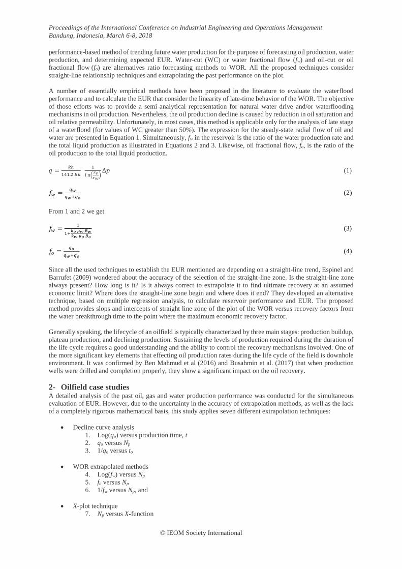
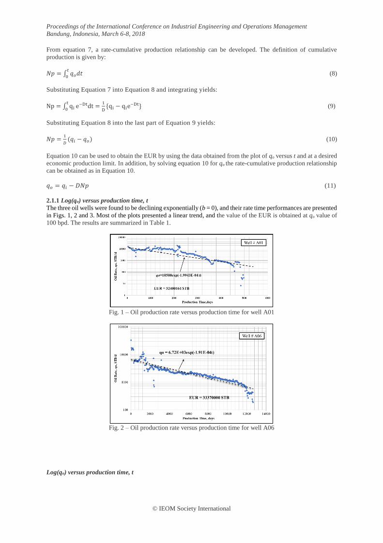
2.1.1 Log(qo) versus production time, t

The three oil wells were found to be declining exponentially (b = 0), and their rate time performances are presented

in Figs. 1, 2 and 3. Most of the plots presented a linear trend, and the value of the EUR is obtained at qo value of

100 bpd. The results are summarized in Table 1.

Fig. 1 – Oil production rate versus production time for well A01


Log(qo) versus production time, t





Table 1 – EUR from log(qo) vs. production time, t

Well Straight-line Eq. Decline rate, D EUR

A01 qo =10500 exp(-1.9943E-04 t) 0.0728/year 52.40MM STB

A06 qo = 6.72E+03 exp(-1.91E-04 t) 0.0697/year 33.37MM STB

A28 qo = 3.48E+03 exp(-2.754E-04 t) 0.1005/year 12.45MM STB

2.1.2 Oil production rate, qo versus Cumulative oil production, Np

The plots of qo vs Np for A01, A06 and A28 are presented in the Figs 4, 5, and 6 respectively. The values of the

EUR for each well are evaluated at qo value of 100 bpd. Table 2 illustrated the results of EUR of the wells.

.

Fig. 4 – Oil production rate versus cumulative oil production for well A01

Fig. 5– Oil production rate versus cumulative oil production for well A06




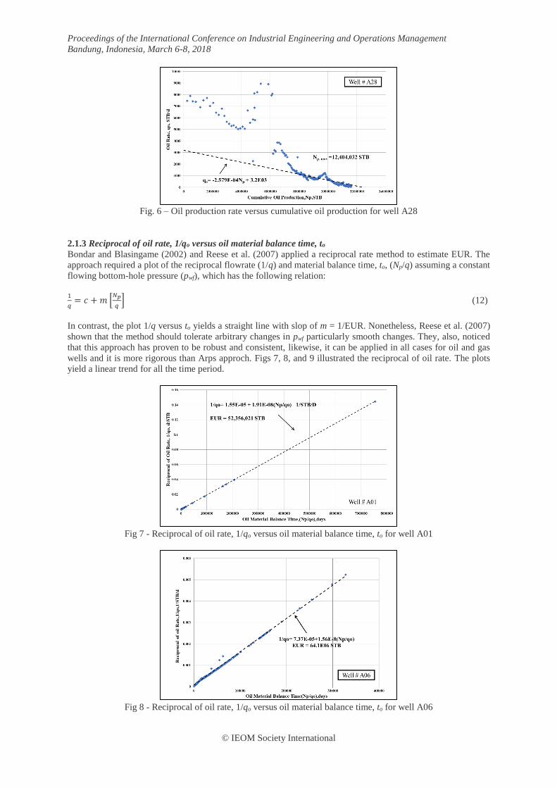
Fig. 6 – Oil production rate versus cumulative oil production for well A28

2.1.3 Reciprocal of oil rate, 1/qo versus oil material balance time, to

Bondar and Blasingame (2002) and Reese et al. (2007) applied a reciprocal rate method to estimate EUR. The

approach required a plot of the reciprocal flowrate (1/q) and material balance time, to, (Np/q) assuming a constant

flowing bottom-hole pressure (pwf), which has the following relation:

1

𝑞= 𝑐 + 𝑚 [

𝑁𝑝

𝑞] (12)

In contrast, the plot 1/q versus to yields a straight line with slop of m = 1/EUR. Nonetheless, Reese et al. (2007)

shown that the method should tolerate arbitrary changes in pwf particularly smooth changes. They, also, noticed

that this approach has proven to be robust and consistent, likewise, it can be applied in all cases for oil and gas

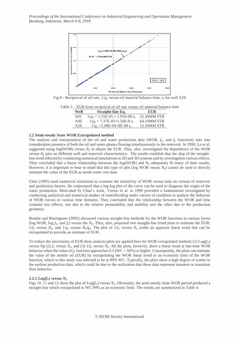
wells and it is more rigorous than Arps approch. Figs 7, 8, and 9 illustrated the reciprocal of oil rate. The plots

yield a linear trend for all the time period.

Fig 7 - Reciprocal of oil rate, 1/qo versus oil material balance time, to for well A01






Table 3 – EUR from reciprocal of oil rate versus oil material balance time

Well Straight-line Eq. EUR

A01 1/qo = 1.55E-05 + 1.91E-08 to 52.36MM STB

A06 1/qo = 7.37E-05+1.56E-8 to 64.10MM STB

A28 1/qo =2.08E-04+8E-08 to 12.50MM STB

2.2 Semi-steady State WOR Extrapolated method

The analysis and interpretation of the oil and water production data (WOR, fw, and fo functions) take into

consideration presence of both the oil and water phases flowing simultaneously in the reservoir. In 1990, Lo et al.

suggested using log(WOR) versus Np to obtain the EUR. They, also, investigated the dependence of the WOR

versus Np plot on different well and reservoir characteristics. The results establish that the slop of the straight-

line trend effected by conducting numerical simulations in 2D and 3D systems and by investigation various effects.

They concluded that a linear relationship between the log(WOR) and Np adequately fit many of their results.

However, it is important to bear in mind that this type of plot (log WOR versus Np) cannot be used to directly

estimate the value of the EUR as needs some core data.

Chan (1995) used numerical simulation to examine the sensitivity of WOR versus time on various of reservoir

and production factors. He conjectured that a log-log plot of the curve can be used to diagnose the origin of the

water production. Motivated by Chan’s work, Yorsos et al. in 1999 provided a fundamental investigated by

conducting analytical and numerical studies of waterflooding under variety of condition to analyze the behavior

of WOR curves in various time domains. They concluded that the relationship between the WOR and time

contains two effects, one due to the relative permeability and mobility and the other due to the production

geometry.

Bondar and Blasingame (2002) discussed various straight-line methods for the WOR functions in various forms

(log WOR, log fw, and fo) versus the Np. They, also, proposed two straight-line trend plots to estimate the EUR;

1/fw versus Np, and 1/qo versus Np/qo. The plot of 1/fw versus Np yields an apparent linear trend that can be

extrapolated to provide an estimate of EUR.

To reduce the uncertainty of EUR three analysis plots are applied here for WOR extrapolated method; (1) Log(fw)

versus Np (2) fo versus Np, and (3) 1/fw versus Np. All the plots, however, show a linear trend at late-time WOR

behavior when the value of fw function approaches 0.5 (WC = 50%) or higher. Consequently, the plots can estimate

the value of the mobile oil (EUR) by extrapolating the WOR linear trend to an economic limit of the WOR

function, which in this study was selected to be at 99% WC. Typically, the plots show a high degree of scatter in

the earliest production data, which could be due to the realization that these data represent transient or transition

flow behavior.

2.2.1 Log(fw) versus Np

Figs 10, 11 and 12 show the plot of Log(fw) versus Np. Obviously, the semi-steady State WOR period produced a

straight-line which extrapolated to WC 99% as an economic limit. The results are summarized in Table 4.




Fig. 10 – Fractional flow of water versus cumulative oil production for well A01



Table 4 – EUR from Log(fw) versus Np


A01 fw = 1.87E-07 exp(2.94E-07 Np) 52.67MM STB

A06 fw = 0.01 exp(7.16E-08 Np) 64.32MM STB

A28 fw = 0.122 exp(16.9E-08 Np) 12.40MM STB

2.2.2 fo versus Np

Figs 13, 14 and 15 show the plot of fo versus Np. The late datapoints (semi-steady state) formed a straight-line

trend. This straight line was extrapolated to an economic limit of 99% WC in order to obtain the EUR and

summarized in Table 5.




Fig. 13 – Fractional flow of oil versus cumulative oil production for well A01



Table 5 – EUR from fo versus Np


A01 fo=12 - 2.28522E-07 Np 52.51MM STB

A06 fo = 8.5 - 1.3381E-07 Np 63.52MM STB

A28 fo = 1.20 - 9.35E-08 Np 12.80MM STB

2.2.3 1/fw versus Np

The Figs 16, 17, and 18 show the semi-state state of fw vs Np extraplotated technique of the well A01, A06 and

A28 respectively. The Figs show linear trend of the late datapoints and the results EUR are tabolated in Table 6.




Fig. 16 – Reciprocal of fractional flow of water versus cumulative oil production for well A01



Table 6 – EUR from 1/fw versus Np


A01 1/fw=19 - 3.416E-07 Np 52.67MM STB

A06 1//fw = 2.62 - 2.5E-08 Np 64.80MM STB

A28 1/fw = 1.92 - 7.187E-08 Np 12.80MM STB

2.3 X-plot

The X-plot technique is based on fractional flow and the Buckley-Leverett calculations. Based on Omoregie and

Ershaghi (1978), an interesting application of the X-plot method is that the linear plot of Np versus X-function

(Equation 12) gives a straight line that can be extrapolated to any desired WC (economic fw) as a mechanism for

determining the corresponding EUR. The extrapolation of the past performance on the plot is a complicated task.

The difficulty arises mainly because a curve fitting by simple polynomial approximation does not result in

satisfactory answers in most cases. Due to the fact that X-function has a parabolic shape the recommendation is

to restrict this technique to fw greater than 50%. Differentiating X-function with respect to fw and equating the first

derivative to zero can prove this restriction. Ershaghi and Abdassah (1984) provides a detailed explanation of this

concept.




𝑥 = ln (1

𝑓𝑤− 1) −

1

𝑓𝑤 (12)

Lijek (1989) examined various WOR analysis techniques and presented analytical methods by which the oil rate

can be modeled as a function of time. He examined the linearity of; WOR versus Np, X-plot method, and 1

𝑊𝑂𝑅+

𝑊𝑂𝑅 versus cumulative water injection (Wi).

In 2002, Bondar and Blasingame considered that the X-plot technique gave the least consistent results compared

to the other methods used. straight-line extrapolation methods produced more consistent estimates of EUR than

the X-plot technique. Also, they concluded that the X-function plot typically does not develop a clear straight-line

trend. According, the logarithm of WOR, WC, or fw function plotted against Np is commonly used for evaluation

and prediction of waterflood performance. This presumed semi-log plot of fw and oil recovery allows extrapolation

of the straight line to any desired fw as a mechanism for determining the corresponding EUR. Straight line

extrapolation method assumes that the mobility ratio is equal to unity and the plot of the log of relative

permeability ratio of the lowing liquids, (krw/kro), versus water saturation, sw, is a straight line.

In 2009, Yang proposed two types of linear plots based on so-called Y-function (Equation 13 and 14); (1) plotting

Y versus tD on the log-log scale gives a straight line trend with a slop of -1 and an intercept of EV/B, and (2) plotting

Y versus reciprocal-of-time (1/tD) is also a straight line with an intercipt of zero and a slop of EV/B.

𝑌 = (𝐸𝑉

𝐵)

1

𝑡𝐷 (13)

With the oil-fraction flow, Y is defined as

𝑌 = 𝑓𝑜(1 − 𝑓𝑜 ) (14)

where B is the relative permeability ratio parameter, and Ev is the volumetric sweep efficincy. The parameter tD is

the ratio of cumulative liquid production to the total pore volume (PV) of the waterflood pattern area (swept and

unswept). Yang indicated that forecasting can be performed with the historical-production data without needing

to calculate parameter EV and B or without the need of knowing reservir volume. Plotting Y vesus QL and Y versus

1/QL on log-log scale yaldeis the features. Likewise, he showed that these plots can be applied to forecast the oil

fraction flow and then to calculate the oil rate with known liquid rate. The analysis technique improve the

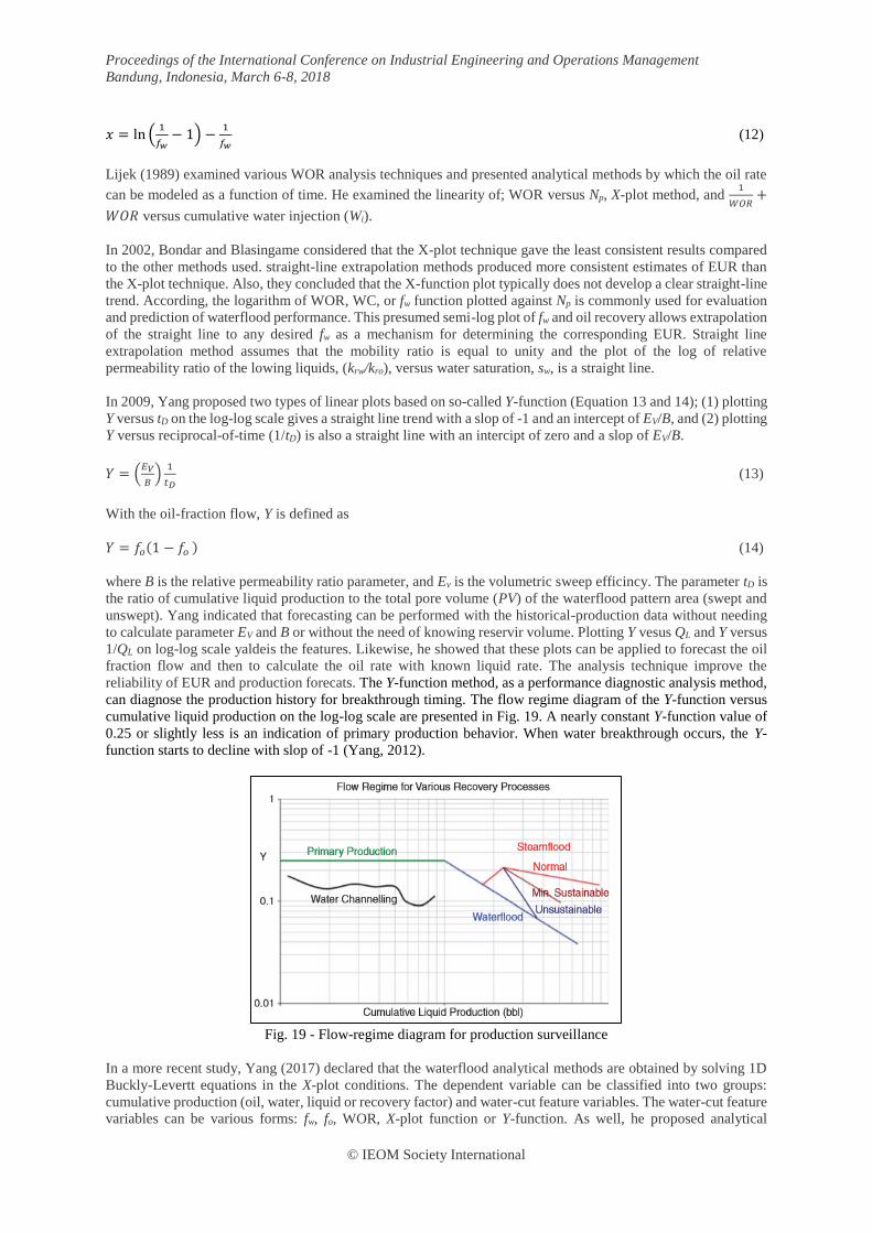
reliability of EUR and production forecats. The Y-function method, as a performance diagnostic analysis method,

can diagnose the production history for breakthrough timing. The flow regime diagram of the Y-function versus

cumulative liquid production on the log-log scale are presented in Fig. 19. A nearly constant Y-function value of

0.25 or slightly less is an indication of primary production behavior. When water breakthrough occurs, the Y-

function starts to decline with slop of -1 (Yang, 2012).

Fig. 19 - Flow-regime diagram for production surveillance

In a more recent study, Yang (2017) declared that the waterflood analytical methods are obtained by solving 1D

Buckly-Levertt equations in the X-plot conditions. The dependent variable can be classified into two groups:

cumulative production (oil, water, liquid or recovery factor) and water-cut feature variables. The water-cut feature

variables can be various forms: fw, fo, WOR, X-plot function or Y-function. As well, he proposed analytical




approach for X-plot method as follows: (1) use Y-function to confirm water breakthrough timing, to clarify

possible impact or reconfiguration events, and to select a post-breakthrough reference point on the linear trend;

(2) obtain cumulative liquid and oil (QL, Qo) and fo for the reference point; and (3) calculate the slop, m of the

straight-line trend and the X-value on the reference point, which will then solve for the intercept, n. When the

parameters m and n are available, the X-plot method is used to predict the EUR. He concluded that the procedure

of combining the X-plot method and Y-function method will reduce uncertainty in the EUR determination.

𝑋 = 𝑙𝑛 (1

𝑓𝑤− 1) −

1

𝑓𝑤 ; 𝑛 = (𝑆𝑤 −

1

𝐵𝑙𝑛

𝐴

𝑀) ; 𝑚 =

1

𝐵 (15)

Where M is the mobility ratio, B is a constant in the expression of the straight line in the semi-log oil to water

relative permeability versus water saturation (𝑘𝑟𝑜 𝑘𝑟𝑤⁄ = 𝐴𝑒−𝐵𝑆𝑤), and A is a constant.

Bondar and Blasingame (2002) mentioned that in all of the cases they considered, the X-plot technique gave the

least consistent results compared to the other methods used. Contrary, Yang (2017) reported that applying of X-

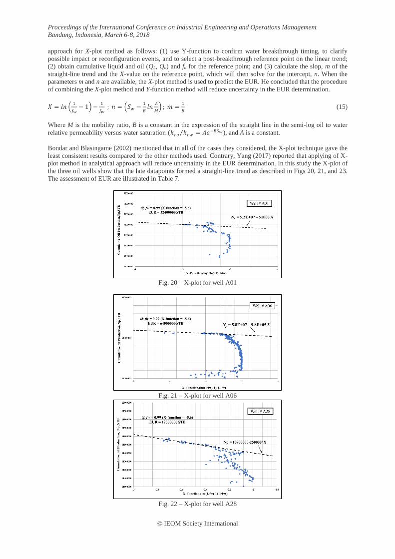
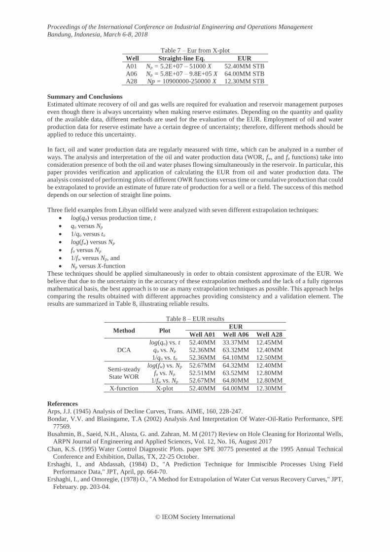
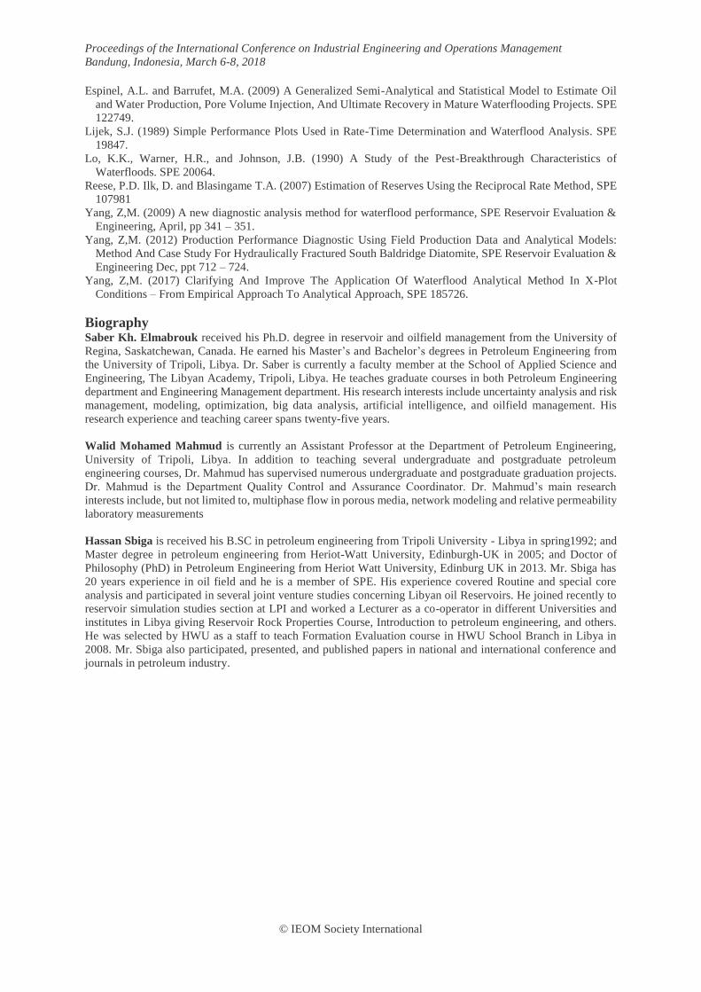
plot method in analytical approach will reduce uncertainty in the EUR determination. In this study the X-plot of

the three oil wells show that the late datapoints formed a straight-line trend as described in Figs 20, 21, and 23.

The assessment of EUR are illustrated in Table 7.

Fig. 20 – X-plot for well A01






Table 7 – Eur from X-plot


A01 Np = 5.2E+07 – 51000 X 52.40MM STB

A06 Np = 5.8E+07 – 9.8E+05 X 64.00MM STB

A28 Np = 10900000-250000 X 12.30MM STB

Summary and Conclusions

Estimated ultimate recovery of oil and gas wells are required for evaluation and reservoir management purposes

even though there is always uncertainty when making reserve estimates. Depending on the quantity and quality

of the available data, different methods are used for the evaluation of the EUR. Employment of oil and water

production data for reserve estimate have a certain degree of uncertainty; therefore, different methods should be

applied to reduce this uncertainty.

In fact, oil and water production data are regularly measured with time, which can be analyzed in a number of

ways. The analysis and interpretation of the oil and water production data (WOR, fw, and fo functions) take into

consideration presence of both the oil and water phases flowing simultaneously in the reservoir. In particular, this

paper provides verification and application of calculating the EUR from oil and water production data. The

analysis consisted of performing plots of different OWR functions versus time or cumulative production that could

be extrapolated to provide an estimate of future rate of production for a well or a field. The success of this method

depends on our selection of straight line points.

Three field examples from Libyan oilfield were analyzed with seven different extrapolation techniques:

• log(qo) versus production time, t

• qo versus Np

• 1/qo versus to

• log(fw) versus Np

• fo versus Np

• 1/fw versus Np, and

• Np versus X-function

These techniques should be applied simultaneously in order to obtain consistent approximate of the EUR. We

believe that due to the uncertainty in the accuracy of these extrapolation methods and the lack of a fully rigorous

mathematical basis, the best approach is to use as many extrapolation techniques as possible. This approach helps

comparing the results obtained with different approaches providing consistency and a validation element. The

results are summarized in Table 8, illustrating reliable results.

Table 8 – EUR results

Method Plot EUR

Well A01 Well A06 Well A28

DCA

log(qo) vs. t 52.40MM 33.37MM 12.45MM

qo vs. Np 52.36MM 63.32MM 12.40MM

1/qo vs. to 52.36MM 64.10MM 12.50MM

Semi-steady

State WOR

log(fw) vs. Np 52.67MM 64.32MM 12.40MM

fo vs. Np 52.51MM 63.52MM 12.80MM

1/fw vs. Np 52.67MM 64.80MM 12.80MM

X-function X-plot 52.40MM 64.00MM 12.30MM

References

Arps, J.J. (1945) Analysis of Decline Curves, Trans. AIME, 160, 228-247.

Bondar, V.V. and Blasingame, T.A (2002) Analysis And Interpretation Of Water-Oil-Ratio Performance, SPE

77569.

Busahmin, B., Saeid, N.H., Alusta, G. and. Zahran, M. M (2017) Review on Hole Cleaning for Horizontal Wells,

ARPN Journal of Engineering and Applied Sciences, Vol. 12, No. 16, August 2017

Chan, K.S. (1995) Water Control Diagnostic Plots. paper SPE 30775 presented at the 1995 Annual Technical

Conference and Exhibition, Dallas, TX, 22-25 October.

Ershaghi, I., and Abdassah, (1984) D., "A Prediction Technique for Immiscible Processes Using Field

Performance Data," JPT, April, pp. 664-70.

Ershaghi, I., and Omoregie, (1978) O., "A Method for Extrapolation of Water Cut versus Recovery Curves," JPT,

February. pp. 203-04.




Espinel, A.L. and Barrufet, M.A. (2009) A Generalized Semi-Analytical and Statistical Model to Estimate Oil

and Water Production, Pore Volume Injection, And Ultimate Recovery in Mature Waterflooding Projects. SPE

122749.

Lijek, S.J. (1989) Simple Performance Plots Used in Rate-Time Determination and Waterflood Analysis. SPE

19847.

Lo, K.K., Warner, H.R., and Johnson, J.B. (1990) A Study of the Pest-Breakthrough Characteristics of

Waterfloods. SPE 20064.

Reese, P.D. Ilk, D. and Blasingame T.A. (2007) Estimation of Reserves Using the Reciprocal Rate Method, SPE

107981

Yang, Z,M. (2009) A new diagnostic analysis method for waterflood performance, SPE Reservoir Evaluation &

Engineering, April, pp 341 – 351.

Yang, Z,M. (2012) Production Performance Diagnostic Using Field Production Data and Analytical Models:

Method And Case Study For Hydraulically Fractured South Baldridge Diatomite, SPE Reservoir Evaluation &

Engineering Dec, ppt 712 – 724.

Yang, Z,M. (2017) Clarifying And Improve The Application Of Waterflood Analytical Method In X-Plot

Conditions – From Empirical Approach To Analytical Approach, SPE 185726.

Biography Saber Kh. Elmabrouk received his Ph.D. degree in reservoir and oilfield management from the University of

Regina, Saskatchewan, Canada. He earned his Master’s and Bachelor’s degrees in Petroleum Engineering from

the University of Tripoli, Libya. Dr. Saber is currently a faculty member at the School of Applied Science and

Engineering, The Libyan Academy, Tripoli, Libya. He teaches graduate courses in both Petroleum Engineering

department and Engineering Management department. His research interests include uncertainty analysis and risk

management, modeling, optimization, big data analysis, artificial intelligence, and oilfield management. His

research experience and teaching career spans twenty-five years.

Walid Mohamed Mahmud is currently an Assistant Professor at the Department of Petroleum Engineering,

University of Tripoli, Libya. In addition to teaching several undergraduate and postgraduate petroleum

engineering courses, Dr. Mahmud has supervised numerous undergraduate and postgraduate graduation projects.

Dr. Mahmud is the Department Quality Control and Assurance Coordinator. Dr. Mahmud’s main research

interests include, but not limited to, multiphase flow in porous media, network modeling and relative permeability

laboratory measurements

Hassan Sbiga is received his B.SC in petroleum engineering from Tripoli University - Libya in spring1992; and

Master degree in petroleum engineering from Heriot-Watt University, Edinburgh-UK in 2005; and Doctor of

Philosophy (PhD) in Petroleum Engineering from Heriot Watt University, Edinburg UK in 2013. Mr. Sbiga has

20 years experience in oil field and he is a member of SPE. His experience covered Routine and special core

analysis and participated in several joint venture studies concerning Libyan oil Reservoirs. He joined recently to

reservoir simulation studies section at LPI and worked a Lecturer as a co-operator in different Universities and

institutes in Libya giving Reservoir Rock Properties Course, Introduction to petroleum engineering, and others.

He was selected by HWU as a staff to teach Formation Evaluation course in HWU School Branch in Libya in

2008. Mr. Sbiga also participated, presented, and published papers in national and international conference and

journals in petroleum industry.

calculation of eur form oil and water production data · by natural water drive or a pressure...

Documents