1

Calculation of mass transfer coefficients for corrosion prediction in two-

phase gas-liquid pipe flow

Luciano D. PAOLINELLI1 and Srdjan NESIC1

1 Institute for Corrosion and Multiphase Technology

Department of Chemical and Biomolecular Engineering, Ohio University,

342 W. State Street, Athens OH, USA,

paolinel@ohio.edu

nesic@ohio.edu

Abstract

Internal corrosion in industrial environments involving gas-liquid flow can be a serious concern. For example, in the oil and gas industry, corrosive water phase is usually transported in tubes and pipes

along with hydrocarbon and gas phases. These gas-liquid flows develop complex flow patterns where

the liquid phase can distribute in quite different ways (as stratified layers, intermittent slugs, annular film, etc.) depending on the gas and liquid flow rates and pipe inclination. In these circumstances, the

water phase can flow at very high velocities compare to either single-phase water flow or two-phase

hydrocarbon-water flow. High water velocities usually lead to high mass transfer rates that can

accelerate corrosion of the metallic pipe surface. In general, proper calculation of corrosion rates via mechanistic electrochemical models requires the knowledge of the mass transfer rate of corrosive

species. However, there are very few studies in the open literature that show specific experimental

data or propose ways to compute mass transfer rates in gas-liquid flow; particularly, for large pipe diameters. This study introduces a methodology for the estimation of mass transfer rates in gas-liquid

flow based on the Chilton-Colburn analogy, eddy diffusivity, and mechanistic gas-liquid flow

modeling. The proposed mechanistic models covers a wide range of fluid’s properties and flow rates, different flow regimes and pipe inclinations, and show good agreement with mass transfer

experimental data from large-scale gas-liquid flow.

Keywords: Gas-liquid flow; mass transfer; flow patterns; mechanistic modeling

Introduction

Internal corrosion can be an important problem in industry that deals with production and/or

transportation of liquid and gas phases. In the oil and gas industry, hydrocarbons are usually

produced with gas and corrosive water (carrying dissolved CO2 and H2S), and transported in

tubes and pipes. Gas lines also deal with hydrocarbon and water condensation, the latter may

lead to corrosion problems as well as “black powder” formation that are all undesired [1].

Gas-liquid flows can develop a wide variety of flow patterns in which the liquid phase can

distribute in different ways. For example, in horizontal flow, relatively low superficial liquid

velocities, and low to moderate superficial gas velocities lead to stratified flow of gas at the

top and liquid at the bottom of the pipe with a smooth or wavy gas liquid interface (“ST”

regime in Figure 1). The operating region for stratified flow drastically narrows even for very

small upward inclination angles (e.g., 1 degree) favoring the occurrence of intermittent flow

regime or slug flow [2].

Slug flow regime occurs at moderate superficial liquid velocities and a wide range of

superficial gas velocities as shown as “SL” regime in Figure 1. This flow regime can develop

very high liquid velocities since the translational velocity of liquid slugs is proportional to the

2

summation of the superficial velocities of the liquid and gas phases. In horizontal flow, the

velocity of the film liquid in the gas pocket zones is relatively low compared to the liquid

slug. However, liquid film velocities can be relatively high in inclined and vertical upward

flows where the liquid film moves counter current while the gas pockets flow with the main

stream.

When superficial gas velocities are high and the liquid holdup is not high enough to bridge the

entire pipe cross-section to produce slugs, the gas phase flows through the core of the pipe

and entrains liquid droplets which are simultaneously deposited all around the pipe

circumference, producing an annular film. This flow regime is called annular mist (“AM”

regime in Figure 1). Momentum transfer from the mixed gas-liquid core flow to the liquid

film can be significant. For high superficial liquid velocities, the gas phase is fully entrained

and dispersed as bubbles in the liquid phase, which is the flow regime indicated as “DB” in

Figure 1.

Figure 1. Calculated gas-liquid flow map. AM: Annular mist flow, DB: Dispersed bubble

flow, SL: Slug/intermittent flow, ST: Stratified flow. Horizontal flow, 𝑑=0.1 m, 𝜌𝑙=1000

kg/m3, 𝜇𝑙=1 mPa.s, 𝜌𝑔=10 kg/m3, 𝜇𝑙=0.018 mPa.s.

Some of the gas-liquid flow regimes mentioned above (e.g., SL and AM) can develop very

high liquid velocities compare to either single-phase water flow or other two-phase

hydrocarbon-water flows. These high liquid velocities lead to high wall shear stresses and

high mass transfer rates that can significantly accelerate corrosion of metallic pipe surfaces. In

general, mechanistic models to calculate corrosion rate are based on the electrochemical

reactions occurring at the pipe surface; e.g., oxidation of iron and reduction of hydronium

ions. For the latter or any other aggressive species under consideration, it is crucial to define

mass transfer rates with reasonable accuracy in order to obtain good prediction of corrosion

rates [3, 4].

The characteristics of mass transport from a bulk liquid phase to a solid pipe wall in

multiphase gas-liquid flow have been studied previously, mainly by means of electrochemical

techniques such as the measurements of limiting currents on arrangements of inert electrodes

3

flush mounted at the pipe surface [5-10]. Only a few studies were performed in pipes with

large diameter (e.g., 0.1m) which are more representative of the flows encountered in the oil

and gas industry [5, 8, 9]. Regarding the calculation of mass transfer rates in large scale gas-

liquid pipe flow, there have been attempts to build correlations derived from the one proposed

by Berger and Hau [11] for single phase pipe flow [8, 12]. Although these suggested

correlations use dimensionless numbers derived from the Chilton-Colburn relationship, they

are not mechanistic and oversimplify the effect of the wall shear stress exerted by the liquid

phase on mass transfer rate and do not cover all flow regimes.

The objective of this study is to introduce a methodology for the estimation of mass transfer

rates in multiphase gas-liquid flow. Two different approaches are used, based on the Chilton-

Colburn analogy and eddy diffusivity, as well as on mechanistic gas-liquid flow modeling to

obtain liquid flow characteristics (liquid velocity and wall shear stress) in the different flow

regimes. Mass transfer calculation results are discussed and compared with available

experimental data obtained in large-scale gas-liquid flow with different flow patterns.

Mass transfer model

Fundamental mass transfer relationship

Mass transfer rates in fully developed turbulent boundary layer can be related to the wall

shear stresses by the Chilton-Colburn analogy [13]:

(𝑓

2)

𝑛

=𝑆ℎ

𝑅𝑒 𝑆𝑐1 3⁄ ; (1)

𝑆𝑐 =𝜇

𝜌𝐷; (2)

𝑆ℎ =𝑘𝑑

𝐷; (3)

𝑅𝑒 =𝜌𝑢𝑑

𝜇 (4)

where 𝑆𝑐, 𝑆ℎ and 𝑅𝑒 are the Schmidt, Sherwood and Reynolds numbers, respectively, 𝐷 is the

diffusion coefficient of a given specie in the studied fluid, 𝑑 is a characteristic length that for

single phase pipe flow is the internal pipe diameter, 𝑓 is the Fanning friction factor, 𝑘 is the

mass transfer coefficient, 𝑢 is the mean velocity of the fluid, 𝜇 is the fluid dynamic viscosity,

and 𝜌 is the fluid density. The exponent 𝑛 is equal to 1 according to [13]. However, some

authors suggested that the exponent can be between 1 and 0.5 [11, 14, 15].

Mass transfer coefficient can be calculated directly from (1) as:

𝑘 = (𝑓

2)

𝑛

𝑢 𝑆𝑐−2 3⁄ = (𝜏

𝜌𝑢2)𝑛

𝑢 𝑆𝑐−2 3⁄ (5)

where 𝜏 is the wall shear stress exerted by the fluid.

The main advantage of equation (5) is that, regardless of the geometrical characteristics of the

flow under study (e.g., pipe flow, rotating cylinder, jet impingement, etc.), it allows the

estimation of the mass transfer rate at any given boundary layer as long as the wall shear

4

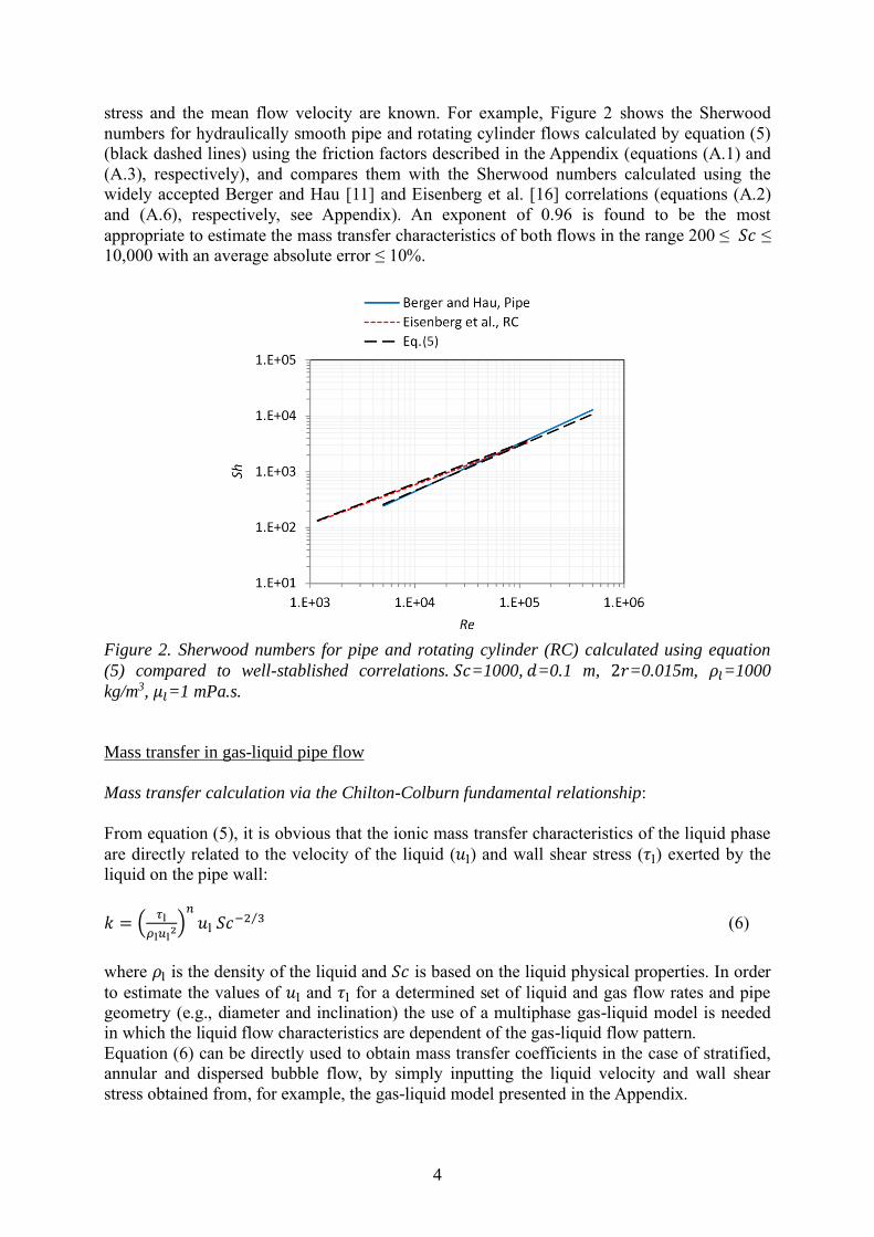
stress and the mean flow velocity are known. For example, Figure 2 shows the Sherwood

numbers for hydraulically smooth pipe and rotating cylinder flows calculated by equation (5)

(black dashed lines) using the friction factors described in the Appendix (equations (A.1) and

(A.3), respectively), and compares them with the Sherwood numbers calculated using the

widely accepted Berger and Hau [11] and Eisenberg et al. [16] correlations (equations (A.2)

and (A.6), respectively, see Appendix). An exponent of 0.96 is found to be the most

appropriate to estimate the mass transfer characteristics of both flows in the range 200 ≤ 𝑆𝑐 ≤

10,000 with an average absolute error ≤ 10%.

Figure 2. Sherwood numbers for pipe and rotating cylinder (RC) calculated using equation

(5) compared to well-stablished correlations. 𝑆𝑐=1000, 𝑑=0.1 m, 2𝑟=0.015m, 𝜌𝑙=1000

kg/m3, 𝜇𝑙=1 mPa.s.

Mass transfer in gas-liquid pipe flow

Mass transfer calculation via the Chilton-Colburn fundamental relationship:

From equation (5), it is obvious that the ionic mass transfer characteristics of the liquid phase

are directly related to the velocity of the liquid (𝑢l) and wall shear stress (𝜏l) exerted by the

liquid on the pipe wall:

𝑘 = (𝜏l

𝜌l𝑢l2)

𝑛

𝑢l 𝑆𝑐−2 3⁄ (6)

where 𝜌l is the density of the liquid and 𝑆𝑐 is based on the liquid physical properties. In order

to estimate the values of 𝑢l and 𝜏l for a determined set of liquid and gas flow rates and pipe

geometry (e.g., diameter and inclination) the use of a multiphase gas-liquid model is needed

in which the liquid flow characteristics are dependent of the gas-liquid flow pattern.

Equation (6) can be directly used to obtain mass transfer coefficients in the case of stratified,

annular and dispersed bubble flow, by simply inputting the liquid velocity and wall shear

stress obtained from, for example, the gas-liquid model presented in the Appendix.

5

In the case of slug flow, the mass transfer coefficient is computed as the average of the mass

transfer coefficients of the liquid slug and film regions:

𝑘 = 𝑘s + 𝑘f = [(𝜏ls

𝜌l𝑢t2)

𝑛

𝑢t𝛽s + (|𝜏lf|

𝜌l𝑢lf2)

𝑛|𝑢lf|(1 − 𝛽s)] 𝑆𝑐−2 3⁄ (7)

where 𝑢t is the velocity of the liquid slug front, 𝑢lf is the velocity of the liquid film, 𝜏ls and 𝜏lf

are the wall shear stresses of the liquid slug and the liquid film, respectively; and 𝛽s is the

relative length of the liquid slug as shown in Figure A.1 in the Appendix. Note that the

velocity and the wall shear stress of the liquid film are computed as absolute value since they

can be negative (counter current flow) in inclined and vertical flows.

Mass transfer computation in systems with simultaneous reactions at the pipe wall and in the

liquid:

In cases where species react with the solid surface as well as with other species in the fluid,

e.g., as the case of hydronium ions in CO2 or H2S corrosion [3, 17, 18], the computation of the

concentration of a given specie at the pipe wall will depend not only on its molecular

diffusion and the transport characteristics of the fluid flow boundary layer but also on the

consumption or generation of this specie close to the solid wall. Therefore, specific functions

to determine turbulent transport characteristics in function of the distance from the solid wall

are needed. The mass transfer rate in the normal direction (𝑦) of a solid wall in steady state

turbulent flow can be written as:

𝑁 = 𝐷𝜕𝐶

𝜕𝑦+ 𝑣′𝐶′̅̅ ̅̅ ̅̅ (8)

where 𝑁 is the mass flux, 𝐶′is the concentration fluctuation, and 𝑣′ is the flow velocity

fluctuation. The term 𝑣′𝐶′̅̅ ̅̅ ̅̅ can be modeled as and eddy diffusivity that is added to the

molecular diffusion:

𝑁 = (𝐷 + 𝐷t)𝜕𝐶

𝜕𝑦 (9)

where the turbulent diffusion of mass is defined by analogy to the eddy diffusion of

momentum as [19]:

𝐷t = (𝑦+

𝐶t)

3𝜇l

𝜌l (10)

where 𝐶t is a constant that can range from 8.8 to 14.5 according to different authors [19, 20],

and 𝑦+ is the dimensionless distance from the solid wall:

𝑦+ = 𝑦𝜌l𝑢

∗

𝜇l (11)

where 𝑢∗ is the friction velocity calculated as √𝜏l 𝜌l⁄ .

Equation (11) is valid provided that the diffusion boundary layer (𝛿) is smaller than the

viscous sublayer of the liquid flow (𝛿+ < 5) which, in general, is true for 𝑆𝑐 >100.

6

The mass flux at the solid wall (𝑁w) can be calculated solving the equation (9) within a

domain larger than 𝛿. The mass transfer coefficient is then defined as:

𝑘 =𝑁w

(𝐶w−𝐶b) (12)

where 𝐶b and 𝐶w are the concentrations of a given specie at the bulk of the fluid and at the

wall surface, respectively.

The use of equations (9) and (10) is direct in the case of gas-liquid flows with stratified,

annular and dispersed bubble flow patterns via the use of the actual wall shear stress of the

liquid phase for the calculation of the friction velocity in equation (11). However, for slug

flow, the hydrodynamic boundary layers of the liquid film and liquid slug can be very

different. Moreover, in some operating conditions period between slugs can be smaller than a

second, which might be a relatively short time to fully develop the hydrodynamic and

diffusion boundary layers. Regardless of these facts, the hydrodynamic boundary layer in slug

flow can be characterized by an average friction velocity:

𝑢∗̅̅ ̅=𝑢∗ls 𝛽s + 𝑢∗

lf (1 − 𝛽s) = √𝜏ls

𝜌l 𝛽s + √

|𝜏lf|

𝜌l (1 − 𝛽s) (13)

Then, 𝑢∗̅̅ ̅ is directly used in equation (11) to compute 𝑦+.

Results and discussion

Ionic mass transfer in gas-water pipe flow

The models proposed above are compared with experimental data of ionic mass transfer from

Langsholt et al. [5] and Wang et al. [8] obtained in large-scale gas-water flows with stratified

and slug flow patterns.

Langsholt et al. used an inclinable multiphase flow loop with an internal diameter 0.1 m and a

length (𝑙) of 15 m. The gas phase was sulphur hexafluoride (SF6) with reported density of

18.6 kg/m3 and calculated viscosity of 1.510-2 mPa.s at operating conditions (20C and

3bar). The liquid phase was an aqueous solution 1 wt.% Na2SO4 with density of 1006 kg/m3

and viscosity of 1 mPa.s. Ionic mass transfer rates were measured by the limiting current

method using an electrochemical probe flush mounted at the bottom of the test section and

oxygen reduction as the monitored reaction with a Schmidt number of 473. Liquid holdup

was also measured using gamma densitometry. The covered operating conditions and

visualized flow patterns, as well as the measured average mass transfer rates and liquid

holdups are listed in Table A.1 in the Appendix.

Wang, et al. also used a multiphase flow loop with an internal diameter 0.1m and a length (𝑙) of 15 m. The gas phase was nitrogen with estimated density of 1.15 kg/m3 and viscosity of

1.710-2 mPa.s at operating conditions (20C and 1.5bar). The liquid phase was an aqueous

solution 0.01M potassium ferri/ferrocyanide and 1M NaOH for the mass transfer

measurements by the limiting current method. The calculated density and viscosities of the

solution are 1043 kg/m3 and 1.1 mPa.s, respectively; and the estimated Schmidt number is

7

1620 [21]. The used operating conditions, observed flow patterns, and measured average mass

transfer rates are listed in Table A.2 in the Appendix.

Figure 3 shows the comparison of the measured mass transfer coefficients in different

conditions and flow patterns with the ones calculated with equations (6) and (7) fed by the

gas-liquid flow model presented in the Appendix. The agreement between the proposed model

and the experimental data is fairly good with an absolute error of 23% and most of the data

lying within the 30% error bounds. The conditions that showed more error were the ones

from 2 upward slug flows from Langsholt et al. A possible reason for these discrepancies

might be related to an over prediction of counter current liquid velocities in the liquid film by

the simplified gas-liquid model in the Appendix.

Mass transfer predictions using the introduced mechanistic model are an improvement over

semi-empirical correlations for gas-liquid flow offered in the literature, which are mostly

developed based on data from air-water flows in relatively small diameter pipes (e.g.,

0.025m), as reviewed in the recent works of Dong and Hibiki [22, 23]. Most of these

correlations are limited for horizontal or upwards/downwards vertical flows, as well as

relatively low superficial gas and liquid Reynolds numbers, making them unfeasible for large

scale flows (e.g., large diameters and gas and liquid flow rates) with different inclinations and

upward or downward orientations. The correlation that performs better over the current

experimental data with an average absolute error of 20% is the one from Dong and Hibiki

[22], which is based on vertical flows. However, it underestimates by about 70% experimental

mass transfer rates measured in flows with liquid holdups smaller than 10%.

Figure 3. Comparison between experimental mass transfer coefficients for large-scale gas-

liquid pipe flow with different flow patterns and mass transfer coefficients calculated with

equations (6) and (7).

As discussed above, in cases where the modeling of transport of species also depend on

chemical reactions occurring in the fluid near the pipe wall, it is more appropriate to use the

8

approach described in equation (9). This equation was solved numerically for all the

experimental cases applying the finite difference method using at least 20 elements in the

diffusion layer (𝛿) and a total domain with a length larger than 4𝛿. Mass transfer coefficients

were then calculated with equation (12). Equation (10) for turbulent diffusion was assessed

using coefficients suggested by Davies (𝐶t=8.85, [20]) and Lin et al. (𝐶t=14.5, [19]); the eddy

diffusivity functions suggested by Notter and Sleicher [24] and Aravinth [25] were also

evaluated. Figure 4 shows the mass transfer rates calculated in single phase flow using the

eddy diffusivity approach compared to the Berger and Hau correlation. Although the eddy

diffusivity approach follows reasonably well the slope with Reynolds number seen in Berger

and Hau’s correlation, the expressions suggested by Davies, Notter and Sleicher, and Aravinth

overestimate mass transfer rates by an average of more than 50%. The Lin et al. formulation

gives better results with an average overestimation of 21%.

Experimental mass transfer coefficients in gas-liquid flow were then modeled using the Lin et

al. formulation as shown in Figure 5. Calculations show an important overestimation of mass

transfer rates with an average absolute error of 34%. Moreover, about 40% of the data lie out

of the 30% error bound including the single phase flow data of Wang. et al. (42% average

error). This behavior was somehow expected since Lin et al.’s expression overestimates mass

transfer rates in single phase flow by at least an average of 20% as previously shown in

Figure 4. An increase in the coefficient 𝐶t in equation (10) to a value of 18.4 leads to an

average absolute error of about 6% respect to Berger and Hau’s correlation, and an average

absolute error of 19% respect to the experimental data from gas-liquid flow as shown in

Figure 6. Higher values of 𝐶t no longer improve the average absolute error on the

experimental data from multiphase flow, and lead to underestimation of mass transfer in

single phase by more than 10% in average.

Figure 4. Comparison between mass transfer rates for single phase pipe wall calculated with

the eddy diffusivity approach and Berger and Hau’s correlation. 𝑆𝑐=1000, 𝑑=0.1 m,

𝜌𝑙=1000 kg/m3, 𝜇𝑙=1 mPa.s.

9

Figure 5. Comparison between experimental mass transfer coefficients for large-scale gas-

liquid pipe flow with different flow patterns and mass transfer coefficients calculated with the

eddy diffusivity approach using Lin et al.’s formulation.

Figure 6. Comparison between experimental mass transfer coefficients for large-scale gas-

liquid pipe flow with different flow patterns and mass transfer coefficients calculated with the

eddy diffusivity approach using equation (10) with 𝐶t=18.4.

Ionic mass transfer in gas-oil-water and oil-water pipe flow

Generally, flows in the oil and gas industry contain significant fractions of liquid

hydrocarbons. In the case of gas-oil-water flows, the produced oil and water phases that can

flow either separated or mixed. If flow conditions (e.g., gas, oil and water flow rates) are

10

viable to produce the full entrainment of the water in the oil phase, the pipe wall will not

likely be water wet and ionic mass transfer would be suppressed [26, 27]. However, if water

either segregates from or is the continuous phase of the liquid mix, mass transfer rates can be

similar to the ones corresponding to gas-water flow without hydrocarbon [9]. Therefore,

calculation of mass transfer rates in gas-oil-water flow can still be done using equations (6)

and (7) (fundamental Chilton-Colburn relationship) or the eddy diffusivity approach, using

liquid velocities and wall shear stresses calculated with the following liquid mixture

properties:

𝜌lm = 𝜌o(1 − 휀w) + 𝜌w휀w (14)

𝜇lm ≅ {𝜇o 휀w < 𝐼𝑃 𝜇w 휀w > 𝐼𝑃

(15)

where 𝜌lm and 𝜇lm are the density and the viscosity of the liquid mixture, respectively; 𝜌o and

𝜇o are the density and viscosity of the oil phase, 𝜌w and 𝜇w are the density and viscosity of

the water phase, 𝐼𝑃 is the phase inversion of the oil-water mixture based on the water volume

content (for crude oil can be approximated as 0.5); and 휀w is the volumetric water fraction in

the liquid mix, which can be approximated as the water cut (no slip between oil and water

phases) :

휀w =𝑢sw

𝑢sw+𝑢so =

𝑢sw

𝑢sl (16)

where 𝑢so and 𝑢sw are the superficial velocities of oil and water; respectively, which sum

gives the total superficial liquid velocity 𝑢sl. Schmidt number is obviously calculated using

the physical properties of the water phase.

In the case of oil-water flow (negligible or no gas phase present), the calculation of mass

transfer rates is performed similarly as to gas-liquid flow. However, an oil-water flow model

is required for the estimation of the velocity and wall shear stress of the water phase.

Summary and conclusions

Two different approaches for mass transfer estimation in multiphase gas-liquid flow have

been introduced and compared against experimental data from large-scale flows with different

flow regimes. In general, the agreement of the offered mass transfer models with the available

experimental data is reasonably good for all the different assessed flow patterns; especially, in

slug flow where the hydrodynamic and diffusion boundary layers fluctuate in relatively short

periods.

Direct computation of mass transfer coefficients can be done with fair accuracy for a wide

variety of flows (single phase pipe and rotating cylinder, and two-phase gas-liquid pipe) by

using the fundamental Chilton-Colburn with an exponent of 0.96 on the friction factor.

Mass transfer calculation via the eddy diffusivity approach tend to overestimate mass transfer

rates for single and multiphase flow when some of the classic formulations in the literature.

The use of the classic cubic variation of eddy diffusivity with a coefficient of 18.4 affecting

the dimensionless wall distance; instead of the smaller values suggested in the literature,

11

proved to be the most appropriate to predict mass transfer rates in single and multiphase flow

with fair accuracy.

The main strength of the proposed models is their mechanistic nature, which allows their use

in systems with wide range of physical properties (different gas and liquid densities and

viscosities) and pipe characteristics (different diameters, inclination, smooth and rough

surfaces). Moreover, better results can surely be achieved if liquid flow characteristics are

estimated using multiphase flow models more advanced and refined than the one currently

offered. This is a significant improvement over semi-empirical correlations suggested in the

literature that are usually tuned for limited ranges of fluid’s properties and flow rates, making

them unreliable for general use. In addition, these correlations cannot be applied to cases

where species react in the fluid as well as at the pipe wall.

Acknowledgements

The authors want to thank the financial support from the multiple companies that participate

of JIPs and other research projects at the Institute for Corrosion and Multiphase Technology at

Ohio University.

Appendix

Experimental data used in the model validation

Table A.1. Experimental conditions, measured liquid holdup and average mass transfer rates

in horizontal and slightly inclined flow from Langsholt et al. [5].

Flow pattern 𝑢sl [m/s] 𝑢sg [m/s] 𝛽 [] 𝛼l [%] 𝑆ℎ

Strat.-wavy 0.021 2.14 0 6.1 1489

Strat.-wavy 0.019 4.11 0 2 2884

Strat.-wavy 0.025 6.34 0 1.2 3491

Strat.-wavy 0.25 6.06 0 11.1 4076

Strat.-wavy 0.25 7.1 0 9.5 4450

Strat.-wavy 0.25 8.18 0 8.2 4762

Strat.-wavy 0.25 5.05 0 12.9 4053

Strat.-wavy 0.25 4.1 0 15.4 3788

Strat.-wavy 0.25 3 0 19.4 3265

Strat.-wavy 0.25 2.03 0 27.2 2587

Strat.-wavy 0.25 0.96 0 42 2034

Strat.-wavy 2 3 2 50 7404

Strat.-wavy 2 5 2 31 8986

Strat.-wavy 2 7 2 21 11300

Strat.-wavy 2 9 2 17 12275

Strat.-wavy 2 12 2 13 13888

Strat.-wavy 1 3 2 42 5627

Strat.-wavy 1 7 2 19 7326

Strat.-wavy 1 9 2 14 8892

Strat.-wavy 1 12 2 9 9913

Strat.-wavy 0.78 5 2 43 4333

12

Slug 0.78 2 2 30 5518

Slug 0.13 2 2 26 1598

Slug 0.1 2 2 25 1582

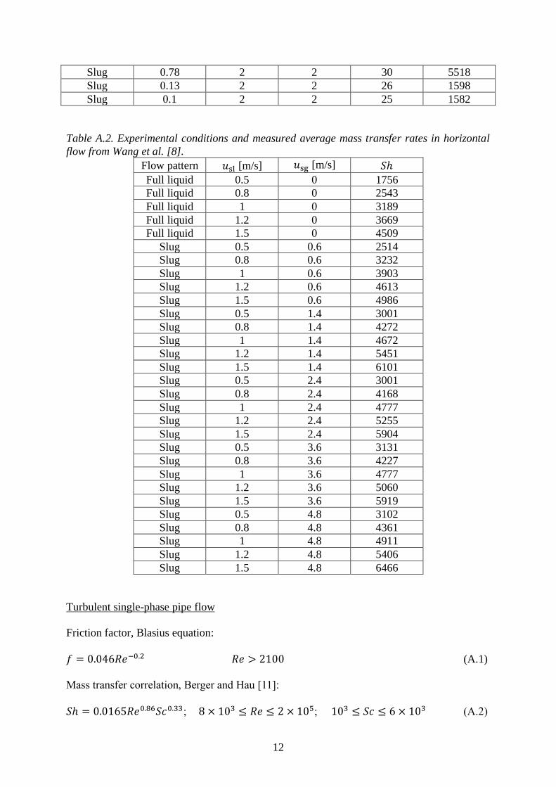
Table A.2. Experimental conditions and measured average mass transfer rates in horizontal

flow from Wang et al. [8].

Flow pattern 𝑢sl [m/s] 𝑢sg [m/s] 𝑆ℎ

Full liquid 0.5 0 1756

Full liquid 0.8 0 2543

Full liquid 1 0 3189

Full liquid 1.2 0 3669

Full liquid 1.5 0 4509

Slug 0.5 0.6 2514

Slug 0.8 0.6 3232

Slug 1 0.6 3903

Slug 1.2 0.6 4613

Slug 1.5 0.6 4986

Slug 0.5 1.4 3001

Slug 0.8 1.4 4272

Slug 1 1.4 4672

Slug 1.2 1.4 5451

Slug 1.5 1.4 6101

Slug 0.5 2.4 3001

Slug 0.8 2.4 4168

Slug 1 2.4 4777

Slug 1.2 2.4 5255

Slug 1.5 2.4 5904

Slug 0.5 3.6 3131

Slug 0.8 3.6 4227

Slug 1 3.6 4777

Slug 1.2 3.6 5060

Slug 1.5 3.6 5919

Slug 0.5 4.8 3102

Slug 0.8 4.8 4361

Slug 1 4.8 4911

Slug 1.2 4.8 5406

Slug 1.5 4.8 6466

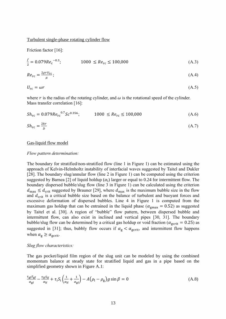
Turbulent single-phase pipe flow

Friction factor, Blasius equation:

𝑓 = 0.046𝑅𝑒−0.2 𝑅𝑒 > 2100 (A.1)

Mass transfer correlation, Berger and Hau [11]:

𝑆ℎ = 0.0165𝑅𝑒0.86𝑆𝑐0.33; 8 × 103 ≤ 𝑅𝑒 ≤ 2 × 105; 103 ≤ 𝑆𝑐 ≤ 6 × 103 (A.2)

13

Turbulent single-phase rotating cylinder flow

Friction factor [16]:

𝑓

2= 0.079𝑅𝑒c

−0.3; 1000 ≤ 𝑅𝑒rc ≤ 100,000 (A.3)

𝑅𝑒rc =2𝜌𝑟𝑈rc

𝜇; (A.4)

𝑈rc = 𝜔𝑟 (A.5)

where 𝑟 is the radius of the rotating cylinder, and 𝜔 is the rotational speed of the cylinder.

Mass transfer correlation [16]:

𝑆ℎrc = 0.079𝑅𝑒rc0.7𝑆𝑐0.356; 1000 ≤ 𝑅𝑒rc ≤ 100,000 (A.6)

𝑆ℎrc =2𝑘𝑟

𝐷 (A.7)

Gas-liquid flow model

Flow pattern determination:

The boundary for stratified/non-stratified flow (line 1 in Figure 1) can be estimated using the

approach of Kelvin-Helmholtz instability of interfacial waves suggested by Taitel and Dukler

[28]. The boundary slug/annular flow (line 2 in Figure 1) can be computed using the criterion

suggested by Barnea [2] of liquid holdup (𝛼l) larger or equal to 0.24 for intermittent flow. The

boundary dispersed bubble/slug flow (line 3 in Figure 1) can be calculated using the criterion

𝑑max ≤ 𝑑crit suggested by Brauner [29], where 𝑑max is the maximum bubble size in the flow

and 𝑑crit is a critical bubble size based on the balance of turbulent and buoyant forces and

excessive deformation of dispersed bubbles. Line 4 in Figure 1 is computed from the

maximum gas holdup that can be entrained in the liquid phase (𝛼gmax = 0.52) as suggested

by Taitel et al. [30]. A region of “bubble” flow pattern, between dispersed bubble and

intermittent flow, can also exist in inclined and vertical pipes [30, 31]. The boundary

bubble/slug flow can be determined by a critical gas holdup or void fraction (𝛼gcrit = 0.25) as

suggested in [31]; thus, bubbly flow occurs if 𝛼g < 𝛼gcrit, and intermittent flow happens

when 𝛼g ≥ 𝛼gcrit.

Slug flow characteristics:

The gas pocket/liquid film region of the slug unit can be modeled by using the combined

momentum balance at steady state for stratified liquid and gas in a pipe based on the

simplified geometry shown in Figure A.1:

𝜏gf𝑆gf

𝛼gf−

𝜏lf𝑆lf

𝛼lf+ 𝜏i𝑆i (

1

𝛼lf+

1

𝛼gf) − 𝐴(𝜌l − 𝜌g)𝑔 sin 𝛽 = 0 (A.8)

14

where 𝜏gf and 𝜏lf are the wall shear stresses due to the flow of the gas bubble and the liquid

film, respectively; 𝜏i is the shear stress at the gas-liquid interface, 𝛼gf (also expressed as:

1 − 𝛼lf) and 𝛼lf are the fractions of pipe cross sectional area (𝐴) occupied by gas and liquid,

respectively; 𝑆gf and 𝑆lf are the pipe perimeters wetted by gas and liquid, respectively; 𝑆i is

the perimeter of the gas-liquid interface, 𝜌g is the gas density; 𝑔 is the gravitational

acceleration, and 𝛽 is the pipe inclination angle measured from the horizontal. The wall shear

stresses are calculated as follows:

𝜏gf =1

2𝑓gf𝜌g𝑢gf

2 (A.9)

𝜏lf =1

2𝑓lf𝜌l𝑢lf

2 (A.10)

and the interfacial stress:

𝜏i =1

2𝑓i𝜌g(𝑢gf − 𝑢lf)|𝑢gf − 𝑢lf| (A.11)

where 𝑢gf and 𝑢lf are the mean velocities of the gas and liquid; respectively; and 𝑓gf, 𝑓lf and 𝑓i

are the friction factors for the gas bubble, liquid film and gas-liquid interface, respectively.

Friction factors are estimated as:

𝑓 = 𝐶f𝑅𝑒−𝑛f (A.12)

where 𝑅𝑒 is the Reynolds number, and 𝐶f and 𝑛f are constants equal to 0.046 and 0.2,

respectively; for turbulent flow 𝑅𝑒 > 2100, and 16 and 1 for laminar flow 𝑅𝑒 2100. In case

the pipe surface is not hydraulically smooth, the explicit friction factor formulas in [32] can

be used. The Reynolds numbers for the gas bubble and liquid film flows are:

𝑅𝑒g =𝜌g𝑢gf𝑑gf

𝜇g (A.13)

𝑅𝑒lf =𝜌l𝑢lf𝑑lf

𝜇l (A.14)

and gas-liquid interface:

𝑅𝑒i =𝜌g|𝑢gf−𝑢lf|𝑑gf

𝜇g (A.15)

where 𝜇g and 𝜇l are the viscosities of the gas and the liquid, respectively; 𝑑gf is the hydraulic

diameter for the gas bubble flow:

𝑑gf =4𝐴𝛼gf

𝑆lg+𝑆i (A.16)

and 𝑑lf is the hydraulic diameter of the liquid film flow:

𝑑lf =4𝐴𝛼lf

𝑆lf (A.17)

15

The mean velocity of the liquid slug cylinder is approximated to the mixture velocity, which

is calculated as the summation of superficial gas and liquid velocities:

𝑢m = 𝑢sg + 𝑢sl (A.18)

No slip is considered between the entrained gas bubbles and the liquid in the slug cylinder.

Then, the velocities of the gas bubble and the liquid film can be related with the gas bubble

and liquid film holdups (𝛼gf and 𝛼lf, respectively) as suggested by Dukler and Hubbard [33]:

𝑢gf = 𝑢t + (𝑢m − 𝑢t) (1−𝛼ls

1−𝛼lf) (A.19)

𝑢lf = 𝑢t (1 −𝛼ls

𝛼lf) + 𝑢m

𝛼ls

𝛼lf (A.20)

where 𝛼ls is the liquid holdup at the slug cylinder, and 𝑢t is the translational velocity at which

the slug propagates, and is estimated as:

𝑢t = 𝐶0𝑢m + 𝑢b (A.21)

where 𝑢b (m/s) is the Taylor bubble velocity that can be neglected in horizontal slug flow, 𝐶0

is the distribution parameter used in the drift-flux model and can be approximated with the

value 1.2 [34].

The liquid holdup at the slug cylinder is approximated using the Gregory et al. correlation

[35]:

𝛼ls = [1 + (𝑢m

8.66)

1.39

]−1

(A.22)

The constant 8.66 in equation above has SI velocity units.

Figure A.1. Schematic representation of the slug flow unit assumed in the gas-liquid model.

The combined momentum balance in equation (A.8) can be solved iteratively to find the

liquid film holdup (𝛼lf). Since equation (A.8) has multiple roots for pipe inclination angles

(𝛽) different than zero; in general, the smaller root is considered as solution of the problem.

16

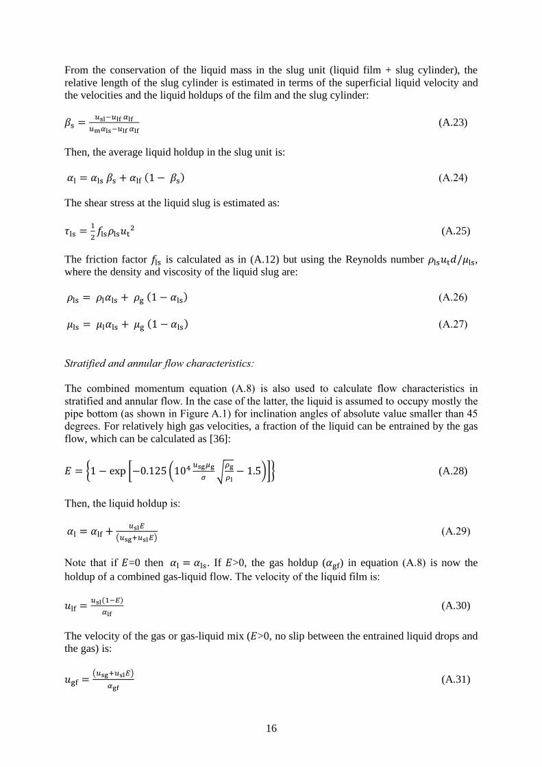
From the conservation of the liquid mass in the slug unit (liquid film + slug cylinder), the

relative length of the slug cylinder is estimated in terms of the superficial liquid velocity and

the velocities and the liquid holdups of the film and the slug cylinder:

𝛽s =𝑢sl−𝑢lf 𝛼lf

𝑢m𝛼ls−𝑢lf 𝛼lf (A.23)

Then, the average liquid holdup in the slug unit is:

𝛼l = 𝛼ls 𝛽s + 𝛼lf (1 − 𝛽s) (A.24)

The shear stress at the liquid slug is estimated as:

𝜏ls =1

2𝑓ls𝜌ls𝑢t

2 (A.25)

The friction factor 𝑓ls is calculated as in (A.12) but using the Reynolds number 𝜌ls𝑢t𝑑/𝜇ls,

where the density and viscosity of the liquid slug are:

𝜌ls = 𝜌l𝛼ls + 𝜌g (1 − 𝛼ls) (A.26)

𝜇ls = 𝜇l𝛼ls + 𝜇g (1 − 𝛼ls) (A.27)

Stratified and annular flow characteristics:

The combined momentum equation (A.8) is also used to calculate flow characteristics in

stratified and annular flow. In the case of the latter, the liquid is assumed to occupy mostly the

pipe bottom (as shown in Figure A.1) for inclination angles of absolute value smaller than 45

degrees. For relatively high gas velocities, a fraction of the liquid can be entrained by the gas

flow, which can be calculated as [36]:

𝐸 = {1 − exp [−0.125 (104 𝑢sg𝜇g

𝜎√

𝜌g

𝜌l− 1.5)]} (A.28)

Then, the liquid holdup is:

𝛼l = 𝛼lf +𝑢sl𝐸

(𝑢sg+𝑢sl𝐸) (A.29)

Note that if 𝐸=0 then 𝛼l = 𝛼ls. If 𝐸>0, the gas holdup (𝛼gf) in equation (A.8) is now the

holdup of a combined gas-liquid flow. The velocity of the liquid film is:

𝑢lf =𝑢sl(1−𝐸)

𝛼lf (A.30)

The velocity of the gas or gas-liquid mix (𝐸>0, no slip between the entrained liquid drops and

the gas) is:

𝑢gf =(𝑢sg+𝑢sl𝐸)

𝛼gf (A.31)

17

When solving equation (A.8) a different interfacial friction closure relationship is used instead

of equation (A.11):

𝜏i =1

2𝑓i𝜌gf(𝑢gf − 𝑢i)|𝑢gf − 𝑢i| (A.32)

where 𝑢i is the velocity of the interface between the liquid film and the gas calculated as in

Oliemans et al. [37]. The interfacial friction factor (𝑓i) is calculated with the Colebrook

equation using an effective roughness described in [37], the hydraulic diameter (𝑑gf) and the

Reynolds number 𝜌gf𝑢gf𝑑gf/𝜇gf, where:

𝜌gf = 𝜌l(1 − 𝛼gr) + 𝜌g𝛼gr (A.33)

𝜇gf = 𝜇l(1 − 𝛼gr) + 𝜇g𝛼gr (A.34)

𝛼gr =𝑢sg

(𝑢sg+𝑢sl𝐸) (A.35)

Dispersed bubble and Bubble flow characteristics:

A homogeneous no-slip model is used to estimate flow characteristics in dispersed bubble

flow. Therefore, the velocity of the liquid and the entrained gas bubbles is considered to be

similar to the mixture velocity:

𝑢l = 𝑢g ≅ 𝑢m (A.36)

The liquid holdup is:

𝛼l =𝑢sl

(𝑢sg+𝑢sl) (A.37)

The wall shear stress is:

𝜏l =1

2𝑓m𝜌m𝑢l

2 (A.38)

where the friction factor 𝑓m is calculates as in (A.12) using the Reynolds number 𝜌m𝑢l𝑑/𝜇m,

where:

𝜌m = 𝜌l𝛼l + 𝜌g (1 − 𝛼l) (A.39)

𝜇m = 𝜇l𝛼l + 𝜇g (1 − 𝛼l) (A.40)

Bubble flow can have significant slip between the liquid and the gas bubbles which rise

quicker due to buoyancy. In this case, drift flux model can be used to properly determine the

liquid and gas holdups. Equations (A.38 to A.40) can then be used to calculate flow

characteristics.

18

References

1. R. Baldwin, Black Powder in the Gas Industry-Sources, Characteristics and Treatment

Mechanical and Fluids Engineering Division, Southwest Research Institute, San Antonio TX

(1997) TA 97-94.

2. D. Barnea, International Journal of Multiphase Flow, 13 (1987) 1.

3. S. Nešić, A. Kahyarian, Y.S. Choi, Corrosion, 75 (2019) 274.

4. Y. Zheng, J. Ning, B. Brown, S. Nešić, Corrosion, 72 (2016) 679.

5. M. Langsholt, M. Nordsveen, K. Lunde, S. Nesic, J. Enerhaug, Wall Shear Stress and Mass

Transfer Rates – Important Parameters in CO2 Corrosion, BHR Group Multiphase 97’,

Cannes, France (1997) pp. 537-552.

6. N. Pecherkin, V. Chekhovich, Mass Transfer in Two-Phase Gas-Liquid Flow in a Tube and

in Channels of Complex Configuration, in: Mass Transfer in Multiphase Systems and its

Applications, Ed. M. El-Amin, InTech, Croatia (2011) pp. 155-178.

7. H. Wang, H.D. Dewald, W.P. Jepson, Journal of The Electrochemical Society, 151 (2004)

114.

8. H. Wang, T. Hong, J.-Y. Cai, W.P. Jepson, Enhanced Mass Transfer and Wall Shear Stress

in Multiphase Slug Flow, NACE Corrosion 2002, Houston TX (2002) Paper 2501.

9. H. Wang, D. Vedapuri, J.Y. Cai, T. Hong, W.P. Jepson, Journal of Energy Resources

Technology, 123 (2000) 144.

10. K. Yan, Y. Zhang, D. Che, Heat and Mass Transfer, 48 (2012) 1193.

11. F.P. Berger, K.F.F.L. Hau, International Journal of Heat and Mass Transfer, 20 (1977)

1185.

12. S. Wang, S. Nesic, On Coupling CO2 Corrosion and Multiphase Flow Models, NACE

Corrosion 2003, Houston TX (2003) Paper 3631.

13. T.H. Chilton, A.P. Colburn, Industrial & Engineering Chemistry, 26 (1934) 1183.

14. S.W. Churchill, Industrial & Engineering Chemistry Fundamentals, 16 (1977) 109.

15. D.W. Hubbard, E.N. Lightfoot, Industrial & Engineering Chemistry Fundamentals, 5

(1966) 370.

16. M. Eisenberg, C.W. Tobias, C.R. Wilke, Journal of The Electrochemical Society, 101

(1954) 306.

17. A. Kahyarian, S. Nesic, Journal of The Electrochemical Society, 166 (2019) 3048.

18. A. Kahyarian, S. Nesic, Electrochimica Acta, 297 (2019) 676.

19. C.S. Lin, R.W. Moulton, G.L. Putnam, Industrial & Engineering Chemistry, 45 (1953)

636.

20. J.T. Davies, Eddy Transfer Near Solid Surfaces, in: Turbulence Phenomena, 1st Ed.,

Elsevier, Netherlands (1972) pp. 121-174.

21. S.L. Gordon, J.S. Newman, C.W. Tobias, Berichte der Bunsengesellschaft für

physikalische Chemie, 70 (1966) 414.

22. C. Dong, T. Hibiki, International Journal of Multiphase Flow, 108 (2018) 124.

23. C. Dong, T. Hibiki, Applied Thermal Engineering, 141 (2018) 866.

24. R.H. Notter, C.A. Sleicher, Chemical Engineering Science, 26 (1971) 161.

25. S. Aravinth, International Journal of Heat and Mass Transfer, 43 (2000) 1399.

26. K.E. Kee, M. Babic, S. Richter, L. Paolinelli, W. Li, S. Nesic, Flow Patterns and Water

Wetting in Gas-Oil-Water Three-phase Flow – A Flow Loop Study, NACE Corrosion 2015,

Houston TX (2015) Paper 6113.

27. L.D. Paolinelli, Study of Phase Wetting in Three-Phase Oil-Water-Gas Horizontal Pipe

Flow - Recommendations for Corrosion Risk Assessment, NACE Corrosion 2018, Houston

TX (2018) Paper 11213.

28. Y. Taitel, A.E. Dukler, AIChE Journal, 22 (1976) 47.

19

29. N. Brauner, International Journal of Multiphase Flow, 27 (2001) 885.

30. Y. Taitel, D. Bornea, A.E. Dukler, AIChE Journal, 26 (1980) 345.

31. D. Barnea, O. Shoham, Y. Taitel, A.E. Dukler, Chemical Engineering Science, 40 (1985)

131.

32. S.E. Haaland, Journal of Fluids Engineering, 105 (1983) 89.

33. A.E. Dukler, M.G. Hubbard, Industrial & Engineering Chemistry Fundamentals, 14

(1975) 337.

34. K.H. Bendiksen, D. Maines, R. Moe, S. Nuland, SPE Production Engineering, 6 (1991)

171.

35. G.A. Gregory, M.K. Nicholson, K. Aziz, International Journal of Multiphase Flow, 4

(1978) 33.

36. G.B. Wallis, One-Dimensional Two-Phase Flow, Mc Graw-Hill, New York (1969) pp.

318-321.

37. R.V.A. Oliemans, B.F.M. Pots, N. Trompé, International Journal of Multiphase Flow, 12

(1986) 711-732.