calculation of scatter in cone beam ct - diva...
TRANSCRIPT

Linkoping University medical dissertations, No. 1051
Calculation of scatter in
cone beam CT
Steps towards a virtual tomograph
Alexandr Malusek
Radiation Physics, Department of Medical and Health SciencesFaculty of Health Sciences, Linkoping University
SE-581 85 Linkoping, Sweden
Linkoping 2008

c© Alexandr Malusek, 2008
Published articles have been reprinted with the permission of the copyright holder.
Printed in Sweden by LiU-Tryck, Linkoping, Sweden, 2008
ISBN 978-91-7393-951-5ISSN 0345-0082
ii

To the people of the Earth.
Some time ago a group of hyper-intelligent pan dimensional beings decided tofinally answer the great question of Life, The Universe and Everything.To this end they built an incredibly powerful computer, Deep Thought.
After the great computer programme had run (a very quick sevenand a half million years) the answer was announced.
The Ultimate answer to Life, the Universe and Everything is(You’re not going to like it)
Is . . . 42
– Douglas Adams
iii

Abstract
Scattered photons—shortly scatter—are generated by interaction processes when photonbeams interact with matter. In diagnostic radiology, they deteriorate image quality sincethey add an undesirable signal that lowers the contrast in projection radiography and causescupping and streak artefacts in computed tomography (CT). Scatter is one of the mostdetrimental factors in cone beam CT owing to irradiation geometries using wide beams.It cannot be fully eliminated, nevertheless its amount can be lowered via scatter reductiontechniques (air gaps, antiscatter grids, collimators) and its effect on medical images can besuppressed via scatter correction algorithms.
Aim: Develop a tool—a virtual tomograph—that simulates projections and performs im-age reconstructions similarly to a real CT scanner. Use this tool to evaluate the effect ofscatter on projections and reconstructed images in cone beam CT. Propose improvementsin CT scanner design and image reconstruction algorithms.
Methods: A software toolkit (CTmod) based on the application development frameworkROOT was written to simulate primary and scatter projections using analytic and MonteCarlo methods, respectively. It was used to calculate the amount of scatter in cone beamCT for anthropomorphic voxel phantoms and water cylinders. Configurations with andwithout bowtie filters, antiscatter grids, and beam hardening corrections were investigated.Filtered back-projection was used to reconstruct images. Automatic threshold segmenta-tion of volumetric CT data of anthropomorphic phantoms with known tissue compositionswas tested to evaluate its usability in an iterative image reconstruction algorithm capableof performing scatter correction.
Results: It was found that computer speed was the limiting factor for the deployment ofthis method in clinical CT scanners. It took several hours to calculate a single projectiondepending on the complexity of the geometry, number of simulated detector elements, andstatistical precision. Data calculated using the CTmod code confirmed the already knownfacts that the amount of scatter is almost linearly proportional to the beam width, thescatter-to-primary ratio (SPR) can be larger than 1 for body-size objects, and bowtie filterscan decrease the SPR in certain regions of projections. Ideal antiscatter grids significantlylowered the amount of scatter. The beneficial effect of classical antiscatter grids in conebeam CT with flat panel imagers was not confirmed by other researchers nevertheless newgrid designs are still being tested. A simple formula estimating the effect of scatter on thequality of reconstructed images was suggested and tested.
Conclusions: It was shown that computer simulations could calculate the amount ofscatter in diagnostic radiology. The Monte Carlo method was too slow for a routine usein contemporary clinical practice nevertheless it could be used to optimize CT scannerdesign and, with some enhancements, it could become a part of an image reconstructionalgorithm that performs scatter correction.
iv

List of papers
I. A. Malusek, M. Sandborg, and G. Alm Carlsson, Simulation of scatter in conebeam CT – effects on projection image quality. Proc of SPIE 5030, (2003)
II: A Malusek, M Magnusson Seger, M Sandborg and G Alm Carlsson, Effect ofscatter on reconstructed image quality in cone beam CT: evaluation of a scatter-reduction optimization function. Radiation Protection Dosimetry 2005; 114:337-340
III. A Malusek, J P Larsson, and G. Alm Carlsson, Monte Carlo study of the de-pendence of the KAP-meter calibration coefficient on beam aperture, X-ray tubevoltage, and reference plane. Phys. Med. Biol. 2007; 52:1157-1170.
IV. A. Malusek, M. Sandborg, and G. Alm Carlsson, CTmod - a toolkit for MonteCarlo simulation of projections including scatter in computed tomography. Ac-cepted for publication in Computer Methods and Programs in Biomedicine inDecember 2007
V. A Malusek, M Magnusson, M Sandborg and G Alm Carlsson, A Monte CarloStudy of the Effect of a Bowtie Filter on the Amount of Scatter in ComputedTomography. To be submitted for publication in Phys Med. Biol.
Other related publications not included in the thesis:
1. Malusek A, Hedtjarn H, Williamson J, Alm Carlsson G, Efficiency gain in MonteCarlo simulations using correlated sampling. Application to calculations of ab-sorbed dose distributions in a brachytherapy geometry. In Hakan Hedjarn,Dosimetry in Brachytherapy: Application of the Monte Carlo method to singlesource dosimetry and use of correlated sampling for accelerated dose calculations.Linkoping University Medical Dissertation No. 790, ISBN-91-7373-549-3, ISSN0345-0082, 2003
2. Larsson P, Malusek A, Persliden J, Alm Carlsson G. Energy dependence in KAP-meter calibration coefficients: Dependence on calibration method, type of KAP-meter, and added filter close to the KAP-meter. In Peter Larsson, Calibrationof Ionization Chambers for Measuring Air Kerma Integrated over Beam Areain Diagnostic Radiology. Linkoping University Medical Dissertation No. 970,ISBN-9185643-32-7, ISSN 0345-0082; 2006
3. Malusek A, Sandborg M, Alm Carlsson G. CTmod - mathemati-cal foundations. ISRN ULI-RAD-R–102–SE, 2007. Available onhttp://huweb.hu.liu.se/inst/imv/radiofysik/publi/rap.html
4. Malusek A, Sandborg M, Alm Carlsson G. Calculation of the en-ergy absorption efficiency function of selected detector arrays usingthe MCNP code, ISRN ULI-RAD-R–103–SE, 2007. Available onhttp://huweb.hu.liu.se/inst/imv/radiofysik/publi/rap.html
v

5. Malusek A, Sandborg M, Alm Carlsson G. Validation of the CT-mod toolkit, ISRN ULI-RAD-R–104–SE, 2007. Available onhttp://huweb.hu.liu.se/inst/imv/radiofysik/publi/rap.html
6. Ullman G, Malusek A, Sandborg M, Dance D R, Alm Carlsson G. Calculationof images from an anthropomorphic chest phantom using Monte Carlo methods.Proc of SPIE 6142, (2006)
vi

Abbreviations and symbols
1D one-dimensional2D two-dimensional3D three-dimensionalBF Bowtie FilterBHC Beam Hardening CorrectionCT Computed TomographyCBCT Cone Beam Computed TomographyCDF Cumulative Distribution FunctionCSDA Continuous Slowing Down ApproximationDRRI Difference Relative to Reference ImageIFCBF Ideal Fully Compensating Bowtie FilterMC Monte CarloMCRTC Monte Carlo Radiation Transport CodesMTF Modulation Transfer FunctionNEQ Noise Equivalent QuantaPDF Probability Density FunctionRNG Random Number Generator
ai atomic fractionc speed of light in vacuumE energyf(x, y) object function in CT; usually the same as µ
f(x, y) reconstructed object function in CTf(E,Ω) energy absorption efficiency functionf(E, ξ) energy absorption efficiency functionF cumulative distribution functionFm coherent scattering form factor of material mFx 1D Fourier transformFx,y 2D Fourier transformI intensity; usually stands for εA
Kc,air air collision kermame electron rest massRSP scatter-to-primary ratiosΩ,E angle-energy distribution of source intensityS source intensitySm incoherent scattering function of material mTi threshold value (a CT number)U tube voltagew statistical weight of a photonZ atomic number
vii

γ random number from a uniform distribution U(0, 1)γ angle of a ray within the fanδ Dirac’s delta functionε energy impartedεA energy imparted per unit surface areaθ scattering angle in particle interactionsθ view angle in CTµ linear attenuation coefficientµen energy absorption coefficient(µen/ρ)air mass energy absorption coefficient for airξ ξ = cos θ, where θ is the incidence angleρi mass density of the material with index iρb,m mass density of the base material with index mσ cross sectionσ standard deviationΣ macroscopic cross sectionΣIn macroscopic cross section of incoherent scatteringΣCo macroscopic cross section of coherent scatteringΣPh macroscopic cross section of photoelectric effectΣtot total macroscopic cross sectionφ azimuthal angleΦ fluenceΦn plane fluenceΦΩ,E angle-energy distribution of fluenceΨ energy fluenceΨn plane energy fluenceΩ solid angleΩ unit vector, direction
viii

Contents
1 Introduction 11.1 Foreword . . . . . . . . . . . . . . . . . . . . . . . . . . . . . . . . . . . . . 11.2 Contemporary CT scanners . . . . . . . . . . . . . . . . . . . . . . . . . . 11.3 The origin of scatter . . . . . . . . . . . . . . . . . . . . . . . . . . . . . . 31.4 The effect of scatter . . . . . . . . . . . . . . . . . . . . . . . . . . . . . . . 41.5 Quantities in radiation physics . . . . . . . . . . . . . . . . . . . . . . . . . 61.6 The aims of this work . . . . . . . . . . . . . . . . . . . . . . . . . . . . . . 7
2 Monte Carlo simulator: the CTmod toolkit 82.1 Basic principles of Monte Carlo methods . . . . . . . . . . . . . . . . . . . 8
2.1.1 Random number generators . . . . . . . . . . . . . . . . . . . . . . 82.1.2 Particle transport model . . . . . . . . . . . . . . . . . . . . . . . . 92.1.3 Geometry, sources, and detectors . . . . . . . . . . . . . . . . . . . 102.1.4 Scoring . . . . . . . . . . . . . . . . . . . . . . . . . . . . . . . . . . 112.1.5 Variance reduction techniques . . . . . . . . . . . . . . . . . . . . . 11
2.2 Physics . . . . . . . . . . . . . . . . . . . . . . . . . . . . . . . . . . . . . . 132.2.1 Photon interactions . . . . . . . . . . . . . . . . . . . . . . . . . . . 132.2.2 Detector response . . . . . . . . . . . . . . . . . . . . . . . . . . . . 132.2.3 Cross section data . . . . . . . . . . . . . . . . . . . . . . . . . . . 23
2.3 Implementation . . . . . . . . . . . . . . . . . . . . . . . . . . . . . . . . . 232.4 Applications . . . . . . . . . . . . . . . . . . . . . . . . . . . . . . . . . . . 23
2.4.1 Projections in CT . . . . . . . . . . . . . . . . . . . . . . . . . . . . 262.4.2 Projections in planar radiography . . . . . . . . . . . . . . . . . . . 262.4.3 Interactive data processing . . . . . . . . . . . . . . . . . . . . . . . 27
2.5 Verification and Validation . . . . . . . . . . . . . . . . . . . . . . . . . . . 272.5.1 The amount of scatter behind a PMMA box . . . . . . . . . . . . . 282.5.2 Primary and scatter projections of water cylinders . . . . . . . . . . 31
3 Computed tomography 373.1 Basic principles . . . . . . . . . . . . . . . . . . . . . . . . . . . . . . . . . 37
3.1.1 2D parallel projection . . . . . . . . . . . . . . . . . . . . . . . . . 373.1.2 Filtered back-projection . . . . . . . . . . . . . . . . . . . . . . . . 383.1.3 Convolution kernel . . . . . . . . . . . . . . . . . . . . . . . . . . . 40
ix

CONTENTS
3.2 Scatter correction . . . . . . . . . . . . . . . . . . . . . . . . . . . . . . . . 413.3 Voxel classification . . . . . . . . . . . . . . . . . . . . . . . . . . . . . . . 42
3.3.1 Voxel phantoms . . . . . . . . . . . . . . . . . . . . . . . . . . . . . 423.3.2 Voxel phantom representation . . . . . . . . . . . . . . . . . . . . . 433.3.3 Threshold segmentation . . . . . . . . . . . . . . . . . . . . . . . . 43
4 The effect of scatter on image quality 474.1 Historical review . . . . . . . . . . . . . . . . . . . . . . . . . . . . . . . . 474.2 Factors affecting scatter projections . . . . . . . . . . . . . . . . . . . . . . 484.3 Quality of reconstructed images . . . . . . . . . . . . . . . . . . . . . . . . 51
5 Review of included papers 545.1 Paper I . . . . . . . . . . . . . . . . . . . . . . . . . . . . . . . . . . . . . . 545.2 Paper II . . . . . . . . . . . . . . . . . . . . . . . . . . . . . . . . . . . . . 555.3 Paper III . . . . . . . . . . . . . . . . . . . . . . . . . . . . . . . . . . . . . 555.4 Paper IV . . . . . . . . . . . . . . . . . . . . . . . . . . . . . . . . . . . . . 565.5 Paper V . . . . . . . . . . . . . . . . . . . . . . . . . . . . . . . . . . . . . 57
Future work 58
Acknowledgments 59
Bibliography 60
x

Chapter 1
Introduction
Where shall I begin, please your Majesty?Begin at the beginning and go on till you come to the end: then stop.
– Lewis Carroll
1.1 Foreword
Calculation of scatter in cone beam CT builds on well established fields of image processing,radiation physics, and computer simulations. More often than not, scientists working inone field have only limited knowledge of terminology and concepts used in other fields.Since this thesis touches all three fields, the author felt that he should introduce even basicconcepts so that readers could easily grasp the information presented in appended papersand related documents. The consequence is that, depending on the readers background,some sections may seem trivial. Readers willing to learn more may find the following booksand documents useful. CT image reconstruction: (Cho Z H et al., 1993; Herman G T, 1980;Kak and Slaney, 1987; Newton T H and Potts D G, 1981; Ter-Pogossian M M et al., 1977).Radiation physics: (Attix, 1986)
1.2 Contemporary CT scanners
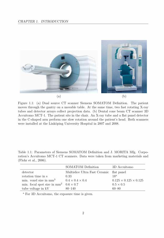
A wide variety of diagnostic medical CT scanners is currently available on the market.The most common are third generation multislice CT scanners, see figure 1.1a. Quiterecently, cone beam CT scanners with flat panel detectors have been introduced, see figure1.1b. Compared to the third or fourth generation CT scanners, they have noticeablylonger rotation times (see table 1.1) but, on the other hand, they can often perform dataacquisition during one rotation. They are also less bulky because of the compact size ofthe flat panel detector.
A typical third generation CT scanner contains one X-ray tube and one detector arraythat are positioned inside the gantry and rotate around the patient. The SOMATOMDefinition CT scanner in figure 1.1a is atypical in this respect. It contains two rotating
1
CHAPTER 1. INTRODUCTION
(a) (b)
Figure 1.1: (a) Dual source CT scanner Siemens SOMATOM Definition. The patientmoves through the gantry on a movable table. At the same time, two fast rotating X-raytubes and detector arrays collect projection data. (b) Dental cone beam CT scanner 3DAccuitomo MCT-1. The patient sits in the chair. An X-ray tube and a flat panel detectorin the C-shaped arm perform one slow rotation around the patient’s head. Both scannerswere installed at the Linkoping University Hospital in 2007 and 2008.
Table 1.1: Parameters of Siemens SOMATOM Definition and J. MORITA Mfg. Corpo-ration’s Accuitomo MCT-1 CT scanners. Data were taken from marketing materials and(Flohr et al., 2006).
SOMATOM Definition 3D Accuitomo
detector Multislice Ultra Fast Ceramic flat panelrotation time in s 0.33 18a
min. voxel size in mm3 0.4× 0.4× 0.4 0.125× 0.125× 0.125min. focal spot size in mm2 0.6× 0.7 0.5× 0.5tube voltage in kV 80–140 60–80a For 3D Accuitomo, the exposure time is given.
2

1.3. THE ORIGIN OF SCATTER
X-ray tubes and detector arrays that can collect projection data simultaneously and thusspeed up data acquisition.
1.3 The origin of scatter
In this thesis, we focus on interactions of photons with matter that are relevant in diagnos-tic radiology. In the energy range from 1 to 150 keV, these interactions are: photoelectriceffect, incoherent scattering, and coherent scattering, see figure 1.2 for a schematic depic-tion of these interactions. In the photoelectric effect, the photon impinging on an atom or
Aγ → A
+
e−
A+
e−
γA
γ
before photoelectric incoherent coherentinteraction effect scattering scattering
Figure 1.2: Schematic depiction of photon interactions in the energy range from 1 keV to150 keV. The figure on the left side shows a photon γ impinging on an atom A. In figureson the right side, e− denotes a liberated electron, A+ denotes the ionized atom, and γdenotes the scattered photon.
a molecule is absorbed and a photoelectron is liberated. The ionization mostly happensin the inner shells (K,L, . . . ). A de-excitation phase follows during which characteristicX-rays or Auger electrons are emitted.
The incoherent scattering, also called the Compton scattering, results in a recoiledelectron and a scattered photon whose energy is lower than the energy of the incidentphoton. Simple models assume that the scattering electron is free and at rest. This leadsto a deterministic relation between the scattering angle and the scattered photon energy—the so called Compton formula. More complicated models assume that the momentumof the scattering electron is distributed according to a known function, see for instance(Carlsson et al., 1982).
The coherent scattering is a process where the photon neither ionizes nor excites thescattering center and thus its energy does not change in the center-of-mass system. In thelaboratory system where the scattering center is at rest, the change of the photon’s energyis negligible.
Any of these processes can remove photons from an X-ray beam and thus, in trans-mission tomography, all three processes must be taken into account. From a practicalpoint of view, the less problematic one is the photoelectric effect since it does not pro-duce scattered photons. (We show in section 1.4 that these deteriorate image quality.)Moreover, the energy of characteristic radiation emitted from biological tissues as a resultof this interaction is small to significantly affect projection images. The frequency of thephotoelectric effect depends on the photon energy, see figure 1.3. For low photon energies,the photoelectric effect dominates over the incoherent scattering. For higher energies, the
3

CHAPTER 1. INTRODUCTION
E / keV20 40 60 80 100 120 140
CD
F
0
0.2
0.4
0.6
0.8
1
totΣ) / CoΣ + PhΣ + InΣ(totΣ) / PhΣ + InΣ(
totΣ / InΣtotΣ / InΣ
totΣ / PhΣ
totΣ / CoΣ
Figure 1.3: Cumulative distribution function, CDF, of a photon interaction in water asa function of photon energy, E. For a given energy, the distance between two adjacentcurves gives the probability of the interaction. For instance for 20 keV, the probability ofthe incoherent scattering is ΣIn/Σtot = 0.22.
roles are reversed. For instance for photon energy of 20 keV, the photoelectric effect, in-coherent scattering, and coherent scattering represent 67%, 22%, and 11%, respectively, ofall photon interactions. For 75 keV, these numbers become 3.8%, 91%, and 4.9%.
Most of the interactions take place inside the volume delimited by the X-ray beam, seefigure 1.4. The highest concentration of interactions is close to the entrance surface anddecreases with depth owing to the exponential attenuation law.
1.4 The effect of scatter
In transmission tomography, scattered photons, in general, deteriorate image quality. Thisfollows from the fact that current image reconstruction techniques like filtered backpro-jection assume that scattered photons are not detected; the presence of scatter breaksassumptions of these techniques and leads to artefacts. Contemporary CT scanners takeseveral measures to reduce the amount of scatter: special collimators are positioned infront of the detector array and the detector elements are separated by septa. However,these measures cannot be applied for cone beam scanners using flat panel imagers. In thesemachines, scatter represents a significant image quality degradation factor.
A completely different situation is in coherent scatter computed tomography, see forinstance (van Stevendaal et al., 2003; Batchelar and Cunningham, 2002; Batchelar et al.,2006). Here, the useful signal is carried by coherently scattered photons. The advantageof this approach is that coherent scattering is more sensitive to the molecular structure ofthe imaged object (see section 2.2.1 about molecular form factors) and thus these scannershave a potential for detecting different biological tissues. Classical CT scanners rely onthe photoelectric effect which happens mostly on the inner shells that are not affected bychemical bonds or on the incoherent scattering which is affected by chemical bonds to asmall degree only.
4

1.4. THE EFFECT OF SCATTERsi
de
view
top
vie
wfr
on
t vi
ew
-20 -15 -10 -5 0 5 10 15 20
-15
-10
-5
0
5
10
15 photoelectric effect
-20
-15
-10
-5
0
5
10
15
20
y / cm-20 -15 -10 -5 0 5 10 15 20
-15
-10
-5
0
5
10
15
-20 -15 -10 -5 0 5 10 15 20
-15
-10
-5
0
5
10
15 incoherent scattering
-20
-15
-10
-5
0
5
10
15
20
y / cm-20 -15 -10 -5 0 5 10 15 20
-15
-10
-5
0
5
10
15
-20 -15 -10 -5 0 5 10 15 20
-15
-10
-5
0
5
10
15 coherent scattering
-20
-15
-10
-5
0
5
10
15
20
y / cm-20 -15 -10 -5 0 5 10 15 20
-15
-10
-5
0
5
10
15
Figure 1.4: Spatial distribution of photon interactions. Simulations were performed for a120 kV fan beam irradiating the chest region of an anthropomorphic phantom. Positions ofphotoelectric effect, incoherent scattering, and coherent scattering interactions are plottedfor the side, top, and front views. Note that the highest concentration of interactions isclose to the entrance surface and that incoherent scattering is the most frequent interaction.
To understand how scatter affects a projection image, consider the geometry in fig-ure 1.5. The source emits a fan beam which impinges on a phantom, for instance acylinder. In case (a), the beam is narrow, e.g. 2 cm. The contribution to energy impartedper unit surface area to the detector at a point (x, y) in the image plane from a virtualvolume source in the region A is approximately the same as the one from the region B.Thus, for moderately wide beams, the amount of scattered radiation is approximately pro-portional to the irradiated volume. In case (b), the beam is wider, for instance 20 cm. Thecontribution at (xa, ya) from the region A is approximately the same as the contribution at(xb, yb) from the region B. Thus, if boundary effects are neglected, the amount of scatteredradiation at (xa, ya) is approximately the same as at (xb, yb)—think about integrating con-tributions to (xa, ya) from all possible positions of the region A and similarly for (xb, yb)and the region B.
5

CHAPTER 1. INTRODUCTION
source
A
B
phantom
(x, y)
image plane
l1
l2
source
A
B
phantom
(xa, ya)
(xb, yb)
image plane
(a) (b)
Figure 1.5: (a) The contribution to energy imparted per unit surface area to the detectorat a point (x, y) from a virtual volume source in the region A is approximately the sameas the one from the region B. Thus the amount of scattered radiation is approximatelyproportional to the irradiated volume. (b) The contribution at (xa, ya) from the region A isapproximately the same as the contribution at (xb, yb) from the region B. Thus, if boundaryeffects are neglected, the amount of scattered radiation at (xa, ya) is approximately the sameas at (xb, yb).
1.5 Quantities in radiation physics
Most of the quantities used in radiation physics are defined in ICRU Report 60 (ICRU,1998). As this document is not easily available to people working in other fields, someof these quantities are defined in the following text. Typical usage of these quantities inMonte Carlo radiation transport codes (MCRTC) is also described.
The energy deposit, εi, is the energy deposited in a single interaction, i, εi = εin−εout+Q,where εin is the energy of the incident ionizing particle (excluding rest energy), εout is thesum of the energies of all ionizing particles leaving the interaction (excluding rest energy),Q is the change in the rest energies of the nucleus and of all particles involved in theinteraction (Q > 0: decrease of rest energy; Q < 0: increase of rest energy). Note thatin the kV diagnostic radiology, all interactions have Q = 0. In MCRTC, energy depositsfrom individual interactions are used to calculate energy imparted to a given volume, seethe following definition.
The energy imparted, ε, to the matter in a given volume is the sum of all energy depositsin the volume, ε =
∑i εi, where the summation is performed over all energy deposits, εi,
in that volume. Its unit is J. In MCRTC, energy imparted to a given volume is used tocalculate the average absorbed dose. This may further be used to calculate the effectivedose (ICRP, 1991) or other quantities related to the risk associated with the use of ionizingradiation.
The following two quantities, fluence and energy fluence, describe a radiation field at agiven point and can be used to describe the response of a thin photon counting and thinenergy counting detectors. But first, we introduce the radiant energy: the radiant energy,R, is the energy (excluding rest energy) of the particles that are emitted, transfered orreceived. Its unit is J. The fluence, Φ, is the quotient of dN by da, where dN is thenumber of particles incident on a sphere of cross-sectional area da, Φ = dN/da. Its unit ism−2. The energy fluence, Ψ, is the quotient of dR by da, where dR is the radiant energy
6
1.6. THE AIMS OF THIS WORK
incident on a sphere of cross-sectional area da, Ψ = dR/da. Its unit is J m−2.The following quantity, collision kerma, is often used to calculate the absorbed dose at
a given point since, in case of charged particle equilibrium, the absorbed dose equals thecollision kerma, D = Kc (Attix, 1986). First we introduce the quantity kerma: the kerma,K, is the quotient of dEtr by dm, where dEtr is the sum of the initial kinetic energiesof all the charged particles liberated by uncharged particles in a mass dm of material,K = dEtr/dm. Its unit is J kg−1, the special name is gray (Gy). The collision kerma, Kc,is the component of kerma, K, where the radiative-loss energy is excluded. It is usuallyexpressed as Kc = K(1 − g), where g is the average fraction of energy transferred toelectrons that is lost through bremsstrahlung.
It should also be noted that, in high energy physics, energy of particles is often givenin electronvolts, 1eV = 1.60217653(14)× 10−19J.
1.6 The aims of this work
The aim of our work was to develop a tool that could simulate projections in computedtomography—a virtual tomograph—and use this tool to optimize CT scanner design andimage reconstruction algorithms. The work was divided into several projects:
• The development of the CTmod toolkit, see Paper IV.
• Evaluation of the effect of individual factors on the amount of scatter in a typicalCT geometry, see Paper I.
• Quantitative estimation of the effect of scatter on the quality of reconstructed images,see Papers II and V.
• Automatic segmentation of imaged objects, see section 3.3.3.
• The development of a scatter correction algorithm, see section 3.2.
7

Chapter 2
Monte Carlo simulator: the CTmodtoolkit
2.1 Basic principles of Monte Carlo methods
A Monte Carlo method is a computational algorithm which relies on repeated randomsampling to compute its results. The name Monte Carlo was first used by physicists work-ing on nuclear weapon projects in the Los Alamos National Laboratory in 1940 but themethod itself had been known long time ago. At present, Monte Carlo methods are used tosolve a wide spectrum of problems in various areas but here we concentrate on the problemof radiation transport and, particularly, on the transport of photons so that we can cal-culate scatter projections in diagnostic radiology. Medical physicists have long benefitedfrom the existence of general purpose Monte Carlo codes like EGS4, EGSnrc, ETRAN,ITS, PENELOPE, MCNP, GEANT4, FLUKA and others, see for instance (Rogers, 2006;Andreo, 1991). Specific needs in the field of medical imaging sparked the creation of spe-cialized codes like SIMSET, SIMIND, SIMSPECT, MCMATV, PETSIM, and EIDOLON,see for instance (Zaidi, 1999). The same very specific needs also inspired the creation ofthe CTmod toolkit—the main subject of this chapter.
To calculate a scatter projection via the Monte Carlo method, we simulate a largenumber of particle histories. Each history consists of a creation of a particle, a transportof the particle through a geometry and, finally, the termination of the particle’s life. Weneed a random number generator (RNG), a model of the particle transport, a model ofthe geometry, and a list of quantities to score. First, we give a brief description of thesecomponents in sections 2.1.1–2.1.5 and then, in section 2.2, we focus on the CTmod code.
2.1.1 Random number generators
True RNGs generate numbers that are truly random. These are seldom used in MonteCarlo simulations since their sequences cannot be repeated should the need arise e.g. fordebugging purposes. Instead, practically all Monte Carlo codes use pseudo-RNGs that
8

2.1. BASIC PRINCIPLES OF MONTE CARLO METHODS
permit the repetition of the sequence. Because of this fact, we often omit the word “pseudo”where there is no danger of a misunderstanding.
First widely used pseudo-RNGs were the linear congruential RNGs. They were fastand simple but they suffered from relatively short periods and poor statistical properties(Entacher, 1998). They are still contained in some system libraries but their use forMonte Carlo simulations is not recommended. The development of high quality RNGs isa science of its own and there is an extensive literature on this subject, see for instance(Hellekalek, 2006). For a programmer, the easiest way is to use RNGs from specializedscintific libraries, for instance GSL (FSF, 2008) or ROOT (CERN, 2008). Among others,they contain the Mersenne Twister generator of Matsumoto and Nishimura (1998) with aperiod of about 106000, the RANLUX algorithm based generator (Luscher, 1994) with aperiod of about 10171 and mathematically proven random properties, and the Tausworthegenerator of L’Ecuyer (1999) with a period of 1026. By default, the CTmod toolkit usesthe Mersenne Twister generator which is recommended by ROOT developers but the othertwo mentioned RNGs can also be used.
2.1.2 Particle transport model
The selection of a proper particle transport model depends on the studied particles and ge-ometry, and on the used variance reduction techniques, see for instance (Lux and Koblinger,1991). In the following, we focus on the analog transport of photons in a 3D geometry but,for the sake of completness, we mention several alternatives too.
The most common approach is that each particle history consists of a series of discreteinteractions that are precisely localized in space. The interactions are independent, i.e.an interaction is not affected by previous ones and depends only on the current particle’sstate. The tracking in the geometry is performed as if the particle moved on line segments.In case of photons and neutrons, a free path of the particle is sampled from an exponentialdistribution. The particle is then moved to the new position and a new interaction issampled. If the particle crosses a boundary between two solids during this step, then theparticle is moved to the boundary and the free path is re-sampled. (Alternative methodsare mentioned later.) In case of electrons, this approach would result in the simulationof a large number of soft collisions since the free path of an electron is, in general, muchshorter than the free path of a photon. Therefore this method is mostly used for lowenergy electrons where high accuracy is needed, for instance in situations where interfaceeffects are studied, see e.g. (Chibani and Li, 2002). Otherwise the concept of a condensedhistory is used (Berger, 1963). In this case, several soft interactions are combined into onecollision event. This must be implemented with great care: a lateral displacement duringeach step must be taken into account and the transport close to solid boundaries mustbe performed in a special way, see for instance the implemention in EGSnrc (Kawrakow,2000) and PENELOPE (Baro et al., 1995).
An alternative aproach to the re-sampling of free path at the boundary of two materialsis to subtract the path already traveled in the first material from the original free pathand use the difference for the calculation of a new free path in the second material. This
9

CHAPTER 2. MONTE CARLO SIMULATOR: THE CTMOD TOOLKIT
aproach is often used for particle tracking in voxel arrays since the re-sampling of the freepath in each voxel would be too time consuming. In this case, the common approach is totreat voxels as homogenous objects and calculate the corresponding free paths accordingly,see for instance the algorithm of Siddon (1985). Particle transport codes usually use thisstraightforward approach but it should be mentioned that in CT, images reconstructedfrom primary projections calculated using Siddon’s algorithm contain artefacts. For thecalculation of line integrals1, special interpolation methods, for instance KTG or Joseph’smethods, are preferred (Danielsson and Magnusson Seger, 2004) but no implementation ofthese methods in a particle transport code is known to the author.
A very different approach to particle tracking in a voxel array is used in the algorithmdescribed by Coleman (1968). In this case, the free path is sampled according to thematerial with the largest linear attenuation coefficient in the geometry and accepted orextended depending on the material in the new position. The amazing feature of this algo-rithm is that it does not calculate contributions from voxels along the particle’s path andtherefore its implementation is easier than the implementation of the Siddon’s algorithm.The Coleman’s algorithm is used for instance in the VOXMAN code (McVey et al., 2003).
Finally we note that CTmod re-samples the free path when a basic solid is entered andre-uses the free path for particle tracking in a voxel array. The latter is done via a modifiedversion of the Siddon’s algorithm, see Paper IV for more details. The Coleman’s algorithmis not used.
2.1.3 Geometry, sources, and detectors
Geometry can be constructed from simple solids using mathematical operations. Thisapproach is used in the MORSE code (Straker et al., 1970) under the name combinatorialgeometry. In computer-aided design and manufacturing (CAD/CAM), it is known asconstructive solid geometry (CSG) and some codes, for instance Geant4 (Agostinelli andet al., 2003), can directly import files in the ISO STEP (ISO, 1994) format. A differentapproach is to represent the geometry via a voxel array. This is often used to representcomplex geometries like anthropomorphic phantoms, see for instance the VOXMAN code.Both approaches can be combined and voxel arrays can be parts of a CSG-like geometry,see for instance (Wang et al., 1993). This approach is also used in CTmod, see Paper IVfor more details.
In diagnostic radiology, the most frequently used photon sources are X-ray tubes. Theseare usually simulated as point or volume sources with a given angle-energy distribution ofemitted photons. Precise measurements of energy spectra are difficult and thus the mostcommon approach is to use tabulated data from (Cranley et al., 1997) or data calculatedusing the algorithm by Birch and Marshall (1979). In CTmod, we also used spectraof several CT scanners that were provided by manufacturers under the non-disclosureagreement.
The most common approach is to approximate the response function of a detector
1In radiation physics, these line integrals are often referred to as the radiological or optical paths.
10

2.1. BASIC PRINCIPLES OF MONTE CARLO METHODS
element via a function depending on the energy of the impinging photon only. In section2.2.2, we extend this concept by taking into account the incidence angle of the photonand, in report (Malusek et al., 2007b), we propose a novel scoring scheme that takes intoaccount the cross talk between detector elements.
2.1.4 Scoring
CTmod may score fluence, energy fluence, plane fluence, plain energy fluence, air collisionkerma, and energy imparted per unit surface area of a detector element using the collisiondensity estimator variance reduction technique described in section 2.1.5. Calculation ofmean values and standard deviations of these quantities is described in (Malusek et al.,2007d). Each quantity is stored in a histogram with equidistant bins that gives the distri-bution of the scored quantity with respect to the energy of the contributing photon. Thisfeature is useful for instance for the simulation of the distribution of fluence with respectto energy at selected points in a cylindrical PMMA phantom. These data may be usedto simulate the signal of ionization chambers that measure various CTDI parameters. ForCT projections, however, the spectral distribution of scored quantites is not of interest andonly one histogram bin is used.
CTmod also scores energy imparted to each solid by summing energy deposits from allinteractions in the solid. This quantity can also be calculated for each voxel of a voxel arrayand CTmod can then report the average absorbed dose to each voxel or the effective doseto an anthropomorphic phantom if corresponding tissue weighting factors were providedby the user. Nevertheles it should be noted that CTmod is not designed for simulations ofabsorbed dose distributions. For this purpose, specialized codes that use for instance ETLestimators (Hedtjarn et al., 2002) of aborbed dose are recommended.
2.1.5 Variance reduction techniques
The purpose of variance reduction techniques is to speed up simulations by lowering thevariance of the scored quantity. CTmod uses source biasing, survival biasing combined withthe Russian roulette, and the collision density estimator also known as point detectors.In source biasing, the original angular distribution of photons generated from an X-raysource is modified, for instance photons that cannot hit the phantom are not emitted.The statistical weight of remaining photons must be decreased accordingly so that meanvalues of scored quantities are not changed. In survival biasing, a photoelectric event doesnot result in the termination of the photon’s history. Instead, a scattering interaction issimulated and the photon’s statistical weight is decreased. To prevent the transport ofa large number of photons that cannot significantly contribute to scored quantities, theRoussian roulette is played: photons whose statistical weight drops below a certain limitare either killed or their statistical weight is increased. The technique of the collisiondensity estimator is depicted in figure 2.1. To calculate a scatter projection, the historyof a photon is simulated and each point detector registers contributions corresponding to
11

CHAPTER 2. MONTE CARLO SIMULATOR: THE CTMOD TOOLKIT
(a) point detectors
X−ray source
phantom
contributionsto pointdetectors
(b) point detectors
scatteringincoherent
scatteringcoherent
contributionsto detectors
trajectoryphoton
effectphotoelectric
X−ray source
Figure 2.1: (a) To calculate a primary projection, line integrals from the source to eachpoint detector are evaluated. (b) To calculate a scatter projection, the history of a photonis simulated and each point detector registers contributions corresponding to line integralsfrom every scattering interaction.
line integrals from every scattering interaction. Detailed description of these techniques isin Paper IV.
A drawback of the collision density estimator is that interactions close to the pointdetector may significantly affect the convergence speed of the scored quantity becausethe contribution to a point detector is inversely proportinal to the square of the distancebetween the interaction and the point detector. In CTmod, the workaround is to positionpoint detectors at least several centimeters from the phantom. Typically, this is not aproblem because there is an air gap between an imaged object and the detector array inevery CT. Moreover, should the problem arise, it is posible to replace point detectors withDXTRAN spheres (Briesmeister, J. F. editor, 2000).
An alternative variance reduction technique to the collision density estimator is theweight window—a combination of phase space splitting and Russian roulette, see for in-stance (Briesmeister, J. F. editor, 2000). This technique splits photons entering preferredparts of the geometry and kills those that leave these regions. As a result, more photons candeposit their energy to active volumes of detector elements. This technique was consideredsuperior to the collision density estimator by some researchers (private communication).CTmod does not implement it since, for general geometries, the setting of weight windowsis not quite straightforward.
Finally, we mention the technique of forced interactions in which the particle is forcedto interact in a certain volume. It is especially useful for thin objects that would be mostlypassed through by photons without any interaction. It is not implemented in CTmod butthe author believes that it could improve the convergence rate of scored quantities since itcould better cover the whole volume of the imaged object with interactions. In an analogsimulation, the highest concentration of inteactions is close to the entrance surface, seefigure 1.2.
12

2.2. PHYSICS
2.2 Physics
2.2.1 Photon interactions
In CTmod, simulated interactions are incoherent scattering, coherent scattering, and pho-toelectric effect. The type of interaction is selected according to the ratio of the macroscopiccross section of the intearaction and the total macroscopic cross section. This ratio dependson photon energy, see figure 1.3. More information about cross sections is in section 2.2.3.
For incoherent scattering, the scattering angle is sampled from the differential crosssection dσincoh/dθ given as
dσincoh(E, θ)
dθ=
dσKN(E, θ)
dθSm(x), (2.1)
according to the algorithm described in Paper IV. In 2.1, E is the incident photon energy,θ is the scattering angle, dσKN/dθ is the Klein-Nishina differential cross section, x =E/(hc) sin(θ/2) is a parameter related to the momentum transfer of the interaction, his the Planck’s constant, c is the speed of light in vacuum, and Sm(x) is the scatteringfunction.
The scattering angle of coherent scattering is sampled from the differential cross sectiondσcoh/dθ given as
dσcoh(E, θ)
dθ=
dσTh(E, θ)
dθF 2
m(x), (2.2)
where dσTh/dθ is the Thompson’s differential cross section, Fm(x) is the form factor, andx is the same parameter as in (2.1). The sampling algorithm is described in Paper IV.
The photoelectric effect results in an absorbed photon in the analog method. In the non-analog method, the statistical weight of the photon is lowered, a coherent or an incoherentscattering is simulated, and the transport of the photon continues; more information is inPaper IV.
2.2.2 Detector response
In contemporary CT scanners, projection data are acquired via detector arrays or flatpanel imagers. These contain active volumes filled with scintillators that emit light whenirradiated by X-rays. The light is detected by photodiodes or other optical elements andconverted to electric signal. The physical processes are complex but it is reasonable toassume that the electric signal intensity produced by a detector element is proportional tothe energy imparted to its active volume.
In the following three subsections we discuss how the energy imparted to active volumescan be scored, how detector arrays consisting of repeated structures may be treated, and,finally, we give several examples of detector response simulations.
13

CHAPTER 2. MONTE CARLO SIMULATOR: THE CTMOD TOOLKIT
Design considerations
The detector response to a radiation field can be simulated in several ways. The moststraightforward approach is to include detector elements in the geometry and score energyimparted to their active volumes. Once the geometry model is correctly implemented, anygeneral purpose MC code can perform the simulation. The major disadvantage of thisapproach is low efficiency of the simulation. The probability that a photon is scatteredtowards a detector element and imparts a certain amount of its energy to the active volumeis small unless large detectors are used; this may be the case in PET but it is not the casein classical transmission CT scanners. A variance reduction technique based on settinga higher preference to photons that can reach detector elements (e.g. weight windowgenerators combined with the Russian roulette) can significantly improve the efficiencybut its implementation is neither straightforward nor simple.
Another approach is to use point detectors that were described in section 2.1.5. Theestimated quantity may be a fluence, energy fluence or the energy imparted per unit area.A modification of this technique was used by Sandborg et al. (1994): The artificial photonwas transported to the point detector and a full scale MC simulation was started. Theadvantage of this technique was that the energy absorption efficiency function—whichwould otherwise occupy a large amount of computer memory and would take long time tocalculate—was not used. The disadvantage was that the simulation of photon transportin all detector elements took a noticeable amount of time.
We opted for pre-calculated energy absorption efficiency functions for two reasons:(i) we used detector geometries where the function depended on the photon energy andincidence angle only, and (ii) we repeated the simulations with the same function manytimes.
Energy imparted to a single detector element
Consider an infinite detector array consisting of one layer of identical hexahedral elements,see figure 2.2. Suppose the angle-energy distribution of photon fluence is known at the
(−1,−1) (−1, 0) (−1, 1)
(0,−1) (0, 0) (0, 1)
(1,−1) (1, 0) (1, 1)
(0,−1) (0, 0) (0, 1)
top view side view
Figure 2.2: Top and side views of an infinite detector array. Each detector element islabeled with a two-dimensional index. Arrows indicate that the angle energy distributionof fluence is known at the center of the entrance surface of each detector element.
center of the entrance surface of each detector element. The task is to estimate the energy
14

2.2. PHYSICS
imparted to a given detector element.A straightforward approach would be to calculate the energy imparted to the given
detector element from a photon field obtained by interpolation from its known values atthe entrance surface of the detector array. But the corresponding Monte Carlo simulationwould be inefficient. In the following, we introduce an alternative method which is moreefficient but its application is limited to photon fields that are sufficiently uniform and todetector arrays that have low cross talk between detector elements.
First, we expand the photon field from the single point (the center of the entrancesurface of the considered detector element) to the whole space outside the detector array,see figure 2.3a. For more information about the concept of an expanded field see (ICRU,
(a) (b) (c)
Figure 2.3: (a) The photon field, ΦΩ,E(Ω, E), at the center of the entrance surface of asingle detector element is expanded to the whole space. (b) The field ΦΩ,E(Ω, E) can besimulated using a virtual surface source of photons that covers the entrance surface of thedetector array. (c) Energy imparted to a single detector element from a virtual sourcecovering the whole entrance surface is the same as the energy imparted to all detectorelements from a virtual surface source covering a single detector element.
1988). Note that any expanded field can be created by a superposition of wide parallelbeams with different directions of flight of photons. The detector response to this field canbe simulated using a virtual surface-source of photons covering the entrance surface of thedetector array, see figure 2.3b.
Lemma 1 : The energy imparted to a detector element D(0,0) by photons generated bya surface-source covering the entrance surface of all detector elements equals the energyimparted to all detector elements by photons generated by a surface-source covering theentrance surface of the detector element D(0,0). The proof is based on the symmetry ofthe repeated structure. The mean contribution of photons impinging on D(i,j) to theenergy imparted to D(0,0) equals the contribution of photons impinging on D(0,0) to theenergy imparted to D(−i,−j). Thus the sum of contributions from photons impinging on alldetector elements to the energy imparted to D(0,0) equals the sum of energies imparted toindividual detector elements by photons impinging on D(0,0).
Lemma 2 : Energy imparted to all detector elements by photons generated by a surface-source covering the entrance surface of the detector element D(0,0) does not change whenthe surface source is shifted horizontally. The proof is based on the one-to-one mappingbetween regions A,B,C, and D in the shifted and original surface-source, see figure 2.4a.
We use the term reference area for the area according to which we sample impingingphotons, i.e. for the area where we know the angle-energy distribution of photon fluence
15

CHAPTER 2. MONTE CARLO SIMULATOR: THE CTMOD TOOLKIT
A B
C D
A′
B′
C′
A
A′
(a) (b)
Figure 2.4: (a) Top view of a detector array. Photons impinging on the area A impart thesame amount of energy into all detector elements as photons impinging on the area A′.Similarly for areas B and C. (b) Side view of a detector array. Trajectories of photonswith the same direction of flight back-projected from the reference area A to the surfaceof the detector array form a new reference area A′ there.
ΦΩ,E(Ω, E). So far, the reference area was the same as the entrance surface of the detectorelement D(0,0). In Lemma 2, we showed that the reference area could be shifted horizontally.In lemma 3, we show that it can be shifted vertically. In this case, the virtual source ofphotons is still located on the surface of the detector array. Its angle-energy distribution ofgenerated photons is defined so that, in free space, the resulting angle-energy distributionof photons at the reference area is the same as ΦΩ,E(Ω, E). In practice, the photons can begenerated at the reference area and their position can be back-projected to the entrancesurface, see figure 2.4b.
Lemma 3 : The energy imparted to all detector elements does not change when thereference area is shifted vertically, see figure 2.4b. The proof consists of two steps. First,consider a parallel beam of photons expanded over the reference area. To simulate suchfield, we back-project positions of photons from the original reference area to a new one onthe detector’s surface. We know from lemma 2 that this new, horizontally shifted referencearea does not change the energy imparted to all detector elements. Second, a general fieldexpanded over the reference area can be considered as a superposition of parallel beams.For each of the parallel beams, the statement is true. Since the energy imparted to alldetector elements is an additive function with respect to the decomposition to the parallelbeams, the statement is true for the general case too.
Lemmas 1–3 give us a recipe on how to calculate the energy imparted to a detectorelement from a field expanded from the center of the entrance surface of a detector elementto the whole space: We select a reference area for the detector element. This referencearea serves as a virtual source of photons. If it is inside the detector element then we back-project positions of photons on the detector array surface. We score the energy impartedto all detector elements.
Examples
Simulations were performed using the MCNP4C code (Briesmeister, J. F. editor, 2000).Three cases were studied, see table 2.1. In all cases, the active volume was a 3 mm thickceramic scintillator Y1.34Gd0.6Eu0.06O3 (Greskovich C. and Duclos S., 1997; van Eijk, 2002)
16

2.2. PHYSICS
Table 2.1: List of studied cases.
case detector array description
A an infinite slab (approximated with a cylinder)B a hexahedral array of detector elements without a collimatorC a hexahedral array of detector elements with a collimator
also known as (Y,Gd)2O3:Eu with density of 5.92 g/cm3. In case A, the active volume ofthe detector element was an infinite slab that was approximated with a large cylinder. Incase B, the active volume of the detector element was a 0.9 mm× 0.9 mm× 3 mm box. In
septaactive volume
top view side view
Figure 2.5: Case B: Top and side views of the 5 × 5 detector array without a collimator.The size of one cell is 1 mm× 1 mm× 3 mm. The active volume (magenta, medium gray)is 0.9 mm × 0.9 mm × 3 mm. Tantalum septa (blue, dark gray) is 0.1 mm thick. Indicesof surfaces defined in the MCNP input file are also shown.
case C, a collimator was placed in front of the detector array of case B and the number ofdetector elements was increased. More information about the configuration is in (Maluseket al., 2007b).
The resulting energy absorption efficiency function, f(E, ξ), and the corresponding rel-ative errors are plotted in figures 2.8–2.10. They demonstrate the importance of a propermodel of the detector array for scatter projection calculations. For photons impingingwith the incidence angle of 0, the septa reduces f(E, ξ) approximately according to thegeometric efficiency which is 0.92/1.02 = 0.81. But for obliquely impinging photons (theseproduce the scatter projection), f(E, ξ) increases in case A by the factor 93.2/91.2 = 1.02and 95.6/91.2 = 1.05 for incidence angles of 30 and 60, respectively, and decreases by52.4/70.3 = 0.75 and 47.1/70.3 = 0.67, respectively, for case B. For case C, the correspond-ing values are 0.42/67.6 = 6.2× 10⁻³ and 0.0074/67.4 = 1.1× 10⁻⁴, respectively.
17

CHAPTER 2. MONTE CARLO SIMULATOR: THE CTMOD TOOLKIT
active volume
septa
air
Figure 2.6: Case C: Side view of a subset of the 101×101 detector array with a collimator.The size of one cell is 1 mm × 1 mm × 8 mm. The size of the active volume (magenta,medium gray) is 0.9 mm× 0.9 mm× 3 mm. The 0.1 mm thick tantalum septa (blue, darkgray) protrudes 5 mm in front of each detector element. The void space in the collimator(green, light gray) is filled by air.
A 3 mm thick ceramic scintillator absorbs most of the impinging photons with energiesfrom 30 to 120 keV. Flat panel imagers, on the other hand, must use significantly thinnerlayers to limit the lateral spread of the emitted light. In this case, the energy absorptionefficiency function may be significantly lower than 1, see figure 2.7.
E / keV0 20 40 60 80 100 120 140
=1)
ξf(
E,
0
0.2
0.4
0.6
0.8
1
Figure 2.7: Energy absorption efficiency, f(E, ξ = 1), of an infinite 3 mm slab of(Y,Gd)2O3:Eu (——), a detector element made of (Y,Gd)2O3:Eu and tantalum septa(– – –), and 600 µm infinite slab of CsI:Tl (· · · · · ·) as a function of photon energy, E,for perpendicularly impinging photons. Statistical error on the 95 % confidence level islower than 1 %.
18

2.2. PHYSICS
(a)
ξ
0
0.2
0.4
0.6
0.8
1
E / keV
020406080100120140
)ξf(
E,
0.6
0.7
0.8
0.9
1
(b)
ξ
0
0.2
0.4
0.6
0.8
1 E / keV0 20 40 60 80 100 120 140
rela
tive
erro
r / %
0
0.2
0.4
0.6
0.8
Figure 2.8: Case A: (a) The energy absorption efficiency function, f(E, ξ), of an infiniteslab as a function of the incident photon energy, E, and the cosine of the incident angle,ξ. (b) The corresponding relative error for the coverage factor k = 3. Note the differentorientation of axes.
19

CHAPTER 2. MONTE CARLO SIMULATOR: THE CTMOD TOOLKIT
(a)
ξ
0
0.2
0.4
0.6
0.8
1
E / keV
020406080100120140
)ξf(
E,
0.3
0.4
0.5
0.6
0.7
0.8
(b)
ξ
0
0.2
0.4
0.6
0.8
1 E / keV0 20 40 60 80 100 120 140
rela
tive
erro
r / %
0.4
0.6
0.8
11.2
1.4
1.6
Figure 2.9: Case B: (a) The energy absorption efficiency function, f(E, ξ), of the detectorarray with a collimator as a function of the incident photon energy, E, and the cosine ofthe incident angle, ξ. (b) The corresponding relative error for the coverage factor k = 3.Note the different orientation of axes.
20

2.2. PHYSICS
(a)
ξ
0
0.2
0.4
0.6
0.8
1
E / keV
020406080100120140
)ξf(
E,
-510
-410
-310
-210
-110
1
(b)
ξ
0
0.2
0.4
0.6
0.8
1 E / keV0 20 40 60 80 100 120 140
rela
tive
erro
r / %
050
100150200250
300
Figure 2.10: Case C: (a) The energy absorption efficiency function, f(E, ξ), of the detectorarray without a collimator as a function of the incident photon energy, E, and the cosineof the incident angle, ξ. Note the different orientation of axes and the log scale. (b) Thecorresponding relative error for the coverage factor k = 3.
21

CHAPTER 2. MONTE CARLO SIMULATOR: THE CTMOD TOOLKIT
Electron transport
CTmod does not simulate electron transport. Electrons liberated in photoelectric effectand incoherent scattering are deposited at the same spot where they are liberated. Thisapproximation is quite reasonable for the calculation of X-ray projections but it may beinadequate for the simulation of a detector response. The CSDA range of 100 keV electronsin silicon is about 1.822 × 10⁻² g/cm2 (Attix, 1986) and thus electron transport relatedeffects may appear in small detector elements. To evaluate them, simulations described insection 2.2.2 were performed with (mode p e) and without (mode p) electron transport.The energy absorption efficiency function, f(E, ξ), for photons with energy E = 100 keVimpinging with incidence angles of 0, 30, and 60 for cases A, B, and C is in table 2.2. The
Table 2.2: The energy absorption efficiency function, f(E, ξ), for the energy of the im-pinging photon E = 100 keV and incidence angles of 0, 30, or 60. Modes “p” and “e”correspond to photon and electron transport, respectively. All values are multiplied by100, the coverage factor is k = 1.
case mode incidence angle
0 30 60
A p 91.17± 0.03 93.16± 0.02 95.67± 0.02A p e 91.16± 0.03 93.16± 0.02 95.59± 0.02B p 70.22± 0.04 52.37± 0.05 47.19± 0.06B p e 70.29± 0.04 52.43± 0.05 47.11± 0.06C p 67.63± 0.01 0.411± 0.002 0.0073± 0.0002C p e 67.64± 0.01 0.416± 0.002 0.0074± 0.0002
additional transport of electrons slowed the simulation down by a factor of more than 100(Malusek et al., 2007b) but it changed the results only little, by less than approximately1%. It indicates that the calculation of f(E, ξ) for active volumes with sizes about 1 mm×1 mm× 3 mm or larger can be performed using the photon transport only. Differences inf(E, ξ) between “p” end “p e” modes were most notable for large incidence angles. In thisconfiguration, electrons are released close to the surface of the active volume and thus havea higher chance of escaping. For cases B and C, the increase of f(E, ξ) for small incidenceangles and “p e” mode of transport can be explained by the production of electrons in thetantalum septa (Z = 73) by the photoelectric effect. These electrons can be transportedto the active volume and deposit their energy there.
22

2.3. IMPLEMENTATION
2.2.3 Cross section data
Cross section data are typically prepared via the AmEpdl97 class library that is a part ofCTmod. AmEpdl97 uses the EPDL97 data library (Cullen et al., 1997). The user mayalso use cross section data from XCOM (Berger et al., 2007) or experimental form factorsfrom literature, for instance from (Peplow and Verghese, 1998). For each material, the usersupplies a file with incoherent scattering, coherent scattering, and photoelectric effect crosssections for a list of photon energies covering the range from 1 to 200 keV. The user mayalso supply a file with incoherent scattering functions Sm(x) and a file with form factorsFm(x) for a suitable list of values of the parameter x, see (2.1).
The EPDL97 data library contains a complete set of data for all elements with atomicnumbers between 1 and 100. Cross sections in the energy range from 1 keV to 1 MeV arein figure 2.11. Incoherent scattering functions and form factors are in figure 2.12.
2.3 Implementation
The CTmod toolkit is implemented as a C++ class library based on the CERN’s appli-cation framework ROOT. It contains over 60 classes and about 25 000 lines of code fromwhich about 8 000 are comments. Another 14 000 lines of code are in files used for testing.The library can be linked with a user code to create an executable file; MC runs are usuallyprepared this way. Alternatively, the library can be linked with an interactive ROOT ses-sion; this method is usually used to visualize the geometry and to process data calculatedin the MC run.
Most of the classes in CTmod can be divided into three categories: object, setup, andmanager classes. An object class represents a real world object like a photon or a cylinder.A setup class contains or references one or more objects; for instance the TomographSetupclass references all objects that are parts of a CT scanner: a source, a phantom geometry,and a detector array. A manager class controls the program flow; it generates photonsfrom the source, transports them through the geometry, and calls scoring routines. Thedistinction between these three categories is not always clear and some classes, e.g. randomnumber generators, do not fall into any of them.
2.4 Applications
CTmod was used to calculate primary and scatter projections in CT, see section 2.4.1,and to calculate projections including scatter in planar radiography, see section 2.4.2. Itwas also used to interactively analyze event data generated in MC simulations, see section2.4.3.
23

CHAPTER 2. MONTE CARLO SIMULATOR: THE CTMOD TOOLKIT
(a)
E / MeV-310 -210 -110 1
/ ba
rnInσ
-110
1
10
(E; Z=1)Inσ(E; Z=100)Inσ
(b)
E / MeV-310 -210 -110 1
/ ba
rnC
oσ
-510
-310
-110
10
310(E; Z=1)Coσ(E; Z=100)Coσ
(c)
E / MeV-310 -210 -110 1
/ ba
rnPhσ
-810
-510
-210
10
410
710 (E; Z=1)Phσ(E; Z=100)Phσ
Figure 2.11: Atomic cross sections for incoherent scattering (a), coherent scattering (b),and photoelectric effect (c) as functions of photon energy, E, from 1 keV to 1 MeV. Theatomic number, Z, ranges from 1 to 100. Data were taken from the EPDL97 data library,1 barn = 10−28 m2.
24

2.4. APPLICATIONS
(a)
-1x / cm710 810 910 1010
mF
-1010
-810
-610
-410
-210
1
210
F(x; Z=1)F(x; Z=100)
(b)
-1x / cm
610 710 810 910 1010
mS
-510
-410
-310
-210
-110
110
210
S(x; Z=1)S(x; Z=100)
Figure 2.12: Form factors (a) and incoherent scattering functions (b) as functions of theparameter x = E/(hc) sin(θ/2) (see the text). Note that Fm(x) and Sm(x) approach Z forlarge and small values of x, respectively. Owing to the log scale on the x-axis, the rangedoes not start at x = 0 cm−1. Linear extrapolation in the log-log scale can be used. Datawere taken from the EPDL97 data library.
25
CHAPTER 2. MONTE CARLO SIMULATOR: THE CTMOD TOOLKIT
2.4.1 Projections in CT
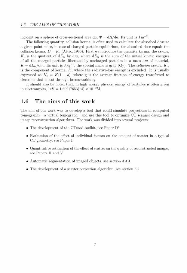
CTmod calculations are typically performed in a simplified geometry consisting of a pointsource, a phantom, and a detector array, see figure 2.18. In the following example that wastaken from (Malusek et al., 2007d), the geometry consisted of a water cylinder with thediameter of 160 mm and height 250 mm and 128 point detectors. The energy absorptionefficiency function of a 3 mm slab of the ceramic scintillator (Y,Gd)2O3 calculated usingMCNP4C was used. Figure 2.13 shows the estimate of the mean energy imparted per unit
i0 50 100
)-2
/ (k
eV c
mpI
-610
-510
-410
-310(a)
i0 50 100
)-2
/ (k
eV c
msI -710
-610
(b)
i0 50 100
spR
-310
-210
-110(c)
Figure 2.13: Profiles of the mean energy imparted per unit area of a a detector elementfor (a) primary, (b) scatter, and (c) scatter to primary ratio for 30 keV (——), 60 keV(- - - -), and 120 keV (· · · · · ·) photons. Each quantity is plotted as a function of thepoint detector index i. Statistical error on the 95 % confidence level was less than 1%.
area to a detector element i by primary, Ip, and scattered, Is, photons. The scatter toprimary ratio Rsp = Is/Ip is also plotted. Values correspond to one photon emitted fromthe source into the solid angle of 4π sr. Note that the amount of scatter strongly dependson the initial photon energy. Other examples of projections calculated using CTmod arein sections 2.5.2 and 4.2.
2.4.2 Projections in planar radiography
Irradiation geometries in planar radiography are similar to those in CT and CTmod canhandle them too. The main difference is that there are no rotating parts there and thusthe setup does not have to be as compact as in CT and air gaps can be used to reduce theamount of scatter. Also, data acquisition can be slower an thus the amount of scatter canfurther be reduced by moving anti-scatter grids. In the following example, a radiographof the Alderson anthropomorphic chest phantom was calculated to test the quality ofthe automatic threshold segmentation method, see section 3.3.3. The projection wascalculated for the tube voltage of 141 kV and BaFBrI screen with surface density of 100mg/cm2. Primary projection was calculated for the matrix of 1760 × 1760 points. Forscatter projection, bilinear interpolation was used to interpolate between the grid of 64×64points. More information about the setup is in (Ullman et al., 2006). Figure 2.14a shows
26

2.5. VERIFICATION AND VALIDATION
(a) (b)
Figure 2.14: Calculated (a) and measured (b) radiograph of the anthropomorphic Aldersonchest phantom. Differences in intensities are mostly due to inaccuracies in the segmentationof the phantom.
a radiograph calculated using CTmod and a radiograph produced by the Fuji FCR 9501CR Thorax system. Higher intensities of bone structures in the calculated image indicatethat the bone density was slightly overestimated by the segmentation process though thedifference may also be affected by non-matching intensity scales in the two images.
2.4.3 Interactive data processing
The CTmod library can be linked with an interactive ROOT session and used for visu-alization of the geometry, and for interactive post-processing of data. Figure 2.15 showsa geometry consisting of a point source, a cylindrical phantom containing four cylindricalrods, and a cylindrical point detector array with 32× 8 detector elements. The figure canbe rotated and zoomed via tools available in ROOT. The content of a voxel array can beinspected by plotting individual slices, see figure 3.2.
An example of interactive data processing using CTmod is in figure 1.4. The leftcolumn contains parallel projections of the VOXMAN phantom using 120 kV spectra.Scatter diagrams were filled with events recorded during a Monte Carlo run.
2.5 Verification and Validation
Verification is a process of determining whether or not the software is coded correctly andconforms to the specified requirements. Validation is a process of evaluating software toensure compliance with physical applicability to the process being modeled. Validationof a code would consist of comparing it with known analytical solutions or against an
27

CHAPTER 2. MONTE CARLO SIMULATOR: THE CTMOD TOOLKIT
Figure 2.15: A typical CTmod geometry: a point source, a cylindrical phantom containingfour rods, and a cylindrical point detector array with 32×8 detector elements. Color codedaxes of local coordinate systems of each object are also plotted (red, green, and blue colorsstand for x-, y-, and z-axes, respectively). Circles surrounding the image are the maincircles of the sphere defining the geometry universe.
already validated computer code, or could include benchmarking the code against relevantexperimental data (Petti and Haire, 1994; Topilsky and et al., 1998).
Verification of important CTmod classes was performed via (i) test runs whose resultswere compared with results obtained by other methods, (ii) inspection of the source code,and (iii) formal derivation of used formulas (Malusek et al., 2007c). Being a toolkit,CTmod cannot be validated as a computer program. Instead, each program based on thistoolkit must be validated separately. Two user codes were created and tested: ctmod1and ctmod2. Section 2.5.1 discusses the validation of ctmod1 that was used to calculatescatter-to-primary ratios of air collision kerma behind a PMMA box. Section 2.5.1 thencompares primary and scatter projections of cylindrical water phantoms calculated usingctmod2 to data calculated using MCNP5.
2.5.1 The amount of scatter behind a PMMA box
The experimental setup consisted of an X-ray tube, a phantom, and a detector, see fig-ure 2.16 and the original article by Siewerdsen and Jaffray (2001). The X-ray tube wasapproximated with a point source emitting photons with an energy spectrum calculated
28

2.5. VERIFICATION AND VALIDATION
dSA = 103.3 cm dAD = 62 cm
T
Hφcone
sourcedetector
dSA = 103.3 cm dAD = 62 cm
T
Wφfan
sourcedetector
side view top view
Figure 2.16: Schematic illustration of the experimental setup. The fan angle was φfan =14.1, the cone angle, φcone, was varied from about 0.5 to 6. The width, W , height, H,and thickness T of the PMMA box are in table 2.3.
using the algorithm by Birch and Marshall (1979) for a tungsten anode, 120 kV, 16 anodeangle, and 0.5 mm total filtration of Cu. Because of the uncertainty in the width andheight of the PMMA phantom in (Siewerdsen and Jaffray, 2001) (private communication),two cases named A and B were simulated, see table 2.3. Their dimensions were derived
Table 2.3: The width, W , height, H, and thickness, T , of the PMMA phantom for casesA and B.
case W H T
cm cm cm
A 40 35 5, 10, 18, 30B 50 40 5, 10, 18, 30
from the limiting cases and thus simulated data for true dimensions should lie betweendata for cases A and B. The detector scored air collision kerma. For more informationabout the setup, see (Malusek et al., 2007e).
Experimental and simulated scatter-to-primary-ratios, RSP, of air collision kerma atthe detector position are in table 2.4. For now, of special interest is the comparison be-tween experimental values and values calculated using ctmod1 with molecular form factorssince these should be more realistic than values calculated using atomic form factors. Cor-responding data are plotted in figure 2.17. The figure indicates that there was a goodagreement for the phantom thickness of 18 cm and cone angles φcone > 2 but for mostother data, the relative difference was large. For instance the relative difference was largerthan 150% for the phantom thickness of 5 cm and cone angles less than 1. These differ-ences were statistically significant, see (Malusek et al., 2007e) for corresponding p-values.It is evident that something was wrong with our computational model (improper X-rayspectrum, oversimplified geometry, incorrect material data, etc.) or with the experimentaldata that could have been affected by factors that were not taken into account (extra-focalradiation from the X-ray tube, scatter from collimators or walls, impurities in PMMA,
29

CHAPTER 2. MONTE CARLO SIMULATOR: THE CTMOD TOOLKITTab
le2.4:
Com
parison
ofscatter-to-p
rimary
values,
RSP,taken
from(S
iewerd
senan
dJaff
ray,2001)
and
calculated
usin
gctm
od1
and
MC
NP
5co
des.
experim
ent
ctmod1
MC
NP
molecu
larform
factorsatom
icform
factorsatom
icform
factorsT
φco
ne
RSP
RSP,case
AR
SP,case
BR
SP,case
AR
SP,case
BR
SP,case
AR
SP,case
Bcm
deg
%%
%%
%%
%5
0.421.54±
0.150.611±
0.0020.613±
0.0020.623±
0.0020.625±
0.0020.661±
0.090.662±
0.095
0.83.10±
0.261.176±
0.0021.178±
0.0021.176±
0.0021.179±
0.0021.178±
0.111.181±
0.115
2.15.81±
0.443.046±
0.0053.055±
0.0052.963±
0.0052.971±
0.0052.961±
0.142.976±
0.145
3.58.43±
0.704.750±
0.0074.765±
0.0074.681±
0.0074.697±
0.0074.751±
0.174.773±
0.175
4.810.38±
0.816.179±
0.0096.200±
0.0096.128±
0.0086.149±
0.0086.215±
0.186.250±
0.185
6.112.27±
0.937.510±
0.017.540±
0.017.472±
0.0097.500±
0.0097.567±
0.187.609±
0.1810
0.422.89±
0.171.593±
0.0031.611±
0.0031.612±
0.0031.630±
0.0031.643±
0.161.664±
0.1610
0.96.10±
0.233.455±
0.0063.493±
0.0063.431±
0.0053.470±
0.0063.585±
0.253.622±
0.2510
2.212.48±
0.358.290±
0.018.380±
0.018.132±
0.018.230±
0.018.141±
0.338.230±
0.3310
3.819.00±
0.5513.560±
0.0213.720±
0.0213.430±
0.0213.600±
0.0213.386±
0.3613.560±
0.3610
5.324.59±
0.7318.110±
0.0218.340±
0.0218.030±
0.0218.260±
0.0218.079±
0.3918.338±
0.3910
5.826.83±
0.7719.570±
0.0219.840±
0.0219.500±
0.0219.770±
0.0219.644±
0.4119.929±
0.4118
0.56.87±
0.695.01±
0.015.17±
0.015.040±
0.0095.19±
0.015.694±
0.775.856±
0.7718
1.012.98±
0.7110.12±
0.0210.43±
0.0210.030±
0.0210.34±
0.0211.169±
0.9811.502±
0.9818
2.122.63±
0.9120.94±
0.0321.58±
0.0320.700±
0.0321.32±
0.0321.483±
1.2422.154±
1.2418
3.837.06±
1.3136.46±
0.0537.63±
0.0536.250±
0.0537.40±
0.0536.922±
1.3638.077±
1.3718
4.948.62±
1.5945.97±
0.0747.49±
0.0745.810±
0.0647.32±
0.0647.662±
1.4849.281±
1.5018
6.058.89±
1.9455.22±
0.0857.12±
0.0855.110±
0.0756.98±
0.0857.565±
1.5759.508±
1.5930
0.513.83±
2.0413.89±
0.0414.78±
0.0413.92±
0.0414.80±
0.0412.900±
1.7014.187±
1.8430
1.020.91±
3.1827.93±
0.0829.74±
0.0927.72±
0.0729.52±
0.0728.634±
2.8930.552±
2.9830
2.142.22±
5.0757.80±
0.161.70±
0.257.50±
0.161.30±
0.153.650±
3.7057.314±
3.8330
3.973.72±
6.27104.60±
0.3111.60±
0.3104.20±
0.2111.30±
0.2108.591±
9.89116.692±
10.0130
4.989.44±
7.18129.60±
0.3138.60±
0.3129.40±
0.3138.30±
0.3130.823±
10.04141.236±
10.2130
5.9111.95±
9.17154.10±
0.4165.00±
0.4153.80±
0.3164.90±
0.3153.898±
10.26165.332±
10.41
30

2.5. VERIFICATION AND VALIDATION
/ degcone
φ0 1 2 3 4 5 6
/ %
SPR
1
10
210
Figure 2.17: Experimental (markers) and simulated (curves) scatter-to-primary-ratios,RSP, for exposure and air collision kerma, respectively. Phantom thickness 5 cm (, ——),10 cm (¤, - - - -), 18 cm (4, · · · · · ·), and 30 cm (♦, — · —). Tube voltage 120 kV,anode angle 16, and total filtration 0.5 mm Cu. Error bars denote statistical uncertaintyof 1 standard deviation. Arrows on the right side of the figure associate curves with cor-responding markers. Only curves for the case A are plotted; the difference between curvesfor cases A and B was small.
etc.). The cause of the discrepancy was not found.
To check that algorithms were implemented correctly in ctmod1, results calculated usingctmod1 were compared to results calculated using MCNP5. MCNP5 does not use molecularform factors and thus atomic form factors were used for ctmod1. The relative difference inair collision kerma of primary photons, Kp
c,air, was less than 0.1% for all cases and was mostlikely caused by approximations used in the numerical integration. The difference in aircollision kerma of scattered photons, Ks
c,air, was not statistically significant, see (Maluseket al., 2007e) for more information.
2.5.2 Primary and scatter projections of water cylinders
CT projections were calculated in a simplified scanner geometry, see figure 2.18, usingthe ctmod2 and MCNP5 codes. The geometry consisted of a point source, a cylindricalphantom and an array of point detectors. The point source emitted monoenergetic photonswith energies of 30, 60, 90, and 120 keV, respectively. In ctmod2, the photons were emittedto a cylindrical fan beam with the source-detector distance R = 1000 mm, beam widthw = 200 mm, and beam length l = 700 mm. MCNP5 does not provide a source likethis by default and thus, as a workaround, photons were emitted from the point sourceisotropically and the beam was shaped by a pair of fully absorbing cylindrical collimators,see (Malusek et al., 2007e) for more information.
31

CHAPTER 2. MONTE CARLO SIMULATOR: THE CTMOD TOOLKIT
y
z
R h
l
source
x
z
w
h
source
x
y
w
l
front view side view top view
Figure 2.18: Schematic view of the CT scanner geometry: the source-detector distanceR = 1000 mm, the source-axis distance h = 700 mm, the beam width 200 mm, and thebeam length l = 900 mm. The length l is measured on a circle whose axis is parallel tothe rotation axis and crosses the point source.
Profiles of primary projections in figure 2.19 show that there was a good agreementbetween energy fluence of primary photons calculated using ctmod2 and MCNP5. Relativedifferences were smaller than 0.5%. They were most likely due to different interpolationof the linear attenuation coefficient; ctmod2 used a lin-lin interpolation in a dense grid ofpoints whilst MCNP5 used a log-log interpolation in a coarser grid.
To demonstrate how small changes in cross section data can affect calculated projec-tions, we also include results obtained with cross section data taken from the DLC-200library that is used in e.g. MCNP4C (Briesmeister, J. F. editor, 2000), see the dottedcurve in figure 2.19. For more information about the difference between DLC-200 andXCOM/NIST tabulations, see (Demarco et al., 2002). Note that MCNP5 uses the EPDL97data library (Cullen et al., 1997) which is also used in CTmod. The fractional increase of
Table 2.5: Comparison of coherent, ΣCo, incoherent, ΣIn, photoelectric, ΣPh, and total,Σtot, macroscopic cross sections in the XCOM, EPDL97, and DLC-200 data libraries for30 keV photons. The density of water was ρ = 1 g/cm3.
library ΣCo/ρ ΣIn/ρ ΣPh/ρ Σtot
cm2 g−1 cm2 g−1 cm2 g−1 cm−1
XCOM 4.69× 10⁻² 1.83× 10⁻¹ 1.46× 10⁻¹ 0.3759EPDL97 4.693235× 10⁻² 1.830623× 10⁻¹ 1.457067× 10⁻¹ 0.375701DLC-200 4.677073× 10⁻² 1.828689× 10⁻¹ 1.310766× 10⁻¹ 0.360716
4% in the linear attenuation coefficient for 30 keV photons in water and the DLC-200 datalibrary compared to the EPDL97 data library (see table 2.5) caused the fractional increaseof 38% in the energy fluence behind the water cylinder with the radius of 32 cm.
Profiles of scatter projections in figure 2.20 show that the agreement between energyfluence of scattered photons calculated using ctmod2 and MCNP5 was good. Large relative
32

2.5. VERIFICATION AND VALIDATION
case A case B
30ke
V
yi0 20 40 60
)-2
/ (k
eV c
mΨ -610
-510
-410
yi0 20 40 60
)-2
/ (k
eV c
mΨ
-910
-810
-710
-610
-510
-410
60ke
V
yi0 20 40 60
)-2
/ (k
eV c
mΨ
-510
-410
yi0 20 40 60
)-2
/ (k
eV c
mΨ -610
-510
-410
90ke
V
yi0 20 40 60
)-2
/ (k
eV c
mΨ
-410
-310
yi0 20 40 60
)-2
/ (k
eV c
mΨ
-610
-510
-410
-310
120
keV
yi0 20 40 60
)-2
/ (k
eV c
mΨ -410
-310
yi0 20 40 60
)-2
/ (k
eV c
mΨ -510
-410
-310
Figure 2.19: Primary projection profiles of water cylinders with radii of 8 cm (case A) and16 cm (case B). Energy fluence of primary photons, Ψp, is plotted as a function of detectorindex for initial photon energies of 30, 60, 90, and 120 keV. Data were calculated usingMCNP5 (), ctmod2 with EPDL97 cross sections (——), and ctmod2 with MCNP4C crosssections (· · · · · ·).
33

CHAPTER 2. MONTE CARLO SIMULATOR: THE CTMOD TOOLKIT
case A case B
30ke
V
yi0 20 40 60
)-2
/ (k
eV c
mΨ 0.4
0.60.8
11.21.41.6
-610×
yi0 20 40 60
)-2
/ (k
eV c
mΨ
0
0.2
0.4
0.6
0.8
-610×
60ke
V
yi0 20 40 60
)-2
/ (k
eV c
mΨ 4
6
8
10
12
-610×
yi0 20 40 60
)-2
/ (k
eV c
mΨ
2
34
56
7-610×
90ke
V
yi0 20 40 60
)-2
/ (k
eV c
mΨ
5
10
15
20
-610×
yi0 20 40 60
)-2
/ (k
eV c
mΨ
8
10
12
14
-610×
120
keV
yi0 20 40 60
)-2
/ (k
eV c
mΨ 10
15
20
25
30
-610×
yi0 20 40 60
)-2
/ (k
eV c
mΨ 16
18
20
22
-610×
Figure 2.20: Scatter projection profiles of water cylinders with radii of 8 cm (case A)and 16 cm (case B). Energy fluence of scattered photons, Ψs, is plotted as a function ofdetector index for initial photon energies of 30, 60, 90, and 120 keV. Data were calculatedusing MCNP5 (), ctmod2 with atomic form factors (——), ctmod2 with molecular formfactors (· · · · · ·), and ctmod2 with coherent scattering approximated with the Thompsoncross sections (– – –).
34

2.5. VERIFICATION AND VALIDATION
differences for points with indices i = 5, 6, 10, 28, 29, 30 are discussed in (Malusek et al.,2007e) and can be explained as statistical fluctuations.
Figure 2.20 also contains profiles of projections calculated using ctmod2 with molecularform factors and ctmod2 with the angular distribution of coherently scattered photonsgiven by the Thompson cross section. For low energy photons (up to 30 keV), molecularform factors modified the scatter projection profiles in the vicinity of edges of the watercylinder when compared to the atomic form factors. For high energy photons, the fractionof coherently scattered photons decreased and the momentum transfer parameter x—whichis explained in connection to (2.1)—increased. As a result, the difference in scatter profilesdue to differences between molecular and atomic form factors became less pronounced.The Thompson cross section, on the other hand, had a significant effect on the shape ofthe scatter profile even for initial photon energies up to 120 keV.
35

CHAPTER 2. MONTE CARLO SIMULATOR: THE CTMOD TOOLKIT
Table 2.6: Energy fluence of primary, Ψp, and scattered, Ψs, photons at positions of detectorelements calculated using ctmod2 with atomic form factors and MCNP5 codes for case A.The index i identifies combinations of the initial photon energy, E, and detector index, iy.
ctmod2 MCNP5
i E iy Ψp Ψs Ψp Ψs
keV keV/cm2 keV/cm2 keV/cm2 keV/cm2
1 30 5 2.387e-04 7.174e-07±2.3e-09 2.387e-04 7.170e-07±0.0e+002 30 10 2.387e-04 8.058e-07±2.9e-09 2.387e-04 8.060e-07±0.0e+003 30 15 2.387e-04 8.846e-07±3.5e-09 2.387e-04 8.870e-07±0.0e+004 30 20 2.387e-04 1.084e-06±6.0e-09 2.387e-04 1.085e-06±0.0e+005 30 25 2.864e-05 1.405e-06±1.2e-08 2.864e-05 1.381e-06±1.2e-086 30 30 7.905e-07 8.887e-07±6.2e-09 7.906e-07 8.686e-07±6.6e-09
7 60 5 4.775e-04 4.811e-06±9.8e-09 4.775e-04 4.794e-06±0.0e+008 60 10 4.775e-04 5.921e-06±1.2e-08 4.775e-04 5.906e-06±0.0e+009 60 15 4.775e-04 7.156e-06±1.5e-08 4.775e-04 7.134e-06±0.0e+00
10 60 20 4.775e-04 8.425e-06±2.0e-08 4.775e-04 8.367e-06±0.0e+0011 60 25 1.495e-04 1.134e-05±5.5e-08 1.495e-04 1.131e-05±6.4e-0812 60 30 2.094e-05 1.121e-05±4.1e-08 2.095e-05 1.120e-05±4.8e-08
13 90 5 7.162e-04 8.430e-06±1.7e-08 7.162e-04 8.404e-06±0.0e+0014 90 10 7.162e-04 1.056e-05±2.0e-08 7.162e-04 1.055e-05±0.0e+0015 90 15 7.162e-04 1.311e-05±2.4e-08 7.162e-04 1.312e-05±0.0e+0016 90 20 7.162e-04 1.582e-05±3.3e-08 7.162e-04 1.582e-05±7.3e-0817 90 25 2.648e-04 2.005e-05±9.4e-08 2.648e-04 2.005e-05±1.1e-0718 90 30 4.913e-05 2.092e-05±7.5e-08 4.914e-05 2.098e-05±1.1e-07
19 120 5 9.549e-04 1.151e-05±2.0e-08 9.549e-04 1.148e-05±0.0e+0020 120 10 9.549e-04 1.472e-05±2.7e-08 9.549e-04 1.467e-05±0.0e+0021 120 15 9.549e-04 1.858e-05±3.3e-08 9.549e-04 1.854e-05±0.0e+0022 120 20 9.549e-04 2.284e-05±4.0e-08 9.549e-04 2.276e-05±9.8e-0823 120 25 3.845e-04 2.865e-05±1.5e-07 3.845e-04 2.823e-05±1.7e-0724 120 30 8.245e-05 3.034e-05±1.2e-07 8.246e-05 3.043e-05±1.5e-07
36
Chapter 3
Computed tomography
3.1 Basic principles
Computed tomography is an imaging method that is used to visualize the internals of anobject from a large number of X-ray projections via mathematical procedures which areknown as tomographic reconstructions. There is a vast amount of literature dedicated tothis intensively evolving field. For the description of its fundamentals, system technology,image quality, and applications we refer the reader to books by Kalender (2005) and Hsieh(2003). The history of CT is covered by Webb (1990) and Kalender (2006) . Mathematicalprinciples of tomographic reconstruction are descibed for instance in books by Kak andSlaney (1987) and Natterer (1986). For a recent review of image reconstruction methods,see (Defrise and Gullberg, 2006).
Here, we restrict the description to areas that we encountered in our work. The conceptsare simplified to limit the extensive use of mathematics which is otherwise crucial in thisfield. Two-dimensional (2D) parallel projections are described in section 3.1.1. These areused in section 3.1.2 to derive a formula for the filtered back-projection. The derivation forfan-beam projections is more complicated and thus we only present the resulting formulaand point out similarities between the two cases. In section 3.1.3, we point out that thequality of the reconstructed image is affected by the choice of the convolution kernel.Scatter correction methods are discussed in section 3.2. They are closely related to theproblem of automatic tissue classification, this subject is discussed in section 3.3.
3.1.1 2D parallel projection
Consider a wide parallel beam of photons that impinges on a phantom and is detectedby a set of detector elements arranged on a line, see figure 3.1a. The problem can beeasily treated via two parameters: the angle φ perpendicular to the ray’s direction, andthe distance, r, between the ray and the origin. The set of points (x, y) forming each raysatisfies the analytical equation
x cos φ + y sin φ = r (3.1)
37
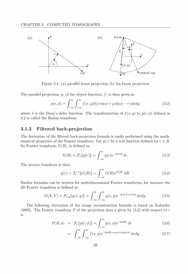
CHAPTER 3. COMPUTED TOMOGRAPHY
(a)
x
y
ray
r
φ
(b) focus
central ray
x
y
L
(x, y)
ray
γθ
Figure 3.1: (a) parallel beam projection (b) fan beam projection
The parallel projection, p, of the object function, f , is then given as
p(r, φ) =
∫ ∞
−∞
∫ ∞
−∞f(x, y)δ(x cos φ + y sin φ− r) dxdy (3.2)
where δ is the Dirac’s delta function. The transformation of f(x, y) to p(r, φ) defined in3.2 is called the Radon transform.
3.1.2 Filtered back-projection
The derivation of the filtered back-projection formula is easily performed using the math-ematical properties of the Fourier transform. Let g(r) be a real function defined for r ∈ R.Its Fourier transform, G(R), is defined as
G(R) = Frg(r) =
∫ ∞
−∞g(r)e−2πirR dr. (3.3)
The inverse transform is then
g(r) = F−1r G(R) =
∫ ∞
−∞G(R)e2πiRr dR. (3.4)
Similar formulas can be written for multidimensional Fourier transforms, for instance the2D Fourier transform is defined as
G(X, Y ) = Fx,yg(x, y) =
∫ ∞
−∞
∫ ∞
−∞g(x, y)e−2πi(Xx+Y y) dxdy. (3.5)
The following derivation of the image reconstruction formula is based on Kalender(2005). The Fourier transform P of the projection data p given by (3.2) with respect to ris
P (R, φ) = Frp(r, φ) =
∫ ∞
−∞p(r, φ)e−2πiRr dr (3.6)
=
∫ ∞
−∞
∫ ∞
−∞f(x, y)e−2πiR(x cos φ+y sin φ) dxdy (3.7)
38

3.1. BASIC PRINCIPLES
Comparing right sides of (3.5) and (3.7) we see that the latter is the 2D Fourier transformof f(x, y) at the point (R cos φ,R sin φ):
F (R cos φ,R sin φ) = P (R, φ) (3.8)
Equation (3.8) is known as the Fourier slice theorem. The function f(x, y) can be obtaineddirectly via an inverse 2D Fourier transform but this procedure must be performed withextreme care, see (Kalender, 2005) for more details. In the following, we only focus onthe derivation of the numerically stable algorithm of the filtered back-projection. First,the inverse Fourier transform of (3.8) with respect to x and y is re-written with respect toX = R cos φ and Y = R sin φ. The Jacobian determinant of this transform is R and thusdX dY = R dR dφ. The object function f(x, y) can then be written as
f(x, y) = F−1x,yF (X, Y ) =
∫ ∞
−∞
∫ ∞
−∞P (R, φ)e2πi(xX+yY ) dXdY (3.9)
=
∫ π
0
[∫ ∞
−∞|R|P (R, φ)e2πiRr dR
]dφ. (3.10)
In (3.10), we used xX + yY = xR cos φ + yR sin φ = Rr, where r = x cos φ + y sin φ.Equation (3.10) gives us the recipe on how to perform image reconstruction. The
algorithm (Kak and Slaney, 1987; Magnusson, 2008) consists of four steps. First, takeprojections p(r, φ). Second, define the so-called ramp-filter in the Fourier domain asH(R) = |R|. Third, perform ramp-filtering by calculating Q(R, φ) = Frp(r, φ)H(R)and q(r, φ) = F−1
r Q(R, φ). Fourth, perform back-projection
f(x, y) =
∫ π
0
q(x cos φ + y sin φ, φ) dφ (3.11)
The derivation of the formula for a fan beam is more complicated and is not presentedhere. Nevertheless the image reconstruction algorithm shares many similarities with theone for parallel beams and thus we mention it here. First, take projections p(γ, θ). Seefigure 3.1b for the definition of angles γ and θ and the distance L. Second, perform pre-weighting by calculating p(γ, θ) = p(γ, θ)R cos γ. Third, calculate the ramp-filter in theFourier domain as K(Γ) = Fγk(γ), where k(γ) = h(γ)(γ/ sin γ)2 and h(γ) = F−1|Γ|.Fourth, perform ramp-filtering by calculating Q(Γ, θ) = Fγp(γ, θ)K(Γ) and q(γ, θ) =F−1
γ Q(Γ, θ). Fifth, perform back-projection
f(x, y) =1
2
∫ 2π
0
1
L(x, y, θ)2q(γ(x, y, θ), θ) dθ (3.12)
In practice, sampled data are used. Then (i) the rampfilter K(Γ) must be band-limitedand its sampling must be performed in the signal domain, and (ii) the continuous Fouriertransforms are replaced by Fast Fourier transforms. A version of this algorithm was usedto perform image reconstruction in Papers III and V.
39
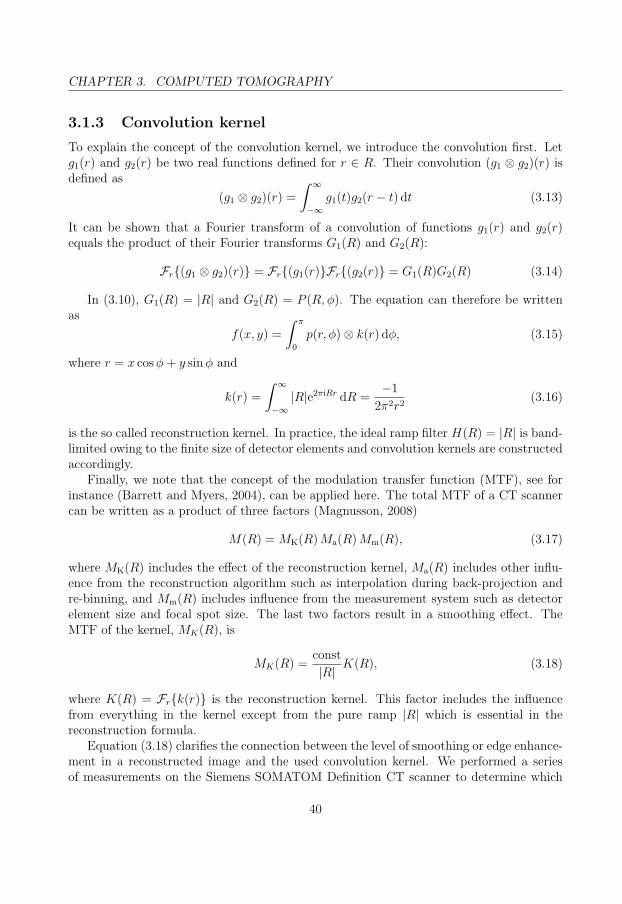
CHAPTER 3. COMPUTED TOMOGRAPHY
3.1.3 Convolution kernel
To explain the concept of the convolution kernel, we introduce the convolution first. Letg1(r) and g2(r) be two real functions defined for r ∈ R. Their convolution (g1 ⊗ g2)(r) isdefined as
(g1 ⊗ g2)(r) =
∫ ∞
−∞g1(t)g2(r − t) dt (3.13)
It can be shown that a Fourier transform of a convolution of functions g1(r) and g2(r)equals the product of their Fourier transforms G1(R) and G2(R):
Fr(g1 ⊗ g2)(r) = Fr(g1(r)Fr(g2(r) = G1(R)G2(R) (3.14)
In (3.10), G1(R) = |R| and G2(R) = P (R, φ). The equation can therefore be writtenas
f(x, y) =
∫ π
0
p(r, φ)⊗ k(r) dφ, (3.15)
where r = x cos φ + y sin φ and
k(r) =
∫ ∞
−∞|R|e2πiRr dR =
−1
2π2r2(3.16)
is the so called reconstruction kernel. In practice, the ideal ramp filter H(R) = |R| is band-limited owing to the finite size of detector elements and convolution kernels are constructedaccordingly.
Finally, we note that the concept of the modulation transfer function (MTF), see forinstance (Barrett and Myers, 2004), can be applied here. The total MTF of a CT scannercan be written as a product of three factors (Magnusson, 2008)
M(R) = MK(R) Ma(R) Mm(R), (3.17)
where MK(R) includes the effect of the reconstruction kernel, Ma(R) includes other influ-ence from the reconstruction algorithm such as interpolation during back-projection andre-binning, and Mm(R) includes influence from the measurement system such as detectorelement size and focal spot size. The last two factors result in a smoothing effect. TheMTF of the kernel, MK(R), is
MK(R) =const
|R| K(R), (3.18)
where K(R) = Frk(r) is the reconstruction kernel. This factor includes the influencefrom everything in the kernel except from the pure ramp |R| which is essential in thereconstruction formula.
Equation (3.18) clarifies the connection between the level of smoothing or edge enhance-ment in a reconstructed image and the used convolution kernel. We performed a seriesof measurements on the Siemens SOMATOM Definition CT scanner to determine which
40

3.2. SCATTER CORRECTION
convolution kernel is the best for the task of an automatic voxel segmentation. In general,no specific kernel could be selected as the best one but some convolution kernels, e.g. H10sand H31s1, noticeably shifted the mean value of the linear attenuation coefficient. For thesegmentation task, these kernels should be avoided.
3.2 Scatter correction
The development of a scatter correction algorithm was one of the goals of our work but,at the end, we have not succeeded to finish it. Nevertheless it is useful to compare ourapproach with the ones used by other researchers.
As described by Rinkel et al. (2007), methods reducing the effect of scatter can bedivided into two basic categories: pre-processing schemes that prevent the scatter to reachthe detector, and post-processing schemes that estimate the amount of scatter from ac-quisition data. A review of these techniques was given by Maher and Malone (1997), theeffect of individual factors on the amount of scatter is also discussed in section 4.2. Here,we only list concepts that have recently been used in cone beam CT.
Zhu et al. (2006) presented a scatter correction method based on primary modulation.The modulator consisted of an array of semitransparent blockers and was inserted betweenthe X-ray tube and the imaged object. The scatter component was extracted from projec-tions under the assumption that it is a slowly varying function in the detector plain. Fora humanoid phantom, this method reduced the relative mean square error of the recon-structed image in the central region of interest from 74.2% to below 1%. Scatter correctionmethod by Rinkel et al. (2007) used an array of beam stoppers placed between the X-raytube and the imaged object. It used scatter calibration through off-line acquisition com-bined with on-line analytical transformation to adapt calibration to the observed object.References to other studies using the beam modulation can be found in the two papersmentioned above, but for us, the most attractive methods were the ones where scattercorrection was performed via software simulation.
Kyriakou et al. (2006) presented a method where the amount of scatter was estimatedvia deterministic and Monte Carlo calculations. He did not present a scatter correctionalgorithm but his method could estimate the amount of scatter in one projection in about30–40 s and so it could be used in any appropriate iterative reconstruction algorithm. Zbi-jewski and Beekman (2006) presented a scatter correction method for a micro-CT based onthe iterative statistical reconstruction algorithm SR-POLY by Elbakri and Fessler (2002).In the Zbijevski’s method, only a small number of photon histories was simulated to obtaineach scatter projection. It resulted in very noisy projection data that were then smoothedusing Gaussian filters. The method worked well for small objects (rats) but it has notbeen tested with human-size phantoms. Bertram et al. (2005) from Phillips evaluated sev-eral different schemes for scatter correction via Monte Carlo simulations. They performedscatter simulations of a voxelized human head and showed that a single constant value for
1See (Siemens, 2007) for the description of these head kernels
41

CHAPTER 3. COMPUTED TOMOGRAPHY
the scatter can noticeably decrease the root-mean-square deviation; higher accuracy canbe achieved with low-order polynomials approximating the scatter shape.
We aimed for an iterative reconstruction algorithm where an analytical method, forinstance the filtered back-projection, was used for the first estimate of the reconstructedimage. An automatic tissue classification scheme would be used to voxelize the imagedobject. Scatter projections would be calculated using the Monte Carlo method. Thesewould be used to correct the voxelization of the imaged object. These steps would berepeated in several iterations. Our method would use concepts contained in (Zbijewskiand Beekman, 2006)—iterative reconstruction algorithm—but the Monte Carlo simulationwould be performed more similar to (Bertram et al., 2005). The problem of voxelizationis mentioned in the following section.
3.3 Voxel classification
There are several experimental methods for determination of the composition of the hu-man body, see (Mattsson and Thomas, 2006). Of special interest for an iterative imagereconstruction algorithm are methods that perform tissue classification automatically. Foranthropomorphic phantoms, we used threshold segmentation described in section 3.3.3.But first we introduce the concept of a voxel phantom and its representation in sections3.3.1 and 3.3.2, respectively.
3.3.1 Voxel phantoms
Voxel phantoms are represented via arrays of voxels (volume elements). Figure 3.2 shows asagittal slice of a voxel phantom that was obtained by manual segmentation of a full bodyscan of a young man by I. G. Zubal from Yale University. The phantom was later modified
X [voxel]0 20 40 60 80 100 120 140 160 180 200 220
Z [
voxe
l]
0
10
20
30
40
50
60
70
0
10
20
30
40
50
Material indices, slice: Y0064
Figure 3.2: Central sagittal slice of the VOXMAN voxel phantom containing materialindices of segmented tissues. Voxel size was 3.81 mm × 2.78 mm × 2.78 mm. Individualvoxels are clearly visible.
by Sandborg (McVey et al., 2003; Sandborg et al., 1994) to include both male and female
42

3.3. VOXEL CLASSIFICATION
specific organs that were required for the calculation of the effective dose. The size of thevoxel array is 90.65 cm × 35.56 cm × 21.95 cm, the dimensions are 238 × 128 × 79, andthe size of each voxel is 3.81 mm × 2.78 mm × 2.78 mm. The body was segmented to 57tissues, see figures 3.3 and 3.4. Each tissue was assigned a material index and a specificdensity. This phantom was used for simulations in Paper I.
3.3.2 Voxel phantom representation
The simplest way to represent a voxel phantom is to store the material index of the tissue foreach voxel. These material indices point to corresponding cross section data and materialdensities. This approach was used in the original version of the VOXMAN code. Amodification that does not require changes in Monte Carlo codes is to create subgroupsof materials that differ in their densities only. This approach was used in CTmod andlater version of VOXMAN code that were used for the calculation of projections (Ullmanet al., 2006). A further enhancement is to store the density of each voxel separately. Thisapproach is available for instance in CTmod.
The previous paragraph describes representations where each voxel contains just onematerial and the varying density may simulate the situation when the voxel is partiallyfilled with vacuum or air. But other approaches were used too. Fuchs (1998) used phantomswhere each voxel contained a mixture of two base materials in a known ratio. The twomaterials were taken from the following four base materials: air, water, bone and iron.The linear attenuation coefficient was calculated from the mixture of the two materials.Similar approach was used by De Man et al. (2001) but, in this case, the calculation of thelinear attenuation coefficient was split to the photoelectric effect and Compton scatteringcomponents. Fessler (2001), used phantoms where each voxel contained a mixture of waterand bone in a known ratio. The density of each voxel was stored as a separate parameter.
3.3.3 Threshold segmentation
In threshold segmentation, each voxel is assigned a material index according to its CTnumber. Typically, the frequency function of CT numbers from a single slice or from thewhole volumetric dataset is plotted and regions defining individual materials are defined.These regions may be further subdivided according to mass density. This recipe was appliedfor the Alderson chest phantom. Distribution of CT numbers in the volume dataset is infigure 3.5. The histogram contains 4096 bins, each bin corresponds to one CT numberchannel. Base materials and their CT ranges are listed in Table 3.1. All 17 subgroups andtheir mass densities are in Table 3.2. The density ratios, ρ/ρb,m, were calculated from meanlinear attenuation coefficients. This voxel phantom was used to calculate the projection infigure 2.14.
43

CHAPTER 3. COMPUTED TOMOGRAPHY
Figure 3.3: 3D visualization of the VOXMAN voxel phantom performed via the Visualiza-tion Toolkit. The skin is partially translucent to make selected internal organs and tissuesvisible.
Figure 3.4: 3D visualization of selected parts of the VOXMAN voxel phantom performedvia the Visualization Toolkit. Left to right: lungs, brain, pelvic bone, and scull. Artefactscaused by the large voxel size are clearly visible in the two figures on the right side.
44

3.3. VOXEL CLASSIFICATION
CT number-1000 -500 0 500 1000
coun
ts p
er c
hann
el
1
10
210
310
410
510
610
710
12
34
56
78
910
1112
1314
1516
17
1T 2T 3T
Figure 3.5: Distribution of CT numbers in the dataset. The total number of samplesis 512 × 512 × 381 ≈ 108. Segmentation thresholds are plotted as dotted vertical lines,corresponding material indices 1, . . . , 17, and effective CT numbers, ce,i, marked by ’+’ arealso shown. Segmentation thresholds defining material ranges are labeled T1, T2, and T3.
Table 3.1: Materials, densities ρb,m, and CT ranges [Tm−1, Tm − 1] used for the thresholdsegmentation.
m material ρb,m/(g cm−3) Tm−1 Tm − 1
1 air 1.2× 10⁻³ -1024 -9762 RSD lung 0.433 -975 -6013 RSD soft tissue 1.056 -600 1294 skeleton spongiosa 1.180 130 1199
45
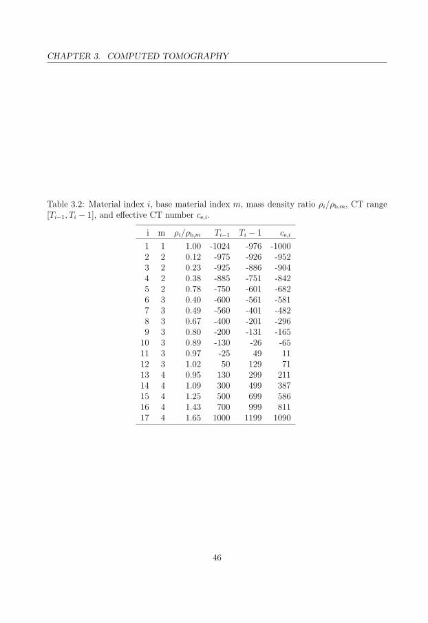
CHAPTER 3. COMPUTED TOMOGRAPHY
Table 3.2: Material index i, base material index m, mass density ratio ρi/ρb,m, CT range[Ti−1, Ti − 1], and effective CT number ce,i.
i m ρi/ρb,m Ti−1 Ti − 1 ce,i
1 1 1.00 -1024 -976 -10002 2 0.12 -975 -926 -9523 2 0.23 -925 -886 -9044 2 0.38 -885 -751 -8425 2 0.78 -750 -601 -6826 3 0.40 -600 -561 -5817 3 0.49 -560 -401 -4828 3 0.67 -400 -201 -2969 3 0.80 -200 -131 -165
10 3 0.89 -130 -26 -6511 3 0.97 -25 49 1112 3 1.02 50 129 7113 4 0.95 130 299 21114 4 1.09 300 499 38715 4 1.25 500 699 58616 4 1.43 700 999 81117 4 1.65 1000 1199 1090
46

Chapter 4
The effect of scatter on image quality
4.1 Historical review
Scientific articles describing the effect of scatter in computed tomography started to appearin the beginning of 1980’s, almost 10 years after the first clinical scan was taken in 1971.In his book from 1980, Herman (1980) could only state that very little data existed inthe open literature regarding the issue of scatter. The secrecy was broken in 1982 whenJohns and Yaffe (1982) described a measurement of the scatter-to-primary ratio (SPR) ina typical fan-beam geometry. They reported values of about 5% for CT body scans ona 4th-generation machine but also noted that the ratio may be higher than 1 in certainconfigurations. Their simple setup based on a lead blocker that was positioned betweenthe X-ray tube and the phantom is, with minor modifications, still in use today. Laterthat year, Joseph and Spital (1982) showed that scatter causes cupping, streaks, and CTnumber inaccuracies in reconstructed images. Glover (1982) demonstrated that scattercauses cupping and dark streaks connecting high-attenuation regions and showed that thescatter-to-primary ratio determines the nature and intensity of scatter artifacts in CTreconstructions. He observed that the intensity of the artifacts is often diminished whena beam-shaping attenuator1 is employed. Finally, he presented a simple scatter correctionalgorithm where the amount of scatter was estimated from simplified single-event or dual-event Compton scatter models and subtracted from the measured signal.
The Monte Carlo method was first utilized for the simulation of the effect of scatteron CT images in 1984 by Kanamori et al. (1985) though this primacy is shadowed by thefact that, in diagnostic radiology, similar studies had already been published, for instance(Kalender, 1981; Chan and Doi, 1983). From more recent studies, we mention the paper byLeliveld et al. (1994) that investigated the significance of scatter in industrial CT scanners.Zbijewski and Beekman (2006) described an artefact reduction method in cone-beam micro-CT which used a Monte Carlo based micro-CT simulator, see (Colijn et al., 2004).
An important factor that affects the quality of reconstructed images is noise. The effectof scatter on image noise was studied by Endo et al. (2001) and Siewerdsen and Jaffray
1Bowtie filters have also been called “beam-shaping attenuators” or “attenuation equalizing filters.”
47
CHAPTER 4. THE EFFECT OF SCATTER ON IMAGE QUALITY
(2001). In the latter study, the magnitude and effects of X-ray scatter in cone beam CTwith a flat panel imager were presented too. Also, there are many articles dedicated to thehandling of noise in image reconstruction algorithms. Since this topic is beyond the scopeof this section—which is the effect of scatter—we refer the reader to the many referenceslisted in the thesis by Zbijewski (2006).
In the following two sections, we extend the list of articles covering the properties andeffects of scatter in cone beam CT with examples from our own research. Section 4.2discusses how individual factors affect scatter projections. The effect of individual factorson the quality of reconstructed images is more difficult to assess since resulting images arestrongly affected by the image reconstruction algorithm. This issue and issues related tothe concept of image quality in general are discussed in section 4.3.
4.2 Factors affecting scatter projections
The amount of scatter is, among others, affected by the tube voltage, beam size, bowtiefilter design, phantom size and composition, and detector array construction. The effect ofthese factors, with the exception of the bowtie filter, was studied in Paper I. The geometryconsisted of a point source that produced a cylindrical fan beam, a cylindrical water phan-tom, and a point detector array, see figure 2.18. The point source produced monoenergeticphotons with the energy of 30, 60, 90, or 120 keV or a polyenergetic beam correspondingto the tube voltage of 120 or 140 kV. The phantom was either the anthropomorphic VOX-MAN phantom or a water cylinder. In the latter case, the head-size water cylinder hadthe radius of 8 cm and height of 25 cm, the body-size cylinder had the radius of 16 cmand height of 50 cm. The detector array consisted of 64 detector elements whose responsewas simulated via the energy absorption efficiency function of a 3 mm thick infinite slabof (Y,Gd)2O3:Eu with the density of 5.92 g/cm3. The configuration with the head-sizecylinder, no antiscatter grid, beam width w = 200 mm, and 120 kV spectrum was takenas the base configuration. Individual effects of the phantom size, antiscatter grid, beamwidth, and tube voltage were estimated via functions rs(iy), rg(iy), rw(iy), and re(iy), re-spectively, where iy was the detector index. These functions were defined as ratios of theenergy imparted to a detector element per unit surface area corresponding to the alteredand base configurations. In the altered configuration, only one factor was varied. Thealternatives were: the body-size cylinder, an antiscatter grid, beam width w = 20 mm,and 140 kV spectrum. See Paper I for more information about the experimental design.
Figure 4.1 shows that the beam width, the antiscatter grid, and the phantom size werethe highly influential factors in this case. For instance the ten times decrease of the beamwidth from 200 to 20 mm resulted in the approximately ten times decrease in the amountof scatter for all detector elements. The antiscatter grid reduced the amount of scatter toapproximately 30% of its original value on the beam axis (for the detector element withiy=32). The body-size cylinder reduced the amount of scatter in the central region but,on the other hand increased it in peripheral regions.
The effect of a bowtie filter was studied in Paper V. The irradiation geometry was the
48

4.2. FACTORS AFFECTING SCATTER PROJECTIONS
iy [1]0 10 20 30 40 50 60
r [1
]
00.20.40.60.8
11.21.41.6
sr
grwr
er
Figure 4.1: The effect of the phantom size rs, antiscatter grid rg, beam width rw, and photonenergy re as a function of the detector index iy. All these quantities are dimensionless; thisis denoted by the symbol [1]. The value r = 1 corresponds to no effect. Large values ofr or values close to zero indicate a strong effect. The beam width factor rw is dominant,factors rs and rg are highly influential.
same as in Paper I. The bowtie filter attenuated the beam without scattering any photonsso that the energy imparted per unit surface area by primary photons as a function of thedetector index was a constant—hence the name “ideal fully-compensating bowtie filter”.Figure 4.2 shows primary and scatter projections for configurations with and without thebowtie filter. These simulations were performed for beam widths of 2, 20, and 200 mmand for the head-size and body-size cylinders. Note the almost linear dependence of theamount of scatter on the beam width. The bowtie filter decreased the contribution fromscattered photons to the detector signal but it also decreased the contribution from primaryphotons. In this respect, figure 4.3 is more illustrative because it shows the effect of thebowtie filter on the scatter-to-primary ratio. The ideal fully-compensating bowtie filterreduced the scatter-to-primary ratio in the central region of the projection but increased itin the peripheral regions. The latter is easy to understand when we realize that, in theseregions, the bowtie filter significantly decreased the contribution from primary photons.
49

CHAPTER 4. THE EFFECT OF SCATTER ON IMAGE QUALITY
w = 2 mm w = 20 mm w = 200 mm
detector index0 500
)-2
/ (k
eV c
mA∈
-810
-710
-610
-510
-410
detector index0 500
)-2
/ (k
eV c
mA∈
-810
-710
-610
-510
-410
detector index0 500
)-2
/ (k
eV c
mA∈
-810
-710
-610
-510
-410
detector index0 500
)-2
/ (k
eV c
mA∈
-810
-710
-610
-510
-410
detector index0 500
)-2
/ (k
eV c
mA∈
-810
-710
-610
-510
-410
detector index0 500
)-2
/ (k
eV c
mA∈
-810
-710
-610
-510
-410
detector index0 500
)-2
/ (k
eV c
mA∈
-810
-710
-610
-510
-410
detector index0 500
)-2
/ (k
eV c
mA∈
-810
-710
-610
-510
-410
detector index0 500
)-2
/ (k
eV c
mA∈
-810
-710
-610
-510
-410
detector index0 500
)-2
/ (k
eV c
mA∈
-810
-710
-610
-510
-410
detector index0 500
)-2
/ (k
eV c
mA∈
-810
-710
-610
-510
-410
detector index0 500
)-2
/ (k
eV c
mA∈
-810
-710
-610
-510
-410
Figure 4.2: Projections of the head-size (first row) and body-size (second row) cylindersfor beam widths w = 2, 20, and 200 mm with and without the bowtie filter (BF). Primaryprojections without BF (– – –) and with BF (— · —), scatter projections without BF(· · · · · ·) and with BF (——). The projections are given in terms of the energy impartedto a detector element per unit surface area, εA, as a function of the detector index whichranges from 1 to 900.
w = 2 mm w = 20 mm w = 200 mm
detector index0 500
spR
-410
-310
-210
-110
1
detector index0 500
spR
-410
-310
-210
-110
1
detector index0 500
spR
-410
-310
-210
-110
1
detector index0 500
spR
-410
-310
-210
-110
1
detector index0 500
spR
-410
-310
-210
-110
1
detector index0 500
spR
-410
-310
-210
-110
1
Figure 4.3: Scatter-to-primary ratios in the central slice for beam widths w = 2, 20, and200 mm with and without the bowtie filter (BF). Head-size cylinder without BF (· · · · · ·)and with BF (——); body-size cylinder without BF (— · —) and with BF (– – –).
50

4.3. QUALITY OF RECONSTRUCTED IMAGES
4.3 Quality of reconstructed images
Quality of a reconstructed image can be judged subjectively, for instance by an observerthat performs a lesion detection task, or according to a physical criterion, for instance via adeviation of the image from an ideal one. The former is usually performed by radiologists.Our simulated images, see figure 4.4, clearly demonstrated the scatter and beam hardening
(a) (b) (c)
Figure 4.4: Reconstructed images of the body-size water cylinder (radius 16 cm, height50 cm) for beam widths 2 mm (a), 20 mm (b), and 200 mm (c). The combined effectof beam hardenning and scatter artefacts is clearly visible. The latter dominates for thebeam width of 200 mm.
artefacts but were too simple for any sensible lesion detection task. Thus we opted for thelatter approach which is more objective but, on the other hand, it also uses an elementof subjectivity in the selection of the ideal image. Our aim was to quantify the effectof scatter in a way that could be used in a scatter correction algorithm. This issue wasstudied in Paper II. We tested the L2-norm based difference relative to a reference image(DRRI) defined as
rr =
[∑Ni,j=1(fij − f r
ij)2
∑Ni,j=1(f
rij)
2
]1/2
, (4.1)
where f and f r are the tested and reference images respectively.
First we used the values of the linear attenuation coefficient as the ideal image, denotedas f o, but the results were not satisfactory, see later. Much better properties of rr wereobtained when the image reconstructed from primary projections only, denoted as fp,was used as the ideal one. Here, we denote the values of rr calculated for the referenceimages fp and f o as rp and ro, respectively. DRRI values for the head-size and body-sizecylinder and for beam widths 2, 20, and 200 mm are in table 4.1. The increase of the beamwidth from 2 to 20 mm, i.e. 10 times, results in almost 10 times higher values of rp, thedifferences are only 1.1 % and 13 % for the head-size and body-size cylinder, respectively.On the contrary, the increase of the beam width from 2 mm to 20 mm results in valuesof ro which are higher by only 6.2% and 66 % for the head-size and body-size cylinder,respectively.
51

CHAPTER 4. THE EFFECT OF SCATTER ON IMAGE QUALITY
Table 4.1: The dependence of the difference relative to the image based on projections byprimary photons, rp, and weighted linear attenuation coefficient, ro, on the beam width wfor the two considered phantoms. Values of rp are affected by the amount of scatter onlywhile values of ro are also affected by the beam hardening and therefore do not approachzero for small beam widths.
w head-size cylinder body-size cylinder[mm] rp ro rp ro
2 1.77× 10⁻³ 4.97× 10⁻² 5.33× 10⁻³ 4.88× 10⁻²
20 1.75× 10⁻² 5.28× 10⁻² 4.64× 10⁻² 8.12× 10⁻²
200 1.16× 10⁻¹ 1.26× 10⁻¹ 2.14× 10⁻¹ 2.39× 10⁻¹
The effect of the bowtie filter (BF) on reconstructed images was studied in PaperV. Profiles of reconstructed images of the head-size cylinder for beam widths 2, 20, and200 mm are in figures 4.5 and 4.6. Reconstructions were performed both with and withouta beam hardening correction (BHC).
In practice, the quality of the whole imaging chain and its components is of interest,not just the quality of reconstructed images. The performance of the detector array canbe characterized via quantities like Noise Equivalent Quanta (NEQ), Detective QuantumEfficiency (DQE), and Modulation Transfer Function (MTF). These concepts are commonin planar radiology but they can be used to characterize detectors in cone beam CT too,see e.g. (Siewerdsen and Jaffray, 2003). The overall assessment of the whole imagingchain performance can be characterized for instance via slice sensitivity profiles, transverseresolution and image noise, see (Flohr et al., 2003, 2006) for more information.
52

4.3. QUALITY OF RECONSTRUCTED IMAGES
w = 2 mm w = 20 mm w = 200 mm
x / cm-20 -10 0 10 20
-1f
/ cm
0.18
0.2
0.22
x / cm-20 -10 0 10 20
-1f
/ cm
0.18
0.2
0.22
x / cm-20 -10 0 10 20
-1f
/ cm
0.18
0.2
0.22
x / cm-20 -10 0 10 20
-1f
/ cm
0.18
0.2
0.22
x / cm-20 -10 0 10 20
-1f
/ cm
0.18
0.2
0.22
x / cm-20 -10 0 10 20
-1f
/ cm
0.18
0.2
0.22
x / cm-20 -10 0 10 20
-1f
/ cm
0.18
0.2
0.22
x / cm-20 -10 0 10 20
-1f
/ cm
0.18
0.2
0.22
x / cm-20 -10 0 10 20
-1f
/ cm
0.18
0.2
0.22
x / cm-20 -10 0 10 20
-1f
/ cm
0.18
0.2
0.22
x / cm-20 -10 0 10 20
-1f
/ cm
0.18
0.2
0.22
x / cm-20 -10 0 10 20
-1f
/ cm
0.18
0.2
0.22
Figure 4.5: Profiles, f , of reconstructed images of the head-size cylinder for beam widthsw = 2, 20, and 200 mm without (first row) and with (second row) the beam hardeningcorrection applied, and without and with the bowtie filter (BF). Reconstruction was per-formed from primary projections without BF (——) and with BF (· · · · · ·), and projectionscontaining primary and scatter without BF (— · —) and with BF (– – –).
w = 2 mm w = 20 mm w = 200 mm
x / cm-20 -10 0 10 20
-1f
/ cm
0.14
0.16
0.18
0.2
x / cm-20 -10 0 10 20
-1f
/ cm
0.14
0.16
0.18
0.2
x / cm-20 -10 0 10 20
-1f
/ cm
0.14
0.16
0.18
0.2
x / cm-20 -10 0 10 20
-1f
/ cm
0.14
0.16
0.18
0.2
x / cm-20 -10 0 10 20
-1f
/ cm
0.14
0.16
0.18
0.2
x / cm-20 -10 0 10 20
-1f
/ cm
0.14
0.16
0.18
0.2
x / cm-20 -10 0 10 20
-1f
/ cm
0.14
0.16
0.18
0.2
x / cm-20 -10 0 10 20
-1f
/ cm
0.14
0.16
0.18
0.2
x / cm-20 -10 0 10 20
-1f
/ cm
0.14
0.16
0.18
0.2
x / cm-20 -10 0 10 20
-1f
/ cm
0.14
0.16
0.18
0.2
x / cm-20 -10 0 10 20
-1f
/ cm
0.14
0.16
0.18
0.2
x / cm-20 -10 0 10 20
-1f
/ cm
0.14
0.16
0.18
0.2
Figure 4.6: The same as in figure 4.5 but for the body-size cylinder.
53

Chapter 5
Review of included papers
Now you will experience the full power of the dark side.– Emperor Palpatine
5.1 Paper I
The paper “Simulation of scatter in cone beam CT – effects on projection image quality”by A. Malusek, M. Sandborg, and G. Alm Carlsson was presented at the SPIE 2003conference and published in the Proceedings of SPIE (Malusek et al., 2003). Its aim wasto estimate the amount of scatter in typical cone beam CT configurations. Projectionswere calculated using CTmod for two cylindrical water phantoms of different sizes andfor an anthropomorphic voxel phantom with and without the presence of an anti-scattergrid. The scatter-to-primary ratio was evaluated for each projection and the dependenceof the amount of scatter on the phantom size, beam width, photon energy, and antiscattergrid was investigated. The response function of the detector array was simulated via theenergy absorption efficiency function of an infinite slab. It was found that the beam widthand the antiscatter grid were the dominant factors that affected the amount of scatterin cone beam CT projections. It was one of the first papers that presented scatter-to-primary ratios for projections of an anthropomorphic voxel phantom, see figure 5.1 andPaper I. The prediction that an antiscatter grid could significantly suppress the amount ofscatter in cone beam CT sparked attention of the scientific community but the subsequentexperimental study by Siewerdsen et al. (2004) showed that effects that were not simulatedby the code (photon interactions inside the grid, blind spots created by grid’s lamellas onthe flat panel imager, and non-optimal arrangement of lamellas in focused grids) had suchdetrimental effects on reconstructed images that the usage of antiscatter grids for conebeam CT was not finally recommended. It should be noted that although great attentionwas paid to every detail, an error resulting in the use of the Thomson cross section insteadof the more realistic coherent scattering cross section caused notable differences in scatterprofiles presented in this paper.
54

5.2. PAPER II
(a)
iy [1]0 10 20 30 40 50 60
[1]
spR
10-2
10-1
1 (b)
iy [1]0 10 20 30 40 50 60
[1]
spR
10-2
10-1
1
(c)
iy [1]0 10 20 30 40 50 60
[1]
spR
10-2
10-1
1
Figure 5.1: Scatter-to-primary ratios, Rsp, of energy imparted per unit surface area of adetector element as function of detector index iy for head (a), chest (b), and pelvis (c)regions of the VOXMAN anthropomorphic phantom calculated for 120 kV (red, darkercurve) and 140 kV (green) tube voltages and beam width of 200 mm.
5.2 Paper II
The paper “Effect of scatter on reconstructed image quality in cone beam CT: evaluationof a scatter-reduction optimization function” by A. Malusek, M. Magnusson Seger, M.Sandborg and G. Alm Carlsson was presented at the Malmo conference in 2004 and pub-lished in Radiation Protection and Dosimetry (Malusek et al., 2005). Its aim was to find afunction that could estimate the amount of scatter quantitatively; the intention was to usethis function in optimization tasks later. This study extended the simulation model used inPaper I but the number of configurations was reduced. Anti-scatter grids were omitted andprojections were calculated for cylindrical water phantoms only. Filtered back projectionwas used to reconstruct simulated images. It was found that the proposed function basedon the L2-norm could estimate the amount of scatter even in the presence of the beamhardening artefact. For wide beams, the beam hardening artefact was significantly weakerthan the scatter artefact but it was evident that, in our future work, both artefacts wouldhave to be treated; we could not concentrate on the scatter artefact only.
5.3 Paper III
The paper “Monte Carlo study of the dependence of the KAP-meter calibration coefficienton beam aperture, X-ray tube voltage, and reference plane” by A. Malusek, J. P. Larsson,and G. Alm Carlsson was published in Physics in Medicine and Biology (Malusek et al.,2007a). The aim of this article was to provide information that could be used during thepreparation of new KAP-meter calibration procedures, see for instance (IAEA, 2007). TheMonte Carlo method was used to study the dependence of the calibration coefficient onthe tube voltage, beam aperture, and reference plane in simplified over-couch geometriesmodeling the VacuTec’s type 70157 KAP-meter both with and without an additional filter.The MCNP5 code was used to calculate (i) energy imparted to air cavities of the KAP-meter, and (ii) spatial distribution of air collision kerma at entrance and exit planes ofthe KAP-meter and at a patient entrance plane. From these data, the air kerma area
55

CHAPTER 5. REVIEW OF INCLUDED PAPERS
product, PKA, and calibration coefficient were calculated and their dependence on the tubevoltage and beam aperture was analyzed. It was found that the variation of the calibrationcoefficient as a function of tube voltage was up to 40% when the additional filter was used,see figure 5.2. Though not directly related to the problem of scatter in cone beam CT, this
exit plane patient plane
U / kV40 60 80 100 120 140
)-1
C2k
/ (G
y m
800
1000
1200
1400
ABC
U / kV40 60 80 100 120 140
)-1
C2k
/ (G
y m
800
1000
1200
1400
AB
C
Figure 5.2: Calibration coefficient, k, as a function of tube voltage, U , for beam apertures3 (——), 12 (- - - -) and the exit and patient planes. Labels corresponding to cases A,B, and C are on the right side of each curve. Values for beam apertures 6 and 9 liedin bands delimited by corresponding 3 and 12 aperture curves. See Paper III for moreinformation.
article is included in this thesis because calculations of the air kerma area product wereoriginally performed using the CTmod code. The other quantity needed to calculate theKAP-meter calibration coefficient, the energy imparted to air cavities of the KAP meter,was calculated using the PENELOPE code since CTmod does not transport the secondaryelectrons which are needed in situations where charged particle equilibrium does not exist.Many of these results can be found in (Larsson, 2006). To simplify the method sectionand to avoid uncertainties caused by differences between cross section data used by thetwo codes in calculation of the calibration coefficient, it was later decided to re-run allsimulations using the MCNP5 code only.
5.4 Paper IV
The paper “CTmod - a toolkit for Monte Carlo simulation of projections including scatterin computed tomography” by A. Malusek, M. Sandborg, and G. Alm Carlsson was acceptedfor publication in Computer Methods and Programs in Biomedicine in December 2007. Itsaim was to provide a description of methods used in the CTmod toolkit. This subject wasalready extensively discussed in chapter 2 and so, to avoid repetition, we refer the readerto Paper IV and the accompanying reports (Malusek et al., 2007b,c,e).
56
5.5. PAPER V
5.5 Paper V
The paper “A Monte Carlo Study of the Effect of a Bowtie Filter on the Amount ofScatter in Computed Tomography” by A. Malusek, M. Magnusson, M. Sandborg, and G.Alm Carlsson is a manuscript from 2006. Its objective was to quantify the effect of abowtie filter on the amount of scatter in cone beam CT. As in Paper II, primary andscatter projections were calculated for two water cylinders and filtered back projectionwas used to reconstruct images. In this version, though, a beam hardening correction wasperformed to address the problem mentioned in section 5.2 and an ideal fully-compensatingbowtie filter was a part of the irradiation geometry. This filter cannot be manufacturedbut the results indicated a possible range of values for real bowtie filters. It was found thatbowtie filters could reduce the scatter-to-primary ratio in certain areas of the projectionimage. It turned out that similar findings had already been reported by Kusoffsky et al.(1976) for an attenuation equalizing filter in diagnostic radiography and by Glover (1982)for a beam-shaping attenuator in computed tomography. Manufacturers of CT scannerswere also aware of it (Stierstofer, 2007). Recently, it was experimentally confirmed byGraham et al. (2007). As data about the amount of scatter produced by the bowtie filterare of interest to manufacturers, latest versions of the manuscript (not included in thisthesis) also contain results for a typical bowtie filter that is used in a contemporary CTscanner. In this case, simulations were performed with both a bowtie filter represented viaan analytical formula and a voxelized bowtie filter that scatters photons.
57

Future work
Computed tomography can be improved in many respects. It has achieved tremendoussuccess over the 30 years of its existence but the reconstructed images are still affected bybeam hardening, scatter, motion, and other artefacts. The idea of a virtual tomographas a tool that could be used to solve at least some of the problems has a great potentialbut is difficult to implement. It is not just the program complexity and the insufficientcomputer speed but also the gap between different scientific disciplines that represent achallenge. Fortunately, with the recently increased interest of the scientific community inmultidisciplinary research, the problems will most likely be overcome. In our particularcase, possible tasks are:
• A better integration of the software calculating scatter projections and the softwareused by scientists developing image reconstruction algorithms. The former is in ourcase a C++ class library based on the ROOT application development frameworkwhile the latter are typically Matlab scripts, sometimes re-coded to C for increasedspeed. To turn our research software to a more production-oriented tool, more em-phasis should be put on the ease of use.
• Improved automatic voxel classification from CT numbers. Voxel classification fromCT numbers is used in some iterative reconstruction algorithms to generate the phan-tom for the calculation of projections that are then compared with real projections,see section 3.1. An improvement in this area would allow a further reduction of thebeam hardening and scatter artefacts.
• An implementation of a scatter correction algorithm based on Monte Carlo simu-lations. Such algorithm has been reported for a micro CT Zbijewski and Beekman(2006) where, due to a smaller size of the imaged object, the contribution of scatterwas easier to predict. For a human-size object, approximative methods are still morefeasible since plenty of CPU power is required to simulate scatter projections. Never-theless advances in computer technology, namely in the area of massive parallelism,open new opportunities for this method too.
58

Acknowledgments
I would like to express my sincere appreciation and gratitude to all who helped me to learnnew things, understand the problems that I encountered, and make this thesis possible.Especially, I would like to thank:
Michael Sandborg, my main supervisor, for the freedom he gave me, for bringing meback on track when I ventured to areas that were too far away from my main researchsubject, and for supporting me in the country where badgers and rabbits roam city streets,and giant bears are said to eat berries only. His unique style of doing things quickly andefficiently is definitely worth of learning.
Gudrun Alm Carlsson, my second supervisor, for teaching me how to write scientificarticles. Her extraordinary clarity in writing, attention to detail, and deep theoreticalknowledge were of great help.
Maria Magnusson for teaching me the secrets of computed tomography. She alwaysmanaged to explain complex topics in a simple way.
I also thank: All my colleagues at the Department of Radiation Physics for their supportand cooperation. Peter Lundberg for his will to use unconventional methods. Eva Lundfor her enthusiasm and for knowing everything that should be known. Hakan Hedtjarnfor collaboration on problems of the correlated sampling. Peter Larsson for collabora-tion on Monte Carlo simulations of KAP-meters. Jonas Soderberg for discussions aboutmicrodosimetry and Monte Carlo simulations in general.
People at ICR/RMT Joint Department of Physics (Chelsea) of the Royal Marsden NHSTrust for their support and collaboration. Especially Dr. David Dance for arranging mystay in London and Dr. Elly Castellano for providing scientific data.
Professor Jeffrey Williamson from the Department of Radiation Oncology, MedicalCollege of Virginia Hospitals, Virginia Commonwealth University, Richmond, USA forcollaboration on problems of the correlated sampling.
All my fellow PhD students. Especially Gustaf Ullman for explaining the challengesthat a Jedi Master must face, and Hakan Gustafsson for funny stories about his adventuresboth on land and under water.
Financial and other support from the Swedish Research Council, Swedish Foundationfor Strategic Research, Swedish government (ALF-medel), and Center for Medical ImageScience and Visualization (CMIV) at Linkoping University is gratefully acknowledged.
59

Bibliography
Agostinelli, S. and et al. (2003). GEANT4 - A Simulation Toolkit. Nuclear Instrumentsand Methods A, (506):250–303.
Andreo, P. (1991). Monte Carlo techniques in medical radiation physics. Phys Med Biol,36(7):861–920.
Attix, F. (1986). Introduction to radiological physics and radiation dosimetry. John Wiley& Sons, Inc.
Baro, J., Sempau, J., Fernandez-Varea, J. M., and Salvat, F. (1995). PENELOPE: Analgorithm for Monte Carlo simulation of the penetration and energy loss of electronsand positrons in matter. Nuclear Instruments and Methods in Physics Research B,(100):31–46.
Barrett, H. and Myers, K. (2004). Foundations of Image Science. John Wiley & Sons, Inc.
Batchelar, D. L. and Cunningham, I. A. (2002). Material-specific analysis using coherent-scatter imaging. Med Phys, 29(8):1651–60.
Batchelar, D. L., Davidson, M. T., Dabrowski, W., and Cunningham, I. A. (2006).Bone-composition imaging using coherent-scatter computed tomography: assessing bonehealth beyond bone mineral density. Med Phys, 33(4):904–15.
Berger, M. (1963). Monte Carlo calculation of the penetration and diffusion of fast chargedparticles. In Alder, B., Fernbach, S., and Rotenberg, M., editors, Methods in Computa-tional Physics, volume 1, pages 135–215. New York: Academic, b edition.
Berger, M., Hubbell, J., Seltzer, S., Chang, J., Coursey, J., Sukumar, R., and Zucker,D. (2007). XCOM: Photon Cross Section Database (version 1.3). Available on:http://physics.nist.gov/xcom.
Bertram, M., Wiegert, J., and Rose, G. (2005). Potential of software-based scatter correc-tions in cone-beam volume CT. In Flynn, M., editor, Proceedings of SPIE, volume 5745,pages 259–270.
60

BIBLIOGRAPHY
Birch, R. and Marshall, M. (1979). Computation of bremsstrahlung X-ray spectra andcomparison with spectra measured with a Ge(Li) detector. Phys Med Biol, 24(3):505–17.
Briesmeister, J. F. editor (2000). MCNP—a general Monte Carlo N-particle transportcode, version 4C. Technical Report LA-13709-M, Los Alamos National Laboratory.
Carlsson, G. A., Carlsson, C. A., Berggren, K. F., and Ribberfors, R. (1982). Calculationof scattering cross sections for increased accuracy in diagnostic radiology. I. Energybroadening of Compton-scattered photons. Med Phys, 9(6):868–79.
CERN (2008). ROOT - An object-oriented data analysis framework. Available onhttp://root.cern.ch/.
Chan, H. and Doi, K. (1983). The validity of Monte Carlo simulation in studies of scatteredradiation in diagnostic radiology. Phys Med Biol, 28(2):109–29.
Chibani, O. and Li, X. (2002). Monte Carlo dose calculations in homogeneous media andat interfaces: a comparison between GEPTS, EGSnrc, MCNP, and measurements. MedPhys, 29(5):835–47.
Cho Z H, Jones J P, and Singh M (1993). Foundations of medical imaging. John Wiley &Sons, New York.
Coleman, W. A. (1968). Mathematical verification of a certain Monte Carlo samplingtechnique and applications of the technique to radiation transport problems. NuclearScience and Engineering, (32):76–81.
Colijn, A. P., Zbijewski, W., Sasov, A., and Beekman, F. J. (2004). Experimental validationof a rapid Monte Carlo based micro-CT simulator. Phys Med Biol, 49(18):4321–33.
Cranley, K., Gilmore, B., Fogarty, G., and Desponds, L. (1997). Catalogue of diagnosticX-ray spectra and other data. Technical Report 78, Institute of Physics and Engineeringin Medicine.
Cullen, D., Hubbell, J., and Kissel, L. (1997). EPDL97: the Evaluated Photon DataLibrary, ’97 Version. UCRL-50400 Vol. 6, Rev. 5, Lawrence Livermore National Labo-ratory.
Danielsson, P. and Magnusson Seger, M. (2004). Combining Fourier and itera-tive methods in computer tomography. Analysis of an iteration scheme. The 2D-case. Technical Report LiTH-ISY-R-2634, Linkoping University. Available onhttp://www.cvl.isy.liu.se/ScOut/TechRep/Papers/LiTHISYR2634.pdf.
De Man, B., Nuyts, J., Dupont, P., Marchal, G., and Suetens, P. (2001). An itera-tive maximum-likelihood polychromatic algorithm for CT. IEEE Trans Med Imaging,20(10):999–1008.
61

BIBLIOGRAPHY
Defrise, M. and Gullberg, G. T. (2006). Image reconstruction. Phys Med Biol, 51(13):R139–54.
Demarco, J., Wallace, R., and Boedeker, K. (2002). An analysis of MCNP cross-sectionsand tally methods for low-energy photon emitters. Phys Med Biol, 47(8):1321–32.
Elbakri, I. A. and Fessler, J. A. (2002). Statistical image reconstruction for polyenergeticX-ray computed tomography. IEEE Trans Med Imaging, 21(2):89–99.
Endo, M., Tsunoo, T., Nakamori, N., and Yoshida, K. (2001). Effect of scattered radiationon image noise in cone beam CT. Med Phys, 28(4):469–74.
Entacher, K. (1998). Bad subsequences of well-known linear congruental pseudorandomnumber generators. ACM Transactions on Modeling and computer simulation, 8(1):61–70.
Fessler, J. (2001). SPIE Handbook of Medical Imaging. SPIE Press, Bellingham, Washing-ton, USA. chapter Statistical Image Reconstruction Methods for Transmission Tomog-raphy, pp. 207–219.
Flohr, T., Stierstorfer, K., Bruder, H., Simon, J., Polacin, A., and Schaller, S. (2003).Image reconstruction and image quality evaluation for a 16-slice CT scanner. Med Phys,30(5):832–45.
Flohr, T. G., McCollough, C. H., Bruder, H., Petersilka, M., Gruber, K., Suss, C., Gras-ruck, M., Stierstorfer, K., Krauss, B., Raupach, R., Primak, A. N., Kuttner, A., Achen-bach, S., Becker, C., Kopp, A., and Ohnesorge, B. M. (2006). First performance evalu-ation of a dual-source CT (DSCT) system. Eur Radiol, 16(2):256–68.
FSF (2008). GNU Scientific Library. http://www.gnu.org/software/gsl/.
Fuchs, T. (1998). Strahlaufhartungskorrekturen in der Computer-Tomographie. PhD thesis,Friedrich-Alexander Universitat Erlangen-Nurnberg.
Glover, G. H. (1982). Compton scatter effects in CT reconstructions. Med Phys, 9(6):860–7.
Graham, S. A., Moseley, D. J., Siewerdsen, J. H., and Jaffray, D. A. (2007). Compen-sators for dose and scatter management in cone-beam computed tomography. Med Phys,34(7):2691–703.
Greskovich C. and Duclos S. (1997). Ceramic scintillators. Annual review of materialsscience, 27:69–88.
Hedtjarn, H., Alm Carlsson, G., and Williamson, J. (2002). Accelerated Monte Carlo baseddose calculations for brachytherapy planning using correlated sampling. Phys Med Biol,47(3):351–76.
62

BIBLIOGRAPHY
Hellekalek, P. (2006). Random Number Generators. Available onhttp://random.mat.sbg.ac.at/.
Herman, G. (1980). Image Reconstruction from Projections. Academic Press.
Herman G T (1980). Fundamentals of Medical Imaging. Academic Press.
Hsieh, J. (2003). Computed tomography: principles, design, artifacts, and recent advances.SPIE.
IAEA (2007). Dosimetry in Diagnostic Radiology: An International Codeof Practice. Technical Report 457, IAEA. Available on http://www-pub.iaea.org/MTCD/publications/PDF/TRS457web.pdf.
ICRP (1991). ICRP Publication 60: 1990 Recommendations of the International Commis-sion on Radiological Protection. Elsevier Science Pub Co.
ICRU (1988). Determination of dose equivalents from external radiation sources—part 2.Technical Report 43, ICRU.
ICRU (1998). Fundamental quantities and units for ionizing radiation. Technical Report 60,ICRU.
ISO (1994). Industrial automation systems and integration - Product data representationand exchange. ISO 10303.
Johns, P. and Yaffe, M. (1982). Scattered radiation in fan beam imaging systems. MedPhys, 9(2):231–9.
Joseph, P. and Spital, R. (1982). The effects of scatter in x-ray computed tomography.Med Phys, 9(4):464–72.
Kak, A. C. and Slaney, M. (1987). Principles of Computerized tomographic Imaging. IEEEPress.
Kalender, W. (1981). Monte Carlo calculations of x-ray scatter data for diagnostic radiol-ogy. Phys Med Biol, 26(5):835–49.
Kalender, W. (2005). Computed Tomography: fundamentals, system technology, imagequality, applications. Publicis Corporate Publishing, 2nd revised edition.
Kalender, W. A. (2006). X-ray computed tomography. Phys Med Biol, 51(13):R29–43.
Kanamori, H., Nakamori, N., Inoue, K., and Takenaka, E. (1985). Effects of scatteredX-rays on CT images. Phys Med Biol, 30(3):239–49.
Kawrakow, I. (2000). Accurate condensed history Monte Carlo simulation of electrontransport. I. EGSnrc, the new EGS4 version. Med Phys, 27(3):485–98.
63

BIBLIOGRAPHY
Kusoffsky, L., Carlsson, C. A., and Edholm, P. (1976). Attenuation equalizing filter indiagnostic radiography. Advantages calculated by a Monte Carlo technique. Acta RadiolTher Phys Biol, 15(3):259–72.
Kyriakou, Y., Riedel, T., and Kalender, W. (2006). Combining deterministic and MonteCarlo calculations for fast estimation of scatter intensities in CT. Phys Med Biol,51(18):4567–86.
Larsson, P. (2006). Calibration of ionization chambers for measuring air kerma integratedover beam area in diagnostic radiology. Linkoping university medical dissertations no.970, Linkoping University.
L’Ecuyer, P. (1999). Tables of Maximally Equidistributed Combined LFSR Generators.Mathematics of Computation, 68(225):261–269.
Leliveld, C., Maas, J., Eijk, C., and Bom, V. (1994). On the significance of scatteredradiation in industrial x-ray computerized tomographic imaging. IEEE Transactions onnuclear science, 41(1).
Luscher, M. (1994). A portable high-quality random number generator for lattice fieldtheory calculations. Computer Physics Communications, 79:100–110.
Lux, I. and Koblinger, L. (1991). Monte Carlo particle transport methods: neutron andphoton calculations. CRC Press Inc., Boca Raton, Florida.
Magnusson, M. (2008). Private communication.
Maher, K. and Malone, J. (1997). Computerized scatter correction in diagnostic radiology.Contemporary Physics, 38(2):131–148.
Malusek, A., Larsson, J. P., and Carlsson, G. A. (2007a). Monte Carlo study of the de-pendence of the KAP-meter calibration coefficient on beam aperture, x-ray tube voltageand reference plane. Phys Med Biol, 52(4):1157–70.
Malusek, A., Sandborg, M., and Alm Carlsson, G. (2003). Simulation of scatter in conebeam CT–efects on projection image quality. In Proceedings of SPIE, volume 5030, pages740–751.
Malusek, A., Sandborg, M., and Alm Carlsson, G. (2007b). Calculation of the en-ergy absorption efficiency function of selected detector arrays using the MCNP code.Technical Report ISRN ULI-RAD-R–103–SE, Linkoping University. Available onhttp://huweb.hu.liu.se/inst/imv/radiofysik/publi/rap.html.
Malusek, A., Sandborg, M., and Alm Carlsson, G. (2007c). CTmod – Mathematical Foun-dations. Technical Report ISRN ULI-RAD-R–102–SE, Linkoping University. Availableon http://huweb.hu.liu.se/inst/imv/radiofysik/publi/rap.html.
64

BIBLIOGRAPHY
Malusek, A., Sandborg, M., and Alm Carlsson, G. (2007d). Ctmod - a toolkit for MonteCarlo simulation of projections including scatter in computed tomography. Accepted forpublication in Computer Methods and Programs in Biomedicine.
Malusek, A., Sandborg, M., and Alm Carlsson, G. (2007e). Validation of the CTmodtoolkit. Technical Report ISRN ULI-RAD-R–104–SE, Linkoping University. Availableon http://huweb.hu.liu.se/inst/imv/radiofysik/publi/rap.html.
Malusek, A., Seger, M., Sandborg, M., and Alm Carlsson, G. (2005). Effect of scatteron reconstructed image quality in cone beam computed tomography: evaluation of ascatter-reduction optimisation function. Radiat Prot Dosimetry, 114(1-3):337–40.
Matsumoto, M. and Nishimura, T. (1998). Mersenne Twister: a 623-dimensionally equidis-tributed uniform pseudo-random number generator. ACM Transactions on Modeling andComputer Simulations, 8(1):3–30.
Mattsson, S. and Thomas, B. J. (2006). Development of methods for body compositionstudies. Phys Med Biol, 51(13):R203–28.
McVey, G., Sandborg, M., Dance, D. R., and Alm Carlsson, G. (2003). A study andoptimisation of lumbar spine x-ray imaging systems. Br J Radiol, (76):177–188.
Natterer, F. (1986). The mathematics of computerized tomography. John Wiley & SonsLtd.
Newton T H and Potts D G, editors (1981). Radiology of the Skull and Brain, Vol 5:Technical Aspects of Computed Tomography. C.V. Mosby Company.
Peplow, D. and Verghese, K. (1998). Measured molecular coherent scattering form factorsof animal tissues, plastics and human breast tissue. Phys Med Biol, 43(9):2431–52.
Petti, D. and Haire, J. (1994). Requirements for U.S. regulatory approval of theinternational thermonuclear experimental reactor (ITER). IEEE. Available onhttp://ieeexplore.ieee.org/iel2/3943/11419/00518495.pdf.
Rinkel, J., Gerfault, L., Esteve, F., and Dinten, J. M. (2007). A new method for x-rayscatter correction: first assessment on a cone-beam CT experimental setup. Phys MedBiol, 52(15):4633–52.
Rogers, D. W. (2006). Fifty years of Monte Carlo simulations for medical physics. PhysMed Biol, 51(13):R287–301.
Sandborg, M., Dance, D., Persliden, J., and Alm Carlsson, G. (1994). A Monte Carloprogram for the calculation of contrast, noise and absorbed dose in diagnostic radiology.Comput Methods Programs Biomed, 42(3):167–80.
65

BIBLIOGRAPHY
Siddon, R. (1985). Fast calculation of the exact radiological path for a three-dimensionalCT array. Med Phys, 12(2):252–5.
Siemens (2007). Somatom DEFINITION Application Guide, software version syngo ct2007a edition.
Siewerdsen, J. and Jaffray, D. (2001). Cone-beam computed tomography with a flat-panelimager: magnitude and effects of x-ray scatter. Med Phys, 28(2):220–31.
Siewerdsen, J. and Jaffray, D. (2003). Three-dimensional NEQ transfer characteristicsof volume CT using direct and indirect-detection flat-panel imagers. In Proceedings ofSPIE, volume 5030.
Siewerdsen, J. H., Moseley, D. J., Bakhtiar, B., Richard, S., and Jaffray, D. A. (2004).The influence of antiscatter grids on soft-tissue detectability in cone-beam computedtomography with flat-panel detectors. Med Phys, 31(12):3506–20.
Stierstofer, K. (2007). Private communication.
Straker, E., Stevens, P., Irving, D., and Cain, V. (1970). The MORSE Code - A MultigroupNeutron and Gamma-Ray Monte Carlo Transport Code. Technical Report ORNL-4585,Oak Ridge Natinal Laboratory.
Ter-Pogossian M M, Phelps M E, Brownell G L, Cox J R, Davis D O, and Evens RG, editors (1977). Reconstruction Tomography in Diagnostic Radiology and NuclearMedicine. University Park Press, Baltimore.
Topilsky, L. N. and et al. (1998). Validation and verification of ITER safety computercodes. IEEE.
Ullman, G., Malusek, A., Sandborg, M., Dance, D., and Alm Carlsson, G. (2006). Calcu-lation of images from an anthropomorphic chest phantom using Monte Carlo methods.In Proceedings of SPIE, volume 6142.
van Eijk, C. (2002). Inorganic scintillators in medical imaging. Phys Med Biol, 47(8):R85–106.
van Stevendaal, U., Schlomka, J. P., Harding, A., and Grass, M. (2003). A reconstructionalgorithm for coherent scatter computed tomography based on filtered back-projection.Med Phys, 30(9):2465–74.
Vogtmeier, G., Dorscheid, R., Engel, K., Luhta, R., Mattson, R., Harwood, B., Appleby,M., Randolph, B., and Klinger, J. (2008). Two-dimensional anti-scatter-grids for com-puted tomography detectors. In Proceedings of SPIE, volume 6913.
Wang, H., Jaszczak, R. J., and Coleman, R. E. (1993). A new composite model of objectsfor Monte Carlo simulation of radiological imaging. Phys Med Biol, 38(9):1235–62.
66

BIBLIOGRAPHY
Webb, S. (1990). From the watching of shadows: the origins of radiological tomography.Adam Hilger, Bristol and New York.
Zaidi, H. (1999). Relevance of accurate Monte Carlo modeling in nuclear medical imaging.Med Phys, 26(4):574–608.
Zbijewski, W. (2006). Model-based image reconstruction in X-ray Computed Tomography.PhD thesis, Utrech University.
Zbijewski, W. and Beekman, F. (2006). Efficient Monte Carlo based scatter artifact reduc-tion in cone-beam micro-CT. IEEE Trans Med Imaging, 25(7):817–27.
Zhu, L., Bennett, N. R., and Fahrig, R. (2006). Scatter correction method for X-ray CTusing primary modulation: theory and preliminary results. IEEE Trans Med Imaging,25(12):1573–87.
67