calculus 2 (dan sloughter)
TRANSCRIPT
7/27/2019 Calculus 2 (Dan Sloughter)
http://slidepdf.com/reader/full/calculus-2-dan-sloughter 1/598
Difference Equations
Differential Equations
to
Section 1.1
Calculus: Areas And Tangents
The study of calculus begins with questions about change. What happens to the velocity of a swinging pendulum as its position changes? What happens to the position of a planet astime changes? What happens to a population of owls as its rate of reproduction changes?Mathematically, one is interested in learning to what extent changes in one quantity affectthe value of another related quantity. Through the study of the way in which quantitieschange we are able to understand more deeply the relationships between the quantitiesthemselves. For example, changing the angle of elevation of a projectile affects the distanceit will travel; by considering the effect of a change in angle on distance, we are able todetermine, for example, the angle which will maximize the distance.
Related to questions of change are problems of approximation. If we desire to approxi-mate a quantity which cannot be computed directly (for example, the area of some planarregion), we may develop a technique for approximating its value. The accuracy of our tech-nique will depend on how many computations we are willing to make; calculus may thenbe used to answer questions about the relationship between the accuracy of the approxi-mation and the number of calculations used. If we double the number of computations,how much do we gain in accuracy? As we increase the number of computations, do theapproximations approach some limiting value? And if so, can we use our approximatingmethod to arrive at an exact answer? Note that once again we are asking questions about
the effects of change.Two fundamental concepts for studying change are sequences and limits of sequences.For our purposes, a sequence is nothing more than a list of numbers. For example,
1,1
2,
1
4,
1
8, . . .
might represent the beginning of a sequence, where the ellipsis indicates that the list isto continue on indefinitely in some pattern. For example, the 5th term in this sequencemight be
1
16=
1
24,
the 8th term 1
128=
1
27,
and, in general, the nth term1
2n−1
where n = 1, 2, 3, . . . . Notice that the sequence is completely specified only when we havegiven the general form of a term in the sequence. Also note that this list of numbers is
1 Copyright c by Dan Sloughter 2000
7/27/2019 Calculus 2 (Dan Sloughter)
http://slidepdf.com/reader/full/calculus-2-dan-sloughter 2/598
2 Calculus: Areas And Tangents Section 1.1
approaching 0, which we would call the limit of the sequence. In the next section of thischapter we will consider in some detail the basic question of determining the limit of asequence.
The following two examples consider these ideas in the context of the two fundamentalproblems of calculus. The first of these is to determine the area of a region in the plane;
the other is to find the line tangent to a curve at a given point on the curve. As the courseprogresses, we will find that general methods for solving these two problems are at theheart of the techniques used in calculus. Moreover, we will see that these two problemsare, surprisingly, closely related, with the area problem actually being the inverse of thetangent problem. This intimate connection was one of the great discoveries of Isaac Newton(1642-1727) and Gottfried Leibniz (1646-1716), although anticipated by Newton’s teacherIsaac Barrow (1630-1677).
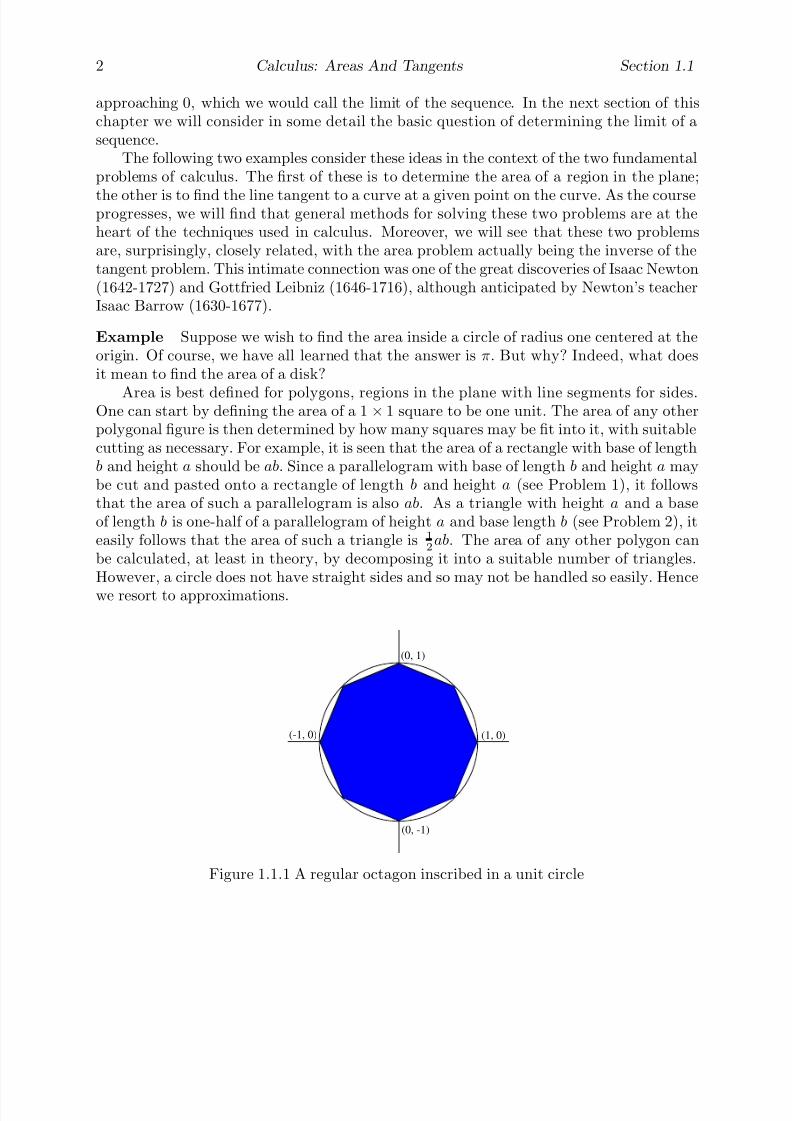
Example Suppose we wish to find the area inside a circle of radius one centered at theorigin. Of course, we have all learned that the answer is π. But why? Indeed, what doesit mean to find the area of a disk?
Area is best defined for polygons, regions in the plane with line segments for sides.One can start by defining the area of a 1 × 1 square to be one unit. The area of any otherpolygonal figure is then determined by how many squares may be fit into it, with suitablecutting as necessary. For example, it is seen that the area of a rectangle with base of lengthb and height a should be ab. Since a parallelogram with base of length b and height a maybe cut and pasted onto a rectangle of length b and height a (see Problem 1), it followsthat the area of such a parallelogram is also ab. As a triangle with height a and a baseof length b is one-half of a parallelogram of height a and base length b (see Problem 2), iteasily follows that the area of such a triangle is 1
2ab. The area of any other polygon can
be calculated, at least in theory, by decomposing it into a suitable number of triangles.However, a circle does not have straight sides and so may not be handled so easily. Hencewe resort to approximations.
(1, 0)
(0, 1)
(-1, 0)
(0, -1)
Figure 1.1.1 A regular octagon inscribed in a unit circle

7/27/2019 Calculus 2 (Dan Sloughter)
http://slidepdf.com/reader/full/calculus-2-dan-sloughter 3/598
Section 1.1 Calculus: Areas And Tangents 3
(1, 0)
(0, 1)
(-1, 0)
(0, -1)
2π8
Figure 1.1.2 Decomposition of a regular octagon into eight isosceles triangles
Let P n be a regular n-sided polygon inscribed in the unit circle centered at the originand let An be the area of P n. For example, Figure 1.1.1 shows P 8 inscribed in the unitcircle. We may decompose P n into n congruent isosceles triangles by drawing line segmentsfrom the center of the circle to the vertices of the polygon, as shown in Figure 1.1.2 for P 8.For each of these triangles, the angle with vertex at the center of the circle has measure360
ndegrees, or 2π
nradians, where π represents the ratio of the circumference of a circle to
its diameter. Hence, since the equal sides of each of the triangles are of length one, eachtriangle has a height of
hn = cosπn
and a base of length
bn = 2sinπn
(see Problem 3). Thus the area of a single triangle is given by
1
2bnhn = cos
πn
sin
πn
=
1
2sin
2π
n
,
where we have used the fact that
sin(2α) = 2 sin(α)cos(α)
for any angle α. Multiplying by n, we see that the area of P n is
An =n
2sin
2π
n
.
We now have a sequence of numbers, A1, A2, A3, . . . , each number in the sequencebeing an approximation to the area of the circle. Moreover, although not entirely obvi-ous, each term in the sequence is a better approximation than its predecessor since the
7/27/2019 Calculus 2 (Dan Sloughter)
http://slidepdf.com/reader/full/calculus-2-dan-sloughter 4/598
4 Calculus: Areas And Tangents Section 1.1
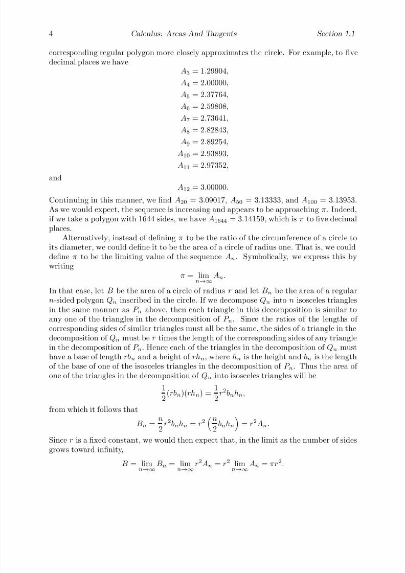
corresponding regular polygon more closely approximates the circle. For example, to fivedecimal places we have
A3 = 1.29904,
A4 = 2.00000,
A5 = 2.37764,
A6 = 2.59808,
A7 = 2.73641,
A8 = 2.82843,
A9 = 2.89254,
A10 = 2.93893,
A11 = 2.97352,
andA12 = 3.00000.
Continuing in this manner, we find A20 = 3.09017, A50 = 3.13333, and A100 = 3.13953.As we would expect, the sequence is increasing and appears to be approaching π. Indeed,if we take a polygon with 1644 sides, we have A1644 = 3.14159, which is π to five decimalplaces.
Alternatively, instead of defining π to be the ratio of the circumference of a circle toits diameter, we could define it to be the area of a circle of radius one. That is, we coulddefine π to be the limiting value of the sequence An. Symbolically, we express this bywriting
π = limn→∞
An.
In that case, let B be the area of a circle of radius r and let Bn be the area of a regular
n-sided polygon Qn inscribed in the circle. If we decompose Qn into n isosceles trianglesin the same manner as P n above, then each triangle in this decomposition is similar toany one of the triangles in the decomposition of P n. Since the ratios of the lengths of corresponding sides of similar triangles must all be the same, the sides of a triangle in thedecomposition of Qn must be r times the length of the corresponding sides of any trianglein the decomposition of P n. Hence each of the triangles in the decomposition of Qn musthave a base of length rbn and a height of rhn, where hn is the height and bn is the lengthof the base of one of the isosceles triangles in the decomposition of P n. Thus the area of one of the triangles in the decomposition of Qn into isosceles triangles will be
1
2
(rbn)(rhn) =1
2
r2bnhn,
from which it follows that
Bn =n
2r2bnhn = r2
n2bnhn
= r2An.
Since r is a fixed constant, we would then expect that, in the limit as the number of sidesgrows toward infinity,
B = limn→∞
Bn = limn→∞
r2An = r2 limn→∞
An = πr2.

7/27/2019 Calculus 2 (Dan Sloughter)
http://slidepdf.com/reader/full/calculus-2-dan-sloughter 5/598
Section 1.1 Calculus: Areas And Tangents 5
-2 -1 1 2 3 4
-2
2
4
6
8
Figure 1.1.3 Parabola y = x2 with tangent line (blue) and a secant line (red)
Hence we arrive at the famous formula for the area of a circle of radius r, in which the
constant π has been defined to be the area of a circle of radius one.
Example In this example we wish to find the line tangent to the curve y = x2, aparabola, at the point (1, 1) . This problem may not at first seem as useful as that of finding the area of a planar region, but we shall find that the ideas behind the solutionhave many applications, and are, ultimately, important in the solution of the area problemas well.
First there is the question of exactly what is a tangent line. At the present it will besufficient to leave the notion at an intuitive level: a tangent line is a line which just touchesa given curve at a point, giving a close approximation between curve and line. In Chapter3, we will see that a line is tangent to a curve C at a point P on C if passes through
P and, in a sense that we will make precise at that time, gives a better approximation toC for points close to P than any other line.
Now let C be the curve with equation y = x2, let P = (1, 1), and let be the linetangent to C at P . Since passes through P , in order to find the equation of we needonly find its slope m. Unfortunately, to find m in the standard way we need to knowtwo points on , and we know only one, namely P . Hence we will again have to resort toapproximations. For example, the line through the points (1, 1) and (2, 4) is not (it is asecant line, rather than a tangent line), but since it intersects C at P and at another pointwhich is close to P , its slope should approximate m (see Figure 1.1.3). Namely, we have
m ≈4 − 1
2 − 1= 3.
Since (32, 94
) is on C and is closer to P than (2, 4), a better approximation is given by theslope of the line passing through (1, 1) and (3
2, 94
), that is,
m ≈
9
4− 1
3
2− 1
=
5
41
2
=5
2.

7/27/2019 Calculus 2 (Dan Sloughter)
http://slidepdf.com/reader/full/calculus-2-dan-sloughter 6/598
6 Calculus: Areas And Tangents Section 1.1
More generally, let n be a positive integer and let mn be the slope of the line through thepoints
1 +1
n,
1 +1
n
2
and P . For example, we have just seen that m1 = 3 and m2 = 5
2
. Now, in general,
mn =
1 +
1
n
2− 1
1 +1
n
− 1
=1 +
2
n+
1
n2− 1
1
n
= n2
n
+1
n2
= 2 +1
n
for n = 1, 2, 3, . . .. Hence
m3 = 2 +1
3=
7
3,
m4 = 2 +1
4=
9
4,
m5 = 2 +1
5=
11
5,
and so on. Moreover, as n increases,1
n decreases toward 0, and so we would expect thatas n increases, mn decreases toward 2. At the same time, as n increases mn more closelyapproximates m. Thus we should have
m = limn→∞
mn = limn→∞
2 +
1
n
= 2.
That is, the slope of the line tangent to C at P is 2. Then the tangent line has equation
y − 1 = 2(x− 1),
ory = 2x− 1.
Here we have used the fact that the equation of a line with slope m and passing throughthe point (a, b) is given by
y − b = m(x− a).
The rest of this chapter will be concerned with the study of sequences and their limits.The next section will consider the basic definitions and computational techniques, while

7/27/2019 Calculus 2 (Dan Sloughter)
http://slidepdf.com/reader/full/calculus-2-dan-sloughter 7/598
Section 1.1 Calculus: Areas And Tangents 7
the remaining sections will discuss some applications. We will return to the problem of finding tangent lines in Chapter 3 and the problem of computing areas in Chapter 4.
Problems
1. Use Figure 1.1.4 to verify that a parallelogram with height a and base of length b hasarea ab.
a
b
Figure 1.1.4 A parallelogram
2. Explain how any triangle is one-half of a parallelogram, and use this to verify theformula for the area of a triangle.
3. Use Figure 1.1.5 to verify the formulas given for the height and base of one of theisosceles triangles in the decomposition of P n.
hn
2
1 bn
π
n
Figure 1.1.5 An isosceles triangle from the decomposition of P n
4. Try the procedure of the tangent example to find the equation of the line tangent tothe following curves at the indicated point.
(a) y = 2x2 at (1, 2) (b) y = x2 + 1 at (1, 2)
(c) y = x3 at (1, 1) (d) y = x2 at (2, 4)
5. For the area example, find the number of sides necessary for the area of the inscribedpolygon to approximate π to 6, 7, 8, 9, and 10 digits after the decimal point.
6. For the tangent example, how large would n have to be in order for |mn− 2| to be lessthan 0.005?
7/27/2019 Calculus 2 (Dan Sloughter)
http://slidepdf.com/reader/full/calculus-2-dan-sloughter 8/598
8 Calculus: Areas And Tangents Section 1.1
7. For the tangent example, let p be the smallest positive integer such that |m p−2| < 0.01.
(a) What is p?
(b) What can you say about |mn − 2| for values of n greater than p?
8. For each of the following sequences {an}, compute a10, a20, a100, a500, and a1000.
(a) an = n sin 1
n
(b) an =
1 +1
n
n
(c) an =10n
n!, where n! = n(n− 1)(n− 2) · · · (2)(1)
9. As we saw in the area example, there is more than one way to define the number π.For example, we can define it either as the area of a circle of unit radius or as theratio of the circumference of a circle to its diameter (of course, if the latter approach istaken, one has to show that this ratio is the same for every circle). Suppose we define
π as the area of a circle of unit radius. Consider a circle with radius r, diameter d,circumference C , and area A. Then we have seen that A = πr2. The following stepsshow that we also have π = C
d.
(a) Let P n be a regular n-sided polygon inscribed in the circle. Let s be the length of a side of P n. By dividing P n into n equal isosceles triangles as we did in the areaexample, argue that
A ≈nrs
2.
(b) Can you see why as n goes to infinity, ns approaches C ?
(c) Now can you see whyA = lim
n→∞
nrs
2=
rC
2?
(d) Use the result in part (c) to show that
π =C
d.
10. You may find an interesting discussion of techniques for computing areas and volumesup to the time of Archimedes (287-212 B.C.) in the first two chapters of The Historical
Development of Calculus by C. H. Edwards (Springer-Verlag New York Inc., 1979).In particular, there is a discussion on pages 31-35 of Archimedes’ proof that the twodefinitions of π mentioned in the area example yield the same number.

7/27/2019 Calculus 2 (Dan Sloughter)
http://slidepdf.com/reader/full/calculus-2-dan-sloughter 9/598
Difference Equations
Differential Equations
to
Section 1.2
Sequences
Recall that a sequence is a list of numbers, such as
1, 2, 3, 4, . . . ,
2, 4, 6, 8, . . . ,
0,1
2,
2
3,
3
4, . . . ,
1,
−1
2,
1
4,
−1
8, . . . ,
or1, −1, 1, −1, . . . .
As we noted in Section 1.1, listing the first few terms of a sequence does not uniquely specifythe remaining terms of the sequence. To fully specify a sequence, we need a formula thatdescribes an arbitrary term in the sequence. For example, the first example above lists thefirst four terms of the sequence {an} with
an = n
for n = 1, 2, 3, . . .; the second example lists the first four terms of {bn} with
bn = 2n
for n = 1, 2, 3, . . .; the third example lists the first four terms of {cn} with
cn = 1 − 1
n
for n = 1, 2, 3, . . .; the fourth lists the first four terms of {dn} with
dn = (−1)n2n
for n = 0, 1, 2, 3, . . .; and the fifth lists the first four terms of {en} with
en = (−1)n
for n = 0, 1, 2, . . ..
1 Copyright c by Dan Sloughter 2000

7/27/2019 Calculus 2 (Dan Sloughter)
http://slidepdf.com/reader/full/calculus-2-dan-sloughter 10/598
2 Sequences Section 1.2
As indicated in Section 1.1, we are often interested in the value, if one exists, whicha sequence approaches. For example, the sequences {an} and {bn} increase beyond anypossible bound as n increases, and hence they have no limiting value. To visualize whatis happening here, you might plot the points of the sequence on the real line. For bothof these sequences, the plotted points will march off to the right without any upper limit.
Although a limit does not exist in these cases, we usually write
limn→∞
an = ∞
and
limn→∞
bn = ∞
to express the fact that the limits do not exist because the terms in the sequence aregrowing without any positive bound. On the other hand, if we plot the points of thesequence {cn}, as in Figure 1.2.1, we see that although they are always increasing (that
is, moving toward the right), nevertheless they never increase beyond 1. Moreover, eventhough no term in the sequence is ever equal to 1, we can see that the points becomearbitrarily close to 1. Hence we say that the limit of the sequence is 1 and we write
limn→∞
cn = 1.
0 1
c c c c c1 2 543
Figure 1.2.1 The first five values of cn = 1 −1
n
Even though they oscillate between positive and negative values, the terms in the sequence{dn} approach closer and closer to 0 as n increases. Since it is possible to make dn as closeas we like to 0 by taking n suitably large, we may write
limn→∞
dn = 0.
Finally, for the sequence {en} there are only two points to plot, alternating between 1and
−1. Since the terms of this sequence oscillate between two numbers, and so do not
approach any fixed limiting value, we say that the sequence does not have a limit.Another approach to visualizing the limiting behavior of a sequence {an} is to plot the
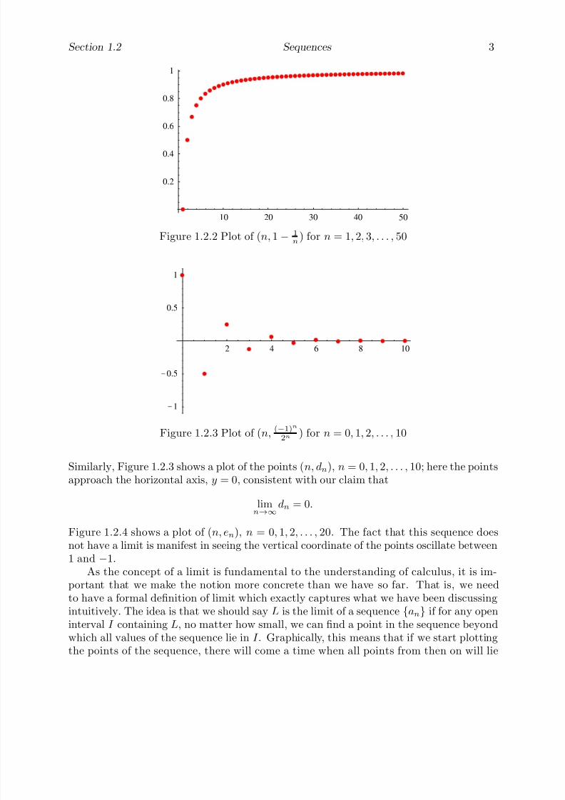
ordered pairs (n, an) in the plane for some range of values of n. For example, Figure 1.2.2shows a plot of the points (n, cn), n = 1, 2, 3, . . . , 50 for the sequence {cn} given above.Note how the points approach the horizontal line y = 1, indicating, as mentioned above,that
limn→∞
cn = 1.
7/27/2019 Calculus 2 (Dan Sloughter)
http://slidepdf.com/reader/full/calculus-2-dan-sloughter 11/598
Section 1.2 Sequences 3
10 20 30 40 50
0.2
0.4
0.6
0.8
1
Figure 1.2.2 Plot of (n, 1 − 1n
) for n = 1, 2, 3, . . . , 50
2 4 6 8 10
-1
-0.5
0.5
1
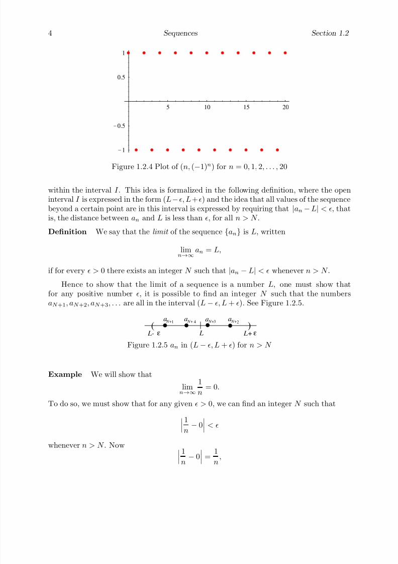
Figure 1.2.3 Plot of (n,(−1)n
2n ) for n = 0, 1, 2, . . . , 10
Similarly, Figure 1.2.3 shows a plot of the points (n, dn), n = 0, 1, 2, . . . , 10; here the pointsapproach the horizontal axis, y = 0, consistent with our claim that
limn→∞
dn = 0.
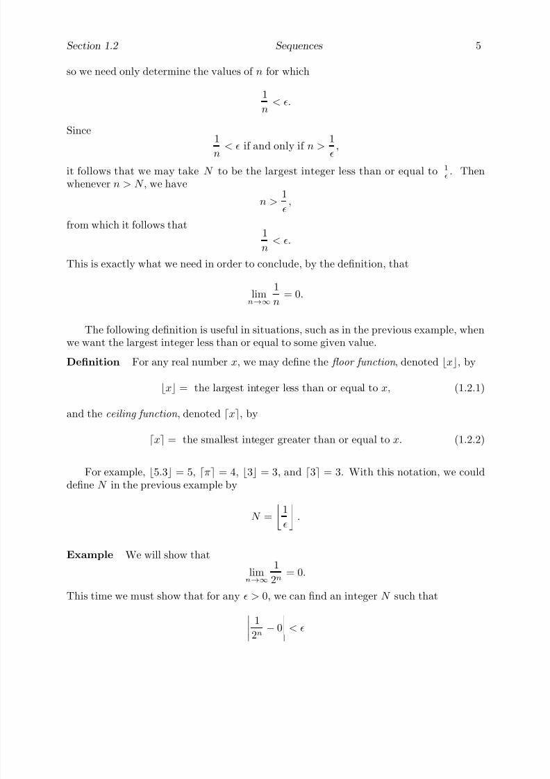
Figure 1.2.4 shows a plot of (n, en), n = 0, 1, 2, . . . , 20. The fact that this sequence doesnot have a limit is manifest in seeing the vertical coordinate of the points oscillate between
1 and −1.As the concept of a limit is fundamental to the understanding of calculus, it is im-
portant that we make the notion more concrete than we have so far. That is, we needto have a formal definition of limit which exactly captures what we have been discussingintuitively. The idea is that we should say L is the limit of a sequence {an} if for any openinterval I containing L, no matter how small, we can find a point in the sequence beyondwhich all values of the sequence lie in I . Graphically, this means that if we start plottingthe points of the sequence, there will come a time when all points from then on will lie
7/27/2019 Calculus 2 (Dan Sloughter)
http://slidepdf.com/reader/full/calculus-2-dan-sloughter 12/598
4 Sequences Section 1.2
5 10 15 20
-1
-0.5
0.5
1
Figure 1.2.4 Plot of (n, (−1)n) for n = 0, 1, 2, . . . , 20
within the interval I . This idea is formalized in the following definition, where the open
interval I is expressed in the form (L− , L + ) and the idea that all values of the sequencebeyond a certain point are in this interval is expressed by requiring that |an − L| < , thatis, the distance between an and L is less than , for all n > N .
Definition We say that the limit of the sequence {an} is L, written
limn→∞
an = L,
if for every > 0 there exists an integer N such that |an − L| < whenever n > N .
Hence to show that the limit of a sequence is a number L, one must show that
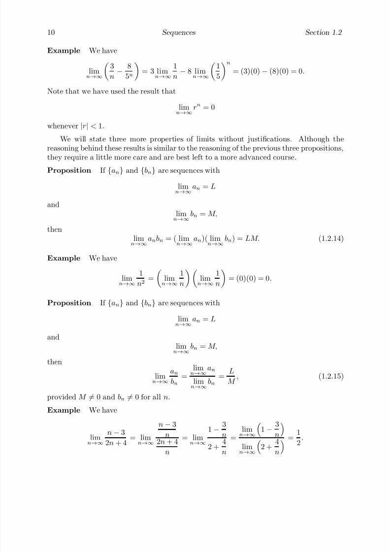
for any positive number , it is possible to find an integer N such that the numbersaN +1, aN +2, aN +3, . . . are all in the interval (L − , L + ). See Figure 1.2.5.
( ) L L- ε L+ ε
a a a N+ N+
a N+1 23 N+ 4
Figure 1.2.5 an in (L − , L + ) for n > N
Example We will show that
limn→∞
1
n
= 0.
To do so, we must show that for any given > 0, we can find an integer N such that
1
n− 0
<
whenever n > N . Now 1
n− 0
=1
n,
7/27/2019 Calculus 2 (Dan Sloughter)
http://slidepdf.com/reader/full/calculus-2-dan-sloughter 13/598
Section 1.2 Sequences 5
so we need only determine the values of n for which
1
n< .
Since 1n
< if and only if n > 1
,
it follows that we may take N to be the largest integer less than or equal to 1
. Thenwhenever n > N , we have
n >1
,
from which it follows that1
n< .
This is exactly what we need in order to conclude, by the definition, that
limn→∞
1
n= 0.
The following definition is useful in situations, such as in the previous example, whenwe want the largest integer less than or equal to some given value.
Definition For any real number x, we may define the floor function , denoted x, by
x = the largest integer less than or equal to x, (1.2.1)
and the ceiling function , denoted x, by
x = the smallest integer greater than or equal to x. (1.2.2)
For example, 5.3 = 5, π = 4, 3 = 3, and 3 = 3. With this notation, we coulddefine N in the previous example by
N =
1
.
Example We will show that
limn→∞
1
2n= 0.
This time we must show that for any > 0, we can find an integer N such that
1
2n− 0
<

7/27/2019 Calculus 2 (Dan Sloughter)
http://slidepdf.com/reader/full/calculus-2-dan-sloughter 14/598

7/27/2019 Calculus 2 (Dan Sloughter)
http://slidepdf.com/reader/full/calculus-2-dan-sloughter 15/598
Section 1.2 Sequences 7
whenever n > N . For example, if we take = 0.001, then, to two decimal places,
log10()
log1012
= 9.97,
and so we would have N = 9.97 = 9.
This N works because, for n > 9, 1
2n− 0
=1
2n≤ 1
210=
1
1024< 0.001.
Problem 12 at the end of this section will ask you to generalize the previous exampleto show that
limn→∞
rn = 0
whenever |r| < 1. This is an important fact that we will make use of later.In this course we will be concerned more with the development of an intuitive un-
derstanding of limits and a computational facility with limits than with the formalism of verifying a specific limit using the above definition. That is not to say that the definitionis unimportant; rather a good grasp of the concept in the definition is important for a fullunderstanding of much of what we will do in calculus. In fact, mathematicians of the 19thcentury arrived at the definition we have stated in their attempts to clarify confusions thathad developed in mathematics since the time of Newton and Leibniz. However, for themost part these difficulties are beyond the scope of a text such as this one.
We will see that a few basic properties of limits, combined with a few simple limits like
the ones in the previous two examples, will enable us to compute easily a large numberof limits. To begin considering these properties, consider the case where we already knowthat
limn→∞
an = L (1.2.3)
and we want to computelimn→∞
kan
for some constant k = 0. Now (1.2.3) tells us that for any > 0, we may find an integerN such that for n > N ,
|an − L| <
|k
|.
It follows that for n > N ,
|kan − kL| = |k||an − L| < |k|
|k| = .
But this is what it means to say that
limn→∞
kan = kL. (1.2.4)

7/27/2019 Calculus 2 (Dan Sloughter)
http://slidepdf.com/reader/full/calculus-2-dan-sloughter 16/598
8 Sequences Section 1.2
Note that (1.2.4) is obviously true as well when k = 0. Hence we have the followingproposition.
Proposition If {an} is a sequence for which
limn→∞
an = L,
then for any constant k we have
limn→∞
kan = k limn→∞
an = kL. (1.2.5)
Example Since we have already seen that
limn→∞
1
n= 0,
it follows that
limn→∞
350n = 350 limn→∞
1n = (350)(0) = 0.
Now suppose we have two sequences {an} and {bn} with
limn→∞
an = L (1.2.6)
andlimn→∞
bn = M. (1.2.7)
Then (1.2.6) and (1.2.7) tell us that for any > 0, we can find integers N 1 and N 2 suchthat
|an − L| < 2
whenever n > N 1 and
|bn − M | <
2
whenever n > N 2. If we let N be the larger of N 1 and N 2, then whenever n > N we willhave
|(an + bn) − (L + M )| = |(an − L) + (bn − M )|≤ |an − L| + |bn − M |<
2+
2= .
(1.2.8)
Note that in (1.2.8) we have used the fact, known as the triangle inequality , that for anyreal numbers x and y,
|x + y| ≤ |x| + |y|. (1.2.9)
Thus we have shownlimn→∞
(an + bn) = L + M. (1.2.10)
Hence we have the following proposition.

7/27/2019 Calculus 2 (Dan Sloughter)
http://slidepdf.com/reader/full/calculus-2-dan-sloughter 17/598
Section 1.2 Sequences 9
Proposition If {an} and {bn} are sequences with
limn→∞
an = L
and
limn→∞ bn = M,
thenlimn→∞
(an + bn) = limn→∞
an + limn→∞
bn = L + M. (1.2.11)
Example We have
limn→∞
4 +
8
n
= lim
n→∞4 + lim
n→∞
8
n= 4 + 8 lim
n→∞
1
n= 4 + (8)(0) = 4.
Note that in the last example we used the fact that if k
is a constant andan =
kforall n, then
limn→∞
an = k.
This follows immediately from the definition since
|an − k| = 0
for all values of n, and so any integer N will work for any value of .Again suppose we have two sequences {an} and {bn} with
limn→∞an =
L
andlimn→∞
bn = M.
Then we have
limn→∞
(an − bn) = limn→∞
an + limn→∞
(−bn) = limn→∞
an + (−1) limn→∞
bn = L − M. (1.2.12).
Proposition If {an} and {bn} are sequences with
limn→∞
an = L
andlimn→∞
bn = M,
thenlimn→∞
(an − bn) = limn→∞
an − limn→∞
bn = L − M. (1.2.13)
7/27/2019 Calculus 2 (Dan Sloughter)
http://slidepdf.com/reader/full/calculus-2-dan-sloughter 18/598
10 Sequences Section 1.2
Example We have
limn→∞
3
n− 8
5n
= 3 lim
n→∞
1
n− 8 lim
n→∞
1
5
n
= (3)(0) − (8)(0) = 0.
Note that we have used the result that
limn→∞
rn = 0
whenever |r| < 1.
We will state three more properties of limits without justifications. Although thereasoning behind these results is similar to the reasoning of the previous three propositions,they require a little more care and are best left to a more advanced course.
Proposition If {an} and {bn} are sequences with
limn→∞
an = L
andlimn→∞
bn = M,
thenlimn→∞
anbn = ( limn→∞
an)( limn→∞
bn) = LM. (1.2.14)
Example We have
limn→∞
1
n2= lim
n→∞
1
n limn→∞
1
n = (0)(0) = 0.
Proposition If {an} and {bn} are sequences with
limn→∞
an = L
andlimn→∞
bn = M,
then
limn→∞
an
bn=
limn→∞
an
limn→∞
bn=
L
M , (1.2.15)
provided M = 0 and bn = 0 for all n.
Example We have
limn→∞
n − 3
2n + 4= lim
n→∞
n − 3
n2n + 4
n
= limn→∞
1 − 3
n
2 +4
n
=limn→∞
1 − 3
n
limn→∞
2 +
4
n
=1
2.
7/27/2019 Calculus 2 (Dan Sloughter)
http://slidepdf.com/reader/full/calculus-2-dan-sloughter 19/598
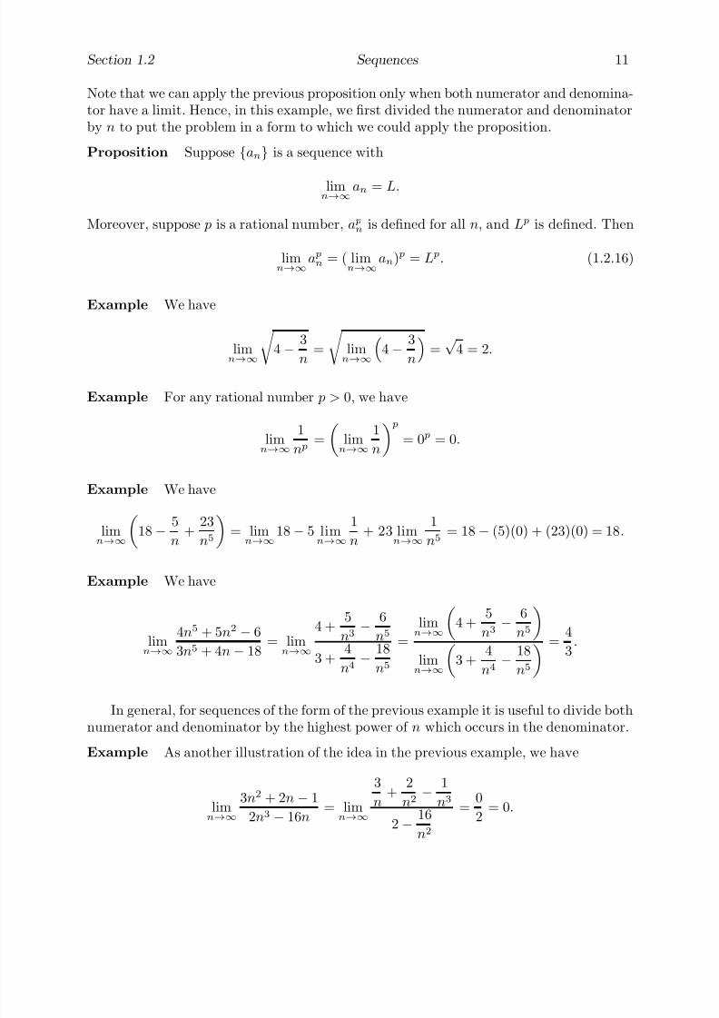
Section 1.2 Sequences 11
Note that we can apply the previous proposition only when both numerator and denomina-tor have a limit. Hence, in this example, we first divided the numerator and denominatorby n to put the problem in a form to which we could apply the proposition.
Proposition Suppose {an} is a sequence with
limn→∞
an = L.
Moreover, suppose p is a rational number, a pn is defined for all n, and L p is defined. Then
limn→∞
a pn = ( limn→∞
an) p = L p. (1.2.16)
Example We have
limn→∞
4 −3
n =
limn→∞
4 −3
n
=
√ 4 = 2
.
Example For any rational number p > 0, we have
limn→∞
1
n p=
limn→∞
1
n
p= 0 p = 0.
Example We have
limn→∞
18 −5
n +
23
n5
= limn→∞18 − 5 limn→∞
1
n + 23 limn→∞
1
n5 = 18 − (5)(0) + (23)(0) = 18.
Example We have
limn→∞
4n5 + 5n2 − 6
3n5 + 4n − 18= lim
n→∞
4 +5
n3− 6
n5
3 +4
n4− 18
n5
=
limn→∞
4 +
5
n3− 6
n5
limn→∞
3 +
4
n4− 18
n5
=4
3.
In general, for sequences of the form of the previous example it is useful to divide bothnumerator and denominator by the highest power of n which occurs in the denominator.
Example As another illustration of the idea in the previous example, we have
limn→∞
3n2 + 2n − 1
2n3 − 16n= lim
n→∞
3
n+
2
n2− 1
n3
2 − 16
n2
=0
2= 0.
7/27/2019 Calculus 2 (Dan Sloughter)
http://slidepdf.com/reader/full/calculus-2-dan-sloughter 20/598
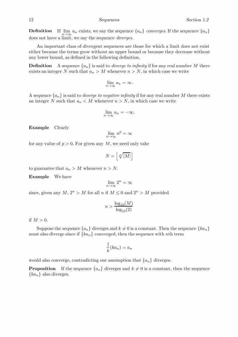
12 Sequences Section 1.2
Definition If limn→∞
an exists, we say the sequence {an} converges . If the sequence {an}does not have a limit, we say the sequence diverges .
An important class of divergent sequences are those for which a limit does not existeither because the terms grow without an upper bound or because they decrease without
any lower bound, as defined in the following definition.Definition A sequence {an} is said to diverge to infinity if for any real number M thereexists an integer N such that an > M whenever n > N , in which case we write
limn→∞
an = ∞.
A sequence {an} is said to diverge to negative infinity if for any real number M there existsan integer N such that an < M whenever n > N , in which case we write
limn→∞
an = −∞.
Example Clearlylimn→∞
n p = ∞
for any value of p > 0. For given any M , we need only take
N =p
|M |
to guarantee that an > M whenever n > N .
Example We havelimn→∞
2n = ∞
since, given any M , 2n > M for all n if M ≤ 0 and 2n > M provided
n >log10(M )
log10(2)
if M > 0.
Suppose the sequence {an} diverges and k = 0 is a constant. Then the sequence {kan}must also diverge since if {kan} converged, then the sequence with nth term
1
k(kan) = an
would also converge, contradicting our assumption that {an} diverges.
Proposition If the sequence {an} diverges and k = 0 is a constant, then the sequence{kan} also diverges.

7/27/2019 Calculus 2 (Dan Sloughter)
http://slidepdf.com/reader/full/calculus-2-dan-sloughter 21/598
Section 1.2 Sequences 13
If the sequence {an} diverges and the sequence {bn} converges, then the sequence{an + bn} also diverges since, if it converged, then the sequence with nth term
(an + bn) − bn = an
would also converge, contradicting our assumption that {an} diverges. Similarly, thesequence {an − bn} diverges.
Proposition If the sequence {an} diverges and the sequence {bn} converges, then thesequences {an + bn} and {an − bn} both diverge.
Suppose the sequence {an} diverges, the sequence {bn} converges, and
limn→∞
bn = 0. (1.2.17)
Now (1.2.17) implies that we can find an integer N such that bn = 0 for all n > N . So if
the sequence {anbn} converged, then the sequence with, for n > N , nth term,1
bn(anbn) = an
would also converge, contradicting our assumption that {an} diverges. Hence {anbn} mustdiverge.
Proposition If the sequence {an} diverges, the sequence {bn} converges, and
limn→∞
bn = 0,
then the sequence {anbn} diverges
Finally, if the sequence {an} diverges, the sequence {bn} converges, and bn = 0 for alln, then the sequence
an
bn
diverges since, if it converged, the sequence with nth term
bn
an
bn
= an
would also converge, contradicting our assumption that {an} diverges.
Proposition If the sequence {an} diverges, the sequence {bn} converges, and bn = 0 forall n, then the sequence
an
bn
diverges.

7/27/2019 Calculus 2 (Dan Sloughter)
http://slidepdf.com/reader/full/calculus-2-dan-sloughter 22/598
14 Sequences Section 1.2
Example Consider
limn→∞
4n3 + n − 2
5n2 − 7n= lim
n→∞
4n +1
n− 2
n2
5
−7
n
. (1.2.18)
Nowlimn→∞
4n = ∞
and
limn→∞
1
n− 2
n2
= 0,
so
limn→∞
4n +
1
n− 2
n2
= ∞.
Moreover,
limn→∞
5 − 7
n
= 5.
Thus the numerator in (1.2.18) diverges while the denominator converges. Hence the ratiodiverges. In fact, it should be clear that
limn→∞
4n3 + n − 2
5n2 − 7n= lim
n→∞
4n +1
n− 2
n2
5 − 7
n
= ∞.
Note that in the previous example it was once again useful to divide numerator anddenominator by the highest power of n in the denominator.
Example We have
limn→∞
15 − 26n5
13 + n2= lim
n→∞
15
n2− 26n3
13
n2+ 1
= −∞.
Example The absolute values of the terms of the sequence {(−2)n} grow without bound,and so the sequence diverges. However, since the terms alternate in sign, the sequenceneither diverges to ∞ nor to −∞.
Monotone sequences
It is sometimes possible to determine that a given sequence converges without explicitlycomputing the limit. One important case involves monotone sequences .

7/27/2019 Calculus 2 (Dan Sloughter)
http://slidepdf.com/reader/full/calculus-2-dan-sloughter 23/598
Section 1.2 Sequences 15
Definition We say a sequence {an} is monotone increasing if an ≤ an+1 for all n. Wesay a sequence {an} is monotone decreasing if an ≥ an+1 for all n. We say a sequence ismonotone if it is either monotone increasing or monotone decreasing.
Now suppose {an} is a monotone increasing sequence. For such a sequence there either
exists a number P such that an ≤ P for all n or there does not exist such an P . In the lattercase, given any real number M , it is then possible to find integer N such that aN > M .Since the sequence is monotone, it follows that an > M for all n > N , and so the sequencediverges to infinity. On the other hand, if there does exist a number P such that an ≤ P
for all n, then there in fact exists a number B such that an ≤ B for all n and B ≤ P
for any number P with the property that an ≤ P for all n. The existence of B, knownas the least upper bound of the sequence {an}, is not at all obvious; indeed, the subtleproperties of the real numbers that imply the existence of B were not fully understooduntil the middle part of the 19th century. However, given the existence of B, it is easyto see that given any > 0, there exists a integer N for which aN > B − (if not, thenB
− would be an upper bound for the sequence smaller than B). Since the sequence is
monotone increasing and an < B for all n, it follows that
|an − B| <
for all n > N . That is, we have shown that the sequence converges and
limn→∞
an = B.
Similar results hold for sequences which are monotone decreasing.
Monotone sequence theorem Suppose the sequence {an} is monotone. If the se-quence is monotone increasing and there exists a number P such that an ≤ P for all n,then the sequence converges. If the sequence is monotone increasing and no such numberP exists, then
limn→∞
an = ∞.
If the sequence is monotone decreasing and there exists a number Q such that an ≥ Q forall n, then the sequence converges. If the sequence is monotone decreasing and no suchnumber Q exists, then
limn→∞
an =
−∞.
Example As we shall see in Sections 1.4 and 1.5, we often work with sequences withouthaving an explicit formula for each term in the sequence. For example, suppose all weknow about the sequence {an} is that a1 = 4 and
an+1 =1
2an

7/27/2019 Calculus 2 (Dan Sloughter)
http://slidepdf.com/reader/full/calculus-2-dan-sloughter 24/598
16 Sequences Section 1.2
for n = 1, 2, 3, . . .. That is, the first term in the sequence is 4 and then each successiveterm is one-half of its predecessor. Thus
a1 = 4,
a2 = 2,
a3 = 1,
a4 =1
2,
and so on. Hence {an} is monotone decreasing. Moreover, every term in the sequence ispositive, so an ≥ 0 for all n. Thus, by the Monotone Sequence Theorem, {an} converges.Moreover, note that
an+1 =1
2an
implies that
limn→∞
an+1 = 12
limn→∞
an. (1.2.19)
If we letL = lim
n→∞an = lim
n→∞an+1,
then (1.2.19) becomes
L =1
2L.
Hence L = 0. That is,limn→∞
an = 0.
Problems
1. For each of the following, find a general expression for the nth term of a sequencewhich would yield these values as the first four terms.
(a) 1,1
3,
1
9,
1
27, . . . (b) 1,
1
2,
1
3,
1
4, . . .
(c) 1,3
2,
5
3,
7
4, . . . (d) −1
3,
1
5, −1
7,
1
9, . . .
2. For each of the following, decide whether the given sequence converges or diverges. If the sequence converges, find its limit.
(a) an =1
3n, n = 0, 1, 2, . . . (b) an = πn, n = 0, 1, 2, . . .
(c) bn =3n − 1
2n + 6, n = 1, 2, 3, . . . (d) cn = cos(πn), n = 0, 1, 2, . . .
(e) an =3n4 − 6n3 + 1
5n3 + n2 + 2, n = 1, 2, 3, . . . (f) bn =
2n5 − 3n2 + 23
7n5 + 13n4 − 12, n = 1, 2, 3, . . .
7/27/2019 Calculus 2 (Dan Sloughter)
http://slidepdf.com/reader/full/calculus-2-dan-sloughter 25/598
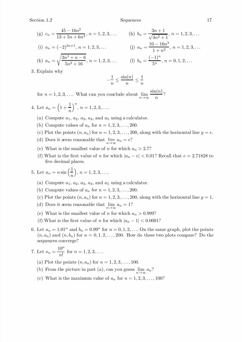
Section 1.2 Sequences 17
(g) cn =45 − 16n2
13 + 5n + 6n3, n = 1, 2, 3, . . . (h) bn =
3n + 1√ 4n2 + 1
, n = 1, 2, 3, . . .
(i) an = (−2)2n+1, n = 1, 2, 3, . . . (j) an =10 − 16n3
1 + n2, n = 1, 2, 3, . . .
(k) an =
3n2
+n
− 65n2 + 16 , n = 1, 2, 3, . . . (l) bn = (−1)
n
5n , n = 0, 1, 2, . . .
3. Explain why
− 1
n≤ sin(n)
n≤ 1
n
for n = 1, 2, 3, . . .. What can you conclude about limn→∞
sin(n)
n?
4. Let an =
1 +1
n
n, n = 1, 2, 3, . . ..
(a) Compute a1, a2, a3, a4, and a5 using a calculator.(b) Compute values of an for n = 1, 2, 3, . . . , 200.
(c) Plot the points (n, an) for n = 1, 2, 3, . . . , 200, along with the horizontal line y = e.
(d) Does it seem reasonable that limn→∞
an = e?
(e) What is the smallest value of n for which an > 2.7?
(f) What is the first value of n for which |an − e| < 0.01? Recall that e = 2.71828 tofive decimal places.
5. Let an = n sin1
n, n = 1, 2, 3, . . ..
(a) Compute a1, a2, a3, a4, and a5 using a calculator.
(b) Compute values of an for n = 1, 2, 3, . . . , 200.
(c) Plot the points (n, an) for n = 1, 2, 3, . . . , 200, along with the horizontal line y = 1.
(d) Does it seem reasonable that limn→∞
an = 1?
(e) What is the smallest value of n for which an > 0.999?
(f) What is the first value of n for which |an − 1| < 0.0001?
6. Let an = 1.01n and bn = 0.99n for n = 0, 1, 2, . . .. On the same graph, plot the points(n, an) and (n, bn) for n = 0, 1, 2, . . . , 200. How do these two plots compare? Do the
sequences converge?
7. Let an =10n
n!for n = 1, 2, 3, . . ..
(a) Plot the points (n, an) for n = 1, 2, 3, . . . , 100.
(b) From the picture in part (a), can you guess limn→∞
an?
(c) What is the maximum value of an for n = 1, 2, 3, . . . , 100?

7/27/2019 Calculus 2 (Dan Sloughter)
http://slidepdf.com/reader/full/calculus-2-dan-sloughter 26/598
18 Sequences Section 1.2
(d) Can you see why
limn→∞
kn
n!= 0
for any constant k?
8. Consider the sequence {an} with a1 = 10 and
an+1 =1
3an
for n = 1, 2, 3, . . .. Plot the points (n, an) for n = 1, 2, 3, . . . 50. Do you think thissequence has a limit? Can you verify this?
9. Consider the sequence {an} with a1 = 2 and
an+1 = 2an
for n = 1, 2, 3, . . .. Plot the points (n, an) for n = 1, 2, 3, . . . , 50. Can you find thelimit of this sequence using the same method you used in part Problem 8? Does thissequence have a limit?
10. Consider the sequence {an} with a1 = 0.9 and
an+1 = 2an(1 − an)
for n = 1, 2, 3, . . .. Plot the points (n, an) for n = 1, 2, 3, . . . , 100. Do you think thissequence has a limit? If so, can you find it?
11. In each of the following, for an arbitrary > 0, find the smallest integer N for which|an − L| < whenever n > N . Verify that your value for N works in the particularcase = 0.001.
(a) an = 1 − 1
n, L = 1 (b) an = 0.98n, L = 0
(c) an =1
n2, L = 0 (d) an =
3n3 − 1
n3, L = 3
12. Show that for any −1 < r < 1, limn→∞
rn = 0.
13. Find sequences {an} and {bn} such that {an} and {bn} both diverge, but {an + bn}converges.
14. Find sequences {an} and {bn} such that {an} diverges, {bn} converges, and {anbn}converges.

7/27/2019 Calculus 2 (Dan Sloughter)
http://slidepdf.com/reader/full/calculus-2-dan-sloughter 27/598
Difference Equations
Differential Equations
to
Section 1.3
The Sum of a Sequence
This section considers the problem of adding together the terms of a sequence. Of course,this is a problem only if more than a finite number of terms of the sequence are nonzero.In this case, we must decide what it means to add together an infinite number of nonzeronumbers. The first example shows how a relatively simple question may lead to suchinfinite summations.
Example Suppose a game is played in which a fair coin is tossed until the first timea head appears. What is the probability that a head appears for the first time on an
even-numbered toss? To solve this problem, we first need to determine the probability of obtaining a head for the first time on any given even numbered toss, and then we needto add all these probabilities together. Let P n denote the probability that the first headappears on the nth toss, n = 1, 2, 3, . . ... Then, since the coin is assumed to be fair,
P 1 =1
2.
Now in order to get a head for the first time on the second toss, we must toss a tail on thefirst toss and then follow that with a head on the second toss. Since one-half of all firsttosses will be tails and then one-half of those tosses will be followed by a second toss of
heads, we should haveP 2 =
1
2
1
2
=
1
4.
Similarly, since one-fourth of all sequences of coin tosses will begin with two tails and thenhalf of these sequences will have a head for the third toss, we have
P 3 =
1
4
1
2
=
1
8.
Continuing in this fashion, it should seem reasonable that, for any n = 1, 2, 3, . . .,
P n = 12n.
Hence we have a sequence of probabilities {P n} for n = 1, 2, 3, . . ., and, in order to find thedesired probability, we need to add up the even-numbered terms in this sequence. Namely,the probability that a head appears for the first time on an even toss is given by
P 2 + P 4 + P 6 + · · · =1
4+
1
16+
1
64+ · · · . (1.3.1)
1 Copyright c by Dan Sloughter 2000
7/27/2019 Calculus 2 (Dan Sloughter)
http://slidepdf.com/reader/full/calculus-2-dan-sloughter 28/598
2 The Sum of a Sequence Section 1.3
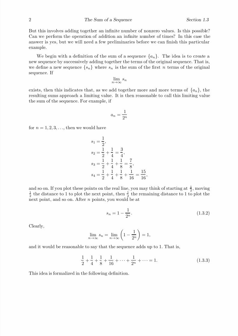
But this involves adding together an infinite number of nonzero values. Is this possible?Can we perform the operation of addition an infinite number of times? In this case theanswer is yes, but we will need a few preliminaries before we can finish this particularexample.
We begin with a definition of the sum of a sequence {an}. The idea is to create a
new sequence by successively adding together the terms of the original sequence. That is,we define a new sequence {sn} where sn is the sum of the first n terms of the originalsequence. If
limn→∞
sn
exists, then this indicates that, as we add together more and more terms of {an}, theresulting sums approach a limiting value. It is then reasonable to call this limiting valuethe sum of the sequence. For example, if
an =1
2n
for n = 1, 2, 3, . . ., then we would have
s1 =1
2,
s2 =1
2+
1
4=
3
4,
s3 =1
2+
1
4+
1
8=
7
8,
s4 =
1
2 +
1
4 +
1
8 +
1
16 =
15
16 ,
and so on. If you plot these points on the real line, you may think of starting at 1
2, moving
1
2the distance to 1 to plot the next point, then 1
2the remaining distance to 1 to plot the
next point, and so on. After n points, you would be at
sn = 1 −1
2n. (1.3.2)
Clearly,
limn→∞ sn = limn→∞1 −
1
2n = 1,
and it would be reasonable to say that the sequence adds up to 1. That is,
1
2+
1
4+
1
8+
1
16+ · · ·+
1
2n+ · · · = 1. (1.3.3)
This idea is formalized in the following definition.

7/27/2019 Calculus 2 (Dan Sloughter)
http://slidepdf.com/reader/full/calculus-2-dan-sloughter 29/598
Section 1.3 The Sum of a Sequence 3
Definition Given a sequence {an}, n = 1, 2, 3, . . ., we define a new sequence {sn} byletting
sn = a1 + a2 + . . . + an (1.3.4)
for n = 1, 2, 3, . . .. If the sequence {sn} converges, then we call
s = limn→∞
sn
the sum of the sequence {an}. The sequence {sn} is called an infinite series and anindividual term sn of this sequence is called a partial sum of the sequence {an}.
Note that we have assumed that the first term in the sequence {an} in the definitionis a1. The sequence could just as well start with any other integer index, in which case thesequence of partial sums {sn} would start with the same index. For example, if the firstterm of the sequence is a0, then the first partial sum is s0.
Since summations involving an infinite number, or even a large finite number, of termsare cumbersome to write using the standard plus sign of addition, Σ (the capital Greek
sigma ) is used to denote the process of summation. In particular, we would write
sn =nj=1
aj = a1 + a2 + · · ·+ an (1.3.5)
and
s = limn→∞
sn = limn→∞
nj=1
aj = limn→∞
(a1 + a2 + · · ·+ an). (1.3.6)
Since (1.3.6) is what we mean by an infinite sum, we will in fact write
s =∞j=1
aj = a1 + a2 + · · ·+ an + · · · . (1.3.7)
For example, in this notation, we may restate our earlier results as
nn=1
1
2n=
1
2+
1
4+
1
8+
1
16=
15
16.
and∞
n=1
1
2n =
1
2 +
1
4 +
1
8 +
1
16 + · · ·+
1
2n + · · · = 1.
We should note that, since the sum of a sequence is the limit of another sequence, andnot all sequences have limits, there are sequences which do not have sums. For example,the sequence with terms an = 1 for n = 1, 2, 3, . . . does not have a sum since
sn = 1 + 1 + · · ·+ 1 n times
= n,

7/27/2019 Calculus 2 (Dan Sloughter)
http://slidepdf.com/reader/full/calculus-2-dan-sloughter 30/598
4 The Sum of a Sequence Section 1.3
from which it follows thatlimn→∞
sn = ∞.
For another example, the sequence {(−1)n}, n = 0, 1, 2, . . ., does not have a sum since
sn = 1, if n = 0, 2, 4, . . .,
0, if n = 1, 3, 5, . . .,
a sequence which clearly does not have a limit.In general it may be difficult to determine the sum of a sequence; in fact, it may be
difficult to determine even if the sequence has a sum. We will return to this problemin Chapter 5 when we have more tools at our disposal, as well as more motivation forstudying infinite series. For now we will look at an important class of sequences for whichthe sum is determined with relative ease. These are the sequences for which the termsare in geometric progression; that is, sequences for which successive terms have a commonratio. We call the infinite series which corresponds to such a sequence a geometric series .
Geometric seriesSuppose {an} is a sequence with an = crn−1, where c = 0 and r are constants andn = 1, 2, 3, . . .. Then the partial sums are
sn = a1 + a2 + a3 + · · ·+ an
= c + cr + cr2 + · · ·+ crn−1
= c(1 + r + r2 + · · ·+ rn−1).
If r = 1, sn = nc and so {sn} does not converge. If r = 1, it is easy to see, using longdivision (or the derivation outlined in Problem 4), that
1 − rn
1 − r= 1 + r + r2 + · · ·+ rn−1. (1.3.8)
Hence, if r = 1,
sn =c(1− rn)
1− r. (1.3.9)
From (1.3.9), it is clear that {sn} does not converge if |r| ≥ 1. But if −1 < r < 1, then
limn→∞
rn−1 = 0,
and so the sequence has the sum
s = limn→∞
sn = limn→∞
c(1− rn
)1− r
= c1− r
. (1.3.10)
That is, we have now seen that
∞n=1
crn−1 =c
1 − r(1.3.11)
whenever −1 < r < 1.
7/27/2019 Calculus 2 (Dan Sloughter)
http://slidepdf.com/reader/full/calculus-2-dan-sloughter 31/598
Section 1.3 The Sum of a Sequence 5
Example We have, using (1.3.11) with c = 1 and r = 1
2,
∞n=1
1
2
n−1= 1 +
1
2+
1
4+
1
8+
1
16+ · · · =
1
1 −1
2
= 2.
Note that this agrees with our previous result that
1
2+
1
4+
1
8+
1
16+ · · · = 1.
Example We have
∞
n=1
2
3
n=∞
n=12
3
2
3
n−1=
2
3
1 −2
3
= 2.
Example We have∞n=0
1
5n
=∞n=0
1
5
n=
1
1 −1
5
=5
4.
Note that in this example the sum starts with n = 0 instead of n = 1 as in (1.3.11).However, it is the initial power of r in (1.3.11) that is important, not how we write theindex. Hence, the sum in this example could be written equally well as
∞n=1
1
5n−1
,
or∞n=2
1
5
n−2,
or∞
n=100
1
5
n−100,
as well as many other ways. The key in applying (1.3.11) is that we identify c and r so
that the first term in the sum is cr
0
= c.Example We have
∞n=2
4(0.34)n =∞n=2
4(0.34)2(0.34)n−2 =4(0.34)2
1− 0.34= 0.7006,
where we have used (1.3.11) with c = 4(0.34)2 and r = 0.34.

7/27/2019 Calculus 2 (Dan Sloughter)
http://slidepdf.com/reader/full/calculus-2-dan-sloughter 32/598
6 The Sum of a Sequence Section 1.3
We are now in a position to compute the sum in (1.3.1), and hence complete our firstexample
Example Let P be the probability that, when tossing a fair coin repeatedly, the firsthead appears on an even toss. Then we have seen that
P = P 2 + P 4 + P 6 + · · · =∞n=1
P 2n,
where
P 2n =
1
2
2n
=
1
2
2n=
1
4
nfor n = 1, 2, 3, . . .. Thus
P =∞n=1
14
n=∞n=1
14
14
n−1=
1
4
1−1
4
= 13
.
Example Economists often talk about the multiplier effect of an infusion of money intoan economy which results in new spending many times greater than the original amountspent. This is a consequence of the recipients of the money spending a certain percentageof their new money, the recipients of this spending again spending a certain percentage of their gain, and so on. For example, suppose the government spends three million dollars,and suppose that at each stage the recipients spend 90% of the money they receive. Then
the first recipients spend (3)(0.9) = 2.7 million dollars, the second recipients spend
(3)(0.9)(0.9) = (3)(0.9)2 = 2.43
million dollars (that is, 90% of the 2.7 million spent by the first recipients), the thirdrecipients spend
(3)(0.92)(0.9) = (3)(0.9)3 = 2.187
million dollars, and so on. If we denote the total amount of spending after n transactionsby S n , then, in millions of dollars,
S 1 = 3,S 2 = 3 + 3(0.9),
S 3 = 3 + 3(0.9) + 3(0.9)2,
S 4 = 3 + 3(0.9) + 3(0.9)2 + 3(0.9)3,
and, in general,S n = 3 + 3(0.9) + 3(0.9)2 + · · ·+ 3(0.9)n−1
7/27/2019 Calculus 2 (Dan Sloughter)
http://slidepdf.com/reader/full/calculus-2-dan-sloughter 33/598
Section 1.3 The Sum of a Sequence 7
for n = 1, 2, 3, . . .. Although in actuality there will be only a finite number of transactions,we can see that as n increases the total spending will approach the sum
S =∞
n=13(0.9)n−1 =
3
1 − 0.9= 30
million dollars. Thus the initial governmental expenditure of three million dollars resultsin approximately 30 million dollars, 10 times the initial amount, in new spending in theeconomy. This partially explains why deficit spending by the government in depressedtimes can be far more beneficial to the economy than the actual amount spent, and whysuch spending during other times can be highly inflationary.
Example This example involves slightly more complicated probabilistic reasoning, aswell as some additional algebraic simplification, before the problem is reduced to the sum-mation of a geometric series. Suppose that a certain female animal has a 10% chance of dying during any given year of her life. Moreover, suppose the animal does not repro-
duce during her first year of life, but every year after has a 20% chance of successfullyreproducing. What is the probability that this animal has offspring before dying?Let P be the probability that the animal has offspring before dying and let P n be the
probability that the animal successfully reproduces for the first time in its nth year. Then
P =∞n=1
P n.
Note that our sum extends to infinity even though in reality it is highly unlikely that anysuch animal would live even to an age of 100 years. We do this because the model weare using, as with all mathematical models, is an idealization of the real situation. In
this case, by assuming that a given animal of this species has a constant 10% chance of dying in any given year, we have implicitly assumed that there is no fixed upper boundto its life-span. Put another way, we have assigned a positive probability to an animal’sliving for, as an example, 1000 years, although this probability is very small (namely,0.91000 ≈ 1.748 × 10−46) and, hence, is not actually ever going to happen.
Since we have assumed that these animals cannot reproduce in their first year of life,we have P 1 = 0. To compute P 2, we note that 90% of all such females will live throughtheir first year and that 20% of these will then have offspring successfully. Hence theproportion of females that successfully reproduce for the first time in their second year is
P 2 = (0.9)(0.2).
To compute P 3 , first we note that the proportion of females living until their third yearwill be (0.9)(0.9) (that is, 90% of the 90% who lived through their first year). Now 80% of these will not have produced offspring successfully in their second year, so the proportionof females who reach their third year without having reproduced is (0 .9)2(0.8). Finally,20% of these will have success in reproducing in their third year. Thus
P 3 = (0.9)2(0.8)(0.2).

7/27/2019 Calculus 2 (Dan Sloughter)
http://slidepdf.com/reader/full/calculus-2-dan-sloughter 34/598
8 The Sum of a Sequence Section 1.3
Similar reasoning yieldsP 4 = (0.9)3(0.8)2(0.2)
(that is, this represents a female who has lived through three years, did not reproduce ineither her second or third year, but did have offspring in her fourth year) and, in general,
P n = (0.9)n−1(0.8)n−2(0.2)
for n = 2, 3, 4, . . .. Hence
P =∞n=1
P n
=∞n=2
(0.9)n−1(0.8)n−2(0.2)
=
∞n=2
(0.2)(0.9)(0.9)n−2
(0.8)n−2
=∞n=2
(0.18)(0.72)n−2
=0.18
1 − 0.72
= 0.6429,
where the answer has been rounded to four decimal places. Thus we conclude that a givenfemale of this species has just over a 64% chance of reproducing during her lifetime.
The harmonic series
It may happen that a sequence {an} does not have a sum even though
limn→∞
an = 0.
One important example of this behavior is provided by the sequence {an} with
an =1
n
for n = 1, 2, 3, . . . . The resulting infinite series with nth partial sum given by
sn = 1 +1
2+
1
3+ · · ·
1
n. (1.3.12)
is called the harmonic series . Since
sn+1 = 1 +1
2+ · · ·+
1
n+
1
n + 1= sn +
1
n + 1> sn, (1.3.13)
7/27/2019 Calculus 2 (Dan Sloughter)
http://slidepdf.com/reader/full/calculus-2-dan-sloughter 35/598
Section 1.3 The Sum of a Sequence 9
the sequence {sn} is monotone increasing. Hence, by the Monotone Sequence Theorem,{sn} either converges or diverges to infinity. Now
s1 = 1,
s2 = 1 +1
2,
s4 = 1 +1
2+
1
3+
1
4> 1 +
1
2+
1
4+
1
4= 1 +
1
2+
1
2= 1 + 2
1
2
,
s8 = 1 +1
2+
1
3+
1
4+
1
5+
1
6+
1
7+
1
8> 1 +
1
2+
1
4+
1
4+
1
8+
1
8+
1
8+
1
8
= 1 +1
2+
1
2+
1
2= 1 + 3
1
2
,
and
s16 = s8 +16
j=91
j
> s8 +16
j=91
16
> 1 + 31
2 +8
16
= 1 + 41
2 .
Continuing in this pattern, we can see that, in general,
s2m > 1 +m
2(1.3.14)
for any m = 0, 1, 2, . . .. Thus, since m2
may be made arbitrarily large, the sequence {sn}does not have an upper bound. Hence we must have
limn→∞
sn = ∞, (1.3.15)
and so the harmonic series does not have a sum.Although the partial sums of the harmonic series diverge to infinity, they grow very
slowly. For example, if n = 500, 000, 000, then sn is between 20 and 21. That is,
20 < 1 +1
2+
1
3+ · · ·+
1
500, 000, 000< 21. (1.3.16)
Problems
1. Find the sum of each of the following infinite series which has a sum.
(a)∞n=1
13
n−1(b)
∞n=1
4(0.21)n−1
(c)∞n=1
2
5n(d)
∞n=0
2
7n
(e)∞n=1
7
1
3
n2
5
n−1(f)
∞n=3
2
3
n
7/27/2019 Calculus 2 (Dan Sloughter)
http://slidepdf.com/reader/full/calculus-2-dan-sloughter 36/598
10 The Sum of a Sequence Section 1.3
(g)∞n=1
3
2
n−1(h)
∞n=1
0.99999n
(i)∞
n=11.00001n (j)
∞
n=305
3n
7n−1
(k)∞
n=100
91
89
n−1(l)
∞n=1
π
4
n
(m)∞n=1
sin(πn) (n)∞n=1
cos(πn)
2. Consider the infinite series with nth partial sum
sn = 1 + 1 +1
2+
1
6+ · · ·+
1
n!=∞j=0
1
j!.
Note that, by definition, 0! = 1.
(a) Show that sn < 3 for all values of n. Hint: Note that
n! = (1)(2)(3) · · · (n) ≥ (1)(2)(2) · · · (2) = 2n−1
for n = 1, 2, 3, . . ..
(b) Combine (a) with the fact that sn+1 > sn for all n to conclude that
∞
j=11
j!
exists and is less than 3.
(c) In fact,∞j=1
1
j!= 1 + 1 +
1
2+
1
6+
1
24+ · · ·
is a well known irrational number. Add up a sufficient number of terms to enableyou to guess the value of the sum. How many terms did it take?
(d) How many terms are necessary to obtain a partial sum that is within 0.000001 of the sum?
3. The sum
4∞n=0
(−1)n
2n + 1= 4
1 −
1
3+
1
5−
1
7+ · · ·
is a well known irrational number.
(a) Add up a sufficient number of terms to enable you to guess the value of the sum.How many terms did it take?

7/27/2019 Calculus 2 (Dan Sloughter)
http://slidepdf.com/reader/full/calculus-2-dan-sloughter 37/598
Section 1.3 The Sum of a Sequence 11
(b) How many terms are necessary to obtain a partial sum that is within 0.01 of thesum?
4. This problem outlines an alternative method for deriving the result of (1.3.8). Supposer = 1. For n = 1, 2, 3, . . ., let
sn = 1 + r + r2 + · · ·+ rn−1.
Show that sn − rsn = 1− rn and conclude that
sn =1− rn
1− r.
5. Using the model we used for the multiplier effect, find the total amount of new spendingresulting from each of the following.
(a) The government spends 2 billion dollars; each recipient spends 80% of what he or
she receives.
(b) The government spends 250 million dollars; each recipient spends 95% of what heor she receives.
(c) The government spends A dollars; each recipient spends 100r%, 0 < r < 1, of whathe or she receives.
6. Government regulations specify that a bank may not loan 100% of its deposits; thebank must keep a certain percentage of its deposits in reserve. For example, if a bankmust keep 15% of its deposits in reserve, then it may loan out $850 from a $1000deposit. Typically, this $850 will again be deposited in a bank, and that bank mayloan out 85% of it. Again, this money will be deposited and 85% of it given out inloans. As this will continue indefinitely, the multiplier effect comes into play and thetotal amount of money in all the deposits resulting from the initial $1000 deposit canbe computed in the same manner as in our example.
(a) Compute the total amount of the deposits resulting from the initial $1000 deposit.
(b) How would the answer in (a) change if the reserve rate was changed from 15% to20%?
(c) How would the answer in (a) change if the reserve rate was changed from 15% to10%?
7. A ball is dropped from a height of 10 meters. Suppose that every time it strikesthe ground, it bounces back to a height which is 75% of the height of the previousbounce. Assuming an infinite number of bounces (again, an idealized mathematicalmodel), how far does the ball travel before it comes to rest? What would happen if itrebounded to only 25% of its initial height?
8. Suppose the animal in the our final example above could not produce offspring for itsfirst 3 years of life. How would this change the probability of a female’s reproducingbefore dying?
7/27/2019 Calculus 2 (Dan Sloughter)
http://slidepdf.com/reader/full/calculus-2-dan-sloughter 38/598
12 The Sum of a Sequence Section 1.3
9. Suppose the animal in our final example above has only an 80% chance of living througha given year. How does this change the probability of a female’s reproducing beforedying?
10. Suppose a female animal of the type discussed in the final example above has a 100r%,0 ≤ r ≤ 1, chance of reproducing each year after its first year.
(a) Find the probability P of a female’s reproducing before dying.
(b) Plot P as a function of r for 0 ≤ r ≤ 1.
(c) Find the value of r for which P = 0.5.
11. How many terms of the harmonic series are needed to obtain a partial sum larger than5? How many terms are needed to obtain a partial sum larger than 10?
12. Plot the points (n, sn), where sn is the nth partial sum of the harmonic series, forn = 1, 2, 3, . . . , 1000. What does this show you about the rate of growth of the partialsums?
13. The first example of this section is a particular case of the more general problem of computing probabilities associated with the waiting time for some event to occur. Asanother example, suppose that an electronic switch works with probability p and failswith probability q = 1 − p. Then, using reasoning analogous to that used in the cointossing example, the probability that the first failure will occur on the nth use of theswitch is pn−1q , n = 1, 2, 3, . . ..
(a) Can you justify this probability?
(b) The reliability of the switch is given by the function
R(n) = probabilty that the switch does not fail until after the nth use
=∞
j=n+1
pj−1q .
Show that R(n) = pn, n = 1, 2, 3, . . ..
(c) Find a way to show that R(n) = pn directly without using an infinite series.
7/27/2019 Calculus 2 (Dan Sloughter)
http://slidepdf.com/reader/full/calculus-2-dan-sloughter 39/598
Difference Equations
Differential Equations
to
Section 1.4
Difference Equations
At this point almost all of our sequences have had explicit formulas for their terms. Thatis, we have looked mainly at sequences for which we could write the nth term as an = f (n)for some known function f . For example, if
an =n + 1
n2 + 3,
then it is an easy matter to compute explicitly, say, a10 = 11
103or a100 = 101
10003. In such
cases we are able to compute any given term in the sequence without reference to anyother terms in the sequence. However, it is often the case in applications that we do notbegin with an explicit formula for the terms of a sequence; rather, we may know onlysome relationship between the various terms. An equation which expresses a value of asequence as a function of the other terms in the sequence is called a difference equation .In particular, an equation which expresses the value an of a sequence {an} as a function of the term an−1 is called a first-order difference equation . If we can find a function f suchthat an = f (n), n = 1, 2, 3, . . ., then we will have solved the difference equation. In thissection we will consider a class of difference equations that are solvable in this sense; inthe next section we will discuss an example where an explicit solution is not possible.
Example Suppose a certain population of owls is growing at the rate of 2% per year. If we let x0 represent the size of the initial population of owls and xn the number of owls n
years later, thenxn+1 = xn + 0.02xn = 1.02xn (1.4.1)
for n = 0, 1, 2, . . .. That is, the number of owls in any given year is equal to the numberof owls in the previous year plus 2% of the number of owls in the previous year. Equation(1.4.1) is an example of a first-order difference equation; it relates the number of owls ina given year with the number of owls in the previous year. Hence we know the value of aspecific xn once we know the value of xn−1. To get the sequence started we have to knowthe value of x0. For example, if initially we have a population of x0 = 100 owls and we
want to know what the population will be after 4 years, we may compute
x1 = 1.02x0 = (1.02)(100) = 102,
x2 = 1.02x1 = (1.02)(102) = 104.04,
x3 = 1.02x2 = (1.02)(104.04) = 106.1208,
andx4 = 1.02x3 = (1.02)(106.1208) = 108.243216.
1 Copyright c by Dan Sloughter 2000
7/27/2019 Calculus 2 (Dan Sloughter)
http://slidepdf.com/reader/full/calculus-2-dan-sloughter 40/598
2 Difference Equations Section 1.4
20 40 60 80 100
100
200
300
400
500
600
700
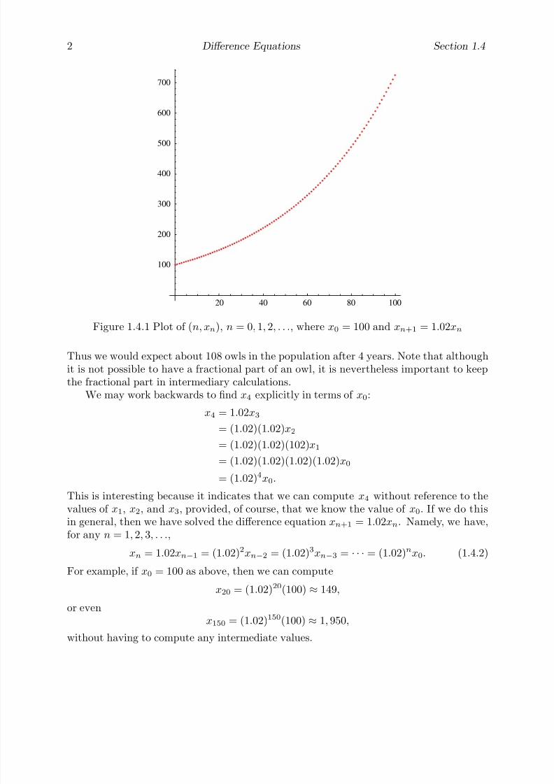
Figure 1.4.1 Plot of (n, xn), n = 0, 1, 2, . . ., where x0 = 100 and xn+1 = 1.02xn
Thus we would expect about 108 owls in the population after 4 years. Note that althoughit is not possible to have a fractional part of an owl, it is nevertheless important to keepthe fractional part in intermediary calculations.
We may work backwards to find x4 explicitly in terms of x0:
x4 = 1.02x3
= (1.02)(1.02)x2
= (1.02)(1.02)(102)x1
= (1.02)(1.02)(1.02)(1.02)x0
= (1.02)4x0.
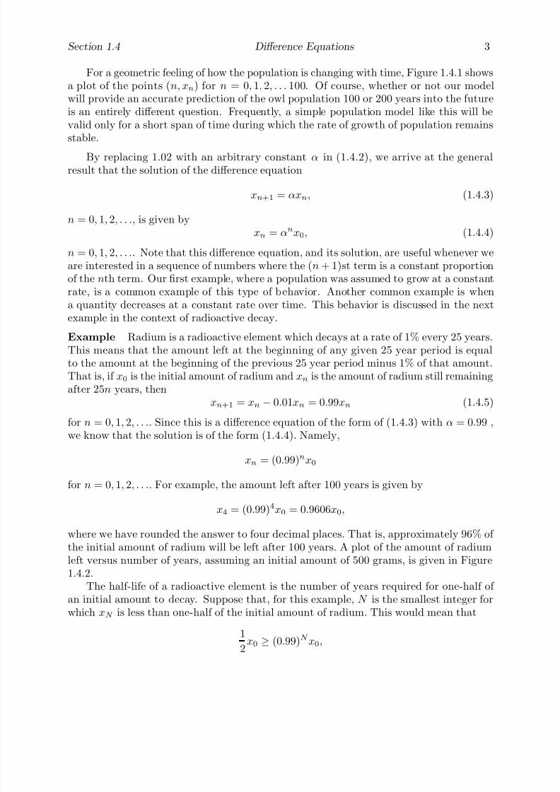
This is interesting because it indicates that we can compute x4 without reference to thevalues of x1, x2, and x3, provided, of course, that we know the value of x0. If we do thisin general, then we have solved the difference equation xn+1 = 1.02xn. Namely, we have,for any n = 1, 2, 3, . . .,
xn = 1.02xn−1 = (1.02)2xn−2 = (1.02)3xn−3 = · · · = (1.02)nx0. (1.4.2)
For example, if x0 = 100 as above, then we can compute
x20 = (1.02)20(100) ≈ 149,
or evenx150 = (1.02)150(100) ≈ 1, 950,
without having to compute any intermediate values.
7/27/2019 Calculus 2 (Dan Sloughter)
http://slidepdf.com/reader/full/calculus-2-dan-sloughter 41/598
Section 1.4 Difference Equations 3
For a geometric feeling of how the population is changing with time, Figure 1.4.1 showsa plot of the points (n, xn) for n = 0, 1, 2, . . . 100. Of course, whether or not our modelwill provide an accurate prediction of the owl population 100 or 200 years into the futureis an entirely different question. Frequently, a simple population model like this will bevalid only for a short span of time during which the rate of growth of population remains
stable.By replacing 1.02 with an arbitrary constant α in (1.4.2), we arrive at the general
result that the solution of the difference equation
xn+1 = αxn, (1.4.3)
n = 0, 1, 2, . . ., is given byxn = αnx0, (1.4.4)
n = 0, 1, 2, . . .. Note that this difference equation, and its solution, are useful whenever weare interested in a sequence of numbers where the (n + 1)st term is a constant proportion
of the nth term. Our first example, where a population was assumed to grow at a constantrate, is a common example of this type of behavior. Another common example is whena quantity decreases at a constant rate over time. This behavior is discussed in the nextexample in the context of radioactive decay.
Example Radium is a radioactive element which decays at a rate of 1% every 25 years.This means that the amount left at the beginning of any given 25 year period is equalto the amount at the beginning of the previous 25 year period minus 1% of that amount.That is, if x0 is the initial amount of radium and xn is the amount of radium still remainingafter 25n years, then
xn+1 = xn − 0.01xn = 0.99xn (1.4.5)
for n = 0, 1, 2, . . .. Since this is a difference equation of the form of (1.4.3) with α = 0.99 ,we know that the solution is of the form (1.4.4). Namely,
xn = (0.99)nx0
for n = 0, 1, 2, . . .. For example, the amount left after 100 years is given by
x4 = (0.99)4x0 = 0.9606x0,
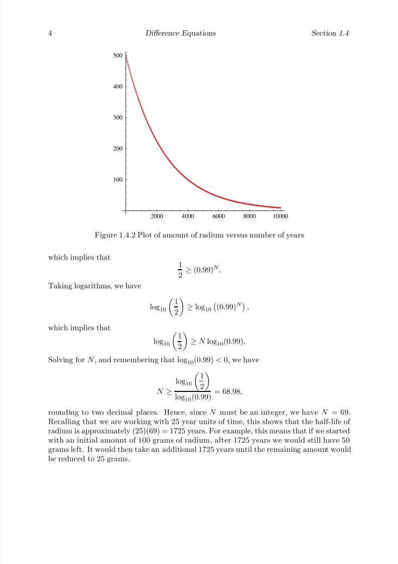
where we have rounded the answer to four decimal places. That is, approximately 96% of the initial amount of radium will be left after 100 years. A plot of the amount of radiumleft versus number of years, assuming an initial amount of 500 grams, is given in Figure1.4.2.
The half-life of a radioactive element is the number of years required for one-half of an initial amount to decay. Suppose that, for this example, N is the smallest integer forwhich xN is less than one-half of the initial amount of radium. This would mean that
1
2x0 ≥ (0.99)N x0,
7/27/2019 Calculus 2 (Dan Sloughter)
http://slidepdf.com/reader/full/calculus-2-dan-sloughter 42/598
4 Difference Equations Section 1.4
2000 4000 6000 8000 10000
100
200
300
400
500
Figure 1.4.2 Plot of amount of radium versus number of years
which implies that1
2≥ (0.99)N .
Taking logarithms, we have
log10
1
2
≥ log10
(0.99)N
,
which implies that
log10
1
2
≥ N log10(0.99).
Solving for N , and remembering that log10(0.99) < 0, we have
N ≥
log10
1
2
log10(0.99) = 68.98,
rounding to two decimal places. Hence, since N must be an integer, we have N = 69.Recalling that we are working with 25 year units of time, this shows that the half-life of radium is approximately (25)(69) = 1725 years. For example, this means that if we startedwith an initial amount of 100 grams of radium, after 1725 years we would still have 50grams left. It would then take an additional 1725 years until the remaining amount wouldbe reduced to 25 grams.
7/27/2019 Calculus 2 (Dan Sloughter)
http://slidepdf.com/reader/full/calculus-2-dan-sloughter 43/598
Section 1.4 Difference Equations 5
Although we have stated the results of the preceding example in discrete time units,namely, units of 25 years each, later we will see that the results hold for continuous timeas well. In other words, although the difference equation (1.4.5) has been set up fornonnegative integer values of n, the solution (1.4.6) is valid for arbitrary nonnegative valuesof n. We will hold off discussion of these ideas until we consider differential equations, the
continuous time versions of difference equations, in Chapter 6.It is interesting to compare the plots in Figures 1.4.1 and 1.4.2. The first is an example
of exponential growth , whereas the second is an example of exponential decay . In the first,the steepness of the graph increases with time; in the second, the graph flattens out overtime. The difference equation (1.4.3) will always lead to the first behavior when α > 1 andto the second when 0 < α < 1.
First-order linear difference equations
Given constants α and β , a difference equation of the form
xn+1 = αxn + β, (1.4.6)
n = 0, 1, 2, . . ., is called a first-order linear difference equation . Note that the differenceequation (1.4.3) is of this form with β = 0. A procedure analogous to the method we usedto solve (1.4.3) will enable us to solve this equation as well. Namely,
xn = αxn−1 + β
= α(αxn−2 + β ) + β
= α2xn−2 + β (α + 1)
= α2(αxn−3 + β ) + β (α + 1)
= α3xn−3 + β (α2 + α + 1)...
= αnx0 + β (αn−1 + αn−2 + · · · + α2 + α + 1).
Note that if α = 1, this gives usxn = x0 + nβ, (1.4.7)
n = 0, 1, 2, . . ., as the solution of the difference equation xn+1 = xn + β . If α = 1, we knowfrom Section 1.3 that
αn−1 + αn−2 + · · · + α2 + α + 1 = 1 − αn
1 − α.
Hence
xn = αnx0 + β
1 − αn
1 − α
, (1.4.8)
n = 0, 1, 2, . . ., is the solution of the first-order linear difference equation xn+1 = αxn + β
when α = 1.
7/27/2019 Calculus 2 (Dan Sloughter)
http://slidepdf.com/reader/full/calculus-2-dan-sloughter 44/598
6 Difference Equations Section 1.4
We have seen examples of first-order linear equations in the population growth andradioactive decay examples above. Another interesting example arises in modeling thechange in temperature of an object placed in an environment held at some constant tem-perature, such as a cup of tea cooling to room temperature or a glass of lemonade warmingto room temperature. If T 0 represents the initial temperature of the object, S the constant
temperature of the surrounding environment, and T n the temperature of the object aftern units of time, then the change in temperature over one unit of time is given by
T n+1 − T n = k(T n − S ), (1.4.9)
n = 0, 1, 2, . . ., where k is a constant which depends upon the object. This difference equa-tion is known as Newton’s law of cooling . The equation says that the change in temperatureover a fixed unit of time is proportional to the difference between the temperature of theobject and the temperature of the surrounding environment. That is, large temperaturedifferences result in a faster rate of cooling (or warming) than do small temperature differ-ences. If S is known and enough information is given to determine k, then this equation
may be rewritten in the form of a first order-linear difference equation and, hence, solvedexplicitly. The next example shows how this may be done.
Example Suppose a cup of tea, initially at a temperature of 180◦F, is placed in a roomwhich is held at a constant temperature of 80◦F. Moreover, suppose that after one minutethe tea has cooled to 175◦F. What will the temperature be after 20 minutes?
If we let T n be the temperature of the tea after n minutes and we let S be the temper-ature of the room, then we have T 0 = 180, T 1 = 175, and S = 80. Newton’s law of coolingstates that
T n+1 − T n = k(T n − 80), (1.4.10)
n = 0, 1, 2, . . ., where k is a constant which we will have to determine. To do so, we make
use of the information given about the change in the temperature of the tea during thefirst minute. Namely, applying (1.4.10) with n = 0, we must have
T 1 − T 0 = k(T 0 − 80).
That is,175 − 180 = k(180 − 80).
Hence−5 = 100k,
and so
k = − 5100
= −0.05.
Thus (1.4.10) becomes
T n+1 − T n = −0.05(T n − 80) = −0.05T n + 4.
HenceT n+1 = T n − 0.05T n + 4 = 0.95T n + 4 (1.4.11)
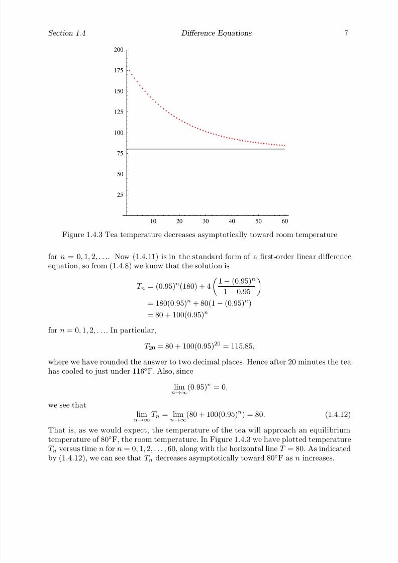
7/27/2019 Calculus 2 (Dan Sloughter)
http://slidepdf.com/reader/full/calculus-2-dan-sloughter 45/598
Section 1.4 Difference Equations 7
10 20 30 40 50 60
25
50
75
100
125
150
175
200
Figure 1.4.3 Tea temperature decreases asymptotically toward room temperature
for n = 0, 1, 2, . . .. Now (1.4.11) is in the standard form of a first-order linear differenceequation, so from (1.4.8) we know that the solution is
T n = (0.95)n(180) + 41 − (0.95)n
1−
0.95 = 180(0.95)n + 80(1 − (0.95)n)
= 80 + 100(0.95)n
for n = 0, 1, 2, . . .. In particular,
T 20 = 80 + 100(0.95)20 = 115.85,
where we have rounded the answer to two decimal places. Hence after 20 minutes the teahas cooled to just under 116◦F. Also, since
limn→∞
(0.95)n = 0,
we see thatlimn→∞
T n = limn→∞
(80 + 100(0.95)n) = 80. (1.4.12)
That is, as we would expect, the temperature of the tea will approach an equilibriumtemperature of 80◦F, the room temperature. In Figure 1.4.3 we have plotted temperatureT n versus time n for n = 0, 1, 2, . . . , 60, along with the horizontal line T = 80. As indicatedby (1.4.12), we can see that T n decreases asymptotically toward 80◦F as n increases.

7/27/2019 Calculus 2 (Dan Sloughter)
http://slidepdf.com/reader/full/calculus-2-dan-sloughter 46/598
8 Difference Equations Section 1.4
Problems
1. Compute the next five terms of each of the following sequences from the given infor-mation.
(a) x0 = 10, xn+1 = xn + 4 (b) y0 = −1, yn+1 = 1yn
(c) x0 = 40, xn+1 = 2xn − 20 (d) z0 = 2, zn+1 = z2n− zn
(e) x0 = 2, x1 = 3, xn+2 = xn+1 + xn (f) x0 = 15, xn =1
3xn−1 + 2
2. Solve the following difference equations with the given initial condition. Use yoursolution to find x10.
(a) xn+1 = 2xn, x0 = 5 (b) xn+1 =3
4xn, x0 = 100
(c)xn+1
= 1.8
xn
+ 10,x0
= 20 (d) 4xn+1 − 2
xn
= 12,x0
= 6(e) xn+1 − xn = 3xn + 4, x0 = 2 (f) 5xn+1 − 3xn = 2xn+1 − xn, x0 = 100
3. A population of weasels is growing at rate of 3% per year. Let wn be the number of weasels n years from now and suppose that there are currently 350 weasels.
(a) Write a difference equation which describes how the population changes from yearto year.
(b) Solve the difference equation of part (a). If the population growth continues at therate of 3%, how many weasels will there be 15 years from now?
(c) Plot wn versus n for n = 0, 1, 2, . . . , 100.
(d) How many years will it take for the population to double?
(e) Find limn→∞
wn. What does this say about the long-term size of the population?
Will this really happen?
4. If the rate of growth of the weasel population in Problem 3 was 5% instead of 3%, howmany years would it take for the population to double?
5. Suppose that the weasel population of Problem 3 would grow at a rate of 3% a year if left to itself, but poachers kill 6 weasels every year for their fur.
(a) Write a difference equation which describes how the population changes from year
to year.
(b) Solve the difference equation of part (a). How many weasels will there be in 15years?
(c) Find limn→∞
wn. What does this say about the long-term size of the population?
(d) Will the population eventually double? If so, how long will this take?
(e) Plot wn versus n for n = 0, 1, 2, . . . , 100.
7/27/2019 Calculus 2 (Dan Sloughter)
http://slidepdf.com/reader/full/calculus-2-dan-sloughter 47/598
Section 1.4 Difference Equations 9
6. Suppose that the weasel population of Problem 3 would grow at a rate of 3% a year if left to itself, but poachers kill 15 weasels every year for their fur.
(a) Write a difference equation which describes how the population changes from yearto year.
(b) Solve the difference equation of part (a). How many weasels will there be in 15years?
(c) Find limn→∞
wn. What does this say about the long-term size of the population?
(d) Will the population eventually double? If so, how long will this take
(e) Will the population eventually die out? If so, how long will this take?
(f) Plot wn versus n for n = 0, 1, 2, . . . , 100.
7. A radioactive element is known to decay at the rate of 2% every 20 years.
(a) If initially you had 165 grams of this element, how much would you have in 60years?
(b) What is the half-life of this element?(c) Suppose that the bones of a certain animal maintain a constant level of this element
while the animal is living, but the element begins to decay as soon as the animaldies. If a bone of this animal is found and is determined to have only 10% of itsoriginal level of this element, how old is the bone?
8. Repeat Problem 7 if the element decays at the rate of 3% every 10 years.
9. A cup of coffee has an initial temperature of 165◦F, but cools to 155◦F in one minutewhen placed in a room with a temperature of 70◦F. Let T n be the temperature of thecoffee after n minutes.
(a) Write a difference equation, in standard first order linear form, which describes thechange in temperature of the coffee from minute to minute.
(b) Solve the difference equation from part (a).
(c) Find the temperature of the coffee after 25 minutes.
(d) Find limn→∞
T n.
(e) Plot T n versus n for n = 0, 1, 2, . . . 120.
(f) Does the temperature ever reach 70◦F?
10. A glass of lemonade, initially at a temperature of 42◦F, is placed in a room witha temperature of 78◦F. If the lemonade warms to 45◦F in 30 seconds, what will its
temperature be in 10 minutes?11. An iron ingot, heated to a temperature of 300◦C, is placed in a liquid bath held at a
constant temperature of 90◦C. If the ingot cools to 250◦C in two minutes, what willits temperature be in 20 minutes?
12. A glass of ginger ale is left in a room. Initially, the ginger ale has a temperatureof 45◦F, but after one minute the temperature has increased to 50◦F and after twominutes it has increased to 54◦F. What is the temperature of the room?

7/27/2019 Calculus 2 (Dan Sloughter)
http://slidepdf.com/reader/full/calculus-2-dan-sloughter 48/598
10 Difference Equations Section 1.4
13. In his book Liber Abaci (Book of the Abacus ), Leonardo of Pisa, also know as Fibonacci,posed the following question: How many pairs of rabbits will be produced in a year,beginning with a single pair, if in every month each pair bears a new pair whichbecomes productive from the second month on? (See A History of Mathematics byCarl B. Boyer, Princeton University Press, 1985, page 281).
(a) Let f n be the number of pairs of rabbits in the nth month. Explain why f 1 = 1and f 2 = 1.
(b) Explain why f n+2 = f n+1 + f n for n = 1, 2, 3, . . ..
(c) Compute f n for n = 3, 4, 5, 6, 7, 8 by hand.
(d) Compute f n for n = 1, 2, 3, . . . , 100.
(e) What is limn→∞
f n?
(f) Compute
rn =f n
f n+1
for n = 1, 2, 3, . . . , 100. Do you think limn→∞
rn exists? If so, what is a good approx-
imation for this limit to five decimal places?
(g) Show that
rn+1 =1
1 + rn.
(h) Using (g) and assuming that limn→∞
rn exists, show that
limn→∞
rn =
√ 5 − 1
2,
the golden section ratio.
14. Given x0 = 0 and x10 = 20, show that xn = 2n satisfies the difference equation
xn =xn−1 + xn+1
2
for n = 1, 2, 3, . . . , 9. This difference equation is a discrete model for the equilib-rium heat distribution along a a straight piece of wire running from 0 to 10 with thetemperature at 0 held at 0◦ and the temperature at 10 held at 20◦.
15. How would the solution to Problem 14 change if we changed the boundary conditionsto x0 = 10 and x10 = 50?
16. An approximate solution of a two-dimensional version of the model in Problem 14 maybe found using a spreadsheet. For example, you might set cells A1-A20 and H1-H20equal to 10 and cells B1-G1 and B20-G20 equal to 0. This would represent a flatrectangular piece of metal with the temperature along the vertical sides held fixed at10◦ and the temperature along the horizontal sides held fixed at 0◦. Now set the valueof every cell inside the rectangle to be equal to the average of the values of its four

7/27/2019 Calculus 2 (Dan Sloughter)
http://slidepdf.com/reader/full/calculus-2-dan-sloughter 49/598
Section 1.4 Difference Equations 11
neighboring cells. For example, you would put the formula (A2+C2+B1+B3)/4 in cellB2 and then copy this cell to all the cells in the block from B2 to G19. Now havethe spreadsheet repeatedly compute the values of the cells until they stabilize (thatis, until they no longer change values when you recompute). If you format the cellvalues so that they are all integers, this should not take too long. What you have now
is the equilibrium heat distribution for the metal plate. Now try different boundaryconditions to obtain different equilibrium heat distributions.
7/27/2019 Calculus 2 (Dan Sloughter)
http://slidepdf.com/reader/full/calculus-2-dan-sloughter 50/598
Difference Equations
Differential Equations
to
Section 1.5
Nonlinear Difference Equations
In Section 1.4 we discussed the difference equation
xn+1 = αxn, (1.5.1)
n = 0, 1, 2, . . ., as a model for either growth or decay and we saw that its solution is givenby
xn = αnx0,
n = 0, 1, 2, . . .. Now
limn→∞
αn =
0, 0 < α < 1,1, α = 1,∞, α > 1,
(1.5.2)
from which it follows that if {xn} is a solution of (1.5.1) with x0 > 0, then
limn→∞
xn = x0 limn→∞
αn =
0, 0 < α < 1,x0, α = 1,∞, α > 1.
(1.5.3)
These limiting values are consistent with our radioactive decay example since, in that case,
0 < α < 1 and we would expect the amount of a radioactive element to decline toward0 over time. The case 0 < α < 1 also may make sense for a population model if thepopulation is declining and heading toward extinction. However, the unbounded growthindefinitely into the future implied by the case α > 1 is very unlikely for a populationmodel: eventually ecological or even sociological problems come to the forefront, such aswhen the population begins to overreach the resources available to it, and the rate of growth of the population changes. Even for bacteria growing in a Petri dish, diminishingfood and space eventually cause a change in the rate of growth. Hence the equation
xn+1 = αxn, (1.5.4)
for n = 0, 1, 2, . . . and α > 1, called the uninhibited , or natural , growth model , althoughoften accurate as a model of population growth over short periods of time, is usually toosimplistic for predictions over long time spans.
The inhibited growth model
Suppose we wish to model the growth of a certain population which, without ecologicalconstraints, would grow at a rate of 100β % per unit of time. That is, if xn represents the
1 Copyright c by Dan Sloughter 2000

7/27/2019 Calculus 2 (Dan Sloughter)
http://slidepdf.com/reader/full/calculus-2-dan-sloughter 51/598
2 Nonlinear Difference Equations Section 1.5
size of the population after n units of time and there are no constraints on the size of thepopulation, then
xn+1 − xn = βxn (1.5.5)
for n = 0, 1, 2, . . .. However, suppose that, because of the limitation of resources, thepopulation will begin to decline if it ever has more than M individuals. We call M thecarrying capacity of the available resources, the maximum population which is sustainableover time. Then it would be reasonable to modify our model by forcing the amount of increase over a unit of time to decrease as the size of the population approaches M andto become negative if the size of the population ever exceeds M . One way to accomplishthis is to multiply the term βxn in (1.5.5) by
M − xn
M ,
a ratio which is close to 1 when xn is small, close to 0 when xn is close to M , and negativewhen xn exceeds M . This leads us to the difference equation
xn+1 − xn = βxn
M − xn
M
,
n = 0, 1, 2, . . ., or, equivalently,
xn+1 = xn +β
M xn(M − xn), (1.5.6)
n = 0, 1, 2, . . ., which we call the inhibited growth model , also known as the discrete logistic
equation . This is an example of a nonlinear difference equation because if we multiply
out the right-hand side of the equation we have a quadratic term, namely,β
M x2
n. Suchequations are, in general, far more difficult to solve than the linear difference equationswe considered in Section 1.4; in fact, many nonlinear difference equations are not solvablein terms of the elementary functions of calculus. Hence we will not consider any methodsfor solving such equations, relying instead on computing specific solutions by iterating theequation using a calculator or, preferably, a computer.
Example Suppose a population of owls, currently numbering 100, has a natural growthrate of 4%, but, because of the limited resources of their natural habitat, can sustain apopulation of no more than 500. If we let xn represent the size of the population n yearsfrom now, then, using the inhibited growth model, we should have
xn+1 = xn + 0.04500
xn(500− xn) = xn + 0.00008xn(500− xn)
for n = 0, 1, 2, . . .. Using this equation we are able to compute, for example, the predictedsize of the population for the next 10 years:
Year 0 1 2 3 4 5 6 7 8 9 10Population 100.0 103.2 106.5 109.8 113.3 116.8 120.3 124.0 127.8 131.5 135.4
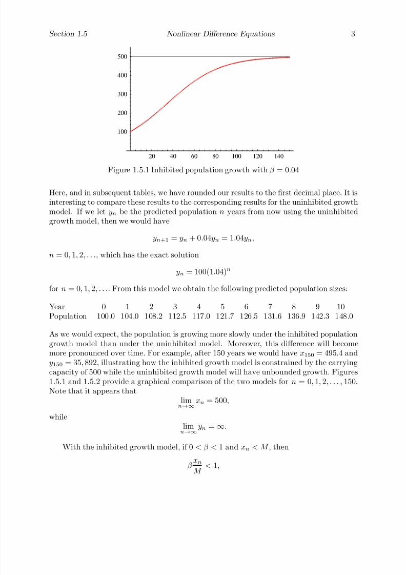
7/27/2019 Calculus 2 (Dan Sloughter)
http://slidepdf.com/reader/full/calculus-2-dan-sloughter 52/598
Section 1.5 Nonlinear Difference Equations 3
20 40 60 80 100 120 140
100
200
300
400
500
Figure 1.5.1 Inhibited population growth with β = 0.04
Here, and in subsequent tables, we have rounded our results to the first decimal place. It is
interesting to compare these results to the corresponding results for the uninhibited growthmodel. If we let yn be the predicted population n years from now using the uninhibitedgrowth model, then we would have
yn+1 = yn + 0.04yn = 1.04yn,
n = 0, 1, 2, . . ., which has the exact solution
yn = 100(1.04)n
for n = 0, 1, 2, . . .. From this model we obtain the following predicted population sizes:
Year 0 1 2 3 4 5 6 7 8 9 10Population 100.0 104.0 108.2 112.5 117.0 121.7 126.5 131.6 136.9 142.3 148.0
As we would expect, the population is growing more slowly under the inhibited populationgrowth model than under the uninhibited model. Moreover, this difference will becomemore pronounced over time. For example, after 150 years we would have x150 = 495.4 andy150 = 35, 892, illustrating how the inhibited growth model is constrained by the carryingcapacity of 500 while the uninhibited growth model will have unbounded growth. Figures1.5.1 and 1.5.2 provide a graphical comparison of the two models for n = 0, 1, 2, . . . , 150.Note that it appears that
limn→∞xn = 500,
whilelimn→∞
yn = ∞.
With the inhibited growth model, if 0 < β < 1 and xn < M , then
β xn
M < 1,

7/27/2019 Calculus 2 (Dan Sloughter)
http://slidepdf.com/reader/full/calculus-2-dan-sloughter 53/598
4 Nonlinear Difference Equations Section 1.5
20 40 60 80 100 120 140
5000
10000
15000
20000
25000
30000
35000
Figure 1.5.2 Uninhibited population growth with β = 0.04
so
xn+1 = xn + β xnM
(M − xn) < xn + (M − xn) = M (1.5.7)
for n = 0, 1, 2, . . .. Thus if 0 < β < 1, and we start with x0 < M , then xn < M for all n.Moreover, since
β xn
M > 0,
we have
xn+1 = xn + β xn
M (M − xn) > xn
for all n. Hence the sequence
{xn
}is monotone increasing and bounded, and so must have
a limit. In Problem 8 you will be asked to verify that this limit is in fact M , as appearedto be the case in the previous example.
If β > 1, it may be the case that there are values of n for which xn > M , in which case
β xn
M (M − xn) < 0
and, as a consequence, xn+1 < xn.
Example Suppose x0 = 100 and M = 500 as in the previous example, but now letβ = 1.5. That is,
xn+1 = xn +1.5
500xn(M − xn) = xn + 0.003xn(500− xn)
for n = 0, 1, 2, . . .. This equation generates the following values:
Year 0 1 2 3 4 5 6 7 8 9 10Population 100.0 220.0 404.8 520.4 448.5 505.3 497.2 501.4 499.3 500.3 499.8
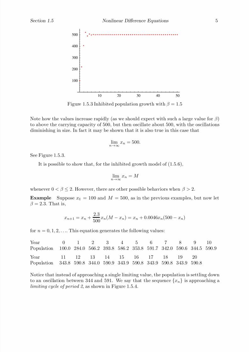
7/27/2019 Calculus 2 (Dan Sloughter)
http://slidepdf.com/reader/full/calculus-2-dan-sloughter 54/598
Section 1.5 Nonlinear Difference Equations 5
10 20 30 40 50
100
200
300
400
500
Figure 1.5.3 Inhibited population growth with β = 1.5
Note how the values increase rapidly (as we should expect with such a large value for β )
to above the carrying capacity of 500, but then oscillate about 500, with the oscillationsdiminishing in size. In fact it may be shown that it is also true in this case that
limn→∞
xn = 500.
See Figure 1.5.3.
It is possible to show that, for the inhibited growth model of (1.5.6),
limn→∞
xn = M
whenever 0 < β ≤ 2. However, there are other possible behaviors when β > 2.
Example Suppose x0 = 100 and M = 500, as in the previous examples, but now letβ = 2.3. That is,
xn+1 = xn +2.3
500xn(M − xn) = xn + 0.0046xn(500− xn)
for n = 0, 1, 2, . . .. This equation generates the following values:
Year 0 1 2 3 4 5 6 7 8 9 10
Population 100.0 284.0 566.2 393.8 586.2 353.8 591.7 342.0 590.6 344.5 590.9
Year 11 12 13 14 15 16 17 18 19 20Population 343.8 590.8 344.0 590.9 343.9 590.8 343.9 590.8 343.9 590.8
Notice that instead of approaching a single limiting value, the population is settling downto an oscillation between 344 and 591. We say that the sequence {xn} is approaching alimiting cycle of period 2 , as shown in Figure 1.5.4.
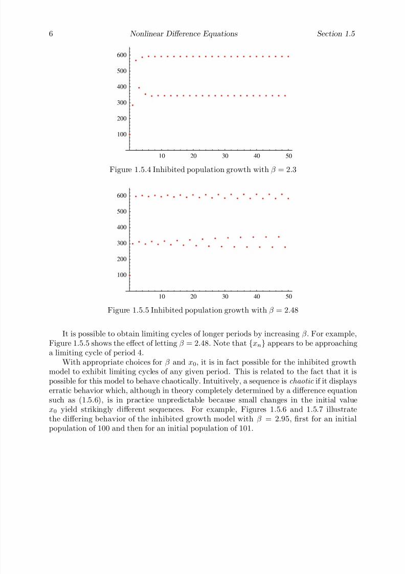
7/27/2019 Calculus 2 (Dan Sloughter)
http://slidepdf.com/reader/full/calculus-2-dan-sloughter 55/598
6 Nonlinear Difference Equations Section 1.5
10 20 30 40 50
100
200
300
400
500
600
Figure 1.5.4 Inhibited population growth with β = 2.3
10 20 30 40 50
100
200
300
400
500
600
Figure 1.5.5 Inhibited population growth with β = 2.48
It is possible to obtain limiting cycles of longer periods by increasing β . For example,Figure 1.5.5 shows the effect of letting β = 2.48. Note that {xn} appears to be approachinga limiting cycle of period 4.
With appropriate choices for β and x0, it is in fact possible for the inhibited growthmodel to exhibit limiting cycles of any given period. This is related to the fact that it ispossible for this model to behave chaotically. Intuitively, a sequence is chaotic if it displayserratic behavior which, although in theory completely determined by a difference equation
such as (1.5.6), is in practice unpredictable because small changes in the initial valuex0 yield strikingly different sequences. For example, Figures 1.5.6 and 1.5.7 illustratethe differing behavior of the inhibited growth model with β = 2.95, first for an initialpopulation of 100 and then for an initial population of 101.
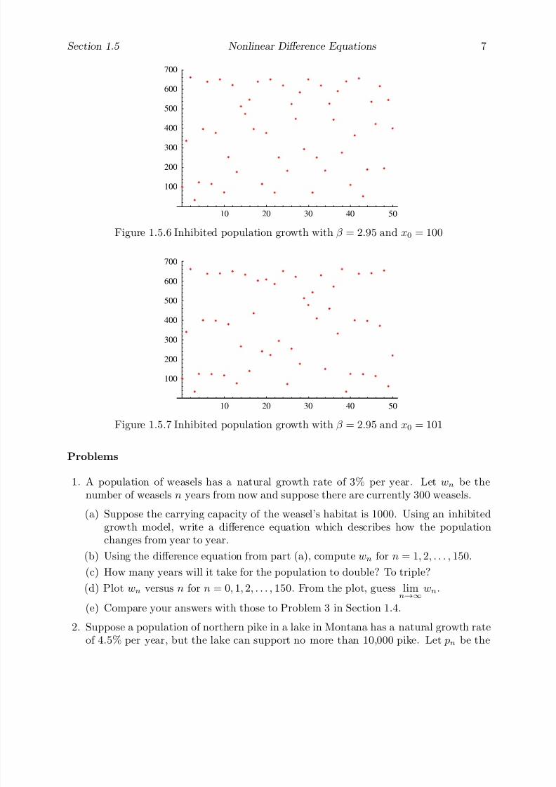
7/27/2019 Calculus 2 (Dan Sloughter)
http://slidepdf.com/reader/full/calculus-2-dan-sloughter 56/598
Section 1.5 Nonlinear Difference Equations 7
10 20 30 40 50
100
200
300
400
500
600
700
Figure 1.5.6 Inhibited population growth with β = 2.95 and x0 = 100
10 20 30 40 50
100
200
300
400
500
600
700
Figure 1.5.7 Inhibited population growth with β = 2.95 and x0 = 101
Problems
1. A population of weasels has a natural growth rate of 3% per year. Let wn be thenumber of weasels n years from now and suppose there are currently 300 weasels.
(a) Suppose the carrying capacity of the weasel’s habitat is 1000. Using an inhibitedgrowth model, write a difference equation which describes how the populationchanges from year to year.
(b) Using the difference equation from part (a), compute wn for n = 1, 2, . . . , 150.
(c) How many years will it take for the population to double? To triple?
(d) Plot wn versus n for n = 0, 1, 2, . . . , 150. From the plot, guess limn→∞
wn.
(e) Compare your answers with those to Problem 3 in Section 1.4.
2. Suppose a population of northern pike in a lake in Montana has a natural growth rateof 4.5% per year, but the lake can support no more than 10,000 pike. Let pn be the
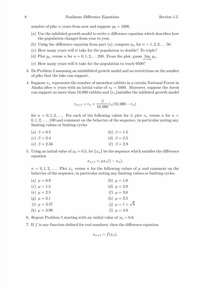
7/27/2019 Calculus 2 (Dan Sloughter)
http://slidepdf.com/reader/full/calculus-2-dan-sloughter 57/598
8 Nonlinear Difference Equations Section 1.5
number of pike n years from now and suppose p0 = 1000.
(a) Use the inhibited growth model to write a difference equation which describes howthe population changes from year to year.
(b) Using the difference equation from part (a), compute pn for n = 1, 2, 3, . . . 50.
(c) How many years will it take for the population to double? To triple?(d) Plot pn versus n for n = 0, 1, 2, . . . 200. From the plot, guess lim
n→∞ pn.
(e) How many years will it take for the population to reach 9500?
3. Do Problem 2 assuming an uninhibited growth model and no restrictions on the numberof pike that the lake can support.
4. Suppose rn represents the number of snowshoe rabbits in a certain National Forest inAlaska after n years with an initial value of r0 = 5000. Moreover, suppose the forestcan support no more than 10,000 rabbits and {rn}satisfies the inhibited growth model
rn+1 = rn + β 10, 000
rn(10, 000− rn)
for n = 0, 1, 2, . . .. For each of the following values for β , plot rn versus n for n =0, 1, 2, . . . , 100 and comment on the behavior of the sequence, in particular noting anylimiting values or limiting cycles
(a) β = 0.5 (b) β = 1.5
(c) β = 2.4 (d) β = 2.5
(e) β = 2.56 (f) β = 2.9
5. Using an initial value of x0 = 0.5, let {xn} be the sequence which satisfies the differenceequation
xn+1 = µxn(1− xn),
n = 0, 1, 2, . . .. Plot xn versus n for the following values of µ and comment on thebehavior of the sequence, in particular noting any limiting values or limiting cycles.
(a) µ = 0.9 (b) µ = 1.0
(c) µ = 1.5 (d) µ = 2.0
(e) µ = 2.5 (f) µ = 3.0
(g) µ = 3.1 (h) µ = 3.5
(i) µ = 3.57 (j) µ = 1 + √ 8(k) µ = 3.99 (l) µ = 4.0
6. Repeat Problem 5 starting with an initial value of x0 = 0.6.
7. If f is any function defined for real numbers, then the difference equation
xn+1 = f (xn),

7/27/2019 Calculus 2 (Dan Sloughter)
http://slidepdf.com/reader/full/calculus-2-dan-sloughter 58/598
Section 1.5 Nonlinear Difference Equations 9
n = 0, 1, 2, . . . , is called a discrete dynamical system . For any given initial conditionx0, the sequence {xn} which satisfies this equation is called an orbit of f . Note thatan orbit of f is simply the sequence of points
x0, f (x0), f (f (x0)), f (f (f (x0))), . . . .
For example, the difference equation in Problem 5 is an example of a discrete dynamicalsystem with f (x) = µx(1 − x). For each of the following, compute 50 terms of thegiven orbit and discuss its behavior.
(a) x0 = 10, f (x) = 2x (b) x0 = 100, f (x) = 0.8x
(c) x0 = 2 f (x) = cos(x) (d) x0 = 2, f (x) = sin(x)
(e) x0 = 5, f (x) =1
2
x +
2
x
(f) x0 = 1, f (x) =
2x2
3x2 − 5
(g) x0 = 0, f (x) = x2 + 1.0 (h) x0 = 0, f (x) = x2 − 0.5
(i) x0 = 0, f (x) = x2
− 0.8 (j) x0 = 0, f (x) = x2
− 1.0(k) x0 = 0, f (x) = x2 − 1.9 (l) x0 = 0, f (x) = x2 − 2.0
8. Assuming that the sequence {xn} satisfying the inhibited growth model equation
xn+1 = xn +β
M xn(M − xn)
has a limit, show that limn→∞
xn = M .

7/27/2019 Calculus 2 (Dan Sloughter)
http://slidepdf.com/reader/full/calculus-2-dan-sloughter 59/598
Difference Equations
Differential Equations
to
Section 2.1
Functions And Their Graphs
Since functions are the basic building blocks out of which mathematicians construct modelsof the physical world, it is essential that any student of mathematics have a firm grasp of the concept. In particular, one must be careful to distinguish between a given function anda notational or graphical representation for it. A function is a type of relationship, a mentalconcept that cannot be seen or touched. Although pictures and symbolic representationsof a function are extremely important in understanding its behavior, the student mustalways keep in mind the distinction between the function itself and its representations.
Modern methods for giving a formal definition of a function, developed in the latterpart of the 19th century, are based on set-theoretic ideas. We will not go into the detailsnecessary to make such a precise definition, but rather aim at an intuitive understandingof the basic concept. For us, a function is a special type of relationship between twoquantities. We often think of this relationship to be one of dependence. That is, if thevalue of one quantity, say y, is determined by the value of another quantity, say x, then wesay that y is a function of x. For example, if x represents the height from which a certainrock is dropped and y represents the velocity with which the rock strikes the ground, thenthe value of y will depend on the value of x and we say that velocity y is a function of heightx. Note here that if y is the terminal velocity of the object, then there are many differentvalues of x which yield the same value of y, namely, any value of x which gives the object
sufficient time to reach its terminal velocity before striking the ground. On the other hand,for a given value of x, there is only one related value of y. It is this latter property thatmakes the relationship between height and impact velocity a function. For any quantitiesrepresented by y and x, in order to say that y is a function of x we require that everyvalue of x be related to exactly one value of y. Such a relationship often arises throughsome physical dependency, a cause creating a deterministic effect, but the definition doesnot require such a link between the quantities in question. A number of examples shouldhelp clarify this concept.
Example Sequences are example of functions. That is, if {xn} is a sequence with n =1, 2, 3, . . ., then every value of n determines exactly one value xn. For example, the area
of a regular polygon inscribed in a unit circle is a function of the number of sides. Also, adifference equation, such asxn+1 = 1.02xn,
n = 0, 1, 2, . . ., makes xn a function of n. For example, the size of a certain population of owls will be a function of the number of years from some starting date.
Example The area of a circle is a function of the radius of the circle.
Example The distance of the earth from the sun is a function of the time of year.
1 Copyright c by Dan Sloughter 2000

7/27/2019 Calculus 2 (Dan Sloughter)
http://slidepdf.com/reader/full/calculus-2-dan-sloughter 60/598
2 Functions And Their Graphs Section 2.1
Example The temperature at a certain fixed point in space is a function of time.
In mathematical terminology, if y is a function of x, then we call x the independent
variable and y the dependent variable . Also, the domain of this function is the set of permissible values for x and the range is the set of all values of y which correspond to somevalue of x.
Example Recall that the nth term of the sequence which gives the area of a regularn-sided polygon inscribed in a unit circle is
An =n
2sin
2π
n
,
n = 3, 4, 5, . . . The domain of this function is the set of integers {3, 4, 5, . . .}. The rangecan be specified only by saying that it is the set of numbers
n
2sin
2π
n
n = 3, 4, 5, . . .
.
Before proceeding further, we should recall the notation for intervals of real numbers.Given any real numbers a and b, we have
(a, b) = {x | a < x < b}, (2.1.1)
(a, b] = {x | a < x ≤ b}, (2.1.2)
[a, b) = {x | a ≤ x < b}, (2.1.3)
[a, b] = {x | a ≤ x ≤ b}, (2.1.4)
(a,∞) = {x | x > a}, (2.1.5)[a,∞) = {x | x ≥ a}, (2.1.6)
(−∞, b) = {x | x < b}, (2.1.7)
and(−∞, b] = {x | x ≤ b}. (2.1.8)
Moreover, we call intervals of the form (2.1.1), (2.1.5), and (2.1.7) open intervals andintervals of the form (2.1.4), (2.1.6), and (2.1.8) closed intervals .
Example If we let d specify the distance from the sun to the earth and t specify thetime of year, then the function that relates d and t has domain
{t | 0 ≤ t ≤ 8760} = [0, 8760],
where t is specified in hours, and range
{d | 91.4 ≤ d ≤ 94.6} = [91.4, 94.6],
where d is specified in millions of miles.
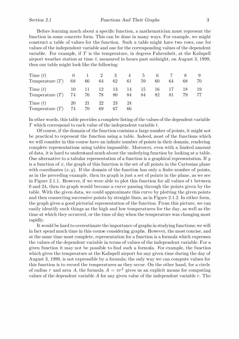
7/27/2019 Calculus 2 (Dan Sloughter)
http://slidepdf.com/reader/full/calculus-2-dan-sloughter 61/598
Section 2.1 Functions And Their Graphs 3
Before learning much about a specific function, a mathematician must represent thefunction in some concrete form. This can be done in many ways. For example, we mightconstruct a table of values for the function. Such a table might have two rows, one forvalues of the independent variable and one for the corresponding values of the dependentvariable. For example, if T is the temperature, in degrees Fahrenheit, at the Kalispell
airport weather station at time t, measured in hours past midnight, on August 3, 1999,then our table might look like the following:
Time (t) 0 1 2 3 4 5 6 7 8 9Temperature (T ) 68 66 64 62 61 59 60 64 68 70
Time (t) 10 11 12 13 14 15 16 17 18 19Temperature (T ) 74 76 78 80 84 84 82 81 79 77
Time (t) 20 21 22 23 24Temperature (T ) 74 70 69 67 66
In other words, this table provides a complete listing of the values of the dependent variableT which correspond to each value of the independent variable t.
Of course, if the domain of the function contains a large number of points, it might notbe practical to represent the function using a table. Indeed, most of the functions whichwe will consider in this course have an infinite number of points in their domain, renderingcomplete representations using tables impossible. Moreover, even with a limited amountof data, it is hard to understand much about the underlying function by looking at a table.One alternative to a tabular representation of a function is a graphical representation. If y
is a function of x, the graph of this function is the set of all points in the Cartesian planewith coordinates (x, y). If the domain of the function has only a finite number of points,as in the preceding example, then its graph is just a set of points in the plane, as we seein Figure 2.1.1. However, if we were able to plot this function for all values of t between0 and 24, then its graph would become a curve passing through the points given by thetable. With the given data, we could approximate this curve by plotting the given pointsand then connecting successive points by straight lines, as in Figure 2.1.2. In either form,the graph gives a good pictorial representation of the function. From this picture, we caneasily identify such things as the high and low temperatures for the day, as well as thetime at which they occurred, or the time of day when the temperature was changing mostrapidly.
It would be hard to overestimate the importance of graphs in studying functions; we willin fact spend much time in this course considering graphs. However, the most concise, and
at the same time most complete, representation for a function is a formula which expressesthe values of the dependent variable in terms of values of the independent variable. For agiven function it may not be possible to find such a formula. For example, the functionwhich gives the temperature at the Kalispell airport for any given time during the day of August 3, 1999, is not expressible by a formula; the only way we can compute values forthis function is to record the temperatures as they occur. On the other hand, for a circleof radius r and area A, the formula A = πr2 gives us an explicit means for computingvalues of the dependent variable A for any given value of the independent variable r. The
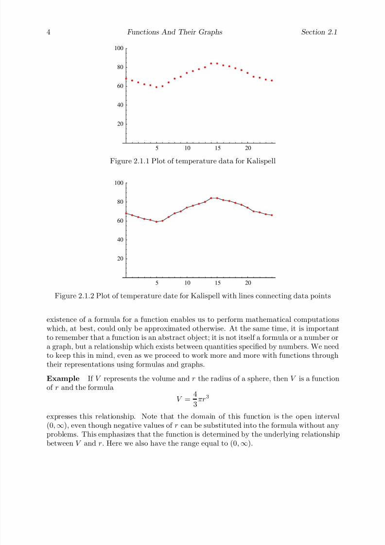
7/27/2019 Calculus 2 (Dan Sloughter)
http://slidepdf.com/reader/full/calculus-2-dan-sloughter 62/598
4 Functions And Their Graphs Section 2.1
5 10 15 20
20
40
60
80
100
Figure 2.1.1 Plot of temperature data for Kalispell
5 10 15 20
20
40
60
80
100
Figure 2.1.2 Plot of temperature date for Kalispell with lines connecting data points
existence of a formula for a function enables us to perform mathematical computationswhich, at best, could only be approximated otherwise. At the same time, it is importantto remember that a function is an abstract object; it is not itself a formula or a number ora graph, but a relationship which exists between quantities specified by numbers. We needto keep this in mind, even as we proceed to work more and more with functions throughtheir representations using formulas and graphs.
Example If V represents the volume and r the radius of a sphere, then V is a functionof r and the formula
V =4
3πr3
expresses this relationship. Note that the domain of this function is the open interval(0,∞), even though negative values of r can be substituted into the formula without anyproblems. This emphasizes that the function is determined by the underlying relationshipbetween V and r. Here we also have the range equal to (0,∞).
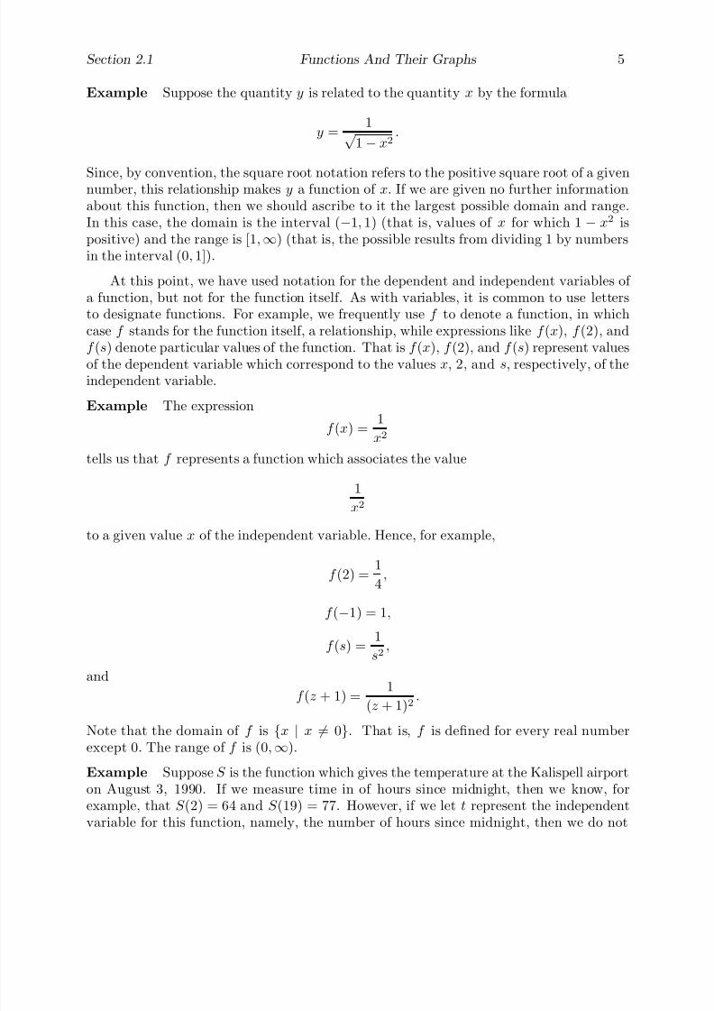
7/27/2019 Calculus 2 (Dan Sloughter)
http://slidepdf.com/reader/full/calculus-2-dan-sloughter 63/598
Section 2.1 Functions And Their Graphs 5
Example Suppose the quantity y is related to the quantity x by the formula
y =1√
1 − x2.
Since, by convention, the square root notation refers to the positive square root of a givennumber, this relationship makes y a function of x. If we are given no further informationabout this function, then we should ascribe to it the largest possible domain and range.In this case, the domain is the interval (−1, 1) (that is, values of x for which 1 − x2 ispositive) and the range is [1,∞) (that is, the possible results from dividing 1 by numbersin the interval (0, 1]).
At this point, we have used notation for the dependent and independent variables of a function, but not for the function itself. As with variables, it is common to use lettersto designate functions. For example, we frequently use f to denote a function, in whichcase f stands for the function itself, a relationship, while expressions like f (x), f (2), and
f (s) denote particular values of the function. That is f (x), f (2), and f (s) represent valuesof the dependent variable which correspond to the values x, 2, and s, respectively, of theindependent variable.
Example The expression
f (x) =1
x2
tells us that f represents a function which associates the value
1
x2
to a given value x of the independent variable. Hence, for example,
f (2) =1
4,
f (−1) = 1,
f (s) =1
s2,
and
f (z + 1) =1
(z + 1)2
.
Note that the domain of f is {x | x = 0}. That is, f is defined for every real numberexcept 0. The range of f is (0,∞).
Example Suppose S is the function which gives the temperature at the Kalispell airporton August 3, 1990. If we measure time in of hours since midnight, then we know, forexample, that S (2) = 64 and S (19) = 77. However, if we let t represent the independentvariable for this function, namely, the number of hours since midnight, then we do not

7/27/2019 Calculus 2 (Dan Sloughter)
http://slidepdf.com/reader/full/calculus-2-dan-sloughter 64/598
6 Functions And Their Graphs Section 2.1
have a general formula to express S (t). For example, we cannot compute S (7.5) or S (3.2),let alone even consider what S (π) might be.
It often happens that the output from one function is used as input for another function.For example, suppose a pebble is dropped in a pond and the resulting circular wave has aradius of 20t centimeters after t seconds. Then if r is the radius of the wave and A is thearea inside the wave, we have r = 20t and A = πr2. But the area inside the wave is also afunction of time, which may be expressed as
A = π(20t)2 = 400πt2.
That is, the area of the circle is a function of the radius, which in turn is a function of time.The function that we arrive at, namely, A as a function of t, is called the composition of the two original functions. In the notation which uses letters to denote functions, we havethe following definition.
Definition If f and g are two functions, then the composition of f and g is the functionf ◦ g whose value at x is given by
f ◦ g(x) = f (g(x)). (2.1.9)
Example If f (x) =√
x and g(x) = x2 + 1, then
f ◦ g(x) = f (g(x)) = f (x2 + 1) =
x2 + 1
andg◦
f (x) = g(f (x)) = g(√
x) = x + 1.
Note that f ◦ g and g ◦ f , as in this example, are not usually the same function.
Classes of functions
The simplest type of functions are those which involve only multiplication and addition.In particular, functions of the form
p(x) = anxn + an−1xn−1 + · · · + a1x + a0, (2.1.10)
where a0, a1, . . . , an are constants and n is a nonnegative integer, are called polynomials .
If an = 0, the degree of the polynomial is n. For example,
q (x) = 3x2 − 13x + 3,
f (t) = 21t34 + 18t2 − π,
and
g(s) =1
2s3 + s + 12 − 4s5

7/27/2019 Calculus 2 (Dan Sloughter)
http://slidepdf.com/reader/full/calculus-2-dan-sloughter 65/598
Section 2.1 Functions And Their Graphs 7
are polynomials, of degrees 2, 34, and 5, respectively, whereas
h(x) =3
x
is not a polynomial. In a sense polynomials are the building blocks for a large family of important functions in calculus. In this regard, one of the major goals of this text is toshow how polynomials may be used to approximate more complicated functions.
Functions which may be written in the form of a polynomial divided by a polynomialare called rational functions . For example,
f (x) =3x2 − 4x + 1
x4 + 1
and
g(s) =12
s+
1
s2
−3s + 1
are both rational functions, the latter because it may be rewritten as a polynomial dividedby a polynomial if all the terms are put over the common denominator s(s2 − 3s + 1).
The function f (x) =√
x is neither a polynomial nor a rational function because x israised to a power which is not an integer. Functions which permit addition, multiplication,division, and rational numbers for powers are called algebraic functions . Thus, for example,
g(t) = t3
2 + 2t2 − 3
is neither a polynomial nor a rational function, but is an algebraic function. Similarly,
h(s) =
s2 + 3s + 2
is an algebraic function. We should note that every polynomial is also a rational functionand every rational function is also an algebraic function.
Functions which are not algebraic are called transcendental . The trigonometric func-tions are examples of transcendental functions. We shall discuss them in detail in the nextsection.
Graphs of functions
We are now in a position to say more about the graphs of functions. With the notation we
have now, the graph of a function f is the set of all points (x, f (x)) in the plane, where xis in the domain of f . For example, you should recall from previous work that the graphof y = x2 is a parabola opening about the x-axis with its vertex at (0, 0). Also, you shouldrecall the shapes of the graphs of such functions as y = x2, y = x3, y = x4, and y = x5.See Figures 2.1.3, and 2.1.4.
Moreover, given a function f and a constant c, you may recall that the graph of y = f (x) + c is the graph of f shifted c units vertically (upward if c > 0 and downward if c < 0), the graph of y = f (x− c) is the graph of f shifted c units horizontally (to the right

7/27/2019 Calculus 2 (Dan Sloughter)
http://slidepdf.com/reader/full/calculus-2-dan-sloughter 66/598
8 Functions And Their Graphs Section 2.1
-10 -5 5 10
-5
5
10
15
20
-10 -5 5 10
-5
5
10
15
20
Figure 2.1.3 Graphs of y = x2 and y = x4
-10 -5 5 10
-20
-15
-10
-5
5
10
15
20
-10 -5 5 10
-20
-15
-10
-5
5
10
15
20
Figure 2.1.4 Graphs of y = x3 and y = x5
if c > 0 and to the left if c < 0), and the graph of y =−
f (x) is the graph of f reflectedabout the x-axis. Hence, for example, the graph of
y = x2 − 3
is a parabola, opening upward about the x-axis, with its vertex at (0,−3); the graph of
y = (x + 2)2 − 3
is a parabola, opening upward about the line x = −2, with vertex at (−2,−3); and thegraph of
y =
−(x + 2)2 + 3
is a parabola, opening downward about the line x = −2, with vertex at (−2, 3). See Figure2.1.5.
Drawing graphs of functions whose basic shapes are not already known to us can bea difficult problem. If the domain of a function f is finite, then drawing its graph isonly a matter of plotting some points in the plane. However, most of the functions wewill encounter in this course will have domains containing an infinite number of points;drawing the graphs of such functions requires much more than plotting a few points. The

7/27/2019 Calculus 2 (Dan Sloughter)
http://slidepdf.com/reader/full/calculus-2-dan-sloughter 67/598
Section 2.1 Functions And Their Graphs 9
-10 -5 5 10
-10
-5
5
10
-10 -5 5 10
-10
-5
5
10
-10 -5 5 10
-10
-5
5
10
Figure 2.1.5 Graphs of y = x2 − 3, y = (x + 2)2 − 3, and y = −(x + 2)2 + 3
problem is that no matter how many points we plot, we still do not know how the functionis behaving at the other points. For example, if we want to graph a function f on theinterval [0, 1], we might first plot the points
(0, f (0)), (0.1, f (0.1)), (0.2, f (0.2)), . . . , (1.0, f (1.0)).
Next, to guess at the behavior of the function between the plotted points, we might join
successive points by straight lines. Of course, this will only give us an approximation to thetrue curve, the accuracy of which will depend on the actual behavior of the curve betweenthe plotted points, something about which we frequently have very little information. Thisis similar to the problem we had with plotting the graph of a temperature function earlier.However, here we can get help if we have a formula for f ; for in that case we can tryplotting more points, say
(0, f (0)), (0.05, f (0.05)), (0.10, f (0.10)), . . . , (1.00, f (1.00)),
or(0, f (0)), (0.01, f (0.01)), (0.02, f (0.02)), . . . , (1.00, f (1.00)).
If the graph of f is a reasonably smooth curve, we will be able to approximate it as well aswe like by plotting a sufficient number of points. This raises two questions: How do we knowthat we have plotted a sufficient number of points? And, given that a sufficient numberof points will most likely be a large number, how do we actually plot them all? Of course,the latter question is answered by using a computer. In fact, this approach to graphing afunction is unreasonable without access to a computer, or at least a calculator. Computersalso provide help in answering the first question. We start by plotting a reasonable numberof points, say 100 or so. If we have reason to doubt the accuracy of the resulting graph,perhaps because the curve is not as smooth as we expected it to be, we can double thenumber of points and plot it again. Because any computer, and in fact many calculators,
do this type of work rapidly, it is reasonable to plot the same function several times untilwe are comfortable with the picture. In Section 3.9 we will learn how to use some of thetechniques of calculus to better understand the geometry of the graph of a function. Thiswill help us identify whether or not the output from a computer is an accurate depictionof the graph.
Example Figure 2.1.6 compares the results of plotting the points
(0, f (0)), (0.1, f (0.1)), (0.2, f (0.2)), . . . , (1.0, f (1.0))
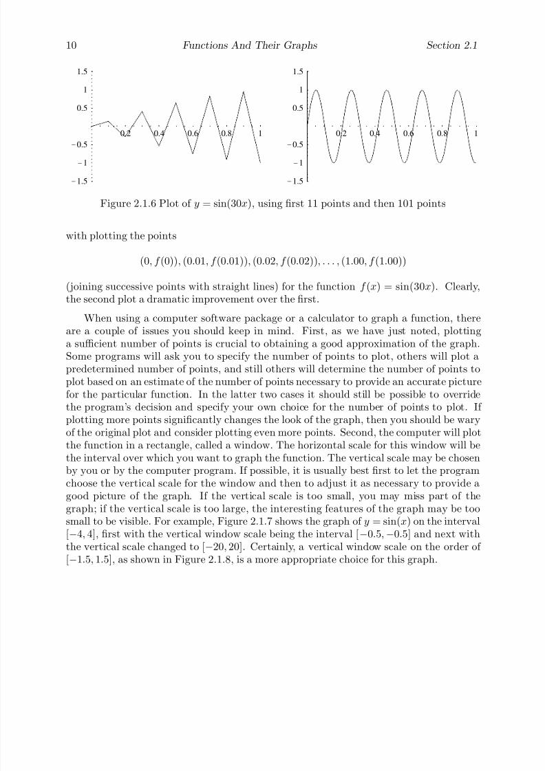
7/27/2019 Calculus 2 (Dan Sloughter)
http://slidepdf.com/reader/full/calculus-2-dan-sloughter 68/598
10 Functions And Their Graphs Section 2.1
0.2 0.4 0.6 0.8 1
-1.5
-1
-0.5
0.5
1
1.5
0.2 0.4 0.6 0.8 1
-1.5
-1
-0.5
0.5
1
1.5
Figure 2.1.6 Plot of y = sin(30x), using first 11 points and then 101 points
with plotting the points
(0, f (0)), (0.01, f (0.01)), (0.02, f (0.02)), . . . , (1.00, f (1.00))
(joining successive points with straight lines) for the function f (x) = sin(30x). Clearly,the second plot a dramatic improvement over the first.
When using a computer software package or a calculator to graph a function, thereare a couple of issues you should keep in mind. First, as we have just noted, plottinga sufficient number of points is crucial to obtaining a good approximation of the graph.Some programs will ask you to specify the number of points to plot, others will plot apredetermined number of points, and still others will determine the number of points toplot based on an estimate of the number of points necessary to provide an accurate picturefor the particular function. In the latter two cases it should still be possible to override
the program’s decision and specify your own choice for the number of points to plot. If plotting more points significantly changes the look of the graph, then you should be waryof the original plot and consider plotting even more points. Second, the computer will plotthe function in a rectangle, called a window. The horizontal scale for this window will bethe interval over which you want to graph the function. The vertical scale may be chosenby you or by the computer program. If possible, it is usually best first to let the programchoose the vertical scale for the window and then to adjust it as necessary to provide agood picture of the graph. If the vertical scale is too small, you may miss part of thegraph; if the vertical scale is too large, the interesting features of the graph may be toosmall to be visible. For example, Figure 2.1.7 shows the graph of y = sin(x) on the interval[−
4, 4], first with the vertical window scale being the interval [−
0.5,−
0.5] and next withthe vertical scale changed to [−20, 20]. Certainly, a vertical window scale on the order of [−1.5, 1.5], as shown in Figure 2.1.8, is a more appropriate choice for this graph.

7/27/2019 Calculus 2 (Dan Sloughter)
http://slidepdf.com/reader/full/calculus-2-dan-sloughter 69/598
Section 2.1 Functions And Their Graphs 11
-4
-2 2 4
-0.4
-0.2
0.2
0.4
-4
-2 2 4
-20
-15
-10
-5
5
10
15
20
Figure 2.1.7 Graph of y = sin(x), first with vertical window [−0.5, 0.5] and then [−20, 20]
-4 -2 2 4
-1.5
-1
-0.5
0.5
1
1.5
Figure 2.1.8 Graph of y = sin(x) with vertical window [−
1.5, 1.5]
Problems
1. In each of the following, x and y denote certain variable quantities. Discuss whether ornot y is a function of x. If y is a function of x, can you write a formula that describesthe relationship? Also, find the domain and range of each function.
(a) x = speed of a train; y = distance the train travels in two hours
(b) x = height above sea level; y = atmospheric pressure
(c) x = time of the year; y = distance from the earth to the moon
(d) x = temperature at the Great Falls airport; y = time of the day
(e) x = length of the side of a square; y = area of the square
(f) x = area of a circle; y = circumference of the circle
(g) x = weight of a letter; y = first class postage for the letter
(h) x = OPEC price for a barrel of oil; y = Dow Jones Industrial Average

7/27/2019 Calculus 2 (Dan Sloughter)
http://slidepdf.com/reader/full/calculus-2-dan-sloughter 70/598
12 Functions And Their Graphs Section 2.1
2. A projectile was shot vertically into the air. The height h of the projectile was measuredat 20 different times t. The following table gives the results, where t is in seconds andh is in meters.
Time (t) 0.00 0.25 0.50 0.75 1.00 1.25 1.50 1.75 2.00 2.25 2.50
Height (h) 0.00 11.6 22.1 31.2 39.2 46.0 51.5 55.7 58.8 60.6 61.3Time (t) 2.75 3.00 3.25 3.50 3.75 4.00 4.25 4.50 4.75 5.00Height (h) 60.6 58.8 55.7 51.5 46.0 39.2 31.2 22.1 11.6 0.00
(a) Graph this data.
(b) Graph this data with lines connecting successive points. Do you think this is areasonable approximation to the graph of h as a function of t?
3. Identify the domain of each of the following functions.
(a) f (x) = x2
−6x (b) g(x) =
√ x2
−9
(c) f (t) = √ t2 + t − 6 (d) h(x) = 3x2 + 6x + 8
(e) f (s) =41
s2 − 9(f) y(t) =
3√ 3 − t2
(g) z(s) =1√
s2 + 6s + 1(h) f (x) =
4
x(x2 + 1)
4. For each of the following pairs of functions, find f ◦g(x), g ◦f (x), f ◦g(3), and f ◦g(3),when they are defined.
(a) f (x) = 4x + 12, g(x) = 5x − 2
(b) f (x) = x2 − 12, g(x) = √ x(c) f (x) = 6x − x2, g(x) =
1
x − 9
5. (a) If the graph of f is a straight line with slope 3 and the graph of g is a straight linewith slope 4, show that the graph of f ◦ g is a straight line with slope 12.
(b) If the graph of f is a straight line with slope m and the graph of g is a straightline with slope n, show that the graph of f ◦ g is a straight line with slope mn.
6. Graph each of the following functions on the given interval.
(a) f (x) = x2 + 6x + 1 on [
−10, 5]
(b) f (x) = x5 + x4 + x3 + x2 + x + 1 on [−5, 5]
(c) f (x) = x5 + 8x4 + x3 + x2 + x + 1 on [−5, 5]
(d) f (x) = x5 + 8x4 + x3 + x2 + x + 1 on [−10, 10]
(e) g(t) =1
1 + t2on [−10, 10]
(f) f (t) =t
1 + t2on [−10, 10]
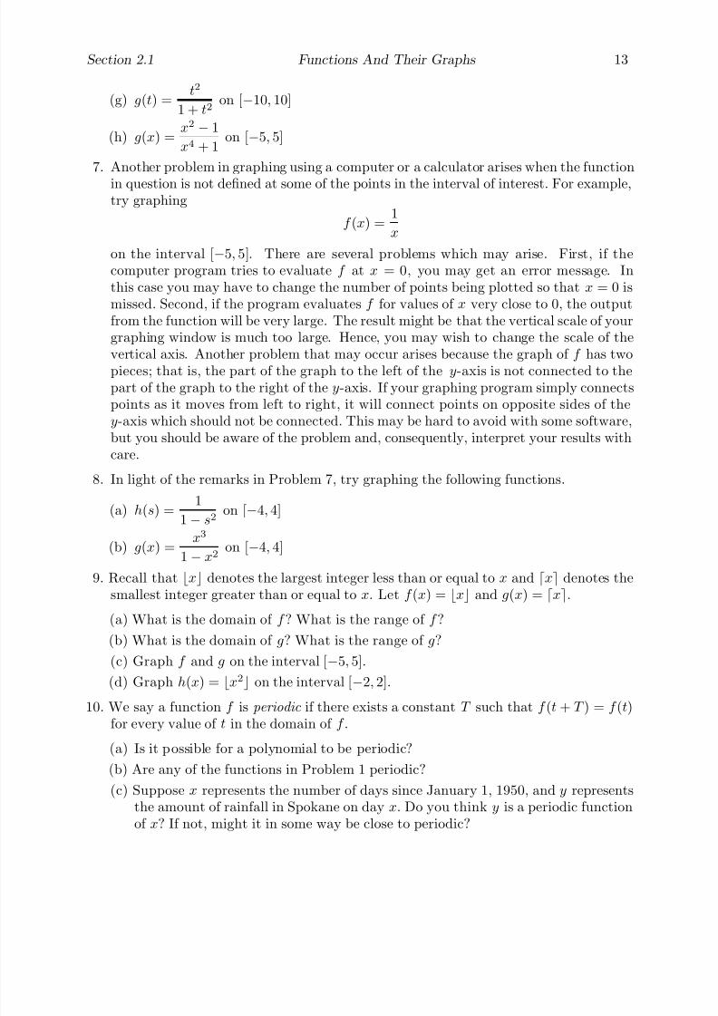
7/27/2019 Calculus 2 (Dan Sloughter)
http://slidepdf.com/reader/full/calculus-2-dan-sloughter 71/598
Section 2.1 Functions And Their Graphs 13
(g) g(t) =t2
1 + t2on [−10, 10]
(h) g(x) =x2 − 1
x4 + 1on [−5, 5]
7. Another problem in graphing using a computer or a calculator arises when the functionin question is not defined at some of the points in the interval of interest. For example,try graphing
f (x) =1
x
on the interval [−5, 5]. There are several problems which may arise. First, if thecomputer program tries to evaluate f at x = 0, you may get an error message. Inthis case you may have to change the number of points being plotted so that x = 0 ismissed. Second, if the program evaluates f for values of x very close to 0, the outputfrom the function will be very large. The result might be that the vertical scale of yourgraphing window is much too large. Hence, you may wish to change the scale of the
vertical axis. Another problem that may occur arises because the graph of f has twopieces; that is, the part of the graph to the left of the y-axis is not connected to thepart of the graph to the right of the y-axis. If your graphing program simply connectspoints as it moves from left to right, it will connect points on opposite sides of they-axis which should not be connected. This may be hard to avoid with some software,but you should be aware of the problem and, consequently, interpret your results withcare.
8. In light of the remarks in Problem 7, try graphing the following functions.
(a) h(s) =1
1
−s2
on [−4, 4]
(b) g(x) =x3
1 − x2on [−4, 4]
9. Recall that x denotes the largest integer less than or equal to x and x denotes thesmallest integer greater than or equal to x. Let f (x) = x and g(x) = x.
(a) What is the domain of f ? What is the range of f ?
(b) What is the domain of g? What is the range of g?
(c) Graph f and g on the interval [−5, 5].
(d) Graph h(x) = x2 on the interval [−2, 2].
10. We say a function f is periodic if there exists a constant T such that f (t + T ) = f (t)for every value of t in the domain of f .
(a) Is it possible for a polynomial to be periodic?
(b) Are any of the functions in Problem 1 periodic?
(c) Suppose x represents the number of days since January 1, 1950, and y representsthe amount of rainfall in Spokane on day x. Do you think y is a periodic functionof x? If not, might it in some way be close to periodic?

7/27/2019 Calculus 2 (Dan Sloughter)
http://slidepdf.com/reader/full/calculus-2-dan-sloughter 72/598
Difference Equations
Differential Equations
to
Section 2.2
Trigonometric Functions
Many processes in nature are cyclic. A pendulum oscillates back and forth, repeating itsmotion over and over; a weight hanging at the end of a spring bobs up and down; the Earthrepeats its orbit about the Sun every 365 days; a population of arctic wolves has periodsof growth followed by periods of decrease, following the fluctuations in the population of their prey; the monthly rainfall at an agricultural research station varies cyclically overthe years and over the decades. To model such natural behavior, a mathematician needsfunctions which repeat their values over intervals of fixed length. These functions are theperiodic functions. Precisely, a function f is periodic if there is a fixed constant T suchthat f (t + T ) = f (t) for every value of t in the domain of f . The smallest such positive T
for which this property holds is called the period of f .
θ
bc
a
Figure 2.2.1 A right triangle
The class of periodic functions that we will consider in this section are the trigonometricfunctions. Although these functions were originally invented to work with problems of measurement, their importance in modern mathematics stems more from their periodicbehavior. We will begin with a definition in terms of measuring the sides of a righttriangle. Consider a right triangle with legs of lengths a and b and hypotenuse of length c.
Moreover, suppose, as in Figure 2.2.1, the angle opposite the leg of length b has measureθ. Then we define the sine of θ, which we write as sin(θ), by
sin(θ) =b
c(2.2.1)
and the cosine of θ, which we write as cos(θ), by
cos(θ) =a
c. (2.2.2)
1 Copyright c by Dan Sloughter 2000
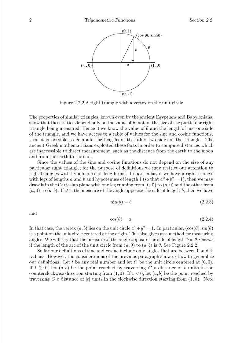
7/27/2019 Calculus 2 (Dan Sloughter)
http://slidepdf.com/reader/full/calculus-2-dan-sloughter 73/598
2 Trigonometric Functions Section 2.2
a
b
(0, -1)
(0, 1)
(1, 0)(-1, 0)
θ
(cos( ), sin( ))θ θ
Figure 2.2.2 A right triangle with a vertex on the unit circle
The properties of similar triangles, known even by the ancient Egyptians and Babylonians,show that these ratios depend only on the value of θ, not on the size of the particular righttriangle being measured. Hence if we know the value of θ and the length of just one sideof the triangle, and we have access to a table of values for the sine and cosine functions,then it is possible to compute the lengths of the other two sides of the triangle. Theancient Greek mathematicians exploited these facts in order to compute distances whichare inaccessible to direct measurement, such as the distance from the earth to the moonand from the earth to the sun.
Since the values of the sine and cosine functions do not depend on the size of anyparticular right triangle, for the purpose of definitions we may restrict our attention toright triangles with hypotenuses of length one. In particular, if we have a right triangle
with legs of lengths a and b and hypotenuse of length 1 (so that a2
+ b2
= 1), then we maydraw it in the Cartesian plane with one leg running from (0 , 0) to (a, 0) and the other from(a, 0) to (a, b). If θ is the measure of the angle opposite the side of length b, then we have
sin(θ) = b (2.2.3)
andcos(θ) = a. (2.2.4)
In that case, the vertex (a, b) lies on the unit circle x2+y2 = 1. In particular, (cos(θ), sin(θ)is a point on the unit circle centered at the origin. This also gives us a method for measuring
angles. We will say that the measure of the angle opposite the side of length b is θ radians if the length of the arc of the unit circle from ( a, 0) to (a, b) is θ. See Figure 2.2.2.
So far our definitions of sine and cosine include only angles that are between 0 and π
2
radians. However, the considerations of the previous paragraph show us how to generalizeour definitions. Let t be any real number and let C be the unit circle centered at (0, 0).If t ≥ 0, let (a, b) be the point reached by traversing C a distance of t units in thecounterclockwise direction starting from (1, 0). If t < 0, let (a, b) be the point reached bytraversing C a distance of |t| units in the clockwise direction starting from (1, 0). Note
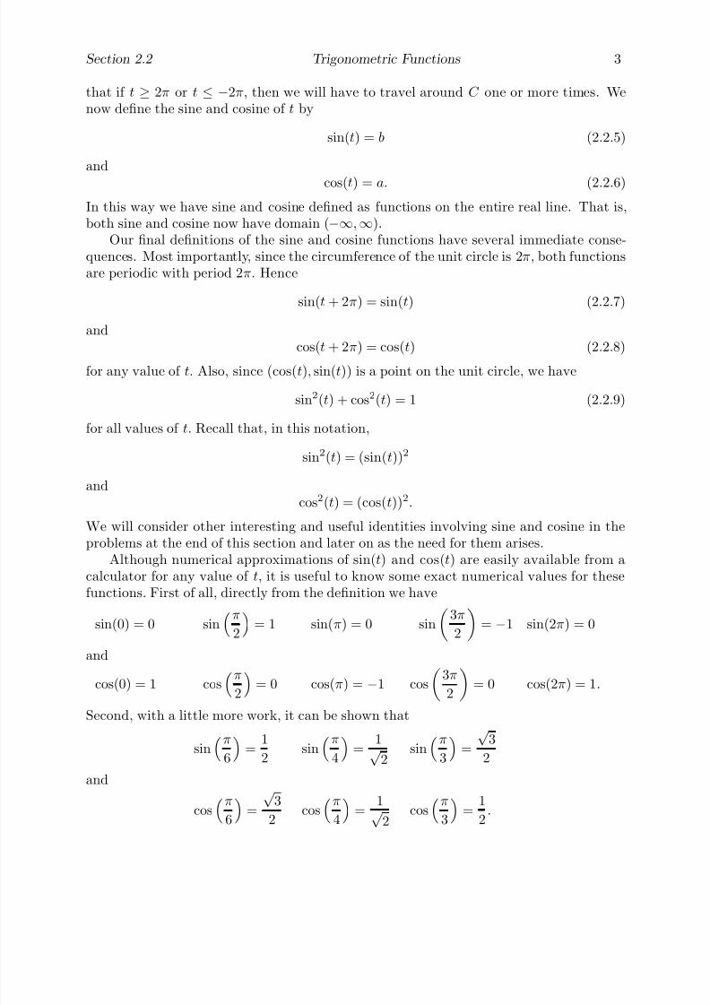
7/27/2019 Calculus 2 (Dan Sloughter)
http://slidepdf.com/reader/full/calculus-2-dan-sloughter 74/598
Section 2.2 Trigonometric Functions 3
that if t ≥ 2π or t ≤ −2π, then we will have to travel around C one or more times. Wenow define the sine and cosine of t by
sin(t) = b (2.2.5)
andcos(t) = a. (2.2.6)
In this way we have sine and cosine defined as functions on the entire real line. That is,both sine and cosine now have domain (−∞, ∞).
Our final definitions of the sine and cosine functions have several immediate conse-quences. Most importantly, since the circumference of the unit circle is 2π, both functionsare periodic with period 2π. Hence
sin(t + 2π) = sin(t) (2.2.7)
and
cos(t + 2π) = cos(t) (2.2.8)for any value of t. Also, since (cos(t), sin(t)) is a point on the unit circle, we have
sin2(t) + cos2(t) = 1 (2.2.9)
for all values of t. Recall that, in this notation,
sin2(t) = (sin(t))2
andcos2(t) = (cos(t))2.
We will consider other interesting and useful identities involving sine and cosine in theproblems at the end of this section and later on as the need for them arises.
Although numerical approximations of sin(t) and cos(t) are easily available from acalculator for any value of t, it is useful to know some exact numerical values for thesefunctions. First of all, directly from the definition we have
sin(0) = 0 sinπ
2
= 1 sin(π) = 0 sin
3π
2
= −1 sin(2π) = 0
and
cos(0) = 1 cosπ
2 = 0 cos(π) = −1 cos3π
2 = 0 cos(2π) = 1.
Second, with a little more work, it can be shown that
sinπ
6
=
1
2sin
π
4
=
1√ 2
sinπ
3
=
√ 3
2
and
cosπ
6
=
√ 3
2cos
π
4
=
1√ 2
cosπ
3
=
1
2.

7/27/2019 Calculus 2 (Dan Sloughter)
http://slidepdf.com/reader/full/calculus-2-dan-sloughter 75/598
4 Trigonometric Functions Section 2.2
(0, -1)
(0, 1)
(1, 0)(-1, 0)
π
6
5π
6( , )a b (- , )ba
( , 0) (- , 0)aa
Figure 2.2.3 Finding sin5π
6
and cos
5π
6
Moreover, combining these values with basic knowledge of the geometry of the unitcircle, it is possible to find exact numerical values for the values of sin(t) and cos(t) fort = 2π
3, 3π
4, 5π
6, 7π
6, 5π
4, 4π
3, 5π
3, 7π
4, and 11π
6.
Example Let (a, b) be the point on the unit circle corresponding to the angle 5π
6. Since
(a, b) is a distance π
6along the unit circle before (−1, 0), the point (−a, b) is a distance π
6
along the unit circle after (1, 0). Hence
−a = cosπ
6
=
√ 3
2
and
b = sinπ
6
=
1
2.
Thus
cos
5π
6
= a = −
√ 3
2
and
sin5π
6
= b =
1
2 .
This is all best seen using a picture such as Figure 2.2.3. Note that the triangle with verticesat (0, 0), (a, b), and (a, 0) is congruent to the triangle with vertices at (0, 0), (−a, b), and(−a, 0).
Of course, because both sine and cosine have period 2π, it is also easy to find exactvalues for sin(t) and cos(t) if t differs from one of the above values by a multiple of 2π.

7/27/2019 Calculus 2 (Dan Sloughter)
http://slidepdf.com/reader/full/calculus-2-dan-sloughter 76/598
Section 2.2 Trigonometric Functions 5
-6
-4
-2 2 4 6
-3
-2
-1
1
2
3
-6
-4
-2 2 4 6
-3
-2
-1
1
2
3
Figure 2.2.4 Graphs of y = sin(t) and y = cos(t)
Graphs of sine and cosine
The graphs of y = sin(t) and y = cos(t) are shown in Figures 2.2.4. Since both functions
have period 2π, the graphs will continue this behavior as t goes to −∞ or ∞, completingone oscillation over every interval of length 2π.The only difference between the graph of y = a sin(t), where a > 0, and the graph of
y = sin(t) is that the former oscillates between −a and a instead of between −1 to 1. Ingeneral, for any constant a = 0, the graph of y = a sin(t) oscillates between −|a| and |a|.We call |a| the amplitude of the function y = a sin(t). Of course, if a < 0, then the graphof y = a sin(t) is the graph of y = |a| sin(t) reflected about the t-axis.
Example The graph of y = 2sin(t) is shown in Figure 2.2.5.
-6 -4 -2 2 4 6
-3
-2
-1
1
2
3
Figure 2.2.5 Graph of y = 2sin(t)
Now consider the graph of the function y = sin(bt). Since the sine function has period2π, this function goes through one complete oscillation as t goes from 0 to 2π
|b| . That is,
y = sin(bt) has period 2π
|b| . Hence, if b > 0 the only difference between the graphs of
y = sin(t) and y = sin(bt) is the length of the period of oscillation. If b < 0, we may use

7/27/2019 Calculus 2 (Dan Sloughter)
http://slidepdf.com/reader/full/calculus-2-dan-sloughter 77/598
6 Trigonometric Functions Section 2.2
-6 -4 -2 2 4 6
-3
-2
-1
1
2
3
Figure 2.2.6 Graph of y = sin(2t)
the fact that
sin(bt) = sin(−|b|t) = − sin(|b|t),
which follows from Problem 10.
Example The graph of y = sin(2t) is shown in Figure 2.2.6.
Finally, consider the graph of y = sin(t − c). As mentioned in Section 2.1, the effect of the c is to shift the graph y = sin(t) horizontally by |c| units, to the right if c > 0 and tothe left if c < 0. We call c the phase angle .
Example The graph of y = sin(t − π) is shown in Figure 2.2.7.
-6 -4 -2 2 4 6
-3
-2
-1
1
2
3
Figure 2.2.7 Graph of y = sin(t − π)
Summarizing the previous comments, the function y = a sin(b(t − c)) has amplitude|a|, period 2π
|b| , and phase angle c.

7/27/2019 Calculus 2 (Dan Sloughter)
http://slidepdf.com/reader/full/calculus-2-dan-sloughter 78/598
Section 2.2 Trigonometric Functions 7
-6 -4 -2 2 4 6
-3
-2
-1
1
2
3
Figure 2.2.8 Graph of y = −3sin(2t − π)
Example Consider the function f (t) =
−3sin(2t
−π). If we write f (t) in the form
f (t) = −3sin
2
t − π
2
,
then we see that f has amplitude 3, period π, and phase angle π
2. The graph of f is shown
in Figure 2.2.8.
Similar remarks hold for the graph of the function y = a cos(b(t−c)), the only differencebeing that, since cos(−t) = cos(t) for all t (see Problem 10), we have
cos(bt) = cos(|b|t)
even when b < 0.
Related functions
The other four trigonometric functions are defined in terms of the sine and cosine functions.The tangent function is defined by
tan(t) =sin(t)
cos(t). (2.2.10)
Note that tan(t) is the slope of the line from (0, 0) to (cos(t), sin(t)). The graph of y =tan(t) has vertical asymptotes at every value of t for which cos(t) = 0, as can be seen inFigure 2.2.9.
The cotangent function is the reciprocal of the tangent function; namely,
cot(t) =1
tan(t)=
cos(t)
sin(t). (2.2.11)
Finally, the secant and cosecant functions are the reciprocals of the cosine and sine func-tions, respectively. Hence
sec(t) =1
cos(t)(2.2.12)
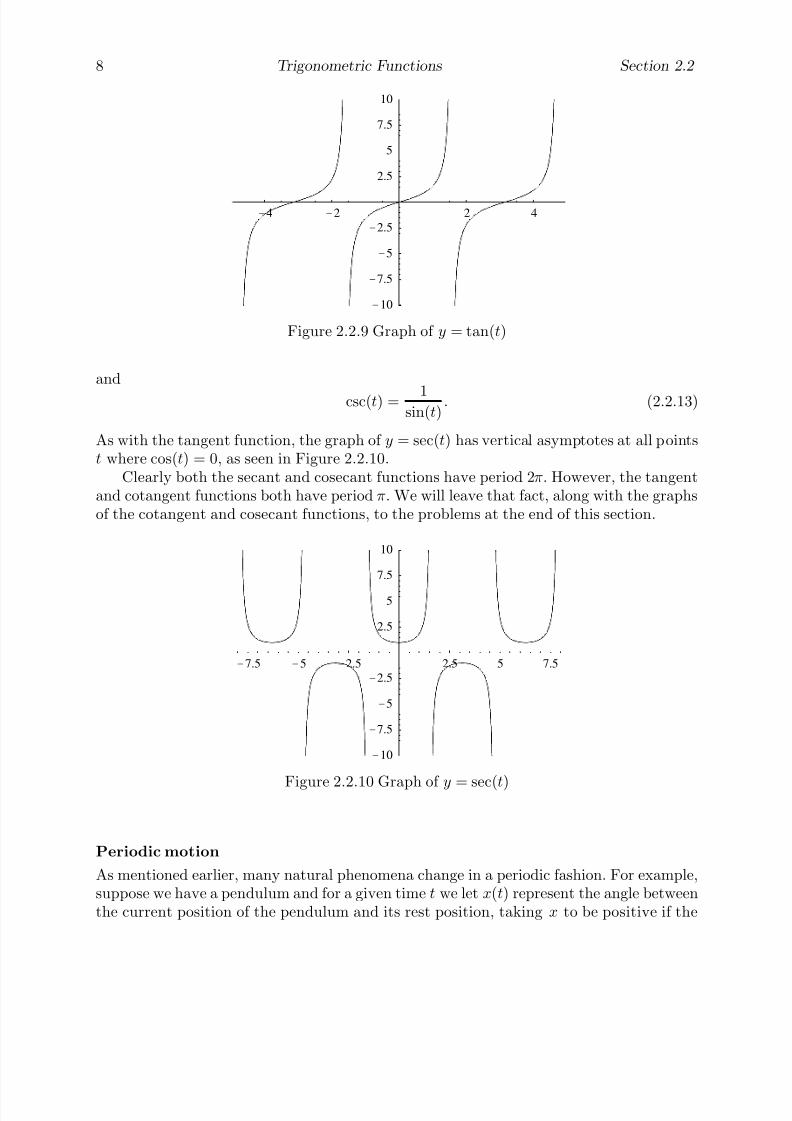
7/27/2019 Calculus 2 (Dan Sloughter)
http://slidepdf.com/reader/full/calculus-2-dan-sloughter 79/598
8 Trigonometric Functions Section 2.2
-4 -2 2 4
-10
-7.5
-5
-2.5
2.5
5
7.5
10
Figure 2.2.9 Graph of y = tan(t)
and
csc(t) = 1sin(t)
. (2.2.13)
As with the tangent function, the graph of y = sec(t) has vertical asymptotes at all pointst where cos(t) = 0, as seen in Figure 2.2.10.
Clearly both the secant and cosecant functions have period 2π. However, the tangentand cotangent functions both have period π. We will leave that fact, along with the graphsof the cotangent and cosecant functions, to the problems at the end of this section.
-7.5 -5 -2.5 2.5 5 7.5
-10
-7.5
-5
-2.5
2.5
5
7.5
10
Figure 2.2.10 Graph of y = sec(t)
Periodic motion
As mentioned earlier, many natural phenomena change in a periodic fashion. For example,suppose we have a pendulum and for a given time t we let x(t) represent the angle betweenthe current position of the pendulum and its rest position, taking x to be positive if the

7/27/2019 Calculus 2 (Dan Sloughter)
http://slidepdf.com/reader/full/calculus-2-dan-sloughter 80/598
Section 2.2 Trigonometric Functions 9
¢ ¢
¢ ¢
£
£¤
¤
b
x(t )
Figure 2.2.11 A pendulum
pendulum is to the right of its rest position and negative otherwise (see Figure 2.2.11). If initially the pendulum is held at a small angle α > 0 and then released, that is, x(0) = α,then, if we ignore friction, it can be shown that
x(
t) =
αcos
gb
t(2.2.14)
where g is the acceleration due to gravity (32 feet per second per second or 9 .8 meters persecond per second) and b is the length of the pendulum. Actually, this is an approximationwhich holds very well for small values of α. Note that the period of x, namely,
2π g
b
= 2π
b
g,
does not depend upon the amplitudeα
. This is an important fact, supposedly first noticedby Galileo, which is crucial in the operation of pendulum clocks. We will consider thisproblem more closely in Chapter 8, where we will derive (2.2.14) and see exactly how theapproximation enters the picture.
Periodic motions need not always be as simple as the motion of a pendulum. Consider,for example, the motion of a molecule of air as a sound wave passes. The action of thesound wave causes a particular molecule of air to oscillate back and forth about someequilibrium position. If we let x(t) represent the position of the air molecule at time t,with x = 0 corresponding to the equilibrium position and x considered to be positive in onedirection from the equilibrium position and negative in the other, then for many soundsx will be a periodic function of t. In general, this will be true for musical sounds, but
not true for sounds we would normally classify as noise. Moreover, even if x is a periodicfunction, it need not be simply a sine or cosine function. The graph of x for a musicalsound, although periodic, may be very complicated. However, many simple sounds, suchas the sound of a tuning fork, are represented by sine curves. For example, if x is thedisplacement of an air molecule for a tuning fork which vibrates at 440 cycles per secondwith a maximum displacement from equilibrium of 0.002 centimeters, then
x(t) = 0.002 sin(880πt).

7/27/2019 Calculus 2 (Dan Sloughter)
http://slidepdf.com/reader/full/calculus-2-dan-sloughter 81/598
10 Trigonometric Functions Section 2.2
-10 -5 5 10
-200
-150
-100
-50
50
100
150
200
Figure 2.2.12 Graph of the air displacement due to the organ note C 3
Notice that this function has period 2π
880π= 1
440, and hence has a frequency of 440 cycles
per second.In the early part of the 19th century, Joseph Fourier (1768-1830) showed that the story
does not end here. Fourier demonstrated that any “nice” periodic curve (for example, onewhich is connected) can be approximated as closely as desired by a sum of sine and cosinefunctions. In particular, this means that for any musical sound the function x may beapproximated well by a sum of sine and cosine functions. For example, in his book The
Science of Musical Sounds (Macmillan, New York, 1926), Dayton Miller shows that, withan appropriate choice of units,
x(t) = 22.4sin(t) + 94.1cos(t) + 49.8 sin(2t) − 43.6cos(2t) + 33.7 sin(3t)
−14.2 cos(3t) + 19.0 sin(4t)
−1.9 cos(4t) + 8.9 sin(5t)
−5.22 cos(5t)
− 8.18 sin(6t) − 1.77 cos(6t) + 6.40 sin(7t) − 0.54 cos(7t) + 3.11 sin(8t)
− 8.34 cos(8t) − 1.28 sin(9t) − 4.10cos(9t) − 0.71 sin(10t) − 2.17 cos(10t)
gives a very good approximation to the displacement curve of a sound wave generated bythe tone C3 of an organ pipe. From the graph of x, shown in Figure 2.2.12, we can see itscomplexity as well as its periodicity. Notice that the terms in this expression for x(t) arewritten in pairs with frequencies which are always integer multiples of the frequency of thefirst pair. This is a general fact which is part of Fourier’s theory; if we added more terms toobtain more accuracy, the next terms would be of the form a sin(11t) + b cos(11t) for someconstants a and b. Notice also that the amplitudes of the sine and cosine curves tend to
decrease as the frequencies are increasing. As a consequence, the higher frequencies haveless impact on the total curve. Put another way, Fourier’s theorem says that every musicalsound is the sum of simple tones which could be generated by tuning forks. Hence in theory,although certainly not in practice, the instruments of any orchestra could all be replacedby tuning forks. On a more practical level, Fourier’s analysis of periodic functions hasbeen fundamental for the development of such modern conveniences as radios, televisions,stereos, and compact disc players. Unfortunately, this is a story which will have to be toldelsewhere.

7/27/2019 Calculus 2 (Dan Sloughter)
http://slidepdf.com/reader/full/calculus-2-dan-sloughter 82/598
Section 2.2 Trigonometric Functions 11
Problems
1. Find the exact values of sin(t), cos(t), tan(t), and sec(t) for the following values of t.
(a)4π
3(b)
7π
6
(c) 2π3
(d) −π4
(e) −2π
3(f)
21π
4
(g)11π
6(h) −11π
6
2. Sketch the graph of each of the following functions over an interval that contains atleast one period of the function both to the right and to the left of the vertical axis.Also, identify the amplitude, period, and phase angle of each curve.
(a) y = sin(3t) (b) y = 3 cos(2t)
(c) y = cos(t − π) (d) x = sin(2t) + 1
(e) x = 4sin(πt) (f) y = −2cos(2t − π)
(g) x = 5 sin(2t + π) (h) y = −3sin(2πt)
3. Starting with the identity sin2(x) + cos2(x) = 1, explain why
1 + tan2(x) = sec2(x).
4. The addition formulas for sine and cosine are
sin(x + y) = sin(x)cos(y) + cos(x)sin(y)
andcos(x + y) = cos(x)cos(y) − sin(x) sin(y).
Use these to derive the double-angle formulas:
(a) sin(2x) = 2sin(x)cos(x) (b) cos(2x) = cos2(x) − sin2(x)
5. Use the double-angle formulas of Problem 4 to derive the half-angle formulas:
(a) cos2(x) =1 + cos(2x)
2(b) sin2(x) =
1 − cos(2x)
2
6. Use the addition formulas of Problem 4 to derive the shift formulas:(a) sin
x − π
2
= − cos(x) (b) cos
x − π
2
= sin(x)
(c) sin
x +π
2
= cos(x) (d) cos
x +
π
2
= − sin(x)
7. Can you picture the identities of Problem 6 in terms of the definitions of sine and cosineusing the unit circle? What do these identities say about the relationship between thegraphs of sine and cosine?
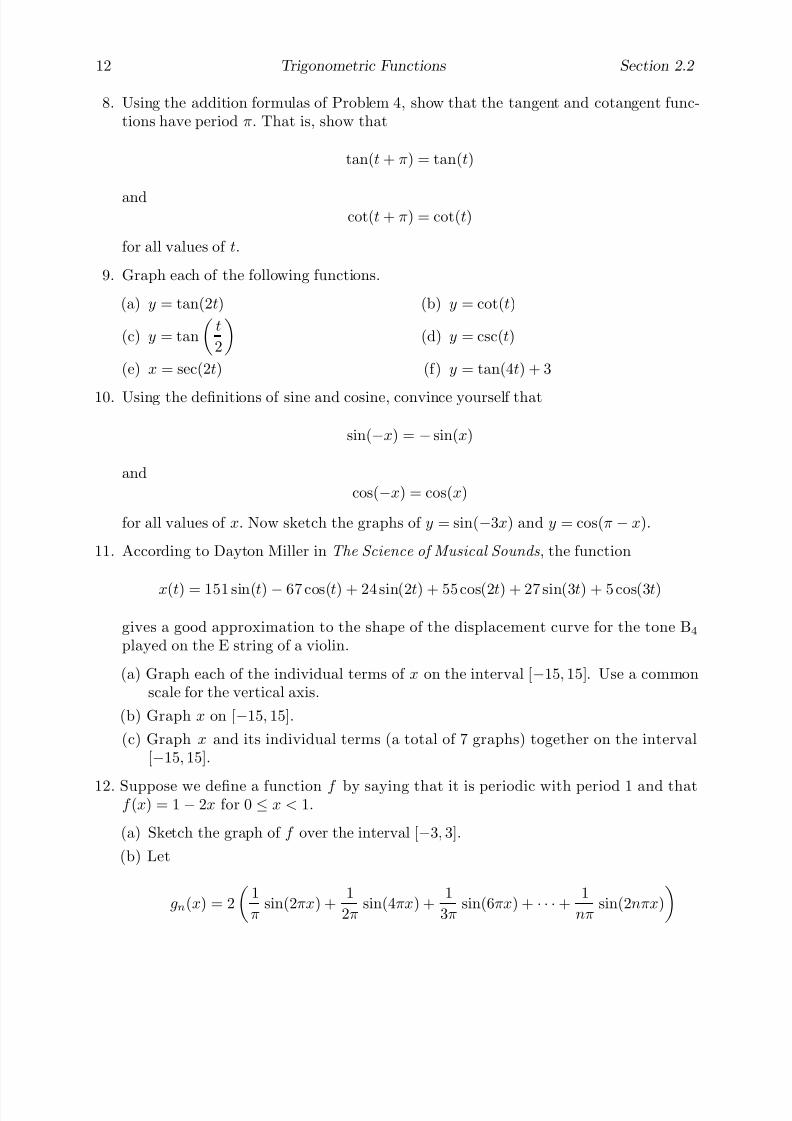
7/27/2019 Calculus 2 (Dan Sloughter)
http://slidepdf.com/reader/full/calculus-2-dan-sloughter 83/598
12 Trigonometric Functions Section 2.2
8. Using the addition formulas of Problem 4, show that the tangent and cotangent func-tions have period π. That is, show that
tan(t + π) = tan(t)
andcot(t + π) = cot(t)
for all values of t.
9. Graph each of the following functions.
(a) y = tan(2t) (b) y = cot(t)
(c) y = tan
t
2
(d) y = csc(t)
(e) x = sec(2t) (f) y = tan(4t) + 3
10. Using the definitions of sine and cosine, convince yourself that
sin(−x) = − sin(x)
and
cos(−x) = cos(x)
for all values of x. Now sketch the graphs of y = sin(−3x) and y = cos(π − x).
11. According to Dayton Miller in The Science of Musical Sounds , the function
x(t) = 151 sin(t) − 67 cos(t) + 24 sin(2t) + 55 cos(2t) + 27 sin(3t) + 5 cos(3t)
gives a good approximation to the shape of the displacement curve for the tone B4
played on the E string of a violin.
(a) Graph each of the individual terms of x on the interval [−15, 15]. Use a commonscale for the vertical axis.
(b) Graph x on [−15, 15].
(c) Graph x and its individual terms (a total of 7 graphs) together on the interval[−15, 15].
12. Suppose we define a function f by saying that it is periodic with period 1 and thatf (x) = 1 − 2x for 0 ≤ x < 1.
(a) Sketch the graph of f over the interval [−3, 3].
(b) Let
gn(x) = 2
1
πsin(2πx) +
1
2πsin(4πx) +
1
3πsin(6πx) + · · · +
1
nπsin(2nπx)
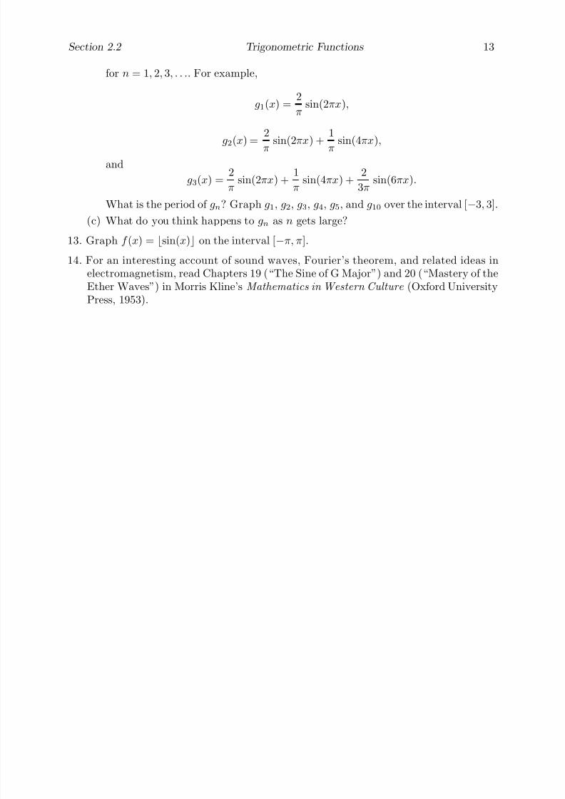
7/27/2019 Calculus 2 (Dan Sloughter)
http://slidepdf.com/reader/full/calculus-2-dan-sloughter 84/598
Section 2.2 Trigonometric Functions 13
for n = 1, 2, 3, . . .. For example,
g1(x) =2
πsin(2πx),
g2(x) =2
π sin(2πx) +1
π sin(4πx),
and
g3(x) =2
πsin(2πx) +
1
πsin(4πx) +
2
3πsin(6πx).
What is the period of gn? Graph g1, g2, g3, g4, g5, and g10 over the interval [−3, 3].
(c) What do you think happens to gn as n gets large?
13. Graph f (x) = sin(x) on the interval [−π, π].
14. For an interesting account of sound waves, Fourier’s theorem, and related ideas inelectromagnetism, read Chapters 19 (“The Sine of G Major”) and 20 (“Mastery of theEther Waves”) in Morris Kline’s Mathematics in Western Culture (Oxford UniversityPress, 1953).
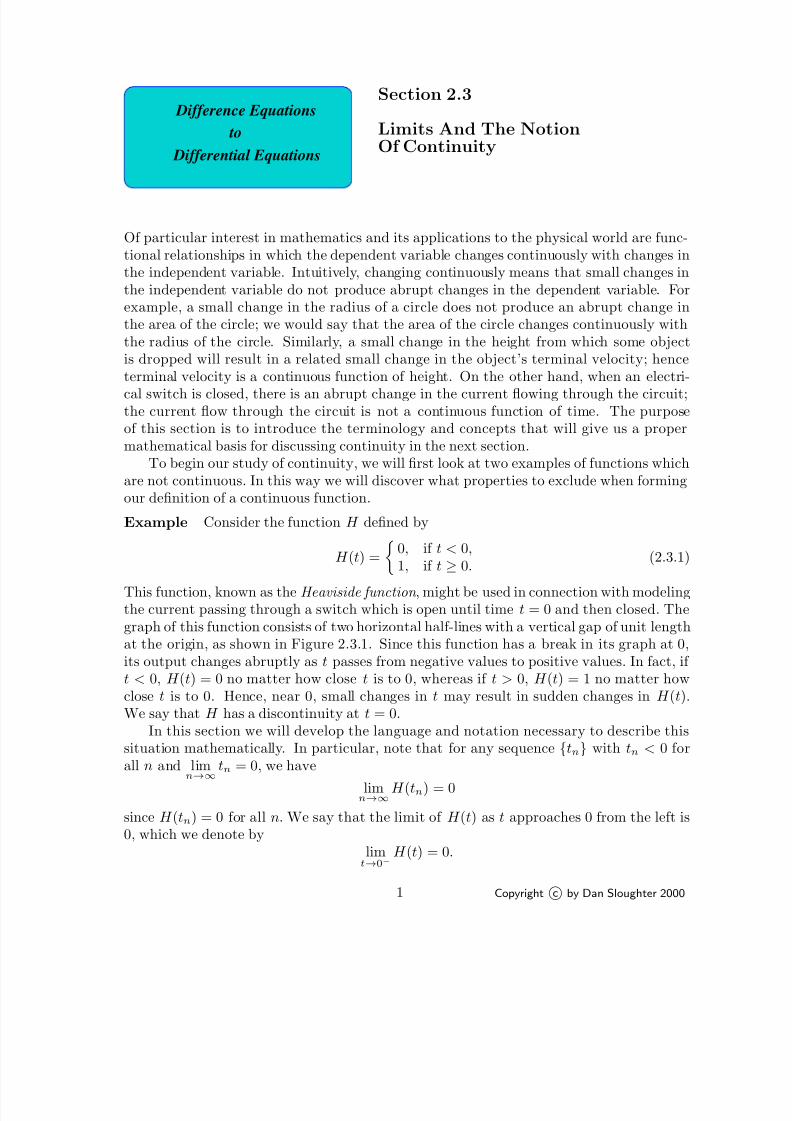
7/27/2019 Calculus 2 (Dan Sloughter)
http://slidepdf.com/reader/full/calculus-2-dan-sloughter 85/598
Difference Equations
Differential Equations
to
Section 2.3
Limits And The NotionOf Continuity
Of particular interest in mathematics and its applications to the physical world are func-tional relationships in which the dependent variable changes continuously with changes inthe independent variable. Intuitively, changing continuously means that small changes inthe independent variable do not produce abrupt changes in the dependent variable. Forexample, a small change in the radius of a circle does not produce an abrupt change inthe area of the circle; we would say that the area of the circle changes continuously withthe radius of the circle. Similarly, a small change in the height from which some objectis dropped will result in a related small change in the object’s terminal velocity; henceterminal velocity is a continuous function of height. On the other hand, when an electri-
cal switch is closed, there is an abrupt change in the current flowing through the circuit;the current flow through the circuit is not a continuous function of time. The purposeof this section is to introduce the terminology and concepts that will give us a propermathematical basis for discussing continuity in the next section.
To begin our study of continuity, we will first look at two examples of functions whichare not continuous. In this way we will discover what properties to exclude when formingour definition of a continuous function.
Example Consider the function H defined by
H (t) =
0, if t < 0,1, if t ≥ 0.
(2.3.1)
This function, known as the Heaviside function , might be used in connection with modelingthe current passing through a switch which is open until time t = 0 and then closed. Thegraph of this function consists of two horizontal half-lines with a vertical gap of unit lengthat the origin, as shown in Figure 2.3.1. Since this function has a break in its graph at 0,its output changes abruptly as t passes from negative values to positive values. In fact, if t < 0, H (t) = 0 no matter how close t is to 0, whereas if t > 0, H (t) = 1 no matter howclose t is to 0. Hence, near 0, small changes in t may result in sudden changes in H (t).We say that H has a discontinuity at t = 0.
In this section we will develop the language and notation necessary to describe thissituation mathematically. In particular, note that for any sequence {tn} with tn < 0 forall n and lim
n
→∞
tn = 0, we have
limn→∞H (tn) = 0
since H (tn) = 0 for all n. We say that the limit of H (t) as t approaches 0 from the left is0, which we denote by
limt→0−
H (t) = 0.
1 Copyright c by Dan Sloughter 2000

7/27/2019 Calculus 2 (Dan Sloughter)
http://slidepdf.com/reader/full/calculus-2-dan-sloughter 86/598
2 Limits And The Notion Of Continuity Section 2.3
-4 -2 2 4
-1
-0.5
0.5
1
1.5
2
Figure 2.3.1 Graph of the Heaviside function
However, for any sequence {tn} with tn > 0 for all n and limn→∞
tn = 0, we have
limn→∞H (tn) = 1
since H (tn) = 1 for all n. We say that the limit of H (t) as t approaches 0 from the rightis 1, which we denote by
limt→0+
H (t) = 1.
Since these two limiting values do not agree, we say that H (t) does not have a limit ast approaches 0. Hence, in this case, the discontinuity of H at 0 is characterized by theabsence of a limiting value for H (t) at 0. In the next section we will make the existenceof a limiting value one of the criteria for a function to be continuous at a point.
Example Now consider the function
g(x) =
−x, if x < 0,1, if x = 0,x, if x > 0.
As with the previous example, this function does not change continuously as x passes fromnegative to positive values. However, the discontinuity arises in a different manner. Notethat if {xn} is a sequence with xn < 0 for all n and lim
n→∞xn = 0, then
limn→∞
g(xn) = limn→∞
(−xn) = − limn→∞
xn = 0.
Thus
limx→0− g(x) = 0.
Similarly, if {xn} is a sequence with xn > 0 for all n and limn→∞
xn = 0, then
limn→∞
g(xn) = limn→∞
xn = 0.

7/27/2019 Calculus 2 (Dan Sloughter)
http://slidepdf.com/reader/full/calculus-2-dan-sloughter 87/598
Section 2.3 Limits And The Notion Of Continuity 3
-6 -4 -2 2 4 6
1
2
3
4
5
Figure 2.3.2 Graph of y = g(x)
Thuslimx→0+
g(x) = 0.
Hence in this case g(x) does have a limiting value as x approaches 0 and we can write
limx→0
g(x) = 0.
However, there is still an sudden change in the value of the function at 0 because g(0) = 1,not 0. Graphically, this shows up as a hole in the graph of g at the origin, as shownin Figure 2.3.2. Thus the abrupt change in values of g(x) results not from the lack of alimiting value as x approaches 0, but rather from the fact that
g(0) = 1 = 0 = limx
→0
g(x).
This illustrates another type of behavior that we will have to exclude in our definition of continuity.
These examples illustrate two ways in which a function may fail to be continuous. Thedefinition which we will discuss in Section 2.4 essentially says that a function is continuousif it does not have either of the problems that we have seen with H and g. However,before pursuing this question further, we must first introduce the notion of a limit for afunction defined on an interval of real numbers. We have already seen the pattern for thisdefinition in the previous examples. Namely, in order to define, for some function f , thelimit of f (x) as x approaches some number c, we consider sequences {xn} that convergeto c and ask if the sequence
{f (xn)
}has a limit. Hence we reduce our new question to the
old problem of limits of sequences that we considered back in Section 1.2. However, wemust be careful about two points. First, there will always be more than one sequence {xn}which converges to a given point c. As we saw in the examples, in order to understandthe behavior of a function near c, we must take into account how the function behaves onall possible sequences that converge to c. Second, we want the limit to describe what is
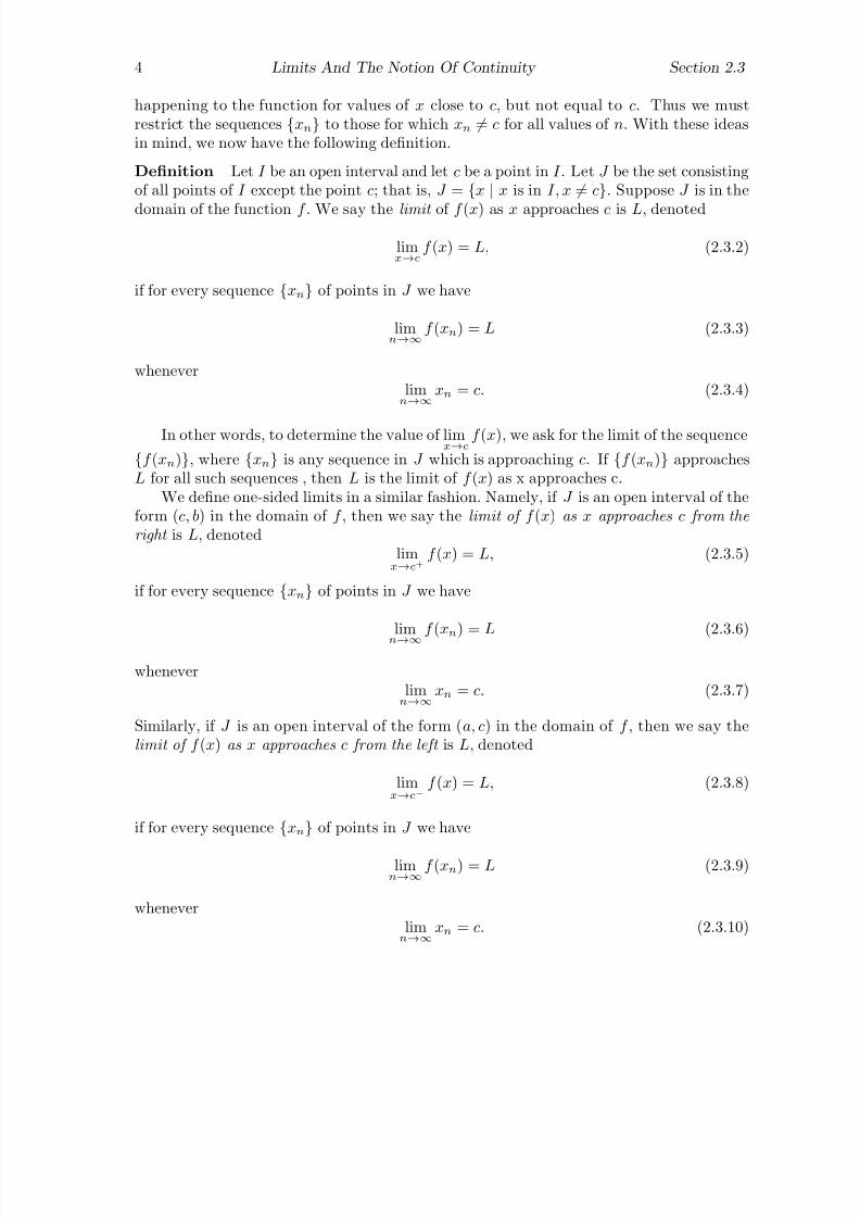
7/27/2019 Calculus 2 (Dan Sloughter)
http://slidepdf.com/reader/full/calculus-2-dan-sloughter 88/598
4 Limits And The Notion Of Continuity Section 2.3
happening to the function for values of x close to c, but not equal to c. Thus we mustrestrict the sequences {xn} to those for which xn = c for all values of n. With these ideasin mind, we now have the following definition.
Definition Let I be an open interval and let c be a point in I . Let J be the set consistingof all points of I except the point c; that is, J = {x | x is in I, x = c}. Suppose J is in the
domain of the function f . We say the limit of f (x) as x approaches c is L, denoted
limx→c
f (x) = L, (2.3.2)
if for every sequence {xn} of points in J we have
limn→∞
f (xn) = L (2.3.3)
wheneverlimn→∞
xn = c. (2.3.4)
In other words, to determine the value of limx→c
f (x), we ask for the limit of the sequence
{f (xn)}, where {xn} is any sequence in J which is approaching c. If {f (xn)} approachesL for all such sequences , then L is the limit of f (x) as x approaches c.
We define one-sided limits in a similar fashion. Namely, if J is an open interval of theform (c, b) in the domain of f , then we say the limit of f (x) as x approaches c from the
right is L, denotedlimx→c+
f (x) = L, (2.3.5)
if for every sequence {xn} of points in J we have
limn→∞
f (xn) = L (2.3.6)
wheneverlimn→∞
xn = c. (2.3.7)
Similarly, if J is an open interval of the form (a, c) in the domain of f , then we say thelimit of f (x) as x approaches c from the left is L, denoted
limx→c−
f (x) = L, (2.3.8)
if for every sequence {xn} of points in J we have
limn→∞
f (xn) = L (2.3.9)
wheneverlimn→∞
xn = c. (2.3.10)

7/27/2019 Calculus 2 (Dan Sloughter)
http://slidepdf.com/reader/full/calculus-2-dan-sloughter 89/598
Section 2.3 Limits And The Notion Of Continuity 5
Note that the existence of a one-sided limit only requires that the limiting value of {f (xn)}be the same for all sequences {xn} which approach c from the same side, whereas theexistence of a limit requires that the limiting value of be the same for all sequences {xn}which approach c. In particular, this means that if
limx→c
f (x) = L
then we must have bothlimx→c+
f (x) = L
andlimx→c−
f (x) = L.
Not surprisingly, this also works in the other direction; in general, we have
limx→c
f (x) = L if and only if both limx→c+
f (x) = L and limx→c−
f (x) = L. (2.3.11)
Since the above definitions are all in terms of limits of sequences, we may use all theproperties of limits of sequences developed in Section 1.2 when discussing the limit of afunction defined on an interval of real numbers.
Example Consider the constant function f (x) = 2 for all x. To compute, for example,limx→3
f (x), we need to compute limn→∞
f (xn) for an arbitrary sequence {xn} with limn→∞
xn = 3.
For such a sequence, we have
limn→∞
f (xn) = limn→∞
2 = 2.
Hencelimx→3
f (x) = 2.
In fact, it should be easy to see that for any value of c
limx→c
f (x) = limx→c
2 = 2,
and, more generally, for any constant k,
limx→c
k = k.
Example Suppose f (x) = x. To find limx
→5
f (x), first let {xn} be any sequence with
limn→∞xn = 5. Thenlimn→∞
f (xn) = limn→∞
xn = 5,
solimx→5
f (x) = 5.
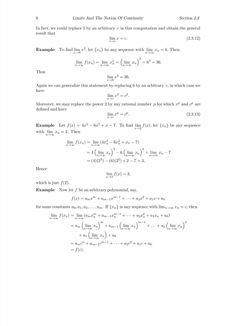
7/27/2019 Calculus 2 (Dan Sloughter)
http://slidepdf.com/reader/full/calculus-2-dan-sloughter 90/598
6 Limits And The Notion Of Continuity Section 2.3
In fact, we could replace 5 by an arbitrary c in this computation and obtain the generalresult that
limx→c
x = c. (2.3.12)
Example To find limx→6
x2, let {xn} be any sequence with limn→∞
xn = 6. Then
limn→∞
f (xn) = limn→∞
x2n =
limn→∞
xn
2= 62 = 36.
Thuslimx→6
x2 = 36.
Again we can generalize this statement by replacing 6 by an arbitrary c, in which case wehave
limx→c
x2 = c2.
Moreover, we may replace the power 2 by any rational number p for which x p and c p aredefined and have
limx→c x p = c p. (2.3.13)
Example Let f (x) = 4x3 − 6x2 + x − 7. To find limx→2
f (x), let {xn} be any sequence
with limn→∞
xn = 2. Then
limn→∞
f (xn) = limn→∞
(4x3n − 6x2n + xn − 7)
= 4
limn→∞
xn
3− 6
limn→∞
xn
2+ lim
n→∞xn − 7
= (4)(23) − (6)(22) + 2 − 7 = 3.
Hencelimx→2
f (x) = 3,
which is just f (2).
Example Now let f be an arbitrary polynomial, say,
f (x) = amxm + am−1xm−1 + · · · + a2x2 + a1x + a0
for some constants a0, a1, a2, . . . , am. If {xn} is any sequence with limn→∞ xn = c, then
limn→∞
f (xn) = limn→∞
(amxmn + am−1xm−1
n + · · · + a2x2n + a1xn + a0)
= am limn→∞
xnm + am−1 lim
n→∞xnm−1 + . . . + a2 lim
n→∞xn2
+ a1
limn→∞
xn
+ a0
= amcn + am−1cm−1 + · · · + a2c2 + a1c + a0
= f (c).
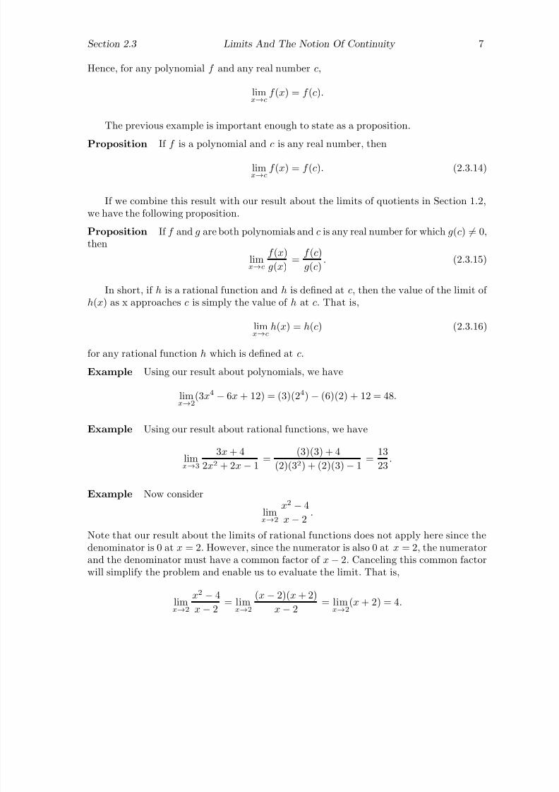
7/27/2019 Calculus 2 (Dan Sloughter)
http://slidepdf.com/reader/full/calculus-2-dan-sloughter 91/598
Section 2.3 Limits And The Notion Of Continuity 7
Hence, for any polynomial f and any real number c,
limx→c
f (x) = f (c).
The previous example is important enough to state as a proposition.
Proposition If f is a polynomial and c is any real number, then
limx→c
f (x) = f (c). (2.3.14)
If we combine this result with our result about the limits of quotients in Section 1.2,we have the following proposition.
Proposition If f and g are both polynomials and c is any real number for which g(c) = 0,then
limx→c
f (x)
g(x)=
f (c)
g(c). (2.3.15)
In short, if h is a rational function and h is defined at c, then the value of the limit of h(x) as x approaches c is simply the value of h at c. That is,
limx→c
h(x) = h(c) (2.3.16)
for any rational function h which is defined at c.
Example Using our result about polynomials, we have
limx→2
(3x4 − 6x + 12) = (3)(24) − (6)(2) + 12 = 48.
Example Using our result about rational functions, we have
limx→3
3x + 4
2x2 + 2x − 1=
(3)(3) + 4
(2)(32) + (2)(3) − 1=
13
23.
Example Now consider
limx→2
x2 − 4
x − 2.
Note that our result about the limits of rational functions does not apply here since thedenominator is 0 at x = 2. However, since the numerator is also 0 at x = 2, the numeratorand the denominator must have a common factor of x − 2. Canceling this common factorwill simplify the problem and enable us to evaluate the limit. That is,
limx→2
x2 − 4
x − 2= lim
x→2
(x − 2)(x + 2)
x − 2= lim
x→2(x + 2) = 4.
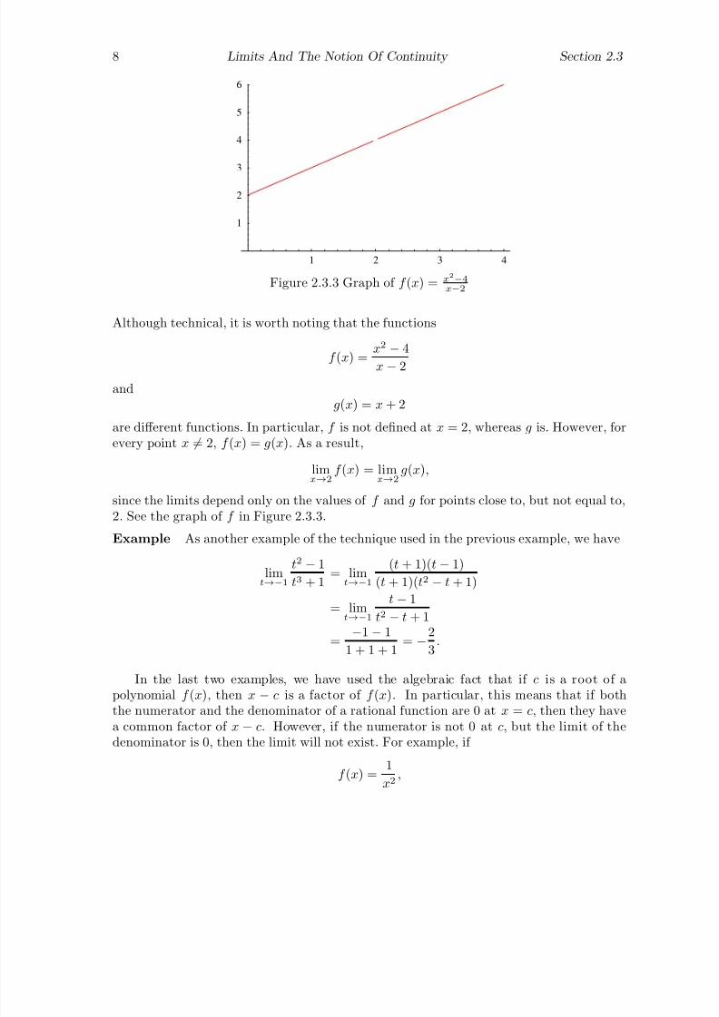
7/27/2019 Calculus 2 (Dan Sloughter)
http://slidepdf.com/reader/full/calculus-2-dan-sloughter 92/598
8 Limits And The Notion Of Continuity Section 2.3
1 2 3 4
1
2
3
4
5
6
Figure 2.3.3 Graph of f (x) = x2−4x−2
Although technical, it is worth noting that the functions
f (x) =x2
−4
x − 2
andg(x) = x + 2
are different functions. In particular, f is not defined at x = 2, whereas g is. However, forevery point x = 2, f (x) = g(x). As a result,
limx→2
f (x) = limx→2
g(x),
since the limits depend only on the values of f and g for points close to, but not equal to,2. See the graph of f in Figure 2.3.3.
Example As another example of the technique used in the previous example, we have
limt→−1
t2 − 1
t3 + 1= lim
t→−1
(t + 1)(t − 1)
(t + 1)(t2 − t + 1)
= limt→−1
t − 1
t2 − t + 1
=−1 − 1
1 + 1 + 1= −2
3.
In the last two examples, we have used the algebraic fact that if c is a root of apolynomial f (x), then x − c is a factor of f (x). In particular, this means that if both
the numerator and the denominator of a rational function are 0 at x = c, then they havea common factor of x − c. However, if the numerator is not 0 at c, but the limit of thedenominator is 0, then the limit will not exist. For example, if
f (x) =1
x2,

7/27/2019 Calculus 2 (Dan Sloughter)
http://slidepdf.com/reader/full/calculus-2-dan-sloughter 93/598
Section 2.3 Limits And The Notion Of Continuity 9
then limx→0
f (x) does not exist, since dividing 1 by x2n, where {xn} is a sequence with
limn→∞
xn = 0, will always result in a sequence of positive numbers which are growing
without bound. Borrowing from the notation we developed in Section 1.2, we may write
limx→0
1
x
2=
∞.
As before, we must be careful to remember that this notation means that, although thefunction does not have a limit as x approaches 0, the value of the function grows withoutany bound as x approaches 0. Similarly, since
1
x> 0
when x > 0, we have
limx→0+
1
x= ∞
and, since1x
< 0
when x < 0,
limx→0−
1
x= −∞.
However, since
f (x) =1
x
behaves differently as x approaches 0 from the right than it does when x approaches 0from the left, all we can say about the limit of f (x) as x approaches 0 is that it does notexist.
Graphically, for a given function f ,
limx→c−
f (x) = ∞
orlimx→c−
f (x) = −∞
tells us that the graph of f will approach the vertical line x = c asymptotically as x
approaches c from the left. The graph will go off along x = c in the positive direction inthe first case and in the negative direction in the second case. Similar remarks hold for x
approaching c from the right when
limx→c+
f (x) = ∞
orlimx→c+
f (x) = −∞.
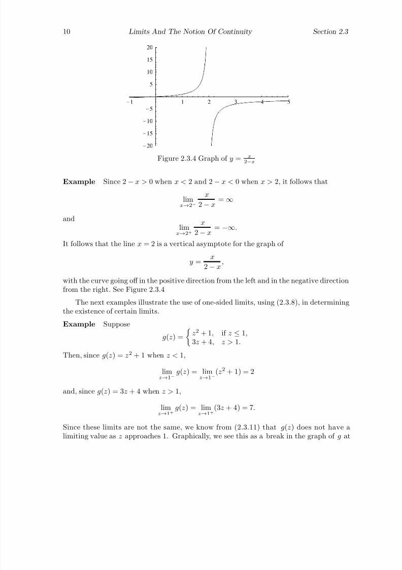
7/27/2019 Calculus 2 (Dan Sloughter)
http://slidepdf.com/reader/full/calculus-2-dan-sloughter 94/598
10 Limits And The Notion Of Continuity Section 2.3
-1 1 2 3 4 5
-20
-15
-10
-5
5
10
15
20
Figure 2.3.4 Graph of y = x2−x
Example Since 2 − x > 0 when x < 2 and 2 − x < 0 when x > 2, it follows that
limx→2−
x
2 − x = ∞and
limx→2+
x
2 − x= −∞.
It follows that the line x = 2 is a vertical asymptote for the graph of
y =x
2 − x,
with the curve going off in the positive direction from the left and in the negative directionfrom the right. See Figure 2.3.4
The next examples illustrate the use of one-sided limits, using (2.3.8), in determiningthe existence of certain limits.
Example Suppose
g(z) =
z2 + 1, if z ≤ 1,3z + 4, z > 1.
Then, since g(z) = z2 + 1 when z < 1,
limz→1−
g(z) = limz→1−
(z2 + 1) = 2
and, since g(z) = 3z + 4 when z > 1,
limz→1+
g(z) = limz→1+
(3z + 4) = 7.
Since these limits are not the same, we know from (2.3.11) that g(z) does not have alimiting value as z approaches 1. Graphically, we see this as a break in the graph of g at
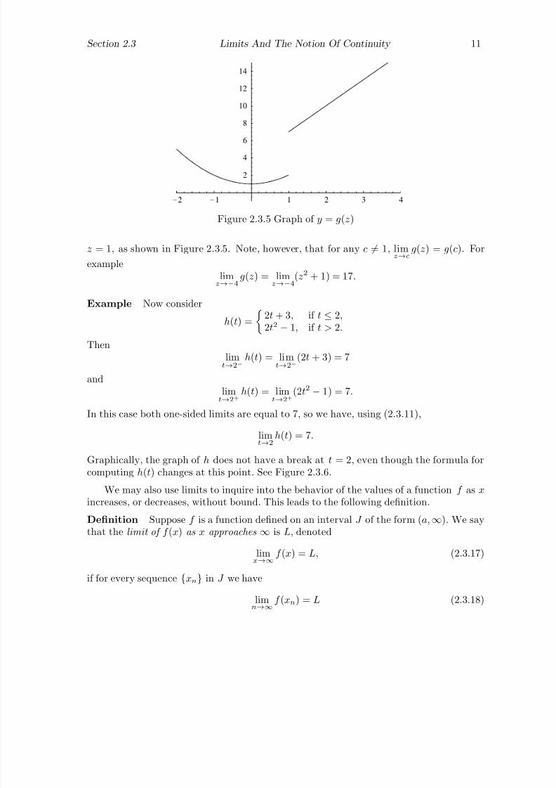
7/27/2019 Calculus 2 (Dan Sloughter)
http://slidepdf.com/reader/full/calculus-2-dan-sloughter 95/598
Section 2.3 Limits And The Notion Of Continuity 11
-2 -1 1 2 3 4
2
4
6
8
10
12
14
Figure 2.3.5 Graph of y = g(z)
z = 1, as shown in Figure 2.3.5. Note, however, that for any c = 1, limz→c
g(z) = g(c). For
example
limz→−4 g(z) = limz→−4(z2
+ 1) = 17.
Example Now consider
h(t) =
2t + 3, if t ≤ 2,2t2 − 1, if t > 2.
Thenlimt→2−
h(t) = limt→2−
(2t + 3) = 7
andlimt→2+
h(t) = limt→2+
(2t2 − 1) = 7.
In this case both one-sided limits are equal to 7, so we have, using (2.3.11),
limt→2
h(t) = 7.
Graphically, the graph of h does not have a break at t = 2, even though the formula forcomputing h(t) changes at this point. See Figure 2.3.6.
We may also use limits to inquire into the behavior of the values of a function f as x
increases, or decreases, without bound. This leads to the following definition.
Definition Suppose f is a function defined on an interval J of the form (a,∞). We saythat the limit of f (x) as x approaches ∞ is L, denoted
limx→∞ f (x) = L, (2.3.17)
if for every sequence {xn} in J we have
limn→∞
f (xn) = L (2.3.18)
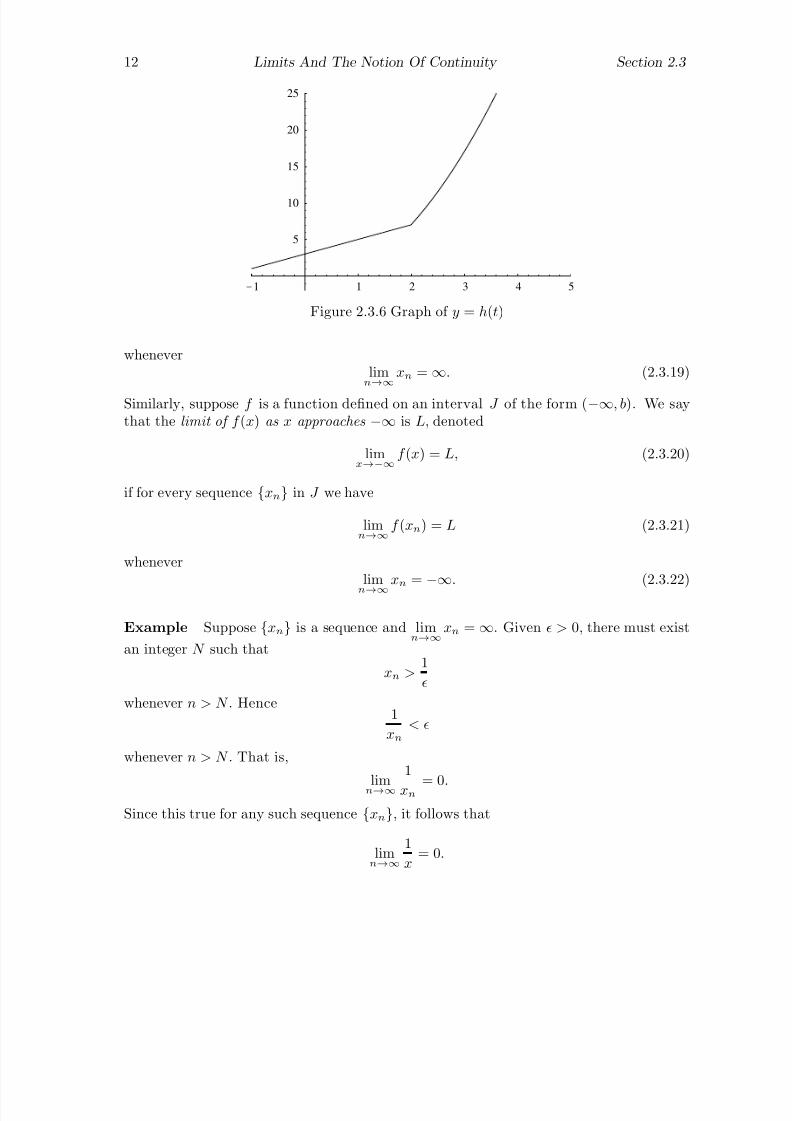
7/27/2019 Calculus 2 (Dan Sloughter)
http://slidepdf.com/reader/full/calculus-2-dan-sloughter 96/598
12 Limits And The Notion Of Continuity Section 2.3
-1 1 2 3 4 5
5
10
15
20
25
Figure 2.3.6 Graph of y = h(t)
wheneverlimn
→∞
xn = ∞. (2.3.19)
Similarly, suppose f is a function defined on an interval J of the form (−∞, b). We saythat the limit of f (x) as x approaches −∞ is L, denoted
limx→−∞
f (x) = L, (2.3.20)
if for every sequence {xn} in J we have
limn→∞
f (xn) = L (2.3.21)
wheneverlimn→∞
xn =−∞
. (2.3.22)
Example Suppose {xn} is a sequence and limn→∞
xn = ∞. Given > 0, there must exist
an integer N such that
xn >1
whenever n > N . Hence1
xn
<
whenever n > N . That is,
limn→∞1
xn = 0.
Since this true for any such sequence {xn}, it follows that
limn→∞
1
x= 0.
7/27/2019 Calculus 2 (Dan Sloughter)
http://slidepdf.com/reader/full/calculus-2-dan-sloughter 97/598
Section 2.3 Limits And The Notion Of Continuity 13
In a similar fashion, we may show that
limn→−∞
1
x= 0.
With these two basic limits, it is possible to compute limits of these types for any rational
function using the same techniques we used in Section 1.2. Namely, given a rationalfunction, dividing numerator and denominator by the highest power appearing in thedenominator simplifies the expression to a form where the limit may be evaluated easily.
Example limx→∞
3x2 + 4x − 6
2x2 − 6x + 2= lim
x→∞
3 +4
x− 6
x2
2 − 6
x+
2
x2
=3
2.
Example limx→∞
3x2 − 6x
4x3 + 2= lim
x→∞
3
x− 6
x2
4 +2
x3
=0
4= 0.
Example We have
limx→−∞
4x3 − 3
2x2 + 6= lim
x→−∞
4x − 3
x2
2 +6
x2
= −∞,
since the denominator is approaching 2 while the numerator decreases without bound asx goes to −∞. Note that, as usual, although the limit does not exist, we make use of thisnotation to indicate the manner in which the limit fails to exist.
Graphically, limx→∞
f (x) = L tells us that the graph of y = f (x) approaches the hori-
zontal line y = L asymptotically as x increases without bound. Similarly, limx→−∞
f (x) = L
tells us that the graph of y = f (x) approaches the horizontal line y = L asymptotically asx decreases without bound.
Example Since
limx→∞
x
x2 + 1= lim
x→∞
1
x
1 +1
x2
= 0
and
limx→−∞
x
x2
+ 1
= limx→−∞
1
x
1 +1
x2
= 0,
we know that the line y = 0, that is, the x-axis, is a horizontal asymptote for the graph of
y =x
x2 + 1.

7/27/2019 Calculus 2 (Dan Sloughter)
http://slidepdf.com/reader/full/calculus-2-dan-sloughter 98/598
14 Limits And The Notion Of Continuity Section 2.3
-20
-10 10 20
-0.6
-0.4
-0.2
0.2
0.4
0.6
Figure 2.3.7 Graph of y = xx2+1
Moreover, sincex
x2
+ 1
> 0
for x > 0 andx
x2 + 1< 0
for x < 0, we know that the approach to the x-axis is from above as x increases and frombelow as x decreases. See Figure 2.3.7.
The following proposition summarizes the basic properties of limits. These are essen-tially restatements of the properties of limits of sequences that we discussed in Section 1.2.The fact that they hold here follows from the way we have defined limits in this section interms of limits of sequences. Moreover, the properties listed in this proposition also holdfor one-sided limits.
Proposition Suppose limx→c
f (x) = L and limx→c
g(x) = M , where L and M are real numbers
and c is a real number, ∞, or −∞. Then
limx→c
kf (x) = kL for any constant k, (2.3.23)
limx→c
(f (x) + g(x)) = L + M, (2.3.24)
limx→c
(f (x) − g(x)) = L − M, (2.3.25)
limx→c
(f (x)g(x)) = LM, (2.3.26)
limx→c
f (x)
g(x) =L
M , (2.3.27)
and, provided p is a rational number for which (f (x)) p and L p are defined,
limx→c
(f (x)) p = LP . (2.3.28)
7/27/2019 Calculus 2 (Dan Sloughter)
http://slidepdf.com/reader/full/calculus-2-dan-sloughter 99/598
Section 2.3 Limits And The Notion Of Continuity 15
Example Using (2.3.28), we have
limx→4
x2 + 3 =
limx→4
(x2 + 3) =√
19.
Example Using the fact hat
√ x2 = |x| =−x, if x < 0,
x, if x ≥ 0,
we have
limx→∞
4x√ x2 + 1
= limx→∞
4√ x2 + 1
x
= limx→∞
4√ x2 + 1√
x2
= limx→∞
4 x2 + 1
x2
= limx→∞
4 1 +
1
x2
= 4
and
limx→−∞
4x√ x2 + 1
= limx→−∞
4√ x2 + 1
x
= limx→−∞ 4√
x2 + 1
−√
x2
= limx→−∞
4
−
x2 + 1
x2
= limx→−∞
4
−
1 +1
x2
= −4.
Hence the lines y = 4 and y = −4 are both horizontal asymptotes for the graph of
y =4x√
x2 + 1.
See Figure 2.3.8.

7/27/2019 Calculus 2 (Dan Sloughter)
http://slidepdf.com/reader/full/calculus-2-dan-sloughter 100/598
16 Limits And The Notion Of Continuity Section 2.3
-10
-5 5 10
-4
-2
2
4
Figure 2.3.8 Graph of y = 4x√ x2+1
Problems
1. Evaluate the following limits.(a) lim
x→2(4x2 − 3x) (b) lim
x→3(x3 − 2x + 3)
(c) limt→1
t2 − 3
t + 5(d) lim
z→−2z + 2
z2 + 3
2. Evaluate the following limits.
(a) limx→2
x3 − 8
x + 2(b) lim
x→3
x2 − x − 6
x − 3
(c) lims→−1
s3 + 1
s4 − 1(d) lim
x→1
√ x − 1
x − 1
(e) limt→2
t3
− 8t − 2
(f) limx→1
x3
− 1x2 − 1
(g) limu→4
u
(u − 4)2(h) lim
x→−2x
x + 2
3. Evaluate the following limits.
(a) limx→1+
(3x2 + 4) (b) limx→3−
1
x − 3
(c) limx→3+
1
x − 3(d) lim
t→−2+t
t + 2
(e) limt→−
2−
t
t + 2(f ) lim
x→10−
x2 − 9x − 10
x2
−8x
−20
4. Evaluate the following limits.
(a) limx→2+
x (b) limx→2−
x(c) lim
x→3−x (d) lim
x→3+x

7/27/2019 Calculus 2 (Dan Sloughter)
http://slidepdf.com/reader/full/calculus-2-dan-sloughter 101/598
Section 2.3 Limits And The Notion Of Continuity 17
(e) limx→0+
cos(x) (f) limx→0+
sin(x)
5. Suppose
g(z) =
3z − 1, if z < 2,7 − z, if z ≥ 2.
(a) Sketch the graph of g.
(b) Find limz→2−
g(z).
(c) Find limz→2+
g(z).
(d) Does limz→2
g(z) exist? If so, what is its value?
6. Suppose
h(t) =
2t + 1, if t ≤ 1,3t − 1, if t > 1.
(a) Sketch the graph of h.
(b) Find limt→1−
h(t).
(c) Find limt→1+
h(t).
(d) Does limt→1
h(t) exist? If so, what is its value?
7. Evaluate the following limits.
(a) limx→∞
(3x + 4) (b) limx→∞
x3 + 3x − 1
2x3 − x2 + 21
(c) limu→∞
u4 + 3u − 6
3u2 + 1(d) lim
z→∞4z2 − 3z + 10
2z3 + 14z + 9
(e) limx→−∞
x5 − 6x + 13x2 + 18x − 25
(f) limx→∞
2√ x + 3√ x + 2
(g) limv→∞
2v + 1
v − 2(h) lim
t→∞
√ t + 1
t + 3
(i) limx→∞
3x + 1√ 4x2 + 5
(j) limx→−∞
3x + 1√ 4x2 + 5
8. Let
f (x) =2x
x − 4.
Find limx→4−
f (x), limx→4+
f (x), limx→−∞
f (x), and limx→∞
f (x). Use this information to sketch
the graph of f .
9. Discuss limx→π
2−
tan(x), limx→π
2+
tan(x), and limx→π
2
tan(x).
10. Do limx→∞
sin(πx) and limn→∞
sin(πn) denote the same thing? Discuss.

7/27/2019 Calculus 2 (Dan Sloughter)
http://slidepdf.com/reader/full/calculus-2-dan-sloughter 102/598
18 Limits And The Notion Of Continuity Section 2.3
11. (a) Explain why
− 1
x≤ sin(x)
x≤ 1
x
for all x .
(b) Use part (a) to find limx→∞
sin(x)
x
.
7/27/2019 Calculus 2 (Dan Sloughter)
http://slidepdf.com/reader/full/calculus-2-dan-sloughter 103/598
Difference Equations
Differential Equations
toSection 2.4
Continuous Functions
Given the work of the previous section, we are now in a position to state a clear definitionof the notion of continuity. We will have several related definitions, but the fundamentaldefinition is that of continuity at a point. Intuitively, continuity at a point c for a functionf means that the values of f for points near c do not change abruptly from the value of f
at c. Section 2.3 has shown that, mathematically, this means that as x approaches c, thevalue of f (x) must be approaching f (c). Hence we have the following basic definition.
Definition We say that a function f is continuous at a point c if
limx→c
f (x) = f (c). (2.4.1)
It is important to note that this definition places three conditions on the behavior of the function f near the point c. Namely, f is continuous at the point c if (1) f is definedat c, (2) lim
x→cf (x) exists, and (3) lim
x→cf (x) = f (c).
Corresponding to one-sided limits, we have the notions of continuity from the left andfrom the right.
Definition We say that a function f is continuous from the left at a point c if
limx→c−
f (x) = f (c). (2.4.2)
We say that a function f is continuous from the right at a point c if
limx→c+
f (x) = f (c). (2.4.3)
Simply to say that a function f is continuous, without specifying some particular point,means that the function is continuous, in the proper sense, at all points where it is defined.Here “in the proper sense” means, for example, that if f is defined only on a closed interval[a, b], then we cannot ask for continuity at a or b, since it is possible to discuss only one-sided limits at these points, but it is possible to inquire about continuity from the right ata and continuity from the left at b.
Definition We say a function f is continuous on the open interval (a, b) if f is continuousat every point in (a, b). We say f is continuous on the closed interval [a, b] if f is continuous
on (a, b), continuous from the right at a, and continuous form the left at b.In the previous section we saw that if f and g are polynomials and c is a point with
g(c) = 0, then
limx→c
f (x)
g(x)=
f (c)
g(c).
1 Copyright c by Dan Sloughter 2000
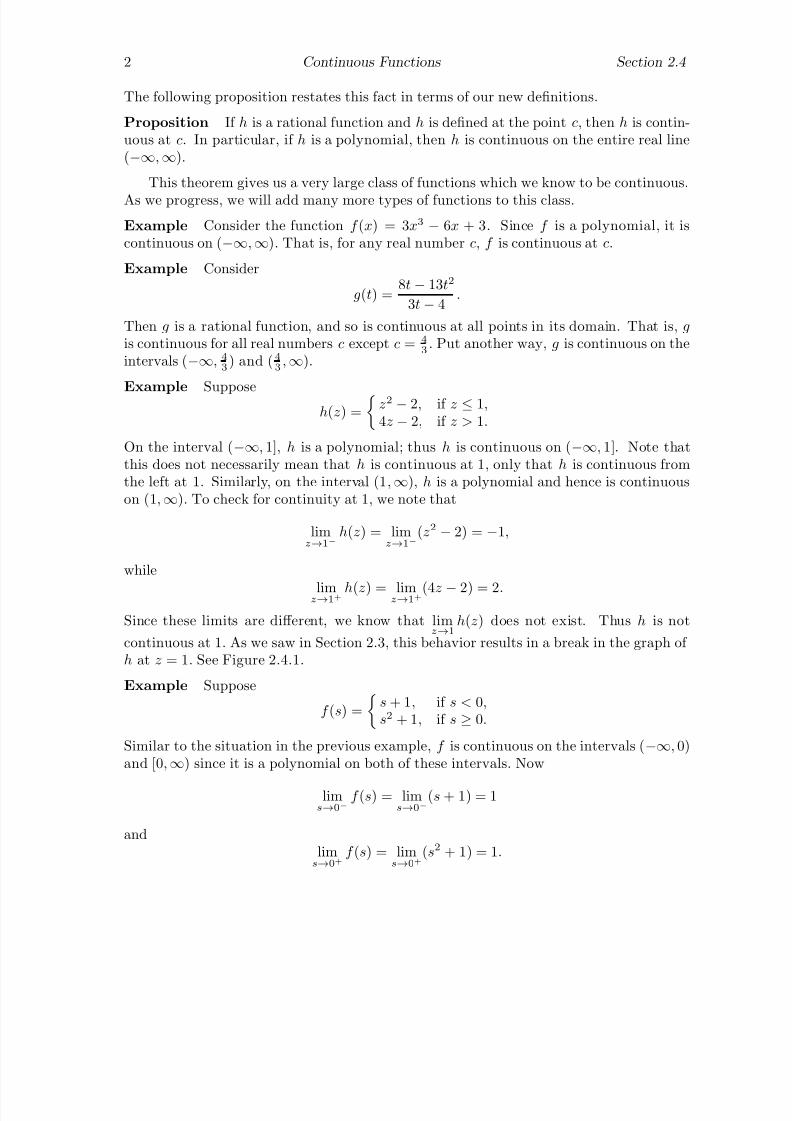
7/27/2019 Calculus 2 (Dan Sloughter)
http://slidepdf.com/reader/full/calculus-2-dan-sloughter 104/598
2 Continuous Functions Section 2.4
The following proposition restates this fact in terms of our new definitions.
Proposition If h is a rational function and h is defined at the point c, then h is contin-uous at c. In particular, if h is a polynomial, then h is continuous on the entire real line(−∞, ∞).
This theorem gives us a very large class of functions which we know to be continuous.
As we progress, we will add many more types of functions to this class.
Example Consider the function f (x) = 3x3 − 6x + 3. Since f is a polynomial, it iscontinuous on (−∞, ∞). That is, for any real number c, f is continuous at c.
Example Consider
g(t) =8t − 13t2
3t − 4.
Then g is a rational function, and so is continuous at all points in its domain. That is, g
is continuous for all real numbers c except c = 4
3. Put another way, g is continuous on the
intervals (−∞, 4
3) and (4
3, ∞).
Example Supposeh(z) =
z2 − 2, if z ≤ 1,4z − 2, if z > 1.
On the interval (−∞, 1], h is a polynomial; thus h is continuous on (−∞, 1]. Note thatthis does not necessarily mean that h is continuous at 1, only that h is continuous fromthe left at 1. Similarly, on the interval (1, ∞), h is a polynomial and hence is continuouson (1, ∞). To check for continuity at 1, we note that
limz→1−
h(z) = limz→1−
(z2 − 2) = −1,
while
limz→1+ h(z) = limz→1+(4z − 2) = 2.
Since these limits are different, we know that limz→1
h(z) does not exist. Thus h is not
continuous at 1. As we saw in Section 2.3, this behavior results in a break in the graph of h at z = 1. See Figure 2.4.1.
Example Suppose
f (s) =
s + 1, if s < 0,s2 + 1, if s ≥ 0.
Similar to the situation in the previous example, f is continuous on the intervals (−∞, 0)and [0, ∞) since it is a polynomial on both of these intervals. Now
lims→0−
f (s) = lims→0−
(s + 1) = 1
andlims→0+
f (s) = lims→0+
(s2 + 1) = 1.

7/27/2019 Calculus 2 (Dan Sloughter)
http://slidepdf.com/reader/full/calculus-2-dan-sloughter 105/598
Section 2.4 Continuous Functions 3
-2 -1 1 2 3 4
-2
2
4
6
8
10
12
Figure 2.4.1 Graph of y = h(z)
-3 -2 -1 1 2 3
-2
2
4
6
8
10
Figure 2.4.2 Graph of y = f (s)
Thus lims→0
f (s) = 1; since f (0) = 1, we have
lims→0
f (s) = 1 = f (0).
Thus f is continuous at 0. Altogether this shows that f is continuous on the entire interval(−∞, ∞). As we see in Figure 2.4.2, the graph of f does not have a break at s = 0.
Example Suppose
g(x) =
x2
−4
x − 2, if x
= 2,
6, if x = 2.
Then, since g is a rational function on the intervals (−∞, 2) and (2, ∞), and is definedthroughout these intervals, g is continuous on the intervals (−∞, 2) and (2, ∞). To check
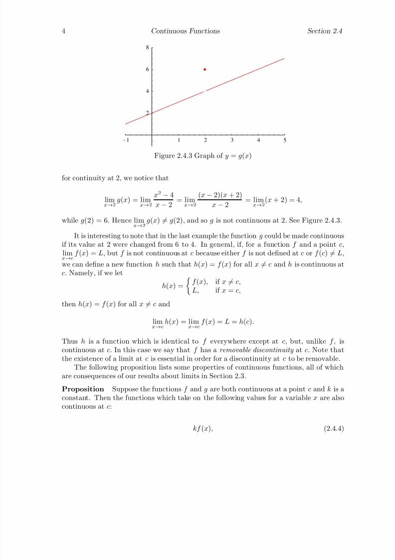
7/27/2019 Calculus 2 (Dan Sloughter)
http://slidepdf.com/reader/full/calculus-2-dan-sloughter 106/598
4 Continuous Functions Section 2.4
-1 1 2 3 4 5
2
4
6
8
Figure 2.4.3 Graph of y = g(x)
for continuity at 2, we notice that
limx→2
g(x) = limx→2
x2
− 4x − 2
= limx→2
(x − 2)(x + 2)x − 2
= limx→2
(x + 2) = 4,
while g(2) = 6. Hence limx→2
g(x) = g(2), and so g is not continuous at 2. See Figure 2.4.3.
It is interesting to note that in the last example the function g could be made continuousif its value at 2 were changed from 6 to 4. In general, if, for a function f and a point c,limx→c
f (x) = L, but f is not continuous at c because either f is not defined at c or f (c) = L,
we can define a new function h such that h(x) = f (x) for all x = c and h is continuous atc. Namely, if we let
h(x) = f (x), if x = c,L, if x = c,
then h(x) = f (x) for all x = c and
limx→c
h(x) = limx→c
f (x) = L = h(c).
Thus h is a function which is identical to f everywhere except at c, but, unlike f , iscontinuous at c. In this case we say that f has a removable discontinuity at c. Note thatthe existence of a limit at c is essential in order for a discontinuity at c to be removable.
The following proposition lists some properties of continuous functions, all of whichare consequences of our results about limits in Section 2.3.
Proposition Suppose the functions f and g are both continuous at a point c and k is aconstant. Then the functions which take on the following values for a variable x are alsocontinuous at c:
kf (x), (2.4.4)
7/27/2019 Calculus 2 (Dan Sloughter)
http://slidepdf.com/reader/full/calculus-2-dan-sloughter 107/598
Section 2.4 Continuous Functions 5
f (x) + g(x), (2.4.5)
f (x) − g(x), (2.4.6)
f (x)g(x), (2.4.7)
f (x)
g(x) , (2.4.8)
provided g(c) = 0, and(f (x)) p, (2.4.9)
provided p is a rational number and (f (x)) p is defined on an open interval containing c.
Example It follows from (2.4.9) that functions of the form f (x) = x p, where p is arational number, are continuous throughout their domain. For example, f (x) =
√ x is
continuous on [0, ∞).
Example Using (2.4.8) and (2.4.9),
g(t) = √ 3t + 22t
is continuous for all points t where 3t + 2 ≥ 0 and t = 0. Thus g is continuous on theintervals [− 2
3, 0) and (0, ∞).
At this point we have the tools necessary to determine questions of continuity foralgebraic functions. We will now show that the sine and cosine functions are continuouson (−∞, ∞). For 0 < x < π
2, consider the point C = (cos(x), sin(x)) on the unit circle
centered at the origin. If we let A = (0, 0) and B = (1, 0), as in Figure 2.4.4, then the areaof ABC is
1
2sin(x).
The area of the sector of the circle cut off by the arc from B to C is the fraction x2π
of thearea of the entire circle; hence, this area is
x
2ππ =
x
2.
Since this sector contains ABC , we have
0 <1
2sin(x) <
x
2,
from which it follows that0 < sin(x) < x.
Sincelim
x→0+x = 0,

7/27/2019 Calculus 2 (Dan Sloughter)
http://slidepdf.com/reader/full/calculus-2-dan-sloughter 108/598
6 Continuous Functions Section 2.4
A
B
C
(1, 0)
(0, 1)
x
sin( ) x
Figure 2.4.4
it follows that
limx→0+
sin(x) = 0.
Moreover, we also have
limx→0−
sin(x) = limx→0+
sin(−x) = − limx→0+
sin(x) = 0,
so
limx→0
sin(x) = 0. (2.4.10)
Since sin(0) = 0, this shows that sine is continuous at 0. Now for −π2
< x < π2
,
cos(x) =
1 − sin2(x).
Hence
limx→0
cos(x) = limx→0
1 − sin2(x) =
1 − lim
x→0
sin2(x) = 1. (2.4.11)
Since cos(0) = 1, this shows that cosine is continuous at 0. For an arbitrary c, we have,using the angle addition formulas for sine and cosine,
limx→c
sin(x) = limh→0
sin(c + h)
= limh→0(sin(c)cos(h) + cos(c)sin(h))= sin(c) lim
h→0
cos(h) + cos(c) limh→0
sin(h)
= sin(c)(1) + cos(c)(0)
= sin(c)

7/27/2019 Calculus 2 (Dan Sloughter)
http://slidepdf.com/reader/full/calculus-2-dan-sloughter 109/598
Section 2.4 Continuous Functions 7
andlimx→c
cos(x) = limh→0
cos(c + h)
= limh→0
(cos(c)cos(h) − sin(c)sin(h))
= cos(c) limh→0
cos(h) − sin(c) limh→0
sin(h)
= cos(c)(1) − sin(c)(0)
= cos(c)
.
Thus we have the following proposition.
Proposition The sine and cosine functions are continuous on (−∞, ∞).
The next proposition is then an immediate consequence of (2.4.8).
Proposition The tangent, cotangent, secant and cosecant functions are continuous atall points in their respective domains.
We have not yet considered the composition of continuous functions. Suppose g iscontinuous at c and f is continuous at g(c). If {xn} is a sequence converging to c, thenwe know, since g is continuous at c, that the sequence {g(xn)} will converge to g(c). Butthen, since f is continuous at g(c), the sequence {f (g(xn))} will converge to f (g(c)). Thatis,
limx→c
f ◦ g(x) = limx→c
f (g(x)) = f (g(c)) = f ◦ g(c). (2.4.12)
Hence f ◦ g is continuous at c.
Proposition If g is continuous at c and f is continuous at g(c), then f ◦ g is continuousat c.
Example The function h(t) = cos(3t + 4) is continuous on (−∞, ∞) since it is thecomposition of the functions g(t) = 3t +4 and f (t) = cos(t), both of which are continuouson (−∞, ∞).
Example Consider the function
g(t) =sin(t2 + 1)
t.
Now the numerator of g is continuous on (−∞, ∞) since it is the composition of h(t) = t2+1and f (t) = sin(t), both of which are continuous on (−∞, ∞). It follows that, since thedenominator of g is continuous on (
−∞,∞
), g is continuous at all points for which thedenominator is not equal to zero, that is, for all t = 0. Thus g is continuous on the intervals(−∞, 0) and (0, ∞).
In Section 2.5 we will consider two properties of continuous functions which partiallyexplain the important role they play in calculus.
7/27/2019 Calculus 2 (Dan Sloughter)
http://slidepdf.com/reader/full/calculus-2-dan-sloughter 110/598
8 Continuous Functions Section 2.4
Problems
1. Discuss the continuity of the given function at the specified point.
(a) f (t) = 3t2 − 6 at t = 2 (b) f (x) =2x + 5
x − 16at x = 17
(c) f (x) = 2x + 5x − 16
at x = 16 (d) h(s) = s
2
− 1s + 1
at s = 1
(e) h(s) =s2 − 1
s + 1at s = −1
2. Discuss the continuity of the function
g(t) =
4t − 1, if t ≤ 2,t + 5, if t > 2,
at t = 2.
3. Discuss the continuity of the following functions.
(a) g(x) = 4x23 − x18 + 16x − 3 (b) f (t) =t2 − t − 6
t + 2
(c) g(t) = 32t − 8
t(d) f (u) =
8
u2 − 4
(e) f (t) =
t2 − 4 (f) g(x) =1√
9 − x2
4. Discuss the continuity of the function
f (x) =
3x + 2, if x < 1,3x + 1, if x ≥ 1.
5. Discuss the continuity of the function
h(z) =
z2 − 1, if z ≤ −1,z − 1, if z > −1.
6. The function
f (t) =t2 − 7t + 12
t − 4
is not continuous at t = 4. Is this discontinuity removable? If it is, define a newfunction g which agrees with f whenever t = 4, but is continuous at 4.
7. The functionf (t) =
t2 − 7t + 12
t − 5
is not continuous at t = 5. Is this discontinuity removable? If it is, define a newfunction g which agrees with f whenever t = 5, but is continuous at 5.

7/27/2019 Calculus 2 (Dan Sloughter)
http://slidepdf.com/reader/full/calculus-2-dan-sloughter 111/598
Section 2.4 Continuous Functions 9
8. Explain why g(x) = x2 sin(x2 + 1) is continuous on (−∞, ∞).
9. Recall that the Heaviside function is defined by
H (t) =
0, if t < 0,1, if t ≥ 0.
(a) Discuss the continuity of f (t) = H (t2 + 1). Graph f on the interval [−5, 5].
(b) Discuss the continuity of g(t) = H (t2 − 1). Graph g on the interval [−5, 5].
(c) Discuss the continuity of h(t) = H (sin(πt)). Graph h on the interval [−5, 5].
10. Discuss the continuity of f (x) = x and g(x) = x.
11. Discuss the continuity of f (x) = sin(x) and g(x) = sin(x).

7/27/2019 Calculus 2 (Dan Sloughter)
http://slidepdf.com/reader/full/calculus-2-dan-sloughter 112/598
Difference Equations
Differential Equations
to
Section 2.5
Some ConsequencesOf Continuity
In this section we consider two properties of functions which are very closely connectedto the notion of continuity. The first of these, the Intermediate Value Theorem, says thatthe graph of a continuous function is a connected continuum in the sense of our normalintuition. That is, the theorem states that as a continuous function changes from one valueto another, it must take on every intermediate value. The second theorem, the ExtremeValue Theorem, says that a continuous function on a closed interval attains a maximumand a minimum value on that interval. This is related to our intuitive notion that if wedraw a continuous curve with definite beginning and ending points, then the curve hasa point where it is higher than at any other point and a point where it is lower thanat any other point. We shall not attempt formal justifications of these theorems; such
justifications require inquiries into the subtleties of real numbers which are best left tomore advanced courses.
We will begin with a statement of the Intermediate Value Theorem, followed by aconsideration of its application to solving equations.
Intermediate Value Theorem If f is a continuous function on a closed interval [a, b]and m is any number between f (a) and f (b), then there is a number c in the interval [a, b]such that f (c) = m.
Example Since f (t) = sin(t) is continuous on [0,
π
2 ] with f (0) = 0 and f (π
2 ) = 1, thefact that 0 < 5
2π< 1 guarantees that there is a number c in [0, π
2] such that
f (c) =5
2π.
Graphically, the situation is as in Figure 2.5.1. Of course, the theorem tells us neitherthe value of c nor how we might find it. The Intermediate Value Theorem is an existencetheorem; it guarantees the existence of a certain value, but does not directly provide anymethod for calculating the value.
Example Suppose f (t) is the height, in inches, of a certain plant t days after it first
emerges from the soil. From our knowledge of how plants grow, it would be reasonableto assume that f is a continuous function. Also, we have f (0) = 0. Now if f (10) = 12,then we know, for example, that there is some time c, 0 < c < 10, such that f (c) = 5.Of course, this is not surprising, and, in fact, we did not have to bring the subject of continuous functions into the problem in order to realize that between the time when theplant was 0 inches tall and the time when it was 12 inches there was a time when itwas 5 inches tall. However, the point of an example like this is to emphasize that theIntermediate Value Theorem simply states a property that we should expect continuous
1 Copyright c by Dan Sloughter 2000
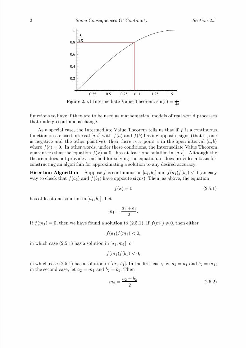
7/27/2019 Calculus 2 (Dan Sloughter)
http://slidepdf.com/reader/full/calculus-2-dan-sloughter 113/598
2 Some Consequences Of Continuity Section 2.5
0.25 0.5 0.75 1 1.25 1.5
0.2
0.4
0.6
0.8
1
c
5
2π
Figure 2.5.1 Intermediate Value Theorem: sin(c) = 5
2π
functions to have if they are to be used as mathematical models of real world processes
that undergo continuous change.As a special case, the Intermediate Value Theorem tells us that if f is a continuous
function on a closed interval [a, b] with f (a) and f (b) having opposite signs (that is, oneis negative and the other positive), then there is a point c in the open interval (a, b)where f (c) = 0. In other words, under these conditions, the Intermediate Value Theoremguarantees that the equation f (x) = 0. has at least one solution in [a, b]. Although thetheorem does not provide a method for solving the equation, it does provides a basis forconstructing an algorithm for approximating a solution to any desired accuracy.
Bisection Algorithm Suppose f is continuous on [a1, b1] and f (a1)f (b1) < 0 (an easyway to check that f (a1) and f (b1) have opposite signs). Then, as above, the equation
f (x) = 0 (2.5.1)
has at least one solution in [a1, b1]. Let
m1 =a1 + b1
2.
If f (m1) = 0, then we have found a solution to (2.5.1). If f (m1) = 0, then either
f (a1)f (m1) < 0,
in which case (2.5.1) has a solution in [a1, m1], or
f (m1)f (b1) < 0,
in which case (2.5.1) has a solution in [m1, b1]. In the first case, let a2 = a1 and b2 = m1;in the second case, let a2 = m1 and b2 = b1. Then
m2 =a2 + b2
2(2.5.2)

7/27/2019 Calculus 2 (Dan Sloughter)
http://slidepdf.com/reader/full/calculus-2-dan-sloughter 114/598
Section 2.5 Some Consequences Of Continuity 3
will approximate a solution to (2.5.1) with an error less than
b2 − a2
2. (2.5.3)
Proceed in a the same manner to define an, bn, and mn for n = 3, 4, 5, . . .. That is, if wehave found an−1, bn−1, and mn−1, and f (mn−1) = 0, let
an = an−1 and bn = mn−1 if f (an−1)f (mn−1) < 0 (2.5.4)
andan = mn−1 and bn = bn−1 if f (mn−1)f (bn−1) < 0. (2.5.5)
Then
mn =an + bn
2(2.5.6)
will approximate a solution of (2.5.1) with an error less than
bn − an
2. (2.5.7)
Repeat the procedure as many times as necessary to obtain the desired level of accuracy.
Example Suppose we wish to find a root to the equation
x5 + x = 1. (2.5.8)
First note that solving (2.5.8) is equivalent to solving
x5
+ x − 1 = 0. (2.5.9)
Lettingf (x) = x5 + x − 1,
we may write (2.5.9) as f (x) = 0. To find an initial interval [a1, b1], we graph f as inFigure 2.5.2. Noting that f (0) = −1 and f (1) = 1, we may start with a1 = 0 and b1 = 1.That is, (2.5.8) has a solution in the [0, 1]. Then
m1 =0 + 1
2= 0.5.
Now f (0.5) = −0.468750, so f (0.5)f (1) < 0. Hence a2 = 0.5, b2 = 1, and
m2 =0.5 + 1.0
2= 0.75.
Now f (0.75) = −0.012695, so f (0.75)f (1) < 0. Hence a3 = 0.75, b3 = 1, and
m3 =0.75 + 1.00
2= 0.875.

7/27/2019 Calculus 2 (Dan Sloughter)
http://slidepdf.com/reader/full/calculus-2-dan-sloughter 115/598
4 Some Consequences Of Continuity Section 2.5
-3 -2 -1 1 2 3
-6
-4
-2
2
4
6
Figure 2.5.2 Graph of f (x) = x5 + x − 1
At this stage we know that 0.875 is an approximation for a solution to (2.5.8) with anerror of no more than
1.00 − 0.75
2= 0.125.
We may continue in this manner until we attain any desired level of accuracy. The followingtable gives the values of an and bn for n = 1, 2, 3, . . . , 10.
an bn mn f (an) f (bn) f (mn)0.000000000 1.000000000 0.500000000 −1.000000000 1.000000000 −0.4687500000.500000000 1.000000000 0.750000000 −0.468750000 1.000000000 −0.0126953000.750000000 1.000000000 0.875000000 −0.012695300 1.000000000 0.3879090000.750000000 0.875000000 0.812500000
−0.012695300 0.387909000 0.166593000
0.750000000 0.812500000 0.781250000 −0.012695300 0.166593000 0.0722883000.750000000 0.781250000 0.765625000 −0.012695300 0.072288300 0.0287006000.750000000 0.765625000 0.757812500 −0.012695300 0.028700600 0.0077369900.750000000 0.757812500 0.753906250 −0.012695300 0.007736990 −0.0025445400.753906250 0.757812500 0.755859380 −0.002544540 0.007736990 0.0025797700.753906250 0.755859380 0.754882815 −0.002544540 0.002579770
Rounding to three decimal places, we see that x = 0.755 approximates a solution of (2.5.8)with an error of no more than, to three decimal places,
0.756−
0.754
2 = 0.001.
In Section 3.6 we will discuss another method, called Newton’s method, for approx-imating a solution to an equation of the form f (x) = 0. At that time we will see thatNewton’s method is faster than the bisection algorithm. However, we will also see thatthere are conditions under which Newton’s method will fail, whereas the bisection algo-rithm will always work.
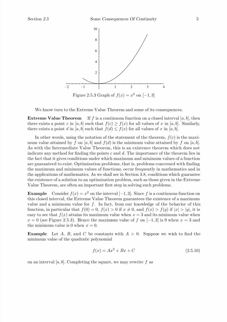
7/27/2019 Calculus 2 (Dan Sloughter)
http://slidepdf.com/reader/full/calculus-2-dan-sloughter 116/598
Section 2.5 Some Consequences Of Continuity 5
-2 -1 1 2 3 4
2
4
6
8
10
Figure 2.5.3 Graph of f (x) = x2 on [−1, 3]
We know turn to the Extreme Value Theorem and some of its consequences.
Extreme Value Theorem If f is a continuous function on a closed interval [a, b], thenthere exists a point c in [a, b] such that f (c) ≥ f (x) for all values of x in [a, b]. Similarly,there exists a point d in [a, b] such that f (d) ≤ f (x) for all values of x in [a, b].
In other words, using the notation of the statement of the theorem, f (c) is the maxi-mum value attained by f on [a, b] and f (d) is the minimum value attained by f on [a, b].As with the Intermediate Value Theorem, this is an existence theorem which does notindicate any method for finding the points c and d. The importance of the theorem lies inthe fact that it gives conditions under which maximum and minimum values of a functionare guaranteed to exist. Optimization problems, that is, problems concerned with finding
the maximum and minimum values of functions, occur frequently in mathematics and inthe applications of mathematics. As we shall see in Section 3.8, conditions which guaranteethe existence of a solution to an optimization problem, such as those given in the ExtremeValue Theorem, are often an important first step in solving such problems.
Example Consider f (x) = x2 on the interval [−1, 3]. Since f is a continuous function onthis closed interval, the Extreme Value Theorem guarantees the existence of a maximumvalue and a minimum value for f . In fact, from our knowledge of the behavior of thisfunction, in particular that f (0) = 0, f (x) > 0 if x = 0, and f (x) > f (y) if |x| > |y|, it iseasy to see that f (x) attains its maximum value when x = 3 and its minimum value whenx = 0 (see Figure 2.5.3). Hence the maximum value of f on [−1, 3] is 9 when x = 3 and
the minimum value is 0 when x = 0.
Example Let A, B, and C be constants with A > 0. Suppose we wish to find theminimum value of the quadratic polynomial
f (x) = Ax2 + Bx + C (2.5.10)
on an interval [a, b]. Completing the square, we may rewrite f as
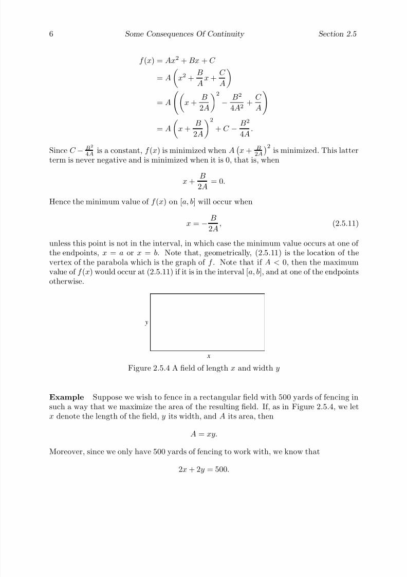
7/27/2019 Calculus 2 (Dan Sloughter)
http://slidepdf.com/reader/full/calculus-2-dan-sloughter 117/598
6 Some Consequences Of Continuity Section 2.5
f (x) = Ax2 + Bx + C
= A
x2 +
B
Ax +
C
A
= A
x + B2A2
− B
2
4A2 + C A
= A
x +
B
2A
2
+ C − B2
4A.
Since C − B2
4Ais a constant, f (x) is minimized when A
x + B
2A
2is minimized. This latter
term is never negative and is minimized when it is 0, that is, when
x +B
2A= 0.
Hence the minimum value of f (x) on [a, b] will occur when
x = − B
2A, (2.5.11)
unless this point is not in the interval, in which case the minimum value occurs at one of the endpoints, x = a or x = b. Note that, geometrically, (2.5.11) is the location of thevertex of the parabola which is the graph of f . Note that if A < 0, then the maximumvalue of f (x) would occur at (2.5.11) if it is in the interval [a, b], and at one of the endpointsotherwise.
x
y
Figure 2.5.4 A field of length x and width y
Example Suppose we wish to fence in a rectangular field with 500 yards of fencing in
such a way that we maximize the area of the resulting field. If, as in Figure 2.5.4, we letx denote the length of the field, y its width, and A its area, then
A = xy.
Moreover, since we only have 500 yards of fencing to work with, we know that
2x + 2y = 500.
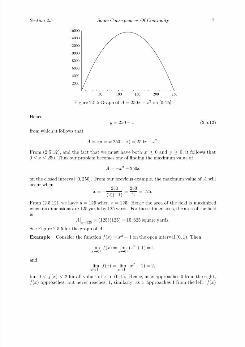
7/27/2019 Calculus 2 (Dan Sloughter)
http://slidepdf.com/reader/full/calculus-2-dan-sloughter 118/598
Section 2.5 Some Consequences Of Continuity 7
50 100 150 200 250
2000
4000
6000
8000
10000
12000
14000
16000
Figure 2.5.5 Graph of A = 250x − x2 on [0, 25]
Hence
y = 250 − x, (2.5.12)
from which it follows that
A = xy = x(250− x) = 250x − x2.
From (2.5.12), and the fact that we must have both x ≥ 0 and y ≥ 0, it follows that0 ≤ x ≤ 250. Thus our problem becomes one of finding the maximum value of
A = −x2 + 250x
on the closed interval [0, 250]. From our previous example, the maximum value of A willoccur when
x = − 250
(2)(−1)=
250
2= 125.
From (2.5.12), we have y = 125 when x = 125. Hence the area of the field is maximizedwhen its dimensions are 125 yards by 125 yards. For these dimensions, the area of the fieldis
Ax=125
= (125)(125) = 15, 625 square yards.
See Figure 2.5.5 for the graph of A.
Example Consider the function f (x) = x2 + 1 on the open interval (0, 1). Then
limx→0+
f (x) = limx→0+
(x2 + 1) = 1
andlimx→1−
f (x) = limx→1−
(x2 + 1) = 2,
but 0 < f (x) < 2 for all values of x in (0, 1). Hence, as x approaches 0 from the right,f (x) approaches, but never reaches, 1; similarly, as x approaches 1 from the left, f (x)

7/27/2019 Calculus 2 (Dan Sloughter)
http://slidepdf.com/reader/full/calculus-2-dan-sloughter 119/598
8 Some Consequences Of Continuity Section 2.5
approaches, but never reaches, 2. Thus f is an example of a continuous function on anopen interval which attains neither a maximum nor a minimum value on the interval.Hence we see why the interval in the statement of the Extreme Value Theorem must be aclosed interval.
Problems
1. Use the bisection algorithm to approximate a solution to each of the following equationson the given interval. Your answer should have an error of no more than 0.005.
(a) x2 − 2 = 0 on [0, 4] (b) x5 − 6x3 + 2x = 2 on [−1, 1]
(c) cos(x) = x on [0, π] (d) 2 sin(x) =√
x + 1 on [0, 2]
2. (a) Plot the graph of g(t) = t2 − cos2(t) on [−π, π].
(b) How many solutions are there to the equation t2 = cos2(t)?
(c) Use the bisection algorithm to estimate the solutions to the equation t2 = cos2(t).
State your answers with an error less than 0.005.3. Suppose if the market price for a certain product is p dollars, then the demand for
that product will be
D( p) =50000 p + 10000
p2units.
At the same time, suppose that at a price of p dollars producers will be willing tosupply
S ( p) =1
3 p2 + 2 p units.
(a) Plot the graphs of D and S on the same graph.
(b) Use the bisection algorithm to estimate the solution to the equation
D( p) = S ( p).
This point is called the equilibrium price because it is the price for which theconsumers’ demand for the product is exactly equal to the manufacturers’ supply.
(c) How many units of the product will be manufactured at the equilibrium price?
(d) What would happen if the producers raised the price above the equilibrium price?What would happen if they lowered the price below the equilibrium price?
(e) What would happen if the producers increased production? What would happen
if they lowered production?4. A farmer wishes to fence in a rectangular field, using a straight river for one side, with
500 yards of fencing. What should the dimensions of the field be in order to maximizethe area of the field?
5. When a potter sells his pots for p dollars apiece, he can sell D( p) = 750−50 p of them.Suppose the pots cost him $5.00 apiece to make. What price should the potter chargein order to maximize his profit?

7/27/2019 Calculus 2 (Dan Sloughter)
http://slidepdf.com/reader/full/calculus-2-dan-sloughter 120/598
Section 2.5 Some Consequences Of Continuity 9
6. Let h(t) = t4 − 1.
(a) Does h have a maximum value on [−1, 2)?
(b) Does h have a minimum value on [−1, 2)?
(c) Are the results of (a) and (b) consistent with the Extreme Value Theorem? Ex-
plain.
7. Recall that the Heavidside function is defined by
H (t) =
0, if t < 0,1, if t ≥ 0.
(a) Note that H (−1) = 0 and H (1) = 1. Is there a point c in (−1, 1) such thatH (c) = 0.5?
(b) Is the result of (a) consistent with the Intermediate Value Theorem?
(c) Does H attain a maximum value on [−1, 1]? Does H attain a minimum value on[−1, 1]?
(d) Are the results of (c) consistent with the Extreme Value Theorem?
8. Suppose g is defined on [−1, 1] by
g(t) =
|t|, if t = 0,1, if t = 0.
(a) Does g attain a maximum value on [−1, 1]? If so, at what points?
(b) Does g attain a minimum value on [−1, 1]? If so, at what points?(c) Are the results of (a) and (b) consistent with the Extreme Value Theorem?
9. Suppose f and g are continuous on [0, 1], f (0) < g(0) and f (1) > g(1). Show thatthere exists a point c in the open interval (0, 1) such that f (c) = g(c).
10. Suppose f is continuous on [0, 1] and 0 ≤ f (x) ≤ 1 for all x in [0, 1]. Show that thereexists a point c in [0, 1] such that f (c) = c.

7/27/2019 Calculus 2 (Dan Sloughter)
http://slidepdf.com/reader/full/calculus-2-dan-sloughter 121/598
Difference Equations
Differential Equations
to
Section 3.1
Best Affine Approximations
We are now in a position to discuss the two central problems of calculus as mentioned inSection 1.1. In this chapter we will take up the problem of finding tangent lines; in Chapter4 we will consider the problem of finding areas. We choose this order only because thework we do in solving the tangent line problem in this chapter will be of use, through theFundamental Theorem of Calculus, in solving area problems in the next.
We begin with some preliminary notation and terminology. If f is a function withdomain contained in the set A and range contained in the set B, then we may denote thisfact by writing f : A
→B. For example, if g(t) =
√ 1−
t2 and R denotes the set of realnumbers, then the statements g : R → R, g : [−1, 1] → R, and g : [−1, 1] → [0, 1] are allcorrect. We will work exclusively with functions of the form f : R → R until Chapter 7,where we will introduce functions of the form f : R→ C and f : C→ C, where C denotesthe set of complex numbers.
We call a function f : R→ R linear if there is a constant m such that f (x) = mx forall values of x. Graphically, linear functions are functions whose graphs are straight linespassing through the origin. We call a function f : R → R affine if there are constantsm and b such that f (x) = mx + b for all values of x. Graphically, affine functions arefunctions whose graphs are straight lines, not necessarily passing through the origin. Putanother way, an affine function is a first degree polynomial. Thus f (x) = 3x is both linear
and affine, whereas g(t) = 4t− 6 is affine but not linear.The problem of finding the tangent line for the graph of a given function f at a point(x0, y0) is really the problem of finding the affine function T which best approximatesf for points close to x0. In this section we will discuss how to solve this problem. Inthe remaining sections of this chapter we will consider techniques for finding best affineapproximations and discuss some applications. In Chapter 5 we will see how to improveupon affine approximations by using higher degree polynomials.
The following example should help to make these ideas more concrete.
Example Consider the problem of approximating the function f (x) =√
x for values of x close to 1. For a first approximation, we might say that
√ x ≈ 1
for x close to 1. In other words, if we let
T (x) = 1
for all x, then we are saying that the affine function T is a good approximation for f whenx is close to 1. Two facts characterize this statement. First, T and f agree at 1; that is,
T (1) = 1 = f (1). (3.1.1)
1 Copyright c by Dan Sloughter 2000

7/27/2019 Calculus 2 (Dan Sloughter)
http://slidepdf.com/reader/full/calculus-2-dan-sloughter 122/598
2 Best Affine Approximations Section 3.1
1 2 3 4
0.5
1
1.5
2
r ( ) x
Figure 3.1.1 Graph of f (x) =√
x and an approximating affine function
Second, the error committed by approximating f by T goes to 0 as x approaches 1. That
is, if we letr(x) = f (x)− T (x),
then r(x) is the error made in approximating f by T at the point x, and
limx→1
r(x) = limx→1
(f (x)− T (x)) = limx→1
(√
x− 1) = 1− 1 = 0. (3.1.2)
Hence we have found an affine function which approximates our function f about x = 1according to some reasonable criterion.
However, it is easy to see that any affine function T whose graph passes through (1, 1)will satisfy (3.1.1) and (3.1.2). First note that if the graph of T is a straight line passingthrough (1, 1) with slope m, then, using the point-slope form for the equation of a line,
T (x) = m(x− 1) + 1.
It then follows thatT (1) = 1 = f (1)
and, if we again let r(x) = f (x)− T (x),
limx→1
r(x) = limx→1
(f (x)− T (x)) = limx→1
(√
x− (m(x− 1) + 1)) = 1 − 1 = 0.
See Figure 3.1.1 for the geometrical interpretation. So now we must ask if there is a value
of m
which makesT
, in some sense, better than any other affine function for approximatingf for x near 1. In answering this question, it is convenient to let h = x− 1 and to define
R(h) = r(1 + h) = f (1 + h)− T (1 + h),
the amount of error committed when f is approximated by T at a point a distance h from1. Since h approaches 0 as x approaches 1, (3.1.1) and (3.1.2) become, in terms of R,
R(0) = 0 (3.1.3)

7/27/2019 Calculus 2 (Dan Sloughter)
http://slidepdf.com/reader/full/calculus-2-dan-sloughter 123/598
Section 3.1 Best Affine Approximations 3
-0.2 -0.1 0 0.1 0.2
0.002
0.004
0.006
0.008
.
m = 0.5
Figure 3.1.2 Graphs of |R(h)| for different values of m
and
limh→0 R(h) = 0. (3.1.4)
In this case, we have
R(h) =√
1 + h− (m((1 + h)− 1) + 1) =√
1 + h− (mh + 1).
Figure 3.1.2 shows the graphs of |R(h)| on the interval [−0.2, 0.2] for m = 0.1, 0.3, 0.4,0.5, 0.6, 0.7, and 0.9. Note that although all these functions approach 0 as h approaches 0,one of the graphs clearly stands out from the others. Namely, when m = 0.5, the absolutevalue of the approximation error appears to approach 0 at a significantly faster rate thandoes the error for other values of m. To see why this is so, consider that
R(h) =√
1 + h− (mh + 1)
= (√
1 + h− (mh + 1))
√ 1 + h + (mh + 1)√ 1 + h + (mh + 1)
=1 + h− (mh + 1)2√
1 + h + mh + 1
=1 + h− (m2h2 + 2mh + 1)√
1 + h + mh + 1
=h(1− 2m)−m2h2
√ 1 + h + mh + 1.
Note that when m = 0.5, the numerator reduces to −m2h2, whereas for other values of m
there is also the term h(1− 2m). This explains why in Figure 3.1.2 the graph for m = 0.5looks parabolic while the other graphs appear more as straight lines. Moreover, since, forsmall values of h, h2 is significantly smaller than h (for example, (0.001)2 = 0.000001 ismuch smaller than 0.001), we see why the approximation errors when m = 0.5 are so muchsmaller than they are for other values of m.

7/27/2019 Calculus 2 (Dan Sloughter)
http://slidepdf.com/reader/full/calculus-2-dan-sloughter 124/598
4 Best Affine Approximations Section 3.1
Intuitively, we should think that for small values of h, R(h) behaves like a multiple of h when m = 0.5 and like a multiple of h2 when m = 0.5. To see this algebraically, it isuseful to consider the quotient
R(h)
h=
1− 2m−m2h
√ 1 + h + mh + 1.
Notice that
limh→0
R(h)
h=
1− 2m
2,
which is 0 only when m = 0.5. We interpret this as an indication that R(h) behaves likea multiple of h for small values of h when m = 0.5, but approaches 0 more rapidly than h
when m = 0.5.
In our example, we saw that
limh→0
R(h)
h
= 0
when m = 0.5, but
limh→0
R(h)
h= 0
for all other values of m. We distinguish the two cases by saying that in the first case R(h)is o(h), whereas in the second case R(h) is only O(h).
Definition A function f is said to be o(h) if
limh→0
f (h)
h= 0. (3.1.5)
Definition A function f is said to be O(h) if there exist constants M and > 0 suchthat f (h)
h
≤ M (3.1.6)
whenever − < h < .
Note that if
limh→0
f (h)
h= L,
then we may find an > 0 such thatf (h)
h− L
≤ 1
whenever |h| < . Hence
L− 1 ≤ f (h)
h≤ L + 1
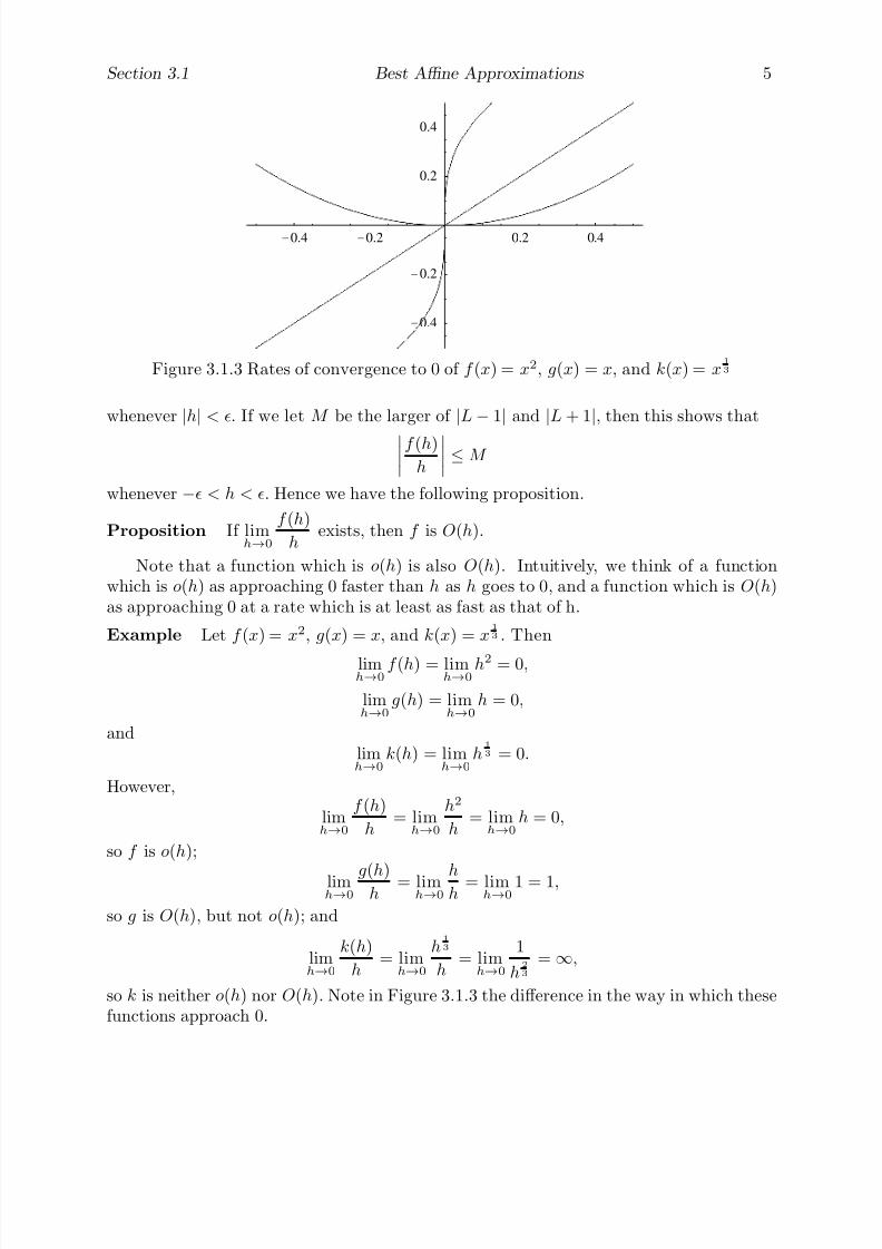
7/27/2019 Calculus 2 (Dan Sloughter)
http://slidepdf.com/reader/full/calculus-2-dan-sloughter 125/598
Section 3.1 Best Affine Approximations 5
-0.4 -0.2 0.2 0.4
-0.4
-0.2
0.2
0.4
Figure 3.1.3 Rates of convergence to 0 of f (x) = x2, g(x) = x, and k(x) = x1
3
whenever
|h
|< . If we let M be the larger of
|L
−1
|and
|L + 1
|, then this shows thatf (h)
h
≤ M
whenever − < h < . Hence we have the following proposition.
Proposition If limh→0
f (h)
hexists, then f is O(h).
Note that a function which is o(h) is also O(h). Intuitively, we think of a functionwhich is o(h) as approaching 0 faster than h as h goes to 0, and a function which is O(h)as approaching 0 at a rate which is at least as fast as that of h.
Example Let f (x) = x2, g(x) = x, and k(x) = x1
3 . Then
limh→0
f (h) = limh→0
h2 = 0,
limh→0
g(h) = limh→0
h = 0,
andlimh→0
k(h) = limh→0
h1
3 = 0.
However,
limh→0
f (h)
h= lim
h→0
h2
h= lim
h→0
h = 0,
so f is o(h);
limh→0
g(h)h
= limh→0
hh
= limh→0
1 = 1,
so g is O(h), but not o(h); and
limh→0
k(h)
h= lim
h→0
h1
3
h= lim
h→0
1
h2
3
= ∞,
so k is neither o(h) nor O(h). Note in Figure 3.1.3 the difference in the way in which thesefunctions approach 0.

7/27/2019 Calculus 2 (Dan Sloughter)
http://slidepdf.com/reader/full/calculus-2-dan-sloughter 126/598
6 Best Affine Approximations Section 3.1
Example Let f (x) = x− x2. Then
limh→0
f (h)
h= lim
h→0
h− h2
h= lim
h→0
(1− h) = 1,
so f is O(h), but not o(h).Example Let g(x) = 2
√ 1 + x− x− 2. Then
limh→0
g(h)
h= lim
h→0
2√
1 + h− h− 2
h
= limh→0
2√
1 + h− (h + 2)
h
2√
1 + h + (h + 2)
2√
1 + h + (h + 2)
= limh→0
4(1 + h)− (h + 2)2
h(2√
1 + h + (h + 2))
= limh→0
4 + 4h− (h2
+ 4h + 4)h(2√
1 + h + h + 2)
= limh→0
−h2
h(2√
1 + h + h + 2)
= limh→0
−h
2√
1 + h + h + 2
=0
4= 0.
Thus g is o(h).
Example Returning to the problem of approximating f (x) = √ x for x close to 1, let
T (x) = m(x− 1) + 1
andR(h) = f (1 + h)− T (1 + h).
We saw above that
limh→0
R(h)
h=
1− 2m
2.
Thus R(h) is o(h) if and only if m = 0.5. In other words, the error in approximatingf (x) =
√ x by the affine function
T (x) =1
2(x− 1) + 1 (3.1.7)
goes to 0 faster as x approaches 1 than the error for any other affine function approximation.Because of this, we will call (3.1.7) the best affine approximation to f at 1. Moreover, we
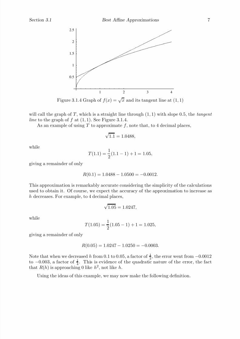
7/27/2019 Calculus 2 (Dan Sloughter)
http://slidepdf.com/reader/full/calculus-2-dan-sloughter 127/598
Section 3.1 Best Affine Approximations 7
1 2 3 4
0.5
1
1.5
2
2.5
Figure 3.1.4 Graph of f (x) =√
x and its tangent line at (1, 1)
will call the graph of T , which is a straight line through (1, 1) with slope 0.5, the tangent
line to the graph of f at (1, 1). See Figure 3.1.4.As an example of using T to approximate f , note that, to 4 decimal places,
√ 1.1 = 1.0488,
while
T (1.1) =1
2(1.1− 1) + 1 = 1.05,
giving a remainder of only
R(0.1) = 1.0488−
1.0500 =−
0.0012.
This approximation is remarkably accurate considering the simplicity of the calculationsused to obtain it. Of course, we expect the accuracy of the approximation to increase ash decreases. For example, to 4 decimal places,
√ 1.05 = 1.0247,
while
T (1.05) =1
2(1.05− 1) + 1 = 1.025,
giving a remainder of only
R(0.05) = 1.0247− 1.0250 = −0.0003.
Note that when we decreased h from 0.1 to 0.05, a factor of 12
, the error went from −0.0012to −0.003, a factor of 1
4. This is evidence of the quadratic nature of the error, the fact
that R(h) is approaching 0 like h2, not like h.
Using the ideas of this example, we may now make the following definition.
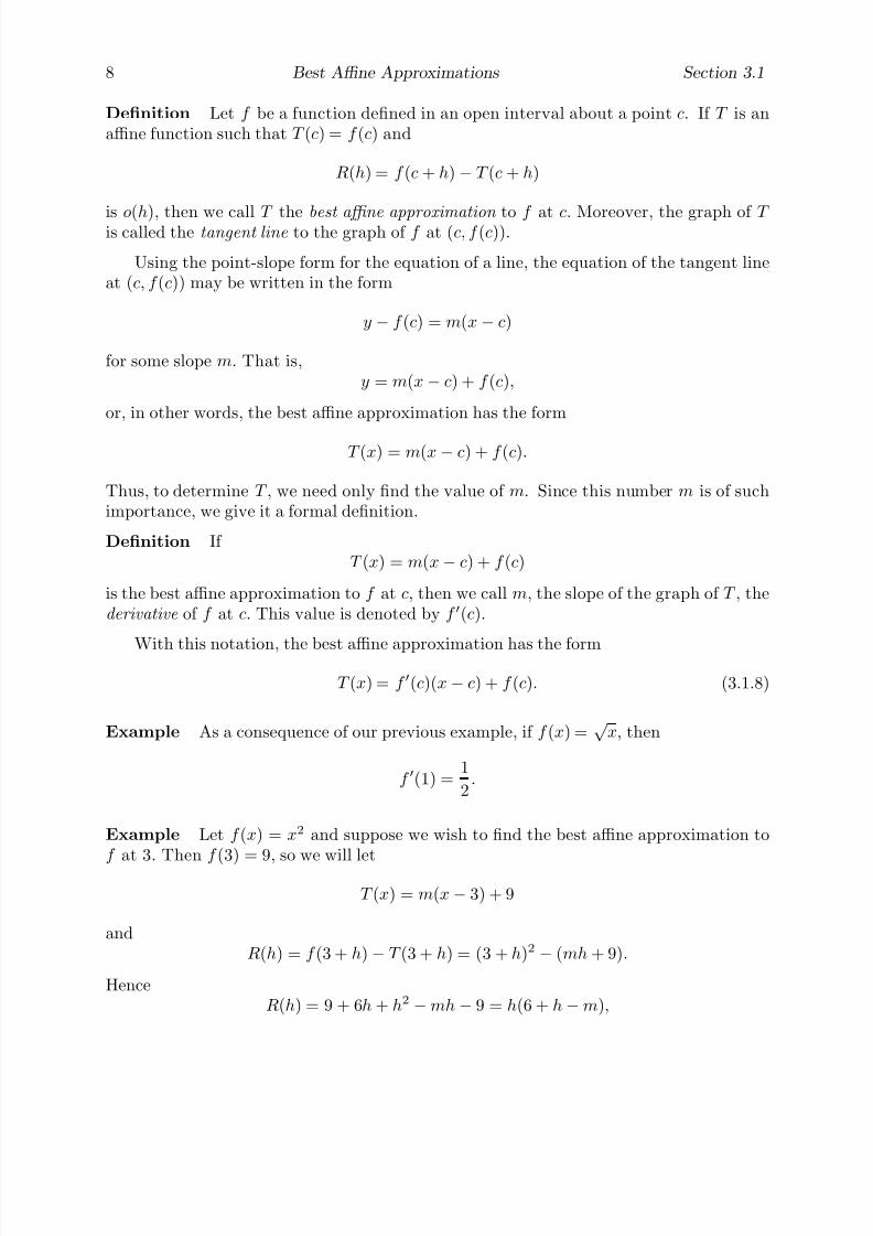
7/27/2019 Calculus 2 (Dan Sloughter)
http://slidepdf.com/reader/full/calculus-2-dan-sloughter 128/598
8 Best Affine Approximations Section 3.1
Definition Let f be a function defined in an open interval about a point c. If T is anaffine function such that T (c) = f (c) and
R(h) = f (c + h)− T (c + h)
is o(h), then we call T the best affine approximation to f at c. Moreover, the graph of T is called the tangent line to the graph of f at (c, f (c)).
Using the point-slope form for the equation of a line, the equation of the tangent lineat (c, f (c)) may be written in the form
y − f (c) = m(x− c)
for some slope m. That is,y = m(x− c) + f (c),
or, in other words, the best affine approximation has the form
T (x) = m(x− c) + f (c).
Thus, to determine T , we need only find the value of m. Since this number m is of suchimportance, we give it a formal definition.
Definition If T (x) = m(x− c) + f (c)
is the best affine approximation to f at c, then we call m, the slope of the graph of T , thederivative of f at c. This value is denoted by f (c).
With this notation, the best affine approximation has the form
T (x) = f (c)(x− c) + f (c). (3.1.8)
Example As a consequence of our previous example, if f (x) =√
x, then
f (1) =1
2.
Example Let f (x) = x2 and suppose we wish to find the best affine approximation tof at 3. Then f (3) = 9, so we will let
T (x) = m(x− 3) + 9
andR(h) = f (3 + h)− T (3 + h) = (3 + h)2 − (mh + 9).
HenceR(h) = 9 + 6h + h2 −mh− 9 = h(6 + h−m),
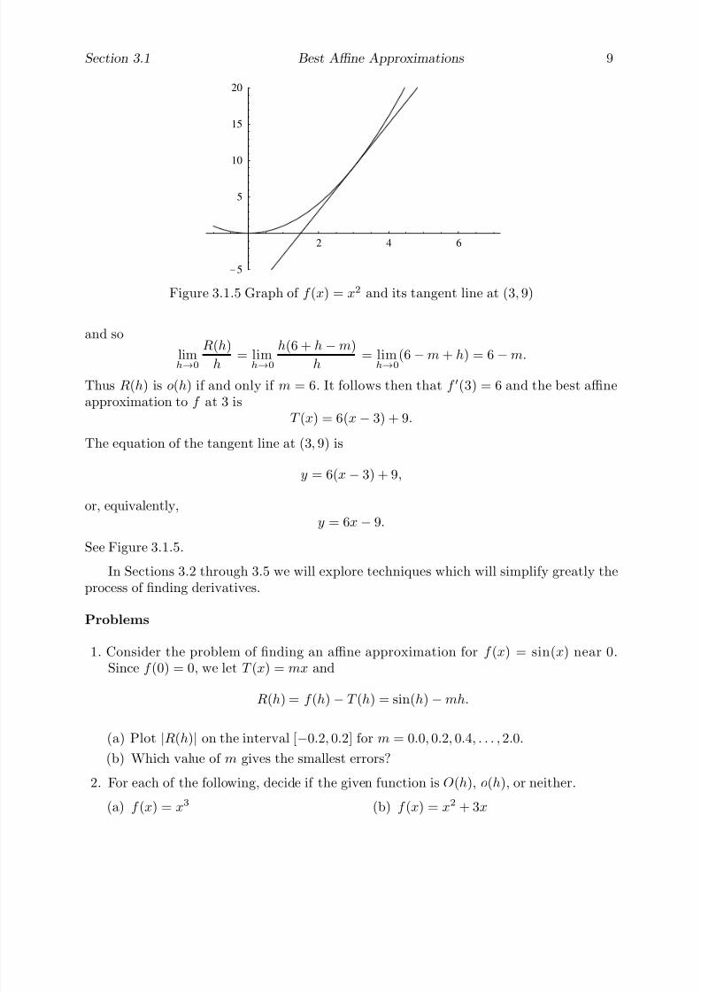
7/27/2019 Calculus 2 (Dan Sloughter)
http://slidepdf.com/reader/full/calculus-2-dan-sloughter 129/598
Section 3.1 Best Affine Approximations 9
2 4 6
-5
5
10
15
20
Figure 3.1.5 Graph of f (x) = x2 and its tangent line at (3, 9)
and so
limh→0
R(h)h
= limh→0
h(6 + h−m)h
= limh→0
(6−m + h) = 6−m.
Thus R(h) is o(h) if and only if m = 6. It follows then that f (3) = 6 and the best affineapproximation to f at 3 is
T (x) = 6(x− 3) + 9.
The equation of the tangent line at (3, 9) is
y = 6(x− 3) + 9,
or, equivalently,
y = 6x− 9.
See Figure 3.1.5.
In Sections 3.2 through 3.5 we will explore techniques which will simplify greatly theprocess of finding derivatives.
Problems
1. Consider the problem of finding an affine approximation for f (x) = sin(x) near 0.Since f (0) = 0, we let T (x) = mx and
R(h) = f (h)− T (h) = sin(h)−mh.
(a) Plot |R(h)| on the interval [−0.2, 0.2] for m = 0.0, 0.2, 0.4, . . . , 2.0.
(b) Which value of m gives the smallest errors?
2. For each of the following, decide if the given function is O(h), o(h), or neither.
(a) f (x) = x3 (b) f (x) = x2 + 3x
7/27/2019 Calculus 2 (Dan Sloughter)
http://slidepdf.com/reader/full/calculus-2-dan-sloughter 130/598
10 Best Affine Approximations Section 3.1
(c) g(t) = 4t3 − 3t2 (d) g(x) =√
4 + x− x
4− 2
(e) f (t) = t4
3 (f) g(t) = t− t3
5
3. Let f (x) =√
x, T (x) =1
2(x− 9) + 3, and S (x) =
1
6(x− 9) + 3.
(a) Graph f , T , and S together. Note that the graphs of T and S are straight linespassing through the point (9, 3) on the graph of f .
(b) Let RT (h) = f (9 + h)− T (9 + h). Is RT (h) o(h)? Is it O(h)?
(c) Let RS (h) = f (9 + h)− S (9 + h). Is RS (h) o(h)? Is it O(h)?
(d) Which of T or S is the best affine approximation to f at 9?
(e) Use the best affine approximation to f at 9 to approximate√
10,√
8.9, and√
9.3.Compare these approximations with values from your calculator.
4. Let g(z) = z2, T (z) = 2(z − 1) + 1, and S (z) = 3(z − 1) + 1.
(a) Graph g, T , and S together. Note that the graphs of T and S are straight linespassing through the point (1, 1) on the graph of g.
(b) Let RT (h) = g(1 + h)− T (1 + h). Is RT (h) o(h)? Is it O(h)?
(c) Let RS (h) = g(1 + h)− S (1 + h). Is RS (h) o(h)? Is it O(h)?
(d) Which of T or S is the best affine approximation to g at 1?
(e) Use the best affine approximation to g at 1 to approximate (1.1)2 and (0.999)2.Compare these approximations with values from your calculator.
5. Find the best affine approximation to f (x) = 2x2 at 1. What is f (1)?
6. Find the best affine approximation tog
(x
) =
1
x at 1. What isg
(1)?7. Find the best affine approximation to f (t) = t2 + t− 1 at 0. What is f (0)?
7/27/2019 Calculus 2 (Dan Sloughter)
http://slidepdf.com/reader/full/calculus-2-dan-sloughter 131/598
Difference Equations
Differential Equations
to
Section 3.2
Best Affine Approximations,Derivatives, and Rates of Change
In this section we will take up the general question of how to find best affine approximationsand also discuss an interpretation of the derivative of a function as an instantaneous rateof change. We will consider specific computational procedures for finding derivatives inSections 3.3 through 3.5.
To begin, suppose f is a function defined on an open interval containing the point c
and let T be an affine function with T (c) = f (c). As in Section 3.1, we may write T in theform
T (x) = m(x−
c) + f (c) (3.2.1)
for some constant m. Let
R(h) = f (c + h)− T (c + h) = f (c + h) − mh− f (c). (3.2.2)
Then
limh→0
R(h)
h= lim
h→0
f (c + h) − T (c + h)
h
= limh→0
f (c + h) − mh − f (c)
h
= limh→0
f (c + h)− f (c)
h− m
.
(3.2.3)
Hence R(h) is o(h), and T is the best affine approximation to f at c, if and only if
limh→0
f (c + h) − f (c)
h− m
= 0, (3.2.4)
which is true if and only if
limh→0
f (c + h)− f (c)
h= m. (3.2.5)
In particular, if
limh→0
f (c + h) − f (c)
h
exists, then f has a best affine approximation at c and
f (c) = limh→0
f (c + h) − f (c)
h. (3.2.6)
1 Copyright c by Dan Sloughter 2000

7/27/2019 Calculus 2 (Dan Sloughter)
http://slidepdf.com/reader/full/calculus-2-dan-sloughter 132/598
2 Best Affine Approximations, Derivatives, and Rates of Change Section 3.2
Conversely, if T (x) = m(x − c) + f (c) is the best affine approximation to f at c, then itfollows that
m = limh→0
f (c + h)− f (c)
h. (3.2.7)
Definition We say a function f is differentiable at a point c if
limh→0
f (c + h) − f (c)
h(3.2.8)
exists.
In summary, if we are given a function f which is differentiable at c, then the bestaffine approximation to f at c exists and is given by
T (x) = f (c)(x − c) + f (c), (3.2.9)
where
f (c) = limh→0
f (
c+
h) −
f (
c)h . (3.2.10)
Conversely, if f has a best affine approximation at a point c, then f is differentiable at c
and the best affine approximation is given by (3.2.9).
Example Consider the problem of finding the best affine approximation to f (x) = x2
at x = 1, a problem we first looked at in Section 1.1. We first need to find the derivativef (1). Using (3.2.10), we have
f (1) = limh→0
f (1 + h) − f (1)
h
= limh→0
(1 + h)2
−1
h
= limh→0
1 + 2h + h2 − 1
h
= limh→0
h(2 + h)
h
= limh→0
(2 + h)
= 2.
From (3.2.9), it now follows that the best affine approximation to f at 1 is
T (x) = 2(x− 1) + 1 = 2x − 1.
Furthermore, from our discussion in Section 3.1, the equation of the line tangent to thegraph of y = x2 at the point (1, 1) is then
y = 2x − 1,
as shown in Figure 3.2.1.

7/27/2019 Calculus 2 (Dan Sloughter)
http://slidepdf.com/reader/full/calculus-2-dan-sloughter 133/598
Section 3.2 Best Affine Approximations, Derivatives, and Rates of Change 3
-4 -2 2 4
-2
2
4
6
8
10
Figure 3.2.1 Graphs of y = x2 and y = 2x − 1
Frequently we will be interested in the derivative of a function not just at a singlepoint, but at many different points. Instead of performing the above calculation at eachpoint separately, we try to compute the derivative at an arbitrary point, after which wecan substitute in any desired point for evaluation. In fact, for any given function f , wemay define a new function f by setting
f (x) = limh→0
f (x + h) − f (x)
h
(3.2.11)
for all points x at which the limit exists. This new function, f , is called the derivative of f . Note that the domain of f may be smaller than the domain of f . If the open interval(a, b) is in the domain of f , we say f is differentiable on (a, b).
Example Let f (x) =√
x. From our work in the Section 3.1 we know that
f (1) =1
2.
Now we will find a general expression for f (x) at an arbitrary point x in (0,∞). Using(3.2.11), we have

7/27/2019 Calculus 2 (Dan Sloughter)
http://slidepdf.com/reader/full/calculus-2-dan-sloughter 134/598
4 Best Affine Approximations, Derivatives, and Rates of Change Section 3.2
f (x) = limh→0
f (x + h) − f (x)
h
= limh→0
√ x + h −√ x
h
= limh→0
√ x + h −√ xh
√ x + h +√ x√ x + h +
√ x
= limh→0
x + h − x
h(√
x + h +√
x)
= limh→0
h
h(√
x + h +√
x)
= limh→0
1√ x + h +
√ x
=1
√ x +√ x=
1
2√
x.
Hence f is differentiable on (0,∞). In particular, we once again have
f (1) =1
2.
Moreover, it is now straightforward to find the best affine approximation to f at any pointc > 0. For example,
f (16) =1
8,
so the best affine approximation to f (x) = √ x at x = 16 is
T (x) =1
8(x − 16) + 4 =
1
8x + 2.
See Figure 3.2.2 for the graphs of f and T .
Example Now consider g(t) = t3. Then
g(t) = limh→0
g(t + h) − g(t)
h
= limh→0
(t + h)3 − t3
h= lim
h→0
t3 + 3t2h + 3th2 + h3 − t3
h
= limh→0
h(3t2 + 3th + h2)
h
= limh→0
(3t2 + 3th + h2)
= 3t2.
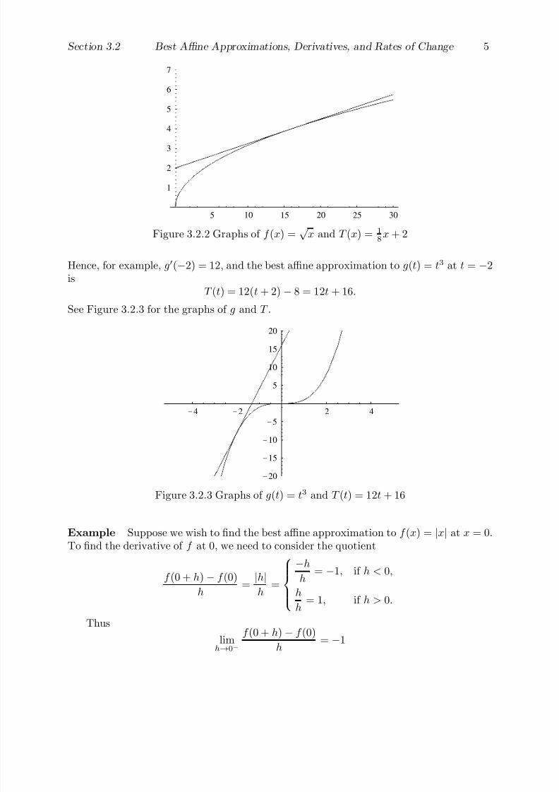
7/27/2019 Calculus 2 (Dan Sloughter)
http://slidepdf.com/reader/full/calculus-2-dan-sloughter 135/598
Section 3.2 Best Affine Approximations, Derivatives, and Rates of Change 5
5 10 15 20 25 30
1
2
3
4
5
6
7
Figure 3.2.2 Graphs of f (x) =√
x and T (x) = 1
8x + 2
Hence, for example, g(
−2) = 12, and the best affine approximation to g(t) = t3 at t =
−2
isT (t) = 12(t + 2) − 8 = 12t + 16.
See Figure 3.2.3 for the graphs of g and T .
-4 -2 2 4
-20
-15
-10
-5
5
10
15
20
Figure 3.2.3 Graphs of g(t) = t3 and T (t) = 12t + 16
Example Suppose we wish to find the best affine approximation to f (x) = |x| at x = 0.To find the derivative of f at 0, we need to consider the quotient
f (0 + h) − f (0)
h=|h|h
=
−h
h= −1, if h < 0,
h
h= 1, if h > 0.
Thus
limh→0−
f (0 + h) − f (0)
h= −1
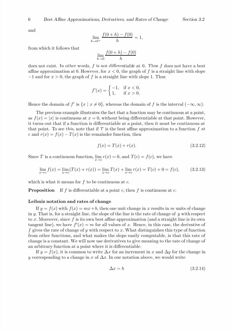
7/27/2019 Calculus 2 (Dan Sloughter)
http://slidepdf.com/reader/full/calculus-2-dan-sloughter 136/598
6 Best Affine Approximations, Derivatives, and Rates of Change Section 3.2
and
limh→0+
f (0 + h) − f (0)
h= 1,
from which it follows that
limh→0
f (0 + h)
−f (0)
h
does not exist. In other words, f is not differentiable at 0. Thus f does not have a bestaffine approximation at 0. However, for x < 0, the graph of f is a straight line with slope−1 and for x > 0, the graph of f is a straight line with slope 1. Thus
f (x) =
−1, if x < 0,1, if x > 0.
Hence the domain of f is {x | x = 0}, whereas the domain of f is the interval (−∞,∞).
The previous example illustrates the fact that a function may be continuous at a point,as f (x) = |x| is continuous at x = 0, without being differentiable at that point. However,it turns out that if a function is differentiable at a point, then it must be continuous atthat point. To see this, note that if T is the best affine approximation to a function f atc and r(x) = f (x) − T (x) is the remainder function, then
f (x) = T (x) + r(x). (3.2.12)
Since T is a continuous function, limx→c
r(x) = 0, and T (c) = f (c), we have
limx→c
f (x) = limx→c
(T (x) + r(x)) = limx→c
T (x) + limx→c
r(x) = T (c) + 0 = f (c), (3.2.13)
which is what it means for f to be continuous at c.
Proposition If f is differentiable at a point c, then f is continuous at c.
Leibniz notation and rates of change
If y = f (x) with f (x) = mx + b, then one unit change in x results in m units of changein y. That is, for a straight line, the slope of the line is the rate of change of y with respectto x. Moreover, since f is its own best affine approximation (and a straight line is its owntangent line), we have f (x) = m for all values of x. Hence, in this case, the derivative of
f gives the rate of change of y with respect to x. What distinguishes this type of functionfrom other functions, and what makes the slope easily computable, is that this rate of change is a constant. We will now use derivatives to give meaning to the rate of change of an arbitrary function at a point where it is differentiable.
If y = f (x), it is common to write ∆x for an increment in x and ∆y for the change iny corresponding to a change in x of ∆x. In our notation above, we would write
∆x = h (3.2.14)

7/27/2019 Calculus 2 (Dan Sloughter)
http://slidepdf.com/reader/full/calculus-2-dan-sloughter 137/598
Section 3.2 Best Affine Approximations, Derivatives, and Rates of Change 7
and
∆y = f (x + ∆x)− f (x). (3.2.15)
Thus we can write
f (x + h)−
f (x)
h =f (x + ∆x)
−f (x)
∆x =∆y
∆x , (3.2.16)
from which we have
f (x) = lim∆x→0
∆y
∆x. (3.2.17)
This type of notation, although not this type of reasoning, motivated Leibniz to denotef (x) by
dy
dx= lim
∆x→0
∆y
∆x. (3.2.18)
If the derivative is to be evaluated at a point c, then we would write
f (c) =dy
dx
x=c
. (3.2.19)
Example If y =√
x, then from our result above we may write
dy
dx=
1
2√
x
and, for example, dy
dx
x=9
=1
2√
9=
1
6.
Now ∆y
∆xrepresents the average rate of change of y over the interval from x to x + ∆x.
That is, this ratio tells us how much y changes per unit change in x over the interval. Aswe let ∆x go to 0, this ratio will approach a limiting value, namely, the derivative , whichwe may interpret as the instantaneous rate of change of y with respect to x. If the rate of change of y with respect to x were not to change over an interval of length 1, then y wouldchange by an amount equal to dy
dxover that interval.
As an example, if s = f (t) gives the position of an object moving in a straight line, then∆s∆t
is the average rate of change of position of the object with respect to time, which we
call its average velocity . Then dsdt
, the derivative of s with respect to t, is the instantaneous
rate of change of position with respect to time; that is, dsdt
is the instantaneous velocity , or,
simply, velocity , of the object. The difference between ∆s∆t
and dsdt
is the difference betweenfinding the average speed for a trip in a car by dividing the total miles traveled by thetotal time elapsed and finding the instantaneous speed at any one time during the trip bylooking at the car’s speedometer.

7/27/2019 Calculus 2 (Dan Sloughter)
http://slidepdf.com/reader/full/calculus-2-dan-sloughter 138/598
8 Best Affine Approximations, Derivatives, and Rates of Change Section 3.2
Example Galileo discovered that if an object is dropped from a initial height of 100feet, then, ignoring the effects of air resistance, its height, in feet, above the ground aftert seconds would be
s = 100 − 16t2.
For example, at time t = 1 the object would be at a height of
st=1
= 100 − 16 = 84 feet
and at time t = 2 it would be at a height of
st=2
= 100 − 64 = 36 feet.
Hence the average velocity of the object over the time interval would be
∆s
∆t=
36 − 84
2 − 1= −48 feet/second.
Note that the average velocity over this time interval is negative because we have takenthe positive direction to be up. The average speed of the object, which is the absolutevalue of the velocity, would be 48 feet per second. To find the instantaneous velocity attime t, we compute
ds
dt= lim
∆t→0
∆s
∆t
= lim∆t→0
(100− 16(t + ∆t)2) − (100 − 16t2)
∆t
= lim∆t→0
100 − 16(t2 + 2t∆t + (∆t)2) − 100 − 16t2
∆t
= lim∆t→0
−32t∆t − 16(∆t)2
∆t
= lim∆t→0
(−32t − 16∆t)
= −32t.
Hence the instantaneous velocity of the object at time t = 1 is
ds
dt
t=1
= −32 feet/second
and the instantaneous velocity at time t = 2 is
ds
dt
t=2
= −64 feet/second.
Although Leibniz seems to have thought of the expression dydx
as a ratio, we should think
of ddx
as the operation of differentiation, which, when applied to y, yields the derivative of
7/27/2019 Calculus 2 (Dan Sloughter)
http://slidepdf.com/reader/full/calculus-2-dan-sloughter 139/598
Section 3.2 Best Affine Approximations, Derivatives, and Rates of Change 9
y with respect to x. In other words, we should not think of dydx
as a ratio, but as ddx
(y).For example, if y = x3, then, using an earlier result from this section, we might write
dy
dx=
d
dx(x3) = 3x2.
The “prime” notation for a derivative is due, not to Newton, but to Joseph LouisLagrange (1736-1813). Newton’s notation, a dot above the dependent variable, representsa derivative with respect to time, denoted by t. For example, in the previous example wemay write
s = −32t
using Newton’s notation. Because of its simplicity and the frequency with which derivativeswith respect to time occur, this is often a useful notation and we will make extensive useof it when we study differential equations in Chapter 8.
Problems
1. Using (3.2.10), find the derivative of each of the following functions at the indicatedpoint.
(a) f (x) = x2 + 1 at x = 2 (b) f (t) =1
tat t = 1
(c) g(x) =1
x2at x = 2 (d) h(t) =
√ t + 1 at t = 3
(e) f (s) =1√
sat s = 1 (f) g(z) = (z + 1)2 at z = −1
2. For each of the functions in Problem 1, find the best affine approximation for thefunction at the indicated point. Also, find the equation of the tangent line at thatpoint and graph the function and its tangent line together.
3. Using (3.2.11), find the derivative of each of the following functions. Note any pointswhere the given function is not differentiable.
(a) f (x) = 2x2 (b) g(x) =1
x
(c) f (t) =1√
t(d) h(z) =
1
3z
(e) y(t) = t2 + 4t (f) g(s) = 2s3
−s2
4. Using your result from part (c) of Problem 3, find the best affine approximation to
f (t) =1√
t
at t = 4. Use it to approximate1√
3.98.
7/27/2019 Calculus 2 (Dan Sloughter)
http://slidepdf.com/reader/full/calculus-2-dan-sloughter 140/598
10 Best Affine Approximations, Derivatives, and Rates of Change Section 3.2
5. Let f (x) = ax2 + bx + c, where a, b, and c are constants. Show that f (x) = 2ax + b.Does this result agree with your results in parts (a) and (e) of Problems 3?
6. Use your result from Problem 5 to find the best affine approximation to
f (x) = 3x2
−2x + 5
at x = −2.
7. Use your result from Problem 5 to find the best affine approximation to
g(t) = −2t2 + 3t − 6
at t = 3.
8. Suppose f is a function with the properties that f (0) = 0 and
limt→0
f (t)t = 1.
Show that f (0) = 1.
9. Suppose g is a function with the properties that g(0) = 0 and g is o(h). Show thatg(0) = 0.
10. Suppose f is a function with the properties that
f (s + t) = f (s)f (t)
for all numbers s and t andlimt→0
f (t) − 1
t= 1.
Show that f (t) = f (t).
11. Suppose f (x) =
3x2, if x < 0x3, if x ≥ 0
. Is f differentiable at x = 0? If it is, find f (0).
12. Suppose g(t) =
5t, if t < 03t2, if t ≥ 0
. Is g differentiable at t = 0? If it is, find g(0).
13. Suppose g(x) = x2
−2x + 2, if x
≤1
4x − 3, if x > 1. Is g differentiable at x = 1? If it is, find
g(1).
14. For each of the following, find the derivative of the dependent variable with respect tothe independent variable. Denote the derivative using Leibniz’s notation.
(a) s = 2t3 (b) z = 2√
t
(c) q = s − 2
s(d) t = x4
7/27/2019 Calculus 2 (Dan Sloughter)
http://slidepdf.com/reader/full/calculus-2-dan-sloughter 141/598
Section 3.2 Best Affine Approximations, Derivatives, and Rates of Change 11
15. Findd
dx(4x2) and
d
du(3√
u − 1).
16. An object is thrown vertically into the air from an initial height of 100 meters abovethe ground with an initial velocity of 10 meters per second. If s represents the height,in meters, of the object above the ground after t seconds and we ignore the effects of
air resistance, thens = 100 + 10t − 4.9t2.
(a) What is the average velocity over the time interval [0, 2]? Over [0, 1]? Over [1, 2]?
(b) Find the velocity v of the object at time t. You may use Problem 5.
(c) What is the velocity after 1 second? After 2 seconds?
(d) When is v = 0? Is v positive or negative before this time? Is v positive or negativeafter this time?
(e) What is the height of the object when v = 0? What is the significance of thisheight?
(f) The rate of change of velocity is called acceleration . Find the acceleration of theobject; that is, find dv
dt.
(g) What is the significance of the fact that dvdt
is a constant?
17. Find the rate of change of the area A of a circle with respect to its radius r.
18. Find the rate of change of the volume V of a sphere with respect to its radius r.
19. Find the rate of change of the area A of a square with respect to the length x of oneof its sides.
20. Find the rate of change of the volume V of a cube with respect to the length x of oneof its sides.

7/27/2019 Calculus 2 (Dan Sloughter)
http://slidepdf.com/reader/full/calculus-2-dan-sloughter 142/598
Difference Equations
Differential Equations
to
Section 3.3
Differentiation of Polynomialsand Rational Functions
In this section we begin the task of discovering rules for differentiating various classesof functions. By the end of Section 3.5 we will be able to differentiate any algebraic ortrigonometric function as a matter of routine without reference to the limits used in Section3.2.
Differentiation of polynomials
We first note that if f is a first degree polynomial, say, f (x) = ax + b for some constantsa and b, then f is an affine function and hence its own best affine approximation. Thusf (x) = a for all x. In particular, if f is a constant function, say, f (x) = b for all x, thenf (x) = 0 for all x.
Next we consider the case of a monomial f (x) = xn, where n is a positive integergreater than 1. Then
f (x) = limh→0
f (x + h)− f (x)
h= lim
h→0
(x + h)n − xn
h. (3.3.1)
Now(x + h)n = xn + nxn−1h + R(h), (3.3.2)
where R(h) represents the remaining terms in the expansion. Since every term in R(h)has a factor of h raised to a power greater than or equal to 2, it follows that R(h) is o(h).Hence we have
f (x) = limh→0
xn + nxn−1h + R(h)− xn
h
= limh→0
nxn−1h + R(h)
h
= limh→0
nxn−1 +
R(h)
h
= nxn−1 + limh→0
R(h)
h
= nxn−1.
Since from our previous result f (x) = 1 when f (x) = x, this formula also works in thecase n = 1. Hence we have the following proposition.
Proposition For any positive integer n,
d
dxxn = nxn−1. (3.3.3)
1 Copyright c by Dan Sloughter 2000
7/27/2019 Calculus 2 (Dan Sloughter)
http://slidepdf.com/reader/full/calculus-2-dan-sloughter 143/598
2 Differentiation of Polynomials and Rational Functions Section 3.3
Example If f (x) = x3, then f (x) = 3x2, as we saw in an example in Section 3.2.
Example Similarly,d
dtt5 = 5t4.
Hence, for example, the equation of the line tangent to the curve x = t5 at (−1,−1) is
x = 5(t + 1)− 1,
orx = 5t + 4.
Once we establish results for the derivative of a constant times a function and for thederivative of the sum of two functions, similar to the results we have for limits, we will beable to easily differentiate any polynomial. So suppose f is a differentiable function andlet k(x) = cf (x), where c is any constant. Then
k(x) = limh→0
k(x + h)− k(x)
h
= limh→0
cf (x + h)− cf (x)
h
= limh→0
c(f (x + h)− f (x))
h
= c limh→0
f (x + h)− f (x)
h
= cf (x).
That is, the derivative of a constant times a function is the constant times the derivativeof the function.
Proposition If f is differentiable and c is any constant, thend
dx(cf (x)) = c
d
dxf (x). (3.3.4)
Example If f (x) = 14x3, then
f (x) = (14)(3x2) = 42x2.
Now suppose f and g are both differentiable functions and let k(x) = f (x) + g(x).Then
k(x) = limh→0
k(x + h)− k(x)
h
= limh→0
(f (x + h) + g(x + h))− (f (x) + g(x))h
= limh→0
f (x + h)− f (x)
h+
g(x + h)− g(x)
h
= limh→0
f (x + h)− f (x)
h+ lim
h→0
g(x + h)− g(x)
h
= f (x) + g(x).

7/27/2019 Calculus 2 (Dan Sloughter)
http://slidepdf.com/reader/full/calculus-2-dan-sloughter 144/598
Section 3.3 Differentiation of Polynomials and Rational Functions 3
Hence the derivative of the sum of two functions is the sum of their derivatives. A similarargument would show that the derivative of the difference of two functions is the differenceof their derivatives.
Proposition If f and g are both differentiable, then
d
dx(f (x) + g(x)) =
d
dxf (x) +
d
dxg(x) (3.3.5)
andd
dx(f (x)− g(x)) =
d
dxf (x)−
d
dxg(x). (3.3.6)
Putting the preceding results together, we are now in a position to easily differentiateany polynomial, as the next examples will illustrate.
Example Suppose f (x) = 3x5 − 6x2 + 2x− 16. Then
f (x) =d
dx(3x5 − 6x2 + 2x− 16)
=d
dx(3x5)−
d
dx(6x2) +
d
dx(2x)−
d
dx(16)
= 3d
dxx5 − 6
d
dxx2 + 2
d
dxx− 0
= (3)(5x4)− (6)(2x) + (2)(1)
= 15x4 − 12x + 2.
Example Of course, it is not necessary to write out in detail all the steps in differentiat-ing a polynomial as we did in the preceding example. For example, if g(t) = 3t12−6t2 + t,then
g(t) = (3)(12t11)− (6)(2t) + 1 = 36t11 − 12t + 1.
In particular, since g(1) = −2 and g(1) = 25, the best affine approximation to g at t = 1is
T (t) = 25(t− 1)− 2 = 25t− 27.
Differentiation of rational functions
We next consider the problem of differentiating the quotient of two functions whose deriva-tives are already known. In particular, combining this result with our result for polynomialswill enable us to easily differentiate any rational function. We might hope that, analogousto the last two results and the related results for limits, the derivative of the quotient of two functions would be equal to the quotient of their derivatives. This turns out not to betrue; nevertheless, there is a nice rule for differentiating quotients.

7/27/2019 Calculus 2 (Dan Sloughter)
http://slidepdf.com/reader/full/calculus-2-dan-sloughter 145/598
4 Differentiation of Polynomials and Rational Functions Section 3.3
Suppose f and g are both differentiable functions and let k(x) = f (x)g(x) . Then, at all
points where g(x) = 0,
k(x) = limh→0
k(x + h)− k(x)
h
= limh→0
f (x + h)g(x + h)
− f (x)g(x)
h
= limh→0
g(x)f (x + h)− g(x + h)f (x)
g(x + h)g(x)
h
= limh→0
g(x)f (x + h)− g(x + h)f (x)
hg(x)g(x + h).
It turns out that by adding and subtracting the term g(x)f (x) (a standard mathematicaltrick of adding 0) in the numerator, we can simplify this limit into a form that we canevaluate. That is,
k(x) = limh→0
g(x)f (x + h)− g(x + h)f (x)
hg(x)g(x + h)
= limh→0
g(x)f (x + h)− g(x)f (x) + g(x)f (x)− g(x + h)f (x)
hg(x)g(x + h)
= limh→0
g(x)(f (x + h)− f (x))− f (x)(g(x + h)− g(x))
hg(x)g(x + h)
= limh→0
g(x)
f (x + h)− f (x)
h
− f (x)
g(x + h)− g(x)
h
g(x)g(x + h) .
Now
limh→0
g(x)
f (x + h)− f (x)
h
= g(x) lim
h→0
f (x + h)− f (x)
h= g(x)f (x), (3.3.7)
limh→0
f (x)
g(x + h)− g(x)
h
= f (x) lim
h→0
g(x + h)− g(x)
h= f (x)g(x), (3.3.8)
andlimh→0
g(x)g(x + h) = g(x) limh→0
g(x + h) = g(x)g(x) = (g(x))2, (3.3.9)
where the limits in (3.3.7) and (3.3.8) follow from the differentiability of f and g, whilethe limit in (3.3.9) follows from the continuity of g (which is a consequence of the differ-entiability of g). Putting everything together, we have
k(x) =g(x)f (x)− f (x)g(x)
(g(x))2, (3.3.10)
a result known as the quotient rule .
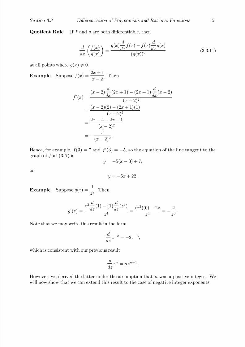
7/27/2019 Calculus 2 (Dan Sloughter)
http://slidepdf.com/reader/full/calculus-2-dan-sloughter 146/598
Section 3.3 Differentiation of Polynomials and Rational Functions 5
Quotient Rule If f and g are both differentiable, then
d
dx
f (x)
g(x)
=
g(x)d
dxf (x)− f (x)
d
dxg(x)
(g(x))2(3.3.11)
at all points where g(x) = 0.
Example Suppose f (x) =2x + 1
x− 2. Then
f (x) =(x− 2)
d
dx(2x + 1)− (2x + 1)
d
dx(x− 2)
(x− 2)2
=(x− 2)(2)− (2x + 1)(1)
(x− 2)2
= 2x− 4− 2x− 1(x− 2)2
= −5
(x− 2)2.
Hence, for example, f (3) = 7 and f (3) = −5, so the equation of the line tangent to thegraph of f at (3, 7) is
y = −5(x− 3) + 7,
ory = −5x + 22.
Example Suppose g(z) =1
z2. Then
g(z) =z2
d
dz(1)− (1)
d
dz(z2)
z4=
(z2)(0)− 2z
z4= −
2
z3.
Note that we may write this result in the form
d
dzz−2 = −2z−3,
which is consistent with our previous result
d
dzzn = nzn−1.
However, we derived the latter under the assumption that n was a positive integer. Wewill now show that we can extend this result to the case of negative integer exponents.

7/27/2019 Calculus 2 (Dan Sloughter)
http://slidepdf.com/reader/full/calculus-2-dan-sloughter 147/598
6 Differentiation of Polynomials and Rational Functions Section 3.3
Suppose f (x) = xn, where n is a negative integer. Then, using the quotient rule andthe fact that −n > 0,
f (x) =d
dxxn
=d
dx 1
x−n
=x−n
d
dx(1)− (1)
d
dx(x−n)
x−2n
=(x−n)(0)− (−nx−n−1)
x−2n
=nx−n−1
x−2n
= nx−n−1+2n
= nxn−1.
We can now state the more general result.
Proposition For any integer n = 0,
d
dxxn = nxn−1. (3.3.12)
Example If f (x) =1
x, then
f (x) = ddx
x−1 = −x−2 = − 1x2
.
Example Similarly,
d
dx
5
x3
=
d
dx(5x−3) = −15x−4 = −
15
x4.
We will eventually see that (3.3.12) holds for rational and irrational exponents as well.We will consider the rational case in Section 3.4, but we will not have the tools for handlingthe irrational case until we discuss exponential and logarithm functions in Chapter 6.
Differentiation of products
We will close this section with a discussion of a rule for differentiating the product of twofunctions. Since the product of two rational functions is again a rational function, this willnot extend the class of functions that we know how to differentiate routinely. However,this rule will be very useful in the future and, even at the present point, can help simplifysome problems.

7/27/2019 Calculus 2 (Dan Sloughter)
http://slidepdf.com/reader/full/calculus-2-dan-sloughter 148/598
Section 3.3 Differentiation of Polynomials and Rational Functions 7
Suppose f and g are both differentiable and k(x) = f (x)g(x). Then
k(x) = limh→0
k(x + h)− k(x)
h= lim
h→0
f (x + h)g(x + h)− f (x)g(x)
h. (3.3.13)
Adding and subtractingf
(x
+h
)g
(x
) in the numerator (again, the mathematical trick of adding 0 in a useful manner) will help simplify this limit. Namely,
k(x) = limh→0
f (x + h)g(x + h)− f (x + h)g(x) + f (x + h)g(x)− f (x)g(x)
h
= limh→0
f (x + h)(g(x + h)− g(x)) + g(x)(f (x + h)− f (x))
h
= limh→0
f (x + h)
g(x + h)− g(x)
h
+ g(x)
f (x + h)− f (x)
h
.
Now
limh→0
f (x+h)
g(x + h)− g(x)
h
= lim
h→0f (x+h) lim
h→0
g(x + h)− g(x)
h= f (x)g(x) (3.3.14)
and
limh→0
g(x)
f (x + h)− f (x)
h
= g(x) lim
h→0
f (x + h)− f (x)
h= g(x)f (x), (3.3.15)
where, as with the derivation of the quotient rule, we have used the differentiability of f
and g as well as the continuity of f in evaluating the limits. Putting everything together,we have
k(x) = f (x)g(x) + g(x)f (x). (3.3.16)
a result known as the product rule .
Product Rule If f and g are both differentiable, then
d
dxf (x)g(x) = f (x)
d
dxg(x) + g(x)
d
dxf (x). (3.3.17)
Example If f (x) = (x4 − 3x2 + 6x− 3)(6x3 + 2x + 5),
then
f (x) = (x4 − 3x2 + 6x− 3)d
dx(6x3 + 2x + 5) + (6x3 + 2x + 5)
d
dx(x4 − 3x2 + 6x− 3)
= (x4 − 3x2 + 6x− 3)(18x2 + 2) + (6x3 + 2x + 5)(4x3 − 6x + 6).
Of course, in this example, f is just a polynomial so we could also find f by multiplying outthe two factors of f and differentiating the polynomial term by term as usual. However,
7/27/2019 Calculus 2 (Dan Sloughter)
http://slidepdf.com/reader/full/calculus-2-dan-sloughter 149/598
8 Differentiation of Polynomials and Rational Functions Section 3.3
the product rule gives us a quicker route to the derivative. Although the result is notsimplified into the standard form of a polynomial, for most applications this form is justas useful as any other.
It is worth noting that although we can now differentiate any rational function in
theory, in practice our methods may not be the most useful. For example, the function
f (x) = (x2 + 1)567
is a polynomial, and so we know how to differentiate it. However, at this point the only waywe could perform the differentiation would be to expand f (x) into standard polynomialform and then differentiate term by term. In Section 3.4 we will learn how to handle thisproblem more directly. At the same time we will extend the class of functions that we candifferentiate routinely to include all algebraic functions.
Problems
1. Find the derivative of each of the following functions.
(a) f (x) = x3 + 6x (b) g(x) = 13x5 − 6x2 + 13
(c) g(t) = 3t− 6t2 (d) y(t) = 4t3 − 18t + 3
(e) f (t) = (3t− 6)2 (f) f (x) = (4x + 5)(6x2 − 1)
2. Find the derivative of each of the following functions.
(a) f (x) = (2x + 1)2 (b) g(t) = (t2 − 3)3
(c) g(x) =x− 3
2x + 5(d) h(s) =
2s− s2
s2 + 1
(e) f (t) =3t4 − 8t + 1
2t3 + 6(f) x(t) =
3
t3− 16t2
(g) h(t) =3
t(h) f (x) =
41
3x7
(i) h(z) = 8z3 −1
2z(j) f (s) =
31
s3+
1
2s2− 16s
3. For each of the following, make use of the product rule in finding the derivative of the
dependent variable with respect to the independent variable.
(a) s = (t2 − 6t + 3)(8t4 + 6t2 − 7)
(b) q = (13t4 + 5t)(3t5 + 4t3 + 16t− 31)
(c) y = (x2 − 2x + 3)(2x2 + 13x− 6)(3x2 − 4x + 1)
(d) z =(x2 − 3x + 6)(8x2 + 3x− 2)
x2 − 6
7/27/2019 Calculus 2 (Dan Sloughter)
http://slidepdf.com/reader/full/calculus-2-dan-sloughter 150/598
Section 3.3 Differentiation of Polynomials and Rational Functions 9
4. Suppose f (2) = −2, f (2) = 6, g(2) = 3, and g(2) = −4. Find k(2) for each of thefollowing.
(a) k(x) = f (x)g(x) (b) k(x) =f (x)
g(x)
(c) k(x) = f (x)(g(x))2 (d) k(x) =f (x)− f (x)g(x)
g(x)
5. Suppose an object moves along the x-axis so that its position at time t is x = −t +t3
6.
(a) Find the velocity, v(t) = x(t), of the object.
(b) What is v(0)? What does this say about the direction of motion of the object attime t = 0?
(c) When is the object at the origin? What is the velocity of the object when it is atthe origin?
(d) For what values of t is the object moving toward the right?
(e) For what values of t is the object moving toward the left?
(f) What is happening at the points where v(t) = 0?
(g) Find the acceleration of the object, a(t) = v(t).
(h) When is the acceleration positive? When is it negative?
(i) Notice that v(1) < 0 and a(1) > 0. What does this say about the motion at timet = 1?
6. (a) Using only the product rule and the fact thatd
dxx = 1, show that
d
dxx2 = 2x.
(b) Now use the product rule to show that
d
dx x3
= 3x2
.(c) Let n > 1 and suppose we know that
d
dxxm = mxm−1
for all m < n. Use the product rule to show that
d
dxxn = nxn−1.
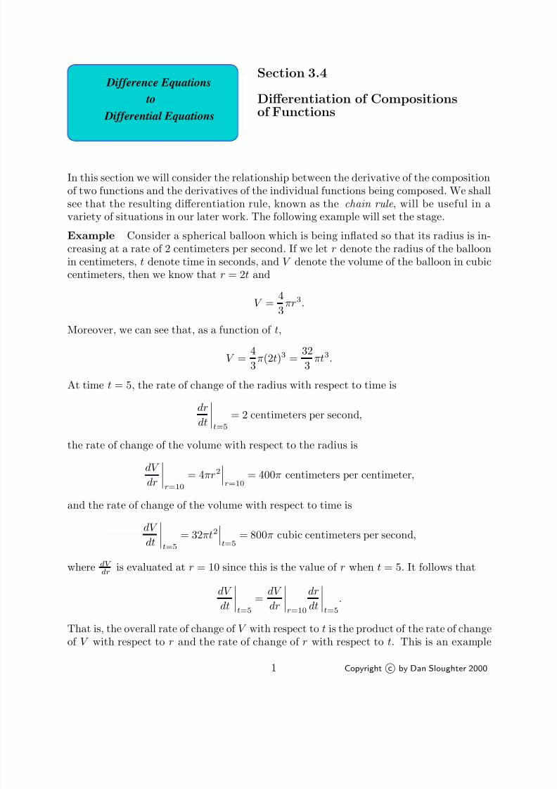
7/27/2019 Calculus 2 (Dan Sloughter)
http://slidepdf.com/reader/full/calculus-2-dan-sloughter 151/598
Difference Equations
Differential Equations
to
Section 3.4
Differentiation of Compositionsof Functions
In this section we will consider the relationship between the derivative of the compositionof two functions and the derivatives of the individual functions being composed. We shallsee that the resulting differentiation rule, known as the chain rule , will be useful in avariety of situations in our later work. The following example will set the stage.
Example Consider a spherical balloon which is being inflated so that its radius is in-creasing at a rate of 2 centimeters per second. If we let r denote the radius of the balloonin centimeters, t denote time in seconds, and V denote the volume of the balloon in cubic
centimeters, then we know that r = 2t and
V =4
3πr3.
Moreover, we can see that, as a function of t,
V =4
3π(2t)3 =
32
3πt3.
At time t = 5, the rate of change of the radius with respect to time is
dr
dtt=5
= 2 centimeters per second,
the rate of change of the volume with respect to the radius is
dV
dr
r=10
= 4πr2r=10
= 400π centimeters per centimeter,
and the rate of change of the volume with respect to time is
dV
dt t=5
= 32πt2t=5= 800π cubic centimeters per second,
where dV dr
is evaluated at r = 10 since this is the value of r when t = 5. It follows that
dV
dt
t=5
=dV
dr
r=10
dr
dt
t=5
.
That is, the overall rate of change of V with respect to t is the product of the rate of changeof V with respect to r and the rate of change of r with respect to t. This is an example
1 Copyright c by Dan Sloughter 2000
7/27/2019 Calculus 2 (Dan Sloughter)
http://slidepdf.com/reader/full/calculus-2-dan-sloughter 152/598
2 Differentiation of Compositions of Functions Section 3.4
of the chain rule. Viewed in this manner, the chain rule is saying that if V changes 400π
times as fast as r and r changes 2 times as fast as t, then V changes (400π)(2) = 800π
times as fast as t.
Another interesting special case of the chain rule arises with the composition of twoaffine functions. Specifically, if f (x) = ax + b and g(x) = cx + d, where a, b, c, and d areall constants, then
f ◦ g(x) = f (g(x)) = f (cx + d) = a(cx + d) + b = acx + ad + b.
Thus the slope of graph of f ◦ g is ac, the product of the slopes of the graphs of f and g.In terms of derivatives, this says that
(f ◦ g)(x) = ac = f (g(x))g(x).
The chain rule says this relationship holds for all differentiable functions.
For the general case, suppose g is differentiable at a point c and f is differentiable atg(c). We wish to compute the value of the derivative of f ◦ g at c. We have
(f ◦ g)(c) = limh→0
f ◦ g(c + h)− f ◦ g(c)
h= lim
h→0
f (g(c + h))− f (g(c))
h. (3.4.1)
As with our demonstrations of the quotient and product rules, we need to manipulate(3.4.1) into a form which allows us to evaluate the limit in terms of what we already know.The trick that works this time is to multiply and divide by g(c + h) − g(c). However, wemust be aware of one possible complication: In order to divide by g(c + h)− g(c) we mustbe assured that g(c + h)− g(c) = 0 for all h in some interval about 0. We will assume that
this is the case. If in fact this were not the case, then one can show that both (f ◦g)
(c) = 0and g(c) = 0, giving us the desired result that
(f ◦ g)(c) = f (g(c))g(c).
With our assumption, we have
(f ◦ g)(c) = limh→0
f (g(c + h))− f (g(c))
g(c + h)− g(c)
g(c + h)− g(c)
h
. (3.4.2)
Since g is differentiable at c, we have
limh→0
g(c + h)− g(c)
h= g(c). (3.4.3)
Since f is differentiable at g(c), if we let s = g(c + h)− g(c), then
limh→0
f (g(c + h))− f (g(c))
g(c + h)− g(c)= lim
s→0
f (g(c) + s)− f (g(c))
s= f (g(c)), (3.4.4)

7/27/2019 Calculus 2 (Dan Sloughter)
http://slidepdf.com/reader/full/calculus-2-dan-sloughter 153/598
Section 3.4 Differentiation of Compositions of Functions 3
where we have used the continuity of g at c to ascertain that s goes to 0 as h goes to 0.Putting (3.4.2), (3.4.3) and (3.4.4) together, we now have
(f ◦ g)(c) = f (g(c))g(c), (3.4.5)
which is our desired result.Chain Rule If f and g are differentiable, then
(f ◦ g)(x) = f (g(x))g(x). (3.4.6)
Example Suppose h(x) = (1 + x2)10. Then h(x) = f ◦ g(x) where g(x) = 1 + x2 andf (x) = x10. Now
g(x) = 2x
andf (x) = 10x9,
so
h(x) = (f ◦ g)(x) = f (g(x))g(x) = f (1 + x2)(2x) = 10(1 + x2)9(2x) = 20x(1 + x2)9.
Note that the preceding example is a particular case of the following general example.If g is a differentiable function, n = 0 is an integer, and h(x) = (g(x))n, then h(x) = f ◦g(x)where f (x) = xn. Then we have
f (x) = nxn−1,
and so
h(x) = (f ◦ g)(x) = f (g(x))g(x) = n(g(x))n−1g(x).
That is,d
dx(g(x)n) = n(g(x))n−1g(x). (3.4.7)
Example To illustrate the previous comments,
d
dx(3x− 2)6 = 6(3x− 2)5
d
dx(3x− 2) = 6(3x− 2)5(3) = 18(3x− 2)5.
ExampleFor another illustration, if
f (x) =3
(x3 + 4)5,
then
f (x) = (−5)(3)(x3 + 4)−6d
dx(x3 + 4) = −15(x3 + 4)−6(3x2) = − 45x2
(x3 + 4)6.

7/27/2019 Calculus 2 (Dan Sloughter)
http://slidepdf.com/reader/full/calculus-2-dan-sloughter 154/598
4 Differentiation of Compositions of Functions Section 3.4
If we translate the chain rule into the notation of Leibniz, we obtain a formulation likethat of the first example. Specifically, if we let y = f (x) and x = g(t), then
dy
dt
t=c
= (f ◦ g)(c) = f (g(c))g(c) =dy
dx
x=g(c)
dx
dt
t=c
. (3.4.8)
For short, we writedy
dt=
dy
dx
dx
dt. (3.4.9)
This formula is easy to remember, but at the same time care must be taken to rememberthat if we want to evaluate dy
dtat t = c, then we must evaluate dy
dxat x = g(c).
Example Suppose that for a certain city, when the population of the city is p, the totalamount of waste deposited in the city landfill every day is given by W = 5
√ p pounds per
day. Moreover, suppose that the population of the city is growing so that t years from nowthe population will be
p = 100, 000(1 + 0.04t + 0.008t2
).
To find the rate of change of W with respect to t five years from now, we note that p = 140, 000 when t = 5 and then compute
dW
dp
p=140,000
=5
2√
p
p=140,000
=5
2√
140, 000
anddp
dt
t=5
= 100, 000(0.04 + 0.016t)t=5
= 12, 000.
Hence the rate of increase of the number of pounds of waste in the landfill after five yearsis, in pounds per day per year,
dW
dt
t=5
=dW
dp
p=140,000
dp
dt
t=5
=
5
2√
140, 000
(12, 000) =
30, 000√ 140, 000
= 80.12,
where the final answer is rounded to 2 decimal places.
Differentiation of algebraic functions
At this point the only thing keeping us from routinely differentiating any algebraic functionis that we do not have a rule for handling exponents which are rational numbers, but not
integers. We now consider this problem. Suppose y = xn, where n = pq for nonzero integers
p and q . Then
yq =
xp
q
q= x p. (3.4.10)
Differentiating the left-hand side of (3.4.9) with respect to x gives us
d
dxyq = qyq−1 dy
dx, (3.4.11)
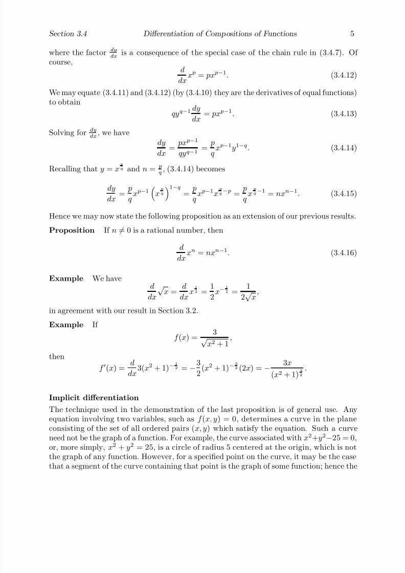
7/27/2019 Calculus 2 (Dan Sloughter)
http://slidepdf.com/reader/full/calculus-2-dan-sloughter 155/598
Section 3.4 Differentiation of Compositions of Functions 5
where the factor dy
dxis a consequence of the special case of the chain rule in (3.4.7). Of
course,d
dxx p = px p−1. (3.4.12)
We may equate (3.4.11) and (3.4.12) (by (3.4.10) they are the derivatives of equal functions)
to obtainqyq−1 dy
dx= px p−1. (3.4.13)
Solving for dydx
, we havedy
dx=
px p−1
qyq−1=
p
q x p−1y1−q. (3.4.14)
Recalling that y = xp
q and n = pq
, (3.4.14) becomes
dy
dx
=p
q
x p−1 xp
q 1−q
=p
q
x p−1xp
q− p =
p
q
xp
q−1 = nxn−1. (3.4.15)
Hence we may now state the following proposition as an extension of our previous results.
Proposition If n = 0 is a rational number, then
d
dxxn = nxn−1. (3.4.16)
Example We haved
dx
√ x =
d
dxx
1
2 =1
2
x−1
2 =1
2√ x
,
in agreement with our result in Section 3.2.
Example If
f (x) =3√
x2 + 1,
then
f (x) =d
dx3(x2 + 1)−
1
2 = −3
2(x2 + 1)−
3
2 (2x) = − 3x
(x2 + 1)3
2
.
Implicit differentiationThe technique used in the demonstration of the last proposition is of general use. Anyequation involving two variables, such as f (x, y) = 0, determines a curve in the planeconsisting of the set of all ordered pairs (x, y) which satisfy the equation. Such a curveneed not be the graph of a function. For example, the curve associated with x2+y2−25 = 0,or, more simply, x2 + y2 = 25, is a circle of radius 5 centered at the origin, which is notthe graph of any function. However, for a specified point on the curve, it may be the casethat a segment of the curve containing that point is the graph of some function; hence the
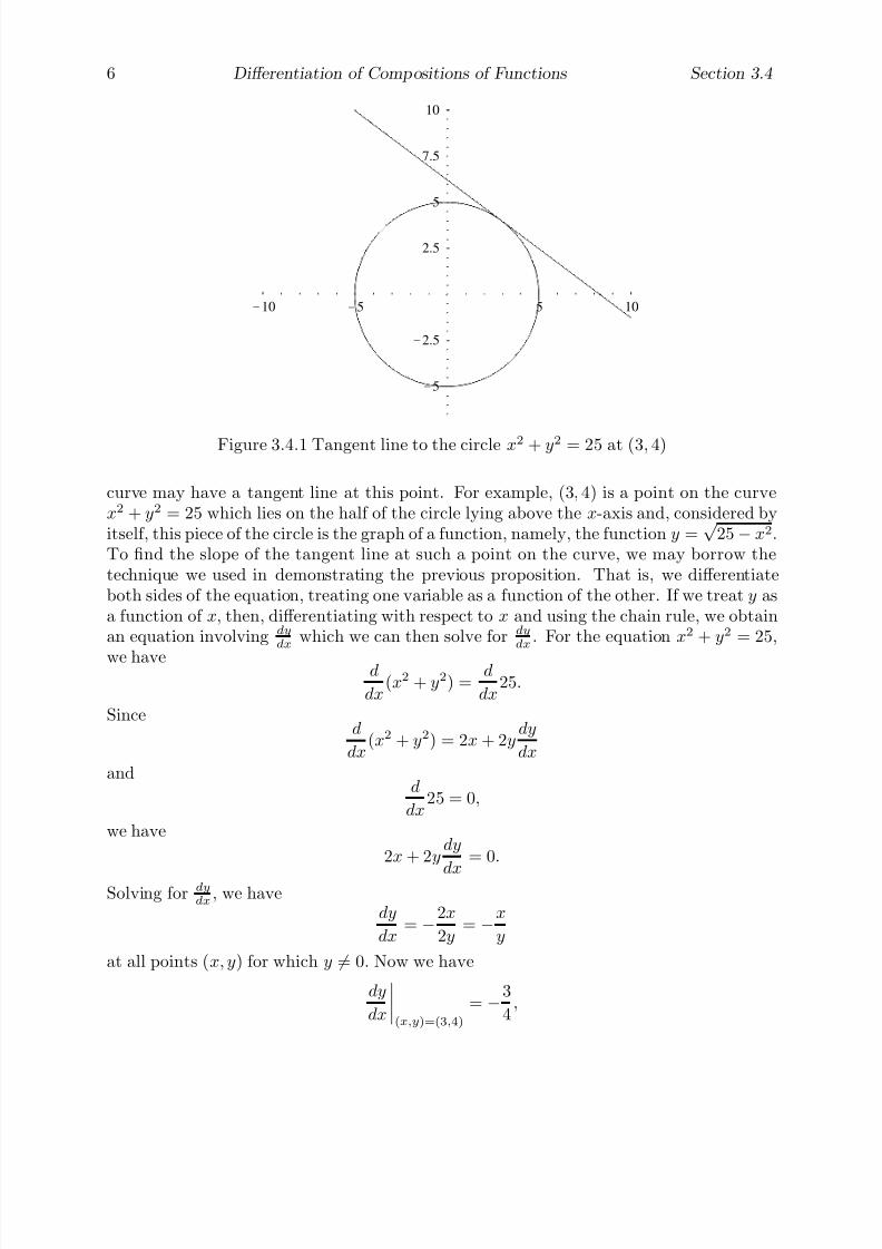
7/27/2019 Calculus 2 (Dan Sloughter)
http://slidepdf.com/reader/full/calculus-2-dan-sloughter 156/598
6 Differentiation of Compositions of Functions Section 3.4
-10 -5 5 10
-5
-2.5
2.5
5
7.5
10
Figure 3.4.1 Tangent line to the circle x2 + y2 = 25 at (3, 4)
curve may have a tangent line at this point. For example, (3, 4) is a point on the curvex2 + y2 = 25 which lies on the half of the circle lying above the x-axis and, considered byitself, this piece of the circle is the graph of a function, namely, the function y =
√ 25− x2.
To find the slope of the tangent line at such a point on the curve, we may borrow thetechnique we used in demonstrating the previous proposition. That is, we differentiateboth sides of the equation, treating one variable as a function of the other. If we treat y asa function of x, then, differentiating with respect to x and using the chain rule, we obtainan equation involving dy
dxwhich we can then solve for dy
dx. For the equation x2 + y2 = 25,
we have d
dx(x2 + y2) =
d
dx25.
Sinced
dx(x2 + y2) = 2x + 2y
dy
dx
andd
dx25 = 0,
we have
2x + 2ydy
dx
= 0.
Solving for dydx
, we havedy
dx= −2x
2y= −x
y
at all points (x, y) for which y = 0. Now we have
dy
dx
(x,y)=(3,4)
= −3
4,

7/27/2019 Calculus 2 (Dan Sloughter)
http://slidepdf.com/reader/full/calculus-2-dan-sloughter 157/598
Section 3.4 Differentiation of Compositions of Functions 7
and so the equation of the tangent line at (3, 4) is
y = −3
4(x− 3) + 4.
The circle with equation x2 + y2 = 25 and the tangent line at (3, 4) are shown in Figure3.4.1. Note that our procedure would not work to find the tangent lines to the circle at(−5, 0) and (5, 0). However, the tangents lines at these points are vertical, and, hence, donot have a slope. Although it is beyond the scope of this book to provide a justification,it is in fact the case that the technique outlined in this example will work to find the slopeof the tangent line at all points on the curve that have a tangent line with a slope.
This technique for finding derivatives is called implicit differentiation because we didnot use an explicit formula for y in terms x. In this case we could have obtained the sameresult by first solving for y in terms of x for values close to (3, 4), giving us y =
√ 25− x2,
and then evaluating the derivative of this function at x = 3. However, this is not alwayspossible or desirable; in many cases implicit differentiation is significantly simpler even if
an explicit solution is possible.
Example Consider the problem of finding the best affine approximation to the curvewith equation
y3 + 3xy2 − xy + x = 7
near the point (2, 1). To find dy
dx, we compute
d
dx(y3 + 3xy2 − xy + x) =
d
dx7,
which give us
d
dxy3 + 3x
d
dxy2 + 3y2
d
dxx−
x
dy
dx+ y
d
dxx
+
d
dxx = 0.
Computing the derivatives on the left-hand side gives us
3y2dy
dx+ 3x
2y
dy
dx
+ 3y2(1)− x
dy
dx− y(1) + 1 = 0.
Hence
3y2dy
dx+ 6xy
dy
dx+ 3y2 − x
dy
dx− y + 1 = 0,
from which it follows that
dy
dx(3y2 + 6xy − x) = y − 3y2 − 1.
Solving for dy
dx, we have
dy
dx=
y − 3y2 − 1
3y2 + 6xy − x,
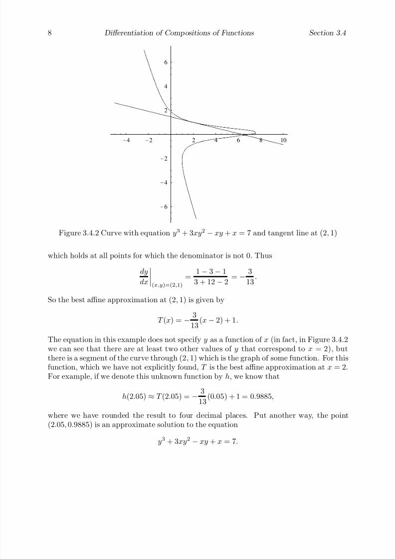
7/27/2019 Calculus 2 (Dan Sloughter)
http://slidepdf.com/reader/full/calculus-2-dan-sloughter 158/598
8 Differentiation of Compositions of Functions Section 3.4
-4 -2 2 4 6 8 10
-6
-4
-2
2
4
6
Figure 3.4.2 Curve with equation y3 + 3xy2 − xy + x = 7 and tangent line at (2, 1)
which holds at all points for which the denominator is not 0. Thus
dy
dx
(x,y)=(2,1)
=1− 3− 1
3 + 12 − 2= − 3
13.
So the best affine approximation at (2, 1) is given by
T (x) = − 3
13(x− 2) + 1.
The equation in this example does not specify y as a function of x (in fact, in Figure 3.4.2we can see that there are at least two other values of y that correspond to x = 2), butthere is a segment of the curve through (2, 1) which is the graph of some function. For thisfunction, which we have not explicitly found, T is the best affine approximation at x = 2.For example, if we denote this unknown function by h, we know that
h(2.05) ≈ T (2.05) = − 313
(0.05) + 1 = 0.9885,
where we have rounded the result to four decimal places. Put another way, the point(2.05, 0.9885) is an approximate solution to the equation
y3 + 3xy2 − xy + x = 7.
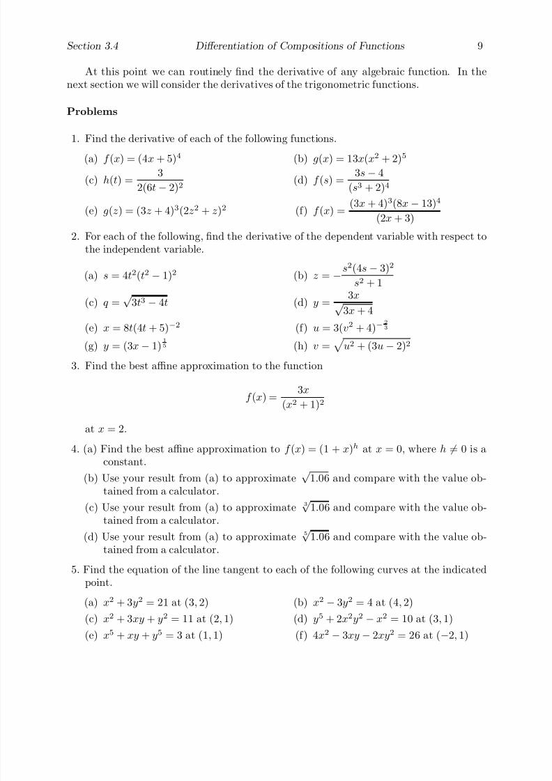
7/27/2019 Calculus 2 (Dan Sloughter)
http://slidepdf.com/reader/full/calculus-2-dan-sloughter 159/598
Section 3.4 Differentiation of Compositions of Functions 9
At this point we can routinely find the derivative of any algebraic function. In thenext section we will consider the derivatives of the trigonometric functions.
Problems
1. Find the derivative of each of the following functions.
(a) f (x) = (4x + 5)4 (b) g(x) = 13x(x2 + 2)5
(c) h(t) =3
2(6t− 2)2(d) f (s) =
3s − 4
(s3 + 2)4
(e) g(z) = (3z + 4)3(2z2 + z)2 (f) f (x) =(3x + 4)3(8x− 13)4
(2x + 3)
2. For each of the following, find the derivative of the dependent variable with respect tothe independent variable.
(a) s = 4t2(t2 − 1)2 (b) z = −s
2
(4s − 3)
2
s2 + 1
(c) q =√
3t3 − 4t (d) y =3x√
3x + 4
(e) x = 8t(4t + 5)−2 (f) u = 3(v2 + 4)−2
3
(g) y = (3x− 1)1
5 (h) v =
u2 + (3u− 2)2
3. Find the best affine approximation to the function
f (x) =3x
(x2 + 1)2
at x = 2.
4. (a) Find the best affine approximation to f (x) = (1 + x)h at x = 0, where h = 0 is aconstant.
(b) Use your result from (a) to approximate√
1.06 and compare with the value ob-tained from a calculator.
(c) Use your result from (a) to approximate 3√
1.06 and compare with the value ob-tained from a calculator.
(d) Use your result from (a) to approximate 5√
1.06 and compare with the value ob-
tained from a calculator.
5. Find the equation of the line tangent to each of the following curves at the indicatedpoint.
(a) x2 + 3y2 = 21 at (3, 2) (b) x2 − 3y2 = 4 at (4, 2)
(c) x2 + 3xy + y2 = 11 at (2, 1) (d) y5 + 2x2y2 − x2 = 10 at (3, 1)
(e) x5 + xy + y5 = 3 at (1, 1) (f) 4x2 − 3xy − 2xy2 = 26 at (−2, 1)
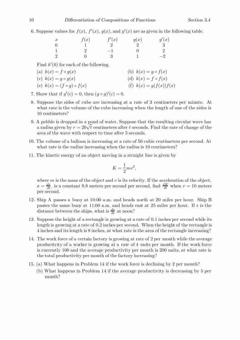
7/27/2019 Calculus 2 (Dan Sloughter)
http://slidepdf.com/reader/full/calculus-2-dan-sloughter 160/598
10 Differentiation of Compositions of Functions Section 3.4
6. Suppose values for f (x), f (x), g(x), and g(x) are as given in the following table.
x f (x) f (x) g(x) g(x)0 1 2 2 31 2 −1 0 22 0 3 1
−2
Find k(0) for each of the following.
(a) k(x) = f ◦ g(x) (b) k(x) = g ◦ f (x)
(c) k(x) = g ◦ g(x) (d) k(x) = f ◦ f (x)
(e) k(x) = (f ◦ g) ◦ f (x) (f) k(x) = g(f (x))f (x)
7. Show that if g(c) = 0, then (g ◦ g)(c) = 0.
8. Suppose the sides of cube are increasing at a rate of 3 centimeters per minute. Atwhat rate is the volume of the cube increasing when the length of one of the sides is10 centimeters?
9. A pebble is dropped in a pond of water. Suppose that the resulting circular wave hasa radius given by r = 20
√ t centimeters after t seconds. Find the rate of change of the
area of the wave with respect to time after 5 seconds.
10. The volume of a balloon is increasing at a rate of 50 cubic centimeters per second. Atwhat rate is the radius increasing when the radius is 10 centimeters?
11. The kinetic energy of an object moving in a straight line is given by
K =1
2mv2,
where m is the mass of the object and v is its velocity. If the acceleration of the object,a = dv
dt, is a constant 9.8 meters per second per second, find dK
dtwhen v = 10 meters
per second.
12. Ship A passes a buoy at 10:00 a.m. and heads north at 20 miles per hour. Ship Bpasses the same buoy at 11:00 a.m. and heads east at 25 miles per hour. If s is thedistance between the ships, what is ds
dtat noon?
13. Suppose the height of a rectangle is growing at a rate of 0.1 inches per second while itslength is growing at a rate of 0.2 inches per second. When the height of the rectangle is4 inches and its length is 8 inches, at what rate is the area of the rectangle increasing?
14. The work force of a certain factory is growing at rate of 2 per month while the averageproductivity of a worker is growing at a rate of 4 units per month. If the work forceis currently 100 and the average productivity per month is 200 units, at what rate isthe total productivity per month of the factory increasing?
15. (a) What happens in Problem 14 if the work force is declining by 2 per month?
(b) What happens in Problem 14 if the average productivity is decreasing by 5 permonth?
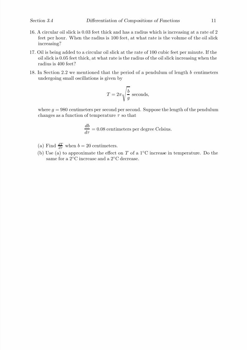
7/27/2019 Calculus 2 (Dan Sloughter)
http://slidepdf.com/reader/full/calculus-2-dan-sloughter 161/598
Section 3.4 Differentiation of Compositions of Functions 11
16. A circular oil slick is 0.03 feet thick and has a radius which is increasing at a rate of 2feet per hour. When the radius is 100 feet, at what rate is the volume of the oil slickincreasing?
17. Oil is being added to a circular oil slick at the rate of 100 cubic feet per minute. If theoil slick is 0.05 feet thick, at what rate is the radius of the oil slick increasing when theradius is 400 feet?
18. In Section 2.2 we mentioned that the period of a pendulum of length b centimetersundergoing small oscillations is given by
T = 2π
b
gseconds,
where g = 980 centimeters per second per second. Suppose the length of the pendulumchanges as a function of temperature τ so that
db
dτ = 0.08 centimeters per degree Celsius.
(a) Find dT dτ
when b = 20 centimeters.
(b) Use (a) to approximate the effect on T of a 1◦C increase in temperature. Do thesame for a 2◦C increase and a 2◦C decrease.

7/27/2019 Calculus 2 (Dan Sloughter)
http://slidepdf.com/reader/full/calculus-2-dan-sloughter 162/598
Difference Equations
Differential Equations
to
Section 3.5
Differentiation of TrigonometricFunctions
We now take up the question of differentiating the trigonometric functions. We will startwith the sine function. From Section 3.2, we know that
d
dxsin(x) = lim
h→0
sin(x + h)− sin(x)
h. (3.5.1)
From the addition formula for sine we have
sin(x + h) = sin(x)cos(h) + sin(h)cos(x), (3.5.2)
and so (3.5.1) becomes
d
dxsin(x) = lim
h→0
sin(x)cos(h) + sin(h)cos(x)− sin(x)
h. (3.5.3)
Now
sin(x)cos(h) + sin(h)cos(x)− sin(x)
h=
sin(x)(cos(h)− 1) + cos(x) sin(h)
h
= sin(x)cos(h)
−1
h
+ cos(x) sin(h)
h
.
Thusd
dxsin(x) = sin(x) lim
h→0
cos(h)− 1
h+ cos(x) lim
h→0
sin(h)
h. (3.5.4)
Our problem then comes down to evaluating the two limits in (3.5.4). The second of theseturns out to be the key, so we will begin with it.
For 0 < h < π
2, consider the point C = (cos(h), sin(h)) on the unit circle centered at
the origin. We first repeat an argument from Section 2.4 to show that sin(h) < h: If welet A = (0, 0) and B = (1, 0), as in Figure 3.5.1, then the area of ABC is
1
2sin(h).
The area of the sector of the circle cut off by the arc from B to C is the fraction h
2πof the
area of the entire circle; hence, this area is
h
2ππ =
h
2.
1 Copyright c by Dan Sloughter 2000

7/27/2019 Calculus 2 (Dan Sloughter)
http://slidepdf.com/reader/full/calculus-2-dan-sloughter 163/598
2 Differentiation of Trigonometric Functions Section 3.5
A
B
C
D
h
(1, 0)
(0, 1)
Figure 3.5.1
Since
ABC is contained in this section, we have
1
2sin(h) <
h
2, (3.5.5)
or simplysin(h) < h. (3.5.6)
Now let D = (1, tan(h)), the point where the line passing through A and C intersectsthe line perpendicular to the x-axis passing through B. Then ABD has area
1
2tan(h) =
sin(h)
2cos(h).
Since ABD contains the sector of the circle considered above, we have
h
2<
sin(h)
2cos(h), (3.5.7)
or
h <sin(h)
cos(h). (3.5.8)
Putting inequalities (3.5.6) and (3.5.8) together gives us
sin(h) < h <sin(h)
cos(h). (3.5.9)
Dividing through by sin(h) yields
1 <h
sin(h)<
1
cos(h), (3.5.10)

7/27/2019 Calculus 2 (Dan Sloughter)
http://slidepdf.com/reader/full/calculus-2-dan-sloughter 164/598
Section 3.5 Differentiation of Trigonometric Functions 3
which, after taking reciprocals, gives us
1 >sin(h)
h> cos(h). (3.5.11)
Now, finally, we can see where all of this has been heading. Since
limh→0+
cos(h) = 1,
(3.5.11) implies that we must have
limh→0+
sin(h)
h= 1. (3.5.12)
To check the limit from the other side, we make use of the identity sin(−x) = − sin(x).Letting t =
−h, we have
limh→0−
sin(h)
h= lim
h→0−
− sin(h)
−h= lim
h→0−
sin(−h)
−h= lim
t→0+
sin(t)
t= 1. (3.5.13)
Together (3.5.12) and (3.5.13) give us the following proposition.
Proposition
limh→0
sin(h)
h= 1. (3.5.14)
With this result, we may now compute
limh→0
1− cos(h)
h= lim
h→0
1− cos(h)
h
1 + cos(h)
1 + cos(h)
= limh→0
1− cos2(h)
h(1 + cos(h))
= limh→0
sin2(h)
h(1 + cos(h))
= limh→0
sin(h)
h
sin(h)
1 + cos(h)
= limh→0
sin(h)
h limh→0
sin(h)
1 + cos(h)
= (1)
0
2
= 0.
Proposition
limh→0
1− cos(h)
h= 0. (3.5.15)

7/27/2019 Calculus 2 (Dan Sloughter)
http://slidepdf.com/reader/full/calculus-2-dan-sloughter 165/598
4 Differentiation of Trigonometric Functions Section 3.5
Of course, from (3.5.15) we have
limh→0
cos(h)− 1
h= − lim
h→0
1− cos(h)
h= 0. (3.5.16)
Putting (3.5.14) and (3.5.16) into (3.5.4) gives us
d
dxsin(x) = sin(x) lim
h→0
cos(h)− 1
h+ cos(x) lim
h→0
sin(h)
h
= sin(x)(0) + cos(x)(1)
= cos(x).
Proposition The function f (x) = sin(x) is differentiable for all x in (−∞,∞) with
d
dxsin(x) = cos(x). (3.5.17)
The derivatives of the other trigonometric functions now follow with the help of somebasic identities. Since cos(x) = sin(x + π
2) and cos(x + π
2) = − sin(x), it follows that
d
dxcos(x) =
d
dxsin
x +
π
2
= cos
x +
π
2
d
dx
x +
π
2
= cos
x +
π
2
= − sin(x).
The other four derivatives are as follows:
d
dxtan(x) =
d
dx
sin(x)
cos(x)
=cos(x)
d
dxsin(x)− sin(x)
d
dxcos(x)
cos2(x)
=cos(x)cos(x)− sin(x)(− sin(x))
cos2(x)
=cos2(x) + sin2(x)
cos2(x)
=1
cos2(x)
= sec2
(x),
d
dxcot(x) =
d
dx
cos(x)
sin(x)
=sin(x)
d
dxcos(x)− cos(x)
d
dxsin(x)
sin2(x)

7/27/2019 Calculus 2 (Dan Sloughter)
http://slidepdf.com/reader/full/calculus-2-dan-sloughter 166/598
Section 3.5 Differentiation of Trigonometric Functions 5
=sin(x)(− sin(x))− cos(x)cos(x)
sin2(x)
=−(sin2(x) + cos2(x))
sin2(x)
= −1
sin2(x)
= − csc2(x),
d
dxsec(x) =
d
dx(cos(x))−1
= −(cos(x))−2d
dxcos(x)
=sin(x)
cos2(x)
= 1
cos(x) sin(x)
cos(x)
= sec(x)tan(x),
andd
dxcsc(x) =
d
dx(sin(x))−1
= −(sin(x))−2d
dxsin(x)
= − cos(x)
sin2(x)
= − 1sin(x)
cos(x)sin(x)
= csc(x)cot(x).
The next proposition summarizes these results.
Proposition The derivatives of the trigonometric functions are as follows:
d
dxsin(x) = cos(x) (3.5.18)
d
dxcos(x) = − sin(x) (3.5.19)
ddx
tan(x) = sec2(x) (3.5.20)
d
dxcot(x) = − csc2(x) (3.5.21)
d
dxsec(x) = sec(x) tan(x) (3.5.22)
d
dxcsc(x) = − csc(x)cot(x) (3.5.23)
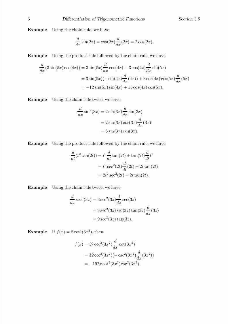
7/27/2019 Calculus 2 (Dan Sloughter)
http://slidepdf.com/reader/full/calculus-2-dan-sloughter 167/598
6 Differentiation of Trigonometric Functions Section 3.5
Example Using the chain rule, we have
d
dxsin(2x) = cos(2x)
d
dx(2x) = 2 cos(2x).
Example Using the product rule followed by the chain rule, we have
d
dx(3 sin(5x) cos(4x)) = 3 sin(5x)
d
dxcos(4x) + 3 cos(4x)
d
dxsin(5x)
= 3 sin(5x)(− sin(4x)d
dx(4x)) + 3 cos(4x) cos(5x)
d
dx(5x)
= −12 sin(5x) sin(4x) + 15 cos(4x) cos(5x).
Example Using the chain rule twice, we have
d
dx sin
2
(3x) = 2 sin(3x)
d
dx sin(3x)
= 2 sin(3x) cos(3x)d
dx(3x)
= 6 sin(3x) cos(3x).
Example Using the product rule followed by the chain rule, we have
d
dt(t2 tan(2t)) = t2
d
dttan(2t) + tan(2t)
d
dtt2
= t2 sec2(2t)d
dt
(2t) + 2t tan(2t)
= 2t2 sec2(2t) + 2t tan(2t).
Example Using the chain rule twice, we have
d
dzsec3(3z) = 3 sec2(3z)
d
dzsec(3z)
= 3 sec2(3z) sec(3z) tan(3z)d
dz(3z)
= 9 sec3(3z) tan(3z).
Example If f (x) = 8 cot4(3x2), then
f (x) = 32 cot3(3x2)d
dxcot(3x2)
= 32 cot3(3x2)(− csc2(3x2)d
dx(3x2))
= −192x cot3(3x2)csc2(3x2).
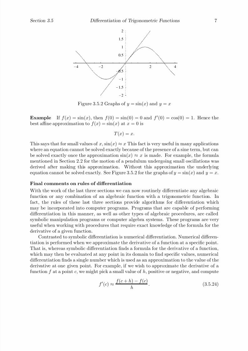
7/27/2019 Calculus 2 (Dan Sloughter)
http://slidepdf.com/reader/full/calculus-2-dan-sloughter 168/598
Section 3.5 Differentiation of Trigonometric Functions 7
-4 -2 2 4
-2
-1.5
-1
-0.5
0.5
1
1.5
2
Figure 3.5.2 Graphs of y = sin(x) and y = x
Example If f (x) = sin(x), then f (0) = sin(0) = 0 and f (0) = cos(0) = 1. Hence the
best affine approximation to f (x) = sin(x) at x = 0 is
T (x) = x.
This says that for small values of x, sin(x) ≈ x This fact is very useful in many applicationswhere an equation cannot be solved exactly because of the presence of a sine term, but canbe solved exactly once the approximation sin(x) ≈ x is made. For example, the formulamentioned in Section 2.2 for the motion of a pendulum undergoing small oscillations wasderived after making this approximation. Without this approximation the underlyingequation cannot be solved exactly. See Figure 3.5.2 for the graphs of y = sin(x) and y = x.
Final comments on rules of differentiationWith the work of the last three sections we can now routinely differentiate any algebraicfunction or any combination of an algebraic function with a trigonometric function. Infact, the rules of these last three sections provide algorithms for differentiation whichmay be incorporated into computer programs. Programs that are capable of performingdifferentiation in this manner, as well as other types of algebraic procedures, are calledsymbolic manipulation programs or computer algebra systems. These programs are veryuseful when working with procedures that require exact knowledge of the formula for thederivative of a given function.
Contrasted to symbolic differentiation is numerical differentiation. Numerical differen-tiation is performed when we approximate the derivative of a function at a specific point.That is, whereas symbolic differentiation finds a formula for the derivative of a function,which may then be evaluated at any point in its domain to find specific values, numericaldifferentiation finds a single number which is used as an approximation to the value of thederivative at one given point. For example, if we wish to approximate the derivative of afunction f at a point c, we might pick a small value of h, positive or negative, and compute
f (c) ≈ f (c + h)− f (c)
h. (3.5.24)
7/27/2019 Calculus 2 (Dan Sloughter)
http://slidepdf.com/reader/full/calculus-2-dan-sloughter 169/598
8 Differentiation of Trigonometric Functions Section 3.5
Of course, we need some procedure for deciding when h is small enough for (3.5.24) to givean accurate estimate for f (c). One technique is to use (3.5.24) repeatedly, cutting h in half each time, until the result does not change through the desired number of decimal places.This method is subject to serious roundoff errors due to the loss of significant digits in thenumerator when two nearly equal numbers are subtracted (see Problem 13). Hence the
numerical approximation of derivatives is not recommended unless it cannot be avoided.Problem 10 suggests an alternative to (3.5.24) which is both more stable for computationsand more accurate for a given value of h.
Problems
1. Find the derivative of each of the following functions.
(a) f (x) = x2 sin(x) (b) g(x) = cos(4x)
(c) g(t) = 3t cos(2t) (d) h(s) = sin2(s)cos(s)
(e) f (t) = sin(3t) cos(4t) (f) g(z) = sin3(4z)
2. Find the derivative of the dependent variable with respect to the independent variablefor each of the following.
(a) y =sin(2x)
x(b) x = 3 tan(2t)
(c) x = sin(4t2 + 1) (d) y = 4θ tan(θ2 − 1)
(e) z =1
cos(2t)(f) q = sec3(3t)
(g) y = x2 csc(2x) (h) s = 3t cot(2t)
3. Evaluate each of the following.
(a)d
dx(sin2(2x)cos2(3x)) (b)
d
dx(sec(x) tan(x))
(c)d
dq sec3(q 2) (d)
d
dt
sin2(t)
cos(t)
(e)d
dz
1 + sin2(z) (f)
d
dr(r2 cos(3r2))
4. Find the best affine approximation to f (x) = tan(2x) at 0.
5. Find the best affine approximation to g(t) = cos(t) at 0.
6. Find the best affine approximation to f (t) = sin2(t) at 0.
7. (a) Find the best affine approximation S to f (x) =√
1 + x at 0.
(b) Find the best affine approximation T to g(x) = sin(4x) at 0.
(c) Find the best affine approximation U to h(x) =
1 + sin(4x) at 0.
(d) What is the relationship between f , g, and h? Is their a similar relationshipbetween S , T , and U ?

7/27/2019 Calculus 2 (Dan Sloughter)
http://slidepdf.com/reader/full/calculus-2-dan-sloughter 170/598
Section 3.5 Differentiation of Trigonometric Functions 9
8. Evaluate the following limits.
(a) limx→0
sin(2x)
x(b) lim
x→0
sin(2x)
sin(3x)
(c) limx→0
tan(x)
x
(d) limh→0
tan(2h)
sin(3h)
(e) limx→0
sin2(x)
x(f) lim
t→0
1− cos(t)
t2
(g) limt→0
sin2(3t)
t2(h) lim
θ→0
tan2(5θ)
sin2(3θ)
9. For each of the following, decide whether or not the given function is o(h) and whetheror not it is O(h).
(a) f (x) = sin(x) (b) f (x) = sin2(x)
(c) g(t) = tan(t) (d) h(t) = tan2(t)
(e) f (t) = 1 − cos(t) (f) g(t) = 1− cos2(t)
10. Given a function f which is differentiable at the point c, define
D(h) =f (c + h)− f (c)
h.
Then, for small values of h, f (c) ≈ D(h).
(a) Let h > 0. A better approximation for f (c) than D(h) is given by averaging D(h)and D(−h). Show that if we define
D1(h) =D(h) + D(−h)
2,
then
D1(h) =f (c + h)− f (c− h)
2h.
What is D1(h) geometrically?
(b) Let h > 0. Another approximation that is sometimes used for f (c) is
D2(h) =4
3 D1h
2− 1
3 D1(h).
Show that
D2(h) =f (c− h)− 8f
c− h
2
+ 8f
c + h
2
− f (c + h)
6h.

7/27/2019 Calculus 2 (Dan Sloughter)
http://slidepdf.com/reader/full/calculus-2-dan-sloughter 171/598
10 Differentiation of Trigonometric Functions Section 3.5
11. Using h = 0.00001, approximate the derivatives of the following functions using D(h),D1(h), and D2(h) (from Problem 10) at the indicated points. Compare your answerswith the exact values.
(a) f (x) = x2 at x = 2 (b) f (x) =1
xat x = 2
(c) f (x) = sin(x) at x = 0 (d) f (x) = 3 sin(x2
) cos(4x) at x = 0
12. Compute D(h), D1(h), and D2(h) (from Problem 10) for the function f (x) = |x| atx = 0. Use h = 0.001. Are your answers reasonable? Can you explain them?
13. For f (x) = x2 and c = 2, compute the values of
en = |4−D(10−n)|
(see Problem 10) for n = 1, 2, . . . , 15. Note that you are computing the absolute valueof the error in approximating f (c) by D(h) for different values of h. Plot the orderedpairs (n, en). Does the absolute value of the error decrease as h decreases? Can you
explain your results?
7/27/2019 Calculus 2 (Dan Sloughter)
http://slidepdf.com/reader/full/calculus-2-dan-sloughter 172/598
Difference Equations
Differential Equations
toSection 3.6
Newton’s Method
Many problems in mathematics involve, at some point or another, solving an equationfor an unknown quantity. An equation of the form f (x) = 0 may be solved for x bysimple algebra if f is an affine function and by the quadratic formula if f is a quadraticpolynomial. There are formulas similar to the quadratic formula for both cubic and quarticpolynomials, but they are, in general, very cumbersome. One of the most interestingresults of mathematics, due to Niels Henrik Abel (1802-1829), is that there does not existan analogue of the quadratic formula for quintic polynomials. For this and other reasons,it turns out that in many situations solving an equation f (x) = 0 for x requires using amethod which can approximate the solutions to a predetermined level of accuracy.
In Section 2.5 we discussed one such method, the bisection algorithm, for approximat-ing the solutions of an equation. The strong point of the bisection algorithm is that, oncean appropriate starting interval has been found, the method will always find a solution toany desired level of accuracy; its weakness lies in the slowness with which the successiveapproximations approach the solution. In this section we will discuss another method,known as Newton’s method , for approximating solutions to an equation. In distinction tothe bisection algorithm, Newton’s method does not always work, but, when it does, it isin general remarkably fast.
Suppose we wish to find a solution to the equation f (x) = 0 for a given function f .
Recall that, geometrically, this corresponds to finding the point where the curve y = f (x)crosses the x-axis. To start Newton’s method, we must first have an initial guess x0.Frequently, we find the initial guess by graphing the curve y = f (x) and letting x0 be apoint close to where the curve crosses the x-axis. Given the initial guess x0, let T 0 be thebest affine approximation to f at x0. That is, define T 0 by
T 0(x) = f (x0)(x − x0) + f (x0). (3.6.1)
The idea behind Newton’s method is to obtain an improved estimate of a solution tof (x) = 0 by replacing the equation f (x) = 0 with the simpler equation T 0(x) = 0. If welet x1 denote the solution to the latter equation, then we have T 0(x1) = 0, that is
f (x0)(x1 − x0) + f (x0), (3.6.2)
from which it follows that
x1 = x0 − f (x0)
f (x0). (3.6.3)
Geometrically, x1 is the point at which the line tangent to f at (x0, f (x0) crosses the x-axis, as shown in Figure 3.6.1. To improve upon this approximation, we solve the equation
1 Copyright c by Dan Sloughter 2000
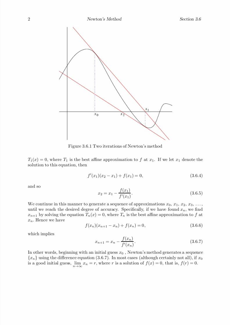
7/27/2019 Calculus 2 (Dan Sloughter)
http://slidepdf.com/reader/full/calculus-2-dan-sloughter 173/598
2 Newton’s Method Section 3.6
x
x x 20
1
Figure 3.6.1 Two iterations of Newton’s method
T 1(x) = 0, where T 1 is the best affine approximation to f at x1. If we let x1 denote thesolution to this equation, then
f (x1)(x2 − x1) + f (x1) = 0, (3.6.4)
and so
x2 = x1 − f (x1)
f (x1). (3.6.5)
We continue in this manner to generate a sequence of approximations x0, x1, x2, x3, . . . ,until we reach the desired degree of accuracy. Specifically, if we have found xn, we findxn+1 by solving the equation T n(x) = 0, where T n is the best affine approximation to f atxn. Hence we have
f (
xn)(
xn+1 −xn
) +f
(xn
) = 0,
(3.6.6)which implies
xn+1 = xn − f (xn)
f (xn). (3.6.7)
In other words, beginning with an initial guess x0 , Newton’s method generates a sequence{xn} using the difference equation (3.6.7). In most cases (although certainly not all), if x0is a good initial guess, lim
n→∞
xn = r, where r is a solution of f (x) = 0, that is, f (r) = 0.
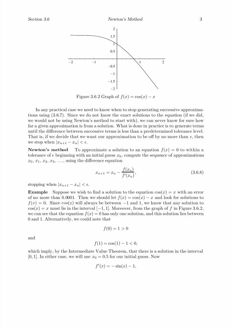
7/27/2019 Calculus 2 (Dan Sloughter)
http://slidepdf.com/reader/full/calculus-2-dan-sloughter 174/598
Section 3.6 Newton’s Method 3
-2 -1 1 2
-2
-1.5
-1
-0.5
0.5
1
1.5
2
Figure 3.6.2 Graph of f (x) = cos(x) − x
In any practical case we need to know when to stop generating successive approxima-
tions using (3.6.7). Since we do not know the exact solutions to the equation (if we did,we would not be using Newton’s method to start with), we can never know for sure howfar a given approximation is from a solution. What is done in practice is to generate termsuntil the difference between successive terms is less than a predetermined tolerance level.That is, if we decide that we want our approximation to be off by no more than , thenwe stop when |xn+1 − xn| < .
Newton’s method To approximate a solution to an equation f (x) = 0 to within atolerance of beginning with an initial guess x0, compute the sequence of approximationsx0, x1, x2, x3, . . . , using the difference equation
xn+1 = xn −f (xn)
f (xn) , (3.6.8)
stopping when |xn+1 − xn| < .
Example Suppose we wish to find a solution to the equation cos(x) = x with an errorof no more than 0.0001. Then we should let f (x) = cos(x) − x and look for solutions tof (x) = 0. Since cos(x) will always be between −1 and 1, we know that any solution tocos(x) = x must lie in the interval [−1, 1]. Moreover, from the graph of f in Figure 3.6.2,we can see that the equation f (x) = 0 has only one solution, and this solution lies between0 and 1. Alternatively, we could note that
f (0) = 1 > 0
andf (1) = cos(1) − 1 < 0,
which imply, by the Intermediate Value Theorem, that there is a solution in the interval[0, 1]. In either case, we will use x0 = 0.5 for our initial guess. Now
f (x) = − sin(x) − 1,

7/27/2019 Calculus 2 (Dan Sloughter)
http://slidepdf.com/reader/full/calculus-2-dan-sloughter 175/598
4 Newton’s Method Section 3.6
so
x1 = x0 − f (x0)
f (x0)= 0.5 − f (0.5)
f (0.5)= 0.755222,
where we have rounded the result to 6 decimal places. Substituting this back into (3.6.8)gives us
x2 = x1 − f (x1)
f (x1)= 0.75222 − f (0.755222)
f (0.755222)= 0.739142.
Since
|x2 − x1| = 0.016080 > 0.0001,
we continue and compute
x3 = x2 − f (x2)
f (x2)= 0.739142 − f (0.739142)
f (0.739142)= 0.739085.
Now we have|x3 − x2| = 0.000057 < 0.0001,
so we stop and use 0.7391 as our approximation to the solution of cos( x) = x. Forcomparison, with the bisection algorithm starting from the initial interval [0 , 1], we wouldhave had to iterate 13 times before obtaining an approximation to the solution with anerror less than 0.0001.
Example As an example of where Newton’s method goes wrong, consider the equationf (x) = 0, where
f (x) =x
1 + x2.
Clearly, x = 0 is the only solution to this equation. However, beginning with an initialguess x0 = 0.75, Newton’s method yields the following sequence (where we have roundedeach value to 5 digits):
x0 = 0.75000
x1 = −1.9286
x2 = −5.2756
x3 = −10.944
x4 =−
22.073
x5 = −44.237
x6 = −88.518
x7 = −177.06
x8 = −354.13
x9 = −708.27
x10 = −1416.5

7/27/2019 Calculus 2 (Dan Sloughter)
http://slidepdf.com/reader/full/calculus-2-dan-sloughter 176/598
Section 3.6 Newton’s Method 5
-12 -10 -8 -6 -4 -2 2
-0.4
-0.2
0.2
0.4
x
x x
1
x
3 20
Figure 3.6.3 Newton’s method diverging from a solution
Instead of converging to the solution at 0, this sequence seems to be diverging toward −∞.
In fact, geometrically this appears to be exactly the case, as can be seen in Figure 3.6.3.Here the problem comes from the fact that the graph of f approaches 0 asymptotically asx goes to −∞. Newton’s method is following the curve as it approaches 0, as it should,but, since there is no solution in this direction, the result is that the iterates are gettingfarther and farther away from the solution at x = 0.
Note that in the last example,
f (x) =1 − x2
(1 + x2)2,
giving us f
(1) = 0. Hence if we had started with an initial guess of x0 = 1, an applicationof the difference equation (3.6.8) would require a division by 0, which, of course, cannot bedone. Geometrically, the tangent line to the graph of f at (1, 0.5) is horizontal, and hencenever crosses the x-axis, implying that there are no solutions to the equation T (x) = 0 if T
is the best affine approximation to f at 1. Thus we must avoid starting Newton’s methodat a point where the derivative is 0.
Problems
1. For each of the following equations, use a graph to obtain initial guesses for solutionsand then apply Newton’s method to locate the solutions within 0.0001.
(a) x5 − 6x3 + 2x = 2 (b) sin(x) = x2
(c) cos(t) = t2 (d) cos2(t) − t2 = 0
(e) 2sin(x) =√
x + 1 (f) 6x4 − 12x3 + 4x − 1 = 0
2. Even though we know that for a positive number c the equation x2−c = 0 has the exactsolutions −√ c and
√ c, we may use Newton’s methods to find decimal approximations
to these square roots.

7/27/2019 Calculus 2 (Dan Sloughter)
http://slidepdf.com/reader/full/calculus-2-dan-sloughter 177/598
6 Newton’s Method Section 3.6
(a) Show that the sequence x0, x1, x2, . . . , of Newton’s method approximations to asolution of x2 − c = 0 satisfies the difference equation
xn+1 =xn +
c
xn
2for n = 0, 1, 2, . . ..
(b) Use the difference equation from (a) to approximate√
2,√
3, and√
11 with anerror of less than 0.00001.
(c) Can you see an intuitive reason why, starting with a positive initial guess, thesequence defined by the difference equation in part (a) might converge to
√ c?
(d) Assuming that L = limn→∞
xn for the sequence defined in (a), show that either
L = −√ c or L =√
c.
3. Use Newton’s method to approximate 3√
2 with an error less than 0.00001.
4. Use Newton’s method to approximate 7√ 5 with an error less than 0.00001.
5. The method outlined in Problem 2 for approximating square roots was known to theGreeks and perhaps to the Babylonians. For an account of this and other aspects of Babylonian algebra, read Chapter 3 of Mathematics in Civilization by H. L. Resnikoff and R. O. Wells, Jr. (Dover Publications, Inc., New York, 1984).
6. What happens when you apply Newton’s method to find solutions to the equation
x3 − 5x = 0
starting with an initial guess of x0 = 1? Explain this geometrically with a graph.
7. We know that when solving an equation f (x) = 0 using Newton’s method, differentinitial guesses may lead to different solutions, and some may not converge to a solu-tion at all. The problem of determining which initial guesses converge to a specifiedsolution is surprisingly complicated, involving what mathematicians call fractals . Foran account of this phenomenon, read pages 217-220 of Chaos by James Gleick (VikingPenguin, Inc., New York, 1987). Also, see the picture on the sixth color plate followingpage 114 in the same book.

7/27/2019 Calculus 2 (Dan Sloughter)
http://slidepdf.com/reader/full/calculus-2-dan-sloughter 178/598
Difference Equations
Differential Equations
to
Section 3.7
Rolle’s Theorem and the
Mean Value Theorem
The two theorems which are at the heart of this section draw connections between theinstantaneous rate of change and the average rate of change of a function. The MeanValue Theorem, of which Rolle’s Theorem is a special case, says that if f is differentiableon an interval, then there is some point in that interval at which the instantaneous rateof change of the function is equal to the average rate of change of the function over theentire interval. For example, if f gives the position of an object moving in a straight line,the Mean Value Theorem says that if the average velocity over some interval of time is 60miles per hour, then at some time during that interval the object was moving at exactly60 miles per hour. This is not a surprising fact, but it does turn out to be the key tounderstanding many useful applications.
Before we turn to a consideration of Rolle’s theorem, we need to establish anotherfundamental result. Suppose an object is thrown vertically into the air so that its positionat time t is given by f (t) and its velocity by v(t) = f (t). Moreover, suppose it reaches itsmaximum height at time t0. On its way up, the object is moving in the positive direction,and so v(t) > 0 for t < t0; on the way down, the object is moving in the negative direction,and so v(t) < 0 for t > t0. It follows, by the Intermediate Value Theorem and the fact thatv is a continuous function, that we must have v(t0) = 0. That is, at time t0, when f (t)reaches its maximum value, we have f (t0) = 0. This is an extremely useful fact which
holds in general for differentiable functions, not only at maximum values but at minimumvalues as well. Before providing a general demonstration, we first need a few definitions.
Definition A function f is said to have a local maximum at a point c if there exists anopen interval I containing c such that f (c) ≥ f (x) for all x in I . A function f is said tohave a local minimum at a point c if there exists an open interval I containing c such thatf (c) ≤ f (x) for all x in I . If f has either a local maximum or a local minimum at c, thenwe say f has a local extremum at c.
In short, f has a local maximum at a point c if the value of f at c is at least as largeas the value of f at any nearby point, and f has a local minimum at a point c if the valueof f at c is at least as small as the value of f at any nearby point. The next example
provides an illustration.
Example Looking at the graph of the function f (x) = x3−3x in Figure 3.7.1, it appearsthat f has a local maximum of 2 at x = −1 and a local minimum of −2 at x = 1. We willconfirm this observation in Section 3.8.
1 Copyright c by Dan Sloughter 2000

7/27/2019 Calculus 2 (Dan Sloughter)
http://slidepdf.com/reader/full/calculus-2-dan-sloughter 179/598
2 Rolle’s Theorem and the Mean Value Theorem Section 3.7
-3 -2 -1 1 2 3
-4
-2
2
4
Figure 3.7.1 Graph of f (x) = x3 − 3x
Now suppose f has local maximum at a point c and suppose f is differentiable at c.
For small enough h > 0, f (c + h) ≤ f (c), so
f (c + h)− f (c) ≤ 0;
thusf (c + h)− f (c)
h≤ 0. (3.7.1)
Clearly, if each term in a sequence is less than or equal to 0, and the sequence has a limit,then the limit of the sequence must be less than or equal to 0. Hence
f
(c) = limh→0+
f (c + h)
−f (c)
h ≤ 0. (3.7.2)
Also, for h < 0 with |h| small enough, we have f (c + h) ≤ f (c), and so
f (c + h)− f (c) ≤ 0.
However, now, since h < 0, we have
f (c + h)− f (c)
h≥ 0, (3.7.3)
from which it follows that
f (c) = limh→0−
f (c + h)− f (c)
h≥ 0. (3.7.4)
Note that (3.7.1) is saying that secant lines to the right of a local maximum have negativeslope, while (3.7.3) is saying that secant lines to the left of a local maximum have positiveslope. Now the only way that both (3.7.2) and (3.7.4) can hold at the same time is if f (c) = 0; that is, the only number which is both less than or equal to 0 and greater than

7/27/2019 Calculus 2 (Dan Sloughter)
http://slidepdf.com/reader/full/calculus-2-dan-sloughter 180/598
Section 3.7 Rolle’s Theorem and the Mean Value Theorem 3
a bc
Figure 3.7.2 Illustration of Rolle’s Theorem
or equal to 0 is 0 itself. Note that our argument here is just a refinement of our commentsabout velocity in the previous paragraph.
A similar argument gives the same result if f has a local minimum at c. The followingproposition puts these together into one statement.
Proposition If f has a local extremum at c and f is differentiable at c, then f (c) = 0.
Example For f (x) = x3 − 3x, as in the previous example, f (x) = 3x2 − 3, and sof (−1) = 0 and f (1) = 0, consistent with our observation that f has a local maximum atx = −1 and local minimum at x = 1. Note, however, that this does not prove that f has
local extrema at x = −1 and x = 1. Indeed, the proposition works in the other direction:if f has a local extremum at c, then f (c) = 0.
This result will be very useful in our work in the next section when we consider theproblem of finding the maximum and minimum values of a given function. For our presentpurpose, consider a function f which is continuous on a closed interval [a, b] and differen-tiable on the open interval (a, b), with f (a) = f (b) = 0. An example of such a functionis shown in Figure 3.7.2. By the Extreme Value Theorem of Section 2.5, we know that f
must have both a minimum value m and a maximum value M on [a, b]. If m = M = 0,then f (x) = 0 for all x in (a, b), and so f (x) = 0 for all x in (a, b). If either m = 0 orM = 0, then f has a local extremum at some point c in (a, b), namely, either a point c
for which f (c) = m or a point c for which f (c) = M . Hence, by the previous proposition,f (c) = 0. We have thus established the following theorem, credited originally to MichelRolle (1652-1719).
Rolle’s Theorem If f is continuous on [a, b], differentiable on (a, b), and f (a) = f (b) =0, then there exists a point c in (a, b) such that f (c) = 0.
Put another way, Rolle’s theorem says that if f is a differentiable function, then be-tween any two solutions of the equation f (x) = 0 there is a point c where f (c) = 0. Used

7/27/2019 Calculus 2 (Dan Sloughter)
http://slidepdf.com/reader/full/calculus-2-dan-sloughter 181/598
4 Rolle’s Theorem and the Mean Value Theorem Section 3.7
ba c
g( ) x
Figure 3.7.3 Illustration of the Mean Value Theorem
in conjunction with the Intermediate Value Theorem, this result can help identify intervalswhere an equation has a unique solution.
Example Solving the equationx5 + x4 = 1 (3.7.5)
is equivalent to solving the equation f (x) = 0 where f (x) = x5 + x4 − 1. Since f (0) = −1and f (1) = 1, the Intermediate Value Theorem tells us that f (x) = 0 has at least onesolution in (0, 1). Moreover,
f (x) = 5x4 + 4x3,
so f (x) > 0 for all x in (0, 1); in particular, there does not exist a point c in (0, 1) such
that f
(c) = 0. Hence, by Rolle’s Theorem, there cannot be two solutions to f (x) = 0 in(0, 1). That is, using the Intermediate Value Theorem and Rolle’s Theorem together, weare able to conclude that there is exactly one solution to (3.7.5) in the interval (0, 1). Wemay now use either the bisection algorithm or Newton’s method to locate this solution.
Geometrically, Rolle’s theorem says if f is a function which satisfies the conditions of the theorem on an interval [a, b], then there is a point c in (a, b) such that the line tangentto the graph of f at (c, f (c)) is horizontal. In this case, that means that the line tangentto the graph of f at (c, f (c)) is parallel to the line passing through the points (a, f (a)) and(b, f (b)), as is seen in Figure 3.7.2. Certainly, if we took this picture and rotated or shiftedthe points (a, f (a)) and (b, f (b)), rigidly moving the graph with these points, then this
conclusion would still follow. That is, if f is continuous on the closed interval [a, b] anddifferentiable on (a, b), then there must exist a point c in (a, b) such that the line tangentto the graph of f at (c, f (c)) is parallel to the line passing through the points (a, f (a)) and(b, f (b)) (see Figure 3.7.3). In other words, there must be a point c in (a, b) such that
f (c) =f (b)− f (a)
b− a. (3.7.6)
This is the content of the Mean Value Theorem.
7/27/2019 Calculus 2 (Dan Sloughter)
http://slidepdf.com/reader/full/calculus-2-dan-sloughter 182/598
Section 3.7 Rolle’s Theorem and the Mean Value Theorem 5
Although the above argument for this result seems plausible, we will present a moreprecise argument. Define a new function g by
g(x) = f (x)− S (x), (3.7.7)
whereS (x) =
f (b)− f (a)
b− a
(x− a) + f (a). (3.7.8)
Geometrically, the graph of S is a line passing through the points (a, f (a)) and (b, f (b)),and g(x) is the distance from the graph of f to the graph of S above the point x (seeFigure 3.7.3). Now g is continuous on [a, b] and differentiable on (a, b); moreover,
g(a) = f (a)− S (a) = f (a)− f (a) = 0 (3.7.9)
andg(b) = f (b)
−S (b) = f (b)
−f (b) = 0. (3.7.10)
Thus g satisfies the conditions of Rolle’s theorem. Hence there exists a point c in (a, b)such that g(c) = 0. But
g(x) = f (x)− f (b)− f (a)
b− a, (3.7.11)
and so g(c) = 0 implies
f (c)− f (b)− f (a)
b− a= 0, (3.7.12)
that is,
f (c) =f (b)− f (a)
b−
a. (3.7.13)
Mean Value Theorem If f is continuous on [a, b] and differentiable on (a, b), thenthere exists a point c in (a, b) such that
f (c) =f (b)− f (a)
b− a. (3.7.14)
Increasing and decreasing functions
Similar to the situation with the Intermediate Value Theorem and the Extreme ValueTheorem, the Mean Value Theorem is an existence theorem. The point of interest is theexistence of c, not in being able to compute a value for c. Although not immediatelyuseful for computations, we will see that the Mean Value Theorem has many importantconsequences. The first of these, which we will consider now, involves determining when afunction is increasing and when it is decreasing.
Definition We say a function f defined on an interval I is increasing on I if for everytwo points u and v in I with u < v, f (u) < f (v). We say a function f defined on aninterval I is decreasing on I if for every two points u and v in I with u < v, f (u) > f (v).

7/27/2019 Calculus 2 (Dan Sloughter)
http://slidepdf.com/reader/full/calculus-2-dan-sloughter 183/598
6 Rolle’s Theorem and the Mean Value Theorem Section 3.7
Example The function f (x) = x2 is increasing on the interval [0,∞) since for any twonumbers u and v with 0 ≤ u < v, f (u) = u2 < v2 = f (v). Moreover, f is decreasing on(−∞, 0] since for any two numbers u and v with u < v ≤ 0, f (u) = u2 > v2 = f (v).
Now suppose f is differentiable on an interval (a, b) with f (x) > 0 for all x in (a, b).If u and v are two points in (a, b) with u < v, then, by the Mean Value Theorem, thereexists a point c with u < c < v such that
f (c) =f (v)− f (u)
v − u. (3.7.15)
Since c is in (a, b), f (c) > 0, so, using (3.7.15),
f (v)− f (u) = f (c)(v − u) > 0. (3.7.16)
Hence f (v) > f (u) and f is increasing on the interval (a, b). Similarly, if f (x) < 0 for allx in (a, b), then we would have f (c) < 0, from which it would follow that f (v) > f (u)
and, hence, that f is decreasing on (a, b). In short, to determine the intervals on which adifferentiable function is increasing and those on which it is decreasing, we need to lookonly for the intervals on which the derivative is positive and those on which it is negative,respectively.
Proposition If f is differentiable on (a, b) and f (x) > 0 for all x in (a, b), then f isincreasing on (a, b). If f is differentiable on (a, b) and f (x) < 0 for all x in (a, b), then f
is decreasing on (a, b).
Geometrically, this proposition is saying that a function is increasing where it haspositive slope and decreasing where it has negative slope. This should seem intuitivelyclear, but it is the Mean Value Theorem which makes the connection between average
rates of change and instantaneous rates of change necessary for establishing the result.
Example Suppose f (x) = 2x3 + 3x2− 12x + 1. To determine where f is increasing andwhere it is decreasing, we first find
f (x) = 6x2 + 6x− 12 = 6(x + 2)(x− 1). (3.7.17)
Hence f (x) = 0 only when x = −2 or x = 1. Since f is continuous, the IntermediateValue Theorem implies that f cannot change sign on the intervals (−∞,−2), (−2, 1), and(1,∞). Since f (−3) = 24 > 0, it follows that f (x) > 0 for all x in (−∞,−2). Similarly,since f (0) = −12 < 0, f (x) < 0 for all x in (−2, 1); and, since f (2) = 24 > 0, f (x) > 0
for all x in (1,∞). It now follows from the previous proposition that f is increasing on theintervals (−∞,−2) and (1,∞) and decreasing on the interval (−2, 1).
Note that we could obtain the same information about f directly from (3.7.17) withoutevaluating f and without invoking the Intermediate Value Theorem. Namely, from thefacts that x + 2 < 0 and x − 1 < 0 whenever x < −2, we may conclude from the (3.7.17)that f (x) > 0 for all x in (−∞,−2). Similarly, whenever −2 < x < 1, we have x + 2 > 0and x − 1 < 0, implying that f (x) < 0 for all x in (−2, 1); and whenever x > 1 we havex + 2 > 0 and x− 1 > 0, implying that f (x) > 0 for all x in (1,∞).
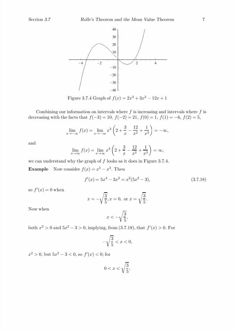
7/27/2019 Calculus 2 (Dan Sloughter)
http://slidepdf.com/reader/full/calculus-2-dan-sloughter 184/598
Section 3.7 Rolle’s Theorem and the Mean Value Theorem 7
-4 -2 2 4
-40
-30
-20
-10
10
20
30
40
Figure 3.7.4 Graph of f (x) = 2x3 + 3x2 − 12x + 1
Combining our information on intervals where f is increasing and intervals where f is
decreasing with the facts that f (−3) = 10, f (−2) = 21, f (0) = 1, f (1) = −6, f (2) = 5,
limx→−∞
f (x) = limx→−∞
x3
2 +
3
x− 12
x2+
1
x3
= −∞,
and
limx→∞
f (x) = limx→∞
x3
2 +
3
x− 12
x2+
1
x3
= ∞,
we can understand why the graph of f looks as it does in Figure 3.7.4.
Example Now consider f (x) = x5
−x3. Then
f (x) = 5x4 − 3x2 = x2(5x2 − 3), (3.7.18)
so f (x) = 0 when
x = −
3
5, x = 0, or x =
3
5.
Now when
x < −
3
5,
both x2 > 0 and 5x2
−3 > 0, implying, from (3.7.18), that f (x) > 0. For
−
3
5< x < 0,
x2 > 0, but 5x2 − 3 < 0, so f (x) < 0; for
0 < x <
3
5,

7/27/2019 Calculus 2 (Dan Sloughter)
http://slidepdf.com/reader/full/calculus-2-dan-sloughter 185/598
8 Rolle’s Theorem and the Mean Value Theorem Section 3.7
x2 > 0 and 5x2 − 3 < 0, so f (x) < 0; and for
x >
3
5,
x2
> 0 and 5x2 − 3 > 0, so f
(x) > 0. Hence f is increasing on
−∞,−
3
5
and 3
5,∞
,
and decreasing on
− 35 , 0
and
0,
3
5
.
Note that we could have determined the sign of f on these four intervals by evaluatingf at a point in each interval and then applying the Intermediate value Theorem. Forexample,
f (−1) = 2 > 0,
f
−1
5
= −14
125 < 0,
f 1
5
= − 14
125< 0,
andf (1) = 2 > 0.
As in the previous example, if we combine this information with the facts
f (−1) = 0,
f −
35
= 6
25
35
,
f (0) = 0,
f
3
5
= − 6
25
3
5,
f (1) = 0,

7/27/2019 Calculus 2 (Dan Sloughter)
http://slidepdf.com/reader/full/calculus-2-dan-sloughter 186/598
Section 3.7 Rolle’s Theorem and the Mean Value Theorem 9
-3 -2 -1 1 2 3
-2
-1.5
-1
-0.5
0.5
1
1.5
2
Figure 3.7.5 Graph of f (x) = x5 − x3
limx→−∞
f (x) = limx→−∞
x51−
1
x2 =
−∞,
and
limx→∞
f (x) = limx→∞
x5
1− 1
x2
= ∞,
we can understand why the graph of f looks as it does in Figure 3.7.5.
Antiderivatives
We will close this section with a look at one more important application of the Mean ValueTheorem. Although not needed for our current discussion, our result will be very usefulin the next chapter. We begin with a definition.
Definition If F and f are functions defined on an open interval (a, b) such that F (x) =f (x) for all x in (a, b), then we call F an antiderivative of f .
In other words, an antiderivative of a function f is another function whose derivativeis f . Although a given function f has at most one derivative, it is possible to have morethan one antiderivative, as the next example demonstrates.
Example F (x) = x3 is an antiderivative of f (x) = 3x2 on (−∞,∞). However, notethat G(x) = x3 + 4 is also an antiderivative of f . In fact, given any constant k,
H (x) = x3 + k (3.7.19)
is an antiderivative of f . This should not be too surprising since specifying the derivativeof a function fixes only the slope of its graph, and the graphs of the functions in (3.7.19)are all in a sense parallel to each other.
This example shows that a given function may have an infinite number of antideriva-tives. However, note that the difference of any two these antiderivatives is a constant. Wewill now show that this is always the case, and, in particular, that (3.7.19) specifies allpossible antiderivatives of f (x) = 3x2.

7/27/2019 Calculus 2 (Dan Sloughter)
http://slidepdf.com/reader/full/calculus-2-dan-sloughter 187/598
10 Rolle’s Theorem and the Mean Value Theorem Section 3.7
First consider a function F defined on an open interval (a, b) for which F (x) = 0 forall x in (a, b). That is, F is an antiderivative of the function which is 0 for all values of x
in (a, b). Now if u and v are any two points in (a, b), then, by the Mean Value Theorem,
F (v)
−F (u)
v − u =F
(c
) (3.7.20)
for some c in (a, b). But F (c) = 0, so
F (v)− F (u)
v − u= 0, (3.7.21)
which implies F (u) = F (v). If we let k = F (u) for a fixed u in (a, b), we now haveF (v) = F (u) = k for all v in (a, b). In other words, if the derivative of a function is 0 onan open interval, then the function must be constant on that interval.
Now supposeF
andG
are two functions defined on an open interval (a, b
) for whichF (x) = G(x) for all x in (a, b). Let H (x) = F (x)−G(x) for all x in (a, b). Then
H (x) = F (x)−G(x) = 0 (3.7.22)
for all x in (a, b). Then, by what we have just shown, there exists a constant k for which
k = H (x) = F (x)−G(x) (3.7.23)
for all x in (a, b). Hence if F an G have the same derivative on an open interval, that is,are antiderivatives of the same function, then they can differ only by a constant.
Proposition If F and G are both antiderivatives of f on an open interval (a, b), thenthere exists an constant k such that
F (x) = G(x) + k (3.7.24)
for all x in (a, b).
Example Sinced
dxsin(x) = cos(x),
we know that G(x) = sin(x) is an antiderivative of f (x) = cos(x) on (−∞,∞). Thus if F
is any antiderivative of f , then
F (x) = sin(x) + k (3.7.25)
for some constant k. In other words, functions of the form given in (3.7.25) are the onlyantiderivatives of f (x) = cos(x). Figure 3.7.6 shows the graphs of (3.7.25) for nine differentvalues of k. Although each of these graphs is the graph of a different function, they are
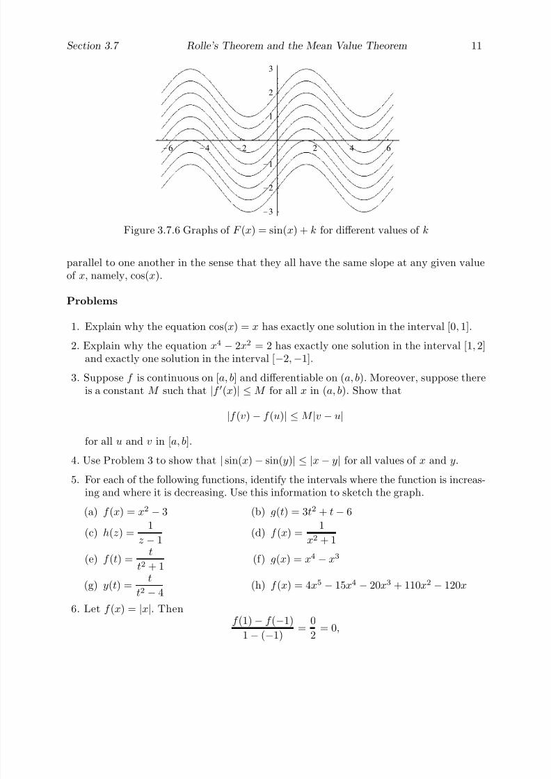
7/27/2019 Calculus 2 (Dan Sloughter)
http://slidepdf.com/reader/full/calculus-2-dan-sloughter 188/598
Section 3.7 Rolle’s Theorem and the Mean Value Theorem 11
-6 -4 -2 2 4 6
-3
-2
-1
1
2
3
Figure 3.7.6 Graphs of F (x) = sin(x) + k for different values of k
parallel to one another in the sense that they all have the same slope at any given value
of x, namely, cos(x).
Problems
1. Explain why the equation cos(x) = x has exactly one solution in the interval [0, 1].
2. Explain why the equation x4 − 2x2 = 2 has exactly one solution in the interval [1, 2]and exactly one solution in the interval [−2,−1].
3. Suppose f is continuous on [a, b] and differentiable on (a, b). Moreover, suppose thereis a constant M such that |f (x)| ≤ M for all x in (a, b). Show that
|f (v)− f (u)| ≤ M |v − u|
for all u and v in [a, b].
4. Use Problem 3 to show that | sin(x)− sin(y)| ≤ |x− y| for all values of x and y.
5. For each of the following functions, identify the intervals where the function is increas-ing and where it is decreasing. Use this information to sketch the graph.
(a) f (x) = x2 − 3 (b) g(t) = 3t2 + t − 6
(c) h(z) =1
z−
1(d) f (x) =
1
x2 + 1
(e) f (t) =t
t2 + 1(f) g(x) = x4 − x3
(g) y(t) =t
t2 − 4(h) f (x) = 4x5 − 15x4 − 20x3 + 110x2 − 120x
6. Let f (x) = |x|. Thenf (1)− f (−1)
1− (−1)=
0
2= 0,
7/27/2019 Calculus 2 (Dan Sloughter)
http://slidepdf.com/reader/full/calculus-2-dan-sloughter 189/598
12 Rolle’s Theorem and the Mean Value Theorem Section 3.7
but there does not exist a point c in (−1, 1) such that f (c) = 0. Does this contradictthe Mean Value Theorem?
7. Suppose f is continuous on [a, b] and differentiable on (a, b).
(a) Show that if f (x) > 0 for all x in (a, b), then f is increasing on [a, b].
(b) Show that if f (x) < 0 for all x in (a, b), then f is decreasing on [a, b].
8. Suppose f and g are continuous on [a, b], differentiable on (a, b), f (a) = g(a), andf (x) < g(x) for all x in (a, b). Show that f (b) < g(b).
9. Show that√
1 + x < 1 +1
2x for x > 0.
10. Show that a +1
a< b +
1
bwhenever 1 < a < b.
11. Find antiderivatives for the following functions.
(a) f (x) = 2x (b) g(t) = t2
(c) g(x) = sin(x) (d) f (z) = sin(2z)
(e) h(x) = x2 − 3x (f) f (x) = 3 cos(4x)
12. Find all antiderivatives of f (x) = 3x2 − 3 and plot the graphs of six of them.
13. Find all antiderivatives of g(t) = sin(2t) and plot the graphs of six of them.
14. If f (x) = − sin2(x) and g(x) = cos2(x), then f (x) = g(x). What does this implyabout the relationship between the functions f and g?
15. If f (t) = tan2(t) and g(t) = sec2(t), then f (t) = g(t). Thus f (t) = g(t) + k for someconstant k. Evaluate f and g at t = 0 in order to determine k.
16. Suppose f is differentiable on an open interval containing the closed interval [a, b].
(a) Show that for any x in (a, b),
f (x) = f (a) + f (c)(x− a)
for some point c with a < c < x.
(b) Let f denote the second derivative of f . That is,
f (x) =d
dxf (x).
Assuming that f is continuous on [a, b] and differentiable on (a, b), show that thereexists a point d with a < d < c such that
f (x) = f (a) + f (a)(x− a) + f (d)(c− a)(x− a).
(c) Compare the results in (a) and (b) to the statement that f (x) ≈ T (x) for x closeto a, where T is the best affine approximation to f at a.

7/27/2019 Calculus 2 (Dan Sloughter)
http://slidepdf.com/reader/full/calculus-2-dan-sloughter 190/598
Section 3.7 Rolle’s Theorem and the Mean Value Theorem 13
(d) Let h = x− a. Show that
f (a + h)− T (a + h) = f (d)(c− a)h.
(e) Assuming f is continuous on [a, b], show that
f (a + h)− T (a + h)
h2
≤ M
for some constant M . This statement means that the remainder function
R(h) = f (a + h)− T (a + h)
is O(h2). That is, R(h) goes to 0 as least as fast as h2. Note that this is a strongerstatement than the statement that R(h) is o(h).
7/27/2019 Calculus 2 (Dan Sloughter)
http://slidepdf.com/reader/full/calculus-2-dan-sloughter 191/598
Difference Equations
Differential Equations
to
Section 3.8
Finding Maximum andMinimum Values
Problems involving finding the maximum or minimum value of a quantity occur frequentlyin mathematics and in the applications of mathematics. A company may want to maximizeits profit or minimize its costs; a farmer may want to maximize the yield from his cropor minimize the amount of irrigation equipment needed to water his fields; an airline maywant to maximize its fuel efficiency or minimize the length of its routes. Methods forsolving some optimization problems are so computationally intense that they challenge,and sometimes even go beyond, the fastest computers currently available. An example of such a problem is the famous traveling salesman problem, in which a salesman wishes tovisit a certain set of cities using the shortest possible route. In this section we will notconsider problems of this type, but rather we will confine ourselves to problems involvingcontinuous functions of a single independent variable.
Closed intervals
We will start with the simplest case. Suppose f is a continuous function on a closed interval[a, b]. From the Extreme Value Theorem we know that f attains both a maximum valueand a minimum value on the interval. We now look for candidates at which these valuesmight occur. To start, an extreme value could occur at one of the endpoints. For example,the maximum value of f (x) = x2 on [0, 1] occurs at x = 1. If an extreme value occurs in
the open interval (a, b) at a point c where f is differentiable, then f has a local extremumat c and so, from our work in Section 3.7, we know that f (c) = 0. For example, theminimum value of f (x) = x2 on [−1, 1] occurs at x = 0 and f (0) = 0. Finally, the onlyother candidates for the locations of extreme values would be points where f is undefined.For example, the minimum value of f (x) = |x| on [−1, 1] occurs at x = 0, where f is notdefined. Hence we are led to the following conclusion: The extreme values of a continuousfunction f on a closed interval are located either at the endpoints of the interval, at pointswhere f is 0, or at points where f is undefined. The following terminology will help usstate this more easily.
Definition If f is differentiable at c and f (c) = 0, then we call c a critical point or
stationary point of f . A point c at which the derivative of f is not defined is called asingular point of f .
Thus we know that the candidates for the location of the extreme values of a continuousfunction on a closed interval fall into three categories: (a) endpoints of the interval, (b)critical points, and (c) singular points. To determine the extreme values of such a functionf , we identify all these points, evaluate f at each one, and identify the largest and smallestvalues.
1 Copyright c by Dan Sloughter 2000

7/27/2019 Calculus 2 (Dan Sloughter)
http://slidepdf.com/reader/full/calculus-2-dan-sloughter 192/598
2 Finding Maximum and Minimum Values Section 3.8
1 2 3 4 5 6
-2
-1.5
-1
-0.5
0.5
1
1.5
2
Figure 3.8.1 Graph of g(t) = cos(t) + sin(t) on [0, 2π]
Example Suppose we wish to find the maximum and minimum values of
g(t) = cos(t) + sin(t)
on the interval [0, 2π]. Then
g(t) = − sin(t) + cos(t),
so g(t) = 0 when
cos(t) = sin(t). (3.8.1)
Now cos(t) and sin(t) are never simultaneously 0, so we may divide both sides of (3.8.1)by cos(t) to see that g(t) = 0 when
tan(t) = 1.
Considering only the interval [0, 2π], this implies t = π4
or t = 5π4
. Since there are nosingular points, we evaluate g at the endpoints and at the critical points:
g(0) = 1
gπ
4
=
1
√ 2 +
1
√ 2 =
√ 2
g5π
4
= − 1√
2− 1√
2= −
√ 2
g(2π) = 1
Thus g has a maximum value of √
2 at t = π4
and a minimum value of −√ 2 at t = 5π4
. SeeFigure 3.8.1.
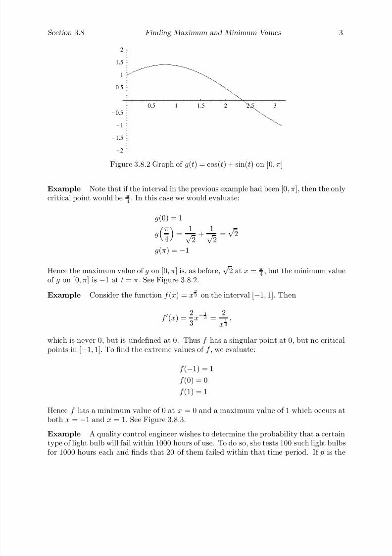
7/27/2019 Calculus 2 (Dan Sloughter)
http://slidepdf.com/reader/full/calculus-2-dan-sloughter 193/598
Section 3.8 Finding Maximum and Minimum Values 3
0.5 1 1.5 2 2.5 3
-2
-1.5
-1
-0.5
0.5
1
1.5
2
Figure 3.8.2 Graph of g(t) = cos(t) + sin(t) on [0, π]
Example Note that if the interval in the previous example had been [0, π], then the onlycritical point would be π
4. In this case we would evaluate:
g(0) = 1
gπ
4
=
1√ 2
+1√
2=√
2
g(π) = −1
Hence the maximum value of g on [0, π] is, as before,√
2 at x = π4
, but the minimum valueof g on [0, π] is −1 at t = π. See Figure 3.8.2.
Example Consider the function f (x) = x 23 on the interval [−1, 1]. Then
f (x) =2
3x−
1
3 =2
x1
3
,
which is never 0, but is undefined at 0. Thus f has a singular point at 0, but no criticalpoints in [−1, 1]. To find the extreme values of f , we evaluate:
f (−1) = 1
f (0) = 0
f (1) = 1
Hence f has a minimum value of 0 at x = 0 and a maximum value of 1 which occurs atboth x = −1 and x = 1. See Figure 3.8.3.
Example A quality control engineer wishes to determine the probability that a certaintype of light bulb will fail within 1000 hours of use. To do so, she tests 100 such light bulbsfor 1000 hours each and finds that 20 of them failed within that time period. If p is the

7/27/2019 Calculus 2 (Dan Sloughter)
http://slidepdf.com/reader/full/calculus-2-dan-sloughter 194/598
4 Finding Maximum and Minimum Values Section 3.8
-1 -0.5 0.5 1
0.2
0.4
0.6
0.8
1
Figure 3.8.3 Graph of f (x) = x2
3 on [−1, 1]
probability that a single light bulb fails within 1000 hours, the probability of the observed
sequence of successes and failures is given by
L( p) = p20(1− p)80,
with 0 ≤ p ≤ 1. Note here that 1− p is the probability that a single light bulb does notfail in the 1000 hour test. If we think of p as representing the proportion of all such lightbulbs that will fail within 1000 hours, then L( p) represents the proportion of times that asequence of 100 tests will yield the observed sequence of successes and failures. The qualitycontrol engineer would like to use this information to estimate p, the true probability of failure for this particular type of light bulb. One common procedure is to estimate p by thevalue ˆ p which maximizes the probability of the observed sequence; that is, ˆ p is the value
of p that makes the given observations most likely to occur. Hence we want to maximizethe function L on the interval [0, 1]. To find the critical points, we compute
L( p) = p20(80(1− p)79(−1)) + (1− p)80(20 p19)
= −80 p20(1− p)79 + 20 p19(1− p)80
= 20 p19(1− p)79(−4 p + (1− p))
= 20 p19(1− p)79(1− 5 p).
Thus L( p) = 0 when p = 0, p = 0.2, or p = 1, and so the only critical point in the interval(0, 1) is 0.2. Evaluating L at the endpoints and at the critical point yields:
L(0) = 0
L(0.2) = (0.2)20(0.8)80 = 1.853× 10⁻²²
L(1) = 0
Thus the quality control engineer would take the value ˆ p = 0.2 as her estimate of theprobability that this type of light bulb will fail within the first 1000 hours of use. SeeFigure 3.8.4.
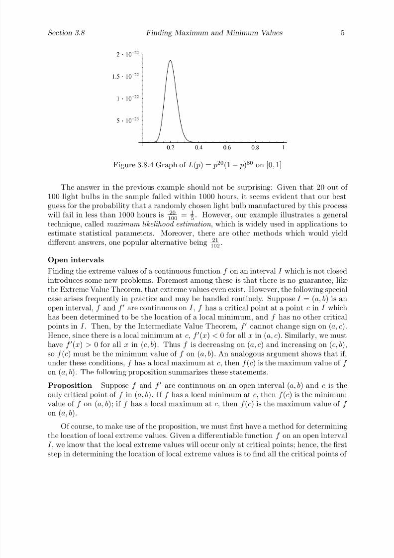
7/27/2019 Calculus 2 (Dan Sloughter)
http://slidepdf.com/reader/full/calculus-2-dan-sloughter 195/598
Section 3.8 Finding Maximum and Minimum Values 5
0.2 0.4 0.6 0.8 1
5·10-23
1·10-
22
1.5·10-22
2·10-22
Figure 3.8.4 Graph of L( p) = p20(1− p)80 on [0, 1]
The answer in the previous example should not be surprising: Given that 20 out of
100 light bulbs in the sample failed within 1000 hours, it seems evident that our bestguess for the probability that a randomly chosen light bulb manufactured by this processwill fail in less than 1000 hours is 20
100= 1
5. However, our example illustrates a general
technique, called maximum likelihood estimation , which is widely used in applications toestimate statistical parameters. Moreover, there are other methods which would yielddifferent answers, one popular alternative being 21
102.
Open intervals
Finding the extreme values of a continuous function f on an interval I which is not closedintroduces some new problems. Foremost among these is that there is no guarantee, like
the Extreme Value Theorem, that extreme values even exist. However, the following specialcase arises frequently in practice and may be handled routinely. Suppose I = (a, b) is anopen interval, f and f are continuous on I , f has a critical point at a point c in I whichhas been determined to be the location of a local minimum, and f has no other criticalpoints in I . Then, by the Intermediate Value Theorem, f cannot change sign on (a, c).Hence, since there is a local minimum at c, f (x) < 0 for all x in (a, c). Similarly, we musthave f (x) > 0 for all x in (c, b). Thus f is decreasing on (a, c) and increasing on (c, b),so f (c) must be the minimum value of f on (a, b). An analogous argument shows that if,under these conditions, f has a local maximum at c, then f (c) is the maximum value of f
on (a, b). The following proposition summarizes these statements.
Proposition Suppose f and f are continuous on an open interval (a, b) and c is theonly critical point of f in (a, b). If f has a local minimum at c, then f (c) is the minimumvalue of f on (a, b); if f has a local maximum at c, then f (c) is the maximum value of f
on (a, b).
Of course, to make use of the proposition, we must first have a method for determiningthe location of local extreme values. Given a differentiable function f on an open intervalI , we know that the local extreme values will occur only at critical points; hence, the firststep in determining the location of local extreme values is to find all the critical points of
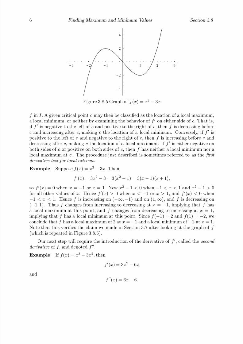
7/27/2019 Calculus 2 (Dan Sloughter)
http://slidepdf.com/reader/full/calculus-2-dan-sloughter 196/598
6 Finding Maximum and Minimum Values Section 3.8
-3 -2 -1 1 2 3
-4
-2
2
4
Figure 3.8.5 Graph of f (x) = x3 − 3x
f in I . A given critical point c may then be classified as the location of a local maximum,
a local minimum, or neither by examining the behavior of f on either side of c. That is,if f is negative to the left of c and positive to the right of c, then f is decreasing beforec and increasing after c, making c the location of a local minimum. Conversely, if f ispositive to the left of c and negative to the right of c, then f is increasing before c anddecreasing after c, making c the location of a local maximum. If f is either negative onboth sides of c or positive on both sides of c, then f has neither a local minimum nor alocal maximum at c. The procedure just described is sometimes referred to as the first
derivative test for local extrema .
Example Suppose f (x) = x3 − 3x. Then
f
(x
) = 3x2
− 3 = 3(x2
− 1) = 3(x− 1)(
x+ 1)
,
so f (x) = 0 when x = −1 or x = 1. Now x2 − 1 < 0 when −1 < x < 1 and x2 − 1 > 0for all other values of x. Hence f (x) > 0 when x < −1 or x > 1, and f (x) < 0 when−1 < x < 1. Hence f is increasing on (−∞,−1) and on (1,∞), and f is decreasing on(−1, 1). Thus f changes from increasing to decreasing at x = −1, implying that f hasa local maximum at this point, and f changes from decreasing to increasing at x = 1,implying that f has a local minimum at this point. Since f (−1) = 2 and f (1) = −2, weconclude that f has a local maximum of 2 at x = −1 and a local minimum of −2 at x = 1.Note that this verifies the claim we made in Section 3.7 after looking at the graph of f
(which is repeated in Figure 3.8.5).
Our next step will require the introduction of the derivative of f
, called the second derivative of f , and denoted f .
Example If f (x) = x3 − 3x2, then
f (x) = 3x2 − 6x
andf (x) = 6x− 6.

7/27/2019 Calculus 2 (Dan Sloughter)
http://slidepdf.com/reader/full/calculus-2-dan-sloughter 197/598
Section 3.8 Finding Maximum and Minimum Values 7
In Leibniz notation, if y = f (x), then f (x) is denoted by d2ydx2
, which may be thoughtof as
d2
dx2y =
d
dx
d
dxy
.
In Newton’s notation, if x = f (t), then x = f
(t).
Example If y = x sin(3x), then
dy
dx= 3x cos(3x) + sin(3x),
sod2y
dx2=
d
dx(3x cos(3x) + sin(3x))
=
−9x sin(3x) + 3 cos(3x) + 3 cos(3x)
= −9x sin(3x) + 6 cos(3x).
Example If x = 3t6 − 2cos(6t), then
x = 18t5 + 12 sin(6t)
and
x = 90t4 + 72 cos(6t).
Now suppose f , f , and f are all continuous on an interval (a, b) containing a criticalpoint c. Moreover, suppose f (c) < 0. Since f is continuous, this assumption in factimplies that f (c) < 0 on some open interval about c, and hence that f is a decreasingfunction on some open interval about c. But f (c) = 0, so for f to be decreasing it mustbe the case that f is positive to the left of c and negative to the right of c. This means, bythe first derivative test discussed above, that f must have a local maximum at c. Similarly,if f (c) > 0, then f is negative to the left of c and positive to the right of c, showing thatf has a local minimum at c. This important result is known as the second derivative test
for local extrema
Second Derivative Test Suppose f , f , and f are all continuous on an open interval
(a, b) and that c is critical point of f in (a, b). Then f has a local maximum at c if f (c) < 0and f has a local minimum at c if f (c) > 0.
Example Consider the function g(x) =x
1 + x2. Then
g(x) =(1 + x2)(1)− (x)(2x)
(1 + x2)2=
1− x2
(1 + x2)2,
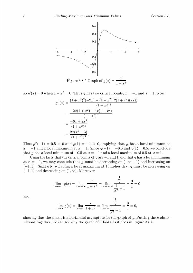
7/27/2019 Calculus 2 (Dan Sloughter)
http://slidepdf.com/reader/full/calculus-2-dan-sloughter 198/598
8 Finding Maximum and Minimum Values Section 3.8
-6 -4 -2 2 4 6
-0.6
-0.4
-0.2
0.2
0.4
0.6
Figure 3.8.6 Graph of g(x) =x
1 + x2
so g(x) = 0 when 1−
x2 = 0. Thus g has two critical points, x =−
1 and x = 1. Now
g(x) =(1 + x2)2(−2x)− (1− x2)(2(1 + x2)(2x))
(1 + x2)4
=−2x(1 + x2)− 4x(1− x2)
(1 + x2)3
=−6x + 2x3
(1 + x2)3
=2x(x2 − 3)
(1 + x2)3.
Thus g(−1) = 0.5 > 0 and g(1) = −1 < 0, implying that g has a local minimum atx = −1 and a local maximum at x = 1. Since g(−1) = −0.5 and g(1) = 0.5, we concludethat g has a local minimum of −0.5 at x = −1 and a local maximum of 0.5 at x = 1.
Using the facts that the critical points of g are −1 and 1 and that g has a local minimumat x = −1, we may conclude that g must be decreasing on (−∞,−1) and increasing on(−1, 1). Similarly, g having a local maximum at 1 implies that g must be increasing on(−1, 1) and decreasing on (1,∞). Moreover,
limx→−∞
g(x) = limx→−∞
x
1 + x2= lim
x→−∞
1
x1
x2
+ 1=
0
1= 0
and
limx→∞
g(x) = limx→∞
x
1 + x2= lim
x→∞
1
x1
x2+ 1
=0
1= 0,
showing that the x-axis is a horizontal asymptote for the graph of g. Putting these obser-vations together, we can see why the graph of g looks as it does in Figure 3.8.6.

7/27/2019 Calculus 2 (Dan Sloughter)
http://slidepdf.com/reader/full/calculus-2-dan-sloughter 199/598
Section 3.8 Finding Maximum and Minimum Values 9
-3 -2 -1 1 2 3
-6
-4
-2
2
4
6
Figure 3.8.7 Graph of f (x) = 5x3 − 3x5
Example Suppose f (x) = 5x3
−3x5. Then
f (x) = 15x2 − 15x4 = 15x2(1− x2) = 15x2(1− x)(1 + x),
from which we see that the critical points of f are −1, 0, and 1. Now
f (x) = 30x− 60x3,
so f (−1) = 30 > 0, f (0) = 0, and f (1) = −30 < 0. Thus f has a local minimum of −2at x = −1 and a local maximum of 2 at x = 1. Unfortunately, f (0) = 0, so the secondderivative test gives us no information about the nature of the critical point 0. However,
since f has a local minimum at x = −1, f must be decreasing on (−∞,−1) and increasingon (−1, 0); moreover, since f has a local maximum at x = 1, f must be increasing on (0, 1)and decreasing on (1,∞). Thus f is increasing on both (−1, 0) and (1, 0), from which weconclude that f has neither a local minimum nor a local maximum at x = 0. If we add inthat f (0) = 0,
limx→−∞
f (x) = limx→−∞
x5
5
x2− 3
= ∞,
and
limx→∞
f (x) = limx→∞
x5
5
x2− 3
= −∞,
we can see why the graph of f look as it does in Figure 3.8.7.
It is worth emphasizing that, for a critical point c, f (c) = 0 gives us no informationabout the nature of the critical point. The point may be the location of a local minimum,as 0 is for f (x) = x4; a local maximum, as 0 is for f (x) = −x4; or neither, as 0 is in theprevious example. Thus, if f (c) = 0 for a critical point c, the second derivative test isnot applicable and some other method, such as the first derivative test, must be used todetermine the nature of the point.
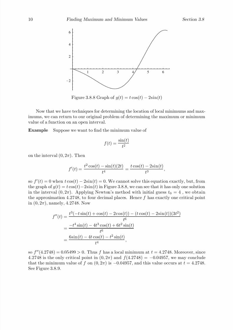
7/27/2019 Calculus 2 (Dan Sloughter)
http://slidepdf.com/reader/full/calculus-2-dan-sloughter 200/598
10 Finding Maximum and Minimum Values Section 3.8
1 2 3 4 5 6
-2
2
4
6
Figure 3.8.8 Graph of g(t) = t cos(t)− 2sin(t)
Now that we have techniques for determining the location of local minimums and max-
imums, we can return to our original problem of determining the maximum or minimumvalue of a function on an open interval.
Example Suppose we want to find the minimum value of
f (t) =sin(t)
t2
on the interval (0, 2π). Then
f (t) =t2 cos(t)− sin(t)(2t)
t4
=t cos(t)− 2sin(t)
t3
,
so f (t) = 0 when t cos(t)− 2sin(t) = 0. We cannot solve this equation exactly, but, fromthe graph of g(t) = t cos(t)−2sin(t) in Figure 3.8.8, we can see that it has only one solutionin the interval (0, 2π). Applying Newton’s method with initial guess t0 = 4 , we obtainthe approximation 4.2748, to four decimal places. Hence f has exactly one critical pointin (0, 2π), namely, 4.2748. Now
f (t) =t3(−t sin(t) + cos(t)− 2cos(t))− (t cos(t)− 2sin(t))(3t2)
t6
=−t4 sin(t)− 4t3 cos(t) + 6t2 sin(t)
t6
=6sin(t)− 4t cos(t)− t2 sin(t)
t4,
so f (4.2748) = 0.05499 > 0. Thus f has a local minimum at t = 4.2748. Moreover, since4.2748 is the only critical point in (0, 2π) and f (4.2748) = −0.04957, we may concludethat the minimum value of f on (0, 2π) is −0.04957, and this value occurs at t = 4.2748.See Figure 3.8.9.

7/27/2019 Calculus 2 (Dan Sloughter)
http://slidepdf.com/reader/full/calculus-2-dan-sloughter 201/598
Section 3.8 Finding Maximum and Minimum Values 11
1 2 3 4 5 6
0.2
0.4
0.6
0.8
1
Figure 3.8.9 Graph of f (t) =sin(t)
t2
ExampleA company wishes to produce a metal can in the shape of a right circularcylinder which minimizes the amount of metal needed in its construction, yet will have a
volume of V cubic centimeters. If we denote the radius of the base of the can by r, theheight of the can by h, and the surface area of the can by S , then
S = 2πr2 + 2πrh, (3.8.2)
where the first term represents the combined area of the base and the top of the can andthe second term represents the area of the side of the can, which, when flattened out, is arectangle of length 2πr (the circumference of the base of the can) and width h. Our goalis to find the values of r and h which minimize S subject to the constraint that the canhas to hold a volume V . This constraint translates into the condition
V = πr2
h,
which means we must have
h =V
πr2. (3.8.3)
h
r
Figure 3.8.10 A cylindrical can

7/27/2019 Calculus 2 (Dan Sloughter)
http://slidepdf.com/reader/full/calculus-2-dan-sloughter 202/598
12 Finding Maximum and Minimum Values Section 3.8
Substituting the value of h in (3.8.3) into (3.8.2), we have
S = 2πr2 +2V
r, (3.8.4)
giving S as a function of r which we want to minimize on the interval (0,∞). Now
dS
dr= 4πr − 2V
r2,
so dS dr
= 0 when
4πr =2V
r2,
that is, when
r3 =V
2π
.
Hence
r =3
V
2π
is the only critical point of S in (0,∞). Moreover,
d2S
dr2= 4π +
4V
r3,
so
d
2
S dr2r= 3√
V
2π
= 4π + 8π = 12π > 0.
Hence S has a local minimum at
r =3
V
2π.
Since this is the only critical point in (0,∞), this is in fact the location of the minimumvalue of S . Now for
r =3
V
2π,
we have, using (3.8.3),
h =V
πr2=
V
πV 2π
2
3
=22
3 π2
3 V
πV 2
3
= 23
V
2π= 2r.
That is, the surface area of the can, and hence the amount of metal used in the can, isminimized when the height of the can is equal to the diameter of the can. Figure 3.8.11

7/27/2019 Calculus 2 (Dan Sloughter)
http://slidepdf.com/reader/full/calculus-2-dan-sloughter 203/598
Section 3.8 Finding Maximum and Minimum Values 13
5 10 15 20
500
1000
1500
2000
Figure 3.8.11 Graph of S = 2πr2 +2000
r
shows the graph of S in the case V = 1000 cubic centimeters, in which case the surfacearea is minimized when r is approximately 5.42 centimeters.
Problems
1. Find the minimum and maximum values, and their locations, for each of the followingfunctions on the given intervals.
(a) f (x) = x2 − 4 on [−3, 4] (b) f (x) = x3 − 3x on [−2, 4]
(c) g(t) = cos(t)− sin(t) on [−π, π] (d) f (t) = 2t3 + 3t2 − 36t on [−4, 3]
(e) g(x) = x2 cos(x) on [−2, 2] (f) f (t) = cos(t) + sin(2t) on [0, π]
(g) f (t) = t2 sin(t) on [0, π]
2. A farmer wishes to fence in a rectangular field with 600 yards of fencing. What shouldthe dimensions of the field be in order to maximize the area of the field?
3. A farmer wishes to fence in a rectangular field, using a straight river for one side, with500 yards of fencing. What should the dimensions of the field be in order to maximizethe area of the field?
4. Suppose the farmer in Problem 2 wishes to divide his field into two equal rectangularfields using a fence parallel to two of the sides. What should the dimensions of thefield be in order to maximize the combined areas of the fields?
5. When a potter sells his pots for p dollars apiece, he can sell D( p) = 2500− p2 of them.Suppose the pots cost him $6.00 apiece to make. What price should the potter chargein order to maximize his profit?
6. A wire of unit length is to be cut into two pieces. One of the pieces will be used toform a square, the other a circle. Where should the wire be cut in order to maximumthe total area enclosed by the square and the circle? Where should it be cut in orderto minimize the total area enclosed by the square and the circle?
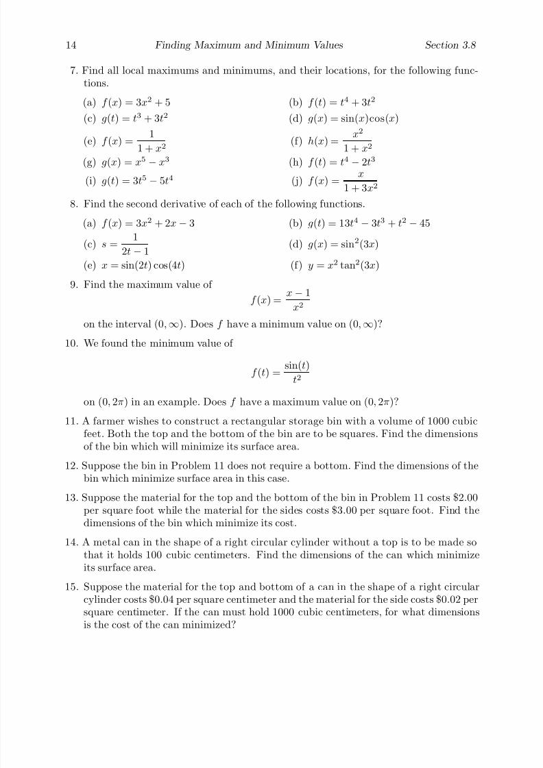
7/27/2019 Calculus 2 (Dan Sloughter)
http://slidepdf.com/reader/full/calculus-2-dan-sloughter 204/598
14 Finding Maximum and Minimum Values Section 3.8
7. Find all local maximums and minimums, and their locations, for the following func-tions.
(a) f (x) = 3x2 + 5 (b) f (t) = t4 + 3t2
(c) g(t) = t3 + 3t2 (d) g(x) = sin(x)cos(x)
(e) f (x) = 11 + x2
(f) h(x) = x2
1 + x2
(g) g(x) = x5 − x3 (h) f (t) = t4 − 2t3
(i) g(t) = 3t5 − 5t4 (j) f (x) =x
1 + 3x2
8. Find the second derivative of each of the following functions.
(a) f (x) = 3x2 + 2x− 3 (b) g(t) = 13t4 − 3t3 + t2 − 45
(c) s =1
2t − 1(d) g(x) = sin2(3x)
(e) x = sin(2t) cos(4t) (f) y = x2
tan2
(3x)9. Find the maximum value of
f (x) =x− 1
x2
on the interval (0,∞). Does f have a minimum value on (0,∞)?
10. We found the minimum value of
f (t) =sin(t)
t2
on (0, 2π) in an example. Does f have a maximum value on (0, 2π)?11. A farmer wishes to construct a rectangular storage bin with a volume of 1000 cubic
feet. Both the top and the bottom of the bin are to be squares. Find the dimensionsof the bin which will minimize its surface area.
12. Suppose the bin in Problem 11 does not require a bottom. Find the dimensions of thebin which minimize surface area in this case.
13. Suppose the material for the top and the bottom of the bin in Problem 11 costs $2.00per square foot while the material for the sides costs $3.00 per square foot. Find thedimensions of the bin which minimize its cost.
14. A metal can in the shape of a right circular cylinder without a top is to be made sothat it holds 100 cubic centimeters. Find the dimensions of the can which minimizeits surface area.
15. Suppose the material for the top and bottom of a can in the shape of a right circularcylinder costs $0.04 per square centimeter and the material for the side costs $0.02 persquare centimeter. If the can must hold 1000 cubic centimeters, for what dimensionsis the cost of the can minimized?

7/27/2019 Calculus 2 (Dan Sloughter)
http://slidepdf.com/reader/full/calculus-2-dan-sloughter 205/598
Section 3.8 Finding Maximum and Minimum Values 15
16. A metal can in the shape of a right circular cylinder is to be made so that it holds 500cubic centimeters. Suppose the top and bottom of the can are cut from square piecesof metal, with the scraps being discarded afterwards. Assuming there is no waste inmaking the side of the can, find the dimensions of the can which minimize the amountof material needed to make it.
17. Show that the rectangle with maximum area for a given perimeter P is a square.
18. Show that the rectangle with minimum perimeter for a given area A is a square.
19. A quality control engineer is studying the failure rate of a certain type of beam understress. Test beams are put under a steady stress for 1000 hours. If p is the probabilitythat the beam passes the test, then 1 − p is the probability that the beam fails thetest. Suppose that in 50 trials, only 5 beams fail the test.
(a) If L( p) is the probability of the observed sequence of successes and failures, explainwhy
L( p) = p45(1
− p)5
for 0 ≤ p ≤ 1.
(b) If ˆ p is the value of p which maximizes L( p) on [0, 1], show that ˆ p = 0.9.
20. According to genetic theory, if a parent provides the gene A with probability θ and thegene a with probability 1 − θ, then the offspring is of genotype AA with probabilityθ2, of genotype Aa with probability 2θ(1 − θ), and of genotype aa with probability(1− θ)2. Suppose that in a sample of 100 people, 31 were observed to be of type AA,48 of type Aa, and 21 of type aa. Let L(θ) be the probability of observing this specificsequence of genotypes.
(a) Explain why
L(θ) = 248
θ110
(1− θ)90
for 0 ≤ θ ≤ 1.
(b) Find the value of θ which maximizes L(θ) on [0, 1]. What are the correspondingvalues for the probabilities of AA, Aa, and aa?
21. In the final example of this section, we showed that the surface area of a right circularcylindrical can is minimized when the height of the can is equal to the diameter of thecan. Check out a local supermarket to see how many cans satisfy this condition. Whatother considerations might be important in the design of a can?
22. We have seen that if x(t) is the position of an object moving on a straight line at time
t, then the velocity of the object is given by v(t) = x(t) and the acceleration is givenby a(t) = v(t). Hence a is the second derivative of x; that is, a(t) = x(t). Suppose anobject is oscillating at the end of a spring so that its position at time t is x = 3sin(πt).
(a) Find v(t).
(b) Find a(t).
(c) Discuss the behavior of the object over the interval [0, 2], taking into account thevalues of x(t), v(t), and a(t).

7/27/2019 Calculus 2 (Dan Sloughter)
http://slidepdf.com/reader/full/calculus-2-dan-sloughter 206/598
Difference Equations
Differential Equations
to
Section 3.9
The Geometry of Graphs
In Section 2.1 we discussed the graph of a function y = f (x) in terms of plotting points(x, f (x)) for many different values of x and connecting the resulting points with straightlines. This is a standard procedure when using a computer and, if the function is wellbehaved and sufficiently many points are plotted, will produce a reasonable picture of thegraph. However, as we noted at that time, this method assumes that the behavior of thegraph between any two successive points is approximated well by a straight line. With asufficient number of points and a differentiable function, this assumption will be reasonable.Yet to understand a graph fully, it is important to have alternative techniques to verifythe picture at least qualitatively. We have already developed several important aids forunderstanding the shape of a graph, including techniques for determining the location of local extreme values and techniques for finding intervals where the function is increasingand intervals where it is decreasing. In this section we will use this information, alongwith additional information contained in the second derivative, to piece together a pictureof the graph of a given function.
To see the importance of the second derivative, consider the graphs of f (x) = x2 andg(x) =
√ x on the interval (0,∞). Now
f (x) = 2x
andg(x) =
1
2√
x,
1 2 3 4 5
1
2
3
4
5
Figure 3.9.1 Graphs of y = x2 and y =√
x
1 Copyright c by Dan Sloughter 2000

7/27/2019 Calculus 2 (Dan Sloughter)
http://slidepdf.com/reader/full/calculus-2-dan-sloughter 207/598
2 The Geometry of Graphs Section 3.9
-3 -2 -1 1 2 3
-1
1
2
3
4
5
-3 -2 -1 1 2 3
-5
-4
-3
-2
-1
1
Figure 3.9.2 Graphs of y = x2 and y = −x2 on (−∞,∞)
so f (x) > 0 and g(x) > 0 for all x in (0,∞). Thus f and g are both increasing on (0,∞).However, the graphs of f and g, as shown in Figure 3.9.1, are dramatically different. The
graph of f is not only increasing, but is becoming steeper and steeper as x increases,whereas the graph of g is increasing, but flattening out as x increases. In other words, f
is itself an increasing function, causing the rate of growth of the function to increase withx, while g is a decreasing function, resulting in a decrease in the rate of growth of g anda flattening out of the graph. In the terminology of the next definition, we say that thegraph of f is concave up on (0,∞) and the graph of g is concave down on (0,∞).
Definition Suppose f is differentiable on the open interval (a, b). If f is an increasingfunction on (a, b), then we say the graph of f is concave up on (a, b). If f is a decreasingfunction on (a, b), then we say the graph of f is concave down on (a, b).
Of course, to check for the intervals where f
is increasing and the intervals where f
isdecreasing, we consider where f , the derivative of f , is positive and where it is negative.
Proposition Suppose f is twice differentiable on the interval (a, b). If f (x) > 0 for allx in (a, b), then the graph of f is concave up on (a, b); if f (x) < 0 for all x in (a, b), thenthe graph of f is concave down on (a, b).
Example Two basic examples to keep in mind are f (x) = x2 and g(x) = −x2. Sincef (x) = 2 > 0 and g(x) = −2 < 0 for all values of x, the graph of f is concave up on(−∞,∞) and the graph of g is concave down on (−∞,∞). See Figure 3.9.2.
Example Consider g(t) = t3. Then g(t) = 6t, so g(t) < 0 when t < 0 and g(t) > 0
when t > 0. Hence the graph of g is concave down on (−∞, 0) and concave up on (0,∞).Notice in Figure 3.9.3 how, even though g is increasing on (−∞,∞), the change in concavityat (0, 0) changes the shape of the graph.
Definition A point on the graph of a function f where the concavity changes from upto down or from down to up is called an inflection point .
Example In our previous example, (0, 0) is an inflection point for the graph of g(t) = t3.
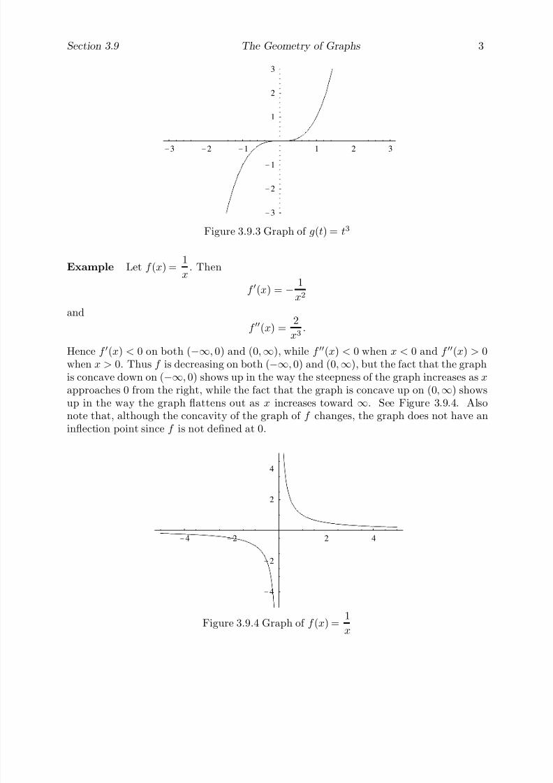
7/27/2019 Calculus 2 (Dan Sloughter)
http://slidepdf.com/reader/full/calculus-2-dan-sloughter 208/598
Section 3.9 The Geometry of Graphs 3
-3 -2 -1 1 2 3
-3
-2
-1
1
2
3
Figure 3.9.3 Graph of g(t) = t3
Example Let f (x) =1
x. Then
f (x) = − 1
x2
and
f (x) =2
x3.
Hence f (x) < 0 on both (−∞, 0) and (0,∞), while f (x) < 0 when x < 0 and f (x) > 0when x > 0. Thus f is decreasing on both (−∞, 0) and (0,∞), but the fact that the graphis concave down on (−∞, 0) shows up in the way the steepness of the graph increases as x
approaches 0 from the right, while the fact that the graph is concave up on (0,∞) showsup in the way the graph flattens out as x increases toward
∞. See Figure 3.9.4. Also
note that, although the concavity of the graph of f changes, the graph does not have aninflection point since f is not defined at 0.
-4 -2 2 4
-4
-2
2
4
Figure 3.9.4 Graph of f (x) =1
x
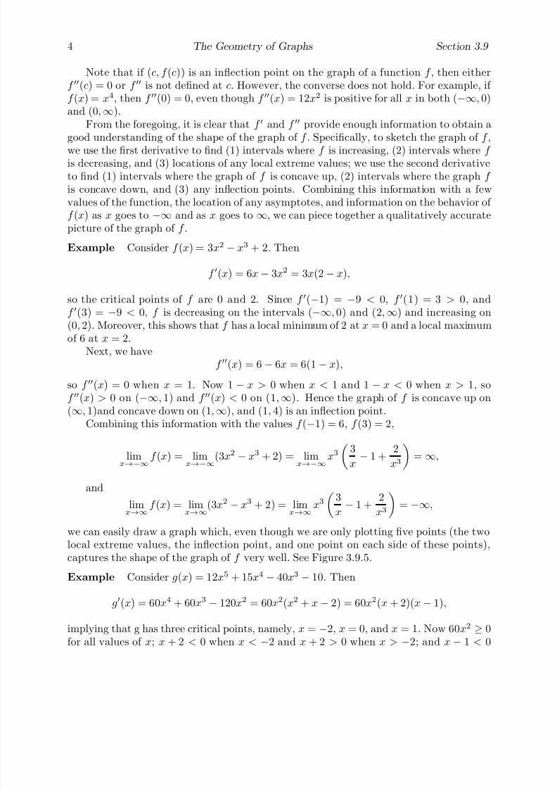
7/27/2019 Calculus 2 (Dan Sloughter)
http://slidepdf.com/reader/full/calculus-2-dan-sloughter 209/598
4 The Geometry of Graphs Section 3.9
Note that if (c, f (c)) is an inflection point on the graph of a function f , then eitherf (c) = 0 or f is not defined at c. However, the converse does not hold. For example, if f (x) = x4, then f (0) = 0, even though f (x) = 12x2 is positive for all x in both (−∞, 0)and (0,∞).
From the foregoing, it is clear that f and f provide enough information to obtain a
good understanding of the shape of the graph of f . Specifically, to sketch the graph of f ,we use the first derivative to find (1) intervals where f is increasing, (2) intervals where f
is decreasing, and (3) locations of any local extreme values; we use the second derivativeto find (1) intervals where the graph of f is concave up, (2) intervals where the graph f
is concave down, and (3) any inflection points. Combining this information with a fewvalues of the function, the location of any asymptotes, and information on the behavior of f (x) as x goes to −∞ and as x goes to ∞, we can piece together a qualitatively accuratepicture of the graph of f .
Example Consider f (x) = 3x2 − x3 + 2. Then
f
(x) = 6x− 3x2
= 3x(2− x),
so the critical points of f are 0 and 2. Since f (−1) = −9 < 0, f (1) = 3 > 0, andf (3) = −9 < 0, f is decreasing on the intervals (−∞, 0) and (2,∞) and increasing on(0, 2). Moreover, this shows that f has a local minimum of 2 at x = 0 and a local maximumof 6 at x = 2.
Next, we havef (x) = 6− 6x = 6(1− x),
so f (x) = 0 when x = 1. Now 1 − x > 0 when x < 1 and 1 − x < 0 when x > 1, sof (x) > 0 on (−∞, 1) and f (x) < 0 on (1,∞). Hence the graph of f is concave up on
(∞, 1)and concave down on (1,∞), and (1, 4) is an inflection point.Combining this information with the values f (−1) = 6, f (3) = 2,
limx→−∞
f (x) = limx→−∞
(3x2 − x3 + 2) = limx→−∞
x3
3
x− 1 +
2
x3
= ∞,
and
limx→∞
f (x) = limx→∞
(3x2 − x3 + 2) = limx→∞
x3
3
x− 1 +
2
x3
= −∞,
we can easily draw a graph which, even though we are only plotting five points (the twolocal extreme values, the inflection point, and one point on each side of these points),captures the shape of the graph of f very well. See Figure 3.9.5.
Example Consider g(x) = 12x5 + 15x4 − 40x3 − 10. Then
g(x) = 60x4 + 60x3 − 120x2 = 60x2(x2 + x− 2) = 60x2(x + 2)(x− 1),
implying that g has three critical points, namely, x = −2, x = 0, and x = 1. Now 60x2 ≥ 0for all values of x; x + 2 < 0 when x < −2 and x + 2 > 0 when x > −2; and x − 1 < 0
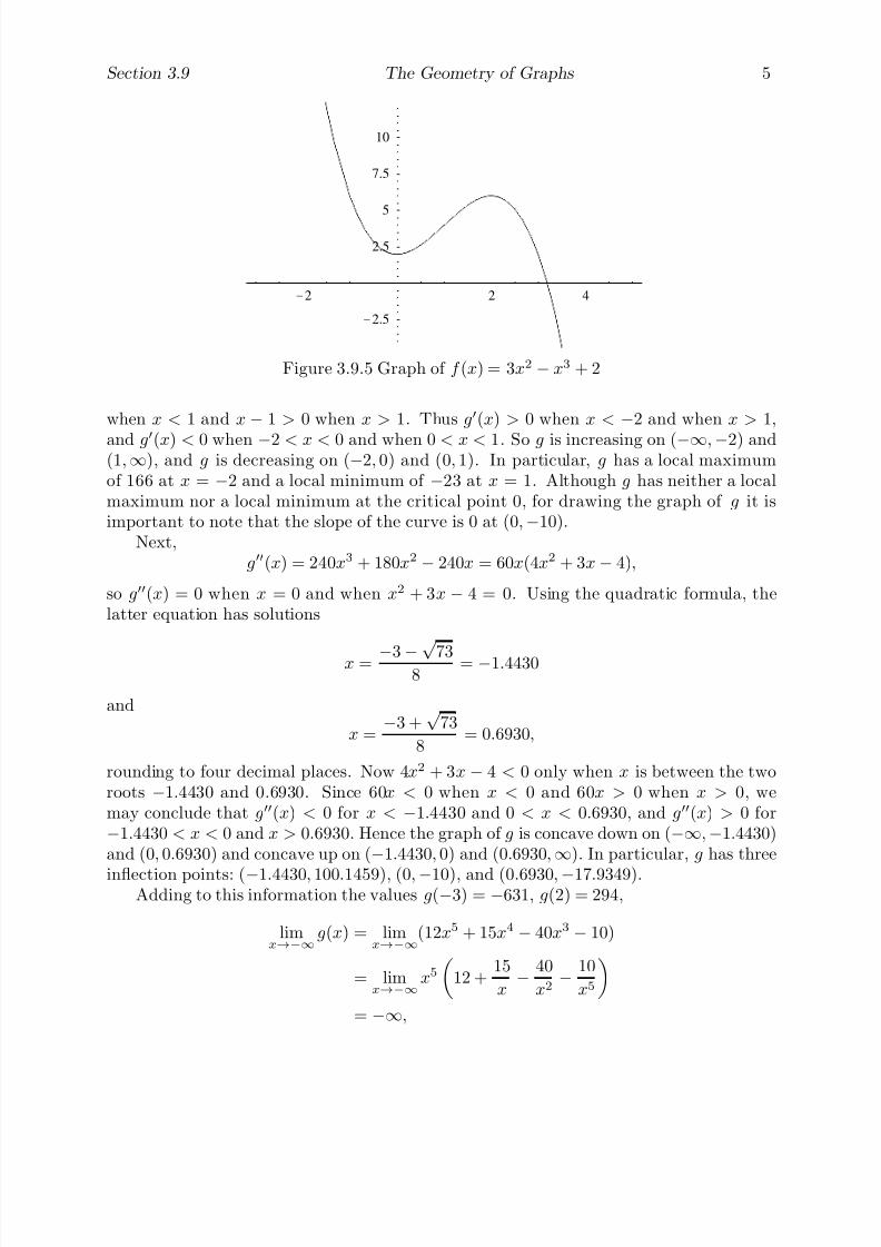
7/27/2019 Calculus 2 (Dan Sloughter)
http://slidepdf.com/reader/full/calculus-2-dan-sloughter 210/598
Section 3.9 The Geometry of Graphs 5
-2 2 4
-2.5
2.5
5
7.5
10
Figure 3.9.5 Graph of f (x) = 3x2 − x3 + 2
when x < 1 and x
−1 > 0 when x > 1. Thus g(x) > 0 when x <
−2 and when x > 1,
and g(x) < 0 when −2 < x < 0 and when 0 < x < 1. So g is increasing on (−∞,−2) and(1,∞), and g is decreasing on (−2, 0) and (0, 1). In particular, g has a local maximumof 166 at x = −2 and a local minimum of −23 at x = 1. Although g has neither a localmaximum nor a local minimum at the critical point 0, for drawing the graph of g it isimportant to note that the slope of the curve is 0 at (0,−10).
Next,g(x) = 240x3 + 180x2 − 240x = 60x(4x2 + 3x− 4),
so g(x) = 0 when x = 0 and when x2 + 3x − 4 = 0. Using the quadratic formula, thelatter equation has solutions
x = −3−√ 738
= −1.4430
and
x =−3 +
√ 73
8= 0.6930,
rounding to four decimal places. Now 4x2 + 3x − 4 < 0 only when x is between the tworoots −1.4430 and 0.6930. Since 60x < 0 when x < 0 and 60x > 0 when x > 0, wemay conclude that g(x) < 0 for x < −1.4430 and 0 < x < 0.6930, and g(x) > 0 for−1.4430 < x < 0 and x > 0.6930. Hence the graph of g is concave down on (−∞,−1.4430)and (0, 0.6930) and concave up on (
−1.4430, 0) and (0.6930,
∞). In particular, g has three
inflection points: (−1.4430, 100.1459), (0,−10), and (0.6930,−17.9349).Adding to this information the values g(−3) = −631, g(2) = 294,
limx→−∞
g(x) = limx→−∞
(12x5 + 15x4 − 40x3 − 10)
= limx→−∞
x5
12 +
15
x− 40
x2− 10
x5
= −∞,
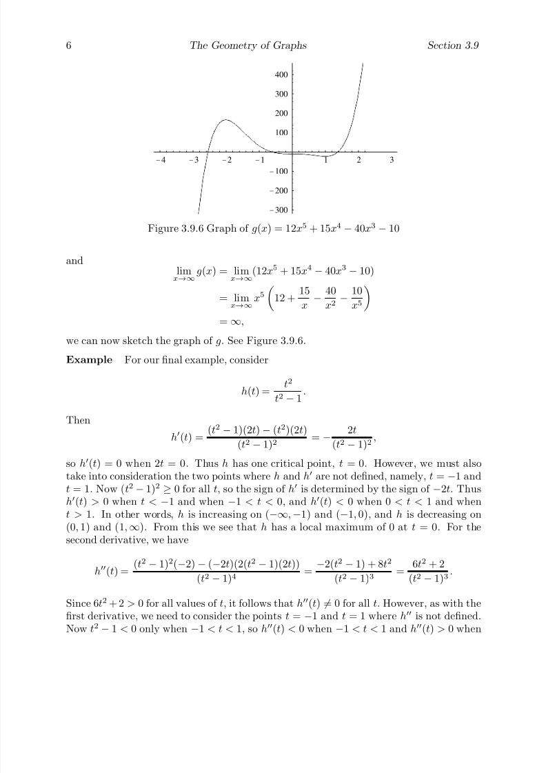
7/27/2019 Calculus 2 (Dan Sloughter)
http://slidepdf.com/reader/full/calculus-2-dan-sloughter 211/598
6 The Geometry of Graphs Section 3.9
-4 -3 -2 -1 1 2 3
-300
-200
-100
100
200
300
400
Figure 3.9.6 Graph of g(x) = 12x5 + 15x4 − 40x3 − 10
and
limx→∞ g(x) = limx→∞(12x5
+ 15x4 − 40x
3 − 10)
= limx→∞
x5
12 +
15
x− 40
x2− 10
x5
= ∞,
we can now sketch the graph of g. See Figure 3.9.6.
Example For our final example, consider
h(t) =t2
t2
−1
.
Then
h(t) =(t2 − 1)(2t)− (t2)(2t)
(t2 − 1)2= − 2t
(t2 − 1)2,
so h(t) = 0 when 2t = 0. Thus h has one critical point, t = 0. However, we must alsotake into consideration the two points where h and h are not defined, namely, t = −1 andt = 1. Now (t2 − 1)2 ≥ 0 for all t, so the sign of h is determined by the sign of −2t. Thush(t) > 0 when t < −1 and when −1 < t < 0, and h(t) < 0 when 0 < t < 1 and whent > 1. In other words, h is increasing on (−∞,−1) and (−1, 0), and h is decreasing on(0, 1) and (1,∞). From this we see that h has a local maximum of 0 at t = 0. For the
second derivative, we have
h(t) =(t2 − 1)2(−2)− (−2t)(2(t2 − 1)(2t))
(t2 − 1)4=−2(t2 − 1) + 8t2
(t2 − 1)3=
6t2 + 2
(t2 − 1)3.
Since 6t2 + 2 > 0 for all values of t, it follows that h(t) = 0 for all t. However, as with thefirst derivative, we need to consider the points t = −1 and t = 1 where h is not defined.Now t2 − 1 < 0 only when −1 < t < 1, so h(t) < 0 when −1 < t < 1 and h(t) > 0 when

7/27/2019 Calculus 2 (Dan Sloughter)
http://slidepdf.com/reader/full/calculus-2-dan-sloughter 212/598
Section 3.9 The Geometry of Graphs 7
-3 -2 -1 1 2 3
-8
-6
-4
-2
2
4
6
8
Figure 3.9.7 Graph of h(t) =t2
t2 − 1
t < −1 and when t > 1. Hence the graph of h is concave down on (−1, 1) and concave upon (−∞,−1) and (1,∞). Note, however, that there are no points of inflection.
Since h is not defined at t = −1 and t = 1, we need to check for vertical asymptotesat these points. We have
limt→−1−
h(t) = limt→−1−
t2
t2 − 1= ∞,
limt→−1+
h(t) = limt→−1+
t2
t2 − 1= −∞,
limt→1−
h(t) = limt→1−
t2
t2 − 1= −∞,
and
limt→1+
h(t) = limt→1+
t2
t2 − 1= ∞,
showing that the graph of h has vertical asymptotes at t = −1 and t = 1. Finally,
limt→−∞
h(t) = limt→−∞
t2
t2 − 1= lim
t→−∞
1
1
−1
t2
= 1
and
limt→∞
h(t) = limt→∞
t2
t2 − 1= lim
t→∞
1
1− 1
t2
= 1
show that the graph of h has a horizontal asymptote at y = 1. With all of this geometricinformation, we may now draw the graph of h, as shown in Figure 3.9.7.

7/27/2019 Calculus 2 (Dan Sloughter)
http://slidepdf.com/reader/full/calculus-2-dan-sloughter 213/598
8 The Geometry of Graphs Section 3.9
Problems
1. Discuss the geometry of the graphs of each of the following functions. That is, findthe intervals where the function is increasing and where it is decreasing, find theintervals where the graph is concave up and where it is concave down, find all localextreme values and where they are located, find all inflection points, find any verticalor horizontal asymptotes, and use this information to sketch the graph.
(a) f (x) = x2 − x (b) g(t) = 3t2 + 2t− 6
(c) g(x) = x3 + 3x2 (d) f (t) = t4 + 2t2
(e) f (x) = x3 − 3x (f) g(x) = 3x5 − 5x3
(g) h(x) = x5 − x3 (h) f (x) = 3x5 − 5x4
(i) g(z) =1
z − 1(j) y(t) =
1
t2 + 1
(k) f (x) = x4 − 2x3 (l) h(t) = t1 + t2
(m) h(t) =t
t2 − 4(n) g(x) =
x
1 + 3x2
(o) f (x) =x2
1 + x2(p) f (x) =
1
x2 − 1
(q) x(t) =2t + 1
t− 1(r) f (z) =
z2
z2 − 4
2. Suppose the function f has the following properties:
f (0) = 0
f (x) > 0 for x in (−∞, 2)
f (x) < 0 for x in (2,∞)
f (x) < 0 for x in (−2, 6)
f (x) > 0 for x in (−∞,−2) and for x (6,∞)
limx→−∞
f (x) = −2
limx→∞
f (x) = 0
Sketch the graph of a function satisfying these conditions.
3. Suppose f (0) = 0 and f (x) = x2 − 1.
(a) Sketch what the graph of f must look like.
(b) Graph f on the same axes with f .
(c) Is there more than one function f which satisfies these conditions?

7/27/2019 Calculus 2 (Dan Sloughter)
http://slidepdf.com/reader/full/calculus-2-dan-sloughter 214/598
Section 3.9 The Geometry of Graphs 9
4. Suppose f (0) = 0 and f (x) = x3 + x2 − 6x.
(a) Sketch what the graph of f must look like.
(b) Graph f on the same axes with f .
(c) Is there more than one function f which satisfies these conditions?
5. Suppose g(1) = 0 and g(t) =1t
.
(a) Sketch what the graph of g must look like on (0,∞).
(b) Graph g on the same axes with g.
(c) Is there more than one function g which satisfies these conditions?
6. Suppose f (0) = 1 and f (x) = f (x). What must the graph of f look like? Is thisenough information to determine the graph of f?
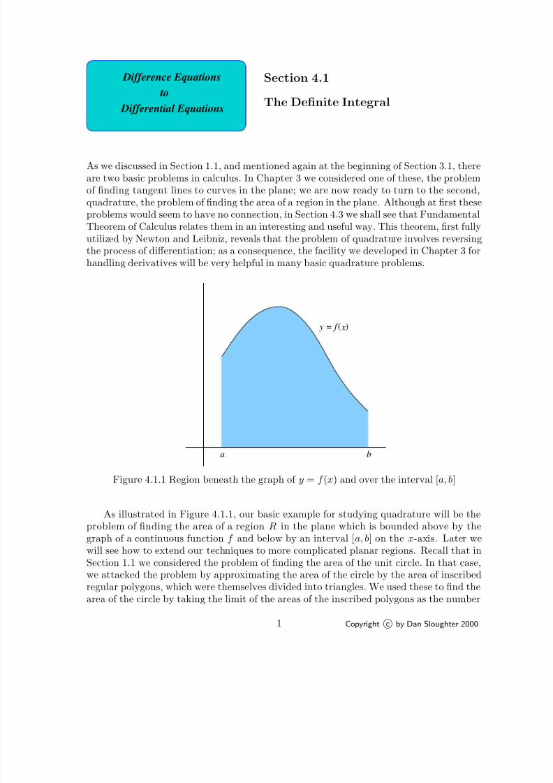
7/27/2019 Calculus 2 (Dan Sloughter)
http://slidepdf.com/reader/full/calculus-2-dan-sloughter 215/598
Difference Equations
Differential Equations
to
Section 4.1
The Definite Integral
As we discussed in Section 1.1, and mentioned again at the beginning of Section 3.1, thereare two basic problems in calculus. In Chapter 3 we considered one of these, the problemof finding tangent lines to curves in the plane; we are now ready to turn to the second,quadrature, the problem of finding the area of a region in the plane. Although at first theseproblems would seem to have no connection, in Section 4.3 we shall see that FundamentalTheorem of Calculus relates them in an interesting and useful way. This theorem, first fullyutilized by Newton and Leibniz, reveals that the problem of quadrature involves reversingthe process of differentiation; as a consequence, the facility we developed in Chapter 3 forhandling derivatives will be very helpful in many basic quadrature problems.
ba
y = f ( ) x
Figure 4.1.1 Region beneath the graph of y = f (x) and over the interval [a, b]
As illustrated in Figure 4.1.1, our basic example for studying quadrature will be theproblem of finding the area of a region R in the plane which is bounded above by thegraph of a continuous function f and below by an interval [a, b] on the x-axis. Later we
will see how to extend our techniques to more complicated planar regions. Recall that inSection 1.1 we considered the problem of finding the area of the unit circle. In that case,we attacked the problem by approximating the area of the circle by the area of inscribedregular polygons, which were themselves divided into triangles. We used these to find thearea of the circle by taking the limit of the areas of the inscribed polygons as the number
1 Copyright c by Dan Sloughter 2000

7/27/2019 Calculus 2 (Dan Sloughter)
http://slidepdf.com/reader/full/calculus-2-dan-sloughter 216/598
2 The Definite Integral Section 4.1
-1 1 2
1
2
3
4
5
6
-1 1 2
1
2
3
4
5
6
Figure 4.1.2 Inscribed and circumscribed rectangles for f (x) = x2
+ 1
of sides went to infinity. Here we will see that it is sufficient to use rectangles, ratherthan triangles, as our units of approximation. That is, we will approximate the area of the desired region by the area of rectangles and then ask about the limit as the number of rectangles used in the approximation goes to infinity. We begin with an example.
Example Consider the region R beneath the graph of the function f (x) = x2 + 1 andabove the interval [−1, 2] on the x-axis. Let A be the area of R. If R1 is the rectanglewith base on the interval [−1, 2] and height f (2) = 5, then, since 5 is the maximum valueof f on [−1, 2], R1 contains R. We call R1 a circumscribed rectangle for the region R.
Hence the area of R is less than the area of R1, showing that A ≤ 15. Similarly, if R2 isthe rectangle with base on the interval [−1, 2] and height f (0) = 1, then, since 1 is theminimum value of f on [−1, 2], R contains R2. We call R2 an inscribed rectangle for theregion R. Hence the area of R is greater than the area of R2, showing that A ≥ 3. See thefigure on the left in Figure 4.1.2.
At this point we know that
3 ≤ A ≤ 15.
To improve our approximations for A, we begin by subdividing the interval [−1, 2] into twoequal intervals, namely [−1, 0.5] and [0.5, 2]. If A1 is the area of the region beneath thecurve over the interval [−1, 0.5], we can construct inscribed and circumscribed rectanglesas we did in the last paragraph and obtain bounds for the area of A1. Indeed, the rectanglewith base on [−1, 0.5] and height f (−1) = 2 circumscribes this region, while the rectanglewith base on [−1, 0.5] and height f (0) = 1 is inscribed in it. Hence we have
3
2≤ A1 ≤ 3.
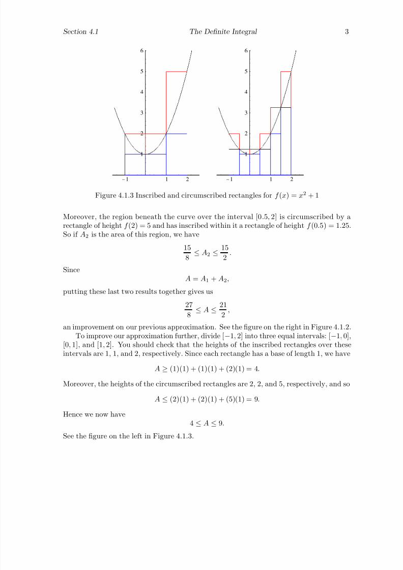
7/27/2019 Calculus 2 (Dan Sloughter)
http://slidepdf.com/reader/full/calculus-2-dan-sloughter 217/598
Section 4.1 The Definite Integral 3
-1 1 2
1
2
3
4
5
6
-1 1 2
1
2
3
4
5
6
Figure 4.1.3 Inscribed and circumscribed rectangles for f (x) = x2 + 1
Moreover, the region beneath the curve over the interval [0.5, 2] is circumscribed by arectangle of height f (2) = 5 and has inscribed within it a rectangle of height f (0.5) = 1.25.So if A2 is the area of this region, we have
15
8≤ A2 ≤ 15
2.
SinceA = A1 + A2,
putting these last two results together gives us
27
8≤ A ≤ 21
2,
an improvement on our previous approximation. See the figure on the right in Figure 4.1.2.To improve our approximation further, divide [−1, 2] into three equal intervals: [−1, 0],
[0, 1], and [1, 2]. You should check that the heights of the inscribed rectangles over theseintervals are 1, 1, and 2, respectively. Since each rectangle has a base of length 1, we have
A ≥ (1)(1) + (1)(1) + (2)(1) = 4.
Moreover, the heights of the circumscribed rectangles are 2, 2, and 5, respectively, and so
A ≤ (2)(1) + (2)(1) + (5)(1) = 9.
Hence we now have4 ≤ A ≤ 9.
See the figure on the left in Figure 4.1.3.

7/27/2019 Calculus 2 (Dan Sloughter)
http://slidepdf.com/reader/full/calculus-2-dan-sloughter 218/598
4 The Definite Integral Section 4.1
It is clear that we can approximate A using inscribed and circumscribed rectangles forany number of intervals. For example, you might check that if we use six intervals of equallength we would have
A ≥
5
4
1
2
+ (1)
1
2
+ (1)
1
2
+
5
4
1
2
+ (2)
1
2
+
13
4
1
2
=
39
8
and
A ≤ (2)
1
2
+
5
4
1
2
+
5
4
1
2
+ (2)
1
2
+
13
4
1
2
+ (5)
1
2
=
59
8
showing that4.875 ≤ A ≤ 7.375,
(see the figure on the right in Figure 4.1.2). Continuing in this manner, subdividingthe interval [−1, 2] into smaller and smaller intervals, we would expect that we couldapproximate A to any desired level of accuracy. Moreover, we would expect that the area
of the inscribed rectangles would increase toward A as the number of intervals increases,and that the area of the circumscribed rectangles would decrease toward A. Put anotherway, we might think of the area A as the unique number which is at once larger than thearea of any set of inscribed rectangles and smaller than the area of any set of circumscribedrectangles. We will use this idea as the basis for our definition of the definite integral .
The definite integral
We now want to take the ideas of the previous example and develop a general procedurewhich, when applied to the appropriate function, will yield the area of certain types of regions in the plane. To do so, we require some preliminary terminology and notation.
Let f be a function defined on an interval [a, b]. We will not require that f be positive
on [a, b], although it will be necessary to require f (x) ≥ 0 for all x in in order to talkabout the area between the graph of f and the interval [a, b], as in the previous example.However, we will assume that f is bounded on [a, b]; that is, we assume there exist numbersm and M such that m ≤ f (x) ≤ M for all x in [a, b]. In particular, by the ExtremeValue Theorem, f is bounded if f is continuous on [a, b]. We will return to the problem of unbounded functions in Section 4.7.
We call a set P = {x0, x1, . . . , xn} a partition of the interval [a, b] if
a = x0 < x1 < x2 < . . . < xn = b.
Such a partition P divides [a, b] into n intervals, [xi−1, xi], of lengths
∆xi = xi − xi−1,
where i = 1, 2, 3, . . . , n. For each such interval [xi−1, xi], let M i be the smallest number suchthat f (x) ≤ M i for all x in [xi−1, xi] and let mi be the largest number such that f (x) ≥ mi
for all x in [xi−1, xi]. Note that if f is continuous on [a, b], then M i is the maximum value
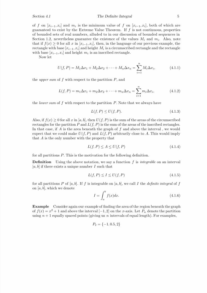
7/27/2019 Calculus 2 (Dan Sloughter)
http://slidepdf.com/reader/full/calculus-2-dan-sloughter 219/598
Section 4.1 The Definite Integral 5
of f on [xi−1, xi] and mi is the minimum value of f on [xi−1, xi], both of which areguaranteed to exist by the Extreme Value Theorem. If f is not continuous, propertiesof bounded sets of real numbers, alluded to in our discussion of bounded sequences inSection 1.2, nevertheless guarantee the existence of the values M i and mi. Also, notethat if f (x) ≥ 0 for all x in [xi−1, xi], then, in the language of our previous example, therectangle with base [xi
−1, xi] and height M i is a circumscribed rectangle and the rectangle
with base [xi−1, xi] and height mi is an inscribed rectangle.Now let
U (f, P ) = M 1∆x1 + M 2∆x2 + · · · + M n∆xn =ni=1
M i∆xi, (4.1.1)
the upper sum of f with respect to the partition P , and
L(f, P ) = m1∆x1 + m2∆x2 + · · · + mn∆xn =ni=1
mi∆xi, (4.1.2)
the lower sum of f with respect to the partition P . Note that we always have
L(f, P ) ≤ U (f, P ). (4.1.3)
Also, if f (x) ≥ 0 for all x in [a, b], then U (f, P ) is the sum of the areas of the circumscribedrectangles for the partition P and L(f, P ) is the sum of the areas of the inscribed rectangles.In that case, if A is the area beneath the graph of f and above the interval , we wouldexpect that we could make U (f, P ) and L(f, P ) arbitrarily close to A. This would implythat A is the only number with the property that
L(f, P ) ≤ A ≤ U (f, P ) (4.1.4)
for all partitions P . This is the motivation for the following definition.
Definition Using the above notation, we say a function f is integrable on an interval[a, b] if there exists a unique number I such that
L(f, P ) ≤ I ≤ U (f, P ) (4.1.5)
for all partitions P of [a, b]. If f is integrable on [a, b], we call I the definite integral of f
on [a, b], which we denote
I =
ba
f (x)dx. (4.1.6)
Example Consider again our example of finding the area of the region beneath the graphof f (x) = x2 + 1 and above the interval [−1, 2] on the x-axis. Let P n denote the partitionusing n + 1 equally spaced points (giving us n intervals of equal length). For examples,
P 2 = {−1, 0.5, 2}

7/27/2019 Calculus 2 (Dan Sloughter)
http://slidepdf.com/reader/full/calculus-2-dan-sloughter 220/598
6 The Definite Integral Section 4.1
andP 6 = {−1, −0.5, 0, 0.5, 1, 1.5, 2}.
Our work above shows that, in our current notation,
U (f, P 6) = 7.375
andL(f, P 6) = 4.875.
Using 100 intervals, and a computer to ease the computations, we find that
U (f, P 100) = 6.075
andL(f, P 100) = 5.925,
where the results have been rounded to three decimal places. This shows that if f isintegrable on [−1, 2], then
5.925 ≤
2
−1(x2 + 1)dx ≤ 6.075.
Of course, we expect f to be integrable, and for the value of the definite integral to be thesought for area under the graph.
It is not easy to verify directly from the definition that a given function is integrable onsome interval. However, it may be shown that any continuous function is integrable. Thereasons for this are rather technical, but we can give some feeling for why this should beso. Suppose f is continuous on [a, b] and let P n = {x0, x1, x2, . . . , xn} denote the partitionof [a, b] using n + 1 equally spaced points. Let M i and mi be as defined above, and let
∆x = ∆xi = b − a
n
be the length of the intervals [xi−1, xi], i = 1, 2, 3, . . . , n. Given any number > 0, wecan choose n large enough (equivalently, ∆x small enough) so that M i − mi < fori = 1, 2, 3, . . . , n. This fact is a consequence of the continuity of f on [a, b], although itrequires a deeper property of continuous functions on closed intervals known as uniform
continuity . We then have
0 ≤ U (f, P n) − L(f, P n)
=n
i=1
M i∆x
−
n
i=1
mi∆x
=ni=1
(M i − mi)∆x <
ni=1
∆x
= n∆x = (b − a).
(4.1.7)

7/27/2019 Calculus 2 (Dan Sloughter)
http://slidepdf.com/reader/full/calculus-2-dan-sloughter 221/598
Section 4.1 The Definite Integral 7
-1 1 2 3 4 5 6
1
2
3
4
5
Figure 4.1.4 Region beneath y = 3 over the interval [0, 5]
Since may be made arbitrarily small, it follows that the difference between upper sumsand lowers sums may be made arbitrarily small, and hence that there must be only onenumber which is between the upper and lower sums for all possible partitions.
Proposition If f is continuous on [a, b], then f is integrable on [a, b].
Example We now know that f (x) = x2 + 1 is integrable on [−1, 2].
Although our motivation for this section has been the computation of area, we havenot actually defined the term. We do so now for the special case we have been considering.
Definition Given an integrable function f with f (x) ≥ 0 for all x in an interval [a, b], letR be the region in the plane bounded above by the curve y = f (x), below by the interval[a, b] on the x-axis, and on the sides by the vertical lines x = a and x = b. Then we definethe area A of R to be
A =
b
a f (x)dx. (4.1.8)
Example Of course, we should verify that the above definition of area agrees with ourprevious notion of area. For example, if f (x) = 3 for all x in [0, 5], then the region beneaththe graph of f and above the x-axis is a rectangle with base of length 5 and height of 3,as shown in Figure 4.1.4. Hence we should have
5
0
3dx = 15.
To verify this, let P = {x0, x1, x2, . . . , xn} be any partition of [0, 5]. Then on any interval
[xi−1, xi], i = 1, 2, 3, . . . , n, the maximum value of f is M i = 3 and the minimum value of f is mi = 3. Hence
U (f, P ) = L(f, P ) =ni=1
3∆xi = 3ni=1
∆xi = (3)(5) = 15,
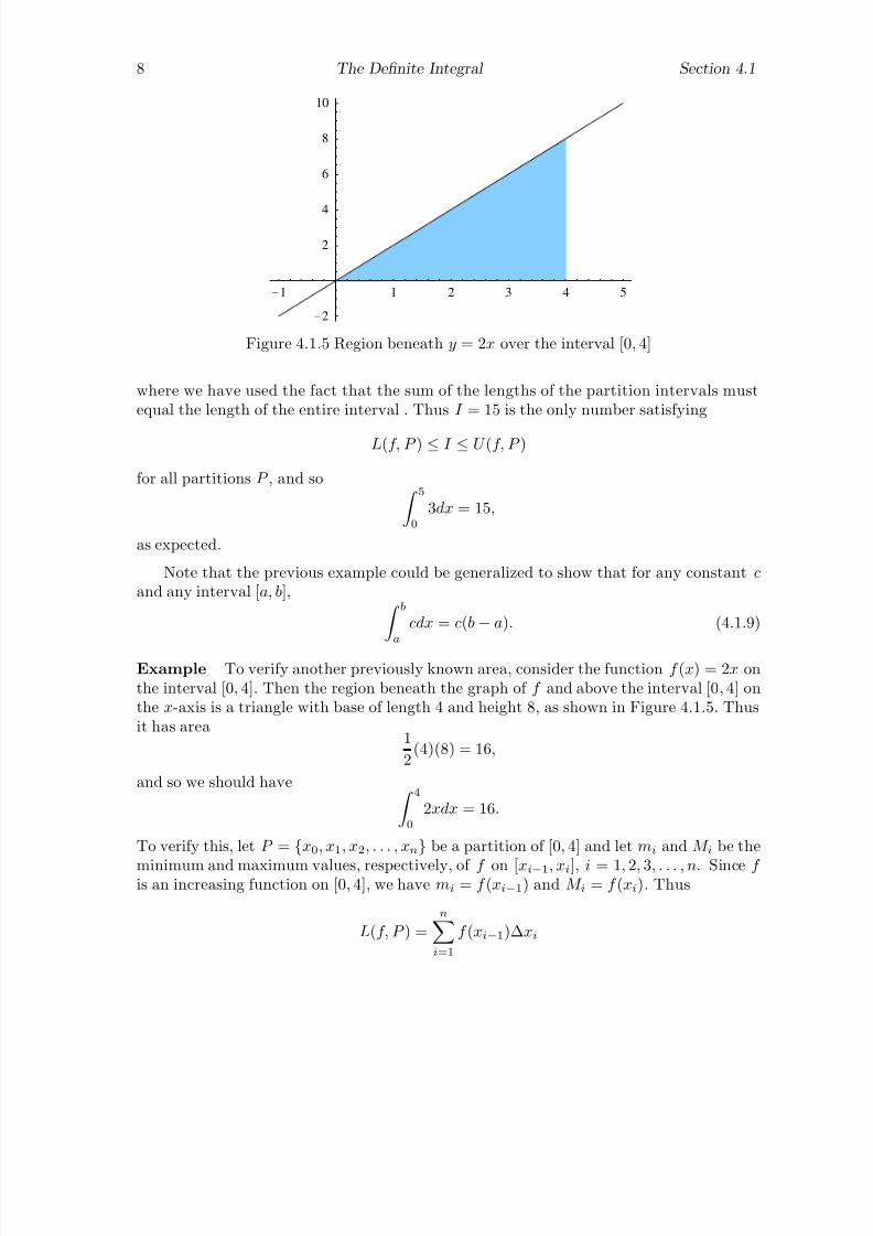
7/27/2019 Calculus 2 (Dan Sloughter)
http://slidepdf.com/reader/full/calculus-2-dan-sloughter 222/598
8 The Definite Integral Section 4.1
-1 1 2 3 4 5
-2
2
4
6
8
10
Figure 4.1.5 Region beneath y = 2x over the interval [0, 4]
where we have used the fact that the sum of the lengths of the partition intervals mustequal the length of the entire interval . Thus I = 15 is the only number satisfying
L(f, P ) ≤ I ≤ U (f, P )
for all partitions P , and so 5
0
3dx = 15,
as expected.
Note that the previous example could be generalized to show that for any constant c
and any interval [a, b], b
a
cdx = c(b − a). (4.1.9)
Example To verify another previously known area, consider the function f (x) = 2x onthe interval [0, 4]. Then the region beneath the graph of f and above the interval [0, 4] onthe x-axis is a triangle with base of length 4 and height 8, as shown in Figure 4.1.5. Thusit has area
1
2(4)(8) = 16,
and so we should have 4
0
2xdx = 16.
To verify this, let P =
{x0, x1, x2, . . . , xn
}be a partition of [0, 4] and let mi and M i be the
minimum and maximum values, respectively, of f on [xi−1, xi], i = 1, 2, 3, . . . , n. Since f is an increasing function on [0, 4], we have mi = f (xi−1) and M i = f (xi). Thus
L(f, P ) =ni=1
f (xi−1)∆xi
7/27/2019 Calculus 2 (Dan Sloughter)
http://slidepdf.com/reader/full/calculus-2-dan-sloughter 223/598
Section 4.1 The Definite Integral 9
and
U (f, P ) =ni=1
f (xi)∆xi.
We will now use a technique which will be useful in the proof of the Fundamental Theoremof Calculus in Section 4.3. Let F (x) = x2. Then F (x) = 2x, so F is an antiderivative
of f . By the Mean Value Theorem, for every interval [xi−1, xi] there exists a point ci in[xi−1, xi] such that
F (xi) − F (xi−1)
xi − xi−1= F (ci) = f (ci). (4.1.10)
Now xi − xi−1 = ∆xi, so from (4.1.10) we obtain
f (ci)∆xi = F (xi) − F (xi−1). (4.1.11)
Moreover, f (xi−1) ≤ f (ci) ≤ f (xi), so
L(
f, P ) =
n
i=1
f (
xi−1)∆xi ≤
n
i=1
f (
ci)∆
xi ≤
n
i=1
f (
xi)∆
xi=
U (
f, P )
.(4.1.12)
But, using (4.1.11),
ni=1
f (ci)∆xi =ni=1
(F (xi) − F (xi−1))
= (F (x1) − F (x0)) + (F (x2) − F (x1)) + (F (x3) − F (x2)) + · · ·+ (F (xn) − F (xn−1))
= −F (x0) + (F (x1) − F (x1)) + (F (x2) − F (x2)) + (F (x3) − F (x3)) + · · ·+ (F (xn
−1)
−F (xn
−1)) + F (xn)
= F (xn) − F (x0).
Now x0 = 0 and xn = 4, so
F (xn) − F (x0) = F (4) − F (0) = 16 − 0 = 16.
It now follows from (4.1.11) that, for any partition P ,
L(f, P ) ≤ 16 ≤ U (f, P ). (4.1.13)
Since we know that f is integrable on [0, 4] (it is continuous on [0, 4]), the definite integral
of f is the only number which satisfies the inequalities in (4.1.13) for any partition P .Hence we must have
4
0
2x = 16,
in agreement with our geometric argument above.

7/27/2019 Calculus 2 (Dan Sloughter)
http://slidepdf.com/reader/full/calculus-2-dan-sloughter 224/598
10 The Definite Integral Section 4.1
0.5 1 1.5 2
0.5
1
1.5
2
Figure 4.1.6 Region beneath y = √ 4 − x2 over the interval [0, 2]
As we proceed with our study of integration we shall from time to time have occasionto verify that areas computed using a definite integral are consistent with areas computedby other geometric means. At the same time, we shall take this consistency as a given.For example, we shall accept that
2
0
4 − x2 dx = π,
since the region beneath the curve y = √ 4 − x2
and above the interval [0, 2] is one-quarterof a circle of radius 2 centered at the origin, as shown in Figure 4.1.6.
Example It is important to realize that not all bounded functions are integrable. As anexample, consider the function
f (x) =
1, if x is a rational number,0, if x is an irrational number.
For example, f (0.12345) = 1 and f
1√ 2
= 0. Let P = {x0, x1, x2, . . . , xn} be a partition
of [0, 1]. Since every interval [xi−1, xi], i = 1, 2, 3, . . . , n, contains both rational and irra-
tional numbers, the minimum value of f on [xi−1, xi] is mi = 0 and the maximum valueof f on [xi−1, xi] is M i = 1. Thus
L(f, P ) =ni=1
mi∆xi = 0
7/27/2019 Calculus 2 (Dan Sloughter)
http://slidepdf.com/reader/full/calculus-2-dan-sloughter 225/598
Section 4.1 The Definite Integral 11
and
U (f, P ) =ni=1
M i∆xi =ni=1
∆xi = 1.
Hence any number between 0 and 1 lies between L(f, P ) and U (f, P ) for any partition P .Since there is not a unique such number, we conclude that f is not integrable on [0, 1].
Computing a definite integral directly from the definition is usually a daunting task.We shall take a first look at approximating definite integrals in this section, and then refinethese techniques in Section 4.2. In Section 4.3 we will look at the Fundamental TheoremCalculus, a result which will, in certain cases, allow us to compute definite integrals exactlywith relative ease.
Riemann sums
Again let f be a function defined on an interval [a, b] and let P = {x0, x1, x2, . . . , xn} bea partition of [a, b]. Recall that in the definition of the upper and lower sums, M i andmi are chosen, in part, so that mi ≤ f (x) ≤ M i for all x in [xi−1, xi], i = 1, 2, 3, . . . , n.It follows that if we choose values c1, c2, c3, . . . , cn so that ci is in the ith interval of thepartition (that is, xi−1 ≤ ci ≤ xi), then
mi ≤ f (ci) ≤ M i (4.1.14)
for i = 1, 2, 3, . . . , n, and so
L(f, P ) =ni=1
mi∆xi ≤ni=1
f (ci)∆xi ≤ni=1
M i∆xi = U (f, P ). (4.1.15)
If f is integrable, it may be shown that is always possible to choose a partition P so that
|U (f, P ) − L(f, P )| < (4.1.16)
for any specified > 0. It follows that, when f is integrable, it is always possible to find,for any given > 0, partitions for which
ba
f (x)dx −ni=1
f (ci)∆xi
< (4.1.17)
for any choice of the points c1, c2, c3, . . . , cn. In fact, it may be shown that if we let L bethe maximum length of the intervals [xi−1, xi], then it is possible to find a δ > 0 such that(4.1.17) will hold for any partition with L < δ .
The sumni=1
f (ci)∆xi (4.1.18)
is called a Riemann sum , after the German mathematician G. B. F. Riemann (1826-1866). From what we have just seen, we may use Riemann sums to approximate definite

7/27/2019 Calculus 2 (Dan Sloughter)
http://slidepdf.com/reader/full/calculus-2-dan-sloughter 226/598
12 The Definite Integral Section 4.1
integrals. We will consider two important special cases of Riemann sums here (we willlook at another in Section 4.2). First, to make calculations simpler, we will restrict topartitions with intervals of equal length. As above, let P n = {x0, x1, x2, . . . , xn} be thepartition of [a, b] using n + 1 equally spaced points and let
∆x =b−
a
n
be the length of the intervals [xi−1, xi], i = 1, 2, 3, . . . , n. Note that
limn→∞
∆x = 0.
Hence, if we choose points c1, c2, c3, . . . , cn with xi−1 ≤ ci ≤ xi, then we have, for anintegrable f ,
b
a f (x)dx = limn→∞
n
i=1
f (ci)∆x. (4.1.19)
In other words, we may approximate the definite integral ba
f (x)dx to any desired level of accuracy using Riemann sums
ni=1
f (ci)∆x (4.1.20)
with sufficiently large n. To do this efficiently requires specifying how the points c1, c2, c3,. . . , cn are to be chosen. One method is to simply choose ci to be the right-hand endpointof the interval [xi
−1, xi]. In that case, since the points in the partition are equally spaced,
we havec1 = x1 = x0 + ∆x = a + ∆x,
c2 = x2 = x1 + ∆x = a + 2∆x,
c3 = x3 = x2 + ∆x = a + 3∆x,
...
cn = xn = xn−1 + ∆x = a + n∆x.
(4.1.21)
Using these points in (4.1.20), we have
ni=1
f (ci)∆x = ∆x
ni=1
f (a + i∆x). (4.1.22)
This approximation is known as the right-hand rule approximation for b
af (x)dx.

7/27/2019 Calculus 2 (Dan Sloughter)
http://slidepdf.com/reader/full/calculus-2-dan-sloughter 227/598
Section 4.1 The Definite Integral 13
Definition If f is integrable on [a, b], the right-hand rule approximation for the definiteintegral b
a
f (x)dx
using n intervals is given by
AR = ∆x
ni=1
f (a + i∆x), (4.1.23)
where
∆x =b − a
n.
A similar rule is derived by using the left-hand endpoints of the intervals. In this casewe choose
c1 = x0 = x0 = a,c2 = x1 = x0 + ∆x = a + ∆x,
c3 = x2 = x1 + ∆x = a + 2∆x,
...
cn = xn−1 = xn−2 + ∆x = a + (n − 1)∆x.
(4.1.24)
Definition If f is integrable on [a, b], the left-hand rule approximation for the definiteintegral
b
a
f (x)dx
using n intervals is given by
AL = ∆x
n−1i=0
f (a + i∆x), (4.1.25)
where
∆x =b − a
n.
Example Returning to our first example, suppose f (x) = x2 + 1 and let A be the areaof the region beneath the graph of f and above the interval [−1, 2]. With n = 6, we have
∆x =2 − (−1)
6=
1
2
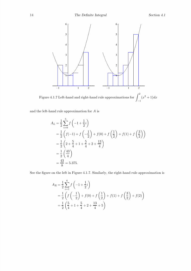
7/27/2019 Calculus 2 (Dan Sloughter)
http://slidepdf.com/reader/full/calculus-2-dan-sloughter 228/598
14 The Definite Integral Section 4.1
-1 1 2
1
2
3
4
5
6
-1 1 2
1
2
3
4
5
6
Figure 4.1.7 Left-hand and right-hand rule approximations for 2−1
(x2 + 1)dx
and the left-hand rule approximation for A is
AL =1
2
5i=0
f
−1 +
1
2i
=1
2
f (−1) + f
−1
2
+ f (0) + f
1
2
+ f (1) + f
3
2
= 12
2 + 5
4+ 1 + 5
4+ 2 + 13
4
=1
2
43
4
=43
8= 5.375.
See the figure on the left in Figure 4.1.7. Similarly, the right-hand rule approximation is
AR =1
2
6
i=1
f
−1 +
1
2i
=1
2
f
−1
2
+ f (0) + f
1
2
+ f (1) + f
3
2
+ f (2)
=1
2
5
4+ 1 +
5
4+ 2 +
13
4+ 5

7/27/2019 Calculus 2 (Dan Sloughter)
http://slidepdf.com/reader/full/calculus-2-dan-sloughter 229/598
Section 4.1 The Definite Integral 15
=1
2
55
4
=55
8= 6.875.
See the figure on the right in Figure 4.1.7. Recall that, for a partition of 6 intervals of
equal length, we computed a lower sum of 4.875 and an upper sum 7.375. Hence, as wewould expect for any Riemann sums, AL and AR lie between the lower and upper sums.
Using n = 100 and a computer, we find AL = 5.955 and AR = 6.045, which again liebetween the lower sum of 5.925 and the upper sum of 6.075.
Example Now let A be the area of the region beneath the graph of
g(t) =1
t
over the interval [1, 10], as shown in Figure 4.1.8. Then
A = 10
1
1
t
dt.
In Section 6.2 we will see that this integral is equal to the natural logarithm of 10, which, to6 decimal places, is 2.302585. The following table summarizes the left-hand and right-handrule approximations for A:
n AR AL |A − AR| |A − AL|10 1.960214 2.770214 0.342371 0.46762920 2.116477 2.521477 0.186108 0.21889240 2.205491 2.407991 0.097094 0.10540680 2.253003 2.354253 0.049582 0.051668
160 2.277534 2.328159 0.025052 0.025574
320 2.289994 2.315307 0.012591 0.012722
2 4 6 8 10
0.2
0.4
0.6
0.8
1
1.2
1.4
Figure 4.1.8 Region beneath y =1
tover the interval [1, 10]

7/27/2019 Calculus 2 (Dan Sloughter)
http://slidepdf.com/reader/full/calculus-2-dan-sloughter 230/598
16 The Definite Integral Section 4.1
As we should expect, the error in our approximations decreases as the number of subdi-visions increases. What is more interesting to note is that, in this particular case, whenthe number of subdivisions is doubled, the error committed by both the right-hand andthe left-hand rules decreases by a factor of, roughly, 1
2. For example, this might lead us to
predict that the error in using 640 intervals would be about 0.0063; in fact, it turns outto be 0.006312 for the right-hand rule and 0.006344 for the left-hand rule. This type of
behavior is typical for this method of approximation, a point we will come back to whenwe investigate other methods of approximation in Section 4.2.
Properties of the definite integral
Since the integral of an integrable function may be computed as the limit of Riemannsums, the basic properties of limits and sums hold true for integrals as well. In particular,if f and g are integrable on [a, b] and k is any constant, then
b
a
(f (x) + g(x))dx =
b
a
f (x)dx +
b
a
g(x)dx, (4.1.26)
ba
(f (x) − g(x))dx =
ba
f (x)dx − ba
g(x)dx, (4.1.27)
and ba
kf (x)dx = k
ba
f (x)dx. (4.1.28)
Example We know that 3
0
xdx =9
2
(since the region under the graph of y = x over the interval [0, 3] is a triangle with base of length 3 and a height of 3) and 3
0
4dx = 12
(either using (4.1.9) or the fact that the region under the graph of y = 4 is a rectanglewith base of length 3 and a height of 4), so it follows from (4.1.24) that
3
0
(x + 4)dx =
3
0
xdx +
3
0
4dx =9
2+ 12 =
33
2.
Example The graph of g(t) = √ 1 − t2 over the interval [−1, 1] is a semicircle of radius1 centered at the origin, so
1
−15
1 − t2 dt = 5
1
−1
1 − t2 dt =
5π
2.

7/27/2019 Calculus 2 (Dan Sloughter)
http://slidepdf.com/reader/full/calculus-2-dan-sloughter 231/598
Section 4.1 The Definite Integral 17
a bc
y = f ( ) x
Figure 4.1.9 b
a
f (x)dx = c
a
f (x)dx + b
c
f (x)dx
Now suppose f is integrable on [a, b] and c is a point with a < c < b. It may be shownthat f is integrable on both [a, c] and [c, b]. Moveover, using partitions which include c,we may write a Riemann sum for f over [a, b] as the sum of two Riemann sums, the firstover the interval [a, c] and the second over the interval [c, b]. After taking limits, it followsthat b
a
f (x)dx =
ca
f (x)dx +
bc
f (x)dx. (4.1.29)
If f (x) ≥ 0 for all x in [a, b], we may think of (4.1.29) as saying that the area under the
graph of f over the interval [a, b] is equal to the area under the graph of f over the interval[a, c] plus the area under the graph of f over the interval [c, b]. See Figure 4.1.9.
Example Suppose
f (x) =
x, if 0 ≤ x ≤ 1,3, if 1 < x ≤ 2.
The region under the graph of f is shown in Figure 4.1.10. Now
2
0
f (x)dx =
1
0
f (x)dx +
2
1
f (x)dx =
1
0
xdx +
2
1
3dx =1
2+ 3 =
7
2.
Technically, before applying (4.1.29) in the previous example we should have verifiedthat f is integrable on [0, 2]. Since f is not continuous on [0, 2], its integrability does notfollow from our previous results. However, f is an example of what is known as a piecewise
continuous function, which we will now define.
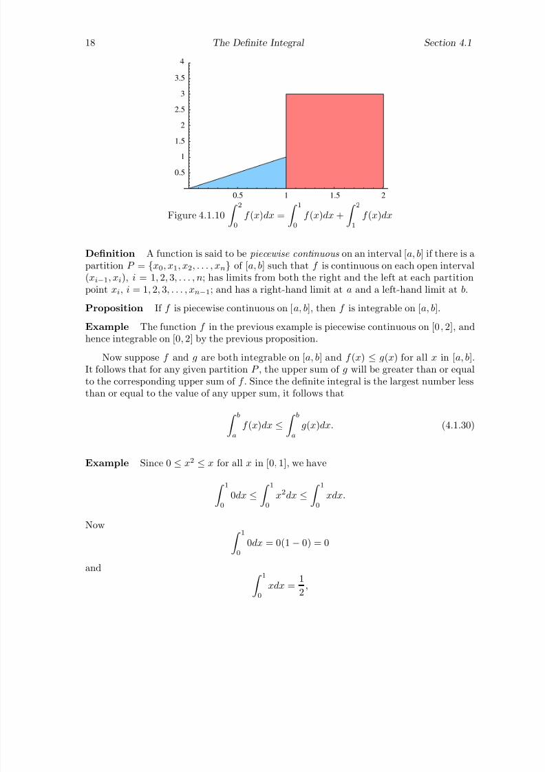
7/27/2019 Calculus 2 (Dan Sloughter)
http://slidepdf.com/reader/full/calculus-2-dan-sloughter 232/598
18 The Definite Integral Section 4.1
0.5 1 1.5 2
0.5
1
1.5
2
2.5
3
3.5
Figure 4.1.10
2
0
f (x)dx =
1
0
f (x)dx +
2
1
f (x)dx
Definition A function is said to be piecewise continuous on an interval [a, b] if there is a
partition P = {x0
, x1
, x2
, . . . , xn} of [a, b] such that f is continuous on each open interval(xi−1, xi), i = 1, 2, 3, . . . , n; has limits from both the right and the left at each partition
point xi, i = 1, 2, 3, . . . , xn−1; and has a right-hand limit at a and a left-hand limit at b.
Proposition If f is piecewise continuous on [a, b], then f is integrable on [a, b].
Example The function f in the previous example is piecewise continuous on [0, 2], andhence integrable on [0, 2] by the previous proposition.
Now suppose f and g are both integrable on [a, b] and f (x) ≤ g(x) for all x in [a, b].It follows that for any given partition P , the upper sum of g will be greater than or equalto the corresponding upper sum of f . Since the definite integral is the largest number lessthan or equal to the value of any upper sum, it follows that
ba
f (x)dx ≤ ba
g(x)dx. (4.1.30)
Example Since 0 ≤ x2 ≤ x for all x in [0, 1], we have
1
0
0dx ≤
1
0
x2dx ≤
1
0
xdx.
Now
10
0dx = 0(1 − 0) = 0
and 1
0
xdx =1
2,
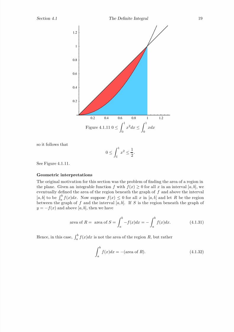
7/27/2019 Calculus 2 (Dan Sloughter)
http://slidepdf.com/reader/full/calculus-2-dan-sloughter 233/598
Section 4.1 The Definite Integral 19
0.2 0.4 0.6 0.8 1 1.2
0.2
0.4
0.6
0.8
1
1.2
Figure 4.1.11 0 ≤
1
0
x2dx ≤
1
0
xdx
so it follows that
0 ≤
1
0
x2 ≤ 1
2.
See Figure 4.1.11.
Geometric interpretations
The original motivation for this section was the problem of finding the area of a region inthe plane. Given an integrable function f with f (x) ≥ 0 for all x in an interval [a, b], weeventually defined the area of the region beneath the graph of f and above the interval
[a, b] to be b
af (x)dx. Now suppose f (x) ≤ 0 for all x in [a, b] and let R be the region
between the graph of f and the interval [a, b]. If S is the region beneath the graph of y = −f (x) and above [a, b], then we have
area of R = area of S =
ba
−f (x)dx = − ba
f (x)dx. (4.1.31)
Hence, in this case, ba
f (x)dx is not the area of the region R, but rather
ba
f (x)dx = −(area of R). (4.1.32)

7/27/2019 Calculus 2 (Dan Sloughter)
http://slidepdf.com/reader/full/calculus-2-dan-sloughter 234/598
20 The Definite Integral Section 4.1
0.2 0.4 0.6 0.8 1
-1
-0.8
-0.6
-0.4
-0.2
Figure 4.1.12 Region between the graph of y = x − 1 and the interval [0, 1]
Example If f (x) = x − 1, then f (x) ≤ 0 for all x in [0, 1]. Since the region between thegraph of f and the interval [0, 1] on the x-axis is a triangle with area 1
2, we must have
1
0
(x − 1)dx = −1
2.
See Figure 4.1.12.
More generally, we may think of ba
f (x)dx as representing the difference of the areaof any regions between the graph of f and the x-axis which lie above the x-axis and thearea of those regions which lie below the x-axis. For example, we have
π−π
sin(x)dx = 0
because the area of the region beneath the graph of y = sin(x) over the interval [0, π] isnegated by the area of the region between the graph y = sin(x) and the interval [−π, 0],as shown in Figure 4.1.13.
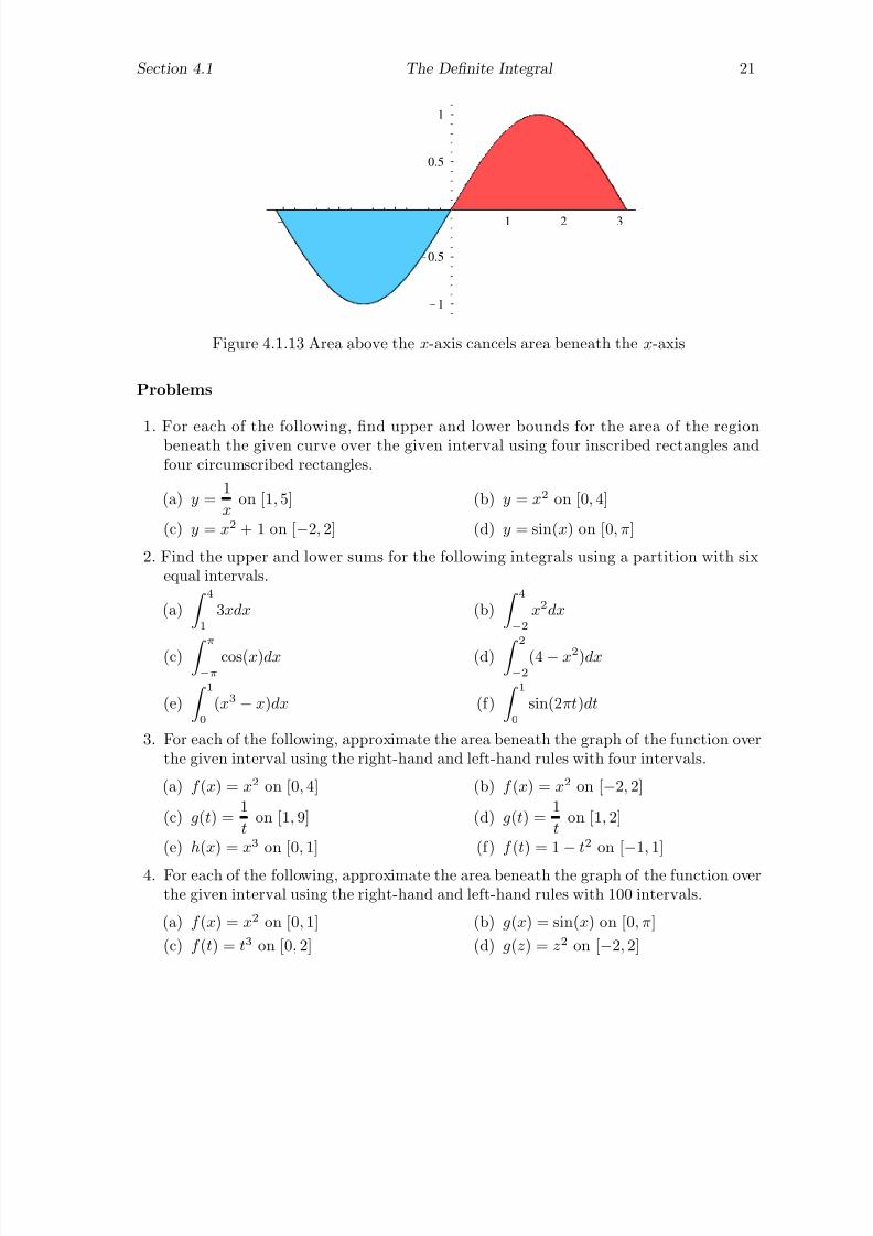
7/27/2019 Calculus 2 (Dan Sloughter)
http://slidepdf.com/reader/full/calculus-2-dan-sloughter 235/598
Section 4.1 The Definite Integral 21
-3
-2
-1 1 2 3
-1
-0.5
0.5
1
Figure 4.1.13 Area above the x-axis cancels area beneath the x-axis
Problems
1. For each of the following, find upper and lower bounds for the area of the regionbeneath the given curve over the given interval using four inscribed rectangles andfour circumscribed rectangles.
(a) y =1
xon [1, 5] (b) y = x2 on [0, 4]
(c) y = x2 + 1 on [−2, 2] (d) y = sin(x) on [0, π]
2. Find the upper and lower sums for the following integrals using a partition with sixequal intervals.
(a)
4
1
3xdx (b)
4
−2x2dx
(c) π−π
cos(x)dx (d) 2−2
(4 − x2)dx
(e)
1
0
(x3 − x)dx (f)
1
0
sin(2πt)dt
3. For each of the following, approximate the area beneath the graph of the function overthe given interval using the right-hand and left-hand rules with four intervals.
(a) f (x) = x2 on [0, 4] (b) f (x) = x2 on [−2, 2]
(c) g(t) =1
ton [1, 9] (d) g(t) =
1
ton [1, 2]
(e) h(x) = x3 on [0, 1] (f) f (t) = 1
−t2 on [
−1, 1]
4. For each of the following, approximate the area beneath the graph of the function overthe given interval using the right-hand and left-hand rules with 100 intervals.
(a) f (x) = x2 on [0, 1] (b) g(x) = sin(x) on [0, π]
(c) f (t) = t3 on [0, 2] (d) g(z) = z2 on [−2, 2]

7/27/2019 Calculus 2 (Dan Sloughter)
http://slidepdf.com/reader/full/calculus-2-dan-sloughter 236/598
22 The Definite Integral Section 4.1
(e) h(x) =1
xon [1, 2] (f) f (x) =
√ 1 − x2 on [−1, 1]
(g) h(θ) = sec(θ) on−π
4,
π
4
(h) g(t) = sin(2t) on
0,
π
2
5. Use the right-hand and left-hand rules with four intervals to approximate the followingdefinite integrals.
(a)
2
0
x2dx (b)
3
2
1
xdx
(c)
π−π
cos(t)dt (d)
1
−3s3ds
(e)
1
−1(x2 − 1)dx (f)
π−π
sin(z)dz
6. Use the right-hand and left-hand rules with 100 intervals to approximate the followingdefinite integrals.
(a) 30
x2
dx (b) 2−1
x3
dx
(c)
2
−2
4 − t2 dt (d)
2π
0
sin(x)dx
(e)
1
−1(x2 − 1)dx (f)
π0
sin(3θ)dθ
(g)
0
−1
x
x2 + 1dx (h)
−2−4
1
tdt
7. Use geometric arguments to determine the value of each of the following definite inte-grals.
(a)
4
0
xdx (b)
3
0
(2x + 3)dx
(c)
3
0
9 − x2 dx (d)
2
−24
4 − t2 dt
(e)
2
−2x3dx (f)
2π
0
sin(t)dt
8. Suppose
f (x) =
x + 1, if 0 ≤ x ≤ 1,4, if 1 < x
≤3.
Combine geometric arguments with properties of definite integrals to determine thevalue of the following definite integrals.
(a)
1
0
f (x)dx (b)
3
1
f (x)dx

7/27/2019 Calculus 2 (Dan Sloughter)
http://slidepdf.com/reader/full/calculus-2-dan-sloughter 237/598
Section 4.1 The Definite Integral 23
(c)
3
0
f (x)dx (d)
2
0
f (x)dx
9. The definition of
ba
f (x)dx assumes a < b.
(a) Explain why it would be reasonable to define
a
a
f (x)dx = 0.
(b) Explain why it would be reasonable to define
ba
f (x)dx = − ab
f (x)dx
whenever a > b.
(c) Using the definitions given in (a) and (b), and assuming that f is integrable onthe appropriate intervals, show that
ba
f (x)dx =
ca
f (x)dx +
bc
f (x)dx
whether a ≤ c ≤ b, a ≤ b ≤ c, b ≤ a ≤ c, b ≤ c ≤ a, c ≤ a ≤ b, or c ≤ b ≤ a. Notethat this generalizes (4.1.29).
10. Suppose f is integrable on [a, b] and m and M are constants such that m ≤ f (x) ≤ M
for all x in [a, b]. Show that
m(b − a) ≤
b
a
f (x)dx ≤ M (b − a).
11. Given that f is integrable on [a, b], it may be shown that g(x) = |f (x)| is also integrableon [a, b]. Show that
ba
f (x)dx
≤ ba
|f (x)|dx.
Hint: Use the fact that −|f (x)| ≤ f (x) ≤ |f (x)| for all x in [a, b].
12. In this section we showed that
4
0
2xdx = 16
directly from the definition of the definite integral (with some help from the MeanValue Theorem).
7/27/2019 Calculus 2 (Dan Sloughter)
http://slidepdf.com/reader/full/calculus-2-dan-sloughter 238/598
24 The Definite Integral Section 4.1
(a) Use these ideas to show that 1
0
xdx =1
2.
(b) More generally, show that
b0
xdx =
b2
2 .
(c) Let
F (x) =
x0
tdt.
What is the relationship between F and the function f (x) = x?
13. In this section we showed that 4
0
2x = 16
directly from the definition of the definite integral (with some help from the Mean
Value Theorem). Use these ideas to show that
1
0
x2dx =1
3.
7/27/2019 Calculus 2 (Dan Sloughter)
http://slidepdf.com/reader/full/calculus-2-dan-sloughter 239/598
Difference Equations
Differential Equations
to
Section 4.2
Numerical Approximationsof Definite Integrals
Computing a definite integral of a function f over an interval [a, b] using upper and lowersums, or even as the limit of Riemann sums, is, for all but the simplest cases, a difficult task.As a result, definite integrals are almost never computed in that manner. For the mostpart, definite integrals are evaluated either using the Fundamental Theorem of Calculusor using numerical approximation techniques. We will take up the Fundamental Theoremof Calculus approach in the next section; in this section we consider several methods fornumerical approximation.
The left-hand and right-hand rules
Recall that for an integrable function f on an interval [a, b], the left-hand rule approxima-
tion for ba
f (x)dx, using n intervals, is given by
AL = h
n−1i=0
f (a + ih) (4.2.1)
and the right-hand rule approximation by
AR = h
ni=1
f (a + ih), (4.2.2)
where
h =b − a
n.
We now look at the accuracy of these approximations. Let xi = a+ih, i = 0, 1, 2, . . . , n,the endpoints for a partition of [a, b] using n intervals of equal length h. Assume f iscontinuous on [a, b] and differentiable on (a, b) and that x is a point in the ith interval,that is, xi−1 ≤ x ≤ xi. Then the Mean Value Theorem tells us that there exists a point ci
in the interval (xi−1, xi) such that
f (ci) =f (x) − f (xi−1)
x − xi−1. (4.2.3)
Solving for f (x) in (4.2.3), we have
f (x) = f (xi−1) + f (ci)(x − xi−1). (4.2.4)
1 Copyright c by Dan Sloughter 2000

7/27/2019 Calculus 2 (Dan Sloughter)
http://slidepdf.com/reader/full/calculus-2-dan-sloughter 240/598
2 Numerical Approximations of Definite Integrals Section 4.2
Integrating both sides of (4.2.4) over the interval [xi−1, xi] gives us xi
xi−1
f (x)dx =
xi
xi−1
f (xi−1)dx +
xi
xi−1
f (ci)(x − xi−1)dx
= f (xi−1)(xi − xi−1) + xi
xi−1
f (ci)(x − xi−1)dx
= f (xi−1)h +
xi
xi−1
f (ci)(x − xi−1)dx,
(4.2.5)
where we have used the fact that the integral of a constant equals the constant multipliedby the length of the interval. Hence b
a
f (x)dx =ni=1
xi
xi−1
f (x)dx
=n
i=1
f (xi−1)h +n
i=1
xi
xi−1
f (ci)(x − xi−1)dx
= AL +ni=1
xi
xi−1
f (ci)(x − xi−1)dx.
(4.2.6)
Thus we have ba
f (x)dx − AL
=
ni=1
xi
xi−1
f (ci)(x − xi−1)dx
≤
ni=1
xi
xi−1
f (ci)(x − xi−1)dx
.
(4.2.7)
Now xi
xi−1
f (ci)(x − xi−1)dx
≤
xi
xi−1
|f (ci)(x − xi−1)|dx, (4.2.8)
(see Problem 11 in Section 4.1), so ba
f (x)dx − AL
≤ni=1
xi
xi−1
|f (ci)(x − xi−1)|dx
=ni=1
xi
xi−1
|f (ci)|(x − xi−1)dx,
(4.2.9)
where the last equality follows from the fact that x − xi−1 ≥ 0 for all x in [xi−1, xi]. Nowsuppose f is defined and continuous on [a, b] and let M be the maximum value of |f (x)|for x in [a, b]. Then xi
xi−1
|f (ci)|(x − xi−1)|dx ≤
xi
xi−1
M (x − xi−1)dx
= M
xi
xi−1
(x − xi−1)dx =M h2
2,
(4.2.10)
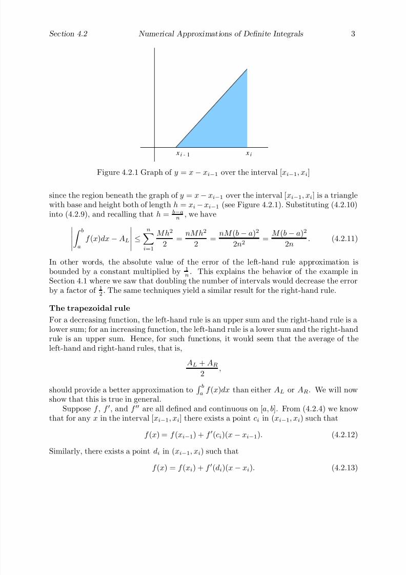
7/27/2019 Calculus 2 (Dan Sloughter)
http://slidepdf.com/reader/full/calculus-2-dan-sloughter 241/598
Section 4.2 Numerical Approximations of Definite Integrals 3
x xi - i1
Figure 4.2.1 Graph of y = x − xi−1 over the interval [xi−1, xi]
since the region beneath the graph of y = x − xi−1 over the interval [xi−1, xi] is a trianglewith base and height both of length h = xi − xi−1 (see Figure 4.2.1). Substituting (4.2.10)into (4.2.9), and recalling that h = b−a
n, we have
ba
f (x)dx − AL
≤ni=1
M h2
2=
nM h2
2=
nM (b − a)2
2n2=
M (b − a)2
2n. (4.2.11)
In other words, the absolute value of the error of the left-hand rule approximation isbounded by a constant multiplied by 1
n. This explains the behavior of the example in
Section 4.1 where we saw that doubling the number of intervals would decrease the errorby a factor of 1
2. The same techniques yield a similar result for the right-hand rule.
The trapezoidal rule
For a decreasing function, the left-hand rule is an upper sum and the right-hand rule is alower sum; for an increasing function, the left-hand rule is a lower sum and the right-handrule is an upper sum. Hence, for such functions, it would seem that the average of theleft-hand and right-hand rules, that is,
AL + AR
2,
should provide a better approximation to
b
af (x)dx than either AL or AR. We will now
show that this is true in general.Suppose f , f , and f are all defined and continuous on [a, b]. From (4.2.4) we knowthat for any x in the interval [xi−1, xi] there exists a point ci in (xi−1, xi) such that
f (x) = f (xi−1) + f (ci)(x − xi−1). (4.2.12)
Similarly, there exists a point di in (xi−1, xi) such that
f (x) = f (xi) + f (di)(x − xi). (4.2.13)

7/27/2019 Calculus 2 (Dan Sloughter)
http://slidepdf.com/reader/full/calculus-2-dan-sloughter 242/598
4 Numerical Approximations of Definite Integrals Section 4.2
Using f in place of f in (4.2.4), there exists a point pi in (xi−1, ci) such that
f (ci) = f (xi−1) + f ( pi)(ci − xi−1) (4.2.14)
and a point q i such that
f (di) = f (xi−1) + f (q i)(di − xi−1) (4.2.15)
Substituting (4.2.14) into (4.2.12) and (4.2.15) into (4.2.13), we have
f (x) = f (xi−1) + (f (xi−1) + f ( pi)(ci − xi−1))(x − xi−1)
= f (xi−1) + f (xi−1)(x − xi−1) + f ( pi)(ci − xi−1)(x − xi−1)(4.2.16)
and
f (x) = f (xi) + (f
(xi−1) + f
(q i)(di − xi−1))(x − xi)= f (xi) + f (xi−1)(x − xi) + f (q i)(di − xi−1)(x − xi).
(4.2.17)
Taking the average of (4.2.16) and (4.2.17) gives us
f (x) =f (x) + f (x)
2
=f (xi−1) + f (xi)
2+
f (xi−1)((x − xi−1) + (x − xi))
2
+f ( pi)(ci − xi−1)(x − xi−1) + f (q i)(di − xi−1)(x − xi)
2.
(4.2.18)
Now
xi
xi−1
f (xi−1) + f (xi)
2dx =
f (xi−1) + f (xi)
2(xi − xi−1) =
f (xi−1) + f (xi)
2h (4.2.19)
and
xi
xi−1
f (xi−1)((x − xi−1) + (x − xi))
2dx = f (xi−1)
xi
xi−1
x −
xi−1 + xi
2
dx
= 0,
(4.2.20)
where the final equality follows from the fact that region between the graph of
y = x −xi−1 + xi
2

7/27/2019 Calculus 2 (Dan Sloughter)
http://slidepdf.com/reader/full/calculus-2-dan-sloughter 243/598
Section 4.2 Numerical Approximations of Definite Integrals 5
1 x i -
i x
Figure 4.2.2 Graph of y = x −xi−1 + xi
2over the interval [xi−1, xi]
and the interval [xi−1, xi] forms two triangles of equal area, one above the x-axis and onebelow (see Figure 4.2.2). Moreover, if K is the maximum value of |f (x)| for x in [a, b],then
f ( pi)(ci − xi−1)(x − xi−1) + f (q i)(di − xi−1)(x − xi)
2
≤K
2(|ci − xi−1||x − xi−1|
+ |di − xi−1||x − xi|).
Since the points ci, di, and x are all in [xi−1, xi], it follows that
f ( pi)(ci − xi−1)(x − xi−1) + f (q i)(di − xi−1)(x − xi)
2
≤ Kh2. (4.2.21)
Hence
xi
xi−1
f ( pi)(ci − xi−1)(x − xi−1) + f (q i)(di − xi−1)(x − xi)
2
dx ≤
xi
xi−1
Kh2dx.
Now xi
xi−1
Kh2dx = Kh2(xi − xi−1) = Kh3, (4.2.22)
so we have
xi
xi−1
f ( pi)(ci − xi−1)(x − xi−1) + f (q i)(di − xi−1)(x − xi)
2
dx ≤ Kh3. (4.2.23)
7/27/2019 Calculus 2 (Dan Sloughter)
http://slidepdf.com/reader/full/calculus-2-dan-sloughter 244/598
6 Numerical Approximations of Definite Integrals Section 4.2
Putting this all together, we have
ba
f (x)dx =ni=1
xi
xi−1
f (x)dx
=ni=1
xi
xi−1
f (xi−1) + f (xi)2
dx
+ni=1
xi
xi−1
f (xi−1)((x − xi−1) + (x − xi))
2dx
+ni=1
xi
xi−1
f ( pi)(ci − xi−1)(x − xi−1) + f (q i)(di − xi−1)(x − xi)
2dx
=ni=1
f (xi−1) + f (xi)
2h + 0
+ni=1
xi
xi−1
f ( pi)(ci − xi−1)(x − xi−1) + f (q i)(di − xi−1)(x − xi)2
dx
=hn
i=1f (xi−1) + h
n
i=1f (xi)
2
+ni=1
xi
xi−1
f ( pi)(ci − xi−1)(x − xi−1) + f (q i)(di − xi−1)(x − xi)
2dx
=AL + AR
2
+
ni=1
xi
xi−1
f ( pi)(ci − xi−1)(x − xi−1) + f (q i)(di − xi−1)(x − xi)
2 dx,
from which it follows, using (4.2.23), that
ba
f (x)dx −AL + AR
2
≤ni=1
Kh3 = nKh3 = nK
b − a
n
3=
K (b − a)3
n2. (4.2.24)
That is, if we approximate ba
f (x)dx by
AL + AR
2,
then the absolute value of the error is bounded by a constant multiplied by 1
n2. In par-
ticular, if we double the number of intervals, we should expect the error to decrease by afactor of
1
2
2=
1
4.

7/27/2019 Calculus 2 (Dan Sloughter)
http://slidepdf.com/reader/full/calculus-2-dan-sloughter 245/598
Section 4.2 Numerical Approximations of Definite Integrals 7
We call
AT =AL + AR
2(4.2.25)
a trapezoidal rule approximation for ba
f (x)dx. The name comes from the fact that (4.2.25)may also be derived by replacing the areas of rectangles by the areas of trapezoids in the
Riemann sum approximations (see Problem 6).
Example In Section 4.1 we saw that the left-hand and right-hand rule approximations
for 2
−1(x2 + 1)dx using n = 6 intervals are AL = 5.375 and AR = 6.875. Hence the
corresponding trapezoidal rule approximation is
AT =5.375 + 6.875
2= 6.125.
With n = 100, the left-hand and right-hand rules give usAL = 5.95545 and AR = 6.04545,yielding a trapezoidal rule approximation of
AT = 5.95545 + 6.045452
= 6.00045.
Example In a Section 4.1 we approximated
A =
10
1
1
tdt
using both left-hand and right-hand rules and, after noting that to 6 decimal places A =2.302585, obtained the following table of values:
n AR AL |A − AR| |A − AL|10 1.960214 2.770214 0.342371 0.46762920 2.116477 2.521477 0.186108 0.21889240 2.205491 2.407991 0.097094 0.10540680 2.253003 2.354253 0.049582 0.051668
160 2.277534 2.328159 0.025052 0.025574320 2.289994 2.315307 0.012591 0.012722
Using these results, we may compute the following trapezoidal rule approximations:
n AT |A − AT |
10 2.365214 0.06262920 2.318977 0.01639240 2.306741 0.00415680 2.303628 0.001043
160 2.302846 0.000265320 2.302650 0.000065
We see that the errors in the trapezoidal rule approximations are significantly smaller thanthe corresponding errors for the left-hand and right-hand rule approximations. Moreover,

7/27/2019 Calculus 2 (Dan Sloughter)
http://slidepdf.com/reader/full/calculus-2-dan-sloughter 246/598
8 Numerical Approximations of Definite Integrals Section 4.2
in agreement with our work above, the errors in the trapezoidal rule approximations de-crease by a factor of, roughly, 1
4when we double the number of intervals. Hence we see
the trapezoidal rule approximations converging to the value of the definite integral at asignificantly faster rate than do the left-hand and right-hand rule approximations.
The midpoint ruleAs above, let f be an integrable function on an interval [a, b], n a positive integer, h = b−a
n,
and, for i = 0, 1, 2, . . . , n, xi = a + ih, (the endpoints of a partition of [a, b] with n intervalsof equal length h). We may think of the trapezoidal rule as improving on the left-handand right-hand rules by approximating the area of the region beneath the graph of f andabove the interval [xi−1, xi] using a rectangle with height equal to the average of f (xi−1)and f (xi). Another approach is to average xi−1 and xi before evaluating f . Since eachinterval is of length h, we may find the midpoint by adding h
2to the left-hand endpoint.
Namely, if we let
c1 = a +h
2 ,
c2 = x1 +h
2= a + h +
h
2= a +
3
2h,
c3 = x2 +h
2= a + 2h +
h
2= a +
5
2h,
...
ci = xi−1 +h
2= a + (i − 1)h +
h
2= a +
i −
1
2
h,
..
.
cn = xn−1 +h
2= a + (n − 1)h +
h
2= a +
n −
1
2
h,
(4.2.26)
then ci is the midpoint of the ith interval [xi−1, xi]. We call
AM =ni=1
f (ci)h = h
ni=1
f
a +
i −
1
2
h
, (4.2.27)
the Riemann sum formed by evaluating f at the points c1, c2, c3, . . . , cn, a midpoint rule
approximation of the definite integral ba f (x)dx.
Example To find the midpoint rule approximation for 2
−1(x2 + 1)dx using n = 6 inter-
vals, we would have
h =2 − (−1)
6= 0.5.
Then the interval endpoints are x0 = −1, x1 = −0.5, x2 = 0, x3 = 0.5, x4 = 1, x5 = 1.5,and x6 = 2, from which we find the midpoints c1 = −0.75, c2 = −0.25, c3 = 0.25, c4 = 0.75,

7/27/2019 Calculus 2 (Dan Sloughter)
http://slidepdf.com/reader/full/calculus-2-dan-sloughter 247/598
Section 4.2 Numerical Approximations of Definite Integrals 9
-1 1 2
1
2
3
4
5
Figure 4.2.3 Midpoint rule approximation for
2
−1
(x2 + 1)dx
c5 = 1.25, and c6 = 1.75 (see Figure 4.2.3). Thus, letting f (x) = x2 + 1, we have
AM = 0.5(f (−0.75) + f (−0.25) + f (0.25) + f (0.75) + f (0.125) + f (1.75))
= 0.5(1.5625 + 1.0625 + 1.0625 + 1.5625 + 2.5625 + 4.0625)
= 5.9375.
With n = 100 intervals, using (4.2.27) with a computer, we have AM = 5.999775.
Example Applying the midpoint rule to the problem of approximating
A =
10
1
1
tdt,
we obtain the following table (again rounded to 6 decimal places):

7/27/2019 Calculus 2 (Dan Sloughter)
http://slidepdf.com/reader/full/calculus-2-dan-sloughter 248/598
10 Numerical Approximations of Definite Integrals Section 4.2
2 4 6 8 10
0.2
0.4
0.6
0.8
1
Figure 4.2.4 Midpoint rule approximation for
10
1
1
tdt
n AM |A − AM |
10 2.272740 0.02984520 2.294504 0.00808140 2.300515 0.00207080 2.302064 0.000521
160 2.302455 0.000130320 2.302552 0.000033
Notice that, as with the trapezoidal rule, doubling the number of intervals decreases theerror by a factor of about 1
4. Moreover, note that the error in each approximation is
approximately 1
2
of the corresponding error for the trapezoidal rule.
An analysis of the error in the midpoint rule, similar to that which we did abovefor the left-hand, right-hand, and trapezoidal rules, would show that the absolute valueof the error is bounded by a constant multiplied by 1
n2. Hence doubling the number of
intervals will decrease the error by, roughly, a factor of 14
, as was evidenced in the previousexample. Moreover, a more careful examination of the error (one requiring the use of Taylor polynomials, which we will discuss in Chapter 5) would show that there is a sensein which it is typically on the order of 1
2the size of the error of the trapezoidal rule.
Simpson’s rule
We saw above that averaging the left-hand and right-hand rules, two approximation meth-ods with errors bounded by a constant multiple of 1
n, resulted in an approximation method,
the trapezoidal rule, with an error bounded by a constant multiple of 1
n2. We might now
think that we could improve on the trapezoidal and midpoint rules, two rules with errorsbounded by a constant multiple of 1
n2, by computing their average. However, it turns out
that the relationship between these two rules is not as simple as with the left-hand andright-hand rules; in fact, one really needs to use Taylor polynomials in order to understandthe error terms fully. At the same time, there is a hint in our previous example. Given
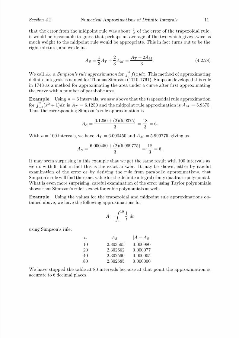
7/27/2019 Calculus 2 (Dan Sloughter)
http://slidepdf.com/reader/full/calculus-2-dan-sloughter 249/598
Section 4.2 Numerical Approximations of Definite Integrals 11
that the error from the midpoint rule was about 1
2of the error of the trapezoidal rule,
it would be reasonable to guess that perhaps an average of the two which gives twice asmuch weight to the midpoint rule would be appropriate. This in fact turns out to be theright mixture, and we define
AS = 13
AT + 23
AM = AT + 2AM
3. (4.2.28)
We call AS a Simpson’s rule approximation for ba
f (x)dx. This method of approximatingdefinite integrals is named for Thomas Simpson (1710-1761). Simpson developed this rulein 1743 as a method for approximating the area under a curve after first approximatingthe curve with a number of parabolic arcs.
Example Using n = 6 intervals, we saw above that the trapezoidal rule approximation
for 2
−1(x2 + 1)dx is AT = 6.1250 and the midpoint rule approximation is AM = 5.9375.
Thus the corresponding Simpson’s rule approximation is
AS =6.1250 + (2)(5.9375)
3=
18
3= 6.
With n = 100 intervals, we have AT = 6.000450 and AM = 5.999775, giving us
AS =6.000450 + (2)(5.999775)
3=
18
3= 6.
It may seem surprising in this example that we get the same result with 100 intervals aswe do with 6, but in fact this is the exact answer. It may be shown, either by carefulexamination of the error or by deriving the rule from parabolic approximations, that
Simpson’s rule will find the exact value for the definite integral of any quadratic polynomial.What is even more surprising, careful examination of the error using Taylor polynomialsshows that Simpson’s rule is exact for cubic polynomials as well.
Example Using the values for the trapezoidal and midpoint rule approximations ob-tained above, we have the following approximations for
A =
10
1
1
tdt
using Simpson’s rule:
n AS |A − AS |10 2.303565 0.00098020 2.302662 0.00007740 2.302590 0.00000580 2.302585 0.000000
We have stopped the table at 80 intervals because at that point the approximation isaccurate to 6 decimal places.

7/27/2019 Calculus 2 (Dan Sloughter)
http://slidepdf.com/reader/full/calculus-2-dan-sloughter 250/598
12 Numerical Approximations of Definite Integrals Section 4.2
0.5 1 1.5 2 2.5 3
0.2
0.4
0.6
0.8
1
Figure 4.2.5 Region beneath y = sin(x) over the interval [0, π]
It may be shown that the absolute value of the error using Simpson’s rule is boundedby a constant multiple of 1
n4, resulting in a dramatic improvement over both the trape-
zoidal and midpoint rules. For Simpson’s rule, doubling the number of intervals typicallydecreases the error by a factor of
1
2
4=
1
16,
a general fact for which we can see some evidence in the preceding example. To be fair,since Simpson’s rule makes use of both the trapezoidal rule and the midpoint rule approxi-mations, the function being integrated must be evaluated both at the endpoints and at themidpoint of each interval. This requires evaluating the function at 2n + 1 points, whereas
the trapezoidal rule evaluates the function at n + 1 points and the midpoint rule evalu-ates the function at n points. Thus, for direct comparison of errors, one should compare,for example, Simpson’s rule with 10 subdivisions to the other rules using 20 subdivisions.Nevertheless, Simpson’s rule converges to the value of the integral much faster than theother methods and, hence, is the method of preference among the ones we have discussed.Even faster methods exist, but we will leave them for a more advanced course.
When approximating the value of an integral, there is in general no practical way toknow how many intervals are necessary in order to obtain an approximation to a desiredlevel of accuracy. Analogous to the way in which we applied Newton’s method, we normallycompute a sequence of approximations, perhaps starting with only two intervals and thendoubling the number of intervals from one approximation to the next, stopping when we
obtain two successive approximations whose difference, in absolute value, is less than thedesired level of accuracy. The next example illustrates this procedure.
Example Suppose we wish to approximate, with an error less than 0.0001, the area A
of the region between one arch of the curve y = sin(x) and the x-axis, as shown in Figure4.2.5. That is, we want to find
A =
π0
sin(x)dx.

7/27/2019 Calculus 2 (Dan Sloughter)
http://slidepdf.com/reader/full/calculus-2-dan-sloughter 251/598
Section 4.2 Numerical Approximations of Definite Integrals 13
Starting with n = 2 intervals and using Simpson’s rule, we generate the following table of approximations, rounding to 6 decimal places:
n AS
2 2.004560
4 2.0002698 2.00001716 2.000001
Since the absolute value of the difference between the last two approximations is less than0.0001, we stop at this point and use 2.0000 as our approximation for A.
Problems
1. Approximate each of the following integrals using the trapezoidal and midpoint ruleswith n = 4 intervals.
(a)
1
0
x2dx (b)
π
0
sin(x)dx
(c)
5
1
1
tdt (d)
1
−1
z3dz
(e)
4
0
(t2 + t)dt (f)
2
0
4 − x2dx
2. Use your results from Problem 1 to compute the corresponding Simpson’s rule approx-imation for each integral.
3. Approximate each of the following integrals using the trapezoidal and midpoint ruleswith n = 50 intervals.
(a)
1
0
x2dx (b)
π0
sin(x)dx
(c)
5
−2
(4x2 + 3x − 6)dx (d)
2
1
sin(x)
xdx
(e)
π0
x2 cos(x)dx (f)
2π
0
1 − sin2(t) dt
(g) 5
−5
1
x2
+ 1
dx (h) π
−π
sin(3x)cos(x)dx
4. Use your results from Problem 3 to compute the corresponding Simpson’s rule approx-imation for each integral.
5. Approximate the following definite integrals using Simpson’s rule. Starting with n = 2intervals, compute a sequence of approximations by doubling the number of intervalsfrom one approximation to the next. Stop when the absolute value of the differencebetween two successive approximations is less than 0.00001.
7/27/2019 Calculus 2 (Dan Sloughter)
http://slidepdf.com/reader/full/calculus-2-dan-sloughter 252/598
14 Numerical Approximations of Definite Integrals Section 4.2
(a)
4
1
x2dx (b)
6
0
(3x2 + 4x − 3)dx
(c)
π0
sin2(x)dx (d)
2π
0
sin2(x)cos2(x)dx
(e) π−π
1 + cos2(θ) dθ (f)
20.1
sin(x)xdx
6. Suppose f is integrable on the interval [a, b]. Divide [a, b] into n equal intervals of length h = b−a
nand let x0, x1, x2, . . . , xn be the endpoints of these intervals. Let AT
be the trapezoidal rule approximation for ba
f (x)dx.
(a) Show that
AT =h
2(f (x0) + 2f (x1) + 2f (x2) + · · · + 2f (xn−1) + f (xn)).
(b) Assume f (x) ≥ 0 for all x in [a, b]. For i = 1, 2, 3, . . . , n, let Ai be the area of thetrapezoid with vertices at (xi−1, 0), (xi−1, f (xi−1)), (xi, f (xi)), and (xi, 0) (that is,Ai is the area of a trapezoid with one side being the interval [ xi−1, xi] and parallelsides extending from the x-axis up to the graph of f ). Then we could approximate ba
f (x)dx by A1 + A2 + A3 + · · · + An. Show that
AT = A1 + A2 + A3 + · · · + An.
7. Suppose f is integrable on the interval [a, b]. Divide [a, b] into 2n equal intervals of length h = b−a
2nand let x0,, x1, x2, . . . , x2n be the endpoints of these intervals. Let
AT and AM be the trapezoidal rule and midpoint rule approximations for ba f (x)dxusing the n intervals with endpoints x0, x2, x4, . . . , x2n. Let AS be the corresponding
Simpson’s rule approximation. Show that
AS =h
3(f (x0) + 4f (x1) + 2f (x2) + 4f (x3) + · · · + 2f (x2n−2) + 4f (x2n−1) + f (x2n)).
8. Let T (t) be the temperature at t hours after midnight at the Kalispell airport andsuppose the following values for T were recorded on March 15, 1955:
Time (t) 0.0 0.5 1.0 1.5 2.0 2.5 3.0 3.5 4.0 4.5Temperature (T ) 40 38 37 36 33 30 28 28 27 26
Time (t) 5.0 5.5 6.0 6.5 7.0 7.5 8.0 8.5 9.0 9.5Temperature (T ) 24 26 30 30 32 35 37 38 40 45
Time (t) 10.0 10.5 11.0 11.5 12.0Temperature (T ) 47 47 48 49 50
(a) Approximate 12
0T (t)dt using Simpson’s rule. You may wish to use the formula in
Problem 7.

7/27/2019 Calculus 2 (Dan Sloughter)
http://slidepdf.com/reader/full/calculus-2-dan-sloughter 253/598
Section 4.2 Numerical Approximations of Definite Integrals 15
(b) What does
A =1
12
12
0
T (t)dt
represent?
(c) How does A compare with 125
24t=0
T
t2
?
9. Find the area beneath one arch of the curve y = sin2(x).
10. Let R be the region in the plane bounded by the curves y = x2 and y = (x − 2)2 andthe x-axis. Find the area of R.

7/27/2019 Calculus 2 (Dan Sloughter)
http://slidepdf.com/reader/full/calculus-2-dan-sloughter 254/598
Difference Equations
Differential Equations
to
Section 4.3
The Fundamental Theorem
of Calculus
We are now ready to make the long-promised connection between differentiation and in-tegration, between areas and tangent lines. We will look at two closely related theorems,both of which are known as the Fundamental Theorem of Calculus. We will call the firstof these the Fundamental Theorem of Integral Calculus .
Suppose f is integrable on [a, b] and F is an antiderivative of f on (a, b) which is con-tinuous on [a, b]. In particular, F (x) = f (x) for all x in (a, b). Let P = {x0, x1, x2, . . . , xn}be a partition of [a, b] and, as usual, let ∆xi = xi − xi−1, i = 1, 2, 3, . . . , n. Now
F (b) − F (a) = F (xn) − F (x0)
= F (xn) + (F (xn−1) − F (xn−1)) + (F (xn−2) − F (xn−2)) + · · ·+ (F (x1)− F (x1))− F (x0)
= (F (xn) − F (xn−1)) + (F (xn−1)− F (xn−2)) + · · ·+ (F (x1)− F (x0))
=ni=1
(F (xi) − F (xi−1)).
(4.3.1)
By the Mean Value Theorem, for every i = 1, 2, 3, . . . , n, there exists a point ci in theinterval [xi−1, xi] such that
F (ci) =F (xi)− F (xi−1)
xi − xi−1. (4.3.2)
Since F (ci) = f (ci) and xi − xi−1 = ∆xi, it follows that
F (xi) − F (xi−1) = f (ci)∆xi. (4.3.3)
Hence, putting (4.3.3) into (4.3.1),
F (b) − F (a) =n
i=1
f (ci)∆xi. (4.3.4)
Thus F (b) − F (a) is equal to the value of a Riemann sum using the partition P , and somust lie between the upper and lower sums for P . That is, we have shown that for anypartition P ,
L(f, P ) ≤ F (b) − F (a) ≤ U (f, P ). (4.3.5)
1 Copyright c by Dan Sloughter 2000

7/27/2019 Calculus 2 (Dan Sloughter)
http://slidepdf.com/reader/full/calculus-2-dan-sloughter 255/598
2 The Fundamental Theorem of Calculus Section 4.3
-0.5 0.5 1 1.5
0.2
0.4
0.6
0.8
1
Figure 4.3.1 Region beneath the graph of f (x) = x2 over the interval [0, 1]
But, since f is integrable, there is only one number that has this property, namely,
b
af (x)dx. In other words, we have shown that b
a
f (x)dx = F (b)− F (a). (4.3.6)
Fundamental Theorem of Integral Calculus If f is integrable on [a, b] and F is anantiderivative of f on (a, b) which is continuous on [a, b], then b
a
f (x)dx = F (b)− F (a). (4.3.7)
This result reveals a sense in which integration is the inverse of differentiation: The
definite integral of a function f may be evaluated easily, using (4.3.7), provided we canfind a function F whose derivative is f .It is common to write
F (x)ba
for F (b) − F (a). With this notation, (4.3.7) becomes ba
f (x)dx = F (x)ba
. (4.3.8)
Example Since
F (x) =
1
3 x3
is an antiderivative of f (x) = x2, we have 10
x2dx =1
3x310
=1
3− 0 =
1
3.
Thus the area under the parabola y = x2 and above the interval [0, 1] on the x-axis isexactly 1
3. See Figure 4.3.1.
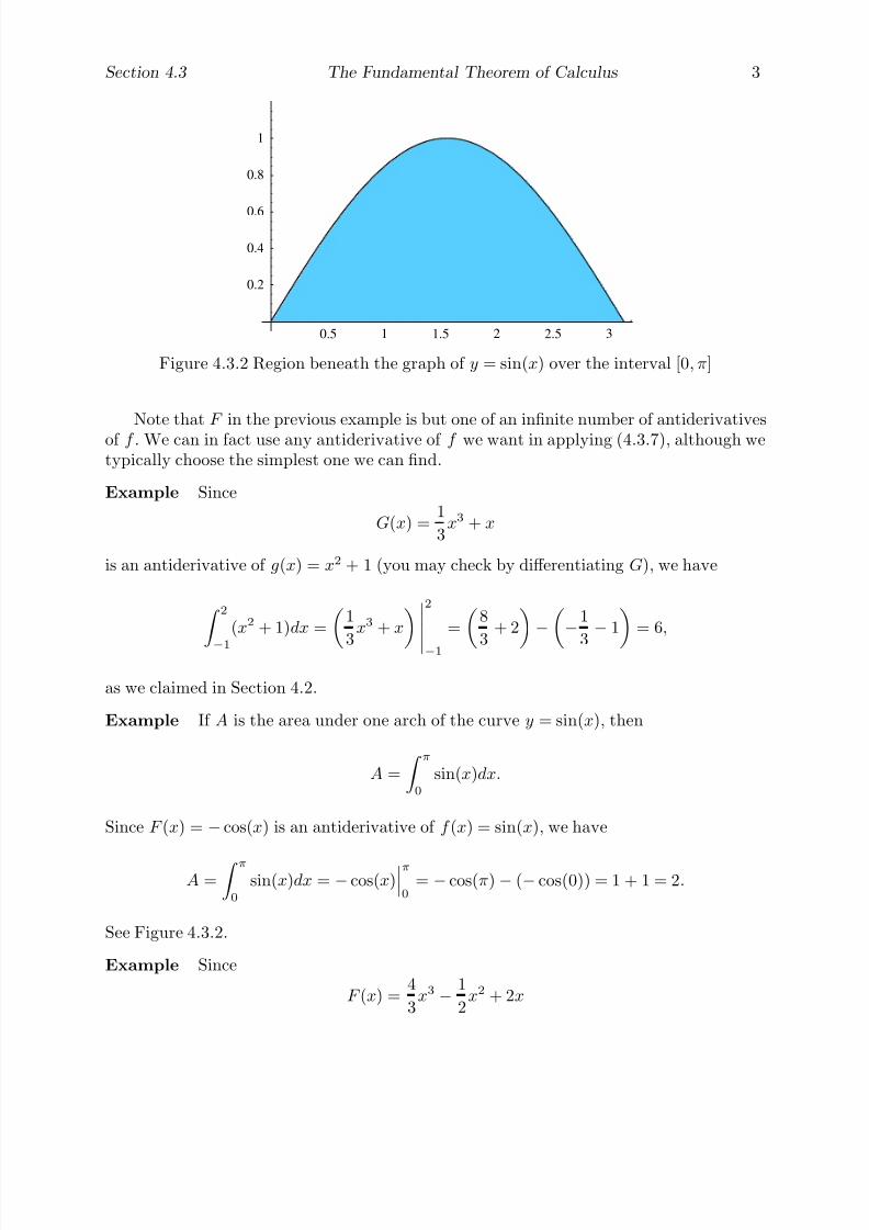
7/27/2019 Calculus 2 (Dan Sloughter)
http://slidepdf.com/reader/full/calculus-2-dan-sloughter 256/598
Section 4.3 The Fundamental Theorem of Calculus 3
0.5 1 1.5 2 2.5 3
0.2
0.4
0.6
0.8
1
Figure 4.3.2 Region beneath the graph of y = sin(x) over the interval [0, π]
Note that F in the previous example is but one of an infinite number of antiderivativesof f . We can in fact use any antiderivative of f we want in applying (4.3.7), although wetypically choose the simplest one we can find.
Example Since
G(x) =1
3x3 + x
is an antiderivative of g(x) = x2 + 1 (you may check by differentiating G), we have
2
−1(x2 + 1)dx =
1
3
x3 + x2
−1=
8
3
+ 2− −1
3 −1 = 6,
as we claimed in Section 4.2.
Example If A is the area under one arch of the curve y = sin(x), then
A =
π0
sin(x)dx.
Since F (x) = − cos(x) is an antiderivative of f (x) = sin(x), we have
A =
π
0
sin(x)dx = − cos(x)π0
= − cos(π) − (− cos(0)) = 1 + 1 = 2.
See Figure 4.3.2.
Example Since
F (x) =4
3x3 − 1
2x2 + 2x

7/27/2019 Calculus 2 (Dan Sloughter)
http://slidepdf.com/reader/full/calculus-2-dan-sloughter 257/598
4 The Fundamental Theorem of Calculus Section 4.3
is an antiderivative of f (x) = 4x2−x + 2 (again, you may check this by differentiating F ),we have 3
−2(4x2 − x + 2)dx =
4
3x3 − 1
2x2 + 2x
3
−2
=
1083− 9
2+ 6− −32
3− 2 − 4
=
325
6.
Example Since
F (t) =2
3t32
is an antiderivative of f (t) =√
t, we have
40√ t dt = 23 t
324
0
= 163 − 0 = 163 .
As can be seen from these examples, the Fundamental Theorem of Integral Calculusprovides us with a powerful tool for evaluating definite integrals exactly. However, to utilizethe theorem we must first find an antiderivative for the function we are integrating. Thisturns out to be a difficult problem in general, and we will devote the next two sections, aswell as parts of Chapter 6, to developing techniques to aid in finding antiderivatives. Forexample,
F (x) = −1
2x3 cos(2x) +
3
4x2 sin(2x) +
3
4x cos(2x) − 3
8sin(2x)
is an antiderivative of f (x) = x3 sin(2x), as may be checked by differentiation, but at thispoint it is not clear how to find such an antiderivative in the first place. Moreover, thereare integrable functions, even relatively simple ones such as
f (x) =sin(x)
x,
which do not have antiderivatives expressible in terms of the elementary functions studiedin calculus.
The Fundamental Theorem of Integral Calculus tells us that if a function f has an
antiderivative, then we may use that antiderivative to evaluate a definite integral of f , butit does not tell us which functions have antiderivatives. The Fundamental Theorem of Dif-ferential Calculus will tell us, in part, that every continuous function has an antiderivative.Before beginning that discussion, we need to extend the definition of the definite integralslightly.
The definition of ba
f (x)dx in Section 4.1 implicitly assumes that a < b. For the workwe are about to do, we need to extend the definition to include a ≥ b, as we did in Problem9 of Section 4.1. First of all, if a = b, it would seem reasonable for the value of the definite

7/27/2019 Calculus 2 (Dan Sloughter)
http://slidepdf.com/reader/full/calculus-2-dan-sloughter 258/598
Section 4.3 The Fundamental Theorem of Calculus 5
integral to be 0 since the region between the graph of the function and the x-axis has beenreduced to a line segment. Hence we make the following definition.
Definition For any function f defined at a point a, we define
aa
f (x)dx = 0. (4.3.9)
Note that with this definition, the statement
ba
f (x)dx =
ca
f (x)dx +
bc
f (x)dx, (4.3.10)
which we discussed in Section 4.1 in the case a < c < b, holds true even if a = c, b = c, ora = b = c. Now suppose we have a < b < c. Then
ca
f (x)dx =
ba
f (x)dx +
cb
f (x)dx, (4.3.11)
from which it follows that
ba
f (x)dx =
ca
f (x)dx − cb
f (x)dx. (4.3.12)
If we define bc
f (x)dx = − cb
f (x)dx, (4.3.13)
then we may rewrite (4.3.12) in the form of (4.3.10). For this reason, we make the followingdefinition.
Definition If b < a and f is integrable on [b, a], we define
ba
f (x)dx = − ab
f (x)dx. (4.3.14)
You may check that with these two extensions to the definition of the definite integral,we may now state the following proposition.
Proposition If f is integrable on a closed interval containing the points a, b, and c, then
ba
f (x)dx =
ca
f (x)dx +
bc
f (x)dx. (4.3.15)

7/27/2019 Calculus 2 (Dan Sloughter)
http://slidepdf.com/reader/full/calculus-2-dan-sloughter 259/598
6 The Fundamental Theorem of Calculus Section 4.3
x ba
y = f ( )t
Figure 4.3.3 F (x) =
x
af (t)dt is the area from a to x
We may now return to our discussion of antiderivatives and the Fundamental Theoremof Differential Calculus. Suppose f is continuous on the interval [a, b]. We want to constructan antiderivative for f on (a, b). From the Fundamental Theorem of Integral Calculus, weknow that if F is an antiderivative of f on (a, b) which is continuous on [a, b], then for anyx in (a, b) we would have x
a
f (t)dt = F (x) − F (a), (4.3.16)
that is,
F (x) = F (a) + x
a
f (t)dt. (4.3.17)
Hence, if we are seeking an antiderivative for f , it makes sense to define
F (x) =
xa
f (t)dt (4.3.18)
and verify that F (x) = f (x) for all x in (a, b). Note that F (x), geometrically, is thecumulative area between the graph of f and the x-axis from a to x, as shown in Figure4.3.3. We need to compute
F (x) = limh→0
F (x + h) − F (x)
h
= limh→0
1
h
x+h
a
f (t)dt
− x
a
f (t)dt (4.3.19)
for x in (a, b). Now x+h
a
f (t)dt =
xa
f (t)dt +
x+hx
f (t)dt, (4.3.20)
so x+h
a
f (t)dt − xa
f (t)dt =
x+hx
f (t)dt. (4.3.21)
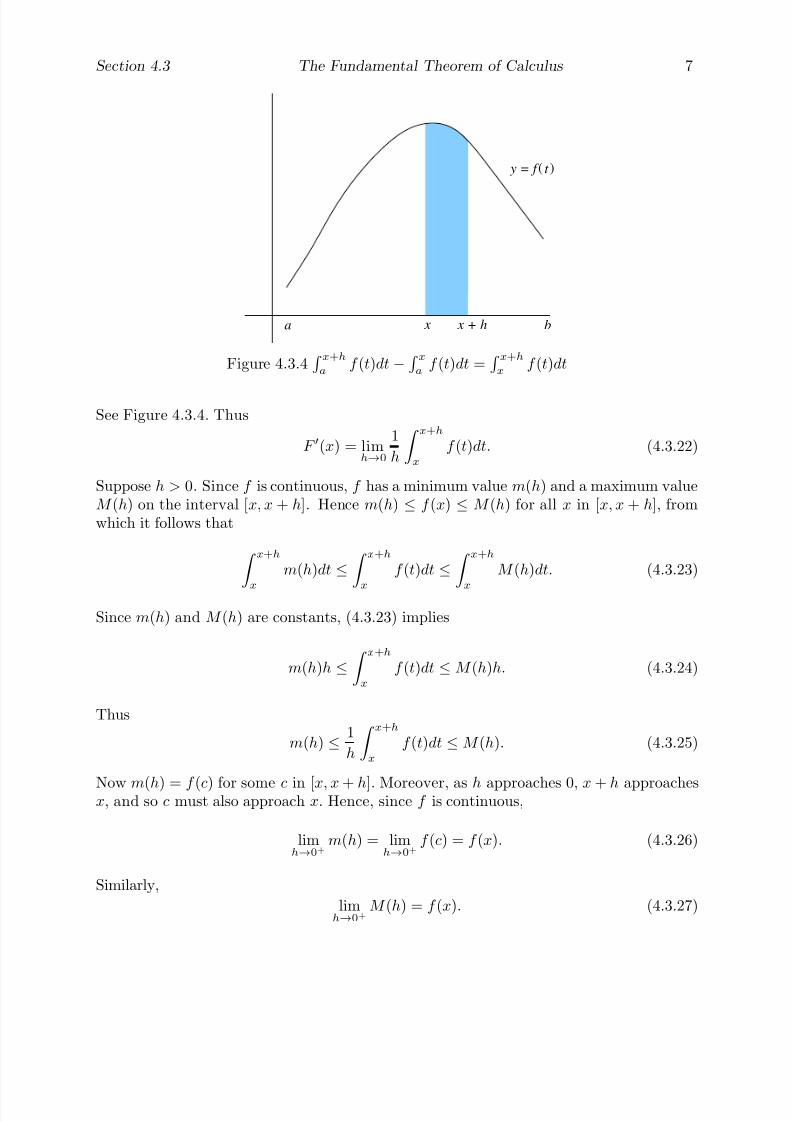
7/27/2019 Calculus 2 (Dan Sloughter)
http://slidepdf.com/reader/full/calculus-2-dan-sloughter 260/598
Section 4.3 The Fundamental Theorem of Calculus 7
ba
y = f ( )t
x + h x
Figure 4.3.4
x+h
af (t)dt −
x
af (t)dt =
x+h
xf (t)dt
See Figure 4.3.4. Thus
F (x) = limh→0
1
h
x+hx
f (t)dt. (4.3.22)
Suppose h > 0. Since f is continuous, f has a minimum value m(h) and a maximum valueM (h) on the interval [x, x + h]. Hence m(h) ≤ f (x) ≤ M (h) for all x in [x, x + h], fromwhich it follows that
x+h
x
m(h)dt ≤ x+h
x
f (t)dt ≤ x+h
x
M (h)dt. (4.3.23)
Since m(h) and M (h) are constants, (4.3.23) implies
m(h)h ≤ x+hx
f (t)dt ≤ M (h)h. (4.3.24)
Thus
m(h) ≤ 1
h
x+h
x
f (t)dt ≤ M (h). (4.3.25)
Now m(h) = f (c) for some c in [x, x + h]. Moreover, as h approaches 0, x + h approachesx, and so c must also approach x. Hence, since f is continuous,
limh→0+
m(h) = limh→0+
f (c) = f (x). (4.3.26)
Similarly,
limh→0+
M (h) = f (x). (4.3.27)
7/27/2019 Calculus 2 (Dan Sloughter)
http://slidepdf.com/reader/full/calculus-2-dan-sloughter 261/598
8 The Fundamental Theorem of Calculus Section 4.3
It now follows from (4.3.25) that
limh→0+
1
h
x+hx
f (t)dt = f (x). (4.3.28)
A similar argument shows that
limh→0−
1
h
x+hx
f (t)dt = f (x), (4.3.29)
and so we may conclude that
F (x) = limh→0
1
h
x+hx
f (t)dt = f (x). (4.3.30)
That is,F (x) =
xa
f (t)dt
is an antiderivative of f on (a, b).
Fundamental Theorem of Differential Calculus If f is continuous on the closedinterval [a, b] and F is the function on (a, b) defined by
F (x) =
xa
f (t)dt, (4.3.31)
then F is differentiable on (a, b) with F (x) = f (x) for all x in (a, b). In other words,
d
dx
xa
f (t)dt = f (x) (4.3.32)
for all x in (a, b).
It is worth noting that (4.3.32) holds for x < a as well, as long as f is continuous ona closed interval which contains both x and a.
Example Let
f (x) =
sin(x)x
, if x = 0,
1, if x = 0.
Then f is continuous on (−∞,∞), so
F (x) =
x0
f (t)dt
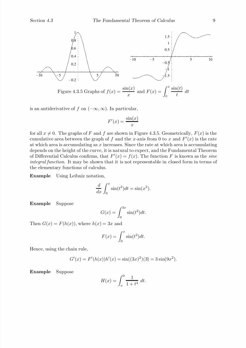
7/27/2019 Calculus 2 (Dan Sloughter)
http://slidepdf.com/reader/full/calculus-2-dan-sloughter 262/598
Section 4.3 The Fundamental Theorem of Calculus 9
-10 -5 5 10
-0.2
0.2
0.4
0.6
0.8
1
-10 -5 5 10
-1.5
-1
-0.5
0.5
1
1.5
Figure 4.3.5 Graphs of f (x) =sin(x)
xand F (x) =
x0
sin(t)
tdt
is an antiderivative of f on (−∞,∞). In particular,
F (x) =sin(x)
x
for all x = 0. The graphs of F and f are shown in Figure 4.3.5. Geometrically, F (x) is thecumulative area between the graph of f and the x-axis from 0 to x and F (x) is the rateat which area is accumulating as x increases. Since the rate at which area is accumulatingdepends on the height of the curve, it is natural to expect, and the Fundamental Theoremof Differential Calculus confirms, that F (x) = f (x). The function F is known as the sine
integral function . It may be shown that it is not representable in closed form in terms of the elementary functions of calculus.
Example Using Leibniz notation,
d
dx
x
0
sin(t2)dt = sin(x2).
Example Suppose
G(x) =
3x0
sin(t2)dt.
Then G(x) = F (h(x)), where h(x) = 3x and
F (x) = x
0
sin(t2)dt.
Hence, using the chain rule,
G(x) = F (h(x))h(x) = sin((3x)2)(3) = 3 sin(9x2).
Example Suppose
H (x) =
0x
1
1 + t4dt.

7/27/2019 Calculus 2 (Dan Sloughter)
http://slidepdf.com/reader/full/calculus-2-dan-sloughter 263/598
10 The Fundamental Theorem of Calculus Section 4.3
Then, using (4.3.14),
H (x) = − x0
1
1 + t4dt,
so
H (x) =−
d
dx
x
0
1
1 + t4dt =
−1
1 + x4.
Example Suppose
F (x) =
x22x
1 + t4 dt.
Then, using (4.3.15) and (4.3.14),
F (x) =
02x
1 + t4 dt +
x20
1 + t4 dt = −
2x0
1 + t4 dt +
x20
1 + t4 dt.
Note that there is nothing special about using 0 in this decomposition, other than therequirement that the function f (t) = √ 1 + t4 be integrable on all of the relevant intervals.Now we have
F (x) = − d
dx
2x0
1 + t4 dt +
d
dx
x20
1 + t4 dt
= −
1 + (2x)4 (2) +
1 + (x2)4 (2x)
= 2x
1 + x8 − 2
1 + 16x4.
To summarize this section, the Fundamental Theorem of Integral Calculus providesus with an elegant method for evaluating definite integrals, but is useful only when we
can find an antiderivative for the function being integrated. The Fundamental Theoremof Differential Calculus tells us that every continuous function has an antiderivative andshows how to construct one using the definite integral. Unfortunately, this brings us incircle and does not provide us with an effective means for finding antiderivatives to use inapplying the Fundamental Theorem of Integral Calculus. For example, we know that
F (x) =
x1
sin(t)
tdt
is an antiderivative of
f (x) =sin(x)
x,
but this is of no help in evaluating, say, 41
sin(x)
xdx.
Hence in order to fully utilize the Fundamental Theorem of Integral Calculus in the evalua-tion of definite integrals, we must develop some procedures to aid in finding antiderivatives.We will turn to this problem in the next section.
7/27/2019 Calculus 2 (Dan Sloughter)
http://slidepdf.com/reader/full/calculus-2-dan-sloughter 264/598
Section 4.3 The Fundamental Theorem of Calculus 11
Problems
1. Evaluate the following definite integrals using the Fundamental Theorem of IntegralCalculus.
(a) 10
xdx (b) 30
(x2 + 2x)dx
(c)
20
x3dx (d)
1−1
x3dx
(e)
20
(2x3 + 3x2 + x − 4)dx (f)
41
1
x2dx
(g)
41
1√ t
dt (h)
80
√ t + 1 dt
(i) π
2
0
sin(x)dx (j) π−π
cos(z)dz
2. Evaluate the following definite integrals using the Fundamental Theorem of IntegralCalculus.
(a)
20
(x + 1)2dx (b)
20
(2x + 1)2dx
(c)
40
√ 1 + 2t dt (d)
π4
0
sec2(x)dx
(e) π
0
sin(2x)dx (f) π
0
5 cos(3x)dx
(g)
π3
0
4sin(3x)dx (h)
π−π
8 cos(5θ)dθ
(i)
√ π0
2x sin(x2)dx (j)
2−1
2x(1 + x2)5dx
(k)
√ π0
x sin(x2)dx (l)
2−1
x(1 + x2)5dx
3. For each of the following functions, graph both f and
F (x) = x0
f (t)dt
together over the given interval.
(a) f (x) = sin(x) on [−2π, 2π] (b) f (x) = sin(x2) on [0, 10]
(c) f (x) =1
1 + x4on [−3, 3] (d) f (x) =
1
x + 1on [0, 10]

7/27/2019 Calculus 2 (Dan Sloughter)
http://slidepdf.com/reader/full/calculus-2-dan-sloughter 265/598
12 The Fundamental Theorem of Calculus Section 4.3
4. Find the derivatives of each of the following functions.
(a) F (x) =
x0
sin2(4t)dt (b) g(x) =
x2
3
t + 2dt
(c) F (x) = π
x
cos3(t)dt (d) G(t) = 0
t 4 − z2 dz
(e) f (x) =
x20
1
1 + s2ds (f) h(z) =
3zz
1 + t2 dt
5. Evaluate the following derivatives.
(a)d
dx
x1
1
1 + t2dt (b)
d
dx
3x1
sin(3t)
tdt
(c)d
dt
5t2
sin2(3x)dx (d)d
dx
x23x
1√ 1 + t2
dt
6. Find the area of the region beneath one arch of the curve y = 3 sin(2x).7. Let R be the region bounded by the curves y = x2 and y = (x − 2)2 and the x-axis.
Find the area of R.
8. Explain why the integral 10
(x − x2)dx
is the area of the region bounded by the curves y = x2 and y = x. Find this area.
9. Explain why the integral
1−1(2− 2x
2
)dx
is the area of the region bounded by the curves y = 1 − x2 and y = x2 − 1. Find thisarea.
7/27/2019 Calculus 2 (Dan Sloughter)
http://slidepdf.com/reader/full/calculus-2-dan-sloughter 266/598
Difference Equations
Differential Equations
to
Section 4.4
Using the Fundamental Theorem
As we saw in Section 4.3, using the Fundamental Theorem of Integral Calculus reducesthe problem of evaluating a definite integral to the problem of finding an antiderivative.Unfortunately, finding antiderivatives, even for relatively simple functions, cannot be doneas routinely as the computation of derivatives. For example, suppose we let f (x) = sin(x),g(x) = x, and
h(x) =f (x)
g(x)=
sin(x)
x.
Then, since we know the derivative of f and we know the derivative of g, it is a simplematter to find the derivative of h using the quotient rule. However, knowing the an-tiderivatives of f and g in no way helps us find the antiderivative of h. In fact, it has beenshown that the antiderivative of h is not expressible in terms of any finite combination of algebraic and elementary transcendental functions. Because of results like this, many of the definite integrals that are encountered in applications cannot be evaluated using theFundamental Theorem of Integral Calculus; instead, they must be approximated using nu-merical techniques such as those we studied in Section 4.2. Of course, when antiderivativesare available, the Fundamental Theorem is the best way to evaluate an integral. To thisend, we will investigate, in this section and in the next, techniques for evaluating definiteintegrals by finding antiderivatives and applying the Fundamental Theorem.
Before we begin, we need to introduce some additional notation and terminology.First of all, we will call the collection of all antiderivatives of a given function f the general
antiderivative of f . For example, if f (x) = 3x2, then the general antiderivative of f isgiven by F (x) = x3 + c, where c is an arbitrary constant.
Second, since the Fundamental Theorem of Calculus draws a close connection betweenantiderivatives and definite integrals, it is customary to borrow the notation for the generalantiderivative from the notation for the definite integral. Hence the general antiderivativeof a function f with respect to the variable x is denoted by
f (x)dx. (4.4.1)
This is usually referred to as the indefinite integral of f with respect to x. Thus the termsindefinite integral and general antiderivative are synonymous, and from this point on wewill prefer the former to the latter.
Example In this notation, we write 3x2dx = x3 + c,
where c is assumed to be an arbitrary constant.
1 Copyright c by Dan Sloughter 2000

7/27/2019 Calculus 2 (Dan Sloughter)
http://slidepdf.com/reader/full/calculus-2-dan-sloughter 267/598
2 Using the Fundamental Theorem Section 4.4
Since finding an indefinite integral involves reversing the process of differentiation, wecan rewrite our basic results about derivatives in terms of indefinite integrals. Hence wehave the following list of integration formulas:
xndx =xn+1
n + 1+ c (where n
=−
1 is a rational number), (4.4.2)
sin(x)dx = − cos(x) + c, (4.4.3)
cos(x)dx = sin(x) + c, (4.4.4)
sec2(x)dx = tan(x) + c, (4.4.5)
csc2(x)dx = − cot(x) + c, (4.4.6)
sec(x)tan(x)dx = sec(x) + c, (4.4.7) csc(x)cot(x)dx = − csc(x) + c. (4.4.8)
Note that each one of these formulas may be verified by checking that the derivativeof the right-hand side is equal to the function inside the integral sign on the left-hand side.Also notice that we have not used any special techniques to find these results; rather, weknow these formulas only because they are the inverses of differentiation formulas that welearned in Chapter 3. Thus, for example, we know that
sec
2
(x)dx = tan(x) + c,
but we do not know, nor do we even know how to begin to find,
sec(x)dx, which wouldat first seem to be an easier problem.
The following proposition is a consequence of the corresponding basic properties of differentiation.
Proposition If the indefinite integrals of f and g exist, then
(f (x) + g(x))dx =
f (x)dx +
g(x)dx (4.4.9)
and (f (x)− g(x))dx =
f (x)dx−
g(x)dx. (4.4.10)
Moreover, for any constant k,
kf (x)dx = k
f (x)dx. (4.4.11)

7/27/2019 Calculus 2 (Dan Sloughter)
http://slidepdf.com/reader/full/calculus-2-dan-sloughter 268/598
Section 4.4 Using the Fundamental Theorem 3
Example Using (4.4.2) with the results of the previous proposition, we have
(5x3 − 3x + 2)dx = 5
x3dx− 3
xdx + 2
1dx =
5
4x4 − 3
2x2 + 2x + c.
It is worth noting that
1dx is typically denoted simply by
dx.
Example Using (4.4.2),
1√
tdt =
t−
1
2 dt =t1
2
12
+ c = 2√
t + c.
Example Using (4.4.2), (4.4.4), and (4.4.9), we have
cos(x) +4
x2 dx = cos(x)dx + 4 x−2dx
= sin(x)− 4x−1 + c
= sin(x)− 4
x+ c.
Sometimes the indefinite integral of a function, although not itself in the list (4.4.2)through (4.4.8), may be found with the use of some intelligent guessing. For example,F (x) = sin(2x) is not an antiderivative of f (x) = cos(2x) since F (x) = 2 cos(2x). However,since F and f differ only by a factor of 2, we can correct for this by dividing F by 2. Thatis,
cos(2x)dx =
1
2 sin(2x) + c.
Again, as with all indefinite integrals, you may verify this result by differentiation.
Example To find
3sin(4x)dx, we might begin with a guess using F (x) = −3 cos(4x).However, F (x) = 12 sin(3x), which differs from the function we are integrating by a factorof 4. Thus, dividing our initial guess by 4, we have
3 sin(4x)dx = −3
4cos(4x) + c.
Example To find √ 2t + 3 dt, we might begin with a guess using
F (t) =(2t + 3)
3
2
32
=2
3(2t + 3)
3
2 .
However,
F (t) =√
2t + 3d
dt(2t + 3) = 2
√ 2t + 3,
7/27/2019 Calculus 2 (Dan Sloughter)
http://slidepdf.com/reader/full/calculus-2-dan-sloughter 269/598
4 Using the Fundamental Theorem Section 4.4
so we need to divide our guess by 2. Hence
√ 2t + 3 dt =
1
3(2t + 3)
3
2 + c.
Example To find 1√
3z + 1dz,
we might start with an initial guess of
F (z) =(3z + 1)
1
2
12
= 2√
3z + 1.
Since
F (z) =3
√ 3z + 1,
we find that 1√
3z + 1dz =
2
3
√ 3z + 1 + c.
Thus, for example,
50
1√ 3z + 1
dz =2
3
√ 3z + 1
5
0
=8
3− 2
3= 2.
The common thread in the previous examples is the need to modify an initial guessbecause of the chain rule. For example, F (x) = sin(2x) is not an antiderivative of f (x) =cos(2x) because the chain rule comes into play when differentiating F , resulting in anextra factor of 2. This process of reversing the chain rule can be taken a step further tohelp evaluate integrals in even more complicated situations. For example, consider theindefinite integral
2x
1 + x2 dx.
The key to evaluating this integral is recognizing that the factor 2x is the derivative of thefunction inside the square root. That is, if we let
f (u) = √ u
andg(x) = 1 + x2,
then 2x
1 + x2 dx =
f (g(x))g(x)dx.

7/27/2019 Calculus 2 (Dan Sloughter)
http://slidepdf.com/reader/full/calculus-2-dan-sloughter 270/598
Section 4.4 Using the Fundamental Theorem 5
Thus we are trying to find an antiderivative of a function which is in the form of the resultfrom a chain rule differentiation. Now if F is an antiderivative of f , then, using the chainrule,
d
dxF (g(x)) = F (g(x))g(x) = f (g(x))g(x).
Hence, thinking of u as 1 + x2, we really only need to find the antiderivative of f withrespect to u. Now
f (u)du =
√ u du =
2
3u3
2 + c,
so, substituting 1 + x2 back in for u, we should have
2x
1 + x2 dx =2
3(1 + x2)
3
2 + c.
You should check this result by differentiation, noting in particular that the factor of 2 x
comes from the use of the chain rule.In general, if F is an antiderivative of f and u = g(x) is some differentiable function
of x, then, by the chain rule,
d
dxF (u) = F (u)
du
dx= f (u)
du
dx. (4.4.12)
Writing this as an integration formula, we have
f (u)
du
dxdx = F (u) + c =
f (u)du. (4.4.13)
This technique to help find indefinite integrals is called integration by substitution .Example To find
2x sin(x2)dx,
we should let u = x2. Thendu
dx= 2x,
so, using (4.4.13) with f (u) = sin(u),
2x sin(x2)dx = sin(u)du
dx
dx
=
sin(u)du
= − cos(u) + c
= − cos(x2) + c.
We summarize this technique as follows.

7/27/2019 Calculus 2 (Dan Sloughter)
http://slidepdf.com/reader/full/calculus-2-dan-sloughter 271/598
6 Using the Fundamental Theorem Section 4.4
Integration by substitution To evaluate an indefinite integral of the form
f (g(x))g(x)dx, (4.4.14)
we may make the substitution u = g(x). We then have f (g(x))g(x)dx =
f (u)
du
dxdx =
f (u)du. (4.4.15)
Of course, this technique will work only if we know an antiderivative for f . Indeed, allwe have done is replace one indefinite integral with another, with the hope that the newintegral will be simpler than the original. In our notation, we can think of the transitionfrom
f (g(x))g(x)dx
to f (u)du
as replacing g(x) by u and g(x)dx by du. Thus in practice we often denote the process of substitution by writing
u = g(x)
du = g(x)dx(4.4.16)
and directly substituting into the integral
f (g(x))g(x)dx
to obtain the integral f (u)du.
We will illustrate this in the next examples.
Example To evaluate the indefinite integral
2x
√ 2 + x2 dx,
we may let u = 2 + x2. Thendu
dx= 2x,
which we write in the form
du = 2xdx.

7/27/2019 Calculus 2 (Dan Sloughter)
http://slidepdf.com/reader/full/calculus-2-dan-sloughter 272/598
Section 4.4 Using the Fundamental Theorem 7
Substituting, we have
2x√
2 + x2dx =
1√
udu = 2
√ u + c = 2
2 + x2 + c. (4.4.17)
Example From (4.4.17), it is easy to see, after dividing through by 2, that x√
2 + x2dx =
2 + x2 + c.
We could also see this directly when making the substitution. Namely, if we let u = 2 + x2,then du = 2xdx may be written as
1
2du = xdx.
Hence, if we substitute 2 + x2
for u and1
2du for xdx, we obtain 2x√
2 + x2dx =
12√ u
du =1
2
1√
udu =
1
2(2√
u) + c =
2 + x2 + c.
Example To evaluate the indefinite integral
5x cos(x2)dx,
we may make the substitution
u = x2
du = 2xdx.
Then1
2du = xdx,
so we have 5x cos(x2)dx =
5
2
cos(u)du =
5
2sin(u) + c =
5
2sin(x2) + c.
Example To evaluate the indefinite integral tan(3x)sec2(3x)dx,
we may make the substitutionu = tan(3x)
du = 3 sec2(3x)dx.
7/27/2019 Calculus 2 (Dan Sloughter)
http://slidepdf.com/reader/full/calculus-2-dan-sloughter 273/598
8 Using the Fundamental Theorem Section 4.4
Then1
3du = sec2(3x)dx,
so we have
tan(3x)sec2(3x)dx = 1
3
udu = 1
6u2 + c = 1
6tan2(3x) + c.
Now suppose we want to evaluate the definite integral
ba
f (g(x))g(x)dx.
If F is an antiderivative of f , then we know that
f (g(x))g(x)dx = F (g(x)) + c. (4.4.18)
Hence ba
f (g(x))g(x)dx = F (g(x))ba
= F (g(b))− F (g(a)). (4.4.19)
Now we also have
g(b)g(a)
f (u)du = F (u)g(b)
g(a)= F (g(b))− F (g(b)). (4.4.20)
Putting (4.4.19) and (4.4.20) together, we see that
ba
f (g(x))g(x)dx =
g(b)g(a)
f (u)du. (4.4.21)
That is, similar to our work with indefinite integrals, we may evaluate the definite integral
ba
f (g(x))g(x)dx
by making a substitutionu = g(x)
du = g(x)dx,(4.4.22)
the only difference being that in the definite integral we must also change the limits of integration. Note that the new limits of integration correspond to the range of values foru given that x is ranging from a to b.

7/27/2019 Calculus 2 (Dan Sloughter)
http://slidepdf.com/reader/full/calculus-2-dan-sloughter 274/598
Section 4.4 Using the Fundamental Theorem 9
Example To evaluate 10
x2
(1 + x3)2dx,
we may make the substitutionu = 1 + x3
du = 3x2.
Then1
3du = x2dx
and u varies from1 + 03 = 1
to1 + 13 = 2
as x varies from 0 to 1, so 10
x2
(1 + x3)2dx =
1
3
21
1
u2du = −1
3
1
u
2
1
= −1
6+
1
3=
1
6.
Example To evaluate π2
0
sin2(x)cos(x)dx,
we may make the substitutionu = sin(x)
du = cos(x)dx.
Then u varies from 0 to 1 as x varies from 0 to π2 , so
π2
0
sin2(x)cos(x)dx =
10
u2du =1
2u3
1
0
=1
3.
Example To evaluate π2
0
cos3(x)sin(x)dx,
we may make the substitutionu = cos(x)
du = − sin(x)dx.
Then −du = − sin(x)dx and u varies from 1 to 0 as x varies from 0 to π2 , so
π2
0
cos3(x)sin(x)dx = − 01
u3du =
10
u3du =1
4u4
1
0
=1
4.
7/27/2019 Calculus 2 (Dan Sloughter)
http://slidepdf.com/reader/full/calculus-2-dan-sloughter 275/598
10 Using the Fundamental Theorem Section 4.4
Example So far all of our examples of substitution have involved reversing the resultsof the chain rule. However, substitutions can be useful in other situations as well. Forexample, to evaluate 3
0
x√
1 + x dx,
the substitutionu = 1 + x
du = dx
turns out to be useful for rearranging the integral into a form which can be evaluated.Namely, since u = 1 + x implies that x = u− 1, we may substitute to obtain
30
x√
1 + x dx =
41
(u− 1)√
u du
= 4
1
(u3
2
−u1
2 )du
=2
5u5
2
4
1
− 2
3u
3
2
4
1
=
64
5− 2
5
−
16
3− 2
3
=116
15.
We will continue the discussion of techniques for using the Fundamental Theorem of Integral Calculus in Section 4.5.
Problems
1. Evaluate the following indefinite integrals.
(a)
(x3 + 3x− 6)dx (b)
(3t2 − 4t + 5)dt
(c)
1
x4dx (d)
3z − 4
z2
dz
(e)
12√
tdt (f)
3√
2 + xdx
(g)
7√ x + 5 dx (h)
(sin(θ)− 2cos(θ))dθ
2. Evaluate the following indefinite integrals.
(a)
sin(3x)dx (b)
cos(4x)dx
(c)
√ 3t − 1 dt (d)
4√
1 + 5zdz

7/27/2019 Calculus 2 (Dan Sloughter)
http://slidepdf.com/reader/full/calculus-2-dan-sloughter 276/598
Section 4.4 Using the Fundamental Theorem 11
(e)
7sec2(2x)dx (f)
3 sec(4x) tan(4x)dx
(g)
2csc2(7x)dx (h)
sin(4x + 1)dx
3. Evaluate the following indefinite integrals.
(a)
6x
1 + 3x2 dx (b)
4x3 cos(x4)dx
(c)
x2(3 + x3)10dx (d)
7x√
4 + 3x2dx
(e)
4t sin(t2)dt (f)
7z cos(3z2 + 1)dz
(g)
sin3(t)cos(t)dt (h)
4cos4(3t) sin(3t)dt
4. Evaluate the following indefinite integrals.
(a)
sin(√ x)√ x
dx (b)
sec2(x)tan2(x)dx
(c)
sec3(4x) tan(4x)dx (d)
sin(θ)cos(θ)dθ
(e)
sin(x)
cos2(x)dx (f)
cos(3t)
1 + sin(3t)dt
(g)
t√
t− 2 dt (h)
z√
z + 1dz
5. Evaluate the following definite integrals.
(a)
1
0
(4x2 − 3x− 5)dx (b)
1
0
1√ 3x + 1
dx
(c)
π4
0
3sin(2x)dx (d)
51
√ 2t− 1 dt
(e)
0− π
12
6 sec(3t) tan(3t)dt (f)
20
1
(7z + 6)2dz
(g)
20
x
x2 + 1 dx (h)
π0
sin4(t)cos(t)dt
6. Evaluate the following definite integrals.
(a)
1−1
5x2
(x3 + 2)2dx (b)
20
3x√ x2 + 1
dx
(c)
√ π
0
3x sin(x2)dx (d)
0−π
2
cos2(t)sin(t)dt
(e)
π2
0
sin3(2t) cos(2t)dt (f)
10
5x(2 + x2)10dx
7/27/2019 Calculus 2 (Dan Sloughter)
http://slidepdf.com/reader/full/calculus-2-dan-sloughter 277/598
12 Using the Fundamental Theorem Section 4.4
(g)
1−1
x(1 + x2)25dx (h)
π3
−π
4
sec2(u) tan(u)du
7. Evaluate the following definite integrals.
(a)
3
0
x
√ x + 1 dx (b)
1
0 x
3 x
2
+ 1 dx
(c)
π
24
− π
12
tan4(4x)sec2(4x)dx (d)
π2
π
6
cot(t)csc2(t)dt
(e)
10
4x(1 + x)25dx (f)
π3
0
sin(2θ)
cos3(2θ)dθ
(g)
51
5u√
2u− 1 du (h)
π0
sin5(w)cos(w)dw
8. Find the area beneath one arch of the curve y = 4 sin(6t).
9. (a) Plot the graph of y = sin2
(x)cos(x) over the interval [0, π].(b) Find the area of the region beneath the graph of y = sin2(x)cos(x) over the interval
0, π2
.
(c) Verify that π0
sin2(x)cos(x)dx = 0
and justify your result geometrically.
7/27/2019 Calculus 2 (Dan Sloughter)
http://slidepdf.com/reader/full/calculus-2-dan-sloughter 278/598
Difference Equations
Differential Equations
to
Section 4.5
More Techniques of Integration
In the last section we saw how we could exploit our knowledge of the chain rule to developa technique for simplifying integrals using suitably chosen substitutions. In this sectionwe shall see how we can develop a second technique, called integration by parts , using theproduct rule. Outside of algebraic manipulation and the use of various functional identities,like the trigonometric identities, substitution and parts are the only basic techniques wehave available to us for simplifying the process of evaluating an integral.
Example Suppose we wish to find x cos(x)dx. Since
cos(x)dx = sin(x) + c,
we might make an initial guess of F (x) = x sin(x) for an antiderivative of f (x) = x cos(x).But, of course, differentiation of F , using the product rule, yields
F (x) = x cos(x) + sin(x),
which differs from the desired result, f (x), by the term sin(x). However, since
sin(x)dx = − cos(x) + c,
we can obtain an antiderivative of f (x) by adding on the term cos(x) to F (x). That is,
G(x) = x sin(x) + cos(x)
is an antiderivative of f (x) since the derivative of cos(x) will cancel the sin(x) term in
F
(x). Explicitly,G(x) = x cos(x) + sin(x)− sin(x) = x cos(x).
Thus x cos(x)dx = x sin(x) + cos(x) + c.
1 Copyright c by Dan Sloughter 2000
7/27/2019 Calculus 2 (Dan Sloughter)
http://slidepdf.com/reader/full/calculus-2-dan-sloughter 279/598
2 More Techniques of Integration Section 4.5
In general, suppose f and g are differentiable functions and we want to evaluate f (x)g(x)dx. (4.5.1)
For example, in our previous example we would have f (x) = x and g(x) = sin(x). Fromthe product rule we know that
d
dxf (x)g(x) = f (x)g(x) + g(x)f (x). (4.5.2)
Thus, integrating both sides of (4.5.2), we have
d
dxf (x)g(x) =
f (x)g(x)dx +
g(x)f (x)dx, (4.5.3)
from which it follows that
f (x)g(x) =
f (x)g(x)dx +
g(x)f (x)dx. (4.5.4)
Rearranging (4.5.4) gives us f (x)g(x)dx = f (x)g(x)−
g(x)f (x)dx. (4.5.5)
Applying (4.5.5) to our example, with f (x) = x and g(x) = sin(x), we have
x cos(x)dx = x sin(x)− sin(x)dx = x sin(x) + cos(x) + c.
In effect, using (4.5.5), we have replaced the problem of evaluating
x cos(x)dx with thesimpler problem of evaluating
sin(x)dx. In general, the success of this method always
depends on the integral g(x)f (x)dx (4.5.6)
being easier to evaluate than the integral
f (x)g
(x)dx. (4.5.7)
It is common with this technique to let u = f (x) and v = g(x) along with the notation,as we did with substitution,
dv = g(x)dx (4.5.8)
anddu = f (x)dx. (4.5.9)
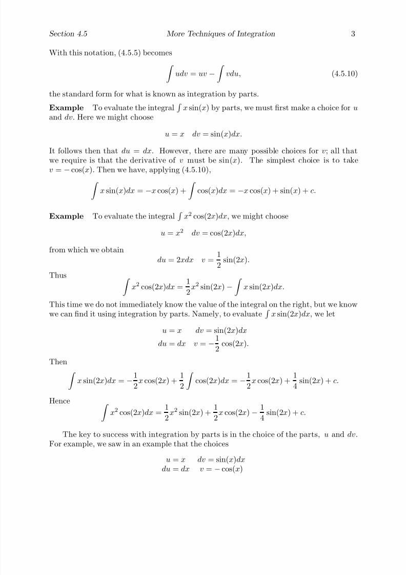
7/27/2019 Calculus 2 (Dan Sloughter)
http://slidepdf.com/reader/full/calculus-2-dan-sloughter 280/598
Section 4.5 More Techniques of Integration 3
With this notation, (4.5.5) becomes udv = uv −
vdu, (4.5.10)
the standard form for what is known as integration by parts.
Example To evaluate the integral
x sin(x) by parts, we must first make a choice for u
and dv. Here we might choose
u = x dv = sin(x)dx.
It follows then that du = dx. However, there are many possible choices for v; all thatwe require is that the derivative of v must be sin(x). The simplest choice is to takev = − cos(x). Then we have, applying (4.5.10),
x sin(x)dx = −x cos(x) + cos(x)dx = −x cos(x) + sin(x) + c.
Example To evaluate the integral
x2 cos(2x)dx, we might choose
u = x2 dv = cos(2x)dx,
from which we obtaindu = 2xdx v =
1
2sin(2x).
Thus x2 cos(2x)dx =
1
2x2 sin(2x)−
x sin(2x)dx.
This time we do not immediately know the value of the integral on the right, but we knowwe can find it using integration by parts. Namely, to evaluate
x sin(2x)dx, we let
u = x dv = sin(2x)dx
du = dx v = −1
2cos(2x).
Then x sin(2x)dx = −1
2x cos(2x) +
1
2
cos(2x)dx = −1
2x cos(2x) +
1
4sin(2x) + c.
Hence
x2 cos(2x)dx =1
2x2 sin(2x) +
1
2x cos(2x)− 1
4sin(2x) + c.
The key to success with integration by parts is in the choice of the parts, u and dv.For example, we saw in an example that the choices
u = x dv = sin(x)dx
du = dx v = − cos(x)

7/27/2019 Calculus 2 (Dan Sloughter)
http://slidepdf.com/reader/full/calculus-2-dan-sloughter 281/598
4 More Techniques of Integration Section 4.5
work well for evaluating
x sin(x)dx. Alternatively, we could have chosen
u = sin(x) dv = xdx
du = cos(x)dx v =1
2x2,
which would yield x sin(x)dx =
1
2x2 sin(x)− 1
2
x2 cos(x)dx.
All of this is correct, but useless (at least for our present purpose) since the resultingintegral on the right is more complicated than the integral with which we started. If wehad started to work the problem this way, we would probably stop at this point and rethinkour strategy.
Example In using integration by parts to evaluate a definite integral, we must remember
to evaluate all the pieces of the resulting antiderivative. For example, to evaluate π3
0
4x cos(3x)dx,
we might chooseu = 4x dv = cos(3x)dx
du = 4dx v =1
3sin(3x).
Then
π30 4x cos(3x)dx =
4
3 x sin(3x)π30 −
4
3 π30 sin(3x)dx
= (0− 0) +4
9cos(3x)
π30
= −4
9− 4
9
= −8
9.
Example Although integration by parts is most frequently of use when integrating func-tions involving transcendental functions, such as the trigonometric functions, there are
other times when the technique may be used. For example, to compute 1
0
x(1 + x)10dx,
we could useu = x dv = (1 + x)10dx
du = dx v =1
11(1 + x)11.

7/27/2019 Calculus 2 (Dan Sloughter)
http://slidepdf.com/reader/full/calculus-2-dan-sloughter 282/598
Section 4.5 More Techniques of Integration 5
Then 1
0
x(1 + x)10dx =1
11x(1 + x)11
10
− 1
11
1
0
(1 + x)11dx
=2048
11− 1
132(1 + x)12
1
0
=2048
11−
4096
132− 1
132
=6827
44.
Notice that we could also evaluate this integral using the substitution u = 1 + x.
Miscellaneous examples
The techniques of substitution and parts are often useful for putting an integral into a formthat can be readily evaluated by the Fundamental Theorem of Integral Calculus. The next
several examples illustrate how basic trigonometric identities are also useful for rewritingintegrals in more easily evaluated forms.
Example To evaluate
sin2(x)dx, we may use the identity
sin2(x) =1− cos(2x)
2(4.5.11)
(see Problem 5, Section 2.2). Then
sin2(x)dx =1
2 (1
−cos(2x))dx =
1
2x−
1
4sin(2x) + c.
Example Similarly, to evaluate
π4
0
cos2(2t)dt,
we use the identity
cos2(x) =1 + cos(2x)
2. (4.5.12)
Then π4
0
cos2(2t)dt =1
2
π4
0
(1 + cos(4t))dt
=1
2t
π
4
0
+1
8sin(4t)
π
4
0
=π
8.

7/27/2019 Calculus 2 (Dan Sloughter)
http://slidepdf.com/reader/full/calculus-2-dan-sloughter 283/598
6 More Techniques of Integration Section 4.5
Example To evaluate
sin2(x)cos2(x)dx, the identity
sin(x)cos(x) =1
2sin(2x) (4.5.13)
is useful (see Problem 4, Section 2.2.). From it we obtain sin2(x)cos2(x)dx =
(sin(x)cos(x))2dx
=
1
2sin(2x)
2
dx
=1
4
sin2(2x)dx
=1
8
(1− cos(4x))dx
= 18
x− 132
sin(4x) + c.
Example To evaluate
sin3(x)dx we may use the identity
sin2(x) = 1− cos2(x)
to writesin3(x) = sin2(x)sin(x) = (1− cos2(x)) sin(x).
Then the substitution u = cos(x)
du = − sin(x)dx
gives us sin3(x)dx =
(1− cos2(x))sin(x)dx
= −
(1− u2)du
= −u +1
3u3 + c
= − cos(x) + 13
cos3(x) + c.
This manipulation is useful in evaluating any integral of the form
sinn(x)dx or, in asimilar fashion,
cosn(x)dx, provided n is a positive odd integer.
Example As a final example, note that the identity
tan2(x) = sec2(x)− 1

7/27/2019 Calculus 2 (Dan Sloughter)
http://slidepdf.com/reader/full/calculus-2-dan-sloughter 284/598
Section 4.5 More Techniques of Integration 7
(see Problem 3, Section 2.2) is useful in evaluating
π4
0
tan2(x)dx.
Namely, π4
0
tan2(x)dx =
π4
0
(sec2(x)− 1)dx
= tan(x)π40
− xπ40
= 1− π
4.
This concludes our discussion of techniques of integration. As we noted above, thereare basically only two techniques for evaluating indefinite integrals, substitution and parts,
and even these rely on an ability to reduce a given integral to a form where an antiderivativeis recognizable. Hence the situation is not nearly as straightforward as it was for findingderivatives and best affine approximations. For this reason, in the past tables of indefiniteintegrals were compiled to aid in the evaluation of integrals; when faced with an integralmore involved than the basic ones we have investigated in these last two sections, onecould hope to find it, or one related to it through a substitution or an integration byparts, in a table. For the most part, tables of integrals have been replaced by computerprograms, such as computer algebra systems, which are capable of finding antiderivativessymbolically. Such programs are then able to evaluate definite integrals exactly usingthe Fundamental Theorem. Although these programs are immensely useful and are aneveryday tool for those working with applications of mathematics, one must use them with
care. In particular, whenever possible, you should check your answer for reasonableness.Moreover, there are integrals which the system will not be able to evaluate symbolically,either because the given integral is beyond the capabilities of the system, or because asymbolic answer does not even exist. In such cases, one must, of necessity, fall back onnumerical approximation techniques.
Problems
1. Evaluate the following indefinite integrals.
(a)
3x sin(x)dx (b)
2x cos(5x)dx
(c)
4x sin(3x)dx (d)
x2 cos(3x)dx
(e)
2x2 sin(4x)dx (f)
x3 cos(x)dx
(g)
3x3 sin(2x)dx (h)
x√
1 + x dx

7/27/2019 Calculus 2 (Dan Sloughter)
http://slidepdf.com/reader/full/calculus-2-dan-sloughter 285/598
8 More Techniques of Integration Section 4.5
2. Evaluate the following definite integrals.
(a)
π0
4x sin(x)dx (b)
π2
−π
2
3x cos(2x)dx
(c)
π
3
0 2t sin(3t)dt (d)
π
2
0 x
2
cos(x)dx
(e)
π4
0
2x2 sin(2x)dx (f)
π4
0
z3 cos(4z)dz
3. Evaluate the following indefinite integrals.
(a)
sin2(2x)dx (b)
cos2(3t)dt
(c)
5sin2(2t)cos2(2t)dt (d)
sin3(3x)dx
(e) 6cos3(2z)dz (f) sin5(t)dt
(g)
cos5(2x)dx (h)
tan2(3θ)dθ
4. Evaluate the following definite integrals.
(a)
π0
sin2(x)dx (b)
π4
0
cos2(2t)dt
(c)
π2
0
3sin2(z)cos2(z)dz (d)
π2
−π
2
cos3(t)dt
(e) π0
sin3
(3t)dt (f) π8−π
8
tan2
(2t)dt
5. Evaluate the following integrals using a computer algebra system.
(a)
cos6(x)dx (b)
sin2(2t)cos4(2t)dt
(c)
sin4(2t)cos4(3t)dt (d)
sec4(3x)dx
(e)
1
−1
1− x2 dx (f)
1
0
x2
1− x2 dx
(g) 2π0
sin8(2t)dt (h) π40
tan6(t)dt
6. Evaluate the following integrals with any method at your disposal.
(a)
π−π
sin4(x)dx (b)
π1
sin(x)
xdx
(c)
5
0
sin(3x2)dx (d)
1
0
1 + x2 dx
7/27/2019 Calculus 2 (Dan Sloughter)
http://slidepdf.com/reader/full/calculus-2-dan-sloughter 286/598
Section 4.5 More Techniques of Integration 9
(e)
2
1
1
xdx (f)
−1
−2
1
tdt
(g)
π0
5− 3sin2(t) dt (h)
2π
0
1
1 + sin2(t)dt
7. If a pendulum of length b is held, at rest, at an angle α from the perpendicular,0 < α < π, and then released, its period T , the time required for one completeoscillation, is given by
T = 4
b
g
π2
0
1 1− k2 sin2(ϕ)
dϕ,
where g = 980 cm/sec2 (the acceleration due to gravity) and k = sin
α2
.
(a) Find the period of a pendulum of length 50 centimeters which is released initiallyfrom an angle of α = π
3.
(b) Repeat (a) for α = π4
, π6
, π50
, and π100
.
(c) In Section 2.2 we noted that for small values of α, if x(t) represents the angle thependulum makes with the perpendicular at time t, then, to a good approximation,
x(t) = α cos
g
bt
.
Thus, in this approximation, x has a period of 2π bg
. For a pendulum of length
50 centimeters, compare this result with your results in parts (a) and (b).(d) For a pendulum of length 50 centimeters, graph T as a function of α for −π
4≤
α ≤ π4
.
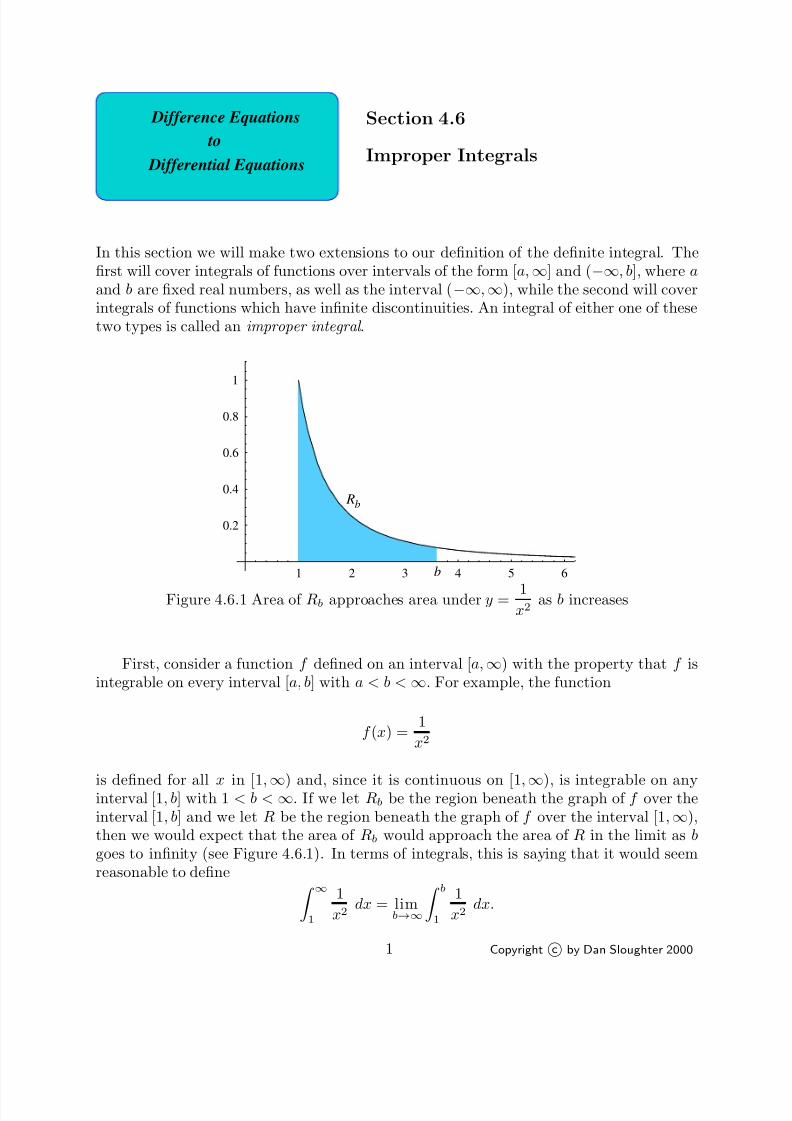
7/27/2019 Calculus 2 (Dan Sloughter)
http://slidepdf.com/reader/full/calculus-2-dan-sloughter 287/598
Difference Equations
Differential Equations
to
Section 4.6
Improper Integrals
In this section we will make two extensions to our definition of the definite integral. Thefirst will cover integrals of functions over intervals of the form [a,∞] and (−∞, b], where a
and b are fixed real numbers, as well as the interval (−∞,∞), while the second will coverintegrals of functions which have infinite discontinuities. An integral of either one of thesetwo types is called an improper integral .
1 2 3 4 5 6
0.2
0.4
0.6
0.8
1
b
Rb
Figure 4.6.1 Area of Rb approaches area under y = 1x2
as b increases
First, consider a function f defined on an interval [a,∞) with the property that f isintegrable on every interval [a, b] with a < b < ∞. For example, the function
f (x) =1
x2
is defined for all x in [1,∞) and, since it is continuous on [1,∞), is integrable on anyinterval [1, b] with 1 < b < ∞. If we let Rb be the region beneath the graph of f over theinterval [1, b] and we let R be the region beneath the graph of f over the interval [1,∞),then we would expect that the area of Rb would approach the area of R in the limit as b
goes to infinity (see Figure 4.6.1). In terms of integrals, this is saying that it would seemreasonable to define
∞
1
1
x2dx = lim
b→∞
b1
1
x2dx.
1 Copyright c by Dan Sloughter 2000

7/27/2019 Calculus 2 (Dan Sloughter)
http://slidepdf.com/reader/full/calculus-2-dan-sloughter 288/598
2 Improper Integrals Section 4.6
That is, we should have ∞
1
1
x2dx = lim
b→∞
b1
1
x2dx
= limb→∞
−
1
xb
1
= limb→∞
−1
b+ 1
= 1.
Geometrically, this result says that R has finite area, namely, 1, even though it has infinitelength.
We now state a general definition for this type of integral.
Definition If f is defined on [a,∞) and integrable on [a, b] for all a < b < ∞, then wedefine
∞a
f (x)dx = limb→∞ ba
f (x)dx, (4.6.1)
provided the limit exists. Similarly, if f is defined on (−∞, b] and integrable on [a, b] forall −∞ < a < b, then we define
b−∞
f (x)dx = lima→−∞
ba
f (x)dx, (4.6.2)
provided the limit exists. Finally, if f is defined on (−∞,∞) and integrable on any finiteinterval [a, b], then we define
∞−∞
f (x)dx = 0−∞
f (x)dx + ∞0
f (x)dx, (4.6.3)
provided both of the integrals on the right exist. In each case where the appropriate limitexists, we say the integral converges ; otherwise, the integral is said to diverge .
Note that the use of 0 in (4.6.3) is not crucial; all that is important is that the integralis broken into two pieces, the meaning of each of the pieces already having been coveredin the earlier parts of the definition.
Example The integral
∞
3
1
x3dx
converges, since
∞
3
1
x3dx = lim
b→∞
b3
1
x3dx
= limb→∞
− 1
2x2
b
3
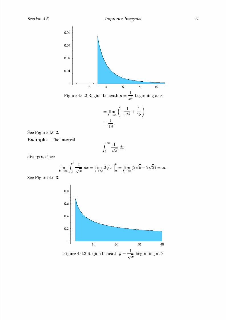
7/27/2019 Calculus 2 (Dan Sloughter)
http://slidepdf.com/reader/full/calculus-2-dan-sloughter 289/598
Section 4.6 Improper Integrals 3
2 4 6 8 10
0.01
0.02
0.03
0.04
Figure 4.6.2 Region beneath y =1
x3beginning at 3
= limb→∞−
1
2b2 +1
18
=1
18.
See Figure 4.6.2.
Example The integral ∞
2
1√ x
dx
diverges, since
limb→∞ b2
1
√ x dx = limb→∞2√ x b2 = limb→∞(2√ b − 2√ 2) = ∞.
See Figure 4.6.3.
10 20 30 40
0.2
0.4
0.6
0.8
Figure 4.6.3 Region beneath y =1√
xbeginning at 2
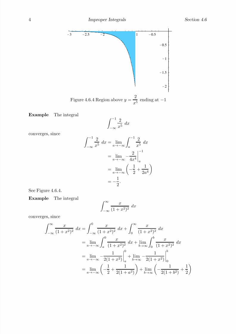
7/27/2019 Calculus 2 (Dan Sloughter)
http://slidepdf.com/reader/full/calculus-2-dan-sloughter 290/598
4 Improper Integrals Section 4.6
-3 -2.5 -2 -1.5 -1 -0.5
-2
-1.5
-1
-0.5
Figure 4.6.4 Region above y =2
x5ending at −1
Example The integral −1
−∞
2
x5dx
converges, since −1
−∞
2
x5dx = lim
a→−∞
−1
a
2
x5dx
= lima→−∞
− 2
4x4
−1
a
= lima→−∞
−1
2+
1
2a4
= −1
2.
See Figure 4.6.4.
Example The integral ∞
−∞
x
(1 + x2)2dx
converges, since
∞
−∞
x
(1 +x2
)
2dx =
0
−∞
x
(1 +x2
)
2dx +
∞
0
x
(1 +x2
)
2dx
= lima→−∞
0a
x
(1 + x2)2dx + lim
b→∞
b0
x
(1 + x2)2dx
= lima→−∞
− 1
2(1 + x2)
0
a
+ limb→∞
− 1
2(1 + x2)
b
0
= lima→−∞
−1
2+
1
2(1 + a2)
+ lim
b→∞
− 1
2(1 + b2)+
1
2
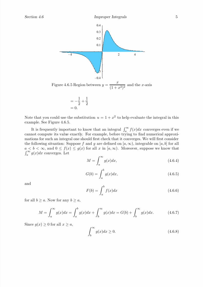
7/27/2019 Calculus 2 (Dan Sloughter)
http://slidepdf.com/reader/full/calculus-2-dan-sloughter 291/598
Section 4.6 Improper Integrals 5
-4 -2 2 4
-0.4
-0.3
-0.2
-0.1
0.1
0.2
0.3
0.4
Figure 4.6.5 Region between y =x
(1 + x2)2and the x-axis
= −1
2 +1
2= 0.
Note that you could use the substitution u = 1 + x2 to help evaluate the integral in thisexample. See Figure 4.6.5.
It is frequently important to know that an integral ∞
a f (x)dx converges even if wecannot compute its value exactly. For example, before trying to find numerical approxi-mations for such an integral one should first check that it converges. We will first considerthe following situation: Suppose f and g are defined on [a,∞), integrable on [a, b] for alla < b <
∞, and 0
≤f (x)
≤g(x) for all x in [a,
∞). Moreover, suppose we know that
∞
a g(x)dx converges. Let
M =
∞
a
g(x)dx, (4.6.4)
G(b) =
ba
g(x)dx, (4.6.5)
and
F (b) =
ba
f (x)dx (4.6.6)
for all b ≥ a. Now for any b ≥ a,
M =
∞
a
g(x)dx =
ba
g(x)dx +
∞
b
g(x)dx = G(b) +
∞
b
g(x)dx. (4.6.7)
Since g(x) ≥ 0 for all x ≥ a, ∞
b
g(x)dx ≥ 0. (4.6.8)
7/27/2019 Calculus 2 (Dan Sloughter)
http://slidepdf.com/reader/full/calculus-2-dan-sloughter 292/598
6 Improper Integrals Section 4.6
Thus (4.6.7) implies that
G(b) = M − ∞
b
g(x)dx ≤ M (4.6.9)
for all b ≥ a. Moreover, f (x) ≤ g(x) for all x ≥ a, so
F (b) =
b
a
f (x)dx ≤
b
a
g(x)dx = G(b) (4.6.10)
for all b ≥ a. Putting (4.6.9) and (4.6.10) together, we have F (b) ≤ M for all b ≥ a .Furthermore, for any c ≥ b ≥ a,
F (c) =
ca
f (x)dx =
ba
f (x)dx +
cb
f (x)dx ≥ ba
f (x)dx = F (b), (4.6.11)
where we know
c
b
f (x)dx≥
0 (4.6.12)
because f (x) ≥ 0 for all x ≥ a. From (4.6.11) we conclude that F is a nondecreasingfunction. Since we already know that F is bounded by M , it follows from our result aboutbounded nondecreasing sequences in Section 1.2 that
limb→∞
F (b) = limb→∞
ba
f (x)dx (4.6.13)
exists. That is,
∞
a
f (x)dx = limb→∞
b
a
f (x)dx (4.6.14)
converges. Moreover, since F (b) ≤ M for all b ≥ a,
∞
a
f (x)dx = limb→∞
F (b) ≤ M =
∞
a
g(x)dx. (4.6.15)
On the other hand, suppose f and g are defined on [a,∞), integrable on [a, b] for alla < b < ∞, 0 ≤ f (x) ≤ g(x) for all x in [a,∞), and
∞
a f (x)dx diverges. If we define F
and G as above, then F (b) is nondecreasing and without a limit as b increases toward ∞.Hence it follows, again from our results in Section 1.2, that we must have
limb→∞F (b) = ∞. (4.6.16)
Since, as above, G(b) ≥ F (b) for all b ≥ a, (4.6.16) implies that
limb→∞
ba
g(x)dx = limb→∞
G(b) = ∞. (4.6.17)
In particular, ∞
a g(x)dx diverges.
7/27/2019 Calculus 2 (Dan Sloughter)
http://slidepdf.com/reader/full/calculus-2-dan-sloughter 293/598
Section 4.6 Improper Integrals 7
We summarize the previous results in the next proposition.
Proposition Suppose f and g are defined on [a,∞), integrable on [a, b] for all a < b < ∞,and 0 ≤ f (x) ≤ g(x) for all x in [a,∞). If
∞
ag(x)dx converges, then
∞
af (x)dx converges
and
0 ≤ ∞
a f (x)dx ≤ ∞
a g(x)dx. (4.6.18)
If ∞
a f (x)dx diverges, then ∞
a g(x)dx diverges.
Similar results hold for integrals on intervals of the form (−∞, b] and (−∞,∞).
Example At present we cannot use the Fundamental Theorem to evaluate
∞
0
1
1 + x2dx
because we do not know an antiderivative for
f (x) = 11 + x2
(although we will find one in Section 6.5). However, since x2 < 1 + x2 for all values of x,we know that
0 <1
1 + x2<
1
x2
for all x > 0. Now we saw above that ∞
1
1
x2dx = 1,
so we know, by the previous proposition, that ∞
1
1
1 + x2dx
converges with ∞
1
1
1 + x2dx ≤ 1. (4.6.19)
Moreover, 1 + x2 ≥ 1 for all x, so1
1 + x2≤ 1
for all x. Hence 10
1
1 + x2dx ≤
10
dx = 1. (4.6.20)
Putting (4.6.19) and (4.6.20) together, we have
∞
0
1
1 + x2dx =
10
1
1 + x2dx +
∞
1
1
1 + x2dx ≤ 1 + 1 = 2.
7/27/2019 Calculus 2 (Dan Sloughter)
http://slidepdf.com/reader/full/calculus-2-dan-sloughter 294/598
8 Improper Integrals Section 4.6
In the problems for Section 6.5, you will be asked to show that
∞
0
1
1 + x2dx =
π
2.
Example Since √ x − 1 < √ x for all x ≥ 0, we see that
0 <1√
x<
1√ x − 1
for all x ≥ 1. Thus, by the previous proposition,
∞
2
1√ x − 1
dx
diverges since we saw above that ∞
2
1√ x
dx
diverges.
Although we will not go into the details, the previous proposition may be generalizedas follows.
Proposition Suppose h(x) ≤ f (x) ≤ g(x) for all x in an interval [a,∞) and f , g, andh are integrable on [a, b] for all a < b < ∞. If both
∞
a h(x)dx and ∞
a g(x)dx converge,
then
∞
a f (x)dx converges as well. Moreover, in that case,
∞
a
h(x)dx ≤ ∞
a
f (x)dx ≤ ∞
a
g(x)dx. (4.6.21)
Note that our previous proposition is a special case of this proposition with h(x) = 0for all x ≥ a. As before, similar results hold for integrals on intervals of the form (−∞, b]and (−∞,∞).
Example Since −1 ≤ sin(x) ≤ 1 for all x, it follows that
−1
x2 ≤sin(x)
x2 ≤1
x2
for all x ≥ 1. Moreover, ∞
1
1
x2dx = 1
and ∞
1
− 1
x2dx = −
∞
1
1
x2dx = −1.
7/27/2019 Calculus 2 (Dan Sloughter)
http://slidepdf.com/reader/full/calculus-2-dan-sloughter 295/598
Section 4.6 Improper Integrals 9
Hence it follows that ∞
1
sin(x)
x2dx
converges and
−1 ≤ ∞1
sin(x)x2
dx ≤ 1.
After noticing that for any function f , −|f (x)| ≤ f (x) ≤ |f (x)| for all values of x, thefollowing proposition is a special case of the previous proposition.
Proposition If f is defined on [a,∞) and ∞
a |f (x)|dx converges, then ∞
a f (x)dx con-verges.
Example Another way to see that
∞
1
sin(x)
x2dx
converges is to note that ∞
1
sin(x)
x2
dx
converges since
0 ≤
sin(x)
x2
≤
| sin(x)|x2
≤ 1
x2
for all x ≥ 1.
Once again, similar results hold for integrals on intervals of the form (−∞, b] and(−∞,∞).
We now consider another extension to our definition of the definite integral. Supposethe function f is defined on the interval (a, b] with
limx→a+
|f (x)| = ∞.
If f is integrable on every interval of the form [c, b] with a < c < b, then we may, analogousto our earlier definitions, define
ba
f (x)dx = limc→a+
bc
f (x)dx, (4.6.22)
provided the limit exists. See Figure 4.6.6.
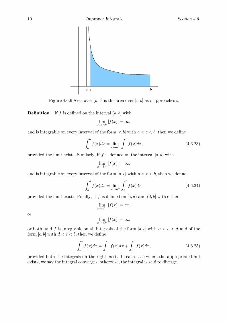
7/27/2019 Calculus 2 (Dan Sloughter)
http://slidepdf.com/reader/full/calculus-2-dan-sloughter 296/598
10 Improper Integrals Section 4.6
bca
Figure 4.6.6 Area over (a, b] is the area over [c, b] as c approaches a
Definition If f is defined on the interval (a, b] with
limx→a+
|f (x)| = ∞,
and is integrable on every interval of the form [c, b] with a < c < b, then we define
ba
f (x)dx = limc→a+
bc
f (x)dx, (4.6.23)
provided the limit exists. Similarly, if f is defined on the interval [a, b) with
limx→b−
|f (x)| = ∞,
and is integrable on every interval of the form [a, c] with a < c < b, then we define
ba
f (x)dx = limc→b−
ca
f (x)dx, (4.6.24)
provided the limit exists. Finally, if f is defined on [a, d) and (d, b] with either
limx→d−
|f (x)| = ∞,
orlim
x→d+|f (x)| = ∞,
or both, and f is integrable on all intervals of the form [a, c] with a < c < d and of theform [c, b] with d < c < b, then we define
ba
f (x)dx =
da
f (x)dx +
bd
f (x)dx, (4.6.25)
provided both the integrals on the right exist. In each case where the appropriate limitexists, we say the integral converges; otherwise, the integral is said to diverge.

7/27/2019 Calculus 2 (Dan Sloughter)
http://slidepdf.com/reader/full/calculus-2-dan-sloughter 297/598
Section 4.6 Improper Integrals 11
0.2 0.4 0.6 0.8 1
2
4
6
8
10
Figure 4.6.7 Region beneath y =1√
xover [0, 1]
Example The integral 10
1√ x
dx
converges since
10
1√ x
= limc→0+
1c
1√ x
dx = limc→0+
2√
x1c
= limc→0+
(2− 2√
c) = 2.
See Figure 4.6.7.
Example The integral 10
1x2
dx
diverges since
10
1
x2dx = lim
c→0+
1c
1
x2dx = lim
c→0+−1
x
1
c
= limc→0+
−1 +
1
c
= ∞.
See Figure 4.6.8.
Example The integral
2
0
1
(x − 1) 23 dx
is improper since
limx→1−
1
(x − 1)23
= ∞
and
limx→1+
1
(x − 1)23
= ∞.

7/27/2019 Calculus 2 (Dan Sloughter)
http://slidepdf.com/reader/full/calculus-2-dan-sloughter 298/598
12 Improper Integrals Section 4.6
0.2 0.4 0.6 0.8 1
10
20
30
40
50
Figure 4.6.8 Region beneath y =1
x2over [0, 1]
Moreover, the integral converges since 10
1
(x − 1)23
dx = limc→1−
c0
1
(x − 1)23
dx
= limc→1−
3(x − 1)13
c
0
= limc→1−
3(c − 1)
13 + 3
= 3
and 21
1
(x − 1)23
dx = limc→1+
2c
1
(x − 1)23
dx
= limc→1+
3(x − 1)13
2
c
= limc→1+
3− 3(c− 1)
13
= 3,
which together imply that
20
1
(x − 1)23
dx =
10
1
(x − 1)23
dx +
21
1
(x − 1)23
dx.
See Figure 4.6.9.

7/27/2019 Calculus 2 (Dan Sloughter)
http://slidepdf.com/reader/full/calculus-2-dan-sloughter 299/598
Section 4.6 Improper Integrals 13
0.5 1 1.5 2
2
4
6
8
10
Figure 4.6.9 Region beneath y =1
(x − 1)23
over [0, 2]
Problems
1. Evaluate the following integrals.
(a)
∞
1
1
x3dx (b)
∞
4
3
x7dx
(c)
∞
10
1
5x4dx (d)
∞
0
1√ x + 1
dx
(e) ∞
0
3
(2x + 3)2
dx (f) ∞
0
sin(x)dx
2. Evaluate the following integrals.
(a)
−2
−∞
3
x2dx (b)
∞
−∞
x
(x2 + 4)4dx
(c)
0−∞
3√ 1 − x
dx (d)
∞
−∞
5t√ t2 + 1
dt
3. For each of the following, decide, without evaluating, whether the integral convergesor diverges.
(a)
∞
1
1
x3 + 2dx (b)
∞
−∞
1
x2 + 5dx
(c)
∞
2
1
(z2 − 2)1/3dz (d)
∞
0
1√ t4 + 1
dt
(e)
∞
1
sin3(t)
t2dt (f)
∞
π
cos(z)
z5dz

7/27/2019 Calculus 2 (Dan Sloughter)
http://slidepdf.com/reader/full/calculus-2-dan-sloughter 300/598
14 Improper Integrals Section 4.6
4. Evaluate the following integrals.
(a)
80
1
x13
dx (b)
10
3
x4dx
(c)
1
0
1
√ 1 − x dx (d)
5
0
5
(t − 2) 25 dt
(e)
0−2
6
(z + 2)2dz (f)
2−1
3
x13
dx
5. (a) Show that ∞
1
1
x pdx
converges for p > 1. Find its value.
(b) Show that ∞1
1x p
dx
diverges for p < 1.
6. (a) Show that 10
1
x pdx
converges for p < 1. Find its value.
(b) Show that
10
1
x p dx
diverges for p > 1.
7. Let
sn = 1 +1
2+
1
3+ · · ·+
1
n
for n = 1, 2, 3, . . .. That is, sn is the nth partial sum of the harmonic series (see Section1.3).
(a) Show that
sn ≤ 1 + n1
1
x dx
for n = 1, 2, 3, . . .. (Hint: Use the right-hand rule to approximate the integral.)
(b) Show that ∞
1
1
xdx
diverges.
7/27/2019 Calculus 2 (Dan Sloughter)
http://slidepdf.com/reader/full/calculus-2-dan-sloughter 301/598
Section 4.6 Improper Integrals 15
(c) Use a geometric argument to conclude that 10
1
xdx
also diverges.
8. For constants σ > 0 and α > 0, the function
p(x) =ασα
xα+1,
where x ≥ σ, is called a Pareto distribution . It is often used in modeling the distributionof incomes or wealth in a population. In the income interpretation, the function
P (x) =
∞
x
p(t)dt,
x ≥ σ, gives the proportion of the population whose income exceeds x. Here σ repre-sents the minimum income of any person in the population and α controls how rapidly
the income distribution diminishes as x increases.(a) Find P (x).
(b) If α > 1, the average income of a population described by this model is
A =
∞
σ
xp(x)dx.
Find A.
(c) Why is the condition α > 1 needed in (b)?
(d) Suppose σ = 10, 000 and α = 1.2. Find A, P (A), and P (2A). Interpret themeaning of these values.
(e) Find the general expression for P (A) as a function of α and graph it. Use thisgraph to interpret the fairness of the income distribution for different values of α.
9. If f is integrable on [−b, b] for all b > 0 and
limb→∞
b−b
f (x)dx
exists, then we call
I (f ) = limb→∞
b−b
f (x)dx
the Cauchy integral of f .(a) Show that if
∞
−∞f (x)dx converges, then
I (f ) =
∞
−∞
f (x)dx.
(b) Find I (f ) and I (g) for f (x) = x and g(x) = sin(x).
(c) Show that the Cauchy integral of f may exist even though ∞
−∞f (x)dx diverges.

7/27/2019 Calculus 2 (Dan Sloughter)
http://slidepdf.com/reader/full/calculus-2-dan-sloughter 302/598
Difference Equations
Differential Equations
toSection 4.7
More on Area
In Section 4.1 we motivated the definition of the definite integral with the idea of findingthe area of a region in the plane. However, to solve the problem we restricted to a veryspecial type of region, namely, a region lying between the graph of a function f and aninterval on the x-axis. We will now consider the more general problem of the area of aregion lying between the graphs of two functions.
a b
y = f ( )
y = g( )
x
x
Figure 4.7.1 Approximating the area between y = f (x) and y = g(x)
Suppose f and g are functions defined on an interval [a, b] with g(x) ≤ f (x) for all x
in [a, b]. We suppose that f and g are integrable on [a, b], from which it follows that thefunction k defined by
k(x) = f (x)− g(x)
is also integrable on [a, b]. Let R be the region lying between the graphs of f and g overthe interval [a, b] and let A be the area of R. In other words, A is the area of the region of
the plane bounded by the curves y = f (x), y = g(x), x = a, and x = b. We begin with anapproximation for A. First, we divide [a, b] into n intervals of equal length
∆x =b − a
n
and let a = x0 < x1 < x2 < x3 < · · · < xn = b be the endpoints of these intervals. Next,for i = 1, 2, 3, . . . , n, let Ri be the region lying between the graphs of f and g over the
1 Copyright c by Dan Sloughter 2000

7/27/2019 Calculus 2 (Dan Sloughter)
http://slidepdf.com/reader/full/calculus-2-dan-sloughter 303/598
2 More on Area Section 4.7
-1.5 -1 -0.5 0.5 1 1.5
0.5
1
1.5
2
Figure 4.7.2 Region bounded by the graphs of y = 2− x2 and y = x2
interval [xi
−1, xi]. If Ai is the area of Ri, then
A =n
i=1
Ai. (4.7.1)
Now f (xi)− g(xi) is the distance between the graphs of f and g at xi, and so
(f (xi)− g(xi))∆x
should approximate Ai reasonably well when ∆x is small. Thus
ni=1
(f (xi)− g(xi))∆x =
ni=1
k(xi)∆x (4.7.2)
will approximate A. Moreover, we should expect that this approximation will improve as∆x decreases, that is, as n increases, and so we should have
A = limn→∞
ni=1
k(xi)∆x. (4.7.3)
But now the right-hand side of (4.7.2) is a Riemann sum, in particular, the right-hand rulesum, and so the right-hand side of (4.7.3) converges to the definite integral of k on [a, b].
Hence we have
A =
b
a
k(x)dx =
b
a
(f (x)− g(x))dx. (4.7.4)
Example Let R be the region bounded by the curves y = 2 − x2 and y = x2, as shownin Figure 4.7.2. Note that these curves intersect when
2− x2 = x2,

7/27/2019 Calculus 2 (Dan Sloughter)
http://slidepdf.com/reader/full/calculus-2-dan-sloughter 304/598
Section 4.7 More on Area 3
1 2 3 4 5
-2
-1
1
2
3
R
R2
1
Figure 4.7.3 Region bounded by the graphs of x = y2 and x = y + 2
which implies that 2x2 = 2, that is, x =−
1 or x = 1. Hence the two curves intersect at(−1, 1) and (1, 1), and so we may describe R as the region between the curves y = 2 − x2
and y = x2 which lies above the interval [−1, 1]. Thus if A is the area of R, we have
A =
1−1
((2− x2)− x2)dx
=
1−1
(2− 2x2)dx
=
2x − 2
3x31
−1
=
2 − 2
3
−−2 +
2
3
=8
3.
Example Let R be the region bounded by the curves x = y2 and x = y + 2. These twocurves intersect when
y2 = y + 2,
which implies that0 = y2 − y − 2 = (y − 2)(y + 1).
Hence the two curves intersect when y = −1 and y = 2, that is, at the points (1,−1) and(4, 2). However, looking at Figure 4.7.3, we see that not all of R lies over the interval [1, 4].In fact, R may be broken up into two regions, R1and R2, where R1 is the region betweenthe curves y =
√ x and y = −√ x over the interval [0, 1] and R2 is the region between the
curves y =√
x and y = x− 2 over the interval [1, 4]. Thus, if A is the area of R, A1 is the

7/27/2019 Calculus 2 (Dan Sloughter)
http://slidepdf.com/reader/full/calculus-2-dan-sloughter 305/598
4 More on Area Section 4.7
area of R1, and A2 is the area of R2, then
A = A1 + A2
= 1
0
(√
x−
(−√
x)) + 4
1
(√
x−
(x−
2))dx
=
10
2√
x dx +
41
(√
x − x + 2)dx
=4
3x32
1
0
+
2
3x32 − 1
2x2 + 2x
4
1
=4
3+
16
3− 8 + 8
−
2
3− 1
2+ 2
=9
2.
The region R in the previous example may also be described as the region lying betweenthe curves x = y2 and x = y+2 over the interval [−1, 2] on the y-axis. In general, analogousto our development above, if f and g are functions defined on an interval [c, d] on the y-axiswith g(y) ≤ f (y) for all y in [c, d], then the area A of the region bounded by x = f (y),x = g(y), y = c, and y = d (see Figure 4.7.4), is given by
A =
d
c
(f (y)− g(y))dy. (4.7.5)
c
d
x = g( )
x = f ( ) y
y
Figure 4.7.4 Region between the curves x = f (y) and x = g(y)

7/27/2019 Calculus 2 (Dan Sloughter)
http://slidepdf.com/reader/full/calculus-2-dan-sloughter 306/598
Section 4.7 More on Area 5
-1 -0.5 0.5 1 1.5 2
-0.5
0.5
1
1.5
2
2.5
R
R2
1
Figure 4.7.5 Region bounded by the graphs of y = x3 − x and y = x2
In particular, for our previous example we have
A =
2−1
(y + 2 − y2)dy
=
1
2y2 + 2y − 1
3y3
2
−1
=
2 + 4 − 8
3
−
1
2− 2 +
1
3
=9
2.
In this case, the second method for solving the problem is a little simpler than the first; ingeneral, it is often useful to look at a problem both ways and evaluate using the simplerof the two approaches.
Example Let R be the region bounded by the curves y = x3 − x and y = x2. Thesecurves intersect when
x3 − x = x2,
that is, when0 = x3 − x2 − x = x(x2 − x − 1).
Hence the curves intersect when x = 0,
x =1−√ 5
2,
or
x =1 +
√ 5
2,
where the latter two values were found using the quadratic formula. From the graphs inFigure 4.7.5, we see that R may be divided into two regions, R1 and R2, where R1 extends

7/27/2019 Calculus 2 (Dan Sloughter)
http://slidepdf.com/reader/full/calculus-2-dan-sloughter 307/598
6 More on Area Section 4.7
from x = 1−√ 5
2to x = 0 and R2 extends from x = 0 to x = 1+
√ 5
2. Note that in R1 we
have x3 − x ≥ x2, whereas x2 ≥ x3 − x in R2. Thus, if A is the area of R, A1 is the areaof R1, and A2 is the area of R2, then
A = A1 + A2
= 01−
√ 5
2
(x3 − x − x2)dx + 1+√ 5
2
0
(x2 − x3 + x)dx
=
1
4x4 − 1
2x2 − 1
3x3
0
1−√ 5
2
+
1
3x3 − 1
4x4 − 1
2x2
1+√ 5
2
0
=13
12.
Problems
1. Find the area of the region bounded by the curves y = x and y = x2.
2. Find the area of the region bounded by the curves y =√
x and y =12
x.
3. Find the area of the region bounded by the curves y = x2 and y = x + 2.
4. Find the area of the region bounded by the curves y = cos(x) and y = x2.
5. Find the area of the region bounded by the curves y = sin(x) and y = x2.
6. Find the area of one of the regions lying between the curves y = cos(x) and y = sin(x)between two consecutive points of intersection.
7. Find the area of the region in the first quadrant bounded by y = cos(x), y = sin(x),and x = 0.
8. Find the area of one of the regions lying between the curves y = cos2(x) and y = sin2(x)between two consecutive points of intersection.
9. Let R be the region bounded by the curves y = x2 and y = 2 − x.
(a) Set up an integral to find the area of R using functions of x.
(b) Set up an integral to find the area of R using functions of y.
(c) Evaluate the simpler of the integrals in (a) and (b).
10. Find the area of the region bounded by the curves x = y2 − 1 and x = 1− y2.
11. Find the area of the region bounded by the curves x = y2 and x = 6 − y.
12. Find the area of the region bounded by the curves y = x3 − 2x and y = x2.13. Find the area of the region bounded by the curves y = x4 − 4x2 and y = 3x3.
14. To estimate the surface area of a lake, 21 measurements of the width of the lake aremade at points spaced 50 yards apart from one end of the lake to the other. Supposethe measurements are, in order, 0, 50, 100, 120, 180, 240, 300, 250, 220, 295, 305, 265,240, 275, 225, 180, 120, 90, 63, 40, and 0, all measured in yards. Use Simpson’s ruleto approximate the surface area of the lake.
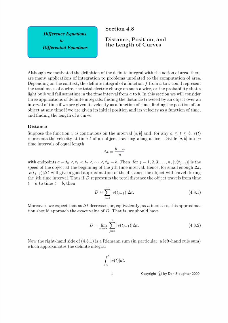
7/27/2019 Calculus 2 (Dan Sloughter)
http://slidepdf.com/reader/full/calculus-2-dan-sloughter 308/598
Difference Equations
Differential Equations
to
Section 4.8
Distance, Position, andthe Length of Curves
Although we motivated the definition of the definite integral with the notion of area, thereare many applications of integration to problems unrelated to the computation of area.Depending on the context, the definite integral of a function f from a to b could representthe total mass of a wire, the total electric charge on such a wire, or the probability that alight bulb will fail sometime in the time interval from a to b. In this section we will considerthree applications of definite integrals: finding the distance traveled by an object over aninterval of time if we are given its velocity as a function of time, finding the position of anobject at any time if we are given its initial position and its velocity as a function of time,and finding the length of a curve.
Distance
Suppose the function v is continuous on the interval [a, b] and, for any a ≤ t ≤ b, v(t)represents the velocity at time t of an object traveling along a line. Divide [a, b] into n
time intervals of equal length
∆t =b − a
n
with endpoints a = t0 < t1 < t2 < · · · < tn = b. Then, for j = 1, 2, 3, . . . , n, |v(tj−1)| is the
speed of the object at the beginning of thej
th time interval. Hence, for small enough ∆t,|v(tj−1)|∆t will give a good approximation of the distance the object will travel during
the jth time interval. Thus if D represents the total distance the object travels from timet = a to time t = b, then
D ≈n
j=1
|v(tj−1)|∆t. (4.8.1)
Moreover, we expect that as ∆t decreases, or, equivalently, as n increases, this approxima-tion should approach the exact value of D. That is, we should have
D = limn→∞
nj=1
|v(tj−1)|∆t. (4.8.2)
Now the right-hand side of (4.8.1) is a Riemann sum (in particular, a left-hand rule sum)which approximates the definite integral
ba
|v(t)|dt.
1 Copyright c by Dan Sloughter 2000

7/27/2019 Calculus 2 (Dan Sloughter)
http://slidepdf.com/reader/full/calculus-2-dan-sloughter 309/598
2 Distance, Position, and the Length of Curves Section 4.8
0.2 0.4 0.6 0.8 1
-6
-4
-2
2
4
6
Figure 4.8.1 Graph of the velocity function v(t) = 4 cos(2πt)
Hence this integral is the value of the limit in (4.8.2), and so we have
D = limn→∞
nj=1
|v(tj−1)|∆t =
ba
|v(t)|dt. (4.8.3)
Example Suppose an object is oscillating at the end of a spring so that its velocity attime t is given by v(t) = 4 cos(2πt). Then the distance D traveled by the object from timet = 0 to time t = 1 is given by
D =
1
0
|4 cos(2πt)|dt = 4
1
0
| cos(2πt)|dt.
Now
cos(2πt) ≥ 0 when 0 ≤ t ≤ 1
4or
3
4≤ t ≤ 1,
and
cos(2πt) ≤ 0 when1
4≤ t ≤ 3
4.
Hence
| cos(2πt)| = cos(2πt) when 0 ≤ t ≤ 1
4or
3
4≤ t ≤ 1,
and
| cos(2πt)| = − cos(2πt) when1
4≤ t ≤ 3
4.
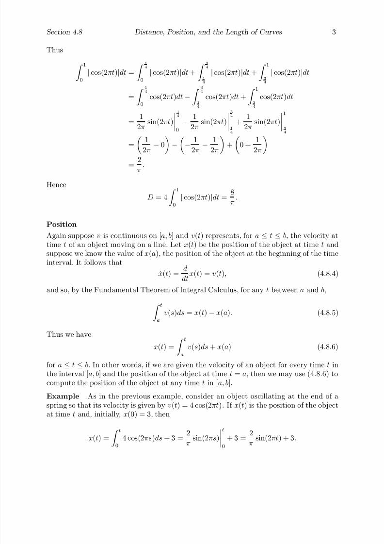
7/27/2019 Calculus 2 (Dan Sloughter)
http://slidepdf.com/reader/full/calculus-2-dan-sloughter 310/598
Section 4.8 Distance, Position, and the Length of Curves 3
Thus
1
0
| cos(2πt)|dt =
14
0
| cos(2πt)|dt +
34
1
4
| cos(2πt)|dt +
1
3
4
| cos(2πt)|dt
= 140
cos(2πt)dt − 3
4
1
4
cos(2πt)dt + 13
4
cos(2πt)dt
=1
2πsin(2πt)
1
4
0
− 1
2πsin(2πt)
3
4
1
4
+1
2πsin(2πt)
1
3
4
=
1
2π− 0
−− 1
2π− 1
2π
+
0 +
1
2π
=2
π.
Hence
D = 4
1
0
| cos(2πt)|dt = 8π
.
Position
Again suppose v is continuous on [a, b] and v(t) represents, for a ≤ t ≤ b, the velocity attime t of an object moving on a line. Let x(t) be the position of the object at time t andsuppose we know the value of x(a), the position of the object at the beginning of the timeinterval. It follows that
x(t) =d
dtx(t) = v(t), (4.8.4)
and so, by the Fundamental Theorem of Integral Calculus, for any t between a and b,
ta
v(s)ds = x(t) − x(a). (4.8.5)
Thus we have
x(t) =
ta
v(s)ds + x(a) (4.8.6)
for a ≤ t ≤ b. In other words, if we are given the velocity of an object for every time t inthe interval [a, b] and the position of the object at time t = a, then we may use (4.8.6) to
compute the position of the object at any time t in [a, b].
Example As in the previous example, consider an object oscillating at the end of aspring so that its velocity is given by v(t) = 4 cos(2πt). If x(t) is the position of the objectat time t and, initially, x(0) = 3, then
x(t) =
t0
4 cos(2πs)ds + 3 =2
πsin(2πs)
t
0
+ 3 =2
πsin(2πt) + 3.
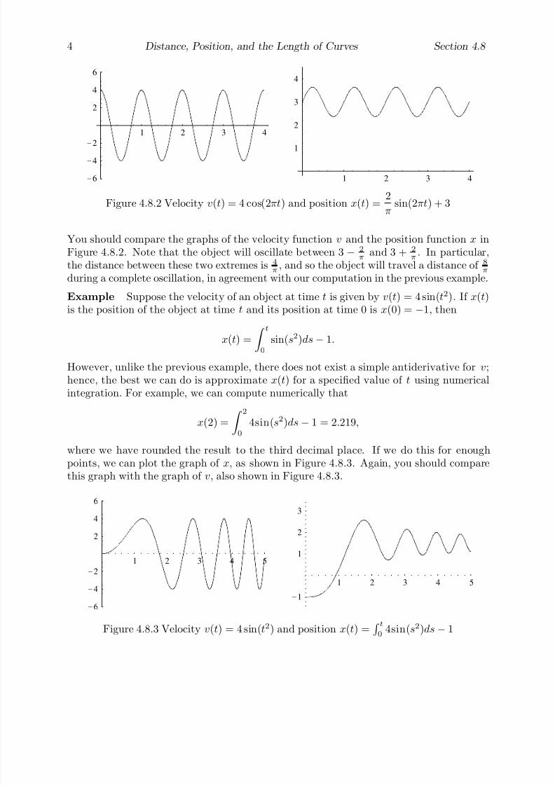
7/27/2019 Calculus 2 (Dan Sloughter)
http://slidepdf.com/reader/full/calculus-2-dan-sloughter 311/598
4 Distance, Position, and the Length of Curves Section 4.8
1 2 3 4
-6
-4
-2
2
4
6
1 2 3 4
1
2
3
4
Figure 4.8.2 Velocity v(t) = 4 cos(2πt) and position x(t) =2
πsin(2πt) + 3
You should compare the graphs of the velocity function v and the position function x inFigure 4.8.2. Note that the object will oscillate between 3 − 2
πand 3 + 2
π. In particular,
the distance between these two extremes is 4
π, and so the object will travel a distance of 8
π
during a complete oscillation, in agreement with our computation in the previous example.
Example Suppose the velocity of an object at time t is given by v(t) = 4 sin(t2). If x(t)is the position of the object at time t and its position at time 0 is x(0) = −1, then
x(t) =
t0
sin(s2)ds − 1.
However, unlike the previous example, there does not exist a simple antiderivative for v;hence, the best we can do is approximate x(t) for a specified value of t using numericalintegration. For example, we can compute numerically that
x(2) =
2
0
4sin(s2)ds − 1 = 2.219,
where we have rounded the result to the third decimal place. If we do this for enoughpoints, we can plot the graph of x, as shown in Figure 4.8.3. Again, you should comparethis graph with the graph of v, also shown in Figure 4.8.3.
1 2 3 4 5
-6
-4
-2
2
4
6
1 2 3 4 5
-1
1
2
3
Figure 4.8.3 Velocity v(t) = 4 sin(t2) and position x(t) = t0
4sin(s2)ds − 1

7/27/2019 Calculus 2 (Dan Sloughter)
http://slidepdf.com/reader/full/calculus-2-dan-sloughter 312/598
Section 4.8 Distance, Position, and the Length of Curves 5
x x x x x x 0 3 41 52
Figure 4.8.4 Approximating a curve with line segments
Length of a curve
Here we will consider the problem of finding the length of a curve which is the graph of some differentiable function. So suppose the function f is continuous on the closed interval[a, b] and differentiable on the open interval (a, b). Let C be the graph of f and let L bethe length of C . As we have done previously, we will first describe a method for findinggood approximations to L. To begin, divide [a, b] into n intervals of equal length
∆x =b − a
n
with endpoints a = x0 < x1 < x2 < · · · < xn = b. For j = 1, 2, 3, . . . , n, we canapproximate the length of the piece of C lying over the jth interval by the distance betweenthe endpoints of this piece, as shown in Figure 4.8.4. That is, since the endpoints of the jth piece are (xj−1, f (xj−1)) and (xj , f (xj)), we can approximate the length of the pieceof C lying over the interval [xj−1, xj ] by
(xj − xj−1)2 + (f (xj) − f (xj−1))2.
Since ∆x = xj − xj−1,
(xj − xj−1)2 + (f (xj) − f (xj−1))2 =
(∆x)2 + (f (xj)− f (xj−1))2
=
(∆x)2
1 +
(f (xj) − f (xj−1))2
(∆x)2
= ∆x
1 +
f (xj) − f (xj−1)
∆x
2
.
(4.8.7)
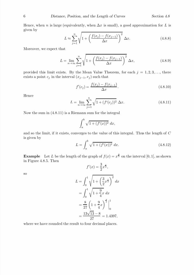
7/27/2019 Calculus 2 (Dan Sloughter)
http://slidepdf.com/reader/full/calculus-2-dan-sloughter 313/598
6 Distance, Position, and the Length of Curves Section 4.8
Hence, when n is large (equivalently, when ∆x is small), a good approximation for L isgiven by
L ≈n
j=1
1 +
f (xj) − f (xj−1)
∆x
2
∆x. (4.8.8)
Moreover, we expect that
L = limn→∞
nj=1
1 +
f (xj) − f (xj−1)
∆x
2
∆x, (4.8.9)
provided this limit exists. By the Mean Value Theorem, for each j = 1, 2, 3, . . ., thereexists a point cj in the interval (xj−1, xj) such that
f (cj) =f (xj) − f (xj−1)
∆x. (4.8.10)
HenceL = lim
n→∞
nj=1
1 + (f (cj))2 ∆x. (4.8.11)
Now the sum in (4.8.11) is a Riemann sum for the integral ba
1 + (f (x))2 dx,
and so the limit, if it exists, converges to the value of this integral. Thus the length of C
is given by
L = ba
1 + (f (x))2 dx. (4.8.12)
Example Let L be the length of the graph of f (x) = x3
2 on the interval [0, 1], as shownin Figure 4.8.5. Then
f (x) =3
2x1
2 ,
so
L =
1
0
1 +
3
2x1
2
2
dx
= 10
1 +
9
4 x dx
=8
27
1 +
9
4x
3
2
1
0
=13√
13 − 8
27= 1.4397,
where we have rounded the result to four decimal places.
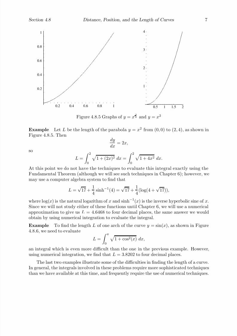
7/27/2019 Calculus 2 (Dan Sloughter)
http://slidepdf.com/reader/full/calculus-2-dan-sloughter 314/598
Section 4.8 Distance, Position, and the Length of Curves 7
0.2 0.4 0.6 0.8 1
0.2
0.4
0.6
0.8
1
0.5 1 1.5 2
1
2
3
4
Figure 4.8.5 Graphs of y = x
3
2 and y = x2
Example Let L be the length of the parabola y = x2 from (0, 0) to (2, 4), as shown inFigure 4.8.5. Then
dy
dx= 2x,
so
L =
2
0
1 + (2x)2 dx =
2
0
1 + 4x2 dx.
At this point we do not have the techniques to evaluate this integral exactly using theFundamental Theorem (although we will see such techniques in Chapter 6); however, wemay use a computer algebra system to find that
L =√
17 +1
4sinh−1(4) =
√ 17 +
1
4(log(4 +
√ 17)),
where log(x) is the natural logarithm of x and sinh−1(x) is the inverse hyperbolic sine of x.Since we will not study either of these functions until Chapter 6, we will use a numericalapproximation to give us L = 4.6468 to four decimal places, the same answer we wouldobtain by using numerical integration to evaluate the integral.
Example To find the length L of one arch of the curve y = sin(x), as shown in Figure4.8.6, we need to evaluate
L =
π
0
1 + cos2(x) dx,
an integral which is even more difficult than the one in the previous example. However,using numerical integration, we find that L = 3.8202 to four decimal places.
The last two examples illustrate some of the difficulties in finding the length of a curve.In general, the integrals involved in these problems require more sophisticated techniquesthan we have available at this time, and frequently require the use of numerical techniques.

7/27/2019 Calculus 2 (Dan Sloughter)
http://slidepdf.com/reader/full/calculus-2-dan-sloughter 315/598
8 Distance, Position, and the Length of Curves Section 4.8
0.5 1 1.5 2 2.5 3
0.2
0.4
0.6
0.8
1
Figure 4.8.6 Graph of y = sin(x) over the interval [0, π]
Problems
1. For each of the following, assume that v(t) is the velocity at time t of an object movingon a line and find the distance traveled by the object over the given time period.
(a) v(t) = 32t over 0 ≤ t ≤ 3 (b) v(t) = −32t + 16 over 0 ≤ t ≤ 3
(c) v(t) = t2 − t − 6 over 0 ≤ t ≤ 2 (d) v(t) = t2 − t − 6 over 0 ≤ t ≤ 4
(e) v(t) = 2 sin(2t) over 0 ≤ t ≤ π (f) v(t) = 3 cos(2πt) over 0 ≤ t ≤ 2
2. Suppose the velocity of a falling object is given by v(t) = −32t feet per second. If the object is at a height of 100 feet at time t = 0, find the height of the object at anarbitrary time t.
3. Suppose x(t) and v(t) are the position and velocity, respectively, at time t of an objectmoving on a line. If x(0) = 5 and v(t) = 3t2 − 6, find x(t).
4. If an object of mass m is connected to a spring, pulled a distance x0 away from itsequilibrium position and released, then, ignoring the effects of friction, the velocity of the object at time t will be given by
v(t) = −x0
k
msin
k
mt
,
where k is a constant that depends on the strength of the spring. Find x(t), theposition of the object at time t.
5. Show that if x(t) = f (t) and f is continuous on [a, b], then
x(t) =
ta
f (s)ds + x(a).

7/27/2019 Calculus 2 (Dan Sloughter)
http://slidepdf.com/reader/full/calculus-2-dan-sloughter 316/598
Section 4.8 Distance, Position, and the Length of Curves 9
6. For each of the following, use the result from Problem 5 to find x(t).
(a) x(t) = 3t3 + 6t − 17 with x(2) = 4 (b) x(t) = 3 cos(6t) − t with x(0) = −1
(c) x(t) = sin2(2t) with x(0) = 2 (d) x(t) = 3t2 sin(2t) with x(0) = 0
(e) x(t) =√
1 + 2t with x(4) = 3
7. Let x(t), v(t), and a(t) be the height, velocity, and acceleration, respectively, at time t
of an object of mass m in free fall near the surface of the earth. Let x0 and v0 be theheight and velocity, respectively, of the object at time t = 0. If we ignore the effectsof air resistance, the force acting on the body is −mg, where g is a constant (g = 9.8meters per second, or 32 feet per second per second). Thus, by Newton’s second lawof motion,
−mg = ma(t),
from which we obtaina(t) = −g.
Using Problem 5, show that
x(t) = −1
2gt2 + v0t + x0.
8. Suppose an object is projected vertically upward from a height of 100 feet with aninitial velocity of 20 feet per second. Use Problem 7 to answer the following questions.
(a) Find x(t), the height of the object at time t.
(b) At what time does the object reach its maximum height?
(c) What is the maximum height reached by the object?
(d) At what time will the object strike the ground?
9. For each of the following, find the length of the graph of the given function over thegiven interval.
(a) f (x) = 2x3
2 over [0, 2] (b) f (x) = sin(2x) over
0,π
2
(c) g(x) = x3 over [−1, 1] (d) g(t) = tan(t) over
−π
4,
π
4
(e) f (t) = sin2(t) over [0, π] (f) g(θ) = sin(θ2) over [0,
√ π ]
10. A sheet of corrugated aluminum is to be made from a flat sheet of aluminum. Suppose
a cross section of the corrugated sheet, when measured in inches, is in the shape of thecurve
y = 2sinπ
4t
.
Find the length of a flat sheet that would be needed to make a corrugated sheet thatis 10 feet long.

7/27/2019 Calculus 2 (Dan Sloughter)
http://slidepdf.com/reader/full/calculus-2-dan-sloughter 317/598
Difference Equations
Differential Equations
to
Section 5.1
Polynomial Approximations
In Chapter 3 we discussed the problem of finding the affine function which best approx-imates a given function about some point. In particular, we found that the best affineapproximation to a function f at a point c is given by
T (x) = f (c)(x − c) + f (c), (5.1.1)
provided that f is differentiable at c. In this section and the next, we will extend the
ideas of Sections 3.1 and 3.2 to the problem of finding polynomial approximations of anygiven degree to a function about some specified point. We shall see that many nonlinearfunctions can be approximated to any desired level of accuracy over a specified intervalif we use polynomials of sufficiently high degree. As an example, compare the graphs of f (x) = sin(x) and
P (x) = x − 1
6x3 +
1
120x5 − 1
5040x7 +
1
362, 880x9
in Figure 5.1.1. They are almost indistinguishable over the interval [−π, π]. In practicalterms, this means there is little difference in working with P (x) instead of f (x) for x
in [−π, π]. Moreover, since polynomials are the simplest of functions, involving only thearithmetic operations of addition, subtraction, and multiplication, the substitution of P
for f can be a very helpful step in simplifying a problem.
-7.5 -5 -2.5 2.5 5 7.5
-3
-2
-1
1
2
3
Figure 5.1.1 Graphs of f (x) = sin(x) and an approximating polynomial
1 Copyright c by Dan Sloughter 2000

7/27/2019 Calculus 2 (Dan Sloughter)
http://slidepdf.com/reader/full/calculus-2-dan-sloughter 318/598
2 Polynomial Approximations Section 5.1
To begin, we need to recall, and then generalize, some definitions and facts fromSections 3.1 and 3.2. First, recall that a function f is said to be o(h) if
limh→0
f (h)
h= 0; (5.1.2)
a function f is said to be O(h) if there exist constants M and such that
f (h)
h
≤ M (5.1.3)
whenever − < h < . In particular, we saw that f is O(h) if
limh→0
f (h)
h
exists. The following definition generalizes to other powers of h this method of character-izing the rate at which a function converges to 0.
Definition For any n > 0, a function f is said to be o(hn) if
limh→0
f (h)
hn= 0. (5.1.4)
For any n > 0, a function f is said to be O(hn) if there exist constants M and such that
f (h)
hn
≤ M (5.1.5)
whenever − < h < .
Similar to our result in Section 3.1, f is O(hn) if
limh→0
f (h)
hn
exists.As before, we use this notation as a means of comparing the rates at which functions
approach 0. As h approaches 0, a function which is O(hn) approaches 0 as least as fast ashn does. Note that for n > m > 0,
limh→0
hn
hm= lim
h→0hn−m = 0 (5.1.6)
since n−m > 0, and so hn goes to 0 faster than hm as h approaches 0. Thus if n > m > 0,as h goes to 0, a function which is O(hn) approaches 0 faster than does a function which
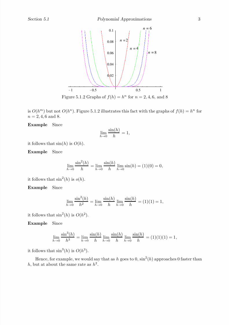
7/27/2019 Calculus 2 (Dan Sloughter)
http://slidepdf.com/reader/full/calculus-2-dan-sloughter 319/598
Section 5.1 Polynomial Approximations 3
-1 -0.5 0.5 1
0.02
0.04
0.06
0.08
0.1n = 6
2n =
4n =
n = 8
Figure 5.1.2 Graphs of f (h) = hn for n = 2, 4, 6, and 8
is O(hm) but not O(hn). Figure 5.1.2 illustrates this fact with the graphs of f (h) = hn forn = 2, 4, 6 and 8.
Example Since
limh→0
sin(h)
h= 1,
it follows that sin(h) is O(h).
Example Since
limh→
0
sin2(h)
h
= limh→
0
sin(h)
h
limh→
0
sin(h) = (1)(0) = 0,
it follows that sin2(h) is o(h).
Example Since
limh→0
sin2(h)
h2= lim
h→0
sin(h)
hlimh→0
sin(h)
h= (1)(1) = 1,
it follows that sin2(h) is O(h2).
Example Since
limh→0
sin3(h)
h3= lim
h→0
sin(h)
hlimh→0
sin(h)
hlimh→0
sin(h)
h= (1)(1)(1) = 1,
it follows that sin3(h) is O(h3).
Hence, for example, we would say that as h goes to 0, sin2(h) approaches 0 faster thanh, but at about the same rate as h2.

7/27/2019 Calculus 2 (Dan Sloughter)
http://slidepdf.com/reader/full/calculus-2-dan-sloughter 320/598
4 Polynomial Approximations Section 5.1
Now suppose that f is O(hn) for some n > 0. This means that as h goes to 0, f
approaches 0 at least as fast as hn does. It should follow that f goes to 0 faster than hm,and so is o(hm), for any 0 < m < n. To see this, let M and > 0 be numbers such that
f (h)
hn
≤M (5.1.7)
for all h in the interval (−, ). Then
f (h)
hm
= |hn−m|
f (h)
hn
≤ |h|n−mM (5.1.8)
for all h in (−, ). Sincelimh→0
|h|n−mM = 0, (5.1.9)
it follows that
limh→0
f (h)hm
= 0, (5.1.10)
and so
limh→0
f (h)
hm= 0. (5.1.11)
Thus f is o(hm).
Proposition If n > m > 0 and f is O(hn), then f is o(hm).
Example We saw above that sin3(h) is O(h3), from which it now follows, for example,that sin3(h) is o(h2).
Next, recall that if f is a function defined in an open interval about a point c and T
is an affine function such that T (c) = f (c) and
R(h) = f (c + h) − T (c + h) (5.1.12)
is o(h), then T is the best affine approximation to f at c. Moreover, as mentioned above,we saw in Chapter 3 that a function f has a best affine approximation at a point c if andonly if f is differentiable at c and, in that case, the best affine approximation is given by
T (x) = f (c) + f (c)(x
−c). (5.1.13)
Putting (5.1.12) and (5.1.13) together and letting x = c + h, or, equivalently, h = x − c,we have that
f (x) − f (c) − f (c)(x − c)
is o(x − c). We may express this by writing
f (x) − f (c) − f (c)(x − c) = o(x − c), (5.1.14)

7/27/2019 Calculus 2 (Dan Sloughter)
http://slidepdf.com/reader/full/calculus-2-dan-sloughter 321/598
Section 5.1 Polynomial Approximations 5
or, solving for f (x), simply
f (x) = f (c) + f (c)(x − c) + o(x − c). (5.1.15)
In words, (5.1.15) says that f (x) is equal to f (c) + f (c)(x − c) plus some function which
is o(x− c), that is, some function which approaches 0 faster than x− c as x approaches c.Example Let f (x) =
√ x. Then
f (1) =1
2,
so the best affine approximation to f at 1 is
T (x) = 1 +1
2(x − 1).
That is, √ x = 1 +
1
2(x−
1) + o(x−
1).
In words, this statement says that√
x is equal to
1 +1
2(x − 1)
plus a term of order higher than x − 1, that is, plus a term which goes to 0 faster thanx − 1 as x approaches 1.
Example Let f (x) = sin(x). Then f (0) = cos(0) = 1, so the best affine approximationto f at 0 is
T (x) = x.Thus
sin(x) = x + o(x),
a fact which is often used in applications to justify replacing the function sin(x) by thefunction x for calculations involving only values of x close to 0.
Now suppose that f is twice continuously differentiable on an interval (c− δ, c + δ ) forsome δ > 0; that is, suppose both f and f exist and are continuous on (c − δ, c + δ ). If T is the best affine approximation to f at c, then, as we have seen,
R(h) = f (c + h)−
T (c + h) (5.1.16)
is o(h). We will show that R is in fact O(h2). Suppose 0 < < δ and − < h < . First,note that
f (c + h) − T (c + h) = f (c + h) − f (c) − f (c)h. (5.1.17)
By the Mean Value Theorem, there is a point u between c and c + h such that
f (c + h) − f (c) = f (u)h. (5.1.18)
7/27/2019 Calculus 2 (Dan Sloughter)
http://slidepdf.com/reader/full/calculus-2-dan-sloughter 322/598
6 Polynomial Approximations Section 5.1
Hence
f (c + h) − T (c + h) = f (u)h − f (c)h = h(f (u) − f (c)). (5.1.19)
Applying the Mean Value Theorem again, there exists a point v between c and u such that
f
(u) − f
(c) = f
(v)(u − c). (5.1.20)
ThusR(h)
h2=
f (c + h) − T (c + h)
h2=
h(u − c)f (v)
h2=
(u − c)f (v)
h. (5.1.21)
If we let M be the maximum value of |f (x)| on [c − , c + ] and note that |u − c| < |h|,then we see that
R(h)
h2
=|u − c||f (v)|
|h| <|h|M
|h| = M (5.1.22)
for all h with − < h < . Hence R(h) is O(h2
).
Proposition If f is twice continuously differentiable on an open interval containing thepoint c and T is the best affine approximation to f at c, then
R(h) = f (c + h) − T (c + h) (5.1.23)
is O(h2).
Letting x = c + h, we can rephrase the proposition to say that
r(x) = f (x) − T (x) (5.1.24)
is O((x − c)2). Similar to our notation above, we may write
f (x) = f (c) + f (c)(x − c) + O((x − c)2). (5.1.25)
For our previous examples, this means that
√ x = 1 +
1
2(x − 1) + O((x − 1)2)
and
sin(x) = x + O(x2).
This is the type of formulation that we wish to generalize to higher order polynomialapproximations. We will introduce these polynomials, called Taylor polynomials , here,but save the verification that they provide the sought-for approximations until the nextsection.
7/27/2019 Calculus 2 (Dan Sloughter)
http://slidepdf.com/reader/full/calculus-2-dan-sloughter 323/598
Section 5.1 Polynomial Approximations 7
Taylor polynomials
The best affine approximation T to a function f at a point c may be described as the onlyfirst degree polynomial satisfying both T (c) = f (c) and T (c) = f (c). This provides a clueas to where to look for higher order polynomial approximations. Namely, given a functionf which is n times differentiable at a point c, we will look for a polynomial P n of degree
at most n with the property that P n(c) = f (c) and the first n derivatives of P n at c agreewith the first n derivatives of f at c. Hence we want to find constants b0, b1, b2, . . . , bn sothat the polynomial
P n(x) = b0 + b1(x − c) + b2(x − c)2 + · · ·+ bn(x − c)n (5.1.26)
satisfiesP (j)n (c) = f (j)(c) (5.1.27)
for j = 0, 1, 2, . . . , n, where P (0)n = P n and, for j > 0, P
(j)n is the jth derivative of P n. Now
P n(c) = b0
P n(c) = b1
P n (c) = 2b2
P n (c) = (3)(2)b3
P (4)n (c) = (4)(3)(2)b4
...
P (n)n (c) = n!bn.
Thus, to satisfy (5.1.27), we must have
f (c) = b0
f (c) = b1
f (c) = 2b2
f (c) = 3!b3
f (4)(c) = 4!b4
...
f
(n)
(c) = n!bn.
Solving for b0, b1, b2, . . . , bn, we have
b0 = f (c)
b1 = f (c)
b2 =f (c)
2

7/27/2019 Calculus 2 (Dan Sloughter)
http://slidepdf.com/reader/full/calculus-2-dan-sloughter 324/598
8 Polynomial Approximations Section 5.1
b3 =f (c)
3!
b4 =f (4)(c)
4!...
bn =f (n)(c)
n!.
That is,
bj =f (j)(c)
j!(5.1.28)
for j = 0, 1, 2, . . . , n. The resulting polynomial is named after Brook Taylor (1685-1731),an English mathematician who was the first to publish work on the related infinite series
that we will consider later in this chapter.
Definition Suppose f is n times differentiable at a point c. Then the polynomial
P n(x) = f (c) + f (c)(x − c) +f (c)
2(x − c)2 +
f (c)
3!(x − c)3 + · · ·+
f (n)(c)
n!(x − c)n
is called the Taylor polynomial of order n for f at c.
Example Consider f (x) = sin(x) and c = 0. Then
f (x) = cos(x)
f (x) = − sin(x)
f (x) = − cos(x)
f (x) = sin(x).
Notice that, if we were to continue finding higher derivatives, this cycle would repeat itself.Evaluating the function and its derivatives at 0, we obtain
f (0) = 0
f (0) = 1
f (0) = 0
f (0) = −1
f (0) = 0,
a cycle which would repeat itself if we were to continue evaluating higher-order derivatives.
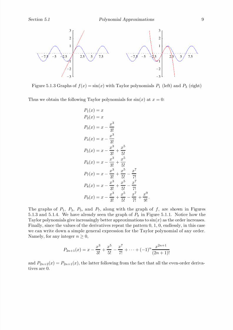
7/27/2019 Calculus 2 (Dan Sloughter)
http://slidepdf.com/reader/full/calculus-2-dan-sloughter 325/598
Section 5.1 Polynomial Approximations 9
-7.5 -5 -2.5 2.5 5 7.5
-3
-2
-1
1
2
3
-7.5 -5 -2.5 2.5 5 7.5
-3
-2
-1
1
2
3
Figure 5.1.3 Graphs of f (x) = sin(x) with Taylor polynomials P 1 (left) and P 3 (right)
Thus we obtain the following Taylor polynomials for sin(x) at x = 0:
P 1(x) = x
P 2(x) = x
P 3(x) = x − x3
3!
P 4(x) = x − x3
3!
P 5(x) = x − x3
3!+
x5
5!
P 6(x) = x − x3
3!+
x5
5!
P 7(x) = x −x3
3! +x5
5! −x7
7!
P 8(x) = x − x3
3!+
x5
5!− x7
7!
P 9(x) = x − x3
3!+
x5
5!− x7
7!+
x9
9!.
The graphs of P 1, P 3, P 5, and P 7, along with the graph of f , are shown in Figures5.1.3 and 5.1.4. We have already seen the graph of P 9 in Figure 5.1.1. Notice how theTaylor polynomials give increasingly better approximations to sin(x) as the order increases.Finally, since the values of the derivatives repeat the pattern 0, 1, 0, endlessly, in this case
we can write down a simple general expression for the Taylor polynomial of any order.Namely, for any integer n ≥ 0,
P 2n+1(x) = x − x3
3!+
x5
5!− x7
7!+ · · · + (−1)n
x2n+1
(2n + 1)!
and P 2n+2(x) = P 2n+1(x), the latter following from the fact that all the even-order deriva-tives are 0.
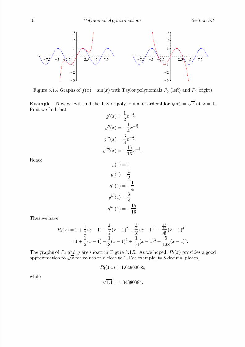
7/27/2019 Calculus 2 (Dan Sloughter)
http://slidepdf.com/reader/full/calculus-2-dan-sloughter 326/598
10 Polynomial Approximations Section 5.1
-7.5 -5 -2.5 2.5 5 7.5
-3
-2
-1
1
2
3
-7.5 -5 -2.5 2.5 5 7.5
-3
-2
-1
1
2
3
Figure 5.1.4 Graphs of f (x) = sin(x) with Taylor polynomials P 5 (left) and P 7 (right)
Example Now we will find the Taylor polynomial of order 4 for g(x) =√
x at x = 1.First we find that
g(x) =1
2
x−1
2
g(x) = −1
4x−
3
2
g(x) =3
8x−
5
2
g(x) = −15
16x−
7
2 .
Henceg(1) = 1
g(1) =1
2
g(1) = −14
g(1) =3
8
g(1) = −15
16.
Thus we have
P 4(x) = 1 +1
2(x − 1) −
14
2(x − 1)2 +
38
3!(x − 1)3 −
1516
4!(x − 1)4
= 1 +
1
2 (x − 1) −1
8 (x − 1)
2
+
1
16 (x − 1)
3
−5
128 (x − 1)
4
.
The graphs of P 4 and g are shown in Figure 5.1.5. As we hoped, P 4(x) provides a goodapproximation to
√ x for values of x close to 1. For example, to 8 decimal places,
P 4(1.1) = 1.04880859,
while √ 1.1 = 1.04880884.
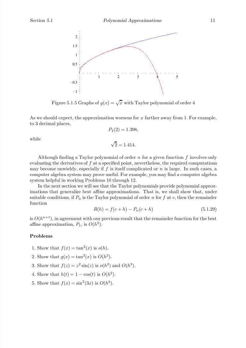
7/27/2019 Calculus 2 (Dan Sloughter)
http://slidepdf.com/reader/full/calculus-2-dan-sloughter 327/598
Section 5.1 Polynomial Approximations 11
1 2 3 4 5
-1
-0.5
0.5
1
1.5
2
Figure 5.1.5 Graphs of g(x) =√
x with Taylor polynomial of order 4
As we should expect, the approximation worsens for x farther away from 1. For example,
to 3 decimal places,P 4(2) = 1.398,
while √ 2 = 1.414.
Although finding a Taylor polynomial of order n for a given function f involves onlyevaluating the derivatives of f at a specified point, nevertheless, the required computationsmay become unwieldy, especially if f is itself complicated or n is large. In such cases, acomputer algebra system may prove useful. For example, you may find a computer algebrasystem helpful in working Problems 10 through 12.
In the next section we will see that the Taylor polynomials provide polynomial approx-imations that generalize best affine approximations. That is, we shall show that, undersuitable conditions, if P n is the Taylor polynomial of order n for f at c, then the remainderfunction
R(h) = f (c + h) − P n(c + h) (5.1.29)
is O(hn+1), in agreement with our previous result that the remainder function for the bestaffine approximation, P 1, is O(h2).
Problems
1. Show that f (x) = tan2(x) is o(h).
2. Show that g(x) = tan2(x) is O(h2).
3. Show that f (z) = z2 sin(z) is o(h2) and O(h3).
4. Show that h(t) = 1 − cos(t) is O(h2).
5. Show that f (x) = sin2(3x) is O(h2).

7/27/2019 Calculus 2 (Dan Sloughter)
http://slidepdf.com/reader/full/calculus-2-dan-sloughter 328/598
12 Polynomial Approximations Section 5.1
6. Show that f (x) = x4
3 is o(h), but not O(h2).
7. For each of the following functions, find the Taylor polynomial of order 4 at the givenpoint c.
(a) f (x) = sin(2x) at c = 0 (b) g(x) = cos(x) at c = 0
(c) f (z) = √ z at c = 4 (d) f (θ) = tan(θ) at θ = 0
(e) h(x) = sin(x) at c = π (f) g(t) = cos(2t) at c = π
(g) f (x) =1
xat c = 1 (h) f (x) = 3x2 + 2x − 9 at c = 0
(i) g(x) =1
1 + x2at c = 0 (j) h(x) = x4 + 5x3 + 4x2 − 9x − 20 at c = 0
(k) g(t) =1
t2at c = 1 (l) h(z) = 8z5 − 3z3 + 6z at c = 0
(m) x(t) = sec(t) at c = 0 (n) f (x) = 3x4 − 4x3 + x2 − 3x − 2 at c = 1
8. Let P 9 be the 9th order Taylor polynomial for f (x) = cos(x) at 0. Graph f and P 9 onthe same axes. On what interval does P 9(x) appear to give a good approximation tocos(x)?
9. Let P 13 be the 13th order Taylor polynomial for f (x) = sin(x) at 0. Graph f and P 13on the same axes. On what interval does P 13(x) appear to give a good approximationto sin(x)?
10. Let P n be the nth order Taylor polynomial for f (x) =1
x2 + 1at 0.
(a) Graph f and P 6 on the same axes. On what interval does P 6(x) appear to give agood approximation to f (x)?
(b) Repeat part (a) for P 10 and P 20.
(c) Do any of the polynomials in parts (a) and (b) appear to give a good approximationto f on the interval [1, 2]?
11. Let P 6 be the 6th order Taylor polynomial for x(t) = tan(t) at 0. Graph x and P 6 onthe same axes and comment.
12. Let P 15 be the 15th order Taylor polynomial for g(x) =√
x at 1. Graph g and P 15 onthe same axes. On what interval does P 15(x) appear to give a good approximation to√
x?

7/27/2019 Calculus 2 (Dan Sloughter)
http://slidepdf.com/reader/full/calculus-2-dan-sloughter 329/598
Difference Equations
Differential Equations
to
Section 5.2
Taylor’s Theorem
The goal of this section is to prove that if P n is the nth order Taylor polynomial for afunction f at a point c, then, under suitable conditions, the remainder function
Rn(h) = f (c + h) − P n(c + h) (5.2.1)
is O(hn+1). This result is a consequence of Taylor’s theorem , which we now state andprove.
Taylor’s Theorem Suppose f is continuous on the closed interval [a, b] and has n + 1continuous derivatives on the open interval (a, b). If x and c are points in (a, b), then
f (x) = f (c) + f (c)(x − c) +f (c)
2!(x − c)2 + · · ·+
f (n)(c)
n!(x − c)n + rn(x), (5.2.2)
where
rn(x) =
x
c
(x − t)n
n!f (n+1)(t)dt. (5.2.3)
That is, if P n is the nth order Taylor polynomial for f at some point c in (a, b) and x isany point in (a, b), then
f (x) = P n(x) + rn(x), (5.2.4)
where rn is given by (5.2.3).
We will show that Taylor’s theorem follows from the Fundamental Theorem of IntegralCalculus combined with repeated applications of integration by parts. Let f be a func-tion satisfying the conditions of the theorem. Since f is an antiderivative of f , by theFundamental Theorem of Integral Calculus we have
f (x) − f (c) =
x
c
f (t)dt. (5.2.5)
Hencef (x) = f (c) +
x
c
f (t)dt, (5.2.6)
which is the statement of Taylor’s theorem when n = 0. For n = 1, we perform anintegration by parts on the integral in (5.2.6) using
u = f (t) dv = dt
du = f (t) v = −(x − t).
1 Copyright c by Dan Sloughter 2000

7/27/2019 Calculus 2 (Dan Sloughter)
http://slidepdf.com/reader/full/calculus-2-dan-sloughter 330/598
2 Taylor’s Theorem Section 5.2
Note that this is not the most obvious choice for v (certainly, v = t would be a simplerchoice), but it is a valid choice and one that leads to the result we desire. Namely, thisgives us
f (x) = f (c) − f (t)(x − t)
x
c
+
x
c
(x − t)f (t)dt
= f (c) + f (c)(x − c) + xc
(x − t)f (t)dt,
which is the statement of Taylor’s theorem for the case n = 1. For n = 2, we performanother integration by parts using
u = f (t) dv = (x− t)dt
du = f (t) v = −(x − t)2
2,
from which we obtain
f (x) = f (c) + f (c)(x − c) − f
(t)(x − t)22
x
c
+ xc
(x − t)22
f (t)dt
= f (c) + f (c)(x − c) +f (c)
2(x − c)2 +
x
c
(x − t)2
2f (t)dt.
Similarly, we obtain Taylor’s theorem for n = 3 by another integration by parts. This timewe have
u = f (t) dv =(x − t)2
2dt
du = f (4)(t) v = −(x − t)3
3!,
which yields
f (x) = f (c) + f (c)(x − c) +f (c)
2(x − c)2 − f (t)(x− t)3
3!
x
c
+
x
c
(x − t)3
3!f (4)(t)dt
= f (c) + f (c)(x − c) +f (c)
2(x − c)2 +
f (c)
3!(x − c)3 +
x
c
(x − t)3
3!f (4)(t)dt.
From this we can see that, for any nonnegative integer n, performing integration by partsn times will yield
f (x) = f (c) + f (c)(x − c) + f
(c)2!
(x − c)2 + f
(c)3!
(x − c)3 + · · ·
+f (n)(c)
n!(x − c)n +
x
c
(x − t)n
n!f (n+1)(t)dt,
(5.2.7)
which is the general statement of Taylor’s theorem.In applying Taylor’s theorem, it is seldom the case that the remainder term rn(x) can
be evaluated exactly. In most cases, we try to find an upper bound for |rn(x)| so that

7/27/2019 Calculus 2 (Dan Sloughter)
http://slidepdf.com/reader/full/calculus-2-dan-sloughter 331/598
Section 5.2 Taylor’s Theorem 3
we know what is the worst possible error that we could commit in approximating f (x)by P n(x). For these purposes, there is an alternative formulation of the remainder termwhich is often more useful than the one given in Taylor’s theorem.
Lagrange’s form of the remainder term Using the same notation as in the statementof Taylor’s theorem, there exists a number k between c and x such that
rn(x) =f (n+1)(k)(x − c)n+1
(n + 1)!. (5.2.8)
To show this, we will assume x > c, the argument in the case x < c being similar. Solet u be the point where f (n+1) attains its maximum value on [c, x] and let v be the pointwhere f (n+1) attains its minimum value on [c, x]. Note that we know such points existbecause we have assumed f (n+1) to be a continuous function on (a, b), and hence on [c, x].Then we have
(x − t)n
n!f (n+1)(v) ≤ (x − t)
n
n!f (n+1)(t) ≤ (x − t)
n
n!f (n+1)(u) (5.2.9)
for all t in [c, x]. Integrating each of the terms in (5.2.9) from c to x, we have
f (n+1)(v)
x
c
(x− t)n
n!dt ≤
x
c
(x − t)n
n!f (n+1)(t)dt ≤ f (n+1)(u)
x
c
(x − t)n
n!dt. (5.2.10)
Now x
c
(x − t)n
n!dt =
(x − t)n+1
(n + 1)!
x
c
=(x − c)n+1
(n + 1)!(5.2.11)
and x
c
(x − t)n
n!f (n+1)(t)dt = rn(x), (5.2.12)
so (5.2.10) implies that
f (n+1)(v)(x − c)n+1
(n + 1)!≤ rn(x) ≤ f (n+1)(u)(x − c)n+1
(n + 1)!. (5.2.13)
Finally, since
g(t) =f (n+1)(t)(x − c)n+1
(n + 1)!
(5.2.14)
is a continuous function of t on the interval [c, x], it follows from (5.2.13) and the Inter-mediate Value Theorem that there exists a number k in [c, x] such that g(k) = rn(x), thatis,
rn(x) =f (n+1)(k)(x − c)n+1
(n + 1)!, (5.2.15)
which is (5.2.8).

7/27/2019 Calculus 2 (Dan Sloughter)
http://slidepdf.com/reader/full/calculus-2-dan-sloughter 332/598
4 Taylor’s Theorem Section 5.2
Of course, we cannot calculate rn(x) exactly without knowing the value of k. However,if we can find a number M such that
|f (n+1)(t)| ≤ M (5.2.16)
for all t between c and x, then (5.2.8) implies that
|rn(x)| ≤ M
(n + 1)!|x − c|n+1. (5.2.17)
Hence, although usually we cannot hope to know the exact amount of error in our approx-imation, in this case we can at least find an upper bound for the size of the error.
We can now show that rn(x) is O((x − c)n+1), or, equivalently, that
Rn(h) = f (c + h) − P n(c + h) (5.2.18)
is O(hn+1). First choose > 0 so that the interval I = [c − , c + ] is contained in theinterval (a, b), and let M be the maximum value of |f (n+1)| on I . Then, using (5.2.17), wehave
|rn(x)| ≤ M
(n + 1)!|x − c|n+1 (5.2.19)
for all x in I . Thus if |h| ≤ ,
|Rn(h)| ≤ M (n + 1)!
|h|n+1, (5.2.20)
from which it follows that Rn(h)
hn+1
≤ M
(n + 1)!. (5.2.21)
That is, Rn(h) is O(hn+1).
Proposition If f satisfies the conditions of Taylor’s theorem and P n is the nth orderTaylor polynomial for f at c, then
Rn(h) = f (c + h) − P n(h) (5.2.22)
is O(hn+1).
Of course, from our previous work we know that this statement implies that Rn(h) isalso o(hn).

7/27/2019 Calculus 2 (Dan Sloughter)
http://slidepdf.com/reader/full/calculus-2-dan-sloughter 333/598
Section 5.2 Taylor’s Theorem 5
With this proposition we may write
f (c + h) = f (c) + f (c)h +f (c)
2!h2 + · · ·+
f (n)(c)
n!hn + O(hn+1), (5.2.23)
or, in terms of x = c + h,
f (x) = f (c) + f (c)(x−c) +f (c)
2!(x−c)2 + · · ·+ f (n)(c)
n!(x−c)n + O((x−c)n+1), (5.2.24)
as long as f is n + 1 times continuously differentiable on an open interval containing c.
Example Recall that the fifth order Taylor polynomial for sin(x) at 0 is
P 5(x) = x − x3
3!+
x5
5!.
Since in this case P 5 = P 6, we now know that
sin(x) = x − x3
3!+
x5
5!+ O(x7).
More explicitly, sinced7
dx7sin(x) = − cos(x),
we have d7
dx7sin(x)
≤ 1
for any value of x. Hence if
r5(x) = sin(x) − P 5(x),then by (5.2.17) it follows that
|r5(x)| ≤ |x|77!
for any value of x. For example,
| sin(1)− P 5(1)| ≤ 1
7!=
1
5040= 0.000198,
to 6 decimal places. That is, the error in approximating sin(1) by P 5(1) is no more than0.000198. In this case the error bound is very close to the actual error, for, to six decimal
place accuracy, sin(1) = 0.841471
and
P 5(1) = 1 − 1
6+
1
120= 0.841667,
which gives an error of sin(1)− P 5(1)| = 0.000196.

7/27/2019 Calculus 2 (Dan Sloughter)
http://slidepdf.com/reader/full/calculus-2-dan-sloughter 334/598
6 Taylor’s Theorem Section 5.2
Note that, in general, for any nonnegative integer n, d2n+3
dx2n+3sin(x)
= | cos(x)|.
Thus d2n+3
dx2n+3sin(x)
≤ 1
for any value of x. Hence, using the fact that in this case P 2n+1 = P 2n+2,
| sin(x) − P 2n+1(x)| ≤ |x|2n+3(2n + 3)!
(5.2.25)
for any value of x. With this inequality we can determine the order necessary for a Taylorpolynomial to give some desired level of accuracy for a particular approximation. Forexample, if we wish to estimate sin(1.4) with an error of less than 0.001 using a Taylorpolynomial about 0, then (5.2.25) says we need only find a nonnegative integer n such that
1.42n+3
(2n + 3)!< 0.001,
in which case P 2n+1(1.4) will provide the desired approximation. For n = 0, 1, 2, and 3,we have the following table:
n1.42n+3
(2n + 3)!
0 0.45733331 0.0448187
2 0.00209153 0.0000569
Hence the smallest value of n that will work is n = 3; thus to attain the desired level of accuracy we would use
P 7(x) = x − x3
3!+
x5
5!− x7
7!.
Checking this to 7 decimal places, we find that
P 7(1.4) = 0.9853938
and sin(1.4) = 0.9854497
an error of only 0.0000559.
Example Combining our work from Section 5.1 about the Taylor polynomial of order 4for f (x) =
√ x at 1 with our new results, we now have
√ x = 1 +
1
2(x − 1) − 1
8(x − 1)2 +
1
16(x − 1)3 − 5
128(x − 1)4 + O((x − 1)5).

7/27/2019 Calculus 2 (Dan Sloughter)
http://slidepdf.com/reader/full/calculus-2-dan-sloughter 335/598
Section 5.2 Taylor’s Theorem 7
If, for example, we wanted to bound the error involved in using P 4(1.6) as an estimate for√ 1.6, we would first note that
f (5)(x) =105
32x9
2
,
which is a decreasing function and hence is maximized on the interval [1 , 1.6] at x = 1.
Thus
|f (5)(x)| ≤ 105
32
for all x in [1, 1.6]. From (5.2.16) it follows that
|√
1.6 − P 4(1.6)| ≤10532
5!|1.6 − 1|5 = 0.0021263,
to 7 decimal places. Checking this on a calculator to 7 decimal places, we have
√ 1.6 = 1.2649111
andP 4(1.6) = 1.2634375,
showing that the error in this case is 0.0014736.
If f is indefinitely differentiable on an interval about a point c and P n is the Taylorpolynomial of order n for f at c, then it is frequently the case that P 1, P 2, P 3, . . . is asequence of increasingly accurate approximating polynomials for f on some interval I
containing the point c. Of course, unless f is itself a polynomial, there is no polynomialP n in this sequence such that f (x) = P n(x) for all x in I . Nevertheless, there are many
functions for whichf (x) = lim
n→∞
P n(x) (5.2.26)
for all x in some interval I . Such functions are said to be analytic . Since a polynomial is just the sum of a finite number of monomials, lim
n→∞
P n(x) may be regarded as an infinite
sum of monomials, an infinite polynomial. That is, if f is an analytic function, then
f (x) = limn→∞
P n(x)
= f (c) + f (c)(x − c) +f (c)
2!(x − c)2 + · · ·+
f (n)(c)
n!(x − c)n + · · ·
=∞n=0
f (n)(c)
n!(x − c)n.
(5.2.27)
for all x in some interval I containing c. An infinite series of this type is called a power
series . Since power series have many of the nice properties of polynomials, such as beingeasy to integrate, a representation of a function f by a power series in this manner can beextremely useful. Although we considered infinite series in Section 1.3, we will need a far
7/27/2019 Calculus 2 (Dan Sloughter)
http://slidepdf.com/reader/full/calculus-2-dan-sloughter 336/598
8 Taylor’s Theorem Section 5.2
more thorough discussion of them before we will be able fully to understand a series like(5.2.27). We will do this in Sections 5.3 through 5.6.
Problems
1. For each of the following functions f , find the Taylor polynomial of order 5 at the pointc, use it to approximate f (a), and find an upper bound for the absolute value of theerror in the approximation.
(a) f (x) = sin(x), c = 0, a = 0.8 (b) f (x) = cos(x), c = 0, a = 1.2
(c) f (x) = sin(2x), c = 0, a = −0.5 (d) f (x) =√
x, c = 1, a = 1.5
(e) f (x) =√
x, c = 9, a = 10 (f) f (x) = x3
2 , c = 1, a = 1.4
(g) f (x) =1
x, c = 1, a = 0.8 (h) f (x) = sin(x), c = 0, a = −1.2
2. Use a Taylor polynomial to approximate sin(0.6) with an error of less than 0.0001.
3. Use a Taylor polynomial to approximate sin(−1.3) with an error of less than 0.00001.4. Use a Taylor polynomial to approximate cos(1.2) with an error of less than 0.0001.
5. Find the Taylor polynomial of smallest order that will approximate sin(x) with anerror of less than 0.0005 for all x in [−2, 2].
6. Suppose L is a function defined on (0,∞) with L(1) = 0 and
L(x) =1
x.
(a) Find P 10, the Taylor polynomial of order 10 for L at 1.
(b) Use P 10 to approximate L(1.5). Find an upper bound for the absolute value of theerror of this approximation.
(c) Find the Taylor polynomial of smallest degree that will approximate L(x) with anerror less than 0.0005 for all x in [1, 1.5].
7. Suppose E is a function defined on (−∞,∞) with E (0) = 1 and E (x) = E (x) for allx.
(a) Find P 10, the Taylor polynomial of order 10 for E at 0.
(b) Use P 10 to approximate E (1).
(c) Given that|E (x)
|< 3x for all x > 0, find an upper bound for the absolute value
of the error in the approximation in part (b).
(d) Find the Taylor polynomial of smallest degree that will approximate E (x) with anerror less than 0.0001 for all x in [0, 2].
8. Let P 9 be the 9th order Taylor polynomial for f (x) = sin(x) at 0. Use P 9 to approxi-mate 3
0
sin(x)
xdx.
7/27/2019 Calculus 2 (Dan Sloughter)
http://slidepdf.com/reader/full/calculus-2-dan-sloughter 337/598
Section 5.2 Taylor’s Theorem 9
9. (a) Find the 6th order Taylor polynomial for f (x) = sin(x2). How is it related to the3rd order Taylor polynomial for g(x) = sin(x)?
(b) Find the 7th order Taylor polynomial for
h(x) =
x
0 sin(t
2
)dt.
How is it related to your answer in (a)?
7/27/2019 Calculus 2 (Dan Sloughter)
http://slidepdf.com/reader/full/calculus-2-dan-sloughter 338/598
Difference Equations
Differential Equations
toSection 5.3
Infinite Series Revisited
Recall from Section 1.3 that for a given sequence {an}, the sequence {sn} with nth term
sn = a1 + a2 + a3 + · · · + an (5.3.1)
is called an infinite series . An individual term sn is called a partial sum and we say theseries is convergent , or has a sum , if lim
n→∞sn exists. If the series is not convergent, we say
it is divergent . We write
limn→∞
sn = a1 + a2 + a3 + · · · + an + · · · =∞n=1
an. (5.3.2)
Example In Section 1.3 we saw that if an = rn, n = 0, 1, 2, . . ., then the associatedinfinite series, called a geometric series, is convergent if and only if −1 < r < 1, in whichcase
∞n=0
rn =1
1 − r. (5.3.3)
For example,∞n=0
13n
= 11 − 1
3
= 32
.
Geometric series comprise one of the few classes of series for which we can evaluate sumsexactly. For most series we can only approximate the sum by computing the partial sumssn for sufficiently large values of n. However, before this procedure becomes meaningful, wemust first know that the series converges. Hence, in this section, as well as in Sections 5.4,5.5, and 5.6, one of our primary goals will be the development of methods for determiningwhether a given series converges or diverges.
We begin by considering several basic properties of infinite series. First, suppose we
know that both∞
n=1an and
∞n=1
bn are convergent series with∞n=1
an = L
and∞n=1
bn = M.
1 Copyright c by Dan Sloughter 2000
7/27/2019 Calculus 2 (Dan Sloughter)
http://slidepdf.com/reader/full/calculus-2-dan-sloughter 339/598
2 Infinite Series Revisited Section 5.3
If sn is the nth partial sum of ∞
n=1an, tn is the nth partial sum of
∞
n=1bn, and un is
the nth partial sum of ∞
n=1(an + bn), then un = sn + tn. Thus
limn→∞
un = limn→∞
(sn + tn) = limn→∞
sn + limn→∞
tn = L + M. (5.3.4)
That is,∞n=1
(an + bn) =∞n=1
an +∞n=1
bn. (5.3.5)
Proposition If ∞
n=1an and
∞
n=1bn both converge, then
∞
n=1(an + bn) converges
and∞n=1
(an + bn) =∞n=1
an +∞n=1
bn. (5.3.6)
Similarly,
∞
n=1(an − bn) converges and
∞n=1
(an − bn) =∞n=1
an −∞n=1
bn. (5.3.7)
Example From our results above, it follows that
∞n=0
1
3n+
1
5n
=∞n=0
1
3n+∞n=0
1
5n=
1
1 − 1
3
+1
1 − 1
5
=3
2+
5
4=
11
4.
Now suppose ∞n=1 an is a convergent series,
∞n=1
an = L,
and k is any constant. If sn is the nth partial sum of ∞
n=1an and tn is the nth partial
sum of the series∞
n=1kan, then tn = ksn. Hence
limn→∞
tn = limn→∞
ksn = k limn→∞
sn = kL. (5.3.8)
That is,∞n=1
kan = k
∞n=1
an. (5.3.9)
Proposition If ∞
n=1an converges and k is any constant, then
∞
n=1an converges and
∞n=1
kan = k
∞n=1
an. (5.3.10)
7/27/2019 Calculus 2 (Dan Sloughter)
http://slidepdf.com/reader/full/calculus-2-dan-sloughter 340/598
Section 5.3 Infinite Series Revisited 3
Example We have
∞n=1
10
2n=
10
2
∞n=1
1
2n−1= 5
∞n=0
1
2n= 5
1
1− 1
2
= 10.
Notice that if ∞
n=1an diverges, then
∞
n=1kan must also diverge for any constant
k = 0. This follows because, if, on the contrary,∞
n=1 kan converged, then, by the previousproposition, so would
∞
n=1an since
∞n=1
an =∞n=1
1
k(kan). (5.3.11)
Proposition If ∞
n=1an diverges, then
∞
n=1kan diverges for any k = 0.
Example In Section 1.3 we saw that the harmonic series
∞n=1
1
n
diverges. It follows that both∞n=1
1
3n=∞n=1
1
3
1
n
and∞
n=1
9
20n=∞
n=1
9
20 1
n
are divergent series.
It is also important to note that since
∞n=1
an =m−1n=1
an +∞
n=m
an (5.3.12)
for any positive integer m, the series∞
n=1an converges if and only if the series
∞
n=m an
converges. In other words, convergence or divergence of a series is never determined by
the behavior of any finite number of terms.
Example It follows from the previous example that
∞n=200
9
20n
diverges.

7/27/2019 Calculus 2 (Dan Sloughter)
http://slidepdf.com/reader/full/calculus-2-dan-sloughter 341/598
4 Infinite Series Revisited Section 5.3
Example The series∞n=4
3
5n
converges. Moreover,
∞n=4
3
5n=∞n=4
3
54
1
5n−4
=
3
625
∞n=0
1
5n=
3
625
1
1 − 1
5
=
3
500.
Now suppose the series∞
n=1an converges with
∞n=1
an = L.
Let sn = a1 + a2 + a3 + · · · + an be the nth partial sum of ∞
n=1 an. Now
an = sn − sn−1,
limn→∞
sn = limn→∞
ni=1
ai =∞i=1
ai = L,
and
limn→∞
sn−1 = limn→∞
n−1i=1
ai =∞i=1
ai = L,
Hence
limn→∞
an = limn→∞
(sn − sn−1) = limn→∞
sn − limn→∞
sn−1 = L − L = 0. (5.3.13)
That is, the nth term of a convergent series must have a limit of 0.
Proposition If ∞
n=1an converges, then
limn→∞
an = 0. (5.3.14)
Note that this result only demonstrates a consequence of a series converging, andso does not provide a criterion to determine convergence. However, it may be useful inshowing that certain series are divergent. Namely, if either the sequence {an} does nothave a limit or
limn→∞
an = 0,
then the series∞
n=1an must diverge. This result is often called the nth term test for
divergence .

7/27/2019 Calculus 2 (Dan Sloughter)
http://slidepdf.com/reader/full/calculus-2-dan-sloughter 342/598
Section 5.3 Infinite Series Revisited 5
Example The series∞n=1
cos
1
n
diverges since
limn→∞
cos
1n
= cos(0) = 1.
Example The series∞
n=1(−1)n diverges since {(−1)n} does not have a limit.
Example Note that
limn→
1
n= 0,
yet the harmonic series∞n=1
1
n
diverges.
p-series
In the next section we will consider a method for determining the convergence or divergenceof a series by comparing a given series with a series which is already known to converge ordiverge. In order to make significant use of such a result it is necessary to have a supply of series whose convergence or divergence is already known. So far geometric series are theonly series we have studied in any detail. Now we will consider the class of series of theform
∞
n=1
1
n p, (5.3.15)
where p is a fixed constant. Such series are called p-series . The following propositioncontains our main result.
Proposition The p-series∞n=1
1
n p, (5.3.16)
converges for p > 1 and diverges for p ≤ 1.
To demonstrate this result, we shall consider four cases. First, suppose p ≤ 0. Then
limn→∞
1
n p=
∞, if p < 0,1, if p = 0.
(5.3.17)
Thus the series diverges by the nth term test for divergence.Next, consider 0 < p < 1. Note that for any n > 0, the partial sum
sn = 1 +1
2 p+
1
3 p+ · · · +
1
n p, (5.3.18)
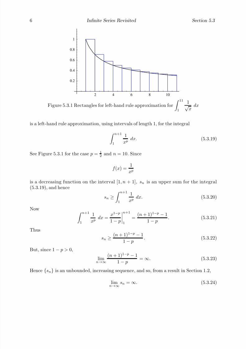
7/27/2019 Calculus 2 (Dan Sloughter)
http://slidepdf.com/reader/full/calculus-2-dan-sloughter 343/598
6 Infinite Series Revisited Section 5.3
2 4 6 8 10
0.2
0.4
0.6
0.8
1
Figure 5.3.1 Rectangles for left-hand rule approximation for
111
1√ x
dx
is a left-hand rule approximation, using intervals of length 1, for the integral
n+11
1
x pdx. (5.3.19)
See Figure 5.3.1 for the case p = 1
2and n = 10. Since
f (x) =1
x p
is a decreasing function on the interval [1, n + 1], sn is an upper sum for the integral(5.3.19), and hence
sn ≥ n+11
1
x pdx. (5.3.20)
Now n+11
1
x pdx =
x1− p
1 − p
n+1
1
=(n + 1)1− p − 1
1− p. (5.3.21)
Thus
sn ≥ (n + 1)1− p − 1
1−
p. (5.3.22)
But, since 1− p > 0,
limn→∞
(n + 1)1− p − 1
1− p= ∞. (5.3.23)
Hence {sn} is an unbounded, increasing sequence, and so, from a result in Section 1.2,
limn→∞
sn = ∞. (5.3.24)

7/27/2019 Calculus 2 (Dan Sloughter)
http://slidepdf.com/reader/full/calculus-2-dan-sloughter 344/598
Section 5.3 Infinite Series Revisited 7
2 4 6 8 10
0.2
0.4
0.6
0.8
1
Figure 5.3.2 Rectangles for right-hand rule approximation for
101
1
x1.5dx
In other words,
∞n=1
1
n p
is a divergent series.For p = 1, the p-series is the harmonic series and so diverges.Finally, consider p > 1. If for any integer n > 1 we let
tn =1
2 p +1
3 p +1
4 p + · · · +1
n p , (5.3.25)
then tn is a right-hand rule approximation, using intervals of length 1, for the integral
n1
1
x pdx. (5.3.26)
See Figure 5.3.2 for the case p = 1.5 and n = 10. Since
f (x) =1
x p
is a decreasing function on the interval [1, n], tn is a lower sum for the integral (5.3.26),and hence
tn ≤ n1
1
x pdx. (5.3.27)
7/27/2019 Calculus 2 (Dan Sloughter)
http://slidepdf.com/reader/full/calculus-2-dan-sloughter 345/598
8 Infinite Series Revisited Section 5.3
Now n1
1
x pdx ≤
∞
1
1
x pdx
= limn→∞
n1
1
x pdx
= limn→∞
x1− p
1 − p
n1
= limn→∞
n1− p − 1
1 − p
=1
p − 1,
(5.3.28)
where the final equality follows from the fact that, since p > 1,
limn→∞
n1− p = limn→∞
1
n p−1= 0. (5.3.29)
Thus
tn ≤ 1
p − 1. (5.3.30)
Now if sn is the nth partial sum of ∞n=1
1
n p,
then s1 = 1 and sn = 1 + tn, n = 2, 3, 4, . . .. Hence
sn ≤ 1 +
1
p − 1 =
p
p − 1 (5.3.31)
for n = 1, 2, 3, . . .. Thus {sn} is a bounded, increasing sequence, and so, from a result inSection 1.2, must have a limit. That is, lim
n→∞sn exists and
∞n=1
1
n p
is a convergent series.
Example The series ∞n=1
1√ n
diverges because it is a p-series with p = 1
2. Moreover, it now follows from our earlier
results that the series∞n=1
3
2√
n

7/27/2019 Calculus 2 (Dan Sloughter)
http://slidepdf.com/reader/full/calculus-2-dan-sloughter 346/598
Section 5.3 Infinite Series Revisited 9
and∞
n=10
1√ n
both diverge as well.
Example The series∞n=1
1
n2
converges because it is a p-series with p = 2. Similar to our last example, it now followsfrom our earlier results that the series
∞n=1
35
6n2
and∞
n=20
7
5n2
both converge as well. Moreover, from (5.3.31), we know that
∞n=1
1
n2≤ 2
2− 1= 2.
In Problem 5 in Section 4.6, you were asked to show that the integral ∞
1
1
x pdx
diverges for p < 1 and converges for p > 1. In Section 6.2 we will see that ∞
1
1
xdx
diverges as well (see also Problem 5 of this section). Combining these facts with our resultsabout p-series, it follows that
∞n=1
1
n p
converges if and only if ∞
1
1x p
dx
converges. This should not be surprising considering the intimate relationship we have seenbetween the partial sums of the series and the left-hand and right-hand rule approximationsfor the integral. The essential ingredient in making these connections was that the function
f (x) =1
x p
7/27/2019 Calculus 2 (Dan Sloughter)
http://slidepdf.com/reader/full/calculus-2-dan-sloughter 347/598
10 Infinite Series Revisited Section 5.3
is continuous, positive, and decreasing on the interval [1,∞) when p > 0. In fact, it can beshown, using arguments similar to those given above, that if g is a continuous, decreasingfunction on [1,∞) with g(x) > 0 for all x ≥ 1, then
∞n=1
g(n)
converges if and only if ∞
1
g(x)dx
converges. You are asked to verify this result, known as the integral test , in Problem 4.
Problems
1. For each of the following infinite series, decide whether the series converges or divergesand explain your answer. If the series is a convergent geometric series, find its sum.
(a)∞n=0
3
5n(b)
∞n=0
4− 1
2n
(c)∞n=1
5
2n+
2
3n
(d)
∞n=1
(−3)n
(e)
∞
n=1
1 −
1
n
(f)
∞
n=1
nsin 1
n
(g)∞
n=10
(−1)n
1000(h)
∞n=2
−3
7
n
2. For each of the following infinite series, decide whether the series converges or divergesand explain your answer.
(a)∞n=1
4
n3(b)
∞n=1
2
n15
(c)∞n=1
1
n2− 5
n4
(d)∞
n=21
3√ n
(e)∞n=1
n−1
3 (f)∞n=1
1
n3
(g)∞n=3
1
234√
n(h)
∞n=5
210 −√ nn2
7/27/2019 Calculus 2 (Dan Sloughter)
http://slidepdf.com/reader/full/calculus-2-dan-sloughter 348/598
Section 5.3 Infinite Series Revisited 11
3. Give an example of divergent series∞
n=1an and
∞
n=1bn for which the series
∞n=1
(an + bn)
converges.
4. Prove the integral test. That is, show that if g is a continuous decreasing function on[1,∞) with g(x) > 0 for all x ≥ 1, then
∞n=1
g(n)
converges if and only if ∞
1
g(x)dx
converges.
5. Use the integral test to determine the convergence or divergence of each of the following.
(a)∞n=1
1
n2 + 3(b)
∞n=2
5√ n− 1
(c)
∞
1
1
xdx (d)
∞n=2
3n√ n2 − 1
6. Find three different examples of divergent series
∞
n=1an with the property that
limn→∞an = 0.7. The following argument has been used to show that
∞n=0
(−1)n =1
2:
Let
L =∞n=0
(−1)n.
ThenL =
∞n=0
(−1)n = 1 +∞n=1
(−1)n = 1−∞n=0
(−1)n = 1 − L.
Thus L = 1 − L, and so L = 1
2. Where is the fallacy in this argument?
7/27/2019 Calculus 2 (Dan Sloughter)
http://slidepdf.com/reader/full/calculus-2-dan-sloughter 349/598
Difference Equations
Differential Equations
to
Section 5.4
Infinite Series:The Comparison Test
In this section we continue our discussion of the convergence properties of infinite series.Now that we have two classes of series, namely, the geometric series and the p-series, forwhich classification as either convergent or divergent is relatively easy, it is reasonable todevelop tests for convergence based on comparing a given series with a series of knownbehavior. We will see this idea first in the comparison test , which we will later generalizewith the limit comparison test .
To begin, suppose
∞
n=1an is a convergent series with an ≥ 0 for all n and
∞
n=1bn
is a series with 0≤
bn≤
an for all n. Let
L =∞n=1
an.
If sn is the nth partial sum of ∞
n=1an and tn is the nth partial sum of
∞
n=1bn, then
tn ≤ sn (5.4.1)
for n = 1, 2, 3, . . .. Since an ≥ 0 for all n, the sequence {sn} is increasing; hence
sn ≤ L (5.4.2)
for all n. Since bn ≥ 0, n = 1, 2, 3, . . ., {tn} is also an increasing sequence which, by(5.4.1) and (5.4.2), is bounded above by L. Hence lim
n→∞tn exists, showing that
∞
n=1bn
converges. Moreover, from (5.4.1),
∞n=1
bn ≤∞n=1
an. (5.4.3)
Now suppose that∞
n=1 an is a divergent series with an ≥ 0 for all n and∞
n=1 bn isa series with an ≤ bn for all n. If sn is the nth partial sum of
∞
n=1an and tn is the nth
partial sum of ∞
n=1bn, then
tn ≥ sn (5.4.4)
for n = 1, 2, 3, . . .. Since an ≥ 0 for all n, {sn} is an increasing sequence; thus, since∞
n=1an diverges, it follows that
limn→∞
sn = ∞.
1 Copyright c by Dan Sloughter 2000

7/27/2019 Calculus 2 (Dan Sloughter)
http://slidepdf.com/reader/full/calculus-2-dan-sloughter 350/598
2 Infinite Series: The Comparison Test Section 5.4
Hence, from (5.4.4), and the fact that {tn} is also an increasing sequence, we have
limn→∞
tn = ∞,
that is, ∞n=1 bn diverges.
The preceding results are summarized in the comparison test.
Comparison Test Suppose an ≥ 0 for n = 1, 2, 3, . . . and∞
n=1an converges. If
0 ≤ bn ≤ an for n = 1, 2, 3, . . ., then∞
n=1bn converges and
∞n=1
bn ≤∞n=1
an. (5.4.5)
Suppose an ≥ 0 for n = 1, 2, 3, . . . and∞
n=1an diverges. If an ≤ bn for n = 1, 2, 3, . . .,
then
∞
n=1bn diverges.
In other words, if the terms of the series∞
n=1 bn are nonnegative and smaller thanthe terms of a series which converges, then
∞
n=1bn must converge; if the terms of the
series∞
n=1bn are larger than those of a divergent series with nonnegative terms, then
∞
n=1bn must diverge.
Example The series∞m=1
1
n2 + 1
converges since
0 <1
n2
+ 1
<1
n2
for n = 1, 2, 3, . . ., and∞n=1
1
n2
is a convergent series (namely, a p-series with p = 2).
Example The series∞n=1
1
2n − 1
diverges since 1
2n − 1>
1
2n> 0
for n = 1, 2, 3, . . ., and∞n=1
1
2n
is a divergent series (since it is a multiple of the harmonic series).

7/27/2019 Calculus 2 (Dan Sloughter)
http://slidepdf.com/reader/full/calculus-2-dan-sloughter 351/598
Section 5.4 Infinite Series: The Comparison Test 3
Example The series∞n=1
sin2(n)
n2
converges since
0 ≤ sin2
(n)n2
≤ 1n2
for n = 1, 2, 3, . . ., and∞n=1
1
n2
is, as in a previous example, a convergent series.
Example The series∞
n=1n + 1
n2
diverges sincen + 1
n2=
n + 1
n
1
n>
1
n> 0
for n = 1, 2, 3, . . ., and∞n=1
1
n,
the harmonic series, is a divergent series.
Example The series∞n=1
1
n3n
converges since
0 <1
n3n≤ 1
3n
for n = 1, 2, 3, . . ., and∞n=1
1
3n
is a convergent series (namely, a geometric series with ratio1
3).We know that if a series
∞
n=1an converges, then lim
n→∞an = 0; however, we have
seen numerous examples, such as the harmonic series, which show the latter condition isnot sufficient to guarantee convergence. To ensure that a series with nth term an ≥ 0satisfying lim
n→∞an = 0 converges, we need additional information about the rate at which
the terms are approaching 0; namely, we need to know that an approaches 0 fast enough toguarantee that the sequence of partial sums, although increasing, is nevertheless bounded.

7/27/2019 Calculus 2 (Dan Sloughter)
http://slidepdf.com/reader/full/calculus-2-dan-sloughter 352/598
4 Infinite Series: The Comparison Test Section 5.4
The problem lies in determining how to measure rates of convergence to 0 and how to decidewhat rates are sufficient for convergence. We have already seen that the comparison test,by comparing an with the terms of a series of known behavior, provides one way to measurewhether or not an is approaching 0 fast enough for the sum to converge. However, findinga series to use for the comparison can be somewhat tricky, even when the behavior of the
series is relatively obvious. For example, the series
∞n=2
1
n2 − 1
should converge, since for large values of n there is very little difference between
1
n2 − 1
and1
n2.
But a direct comparison will not work, since
1
n2 − 1>
1
n2
for n = 2, 3, 4, . . .. Hence it would be useful to have a method for describing the rate atwhich a sequence {an} converges to 0 and a test which exploits this description. We willsupply the former with the next definition, a version of the “O” and “o” notation adaptedfor sequences, and the latter with the limit comparison test.
Definition If {an} and {bn} are sequences with
limn→∞
bn
an= 0, (5.4.6)
then we say bn is o(an). If {an} and {bn} are sequences and there exists an integer N anda constant M such that
bn
an
≤ M (5.4.7)
for all n > N , then we say bn is O(an).Similar to our earlier results, if
limn→∞
bn
an
exists, then bn is O(an) (see Problem 5). Analogous to our earlier use of this notation, if
limn→∞
an = 0,
7/27/2019 Calculus 2 (Dan Sloughter)
http://slidepdf.com/reader/full/calculus-2-dan-sloughter 353/598
Section 5.4 Infinite Series: The Comparison Test 5
limn→∞
bn = 0,
and bn is o(an), then bn is approaching 0 faster than an as n → ∞; if
limn→∞
an = 0,
limn→∞
bn = 0,
and bn is O(an), then bn is approaching 0 at least as fast as an as n → ∞. Of course, if bn is o(an), then bn is also O(an).
Example 1
3n2+4is O
1
n2
since
limn→∞
1
3n2 + 41
n2
= limn→∞
n2
3n2 + 4= lim
n→∞
1
3 +4
n2
=1
3.
Example 1
n4+6is o
1
n3
since
limn→∞
1
n4 + 61
n3
= limn→∞
n3
n4 + 6= lim
n→∞
1
n
1 +6
n4
= 0.
Now consider two series, ∞n=1 an and ∞n=1 bn, where an > 0 and bn
≥0 for all n, bn
is O(an), and∞
n=1 an converges. Then there is an integer N and a constant M such that
bn
an≤ M (5.4.8)
for all n > N . Hencebn ≤ M an (5.4.9)
for all n > N , so the series∞
n=N +1
bn
converges by comparison with the convergent series
∞n=N +1
M an.
Thus∞
n=1bn is also a convergent series.

7/27/2019 Calculus 2 (Dan Sloughter)
http://slidepdf.com/reader/full/calculus-2-dan-sloughter 354/598
6 Infinite Series: The Comparison Test Section 5.4
Next consider two series,∞
n=1an and
∞
n=1bn, where an ≥ 0 and bn > 0 for all n,
an is O(bn), and∞
n=1an diverges. Then there exists an integer N and a constant M > 0
such thatan
bn≤ M (5.4.10)
for all n > N . Hence bn ≥ an
M (5.4.11)
for all n > N , so the series∞
n=N +1
bn
diverges by comparison with the divergent series
∞n=N +1
an
M .
Thus∞
n=1 bn is also a divergent series.The preceding results are summarized in the limit comparison test.
Limit Comparison Test Suppose an > 0 for n = 1, 2, 3, . . . and∞
n=1an converges.
If bn ≥ 0 for n = 1, 2, 3, . . . and bn is O(an), then∞
n=1bn also converges. Suppose an ≥ 0
for n = 1, 2, 3, . . . and∞
n=1an diverges. If bn > 0 for n = 1, 2, 3, . . . and an is O(bn), then
∞
n=1bn also diverges.
In other words, if the terms of the series∞
n=1bn are nonnegative and approach 0
at least as fast as the terms of a convergent series with positive terms, then∞
n=1bn
converges; if the terms of a divergent series are nonnegative and approach 0 at least as fastas the terms of the series
∞
n=1bn, which are positive, then
∞
n=1bn diverges.
Example Consider the series∞n=2
1
n2 − 1.
As mentioned above, we would expect this series to behave very much like the convergentseries
∞n=2
1
n2.
Now
limn→∞
1
n2
− 11
n2
= limn→∞
n
2
n2 − 1 = limn→∞
11 − 1
n2
= 1,
so 1
n2−1is O
1
n2
. Hence
∞n=2
1
n2 − 1
converges by the limit comparison test.
7/27/2019 Calculus 2 (Dan Sloughter)
http://slidepdf.com/reader/full/calculus-2-dan-sloughter 355/598
Section 5.4 Infinite Series: The Comparison Test 7
Example Consider the series∞n=1
2n2
n3 + 2.
Since the nth term of this series is a rational function of n with a numerator of degree
2 and a denominator of degree 3, we might expect this series to behave much like thedivergent series
∞n=1
1
n.
Now
limn→∞
1
n2n2
n3 + 2
= limn→∞
n3 + 2
2n3= lim
n→∞
1
2+
1
n3
=
1
2,
so
1
n is O 2n
2
n3
+2
. Hence∞n=1
2n2
n3 + 2.
diverges by the limit comparison test.
Problems
1. For each of the following infinite series, decide whether the series converges or divergesand explain your answer.
(a)∞n=1
32n
(b)∞n=1
1n3 + 2
(c)∞n=3
2√ n − 2
(d)∞n=1
1√ n3 + 1
(e)∞n=1
π−n (f)∞n=1
cos2(n)
n4
(g)∞n=1
1
3n− n−
3
2
(h)
∞n=1
n
n + 2
2. For each of the following infinite series, decide whether the series converges or divergesand explain your answer.
(a)∞n=1
1
n sin2(n)(b)
∞n=1
n2 + 1
n3 + 2n
(c)∞n=1
3n − 1
2n4 + 2(d)
∞n=1
n − 1
n2n

7/27/2019 Calculus 2 (Dan Sloughter)
http://slidepdf.com/reader/full/calculus-2-dan-sloughter 356/598
8 Infinite Series: The Comparison Test Section 5.4
(e)∞n=1
(n + 1)3−n
n(f)
∞n=1
√ n + 1
2n
(g)∞
n=23
3n5 + 1
13n7 − 2(h)
∞n=2
n + 1
n2 − 2
3. (a) Give an example of a convergent series∞
n=1an and a divergent series
∞
n=1bn
with the property that bn ≤ an for all n.
(b) Give an example of a divergent series∞
n=1an and a convergent series
∞
n=1bn
with the property that an ≤ bn for all n.
(c) Comment on why the comparison test does not apply to the series in (a) and (b).
4. Explain why ∞
1
1
4x5 − 2dx
converges.
5. Show that if
limn→∞
bn
an
exists, then bn is O(an).
7/27/2019 Calculus 2 (Dan Sloughter)
http://slidepdf.com/reader/full/calculus-2-dan-sloughter 357/598
Difference Equations
Differential Equations
to
Section 5.5
Infinite Series:
The Ratio Test
In the last section we saw that we could demonstrate the convergence of a series∞
n=1an,
where an ≥ 0 for all n, by showing that an approaches 0 as n → ∞ as fast as the termsof another series with nonnegative terms which is already known to converge. Both of thetechniques developed in Section 5.4, the comparison test and the limit comparison test,proved to be very useful; however, they both suffer from the drawback of requiring that wefirst find a series of known behavior which allows for the proper comparison with the seriesunder consideration. In this section we shall consider another test for convergence, the ratio
test , which determines whether or not the terms of a series are approaching 0 at a ratesufficient for the series to converge without reference to any other series. Although this testdoes not require knowledge of any other series, it has the limitation of being inconclusivein certain circumstances. Unfortunately, there is no single test for convergence which isuseful under all conditions.
The ratio test determines if the terms of a given series are approaching 0 at a ratesufficient for convergence by considering the ratio between successive terms of the series.Specifically, suppose an > 0 for n = 1, 2, 3, . . . and
limn→∞
an+1
an= ρ. (5.5.1)
If ρ < 1, then there is an integer N and a number r with ρ < r < 1 such that
an+1
an< r (5.5.2)
for all n > N . Thenan+1 < ran (5.5.3)
for all n > N , soaN +2 < raN +1,
aN +3 < raN +2 < r2aN +1,
aN +4 < raN +3 < r3aN +1,
and, in general, for any integer m > 2,
aN +m < rm−1aN +1. (5.5.4)
That is, aN +m
rm−1
< aN +1 (5.5.5)
1 Copyright c by Dan Sloughter 2000

7/27/2019 Calculus 2 (Dan Sloughter)
http://slidepdf.com/reader/full/calculus-2-dan-sloughter 358/598
2 Infinite Series: The Ratio Test Section 5.5
for m = 2, 3, 4, . . .. Letting n = N + m, in which case m = n − N , we have
an
rn−N −1
< aN +1 (5.5.6)
for all n > N + 1. Thus an is O(r
n−N −1
). Moreover,∞n=1
rn−N −1 = r−N ∞n=1
rn−1 (5.5.7)
converges since∞
n=1rn−1 is a geometric series and 0 < r < 1. Thus
∞
n=1an converges
by the limit comparison test.Now suppose ρ > 1, in which we include the possibility that ρ = ∞. Then there is an
integer N such thatan+1
an> 1 (5.5.8)
for all n > N . Hence an+1 > an for all n > N , and so
aN +1 < aN +2 < aN +3 < aN +4 < · · · . (5.5.9)
In particular, an > aN +1 for n = N + 2, N + 3, N + 4, . . .. It follows that either limn→∞
an
does not exist or
limn→∞
an > aN +1 > 0. (5.5.10)
Thus
∞
n=1an diverges by the nth term test for divergence.
We now summarize the above results.Ratio Test Suppose an > 0 for n = 1, 2, 3, . . . and
ρ = limn→∞
an+1
an. (5.5.11)
Then∞
n=1an converges if ρ < 1 and diverges if ρ > 1.
The examples below will show that the ratio test is inconclusive if ρ = 1. Namely,the third example considers a divergent series for which ρ = 1 and the fourth exampleconsiders a convergent series for which ρ = 1. Hence some other test will be necessary to
determine the behavior of any series for which the ratio test yields ρ = 1.
Example For the series∞n=1
n
3n,
if we let
an =n
3n,
7/27/2019 Calculus 2 (Dan Sloughter)
http://slidepdf.com/reader/full/calculus-2-dan-sloughter 359/598
Section 5.5 Infinite Series: The Ratio Test 3
n = 1, 2, 3, . . ., then
ρ = limn→∞
an+1
an= lim
n→∞
n + 1
3n+1n
3n
= limn→∞
n + 1
n
3n
3n+1
=
1
3limn→∞
1 +
1
n
=
1
3.
Thus ρ < 1 and the series converges.
Example For the series∞n=1
5n
n + 2,
if we let
an =5n
n + 2,
n = 1, 2, 3, . . ., then
ρ = limn→∞
an+1
an= lim
n→∞
5n+1
n + 35n
n + 2
= limn→∞
n + 2
n + 3
5n+1
5n
= 5 lim
n→∞
1 + 2n
1 +3
n
= 5.
Thus ρ > 1 and the series diverges.
Example For the harmonic series∞n=1
1
n,
the ratio test yields
ρ = limn→∞
1
n + 11
n
= limn→∞
n
n + 1= lim
n→∞
1
1 +1
n
= 1.
This shows that it is possible for a series to diverge when ρ = 1.
Example For the convergent p-series
∞n=1
1
n2,
the ratio test yields
ρ = limn→∞
1
(n + 1)2
1
n2
= limn→∞
n2
(n + 1)2= lim
n→∞
n
n + 1
2= lim
n→∞
1
1 +1
n
2
= 1.
This shows that is possible for a series to converge when ρ = 1.
7/27/2019 Calculus 2 (Dan Sloughter)
http://slidepdf.com/reader/full/calculus-2-dan-sloughter 360/598
4 Infinite Series: The Ratio Test Section 5.5
Example For the series∞n=1
3n
n!,
if we let
an =3n
n! ,
n = 1, 2, 3, . . ., then
ρ = limn→∞
an+1
an= lim
n→∞
3n+1
(n + 1)!3n
n!
= limn→∞
n!
(n + 1)!
3n+1
3n
= lim
n→∞
3
n + 1= 0.
Thus ρ < 1 and the series converges.
Problems
1. For each of the following infinite series, decide whether the series converges or divergesand explain your answer.
(a)∞n=1
n
2n(b)
∞n=1
2n
n
(c)∞n=1
5n
n!(d)
∞n=1
7n+2
(n + 1)!
(e)
∞n=1
n2
n! (f)
∞n=1
4
n2n
(g)∞n=1
1
n!(h)
∞n=1
πn
5n + 2
2. For each of the following infinite series, decide whether the series converges or divergesand explain your answer.
(a)∞n=1
1√ 4n − 2
(b)∞n=1
3
5n
(c)
∞n=1
3n+5
(2n)!(d)
∞n=1
(2n)!n!n!
(e)∞n=1
n!n!
(2n)!(f)
∞n=1
3n + 2
72n
(g)∞n=1
3n + 1
2n − 1(h)
∞n=1
3
5n− 3n
5n

7/27/2019 Calculus 2 (Dan Sloughter)
http://slidepdf.com/reader/full/calculus-2-dan-sloughter 361/598
Section 5.5 Infinite Series: The Ratio Test 5
3. Define
f (x) =∞n=1
x2n
n.
(a) Find the domain of f . That is, find all values of x for which the series
∞n=1
x2n
n
converges.
(b) Plot an approximation to the graph of f on the domain found in (a) using
f (x) ≈100n=1
x2n
n.
4. Define
g(t) =∞n=0
t2n
n!.
(a) Find the domain of g. That is, find all values of t for which the series
∞n=0
t2n
n!
converges.
(b) Plot an approximation to the graph of g on the interval [−2, 2] using
g(t) ≈50n=0
t2n
n!.
5. Suppose the terms of the series∞
n=1an satisfy the difference equation
an+1 =(n + 1)an
2n
with a1 = 10. Does this series converge or diverge? Explain.
6. Suppose, for n = 1, 2, 3, . . ., an ≥ 0 and
α = limn→∞
n
√ an.
Show that∞
n=1an converges if α < 1 and diverges if α > 1. This result is known as
the root test .

7/27/2019 Calculus 2 (Dan Sloughter)
http://slidepdf.com/reader/full/calculus-2-dan-sloughter 362/598
Difference Equations
Differential Equations
to
Section 5.6
Infinite Series:Absolute Convergence
At this point we have limited our study of series primarily to those series having nonnega-tive terms, the only exceptions being some geometric series and series which are multiplesof series with nonnegative terms. In this section we shall consider the more general questionof series with negative as well as positive terms.
An important consideration when looking at the behavior of an arbitrary series
∞
n=1
an (5.6.1)
is the behavior of the related series∞n=1
|an|. (5.6.2)
Of course, if all the terms of (5.6.1) are nonnegative, then (5.6.1) and (5.6.2) are the sameseries. In any case, (5.6.2) has all nonnegative terms, so we may use our results of thelast three sections to help determine whether or not it converges. Suppose that, by onemethod or another, we have shown that (5.6.2) converges. Then, since
0 ≤ an + |an| ≤ 2|an| (5.6.3)
for any n, we know, by the comparison test, that the series
∞n=1
(an + |an|) (5.6.4)
converges. Hence∞n=1
an =∞n=1
(an + |an|) −∞n=1
|an| (5.6.5)
converges since it is the difference of two convergent series. That is, the convergence of (5.6.2) implies the convergence of (5.6.1).
Proposition If ∞
n=1|an| converges, then
∞
n=1an converges.
Definition The series∞
n=1an is said to converge absolutely if the series
∞
n=1|an|
converges.
With this terminology, the previous proposition says that any series which convergesabsolutely also converges. We shall see later that the converse of this statement does nothold; namely, there are series which converge, but do not converge absolutely.
1 Copyright c by Dan Sloughter 2000

7/27/2019 Calculus 2 (Dan Sloughter)
http://slidepdf.com/reader/full/calculus-2-dan-sloughter 363/598
2 Infinite Series: Absolute Convergence Section 5.6
Example The series
∞n=1
(−1)n
n2= −1 +
1
4− 1
9+
1
16− 1
25+ · · ·
converges absolutely since the series
∞n=1
(−1)n
n2
=∞n=1
1
n2
converges. In particular, it follows that
∞n=1
(−1)n
n2
converges.
Example The series
∞n=1
(−1)n+1
n= 1 − 1
2+
1
3− 1
4+
1
5− 1
6+ · · · ,
known as the alternating harmonic series , is not absolutely convergent since
∞
n=1
(−1)n+1
n
=
∞
n=1
1
n
is the harmonic series, which diverges. Hence the previous proposition does not provide anyinformation on the behavior of the alternating harmonic series itself. We shall see belowthat in fact the alternating harmonic series converges even though it is not absolutelyconvergent.
In general, determining whether a series which is not absolutely convergent is conver-gent or divergent is a difficult problem. However, there is one particular type of series forwhich we have, under certain conditions, a simple test. These series are the alternating
series , the series which, like those in the previous examples, alternate in sign from oneterm to the next.
Definition A series in which the terms are alternately positive and negative is called analternating series .
Now suppose∞
n=1 an is an alternating series which satisfies the following two condi-tions:
(1) |an+1| ≤ |an| for n = 1, 2, 3, . . . ,
(2) limn→∞
|an| = 0.

7/27/2019 Calculus 2 (Dan Sloughter)
http://slidepdf.com/reader/full/calculus-2-dan-sloughter 364/598
Section 5.6 Infinite Series: Absolute Convergence 3
For the sake of the discussion we will assume that a1 > 0, although that will not affect ourconclusion. If sn is the nth partial sum of this series, then
s1 = a1, (5.6.6)
and, since a2 < 0,s2 = a1 + a2 = s1 + a2 < s1. (5.6.7)
Next, since a3 > 0,s3 = a1 + a2 + a3 = s2 + a3 > s2. (5.6.8)
Moreover, condition (1) implies a2 + a3 ≤ 0, from which it follows that
s3 = a1 + a2 + a3 = s1 + a2 + a3 ≤ s1. (5.6.9)
Thus we have s2 ≤ s3 ≤ s1. Next,
s4 = s3 + a4 < s3 (5.6.10)
since a4 < 0 ands4 = s2 + a3 + a4 ≥ s2 (5.6.11)
since a3 + a4 ≥ 0. Thus s2 ≤ s4 ≤ s3 ≤ s1. For the next step,
s5 = s4 + a5 > s4 (5.6.12)
since a5 > 0 ands5 = s3 + a4 + a5
≤s3 (5.6.13)
since a4 + a5 ≤ 0. Thus s2 ≤ s4 ≤ s5 ≤ s3 ≤ s1. Continuing in this way, we see that
s2 ≤ s4 ≤ s6 ≤ s5 ≤ s3 ≤ s1 (5.6.14)
ands2 ≤ s4 ≤ s6 ≤ s7 ≤ s5 ≤ s3 ≤ s1. (5.6.15)
In general, for any positive integer n,
s2 ≤ s4 ≤ · · · ≤ s2n ≤ · · · ≤ s2n−1 ≤ · · · ≤ s5 ≤ s3 ≤ s1. (5.6.16)
That is, for n = 1, 2, 3, . . ., {s2n} is a bounded increasing sequence and {s2n−1} is abounded decreasing sequence. Thus both sequences have limits, say
limn→∞
s2n = L (5.6.17)
andlimn→∞
s2n−1 = M. (5.6.18)

7/27/2019 Calculus 2 (Dan Sloughter)
http://slidepdf.com/reader/full/calculus-2-dan-sloughter 365/598
4 Infinite Series: Absolute Convergence Section 5.6
But then
L − M = limn→∞
s2n − limn→∞
s2n−1 = limn→∞
(s2n − s2n−1) = limn→∞
a2n = 0,
where the final equality follows from condition (2). Hence L = M , so
limn→∞
sn = L. (5.6.19)
In other words,∞
n=1 an converges. This conclusion, known as Leibniz’s theorem , gives asimple criterion for determining the convergence of some alternating series.
Leibniz’s theorem Suppose∞
n=1an is an alternating series for which |an+1| ≤ |an|
for n = 1, 2, 3, . . .. If limn→∞
|an| = 0, (5.6.20)
then∞
n=1 an converges.Example The alternating harmonic series
∞n=1
(−1)n+1
n
satisfies the conditions of Leibniz’s theorem: If we let
an =(−1)n+1
n,
n = 1, 2, 3, . . ., then
|an+1| =1
n + 1<
1
n= |an|
and
limn→∞
|an| = limn→∞
1
n= 0.
Thus, as we claimed earlier, the alternating harmonic series converges.
Definition A series which converges but does not converge absolutely is said to converge
conditionally .
The previous example shows that the alternating harmonic series is an example of aseries which converges conditionally.
From the discussion prior to Leibniz’s theorem, we see that if ∞
n=1an satisfies the
conditions of Leibniz’s theorem, a1 > 0, sn is its nth partial sum, and
s =∞n=1
an, (5.6.21)
7/27/2019 Calculus 2 (Dan Sloughter)
http://slidepdf.com/reader/full/calculus-2-dan-sloughter 366/598
Section 5.6 Infinite Series: Absolute Convergence 5
then we must have
s2 ≤ s4 ≤ · · · ≤ s6 ≤ · · · ≤ s ≤ · · · ≤ s5 ≤ s3 ≤ s1. (5.6.22)
Note that for any positive integer n we have sn+1 ≤ s ≤ sn if n is odd and sn ≤ s ≤ sn+1
if n is even. Thus, in either case,
|s − sn| ≤ |sn+1 − sn| = |an+1|, (5.6.23)
a result which also holds if a1 < 0
Proposition Suppose∞
n=1an is a convergent alternating series for which |an+1| ≤ |an|
for n = 1, 2, 3, . . .. If
s =∞n=1
an (5.6.24)
andsn =
nj=1
aj , (5.6.25)
then, for any n = 1, 2, 3, . . .,|s − sn| ≤ |an+1|. (5.6.26)
Hence for those alternating series which satisfy the conditions of the proposition, theerror committed in approximating the sum of the series by a particular partial sum is nogreater in absolute value than the absolute value of the next term in the series.
Example For the alternating harmonic series, if
s =∞n=1
(−1)n+1
n
and
sn = 1 − 1
2+
1
3− 1
4+ · · · +
(−1)n+1
n=∞j=1
(−1)j+1
j,
then
|s
−sn
| ≤1
n + 1for n = 1, 2, 3, . . .. For example
s100 = 1 − 1
2+
1
3− 1
4+ · · · +
1
99− 1
100= 0.688172,
so
|s − s100| ≤ 1
101= 0.009901,
7/27/2019 Calculus 2 (Dan Sloughter)
http://slidepdf.com/reader/full/calculus-2-dan-sloughter 367/598
6 Infinite Series: Absolute Convergence Section 5.6
where both results have been rounded to 6 decimal places. In other words, the sum of thealternating harmonic series differs from 0.688172 by less than 0.009901. In fact, since thenext term in the series is positive, we know that s must lie between 0.688172 and
0.688172 + 0.009901 = 0.698073.
We will see in Section 6.2 that the sum of the alternating harmonic series is exactly thenatural logarithm of 2, which, to 6 decimal places, is 0.693147
Problems
1. For each of the following infinite series, answer the questions: Does the series convergeabsolutely? Does the series converge conditionally? Does the series converge?
(a)∞n=1
(−1)n−1
n3(b)
∞n=1
(−1)n√ n
(c)∞n=1
3n2 − 14n2 + 2
(d)∞n=0
(−3)nn!
(e)∞n=1
(−1)n+1√ n + 3
(f)∞n=3
(−1)nπn
(g)∞n=0
(−1)nn!
2n(h)
∞n=1
−2
3
n−1
2. For each of the following infinite series, answer the questions: Does the series convergeabsolutely? Does the series converge conditionally? Does the series converge?
(a)∞n=1
(−1)n+1(n2 + 1)3n5 − 2
(b)∞n=0
− 35n
(c)∞n=0
32n
(2n)!(d)
∞n=0
(−1)n22n+1
(2n + 1)!
(e)∞n=0
(−1)nπ2n
(2n)!(f)
∞n=14
(−2)n√ n + 1
(g)∞n=1
(−1)n(n + 1)
2n − 1(h)
∞n=2
1 − n
2n2
3. (a) Approximate
s =∞n=0
(−1)n
n!
using
s15 =15n=0
(−1)n
n!.
7/27/2019 Calculus 2 (Dan Sloughter)
http://slidepdf.com/reader/full/calculus-2-dan-sloughter 368/598
Section 5.6 Infinite Series: Absolute Convergence 7
(b) Find an upper bound for the error in approximating s by s15.
(c) Find the smallest n such that the absolute value of the error in approximating s
by
sn =n
j=0
(−1)j
j!
is less than 0.000001. What is this approximation?
4. (a) Approximate
s =∞n=1
(−1)n+1
n2n
by
s50 =50n=1
(−1)n+1
n2n.
(b) Find an upper bound for the absolute value of the error in approximating s by s50.
(c) Find the smallest n such that the absolute value of the error in approximating s
by
sn =n
j=1
(−1)j+1
j2j
is less than 0.0001. What is this approximation?
5. In our development of Leibniz’s theorem, we assumed that a1 > 0. Discuss the changeswhich must be made in the discussion if a1 < 0.
7/27/2019 Calculus 2 (Dan Sloughter)
http://slidepdf.com/reader/full/calculus-2-dan-sloughter 369/598
Difference Equations
Differential Equations
toSection 5.7
Power Series
We are now in a position to pick up the story we left off in Section 5.2: the extension of Taylor polynomials to Taylor series. We shall see that a Taylor series is a type of infiniteseries whose nth partial sum is a Taylor polynomial. Such series are examples of powerseries, objects that we will study in this section before considering Taylor series in Section5.8.
Definition An infinite series of the form
∞n=0
an(x − c)n = a0 + a1(x − c) + a2(x − c)2 + · · · (5.7.1)
is called a power series in x about c.
Example The infinite series
∞n=0
xn
n!= 1 + x +
x2
2!+
x3
3!+ · · ·
is a power series in x about 0. Note that if we let
bn =xn
n!
= |x|n
n!
for n = 0, 1, 2, . . ., then
limn→∞
bn+1
bn= lim
n→∞
|x|n+1
(n + 1)!
|x|n
n!
= limn→∞
|x|
n + 1= 0
for any value of x. That is, by the ratio test, the series is absolutely convergent, and
hence convergent, for any value of x. Thus if we define a function, called the exponential function , by
exp(x) =∞n=0
xn
n!(5.7.2)
then this function is defined for all values of x. We shall have much more to say about thisfunction, which may be thought of as the simplest “infinite” polynomial which is definedfor all real numbers, in Chapter 6.
1 Copyright c by Dan Sloughter 2000
7/27/2019 Calculus 2 (Dan Sloughter)
http://slidepdf.com/reader/full/calculus-2-dan-sloughter 370/598
2 Power Series Section 5.7
Notice that the convergence of (5.7.2) for all x implies, by the nth term test for diver-gence, that
limn→∞
xn
n!= 0 (5.7.3)
for any value of x. We have seen particular cases of this limit in the past, but this is the
first time we have had a simple proof that it is always 0.
Example Recall that the Taylor polynomial of order 2n + 1 for sin(x) at 0 is
P 2n+1(x) =n
k=0
(−1)kx2k+1
(2k + 1)!.
Hence P 2n+1(x) is a partial sum of the power series
∞
k=0
(−1)kx2k+1
(2k + 1)!
. (5.7.4)
If, for k = 0, 1, 2, . . ., we let
bk =
(−1)kx2k+1
(2k + 1)!
=|x|2k+1
(2k + 1)!,
then
limk→∞
bk+1
bk= lim
k→∞
|x|2k+3
(2k + 3)!
|x|
2k+1
(2k + 1)!
= limk→∞
|x|2
(2k + 3)(2k + 2)= 0
for all values of x. Thus, by the ratio test, (5.7.4) is absolutely convergent, and henceconvergent, for all values of x. Moreover, from our work in Section 5.2, we know that
| sin(x)− P 2n+1(x)| ≤|x|2n+3
(2n + 3)!
for all values of x. Since (using (5.7.3))
limn→∞
|x|
2n+3
(2n + 3)! = 0,
it follows thatlimn→∞
| sin(x)− P 2n+1(x)| = 0
for all values of x. Hencesin(x) = lim
n→∞P 2n+1(x)

7/27/2019 Calculus 2 (Dan Sloughter)
http://slidepdf.com/reader/full/calculus-2-dan-sloughter 371/598
Section 5.7 Power Series 3
for all values of x. That is, for any value of x,
sin(x) =∞k=0
(−1)kx2k+1
(2k + 1)!. (5.7.5)
Example The series∞
n=0 xn is a power series in x about 0. From our work on geometricseries, we know that this series will converge absolutely when −1 < x < 1 and will divergeotherwise. In fact, we have seen that
1
1− x=
∞n=0
xn
for −1 < x < 1.
These examples show that some functions may be expressed as power series. Suchfunctions are examples of analytic functions , which we now define.
Definition If f is a function for which there exists constants a0, a1, a2, . . . such that
f (x) =∞n=0
an(x − c)n (5.7.6)
for all values of x in some open interval about c, then we say f is analytic at c. If for someh > 0 the equality (5.7.6) holds for all x in the interval I = (c − h, c + h), then we say f
is analytic on I and we call∞
n=0
an(x − c)n
a power series representation of f on I .
Example From the previous examples we see that
f (x) = exp(x)
andg(x) = sin(x)
are analytic on (−∞,∞) and
h(x) =1
1 − xis analytic on (−1, 1).
Before we can work effectively with power series we need to consider their convergencebehavior. First note that the power series
∞n=0
an(x − c)n (5.7.7)

7/27/2019 Calculus 2 (Dan Sloughter)
http://slidepdf.com/reader/full/calculus-2-dan-sloughter 372/598
4 Power Series Section 5.7
converges at x = c since in that case all terms after the first are 0. Next, suppose theseries converges at a point x = c + r, where r > 0. That is, suppose
∞
n=0 anrn converges.Then, by the nth term test for divergence,
limn→∞
anrn = 0. (5.7.8)
In particular, there exists an integer N such that
|anrn| < 1 (5.7.9)
for all n > N . Hence for any x and n > N ,
|an(x − c)n|
x − c
r n = |anrn| < 1. (5.7.10)
In particular, |an(x − c)n| is
O
x − c
r
n
.
Now if c − r < x < c + r, then x − c
r
< 1
and∞
n=0
x − c
rn
is a convergent geometric series. Thus, by the limit comparison test,
∞n=0
an(x − c)n
converges absolutely. In other words, we have shown that if (5.7.7) converges at c + r withr > 0, then it converges absolutely for all x in (c− r, c + r). The same argument works toshow that if (5.7.7) converges at c− r with r > 0, then it converges absolutely for all x in
(c− r, c + r). Letting R be the largest real number such that (5.7.7) converges absolutelyfor all x for which |x − c| < R, where we allow R = ∞ if (5.7.7) converges for all x, itfollows that
∞n=0
an(x − c)n
converges absolutely on (c − R, c + R) ((−∞,∞) if R = ∞) and diverges for all x with|x − c| > R.

7/27/2019 Calculus 2 (Dan Sloughter)
http://slidepdf.com/reader/full/calculus-2-dan-sloughter 373/598
Section 5.7 Power Series 5
Proposition For a power series
∞n=0
an(x − c)n,
there exists an R, with R = 0, R > 0, or R = ∞, such that the series converges absolutelyfor all x satisfying |x − c| < R and diverges for all x satisfying |x − c| > R.
Definition With the notation of the previous proposition, the interval (c − R, c + R)((−∞,∞) if R = ∞) is called the interval of convergence and R is called the radius of
convergence of the power series.
Note that the proposition does not say anything about the behavior of the series atx = c − R or x = c + R. In fact, any type of behavior is possible at the endpoints of theinterval of convergence; for a given series, these points must be checked individually forconvergence. Moreover, although the proposition does not provide a method for findingthe interval of convergence of a series, the next examples illustrate that the ratio test is
very useful in this regard.
Example Consider the power series
∞n=1
(−1)n+1xn
n2n. (5.7.11)
If we let
bn =
(−1)n+1xn
n2n
=|x|n
n2n,
then
limn→∞
bn+1
bn= lim
n→∞
|x|n+1
(n + 1)2n+1
|x|n
n2n
= limn→∞
n
n + 1
|x|
2=|x|
2.
Hence, by the ratio test, (5.7.11) is absolutely convergent when
|x|
2< 1,
that is, when −2 < x < 2. Thus the radius of convergence is R = 2 and the interval of convergence is (−2, 2). Now at x = −2, (5.7.11) becomes
∞n=1
(−1)n+1(−2)n
n2n=
∞n=1
(−1)n+1(−1)n2n
n2n=
∞n=1
(−1)2n+1
n=
∞n=1
−1
n,
which is a multiple of the harmonic series and hence divergent. At x = 2, (5.7.11) becomes
∞n=1
(−1)n+12n
n2n=
∞n=1
(−1)n+1
n,

7/27/2019 Calculus 2 (Dan Sloughter)
http://slidepdf.com/reader/full/calculus-2-dan-sloughter 374/598
6 Power Series Section 5.7
which is the alternating harmonic series and hence convergent, although not absolutelyconvergent. Putting this together, we see that the power series
∞
n=1(−1)n+1xn
n2n
converges absolutely for all x in (−2, 2), converges conditionally at x = 2, and diverges forall other x.
Example In the first example of this section we used the ratio test to show that thepower series
∞n=1
xn
n!
converges absolutely for all values of x. Hence in this case the interval of convergence is(−∞,∞) and the radius of convergence is R = ∞.
Example Consider the power series∞
n=1 n!xn. If we let
bn = |n!xn| = n!|x|n,
then
limn→∞
bn+1
bn= lim
n→∞
(n + 1)!|x|n+1
n!|x|n= lim
n→∞(n + 1)|x| =
0, if x = 0,∞, if x = 0.
Hence, by the ratio test, this power series converges only when x = 0. Accordingly, theradius of convergence is R = 0.
Example Consider the power series
∞n=1
(x − 1)n
n. (5.7.12)
If we let
bn =
(x − 1)n
n
=|x − 1|n
n,
then
limn→∞
bn+1
bn = limn→∞
|x − 1|n+1
n + 1
|x − 1|n
n
= limn→∞ n
n + 1|x − 1| = |x − 1|.
Using the ratio test, we see that (5.7.12) converges absolutely when |x− 1| < 1. Thus theradius of convergence is R = 1 and the interval of convergence is (0, 2). At x = 0, (5.7.12)becomes
∞n=1
(−1)n
n= −
∞n=1
(−1)n+1
n,
7/27/2019 Calculus 2 (Dan Sloughter)
http://slidepdf.com/reader/full/calculus-2-dan-sloughter 375/598
Section 5.7 Power Series 7
which is a multiple of the alternating harmonic series and so converges conditionally. Atx = 2, (5.7.12) becomes
∞n=1
1
n,
which is the harmonic series and so diverges. Hence the power series
∞n=1
(x − 1)n
n
converges absolutely for x in the interval (0, 2), converges conditionally at x = 0, anddiverges for all other x.
A power series resembles a polynomial; in fact, often it is convenient to think of a powerseries as a polynomial of infinite degree. Among the many nice properties of polynomialsis the ease with which they may be differentiated and integrated. Our next result states
that power series may be differentiated and integrated term by term in the same manneras polynomials. Although we have the tools to provide justifications for these statements,they are technical and perhaps best left to a more advanced text.
Differentiation and integration of power series Suppose the radius of convergenceof the power series
∞n=0
an(x − c)n
is R > 0 and let
f (x) =∞
n=0
an(x − c)n
for x in (c −R, c + R). Then
f (x) =∞n=0
d
dxan(x − c)n =
∞n=1
nan(x − c)n−1 (5.7.13)
for all x in (c −R, c + R) and
b
c
f (x)dx =∞
n=0
b
c
an(x − c)ndx =∞
n=0
an(b− c)n+1
n + 1
(5.7.14)
for all b in (c −R, c + R).
Example Recall that the interval of convergence of
exp(x) =∞n=0
xn
n!

7/27/2019 Calculus 2 (Dan Sloughter)
http://slidepdf.com/reader/full/calculus-2-dan-sloughter 376/598
8 Power Series Section 5.7
is (−∞,∞). Hence
d
dxexp(x) =
d
dx
∞n=0
xn
n!
=∞
n=0
d
dxxn
n!
=∞n=1
nxn−1
n!
=∞n=1
xn−1
(n − 1)!
=∞n=0
xn
n!
= exp(x)
for all x in (−∞,∞). That is, the function exp(x) is its own derivative. We will have muchmore to say about this interesting property of the exponential function in Chapter 6.
Example From our work above we know that
sin(x) =∞n=0
(−1)nx2n+1
(2n + 1)!
for all x in (−∞,∞). Now
x0
sin(t)dt = − cos(t)x0
= − cos(x) + 1
for any x. However, we also know that
x
0
sin(t)dt =
x
0
∞n=0
(−1)nt2n+1
(2n + 1)!
dt
=∞n=0
x
0
(−1)nt2n+1
(2n + 1)!dt
=∞n=0
(−1)n
t2n+2
(2n + 2)(2n + 1)!
x
0
=∞n=0
(−1)nx2n+2
(2n + 2)!
=∞n=1
(−1)n−1x2n
(2n)!.
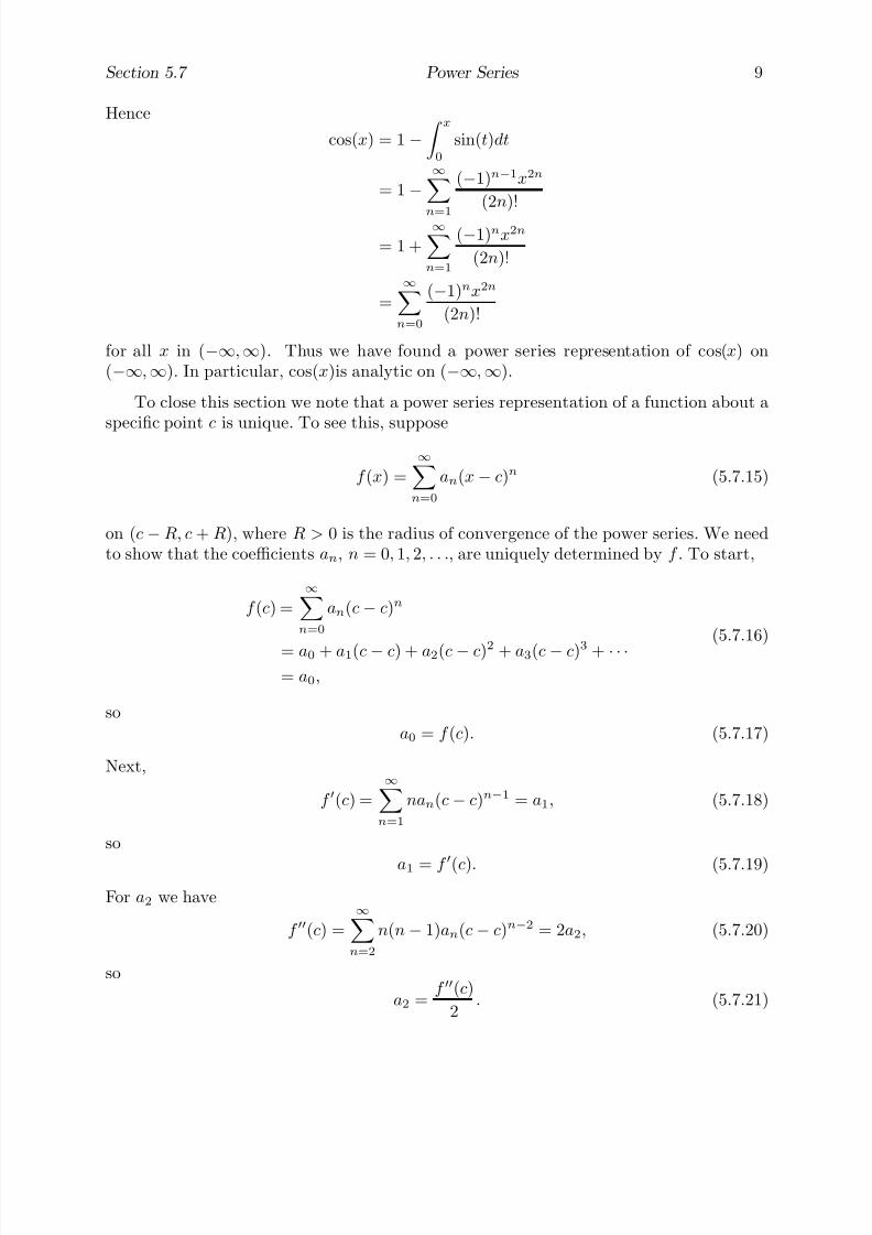
7/27/2019 Calculus 2 (Dan Sloughter)
http://slidepdf.com/reader/full/calculus-2-dan-sloughter 377/598
Section 5.7 Power Series 9
Hence
cos(x) = 1 −
x
0
sin(t)dt
= 1 −∞
n=1
(−1)n−1x2n
(2n)!
= 1 +∞n=1
(−1)nx2n
(2n)!
=∞n=0
(−1)nx2n
(2n)!
for all x in (−∞,∞). Thus we have found a power series representation of cos(x) on(−∞,∞). In particular, cos(x)is analytic on (−∞,∞).
To close this section we note that a power series representation of a function about aspecific point c is unique. To see this, suppose
f (x) =∞n=0
an(x − c)n (5.7.15)
on (c −R, c + R), where R > 0 is the radius of convergence of the power series. We needto show that the coefficients an, n = 0, 1, 2, . . ., are uniquely determined by f . To start,
f (c) =∞n=0
an(c− c)n
= a0 + a1(c− c) + a2(c − c)2 + a3(c − c)3 + · · ·= a0,
(5.7.16)
soa0 = f (c). (5.7.17)
Next,
f (c) =∞n=1
nan(c− c)n−1 = a1, (5.7.18)
so
a1 = f
(c). (5.7.19)
For a2 we have
f (c) =∞n=2
n(n− 1)an(c − c)n−2 = 2a2, (5.7.20)
so
a2 =f (c)
2. (5.7.21)
7/27/2019 Calculus 2 (Dan Sloughter)
http://slidepdf.com/reader/full/calculus-2-dan-sloughter 378/598
10 Power Series Section 5.7
In general, for k = 0, 1, 2, . . .,
f (k)(c) =∞n=k
n(n− 1) · · · (n − k + 1)an(c− c)n−k = k!ak, (5.7.22)
from which it follows that
ak =f (k)(c)
k!. (5.7.23)
As a consequence, the power series representation of f about c is uniquely determined bythe values of the derivatives of f at c.
Proposition Suppose
f (x) =∞
n=0an(x − c)n (5.7.24)
on (c −R, c + R), where R > 0 is the radius of convergence of the power series. Then
an =f (n)(c)
n!(5.7.25)
for n = 0, 1, 2, . . ..
Note that the coefficients an as given by (5.7.25) are the same as the coefficients usedin the definition of the Taylor polynomial of f at c. This observation leads immediatelyto the question of extending Taylor polynomials to Taylor series, the topic of Section 5.8.
Our final example of this section illustrates how (5.7.25) may be used to find thederivatives of f at c if we already know a power series representation for f about c.
Example In a previous example we saw that if
f (x) =1
1− x,
then
f (x) =∞
n=0
xn
for all x in (−1, 1). In this series, the coefficient of xn is 1 for all n, so, by the previousproposition,
1 =f (n)(0)
n!
for n = 0, 1, 2, . . .. That is, f (n)(0) = n! for all n.
7/27/2019 Calculus 2 (Dan Sloughter)
http://slidepdf.com/reader/full/calculus-2-dan-sloughter 379/598
Section 5.7 Power Series 11
Problems
1. For each of the following power series, find the interval of convergence and determinethe behavior of the series at the endpoints of the interval. State clearly where the seriesconverges absolutely, where it converges conditionally, and where it diverges. Also, for
each series write out the first 5 nonzero terms.
(a)∞n=1
xn
n(b)
∞n=1
(−1)n+1xn
n
(c)∞n=1
nxn (d)∞n=0
x2n
n!
(e)∞n=0
(x − 2)n+1
n + 1(f)
∞n=0
(−1)nxn
3n
(g)
∞n=1
(x − 1)n
n2 (h)
∞n=1
n3
x2n
2. For each of the following power series, find the interval of convergence and determinethe behavior of the series at the endpoints of the interval. State clearly where the seriesconverges absolutely, where it converges conditionally, and where it diverges. Also, foreach series write out the first 5 nonzero terms.
(a)∞n=0
(x − 3)n
n!(b)
∞n=1
xn
n5n
(c)∞
n=0
x2n
2n
(d)∞
n=1
(−1)n+1(x − 6)n
n3n
(e)∞n=1
x2n+1
n(f)
∞n=0
(−1)n(x − 1)2n
(2n)!
(g)∞n=1
3nxn (h)∞n=0
(−1)nx2n+1
(2n + 1)(2n + 1)!
3. (a) Using the fact that
1
1− x=
∞
n=0xn
for −1 < x < 1, find a power series representation about 0 for
f (x) =1
1 + x
on (−1, 1).
(b) Use your result from (a) to find f (35)(0).

7/27/2019 Calculus 2 (Dan Sloughter)
http://slidepdf.com/reader/full/calculus-2-dan-sloughter 380/598
12 Power Series Section 5.7
(c) Use your result from (a) to find a power series representation about 0 for
x
0
1
1 + tdt
on (−1, 1). Determine where the series converges absolutely, where it convergesconditionally, and where it diverges.
(d) Use your result from (c) to find an infinite series representation for
10
1
1 + tdt.
Use this series to estimate the integral with an error of no more than 0.001 inabsolute value.
4. Use the power series representations of sin(x) and cos(x) about 0 to prove the following
identities.(a) sin(−x) = − sin(x) (b) cos(−x) = cos(x)
(c)d
dxsin(x) = cos(x) (d)
d
dxcos(x) = − sin(x)
5. Using the power series representation of cos(x) about 0, find an infinite series repre-sentation of cos(1). Use the infinite series to estimate cos(1) with an error of no morethan 0.000001.
6. Use the fact thatd
dx 1
1 − x =1
(1− x)2
to find a power series representation about 0 for
g(x) =1
(1− x)2.
Find the interval of convergence for this power series and determine the behavior of the series at the endpoints.
7. Use your result from Problem 6 to evaluate
∞n=1
n
2n−1 .
8. (a) A fair coin is tossed repeatedly. In Section 1.3 we saw that the probability that ahead appears for the first time on the nth toss is
P n =1
2n

7/27/2019 Calculus 2 (Dan Sloughter)
http://slidepdf.com/reader/full/calculus-2-dan-sloughter 381/598
Section 5.7 Power Series 13
for n = 1, 2, 3, . . .. The average number of tosses before the first head appears isthen given by
A =∞n=1
nP n.
Use Problem 7 to find A.(b) A manufacturer of circuit boards tests every board as it comes off the assembly
line. If the probability that a board passes the test is p and the probability thatit fails is q = 1 − p, then the probability that n boards are tested before the firstdefective board is encountered is P n = pn−1q . The average number of boardstested before finding a defective one is then
A =∞n=1
nP n.
Find A.
7/27/2019 Calculus 2 (Dan Sloughter)
http://slidepdf.com/reader/full/calculus-2-dan-sloughter 382/598
Difference Equations
Differential Equations
to
Section 5.8
Taylor Series
In this section we will put together much of the work of Sections 5.1-5.7 in the context of a discussion of Taylor series. We begin with two definitions.
Definition If f is a function such that f (n) is continuous on an open interval (a, b) forn = 0, 1, 2, . . ., then we say f is C ∞ on (a, b).
Definition If f is C ∞ on an interval (a, b) and c is a point in (a, b), then the powerseries
∞n=0
f (n)(c)
n!(x − c)n = f (c) + f (c)(x − c) +
f (c)
2!(x − c)2 +
f (c)
3!(x − c)3 + · · · (5.8.1)
is called the Taylor series for f about c.
A Taylor series is a power series constructed from a given function in the same manneras a Taylor polynomial. As with any power series about c, the Taylor series for a functionf about c converges at x = c, but does not necessarily converge at any other points. If itdoes converge for other values of x, it will converge absolutely on an interval (c−R, c + R),where R is the radius of convergence. However, even if the series converges at x = c, itneed not converge to f (x). That is, a function may be C ∞ without being analytic. (SeeProblem 12 of Section 6.1 for an example.) If the Taylor series does converge to f (x) forall x in the interval of convergence, then it is the unique power series representation for f
on this interval.If P n is the nth order Taylor polynomial for f at c, then P n is a partial sum of the
Taylor series for f about c. Hence to show that the Taylor series converges to f at x, weneed to show that
f (x) = limn→∞
P n(x). (5.8.2)
Equivalently, we need to show that
limn→∞
rn(x) = 0, (5.8.3)
where
rn(x) = f (x)− P n(x). (5.8.4)
In this regard, the error bounds for rn(x) developed in Section 5.2 can be very useful.
1 Copyright c by Dan Sloughter 2000

7/27/2019 Calculus 2 (Dan Sloughter)
http://slidepdf.com/reader/full/calculus-2-dan-sloughter 383/598
2 Taylor Series Section 5.8
Example For any n = 0, 1, 2, . . ., if P 2n+1 is the Taylor polynomial of order 2n + 1 forf (x) = sin(x) at 0, then
P 2n+1(x) =n
k=0
(−1)kx2k+1
(2k + 1)!.
In Section 5.2 we saw that if
r2n+1(x) = sin(x)− P 2n+1(x),
then
|r2n+1(x)| ≤|x|2n+3
(2n + 3)!
for any value of x. In Section 5.7 we saw that, for any x,
limn→∞
|x|2n+3
(2n + 3)!= 0,
solimn→∞
|r2n+1(x)| = 0.
Hencesin(x) = lim
n→∞P 2n+1(x)
for all x. That is,
sin(x) =∞n=0
(−1)nx2n+1
(2n + 1)!= x −
x3
3!+
x5
5!−
x7
7!+ · · · (5.8.5)
for all x. Thus the Taylor series for sin(x) about 0 provides a power series representationfor sin(x) on the interval (−∞,∞). Note that this example is essentially a restatement of our second example in Section 5.7.
In many cases showinglimn→∞
rn(x) = 0 (5.8.6)
is difficult. However, since power series representations are unique, if we are able to finda power series representation for a given function by manipulating some other knownrepresentation, then we know that this series is the Taylor series for that function. This isin fact the way many Taylor series representations are found in practice.
Example Since1
1 − x=
∞n=0
xn = 1 + x + x2 + x3 + · · ·
for −1 < x < 1, it follows that
1
1 + x=
1
1− (−x)=
∞n=0
(−x)n =∞n=0
(−1)nxn = 1− x + x2 − x3 + · · ·

7/27/2019 Calculus 2 (Dan Sloughter)
http://slidepdf.com/reader/full/calculus-2-dan-sloughter 384/598
Section 5.8 Taylor Series 3
for −1 < −x < 1, that is, −1 < x < 1. Hence we have found a Taylor series representationfor
f (x) =1
1 + x
on (−1, 1).
Example Similar to the previous example, we have
1
1 + x2=
1
1− (−x2)=
∞n=0
(−x2)n =∞n=0
(−1)nx2n = 1− x2 + x4 − x6 + · · ·
for −1 < x2 < 1, that is, −1 < x < 1. Thus we have found a Taylor series representationfor
f (x) =1
1 + x2
on (−1, 1).
Example In Section 5.7 we saw how the relationship
cos(x) = 1 −
x
0
sin(t)dt
combined with the Taylor series representation
sin(x) =∞n=0
(−1)nx2n+1
(2n + 1)!
yields
cos(x) =
∞n=1
(−1)nx2n
(2n)! = 1−x2
2! +x4
4! −x6
6! + · · · (5.8.7)
for all values of x. Thus (5.8.7) is the Taylor series representation for cos(x) about 0 on(−∞,∞).
Example Since
sin(x) =∞n=0
(−1)nx2n+1
(2n + 1)!
for all values of x, it follows that
sin(x)x
=
∞n=0
(−1)n
x2n
(2n + 1)!= 1 − x
2
3!+ x
4
5!− x
6
7!+ · · ·
for all x = 0. In fact, if we define
f (x) =
sin(x)
x, if x = 0,
1, if x = 0,
7/27/2019 Calculus 2 (Dan Sloughter)
http://slidepdf.com/reader/full/calculus-2-dan-sloughter 385/598
4 Taylor Series Section 5.8
then the Taylor series representation for f about 0 on (−∞,∞) is given by
f (x) =∞n=0
(−1)nx2n
(2n + 1)!= 1 −
x2
3!+
x4
5!−
x6
7!+ · · · (5.8.8)
Example Since1
1− x=
∞n=0
xn
for −1 < x < 1,
d
dx
1
1 − x
=
d
dx
∞n=0
xn =∞n=0
d
dxxn =
∞n=1
nxn−1
for −1 < x < 1. Butd
dx
1
1− x
= 1
(1− x)2,
so we have the Taylor series representation
1
(1− x)2=
∞n=1
nxn−1 = 1 + 2x + 3x2 + 4x3 + · · ·
for all x in (−1, 1).
The final two examples of this section will illustrate the use of Taylor series in solving
problems that we could not handle before.Example Define
f (x) =
sin(x)
x, if x = 0,
1, if x = 0.
Then, as we saw above,
f (x) =∞
n=0(−1)nx2n
(2n + 1)!= 1 −
x2
3!+
x4
5!−
x6
7!+ · · ·
is the Taylor series representation for f about 0 on (−∞,∞). Now f is continuous on(−∞,∞) and so has an antiderivative on (−∞,∞), but, as we have mentioned before, thisantiderivative is not expressible in terms of the elementary functions of calculus. However,by the Fundamental Theorem of Calculus, the function
Si(x) =
x
0
f (t)dt, (5.8.9)
7/27/2019 Calculus 2 (Dan Sloughter)
http://slidepdf.com/reader/full/calculus-2-dan-sloughter 386/598
Section 5.8 Taylor Series 5
called the sine integral function , is an antiderivative of f . Moreover, even though wecannot express this integral in terms of the elementary functions, we can find its Taylorseries representation. That is,
Si(x) = x0 ∞n=0
(−1)nt2n
(2n + 1)!
dt
=∞n=0
x
0
(−1)nt2n
(2n + 1)!dt
=∞n=0
(−1)nt2n+1
(2n + 1)(2n + 1)!
x
0
=∞n=0
(−1)nx2n+1
(2n + 1)(2n + 1)!
= x −x3
3 · 3! +x5
5 · 5! −x7
7 · 7! + · · · (5.8.10)
for all values of x. In particular,
Si(1) =
10
sin(x)
xdx =
∞n=0
(−1)n
(2n + 1)(2n + 1)!= 1 −
1
3 · 3!+
1
5 · 5!−
1
7 · 7!+ · · · .
Since this is an alternating series which satisfies the conditions of Leibniz’s theorem, if
sn=
n
k=0
(−1)k
(2k + 1)(2k + 1)!,
then
|Si(1)− sn| ≤1
(2n + 3)(2n + 3)!.
For example, if we want to approximate Si(1) with an error of no more than 0.0001, wenote that for n = 1 we have, to 6 decimal places,
1
(2n + 3)(2n + 3)!=
1
5 · 5!=
1
600= 0.001667,
while for n = 2 we have
1
(2n + 3)(2n + 3)!=
1
7 · 7!=
1
35, 280= 0.000028.
Thus
s2 = 1 −1
3 · 3!+
1
5 · 5!= 0.946111
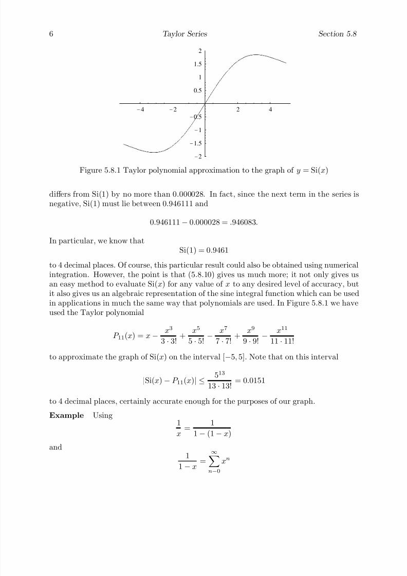
7/27/2019 Calculus 2 (Dan Sloughter)
http://slidepdf.com/reader/full/calculus-2-dan-sloughter 387/598
6 Taylor Series Section 5.8
-4 -2 2 4
-2
-1.5
-1
-0.5
0.5
1
1.5
2
Figure 5.8.1 Taylor polynomial approximation to the graph of y = Si(x)
differs from Si(1) by no more than 0.000028. In fact, since the next term in the series is
negative, Si(1) must lie between 0.946111 and
0.946111 − 0.000028 = .946083.
In particular, we know thatSi(1) = 0.9461
to 4 decimal places. Of course, this particular result could also be obtained using numericalintegration. However, the point is that (5.8.10) gives us much more; it not only gives usan easy method to evaluate Si(x) for any value of x to any desired level of accuracy, butit also gives us an algebraic representation of the sine integral function which can be used
in applications in much the same way that polynomials are used. In Figure 5.8.1 we haveused the Taylor polynomial
P 11(x) = x −x3
3 · 3!+
x5
5 · 5!−
x7
7 · 7!+
x9
9 · 9!−
x11
11 · 11!
to approximate the graph of Si(x) on the interval [−5, 5]. Note that on this interval
|Si(x)− P 11(x)| ≤513
13 · 13!= 0.0151
to 4 decimal places, certainly accurate enough for the purposes of our graph.Example Using
1
x=
1
1− (1− x)
and1
1 − x=
∞n−0
xn
7/27/2019 Calculus 2 (Dan Sloughter)
http://slidepdf.com/reader/full/calculus-2-dan-sloughter 388/598
Section 5.8 Taylor Series 7
for −1 < x < 1, we have
1
x=
∞n=0
(1− x)n =∞n=0
(−1)n(x − 1)n (5.8.11)
for −1 < 1−x < 1, that is, 0 < x < 2. Hence (5.8.11) gives the Taylor series representationfor
f (x) =1
x
about 1. Similar to our work in the previous example, we may now find an antiderivativefor f on (0, 2) by integration. Namely,
x
1
1
tdt =
x
1
∞n=0
(−1)n(t− 1)n
dt
=∞n=0
x1
(−1)n(t − 1)ndt
=∞n=0
(−1)n(t − 1)n+1
n + 1
x
1
=∞n=0
(−1)n(x − 1)n+1
n + 1
= (x − 1)−(x − 1)2
2+
(x − 1)3
3−
(x − 1)4
4+ · · ·
provides a Taylor series representation for an antiderivative of f on the interval (0, 2).In Chapter 6 we will call this function the natural logarithm function , denoted log(x),although there we will use other means in order to define it on the interval (0 ,∞). Inparticular, note that this series converges at x = 2 as well, giving us, with this definitionof log(x),
log(2) =∞n=0
(−1)n
n + 1=
∞n=1
(−1)n+1
n.
Hence log(2) is the sum of the alternating harmonic series, a number for which we foundan approximation in Section 5.6.
Problems
1. Show directly that
cos(x) =∞n=0
(−1)nx2n
(2n)!
for all x in (−∞,∞).

7/27/2019 Calculus 2 (Dan Sloughter)
http://slidepdf.com/reader/full/calculus-2-dan-sloughter 389/598
8 Taylor Series Section 5.8
2. Using any method, find Taylor series representations about 0 for the following func-tions. State the interval on which the representation is valid. Also, write out the firstfive nonzero terms of each series.
(a) cos(x2) (b) sin(2x)
(c)1
1− t2 (d)1
2x − 1
(e)1
(1 + t)2(f)
1
1 + 4x2
(g) f (x) =
1− cos(x)
x, if x = 0,
0, if x = 0
3. (a) Use the identity
cos2(x) =1 + cos(2x)
2
to find the Taylor series representation for cos2(x) about 0. On what interval isthis representation valid?
(b) What is the Taylor polynomial of order 8 for cos2(x) at 0?
4. (a) Use Problem 3 and the identity
sin2(x) = 1 − cos2(x)
to find the Taylor series representation for sin2(x) about 0. On what interval isthis representation valid?
(b) What is the Taylor polynomial of order 8 for sin2(x) at 0?
5. (a) Use the Taylor series representation about 0 for sin(x) to find the Taylor seriesrepresentation for sin(x2) about 0. On what interval is this representation valid?
(b) What is the Taylor polynomial of order 10 for sin(x2) at 0?
(c) Find the Taylor series representation about 0 for
S (x) =
x
0
sin(t2)dt.
On what interval is this representation valid?
(d) What is the Taylor polynomial of order 11 for S (x) at 0?
(e) Approximate S (1) with an error of less than 0.00001.
6. LetP n
be the Taylor polynomial of ordern
at 0 forf (x) =
1
1 + x2.
Plot f , P 2, P 4, and P 10 together over the interval [−1.5, 1.5]. Why do the Taylorpolynomials not give a good approximation to f (x) when |x| > 1?
7. Findd9
dx9Si(x)
x=0
.

7/27/2019 Calculus 2 (Dan Sloughter)
http://slidepdf.com/reader/full/calculus-2-dan-sloughter 390/598
Difference Equations
Differential Equations
toSection 5.9
Some Limit Calculations
In this section we will discuss the use of Taylor polynomials in computing certain types of limits. Although this material could have been treated directly after Section 5.2, we havesaved it until now so as not to break into the development of Taylor series. To illustrate theideas of this section, we begin with two examples, the first of which is already well-knownto us.
Example Consider the problem of evaluating
limx→0
sin(x)x
.
The reason this limit presents a problem is that, although the function in question is aquotient of two continuous functions, both the numerator and the denominator approach0 as x approaches 0. Now from our work on Taylor polynomials we know that
sin(x) = x + o(x),
so
sin(x)x
= x + o(x)x
= 1 + o(x)x
.
But, by definition,
limx→0
o(x)
x= 0.
Thus
limx→0
sin(x)
x= lim
x→0
x + o(x)
x= lim
x→0
1 +
o(x)
x
= 1.
Example The limit
limx→0
1− cos(x)
x2
presents the same type of problem. Using the Taylor polynomial of order 2 for cos(x), weknow that
cos(x) = 1− x2
2+ o(x2).
1 Copyright c by Dan Sloughter 2000

7/27/2019 Calculus 2 (Dan Sloughter)
http://slidepdf.com/reader/full/calculus-2-dan-sloughter 391/598
2 Some Limit Calculations Section 5.9
Hence
limx→0
1− cos(x)
x2= lim
x→0
1−
1− x2
2+ o(x2)
x2
= limx→0
x2
2 − o(x
2
)x2
= limx→0
1
2− o(x2)
x2
=1
2.
The point in both of these examples was to use the fact that if f is n + 1 timescontinuously differentiable on an interval about the point c, then, as we saw in Section 5.2,
f (x) = f (c) + f (c)(x− c) + f
(c)2!
(x− c)2 + · · ·+ f (n)(c)n!
(x− c)n + o((x− c)n). (5.9.1)
Hence if f and g are both n + 1 times continuously differentiable on an interval about c,f (n)(c) = 0, f (k)(c) = 0 for k = 0, 1, 2, . . . , n− 1, and g(k)(c) = 0 for k = 0, 1, 2, . . . , n − 1,then
f (x) =f (n)(c)
n!(x− c)n + o((x− c)n) (5.9.2)
and
g(x) =g(n)(c)
n!
(x
−c)n + o((x
−c)n). (5.9.3)
Hence
limx→c
g(x)
f (x)= lim
x→c
g(n)(c)
n!(x− c)n + o((x− c)n)
f (n)(c)
n!(x− c)n + o((x− c)n)
= limx→c
g(n)(c)
n!+
o((x− c)n)
(x− c)n
f (n)(c)
n! +
o((x
−c)n)
(x− c)n
=
g(n)(c)
n!f (n)(c)
n!
=g(n)(c)
f (n)(c). (5.9.4)
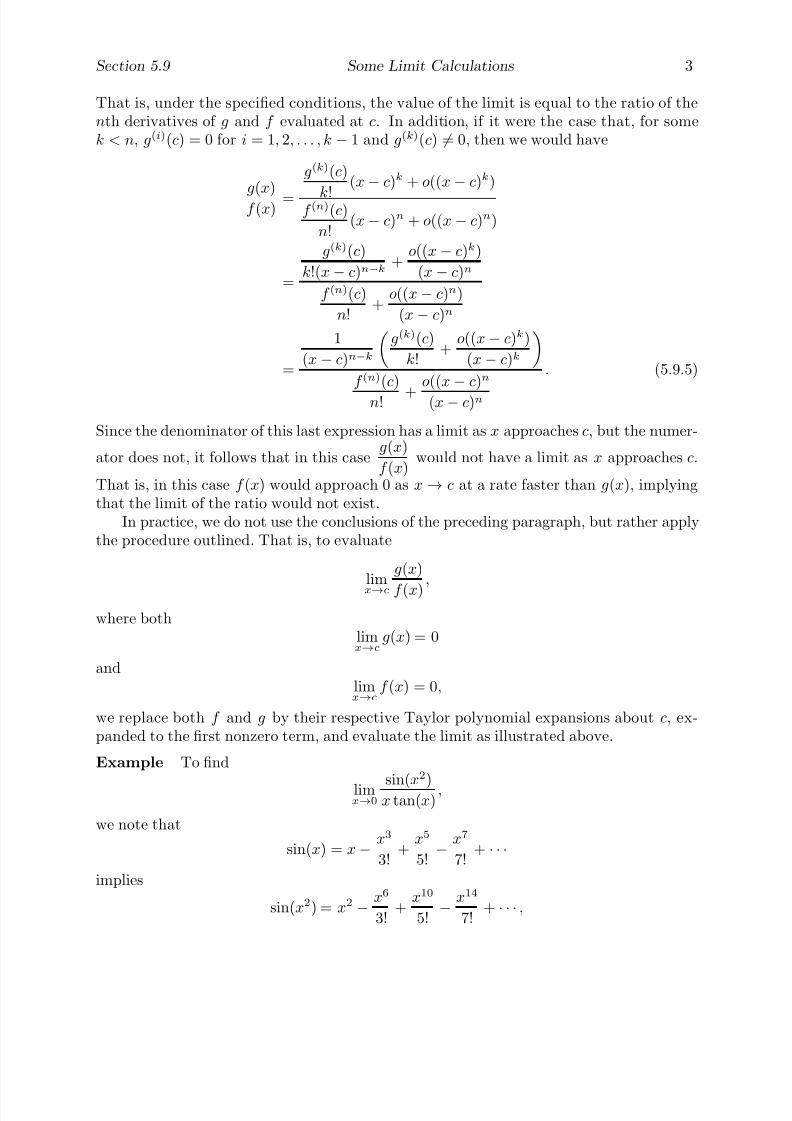
7/27/2019 Calculus 2 (Dan Sloughter)
http://slidepdf.com/reader/full/calculus-2-dan-sloughter 392/598
Section 5.9 Some Limit Calculations 3
That is, under the specified conditions, the value of the limit is equal to the ratio of thenth derivatives of g and f evaluated at c. In addition, if it were the case that, for somek < n, g(i)(c) = 0 for i = 1, 2, . . . , k − 1 and g(k)(c) = 0, then we would have
g(
x)f (x) =
g(k)(c)
k!
(x
−c)k + o((x
−c)k)
f (n)(c)
n!(x− c)n + o((x− c)n)
=
g(k)(c)
k!(x− c)n−k+
o((x− c)k)
(x− c)n
f (n)(c)
n!+
o((x− c)n)
(x− c)n
=
1
(x− c)n−k
g(k)(c)
k!+
o((x− c)k)
(x− c)k
f (n)(c)
n! +o((x
−c)n
(x− c)n
. (5.9.5)
Since the denominator of this last expression has a limit as x approaches c, but the numer-
ator does not, it follows that in this caseg(x)
f (x)would not have a limit as x approaches c.
That is, in this case f (x) would approach 0 as x → c at a rate faster than g(x), implyingthat the limit of the ratio would not exist.
In practice, we do not use the conclusions of the preceding paragraph, but rather applythe procedure outlined. That is, to evaluate
limx→c
g(x)
f (x),
where bothlimx→c
g(x) = 0
andlimx→c
f (x) = 0,
we replace both f and g by their respective Taylor polynomial expansions about c, ex-panded to the first nonzero term, and evaluate the limit as illustrated above.
Example To find
limx→0
sin(x
2
)x tan(x)
,
we note that
sin(x) = x− x3
3!+
x5
5!− x7
7!+ · · ·
implies
sin(x2) = x2 − x6
3!+
x10
5!− x14
7!+ · · · ,
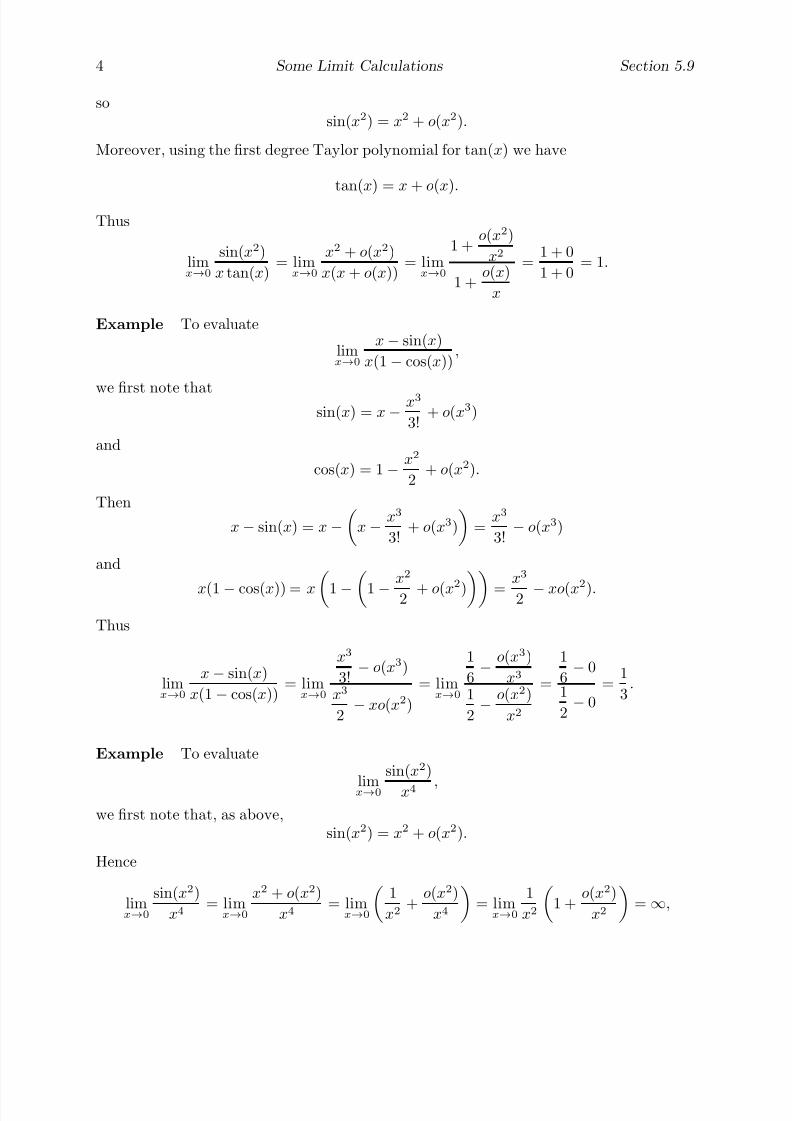
7/27/2019 Calculus 2 (Dan Sloughter)
http://slidepdf.com/reader/full/calculus-2-dan-sloughter 393/598
4 Some Limit Calculations Section 5.9
sosin(x2) = x2 + o(x2).
Moreover, using the first degree Taylor polynomial for tan(x) we have
tan(x) = x + o(x).
Thus
limx→0
sin(x2)
x tan(x)= lim
x→0
x2 + o(x2)
x(x + o(x))= lim
x→0
1 +o(x2)
x2
1 +o(x)
x
=1 + 0
1 + 0= 1.
Example To evaluate
limx→0
x− sin(x)
x(1− cos(x)),
we first note thatsin(x) = x− x3
3!+ o(x3)
and
cos(x) = 1− x2
2+ o(x2).
Then
x− sin(x) = x−
x− x3
3!+ o(x3)
=
x3
3!− o(x3)
and
x(1− cos(x)) = x
1− 1−x2
2 + o(x2)
=x3
2 − xo(x2).
Thus
limx→0
x− sin(x)
x(1− cos(x))= lim
x→0
x3
3!− o(x3)
x3
2− xo(x2)
= limx→0
1
6− o(x3)
x3
1
2− o(x2)
x2
=
1
6− 0
1
2− 0
=1
3.
Example To evaluate
limx→0
sin(x2)
x4 ,
we first note that, as above,sin(x2) = x2 + o(x2).
Hence
limx→0
sin(x2)
x4= lim
x→0
x2 + o(x2)
x4= lim
x→0
1
x2+
o(x2)
x4
= lim
x→0
1
x2
1 +
o(x2)
x2
= ∞,

7/27/2019 Calculus 2 (Dan Sloughter)
http://slidepdf.com/reader/full/calculus-2-dan-sloughter 394/598
Section 5.9 Some Limit Calculations 5
where the final equality follows after noting that
limx→0
1 +
o(x2)
x2
= 1,
while
limx→0
1
x2= ∞.
The essence of (5.9.4) is also captured in the following statement, known as l’Hˆ opital’s
rule .
l’Hopital’s rule If f and g are twice continuously differentiable on an interval aboutthe point c and both g(c) = 0 and f (c) = 0, then
limx→c
g(x)
f (x)= lim
x→c
g(x)
f (x). (5.9.6)
This is equivalent to our previous result, assuming the conditions specified at thattime, because repeated applications of l’Hopital’s rule yield
limx→c
g(x)
f (x)
= limx→c
g(x)
f
(x)
= limx→c
g(x)
f
(x)
=
· · ·= lim
x→c
g(n)(x)
f
(n)
(x)
=g(n)(c)
f
(n)
(c)
, (5.9.7)
which is (5.9.4). As before, if for some k < n, g(i)(c) = 0 for i = 0, 1, 2, . . . , k − 1 andg(k)(c) = 0, then
limx→c
g(k)(x)
f (k)(x)
does not exist andg(x)
f (x)does not have a limit as x approaches c.
Example We will illustrate l’Hopital’s rule first with another well-known limit. Namely,
limx→0
1− cos(x)
x= lim
x→0
d
dx(1− cos(x))
d
dxx
= limx→0
sin(x)
1= 0.

7/27/2019 Calculus 2 (Dan Sloughter)
http://slidepdf.com/reader/full/calculus-2-dan-sloughter 395/598
6 Some Limit Calculations Section 5.9
Example As an illustration of how it may be necessary to apply l’Hopital’s rule morethan once, we have
limx→0
sin(x)− x
x3= lim
x→0
d
dx(sin(x)− x)
d
dx x
3
= limx→0
(cos(x)− 1)
3x2
= limx→0
d
dx(cos(x)− 1)
d
dx3x2
= limx→0
− sin(x)
6x
=−
1
6limx→0
sin(x)
x
= −1
6.
Note that this particular problem could have been done more quickly using the fact that
sin(x)− x = −x3
6+ o(x3).
Although we will not do so here, it is possible to demonstrate that l’Hopital’s rule ismore widely applicable than what we have indicated so far. In particular, we may alsoapply l’Hopital’s rule to one-sided limits and to limits as x approaches ∞ or x approaches−∞, provided, of course, that both g(x) and f (x) are approaching 0 and are twice contin-uously differentiable on the appropriate intervals. The following examples illustrate theseapplications.
Example Using l’Hopital’s rule, we have
limx→π
+
sin(x)
√ x− π
= limx→π
+
d
dxsin(x)
ddx√ x− π
= limx→π+
cos(x)1
2√
x− π
= limx→π+
2cos(x)√
x− π
= 0.

7/27/2019 Calculus 2 (Dan Sloughter)
http://slidepdf.com/reader/full/calculus-2-dan-sloughter 396/598
Section 5.9 Some Limit Calculations 7
Example Using l’Hopital’s rule, we have
limx→∞
x sin1
x = limx→∞
sin
1
x
1
x
= limx→∞
d
dxsin
1
x
d
dx
1
x
= limx→∞
− 1
x2cos
1
x
− 1
x2
= limx→∞ cos 1
x
= 1.
Notice we could have computed this limit by substituting h =1
x, thus obtaining
limx→∞
x sin
1
x
= lim
h→0+
sin(h)
h= 1.
Finally, it is also possible to demonstrate that l’Hopital’s rule applies when both thenumerator and the denominator are approaching ∞. That is, if f and g are twice contin-uously differentiable at c and both
limx→c
f (x) = ∞
and
limx→c
g(x) =
∞,
then
limx→c
g(x)
f (x)= lim
x→c
g(x)
f (x). (5.9.8)
As before, this also applies for one-sided limits and for limits as x approaches ∞ or −∞.Moreover, one or both of g(x) and f (x) may be approaching −∞.

7/27/2019 Calculus 2 (Dan Sloughter)
http://slidepdf.com/reader/full/calculus-2-dan-sloughter 397/598
8 Some Limit Calculations Section 5.9
Example Using l’Hopital’s rule,
limx→∞
3x + 1√ x2 + 4
= limx→∞
d
dx(3x + 1)
d
dx x2 + 4
= limx→∞
3x√
x2 + 4
= limx→∞
3√
x2 + 4
x
= limx→∞
3
x2 + 4
x2
= limx→∞
3
1 +
4
x2
= 3.
Of course, we could have also computed this limit by dividing both the numerator anddenominator by x to obtain
limx→∞
3x + 1√ x2 + 4
= limx→∞
3 +1
x√ x2 + 4
x
= limx→∞
3 +1
x x2 + 4
x2
= limx→∞
3 +1
x 1 +
4
x2
= 3.
Problems
1. Use Taylor polynomials to find the following limits.
(a) limx→0
sin(3x)
x(b) lim
t→0
t− sin(t)
t2
(c) limx→0
cos(x)− 1 +x2
2x4
(d) limx→0
sin(x2)
sin2(x)
(e) limu→0
tan(u)
sin(u)(f) lim
t→0
sin(t)− t
t3
(g) limy→0
tan(3y)
tan(5y)(h) lim
x→0
tan(x2)
sin(x2)
(i) limx→0
√ 1 + x− 1
3x(j) lim
t→0
√ 1 + t− 1− t
23t2

7/27/2019 Calculus 2 (Dan Sloughter)
http://slidepdf.com/reader/full/calculus-2-dan-sloughter 398/598
Section 5.9 Some Limit Calculations 9
2. Use l’Hopital’s rule to evaluate the following limits.
(a) limx→0
sin(5x)
3x(b) lim
t→0
1− cos(3t)
t2
(c) limx→0
1− sec(x)
x(d) lim
t→π
4
1− tan(t)
cos(2t)
(e) limx→0+
sin(2x)√ x
(f) limx→0
1− cos(x)
sin(x)
(g) limx→∞
x sin
1
x2
(h) lim
x→0
3x2
sin2(x)
3. Evaluate the following limits using any method you prefer.
(a) limx→∞
3x2 − 2x + 1
16x2 + 2(b) lim
x→0
tan(x2)
sin2(x)
(c) limx→0
1−
sin(x)
x3x2 (d) lim
x→0(1 + x)
13 − 1
x
(e) limx→0
(1 + x)13 − 1− x
3x2
(f) limt→0
1− cos(t)
t sin(2t)
(g) limx→1
√ x− 1
x− 1(h) lim
x→π
cos(x) + 1
x− π
(i) limt→0
cos(t)− 1 +t2
2t2 sin(t2)
(j) limu→0
sin(u2)− u2
u4(1− cos(u))
4. Let g(x) =
x2 sin
1x
, if x = 0,
0, if x = 0.
(a) Show that g(0) = 0, and hence that g(x) = o(x).
(b) Use the preceding result and the fact that tan(x) = x + o(x) to show that
limx→0
x2 sin
1
x
tan(x)= 0.
(c) Letting f (x) = tan(x), show that
limx→0
g(x)
f (x)= lim
x→0
g(x)
f (x).
Which condition in the statement of l’Hopital’s rule does not hold for this example?
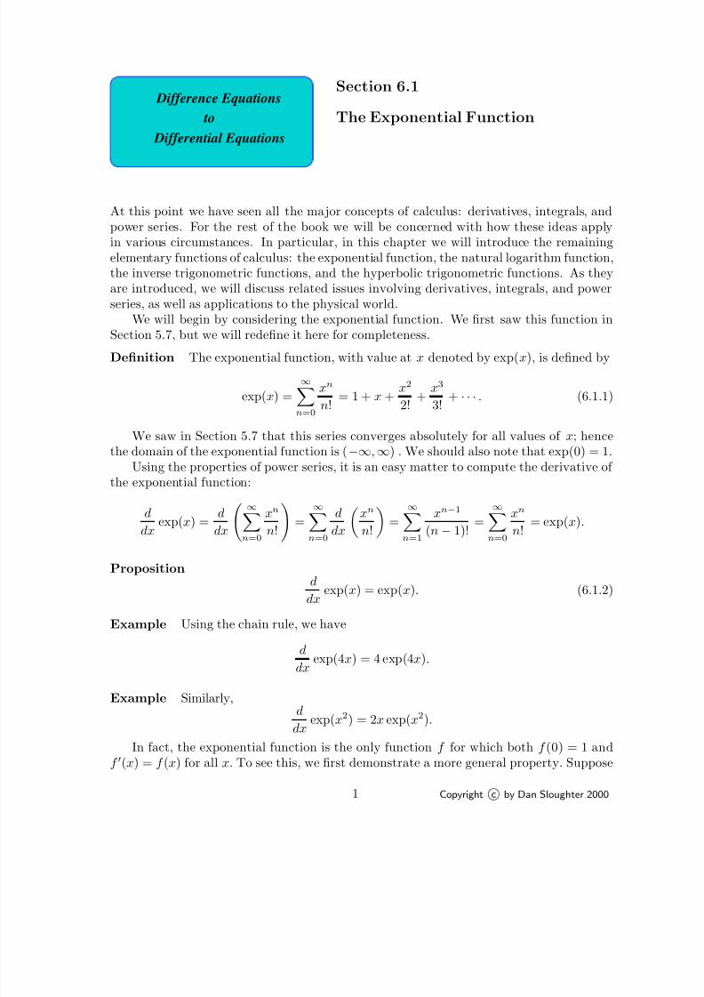
7/27/2019 Calculus 2 (Dan Sloughter)
http://slidepdf.com/reader/full/calculus-2-dan-sloughter 399/598
Difference Equations
Differential Equations
to
Section 6.1
The Exponential Function
At this point we have seen all the major concepts of calculus: derivatives, integrals, andpower series. For the rest of the book we will be concerned with how these ideas applyin various circumstances. In particular, in this chapter we will introduce the remainingelementary functions of calculus: the exponential function, the natural logarithm function,the inverse trigonometric functions, and the hyperbolic trigonometric functions. As theyare introduced, we will discuss related issues involving derivatives, integrals, and powerseries, as well as applications to the physical world.
We will begin by considering the exponential function. We first saw this function inSection 5.7, but we will redefine it here for completeness.
Definition The exponential function, with value at x denoted by exp(x), is defined by
exp(x) =∞n=0
xn
n!= 1 + x +
x2
2!+
x3
3!+ · · · . (6.1.1)
We saw in Section 5.7 that this series converges absolutely for all values of x; hencethe domain of the exponential function is (−∞,∞) . We should also note that exp(0) = 1.
Using the properties of power series, it is an easy matter to compute the derivative of the exponential function:
d
dx exp(x) =
d
dx ∞n=0
xn
n! =
∞n=0
d
dxxn
n! =
∞n=1
xn−1
(n − 1)! =
∞n=0
xn
n! = exp(x).
Propositiond
dxexp(x) = exp(x). (6.1.2)
Example Using the chain rule, we have
d
dxexp(4x) = 4 exp(4x).
Example Similarly,d
dxexp(x2) = 2x exp(x2).
In fact, the exponential function is the only function f for which both f (0) = 1 andf (x) = f (x) for all x. To see this, we first demonstrate a more general property. Suppose
1 Copyright c by Dan Sloughter 2000

7/27/2019 Calculus 2 (Dan Sloughter)
http://slidepdf.com/reader/full/calculus-2-dan-sloughter 400/598
2 The Exponential Function Section 6.1
f is any function for which f (0) = c and f (x) = kf (x) for all x, where c and k areconstants. Then it follows that
f (x) =d
dx(kf (x)) = kf (x) = k2f (x),
f (x) =d
dx
(k2f (x)) = k2f (x) = k3f (x),
and, in general,f (n)(x) = knf (x) (6.1.3)
for n = 0, 1, 2, . . .. Hencef (n)(0) = knc (6.1.4)
for n = 0, 1, 2, . . .. Thus the Taylor series for f about 0 is given by
∞n=0
f (n)(0)
n!xn =
∞n=0
ckn
n!xn = c
∞n=0
(kx)n
n!= c exp(kx), (6.1.5)
where the final equality follows from the definition of the exponential function. Now, as aconsequence of Taylor’s theorem, if P n is the nth order Taylor polynomial for f at 0, then
|f (x) − P n(x)| ≤ M
(n + 1)!|x|n+1, (6.1.6)
where M is the maximum value of |f (n+1)| on the closed interval from 0 to x. But
f (n+1)(x) = kn+1f (x),
soM = |k|n+1L
where L is the maximum value of |f | on the closed interval from 0 to x. Hence
|f (x) − P n(x)| ≤ |k|n+1L
(n + 1)!|x|n+1 =
L|kx|n+1(n + 1)!
. (6.1.7)
As we have seen before,
limn→∞
L|kx|n+1(n + 1)!
= 0 (6.1.8)
for any value of x, so it follows that
f (
x) = limn→∞
P n(
x) =
∞
n=0
f (n)(0)
n!xn
(6.1.9)
for all x. In other words, f has a Taylor series representation, and so, using (6.1.5), wehave
f (x) = c exp(x).
7/27/2019 Calculus 2 (Dan Sloughter)
http://slidepdf.com/reader/full/calculus-2-dan-sloughter 401/598
Section 6.1 The Exponential Function 3
Proposition If f is a function for which f (0) = c and f (x) = kf (x) for all x, where c
and k are constants, thenf (x) = c exp(x) (6.1.10)
for all x.In particular, if we let c = 1 and k = 1 in this proposition, then f (x) = exp(x).
In many ways, it is this property that makes the exponential function one of the mostimportant functions in mathematics.
Now consider a function f defined by f (x) = exp(x + b) for some constant b. Then
f (x) = exp(x + b) = f (x),
so, by the previous proposition, we must have f (x) = c exp(x) for all x, where c = f (0) =exp(b). That is, for all values of x,
exp(x + b) = f (x) = exp(b) exp(x).
This demonstrates a fundamental algebraic property of the exponential function: For anynumbers a and b,
exp(a + b) = exp(a)exp(b). (6.1.11)
It follows from (6.1.11) that for any number a,
exp(a) exp(−a) = exp(a − a) = exp(0) = 1.
That is,
exp(−a) =1
exp(a)(6.1.12)
More generally, using both (6.1.11) and (6.1.12), we have
exp(a − b) = exp(a)exp(−b) =exp(a)
exp(b). (6.1.13)
for any numbers a and b, another important algebraic property of the exponential function.
We shall soon see that the number exp(1) plays a special role in this discussion.
Definition The value of the exponential function at 1 is denoted by e. That is,
e = exp(1) = 1 + 1 +1
2+
1
3!+ · · · . (6.1.14)
It may be shown, although not easily, that e is an irrational number. Much more easily(see Problem 5), it may be shown that, to 5 decimal places, e is given by 2.71828. The useof the letter e to denote this number originates with Leonhard Euler (1707-1783), one of the most prolific mathematicians of all time.
7/27/2019 Calculus 2 (Dan Sloughter)
http://slidepdf.com/reader/full/calculus-2-dan-sloughter 402/598
4 The Exponential Function Section 6.1
Notice that for any positive integer n,
exp(n) = exp(1 + 1 + · · · + 1 n times
) = exp(1) exp(1) · · · exp(1) n times
= (exp(1))n = en (6.1.15)
and
exp(−n) = 1exp(n)
= 1en
= e−n. (6.1.16)
Combining this with exp(0) = 1, we have
exp(n) = en (6.1.17)
for all integers n. Moreover, for any integer n = 0,exp
1
n
n
= exp
1
n
exp
1
n
· · · exp
1
n
n times
= exp
1
n+
1
n+ · · · +
1
n
n times
= exp(1) = e,
showing that
exp
1
n
= e
1
n . (6.1.18)
Hence if m and n are integers with n = 0, then
expm
n
= exp
1
n+
1
n+ · · · +
1
n
m times
=
exp
1
n
m
=
e1
n
m= e
m
n . (6.1.19)
The next proposition summarizes these facts.
Proposition For any rational number r,
exp(r) = er. (6.1.20)
That is, evaluating the exponential function at a rational number r is equivalent to
raising e to the rth power. A natural question at this point is to ask whether the same resultholds for irrational numbers. A little thought shows that this question is not meaningful;although we know what it means to raise a number to a rational power (namely, for integersm and n,
am
n = n√
am,

7/27/2019 Calculus 2 (Dan Sloughter)
http://slidepdf.com/reader/full/calculus-2-dan-sloughter 403/598
Section 6.1 The Exponential Function 5
that is, am
n is the nth root of the mth power of a), we have never defined what it means toraise a number to an irrational power. For example, at this point we do not have a meaningto associate with the symbol 2π. We will now take the first step toward remedying thissituation by defining es for an irrational number s.
Definition If s is an irrational number, then we define
es = exp(s). (6.1.21)
With this definition we can now say that
exp(x) = ex (6.1.22)
for any real number x. The properties of the exponential function stated in (6.1.11) and(6.1.13) may be restated as
ex+y = exey (6.1.23)
and
e
x−y
=
ex
ey (6.1.24)for any real numbers x and y. Hence exponents behave in this new situation exactly theway we should expect them to behave.
From our previous result that
d
dxexp(x) = exp(x),
it now follows thatd
dxex = ex. (6.1.25)
From this differentiation rule we obtain the indefinite integral exdx = ex + c. (6.1.26)
Example Using the chain rule, we have
d
dxe2x = 2e2x.
Example Using the product and chain rules,
ddx
3xe4x
2= 3x d
dx
e4x
2+ e4x
2 ddx
(3x)
= (3x)
8xe4x2
+
e4x2
(3)
= (3 + 24x2)e4x2
.

7/27/2019 Calculus 2 (Dan Sloughter)
http://slidepdf.com/reader/full/calculus-2-dan-sloughter 404/598
6 The Exponential Function Section 6.1
Example Sinced
dxe−4x = −4e−4x,
it follows that
e−4xdx = −1
4e−4x + c.
Notice the similarity between the evaluation of the integral in the last example andthe evaluation of the integral
cos(−4x)dx = −1
4sin(−4x) + c.
In fact, just as, for any a = 0, cos(ax)dx =
1
asin(ax) + c,
we have eaxdx =
1
aeax + c. (6.1.27)
Example To evaluate
3xe2x
2
dx, we use the substitution
u = 2x2
du = 4xdx.
Then1
4
du = xdx, so
3xe2x
2
dx =3
4
eudu =
3
4eu + c =
3
4e2x
2
+ c.
Example To evaluate
2xexdx, we use integration by parts with
u = 2x dv = exdx
du = 2dx v = ex.
Then 2xexdx = 2xex − 2exdx = 2xex − 2ex + c.
Notice the similarity between the technique for evaluating the integral in the last
example and the technique for evaluating
2x sin(x)dx.

7/27/2019 Calculus 2 (Dan Sloughter)
http://slidepdf.com/reader/full/calculus-2-dan-sloughter 405/598
Section 6.1 The Exponential Function 7
-4 -2 2 4
5
10
15
20
25
30
Figure 6.1.1 Graph of y = ex
Example The integral
ex sin(x)dx may also be handled by integration by parts, al-
though with a little more work than in the previous example. Here we will letu = sin(x) dv = exdx
du = cos(x)dx v = ex.
Then ex sin(x)dx = ex sin(x) −
ex cos(x)dx.
We now perform another integration by parts by choosing
u = cos(x) dv = exdx
du = − sin(x)dx v = ex.
Then ex sin(x) = ex sin(x) −
ex cos(x) +
ex sin(x)dx
= ex sin(x) − ex cos(x) −
ex sin(x)dx.
At first glance it may seem that we are back to where we started; however, all we need to
do now is solve for
ex sin(x)dx. That is, we have
2
ex sin(x)dx = ex sin(x) − ex cos(x) = ex(sin(x) − cos(x)),
so ex sin(x)dx =
1
2ex(sin(x) − cos(x)) + c.
Note that we have added an arbitrary constant c since we are seeking the general an-tiderivative.

7/27/2019 Calculus 2 (Dan Sloughter)
http://slidepdf.com/reader/full/calculus-2-dan-sloughter 406/598
8 The Exponential Function Section 6.1
-4 -2 2 4
5
10
15
20
25
30
Figure 6.1.2 Graph of y = e−x
We now have sufficient information about the exponential function to understand thegeometry of its graph. Since e > 0 , we know that ex > 0 for all rational values of x, and
hence, by continuity, for all values of x. Since e > 1, it follows that
limx→∞
ex = ∞ (6.1.28)
and
limx→−∞
ex = limu→∞
e−u = limu→∞
1
eu= 0. (6.1.29)
Moreover, sinced
dxex = ex > 0 (6.1.30)
andd2
dx2
ex = ex > 0 (6.1.31)
for all x, the graph of y = ex is always increasing and always concave up. Moreover,(6.1.30) and (6.1.31) indicate that as x increases, the graph is not only increasing, but itsslope is increasing at the same rate that y is increasing. Thus we should expect y to growat a very rapid rate, as we see in Figure 6.1.1. This rate of growth is characterized asexponential growth . Figure 6.1.2 shows the graph of y = e−x , which is the graph of y = ex
reflected about the y-axis. In this case y decreases asymptotically toward 0 as x increases;this is known as exponential decay
We will close this section with an application to the problem of uninhibited populationgrowth, a problem we first considered in Section 1.4.
Uninhibited population growth
Recall from Section 1.4 that if xn represents the size of a population after n units of timeand the population grows at a constant rate of α100% per unit of time, then the sequence{xn} must satisfy the linear difference equation
xn+1 − xn = αxn (6.1.32)

7/27/2019 Calculus 2 (Dan Sloughter)
http://slidepdf.com/reader/full/calculus-2-dan-sloughter 407/598
Section 6.1 The Exponential Function 9
for n = 0, 1, 2, . . .. At that time we saw that the solution of this equation is given by
xn = (1 + α)nx0. (6.1.33)
The crucial aspect of (6.1.32) is the statement that amount of change in the size of thepopulation over any unit of time is proportional to the current size of the population.
Hence if x(t) represents the size of a population at time t, where the population canchange continuously over time, then the continuous time analog of (6.1.32) is the differential
equation
x(t) = αx(t) (6.1.34)
for all time t. If x0 is the size of the population at time t = 0, then we know from ourwork in this section that the only solution to this equation is the function
x(t) = x0eαt. (6.1.35)
Hence if the size of a population is growing at a rate which is proportional to itself, anassumption which, as we noted in Section 1.4, is often reasonable over short periods of
time, then the population will grow exponentially. As in Section 1.4, we refer to suchgrowth as uninhibited population growth .
Example In 1970 the population of the United States was 203.3 million and in 1980the population was 226.5 million. Assuming an uninhibited growth model and letting x(t)represent the population t years after 1970, by (6.1.35) we should have
x(t) = 203.3eαt
for some constant α. Since x(10) = 226.5, we can find α by solving
226.5 = 203.3e10α.
That is, we need to find a value for α such that
e10α =226.5
203.3= 1.114.
Unfortunately, solving this equation exactly requires being able to reverse the process of applying the exponential function. In other words, we need an inverse for the exponentialfunction. We shall take up that problem in the next section; for now we may use anumerical approximation. You should verify that α = 0.0108 satisfies the equation. Thusthis model would predict the population of the United States t years after 1970 to be
x(t) = 203.3e0.0108t.
For example, this model would predict a 1990 population of
x(20) = 203.3e(0.0108)(20) = 252.3
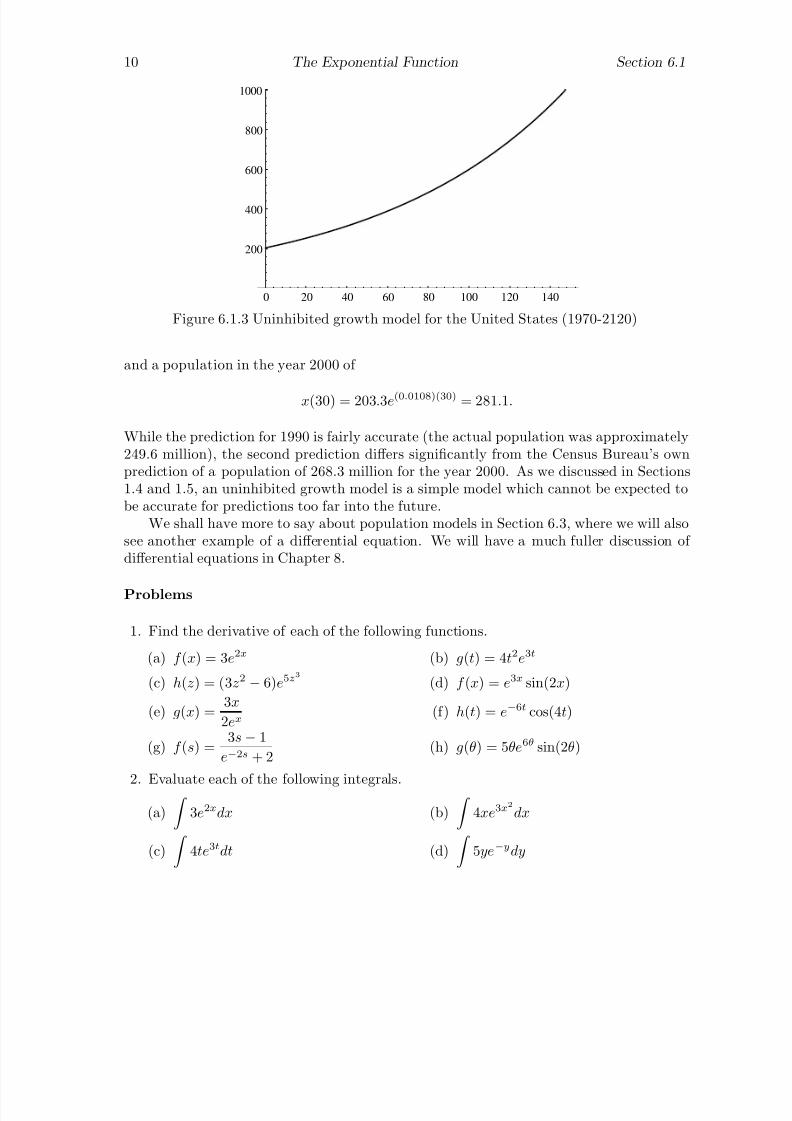
7/27/2019 Calculus 2 (Dan Sloughter)
http://slidepdf.com/reader/full/calculus-2-dan-sloughter 408/598
10 The Exponential Function Section 6.1
0 20 40 60 80 100 120 140
200
400
600
800
1000
Figure 6.1.3 Uninhibited growth model for the United States (1970-2120)
and a population in the year 2000 of
x(30) = 203.3e(0.0108)(30) = 281.1.
While the prediction for 1990 is fairly accurate (the actual population was approximately249.6 million), the second prediction differs significantly from the Census Bureau’s ownprediction of a population of 268.3 million for the year 2000. As we discussed in Sections1.4 and 1.5, an uninhibited growth model is a simple model which cannot be expected tobe accurate for predictions too far into the future.
We shall have more to say about population models in Section 6.3, where we will alsosee another example of a differential equation. We will have a much fuller discussion of differential equations in Chapter 8.
Problems
1. Find the derivative of each of the following functions.
(a) f (x) = 3e2x (b) g(t) = 4t2e3t
(c) h(z) = (3z2 − 6)e5z3
(d) f (x) = e3x sin(2x)
(e) g(x) =3x
2ex(f) h(t) = e−6t cos(4t)
(g) f (s) =3s − 1
e−2s + 2(h) g(θ) = 5θe6θ sin(2θ)
2. Evaluate each of the following integrals.
(a)
3e2xdx (b)
4xe3x
2
dx
(c)
4te3tdt (d)
5ye−ydy
7/27/2019 Calculus 2 (Dan Sloughter)
http://slidepdf.com/reader/full/calculus-2-dan-sloughter 409/598
Section 6.1 The Exponential Function 11
(e)
z2ezdz (f)
x3e−2xdx
(g)
ex cos(x)dx (h)
e−2t sin(3t)dt
3. Find the maximum value of f (x) = x2e−x on the interval (0,∞).
4. (a) Use the Taylor series for e−x to show that e−1 > 13 . Hence conclude that e < 3.(b) Show that if P n is the nth order Taylor polynomial for ex at 0, then
|ex − P n(x)| ≤ 3x
(n + 1)!|x|n+1
for any value of x.
(c) Use (b) to find an approximation for e with an error of less than 0.000005.
5. Find the following limits.
(a) limx→∞
xe−x (b) limx→0
ex − 1
x
(c) limt→0
e−t − 1t
(d) limx→∞
x2e−2x
6. (a) Show that limx→∞
xne−x = 0 for any positive integer n.
(b) Use (a) to show that if p is any polynomial, then limx→∞
p(x)e−x = 0. This shows
that ex grows faster as x →∞ than any polynomial function.
7. Graph the following functions on the specified intervals.
(a) f (t) = 3e2t on [−3, 3] (b) g(x) = 4x2e−2x on [0, 5]
(c) g(t) =et − e−t
et + e−ton [−10, 10] (d) f (t) = e−
t
4 sin(3t) on [0, 10]
8. Evaluate the following improper integrals.
(a)
∞
0
e−xdx (b)
∞
0
3e−2xdx
(c)
∞
0
xe−xdx (d)
∞
0
3xe−2xdx
(e)
∞
0
x2e−xxdx (f)
∞
0
xe−x2
dx
9. Use the integral test to show that the infinite series∞
n=0e−n converges.
10. (a) Find the Taylor series for f (x) = e−x2
.(b) Use (a) to find the the Taylor series for
erf(x) =2√ π
x0
e−t2
dt,

7/27/2019 Calculus 2 (Dan Sloughter)
http://slidepdf.com/reader/full/calculus-2-dan-sloughter 410/598
12 The Exponential Function Section 6.1
known as the error function .
(c) Use your result in (b) to approximate erf(1) with an error less than 0.0001.
11. Suppose x(t) is the population of a certain country t years after 1985, x(0) = 23.4million, and
x(t) = 0.008x(t).
(a) What will the population of the country be in the year 2000?
(b) In what year will the population be twice what it was in 1985?
12. Let
f (x) =
e−
1
x2 , if x = 00, if x = 0.
(a) Graph f on the interval [−5, 5].
(b) Show that f (0) = 0.
(c) Show that f (n)(0) = 0 for n = 0, 1, 2, . . ..
(d) Show that f is C ∞ on (−∞,∞).
(e) Note that the Taylor series for f about 0 converges for all x in (−∞,∞), but doesnot converge to f (x) except at 0. Thus f is C ∞ on (−∞,∞), but not analytic at0.
7/27/2019 Calculus 2 (Dan Sloughter)
http://slidepdf.com/reader/full/calculus-2-dan-sloughter 411/598
Difference Equations
Differential Equations
to
Section 6.2
The Natural Logarithm Function
In the last example of Section 6.1 we saw the need for solving an equation of the form
ex = b.
for x in terms of b. In general, for a given function f , a function g defined on the range of f is called the inverse of f if
g(f (x)) = x (6.2.1)
for all x in the domain of f and f (g(x)) = x (6.2.2)
for all x in the domain of g. That is, if f (x) = y, then g(y) = x and if g(x) = y, thenf (y) = x. In order for a function f to have an inverse function g, for every point y in therange of f there must exist a unique point x in the domain of f such that f (x) = y, inwhich case g(y) = x. In other words, for any two points x1 and x2 in the domain of f , wemust have f (x1) = f (x2). Now this will be the case if f is increasing on its domain, since,for such an f , x1 < x2 implies f (x1) < f (x2). In particular, a function f with domain(a, b) will have an inverse if f (x) > 0 for all x in (a, b). Hence, since
d
dx ex
= ex
> 0
for all x in (−∞,∞), the function f (x) = ex must have an inverse defined for every pointin its range, namely, (0,∞). We call this inverse function the natural logarithm function .
Definition The inverse of the exponential function is called the natural logarithm func-
tion . The value of the natural logarithm function at a point x is denoted log(x).
Thus, by definition,log(ex) = x (6.2.3)
and
elog(x)
= x. (6.2.4)Equivalently,
y = ex if and only if log(y) = x. (6.2.5)
Another common notation for log(x) is ln(x). In fact, most calculators use ln(x) forthe natural logarithm of x and log(x) for the base 10 logarithm of x. However, since thenatural logarithm function is the fundamental logarithm function of interest to us, we willdenote it by log(x) and often refer to it simply as the logarithm function.
1 Copyright c by Dan Sloughter 2000
7/27/2019 Calculus 2 (Dan Sloughter)
http://slidepdf.com/reader/full/calculus-2-dan-sloughter 412/598
2 The Natural Logarithm Function Section 6.2
Example In the last example of Section 6.1 we needed to solve the equation
e10α = 1.114.
Taking the natural logarithm of both sides of this equation gives us
log(e10α) = log(1.114),
from which we obtain10α = log(1.114),
and hence
α =log(1.114)
10.
Using a calculator and rounding to 4 decimal places, we find that α = 0.0108.
Being the inverse of the exponential function, the logarithm function has domain (0 ,
∞)
(which is the range of the exponential function) and range (−∞,∞) (which is the domainof the exponential function). Also, since e0 = 1 and e1 = e, it follows that log(1) = 0 andlog(e) = 1.
Several basic algebraic properties of the logarithm function follow immediately fromthe algebraic properties of the exponential function. For example, since, for any positivenumbers a and b,
elog(a)+log(b) = elog(a)elog(b) = ab,
it follows, after taking the logarithm of both sides, that
log(ab) = log(a) + log(b). (6.2.6)
Similarly, since, for any positive numbers a and b,
elog(a)−log(b) = elog(a)e− log(b) =elog(a)
elog(b)=
a
b,
we havelog
a
b
= log(a) − log(b). (6.2.7)
In particular,
log1
b = log(1)
−log(b) =
−log(b)
for any b > 0. Finally, if a > 0 and b is a rational number, then
eb log(a) =
elog(a)b
= ab
implies thatlog(ab) = b log(a). (6.2.8)

7/27/2019 Calculus 2 (Dan Sloughter)
http://slidepdf.com/reader/full/calculus-2-dan-sloughter 413/598
Section 6.2 The Natural Logarithm Function 3
We have restricted b to rational values here because we have not defined ab for irrationalvalues of b, except in the single case when a = e. However, the expression
eb log(a)
is defined for any value of b, rational or irrational. Hence the following definition providesa natural extension to the meaning of raising a number a > 0 to a power.
Definition If a > 0 and b is an irrational number, then we define
ab = eb log(a). (6.2.9)
With this definition, we have
log(ab) = b log(a). (6.2.10)
for a > 0 and any value of b.
Example We now see that
2π = eπ log(2),
which, using a calculator, is 8.8250 to 4 decimal places.
The derivative of the logarithm function may be found using our knowledge of thederivative of the exponential function. Specifically, if y = log(x), then ey = x. Thus,differentiating both sides of this expression with respect to x,
ddx
ey = ddx
x,
from which we obtain
eydy
dx= 1.
Hencedy
dx=
1
ey=
1
x.
Since we started with y = log(x), this gives us the following proposition.
Propositiond
dxlog(x) =
1
x. (6.2.11)
Example Combining the chain rule with the previous proposition, we have
d
dxlog(x2 + 1) =
1
x2 + 1
(2x) =
2x
x2 + 1.

7/27/2019 Calculus 2 (Dan Sloughter)
http://slidepdf.com/reader/full/calculus-2-dan-sloughter 414/598
4 The Natural Logarithm Function Section 6.2
Example It is worth noting that, in general, for any differentiable function f ,
d
dxlog(f (x)) =
1
f (x)
f (x) =
f (x)
f (x). (6.2.12)
Thus, for another example,
d
dxlog(3x4 + 8) =
12x3
3x4 + 8.
Example In some circumstances it is useful to use the properties of the logarithm func-tion before attempting to differentiate. For example,
d
dxlog
3x
4x2 + 2
=d
dx
log(3x) + log(4x2 + 2)
12
=d
dx
log(3) + log(x) +
1
2log(4x2 + 2)
= 1x
+ 12
8x4x2 + 2
=1
x+
2x
2x2 + 1.
Turning to integrals, we note that
d
dxlog(x) =
1
x
implies that
1
x
dx = log(x) + c,
provided x is in the domain of the logarithm function, that is, x > 0. For x < 0, we have
d
dxlog |x| =
d
dxlog(−x) =
1
−x(−1) =
1
x,
showing that 1
xdx = log |x| + c
for x < 0. Since |x| = x when x > 0, we can combine the above results into one statement.
Proposition 1x
dx = log |x| + c. (6.2.13)
Example To evaluate
x
x2 + 1dx we make the substitution
u = x2 + 1
du = 2xdx.

7/27/2019 Calculus 2 (Dan Sloughter)
http://slidepdf.com/reader/full/calculus-2-dan-sloughter 415/598
Section 6.2 The Natural Logarithm Function 5
Thus1
2du = xdx, so
x
x2 + 1dx =
1
2
1
udu =
1
2log |u| + c =
1
2log(x2 + 1) + c,
where we have removed the absolute value sign since x2 + 1 > 0 for all x.
Example To evaluate tan(x)dx =
sin(x)
cos(x)dx,
we make the substitutionu = cos(x)
du = − sin(x)dx.
Thus −du = sin(x)dx, so
tan(x)dx = − 1
udu = − log |u| + c = − log | cos(x)| + c.
Example To evaluate
sec(x)dx, we first multiply sec(x) by
sec(x) + tan(x)
sec(x) + tan(x)
to obtain
sec(x)dx =
sec2(x) + sec(x) tan(x)
sec(x) + tan(x) dx.
Then we make the substitution
u = sec(x) + tan(x)
du = (sec(x) tan(x) + sec2(x))dx.
Hence sec(x)dx =
1
udu = log |u| + c = log | sec(x) + tan(x)| + c.
Note that this example does not illustrate a general technique for evaluating integrals, but
rather a nice trick that works in this specific case. In fact, it is just as easy to rememberthe value of the integral as it is to remember the trick that was used to find it.
Example We may evaluate
log(x)dx using integration by parts. To do so, we choose
u = log(x) dv = dx
du =1
xdx v = x.
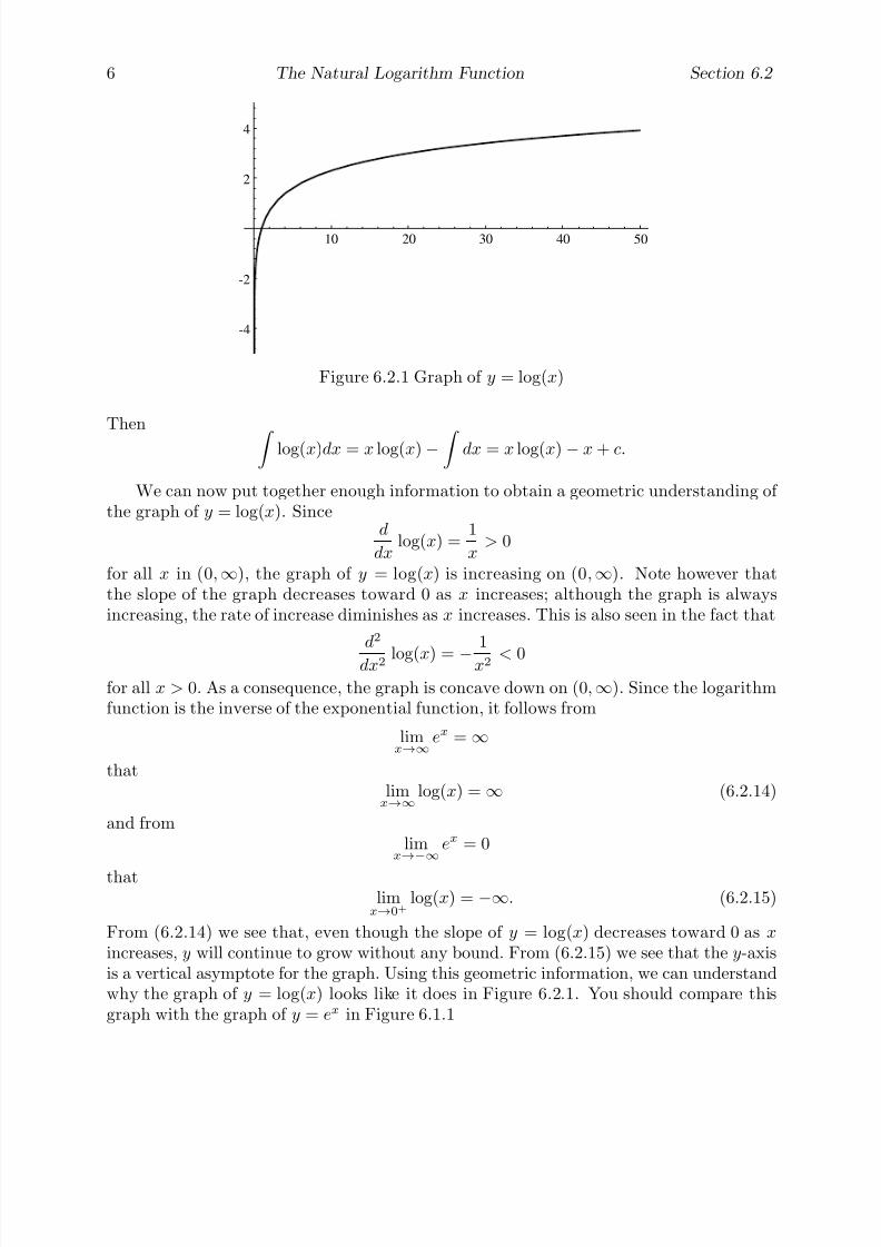
7/27/2019 Calculus 2 (Dan Sloughter)
http://slidepdf.com/reader/full/calculus-2-dan-sloughter 416/598
6 The Natural Logarithm Function Section 6.2
10 20 30 40 50
-4
-2
2
4
Figure 6.2.1 Graph of y = log(x)
Then log(x)dx = x log(x)−
dx = x log(x) − x + c.
We can now put together enough information to obtain a geometric understanding of the graph of y = log(x). Since
d
dxlog(x) =
1
x> 0
for all x in (0,∞), the graph of y = log(x) is increasing on (0,∞). Note however thatthe slope of the graph decreases toward 0 as x increases; although the graph is alwaysincreasing, the rate of increase diminishes as x increases. This is also seen in the fact that
d2
dx2 log(x) = −1
x2 < 0
for all x > 0. As a consequence, the graph is concave down on (0,∞). Since the logarithmfunction is the inverse of the exponential function, it follows from
limx→∞
ex = ∞that
limx→∞
log(x) = ∞ (6.2.14)
and fromlim
x→−∞ex = 0
thatlim
x→0+log(x) = −∞. (6.2.15)
From (6.2.14) we see that, even though the slope of y = log(x) decreases toward 0 as x
increases, y will continue to grow without any bound. From (6.2.15) we see that the y-axisis a vertical asymptote for the graph. Using this geometric information, we can understandwhy the graph of y = log(x) looks like it does in Figure 6.2.1. You should compare thisgraph with the graph of y = ex in Figure 6.1.1

7/27/2019 Calculus 2 (Dan Sloughter)
http://slidepdf.com/reader/full/calculus-2-dan-sloughter 417/598
Section 6.2 The Natural Logarithm Function 7
We will use the relationship
log(x) =
x1
1
tdt (6.2.16)
to find the Taylor series representation for the logarithm function. Since, as we saw in
Section 5.8,1
t=
1
1− (1− t)=
∞n=0
(1− t)n =∞n=0
(−1)n(t − 1)n
for 0 < t < 2, it follows that
log(x) =
x1
1
tdt
=∞n=0
(−1)n x1
(t − 1)ndt
=∞n=0
(−1)n
(x − 1)n+1
n + 1
=∞n=1
(−1)n+1(x − 1)n
n
= (x − 1) − (x − 1)2
2+
(x − 1)3
3− (x − 1)4
4+ · · ·
for 0 < x < 2. Hence
log(x) =∞
n=1
(−1)n+1(x − 1)n
n
= (x
−1)
−
(x − 1)2
2
+(x − 1)3
3 −
(x − 1)4
4
+
· · ·is the Taylor series representation of log(x) on (0, 2). Notice that at x = 0, this seriesbecomes a multiple of the harmonic series, and so does not converge, while at x = 2, it isthe alternating harmonic series, which does converge. Thus we would suspect that
log(2) =∞n=1
(−1)n+1
n= 1 − 1
2+
1
3− 1
4+ · · · .
This is in fact true, and may be verified using Taylor’s theorem (see Problem 6).
We will end this section by extending an old result. In Chapter 3 we saw that for any
rational number n = 0, d
dxxn = nxn−1.
Now that we have defined xn for irrational n (provided x > 0), we see that
d
dxxn =
d
dxen log(x) =
n
xen log(x) =
nxn
x= nxn−1
for any real number n = 0.
7/27/2019 Calculus 2 (Dan Sloughter)
http://slidepdf.com/reader/full/calculus-2-dan-sloughter 418/598
8 The Natural Logarithm Function Section 6.2
Proposition For any real number n = 0,
d
dxxn = nxn−1. (6.2.17)
Example Note thatd
dxxπ = πxπ−1,
whiled
dxπx =
d
dxex log(π) = log(π)ex log(π) = log(π)πx.
In Section 6.3 we will consider some applications of the exponential and logarithmfunctions.
Problems
1. Let a = log(2) and b = log(3). Find the following in terms of a and b.
(a) log(6) (b) log(1.5)
(c) log(9) (d) log(12)
2. Find the derivative of each of the following functions.
(a) f (x) = log(3x2) (b) g(t) = t3 log(3t + 4)
(c) g(x) = log
4x2√
x2 + 5
(d) h(t) = log
13t2 + 1
5t + 3
(e) f (x) = e2x
log(5x) (f) g(z) = 3z log(4z + 5)(g) h(x) = log(log(x)) (h) f (x) = 2x
(i) f (x) = xe (j) f (t) = log
4t2 + 3
t4 + 1
3. Evaluate each of the following integrals.
(a)
1
2xdx (b)
3x
x2 + 2dx
(c)
5x
3x2 + 1dx (d)
3x2
4x3 + 15dx
(e)
tan(3x)dx (f)
cot(x)dx
(g)
csc(x)dx (h)
ex − e−x
ex + e−xdx
4. Evaluate each of the following integrals.
(a)
log(3x)dx (b)
x log(x)dx
7/27/2019 Calculus 2 (Dan Sloughter)
http://slidepdf.com/reader/full/calculus-2-dan-sloughter 419/598
Section 6.2 The Natural Logarithm Function 9
(c)
log(x)
xdx (d)
3x2 log(x)dx
(e)
log(x + 1)dx (f)
(x2 + 3) log(x)dx
(g) 1
x log(x) dx (h)
2x
dx
5. (a) Show that
limx→∞
log(x)
x= 0.
What does this say about the rate of growth of log(x) as x increases?
(b) Show that for any real number p > 0,
limx→∞
log(x)
x p= 0.
What does this say about the rate of growth of log(x) as x increases?
6. (a) Use Taylor’s theorem to show that the alternating harmonic series converges tolog(2). That is, if rn(x) is the error in approximating log(x) by the nth orderTaylor polynomial at x, show that lim
n→∞rn(2) = 0.
(b) Use the Taylor series for log(x) about 1 to approximate log(2) with an error of lessthan 0.005.
(c) Use the Taylor series for log(x) about 1 to approximate log(1.5) with an error of less than 0.001.
7. Graph each of the following on the given interval.
(a) y = log(3x) on (0, 20] (b) y = log |x| on [−20, 20]
(c) x =log(t)
ton (0, 10] (d) x = t2 log(t) on (0, 3]
(e) y = sin(log(θ)) on (0, 2] (f) y = log(x2) on (0, 50]
8. Compare the graphs of y = 2x and y =
1
2
x
.
9. Use the integral test to show that the harmonic series∞n=1
1
ndiverges.
10. (a) Find limx→∞
log(log(x)).
(b) Show that
limx→∞
log(log(x))
log(x)= 0.
What does this say about the rate of growth of log(log(x)) as x increases?
(c) Graph y = log(log(x)).
7/27/2019 Calculus 2 (Dan Sloughter)
http://slidepdf.com/reader/full/calculus-2-dan-sloughter 420/598
10 The Natural Logarithm Function Section 6.2
(d) Find the value of x such that log(x) = 20.
(e) Find the value of x such that log(log(x)) = 20.
11. Find the length of the curve y = log(x) over the interval [1, 10].
12. Suppose x is a function with x(t) = αx(t), x(0) = 100, and x(5) = 200. Find x(t).
13. Given that g is the inverse function of f , show that
g(x) =1
f (g(x)).
Use this result to show thatd
dxlog(x)) =
1
x.
7/27/2019 Calculus 2 (Dan Sloughter)
http://slidepdf.com/reader/full/calculus-2-dan-sloughter 421/598
Difference Equations
Differential Equations
to
Section 6.3
Models of Growth and Decay
In this section we will look at several applications of the exponential and logarithm func-tions to problems involving growth and decay, including compound interest, radioactivedecay, and population growth.
Compound interest
Suppose a principal of P dollars is deposited in a bank which pays 100i% interest com-pounded n times a year. That is, each year is divided into n units and after each unit of time the bank pays 100i
n% interest on all money currently in the account, including money
that was earned as interest at an earlier time. Thus if xm represents the amount of moneyin the account after m units of time, xm must satisfy the difference equation
xm+1 − xm =i
nxm, (6.3.1)
m = 0, 1, 2, . . ., with initial condition x0 = P . Hence the sequence {xm} satisfies the lineardifference equation
xm+1 =
1 +
i
n
xm, (6.3.2)
and so, from our work in Section 1.4, we know that
xm =
1 +
i
n
m
x0 =
1 +
i
n
m
P (6.3.3)
for m = 0, 1, 2, . . .. If we let A(t) be the amount in the account after t years, then, sincethere are nt compounding periods in t years,
A(t) = xnt =
1 +
i
n
nt
P (6.3.4)
Example Suppose $1,000 is deposited at 5% interest which is compounded quarterly. If A(t) is the amount in the account after t years, then, for example,
A(5) = 1000
1 +
0.05
4
20
= 1, 282.04,
rounded to the nearest cent. If the interest were compounded monthly instead, then wewould have
A(5) = 1000
1 +
0.05
12
60
= 1, 283.36.
1 Copyright c by Dan Sloughter 2000

7/27/2019 Calculus 2 (Dan Sloughter)
http://slidepdf.com/reader/full/calculus-2-dan-sloughter 422/598
2 Models of Growth and Decay Section 6.3
Of course, the more frequent the compounding, the faster the amount in the accountwill grow. At the same time, there is no limit to how often the bank could compound.However, is there some limit to how fast the account can grow? That is, for a fixed valueof t, is A(t) bounded as n grows? To answer this question, we need to consider
limn→∞
1 +
i
n
nt
.
To evaluate this limit, first consider the limit
limx→∞
1 +
k
x
x
,
where k is a constant. If we let
y =
1 +
k
x
x
,
then
log(y) = x log
1 +
k
x
.
Using l’Hopital’s rule, we have
limx→∞
log(y) = limx→∞
x log
1 +
k
x
= limx→∞
log
1 + kx
1x
= limx→∞
ddx
log
1 + kx
ddx
1x
= limx→∞
11+k
x
− k
x2
− 1
x2
= limx→∞
k
1 + kx
= k.
It now follows thatlimx→∞
y = limx→∞
elog(y) = ek.
That is, we have the following proposition.
Proposition For any constant k,
limx→∞
1 +
k
x
x
= ek. (6.3.5)

7/27/2019 Calculus 2 (Dan Sloughter)
http://slidepdf.com/reader/full/calculus-2-dan-sloughter 423/598
Section 6.3 Models of Growth and Decay 3
10 20 30 40 50
2000
4000
6000
8000
0000
2000
Figure 6.3.1 Compounding quarterly versus compounding continuously (5% interest)
It now follows that
limn→∞
1 +
i
n
nt
=
limn→∞
1 +
i
n
nt
= (ei)t = eit. (6.3.6)
Hence
limn→∞
A(t) = limn→∞
P
1 + in
nt
= P eit.
Thus no matter how many times interest is compounded per year, the amount after t yearswill never exceed P eit. We think of P eit as the amount that would be in the account if interest were compounded continuously .
Example In the previous example, with P = $1, 000 and i = 0.05, the amount after fiveyears of interest compounded continuously would be
1000e(0.05)(5) = 1, 284.03.
In other words, assuming a 5% interest rate, no matter how many times per year thebank compounds the interest, the amount in the account after five years can never exceed$1,284.03. As Figure 6.3.1 shows, in this case there is only a slight difference betweencompounding quarterly and compounding continuously over a period of 50 years.
Growth and decay
We saw in Chapter 1 that the linear difference equation
xn+1 − xn = αxn (6.3.7)
may be used as as simple model for the growth of a population when α > 0 or as a modelfor radioactive decay when α < 0. As we discussed in Section 6.1, the continuous timeversion of this model is the differential equation
x(t) = αx(t). (6.3.8)
7/27/2019 Calculus 2 (Dan Sloughter)
http://slidepdf.com/reader/full/calculus-2-dan-sloughter 424/598
4 Models of Growth and Decay Section 6.3
At that time we saw that the solution of this equation is given by
x(t) = x0eαt, (6.3.9)
where x0 = x(0). As before, when α > 0 this is a model for uninhibited, also called natural,population growth, while when α < 0 it is a model for radioactive decay. More generally,this model is applicable whenever a quantity is known to change at a rate proportional to
itself, as expressed by (6.3.8).
Example Suppose the population of a certain country was 23 million in 1990 and 27million in 1995. Assuming an uninhibited population growth model, if x(t) represents thesize of the population, in millions, t years after 1990, then
x(t) = 23eαt
for some value of α. To find α, we note that
27 = x(5) = 23e5α.
Hence
e5α =27
23,
from which we obtain
5α = log
27
23
.
Thus
α =1
5log
27
23
= 0.0321,
where we have rounded to four decimal places. Hence
x(t) = 23e0.0321t.
For example, this model would predict a population in 2000 of
x(10) = 23e(0.0321)(10) = 31.7 million.
Also, assuming this model continues to be valid, we could compute how many years itwould take for the population to reach any given size. For example, if T is the number of years until the population doubles, then we would have
46 = x(T ) = 23e0.0321T .
Thuse0.0321T = 2,

7/27/2019 Calculus 2 (Dan Sloughter)
http://slidepdf.com/reader/full/calculus-2-dan-sloughter 425/598
Section 6.3 Models of Growth and Decay 5
so0.0321T = log(2)
and
T =log(2)
0.0321= 21.6,
to one decimal place. Hence a population growing at this rate will double in size in less
than 22 years.Example A common method for dating fossilized remains of animal and plant life is tocompare the amount of carbon-14 to the amount of carbon-12 in the fossil. For example, thebones of a living animal contain approximately equal amounts of these two elements, butafter death the carbon-14 begins to decay, whereas the carbon-12, not being radioactive,remains at a constant level. Hence it is possible to determine the age of the fossil from theamount of carbon-14 that remains. In particular, if x(t) is the amount of carbon-14 in thefossil t years after the animal died, then
x(t) = αx(t)
for some constant α, and sox(t) = x0eαt,
where x0 is the initial amount of carbon-14. Since it is known that the half-life of carbon-14is 5,730 years (that is, one-half of any initial amount of carbon-14 will decay over a periodof 5,730 years), we can find the value of α. Namely, we know that
1
2x0 = x(5730) = x0e5730α,
so
e5730α =1
2.
Hence5730α = − log(2),
so
α = −log(2)
5730.
For example, suppose a fossilized bone is found which has 10% of its original carbon-14.If T is the time since the death of the animal, we must have
1
10x0 = x(T ) = x0eαT .
Thus
eαT =1
10,
soαT = − log(10)

7/27/2019 Calculus 2 (Dan Sloughter)
http://slidepdf.com/reader/full/calculus-2-dan-sloughter 426/598
6 Models of Growth and Decay Section 6.3
and
T = −log(10)
α= 5730
log(10)
log(2)= 19, 035 years,
rounding to the nearest year. Hence the fossil is from an animal that died more than19,000 years ago.
Inhibited growth models
In Section 1.5 we discussed a modification of the uninhibited growth model which took intoaccount the limits placed on growth by environmental factors. In this model, which wecalled the inhibited growth model, if xn is the size of the population after n units of time,α is the natural growth rate of the population (that is, the rate of growth the populationwould experience if it were not for the limiting factors), and M is the maximum populationwhich is sustainable in the given environment, then
xn+1 − xn = αxn
M − xn
M
(6.3.10)
for n = 0, 1, 2, . . .. Hence this model modifies the natural rate of growth by the factor
M − xn
M
, (6.3.11)
representing the proportion of room which is left for future growth. As a result, when xn
is small, (6.3.11) is close to 1 and the population grows at a rate close to its natural rate;however, as xn increases toward M , (6.3.11) decreases, causing the rate of the growth of the population to decrease toward 0.
Now (6.3.10) says that the amount of increase in the population during one unit of time is jointly proportional to the size of the population and the proportion of room leftfor growth. Thus for a continuous time model, if x(t) is the size of the population at time
t, then the rate of change of x(t) should be jointly proportional to x(t) andM − x(t)
M .
That is, x(t) should satisfy the differential equation
x(t) = αx(t)M − x(t)
M =
α
M
x(t)(M − x(t)). (6.3.12)
This equation is called the logistic differential equation . It has many applications otherthan population growth; for example, it is frequently used as a model for the spread of an infectious disease, where x(t) represents the number of people who have contracted thedisease by time t, M is the total size of the population that could potentially be infected,and α is a parameter controlling the rate at which the disease spreads.
To solve the logistic differential equation, we begin by rewriting (6.3.12) as
x(t)
x(t)(M − x(t))=
α
M . (6.3.13)

7/27/2019 Calculus 2 (Dan Sloughter)
http://slidepdf.com/reader/full/calculus-2-dan-sloughter 427/598
Section 6.3 Models of Growth and Decay 7
Since this is an equation involving the derivative of the function we are trying to find, wemight try integrating as a step toward finding x(t). That is, if we replace t by s in (6.3.13)and then integrate from 0 to t, we obtain
t0
x(s)
x(s)(M − x(s))ds =
t0
α
M ds =
α
M t. (6.3.14)
To evaluate the remaining integral in (6.3.14), we first make the substitution
u = x(s)
du = x(s)ds.
Then, letting x0 = x(0), which we assume to be less than M , we have
t0
x(s)
x(s)(M − x(s))ds =
x(t)x0
1
u(M − u)du. (6.3.15)
To evaluate this integral, we use the algebraic fact, known as partial fraction decomposition ,that there exist constants A and B such that
1
u(M − u)
=A
u
+B
M − u
. (6.3.16)
Once we find the values for A and B, the integration will follow easily. Now (6.3.16) impliesthat
1
u(M − u)=
A(M − u) + Bu
u(M − u).
Since two rational functions with equal denominators are equal only if their numeratorsare also equal, it follows that
1 = A(M − u) + Bu.
This final equality must hold for all values of u, so, in particular, when u = 0 we obtain
1 = AM
and when u = M we have 1 = BM.
It follows that
A =1
M
and
B =1
M .
Hence1
u(M − u)=
1
M
1
u+
1
M
1
M − u,

7/27/2019 Calculus 2 (Dan Sloughter)
http://slidepdf.com/reader/full/calculus-2-dan-sloughter 428/598
8 Models of Growth and Decay Section 6.3
and so x(t)x0
1
u(M − u)du =
1
M
x(t)x0
1
udu +
1
M
x(t)x0
1
M − udu
=
1
M log(u)−
1
M log(M − u)
x(t)
x0
= 1M
log
uM − u
x(t)
x0
=1
M log
x(t)
M − x(t)
−
1
M log
x0
M − x0
=1
M log
x(t)
M − x(t)
M − x0
x0
.
Here we have used the fact that x(t) > 0 for all t and the assumption that we are workingwith values of t for which x(t) < M to avoid the need for absolute values. We will seebelow that in fact the latter assumption holds for all t. Combining with (6.3.14), we have
1
M log
x(t)
M − x(t)
M − x0
x0
=
α
M t.
Multiply both sides by M and the applying the exponential function gives us
x(t)
M − x(t)
M − x0
x0
= eαt.
Letting
β =M − x0
x0, (6.3.17)
we haveβx(t) = eαt(M − x(t)).
Henceβx(t) + x(t)eαt = M eαt,
so(β + eαt)x(t) = Meαt.
This gives us
x(t) =M eαt
β + eαt,
or, after dividing through by eαt,
x(t) =M
1 + βe−αt. (6.3.18)

7/27/2019 Calculus 2 (Dan Sloughter)
http://slidepdf.com/reader/full/calculus-2-dan-sloughter 429/598
Section 6.3 Models of Growth and Decay 9
Note that since 1 + βe−αt > 1 for all t, we have, as we assumed above, x(t) < M for all t.If we substitute back in the value for β , we have, finally,
x(t) =x0M
x0 + (M − x0)e−αt. (6.3.19)
Note that
limt→∞x(t) = limt→∞
x0M
x0 + (M − x0)e−αt =
x0M
x0 = M, (6.3.20)
showing that the population, although never exceeding M , will nevertheless approach M
asymptotically.
Example The population of the United States was 179.3 million in 1960, 203.3 millionin 1970, and 226.5 million in 1980. Let x(t) represent the population, in millions, of theUnited States t years after 1960. To fit the logistic model to this data, we need to findconstants α and M so that
x(t) =179.3M
179.3 + (M − 179.3)e−αt
for t = 10 and t = 20 (note that we already have x(0) = 179.3). That is, we need to solvethe equations
203.3 = x(10) = 179.3M 179.3 + (M − 179.3)e−10α
226.5 = x(20) =179.3M
179.3 + (M − 179.3)e−20α
for α and M . Working with the first equation, we have
(203.3)(179.3) + (203.3)(M − 179.3)e−10α = 179.3M,
which gives us(203.3)(M − 179.3)e−10α = 179.3(M − 203.3).
Thus
e−10α =179.3(M − 203.3)
203.3(M − 179.3). (6.3.21)
Similarly, the second equation gives us
e−20α =179.3(M − 226.5)
226.5(M − 179.3).
Nowe−20α =
e−10α
2,
so we have179.3(M − 226.5)
226.5(M − 179.3)=
179.3(M − 203.3)
203.3(M − 179.3)
2
.

7/27/2019 Calculus 2 (Dan Sloughter)
http://slidepdf.com/reader/full/calculus-2-dan-sloughter 430/598
10 Models of Growth and Decay Section 6.3
0 20 40 60 80 100 120 140
50
100
150
200
250
300
350
400
Figure 6.3.2 Inhibited growth model for the United States (1960-2110)
Thus(203.3)2(M − 226.5)(M − 179.3) = (179.3)(226.5)(M − 203.3)2,
which, when expanded, gives us
(203.3)2(M 2 − 405.8M + (179.3)(226.5)) = (179.3)(226.5)(M 2 − 406.6M + (203.3)2).
Hence719.44M 2 − 259, 459.59M = 0.
Since M = 0, the desired solution must be
M =259, 459.59
719.44= 360.6,
rounded to the first decimal place. Substituting this value for M into (6.3.21), we have
e−10α =179.3(360.6− 203.3)
203.3(360.6− 179.3),
and so
α = −1
10log
179.3(360.6− 203.3)
203.3(360.6− 179.3)
= 0.02676,
rounded to five decimal places. Thus we have
x(t) =(179.3)(360.6)
179.3 + (360.6− 179.3)e−0.02676t=
64, 655.6
179.3 + 181.3e−0.02676t.
For example, this model would predict a population in 1990 of
x(30) =64, 655.6
179.3 + 181.3e−(0.02676)(30)= 248.2 million
and a population in 2000 of
x(40) =64, 655.6
179.3 + 181.3e−(0.02676)(40)= 267.8 million.

7/27/2019 Calculus 2 (Dan Sloughter)
http://slidepdf.com/reader/full/calculus-2-dan-sloughter 431/598
Section 6.3 Models of Growth and Decay 11
The 1990 prediction is very close to the actual population in 1990, which was approx-imately 249.6 million, and the prediction for the year 2000 is very close to the CensusBureau’s prediction of 268.3 million. Recall that the uninhibited growth model for theUnited States, based on population data for 1970 and 1980, predicted a population of 281.1 million for the year 2000. To see how different the two models are, you should com-pare the graph for the uninhibited growth model, shown in Figure 6.1.3, with the graphof the inhibited growth model, shown in Figure 6.3.2.
Problems
1. Evaluate the following limits.
(a) limn→∞
1 +
1
n
n
(b) limn→∞
1 +
5
n
n
(c) limn→∞
1−
2
n
n
(d) limn→∞
1−
3
n
n
(e) limn→∞
1 +
2
n2
n
(f) limn→∞
1−
4
n+
1
n2
n
2. Suppose $1500 is deposited in a bank account paying 5.5% interest. Find the amountin the account after 5 years if the interest is compounded (a) quarterly, (b) monthly,
(c) weekly, (d) daily, and (e) continuously.
3. Suppose $4500 is deposited in a bank account paying 6.25% interest. Find the amountin the account after 7 years if the interest is compounded (a) quarterly, (b) monthly,(c) weekly, (d) daily, and (e) continuously.
4. A customer deposits P dollars in a bank account. Which is more advantageous to thebank customer: 5% interest compounded continuously, 5.25% interest compoundedmonthly, or 5.5% interest compounded quarterly?
5. Let A(x) be amount in a bank account after one year if $1000 is deposited at 5%interest compounded x times per year.
(a) Plot A(x) on the interval [1, 100].
(b) Show that A(x) is an increasing function on (1,∞).
6. A bone fossil is determined to have 5% of its original carbon-14 remaining. How oldis the fossil?
7. Suppose an analysis of a bone fossil shows that it has between 4% and 6% of its originalcarbon-14. Find upper and lower bounds for the age of the fossil.
8. Carbon-11 has a half-life of 20 minutes. Given an initial amount x0, find x(t), theamount of carbon-11 remaining after t minutes. How long will it take before there isonly 10% left? How long until only 5% remains?
9. Plutonium-239, the fuel for nuclear reactors, has a half-life of 24,000 years. Given aninitial amount x0, find x(t), the amount of plutonium-239 remaining after t years. How

7/27/2019 Calculus 2 (Dan Sloughter)
http://slidepdf.com/reader/full/calculus-2-dan-sloughter 432/598
12 Models of Growth and Decay Section 6.3
many years will it take before there is only 10% left? How many years until only 5%remains?
10. If 1% of a certain radioactive element decays in one year, what is the half-life of theelement?
11. (a) In 1960 the population of the United States was 179.3 million and in 1970 it was203.3 million. If y(t) represents the size of the population of the United States t
years after 1960, find an expression for y(t) using an uninhibited growth model.(b) Use y(t) from part (a) to predict the population of the United States in 1980, 1990,
and 2000. How accurate are these predictions?
(c) Let x(t) be the population of the United States t years after 1960 as given by theinhibited growth model used in the last example in the section. Compare y(t) tox(t) by graphing them together over the interval [0, 200].
12. The population of the United States was 3,929,214 in 1790, 5,308,483 in 1800, and7,239,881 in 1810.
(a) Let y(t) be the population of the United States t years after 1790 as predicted byan uninhibited growth model using the data from 1790 and 1800. Graph y(t) overthe interval [0, 100] and find the predicted population for 1810, 1820, 1840, 1870,1900, and 1990. How accurate are these predictions?
(b) Let x(t) be the population of the United States t years after 1790 as predicted byan inhibited growth model using the data from 1790, 1800, and 1810. Graph x(t)over the interval [0, 200] and find the predicted population for 1820, 1840, 1870,1900, and 1990. How accurate are these predictions? How do they compare withyour results in a part (a)? What does this model predict for the eventual limitingpopulation of the United States?
13. The population of the United States was 75,994,575 in 1900, 91,972,266 in 1910, and105,710,620 in 1920.
(a) Let y(t) be the population of the United States t years after 1900 as predicted byan uninhibited growth model using the data from 1900 and 1910. Graph y(t) overthe interval [0, 100] and find the predicted population for 1920, 1930, 1950, 1970,1990, and 2000. How accurate are these predictions? Using this model, in whatyear will the population be twice what it was in 1900?
(b) Let x(t) be the population of the United States t years after 1900 as predictedby an inhibited growth model using the data from 1900, 1910, and 1920. Graphx(t) over the interval [0, 200] and find the predicted population for 1930, 1950,1970, 1990, and 2000. How accurate are these predictions? How do they comparewith your results in a part (a)? What does this model predict for the eventuallimiting population of the United States? Using this model, in what year will thepopulation be twice what it was in 1900?
14. Show that the graph of a solution to the logistic differential equation
x(t) =α
M x(t)(M − x(t)),

7/27/2019 Calculus 2 (Dan Sloughter)
http://slidepdf.com/reader/full/calculus-2-dan-sloughter 433/598
Section 6.3 Models of Growth and Decay 13
with 0 < x(0) < M , is concave up when
x(t) <M
2
and concave down when
x(t) >M
2.
What does this say about the rate of growth of the population?
7/27/2019 Calculus 2 (Dan Sloughter)
http://slidepdf.com/reader/full/calculus-2-dan-sloughter 434/598
Difference Equations
Differential Equations
to
Section 6.4
Integration of Rational Functions
In this section we will take a more detailed look at the use of partial fraction decomposi-tions in evaluating integrals of rational functions, a technique we first encountered in theinhibited growth model example in the previous section. However, we will not be able tocomplete the story until after the introduction of the inverse tangent function in Section6.5.
We begin with a few examples to illustrate how some integration problems involvingrational functions may be simplified either by a long division or by a simple substitution.
Example To evaluate
x2
x + 1dx, we first perform a long division of x + 1 into x2 to
obtainx2
x + 1= x − 1 +
1
x + 1.
Then x2
x + 1dx =
x − 1 +
1
x + 1
dx =
1
2x2 − x + log |x + 1| + c.
Example To evaluate
2x + 1
x2 + xdx, we make the substitution
u = x2 + x
du = (2x + 1)dx.
Then 2x + 1
x2 + xdx =
1
udu = log |u| + c = log |x2 + x| + c.
Example To evaluate
x
x + 1dx, we perform a long division of x + 1 into x to obtain
x
x+ 1
= 1 −1
x+ 1
.
Then x
x + 1dx =
1 −
1
x + 1
dx = x − log |x + 1| + c.
Alternatively, we could evaluate this integral with the substitution
u = x + 1
du = dx.
1 Copyright c by Dan Sloughter 2000
7/27/2019 Calculus 2 (Dan Sloughter)
http://slidepdf.com/reader/full/calculus-2-dan-sloughter 435/598
2 Integration of Rational Functions Section 6.4
With this substitution, x = u − 1, so we have x
x + 1dx =
u − 1
udu
= 1 −1
u du
= u − log |u| + c
= x + 1 − log |x + 1| + c.
Note that this is the same answer we obtained above, although with a different constantof integration.
Partial fraction decomposition: Distinct linear factors
Now we consider the general problem of evaluating
f (x)
g(x) dx
where both f and g are polynomials. We will assume that the degree of g is less than thedegree of f . As illustrated in the first and third examples above, if this is not the case,we can first perform a long division to simplify the quotient into the form of a polynomialplus a remainder term which is a rational function with numerator of degree less than thedenominator. To begin we will suppose that g factors completely into n distinct linearfactors. That is, suppose there are constants a1, a2, . . . , an and b1, b2, . . . , bn such that
g(x) = (a1x + b1)(a2x + b2) · · · (anx + bn), (6.4.1)
where the factors on the right are all distinct. From a theorem of linear algebra, which wewill not attempt to prove here, there exist constants A1, A2, . . . , An such that
f (x)
g(x)=
A1
a1x + b1+
A2
a2x + b2+ · · · +
An
anx + bn. (6.4.2)
The expression on the right of (6.4.2) is called the partial fraction decomposition of f (x)
g(x).
Once the constants A1, A2, . . . , An are determined, the evaluation of
f (x)
g(x)dx
becomes a routine problem. The next examples will illustrate one method for finding theseconstants.
Example To evaluate
1
(x − 2)(x − 3)dx, we need to find constants A and B such
that1
(x − 2)(x − 3)=
A
x − 2+
B
x − 3.
7/27/2019 Calculus 2 (Dan Sloughter)
http://slidepdf.com/reader/full/calculus-2-dan-sloughter 436/598
Section 6.4 Integration of Rational Functions 3
Combining the terms on the right, we have
1
(x − 2)(x − 3)=
A(x − 3) + B(x − 2)
(x − 2)(x − 3).
Now two rational functions with equal denominators are equal only if their numerators arealso equal; hence we must have
1 = A(x − 3) + B(x − 2)
for all values of x. In particular, for x = 2 we obtain
1 = −A,
from which it follows that A = −1, and for x = 3 we have
1 = B.
Thus1
(x − 2)(x − 3)= −
1
x − 2+
1
x − 3,
so 1
(x − 2)(x − 3)dx = −
1
x − 2dx +
1
x − 3dx
= − log |x − 2| + log |x − 3| + c.
Example To evaluate 3x
(x + 5)(2x − 1) dx, we need to find constants A and B such
that3x
(x + 5)(2x − 1)=
A
x + 5+
B
2x − 1.
Combining the terms on the right, we have
3x
(x + 5)(2x − 1)=
A(2x − 1) + B(x + 5)
(x + 5)(2x − 1).
As before, it follows that
3x = A(2x − 1) + B(x + 5)
for all values of x. In particular, for x = −5 we obtain
−15 = −11A,
from which it follows that
A =15
11,
7/27/2019 Calculus 2 (Dan Sloughter)
http://slidepdf.com/reader/full/calculus-2-dan-sloughter 437/598
4 Integration of Rational Functions Section 6.4
and for x =1
2we have
3
2=
11
2B,
from which it follows that
B =
3
11 .
Hence3x
(x + 5)(2x − 1)=
15
11
1
x + 5+
3
11
1
2x − 1,
so 1
(x + 5)(2x − 1)dx =
15
11
1
x + 5dx +
3
11
1
2x − 1dx
=15
11log |x + 5| +
3
22log |2x − 1| + c.
Partial fraction decomposition: Repeated linear factorsReturning to the general problem of evaluating
f (x)
g(x)dx,
where f and g are both polynomials and the degree of f is less than the degree of g,we will now consider the case where g factors completely into linear factors, allowing forthe possibility that one or more of these factors may be repeated. Specifically, supposethe factor ax + b occurs n times in the factorization of g. Then the partial fraction
decomposition of f (x)
g(x)must contain a sum of terms of the form
A1
ax + b+
A2
(ax + b)2+ · · · +
An
(ax + b)n, (6.4.3)
for some constants A1, A2, . . . , An, in addition to similar terms for every other factor of g.This is best illustrated in an example.
Example To evaluatex + 1
(x − 1)3(x − 2)dx, we need to find constants A, B, C , and D
such thatx + 1
(x − 1)3
(x − 2)
=A
x − 1
+B
(x − 1)2
+C
(x − 1)3
+D
x − 2
. (6.4.4)
That is, this partial fraction decomposition contains three terms corresponding to thefactor x − 1, since it is repeated three times, and only one term corresponding to the factorx − 2, since it occurs only once. Moreover, the degrees of the denominators of the termsfor x − 1 increase from 1 to 3. Now combining the terms on the right of (6.4.4), we have
x + 1
(x − 1)3(x − 2)=
A(x − 1)2(x − 2) + B(x − 1)(x − 2) + C (x − 2) + D(x − 1)3
(x − 1)3(x − 2).
7/27/2019 Calculus 2 (Dan Sloughter)
http://slidepdf.com/reader/full/calculus-2-dan-sloughter 438/598
Section 6.4 Integration of Rational Functions 5
Again, it follows that
x + 1 = A(x − 1)2(x − 2) + B(x − 1)(x − 2) + C (x − 2) + D(x − 1)3 (6.4.5)
for all values of x. However, because of the repeated factors, we cannot choose values for x
which will isolate each of the constants one at a time as we did in the previous examples.Instead, we will illustrate another technique for finding the constants. By multiplying out(6.4.5) and collecting terms, we obtain
x + 1 = A(x3 − 4x2 + 5x − 2) + B(x2 − 3x + 2) + C (x − 2) + D(x3 − 3x2 + 3x − 1)
= (A + D)x3 + (−4A + B − 3D)x2 + (5A − 3B + C + 3D)x − 2A + 2B − 2C − D
for all values of x. Since two polynomials are equal only if they have equal coefficients, wecan equate the coefficients of x + 1 with the coefficients of the polynomial on the right toobtain the four equations
A+
D= 0
−4A + B − 3D = 0
5A − 3B + C + 3D = 1
−2A + 2B − 2C − D = 1.
(6.4.6)
From the first equation we learn that
D = −A.
Substituting this into the second equation gives us
B = A.
Substituting both of these values into the third equation results in
C = A + 1.
Finally, substituting for D, B, and C in the fourth equation gives us
−2A + 2A − 2(A + 1) + A = 1,
which gives usA
= −3. HenceB
= −3,C
= −2, andD
= 3. Thus x + 1
(x − 1)3(x − 2)dx = −
3
(x − 1)dx −
3
(x − 1)2dx
−
2
(x − 1)3dx +
3
x − 2dx
= −3log |x − 1| +3
x − 1+
1
(x − 1)2+ 3 log |x − 2| + c.

7/27/2019 Calculus 2 (Dan Sloughter)
http://slidepdf.com/reader/full/calculus-2-dan-sloughter 439/598
6 Integration of Rational Functions Section 6.4
Note that in solving for A, B, C , and D, we could have first substituted x = 1 and x = 2into (6.4.5) to obtain values for C and D, respectively. These values could have then beenused to simplify (6.4.6) before solving for A and B.
The Fundamental Theorem of Algebra states that every polynomial factors into aproduct of linear factors and irreducible quadratic factors; hence, to complete the story of integrating rational functions, we need to consider the case where the factorization of thedenominator includes irreducible quadratic factors. However, we will learn in Section 6.5that for an irreducible quadratic polynomial g,
1
g(x)dx
involves the inverse tangent function. Thus we need to discuss the inverse trigonometricfunctions before continuing the story of integrating rational functions.
Problems
1. Evaluate each of the following integrals.
(a)
x − 1
xdx (b)
x
x − 1dx
(c)
3x2
x − 2dx (d)
x3 + 1
x + 2dx
(e)
4x + 1
2x2 + x − 3dx (f)
x + 2
x2 + 4x + 1dx
2. Evaluate each of the following integrals.
(a)
1
(x + 2)(x − 4)dx (b)
3
(x − 3)(x − 7)dx
(c)
3x
(2x + 3)(x + 1)dx (d)
3x + 1
(x − 2)(x + 3)dx
(e)
x
x2 + x − 6dx (f)
3x
(x + 2)(x − 3)(x + 1)dx
(g)
3
x2 + 5x + 6dx (h)
3x + 2
(x2 − 4)(x2 − 9)dx
3. Evaluate each of the following integrals.
(a)
1
(x − 1)2dx (b)
1
(x − 1)2(x + 2)dx
(c)
x
x2 + 2x + 1dx (d)
3x + 1
(x + 2)3(x − 1)dx
(e)
5
(x + 2)3dx (f)
4
(x2 − 4)2dx
7/27/2019 Calculus 2 (Dan Sloughter)
http://slidepdf.com/reader/full/calculus-2-dan-sloughter 440/598
Section 6.4 Integration of Rational Functions 7
(g)
3x2
(x + 1)2(x − 3)dx (h)
5x − 1
(2x + 1)2(x + 2)dx
4. Evaluate each of the following integrals.
(a) 1
(3x + 2)2
dx (b) 3
x2
+ 7x + 10
dx
(c)
9x2 − 4x
3x3 − 2x2 + 5dx (d)
2x
(x2 − 1)(x2 − 4)dx
(e)
1
−1
1
x2 − 4dx (f)
1
0
1
x2 − x − 6dx
(g)
4x + 5
(x − 2)2(x + 5)dx (h)
x3
x2 − 1dx
5. Solve the differential equation
x(t) = (x(t) − 1)(x(t) + 1)
using the method used to solve the logistic differential equation in Section 6.3. Assumex(0) = 0 and −1 < x(t) < 1 for all t.
7/27/2019 Calculus 2 (Dan Sloughter)
http://slidepdf.com/reader/full/calculus-2-dan-sloughter 441/598
Difference Equations
Differential Equations
to
Section 6.5
Inverse Trigonometric Functions
In this section we will introduce the inverse trigonometric functions. We will begin withthe inverse tangent function since, as indicated in Section 6.4, we need it to complete thestory of the integration of rational functions.
Strictly speaking, the tangent function does not have an inverse. Recall that in orderfor a function f to have an inverse function, for every y in the range of f there must beexactly one x in the domain of f such that f (x) = y. This is false for the tangent functionsince, for example, both tan(0) = 0 and tan(π) = 0. In fact, since the tangent function isperiodic with period π, if tan(x) = y, then tan(x + nπ) = y for any integer n. However,the tangent function is increasing on the interval
−π
2, π2
, taking on every value in its
range (−∞,∞) exactly once. Hence we may define an inverse for the tangent functionif we consider it with the restricted domain
−π
2, π2
. That is, we will define an inverse
tangent function so that it takes on only values in−π
2, π2
.
Definition The arc tangent function , with value at x denoted by either arctan(x) ortan−1(x), is the inverse of the tangent function with restricted domain
−π
2, π2
.
In other words, for −π
2< y < π
2,
y = tan−1(x) if and only if tan(y) = x. (6.5.1)
For example, tan−1(0) = 0, tan−1(1) = π
4, and tan−1(−1) = −π
4. In particular, note that
even though tan(π) = 0, tan−1(0) = 0 since 0 is between −π
2and π
2, but π is not between
−π
2and π
2.
The domain of the arc tangent function is (−∞,∞), the range of the tangent function,and the range of the arc tangent function is
−π
2, π2
, the domain of the restricted tangent
function. Moreover, since
limx→
π
2−
tan(x) = ∞
and
limx→−
π
2+ tan(x) = −∞,
we have
limx→∞
tan−1(x) =π
2(6.5.2)
and
limx→−∞
tan−1(x) = −π
2. (6.5.3)
1 Copyright c by Dan Sloughter 2000
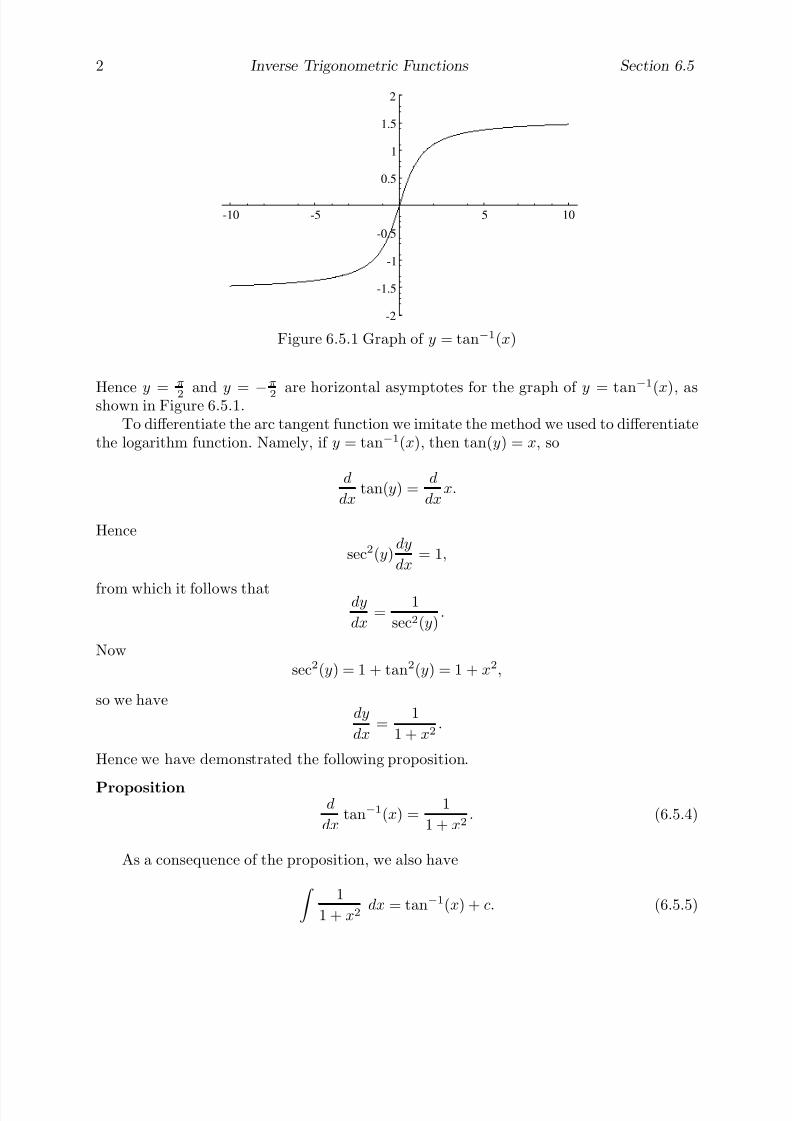
7/27/2019 Calculus 2 (Dan Sloughter)
http://slidepdf.com/reader/full/calculus-2-dan-sloughter 442/598
2 Inverse Trigonometric Functions Section 6.5
-10 -5 5 10
-2
-1.5
-1
-0.5
0.5
1
1.5
2
Figure 6.5.1 Graph of y = tan−1(x)
Hence y =π
2 and y = −π
2 are horizontal asymptotes for the graph of y = tan−1
(x), asshown in Figure 6.5.1.To differentiate the arc tangent function we imitate the method we used to differentiate
the logarithm function. Namely, if y = tan−1(x), then tan(y) = x, so
d
dxtan(y) =
d
dxx.
Hence
sec2(y)dy
dx= 1,
from which it follows that dy
dx=
1
sec2(y).
Nowsec2(y) = 1 + tan2(y) = 1 + x2,
so we havedy
dx=
1
1 + x2.
Hence we have demonstrated the following proposition.
Propositiond
dxtan−1(x) =
1
1 + x2. (6.5.4)
As a consequence of the proposition, we also have
1
1 + x2dx = tan−1(x) + c. (6.5.5)
7/27/2019 Calculus 2 (Dan Sloughter)
http://slidepdf.com/reader/full/calculus-2-dan-sloughter 443/598
Section 6.5 Inverse Trigonometric Functions 3
Note that 1 + x2 is an irreducible quadratic polynomial. We will see more examples of this type in the following examples.
Example Using the chain rule, we have
d
dx tan
−1
(4x
2
) =
8x
1 + 16x4 .
Example Evaluating
tan−1(x)dx is similar to evaluating
log(x)dx. That is, we will
use integration by parts with
u = tan−1(x) dv = dx
du =1
1 + x2dx v = x.
Then tan−1
(x)dx = x tan−1
(x)− x
1 + x2 dx.
Using the substitutionu = 1 + x2
du = 2xdx,
we have1
2du = xdx, from which it follows that
x
1 + x2dx =
1
2
1
udu =
1
2log |u|+ c =
1
2log(1 + x2) + c.
Thus tan−1(x)dx = x tan−1(x)− 1
2log(1 + x2) + c.
Example To evaluate
1
1 + 4x2dx, we make the substitution
u = 2x
du = 2dx.
Then
1
2 du = dx, so 1
1 + 4x2dx =
1
2
1
1 + u2du =
1
2tan−1(u) + c =
1
2tan−1(2x) + c.
Example To evaluate
1
x2 + x + 1dx, we first note that x2 + x + 1 does not factor,
that is, is irreducible, and so we cannot use a partial fraction decomposition. In general,
7/27/2019 Calculus 2 (Dan Sloughter)
http://slidepdf.com/reader/full/calculus-2-dan-sloughter 444/598
4 Inverse Trigonometric Functions Section 6.5
a quadratic polynomial ax2 + bx + c is irreducible if b2 − 4ac < 0 since, in that case, thequadratic formula yields complex solutions for the equation ax2+bx + c = 0. For x2+x + 1we have b2 − 4ac = −3. In this case it is helpful to simplify the function algebraically bycompleting the square of the denominator, thus making the problem similar to the previousexample. That is, since
x2 + x + 1 =
x + 12
2
+ 34
,
we have 1
x2 + x + 1dx =
1
x + 1
2
2+ 3
4
dx =4
3
1
4
3
x + 1
2
2+ 1
dx.
Now we can make the substitution
u = 4
3
x +1
2
du =
4
3dx.
Then
3
4du = dx, so
1
x2 + x + 1dx =
4
3
3
4
1
u2 + 1du
=
43
tan−1(u) + c
=
4
3tan−1
4
3
x +
1
2
+ c.
Partial fraction decomposition: Irreducible quadratic factors
The last two examples illustrate techniques that we may use to evaluate the integral of a rational function with an irreducible quadratic polynomial in the denominator. With
this we are now in a position to consider the final case of partial fraction decomposition.Specifically, suppose we want to evaluate
f (x)
g(x)dx,
where f and g are both polynomials and the degree of f is less than the degree of g.Moreover, suppose that (ax2 + bx + c)n is a factor of g, where n is a positive integer and
7/27/2019 Calculus 2 (Dan Sloughter)
http://slidepdf.com/reader/full/calculus-2-dan-sloughter 445/598
Section 6.5 Inverse Trigonometric Functions 5
ax2 + bx + c is irreducible. Then the partial fraction decomposition of f (x)
g(x)must contain
a sum of terms of the form
A1x + B1
ax2 + bx + c+
A2x + B2
(ax2 + bx + c)2+ · · ·+
Anx + Bn
(ax2 + bx + c)n, (6.5.6)
where A1, A2, . . . , An and B1, B2, . . . , Bn are constants. Note that the terms in the partialfraction decomposition corresponding to an irreducible quadratic factor differ from theterms for a linear factor in that the numerators of the terms in (6.5.6) need not be constants,but may be first degree polynomials themselves. As before, this is best illustrated with anexample.
Example To evaluate
1 + x
x(1 + x2)dx we need to find constants A, B, and C such that
1 + x
x(1 + x2)=
A
x+
Bx + C
1 + x2.
Combining the terms on the right, we have
1 + x
x(1 + x2)=
A(1 + x2) + (Bx + C )x
x(1 + x2).
Hence1 + x = A(1 + x2) + (Bx + C )x = (A + B)x2 + Cx + A.
Equating the coefficients of the polynomials on the left and right gives us the system of equations
A + B = 0,
C = 1,
A = 1.
Thus B = −1 and
1 + x
x(1 + x2)=
1
x+
1 − x
1 + x2=
1
x+
1
1 + x2− x
1 + x2.
Hence 1 + x
x(1 + x2)dx =
1
xdx +
1
1 + x2dx −
x
1 + x2dx
= log |x|+ tan−1
(x)−1
2 log(1 + x2
) + c.
where the final integral follows from the substitution u = 1 + x2 as in an earlier example.
If, unlike this example, the partial fraction decomposition of f (x)
g(x)results in a term of
the formAx + B
(ax2 + bx + c)n,
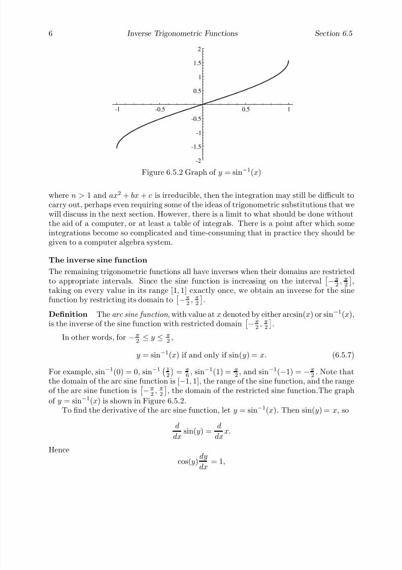
7/27/2019 Calculus 2 (Dan Sloughter)
http://slidepdf.com/reader/full/calculus-2-dan-sloughter 446/598
6 Inverse Trigonometric Functions Section 6.5
-1 -0.5 0.5 1
-2
-1.5
-1
-0.5
0.5
1
1.5
2
Figure 6.5.2 Graph of y = sin−1(x)
where n > 1 and ax2 + bx + c is irreducible, then the integration may still be difficult tocarry out, perhaps even requiring some of the ideas of trigonometric substitutions that wewill discuss in the next section. However, there is a limit to what should be done withoutthe aid of a computer, or at least a table of integrals. There is a point after which someintegrations become so complicated and time-consuming that in practice they should begiven to a computer algebra system.
The inverse sine function
The remaining trigonometric functions all have inverses when their domains are restrictedto appropriate intervals. Since the sine function is increasing on the interval
−π
2, π2
,
taking on every value in its range [1, 1] exactly once, we obtain an inverse for the sine
function by restricting its domain to−π
2 ,π
2
.
Definition The arc sine function , with value at x denoted by either arcsin(x) or sin−1(x),is the inverse of the sine function with restricted domain
−π
2, π2
.
In other words, for −π
2≤ y ≤ π
2,
y = sin−1(x) if and only if sin(y) = x. (6.5.7)
For example, sin−1(0) = 0, sin−11
2
= π
6, sin−1(1) = π
2, and sin−1(−1) = −π
2. Note that
the domain of the arc sine function is [−1, 1], the range of the sine function, and the rangeof the arc sine function is −
π
2, π2 , the domain of the restricted sine function.The graph
of y = sin−1(x) is shown in Figure 6.5.2.To find the derivative of the arc sine function, let y = sin−1(x). Then sin(y) = x, so
d
dxsin(y) =
d
dxx.
Hence
cos(y)dy
dx= 1,
7/27/2019 Calculus 2 (Dan Sloughter)
http://slidepdf.com/reader/full/calculus-2-dan-sloughter 447/598
Section 6.5 Inverse Trigonometric Functions 7
and sody
dx=
1
cos(y).
Nowcos2(y) = 1
−sin2(y) = 1 + x2,
so cos(y) = ±√ 1 − x2. Since −π
2≤ y ≤ π
2, cos(y) ≥ 0. Thus cos(y) = √ 1 − x2, and
dy
dx=
1√ 1− x2
.
Propositiond
dxsin−1(x) =
1√ 1− x2
. (6.5.8)
As a consequence of this proposition, we also have 1√
1 − x2dx = sin−1(x) + c. (6.5.9)
Example Using the product and chain rules,
d
dx
x sin−1(2x)
=
2x√ 1 − 4x2
+ sin−1(2x).
Example To evaluate 1
√ 4 − x2
dx, we first note that
1
4 − x2=
1 4
1− x2
4
=1
2
1 1 − x
2
4
.
Then the substitutionu =
x
2
du =1
2dx
gives us 1√
4 − x2dx =
1√
1 − u2du = sin−1(u) + c = sin−1
x
2
+ c.
The inverse secant function
Defining an inverse for the secant function is slightly more complicated than defining thearc tangent or arc sine functions. On the interval
0, π
2
, the secant function is increasing

7/27/2019 Calculus 2 (Dan Sloughter)
http://slidepdf.com/reader/full/calculus-2-dan-sloughter 448/598
8 Inverse Trigonometric Functions Section 6.5
-4 -2 2 4
0.5
1
1.5
2
2.5
3
3.5
Figure 6.5.3 Graph of y = sec−1(x)
and takes on all values in the interval [1,∞); on the interval
π2
, π, the secant functionis also increasing, taking on all values in the interval (−∞, 1]. Hence between these two
intervals the secant function takes on every value in its range exactly once. From theseconsiderations we obtain the following definition.
Definition The arc secant function , with value at x denoted by either arcsec(x) orsec−1(x), is the inverse of the secant function with domain restricted to the intervals
0, π2
and
π
2, π
.
Thus for 0 ≤ y < π
2or π
2< y ≤ π,
y = sec−1(x) if and only if sec(y) = x. (6.5.10)
For example, sec−1(2) = π
3, sec−1(1) = 0, sec−1(−2) = 2π
3, and sec−1(−1) = π. Note that
the domain of the arc secant function consists of the two intervals (−∞,−1] and [1,∞),the range of the secant function, and the range is composed of the two intervals
0, π
2
and
π
2, π
, the domain of the restricted secant function.Since
limx→
π
2−
sec(x) = ∞
andlim
x→π
2+
sec(x) = −∞,
it follows thatlimx→∞
sec−1(x) =π
2(6.5.11)
andlim
x→−∞
sec−1(x) =π
2. (6.5.12)
Thus the line y = π
2is a horizontal asymptote for the graph of y = sec−1(x) both as x
goes to ∞ and as x goes to −∞, as shown in Figure 6.5.3.

7/27/2019 Calculus 2 (Dan Sloughter)
http://slidepdf.com/reader/full/calculus-2-dan-sloughter 449/598
Section 6.5 Inverse Trigonometric Functions 9
To find the derivative of the arc secant function, let y = sec−1(x). Then sec(y) = x, so
d
dxsec(y) =
d
dxx.
Hencesec(y) tan(y)
dy
dx= 1,
and sody
dx=
1
sec(y) tan(y).
Now sec(y) = x and
tan2(y) = sec2(y)− 1 = x2 − 1.
Hence tan(y) = ±√ x2 − 1. If x is in [1,∞), then 0 ≤ y < π
2and tan(y) ≥ 0; if x is in
(−∞
,
−1], then π
2< y
≤π and tan(y)
≤0. Thus
sec(y) tan(y) =
x√
x2 − 1, if x ≥ 1−x√
x2 − 1, if x ≤ −1.
Since |x| = x when x ≥ 1 and |x| = −x when x ≤ −1, it follows that
sec(y) tan(y) = |x|
x2 − 1.
Hencedy
dx=
1
|x|√ x2 − 1.
Propositiond
dxsec−1(x) =
1
|x|√ x2 − 1. (6.5.13)
Example Using the chain rule, we have
d
dxsec−1(3x) =
3
|3x|√ 9x2 − 1=
1
|x|√ 9x2 − 1.
We will leave the definition of inverse functions for the cotangent, cosine, and cosecantfunctions for the problems at the end of the section. In the next section we will see howthe arc tangent, arc sine, and arc secant functions are useful in evaluating certain integrals;the arc cotangent, arc cosine, and arc cosecant functions could be used in similar roles,but, wherever they are used, we could just as well use arc tangent, arc sine, or arc secant.Hence the former, although useful in other situations, will not be as important for ourpresent study as the latter.

7/27/2019 Calculus 2 (Dan Sloughter)
http://slidepdf.com/reader/full/calculus-2-dan-sloughter 450/598
10 Inverse Trigonometric Functions Section 6.5
Problems
1. Find the derivatives of each of the following functions.
(a) f (x) = x tan−1(x) (b) g(t) = tan−1(3t2)
(c) g(x) = sin−1
(3x)x
(d) f (x) = 3x sec−1(5x)
2. Evaluate each of the following.
(a) tan−1
1√ 3
(b) tan−1(−
√ 3)
(c) sin−1
√ 3
2
(d) sec−1
− 2√
3
(e) sin−1sin3π
4 (f) sinsin−1−1√
2
3. Evaluate the following integrals.
(a)
1
1 + 2x2dx (b)
4x
2 + x2dx
(c)
3
x2 + 4dx (d)
5
x2 + 2x + 3dx
(e)
x
x2 + 4x + 5dx (f)
x + 1
x2 + 2x + 6dx
(g) 1
−1
1
1 + x2dx (h)
13
0
1
1 + 9x2dx
4. Evaluate the following integrals.
(a)
1
x3 + xdx (b)
2 + x
x(4x2 + 1)dx
(c)
1
x2(x2 + 1)dx (d)
1
(x + 1)(x2 + 2)dx
(e)
sin−1(x)dx (f)
tan−1(3x)dx
(g) 5
√ 1− 9x2
dx (h) 1
√ 4 − 8x2
dx
(i)
3x√
1− x2dx (j)
2
−2
1√ 16− x2
dx
5. The cosine function has an inverse, called the arc cosine function , if its domain isrestricted to [0, π]. That is, for 0 ≤ y ≤ π,
y = cos−1(x) if and only if cos(y) = x.

7/27/2019 Calculus 2 (Dan Sloughter)
http://slidepdf.com/reader/full/calculus-2-dan-sloughter 451/598
Section 6.5 Inverse Trigonometric Functions 11
(a) Show thatd
dxcos−1(x) = − 1√
1 − x2.
(b) Show that sec−1(x) = cos−1
1
x
.
(c) Use the result from (b) to find
d
dx sec−1
(x).(d) Use the fact that
d
dxsin−1(x) =
d
dx(− cos−1(x))
to show thatsin−1(x) + cos−1(x) =
π
2for all x in [−1, 1].
6. The cotangent function has an inverse, called the arc cotangent function , if its domainis restricted to (0, π). That is, for 0 < y < π,
y = cot−1
(x) if and only if cot(y) = x.
Show thatd
dxcot−1(x) = − 1
1 + x2.
7. The cosecant function has an inverse, called the arc cosecant function , if its domain isrestricted to the intervals
−π
2, 0
and
0, π2
. That is, for −π
2≤ y < 0 or 0 < y ≤ π
2,
y = csc−1(x) if and only if csc(y) = x.
Show thatd
dxcsc−1(x) = − 1
|x|√ x2 − 1.
8. Evaluate ∞
−∞
1
1 + x2
dx.
9. (a) Use the fact that
tan−1(x) =
x
0
1
1 + t2dt
to find the Taylor series expansion for tan−1(x) about 0. On what interval doesthis series converge?
(b) Use your result in (a) and the fact that π = 4tan−1(1) to approximate π with anerror of no more than 0.001.
10. (a) Show thatd
dx tan−1 1
x
= −1
1 + x2 .
(b) Use the result from (a) to show that
tan−1(x) + tan−1
1
x
=
π
2
for all x > 0.
(c) Find a result similar to (b) for x < 0.

7/27/2019 Calculus 2 (Dan Sloughter)
http://slidepdf.com/reader/full/calculus-2-dan-sloughter 452/598
Difference Equations
Differential Equations
to
Section 6.6
Trigonometric Substitutions
In the last section we saw that 1√
1 − x2dx = sin−1(x) + c.
However, we arrived at this result as a consequence of our differentiation of the arc sinefunction, not as the outcome of the application of some systematic approach to the evalua-tion of integrals of this type. In this section we will explore how substitutions based on the
arc sine, arc tangent, and arc secant functions provide a systematic method for evaluatingintegrals similar to this one.
Sine substitutions
To begin, consider evaluating 1√
1 − x2dx
by using the substitution u = sin−1(x). The motivation for such a substitution stems fromthe fact that, for −π
2≤ u ≤ π
2, u = sin−1(x) if and only if x = sin(u). In the latter form,
we see that
dx = cos(u)duand
1 − x2 =
1− sin2(u) =
cos2(u) = | cos(u)|. (6.6.1)
Since cos(u) ≥ 0 when π
2≤ u ≤ π
2, (6.6.1) becomes
1 − x2 = cos(u).
Thus 1√
1
−x2
dx =
cos(u)
cos(u)du =
du = u + c = sin−1(x) + c.
Of course, there is nothing new in the result itself; it is the technique, which we maygeneralize to other integrals of a similar type, which is of interest. Specifically, for anintegral with a factor of the form
a2 − x2
or1√
a2 − x2,
1 Copyright c by Dan Sloughter 2000
7/27/2019 Calculus 2 (Dan Sloughter)
http://slidepdf.com/reader/full/calculus-2-dan-sloughter 453/598
2 Trigonometric Substitutions Section 6.6
where a > 0, the substitution
x = a sin(u),π
2≤ u ≤ π
2, (6.6.2)
may prove to be useful because of the simplification
a2 − x2 =
a2 − a2 sin2(x) =
a2(1− sin2(u)) = a
cos2(u) = a cos(u). (6.6.3)
Although this substitution is equivalent to the substitution u = sin−1x
a
, we will see that
it is more convenient to work with it in the form x = a sin(u).
Example To evaluate the integral
1√
9 − x2dx, we make the substitution
x = 3sin(u),−π
2< u <
π
2,
dx = 3 cos(u)du.
Note that we omit both u = −π
2and u = π
2since the function being integrated is not
defined at either x = −3 or x = 3. Then
1√ 9− x2
dx =
3cos(u)
9− 9sin2(u)du
=
3cos(u)
3
1 − sin2(u)du
= cos(u) cos2(u)
du
=
cos(u)
cos(u)du
=
du
= u + c.
Now x = 3sin(u) implies that u = sin−1x
3
, so we have
1
√ 9 − x2
dx = sin−1 x
3 + c.
Example To evaluate
4 − x2 dx, we make the substitution
x = 2sin(u),−π
2≤ u ≤ π
2,
dx = 2 cos(u)du.
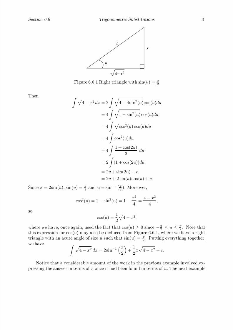
7/27/2019 Calculus 2 (Dan Sloughter)
http://slidepdf.com/reader/full/calculus-2-dan-sloughter 454/598
Section 6.6 Trigonometric Substitutions 3
x 2
u
x
2
4
Figure 6.6.1 Right triangle with sin(u) = x
2
Then 4 − x2 dx = 2
4 − 4sin2(u)cos(u)du
= 4
1 − sin2
(u) cos(u)du
= 4
cos2(u) cos(u)du
= 4
cos2(u)du
= 4
1 + cos(2u)
2du
= 2
(1 + cos(2u))du
= 2u + sin(2u) + c= 2u + 2 sin(u)cos(u) + c.
Since x = 2sin(u), sin(u) = x
2and u = sin−1
x
2
. Moreover,
cos2(u) = 1− sin2(u) = 1− x2
4=
4− x2
4,
so
cos(u) =1
2
4 − x2,
where we have, once again, used the fact that cos(u)
≥0 since
−π
2
≤u
≤π
2. Note that
this expression for cos(u) may also be deduced from Figure 6.6.1, where we have a righttriangle with an acute angle of size u such that sin(u) = x
2. Putting everything together,
we have 4− x2 dx = 2sin−1
x
2
+
1
2x
4 − x2 + c.
Notice that a considerable amount of the work in the previous example involved ex-pressing the answer in terms of x once it had been found in terms of u. The next example

7/27/2019 Calculus 2 (Dan Sloughter)
http://slidepdf.com/reader/full/calculus-2-dan-sloughter 455/598
4 Trigonometric Substitutions Section 6.6
illustrates how this work is unnecessary when evaluating definite integrals since we canchange the limits of integration and, from that point on, do all our work in terms of u.
Example Recall that, for r > 0, the graph of y =√
r2 − x2 is the upper half of a circleof radius r centered at the origin. Hence we should have
2 r−r
r2 − x2 dr = πr2.
We are now able to verify this. Let
x = r sin(u),−π
2≤ u ≤ π
2,
dx = r cos(u)du.
Then u = sin−1x
r
, so when x = −r,
u = sin−1(−
1) =−
π
2,
and when x = r,
u = sin−1(1) =π
2.
Thus
2
r
−r
r2 − x2 dx = 2
π2
−π
2
r2 − r2 sin2(u) r cos(u)du
= 2
π2
−π
2
r2
cos2(u)cos(u)du
= 2r2 π2−π
2
cos2(u)du
= 2r2 π
2
−π
2
1 + cos(2u)
2du
= r2 π
2
−π
2
(1 + cos(2u))du
= r2
u +sin(2u)
2
π
2
−π
2
=r2 π
2 + 0− −
π
2 + 0
= πr2.
Tangent substitutions
In a similar fashion, the substitution
x = a tan(u),−π
2< u <
π
2, (6.6.4)
7/27/2019 Calculus 2 (Dan Sloughter)
http://slidepdf.com/reader/full/calculus-2-dan-sloughter 456/598
Section 6.6 Trigonometric Substitutions 5
may be useful for integrals which have a factor of the form
a2 + x2,
1
√ a2
+ x2
,
or1
a2 + x2
because of the simplification
a2 + x2 = a2 + a2 tan2(u) = a2(1 + tan2(u)) = a2 sec2(u). (6.6.5)
Note that with our restriction on u, this substitution is equivalent to the substitutionu = tan−1
x
a
.
Example To evaluate the integral 1
4 + x2 dx, we make the substitution
x = 2 tan(u),−π
2< u <
π
2,
dx = 2 sec2(u)du.
Then 1
4 + x2dx =
2sec2(u)
4 + 4 tan2(u)du
=1
2
sec2(u)
1 + tan
2
(u
)
du
=1
2
sec2(u)
sec2(u)du
=1
2
du
=1
2u + c.
Since x = 2tan(u), u = tan−1x
2
. Thus
1
4 + x2
dx =1
2tan−1 x
2 + c.
Example To evaluate
1√
1 + x2dx, we make the substitution
x = tan(u),−π
2< u <
π
2,
dx = sec2(u)du.

7/27/2019 Calculus 2 (Dan Sloughter)
http://slidepdf.com/reader/full/calculus-2-dan-sloughter 457/598
6 Trigonometric Substitutions Section 6.6
x 2
u
x
1
1
Figure 6.6.2 Right triangle with tan(u) = x
Then 1 + x2 =
1 + tan2(u) =
sec2(u) = | sec(u)|.
Since −π
2< u < π
2, sec(u) > 0, so | sec(u)| = sec(u). Hence
1
1 + x2dx =
sec2(u)
sec(u)du
=
sec(u)du
= log | sec(u) + tan(u)| + c,
where the final integral follows from an example in Section 6.2. Now tan( u) = x, so
sec2(u) = 1 + tan2(u) = 1 + x2.
Since sec(u) > 0, it follows that
sec(u) =
1 + x2.
Note that this expression for sec(u) may also be deduced from Figure 6.6.2, where we havea right triangle with an acute angle of size u such that tan(u) = x. Thus
1√
1 + x2dx = log
1 + x2 + x
+ c.
Secant substitutions
For integrals involving a factor of the form
x2 − a2
or1√
x2 − a2,
7/27/2019 Calculus 2 (Dan Sloughter)
http://slidepdf.com/reader/full/calculus-2-dan-sloughter 458/598
Section 6.6 Trigonometric Substitutions 7
where a > 0, the substitutionx = a sec(u) (6.6.6)
may be useful. With this substitution,
x2
−a2
= a2
sec
2
(u
)−a2
=a
sec
2
(u
)− 1 =a
tan
2
(u
) =a| tan(
u)|
.(6.6.7)
Now√
x2 − a2 is meaningful only if either x ≥ a or x ≤ −a. Since x = a sec(u), the formercase corresponds to u in the interval [0, π
2) and the latter to u in the interval (π
2, π]. For
0 ≤ u < π
2, tan(u) ≥ 0, so
x2 − a2 = a tan(u);
for π
2< u ≤ π, tan(u) ≤ 0, so
x2 − a2 = −a tan(u).
Hence it is important when evaluating integrals of this type to be careful about whichvalues of x are of interest.
Example To evaluate
1√
x2 − 9dx for x > 3, we make the substitution
x = 3 sec(u), 0 < u <π
2,
dx = 3 sec(u) tan(u)du.
Then 1√
x2
−9
dx =
3sec(u) tan(u)
9sec2(u)−
9du
=
3sec(u) tan(u)
3
sec2(u)− 1du
=
sec(u) tan(u)
tan2(u)du
=
sec(u) tan(u)
tan(u)du
=
sec(u)du
= log|
sec(u) + tan(u)|
+ c.
Now sec(u) = x
3, so
tan2(u) = sec2(u)− 1 =x2
9− 1 =
x2 − 9
9.
Hence
tan(u) =1
3
x2 − 9,

7/27/2019 Calculus 2 (Dan Sloughter)
http://slidepdf.com/reader/full/calculus-2-dan-sloughter 459/598
8 Trigonometric Substitutions Section 6.6
x 2
u
x
3
9
Figure 6.6.3 Right triangle with sec(u) = x
3
where we have used the fact that tan(u) > 0 since 0 < u < π
2. Note that this expression
for sec(u) may also be deduced from Figure 6.6.3, where we have a right triangle with anacute angle of size u such that sec(u) = x
3. Thus
1√
x2 − 9dx = log
x3
+ 13
x2 − 9
= log |x +
x2 − 9| − log(3) + c.
Since log(3) is a constant, we may combine it with the arbitrary constant of integration.Moreover, since we are assuming x > 3, we may remove the absolute value and write
1√
x2 − 9dx = log(x +
x2 − 9) + c.
Problems
1. Evaluate the following integrals.
(a)
3√
16 − x2dx (b)
x√
4 − x2dx
(c)
5 − z2 dz (d)
5
6 + x2dx
(e)
1√
4 + x2dx (f)
4x√
1 + x2dx
2. Evaluate the following integrals.
(a)
z
1− z2 dz (b)
1
(1− x2)3
2
dx
(c)
1√
x2 − 4dx, x > 2 (d)
1√
x2 − 4dx, x < −2
(e)
4√
3− 2x2dx (f)
3
5 + 2x2dx

7/27/2019 Calculus 2 (Dan Sloughter)
http://slidepdf.com/reader/full/calculus-2-dan-sloughter 460/598
Section 6.6 Trigonometric Substitutions 9
(g)
4 − t2 dt (h)
1 − 4x2 dx
3. Evaluate the following integrals.
(a) 3
0 9 −
t2 dt (b) 1
−1 1 + x2 dx
(c)
1
0
1
(1 + x2)3
2
dx (d)
1
0
x2
1− x2 dx
(e)
10
5√ 2
1√ x2 − 25
dx (f)
2
√ 2
3
x2√
x2 − 1dx
4. Evaluate 1
1 − x2dx
using (a) partial fractions and (b) the substitution x = sin(u). How do the two methods
compare?
5. Evaluate 1√
1 − x2dx
using the substitution x = cos(u) with 0 < u < π.
6. (a) Evaluate 1√
x2 − 9dx
for x <
−3.
(b) Show that 1√
x2 − 9dx = log |x +
x2 − 9|+ c,
for both x > 3 and x < −3.
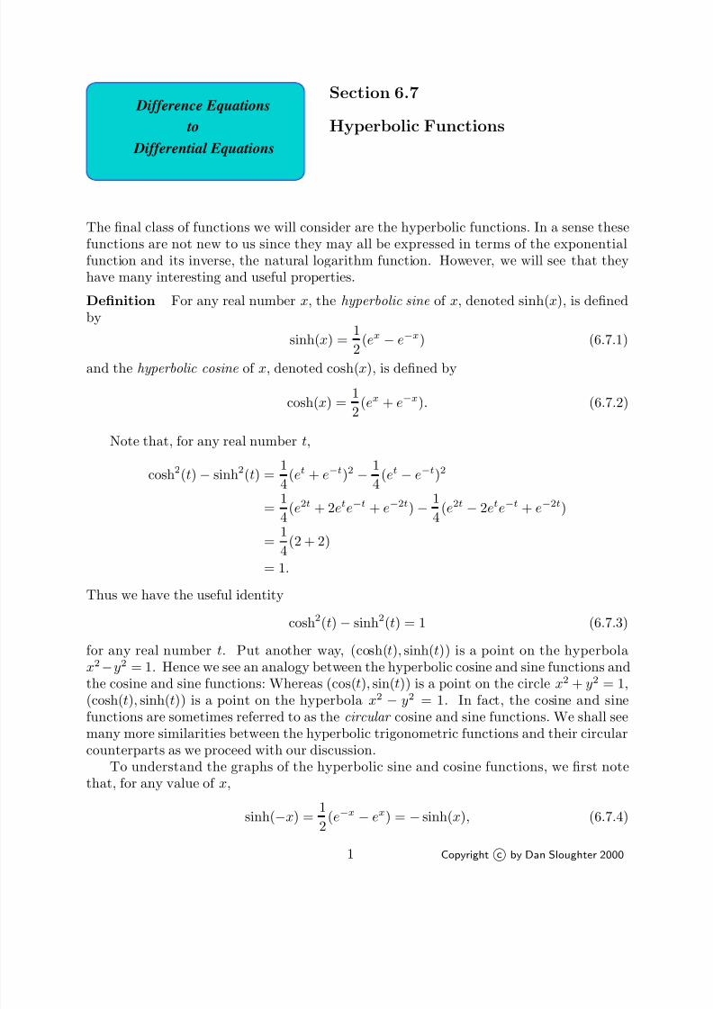
7/27/2019 Calculus 2 (Dan Sloughter)
http://slidepdf.com/reader/full/calculus-2-dan-sloughter 461/598
Difference Equations
Differential Equations
to
Section 6.7
Hyperbolic Functions
The final class of functions we will consider are the hyperbolic functions. In a sense thesefunctions are not new to us since they may all be expressed in terms of the exponentialfunction and its inverse, the natural logarithm function. However, we will see that theyhave many interesting and useful properties.
Definition For any real number x, the hyperbolic sine of x, denoted sinh(x), is definedby
sinh(x) =1
2
(ex
−e−x) (6.7.1)
and the hyperbolic cosine of x, denoted cosh(x), is defined by
cosh(x) =1
2(ex + e−x). (6.7.2)
Note that, for any real number t,
cosh2(t)− sinh2(t) =1
4(et + e−t)2 − 1
4(et − e−t)2
=1
4(e2t + 2ete−t + e−2t)− 1
4(e2t − 2ete−t + e−2t)
= 14
(2 + 2)
= 1.
Thus we have the useful identity
cosh2(t)− sinh2(t) = 1 (6.7.3)
for any real number t. Put another way, (cosh(t), sinh(t)) is a point on the hyperbolax2−y2 = 1. Hence we see an analogy between the hyperbolic cosine and sine functions andthe cosine and sine functions: Whereas (cos(t), sin(t)) is a point on the circle x2 + y2 = 1,
(cosh(t), sinh(t)) is a point on the hyperbola x
2
− y
2
= 1. In fact, the cosine and sinefunctions are sometimes referred to as the circular cosine and sine functions. We shall seemany more similarities between the hyperbolic trigonometric functions and their circularcounterparts as we proceed with our discussion.
To understand the graphs of the hyperbolic sine and cosine functions, we first notethat, for any value of x,
sinh(−x) =1
2(e−x − ex) = − sinh(x), (6.7.4)
1 Copyright c by Dan Sloughter 2000
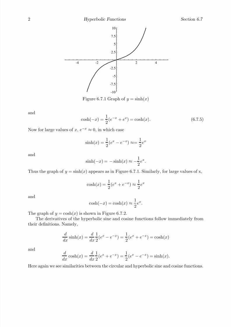
7/27/2019 Calculus 2 (Dan Sloughter)
http://slidepdf.com/reader/full/calculus-2-dan-sloughter 462/598
2 Hyperbolic Functions Section 6.7
-4 -2 2 4
-10
-7.5
-5
-2.5
2.5
5
7.5
10
Figure 6.7.1 Graph of y = sinh(x)
andcosh(−x) =
1
2(e−x + ex) = cosh(x). (6.7.5)
Now for large values of x, e−x ≈ 0, in which case
sinh(x) =1
2(ex − e−x) ≈=
1
2ex
and
sinh(−x) = − sinh(x) ≈ −1
2ex.
Thus the graph of y = sinh(x) appears as in Figure 6.7.1. Similarly, for large values of x,
cosh(x) =1
2(ex + e−x) ≈ 1
2ex
and
cosh(−x) = cosh(x) ≈ 1
2ex.
The graph of y = cosh(x) is shown in Figure 6.7.2.The derivatives of the hyperbolic sine and cosine functions follow immediately from
their definitions. Namely,
d
dxsinh(x) =
d
dx
1
2(ex − e−x) =
1
2(ex + e−x) = cosh(x)
andd
dxcosh(x) =
d
dx
1
2(ex + e−x) =
1
2(ex − e−x) = sinh(x).
Here again we see similarities between the circular and hyperbolic sine and cosine functions.
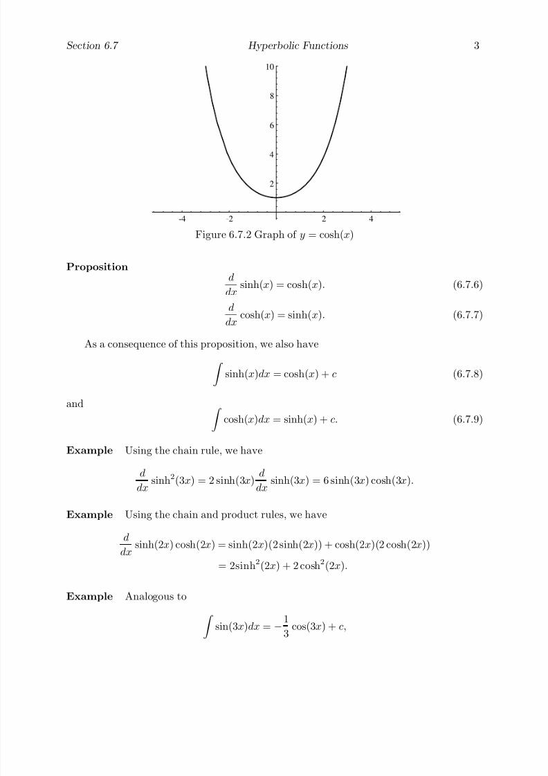
7/27/2019 Calculus 2 (Dan Sloughter)
http://slidepdf.com/reader/full/calculus-2-dan-sloughter 463/598
Section 6.7 Hyperbolic Functions 3
-4 -2 2 4
2
4
6
8
10
Figure 6.7.2 Graph of y = cosh(x)
Proposition d
dxsinh(x) = cosh(x). (6.7.6)
d
dxcosh(x) = sinh(x). (6.7.7)
As a consequence of this proposition, we also have
sinh(x)dx = cosh(x) + c (6.7.8)
and
cosh(x)dx = sinh(x) + c. (6.7.9)
Example Using the chain rule, we have
d
dxsinh2(3x) = 2 sinh(3x)
d
dxsinh(3x) = 6 sinh(3x) cosh(3x).
Example Using the chain and product rules, we have
d
dx sinh(2x) cosh(2x) = sinh(2x)(2 sinh(2x)) + cosh(2x)(2 cosh(2x))
= 2sinh2(2x) + 2 cosh2(2x).
Example Analogous to
sin(3x)dx = −1
3cos(3x) + c,
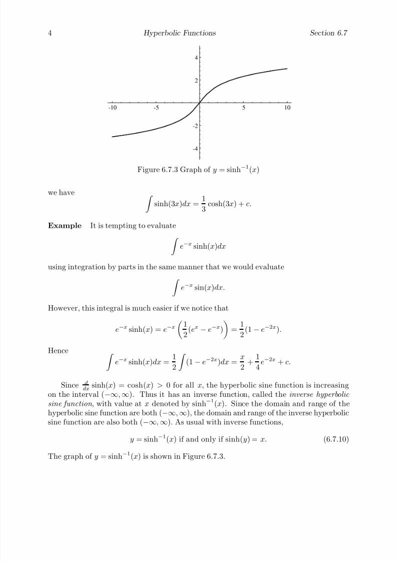
7/27/2019 Calculus 2 (Dan Sloughter)
http://slidepdf.com/reader/full/calculus-2-dan-sloughter 464/598
4 Hyperbolic Functions Section 6.7
-10 -5 5 10
-4
-2
2
4
Figure 6.7.3 Graph of y = sinh−1(x)
we have
sinh(3x)dx = 13
cosh(3x) + c.
Example It is tempting to evaluate
e−x sinh(x)dx
using integration by parts in the same manner that we would evaluate
e−x sin(x)dx.
However, this integral is much easier if we notice that
e−x sinh(x) = e−x
1
2(ex − e−x)
=
1
2(1− e−2x).
Hence e−x sinh(x)dx =
1
2
(1− e−2x)dx =
x
2+
1
4e−2x + c.
Since d
dxsinh(x) = cosh(x) > 0 for all x, the hyperbolic sine function is increasing
on the interval (−∞,∞). Thus it has an inverse function, called the inverse hyperbolic sine function , with value at x denoted by sinh−1(x). Since the domain and range of thehyperbolic sine function are both (−∞,∞), the domain and range of the inverse hyperbolicsine function are also both (−∞,∞). As usual with inverse functions,
y = sinh−1(x) if and only if sinh(y) = x. (6.7.10)
The graph of y = sinh−1(x) is shown in Figure 6.7.3.
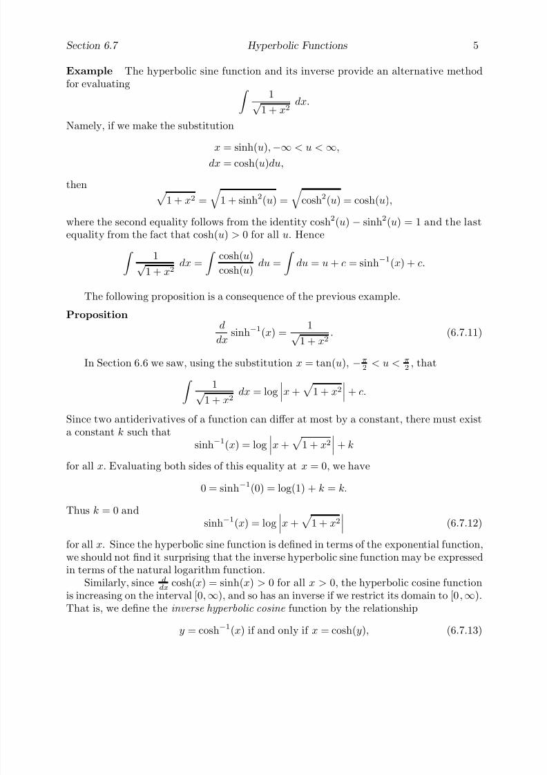
7/27/2019 Calculus 2 (Dan Sloughter)
http://slidepdf.com/reader/full/calculus-2-dan-sloughter 465/598
Section 6.7 Hyperbolic Functions 5
Example The hyperbolic sine function and its inverse provide an alternative methodfor evaluating
1√ 1 + x2
dx.
Namely, if we make the substitution
x = sinh(u),−∞ < u < ∞,
dx = cosh(u)du,
then 1 + x2 =
1 + sinh2(u) =
cosh2(u) = cosh(u),
where the second equality follows from the identity cosh2(u) − sinh2(u) = 1 and the lastequality from the fact that cosh(u) > 0 for all u. Hence
1
√ 1 + x2
dx = cosh(u)
cosh(u)du = du = u + c = sinh−1(x) + c.
The following proposition is a consequence of the previous example.
Propositiond
dxsinh−1(x) =
1√ 1 + x2
. (6.7.11)
In Section 6.6 we saw, using the substitution x = tan(u), −π
2< u < π
2, that
1√
1 + x2dx = log
x +
1 + x2
+ c.
Since two antiderivatives of a function can differ at most by a constant, there must exista constant k such that
sinh−1(x) = logx +
1 + x2
+ k
for all x. Evaluating both sides of this equality at x = 0, we have
0 = sinh−1(0) = log(1) + k = k.
Thus k = 0 andsinh−1(x) = log
x +
1 + x2
(6.7.12)
for all x. Since the hyperbolic sine function is defined in terms of the exponential function,we should not find it surprising that the inverse hyperbolic sine function may be expressedin terms of the natural logarithm function.
Similarly, since d
dxcosh(x) = sinh(x) > 0 for all x > 0, the hyperbolic cosine function
is increasing on the interval [0,∞), and so has an inverse if we restrict its domain to [0,∞).That is, we define the inverse hyperbolic cosine function by the relationship
y = cosh−1(x) if and only if x = cosh(y), (6.7.13)

7/27/2019 Calculus 2 (Dan Sloughter)
http://slidepdf.com/reader/full/calculus-2-dan-sloughter 466/598
6 Hyperbolic Functions Section 6.7
2 4 6 8 10
1
2
3
4
5
Figure 6.7.4 Graph of y = cosh−1(x)
where we require y ≥ 0. Note that since cosh(x) ≥ 1 for all x, the domain of of the inversehyperbolic cosine function is [1,∞). The graph of y = cosh−1(x) is shown in Figure 6.7.4.
In Problem 3 at the end of this section you are asked to show that
1√
x2 − 1dx = cosh−1(x) + c
for x > 1, from which the following proposition follows.
Proposition
d
dx cosh−1
(x) =
1
√ x2 − 1 . (6.7.14)
In the same problem you are asked to show that, for x ≥ 1,
cosh−1(x) = logx +
x2 − 1
(6.7.15)
Example In Section 6.6 we evaluated the integral
1√
x2 − 9dx,
for x > 3, using the substitution x = 3 sec(u), 0 < u < π
2. The substitution
x = 3 cosh(u), u > 0,
dx = 3 sinh(u)du
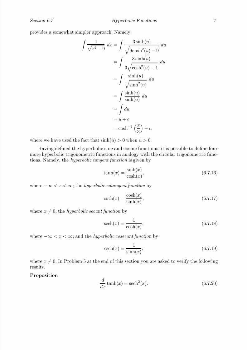
7/27/2019 Calculus 2 (Dan Sloughter)
http://slidepdf.com/reader/full/calculus-2-dan-sloughter 467/598
Section 6.7 Hyperbolic Functions 7
provides a somewhat simpler approach. Namely,
1√
x2 − 9dx =
3 sinh(u)
9cosh2(u)− 9du
=
3 sinh(u
)3
cosh2(u)− 1du
=
sinh(u) sinh2(u)
du
=
sinh(u)
sinh(u)du
=
du
= u + c
= cosh−1x
3
+ c,
where we have used the fact that sinh(u) > 0 when u > 0.
Having defined the hyperbolic sine and cosine functions, it is possible to define fourmore hyperbolic trigonometric functions in analogy with the circular trigonometric func-tions. Namely, the hyperbolic tangent function is given by
tanh(x) =sinh(x)
cosh(x), (6.7.16)
where −∞ < x < ∞; the hyperbolic cotangent function by
coth(x) =cosh(x)
sinh(x), (6.7.17)
where x = 0; the hyperbolic secant function by
sech(x) =1
cosh(x), (6.7.18)
where −∞ < x < ∞; and the hyperbolic cosecant function by
csch(x) = 1sinh(x)
, (6.7.19)
where x = 0. In Problem 5 at the end of this section you are asked to verify the followingresults.
Propositiond
dxtanh(x) = sech2(x). (6.7.20)
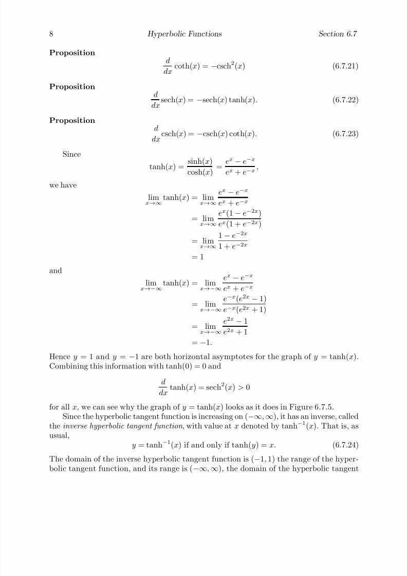
7/27/2019 Calculus 2 (Dan Sloughter)
http://slidepdf.com/reader/full/calculus-2-dan-sloughter 468/598
8 Hyperbolic Functions Section 6.7
Propositiond
dxcoth(x) = −csch2(x) (6.7.21)
Propositiond
dx sech(x) = −sech(x) tanh(x). (6.7.22)
Propositiond
dxcsch(x) = −csch(x) coth(x). (6.7.23)
Since
tanh(x) =sinh(x)
cosh(x)=
ex − e−x
ex + e−x,
we have
limx→∞ tanh(x
) = limx→∞
ex
−e−x
ex + e−x
= limx→∞
ex(1− e−2x)
ex(1 + e−2x)
= limx→∞
1− e−2x
1 + e−2x
= 1
and
limx→−∞
tanh(x) = limx→−∞
ex − e−x
ex + e−x
= limx→−∞
e−x
(e2x
− 1)e−x(e2x + 1)
= limx→−∞
e2x − 1
e2x + 1
= −1.
Hence y = 1 and y = −1 are both horizontal asymptotes for the graph of y = tanh(x).Combining this information with tanh(0) = 0 and
d
dxtanh(x) = sech2(x) > 0
for all x, we can see why the graph of y = tanh(x) looks as it does in Figure 6.7.5.Since the hyperbolic tangent function is increasing on (−∞,∞), it has an inverse, called
the inverse hyperbolic tangent function , with value at x denoted by tanh−1(x). That is, asusual,
y = tanh−1(x) if and only if tanh(y) = x. (6.7.24)
The domain of the inverse hyperbolic tangent function is (−1, 1) the range of the hyper-bolic tangent function, and its range is (−∞,∞), the domain of the hyperbolic tangent
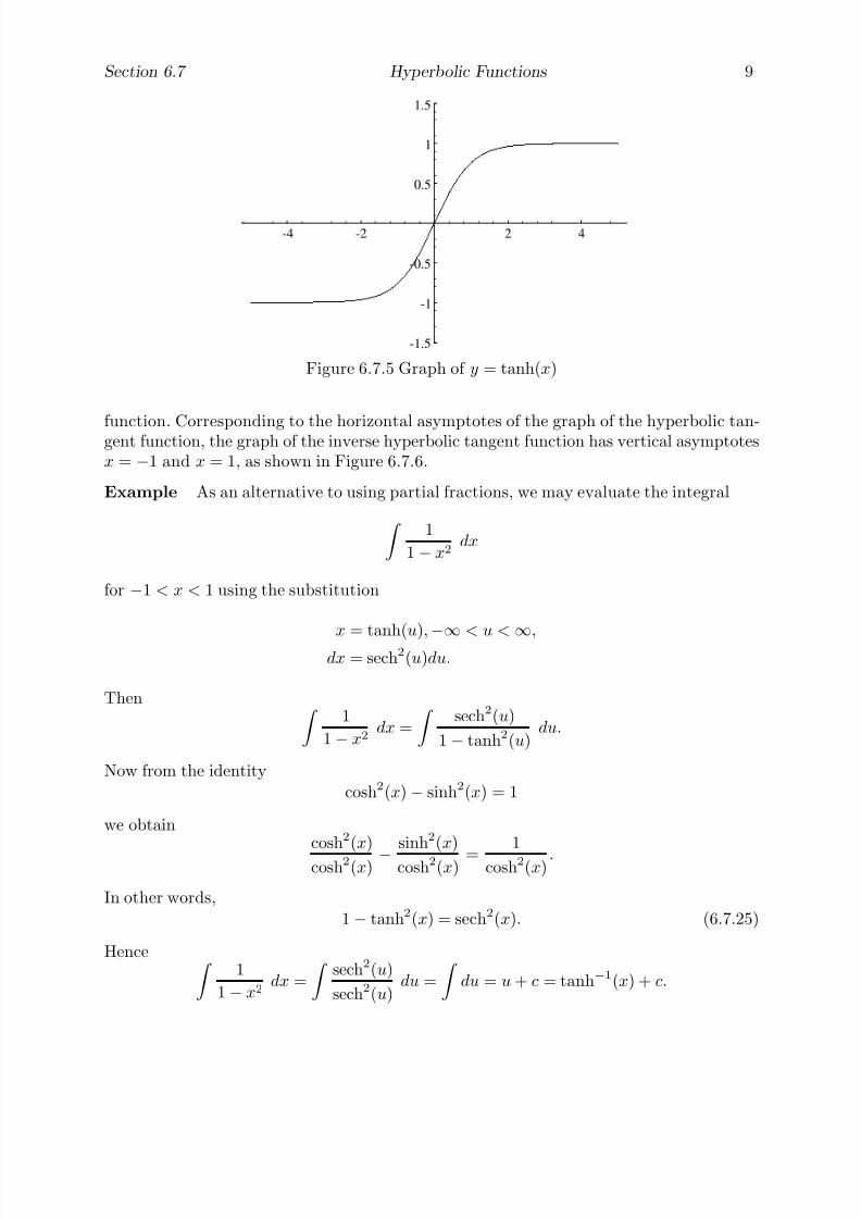
7/27/2019 Calculus 2 (Dan Sloughter)
http://slidepdf.com/reader/full/calculus-2-dan-sloughter 469/598
Section 6.7 Hyperbolic Functions 9
-4 -2 2 4
-1.5
-1
-0.5
0.5
1
1.5
Figure 6.7.5 Graph of y = tanh(x)
function. Corresponding to the horizontal asymptotes of the graph of the hyperbolic tan-gent function, the graph of the inverse hyperbolic tangent function has vertical asymptotesx = −1 and x = 1, as shown in Figure 6.7.6.
Example As an alternative to using partial fractions, we may evaluate the integral
1
1− x2dx
for −1 < x < 1 using the substitution
x = tanh(u),−∞
< u <∞
,
dx = sech2(u)du.
Then 1
1− x2dx =
sech2(u)
1− tanh2(u)du.
Now from the identity
cosh2(x)− sinh2(x) = 1
we obtaincosh2(x)
cosh2(x) −sinh2(x)
cosh2(x) =1
cosh2(x) .
In other words,
1− tanh2(x) = sech2(x). (6.7.25)
Hence 1
1− x2dx =
sech2(u)
sech2(u)du =
du = u + c = tanh−1(x) + c.

7/27/2019 Calculus 2 (Dan Sloughter)
http://slidepdf.com/reader/full/calculus-2-dan-sloughter 470/598
10 Hyperbolic Functions Section 6.7
-1.5 -1 -0.5 0.5 1 1.5
-4
-2
2
4
Figure 6.7.6 Graph of y = tanh−1(x)
Note that (6.7.25) gives us the useful identity
tanh2(x) + sech2(x) = 1 (6.7.26)
for all x. Moreover, we have the following proposition as a consequence of this example.
Proposition
d
dxtanh−1(x) =
1
1− x2. (6.7.27)
If we were to use partial fractions to evaluate the integral of the previous example, we
would obtain, for −1 < x < 1,
1
1− x2dx =
1
2log(1 + x)− 1
2log(1− x) + c =
1
2log
1 + x
1− x
+ c.
It follows that
tanh−1(x) =1
2log
1 + x
1− x
+ k
for some constant k. Evaluating at 0, we have
0 = 0 + k.
Thus k = 0 and we have
tanh−1(x) =1
2log
1 + x
1− x
(6.7.28)
for 1 < x < 1.
7/27/2019 Calculus 2 (Dan Sloughter)
http://slidepdf.com/reader/full/calculus-2-dan-sloughter 471/598
Section 6.7 Hyperbolic Functions 11
Problems
1. Differentiate each of the following functions.
(a) f (x) = sinh(3x) (b) g(t) = 3t cosh(4t)
(c) f (t) = 3t sinh(t) cosh(2t) (d) g(x) = 4x sinh(3x
2
− 1)(e) y(t) = 5t2 cosh2(4t) (f) f (t) = 3 cosh2(2t)− 13 sinh(3t2)
2. Evaluate each of the following integrals.
(a)
sinh(3x)dx (b)
cosh(4t− 3)dt
(c)
sinh(z) cosh(z)dz (d)
3x sinh(2x)dx
(e)
e−2t cosh(2t)dt (f)
cosh2(x) sinh(x)dx
(g)
5t2 cosh(2t)dt (h)
sinh(t)cosh2(t)
dt
3. (a) Use the substitution x = cosh(u), u > 0, to show that
1√
x2 − 1dx = cosh−1(x) + c
for x > 1.
(b) Use the substitution x = sec(u), 0 < u < π
2, to show that
1√ x2 − 1 dx = log
x +
x2 − 1
+ c
for x > 1.
(c) Using (a) and (b), show that
cosh−1(x) = logx +
x2 − 1
for x > 1.
4. Evaluate the following integrals.
(a)
1√ 4 + x2
dx (b)
1√ x2 − 4
dx,x > 2
(c)
3√
9 + 3t2dt (d)
1√
x2 − 1dx,x < −1
5. Verify the following derivatives.
(a)d
dxtanh(x) = sech2(x) (b)
d
dxcoth(x) = −csch2(x)

7/27/2019 Calculus 2 (Dan Sloughter)
http://slidepdf.com/reader/full/calculus-2-dan-sloughter 472/598
12 Hyperbolic Functions Section 6.7
(c)d
dxsech(x) = −sech(x) tanh(x) (d)
d
dxcsch(x) = −csch(x) coth(x)
6. Differentiate each of the following functions.
(a) f (x) = 3x tanh(4x) (b) g(t) = sech2(3t)
(c) h(θ) = 4tanh2
(θ)sech(θ) (d) f (x) = 5xsech(4x)− 21 tanh3
(4x)7. Evaluate each of the following integrals.
(a)
tanh(x)dx (b)
tanh(2x)sech(2x)dx
(c)
1
4− x2dx (d)
5
9− 3t2dt
8. Graph each of the following functions on an appropriate interval.
(a) y = sech(x) (b) y = coth(x)
(c) y = csch(x) (d) y = 3 tanh(4x)

7/27/2019 Calculus 2 (Dan Sloughter)
http://slidepdf.com/reader/full/calculus-2-dan-sloughter 473/598
Difference Equations
Differential Equations
to
Section 7.1
The Algebra of ComplexNumbers
At this point we have considered only real-valued functions of a real variable. That is,all of our work has centered on functions of the form f : R → R, functions which take areal number to a real number. In this chapter we will discuss complex numbers and thecalculus of associated functions. In particular, if we let C represent the set of all complexnumbers, then we will be interested in functions of the form f : R → C and f : C → C .We will begin the story in this section with a discussion of what complex numbers are andhow we work with them.
Perhaps because of their name, it is sometimes thought that complex numbers are insome way more mysterious than real numbers, that a number such as i = √ −1 is not as“real” as a number like 2 or −351.127 or even π. However, all of these numbers are equallymeaningful, they are all useful mathematical abstractions. Although complex numbersare a relatively recent invention of mathematics, dating back just over 200 years in theircurrent form, it is also the case that negative numbers, which were once called fictitiousnumbers to indicate that they were less “real” than positive numbers, have only beenaccepted for about the same period of time, and we have only started to understand thenature of real numbers during the past 150 years or so. In fact, if you think about theirunderlying meaning, π is a far more “complex” number than i.
Although complex numbers originate with attempts to solve certain algebraic equa-
tions, such asx2 + 1 = 0,
we will give a geometric definition which identifies complex numbers with points in theplane. This definition not only gives complex numbers a concrete geometrical meaning,but also provides us with a powerful algebraic tool for working with points in the plane.
Definition A complex number is an ordered pair of real numbers with addition definedby
(a, b) + (c, d) = (a + c, b + d) (7.1.1)
and multiplication defined by
(a, b)× (c, d) = (ac− bd, ad + bc), (7.1.2)
where a, b, c, and d are any real numbers.We will let i denote the complex number (0, 1). Then, by our definition of multiplica-
tion,
i2 = (0, 1) × (0, 1) = (0 − 1, 0 + 0) = (−1, 0). (7.1.3)
1 Copyright c by Dan Sloughter 2000

7/27/2019 Calculus 2 (Dan Sloughter)
http://slidepdf.com/reader/full/calculus-2-dan-sloughter 474/598
2 The Algebra of Complex Numbers Section 7.1
¢b
a
z = a + bi
Figure 7.1.1 Geometric representation of a complex number
If we identify the real number a with the complex number (a, 0), then we have
ai = (a, 0)
×(0, 1) = (0
−0, a + 0) = (0, a).
Then for any two real numbers, we have
(a, b) = (a, 0) + (0, b) = a + bi. (7.1.4)
That is, a + bi is another way to write the complex number (a, b). In particular, with thisconvention, (7.1.3) becomes
i2 = −1, (7.1.5)
that is,i =
√ −1. (7.1.6)
Moreover, we may write (7.1.1) as
(a + bi) + (c + di) = (a + c) + (b + d)i (7.1.7)
and (7.1.2) as(a + bi) × (c + di) = (ac − bd) + (ad + bc)i. (7.1.8)
In fact, we may view the latter as a consequence of the ordinary algebraic expansion of the product
(a + bi)(c + di)
combined with the equality i2 =
−1. That is,
(a + bi)(c + di) = ac + adi + bci + bdi2 = (ac− bd) + (ad + bc)i.
It also follows from this formulation that if r is a real number, which we identify withr + 0i, and z = a + bi is a complex number, then
rz = r(a + bi) = (r + 0i)(a + bi) = ra + rbi. (7.1.9)
7/27/2019 Calculus 2 (Dan Sloughter)
http://slidepdf.com/reader/full/calculus-2-dan-sloughter 475/598
Section 7.1 The Algebra of Complex Numbers 3
As indicated above, we let C denote the set of all complex numbers. Because of ouridentification of C with the plane, we usually refer to C as the complex plane . Since thedescription of complex numbers as points in the plane is often associated with the work of Carl Friedrich Gauss (1777-1855) (although appearing first in the work of Caspar Wessel(1745-1818)), C is also referred to as the Gaussian plane .
Example (3 + 4i) + (5 − 6i) = 8 − 2i.
Example (2 + i)(3− 2i) = 6 − 4i + 3i − 2i2 = 8 − i.
Example −3(4 + 2i) = −12 − 6i.
We have yet to define subtraction and division for complex numbers. If z and w arecomplex numbers, we may define
z − w = z + (−1)w. (7.1.10)
It follows that if z = a + bi and w = c + di, then
z − w = a + bi + (−c − di) = (a − c) + (b − d)i. (7.1.11)
As a first step toward defining division, note that if z = a + bi with either a = 0 or b = 0,then
(a + bi)
a − bi
a2 + b2
=
a2 − b2i2
a2 + b2=
a2 + b2
a2 + b2= 1.
In other words,a − bi
a2 + b2
is the multiplicative inverse, or reciprocal, of z = a + bi. Hence we will write
z−1 =1
z=
a − bi
a2 + b2. (7.1.12)
Given another complex number w, we may define w divided by z by
w
z= wz−1. (7.1.13)
Definition Given a complex number z = a + bi, the number a−bi is called the conjugate
of z and is denoted z.
Note that if z = a + bi, then
zz = (a + bi)(a − bi) = a2 + b2. (7.1.14)
Hence √ zz =
a2 + b2, (7.1.15)
which is the distance in the complex plane from z to the origin.

7/27/2019 Calculus 2 (Dan Sloughter)
http://slidepdf.com/reader/full/calculus-2-dan-sloughter 476/598
4 The Algebra of Complex Numbers Section 7.1
Definition Given a complex number z, the magnitude of z, denoted |z|, is defined by
|z| =√
zz. (7.1.16)
The magnitude of a complex number generalizes the idea of the absolute value of areal number, and in fact reduces to the absolute value when z is a real number. Moreover,note that if z = a + bi, with either a = 0 or b = 0, we may now write
z−1 =z
|z|2 . (7.1.17)
Although (7.1.12) and (7.1.17) are useful expressions, in most situations the easiest wayto simplify a quotient of two complex numbers is to multiply numerator and denominatorby the conjugate of the denominator.
Example
2 + i
1 + i =
2 + i
1 + i
1
−i
1 − i =
2
−2i + i + 1
1 + 1 =
3
−i
2 =
3
2 −1
2 i.
Definition Given a complex number z = a + bi, we call a the real part of z, denoted(z), and b the imaginary part of z, denoted (z).
Because of this definition, we call the horizontal axis of the complex plane the real axis
and the vertical axis the imaginary axis . In this way we may identify the real number linewith the the real axis of the complex plane. A complex number of the form bi, where b
is a real number, lies on the imaginary axis of the complex plane and is said to be purely
imaginary . However, we should be careful with our interpretation of this terminology: apurely imaginary number is just as “real”, in the ordinary sense of real, as a real number, inthe same way that an irrational number is just as “rational”, in the sense of reasonable, asa rational number. Note that with this terminology, the conjugate z of a complex numberz is the point in the complex plane obtained by reflecting z about the real axis.
Example If z = 3 + 6i, then (z) = 3, (z) = 6, z = 3 − 6i, and
|z| =√
9 + 36 =√
45 = 3√
5.
With the above definitions, we may work with the arithmetic and algebra of complexnumbers in the same way we work with real numbers. For example, for any complex
numbers z and w,z + w = w + z
and
zw = wz.
You will be asked to verify these and other standard properties of the complex numbersin Problem 7 at the end of this section.

7/27/2019 Calculus 2 (Dan Sloughter)
http://slidepdf.com/reader/full/calculus-2-dan-sloughter 477/598
Section 7.1 The Algebra of Complex Numbers 5
cos( )θ
¡ ¢
£ £ £ £ £ £ £ £
£ £ £ £ £ £ £ £
£ £ £ £ £ £ £ £
£ £ £ £ £ £ £ £
£ £ £ £ £ £ £ £
£ £ £ £ £ £ £ £
¤ ¤ ¤ ¤ ¤ ¤ ¤ ¤
¤ ¤ ¤ ¤ ¤ ¤ ¤ ¤
¤ ¤ ¤ ¤ ¤ ¤ ¤ ¤
¤ ¤ ¤ ¤ ¤ ¤ ¤ ¤
¤ ¤ ¤ ¤ ¤ ¤ ¤ ¤
¤ ¤ ¤ ¤ ¤ ¤ ¤ ¤
y
x
z = x + yi
r
θ
θsin( )
r
r
Figure 7.1.2 Polar coordinates for a complex number
Polar notation
When we write a complex number z in the form z = x + yi, we refer to x and y as therectangular or Cartesian coordinates of z. We now consider another method of representingcomplex numbers. Let us begin with a complex number z = x + yi written in rectangularform. Assume for the moment that x and y are not both 0. If we let θ be the angle betweenthe real axis and the line segment from (0, 0) to (x, y), measured in the counterclockwisedirection, then z is completely determined by the two numbers |z| and θ. We call θ theargument of z and denote it by arg(z). Geometrically, if we are given |z| and θ, we canlocate z in the complex plane by taking the line segment of length |z| lying on the positivereal axis, with a fixed endpoint at the origin, and rotating it counterclockwise through anangle θ; the final resting point of the rotating endpoint is the location of z. Algebraically,if z = x + yi is a complex number with r = |z| and θ = arg(z), then
x = r cos(θ) (7.1.18)
andy = r sin(θ). (7.1.19)
Together, r and θ are called the polar coordinates of z. See Figure 7.1.2.
Example If |z| = 2 and arg(z) = π
6, then
z = 2 cosπ
6
+ 2 sin
π
6
i =
√ 3 + i.
Example If z = 1 − i, then |z| = √ 2 and arg(z) = −π
4 .
Note that in the last example we could have taken arg(z) = 7π
4, or, in fact,
arg(z) = −π
4+ 2nπ
for any integer n. In particular, there are an infinite number of possible values for arg(z)and we will let arg(z) stand for any one of these values. At the same time, it is often

7/27/2019 Calculus 2 (Dan Sloughter)
http://slidepdf.com/reader/full/calculus-2-dan-sloughter 478/598
6 The Algebra of Complex Numbers Section 7.1
important to choose arg(z) in a consistent fashion; to this end, we call the value of arg(z)which lies in the interval (−π, π] the principal value of arg(z) and denote it by Arg(z). Forour example, Arg(z) = −π
4.
In general, if we are given a complex number in rectangular coordinates, say z = x+yi,then, as we can see from Figure 7.1.2, the polar coordinates r = |z| and θ = Arg(z) are
determined byr =
x2 + y2 (7.1.20)
and
tan(θ) =y
x, (7.1.21)
where the latter holds only if x = 0. If x = 0 and y = 0, then z is purely imaginary andhence lies on the imaginary axis of the complex plane. In that case, θ = π
2if y > 0 and
θ = −π
2if y < 0. If both x = 0 and y = 0, then z is completely specified by the condition
r = 0 and θ may take on any value.Note that, since the range of the arc tangent function is (
−π
2, π2
), the condition
tan(θ) =y
x
only implies that
θ = tan−1y
x
if x > 0, that is, if θ is between −π
2and π
2.
Example Suppose z = −1 −√ 3i. Then
|z| = √ 1 + 3 = 2
and, if θ = Arg(z),
tan(θ) =−√ 3−1
=√
3.
Since z lies in the third quadrant, we have
Arg(z) = −2π
3.
Now suppose z1 and z2 are two nonzero complex numbers with |z1| = r1, |z2| = r2,arg(z1) = θ1, and arg(z2) = θ2. Then
z1 = r1 cos(θ1) + r1 sin(θ1)i = r1(cos(θ1) + sin(θ1)i)
and
z2 = r2 cos(θ2) + r2 sin(θ2)i = r2(cos(θ2) + sin(θ2)i).

7/27/2019 Calculus 2 (Dan Sloughter)
http://slidepdf.com/reader/full/calculus-2-dan-sloughter 479/598
Section 7.1 The Algebra of Complex Numbers 7
¢ ¢
£ £
¤ ¤
¥ ¥ ¥ ¥ ¥ ¥
¥ ¥ ¥ ¥ ¥ ¥
¥ ¥ ¥ ¥ ¥ ¥
¦ ¦ ¦ ¦ ¦ ¦
¦ ¦ ¦ ¦ ¦ ¦
¦ ¦ ¦ ¦ ¦ ¦θ
2θ
r
r 2
z
z2
Figure 7.1.3 Geometry of z and z2 in the complex plane
Hence
z1z2 = (r1 cos(θ1) + r1 sin(θ1)i)(r2 cos(θ2) + r2 sin(θ2)i)
= r1r2(cos(θ1) cos(θ2) + cos(θ1) sin(θ2)i + sin(θ1)cos(θ2)i− sin(θ1) sin(θ2))= r1r2(cos(θ1)cos(θ2) − sin(θ1) sin(θ2) + (sin(θ1)cos(θ2) + cos(θ1) sin(θ2))i)
= r1r2(cos(θ1 + θ2) + sin(θ1 + θ2)i).
It follows that|z1z2| = r1r2 = |z1||z2| (7.1.22)
andarg(z1z2) = θ1 + θ2 = arg(z1) + arg(z2). (7.1.23)
In other words, the magnitude of the product of two complex numbers is the product of
their respective magnitudes and the argument of the product of two complex numbers isthe sum of their respective arguments.
In particular, for any complex number z, |z2| = |z|2 and arg(z2) = 2arg(z). Moregenerally, for any positive integer n,
|zn| = |z|n (7.1.24)
andarg(zn) = n arg(z). (7.1.25)
See Figure 7.1.3.If z is a complex number with
|z|
= r and arg(z) = θ, then
z = r(cos(θ) + sin(θ)i)
andz = r(cos(θ) − sin(θ)i) = r(cos(−θ) + sin(−θ)i). (7.1.26)
Hence|z| = |z| (7.1.27)
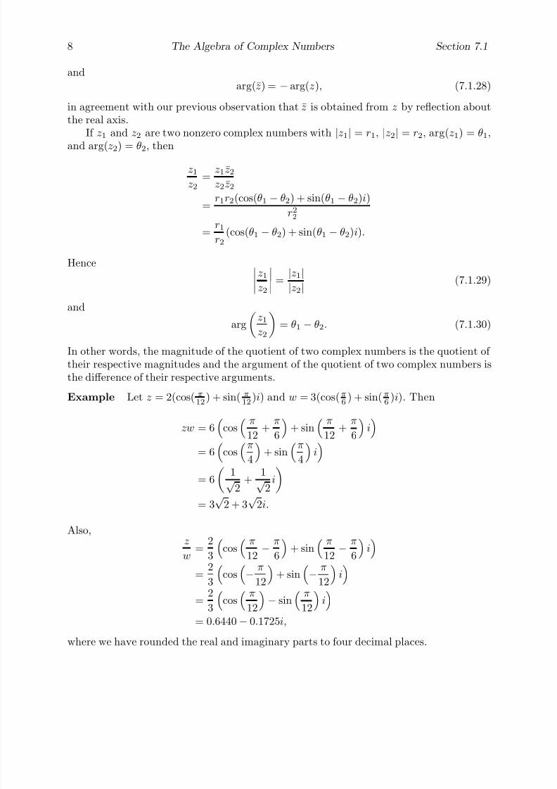
7/27/2019 Calculus 2 (Dan Sloughter)
http://slidepdf.com/reader/full/calculus-2-dan-sloughter 480/598
8 The Algebra of Complex Numbers Section 7.1
andarg(z) = − arg(z), (7.1.28)
in agreement with our previous observation that z is obtained from z by reflection aboutthe real axis.
If z1
and z2
are two nonzero complex numbers with |z1| = r1
, |z2| = r2
, arg(z1
) = θ1
,and arg(z2) = θ2, then
z1
z2=
z1z2
z2z2
=r1r2(cos(θ1 − θ2) + sin(θ1 − θ2)i)
r22
=r1
r2(cos(θ1 − θ2) + sin(θ1 − θ2)i).
Hence z1z2
= |z1||z2| (7.1.29)
and
arg
z1
z2
= θ1 − θ2. (7.1.30)
In other words, the magnitude of the quotient of two complex numbers is the quotient of their respective magnitudes and the argument of the quotient of two complex numbers isthe difference of their respective arguments.
Example Let z = 2(cos( π
12) + sin( π
12)i) and w = 3(cos(π
6) + sin(π
6)i). Then
zw = 6
cos π
12+
π
6
+ sin
π
12+
π
6
i
= 6
cosπ
4
+ sin
π
4
i
= 6
1√
2+
1√ 2
i
= 3√
2 + 3√
2i.
Also,z
w =
2
3
cos π
12 −π
6
+ sin π
12 −π
6
i
=2
3
cos
− π
12
+ sin
− π
12
i
=2
3
cos
π
12
− sin
π
12
i
= 0.6440 − 0.1725i,
where we have rounded the real and imaginary parts to four decimal places.
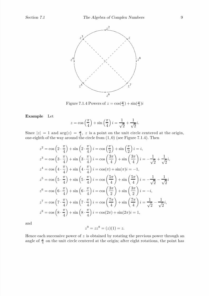
7/27/2019 Calculus 2 (Dan Sloughter)
http://slidepdf.com/reader/full/calculus-2-dan-sloughter 481/598
Section 7.1 The Algebra of Complex Numbers 9
z2
z3
4 z
z5
z6
z7
z8
z
Figure 7.1.4 Powers of z = cos(π
4 ) + sin(π
4 )i
Example Let
z = cosπ
4
+ sin
π
4
i =
1√ 2
+1√
2i.
Since |z| = 1 and arg(z) = π
4, z is a point on the unit circle centered at the origin,
one-eighth of the way around the circle from (1 , 0) (see Figure 7.1.4). Then
z2 = cos
2 · π
4
+ sin
2 · π
4
i = cos
π
2
+ sin
π
2
i = i,
z3 = cos
3 · π4
+ sin
3 · π
4
i = cos
3π4
+ sin
3π4
i = − 1√
2+ 1√
2i,
z4 = cos
4 · π
4
+ sin
4 · π
4
i = cos(π) + sin(π)i = −1,
z5 = cos
5 · π
4
+ sin
5 · π
4
i = cos
5π
4
+ sin
5π
4
i = − 1√
2− 1√
2i
z6 = cos
6 · π
4
+ sin
6 · π
4
i = cos
3π
2
+ sin
3π
2
i = −i,
z7 = cos7 · π
4 + sin7 · π
4 i = cos
7π
4
+ sin
7π
4
i =
1√ 2
− 1√ 2
i,
z8 = cos
8 · π
4
+ sin
8 · π
4
i = cos(2π) + sin(2π)i = 1,
andz9 = zz8 = (z)(1) = z.
Hence each successive power of z is obtained by rotating the previous power through anangle of π
4on the unit circle centered at the origin; after eight rotations, the point has

7/27/2019 Calculus 2 (Dan Sloughter)
http://slidepdf.com/reader/full/calculus-2-dan-sloughter 482/598
10 The Algebra of Complex Numbers Section 7.1
returned to where it started. See Figure 7.1.4. Notice in particular that z is a root of thepolynomial
P (w) = w8 − 1.
In fact, zn is a solution of w8 − 1 = 0 for any positive integer n since
(zn)8 − 1 = (z8)n − 1 = 1n − 1 = 1 − 1 = 0.
Thus there are eight distinct roots of P (w), namely, z, z2, z3, z4, z5, z6, z7, and z8, onlytwo of which, z4 = −1 and z8 = 1, are real numbers.
Problems
1. Evaluate the following if w = 3 − 4i and z = −2 + 7i.
(a) w + z (b) w − z
(c) 3w
−2z (d) w
(e) zw (f)z
w
(g) |z| (h)z2 − w
z + w
(i) (z − w) (j) (3z + w)
2. Find the real and imaginary parts of each of the following.
(a)1
i(b)
3
1 + 2i
(c)3− 4i
−2 + 3i
(d) (1 + i)3
3. For each of the following, write the given z in rectangular coordinates and plot it inthe complex plane.
(a) |z| = 3, Arg(z) =π
2(b) |z| = 5, Arg(z) =
2π
3
(c) |z| = 0.5, Arg(z) = −3π
4(d) |z| = 2, Arg(z) = π
4. For each of the following, find |z| and Arg(z) and plot z in the complex plane.
(a) z = −i (b) z = −5
(c) z = 1 + i (d) z = −1 − i(e) z = 2 + 2
√ 3i (f) z =
√ 3 − i
5. Suppose w and z are complex numbers with |w| = 3, Arg(w) = π
6, |z| = 2, and
Arg(z) = −π
3. Find both polar and rectangular coordinates for each of the following.
(a) w2 (b) z3
(c) wz (d)w
z
7/27/2019 Calculus 2 (Dan Sloughter)
http://slidepdf.com/reader/full/calculus-2-dan-sloughter 483/598
Section 7.1 The Algebra of Complex Numbers 11
(e)z
w2(f) w5
6. Find all the roots of the polynomial P (z) = z6−1 and plot them in the complex plane.
7. Let v = a1 + b1i, w = a2 + b2i, and z = a3 + b3i be complex numbers. Verify each of the following.
(a) v + w = w + v (b) vw = wv
(c) v(w + z) = vw + vz (d) (v + w) + z = v + (w + z)
(e) v(wz) = (vw)z (f) (w + z)2 = w2 + 2wz + z2
8. Suppose z is a complex number with |z| = r and arg(z) = θ.
(a) Let w be a complex number with |w| =√
r and arg(w) = θ
2. Show that w2 = z.
(b) Let v be a complex number with |v| =√
r and arg(v) = θ
2+ π. Show that v2 = z.
(c) From (a) and (b) we see that every nonzero complex number has two distinctsquare roots. Find the square roots, in rectangular form, of 1 +
√ 3i and
−9.

7/27/2019 Calculus 2 (Dan Sloughter)
http://slidepdf.com/reader/full/calculus-2-dan-sloughter 484/598
Difference Equations
Differential Equations
to
Section 7.2
The Calculus of ComplexFunctions
In this section we will discuss limits, continuity, differentiation, and Taylor series in thecontext of functions which take on complex values. Moreover, we will introduce complexextensions of a number of familiar functions. Since complex numbers behave algebraicallylike real numbers, most of our results and definitions will look like the analogous resultsfor real-valued functions. We will avoid going into much detail; the complete story of thecalculus of complex-valued functions is best left to a course in complex analysis. However,we will see enough of the story to enable us to make effective use of complex numbers inelementary calculations.
We begin with a definition of the limit of a sequence of complex numbers.
Definition We say that the limit of a sequence of complex numbers {zn} is L, and write
limn→∞
zn = L,
if for every > 0 there exists an integer N such that
|zn − L| <
whenever n > N .
Notice that the only difference between this definition and the definition of the limit of a sequence given in Section 1.2 is the use of the magnitude of a complex number in place of the absolute value of a real number. Even here, the notation is the same. The point is thesame as it was in Chapter 1: the limit of the sequence {zn} is L if we can always ensurethat the values of the sequence are within a desired distance of L by going far enough outin the sequence.
Now if zn = xn + yni and L = a + bi, then limn→∞
zn = L if and only if
limn→∞
|zn − L| = limn→∞
(xn − a)2 + (yn − b)2 = 0,
the latter of which occurs if and only if limn→∞
xn = a and limn→∞
yn = b. Hence we have the
following useful result.
Proposition Let zn = xn + yni and L = a + bi. Then
limn→∞
zn = L
1 Copyright c by Dan Sloughter 2000

7/27/2019 Calculus 2 (Dan Sloughter)
http://slidepdf.com/reader/full/calculus-2-dan-sloughter 485/598
2 The Calculus of Complex Functions Section 7.2
if and only if limn→∞
xn = a and limn→∞
yn = b.
Thus to determine the limiting behavior of a sequence {zn} of complex numbers, weneed only consider the behavior of the two sequences of real numbers, {(zn)} and {(zn)}.
Example Suppose
zn =3n − 1
2n + 2+
n + 1
n − 1i
for n = 1, 2, 3, . . .. Then
limn→∞
(zn) = limn→∞
3n − 1
2n + 2= lim
n→∞
3− 1n
2 + 2n
=3
2
and
limn→∞
(zn) = limn→∞
n + 1
n − 1= lim
n→∞
1 + 1n
1 − 1n
= 1,
so
limn→∞
zn = 32
+ i.
Example Suppose
zn =1
n
cos
nπ
3
+ sin
nπ
3
i
for n = 1, 2, 3, . . .. Then
limn→∞
(zn) = limn→∞
cosnπ
3
n
= 0
and
limn→∞
(zn) = lim
n→∞
sinnπ
3
n
= 0,
solimn→∞
zn = 0.
Geometrically, since |zn| = 1n
and arg(zn) = nπ
3 , the points in this sequence are convergingto 0 along a spiral path, as seen in Figure 7.2.1.
Having defined the limit of a sequence of complex numbers, we may define the limit of a complex-valued function, as in Section 2.3, and then define continuity, as in Section 2.4.
Definition Suppose f : C → C, that is, f is a complex-valued function of a complexvariable. We say the limit of f (z) as z approaches a is L, written
limz→a f (z) = L,
if whenever {zn} is a sequence of points with zn = a for all n and limn→∞
zn = a, then
limn→∞
f (zn) = L.

7/27/2019 Calculus 2 (Dan Sloughter)
http://slidepdf.com/reader/full/calculus-2-dan-sloughter 486/598
Section 7.2 The Calculus of Complex Functions 3
-1 -0 .75 -0.5 -0.25 0.25 0.5 0.75 1
-1
-0.75
-0.5
-0.25
0.25
0.5
0.75
1
Figure 7.2.1 Plot of the points zn = 1n
cos
nπ
3
+ sin
nπ
3
i
, n = 1, 2, 3, . . . 20
Definition We say the function f : C→ C is continuous at a if limz→a
f (z) = f (a).
As with real-valued functions of a real variable, it is easy to show that algebraicfunctions of a complex variable are continuous wherever they are defined. In particular,complex polynomials, that is, functions P of the form
P (z) = anzn + an−1zn−1 + · · · + a1z + a0,
where n is a nonnegative integer and the coefficients a0, a1, . . . , an are complex numbers,are continuous at all points in the complex plane. Complex rational functions, that is,functions R of the form
R(z) =P (z)
Q(z),
where both P and Q are polynomials, are continuous at all points where they are defined.
Example Since f (z) = 3z2− iz + 4− 5i is a polynomial, it is continuous at all points inthe complex plane. In particular,
limz→i
f (z) = limz→i
(3z2 − iz + 4 − 5i) = 3i2 − (i)(i) + 4 − 5i = 2 − 5i.
Example Algebraic simplification may be useful in evaluating limits here as it was inSection 2.3. For example,
limz→i
z
−i
z2 + 1 = limz→i
z
−i
(z − i)(z + i) = limz→i
1
z + i =
1
2i =
1
2i
i
i = −1
2 i.
Although this is not the time to go into any detail about the geometric meaning of thederivative of a function f : C→ C, the algebraic definition and manipulation of derivativesfollows the pattern of the results for real-valued functions in Chapter 3.
7/27/2019 Calculus 2 (Dan Sloughter)
http://slidepdf.com/reader/full/calculus-2-dan-sloughter 487/598
4 The Calculus of Complex Functions Section 7.2
Definition If f : C→ C, then the derivative of f at a, denoted f (a), is given by
f (a) = limh→0
f (a + h) − f (a)
h, (7.2.1)
provided the limit exists.
Note that h in this definition is, in general, a complex number, not just a real number.Since the algebraic properties of the complex numbers are very similar to the algebraicproperties of the real numbers, much of what we learned about differentiation in Chapter3 still holds true in our new situation. For example, if n is a nonzero rational number,then
d
dzzn = nzn−1. (7.2.2)
Moreover, all the techniques we learned for computing derivatives in Sections 3.3 and 3.4,including the quotient, product, and chain rules, still hold.
Example If f (z) = 3z5 + iz3 − (3 + 2i)z, then
f (z) = 15z4 + 3iz2 − 3 − 2i.
Example If
g(w) =(3 + i)w2
2w − 1,
then, using the quotient rule,
g(w) =(2w − 1)(6 + 2i)w − (3 + i)w2(2)
(2w − 1)2=
(6 + 2i)(w2 − w)
(2w − 1)2.
From this point it is possible to follow the pattern of Chapter 5 and develop the theoryof polynomial approximations using Taylor polynomials, defined in a manner analogous tothe definition in Section 5.1, as well as the theory of power series and Taylor series. Inparticular, a power series
∞n=0
an(z − a)n, (7.2.3)
where a0, a1, a2, . . . and a are complex numbers, is said to converge absolutely at thosepoints z for which the series
∞
n=0
|an||z − a|n (7.2.4)
converges. Since the latter series involves only real numbers, its convergence may bedetermined using the tests developed in Chapter 5. As before, absolute convergence impliesconvergence. Moreover, if the series (7.2.3) converges at points other than a, then thereexists an R, either a positive real number or ∞, such that the series converges absolutely
7/27/2019 Calculus 2 (Dan Sloughter)
http://slidepdf.com/reader/full/calculus-2-dan-sloughter 488/598
Section 7.2 The Calculus of Complex Functions 5
for all z such that |z − a| < R and diverges for all z such that |z − a| > R. However, notethat in this case the set of all points in the complex plane such that |z − a| < R is a diskof radius R centered at a, not an interval as it was in the real number case.
Example Consider the power series
∞n=0
zn. (7.2.5)
Since the series∞n=0
|z|n
is a geometric series, it converges for all values of z for which |z| < 1. Hence
∞n=0
zn
converges for all z for which |z| < 1, that is, for all z inside the unit circle centered at theorigin of the complex plane. Thus the radius of convergence of (7.2.5) is R = 1. Using thesame argument as we used in Section 1.3, we can show that
∞n=0
zn =1
1 − z
for all z with |z| < 1. For example,
∞n=0
i
2
n=
1
1
−i
2
=2
2
−i
=2(2 + i)
(2
−i)(2 + i)
=4
5+
2
5i.
Example Consider the power series
∞n=0
zn
n!. (7.2.6)
To determine its radius of convergence, we apply the ratio test to the series
∞n=0
zn
n!
=∞n=0
|z|nn!
, (7.2.7)
obtaining
ρ = limn→∞
|z|n+1(n + 1)!
|z|nn!
= limn→∞
|z|n + 1
= 0
7/27/2019 Calculus 2 (Dan Sloughter)
http://slidepdf.com/reader/full/calculus-2-dan-sloughter 489/598
6 The Calculus of Complex Functions Section 7.2
for all values of z. Since ρ = 0 for any value of z, (7.2.7) converges for all z in the complexplane. That is, the radius of convergence of (7.2.6) is R = ∞. Of course, we also knowthat (7.2.7) converges for all z because, from our work in Section 6.1, it is equal to e|z|.
The power series in the last example is the extension to complex numbers of the serieswe used to define the exponential function in Section 6.1. With it, we can define the
complex exponential function.
Definition The complex exponential function , with value at z denoted by exp(z), isdefined for all points in the complex plane by
exp(z) =∞n=0
zn
n!. (7.2.8)
Of course, this definition agrees with our old definition when z is real.In Chapter 6 we used the exponential function to give meaning to exponents which
were not rational numbers. Similarly, the complex exponential function may be used to
define complex exponents. However, we will only consider the case of raising e to a complexpower.
Definition If z is a complex number with (z) = 0, then we define ez = exp(z).
With this definition we now have ez = exp(z) for all z in the complex plane, the casewhen (z) = 0, that is, when z is real, having been treated in Section 6.1. Althoughwe will not repeat them here, the arguments from Section 6.1 come over to establish thefollowing proposition.
Proposition For any complex numbers w and z,
ew+z = ewez (7.2.9)
and
ew−z =ew
ez. (7.2.10)
Also, as in Section 6.1, direct differentiation of (7.2.8) yields the following result.
Proposition
d
dzez = ez . (7.2.11)
Example Using the product and chain rules,
d
dz
z2e−z
2
= z2(−2z)e−z2
+ 2ze−z2
= 2z(1 − z2)e−z2
.
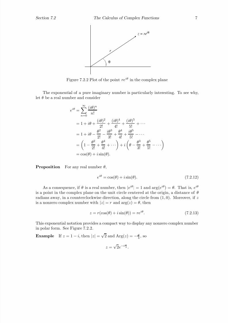
7/27/2019 Calculus 2 (Dan Sloughter)
http://slidepdf.com/reader/full/calculus-2-dan-sloughter 490/598
Section 7.2 The Calculus of Complex Functions 7
θi ¢
£ £ £ £ £ £ £ £
£ £ £ £ £ £ £ £
£ £ £ £ £ £ £ £
£ £ £ £ £ £ £ £
£ £ £ £ £ £ £ £
£ £ £ £ £ £ £ £
¤ ¤ ¤ ¤ ¤ ¤ ¤ ¤
¤ ¤ ¤ ¤ ¤ ¤ ¤ ¤
¤ ¤ ¤ ¤ ¤ ¤ ¤ ¤
¤ ¤ ¤ ¤ ¤ ¤ ¤ ¤
¤ ¤ ¤ ¤ ¤ ¤ ¤ ¤
¤ ¤ ¤ ¤ ¤ ¤ ¤ ¤
r
θ
z = re
Figure 7.2.2 Plot of the point reiθ in the complex plane
The exponential of a pure imaginary number is particularly interesting. To see why,let θ be a real number and consider
eiθ =∞
n=0
(iθ)n
n!
= 1 + iθ +(iθ)2
2!+
(iθ)4
4!+
(iθ)5
5!+ · · ·
= 1 + iθ − θ2
2!− iθ3
3!+
θ4
4!+
iθ5
5!− · · ·
=
1 − θ2
2!+
θ4
4!+ · · ·
+ i
θ − θ3
3!+
θ5
5!− · · ·
= cos(θ) + i sin(θ).
Proposition For any real number θ,
eiθ = cos(θ) + i sin(θ). (7.2.12)
As a consequence, if θ is a real number, then |eiθ| = 1 and arg(eiθ) = θ. That is, eiθ
is a point in the complex plane on the unit circle centered at the origin, a distance of θ
radians away, in a counterclockwise direction, along the circle from (1, 0). Moreover, if z
is a nonzero complex number with |z| = r and arg(z) = θ, then
z = r(cos(θ) + i sin(θ)) = reiθ. (7.2.13)
This exponential notation provides a compact way to display any nonzero complex numberin polar form. See Figure 7.2.2.
Example If z = 1 − i, then |z| =√
2 and Arg(z) = −π
4 , so
z =√
2e−iπ
4 .

7/27/2019 Calculus 2 (Dan Sloughter)
http://slidepdf.com/reader/full/calculus-2-dan-sloughter 491/598
8 The Calculus of Complex Functions Section 7.2
Moreover,z =
√ 2ei
π
4
andz2 = 2e−2i
π
4 = 2e−iπ
2 = −2i.
Example If w = 3eiπ
3 and z = 5eiπ
8 , then
wz =
3eiπ
3
5ei
π
8
= 15ei(
π
3+π
8 ) = 15ei11π24
andw
z=
3eiπ
3
5eiπ
8=
3
5ei(
π
3−π
8 ) =3
5ei
5π24 .
Since for any real number θ,
eiθ = cos(θ) + i sin(θ),
it follows that e−iθ = cos(−θ) + i sin(−θ) = cos(θ) − i sin(θ).
Henceeiθ − e−iθ = cos(θ) + i sin(θ) − (cos(θ) − i sin(θ)) = 2i sin(θ). (7.2.14)
Solving (7.2.14) for sin(θ), we have
sin(θ) =1
2i(eiθ − e−iθ).
Similarly,eiθ + e−iθ = cos(θ) + i sin(θ) + cos(θ)
−i sin(θ) = 2 cos(θ), (7.2.15)
from which we obtain
cos(θ) =1
2(eiθ + e−iθ).
Proposition For any real number θ,
sin(θ) =1
2i(eiθ − e−iθ) (7.2.16)
and
cos(θ) =1
2(eiθ + e−iθ). (7.2.17)
These formulas are very similar to the formulas we used to define the hyperbolic sineand cosine functions in Section 6.7. We will now use these formulas to define the complexsine and cosine functions; at the same time, we will extend the definitions of the hyperbolicsine and cosine functions. In doing so, we will see just how closely related the circular andhyperbolic trigonometric functions really are.

7/27/2019 Calculus 2 (Dan Sloughter)
http://slidepdf.com/reader/full/calculus-2-dan-sloughter 492/598
Section 7.2 The Calculus of Complex Functions 9
Definition The complex sine function , with value at z denoted by sin(z), and thecomplex cosine function , with value at z denoted by cos(z), are defined for all z in thecomplex plane by
sin(z) =1
2i(eiz − e−iz) (7.2.18)
andcos(z) =
1
2(eiz + e−iz). (7.2.19)
The complex hyperbolic sine function , with value at z denoted by sinh(z), and the complex
hyperbolic cosine function , with value at z denoted by cosh(z), are defined for all z in thecomplex plane by
sinh(z) =1
2(ez − e−z) (7.2.20)
and
cosh(z) =1
2(ez + e−z). (7.2.21)
Note that these functions are defined so that they agree with their original versionswhen evaluated at real numbers.
With these definitions it is a simple matter to prove that
d
dzsin(z) = cos(z), (7.2.22)
d
dzcos(z) = − sin(z), (7.2.23)
d
dzsinh(z) = cosh(z), (7.2.24)
andd
dzcosh(z) = sinh(z). (7.2.25)
For example,d
dzcos(z) =
d
dz
1
2(eiz + e−iz)
=1
2(ieiz − ie−iz)
=i
2(eiz − e−iz)
= i22i
(eiz − e−iz)
= −1
2(eiz − e−iz)
= − sin(z).
7/27/2019 Calculus 2 (Dan Sloughter)
http://slidepdf.com/reader/full/calculus-2-dan-sloughter 493/598
10 The Calculus of Complex Functions Section 7.2
Example Note that
sin(i) =1
2i(ei
2 − e−i2
)
=1
2i(e−1 − e1)
= −1
i sinh(1)
= − i
i2sinh(1)
= i sinh(1).
Example Using the product and chain rules, we have
d
dzsin(2z) cos(3z) = sin(2z)(− sin(3z))(3) + cos(3z) cos(2z)(2)
= −3 sin(2z) sin(3z) + 2 cos(2z) cos(3z).
The final complex-valued function we will define is the complex logarithm function.Analogous to our other definitions in this section, we would like this function to share thebasic characteristic properties of the ordinary logarithm function and to agree with thatfunction when evaluated at a positive real number. In particular, if we let Log(z) denotethe complex logarithm of a complex number z and log(r) denote the real logarithm of apositive real number r, then for a nonzero complex number z with |z| = r and Arg(z) = θ
we would like to have
Log(z) = Log(reiθ) = Log(r) + Log(eiθ) = log(r) + iθ. (7.2.26)
Moreover, using (7.2.26) to define the complex logarithm function will guarantee thatour new function agrees with the ordinary logarithm function when evaluated at positive
real numbers, for if z is a positive real number, then |z| = z and Arg(z) = 0, giving usLog(z) = log(z).
Definition The complex logarithm function , with value at z denoted by Log(z), is definedfor all nonzero complex numbers z with |z| = r and Arg(z) = θ by
Log(z) = log(r) + iθ, (7.2.27)
where log(r) is the ordinary real-valued logarithm of r.
Note that we have used the principal value of arg(z), that is, Arg(z), in the definitionof Log(z) in order to give Log(z) a unique value. Moreover, note that this definition givesmeaning to the logarithm of a negative real number, although it still does not define the
logarithm of 0.
Example Since |2 − 2i| =√
8 and Arg(2 − 2i) = −π
4 , we have
Log(2− 2i) = log(√
8) − π
4i =
1
2log(8)− π
4i =
3
2log(2)− π
4i.
7/27/2019 Calculus 2 (Dan Sloughter)
http://slidepdf.com/reader/full/calculus-2-dan-sloughter 494/598
Section 7.2 The Calculus of Complex Functions 11
Example Since | − 4| = 4 and Arg(−4) = π, we have
Log(−4) = log(4) + πi = 2 log(2) + πi.
Problems
1. For each of the following, find limn→∞
zn. Also, plot z1, z2, z3, . . . , z15 in the complex
plane.
(a) zn =3 − n
n+
n + 1
2n + 3i (b)
2 − n
n2−
4 +6
n
i
(c) zn = 3eiπ
n (d) zn = eiπ(n−1)n
2. Evaluate each of the following limits.
(a) limz→i
(4z3 − 6z + 3) (b) limz→1−i
(z2 − 3z)
(c) limw→3i
w2 + 9w − 3i
(d) limz→i
z4 − 1z2 + 1
3. Find the derivative of each of the following functions.
(a) f (z) = 3z2 − 6z5 + 18i (b) g(w) =13w − 6i + 3
w + i
(c) f (z) = (z − 4i)e−z2
(d) h(s) = (s2 + 1) exp(3s2 − si)
4. (a) Show that
1
1 + z2=
∞n=0
(−1)nz2n
for all z with |z| < 1.
(b) How does (a) help explain why, for real values of x, the Taylor series
1
1 + x2=
∞n=0
(−1)nx2n
converges only on the interval (−1, 1)?
5. (a) If z = x + yi, show that(ez) = ex cos(y)
and (ez) = ex sin(y).
(b) If z = x + yi, find |ez | and arg(ez).
6. Show that eiπ + 1 = 0.
7/27/2019 Calculus 2 (Dan Sloughter)
http://slidepdf.com/reader/full/calculus-2-dan-sloughter 495/598
12 The Calculus of Complex Functions Section 7.2
7. Verify the differentiation formulas for sin(z), sinh(z), and cosh(z).
8. (a) Show that −1−2
1
xdx = − log(2).
(b) Some computer algebra systems evaluate the integral in (a) as −1−2
1
xdx = Log(−1) − Log(−2).
Reconcile this answer with the answer in (a).
9. Let z and w be complex numbers with −π
2 < Arg(z) < π
2 and −π
2 < Arg(w) < π
2 .Verify the following two properties of the complex logarithm.
(a) Log(wz) = Log(w) + Log(z)
(b) Log w
z = Log(w) − Log(z)
10. For a positive integer n, an nth root of unity is a complex number z with the propertythat zn = 1. Show that for m = 0, 1, . . . , n− 1,
zm = ei2mπn
is an nth root of unity. Plot these points in the complex plane for n = 10.
11. (a) Use the fact that
sin(z) =1
2i(eiz − e−iz)
to find the complex power series representation for sin(z).
(b) Use the fact that
cos(z) =1
2(eiz + e−iz)
to find the complex power series representation for cos(z).
12. Define a complex version of the tangent function and show that
tan(z) =1
i
eiz − e−iz
eiz + e−iz
.
13. (a) Show that sin(ix) = i sinh(x) for every real number x.
(b) Show that cos(ix) = cosh(x) for every real number x.
14. Let z = x + yi.
(a) Show that(sin(z)) = sin(x) cosh(y)
7/27/2019 Calculus 2 (Dan Sloughter)
http://slidepdf.com/reader/full/calculus-2-dan-sloughter 496/598
Section 7.2 The Calculus of Complex Functions 13
and(sin(z)) = cos(x) sinh(y).
(b) Show that(cos(z)) = cos(x) cosh(y)
and (sin(z)) = − sin(x) sinh(y).
15. (a) Show that for any nonzero complex number z, eLog(z) = z.
(b) If z is a nonzero complex number, does it necessarily follow that Log(ez) = z?
7/27/2019 Calculus 2 (Dan Sloughter)
http://slidepdf.com/reader/full/calculus-2-dan-sloughter 497/598
Difference Equations
Differential Equations
to
Section 7.3
Complex-Valued Functions:Motion in the Plane
In Section 7.2 we considered the problem of extending the elementary functions of calculusto complex-valued functions of a complex variable, while at the same time extending manyof the concepts of the first six chapters to these new functions. In this section we willconsider complex-valued functions of a real variable, that is, functions of the form f : R→C. Such functions are often used to describe the motion of an object in the plane; if wethink of the real variable t as measuring time, then we may interpret f (t) as the locationof an object in the complex plane at time t.
Since limits are at the foundation of most concepts in calculus, we begin with a defi-nition of limit in this setting.
Definition Suppose f : R→ C and f is defined for all t in an interval about the pointa. We say that the limit of f (t) as t approaches a is L, denoted
limt→a
f (t) = L,
if whenever {tn} is a sequence of real numbers with tn = a for all n and
limn→∞
tn = a,
thenlimn→∞
f (tn) = L.
Suppose f : R→ C. If we let x(t) = (f (t)) and y(t) = (f (t)), then
f (t) = x(t) + iy(t).
Hence, from our work in Section 7.2,
limt→a
f (t) = limt→a
x(t) + i limt→a
y(t). (7.3.1)
This result also holds if we modify our definition of limit to include one-sided limits andlimits to ∞ or −∞.
Example Suppose a particle moves in the plane so that its position at time t is givenby
f (t) = cos(2πt) + i sin(2πt) = e2πit.
If we let C denote the unit circle centered at the origin, then f (t) is a point in the complexplane on C , 2πt units from (1, 0) in the counterclockwise direction along the circumference
1 Copyright c by Dan Sloughter 2000

7/27/2019 Calculus 2 (Dan Sloughter)
http://slidepdf.com/reader/full/calculus-2-dan-sloughter 498/598
2 Complex-Valued Functions: Motion in the Plane Section 7.3
t
t
t
t
= 0.25
= 0, 1
= 0.75
= 0.5
Figure 7.3.1 Motion of a particle on the unit circle centered at the origin
of C . For example, at time t = 0 the particle is at f (0) = 1, at time t = 14 the particle
is at f 14
= i, at time t = 1
2 the particle is at f 12
= −1, at t = 3
4 the particle is at
f 34
= −i, and at time t = 1 the particle is at f (1) = 1. Note that f has period 1,
so the particle traverses C once in the counterclockwise direction as t goes from 0 to 1,after which the particle will repeat this motion over every interval of time of length 1. See
Figure 7.3.1. As an example of a limit, we note that
limt→−
1
4
f (t) = limt→−
1
4
cos(2t) + i limt→−
1
4
sin(2t) = cos−π
2
+ i sin
−π
2
= −i.
Note that the path of the particle shown in Figure 7.3.1 is not the graph of the functionf , but rather a plot of f (t) for values of t from 0 to 1. In general, if f (t) = x(t) + iy(t)represents the position of a particle moving in the complex plane at time t, we can obtaina good representation of the path of the particle over an interval of time [a, b] by plottingthe points (x(t), y(t)) for a large number of points in [a, b] and connecting these pointswith straight lines, similar to the procedure we used for plotting the graph of a function
in Section 2.1.Example Suppose a particle moves in the plane so that its position at time t is givenby
z(t) = tanh(t) + isech(t).
Then (z(t)) = tanh(t), (z(t)) = sech(t), and
|z(t)| =
tanh2(t) + sech2(t) = 1.

7/27/2019 Calculus 2 (Dan Sloughter)
http://slidepdf.com/reader/full/calculus-2-dan-sloughter 499/598
Section 7.3 Complex-Valued Functions: Motion in the Plane 3
t t < 0 > 0
t = 0
Figure 7.3.2 Motion on the upper half of the unit circle
Thus the particle is moving along the unit circle C as in the previous example. However,since sech(t) > 0 for all t, the particle is always on the upper half of C . Moreover, z(0) = i,
limt→∞
z(t) = limt→∞
tanh(t) + i limt→∞
sech(t) = 1
and
limt→−∞
z(t) = limt→−∞
tanh(t) + i limt→−∞
sech(t) = −1.
Combining these results with the fact that (z(t)) = tanh(t) is an increasing function, wesee that as time flows from −∞ to ∞, the particle moves from left to right on the upperhalf of C , coming from the point (−1, 0) as t increases from −∞ and approaching the point(1, 0) as t increases toward
∞. See Figure 7.3.2.
We may now define continuity and differentiability in analogy with our previous defi-nitions.
Definition We say a function f : R→ C is continuous at a if limt→a
f (t) = f (a).
If x(t) = (f (t)) and y(t) = (f (t)), then
limt→a
f (t) = f (a)
if and only if
limt→a x(t) = x(a)
and
limt→a
y(t) = y(a).
Hence f is continuous at a if and only if both x and y are continuous at a. For example,the functions in the previous examples are both continuous for every t in (−∞,∞) sincethe functions cos(t), sin(t), tanh(t), and sech(t) are continuous for all t in (−∞,∞).
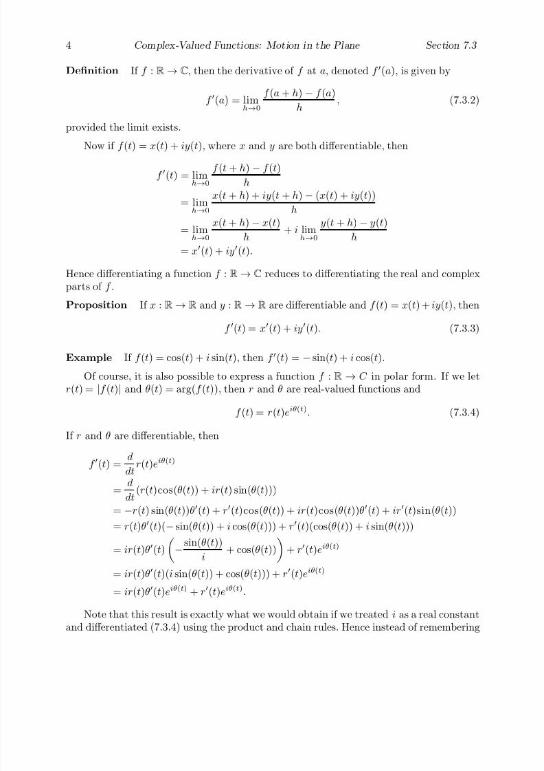
7/27/2019 Calculus 2 (Dan Sloughter)
http://slidepdf.com/reader/full/calculus-2-dan-sloughter 500/598
4 Complex-Valued Functions: Motion in the Plane Section 7.3
Definition If f : R→ C, then the derivative of f at a, denoted f (a), is given by
f (a) = limh→0
f (a + h)− f (a)
h, (7.3.2)
provided the limit exists.
Now if f (t) = x(t) + iy(t), where x and y are both differentiable, then
f (t) = limh→0
f (t + h)− f (t)
h
= limh→0
x(t + h) + iy(t + h)− (x(t) + iy(t))
h
= limh→0
x(t + h)− x(t)
h+ i lim
h→0
y(t + h)− y(t)
h
= x(t) + iy(t).
Hence differentiating a function f : R→ C reduces to differentiating the real and complexparts of f .
Proposition If x : R→ R and y : R→ R are differentiable and f (t) = x(t) + iy(t), then
f (t) = x(t) + iy(t). (7.3.3)
Example If f (t) = cos(t) + i sin(t), then f (t) = − sin(t) + i cos(t).
Of course, it is also possible to express a function f : R → C in polar form. If we letr(t) = |f (t)| and θ(t) = arg(f (t)), then r and θ are real-valued functions and
f (t) = r(t)eiθ(t). (7.3.4)
If r and θ are differentiable, then
f (t) =d
dtr(t)eiθ(t)
=d
dt(r(t)cos(θ(t)) + ir(t) sin(θ(t)))
= −r(t) sin(θ(t))θ(t) + r(t)cos(θ(t)) + ir(t)cos(θ(t))θ(t) + ir(t)sin(θ(t))
= r(t)θ(t)(− sin(θ(t)) + i cos(θ(t))) + r(t)(cos(θ(t)) + i sin(θ(t)))
= ir(t)θ(t)− sin(θ(t))
i+ cos(θ(t))
+ r(t)eiθ(t)
= ir(t)θ(t)(i sin(θ(t)) + cos(θ(t))) + r(t)eiθ(t)
= ir(t)θ(t)eiθ(t) + r(t)eiθ(t).
Note that this result is exactly what we would obtain if we treated i as a real constantand differentiated (7.3.4) using the product and chain rules. Hence instead of remembering

7/27/2019 Calculus 2 (Dan Sloughter)
http://slidepdf.com/reader/full/calculus-2-dan-sloughter 501/598
Section 7.3 Complex-Valued Functions: Motion in the Plane 5
the formula, we need only remember that we should differentiate a function given in polarform using the product rule and treating i as we would any constant. In particular, takingr(t) = 1 for all t, we have
d
dteiθ(t) = iθ(t)eiθ(t). (7.3.5)
Example If f (t) = 4teit2
, then
f (t) = 4t(2it)eit2
+ 4eit2
= (4 + 8it2)eit2
.
To understand the derivative geometrically, consider the setting where z(t) = x(t) +iy(t) represents the position at time t of a particle moving in the plane. Then x(t)represents the velocity of the particle in the x direction and y(t) represents the velocityof the particle in the y direction. In other words, if all forces acting on the particle wereto cease at time t0, then, according to Newton’s first law, during the next unit of timethe particle would move in a straight line, x(t
0) units in the x direction and y(t
0) units
in the y direction. That is, in one unit of time the particle would travel along a straightline from (x(t0), y(t0)) to (x(t0) + x(t0), y(t0) + y(t0)). Hence the particle would move,in a straight line, from z(t0) to z(t0) + z(t0). Moreover, since the distance traveled in thisunit of time is |z(t0)|, the speed of the particle at time t0 is given by |z(t0)|. In short,arg(z(t0)) tells us the direction in which the particle is moving at time t0 and |z(t0)| tellsus the speed at which the particle is traveling at that instant. These considerations makethe next definition reasonable.
Definition If z(t) gives the position at time t of a particle moving in the plane, then wecall z(t) the velocity of the particle and we call |z(t)| the speed of the particle.
Notice that this definition is directly analogous to our treatment of motion along astraight line in earlier chapters. In that case, if f (t) represented the position of a particlemoving along a straight line, then we called f (t) the velocity of the particle and |f (t)|the speed of the particle at time t.
Also notice that if for a given time t0 we draw an arrow from z(t0) to z(t0) + z(t0),then this arrow points in the direction of motion of the particle at time t0. Moreover, if x(t0) = 0, then this arrow has slope
y(t0)
x(t0).
Now, from the chain rule, we have
dy
dt=
dy
dx
dx
dt,
from which we obtain
dy
dx=
dy
dtdx
dt
=y(t)
x(t).
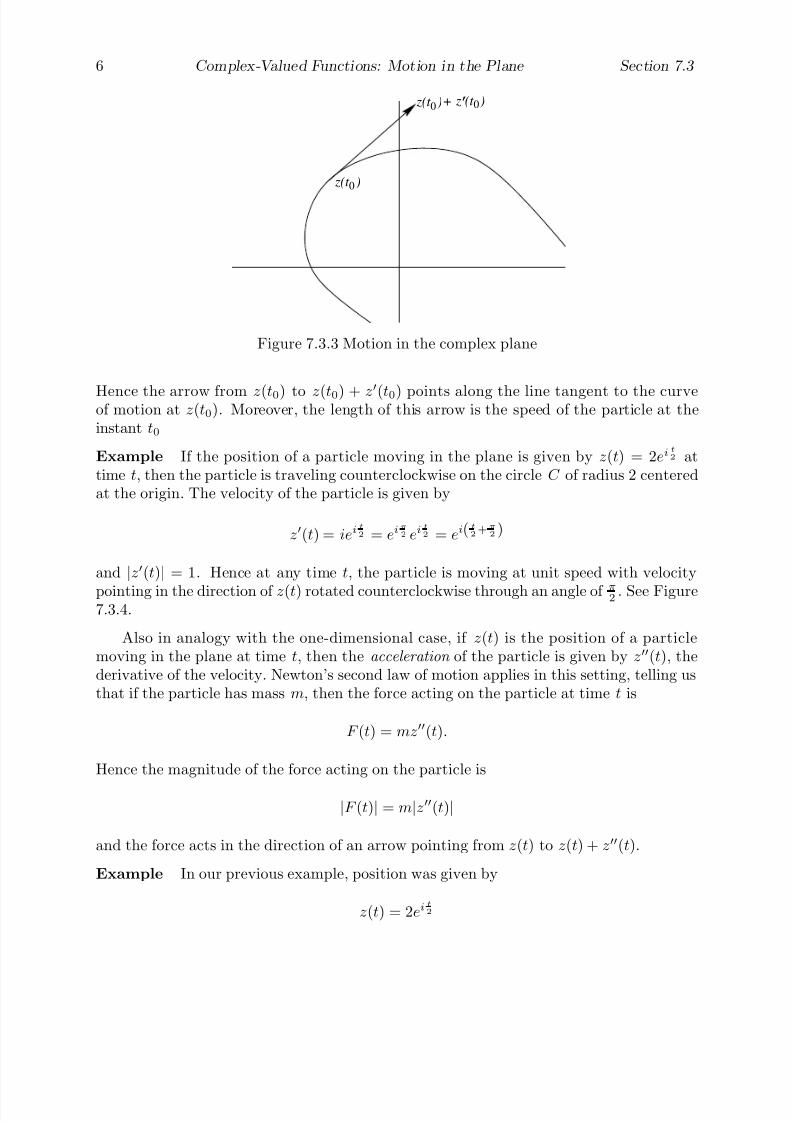
7/27/2019 Calculus 2 (Dan Sloughter)
http://slidepdf.com/reader/full/calculus-2-dan-sloughter 502/598
6 Complex-Valued Functions: Motion in the Plane Section 7.3
z(t )0
z(t )0+ z (t )0’
Figure 7.3.3 Motion in the complex plane
Hence the arrow from z(t0) to z(t0) + z
(t0) points along the line tangent to the curveof motion at z(t0). Moreover, the length of this arrow is the speed of the particle at theinstant t0
Example If the position of a particle moving in the plane is given by z(t) = 2eit
2 attime t, then the particle is traveling counterclockwise on the circle C of radius 2 centeredat the origin. The velocity of the particle is given by
z(t) = ieit
2 = eiπ
2 eit
2 = ei(t
2+π
2 )
and
|z(t)
|= 1. Hence at any time t, the particle is moving at unit speed with velocity
pointing in the direction of z(t) rotated counterclockwise through an angle of π2 . See Figure7.3.4.
Also in analogy with the one-dimensional case, if z(t) is the position of a particlemoving in the plane at time t, then the acceleration of the particle is given by z(t), thederivative of the velocity. Newton’s second law of motion applies in this setting, telling usthat if the particle has mass m, then the force acting on the particle at time t is
F (t) = mz(t).
Hence the magnitude of the force acting on the particle is
|F (t)| = m|z(t)|
and the force acts in the direction of an arrow pointing from z(t) to z(t) + z(t).
Example In our previous example, position was given by
z(t) = 2eit
2

7/27/2019 Calculus 2 (Dan Sloughter)
http://slidepdf.com/reader/full/calculus-2-dan-sloughter 503/598
Section 7.3 Complex-Valued Functions: Motion in the Plane 7
Figure 7.3.4 Arrows indicating velocity and acceleration at time t = π
2
and velocity byz(t) = iei
t
2 .
Thus the acceleration of the particle is
z(t) =
−1
2
eit
2 .
Note that
z(t) = −1
4z(t),
showing that the force acting on the particle is directed toward the center of the circle C .See Figure 7.3.4.
Since we may compute the derivative of a complex-valued function by differentiatingits complex and real parts separately, it is reasonable to define the definite integral of sucha function in terms of the integrals of its real and complex parts.
Definition Suppose f : R
→C with f (t) = x(t) + iy(t). If x and y are both integrable
on the interval [a, b], then we define the definite integral of f over the interval [a, b] by b
a
f (t)dt =
b
a
x(t)dt + i
b
a
y(t)dt. (7.3.6)
Example If
f (t) = sin(t) + i cos
t
2
,

7/27/2019 Calculus 2 (Dan Sloughter)
http://slidepdf.com/reader/full/calculus-2-dan-sloughter 504/598
8 Complex-Valued Functions: Motion in the Plane Section 7.3
then π
0
f (t)dt =
π
0
sin(t)dt + i
π
0
cos
t
2
dt
= − cos(t)π
0+ 2i sin
t
2
π
0
= (1 + 1) + i(2− 0)
= 2 + 2i.
If F : R → C and f : R → C are continuous on [a, b], with F (t) = X (t) + iY (t),f (t) = x(t) + iy(t), and f (t) = F (t) for all t in (a, b), then
b
a
f (t)dt =
b
a
x(t)dt + i
b
a
y(t)dt
= X (t)b
a
+ iY (t)b
a
= (X (b)−X (a)) + i(Y (a)− Y (b))
= (X (b) + iY (b))− (X (a) + iY (a))
= F (b)− F (a).
Hence we have a version of the Fundamental Theorem of Integral Calculus which may beapplied directly to complex-valued functions of a real variable.
Proposition If F : R→ C and f : R→ C are continuous on [a, b] with f (t) = F (t) forall t in [a, b], then
b
a f (t)dt = F (b)− F (a).
Example If f (t) = e3it, then
π
0
f (t)dt =
π
0
e3itdt =1
3ie3it
π0
=1
3i(e3iπ − e0) =
1
3i(−1− 1) = − 2
3i=
2
3i.
Example Integration by parts, which we derived in Section 4.5 from the product rule,is applicable in our current situation. For example, to evaluate
π
0
3teitdt,
we letu = 3t dv = eitdt
du = 3dt v =1
ieit = −ieit.

7/27/2019 Calculus 2 (Dan Sloughter)
http://slidepdf.com/reader/full/calculus-2-dan-sloughter 505/598
Section 7.3 Complex-Valued Functions: Motion in the Plane 9
F
α
v0
Figure 7.3.5 Motion of a projectile
Then π
0
3teitdt = −3tieitπ0
+
π
0
3ieitdt
= −3πieiπ + 0 + 3eitπ0
= −3πi(−1) + 3eiπ − 3e0
= 3πi − 3− 3
= −6 + 3πi.
In our final example for this section, we consider the problem of finding the motion
of a projectile moving close to the surface of the earth. This problem will not only tietogether many of the concepts of this section, but it will also provide a preview of Section7.4 and our discussion of differential equations in Chapter 8.
Example Suppose a projectile of mass m is fired from the surface of the earth at anangle α, where 0 < α < π
2 . We will consider the motion of the projectile as a path inthe complex plane with its position at time t given by z(t). Further, we assume that itsinitial position is z(0) = 0 and its initial velocity is z(0) = v0. Ignoring the effects of airresistance, the only force acting on the projectile during its flight is the force of gravity,acting vertically downward. Hence at any time t the force is given by F = −mgi, whereg is the acceleration due to gravity (32 feet/second2 or 9.8 meters/second2). See Figure
7.3.5. Thus Newton’s second law of motion gives us−mgi = mz(t),
that is,−gi = z(t),
at any time t. If we let v(t) be the velocity of the projectile at time t, then
v(t) = z(t) = −gi.
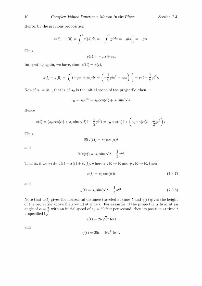
7/27/2019 Calculus 2 (Dan Sloughter)
http://slidepdf.com/reader/full/calculus-2-dan-sloughter 506/598
10 Complex-Valued Functions: Motion in the Plane Section 7.3
Hence, by the previous proposition,
v(t)− v(0) =
t
0
v(s)ds = −
t
0
gids = −gist0
= −gti.
Thusv(t) = −gti + v0.
Integrating again, we have, since z(t) = v(t),
z(t)− z(0) =
t0
(−gsi + v0)ds =
−1
2gis2 + v0s
t0
= v0t− 1
2gt2i.
Now if s0 = |v0|, that is, if s0 is the initial speed of the projectile, then
v0 = s0eiα
= s0 cos(α) + s0 sin(α)i.
Hence
z(t) = (s0 cos(α) + s0 sin(α)i)t − 1
2gt2i = s0 cos(α)t +
s0 sin(α)t− 1
2gt2
i.
Thus
(z(t)) = s0 cos(α)t
and
(z(t)) = s0 sin(α)t− 12
gt2.
That is, if we write z(t) = x(t) + iy(t), where x : R→ R and y : R→ R, then
x(t) = s0 cos(α)t (7.3.7)
and
y(t) = s0 sin(α)t − 1
2gt2. (7.3.8)
Note that x(t) gives the horizontal distance traveled at time t and y(t) gives the heightof the projectile above the ground at time t. For example, if the projectile is fired at anangle of α = π
6 with an initial speed of s0 = 50 feet per second, then its position at time t
is specified by
x(t) = 25√
3t feet
and
y(t) = 25t − 16t2 feet.
7/27/2019 Calculus 2 (Dan Sloughter)
http://slidepdf.com/reader/full/calculus-2-dan-sloughter 507/598
Section 7.3 Complex-Valued Functions: Motion in the Plane 11
10 20 30 40 50 60
2
4
6
8
10
Figure 7.3.6 Motion of a projectile
A plot of this motion is shown in Figure 7.3.6.In the next section we will consider a more complicated motion problem, namely, the
two-body problem, the problem of determining the orbit of a planet about its sun.
Problems
1. For each of the following, suppose the given function specifies the position of a particlemoving in the complex plane. Plot the path of the motion over the given time interval,indicating the direction of motion with arrows on the curve.
(a) f (t) = cos(2t) + i sin(2t), 0 ≤ t ≤ π
(b) z(t) = 4 cos(t) + i sin(t), 0 ≤ t ≤ 2π
(c) g(t) = sin
t
2
+ i cos
t
2
, 0 ≤ t ≤ 3π
(d) z(t) = sech(2t) + i tanh(2t), −∞ < t < ∞(e) f (t) = 2t + it2, −4 ≤ t ≤ 4
(f) g(t) = t2 + it4, −2 ≤ t ≤ 2
(g) z(t) = 3eit, −π ≤ t ≤ π
(h) h(t) = 3teit, 0 ≤ t ≤ 6π
(i) z(t) =
3
t e
2it
, 1 ≤ t ≤ 202. Differentiate each of the functions in the previous problem.
3. For each of the following, suppose the given function specifies the position of a particlemoving in the complex plane. Find the velocity, speed, and the acceleration for eachat the specified time.
(a) z(t) = cos(2t) + i sin(2t), t =π
6
7/27/2019 Calculus 2 (Dan Sloughter)
http://slidepdf.com/reader/full/calculus-2-dan-sloughter 508/598
12 Complex-Valued Functions: Motion in the Plane Section 7.3
(b) f (t) = 3 sin(t) + i cos(2t), t = π
(c) z(t) = tanh(t) + isech(t), t = 3
(d) h(t) = 4t2 + i(4t− 1), t = 1
(e) z(t) = 5eit, t =π
2
(f) f (t) = 4t2e2it, t =5π
3
4. Evaluate the following integrals.
(a)
40
(2t + it)dt (b)
π0
(sin(t) + i cos(3t))dt
(c)
π2
0
(−3 sin(2t) + it3)dt (d)
π3
0
5eitdt
(e)
π0
2te3itdt (f)
π0
t2eitdt
5. Suppose z(t) specifies the position at time t of a particle moving in the complex plane.If we know z(0) = 1 + i and z(t) = cos(t) + i sin(t), find z(t) and plot the path of theobject for 0 ≤ t ≤ 2π.
6. In the last example of this section we saw that if a projectile is fired from the surfaceof the earth at an angle α, 0 < α < π
2 , with an initial speed of s0 feet per second, thenthe x and y coordinates of its position after t seconds are given by
x = s0 cos(α)t
andy = s0 sin(α)t − 16t2.
(a) Find the time t at which the projectile strikes the ground.
(b) The range R of the projectile is the value of x when the projectile strikes theground. Use your result from (a) to find R.
(c) Show that R is maximized when α = π
4 .
(d) Solve the first equation for t in terms of x and substitute this result into the secondequation to show that path of the projectile is a parabola.
7. A projectile is fired from the surface of the earth at an angle α, 0 < α <π
2 , with aninitial speed of 150 feet per second.
(a) Using the results of the previous problem, find the maximum range for the projec-tile.
(b) What is the range of the projectile if α = π
6 ? If α = π
3 ? In each case, when doesthe projectile strike the ground?
(c) Plot the path of motion for α = π
6 , α = π
4 , and α = π
3 .
7/27/2019 Calculus 2 (Dan Sloughter)
http://slidepdf.com/reader/full/calculus-2-dan-sloughter 509/598
Section 7.3 Complex-Valued Functions: Motion in the Plane 13
8. Suppose a particle moves in the complex plane so that its position at time t is givenby z(t) = x(t) + iy(t), where
x(t) =
t
0
cos
πs2
2
ds
and
y(t) =
t
0
sin
πs2
2
ds.
(a) Plot the path of motion for −5 ≤ t ≤ 5, indicating the direction of motion witharrows on the curve.
(b) Find the velocity and acceleration of the particle.
9. If f : R→ R is such that ∞
−∞
|f (t)|dt < ∞,
then the function
ϕ(λ) =
∞
−∞
f (t)eiλtdt
is called the Fourier transform of f .
(a) Show that
ϕ(λ) =∞n=0
(iλ)n
n!
∞
−∞
tnf (t)dt.
(b) Show that
ϕ(λ) =
∞n=0
in+1
λn
n!
∞−∞
tn+1f (t)dt.
(c) Show thatϕ(0)
i=
∞
−∞
tf (t)dt.
(d) Show thatϕ(n)(0)
in=
∞
−∞
tnf (t)dt
for n = 0, 1, 2, . . ..
10. Let
f (t) =
e−t, for t ≥ 0,0, for t < 0.
(a) With reference to the previous problem, show that the Fourier transform of f is
ϕ(λ) =1
1− iλ.

7/27/2019 Calculus 2 (Dan Sloughter)
http://slidepdf.com/reader/full/calculus-2-dan-sloughter 510/598
14 Complex-Valued Functions: Motion in the Plane Section 7.3
(b) Use the results from (a) and Problem 9 to evaluate
∞
0
tne−tdt
for n = 0, 1, 2, 3, 4.(c) For s > 0, the function
Γ(s) =
∞
0
ts−1e−tdt
is called the gamma function . Show that
Γ(n + 1) = n!
for n = 0, 1, 2, . . ..
11. With reference to Problem 9, find the Fourier transform of
f (t) = e−t2
2
and use it to evaluate ∞
−∞
tne−t2
2 dt
for n = 0, 1, 2, 3, 4.
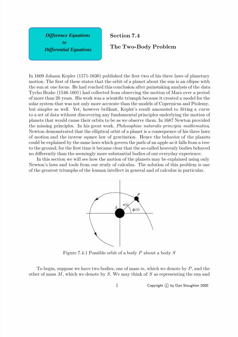
7/27/2019 Calculus 2 (Dan Sloughter)
http://slidepdf.com/reader/full/calculus-2-dan-sloughter 511/598
Difference Equations
Differential Equations
to
Section 7.4
The Two-Body Problem
In 1609 Johann Kepler (1571-1630) published the first two of his three laws of planetarymotion. The first of these states that the orbit of a planet about the sun is an ellipse withthe sun at one focus. He had reached this conclusion after painstaking analysis of the dataTycho Brahe (1546-1601) had collected from observing the motion of Mars over a periodof more than 20 years. His work was a scientific triumph because it created a model for thesolar system that was not only more accurate than the models of Copernicus and Ptolemy,but simpler as well. Yet, however brilliant, Kepler’s result amounted to fitting a curveto a set of data without discovering any fundamental principles underlying the motion of planets that would cause their orbits to be as we observe them. In 1687 Newton providedthe missing principles. In his great work, Philosophiae naturalis principia mathematica ,Newton demonstrated that the elliptical orbit of a planet is a consequence of his three lawsof motion and the inverse square law of gravitation. Hence the behavior of the planetscould be explained by the same laws which govern the path of an apple as it falls from a treeto the ground; for the first time it became clear that the so-called heavenly bodies behavedno differently than the seemingly more substantial bodies of our everyday experience.
In this section we will see how the motion of the planets may be explained using onlyNewton’s laws and tools from our study of calculus. The solution of this problem is oneof the greatest triumphs of the human intellect in general and of calculus in particular.
S
P
r(t)
θ (t)
Figure 7.4.1 Possible orbit of a body P about a body S
To begin, suppose we have two bodies, one of mass m, which we denote by P , and theother of mass M , which we denote by S . We may think of S as representing the sun and
1 Copyright c by Dan Sloughter 2000
7/27/2019 Calculus 2 (Dan Sloughter)
http://slidepdf.com/reader/full/calculus-2-dan-sloughter 512/598
2 The Two-Body Problem Section 7.4
P as representing a planet. It is possible to show that Newton’s laws of motion hold ina coordinate system with the origin located at the center of mass of the two bodies; forsimplicity, we will assume that M is significantly larger than m (as it is if S is the sun andP is a planet, asteroid, or comet), allowing us to assume that the center of mass is locatedat S . Thus we choose a coordinate system for the complex plane so that S is at the origin
and we let z(t) represent the position of P with respect to S at time t. If we express z(t)in polar coordinates, then
z(t) = r(t)eiθ(t), (7.4.1)
where r and θ are real-valued functions, as shown in Figure 7.4.1. For simplicity of notation,we will usually drop the explicit reference to t and simply write
z = reiθ. (7.4.2)
By Newton’s law of gravitation the magnitude of the gravitational force of attractionbetween the two bodies is
|F | = GM mr2
, (7.4.3)
where G is a constant, approximately
6.67× 10⁻¹¹N m2
kg2
if we measure force in Newtons, distance in meters, and mass in kilograms. Since gravityis an attractive force and we are assuming S to be at rest at the origin, F is directed fromP toward the origin. Hence we have
F = −GM m
r2eiθ. (7.4.4)
Moreover, we assume that this is the only force acting on the two bodies. Now if v(t) anda(t) represent the velocity and acceleration, respectively, of P at time t, then, by Newton’ssecond law of motion, F = ma, we must have
ma = −GM m
r2eiθ. (7.4.5)
Letting k = GM , this simplifies to
a = −k
r2eiθ. (7.4.6)
From our work in Section 7.3 we know that
v =dz
dt=
d
dtreiθ = ireiθ
dθ
dt+ eiθ
dr
dt(7.4.7)

7/27/2019 Calculus 2 (Dan Sloughter)
http://slidepdf.com/reader/full/calculus-2-dan-sloughter 513/598
Section 7.4 The Two-Body Problem 3
and
a =dv
dt
=d
dtireiθ
dθ
dt
+ eiθdr
dt
= ireiθd
dt
dθ
dt
+
dθ
dt
d
dt(ireiθ) + eiθ
d
dt
dr
dt
+
dr
dt
d
dt(eiθ)
= ireiθd2θ
dt2+
dθ
dt
i2reiθ
dθ
dt+ ieiθ
dr
dt
+ eiθ
d2r
dt2+
dr
dtieiθ
dθ
dt
= ireiθd2θ
dt2− reiθ
dθ
dt
2
+ ieiθdθ
dt
dr
dt+ eiθ
d2r
dt2+ ieiθ
dθ
dt
dr
dt
= −reiθ
dθ
dt
2
+ eiθd2r
dt2+ i
reiθ
d2θ
dt2+ 2eiθ
dθ
dt
dr
dt
. (7.4.8)
Putting (7.4.6) and (7.4.8) together gives us
−k
r2eiθ = −reiθ
dθ
dt
2
+ eiθd2r
dt2+ i
reiθ
d2θ
dt2+ 2eiθ
dθ
dt
dr
dt
.
After dividing through by eiθ we have
−k
r2= −r
dθ
dt
2
+d2r
dt2+ i
r
d2θ
dt2+ 2
dθ
dt
dr
dt
. (7.4.9)
The equality in (7.4.9) implies that the the real part of the left-hand side of the equationis equal to the real part of the right-hand side of the equation and the imaginary part of the left-hand side of the equation is equal to the imaginary part of the right-hand side of the equation. That is,
−k
r2= −r
dθ
dt
2
+d2r
dt2(7.4.10)
and
0 = rd2θ
dt2+ 2
dθ
dt
dr
dt. (7.4.11)
Multiplying both sides of (7.4.11) by r gives us
0 = r2d2θ
dt2+ 2r
dθ
dt
dr
dt. (7.4.12)
However,d
dt
r2
dθ
dt
= r2
d2θ
dt2+ 2r
dθ
dt
dr
dt,

7/27/2019 Calculus 2 (Dan Sloughter)
http://slidepdf.com/reader/full/calculus-2-dan-sloughter 514/598
4 The Two-Body Problem Section 7.4
so (7.4.12) implies thatd
dt
r2
dθ
dt
= 0. (7.4.13)
Since a function with 0 for its derivative must be a constant function, it follows that
r2dθ
dt= c (7.4.14)
for some constant c. In any interval of time of interest, we will have r > 0, that is, S
and P are not a the same point in space, and so r2 > 0. It follows that if c = 0, thendθ
dt= 0 for all t, corresponding to the relatively uninteresting case when θ is a constant
and P moves along a straight line passing through S . The more interesting cases are when
c < 0 or c > 0. Since the former case implies thatdθ
dt< 0 for all t and the latter implies
dθ
dt>
0 for allt, the choice of sign for
cultimately depends on our choice of orientation in
our coordinate system, that is, the direction in which we measure positive angles. Hence,
without loss of generality, we may assume c > 0 or, equivalently,dθ
dt> 0.
We will now use the substitution s = 1r
to put (7.4.10) into a simpler form. With thissubstitution, r = 1
s, so
dr
dt=
d
dt
1
s
= −
1
s2ds
dt= −
1
s2ds
dθ
dθ
dt. (7.4.15)
Since, from (7.4.14),
dθdt
= cr2
= cs2, (7.4.16)
we havedr
dt= −c
ds
dθ. (7.4.17)
Differentiating again,
d2r
dt2=
d
dt
−c
ds
dθ
= −c
d
dt
ds
dθ
= −c
d
dθ
ds
dθ
dθ
dt= −c
dθ
dt
d2s
dθ2. (7.4.18)
Hence, using (7.4.16),d2r
dt2= −c2s2
d2s
dθ2. (7.4.19)
Finally, substituting (7.4.16), (7.4.19), and s = 1r
into (7.4.10) gives us
−ks2 = −1
s(cs2)2 − c2s2
d2s
dθ2= −c2s3 − c2s2
d2s
dθ2. (7.4.20)
7/27/2019 Calculus 2 (Dan Sloughter)
http://slidepdf.com/reader/full/calculus-2-dan-sloughter 515/598
Section 7.4 The Two-Body Problem 5
Dividing both sides of this equation by −c2s2, we have
d2s
dθ2+ s =
k
c2. (7.4.21)
This is the differential equation to which all our work has been leading. The solution of
this equation will be an expression for s as a function of θ; since r is in turn a function of s, namely, r = 1
s, this will give us r as a function of θ and allow us to determine the path
of motion of P . Note, however, that we will not have found r as a function of t. In otherwords, we will be able to determine the path of motion of P , but we will not be able todetermine where along that path P is at any specific time t.
To solve (7.4.21), we first note that if y(θ) is a solution of the equation
d2y
dθ2+ y = 0,
then the function
x(θ) = y(θ) +
k
c2
satisfies the equationd2x
dθ2+ x =
k
c2
sinced2
dθ2
y +
k
c2
+
y +
k
c2
=
d2y
dθ2+ y +
k
c2= 0 +
k
c2=
k
c2.
Hence to solve (7.4.21), we need only solve the equation
d2s
dθ2
+ s = 0. (7.4.22)
That is, we need only find a function s of θ such that
d2s
dθ2= −s. (7.4.23)
Now (7.4.22) simply says that s is a function with the property that its second derivativeis the negative of itself. But we already know two such functions, namely, sin(θ) andcos(θ); moreover, for any constants A and B, the function A sin(θ) + B cos(θ) also has thisproperty. Although the justification is beyond our resources at this point, it is in fact truethat any solution of (7.4.23) must be of the form
A sin(θ) + B cos(θ) (7.4.24)
for some constants A and B. From this it now follows that our sought after solution to(7.4.21) must have the form
s = A sin(θ) + B cos(θ) +k
c2(7.4.25)
for some constants A and B.
7/27/2019 Calculus 2 (Dan Sloughter)
http://slidepdf.com/reader/full/calculus-2-dan-sloughter 516/598
6 The Two-Body Problem Section 7.4
We will now find values for the constants A and B so that
ds
dθ
θ=0
= 0 (7.4.26)
and
d2
sdθ2
θ=0
≤ 0. (7.4.27)
Intuitively, this means we are looking for values which satisfy conditions for s to have alocal maximum at θ = 0. Equivalently, these conditions will hold if r has a local minimumat θ = 0. We make think of this as choosing the constants A and B in such a way that P
is closest to S when the path of P crosses the positive real axis. Now
ds
dθ= A cos(θ)−B sin(θ),
sods
dθθ=0 = A, (7.4.28)
andd2s
dθ2= −A sin(θ)−B cos(θ),
sod2s
dθ2
θ=0
= −B. (7.4.29).
Hence the conditions (7.4.26) and (7.4.27) are satisfied if we set A = 0 and we requireB ≥ 0. In other words, the conditions (7.4.26) and (7.4.27) are satisfied by
s = B cos(θ) + kc2
, (7.4.30)
where B ≥ 0.In terms of r, (7.4.30) gives us
1
r= B cos(θ) +
k
c2=
c2B cos(θ) + k
c2,
so
r =c2
c2
B cos(θ) + k
=
c2
k
1 + c2
Bk
cos(θ)
. (7.4.31)
If we let α = c2
kand = αB, then our expression for r as a function of θ reduces to
r =α
1 + cos(θ), (7.4.32)
where ≥ 0 and α > 0 are constants.

7/27/2019 Calculus 2 (Dan Sloughter)
http://slidepdf.com/reader/full/calculus-2-dan-sloughter 517/598
Section 7.4 The Two-Body Problem 7
-3 -2 -1 1 2 3
-3
-2
-1
1
2
3
Figure 7.4.2 Circular orbit for P when = 0 and α = 2
Note that, as indicated above, our solution does not give us values of r and θ forspecified values of t, but rather (7.4.32) gives us a value of r for any specified value of θ.In other words, our solution does not give us the position of P for a given time t, but itdoes tell us the location of P as a function of θ. Indeed, if we plot the points z = reiθ
for all values of θ in the interval [−π, π], with r given by (7.4.32), then the resulting curvewill be the path of the orbit of P about S . For example, if = 0, then r = α for all t andthe orbit of P is a circle of radius α with center at S , as shown in Figure 7.4.2 for α = 2.
Note that because of our assumption thatdθ
dt> 0, the motion along this curve, and all
subsequent curves, will be in the counter-clockwise direction.If 0 < < 1, then cos(θ) has a maximum value of when θ = 0 and a minimum value
of − when θ = −π or θ = π. Thus the minimum value of r is
r(0) =α
1 +
and the maximum value of r is
r(−π) = r(π) =α
1− .
Hence the orbit of P about S is a closed curve with
α
1 + ≤ r ≤
α
1−
for all θ. An example for α = 2 and = 0.5, in which case 43 ≤ r ≤ 4 for all θ, is shown in
Figure 7.4.3.Note that
lim→1−
r(0) = lim→1−
α
1 + =
α
2,
whereaslim→1−
r(π) = lim→1−
α
1− = ∞.

7/27/2019 Calculus 2 (Dan Sloughter)
http://slidepdf.com/reader/full/calculus-2-dan-sloughter 518/598
8 The Two-Body Problem Section 7.4
-5 -4 -3 -2 -1 1 2
-3
-2
-1
1
2
3
Figure 7.4.3 Orbit of P for = 0.5 and α = 2
Hence as approaches 1 from the left, the point of closest approach of P to S shrinkstoward α
2 , but the point at which P is farthest from S increases without bound. Thus, as
varies from 0 to 1, the orbit of P flattens out, changing from a circle to a long oblong shape.Figure 7.4.4 shows the orbit of P for α =2 and = 0.95, in which case 1.026 ≤ r ≤ 40 forall θ . Because of this behavior, is called the eccentricity of the orbit of P .
-40 -30 -20 -10
-15
-10
-5
5
10
15
Figure 7.4.4 Orbit of P for = 0.95 and α = 2
When = 1, r is not defined for θ = −π and θ = π. In fact, in this case
limθ→π−
r(θ) = limθ→π−
α
1 + cos(θ)= ∞
and
limθ→−π+
r(θ) = limθ→−π+
α
1 + cos(θ)= ∞.
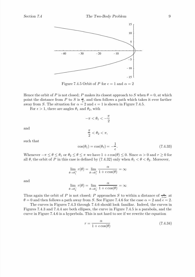
7/27/2019 Calculus 2 (Dan Sloughter)
http://slidepdf.com/reader/full/calculus-2-dan-sloughter 519/598
Section 7.4 The Two-Body Problem 9
-40 -30 -20 -10
-15
-10
-5
5
10
15
Figure 7.4.5 Orbit of P for = 1 and α = 2
Hence the orbit of P
is not closed;P
makes its closest approach toS
whenθ
= 0, at whichpoint the distance from P to S is α
2 , and then follows a path which takes it ever fartheraway from S . The situation for α = 2 and = 1 is shown in Figure 7.4.5.
For > 1, there are angles θ1 and θ2, with
−π < θ1 < −π
2
andπ
2< θ2 < π,
such that
cos(θ1) = cos(θ2) = −1 . (7.4.33)
Whenever −π ≤ θ ≤ θ1 or θ2 ≤ θ ≤ π we have 1 + cos(θ) ≤ 0. Since α > 0 and r ≥ 0 forall θ, the orbit of P in this case is defined by (7.4.32) only when θ1 < θ < θ2. Moreover,
limθ→θ
+
1
r(θ) = limθ→θ
+
1
α
1 + cos(θ)= ∞
andlim
θ→θ−
2
r(θ) = limθ→θ
−
2
α
1 + cos(θ)= ∞
Thus again the orbit of P is not closed; P approaches S to within a distance of α1+ at
θ = 0 and then follows a path away from S . See Figure 7.4.6 for the case α = 2 and = 2.The curves in Figures 7.4.3 through 7.4.6 should look familiar. Indeed, the curves in
Figures 7.4.3 and 7.4.4 are both ellipses, the curve in Figure 7.4.5 is a parabola, and thecurve in Figure 7.4.6 is a hyperbola. This is not hard to see if we rewrite the equation
r =α
1 + cos(θ)(7.4.34)
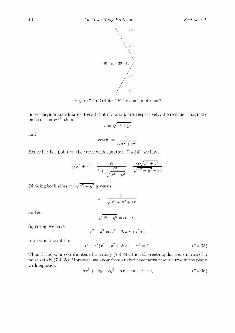
7/27/2019 Calculus 2 (Dan Sloughter)
http://slidepdf.com/reader/full/calculus-2-dan-sloughter 520/598
10 The Two-Body Problem Section 7.4
-40 -30 -20 -10
-40
-20
20
40
Figure 7.4.6 Orbit of P for = 2 and α = 2
in rectangular coordinates. Recall that if x
andy
are, respectively, the real and imaginaryparts of z = reiθ, then
r =
x2 + y2
andcos(θ) =
x x2 + y2
.
Hence if z is a point on the curve with equation (7.4.34), we have
x2 + y2 =
α
1 +x
x2 + y2
=α
x2 + y2
x2 + y2 + x.
Dividing both sides by
x2 + y2 gives us
1 =α
x2 + y2 + x,
and so x2 + y2 = α− x.
Squaring, we have
x
2
+ y
2
= α
2
− 2αx +
2
x
2
,from which we obtain
(1− 2)x2 + y2 + 2αx− α2 = 0. (7.4.35)
Thus if the polar coordinates of z satisfy (7.4.34), then the rectangular coordinates of z
must satisfy (7.4.35). Moreover, we know from analytic geometry that a curve in the planewith equation
ax2 + bxy + cy2 + dx + ey + f = 0, (7.4.36)

7/27/2019 Calculus 2 (Dan Sloughter)
http://slidepdf.com/reader/full/calculus-2-dan-sloughter 521/598
Section 7.4 The Two-Body Problem 11
where a, b, c, d, e, and f are all constants, is an ellipse if b2 − 4ac < 0, a parabola if b2 − 4ac = 0, and a hyperbola if b2 − 4ac > 0. Because of this result, we call the number
D = b2 − 4ac (7.4.37)
the discriminant of (7.4.36). In the case of (7.4.35), we have
D = 0− 4(1− 2
) = −4(1− 2
). (7.4.38)Thus D < 0 when 0 ≤ < 1, D = 0 when = 1, and D > 0 when > 1. Since we havealready seen that the orbit of P is a circle when = 0 (a circle being a particular case of an ellipse), we now have the following classification of the orbit of P about S in terms of the eccentricity :
Eccentricity Orbit of P
= 0 Circle0 < < 1 Ellipse = 1 Parabola > 1 Hyperbola
Recall that, collectively, these curves are known as the conic sections.We have seen that starting with the assumptions of Newton’s law of gravitation and
his second law of motion, we may conclude that the orbit of a body P about anotherbody S must be a conic section. As great as Newton’s accomplishment was, scientifically,mathematically, and philosophically, it is not the end of the story. The work we havedone only accounts for the interaction of two bodies, isolated without any forces actingon them other than their mutual gravitational attraction. In reality, to model our entiresolar system we would have to consider, at the minimum, the effects of the gravitationalfields of the sun plus at least nine planets, as well as numerous moons, asteroids, andcomets. Because of these other considerations, the orbits of the planets are not true
ellipses, although, since by far the most dominant force acting on any one planet is thegravitational attraction between it and the sun, the deviation from elliptical paths is small.The problem of the motion of three or more bodies interacting under the influence of theirmutual gravitational attraction has challenged mathematicians since the time of Newton.However, we now know that this problem, known as the n-body problem , cannot, in general,be solved exactly. Since the work of Henri Poincare (1854-1912), advances on this problemhave been directed toward qualitative and numerical descriptions of the orbits, not towardexact analytic solutions. In fact it was Poincare who first showed that even in the caseof only three bodies, the orbits can be highly complex, revealing a sensitivity to initialconditions that would make predictions about the future path of a given body effectivelyimpossible. The work on this problem continues to the present.
Problems
1. The perihelion of the orbit of a planet is the point of the orbit which is closest tothe sun. The following table gives the eccentricity and the distance from the sun atperihelion for each of the known planets in our solar system. Note the distances aregiven in astronomical units, where one astronomical unit is approximately 92.9 millionmiles, the mean distance from the earth to the sun.

7/27/2019 Calculus 2 (Dan Sloughter)
http://slidepdf.com/reader/full/calculus-2-dan-sloughter 522/598
12 The Two-Body Problem Section 7.4
Planet Eccentricity Distance at Perihelion
Mercury 0.21 0.31Venus 0.01 0.72Earth 0.02 0.98Mars 0.09 1.38Jupiter 0.05 4.95Saturn 0.06 9.02Uranus 0.05 18.3Neptune 0.01 29.8Pluto 0.25 29.8
(a) Plot the orbits of each of the planets.
(b) The aphelion of the orbit of a planet is the point of the orbit which is farthest fromthe sun. Find the distance of each planet from the sun at aphelion.
(c) Which orbits are closest to being circular? Which ones deviate the most from being
circular?(d) Plot the orbits of Neptune and Pluto together. How do they differ?
2. The orbit of the Comet Kohoutek has an eccentricity of 0.9999 and its distance fromthe sun at perihelion is 0.14 astronomical units. Plot the orbit of Comet Kohoutekand compare it with the orbit of Pluto from Problem 1. How far away from the sun isComet Kohoutek at aphelion?
3. The orbit of Halley’s comet has an eccentricity of 0.967 and its distance from the sunat perihelion is 0.59 astronomical units. Plot the orbit of Halley’s comet and compareit with the orbits of Pluto and Comet Kohoutek as found in Problems 1 and 2. How
far away from the sun is Halley’s comet at aphelion?4. The orbit of Encke’s comet has an eccentricity of 0.847 and its distance from the sun
at perihelion is 0.34 astronomical units. Plot the orbit of Encke’s comet and compareit with the orbits of Pluto, Comet Kohoutek, and Halley’s comet as found in Problems1, 2, and 3. How far away from the sun is Encke’s comet at aphelion?
5. (a) Use the information in Problem 1 to find the equation for the orbit of the earth inrectangular coordinates (that is, an equation of the form (7.4.35)).
(b) Use your result from (a) and the techniques of Section 4.8 to find the length of theearth’s orbit. Convert your answer into miles.
(c) What is the average speed of the earth in miles per hour?6. (a) Use the information in Problem 1 to find the equation for the orbit of Pluto in
rectangular coordinates (that is, an equation of the form (7.4.35)).
(b) Use your result from (a) and the techniques of Section 4.8 to find the length of Pluto’s orbit. Convert your answer into miles.
(c) What is the average speed of Pluto in miles per hour? You will need to know thatit takes Pluto 248 years to complete one orbit about the sun.
7/27/2019 Calculus 2 (Dan Sloughter)
http://slidepdf.com/reader/full/calculus-2-dan-sloughter 523/598
Section 7.4 The Two-Body Problem 13
7. To solve the two-body problem we had to solve a differential equation of the form
d2y
dt2= −y.
In this problem we consider the equation
d2y
dt2= y. (7.4.39)
(a) Find two functions, y1(t) and y2(t), which satisfy (7.4.39) and are such that y2(t)is not a constant multiple of y1(t).
(b) Show thaty(t) = Ay1(t) + By2(t)
satisfies (7.4.39) for any constants A and B.
(c) Find a solution y(t) of (7.4.39) such that y(0) = 2 and
dy
dt
t=0
= 4.

7/27/2019 Calculus 2 (Dan Sloughter)
http://slidepdf.com/reader/full/calculus-2-dan-sloughter 524/598
Difference Equations
Differential Equations
to
Section 8.1
Numerical Solutions of Differential Equations
If x is a function of a real variable t and f is a function of both x and t, then the equation
x(t) = f (x(t), t) (8.1.1)
is called a first order differential equation . Solving such an equation involves more thanalgebraic manipulation; indeed, although the equation itself involves three quantities, x,x, and t, to find a solution we must identify a function x, defined solely in terms of the independent variable t, which satisfies the relationship of (8.1.1) for all t in some
open interval. For many equations, exact solution is not possible and we have to rely onapproximations. In this chapter we will discuss techniques for finding both approximateand, where possible, exact solutions to differential equations.
We have already seen many examples of differential equations: in Section 4.8 whenwe discussed finding the position of an object moving in a straight line given its velocityfunction and its initial position, in Section 6.3 when we discussed models for growth anddecay, in Section 7.3 when we discussed the motion of a projectile, and in Section 7.4when we considered the two-body problem. Indeed, in many ways the study of differentialequations is at the heart of calculus. To study the interaction of physical bodies in theworld is to study the ramifications of physical laws such as the law of gravitation andNewton’s second law of motion, laws which frequently lead, as we saw in Section 7.4, to
questions involving the solution of differential equations. Newton was the first to realizethe power of calculus for solving a vast array of physical problems. The mathematiciansthat followed him enlarged and refined his techniques until they began to believe that theentire future of the universe, as well as its past, could be discerned from a knowledge of the current positions and velocities of all physical bodies and the forces at work betweenthem. In such a world view, nothing is undetermined in itself; what appears to us asundetermined is simply a reflection of our ignorance of the forces involved. As an exampleof this view, writing in 1795, Pierre Simon Laplace (1749-1827) said:
Given for one instant an intelligence which could comprehend all the forces by whichnature is animated and the respective situation of the beings who compose it — an
intelligence sufficiently vast to submit these data to analysis — it would embrace inthe same formula the movements of the greater bodies of the universe and those of thelightest atom; for it, nothing would be uncertain and the future, as the past, would bepresent to its eyes. *
* P. S. Laplace, Essai philosphique sur les probabilites (Paris, 1814), translated by F. W.Truscott and F. L. Emory, A Philosophical Essay on Probabilities (New York, 1951), page3.
1 Copyright c by Dan Sloughter 2000
7/27/2019 Calculus 2 (Dan Sloughter)
http://slidepdf.com/reader/full/calculus-2-dan-sloughter 525/598
2 Numerical Solutions of Differential Equations Section 8.1
Today we know more about the limits to our knowledge, but, nevertheless, the study of differential equations remains a key component to our understanding of the universe.
To begin our study, consider the equation
x(t) = f (x(t), t) (8.1.2)
with the initial condition x(t0) = x0. To simplify notation, we will frequently omit theindependent variable when referring to x(t) and write simply
x = f (x, t). (8.1.3)
Now if f (x, t) depends only on the value of t, that is, if f (x, t) = g(t) for all values of x, where g is a function of t alone, then we may solve (8.1.3) by integration. That is,integrating both sides (8.1.3) gives us
t
t0
x(s)ds = t
t0
g(s)ds. (8.1.4)
Substituting t
t0
x(s)ds = x(t)− x(t0),
into (8.1.4), we have
x(t) = x(t0) +
t
t0
g(s)ds. (8.1.5)
Assuming we can compute the definite integral, which, provided g is continuous, can atleast always be done numerically, we have solved the differential equation. This is the typeof differential equation we considered in Section 4.8.
Example Consider the equation
x = 4 sin(3t)
with initial condition x(0) = 5. Then
x(t) = 5 +
t
0
4 sin(3s)ds
= 5−4
3 cos(3s)t0
= 5− 4
3cos(3t) +
4
3
=1
3(19− 4 cos(3t)).
More generally, suppose f in (8.1.3) depends on both x and t. In that case, sincethe right-hand side of the equation involves the unknown function x, we cannot simply

7/27/2019 Calculus 2 (Dan Sloughter)
http://slidepdf.com/reader/full/calculus-2-dan-sloughter 526/598
Section 8.1 Numerical Solutions of Differential Equations 3
integrate both sides of the equation. We have solved some equations like this in earliersections, such as the inhibited population growth model
x =α
M x(M − x)
in Section 6.3, and we will discuss general techniques for finding exact solutions for severaltypes of equations in the coming sections. However, in this section we will concentrateon direct numerical techniques for approximating solutions. Indeed, knowing the difficultyof evaluating ordinary definite integrals, it is not hard to believe that many, if not most,differential equations may be solved only through numerical approximation.
Although the function x in equation (8.1.3) is unknown, we do have enough informationto find its best affine approximation at t0. Namely, the best affine approximation to x att0 is
T (t) = x0 + x(t0)(t− t0) = x0 + f (x0, t0)(t− t0). (8.1.6)
Hence, from our work with Taylor’s theorem in Section 5.2 and assuming f (x(t), t) is a
continuous function, we have
x(t) = x0 + f (x0, t0)(t− t0) + O((t− t0)2). (8.1.7)
Equivalently,x(t0 + h) = x0 + hf (x0, t0) + O(h2). (8.1.8)
Thus for a small value of h,x1 = x0 + hf (x0, t0)
will provide a good approximation to x(t0 + h). However, we want to do more than this;since x is a function, we want to be able to approximate its values over an entire interval,say [t0, t1]. To do so, we choose a small value for h and iterate the process that gave usx1. Specifically, we let sk = t0 + kh, k = 0, 1, . . . , n, where n is chosen large enough thatsn ≥ t1, and compute
xk+1 = xk + hf (xk, sk) (8.1.9)
for k = 0, 1, . . . , n − 1. That is, we compute an approximation for x(sk+1) by apply-ing the best affine approximation to our approximation for x(sk), repeating the processenough times until we have approximated x over the entire interval [t0, t1]. This methodof approximation is known as Euler’s method .
Euler’s method To approximate a solution to the equation
˙x
=f
(x, t
)with initial condition x(t0) = x0 on an interval [t0, t1], choose a small value for h > 0and an integer n such that t0 + nh ≥ t1. Letting sk = t0 + kh, k = 0, 1, . . . , n, computex1, x2, . . . , xn using the difference equation
xk+1 = xk + hf (xk, sk). (8.1.10)
Then xk is an approximation for x(t + kh).
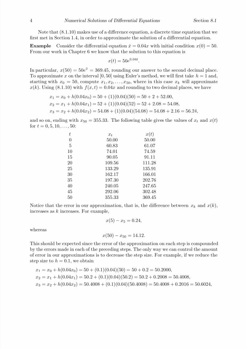
7/27/2019 Calculus 2 (Dan Sloughter)
http://slidepdf.com/reader/full/calculus-2-dan-sloughter 527/598
4 Numerical Solutions of Differential Equations Section 8.1
Note that (8.1.10) makes use of a difference equation, a discrete time equation that wefirst met in Section 1.4, in order to approximate the solution of a differential equation.
Example Consider the differential equation x = 0.04x with initial condition x(0) = 50.From our work in Chapter 6 we know that the solution to this equation is
x(t) = 50e0.04t
.
In particular, x(50) = 50e2 = 369.45, rounding our answer to the second decimal place.To approximate x on the interval [0, 50] using Euler’s method, we will first take h = 1 and,starting with x0 = 50, compute x1, x2, . . . , x50, where in this case xk will approximatex(k). Using (8.1.10) with f (x, t) = 0.04x and rounding to two decimal places, we have
x1 = x0 + h(0.04x0) = 50 + (1)(0.04)(50) = 50 + 2 + 52.00,
x2 = x1 + h(0.04x1) = 52 + (1)(0.04)(52) = 52 + 2.08 = 54.08,
x3 = x2 + h(0.04x2) = 54.08 + (1)(0.04)(54.08) = 54.08 + 2.16 = 56.24,
and so on, ending with x50 = 355.33. The following table gives the values of xt and x(t)for t = 0, 5, 10, . . . , 50:
t xt x(t)0 50.00 50.005 60.83 61.07
10 74.01 74.5915 90.05 91.1120 109.56 111.2825 133.29 135.9130 162.17 166.0135 197.30 202.7640 240.05 247.6545 292.06 302.4850 355.33 369.45
Notice that the error in our approximation, that is, the difference between xk and x(k),increases as k increases. For example,
x(5)− x5 = 0.24,
whereasx(50)− x50 = 14.12.
This should be expected since the error of the approximation on each step is compoundedby the errors made in each of the preceding steps. The only way we can control the amountof error in our approximations is to decrease the step size. For example, if we reduce thestep size to h = 0.1, we obtain
x1 = x0 + h(0.04x0) = 50 + (0.1)(0.04)(50) = 50 + 0.2 = 50.2000,
x2 = x1 + h(0.04x1) = 50.2 + (0.1)(0.04)(50.2) = 50.2 + 0.2008 = 50.4008,
x3 = x2 + h(0.04x2) = 50.4008 + (0.1)(0.04)(50.4008) = 50.4008 + 0.2016 = 50.6024,

7/27/2019 Calculus 2 (Dan Sloughter)
http://slidepdf.com/reader/full/calculus-2-dan-sloughter 528/598
Section 8.1 Numerical Solutions of Differential Equations 5
10 20 30 40 50
50
100
150
200
250
300
350
400
Figure 8.1.1 Approximate solutions of x = 0.04x
and so on, ending with x500 = 367.98 as our approximation for x(50). In general, withh = 0.1, xk is an approximation for x(0+kh) = x(0.1k). Equivalently, x(t) is approximatedby xk where k = 10t, provided 10t is an integer. The following table gives the values of x10t and x(t) for t = 0, 5, 10, . . . , 50:
t x10t x(t)0 50.00 50.005 61.05 61.07
10 74.53 74.5915 91.00 91.1120 111.10 111.2825 135.64 135.91
30 165.61 166.0135 202.19 202.7640 246.86 247.6545 301.40 302.4850 367.98 369.45
As expected, reducing the step size from h = 1 to h = 0.1 greatly reduces the errorin the approximations. Figure 8.1.1 shows the graphs of both our approximations to x
(the graph of x is not shown since, on this scale, it is essentially the same as our secondapproximation).
Example The differential equation in the previous example could be used to model apopulation which is growing at a rate of approximately 4% per unit of time, starting withan initial population of 50. As a modification of this model, consider a case where the rateof growth of the population is decreasing over time. For example, the rate of growth mightstart out at 4% but decrease over time toward 2%. If x(t) is the population after t unitsof time, then the differential equation
x = 0.02(1 + e−t
10 )x
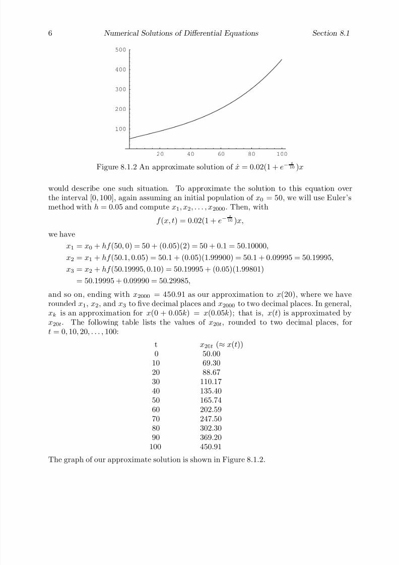
7/27/2019 Calculus 2 (Dan Sloughter)
http://slidepdf.com/reader/full/calculus-2-dan-sloughter 529/598
6 Numerical Solutions of Differential Equations Section 8.1
20 40 60 80 100
100
200
300
400
500
Figure 8.1.2 An approximate solution of x = 0.02(1 + e−t
10 )x
would describe one such situation. To approximate the solution to this equation over
the interval [0, 100], again assuming an initial population of x0 = 50, we will use Euler’smethod with h = 0.05 and compute x1, x2, . . . , x2000. Then, with
f (x, t) = 0.02(1 + e−t
10 )x,
we have
x1 = x0 + hf (50, 0) = 50 + (0.05)(2) = 50 + 0.1 = 50.10000,
x2 = x1 + hf (50.1, 0.05) = 50.1 + (0.05)(1.99900) = 50.1 + 0.09995 = 50.19995,
x3 = x2 + hf (50.19995, 0.10) = 50.19995 + (0.05)(1.99801)
= 50.19995 + 0.09990 = 50.29985,
and so on, ending with x2000 = 450.91 as our approximation to x(20), where we haverounded x1, x2, and x3 to five decimal places and x2000 to two decimal places. In general,xk is an approximation for x(0 + 0.05k) = x(0.05k); that is, x(t) is approximated byx20t. The following table lists the values of x20t, rounded to two decimal places, fort = 0, 10, 20, . . . , 100:
t x20t (≈ x(t))0 50.00
10 69.3020 88.6730 110.1740 135.4050 165.7460 202.5970 247.5080 302.3090 369.20
100 450.91
The graph of our approximate solution is shown in Figure 8.1.2.
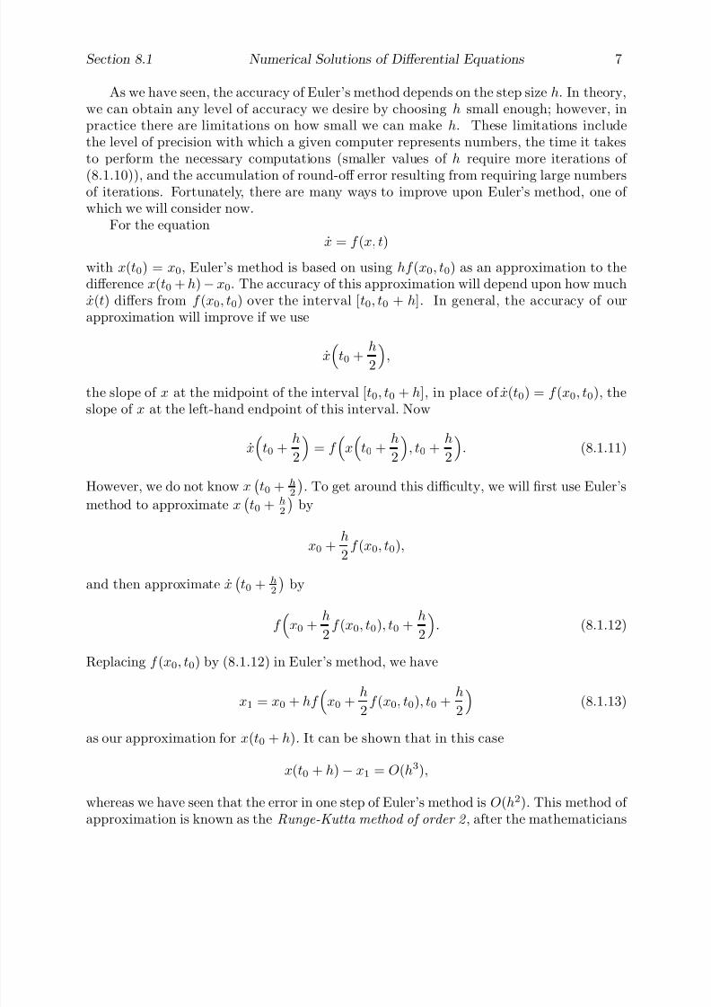
7/27/2019 Calculus 2 (Dan Sloughter)
http://slidepdf.com/reader/full/calculus-2-dan-sloughter 530/598
Section 8.1 Numerical Solutions of Differential Equations 7
As we have seen, the accuracy of Euler’s method depends on the step size h. In theory,we can obtain any level of accuracy we desire by choosing h small enough; however, inpractice there are limitations on how small we can make h. These limitations includethe level of precision with which a given computer represents numbers, the time it takesto perform the necessary computations (smaller values of h require more iterations of
(8.1.10)), and the accumulation of round-off error resulting from requiring large numbersof iterations. Fortunately, there are many ways to improve upon Euler’s method, one of which we will consider now.
For the equationx = f (x, t)
with x(t0) = x0, Euler’s method is based on using hf (x0, t0) as an approximation to thedifference x(t0 + h)− x0. The accuracy of this approximation will depend upon how muchx(t) differs from f (x0, t0) over the interval [t0, t0 + h]. In general, the accuracy of ourapproximation will improve if we use
x
t0 + h2
,
the slope of x at the midpoint of the interval [t0, t0 + h], in place of x(t0) = f (x0, t0), theslope of x at the left-hand endpoint of this interval. Now
x
t0 +h
2
= f
x
t0 +h
2
, t0 +
h
2
. (8.1.11)
However, we do not know x
t0 + h
2
. To get around this difficulty, we will first use Euler’s
method to approximate x
t0 + h
2
by
x0 +h
2f (x0, t0),
and then approximate x
t0 + h
2
by
f
x0 +h
2f (x0, t0), t0 +
h
2
. (8.1.12)
Replacing f (x0, t0) by (8.1.12) in Euler’s method, we have
x1 = x0 + hf
x0 +
h
2 f (x0, t0), t0 +
h
2
(8.1.13)
as our approximation for x(t0 + h). It can be shown that in this case
x(t0 + h)− x1 = O(h3),
whereas we have seen that the error in one step of Euler’s method is O(h2). This method of approximation is known as the Runge-Kutta method of order 2 , after the mathematicians

7/27/2019 Calculus 2 (Dan Sloughter)
http://slidepdf.com/reader/full/calculus-2-dan-sloughter 531/598
8 Numerical Solutions of Differential Equations Section 8.1
Carl Runge (1856-1927) and M. W. Kutta (1867-1944). In general, an approximationmethod is said to be of order n if the error in one step is O(hn+1). There are Runge-Kuttaformulas for approximations of higher order, but we will consider only this order 2 formula.
Second order Runge-Kutta To approximate the solution of the equation
x = f (x, t)
with initial condition x(t0) = x0 on an interval [t0, t1], choose a small value for h > 0 andan integer n such that t0 + nh ≥ t1. Letting sk = t0 + kh, k = 0, 1, 2, . . . n, compute
m =h
2f (xk, sk)
and
xk+1 = xk + hf
xk + m, sk +h
2
(8.1.14)
for k = 0, 1, . . . n− 1. Then xk is an approximation for x(t0 + kh).
Example We will approximate the solution of x = 0.04x with x(0) = 50 on the interval[0, 50] using the second order Runge-Kutta method with h = 0.1. Using f (x, t) = 0.04x
and rounding to four decimal places, we have
x1 = 50 + 0.1f (50 + 0.05f (50, 0), 0.05)
= 50 + 0.1f (50.1, 0.05)
= 50 + 0.2004
= 50.2004,
x2 = 50.2004 + 0.1f (50.2004 + 0.05f (50.2004, 0.1), 0.15)
= 50.2004 + 0.1f (50.3008, 0.15)
= 50.2004 + 0.2012
= 50.4016,
and so on, up to x500 = 369.4508. Since h = 0.1, x10t gives us an approximation forx(t) whenever 10t is an integer. The following table gives the values of x10t and x(t) fort = 0, 5, 10, . . ., 50:
t x10t x(t)0 50.0000 50.00005 61.0701 61.0701
10 74.5912 74.5912
15 91.1058 91.105920 111.2768 111.277025 135.9137 135.914130 166.0053 166.005835 202.7592 202.760040 247.6506 247.651645 302.4809 302.482450 369.4508 369.4528

7/27/2019 Calculus 2 (Dan Sloughter)
http://slidepdf.com/reader/full/calculus-2-dan-sloughter 532/598
Section 8.1 Numerical Solutions of Differential Equations 9
Comparing these values with the values we obtained with Euler’s method for the sameequation, we see that we have decreased our error significantly without decreasing the stepsize. Hence we have gained accuracy without greatly increasing the number of computa-tions required.
Example In Problem 7 in Section 4.8 (which is repeated in Problem 2 at the end of this section) we discussed the problem of a body in free fall near the surface of the earth,neglecting the effects of air resistance. In that case, if the body has mass m and F isthe force acting on the body, then, since we are neglecting all forces except for that of gravity, F = −mg, where g = 32 feet/second2. However, if we consider the effects of air resistance, then we have to modify F to account for this additional force acting in adirection opposite to that of gravity. One common assumption is that air resistance isproportional to velocity; in that case, we have
F = −32m− kv, (8.1.15)
where k > 0 is a constant which depends on the particular body and v is the velocity of thebody. Note that kv < 0 since v < 0, so the additional force −kv is acting in the oppositedirection of gravity. Now if a is the acceleration of the body, F = ma implies
ma = −32m− kv, (8.1.16)
and so
a = −32− k
mv. (8.1.17)
Since a = v, (8.1.17) gives us the differential equation
v = −32− cv, (8.1.18)
where
c =k
m
is a constant which depends both on the mass of the body and its air resistance. For
example, suppose we have a situation where c = 0.1 and the body is released from resthigh above the ground. Then we are interested in the solution of the equation
v = −32− 0.1v
with the initial condition v(0) = 0. The following table gives the results from applying thesecond order Runge-Kutta method with step size h = 0.1 over the interval [0, 70]:
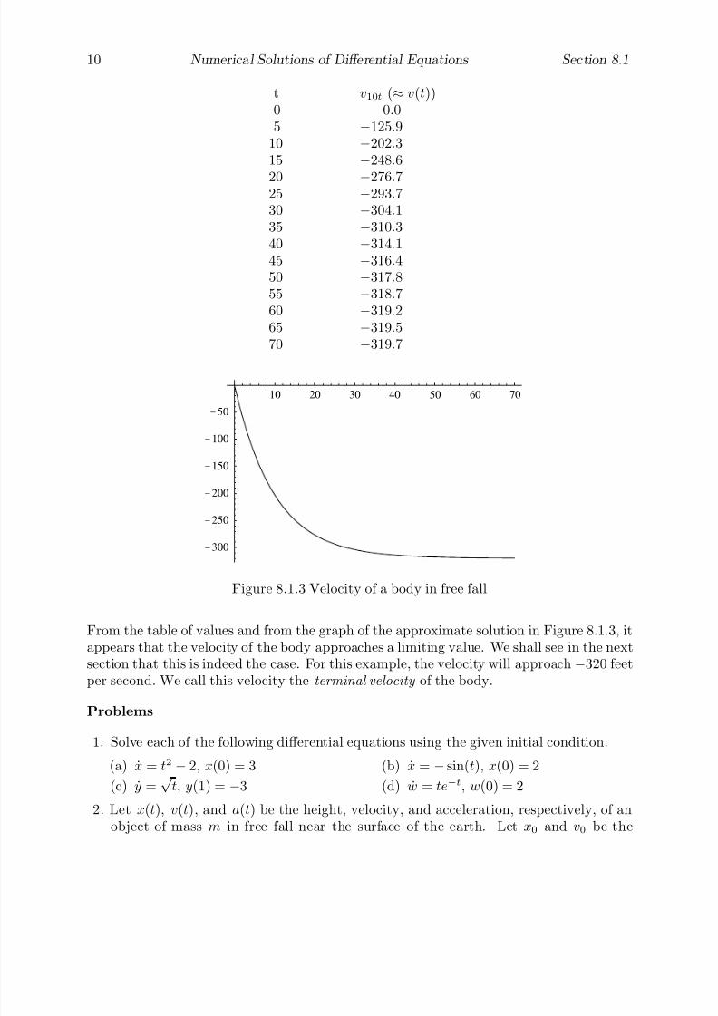
7/27/2019 Calculus 2 (Dan Sloughter)
http://slidepdf.com/reader/full/calculus-2-dan-sloughter 533/598
10 Numerical Solutions of Differential Equations Section 8.1
t v10t (≈ v(t))0 0.05 −125.9
10 −202.315 −248.6
20 −276.725 −293.730 −304.135 −310.340 −314.145 −316.450 −317.855 −318.760 −319.265 −319.570
−319.7
10 20 30 40 50 60 70
-300
-250
-200
-150
-100
-50
Figure 8.1.3 Velocity of a body in free fall
From the table of values and from the graph of the approximate solution in Figure 8.1.3, itappears that the velocity of the body approaches a limiting value. We shall see in the nextsection that this is indeed the case. For this example, the velocity will approach −320 feetper second. We call this velocity the terminal velocity of the body.
Problems
1. Solve each of the following differential equations using the given initial condition.
(a) x = t2 − 2, x(0) = 3 (b) x = − sin(t), x(0) = 2
(c) y =√
t, y(1) = −3 (d) w = te−t, w(0) = 2
2. Let x(t), v(t), and a(t) be the height, velocity, and acceleration, respectively, of anobject of mass m in free fall near the surface of the earth. Let x0 and v0 be the

7/27/2019 Calculus 2 (Dan Sloughter)
http://slidepdf.com/reader/full/calculus-2-dan-sloughter 534/598
Section 8.1 Numerical Solutions of Differential Equations 11
height and velocity, respectively, of the object at time t0. If we ignore the effectsof air resistance, the force acting on the body is −mg, where g is a constant (g =
9.8 meters/second2 or g = 32 feet/second2). Thus by Newton’s second law of motion,
−mg = ma(t),
and soa(t) = −g.
Show that
x(t) = −1
2gt2 + v0t + x0.
3. Suppose an object is projected vertically upward from a height of 100 feet with aninitial velocity of 20 feet per second. Use Problem 2 to answer the following questions.
(a) Find x(t), the height of the object at time t.
(b) At what time does the object reach its maximum height?(c) What is the maximum height reached by the object?
(d) At what time will the object strike the ground?
4. For each of the following, use Euler’s method to approximate the solution of the equa-tion over the given interval I using the step size h specified. Plot your result.
(a) x = e−2t2
, x(0) = 1, I = [0, 10], h = 0.1
(b) x = −0.96x, x(0) = 100, I = [0, 100], h = 0.5
(c) y = 0.05y − 5, y(0) = 200, I = [0, 50], h = 0.05
(d) x = 0.002x(100−
x), x(0) = 10, I = [0, 200], h = 0.1
(e) y = 0.02(1 + 0.5e−t
15 )y, y(0) = 10, I = [0, 150], h = 0.5
(f ) x = cos(x2), x(0) = 0, I = [0, 10], h = 0.01
(g) x = 0.045x + 0.4t, x(0) = 30, I = [0, 40], h = 0.1
(h) x = 0.1x + cos(t), x(0) = 0, I = [0, 10], h = 0.05
5. Use the second order Runge-Kutta method to approximate solutions to the equationsin Problem 4.
6. In 1990 the population of India was 853.4 million. If P (t) is the population of India t
years after 1990, suppose P satisfies the differential equation
P = k(t)P,
where k(t) is the rate of growth of the population at time t. For example, at the startof 1990 the population of India was growing at a rate of 2.1% per year, so k(0) = 0.021.
(a) Suppose the rate of growth remains constant; that is, suppose k(t) = 0.021 for allt ≥ 0. Find P (t). In what year will the population reach 1 billion? In what yearwill it reach 2 billion? In what year will it reach 3 billion?
7/27/2019 Calculus 2 (Dan Sloughter)
http://slidepdf.com/reader/full/calculus-2-dan-sloughter 535/598
12 Numerical Solutions of Differential Equations Section 8.1
(b) Now suppose k(t) is decreasing toward 1% in such a way that
k(t) = 0.01(1 + 1.1e−t
30 ).
Use the second order Runge-Kutta method to approximate P over the interval
[0, 100] using a step size of h = 0.1. In what year will the population reach 1billion? In what year will it reach 2 billion? In what year will it reach 3 billion?
(c) Plot your results from (a) and (b) together.
7. In the final example in this section we considered the problem of an object in free fallwhen the air resistance is proportional to the velocity of the object. Now consider thecase where the air resistance is proportional to the square root of the speed.
(a) If s is the speed of the object, in feet per second, t seconds after it is released,explain why s satisfies the differential equation
s = 32
−c√
s,
s(0) = 0, for some constant c > 0.
(b) Using c = 1, use the second order Runge-Kutta method to solve the equation in(a) over the interval [0, 500] using a step size of h = 0.5. Plot your results.
(c) Does the object appear to approach a limiting speed? If so, what is the terminalspeed?
(d) Solve the equation32− c
√ s = 0
for s. Explain the connection between this answer and your answer in (c).
8. In the final example in this section we considered the problem of an object in free fallwhen the air resistance is proportional to the velocity of the object. Now consider thecase where the air resistance is proportional to the square of the velocity.
(a) If v is the velocity of the object, in feet per second, t seconds after it is released,explain why v satisfies the differential equation
v = −32 + cv2,
v(0) = 0, for some constant c > 0.
(b) Using c = 0.01, use the second order Runge-Kutta method to approximate the
solution to the equation in (a) over the interval [0, 20] using a step size of h = 0.02.Plot your results.
(c) Does the object appear to approach a limiting velocity? If so, what is the terminalvelocity?
(d) Solve the equation−32 + cv2 = 0
for v. Explain the connection between this answer and your answer in (c).

7/27/2019 Calculus 2 (Dan Sloughter)
http://slidepdf.com/reader/full/calculus-2-dan-sloughter 536/598
Section 8.1 Numerical Solutions of Differential Equations 13
9. Suppose the population of a certain country was 56 million in 2000 and the natural rateof the growth of the population was 2% per year. Moreover, suppose k(t) representsthe net rate of growth of the population due to immigration and emigration t yearsafter 2000.
(a) Let P (t) be the population of the country t years after 2000. Explain why P should
satisfy the differential equation
P = 0.02P + k(t),
with P (0) = 56.
(b) If k(t) = 0.04t, use the second order Runge-Kutta method to approximate thesolution to the equation in (a) over the interval [0, 25] using a step size of h = 0.05.Plot your results.
(c) What does this model predict for the population of the country in the year 2010?
(d) When will the population of the country reach 100 million?
7/27/2019 Calculus 2 (Dan Sloughter)
http://slidepdf.com/reader/full/calculus-2-dan-sloughter 537/598
Difference Equations
Differential Equations
to
Section 8.2
Separation of Variables
In the previous section we discussed two methods for approximating the solution of adifferential equation
x = f (x, t)
with initial condition x(t0) = x0. We will now consider, in this section as well as inSections 8.3 and 8.4, techniques for finding closed form solutions for such equations, thatis, solutions expressible in terms of the elementary functions of calculus. To do so willrequire considering different classes of equations depending on the form of the function f .
As in ordinary integration, finding a closed form expression for the solution of a differentialequation is frequently a difficult, if not impossible, problem which requires us to exploitwhatever information we can gain from the form of the function. In this section we willconsider a class of equations known as separable equations and in Sections 8.3 and 8.4 wewill consider linear equations.
We call a differential equationx = f (x, t) (8.2.1)
with initial condition x(t0) = x0 separable , or say it has separable variables , if f (x, t) =g(x)h(t) for some functions g and h, where g depends only on x and h depends only on t.We will assume that g and h are both continuous and hence, in particular, integrable. In
that case, (8.2.1) becomes x = g(x)h(t) (8.2.2)
which implies thatx
g(x)= h(t) (8.2.3)
at all points for which g(x) = 0. Integrating (8.2.3) from t0 to t (assuming g(x(s)) = 0 forall s between t0 and t), we have
tt0
1
g(x(s))x(s)ds =
tt0
h(s)ds, (8.2.4)
where we have used s as the variable of integration so that our answer will be in terms of t. Now the substitution
u = x(s)
du = x(s)
gives us tt0
1
g(s)x(s)ds =
x(t)x(t0)
1
g(u)du =
xx0
1
g(u)du (8.2.5)
1 Copyright c by Dan Sloughter 2000

7/27/2019 Calculus 2 (Dan Sloughter)
http://slidepdf.com/reader/full/calculus-2-dan-sloughter 538/598
2 Separation of Variables Section 8.2
for the integral on the left-hand side. Hence, putting (8.2.4) and (8.2.5) together,
xx0
1
g(u)du =
tt0
h(s)ds. (8.2.6).
Thus we can solve an equation with separable variables provided we are able to evaluateboth of the integrals in (8.2.6) and then solve the resulting equation for x. The processmay break down at either of these final two steps, in which case we must fall back onnumerical approximations even though the equation is separable.
Separation of variables If g and h are continuous functions of x and t, respectively,and x satisfies the differential equation
x = g(x)h(t) (8.2.7)
with x(t0) = x0, then x
x0
1g(u)
du =
t
t0
h(s)ds, (8.2.8)
provided g(u) = 0 for all u between x0 and x.
Note that this is the same method we used to solve the inhibited growth model equationin Section 6.3.
Example Consider the equationx = 0.4x
with x(0) = 100. This is a separable equation with, in the notation used above, g(x) = x
and h(t) = 0.4 . (Note that the choices for g and h are not unique.) Using (8.2.8), we have x100
1
udu =
t0
0.4ds,
Now, assuming x > 0,
x100
1
udu = log(u)
x100
= log(x)− log(1000) = log x
100
,
and t
0
0.4ds = 0.4st0
= 0.4t.
Hence we havelog
x
100
= 0.4t,
from which we obtainx
100= e0.4t

7/27/2019 Calculus 2 (Dan Sloughter)
http://slidepdf.com/reader/full/calculus-2-dan-sloughter 539/598
Section 8.2 Separation of Variables 3
and, finally,x = 100e0.4t.
Note that this is the solution we should expect from our study of equations of this formin Sections 6.1 and 6.3.
Example Consider the equationy = −2yt (8.2.9)
with y(0) = y0 = 0. This is a separable equation with, in the notation used above, g(y) = y
and h(t) = −2t . Using (8.2.8), we have
yy0
1
udu = −
t0
2sds.
Now
y
y0
1
udu = log |u|
y
y0
= log |y| − log |y0| = log y
y0
and
−
t0
2sds = −s2t0
= −t2.
Hence we havelog
y
y0
= −t2,
from which it follows that y
y0
= e−t2
.
Now e−t2
> 0 for all t, so y(t) is never 0. Since y is continuous (which follows from ourassumption that it is differentiable), this means that either y(t) > 0 for all t or y(t) < 0for all t. Since y(0) = y0, y(t) > 0 for all t if y0 > 0 and y(t) < 0 for all t if y0 < 0. Ineither case,
y(t)
y0> 0
for all t, so y
y0
=y
y0.
Hence we havey
y0 = e
−t2
,
ory = y0e−t
2
. (8.2.10)
Note that (8.2.10) also specifies a solution of (8.2.9) when y0 = 0, namely, the solutiony(t) = 0 for all t. By leaving the value of y0 unspecified, we have found the general form of all possible solutions for the equation. We call the family of all possible solutions given by(8.2.10) the general solution of the equation (8.2.9). Any solution obtained by specifying

7/27/2019 Calculus 2 (Dan Sloughter)
http://slidepdf.com/reader/full/calculus-2-dan-sloughter 540/598
4 Separation of Variables Section 8.2
0.5 1 1.5 2 2.5
-10
-5
5
10
Figure 8.2.1 Four particular solutions of y = −2yt
a value of y0, say, for example, y0 = 10, is called a particular solution of the equation.
Figure 8.2.1 shows the graphs of four particular solutions for this equation.
As noted in the first example, the choices for g and h are not unique. For example, inthe second example we could just as well have taken g(y) = 2y and h(t) = t. However, oneshould attempt to choose g and h in such a way that the subsequent steps in the solutionare as simple as possible.
Example Consider the equation
x = −t
x
with x(0) = x0 = 0. Separating the variables, we have
xx0
udu = − t0
sds.
Now xx0
udu = u2xx0
= x2 − x20
and
−
t0
sds = −s2t0
= −t2,
and sox2 − x2
0= −t2,
orx2 + t2 = x2
0.
This equation implicitly defines x as a function of t. Indeed, from this equation we can seethat the graph of x is part of circle of radius x0 centered at the origin. Solving explicitlyfor x, we have
x =
x20 − t2

7/27/2019 Calculus 2 (Dan Sloughter)
http://slidepdf.com/reader/full/calculus-2-dan-sloughter 541/598
Section 8.2 Separation of Variables 5
if x0 > 0 and
x = −
x20 − t2
if x0 < 0. Note that x is only defined for −x0 < t < x0.
Example In Section 8.1 we considered the equation
v = −g −k
mv,
with v(0) = 0, as a model for the velocity of an object in free fall near the surface of theearth when the force due to air resistance is proportional to velocity. Here v is the velocityof the object, g, as usual, is 32 feet per second per second or 9.8 meters per second persecond, m is the mass of the object, and k > 0 is a constant which depends on the airresistance of the particular object. If we write this equation in the form
v = −g1 +k
gm
v (8.2.11)
and separate variables, using
f (v) = 1 +k
gmv
andh(t) = −g,
then we have v0
1
1 + kgm
udu = −
t0
gds.
Now v0
1
1 + kgm
udu =
gm
klog
1 +k
gmu
v0
=gm
klog
1 +k
gmv
and
−
t0
gds = −gs
t0
= −gt,
sogm
klog
1 +k
gmv
= −gt.
Hence
log1 + k
gmv = −kt
m,
from which it follows that 1 +k
gmv
= e−kt
m .
Thus either
1 +k
gmv = e−
kt
m
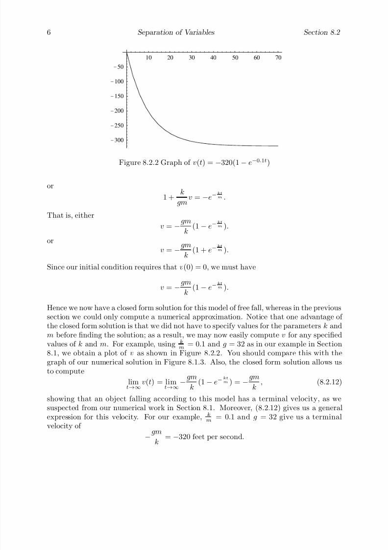
7/27/2019 Calculus 2 (Dan Sloughter)
http://slidepdf.com/reader/full/calculus-2-dan-sloughter 542/598
6 Separation of Variables Section 8.2
10 20 30 40 50 60 70
-300
-250
-200
-150
-100
-50
Figure 8.2.2 Graph of v(t) = −320(1− e−0.1t)
or
1 + kgm
v = −e−ktm .
That is, either
v = −gm
k(1− e−
kt
m ).
orv = −
gm
k(1 + e−
kt
m ).
Since our initial condition requires that v(0) = 0, we must have
v = −
gm
k (1− e−kt
m
).
Hence we now have a closed form solution for this model of free fall, whereas in the previoussection we could only compute a numerical approximation. Notice that one advantage of the closed form solution is that we did not have to specify values for the parameters k andm before finding the solution; as a result, we may now easily compute v for any specifiedvalues of k and m. For example, using k
m= 0.1 and g = 32 as in our example in Section
8.1, we obtain a plot of v as shown in Figure 8.2.2. You should compare this with thegraph of our numerical solution in Figure 8.1.3. Also, the closed form solution allows usto compute
limt→∞v(t) = limt→∞−
gm
k (1− e
−kt
m
) = −
gm
k , (8.2.12)
showing that an object falling according to this model has a terminal velocity, as wesuspected from our numerical work in Section 8.1. Moreover, (8.2.12) gives us a generalexpression for this velocity. For our example, k
m= 0.1 and g = 32 give us a terminal
velocity of
−gm
k= −320 feet per second.
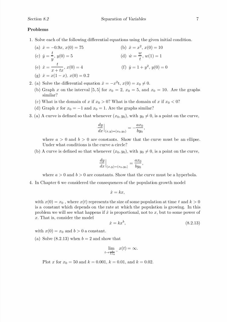
7/27/2019 Calculus 2 (Dan Sloughter)
http://slidepdf.com/reader/full/calculus-2-dan-sloughter 543/598
Section 8.2 Separation of Variables 7
Problems
1. Solve each of the following differential equations using the given initial condition.
(a) x = −0.9x, x(0) = 75 (b) x = x2, x(0) = 10
(c) y =t
y , y(0) = 5 (d) w =w
t , w(1) = 1
(e) x =t
x + tx, x(0) = 4 (f) y = 1 + y2, y(0) = 0
(g) x = x(1− x), x(0) = 0.2
2. (a) Solve the differential equation x = −x2t, x(0) = x0 = 0.
(b) Graph x on the interval [5, 5] for x0 = 2, x0 = 5, and x0 = 10. Are the graphssimilar?
(c) What is the domain of x if x0 > 0? What is the domain of x if x0 < 0?
(d) Graph x for x0 = −1 and x0 = 1. Are the graphs similar?
3. (a) A curve is defined so that whenever (x0, y0), with y0 = 0, is a point on the curve,
dy
dx
(x,y)=(x0,y0)
= −ax0
by0,
where a > 0 and b > 0 are constants. Show that the curve must be an ellipse.Under what conditions is the curve a circle?
(b) A curve is defined so that whenever (x0, y0), with y0 = 0, is a point on the curve,
dy
dx (x,y)=(x0,y0)=
ax0
by0,
where a > 0 and b > 0 are constants. Show that the curve must be a hyperbola.
4. In Chapter 6 we considered the consequences of the population growth model
x = kx,
with x(0) = x0 , where x(t) represents the size of some population at time t and k > 0is a constant which depends on the rate at which the population is growing. In thisproblem we will see what happens if x is proportional, not to x, but to some power of x. That is, consider the model
x = kxb, (8.2.13)
with x(0) = x0 and b > 0 a constant.
(a) Solve (8.2.13) when b = 2 and show that
limt→ 1
kx0
−
x(t) = ∞.
Plot x for x0 = 50 and k = 0.001, k = 0.01, and k = 0.02.
7/27/2019 Calculus 2 (Dan Sloughter)
http://slidepdf.com/reader/full/calculus-2-dan-sloughter 544/598
8 Separation of Variables Section 8.2
(b) Solve (8.2.13) when b > 1. Find c such that
limt→c−
x(t) = ∞.
Plot x for x0 = 50, k = 0.01, and b = 1.5, b = 1.2, and b = 1.01.
(c) Solve (8.2.13) when b = 0.5. Show that x is a quadratic polynomial and
limt→∞
x(t) = ∞.
Plot x for x0 = 50 and k = 0.01, k = 0.02, and k = 0.05.
(d) Solve (8.2.13) when 0 < b < 1 and show that
limt→∞
x(t) = ∞.
Plot x for x0 = 50, k = 0.01, and b = 0.2, b = 0.4, and b = 0.9.
(e) Compare the rates of growth for 0 < b < 1, b = 1, and b > 1. Which model leads tothe slowest population growth? Which model leads to the most rapid populationgrowth? Why is the case b > 1 sometimes referred to as the doomsday model ?
5. Suppose the force due to air resistance acting on a falling body of mass m is propor-tional to the square of the velocity v.
(a) Explain why v satisfies the differential equation
v = −g +k
mv2,
where k > 0 is a constant.(b) Assuming v(0) = 0, solve the equation in (a) for v.
(c) Show that the terminal velocity of the object is −
mg
k.
(d) Plot v over the interval [0, 20] using g = 32 and km
= 0.01. Compare this plot withthe plot of the numerical solution found in Problem 8 of Section 8.1.
6. In Section 1.4 we discussed the discrete time version of Newton’s law of cooling. Briefly,this law says if an object with an initial temperature of T 0 is placed in an environmentwhich is held at a constant temperature S , then the rate of change of the temperature T
of the object is proportional to the difference between T and S . In terms of differentialequations, this says that T must satisfy the equation
T = k(T − S )
for some constant k.
(a) Show thatT = S + (T 0 − S )ekt

7/27/2019 Calculus 2 (Dan Sloughter)
http://slidepdf.com/reader/full/calculus-2-dan-sloughter 545/598
Section 8.2 Separation of Variables 9
and verify thatlimt→∞
T (t) = S.
(b) A cup of coffee, initially at a temperature of 115◦F, is placed on a table in a roomheld at a constant temperature of 72◦F. If after five minutes the coffee has cooled
to 105◦F, what is the temperature of the coffee after 20 minutes? How long will ittake the coffee to cool to 80◦F? Graph T.
(c) A glass of lemonade, initially at a temperature of 40◦F, is placed on a table in aroom held at a constant temperature of 75◦F. If after 10 minutes the lemonade haswarmed to 48◦F, what is the temperature of the lemonade after 30 minutes? Howlong will it take the lemonade to warm to 65◦F? Graph T.
(d) A cup of coffee, initially at a temperature of 110◦F, is placed on a table in a room.After five minutes the coffee has cooled to 100◦F and after ten minutes the coffeehas cooled to 92◦F. What is the temperature of the room?

7/27/2019 Calculus 2 (Dan Sloughter)
http://slidepdf.com/reader/full/calculus-2-dan-sloughter 546/598
Difference Equations
Differential Equations
to
Section 8.3
First Order LinearDifferential Equations
We will now consider closed form solutions for another important class of differentialequations. A differential equation
x = f (x, t)
with x(t0) = x0 is called a linear equation if
f (x, t) = p(t)x + q (t) (8.3.1)
for some functions p and q which depend only on t. We will assume that both p and q are
continuous functions. Note that under certain circumstances, such as q (t) = 0 for all t, alinear equation is also separable. The solution of such equations is based on the followingobservation: If we let
P (t) =
tt0
p(s)ds, (8.3.2)
thend
dt
xe−P (t)
= −xp(t)e−P (t) + xe−P (t) = e−P (t)(x− p(t)x). (8.3.3)
Now we want x = p(t)x + q (t), that is, x− p(t)x = q (t), so we are looking for a function x
such thatd
dtxe−P (t)
= q (t)e−P (t). (8.3.4)
Integrating (8.3.4) from t0 to t (using u for our variable of integration), we have
tt0
d
du
x(u)e−P (u)
du =
tt0
q (u)e−P (u)du. (8.3.5)
Now tt0
d
du
x(u)e−P (u)
du = x(u)e−P (u)
tt0
= x(t)e−P (t) − x(t0)e−P (t0)
= x(t)e−P (t) − x0
(8.3.6)
since P (t0) = 0 and x(t0) = x0. Hence we want
x(t)e−P (t) − x0 =
tt0
q (u)e−P (u)du. (8.3.7)
1 Copyright c by Dan Sloughter 2000

7/27/2019 Calculus 2 (Dan Sloughter)
http://slidepdf.com/reader/full/calculus-2-dan-sloughter 547/598
2 First Order Linear Differential Equations Section 8.3
Solving (8.3.7) for x(t), we have
x(t) = eP (t) t
t0
q (u)e−P (u)du + x0
. (8.3.8)
Similar to our situation with separable equations, (8.3.8) provides a closed form solution
to our equation only if the requisite integrals may be computed in closed form. If not,numerical techniques will be necessary.
Linear equations If p and q are continuous, x satisfies the differential equation
x = p(t)x + q (t) (8.3.9)
with x(t0) = x0, and
P (t) =
tt0
p(s)ds, (8.3.10)
then
x(t) = eP (t) t
t0
q (u)e−P (u)du + x0 . (8.3.11)
Example Consider the equation
x =x
t+ 4t
with x(1) = 5. This is a linear equation with, in the notation used above,
p(t) =1
t
andq (t) = 4t.
ThenP (t) =
t
1
1
sds = log(s)
t1
= log(t),
where, in order for the integral to exist, we have restricted t to be positive. Thus, using(8.3.11),
x = elog(t) t
1
4ue− log(u)du + 5
= t
t1
4u
udu + 5
= t t
1
4du + 5= t
4ut1
+ 5
= t(4t− 4) + 5t
= 4t2 + t.
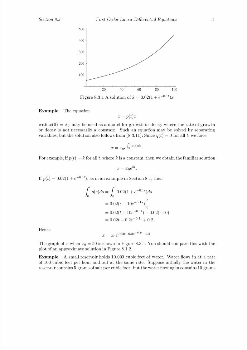
7/27/2019 Calculus 2 (Dan Sloughter)
http://slidepdf.com/reader/full/calculus-2-dan-sloughter 548/598
Section 8.3 First Order Linear Differential Equations 3
20 40 60 80 100
100
200
300
400
500
Figure 8.3.1 A solution of x = 0.02(1 + e−0.1t)x
Example The equationx = p(t)x
with x(0) = x0 may be used as a model for growth or decay where the rate of growthor decay is not necessarily a constant. Such an equation may be solved by separatingvariables, but the solution also follows from (8.3.11): Since q (t) = 0 for all t, we have
x = x0e
t
0 p(s)ds
.
For example, if p(t) = k for all t, where k is a constant, then we obtain the familiar solution
x = x0ekt.
If p(t) = 0.02(1 + e−0.1t), as in an example in Section 8.1, then
t0
p(s)ds =
t0
0.02(1 + e−0.1s)ds
= 0.02(s− 10e−0.1s)t0
= 0.02(t− 10e−0.1t)− 0.02(−10)
= 0.02t− 0.2e−0.1t + 0.2.
Hencex = x0e
0.02t−0.2e−0.1t+0.2.
The graph of x when x0 = 50 is shown in Figure 8.3.1. You should compare this with theplot of an approximate solution in Figure 8.1.2.
Example A small reservoir holds 10,000 cubic feet of water. Water flows in at a rateof 100 cubic feet per hour and out at the same rate. Suppose initially the water in thereservoir contains 5 grams of salt per cubic foot, but the water flowing in contains 10 grams
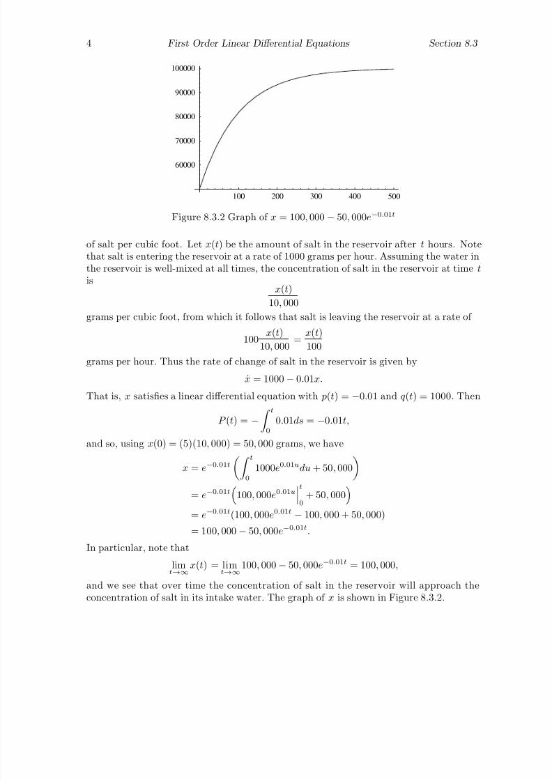
7/27/2019 Calculus 2 (Dan Sloughter)
http://slidepdf.com/reader/full/calculus-2-dan-sloughter 549/598
4 First Order Linear Differential Equations Section 8.3
100 200 300 400 500
60000
70000
80000
90000
100000
Figure 8.3.2 Graph of x = 100, 000 − 50, 000e−0.01t
of salt per cubic foot. Let x(t) be the amount of salt in the reservoir after t hours. Notethat salt is entering the reservoir at a rate of 1000 grams per hour. Assuming the water in
the reservoir is well-mixed at all times, the concentration of salt in the reservoir at timet
isx(t)
10, 000
grams per cubic foot, from which it follows that salt is leaving the reservoir at a rate of
100x(t)
10, 000=
x(t)
100
grams per hour. Thus the rate of change of salt in the reservoir is given by
x = 1000− 0.01x.
That is, x satisfies a linear differential equation with p(t) = −0.01 and q (t) = 1000. Then
P (t) = −
t
0
0.01ds = −0.01t,
and so, using x(0) = (5)(10, 000) = 50, 000 grams, we have
x = e−0.01t t
0
1000e0.01udu + 50, 000
= e−0.01t
100, 000e0.01ut0
+ 50, 000
= e−0.01t(100, 000e0.01t − 100, 000 + 50, 000)
= 100, 000 − 50, 000e−0.01t.
In particular, note that
limt→∞
x(t) = limt→∞
100, 000− 50, 000e−0.01t = 100, 000,
and we see that over time the concentration of salt in the reservoir will approach theconcentration of salt in its intake water. The graph of x is shown in Figure 8.3.2.
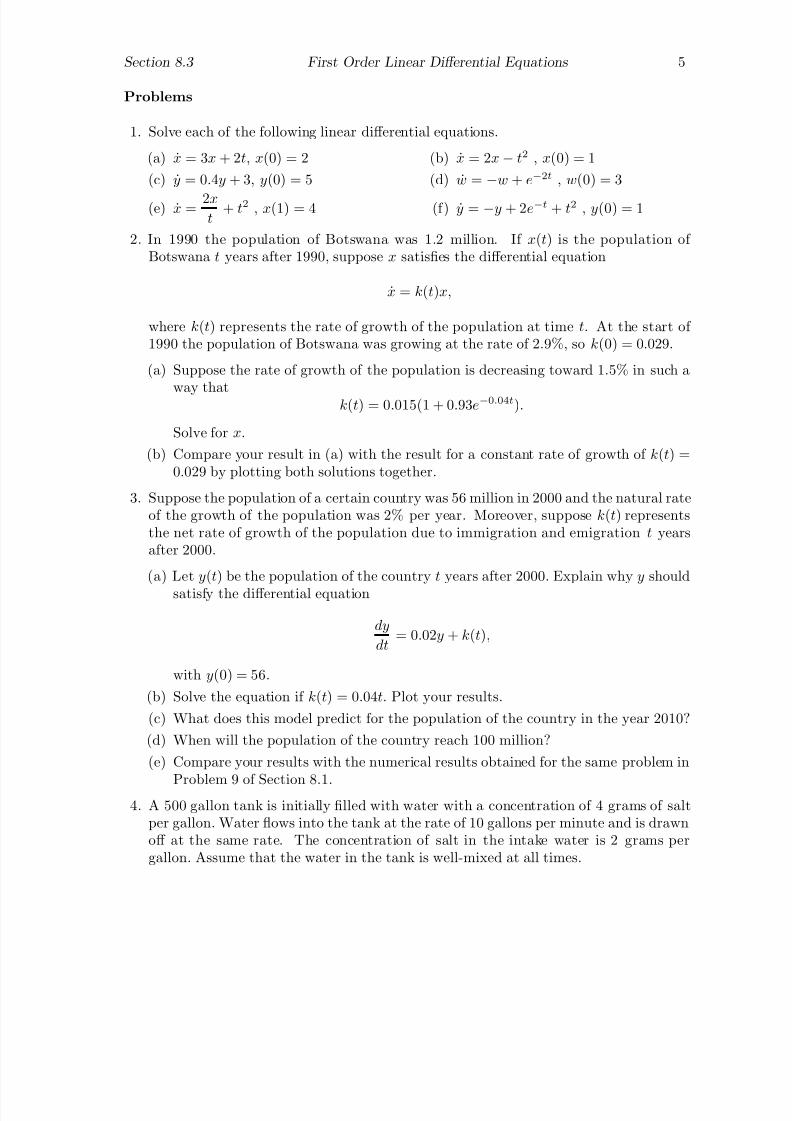
7/27/2019 Calculus 2 (Dan Sloughter)
http://slidepdf.com/reader/full/calculus-2-dan-sloughter 550/598
Section 8.3 First Order Linear Differential Equations 5
Problems
1. Solve each of the following linear differential equations.
(a) x = 3x + 2t, x(0) = 2 (b) x = 2x− t2 , x(0) = 1
(c) y = 0.4y + 3, y(0) = 5 (d) w = −w + e−2t , w(0) = 3
(e) x = 2xt
+ t2 , x(1) = 4 (f) y = −y + 2e−t + t2 , y(0) = 1
2. In 1990 the population of Botswana was 1.2 million. If x(t) is the population of Botswana t years after 1990, suppose x satisfies the differential equation
x = k(t)x,
where k(t) represents the rate of growth of the population at time t. At the start of 1990 the population of Botswana was growing at the rate of 2.9%, so k(0) = 0.029.
(a) Suppose the rate of growth of the population is decreasing toward 1.5% in such a
way that k(t) = 0.015(1 + 0.93e−0.04t).
Solve for x.
(b) Compare your result in (a) with the result for a constant rate of growth of k(t) =0.029 by plotting both solutions together.
3. Suppose the population of a certain country was 56 million in 2000 and the natural rateof the growth of the population was 2% per year. Moreover, suppose k(t) representsthe net rate of growth of the population due to immigration and emigration t yearsafter 2000.
(a) Let y(t) be the population of the country t years after 2000. Explain why y should
satisfy the differential equation
dy
dt= 0.02y + k(t),
with y(0) = 56.
(b) Solve the equation if k(t) = 0.04t. Plot your results.
(c) What does this model predict for the population of the country in the year 2010?
(d) When will the population of the country reach 100 million?
(e) Compare your results with the numerical results obtained for the same problem in
Problem 9 of Section 8.1.4. A 500 gallon tank is initially filled with water with a concentration of 4 grams of salt
per gallon. Water flows into the tank at the rate of 10 gallons per minute and is drawnoff at the same rate. The concentration of salt in the intake water is 2 grams pergallon. Assume that the water in the tank is well-mixed at all times.

7/27/2019 Calculus 2 (Dan Sloughter)
http://slidepdf.com/reader/full/calculus-2-dan-sloughter 551/598
6 First Order Linear Differential Equations Section 8.3
(a) Let x(t) be the amount of salt in the tank at time t. Find a linear differentialequation for x which models this situation.
(b) Solve the equation from (a) and graph the solution. What happens to x as t
increases?
5. Suppose a tank holds V liters of a liquid which contains a certain chemical at a con-
centration of k0 grams per liter. Liquid flows into the tank at rate of q liters per secondand is drawn off at the same rate. The concentration of the chemical in the intakeliquid is k grams per liter.
(a) If x(t) is the amount of the chemical in the tank at time t, show that x satisfiesthe linear differential equation
x = qk −q
V x
with x(0) = k0V .
(b) Solve the equation in (a). What happens to x as t→∞?
6. An equation of the formx = p(t)x + q (t)xn (8.3.12)
is called a Bernoulli equation . Note that the equation is linear if either n = 0 or n = 1.
(a) Assume n = 0 and n = 1. Show that the substitution w = x1−n in (8.3.12) resultsin the linear differential equation
w = (1− n) p(t)w + (1 − n)q (t).
(b) Use the result of (a) to solve the equation
x =
x
t − x
2
with x(1) = 1.
(c) Use the result of (a) to solve the equation
x = x(1− x)
with x(0) = 0.5.
7. Note that (c) of Problem 6 is a particular example of the logistic differential equationthat we studied in Section 6.3 in our discussion of the inhibited population growthmodel. In general, we considered the logistic equation
x =α
M x(M − x)
with x(0) = x0, where x(t) is the size of the population at time t, α is the naturalgrowth rate of the population, and M is the maximum size of the population that is
7/27/2019 Calculus 2 (Dan Sloughter)
http://slidepdf.com/reader/full/calculus-2-dan-sloughter 552/598
Section 8.3 First Order Linear Differential Equations 7
sustainable in the given environment. Write this equation in the form of a Bernoulliequation and use the result from (a) of Problem 6 to show that
x =M
1 + βe−αt
whereβ =
M − x0
x0.

7/27/2019 Calculus 2 (Dan Sloughter)
http://slidepdf.com/reader/full/calculus-2-dan-sloughter 553/598
Difference Equations
Differential Equations
to
Section 8.4
Second Order LinearDifferential Equations
To this point we have we have considered only first order differential equations. However,many of the most interesting differential equations involve second derivatives. Indeed,since acceleration is the second derivative of position, Newton’s second law of motion,F = ma, is a second order differential equation. In general, if f is a known function of three variables, then the equation
x = f (x,x,t) (8.4.1)
is called a second order differential equation . If we let y = x, then (8.4.1) may be writtenas a pair of first order differential equations
x = y
y = f (y , x , t).(8.4.2)
Hence moving from the study of first order differential equations to the study of secondorder differential equations is analogous to moving from the study of one algebraic equationin one unknown to the study of two algebraic equations in two unknowns. We will makeuse of this fact when we consider numerical approximations to solutions of second orderequations in Section 8.6.
As was the case with first order equations, the existence of a closed form solution to asecond order differential equation and our ability to find one when it exists depends verymuch on the form of the function f in (8.4.1). We shall consider closed form solutionsfor only one class of such equations, leaving other equations for either the numerical ap-proximations of Section 8.6 or the infinite series techniques of Section 8.7. Here we areconcerned with equations of the form
x + bx + cx = 0, (8.4.3)
which we call a second order homogeneous linear differential equation with constant coeffi-
cients , corresponding tof (x,x,t) = −bx− cx
in (8.4.1). The term homogeneous refers to the fact that the function x(0) = 0 for all t isa solution of the equation and the phrase constant coefficients refers to the fact that b andc are assumed to be constants.
To begin our study of these equations, suppose x1(t) and x2(t) are both solutions of (8.4.3) and let x(t) = c1x1(t) + c2x2(t) for constants c1 and c2. Then
1 Copyright c by Dan Sloughter 2000

7/27/2019 Calculus 2 (Dan Sloughter)
http://slidepdf.com/reader/full/calculus-2-dan-sloughter 554/598
2 Second Order Linear Differential Equations Section 8.4
x + bx + cx = (c1x1 + c2x2) + b(c1x + c2x2) + c(c1x1 + c2x2)
= c1(x1 + bx1 + cx1) + c2(x2 + bx2 + cx2)
= (c1)(0) + (c2)(0) = 0.
That is, x is also a solution of (8.4.3).Proposition If x1 and x2 are both solutions of the equation
x + bx + cx = 0,
then x = c1x1 + c2x2 is also a solution of this equation for any constants c1 and c2.
The next proposition is key to our method of solving equations of the form (8.4.3),although we will leave its justification to a more advanced course. First we introduce adefinition which will make the proposition, as well as our later results, easier to state.
Definition If f and g are functions for which neither one is a constant multiple of the
other, then we say f and g are linearly independent .
Proposition Suppose x1 and x2 are linearly independent solutions of the equation
x + bx + cx = 0.
Then for any solution x, there exist constants c1 and c2 such that
x = c1x1 + c2x2. (8.4.4)
The equation
x + bx + cx = 0 (8.4.5)
will have a unique solution only when we place some restrictions on x. For example, if wespecify initial conditions for both x and x, say, x(t0) = x0 and x(t0) = y0, then (8.4.4) willhave a unique solution which satisfies these conditions. This statement is far from obvious,but should appear reasonable in light of the observation, made above, that we could writethis equation as a pair of first order equations
x = y
y = −by − cx.(8.4.6)
Hence our method of attack in solving (8.4.4) will be to first find two linearly independentsolutions, say, x1 and x2, and then find values for constants c1 and c2 such that x =c1x1 + c2x2 satisfies the given initial conditions.
To find two linearly independent solutions of (8.4.4), we begin with the observationthat if x satisfies this equation, then x is equal to a sum of constant multiples of x andx. Hence it would be reasonable to begin with x = ekt, for some constant k, as an initialguess. In that case,
x = kekt

7/27/2019 Calculus 2 (Dan Sloughter)
http://slidepdf.com/reader/full/calculus-2-dan-sloughter 555/598
Section 8.4 Second Order Linear Differential Equations 3
andx = k2ekt,
so x will be a solution of (8.4.4) if and only if
k2ekt + bkekt + cekt = ekt(k2 + bk + c) = 0 (8.4.7)
for all t. Since ekt = 0 for all t, this will happen if and only if
k2 + bk + c = 0. (8.4.8)
Hence x = ekt is a solution to (8.4.4) if and only if k is a root of (8.4.8).
Definition The equationk2 + bk + c = 0 (8.4.9)
is called the characteristic equation of the differential equation
x + bx + cx = 0.
Since the characteristic equation is quadratic in k, its roots are given by the quadraticformula, namely,
k1 =−b−√ b2 − 4c
2(8.4.10)
and
k2 =−b +
√ b2 − 4c
2. (8.4.11)
At this point, our search for solutions breaks into three cases, depending on whether k1and k2 are (1) distinct real numbers (that is, b2 − 4c > 0), (2) distinct complex numbers(that is, b2 − 4c < 0), or (3) real, but equal (that is, b2 − 4c = 0).
Case 1: Distinct real roots
Suppose k1 and k2 are distinct real roots of the characteristic equation. In that case,x1 = ek1t and x2 = ek2t are linearly independent solutions of
x + bx + cx = 0
and all that remains is to find constants c1
and c2
such that
x = c1ek1t + c2ek2t (8.4.12)
satisfies the given initial conditions.
Example Consider the equation
x + x− 6x = 0

7/27/2019 Calculus 2 (Dan Sloughter)
http://slidepdf.com/reader/full/calculus-2-dan-sloughter 556/598
4 Second Order Linear Differential Equations Section 8.4
-3 -2 -1 1 2 3
-40
-20
20
40
Figure 8.4.1 Solution of x + x− 6x = 0 with x(0) = 0 and x(0) = 1
with initial conditions x(0) = 0 and x(0) = 1. For the characteristic equation we have
0 = k2 + k − 6 = (k + 3)(k − 2).
Hence the roots of the characteristic equation are k1 = −3 and k2 = 2. Thus we must have
x = c1e−3t + c2e2t
for some constants c1 and c2. Now
x = −3c1e−3t + 2c2e2t,
sox(0) = c1 + c2
and x(0) = −3c1 + 2c2.
Hence the initial conditions imply that
c1 + c2 = 0
−3c1 + 2c2 = 1.
The first equation implies c1 = −c2. Substituting into the second equation, we have
1 = 3c2 + 2c2 = 5c2.
Hence
c2 =
1
5and
c1 = −1
5.
Thus
x = −1
5e−3t +
1
5e2t.
The graph of x is shown in Figure 8.4.1
7/27/2019 Calculus 2 (Dan Sloughter)
http://slidepdf.com/reader/full/calculus-2-dan-sloughter 557/598
Section 8.4 Second Order Linear Differential Equations 5
Case 2: Complex roots
Suppose k1 and k2 are distinct complex roots of the characteristic equation. As before,ek1t and ek2t are linearly independent solutions of
x + bx + cx = 0.
However, these are complex-valued functions and for most applications we are looking forreal-valued solutions. Now if we let
p = − b
2(8.4.13)
and
q =
√ 4c− b2
2, (8.4.14)
then k1 = p− qi and k2 = p + qi. Hence
ek1t
= e( p−qi)t
= e pt
e−iqt
= e pt
(cos(qt)− i sin(qt)) (8.4.15)
andek2t = e( p+qi)t = e pteiqt = e pt(cos(qt) + i sin(qt)). (8.4.16)
Since these are both solutions, we know that
x1 =1
2ek1t +
1
2ek2t = e pt cos(qt) (8.4.17)
and
x2 =
1
2iek2t
−1
2iek1t
=e pt
sin(qt
) (8.4.18)are also solutions. Then x1 and x2 are linearly independent real-valued solutions, so anyreal-valued solution must be of the form
x = c1x1 + c2x2 = e pt(c1 cos(qt) + c2 sin(qt)) (8.4.19)
for some constants c1 and c2 .
Example Consider the equation
x + 2x + 5x = 0
with initial conditions x(0) = 2 and x(0) = 0. The characteristic equation is
k2 + 2k + 5 = 0,
which has roots−2±√ 4− 20
2= −1± 2i.

7/27/2019 Calculus 2 (Dan Sloughter)
http://slidepdf.com/reader/full/calculus-2-dan-sloughter 558/598
6 Second Order Linear Differential Equations Section 8.4
1 2 3 4 5
0.5
1
1.5
2
Figure 8.4.2 Solution of x + 2x + 5x = 0 with x(0) = 2 and x(0) = 0
Hence, by (8.4.19), we must have
x = e−t(c1 cos(2t) + c2 sin(2t))
for some constants c1 and c2. Now
x = e−t(−2c1 sin(2t) + 2c2 cos(2t))− e−t(c1 cos(2t) + c2 sin(2t)),
sox(0) = c1
and
x(0) = 2c2 − c1.
Hence the initial conditions x(0) = 2 and x(0) = 0 imply that c1 = 2 and
0 = 2c2 − 2.
Thus c2 = 1 and we havex = e−t(2 cos(2t) + sin(2t)).
The graph of x is shown in Figure 8.4.2.
Case 3: Single real root
Suppose the characteristic equation has a single real root. In this case,
k1 = k2 = − b
2. (8.4.20)
For simplicity, let us call this common value k. Then x1 = ekt is a solution of the equation
x + bx + cx = 0,

7/27/2019 Calculus 2 (Dan Sloughter)
http://slidepdf.com/reader/full/calculus-2-dan-sloughter 559/598
Section 8.4 Second Order Linear Differential Equations 7
but in order to specify all possible solutions we need to find another solution which islinearly independent of x1. We will show that, in this case, x2 = tekt is such a solution.Now
x2 = ktekt + ekt = (1 + kt)ekt (8.4.21)
and x2 = (1 + kt)kekt + kekt = (2k + k2t)ekt. (8.4.22)
Hence, remembering that k is a root of the characteristic equation (that is, k2+ bk + c = 0)and k = − b
2 , we have
x2 + bx2 + cx2 = (2k + k2t)ekt + b(1 + kt)ekt + ctekt
= ekt(2k + k2t + b + bkt + ct)
= ekt((k2 + bk + c)t + 2k + b)
= ekt(2k + b)
= ekt− 2b
2+ b
= 0
for all t. Hence x2 is another solution, clearly linearly independent of x1. Thus for anysolution x, there exist constants c1 and c2 such that
x = c1x1 + c2x2 = c1ekt + c2tekt. (8.4.23)
Example Consider the equation
x + 2x + x = 0
with initial conditions x(0) = 10 and x(0) = −20. The characteristic equation is
0 = k2 + 2k + 1 = (k + 1)2
which has the single root k = −1. Hence
x = c1e−t + c2te−t
for some constants c1 and c2. Now
x = −c1e−t − c2te−t + c2e−t,
so x(0) = c1 and x(0) = −c1 + c2. Hence the initial conditions x(0) = 10 and x(0) = −20imply that c1 = 10 and
−20 = −10 + c2.

7/27/2019 Calculus 2 (Dan Sloughter)
http://slidepdf.com/reader/full/calculus-2-dan-sloughter 560/598
8 Second Order Linear Differential Equations Section 8.4
2 4 6 8 10
2
4
6
8
10
Figure 8.4.3 Solution of x + 2x + x = 0 with x(0) = 10 and x(0) = −20
Thus c2 =
−10 and we have
x = 10e−t − 10te−t = 10(1− t)e−t.
The graph of x is shown in Figure 8.4.3.
Summary
If x1 and x2 are linearly independent solutions of the equation
x + bx + cx = 0, (8.4.24)
then any solution of (8.4.24) is of the form x = c1x1 + c2x2 for some constants c1 and c2.
The family of all solutions x = c1x1 + c2x2 is called the general solution of (8.4.24). Asolution with specified values for c1 and c2 is called a particular solution .
Let k1 and k2 be the roots of the characteristic equation
k2 + bk + c = 0. (8.4.25)
If k1 and k2 are real numbers with k1 = k2, then the general solution of (8.4.24) is
x = c1ek1t + c2ek2t. (8.4.26)
If k1 and k2 are complex numbers with k1 = p − qi and k2 = p + qi, then the general
solution of (8.4.24) is x = e pt(c1 cos(qt) + c2 sin(qt)). (8.4.27)
Finally, if k = k1 = k2, then the general solution of (8.4.24) is
x = c1ekt + c2tekt. (8.4.28)
In the next section we will discuss the motion of a pendulum and the motion of a massvibrating at the end of a spring as applications of the equations considered in this section.
7/27/2019 Calculus 2 (Dan Sloughter)
http://slidepdf.com/reader/full/calculus-2-dan-sloughter 561/598
Section 8.4 Second Order Linear Differential Equations 9
Problems
1. Solve each of the following differential equations and plot the solution.
(a) x + x− 2x = 0, x(0) = 0, x(0) = 2
(b) x =−
x, x(0) = 10, x(0) = 5
(c) x + 3x + 2x = 0, x(0) = 1, x(0) = 0
(d) x− 4x + 4x = 0, x(0) = 5, x(0) = 0
(e) x− 2x + 2x = 0, x(0) = 10, x(0) = 4
(f) −x + 2x− 4x = 0, x(0) = 1, x(0) = 0
(g) x + 4x + 20x = 0, x(0) = 0, x(0) = 3
(h) 2x + 3x− 2x = 0, x(0) = 0, x(0) = −2
(i) x + 6x + 9x = 0, x(0) = −6, x(0) = 4
2. Consider the equation x + 2x− 3x = 0.
(a) If x(0) = 1, plot the solutions for x(0) = 0, x(0) = −5, and x(0) = 5. How dothese solutions compare?
(b) If x(0) = 0, plot the solutions for x(0) = 0, x(0) = −2, and x(0) = 2. How dothese solutions compare?
3. Consider the equation x + 2x + 10x = 0.
(a) If x(0) = 1, plot the solutions for x(0) = 0, x(0) = −10, and x(0) = 10. How dothese solutions compare?
(b) If x(0) = 10, plot the solutions for x(0) = 0, x(0) = −5, and x(0) = 5. How dothese solutions compare?
4. Consider the equation x + 4x + 4x = 0.(a) If x(0) = −15, plot the solutions for x(0) = 0, x(0) = −5, and x(0) = 5. How do
these solutions compare?
(b) If x(0) = 10, plot the solutions for x(0) = 0, x(0) = −20, and x(0) = 20. How dothese solutions compare?
5. The techniques developed in this section may be used to solve higher order homoge-neous linear differential equations with constant coefficients. Generalize the methodsof this section to find the general solution for each of the following equations.
(a)d3x
dt3+ 2
d2x
dt2 −dx
dt −2x = 0
(b)d3x
dt3+ 3
d2x
dt2+ 3
dx
dt+ x = 0
6. Show that if b and c are both positive and x is a solution of
x + bx + cx = 0,
then limt→∞
x(t) = 0.
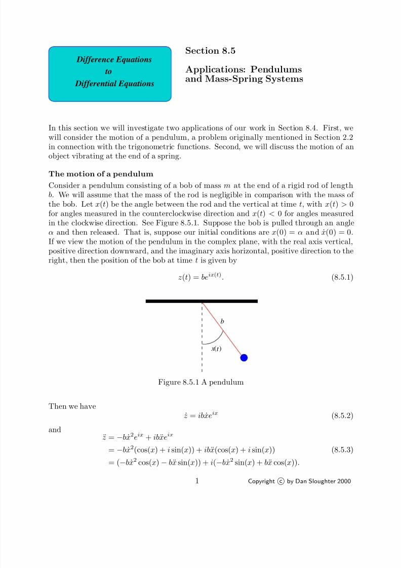
7/27/2019 Calculus 2 (Dan Sloughter)
http://slidepdf.com/reader/full/calculus-2-dan-sloughter 562/598
Difference Equations
Differential Equations
to
Section 8.5
Applications: Pendulumsand Mass-Spring Systems
In this section we will investigate two applications of our work in Section 8.4. First, wewill consider the motion of a pendulum, a problem originally mentioned in Section 2.2in connection with the trigonometric functions. Second, we will discuss the motion of anobject vibrating at the end of a spring.
The motion of a pendulum
Consider a pendulum consisting of a bob of mass m at the end of a rigid rod of lengthb
. We will assume that the mass of the rod is negligible in comparison with the mass of the bob. Let x(t) be the angle between the rod and the vertical at time t, with x(t) > 0for angles measured in the counterclockwise direction and x(t) < 0 for angles measuredin the clockwise direction. See Figure 8.5.1. Suppose the bob is pulled through an angleα and then released. That is, suppose our initial conditions are x(0) = α and x(0) = 0.If we view the motion of the pendulum in the complex plane, with the real axis vertical,positive direction downward, and the imaginary axis horizontal, positive direction to theright, then the position of the bob at time t is given by
z(t) = beix(t). (8.5.1)
¢ ¢
¢ ¢
£
£¤
¤
b
x(t )
Figure 8.5.1 A pendulum
Then we havez = ibxeix (8.5.2)
andz = −bx2eix + ibxeix
= −bx2(cos(x) + i sin(x)) + ibx(cos(x) + i sin(x))
= (−bx2 cos(x)− bx sin(x)) + i(−bx2 sin(x) + bx cos(x)).
(8.5.3)
1 Copyright c by Dan Sloughter 2000
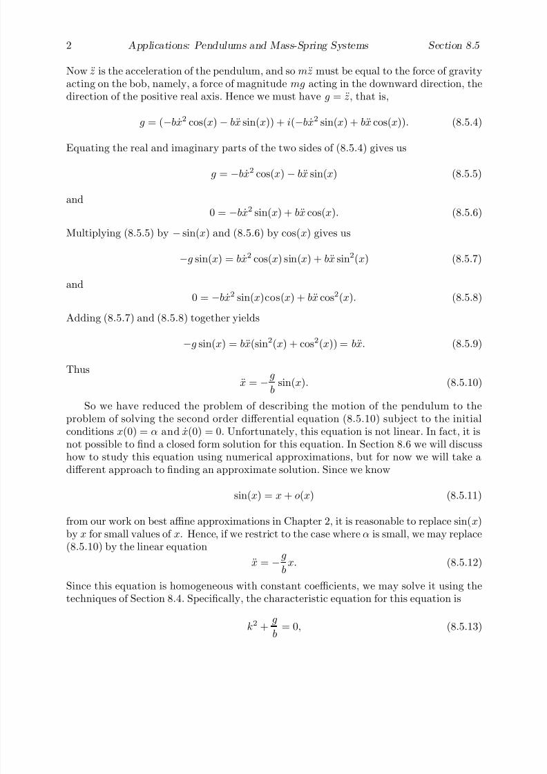
7/27/2019 Calculus 2 (Dan Sloughter)
http://slidepdf.com/reader/full/calculus-2-dan-sloughter 563/598
2 Applications: Pendulums and Mass-Spring Systems Section 8.5
Now z is the acceleration of the pendulum, and so mz must be equal to the force of gravityacting on the bob, namely, a force of magnitude mg acting in the downward direction, thedirection of the positive real axis. Hence we must have g = z, that is,
g = (
−bx2 cos(x)
−bx sin(x)) + i(
−bx2 sin(x) + bx cos(x)). (8.5.4)
Equating the real and imaginary parts of the two sides of (8.5.4) gives us
g = −bx2 cos(x)− bx sin(x) (8.5.5)
and0 = −bx2 sin(x) + bx cos(x). (8.5.6)
Multiplying (8.5.5) by − sin(x) and (8.5.6) by cos(x) gives us
−g sin(x) = bx2 cos(x) sin(x) + bx sin2(x) (8.5.7)
and0 = −bx2 sin(x)cos(x) + bx cos2(x). (8.5.8)
Adding (8.5.7) and (8.5.8) together yields
−g sin(x) = bx(sin2(x) + cos2(x)) = bx. (8.5.9)
Thusx = −g
bsin(x). (8.5.10)
So we have reduced the problem of describing the motion of the pendulum to theproblem of solving the second order differential equation (8.5.10) subject to the initialconditions x(0) = α and x(0) = 0. Unfortunately, this equation is not linear. In fact, it isnot possible to find a closed form solution for this equation. In Section 8.6 we will discusshow to study this equation using numerical approximations, but for now we will take adifferent approach to finding an approximate solution. Since we know
sin(x) = x + o(x) (8.5.11)
from our work on best affine approximations in Chapter 2, it is reasonable to replace sin( x)by x for small values of x. Hence, if we restrict to the case where α is small, we may replace(8.5.10) by the linear equation
x = −g
bx. (8.5.12)
Since this equation is homogeneous with constant coefficients, we may solve it using thetechniques of Section 8.4. Specifically, the characteristic equation for this equation is
k2 +g
b= 0, (8.5.13)
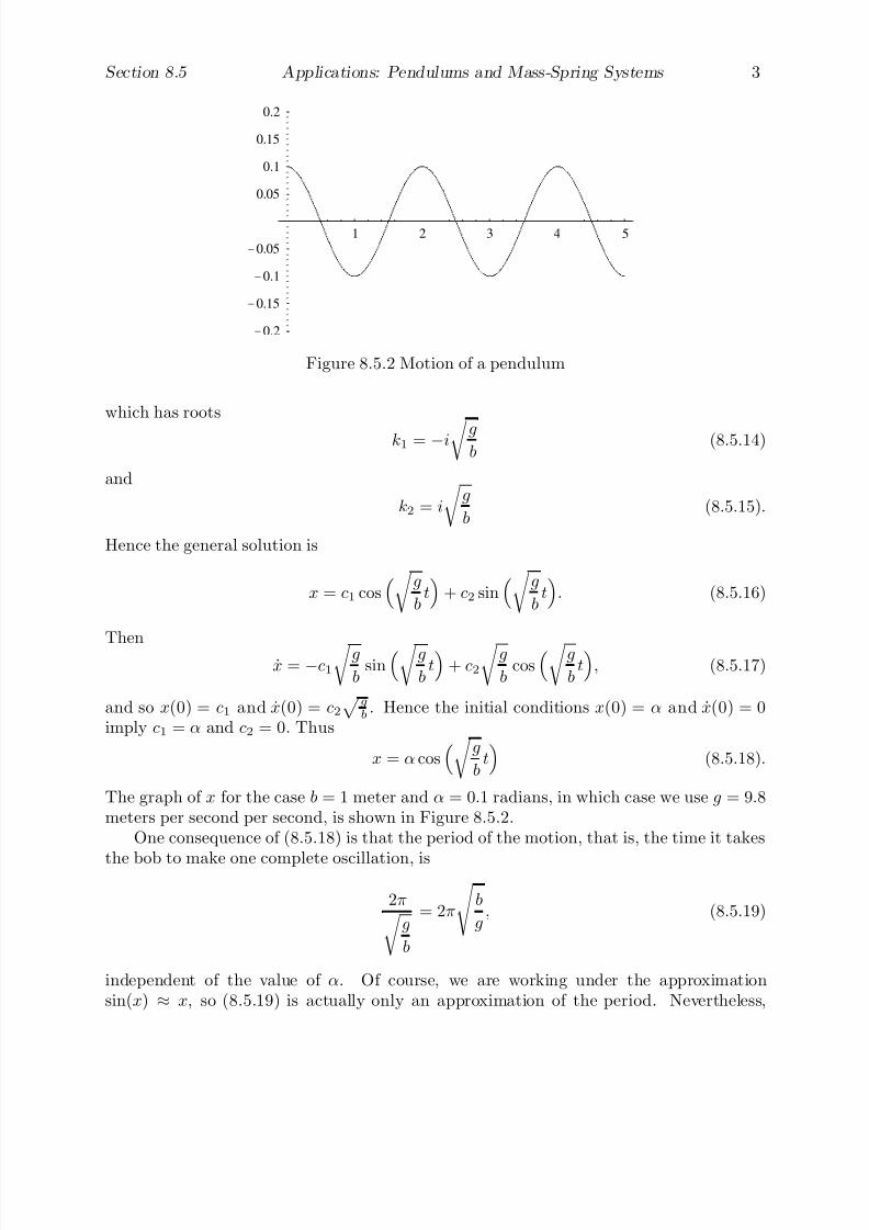
7/27/2019 Calculus 2 (Dan Sloughter)
http://slidepdf.com/reader/full/calculus-2-dan-sloughter 564/598
Section 8.5 Applications: Pendulums and Mass-Spring Systems 3
1 2 3 4 5
-0.2
-0.15
-0.1
-0.05
0.05
0.1
0.15
0.2
Figure 8.5.2 Motion of a pendulum
which has roots
k1 = −i
gb
(8.5.14)
and
k2 = i
g
b(8.5.15).
Hence the general solution is
x = c1 cos g
bt
+ c2 sin g
bt
. (8.5.16)
Thenx = −c1
g
bsin g
bt
+ c2
g
bcos
gb
t
, (8.5.17)
and so x(0) = c1 and x(0) = c2
gb
. Hence the initial conditions x(0) = α and x(0) = 0imply c1 = α and c2 = 0. Thus
x = α cos g
bt
(8.5.18).
The graph of x for the case b = 1 meter and α = 0.1 radians, in which case we use g = 9.8meters per second per second, is shown in Figure 8.5.2.
One consequence of (8.5.18) is that the period of the motion, that is, the time it takes
the bob to make one complete oscillation, is
2π g
b
= 2π
b
g, (8.5.19)
independent of the value of α. Of course, we are working under the approximationsin(x) ≈ x, so (8.5.19) is actually only an approximation of the period. Nevertheless,
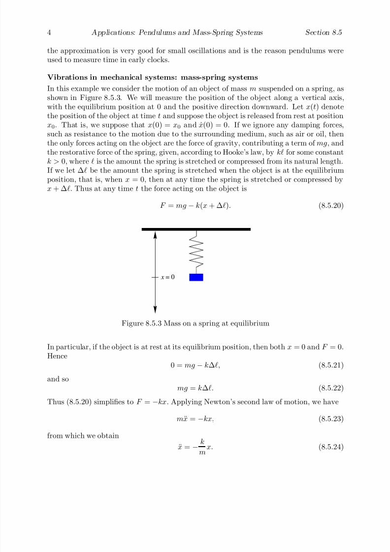
7/27/2019 Calculus 2 (Dan Sloughter)
http://slidepdf.com/reader/full/calculus-2-dan-sloughter 565/598
4 Applications: Pendulums and Mass-Spring Systems Section 8.5
the approximation is very good for small oscillations and is the reason pendulums wereused to measure time in early clocks.
Vibrations in mechanical systems: mass-spring systems
In this example we consider the motion of an object of mass m suspended on a spring, as
shown in Figure 8.5.3. We will measure the position of the object along a vertical axis,with the equilibrium position at 0 and the positive direction downward. Let x(t) denotethe position of the object at time t and suppose the object is released from rest at positionx0. That is, we suppose that x(0) = x0 and x(0) = 0. If we ignore any damping forces,such as resistance to the motion due to the surrounding medium, such as air or oil, thenthe only forces acting on the object are the force of gravity, contributing a term of mg, andthe restorative force of the spring, given, according to Hooke’s law, by k for some constantk > 0, where is the amount the spring is stretched or compressed from its natural length.If we let ∆ be the amount the spring is stretched when the object is at the equilibriumposition, that is, when x = 0, then at any time the spring is stretched or compressed byx + ∆. Thus at any time t the force acting on the object is
F = mg − k(x + ∆). (8.5.20)
¢ ¢ ¢
¢ ¢ ¢
¢ ¢ ¢
x = 0
Figure 8.5.3 Mass on a spring at equilibrium
In particular, if the object is at rest at its equilibrium position, then both x = 0 and F = 0.Hence
0 = mg − k∆, (8.5.21)
and so
mg = k∆. (8.5.22)
Thus (8.5.20) simplifies to F = −kx. Applying Newton’s second law of motion, we have
mx = −kx, (8.5.23)
from which we obtain
x = − k
mx. (8.5.24)

7/27/2019 Calculus 2 (Dan Sloughter)
http://slidepdf.com/reader/full/calculus-2-dan-sloughter 566/598
Section 8.5 Applications: Pendulums and Mass-Spring Systems 5
2 4 6 8 10 12 14
-3
-2
-1
1
2
3
Figure 8.5.4 Motion of a mass-spring system without damping
This equation is of the same form as the equation derived above for approximating the
motion of a pendulum. Hence, using the same reasoning, the solution is
x = x0 cos k
mt
. (8.5.25)
The graph of x for k = 10, m = 5, and x0 = 2 is shown in Figure 8.5.4.Notice that the period of the motion is
T =2π
km
= 2π
m
k. (8.5.26)
The frequency of the motion, that is, the number of complete oscillations in one unit of time, is
f =1
T =
1
2π
k
m. (8.5.27)
Hence for a fixed mass, increasing the spring constant, that is, increasing the stiffness of the spring, decreases the period and increases the frequency; for a fixed spring constant,increasing the mass increases the period and decreases the frequency.
Now suppose there is a damping force, a force resisting the motion of the object, which
is proportional to the velocity. This adds an additional term of −cx, where c is a positiveconstant, to the force acting on the object, giving us F = −kx − cx. Thus
mx = −kx − cx, (8.5.28)
and so
x +c
mx +
k
mx = 0 (8.5.29)

7/27/2019 Calculus 2 (Dan Sloughter)
http://slidepdf.com/reader/full/calculus-2-dan-sloughter 567/598
6 Applications: Pendulums and Mass-Spring Systems Section 8.5
replaces (8.5.24) as the equation describing the motion of the object. To simplify thenotation, we will let
b =c
2m
and
a =
km
.
Then our differential equation becomes
x + 2bx + a2x = 0, (8.5.30)
with characteristic equation (using s for the variable)
s2 + 2bs + a2 = 0. (8.5.31)
Hence the roots of the characteristic equation are
s1 =−2b−√ 4b2 − 4a2
2= −b−
b2 − a2 (8.5.32)
and
s2 =−2b +
√ 4b2 − 4a2
2= −b +
b2 − a2. (8.5.33)
Thus the behavior of the system depends on whether b2−a2 > 0, b2−a2 = 0, or b2−a2 < 0.Equivalently, since
b2 − a2 =c2
4m2 −k
m ,
the behavior of the system depends on whether c2 > 4mk, c2 = 4mk, or c2 < 4mk. In thefirst case the system is said to be overdamped , in the second it is critically damped , and inthe third it is underdamped .
First consider the overdamped case b2−a2 > 0. In this case the characteristic equationhas distinct real roots, so the general solution is
x = c1es1t + c2es2t. (8.5.34)
Nowx = c1s1es1t + c2s2es2t, (8.5.35)
so x(0) = c1 + c2 and x(0) = c1s1 + c2s2. Hence the initial conditions, x(0) = x0 andx(0) = 0, give us
x0 = c1 + c2
and0 = c1s1 + c2s2.
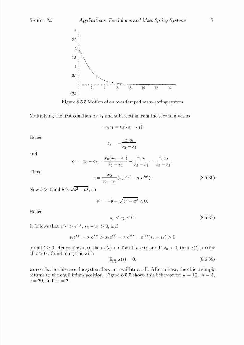
7/27/2019 Calculus 2 (Dan Sloughter)
http://slidepdf.com/reader/full/calculus-2-dan-sloughter 568/598
Section 8.5 Applications: Pendulums and Mass-Spring Systems 7
2 4 6 8 10 12 14
-0.5
0.5
1
1.5
2
2.5
3
Figure 8.5.5 Motion of an overdamped mass-spring system
Multiplying the first equation by s1 and subtracting from the second gives us
−x0s1 = c2(s2 − s1).
Hencec2 = − x0s1
s2 − s1
and
c1 = x0 − c2 =x0(s2 − s1)
s2 − s1+
x0s1
s2 − s1=
x0s2
s2 − s1.
Thusx =
x0
s2 − s1(s2es1t
−s1es2t). (8.5.36)
Now b > 0 and b >√
b2 − a2, so
s2 = −b +
b2 − a2 < 0.
Hences1 < s2 < 0. (8.5.37)
It follows that es2t > es1t, s2 − s1 > 0, and
s2es1t
−s1es2t > s2es2t
−s1es2t = es2t(s2
−s1) > 0
for all t ≥ 0. Hence if x0 < 0, then x(t) < 0 for all t ≥ 0, and if x0 > 0, then x(t) > 0 forall t > 0 . Combining this with
limt→∞
x(t) = 0, (8.5.38)
we see that in this case the system does not oscillate at all. After release, the object simplyreturns to the equilibrium position. Figure 8.5.5 shows this behavior for k = 10, m = 5,c = 20, and x0 = 2.
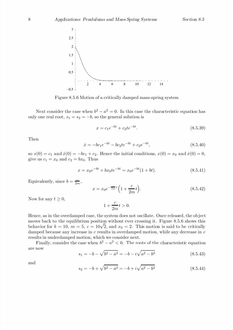
7/27/2019 Calculus 2 (Dan Sloughter)
http://slidepdf.com/reader/full/calculus-2-dan-sloughter 569/598
8 Applications: Pendulums and Mass-Spring Systems Section 8.5
2 4 6 8 10 12 14
-0.5
0.5
1
1.5
2
2.5
3
Figure 8.5.6 Motion of a critically damped mass-spring system
Next consider the case when b2
−a2 = 0. In this case the characteristic equation has
only one real root, s1 = s2 = −b, so the general solution is
x = c1e−bt + c2te−bt. (8.5.39)
Thenx = −bc1e−bt − bc2te−bt + c2e−bt, (8.5.40)
so x(0) = c1 and x(0) = −bc1 + c2. Hence the initial conditions, x(0) = x0 and x(0) = 0,give us c1 = x0 and c2 = bx0. Thus
x = x0e−bt + bx0te−bt = x0e−bt(1 + bt). (8.5.41)
Equivalently, since b = c2m ,
x = x0e−c
2mt
1 +c
2mt
. (8.5.42)
Now for any t ≥ 0,
1 +c
2mt > 0.
Hence, as in the overdamped case, the system does not oscillate. Once released, the objectmoves back to the equilibrium position without ever crossing it. Figure 8.5.6 shows thisbehavior for k = 10, m = 5, c = 10
√ 2, and x0 = 2. This motion is said to be critically
damped because any increase in c results in overdamped motion, while any decrease in cresults in underdamped motion, which we consider next.
Finally, consider the case when b2 − a2 < 0. The roots of the characteristic equationare now
s1 = −b−
b2 − a2 = −b− i
a2 − b2 (8.5.43)
ands2 = −b +
b2 − a2 = −b + i
a2 − b2 (8.5.44)
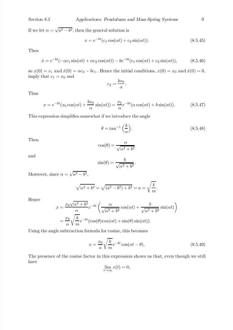
7/27/2019 Calculus 2 (Dan Sloughter)
http://slidepdf.com/reader/full/calculus-2-dan-sloughter 570/598
Section 8.5 Applications: Pendulums and Mass-Spring Systems 9
If we let α =√
a2 − b2, then the general solution is
x = e−bt(c1 cos(αt) + c2 sin(αt)). (8.5.45)
Then
x = e−bt(−αc1 sin(αt) + αc2 cos(αt))− be−bt(c1 cos(αt) + c2 sin(αt)), (8.5.46)
so x(0) = c1 and x(0) = αc2 − bc1. Hence the initial conditions, x(0) = x0 and x(0) = 0,imply that c1 = x0 and
c2 =bx0
α.
Thus
x = e−bt(x0 cos(αt) +bx0
αsin(αt)) =
x0
αe−bt(α cos(αt) + b sin(αt)). (8.5.47)
This expression simplifies somewhat if we introduce the angle
θ = tan−1 b
α
. (8.5.48)
Thencos(θ) =
α√ α2 + b2
and
sin(θ) =b√
α2 + b2.
Moreover, since α = √ a2 − b2,
α2 + b2 =
(a2 − b2) + b2 = a =
k
m.
Hence
x =x0
√ α2 + b2
αe−bt
α√
α2 + b2cos(αt) +
b√ α2 + b2
sin(αt)
=x0
α
k
me−bt(cos(θ)cos(αt) + sin(θ) sin(αt)).
Using the angle subtraction formula for cosine, this becomes
x =x0
α
k
me−bt cos(αt− θ). (8.5.49)
The presence of the cosine factor in this expression shows us that, even though we stillhave
limt→∞
x(t) = 0,
7/27/2019 Calculus 2 (Dan Sloughter)
http://slidepdf.com/reader/full/calculus-2-dan-sloughter 571/598
10 Applications: Pendulums and Mass-Spring Systems Section 8.5
2 4 6 8 10 12 14
-1
-0.5
0.5
1
1.5
2
2.5
3
Figure 8.5.7 Motion of an underdamped mass-spring system
the underdamped mass-spring system will oscillate about the equilibrium position with a
decreasing amplitude of x0
α
k
me−bt. (8.5.50)
Figure 8.5.7 shows this behavior for k = 10, m = 5, c = 5, and x0 = 2.
Problems
1. In an experiment to determine g, a pendulum of length 50 centimeters is observed tohave a period of oscillation of 1.42 seconds. Approximate g based on this observation.
2. The period of oscillation of a pendulum of length b given in (8.5.19) is, as mentioned,
only an approximation of the true period. It can be shown that the true period of apendulum released from an angle α is given by
T = 4
b
g
π2
0
1 1− k2 sin2(φ)
dφ,
where 0 < α < π and k = sinα2
.
(a) Find the period of oscillation for a pendulum of length 50 centimeters for α = π4 ,
α = π6 , α = π
50 , and α = π100 . Compare these results with the approximation given
in (8.5.19).
(b) Graph T as a function of α for −π
4 ≤ α ≤π
4 . For comparison, also plot thehorizontal line
T = 2π
b
g.
3. Consider a mass-spring system with x0 = 10, x(0) = 0, k = 10, and m = 10. Plotx(t) for c = 0, c = 5, c = 10, c = 20, c = 25, and c = 30. Identify each motion asoverdamped, critically damped, underdamped, or undamped.
7/27/2019 Calculus 2 (Dan Sloughter)
http://slidepdf.com/reader/full/calculus-2-dan-sloughter 572/598
Section 8.5 Applications: Pendulums and Mass-Spring Systems 11
4. Consider a mass-spring system with x0 = 10, x(0) = 0, m = 10, and c = 20. Plot x(t)for k = 2, k = 5, k = 10, and k = 15. Identify each motion as overdamped, criticallydamped, underdamped, or undamped.
5. Consider the underdamped motion of a mass-spring system expressed in (8.5.49).
(a) Show that the maximum values of x(t) occur at t = 0, T, 2T , . . ., where
T =2π
k
m− c2
4m2
.
Note that when c = 0, T reduces to the period of the motion for the mass-springsystem without damping.
(b) Show that if x1 and x2 are two successive maximum values of x(t), then
x1
x2 = e
cT
2m
.
6. Inside the earth, the force of gravity acting on an object is proportional to the distancebetween the object and the center of the earth.
(a) Suppose a hole is drilled through the earth from pole to pole and a rock is droppedinto the hole. If x(t) is the distance from the object to the center of the earth attime t, show that, ignoring any resistive forces,
x = R cos g
Rt,
where R is the radius of the earth.
(b) How long, in minutes, does it take for the rock to make one complete trip frompole to pole and back? Use R = 3950 miles.
(c) What is the velocity of the rock, in miles per hour, when it reaches the center of the earth?

7/27/2019 Calculus 2 (Dan Sloughter)
http://slidepdf.com/reader/full/calculus-2-dan-sloughter 573/598
Difference Equations
Differential Equations
to
Section 8.6
The Geometry of Solutions:The Phase Plane
As mentioned in Section 8.4, we may represent a second order differential equation
x = f (x, x, t) (8.6.1)
as a system of two first order equations
x = y
y = f (x ,y,t).
(8.6.2)
More generally, if g and f are functions of x, y, and t, we may consider a system of equations
x = g(x ,y,t)
y = f (x ,y,t),(8.6.3)
of which (8.6.2) is a particular case when g(x ,y,t) = y. In this section we shall considerthe behavior of solutions to such systems of equations, paying particular attention to thosearising in the manner of (8.6.2).
Definition Suppose x(t) and y(t) are solutions of the system
x = g(x ,y,t)
y = f (x ,y,t)
for t in an interval [a, b]. The curve in the plane with coordinates (x(t), y(t)), a ≤ t ≤ b, iscalled a phase curve of the system. The plane in which the phase curve is plotted is calledthe phase plane of the system.
Note that if the system of equations arises from a second order differential equation,then a phase curve is a plot of x(t) versus x(t). In many common cases, this is a plot of
velocity versus position.
Definition Suppose the constant functions x(t) = x0 and y(t) = y0 is a solution of thesystem
x = g(x ,y,t)
y = f (x ,y,t).
Then the point (x0, y0) is called a stationary point of the system.
1 Copyright c by Dan Sloughter 2000
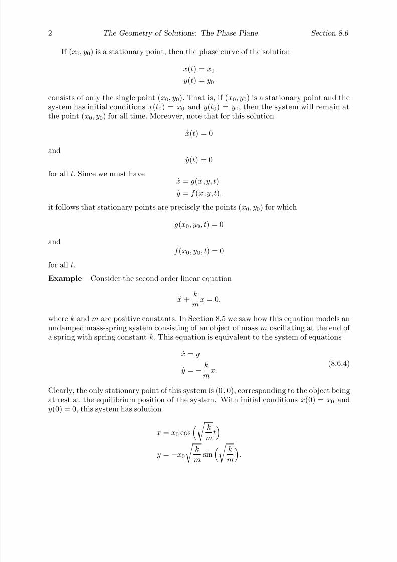
7/27/2019 Calculus 2 (Dan Sloughter)
http://slidepdf.com/reader/full/calculus-2-dan-sloughter 574/598
2 The Geometry of Solutions: The Phase Plane Section 8.6
If (x0, y0) is a stationary point, then the phase curve of the solution
x(t) = x0
y(t) = y0
consists of only the single point (x0, y0). That is, if (x0, y0) is a stationary point and thesystem has initial conditions x(t0) = x0 and y(t0) = y0, then the system will remain atthe point (x0, y0) for all time. Moreover, note that for this solution
x(t) = 0
andy(t) = 0
for all t. Since we must havex = g(x ,y,t)
˙y
=f
(x ,y,t
),
it follows that stationary points are precisely the points (x0, y0) for which
g(x0, y0, t) = 0
andf (x0, y0, t) = 0
for all t.
Example Consider the second order linear equation
x + km
x = 0,
where k and m are positive constants. In Section 8.5 we saw how this equation models anundamped mass-spring system consisting of an object of mass m oscillating at the end of a spring with spring constant k. This equation is equivalent to the system of equations
x = y
y = − k
mx.
(8.6.4)
Clearly, the only stationary point of this system is (0 , 0), corresponding to the object beingat rest at the equilibrium position of the system. With initial conditions x(0) = x0 andy(0) = 0, this system has solution
x = x0 cos k
mt
y = −x0
k
msin k
m
.
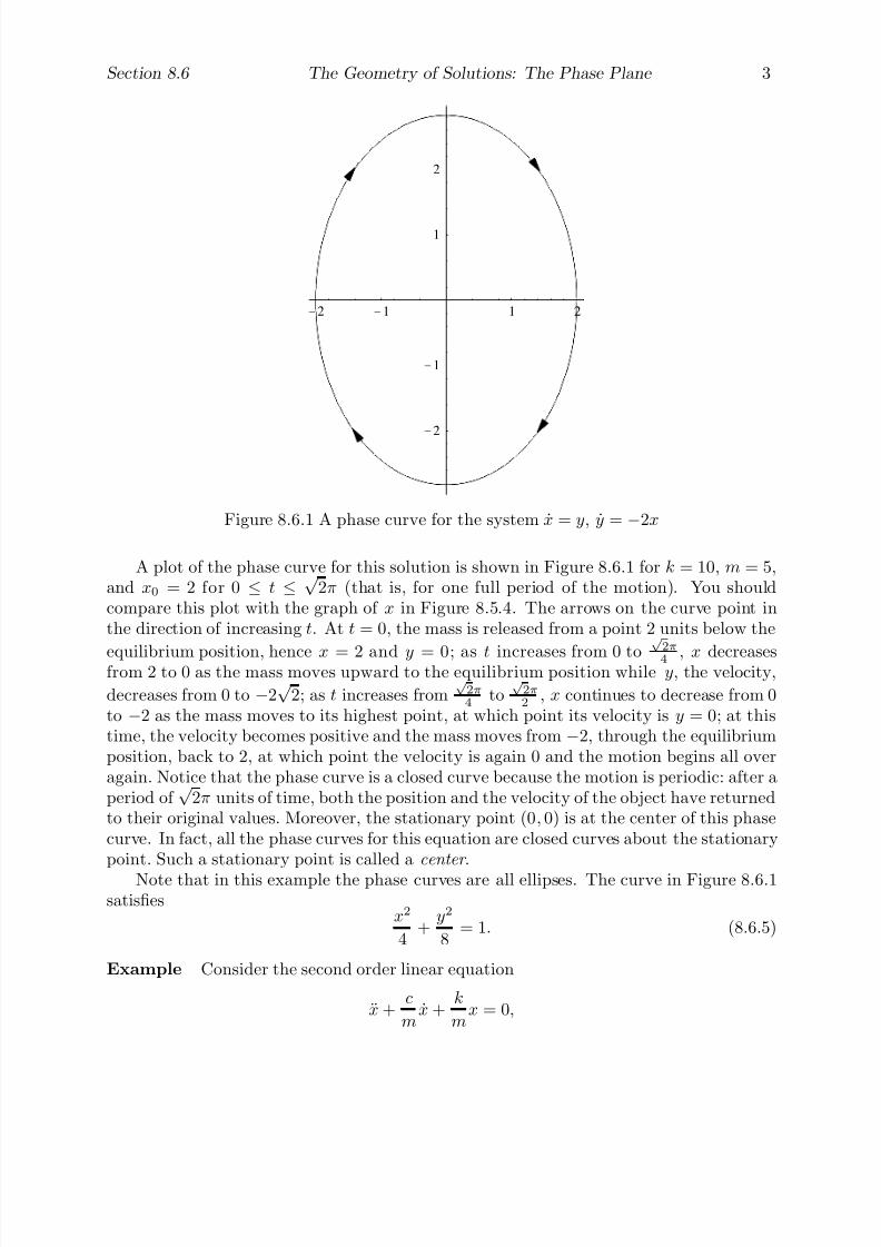
7/27/2019 Calculus 2 (Dan Sloughter)
http://slidepdf.com/reader/full/calculus-2-dan-sloughter 575/598
Section 8.6 The Geometry of Solutions: The Phase Plane 3
-2 -1 1 2
-2
-1
1
2
Figure 8.6.1 A phase curve for the system x = y, y = −2x
A plot of the phase curve for this solution is shown in Figure 8.6.1 for k = 10, m = 5,and x0 = 2 for 0 ≤ t ≤ √
2π (that is, for one full period of the motion). You shouldcompare this plot with the graph of x in Figure 8.5.4. The arrows on the curve point inthe direction of increasing t. At t = 0, the mass is released from a point 2 units below the
equilibrium position, hence x = 2 and y = 0; as t increases from 0 to
√ 2π4 , x decreases
from 2 to 0 as the mass moves upward to the equilibrium position while y, the velocity,
decreases from 0 to −2√
2; as t increases from√ 2π4
to√ 2π2
, x continues to decrease from 0to −2 as the mass moves to its highest point, at which point its velocity is y = 0; at thistime, the velocity becomes positive and the mass moves from −2, through the equilibriumposition, back to 2, at which point the velocity is again 0 and the motion begins all overagain. Notice that the phase curve is a closed curve because the motion is periodic: after aperiod of
√ 2π units of time, both the position and the velocity of the object have returned
to their original values. Moreover, the stationary point (0, 0) is at the center of this phasecurve. In fact, all the phase curves for this equation are closed curves about the stationarypoint. Such a stationary point is called a center .
Note that in this example the phase curves are all ellipses. The curve in Figure 8.6.1satisfies
x2
4+
y2
8= 1. (8.6.5)
Example Consider the second order linear equation
x +c
mx +
k
mx = 0,
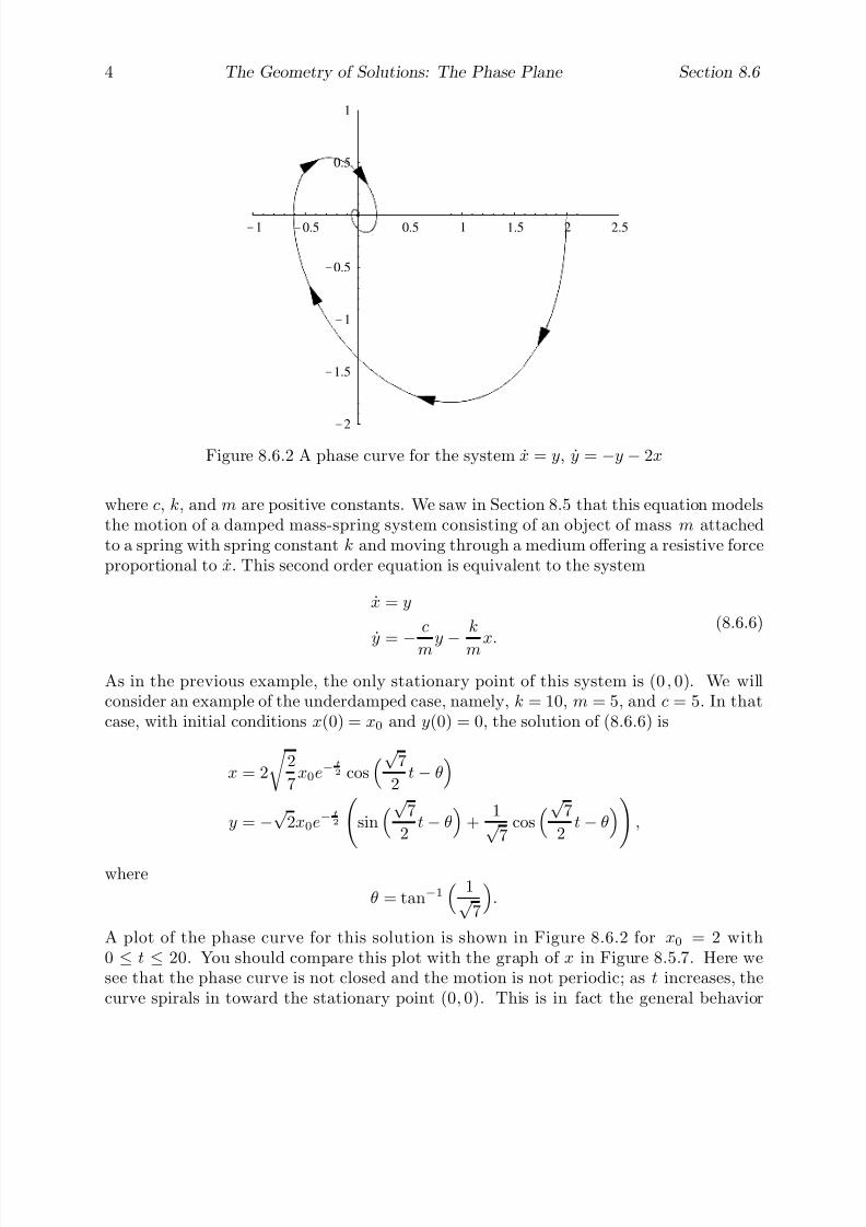
7/27/2019 Calculus 2 (Dan Sloughter)
http://slidepdf.com/reader/full/calculus-2-dan-sloughter 576/598
4 The Geometry of Solutions: The Phase Plane Section 8.6
-1 -0.5 0.5 1 1.5 2 2.5
-2
-1.5
-1
-0.5
0.5
1
Figure 8.6.2 A phase curve for the system x = y, y = −y − 2x
where c, k, and m are positive constants. We saw in Section 8.5 that this equation modelsthe motion of a damped mass-spring system consisting of an object of mass m attachedto a spring with spring constant k and moving through a medium offering a resistive forceproportional to x. This second order equation is equivalent to the system
x = y
y = −c
m y −k
m x.
(8.6.6)
As in the previous example, the only stationary point of this system is (0 , 0). We willconsider an example of the underdamped case, namely, k = 10, m = 5, and c = 5. In thatcase, with initial conditions x(0) = x0 and y(0) = 0, the solution of (8.6.6) is
x = 2
2
7x0e−
t
2 cos√ 7
2t− θ
y = −√
2x0e−t
2
sin√ 7
2t− θ
+
1√ 7
cos√ 7
2t− θ
,
where
θ = tan−1 1√
7
.
A plot of the phase curve for this solution is shown in Figure 8.6.2 for x0 = 2 with0 ≤ t ≤ 20. You should compare this plot with the graph of x in Figure 8.5.7. Here wesee that the phase curve is not closed and the motion is not periodic; as t increases, thecurve spirals in toward the stationary point (0, 0). This is in fact the general behavior

7/27/2019 Calculus 2 (Dan Sloughter)
http://slidepdf.com/reader/full/calculus-2-dan-sloughter 577/598
Section 8.6 The Geometry of Solutions: The Phase Plane 5
of phase curves for this system: No matter what the initial condition, as t increases,both the position and velocity functions decay toward 0 as the mass performs smaller andsmaller oscillations about the equilibrium. In this case we call the stationary point a stable
equilibrium . In general, a stationary point (x0, y0) is a stable equilibrium if for any initialconditions sufficiently close to (x0, y0), the resulting phase curve approaches (x0, y0) in the
limit as t →∞. In this example, every phase curve approaches (0, 0) as t →∞.
A stationary point (x0, y0) is called an unstable equilibrium if there is a fixed distanced such that it is possible to find initial conditions arbitrarily close to (x0, y0) for which theresulting phase curve will eventually be farther than d away from (x0, y0).
Example Taking k = 10, m = 5, and c = −5 in the system (8.6.6) would lead to thesolution
x = 2
2
7x0e
t
2 cos√ 7
2t− θ
y =√
2x0et
2 1
√ 7cos
√ 7
2
t
−θ− sin
√ 7
2
t
−θ ,
where
θ = tan−1− 1√
7
.
In this case, the stationary point (0, 0) is an unstable equilibrium because, since et
2 increaseswith t, the phase curves spiral away from the stationary point (0, 0). A plot of the phasecurve for this solution is shown in Figure 8.6.3 for x0 = 0.01 with 0 ≤ t ≤ 10.
We will see another example of an unstable equilibrium when we return to the pendu-lum example below.
Numerical approximations
Although useful in general, the ideas developed above are most helpful when exact solutionsare not available and we must rely upon numerical approximations in order to understandthe behavior of solutions. However, before we can consider such examples, we must firstmodify our numerical techniques from Section 8.1 to the current situation. Since the secondorder Runge-Kutta method is more accurate than Euler’s method, we will discuss only themodification of the former.
Suppose we wish to approximate the solution of the system
x = g(x ,y,t)y = f (x ,y,t),
(8.6.7)
with initial conditions x(t0) = x0 and y(t0) = y0, at time t0 + h. First we approximate x
at t0 + h2
by x0 + m1, where
m1 =h
2x(t0) =
h
2g(x0, y0, t0), (8.6.8)
7/27/2019 Calculus 2 (Dan Sloughter)
http://slidepdf.com/reader/full/calculus-2-dan-sloughter 578/598
6 The Geometry of Solutions: The Phase Plane Section 8.6
-0.2 0.2 0.4 0.6 0.8 1
-1
-0.5
0.5
1
Figure 8.6.3 A phase curve for the system x = y, y = y − 2x
and y at t0 + h2
by y0 + m2, where
m2 =h
2
y(t0) =h
2
f (x0, y0, t0). (8.6.9)
Then the second order Runge-Kutta approximations to x(t0 + h) and y(t0 + h) are givenby
x1 = x0 + hg
x0 + m1, y0 + m2, t0 +h
2
(8.6.10)
and
y1 = y0 + hf
x0 + m1, y0 + m2, t0 +h
2
, (8.6.11)

7/27/2019 Calculus 2 (Dan Sloughter)
http://slidepdf.com/reader/full/calculus-2-dan-sloughter 579/598
Section 8.6 The Geometry of Solutions: The Phase Plane 7
respectively. As before, to approximate the solution over an interval [t0, t1], we iterate theabove process as many times as necessary.
Second order Runge-Kutta To approximate the solution of the system of equations
x = g(x ,y,t)
y = f (x ,y,t)
with initial conditions x(t0) = x0 and y(t0) = y0 on an interval [t0, t1], choose a small valuefor h > 0 and an integer n such that t0 + nh ≥ t1. Letting sk = t0 + kh, compute
m1 =h
2g(xk, yk, sk)
m2 =h
2f (xk, yk, sk)
(8.6.12)
and
xk+1 = xk + hg
xk + m1, yk + m2, sk +
h
2
yk+1 = yk + hf
xk + m1, yk + m2, sk +h
2
(8.6.13)
for k = 0, 1, 2, . . . , n − 1. Then xk is an approximation for x(t0 + kh) and yk is anapproximation for y(t0 + kh).
Example In this example we consider a simple case for modeling a predator-prey envi-ronment. Suppose animals of species A prey on animals of species B. For our example,species A will be foxes and species B will be rabbits, although they could be any twospecies that have the predator-prey relationship we are about to describe. We assumethat the food supply of the rabbits is essentially unlimited and the foxes are their onlynatural enemy in the given environment, while, on the other hand, we assume the foxesare dependent upon the rabbits for the bulk of their food supply. We also assume that thefoxes have no natural enemies. Let y(t) be the size of the fox population and let x(t) bethe size of the rabbit population at time t. If there were no foxes, the rabbits would enjoyuninhibited growth and we would have
x = αx
for some constant α > 0 representing the natural growth rate of rabbits in the givenenvironment. However, if we assume that the number of encounters between rabbits andfoxes is proportional to the product of the two populations and, furthermore, that a certainproportion of these encounters results in a rabbit becoming a meal for a fox, then x willbe decreased by an amount βxy for some constant β > 0. Hence we have
x = αx− βxy = x(α− βy).
At the same time, if there were no rabbits, the fox population would decline for want of food, that is, we would expect
y = −γy
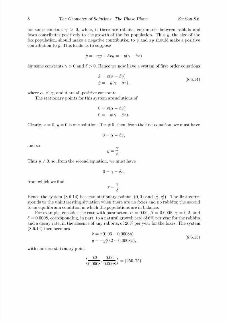
7/27/2019 Calculus 2 (Dan Sloughter)
http://slidepdf.com/reader/full/calculus-2-dan-sloughter 580/598
8 The Geometry of Solutions: The Phase Plane Section 8.6
for some constant γ > 0, while, if there are rabbits, encounters between rabbits andfoxes contributes positively to the growth of the fox population. Thus y, the size of thefox population, should make a negative contribution to y and xy should make a positivecontribution to y. This leads us to suppose
y = −γy + δxy = −y(γ − δx)
for some constants γ > 0 and δ > 0. Hence we now have a system of first order equations
x = x(α− βy)
y = −y(γ − δx),(8.6.14)
where α, β , γ , and δ are all positive constants.The stationary points for this system are solutions of
0 = x(α
−βy)
0 = −y(γ − δx).
Clearly, x = 0, y = 0 is one solution. If x = 0, then, from the first equation, we must have
0 = α− βy,
and soy =
α
β .
Thus y = 0, so, from the second equation, we must have
0 = γ − δx,
from which we findx =
γ
δ .
Hence the system (8.6.14) has two stationary points: (0, 0) and ( γ δ
, αβ
). The first corre-sponds to the uninteresting situation when there are no foxes and no rabbits; the secondto an equilibrium condition in which the populations are in balance.
For example, consider the case with parameters α = 0.06, β = 0.0008, γ = 0.2, andδ = 0.0008, corresponding, in part, to a natural growth rate of 6% per year for the rabbits
and a decay rate, in the absence of any rabbits, of 20% per year for the foxes. The system(8.6.14) then becomesx = x(0.06− 0.0008y)
y = −y(0.2− 0.0008x),(8.6.15)
with nonzero stationary point
0.2
0.0008,
0.06
0.0008
= (250, 75).

7/27/2019 Calculus 2 (Dan Sloughter)
http://slidepdf.com/reader/full/calculus-2-dan-sloughter 581/598
Section 8.6 The Geometry of Solutions: The Phase Plane 9
Hence a population of 250 rabbits and 75 foxes would be in equilibrium and would notchange over time; the natural yearly increase in the rabbit population is accounted forexactly by the appetite of the foxes. To see what happens in other cases, suppose we startwith an initial population of x0 = 400 rabbits and y0 = 50 foxes. We will approximate thesolution to (8.6.15) over the interval [0, 150] using the second order Runge-Kutta method
with a step size of h = 0.05. To start, using
g(x ,y,t) = x(0.06− 0.0008y)
f (x ,y,t) = −y(0.2− 0.0008x),
we compute
m1 =h
2g(x0, y0, t0) = (0.025)(400)(0.06− (0.0008)(50)) = 0.2
m2 =h
2f (x0, y0, t0) = −(0.025)(50)(0.2− (0.0008)(400)) = 0.15
and
x1 = x0 + hg
x0 + m1, y0 + m2, t0 +h
2
= 400 + (0.05)g(400.2, 50.15, 0.025)
= 400 + (0.05)(400.2)(0.06− (0.0008)(50.15))
= 400.3978
y1 = y0 + hf
x0 + m1, y0 + m2, t0 +h
2
= 50 + (0.05)f (400.2, 50.15, 0.025)
= 50− (0.05)(50.15)(0.2− (0.0008)(400.2))= 50.3013,
where we have rounded x1 and y1 to four decimal places. Then x1 is an approximation forx(0.05) and y1 is an approximation for y(0.05). In general, x20t and y20t are approximationsfor x(t) and y(t) when 20t is an integer. Table 8.6.1 gives our results for t = 0, 5, 10, . . . , 150,where we have rounded the values to the nearest integer.
Notice the cyclic nature of both x and y. In the early years, the population of foxesincreases due to the plentiful supply of rabbits for food. However, eventually (sometimebetween 15 and 20 years) the increasing fox population causes a decrease in the rabbitpopulation to the point where the population of foxes begins to decline. As the fox popu-
lation declines, there comes a point (between 30 and 35 years) when the rabbit populationbegins to increase, which in turn eventually leads to an increase in the fox population,starting sometime between 55 and 60 years. At this point, the cycle begins again. Thisbehavior is most evident in Figure 8.6.4, where the numerical solutions for x and y havebeen plotted over the interval [0, 150]. Notice how the periods of the two curves are thesame, but their phases are different. This phase difference occurs because, for example,a decrease in the rabbit population does not lead to an immediate decrease in the foxpopulation; in fact, the fox population will continue to grow until the rabbit population
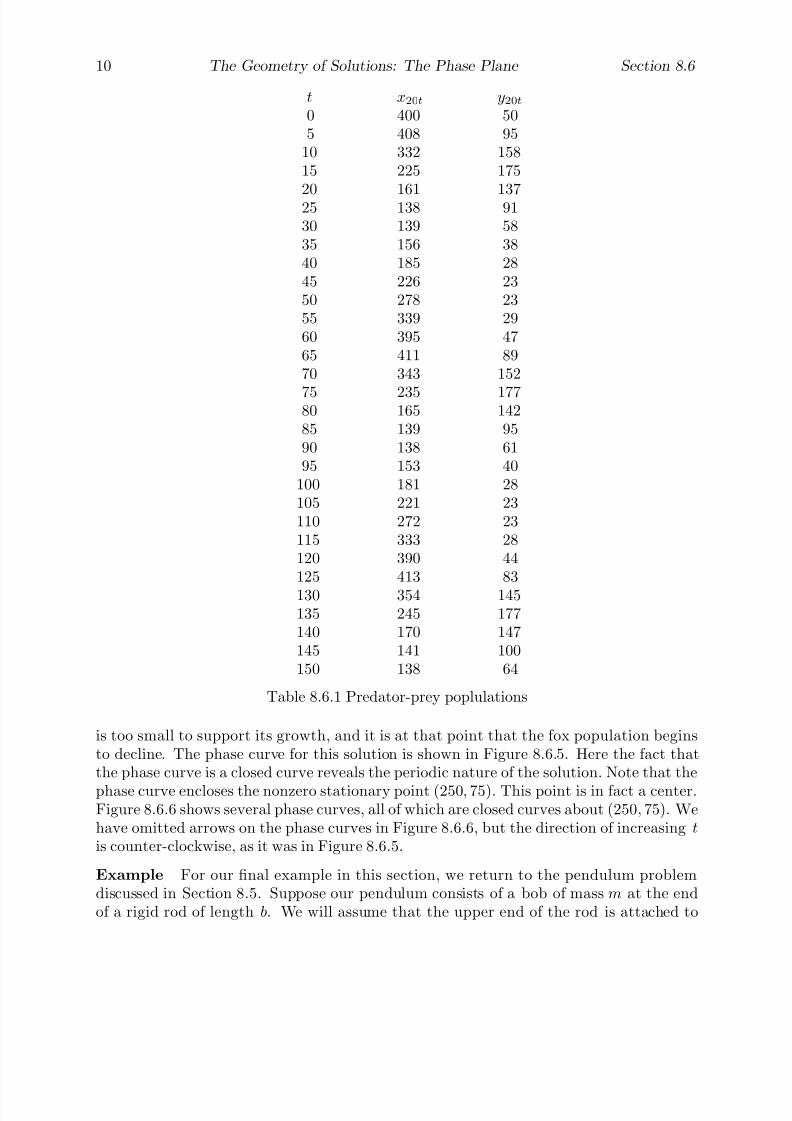
7/27/2019 Calculus 2 (Dan Sloughter)
http://slidepdf.com/reader/full/calculus-2-dan-sloughter 582/598
10 The Geometry of Solutions: The Phase Plane Section 8.6
t x20t y20t0 400 505 408 95
10 332 15815 225 175
20 161 13725 138 9130 139 5835 156 3840 185 2845 226 2350 278 2355 339 2960 395 4765 411 8970 343 152
75 235 17780 165 14285 139 9590 138 6195 153 40
100 181 28105 221 23110 272 23115 333 28120 390 44125 413 83130 354 145135 245 177140 170 147145 141 100150 138 64
Table 8.6.1 Predator-prey poplulations
is too small to support its growth, and it is at that point that the fox population beginsto decline. The phase curve for this solution is shown in Figure 8.6.5. Here the fact thatthe phase curve is a closed curve reveals the periodic nature of the solution. Note that the
phase curve encloses the nonzero stationary point (250, 75). This point is in fact a center.Figure 8.6.6 shows several phase curves, all of which are closed curves about (250 , 75). Wehave omitted arrows on the phase curves in Figure 8.6.6, but the direction of increasing t
is counter-clockwise, as it was in Figure 8.6.5.
Example For our final example in this section, we return to the pendulum problemdiscussed in Section 8.5. Suppose our pendulum consists of a bob of mass m at the endof a rigid rod of length b. We will assume that the upper end of the rod is attached to
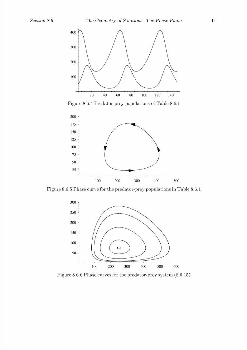
7/27/2019 Calculus 2 (Dan Sloughter)
http://slidepdf.com/reader/full/calculus-2-dan-sloughter 583/598
Section 8.6 The Geometry of Solutions: The Phase Plane 11
20 40 60 80 100 120 140
100
200
300
400
Figure 8.6.4 Predator-prey populations of Table 8.6.1
100 200 300 400 500
25
50
75
100
125
150
175
200
Figure 8.6.5 Phase curve for the predator-prey populations in Table 8.6.1
100 200 300 400 500 600
50
100
150
200
250
300
Figure 8.6.6 Phase curves for the predator-prey system (8.6.15)

7/27/2019 Calculus 2 (Dan Sloughter)
http://slidepdf.com/reader/full/calculus-2-dan-sloughter 584/598
12 The Geometry of Solutions: The Phase Plane Section 8.6
-10 -7.5 -5 -2.5 2.5 5 7.5 10
-6
-4
-2
2
4
6
Figure 8.6.7 Phase curves for a pendulum: x = y, y = −4.9sin(x)
another rod, held fixed and perpendicular to the plane of motion of the pendulum, in such
a way that the pendulum is free to move through complete circles about this axis. If welet x(t) be the angle between the rod and the vertical at time t, then we showed in Section8.5 that x must satisfy the equation
x = −g
bsin(x).
Equivalently, as a system of first order equations, we have
x = y
y =−
g
bsin(x).
(8.6.16)
The stationary points for this system are the points (x, y) where y = 0 and sin(x) = 0.Hence there are an infinite number of stationary points, namely, (nπ, 0) for n = 0, 1, 2, . . ..Note that for even values of n, the stationary points (nπ, 0) correspond to the pendulumhanging at rest with the bob end down. We should expect these stationary points to becenters since, without friction, any nearby initial conditions would result in the pendulumoscillating about the given stationary point. For odd values of n, the stationary points(nπ, 0) correspond to the pendulum balancing with the bob end up. We should expect thatany initial condition near one of these stationary points would result in motion away fromthe given stationary point. That is, any slight motion away from the balanced position
should cause the pendulum to fall and begin an oscillatory motion. Hence these stationarypoints should be unstable equilibriums. A look at the phase curves in Figure 8.6.7, shownfor a pendulum of length 2 meters, supports these statements: For any integer k, (2kπ, 0)is a center and ((2k − 1)π, 0) is an unstable equilibrium. We have again omitted arrowson the phase curves in Figure 8.6.7, but the direction of increasing t is from left to rightabove the x-axis and from right to left below the x-axis.
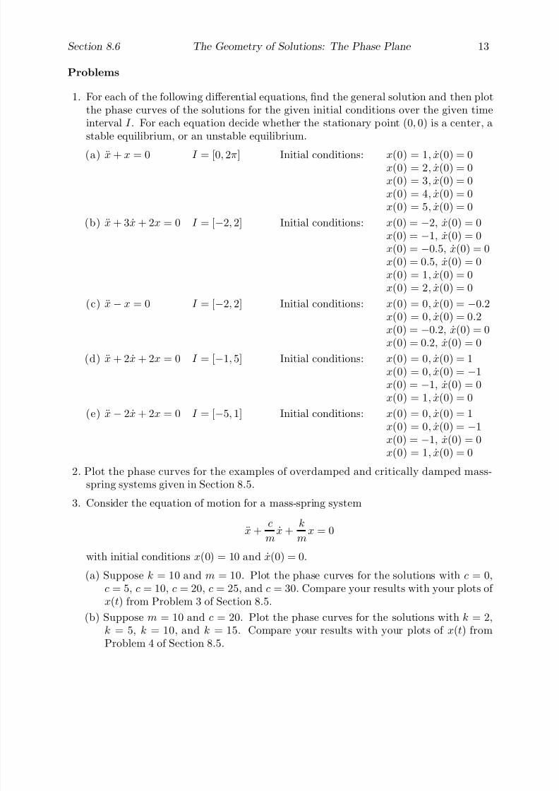
7/27/2019 Calculus 2 (Dan Sloughter)
http://slidepdf.com/reader/full/calculus-2-dan-sloughter 585/598
Section 8.6 The Geometry of Solutions: The Phase Plane 13
Problems
1. For each of the following differential equations, find the general solution and then plotthe phase curves of the solutions for the given initial conditions over the given timeinterval I . For each equation decide whether the stationary point (0, 0) is a center, a
stable equilibrium, or an unstable equilibrium.(a) x + x = 0 I = [0, 2π] Initial conditions: x(0) = 1, x(0) = 0
x(0) = 2, x(0) = 0x(0) = 3, x(0) = 0x(0) = 4, x(0) = 0x(0) = 5, x(0) = 0
(b) x + 3x + 2x = 0 I = [−2, 2] Initial conditions: x(0) = −2, x(0) = 0x(0) = −1, x(0) = 0x(0) = −0.5, x(0) = 0x(0) = 0.5, x(0) = 0
x(0) = 1, x(0) = 0x(0) = 2, x(0) = 0
(c) x− x = 0 I = [−2, 2] Initial conditions: x(0) = 0, x(0) = −0.2x(0) = 0, x(0) = 0.2x(0) = −0.2, x(0) = 0x(0) = 0.2, x(0) = 0
(d) x + 2x + 2x = 0 I = [−1, 5] Initial conditions: x(0) = 0, x(0) = 1x(0) = 0, x(0) = −1x(0) = −1, x(0) = 0x(0) = 1, x(0) = 0
(e) x− 2x + 2x = 0 I = [−5, 1] Initial conditions: x(0) = 0, x(0) = 1x(0) = 0, x(0) = −1x(0) = −1, x(0) = 0x(0) = 1, x(0) = 0
2. Plot the phase curves for the examples of overdamped and critically damped mass-spring systems given in Section 8.5.
3. Consider the equation of motion for a mass-spring system
x +c
mx +
k
mx = 0
with initial conditions x(0) = 10 and x(0) = 0.
(a) Suppose k = 10 and m = 10. Plot the phase curves for the solutions with c = 0,c = 5, c = 10, c = 20, c = 25, and c = 30. Compare your results with your plots of x(t) from Problem 3 of Section 8.5.
(b) Suppose m = 10 and c = 20. Plot the phase curves for the solutions with k = 2,k = 5, k = 10, and k = 15. Compare your results with your plots of x(t) fromProblem 4 of Section 8.5.
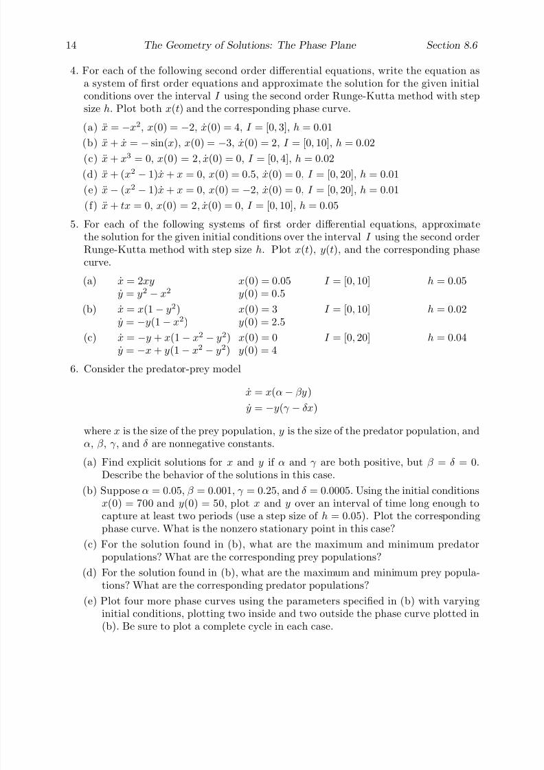
7/27/2019 Calculus 2 (Dan Sloughter)
http://slidepdf.com/reader/full/calculus-2-dan-sloughter 586/598
14 The Geometry of Solutions: The Phase Plane Section 8.6
4. For each of the following second order differential equations, write the equation asa system of first order equations and approximate the solution for the given initialconditions over the interval I using the second order Runge-Kutta method with stepsize h. Plot both x(t) and the corresponding phase curve.
(a) x =−
x2, x(0) =−
2, x(0) = 4, I = [0, 3], h = 0.01
(b) x + x = − sin(x), x(0) = −3, x(0) = 2, I = [0, 10], h = 0.02
(c) x + x3 = 0, x(0) = 2, x(0) = 0, I = [0, 4], h = 0.02
(d) x + (x2 − 1)x + x = 0, x(0) = 0.5, x(0) = 0, I = [0, 20], h = 0.01
(e) x− (x2 − 1)x + x = 0, x(0) = −2, x(0) = 0, I = [0, 20], h = 0.01
(f) x + tx = 0, x(0) = 2, x(0) = 0, I = [0, 10], h = 0.05
5. For each of the following systems of first order differential equations, approximatethe solution for the given initial conditions over the interval I using the second orderRunge-Kutta method with step size h. Plot x(t), y(t), and the corresponding phasecurve.
(a) x = 2xy x(0) = 0.05 I = [0, 10] h = 0.05y = y2 − x2 y(0) = 0.5
(b) x = x(1− y2) x(0) = 3 I = [0, 10] h = 0.02y = −y(1− x2) y(0) = 2.5
(c) x = −y + x(1− x2 − y2) x(0) = 0 I = [0, 20] h = 0.04y = −x + y(1− x2 − y2) y(0) = 4
6. Consider the predator-prey model
x = x(α
−βy)
y = −y(γ − δx)
where x is the size of the prey population, y is the size of the predator population, andα, β , γ , and δ are nonnegative constants.
(a) Find explicit solutions for x and y if α and γ are both positive, but β = δ = 0.Describe the behavior of the solutions in this case.
(b) Suppose α = 0.05, β = 0.001, γ = 0.25, and δ = 0.0005. Using the initial conditionsx(0) = 700 and y(0) = 50, plot x and y over an interval of time long enough tocapture at least two periods (use a step size of h = 0.05). Plot the correspondingphase curve. What is the nonzero stationary point in this case?
(c) For the solution found in (b), what are the maximum and minimum predatorpopulations? What are the corresponding prey populations?
(d) For the solution found in (b), what are the maximum and minimum prey popula-tions? What are the corresponding predator populations?
(e) Plot four more phase curves using the parameters specified in (b) with varyinginitial conditions, plotting two inside and two outside the phase curve plotted in(b). Be sure to plot a complete cycle in each case.
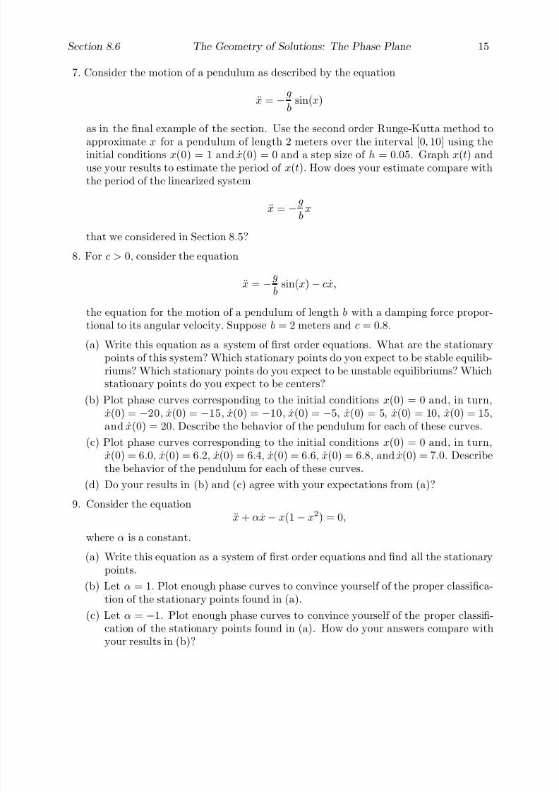
7/27/2019 Calculus 2 (Dan Sloughter)
http://slidepdf.com/reader/full/calculus-2-dan-sloughter 587/598
Section 8.6 The Geometry of Solutions: The Phase Plane 15
7. Consider the motion of a pendulum as described by the equation
x = −g
bsin(x)
as in the final example of the section. Use the second order Runge-Kutta method to
approximate x for a pendulum of length 2 meters over the interval [0, 10] using theinitial conditions x(0) = 1 and x(0) = 0 and a step size of h = 0.05. Graph x(t) anduse your results to estimate the period of x(t). How does your estimate compare withthe period of the linearized system
x = −g
bx
that we considered in Section 8.5?
8. For c > 0, consider the equation
x = −gb
sin(x)− cx,
the equation for the motion of a pendulum of length b with a damping force propor-tional to its angular velocity. Suppose b = 2 meters and c = 0.8.
(a) Write this equation as a system of first order equations. What are the stationarypoints of this system? Which stationary points do you expect to be stable equilib-riums? Which stationary points do you expect to be unstable equilibriums? Whichstationary points do you expect to be centers?
(b) Plot phase curves corresponding to the initial conditions x(0) = 0 and, in turn,
x(0) = −20, x(0) = −15, x(0) = −10, x(0) = −5, x(0) = 5, x(0) = 10, x(0) = 15,and x(0) = 20. Describe the behavior of the pendulum for each of these curves.
(c) Plot phase curves corresponding to the initial conditions x(0) = 0 and, in turn,x(0) = 6.0, x(0) = 6.2, x(0) = 6.4, x(0) = 6.6, x(0) = 6.8, and x(0) = 7.0. Describethe behavior of the pendulum for each of these curves.
(d) Do your results in (b) and (c) agree with your expectations from (a)?
9. Consider the equationx + αx− x(1− x2) = 0,
where α is a constant.
(a) Write this equation as a system of first order equations and find all the stationarypoints.
(b) Let α = 1. Plot enough phase curves to convince yourself of the proper classifica-tion of the stationary points found in (a).
(c) Let α = −1. Plot enough phase curves to convince yourself of the proper classifi-cation of the stationary points found in (a). How do your answers compare withyour results in (b)?

7/27/2019 Calculus 2 (Dan Sloughter)
http://slidepdf.com/reader/full/calculus-2-dan-sloughter 588/598
Difference Equations
Differential Equations
toSection 8.7
Power Series Solutions
In this section we consider one more approach to finding solutions, or approximate so-lutions, to differential equations. Although the method may be applied to first orderequations, our discussion will center on second order equations.
The idea is simple: Assuming that the equation
x = f (x, x, t) (8.7.1)
has a solution which is analytic on an interval about t = t0, we express x as a power series
x(t) =∞n=0
an(t− t0)n, (8.7.2)
compute x and x, substitute the results into the equation, solve for the coefficients a0, a1,a2, . . . , and verify that the resulting series converges on an interval about t0. As we shallsee, in practice the difficult part is solving for the coefficients. This method will lead us to aclosed form solution for the equation only in the rare case that we are able to recognize theresulting power series as the Taylor series of some known function. One advantage of this
technique over numerical methods, such as the Runge-Kutta method, is that we are ableto work with general solutions and equations involving unspecified parameters, whereaswith a numerical method every quantity must be specified as a number. The disadvantageof this technique is that it is not as widely applicable, due to the difficulty of solving forthe coefficients, and, when numerical results are needed, one must still approximate theinfinite series which results when evaluating x at a point.
To illustrate the procedure, we will begin with an example which we know to be solvableby the techniques of Section 8.4.
Example Consider the equation
x = −x. (8.7.3)
This is a constant coefficient homogeneous linear equation with characteristic equationk2 + 1 = 0. Since the roots of the characteristic equation are −i and i, we know from ourwork in Section 8.4 that the general solution of this equation is
x = c1 cos(t) + c2 sin(t),
where c1 and c2 are arbitrary constants.
1 Copyright c by Dan Sloughter 2000

7/27/2019 Calculus 2 (Dan Sloughter)
http://slidepdf.com/reader/full/calculus-2-dan-sloughter 589/598
2 Power Series Solutions Section 8.7
We may obtain the same result using power series. If we suppose that x is analytic onan interval about t = 0, then we may write
x(t) =∞
n=0antn
for some constants a0, a1, a2, . . . . Differentiating, we have
x(t) =∞n=1
nantn−1 =∞n=0
(n + 1)an+1tn
and
x(t) =∞n=2
n(n− 1)antn−2 =∞n=0
(n + 2)(n + 1)an+2tn.
Substituting into (8.7.3) gives us
∞n=0
(n + 2)(n + 1)an+2tn = −∞n=0
antn.
Since power series representations are unique, the coefficient of tn in the power series onthe left must equal the coefficient of tn in the power series on the right for all values of n.That is, we must have
(n + 2)(n + 1)an+2 = −an
for n = 0, 1, 2, . . .. Hence the coefficients of the power series representation of x satisfy thedifference equation
an+2 = −an
(n + 2)(n + 1)(8.7.4)
for n = 0, 1, 2, . . .. Note that (8.7.4) does not restrict either a0 or a1, but determines all of the other coefficients once these values are specified. Thus, given any values for a0 and a1,
a2 = −a0
(2)(1)= −
a0
2,
a3 = −a1
(3)(2)= −
a1
3!,
a4 = − a2(4)(3)
= a0(4)(3)(2)
= a04!
,
a5 = −a3
(5)(4)=
a1
(5)(4)(3)(2)=
a1
5!,
a6 = −a4
(6)(5)= −
a0
(6)(5)(4)(3)(2)= −
a0
6!,
a7 = −a5
(7)(6)= −
a1
(7)(6)(5)(4)(3)(2)= −
a1
7!,
7/27/2019 Calculus 2 (Dan Sloughter)
http://slidepdf.com/reader/full/calculus-2-dan-sloughter 590/598
Section 8.7 Power Series Solutions 3
and so on. In fact, we see that for k = 0, 1, 2, . . .,
a2k =(−1)ka0
(2k)!
and
a2k+1 =(−1)ka1
(2k + 1)!.
In most cases, this is as far as we can go; we would now check for the interval of convergenceof the resulting power series and conclude that x is a solution of (8.7.3) on that interval.However, in this case we see that
x =∞n=0
antn
= a0 + a1t−a0
2t2 −
a1
3!t3 +
a0
4!t4 +
a1
5!t5 −
a0
6!t6 −
a1
7!t7 + · · ·
= a0
1 −
t2
2+
t4
4!−
t6
6!+ · · ·
+ a1
t −
t3
3!+
t5
5!−
t7
7!+ · · ·
= a0 cos(t) + a1 sin(t),
the general solution that we noted above. Hence there is no need to check for the intervalof convergence since we recognize our power series representation of x as the Taylor seriesof a familiar function.
In general, if
x =∞
n=0
an(t− t0)n, (8.7.5)
then x(t0) = a0 and x(t0) = a1. Hence if we are seeking the solution of a differentialequation in this form, then the values of a0 and a1 are determined by any initial conditionswhich specify x(t0) and x(t0). Thus we shall see that all of our examples will be of thegeneral form of the previous example. Namely, after substituting x, x, and x into theequation, we will find a difference equation which determines the coefficients, a2, a3, a4,. . . , in terms of a0 and a1. However, unlike the first example, our remaining exampleswill not result in closed form expressions for our solutions. Nevertheless, we will findpower series representations for the solutions which may be used to approximate a specificsolution to any desired order on some interval of convergence.
Example Consider the equation
x − tx = 0. (8.7.6)
Suppose x is analytic on an interval about t = 0 and write
x =∞n=0
antn

7/27/2019 Calculus 2 (Dan Sloughter)
http://slidepdf.com/reader/full/calculus-2-dan-sloughter 591/598
4 Power Series Solutions Section 8.7
for some constants a0, a1, a2, . . . . Then, as in the previous example,
x =∞n=1
nantn−1 =∞n=0
(n + 1)an+1tn
and
x =∞n=2
n(n− 1)antn−2 =∞n=0
(n + 2)(n + 1)an+2tn.
Substituting into (8.7.6) gives us
∞n=0
(n + 2)(n + 1)an+2tn − t
∞n=0
antn = 0,
from which it follows that∞n=0
(n + 2)(n + 1)an+2tn =∞n=0
antn+1.
Since the powers of t in the series on the left begin with 0 while that the powers of t inthe series on the right begin with 1, we will move the constant term of the series on theleft out of the summation and adjust the index of the sum on the right so that it agreeswith the index of the sum on the left. We then have
2a2 +
∞n=1
(n + 2)(n + 1)an+2tn =
∞n=1
an−1tn.
We can now use the uniqueness of power series representations to equate the coefficientson the two sides of this equation, giving us
2a2 = 0
and, for n = 1, 2, 3, . . .,
(n + 2)(n + 1)an+2 = an−1.
Hence the coefficients of the power series for x are specified by
a2 = 0
and the difference equation
an+2 =an−1
(n + 2)(n + 1)(8.7.7)

7/27/2019 Calculus 2 (Dan Sloughter)
http://slidepdf.com/reader/full/calculus-2-dan-sloughter 592/598
Section 8.7 Power Series Solutions 5
for n = 1, 2, 3, . . .. As in the previous example, these equations do not restrict the valuesof a0 and a1. However, after specifying a0 and a1 by the initial conditions x(0) = a0 andx(0) = a1, we may compute
a2 = 0,
a3 =
a0
(3)(2) =
a0
6 ,
a4 =a1
(4)(3)=
a1
12,
a5 =a2
(5)(4)= 0,
a6 =a3
(6)(5)=
a0
180,
a7 =a4
(7)(6)=
a1
504,
and so on for as many terms as are desired. We then have
x = a0 + a1t +a0
6t3 +
a1
12t4 +
a0
180t6 +
a1
504t7 + · · ·
= a0
1 +
t3
6+
t6
180+ · · ·
+ a1
t +
t4
12+
t7
504+ · · ·
.
To find the interval of convergence for x, we look at the two series on the right individually.Applying the ratio test to the first series, and making use of the difference equation (8.7.7)to find a3n+3 in terms of a3n, we have, for any value of t,
ρ = limn→∞
a3n+3t3n+3
a3nt3n
= limn→∞
a3n
(3n + 3)(3n + 2)
a3n
|t|3 = lim
n→∞
|t|3
(3n + 3)(3n + 2)= 0.
Hence ρ < 1 for all t and the series converges on (−∞,∞). Similarly, for the second serieswe have, for any value of t,
ρ = limn→∞
a3n+4t3n+4
a3n+1t3n+1
= limn→∞
a3n+1
(3n + 4)(3n + 3)
a3n+1
|t|3 = lim
n→∞
|t|3
(3n + 4)(3n + 3)= 0.
Again, ρ < 1 for all t and this series also converges on (−∞,∞). Thus we have found asolution for (8.7.6) which is analytic on (−∞,∞).
The computation of the interval of convergence of a solution found in the manner of thelast example can be very involved. Although the justification of the following propositionis itself too involved for us to go into at this point, we will make use of it in our final twoexamples.

7/27/2019 Calculus 2 (Dan Sloughter)
http://slidepdf.com/reader/full/calculus-2-dan-sloughter 593/598
6 Power Series Solutions Section 8.7
Proposition Suppose p(t) and q (t) are analytic on the interval (t0−R, t0+R). Then forany two constants a0 and a1, there is a unique function x(t), analytic on (t0 − R, t0 + R),which satisfies the differential equation
x + p(t)x + q (t)x = 0 (8.7.8)
with initial conditions x(t0) = a0 and x(t0) = a1.
In our previous example, we have, in the notation of the proposition, p(t) = 0 andq (t) = −t, both of which are analytic on (−∞,∞). Hence it follows from the proposition,as we saw by direct computation, that our power series solution converges on (−∞,∞).
Note that this proposition also tells us that analytic solutions to an equation of theform (8.7.8) will exist provided p and q are both analytic. Equation (8.7.8) is similar tothe equations we studied in Section 8.4, the difference being that (8.7.8) does not requirethe coefficients of x and x to be constants.
Example Consider the equation
(1− t)x + x = 0. (8.7.9)
Suppose x is analytic on an interval about t = 0 and write
x =∞n=0
antn
for some constants a0, a1, a2, . . . . Then, as before,
x =∞n=1
nantn−1 =∞n=0
(n + 1)an+1tn
and
x =∞n=2
n(n− 1)antn−2 =∞n=0
(n + 2)(n + 1)an+2tn.
Substituting into (8.7.9) gives us
(1− t)∞n=0
(n + 2)(n + 1)an+2tn +∞n=0
antn = 0.
Expanding the first term, we have
∞n=0
(n + 2)(n + 1)an+2tn −∞n=0
(n + 2)(n + 1)an+2tn+1 +∞n=0
antn = 0.
7/27/2019 Calculus 2 (Dan Sloughter)
http://slidepdf.com/reader/full/calculus-2-dan-sloughter 594/598
Section 8.7 Power Series Solutions 7
To adjust for the fact that the powers of t begin with 1 in the middle series, but with 0for the other series, we move the constant terms of the latter series out of the summationand adjust the index of the middle series to obtain
2a2 +∞
n=1
(n + 2)(n + 1)an+2tn −∞
n=1
(n + 1)nan+1tn + a0 +∞
n=1
antn = 0,
from which we obtain
a0 + 2a2 +∞n=1
((n + 2)(n + 1)an+2 − (n + 1)nan+1 + an)tn = 0.
Using the uniqueness of power series representations, we conclude that all the coefficientson the left-hand side of this equation must be 0. Hence
a0 + 2a2 = 0
and, for n = 1, 2, 3, . . .,
(n + 2)(n + 1)an+2 − (n + 1)nan+1 + an = 0.
Thusa2 = −
a0
2(8.7.10)
and
an+2 =(n + 1)nan+1 − an
(n + 2)(n + 1)(8.7.11)
for n = 1, 2, 3, . . . . Since (8.7.11) becomes (8.7.10) when n = 0, we may combine theminto a single difference equation,
an+2 =(n + 1)nan+1 − an
(n + 2)(n + 1)(8.7.12)
for n = 0, 1, 2, . . .. As always, a0 and a1 are determined by the initial conditions and a2,a3, a4, . . . may be computed from (8.7.12). For example,
a2 = −a0
2,
a3 =2a2 − a1
(3)(2)
= −a0 + a1
6
,
a4 =(3)(2)a3 − a2
(4)(3)=−(a0 + a1) +
a0
212
= −a0 + 2a1
24,
and
a5 =(4)(3)a4 − a3
(5)(4)=−
1
2(a0 + 2a1) +
1
6(a0 + a1)
20= −
2a0 + 5a1
120.

7/27/2019 Calculus 2 (Dan Sloughter)
http://slidepdf.com/reader/full/calculus-2-dan-sloughter 595/598
8 Power Series Solutions Section 8.7
Hence
x = a0 + a1t−a0
2t2 −
(a0 + a1)
6t3 −
(a0 + 2a1)
24t4 −
(2a0 + 5a1)
120t5 + · · ·
= a01 −t2
2
−t3
6
−t4
24
−t5
60
− · · ·+ a1t−t3
6
−t4
12
−t5
24
− · · · .
Finally, if we rewrite (8.7.9) as
x +1
1− tx = 0,
then, in the notation of the previous proposition,
p(t) = 0
and
q (t) =1
1− t
.
Now p is analytic on (−∞,∞), but, considering intervals about 0, q is analytic on only(−1, 1). Thus the proposition guarantees only that our solution will be analytic on (−1, 1).That is, we know that the two power series in the expression for x converge at least on(−1, 1).
Example For an example involving an unspecified parameter, consider the equation
x − 2tx + 2rx = 0, (8.7.13)
where r is a constant. Known as Hermite’s equation , the solutions to this equation areimportant in certain areas of mathematics and quantum mechanics. As usual, we supposex is analytic on an interval about t = 0, write
x =∞n=0
antn
for some constants a0, a1, a2, . . . , and compute
x =∞n=1
nantn−1 =∞n=0
(n + 1)an+1tn
andx =
∞n=2
n(n− 1)antn−2 =∞n=0
(n + 2)(n + 1)an+2tn.
Substituting into (8.7.13), we have
∞n=0
(n + 2)(n + 1)an+2tn − 2t
∞n=0
(n + 1)an+1tn + 2r
∞n=0
antn = 0.

7/27/2019 Calculus 2 (Dan Sloughter)
http://slidepdf.com/reader/full/calculus-2-dan-sloughter 596/598
Section 8.7 Power Series Solutions 9
Thus∞n=0
(n + 2)(n + 1)an+2tn −∞n=0
2(n + 1)an+1tn+1 +∞n=0
2rantn = 0.
Adjusting all these series to start with t raised to the first power gives us
2a2 +∞n=1
(n + 2)(n + 1)an+2tn −∞n=1
2nantn + 2ra0 +∞n=1
2rantn = 0.
Hence
2ra0 + 2a2 +∞n=1
((n + 2)(n + 1)an+2 + 2(r − n)an)tn = 0.
Therefore, by the uniqueness of power series representations, we must have
2ra0 + 2a2 = 0
and, for n = 1, 2, 3, . . .,
(n + 2)(n + 1)an+2 + 2(r − n)an = 0.
Thusa2 = −ra0 (8.7.14)
and
an+2 = −2(r − n)an
(n + 2)(n + 1)(8.7.15)
for n = 1, 2, 3, . . .. Since (8.7.15) becomes (8.7.14) when n = 0, we see that, after a0 anda1, the coefficients of the solution are determined by the difference equation
an+2 = −2(r − n)an
(n + 2)(n + 1), (8.7.16)
n = 0, 1, 2, . . .. For example, we have
a2 = −ra0,
a3 = −2(r − 1)a1
(3)(2)= −
2(r − 1)a1
3!,
a4 = −2(r − 2)a2
(4)(3)=
22r(r − 2)a0
4!,
a5 = −2(r − 3)a3
(5)(4)=
22(r − 1)(r − 3)a1
5!,
a6 = −2(r − 4)a4
(6)(5)= −
23r(r − 2)(r − 4)a0
6!,

7/27/2019 Calculus 2 (Dan Sloughter)
http://slidepdf.com/reader/full/calculus-2-dan-sloughter 597/598
10 Power Series Solutions Section 8.7
and
a7 = −2(r − 5)a5
(7)(6)= −
23(r − 1)(r − 3)(r − 5)a1
7!.
Thus
x = a0 + a1t − ra0t2 −2(r − 1)a1
3!t3 +
22r(r − 2)a0
4!t4 +
22(r − 1)(r − 3)a1
5!t5
−23r(r − 2)(r − 4)a0
6!t6 −
23(r − 1)(r − 3)(r − 5)a1
7!t7 + · · ·
= a0
1 − rt2 +
22r(r − 2)
4!t4 −
23r(r − 2)(r − 4)
6!t6 + · · ·
+ a1
t−
2(r − 1)
3!t3 +
22(r − 1)(r − 3)
5!t5 −
23(r − 1)(r − 3)(r − 5)
7!t7 + · · ·
.
In the notation of the previous proposition, we have p(t) = 2t and q (t) = 2r, both of whichare analytic on (−∞,∞). Hence it follows that the two series in our solution converge forall values of t.
Moreover, note that if we let
x1(t) = 1 − rt2 +22r(r − 2)
4!t4 −
23r(r − 2)(r − 4)
6!t6 + · · ·
and
x2(t) = t−
2(r − 1)
3! t
3
+
22(r − 1)(r − 3)
5! t
5
−
23(r − 1)(r − 3)(r − 5)
7! t
7
+ · · · ,
so that
x(t) = a0x1(t) + a1x2(t),
then x1 is a polynomial when r is a nonnegative even integer and x2 is a polynomial whenr is a positive odd integer. That is, when r is a nonnegative integer, Hermite’s equationwill have a polynomial solution. When suitably normalized, as described in Problem 6below, these polynomials are called Hermite polynomials .
Our final example shows the strength of the power series method of solving differential
equations. Through one computation we have found analytic solutions to an entire familyof equations parametrized by the real number r. As an added consequence, we havediscovered that the equation has polynomial solutions for certain values of the parameterr. If we were only interested in numerical values of a solution of Hermite’s equation forone value of r and one set of initial conditions, then using a numerical method, such asthe Runge-Kutta method of Section 8.6, would be the proper approach; however, we cansee that the power series approach leads to a much richer understanding of the solutionsto the general form of the equation.

7/27/2019 Calculus 2 (Dan Sloughter)
http://slidepdf.com/reader/full/calculus-2-dan-sloughter 598/598
Section 8.7 Power Series Solutions 11
Problems
1 Solve the following first order differential equations using power series with the initial