calculus of variations functional euler’s equation v-1 maximum and minimum of functions v-2...
Post on 22-Dec-2015
216 views
TRANSCRIPT
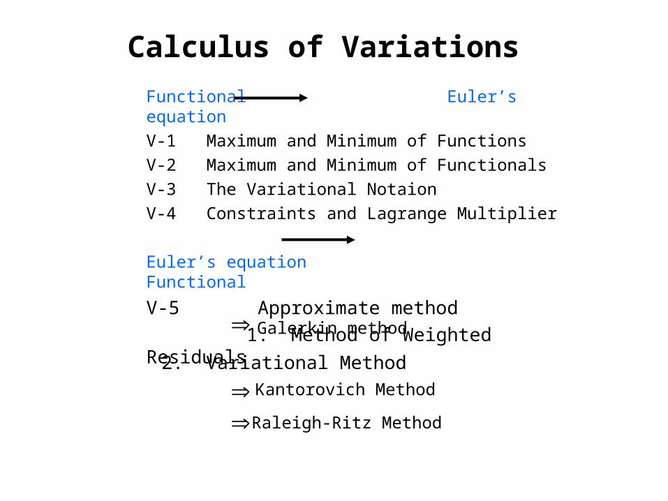
Calculus of Variations
Functional Euler’s equation
V-1 Maximum and Minimum of Functions
V-2 Maximum and Minimum of Functionals
V-3 The Variational Notaion
V-4 Constraints and Lagrange Multiplier
Euler’s equation Functional
V-5 Approximate method
1. Method of Weighted Residuals
Raleigh-Ritz Method
2. Variational Method
Kantorovich Method
Galerkin method
2
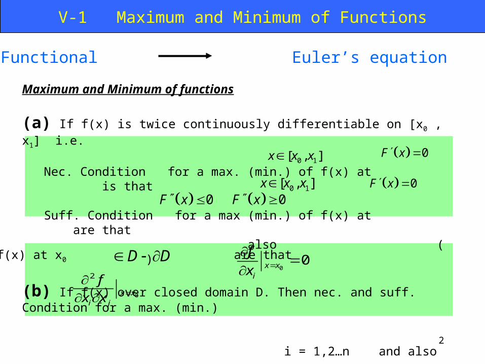
V-1 Maximum and Minimum of Functions
Maximum and Minimum of functions
(a) If f(x) is twice continuously differentiable on [x0 , x1] i.e.
Nec. Condition for a max. (min.) of f(x) at is that
Suff. Condition for a max (min.) of f(x) at are that also ( )
(b) If f(x) over closed domain D. Then nec. and suff. Condition for a max. (min.) i = 1,2…n and also that is a negative infinite .
0 1[ , ]x x x 0F x
0 1[ , ]x x x 0F x
0F x 0F x
D D 0
0x xi
f
x
of f(x) at x0 are that
0
2
x xi j
f
x x
Part A Functional Euler’s equation
3
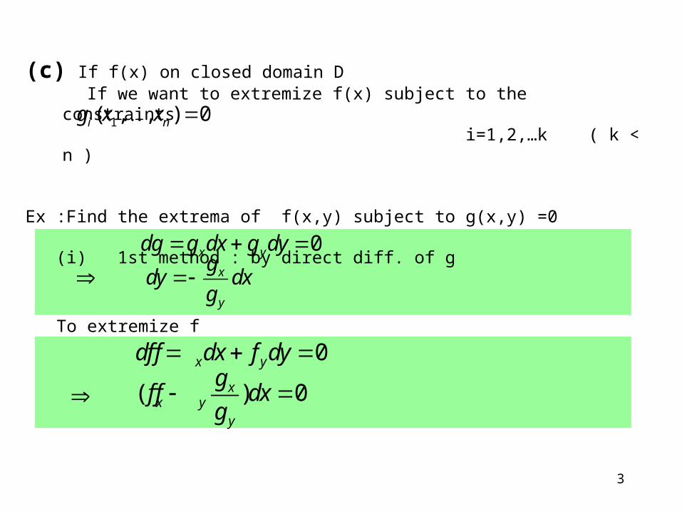
(c) If f(x) on closed domain D If we want to extremize f(x) subject to the constraints i=1,2,…k ( k < n )
Ex :Find the extrema of f(x,y) subject to g(x,y) =0 (i) 1st method : by direct diff. of g
1( , , ) 0i ng x x
0x ydg g dx g dy
x
y
gdy dx
g
0x ydf f dx f dy
( ) 0xx y
y
gf f dx
g
To extremize f
4
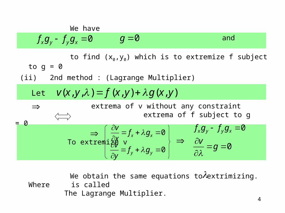
We have and
to find (x0,y0) which is to extremize f subject to g = 0
0x y y xf g f g 0g
(ii) 2nd method : (Lagrange Multiplier)
extrema of v without any constraint extrema of f subject to g = 0
To extremize v
( , , ) ( , ) ( , )v x y f x y g x y
0x x
vf g
x
0y y
vf g
y
0x y y xf g f g
0v
g
Let
We obtain the same equations to extrimizing. Where is called The Lagrange Multiplier.
5
V-2 Maximum and Minimum of Functionals
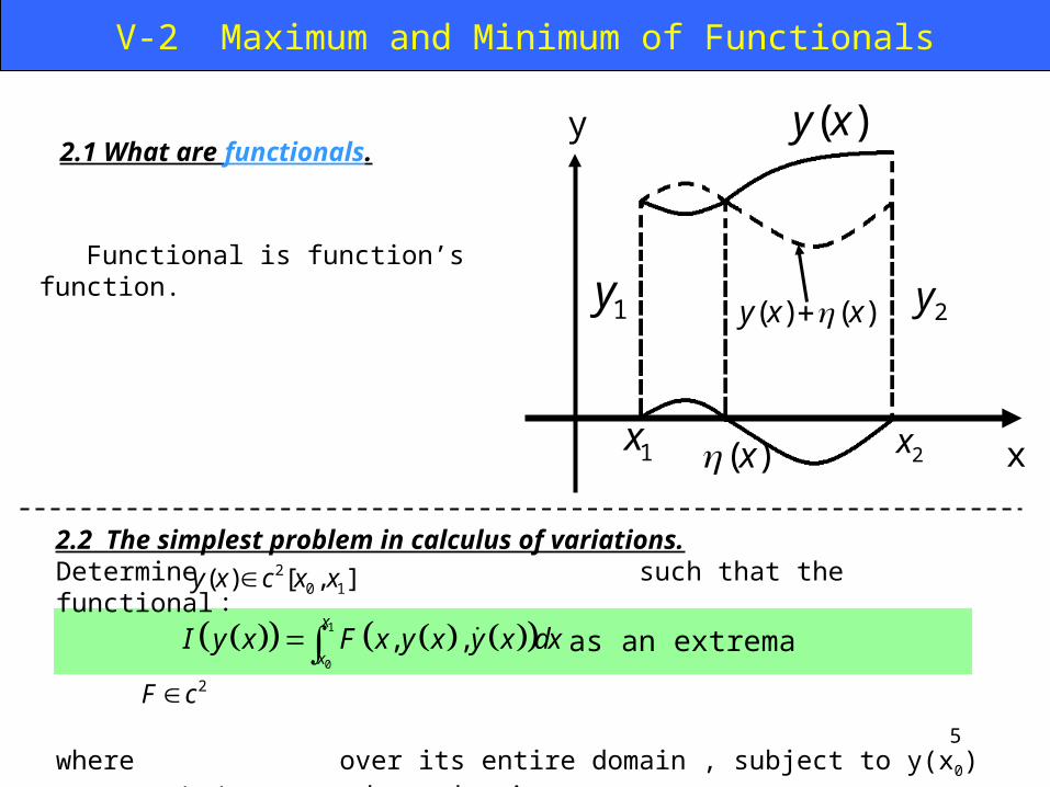
2.1 What are functionals.
Functional is function’s function.
2.2 The simplest problem in calculus of variations.Determine such that the functional :
where over its entire domain , subject to y(x0) = y0 , y(x1) = y1at the end points.
1
0
, ,x
xI y x F x y x y x dx
20 1( ) [ , ]y x c x x
2F c
as an extrema
1y 2y
( )y x
1x 2x( )x
( ) ( )y x x
x
y
6
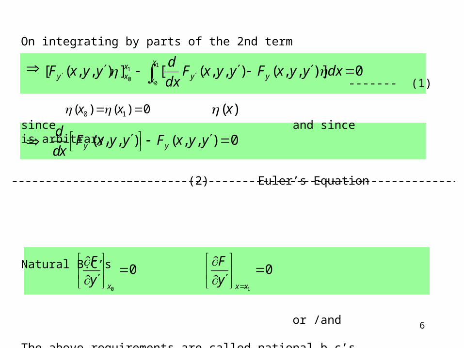
On integrating by parts of the 2nd term
------- (1)
since and since is arbitrary.
-------- (2) Euler’s Equation
Natural B.C’s
or /and
The above requirements are called national b.c’s.
0)],,(),,([]),,([1
0
1
0 dxyyxFyyxF
dx
dyyxF
x
x yyxxy
0 1( ) ( ) 0x x ( )x
( , , ) ( , , ) 0y y
dF x y y F x y y
dx
0
0x
F
y
1
0x x
F
y
7
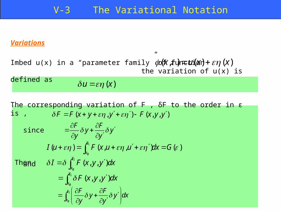
Variations
Imbed u(x) in a “parameter family” of function the variation of u(x) is defined as
The corresponding variation of F , δF to the order in ε is ,
since
and
( , ) ( ) ( )x u x x
( )u x
1
0
( ) ( , , ) ( )x
xI u F x u u dx G
( , ) ( , , )F F x y y F x y y F F
y yy y
1
0
( , , )x
xI F x y y dx
1
0
( , , )x
xF x y y dx
Then
1
0
x
x
F Fy y dx
y y
V-3 The Variational Notation
8
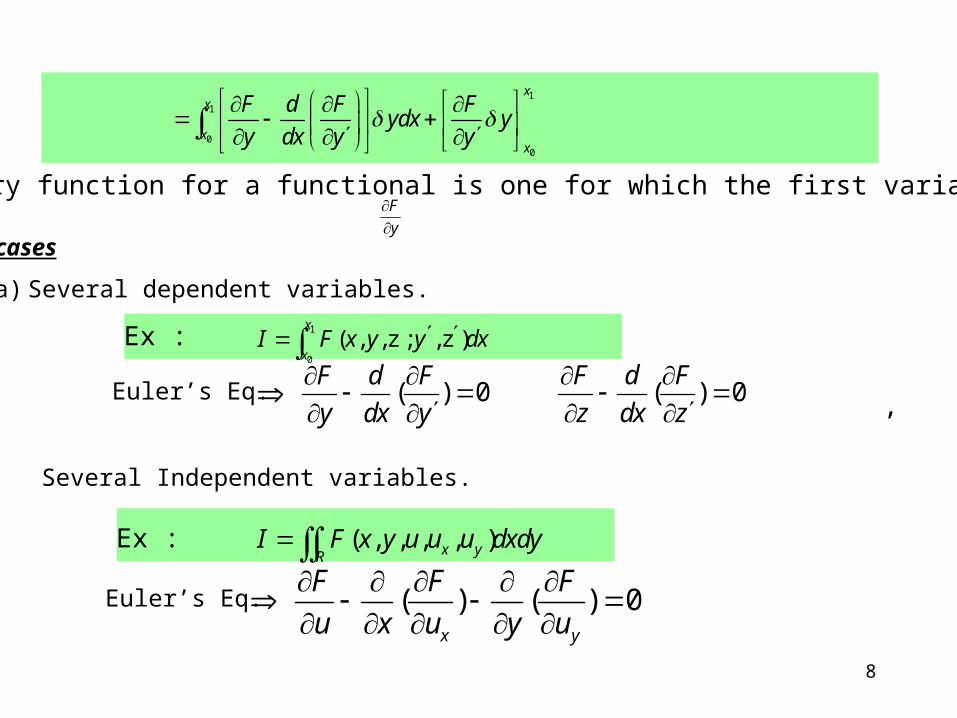
Thus a stationary function for a functional is one for which the first variation = 0.
For the more general cases
,
1
1
0
0
xx
xx
F d F Fydx y
y dx y y
1
0
( , , z ; , z )x
xI F x y y dx Ex :
Ex : ( , , , , )x yRI F x y u u u dxdy
Euler’s Eq.
Euler’s Eq.
F
y
( ) 0F d F
y dx y
( ) 0
F d F
z dx z
(b) Several Independent variables.
(a) Several dependent variables.
( ) ( ) 0x y
F F F
u x u y u
9
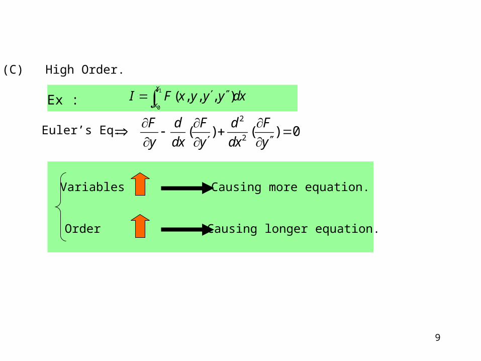
Variables Causing more equation.
Order Causing longer equation.
Ex :1
0
( , , , )x
xI F x y y y dx
Euler’s Eq.2
2( ) ( ) 0
F d F d F
y dx y dx y
(C) High Order.
10
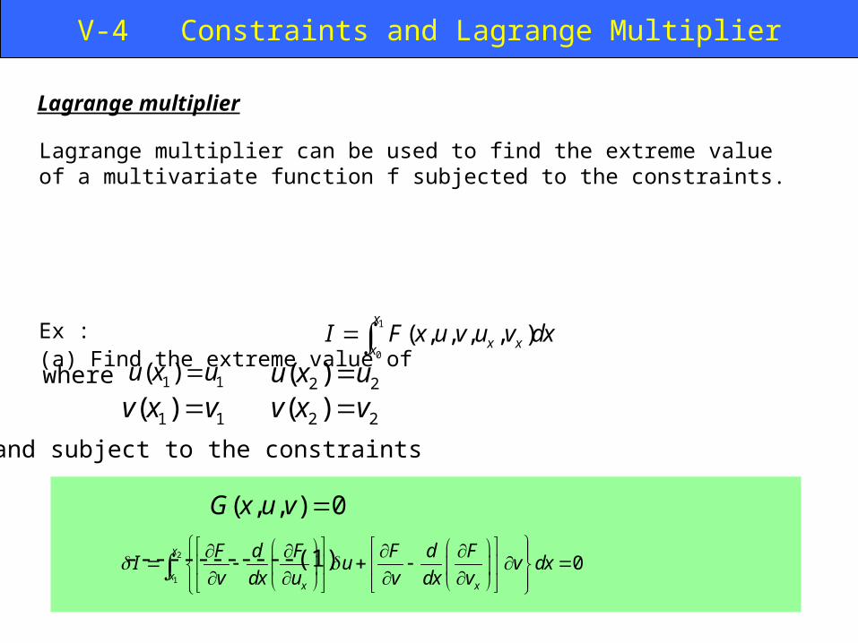
V-4 Constraints and Lagrange Multiplier
Lagrange multiplier can be used to find the extreme value of a multivariate function f subjected to the constraints.
Ex : (a) Find the extreme value of
------------(1) From -----------(2)
1
0
( , , , , )x
x xxI F x u v u v dx
1 1( )u x u 2 2( )u x u1 1( )v x v 2 2( )v x v
where
and subject to the constraints
( , , ) 0G x u v
2
1
0x
xx x
F d F F d FI u v dx
v dx u v dx v
Lagrange multiplier
11
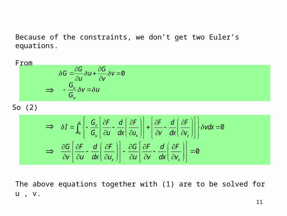
Because of the constraints, we don’t get two Euler’s equations.
From
The above equations together with (1) are to be solved for u , v.
0G G
G u vu v
v
u
Gv u
G
So (2)
1
0
0x
v
xu x x
G F d F F d FI vdx
G u dx u v dx v
0x x
G F d F G F d F
v u dx u u v dx v
12
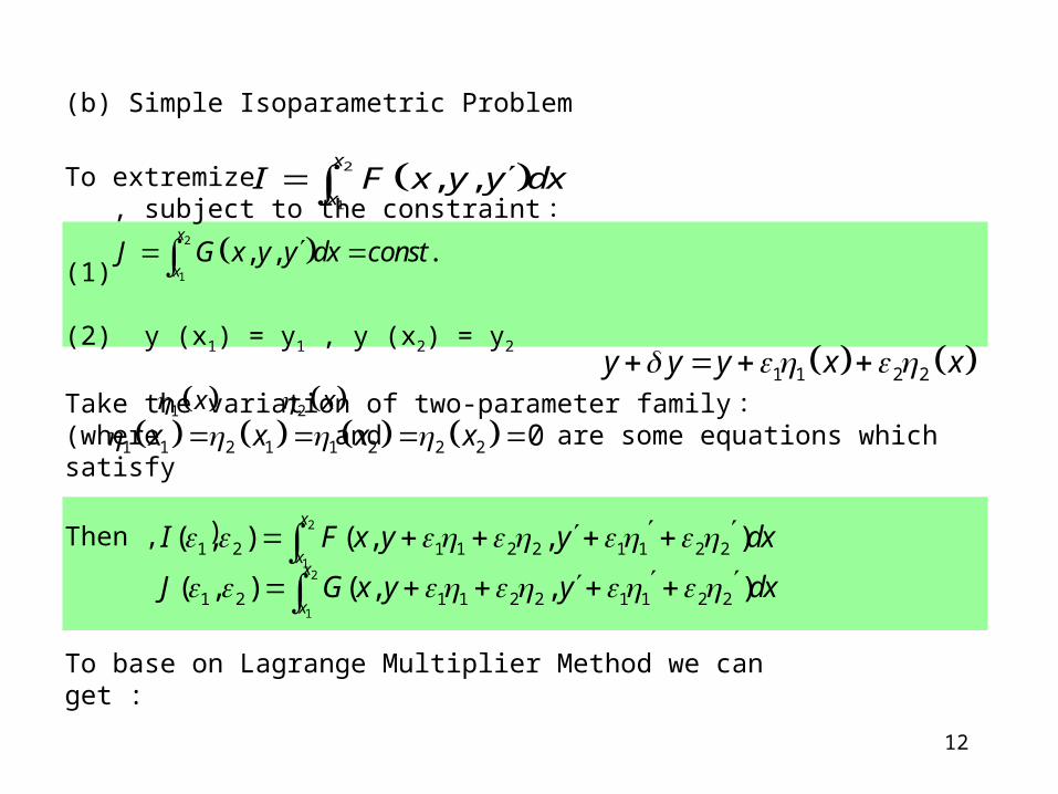
(b) Simple Isoparametric Problem
To extremize , subject to the constraint :
(1)
(2) y (x1) = y1 , y (x2) = y2
Take the variation of two-parameter family :(where and are some equations which satisfy )
2
1
, ,x
xI F x y y dx
2
1
, , .x
xJ G x y y dx const
1 1 2 2y y y x x 1 x 2 x
1 1 2 1 1 2 2 2 0x x x x
Then ,
To base on Lagrange Multiplier Method we can get :
2
11 2 1 1 2 2 1 1 2 2( , ) ( , , )
x
xI F x y y dx
2
11 2 1 1 2 2 1 1 2 2( , ) ( , , )
x
xJ G x y y dx
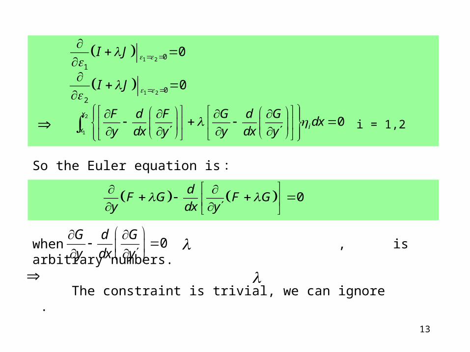
13
1 2 0
1
0I J
1 2 0
2
0I J
2
1
0x
ix
F d F G d Gdx
y dx y y dx y
i = 1,2
So the Euler equation is :
when , is arbitrary numbers.
The constraint is trivial, we can ignore .
0d
F G F Gy dx y
0G d G
y dx y
14
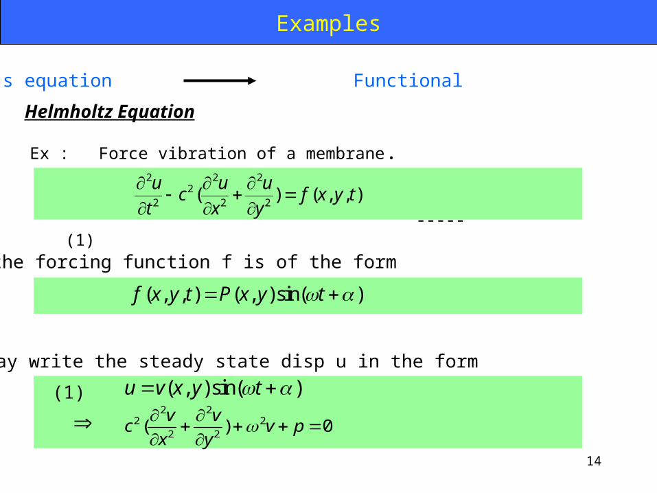
( , , ) ( , )sin( )f x y t P x y t
( , )sin( )u v x y t
2 2
2 22 2
( ) 0v v
c v px y
Euler’s equation Functional
Examples
we may write the steady state disp u in the form
if the forcing function f is of the form
(1)
2 2 22
2 2 2( ) ( , , )
u u uc f x y t
t x y
Ex : Force vibration of a membrane.
-----(1)
Helmholtz Equation
15
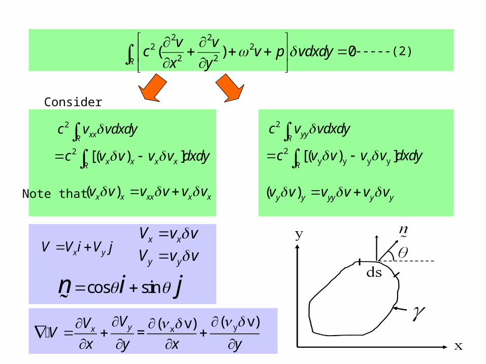
2 22 2
2 2( ) 0
R
v vc v p vdxdy
x y
-----(2)
2xxR
c v vdxdy2 [( ) ]x x x xRc v v v v dxdy
Consider
2yyR
c v vdxdy2
y y y y[( ) ]R
c v v v v dxdy ( )x x xx x xv v v v v v ( )y y yy y yv v v v v v
cos sinn i j
x yV V i V j x xV v v
y yV v v
yx( v)( v)
=yxVV
Vx y x y
Note that
16
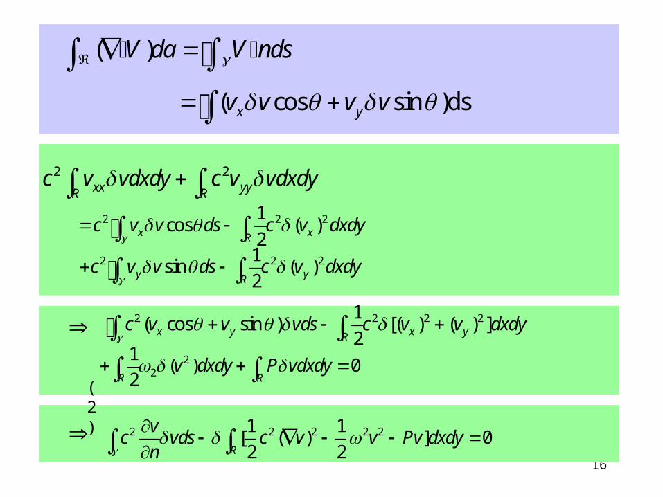
2 2xx yyR R
c v vdxdy c v vdxdy
2 2 21sin ( )
2y yRc v v ds c v dxdy
(2)
2 2 2 21( cos sin ) [( ) ( ) ]
2x y x yRc v v vds c v v dxdy
22
1( ) 0
2R Rv dxdy P vdxdy
2 2 2 2 21 1[ ( ) ] 02 2R
vc vds c v v Pv dxdy
n
( )V da V nds ( cos sin )dsx yv v v v
2 2 21cos ( )
2x xRc v v ds c v dxdy
17
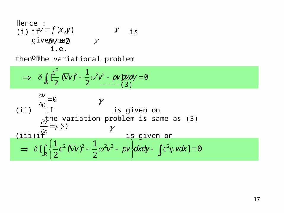
Hence : (i) if is given on i.e. on
then the variational problem
-----(3)
(ii) if is given on the variation problem is same as (3)
(iii) if is given on
( , )v f x y0v
2
2 2 21[ ( ) ] 0
2 2R
cv v pv dxdy
0v
n
( )v
sn
2 2 2 2 21 1[ ( ) ] 0
2 2Rc v v pv dxdy c vdx
18
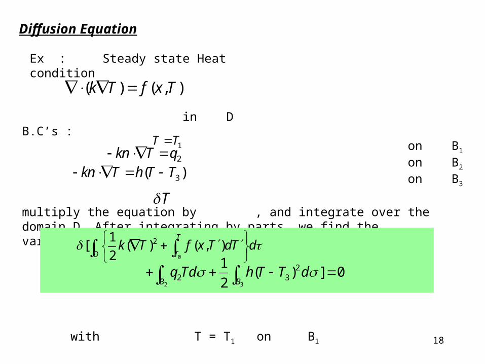
Ex : Steady state Heat condition
in D( ) ( , )k T f x T
B.C’s : on B1
on B2
on B3
multiply the equation by , and integrate over the domain D. After integrating by parts, we find the variational problem as follow.
with T = T1 on B1
1T T2kn T q
3( )kn T h T T
T
0
21[ ( ) ( , )
2
T
D Tk T f x T dT d
2 3
22 3
1( ) ] 0
2B Bq Td h T T d
Diffusion Equation
19
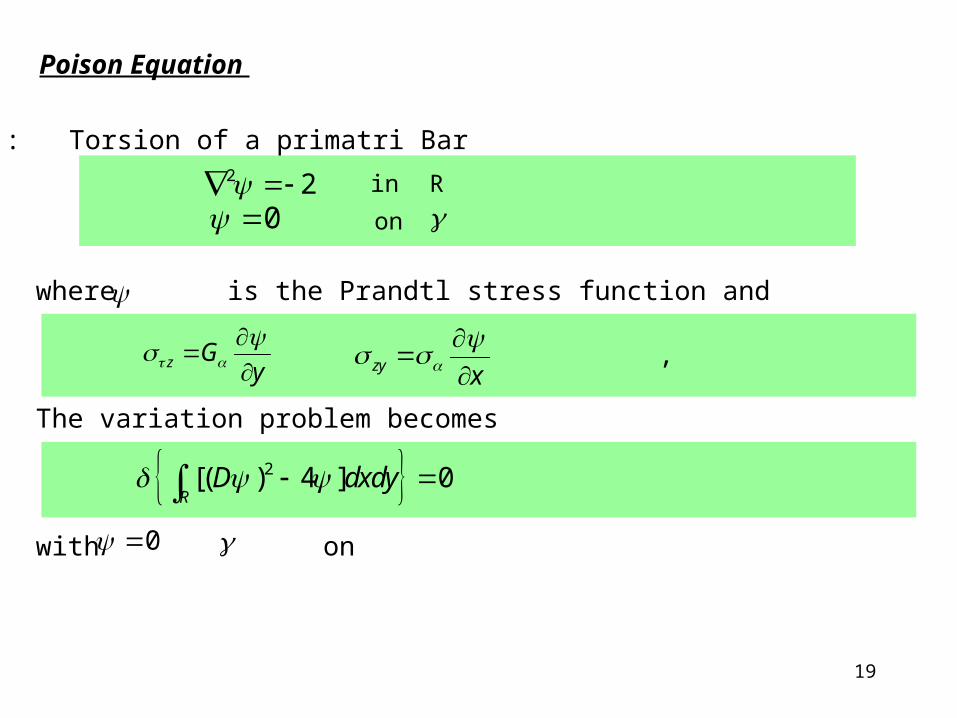
2 2 0 on
in R
Ex : Torsion of a primatri Bar
where is the Prandtl stress function and , The variation problem becomes
with on
z Gy
zy x
2[( ) 4 ] 0RD dxdy
0
Poison Equation
20
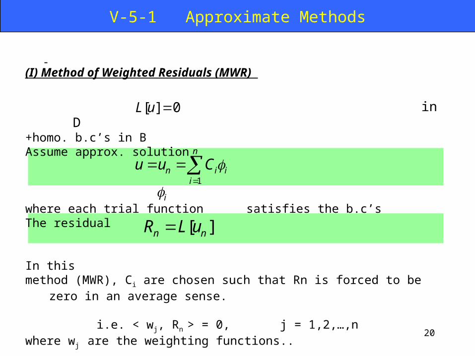
V-5-1 Approximate Methods
(I) Method of Weighted Residuals (MWR)
in D+homo. b.c’s in BAssume approx. solution
where each trial function satisfies the b.c’sThe residual
In this method (MWR), Ci are chosen such that Rn is forced to be zero in an average
sense.
i.e. < wj, Rn > = 0, j = 1,2,…,nwhere wj are the weighting functions..
[ ] 0L u
1
n
n i ii
u u C
i
[ ]n nR L u
21
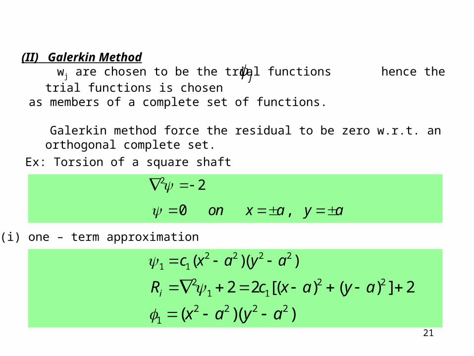
(II) Galerkin Method wj are chosen to be the trial functions hence the trial functions is chosen as members of a complete set of functions.
Galerkin method force the residual to be zero w.r.t. an orthogonal complete set.
j
Ex: Torsion of a square shaft
2 2
0 ,on x a y a
(i) one – term approximation
2 2 2 21 1( )( )c x a y a
2 2 21 12 2 [( ) ( ) ] 2iR c x a y a
2 2 2 21 ( )( )x a y a
22
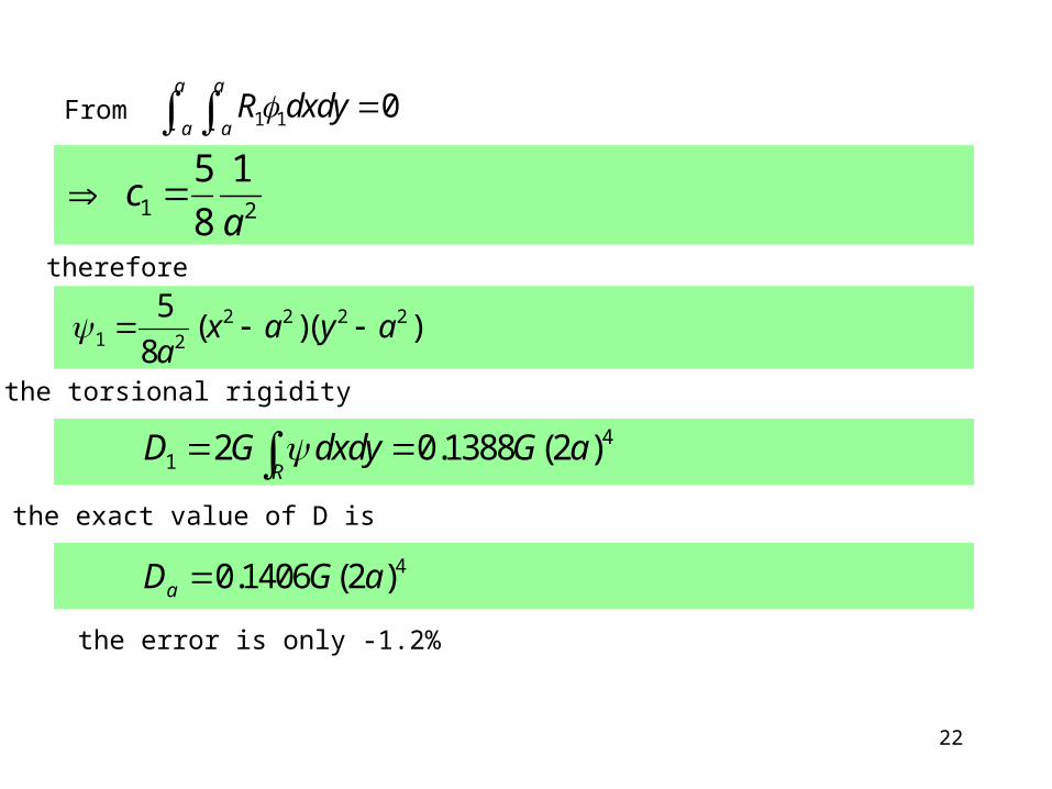
From 1 1 0a a
a aR dxdy
1 2
5 1
8c
a
therefore
2 2 2 21 2
5( )( )
8x a y a
a
the torsional rigidity
41 2 0.1388 (2 )
RD G dxdy G a
the exact value of D is
40.1406 (2 )aD G a
the error is only -1.2%
23
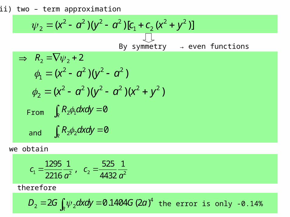
2 2 2 2 2 22 1 2( )( )[ ( )]x a y a c c x y
By symmetry → even functions
2 2 2R 2 2 2 2
1 ( )( )x a y a 2 2 2 2 2 2
2 ( )( )( )x a y a x y
From 2 1 0RR dxdy
and 2 2 0RR dxdy
we obtain
1 22 2
1295 1 525 1,
2216 4432c c
a a
therefore
42 22 0.1404 (2 )
RD G dxdy G a the error is only -0.14%
(ii) two – term approximation
24
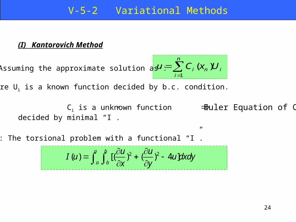
(I) Kantorovich Method
1
( )n
i n ii
u C x U
Assuming the approximate solution as :
where Ui is a known function decided by b.c. condition.
Ex : The torsional problem with a functional “I”.
2 2( ) [( ) ( ) 4 ]a b
a b
u uI u u dxdy
x y
V-5-2 Variational Methods
Ci is a unknown function decided by minimal “I”. Euler Equation of Ci
25
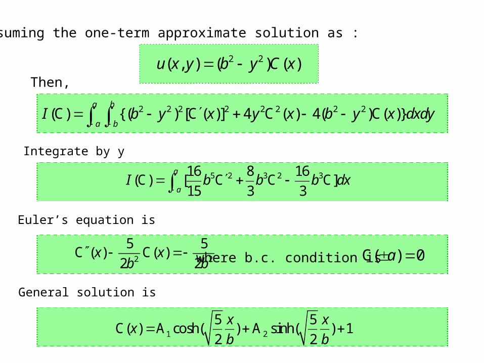
Assuming the one-term approximate solution as :
2 2( , ) ( ) ( )u x y b y C x Then,
2 2 2 2 2 2 2 2(C) {( ) [C ( )] 4 C ( ) 4( )C( )}a b
a bI b y x y x b y x dxdy
Integrate by y
5 2 3 2 316 8 16(C) [ C C C]
15 3 3
a
aI b b b dx
Euler’s equation is
2 2
5 5C ( ) C( )
2 2x x
b b where b.c. condition is C( ) 0a
General solution is
1 2
5 5C( ) A cosh( ) A sinh( ) 1
2 2
x xx
b b
26
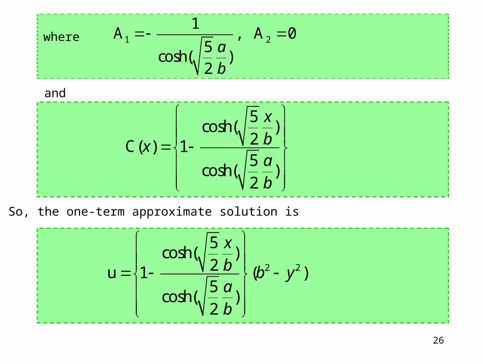
1 2
1A , A 0
5cosh( )
2ab
where
and
5cosh( )
2C( ) 15
cosh( )2
xbxab
So, the one-term approximate solution is
2 2
5cosh( )
2u 1 ( )5
cosh( )2
xb b yab
27
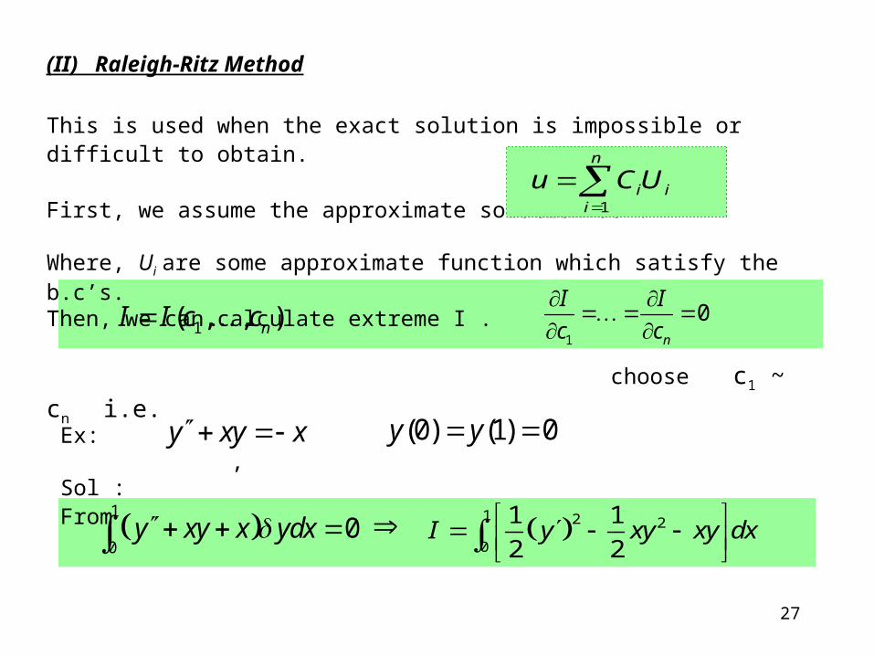
(II) Raleigh-Ritz Method
This is used when the exact solution is impossible or difficult to obtain.
First, we assume the approximate solution as :
Where, Ui are some approximate function which satisfy the b.c’s.Then, we can calculate extreme I .
choose c1 ~ cn i.e.
1
n
i ii
u CU
1( , , )nI I c c 1
0n
I I
c c
y xy x (0) (1) 0y y
1
00y xy x ydx
1 2 2
0
1 1
2 2I y xy xy dx
Ex: , Sol :From
28
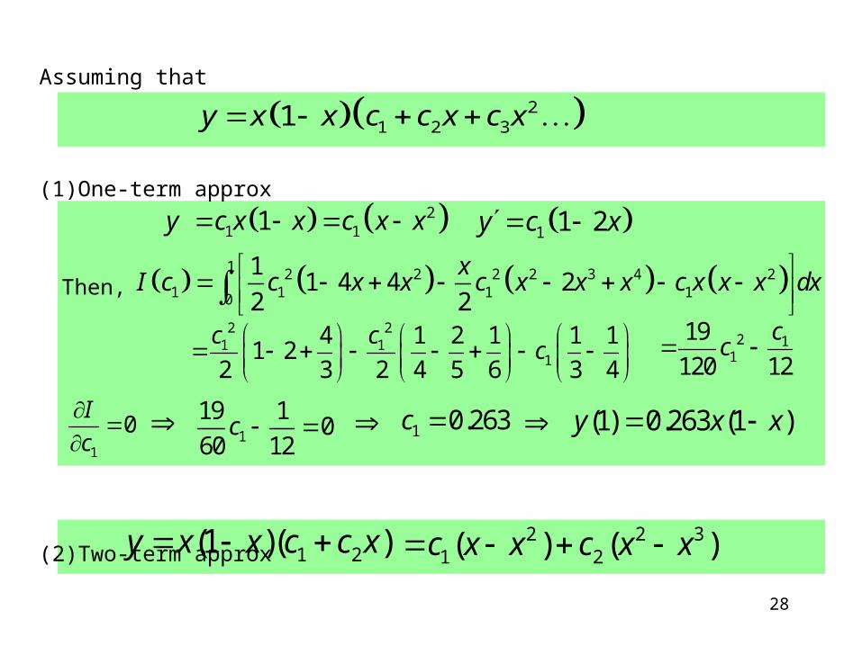
Assuming that
(1)One-term approx
(2)Two-term approx
21 2 31y x x c c x c x
21 11y c x x c x x 1 1 2y c x
1 2 2 2 2 3 4 21 1 1 10
11 4 4 2
2 2
xI c c x x c x x x c x x x dx
2 21 1
1
4 1 2 1 1 11 2
2 3 2 4 5 6 3 4
c cc
2 1
1
19
120 12
cc
1
0I
c
1
19 10
60 12c
1 2(1 )( )y x x c c x 2 2 31 2( ) ( )c x x c x x
(1) 0.263 (1 )y x x 1 0.263c
Then,
29
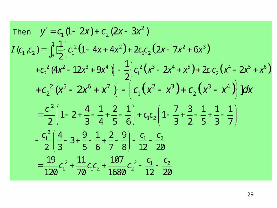
Then 2
1 2(1 2 ) (2 3 )y c x c x x
1 2 2 2 31 2 1 1 20
1( , ) [ 1 4 4 2 2 7 6
2I c c c x x c c x x x
2 2 3 4 2 3 4 5 4 5 63 1 1 2
1(4 12 9 ) 2 2 2
2c x x x c x x x c c x x x
2 5 6 7 2 3 3 42 1 2( 2 ) ]c x x x c x x c x x dx
21
1 2
4 1 2 1 7 3 1 1 11 2 1
2 3 4 5 6 3 2 5 3 7
cc c
2
1 1 24 9 1 2 93
2 3 5 6 7 8 12 20
c c c
2 2 1 21 1 2 2
19 11 107
120 70 1680 12 20
c cc c c c
30
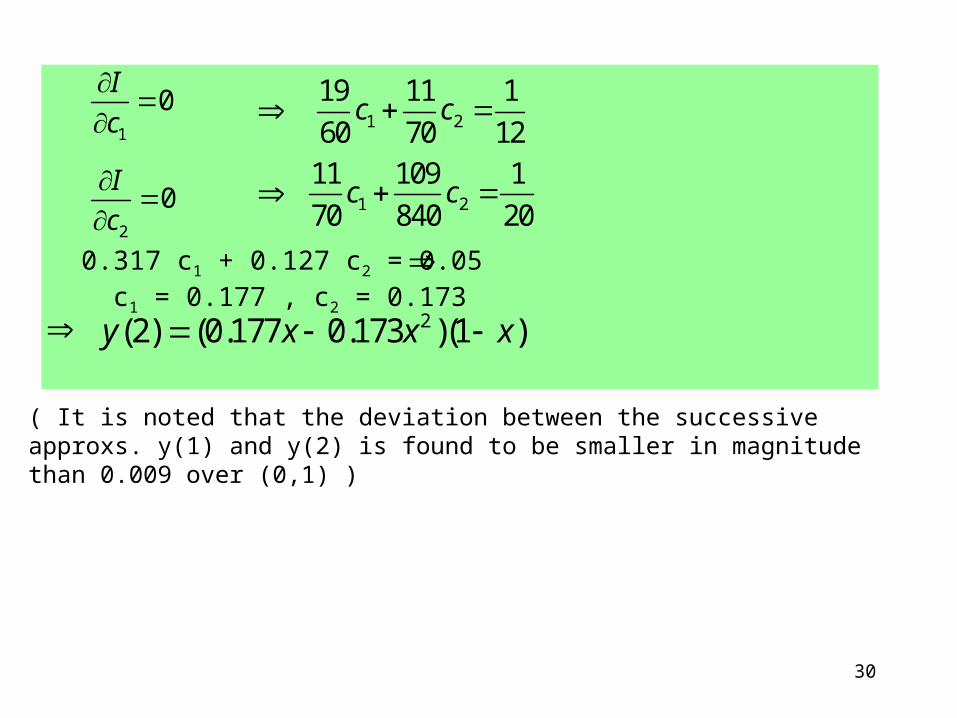
0.317 c1 + 0.127 c2 = 0.05 c1 = 0.177 , c2 = 0.173
1
0I
c
1 2
19 11 1
60 70 12c c
2(2) (0.177 0.173 )(1 )y x x x
( It is noted that the deviation between the successive approxs. y(1) and y(2) is found to be smaller in magnitude than 0.009 over (0,1) )
2
0I
c
1 2
11 109 1
70 840 20c c