calculuscurves nolinks

8/3/2019 CalculusCurves nolinks

http://slidepdf.com/reader/full/calculuscurves-nolinks 1/67

Curves and Gradient

On Curves, every point has a different Gradient

Can you find a rule for getting the Gradient atany point on a Curve?

−4 −3 −2 −1 1 2 3 4 5

1

2

3

4

5

6

7



The Derived FunctionConsider the curve y = f ( x ) (in red) and the gradient of the tangent

at P. Note that as h tends toward 0 the gradient of the line PQapproaches the gradient of the curve at P.

f ( x) =

0

lim

→h h

x f h x f )()( −+



−4 −3 −2 −1 1 2 3 4 5

1

2

3

4

5

6

7



−4 −3 −2 −1 1 2 3 4 5

−1

1

2

3

4

5

6

7



−4 −3 −2 −1 1 2 3 4 5

1

2

3

4

5

6

7

8



For y = x2

Gradient for different x values

X at points -2 -1 0 1 2

gradient -4 -2 0 2 4

What is the Rule for finding gradient at different points (x)?

For y = x2

the Gradient Rule is y’ = 2x

So at the Point where x=1.5, the Gradient is..m = 2x1.5 = 3

−4 −3 −2 −1 1 2 3 4 5

−1

1

2

3

4

5

6

7



−8 −7 −6 −5 −4 −3 −2 −1 1 2 3 4 5 6 7 8

−7

−6

−5

−4

−3

−2

−1

1

2

3

4

5

6

7

y = x^3

At x = -1, Gradient = 3

−8 −7 −6 −5 −4 −3 −2 −1 1 2 3 4 5 6 7 8

−7

−6

−5

−4

−3

−2

−1

1

2

3

4

5

6

7

y = x^3

At x = -2, Gradient = 12

−8 −7 −6 −5 −4 −3 −2 −1 1 2 3 4 5 6 7 8

−7

−6

−5

−4

−3

−2

−1

1

2

3

4

5

6

7

y = x^3

At x = 1, Gradient = 3

−8 −7 −6 −5 −4 −3 −2 −1 1 2 3 4 5 6 7 8

−3

−2

−1

1

2

3

4

5

6

7

8

9

10

11

y = x^3

At x = 2, Gradient = 12

−8 −7 −6 −5 −4 −3 −2 −1 1 2 3 4 5 6 7 8

−6

−5

−4

−3

−2

−1

1

2

3

4

5

6

7

8

y = x^3

At x = 0 Gradient = 0

For Y = x 3



For y = x3

Gradient for different x values

X at points -2 -1 0 1 2

gradient 12 3 0 3 12

What is the Rule for finding gradient at different points (x)?

For y = x3

the Gradient Rule is y’ = 3x2

So at the Point where x=1.5, the Gradient is 3x1.52

=7.75

−8 −7 −6 −5 −4 −3 −2 −1 1 2 3 4 5 6 7 8

−4

−3

−2

−1

1

2

3

4

5

6

7

8

9

10

y = x^3

At x = 1.5 Gradient =7.75



General Rule for getting the Gradient Formula

for ANY Curve’s Equation

For y = x2 y’ = 2x

For y = x3 y’ = 3x2

So to get any Gradient Formula

For a given Curve we use this rule…

Use the Curve’s equation…

“times by the Power & take 1 from the power”



Differentiation rules

Finding the Gradient rule is called Differentiation

The Gradient rule is called dy/dx or y’ or f’(x)

We must write the Original Curve equation using Powers.

There are short cuts to get the y’ for some harder Curve Equations.

Note these types of equations & the short cut way to get its y’…

For Y = ( 3x - 4 )5……..Use “fn of a fn” or “ bracket rule”

For Y = 1 / (3x2 – 1) …use negative powers: y = (3x2 – 1 ) -5

For Y = 4x / ( 3x2 – 1 )… use the Quotient rule

For y = ( 3x2 – 1) ( 3x - 4 )5…… use the Product rule



Equations of Tangents and Normals

Tangents are straight Lines which

touch Curves at a point of Contact .

Normals are straight lines that are perpendicular to tangents, passing

through the point of contact.



−3.0 −2.0 −1.0 1.0 2.0 3.0 4.0A

B

C

Tangent & Normal

Tangent

Norma l

Point of contact

( x1 , y1 )

For Tangent’s Gradient

get Curve’s dy/dx, then sub

x1 into dy/dx

Normal

tangent

For Normal’s Gradient:

Get Tangent’s, then “flip

& change the Sign”



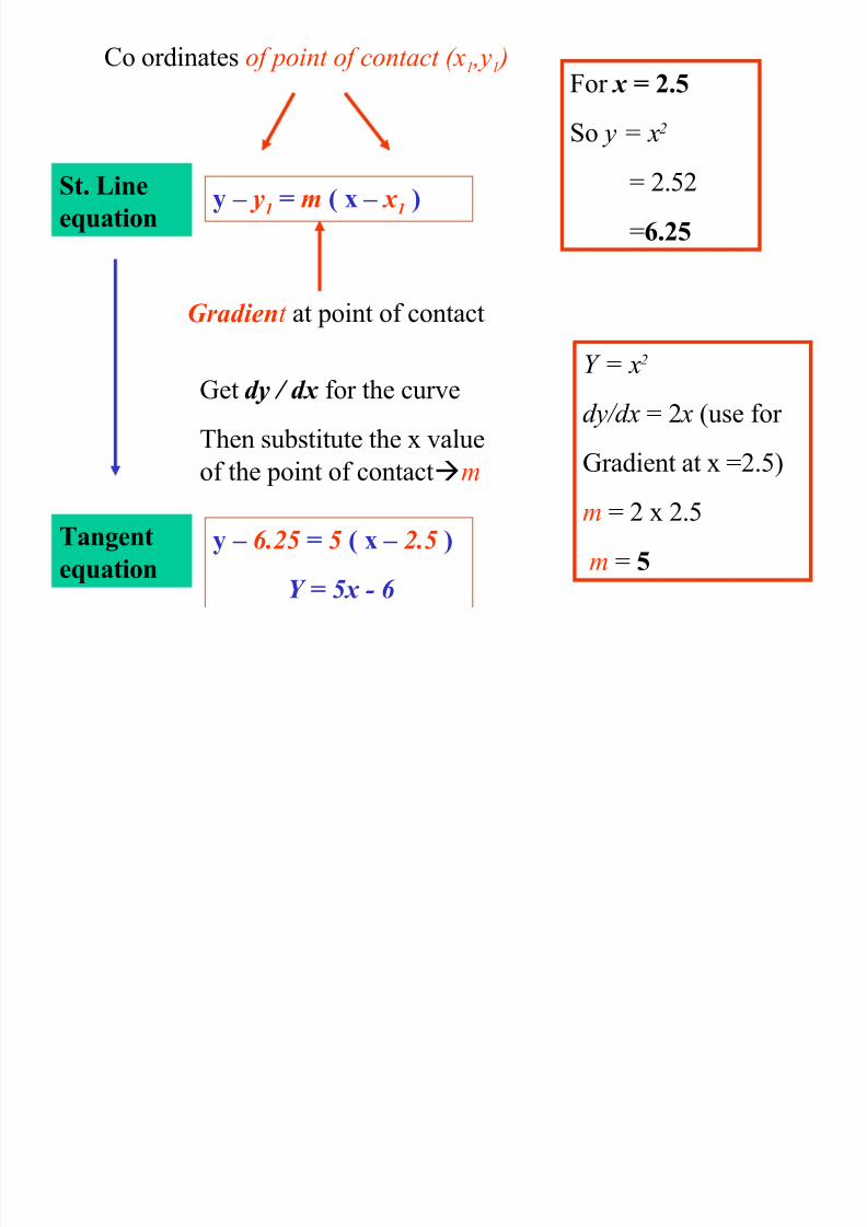
y – 6.25 = 5 ( x – 2.5 )

Y = 5x - 6

Gradient at point of contact

Co ordinates of point of contact (x1 ,y1 )

Get dy / dx for the curve

Then substitute the x value

of the point of contactm

Y = x2

dy/dx = 2 x (use for

Gradient at x =2.5)

m = 2 x 2.5

m = 5

For x = 2.5

So y = x2

= 2.52

=6.25

y – y1 = m ( x – x 1 )

Tangent

equation

St. Line

equation



B

#/2 = 1.2 # = 2.5

Tangent & Gradient

Tangent

Gradient Pt B has x value =

For x 1 = 2.5

So y1 = x2

= 2.52

=6.25

Y = x2

dy/dx = 2 x (use for

Gradient at x =2.5)

m = 2 x 2.5

m = 5

y – y1 = m ( x – x 1 )

y – 6.25 = 5 ( x – 2.5 )

Y = 5x - 6



Equation of Normals

1. GET THE CURVE’S DY/DX

2. SUSTITUTE THE X-VALUE OF THECONTACT POINT. (this gets the tangent

gradient).

3. FLIP & CHANGE THE SIGN (this gets the

normal’s gradient, m ).

4. Use the formula y –y1 = m ( x – x 1 ) for

the normal’s equation.

( x1, y1 ) are the co ordinates of the point of contact



Curves and Gradient2

Where is the Gradient = 0 ? ….For what x value(s)?

Where is the Gradient Positive? ….For what x value(s)?

Where is the Gradient Negative ? ….For what x value(s)?

The Gradient features of Curves….Positive Negative Zero

Help us to Describe Curves and to Draw them



5.0

−15.0

−10.0

−5.0

5.0

10.0

15.0

y = x^3-12x



5.0

−15.0

−10.0

−5.0

5.0

10.0

15.0

y = 12x - x^3



5.0

−15.0

−10.0

−5.0

5.0

10.0

15.0

y = x^4 - 8x^2



5.0

−15.0

−10.0

−5.0

5.0

10.0

15.0

y = 8x^2 - x^4



5.0

y = (x - 4)^3



5.0

y = (4 - x)^3



5.0

10.0

y = x^4- 16/3*x^3 + 8x^2



5.0

y = 8/3*x^3 - x^4



5.0

y = x^4 + 2



5.0

y = 5 - x^4



Stationary Points

Where the Gradient is 0 “Stationary Points”..the curve “turns”

Either side of these Stationary Points (flat)….

the Gradient could be Positive (“Increasing”) or

Negative (“Decreasing”)

−4 −3 −2 −1 1 2 3 4 5

−4

−3

−2

−1

1

2

3

4y = x^2

−4 −3 −2 −1 1 2 3 4 5

−4

−3

−2

−1

1

2

3

4y = -x^2

−4 −3 −2 −1 1 2 3 4 5

−4

−3

−2

−1

1

2

3

4 y = x^3



Curve Sketching example.

Finding the Stationary Points

Curve Equation

Get dy/dx

1stDerivative

Solvedy/dx=0

Get thematching

Y-value(s)

F(x) F’(x) F’(x) = 0

X =..

Use f(x) ;substitute the xvalue(s) and get

the matching Y-values

This gets the Stationary Points for the curve …

“Flats” atthese x’s




Finding the Stationary Points

Curve Equation

Get dy/dx

1stDerivative

Solvedy/dx=0

Get thematching

Y-value(s)

Y = X3 – 3x Y’ = 3x2 - 3 3x2 – 3 = 0

X2 = 1

X = +1 & -1

For X=1 get

>y=13-3x1=-2

For x=-1 get ..

Y=-13-3x-1=2

Stationary Points for the curve are… (1,-2) & (-1,2)

“Flats” at

these x’s



−4 −2 2 4

−4

−2

2

4

(x,y) = (1,-2)

(x,y) = (-1,2)


Sketching using the Stationary Points

1.Plot Point (1.-2)

Turning point”max2.Plot Point (1.-2)

Turning point”min




Sketching using the Stationary Points

−4 −2 2 4

−4

−2

2

4y = x^3 - 3x

(x,y) = (1,-2)

(x,y) = (-1,2)

2.Plot Point (1.-2)

Turning point”min

1.Plot Point (1.-2)

Turning point”max

3.Join the dots & fill in



Concavity

Maximum, Minium or….?

3 types of turning points/ stationary points.

Minimum

Maximum

Horizontal inflexion

How do we find which type of stationary point we have?



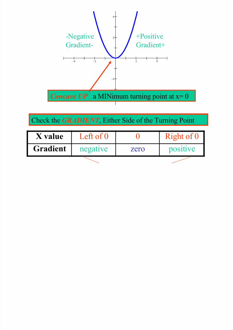
−4 −2 2 4

−4

−2

2

4

Concave UP a MINimum turning point at x= 0

Check the GRADIENT , Either Side of the Turning Point

-NegativeGradient- +PositiveGradient+

X value Left of 0 0 Right of 0

Gradient negative zero positive



−4 −3 −2 −1 1 2 3 4 5

−4

−3

−2

−1

1

2

3

4y = -x^2Concave DOWN a MAXimum turning point at x=0

Check the GRADIENT , Either Side of the Turning Point


Gradient positive zero negative

-Negative

Gradient-+Positive

Gradient+



−4 −3 −2 −1 1 2 3 4 5

−4

−3

−2

−1

1

2

3

4 y = x^3

½ MIN JOINED TO ½ MAX

HORIZONTAL INFLEXION

Flat Point at x = 0

-Negative

Gradient-

-Negative

Gradient-

Check the GRADIENT , Either Side of this Turning Point


Gradient negative zero negative



Types of Turning Points

How to determine the Nature of Stationary points

1. Solve dy/dx = 0 to get the x values of the stationary

points

2. Check the SIGN of the Gradient either side of each x

value ( Positive? Negative? ). Thus see if

3. Min ..concave UP4. Max .. concave DOWN

5. Horizontal Inflexion… SAME gradient left & right



X value Left of SP SP X Right of SP

Gradient ? zero ?

Concave DOWN a MAXimum turning point at x=0

Concave UP a MINimum turning point at x= 0

Horizontal Inflexion..½ MIN JOINED TO ½ MAX

Neg zero Pos

Neg zero Neg Pos zero Pos

Pos zero Neg



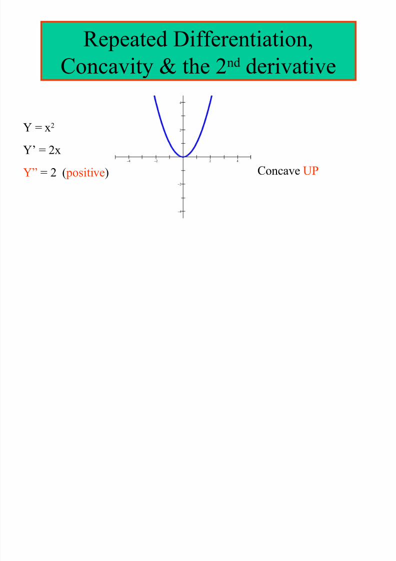
Repeated Differentiation,

Concavity & the 2nd derivative

Y = x2

Y’ = 2x

Y” = 2 ( positive)

−4 −2 2 4

−4

−2

2

4

Concave UP

BOTH “CONCAVE UP” & “CONCAVE DOWN”.



BOTH CONCAVE UP & CONCAVE DOWN .

WHERE DOES CONCAVITY CHANGE ?

−4 −3 −2 −1 0 1 2 3 4 5−2 0

−1 5

−1 0

−5

0

5

10

15

M=0

M=-9

M=-11

M=-12

M=-11

M=-9

M=0

Y=12x-x3

Y’=12-3x2

Y”= -6x

Where is Gradient the Greatest,

between the 2

turning points?

The concavity changes at some point between the 2 turning points.



Y = x2

Y’ = 2x

Y” = 2 ( positive)−4 −2 2 4

−4

−2

2

4

Concave UP

Y = -x2

Y’ = -2x

Y” = -2 (negative) Concave DOWN

−4 −3 −2 −1 1 2 3 4 5

−4

−3

−2

−1

1

2

3

4y = -x^2



Y=12x-x3

Y’=12-3x2

Y”= -6x

Y” values at

Pts. ..2nd

derivative values

shown.

Y”=12

Y”=6

Y”=3

Y”=0

Y”=-3

Y”=-6

Y”=-12

The Sign of Y” value at a point indicates the Concavity at that point.

Positive+ Y” C.UP …. Negative- Y” C.DOWN

The Sign of the Y” value at a Point, and the Concavity at that point.



−4 −3 −2 −1 0 1 2 3 4 5−2 0

−1 5

−1 0

−5

0

5

10

15

Y”=0 for the x-value at

this point ( x= -1.2)

Y”=0 for the x-value

at this point ( x=1.2)

Y=8x^2-x^4

Inflexion points & 2nd Derivative (y”)



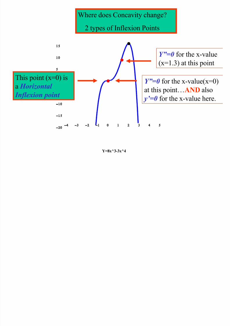
−4 −3 −2 −1 0 1 2 3 4 5−2 0

−1 5

−1 0

−5

0

5

10

15

Where does Concavity change?

2 types of Inflexion Points

Y”=0 for the x-value

(x=1.3) at this point

Y”=0 for the x-value(x=0)

at this point…AND also

y’=0 for the x-value here.

This point (x=0) isa Horizontal

Inflexion point

Y=8x^3-3x^4



2 types of Inflexion Points

“ordinary” InflexionPoint

“Horizontal

Inflexion Point

“Visible” pt.

y”=0 AND

y’=0

“Not Visible”..

y”=0

Finding Inflexion Points Where the change in Concavity occurs



Finding Inflexion Points..Where the change in Concavity occurs

Solve Y” = 0 x-values of possible Inflexions (both types)

Y = f(x) y’ = f’(x) y” = f”(x)

Solve

f’(x) = 0

stat.point

x -values

Solve f”(x)

= 0 possible

InflexionPt

x -values

Test if

genuine:

Check y”

changes+/-

Get the

y-values

using

y=f(x)

Get the

y-values

using

y=f(x)

Test if

Concave UP

or Down, or

Horz Inflxn:

Stationary

points

Inflexion

points

30

yOriginal

Moving tangent to a cubic



-20

-15

-10

-5

0

5

10

15

20

25

-5 -4 -3 -2 -1 0 1 2 3 4 5

x

y functionMoving tangent to a cubicPress the spinners to change the coefficients.

y = 1 x³ – 3 x² + 3 x + 5

ngent at x = 1.0

Function is y = 1x³ – 3x² + 3x + 5

At x = 1.0 , the gradient is 0.00

at x = 1.0 , the value of Y" is 0

T

Y=x3-3x2+3x+5

Y’=3x2-6x+3

Y”=6x-6

Stationary Pts :Y’ = 0 x = 1

Inflexion Pts : Y” = 0 x =1

25

30

y Original

functiony = 1 x³ – 3 x² – 6 x + 5



-20

-15

-10

-5

0

5

10

15

20

25

-5 -4 -3 -2 -1 0 1 2 3 4 5

x

y

ngent at x = 1.0

Function is y = 1x³ – 3x² – 6x + 5

At x = 1.0 , the gradient is -9.00

at x = 1.0 , the value of Y" is 0

T

Y=x3-3x2-6x+5

Y’=3x2-6x-6

Y”=6x-6

Stationary Pts :Y’ = 0 x = -0.8 & x = 2.7

Inflexion Pts : Y” = 0 x =1

Concave UP x>1 & Concave DOWN x<1

3



−2 −1 1 2 3

−2

−1

1

2

Y = x4 – x2

Y’ = 4x3 – 2x

y’” = 12x2-2

Stationary Pts :Y’ = 0 x = 0 & x = 0.7 & x = -0.7

Inflexion Pts : Y” = 0 x =0.4 & x= -0.4

Concave UP : x<-0.4 & x>0.4 Concave Down –0.4,x,0.4



−5 5 10

−5

5

B

6-3## = 6.00

-6# = 0.00

Gradient =

Y" value =

Gradient & Y" values at Points on the Curve.

Anim>use # slider

y=6x-x^3

Concave up

Y” positive

Concave down

Y” negative

Inflexion pt..

Y” = 0, for this

point’s x value

C



−5 5

−5

5

B

y=6x-x^3

Decreasing

X<-1.4

Decreasing

X>1.4

Increasing-

1.4<x<1.4



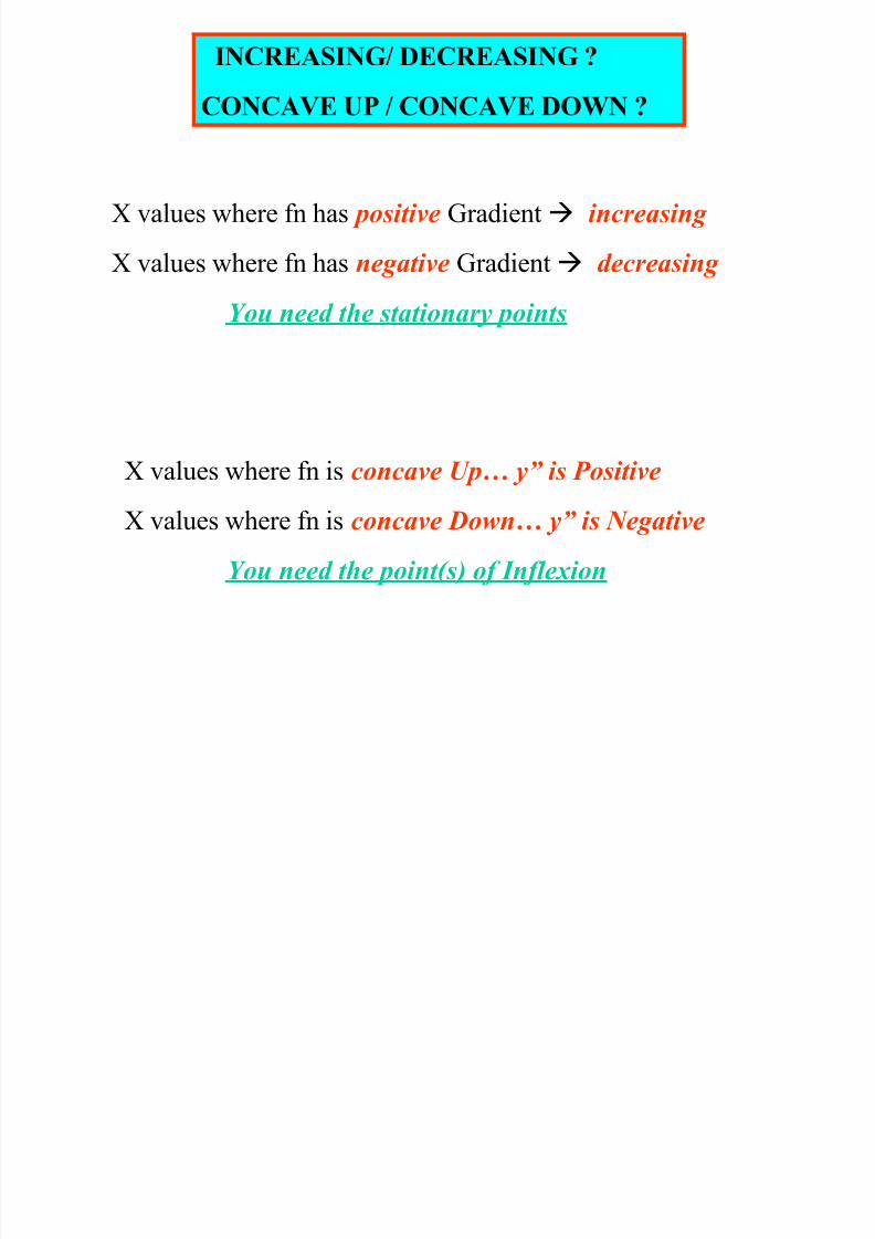
INCREASING/ DECREASING ?

CONCAVE UP / CONCAVE DOWN ?

X values where fn has positive Gradient increasing

X values where fn has negative Gradient decreasing

You need the stationary points

X values where fn is concave Up… y” is Positive

X values where fn is concave Down… y” is Negative

You need the point(s) of Inflexion

G phs f R l Lif Sit ti ns (2)



Discuss what happens to p as q increases in each of the graphs below,

then match each graph to a statement on the right.

p increases quickly at

first, then more slowly

1 2

3

q q

q

p p

p

4 q

p

p increases slowly at

first, then more quickly

p increases slowly at

first, then more quickly

then slowly again

p increases quickly at

first, then more slowly,

then quickly again

2

1

4

3

Graphs of Real-Life Situations (2)

Graphs of Real Life Situations (4)



Population

P o p u l a t i o n

1955 2005

The graphs below show how the population of four small African countries

changed over a 50 year period. Match each graph to a statement.

P o p u l a t i o n

1955 2005

P o p u l a t i o n

1955 2005

P o p u l a t i o n

1955 2005

The population

declined steadily over

the period.

The population

increased slowly at

first, but then increasedmore quickly.

The population

increased steadily over

the period.

The population

increased quickly at

first, but then increased

more slowly.

1 2

3 4

Graphs of Real-Life Situations (4)

Water is poured into each of the containers below at a



Water 11 2 3 4

dd d

t t

d

tt

Water is poured into each of the containers below at a

constant rate of 250 ml per second. The graphs show

how the depth d of the water varies with time t. Match

the container to its corresponding graph.

A B C D



Graph of 1st Derivative Y’

from the Original Function graph Y

Can you see connections between a function’s Graph

and the graph of its Derivative?

A Function’s Derivative Graph shows the

ORIGINAL-Graph’s Gradient Values

Can you tell the Original Graph’s Gradient-features from

its Gradient f” Graph, & hence do a sketch of f(x)?

a b c d e f from to y on 1



0 0 0 1 0 0 -4 4 y' on 1

x 5

x 4

x 3

x 2

x c

Function Derivative

-2

0

2

4

6

8

1 0

1 2

1 4

1 6

1 8

-6 -4 -2 0 2 4 6

-1 0

-8

-6

-4

-2

0

2

4

6

8

10

-6 -4 -2 0 2 4 6

Gradient values

Where is the Gradient Zero? Positive? Negative?




0 0 1 1 0 0 -4 4 y' on 1

x 5

x 4

x 3

x 2

x c

Function Derivative

-6 0

-4 0

-2 0

0

2 0

4 0

6 0

8 0

1 0 0

-6 -4 -2 0 2 4 6

-1 0

0

10

20

30

40

50

60

-6 -4 -2 0 2 4 6

Gradient values





y

0 1 -4.5 -2.5 0 0 -4 6.1 y' on 1

x 5

x 4

x 3

x 2

x c

Function Derivative

-200

-100

0

100

200

300

400

500

600

-6 -4 -2 0 2 4 6 8

-500

-400

-300

-200

-100

0

100

200

300

400

500

-6 -4 -2 0 2 4 6 8

Gradient values




Max Min Problems

Calculus finds Min/Max points on curves from their equations.

We use the same ideas to solve these Practical Problems.

We can find the Maximum Area possible for a box, (with specified

volume & shape restrictions) form the various boxes that fit these

specifications.

We need a formula to differentiate for the Max (or Min)

property required (such as Area). This is based on given a

variable of the given shape (such as length of its base).



A Stone is thrown

into the Air

The Height of the Stone

at different times is given

by this formula:

H = 4 + 3t - t 2

Find the Time when the Maximum height occurs using Calculus.

The actual Maximum Height.

Confirm it is a Max using Calculus.

−6 −4 −2 2 4 6

−4

−2

2

4

6y = 4 + 3x - x^2

For Time from T = 0 to when it hits the ground (t=4)

For t = 1.5 --> h = 6.25



A Stone is thrown

into the Air

The Height of the Stone

at different times is given

by this formula:

H = 4 + 3t - t 2

Maximum height occurs when dh/dt =0 0 =3 – 2t t =1.5

Maximum Height? ..When t =1.5 , h = 4 + 3 x 1.5 – 1.52 So h=6.25

It is a Max since h” is Negative when t = 1.5. Thus Max when t = 1.5..

−6 −4 −2 2 4 6

−4

−2

2

4

6y = 4 + 3x - x^2

For Time from T = 0 to when it hits the ground (t=4)

For t = 1.5 --> h = 6.25

Y k B i h V l f 240 2



You want to make a Box with a Volume of 240 m2

Using the LEAST amount of Cardboard

What is the formula for the Surface Area of this Box?

The Box must be a Rectangular

Prism with a Square base

What is the Formula for

the Volume of this Box?

A = 2x 2 + 4xh

V = x 2 x h

So 240 = x 2 x h

x

x

h

Using Calculus to solve Maximum / Minimum Problems



Box Area (Volume=240, x is square base side) A= 2x 2 + 960/x

How do you get this Area equation? Use the 2nd equationto eliminate the unwanted variable

from the main equation

How does Calculus get

the Minimum Area?

A= 2x 2 + 960/x

dA/dx =4x – 960/x 2

Solve 0 = 4x –960/x 2

X = 6.2

A = 2x 2 + 4x h

A = 2x 2 + 4x( 240/x 2 )

1 2 3 4 5 6 7 8

10 0

20 0

30 0

40 0

50 0

60 0

70 0

80 0

90 0

y = 2xx + (960/x)

T he S qu are

4 A r e a v C i r c l e P



and Circle problem 1 9 2 2 1 9 2 2 1 9 2 2 1 9 2 2 1 9 2 2 1 9 2 2 1 9 2 2 1 9 2 2 1 9 2 2

1 9 2 2 1 9 2 2 1 9 2 2 1 9 2 2 1 9 2 2 1 9 2 2 1 9 2 2 1 9 2 2 1 9 2 2

1 9 2 2 1 9 2 2 1 9 2 2 1 9 2 2 1 9 2 2 1 9 2 2 1 9 2 2 1 9 2 2 1 9 2 2

1 9 2 2 1 9 2 2 1 9 2 2 1 9 2 2 1 9 2 2 1 9 2 2 1 9 2 2 1 9 2 2 1 9 2 2

1 9 2 2 1 9 2 2 1 9 2 2 1 9 2 2 1 9 2 2 1 9 2 2 1 9 2 2 1 9 2 2 1 9 2 2

1 9 2 2 1 9 2 2 1 9 2 2 1 9 2 2 1 9 2 2 1 9 2 2 1 9 2 2 1 9 2 2 1 9 2 2

1 9 2 2 1 9 2 2 1 9 2 2 1 9 2 2 1 9 2 2 1 9 2 2 1 9 2 2 1 9 2 2 1 9 2 2

1 9 2 2 1 9 2 2 1 9 2 2 1 9 2 2 1 9 2 2 1 9 2 2 1 9 2 2 1 9 2 2 1 9 2 2

1 9 2 2 1 9 2 2 1 9 2 2 1 9 2 2 1 9 2 2 1 9 2 2 1 9 2 2 1 9 2 2 1 9 2 2

1 9 2 2 1 9 2 2 1 9 2 2 1 9 2 2 1 9 2 2 1 9 2 2 1 9 2 2 1 9 2 2 1 9 2 2

1 9 2 2 1 9 2 2 1 9 2 2 1 9 2 2 1 9 2 2 1 9 2 2 1 9 2 2 1 9 2 2 1 9 2 2

1 9 2 2 1 9 2 2 1 9 2 2 1 9 2 2 1 9 2 2 1 9 2 2 1 9 2 2 1 9 2 2 1 9 2 2

1 9 2 2 1 9 2 2 1 9 2 2 1 9 2 2 1 9 2 2 1 9 2 2 1 9 2 2 1 9 2 2 1 9 2 2

1 9 2 2 1 9 2 2 1 9 2 2 1 9 2 2 1 9 2 2 1 9 2 2 1 9 2 2 1 9 2 2 1 9 2 2

1 9 2 2 1 9 2 2 1 9 2 2 1 9 2 2 1 9 2 2 1 9 2 2 1 9 2 2 1 9 2 2 1 9 2 2

1 9 2 2 1 9 2 2 1 9 2 2 1 9 2 2 1 9 2 2 1 9 2 2 1 9 2 2 1 9 2 2 1 9 2 2

1 9 2 2 1 9 2 2 1 9 2 2 1 9 2 2 1 9 2 2 1 9 2 2 1 9 2 2 1 9 2 2 1 9 2 2

1 9 2 2 1 9 2 2 1 9 2 2 1 9 2 2 1 9 2 2 1 9 2 2 1 9 2 2 1 9 2 2 1 9 2 2

1 9 2 2 1 9 2 2 1 9 2 2 1 9 2 2 1 9 2 2 1 9 2 2 1 9 2 2 1 9 2 2 1 9 2 2

1 9 2 2 1 9 2 2 1 9 2 2 1 9 2 2 1 9 2 2 1 9 2 2 1 9 2 2 1 9 2 2 1 9 2 2

1 9 2 2 1 9 2 2 1 9 2 2 1 9 2 2 1 9 2 2 1 9 2 2 1 9 2 2 1 9 2 2 1 9 2 2

1 9 2 2 1 9 2 2 1 9 2 2 1 9 2 2 1 9 2 2 1 9 2 2 1 9 2 2 1 9 2 2 1 9 2 2

1 9 2 2 1 9 2 2 1 9 2 2 1 9 2 2 1 9 2 2 1 9 2 2 1 9 2 2 1 9 2 2 1 9 2 2

1 9 2 2 1 9 2 2 1 9 2 2 1 9 2 2 1 9 2 2 1 9 2 2 1 9 2 2 1 9 2 2 1 9 2 2

1 9 2 2 1 9 2 2 1 9 2 2 1 9 2 2 1 9 2 2 1 9 2 2 1 9 2 2 1 9 2 2 1 9 2 2

- 4

- 3

- 2

- 1

0

1

2

3

- 4 - 3 - 2 - 1 0 1 2 3 4

0

5

1 0

1 5

2 0

2 5

3 0

3 5

0 1 0 2 0 3 0

L e n g t h o f c i rc le

T o t a l A r e a o f S q u a r e

a n d C i r c l e

A 2 0 c m st r i n g i s c u t i

p i e c e s. T h e f i rst p i e c esh a p e d i n t o a c i rc l e a

se c o n d i n to a s q u a r e .

W h e r e w a s th e s tr i n g

i s fo u n d t h a t th e t o ta l

th e s q u a r e a n d c i r c l e

b e e n m i n im i se d ?

calculuscurves nolinks

Documents