calfem - a finite element toolbox to matlab, version 3homes.civil.aau.dk/lda/fem/pdfcalfem.pdf ·...
TRANSCRIPT

Structural Mechanics & Solid MechanicsDepartment
ofMechanics
andMaterials
Report TVSM
-9001C
A L F E M
- A FIN
ITE ELEMEN
T TOO
LBOX
TO M
ATLA
B Version 3.3
C A L F E MA finite element toolbox to MATLABVersion 3.3

C A L F E MA finite element toolbox to MATLAB
Version 3.3
Copyright © 1999 by Structural Mechanics, LTH, Sweden.Printed by JABE Offset, Lund, Sweden.
ISRN LUTVDG/TVSM--99/9001--SE (1-265)ISSN 0281-6679
Department of Mechanics and Materials
Structural Mechanics

The software described in this document is furnished under a license agreement. Thesoftware may be used or copied only under terms in the license agreement.
No part of this manual may be photocopied or reproduced in any form without the priorwritten consent by the Division of Structural Mechanics.
CALFEMFebruary 1999
c© Copyright 1992–99 by the Division of Structural Mechanics and the Department of SolidMechanics at Lund University. All rights reserved.
CALFEM is the trademark of the Division of Structural Mechanics, Lund University.Matlab is the trademark of The MathWorks, Inc.
The Division of Structural MechanicsLund UniversityPO Box 118S–221 00 LundSWEDENPhone: +46 46 222 0000Fax: +46 46 222 4420
The Department of Solid MechanicsLund UniversityPO Box 118S–221 00 LundSWEDENPhone: +46 46 222 0000Fax: +46 46 222 4620
E-mail addresses:
[email protected] CALFEM questions and [email protected] general questions to the departments
Homepage:
http://www.byggmek.lth.se/Calfem
Preface
CALFEM©R is an interactive computer program for teaching the finite element method(FEM). The name CALFEM is an abbreviation of ”Computer Aided Learning of the FiniteElement Method”. The program can be used for different types of structural mechanicsproblems and field problems.
CALFEM, the program and its built-in philosophy have been developed at the Division ofStructural Mechanics starting in the late 70’s. Many coworkers, former and present, havebeen engaged in the development at different stages, of whom we might mention
Per-Erik Austrell Hakan Carlsson Ola DahlblomJonas Lindemann Anders Olsson Karl-Gunnar OlssonKent Persson Anders Peterson Hans PeterssonMatti Ristinmaa Goran Sandberg
The present release of CALFEM, as a toolbox to MATLAB, represents the latest develop-ment of CALFEM. The functions for finite element applications are all MATLAB functions(M-files) as described in the MATLAB manual. We believe that this environment increasesthe versatility and handling of the program and, above all, the ease of teaching the finiteelement method.
Lund, November 22, 2000
Division of Structural Mechanics and Division of Solid Mechanics

Contents
1 Introduction 1 – 1
2 General purpose functions 2 – 1
3 Matrix functions 3 – 1
4 Material functions 4 – 1
5 Element functions 5.1 – 15.1 Introduction . . . . . . . . . . . . . . . . . . . . . . . . . . . . . . . . . . . 5.1 – 15.2 Spring element . . . . . . . . . . . . . . . . . . . . . . . . . . . . . . . . . 5.2 – 15.3 Bar elements . . . . . . . . . . . . . . . . . . . . . . . . . . . . . . . . . . 5.3 – 15.4 Heat flow elements . . . . . . . . . . . . . . . . . . . . . . . . . . . . . . . 5.4 – 15.5 Solid elements . . . . . . . . . . . . . . . . . . . . . . . . . . . . . . . . . . 5.5 – 15.6 Beam elements . . . . . . . . . . . . . . . . . . . . . . . . . . . . . . . . . 5.6 – 15.7 Plate element . . . . . . . . . . . . . . . . . . . . . . . . . . . . . . . . . . 5.7 – 1
6 System functions 6.1 – 16.1 Introduction . . . . . . . . . . . . . . . . . . . . . . . . . . . . . . . . . . . 6.1 – 16.2 Static system functions . . . . . . . . . . . . . . . . . . . . . . . . . . . . . 6.2 – 16.3 Dynamic system functions . . . . . . . . . . . . . . . . . . . . . . . . . . . 6.3 – 1
7 Statements and macros 7 – 1
8 Graphics functions 8 – 1
9 User’s Manual, examples 9.1 – 19.1 Introduction . . . . . . . . . . . . . . . . . . . . . . . . . . . . . . . . . . . 9.1 – 19.2 MATLAB introduction . . . . . . . . . . . . . . . . . . . . . . . . . . . . . 9.2 – 19.3 Static analysis . . . . . . . . . . . . . . . . . . . . . . . . . . . . . . . . . 9.3 – 19.4 Dynamic analysis . . . . . . . . . . . . . . . . . . . . . . . . . . . . . . . . 9.4 – 19.5 Nonlinear analysis . . . . . . . . . . . . . . . . . . . . . . . . . . . . . . . 9.5 – 1


1 Introduction
The computer program CALFEM is a MATLAB toolbox for finite element applications.This manual concerns mainly the finite element functions, but it also contains descriptionsof some often used MATLAB functions.
The finite element analysis can be carried out either interactively or in a batch orientedfashion. In the interactive mode the functions are evaluated one by one in the MATLABcommand window. In the batch oriented mode a sequence of functions are written in a filenamed .m-file, and evaluated by writing the file name in the command window. The batchoriented mode is a more flexible way of performing finite element analysis because the.m-file can be written in an ordinary editor. This way of using CALFEM is recommendedbecause it gives a structured organization of the functions. Changes and reruns are alsoeasily executed in the batch oriented mode.
A command line consists typically of functions for vector and matrix operations, calls tofunctions in the CALFEM finite element library or commands for workspace operations.An example of a command line for a matrix operation is
C = A + B′
where two matrices A and B’ are added together and the result is stored in matrix C .The matrix B’ is the transpose of B. An example of a call to the element library is
Ke = bar1e(k)
where the two-by-two element stiffness matrix Ke is computed for a spring element withspring stiffness k, and is stored in the variable Ke. The input argument is given withinparentheses ( ) after the name of the function. Some functions have multiple input argu-ments and/or multiple output arguments. For example
[lambda,X] = eigen(K,M)
computes the eigenvalues and eigenvectors to a pair of matrices K and M. The outputvariables - the eigenvalues stored in the vector lambda and the corresponding eigenvectorsstored in the matrix X - are surrounded by brackets [ ] and separated by commas. Theinput arguments are given inside the parentheses and also separated by commas.
The statement
help function
provides information about purpose and syntax for the specified function.
1 – 1 INTRODUCTION

The available functions are organized in groups as follows. Each group is described in aseparate chapter.
Groups of functions
General purposecommands for managing variables, workspace, output etc
Matrix functions for matrix handling
Material functions for computing material matrices
Element functions for computing element matrices and element forces
System functions for setting up and solving systems of equations
Statementfunctions for algorithm definitions
Graphics functions for plotting
INTRODUCTION 1 – 2
2 General purpose functions
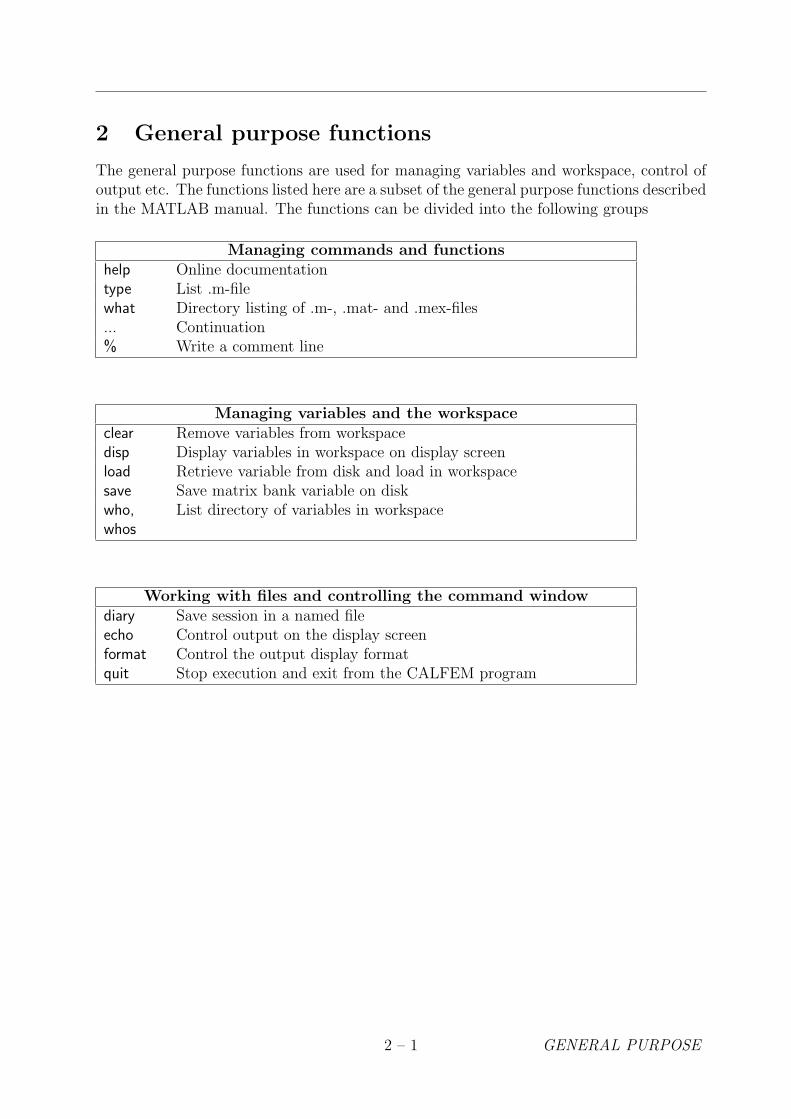
The general purpose functions are used for managing variables and workspace, control ofoutput etc. The functions listed here are a subset of the general purpose functions describedin the MATLAB manual. The functions can be divided into the following groups
Managing commands and functionshelp Online documentationtype List .m-filewhat Directory listing of .m-, .mat- and .mex-files... Continuation% Write a comment line
Managing variables and the workspaceclear Remove variables from workspacedisp Display variables in workspace on display screenload Retrieve variable from disk and load in workspacesave Save matrix bank variable on diskwho,whos
List directory of variables in workspace
Working with files and controlling the command windowdiary Save session in a named fileecho Control output on the display screenformat Control the output display formatquit Stop execution and exit from the CALFEM program
2 – 1 GENERAL PURPOSE

clear
Purpose:
Remove variables from workspace.
Syntax:
clearclear name1 name2 name3 ...
Description:
clear removes all variables from workspace.
clear name1 name2 name3 ... removes specified variables from workspace.
Note:
This is a MATLAB built-in function. For more information about the clear function,type help clear.
GENERAL PURPOSE 2 – 2
diary
Purpose:
Save session in a disk file.
Syntax:
diary filenamediary offdiary on
Description:
diary filename writes a copy of all subsequent keyboard input and most of the resultingoutput (but not graphs) on the named file. If the file filename already exists, theoutput is appended to the end of that file.
diary off stops storage of the output.
diary on turns it back on again, using the current filename or default filename diaryif none has yet been specified.
The diary function may be used to store the current session for later runs. To makethis possible, finish each command line with semicolon ’;’ to avoid the storage ofintermediate results on the named diary file.
Note:
This is a MATLAB built-in function. For more information about the diary function,type help diary.
2 – 3 GENERAL PURPOSE

disp
Purpose:
Display a variable in matrix bank on display screen.
Syntax:
disp(A)
Description:
disp(A) displays the matrix A on the display screen.
Note:
This is a MATLAB built-in function. For more information about the disp function,type help disp.
GENERAL PURPOSE 2 – 4

echo
Purpose:
Control output on the display screen.
Syntax:
echo onecho offecho
Description:
echo on turns on echoing of commands inside Script-files.
echo off turns off echoing.
echo by itself, toggles the echo state.
Note:
This is a MATLAB built-in function. For more information about the echo function,type help echo.
2 – 5 GENERAL PURPOSE
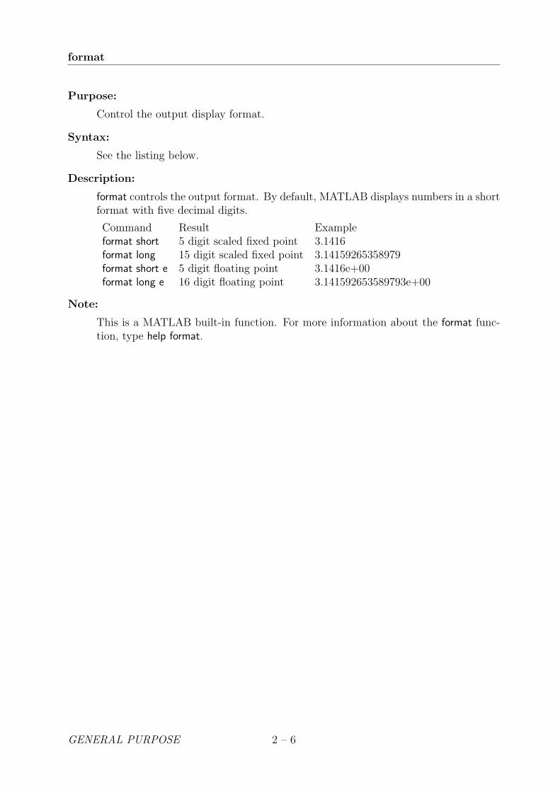
format
Purpose:
Control the output display format.
Syntax:
See the listing below.
Description:
format controls the output format. By default, MATLAB displays numbers in a shortformat with five decimal digits.
Command Result Exampleformat short 5 digit scaled fixed point 3.1416format long 15 digit scaled fixed point 3.14159265358979format short e 5 digit floating point 3.1416e+00format long e 16 digit floating point 3.141592653589793e+00
Note:
This is a MATLAB built-in function. For more information about the format func-tion, type help format.
GENERAL PURPOSE 2 – 6
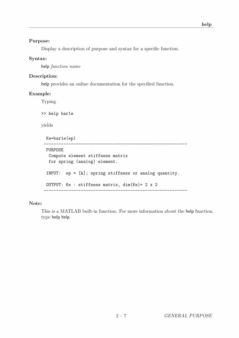
help
Purpose:
Display a description of purpose and syntax for a specific function.
Syntax:
help function name
Description:
help provides an online documentation for the specified function.
Example:
Typing
>> help bar1e
yields
Ke=bar1e(ep)
----------------------------------------------------------
PURPOSE
Compute element stiffness matrix
for spring (analog) element.
INPUT: ep = [k]; spring stiffness or analog quantity.
OUTPUT: Ke : stiffness matrix, dim(Ke)= 2 x 2
----------------------------------------------------------
Note:
This is a MATLAB built-in function. For more information about the help function,type help help.
2 – 7 GENERAL PURPOSE
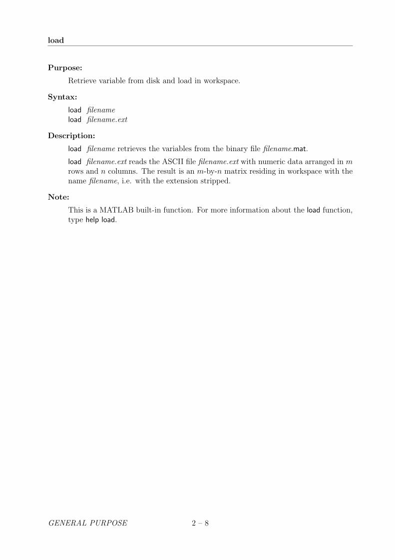
load
Purpose:
Retrieve variable from disk and load in workspace.
Syntax:
load filenameload filename.ext
Description:
load filename retrieves the variables from the binary file filename.mat.
load filename.ext reads the ASCII file filename.ext with numeric data arranged in mrows and n columns. The result is an m-by-n matrix residing in workspace with thename filename, i.e. with the extension stripped.
Note:
This is a MATLAB built-in function. For more information about the load function,type help load.
GENERAL PURPOSE 2 – 8

quit
Purpose:
Terminate CALFEM session.
Syntax:
quit
Description:
quit filename terminates the CALFEM without saving the workspace.
Note:
This is a MATLAB built-in function. For more information about the quit function,type help quit.
2 – 9 GENERAL PURPOSE

save
Purpose:
Save workspace variables on disk.
Syntax:
save filenamesave filename variablessave filename variables -ascii
Description:
save filename writes all variables residing in workspace in a binary file named file-name.mat
save filename variables writes named variables, separated by blanks, in a binary filenamed filename.mat
save filename variables -ascii writes named variables in an ASCII file named filename.
Note:
This is a MATLAB built-in function. For more information about the save function,type help save.
GENERAL PURPOSE 2 – 10
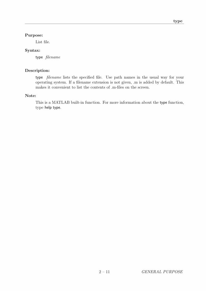
type
Purpose:
List file.
Syntax:
type filename
Description:
type filename lists the specified file. Use path names in the usual way for youroperating system. If a filename extension is not given, .m is added by default. Thismakes it convenient to list the contents of .m-files on the screen.
Note:
This is a MATLAB built-in function. For more information about the type function,type help type.
2 – 11 GENERAL PURPOSE
what
Purpose:
Directory listing of .m-files, .mat-files and .mex-files.
Syntax:
whatwhat dirname
Description:
what lists the .m-files, .mat-files and .mex-files in the current directory.
what dirname lists the files in directory dirname in the MATLAB search path. Thesyntax of the path depends on your operating system.
Note:
This is a MATLAB built-in function. For more information about the what function,type help what.
GENERAL PURPOSE 2 – 12

who, whos
Purpose:
List directory of variables in matrix bank.
Syntax:
whowhos
Description:
who lists the variables currently in memory.
whos lists the current variables and their size.
Examples:
who
Your variables are:
A B CK M Xk lambda
whos
name size elements bytes density complexA 3-by-3 9 72 Full NoB 3-by-3 9 72 Full NoC 3-by-3 9 72 Full NoK 20-by-20 400 3200 Full NoM 20-by-20 400 3200 Full NoX 20-by-20 400 3200 Full Nok 1-by-1 1 8 Full No
lambda 20-by-1 20 160 Full No
Grand total is 1248 elements using 9984 bytes
Note:
These are MATLAB built-in functions. For more information about the functions,type help who or help whos.
2 – 13 GENERAL PURPOSE

...
Purpose:
Continuation.
Syntax:
...
Description:
An expression can be continued on the next line by using ... .
Note:
This is a MATLAB built-in function.
GENERAL PURPOSE 2 – 14
%
Purpose:
Write a comment line.
Syntax:
% arbitrary text
Description:
An arbitrary text can be written after the symbol %.
Note:
This is a MATLAB built-in character.
2 – 15 GENERAL PURPOSE


3 Matrix functions
The group of matrix functions comprises functions for vector and matrix operations andalso functions for sparse matrix handling. MATLAB has two storage modes, full and sparse.Only nonzero entries and their indices are stored for sparse matrices. Sparse matrices arenot created automatically. But once initiated, sparsity propagates. Operations on sparsematrices produce sparse matrices and operations on a mixture of sparse and full matricesalso normally produce sparse matrices.
The following functions are described in this chapter:
Vector and matrix operations[ ] ( ) = Special characters’ . , ; Special characters: Create vectors and do matrix subscripting+ – ∗ / Matrix arithmeticabs Absolute valuedet Matrix determinantdiag Diagonal matrices and diagonals of a matrixinv Matrix inverselength Vector lengthmax Maximum element(s) of a matrixmin Minimum element(s) of a matrixones Generate a matrix of all onesred Reduce the size of a square matrixsize Matrix dimensionssqrt Square rootsum Sum of the elements of a matrixzeros Generate a zero matrix
Sparse matrix handlingfull Convert sparse matrix to full matrixsparse Create sparse matrixspy Visualize sparsity structure
3 – 1 MATRIX

[ ] ( ) = ’ . , ;
Purpose:
Special characters.
Syntax:
[ ] ( ) = ’ . , ;
Description:
[ ] Brackets are used to form vectors and matrices.
( ) Parentheses are used to indicate precedence in arithmetic expressions and tospecify an element of a matrix.
= Used in assignment statements.
’ Matrix transpose. X’ is the transpose of X. If X is complex, the apostrophesign performs complex conjugate as well. Do X.’ if only the transpose of thecomplex matrix is desired
. Decimal point. 314/100, 3.14 and 0.314e1 are all the same.
, Comma. Used to separate matrix subscripts and function arguments.
; Semicolon. Used inside brackets to end rows. Used after an expression tosuppress printing or to separate statements.
Examples:
By the statement
a = 2
the scalar a is assigned a value of 2. An element in a matrix may be assigned a valueaccording to
A(2, 5) = 3
The statement
D = [ 1 2 ; 3 4]
results in matrix
D =
[1 23 4
]stored in the matrix bank. To copy the contents of the matrix D to a matrix E, use
E = D
The character ’ is used in the following statement to store the transpose of the matrixA in a new matrix F
F = A′
Note:
These are MATLAB built-in characters.
MATRIX 3 – 2

:
Purpose:
Create vectors and do matrix subscripting.
Description:
The colon operator uses the following rules to create regularly spaced vectors:
j : k is the same as [ j, j + 1, ... , k ]
j : i : k is the same as [ j, j + i, j + 2i, ... , k ]
The colon notation may also be used to pick out selected rows, columns, and elementsof vectors and matrices:
A( : , j ) is the j :th column of A
A( i , : ) is the i :th row of A
Examples:
The colon ’:’ used with integers
d = 1 : 4
results in a row vector
d = [ 1 2 3 4 ]
stored in the workspace.
The colon notation may be used to display selected rows and columns of a matrix onthe terminal. For example, if we have created a 3-times-4 matrix D by the statement
D = [ d ; 2 ∗ d ; 3 ∗ d ]
resulting in
D =
1 2 3 42 4 6 83 6 9 12
columns three and four are displayed by entering
D( : , 3 : 4 )
resulting in
D( : , 3 : 4 ) =
3 46 89 12
In order to copy parts of the D matrix into another matrix the colon notation is usedas
E( 3 : 4 , 2 : 3 ) = D( 1 : 2 , 3 : 4 )
3 – 3 MATRIX

:
Assuming the matrix E was a zero matrix before the statement is executed, the resultwill be
E =
0 0 0 00 0 0 00 3 4 00 6 8 0
Note:
This is a MATLAB built-in character.
MATRIX 3 – 4
+ − ∗ /
Purpose:
Matrix arithmetic.
Syntax:
A + BA − BA ∗ BA/s
Description:
Matrix operations are defined by the rules of linear algebra.
Examples:
An example of a sequence of matrix-to-matrix operations is
D = A + B− C
A matrix-to-vector multiplication followed by a vector-to-vector subtraction may bedefined by the statement
b = c− A ∗ x
and finally, to scale a matrix by a scalar s we may use
B = A/s
Note:
These are MATLAB built-in operators.
3 – 5 MATRIX

abs
Purpose:
Absolute value.
Syntax:
B=abs(A)
Description:
B=abs(A) computes the absolute values of the elements of matrix A and stores themin matrix B.
Examples:
Assume the matrix
C =
[−7 4−3 −8
]
The statement D=abs(C) results in a matrix
D =
[7 43 8
]
stored in the workspace.
Note:
This is a MATLAB built-in function. For more information about the abs function,type help abs.
MATRIX 3 – 6

det
Purpose:
Matrix determinant.
Syntax:
a=det(A)
Description:
a=det(A) computes the determinant of the matrix A and stores it in the scalar a.
Note:
This is a MATLAB built-in function. For more information about the det function,type help det.
3 – 7 MATRIX

diag
Purpose:
Diagonal matrices and diagonals of a matrix.
Syntax:
M=diag(v)v=diag(M)
Description:
For a vector v with n components, the statement M=diag(v) results in an n × nmatrix M with the elements of v as the main diagonal.
For a n× n matrix M, the statement v=diag(M) results in a column vector v with ncomponents formed by the main diagonal in M.
Note:
This is a MATLAB built-in function. For more information about the diag function,type help diag.
MATRIX 3 – 8
full
Purpose:
Convert sparse matrices to full storage class.
Syntax:
A=full(S)
Description:
A=full(S) converts the storage of a matrix from sparse to full. If A is already full,full(A) returns A.
Note:
This is a MATLAB built-in function. For more information about the full function,type help full.
3 – 9 MATRIX
inv
Purpose:
Matrix inverse.
Syntax:
B=inv(A)
Description:
B=inv(A) computes the inverse of the square matrix A and stores the result in thematrix B.
Note:
This is a MATLAB built-in function. For more information about the inv function,type help inv.
MATRIX 3 – 10

length
Purpose:
Vector length.
Syntax:
n=length(x)
Description:
n=length(x) returns the dimension of the vector x.
Note:
This is a MATLAB built-in function. For more information about the length function,type help length.
3 – 11 MATRIX

max
Purpose:
Maximum element(s) of a matrix.
Syntax:
b=max(A)
Description:
For a vector a, the statement b=max(a) assigns the scalar b the maximum elementof the vector a.
For a matrix A, the statement b=max(A) returns a row vector b containing themaximum elements found in each column vector in A.
The maximum element found in a matrix may thus be determined byc=max(max(A)).
Examples:
Assume the matrix B is defined as
B =
[−7 4−3 −8
]
The statement d=max(B) results in a row vector
d =[−3 4
]The maximum element in the matrix B may be found by e=max(d) which results inthe scalar e = 4.
Note:
This is a MATLAB built-in function. For more information about the max function,type help max.
MATRIX 3 – 12

min
Purpose:
Minimum element(s) of a matrix.
Syntax:
b=min(A)
Description:
For a vector a, the statement b=min(a) assigns the scalar b the minimum element ofthe vector a.
For a matrix A, the statement b=min(A) returns a row vector b containing the min-imum elements found in each column vector in A.
The minimum element found in a matrix may thus be determined by c=min(min(A)).
Examples:
Assume the matrix B is defined as
B =
[−7 4−3 −8
]
The statement d=min(B) results in a row vector
d =[−7 −8
]The minimum element in the matrix B is then found by e=min(d), which results inthe scalar e = −8.
Note:
This is a MATLAB built-in function. For more information about the min function,type help min.
3 – 13 MATRIX

ones
Purpose:
Generate a matrix of all ones.
Syntax:
A=ones(m,n)
Description:
A=ones(m,n) results in an m-times-n matrix A with all ones.
Note:
This is a MATLAB built-in function. For more information about the ones function,type help ones.
MATRIX 3 – 14

red
Purpose:
Reduce the size of a square matrix by omitting rows and columns.
Syntax:
B=red(A,b)
Description:
B=red(A,b) reduces the square matrix A to a smaller matrix B by omitting rows andcolumns of A. The indices for rows and columns to be omitted are specified by thecolumn vector b.
Examples:
Assume that the matrix A is defined as
A =
1 2 3 45 6 7 89 10 11 1213 14 15 16
and b as
b =
[24
]
The statement B=red(A,b) results in the matrix
B =
[1 39 11
]
3 – 15 MATRIX

size
Purpose:
Matrix dimensions.
Syntax:
d=size(A)[m,n]=size(A)
Description:
d=size(A) returns a vector with two integer components, d=[m,n], from the matrixA with dimensions m times n.
[m,n]=size(A) returns the dimensions m and n of the m× n matrix A.
Note:
This is a MATLAB built-in function. For more information about the size function,type help size.
MATRIX 3 – 16
sparse
Purpose:
Create sparse matrices.
Syntax:
S=sparse(A)S=sparse(m,n)
Description:
S=sparse(A) converts a full matrix to sparse form by extracting all nonzero matrixelements. If S is already sparse, sparse(S) returns S.
S=sparse(m,n) generates an m-times-n sparse zero matrix.
Note:
This is a MATLAB built-in function. For more information about the sparse function,type help sparse.
3 – 17 MATRIX

spy
Purpose:
Visualize matrix sparsity structure.
Syntax:
spy(S)
Description:
spy(S) plots the sparsity structure of any matrix S. S is usually a sparse matrix, butthe function also accepts full matrices and the nonzero matrix elements are plotted.
Note:
This is a MATLAB built-in function. For more information about the spy function,type help spy.
MATRIX 3 – 18
sqrt
Purpose:
Square root.
Syntax:
B=sqrt(A)
Description:
B=sqrt(A) computes the square root of the elements in matrix A and stores the resultin matrix B.
Note:
This is a MATLAB built-in function. For more information about the sqrt function,type help sqrt.
3 – 19 MATRIX
sum
Purpose:
Sum of the elements of a matrix.
Syntax:
b=sum(A)
Description:
For a vector a, the statement b=sum(a) results in a scalar a containing the sum ofall elements of a.
For a matrix A, the statement b=sum(A) returns a row vector b containing the sumof the elements found in each column vector of A.
The sum of all elements of a matrix is determined by c=sum(sum(A)).
Note:
This is a MATLAB built-in function. For more information about the sum function,type help sum.
MATRIX 3 – 20

zeros
Purpose:
Generate a zero matrix.
Syntax:
A=zeros(m,n)
Description:
A=zeros(m,n) results in an m-times-n matrix A of zeros.
Note:
This is a MATLAB built-in function. For more information about the zeros function,type help zeros.
3 – 21 MATRIX

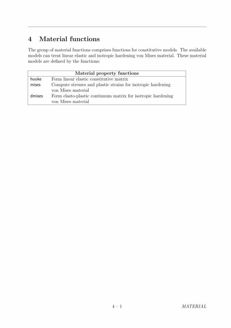
4 Material functions
The group of material functions comprises functions for constitutive models. The availablemodels can treat linear elastic and isotropic hardening von Mises material. These materialmodels are defined by the functions:
Material property functionshooke Form linear elastic constitutive matrixmises Compute stresses and plastic strains for isotropic hardening
von Mises materialdmises Form elasto-plastic continuum matrix for isotropic hardening
von Mises material
4 – 1 MATERIAL

hooke
Purpose:
Compute material matrix for a linear elastic and isotropic material.
Syntax:
D = hooke(ptype,E,v)
Description:
hooke computes the material matrix D for a linear elastic and isotropic material.
The variable ptype is used to define the type of analysis.
ptype =
1 plane stress.2 plane strain.3 axisymmetry.4 three dimensional analysis.
The material parameters E and v define the modulus of elasticity E and the Poisson’sratio ν, respectively.
For plane stress, ptype=1, D is formed as
D =E
1− ν2
1 ν 0ν 1 0
0 01− ν
2
For plane strain, ptype=2 and axisymmetry, ptype=3, D is formed as
D =E
(1 + ν)(1− 2ν)
1− ν ν ν 0
ν 1− ν ν 0
ν ν 1− ν 0
0 0 0 12(1− 2ν)
For the three dimensional case, ptype=4, D is formed as
D =E
(1 + ν)(1− 2ν)
1− ν ν ν 0 0 0
ν 1− ν ν 0 0 0
ν ν 1− ν 0 0 0
0 0 0 12(1− 2ν) 0 0
0 0 0 0 12(1− 2ν) 0
0 0 0 0 0 12(1− 2ν)
MATERIAL 4 – 2

mises
Purpose:
Compute stresses and plastic strains for an elasto-plastic isotropic hardening vonMises material.
Syntax:
[es,deps,st]=mises(ptype,mp,est,st)
Description:
mises computes updated stresses es, plastic strain increments deps, and states vari-ables st for an elasto-plastic isotropic hardening von Mises material.
The input variable ptype is used to define the type of analysis, cf. hooke. The vectormp contains the material constants
mp = [ E ν h ]
where E is the modulus of elasticity, ν is the Poisson’s ratio, and h is the plasticmodulus. The input matrix est contains trial stresses obtained by using the elas-tic material matrix D in plants or some similar s-function, and the input vector stcontains the state parameters
st = [ yi σy εpeff ]
at the beginning of the step. The scalar yi states whether the material behaviouris elasto-plastic (yi=1), or elastic (yi=0). The current yield stress is denoted by σy
and the effectiv plastic strain by εpeff .
The output variables es and st contain updated values of es and st obtained byintegration of the constitutive equations over the actual displacement step. Theincrements of the plastic strains are stored in the vector deps.
If es and st contain more than one row, then every row will be treated by the com-mand.
Note:
It is not necessary to check whether the material behaviour is elastic or elasto-plastic,this test is done by the function. The computation is based on an Euler-Backwardmethod, i.e. the radial return method.
Only the cases ptype=2, 3 and 4, are implemented.
4 – 3 MATERIAL

dmises
Purpose:
Form the elasto-plastic continuum matrix for an isotropic hardening von Mises ma-terial.
Syntax:
D=dmises(ptype,mp,es,st)
Description:
dmises forms the elasto-plastic continuum matrix for an isotropic hardening von Misesmaterial.
The input variable ptype is used to define the type of analysis, cf. hooke. The vectormp contains the material constants
mp = [ E ν h ]
where E is the modulus of elasticity, ν is the Poisson’s ratio, and h is the plasticmodulus. The matrix es contains current stresses obtained from plants or somesimilar s-function, and the vector st contains the current state parameters
st = [ yi σy εpeff ]
where yi=1 if the material behaviour is elasto-plastic, and yi=0 if the materialbehaviour is elastic. The current yield stress is denoted by σy, and the currenteffective plastic strain by εpeff .
Note:
Only the case ptype=2 is implemented.
MATERIAL 4 – 4

5 Element functions
5.1 Introduction
The group of element functions contains functions for computation of element matricesand element forces for different element types. The element functions have been dividedinto the following groups
Spring element
Bar elements
Heat flow elements
Solid elements
Beam elements
Plate element
For each element type there is a function for computation of the element stiffness matrixKe. For most of the elements, an element load vector f e can also be computed. Thesefunctions are identified by their last letter -e.
Using the function assem, the element stiffness matrices and element load vectors areassembled into a global stiffness matrix K and a load vector f . Unknown nodal values oftemperatures or displacements a are computed by solving the system of equations Ka = fusing the function solveq. A vector of nodal values of temperatures or displacements for aspecific element are formed by the function extract.
When the element nodal values have been computed, the element flux or element stressescan be calculated using functions specific to the element type concerned. These functionsare identified by their last letter -s.
For some elements, a function for computing the internal force vector is also available.These functions are identified by their last letter -f.
5.1 – 1 ELEMENT

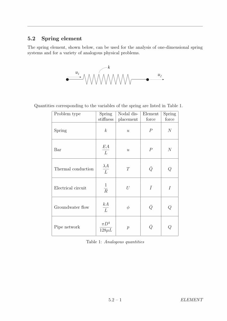
5.2 Spring element
The spring element, shown below, can be used for the analysis of one-dimensional springsystems and for a variety of analogous physical problems.
ku1 u2
●●
Quantities corresponding to the variables of the spring are listed in Table 1.
Problem type Spring Nodal dis- Element Springstiffness placement force force
Spring k u P N
BarEA
Lu P N
Thermal conductionλA
LT Q Q
Electrical circuit1
RU I I
Groundwater flowkA
Lφ Q Q
Pipe networkπD4
128µLp Q Q
Table 1: Analogous quantities
5.2 – 1 ELEMENT
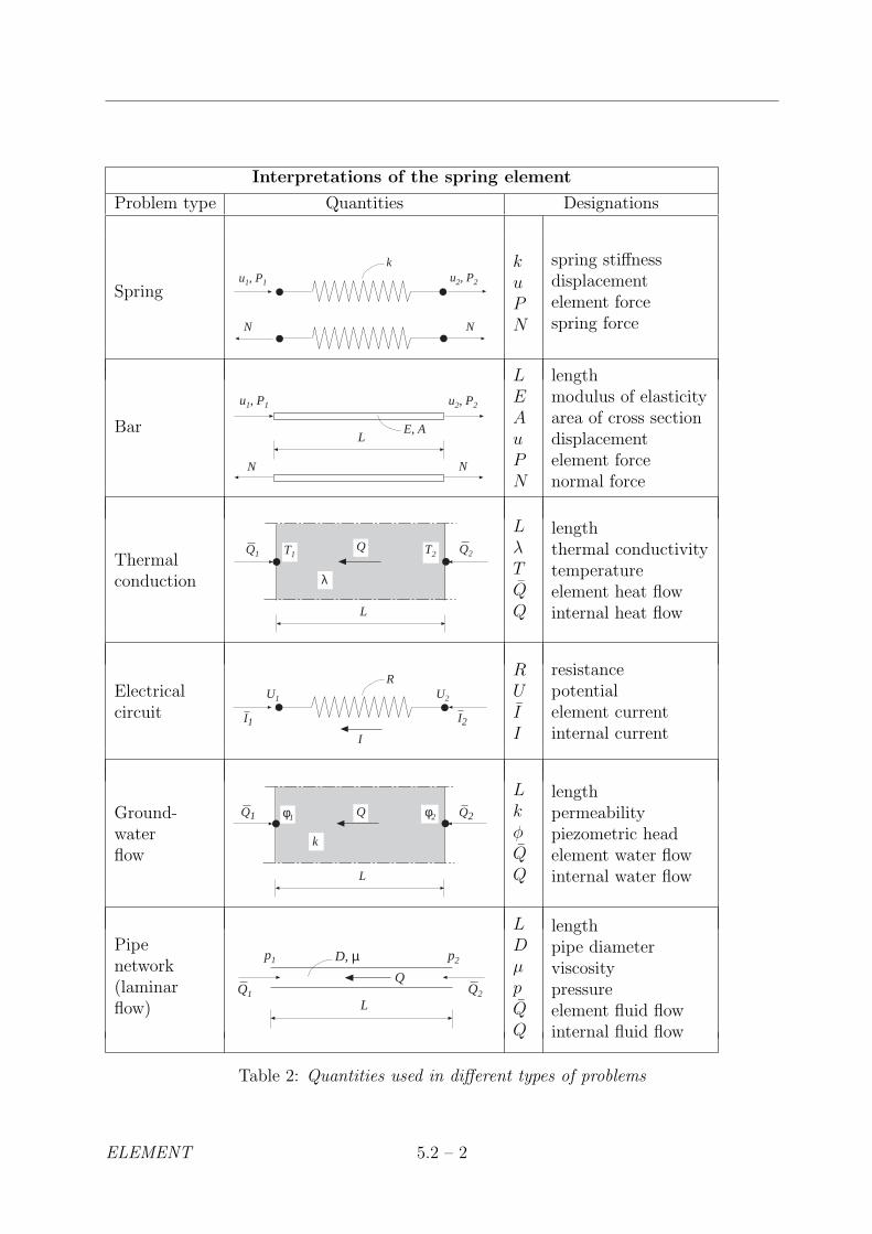
Interpretations of the spring element
Problem type Quantities Designations
Spring
ku2, P2
N N
●●
●●
u1, P1
kuPN
spring stiffnessdisplacementelement forcespring force
Bar E, A
N N
L
u2, P2u1, P1
LEAuPN
lengthmodulus of elasticityarea of cross sectiondisplacementelement forcenormal force
Thermalconduction λ
Q1Q
●●
L
Q2T2T1
LλTQQ
lengththermal conductivitytemperatureelement heat flowinternal heat flow
Electricalcircuit
RU2U1
I1
I
●●I2
RUII
resistancepotentialelement currentinternal current
Ground-waterflow
● ●
k
Q1 Q Q2
L
φ1 φ2
LkφQQ
lengthpermeabilitypiezometric headelement water flowinternal water flow
Pipenetwork(laminarflow)
p1 p2
Q
D, µ
LQ2Q1
LDµpQQ
lengthpipe diameterviscositypressureelement fluid flowinternal fluid flow
Table 2: Quantities used in different types of problems
ELEMENT 5.2 – 2

The following functions are available for the spring element:
Spring functionsspring1e Compute element matrixspring1s Compute spring force
5.2 – 3 ELEMENT
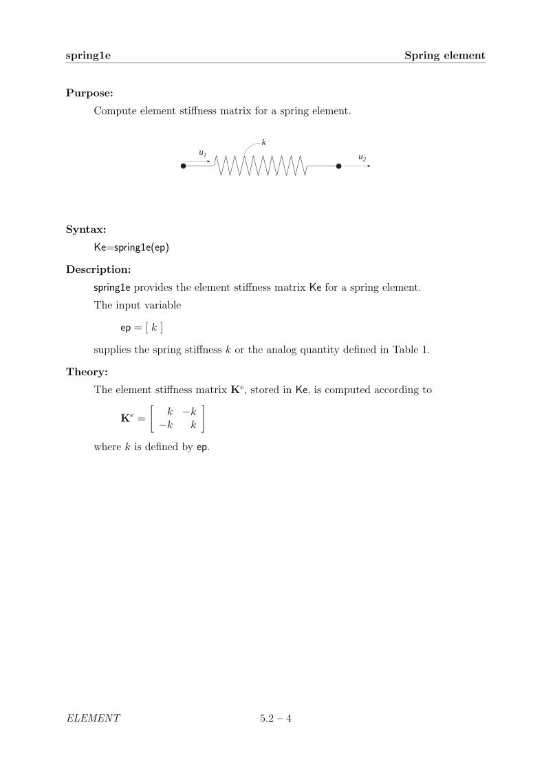
spring1e Spring element
Purpose:
Compute element stiffness matrix for a spring element.
ku1 u2
●●
Syntax:
Ke=spring1e(ep)
Description:
spring1e provides the element stiffness matrix Ke for a spring element.
The input variable
ep = [ k ]
supplies the spring stiffness k or the analog quantity defined in Table 1.
Theory:
The element stiffness matrix Ke, stored in Ke, is computed according to
Ke =
[k −k
−k k
]
where k is defined by ep.
ELEMENT 5.2 – 4
Spring element spring1s
Purpose:
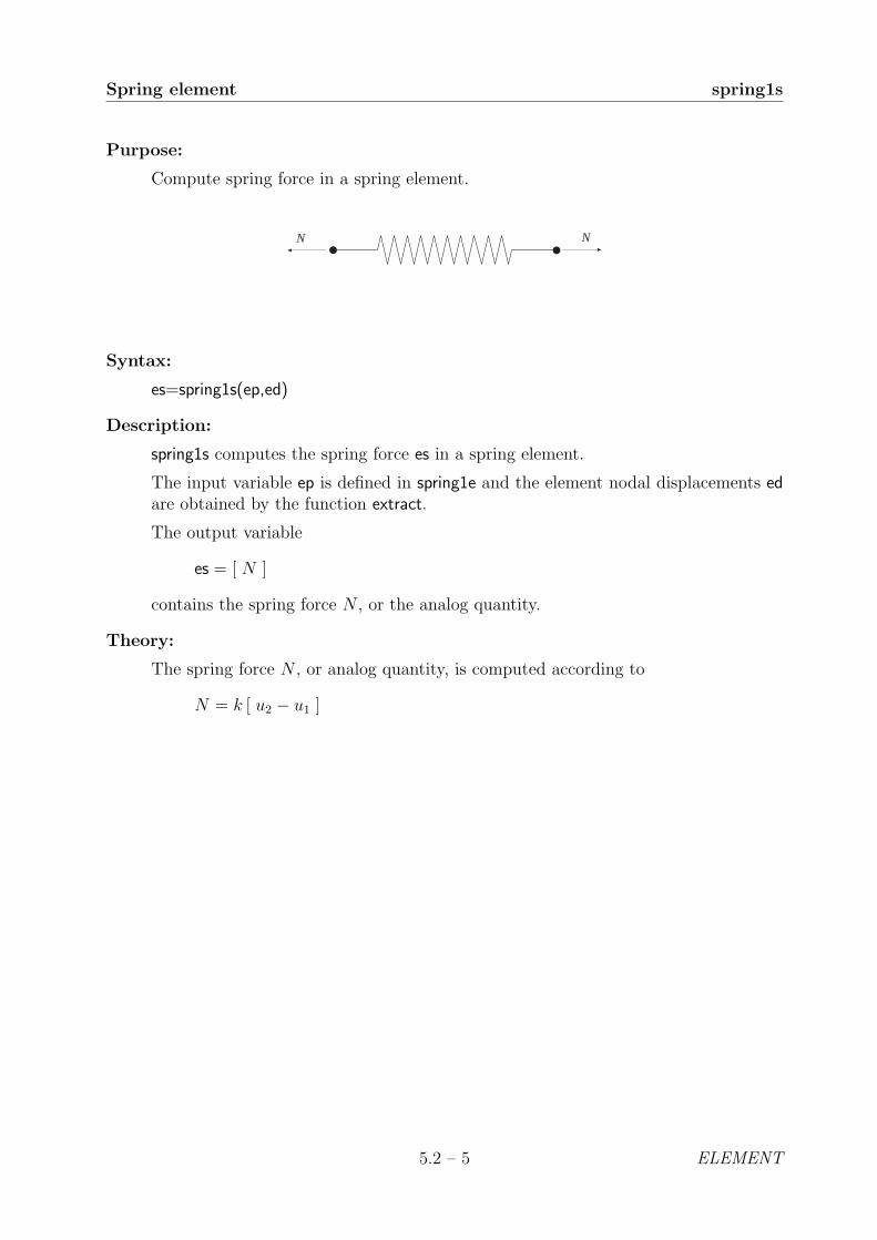
Compute spring force in a spring element.
N N●●
Syntax:
es=spring1s(ep,ed)
Description:
spring1s computes the spring force es in a spring element.
The input variable ep is defined in spring1e and the element nodal displacements edare obtained by the function extract.
The output variable
es = [ N ]
contains the spring force N , or the analog quantity.
Theory:
The spring force N , or analog quantity, is computed according to
N = k [ u2 − u1 ]
5.2 – 5 ELEMENT


Spring element spring1s
5.3 Bar elements
Bar elements are available for one, two, and three dimensional analysis. For the onedimensional element, see the spring element.
Bar elements
u1
u2
u3
u4
bar2ebar2g
u1
u2
u3
u4
u5
u6
bar3e
Two dimensional bar functionsbar2e Compute element matrixbar2g Compute element matrix for geometric nonlinear elementbar2s Compute normal force
Three dimensional bar functionsbar3e Compute element matrixbar3s Compute normal force
5.3 – 1 ELEMENT
bar2e Two dimensional bar element
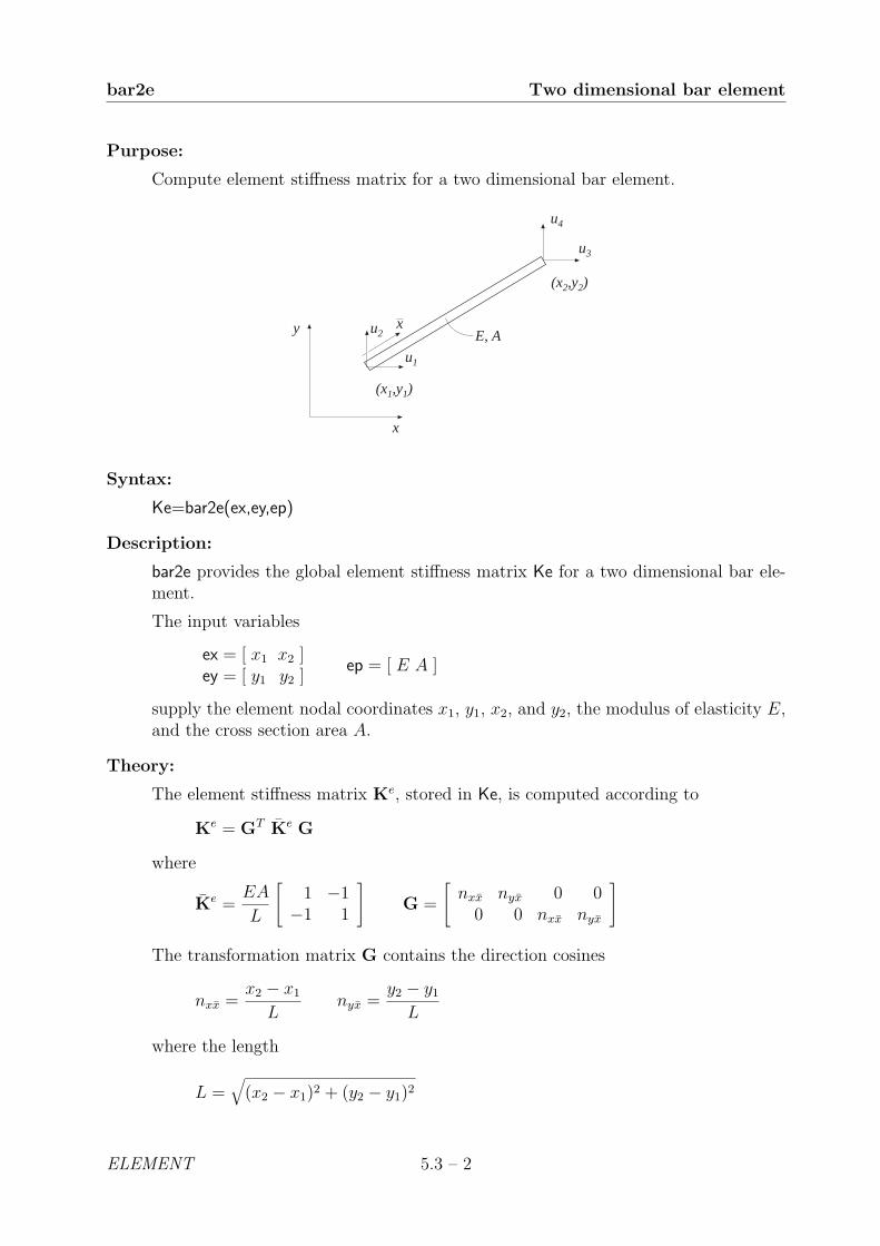
Purpose:
Compute element stiffness matrix for a two dimensional bar element.
E, A
x
y
(x2,y2)
(x1,y1)
x
u1
u2
u3
u4
Syntax:
Ke=bar2e(ex,ey,ep)
Description:
bar2e provides the global element stiffness matrix Ke for a two dimensional bar ele-ment.
The input variables
ex = [ x1 x2 ]ey = [ y1 y2 ]
ep = [ E A ]
supply the element nodal coordinates x1, y1, x2, and y2, the modulus of elasticity E,and the cross section area A.
Theory:
The element stiffness matrix Ke, stored in Ke, is computed according to
Ke = GT Ke G
where
Ke =EA
L
[1 −1
−1 1
]G =
[nxx nyx 0 0
0 0 nxx nyx
]
The transformation matrix G contains the direction cosines
nxx =x2 − x1
Lnyx =
y2 − y1
L
where the length
L =√
(x2 − x1)2 + (y2 − y1)2
ELEMENT 5.3 – 2

Two dimensional bar element bar2g
Purpose:
Compute element stiffness matrix for a two dimensional geometric nonlinear bar.
E, A
x
y
(x2,y2)
(x1,y1)
xE, A, N
u1
u2
u3
u4
Syntax:
Ke=bar2g(ex,ey,ep,N)
Description:
bar2g provides the element stiffness matrix Ke for a two dimensional geometric non-linear bar element.
The input variables ex, ey and ep are described in bar2e. The input variable
N = [ N ]
contains the value of the normal force, which is positive in tension.
Theory:
The global element stiffness matrix Ke, stored in Ke, is computed according to
Ke = GT Ke G
where
Ke =EA
L
1 0 −1 00 0 0 0
−1 0 1 00 0 0 0
+N
L
0 0 0 00 1 0 −10 0 0 00 −1 0 1
G =
nxx nyx 0 0nxy nyy 0 0
0 0 nxx nyx
0 0 nxy nyy
5.3 – 3 ELEMENT

bar2g Two dimensional bar element
The transformation matrix G contains the direction cosines
nxx = nyy =x2 − x1
Lnyx = −nxy =
y2 − y1
L
where the length
L =√
(x2 − x1)2 + (y2 − y1)2
ELEMENT 5.3 – 4
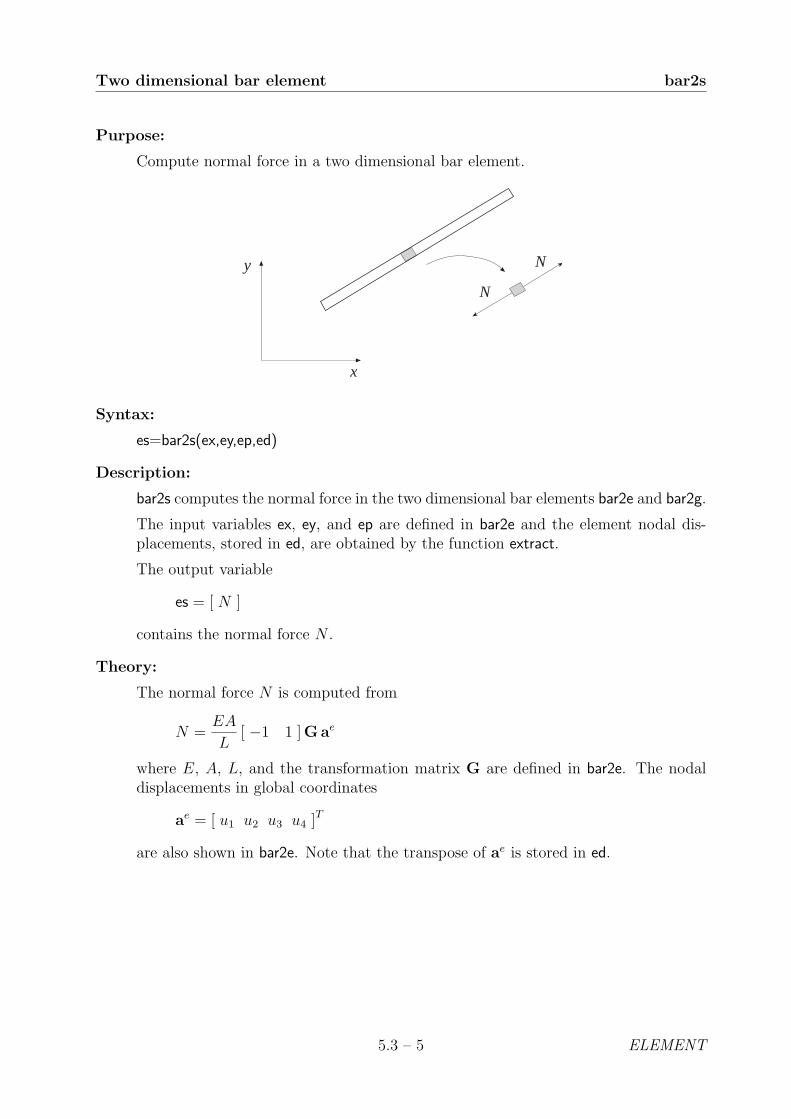
Two dimensional bar element bar2s
Purpose:
Compute normal force in a two dimensional bar element.
x
y N
N
Syntax:
es=bar2s(ex,ey,ep,ed)
Description:
bar2s computes the normal force in the two dimensional bar elements bar2e and bar2g.
The input variables ex, ey, and ep are defined in bar2e and the element nodal dis-placements, stored in ed, are obtained by the function extract.
The output variable
es = [ N ]
contains the normal force N .
Theory:
The normal force N is computed from
N =EA
L[ −1 1 ]Gae
where E, A, L, and the transformation matrix G are defined in bar2e. The nodaldisplacements in global coordinates
ae = [ u1 u2 u3 u4 ]T
are also shown in bar2e. Note that the transpose of ae is stored in ed.
5.3 – 5 ELEMENT

bar3e Three dimensional bar element
Purpose:
Compute element stiffness matrix for a three dimensional bar element.
E, A
(x1,y1,z1)
(x2,y2,z2)
zx
y x
u1
u2
u3
u4
u5
u6
Syntax:
Ke=bar3e(ex,ey,ez,ep)
Description:
bar3e provides the element stiffness matrix Ke for a three dimensional bar element.
The input variables
ex = [ x1 x2 ]ey = [ y1 y2 ]ez = [ z1 z2 ]
ep = [ E A ]
supply the element nodal coordinates x1, y1, z1, x2 etc, the modulus of elasticity E,and the cross section area A.
Theory:
The global element stiffness matrix Ke is computed according to
Ke = GT Ke G
where
Ke =EA
L
[1 −1
−1 1
]G =
[nxx nyx nzx 0 0 00 0 0 nxx nyx nzx
]
The transformation matrix G contains the direction cosines
nxx =x2 − x1
Lnyx =
y2 − y1
Lnzx =
z2 − z1
L
where the length L =√
(x2 − x1)2 + (y2 − y1)2 + (z2 − z1)2.
ELEMENT 5.3 – 6

Three dimensional bar element bar3s
Purpose:
Compute normal force in a three dimensional bar element.
N
N
zx
y
Syntax:
es=bar3s(ex,ey,ez,ep,ed)
Description:
bar3s computes the normal force in a three dimensional bar element.
The input variables ex, ey, ez, and ep are defined in bar3e, and the element nodaldisplacements, stored in ed, are obtained by the function extract.
The output variable
es = [ N ]
contains the normal force N of the bar.
Theory:
The normal force N is computed from
N =EA
L[ −1 1 ]Gae
where E, A, L, and the transformation matrix G are defined in bar3e. The nodaldisplacements in global coordinates
ae = [ u1 u2 u3 u4 u5 u6 ]T
are also shown in bar3e. Note that the transpose of ae is stored in ed.
5.3 – 7 ELEMENT

5.4 Heat flow elements
Heat flow elements are available for one, two, and three dimensional analysis. For onedimensional heat flow the spring element spring1 is used.
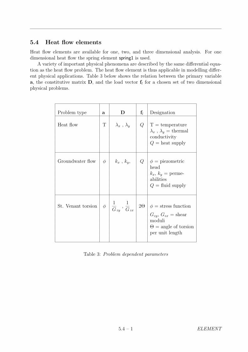
A variety of important physical phenomena are described by the same differential equa-tion as the heat flow problem. The heat flow element is thus applicable in modelling differ-ent physical applications. Table 3 below shows the relation between the primary variablea, the constitutive matrix D, and the load vector fl for a chosen set of two dimensionalphysical problems.
Problem type a D fl Designation
Heat flow T λx , λy Q T = temperatureλx , λy = thermalconductivityQ = heat supply
Groundwater flow φ kx , ky, Q φ = piezometricheadkx, ky = perme-abilitiesQ = fluid supply
St. Venant torsion φ1
G zy,
1
G zx2Θ φ = stress function
Gzy, Gzx = shearmoduliΘ = angle of torsionper unit length
Table 3: Problem dependent parameters
5.4 – 1 ELEMENT

Heat flow elements
●
●
●
T2
T3
T1
flw2te
●
●
●
●
T4 T3
T1
T2
flw2qeflw2i4e
●
●
●
●
●
●
●
●
T4
T3
T1
T2
T7
T6T8
T5
flw2i8e
●
●
●●
●
●
●
●
T4 T3
T1 T2
T7
T6
T8
T5
flw3i8e
2D heat flow functionsflw2te Compute element matrices for a triangular elementflw2ts Compute temperature gradients and fluxflw2qe Compute element matrices for a quadrilateral elementflw2qs Compute temperature gradients and fluxflw2i4e Compute element matrices, 4 node isoparametric elementflw2i4s Compute temperature gradients and fluxflw2i8e Compute element matrices, 8 node isoparametric elementflw2i8s Compute temperature gradients and flux
3D heat flow functionsflw3i8e Compute element matrices, 8 node isoparametric elementflw3i8s Compute temperature gradients and flux
ELEMENT 5.4 – 2

Two dimensional heat flow elements flw2te
Purpose:
Compute element stiffness matrix for a triangular heat flow element.
T2
T3
T1 ●
(x1,y1)
●
●
(x3,y3)
(x2,y2)
x
y
Syntax:
Ke=flw2te(ex,ey,ep,D)[Ke,fe]=flw2te(ex,ey,ep,D,eq)
Description:
flw2te provides the element stiffness (conductivity) matrix Ke and the element loadvector fe for a triangular heat flow element.
The element nodal coordinates x1, y1, x2 etc, are supplied to the function by exand ey, the element thickness t is supplied by ep and the thermal conductivities (orcorresponding quantities) kxx, kxy etc are supplied by D.
ex = [ x1 x2 x3 ]ey = [ y1 y2 y3 ]
ep = [ t ] D =
[kxx kxy
kyx kyy
]
If the scalar variable eq is given in the function, the element load vector fe is com-puted, using
eq = [ Q ]
where Q is the heat supply per unit volume.
Theory:
The element stiffness matrix Ke and the element load vector fel , stored in Ke and fe,respectively, are computed according to
Ke = (C−1)T∫
AB
TD B t dA C−1
fel = (C−1)T∫
AN
TQ t dA
with the constitutive matrix D defined by D.
The evaluation of the integrals for the triangular element is based on the lineartemperature approximation T (x, y) and is expressed in terms of the nodal variablesT1, T2 and T3 as
T (x, y) = Neae = N C−1ae
5.4 – 3 ELEMENT
flw2te Two dimensional heat flow elements
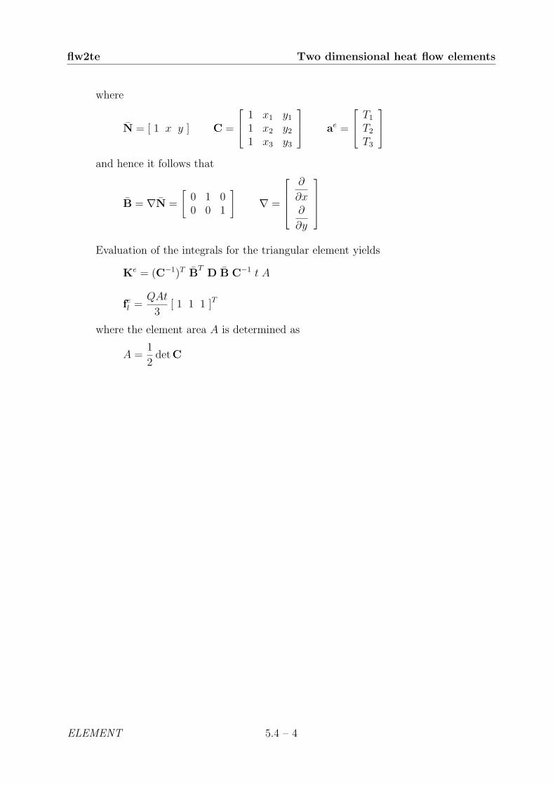
where
N = [ 1 x y ] C =
1 x1 y1
1 x2 y2
1 x3 y3
ae =
T1
T2
T3
and hence it follows that
B = ∇N =
[0 1 00 0 1
]∇ =
∂
∂x∂
∂y
Evaluation of the integrals for the triangular element yields
Ke = (C−1)T BT
D B C−1 t A
fel =QAt
3[ 1 1 1 ]T
where the element area A is determined as
A =1
2detC
ELEMENT 5.4 – 4

Two dimensional heat flow elements flw2ts
Purpose:
Compute heat flux and temperature gradients in a triangular heat flow element.
Syntax:
[es,et]=flw2ts(ex,ey,D,ed)
Description:
flw2ts computes the heat flux vector es and the temperature gradient et (or corre-sponding quantities) in a triangular heat flow element.
The input variables ex, ey and the matrix D are defined in flw2te. The vector edcontains the nodal temperatures ae of the element and is obtained by the functionextract as
ed = (ae)T = [ T1 T2 T3 ]
The output variables
es = qT = [ qx qy ]
et = (∇T )T =
[∂T
∂x
∂T
∂y
]
contain the components of the heat flux and the temperature gradient computed inthe directions of the coordinate axis.
Theory:
The temperature gradient and the heat flux are computed according to
∇T = B C−1 ae
q = −D∇T
where the matrices D, B, and C are described in flw2te. Note that both the tem-perature gradient and the heat flux are constant in the element.
5.4 – 5 ELEMENT
flw2qe Two dimensional heat flow elements
Purpose:
Compute element stiffness matrix for a quadrilateral heat flow element.
T2
T4
T1
●
(x1,y1)
●
●
(x4,y4)
(x2,y2)
T3● (x3,y3)
x
y●
T5
Syntax:
Ke=flw2qe(ex,ey,ep,D)[Ke,fe]=flw2qe(ex,ey,ep,D,eq)
Description:
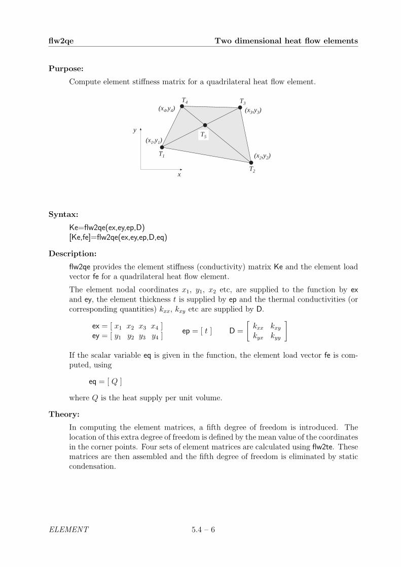
flw2qe provides the element stiffness (conductivity) matrix Ke and the element loadvector fe for a quadrilateral heat flow element.
The element nodal coordinates x1, y1, x2 etc, are supplied to the function by exand ey, the element thickness t is supplied by ep and the thermal conductivities (orcorresponding quantities) kxx, kxy etc are supplied by D.
ex = [ x1 x2 x3 x4 ]ey = [ y1 y2 y3 y4 ]
ep = [ t ] D =
[kxx kxy
kyx kyy
]
If the scalar variable eq is given in the function, the element load vector fe is com-puted, using
eq = [ Q ]
where Q is the heat supply per unit volume.
Theory:
In computing the element matrices, a fifth degree of freedom is introduced. Thelocation of this extra degree of freedom is defined by the mean value of the coordinatesin the corner points. Four sets of element matrices are calculated using flw2te. Thesematrices are then assembled and the fifth degree of freedom is eliminated by staticcondensation.
ELEMENT 5.4 – 6

Two dimensional heat flow elements flw2qs
Purpose:
Compute heat flux and temperature gradients in a quadrilateral heat flow element.
Syntax:
[es,et]=flw2qs(ex,ey,ep,D,ed)[es,et]=flw2qs(ex,ey,ep,D,ed,eq)
Description:
flw2qs computes the heat flux vector es and the temperature gradient et (or corre-sponding quantities) in a quadrilateral heat flow element.
The input variables ex, ey, eq and the matrix D are defined in flw2qe. The vector edcontains the nodal temperatures ae of the element and is obtained by the functionextract as
ed = (ae)T = [ T1 T2 T3 T4 ]
The output variables
es = qT = [ qx qy ]
et = (∇T )T =
[∂T
∂x
∂T
∂y
]
contain the components of the heat flux and the temperature gradient computed inthe directions of the coordinate axis.
Theory:
By assembling four triangular elements as described in flw2te a system of equationscontaining 5 degrees of freedom is obtained. From this system of equations theunknown temperature at the center of the element is computed. Then according tothe description in flw2ts the temperature gradient and the heat flux in each of thefour triangular elements are produced. Finally the temperature gradient and theheat flux of the quadrilateral element are computed as area weighted mean valuesfrom the values of the four triangular elements. If heat is supplied to the element,the element load vector eq is needed for the calculations.
5.4 – 7 ELEMENT

flw2i4e Two dimensional heat flow elements
Purpose:
Compute element stiffness matrix for a 4 node isoparametric heat flow element.
T4
●
●
●
(x4,y4) ●
x
y
T3
T1
(x1,y1)
(x3,y3)
(x2,y2)
T2
Syntax:
Ke=flw2i4e(ex,ey,ep,D)[Ke,fe]=flw2i4e(ex,ey,ep,D,eq)
Description:
flw2i4e provides the element stiffness (conductivity) matrix Ke and the element loadvector fe for a 4 node isoparametric heat flow element.
The element nodal coordinates x1, y1, x2 etc, are supplied to the function by ex andey. The element thickness t and the number of Gauss points n
(n× n) integration points, n = 1, 2, 3
are supplied to the function by ep and the thermal conductivities (or correspondingquantities) kxx, kxy etc are supplied by D.
ex = [ x1 x2 x3 x4 ]ey = [ y1 y2 y3 y4 ]
ep = [ t n ] D =
[kxx kxy
kyx kyy
]
If the scalar variable eq is given in the function, the element load vector fe is com-puted, using
eq = [ Q ]
where Q is the heat supply per unit volume.
ELEMENT 5.4 – 8
Two dimensional heat flow elements flw2i4e
Theory:
The element stiffness matrix Ke and the element load vector fel , stored in Ke and fe,respectively, are computed according to
Ke =∫
ABeT D Be t dA
fel =∫
ANeT Q t dA
with the constitutive matrix D defined by D.
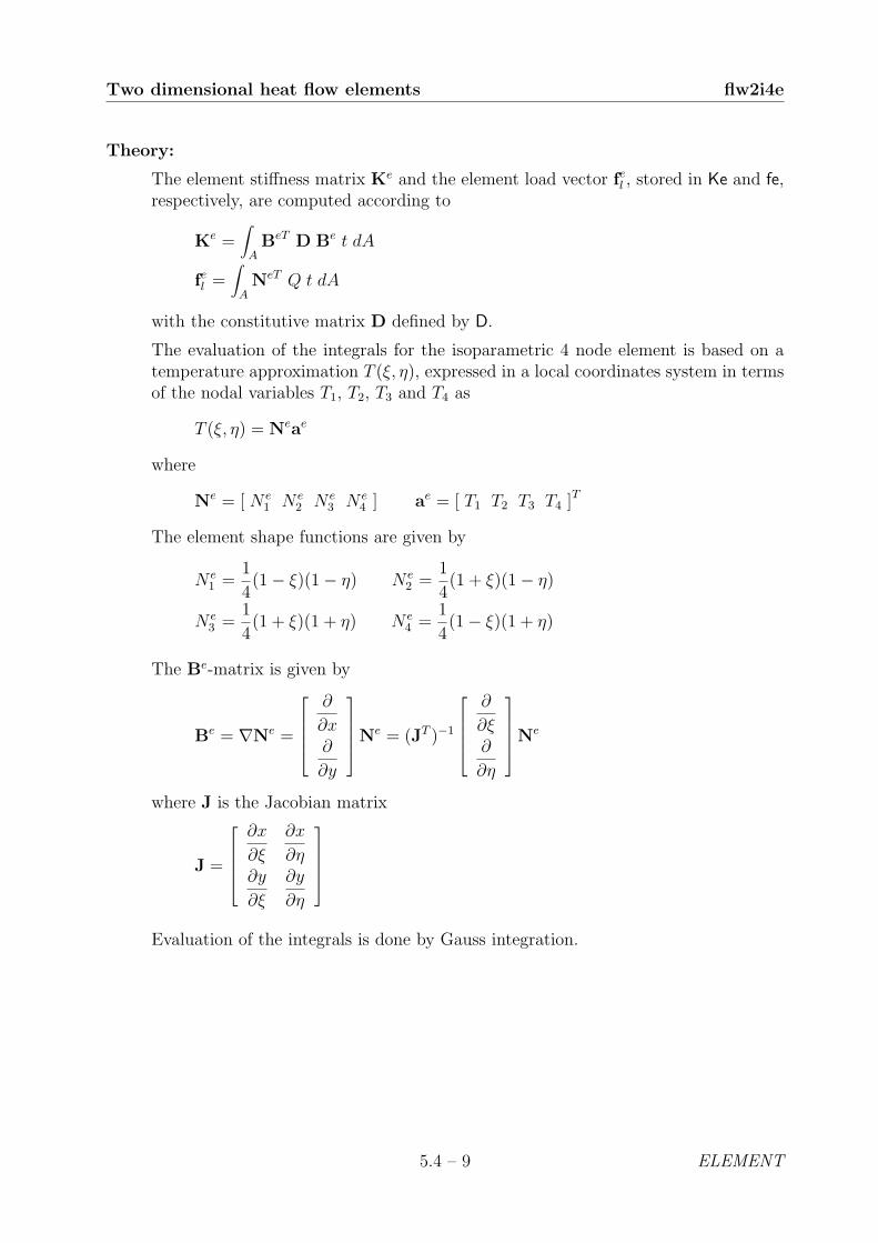
The evaluation of the integrals for the isoparametric 4 node element is based on atemperature approximation T (ξ, η), expressed in a local coordinates system in termsof the nodal variables T1, T2, T3 and T4 as
T (ξ, η) = Neae
where
Ne = [ N e1 N e
2 N e3 N e
4 ] ae = [ T1 T2 T3 T4 ]T
The element shape functions are given by
N e1 =
1
4(1− ξ)(1− η) N e
2 =1
4(1 + ξ)(1− η)
N e3 =
1
4(1 + ξ)(1 + η) N e
4 =1
4(1− ξ)(1 + η)
The Be-matrix is given by
Be = ∇Ne =
∂
∂x∂
∂y
Ne = (JT )−1
∂
∂ξ∂
∂η
Ne
where J is the Jacobian matrix
J =
∂x
∂ξ
∂x
∂η∂y
∂ξ
∂y
∂η
Evaluation of the integrals is done by Gauss integration.
5.4 – 9 ELEMENT

flw2i4s Two dimensional heat flow elements
Purpose:
Compute heat flux and temperature gradients in a 4 node isoparametric heat flowelement.
Syntax:
[es,et,eci]=flw2i4s(ex,ey,ep,D,ed)
Description:
flw2i4s computes the heat flux vector es and the temperature gradient et (or corre-sponding quantities) in a 4 node isoparametric heat flow element.
The input variables ex, ey, ep and the matrix D are defined in flw2i4e. The vector edcontains the nodal temperatures ae of the element and is obtained by extract as
ed = (ae)T = [ T1 T2 T3 T4 ]
The output variables
es = qT =
q1x q1
y
q2x q2
y...
...
qn2
x qn2
y
et = (∇T )T =
∂T
∂x
1 ∂T
∂y
1
∂T
∂x
2 ∂T
∂y
2
......
∂T
∂x
n2
∂T
∂y
n2
eci =
x1 y1
x2 y2...
...xn2 yn2
contain the heat flux, the temperature gradient, and the coordinates of the integra-tion points. The index n denotes the number of integration points used within theelement, cf. flw2i4e.
Theory:
The temperature gradient and the heat flux are computed according to
∇T = Be ae
q = −D∇T
where the matrices D, Be, and ae are described in flw2i4e, and where the integrationpoints are chosen as evaluation points.
ELEMENT 5.4 – 10
Two dimensional heat flow elements flw2i8e
Purpose:
Compute element stiffness matrix for an 8 node isoparametric heat flow element.
x
y
●
●
●
●
●
●
●
●
T4
T3
T1
T2
T7
T6T8
T5
Syntax:
Ke=flw2i8e(ex,ey,ep,D)[Ke,fe]=flw2i8e(ex,ey,ep,D,eq)
Description:
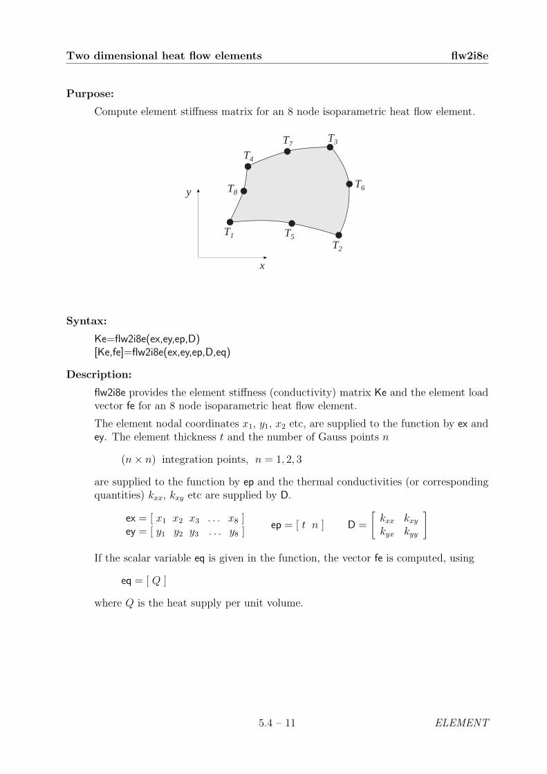
flw2i8e provides the element stiffness (conductivity) matrix Ke and the element loadvector fe for an 8 node isoparametric heat flow element.
The element nodal coordinates x1, y1, x2 etc, are supplied to the function by ex andey. The element thickness t and the number of Gauss points n
(n× n) integration points, n = 1, 2, 3
are supplied to the function by ep and the thermal conductivities (or correspondingquantities) kxx, kxy etc are supplied by D.
ex = [ x1 x2 x3 . . . x8 ]ey = [ y1 y2 y3 . . . y8 ]
ep = [ t n ] D =
[kxx kxy
kyx kyy
]
If the scalar variable eq is given in the function, the vector fe is computed, using
eq = [ Q ]
where Q is the heat supply per unit volume.
5.4 – 11 ELEMENT

flw2i8e Two dimensional heat flow elements
Theory:
The element stiffness matrix Ke and the element load vector fel , stored in Ke and fe,respectively, are computed according to
Ke =∫
ABeT D Be t dA
fel =∫
ANeT Q t dA
with the constitutive matrix D defined by D.
The evaluation of the integrals for the 2D isoparametric 8 node element is based on atemperature approximation T (ξ, η), expressed in a local coordinates system in termsof the nodal variables T1 to T8 as
T (ξ, η) = Neae
where
Ne = [ N e1 N e
2 N e3 . . . N e
8 ] ae = [ T1 T2 T3 . . . T8 ]T
The element shape functions are given by
N e1 = −1
4(1− ξ)(1− η)(1 + ξ + η) N e
5 =1
2(1− ξ2)(1− η)
N e2 = −1
4(1 + ξ)(1− η)(1− ξ + η) N e
6 =1
2(1 + ξ)(1− η2)
N e3 = −1
4(1 + ξ)(1 + η)(1− ξ − η) N e
7 =1
2(1− ξ2)(1 + η)
N e4 = −1
4(1− ξ)(1 + η)(1 + ξ − η) N e
8 =1
2(1− ξ)(1− η2)
The Be-matrix is given by
Be = ∇Ne =
∂
∂x∂
∂y
Ne = (JT )−1
∂
∂ξ∂
∂η
Ne
where J is the Jacobian matrix
J =
∂x
∂ξ
∂x
∂η∂y
∂ξ
∂y
∂η
Evaluation of the integrals is done by Gauss integration.
ELEMENT 5.4 – 12
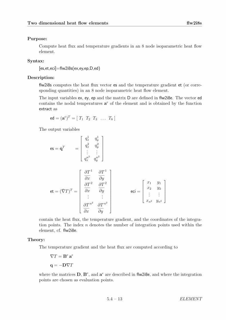
Two dimensional heat flow elements flw2i8s
Purpose:
Compute heat flux and temperature gradients in an 8 node isoparametric heat flowelement.
Syntax:
[es,et,eci]=flw2i8s(ex,ey,ep,D,ed)
Description:
flw2i8s computes the heat flux vector es and the temperature gradient et (or corre-sponding quantities) in an 8 node isoparametric heat flow element.
The input variables ex, ey, ep and the matrix D are defined in flw2i8e. The vector edcontains the nodal temperatures ae of the element and is obtained by the functionextract as
ed = (ae)T = [ T1 T2 T3 . . . T8 ]
The output variables
es = qT =
q1x q1
y
q2x q2
y...
...
qn2
x qn2
y
et = (∇T )T =
∂T
∂x
1 ∂T
∂y
1
∂T
∂x
2 ∂T
∂y
2
......
∂T
∂x
n2
∂T
∂y
n2
eci =
x1 y1
x2 y2...
...xn2 yn2
contain the heat flux, the temperature gradient, and the coordinates of the integra-tion points. The index n denotes the number of integration points used within theelement, cf. flw2i8e.
Theory:
The temperature gradient and the heat flux are computed according to
∇T = Be ae
q = −D∇T
where the matrices D, Be, and ae are described in flw2i8e, and where the integrationpoints are chosen as evaluation points.
5.4 – 13 ELEMENT

flw3i8e Three dimensional heat flow elements
Purpose:
Compute element stiffness matrix for an 8 node isoparametric element.
zx
y
●
●
●●
●
●
●
●
T4 T3
T1 T2
T7
T6
T8
T5
Syntax:
Ke=flw3i8e(ex,ey,ez,ep,D)[Ke,fe]=flw3i8e(ex,ey,ez,ep,D,eq)
Description:
flw3i8e provides the element stiffness (conductivity) matrix Ke and the element loadvector fe for an 8 node isoparametric heat flow element.
The element nodal coordinates x1, y1, z1 x2 etc, are supplied to the function by ex,ey and ez. The number of Gauss points n
(n× n× n) integration points, n = 1, 2, 3
are supplied to the function by ep and the thermal conductivities (or correspondingquantities) kxx, kxy etc are supplied by D.
ex = [ x1 x2 x3 . . . x8 ]ey = [ y1 y2 y3 . . . y8 ]ez = [ z1 z2 z3 . . . z8 ]
ep = [ n ] D =
kxx kxy kxz
kyx kyy kyz
kzx kzy kzz
If the scalar variable eq is given in the function, the element load vector fe is com-puted, using
eq = [ Q ]
where Q is the heat supply per unit volume.
Theory:
The element stiffness matrix Ke and the element load vector fel , stored in Ke and fe,respectively, are computed according to
Ke =∫
VBeT D Be dV
fel =∫
VNeT Q dV
ELEMENT 5.4 – 14
Three dimensional heat flow elements flw3i8e
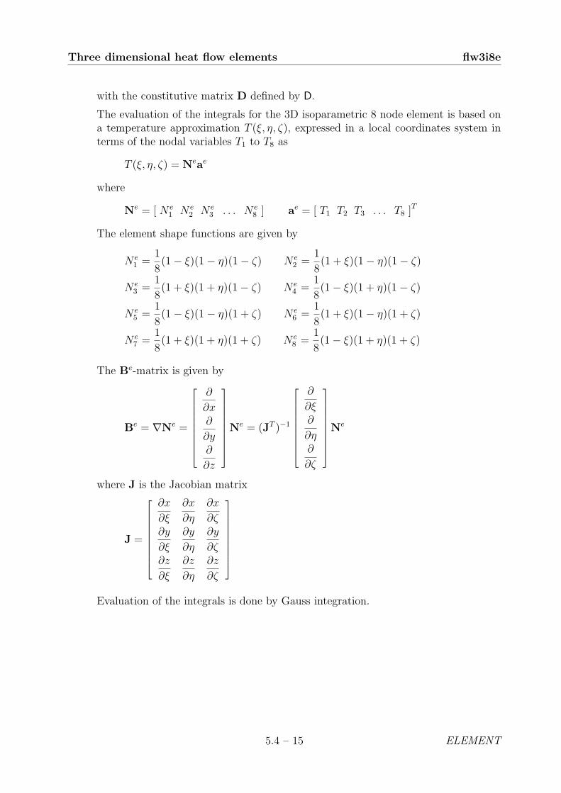
with the constitutive matrix D defined by D.
The evaluation of the integrals for the 3D isoparametric 8 node element is based ona temperature approximation T (ξ, η, ζ), expressed in a local coordinates system interms of the nodal variables T1 to T8 as
T (ξ, η, ζ) = Neae
where
Ne = [ N e1 N e
2 N e3 . . . N e
8 ] ae = [ T1 T2 T3 . . . T8 ]T
The element shape functions are given by
N e1 =
1
8(1− ξ)(1− η)(1− ζ) N e
2 =1
8(1 + ξ)(1− η)(1− ζ)
N e3 =
1
8(1 + ξ)(1 + η)(1− ζ) N e
4 =1
8(1− ξ)(1 + η)(1− ζ)
N e5 =
1
8(1− ξ)(1− η)(1 + ζ) N e
6 =1
8(1 + ξ)(1− η)(1 + ζ)
N e7 =
1
8(1 + ξ)(1 + η)(1 + ζ) N e
8 =1
8(1− ξ)(1 + η)(1 + ζ)
The Be-matrix is given by
Be = ∇Ne =
∂
∂x∂
∂y∂
∂z
Ne = (JT )−1
∂
∂ξ∂
∂η∂
∂ζ
Ne
where J is the Jacobian matrix
J =
∂x
∂ξ
∂x
∂η
∂x
∂ζ∂y
∂ξ
∂y
∂η
∂y
∂ζ∂z
∂ξ
∂z
∂η
∂z
∂ζ
Evaluation of the integrals is done by Gauss integration.
5.4 – 15 ELEMENT

flw3i8s Three dimensional heat flow elements
Purpose:
Compute heat flux and temperature gradients in an 8 node isoparametric heat flowelement.
Syntax:
[es,et,eci]=flw3i8s(ex,ey,ez,ep,D,ed)
Description:
flw3i8s computes the heat flux vector es and the temperature gradient et (or corre-sponding quantities) in an 8 node isoparametric heat flow element.
The input variables ex, ey, ez, ep and the matrix D are defined in flw3i8e. The vectored contains the nodal temperatures ae of the element and is obtained by the functionextract as
ed = (ae)T = [ T1 T2 T3 . . . T8 ]
The output variables
es = qT =
q1x q1
y q1z
q2x q2
y q2z
......
...
qn3
x qn3
y qn3
z
et = (∇T )T =
∂T
∂x
1 ∂T
∂y
1 ∂T
∂z
1
∂T
∂x
2 ∂T
∂y
2 ∂T
∂z
2
......
...
∂T
∂x
n3
∂T
∂y
n3
∂T
∂z
n3
eci =
x1 y1 z1
x2 y2 z2...
......
xn3 yn3 zn3
contain the heat flux, the temperature gradient, and the coordinates of the integra-tion points. The index n denotes the number of integration points used within theelement, cf. flw3i8e.
Theory:
The temperature gradient and the heat flux are computed according to
∇T = Be ae
q = −D∇T
where the matrices D, Be, and ae are described in flw3i8e, and where the integrationpoints are chosen as evaluation points.
ELEMENT 5.4 – 16
5.5 Solid elements
Solid elements are available for two dimensional analysis in plane stress (panels) and planestrain, and for general three dimensional analysis. In the two dimensional case there area triangular three node element, a quadrilateral four node element, two rectangular fournode elements, and quadrilateral isoparametric four and eight node elements. For threedimensional analysis there is an eight node isoparametric element.
The elements are able to deal with both isotropic and anisotropic materials. The triangularelement and the three isoparametric elements can also be used together with a nonlinearmaterial model. The material properties are specified by supplying the constitutive matrixD as an input variable to the element functions. This matrix can be formed by the functionsdescribed in Section 4.
5.5 – 1 ELEMENT

Solid elements
u1●
●
●u2
u5
u6
u3
u4
plante
●
●
●
u7
u8
u1
u2
u5
u6
u3
u4●
planqe
●
●
●
●
u7
u8
u1
u2
u5
u6
u3
u4
planreplantce
u7
u8
u2
u5
u6
u3
u4
u1●
●
●
●
plani4e
u1
u2
●
●
●
●
●
●
●
●
2
3
4
6
7
8
51
plani8e
●
●
●●
●
●
●
●
u3
u1
u2
soli8e
ELEMENT 5.5 – 2

2D solid functionsplante Compute element matrices for a triangular elementplants Compute stresses and strainsplantf Compute internal element forcesplanqe Compute element matrices for a quadrilateral elementplanqs Compute stresses and strainsplanre Compute element matrices for a rectangular Melosh elementplanrs Compute stresses and strainsplantce Compute element matrices for a rectangular Turner-Clough elementplantcs Compute stresses and strainsplani4e Compute element matrices, 4 node isoparametric elementplani4s Compute stresses and strainsplani4f Compute internal element forcesplani8e Compute element matrices, 8 node isoparametric elementplani8s Compute stresses and strainsplani8f Compute internal element forces
3D solid functionssoli8e Compute element matrices, 8 node isoparametric elementsoli8s Compute stresses and strainssoli8f Compute internal element forces
5.5 – 3 ELEMENT

plante Two dimensional solid elements
Purpose:
Compute element matrices for a triangular element in plane strain or plane stress.
x
y
(x1,y1)
(x2,y2)
(x3,y3)
u1●
●
●u2
u5
u6
u3
u4
Syntax:
Ke=plante(ex,ey,ep,D)[Ke,fe]=plante(ex,ey,ep,D,eq)
Description:
plante provides an element stiffness matrix Ke and an element load vector fe for atriangular element in plane strain or plane stress.
The element nodal coordinates x1, y1, x2 etc. are supplied to the function by ex andey. The type of analysis ptype and the element thickness t are supplied by ep,
ptype = 1 plane stressptype = 2 plane strain
and the material properties are supplied by the constitutive matrix D. Any arbitraryD-matrix with dimensions from (3 × 3) to (6 × 6) may be given. For an isotropicelastic material the constitutive matrix can be formed by the function hooke, seeSection 4.
ex = [ x1 x2 x3 ]ey = [ y1 y2 y3 ]
ep = [ ptype t ]
D =
D11 D12 D13
D21 D22 D23
D31 D32 D33
or D =
D11 D12 D13 D14 [D15 ] [D16 ]D21 D22 D23 D24 [D25 ] [D26 ]D31 D32 D33 D34 [D35 ] [D36 ]D41 D42 D43 D44 [D45 ] [D46 ]
[D51 ] [D52 ] [D53 ] [D54 ] [D55 ] [D56 ][D61 ] [D62 ] [D63 ] [D64 ] [D65 ] [D66 ]
ELEMENT 5.5 – 4
Two dimensional solid elements plante
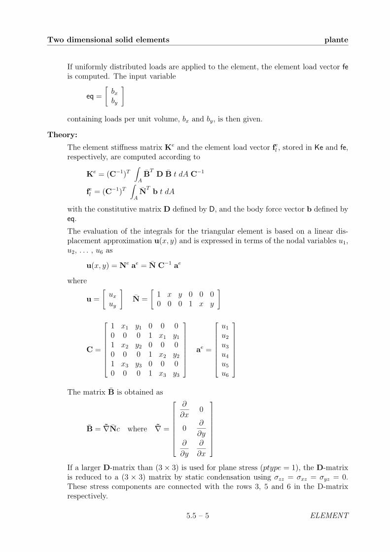
If uniformly distributed loads are applied to the element, the element load vector feis computed. The input variable
eq =
[bxby
]
containing loads per unit volume, bx and by, is then given.
Theory:
The element stiffness matrix Ke and the element load vector fel , stored in Ke and fe,respectively, are computed according to
Ke = (C−1)T∫
AB
TD B t dA C−1
fel = (C−1)T∫
AN
Tb t dA
with the constitutive matrix D defined by D, and the body force vector b defined byeq.
The evaluation of the integrals for the triangular element is based on a linear dis-placement approximation u(x, y) and is expressed in terms of the nodal variables u1,u2, . . . , u6 as
u(x, y) = Ne ae = N C−1 ae
where
u =
[ux
uy
]N =
[1 x y 0 0 00 0 0 1 x y
]
C =
1 x1 y1 0 0 00 0 0 1 x1 y1
1 x2 y2 0 0 00 0 0 1 x2 y2
1 x3 y3 0 0 00 0 0 1 x3 y3
ae =
u1
u2
u3
u4
u5
u6
The matrix B is obtained as
B = ∇Nc where ∇ =
∂
∂x0
0∂
∂y∂
∂y
∂
∂x
If a larger D-matrix than (3× 3) is used for plane stress (ptype = 1), the D-matrixis reduced to a (3 × 3) matrix by static condensation using σzz = σxz = σyz = 0.These stress components are connected with the rows 3, 5 and 6 in the D-matrixrespectively.
5.5 – 5 ELEMENT
plante Two dimensional solid elements
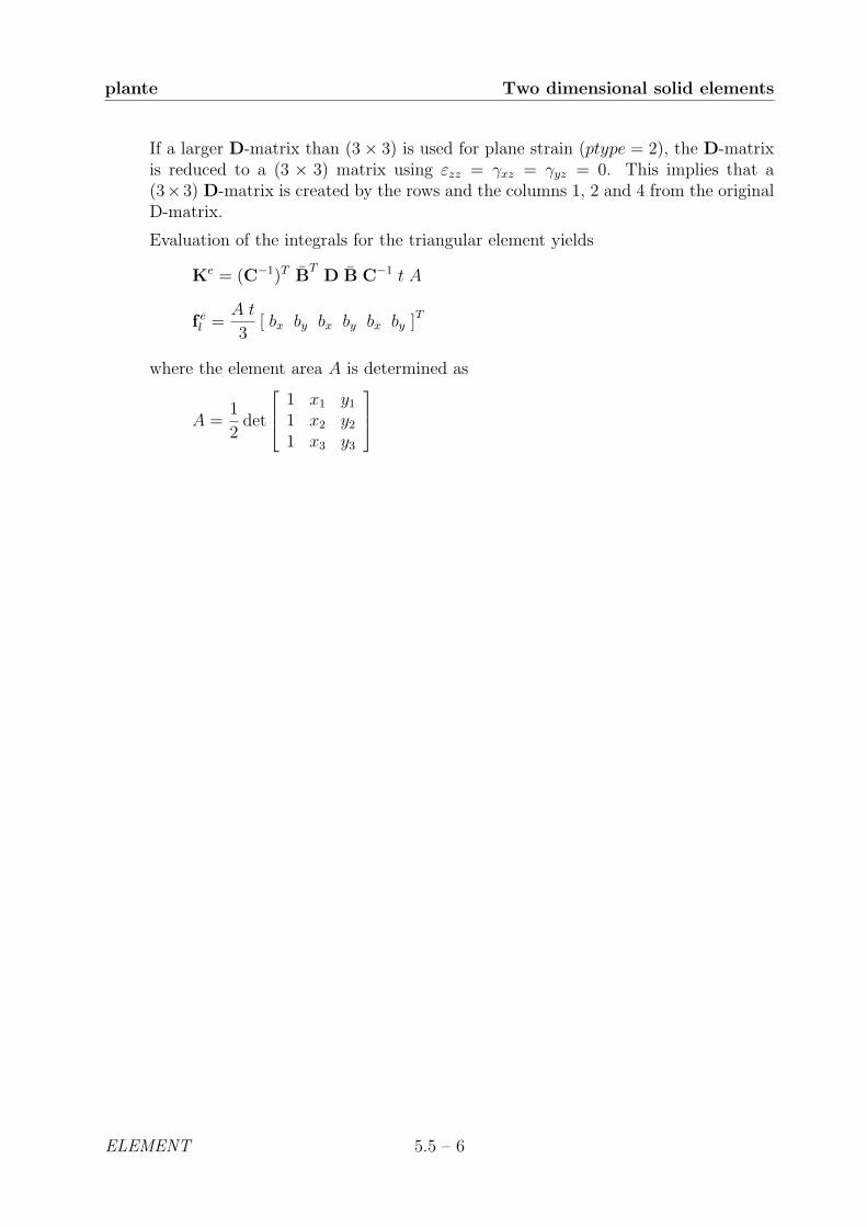
If a larger D-matrix than (3× 3) is used for plane strain (ptype = 2), the D-matrixis reduced to a (3 × 3) matrix using εzz = γxz = γyz = 0. This implies that a(3×3) D-matrix is created by the rows and the columns 1, 2 and 4 from the originalD-matrix.
Evaluation of the integrals for the triangular element yields
Ke = (C−1)T BT
D B C−1 t A
f el =
A t
3[ bx by bx by bx by ]T
where the element area A is determined as
A =1
2det
1 x1 y1
1 x2 y2
1 x3 y3
ELEMENT 5.5 – 6

Two dimensional solid elements plants
Purpose:
Compute stresses and strains in a triangular element in plane strain or plane stress.
u1●
●
●u2
u5
u6
u3
u4
σxx
σxy
σyy
σxx
σxy
σyy
x
y
Syntax:
[es,et]=plants(ex,ey,ep,D,ed)
Description:
plants computes the stresses es and the strains et in a triangular element in planestrain or plane stress.
The input variables ex, ey, ep and D are defined in plante. The vector ed containsthe nodal displacements ae of the element and is obtained by the function extract as
ed = (ae)T = [ u1 u2 . . . u6 ]
The output variables
es = σT = [ σxx σyy [σzz] σxy [σxz] [σyz] ]
et = εT = [ εxx εyy [εzz] γxy [γxz] [γyz] ]
contain the stress and strain components. The size of es and et follows the size of D.Note that for plane stress εzz 6= 0, and for plane strain σzz 6= 0.
Theory:
The strains and stresses are computed according to
ε = B C−1 ae
σ = D ε
where the matrices D, B, C and ae are described in plante. Note that both thestrains and the stresses are constant in the element.
5.5 – 7 ELEMENT

plantf Two dimensional solid elements
Purpose:
Compute internal element force vector in a triangular element in plane strain orplane stress.
Syntax:
ef=plantf(ex,ey,ep,es)
Description:
plantf computes the internal element forces ef in a triangular element in plane strainor plane stress.
The input variables ex, ey and ep are defined in plante, and the input variable es isdefined in plants.
The output variable
ef = fTi = [ fi1 fi2 . . . fi6 ]
contains the components of the internal force vector.
Theory:
The internal force vector is computed according to
fi =∫
ABT σ t dA
where the matrices B and σ are defined in plante and plants, respectively.
Evaluation of the integral for the triangular element yields
fi = B C−1 σ t A
ELEMENT 5.5 – 8

Two dimensional solid elements planqe
Purpose:
Compute element matrices for a quadrilateral element in plane strain or plane stress.
x
y
2
3
4
(x1,y1)
u7
u8
u2
u5
u6
u3
u4
u1●
●
●
●
Syntax:
Ke=planqe(ex,ey,ep,D)[Ke,fe]=planqe(ex,ey,ep,D,eq)
Description:
planqe provides an element stiffness matrix Ke and an element load vector fe for aquadrilateral element in plane strain or plane stress.
The element nodal coordinates x1, y1, x2 etc. are supplied to the function by ex andey. The type of analysis ptype and the element thickness t are supplied by ep,
ptype = 1 plane stressptype = 2 plane strain
and the material properties are supplied by the constitutive matrix D. Any arbitraryD-matrix with dimensions from (3 × 3) to (6 × 6) may be given. For an isotropicelastic material the constitutive matrix can be formed by the function hooke, seeSection 4.
ex = [ x1 x2 x3 x4 ]ey = [ y1 y2 y3 y4 ]
ep = [ ptype t ]
D =
D11 D12 D13
D21 D22 D23
D31 D32 D33
or D =
D11 D12 D13 D14 [D15 ] [D16 ]D21 D22 D23 D24 [D25 ] [D26 ]D31 D32 D33 D34 [D35 ] [D36 ]D41 D42 D43 D44 [D45 ] [D46 ]
[D51 ] [D52 ] [D53 ] [D54 ] [D55 ] [D56 ][D61 ] [D62 ] [D63 ] [D64 ] [D65 ] [D66 ]
5.5 – 9 ELEMENT

planqe Two dimensional solid elements
If uniformly distributed loads are applied on the element, the element load vector feis computed. The input variable
eq =
[bxby
]
containing loads per unit volume, bx and by, is then given.
Theory:
In computing the element matrices, two more degrees of freedom are introduced.The location of these two degrees of freedom is defined by the mean value of thecoordinates at the corner points. Four sets of element matrices are calculated usingplante. These matrices are then assembled and the two extra degrees of freedom areeliminated by static condensation.
ELEMENT 5.5 – 10
Two dimensional solid elements planqs
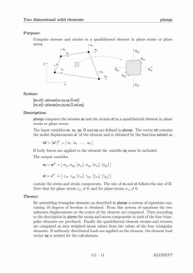
Purpose:
Compute stresses and strains in a quadrilateral element in plane strain or planestress.
u7
u8
u2
u5
u6
u3
u4
u1●
●
●
●
σxx
σxy
σyy
σxx
σxy
σyy
x
y
Syntax:
[es,et]=planqs(ex,ey,ep,D,ed)[es,et]=planqs(ex,ey,ep,D,ed,eq)
Description:
planqs computes the stresses es and the strains et in a quadrilateral element in planestrain or plane stress.
The input variables ex, ey, ep, D and eq are defined in planqe. The vector ed containsthe nodal displacements ae of the element and is obtained by the function extract as
ed = (ae)T = [ u1 u2 . . . u8 ]
If body forces are applied to the element the variable eq must be included.
The output variables
es = σT = [ σxx σyy [σzz] σxy [σxz] [σyz] ]
et = εT = [ εxx εyy [εzz] γxy [γxz] [γyz] ]
contain the stress and strain components. The size of es and et follows the size of D.Note that for plane stress εzz 6= 0, and for plane strain σzz 6= 0.
Theory:
By assembling triangular elements as described in planqe a system of equations con-taining 10 degrees of freedom is obtained. From this system of equations the twounknown displacements at the center of the element are computed. Then accordingto the description in plants the strain and stress components in each of the four trian-gular elements are produced. Finally the quadrilateral element strains and stressesare computed as area weighted mean values from the values of the four triangularelements. If uniformly distributed loads are applied on the element, the element loadvector eq is needed for the calculations.
5.5 – 11 ELEMENT

planre Two dimensional solid elements
Purpose:
Compute element matrices for a rectangular (Melosh) element in plane strain orplane stress.
x
y
(x1,y1)
(x4,y4)
(x2,y2)
(x3,y3)●
●
●
●
u7
u8
u1
u2
u5
u6
u3
u4
Syntax:
Ke=planre(ex,ey,ep,D)[Ke,fe]=planre(ex,ey,ep,D,eq)
Description:
planre provides an element stiffness matrix Ke and an element load vector fe for arectangular (Melosh) element in plane strain or plane stress. This element can onlybe used if the element edges are parallel to the coordinate axis.
The element nodal coordinates (x1, y1) and (x3, y3) are supplied to the function byex and ey. The type of analysis ptype and the element thickness t are supplied by ep,
ptype = 1 plane stressptype = 2 plane strain
and the material properties are supplied by the constitutive matrix D. Any arbitraryD-matrix with dimensions from (3 × 3) to (6 × 6) may be given. For an isotropicelastic material the constitutive matrix can be formed by the function hooke, seeSection 4.
ex = [ x1 x3 ]ey = [ y1 y3 ]
ep = [ ptype t ]
D =
D11 D12 D13
D21 D22 D23
D31 D32 D33
or D =
D11 D12 D13 D14 [D15 ] [D16 ]D21 D22 D23 D24 [D25 ] [D26 ]D31 D32 D33 D34 [D35 ] [D36 ]D41 D42 D43 D44 [D45 ] [D46 ]
[D51 ] [D52 ] [D53 ] [D54 ] [D55 ] [D56 ][D61 ] [D62 ] [D63 ] [D64 ] [D65 ] [D66 ]
ELEMENT 5.5 – 12

Two dimensional solid elements planre
If uniformly distributed loads are applied on the element, the element load vector feis computed. The input variable
eq =
[bxby
]
containing loads per unit volume, bx and by, is then given.
Theory:
The element stiffness matrix Ke and the element load vector fel , stored in Ke and fe,respectively, are computed according to
Ke =∫
ABeT D Be t dA
fel =∫
ANeT b t dA
with the constitutive matrix D defined by D, and the body force vector b defined byeq.
The evaluation of the integrals for the rectangular element is based on a bilineardisplacement approximation u(x, y) and is expressed in terms of the nodal variablesu1, u2, . . ., u8 as
u(x, y) = Ne ae
where
u =
[ux
uy
]Ne =
[N e
1 0 N e2 0 N e
3 0 N e4 0
0 N e1 0 N e
2 0 N e3 0 N e
4
]ae =
u1
u2...u8
With a local coordinate system located at the center of the element, the elementshape functions N e
1 −N e4 are obtained as
N e1 =
1
4ab(x− x2)(y − y4)
N e2 = − 1
4ab(x− x1)(y − y3)
N e3 =
1
4ab(x− x4)(y − y2)
N e4 = − 1
4ab(x− x3)(y − y1)
where
a =1
2(x3 − x1) and b =
1
2(y3 − y1)
5.5 – 13 ELEMENT
planre Two dimensional solid elements
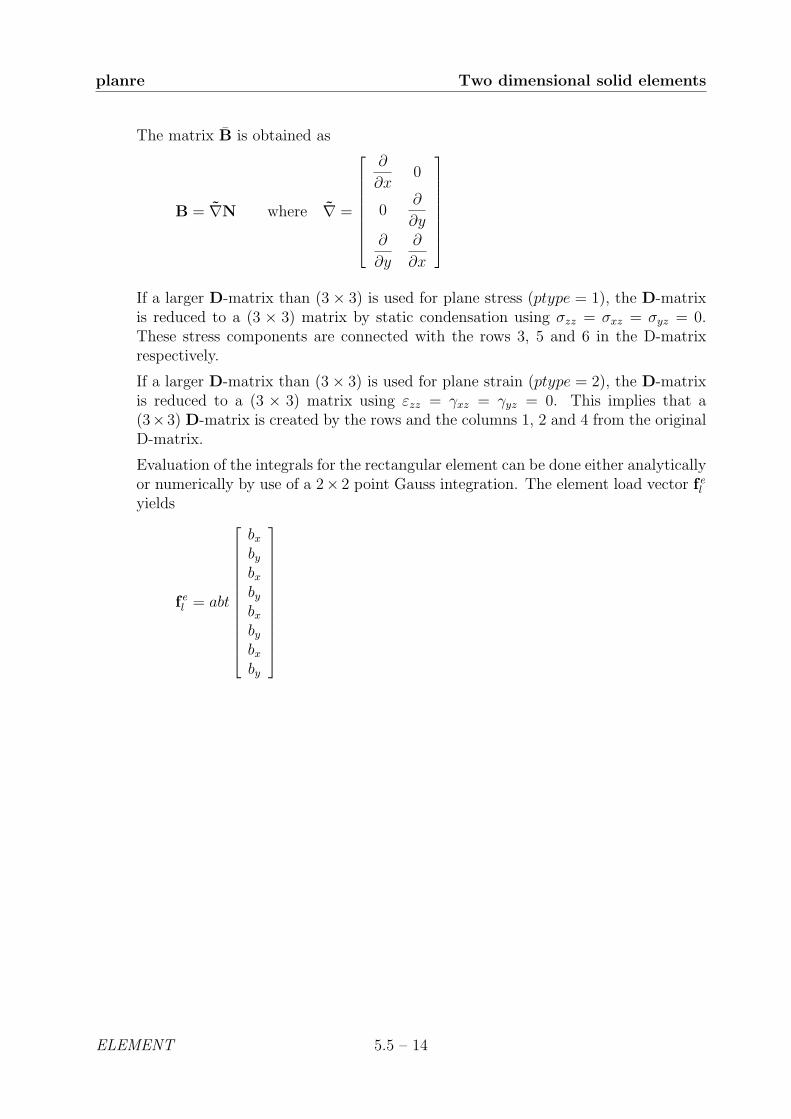
The matrix B is obtained as
B = ∇N where ∇ =
∂
∂x0
0∂
∂y∂
∂y
∂
∂x
If a larger D-matrix than (3× 3) is used for plane stress (ptype = 1), the D-matrixis reduced to a (3 × 3) matrix by static condensation using σzz = σxz = σyz = 0.These stress components are connected with the rows 3, 5 and 6 in the D-matrixrespectively.
If a larger D-matrix than (3× 3) is used for plane strain (ptype = 2), the D-matrixis reduced to a (3 × 3) matrix using εzz = γxz = γyz = 0. This implies that a(3×3) D-matrix is created by the rows and the columns 1, 2 and 4 from the originalD-matrix.
Evaluation of the integrals for the rectangular element can be done either analyticallyor numerically by use of a 2× 2 point Gauss integration. The element load vector f e
l
yields
f el = abt
bxbybxbybxbybxby
ELEMENT 5.5 – 14
Two dimensional solid elements planrs
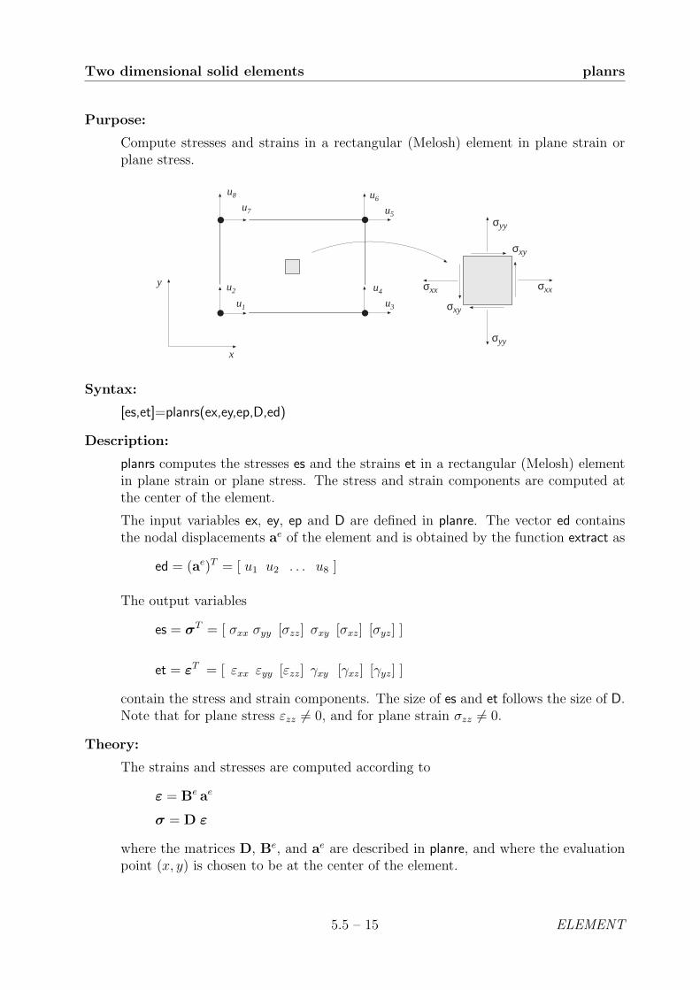
Purpose:
Compute stresses and strains in a rectangular (Melosh) element in plane strain orplane stress.
●
●
●
●
u7
u8
u1
u2
u5
u6
u3
u4σxx
σxy
σyy
σxx
σxy
σyy
x
y
Syntax:
[es,et]=planrs(ex,ey,ep,D,ed)
Description:
planrs computes the stresses es and the strains et in a rectangular (Melosh) elementin plane strain or plane stress. The stress and strain components are computed atthe center of the element.
The input variables ex, ey, ep and D are defined in planre. The vector ed containsthe nodal displacements ae of the element and is obtained by the function extract as
ed = (ae)T = [ u1 u2 . . . u8 ]
The output variables
es = σT = [ σxx σyy [σzz] σxy [σxz] [σyz] ]
et = εT = [ εxx εyy [εzz] γxy [γxz] [γyz] ]
contain the stress and strain components. The size of es and et follows the size of D.Note that for plane stress εzz 6= 0, and for plane strain σzz 6= 0.
Theory:
The strains and stresses are computed according to
ε = Be ae
σ = D ε
where the matrices D, Be, and ae are described in planre, and where the evaluationpoint (x, y) is chosen to be at the center of the element.
5.5 – 15 ELEMENT

plantce Two dimensional solid elements
Purpose:
Compute element matrices for a rectangular (Turner-Clough) element in plane strainor plane stress.
x
y
(x1,y1)
(x4,y4)
(x2,y2)
(x3,y3)●
●
●
●
u7
u8
u1
u2
u5
u6
u3
u4
Syntax:
Ke=plantce(ex,ey,ep)[Ke,fe]=plantce(ex,ey,ep,eq)
Description:
plantce provides an element stiffness matrix Ke and an element load vector fe for arectangular (Turner-Clough) element in plane strain or plane stress. This elementcan only be used if the material is isotropic and if the element edges are parallel tothe coordinate axis.
The element nodal coordinates (x1, y1) and (x3, y3) are supplied to the function by exand ey. The state of stress ptype, the element thickness t and the material propertiesE and ν are supplied by ep. For plane stress ptype = 1 and for plane strain ptype = 2.
ex = [ x1 x3 ]ey = [ y1 y3 ]
ep = [ ptype t E ν ]
If uniformly distributed loads are applied to the element, the element load vector feis computed. The input variable
eq =
[bxby
]
containing loads per unit volume, bx and by, is then given.
ELEMENT 5.5 – 16

Two dimensional solid elements plantce
Theory:
The element stiffness matrix Ke and the element load vector fel , stored in Ke and fe,respectively, are computed according to
Ke =∫
ABeT D Be t dA
fel =∫
ANeT b t dA
where the constitutive matrix D is described in hooke, see Section 4, and the bodyforce vector b is defined by eq.
The evaluation of the integrals for the Turner-Clough element is based on a dis-placement field u(x, y) built up of a bilinear displacement approximation superposedby bubble functions in order to create a linear stress field over the element. Thedisplacement field is expressed in terms of the nodal variables u1, u2, . . ., u8 as
u(x, y) = Ne ae
where
u =
[ux
uy
]Ne =
[N e
1 N e5 N e
2 N e5 N e
3 N e5 N e
4 N e5
N e6 N e
1 N e6 N e
2 N e6 N e
3 N e6 N e
4
]ae =
u1
u2...u8
With a local coordinate system located at the center of the element, the elementshape functions N e
1 −N e6 are obtained as
N e1 =
1
4ab(a− x)(b− y)
N e2 =
1
4ab(a+ x)(b− y)
N e3 =
1
4ab(a+ x)(b+ y)
N e4 =
1
4ab(a− x)(b+ y)
N e5 =
1
8ab
[(b2 − y2) + ν(a2 − x2)
]N e
6 =1
8ab
[(a2 − x2) + ν(b2 − y2)
]where
a =1
2(x3 − x1) and b =
1
2(y3 − y1)
5.5 – 17 ELEMENT

plantce Two dimensional solid elements
The matrix B is obtained as
B = ∇N where ∇ =
∂
∂x0
0∂
∂y∂
∂y
∂
∂x
Evaluation of the integrals for the Turner-Clough element can be done either ana-lytically or numerically by use of a 2× 2 point Gauss integration. The element loadvector f e
l yields
f el = abt
bxbybxbybxbybxby
ELEMENT 5.5 – 18

Two dimensional solid elements plantcs
Purpose:
Compute stresses and strains in a Turner-Clough element in plane strain or planestress.
●
●
●
●
u7
u8
u1
u2
u5
u6
u3
u4σxx
σxy
σyy
σxx
σxy
σyy
x
y
Syntax:
[es,et]=plantcs(ex,ey,ep,ed)
Description:
plantcs computes the stresses es and the strains et in a rectangular Turner-Clough ele-ment in plane strain or plane stress. The stress and strain components are computedat the center of the element.
The input variables ex, ey, and ep are defined in plantce. The vector ed contains thenodal displacements ae of the element and is obtained by the function extract as
ed = (ae)T = [ u1 u2 . . . u8 ]
The output variables
es = σT = [ σxx σyy [σzz] σxy [σxz] [σyz] ]
et = εT = [ εxx εyy [εzz] γxy [γxz] [γyz] ]
contain the stress and strain components. The size of es and et follows the size of D.Note that for plane stress εzz 6= 0, and for plane strain σzz 6= 0.
Theory:
The strains and stresses are computed according to
ε = Be ae
σ = D ε
where the matrices D, Be, and ae are described in plantce, and where the evaluationpoint (x, y) is chosen to be at the center of the element.
5.5 – 19 ELEMENT

plani4e Two dimensional solid elements
Purpose:
Compute element matrices for a 4 node isoparametric element in plane strain orplane stress.
x
y
2
3
4
(x1,y1)
u7
u8
u2
u5
u6
u3
u4
u1●
●
●
●
Syntax:
Ke=plani4e(ex,ey,ep,D)[Ke,fe]=plani4e(ex,ey,ep,D,eq)
Description:
plani4e provides an element stiffness matrix Ke and an element load vector fe for a 4node isoparametric element in plane strain or plane stress.
The element nodal coordinates x1, y1, x2 etc. are supplied to the function by ex andey. The type of analysis ptype, the element thickness t, and the number of Gausspoints n are supplied by ep.
ptype = 1 plane stress (n× n) integration pointsptype = 2 plane strain n = 1, 2, 3
The material properties are supplied by the constitutive matrix D. Any arbitrary D-matrix with dimensions from (3× 3) to (6× 6) maybe given. For an isotropic elasticmaterial the constitutive matrix can be formed by the function hooke, see Section 4.
ex = [ x1 x2 x3 x4 ]ey = [ y1 y2 y3 y4 ]
ep = [ ptype t n ]
D =
D11 D12 D13
D21 D22 D23
D31 D32 D33
or D =
D11 D12 D13 D14 [D15 ] [D16 ]D21 D22 D23 D24 [D25 ] [D26 ]D31 D32 D33 D34 [D35 ] [D36 ]D41 D42 D43 D44 [D45 ] [D46 ]
[D51 ] [D52 ] [D53 ] [D54 ] [D55 ] [D56 ][D61 ] [D62 ] [D63 ] [D64 ] [D65 ] [D66 ]
If different Di -matrices are used in the Gauss points these Di -matrices are storedin a global vector D. For numbering of the Gauss points, see eci in plani4s.
D =
D1
D2...
Dn2
ELEMENT 5.5 – 20

Two dimensional solid elements plani4e
If uniformly distributed loads are applied to the element, the element load vector feis computed. The input variable
eq =
[bxby
]containing loads per unit volume, bx and by, is then given.
Theory:
The element stiffness matrix Ke and the element load vector fel , stored in Ke and fe,respectively, are computed according to
Ke =∫
ABeT D Be t dA
fel =∫
ANeT b t dA
with the constitutive matrix D defined by D, and the body force vector b defined byeq.
The evaluation of the integrals for the isoparametric 4 node element is based on adisplacement approximation u(ξ, η), expressed in a local coordinates system in termsof the nodal variables u1, u2, . . ., u8 as
u(ξ, η) = Ne ae
where
u =
[ux
uy
]Ne =
[N e
1 0 N e2 0 N e
3 0 N e4 0
0 N e1 0 N e
2 0 N e3 0 N e
4
]ae =
u1
u2...u8
The element shape functions are given by
N e1 =
1
4(1− ξ)(1− η) N e
2 =1
4(1 + ξ)(1− η)
N e3 =
1
4(1 + ξ)(1 + η) N e
4 =1
4(1− ξ)(1 + η)
The matrix B is obtained as
B = ∇N where ∇ =
∂
∂x0
0∂
∂y∂
∂y
∂
∂x
and where
∂
∂x∂
∂y
= (JT )−1
∂
∂ξ∂
∂η
J =
∂x
∂ξ
∂x
∂η∂y
∂ξ
∂y
∂η
5.5 – 21 ELEMENT

plani4e Two dimensional solid elements
If a larger D-matrix than (3× 3) is used for plane stress (ptype = 1), the D-matrixis reduced to a (3 × 3) matrix by static condensation using σzz = σxz = σyz = 0.These stress components are connected with the rows 3, 5 and 6 in the D-matrixrespectively.
If a larger D-matrix than (3× 3) is used for plane strain (ptype = 2), the D-matrixis reduced to a (3 × 3) matrix using εzz = γxz = γyz = 0. This implies that a(3×3) D-matrix is created by the rows and the columns 1, 2 and 4 from the originalD-matrix.
Evaluation of the integrals is done by Gauss integration.
ELEMENT 5.5 – 22

Two dimensional solid elements plani4s
Purpose:
Compute stresses and strains in a 4 node isoparametric element in plane strain orplane stress.
u7
u8
u2
u5
u6
u3
u4
u1●
●
●
●
σxx
σxy
σyy
σxx
σxy
σyy
x
y
Syntax:
[es,et,eci]=plani4s(ex,ey,ep,D,ed)
Description:
plani4s computes stresses es and the strains et in a 4 node isoparametric element inplane strain or plane stress.
The input variables ex, ey, ep and the matrix D are defined in plani4e. The vector edcontains the nodal displacements ae of the element and is obtained by the functionextract as
ed = (ae)T = [ u1 u2 . . . u8 ]
The output variables
es = σT =
σ1xx σ1
yy [σ1zz] σ1
xy [σ1xz]
[σ1
yz
]σ2
xx σ2yy [σ2
zz] σ2xy [σ2
xz][σ2
yz
]...
......
......
...
σn2
xx σn2
yy
[σn2
zz
]σn2
xy
[σn2
xz
] [σn2
yz
]
et = εT =
ε1xx ε1
yy [ε1zz] γ1
xy [γ1xz]
[γ1
yz
]ε2
xx ε2yy [ε2
zz] γ2xy [γ2
xz][γ2
yz
]...
......
......
...
εn2
xx εn2
yy
[εn2
zz
]γn2
xy
[γn2
xz
] [γn2
yz
]
eci =
x1 y1
x2 y2...
...xn2 yn2
contain the stress and strain components, and the coordinates of the integrationpoints. The index n denotes the number of integration points used within the ele-ment, cf. plani4e. The number of columns in es and et follows the size of D. Notethat for plane stress εzz 6= 0, and for plane strain σzz 6= 0.
5.5 – 23 ELEMENT

plani4s Two dimensional solid elements
Theory:
The strains and stresses are computed according to
ε = Be ae
σ = D ε
where the matrices D, Be, and ae are described in plani4e, and where the integrationpoints are chosen as evaluation points.
ELEMENT 5.5 – 24
Two dimensional solid elements plani4f
Purpose:
Compute internal element force vector in a 4 node isoparametric element in planestrain or plane stress.
Syntax:
ef=plani4f(ex,ey,ep,es)
Description:
plani4f computes the internal element forces ef in a 4 node isoparametric element inplane strain or plane stress.
The input variables ex, ey and ep are defined in plani4e, and the input variable es isdefined in plani4s.
The output variable
ef = fTi = [ fi1 fi2 . . . fi8 ]
contains the components of the internal force vector.
Theory:
The internal force vector is computed according to
fi =∫
ABT σ t dA
where the matrices B and σ are defined in plani4e and plani4s, respectively.
Evaluation of the integral is done by Gauss integration.
5.5 – 25 ELEMENT
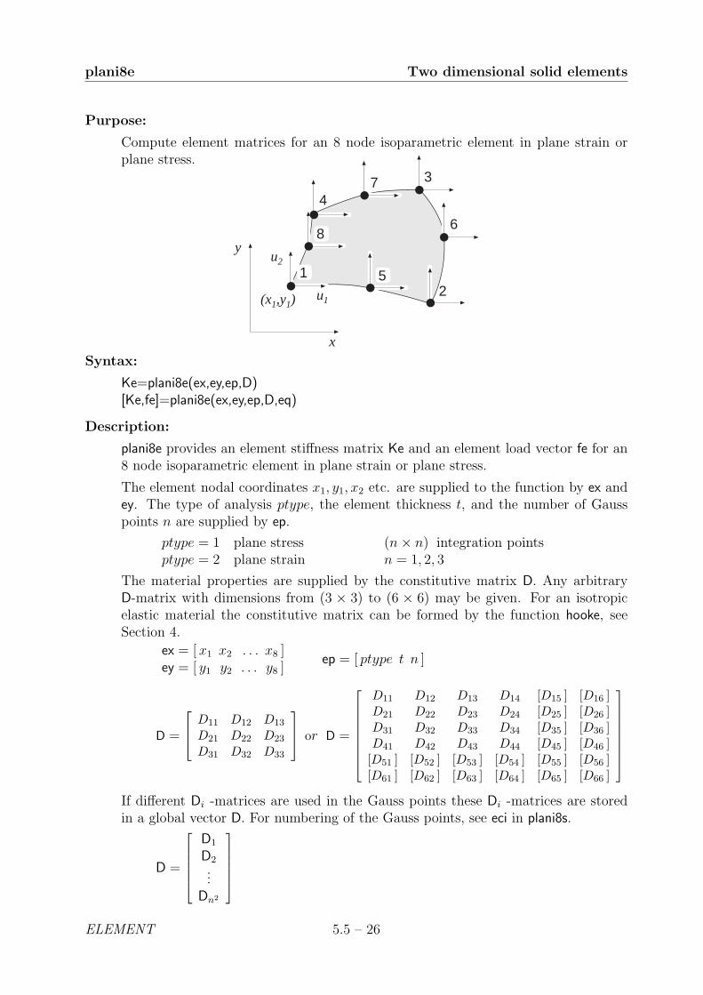
plani8e Two dimensional solid elements
Purpose:
Compute element matrices for an 8 node isoparametric element in plane strain orplane stress.
x
y
(x1,y1) u1
u2
●
●
●
●
●
●
●
●
2
3
4
6
7
8
51
Syntax:
Ke=plani8e(ex,ey,ep,D)[Ke,fe]=plani8e(ex,ey,ep,D,eq)
Description:
plani8e provides an element stiffness matrix Ke and an element load vector fe for an8 node isoparametric element in plane strain or plane stress.
The element nodal coordinates x1, y1, x2 etc. are supplied to the function by ex andey. The type of analysis ptype, the element thickness t, and the number of Gausspoints n are supplied by ep.
ptype = 1 plane stress (n× n) integration pointsptype = 2 plane strain n = 1, 2, 3
The material properties are supplied by the constitutive matrix D. Any arbitraryD-matrix with dimensions from (3 × 3) to (6 × 6) may be given. For an isotropicelastic material the constitutive matrix can be formed by the function hooke, seeSection 4.
ex = [ x1 x2 . . . x8 ]ey = [ y1 y2 . . . y8 ]
ep = [ ptype t n ]
D =
D11 D12 D13
D21 D22 D23
D31 D32 D33
or D =
D11 D12 D13 D14 [D15 ] [D16 ]D21 D22 D23 D24 [D25 ] [D26 ]D31 D32 D33 D34 [D35 ] [D36 ]D41 D42 D43 D44 [D45 ] [D46 ]
[D51 ] [D52 ] [D53 ] [D54 ] [D55 ] [D56 ][D61 ] [D62 ] [D63 ] [D64 ] [D65 ] [D66 ]
If different Di -matrices are used in the Gauss points these Di -matrices are storedin a global vector D. For numbering of the Gauss points, see eci in plani8s.
D =
D1
D2...
Dn2
ELEMENT 5.5 – 26
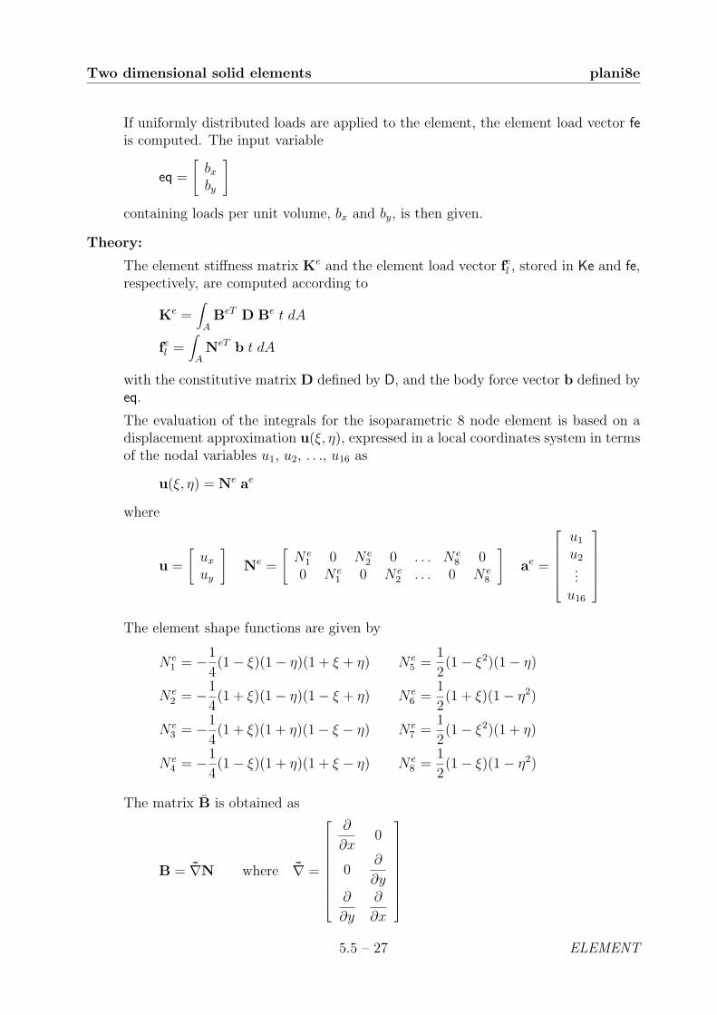
Two dimensional solid elements plani8e
If uniformly distributed loads are applied to the element, the element load vector feis computed. The input variable
eq =
[bxby
]
containing loads per unit volume, bx and by, is then given.
Theory:
The element stiffness matrix Ke and the element load vector fel , stored in Ke and fe,respectively, are computed according to
Ke =∫
ABeT D Be t dA
fel =∫
ANeT b t dA
with the constitutive matrix D defined by D, and the body force vector b defined byeq.
The evaluation of the integrals for the isoparametric 8 node element is based on adisplacement approximation u(ξ, η), expressed in a local coordinates system in termsof the nodal variables u1, u2, . . ., u16 as
u(ξ, η) = Ne ae
where
u =
[ux
uy
]Ne =
[N e
1 0 N e2 0 . . . N e
8 00 N e
1 0 N e2 . . . 0 N e
8
]ae =
u1
u2...u16
The element shape functions are given by
N e1 = −1
4(1− ξ)(1− η)(1 + ξ + η) N e
5 =1
2(1− ξ2)(1− η)
N e2 = −1
4(1 + ξ)(1− η)(1− ξ + η) N e
6 =1
2(1 + ξ)(1− η2)
N e3 = −1
4(1 + ξ)(1 + η)(1− ξ − η) N e
7 =1
2(1− ξ2)(1 + η)
N e4 = −1
4(1− ξ)(1 + η)(1 + ξ − η) N e
8 =1
2(1− ξ)(1− η2)
The matrix B is obtained as
B = ∇N where ∇ =
∂
∂x0
0∂
∂y∂
∂y
∂
∂x
5.5 – 27 ELEMENT
plani8e Two dimensional solid elements
and where∂
∂x∂
∂y
= (JT )−1
∂
∂ξ∂
∂η
J =
∂x
∂ξ
∂x
∂η∂y
∂ξ
∂y
∂η
If a larger D-matrix than (3× 3) is used for plane stress (ptype = 1), the D-matrixis reduced to a (3 × 3) matrix by static condensation using σzz = σxz = σyz = 0.These stress components are connected with the rows 3, 5 and 6 in the D-matrixrespectively.
If a larger D-matrix than (3× 3) is used for plane strain (ptype = 2), the D-matrixis reduced to a (3 × 3) matrix using εzz = γxz = γyz = 0. This implies that a(3×3) D-matrix is created by the rows and the columns 1, 2 and 4 from the originalD-matrix.
Evaluation of the integrals is done by Gauss integration.
ELEMENT 5.5 – 28
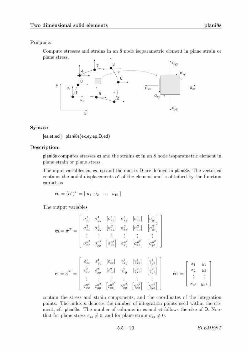
Two dimensional solid elements plani8s
Purpose:
Compute stresses and strains in an 8 node isoparametric element in plane strain orplane stress.
u1
u2
●
●
●
●
●
●
●
●
2
3
4
6
7
8
51σxx
σxy
σyy
σxx
σxy
σyy
x
y
Syntax:
[es,et,eci]=plani8s(ex,ey,ep,D,ed)
Description:
plani8s computes stresses es and the strains et in an 8 node isoparametric element inplane strain or plane stress.
The input variables ex, ey, ep and the matrix D are defined in plani8e. The vector edcontains the nodal displacements ae of the element and is obtained by the functionextract as
ed = (ae)T = [ u1 u2 . . . u16 ]
The output variables
es = σT =
σ1xx σ1
yy [σ1zz] σ1
xy [σ1xz]
[σ1
yz
]σ2
xx σ2yy [σ2
zz] σ2xy [σ2
xz][σ2
yz
]...
......
......
...
σn2
xx σn2
yy
[σn2
zz
]σn2
xy
[σn2
xz
] [σn2
yz
]
et = εT =
ε1xx ε1
yy [ε1zz] γ1
xy [γ1xz]
[γ1
yz
]ε2
xx ε2yy [ε2
zz] γ2xy [γ2
xz][γ2
yz
]...
......
......
...
εn2
xx εn2
yy
[εn2
zz
]γn2
xy
[γn2
xz
] [γn2
yz
]
eci =
x1 y1
x2 y2...
...xn2 yn2
contain the stress and strain components, and the coordinates of the integrationpoints. The index n denotes the number of integration points used within the ele-ment, cf. plani8e. The number of columns in es and et follows the size of D. Notethat for plane stress εzz 6= 0, and for plane strain σzz 6= 0.
5.5 – 29 ELEMENT
plani8s Two dimensional solid elements
Theory:
The strains and stresses are computed according to
ε = Be ae
σ = D ε
where the matrices D, Be, and ae are described in plani8e, and where the integrationpoints are chosen as evaluation points.
ELEMENT 5.5 – 30

Two dimensional solid elements plani8f
Purpose:
Compute internal element force vector in an 8 node isoparametric element in planestrain or plane stress.
Syntax:
ef=plani8f(ex,ey,ep,es)
Description:
plani8f computes the internal element forces ef in an 8 node isoparametric elementin plane strain or plane stress.
The input variables ex, ey and ep are defined in plani8e, and the input variable es isdefined in plani8s.
The output variable
ef = fTi = [ fi1 fi2 . . . fi16 ]
contains the components of the internal force vector.
Theory:
The internal force vector is computed according to
fi =∫
ABT σ t dA
where the matrices B and σ are defined in plani8e and plani8s, respectively.
Evaluation of the integral is done by Gauss integration.
5.5 – 31 ELEMENT

soli8e Three dimensional solid elements
Purpose:
Compute element matrices for an 8 node isoparametric solid element.
zx
y
2
34
6
78
5
(x1,y1,z1) ●
●
●●
●
●
●
●
u3
u1
u2
Syntax:
Ke=soli8e(ex,ey,ez,ep,D)[Ke,fe]=soli8e(ex,ey,ez,ep,D,eq)
Description:
soli8e provides an element stiffness matrix Ke and an element load vector fe for an 8node isoparametric solid element.
The element nodal coordinates x1, y1, z1, x2 etc. are supplied to the function by ex,ey and ez, and the number of Gauss points n are supplied by ep.
(n× n) integration points, n = 1, 2, 3
The material properties are supplied by the constitutive matrix D. Any arbitraryD-matrix with dimensions (6×6) may be given. For an isotropic elastic material theconstitutive matrix can be formed by the function hooke, see Section 4.
ex = [ x1 x2 . . . x8 ]ey = [ y1 y2 . . . y8 ]ez = [ z1 z2 . . . z8 ]
ep = [ n ] D =
D11 D12 · · · D16
D21 D22 · · · D26...
.... . .
...D61 D62 · · · D66
If different Di -matrices are used in the Gauss points these Di -matrices are storedin a global vector D. For numbering of the Gauss points, see eci in soli8s.
D =
D1
D2...
Dn3
If uniformly distributed loads are applied to the element, the element load vector feis computed. The input variable
eq =
bxbybz
ELEMENT 5.5 – 32
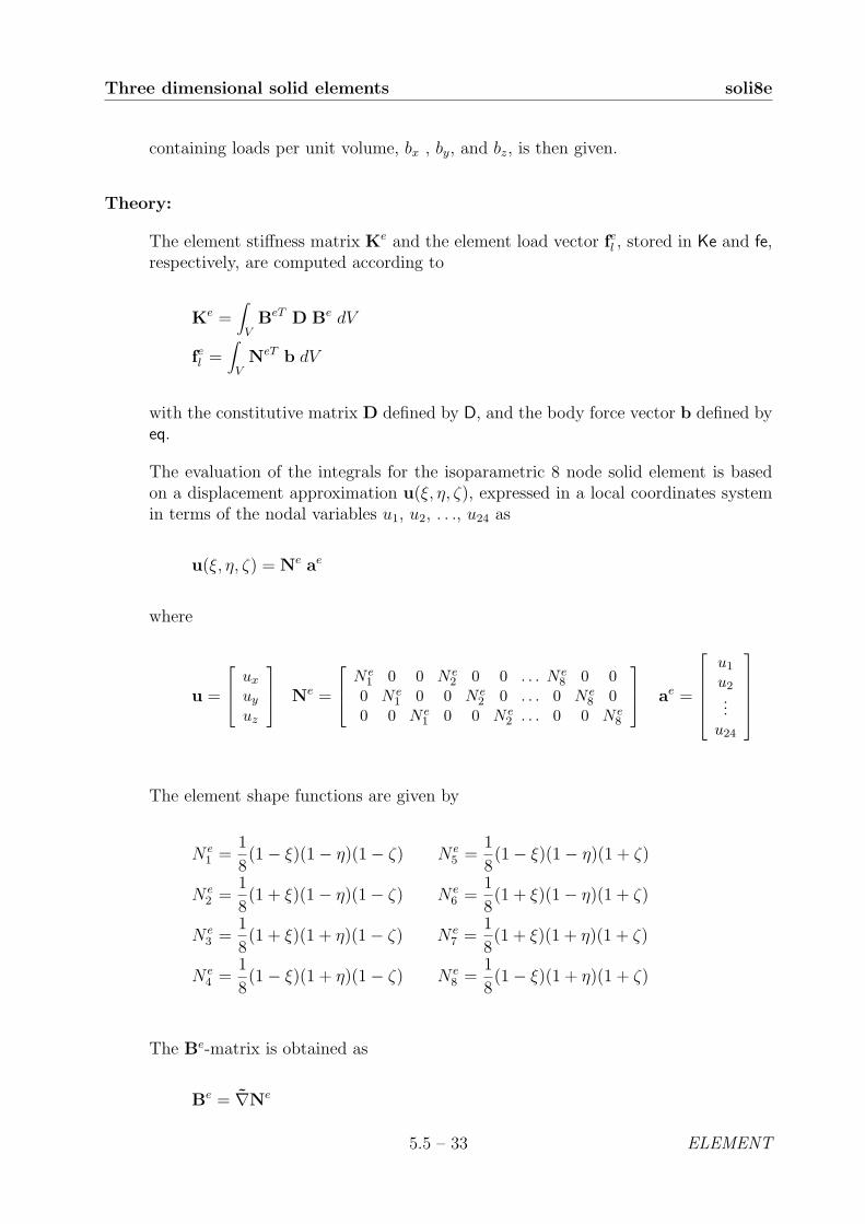
Three dimensional solid elements soli8e
containing loads per unit volume, bx , by, and bz, is then given.
Theory:
The element stiffness matrix Ke and the element load vector fel , stored in Ke and fe,respectively, are computed according to
Ke =∫
VBeT D Be dV
fel =∫
VNeT b dV
with the constitutive matrix D defined by D, and the body force vector b defined byeq.
The evaluation of the integrals for the isoparametric 8 node solid element is basedon a displacement approximation u(ξ, η, ζ), expressed in a local coordinates systemin terms of the nodal variables u1, u2, . . ., u24 as
u(ξ, η, ζ) = Ne ae
where
u =
ux
uy
uz
Ne =
N e1 0 0 N e
2 0 0 . . . N e8 0 0
0 N e1 0 0 N e
2 0 . . . 0 N e8 0
0 0 N e1 0 0 N e
2 . . . 0 0 N e8
ae =
u1
u2...
u24
The element shape functions are given by
N e1 =
1
8(1− ξ)(1− η)(1− ζ) N e
5 =1
8(1− ξ)(1− η)(1 + ζ)
N e2 =
1
8(1 + ξ)(1− η)(1− ζ) N e
6 =1
8(1 + ξ)(1− η)(1 + ζ)
N e3 =
1
8(1 + ξ)(1 + η)(1− ζ) N e
7 =1
8(1 + ξ)(1 + η)(1 + ζ)
N e4 =
1
8(1− ξ)(1 + η)(1− ζ) N e
8 =1
8(1− ξ)(1 + η)(1 + ζ)
The Be-matrix is obtained as
Be = ∇Ne
5.5 – 33 ELEMENT

soli8e Three dimensional solid elements
where
∇ =
∂
∂x0 0
0∂
∂y0
0 0∂
∂z∂
∂y
∂
∂x0
∂
∂z0
∂
∂x
0∂
∂z
∂
∂y
∂
∂x∂
∂y∂
∂z
= (JT )−1
∂
∂ξ∂
∂η∂
∂ζ
J =
∂x
∂ξ
∂x
∂η
∂x
∂ζ∂y
∂ξ
∂y
∂η
∂y
∂ζ∂z
∂ξ
∂z
∂η
∂z
∂ζ
Evaluation of the integrals is done by Gauss integration.
ELEMENT 5.5 – 34
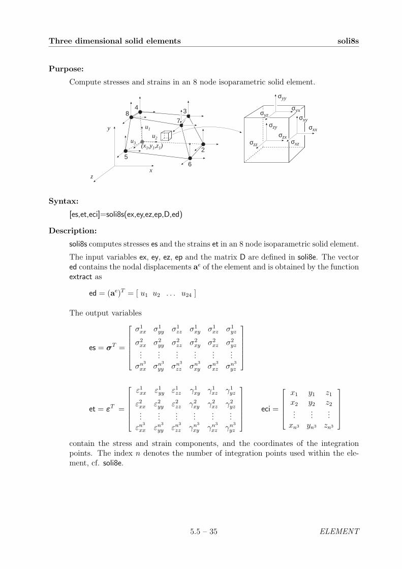
Three dimensional solid elements soli8s
Purpose:
Compute stresses and strains in an 8 node isoparametric solid element.
σzz
σzx
σxx
σxyσzy
σyy
σyxσyz
σxz
zx
y
2
34
6
78
5
(x1,y1,z1) ●
●
●●
●
●
●
●
u3
u2
u1
Syntax:
[es,et,eci]=soli8s(ex,ey,ez,ep,D,ed)
Description:
soli8s computes stresses es and the strains et in an 8 node isoparametric solid element.
The input variables ex, ey, ez, ep and the matrix D are defined in soli8e. The vectored contains the nodal displacements ae of the element and is obtained by the functionextract as
ed = (ae)T = [ u1 u2 . . . u24 ]
The output variables
es = σT =
σ1
xx σ1yy σ1
zz σ1xy σ1
xz σ1yz
σ2xx σ2
yy σ2zz σ2
xy σ2xz σ2
yz...
......
......
...
σn3
xx σn3
yy σn3
zz σn3
xy σn3
xz σn3
yz
et = εT =
ε1
xx ε1yy ε1
zz γ1xy γ1
xz γ1yz
ε2xx ε2
yy ε2zz γ2
xy γ2xz γ2
yz...
......
......
...
εn3
xx εn3
yy εn3
zz γn3
xy γn3
xz γn3
yz
eci =
x1 y1 z1
x2 y2 z2...
......
xn3 yn3 zn3
contain the stress and strain components, and the coordinates of the integrationpoints. The index n denotes the number of integration points used within the ele-ment, cf. soli8e.
5.5 – 35 ELEMENT

soli8s Three dimensional solid elements
Theory:
The strains and stresses are computed according to
ε = Be ae
σ = D ε
where the matrices D, Be, and ae are described in soli8e, and where the integrationpoints are chosen as evaluation points.
ELEMENT 5.5 – 36

Three dimensional solid elements soli8f
Purpose:
Compute internal element force vector in an 8 node isoparametric solid element.
Syntax:
ef=soli8f(ex,ey,ez,ep,es)
Description:
soli8f computes the internal element forces ef in an 8 node isoparametric solid element.
The input variables ex, ey, ez and ep are defined in soli8e, and the input variable esis defined in soli8s.
The output variable
ef = fTi = [ fi1 fi2 . . . fi24 ]
contains the components of the internal force vector.
Theory:
The internal force vector is computed according to
fi =∫
VBT σ dV
where the matrices B and σ are defined in soli8e and soli8s, respectively.
Evaluation of the integral is done by Gauss integration.
5.5 – 37 ELEMENT


5.6 Beam elements
Beam elements are available for two, and three dimensional linear static analysis. Twodimensional beam elements for nonlinear geometric and dynamic analysis are also available.
Beam elements
u1
u2
u4
u5
u6
u3
beam2ebeam2tbeam2wbeam2gbeam2d
u1
u2
u4
u5
u6
u3
u7
u8
u10
u11
u12
u9
beam3e
2D beam elementsbeam2e Compute element matricesbeam2s Compute section forcesbeam2t Compute element matrices for Timoshenko beam elementbeam2ts Compute section forces for Timoshenko beam elementbeam2w Compute element matrices for beam element on elastic foundationbeam2ws Compute section forces for beam element on elastic foundationbeam2g Compute element matrices with respect to geometric nonlinearitybeam2gs Compute section forces for geometric nonlinear beam elementbeam2d Compute element matrices, dynamic analysisbeam2ds Compute section forces, dynamic analysis
3D beam elementsbeam3e Compute element matricesbeam3s Compute section forces
5.6 – 1 ELEMENT
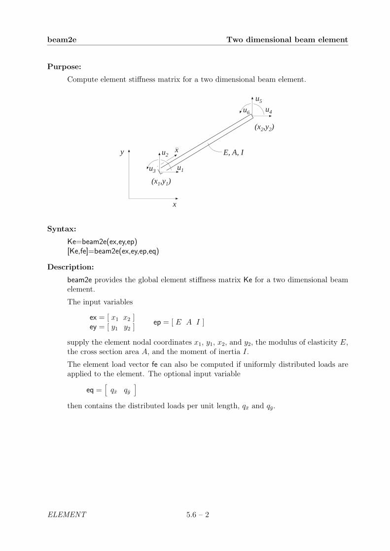
beam2e Two dimensional beam element
Purpose:
Compute element stiffness matrix for a two dimensional beam element.
E, A, I
x
y
(x1,y1)
(x2,y2)
x
u1
u2
u4
u5
u6
u3
Syntax:
Ke=beam2e(ex,ey,ep)[Ke,fe]=beam2e(ex,ey,ep,eq)
Description:
beam2e provides the global element stiffness matrix Ke for a two dimensional beamelement.
The input variables
ex = [ x1 x2 ]ey = [ y1 y2 ]
ep = [ E A I ]
supply the element nodal coordinates x1, y1, x2, and y2, the modulus of elasticity E,the cross section area A, and the moment of inertia I.
The element load vector fe can also be computed if uniformly distributed loads areapplied to the element. The optional input variable
eq =[qx qy
]then contains the distributed loads per unit length, qx and qy.
ELEMENT 5.6 – 2
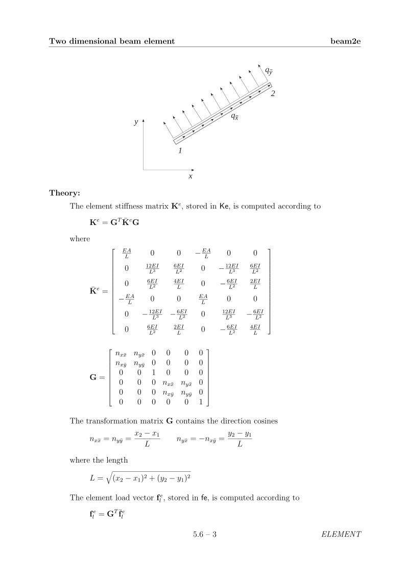
Two dimensional beam element beam2e
x
y
1
2
qy
qx
Theory:
The element stiffness matrix Ke, stored in Ke, is computed according to
Ke = GT KeG
where
Ke =
EAL
0 0 −EAL
0 0
0 12EIL3
6EIL2 0 −12EI
L36EIL2
0 6EIL2
4EIL
0 −6EIL2
2EIL
−EAL
0 0 EAL
0 0
0 −12EIL3 −6EI
L2 0 12EIL3 −6EI
L2
0 6EIL2
2EIL
0 −6EIL2
4EIL
G =
nxx nyx 0 0 0 0nxy nyy 0 0 0 00 0 1 0 0 00 0 0 nxx nyx 00 0 0 nxy nyy 00 0 0 0 0 1
The transformation matrix G contains the direction cosines
nxx = nyy =x2 − x1
Lnyx = −nxy =
y2 − y1
L
where the length
L =√
(x2 − x1)2 + (y2 − y1)2
The element load vector f el , stored in fe, is computed according to
f el = GT f e
l
5.6 – 3 ELEMENT

beam2e Two dimensional beam element
where
f el =
qxL
2qyL
2qyL
2
12qxL
2qyL
2
−qyL2
12
ELEMENT 5.6 – 4

Two dimensional beam element beam2s
Purpose:
Compute section forces in a two dimensional beam element.
N1
M1
x
y
V1
NnMn
Vn
NM
V
N
M
V
Syntax:
es=beam2s(ex,ey,ep,ed)es=beam2s(ex,ey,ep,ed,eq)[es,edi,eci]=beam2s(ex,ey,ep,ed,eq,n)
Description:
beam2s computes the section forces and displacements in local directions along thebeam element beam2e.
The input variables ex, ey, ep and eq are defined in beam2e, and the element displace-ments, stored in ed, are obtained by the function extract. If distributed loads areapplied to the element, the variable eq must be included. The number of evaluationpoints for section forces and displacements are determined by n. If n is omitted, onlythe ends of the beam are evaluated.
The output variables
es = [ N V M ] edi = [ u v ] eci = [ x ]
consist of column matrices that contain the section forces, the displacements, andthe evaluation points on the local x-axis. The explicit matrix expressions are
es =
N1 V1 M1
N2 V2 M2...
......
Nn Vn Mn
edi =
u1 v1
u2 v2...
...un vn
eci =
0x2...
xn−1
L
where L is the length of the beam element.
Theory:
5.6 – 5 ELEMENT

beam2s Two dimensional beam element
The evaluation of the section forces is based on the solutions of the basic equations
EAd2u
dx2+ qx = 0 EI
d4v
dx4− qy = 0
From these equations, the displacements along the beam element are obtained as thesum of the homogeneous and the particular solutions
u =
[u(x)v(x)
]= uh + up
where
uh = N C−1 G ae up =
[up(x)vp(x)
]=
qxLx
2EA(1− x
L)
qyL2x2
24EI(1− x
L)2
and
N =
[1 x 0 0 0 00 0 1 x x2 x3
]C =
1 0 0 0 0 00 0 1 0 0 00 0 0 1 0 01 L 0 0 0 00 0 1 L L2 L3
0 0 0 1 2L 3L2
ae =
u1
u2...u6
The transformation matrix Ge and nodal displacements ae are described in beam2e.Note that the transpose of ae is stored in ed.
Finally the section forces are obtained from
N = EAdu
dxV = −EI d
3v
dx3M = EI
d2v
dx2
Examples:
Section forces or element displacements can easily be plotted. The bending momentM along the beam is plotted by
>> plot(eci,es(:,3))
ELEMENT 5.6 – 6
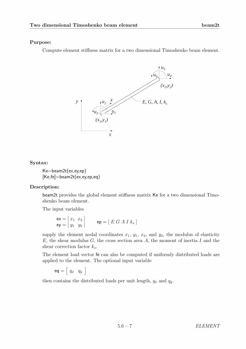
Two dimensional Timoshenko beam element beam2t
Purpose:
Compute element stiffness matrix for a two dimensional Timoshenko beam element.
E, A, I
x
y
(x1,y1)
(x2,y2)
x E, G, A, I, ks
u1
u2
u4
u5
u6
u3
Syntax:
Ke=beam2t(ex,ey,ep)[Ke,fe]=beam2t(ex,ey,ep,eq)
Description:
beam2t provides the global element stiffness matrix Ke for a two dimensional Timo-shenko beam element.
The input variables
ex = [ x1 x2 ]ey = [ y1 y2 ]
ep = [ E G A I ks ]
supply the element nodal coordinates x1, y1, x2, and y2, the modulus of elasticityE, the shear modulus G, the cross section area A, the moment of inertia I and theshear correction factor ks.
The element load vector fe can also be computed if uniformly distributed loads areapplied to the element. The optional input variable
eq =[qx qy
]then contains the distributed loads per unit length, qx and qy.
5.6 – 7 ELEMENT

beam2t Two dimensional Timoshenko beam element
x
y
1
2
qy
qx
Theory:
The element stiffness matrix Ke, stored in Ke, is computed according to
Ke = GT KeG
where G is described in beam2e, and Ke is given by
Ke =
EAL
0 0 −EAL
0 0
0 12EIL3(1+µ)
6EIL2(1+µ)
0 − 12EIL3(1+µ)
6EIL2(1+µ)
0 6EIL2(1+µ)
4EI(1+ µ4)
L(1+µ)0 − 6EI
L2(1+µ)
2EI(1−µ2)
L(1+µ)
−EAL
0 0 EAL
0 0
0 − 12EIL3(1+µ)
− 6EIL2(1+µ)
0 12EIL3(1+µ)
− 6EIL2(1+µ)
0 6EIL2(1+µ)
2EI(1−µ2)
L(1+µ)0 − 6EI
L2(1+µ)
4EI(1+µ4)
L(1+µ)
with
µ =12EI
L2GAks
ELEMENT 5.6 – 8
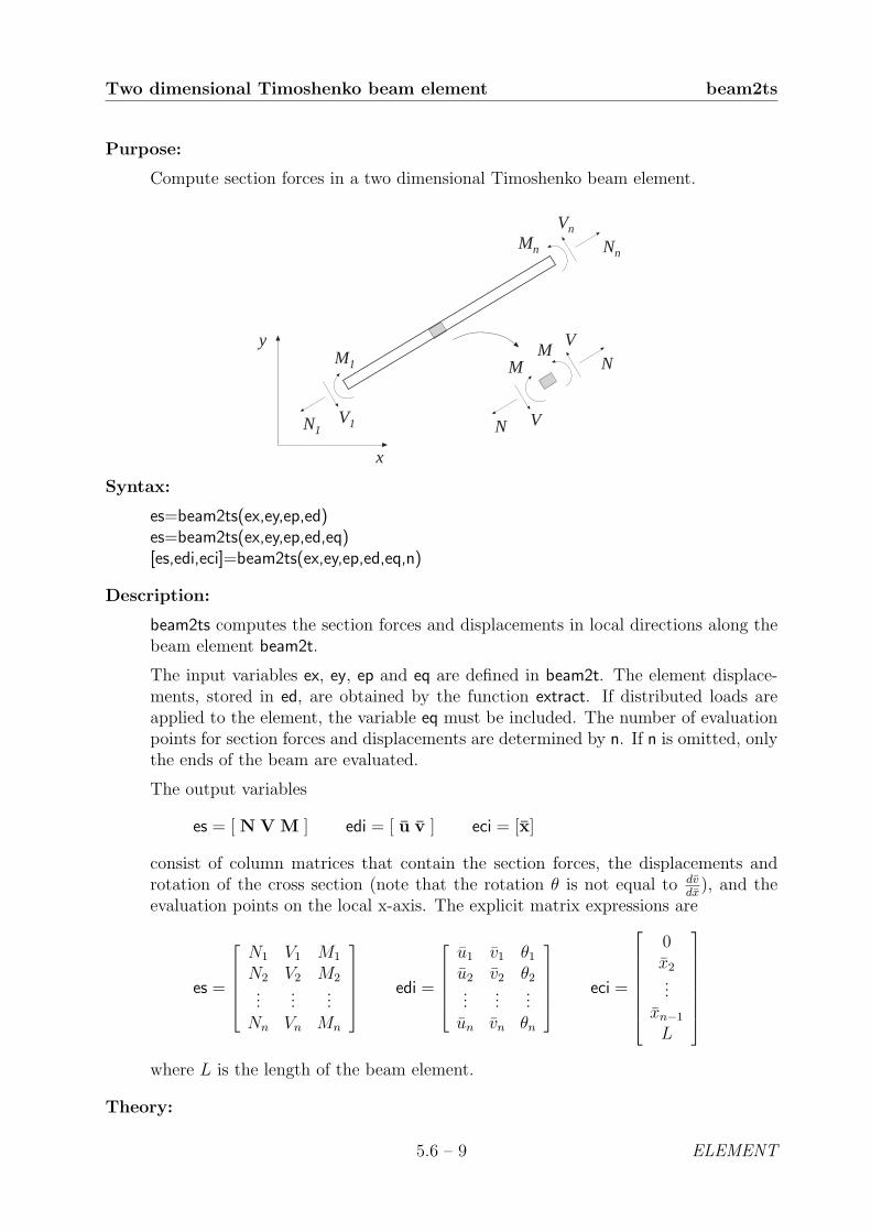
Two dimensional Timoshenko beam element beam2ts
Purpose:
Compute section forces in a two dimensional Timoshenko beam element.
N1
M1
x
y
V1
NnMn
Vn
NM
V
N
M
V
Syntax:
es=beam2ts(ex,ey,ep,ed)es=beam2ts(ex,ey,ep,ed,eq)[es,edi,eci]=beam2ts(ex,ey,ep,ed,eq,n)
Description:
beam2ts computes the section forces and displacements in local directions along thebeam element beam2t.
The input variables ex, ey, ep and eq are defined in beam2t. The element displace-ments, stored in ed, are obtained by the function extract. If distributed loads areapplied to the element, the variable eq must be included. The number of evaluationpoints for section forces and displacements are determined by n. If n is omitted, onlythe ends of the beam are evaluated.
The output variables
es = [ N V M ] edi = [ u v ] eci = [x]
consist of column matrices that contain the section forces, the displacements androtation of the cross section (note that the rotation θ is not equal to dv
dx), and the
evaluation points on the local x-axis. The explicit matrix expressions are
es =
N1 V1 M1
N2 V2 M2...
......
Nn Vn Mn
edi =
u1 v1 θ1
u2 v2 θ2...
......
un vn θn
eci =
0x2...
xn−1
L
where L is the length of the beam element.
Theory:
5.6 – 9 ELEMENT

beam2ts Two dimensional Timoshenko beam element
The evaluation of the section forces is based on the solutions of the basic equations
EAd2u
dx2+ qx = 0 EI
d3θ
dx3− qy = 0 EI
d4v
dx4− qy = 0
(The equations are valid if qy is not more than a linear function of x). From theseequations, the displacements along the beam element are obtained as the sum of thehomogeneous and the particular solutions
u =
u(x)v(x)θ(x)
= uh + up
where
uh = N C−1 G ae up =
up(x)vp(x)θp(x)
=
qxLx
2EA(1− x
L)
qyL2x2
24EI(1− x
L)2 +
qyLx
2GAks
(1− x
L)
qyL2x
12EI(1− 2x
L)(1− x
L)
and
N =
1 x 0 0 0 00 0 1 x x2 x3
0 0 0 1 2x 3(x2 + 2α)
α =EI
GAks
C =
1 0 0 0 0 00 0 1 0 0 00 0 0 1 0 6α1 L 0 0 0 00 0 1 L L2 L3
0 0 0 1 2L 3(L2 + 2α)
ae =
u1
u2...u6
The transformation matrix G and nodal displacements ae are described in beam2e.Note that the transpose of ae is stored in ed.
Finally the section forces are obtained from
N = EAdu
dxV = GAks(
dv
dx− θ) M = EI
dθ
dx
ELEMENT 5.6 – 10

Two dimensional beam element beam2w
Purpose:
Compute element stiffness matrix for a two dimensional beam element on elasticfoundation.
x
y
kakt
Syntax:
Ke=beam2w(ex,ey,ep)[Ke,fe]=beam2w(ex,ey,ep,eq)
Description:
beam2w provides the global element stiffness matrix Ke for a two dimensional beamelement on elastic foundation.
The input variables ex and ey are described in beam2e, and
ep = [ E A I ka kt ]
contains the modulus of elasticity E, the cross section areaA, the moment of inertia I,the spring stiffness in the axial direction ka, and the spring stiffness in the transversedirection kt.
The element load vector fe can also be computed if uniformly distributed loads areapplied to the element. The optional input variable eq, described in beam2e, containsthe distributed loads.
5.6 – 11 ELEMENT
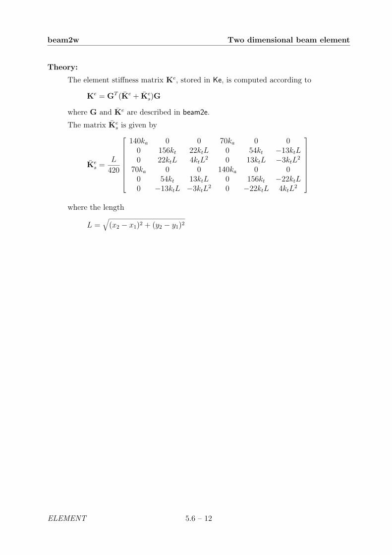
beam2w Two dimensional beam element
Theory:
The element stiffness matrix Ke, stored in Ke, is computed according to
Ke = GT (Ke + Kes)G
where G and Ke are described in beam2e.
The matrix Kes is given by
Kes =
L
420
140ka 0 0 70ka 0 00 156kt 22ktL 0 54kt −13ktL0 22ktL 4ktL
2 0 13ktL −3ktL2
70ka 0 0 140ka 0 00 54kt 13ktL 0 156kt −22ktL0 −13ktL −3ktL
2 0 −22ktL 4ktL2
where the length
L =√
(x2 − x1)2 + (y2 − y1)2
ELEMENT 5.6 – 12
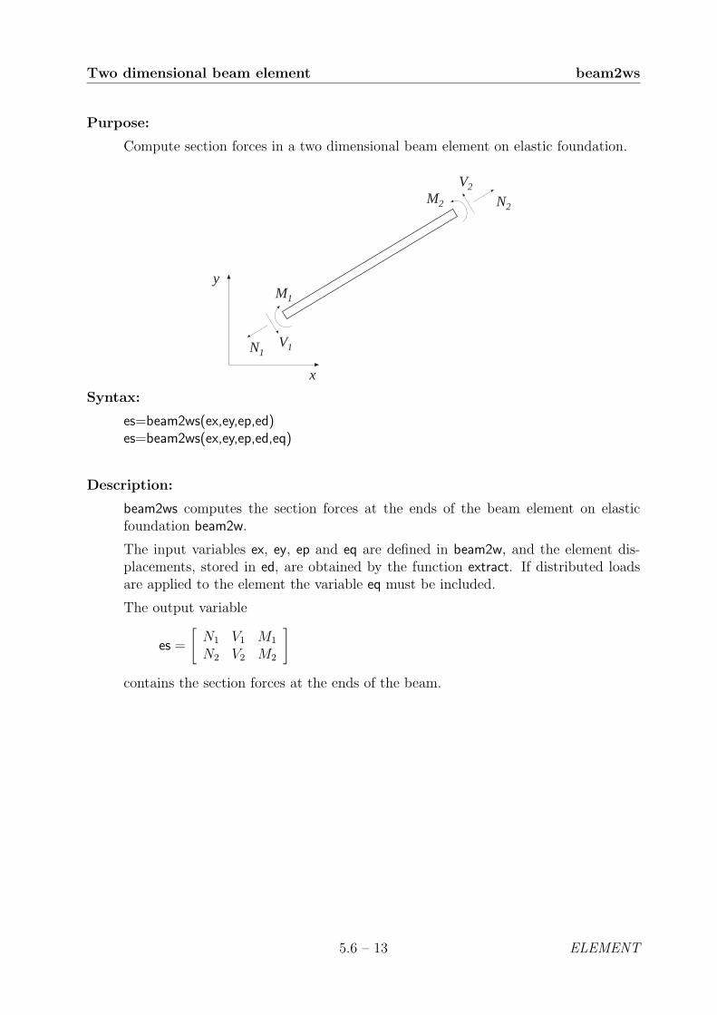
Two dimensional beam element beam2ws
Purpose:
Compute section forces in a two dimensional beam element on elastic foundation.
N1
M1
x
y
V1
N2M2
V2
Syntax:
es=beam2ws(ex,ey,ep,ed)es=beam2ws(ex,ey,ep,ed,eq)
Description:
beam2ws computes the section forces at the ends of the beam element on elasticfoundation beam2w.
The input variables ex, ey, ep and eq are defined in beam2w, and the element dis-placements, stored in ed, are obtained by the function extract. If distributed loadsare applied to the element the variable eq must be included.
The output variable
es =
[N1 V1 M1
N2 V2 M2
]
contains the section forces at the ends of the beam.
5.6 – 13 ELEMENT

beam2ws Two dimensional beam element
Theory:
The section forces at the ends of the beam are obtained from the element force vector
P = [ −N1 − V1 −M1 N2 V2 M2 ]T
computed according to
P = (Ke + Kes) G ae − fl
The matrices Ke and G, are described in beam2e, and the matrix Kes is described in
beam2w. The nodal displacements
ae = [ u1 u2 u3 u4 u5 u6 ]T
are shown in beam2e. Note that the transpose of ae is stored in ed.
ELEMENT 5.6 – 14

Two dimensional beam element beam2g
Purpose:
Compute element stiffness matrix for a two dimensional nonlinear beam element.
u1
u2
u4
u5
E, A, I, N
x
y
u6
u3
(x1,y1)
(x2,y2)
x
Syntax:
Ke=beam2g(ex,ey,ep,N)[Ke,fe]=beam2g(ex,ey,ep,N,eq)
Description:
beam2g provides the global element stiffness matrix Ke for a two dimensional beamelement with respect to geometrical nonlinearity.
The input variables ex, ey, and ep are described in beam2e, and
N = [ N ]
contains the value of the predefined normal force N , which is positive in tension.
The element load vector fe can also be computed if a uniformly distributed transverseload is applied to the element. The optional input variable
eq = [ qy ]
then contains the distributed transverse load per unit length, qy. Note that eq is ascalar and not a vector as in beam2e
5.6 – 15 ELEMENT

beam2g Two dimensional beam element
Theory:
The element stiffness matrix Ke, stored in the variable Ke, is computed according to
Ke = GT KeG
where G is described in beam2e, and Ke is given by
Ke =
EAL
0 0 −EAL
0 0
0 12EIL3 φ5
6EIL2 φ2 0 −12EI
L3 φ56EIL2 φ2
0 6EIL2 φ2
4EILφ3 0 −6EI
L2 φ22EILφ4
−EAL
0 0 EAL
0 0
0 −12EIL3 φ5 −6EI
L2 φ2 0 12EIL3 φ5 −6EI
L2 φ2
0 6EIL2 φ2
2EILφ4 0 −6EI
L2 φ24EILφ3
For axial compression (N < 0), we have
φ1 =kL
2cot
kL
2φ2 =
1
12
k2L2
(1− φ1)φ3 =
1
4φ1 +
3
4φ2
φ4 = −1
2φ1 +
3
2φ2 φ5 = φ1φ2
with
k =π
L
√ρ
For axial tension (N > 0), we have
φ1 =kL
2coth
kL
2φ2 = − 1
12
k2L2
(1− φ1)φ3 =
1
4φ1 +
3
4φ2
φ4 = −1
2φ1 +
3
2φ2 φ5 = φ1φ2
with
k =π
L
√−ρ
The parameter ρ is given by
ρ = − NL2
π2EI
ELEMENT 5.6 – 16

Two dimensional beam element beam2g
The equivalent nodal loads f el stored in the variable fe are computed according to
f el = GT f e
where
f e = qL[
01
2
L
12ψ 0
1
2− L
12ψ]T
For an axial compressive force, we have
ψ = 6
(2
(kL)2− 1 + cos kL
kL sin kL
)
and for an axial tensile force
ψ = 6
(1 + cosh kL
kL sinh kL− 2
(kL)2
)
5.6 – 17 ELEMENT

beam2gs Two dimensional beam element
Purpose:
Compute section forces in a two dimensional nonlinear beam element.
N1
M1
x
y
V1
N2M2
V2
Syntax:
es=beam2gs(ex,ey,ep,ed,N)es=beam2gs(ex,ey,ep,ed,N,eq)
Description:
beam2gs computes the section forces at the ends of the nonlinear beam elementbeam2g.
The input variables ex, ey, and ep are defined in beam2e, and the variables N and eqin beam2g. The element displacements, stored in ed, are obtained by the functionextract. If a distributed transversal load is applied to the element, the variable eqmust be included.
The output variable
es =
[N1 V1 M1
N2 V2 M2
]
contains the section forces at the ends of the beam.
ELEMENT 5.6 – 18
Two dimensional beam element beam2gs
Theory:
The section forces at the ends of the beam are obtained from the element force vector
P = [ −N1 − V1 −M1 N2 V2 M2 ]T
computed according to
P = Ke G ae − fl
The matrix G is described in beam2e. The matrix Ke and the nodal displacements
ae = [ u1 u2 u3 u4 u5 u6 ]T
are described in beam2g. Note that the transpose of ae is stored in ed.
5.6 – 19 ELEMENT

beam2d Two dimensional beam element
Purpose:
Compute element stiffness, mass and damping matrices for a two dimensional beamelement.
u1
u2
u4
u5
E, A, I, m
x
y
u6
u3
(x1,y1)
(x2,y2)
x
Syntax:
[Ke,Me]=beam2d(ex,ey,ep)[Ke,Me,Ce]=beam2d(ex,ey,ep)
Description:
beam2d provides the global element stiffness matrix Ke, the global element massmatrix Me, and the global element damping matrix Ce, for a two dimensional beamelement.
The input variables ex and ey are described in beam2e, and
ep = [ E A I m [ a0 a1] ]
contains the modulus of elasticity E, the cross section area A, the moment of inertiaI, the mass per unit length m, and the Raleigh damping coefficients a0 and a1. If a0
and a1 are omitted, the element damping matrix Ce is not computed.
ELEMENT 5.6 – 20

Two dimensional beam element beam2d
Theory:
The element stiffness matrix Ke, the element mass matrix Me and the elementdamping matrix Ce, stored in the variables Ke, Me and Ce, respectively, are computedaccording to
Ke = GT KeG Me = GTMeG Ce = GT CeG
where G and Ke are described in beam2e.
The matrix Me is given by
Me =mL
420
140 0 0 70 0 00 156 22L 0 54 −13L0 22L 4L2 0 13L −3L2
70 0 0 140 0 00 54 13L 0 156 −22L0 −13L −3L2 0 −22L 4L2
and the matrix Ce is computed by combining Ke and Me
Ce = a0Me + a1K
e
5.6 – 21 ELEMENT

beam2ds Two dimensional beam element
Purpose:
Compute section forces for a two dimensional beam element in dynamic analysis.
N1
M1
x
y
V1
N2M2
V2
Syntax:
es=beam2ds(ex,ey,ep,ed,ev,ea)
Description:
beam2ds computes the section forces at the ends of the dynamic beam elementbeam2d.
The input variables ex, ey, and ep are defined in beam2d. The element displace-ments, the element velocities, and the element accelerations, stored in ed, ev, and earespectively, are obtained by the function extract.
The output variable
es =
[N1 V1 M1
N2 V2 M2
]
contains the section forces at the ends of the beam.
ELEMENT 5.6 – 22

Two dimensional beam element beam2ds
Theory:
The section forces at the ends of the beam are obtained from the element force vector
P = [ −N1 − V1 −M1 N2 V2 M2 ]T
computed according to
P = Ke G ae + Ce G ae + Me G ae
The matrices Ke and G are described in beam2e, and the matrices Me and Ce aredescribed in beam2d. The nodal displacements
ae = [ u1 u2 u3 u4 u5 u6 ]T
shown in beam2d also define the directions of the nodal velocities
ae = [ u1 u2 u3 u4 u5 u6 ]T
and the nodal accelerations
ae = [ u1 u2 u3 u4 u5 u6 ]T
Note that the transposes of ae, ae, and ae are stored in ed, ev, and ea respectively.
5.6 – 23 ELEMENT

beam3e Three dimensional beam element
Purpose:
Compute element stiffness matrix for a three dimensional beam element.
zx
y
u1
u2
u4
u5
u6
u3
u7
u8
u10
u11
u12
u9
(x1,y1,z1)
(x2,y2,z2)
yx
z
Syntax:
Ke=beam3e(ex,ey,ez,eo,ep)[Ke,fe]=beam3e(ex,ey,ez,eo,ep,eq)
Description:
beam3e provides the global element stiffness matrix Ke for a three dimensional beamelement.
The input variables
ex = [ x1 x2 ]ey = [ y1 y2 ]ez = [ z1 z2 ]
eo = [ xz yz zz ]
supply the element nodal coordinates x1, y1, etc. as well as the direction of the localbeam coordinate system (x, y, z). By giving a global vector (xz, yz, zz) parallel withthe positive local z axis of the beam, the local beam coordinate system is defined.The variable
ep = [ E G A Iy Iz Kv ]
supplies the modulus of elasticity E, the shear modulus G, the cross section areaA, the moment of inertia with respect to the y axis Iy, the moment of inertia withrespect to the z axis Iz, and St Venant torsional stiffness Kv.
ELEMENT 5.6 – 24

Three dimensional beam element beam3e
The element load vector fe can also be computed if uniformly distributed loads areapplied to the element. The optional input variable
eq = [ qx qy qz qω ]
then contains the distributed loads. The positive directions of qx, qy, and qz followthe local beam coordinate system. The distributed torque qω is positive if directedin the local x-direction, i.e. from local y to local z. All the loads are per unit length.
Theory:
The element stiffness matrix Ke is computed according to
Ke = GT KeG
where
Ke =
k1 0 0 0 0 0 −k1 0 0 0 0 00 12EIz
L3 0 0 0 6EIz
L2 0 −12EIz
L3 0 0 0 6EIz
L2
0 0 12EIy
L3 0 −6EIy
L2 0 0 0 −12EIy
L3 0 −6EIy
L2 00 0 0 k2 0 0 0 0 0 −k2 0 0
0 0 −6EIy
L2 0 4EIy
L0 0 0 6EIy
L2 0 2EIy
L0
0 6EIz
L2 0 0 0 4EIz
L0 −6EIz
L2 0 0 0 2EIz
L
−k1 0 0 0 0 0 k1 0 0 0 0 00 −12EIz
L3 0 0 0 −6EIz
L2 0 12EIz
L3 0 0 0 −6EIz
L2
0 0 −12EIy
L3 0 6EIy
L2 0 0 0 12EIy
L3 0 6EIy
L2 00 0 0 −k2 0 0 0 0 0 k2 0 0
0 0 −6EIy
L2 0 2EIy
L0 0 0 6EIy
L2 0 4EIy
L0
0 6EIz
L2 0 0 0 2EIz
L0 −6EIz
L2 0 0 0 4EIz
L
in which k1 = EA
Land k2 = GKv
L, and where
G =
nxx nyx nzx 0 0 0 0 0 0 0 0 0nxy nyy nzy 0 0 0 0 0 0 0 0 0nxz nyz nzz 0 0 0 0 0 0 0 0 00 0 0 nxx nyx nzx 0 0 0 0 0 00 0 0 nxy nyy nzy 0 0 0 0 0 00 0 0 nxz nyz nzz 0 0 0 0 0 00 0 0 0 0 0 nxx nyx nzx 0 0 00 0 0 0 0 0 nxy nyy nzy 0 0 00 0 0 0 0 0 nxz nyz nzz 0 0 00 0 0 0 0 0 0 0 0 nxx nyx nzx
0 0 0 0 0 0 0 0 0 nxy nyy nzy
0 0 0 0 0 0 0 0 0 nxz nyz nzz
5.6 – 25 ELEMENT
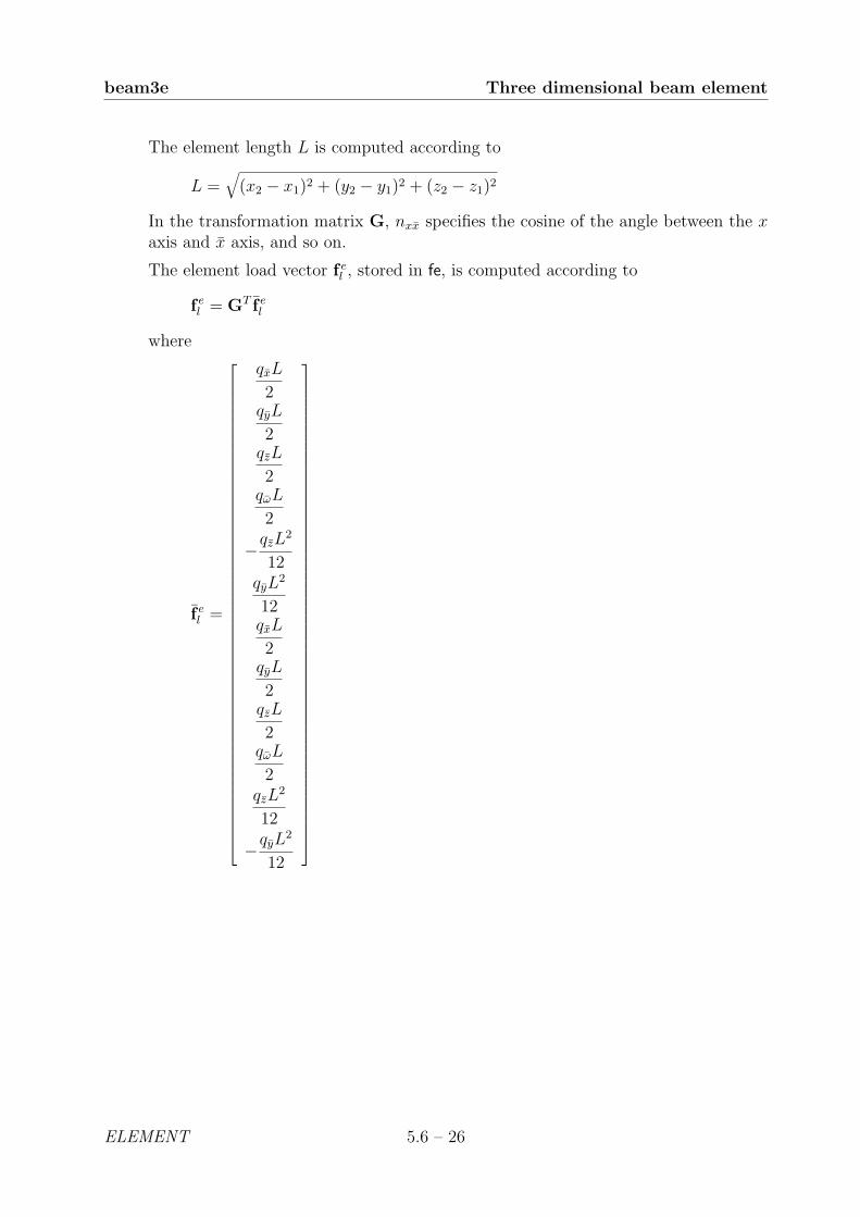
beam3e Three dimensional beam element
The element length L is computed according to
L =√
(x2 − x1)2 + (y2 − y1)2 + (z2 − z1)2
In the transformation matrix G, nxx specifies the cosine of the angle between the xaxis and x axis, and so on.
The element load vector f el , stored in fe, is computed according to
f el = GT f e
l
where
f el =
qxL
2qyL
2qzL
2qωL
2
−qzL2
12qyL
2
12qxL
2qyL
2qzL
2qωL
2qzL
2
12
−qyL2
12
ELEMENT 5.6 – 26

Three dimensional beam element beam3s
Purpose:
Compute section forces in a three dimensional beam element.
zx
y
Tn
My,n
Mz,n
Nn
Vz,n
My,1
T1
Mz,1
N1Vy,1
Vz,1
Vy,n
yx
z
TN
MzVz
Vy
My
TN
My
Vy
VzMz
Syntax:
es=beam3s(ex,ey,ez,eo,ep,ed)es=beam3s(ex,ey,ez,eo,ep,ed,eq)[es,edi,eci]=beam3s(ex,ey,ez,eo,ep,ed,eq,n)
Description:
beam3s computes the section forces and displacements in local directions along thebeam element beam3e.
The input variables ex, ey, ez, eo, and ep are defined in beam3e, and the elementdisplacements, stored in ed, are obtained by the function extract. If distributedloads are applied to the element, the variable eq must be included. The number ofevaluation points for section forces and displacements are determined by n. If n isomitted, only the ends of the beam are evaluated.
The output variables
es = [ N Vy Vz T My Mz ] edi = [ u v w ϕ ] eci = [ x ]
consist of column matrices that contain the section forces, the displacements, andthe evaluation points on the local x-axis. The explicit matrix expressions are
es =
N1 Vy1 Vz1 T My1 Mz1
N2 Vy2 Vz2 T My2 Mz2...
......
......
...Nn Vyn Vzn T Myn Mzn
5.6 – 27 ELEMENT

beam3s Three dimensional beam element
edi =
u1 v1 w1 ϕ1
u2 v2 w2 ϕ2...
......
...un vn wn ϕn
eci =
0x2...
xn−1
L
where L is the length of the beam element.
Theory:
The evaluation of the section forces is based on the solutions of the basic equations
EAd2u
dx2+ qx = 0 EIz
d4v
dx4− qy = 0
EIyd4w
dx4− qz = 0 GKv
d2ϕ
dx2+ qω = 0
From these equations, the displacements along the beam element are obtained as thesum of the homogeneous and the particular solutions
u =
u(x)v(x)w(x)ϕ(x)
= uh + up
where
uh = N C−1 G ae up =
up(x)vp(x)wp(x)ϕp(x)
=
qxLx
2EA(1− x
L)
qyL2x2
24EIz(1− x
L)2
qzL2x2
24EIy(1− x
L)2
qωLx
2GKv
(1− x
L)
and
N =
1 x 0 0 0 0 0 0 0 0 0 00 0 1 x x2 x3 0 0 0 0 0 00 0 0 0 0 0 1 x x2 x3 0 00 0 0 0 0 0 0 0 0 0 1 x
ELEMENT 5.6 – 28

Three dimensional beam element beam3s
C =
1 0 0 0 0 0 0 0 0 0 0 00 0 1 0 0 0 0 0 0 0 0 00 0 0 0 0 0 1 0 0 0 0 00 0 0 0 0 0 0 0 0 0 1 00 0 0 0 0 0 0 1 0 0 0 00 0 0 1 0 0 0 0 0 0 0 01 L 0 0 0 0 0 0 0 0 0 00 0 1 L L2 L3 0 0 0 0 0 00 0 0 0 0 0 1 L L2 L3 0 00 0 0 0 0 0 0 0 0 0 1 L0 0 0 0 0 0 0 1 2L 3L2 0 00 0 0 1 2L 3L2 0 0 0 0 0 0
ae =
u1
u2...u12
The transformation matrix Ge and nodal displacements ae are described in beam3e.Note that the transpose of ae is stored in ed.
Finally the section forces are obtained from
N = EAdu
dxVy = −EIz
d3v
dx3Vz = −EIy
d3w
dx3
T = GKvdϕ
dxMy = EIy
d2w
dx2Mz = EIz
d2v
dx2
Examples:
Section forces or element displacements can easily be plotted. The bending momentMy along the beam is plotted by
>> plot(eci,es(:,5))
5.6 – 29 ELEMENT


5.7 Plate element
Only one plate element is currently available, a rectangular 12 dof element. The elementpresumes a linear elastic material which can be isotropic or anisotropic.
Plate elements
u8
u9
u2
u3 u6
u4u1
u5
u7
u11
u10
u12
platre
Plate functionsplatre Compute element matricesplatrs Compute section forces
5.7 – 1 ELEMENT

platre Plate element
Purpose:
Compute element stiffness matrix for a rectangular plate element.
zx
y
(x4 ,y4)
(x1 ,y1)
(x3 ,y3)
(x2 ,y2)
t
u8
u9
u2
u3 u6
u4u1
u5
u7
u11
u10
u12
Syntax:
Ke=platre(ex,ey,ep,D)[Ke,fe]=platre(ex,ey,ep,D,eq)
Description:
platre provides an element stiffness matrix Ke, and an element load vector fe, for arectangular plate element. This element can only be used if the element edges areparallel to the coordinate axis.
The element nodal coordinates x1, y1, x2 etc. are supplied to the function by ex andey, the element thickness t by ep, and the material properties by the constitutivematrix D. Any arbitrary D-matrix with dimensions (3× 3) and valid for plane stressmay be given. For an isotropic elastic material the constitutive matrix can be formedby the function hooke, see Section 4.
ex = [ x1 x2 x3 x4 ]ey = [ y1 y2 y3 y4 ]
ep = [ t ] D =
D11 D12 D13
D21 D22 D23
D31 D32 D33
If a uniformly distributed load is applied to the element, the element load vector feis computed. The input variable
eq = [ qz ]
then contains the load qz per unit area in the z-direction.
ELEMENT 5.7 – 2
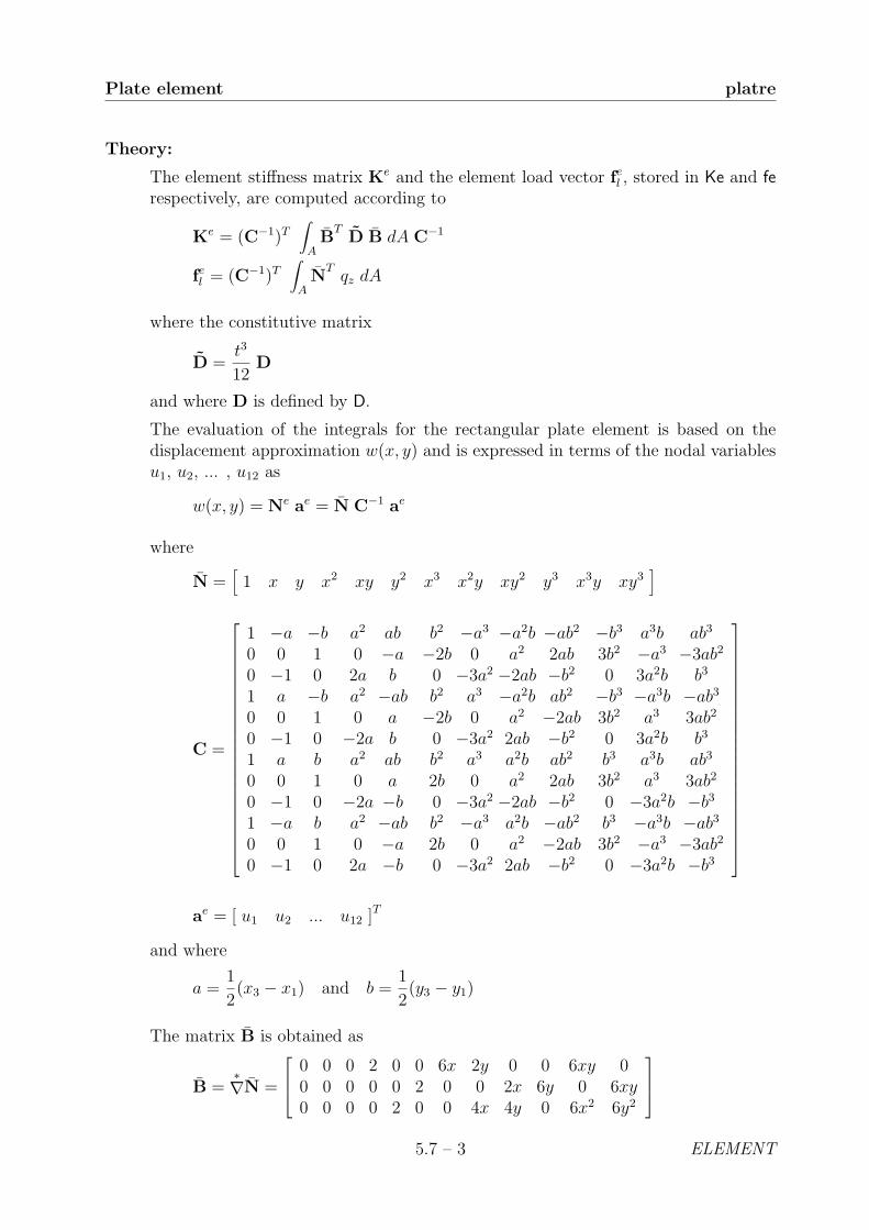
Plate element platre
Theory:
The element stiffness matrix Ke and the element load vector fel , stored in Ke and ferespectively, are computed according to
Ke = (C−1)T∫
AB
TD B dA C−1
fel = (C−1)T∫
AN
Tqz dA
where the constitutive matrix
D =t3
12D
and where D is defined by D.
The evaluation of the integrals for the rectangular plate element is based on thedisplacement approximation w(x, y) and is expressed in terms of the nodal variablesu1, u2, ... , u12 as
w(x, y) = Ne ae = N C−1 ae
where
N =[
1 x y x2 xy y2 x3 x2y xy2 y3 x3y xy3]
C =
1 −a −b a2 ab b2 −a3 −a2b −ab2 −b3 a3b ab3
0 0 1 0 −a −2b 0 a2 2ab 3b2 −a3 −3ab2
0 −1 0 2a b 0 −3a2 −2ab −b2 0 3a2b b3
1 a −b a2 −ab b2 a3 −a2b ab2 −b3 −a3b −ab30 0 1 0 a −2b 0 a2 −2ab 3b2 a3 3ab2
0 −1 0 −2a b 0 −3a2 2ab −b2 0 3a2b b3
1 a b a2 ab b2 a3 a2b ab2 b3 a3b ab3
0 0 1 0 a 2b 0 a2 2ab 3b2 a3 3ab2
0 −1 0 −2a −b 0 −3a2 −2ab −b2 0 −3a2b −b31 −a b a2 −ab b2 −a3 a2b −ab2 b3 −a3b −ab30 0 1 0 −a 2b 0 a2 −2ab 3b2 −a3 −3ab2
0 −1 0 2a −b 0 −3a2 2ab −b2 0 −3a2b −b3
ae = [ u1 u2 ... u12 ]T
and where
a =1
2(x3 − x1) and b =
1
2(y3 − y1)
The matrix B is obtained as
B =∗∇N =
0 0 0 2 0 0 6x 2y 0 0 6xy 00 0 0 0 0 2 0 0 2x 6y 0 6xy0 0 0 0 2 0 0 4x 4y 0 6x2 6y2
5.7 – 3 ELEMENT

platre Plate element
where
∗∇ =
∂2
∂x2
∂2
∂y2
2∂2
∂x∂y
Evaluation of the integrals for the rectangular plate element is done analytically.Computation of the integrals for the element load vector f e
l yields
f el = qzLxLy
[1
4
Ly
24− Lx
24
1
4
Ly
24
Lx
24
1
4− Ly
24
Lx
24
1
4− Ly
24− Lx
24
]Twhere
Lx = x3 − x1 and Ly = y3 − y1
ELEMENT 5.7 – 4

Plate element platrs
Purpose:
Compute section forces in a rectangular plate element.
Mxy
Mxy
MxyMxy Mxx
Myy
Myy
Vxz
Vyz
Vxz
Vyz
Mxx
zx
y
(x4 ,y4)
(x1 ,y1)
(x3 ,y3)
(x2 ,y2)
t
u8
u9
u2
u3 u6
u4u1
u5
u7
u11
u10
u12
Syntax:
[es,et]=platrs(ex,ey,ep,D,ed)
Description:
platrs computes the section forces es and the curvature matrix et in a rectangularplate element. The section forces and the curvatures are computed at the center ofthe element.
The input variables ex, ey, ep and D are defined in platre. The vector ed contains thenodal displacements ae of the element and is obtained by the function extract as
ed = (ae)T = [ u1 u2 ... u12 ]
The output variables
es =[MT VT
]= [ Mxx Myy Mxy Vxz Vyz ]
et = κT = [ κxx κyy κxy ]
contain the section forces and curvatures in global directions.
5.7 – 5 ELEMENT

platrs Plate element
Theory:
The curvatures and the section forces are computed according to
κ =
κxx
κyy
κxy
= B C−1 ae
M =
Mxx
Myy
Mxy
= D κ
V =
[Vxz
Vyz
]= ∇ M
where the matrices D, B, C and ae are described in platre, and where
∇ =
∂
∂x0
∂
∂y
0∂
∂y
∂
∂x
ELEMENT 5.7 – 6
6 System functions
6.1 Introduction
The group of system functions comprises functions for the setting up, solving, and elimi-nation of systems of equations. The functions are separated in two groups:
Static system functions
Dynamic system functions
Static system functions concern the linear system of equations
Ka = f
where K is the global stiffness matrix and f is the global load vector. Often used staticsystem functions are assem and solveq. The function assem assembles the global stiffnessmatrix and solveq computes the global displacement vector a considering the boundaryconditions. It should be noted that K, f , and a also represent analogous quantities insystems others than structural mechanical systems. For example, in a heat flow problemK represents the conductivity matrix, f the heat flow, and a the temperature.
Dynamic system functions are related to different aspects of linear dynamic systems ofcoupled ordinary differential equations according to
C d + K d = f
for first-order systems andMd + Cd + Kd = f
for second-order systems. First-order systems occur typically in transient heat conductionand second-order systems occur in structural dynamics.
6.1 – 1 SYSTEM

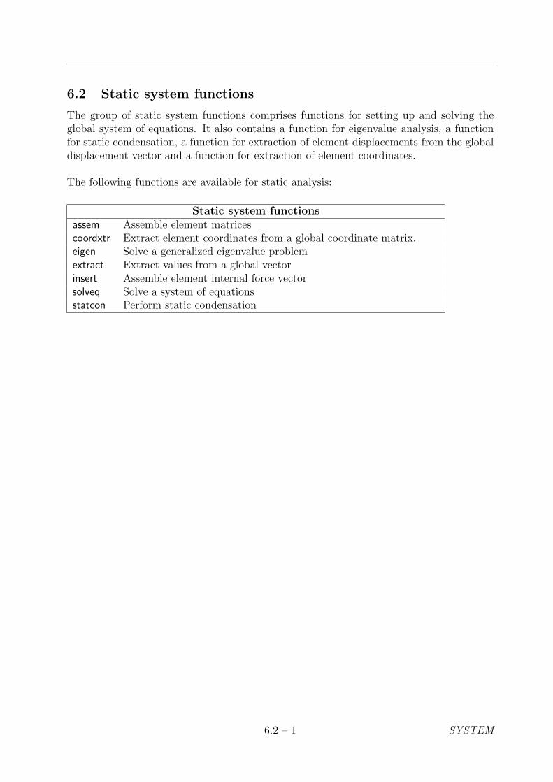
6.2 Static system functions
The group of static system functions comprises functions for setting up and solving theglobal system of equations. It also contains a function for eigenvalue analysis, a functionfor static condensation, a function for extraction of element displacements from the globaldisplacement vector and a function for extraction of element coordinates.
The following functions are available for static analysis:
Static system functionsassem Assemble element matricescoordxtr Extract element coordinates from a global coordinate matrix.eigen Solve a generalized eigenvalue problemextract Extract values from a global vectorinsert Assemble element internal force vectorsolveq Solve a system of equationsstatcon Perform static condensation
6.2 – 1 SYSTEM
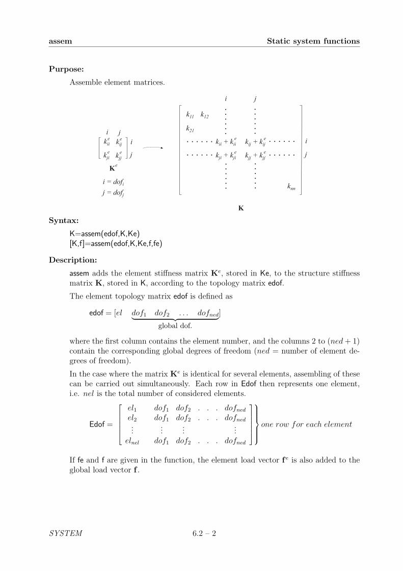
assem Static system functions
Purpose:
Assemble element matrices.
kii
kji
e
e
kij
kjj
e
e
i ji
jeK
i = dofi
j = dofj
K
kii + kii
kji + kji
k21
kij + kij
kjj + kjj
knn
k11 k12
e
e
e
e
i j
i
j......
......
...... . . . . . .
. . . . . .
......
..
..
..
..
..
..
Syntax:
K=assem(edof,K,Ke)[K,f]=assem(edof,K,Ke,f,fe)
Description:
assem adds the element stiffness matrix Ke, stored in Ke, to the structure stiffnessmatrix K, stored in K, according to the topology matrix edof.
The element topology matrix edof is defined as
edof = [el dof1 dof2 . . . dofned︸ ︷︷ ︸global dof.
]
where the first column contains the element number, and the columns 2 to (ned+ 1)contain the corresponding global degrees of freedom (ned = number of element de-grees of freedom).
In the case where the matrix Ke is identical for several elements, assembling of thesecan be carried out simultaneously. Each row in Edof then represents one element,i.e. nel is the total number of considered elements.
Edof =
el1el2...
elnel
dof1 dof2 . . . dofned
dof1 dof2 . . . dofned...
......
dof1 dof2 . . . dofned
one row for each element
If fe and f are given in the function, the element load vector f e is also added to theglobal load vector f .
SYSTEM 6.2 – 2

Static system functions coordxtr
Purpose:
Extract element coordinates from a global coordinate matrix.ln
kn
(xn ,yn)
l1
k1
l6
k6
l2
k2
l5
k5
(x2, y2)
1 2
(x6, y6)
(x1, y1) (x5 , y5)
4
nel
nen =4
5
3
Ex = x1 x2 x7 x6
Ey = y1 y2 y7 y6
●● ●● ●
●● ●● ●
●● ●● ●
●● ●● ●
●● ●● ●
...
...
Syntax:
[Ex,Ey,Ez]=coordxtr(Edof,Coord,Dof,nen)
Description:
coordxtr extracts element nodal coordinates from the global coordinate matrix Coordfor elements with equal numbers of element nodes and dof’s.
Input variables are the element topology matrix Edof, defined in assem, the globalcoordinate matrix Coord, the global topology matrix Dof, and the number of elementnodes nen in each element.
Coord =
x1 y1 [z1]x2 y2 [z2]x3 y3 [z3]...
......
xn yn [zn]
Dof =
k1 l1 ... m1
k2 l2 ... m2
k3 l3 ... m3...
... ......
kn ln ... mn
nen = [ nen ]
The nodal coordinates defined in row i of Coord correspond to the degrees of freedomof row i in Dof. The components ki, li and mi define the degrees of freedom of nodei, and n is the number of global nodes for the considered part of the FE-model.
6.2 – 3 SYSTEM
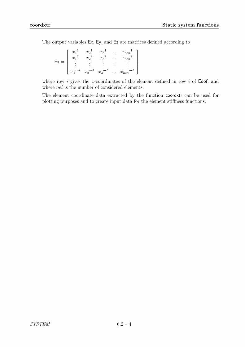
coordxtr Static system functions
The output variables Ex, Ey, and Ez are matrices defined according to
Ex =
x1
1 x21 x3
1 ... xnen1
x12 x2
2 x32 ... xnen
2
......
......
...x1
nel x2nel x3
nel ... xnennel
where row i gives the x-coordinates of the element defined in row i of Edof, andwhere nel is the number of considered elements.
The element coordinate data extracted by the function coordxtr can be used forplotting purposes and to create input data for the element stiffness functions.
SYSTEM 6.2 – 4

Static system functions eigen
Purpose:
Solve the generalized eigenvalue problem.
Syntax:
L=eigen(K,M)L=eigen(K,M,b)[L,X]=eigen(K,M)[L,X]=eigen(K,M,b)
Description:
eigen solves the eigenvalue problem
| K− λM |= 0
where K and M are square matrices. The eigenvalues λ are stored in the vector Land the corresponding eigenvectors in the matrix X.
If certain rows and columns in matrices K and M are to be eliminated in computingthe eigenvalues, b must be given in the function. The rows (and columns) that areto be eliminated are described in the vector b defined as
b =
dof1
dof2...
dofnb
The computed eigenvalues are given in order ranging from the smallest to the largest.The eigenvectors are normalized in order that
XT MX = I
where I is the identity matrix.
6.2 – 5 SYSTEM
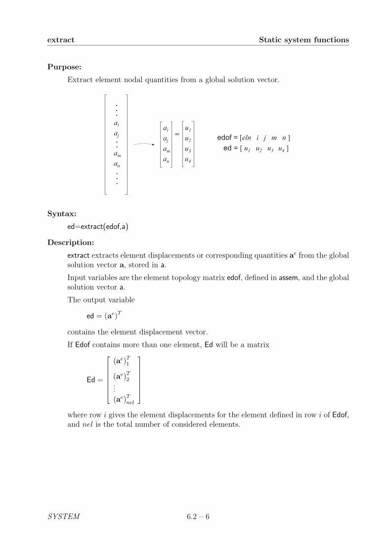
extract Static system functions
Purpose:
Extract element nodal quantities from a global solution vector.
=
ai
aj
am
an
ai
aj
am
an
u1
u2
u3
u4
edof = [eln i j m n ]ed = [ u1 u2 u3 u4 ]
...
..
.
..
Syntax:
ed=extract(edof,a)
Description:
extract extracts element displacements or corresponding quantities ae from the globalsolution vector a, stored in a.
Input variables are the element topology matrix edof, defined in assem, and the globalsolution vector a.
The output variable
ed = (ae)T
contains the element displacement vector.
If Edof contains more than one element, Ed will be a matrix
Ed =
(ae)T
1
(ae)T2
...
(ae)Tnel
where row i gives the element displacements for the element defined in row i of Edof,and nel is the total number of considered elements.
SYSTEM 6.2 – 6
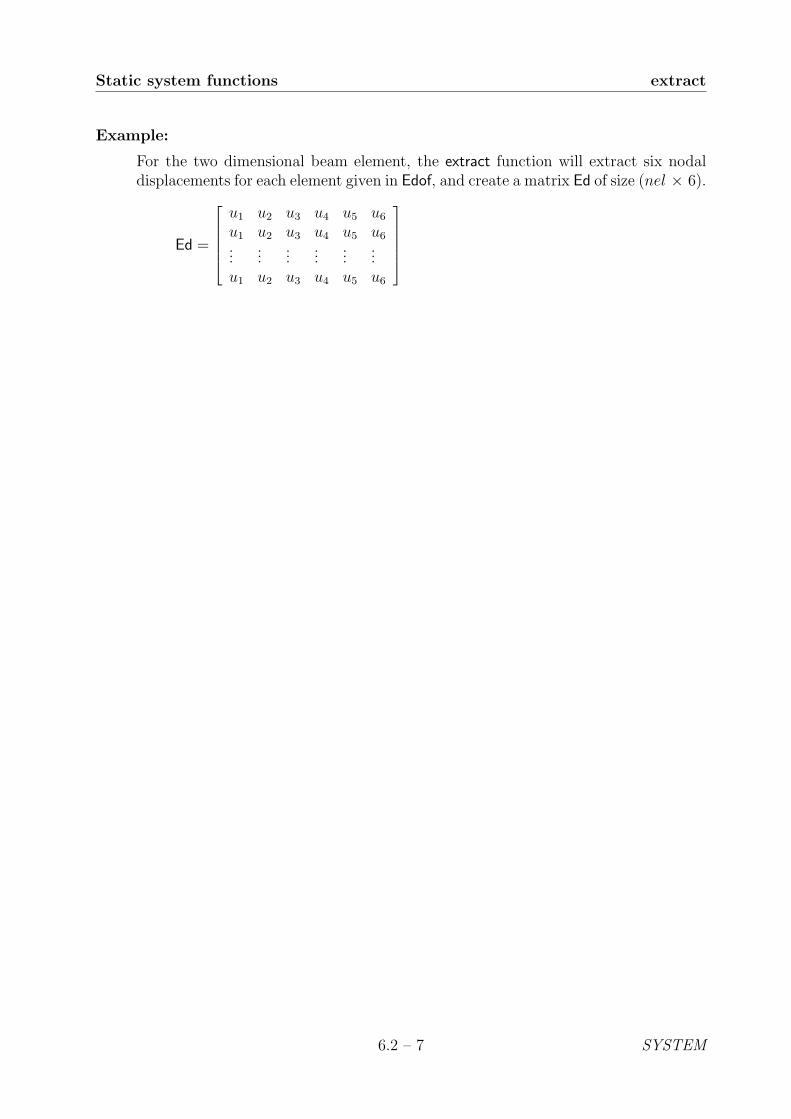
Static system functions extract
Example:
For the two dimensional beam element, the extract function will extract six nodaldisplacements for each element given in Edof, and create a matrix Ed of size (nel × 6).
Ed =
u1 u2 u3 u4 u5 u6
u1 u2 u3 u4 u5 u6...
......
......
...u1 u2 u3 u4 u5 u6
6.2 – 7 SYSTEM

insert Static system functions
Purpose:
Assemble internal element forces in a global force vector.
fi
fj
e
e
f e
i = dofi
j = dofj
f1
f2....fi + fi
e
fj + fje
....fn
f
Syntax:
f=insert(edof,f,ef)
Description:
insert adds the internal element load vector f ei , stored in ef, to the global internal
force vector f, stored in f, according to the topology matrix edof. The function is foruse in nonlinear analysis.
The element topology matrix edof is defined in assem. The vector f is the globalinternal force vector, and the vector ef is the internal element force vector computedfrom the element stresses, see for example plani4f.
SYSTEM 6.2 – 8

Static system functions solveq
Purpose:
Solve equation system.
Syntax:
a=solveq(K,f)a=solveq(K,f,bc)[a,Q]=solveq(K,f,bc)
Description:
solveq solves the equation system
K a = f
where K is a matrix and a and f are vectors.
The matrix K and the vector f must be predefined. The solution of the system ofequations is stored in a vector a which is created by the function.
If some values of a are to be prescribed, the row number and the corresponding valuesare given in the boundary condition matrix
bc =
dof1
dof2...
dofnbc
u1
u2...
unbc
where the first column contains the row numbers and the second column the corre-sponding prescribed values.
If Q is given in the function, reaction forces are computed according to
Q = K a− f
6.2 – 9 SYSTEM

statcon Static system functions
Purpose:
Reduce system of equations by static condensation.
Syntax:
[K1,f1]=statcon(K,f,b)
Description:
statcon reduces a system of equations
K a = f
by static condensation.
The degrees of freedom to be eliminated are supplied to the function by the vector
b =
dof1
dof2...
dofnb
where each row in b contains one degree of freedom to be eliminated.
The elimination gives the reduced system of equations
K1 a1 = f1
where K1 and f1 are stored in K1 and f1 respectively.
SYSTEM 6.2 – 10
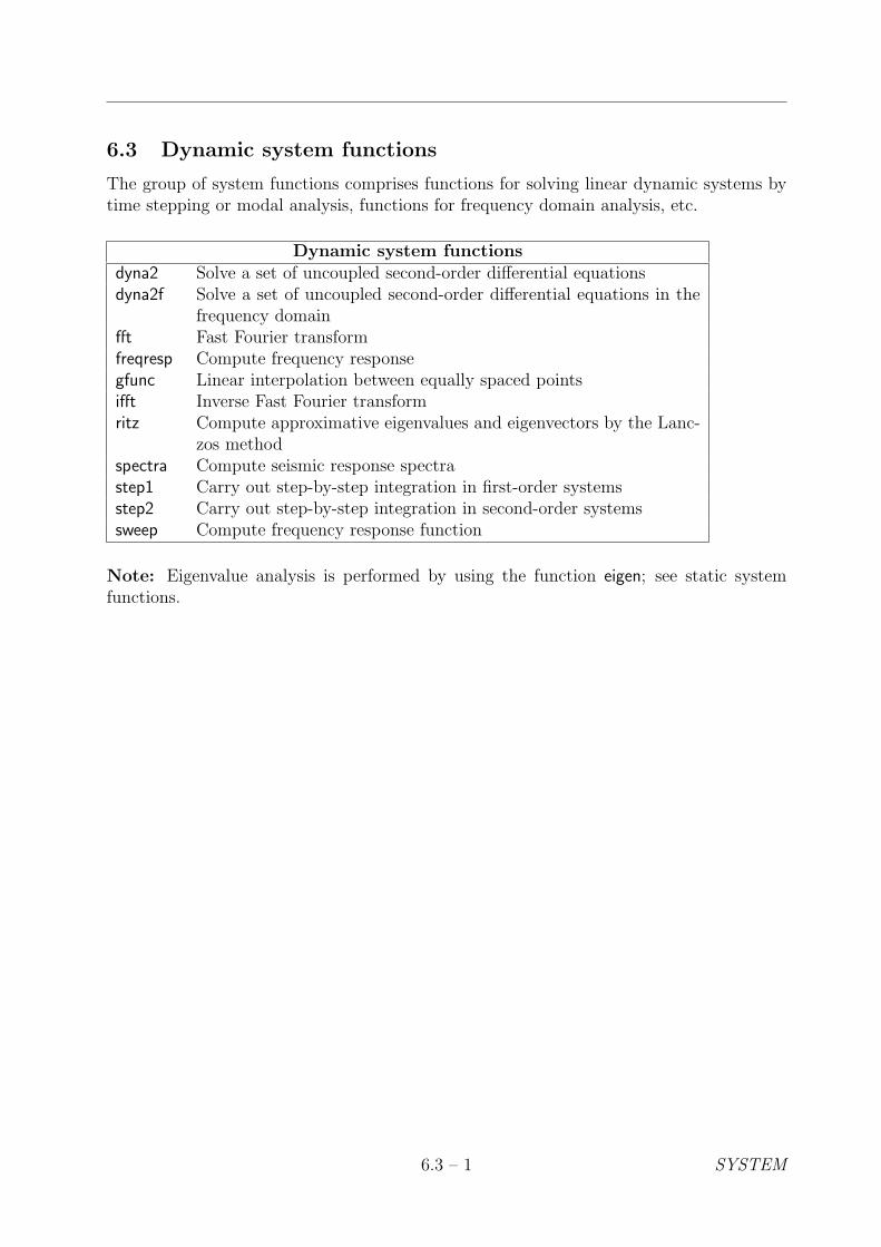
6.3 Dynamic system functions
The group of system functions comprises functions for solving linear dynamic systems bytime stepping or modal analysis, functions for frequency domain analysis, etc.
Dynamic system functionsdyna2 Solve a set of uncoupled second-order differential equationsdyna2f Solve a set of uncoupled second-order differential equations in the
frequency domainfft Fast Fourier transformfreqresp Compute frequency responsegfunc Linear interpolation between equally spaced pointsifft Inverse Fast Fourier transformritz Compute approximative eigenvalues and eigenvectors by the Lanc-
zos methodspectra Compute seismic response spectrastep1 Carry out step-by-step integration in first-order systemsstep2 Carry out step-by-step integration in second-order systemssweep Compute frequency response function
Note: Eigenvalue analysis is performed by using the function eigen; see static systemfunctions.
6.3 – 1 SYSTEM

dyna2 Dynamic system functions
Purpose:
Compute the dynamic solution to a set of uncoupled second-order differential equa-tions.
Syntax:
X=dyna2(w2,xi,f,g,dt)
Description:
dyna2 computes the solution to the set
xi + 2ξiωixi + ω2i xi = fig(t), i = 1, ...,m
of differential equations, where g(t) is a piecewise linear time function.
The set of vectors w2, xi and f contains the squared circular frequencies ω2i , the
damping ratios ξi and the applied forces fi, respectively. The vector g defines theload function in terms of straight line segments between equally spaced points intime. This function may have been formed by the command gfunc.
The dynamic solution is computed at equal time increments defined by dt. Includingthe initial zero vector as the first column vector, the result is stored in the m-by-nmatrix X, n− 1 being the number of time steps.
Note:
The accuracy of the solution is not a function of the output time increment dt, sincethe command produces the exact solution for straight line segments in the loadingtime function.
See also:
gfunc
SYSTEM 6.3 – 2

Dynamic system functions dyna2f
Purpose:
Compute the dynamic solution to a set of uncoupled second-order differential equa-tions.
Syntax:
Y=dyna2f(w2,xi,f,p,dt)
Description:
dyna2f computes the solution to the set
xi + 2ξiωixi + ω2i xi = fig(t), i = 1, ...,m
of differential equations in the frequency domain.
The vectors w2, xi and f are the squared circular frequencies ω2i , the damping ratios
ξi and the applied forces fi, respectively. The force vector p contains the Fouriercoefficients p(k) formed by the command fft.
The solution in the frequency domain is computed at equal time increments definedby dt. The result is stored in the m-by-n matrix Y, where m is the number ofequations and n is the number of frequencies resulting from the fft command. Thedynamic solution in the time domain is achieved by the use of the command ifft.
Example:
The dynamic solution to a set of uncoupled second-order differential equations canbe computed by the following sequence of commands:
>> g=gfunc(G,dt);
>> p=fft(g);
>> Y=dyna2f(w2,xi,f,p,dt);
>> X=(real(ifft(Y.’)))’;
where it is assumed that the input variables G, dt, w2, xi and f are properly defined.Note that the ifft command operates on column vectors if Y is a matrix; thereforeuse the transpose of Y. The output from the ifft command is complex. Thereforeuse Y.’ to transpose rows and columns in Y in order to avoid the complex conjugatetranspose of Y; see Section 3. The time response is represented by the real part ofthe output from the ifft command. If the transpose is used and the result is storedin a matrix X, each row will represent the time response for each equation as theoutput from the command dyna2.
See also:
gfunc, fft, ifft
6.3 – 3 SYSTEM

fft Dynamic system functions
Purpose:
Transform functions in time domain to frequency domain.
Syntax:
p=fft(g)p=fft(g,N)
Description:
fft transforms a time dependent function to the frequency domain.
The function to be transformed is stored in the vector g. Each row in g containsthe value of the function at equal time intervals. The function represents a span−∞ ≤ t ≤ +∞ ; however, only the values within a typical period are specified by g.
The fft command can be used with one or two input arguments. If N is not specified,the numbers of frequencies used in the transformation is equal to the the numbersof points in the time domain, i.e. the length of the variable g, and the output willbe a vector of the same size containing complex values representing the frequencycontent of the input signal.
The scalar variable N can be used to specify the numbers of frequencies used in theFourier transform. The size of the output vector in this case will be equal to N.It should be remembered that the highest harmonic component in the time signalthat can be identified by the Fourier transform corresponds to half the samplingfrequency. The sampling frequency is equal to 1/dt, where dt is the time incrementof the time signal.
The complex Fourier coefficients p(k) are stored in the vector p, and are computedaccording to
p(k) =N∑
j=1
x(j)ω(j−1)(k−1)N ,
where
ωN = e−2πi/N .
Note:
This is a MATLAB built-in function.
SYSTEM 6.3 – 4
Dynamic system functions freqresp
Purpose:
Compute frequency response of a known discrete time response.
Syntax:
[Freq,Resp] = freqresp(D,dt)
Description:
freqresp computes the frequency response of a discrete dynamic system.
D is the time history function and dt is the sampling time increment, i.e. the timeincrement used in the time integration procedure.
Resp contains the computed response as a function of frequency. Freq contains thecorresponding frequencies.
Example:
The result can be visualized by
>> plot(Freq,Resp)
>> xlabel(’frequency (Hz)’)
or
>> semilogy(Freq,Resp)
>> xlabel(’frequency (Hz)’)
The dimension of Resp is the same as that of the original time history function.
Note:
The time history function of a discrete system computed by direct integration behavesoften in an unstructured manner. The reason for this is that the time history is amixture of several participating eigenmodes at different eigenfrequencies. By using aFourier transform, however, the response as a function of frequency can be computedefficiently. In particular it is possible to identify the participating frequencies.
6.3 – 5 SYSTEM

gfunc Dynamic system functions
Purpose:
Form vector with function values at equally spaced points by linear interpolation.
●
●
●
●
●
t
g(t)
●
(t2,g(t2))
(t1,g(t1))
(t3,g(t3))
(t4,g(t4))
(t5,g(t5))
(tN,g(tN))
●
Syntax:
[t,g]=gfunc(G,dt)
Description:
gfunc uses linear interpolation to compute values at equally spaced points for adiscrete function g given by
G =
t1 g(t1)t2 g(t2)...tN g(tN)
,
as shown in the figure above.
Function values are computed in the range t1 ≤ t ≤ tN , at equal increments, dt beingdefined by the variable dt. The number of linear segments (steps) is (tN − t1)/dt.The corresponding vector t is also computed. The result can be plotted by using thecommand plot(t,g).
SYSTEM 6.3 – 6

Dynamic system functions ifft
Purpose:
Transform function in frequency domain to time domain.
Syntax:
x=ifft(y)x=ifft(y,N)
Description:
ifft transforms a function in the frequency domain to a function in the time domain.
The function to be transformed is given in the vector y. Each row in y containsFourier terms in the interval −∞ ≤ ω ≤ +∞.
The fft command can be used with one or two input arguments. The scalar variableN can be used to specify the numbers of frequencies used in the Fourier transform.The size of the output vector in this case will be equal to N. See also the descriptionof the command fft.
The inverse Fourier coefficients x(j), stored in the variable x, are computed accordingto
x(j) = (1/N)N∑
k=1
y(k)ω−(j−1)(k−1)N ,
where
ωN = e−2πi/N .
Note:
This is a MATLAB built-in function.
See also:
fft
6.3 – 7 SYSTEM
ritz Dynamic system functions
Purpose:
Compute approximative eigenvalues and eigenvectors by the Lanczos method.
Syntax:
L=ritz(K,M,f,m)L=ritz(K,M,f,m,b)[L,X]=ritz(K,M,f,m)[L,X]=ritz(K,M,f,m,b)
Description:
ritz computes, by the use of the Lanczos algorithm, m approximative eigenvalues andm corresponding eigenvectors for a given pair of n-by-n matrices K and M and agiven non-zero starting vector f.
If certain rows and columns in matrices K and M are to be eliminated in computingthe eigenvalues, b must be given in the command. The rows (and columns) to beeliminated are described in the vector b defined as
b =
dof1
dof2...
dofnb
.
Note:
If the number of vectors, m, is chosen less than the total number of degrees-of-freedom, n, only about the first m/2 Ritz vectors are good approximations of thetrue eigenvectors. Recall that the Ritz vectors satisfy the M-orthonormality condition
XT M X = I,
where I is the identity matrix.
SYSTEM 6.3 – 8

Dynamic system functions spectra
Purpose:
Compute seismic response spectra for elastic design.
Syntax:
s=spectra(a,xi,dt,f)
Description:
spectra computes the seismic response spectrum for a known acceleration historyfunction.
The computation is based on the vector a, that contains an acceleration time historyfunction defined at equal time steps. The time step is specified by the variable dt.The value of the damping ratio is given by the variable xi.
Output from the computation, stored in the vector s, is achieved at frequenciesspecified by the column vector f.
Example:
The following procedure can be used to produce a seismic response spectrum for adamping ratio ξ = 0.05, defined at 34 logarithmicly spaced frequency points. Theacceleration time history a has been sampled at a frequency of 50 Hz, correspondingto a time increment dt = 0.02 between collected points:
>> freq=logspace(0,log10(2^(33/6)),34);
>> xi=0.05;
>> dt=0.02;
>> s=spectra(a,xi,dt,freq’);
The resulting spectrum can be plotted by the command
>> loglog(freq,s,’*’)
6.3 – 9 SYSTEM

step1 Dynamic system functions
Purpose:
Compute the dynamic solution to a set of first order differential equations.
Syntax:
Tsnap=step1(K,C,d0,ip,f,pbound)[Tsnap,D,V]=step1(K,C,d0,ip,f,pbound)
Description:
step1 computes at equal time steps the solution to a set of first order differentialequations of the form
Cd + Kd = f(x, t),
d(0) = d0.
The command solves transient field problems. In the case of heat conduction, K andC represent the n× n conductivity and capacity matrices, respectively.
The initial conditions are given by the vector d0 containing initial values of d. Thetime integration procedure is governed by the parameters given in the vector ipdefined as
ip = [dt T α [nsnap nhist timei ... dofi ... ]] ,
︸ ︷︷ ︸list ofnsnapmoments
︸ ︷︷ ︸list ofnhistdofs
where dt specifies the time increment in the time stepping scheme, T total time andα a time integration constant; see [1]. The parameter nsnap denotes the number ofsnapshots stored in Tsnap. The selected elapsed times are specified in (timei ... ),whereas nhist is the number of time histories stored in D and V. The selected degrees-of-freedom are specified in (dofi ... ). The following table lists frequently used valuesof α:
α = 0 Forward difference; forward Euler,
α = 12
Trapezoidal rule; Crank-Nicholson,
α = 1 Backward difference; backward Euler.
The matrix f contains the time-dependent load vectors. If no external loads areactive, the matrix corresponding to f should be replaced by []. The matrix f containsthe time-dependent prescribed values of the field variable. If no field variables areprescribed the matrix corresponding to pbound should be replaced by []. Matrix f isorganized in the following manner:
SYSTEM 6.3 – 10

Dynamic system functions step1
f =
time history of the load at dof1
time history of the load at dof2...time history of the load at dofn
.
The dimension of f is
(number of degrees-of-freedom)× (number of timesteps + 1).
The matrix pbound is organized in the following manner:
pbound =
dof1 time history of the field variabledof2 time history of the field variable...
...dofm2 time history of the field variable
.
The dimension of pbound is
(number of dofs with prescribed field values)× (number of timesteps + 2).
The time history functions can be generated using the command gfunc. If all thevalues of the time histories of f or pbound are kept constant, these values need to bestated only once. In this case the number of columns in f is one and in pbound two.
It is highly recommended to define f as sparse (a MATLAB built-in function). Inmost cases only a few degrees-of-freedom are affected by the exterior load, and hencethe matrix contains only few non-zero entries.
The computed snapshots are stored in Tsnap, one column for each requested snapshotaccording to ip, i.e. the dimension of Tsnap is (number of dofs) × nsnap. Thecomputed time histories of d and d are stored in D and V, respectively, one linefor each requested degree-of-freedom according to ip. The dimension of D is nhist×(number of timesteps + 1).
6.3 – 11 SYSTEM

step2 Dynamic system functions
Purpose:
Compute the dynamic solution to a set of second order differential equations.
Syntax:
Dsnap=step2(K,C,M,d0,v0,ip,f,pdisp)[Dsnap,D,V,A]=step2(K,C,M,d0,v0,ip,f,pdisp)
Description:
step2 computes at equal time steps the solution to a second order differential equa-tions of the form
Md + Cd + Kd = f(x, t),
d(0) = d0,
d(0) = v0.
In structural mechanics problems, K , C and M represent the n×n stiffness, dampingand mass matrices, respectively.
The initial conditions are given by the vectors d0 and v0, containing initial dis-placements and initial velocities. The time integration procedure is governed by theparameters given in the vector ip defined as
ip = [dt T α δ [nsnap nhist timei ... dofi ... ]] ,︸ ︷︷ ︸list ofnsnapmoments
︸ ︷︷ ︸list ofnhistdofs
where dt specifies the time increment in the time stepping scheme, T the total timeand α and δ time integration constants for the Newmark family of methods; see[1]. The parameter nsnap denotes the number of snapshots stored in Dsnap. Theselected elapsed times are specified in (timei ... ), whereas nhist is the number oftime histories stored in D, V and A. The selected degrees-of-freedom are specified in(dofi ... ). The following table lists frequently used values of α and δ:
α = 14
δ = 12
Average acceleration (trapezoidal) rule,
α = 16
δ = 12
Linear acceleration,
α = 0 δ = 12
Central difference.
The matrix f contains the time-dependent load vectors. If no external loads are active,the matrix corresponding to f should be replaced by []. The matrix pdisp containsthe time-dependent prescribed displacement. If no displacements are prescribed thematrix corresponding to pdisp should be replaced by [].
The matrix f is organized in the following manner:
SYSTEM 6.3 – 12
Dynamic system functions step2
f =
time history of the load at dof1
time history of the load at dof2...time history of the load at dofn
.
The dimension of f is
(number of degrees-of-freedom)× (number of timesteps + 1).
The matrix pdisp is organized in the following manner
pdisp =
dof1 time history of the displacementdof2 time history of the displacement...
...dofm2 time history of the displacement
.
The dimension of pdisp is
(number of dofs with prescribed displacement)× (number of timesteps + 2).
The time history functions can be generated using the command gfunc. If all thevalues of the time histories of f or pdisp are kept constant, these values need to bestated only once. In this case the number of columns in f is one and in pdisp two.
It is highly recommended to define f as sparse (a MATLAB built-in function). Inmost cases only a few degrees-of-freedom are affected by the exterior load, and hencethe matrix contains only few non-zero entries.
The computed displacement snapshots are stored in Dsnap, one column for eachrequested snapshot according to ip, i.e. the dimension of Dsnap is (number of dofs)×nsnap. The computed time histories of d, d and d are stored in D, V and A,respectively, one line for each requested degree-of-freedom according to ip. Thedimension of D is nhist× (number of timesteps + 1).
6.3 – 13 SYSTEM

sweep Dynamic system functions
Purpose:
Compute complex frequency response functions.
Syntax:
Y=sweep(K,C,M,p,w)
Description:
sweep computes the complex frequency response function for a system of the form
[K + iωC− ω2M]y(ω) = p.
Here K, C and M represent the m-by-m stiffness, damping and mass matrices, re-spectively. The vector p defines the amplitude of the force. The frequency responsefunction is computed for the values of ω given by the vector w.
The complex frequency response function is stored in the matrix Y with dimensionm-by-n, where n is equal to the number of circular frequencies defined in w.
Example:
The steady-state response can be computed by
>> X=real(Y*exp(i*w*t));
and the amplitude by
>> Z=abs(Y);
SYSTEM 6.3 – 14
7 Statements and macros
Statements describe algorithmic actions that can be executed. There are two differenttypes of control statements, conditional and repetitive. The first group defines conditionaljumps whereas the latter one defines repetition until a conditional statement is fulfilled.Macros are used to define new functions to the MATLAB or CALFEM structure, or tostore a sequence of statements in an .m-file.
Control statementsif Conditional jumpfor Initiate a loopwhile Define a conditional loop
Macrosfunction Define a new functionscript Store a sequence of statements
7 – 1 STATEMENTS
if
Purpose:
Conditional jump.
Syntax:
if logical expression...elseif logical expression...else...end
Description:
if initiates a conditional jump. If logical expression produces the value True thestatements following if are executed. If logical expression produces the value Falsethe next conditional statement elseif is checked.
elseif works like if. One or more of the conditional statement elseif can be added afterthe initial conditional statement if.
If else is present, the statements following else are executed if the logical expressionsin all if and elseif statements produce the value False. The if loop is closed by end todefine the loop sequence.
The following relation operators can be used
== equal
>= greater than or equal to
> greater than
<= less than or equal to
< less than
∼= not equal
Note:
This is MATLAB built-in language.
STATEMENTS 7 – 2
for
Purpose:
Initiate a loop.
Syntax:
for i = start : inc : stop...end
Description:
for initiates a loop which terminates when i>stop. The for loop is closed by end todefine the loop sequence.
Examples:
for i = 1 : 10 i takes values from 1 to 10.for i = 1 : 2 : 10 i equals 1, 3, 5, 7, 9.for i = 20 : -1 : 1 i equals 20, 19 ... 2, 1.
Note:
This is MATLAB built-in language.
7 – 3 STATEMENTS
while
Purpose:
Define a conditional loop.
Syntax:
while logical expression...end
Description:
while initiates a conditional loop which terminates when logical expression equalsFalse. The while loop is closed by end to define the loop sequence.
The different relation operators that can be used can be found under the if command.
Examples:
A loop continuing until a equals b
while a∼=b...end
Note:
This is MATLAB built-in language.
STATEMENTS 7 – 4
function
Purpose:
Define a new function.
Syntax:
function[ out1 , out2 , ... ]=name( in1 , in2 , ... )
Description:
name is replaced by the name of the function. The input variables in1, in2, ... can bescalars, vectors or matrices, and the same holds for the output variables out1, out2,... .
Example:
To define the CALFEM function spring1e a file named spring1e.m is created. The filecontains the following statements:
function [Ke]=spring1e(k)% Define the stiffness matrix% for a one dimensional spring% with spring stiffness kKe=[ k, -k; -k, k ]
i.e. the function spring1e is defined to return a stiffness matrix.
Note:
This is MATLAB built-in language.
7 – 5 STATEMENTS

script
Purpose:
Execute a stored sequence of statements.
Syntax:
name
Description:
name is replaced by the name of the script.
Example:
The statements below are stored in a file named spring.m and executed by typingspring in the MATLAB command window.
% Stiffness matrix for a one dimensional% spring with stiffness k=10k=10;[Ke]=spring1e(k);
Note:
This is MATLAB built-in language.
STATEMENTS 7 – 6

8 Graphics functions
The group of graphics functions comprises functions for element based graphics. Meshplots, displacements, section forces, flows, iso lines and principal stresses can be displayed.The functions are divided into two dimensional, and general graphics functions.
Two dimensional graphics functionsplot Plot lines and points in 2D spacefill Draw filled 2D polygonseldraw2 Draw undeformed finite element mesheldisp2 Draw deformed finite element mesheldia2 Draw section force diagramelflux2 Plot flux vectorseliso2 Draw isolines for nodal quantitieselprinc2 Plot principal stresses
General graphics functionsaxis Axis scaling and appearanceclf Clear current figurefigure Create figuresgrid Grid lineshold Hold current graphprint Print graph or save graph to filetext Add text to current plottitle Titles for 2D and 3D plotsxlabel,ylabel,zlabel
Axis labels for 2D and 3D plots
8 – 1 GRAPHICS

axis
Purpose:
Plot axis scaling and appearance.
Syntax:
axis([xmin xmax ymin ymax])axis([xmin xmax ymin ymax zmin zmax])axis autoaxis squareaxis equalaxis offaxis on
Description:
axis([xmin xmax ymin ymax]) sets scaling for the x- and y-axes on the current 2D plot.
axis([xmin xmax ymin ymax zmin zmax]) sets the scaling for the x-, y- and z-axes onthe current 3D plot.
axis auto returns the axis scaling to its default automatic mode where, for each plot,xmin = min(x), xmax = max(x), etc.
axis square makes the current axis box square in shape.
axis equal changes the current axis box size so that equal tick mark increments onthe x- and y-axes are equal in size. This makes plot(sin(x),cos(x)) look like a circle,instead of an oval.
axis normal restores the current axis box to full size and removes any restrictions onthe scaling of the units. This undoes the effects of axis square and axis equal.
axis off turns off all axis labeling and tick marks.
axis on turns axis labeling and tick marks back on.
Note:
This is a MATLAB built-in function. For more information about the axis function,type help axis.
GRAPHICS 8 – 2
clf
Purpose:
Clear current figure (graph window).
Syntax:
clf
Description:
clf deletes all objects (axes) from the current figure.
Note:
This is a MATLAB built-in function. For more information about the clf function,type help clf.
8 – 3 GRAPHICS
eldraw2
Purpose:
Draw the undeformed mesh for a two dimensional structure.
Syntax:
eldraw2(Ex,Ey)eldraw2(Ex,Ey,plotpar)eldraw2(Ex,Ey,plotpar,elnum)
Description:
eldraw2 displays the undeformed mesh for a two dimensional structure.
Input variables are the coordinate matrices Ex and Ey formed by the function co-ordxtr.
The variable plotpar sets plot parameters for linetype, linecolor and node marker.
plotpar = [ linetype linecolor nodemark ]
linetype = 1 solid line linecolor = 1 black2 dashed line 2 blue3 dotted line 3 magenta
4 red
nodemark = 1 circle2 star0 no mark
Default is solid black lines with circles at nodes.
Element numbers can be displayed at the center of the element if a column vectorelnum with the element numbers is supplied. This column vector can be derived fromthe element topology matrix Edof,
elnum=Edof(:,1)
i.e. the first column of the topology matrix.
Limitations:
Supported elements are bar, beam, triangular three node, and quadrilateral fournode elements.
GRAPHICS 8 – 4

eldisp2
Purpose:
Draw the deformed mesh for a two dimensional structure.
Syntax:
[magnfac]=eldisp2(Ex,Ey,Ed)[magnfac]=eldisp2(Ex,Ey,Ed,plotpar)eldisp2(Ex,Ey,Ed,plotpar,magnfac)
Description:
eldisp2 displays the deformed mesh for a two dimensional structure.
Input variables are the coordinate matrices Ex and Ey formed by the function co-ordxtr, and the element displacements Ed formed by the function extract.
The variable plotpar sets plot parameters for linetype, linecolor and node marker.
plotpar=[ linetype linecolor nodemark ]
linetype = 1 solid line linecolor = 1 black2 dashed line 2 blue3 dotted line 3 magenta
4 red
nodemark = 1 circle2 star0 no mark
Default is dashed black lines with circles at nodes.
The magnification factor magnfac is a scalar that magnifies the element displacementsfor visibility. The magnification factor is set automatically if it is omitted in the inputlist.
Limitations:
Supported elements are bar, beam, triangular three node, and quadrilateral fournode elements.
8 – 5 GRAPHICS

eldia2
Purpose:
Draw the section force diagrams of a two dimensional beam element.
x
y
x
y
x
y
x
y
Syntax:
[magnfac]=eldia2(ex,ey,es,eci)eldia2(ex,ey,es,eci,magnfac)eldia2(ex,ey,es,eci,magnfac,magnitude)
Description:
eldia2 plots a section force diagram of a two dimensional beam element in its globalposition.
The input variables ex and ey are defined in beam2e and the input variables
es =
S1
S2...
Sn
eci =
x1
x2...
xn
consist of column matrices that contain section forces and corresponding local x-coordinates respectively. The values in es and eci are computed in beam2s. It shouldbe noted, however, that whereas all three section forces are computed in beam2s onlyone of them shall be given as input to eldia2 by es.
GRAPHICS 8 – 6

eldia2
The magnification factor magnfac is a scalar that magnifies the diagram for visibility.magnfac is set automatically if it is omitted in the input list.
The optional input
magnitude = [ S x y ]
adds a scaled bar, with length equivalent to a reference force S, starting at coordi-nates (x, y). If no coordinates are given the starting point will be (0,-0.5).
Limitations:
Supported elements are two dimensional beam elements.
8 – 7 GRAPHICS

elflux2
Purpose:
Draw element flow arrows for two dimensional elements.
Syntax:
[magnfac]=elflux2(Ex,Ey,Es)[magnfac]=elflux2(Ex,Ey,Es,plotpar)elflux2(Ex,Ey,Es,plotpar,magnfac)
Description:
elflux2 displays element heat flux vectors (or corresponding quantities) for a numberof elements of the same type. The flux vectors are displayed as arrows at the elementcentroids. Note that only the flux vectors are displayed. To display the element mesh,use eldraw2.
Input variables are the coordinate matrices Ex and Ey, and the element flux matrixEs defined in flw2ts or flw2qs.
The variable plotpar sets plot parameters for the flux arrows.
plotpar=[ arrowtype arrowcolor ]
arrowtype = 1 solid arrowcolor = 1 black2 dashed 2 blue3 dotted 3 magenta
4 red
Default, if plotpar is omitted, is solid black arrows.
The magnification factor magnfac is a scalar that magnifies the arrows in relation tothe element size. The magnification factor is set automatically if it is omitted in theinput list.
Limitations:
Supported elements are triangular 3 node and quadrilateral 4 node elements.
GRAPHICS 8 – 8
eliso2
Purpose:
Display element iso lines for two dimensional elements.
Syntax:
eliso2(Ex,Ey,Ed,isov)eliso2(Ex,Ey,Ed,isov,plotpar)
Description:
eliso2 displays element iso lines for a number of elements of the same type. Note thatonly the iso lines are displayed. To display the element mesh, use eldraw2.
Input variables are the coordinate matrices Ex and Ey formed by the function co-ordxtr, and the element nodal quantities (e.g displacement or energy potential) matrixEd defined in extract.
If isov is a scalar it determines the number of iso lines to be displayed. If isov is avector it determines the values of the iso lines to be displayed (number of iso linesequal to length of vector isov).
isov = [ isolines]isov = [ isovalue(1) ... isovalue(n) ]
The variable plotpar sets plot parameters for the iso lines.
plotpar=[ linetype linecolor textfcn ]
arrowtype = 1 solid arrowcolor = 1 black2 dashed 2 blue3 dotted 3 magenta
4 red
textfcn = 0 the iso values of the lines will not be printed1 the iso values of the lines will be printed at the iso lines2 the iso values of the lines will be printed where the cursor indicates
Default is solid, black lines and no iso values printed.
Limitations:
Supported elements are triangular 3 node and quadrilateral 4 node elements.
8 – 9 GRAPHICS
elprinc2
Purpose:
Draw element principal stresses as arrows for two dimensional elements.
Syntax:
[magnfac]=elprinc2(Ex,Ey,Es)[magnfac]=elprinc2(Ex,Ey,Es,plotpar)elprinc2(Ex,Ey,Es,plotpar,magnfac)
Description:
elprinc2 displays element principal stresses for a number of elements of the same type.The principal stresses are displayed as arrows at the element centroids. Note thatonly the principal stresses are displayed. To display the element mesh, use eldraw2.
Input variables are the coordinate matrices Ex and Ey, and the element stressesmatrix Es defined in plants or planqs
The variable plotpar sets plot parameters for the principal stress arrows.
plotpar=[ arrowtype arrowcolor ]
arrowtype = 1 solid arrowcolor = 1 black2 dashed 2 blue3 dotted 3 magenta
4 red
Default, if plotpar is omitted, is solid black arrows.
The magnification factor magnfac is a scalar that magnifies the arrows in relation tothe element size. The magnification factor is set automatically if it is omitted in theinput list.
Limitations:
Supported elements are triangular 3 node and quadrilateral 4 node elements.
GRAPHICS 8 – 10

figure
Purpose:
Create figures (graph windows).
Syntax:
figure(h)
Description:
figure(h) makes the h’th figure the current figure for subsequent plotting functions.If figure h does not exist, a new one is created using the first available figure handle.
Note:
This is a MATLAB built-in function. For more information about the figure function,type help figure.
8 – 11 GRAPHICS

fill
Purpose:
Filled 2D polygons.
Syntax:
fill(x,y,c)fill(X,Y,C)
Description:
fill(x,y,c) fills the 2D polygon defined by vectors x and y with the color specified byc. The vertices of the polygon are specified by pairs of components of x and y. Ifnecessary, the polygon is closed by connecting the last vertex to the first.
If c is a vector of the same length as x and y, its elements are used to specify colorsat the vertices. The color within the polygon is obtained by bilinear interpolation inthe vertex colors.
If X, Y and C are matrices of the same size, fill(X,Y,C) draws one polygon per columnwith interpolated colors.
Example:
The solution of a heat conduction problem results in a vector d with nodal tem-peratures. The temperature distribution in a group of triangular 3 node (nen=3)or quadrilateral 4 node (nen=4) elements, with topology defined by edof, can bedisplayed by
[ex,ey]=coordxtr(edof,Coord,Dof,nen)
ed=extract(edof,d)
colormap(hot)
fill(ex’,ey’,ed’)
Note:
This is a MATLAB built-in function. For more information about the fill function,type help fill.
GRAPHICS 8 – 12
grid
Purpose:
Grid lines for 2D and 3D plots.
Syntax:
grid ongrid offgrid
Description:
grid on adds grid lines on the current axes.
grid off takes them off.
grid by itself, toggles the grid state.
Note:
This is a MATLAB built-in function. For more information about the grid function,type help grid.
8 – 13 GRAPHICS

hold
Purpose:
Hold the current graph.
Syntax:
hold onhold offhold
Description:
hold on holds the current graph.
hold off returns to the default mode where plot functions erase previous plots.
hold by itself, toggles the hold state.
Note:
This is a MATLAB built-in function. For more information about the hold function,type help hold.
GRAPHICS 8 – 14
plot
Purpose:
Linear two dimensional plot.
Syntax:
plot(x,y)plot(x,y,’linetype’)
Description:
plot(x,y) plots vector x versus vector y. Straight lines are drawn between each pairof values.
Various line types, plot symbols and colors may be obtained with plot(x,y,s) where sis a 1, 2, or 3 character string made from the following characters:
– solid line . point y yellow: dotted line o circle m magenta-. dashdot line x x-mark c cyan- - dashed line + plus r red
* star g greenb bluew whitek black
Default is solid blue lines.
Example:
The statement
plot(x,y,’-’,x,y,’ro’)
plots the data twice, giving a solid blue line with red circles at the data points.
Note:
This is a MATLAB built-in function. For more information about the plot function,type help plot.
8 – 15 GRAPHICS

Purpose:
Create hardcopy output of current figure window.
Syntax:
print [filename]
Description:
print with no arguments sends the contents of the current figure window to thedefault printer. print filename creates a PostScript file of the current figure windowand writes it to the specified file.
Note:
This is a MATLAB built-in function. For more information about the print function,type help print.
GRAPHICS 8 – 16

text
Purpose:
Add text to current plot.
Syntax:
text(x,y,’string’)
Description:
text adds the text in the quotes to location (x,y) on the current axes, where (x,y)is in units from the current plot. If x and y are vectors, text writes the text at alllocations given. If ’string’ is an array with the same number of rows as the length ofx and y, text marks each point with the corresponding row of the ’string’ array.
Note:
This is a MATLAB built-in function. For more information about the text function,type help text.
8 – 17 GRAPHICS

title
Purpose:
Titles for 2D and 3D plots.
Syntax:
title(’text’)
Description:
title adds the text string ’text’ at the top of the current plot.
Note:
This is a MATLAB built-in function. For more information about the title function,type help title.
GRAPHICS 8 – 18

xlabel, ylabel, zlabel
Purpose:
x-, y-, and z-axis labels for 2D and 3D plots.
Syntax:
xlabel(’text’)ylabel(’text’)zlabel(’text’)
Description:
xlabel adds text beside the x-axis on the current plot.
ylabel adds text beside the y-axis on the current plot.
zlabel adds text beside the z-axis on the current plot.
Note:
This is a MATLAB built-in function. For more information about the functions,type help xlabel, help ylabel, or help zlabel.
8 – 19 GRAPHICS


9 User’s Manual, examples
9.1 Introduction
This set of examples is defined with the ambition to serve as a User’s Manual. Theexamples, except the introductory ones, are written as .m-files (script files) and suppliedtogether with the CALFEM functions.
The User’s Manual examples are separated into four groups:
MATLAB introduction
Static analysis
Dynamic analysis
Nonlinear analysis
The MATLAB introduction examples explain some basic concepts and introduce a setof standard MATLAB functions usable in the finite element context. The static linearexamples illustrate finite element analysis of different structures loaded by stationary loads.The dynamic linear examples illustrate some basic features in dynamics, such as modalanalysis and time stepping procedures. The examples of nonlinear analysis cover subjectssuch as second order theory and buckling.
9.1 – 1 EXAMPLES

9.2 MATLAB introduction
The examples in this section illustrate basic MATLAB concepts such as handling ofworkspace, variables and functions. The examples are:
MATLAB introduction
exi1 Handling matrices
exi2 Matrix and array operations
exi3 Create and handle .m-files
exi4 Display formats
exi5 Create a session .log-file
exi6 Graphic display of vectors
9.2 – 1 EXAMPLES
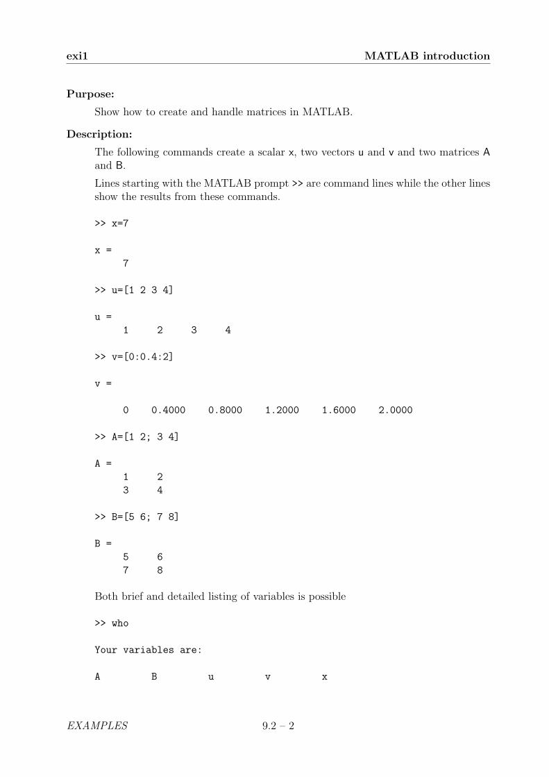
exi1 MATLAB introduction
Purpose:
Show how to create and handle matrices in MATLAB.
Description:
The following commands create a scalar x, two vectors u and v and two matrices Aand B.
Lines starting with the MATLAB prompt >> are command lines while the other linesshow the results from these commands.
>> x=7
x =
7
>> u=[1 2 3 4]
u =
1 2 3 4
>> v=[0:0.4:2]
v =
0 0.4000 0.8000 1.2000 1.6000 2.0000
>> A=[1 2; 3 4]
A =
1 2
3 4
>> B=[5 6; 7 8]
B =
5 6
7 8
Both brief and detailed listing of variables is possible
>> who
Your variables are:
A B u v x
EXAMPLES 9.2 – 2

MATLAB introduction exi1
>> whos
Name Size Bytes Class
A 2x2 32 double array
B 2x2 32 double array
u 1x4 32 double array
v 1x6 48 double array
x 1x1 8 double array
Grand total is 19 elements using 152 bytes
The value of a variable is displayed by writing the variable name,
>> u
u =
1 2 3 4
and the dimension (m×n) of a variable is obtained by
>> size(u)
ans =
1 4
where the answer is temporarily stored in the vector ans.
The variable x is removed from workspace by
>> clear x
To remove all variables from workspace, clear without argument is used.
Assignment of a value to an element in a matrix is made as
>> A(2,2)=9
A =
1 2
3 9
9.2 – 3 EXAMPLES

exi1 MATLAB introduction
To select a complete row or column colon notation is used.
>> s=A(:,1)
s =
1
3
>> t=A(2,:)
t =
3 9
A zero matrix K (4×4) is generated by
>> K=zeros(4,4)
K =
0 0 0 0
0 0 0 0
0 0 0 0
0 0 0 0
Similarly an (m×n) matrix of all ones can be generated by ones(m,n).
Expand an already defined matrix
>> H=[A;B]
H =
1 2
3 9
5 6
7 8
>> J=[A B]
J =
1 2 5 6
3 9 7 8
EXAMPLES 9.2 – 4
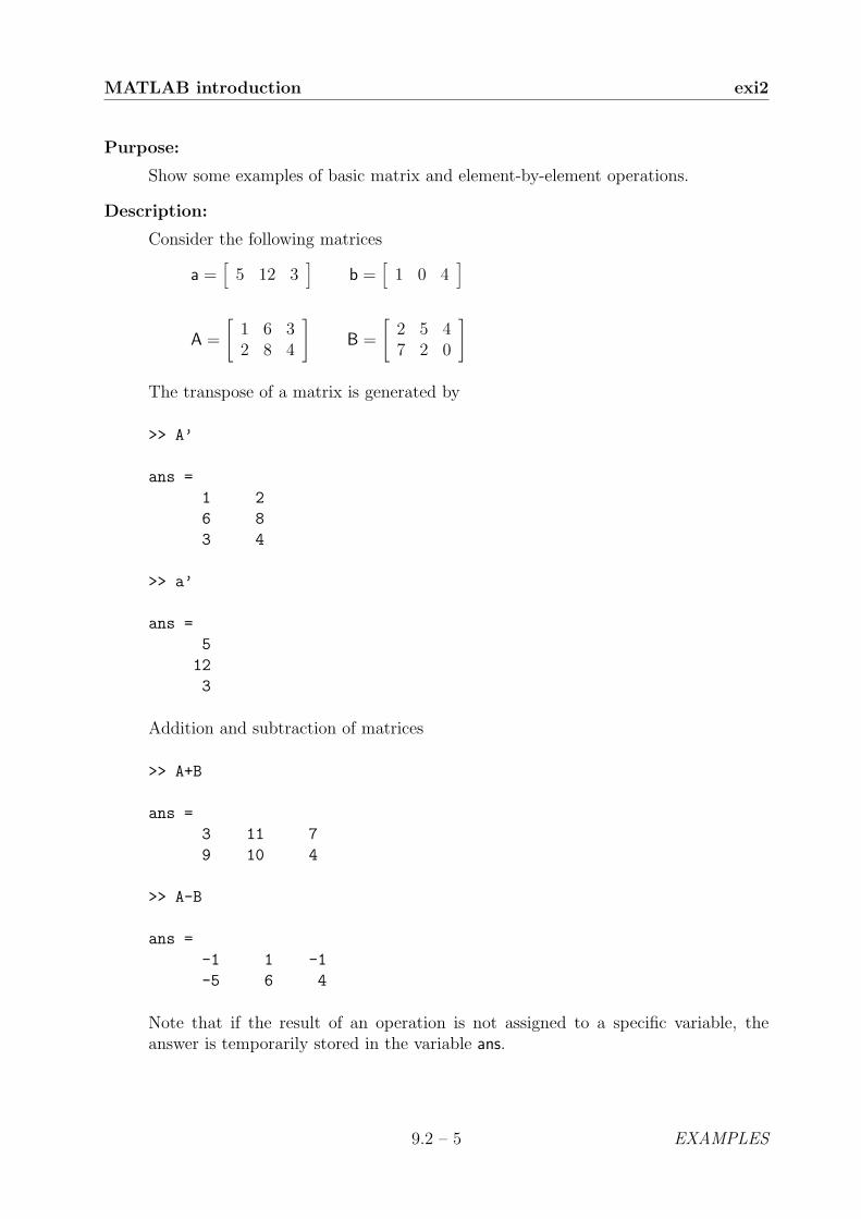
MATLAB introduction exi2
Purpose:
Show some examples of basic matrix and element-by-element operations.
Description:
Consider the following matrices
a =[
5 12 3]
b =[
1 0 4]
A =
[1 6 32 8 4
]B =
[2 5 47 2 0
]
The transpose of a matrix is generated by
>> A’
ans =
1 2
6 8
3 4
>> a’
ans =
5
12
3
Addition and subtraction of matrices
>> A+B
ans =
3 11 7
9 10 4
>> A-B
ans =
-1 1 -1
-5 6 4
Note that if the result of an operation is not assigned to a specific variable, theanswer is temporarily stored in the variable ans.
9.2 – 5 EXAMPLES

exi2 MATLAB introduction
Multiplication of matrices
>> a*b’
ans =
17
>> a’*b
ans =
5 0 20
12 0 48
3 0 12
>> A’*B
ans =
16 9 4
68 46 24
34 23 12
>> C=B*A’
C =
44 60
19 30
To perform arithmetic operations, matrix dimensions must agree
>> D=A*B
??? Error using ==> *
Inner matrix dimensions must agree.
The inverse of a square matrix
>> inv(C)
ans =
0.1667 -0.3333
-0.1056 0.2444
EXAMPLES 9.2 – 6

MATLAB introduction exi2
The determinant of a square matrix
>> det(C)
ans =
180
An array or element-by-element arithmetic operation is denoted by a period (.) pre-ceding an operator. Examples are element-by-element multiplication (.*), division(./), and powers (.^).
>> a.*b
ans =
5 0 12
>> A.*B
ans =
2 30 12
14 16 0
Matrices in element-by-element operations must obviously have the same dimensions.
Mathematical functions applied to arrays are also evaluated element-by-element.
>> sin([0 1 2 3 4]*pi/2)
ans =
0 1 0 -1 0
9.2 – 7 EXAMPLES

exi3 MATLAB introduction
Purpose:
Show how to handle script files and function files.
Description:
When starting a MATLAB session the default working directory is according toinitial settings, for example C:\USER. A new working directory can be chosen bytyping for example
>> cd A:
which makes the root directory in drive A the working directory.
Files containing MATLAB and/or CALFEM statements are characterized by thesuffix .m. For example the file bar2e.m contains statements to evaluate the elementstiffness matrix for a two dimensional bar element. An .m-file is allowed to includereferences to other .m-files, and also to call itself recursively.
Two types of .m-files can be used, script files and function files. Script files collect asequence of statements under one command name. Function files allow new functionswith input and/or output variables to be defined. Both script files and function filesare ordinary ASCII text files and can therefore be created in an arbitrary editor.In the MATLAB environment an .m-file editor can be activated from the pull downmenu on top of the MATLAB window.
An example of a script file is given below. The following sequence of statements istyped in the .m-file editor, and saved as test.m.
% ----- Script file test.m -----
A=[0 4;2 8]
B=[3 9;5 7]
C=A*B
% ------------ end -------------
A line starting with an % is regarded as a comment line.
The statements are executed by writing the file name (without the suffix .m) in thecommand window
>> test
A =
0 4
2 8
EXAMPLES 9.2 – 8

MATLAB introduction exi3
B =
3 9
5 7
C =
20 28
46 74
The second type of .m-files is the function file. The first line of these files containsthe word function. The example below is a function that computes the second andthird power of a scalar.
function [b,c]=func1(a)
% ----- function file ’func1.m’ -----
b=a*a;
c=a*a*a;
% ------------- end -----------------
The semi-colon prohibits the echo display of the variables on the screen.
The file can be created using an ordinary editor, and it must be saved as func1.m i.e.the file name without extension must be the same as the function name.
The second and third power of 2 are calculated by typing
>> [b,c]=func1(2)
producing
b =
4
c =
8
See also function and script in Section 7.
9.2 – 9 EXAMPLES

exi4 MATLAB introduction
Purpose:
Show different display formats.
Description:
Consider the following matrix operation
>> A=[0 4;2 8];
>> B=[3 9;5 7];
>> C=A*B/2537
C =
0.0079 0.0110
0.0181 0.0292
The result from the computation of C above is shown in the default format, displayingfour significant decimal digits.
Other formats can be defined by the command format
>> format long
>> C
C =
0.00788332676389 0.01103665746945
0.01813165155696 0.02916830902641
>> format short e
>> C
C =
7.8833e-03 1.1037e-02
1.8132e-02 2.9168e-02
>> format long e
>> C
C =
7.883326763894364e-03 1.103665746945211e-02
1.813165155695703e-02 2.916830902640915e-02
EXAMPLES 9.2 – 10
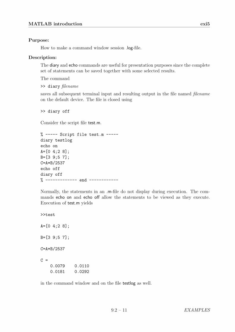
MATLAB introduction exi5
Purpose:
How to make a command window session .log-file.
Description:
The diary and echo commands are useful for presentation purposes since the completeset of statements can be saved together with some selected results.
The command
>> diary filename
saves all subsequent terminal input and resulting output in the file named filenameon the default device. The file is closed using
>> diary off
Consider the script file test.m.
% ----- Script file test.m -----
diary testlog
echo on
A=[0 4;2 8];
B=[3 9;5 7];
C=A*B/2537
echo off
diary off
% ------------- end ------------
Normally, the statements in an .m-file do not display during execution. The com-mands echo on and echo off allow the statements to be viewed as they execute.Execution of test.m yields
>>test
A=[0 4;2 8];
B=[3 9;5 7];
C=A*B/2537
C =
0.0079 0.0110
0.0181 0.0292
in the command window and on the file testlog as well.
9.2 – 11 EXAMPLES

exi6 MATLAB introduction
Purpose:
How to display vectors and handle the graphics window.
Description:
The contents of a vector versus the vector index or a vector versus another vectorcan be displayed in the graphics window. Consider the vectors
x =[
1 2 5]
y =[
5 22 16]
The function
>> plot(y)
plots the contents of the vector y versus vector index and
>> plot(x,y)
plots the contents of the vector y versus the vector x.
The commands
title(’text’ )xlabel(’xlabel’ )ylabel(’ylabel’ )
write text as a title of the current plot, and xlabel and ylabel as labels of the coordinateaxis.
Grid lines are added with
grid
and
clf
clears the current figure.
EXAMPLES 9.2 – 12
9.3 Static analysis
This section illustrates some linear static finite element calculations. The examples dealwith structural problems as well as field problems such as heat conduction.
Static analysis
exs1 Linear spring system
exs2 One-dimensional heat flow
exs3 Simply supported beam
exs4 Plane truss
exs5 Plane frame
exs6 Geometry based frame analysis
exs7 Two dimensional diffusion
The introductory example exs1 illustrates the basic steps in the finite element method fora simple structure of one-dimensional linear springs. The linear spring or analogy elementis also used in example exs2 to solve a problem of heat conduction through a wall. Asimply supported beam is analysed in example exs3. Element forces and reactions at thesupports are calculated. A two dimensional plane truss is analysed in example exs4 anda two dimensional plane frame is analysed in example exs5. A frame built up from bothbeams and bars is analysed in example exs6. The finite element model is defined from thegeometry. Graphics facilities are also explained in example exs5 and exs6.
Note: The examples listed above are supplied as .m-files on the CALFEM diskette underthe directory examples. The example files are named according to the table.
9.3 – 1 EXAMPLES

exs1 Static analysis
Purpose:
Show the basic steps in a finite element calculation.
Description:
The general procedure in linear finite element calculations is carried out for a simplestructure. The steps are
• define the model
• generate element matrices
• assemble element matrices into the global system of equations
• solve the global system of equations
• evaluate element forces
Consider the system of three linear elastic springs, and the corresponding finiteelement model. The system of springs is fixed in its ends and loaded by a single loadF .
●●●3
3
2
1
21
k
2k
2k
F
The computation is initialized by defining the topology matrix Edof, containing ele-ment numbers and global element degrees of freedom,
>> Edof=[1 1 2;
2 2 3;
3 2 3];
the global stiffness matrix K (3×3) of zeros,
>> K=zeros(3,3)
K =
0 0 0
0 0 0
0 0 0
EXAMPLES 9.3 – 2

Static analysis exs1
and the load vector f (3×1) with the load F = 100 in position 2.
>> f=zeros(3,1); f(2)=100
f =
0
100
0
Element stiffness matrices are generated by the function spring1e. The element prop-erty ep for the springs contains the spring stiffnesses k and 2k respectively, wherek = 1500.
>> k=1500; ep1=k; ep2=2*k;
>> Ke1=spring1e(ep1)
Ke1 =
1500 -1500
-1500 1500
>> Ke2=spring1e(ep2)
Ke2 =
3000 -3000
-3000 3000
The element stiffness matrices are assembled into the global stiffness matrix K ac-cording to the topology.
>> K=assem(Edof(1,:),K,Ke2)
K =
3000 -3000 0
-3000 3000 0
0 0 0
>> K=assem(Edof(2,:),K,Ke1)
K =
3000 -3000 0
-3000 4500 -1500
0 -1500 1500
9.3 – 3 EXAMPLES

exs1 Static analysis
>> K=assem(Edof(3,:),K,Ke2)
K =
3000 -3000 0
-3000 7500 -4500
0 -4500 4500
The global system of equations is solved considering the boundary conditions givenin bc.
>> bc= [1 0; 3 0];
>> a=solveq(K,f,bc)
a =
0
0.0133
0
Element forces are evaluated from the element displacements. These are obtainedfrom the global displacements a using the function extract.
>> ed1=extract(Edof(1,:),a)
ed1 =
0 0.0133
>> ed2=extract(Edof(2,:),a)
ed2 =
0.0133 0
>> ed3=extract(Edof(3,:),a)
ed3 =
0.0133 0
EXAMPLES 9.3 – 4

Static analysis exs1
The spring forces are evaluated using the function spring1s.
>> es1=spring1s(ep2,ed1)
es1 =
40
>> es2=spring1s(ep1,ed2)
es2 =
-20
>> es3=spring1s(ep2,ed3)
es3 =
-40
9.3 – 5 EXAMPLES
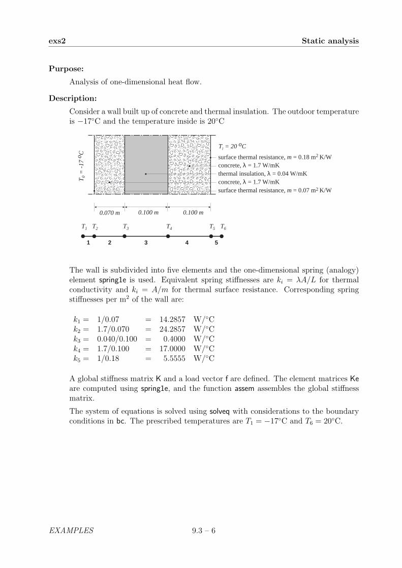
exs2 Static analysis
Purpose:
Analysis of one-dimensional heat flow.
Description:
Consider a wall built up of concrete and thermal insulation. The outdoor temperatureis −17◦C and the temperature inside is 20◦C
● ● ● ●●●
T1 T2 T3 T4 T5 T6
1 2 3 4 5
0.100 m0.070 m
Ti = 20 oC
T0
= -
17
oC
surface thermal resistance, m = 0.18 m2 K/Wconcrete, λ = 1.7 W/mKthermal insulation, λ = 0.04 W/mKconcrete, λ = 1.7 W/mKsurface thermal resistance, m = 0.07 m2 K/W
0.100 m
The wall is subdivided into five elements and the one-dimensional spring (analogy)element spring1e is used. Equivalent spring stiffnesses are ki = λA/L for thermalconductivity and ki = A/m for thermal surface resistance. Corresponding springstiffnesses per m2 of the wall are:
k1 = 1/0.07 = 14.2857 W/◦Ck2 = 1.7/0.070 = 24.2857 W/◦Ck3 = 0.040/0.100 = 0.4000 W/◦Ck4 = 1.7/0.100 = 17.0000 W/◦Ck5 = 1/0.18 = 5.5555 W/◦C
A global stiffness matrix K and a load vector f are defined. The element matrices Keare computed using spring1e, and the function assem assembles the global stiffnessmatrix.
The system of equations is solved using solveq with considerations to the boundaryconditions in bc. The prescribed temperatures are T1 = −17◦C and T6 = 20◦C.
EXAMPLES 9.3 – 6

Static analysis exs2
>> Edof=[1 1 2
2 2 3;
3 3 4;
4 4 5;
5 5 6];
>> K=zeros(6);
>> f=zeros(6,1);
>> ep1=[ 1/0.07 ]; ep2=[ 1.7/0.07 ];
>> ep3=[ 0.040/0.10 ]; ep4=[ 1.7/0.10 ];
>> ep5=[ 1/0.18 ];
>> Ke1=spring1e(ep1); Ke2=spring1e(ep2);
>> Ke3=spring1e(ep3); Ke4=spring1e(ep4);
>> Ke5=spring1e(ep5);
>> K=assem(Edof(1,:),K,Ke1); K=assem(Edof(2,:),K,Ke2);
>> K=assem(Edof(3,:),K,Ke3); K=assem(Edof(4,:),K,Ke4);
>> K=assem(Edof(5,:),K,Ke5);
>> bc=[1 -17; 6 20];
>> T=solveq(K,f,bc)
T =
-17.0000
-16.0912
-15.5567
16.8995
17.6632
20.0000
The temperature values in the node points are given in the vector T.
After solving the system of equations, the heat flow through the wall is computedusing extract and spring1s.
>> ed1=extract(Edof(1,:),T);
>> ed2=extract(Edof(2,:),T);
>> ed3=extract(Edof(3,:),T);
>> ed4=extract(Edof(4,:),T);
>> ed5=extract(Edof(5,:),T);
9.3 – 7 EXAMPLES

exs2 Static analysis
>> q1=spring1s(ep1,ed1)
q1 =
12.9825
>> q2=spring1s(ep2,ed2)
q2 =
12.9825
>> q3=spring1s(ep3,ed3)
q3 =
12.9825
>> q4=spring1s(ep4,ed4)
q4 =
12.9825
>> q5=spring1s(ep5,ed5)
q5 =
12.9825
The heat flow through the wall, equal for all elements, is q = 13.0 W/m2.
EXAMPLES 9.3 – 8

Static analysis exs3
Purpose:
Analysis of a simply supported beam.
Description:
Consider the simply supported beam loaded by a single load f = 10000 N, appliedat a point 1 meter from the left support. The corresponding finite element mesh isalso shown. The following data apply to the beam
Young’s modulus E = 2.10e11 N/m2
Cross section area A = 45.3e−4 m2
Moment of inertia I = 2510e−8 m4
9 m
10
11
12
1 2 3
f = 10 kN
7
8
94
5
61
2
3
The element topology is defined by the topology matrix
>> Edof=[1 1 2 3 4 5 6
2 4 5 6 7 8 9
3 7 8 9 10 11 12];
The system matrices, i.e. the stiffness matrix K and the load vector f, are defined by
>> K=zeros(12); f=zeros(12,1); f(5)=-10000;
The element property vector ep, the element coordinate vectors ex and ey, and theelement stiffness matrix Ke, are generated. Note that the same coordinate vectorsare applicable for all elements because they are identical.
9.3 – 9 EXAMPLES

exs3 Static analysis
>> E=2.1e11; A=45.3e-4; I=2510e-8; ep=[E A I];
>> ex=[0 3]; ey=[0 0];
>> Ke=beam2e(ex,ey,ep)
Ke =
1.0e+08 *
3.1710 0 0 -3.1710 0 0
0 0.0234 0.0351 0 -0.0234 0.0351
0 0.0351 0.0703 0 -0.0351 0.0351
-3.1710 0 0 3.1710 0 0
0 -0.0234 -0.0351 0 0.0234 -0.0351
0 0.0351 0.0351 0 -0.0351 0.0703
Based on the topology information, the global stiffness matrix can be generated byassembling the element stiffness matrices
>> K=assem(Edof,K,Ke);
Finally, the solution can be calculated by defining the boundary conditions in bc andsolving the system of equations. Displacements a and reaction forces Q are computedby the function solveq.
>> bc=[1 0; 2 0; 11 0]; [a,Q]=solveq(K,f,bc);
The section forces es are calculated from element displacements Ed
>> Ed=extract(Edof,a);
>> es1=beam2s(ex,ey,ep,Ed(1,:));
>> es2=beam2s(ex,ey,ep,Ed(2,:));
>> es3=beam2s(ex,ey,ep,Ed(3,:));
EXAMPLES 9.3 – 10

Static analysis exs3
Results
a = Q =
0 1.0e+03 *
0
-0.0095 0
0 6.6667
-0.0228 -0.0000
-0.0038 0
0 -0.0000
-0.0199 -0.0000
0.0047 0
0 -0.0000
0 -0.0000
0.0076 0
3.3333
0.0000
es1 =
1.0e+04 *
0 -0.6667 0.0000
0 -0.6667 2.0000
es2 =
1.0e+04 *
0 0.3333 2.0000
0 0.3333 1.0000
es3 =
1.0e+04 *
0 0.3333 1.0000
0 0.3333 0.0000
9.3 – 11 EXAMPLES

exs4 Static analysis
Purpose:
Analysis of a plane truss.
Description:
Consider a plane truss, loaded by a single force P = 0.5 MN.
2 m 2 m
2 m
P = 0.5 MN
30o
The corresponding finite element model consists of ten elements and twelve degreesof freedom.
11
2
3
4
9
10
5
6
11
12
7
8
2
3
4
6
7
9.
5
8
10
● ●
● ●
●
●x
y
A = 25.0e−4 m2
E = 2.10e5 MPa
The topology is defined by the matrix
>> Edof=[1 1 2 5 6;
2 3 4 7 8;
3 5 6 9 10;
4 7 8 11 12;
5 7 8 5 6;
6 11 12 9 10;
7 3 4 5 6;
8 7 8 9 10;
9 1 2 7 8;
10 5 6 11 12];
EXAMPLES 9.3 – 12

Static analysis exs4
A global stiffness matrix K and a load vector f are defined. The load P is dividedinto x and y components and inserted in the load vector f.
>> K=zeros(12);
>> f=zeros(12,1); f(11)=0.5e6*sin(pi/6); f(12)=-0.5e6*cos(pi/6);
The element matrices Ke are computed by the function bar2e. These matrices arethen assembled in the global stiffness matrix using the function assem.
>> A=25.0e-4; E=2.1e11; ep=[E A];
>> ex1=[0 2]; ex2=[0 2]; ex3=[2 4]; ex4=[2 4]; ex5=[2 2];
>> ex6=[4 4]; ex7=[0 2]; ex8=[2 4]; ex9=[0 2]; ex10=[2 4];
>> ey1=[2 2]; ey2=[0 0]; ey3=[2 2]; ey4=[0 0]; ey5=[0 2];
>> ey6=[0 2]; ey7=[0 2]; ey8=[0 2]; ey9=[2 0]; ey10=[2 0];
>> Ke1=bar2e(ex1,ey1,ep); Ke2=bar2e(ex2,ey2,ep);
>> Ke3=bar2e(ex3,ey3,ep); Ke4=bar2e(ex4,ey4,ep);
>> Ke5=bar2e(ex5,ey5,ep); Ke6=bar2e(ex6,ey6,ep);
>> Ke7=bar2e(ex7,ey7,ep); Ke8=bar2e(ex8,ey8,ep);
>> Ke9=bar2e(ex9,ey9,ep); Ke10=bar2e(ex10,ey10,ep);
>> K=assem(Edof(1,:),K,Ke1); K=assem(Edof(2,:),K,Ke2);
>> K=assem(Edof(3,:),K,Ke3); K=assem(Edof(4,:),K,Ke4);
>> K=assem(Edof(5,:),K,Ke5); K=assem(Edof(6,:),K,Ke6);
>> K=assem(Edof(7,:),K,Ke7); K=assem(Edof(8,:),K,Ke8);
>> K=assem(Edof(9,:),K,Ke9); K=assem(Edof(10,:),K,Ke10);
The system of equations is solved considering the boundary conditions in bc.
>> bc=[1 0;2 0;3 0;4 0];
>> a=solveq(K,f,bc)
a =
0
0
0
0
0.0024
-0.0045
-0.0016
-0.0042
0.0030
-0.0107
-0.0017
-0.0113
9.3 – 13 EXAMPLES

exs4 Static analysis
The displacement at the point of loading is −1.7 · 10−3 m in the x-direction and−11.3 · 10−3 m in the y-direction.
Normal forces are evaluated from element displacements. These are obtained fromthe global displacements a using the function extract. The normal forces are evaluatedusing the function bar2s.
>> ed1=extract(Edof(1,:),a); ed2=extract(Edof(2,:),a);
>> ed3=extract(Edof(3,:),a); ed4=extract(Edof(4,:),a);
>> ed5=extract(Edof(5,:),a); ed6=extract(Edof(6,:),a);
>> ed7=extract(Edof(7,:),a); ed8=extract(Edof(8,:),a);
>> ed9=extract(Edof(9,:),a); ed10=extract(Edof(10,:),a);
>> N1=bar2s(ex1,ey1,ep,ed1)
N1 =
6.2594e+05
>> N2=bar2s(ex2,ey2,ep,ed2)
N2 =
-4.2310e+05
>> N3=bar2s(ex3,ey3,ep,ed3)
N3 =
1.7064e+05
>> N4=bar2s(ex4,ey4,ep,ed4)
N4 =
-1.2373e+04
>> N5=bar2s(ex5,ey5,ep,ed5)
N5 =
-6.9447e+04
>> N6=bar2s(ex6,ey6,ep,ed6)
N6 =
1.7064e+05
>> N7=bar2s(ex7,ey7,ep,ed7)
N7 =
-2.7284e+05
EXAMPLES 9.3 – 14

Static analysis exs4
>> N8=bar2s(ex8,ey8,ep,ed8)
N8 =
-2.4132e+05
>> N9=bar2s(ex9,ey9,ep,ed9)
N9 =
3.3953e+05
>> N10=bar2s(ex10,ey10,ep,ed10)
N10 =
3.7105e+05
The largest normal force N = 0.62 MN is obtained in element 1 and is equivalent toa normal stress σ = 250 MPa.
9.3 – 15 EXAMPLES
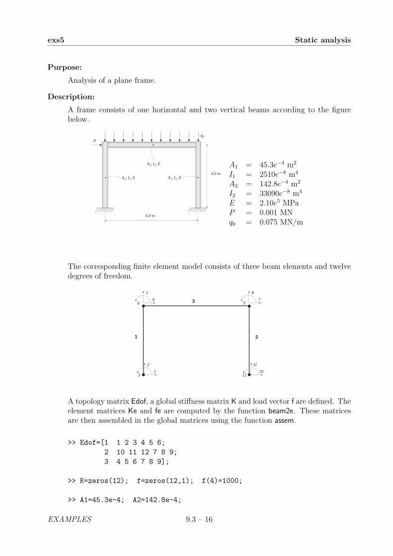
exs5 Static analysis
Purpose:
Analysis of a plane frame.
Description:
A frame consists of one horizontal and two vertical beams according to the figurebelow.
A1, I1, E
Pq0
4.0 m
6.0 m
A2, I2, E
A1, I1, E
A1 = 45.3e−4 m2
I1 = 2510e−8 m4
A2 = 142.8e−4 m2
I2 = 33090e−8 m4
E = 2.10e5 MPaP = 0.001 MNq0 = 0.075 MN/m
The corresponding finite element model consists of three beam elements and twelvedegrees of freedom.
1
2
310
11
12
4
5
67
8
9
1 2
3● ●
●●
A topology matrix Edof, a global stiffness matrix K and load vector f are defined. Theelement matrices Ke and fe are computed by the function beam2e. These matricesare then assembled in the global matrices using the function assem.
>> Edof=[1 1 2 3 4 5 6;
2 10 11 12 7 8 9;
3 4 5 6 7 8 9];
>> K=zeros(12); f=zeros(12,1); f(4)=1000;
>> A1=45.3e-4; A2=142.8e-4;
EXAMPLES 9.3 – 16
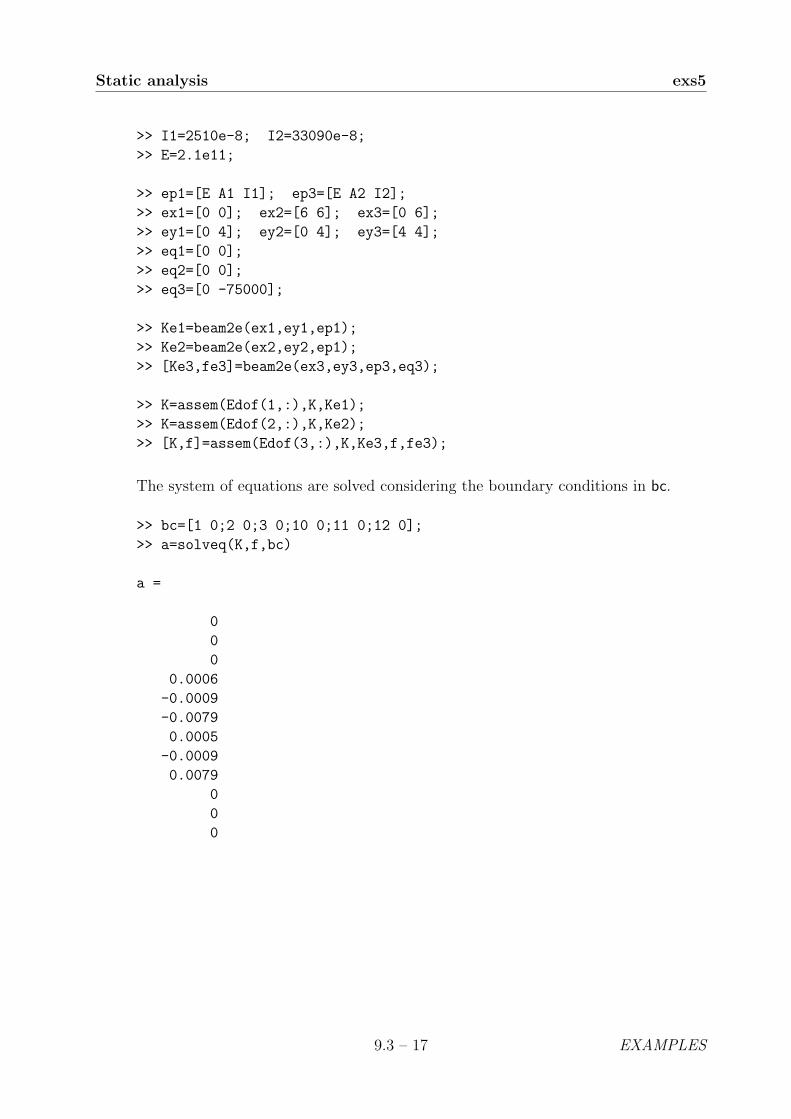
Static analysis exs5
>> I1=2510e-8; I2=33090e-8;
>> E=2.1e11;
>> ep1=[E A1 I1]; ep3=[E A2 I2];
>> ex1=[0 0]; ex2=[6 6]; ex3=[0 6];
>> ey1=[0 4]; ey2=[0 4]; ey3=[4 4];
>> eq1=[0 0];
>> eq2=[0 0];
>> eq3=[0 -75000];
>> Ke1=beam2e(ex1,ey1,ep1);
>> Ke2=beam2e(ex2,ey2,ep1);
>> [Ke3,fe3]=beam2e(ex3,ey3,ep3,eq3);
>> K=assem(Edof(1,:),K,Ke1);
>> K=assem(Edof(2,:),K,Ke2);
>> [K,f]=assem(Edof(3,:),K,Ke3,f,fe3);
The system of equations are solved considering the boundary conditions in bc.
>> bc=[1 0;2 0;3 0;10 0;11 0;12 0];
>> a=solveq(K,f,bc)
a =
0
0
0
0.0006
-0.0009
-0.0079
0.0005
-0.0009
0.0079
0
0
0
9.3 – 17 EXAMPLES
exs5 Static analysis
The element displacements are obtained from the function extract, and the functionbeam2s computes the section forces.
>> Ed=extract(Edof,a);
>> es1=beam2s(ex1,ey1,ep1,Ed(1,:),eq1,20)
es1 =
1.0e+05 *
-2.2467 0.1513 0.1981
-2.2467 0.1513 0.1662
: : :
-2.2467 0.1513 -0.4070
>> es2=beam2s(ex2,ey2,ep1,Ed(2,:),eq2,20)
es2 =
1.0e+05 *
-2.2533 -0.1613 -0.2185
-2.2533 -0.1613 -0.1845
: : :
-2.2533 -0.1613 0.4266
>> es3=beam2s(ex3,ey3,ep3,Ed(3,:),eq3,20)
es3 =
1.0e+05 *
-0.1613 -2.2467 -0.4070
-0.1613 -2.0099 0.2651
: : :
-0.1613 2.2533 -0.4266
EXAMPLES 9.3 – 18

Static analysis exs5
Section force diagrams are displayed using the function eldia2.
>> figure(1)
>> magnfac=eldia2(ex1,ey1,es1(:,1),eci1);
>> magnitude=[3e5 0.5 0];
>> eldia2(ex1,ey1,es1(:,1),eci1,magnfac);
>> eldia2(ex2,ey2,es2(:,1),eci2,magnfac);
>> eldia2(ex3,ey3,es3(:,1),eci3,magnfac,magnitude);
>> axis([-1.5 7 -0.5 5.5])
>> figure(2)
>> magnfac=eldia2(ex3,ey3,es3(:,2),eci3);
>> magnitude=[3e5 0.5 0];
>> eldia2(ex1,ey1,es1(:,2),eci1,magnfac);
>> eldia2(ex2,ey2,es2(:,2),eci2,magnfac);
>> eldia2(ex3,ey3,es3(:,2),eci3,magnfac,magnitude);
>> axis([-1.5 7 -0.5 5.5])
>> figure(3)
>> magnfac=eldia2(ex3,ey3,es3(:,3),eci3);
>> magnitude=[3e5 0.5 0];
>> eldia2(ex1,ey1,es1(:,3),eci1,magnfac);
>> eldia2(ex2,ey2,es2(:,3),eci2,magnfac);
>> eldia2(ex3,ey3,es3(:,3),eci3,magnfac,magnitude);
>> axis([-1.5 7 -0.5 5.5])
9.3 – 19 EXAMPLES
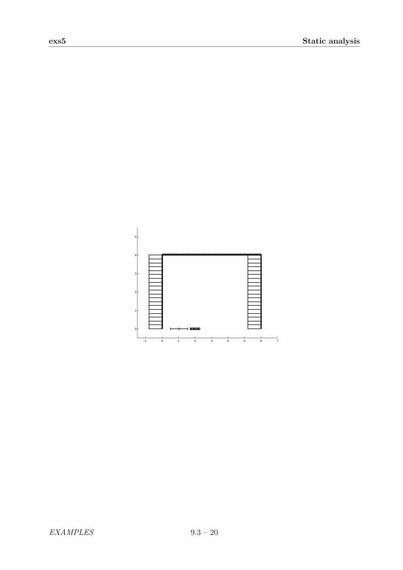
exs5 Static analysis
−1 0 1 2 3 4 5 6 7
0
1
2
3
4
5
300000 300000 300000 300000 300000 300000 300000
EXAMPLES 9.3 – 20
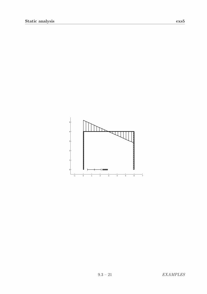
Static analysis exs5
−1 0 1 2 3 4 5 6 7
0
1
2
3
4
5
300000 300000 300000 300000 300000 300000 300000
9.3 – 21 EXAMPLES
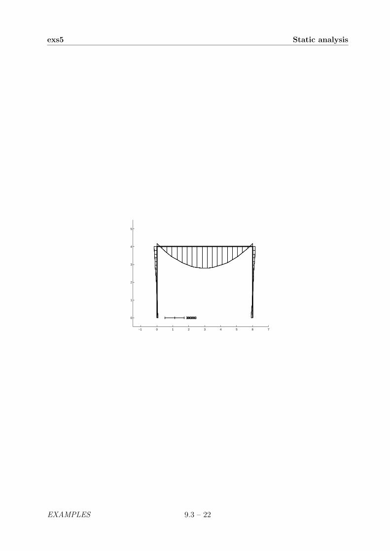
exs5 Static analysis
−1 0 1 2 3 4 5 6 7
0
1
2
3
4
5
300000 300000 300000 300000 300000 300000 300000
EXAMPLES 9.3 – 22

Static analysis exs6
Purpose:
Set up a frame, consisting of both beams and bars, and illustrate the calculations byuse of graphics functions.
Description:
A frame consists of horizontal and vertical beams, and is stabilized with diagonalbars.
1
5
3
2 4
6
7
8
9.
10
13
14
15
7
8
9
1
2
3
16
17
18
10
11
12
4
5
6
x10
0
1
2 P
y
The frame with its coordinates and loading is shown in the left figure, and the finiteelement model in the right. In the following, the statements for analysing the frameare given as an .m-file.
The matrices of the global system i.e. the stiffness matrix K, the load vector f, thecoordinate matrix Coord, and the corresponding degrees of freedom matrix Dof aredefined by
% ----- System matrices -----
K=zeros(18,18);
f=zeros(18,1); f(13)=1;
Coord=[0 0;
1 0;
0 1;
1 1;
0 2;
1 2];
9.3 – 23 EXAMPLES

exs6 Static analysis
Dof=[1 2 3;
4 5 6;
7 8 9;
10 11 12;
13 14 15;
16 17 18];
The material properties, the topology, and the element coordinates for the beamsand bars respectively, are defined by
% ----- Element properties, topology and coordinates -----
ep1=[1 1 1];
Edof1=[1 1 2 3 7 8 9;
2 7 8 9 13 14 15;
3 4 5 6 10 11 12;
4 10 11 12 16 17 18;
5 7 8 9 10 11 12;
6 13 14 15 16 17 18];
[Ex1,Ey1]=coordxtr(Edof1,Coord,Dof,2);
ep2=[1 1];
Edof2=[7 1 2 10 11;
8 7 8 16 17;
9 7 8 4 5;
10 13 14 10 11];
[Ex2,Ey2]=coordxtr(Edof2,Coord,Dof,2);
To check the model, the finite element mesh can be drawn.
eldraw2(Ex1,Ey1,[1 3 1]);
eldraw2(Ex2,Ey2,[1 2 1]);
The element stiffness matrices are generated and assembled in two loops, one for thebeams and one for the bars. The element stiffness functions beam2e and bar2e usethe element coordinate matrices ex and ey. These matrices are extracted from theglobal coordinates Coord by the function coordxtr above.
EXAMPLES 9.3 – 24
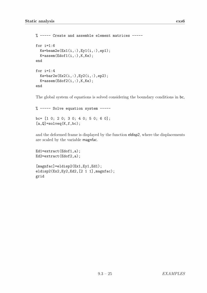
Static analysis exs6
% ----- Create and assemble element matrices -----
for i=1:6
Ke=beam2e(Ex1(i,:),Ey1(i,:),ep1);
K=assem(Edof1(i,:),K,Ke);
end
for i=1:4
Ke=bar2e(Ex2(i,:),Ey2(i,:),ep2);
K=assem(Edof2(i,:),K,Ke);
end
The global system of equations is solved considering the boundary conditions in bc,
% ----- Solve equation system -----
bc= [1 0; 2 0; 3 0; 4 0; 5 0; 6 0];
[a,Q]=solveq(K,f,bc);
and the deformed frame is displayed by the function eldisp2, where the displacementsare scaled by the variable magnfac.
Ed1=extract(Edof1,a);
Ed2=extract(Edof2,a);
[magnfac]=eldisp2(Ex1,Ey1,Ed1);
eldisp2(Ex2,Ey2,Ed2,[2 1 1],magnfac);
grid
9.3 – 25 EXAMPLES

exs6 Static analysis
-1 -0.5 0 0.5 1 1.50
0.5
1
1.5
2
x
y
EXAMPLES 9.3 – 26

Static analysis exs7
Purpose:
Analysis of two dimensional diffusion.
Description:
1 2 3
4 5 6
7 8 9
10 11 12
13 14 15
1 2
3 4
5 6
7 8
x
y
c = 0
c = 0
c = 10-3 kg/m3
c = 0
0.1 m
0.1 m
Description:
Consider a filter paper of square shape. Three sides are in contact with pure waterand the fourth side is in contact with a solution of concentration c = kg/m3. Thelength of each side is 0.100 m. Using symmetry, only half of the paper has to beanalyzed. The paper and the corresponding finite element mesh are shown. Thefollowing boundary conditions are applied
c(0, y) = c(x, 0) = c(0.1, y) = 0c(x, 0.1) = 10−3
The element topology is defined by the topology matrix
>> Edof=[1 1 2 5 4
2 2 3 6 5
3 4 5 8 7
4 5 6 9 8
5 7 8 11 10
6 8 9 12 11
7 10 11 14 13
8 11 12 15 14];
9.3 – 27 EXAMPLES

exs7 Static analysis
The system matrices, i.e. the stiffness matrix K and the load vector f, are defined by
>> K=zeros(15); f=zeros(15,1);
Because of the same geometry, orientation, and constitutive matrix for all elements,only one element stiffness matrix Ke has to be computed. This is done by the functionflw2qe.
>> ep=1; D=[1 0; 0 1];
>> ex=[0 0.025 0.025 0]; ey=[0 0 0.025 0.025];
>> Ke=flw2qe(ex,ey,ep,D)
>> Ke =
0.7500 -0.2500 -0.2500 -0.2500
-0.2500 0.7500 -0.2500 -0.2500
-0.2500 -0.2500 0.7500 -0.2500
-0.2500 -0.2500 -0.2500 0.7500
Based on the topology information, the global stiffness matrix is generated by as-sembling this element stiffness matrix Ke in the global stiffness matrix K
>> K=assem(Edof,K,Ke);
Finally, the solution is calculated by defining the boundary conditions bc and solvingthe system of equations. The boundary condition at dof 13 is set to 0.5×10³ as anaverage of the concentrations at the neighbouring boundaries. Displacements a andreaction forces Q are computed by the function solveq.
>> bc=[1 0;2 0;3 0;4 0;7 0;10 0;13 0.5e-3;14 1e-3;15 1e-3];
>> [a,Q]=solveq(K,f,bc);
The element flows q are calculated from element concentration Ed
>> Ed=extract(Edof,a);
>> for i=1:8
>> es=flw2qs(ex,ey,ep,D,Ed(i,:));
>> end
EXAMPLES 9.3 – 28
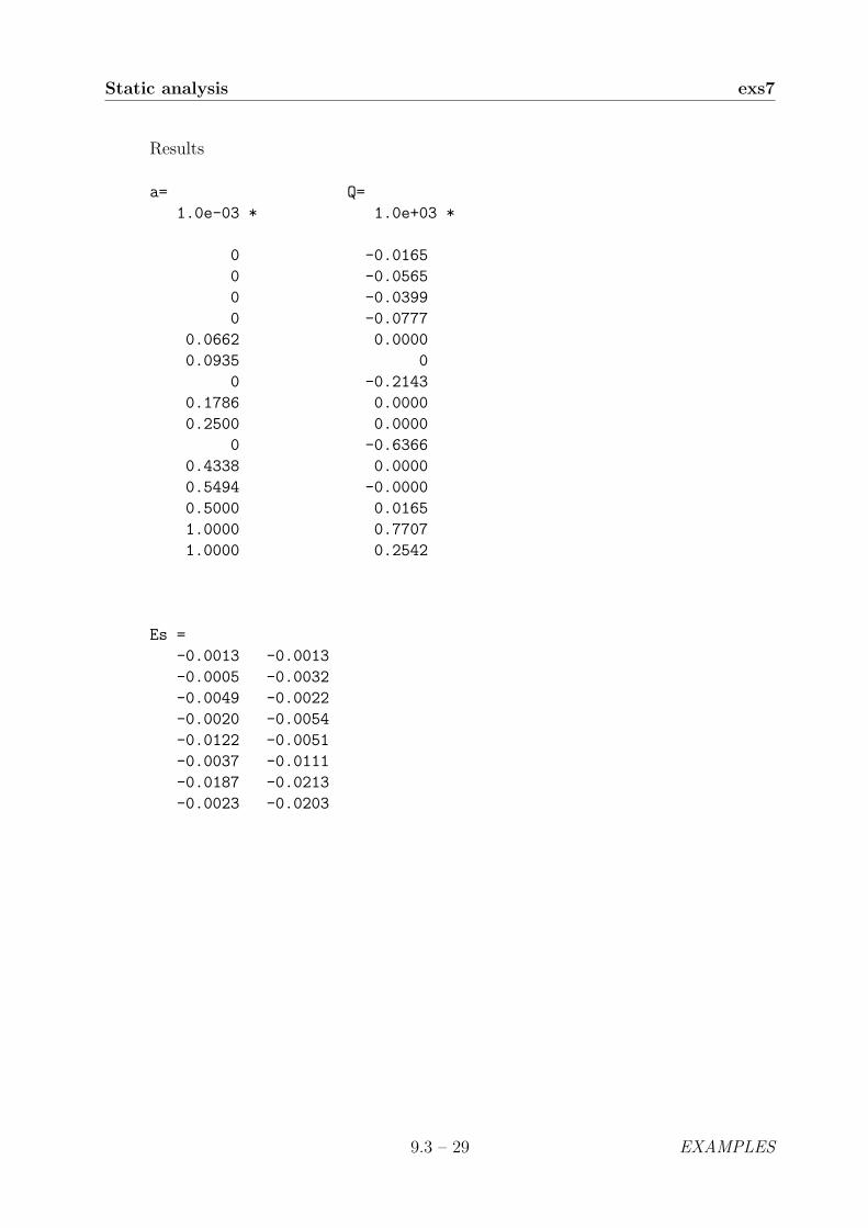
Static analysis exs7
Results
a= Q=
1.0e-03 * 1.0e+03 *
0 -0.0165
0 -0.0565
0 -0.0399
0 -0.0777
0.0662 0.0000
0.0935 0
0 -0.2143
0.1786 0.0000
0.2500 0.0000
0 -0.6366
0.4338 0.0000
0.5494 -0.0000
0.5000 0.0165
1.0000 0.7707
1.0000 0.2542
Es =
-0.0013 -0.0013
-0.0005 -0.0032
-0.0049 -0.0022
-0.0020 -0.0054
-0.0122 -0.0051
-0.0037 -0.0111
-0.0187 -0.0213
-0.0023 -0.0203
9.3 – 29 EXAMPLES

exs7 Static analysis
The following .m-file shows an alternative set of commands to perform the diffusionanalysis of exs7. By use of global coordinates, an FE-mesh is generated. Also plotswith flux-vectors and contour lines are created.
% ----- System matrices -----
K=zeros(15); f=zeros(15,1);
Coord=[0 0 ; 0.025 0 ; 0.05 0
0 0.025; 0.025 0.025; 0.05 0.025
0 0.05 ; 0.025 0.05 ; 0.05 0.05
0 0.075; 0.025 0.075; 0.05 0.075
0 0.1 ; 0.025 0.1 ; 0.05 0.1 ];
Dof=[1; 2; 3
4; 5; 6
7; 8; 9
10;11;12
13;14;15];
% ----- Element properties, topology and coordinates -----
ep=1; D=[1 0;0 1];
Edof=[1 1 2 5 4
2 2 3 6 5
3 4 5 8 7
4 5 6 9 8
5 7 8 11 10
6 8 9 12 11
7 10 11 14 13
8 11 12 15 14];
[Ex,Ey]=coordxtr(Edof,Coord,Dof,4);
% ----- Generate FE-mesh -----
eldraw2(Ex,Ey,[1 3 0],Edof(:,1));
pause; clf;
% ----- Create and assemble element matrices -----
for i=1:8
Ke=flw2qe(Ex(i,:),Ey(i,:),ep,D);
K=assem(Edof(i,:),K,Ke);
end;
% ----- Solve equation system -----
bc=[1 0;2 0;3 0;4 0;7 0;10 0;13 0.5e-3;14 1e-3;15 1e-3];
EXAMPLES 9.3 – 30

Static analysis exs7
[a,Q]=solveq(K,f,bc)
% ----- Compute element flux vectors -----
Ed=extract(Edof,a);
for i=1:8
Es(i,:)=flw2qs(Ex(i,:),Ey(i,:),ep,D,Ed(i,:))
end
% ----- Draw flux vectors and contour lines -----
eldraw2(Ex,Ey); elflux2(Ex,Ey,Es); pause; clf;
eldraw2(Ex,Ey); eliso2(Ex,Ey,Ed,5);
−0.02 0 0.02 0.04 0.06 0.080
0.01
0.02
0.03
0.04
0.05
0.06
0.07
0.08
0.09
0.1
x
y
Flux vectors
9.3 – 31 EXAMPLES
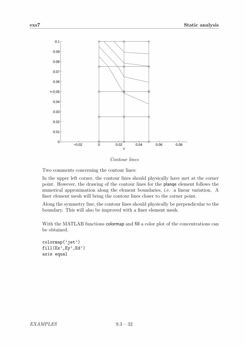
exs7 Static analysis
−0.02 0 0.02 0.04 0.06 0.080
0.01
0.02
0.03
0.04
0.05
0.06
0.07
0.08
0.09
0.1
x
y
Contour lines
Two comments concerning the contour lines:
In the upper left corner, the contour lines should physically have met at the cornerpoint. However, the drawing of the contour lines for the planqe element follows thenumerical approximation along the element boundaries, i.e. a linear variation. Afiner element mesh will bring the contour lines closer to the corner point.
Along the symmetry line, the contour lines should physically be perpendicular to theboundary. This will also be improved with a finer element mesh.
With the MATLAB functions colormap and fill a color plot of the concentrations canbe obtained.
colormap(’jet’)
fill(Ex’,Ey’,Ed’)
axis equal
EXAMPLES 9.3 – 32

9.4 Dynamic analysis
This section concerns linear dynamic finite element calculations. The examples illustratesome basic features in dynamics such as modal analysis and time stepping procedures.
Dynamic analysis
exd1 Modal analysis of frame
exd2 Transient analysis
exd3 Reduced system transient analysis
exd4 Time varying boundary condition
Note: The examples listed above are supplied as .m-files on the CALFEM diskette underthe directory examples. The example files are named according to the table.
9.4 – 1 EXAMPLES

exd1 Dynamic analysis
Purpose:
Set up the finite element model and perform eigenvalue analysis for a simple framestructure.
Description:
Consider the two dimensional frame shown below. A vertical beam is fixed at itslower end, and connected to a horizontal beam at its upper end. The horizontalbeam is simply supported at the right end. The length of the vertical beam is 3 mand of the horizontal beam 2 m. The following data apply to the beams
vertical beam horizontal beamYoung’s modulus (N/m2) 3e10 3e10Cross section area (m2) 0.1030e-2 0.0764e-2Moment of inertia (m4) 0.171e-5 0.0801e-5Density (kg/m3) 2500 2500
78
9 1011
1213
14
15
12
3
45
6
1
2
3 4
2 m
3 m
a) b)
The structure is divided into 4 elements. The numbering of elements and degrees-of-freedom are apparent from the figure. The following .m-file defines the finite elementmodel.
% --- material data ------------------------------------------
E=3e10; rho=2500;
Av=0.1030e-2; Iv=0.0171e-4; % IPE100
Ah=0.0764e-2; Ih=0.00801e-4; % IPE80
epv=[E Av Iv rho*Av]; eph=[E Ah Ih rho*Ah];
EXAMPLES 9.4 – 2

Dynamic analysis exd1
% --- topology ----------------------------------------------
Edof=[1 1 2 3 4 5 6
2 4 5 6 7 8 9
3 7 8 9 10 11 12
4 10 11 12 13 14 15];
% --- list of coordinates -----------------------------------
Coord=[0 0; 0 1.5; 0 3; 1 3; 2 3];
% --- list of degrees-of-freedom ----------------------------
Dof=[1 2 3; 4 5 6; 7 8 9; 10 11 12; 13 14 15];
% --- generate element matrices, assemble in global matrices -
K=zeros(15); M=zeros(15);
[Ex,Ey]=coordxtr(Edof,Coord,Dof,2);
for i=1:2
[k,m,c]=beam2d(Ex(i,:),Ey(i,:),epv);
K=assem(Edof(i,:),K,k); M=assem(Edof(i,:),M,m);
end
for i=3:4
[k,m,c]=beam2d(Ex(i,:),Ey(i,:),eph);
K=assem(Edof(i,:),K,k); M=assem(Edof(i,:),M,m);
end
The finite element mesh is plotted, using the following commands
clf;
eldraw2(Ex,Ey,[1 2 2],Edof);
grid; title(’2D Frame Structure’);
pause;
-0.5 0 0.5 1 1.5 2 2.50
0.5
1
1.5
2
2.5
32-D Frame Structure
x
y
1
2
3 4
Finite element mesh
9.4 – 3 EXAMPLES

exd1 Dynamic analysis
A standard procedure in dynamic analysis is eigenvalue analysis. This is accom-plished by the following set of commands.
b=[1 2 3 14]’;[La,Egv]=eigen(K,M,b);Freq=sqrt(La)/(2*pi);
Note that the boundary condition matrix, b, only lists the degrees-of-freedom thatare zero. The results of these commands are the eigenvalues, stored in La, and theeigenvectors, stored in Egv. The corresponding frequencies in Hz are calculated andstored in the column matrix Freq.
Freq = [6.9826 43.0756 66.5772 162.7453 230.2709 295.6136
426.2271 697.7628 877.2765 955.9809 1751.3]T
The eigenvectors can be plotted by entering the commands below.
figure(1), clf, grid, title(’The first eigenmode’),
eldraw2(Ex,Ey,[2 3 1]);
Edb=extract(Edof,Egv(:,1)); eldisp2(Ex,Ey,Edb,[1 2 2]);
FreqText=num2str(Freq(1)); text(.5,1.75,FreqText);
pause;
-0.5 0 0.5 1 1.5 2 2.50
0.5
1
1.5
2
2.5
3The first eigenmode
x
y
6.983
The first eigenmode, 6.98 Hz
EXAMPLES 9.4 – 4

Dynamic analysis exd1
An attractive way of displaying the eigenmodes is shown in the figure below. Theresult is accomplished by translating the different eigenmodes in the x-direction, seethe Ext-matrix defined below, and in the y-direction, see the Eyt-matrix.
clf, axis(’equal’), hold on, axis off
magnfac=0.5;
title(’The first eight eigenmodes (Hz)’ )
for i=1:4;
Ext=Ex+(i-1)*3; eldraw2(Ext,Ey,[2 3 1]);
Edb=extract(Edof,Egv(:,i));
eldisp2(Ext,Ey,Edb,[1 2 2],magnfac);
FreqText=num2str(Freq(i)); text(3*(i-1)+.5,1.5,FreqText);
end;
Eyt=Ey-4;
for i=5:8;
Ext=Ex+(i-5)*3; eldraw2(Ext,Eyt,[2 3 1]);
Edb=extract(Edof,Egv(:,i));
eldisp2(Ext,Eyt,Edb,[1 2 2],magnfac);
FreqText=num2str(Freq(i)); text(3*(i-5)+.5,-2.5,FreqText);
end
The first eight eigenmodes (Hz)
6.983 43.08 66.58 162.7
230.3 295.6 426.2 697.8
The first eight eigenmodes. Frequencies are given in Hz.
9.4 – 5 EXAMPLES

exd2 Dynamic analysis
Purpose:
The frame structure defined in exd1 is exposed in this example to a transient load.The structural response is determined by a time stepping procedure.
Description:
The structure is exposed to a transient load, impacting on the center of the verticalbeam in horizontal direction, i.e. at the 4th degree-of-freedom. The time history ofthe load is shown below. The result shall be displayed as time history plots of the4th degree-of-freedom and the 11th degree-of-freedom. At time t = 0 the frame is atrest. The timestep is chosen as ∆t = 0.001 seconds and the integration is performedfor T = 1.0 second. At every 0.1 second the deformed shape of the whole structureshall be displayed.
-0.5 0 0.5 1 1.5 2 2.50
0.5
1
1.5
2
2.5
3The first eigenmode
x
y
6.983
Time history of the impact load
The load is generated using the gfunc-function. The time integration is performedby the step2-function. Because there is no damping present, the C-matrix is enteredas [ ].
dt=0.005; T=1;
% --- the load -----------------------------------------------
G=[0 0; 0.15 1; 0.25 0; T 0]; [t,g]=gfunc(G,dt);
f=zeros(15, length(g)); f(4,:)=1000*g;
% --- boundary condition, initial condition ------------------
bc=[1 0; 2 0; 3 0; 14 0];
d0=zeros(15,1); v0=zeros(15,1);
% --- output parameters --------------------------------------
ntimes=[0.1:0.1:1]; nhist=[4 11];
% --- time integration parameters ----------------------------
ip=[dt T 0.25 0.5 10 2 ntimes nhist];
% --- time integration ---------------------------------------
k=sparse(K); m=sparse(M);
EXAMPLES 9.4 – 6

Dynamic analysis2 exd2
[Dsnap,D,V,A]=step2(k,[],m,d0,v0,ip,f,bc);
The requested time history plots are generated by the following commands
figure(1), plot(t,D(1,:),’-’,t,D(2,:),’--’)
grid, xlabel(’time (sec)’), ylabel(’displacement (m)’)
title(’Displacement(time) for the 4th and 11th’...
’ degree-of-freedom’)
text(0.3,0.009,’solid line = impact point, x-direction’)
text(0.3,0.007,’dashed line = center, horizontal beam,’...
’ y-direction’)
0 0.2 0.4 0.6 0.8 1-0.01
-0.005
0
0.005
0.01
0.015
0.02
time (sec)
disp
lace
men
t (m
)
Displacement(time) at the 4th and 11th degree-of-freedom
solid line = impact point, x-direction
dashed line = center, horizontal beam, y-direction
Time history at DOF 4 and DOF 11.
The deformed shapes at time increment 0.1 sec are stored in Dsnap. They are visu-alized by the following commands:
figure(2),clf, axis(’equal’), hold on, axis off
magnfac=25;
title(’Snapshots (sec), magnification = 25’);
for i=1:5;
Ext=Ex+(i-1)*3; eldraw2(Ext,Ey,[2 3 0]);
Edb=extract(Edof,Dsnap(:,i));
eldisp2(Ext,Ey,Edb,[1 2 2],magnfac);
Time=num2str(ntimes(i)); text(3*(i-1)+.5,1.5,Time);
end;
Eyt=Ey-4;
for i=6:10;
Ext=Ex+(i-6)*3; eldraw2(Ext,Eyt,[2 3 0]);
9.4 – 7 EXAMPLES

exd2 Dynamic analysis
Edb=extract(Edof,Dsnap(:,i));
eldisp2(Ext,Eyt,Edb,[1 2 2],magnfac);
Time=num2str(ntimes(i)); text(3*(i-6)+.5,-2.5,Time);
end
Snapshots (sec), magnification = 25
0.1 0.2 0.3 0.4 0.5
0.6 0.7 0.8 0.9 1
Snapshots of the deformed geometry for every 0.1 sec.
EXAMPLES 9.4 – 8
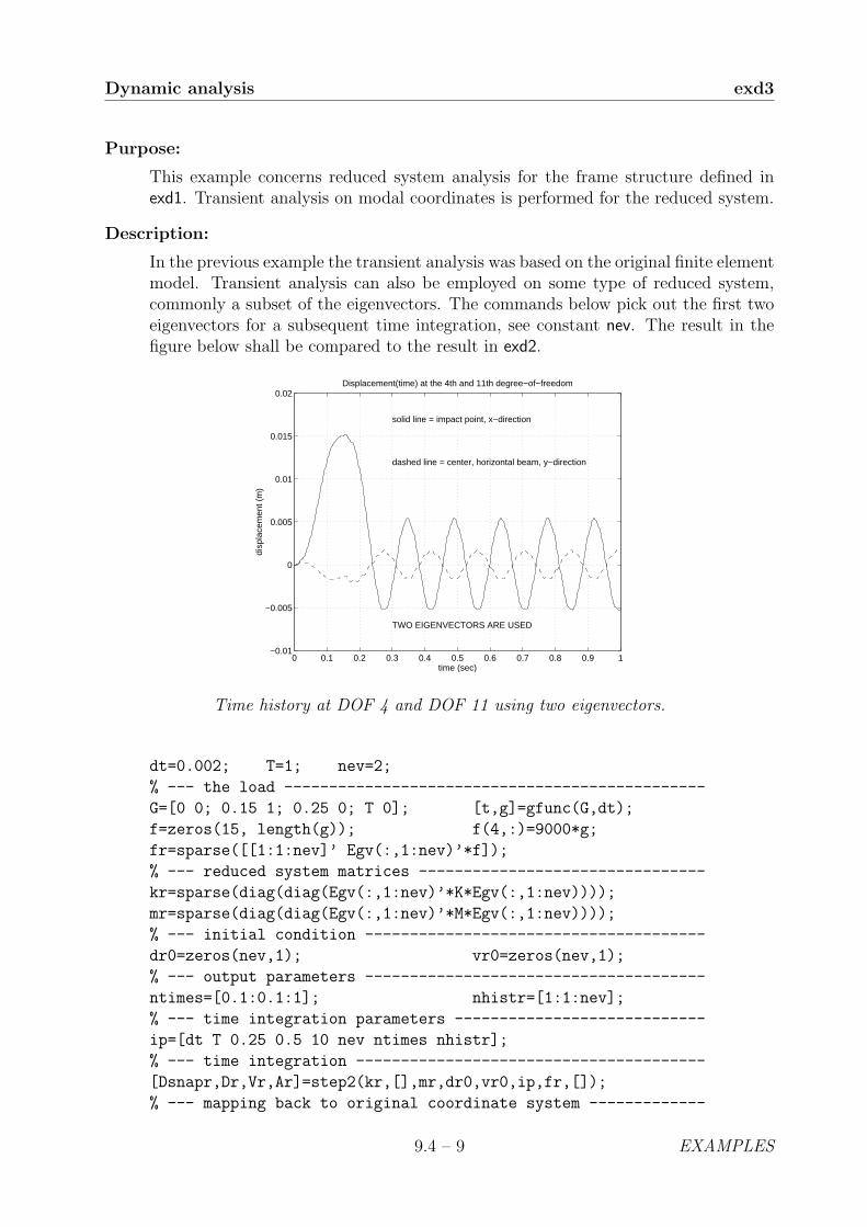
Dynamic analysis exd3
Purpose:
This example concerns reduced system analysis for the frame structure defined inexd1. Transient analysis on modal coordinates is performed for the reduced system.
Description:
In the previous example the transient analysis was based on the original finite elementmodel. Transient analysis can also be employed on some type of reduced system,commonly a subset of the eigenvectors. The commands below pick out the first twoeigenvectors for a subsequent time integration, see constant nev. The result in thefigure below shall be compared to the result in exd2.
0 0.1 0.2 0.3 0.4 0.5 0.6 0.7 0.8 0.9 1−0.01
−0.005
0
0.005
0.01
0.015
0.02
time (sec)
disp
lace
men
t (m
)
Displacement(time) at the 4th and 11th degree−of−freedom
solid line = impact point, x−direction
dashed line = center, horizontal beam, y−direction
TWO EIGENVECTORS ARE USED
Time history at DOF 4 and DOF 11 using two eigenvectors.
dt=0.002; T=1; nev=2;
% --- the load -----------------------------------------------
G=[0 0; 0.15 1; 0.25 0; T 0]; [t,g]=gfunc(G,dt);
f=zeros(15, length(g)); f(4,:)=9000*g;
fr=sparse([[1:1:nev]’ Egv(:,1:nev)’*f]);
% --- reduced system matrices --------------------------------
kr=sparse(diag(diag(Egv(:,1:nev)’*K*Egv(:,1:nev))));
mr=sparse(diag(diag(Egv(:,1:nev)’*M*Egv(:,1:nev))));
% --- initial condition --------------------------------------
dr0=zeros(nev,1); vr0=zeros(nev,1);
% --- output parameters --------------------------------------
ntimes=[0.1:0.1:1]; nhistr=[1:1:nev];
% --- time integration parameters ----------------------------
ip=[dt T 0.25 0.5 10 nev ntimes nhistr];
% --- time integration ---------------------------------------
[Dsnapr,Dr,Vr,Ar]=step2(kr,[],mr,dr0,vr0,ip,fr,[]);
% --- mapping back to original coordinate system -------------
9.4 – 9 EXAMPLES
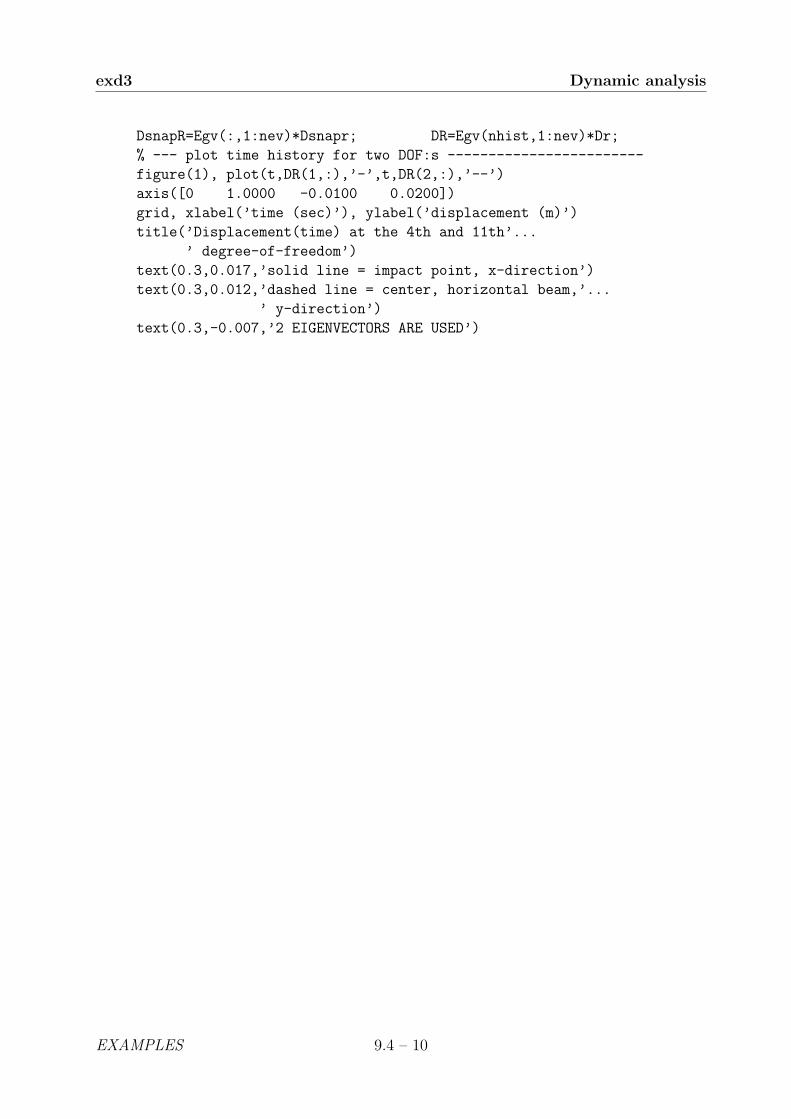
exd3 Dynamic analysis
DsnapR=Egv(:,1:nev)*Dsnapr; DR=Egv(nhist,1:nev)*Dr;
% --- plot time history for two DOF:s ------------------------
figure(1), plot(t,DR(1,:),’-’,t,DR(2,:),’--’)
axis([0 1.0000 -0.0100 0.0200])
grid, xlabel(’time (sec)’), ylabel(’displacement (m)’)
title(’Displacement(time) at the 4th and 11th’...
’ degree-of-freedom’)
text(0.3,0.017,’solid line = impact point, x-direction’)
text(0.3,0.012,’dashed line = center, horizontal beam,’...
’ y-direction’)
text(0.3,-0.007,’2 EIGENVECTORS ARE USED’)
EXAMPLES 9.4 – 10

Dynamic analysis exd4
Purpose:
This example deals with a time varying boundary condition and time integration forthe frame structure defined in exd1.
Description:
Suppose that the support of the vertical beam is moving in the horizontal direction.The commands below prepare the model for time integration. Note that the structureof the boundary condition matrix bc differs from the structure of the load matrix fdefined in exd2.
The first eight eigenmodes (Hz)
6.983 43.08 66.58 162.7
230.3 295.6 426.2 697.8
Time dependent boundary condition at the support, DOF 1.
dt=0.002; T=1;
% --- boundary condition, initial condition ------------------
G=[0 0; 0.1 0.02; 0.2 -0.01; 0.3 0.0; T 0]; [t,g]=gfunc(G,dt);
bc=zeros(4, 1 + length(g));
bc(1,:)=[1 g]; bc(2,1)=2; bc(3,1)=3; bc(4,1)=14;
d0=zeros(15,1); v0=zeros(15,1);
% --- output parameters --------------------------------------
ntimes=[0.1:0.1:1]; nhist=[1 4 11];
% --- time integration parameters ----------------------------
ip=[dt T 0.25 0.5 10 3 ntimes nhist];
% --- time integration ---------------------------------------
k=sparse(K); m=sparse(M);
[Dsnap,D,V,A]=step2(k,[],m,d0,v0,ip,[],bc);
% --- plot time history for two DOF:s ------------------------
figure(1), plot(t,D(1,:),’-’,t,D(2,:),’--’,t,D(3,:),’-.’)
grid, xlabel(’time (sec)’), ylabel(’displacement (m)’)
title(’Displacement(time) at the 1st, 4th and 11th’...
’ degree-of-freedom’)
text(0.2,0.022,’solid line = bottom, vertical beam,’...
9.4 – 11 EXAMPLES

exd4 Dynamic analysis
’ x-direction’)
text(0.2,0.017,’dashed line = center, vertical beam,’...
’ x-direction’)
text(0.2,0.012,’dashed-dotted line = center,’...
’ horizontal beam, y-direction’)
% --- plot displacement for some time increments -------------
figure(2),clf, axis(’equal’), hold on, axis off
magnfac=20;
title(’Snapshots (sec), magnification = 20’);
for i=1:5;
Ext=Ex+(i-1)*3; eldraw2(Ext,Ey,[2 3 0]);
Edb=extract(Edof,Dsnap(:,i));
eldisp2(Ext,Ey,Edb,[1 2 2],magnfac);
Time=num2str(ntimes(i)); text(3*(i-1)+.5,1.5,Time);
end;
Eyt=Ey-4;
for i=6:10;
Ext=Ex+(i-6)*3; eldraw2(Ext,Eyt,[2 3 0]);
Edb=extract(Edof,Dsnap(:,i));
eldisp2(Ext,Eyt,Edb,[1 2 2],magnfac);
Time=num2str(ntimes(i)); text(3*(i-6)+.5,-2.5,Time);
end
0 0.2 0.4 0.6 0.8 1-0.02
-0.015
-0.01
-0.005
0
0.005
0.01
0.015
0.02
0.025Displacement(time) at the 1st, 4th and 11th degree-of-freedom
solid line = bottom, vertical beam, x-direction
dashed line = center, vertical beam, x-direction
dashed-dotted line = center, horizontal beam, y-direction
Time history at DOF 1, DOF 4 and DOF 11.
EXAMPLES 9.4 – 12
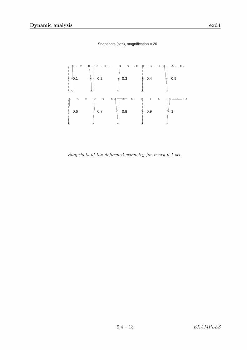
Dynamic analysis exd4
Snapshots (sec), magnification = 20
0.1 0.2 0.3 0.4 0.5
0.6 0.7 0.8 0.9 1
Snapshots of the deformed geometry for every 0.1 sec.
9.4 – 13 EXAMPLES

9.5 Nonlinear analysis
This section illustrates some nonlinear finite element calculations.
Nonlinear analysis
exN1 Second order theory analysis of a frame
exN2 Buckling analysis of a frame
Note: The examples listed above are supplied as .m-files on the CALFEM diskette underthe directory examples. The example files are named according to the table.
9.5 – 1 EXAMPLES

exn1 Nonlinear analysis
Purpose:
Analysis of a plane frame using second order theory.
Description:
The frame of exs5 is analysed again, but it is now subjected to a load case includinga horizontal load and two vertical point loads. Second order theory is used.
H
P P
A B
A1, I1, E4.0 m
6.0 m
A2, I2, E
A1, I1, E
A1 = 45.3e−4 m2
I1 = 2510e−8 m4
A2 = 142.8e−4 m2
I2 = 33090e−8 m4
E = 2.10e5 MPaP = 1 MNH = 0.001 MN
The finite element model consisting of three beam elements and twelve degrees offreedom is repeated here.
1
2
310
11
12
4
5
67
8
9
1 2
3● ●
●●
The following .m-file defines the finite element model.
% ----- Topology -----
Edof=[1 1 2 3 4 5 6;
2 10 11 12 7 8 9;
3 4 5 6 7 8 9];
EXAMPLES 9.5 – 2

Nonlinear analysis exn1
% ----- Element properties and global coordinates -----
E=2.1e11;
A1=45.3e-4; A2=142.8e-4;
I1=2510e-8; I2=33090e-8;
ep1=[E A1 I1]; ep3=[E A2 I2];
Ex=[0 0;6 6;0 6]; Ey=[0 4;0 4;4 4];
% ----- Load vector -----
f=zeros(12,1);
f(4)=1000; f(5)=-1000000; f(8)=-1000000;
The beam element function of the second order theory beam2g requires a normalforce as input variable. In the first iteration this normal force is chosen to zero.This means that the first iteration is equivalent to a linear first order analysis usingbeam2e. Since the normal forces are not known initially, an iterative procedure hasto be applied, where the normal forces N are updated according to the results ofthe former iteration. The iterations continue until the difference in normal force ofthe two last iteration steps is less than an accepted error eps, (N−N0)/N0 < eps.The small value given to the initial normal force N(1) is to avoid division by zeroin the second convergence check. If N does not converge in 20 steps the analysis isinterrupted.
% ----- Initial values for the iteration -----
eps=0.01; % Error norm
N=[0.01 0 0]; % Initial normal forces
N0=[1 1 1]; % Normal forces of the initial former iteration
n=0; % Iteration counter
% ----- Iteration procedure -----
while(abs((N(1)-N0(1))/N0(1)) > eps)
n=n+1;
K=zeros(12,12);
Ke1=beam2g(Ex(1,:),Ey(1,:),ep1,N(1));
Ke2=beam2g(Ex(2,:),Ey(2,:),ep1,N(2));
Ke3=beam2g(Ex(3,:),Ey(3,:),ep3,N(3));
K=assem(Edof(1,:),K,Ke1);
K=assem(Edof(2,:),K,Ke2);
K=assem(Edof(3,:),K,Ke3);
9.5 – 3 EXAMPLES
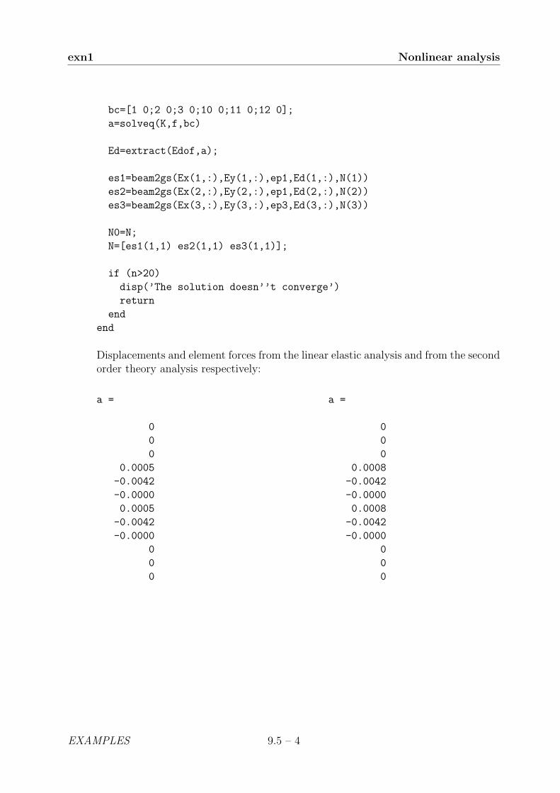
exn1 Nonlinear analysis
bc=[1 0;2 0;3 0;10 0;11 0;12 0];
a=solveq(K,f,bc)
Ed=extract(Edof,a);
es1=beam2gs(Ex(1,:),Ey(1,:),ep1,Ed(1,:),N(1))
es2=beam2gs(Ex(2,:),Ey(2,:),ep1,Ed(2,:),N(2))
es3=beam2gs(Ex(3,:),Ey(3,:),ep3,Ed(3,:),N(3))
N0=N;
N=[es1(1,1) es2(1,1) es3(1,1)];
if (n>20)
disp(’The solution doesn’’t converge’)
return
end
end
Displacements and element forces from the linear elastic analysis and from the secondorder theory analysis respectively:
a = a =
0 0
0 0
0 0
0.0005 0.0008
-0.0042 -0.0042
-0.0000 -0.0000
0.0005 0.0008
-0.0042 -0.0042
-0.0000 -0.0000
0 0
0 0
0 0
EXAMPLES 9.5 – 4

Nonlinear analysis exn1
es1 = es1 =
1.0e+05 * 1.0e+05 *
-9.9967 -0.0050 -0.0102 -9.9954 -0.0050 -0.0142
-9.9967 -0.0050 0.0098 -9.9954 -0.0050 0.0138
es2 = es2 =
1.0e+06 * 1.0e+06 *
-1.0003 -0.0005 -0.0010 -1.0005 -0.0005 -0.0014
-1.0003 -0.0005 0.0010 -1.0005 -0.0005 0.0014
es3 = es3 =
-499.5747 326.9323 981.6016 1.0e+03 *
-499.5747 326.9323 -979.9922
-0.4996 0.4595 1.3793
-0.4996 0.4595 -1.3777
Using the second order theory, the horizontal displacement of the upper left cornerof the frame increases from 0.5 to 0.8 mm. Both moments MA and MB are increasedfrom 1.0 to 1.4 kNm.
9.5 – 5 EXAMPLES

exn2 Nonlinear analysis
Purpose:
Buckling analysis of a plane frame.
Description:
The frame of exn1 is in this example analysed with respect to security against bucklingfor a case when all loads are increased proportionally. The initial load distributionof exn1 is increased by a loading factor alpha until buckling occurs, i.e. the deter-minant of the stiffness matrix K passes zero. For each value of alpha a second ordertheory calculation of type exn1 is performed. The horizontal displacement a4 andthe moment MA are plotted against alpha. The shape of the buckling mode is alsoplotted using the last computed displacement vector before buckling occurs.
The finite element model, i.e. the vectors Edof, ep1, ep3, Ex, and Ey, defined in exn1is used.
% ----- Initial loads -----
f0=zeros(12,1);
f0(4)=1000; f0(5)=-1000000; f0(8)=-1000000;
% ----- Increase loads until det(K)=0 -----
j=0;
for alpha=1:0.1:20
j=j+1;
N=[0.1 0 0];
N0=[1 1 1];
% ----- Iteration for convergence -----
eps=0.00001;
n=0;
while(abs((N(1)-N0(1))/N0(1)) > eps)
n=n+1;
K=zeros(12,12);
f=f0*alpha;
Ke1=beam2g(Ex(1,:),Ey(1,:),ep1,N(1));
Ke2=beam2g(Ex(2,:),Ey(2,:),ep1,N(2));
Ke3=beam2g(Ex(3,:),Ey(3,:),ep3,N(3));
EXAMPLES 9.5 – 6

Nonlinear analysis exn2
K=assem(Edof(1,:),K,Ke1);
K=assem(Edof(2,:),K,Ke2);
K=assem(Edof(3,:),K,Ke3);
bc=[1 0;2 0;3 0;10 0;11 0;12 0];
[a,Q]=solveq(K,f,bc);
Ed=extract(Edof,a);
es1=beam2gs(Ex(1,:),Ey(1,:),ep1,Ed(1,:),N(1));
es2=beam2gs(Ex(2,:),Ey(2,:),ep1,Ed(2,:),N(2));
es3=beam2gs(Ex(3,:),Ey(3,:),ep3,Ed(3,:),N(3));
N0=N;
N=[es1(1,1) es2(1,1) es3(1,1)];
if (n>20)
disp(’The solution doesn’’t converge’)
return
end
end
% ----- Check the determinant for buckling -----
Kred=red(K,bc(:,1));
if (det(Kred) <= 0)
disp(’Determinant <= 0, buckling load passed’)
break
end
disp([’Alpha= ’,num2str(alpha),’ is OK!’,int2str(n), ...
’ iterations are performed.’])
disp(’ ’)
% ----- Save values for plotting of results -----
deform(j)=a(4);
M(j)=Q(3);
loadfact(j)=alpha;
bmode=a;
end
9.5 – 7 EXAMPLES
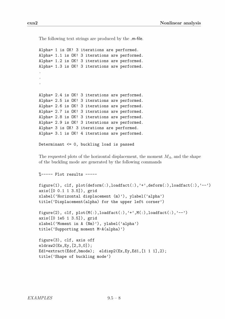
exn2 Nonlinear analysis
The following text strings are produced by the .m-file.
Alpha= 1 is OK! 3 iterations are performed.
Alpha= 1.1 is OK! 3 iterations are performed.
Alpha= 1.2 is OK! 3 iterations are performed.
Alpha= 1.3 is OK! 3 iterations are performed.
.
.
.
Alpha= 2.4 is OK! 3 iterations are performed.
Alpha= 2.5 is OK! 3 iterations are performed.
Alpha= 2.6 is OK! 3 iterations are performed.
Alpha= 2.7 is OK! 3 iterations are performed.
Alpha= 2.8 is OK! 3 iterations are performed.
Alpha= 2.9 is OK! 3 iterations are performed.
Alpha= 3 is OK! 3 iterations are performed.
Alpha= 3.1 is OK! 4 iterations are performed.
Determinant <= 0, buckling load is passed
The requested plots of the horizontal displacement, the moment MA, and the shapeof the buckling mode are generated by the following commands
%----- Plot results -----
figure(1), clf, plot(deform(:),loadfact(:),’+’,deform(:),loadfact(:),’--’)
axis([0 0.1 1 3.5]), grid
xlabel(’Horizontal displacement (m)’), ylabel(’alpha’)
title(’Displacement(alpha) for the upper left corner’)
figure(2), clf, plot(M(:),loadfact(:),’+’,M(:),loadfact(:),’--’)
axis([0 1e5 1 3.5]), grid
xlabel(’Moment in A (Nm)’), ylabel(’alpha’)
title(’Supporting moment M-A(alpha)’)
figure(3), clf, axis off
eldraw2(Ex,Ey,[2,3,0]);
Ed1=extract(Edof,bmode); eldisp2(Ex,Ey,Ed1,[1 1 1],2);
title(’Shape of buckling mode’)
EXAMPLES 9.5 – 8
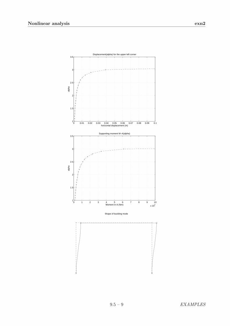
Nonlinear analysis exn2
0 0.01 0.02 0.03 0.04 0.05 0.06 0.07 0.08 0.09 0.11
1.5
2
2.5
3
3.5
horizontal displacement (m)
alph
a
Displacement(alpha) for the upper left corner
0 1 2 3 4 5 6 7 8 9 10
x 104
1
1.5
2
2.5
3
3.5
Moment in A (Nm)
alph
a
Supporting moment M−A(alpha)
Shape of buckling mode
9.5 – 9 EXAMPLES
Index
abs . . . . . . . . . . . . 3 – 6assem . . . . . . . . . 6.2 – 2axis . . . . . . . . . . . 8 – 2bar2e . . . . . . . . . . 5.3 – 2bar2g . . . . . . . . . . 5.3 – 3bar2s . . . . . . . . . . 5.3 – 5bar3e . . . . . . . . . . 5.3 – 6bar3s . . . . . . . . . . 5.3 – 7beam2d . . . . . . . 5.6 – 20beam2ds . . . . . . . 5.6 – 22beam2e . . . . . . . . 5.6 – 2beam2g . . . . . . . . 5.6 – 15beam2gs . . . . . . . 5.6 – 18beam2s . . . . . . . . 5.6 – 5beam2t . . . . . . . . 5.6 – 7beam2ts . . . . . . . 5.6 – 9beam2w . . . . . . . 5.6 – 11beam2ws . . . . . . 5.6 – 13beam3e . . . . . . . . 5.6 – 24beam3s . . . . . . . . 5.6 – 27clear . . . . . . . . . . . 2 – 2clf . . . . . . . . . . . . . 8 – 3coordxtr . . . . . . . 6.2 – 3det . . . . . . . . . . . . 3 – 7diag . . . . . . . . . . . 3 – 8diary . . . . . . . . . . 2 – 3disp . . . . . . . . . . . 2 – 4dmises . . . . . . . . . 4 – 4dyna2 . . . . . . . . . 6.3 – 2dyna2f . . . . . . . . . 6.3 – 3echo . . . . . . . . . . . 2 – 5eigen . . . . . . . . . . 6.2 – 5eldisp2 . . . . . . . . 8 – 5eldraw2 . . . . . . . . 8 – 4eldia2 . . . . . . . . . 8 – 6elflux2 . . . . . . . . . 8 – 8eliso2 . . . . . . . . . . 8 – 9elprinc2 . . . . . . . 8 – 10extract . . . . . . . . 6.2 – 6fft . . . . . . . . . . . . . 6.3 – 4
figure . . . . . . . . . . 8 – 11fill . . . . . . . . . . . . . 8 – 12flw2i4e . . . . . . . . 5.4 – 8flw2i4s . . . . . . . . . 5.4 – 10flw2i8e . . . . . . . . 5.4 – 11flw2i8s . . . . . . . . . 5.4 – 13flw2qe . . . . . . . . . 5.4 – 6flw2qs . . . . . . . . . 5.4 – 7flw2te . . . . . . . . . 5.4 – 3flw2ts . . . . . . . . . 5.4 – 5flw3i8e . . . . . . . . 5.4 – 14flw3i8s . . . . . . . . . 5.4 – 16for . . . . . . . . . . . . . 7 – 3format . . . . . . . . . 2 – 6freqresp . . . . . . . 6.3 – 5full . . . . . . . . . . . . 3 – 9gfunc . . . . . . . . . . 6.3 – 6grid . . . . . . . . . . . 8 – 13help . . . . . . . . . . . 2 – 7hold . . . . . . . . . . . 8 – 14hooke . . . . . . . . . . 4 – 2if . . . . . . . . . . . . . . 7 – 2ifft . . . . . . . . . . . . 6.3 – 7insert . . . . . . . . . . 6.2 – 8inv . . . . . . . . . . . . 3 – 10length . . . . . . . . . 3 – 11load . . . . . . . . . . . 2 – 8max . . . . . . . . . . . 3 – 12min . . . . . . . . . . . 3 – 13mises . . . . . . . . . . 4 – 3ones . . . . . . . . . . . 3 – 14plani4e . . . . . . . . 5.5 – 20plani4f . . . . . . . . 5.5 – 25plani4s . . . . . . . . 5.5 – 23plani8e . . . . . . . . 5.5 – 26plani8f . . . . . . . . 5.5 – 31plani8s . . . . . . . . 5.5 – 29planqe . . . . . . . . . 5.5 – 9planqs . . . . . . . . . 5.5 – 11

Index
planre . . . . . . . . . 5.5 – 12planrs . . . . . . . . . 5.5 – 15plantce . . . . . . . . 5.5 – 16plantcs . . . . . . . . 5.5 – 19plante . . . . . . . . . 5.5 – 4plantf . . . . . . . . . 5.5 – 8plants . . . . . . . . . 5.5 – 7platre . . . . . . . . . 5.7 – 2platrs . . . . . . . . . . 5.7 – 5plot . . . . . . . . . . . 8 – 15print . . . . . . . . . . 8 – 16function . . . . . . . 7 – 5script . . . . . . . . . . 7 – 6quit . . . . . . . . . . . 2 – 9red . . . . . . . . . . . . 3 – 15ritz . . . . . . . . . . . . 6.3 – 8save . . . . . . . . . . . 2 – 10size . . . . . . . . . . . . 3 – 16soli8e . . . . . . . . . . 5.5 – 32soli8f . . . . . . . . . . 5.5 – 37soli8s . . . . . . . . . . 5.5 – 35solveq . . . . . . . . . 6.2 – 9sparse . . . . . . . . . 3 – 17spectra . . . . . . . . 6.3 – 9spring1e . . . . . . . 5.2 – 4spring1s . . . . . . . 5.2 – 5spy . . . . . . . . . . . . 3 – 18sqrt . . . . . . . . . . . 3 – 19statcon . . . . . . . . 6.2 – 10step1 . . . . . . . . . . 6.3 – 10step2 . . . . . . . . . . 6.3 – 12sum . . . . . . . . . . . 3 – 20sweep . . . . . . . . . 6.3 – 14text . . . . . . . . . . . 8 – 17title . . . . . . . . . . . 8 – 18type . . . . . . . . . . . 2 – 11what . . . . . . . . . . 2 – 12while . . . . . . . . . . 7 – 4who . . . . . . . . . . . 2 – 13whos . . . . . . . . . . 2 – 13
xlabel . . . . . . . . . 8 – 19ylabel . . . . . . . . . 8 – 19zeros . . . . . . . . . . 3 – 21zlabel . . . . . . . . . . 8 – 19