calibrating nacelle lidars - dtu orbitorbit.dtu.dk/files/57802786/calibrating_nacelle_lidars.pdf ·...
TRANSCRIPT

General rights Copyright and moral rights for the publications made accessible in the public portal are retained by the authors and/or other copyright owners and it is a condition of accessing publications that users recognise and abide by the legal requirements associated with these rights.
• Users may download and print one copy of any publication from the public portal for the purpose of private study or research. • You may not further distribute the material or use it for any profit-making activity or commercial gain • You may freely distribute the URL identifying the publication in the public portal
If you believe that this document breaches copyright please contact us providing details, and we will remove access to the work immediately and investigate your claim.
Downloaded from orbit.dtu.dk on: Sep 11, 2018
Calibrating nacelle lidars
Courtney, Michael
Publication date:2013
Document VersionPublisher's PDF, also known as Version of record
Link back to DTU Orbit
Citation (APA):Courtney, M. (2013). Calibrating nacelle lidars. DTU Wind Energy. (DTU Wind Energy E; No. 0020).
DTU – Wind Energy
Risø Campus
Roskilde, Denmark
January 2013
Calibrating nacelle lidars
DTU Wind Energy E-0020
Michael Courtney

2 DTU Wind Energy E-0020
Author: Michael Courtney
Title: Calibrating nacelle lidars
Institute: DTU Wind Energy
DTU Wind Energy E-0020
January 2013
Abstract:
Nacelle mounted, forward looking wind lidars are beginning to be used to provide reference wind speed measurements for the power performance testing of wind
turbines. In such applications, a formal calibration procedure with a corresponding
uncertainty assessment will be necessary. This report presents four concepts for performing such a nacelle lidar calibration. Of the four methods, two are found to
be immediately relevant and are pursued in some detail.
The first of these is a line of sight calibration method in which both lines of sight
(for a two beam lidar) are individually calibrated by accurately aligning the beam
to pass close to a reference wind speed sensor. A testing procedure is presented, reporting requirements outlined and the uncertainty of the method analysed. It is
seen that the main limitation of the line of sight calibration method is the time
required to obtain a representative distribution of radial wind speeds.
An alternative method is to place the nacelle lidar on the ground and incline the
beams upwards to bisect a mast equipped with reference instrumentation at a known height and range. This method will be easier and faster to implement and
execute but the beam inclination introduces extra uncertainties. A procedure for
conducting such a calibration is presented and initial indications of the uncertainties given.
A discussion of the merits and weaknesses of the two methods is given together with some proposals for the next important steps to be taken in this work
Project Number:
EUDP: Nacelle lidar for power performance measurement (journal no.
64009-0273)
Pages: 43
ISBN: 978-87-92896-29-2
Technical University of Denmark
Department of Wind Energy
Brovej Building 118
DK-2800 Kgs. Lyngby
Denmark
www.vindenergi.dtu.dk

3 DTU Wind Energy E-0020
Preface
This report concerns methods for calibrating lidars intended for service as nacelle-mounted sensors
used in power curve measurements. It has been performed as part of the EUDP Nacelle-Lidar project
which aims at developing and commercialising a procedure for using nacelle-mounted lidars to
perform wind speed measurements in power performance measurements as direct replacements to
traditional met mast instrumentation. By developing a procedure that avoids the need for mast
mounted instruments, the met mast itself is eradicated. The cost savings are significant especially
offshore, allowing power curve measurements to be made where before the costs would have been
prohibitive.
Whilst the main body of the project has been concerned with the application of the nacelle-lidar to the
actual power curve procedure, it became apparent that a traceable calibration of the lidar as the
reference sensor was mandatory. In this report, various techniques are examined. Two are found to be
applicable and might find commercial application.
Following on from this work, it is envisaged that one or two of the applicable methods will become
standardised. It is hoped that the work reported here will form a central part of this standardisation,
albeit in a more formal and less exploratory format.

4 DTU Wind Energy E-0020
Contents
1. Introduction ......................................................................................................... 6
2. Tilt and roll calibration procedure ....................................................................... 7 2.1 Why the tilt and roll calibration is necessary ................................................ 7 2.2 Tilt and roll calibration concept .................................................................... 7 2.3 Geometrical development ............................................................................. 8 2.4 Procedure ...................................................................................................... 9 2.5 Reporting .................................................................................................... 11
2.5.1 Measurements ...................................................................................... 11 2.5.2 Derived results ..................................................................................... 12
2.6 Uncertainties ............................................................................................... 12
3. Ideal nacelle-lidar calibration method ............................................................... 14 3.1 Concept ....................................................................................................... 14 3.2 Why this is so difficult to achieve? ............................................................. 14
4. Line-of-sight calibration procedure ................................................................... 14 4.1 Concept ....................................................................................................... 14 4.2 Theoretical development – what to compare with what ............................. 15 4.3 Procedure .................................................................................................... 17
4.3.1 Requirements for infrastructure ........................................................... 17 4.3.2 Making the measurements .................................................................... 20
4.4 Data analysis ............................................................................................... 21 4.4.1 Determining the approximate line-of-sight direction ........................... 21 4.4.2 Filtering the data................................................................................... 22 4.4.3 Requirements on data distribution ........................................................ 23 4.4.4 Finding the precise line of sight direction ............................................ 23 4.4.5 Calibrating the radial wind speed ......................................................... 25 4.4.6 Calibration results combined to a horizontal wind speed calibration ... 26 4.4.7 Finding the sensed range ...................................................................... 27
4.5 Uncertainties ............................................................................................... 27 4.5.1 Line of sight reference wind speed uncertainties ................................. 27 4.5.2 Combined Radial Wind Speed Uncertainties ....................................... 29 4.5.3 Statistical uncertainties from the calibration results ............................. 30 4.5.4 Total uncertainty for one line-of-sight ................................................. 30 4.5.5 Combining to horizontal wind speed uncertainties .............................. 30
4.6 Reporting .................................................................................................... 31 4.6.1 Experimental setup ............................................................................... 31 4.6.2 Beam 0 alignment................................................................................. 32 4.6.3 Beam calibration measurements ........................................................... 32 4.6.4 Beam 1 alignment................................................................................. 32 4.6.5 Removal of lidar from platform (end of beam 1 measurements) ......... 32 4.6.6 Results for each individual beam ......................................................... 32 4.6.7 Results combined to horizontal wind speed ......................................... 34
5. Testing horizontally in a mast ........................................................................... 35 5.1 Concept ....................................................................................................... 35 5.2 Procedure .................................................................................................... 35 5.3 Data analysis ............................................................................................... 36 5.4 Uncertainties ............................................................................................... 37

5 DTU Wind Energy E-0020
6. Testing from the ground with an inclined beam ................................................ 37 6.1 Concept ....................................................................................................... 37 6.2 Procedure .................................................................................................... 38 6.3 Data analysis ............................................................................................... 39 6.4 Uncertainties ............................................................................................... 39
7. Discussion ......................................................................................................... 40 7.1 Comparison of methods .............................................................................. 40 7.2 Further work required ................................................................................. 41
7.2.1 Line of sight method ............................................................................ 41 7.2.2 Tilted beam, ground based method ...................................................... 42
8. Conclusion ......................................................................................................... 42
Acknowledgements ........................................................................................................ 43
References ...................................................................................................................... 43
6 DTU Wind Energy E-0020
1. Introduction It has long been an ambition to use a wind turbine itself as a platform for wind sensors for power and
load measurements, avoiding the need for an upstream measurement mast. Nacelle mounted cup
anemometers have been thoroughly investigated and methods developed that enable cup anemometers
mounted behind the rotor to give an indication of the free-stream wind speed. Such methods require
calibration from one wind turbine type to another and are associated with a rather large uncertainty.
With a nacelle-mounted, forward looking wind lidar, the influence of the wind turbine is no longer an
issue since the lidar can sense the wind as far ahead of the wind turbine as we desire.
Nacelle mounted pulsed lidars have already been demonstrated as being suitable for use in power
curve measurements Error! Reference source not found.. Although the scatter in the power curve
was reduced in comparison to a simultaneous power curve based on a traditional mast-mounted cup
anemometer, the experiment identified a discrepancy between the cup anemometer and lidar wind
speeds that was not immediately easy to resolve. This highlighted the need for a traceable calibration
procedure for the nacelle lidar that could form the basis of an uncertainty budget. It is such a
calibration procedure that is the ultimate goal of this report. Our aim is to achieve accuracy as
comparable as possible to the cup anemometer that is being replaced bearing in mind that since a cup
anemometer (or equivalent) is the reference instrument in the lidar calibration we can never achieve a
better uncertainty than this.
Clearly wind speed is the fundamental parameter for the calibration but it is not sufficient to calibrate
wind speed alone. As we are measuring remotely it is also important to determine the accuracy of the
sensing range since, due to the blockage in front of the rotor, an error here (measuring at the wrong
distance in front of the rotor) will convert to a wind speed error. Thus a calibration procedure should
include some check of the sensing range accuracy. Here we need to be sure to within some tens of
meters that we are sensing in the correct location.
In a closer examination of how well a nacelle-lidar based power curve measurement can comply with
the requirements of the IEC 61400-12-1 standard Error! Reference source not found., it was shown
that the tilting (and rolling) of the lidar beam arising from tower deformations of the loaded wind
turbine must be monitored in order to establish whether the wind speed height accuracy requirement of
the standard (±2.5% of hub height) remains satisfied. To maintain this requirement at a distance in
front of the wind turbine of 2.5D, the tilt angle should not exceed about ± 0.6˚ for a typical turbine
geometry. In order to achieve this, nacelle lidar should incorporate an accurate inclinometer both to
facilitate accurate installation and to monitor the tilt and roll lidar of the lidar beams in service. Given
the small angular range, a high and documented accuracy is required (say ±0.1˚). This can not be
achieved without a calibration of the tilt and roll sensor.
The technique for calibrating ground-based wind lidars is very obvious - put them on the ground next
to a mast mounted with reference instruments and compare the reported wind speeds. For a nacelle-
based lidar the calibration method most closely matching the manner of service operation would be to
mount the nacelle lidar at a height corresponding to wind turbine hub-height and shoot the beams
towards an equally high mast situated at a distance of 200-300m (a typical value for 2.5D). This is
difficult and very expensive to achieve especially since the stiffness of the lidar mounting is important
to avoid uncertainties in the calibration due to beam tilting.
Instead we have investigated three techniques that each deviate in some way from this ideal. Firstly we
examine a method based on placing the lidar on a stiff, low platform and shooting the beams towards a
distant mast. Since horizontal homogeneity is impossible to achieve at low heights, this method
performs a line-of-sight calibration instead where the individual lidar radial speeds are compared to

7 DTU Wind Energy E-0020
reference speeds measured by a sonic anemometer. As we will see, this method is accurate but rather
time consuming, labour intensive and therefore expensive.
A simpler technique involving only one mast is to mount the lidar in a mast, shooting outwards and
compare the lidar reported wind speeds at the smallest possible range to reference measurements made
on the mast itself. With this method we are no longer making a calibration of the lidar at a range close
to that which will be used in the power curve test.
If we drop the principle of keeping the lidar beam horizontal we can permit testing of the lidar from a
ground mounting with a beam inclined upwards to intersect a cup anemometer at a known height at the
correct measuring range. This is the third method to be presented.
In the following chapters we present the techniques for the ground calibration and for each of the three
speed calibration techniques. We then compare and contrast the various methods and conclude by
recommending which methods to proceed with as the basis for the nacelle lidar power curve method.
2. Tilt and roll calibration procedure
2.1 Why the tilt and roll calibration is necessary
Here we describe the tilt and roll calibration procedure. This has two purposes. Firstly as we explored
in the previous section, the measurement accuracy of a nacelle lidar is dependent on accurate
measurement of the tilting and rolling of the lidar beams since these deformations will alter the
effective sensing height of the instrument. Accurate calibration of the tilt and roll sensors is required
regardless of the speed calibration procedure chosen. For the line-of-sight calibration procedure, the
accuracy of the resulting horizontal wind speed depends also on the accuracy of the beam opening
angles and these also have to be measured as part of the tilt and roll calibration procedure. In practice,
the opening angle measurement is only a further geometrical manipulation of the distance
measurements already taken in the tilt and roll calibration.
2.2 Tilt and roll calibration concept
The aim is to precisely determine the position of the two lidar beams in relation to the origin of the
beams at the lidar telescope. The beam position is identified by an iterative process of blocking and
un-blocking of the beam as identified from the reported signal strength (CNR). The end result of this
process is a wooden target with a small hole through which the beam is known to pass. With the help
of a theodolite the height of the beam positions is determined relative to a horizontal plane passing
through the telescope origin and the distances from the telescope are measured with a laser distance
meter. By repeating this process with the Wind Iris displaced slightly in tilt and roll (a total of between
4 and 6 different positions) both the gain and the offset of the tilt and roll sensors can be determined.
8 DTU Wind Energy E-0020
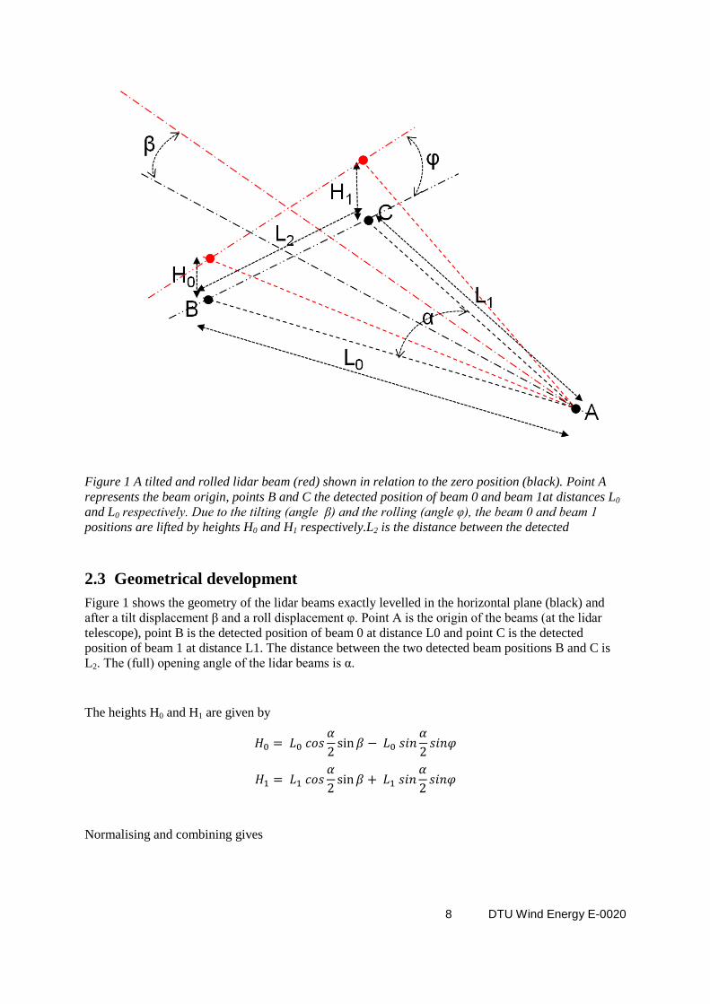
Figure 1 A tilted and rolled lidar beam (red) shown in relation to the zero position (black). Point A
represents the beam origin, points B and C the detected position of beam 0 and beam 1at distances L0
and L0 respectively. Due to the tilting (angle β) and the rolling (angle φ), the beam 0 and beam 1
positions are lifted by heights H0 and H1 respectively.L2 is the distance between the detected
2.3 Geometrical development
Figure 1 shows the geometry of the lidar beams exactly levelled in the horizontal plane (black) and
after a tilt displacement β and a roll displacement φ. Point A is the origin of the beams (at the lidar
telescope), point B is the detected position of beam 0 at distance L0 and point C is the detected
position of beam 1 at distance L1. The distance between the two detected beam positions B and C is
L2. The (full) opening angle of the lidar beams is α.
The heights H0 and H1 are given by
Normalising and combining gives
9 DTU Wind Energy E-0020
( )
and
( )
From the cosine rule of triangles, the opening angle α is given by
(
)
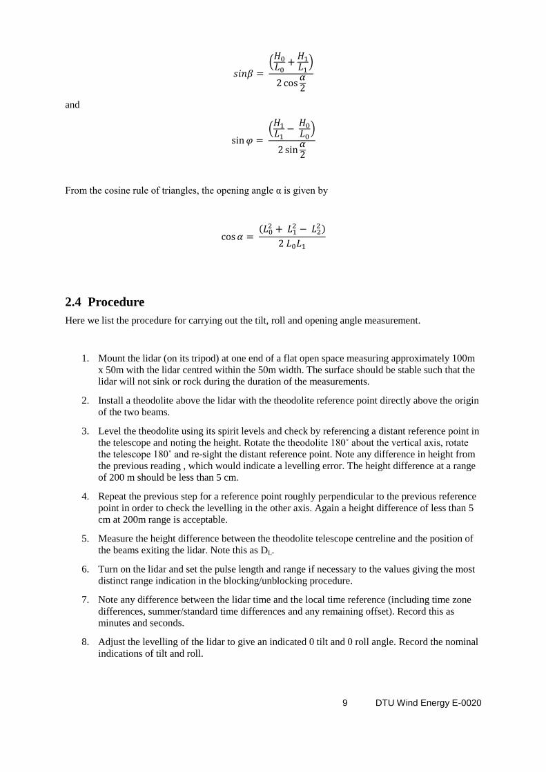
2.4 Procedure
Here we list the procedure for carrying out the tilt, roll and opening angle measurement.
1. Mount the lidar (on its tripod) at one end of a flat open space measuring approximately 100m
x 50m with the lidar centred within the 50m width. The surface should be stable such that the
lidar will not sink or rock during the duration of the measurements.
2. Install a theodolite above the lidar with the theodolite reference point directly above the origin
of the two beams.
3. Level the theodolite using its spirit levels and check by referencing a distant reference point in
the telescope and noting the height. Rotate the theodolite 180˚ about the vertical axis, rotate
the telescope 180˚ and re-sight the distant reference point. Note any difference in height from
the previous reading , which would indicate a levelling error. The height difference at a range
of 200 m should be less than 5 cm.
4. Repeat the previous step for a reference point roughly perpendicular to the previous reference
point in order to check the levelling in the other axis. Again a height difference of less than 5
cm at 200m range is acceptable.
5. Measure the height difference between the theodolite telescope centreline and the position of
the beams exiting the lidar. Note this as DL.
6. Turn on the lidar and set the pulse length and range if necessary to the values giving the most
distinct range indication in the blocking/unblocking procedure.
7. Note any difference between the lidar time and the local time reference (including time zone
differences, summer/standard time differences and any remaining offset). Record this as
minutes and seconds.
8. Adjust the levelling of the lidar to give an indicated 0 tilt and 0 roll angle. Record the nominal
indications of tilt and roll.

10 DTU Wind Energy E-0020
9. At a distance of about 80m detect the approximate position of each of the two beams. For
example walking across the path of the beam will block the beam and this will be detected as a
sudden drop in CNR for the 150m range.
10. Install a wooden frame at each of these two positions such that the beam is contained within
the frame.
11. For the left wooden frame, using the same blocking/unblocking technique, determine the
vertical position of the beam and fix two slats horizontally across the frame such that the beam
is contained in a 2-3 cm gap between the slats.
12. Repeat the previous step for the horizontal direction, again fixing two vertical slats to localize
the horizontal beam position within a 2-3 cm gap. There is now a 2-3 cm square aperture
through which the beam passes.
13. Repeat the last 2 steps for the right beam. Both beam positions are now identified and
measurement can begin.
14. Note the measurement start time according to the local time reference
(hours:minutes:seconds).
15. Re-check the lidar to theodolite height offset (DL) and record.
16. Aim the telescope towards the left beam position (corresponding to point B in Figure 1)
without sinking the telescope (i.e. keeping the telescope horizontal).
17. Hold a measuring stick vertically at the beam position with one end at the centre of the beam
aperture and by sighting through the telescope, determine the vertical distance between the
theodolite horizontal plane and the beam aperture. Positive is defined as the theodolite
horizontal plane (telescope centre) above the aperture, negative as below. Note this quantity as
D0.
18. Repeat the previous two steps for the right beam position (corresponding to point C in Figure
1). Note the height difference (same sign convention) as D1.
19. Using a laser distance meter or tape measure, determine the distances lidar (beam origin) to
left beam position (L0), lidar to right beam position (L1) and left to right beam position (L2) in
accordance with Figure 1. Record these quantities.
20. Record the measurement end time according to the local time reference
(hours:minutes:seconds).
21. Change the levelling of the lidar by an increment of about 0.2˚ in tilt and roll. Record the
nominal values.
22. The beam positions at B and C will now be different. Return to step 11 and repeat the
procedure (steps 11-20) for the new values of tilt and roll.
23. Repeat steps 11-20 with other settings of tilt and roll (within the range ±1˚) until there are 4
different values for tilt and four different values for roll.
24. Re-level the lidar to 0˚ tilt, 0˚ roll and execute steps 11-20 for a final time.
25. Re-check the theodolite levelling in steps 3 and 4. Note the results.
26. Remove the theodolite carefully without disturbing the lidar.
27. If necessary, mount and align rifle sight devices needed for subsequent Line-of-Sight or
Tilted-beam calibration procedures.
11 DTU Wind Energy E-0020
2.5 Reporting
2.5.1 Measurements
The following quantities should be recorded and reported in accordance with the procedure:
Lidar type
Serial number
Date
Location
Theodolite identification
Distance measuring equipment
Personnel
Comments (adverse weather conditions, technical issues etc.)
Lidar pulse setting [ns]
Lidar range used for beam identification [m]
Lidar indicated time [hh:mm:ss] Simultaneous local reference time [hh:mm:ss]
Theodolite reference point in lidar axis direction [description]
Distance from lidar [m]
Height with telescope in measuring position [m.xx]
Height with telescope reversed and rotated 180˚ [m.xx]
Theodolite reference point perpendicular to lidar axis direction [description]
Distance from lidar [m]
Height with telescope in measuring position [m.xx]
Height with telescope reversed and rotated 180˚ [m.xx]
For each combination of tilt and roll record:
Start time [hh:mm:ss]
Indicated pitch [degrees.xx]
Indicated roll [degrees.xx]
DL = Height of theodolite above lidar beams (+ve above) [m.xxx]
D0 = Height of theodolite horizontal plane above left beam aperture [m.xxx]
D1 = Height of theodolite horizontal plane above left beam aperture [m.xxx]
L0 =Distance from lidar to left beam position (length AB) [m.xxx]
L1=Distance from lidar to right beam position (length AC) [m.xxx]
L2=Distance from left beam position to right beam position (length BC) [m.xxx]
Stop time [hh:mm:ss]
12 DTU Wind Energy E-0020
2.5.2 Derived results
For each combination of tilt and roll record:
Start time
Stop time
Indicated pitch
Average and standard deviation of indicated pitch (from recorded lidar data)
Indicated roll
Average and standard deviation of indicated roll (from recorded lidar data)
H0 = DL-D0
H1 = DL-D1
(
)
α (full opening angle)
( )
β (measured pitch angle)
( )
φ (measured roll angle)
For the sets of completed tilt and roll measurements:
Plot average indicated roll ( ) as a function of measured roll ( ) and perform a linear regression.
Report the results in the form:
Plot average indicated pitch ( ) as a function of measured pitch ( ) and perform a linear regression.
Report the results in the form:
2.6 Uncertainties
The main sources of uncertainty in the tilt and roll measurements will be
The zero offset of the theodolite, and for the roll and tilt directions respectively

13 DTU Wind Energy E-0020
The height determination of the position of the beam at each beam location . The
uncertainties at the two beam positions can be considered equal but uncorrelated.
The length measurements . Again each length measurement can be considered equally
uncertain but uncorrelated to each other. For the tilt and roll measurements we can intuitively
see that the length uncertainties play a minor roll and will be ignored in the analysis.
The roll uncertainty will be given by the geometrical sum of the height uncertainties at A and B
multiplied by their respective partial derivatives and the theodolite offset uncertainty. Putting , this gives
√( (
( ))
)
Similarly the pitch uncertainty will be
√( (
( ))
)
Typical numerical values could be
giving
and
14 DTU Wind Energy E-0020
3. Ideal nacelle-lidar calibration method
3.1 Concept
The most obvious method for calibrating a nacelle-lidar would be to mount it on a sufficiently high,
very stiff tower and point its centreline towards a second tower or mast equipped with reference wind
speed measurements. The angle formed by the two beams would be bisected by the line between the
masts and the beams would be sampling wind at equal distances on either side of the masts. The lidar
wind speed would be compared to the wind speed measured by a reference, top-mounted cup
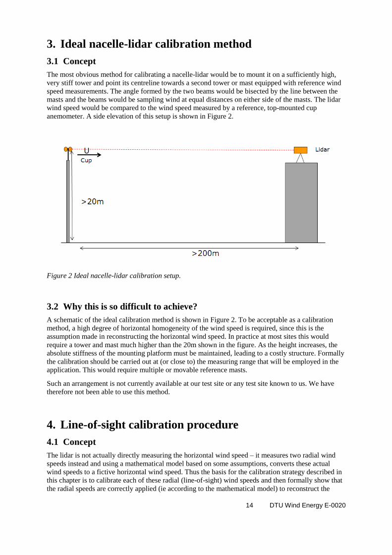
anemometer. A side elevation of this setup is shown in Figure 2.
Figure 2 Ideal nacelle-lidar calibration setup.
3.2 Why this is so difficult to achieve?
A schematic of the ideal calibration method is shown in Figure 2. To be acceptable as a calibration
method, a high degree of horizontal homogeneity of the wind speed is required, since this is the
assumption made in reconstructing the horizontal wind speed. In practice at most sites this would
require a tower and mast much higher than the 20m shown in the figure. As the height increases, the
absolute stiffness of the mounting platform must be maintained, leading to a costly structure. Formally
the calibration should be carried out at (or close to) the measuring range that will be employed in the
application. This would require multiple or movable reference masts.
Such an arrangement is not currently available at our test site or any test site known to us. We have
therefore not been able to use this method.
4. Line-of-sight calibration procedure
4.1 Concept
The lidar is not actually directly measuring the horizontal wind speed – it measures two radial wind
speeds instead and using a mathematical model based on some assumptions, converts these actual
wind speeds to a fictive horizontal wind speed. Thus the basis for the calibration strategy described in
this chapter is to calibrate each of these radial (line-of-sight) wind speeds and then formally show that
the radial speeds are correctly applied (ie according to the mathematical model) to reconstruct the
15 DTU Wind Energy E-0020
fictive horizontal speed. Since this reconstruction is based on the opening angle of the lidar beams, we
must also verify this. Having successfully completed these steps we have shown that the lidar
performs as it is intended and equally important, we are able to assign an uncertainty, relating the
measurement to international standards.
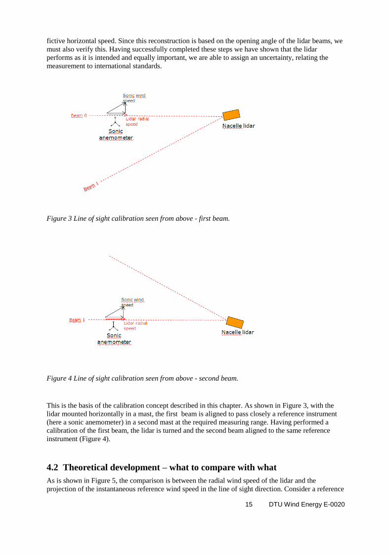
Figure 3 Line of sight calibration seen from above - first beam.
Figure 4 Line of sight calibration seen from above - second beam.
This is the basis of the calibration concept described in this chapter. As shown in Figure 3, with the
lidar mounted horizontally in a mast, the first beam is aligned to pass closely a reference instrument
(here a sonic anemometer) in a second mast at the required measuring range. Having performed a
calibration of the first beam, the lidar is turned and the second beam aligned to the same reference
instrument (Figure 4).
4.2 Theoretical development – what to compare with what
As is shown in Figure 5, the comparison is between the radial wind speed of the lidar and the
projection of the instantaneous reference wind speed in the line of sight direction. Consider a reference
16 DTU Wind Energy E-0020
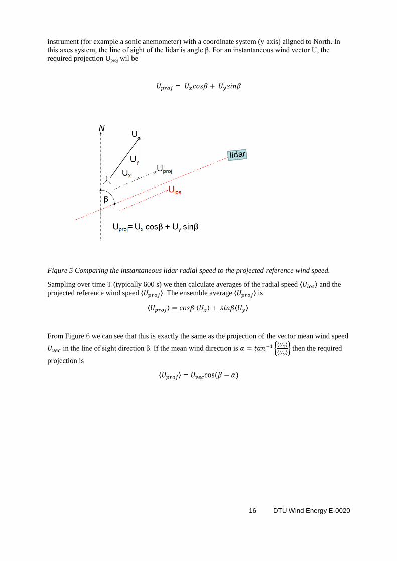
instrument (for example a sonic anemometer) with a coordinate system (y axis) aligned to North. In
this axes system, the line of sight of the lidar is angle β. For an instantaneous wind vector U, the
required projection Uproj wil be
Figure 5 Comparing the instantaneous lidar radial speed to the projected reference wind speed.
Sampling over time T (typically 600 s) we then calculate averages of the radial speed ⟨ ⟩ and the
projected reference wind speed ⟨ ⟩. The ensemble average ⟨ ⟩ is
⟨ ⟩ ⟨ ⟩ ⟨ ⟩
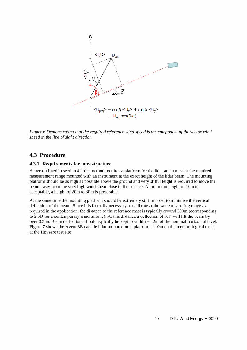
From Figure 6 we can see that this is exactly the same as the projection of the vector mean wind speed
in the line of sight direction β. If the mean wind direction is {⟨ ⟩
⟨ ⟩} then the required
projection is
⟨ ⟩ ( )
17 DTU Wind Energy E-0020
Figure 6 Demonstrating that the required reference wind speed is the component of the vector wind
speed in the line of sight direction.
4.3 Procedure
4.3.1 Requirements for infrastructure
As we outlined in section 4.1 the method requires a platform for the lidar and a mast at the required
measurement range mounted with an instrument at the exact height of the lidar beam. The mounting
platform should be as high as possible above the ground and very stiff. Height is required to move the
beam away from the very high wind shear close to the surface. A minimum height of 10m is
acceptable, a height of 20m to 30m is preferable.
At the same time the mounting platform should be extremely stiff in order to minimise the vertical
deflection of the beam. Since it is formally necessary to calibrate at the same measuring range as
required in the application, the distance to the reference mast is typically around 300m (corresponding
to 2.5D for a contemporary wind turbine). At this distance a deflection of 0.1˚ will lift the beam by
over 0.5 m. Beam deflections should typically be kept to within ±0.2m of the nominal horizontal level.
Figure 7 shows the Avent 3B nacelle lidar mounted on a platform at 10m on the meteorological mast
at the Høvsøre test site.

18 DTU Wind Energy E-0020
Figure 7 The Avent 3B nacelle lidar mounted on a platform 10 m above the ground at the DTU test
site.
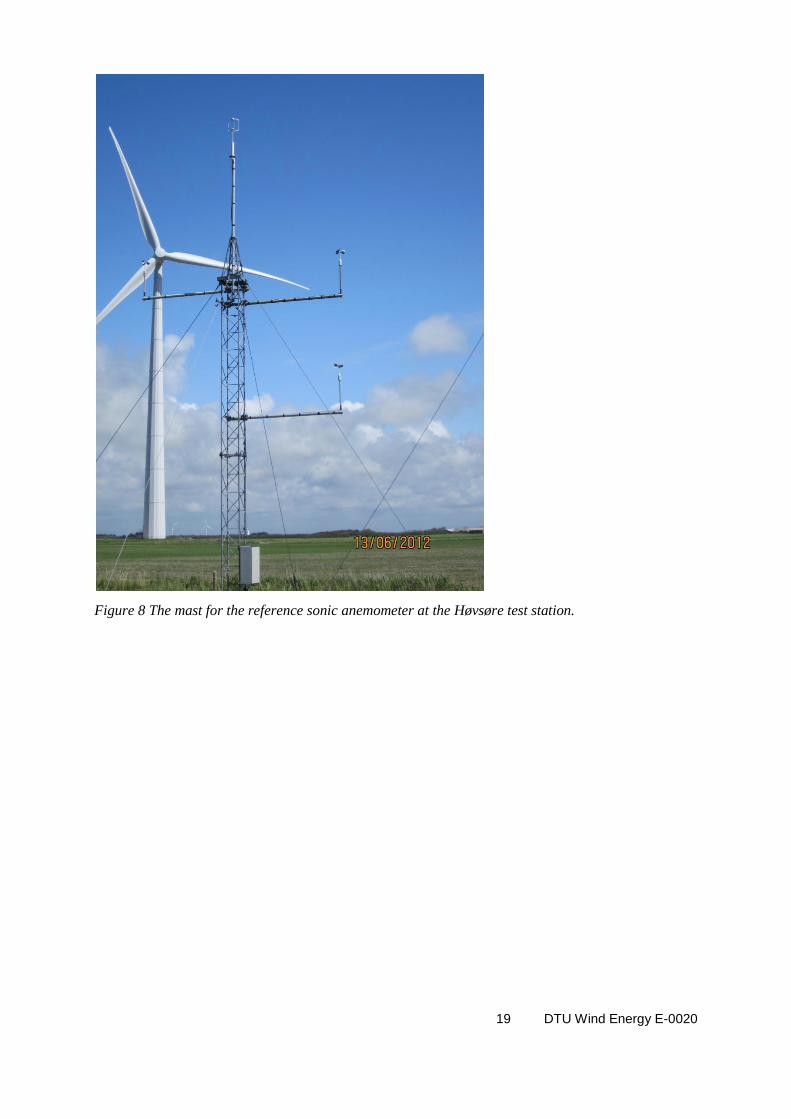
The mast for the reference instrument should lift the top-mounted reference sensor to the exact height
of the lidar beam. If there are small differences in ground level between the platform and reference
mast, it is important to ensure that the beam passes exactly past the reference sensor, not that the
height above the ground is exactly the same. Since we require both wind speed and wind direction, an
ideal instrument is a good sonic anemometer.
If this choice is unacceptable a combination of a cup anemometer and a wind vane could be used. The
difficulty here is that both instruments must be mounted so that flow distortion is negligible. A
distorted wind direction measurement is just as unacceptable as a flow distorted speed measurement
since both will result in an erroneous projected wind speed. One solution is to mount each sensor on a
separate mast separated by about 5m. The masts should be arranged with their axis perpendicular to
the line of sight direction. A calibration exercise should be carried using for example a sonic
anemometer in place of the cup in order to document that the direction measured at both locations is
truly identical.
A traceable wind tunnel calibration of the wind sensor is required.
In addition to the top mounted reference sensor it is advised that the mast is equipped with an
additional boom mounted sensor , 2-3 m under the top sensor. The purpose of this instrument is both
as a plausibility check for the top mounted sensor and also more importantly, to provide an estimate of
the wind shear. Other instrumentation such as temperature and precipitation is also recommended. For
testing in winter (with the possibility of rimed instruments), a temperature sensor is mandatory.
19 DTU Wind Energy E-0020
Figure 8 The mast for the reference sonic anemometer at the Høvsøre test station.

20 DTU Wind Energy E-0020
4.3.2 Making the measurements
Perform a tilt and roll calibration as described in section 2.4. In the final zero tilt and roll test
mount and align two rifle sights with the beam position indicators.
Mount the lidar on the platform carefully avoiding disturbing the rifle sight alignments.
Using the rifle sight for the first beam, turn the lidar and adjust its position until the sight is
approximately aligned to the reference sensor on the reference mast.
Turn on the lidar and set the range to the distance to the reference mast.
Using a sliding wooden ruler mounted in a support frame as shown in , detect the beam
position by observing when the lidar beam is blocked and unblocked for different lengths and
different angles of the ruler. Beam blockage is detected from large increases in the signal to
noise ratio (CNR). Note the ruler angle and length so that the exact beam position can be
calculated.
If necessary, make fine adjustments of the lidar position to give a beam position within ±5 cm
of the centre height of the sonic anemometer.
Figure 9 The sliding wooden ruler in a support frame used to detect the beam position relative to the
sonic anemometer.
21 DTU Wind Energy E-0020
Complete the lidar configuration by including ranges at the minimum and maximum ranges
and a number of 10 m spaced ranges centered around the nominal range (to be used to
determine the actual sensing range). Remember that the ranges set in the lidar configuration
will be along the centerline (i.e. planes perpendicular to the axis), not along a line of sight.
Multiply the los distance by the cosine of the half-opening angle to get the correct centerline
range.
Ensure that the lidar time is correctly set and that it is able regularly to re-synchronise using a
GPS or internet time reference.
Ensure that the reference mast logger is correctly configured. In particular ensure that any
calibration constants are entered correctly and that the logger time is both correct and is able
regularly to re-synchronise, preferably using the same reference source as the lidar.
Measurements can now commence for the first beam.
During the measurements regularly monitor the lidar and logger paying particular attention to
lidar and reference instrument signal plausibility and to the lidar and logger time
synchronization. Regular and automatic upload of data is recommended
When an adequate distribution (discussed below) of line of sight wind speeds has been
acquired, the lidar can be re-positioned (turned) to align the second beam with the reference
instrument.
BEFORE moving the lidar, re-check the beam position relative to the reference instrument
using the sliding ruler. Note the results.
Turn the lidar to align the second beam with the reference instrument. Use the rifle sight to
achieve a rough alignment and fine-adjust using the sliding ruler. Note the beam position
indicated by the angle and length of the sliding ruler.
Measurements can now commence on the second beam.
When an adequate distribution of line of sight speeds has also been acquired for the second
beam, the measurements are finished.
BEFORE removing the lidar, re-check the beam position relative to the reference instrument
using the sliding ruler. Note the results.
4.4 Data analysis
Performing a line-of-sight calibration is not as straight forward as a conventional instrument
comparison since we must actually compare the projection along the line-of-sight of the wind speed
measured by the sonic anemometer to the lidar’s radial speed. This requires us to know or determine
the line-of-sight direction. Secondly we produce scatter plots of the ten minute mean of the radial wind
speed plotted against the ten minute vector mean wind speed of the sonic anemometer projected along
the line of sight. This provides us with the actual calibration. A final step is to check that the lidar
senses at the correct range. We do this by performing correlations of the fast Wind Iris data (0.5Hz)
with a projected sonic wind speed for a number of adjacent Wind Iris ranges – the range with the
highest correlation being identified as that sensing physically closest to the sonic anemometer. We will
elaborate on each of these three steps in the following sections.
4.4.1 Determining the approximate line-of-sight direction Although this direction is given geometrically by the position of the two masts (assuming a perfect
alignment), our approach has been to determine this direction from the data since exact alignment of
22 DTU Wind Energy E-0020
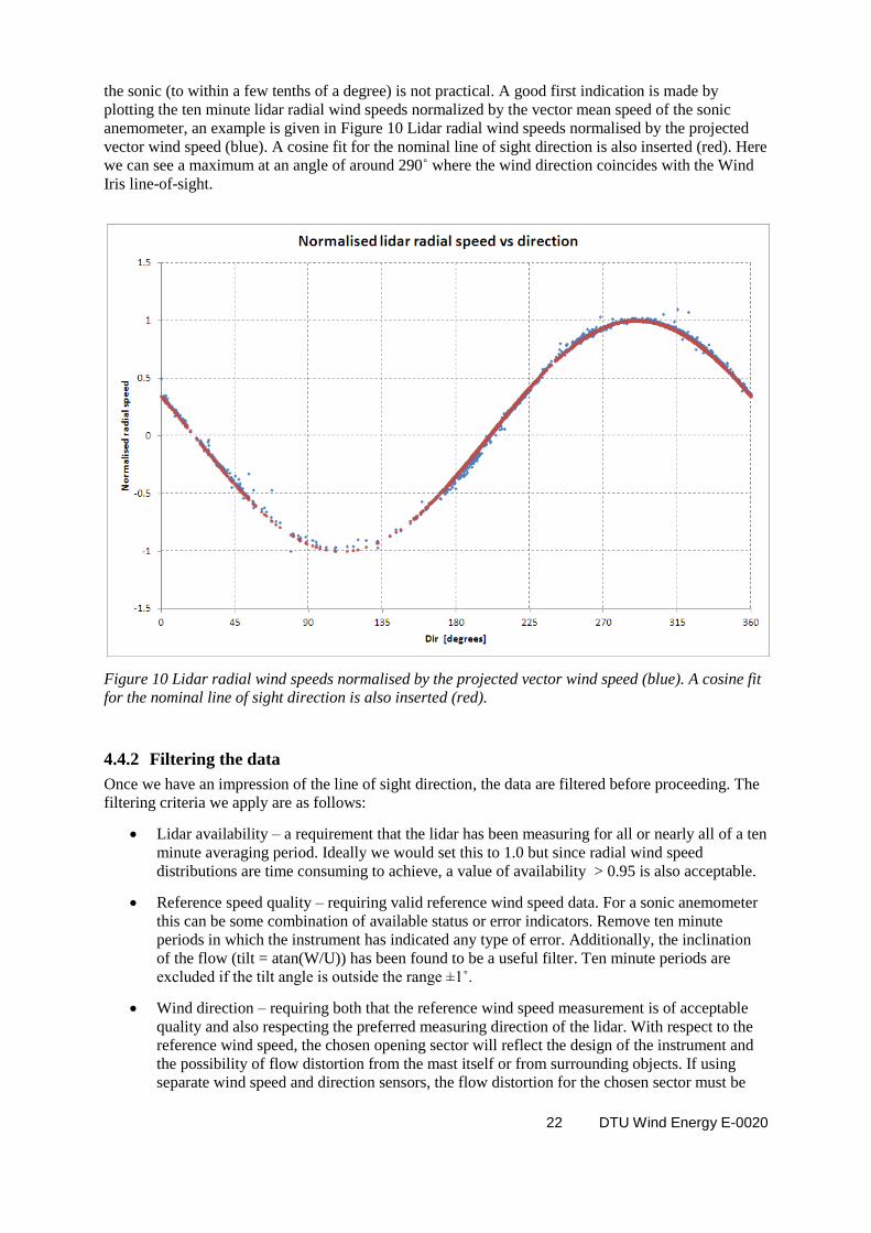
the sonic (to within a few tenths of a degree) is not practical. A good first indication is made by
plotting the ten minute lidar radial wind speeds normalized by the vector mean speed of the sonic
anemometer, an example is given in Figure 10 Lidar radial wind speeds normalised by the projected
vector wind speed (blue). A cosine fit for the nominal line of sight direction is also inserted (red). Here
we can see a maximum at an angle of around 290˚ where the wind direction coincides with the Wind
Iris line-of-sight.
Figure 10 Lidar radial wind speeds normalised by the projected vector wind speed (blue). A cosine fit
for the nominal line of sight direction is also inserted (red).
4.4.2 Filtering the data
Once we have an impression of the line of sight direction, the data are filtered before proceeding. The
filtering criteria we apply are as follows:
Lidar availability – a requirement that the lidar has been measuring for all or nearly all of a ten
minute averaging period. Ideally we would set this to 1.0 but since radial wind speed
distributions are time consuming to achieve, a value of availability > 0.95 is also acceptable.
Reference speed quality – requiring valid reference wind speed data. For a sonic anemometer
this can be some combination of available status or error indicators. Remove ten minute
periods in which the instrument has indicated any type of error. Additionally, the inclination
of the flow (tilt = atan(W/U)) has been found to be a useful filter. Ten minute periods are
excluded if the tilt angle is outside the range ±1˚.
Wind direction – requiring both that the reference wind speed measurement is of acceptable
quality and also respecting the preferred measuring direction of the lidar. With respect to the
reference wind speed, the chosen opening sector will reflect the design of the instrument and
the possibility of flow distortion from the mast itself or from surrounding objects. If using
separate wind speed and direction sensors, the flow distortion for the chosen sector must be
23 DTU Wind Energy E-0020
minimal for both sensors. Once more, the sector choice will be a compromise between
absolute data quality and achieving a usable and timely distribution of radial wind speeds. For
example we have used as a filter the nominal projection angle ±90˚ for obtaining a fairly fast
dataset but would recommend filtering on nominal projection angle ±40˚ when using a sonic
anemometer as reference instrument. Only flow towards the lidar is accepted as the lidar is
designed to measure in this way.
Wind speed. Formally we should use the reference instrument only within the range in which
it is calibrated, typically 4-16 m/s. To be consistent, we should apply this filter to the
horizontal wind speed before it is projected to the radial direction. In practice, we have not
applied a wind speed filter since we have been challenged to fill our distribution.
4.4.3 Requirements on data distribution
In the previous section we examined what filtering conditions should be applied to the data. Here we
consider what requirements should be placed on the distribution of radial wind speeds once the filters
have been applied. Traditionally wind speed instruments are calibrated in the range 4-16 m/s. In terms
of radial wind speed, for an opening angle of φ, this would be 4cosφ -> 16cosφ m/s which for a 15˚
opening angle, amounts to almost the same (3.9 -> 15.5 m/s).
A serious practical difficulty is that the high end of the radial wind speed range is hard to achieve since
we require both high wind speeds and from close to the line of sight wind direction. If we formally
require that the projected wind speed is derived from a horizontal wind speed within the calibration
range of the sensor, we have an even larger problem since we can not accept projections of slightly
off-direction wind speeds from outside the calibrated sensor range. This will probably require that the
calibration range of the reference sensor is extended beyond the range required for the radial wind
speeds (e.g. up to 20 m/s).
To make matters worse, we have to do this (at least) twice – once for each beam. In practice we will
rarely achieve radial wind speeds higher than about 12 m/s. A pragmatic approach is to require at least
wind speeds up to 10 m/s with at least filled (minimum 3 points) 0.5 m/s bins up to this speed. A more
ambitious requirement could be for populated 0.5 m/s wind speed bins up to 12 m/s but higher than
this is probably unrealistic. A minimum of 300 data points should also be required. The criteria apply
independently to each beam.
The consequence of incomplete distributions is that the calibration transfer function might be slightly
incorrect (in the case of non-linearity) but more seriously that uncertainty estimates simply can not be
calculated for the missing wind speed bins. Obtaining a satisfactory distribution of data remains a
severe challenge to this method.
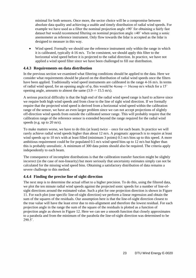
4.4.4 Finding the precise line of sight direction
The next step is to determine the actual offset to a higher precision. To do this, using the filtered data,
we plot the ten minute radial wind speeds against the projected sonic speeds for a number of line-of-
sight directions around the estimated value. Such a plot for one projection direction is shown in Figure
11. For each plot (one specific line-of-sight direction) we perform a linear regression and obtain the
sum of the squares of the residuals. Our assumption here is that the line-of-sight direction closest to
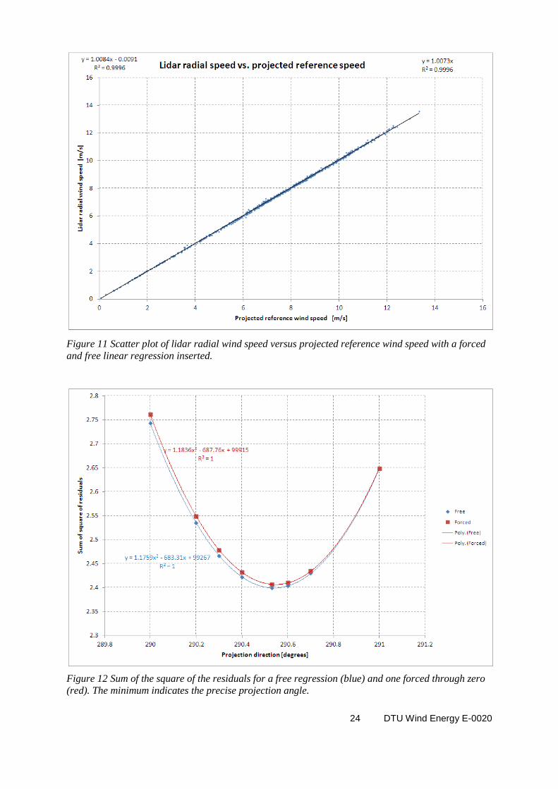
the true value will have the least error due to mis-alignment and therefore the lowest residual. For each
projection angle in the range the sum of the square of the residuals is plotted as a function of
projection angle as shown in Figure 12. Here we can see a smooth function that closely approximates
to a parabola and from the minimum of the parabola the line-of-sight direction was determined to be
290.5˚.
24 DTU Wind Energy E-0020
Figure 11 Scatter plot of lidar radial wind speed versus projected reference wind speed with a forced
and free linear regression inserted.
Figure 12 Sum of the square of the residuals for a free regression (blue) and one forced through zero
(red). The minimum indicates the precise projection angle.

25 DTU Wind Energy E-0020
Figure 13 Plot of binned lidar radial wind speed versus binned projected reference wind speed with a
forced and free linear regression inserted.
4.4.5 Calibrating the radial wind speed Having found the line-of-sight direction, the linear relationship between the lidar radial speed and the
projected sonic speed can now be found. In fact we already achieved this in the last step in finding the
line-of-sight since the necessary information are calculated in the regression analysis. As shown in
Figure 14, we simply read off the value of the gain (and offset for the free regression) at the projection
angle giving the minimum residual. This figure also gives an impression of the sensitivity of the gain
to the projection angle. It can be seen that in the entire range of the plot, the gain varies by less than
1%.
Having performed the regression analysis with the scatter plotted (un-binned) data, the analysis should
be repeated using the determined line of sight direction and with binned projected reference wind
speed data and binned radial wind speed data. An example is shown in Figure 13.
The binned analysis will provide regression results that are somewhat less sensitive to the exact data
distribution and equally importantly, will provide the mean deviations and standard deviations
necessary for the uncertainty analysis. The parameters required for the binned analysis are, for each
bin:
Mean projected reference wind speed (using the projection angle determined from the initial
un-binned analysis).
Number of samples in the bin
Mean lidar radial wind speed
Standard deviation of the lidar radial wind speed
Mean deviation (lidar radial speed – projected reference wind speed)

26 DTU Wind Energy E-0020
Standard deviation of the deviation.
The uncertainty results will be used on horizontal wind speeds, not directly on radial wind speeds. In
order for the uncertainty components to be directly applied to conventional horizontal wind speed bin
sizes and alignment, for a lidar with an half-opening angle φ, it is necessary to use a radial bin size of
0.5*cosφ. To get the correct bin alignment, add first 0.25*cosφ to the projected speed, divide by the
bin size and take the unrounded integer (function floor()) as a bin index number.
(( ) ( ))⁄
Figure 14 Reading off the gain at the minimum value of the residuals.
4.4.6 Calibration results combined to a horizontal wind speed calibration
It is recommended that the vector mean wind speed is used. In this case the horizontal wind speed
for each 10 minute period can be obtained by first calculating the longitudinal and transverse speed
components, and respectively from the means of the radial speeds and
( )
( )
The horizontal wind speed is simply

27 DTU Wind Energy E-0020
√
Using this formulation, the individual radial wind speeds can be corrected according to their respective
calibration expressions before being used to calculate and .
4.4.7 Finding the sensed range In order to validate that the lidar is sensing the radial wind speeds at approximately the correct range
we perform a correlation exercise between the fast sampled reference projected wind speed and the
fast sampled lidar radial wind speeds for each lidar range recorded. The lidar range having the highest
correlation to the reference wind speed is deemed to be the range at which the lidar is truly sensing the
reference wind speed. This range should ideally coincide with the actual distance between the lidar
and the reference mast which has been previously measured. Any discrepancy will indicate an error in
the sensing range of the lidar.
Practically, even with synchronized clocks in the lidar and mast logger, we can in general expect some
time lag between the lidar and the projected reference wind speed. The correlation is performed over a
number of time lags to first identify the highest correlated time lag. For this time lag, the range having
the highest correlation to the projected reference wind speed is then identified.
The analysis should be performed with a number of ten minute periods each possessing different wind
directions and wind speeds in order to assess to robustness of the method. Before this correlation
exercise can be performed, the exactWe start by block averaging the projected wind speed data
(assumed sampled faster than the lidar ‘fast’ data rate) to give ten minute time series of wind and lidar
data with the same number of points (typically around 430 points per 10 minutes). Because the exact
time synchronization between the lidar and the reference wind speed is unknown, a correlation is
performed for a range of time lags (+- 15 s) between the sonic and each of the lidar lags. A matrix of
correlation coefficients is produced (time lag vs range) and the absolute maximum element located.
This identifies both the time lag and the range having the highest correlation.
4.5 Uncertainties
Assessing the uncertainties for the line of sight calibration is quite complex. There are two separate
physical calibrations of each of the lines of sight. Line-of-sight wind speed uncertainties can be
calculated for these two calibrations considering the reference uncertainties and the calibration
uncertainties. The two line-of-sight wind speeds are used to calculate the horizontal wind speeds. The
line of sight uncertainties need then to combined using the influence coefficients calculated from the
horizontal wind speed algorithm. Finally the uncertainty of the opening angle should be considered
and its influence included in the uncertainty budget.
4.5.1 Line of sight reference wind speed uncertainties
Here we discuss and attempt to quantify the reference wind speed uncertainties. They will be
summarised and combined in the subsequent section. The individual uncertainties will be estimated
here using a coverage factor of 1. The final line-of-sight uncertainty should be reported with a
coverage factor of 2 (95% confidence level).
4.5.1.1 Calibration uncertainty.
Taken from the calibration certificate and adjusted to a coverage factor (k) of 1. For the example
below we have taken a value of 0.035 m/s.
28 DTU Wind Energy E-0020
4.5.1.2 Operational uncertainty
Here provisionally we use the same values as a cup anemometer, 0.015 m/s + 0.15% (for k=1). This
should be examined more closely and in particular justified according to the turbulence intensity
classification of the instrument. For this reason, a cup anemometer will probably have a higher
operational uncertainty than a cup anemometer in this environment (high turbulence intensity). A plot
of turbulence intensity as a function of (horizontal) wind speed bin is required.
4.5.1.3 Mounting uncertainty
The sonic anemometer is top-mounted. An uncertainty of 0.25% is applied to account for any flow
distortion effects caused by the top of the mast.
4.5.1.4 Flow distortion uncertainty
For a sonic anemometer the measured wind speed will depend to some degree on the azimuth angle of
the wind (i.e the wind direction) since the flow will be distorted by the internal structure of the
anemometer. The size of the uncertainty will depend a lot on the sonic design and how it is orientated
to the flow. For example for an asymmetric head design with the preferred opening angle aligned to
the line-of-sight, the flow distortion error will be smaller than for a symmetrical design aligned with a
support strut in the line of sight direction.
From our wind tunnel calibration the Gill Windmaster (Asymmetric), for the preferred opening angle
the flow distortion (normalised mean deviation) is approximately a linear function with a slope of
8x10⁻⁵
per degree. For a -40˚ offset from the centre direction this would give an error of about 0.3%.
This would however be compensated for by +ve directions. Here we estimate the flow distortion
uncertainty as 0.05% per ±10˚ of opening sector, centred on the true sonic centreline. This is a
conservative estimate since due to averaging, the total uncertainty is probably much less. In addition,
the uncertainty will be also registered as increased scatter and to a certain degree, double counted.
To minimize the flow distortion error, the sonic anemometer should be used within its preferred
opening sector and as close to the calibration direction as possible. For this reason the opening sector
should be kept as low as reasonably possible (making a compromise between the conflicting constraint
of requiring a good data population).
An alternative strategy would be to use a combination of a (top-mounted) cup anemometer for the
wind speed together with a wind vane (or sonic anemometer) to give the wind direction information
necessary to make the line-of-sight projection. To avoid significant flow distortion, this probably
necessitates two masts (one for each instrument) placed 5-10 m apart since a boom mounted direction
sensor might also be influenced by the mast. In the case of two masts (one with a top-mounted cup)
the avoided flow distortion uncertainty should be substituted by an uncertainty associated with the
spatial separation of the two measurement sensors.
4.5.1.5 Wind direction uncertainty
Since the core of the calibration method is comparing the lidar-line-of-sight speed to the projected
reference wind speed, the accuracy of the wind direction measurement is also significant. Usually
wind direction measurement uncertainty is dominated by the uncertainty in the offset – knowing
exactly where the sensor is pointing in absolute direction. This is directly linked to the installation
method and experience of the involved personnel. It is usual for this uncertainty to lie between 1 and 5
degrees. In our calibration methodology we are actually uninterested in the absolute offset since we
use the data themselves to determine the line-of-sight direction in the instrument’s own reference
frame. The uncertainties related to this direction determination will be dealt with below.
Apart from the direction offset uncertainty, which as explained above, we disregard here, it is also
important to consider the relative accuracy of the direction measurement which could be influenced by
‘gain’ errors or distortion due to flow distortion (both from external and internal sources). Specifically
for our top-mounted sonic anemometer the main direction error source will come from flow distortion
due to the internal struts of the instrument. We do not anticipate large errors since the sonic
anemometer implements a flow correction algorithm based on wind tunnel measurements. From the

29 DTU Wind Energy E-0020
wind tunnel calibration, we have a plot of the sonic anemometer reported angle as a function of wind
tunnel direction (direction of the rotated sonic anemometer relative to the tunnel axis). This shows a
standard error of 0.4˚ with no obvious trend. At 40˚ off-axis, a 0.4˚ direction error will result in a
projected speed error 0f 0.5%. For well distributed wind directions (around the sonic centreline) we do
not anticipate nearly such a large uncertainty contribution from this error source. Additionally, the
effect of the direction error on the projected speed is weighted by the sin of the angle between the
wind direction and the projection angle. For wind directions close to the projection angle, the effect of
a direction error is very small (since the cosine of the angle is very insensitive).Our best estimate is to
set the value to 0.02% per ±10˚ of permitted opening sector. Once again this is a conservative estimate
since the higher scatter will already be counted as increased statistical uncertainty.
4.5.1.6 Line-of-sight determination uncertainty
Using the methodology described in Section 4.4.4,we determine the line-of-sight direction by varying
the reference speed projection direction and finding the projection angle giving the minimum sum of
residuals in the regression of lidar line-of-sight speeds versus projected reference speed. Over a 1
degree range of projection angle, the forced fit gain can typically vary by 1%. Since we estimate the
uncertainty in the determined line-of-sight angle to be 0.1˚ we will set the uncertainty due to the line-
of-sight determination to be 0.1%. This is a conservative estimate since an incorrect line-of-sight angle
will result in a higher statistical uncertainty in the calibration results.
4.5.1.7 Beam height uncertainty
Central to the calibration method is that the lidar beam passes exactly beside the reference wind speed
instrument, i.e. at exactly the same height. If the beam is too high, due to the vertical wind shear, the
lidar will sense a wind speed higher than the reference instrument and conversely a too low wind
speed if the height is too low.
The accuracy of the beam height is clearly central to our uncertainty budget. Depending on the method
used and the experience of the personnel the beam height uncertainty may vary widely. With the
method we have developed (described in Section Error! Reference source not found.) we estimate
(conservatively) the uncertainty to by 10 cm. For a power law exponent of 0.2, this will relate to a
wind speed uncertainty of 0.2%.
In order to verify the magnitude of this uncertainty the average value of the power law wind exponent
should be calculated per wind speed bin and presented in the results. Furthermore the measurements of
the beam position relative to the position of the reference sensor should be reported both for the
installation and again immediately prior to removal (turning for the first beam) for each beam
separately.
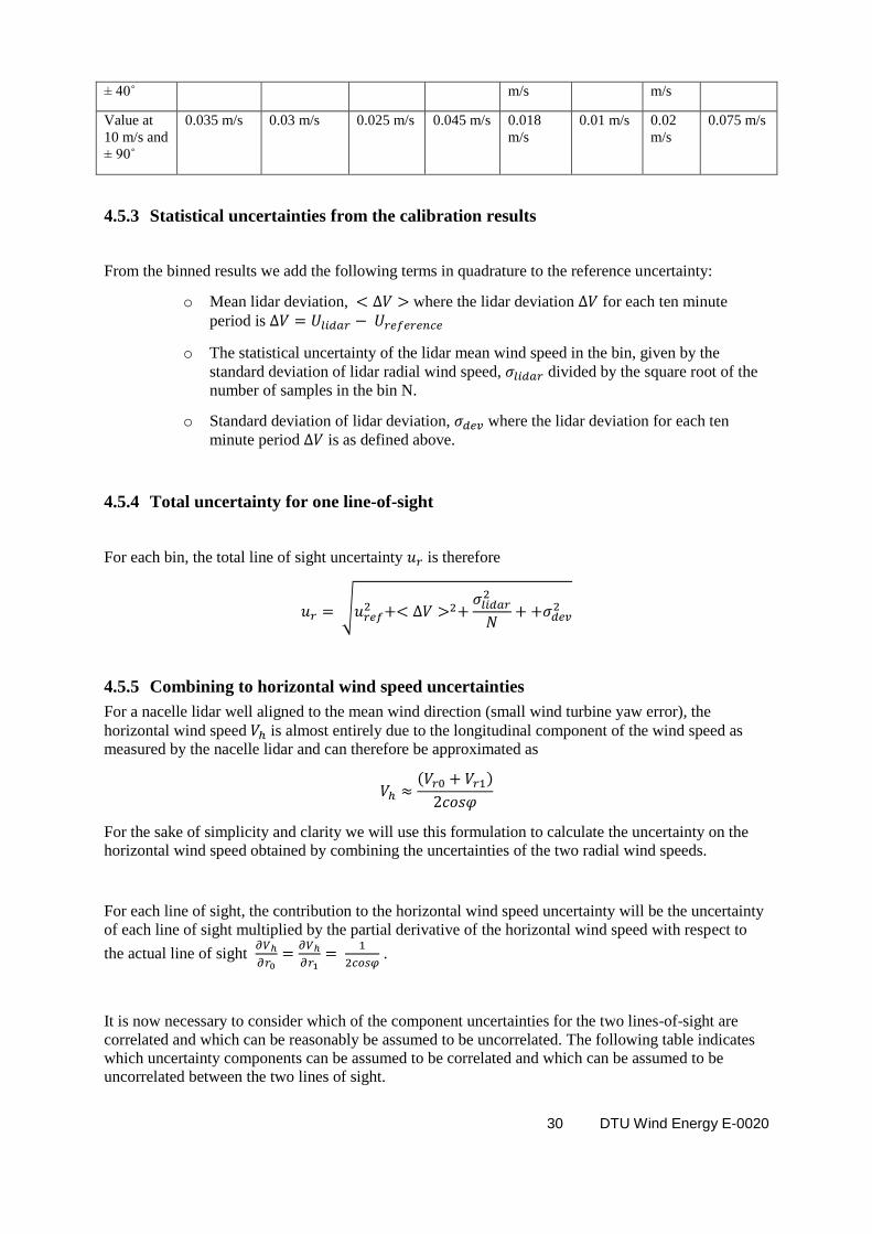
4.5.2 Combined Radial Wind Speed Uncertainties
Here we summarise the individual radial wind speed uncertainties (for a coverage factor (k) of 1) and
combine them. Since all the uncertainties can be considered as independent, the combination is a
simple geometrical sum.
Calibration Operational Mounting Flow-
distortion
Wind
direction
LOS
direction
Beam
height
Combined
(k=1)
Symbol
Expression 0.035 m/s 0.015 m/s +
0.15%
0.25% 0.05%
per ±10˚
sector
0.02%
per ±10˚
sector
0.1% 0.2% √∑
Value at
10 m/s and
0.035 m/s 0.03 m/s 0.025 m/s 0.02 m/s 0.008 0.01 m/s 0.02 0.061 m/s
30 DTU Wind Energy E-0020
± 40˚ m/s m/s
Value at
10 m/s and
± 90˚
0.035 m/s 0.03 m/s 0.025 m/s 0.045 m/s 0.018
m/s
0.01 m/s 0.02
m/s
0.075 m/s
4.5.3 Statistical uncertainties from the calibration results
From the binned results we add the following terms in quadrature to the reference uncertainty:
o Mean lidar deviation, where the lidar deviation for each ten minute
period is
o The statistical uncertainty of the lidar mean wind speed in the bin, given by the
standard deviation of lidar radial wind speed, divided by the square root of the
number of samples in the bin N.
o Standard deviation of lidar deviation, where the lidar deviation for each ten
minute period is as defined above.
4.5.4 Total uncertainty for one line-of-sight
For each bin, the total line of sight uncertainty is therefore
√
4.5.5 Combining to horizontal wind speed uncertainties
For a nacelle lidar well aligned to the mean wind direction (small wind turbine yaw error), the
horizontal wind speed is almost entirely due to the longitudinal component of the wind speed as
measured by the nacelle lidar and can therefore be approximated as
( )
For the sake of simplicity and clarity we will use this formulation to calculate the uncertainty on the
horizontal wind speed obtained by combining the uncertainties of the two radial wind speeds.
For each line of sight, the contribution to the horizontal wind speed uncertainty will be the uncertainty
of each line of sight multiplied by the partial derivative of the horizontal wind speed with respect to
the actual line of sight
.
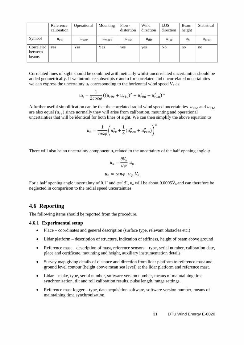
It is now necessary to consider which of the component uncertainties for the two lines-of-sight are
correlated and which can be reasonably be assumed to be uncorrelated. The following table indicates
which uncertainty components can be assumed to be correlated and which can be assumed to be
uncorrelated between the two lines of sight.
31 DTU Wind Energy E-0020
Reference
calibration
Operational Mounting Flow-
distortion
Wind
direction
LOS
direction
Beam
height
Statistical
Symbol
Correlated
between
beams
yes Yes Yes yes yes No no no
Correlated lines of sight should be combined arithmetically whilst uncorrelated uncertainties should be
added geometrically. If we introduce subscripts c and u for correlated and uncorrelated uncertainties
we can express the uncertainty uh corresponding to the horizontal wind speed Vh as
(( )
)
A further useful simplification can be that the correlated radial wind speed uncertainties and are also equal ( ) since normally they will arise from calibration, mounting and operational
uncertainties that will be identical for both lines of sight. We can then simplify the above equation to
(
(
))
There will also be an uncertainty component uo related to the uncertainty of the half opening angle φ
For a half opening angle uncertainty of 0.1˚ and φ=15˚, uo will be about 0.0005Vh and can therefore be
neglected in comparison to the radial speed uncertainties.
4.6 Reporting
The following items should be reported from the procedure.
4.6.1 Experimental setup
Place – coordinates and general description (surface type, relevant obstacles etc.)
Lidar platform – description of structure, indication of stiffness, height of beam above ground
Reference mast – description of mast, reference sensors – type, serial number, calibration date,
place and certificate, mounting and height, auxiliary instrumentation details
Survey map giving details of distance and direction from lidar platform to reference mast and
ground level contour (height above mean sea level) at the lidar platform and reference mast.
Lidar – make, type, serial number, software version number, means of maintaining time
synchronisation, tilt and roll calibration results, pulse length, range settings.
Reference mast logger – type, data acquisition software, software version number, means of
maintaining time synchronisation.
32 DTU Wind Energy E-0020
4.6.2 Beam 0 alignment
Date and time
Personnel
Measured beam position relative to reference instrument
4.6.3 Beam calibration measurements
The following items should be logged during the calibration measurements:
Lidar – ten minute means, standard deviations, minimums and maximums of radial wind
speed, signal-to-noise ratio, spectral broadening, radial wind speed availability, tilt, roll.
Lidar – time-stamped time series of radial wind speed, signal-to-noise ratio, spectral
broadening.
Reference sensors - ten minute means, standard deviations, minimums and maximums of
instantaneous wind speed and wind direction and/or components of wind speed in two
orthogonal directions in the horizontal plane, vertical wind speed component or tilt angle.
Reference sensors – time-stamped time series of horizontal wind speed components.
4.6.4 Beam 1 alignment
Date and time
Personnel
Measured beam 0 position relative to reference instrument BEFORE re-alignment
Measured beam position relative to reference instrument.
4.6.5 Removal of lidar from platform (end of beam 1 measurements)
Date and time
Personnel
Measured beam 1 position relative to reference instrument BEFORE removal.
4.6.6 Results for each individual beam
Dataset start and finish timestamps
Plot of radial wind speed normalised by vector average reference wind speed versus wind
speed (unfiltered data)
Exact filtering conditions employed and the number of records removed by each condition
Histogram of radial wind speed distribution after filtering
Plots of sum of squares of residuals for forced and free linear regressions over a 1 degree
range containing the minimum of these quantities.
33 DTU Wind Energy E-0020
Exact line of sight direction (in direction reference sensor system and if different, related to
absolute direction)
Regression results for scatter plot including
o Forced regression (offset forced through zero), gain with standard error
o Forced regression, coefficient of determination (R2)
o Free regression (offset determined as a parameter), gain with standard error
o Free regression, offset with standard error
o Free regression, coefficient of determination (R2)
For data binned on the projected reference wind speed such that the resultant horizontal wind
speed bins will be 0.5 m/s and aligned on x.0 and x.5 m/s boundaries:
o Bin number (( ) ( ))⁄
o Samples in bin
o Mean projected reference wind speed
o Standard deviation of projected reference wind speed
o Mean lidar radial wind speed
o Standard deviation of lidar radial wind speed,
o Mean lidar deviation,
o Standard deviation of lidar deviation,
Regression results for the binned data including
o Forced regression (offset forced through zero), gain with standard error
o Forced regression, coefficient of determination (R2)
o Free regression (offset determined as a parameter), gain with standard error
o Free regression, offset with standard error
o Free regression, coefficient of determination (R2)
Average turbulence intensity plotted as a function of binned horizontal wind speed
Average power law shear exponent plotted as a function of binned horizontal wind speed
LOS uncertainty components as given in section 4.5.2
Range check for each beam – Report the actual distance between the lidar platform and the
reference mast. For a number (5 -10) of ten minute periods with different directions and wind
speeds, for each beam individually, report in tabular form:
o Run identification (time period)
o Wind direction
o Wind speed

34 DTU Wind Energy E-0020
o Time lag for maximum correlation
o Range for and value of maximum correlation
4.6.7 Results combined to horizontal wind speed
LOS uncertainties combined to horizontal wind speed uncertainties
Algorithm check (only required if using reported scalar wind speed means).
o Give the algorithms relating measured radial wind speed to horizontal wind speed and
relative wind direction.
o Document that from the ‘fast’ lidar data, the consecutive reported values of radial
wind speed combine to horizontal wind speed and relative wind direction precisely
according to the theoretical expressions.
o Document that ten minute averages of instantaneous wind speed from the ‘fast’ data
are identical to the ten minute average values reported in the ‘average’ data.
o Document that ten minute averages of orthogonal wind speed components (typically
aligned and perpendicular to the lidar axis) from the ‘fast’ data are identical to the
corresponding ten minute averages reported in the ‘average’ data.

35 DTU Wind Energy E-0020
5. Testing horizontally in a mast Another possibility for nacelle lidar calibration is to mount the lidar in a mast and compare the lidar
measured horizontal wind speeds with those reported from the mast instrumentation. We will briefly
examine this concept and investigate its practical viability.
Figure 15 Plan view of a nacelle lidar mounted in a mast for calibration against a reference
instrument in the same mast.
5.1 Concept
One simple method for calibrating a nacelle lidar would be to mount it in a mast at a flat and
homogeneous site, sufficiently high such that the homogeneity condition is fulfilled to a high degree at
the beam sensing points. Horizontal wind speed estimates calculated by the lidar from the sensed
radial wind speeds can then be compared to measurements from reference instruments on the mast
itself. In order to have reasonable correlation between the wind speed measurements, the distance
between the lidar sensing position and the mast should be kept to a minimum. In practice this means
setting the lidar at its minimum range (typically 80m). However if the application is an IEC 61400-12-
1 compliant power curve measurement, the lidar will almost certainly be set to a much larger range,
corresponding to 2.5 rotor diameters, probably between 200 and 350m. The difference in range
between the calibration and the application if even permissible is a formal procedure, must be
represented by a significant uncertainty that is difficult or impossible to quantify (see Section 5.4).
Alternatively we could set the correct (application) lidar range and still make the comparison with the
mast. At such distances the correlation would significantly decrease and actual terrain induced
differences in wind speed might also become significant. In fact it would be necessary to perform a
site calibration to use this concept, in which case we have actually the setup required for our ideal lidar
calibration described in Section 3.
5.2 Procedure
Since this calibration method will depend on the accuracy of the internal tilt and roll sensors for
ensuring a horizontal and level beam, a tilt and roll calibration should first be carried out. The lidar can
then be installed in a suitable mast, probably at least 50m above the ground in order to maximize
homogeneity. Calibrated reference instrumentation should be available at the chosen height. Pay

36 DTU Wind Energy E-0020
particular attention to the offset of the wind direction sensor since this will undoubtedly be a
significant source of uncertainty in a direction calibration.
Having raised the lidar up into the mast (probably the most challenging aspect of this method) the
system should be levelled according to the internal tilt and roll sensors. In order to check wind
direction performance, the best option is to align one of the lidar beams to some object visible when
sighting horizontally at the given height (eg. another mast or a wind turbine). Here a rifle sight
mounted during the tilt and roll calibration can again be of service.
Check that the lidar ranges are set appropriately and that both the lidar and mast data logger are
synchronised to the same time source. Measurements can now begin. Since we are comparing
recovered horizontal wind speeds to reference wind speeds, only one measurement campaign is
needed. It is more reasonable than for the los calibration to require a full distribution of wind speeds in
the conventional 4-16 m/s range since here we are comparing wind speed (not projections) and we are
almost certainly measuring considerably higher. A conservative requirement would be for a minimum
of 600 points after filtering with at least three points in each 0.5 m/s wind speed bin between 4 and 16
m/s.
5.3 Data analysis
The analysis is a simple regression analysis of the lidar measured horizontal wind speeds against the
reference wind speed measurements. Traditionally scalar means (both for the lidar and the reference
wind speed) are used for this comparison. Vector mean comparisons could also usefully be made and
would negate differences due to the different sensitivity to the transverse turbulence.
Before performing the regression analysis, the data should be filtered, considering:
Lidar availability ( > 0.95 or =1.0)
Wind sector – chosen to give high quality reference wind speed data and avoiding sectors with
significant flow in-homogeneity at the lidar sensing locations.
Wind speed (4 – 16 m/s)
Any reference wind speed quality parameters
Temperature ( > 2C) to avoid sensor icing.
The regression analysis should be performed for binned and un-binned data reporting regression
coefficients for both forced and free linear regressions.
From the binned data, for each bin we derive the following parameters for use in the uncertainty
estimation:
o Bin number (( ) ( ))⁄
o Samples in bin
o Mean reference horizontal wind speed
o Standard deviation of reference wind speed
o Mean lidar horizontal wind speed
o Standard deviation of lidar horizontal wind speed,
37 DTU Wind Energy E-0020
o Mean lidar deviation,
o Standard deviation of lidar deviation,
5.4 Uncertainties
The uncertainties come from three main sources:
Reference speed uncertainty √
Calibration uncertainty √
Range uncertainty
The last term expresses the uncertainty associated with calibrating at one lidar range and
measuring at a (presumably) very different range. Since this does not seem to be very good practice,
the value of this uncertainty should be correspondingly large. This is the fundamental weakness of this
calibration method.
6. Testing from the ground with an inclined beam In the previous section we investigated a direct horizontal wind speed calibration method that was
based on a lidar mounted high in a mast. This method was difficult to implement because of the high
installation and had high (undefined) uncertainties because the calibration was not being made at the
correct measuring range of the lidar.
Here we examine another direct horizontal wind speed calibration method (as opposed to line of sight
calibration) that effectively eradicates the two weaknesses of the previous method.
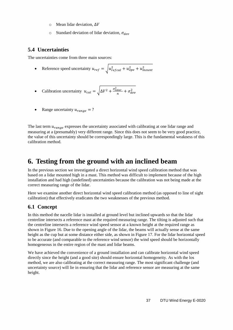
6.1 Concept
In this method the nacelle lidar is installed at ground level but inclined upwards so that the lidar
centreline intersects a reference mast at the required measuring range. The tilting is adjusted such that
the centreline intersects a reference wind speed sensor at a known height at the required range as
shown in Figure 16. Due to the opening angle of the lidar, the beams will actually sense at the same
height as the cup but at some distance either side, as shown in Figure 17. For the lidar horizontal speed
to be accurate (and comparable to the reference wind sensor) the wind speed should be horizontally
homogeneous in the entire region of the mast and lidar beams.
We have achieved the convenience of a ground installation and can calibrate horizontal wind speed
directly since the height (and a good site) should ensure horizontal homogeneity. As with the los
method, we are also calibrating at the correct measuring range. The most significant challenge (and
uncertainty source) will lie in ensuring that the lidar and reference sensor are measuring at the same
height.
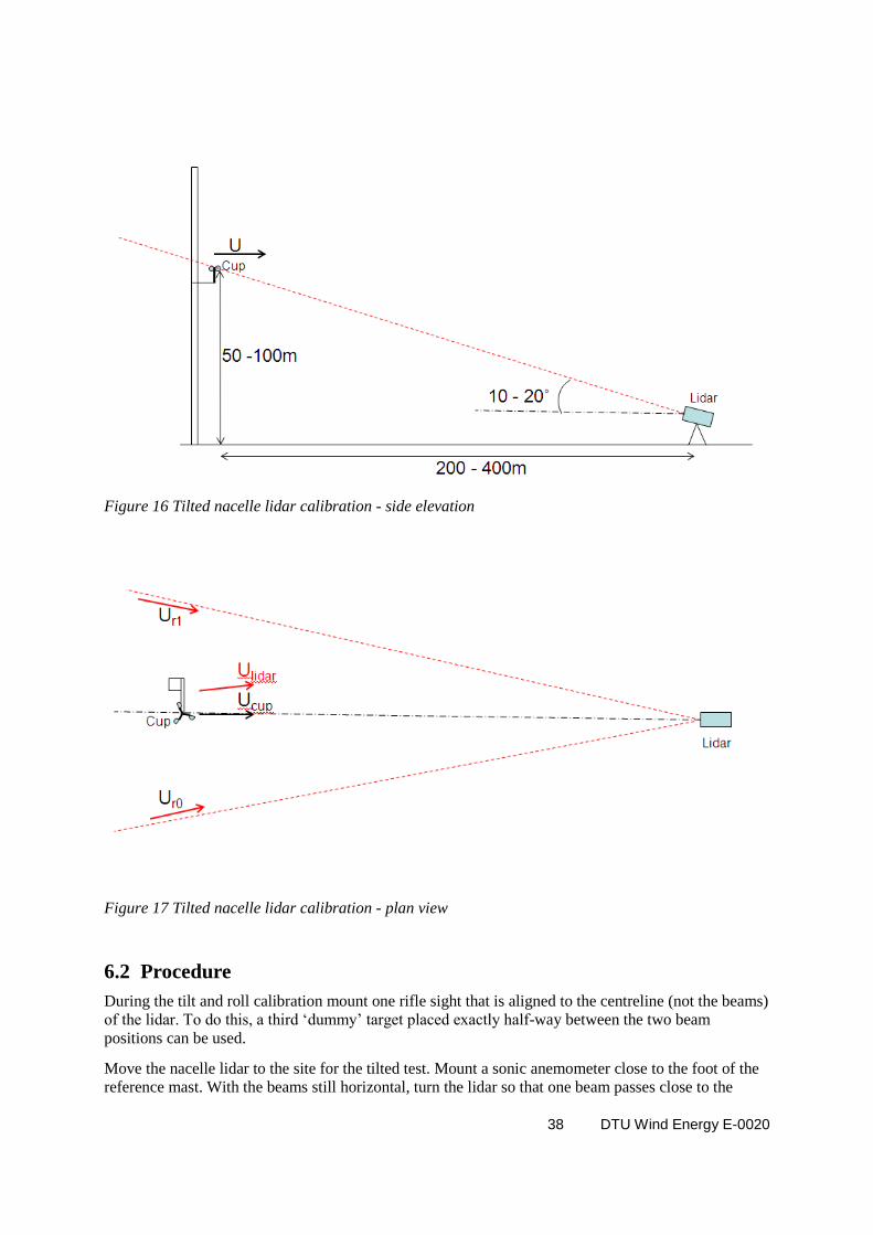
38 DTU Wind Energy E-0020
Figure 16 Tilted nacelle lidar calibration - side elevation
Figure 17 Tilted nacelle lidar calibration - plan view
6.2 Procedure
During the tilt and roll calibration mount one rifle sight that is aligned to the centreline (not the beams)
of the lidar. To do this, a third ‘dummy’ target placed exactly half-way between the two beam
positions can be used.
Move the nacelle lidar to the site for the tilted test. Mount a sonic anemometer close to the foot of the
reference mast. With the beams still horizontal, turn the lidar so that one beam passes close to the
39 DTU Wind Energy E-0020
sonic anemometer. Using the correlation technique described in section 4.4.7, perform a range check
measurement. This is necessary both for completeness of the calibration but also because with a tilted
beam, the actual lidar sensing height will depend critically on the sensing range. To be completely
formal, the range check should be made with each beam in succession. Pay attention to the difference
between perpendicular plane ranges (as set in the lidar configuration) and los ranges.
Having determined any necessary offset to the lidar sensing range, apply this adjustment to the lidar
configuration. Calculate the nominal tilting angle required based on the reference sensor height, the
distance between the lidar and the mast base and any difference in ground level between these two
positions. Be aware if the lidar configuration allows specification of a tilted beam and if this is the
case, pay attention to the exact definition of the measuring range. Enter the tilting angle is possible
(alternatively modify beam azimuth and zenith settings).
Turn the lidar so that the centreline is aligned with the mast and tilt the lidar so that the rifle sight
cross-hairs are centred on the reference wind sensor. Check that the actual reported tilting angle is
close to the nominal value calculated and fine adjust the lidar so that the roll angle is zero, whilst
keeping the cross-hairs at the correct location. The lidar should now be at the correct angle and the
range should be correct for the beam centres to be at the same height as the cup anemometer.
Ensure that the lidar and mast data loggers are time synchronised and can maintain this synchronicity.
The measurement campaign can now commence.
6.3 Data analysis
Assuming that the lidar correctly reconstructs the horizontal speed taking due consideration for the
tilting angle, the data analysis proceeds exactly as for the previous method described in section 5.3.
The same data population requirements and the same filtering conditions can be employed.
6.4 Uncertainties
The uncertainties come from three main sources:
Reference speed uncertainty √
Calibration uncertainty √
Height uncertainty
The last term represents the uncertainty in comparing the reference wind speed to a lidar wind
speed at a slightly different height. Let us assume that the largest component of this height uncertainty
is the actual measuring range. If we have an uncertainty of 5m on this range, we can expect a height
error uncertainty of say 5m * sin(15) = 1.3m. Including also the accuracy of the initial beam alignment
(how good the rifle sight aim is), an overall height uncertainty of 2m is not unreasonable. A simple
conversion to a speed uncertainty would be to use the power law. At 50m measuring height and with
an exponent of 0.2 we would get
((
)
)
or an uncertainty of 0.8% of the wind speed.
40 DTU Wind Energy E-0020
An alternative strategy could be to measure the actual wind shear using wind speed sensors 10 m
above and 10 m below the actual reference height. This could give an actual (possibly bin-wise) value
for the absolute wind shear (in (m/s)/m ) which could be used to calculate the speed uncertainty from
the height uncertainty (using simple multiplication).
A local wind shear measurement could be used in other ways as well; to filter out periods with large
wind shear or alternatively to derive the height error directly using multi-parametric regression
techniques such as used in ground based wind lidar calibration.
7. Discussion
7.1 Comparison of methods
We have described four different methods for calibrating nacelle lidars. The ideal method (Section 3)
was seen to be very difficult to achieve requiring high and very rigid structures and a location with a
very high degree of horizontal homogeneity. Since these facilities are not available now or in the
foreseeable future, we have not pursued this concept.
The second method examined (Section 4) was to calibrate the line of sight wind speeds of the lidar
directly by accurately positioning the beam to pass close beside a reference wind speed sensor at the
desired measurement range. This method can be realised at relatively low heights at a site where the
wind speed can be considered homogeneous in the probe length of one beam (as opposed to
homogeneous between two separated probe volumes for a horizontal wind speed calibration). Greater
homogeneity and reduced sensitivity to height induced errors can be obtained by carrying out the
measurement as high as possible. A considerable limitation of this method is the time necessary to
obtain an acceptable distribution of radial wind speeds since we are concerned with the projection of
the horizontal wind speed along the line of sight. Especially high radial wind speeds are problematical
since a combination of high horizontal wind speed and correct wind direction is necessary in order to
obtain acceptable data. To compound this, unless a custom facility with two accurately positioned
reference masts is built, each line of sight has to be calibrated one after the other. In this case, several
months of testing will normally be necessary and even then with no guarantee of satisfactory data
distributions. Both due to the long testing period and the high degree of manual manipulation
(platform mounting and beam alignments) this method will be expense.
How to use the individual line of sight calibrations is not immediately apparent, especially if they are
significantly different. However a consensus is emerging that it is more accurate to use vector mean
wind speeds from nacelle lidars since the cross-contamination of the turbulence components can give
rise to over-estimation of especially the transverse turbulence component, leading to significant errors
in scalar averages. In the case that vector averaging is chosen, line of sight calibrations can be readily
applied since the vector averages can be derived directly from the ten minute averaged and calibration
corrected, individual radial wind speeds.
A third method when only one mast is available (Section 5) is to mount the lidar high in the mast and
compare the lidar wind speed measurements made at the shortest possible range with wind speed
measurements from reference instruments on the mast itself. Since for power curve testing, we are
most likely to need lidar measurements at a fairly long range, this method is not rigorous since in the
calibration we are not using the lidar at the application range. If we instead compare the lidar speed
measurements made at the correct (power curve) range, the correlation to the mast will be poor and
more importantly, unless the site is exceptionally homogeneous, a site calibration will be necessary to
relate the remote wind speeds at the lidar sensing points to those measured at the mast. A calibration
made through a site calibration is unlikely to provide sensibly low uncertainties.
The single mast method might have some value as a plausibility test, for example for a line of sight
calibrated nacelle lidar but for the reasons explained above we do not envisage developing this concept
as an actual calibration procedure.

41 DTU Wind Energy E-0020
Although the line of sight method is rigorous and will provide calibrations with reasonably low
uncertainties, it will be very lengthy in execution and rather expensive. As we saw above, the single
mast method is not a satisfactory alternative. Instead we have investigated a method where the lidar is
placed on the ground and the beams tilted up to reference mast at the desired range at a known height
(Section 6). The ground placement of the lidar is logistically simple and will mean that this method is
invariably cheaper than a line of sight calibration. We are comparing horizontal wind speeds from a
reference instrument with horizontal wind speeds as reported by the nacelle lidar. This requires the site
to be sufficiently horizontally homogeneous at scales spanning the sensing points of the two beams. If
this can be achieved, the calibration should be much faster since we now have to satisfy a horizontal,
not a projected wind speed distribution combined with the fact that we are (probably) measuring much
higher than the line of sight method.
However we must also recognise that this method is using the lidar in a configuration with markedly
tilted beams, unlike in the envisaged application. We are relying on the ability of the lidar to correctly
recover horizontal wind speeds when configured with the appropriate geometry. In fact the lidar is
using the same algorithm at any inclination - a truly horizontal installation simply being a special case
where many terms disappear. A series of calibrations at different inclination angles is required to
demonstrate the generality of the method. Comparison and close agreement to a line of sight
calibration would be an additional strengthening of the validity of this method.
7.2 Further work required
As can be gleaned from the previous section, we will actively pursue both the line of sight and the
tilted beam ground based calibration techniques; the first to give high accuracy at high expense and a
long testing period, the second to give a cheaper, faster but invariably less accurate calibration. Time
will tell which of these methods (or others) come to prevail.
As can also be gleaned from this whole report, the two methods are not equally mature. In fact the vast
majority of resources have been used developing the line of sight method. We will in this section
outline what we see as the next important steps for both methods.
7.2.1 Line of sight method
This method has the most maturity and using the procedure described in this report, could readily be
used as part of a formal power curve measurement campaign. Quality accreditation of the method is
the next major step to be taken. Before this, a number of calibrations should be performed and reported
according to the procedure laid out in this document. It is anticipated that the feed-back from these
calibrations will hone the procedure in preparation for formal quality accreditation.
The most recent and probably most contentious part of this procedure is the uncertainty analysis. This
will be re-examined in the coming months and it is hoped that constructive feedback on this document
can greatly assist in this process.
Specific points to examine:
How operational uncertainties are applied for a cup and sonic anemometer
Do we need to add uncertainties associated with the wake of the mast and the in-homogeneity
of the terrain along the probe length?
More rigorous analysis of how to combine LOS uncertainties to horizontal wind speed
uncertainties.
Can we use 2 minute averages instead of 10 minutes to fill the speed distributions quicker?
42 DTU Wind Energy E-0020
7.2.2 Tilted beam, ground based method
The tilted beam, ground based method is much less mature and has yet to be performed in the
procedure laid out here. In particular the range checking routine is completely unproven but will be an
important component of the procedure especially in respect of obtaining measurements at the correct
height. This is clearly an important next step. Ideally a nacelle lidar should first undergo a line of sight
calibration on both beams, including a thorough range calibration. Subsequently this lidar should be
calibrated with the procedure outlined in Section 6, preferably at two different inclination angles. All
three calibrations should be reported and the uncertainties assessed as prescribed in this document.
This will give a much more solid basis for deciding whether one or other or both of the two methods
should be promoted as commercial calibration products.
8. Conclusion We have examined calibration methods for nacelle lidars. Firstly a tilt and roll calibration method was
described in which the internal tilt and roll sensors are calibrated. The opening angle of the lidar
beams is also measured. This tilt and roll calibration is necessary for all applications where the tilting
and rolling of the lidar beams will occur in a vertically sheared wind field.
A line-of-sight calibration technique for wind speed and measuring range was then described. This
method results in an acceptably low uncertainty. It has the disadvantages of being time consuming
since two individual lines of sight must be calibrated separately. Alternatively, both lines of sight
could be calibrated simultaneously with a setup using one platform and two masts but it would be
necessary to use individual reference sensors. A second reason for long test durations is that the
comparison is made between projected wind speeds and lidar radial wind speeds. High values of these
parameters can only be measured when high wind speeds occur in a wind direction close to the line-of-
sight direction.
More simply, the lidar can be placed fairly high in a mast and the reported wind speeds compared with
those measured from the mast itself. The main difficulty of this method is the difficulty of performing
a lidar installation high up on a mast. It main failing and ultimately the reason for its rejection is the
fact that the comparison of the reference wind speed is made to lidar measurements taken at the
shortest possible range. This is formally unacceptable – a calibration should be made using the ranges
and settings to be actually used in the application.
A hybrid method has also been proposed in which the lidar is placed on the ground but the beams are
tilted to perform a calibration at a known range and height at a distant reference mast. This has the
advantages of relatively simple logistics (no climbing is necessary) and the high sensing height allows
a direct comparison of horizontal wind speeds to be performed. The time required for a calibration is
therefore much shorter. The achievable uncertainty is probably higher (poorer) than the line of sight
calibration but this remains to be confirmed. More advanced (multi-parametric) analysis techniques
might indeed be able to eradicate this uncertainty if the local wind speed gradient is also measured.
In conclusion, we have described a procedure for a line of sight calibration technique that confers
traceability to nacelle lidar measurements and provides uncertainties to be calculated. This is an
essential component to an application requiring traceable measurements such as a power curve
measurement.
43 DTU Wind Energy E-0020
Acknowledgements The work described in this report has been carried out under an EUDP funded project (journal no.
64009-0273).
All of the practical work described in this report has been conducted at the DTU Test Station for Large
Wind Turbines at Høvsøre in West Jutland, Denmark. The author is deeply indebted to Anders
Vestergaard and Valur Vestmann for their skill, dedication, great humour and ingenuity. Most of the
practical headway made in calibrating nacelle lidars can be attributed to these two gentlemen.
The author is also deeply grateful for the fruitful cooperation with Avent Lidar, in particular with
Samuel Davoust, Mathieu Bardon and Marc Brodier. Mathieu is also recognised for his significant
contributions to developing the tilt and roll calibration method.
Thanks to my close colleagues Rozenn Wagner and Troels Friis Pedersen for many good and
sometimes provocative discussions.
Finally thanks to Rebeca Rivera (DONG Energy) and Ioannis Antoniou (Siemens Wind Power) for
their many excellent comments to this report.
References
[1] Wagner, Rozenn et al. "Power performance measured using a nacelle lidar". In: Proceedings.
EWEA. 2011.
[2] Wagner, Rozenn et al. "Nacelle lidar power performance measurement in the context of the
IEC 61400-12-1 standard". In: Proceedings. EWEA. 2011.
[3] Courtney M.; Calibration of Avent Wind IRIS D100123. DTU Wind Energy Report I0034,
September 2012